Embed Size (px)
Citation preview

Introduction Poisson Dirichlet process Results Summary
Estimating the size of the transcriptomeStatistical Modeling and Machine Learning in Computational
Systems Biology June 22-26, 2009, Tampere, Finland
Ole Winther
Technical University of Denmark (DTU) & University of Copenhagen (KU)
June 24, 2009
Ole Winther DTU & KU

Introduction Poisson Dirichlet process Results Summary
Overview
All lectures
1 Introduction to graphical models and Bayesian networks2 Estimating the size of the transcriptome3 Using biological prior information in motif discovery4 Learning linear Bayes networks with sparse Bayesian
models
Common theme:• Complex Bayesian model building possible and
advantageous• Model checking – prediction, marginal- and test-likelihood
Ole Winther DTU & KU

Introduction Poisson Dirichlet process Results Summary
Overview
Lecture 2
• How many species? or in a genomic content• Estimating the size of the transcriptome• High throughput sequencing• Non-parametric Bayesian model• The model is always wrong (and Bayes can’t tell)• Model checking with cross-validation.
Ole Winther DTU & KU

Introduction Poisson Dirichlet process Results Summary
Motivation
How many species?
Ole Winther DTU & KU

Introduction Poisson Dirichlet process Results Summary
DNA sequence tags - CAGE
Carninci et. al. Nat. Gen. 2006
Ole Winther DTU & KU

Introduction Poisson Dirichlet process Results Summary
DNA sequence tags - CAGE
5 10 15 20 25 300
200
400
600
800
1000
1200
1400
1600
1800
m(n
)
n200 400 600 800 1000 1200
0
10
20
30
40
50
60
m(n
)
n
Cerebellum library - frequency of frequency plot.
Ole Winther DTU & KU

Introduction Poisson Dirichlet process Results Summary
DNA sequence tags - CAGE
5 10 15 20 25 300
200
400
600
800
1000
1200
1400
1600
1800
2000
m(n
)
n5000 10000 15000
0
10
20
30
40
50
60
m(n
)
n
Embryo library
Ole Winther DTU & KU

Introduction Poisson Dirichlet process Results Summary
High-throughput sequencing technologies
Solexa and Solid sequencing offer 106 − 108 reads of length20-60 nt at a price comparable to a micro-array.• CAGE = cap analysis gene expression. 5’ end of mRNAs.
Pinpoints transcription start sites (TSSs). High throughput.• EST = expressed sequence tag. Relatively low throughput.
Used for gene identification.• SAG = Serial analysis of gene expression. Medium
throughput and longer reads.• RNA seq or whole transcriptome shotgun sequencing.
High throughput and longer reads.
Ole Winther DTU & KU

Introduction Poisson Dirichlet process Results Summary
Non-parametric statistics
• Non-parametric statistics from Wikipedia:
“distribution free methods which do not rely onassumptions that the data are drawn from a givenprobability distribution. As such it is the opposite ofparametric statistics. It includes non-parametric statisticalmodels, inference and statistical tests. . . .”
• Non-parametric models have parameters that are learnedin the same way as in parametric statistics.
• Lijoi, Mena and Prünster, in a series of papers, recentlyapplied the Poisson-Dirichlet process (chinese restaturant)in the context of genomic tag data.
Ole Winther DTU & KU

Introduction Poisson Dirichlet process Results Summary
Non-parametric statistics
Setting up the problem• Library of n tags (reads)• A sequence of genomic coordinates (c1, c2, . . . , cn).• Contains k unique TSSs with counts n = (n1, . . . ,nk ),
n =∑k
j=1 nj .• Label the tags in order of their arrival such that
ci ∈ {1, . . . , k}.• The n + 1th tag may either be one of the k previously seen
TSSs or a new one. to belong to one:cn+1 ∈ {1, . . . , k + 1}.
Ole Winther DTU & KU
Introduction Poisson Dirichlet process Results Summary
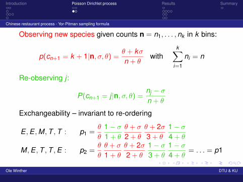
Chinese restaurant process - Yor-Pitman sampling formula
Observing new species given counts n = n1, . . . ,nk in k bins:
p(cn+1 = k + 1|n, σ, θ) =θ + kσn + θ
withk∑
i=1
ni = n
Re-observing j :
P(cn+1 = j |n, σ, θ) =nj − σn + θ
Exchangeability – invariant to re-ordering
E ,E ,M,T ,T : p1 =θ
θ
1− σ1 + θ
θ + σ
2 + θ
θ + 2σ3 + θ
1− σ4 + θ
M,E ,T ,T ,E : p2 =θ
θ
θ + σ
1 + θ
θ + 2σ2 + θ
1− σ3 + θ
1− σ4 + θ
= . . . = p1
Ole Winther DTU & KU

Introduction Poisson Dirichlet process Results Summary
Chinese restaurant process - Yor-Pitman sampling formula
• Likelihood function, e.g. E ,E ,M,T ,T
p(n|σ, θ) =θ
θ
1− σ1 + θ
θ + σ
2 + θ
θ + 2σ3 + θ
1− σ4 + θ
=1∏n−1
i=1 (i + θ)
k−1∏j=1
(θ + jσ)k∏
i ′=1
ni′−1∏j ′=1
(j ′ − σ)
• Flat prior for σ ∈ [−θ/k ,1] and θ ≥ 0 pseudo-countparameter.
• Predictions – simulate new sequence cn+1, cn+2, . . . , cn+n′ :
p(cn+1, . . . , cn+n′ |n) =
∫p(cn+1, . . . , cn+n′ |n, σ, θ) p(σ, θ) dσdθ
with Gibbs sampling (σ, θ) and Yor-Pitman sampling forcn+1, . . ..
• 95% highest posterior density (HPD) intervals.Ole Winther DTU & KU

Introduction Poisson Dirichlet process Results Summary
Averaging and maximum likelihood
0.15 0.16 0.17 0.18
1160
1180
1200
1220
1240
1260
1280
1300
1320
1340
−48.25−46.94
−45.64−44.33
−43.03−41.73
−40.42−39.12
−39.12
−37.82
−37.82
−36.51
−36.51
−35.21
−35.21
−33.9
−33.9
−32.6
−32.6
−31.3
−31.3
−29.99
−29.99
−28.69
−28.69
−27.38
−27.38
−26.08
−26.08
−24.78
−24.78
−23.47
−23.47
−22.17
−22.17
−20.86
−20.86
−19.56
−19.56
−18.26
−18.26
−16.95
−16.95
−15.65
−15.65
−14.34
−14.34
−14.34
−13.04
−13.04
−13.04
−11.74
−11.74
−11.74
−11.74
−10.43
−10.43
−10.43
−10.43
−9.13
−9.13−9.13
−9.13
−7.82
−7.82
−7.82
−7.82
−6.52
−6.52−6.52
−6.52
−5.22
−5.22
−5.22
−5.22
−3.91
−3.91
−3.91
−3.91
−2.61
−2.61
−2.61
−2.61
−1.3
−1.3
−1.3
embryo log L − log LML
contours
σ
θ
0.03 0.04 0.05 0.06
2020
2040
2060
2080
2100
2120
2140
2160
2180
−39.7−38.66
−36.57−35.52−34.48
−34.48
−33.43
−33.43
−32.39
−32.39
−31.35
−31.35
−30.3
−30.3
−29.26
−29.26
−28.21
−28.21
−27.17
−27.17
−26.12
−26.12
−25.08
−25.08
−24.03
−24.03
−22.99
−22.99
−21.94
−21.94
−20.9
−20.9
−19.85
−19.85
−18.81
−18.81
−17.76
−17.76
−16.72
−16.72
−15.67
−15.67
−15.67
−14.63
−14.63
−14.63
−14.63
−13.58
−13.58
−13.58
−13.58
−12.54
−12.54
−12.54
−12.54
−11.49
−11.49
−11.49
−11.49
−10.45
−10.45
−10.45
−10.45
−9.4
−9.4
−9.4
−9.4
−8.36
−8.36
−8.36
−8.36
−7.31
−7.31
−7.31
−7.31
−6.27
−6.27
−6.27
−6.27−5.22
−5.22
−5.22
−5.22
−4.18
−4.18
−4.18
−4.18
−4.18
−3.13
−3.13
−3.13
−3.13
−3.13
−2.09
−2.09
−2.09
−2.09
−2.09
−1.04
−1.04−1.04
−1.04
cerebellum log L − log LML
contours
σ
θ
Ole Winther DTU & KU
Introduction Poisson Dirichlet process Results Summary
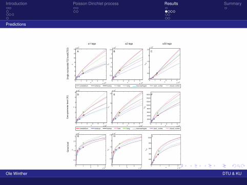
Predictions
0 1 2 3 4
x 106
0
0.5
1
1.5
2
2.5
3
x 104
n
k
0 1 2 3 4
x 106
0
0.5
1
1.5
2
2.5x 10
4
n
k 2
0 1 2 3
x 105
0
200
400
600
800
1000
n
k 30
0 1 2 3 4 5
x 106
0
5
10
15
x 104
n
k 2
0 1 2 3 4 5
x 106
0
2000
4000
6000
8000
10000
12000
14000
16000
n
k 30
0 1 2 3 4 5
x 106
0
1
2
3
4
5
6x 10
5
n
k
0 1 2 3 4 5
x 106
0
2
4
6
8
10
12
14x 10
5
n
k
0 1 2 3 4 5
x 106
0
0.5
1
1.5
2
2.5
3
3.5x 10
5
n
k 2
0 1 2 3 4 5
x 106
0
0.5
1
1.5
2
2.5x 10
4
n
k 30
cerebellum embryo hcamp liver lung macrophages som_cortex visual_cortex
cerebellum embryo hcamp liver lung macrophages som_cortex visual_cortex
Sin
gle
nu
cleo
tid
e TS
S le
vel(C
TSS)
Co
re p
rom
ote
r lev
el (
TC)
Gen
e le
vel
≥1 tags ≥2 tags ≥30 tags
A B C
D E F
G H I
Ole Winther DTU & KU

Introduction Poisson Dirichlet process Results Summary
Predictions
Cross validation – notice anything funny?
2 4 6 8 10
x 105
0
0.5
1
1.5
2
2.5
3
3.5
4x 10
5
n
k
cerebellum
1.34
1.35
1.36
x 105
2.8
3
3.2x 10
4
253234400
420
440
0.5 1 1.5 2 2.5
x 106
0
0.5
1
1.5
2
2.5
3
3.5
4x 10
5
n
k
embryo
1.38
1.4
1.42x 10
5
3.2
3.4
3.6x 10
4
6321971450
1500
1 2 3 4 5
x 106
0
1
2
3
4
5
6
7
x 105
n
k
hcamp
2.9833.023.043.063.08x 10
5
1
1.05
1.1x 10
5
1.38824e+06
5150
5200
5250
1 2 3 4
x 106
0
1
2
3
4
5
6
7
8x 10
5
n
k
liver
2.822.842.862.88
x 105
7.5
8x 10
4
1.21871e+06
3750
3800
3850
1 2 3 4 5
x 106
0
2
4
6
8
10
x 105
n
k
lung
3.95
4x 10
5
0.9811.021.041.061.08x 10
5
1.29824e+06
435044004450
2 4 6
x 105
0
2
4
6
8
10
12
14
16
18
x 104
n
k
macrophage
6.6
6.7
6.8
x 104
1.7
1.8
1.9x 10
4
169919420
440
460
480
2 4 6 8
x 105
0
0.5
1
1.5
2
2.5
3
3.5x 10
5
n
k
som cortex
1.16
1.17
1.18x 10
5
2.2
2.4
x 104
208943
310320330340350
2 4 6 8
x 105
0
0.5
1
1.5
2
2.5
3
3.5
x 105
n
k
vis cortex
1.24
1.25
1.26x 10
5
2.6
2.8
x 104
232690
400
420
Ole Winther DTU & KU

Introduction Poisson Dirichlet process Results Summary
Predictions
Cross validation – cerebellum
2 4 6 8 10
x 105
0
0.5
1
1.5
2
2.5
3
3.5
4x 10
5
n
k
cerebellum
1.34
1.35
1.36
x 105
2.8
3
3.2x 10
4
253234400
420
440
Ole Winther DTU & KU

Introduction Poisson Dirichlet process Results Summary
Predictions
Cross validation – embryo
0.5 1 1.5 2 2.5
x 106
0
0.5
1
1.5
2
2.5
3
3.5
4x 10
5
n
k
embryo
1.38
1.4
1.42x 10
5
3.2
3.4
3.6x 10
4
6321971450
1500
Ole Winther DTU & KU

Introduction Poisson Dirichlet process Results Summary
Coverage
• We can actually predict more than just k .• Each observed species in the library has a certain
frequency.• We estimate a probability for each species based upon
model and observed frequencynj − σn + θ
Probabilities don’t add up to one.• The coverage says how we have already seen.• Coverage (weight species by their observation
probabilities):
Coverage =k∑
j=1
nj − σn + θ
= 1− θ + kσn + θ
.
Ole Winther DTU & KU

Introduction Poisson Dirichlet process Results Summary
Coverage
Coverage predictions
Library sample stats parameters 90.0 % coverage predictionsCTSS n k coverage σML θML coverage n k
cerebellum 253234 133923 0.592 0.728 9714 0.849 10000000 2068648embryo 632197 138190 0.836 0.749 475 0.900 4576200 610448hcamp 1388237 299038 0.859 0.639 6217 0.900 3633400 560111liver 1218713 282555 0.831 0.722 2027 0.900 8032400 1109792lung 1298243 393792 0.776 0.727 5441 0.872 10000000 1756587macrophages 169919 66257 0.716 0.699 2620 0.900 5529000 787295som cortex 208943 115480 0.565 0.748 7980 0.834 10000000 2206260visual cortex 232690 123847 0.587 0.736 8431 0.845 10000000 2090184
99.9 % coverage predictionsgene n k coverage σML θML coverage n k
cerebellum 203481 15079 0.980 0.069 3090 0.990 436800 18312embryo 510662 16869 0.989 0.254 1161 0.990 554400 17320hcamp 983532 18665 0.995 0.210 1292 already reachedliver 1015553 18711 0.995 0.223 1192 already reachedlung 1015700 23121 0.994 0.142 2418 already reachedmacrophages 141236 10643 0.974 0.233 1223 0.990 495400 16020som cortex 170823 13813 0.977 0.093 2720 0.990 434000 17675visual cortex 189515 14080 0.979 0.086 2744 0.990 420000 17302
Ole Winther DTU & KU

Introduction Poisson Dirichlet process Results Summary
Parametric approach
Comparison TSSs: True, non-parametric and parametric Zhuet. al., PLoS ONE, 2008.
Ole Winther DTU & KU

Introduction Poisson Dirichlet process Results Summary
Parametric approach
Comparison genes: True, non-parametric and parametric.
Ole Winther DTU & KU

Introduction Poisson Dirichlet process Results Summary
Summary
• Non-parametric Poisson Dirichlet (PD) process for complexdata.
• The model is always wrong! (as revealed in modelchecking with sufficient data).
• We need more complex model. With so much data onlyunderfitting is a problem. Go beyond PD.
• Joint w Albin Sandelin, Eivind Valen and Anders Krogh, KUbuilding upon Lijoi, Mena and Prünster.
Ole Winther DTU & KU