Embed Size (px)
Citation preview
ESTIMATING THE SIZE OF THE INFORMAL ECONOMY IN BARBADOS
KEVIN GREENIDGE, CARLOS HOLDER and
STUART MAYERS
ABSTRACT
In Barbados, and the Caribbean as a whole, very little research has been done on the
topic of the informal economy. This paper estimates the size of the Barbadian informal
sector for the period 1972-2007. In light of our analysis of the stationary properties of
the data, which suggests a mixture of I(0) and I(1) variables, this study specifies an
unrestricted error correction model and employs a general-to-specific (GETs) modelling
procedure, allowing us to minimise the possibility of estimating spurious relations while
retaining the long-run information. Our estimates indicate that this sector is quite large
and has grown over time to about one-third the size of the official economy. These results
are consistent with the stylised fact about the Barbadian economy, in particular the large
number of persons employed in small businesses and trading as well as the number of
tax returns filed on an annual basis versus the stated level of employment. The finding
of a significant informal sector also has implications for the conduct of both monetary
and fiscal policy. At the minimum it means that possible spillover effects between the
two sectors must be taken into consideration in the design and execution of policies.
KEVIN GREENIDGE, CARLOS HOLDER and STUART MAYERS / 197
1.0 Introduction
The informal economy is a phenomenon that spans all income classes and
all economic sectors. It consists of various types of activities, ranging
from domestic work (maids, mechanics, gardeners) to registered
businesses that underestimate their sales and overestimate their
expenditure. There have, however, always been problems in trying to
estimate its size and value. Informal economy data are not reflected in the
national statistics and may lead to inaccurate macro indicators. Not
taking into account economic activities in the informal sector can result in
the level of GDP and other data being downward biased, giving an
inaccurate impression of the economy and impeding international
comparability. In addition, trend estimates may also be biased if the
economic activities missing from GDP grow at different rates from those
included. For example, it is often conjectured that informal sector
activities expand at precisely the time the official economy is contracting.
Such data may consequently result in erroneous policy decisions.
This paper is the first stage in a proposed two-stage process in
trying to assess the size and relevance of the informal economy in
Barbados. In this stage, we use a general-to-specific (GETs) modelling
procedure within the context of an unrestricted error-correction model,
which allows us to minimise the possibility of estimating spurious
relations while retaining the long-run information. To the best of our
knowledge, this is the first time such an approach has been used to
estimate the size of the informal economy. We chose this procedure
because our results on the stationary properties of the data, which are
discussed in the estimation section below, present a mixture of I(0) and
I(1) variables and it is now widely accepted that the general-to-specific
procedure is as good as, if not more appropriate than, various
cointegration techniques as an alternative estimation procedure in dealing
with small data samples even when the data series under consideration are
nonstationary (see for example, Inder 1993; and Pagan, 1995). The
second stage of the investigation will entail surveying and quantifying the
9198 / BUSINESS, FINANCE & ECONOMICS IN EMERGING ECONOMIES VOL. 4 NO. 1 2009
contributions of the sub-sectors to gross domestic product (GDP). This
we expect will support the findings of this paper.
The next section attempts to define the informal economy, and
identify its main causes. It also discusses the advantages and disadvantages
of the shadow economy and looks at the methods used in estimating its
size. Section 3 deals with some of the studies that were conducted in the
Caribbean and gives a review of their results. In section 4, the size of the
informal economy in Barbados is estimated, using the currency demand
approach. The paper concludes with some remarks and policy
implications.
2.0 Understanding the Informal Economy
2.1 Definition of Terms
In the literature, several terms are commonly used to define the
unmeasured economy. Terms such as informal, hidden, underground,
invisible and shadow are but a few. Many of these concepts are used
interchangeably to describe the same phenomenon.
Any economic activity that does not appear in the statistics of the
national income and GDP is considered to be part of the hidden
economy. When asked, many people think of the informal economy as
being illegal activities; however this is not necessarily so. While it may be
true that all illegal activities are part of the hidden economy, there are
many legal ones that also contribute. For example, when a carpenter who
is employed in the official economy is paid to do work for a friend outside
of his working hours, and does not report this income to the tax
authorities, he too is participating in the informal economy. A teacher
who gets paid for out-of-class lessons may also be participating in this
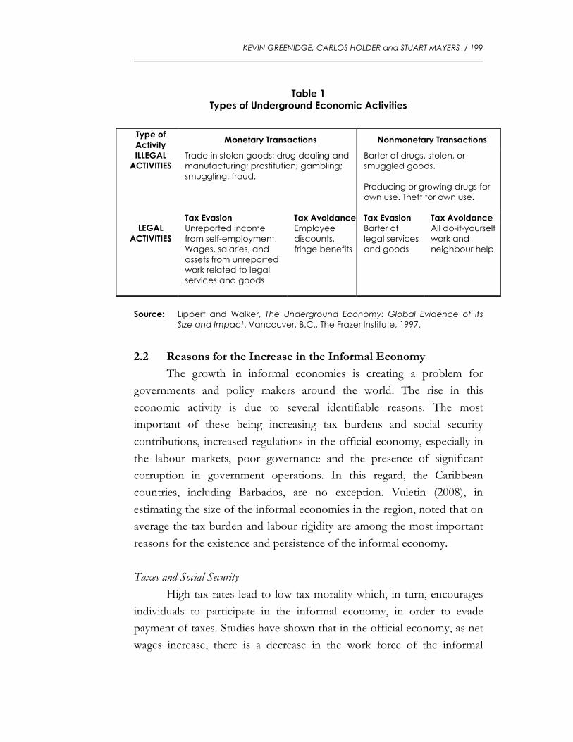
economy if this income is not reflected on the tax form. Table 1 shows
some of the various ways, both legal and illegal, in which people can
participate in the informal economy.
KEVIN GREENIDGE, CARLOS HOLDER and STUART MAYERS / 199
Table 1 Types of Underground Economic Activities
Type of Activity
Monetary Transactions Nonmonetary Transactions
ILLEGAL ACTIVITIES
Trade in stolen goods; drug dealing and
manufacturing; prostitution; gambling;
smuggling; fraud.
Barter of drugs, stolen, or
smuggled goods.
Producing or growing drugs for
own use. Theft for own use.
Tax Evasion Tax Avoidance Tax Evasion Tax Avoidance LEGAL
ACTIVITIES Unreported income
from self-employment.
Wages, salaries, and
assets from unreported
work related to legal
services and goods
Employee
discounts,
fringe benefits
Barter of
legal services
and goods
All do-it-yourself
work and
neighbour help.
Source: Lippert and Walker, The Underground Economy: Global Evidence of its
Size and Impact. Vancouver, B.C., The Frazer Institute, 1997.
2.2 Reasons for the Increase in the Informal Economy
The growth in informal economies is creating a problem for
governments and policy makers around the world. The rise in this
economic activity is due to several identifiable reasons. The most
important of these being increasing tax burdens and social security
contributions, increased regulations in the official economy, especially in
the labour markets, poor governance and the presence of significant
corruption in government operations. In this regard, the Caribbean
countries, including Barbados, are no exception. Vuletin (2008), in
estimating the size of the informal economies in the region, noted that on
average the tax burden and labour rigidity are among the most important
reasons for the existence and persistence of the informal economy.
Taxes and Social Security
High tax rates lead to low tax morality which, in turn, encourages
individuals to participate in the informal economy, in order to evade
payment of taxes. Studies have shown that in the official economy, as net
wages increase, there is a decrease in the work force of the informal
9200 / BUSINESS, FINANCE & ECONOMICS IN EMERGING ECONOMIES VOL. 4 NO. 1 2009
economy. Furthermore, the larger the difference between input and the
after tax earnings from work, the greater the incentive for persons to
participate in the informal economy. As such, the tax regime and the
social security system will have significant influence on the growth of the
informal economy. In the case of Barbados, Vuletin (2008, pp. 14)
concludes that “the main component influencing the informal economy is
the tax burden”, which is not surprising since Barbados has one of the
highest marginal statutory personal tax rates in the region.
Government Regulations
Research has indicated that countries with more regulations on
their economies have larger informal economies (Johnson et al., 1997).
Regulations such as licensing requirements, labour market regulations,
restrictions for foreigners and trade barriers, all aid in increasing the cost
of labour and consequently cause many people to shift to the informal
economy. It is often the case that employers react to these high costs by
transferring them to their employees or even by reducing their labour
force. These employees then find other sources of income, often through
the informal economy. Intense regulations can also cause employers to
stay in the informal economy to avoid higher and non-transferable legal
burdens.
Some countries, such as France, have even implemented
restrictions on hours worked in order to reduce unemployment. While
this is a commendable attempt to distribute limited working opportunities
more fairly, it creates the incentive and the time for people to participate
in the informal economy.
Governance and Corruption
Countries with strong and efficient government institutions have
smaller informal economies. It has been found that there is an increase in
the growth of the informal economy in societies where governments do
not effectively and fairly carry out their tax laws and regulations.
KEVIN GREENIDGE, CARLOS HOLDER and STUART MAYERS / 201
2.3 Advantages and Disadvantages of the Informal Economy
There are several advantages that an informal economy may offer.
For one, it encourages entrepreneurship and creativity. It also supports
the official economy, since most of the income that is earned in the
informal economy is spent in the official sector. The presence of an
informal economy may also force prices in the official economy to fall in
order to remain competitive. This benefits the consumers, including those
who work in the official sector. The informal economy also affords
displaced workers from the formal economy the opportunity to generate
their own income, rather than relying on government benefit or nothing
at all. Finally, perhaps the greatest benefits of the informal economy is
that it provides employment, especially in times of scarce work
opportunities, and gives families an avenue through which they can meet
their needs and improve their way of life.
Nonetheless, there are some disadvantages. First, it takes away
valuable government revenue. This may lead to increased tax rates in
order to sustain revenue levels. The loss in revenue may result in a decline
in the provision of public goods and services that would have otherwise
benefitted the general public. Its presence also creates a problem for
policymakers as it distorts economic information by overstating key ratios
such as unemployment and debt-to-GDP, and understates growth rates.
Consequently, policies may be erroneous and cause adverse reactions. It
also generates unfair competition vis-à-vis the official economy and
thereby effectively lowering the official economy’s income. Lastly, it may
result in increased corruption and political lobbying.
2.4 Measuring or Estimating the Informal Economy
The process of measuring the informal economy is a difficult one
since there is often a lack of information, as persons prefer anonymity.
Nevertheless, there are many techniques used to estimate the size and
structure of the informal economy. These methods can be placed into
three main categories: Direct, Indirect, and Model approaches, with each
having its own strengths and weaknesses. Most of the techniques used are
indirect and may provide a wide range of estimates.
9202 / BUSINESS, FINANCE & ECONOMICS IN EMERGING ECONOMIES VOL. 4 NO. 1 2009
2.4.1 Direct Approaches
There are two direct approaches to estimating the size of the
informal economy, the Sample Survey and the Tax Audit procedures.
Both techniques provide detailed information about the structure of the
hidden economy, however they only provide lower-bound estimates
(minimum range which may be considered accurate) for the size of the
activity. The direct approaches are sometimes referred to as micro
approaches.
The Sample Survey
The survey technique is relatively new, only being actively used in
the last two decades. The main benefits from using this method are the in-
depth conclusions that can be drawn from its results. Useful information
about the size and structure of the informal economy can be derived from
this process. However, the obtained results greatly depend on the
structure of the questionnaire. A badly formulated questionnaire does not
give persons the incentive to reveal their participation in the informal
economy and cooperate with the survey. This unwillingness can lead to
unreliable results, and hence accurate estimations and inferences cannot to
be made.
The Tax Audit
Differences between the income submitted for tax purposes and
that which is calculated by tax audits lead to information on the informal
economy (Frey and Pommerehne, 1984). Threats of fines and
imprisonment force participants to reveal this hidden income, which
would have otherwise provided the government with useful revenue.
The tax audit method leads to a few difficulties. The estimates based on
this technique do not provide complete information about the size of the
informal economy and these results tend to be biased. The data that is
used (tax compliance data) may itself be a biased sample of the
population. Only persons who complete tax forms are considered for
KEVIN GREENIDGE, CARLOS HOLDER and STUART MAYERS / 203
audit but most persons submitting these forms will comply and submit
accurate information. However, this bias is somewhat lessened because
the selection of those persons to be audited is done based on tax forms
that show some possibility of fraud. This procedure only displays the
fraction of the economy that the authorities were able to catch.
2.4.2 Indirect Approaches
These techniques allow for estimates to be drawn from seemingly
unrelated information. This is useful because, as stated before, many
persons do not want the relevant authorities to know of their participation
in the informal economy, and hence try their best to conceal it. These
procedures try to deal with this problem. The indirect processes are
sometimes called macro approaches since they use macroeconomic
indicators to extract information about the development of the informal
economy. Accounting statistics, the labour statistics, the monetary
balances, and the physical outputs are all types of the indirect approach.
The indirect approaches have many benefits but also have
shortcomings. They provide information on the size of the economy but
are unreliable when it comes to determining its structure. Another
problem is that they often require some assumptions to be made, which
often cannot be proven.
Accounting Statistics
The accounting statistics approach can be used at both the
individual and the national level to derive estimates of the informal
economy. It uses discrepancies between expenditure and income to draw
conclusions (Schneider and Enste, 2000). In the presence of the informal
economy, the income (and production) measure of national income will
not be the same as the expenditure measure, and in fact, the latter will be
much higher. Therefore, the surplus of expenditure over income is an
indicator of the size of the informal economy.
The individual level, rather than at the national level, may yield
better results. Processes like the Family Expenditure Survey in the United
Kingdom, separately measure income and expenditure on a daily basis,
9204 / BUSINESS, FINANCE & ECONOMICS IN EMERGING ECONOMIES VOL. 4 NO. 1 2009
using record books and information on credit and hire purchase. It
provides more detailed information about the sectors and industries in
which work can be obtained. However, the figures generated are almost
identical to those on the national level.
This technique is useful and easy when the relevant information on
expenditure is available, however it will only capture the lowest range of
estimates of the informal economy that can be considered to be accurate.
Expenditure data is difficult to collect because it is almost impossible to
keep accurate records of every transaction that takes place. Expenditure
information may even be dependent on income information, which may
lead to inaccurate estimates. In addition, the discrepancy used to make
these estimates often includes errors and omissions in the accounting
statistics. In fact, the difference between the two aggregates is almost
always attributed to the error and omission terms and, as such, would
make the resulting estimates unreliable.
Labour Force Statistics
The labour force statistics method assumes that the participation in
the official labour force remains constant. Hence, any decline in the
participation in the official work force can be assumed to be an estimate
for growth in the informal economy, ceteris paribus, (O'Neill, 1983). More
specifically, this approach assumes increasing informal economic activity
when the ratio of employment to population is decreasing with the ratio
of labour supply to population relatively constant.
However, although it is relatively simple in its calculations, this
method is flawed in its major assumption, the constancy of the
participation rate, as individuals may leave the official economy for
reasons other than to participate in the informal economy. Furthermore, it
is compounded by the fact that persons can work in both the official and
informal economies. Such persons go undetected and are not considered
as part of the informal economy’s work force. Thus, this procedure leads
to unreliable results and gives weak estimates of the size of the informal
economy.
KEVIN GREENIDGE, CARLOS HOLDER and STUART MAYERS / 205
Monetary Balances
The monetary balances approach seems to be the most commonly
used system to estimate the size of the informal economy. The three
common procedures that fall under the monetary balances approach
involve realistic assumptions about the volume of monetary transactions
and the use of currency.
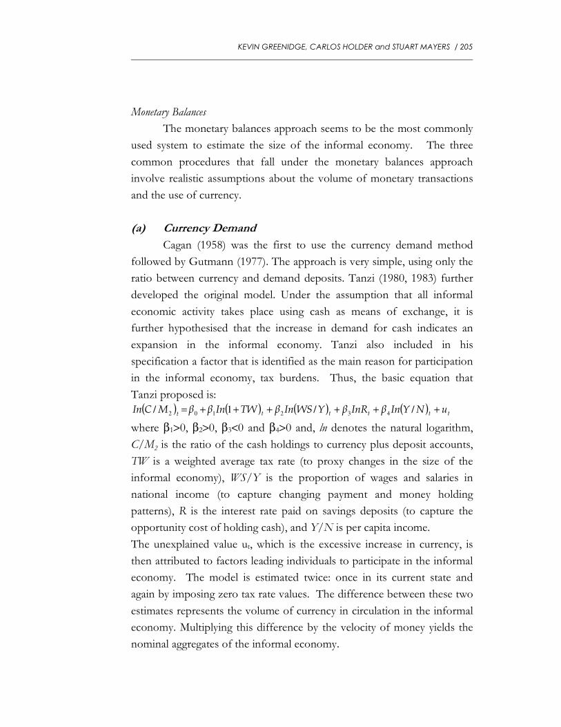
(a) Currency Demand
Cagan (1958) was the first to use the currency demand method
followed by Gutmann (1977). The approach is very simple, using only the
ratio between currency and demand deposits. Tanzi (1980, 1983) further
developed the original model. Under the assumption that all informal
economic activity takes place using cash as means of exchange, it is
further hypothesised that the increase in demand for cash indicates an
expansion in the informal economy. Tanzi also included in his
specification a factor that is identified as the main reason for participation
in the informal economy, tax burdens. Thus, the basic equation that
Tanzi proposed is:
( ) ( ) ( ) ( ) ttttttuNYInβInRβYWSInβTWInββMCIn ++++++= //1/ 432102
where β1>0, β2>0, β3<0 and β4>0 and, ln denotes the natural logarithm,
C/M2 is the ratio of the cash holdings to currency plus deposit accounts,
TW is a weighted average tax rate (to proxy changes in the size of the
informal economy), WS/Y is the proportion of wages and salaries in
national income (to capture changing payment and money holding
patterns), R is the interest rate paid on savings deposits (to capture the
opportunity cost of holding cash), and Y/N is per capita income.
The unexplained value ut, which is the excessive increase in currency, is
then attributed to factors leading individuals to participate in the informal
economy. The model is estimated twice: once in its current state and
again by imposing zero tax rate values. The difference between these two
estimates represents the volume of currency in circulation in the informal
economy. Multiplying this difference by the velocity of money yields the
nominal aggregates of the informal economy.
9206 / BUSINESS, FINANCE & ECONOMICS IN EMERGING ECONOMIES VOL. 4 NO. 1 2009
This procedure may underestimate the size of the informal
economy, because not all of the transactions that take place use cash as
means of exchange. The method also assumes that there is a base year of
no hidden economic activity.
(b) Transactions
Feige (1979) developed the transaction method to estimating the
size of the informal economy utilising information on the overall volume
of transactions in the total economy. Information is generated by the well
known Fisherian equation:
pTMV =
where M denotes money supply, V is the velocity of money, p is the
price level of transactions and T is the volume of transactions.
It is assumed that there is a constant relationship between the
volume of transactions and the total official GDP over time (Feige, 1979;
1989; 1996). Assumptions are also made about the velocity of money and
also that there is a base year of no hidden economic activity. From this
data, the total GDP can be calculated. The difference between the total
and the official GDP is the GDP of the informal economy.
The assumption that there is a base year of no hidden economy is
problematic. This is compounded by assuming (i) a fixed transaction ratio
over time and (ii) that the informal economy is the only factor affecting a
change in the transaction ratio. These are strong assumptions and raise
questions about the reliability of the results.
(c) Physical Outputs - (Electricity Consumption)
The physical outputs method assumes that electricity consumption
is the best indicator for overall economic activity (official and
unofficial/informal) (Kaliberda and Kaufmann, 1996). Because the
electricity/GDP elasticity has been observed to be close to one, the
growth rate of the official GDP can be subtracted from the growth rate of
electricity consumption. The resultant value is attributed to the growth of
the informal economy.
KEVIN GREENIDGE, CARLOS HOLDER and STUART MAYERS / 207
This method is easy to use because of the availability of the
information required. However, there are problems that have arisen with
its application. First, not all of the informal economic activity requires
electricity, other sources of energy can be used. Second, due to
technological advances, electricity consumption has become more
efficient. Third, the electricity/GDP elasticity may vary over time.
2.4.3 The Model Approach
This technique considers both the causes and the effects of the
informal economy over time. It is based on the dynamic multiple-
indicators multiple-causes (DYMIMIC) model, which consists of two
parts: a measurement model, linking the observed indicators to the size of
the informal economy; and a structural-equations model, specifying causal
relationships among the observed indicators. The three main causes
identified are tax burdens, government regulations and tax morality. The
three main indicators are the development of monetary aggregates, labour
markets, and production market. The method is in-depth and
comprehensive. However, it requires an extensive amount of data, which
is often not available, thus rendering this technique inapplicable.
3.0 Previous Studies on the Informal Economy in the Caribbean
The task of estimating the size of the informal economy in the Caribbean
has not been given as much attention as its importance merits. To date
only a few studies have been carried out in Jamaica, Trinidad and Tobago,
Guyana and Barbados.
3.1 Jamaica
Earlier information concerning the Jamaican informal economy
was gathered through studies of sidewalk vendors or higglers. (see for
example, LeFranc et al., 1987; and Smikle and Taylor, 1977).
Investigations were done in the form of surveys. One of these targeted
informal commercial importers, while the others sought to collect data on
the traditional higgler, who traded in parochial and curb-side markets.
9208 / BUSINESS, FINANCE & ECONOMICS IN EMERGING ECONOMIES VOL. 4 NO. 1 2009
These studies did not provide information on the size of the economy.
They only generated information on the kinds of activities that were
taking place, giving the profile of the typical higgler and a breakdown of
their average weekly costs. Smikle and Taylor (1977) estimated that
115,006 members of the higgler population traded in the markets and
their environs, while another 1,046 existed in curbside markets. The
surveys were unable to provide reliable data on the financial activities
within the informal economy.
Witter and Kirton (1990) represented one of the first studies on
the informal sectors in Jamaica to utilise rigorous econometric analysis. As
part of their investigation the authors estimated excessive growth in the
use of cash in the economy as a proxy of the growth of the informal
economy. Their estimates show the informal economy increasing as a
ratio of formal GDP from 8% in 1962 to 24% in 1984. In addition, they
found that the income velocity of money in the informal sector was 10%
higher than in the formal sector. Witter and Kirton also provided some
estimates on employment in the informal sector which suggested that in
1985 almost 20% of the population aged 14 and over were employed in
the informal economy.
A more recent study, by the Inter-American Development Bank
(IADB) (2006), estimated the size of the informal sector in Jamaica and
reported that the informal economy, represented a large and growing
share of the overall economy; more than doubling in size since the 1980s.
Using various methods, including monetary and other indirect
approaches, the IADB report puts the size of the informal sector in
Jamaica at just over 40% of official GDP in 2001. In addition, the report
suggested that the informal sector grew significantly faster than the formal
economy during the 1990s.
Vuletin (2008) estimated the size of the informal economy for 32
mainly Latin American and Caribbean countries, including Jamaica, using
a DYMIMIC approach. Vuletin’s estimates are consistent with the IADB
(2006) report and place the informal economy of Jamaica at 35% of
official GDP in 2000.
KEVIN GREENIDGE, CARLOS HOLDER and STUART MAYERS / 209
3.2 Trinidad and Tobago
Maurin et al. (2006) obtained estimates for the hidden economy in
Trinidad and Tobago utilising the Tanzi currency demand approach,
applied to data spanning the period 1970-1999. They employed a
structural cointegration approach containing two long-run relationships
linking the demand for currency with other variables. They solved the
model using a Gauss-Siedel algorithm and, under the assumption that the
velocity of “illegal” money is the same as that of legal money, concluded
that the hidden economy rose from a low of about 14% of measured
GDP in 1970 to a high of 36% in 1981, and in 1999 was about 20% of the
official economy. They suggested that the use of a direct survey would
yield more detailed information, which could be useful for the design of
policy. Vuletin (2008) also included estimates of the size of the informal
economy in Trinidad and Tobago, which suggested that the country’s
informal economy is around 25% of official GDP in 2000.
The size of the informal economy in Trinidad and Tobago, based
on these estimates, is much larger if we consider that a significant
proportion of the official economy is the energy sector, in which very
little activity escapes the official GDP statistics1. The energy sector
contributes about 40% of official GDP2, which implies that hidden
economy currently stands at 33% of non-energy GDP.
3.3 Barbados
An extensive Informal Sector Survey was conducted by the
Barbados Statistical Service Department (1998). The survey sought to
improve the social and economic statistics on the informal sector in the
island, analyse the situation of the workers and make recommendations to
assist in the design of policies to increase productivity of the sector.
The information gathered from this survey showed various forms
of informal economic activity - agriculture, construction, distribution and
1 This is because the sector dominated by large international corporations or their affiliates, and by large state-owned companies.
2 Based on 2004 GDP estimates.
9210 / BUSINESS, FINANCE & ECONOMICS IN EMERGING ECONOMIES VOL. 4 NO. 1 2009
tourism, to name a few. Distribution and agriculture were identified as
being the most populous of these sectors with 2,313 and 1,562 persons
respectively. It was estimated that there were 5,720 informal business
operators, compared to 14,172 in the formal economy. The total
employment calculated in the informal economy numbered 6,904, as
opposed to 117,575 in the formal economy.
Detailed information was also gathered on the backgrounds of
informal economy operators, such as, level of education, starting capital,
credit information, input costs, and the duration of their informal
business lives, but the size of the informal economy was not estimated.
However, care must be taken when using this technique, because most
interviewees tend to understate income and overstate expenses, thus
obscuring results. Also several operators within the informal sector
would not have identified themselves.
Vuletin (2008) is the only study we found that provided a
proximate size of the informal economy in Barbados. The author’s
estimates suggested that, in 2000, the informal economy in Barbados was
roughly 36% of GDP.
3.4 Guyana
Faal (2003) also utilised a Tanzi-type currency demand model to
estimate the informal economy in Guyana. The author’s findings indicate
the existence of a large informal economy ranging from 27% of GDP in
1970 to as high as 101% in 1989. Thereafter, as macroeconomic reforms
were implemented the size of the informal economy declined to 55% in
2000.
Faal concluded that a long-run strategy based on market-based
reforms, including fiscal reforms, improved governance and stronger
institutions are effective in reducing the informal economy. Thomas
(1989) also investigated the structure of the informal economy in Guyana
with emphasis on the foreign currency market, but failed to give estimates
on the size of the sector. The estimates by Vuletin (2008) for Guyana are
consistent with those of Faal, suggesting that the informal economy in
Guyana was approximately 57% of official GDP in 2000.
KEVIN GREENIDGE, CARLOS HOLDER and STUART MAYERS / 211
4.0 Estimates for Barbados
The currency demand approach is chosen to estimate the size of the
informal economy in Barbados because of the availability of reliable time
series data for the monetary sector as well as the tax burden and, as
discussed above, it is the most widely used indirect method in the
literature. In this regard, we modified the Tanzi equation along the lines
taken by Bajada (1999) and Faal (2003). Also, as in Bajada (1999) we
utilise a general unrestricted error correction model but, instead of simply
estimating the model with a set number of lags (for example, testing 1 lag
against 2 and using the selected length across all variables in the model),
we use the GETs approach to eliminate statistically irrelevant variables
thus reducing this ‘general’ model to a more parsimonious, congruent one,
allowing for more efficient estimation and inference.
The currency demand model specifies that:
( )TTrE�RYDfC ,,,,,= (1)
where C is real currency per capita, YD is real disposable income per
capita, R is the interest rate, π represents the rate of inflation, E denotes
private consumption expenditure as a ratio of GDP, Tr is a technological
trend variable, and T is the tax rate. Currency demand is expressed in real
per capita terms to eliminate the impact of inflation and population
growth on the demand for currency.
Real disposable income and interest rates are expected to have
similar impacts on the demand for currency as they would have on the
demand for money. Disposable income is substituted for income since
we are examining the excess sensitivity of taxes on currency (see Bajada
1999). Inflation becomes relevant since increasing prices will either cause
individuals to hold more cash to meet daily demand or induce them to
hold less as its value may be eroded.
Like Bajada, private consumption expenditure to GDP is added to
capture currency demand arising as a result of spending on goods and
services (desired demand) in the official economy by participants of the
9212 / BUSINESS, FINANCE & ECONOMICS IN EMERGING ECONOMIES VOL. 4 NO. 1 2009
informal economy, which would not normally be captured by the measure
utilised for disposable income.
Technological developments (ATMs, point of sale cards, etc.),
which are currency substitutes and will have an impact on the demand for
currency, are represented by the trend variable. Finally, our key
assumption, as was Tanzi’s, is that the informal economy is more cash
intensive than the official economy. As such, increases in taxes lead to an
expansion of the informal economy and consequently to greater use of
cash.
Data and Estimation of the Currency Demand Function
The data, sourced from the Central Bank of Barbados, is of annual
frequency covering the period 1972-2007. Real currency per capita is
measured as the stock of notes and coins in the hands of the public
deflated by the GDP deflator and further expressed as a ratio of the
population. Real disposable income per capita is calculated as nominal
GDP less direct taxes on incomes, also deflated by the GDP deflator and
divided by the population. The interest rate is represented by the
commercial banks’ weighted average deposit rate. The tax rate is direct
taxes on incomes expressed as a percentage of GDP. The inflation rate is
the change in the consumer price index. Private consumption expenditure
is taken from the national accounts and expressed as a percentage of
GDP. All variables are expressed in natural logarithm.
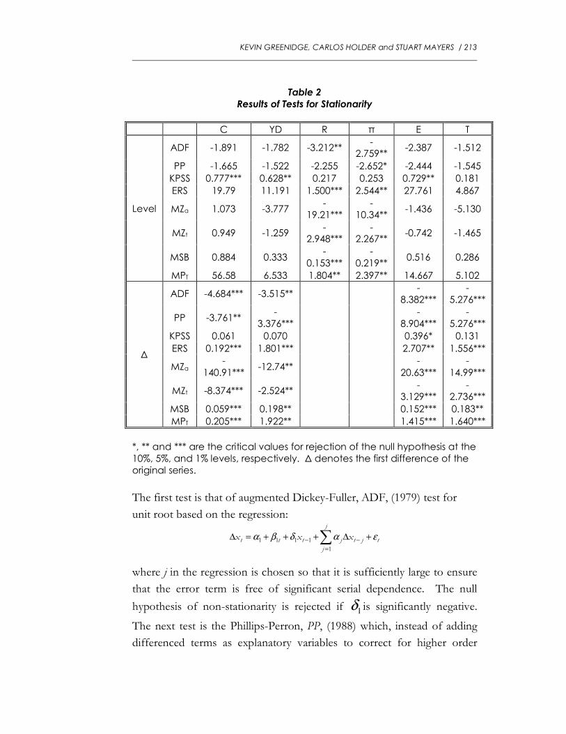
We begin by investigating the stationary properties of the data, as
this can influence the estimation procedure we choose. In this regard, a
number of stationarity tests are applied to the levels and first differences
of the variables. The results are presented in Table 2.
KEVIN GREENIDGE, CARLOS HOLDER and STUART MAYERS / 213
Table 2
Results of Tests for Stationarity
C YD R π E T
Level
ADF -1.891 -1.782 -3.212** -
2.759** -2.387 -1.512
PP -1.665 -1.522 -2.255 -2.652* -2.444 -1.545
KPSS 0.777*** 0.628** 0.217 0.253 0.729** 0.181
ERS 19.79 11.191 1.500*** 2.544** 27.761 4.867
MZα 1.073 -3.777 -
19.21***
-
10.34** -1.436 -5.130
MZt 0.949 -1.259 -
2.948*** -
2.267** -0.742 -1.465
MSB 0.884 0.333 -
0.153***
-
0.219** 0.516 0.286
MPT 56.58 6.533 1.804** 2.397** 14.667 5.102
∆
ADF -4.684*** -3.515** -
8.382***
-
5.276***
PP -3.761** -
3.376***
-
8.904***
-
5.276***
KPSS 0.061 0.070 0.396* 0.131
ERS 0.192*** 1.801*** 2.707** 1.556***
MZα -
140.91*** -12.74**
-
20.63***
-
14.99***
MZt -8.374*** -2.524** -
3.129*** -
2.736***
MSB 0.059*** 0.198** 0.152*** 0.183**
MPT 0.205*** 1.922** 1.415*** 1.640***
*, ** and *** are the critical values for rejection of the null hypothesis at the
10%, 5%, and 1% levels, respectively. ∆ denotes the first difference of the
original series.
The first test is that of augmented Dickey-Fuller, ADF, (1979) test for
unit root based on the regression:
tjt
j
j
jttt xxx εαδβα +∆+++=∆ −
=
− ∑1
1111
where j in the regression is chosen so that it is sufficiently large to ensure
that the error term is free of significant serial dependence. The null
hypothesis of non-stationarity is rejected if 1δ is significantly negative.
The next test is the Phillips-Perron, PP, (1988) which, instead of adding
differenced terms as explanatory variables to correct for higher order
9214 / BUSINESS, FINANCE & ECONOMICS IN EMERGING ECONOMIES VOL. 4 NO. 1 2009
serial correlation, makes the correction on the t-statistic of the δ
coefficient. However, the PP test, as originally defined, suffers from
severe size distortions when there are negative-moving average errors (see
Perron and Ng, 1996; and Schwert, 1989). Although the ADF test is
more accurate under such conditions, its power is still significantly
reduced. In lieu of this, we used both the Elliot et al. (ERS) Point Optimal
test (1996), which has improved power characteristics over the ADF test,
and the Ng and Perron (2001) testing procedure (NP) which exhibits less
size distortions compared to the PP test. Both tests are well documented
in the literature. The other three tests, denoted as dd
tdα MSBandMZMZ , , are
modifications of the PP statistics (the αZ and tZ statistics of Phillips
and Perron) and the Bhargava statistic with corrections for size distortions
in the case of negatively correlated residuals.
However, all the above tests take a unit root as the null hypothesis,
which means that they have a high probability of falsely rejecting the null
of non-stationarity when the data generation process is close to a
stationary process (Blough, 1992; Harris, 1995). Therefore we also utilised
the KPSS test described in Kwiatkowski et al. (1992) where the null
hypothesis is specified as a stationary process.
The results indicated that both R and π are both integrated of
order zero, I(0), while the other series have a unit root in their levels but
not in their first differences, hence are I(1). Note that the various tests are
in agreement except in the case of the tax rate. Here the KPSS suggested
that it is stationary, while the others pointed to an I(1) process. A
graphical inspection showed a sharp dip in the tax rate in 1988 and when
we allowed for a blip in the unit root test (using the procedure in Lanne et
al., 2002; and Saikkonen and Lutkepohl, 2002) it confirmed that the series
is stationary3.
Since we have a mixture of I(0) and I(1) variables we opted to use
the GETs procedure as it is still an open debate on how to appropriately
3 These results are available from the authors upon request.
KEVIN GREENIDGE, CARLOS HOLDER and STUART MAYERS / 215
handle combinations of stationary and non-stationary variables in
standard cointegration frameworks like that of Johansen. In addition,
Monte Carlo studies have shown that the GETs procedure is as good as,
if not more appropriate than, other cointegration techniques in dealing
with small data samples, even in the presence of I(1) variables4. With the
GETs procedure we can minimise the possibility of estimating spurious
relations while retaining long-run information and at the same time derive
a currency demand model that is suitable for economic interpretation.
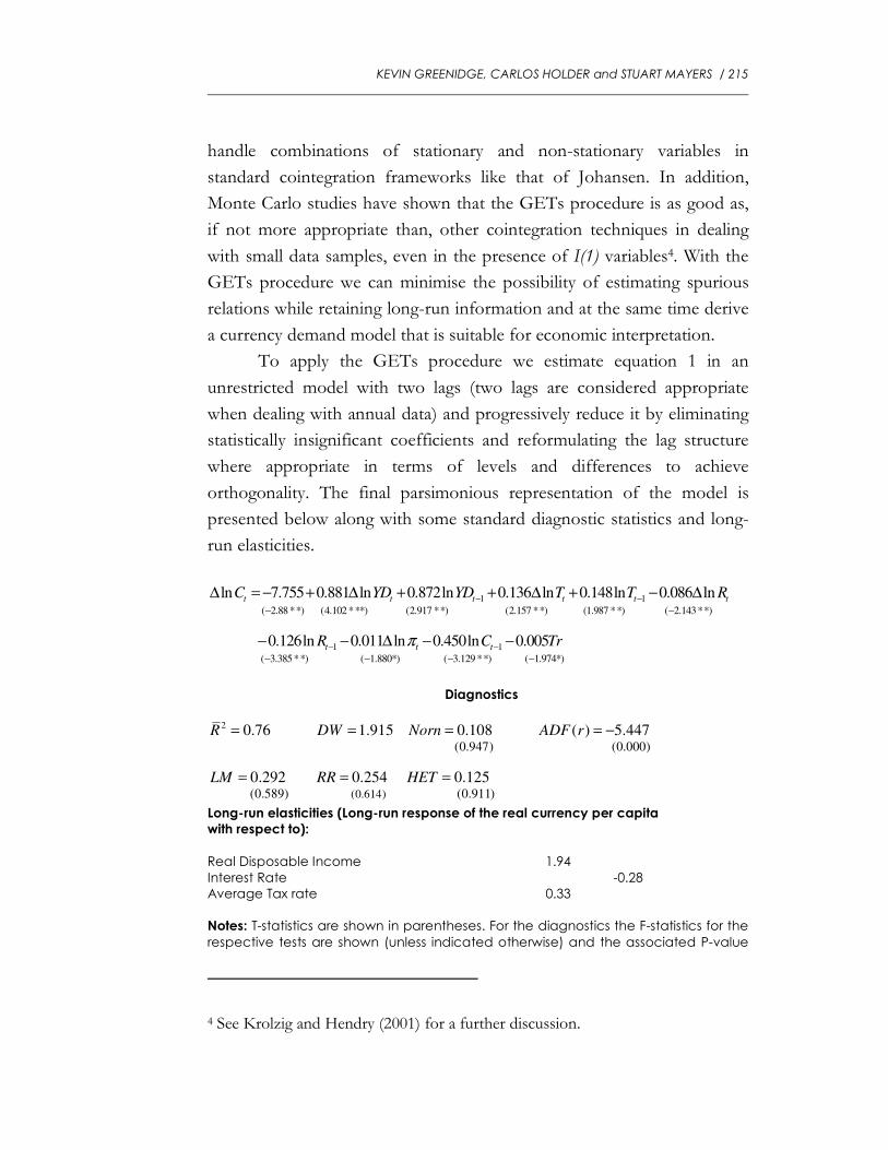
To apply the GETs procedure we estimate equation 1 in an
unrestricted model with two lags (two lags are considered appropriate
when dealing with annual data) and progressively reduce it by eliminating
statistically insignificant coefficients and reformulating the lag structure
where appropriate in terms of levels and differences to achieve
orthogonality. The final parsimonious representation of the model is
presented below along with some standard diagnostic statistics and long-
run elasticities.
1 1
1 1
( 2.88 **) (4.102 ***) (2.917 **) (2.157 **) (1.987 **) ( 2.143**)
( 3.385**) ( 1.880*) ( 3.129 **) (
ln 7.755 0.881 ln 0.872ln 0.136 ln 0.148ln 0.086 ln
0.126ln 0.011 ln 0.450ln 0.005
t t t t t t
t t t
C YD YD T T R
R C Trπ
− −
− −
− −
− − −
∆ = − + ∆ + + ∆ + − ∆
− − ∆ − −1.974*)−
Diagnostics
2
(0.614)
(0.947) (0.000)
(0.589) (0.911)
0.76 1.915 0.108 ( ) 5.447
0.292 0.254 0.125
R DW Norn ADF r
LM RR HET
= = = = −
= = =
Long-run elasticities (Long-run response of the real currency per capita with respect to): Real Disposable Income 1.94
Interest Rate -0.28
Average Tax rate 0.33
Notes: T-statistics are shown in parentheses. For the diagnostics the F-statistics for the
respective tests are shown (unless indicated otherwise) and the associated P-value
4 See Krolzig and Hendry (2001) for a further discussion.
9216 / BUSINESS, FINANCE & ECONOMICS IN EMERGING ECONOMIES VOL. 4 NO. 1 2009
in square brackets. DW is the Durbin-Watson statistic. SC is the Lagrange multiplier
test of residual serial correlation (Chi-square of degree 1). FF is the Ramsey RESET test
for incorrect functional form using the square of the fitted values (Chi-square of
degree 1). Norn is the test for normality of the residuals based on the Jarque-Bera
test statistic (Chi-square of degree 1). HET is the Heteroskedasticity test based on the
regression of squared residuals on squared fitted values. ADF(r) is the Augmented
Dickey-Fuller unit root test
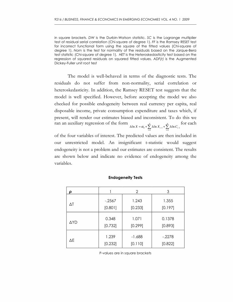
The model is well-behaved in terms of the diagnostic tests. The
residuals do not suffer from non-normality, serial correlation or
heteroskedasticity. In addition, the Ramsey RESET test suggests that the
model is well specified. However, before accepting the model we also
checked for possible endogeneity between real currency per capita, real
disposable income, private consumption expenditure and taxes which, if
present, will render our estimates biased and inconsistent. To do this we ran an auxiliary regression of the form
0 1 1
1 1
ln ln lnt t
i i
X X C
ρ ρ
α − −
= =
∆ = + ∆ + ∆∑ ∑for each
of the four variables of interest. The predicted values are then included in
our unrestricted model. An insignificant t-statistic would suggest
endogeneity is not a problem and our estimates are consistent. The results
are shown below and indicate no evidence of endogeneity among the
variables.
Endogeneity Tests
ρ 1 2 3
∆T -.2567
[0.801]
1.243
[0.233]
1.355
[0.197]
∆YD 0.348
[0.732]
1.071
[0.299]
0.1378
[0.893]
∆E 1.239
[0.232]
-1.688
[0.110]
-.2278
[0.822]
P-values are in square brackets
KEVIN GREENIDGE, CARLOS HOLDER and STUART MAYERS / 217
The ADF(r) statistic confirms that the variables in the currency
demand equation form an equilibrium (cointegrated) relationship, while
the coefficient on lnCt-1 suggests an adjustment speed of 45%. Thus, it
takes approximately two years for holders of currency to fully adjust to
shocks affecting their demand. All the variables of our final model are
correctly signed. The coefficient on disposable income indicates that
expansions in income increase the use of currency with a long-run
elasticity of 1.9 percent. Interest rate has a negative effect on real currency
demand which is consistent with the theory that it represents the
opportunity cost of holding money. A one percentage point increase in
the nominal interest rate brings about a 0.09 percentage point decline in
real currency demand in the short run, with a steady-state effect of -0.28
of a percentage point. The coefficient on the average tax rate is positive
indicating that an increase in the tax rate induces higher currency demand,
consistent with Tanzi’s postulate. A one percentage point increase in the
average tax rate leads to roughly a 0.14 percentage point rise in currency
demand in the short-run and over time currency demand expands to 0.33
percentage points. As expected, the increasing use of technology
significantly reduces the need to use cash for transactional purposes.
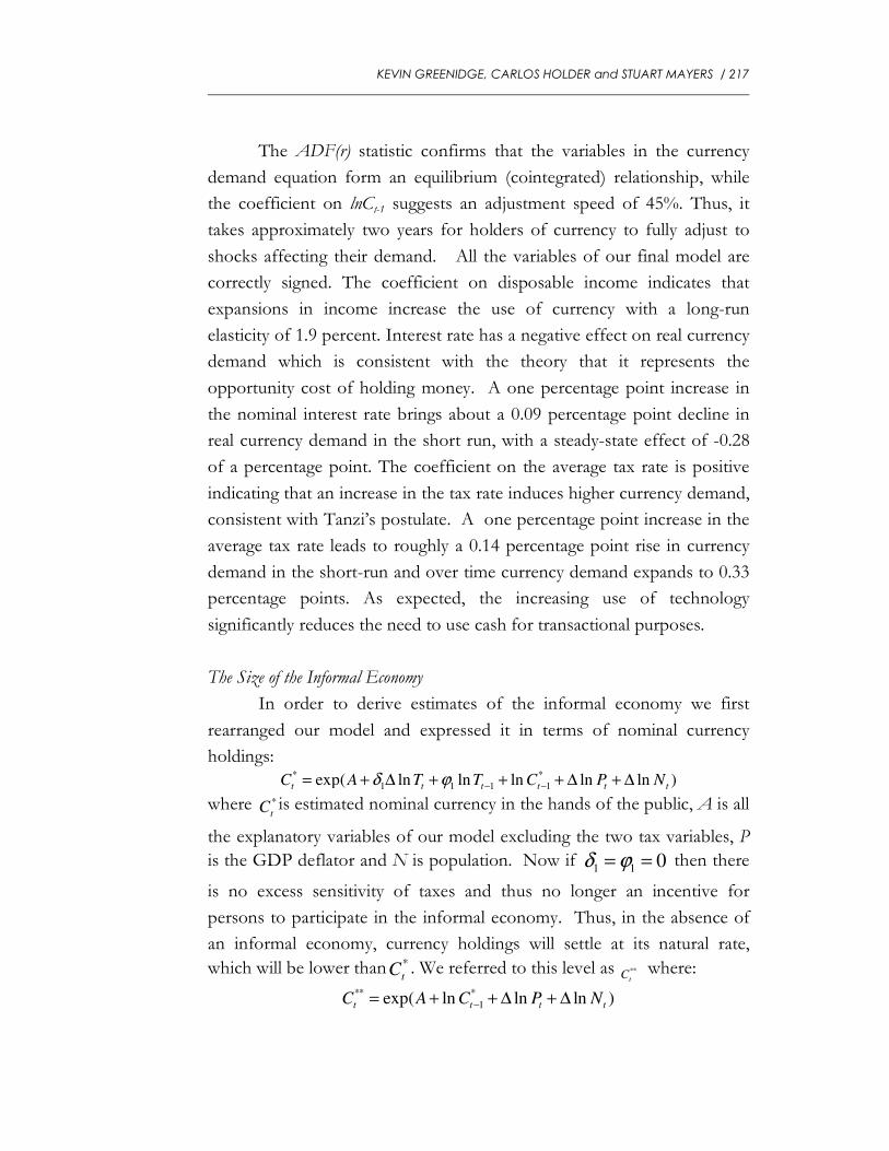
The Size of the Informal Economy
In order to derive estimates of the informal economy we first
rearranged our model and expressed it in terms of nominal currency
holdings: * *
1 1 1 1exp( ln ln ln ln ln )t t t t t t
C A T T C P Nδ ϕ − −= + ∆ + + + ∆ + ∆
where *
tC is estimated nominal currency in the hands of the public, A is all
the explanatory variables of our model excluding the two tax variables, P
is the GDP deflator and N is population. Now if 1 1 0δ ϕ= = then there
is no excess sensitivity of taxes and thus no longer an incentive for
persons to participate in the informal economy. Thus, in the absence of
an informal economy, currency holdings will settle at its natural rate,
which will be lower than *
tC . We referred to this level as **
tC
where:
** *
1exp( ln ln ln )t t t t
C A C P N−= + + ∆ + ∆
9218 / BUSINESS, FINANCE & ECONOMICS IN EMERGING ECONOMIES VOL. 4 NO. 1 2009
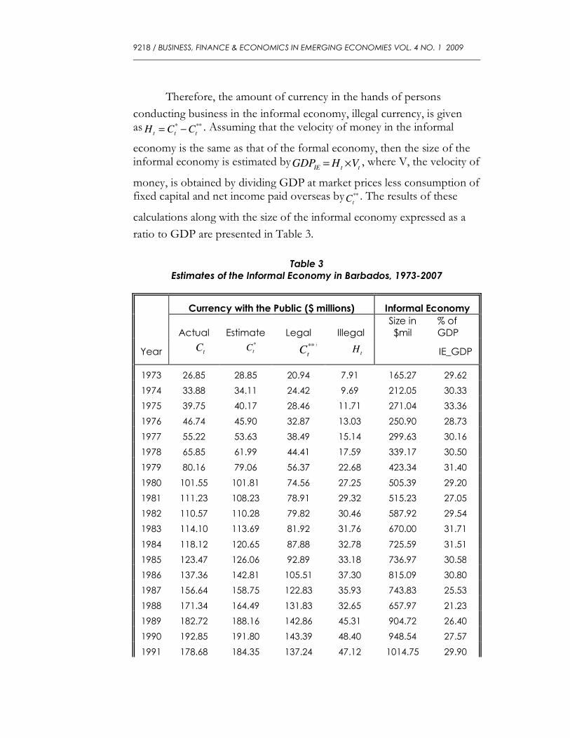
Therefore, the amount of currency in the hands of persons
conducting business in the informal economy, illegal currency, is given as * **
t t tH C C= − . Assuming that the velocity of money in the informal
economy is the same as that of the formal economy, then the size of the informal economy is estimated by
IE t tGDP H V= × , where V, the velocity of
money, is obtained by dividing GDP at market prices less consumption of fixed capital and net income paid overseas by **
tC . The results of these
calculations along with the size of the informal economy expressed as a
ratio to GDP are presented in Table 3.
Table 3
Estimates of the Informal Economy in Barbados, 1973-2007
Currency with the Public ($ millions) Informal Economy
Actual Estimate Legal Illegal
Size in
$mil
% of
GDP
Year
IE_GDP
1973 26.85 28.85 20.94 7.91 165.27 29.62
1974 33.88 34.11 24.42 9.69 212.05 30.33
1975 39.75 40.17 28.46 11.71 271.04 33.36
1976 46.74 45.90 32.87 13.03 250.90 28.73
1977 55.22 53.63 38.49 15.14 299.63 30.16
1978 65.85 61.99 44.41 17.59 339.17 30.50
1979 80.16 79.06 56.37 22.68 423.34 31.40
1980 101.55 101.81 74.56 27.25 505.39 29.20
1981 111.23 108.23 78.91 29.32 515.23 27.05
1982 110.57 110.28 79.82 30.46 587.92 29.54
1983 114.10 113.69 81.92 31.76 670.00 31.71
1984 118.12 120.65 87.88 32.78 725.59 31.51
1985 123.47 126.06 92.89 33.18 736.97 30.58
1986 137.36 142.81 105.51 37.30 815.09 30.80
1987 156.64 158.75 122.83 35.93 743.83 25.53
1988 171.34 164.49 131.83 32.65 657.97 21.23
1989 182.72 188.16 142.86 45.31 904.72 26.40
1990 192.85 191.80 143.39 48.40 948.54 27.57
1991 178.68 184.35 137.24 47.12 1014.75 29.90
*
tC **
tC
**
tCt
Ct
H
KEVIN GREENIDGE, CARLOS HOLDER and STUART MAYERS / 219
1992 176.85 171.27 123.57 47.70 1135.68 35.75
1993 176.99 182.93 132.96 49.97 1118.29 33.88
1994 189.60 187.97 136.99 50.98 1149.89 33.11
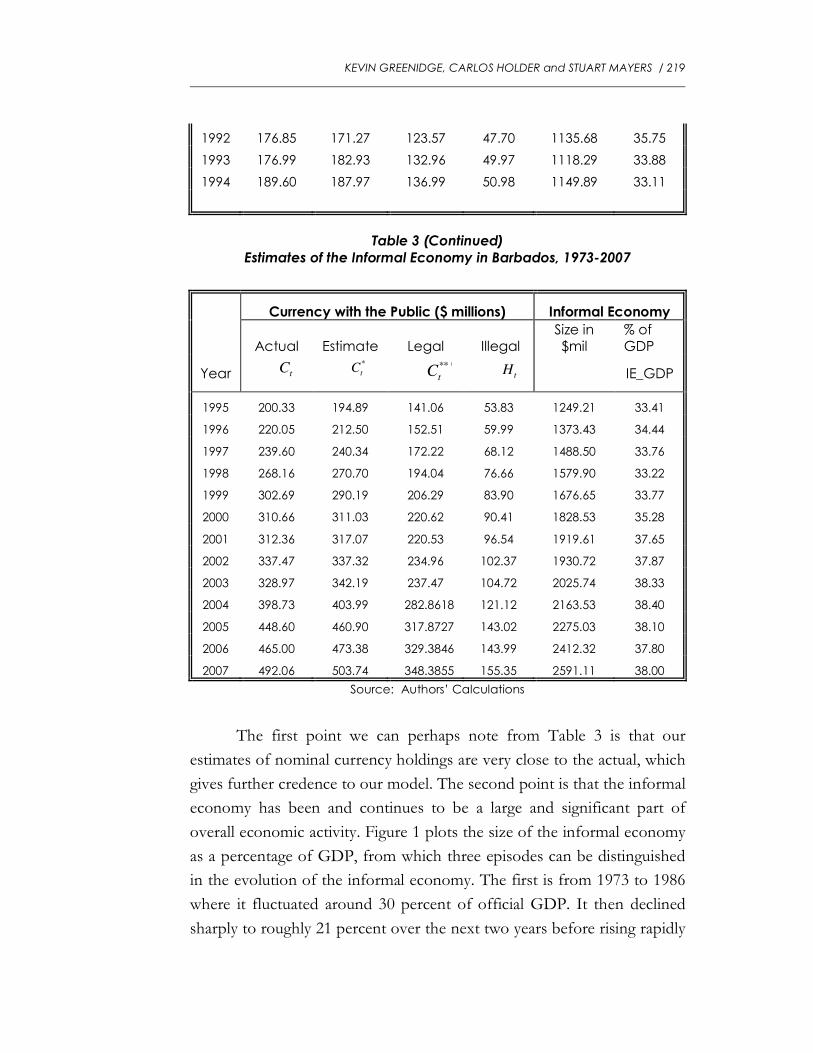
Table 3 (Continued)
Estimates of the Informal Economy in Barbados, 1973-2007
Currency with the Public ($ millions) Informal Economy
Actual Estimate Legal Illegal Size in $mil
% of GDP
Year
IE_GDP
1995 200.33 194.89 141.06 53.83 1249.21 33.41
1996 220.05 212.50 152.51 59.99 1373.43 34.44
1997 239.60 240.34 172.22 68.12 1488.50 33.76
1998 268.16 270.70 194.04 76.66 1579.90 33.22
1999 302.69 290.19 206.29 83.90 1676.65 33.77
2000 310.66 311.03 220.62 90.41 1828.53 35.28
2001 312.36 317.07 220.53 96.54 1919.61 37.65
2002 337.47 337.32 234.96 102.37 1930.72 37.87
2003 328.97 342.19 237.47 104.72 2025.74 38.33
2004 398.73 403.99 282.8618 121.12 2163.53 38.40
2005 448.60 460.90 317.8727 143.02 2275.03 38.10
2006 465.00 473.38 329.3846 143.99 2412.32 37.80
2007 492.06 503.74 348.3855 155.35 2591.11 38.00
Source: Authors’ Calculations
The first point we can perhaps note from Table 3 is that our
estimates of nominal currency holdings are very close to the actual, which
gives further credence to our model. The second point is that the informal
economy has been and continues to be a large and significant part of
overall economic activity. Figure 1 plots the size of the informal economy
as a percentage of GDP, from which three episodes can be distinguished
in the evolution of the informal economy. The first is from 1973 to 1986
where it fluctuated around 30 percent of official GDP. It then declined
sharply to roughly 21 percent over the next two years before rising rapidly
*
tC **
tC
**
tCt
Ct
H
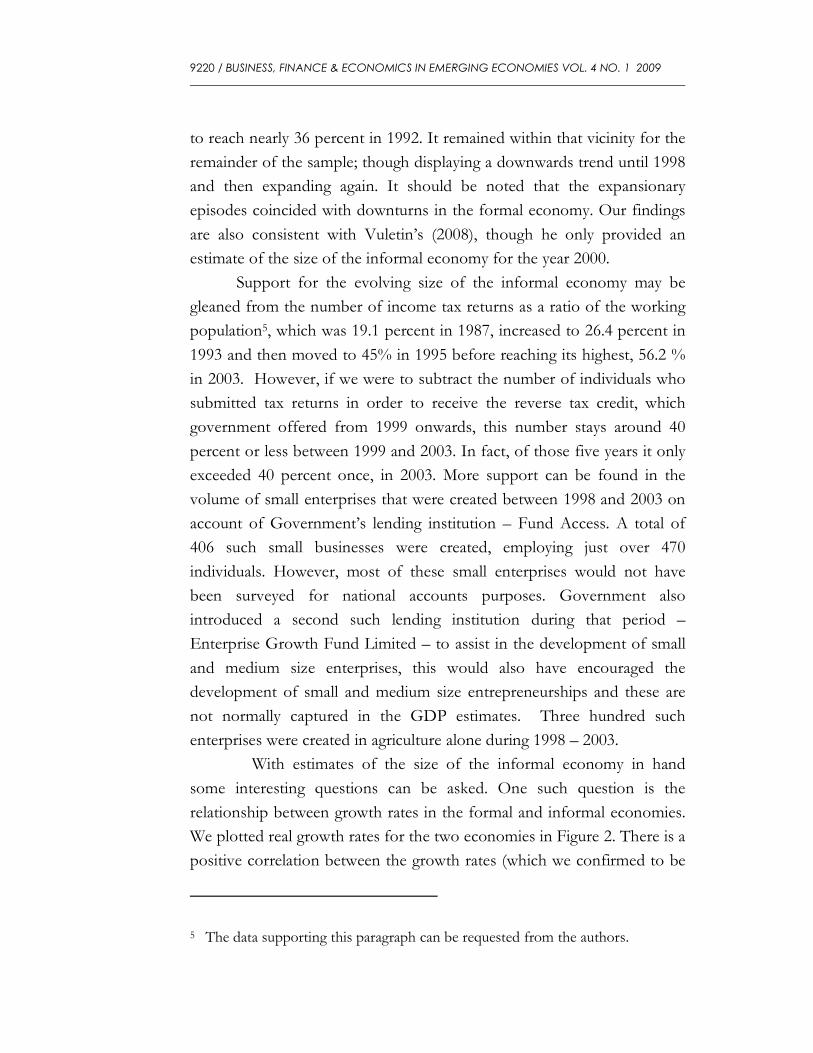
9220 / BUSINESS, FINANCE & ECONOMICS IN EMERGING ECONOMIES VOL. 4 NO. 1 2009
to reach nearly 36 percent in 1992. It remained within that vicinity for the
remainder of the sample; though displaying a downwards trend until 1998
and then expanding again. It should be noted that the expansionary
episodes coincided with downturns in the formal economy. Our findings
are also consistent with Vuletin’s (2008), though he only provided an
estimate of the size of the informal economy for the year 2000.
Support for the evolving size of the informal economy may be
gleaned from the number of income tax returns as a ratio of the working
population5, which was 19.1 percent in 1987, increased to 26.4 percent in
1993 and then moved to 45% in 1995 before reaching its highest, 56.2 %
in 2003. However, if we were to subtract the number of individuals who
submitted tax returns in order to receive the reverse tax credit, which
government offered from 1999 onwards, this number stays around 40
percent or less between 1999 and 2003. In fact, of those five years it only
exceeded 40 percent once, in 2003. More support can be found in the
volume of small enterprises that were created between 1998 and 2003 on
account of Government’s lending institution – Fund Access. A total of
406 such small businesses were created, employing just over 470
individuals. However, most of these small enterprises would not have
been surveyed for national accounts purposes. Government also
introduced a second such lending institution during that period –
Enterprise Growth Fund Limited – to assist in the development of small
and medium size enterprises, this would also have encouraged the
development of small and medium size entrepreneurships and these are
not normally captured in the GDP estimates. Three hundred such
enterprises were created in agriculture alone during 1998 – 2003.
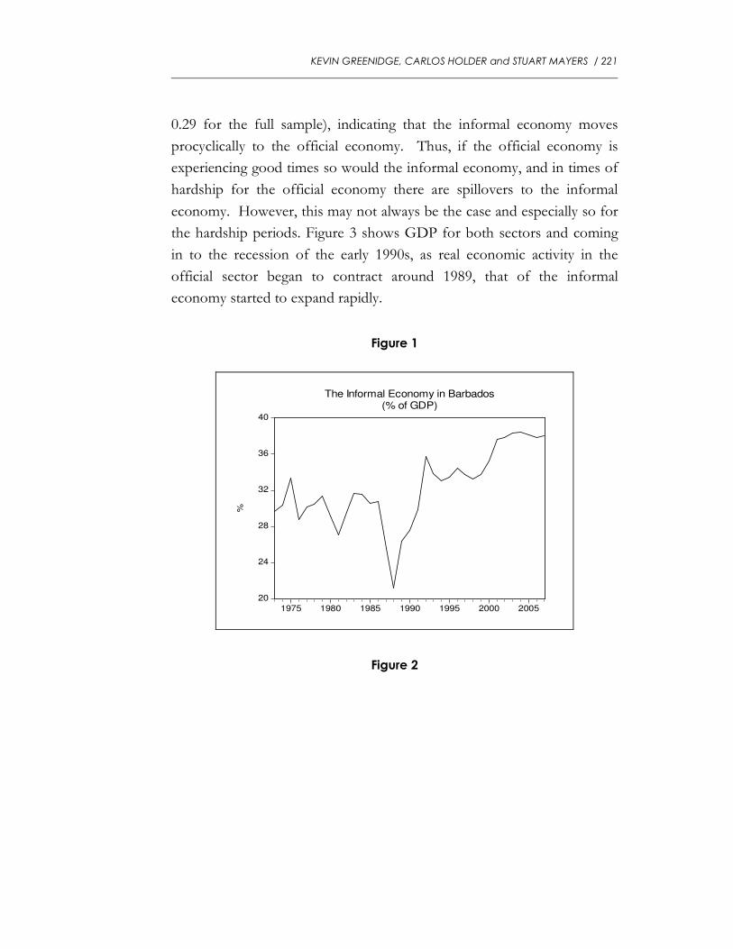
With estimates of the size of the informal economy in hand
some interesting questions can be asked. One such question is the
relationship between growth rates in the formal and informal economies.
We plotted real growth rates for the two economies in Figure 2. There is a
positive correlation between the growth rates (which we confirmed to be
5 The data supporting this paragraph can be requested from the authors.
KEVIN GREENIDGE, CARLOS HOLDER and STUART MAYERS / 221
0.29 for the full sample), indicating that the informal economy moves
procyclically to the official economy. Thus, if the official economy is
experiencing good times so would the informal economy, and in times of
hardship for the official economy there are spillovers to the informal
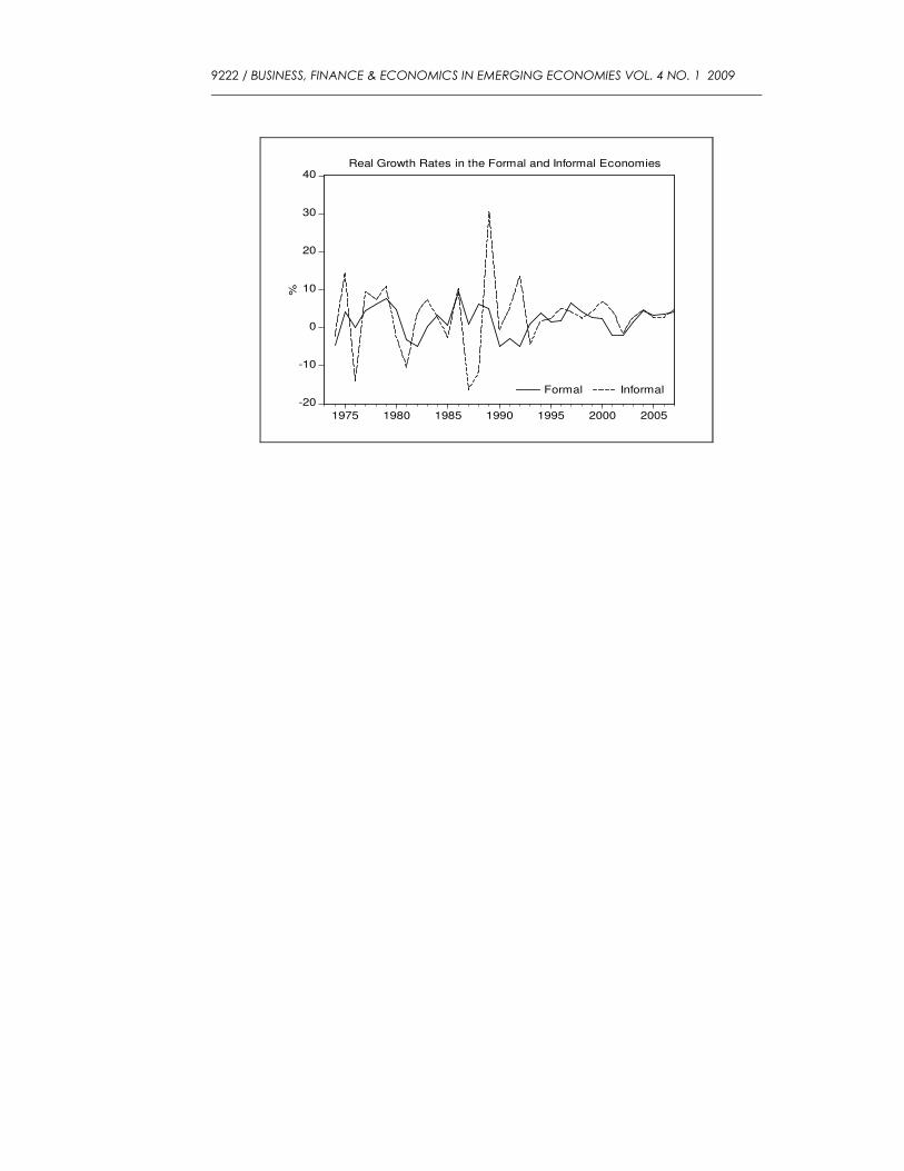
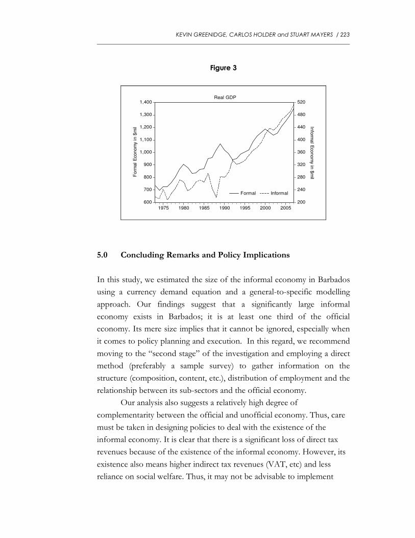
economy. However, this may not always be the case and especially so for
the hardship periods. Figure 3 shows GDP for both sectors and coming
in to the recession of the early 1990s, as real economic activity in the
official sector began to contract around 1989, that of the informal
economy started to expand rapidly.
Figure 1
20
24
28
32
36
40
1975 1980 1985 1990 1995 2000 2005
The Informal Economy in Barbados(% of GDP)
%
Figure 2
9222 / BUSINESS, FINANCE & ECONOMICS IN EMERGING ECONOMIES VOL. 4 NO. 1 2009
-20
-10
0
10
20
30
40
1975 1980 1985 1990 1995 2000 2005
Formal Informal
%
Real Growth Rates in the Formal and Informal Economies
KEVIN GREENIDGE, CARLOS HOLDER and STUART MAYERS / 223
Figure 3
600
700
800
900
1,000
1,100
1,200
1,300
1,400
200
240
280
320
360
400
440
480
520
1975 1980 1985 1990 1995 2000 2005
Formal Informal
Form
al E
conom
y in
$m
il
Info
rmal E
conom
y in $
mil
Real GDP
5.0 Concluding Remarks and Policy Implications
In this study, we estimated the size of the informal economy in Barbados
using a currency demand equation and a general-to-specific modelling
approach. Our findings suggest that a significantly large informal
economy exists in Barbados; it is at least one third of the official
economy. Its mere size implies that it cannot be ignored, especially when
it comes to policy planning and execution. In this regard, we recommend
moving to the “second stage” of the investigation and employing a direct
method (preferably a sample survey) to gather information on the
structure (composition, content, etc.), distribution of employment and the
relationship between its sub-sectors and the official economy.
Our analysis also suggests a relatively high degree of
complementarity between the official and unofficial economy. Thus, care
must be taken in designing policies to deal with the existence of the
informal economy. It is clear that there is a significant loss of direct tax
revenues because of the existence of the informal economy. However, its
existence also means higher indirect tax revenues (VAT, etc) and less
reliance on social welfare. Thus, it may not be advisable to implement
9224 / BUSINESS, FINANCE & ECONOMICS IN EMERGING ECONOMIES VOL. 4 NO. 1 2009
policies (compliance policies) to force the informal sector out of
existence, instead remove the incentives for participants to engage in
informal sector activities (lower the tax burden, eliminate unnecessary
regulations, etc.), thereby, gradually integrating the informal economy into
the formal economy.
Finally, it would also be interesting to extend our approach to
other Caribbean countries and thus be able to make direct comparisons
with the findings of other studies and, more importantly, undertake cross-
country analyses.
REFERENCES
Bajada, C. 1999. "Estimates of the Underground Economy in Australia",
Economic Record, Vol. 75, No. 231, 369-384.
Barbados Statistical Service Department 1998. Informal Sector Survey,
1997/1998, Bridgetown, Barbados: Barbados Statistical Service..
Blough, S. R. 1992. "The Relationship between Power and Level for
Generic Unit Root Tests in Finite Samples", Journal of Applied
Econometrics. Vol. 7, No. 3, 295-308.
Cagan, P. 1958. "The Demand for Currency Relative to the Total Money
Supply", Journal of Political Economy. Vol. 66, No. 3, 302-328.
Dickey, D. A. and Fuller, W. 1979., "Distribution of the Estimators for
Autoregressive Time Series with a Unit Root". Journal of the
American Statistical Association, Vol. 74, No. 366, 427-431.
Elliott, G., Rothenberg, T. J., and Stock, J. H. 1996. "Efficient Tests for
an Autoregressive Unit Root", Econometrica, Vol. 64, No. 4, pp.
813-836.
Faal, E. 2003. "Currency Demand, the Underground Economy, and Tax
Evasion: The Case of Guyana", Working Paper 03/07, International
Monetary Fund.
KEVIN GREENIDGE, CARLOS HOLDER and STUART MAYERS / 225
Feige, E. L. 1979. "How Big is the Irregular Economy?". Challenge, Vol.
22, No. 1, 5-13.
Feige, E. L. 1989. The Underground Economies: Tax Evasion and Information
Distortion, Cambridge: Cambridge University Press.
Feige, E. L. 1996. "Overseas Holdings of U.S. Currency and the
Underground Economy," in Exploring the underground economy: Studies
of Illegal and Unreported Activity, edited by S. Pozo, Michigan: UpJohn
Institute for Employment Research.
Frey, B. S. and Pommerehne, W. W. 1984. "The Hidden Economy: State
and Prospects for Measurement", Review of Income and Wealth, Vol.
30, No. 1, 1-23.
Gutmann, P. M. 1977. "The Subterranean Economy". Financial Analysts
Journal, Vol. 34, No. 1, 24-27.
Harris, R. I. D. 1995. Using Cointegration Analysis in Econometric Modelling,
London: Prentice Hall/Harvester Wheatsheaf.
Inder, B. 1993. "Estimating Long-Run Relationships in Economics: A
Comparison of Different Approaches", Journal of Econometrics, Vol.
57, No. 1-3, 53-68.
Inter-American Development Bank 2006. "The Informal Sector of
Jamaica". Economic and Sector Studies Series, RE3-06-010.
Johnson, S., Kaufmann, D., and Shleifer, A. 1997. "The Unofficial
Economy in Transition". Brookings Papers on Economic Activity No. 2,
159-221.
Kaliberda, A. and Kaufmann, D. 1996. "Integrating the Unofficial
Economy into the Dynamics of Post-Socialist Economies: A
Framework of Analysis and Evidence". The World Bank Policy
Research Working Paper Series, No. 1691.
Krolzig, H. M. and Hendry, D. F. 2001. "Computer Automation of
General-to-Specific Model Selection Procedures". Journal of
Economic Dynamics and Control, Vol. 25, No. 6-7, 831-866.
Kwiatkowski, D., Phillips, P. C. B., Schmidt, P., and Shin, Y. 1992.
"Testing The Null Hypothesis Of Stationarity Against The
Alternative Of A Unit Root: How Sure Are We That Economic
9226 / BUSINESS, FINANCE & ECONOMICS IN EMERGING ECONOMIES VOL. 4 NO. 1 2009
Time Series Have A Unit Root?". Journal of Econometrics, Vol. 54,
No. 1-3, 159-178.
Lanne, M., Lutkepohl, H., and Saikkonen, P. 2002. "Comparison of Unit
Root Tests for Time Series with Level Shifts". Journal of Time Series
Analysis, Vol. 23, No. 6, 667-685.
LeFranc, MacFarane, G., and Taylor, H. 1987. Petty Trading and Labor
Market Mobility: Higglers in the Kingston Metropolitan Area. Paper
presented at Caribbean Studies Association Conference: Belize.
Maurin, A., Sookram, S., and Watson, P. K. 2006. "Measuring the Size of
the Hidden Economy in Trinidad and Tobago, 1973-1999",
International Economic Journal, Vol. 20, No. 3, 321-341.
Ng, S. and Perron, P. 2001. "Lag Length Selection and the Construction
of Unit Root Tests with Good Size and Power". Econometrica, Vol.
69, No. 6, 1519-1554.
O'Neill, D. M. 1983. "Growth of the Underground Economy, 1950-81:
Some Evidence from the Current Population Survey". A Study for
Joint Economic Committee, Congress of the United States.
Pagan, A. 1995. "The Three Econometric Methodologies: An Update." in
Surveys in Econometrics, edited by L. Oxley et al., Oxford: Blackwell.
Perron, P. and Ng, S. 1996. "Useful Modifications to Some Unit Root
Tests with Dependent Errors and Their Local Asymptotic
Properties", Review of Economic Studies, Vol. 63, No. 3, 435-463.
Phillips, P. C. B. and Perron, P. 1988. "Testing for a Unit Root in Time
Series Regression", Biometrika, Vol. 75, No. 2, 335-346.
Saikkonen, P. and Lutkepohl, H. 2002. "Testing for a Unit Root in a Time
Series with a Level Shift at Unknown Time", Econometric Theory,
Vol. 18, No. 2, 313-348.
Schneider, F. and Enste, D. H. 2000. "Shadow Economies: Size, Causes,
and Consequences", Journal of Economic Literature, Vol. 38, No. 1,
77-114.
Schwert, G. W. 1989. "Tests for Unit Roots: A Monte Carlo
Investigation", Journal of Business and Economic Statistics, Vol. 7, No.
2, 147-159.
KEVIN GREENIDGE, CARLOS HOLDER and STUART MAYERS / 227
Smikle, C. and Taylor, H. 1977. Higgler Survey, Jamaica: Agricultural
Planning Unit.
Tanzi, V. 1980. "The Underground Economy in the United States:
Estimates and Implications", Banca Nazionale del Lavoro Quarterly
Review No. 135, 427-453.
Tanzi, V. 1983. "The Underground Economy in the United States: Annual
Estimates, 1930-80", International Monetary Fund Staff Papers, Vol. 30,
No. 2, 283-305.
Vuletin, G. J. 2008. "Measuring the Informal Economy in Latin America
and the Caribbean". Working Paper WP/08/102, International
Monetary Fund.
Witter, M. and Kirton, C. 1990. "The Informal Economy in Jamaica,
Some Empirical Exercises". Kingston, Jamaica, Institute of Social and
Economic Research, Working Paper 36, The University of the West Indies.