Estimating the Number of Species in a Population

by

Shinji Uemura

A Project

Submitted to the Faculty

of the

WORCESTER POLYTECHNIC INSTITUTE

In partial fulfillment of the requirements for the

Degree of Master of Science

in

Applied Statistics

by

December 2006

APPROVED:

Professor Corinne Grace B. Burgos, Advisor

Professor Bogdan M. Vernescu, Department Head

Abstract

This paper is concerned with the estimation of the number of species in a popu-

lation. This is a familiar problem in ecological studies. Many scientists and statis-

ticians have studied this problem. The method in estimating the number of species

can be used in many other areas such as estimating the number of author’s vocab-

ulary.

Many approaches have been proposed, some purely data-analytic and others

based in sampling theory. We consider the latter case and focus on three methods

in this paper. First one was based on the paper of Efron and Thisted [7]. Second

one was given by Boneh, et. al. [4]. Third one was about Bayesian method and

was proposed by Rodrigues, et. al. [22]. And we compare these methods using Mt.

Kenya data and Mt. Mandalagan data.

As a result, the first two methods underestimate the number of species in the

population for both data sets. The Bayesian method gives us more reasonable

estimates and credible intervals. But we need to know the upper bound value

beforehand, which is usually provided by an expert or analyst involved in the study.

Thus, we need to construct another model which does not have to have the upper

bound value for further research.

Acknowledgements

First and formost, I would like to express my deepest gratitude to my advisor, Dr.

Corinne Burgos, for not only advising me on this project but also for her patience

and encouragement while doing so.

I would also like to thank the rest of the Statistics professors at Worcester Poly-

technic Institute for all of their guidance and support as well.

And to my entire family for their support, both financially and emotionally, I

am extremely greateful. Without their constant understanding and compassion, I

would not have been able to accomplish all that I have already.

i

Contents

1 Background 1

1.1 Introduction . . . . . . . . . . . . . . . . . . . . . . . . . . . . . . . . 1

1.2 Statement of the Problem . . . . . . . . . . . . . . . . . . . . . . . . 5

2 Review of Related Literature 8

2.1 Estimating the Number of Species: A Review by J. Bunge and M.

Fitzpatrick [5] . . . . . . . . . . . . . . . . . . . . . . . . . . . . . . . 8

2.1.1 Finite Population, Hypergeometric Sample . . . . . . . . . . . 9

2.1.2 Finite Population, Bernoulli Sample . . . . . . . . . . . . . . . 10

2.1.3 Infinite Population, Multinomial Sample . . . . . . . . . . . . 10

2.2 Bayesian Estimation of the Number of Species by W. A. Lewins and

D. N. Joanes [15] . . . . . . . . . . . . . . . . . . . . . . . . . . . . . 11

2.2.1 Model of W. A. Lewins and D. N. Joanes . . . . . . . . . . . . 11

2.3 Estimating the Total Number of Distinct Species Using Presence and

Absence Data by S. A. Mingoti and G. Meeden [17] . . . . . . . . . . 12

2.3.1 Model of S. A. Mingoti and G. Meeden . . . . . . . . . . . . . 13

2.4 The Relation Between the Number of Species and the Number of

Individuals in a Random Sample of an Animal Population by R. A.

Fisher [9] . . . . . . . . . . . . . . . . . . . . . . . . . . . . . . . . . 14

ii

2.5 Estimating the Prediction Function and the Number of Unseen Species

in Sampling with Replacement by S. Boneh, A. Boneh and R. J. Caron

[4] . . . . . . . . . . . . . . . . . . . . . . . . . . . . . . . . . . . . . 18

2.6 Estimating the Number of Unseen Species: How Many Words Did

Shakespeare Know? by B. Efron and R. Thisted [7] . . . . . . . . . . 21

3 Bayesian Approach 24

3.1 Bayesian Inference . . . . . . . . . . . . . . . . . . . . . . . . . . . . 24

3.1.1 Bayes’ Rule . . . . . . . . . . . . . . . . . . . . . . . . . . . . 24

3.1.2 Prediction . . . . . . . . . . . . . . . . . . . . . . . . . . . . . 25

3.1.3 Likelihood . . . . . . . . . . . . . . . . . . . . . . . . . . . . . 26

3.2 Hierarchical Bayesian Analysis for the Number of Species by J. Ro-

drigues, L. A. Milan and J.G. Leite [22] . . . . . . . . . . . . . . . . . 26

4 Numerical Examples 33

4.1 Mount Kenya Experiment . . . . . . . . . . . . . . . . . . . . . . . . 33

4.2 Mount Mandalagan Experiment . . . . . . . . . . . . . . . . . . . . . 40

4.3 Conclusion . . . . . . . . . . . . . . . . . . . . . . . . . . . . . . . . . 46

A Fortran Code 48

iii

List of Figures

1.1 Existing Literature on the Problem of Estimating the Number of

Classes in a Population . . . . . . . . . . . . . . . . . . . . . . . . . . 4

4.1 Plot: Posterior Mode vs Upper Bound for the Mt. Kenya Data . . . . 38

4.2 Plot: Standard Error vs Upper Bound for the Mt. Kenya Data . . . . 39

4.3 Plot: Posterior Mode vs Upper Bound for the Mt. Mandalagan Data 45

4.4 Plot: Standard Error vs Upper Bound for the Mt. Mandalagan Data 46

iv

List of Tables

1.1 Number of Observed Species of Insects in the Sample in Mt. Kenya . 6

1.2 Number of Observed Species of Trees in One Hectare Plot in Mt.

Mandalagan, Negros Occidental . . . . . . . . . . . . . . . . . . . . . 7

4.1 Bias-Correction Iterations for the Mt. Kenya Data . . . . . . . . . . . 35

4.2 Pointwise Comparison for the Estimators of the Mt. Kenya Data,

∆(t) and Ψ∗(t) . . . . . . . . . . . . . . . . . . . . . . . . . . . . . . 36

4.3 Analysis of the Mt. Kenya Data Using Different Upper Bounds . . . 37

4.4 Bias-Correction Iterations for the Mt. Mandalagan . . . . . . . . . . 42

4.5 Pointwise Comparison for the Estimators of the Mt. Mandalagan

Data, ∆(t) and Ψ∗(t) . . . . . . . . . . . . . . . . . . . . . . . . . . . 43

4.6 Analysis of the Mt. Mandalagan Data Using Different Upper Bounds 44

v

Chapter 1

Background

1.1 Introduction

How many species are there? We may be interested in estimating the total

number of species by considering the number of species obtained in a sample. For

example, biologists and ecologists may be interested in estimating the number of

species in a population of plants or animals (Mann)[16]. Numismatists may be

concerned with estimating the number of dies used to produce an ancient coin is-

sue (Stam)[25]. Linguists may be interested in estimating the size of an author’s

vocabulary (Efron and Thisted)[7]. There are many other applications, including

estimating the number of distinct records in a filing system where many records

are duplicated (Arnold and Beaver)[1], undiscovered ”observational phenomena” in

astronomy (Harwit and Hildebrand)[14], errors in a software system (Bickel and

Yahav)[3], executions in South Vietnam (Bickel and Yahav)[2], connected compo-

nents in a graph (Frank)[10], and so on. And much previous work has stemmed from

a parametric model due to Fisher, Corbet and Williams)[9], where Fisher fitted a

theoretical distribution to Williams’s data on macrolepidoptera. Also, Good[11]

1

and, later, Good and Toulmin[12] derived a model based on a set of statistical hy-

potheses concerning the population frequencies of the individual species. However,

throughout we focus exclusively on estimation of C itself, we have to leave aside

many interesting related topics, such as stochastic abundance models (Engen)[8],

measurement of ”diversity” (Patil and Taillie)[19], and so on. We also avoid related

areas such as capture-recapture problems (Pollock)[20] and estimation of the num-

ber of faults in software in continuous time, which, according to Nayak[18], ”can

be regarded as a continuous analogue of the problem of estimating the number of

species in a biological population.”

To estimate the number of species C in a population, we take a sample of size n

from a population, finite or infinite, partitioned into C classes, where C is unknown.

The outcome of this sampling theoretically can be represented by the random vector

n = [n1, ..., nC ]′, where ni is the number of sample items from the ith class, i =

1, ..., C and ni > 0. In short, the random vector n is not observable. Instead

the observable random vector is c = [c1, ..., cn]′, where cj is the number of classes

represented j times in the sample, j = 1, ..., n. The problem is to estimate the

number of classes C based solely on the vector of frequencies of observed classes c.

This vector c is allso called the ”frequencies of frequencies.” Herein c will denote the

total number of classes in the sample, so that c =n∑

j=1

cj. Note that

n =C∑

i=1

ni =n∑

j=1

jcj.

We prefer to write the total number of observed individuals n as the second sum

because the number of species in the population C is unknown.

Many approaches have been considered. Some of them are based on data-analytic

methods and others are based on sampling-theoretic methods (see Figure 1.1). In

2

this paper, we focus on the latter case. If a population is finite, samples may be taken

with replacement (multinomial sampling) or without replacement (hypergeometric

sampling), or by Bernoulli sampling. But a finite population will not be realistic

in many situations because the population size will be unknown. If a population

is infinite, samples may be taken by multinomial sampling or Bernoulli sampling,

or the samples may be the result of random Poisson contributions of each class.

Given a sampling model, one may approach estimation of the number of species via

a parametric or nonparametric formulation; in either case there may be frequentist

and Bayesian procedures.

3

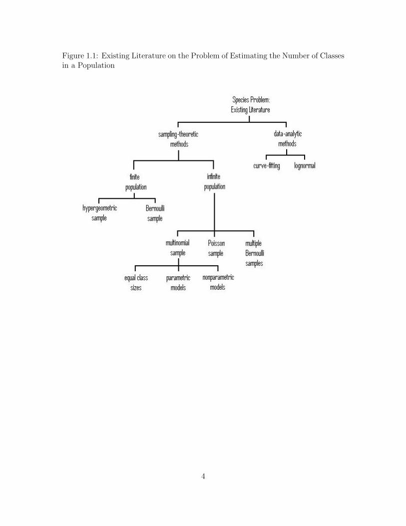
Figure 1.1: Existing Literature on the Problem of Estimating the Number of Classesin a Population

4

1.2 Statement of the Problem

This project aims to achieve the following:

First of all, we give a comprehensive review of methods or approaches to the

problem of estimating the number of species in a population. Secondly, we examine

in detail the different models used in Bayesian approaches. Lastly, we propose a

simple Bayesian model in estimating the number of species in a population.

On two datasets of the number of species in a natural population, we employ

methods from Efron and Thisted [7] and Boneh, Boneh and Caron [4] as imple-

mented in [21] and the Bayesian procedure.

The first dataset is the species distribution of a sample from Mount Kenya. This

dataset was used by Lewins and Joanes [15]. An experiment was performed to get

information on the insect population within a particular region. In consultation with

the experimenters an appropriate prior mode of 45 species was identified. And also

the experimenters were confident that the total number of species in the population

lay between 35 and 55. The dataset is shown in Table 1.1. Here, the sampe size, n,

is 1043 and the total number of observed species in the sample, s′, is 32.

The second dataset is the species distribution of a sample from Mount Man-

dalagan. This dataset was used by Cordon [6]. He obtained these data through

counting the number of different kinds of trees in one hectare plot with a dimension

of 500m×20m. In this case, the unseen species is the unobserved species of trees in

one hectare plot that exist in Mt. Mandalagan. The data set is shown in Table 1.2.

Here, the sample size is 582 in one hectare plot and there are 49 distinct species of

trees in the area.

5

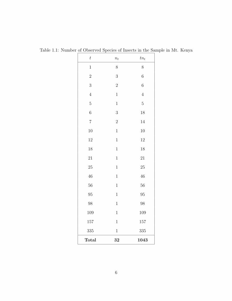
Table 1.1: Number of Observed Species of Insects in the Sample in Mt. Kenya

t nt tnt

1 8 8

2 3 6

3 2 6

4 1 4

5 1 5

6 3 18

7 2 14

10 1 10

12 1 12

18 1 18

21 1 21

25 1 25

46 1 46

56 1 56

95 1 95

98 1 98

109 1 109

157 1 157

335 1 335

Total 32 1043

6

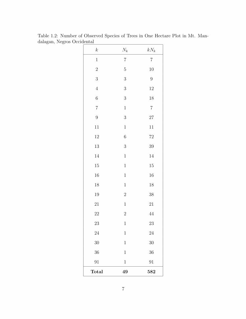
Table 1.2: Number of Observed Species of Trees in One Hectare Plot in Mt. Man-dalagan, Negros Occidental

k Nk kNk

1 7 7

2 5 10

3 3 9

4 3 12

6 3 18

7 1 7

9 3 27

11 1 11

12 6 72

13 3 39

14 1 14

15 1 15

16 1 16

18 1 18

19 2 38

21 1 21

22 2 44

23 1 23

24 1 24

30 1 30

36 1 36

91 1 91

Total 49 582

7

Chapter 2

Review of Related Literature

In this chapter, the papers most relevant to this research is discussed. Com-

ments about the features of previous research are also given.

2.1 Estimating the Number of Species: A Review

by J. Bunge and M. Fitzpatrick [5]

This paper, to date, has given the most comprehensive review of the avail-

able methods and approaches to estimating the number of species in a population.

The authors give a very detailed and structured presentation of the problem and

approaches to it. Some of the details we give below.

Suppose that a population, finite or infinite, is partitioned into C classes.

In many cases we are interested in estimation of C itself. Although estimation of

the relative class proportions is well understood when C is known, estimation of C

itself appears to be quite difficult. Unfortunately, many interesting related topics are

excluded from this paper. Given a sampling model, one may approach estimation

of C via a parametric or nonparametric formulation; in either case there may be

8

frequentist and Bayesian procedures.

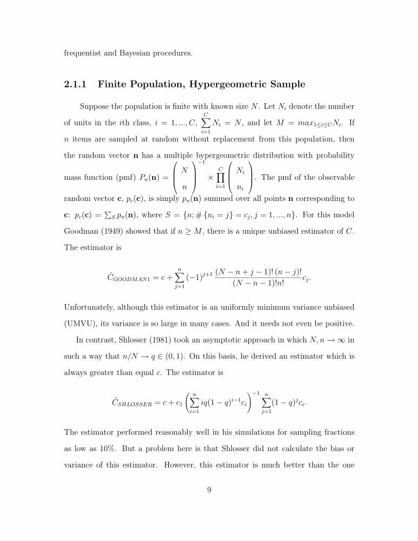
2.1.1 Finite Population, Hypergeometric Sample

Suppose the population is finite with known size N . Let Ni denote the number

of units in the ith class, i = 1, ..., C,C∑

i=1

Ni = N , and let M = max1≤i≤CNi. If

n items are sampled at random without replacement from this population, then

the random vector n has a multiple bypergeometric distribution with probability

mass function (pmf) Pn(n) =

N

n

−1

×C∏

i=1

Ni

ni

. The pmf of the observable

random vector c, pc(c), is simply pn(n) summed over all points n corresponding to

c: pc(c) =∑

S pn(n), where S = {n; # {ni = j} = cj, j = 1, ..., n}. For this model

Goodman (1949) showed that if n ≥ M , there is a unique unbiased estimator of C.

The estimator is

CGOODMAN1 = c +n∑

j=1

(−1)j+1 (N − n + j − 1)! (n− j)!

(N − n− 1)!n!cj.

Unfortunately, although this estimator is an uniformly minimum variance unbiased

(UMVU), its variance is so large in many cases. And it needs not even be positive.

In contrast, Shlosser (1981) took an asymptotic approach in which N, n →∞ in

such a way that n/N → q ∈ (0, 1). On this basis, he derived an estimator which is

always greater than equal c. The estimator is

CSHLOSSER = c + c1

(n∑

i=1

iq(1− q)i−1ci

)−1 n∑j=1

(1− q)jci.

The estimator performed reasonably well in his simulations for sampling fractions

as low as 10%. But a problem here is that Shlosser did not calculate the bias or

variance of this estimator. However, this estimator is much better than the one

9

derived by Goodman.

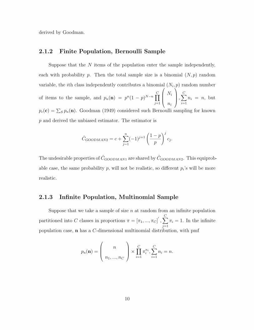
2.1.2 Finite Population, Bernoulli Sample

Suppose that the N items of the population enter the sample independently,

each with probability p. Then the total sample size is a binomial (N, p) random

variable, the ith class independently contributes a binomial (Ni, p) random number

of items to the sample, and pn(n) = pn(1 − p)N−nC∏

j=1

Ni

ni

,C∑

i=1

ni = n, but

pc(c) =∑

S pn(n). Goodman (1949) considered such Bernoulli sampling for known

p and derived the unbiased estimator. The estimator is

CGOODMAN2 = c +n∑

j=1

(−1)j+1

(1− p

p

)j

cj.

The undesirable properties of CGOODMAN1 are shared by CGOODMAN2. This equiprob-

able case, the same probability p, will not be realistic, so different pi’s will be more

realistic.

2.1.3 Infinite Population, Multinomial Sample

Suppose that we take a sample of size n at random from an infinite population

partitioned into C classes in proportions π = [π1, ..., πC ]′,

C∑j=1

πi = 1. In the infinite

population case, n has a C-dimensional multinomial distribution, with pmf

pn(n) =

n

n1, ..., nC

× C∏i=1

πnii ,

C∑i=1

ni = n.

10

2.2 Bayesian Estimation of the Number of Species

by W. A. Lewins and D. N. Joanes [15]

In this paper, a Bayesian approach is used to estimate the number of species in

a population. Many works have been done by Fisher, Corbet and Williams (1943),

and Good and Toulmin (1956). But the estimation of the total number of species

in the population was not the prime concern of those works. When such estimation

has been the main aim, it has usually been assumed that the species have equal

relative abundances. More recently, nonequiprobable models have been derived by

Efron and Thisted (1976) and Hill (1979). Hill’s model is based on a zero-truncated

negative binomial prior distribution for the number of species, and results of this

paper are also based on this distribution.

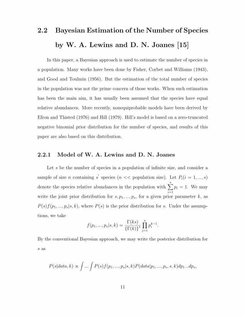
2.2.1 Model of W. A. Lewins and D. N. Joanes

Let s be the number of species in a population of infinite size, and consider a

sample of size n containing s′species (n << population size). Let Pi(i = 1, ..., s)

denote the species relative abundances in the population withs∑

i=1

pi = 1. We may

write the joint prior distribution for s, p1, ..., ps, for a given prior parameter k, as

P (s)f(p1, ..., ps|s, k), where P (s) is the prior distribution for s. Under the assump-

tions, we take

f(p1, ..., ps|s, k) =Γ(ks)

{Γ(k)}s

s∏j=1

pk−1i .

By the conventional Bayesian approach, we may write the posterior distribution for

s as

P (s|data, k) ∝∫

...∫

P (s)f(p1, ..., ps|s, k)P (data|p1, ..., ps, s, k)dp1...dps,

11

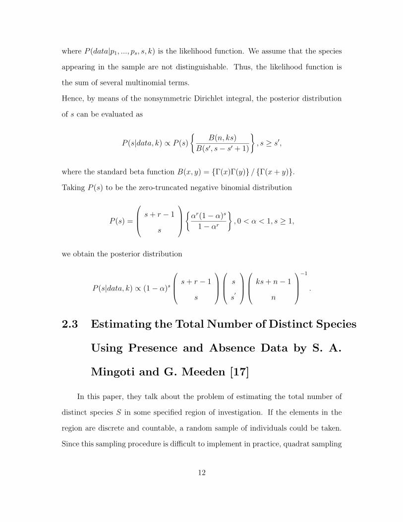
where P (data|p1, ..., ps, s, k) is the likelihood function. We assume that the species

appearing in the sample are not distinguishable. Thus, the likelihood function is

the sum of several multinomial terms.

Hence, by means of the nonsymmetric Dirichlet integral, the posterior distribution

of s can be evaluated as

P (s|data, k) ∝ P (s)

{B(n, ks)

B(s′, s− s′ + 1)

}, s ≥ s′,

where the standard beta function B(x, y) = {Γ(x)Γ(y)} / {Γ(x + y)}.

Taking P (s) to be the zero-truncated negative binomial distribution

P (s) =

s + r − 1

s

{

αr(1− α)s

1− αr

}, 0 < α < 1, s ≥ 1,

we obtain the posterior distribution

P (s|data, k) ∝ (1− α)s

s + r − 1

s

s

s′

ks + n− 1

n

−1

.

2.3 Estimating the Total Number of Distinct Species

Using Presence and Absence Data by S. A.

Mingoti and G. Meeden [17]

In this paper, they talk about the problem of estimating the total number of

distinct species S in some specified region of investigation. If the elements in the

region are discrete and countable, a random sample of individuals could be taken.

Since this sampling procedure is difficult to implement in practice, quadrat sampling

12

is used here. This procedure is more feasible for many real situations. There are two

different ways to perform the quadrat sampling. One is that the region is divided

into N quadrats of equal area, N < ∞, and then we take a random sample of n

quadrats from N , n ≥ 1 and n < N . The other is to place at random n quadrats

of equal area and ficed shape in the region of investigation. In both cases the n

quadrats in the sample are assumed to be disjoint and are totally observed. So if

quadrat sampling is performed in fact, a random sample of space is taken instead of

a random sample of individuals. Within each sampled quadrat the distinct species

present are observed and an empirical Bayes estimator of the total number of species

S in the region is constructed. Finally, they develop an approximate estimate of

standard deviation for the empirical Bayes estimator and study the behavior of

confidence intervals based on this estimate.

2.3.1 Model of S. A. Mingoti and G. Meeden

Suppose that the region of investigation is divided into N disjoint quadrats of

equal area, not necessarily of the same shape, N < ∞. Let S be the total number of

distinct species present in teh region and let s1, ..., sS be the names of those S species.

s1, ..., sS are unknown and S is assumed to be finite. Let pi be the probability of

species si being observed in a typical quadrat of the region, i = 1, ..., S. pi is not

necessarily the probability that the species si is present in the quadrat but can also

be the probability of observing the species si in the quadrat.

let’s assume that p1, ..., pS are independent and identically distributed random

variables from a beta density with parameters α > 0 and β > 0, α and β being

known. Suppose a random sample of n quadrats, n ≥ 1, is taken from the collection

of N quadrats. Let Xi be the number of quadrats in the sample where the species

si was observed, i = 1, ..., S, and let nx be the number of species observed in exactly

13

x quadrats in the sample, nx ∈ {0, 1, ..., S} , x ∈ {0, 1, ..., n}. Then for each species

si the probability that it will be observed in exactly x quadrats in the sample is

γx =∫ 1

0Pr(Xi = x|pi)

Γ(α + β)

Γ(α)Γ(β)pα−1

i (1− pi)β−1dpi

=Γ(α + β)

Γ(α)Γ(β)

∫ 1

0

n

x

px+α−1(1− p)n−x+β−1dp

=

n

x

Γ(α + β)

Γ(α)Γ(β)

Γ(x + α)Γ(n + β − x)

Γ(n + α + β).

So γx is the same for any species si, and represents the probability that a typical

species will be observed in exactly x quadrats of those n quadrats in the sample.

Given S and γx (x = 0, 1, ..., n), nx is a binomial random variable with expectation

given by

nx = ES(nx) = Sγx.

2.4 The Relation Between the Number of Species

and the Number of Individuals in a Random

Sample of an Animal Population by R. A.

Fisher [9]

He talks about the relationship between the Poisson Series and the Negative

Binomial distribution first. If successive independent equal samples are taken from

homogeneous material in biological sampling, the number of individuals observed

in different samples will vary in a definite manner. The distribution of the number

14

observed will be the Poisson series, which has a single parameter m expressed in

terms of the number expected. The distribution is given by

e−m mn

n!,

where n is the variate representing the number observed in any sample and m is the

number expected, which is the average value of n. m will be proportional to the

size of the sample taken.

An important extension of the Poisson series is provided by the supposition that

the values of m are distributed in a known and simple manner. Since m must be

positive, the simplest supposition as to its distribution is that it has the Eulerian

form such that the element of frequency or probability with which it falls in any

infinitesimal range dm is

df =1

(k − 1)!p−kmk−1e−m/νdm.

If we multiply this expression by the probability of observing n organisms and

integrate with respect to m over its whole range from 0 to ∞, we have

∫ ∞

0

1

(k − 1)!p−kmk−1e−m/pe−m mn

n!dm =

(k + n− 1)!

(k − 1)!n!

pn

(1 + p)k+n· · · ⊗,

which is the probability of observing the number n. Since this distribution is related

to the negative binomial expansion

(1− p

1 + p

)−k

=∞∑

n=0

(k + n− 1)!

(k − 1)!n!

(p

1 + p

)n

,

it has become the Negative Binomial distribution. The parameter p is proportional

15

to the sample size and the parameter k measures the variability of the different

expectations of the component Poisson series. The expectation, or mean value of n,

is pk.

Next, he talks about the limiting form of the negative binomial, excluding zero

observations. In many of its applications the number n observed in any sample may

have all integral values including zero. However, in its application to the number

of representatives of different species obtained in a collection, only frequencies of

numbers greater than zero will be observable, since by itself the collection gives no

indication of the number of species which are not found in it. Now, the abundance

in nature of different species of the same group generally varies very greatly, so that,

the negative binomial has a value of k so small as to be almost indeterminate in

magnitude or indistinguishable from zero. That it is not really zero for collections

of wild species follows from the fact that the total number of species, and therefore

the total number not included in the collection, is really finite. However, the real

situation in which many species are so rare that their chance of inclusion is small is

well represented by the limiting form taken by the negative binomial distribution,

when k tends to zero.

If we put k = 0 in right-hand side of expression ⊗, write x for p/(p + 1), so

that x stands for a positive number less than 1, and replace the constant factor

(k − 1)! in denominator by a new constant factor alpha in the numerator, we have

an expression for the expected number of species with n individuals, where n cannot

be zero,

α

nxn.

16

The total number of species expected is

S =∞∑

n=1

α

nxn = −α log(1− x).

The total number of individuals expected is

N =∞∑

n=1

αxn =αx

1− x.

If x is eliminated from the two equations, it appears that

S = α log(1 +

N

α

), N = α(eS/α − 1),

and

N

S= (eS/α − 1)÷ S/α.

These numerical processes are exhibited for fitting the series to observations con-

taining given numbers of species and individuals, and for estimating the parameter

α representing the richness in species of the material sampled; secondly, for calcu-

lating the standard error of α, and thirdly, for testing whether the series exhibits a

significant deviation from the limiting form used.

17

2.5 Estimating the Prediction Function and the

Number of Unseen Species in Sampling with

Replacement by S. Boneh, A. Boneh and R.

J. Caron [4]

We introduce the two basic models presented by Boneh, Boneh and Caron which

will be used as basis for the two estimators. Suppose there are s species sampled

independently with replacement and each has probabilities p1, ..., ps, 0 < pi < 1 so

that∑s

i=1 pi = 1. Alternatively, consider s parallel independent Poisson processes

with positibe parameters λ1, ..., λs. The probabilities and the mean of the Poisson

processes can be ralated by interpreting the occurences of the jth Poisson process

as observations of the jth species, with the parameters related by pj = λj/(λ1 + ...+

λs), j = 1, 2, ..., s.

Let [−1, 0] be the time interval over which the occurrences of the Poisson processes

were recorded. This time interval would correspond to a given information about a

sample. A process is said to have been detected if there was at least one occurrence

of that process. Let D(t) be the number of new detections in (0, t] but not in [−1, 0].

Its expected value, denoted by Ψ(t) = E[D(t)], is called the prediction function. Let

Nk be the number of species observed exactly k times in [−1, 0], k = 1, 2, ....

We define and specify the prediction function Ψ(t) as

Ψ(t) =s∑

j=1

e−λj −s∑

j=1

e−λj(1+t)

=∞∑

k=1

(−1)k+1E(Nk)tk.

18

This prediction function computes the expected number of newly detected species

in (0, t] but not in [−1, 0].

The three properties of the prediction function Ψ(t) are the following:

1. Ψ(t) = 0

2. Ψ(t) has a horizontal asymptote (i.e., Ψ(∞) < ∞)

3. Ψ(t) has infinite order alternating copositivity.

Boneh, Boneh and Caron suggest an alternative by expressing the prediction

function, Ψ(t) =∑s

j=1 e−λj −∑sj=1 e−λj(1+t), and then estimating the parameter s

and λ1, ..., λs, rather than E(Nk). So, we get the maximum likelihood estimators

(MLEs) for these parameters. In getting the MLE of s, we consider all the number

of distinct species according to the number of times that they appeared denoted by

Nk. Recall that Nk is the number of species that appeared k times. To maximize

the value of s, we get the total number of distinct species as will be given by Nk up

to the maximum value of k. Thus,

s =kmax∑k=1

Nk,

where kmax = max {k : Nk > 0}.

We have λj, ..., λs for the MLEs of λ1, ..., λs, where λj is the number of occur-

rences of the jth eprocess during the interval [−1, 0]. Thus, an estimate of Ψ(t)

is

Ψ(t) =s∑

j=1

e−λj −s∑

j=1

e−λj(1+t)

Since processes can be observed with the same number of times Nk, it will have

19

the same esitmate for λ so that these processes can be grouped. Hence,

Ψ(t) =kmax∑k=1

Nke−k −

kmax∑k=1

Nke−k(1+t)

This estimator is biased. In order to reduce the bias, Boneh, Boneh and Caron

suggested a bias reduction algorithm given below.

Given Nk, k = 1, 2, ...

1. Calculate U0 =∑kmax

k=1 Nke−k.

2. Set i = 1.

3. If U0 ≥ N1, then set Ui = 0.

4. Set Ui = U0 + Ui−1e−N1/Ui−1 .

5. If a stopping criterion is not met, replace i with i + 1 and repeat step 4.

A common stopping criterion for step 5 is to stop as soon as Ui+1 − Ui < δ for

some predetermined δ > 0 where δ is a relatively small value. This means that

if there is a very little difference between succeeding values Ui and Ui+1 then the

algorithm should be terminated.

Hence, the second estimator of the prediction function for estimating the number

of unseen species, denoted by Ψ∗(t), is given by

Ψ∗(t) = Ψ(t) + Ue−λ∗ + Ue−λ∗(1+t),

where Ψ(t) =∑kmax

k=1 Nke−k − ∑kmax

k=1 Nke−k(1+t), U is the last iteration value, and

λ∗ = N1/U .

20

2.6 Estimating the Number of Unseen Species:

How Many Words Did Shakespeare Know?

by B. Efron and R. Thisted [7]

We present the species trapping terminology of Efron and Thisted [7] that will

be used in estimating the number of unseen species. Suppose there is a population

consisting of S species where S is unknown. Suppose in a trapping procedure for

one unit of time, we were able to sample s species where s = 1, 2, ..., S. Let xs be the

random variable that represents the number of captured menbers of species s. We

only observe values of xs which are greater than zero becouse there is no such thing

as a negative number of species. The case xs = 0 is negligible since it will not be

counted in the sample. Moreover, we cannot possibly count the number of captured

members of species s if we have no knowledge that this particular species s exists.

The basic distributional assumption for this trapping procedure is that members of

species s enter the trap following a Poisson process. This means that members of

species s enter the trap (success) per unit time. It is also assumed that the members

of species s that enters the trap following a Poisson process has an expectation of

λs per unit time. Thus, xs has a Poisson distribution with mean λs, s = 1, 2, ..., S.

We further assume that the individual Poisson processes are independent of one

another.

The trapping period can be presented in the period [−1, 0]. Since we want to

estimate the exact number of species in the sample, we wish to extrapolate from the

counts in [−1, 0] to a time t in the futrue. Extrapolating is similar to forecasting or

predicting the future observations using observations from periods -1 to 0 to predict

the observations for the next t periods, that is, period (0, t]. Recall that xs denotes

21

the number of captured members of species s in time period [−1, 0]. This xs will

be helpful in knowing how many members of species s will be on the time period

(0, t]. Let nx be the number of species observed exactly x times in [−1, 0]. This

value may be computed from the available values of xs. It will also be used, like

xs, in computing the estimate for the unseen species. We present the estimator

proposed by Efron and Thisted for the number of unknown species. Let ∆(t) be the

expected number of species observed in the period (0, t] (future), but not in [−1, 0]

(observed period), or it is the expected number of new species to be found in the

next t time units. Recall that Ψ(t) is the expected value of D(t), the number of new

detections in (0, t] but not in [−1, 0]. Thus, ∆(t) is the same as Ψ(t).

∆(t) = Ψ(t) =s∑

j=1

e−λj(1− e−λjt).

Let nx be the number of species observed exactly x times in [−1, 0] which is

similar to Nk based in our basic model. The ecpected value of nx is denoted by ηx.

So, we have

∆(t) = Ψ(t) =∞∑

k=1

(−1)k+1E(nk)tk = η1t− η2t

2 + η3t3 − · · · .

The right hand side of the equation above need not converge, but if we assume

that it does, the equation below suggests the unbiased estimator for ∆(t). The unbi-

ased estimator of ∆(t) is the first proposed estimator that will be used in estimating

the number of unseen species. This is given by

∆(t) = n1t− n2t2 + n3t

3 − · · · .

This equation, unfortunately, is useless for t larger than one because the geomet-

22

rically increasing magnitude of tx produces wild oscillations as the number of terms

increases. This then forces the series not to converge.

These methods described in the last two sections will be used in the numerical

examples in Chapter 4.

23

Chapter 3

Bayesian Approach

3.1 Bayesian Inference

Bayesian statistical conclusions about a parameter θ is made in terms of a

probability statement. This probability statement is conditional on the observed

value of y, and in our notation is written simply as p(θ|y). In this section, we

present the basic mathematics and notation of Bayesian inference.

3.1.1 Bayes’ Rule

In order to make probability statement about θ given y, we must begin with a

model providing a joint probability distribution for θ and y. The joint probability

mass or density function can be written as a product of two densities that are often

referred to as the prior distribution p(θ) and the data distribution p(y|θ) respectively:

p(θ, y) = p(θ)p(y|θ).

24

Simply conditioning on the known value of the data y, using the basic property of

conditional probability known as Bayes’ rule, yields the posterior density:

p(θ|y) =p(θ, y)

p(y)=

p(θ)p(y|θ)p(y)

,

where p(y) =∑

θ p(θ)p(y|θ), and the sum is over all possible values of θ (or p(y) =∫p(θ)p(y|θ)dθ in the case of continuous θ). An equivalent form of the posterior

density above omits the factor p(y), which does not depend on θ and, with fixed

y, can thus be considered a constant, yielding the unnormalized posterior density,

which is the right side of the following expression:

p(θ|y) ∝ p(θ)p(y|θ).

These simple expressions encapsulate the technical core of Bayesian inference: the

primary task of any specific application is to develop the model p(θ, y) and perform

the necessary computations to summarize p(θ|y) in appropriate ways.

3.1.2 Prediction

To make inferences about an unknown observable, often called predictive infer-

ences, we follow a similar logic. Before the data y are considered, the distribution

of the unknown but observable y is

p(y) =∫

p(y, θ)dθ =∫

p(θ)p(y|θ)dθ.

This is often called the marginal distribution of y, but a more informative name is

the prior predictive distribution: prior because it is not conditional on a previous

observation of the process, and predictive because it is the distribution for a quantity

25

that is observable.

3.1.3 Likelihood

Using Bayes’ rule with a chosen probability model means that the data y af-

fect the posterior inference, which is given by p(θ) ∝ p(θ)p(y|θ), only through the

function p(y|θ), which, when regarded as a function of θ, for fixed y, is called the

likelihood function. In this way Bayesian inference obeys what is sometimes called

the likelihood principle, which states that for a given sample of data, any two proba-

bility models p(y|θ) that have the same likelihood function yield the same inference

for θ.

The likelifood principle is reasonable, but only within the framework of the model

or family of models adopted for a particular analysis. In practice, one can rarely be

confident that the chosen model is the correct model.

3.2 Hierarchical Bayesian Analysis for the Num-

ber of Species by J. Rodrigues, L. A. Milan

and J.G. Leite [22]

We present a method for estimation of the number of species in a population

through a hierarchical Bayesian model. Suppose Xi is the number of individuals from

species i in the sample, i = 1, ..., N ; N is the number of species in the population;

Nj =∑N

i=1 I(Xi=j), j ≥ 1 are the frequencies of frequencies where IA means the

indicator function of the set A; n =∑

j≥1 jNj is the sample size and W =∑

j≥1 Nj is

the number of different species in the sample. This hierarchical Bayesian model was

presented in [22] and we modify one step in generating samples from the conditional

26

posterior of one of the parameters.

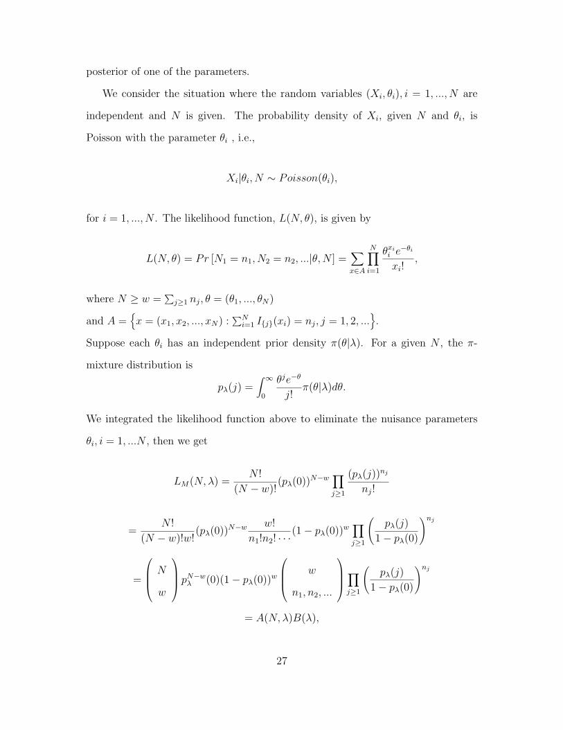
We consider the situation where the random variables (Xi, θi), i = 1, ..., N are

independent and N is given. The probability density of Xi, given N and θi, is

Poisson with the parameter θi , i.e.,

Xi|θi, N ∼ Poisson(θi),

for i = 1, ..., N . The likelihood function, L(N, θ), is given by

L(N, θ) = Pr [N1 = n1, N2 = n2, ...|θ, N ] =∑x∈A

N∏i=1

θxii e−θi

xi!,

where N ≥ w =∑

j≥1 nj, θ = (θ1, ..., θN)

and A ={x = (x1, x2, ..., xN) :

∑Ni=1 I{j}(xi) = nj, j = 1, 2, ...

}.

Suppose each θi has an independent prior density π(θ|λ). For a given N , the π-

mixture distribution is

pλ(j) =∫ ∞

0

θje−θ

j!π(θ|λ)dθ.

We integrated the likelihood function above to eliminate the nuisance parameters

θi, i = 1, ...N , then we get

LM(N, λ) =N !

(N − w)!(pλ(0))

N−w∏j≥1

(pλ(j))nj

nj!

=N !

(N − w)!w!(pλ(0))N−w w!

n1!n2! · · ·(1− pλ(0))

w∏j≥1

(pλ(j)

1− pλ(0)

)nj

=

N

w

pN−wλ (0)(1− pλ(0))

w

w

n1, n2, ...

∏j≥1

(pλ(j)

1− pλ(0)

)nj

= A(N, λ)B(λ),

27

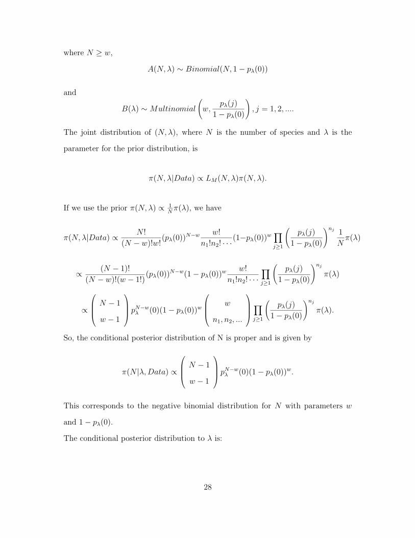
where N ≥ w,

A(N, λ) ∼ Binomial(N, 1− pλ(0))

and

B(λ) ∼ Multinomial

(w,

pλ(j)

1− pλ(0)

), j = 1, 2, ....

The joint distribution of (N, λ), where N is the number of species and λ is the

parameter for the prior distribution, is

π(N, λ|Data) ∝ LM(N, λ)π(N, λ).

If we use the prior π(N, λ) ∝ 1N

π(λ), we have

π(N, λ|Data) ∝ N !

(N − w)!w!(pλ(0))

N−w w!

n1!n2! · · ·(1−pλ(0))

w∏j≥1

(pλ(j)

1− pλ(0)

)nj 1

Nπ(λ)

∝ (N − 1)!

(N − w)!(w − 1!)(pλ(0))N−w(1− pλ(0))

w w!

n1!n2! · · ·∏j≥1

(pλ(j)

1− pλ(0)

)nj

π(λ)

∝

N − 1

w − 1

pN−wλ (0)(1− pλ(0))

w

w

n1, n2, ...

∏j≥1

(pλ(j)

1− pλ(0)

)nj

π(λ).

So, the conditional posterior distribution of N is proper and is given by

π(N |λ, Data) ∝

N − 1

w − 1

pN−wλ (0)(1− pλ(0))

w.

This corresponds to the negative binomial distribution for N with parameters w

and 1− pλ(0).

The conditional posterior distribution to λ is:

28

π(λ|N, Data) ∝ pN−wλ (0)

∏j≥1

pnj

λ (j)π(λ).

We wish to evaluate the posterior distribution of N and λ based on the Poisson-

gamma mixture distribution. We express the prior not as a function of λ but as a

function of parameters α and β as follows:

θi|α, β ∼ Γ[β,

1− α

α

], λ = (α, β), β > 0

where the π-mixture is

pλ(j) =∫ ∞

0

θje−θ

j!π(θ|α, β)dθ

=∫ ∞

0

θje−θ

j!

(1− α

α

)β θβ−1e−( 1−αα )θ

Γ(β)dθ

=(1− α)β

αβΓ(β)j!

∫ ∞

0e−( 1

α)θθβ+j−1dθ

=(1− α)β

αβΓ(β)j!

Γ(β + j)(1α

)β+j

∫ ∞

0

(1α

)β+j

Γ(β + j)e−( 1

α)θθβ+j−1dθ

=(1− α)β

Γ(β)

Γ(β + j)

j!αj = NB[j; β, 1− α],

for j = 0, 1, .... If j = 0, then we have

pλ(0) = (1− α)β.

We assume the non-informative prior for all parameters π(N, α, β) ∝ 1N

, so that the

29

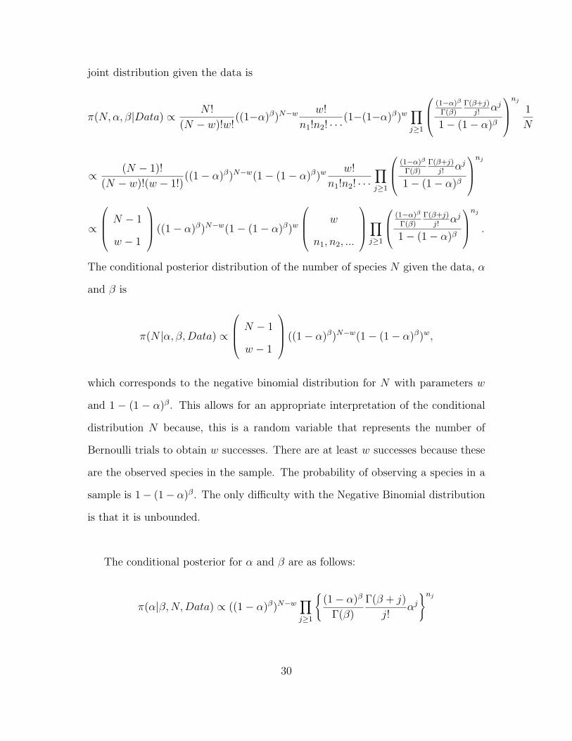
joint distribution given the data is

π(N, α, β|Data) ∝ N !

(N − w)!w!((1−α)β)N−w w!

n1!n2! · · ·(1−(1−α)β)w

∏j≥1

(1−α)β

Γ(β)Γ(β+j)

j!αj

1− (1− α)β

nj

1

N

∝ (N − 1)!

(N − w)!(w − 1!)((1− α)β)N−w(1− (1− α)β)w w!

n1!n2! · · ·∏j≥1

(1−α)β

Γ(β)Γ(β+j)

j!αj

1− (1− α)β

nj

∝

N − 1

w − 1

((1− α)β)N−w(1− (1− α)β)w

w

n1, n2, ...

∏j≥1

(1−α)β

Γ(β)Γ(β+j)

j!αj

1− (1− α)β

nj

.

The conditional posterior distribution of the number of species N given the data, α

and β is

π(N |α, β, Data) ∝

N − 1

w − 1

((1− α)β)N−w(1− (1− α)β)w,

which corresponds to the negative binomial distribution for N with parameters w

and 1 − (1 − α)β. This allows for an appropriate interpretation of the conditional

distribution N because, this is a random variable that represents the number of

Bernoulli trials to obtain w successes. There are at least w successes because these

are the observed species in the sample. The probability of observing a species in a

sample is 1− (1− α)β. The only difficulty with the Negative Binomial distribution

is that it is unbounded.

The conditional posterior for α and β are as follows:

π(α|β, N, Data) ∝ ((1− α)β)N−w∏j≥1

{(1− α)β

Γ(β)

Γ(β + j)

j!αj

}nj

30

∝ (1− α)βN∏j≥1

{Γ(β + j)

Γ(β)j!αj

}nj

∝ (1− α)βNαn∏j≥1

{Γ(β + j)

Γ(β)j!

}nj

∝ Γ(n + 1 + βN + 1)

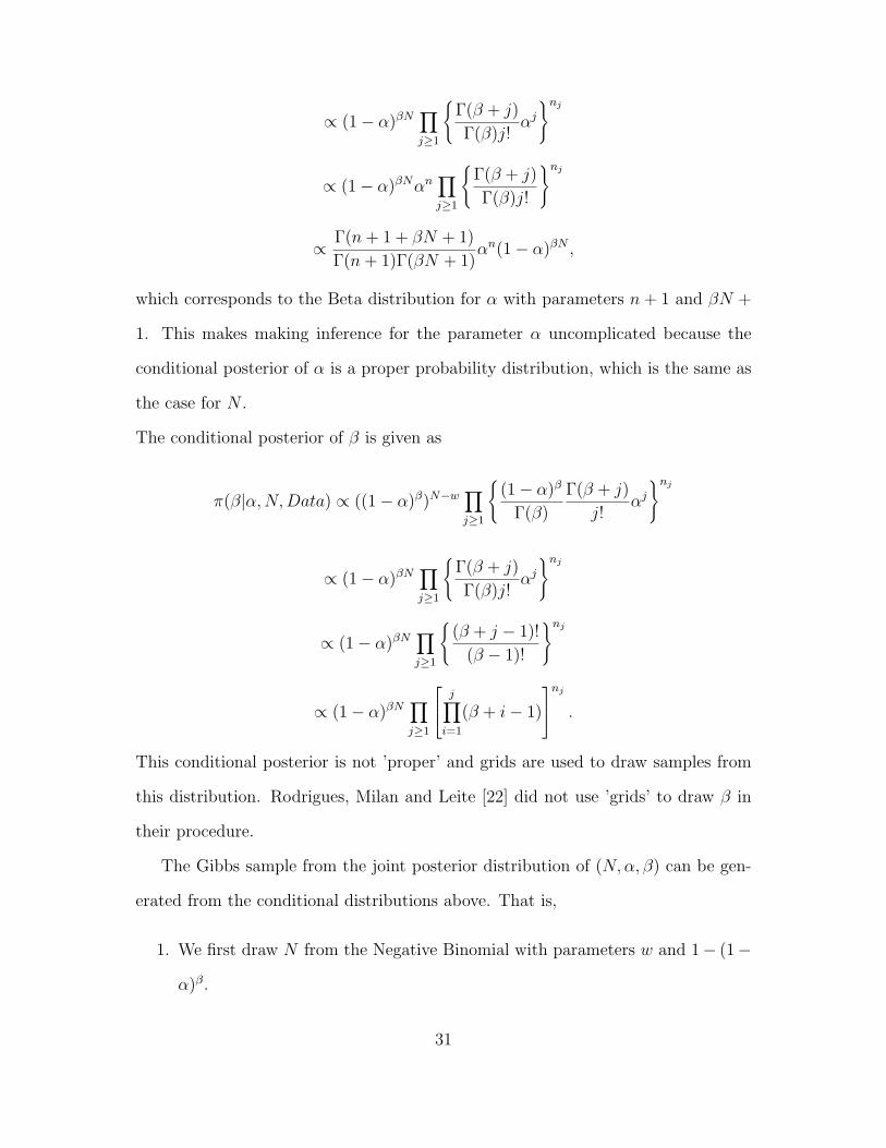
Γ(n + 1)Γ(βN + 1)αn(1− α)βN ,

which corresponds to the Beta distribution for α with parameters n + 1 and βN +

1. This makes making inference for the parameter α uncomplicated because the

conditional posterior of α is a proper probability distribution, which is the same as

the case for N .

The conditional posterior of β is given as

π(β|α, N, Data) ∝ ((1− α)β)N−w∏j≥1

{(1− α)β

Γ(β)

Γ(β + j)

j!αj

}nj

∝ (1− α)βN∏j≥1

{Γ(β + j)

Γ(β)j!αj

}nj

∝ (1− α)βN∏j≥1

{(β + j − 1)!

(β − 1)!

}nj

∝ (1− α)βN∏j≥1

j∏i=1

(β + i− 1)

nj

.

This conditional posterior is not ’proper’ and grids are used to draw samples from

this distribution. Rodrigues, Milan and Leite [22] did not use ’grids’ to draw β in

their procedure.

The Gibbs sample from the joint posterior distribution of (N, α, β) can be gen-

erated from the conditional distributions above. That is,

1. We first draw N from the Negative Binomial with parameters w and 1− (1−

α)β.

31

2. Next we draw α from a Beta distribution with parameters n + 1 and βN + 1.

3. Lastly, we draw β from its conditional posterior using grids.

From this Gibbs sample, we obtain the point estimate for the number of species, the

standard error and 95% credible intervals. The point estimate is the posterior mode

of the Gibbs sample, and the bounds of the 95% credible intervals are the 2.5% and

97.5% percentiles of the sample.

32

Chapter 4

Numerical Examples

4.1 Mount Kenya Experiment

By using the methods from Efron and Thisted and Boneh, Boneh and Caron,

as implemented by Ramos and R. Villaflor [21] I will get the following results. First,

note that nt is nx so that in using the first estimator, which is ∆(t) = n1t− n2t2 +

n3t3− · · ·, the expected number of insects that would be observed in the rest of the

area can be identified as

∆(t) = 8t1 − 3t2 + 2t3 − t4 + t5 − 3t6 + 2t7 − t10 − t12 − t18

+t21 + t25 − t46 − t56 + t95 − t98 + t109 + t157 + t335.

Using the second estimator, which is Ψ(t) =∑kmax

k=1 Nke−k − ∑kmax

k=1 Nke−k(1+t),

with kmax = 335 and some of the nt’s zero, the estimated number of insects that

would be seen in the rest of the area would be

Ψ(t) =kmax∑k=1

Nke−k −

kmax∑k=1

Nke−k(1+t)

33

= 3.482981−(8e−1(1+t) + 3e−2(1+t) + 2e−3(1+t) + · · ·+ e−157(1+t) + e−335(1+t)

).

We now apply the bias reduction algorithm. Table 4.1 shows the summary of the

bias-correction iterations. These iterations stops at 9 since the stopping criterion,

Ui+1 − Ui < δ, where δ = 0.001, is met. Since we stop at 9, we will get the

value of U11 which is 4.040747 as the value of U in the second estimator, which is

Ψ∗(t) = Ψ(t) + Ue−λ∗ + Ue−λ∗(1+t) . Also note that N1/U = λ∗ which is equal to

1.979832. Given these values, the corrected second estimator will be

Ψ∗(t) = Ψ(t) + 4.040747e−1.979832 + 4.040747e−1.979832(1+t).

For further illustration, we give some pointwise comparisons between ∆(t) and

Ψ∗(t) for different values of t as shown in Table 4.2. Notice that as t becomes larger,

the value of Ψ∗(t) approaches 4. Thus, we can say that Ψ∗(∞) = 4. This means

that we expect to find 4 new distinct species of insects in addition to the insects

that were already observed.

34

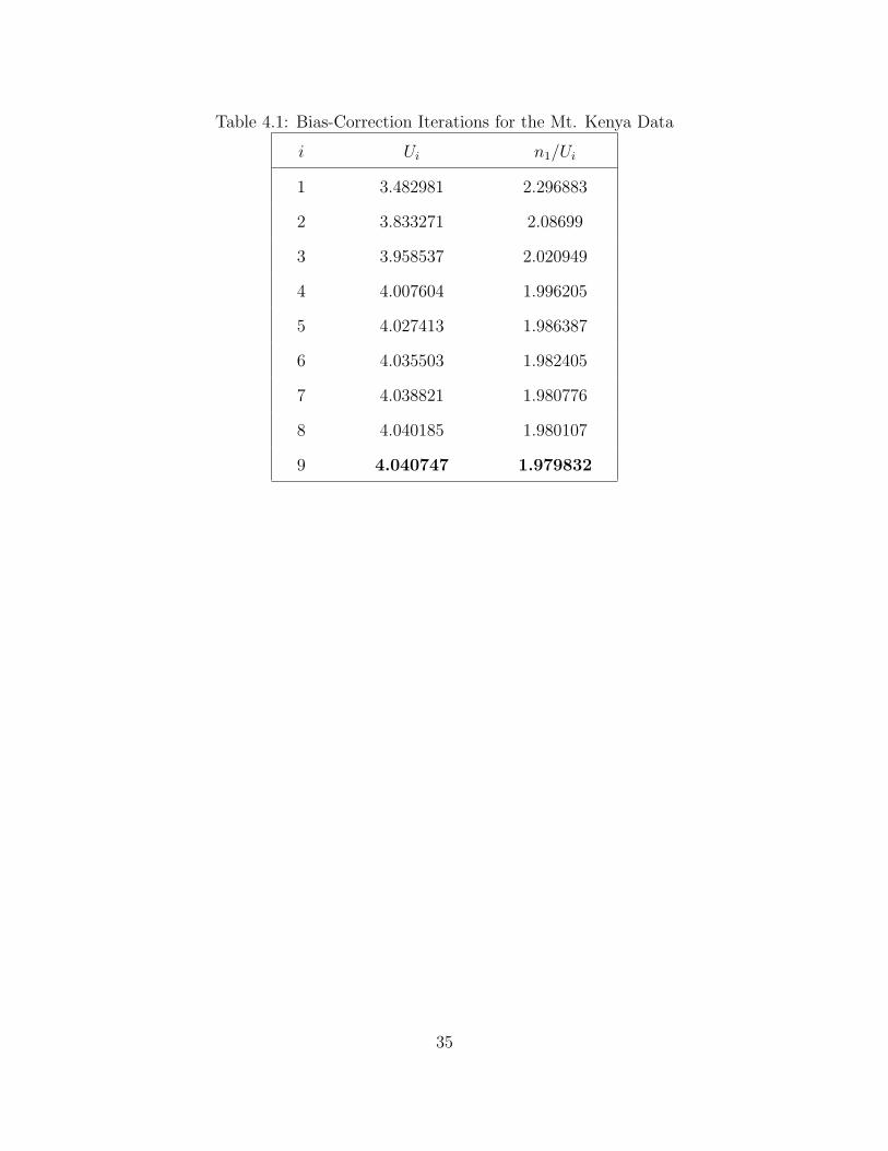
Table 4.1: Bias-Correction Iterations for the Mt. Kenya Data

i Ui n1/Ui

1 3.482981 2.296883

2 3.833271 2.08699

3 3.958537 2.020949

4 4.007604 1.996205

5 4.027413 1.986387

6 4.035503 1.982405

7 4.038821 1.980776

8 4.040185 1.980107

9 4.040747 1.979832

35

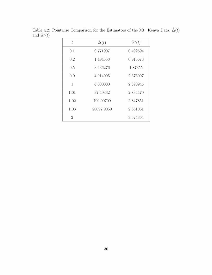
Table 4.2: Pointwise Comparison for the Estimators of the Mt. Kenya Data, ∆(t)and Ψ∗(t)

t ∆(t) Ψ∗(t)

0.1 0.771907 0.492694

0.2 1.494553 0.915673

0.5 3.436276 1.87355

0.9 4.914095 2.676097

1 6.000000 2.820945

1.01 37.49332 2.834479

1.02 790.90709 2.847851

1.03 20097.9059 2.861061

2 3.624364

36

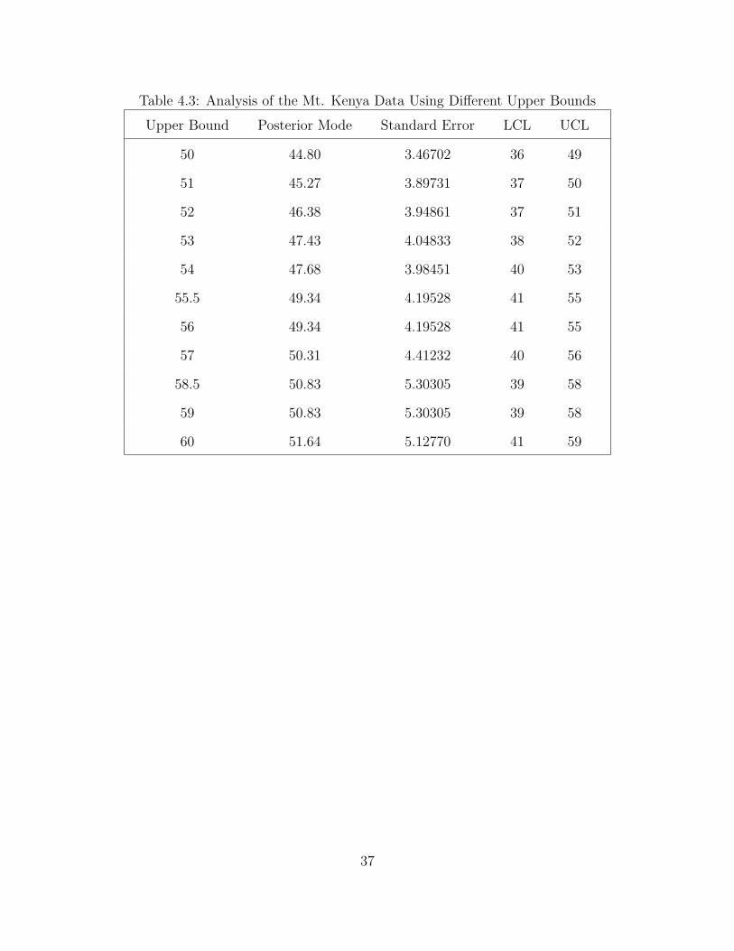
Table 4.3: Analysis of the Mt. Kenya Data Using Different Upper Bounds

Upper Bound Posterior Mode Standard Error LCL UCL

50 44.80 3.46702 36 49

51 45.27 3.89731 37 50

52 46.38 3.94861 37 51

53 47.43 4.04833 38 52

54 47.68 3.98451 40 53

55.5 49.34 4.19528 41 55

56 49.34 4.19528 41 55

57 50.31 4.41232 40 56

58.5 50.83 5.30305 39 58

59 50.83 5.30305 39 58

60 51.64 5.12770 41 59

37

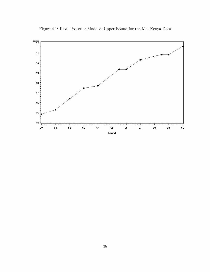
Figure 4.1: Plot: Posterior Mode vs Upper Bound for the Mt. Kenya Data

38

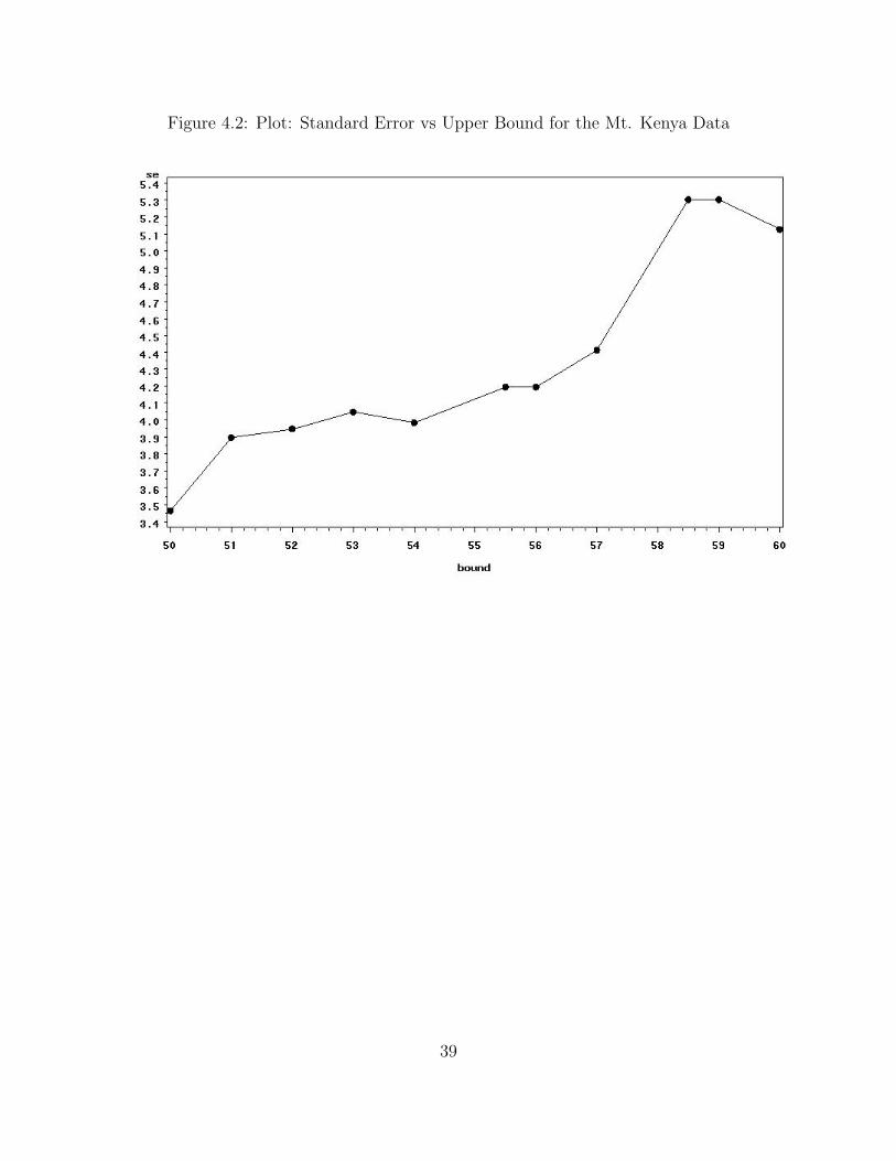
Figure 4.2: Plot: Standard Error vs Upper Bound for the Mt. Kenya Data

39

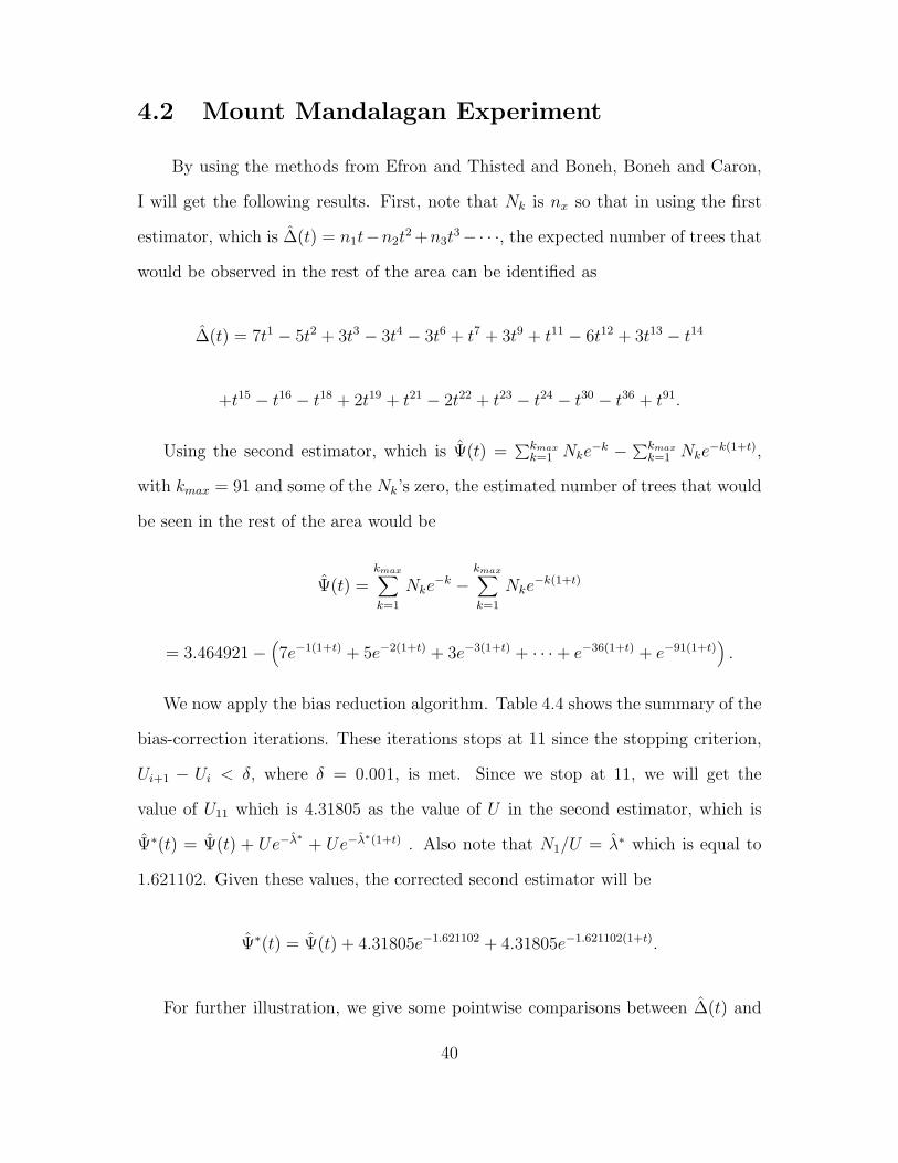
4.2 Mount Mandalagan Experiment

By using the methods from Efron and Thisted and Boneh, Boneh and Caron,

I will get the following results. First, note that Nk is nx so that in using the first

estimator, which is ∆(t) = n1t−n2t2 +n3t

3−· · ·, the expected number of trees that

would be observed in the rest of the area can be identified as

∆(t) = 7t1 − 5t2 + 3t3 − 3t4 − 3t6 + t7 + 3t9 + t11 − 6t12 + 3t13 − t14

+t15 − t16 − t18 + 2t19 + t21 − 2t22 + t23 − t24 − t30 − t36 + t91.

Using the second estimator, which is Ψ(t) =∑kmax

k=1 Nke−k − ∑kmax

k=1 Nke−k(1+t),

with kmax = 91 and some of the Nk’s zero, the estimated number of trees that would

be seen in the rest of the area would be

Ψ(t) =kmax∑k=1

Nke−k −

kmax∑k=1

Nke−k(1+t)

= 3.464921−(7e−1(1+t) + 5e−2(1+t) + 3e−3(1+t) + · · ·+ e−36(1+t) + e−91(1+t)

).

We now apply the bias reduction algorithm. Table 4.4 shows the summary of the

bias-correction iterations. These iterations stops at 11 since the stopping criterion,

Ui+1 − Ui < δ, where δ = 0.001, is met. Since we stop at 11, we will get the

value of U11 which is 4.31805 as the value of U in the second estimator, which is

Ψ∗(t) = Ψ(t) + Ue−λ∗ + Ue−λ∗(1+t) . Also note that N1/U = λ∗ which is equal to

1.621102. Given these values, the corrected second estimator will be

Ψ∗(t) = Ψ(t) + 4.31805e−1.621102 + 4.31805e−1.621102(1+t).

For further illustration, we give some pointwise comparisons between ∆(t) and

40

Ψ∗(t) for different values of t as shown in Table 4.5. Notice that as t becomes larger,

the value of Ψ∗(t) approaches 4. Thus, we can say that Ψ∗(∞) = 4. This means

that we expect to find 4 new distinct species of trees in addition to the trees that

were already observed.

41

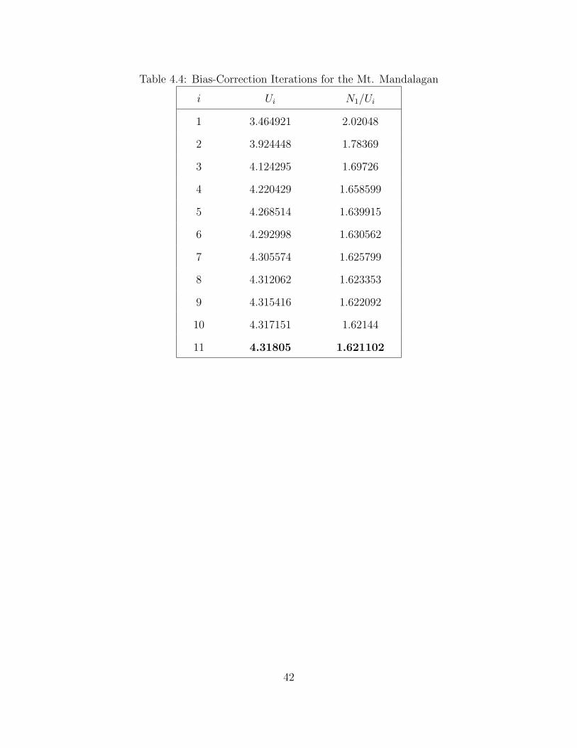
Table 4.4: Bias-Correction Iterations for the Mt. Mandalagan

i Ui N1/Ui

1 3.464921 2.02048

2 3.924448 1.78369

3 4.124295 1.69726

4 4.220429 1.658599

5 4.268514 1.639915

6 4.292998 1.630562

7 4.305574 1.625799

8 4.312062 1.623353

9 4.315416 1.622092

10 4.317151 1.62144

11 4.31805 1.621102

42

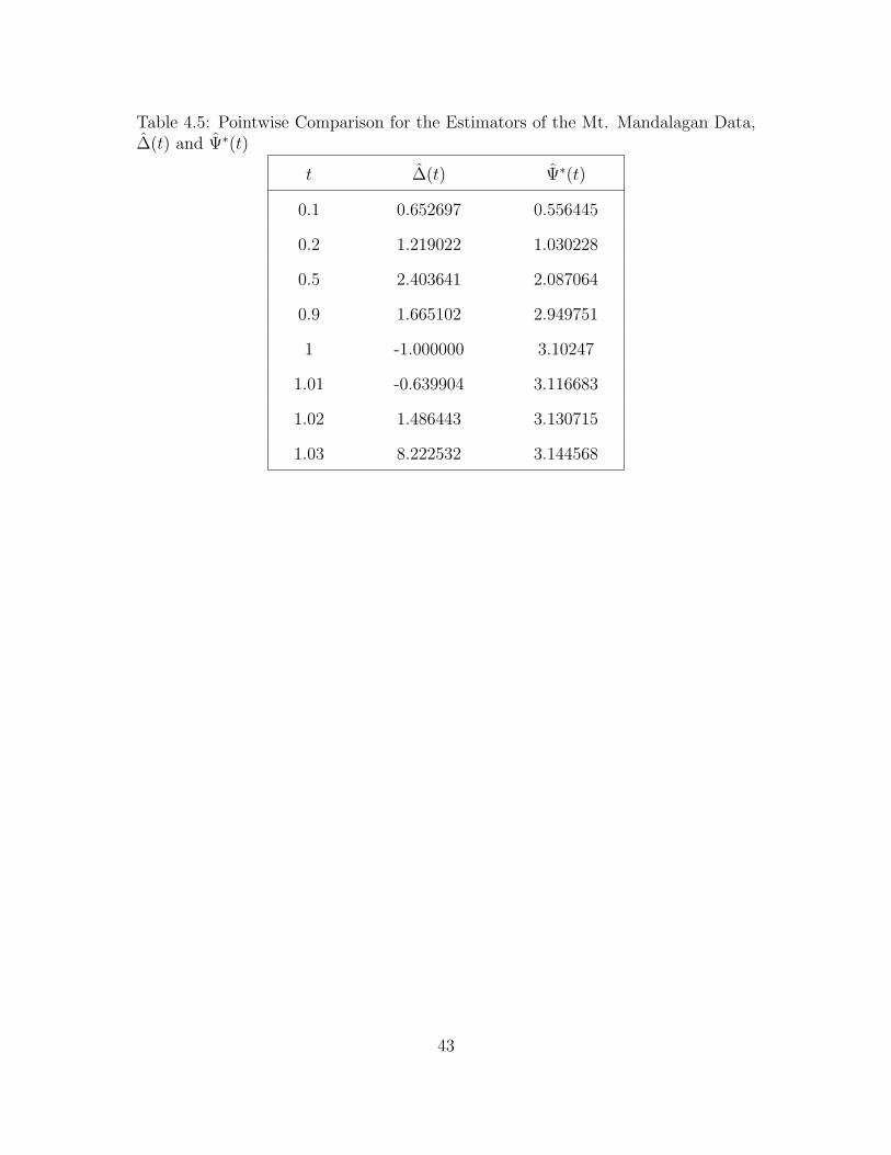
Table 4.5: Pointwise Comparison for the Estimators of the Mt. Mandalagan Data,∆(t) and Ψ∗(t)

t ∆(t) Ψ∗(t)

0.1 0.652697 0.556445

0.2 1.219022 1.030228

0.5 2.403641 2.087064

0.9 1.665102 2.949751

1 -1.000000 3.10247

1.01 -0.639904 3.116683

1.02 1.486443 3.130715

1.03 8.222532 3.144568

43

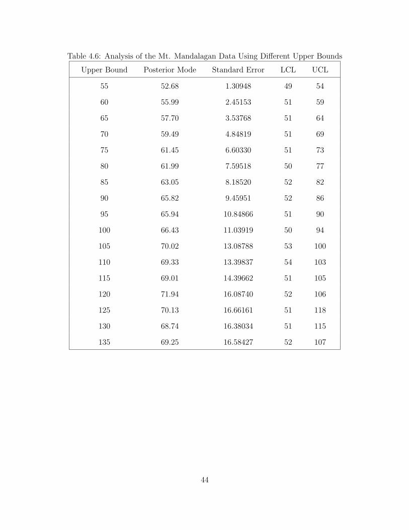
Table 4.6: Analysis of the Mt. Mandalagan Data Using Different Upper Bounds

Upper Bound Posterior Mode Standard Error LCL UCL

55 52.68 1.30948 49 54

60 55.99 2.45153 51 59

65 57.70 3.53768 51 64

70 59.49 4.84819 51 69

75 61.45 6.60330 51 73

80 61.99 7.59518 50 77

85 63.05 8.18520 52 82

90 65.82 9.45951 52 86

95 65.94 10.84866 51 90

100 66.43 11.03919 50 94

105 70.02 13.08788 53 100

110 69.33 13.39837 54 103

115 69.01 14.39662 51 105

120 71.94 16.08740 52 106

125 70.13 16.66161 51 118

130 68.74 16.38034 51 115

135 69.25 16.58427 52 107

44

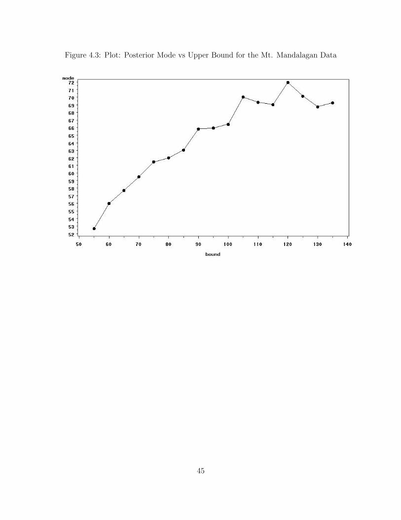
Figure 4.3: Plot: Posterior Mode vs Upper Bound for the Mt. Mandalagan Data

45

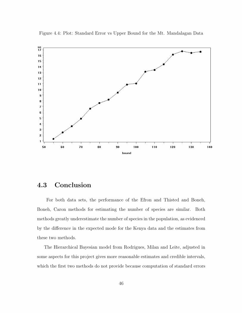
Figure 4.4: Plot: Standard Error vs Upper Bound for the Mt. Mandalagan Data

4.3 Conclusion

For both data sets, the performance of the Efron and Thisted and Boneh,

Boneh, Caron methods for estimating the number of species are similar. Both

methods greatly underestimate the number of species in the population, as evidenced

by the difference in the expected mode for the Kenya data and the estimates from

these two methods.

The Hierarchical Bayesian model from Rodrigues, Milan and Leite, adjusted in

some aspects for this project gives more reasonable estimates and credible intervals,

which the first two methods do not provide because computation of standard errors

46

are difficult.

The posterior mode of N increases monotonically as the upper bound increases.

However, the standard errors do not behave the same way. The upper bound for the

distribution must be known beforehand, provided by an expert or analyst involved

in the study. This upper bound cannot be obtained from the sample data. In fact,

in most of the credible intervals, the upper limit is almost equal to the set upper

bound.

47

Appendix A

Fortran Code

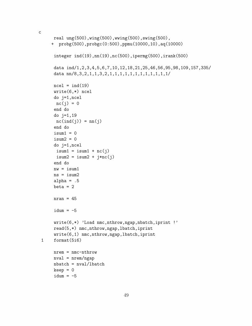
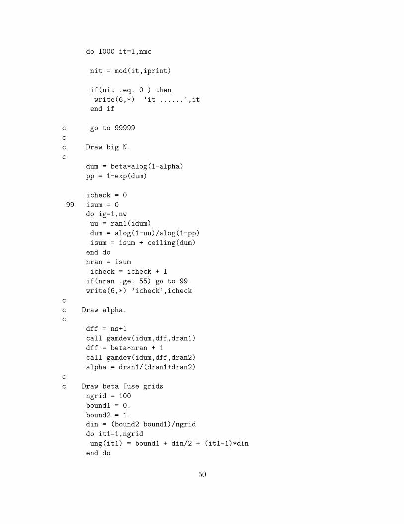
Fortran was used extensively in this project to perform simulations. Fortran is

a general-purpose, procedural, imperative programming language that is especially

suited to numeric computation and scientific computing.

The remaining pages in this appendix document the Fortran code used in this

project.

48

c

real ung(500),wing(500),wwing(500),swing(500),

+ probg(500),probgc(0:500),ppmu(10000,10),aq(10000)

integer ind(19),nn(19),nc(500),ipermg(500),irank(500)

data ind/1,2,3,4,5,6,7,10,12,18,21,25,46,56,95,98,109,157,335/

data nn/8,3,2,1,1,3,2,1,1,1,1,1,1,1,1,1,1,1,1/

ncel = ind(19)

write(6,*) ncel

do j=1,ncel

nc(j) = 0

end do

do j=1,19

nc(ind(j)) = nn(j)

end do

isum1 = 0

isum2 = 0

do j=1,ncel

isum1 = isum1 + nc(j)

isum2 = isum2 + j*nc(j)

end do

nw = isum1

ns = isum2

alpha = .5

beta = 2

nran = 45

idum = -5

write(6,*) ’Load nmc,nthrow,ngap,nbatch,iprint !’

read(5,*) nmc,nthrow,ngap,lbatch,iprint

write(6,1) nmc,nthrow,ngap,lbatch,iprint

1 format(5i6)

nrem = nmc-nthrow

nval = nrem/ngap

nbatch = nval/lbatch

keep = 0

idum = -5

49

do 1000 it=1,nmc

nit = mod(it,iprint)

if(nit .eq. 0 ) then

write(6,*) ’it ......’,it

end if

c go to 99999

c

c Draw big N.

c

dum = beta*alog(1-alpha)

pp = 1-exp(dum)

icheck = 0

99 isum = 0

do ig=1,nw

uu = ran1(idum)

dum = alog(1-uu)/alog(1-pp)

isum = isum + ceiling(dum)

end do

nran = isum

icheck = icheck + 1

if(nran .ge. 55) go to 99

write(6,*) ’icheck’,icheck

c

c Draw alpha.

c

dff = ns+1

call gamdev(idum,dff,dran1)

dff = beta*nran + 1

call gamdev(idum,dff,dran2)

alpha = dran1/(dran1+dran2)

c

c Draw beta [use grids

ngrid = 100

bound1 = 0.

bound2 = 1.

din = (bound2-bound1)/ngrid

do it1=1,ngrid

ung(it1) = bound1 + din/2 + (it1-1)*din

end do

50

do it1=1,ngrid

rbeta = ung(it1)/(1-ung(it1))

arg1 = rbeta*nran*alog(1-alpha)

sum = 0.

do j=1,ncel

do i=1,j

sum = sum + nc(j)*alog(rbeta + i - 1)

end do

end do

arg2 = sum

wing(it1) = arg1 + arg2

wwing(it1) = arg1 + arg2

end do

call sort(ngrid,wwing,ipermg,irankg,swing)

term0 = swing(ngrid)

asum = 0.

do it1=1,ngrid

asum = asum + exp(wing(it1)-term0)

end do

do it1=1,ngrid

probg(it1) = exp(wing(it1)-term0)/asum

end do

probgc(0) = 0.

do it1=1,ngrid

probgc(it1) = probgc(it1-1) + probg(it1)

end do

uu = ran1(idum)

do it1=1,ngrid

if(uu .gt. probgc(it1-1) .and. uu .le. probgc(it1)) then

ipick = it1

end if

end do

c write(6,*) ’ipick’,ipick

ungg = ung(ipick-1) + (ung(ipick)-ung(ipick-1))*ran1(idum)

beta = ungg/(1-ungg)

if(nit .eq. 0) then

write(6,*) ’nran alpha beta’,nran,alpha,beta

end if

51

if(it .gt. nthrow) then

itt = mod(it-nthrow,ngap)

if( itt .eq. 0 ) then

keep = keep + 1

ppmu(keep,1) = nran

ppmu(keep,2) = alpha

ppmu(keep,3) = beta

end if

end if

1000 continue

npar = 3

c

C Study autocorrelation in Gibbs Sampler.

C

Do 3310 j=1,npar

c write(6,3311)

c write(10,3311)

3311 format(20x,’lag’,5x,’correlation’,5x,’sterr’/)

sum= 0.

do 3315 it=1,nval

3315 SUM = SUM + ppmu(it,j)

savg = sum/nval

sum = 0.

do 3320 it=1,nval

3320 sum = sum + (ppmu(it,j)-savg)**2

co = sum/nval

do 3325 KKK=1,20

sum = 0.

DO 3330 it=1,nval-kkk

3330 sum = sum + (ppmu(it,j)-savg)*(ppmu(it+kkk,j)-savg)

cors = (sum/nval)/co

str = sqrt( (nval-kkk)/(nval*(nval+2.)) )

write(6,3331) j,kkk,cors,str

write(10,3331) j,kkk,cors,str

3331 format(10x,2i10,2f10.4/)

3325 continue

3310 continue

do it=1,nval

write(7,’(i5,3f10.5)’) it,(ppmu(it,k),k=1,npar)

52

end do

do k=1,npar

do it=1,nval

aq(it) = ppmu(it,k)

end do

call monte(lbatch,nbatch,aq,avg,std,bstd,c025,c975)

write(6,’(i5,5f12.5)’) k,avg,std,bstd,c025,c975

write(8,’(i5,5f12.5)’) k,avg,std,bstd,c025,c975

end do

stop

end

c

include ’allrouma556.f’

c

53

Bibliography

[1] Arnold, B. C., and Beaver, R. J. (1988) ”Estimation of the Number fo Classesin a Population,” Biometrical Journal, 30, pp.413-424.

[2] Bickel, P. J., and Yahav, J. A. (1985) ”On estimating the Number of UnseenSpecies: How Many Executions Were There?,” Technical Report No.43, Uni-versity of California, Berkeley, Bept. of Statistics.

[3] Bickel, P. J., and Yahav, J. A. (1988) ”On estimating the Number of UnseenSpecies and System Reliability,” in Statistical Decision Theory and RelatedTopics IV, 2, eds. S. S. Gupta and J. O. Berger, New York: Springer-Verlag,pp.265-271.

[4] Boneh, S., Boneh, A., and Caron, R. J. (1998) ”Estimating the PredictionFunction and the Number of Unseen Species in Sampling with Replacement,”Journal of the American Statistical Association, 93, No.441., pp.372-379.

[5] Bunge, J., and Fitzpatrick, M. (1993), ”Estimating the Number of Species: AReview,” Journal of the American Statistical Association, 88, No.421., pp.364-373.

[6] Cordon, A. B. (2003), ”Vegetation Analysis of Lower Montane Rainforest inMt. Mandalagan, Negros Occidental,” Master’s Thesis, De La Salle University-Manila.

[7] Efron, B., and Thisted, R. (1976) ”Estimating the Number of Unseen Species:How Many Words Did Shakespeare Know?,” Biometrika, 63, No.3., pp.435-447.

[8] Engen, S. (1978) ”Stochastic Abundance Models,” London: Chapman and Hall.

[9] Fisher, R. A., Corbet, A. S., and Williams, C. B. (1943) ”The Relation Betweenthe Number of Species and the Number of Individuals in a Random Sample ofan Animal Population,” The Journal of Animal Ecology, 12, No.1., pp.42-58.

[10] Frank, O. (1978) ”Estimation of the Number of Connected Components ina Graph by Using a Sampled Subgraph,” Scandinavian Journal of Statistics,Theory and Applications, 5, pp.177-188.

54

[11] Good, I. J. (1953) ”The Population Frequencies of Species and the Estimationof Population Parameters,” Biometrika, 40, pp.237-264.

[12] Good, I. J., and Toulmin, G. H. (1956) ”The Number of New Species, and theIncrease in Population Coverage, when a Samples is Increased,” Biometrika,43, pp.45-63.

[13] Goodman, L. A. (1949) ”On the Estimation of the Number of Classes in aPopulation,” The Annals of Mathematical Statistics, 20, No.4., pp.572-579.

[14] Harwit, M., and Hildebrand, R. (1986) ”How Many More Discoveries in theUniverse?,” Nature, 320, pp.724-726.

[15] Lewins, W. A., and Joanes, D. N. (1984) ”Bayesian Estimation of the Numberof Species,” Biometrics, 40, No.2., pp.323-328.

[16] Mann, C. C. (1991) ”Extinction: Are Ecologists Crying Wolf?,” Science, NewSeries, 253, No.5021., pp.736-738.

[17] Mingoti, S. A., and Meeden, G. (1992) ”Estimating the Total Number of Dis-tinct Species Using Presence and Absence Data,” Biometrics, 48, No.3., pp.863-875.

[18] Nayak, T. K. (1989) ”A Note on Estimating the Number of Errors in a Systemby Recapture Sampling,” Statistics and Probability Letters, 7, pp.191-194.

[19] Patil, G. P., and Taillie, C. (1982) ”Diversity as a Concept and its Measure-ment” (with comment), Journal of the American Statistical Association, 77,pp.548-567.

[20] Pollock, K. H. (1991) ”Modeling Capture, Recapture, and Removal Statisticsfor Estimation of Demographic Parameters for Fish and Wildlife Populations:Past, Present, and Future,” Journal of the American Statistical Association,86, pp.225-238.

[21] Ramos, K., and Villaflor, R. (2005) ”On Estimating the Number of SpeciesUsing the Prediction Function Ψ(t),” Undergraduate Thesis, De La SalleUniversity-Manila.

[22] Rodrigues, J., Milan, L. A., and Leite, J. G. (2000) ”Hi-erarchical Bayesian Analysis for the Number of Species,”http://www.ime.usp.br/∼cpereira/publications/creta.htm

[23] Sanathanan, L. (1972) ”Estimating the Size of a Multinomial Population,” TheAnnals of Mathematical Statistics, 43, No.1., pp.142-152.

[24] Solow, A. R. (1994) ”On the Bayesian Estimation of the Number of Species ina Community,” Ecology, 75, No.7., pp.2139-2142.

55

[25] Stam, A. J. (1987) ”Statistical Problem in Ancient Numismatics,” StatisticaNeerlandica, 41, pp.151-173.

[26] Thisted, R., and Efron, B. (1987) ”Did Shakespeare Write a Newly-DiscoveredPoem?,” Biometrika, 74, No.3., pp.445-455.

56