WP/05/77

Estimating the Implicit Inflation Target: An Application to U.S. Monetary Policy

Daniel Leigh

© 2005 International Monetary Fund WP/05/77

IMF Working Paper

European Department

Estimating the Implicit Inflation Target: An Application to U.S. Monetary Policy

Prepared by Daniel Leigh1

Authorized for distribution by Ashoka Mody

April 2005

Abstract

This Working Paper should not be reported as representing the views of the IMF. The views expressed in this Working Paper are those of the author(s) and do not necessarily represent those of the IMF or IMF policy. Working Papers describe research in progress by the author(s) and are published to elicit comments and to further debate.

This paper proposes a new method of estimating the Taylor rule with a time-varying implicit inflation target and a time-varying natural rate of interest. The inflation target and the natural rate are modeled as random walks and are estimated using maximum likelihood and the Kalman filter. I apply this method to U.S. monetary policy over the past 25 years and find considerable time variation in the implicit target, confirming hypotheses about “opportunisticdisinflation” and the recent “deflation scare.” JEL Classification Numbers: C22, E31, E52 Keywords: Taylor rule, time-varying parameters, Kalman filter Author(s) E-Mail Address: dleigh@imf.org

1 I am grateful to Laurence Ball, Nicoletta Batini, Douglas Laxton, Thomas Lubik, Athanasios Orphanides, Adam Posen, Pau Rabanal, Calvin Schnure, and Jonathan Wright for helpful comments.

- 2 -

Contents Page I. Introduction ............................................................................................................................3 II. Methodology .........................................................................................................................4

A. The Taylor Rule Model.............................................................................................4 B. Interest Rate Smoothing ............................................................................................6 C. Estimating rn

t .............................................................................................................6 D. Estimating π*t............................................................................................................8

III. Data ......................................................................................................................................9

A. Inflation.....................................................................................................................9 B. Nominal Interest Rate................................................................................................9 C. Output Gap ................................................................................................................9

IV. Results................................................................................................................................11

A. Estimates of the Signal-to-Noise Ratio...................................................................11 B. Taylor Rule Parameter Estimates............................................................................11 C. Estimates of the Implicit Target ..............................................................................12

V. Robustness Analysis ...........................................................................................................16

A. Alternative π*0 ........................................................................................................16 B. Alternative λ ............................................................................................................17

VI. Conclusion ........................................................................................................................ 18 Appendix I. The Natural Rate of Interest ................................................................................................20 References................................................................................................................................22 Figures 1. The Real Federal Rate and the Natural Rate of Interest ........................................................7 2. The Output Gap...................................................................................................................11 3. Actual Inflation and the Implicit Target .............................................................................13 4. Actual and Fitted Federal Funds Target Rate .....................................................................16 5. Actual Inflation and the Implicit Target for Different π*0s ................................................17 6. Actual Inflation and the Implicit Target for Different λs....................................................18 Tables 1. Taylor Rule Estimation Results ..........................................................................................12 2. Robustness Analysis: Estimation Results for Different π*0s..............................................17 3. Robustness Analysis: Estimation Results for Different λs .................................................18

- 3 -

I. INTRODUCTION

Over the past 25 years, inflation in the United States has declined from double digits in the 1970s to close to 1 percent by the early 2000s. An important question is: how has the Federal Reserve conducted monetary policy during this broadly successful period?

A large literature on monetary policy rules has addressed this question by measuring how policy interest rates react to deviations of inflation and real activity from their target levels. The accepted wisdom is that, since 1979, the Federal Open Market Committee (FOMC) has consistently responded to increases in inflation above the target level by raising the real federal funds rate above its natural rate, in accordance with the Taylor principle. There is also a consensus that the Fed has responded to deviations of output from potential. Other things being equal, when output falls below potential, the Fed lowers the real federal funds rate below its natural rate.2

An important implicit assumption in most of the policy rules literature is that the natural rate of interest and the target level of inflation are constant for the duration of the sample period. For example, Clarida et al. (1998) estimate the Federal Reserve's policy reaction function over 1979-94 under the assumption of a constant natural rate of interest of 3.5 percent, and a constant inflation target, and conclude that the target has been 4 percent over this period.

However, given the growing evidence that the natural rate of interest is affected by factors such as productivity growth and that the natural rate of interest has varied over the past 25 years, the assumption of a constant natural rate seems unduly restrictive. For example, Laubach and Williams (2003) find substantial variation in the natural rate of interest over the past four decades in the U.S. The authors suggest that the natural rate varies about one-for-one with changes in the growth rate of potential GDP.3

Regarding the inflation target, statements made by Federal Reserve policymakers over the past quarter century suggest that the inflation objective has also varied. Since the Federal Reserve does not have an explicit target and since inflation has changed noticeably over the past 25 years, the assumption of a constant target seems overly restrictive.

This paper therefore relaxes the assumption of a constant natural rate and a constant inflation objective and proposes a new method of estimating the Taylor rule when these

2 Orphanides (2002, 2004) finds that Fed policy before 1979 was also consistent with the Taylor principle and that the Great Inflation of the 1970s arose because policymakers had overestimated the degree of slack in the economy. However, this paper focuses on the Volcker-Greenspan period during which inflation declined, i.e., from 1979 to the present.

3 Maccini et al. (2004) identify long-run changes (regime shifts) in the natural rate with low real rates in the 1970s and high rates in the early 1980s.

- 4 -

parameters vary. First, I obtain an estimate of the time-varying natural rate of interest using the Kalman filter and a model that links the natural rate to changes in trend productivity growth and to a random component, as in Laubach and Williams (2003). Secondly, I use this estimate of the natural rate to estimate the time-varying inflation target in the context of a forward-looking Taylor rule. I model the implicit inflation target as a random walk and conduct the estimation using the Kalman filter and the median-unbiased estimator proposed by Stock and Watson (1998).

My main findings are four: (i) stability tests indicate significant variation in the Federal Reserve's implicit target over the 1979-2004 period; (ii) in the early 1980s, the inflation target estimate is near 3 percent, indicating that the Federal Reserve under Volcker sought to substantially reduce inflation from its double digit level; (iii) in the late 1980s and early 1990s, the target is close to actual inflation of 3-4 percent and declines to 1-2 percent only after the 1990-91 recession reduces inflation, a finding that corroborates qualitative historical evidence of an “opportunistic approach to disinflation” at the Fed; (iv) finally, over 2001-04, the target rises to 2-3 percent, a development that can be interpreted as a response by the FOMC to the risks of hitting the zero bound on nominal interest rates.

The rest of the paper is organized as follows. Section II describes the methodology, Section III describes the data used in the analysis, Section IV discusses the results, Section V reports the results of a robustness analysis, and Section VI concludes.

II. METHODOLOGY

In this section, I describe the Taylor rule model of monetary policy and explain my estimation approach.

A. The Taylor Rule Model

The Taylor rule model assumes that central banks respond in a systematic fashion to deviations of expected inflation from the desired level. For instance, when the inflation forecast rises above the target, the Taylor rule prescribes raising nominal interest rates enough to raise real interest rates (the so-called “Taylor principle”). The rule also allows for some output stabilization by prescribing lower interest rates when output falls below potential. The central bank has a target for the nominal interest rate that evolves according to the following equation.

i*t = rn + πet + (β-1)(πe

t – π*)+γ ty~

, (1) where i*t is the target level of the federal funds rate, πe

t is expected inflation (the inflation

forecast), ty~

is the output gap (the percentage difference between actual and potential real GDP), rn is the natural rate of interest, and π* is the inflation target.

An important condition for the Taylor rule to stabilize inflation is β > 1, i.e., when the inflation forecast rises above target, the policymaker raises nominal interest rates enough to

- 5 -

raise the target for the real federal funds rate, r*t = i*t - πet. Other things being equal, the central

bank thus responds to increases in inflation above target by raising the target for the real federal funds rate above the natural rate, i.e. the real rate gap, r*t - rn, responds positively to the inflation gap, πe

t –π*. This condition is called the “Taylor principle.” Output stabilization, or “leaning against the wind,” implies a positive value for γ.

The conventional approach to estimating Taylor rules assumes a constant natural rate of interest, rn, and a constant inflation target, π*. Equation (1) can thus be rewritten as:

i*t = α + βπe

t + γ ty~

, (2) where the composite intercept term, α = rn- (β-1)π*, comprises both the constant natural rate and the constant inflation target. By estimating α and β and by making an assumption regarding the value of rn, one can then solve for the estimated constant inflation target, π*, using the following expression:

1*

−−

=β

απnr . (3)

For example, Clarida et al. (1998) assume that rn equals 3.5 percent, the average of the real federal funds rate over the 1979-94 sample. Using their estimates of α and β, the authors then obtain an estimate of π* = 4 percent.

I therefore relax the assumption of a constant natural rate and a constant inflation objective and propose a new method of estimating the Taylor rule when these parameters vary.4 The distinguishing features of my approach are: (i) I allow the inflation target, π*, to vary over time; (ii) I allow the natural rate of interest, rn, in the Taylor rule to vary over time; and (iii) I use the Kalman filter and maximum likelihood to estimate the target and the Taylor rule parameters jointly.5 Thus, Equation (1) becomes:

i*t = rn

t + πet + (β-1)(πe

t – π*t)+γ ty~

, (4) where the t subscripts on the natural rate of interest and on the inflation target indicate time variation. 4 Leigh (2004) applies this approach to Japanese monetary policy over 1979-2004.

5 Boivin (2004) and Rabanal (2004) both allow for time-variation in the intercept term, α, and in the response coefficients using samples that start in the 1960s. My approach is substantially different, I separately model time variation in rn and π* for the post-1979 period.

- 6 -

B. Interest Rate Smoothing

A concern that arises when estimating Taylor rules such as those in Equations (1) and (4) is that they do not account for the tendency of central banks to smooth interest rate changes. Reasons for wishing to adjust interest rates gradually in response to news include the possible loss of credibility following sudden policy reversals, as discussed in Clarida et al. (1998). Following the literature, I therefore assume that the central bank adjusts the actual nominal interest rate, it, gradually toward i*t, the target federal funds rate: it = (1-ρ)i*t + ρit-1 + ε0,t , (5) where i*t is as in Equation (4), )1,0(∈ρ is the degree of interest rate inertia, and ε0,t is a mean zero i.i.d. normal disturbance.6

C. Estimating rn

The first stage in my analysis is to estimate the time-varying natural rate, rnt. To obtain

an estimate of the natural rate, I apply the Kalman filter approach of Laubach and Williams (2003). The LW model links the natural rate to changes in the trend growth rate of GDP and to a random component. The authors report results for a baseline case where the natural rate of interest follows a random walk as well as for the case where it is stationary. I use the simpler baseline case.

The main identifying assumption is that the output gap converges to zero if the real rate gap is zero. This assumption is formalized in the following I.S. curve equation. yt = y*t + Ay(L)(yt-1 – y*t-1) + Ar(L)(rt-1 – rn

t-1) + ε1,t , (6) where yt is the log of GDP and y*t is the log of potential GDP. The difference between actual and potential GDP, i.e., yt – y*t, is the output gap. The numbers of lags are determined by the data. Details of the LW approach are provided in the appendix.

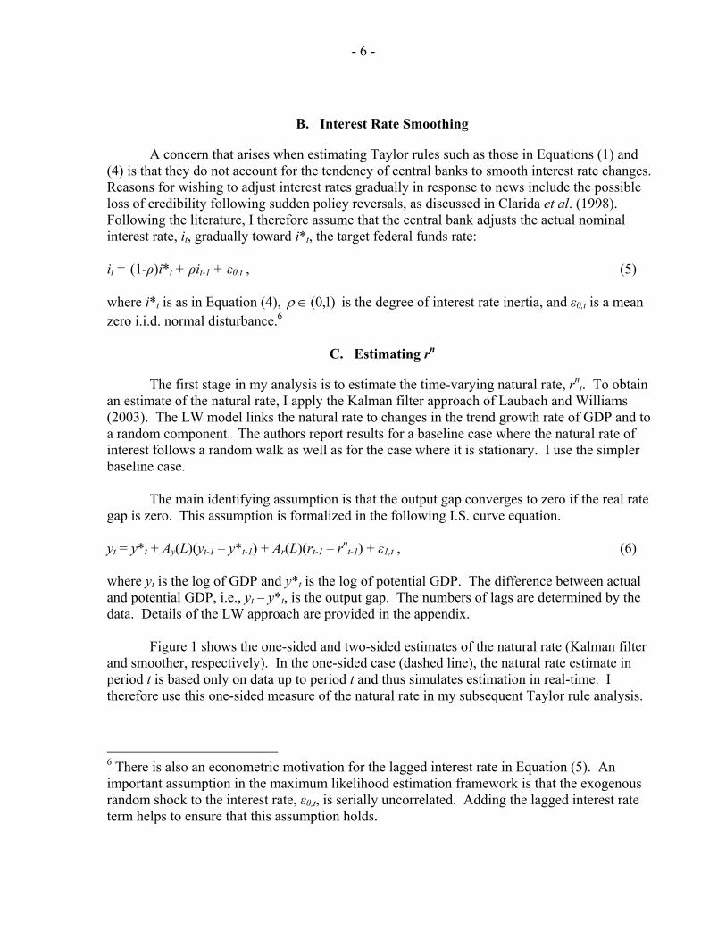
Figure 1 shows the one-sided and two-sided estimates of the natural rate (Kalman filter and smoother, respectively). In the one-sided case (dashed line), the natural rate estimate in period t is based only on data up to period t and thus simulates estimation in real-time. I therefore use this one-sided measure of the natural rate in my subsequent Taylor rule analysis.

6 There is also an econometric motivation for the lagged interest rate in Equation (5). An important assumption in the maximum likelihood estimation framework is that the exogenous random shock to the interest rate, ε0,t, is serially uncorrelated. Adding the lagged interest rate term helps to ensure that this assumption holds.

- 7 -

The smooth two-sided estimate of the natural rate in period t is based on data from the entire sample.7 Figure 1 also shows the real federal funds rate (thick solid line).

Figure 1. Real Federal Funds Rate and the Natural Rate of Interest

1980 1985 1990 1995 2000-2

0

2

4

6

8

10

12

14

Perc

ent

Year

Real Fed Funds RateKalman Smoother Kalman Filter

The path of the natural rate of interest in Figure 1 is intuitive and corroborated by historical evidence. In the 1980s, the natural rate is relatively high at about 3 percent. This finding is in line with the notion that the large deficits of the 1980s translated into higher real interest rates. The decline in the natural rate during the 1991 recession can be interpreted as resulting from an I.S. curve shift associated with the credit crunch. Finally, the natural rate rises again during the late 1990s when productivity growth increased.

7 The estimates of the model parameters are from data for the full sample so the analogy to real-time is not exact.

- 8 -

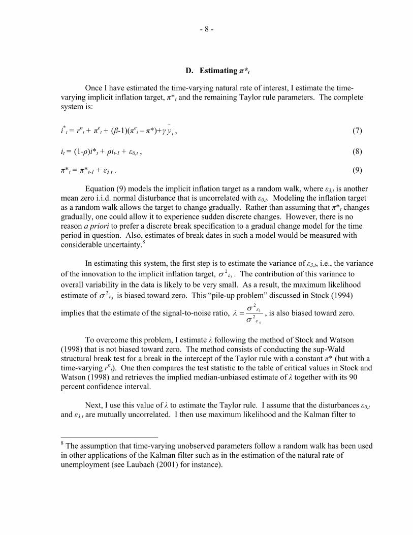
D. Estimating π*t

Once I have estimated the time-varying natural rate of interest, I estimate the time-varying implicit inflation target, π*t and the remaining Taylor rule parameters. The complete system is:

i*t = rn

t + πet + (β-1)(πe

t – π*)+γ ty~

, (7) it = (1-ρ)i*t + ρit-1 + ε0,t , (8) π*t = π*t-1 + ε3,t . (9)

Equation (9) models the implicit inflation target as a random walk, where ε3,t is another mean zero i.i.d. normal disturbance that is uncorrelated with ε0,t. Modeling the inflation target as a random walk allows the target to change gradually. Rather than assuming that π*t changes gradually, one could allow it to experience sudden discrete changes. However, there is no reason a priori to prefer a discrete break specification to a gradual change model for the time period in question. Also, estimates of break dates in such a model would be measured with considerable uncertainty.8

In estimating this system, the first step is to estimate the variance of ε3,t, i.e., the variance of the innovation to the implicit inflation target, 3

2εσ . The contribution of this variance to

overall variability in the data is likely to be very small. As a result, the maximum likelihood estimate of 3

2εσ is biased toward zero. This “pile-up problem” discussed in Stock (1994)

implies that the estimate of the signal-to-noise ratio, 0

3

2

2

ε

ε

σσλ = , is also biased toward zero.

To overcome this problem, I estimate λ following the method of Stock and Watson

(1998) that is not biased toward zero. The method consists of conducting the sup-Wald structural break test for a break in the intercept of the Taylor rule with a constant π* (but with a time-varying rn

t). One then compares the test statistic to the table of critical values in Stock and Watson (1998) and retrieves the implied median-unbiased estimate of λ together with its 90 percent confidence interval.

Next, I use this value of λ to estimate the Taylor rule. I assume that the disturbances ε0,t and ε3,t are mutually uncorrelated. I then use maximum likelihood and the Kalman filter to

8 The assumption that time-varying unobserved parameters follow a random walk has been used in other applications of the Kalman filter such as in the estimation of the natural rate of unemployment (see Laubach (2001) for instance).

- 9 -

obtain estimates of the parameters }{ 20,,, σργβ and of π*t, as described in Harvey (1989).

Standard errors are obtained using the delta method.

To obtain an initial estimate of the state variable, π*0, in 1979Q3, I refer to statements made by Paul Volcker, Fed Chairman at the time. From 1979 to 1982, the Federal Reserve conducted an aggressive disinflationary policy and successfully reduced inflation from double digits to 4 percent by the mid-1980s. As Tobin (2002) explains, “Volcker then declared victory over inflation and piloted the economy through its long 1980s recovery” (Tobin, 2002). Inflation remained near 4 percent until the early 1990s.

Therefore, a plausible value of the Fed's inflation target in 1979, at the start of the Volcker disinflation, is π*0 = 4 percent. Moreover, as Section V explains, the results are robust to alternative methods of initializing π*0. Specifically, the path of the estimated target after the first few years of the sample is very similar for a range of values for π*0. The estimates of the Taylor rule coefficients are also similar.9

9 I initialize the remaining Taylor rule parameters using OLS, as in Hamilton (1994), i.e., I estimate the Taylor rule with a constant π* (but a time-varying rn

t) using OLS and the full sample. I then conduct the maximum likelihood estimation starting from the initial OLS estimates of the parameters }{ 2

0,,, σργβ .

III. DATA

A. Inflation

My measure of inflation is the annualized quarterly growth rate of the price index for personal consumption expenditures excluding food and energy, referred to as core PCE inflation. This rate is, as many authors suggest, the Federal Reserve's preferred inflation indicator. Expected inflation, πe

t, is the expectation of average inflation over the four quarters ahead. Following Laubach and Williams (2003), the expectations are based on out-of-sample forecasts using an univariate AR(3) with a 40-quarter rolling-regression window.

Specifically, the variable ⎟⎟⎠

⎞⎜⎜⎝

⎛−+ 14

t

t

PP

is forecast using ⎟⎟⎠

⎞⎜⎜⎝

⎛−

−

11t

t

PP

and two lags of ⎟⎟⎠

⎞⎜⎜⎝

⎛−

−

11t

t

PP

,

where Pt is the level of the core PCE index in quarter t. The source of the data is the Federal Reserve Bank of St. Louis. The sample of analysis is 1979Q3 to 2004Q1.

B. Nominal Interest Rate

The nominal policy interest rate is the annualized federal funds rate. The source of the federal funds rate data is the Federal Reserve Bank of St. Louis.

C. Output Gap

- 10 -

My output gap series is the real-time estimate of the output gap taken from the Greenbooks of the Federal Reserve Board of Governors. The Greenbook estimates are produced by economists at the Board of Governors before each meeting of the FOMC. Federal Reserve staff use a variety of techniques to estimate the output gap, such as measuring the potential level of output using a production function and then subtracting this estimate of potential from the actual level of output.10

Importantly, in any given quarter, the Fed staff base their real-time estimate of the output gap only on information that has accumulated up to that quarter. The Greenbook estimates thus represent the latest information that policymakers have available to them when they take interest rate decisions.

Using real-time output gap data distinguishes this paper from much of the empirical work on policy rules. The canonical approach is to use retrospective ex post output gap data that were not available to policy makers in real time. For example, the output gap data used in Clarida et al. (1998) are obtained by first fitting a quadratic trend to the entire output series and then subtracting this trend from the actual level of output. However, as Orphanides (2001) argues, analyzing policy rules using real-time data rather than retrospective data provides a more plausible estimate of policymakers' intended reactions to the economy.11

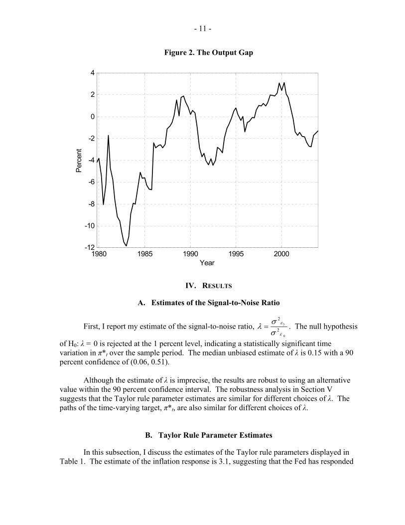
The Greenbook output gap data are available for the period ending in 1995Q4.12 For the 1996-2004 period, I supplement the Greenbook series with the Congressional Budget Office (CBO) output gap estimates. The CBO output gaps are estimated using a production function approach and are similar to the Greenbook output gaps in the periods in which both series are available.13 Figure 2 displays the output gap.

10 For a discussion of techniques used to estimate the output gap, see Haltmaier (2001).

11 Using real-time data to estimate the policy reaction function is an approach adopted by Orphanides (2001), Boivin (2003), and Kuttner (2004), among others.

12 I am grateful to Athanasios Orphanides for providing me with the Greenbook output gap data that he has compiled for the period ending 1995Q4.

13 For a detailed explanation of the CBO output gap estimation procedure, see Arnold (2004).

- 11 -

Figure 2. The Output Gap

1980 1985 1990 1995 2000-12

-10

-8

-6

-4

-2

0

2

4Pe

rcen

t

Year

IV. RESULTS

A. Estimates of the Signal-to-Noise Ratio

First, I report my estimate of the signal-to-noise ratio, 0

3

2

2

ε

ε

σσλ = . The null hypothesis

of H0: λ = 0 is rejected at the 1 percent level, indicating a statistically significant time variation in π*t over the sample period. The median unbiased estimate of λ is 0.15 with a 90 percent confidence of (0.06, 0.51).

Although the estimate of λ is imprecise, the results are robust to using an alternative value within the 90 percent confidence interval. The robustness analysis in Section V suggests that the Taylor rule parameter estimates are similar for different choices of λ. The paths of the time-varying target, π*t, are also similar for different choices of λ.

B. Taylor Rule Parameter Estimates

In this subsection, I discuss the estimates of the Taylor rule parameters displayed in Table 1. The estimate of the inflation response is 3.1, suggesting that the Fed has responded

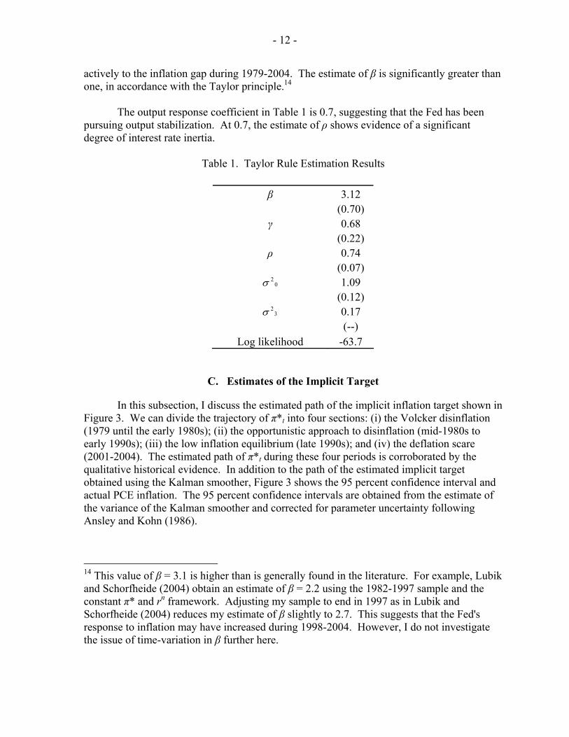
- 12 -

actively to the inflation gap during 1979-2004. The estimate of β is significantly greater than one, in accordance with the Taylor principle.14

The output response coefficient in Table 1 is 0.7, suggesting that the Fed has been pursuing output stabilization. At 0.7, the estimate of ρ shows evidence of a significant degree of interest rate inertia.

Table 1. Taylor Rule Estimation Results

β 3.12 (0.70) γ 0.68 (0.22) ρ 0.74 (0.07)

02σ 1.09 (0.12)

32σ 0.17

(--) Log likelihood -63.7

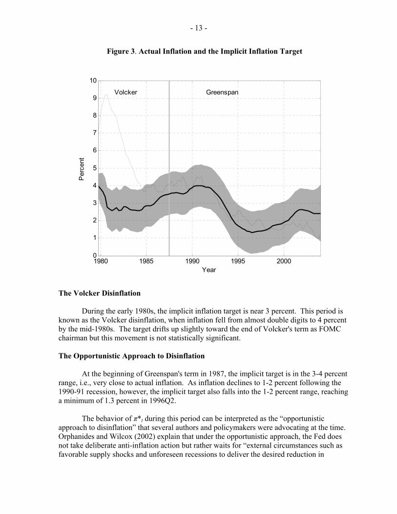
C. Estimates of the Implicit Target

In this subsection, I discuss the estimated path of the implicit inflation target shown in Figure 3. We can divide the trajectory of π*t into four sections: (i) the Volcker disinflation (1979 until the early 1980s); (ii) the opportunistic approach to disinflation (mid-1980s to early 1990s); (iii) the low inflation equilibrium (late 1990s); and (iv) the deflation scare (2001-2004). The estimated path of π*t during these four periods is corroborated by the qualitative historical evidence. In addition to the path of the estimated implicit target obtained using the Kalman smoother, Figure 3 shows the 95 percent confidence interval and actual PCE inflation. The 95 percent confidence intervals are obtained from the estimate of the variance of the Kalman smoother and corrected for parameter uncertainty following Ansley and Kohn (1986). 14 This value of β = 3.1 is higher than is generally found in the literature. For example, Lubik and Schorfheide (2004) obtain an estimate of β = 2.2 using the 1982-1997 sample and the constant π* and rn framework. Adjusting my sample to end in 1997 as in Lubik and Schorfheide (2004) reduces my estimate of β slightly to 2.7. This suggests that the Fed's response to inflation may have increased during 1998-2004. However, I do not investigate the issue of time-variation in β further here.

- 13 -

Figure 3. Actual Inflation and the Implicit Inflation Target

Volcker GreenspanP

erce

nt

Year1980 1985 1990 1995 20000

1

2

3

4

5

6

7

8

9

10

The Volcker Disinflation

During the early 1980s, the implicit inflation target is near 3 percent. This period is known as the Volcker disinflation, when inflation fell from almost double digits to 4 percent by the mid-1980s. The target drifts up slightly toward the end of Volcker's term as FOMC chairman but this movement is not statistically significant. The Opportunistic Approach to Disinflation

At the beginning of Greenspan's term in 1987, the implicit target is in the 3-4 percent range, i.e., very close to actual inflation. As inflation declines to 1-2 percent following the 1990-91 recession, however, the implicit target also falls into the 1-2 percent range, reaching a minimum of 1.3 percent in 1996Q2.

The behavior of π*t during this period can be interpreted as the “opportunistic approach to disinflation” that several authors and policymakers were advocating at the time. Orphanides and Wilcox (2002) explain that under the opportunistic approach, the Fed does not take deliberate anti-inflation action but rather waits for “external circumstances such as favorable supply shocks and unforeseen recessions to deliver the desired reduction in

- 14 -

inflation” (Orphanides and Wilcox, 2002, p.47). Weaknesses in the banking system and the output costs associated with deliberate anti-inflation actions may have prompted the Fed not to tighten policy in the early Greenspan years.

This strategy was endorsed by a number of monetary policymakers. In 1989, President Boehne of the Federal Reserve Bank of Philadelphia suggested that, rather than lowering inflation by tightening policy, the Fed should wait for the next recession to lower inflation. Once inflation declined, Boehne suggested that the Fed should seek to keep inflation at the lower level. As Vice Chairman Blinder put it in 1994, such a policy would allow one to “pocket the gains when good fortune runs our way” and to “chip away at the already-low inflation rate” (Blinder, 1994, p.4, as quoted in Orphanides and Wilcox, 2002).15 The Low-Inflation Equilibrium

In the late 1990s, both the implicit target and actual inflation remain in the 1-2 percent range. This low inflation is consistent with the view that very low inflation is desirable. At the 1996 Jackson Hole Symposium, a distinguished group of central bankers, academics, and financial market representatives met to discuss policies for achieving price stability and agreed that low or zero inflation was the appropriate goal for monetary policy.

There was, however, disagreement about whether a little inflation should be tolerated. Specifically, Stanley Fischer and Lawrence Summers argued that it was best to target an inflation rate in the 1-3 percent range, while other conference participants argued that a lower target in the 0-2 percent range was preferable.16 The Deflation Scare

Figure 3 suggests that, during the 2001 to 2004 period, the implicit inflation target drifted upward into the 2 to 3 percent range. This econometric finding is intuitive given the pronouncements of policymakers and the recommendations of influential academic papers at the time.

With inflation near 1 percent and the economy in recession in 2001, avoiding deflation and a Japan-style liquidity trap became an important consideration at the Fed. Governor Bernanke (2002) and Bernanke and Reinhart (2004) explain that the Fed can avoid deflation by offering a commitment to the public “to keep the short rate low for a longer period than previously expected” (Bernanke and Reinhart, 2004).17 15 The disinflation of the 1990s is associated with the 1990-91 recession, and the supply shocks of rapid productivity growth in the latter half of the decade.

16 For a summary of the symposium, see George A. Kahn (1996).

17 For an analysis of how other central banks responded to the “deflation scare,” see for example Kuttner and Posen (2004), who discuss the case of Japan in the 1990s.

- 15 -

As Eggertsson and Woodford (2003) explain, committing to an unusually long period of low interest rates is equivalent to a temporary increase in the time-varying inflation target. The inflation target rises above the level that is optimal under normal circumstances and only declines once the economy has experienced a boom and a period of higher inflation.18 Actual Versus Fitted Interest Rates

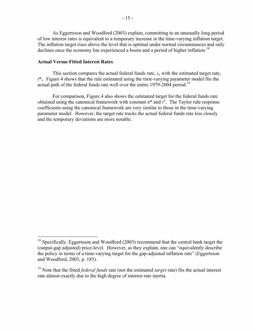
This section compares the actual federal funds rate, it, with the estimated target rate, i*t. Figure 4 shows that the rule estimated using the time-varying parameter model fits the actual path of the federal funds rate well over the entire 1979-2004 period.19

For comparison, Figure 4 also shows the estimated target for the federal funds rate obtained using the canonical framework with constant π* and rn. The Taylor rule response coefficients using the canonical framework are very similar to those in the time-varying parameter model. However, the target rate tracks the actual federal funds rate less closely and the temporary deviations are more notable.

18 Specifically, Eggertsson and Woodford (2003) recommend that the central bank target the (output-gap adjusted) price-level. However, as they explain, one can “equivalently describe the policy in terms of a time-varying target for the gap-adjusted inflation rate” (Eggertsson and Woodford, 2003, p. 185).

19 Note that the fitted federal funds rate (not the estimated target rate) fits the actual interest rate almost exactly due to the high degree of interest rate inertia.

- 16 -

Figure 4. Actual and Estimated Federal funds Target Rate

1980 1985 1990 1995 20000

2

4

6

8

10

12

14

16

18

20

22P

erce

nt

Year

ActualTime-varying r*t and π*tConstant r* and π*

V. ROBUSTNESS ANALYSIS

This section discusses the robustness of the estimates of the Taylor rule and of the implicit inflation target to different values of (i) the initial implicit target, π*0, and (ii) the signal-to-noise ratio, λ.

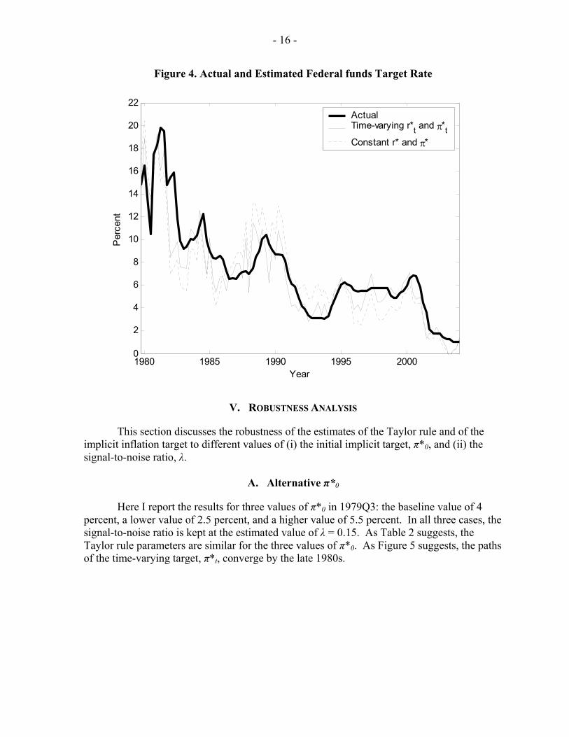
A. Alternative π*0

Here I report the results for three values of π*0 in 1979Q3: the baseline value of 4 percent, a lower value of 2.5 percent, and a higher value of 5.5 percent. In all three cases, the signal-to-noise ratio is kept at the estimated value of λ = 0.15. As Table 2 suggests, the Taylor rule parameters are similar for the three values of π*0. As Figure 5 suggests, the paths of the time-varying target, π*t, converge by the late 1980s.

- 17 -

Table 2. Robustness Analysis: Estimation Results for Different π*0s

Parameter Baseline π*0=4% Low π*0=2.5% High π*0=5.5% β 3.12 2.80 3.36 (0.70) (0.54) (1.08) γ 0.68 0.74 0.58 (0.22) (0.21) (0.29) ρ 0.74 0.71 0.81 (0.07) (0.06) (0.07)

02σ 1.09 1.04 1.24 (0.12) (0.11) (0.12)

32σ 0.17 0.16 0.19 (--) (--) (--)

Log likelihood -63.7 -60.8 -67.9

Figure 5. Actual Inflation and the Implicit Inflation Target for Different π*0s

1980 1985 1990 1995 20000

1

2

3

4

5

6

7

8

9

10

Perc

ent

Year

Actual π*0=2.5% π*0=4.0% (baseline)π*0=5.5%

B. Alternative λ

Here I report the results for three values of λ, the signal-to-noise ratio: the baseline estimated value of λ = 0.15; the low end of the 90 percent confidence interval, λ = 0.06; and the high end of the 90 percent confidence interval, λ = 0.51. In each case, the initial value of

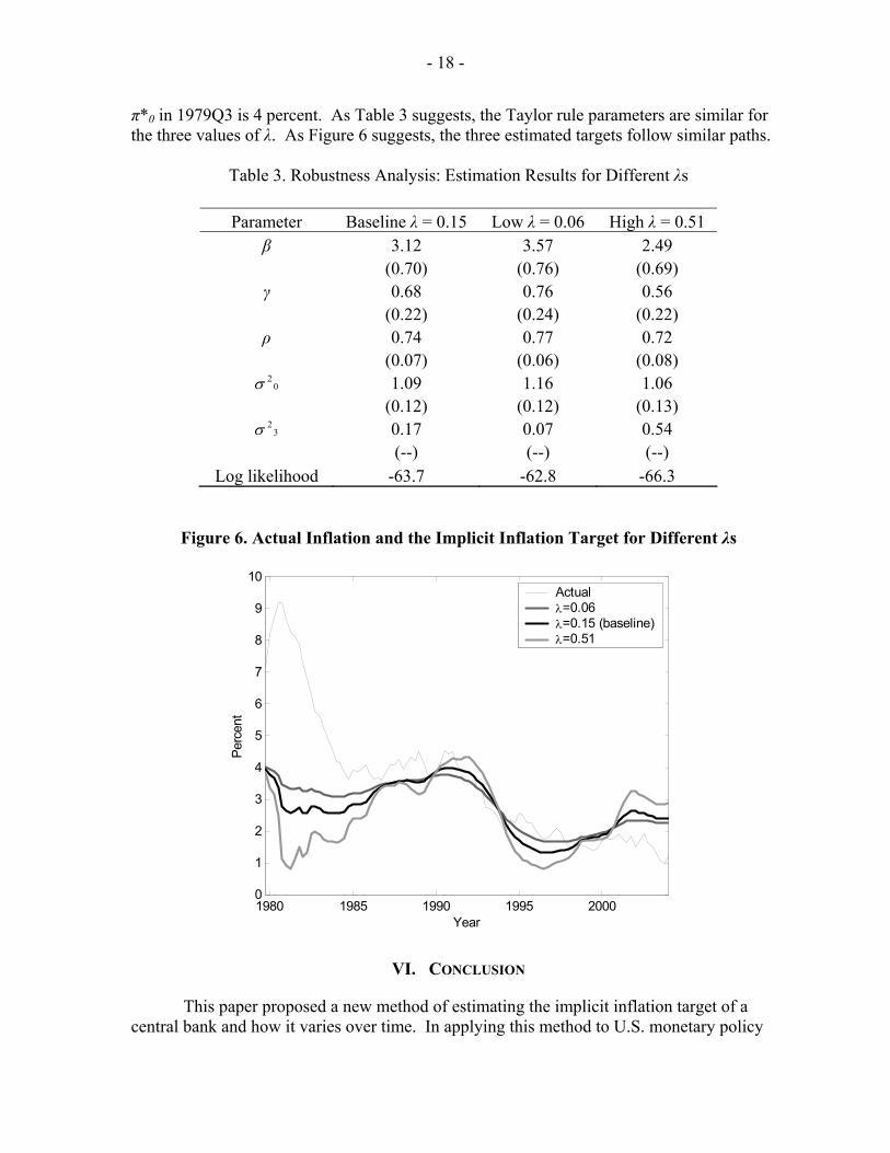
- 18 -

π*0 in 1979Q3 is 4 percent. As Table 3 suggests, the Taylor rule parameters are similar for the three values of λ. As Figure 6 suggests, the three estimated targets follow similar paths.

Table 3. Robustness Analysis: Estimation Results for Different λs

Parameter Baseline λ = 0.15 Low λ = 0.06 High λ = 0.51 β 3.12 3.57 2.49 (0.70) (0.76) (0.69) γ 0.68 0.76 0.56 (0.22) (0.24) (0.22) ρ 0.74 0.77 0.72 (0.07) (0.06) (0.08)

02σ 1.09 1.16 1.06 (0.12) (0.12) (0.13)

32σ 0.17 0.07 0.54 (--) (--) (--)

Log likelihood -63.7 -62.8 -66.3

Figure 6. Actual Inflation and the Implicit Inflation Target for Different λs

1980 1985 1990 1995 20000

1

2

3

4

5

6

7

8

9

10

Perc

ent

Year

Actual λ=0.06 λ=0.15 (baseline)λ=0.51

VI. CONCLUSION

This paper proposed a new method of estimating the implicit inflation target of a central bank and how it varies over time. In applying this method to U.S. monetary policy

- 19 -

over the past 25 years, I find that the Federal Reserve's implicit target has varied substantially during this broadly successful quarter century.

My analysis of the inflation target reveals four broad periods in recent monetary history: (i) the Volcker disinflation (1979 until the early 1980s); (ii) the opportunistic approach to disinflation (mid-1980s to early 1990s); (iii) the low inflation equilibrium (late 1990s); and (iv) the deflation scare (2001-04). The estimated path of π*t during these four periods is corroborated by the qualitative historical evidence.

This paper has focused on U.S. monetary policy. The analytical framework can easily be adapted to estimating the implicit inflation target in other countries. For example, Leigh (2004) considers how the implicit inflation target varied in Japan during the 1990s. An interesting direction for future research that I am actively pursuing is to investigate whether the implicit inflation target is more stable in countries with an explicit inflation targeting framework, such as the United Kingdom, New Zealand and Sweden, than in countries without an explicit numeric target, such as the United States and Japan.

The results in this paper raise the following question: is a time-varying inflation target preferable to a constant target? The finding that the inflation target has varied considerably during a successful period in U.S. monetary history suggests that a time-varying inflation target has advantages. Future research could investigate this question further.

APPENDIX I - 20 -

THE NATURAL RATE OF INTEREST

This appendix describes the Kalman filter approach for obtaining an estimate of the time-varying natural rate, rn

t, as in Laubach and Williams (2003). The two basic identifying assumptions are that (i) the output gap converges to zero if the real rate gap is zero and (ii) the change in inflation converges to zero if the output gap is zero. The first assumption is formalized by the following I.S. equation: yt = y*t + Ay(L)(yt-1 – y*t-1) + Ar(L)(rt-1 – rn

t-1) + ε1,t , (A.1) where yt is the log of GDP and y*t is the log of potential GDP. The difference between actual and potential GDP, i.e. yt – y*t, is the output gap. Term ε1,t denotes a mean zero i.i.d. normal shock to output. The second assumption is formalized by the following Phillips curve: πt = Bπ(L)πt-1 + By(L)(yt-1 – y*t-1) + Bπ(L)xt + ε2,t , (A.2) where xt denotes the data matrix containing the relative oil and non-oil import price inflation series. The inflation rate depends on lags of inflation with the unity sum restriction on the coefficients, relative oil and non-oil import price inflation, and the output gap. Thus, stable inflation is consistent with both the real interest rate and output equaling their respective natural rates. The term ε2,t denotes a mean zero i.i.d. normal shock to output.20 The unobserved state variables are modeled as follows. The natural rate of interest evolves according to rn

t = cgt + zt , (A.3) where c is a constant term, gt is the unobserved trend in productivity growth, and zt is a stochastic drift term that follows the process zt = Dz(L) zt-1 + ε4,t . (A.4) LW report results for a baseline case where zt is a random walk, so that ∆zt = ε4,t, as well as for the case where zt is stationary. I use the simpler baseline case. Consequently, the natural rate of interest follows a random walk. Potential evolves according to 20 The number of lags are determined by the data. Specifically, as in LW, I include two lags of the output and real interest rate gap in the output equation. I include eight lags of inflation and one lag of output in the inflation equation.

APPENDIX I - 21 -

y*t = y*t-1 + gt-1 + ε5,t. (A.5) Finally, for reasons of parsimony, LW assume that the trend growth rate, gt, follows a random walk, gt = gt-1 + ε6,t. (A.6) LW estimate Equations (A.1) through (A.6) using maximum likelihood and the Kalman filter to yield (a) estimates of the model parameters, and (b) estimates of the time-varying paths of the unobserved state variables. LW apply this approach to the 1961Q1 to 2002Q1 sample. I extend the sample to 2004Q1 and estimate the equations using the 1961Q1 to 2004Q1 period. The advantage of conducting the estimation over this long sample is that I do not need to initialize rn

t in 1979Q3.

- 22 -

REFERENCES

Ansley, Craig F. and Robert Kohn, 1986, “Prediction Mean Squared Error for State Space Models with Estimated Parameters,” Biometrika, Vol. 73, pp. 467–73.

Arnold, Robert, 2004, “A Summary of Alternative Methods for Estimating Potential GDP,”

Macroeconomic Analysis Division, Congressional Budget Office, (March), Available via Internet http://www.cbo.gov.

Bernanke, Ben S. and Vincent R. Reinhart, 2004, “Conducting Monetary Policy at Very Low

Short-Term Interest Rates,” Board of Governors of the Federal Reserve System, (Washington, D.C).

Bernanke, Ben S., 2002, “Deflation: Making Sure ‘It’ Doesn't Happen Here,” Remarks

Before the National Economists Club, (November 21, 2002), (Washington, D.C.). Blinder, Alan S., 1994, “Opening Statement of Alan S. Blinder at Confirmation Hearing

Before the U.S. Senate Committee on Banking, Housing, and Urban Affairs” (May), mimeo, Federal Reserve Board.

Boivin, Jean, 2004, “Has U.S. Monetary Policy Changed? Evidence from Drifting

Coefficients and Real-Time Data,” (manuscript, New York: Columbia University). Clarida, Richard, Jordi Gali and Mark Gertler, 1998, “Monetary Policy Rules in Practice:

Some International Evidence,” European Economic Review, Vol. 42, pp. 1033-1067. Eggertsson, Gauti and Woodford, Michael, 2003, “The Zero Bound on Interest Rates and

Optimal Monetary Policy,” Brookings Papers on Economic Activity, Vol. 1, pp. 139-233. Federal Reserve Board, 1989, “Transcript of the Federal Open Market Committee Meeting”

(December) mimeo. Haltmaier, Jane, 2001, “The Use of Cyclical Indicators in Estimating the Output Gap in

Japan,” Federal Reserve Board International Finance Discussion Paper No. 2001-701 (April).

Hamilton, James D., 1994, Time Series Analysis, (Princeton, New Jersey: Princeton

University Press). Kettl, Donald F., 1986, Leadership at the Fed, (New Haven, Connecticut: Yale University

Press). Kahn, George A., 1996, “Symposium Summary” in Achieving Price Stability, Federal

Reserve Bank of Kansas City, 1996.

- 23 -

Kuttner, Kenneth N., 2004, “The Role of Policy Rules in Inflation Targeting,” Federal Reserve Bank of St. Louis Review, July/August 2004, 86(4), pp. 89-111.

Kuttner, Kenneth N. and Adam S. Posen, 2004, “The Difficulty of Discerning What’s Too

Tight: Taylor Rules and Japanese Monetary Policy,” North American Journal of Economics and Finance, Vol. 15, pp. 53–74.

Laubach, Thomas, 2001, “Measuring the NAIRU: Evidence from Seven Economies,'' Review

of Economics and Statistics, Vol. 83, (May), pp. 218-31. Laubach, Thomas, and John C. Williams, 2003, “Measuring the Natural Rate of Interest,”

The Review of Economics and Statistics, Vol. 85(4) (November). Leigh, Daniel, 2004, “Monetary Policy and the Dangers of Deflation: Lessons from Japan”

Working Paper No. 511, (Department of Economics: Johns Hopkins University). Lubik, Thomas A., and Frank Schorfheide, 2004, “Testing for Indeterminacy: An

Application to U.S. Monetary Policy,” American Economic Review, Vol. 94, No. 1, pp. 190-217.

Maccini, Louis, Bartholomew Moore and Huntley Schaller, 2004, “The Interest Rate,

Learning, and Inventory Investment”, American Economic Review, Vol. 94, No. 5, December 2004.

Meltzer, Allan H., 2003, “A New Beginning, 1951-60,” manuscript, (Pittsburg,

Pennsylvania: Carnegie-Mellon University). Orphanides, Athanasios, 2001, “Monetary Policy Rules Based on Real-time Data,” American

Economic Review, Vol. 91, pp. 964-85. Orphanides, Athanasios, 2002, “Monetary Policy Rules and the Great Inflation,” American

Economic Review, Vol. 92, pp. 115-120. Orphanides, Athanasios, 2003, “Historical Monetary Policy Analysis and the Taylor Rule,”

Journal of Monetary Economics, Vol. 50 (July), pp. 983-1022. Orphanides, Athanasios, 2004, “Monetary Policy Rules, Macroeconomic Stability, and

Inflation: A View from the Trenches,” Journal of Money, Credit and Banking, April 2004.

Orphanides, Athanasios and David Wilcox, 2002, “The Opportunistic Approach to

Disinflation,” International Finance, Vol. 5, pp. 47-71. Rabanal, Pau, 2004, “Monetary Policy Rules and the U.S. Business Cycle: Evidence and

Implications,” IMF Working Paper No. 04/164, (Washington: International Monetary Fund).

- 24 -

Staiger, Douglas, James H. Stock and Mark W. Watson, 1997, “How Precise Are Estimates

of the Natural Rate of Unemployment?” (pp. 195-242), in C. Romer and D. Romer (eds.), Reducing Inflation: Motivation and Strategy (Chicago: Chicago University Press and Cambridge, Massachusetts: National Bureau of Economic Research).

Stock, James H. and Mark W. Watson, 1998, “Median Unbiased Estimation of Coefficient

Variance in a Time Varying Parameter Model,” Journal of the American Statistical Association, Vol. 93, pp. 349–58.

Tobin, James, 2002, “Monetary Policy” in David R. Henderson (ed.), 2002, The Concise

Encyclopedia of Economics, Indianapolis: Liberty Fund, Inc., Available via Internet at http://www.econlib.org/library/Enc/MonetaryPolicy.html.

U.S. Board of Governors of the Federal Reserve System, various years, Transcripts of

Federal Open Market Committee. U.S. Board of Governors of the Federal Reserve System, various years, Federal Reserve

Bulletin. U.S. Office of the President, various years, Economic Report of the President, (Washington

D.C.: U.S. Government Printing Office).