Estimating the impact of climate change on crop yields:The importance of non-linear temperature effects

Wolfram Schlenker♣ and Michael J. Roberts♠

September 2006

Abstract

There has been an active debate whether global warming will result in a net gain or net lossfor United States agriculture. With mounting evidence that climate is warming, we showthat such warming will have substantial impacts on agricultural yields by the end of the cen-tury: yields of three major crops in the United States are predicted to decrease by 25-44%under the slowest warming scenario and 60-79% under the most rapid warming scenario inour preferred model. We use a 55-year panel of crop yields in the United States and pair itwith a unique fine-scale weather data set that incorporates the whole distribution of tem-peratures between the minimum and maximum within each day and across all days in thegrowing season. The key contribution of our study is in identifying a highly non-linear andasymmetric relationship between temperature and yields. Yields increase in temperatureuntil about 29◦C for corn and soybeans and 33◦C for cotton, but temperatures above thesethresholds quickly become very harmful, and the slope of the decline above the optimum issignificantly steeper than the incline below it. Previous studies average temperatures over aseason, month, or day and thereby dilute this highly non-linear relationship. We use encom-passing tests to compare our model with others in the literature and find its out-of-sampleforecasts are significantly better. The stability of the estimated relationship across regions,crops, and time suggests it may be transferable to other crops and countries.

Keywords: Agriculture, Nonlinear temperature effects, Climate change.JEL code: Q54, C23

♣ Department of Economics and School of International and Public Affairs, Columbia University, 420 West118th Street, Room. 1308, MC 3323, New York, NY 10027. Email: ws2162@columbia.edu. Phone: (212)854-1806.♠ Economic Research Service, United States Department of Agriculture. 1800 M Street NW, Washington,DC 20036. Email: mroberts@ers.usda.gov. Phone (202) 694-5557.Views expressed are the authors’, not necessarily those of the U.S. Department of Agriculture.

1 Introduction

With accumulating evidence that greenhouse gas concentrations are warming the world’s

climate, research increasingly focuses on impacts likely to occur under different warming

scenarios. Agriculture is a key focus due to its obvious links to weather and climate, as

well as the inelastic demand for staple food commodities. Although there is some consensus

that warming will likely be harmful to agriculture in tropic and sub-tropic zones, active

debate continues about whether warming will be a net gain or loss for agriculture in the

more temperate United States and Europe (Mendelsohn et al. 1994, Darwin 1999, Schlenker

et al. 2006, Kelly et al. 2005, Timmins 2006, Ashenfelter and Storchmann 2006, Deschenes

and Greenstone 2006).

This paper develops novel estimates of the link between weather and yields for several

prevalent crops grown in the United States: corn, soybeans, and cotton. Corn and soybeans

are the nation’s most prevalent crops and are the predominant source of feed grains in

cattle, dairy, poultry, and hog production. Cotton is next largest crop in the U.S. and more

suitable to warmer climates than corn and soybeans. We pair yield data for these crops

with a newly constructed fine-scale weather data set to develop a large panel that spans

most U.S. counties from 1950 to 2004. The new weather data includes daily precipitation

and the time a crop is exposed to each 1-degree Celsius temperature interval. We estimate

these data for the specific locations where crops are grown in every county. These data

are combined with publicly-available yield data from the U.S. Department of Agriculture’s

National Agricultural Statistical Service (USDA-NASS).

The new fine-scale weather data facilitates estimation of a flexible model in order to

identify nonlinearities and breakpoints in the effect of temperature on yield. If temperatures

are averaged over time or space, and the true underlying relationship is nonlinear (e.g.,

increasing and then decreasing in temperature), standard regression techniques dilute the

true underlying curvature in the relationship. Accurate estimation of non-linear effects is

particularly important when predicting effects on non-marginal changes in temperatures, as

is expected under climate change.

Unraveling the nonlinear relationship between weather and agricultural output has impli-

cations beyond climate change impacts. Many empirical studies use weather as an instrument

as it is arguably exogenous. However, the standard instrumental variables (IV) approach

assumes that the marginal effect is constant, which we show to be a bad assumption for tem-

peratures. Second, total liabilities of crop insurance in the United States totaled 47 billion

in 2004, with a subsidy of 2.5 billion. Identifying a stronger link between weather and crop

1

yields may facilitate the creation of financial instruments to spread crop yield risk in a way

that is not subject to moral hazard.

We find a robust nonlinear relationship between weather and yields that is consistent

across space, time, and crops: plant growth increases approximately linearly in temperature

up to a point where additional heat quickly becomes harmful. The non-linear relationship

is starkly asymmetric, with the slope of the decline above the peak being much steeper

than the slope of the incline below it. Despite significant technological progress over our

55-year sample period, we find no evidence that crops have become significantly better at

withstanding extreme heat above the upper threshold. Moreover, hotter southern states

exhibit the same threshold as cooler states in the north, suggesting that there is limited

potential for adaptations.

Encompassing tests show our nonlinear model predicts yields out-of-sample significantly

better than other approaches in the literature. While our model is better at predicting actual

yields, the sharp asymmetry where temperatures above a critical threshold quickly become

harmful also implies that if climate change shifts the temperature distribution above such a

threshold, the impacts would be significant.

We use our estimated model to forecast yields under several climate change scenarios.

Global warming shifts the temperature distribution upward enough that damaging heat

waves are observed more frequently. As a result, yields at the end of the century are predicted

to decrease by 44% for corn, 33-34% for soybeans, and 26-31% for cotton under a slow

warming scenario (B1) and 79-80%, 71-72%, and 60-78%, respectively, under a quick warming

scenario (A1). These predictions are highly significant and consistent across alternative

model specifications.

The next section reviews past literature and motivates our new approach. Section 3

provides a description of our model. In Section 4 we describe the construction of the fine-

scale weather estimates and yield data. Section 5 reports a detailed empirical analysis of

crop yields before Section 6 presents robustness checks, and Section 7 compares the model’s

out-of-sample predictions with other approaches found in the literature. Section 8 reports

predictions under several of the latest climate change scenarios. We conclude in Section 9.

2 Background and Motivation

Many studies link weather and climate to outcomes such as yields, land values, and farm

profits. These studies span several disciplines and methods. Agronomists sometimes estimate

2

simple regressions but usually link weather and nutrient inputs to yields using crop simulation

models. Economists have linked climate (average weather) to land values in cross-sectional

hedonic studies. They have also linked weather to crop yields and profits using simple

regressions and more complex structural models, and sometimes have used agronomists’

simulation models. The different approaches have different strengths and weaknesses. We

briefly review these approaches here to help motivate our new approach, which combines

strengths from each one.

2.1 Agronomic Simulation Models

Agronomic studies emphasize the dynamic physiological process of plant growth and seed

formation. This process is understood to be quite complex and dynamic in nature and

thus not easily molded into a simple regression framework. Instead, these studies use a

rich theoretical model to simulate yields given daily weather inputs, nutrient applications,

and initial soil conditions. Models specific to each crop take inputs as exogenous, without

economic or behavioral considerations. Economists may think of these models as complex

production functions. Micro-parameters embedded in these models are taken as ”reasonable

assumptions” or taken one-at-a-time from experimental studies. In some cases, simulated

yields are compared to observed yields with some success. But we are not aware of any

study that has tested a simulation model using data besides that used to calibrate it. Current

versions of models developed for many crops are maintained by the Decision Support System

for Agrotechnology Transfer (http://www.icasa.net/dssat/).

At the heart these models is a state-dependent plant growth function. Plant growth po-

tential is linked to temperature (available energy) while an absence of other factors (moisture

and nutrients) may limit growth below this potential. The agronomic concept of ”growing

degree days,” a highly nonlinear function of temperature, can be linked to the basic concept

of growth potential. The shape of this function has been estimated rather imprecisely due

to the relatively few observations available from experimental field trials.

A key strength of this growth function, and simulation models generally, is they way

they incorporate the whole distribution of weather outcomes realized over the growing sea-

son. This differs from standard regression approaches, discussed below, which generally use

average weather outcomes or averages from particular months. While our model is far sim-

pler than crop simulation models, we show how it incorporates the whole distribution of

weather outcomes and generalizes the concept of growing degree days.

There are two general problems with crop simulation models. First, there is considerable

3

uncertainty about physiological process (functional form) and the many parameters in these

highly non-linear models. Given the complex dynamic and non-linear nature of the models,

it is not possible to estimate them statistically (Wallach et al. 2001). If it were possible, many

agronomists would be skeptical about the physiological interpretation of these estimates and

there are worries about possible misspecification and omitted variables biases (Sinclair and

Seligman 2000, Long et al. 2005). The second critical problem is the assumption of exogenous

production systems and nutrient applications: there is no account for behavioral response

on behalf of farmers.

In some circles, there seems to be an understandable skepticism about how these models

should be calibrated and how one model can be empirically compared to another (Sinclair and

Seligman 1996, Sinclair and Seligman 2000). Nevertheless, these models are the predominant

tool used to evaluate likely effects from climate change on crop yields. Examples include

Black and Thompson (1978), Adams et al. (1995), Brown and Rosenberg (1999), Mearns et

al. (2001), and Stockle et al. (2003), but there are many others.

2.2 Hedonic and Other Cross-Sectional Studies

The most widely received economic studies use hedonic models to link land values to land

characteristics, including climate, using relatively simple reduced-form linear regression mod-

els (e.g., Mendelsohn et al. (1994); Schlenker et al. (2006); Ashenfelter and Storchmann

(2006)). For evaluation of impacts from climate change, the strength of the approach is

that it can account for a large degree of behavioral response. Cooler areas are likely to

become more like warmer areas, with crops choice, management, and land values changing

in accordance with climate changes. Analysis of yields, particularly using simulation models

which take both crop choice and management practices as exogenous, cannot capture these

adaptive changes.

Some changes, however, cannot be evaluated, even with a hedonic model. To the extent

that global warming changes the overall production capacity of crops, relative commodity

prices will change, which in turn will affect land values, and thus induce feedback effects on

crop choice and management practices (earlier studies argue price effects will be small). Nor

can hedonic models account for passive or induced technological change.

Perhaps a greater concern with the hedonic approach is possible confounding from omit-

ted variables or model misspecification. Climate variables (e.g., average temperature) and

other critical variables, such as soil types, distance to cities, and irrigation, are all spatially

correlated. If critical variables correlated with climate are omitted from the regression model,

4

or the functional form the regression model is incorrect, the climate variables may pick up

effects of variables besides climate and lead to biased estimates and predictions. Indeed,

earlier work shows how omission of irrigation critically influences predicted climate impacts

(Schlenker et al. 2005). Hedonic studies become more credible when findings are robust to

many alternative specifications (Schlenker et al. 2006). Timmins (2006) relies on a cross-

section of farmland values and shows how under certain assumptions about the error-term

structure, use-specific error terms can be recovered.

2.3 Time-Series and Panel Studies

Omitted variables bias has been a concern since the early part of the last century, when

Ronald Fisher wrote ”Studies in Crop Variation I-VI.” The ostensible purpose of the pa-

pers was to discern the influences of nutrient applications and soil types on crop yields.

The challenge was to discern the effects of these factors given considerable confounding,

particularly from weather, which, like nutrient applications and soil types, were strongly

spatially correlated. Fisher used this setting to motivate development of modern experi-

mental methods, including random assignment of treatment levels and split-plot designs, as

well as formal statistical concepts, including maximum likelihood and analysis of variance.

Fisher’s experimental designs and subsequent refinement of them would later help to facil-

itate rapid growth in agricultural productivity through the rest of the century, and more

broadly, statistical assessment of experimental outcomes in all scientific disciplines.

Studies employing panel data attempt to mitigate confounding using a richer set of

control variables and location and/or year fixed effects. Recent studies include Kaylen et

al. (1992) who link yield to weather outcomes and find that yield variability has increased

partly due to an increase in weather variability. Kelly et al. (2005) use a panel data set

of county-level profits for midwestern states to discern the influence of climate (weather

averages) from yearly weather shocks, i.e., the authors include both historic mean climate

and variability (standard deviation between years) as well as yearly weather shocks. Since

the authors include climate averages (which are constant in the cross-section), they can not

include county fixed effects because they would be perfectly collinear with climate. Deschenes

and Greenstone (2006) link profits and yields to weather fluctuations for the entire U.S.

using county fixed effects to capture all time-invariant factors like soil quality. They assume

remaining year-to-year variation in weather is random.

5

3 A New Model and Approach

Our objective is to discern the effect of weather, particularly heat, on crop yields using a new

and rich data set and a novel approach that allows us to estimate nonlinear effects of heat

over the growing season. By using the whole distribution of temperature outcomes (which

is critical for estimating non-linear effects), we depart from earlier cross-sectional and panel

data studies and share a common thread with the agronomic literature that employs crop

simulation models. Unlike agronomic literature, we incorporate our model into a statistical

regression framework. We focus on yields because yields are linked to the year a plant

is grown (unlike profits which can be affected by storage), avoid potentially confounding

influences of price changes, and because many observations are available for each county and

crop. Here we describe our model and discuss exogeneity assumptions and Identification.

3.1 Statistical Model

Following the spirit of the agronomic literature we postulate that the effect of heat on relative

plant growth is cumulative over time, so yield is the integral of plant growth over the growing

season. In other words, we assume the effect of temperature is perfectly substitutable over

time. In extreme cases, this assumption is implausible. For example, if frost or extreme heat

were to kill the plant it would obviously affect future growth. Specifically, plant growth g(h)

depends nonlinearly on heat h and log yield, yit, in county i and year t is

yit =

∫ h

h

g(h)φit(h)dh + zitδ + ci + εit (1)

where φit(h) is the time distribution of heat over the growing season in county i and year

t. We fix the growing season to months March through August for corn and soybeans and

the months April through October for cotton. Fixing it exogenously makes it robust to

farmers’ decisions like planting dates. Observed temperatures during this time period range

between the lower bound h and the upper bound h. Other factors, such as precipitation and

technological change, are denoted zit, and ci is a time-invariant county fixed effect to control

for time-invariant heterogeneity.

While time separability is rooted in agronomic experiments, we implicitly validate this

assumption by showing a statistically significant relationship between the cumulative dis-

tribution of temperatures and yields. We would not observe this if time separability were

not appropriate, because random pairing of various temperatures over a season and between

6

years would not provide clear identification. In the empirical section we split the six-month

growing season into two three-months intervals and find comparable estimates for both subin-

tervals, i.e., temperature effects in the early and later states of the plant cycle are similar.

Earlier studies using quadratic specifications in average temperature for various months find

this quadratic relationship to vary by month of the year. More specifically, July tempera-

tures, the hottest month, usually peak at a very low level (around 22◦C), while higher April

temperatures are always beneficial. However, if the true underlying relationship is asym-

metric, the quadratic functional form might be restrictive. Since average temperatures in

April and July are correlated, the former will pick up the beneficial effects of moderate heat,

while the latter will pick up the effects of harmful extreme heat. Hence, the difference in

coefficients between months does not necessarily imply that the effects vary by season, but

might be a result of an inappropriate implicit assumption that the relationship is symmetric.

A special case of time-separable growth is the concept of growing degree days, typically

defined as the sum of truncated degrees between two bounds. For example, Ritchie and

NeSmith (1991) suggests bounds of 8◦C and 32◦C for ”beneficial heat”. For example, a day

of 9◦C contributes 1 degree day, a day of 10◦C contributes 2 degree days, up to a temperature

of 32◦C, which contributes 24 degree days. All temperatures above 32◦C also contribute 24

degree days. Degree days are then summed over the entire season. Temperatures above 34◦C

are included as a separate variable and speculated to be harmful. These particular bounds

have been implemented in a cross-sectional analysis by Schlenker et al. (2006). Thus, growing

degree days are the special case of our model where (using the above bounds as an example)

g(h) =

0 if h ≤ 8

h− 8 if 8 < h < 32

24 if 32 ≤ h

The exact degree day bounds are still debated, partly because earlier studies use a limited

number of observations from field experiments to identify them. There is also uncertainty

about temperature effects above the upper bound. While some speculate that high temper-

atures are harmful, the critical temperature and severity of damages remain uncertain. We

use a flexible functional form allows us to identify effects of extreme heat.

In the data section we explain how we derive the amount of time a plant is exposed to each

1-degree Celsius interval. With these data, we approximate the integral over temperature

with

yit =49∑

h=−5

g(h + 0.5)[Φit(h + 1)− Φit(h)] + zitδ + ci + εit (2)

7

where Φit(h) is the cumulative distribution function of heat in county i and year t. We

consider two specifications of this model.

First we model g(h) as a m-th order Chebychev polynomial of the form g(h) =∑m

j=1 γjTj(h),

where Tj() is the j− th order Chebyshev polynomial. We rely on Chebyshev polynomials be-

cause each term is orthogonal which makes least-squares estimates numerically more stable.

By interchanging the sum we obtain

yit =49∑

h=−5

m∑j=1

γjTj (h + 0.5) [Φit (h + 1)− Φit (h)] + zitδ + ci + εit

=m∑

j=1

γj

49∑

h=−5

Tj (h + 0.5) [Φit (h + 1)− Φit (h)]

︸ ︷︷ ︸xit,j

+zitδ + ci + εit (3)

where xij,t is the exogenous variable obtained by summing the j − th Chebyshev polyno-

mial evaluated at each temperature interval midpoint, multiplied by the time spent in each

temperature interval. We successively use higher-order polynomials until our estimated re-

lationship appears stable

The polynomial regressions are parsimonious and easy to interpret. As a more flexible

alternative model, we use dummy variables for each one-degree interval. The dummy-variable

model, spelled out in detail below, effectively regresses yield on season-total time within each

degree interval. Note that standard non-parametric methods, such as local regression or cubic

splines, are not possible, because each yield outcome is associated with a whole temperature

distribution.

Because temperatures rarely exceed 39◦C (102 degrees Fahrenheit) in counties where corn

and soybeans are grown, we lump all the time a plant is exposed to a temperature above

39◦C into one category. (Temperature intervals above 39◦C have a frequency of less than

one hour during the growing season for soybeans and corn. For cotton the analogous cutoff

is 42◦C). The model becomes (where Φit(40) is set to 1 for corn and soybeans).

yit =39∑

j=−5

γj [Φit(h + 1)− Φit(h)]︸ ︷︷ ︸xit,j

+zitδ + ci + εit (4)

Note that county fixed effects ci capture the additive influence of time-invariant factors in the

cross-section. The error terms, however, remain spatially correlated within each year. We

therefore use the non-parametric routine by Conley (1999) to adjust the variance-covariance

8

matrix for spatial correlation. We also use bootstrap simulations where we resample entire

years with replacement, as weather between years is plausibly i.i.d., but error terms within

a year are spatially correlated.

While equations (3) and (4) specify our main two models, the concept of degree days is

a special case where the function g(h) is piecewise linear. In a sensitivity check we therefore

estimate a piecewise-linear model, i.e., growth is forced to increase linearly in temperature up

to an endogenous plateau, and then forced to decrease linearly above an endogenous upper

bound. Since our data is aggregated by 1-degree Celsius intervals, we loop over possible

combinations of bounds and pick the ones with the least sum of squared residuals.

3.2 Exogeneity and Identification

Because we use observational data, confounding is the pervasive concern. In this case,

however, observational data are the only choice. The main reason is that with observational

data we can estimate the consummate effects of the weather on yields, which may differ from

effects of weather ceteris paribus. The consummate effects of the weather depend on weather

itself and on farmers’ management practices, which may also be influenced by weather. The

experimental plot designs developed by Fisher and refined over the years by statisticians and

agronomists cannot measure these effects because the designs were constructed to measure

the effects of practices, not weather. The behavioral element was deliberately controlled.

While greenhouses may be used to experimentally vary temperature and moisture, such a

design cannot mimic naturally occurring behavioral response. We therefore embrace a focus

on observed, and arguably random, year-to-year variation in weather. We use county fixed

effects to limit identification from cross-sectional variation in climate, which would be more

susceptible to confounding from omitted variables.

Fixed-effects models are often described as within estimators because identification comes

from deviations from within-group averages. However, when fixed effects are used in con-

junction with a non-linear specification of other covariates, identification of the curvature

stems in part from between-group variation, which may be more subject to confounding.

Fixed effects only shift the intercept. Thus, a key assumption is that non-linearity in the

cross-section is exogenous and behaves similarly to non-linear effects over time. We test

this assumption below by examining many different subgroups that limit time-series and/or

cross-sectional variation.

9

4 Data

4.1 Dependent Variable

Our dependent variable consists of publicly-available yield data for corn, soybean and cotton

for the years 1950-2004. The U.S. Department of Agriculture’s National Agricultural Sta-

tistical Service (USDA-NASS) reports yields as total production per acres harvested. There

is hence a potential selection bias as during extremely bad years farmers might decide it

does not pay to harvest, making the harvested area endogenous. We therefore also obtained

the area planted for roughly 80% of our data, and conducted a sensitivity check by deriving

yields as total production divided by acres planted. The results do not change. Since the

area planted is not reported in all areas and years, we focus in our analysis on yields per

acres harvested.

4.2 Weather Variables

Earlier studies have examined average temperatures over a longer time horizon (e.g., an

entire season, month, or day), which can hide extreme events like maximum temperatures

that occur during a fraction of the day. The construction of our fine-scale weather aids

identification of non-linear weather effects that are diluted with courser data or if weather

outcomes are averaged over time or space. We hence first develop daily predictions of

minimum and maximum temperature on a 2.5x2.5mile grid for the entire U.S. before we

derive the time a crop is exposed to each 1 degree Celsius interval in each grid cell. We

then match those predictions with the cropland area in each 2.5x2.5 miles grid cell, and

aggregate the whole distribution of outcomes for all days in the growing season in each

county. Since our study emphasizes non-linearities, we stress that we first derive the time

a plant is exposed to each 1 degree Celsius interval before we average the grid cells in a

county, and not vice versa. (Data development is briefly described here and in more detail

in Schlenker and Roberts (2006).)

Thom (1966) developed a method to predict the distribution of daily temperatures from

the distribution of average monthly temperatures. This method appears appropriate for

predicting the average probability that a certain weather outcome will be realized, but less

appropriate in predicting a specific weather outcome in a particular year. As a result, these

methods work well in a forward-looking cross-sectional analysis where the dependent variable

is tied to weather expectations (for example, the link between land values and climate), but

10

less well in our analysis where the dependent variable (yield) linked to specific weather

outcomes. Directly obtaining daily values on a small scale requires a spatial smoothing

procedure to approximate daily weather outcomes between individual weather stations.

The ”Parameter-elevation Regressions on Independent Slopes Model” (PRISM) is widely

regarded as one of the best interpolation procedures (http://www.ocs.orst.edu/prism/). It

accounts for elevation and prevailing winds to predict weather outcomes on 2.5x2.5 mile grid

across the contiguous United States. However, the PRISM data are on a monthly time scale.

We therefore combine the advantages of the PRISM model (good spatial interpolation) with

better temporal coverage of individual weather stations (daily instead of monthly values).

We pair each of the 259,287 PRISM grids that cover agricultural area in a LandSat satellite

scan with the closest seven weather stations having a continuous record of daily observations.

We then regress monthly averages at each PRISM cell against monthly averages at each of the

seven closest stations, plus fixed effects for each month. (Linking monthly PRISM averages

to averages at individual weather stations approximates the spatial smoothing procedure in

the PRISM model. The R-squares are usually in excess of 0.999). The derived relationship

between monthly PRISM grid averages and monthly averages at each of the seven closest

stations is then used to predict daily records at each PRISM grid from the daily records at

the seven closest weather stations.

We use a cross-validation exercise to test whether the results from monthly regressions

can be used to predict daily outcomes. Specifically, we construct a daily weather record at

each PRISM cell that harbors a weather station without using that weather station in the

interpolation. We then compare predicted daily outcomes at the PRISM cell with a weather

station to actual outcomes recorded at the weather station in the grid cell. The mean

absolute error is 1.36◦C for minimum temperature and 1.49◦C for maximum temperature,

while the average standard deviations are 9.37 and 10.56, respectively.

We approximate the distribution of temperatures within a day with a sinusoidal curve

between minimum and maximum temperatures. In a sensitivity check we instead use a lin-

ear interpolation between minimum and maximum temperature. Both methods give similar

results. We derive the time spent in each 1◦C-degree temperature interval between −5◦C

and +50◦C. Finally, we construct the area-weighted averages over all PRISM grid cells in

a county. Note that we first derive the weather variables and then average over the agricul-

tural area, not vice versa, which is important for our exploration of non-linear effects. The

agricultural area in each cell was obtained from LandSat satellite images. Vince Breneman

and Shawn Bucholtz at the Economic Research Service were kind enough to provide us with

11

the agricultural area in each PRISM grid cell. Since we use the LandSat scan of a given

year, we are not able to pick up shifts in growing regions.

Descriptive statistics for temperature, precipitation, and yields of corn (for grain), soy-

beans, and upland cotton are reported in Table 1. (The left column in Figure 4 below

displays a histogram of how many days a crop is exposed to each 1-degree Celsius interval).

Note that some yields appear artificially low. These few outliers are very infrequent. If

we drop them, the results do not change, but the cutoff point becomes somewhat arbitrary

(The outliers have little influence because we use log yield, so they have small errors). The

weather variables are summed over the six-months period from March through August for

corn and soybeans, and the seven-months period April through October for cotton. As noted

above, exogenously fixing this time period allows for an endogenous choice of the growing

season within this time frame.

We divide the United States into several regions as shown in Figure 1. The default data

set for corn and soybeans is the union of northern, interior, and southern states–what we

label eastern counties. We exclude the Western United States east of the 100 degree meridian

and Florida because agricultural production in these area relies on heavily subsidized access

to irrigation water. Since the access to subsidized water rights is correlated with climate,

omitting these variables, which vary on the sub-county level of irrigation districts, will result

in biased coefficient estimates on the climatic variables (Schlenker et al. 2005). Cotton is

predominantly grown in the south and west, and we include all states in the analysis to

obtain a larger sample of counties.

4.3 Climate Change Scenarios

We forecast the impact of a changing climate using the latest climate change predictions from

the Hadley 3 model (http://www.metoffice.com/research/hadleycentre/). This is a major

climate change model that will form the basis for the next report by the Intergovernmental

Panel on Climate Change (IPCC). We obtained monthly model output for both minimum

and maximum temperatures under four major emissions scenarios (A1, A2, B1, and B2) for

the years 1960-2099. Each scenario rests on a different assumption about population growth

and availability of alternative fuels, among other factors (Nakicenovic, ed 2000).

Climate changes are estimated as follows. At each of 216 Hadley grid nodes covering

the United States, we find the predicted difference in monthly mean temperature for 2020-

2049 (medium-term), 2070-2099 (long-term), and historic averages (1960-1989). Next, the

predicted change in monthly minimum and maximum temperature at each 2.5x2.5 mile

12

PRISM grid is calculated as the weighted average of the monthly mean change in the four

surrounding Hadley grid points, where the weights are proportional to the inverse squared

distance and forced to sum to one. In a final step, we add the predicted changes in monthly

minimum and maximum temperatures at each PRISM grid to observed daily time series

from 1960 to 1989. In other words, we leave the variability constant but shift the mean.

We use an analogous approach for precipitation, except that we rely on the ratio of future

rainfall compared to historic rainfall instead of absolute changes. Each county’s weather

outcomes in a climate scenario are the area-weighted averages of all PRISM grids that cover

farmland. Predicted changes for the B2-scenario (which assumes a intermediate growth in

CO2 concentrations) is listed in Table 2.

5 Estimation Results

This section presents our main empirical results. We first present an analysis for corn,

a relatively high-value crop that comprises more acreage than any other cash crop in the

United States. After presenting results for three specifications for corn, we briefly report

similar results for soybeans and cotton. Like corn, soybeans, the second largest commodity

crop in the U.S, are grown over an extensive geographic area. The extensive geographic

spread of corn and soybean production aids empirical analysis because it provides more data

and more variation in weather outcomes within years. Cotton, a higher-value crop with less

acreage, is predominantly found in warmer-weather areas of the western and southern United

States. We include cotton, a warm-weather crop, to check whether warming is less damaging

or beneficial for a crop that thrives in warmer climates. In Section 6 we conduct specification

checks before we compare results with other approaches in the literature in Section 7.

5.1 Corn

We first estimate the model using Chebyshev polynomials as outlined in equation (3) above.

Since previous studies relied on linear and quadratic models, we start with a linear model

and then add additional polynomials up to degree six. In a later step, we abandon the

polynomials and rely on a non-parametric dummy-variables approach instead.

13

5.1.1 Chebyshev Polynomials

Our dependent variable is log corn yield, which we link to the product between the time spent

in each 1◦C interval in the months March-August and the jth-order Chebyshev polynomial

evaluated at the midpoint of the interval. Even the upper intervals of warm temperatures

are frequently observed in our data and our estimates will be well identified. The distri-

bution of temperatures is given in Table 1 and displayed as a grey histogram in the left

column of Figure 4 below. Other control variables includes a linear and quadratic term for

total precipitation in the growing season March-August and quadratic time trends estimated

separately for each state. County fixed effects ci capture all time-invariant factors, such as

soil characteristics and proximity to markets. Our standard errors are adjusted to account

for a spatial correlation of errors εit within years but not across years.

A regression with county fixed effects and quadratic time trends for each state has an

R-square of 0.66, so two-thirds of the variance in corn yields is explained by time-invariant

factors and an almost threefold increase in yields in our 55-year study period.

Table 3 presents regression results for the full data set including all northern, southern,

and interior counties as shown in Figure 1. The six columns use Chebyshev polynomials of

degree 1 through degree 6. The first six rows give the coefficient estimates on the Chebyshev

polynomials and associated t-values, corrected for spatial correlation of the errors, are in

parentheses Conley (1999). Conley (1999) is an application of Newey and West (1987). We

use a Barlett window in both the longitude and latitude dimension and a cutoff value of 5

decimal degrees, or approximately 350 miles. Accounting for the spatial correlation of the

contemporaneous error terms lowers t-values by a factor of 6, on average, as compared to

standard OLS estimates.

Because coefficients on Chebyshev polynomials are difficult to interpret, we display the

fitted curves on the relevant temperature range [5◦C, 40◦C] in Figure 2 as a solid line. County

fixed effects shift the curve up and down. To facilitate comparison between specifications,

we normalize all plots for a specific crop relative to a baseline temperatures. We use baseline

temperatures from agronomic experiments, when plant growth was found to start, i.e., 8◦C

for corn and soybeans and 12◦C for cotton. Because we are ultimately interested in the

effects of changes in the temperature distribution, levels drop out, so this normalization has

no influence on the predicted changes in yields. The 95% confidence band, adjusted for the

spatial correlation of the error, is added as dashed lines. The figure shows how misleading

a simple linear or even quadratic functional form can be – the negative slope above 29◦C is

much steeper than the positive slope at more temperate and cool temperatures. Once we

14

add polynomials of fifth order or higher, the relationship becomes relatively stable.

Results obtained using fifth-order Chebyshev polynomials support the concept of degree

days: yields increase roughly linearly in temperature between 8◦C up to 25◦C, before they

level off and start decreasing sharply above 29◦C. We define the breakpoint between ”good”

yield-enhancing increases in temperatures to ”bad” yield-decreasing temperatures where the

slope changes from positive to negative. This finding is a key contribution of this paper: to

estimate this breakpoint more precisely. Since Chebyshev polynomials are by design smooth,

it is difficult to depict the exact breakpoint from the graph, and we rely on dummy variables

in a second step to pinpoint the breakpoint at 29◦C.

Precipitation exhibits an inverted U-shaped relationship. The optimal precipitation level

hence is the coefficient on the linear term divided by twice the negative coefficient on the

quadratic term. The optimal precipitation level ranges from 25-31 inches, which is compara-

ble to the optimum obtained from agronomic experiments. Peak precipitation levels in the

six columns of Table 3 are 31.4, 29.0, 28.5 26.7, 24.7, and 24.9 inches. (Note that precipita-

tion is measured in cm). Because the specification regresses log corn yields on temperature

and precipitation variables, the marginal effect of temperature depends on rainfall. Below,

we show how precipitation mitigates the harmful effects of heat. At the same time, daily

records show that the correlation between temperatures and precipitation are rather low,

so our model identifies the correct average effect of each temperature, even if the log-linear

specification does not fully capture all interactions between temperature and precipitation.

County fixed-effects capture all time-invariant effects, including soil-quality and even

average climates to which a farmer can adapt. Thus, while our model implicitly captures

short-run adaptations to current and impending and forecastable weather events, it cannot

capture longer-run adaptations. This limitation exists in all studies, though perhaps less so

in hedonic analyses. Hedonic studies, however, may be more susceptible to omitted variables

bias. The fixed effects are displayed in Figure 3. The largest fixed effect (best average growing

conditions) are found in the traditional ”corn belt” states, while counties further north and

south tend to have lower fixed effects.

5.1.2 Dummy variables

The advantage of the fifth-order Chebyshev polynomial is that it reduces the data to five

parameters that are easy to interpret and display, yet the functional form might still be too

restrictive. We hence replicate the analysis using 50 dummy variables for each 1◦C interval

between -5◦C and 39◦C as well as a dummy for temperatures above 39◦C for a total of 45

15

variables. The point estimates as well as confidence intervals over the relevant range are pre-

sented in the top middle panel of Figure 4. Note that only weather deviations from county

means enter the identification in this linear functional form. The use of fixed effects jointly

demeans both the dependent and independent variables; however, the demeaned squared

term is different from the square of the demeaned term, and hence the identification also

rests on weather averages (climate) for nonlinear functional forms. The estimated relation-

ship is similar to the ones we obtained using Chebyshev polynomials. Harmful effects of

temperatures in excess of 29◦C are clearly visible, as the point estimates of dummies start

to drop. There is some noise for lower temperatures as time in these categories change little

from year to year. Similarly, confidence intervals for temperatures above 39◦C become larger

as these temperatures are observed less frequently in corn-growing counties.

5.1.3 Piecewise Linear

The Chebyshev polynomial and dummy variable approach are our preferred model estimates,

the former because it reduced the data to a few parsimonious parameters that are easy to

interpret, the latter because it is more flexible. However, in a third regression we would

like to contrast our results to the concept of degree days, which by assumption is piecewise

linear. The right panel of Figure 4 displays estimates of such piecewise linear function.

As described in the previous paragraph, the amount of time in each 1-degree has little

year-to-year variance for lower and moderate temperature intervals, which makes the like-

lihood function extremely flat with respect to the lower bound. We therefore fix the lower

bound to be 8◦C for corn, but allow the linearly increasing part to end anywhere between

20−34◦C, where it could start to plateau. The downward sloping portion is allowed to start

at 20 − 34◦C and plateau anywhere between 20◦C and 45◦C. We fixed the lower bound at

various other levels and consistently get the same breakpoints where temperatures become

harmful. The piecewise linear function shows how ”good” yield-enhancing temperatures

suddenly switch and become harmful once temperatures exceed 29◦C. To maximize yields,

a farmer would like constant temperatures of 29◦C. The damaging effects of hotter temper-

atures are much larger in relative magnitude than the reductions in yields if temperatures

fall short of 29◦C. Hence even a limited number of heat waves will severely reduce yields.

Due to space constraints we do not report climate change impacts using the piecewise linear

function, but they are comparable for corn and soybeans, and deviate slightly for cotton,

suggesting that the concept of degree days is appropriate for the former two but maybe not

the latter.

16

5.2 Soybeans and Cotton

We replicated similar analyses for soybeans using all counties in states in Figure 1 that lie

east of the 100 degree meridian. We end up with 80854 observations in 2075 counties. The

regression results are comparable to those for corn. Precipitation effects peak at 27.4 inches,

again close to optimum observed in field experiments.

The middle row of Figure 4 reports the results for soybeans. The left panel shows the

fifth-order Chebyshev polynomial which is added in grey for comparison in the remaining

two panels: the one using 1◦C dummy variables (middle) and the one using a piecewise

linear function (right panel). The results are similar to those for corn: the threshold when

temperatures become harmful is at 29◦C.

Corn and Soybeans are grown in a wide geographic range and are the top two commodity

crops in acreage in the U.S. accounting for 32% of crop acreage. We consider cotton next,

a crop that is grown predominantly in warmer climates. In order to obtain a larger spatial

coverage we pool cotton yields from irrigated West and parts of Texas with cotton yields from

non-irrigated southern states. An analysis using only counties in the south gives comparable

results but has much larger standard errors. The relationship between temperature and log

yields is displayed in the last row of Figure 4. The left panel shows the estimated 5-th order

Chebychev polynomial, which, for comparison, is plotted in grey in the remaining two panels.

The middle panel uses dummies for each 1◦C degree interval and the right panel estimates

the piecewise-linear function with the lowest sum of squared errors. For the piecewise-linear

model, we f ix the lower bound at 12◦C, the lower bound found in the agronomic literature.

Cotton is a warm weather crop, and hence the threshold when temperatures become harmful

increases to 33◦C. The confidence interval increases significantly as well. This might be partly

due to fact that the sample frame is much smaller (980 counties with cotton yields, while

we had 2075 counties with soybeans yields and 2275 with corn yields). However, as we will

show below, the impacts of climate change are statistically significant.

6 Sensitivity Checks

The last section reported basic regression results for all three crops. In this section we

consider a series of specification checks for our corn yield models. We focus on corn for

brevity (results for soybeans and corn are similar) and because it is the largest and most

prevalent crop grown the United States. In the next section we compare our model with

others in the literature.

17

6.1 Geographic Subregions - Potential for Adaptation

In a first sensitivity analysis we examine whether the regression results are comparable for

various climatic subregions. We replicate the analysis for northern, interior, and southern

counties using the preferred 5th-order Chebyshev polynomial and dummy variables approach.

The regression results for the Chebyshev-polynomials are listed in the first three columns

of Table 4, and the Chebyshev polynomials are shown in the top row of Figure 5. All three

subsets show similar point estimates for the relationship between temperature and yields,

suggesting that there is only limited potential for adaptation to higher average temperatures.

If adaptation potential were present, hotter southern counties would exhibit a different func-

tional relationship between yields and temperature. At the same time, confidence intervals

increase significantly for southern counties, likely due to the fact that the growing season is

shorter in the south and hence warm temperatures are observed after the crop is harvested.

Since weather is fairly uncorrelated between months, this will not induce bias but noise.

By pooling geographic regions we are measuring the average marginal effect, and it appears

interesting to examine whether the marginal effect varies systematically across states. We

hence compare the pooled results for eastern to the results from regressions using one state

at a time for the 24 states that are not intersected by the 100 degree meridian. Again, the

results appear stable across states, but the confidence intervals sometimes increase signifi-

cantly due to reduced sample sizes. Due to space constraints, the results are available in an

additional appendix.

While the results on the Chebyshev polynomials give graphical evidence that the rela-

tionship is stable across various subregions, we can also test this conjecture formally with

the help of the less restrictive dummy variables approach. The ultimate question is how well

farmers could adapt to a warmer climate by switching to other corn varieties. To answer

this question, we estimate the area-weighted impacts on all eastern counties using all obser-

vations in the estimation of the coefficients and compare it to the impacts we would obtain

if we only used southern counties in the estimation of the coefficients. The rationale for the

latter is that in the warmer south farmers supposedly adapted to hotter temperatures by

growing the appropriate variety of corn. We do this for both the medium-term (2020-2049)

and long-term (2070-2099) for all four emissions scenarios (A1, A2, B1, and B2). Out of the

eight estimates, none is statistically different.

18

6.2 Technological Change

Due to technological progress, corn yields have increased 2.6-fold between the 1950s and

1990s. The quadratic time trends show slowing technological progress, i.e. average growth

rates have risen fastest in the 1950s and have since slowed. One possible question is whether

technological change not only increased average yields but also the ability of corn to with-

stand extreme heat above 29◦C. We examine this issue by estimating the model for two

subsets of data spanning the years 1950-1977 and 1978-2004.

We start again with the fifth-order Chebyshev polynomial as it offers a clear graphical

representation of the fitted curve. The last two columns of Table 4 report the regression

results and the first two columns of the middle row of Figure 5 plot the estimated relationship

between temperature and yields for each time span. Note how the effect of yield trends is

reflected in the R-square. The first subset, years 1950-1977, is the period with the largest

average increase in yields. Accordingly the yield trends pick up a significant portion of the

variation of the dependent variable, and hence the regression has a higher R-square. The

estimated relationship shows little difference between the later and earlier time periods. This

suggest that while there was an almost threefold increase in average yields in our sample

period, technological progress did not make plants more resistant to extreme heat. The

threefold increase in yields in our study might be disguised by changes in cropping areas.

For example, if over the years more marginal land was included in the sample, the estimated

increase in yields would be downward biased. However, the number is comparable to other

estimates that keep the planting area fixed. Also, the total amount of cropland in the U.S.

has changed little since 1950.

In a second step we replicate the analysis using our dummy variables approach. Similar

to the previous section where we tested for adaptation possibilities by restricting the data

set to southern counties in the estimation, we now restrict the data set to the last subperiod

1987-2004 and test whether predicted climate change impacts are significantly different. If

heat tolerance of plants had increased over time, one would expect the revised model to give

lower damage estimates. However, none of our eight comparison gives significantly different

results, suggesting that technological progress has not made plants significantly more heat

resistant. The results are given in the climate impact section below.

In this section we have broken the analysis into two subperiods of about 27 years each and

gotten similar results. One might wonder what sample size is required for the identification

of our model as other variables, like profits, are only available for the Census years 1987,

1992, 1997, 2002. We replicate the analysis using county-fixed with only four observations

19

per county for these four Census years in the bottom right panel of Figure 5. Not only do

the confidence intervals increase significantly, but the point estimate for the harmful effects

of extreme heat are no longer observable. With this limited data set, we no longer find a

statistically significant relationship between temperatures and yields.

6.3 Interaction with Water Availability

One issue is how water availability, either through precipitation or irrigation, mitigates the

harmful effects of heat. Many plants can withstand heat better if sufficient water is applied.

If irrigation is a perfect substitute for precipitation, then irrigated counties should depend less

on precipitation. Yet precipitation peaks at comparable levels for subgroups of states that

rely to various degrees on irrigation. (The optimal precipitation levels of the five regressions

in Table 4 are 21.9, 24.9, 25.1, 25.7, and 23.7 inches, respectively). However, none of our

counties relies on heavily subsidized irrigation water.

Because precipitation and temperatures have a surprisingly low correlation of 0.09, the

current approach will correctly predict the average impact of heat. The importance of water

(i.e., precipitation in non-irrigated areas) is illustrated in Figure 6, which breaks the data

set of all eastern counties into quartiles by total precipitation for the months of June and

July. Consecutively higher quartiles include all years and counties with more rainfall during

the hottest months. Figure 6 clearly shows how harmful effects of heat are mitigated by

more precipitation. Note that precipitation is random enough that most quartiles include

observations from almost all counties.

6.4 Length of Growing Season and Time Separability

Here we consider several definitions of the growing season: The starting month is set to

be March, April, and May, while the growing season is allowed to end in either August or

September. The results are given in the first two rows of Figure 7. Point estimates remain

stable across specifications, but confidence intervals increase for later starting months. Such

behavior is consistent with the assumed time separability of temperatures. Using a start

date of May omits temperatures in earlier parts of the seasons, and widens the confidence

band over the lower range of temperatures. At the same time, weather is arguably random,

so omitting part of the season does not introduce bias.

Finally, the last rows of Figure 7 splits the six-months growing season into two three-

months periods, and the overall shape still remains fairly constant suggesting that time

20

separability is appropriate.

6.5 Other Issues

First, the top left panel of Figure 4 uses year-fixed effects instead of quadratic time trends

by state. Although the use of year-fixed effects avoids assumptions regarding the form of

the trend, it has a potential drawback: If weather is highly spatially correlated, the year

fixed effects may remove most year-to-year variance in weather, severely limiting our source

of identification. Our results, however, do not bear this out. The estimated effects of

temperature on yield are insensitive to how we model the time trend.

Second, the top left panel of Figure 4 also includes two confidence intervals: one con-

structed using Conley’s technique (black dashed line) and one using a bootstrap technique

(black solid line) where we resample years with replacement. In each of the 10000 runs

we randomly pick 55 years with replacement and pool all data from these years. Because

weather is random between years, but error terms might be spatially correlated within years,

such a procedure gives consistent estimates of the variance-covariance matrix of parameter

estimates. The confidence bands increase slightly compared to the nonparametric approach

by Conley.

Third, the data by the National Agricultural Statistical Service reports yields by acre

harvested. There is hence a potential selection problem during extremely bad years when

yields are close to zero and farmers choose not to harvest. The yield measure may therefore

underestimate of the harmful effects of heat waves. However, when we divide total production

quantity by acres planted instead of acres harvested, we obtain similar results which are

available in an appendix. Because data on planted acres is missing for 20% of our data, we

use production per harvested acre in the body of the paper.

Fourth, we test the sensitivity of our results to the chosen sinusoidal interpolation between

minimum and maximum temperature by replicating the analysis using a linear interpolation

instead. The results are again similar to our initial estimates and available in an appendix.

7 Comparisons with Other Models in the Literature

Table 5 reports statistical tests that use out-of-sample predictions to compare our models

(dummy variables as well as the fifth-order Chebyshev polynomial) to other approaches in

21

the literature. Models are listed in order of best out-of-sample fit. We first motivate our

tests and then discuss results.

We estimate each model using 85% of the data and use the estimates to predict the

remaining 15%. We reset the random sampler in MATLAB to state 0 for each run so

the same in-sample and out-of-sample observations are used for each model. The rationale

behind such a test is straight forward: The ultimate goal of this paper is to predict how

yields relate to weather. We examine how well a model performs by examining how well it

can predict out-of-sample yields. The model that consistently results in the lowest forecast

errors can arguably be called the best model. Column 1 of Table 5 hence reports the root

mean squared prediction error of each model (RMS) of the out-of-sample forecast. It is

important to compare out-of-sample predictions as one wants to rule out ”over-fitted” or

mispecified models. It is unlikely that a spurious relationship will extend out-of-sample. An

example might illustrate this point: Someone discovered that before 2006, Germany had

won the world cup if and only if the final was played on a single-digit day in July. The

model with the best (perfect) in-sample prediction whether Germany would win the world

cup hence examined on what day the final was to take place. The organizer had scheduled

the final for July 8th, 2006, but to the big dismay of one of the authors, the out-of sample

prediction was inaccurate, as Italy won the world cup.

The RMS examines which model is individually best at forecasting yields. Granger

extended the analysis and examined what convex combination of two forecasts will give the

best prediction. Intuitively, if the best forecast gives both model 1 and model 2 an equal

weight of 0.5, the models ”contribute” approximately the same to the optimal forecast. On

the other extreme, if one model were to receive a weight of 1, while the other model receives

a weight of zero, the latter would not ”add” anything to the forecast of the former. Columns

2 and 3 of Table 5 report the Granger weights when the 1-degree dummy variables and the

fifth-order Chebyshev polynomial, respectively, are compared to all other models.

While models might give different RMS errors, one might wonder whether the differences

are due to chance or whether they are statistically significant. The Morgan-Granger-Newbold

statistic examines the Null-hypothesis whether both models have equal forecast accuracy

(Diebold and Mariano 1995). The test statistic is approximately standard normal. These

statistics are reported in columns 4 and 5, for comparisons with the dummy-variable and

Chebychev models, respectively.

We compare our two models, the 1-degree Celsius dummy variable approach as well as

the 5th-order Chebyshev polynomial to the following alternatives:

22

1. Mendelsohn et al. (1994) use a quadratic specification in average temperature and total

precipitation for the months January, April, July, and October. (As mentioned above,

in a cross-sectional analysis of farmland values, a similar Morgan-Granger-Newbold

test favored Thom’s formula over monthly averages. The cross-sectional analysis uses

expectation of the average climate and not weather outcomes in a particular year, and

the interpolation works better for averages than for a single year).

2. Schlenker et al. (2006) include a quadratic functional form in degree days 8-32◦C as

well as the square root of degree days above 34◦C, which are obtained with help of

an interpolation method (Thom’s formula) from monthly data. (The interpolation

method is necessary as the concept of degree days is based on daily observations and

not monthly observations, yet many data sets only give monthly observations. Thom’s

formula relates monthly variance of temperatures to the daily variance of tempera-

tures).

3. This paper argues the appropriate bounds for corn are degree days 8-29◦C and above

29◦C. We hence replicates Thom’s formula using these bounds as well as the bounds

under point (2).

4. Deschenes and Greenstone (2006) first derive the average daily temperature in a county

by taking the mean between daily minimum and maximum temperature of all stations

in a county. Since average temperatures hardly ever exceed 32◦C, the authors do not

include any category above 32◦C. (Deschenes and Greenstone (2006) simply average

all minimum and maximum temperature readings in a county, while we construct

minimum and maximum temperatures over the farmland area in a county with the

help of satellite imagines. We use the weather data over all farmland in the tests below

to make it comparable to other implementations in this paper, but obtain comparable

results if we average all stations in a county.)

5. In this paper we use a quadratic specification using both the original bounds of Desch-

enes and Greenstone (2006) as well as the best bounds found in this paper, i.e., degree

days 8-29◦C.

Kelly et al. (2005), briefly described above, use a panel data set of county-level profits

for midwestern states to discern the influence of climate (weather averages) from yearly

weather shocks, i.e., the authors include both historic mean climate and variability (standard

23

deviation between years). Since climate does not change over time, they cannot include

county fixed effects. In our replications we focus on models that use county-fixed effects.

The first column of Table 5 reveals that both the 1-degree Celsius dummy variable ap-

proach as well as the fifth-order Chebyshev polynomial clearly dominate all other models in

terms of root mean squared error. For comparison, a model with county fixed effects and

quadratic yield trends by state, but no weather variables, gives a RMS of 0.270. Difference in

RMS are statistically significant as the Morgan-Granger-Newbold tests reveal in the last two

columns. The Null-hypothesis of equal forecasting accuracy is rejected in all comparisions.

Finally, the optimal Granger weight in the best combined forecast between one of our

models (as defined in columns 2 and 3) is always higher on our model compared to inferior

models listed in the rows. We report the weight on the model in the column, and the

weight on the model in the row is simply one minus the weight on the model in the column.

Moreover, degree days models that do not include a category for harmful heat above an upper

threshold (the last two rows) perform far worse when compared to any model that accounts

for damaging heat. The quadratic functional in 8-32◦C outperforms the one using 8-29◦C,

even though the latter are the appropriate bounds. This is, however, not surprising as the

concave quadratic 8-32◦C is better at picking up some of the harmful effects of extreme heat,

which are omitted as a separate category. This reinforces our point about the importance

of the nonlinear relationship between temperature and crop growth: once temperatures

exceed an upper threshold, they quickly become very harmful. Our nonparametric approach

utilizing the distribution of temperatures within a day is best at picking up this nonlinear

relationship.

While we have established the validity of our models compared to others, one might

wonder whether they give significantly different climate impacts. We examine this question

in the next section.

8 Climate Change Impacts

This section predicts impacts of various climate change scenarios on crop yields. In the

previous section we presented two models of the relationship between temperature and yields:

(i) a fifth-order Chebyshev polynomial; (ii) a model using dummy variables for each 1◦C

degree Celsius interval. The regression results from each of these models is used to evaluate

the effects of climate change on crop yields.

Climate change scenarios are taken from the Hadley HCM3 model that will underly

24

the next report of the Intergovernmental Panel on Climate Change. Emissions scenarios

are outlined in Nakicenovic, ed (2000). These scenarios give predicted changes for both

minimum and maximum temperatures , and we use both to construct the predicted changes

in the distribution of daily temperatures as well as predicted changes for precipitation. The

model run B1 assumes the slowest rate of warming over the next century, while model

run A1 assumes continued use of fossil fuels, which results in the largest increase in CO2-

concentrations and temperatures. Model B2’s warming scenario falls in the middle. We

choose the first two scenarios, A1 and B1, to derive the range of possible climate change

scenarios and display the spatial extent of the predicted damages for the intermediate B2

scenario. In an appendix available upon request, we also simulate the effects of uniform

temperature increases, which might be easier to interpret. Construction of the forecast data

was described in section 4. Predicted changes in the temperature distribution under the B2

scenario are given in Table 2. The table reports predictions over both the medium term

(2020-2049) and long-term (2070-2099) for the 2275 eastern counties with corn yield data.

8.1 Impact on Corn Yields

Predicted impacts under the B1 scenario are given in the top of Table 6. We examine the

range of predicted impacts on the 2275 eastern counties in our sample under both specifica-

tions. The first four columns give the mean, minimum, maximum, and standard deviation

of the predicted impacts among the 2275 counties for the average weather outcome in the

medium-term (2020-2049). The last four columns give the range of predictions in the long-

term (2070-2099). For each specification we separate the impacts into changes attributable

to temperature and precipitation and give the total impact in the third row. The first three

rows use the fifth-order Chebyshev polynomial from the fifth panel of Figure 2, while the

next set of estimates uses the 1◦C-dummy specification displayed in the top middle panel of

Figure 4.

Several results are noteworthy: First, the estimates imply a sharp decline in corn yields,

ranging from 29% in the short term to 46% in the long-term, even under the slower warming

trend B1. Second, changes in temperatures are more important than the accompanying

changes in precipitation. This is partly due the fact that we allow for highly nonlinear effects

in temperatures but lump all precipitation in the growing season together. As noted above,

temperatures have a low correlation with precipitation, and this procedure hence gives correct

average effect of temperature changes. Third, the maximum impact of temperature increases

is positive, i.e., there are some northern counties that benefit from warming. Finally, the

25

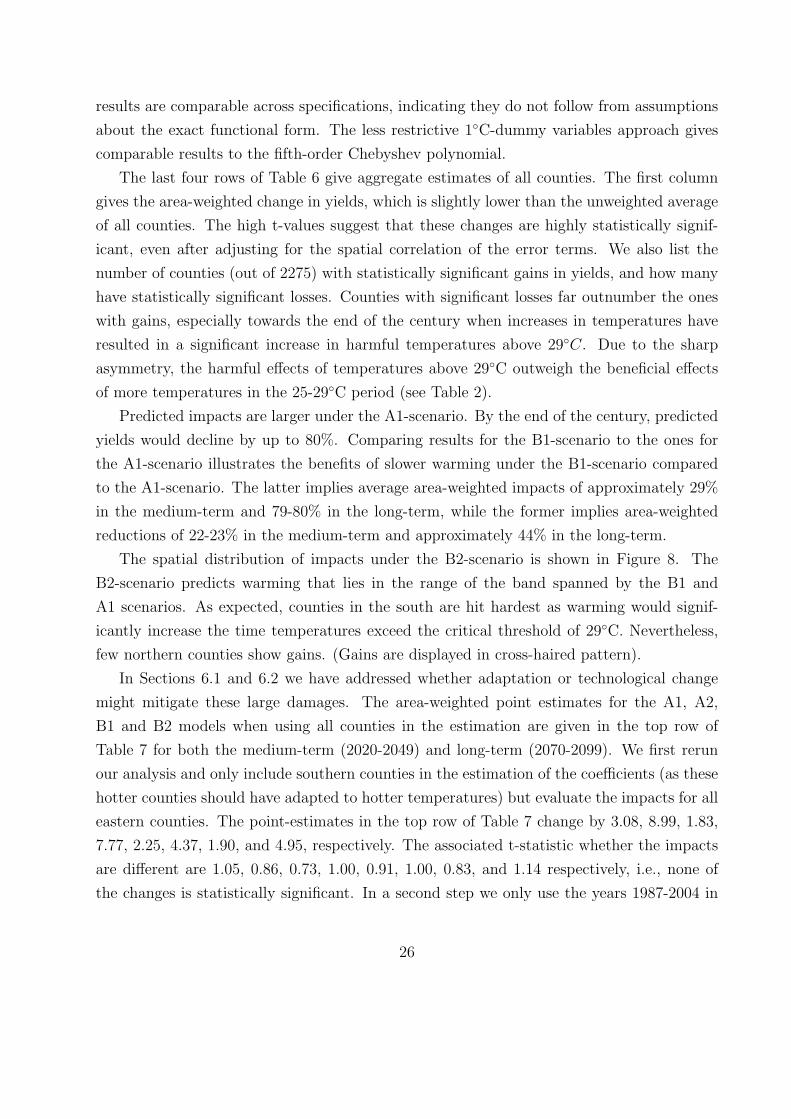
results are comparable across specifications, indicating they do not follow from assumptions

about the exact functional form. The less restrictive 1◦C-dummy variables approach gives

comparable results to the fifth-order Chebyshev polynomial.

The last four rows of Table 6 give aggregate estimates of all counties. The first column

gives the area-weighted change in yields, which is slightly lower than the unweighted average

of all counties. The high t-values suggest that these changes are highly statistically signif-

icant, even after adjusting for the spatial correlation of the error terms. We also list the

number of counties (out of 2275) with statistically significant gains in yields, and how many

have statistically significant losses. Counties with significant losses far outnumber the ones

with gains, especially towards the end of the century when increases in temperatures have

resulted in a significant increase in harmful temperatures above 29◦C. Due to the sharp

asymmetry, the harmful effects of temperatures above 29◦C outweigh the beneficial effects

of more temperatures in the 25-29◦C period (see Table 2).

Predicted impacts are larger under the A1-scenario. By the end of the century, predicted

yields would decline by up to 80%. Comparing results for the B1-scenario to the ones for

the A1-scenario illustrates the benefits of slower warming under the B1-scenario compared

to the A1-scenario. The latter implies average area-weighted impacts of approximately 29%

in the medium-term and 79-80% in the long-term, while the former implies area-weighted

reductions of 22-23% in the medium-term and approximately 44% in the long-term.

The spatial distribution of impacts under the B2-scenario is shown in Figure 8. The

B2-scenario predicts warming that lies in the range of the band spanned by the B1 and

A1 scenarios. As expected, counties in the south are hit hardest as warming would signif-

icantly increase the time temperatures exceed the critical threshold of 29◦C. Nevertheless,

few northern counties show gains. (Gains are displayed in cross-haired pattern).

In Sections 6.1 and 6.2 we have addressed whether adaptation or technological change

might mitigate these large damages. The area-weighted point estimates for the A1, A2,

B1 and B2 models when using all counties in the estimation are given in the top row of

Table 7 for both the medium-term (2020-2049) and long-term (2070-2099). We first rerun

our analysis and only include southern counties in the estimation of the coefficients (as these

hotter counties should have adapted to hotter temperatures) but evaluate the impacts for all

eastern counties. The point-estimates in the top row of Table 7 change by 3.08, 8.99, 1.83,

7.77, 2.25, 4.37, 1.90, and 4.95, respectively. The associated t-statistic whether the impacts

are different are 1.05, 0.86, 0.73, 1.00, 0.91, 1.00, 0.83, and 1.14 respectively, i.e., none of

the changes is statistically significant. In a second step we only use the years 1987-2004 in

26

the estimation of the coefficients (to test whether heat tolerance has increased for the last

subperiod). The point-estimates in the top row of Table 7 change by 0.54, 9.23, 0.32, 7.64,

0.18, 2.99, 0.08, and 3.3, respectively. The associated t-statistic whether the impacts are

different are 0.26, 0.93, 0.18, 1.04, 0.11, 0.85, 0.05, and 0.89, respectively, i.e., again none of

the changes is statistically significant.

8.2 Comparison of Impacts on Corn Yields to Other Models

Table 5 has shown that our model is far better at predicting yields out of sample than other

approaches in the literature. For comparison, we replicate other approaches found in the

literature and predict the potential effects of an increase in temperatures in Table 7.

In a first step we calculate aggregated impacts (weighted by the farmland area in a county)

under each model in the first seven rows of Table 7. Differences in predictions can exceed

30 percentage points as the highly non-linear and asymmetrical relationship os inadequately

modeled by some of the other approaches.

Second, the aggregate impact might disguise that a model is systematically over- or

underpredicting impacts for certain geographic regions. For example, a quadratic functional

form led to peak temperature levels of 22◦C as it was picking up the sharp asymmetry. This

would lead to overestimated damages for counties that usually have temperatures between

220◦ and 29◦C, and overestimate them for counties with very high temperatures. Accordingly,

we calculate the mean absolute prediction error compared to our least restrictive model, the

1◦C dummy variable model in the last six rows of Table 7. In each county, the predicted

change in yields is calculated for both the preferred and the comparison model, and we

then average over the absolute differences in all counties included in our data set. Note

that even though monthly averages outperformed Thom’s formula when predicting yearly

yields in Table 7, the latter now performs better as the average absolute prediction error is

lower. This is not surprising as climate impacts are evaluated over a 30-year period, and as

mentioned above, while Thom’s formula is bad at predicting weather (heat waves) in a given

year, it fares much better at predicting the average occurrence of harmful heat waves. On

the other hand, models that only include one degree days category for beneficial degree days,

but not for the harmful effects of extreme heat, perform the worst and give large prediction

errors.

Because we examine year-to-year fluctuations to establish the link between temperatures

and yields, a farmer cannot switch crops in response to higher average weather outcomes as

the seeds are planted before the weather is realized. In this sense our study will provide a

27

lower bound of impacts. At the same time, corn is grown over an extensive geographic region,

and the harmful effects are consistent across space and time. If adaptation possibilities were

readily available, one might wonder why farmers in warmer, southern parts of the country

currently grow corn having no more heat tolerance than corn grown further north. To put

our estimates in perspective, we can contrast them in Figure 8 with predicted changes in

farmland values from the cross-sectional analysis that incorporate adaptation possibilities for

the same climate change scenario in Figure 1 of Schlenker et al. (2006). While the estimates

impacts on corn yields are higher than the ones obtained from a cross-section, the geographic

distribution of impacts is similar.

8.3 Impacts on Soybeans Yields

The predicted impacts of global warming on soybeans yields are shown in Table 8. In the

medium-term, area-weighted yields are predicted to decrease by 16-21%, while, depending on

the climate scenario chosen, they are predicted to decline between 33-34% (B1) and 71-72%

(A1) by the end of the century. These effects are large, highly significant, and consistent

between both models.

8.4 Impact on Cotton Yields

Table 9 reports predicted impacts from climate change on cotton yields. The predicted

area-weighted impacts range from 18-19% in the medium term (2020-2049) to 25-31% in the

long-term under the B1-scenario and 60-78% under the A1-scenario.

9 Conclusions

An extensive literature relates weather outcomes to crop yields. Traders of corn futures, risk

management agencies interested in designing improved crop insurance contracts, as well as

regulators assessing the effects of climate change all require an accurate relationship between

temperature and yields. Previous empirical studies mostly utilize aggregated weather data

or crop simulation models. Reduced-form estimates based on aggregated data obscures non-

linear effects. Simulation methods embed strong assumptions in complex dynamic models

that rely on calibration methods for a small geographic scale and a limited number of ob-

servations, which makes identification difficult. Hence, the exact bounds for various regions

of nonlinear growth are still debated.

28

In this paper we use a unique fine-scale data set of daily weather records and link the

entire distribution of temperatures within each day to corn, soybeans, and cotton yields on

a large geographic scale for the 55-year time period from 1950 to 2004. This large data set

is crucial: for comparison, a panel consisting only of the last four Census years used in other

studies does not give any significant results as the sample size is too small.

We find a robust and significant nonlinear relationship between temperature and yields

that is in line with the concept of degree days, i.e., yields are linearly increasing in tem-

perature for moderate temperatures, but become quickly harmful once temperatures exceed

29◦C for corn and soybeans, and 33◦C for cotton. This relationship is highly significant even

after allowing for the spatial correlation of the error terms, which reduce average t-values by

a factor of 6.

Encompassing tests show that our new estimate is significantly better at predicting yields

than other approaches found in the literature. Our flexible functional form reveals that

growth is highly nonlinear and asymmetric in temperature, yet most of the previous studies

use a quadratic functional form and thereby impose symmetry, i.e., assume that temperature

deviations below and above the optimal growing temperature give equivalent reductions in

yield. This is assumed symmetry gives counterintuitive results (optimal growing tempera-

tures sometimes peak at 22◦C, which seem to low, and hence give biased estimates of the an

increase in temperatures as shown in Table 7. The crucial component in an accurate predic-

tion of yields is the frequency with which the upper threshold is crossed, when temperatures

quickly become very harmful. Accordingly, models that do not include a separate category

for harmful heat waves perform worst and lead to average absolute prediction errors of up

to 30% compared to our preferred model.

Because we use year-to-year fluctuations in weather, farmers are incapable of adapting to

any random weather shock by switching crops as the weather shocks are only realized after the

crops are planted. A permanent shift to higher average temperatures might induce farmers to

grow different crops, and our estimates might therefore overestimate true losses. At the same

time, corn is currently grown in many geographic areas, and counties in the hotter southern

regions show comparable harmful effects of extreme heat. If adaptation possibilities were

cheaply available, one might wonder why these farmers are currently growing corn or why

they are not capable to adapting to these higher average temperatures. Moreover, we find

no evidence that technological progress increased heat tolerance over the last 55 years: while

average yields have gone up almost threefold, the breakpoint where temperatures become

harmful is the same in later time periods as it is in earlier periods.

29

The relationship between temperatures and crop yields is used to derive the effects of

changes in average weather on crop yields. The estimated damages are large, highly sig-

nificant, and robust to various model specifications. Under our preferred model using 1◦C

degree dummy variables, impacts for corn, soybeans, and cotton imply a 79%, 71%, and

60% reductions in yields, respectively, under the rapid warming scenario (A1) and a 44%,

33%, and 25% under the slower warming scenario (B1). As mentioned above, our analysis

will not be able to pick up changes in cropping patterns as a response to climate change.

We therefore compare our results to estimates obtained from a cross-sectional analysis using

farmland values that incorporate adaptations, which also give large negative impacts, albeit

at a lower magnitude.

It should be noted that our analysis focuses on yield responses. How these yield responses

translate into welfare change depends on world food supply. Rosenzweig and Hillel (1998)

predict significant shifts in production regions, but limited effects on world food supply and

price. For example, the main corn growing region would shift north into Canada. In such

a cases farmers bear all consequences of predicted reductions in yields, while consumers are

not impacted at all. If, on the other hand, world food supplies were dropping, prices for

agricultural goods would rise, especially given the inelastic demand of agricultural goods.

Rising food prices shift the burden from farmers to consumers. Farmers will fare compara-

tively better as reductions in harvest quantities are offset by rising prices per unit harvested.

Consumers, on the other hand, would face higher food expenditures.

Important caveats are that our analysis does not incorporate technological progress that

may be induced by warmer temperatures and large yields losses. Yet, as pointed out above,

plants have not become more heat tolerant over the last 55 years even though average yields

increased almost threefold. And corn grown in the warmer southern region shows no more

heat tolerance than the cooler north. A second caveat pertains to the fact that we are unable

to account for effects stemming from CO2-fertilization. Plants use CO2 as an input in the

photosynthesis process and increasing CO2 levels might hence spur plant growth. While

CO2-fertilization may significantly offset impacts predicted in this study, the magnitude of

the effect is still debated. At present possible CO2 effects associated with climate change

are not sufficiently understood. Long et al. (2005) and Long et al. (2006) recently stressed

that existing laboratory studies as well as field experiments might overestimate this effect.

30

References

Adams, Richard M., Ronald A. Flemming, Ching-Chang Chang, Bruce A. Mc-Carl, and Cynthia Rosenzweig, “A Reassessment of the Economic Effects of GlobalClimate Change on U.S. Agriculture,” Climatic Change, June 1995, 30 (2), 147–167.

Ashenfelter, Orley and Karl Storchmann, “Using a Hedonic Model of Solar Radiationto Assess the Economic Effect of Climate Change: The Case of Mosel Valley Vineyards,”NBER Working Paper 12380, July 2006.

Black, J. Roy and Stanley R. Thompson, “Some Evidence on Weather-Crop-YieldInteraction,” American Journal of Agricultural Economics, August 1978, 60 (3), 540–543.

Brown, Robert. A. and Norman J. Rosenberg, “Climate Change Impacts on thePotential Productivity of Corn and Winter Wheat in Their Primary United StatesGrowing Regions.,” Climatic Change, January 1999, 41 (1), 73–107.

Conley, Timothy G., “GMM Estimation with Cross Sectional Dependence,” Journal ofEconometrics, September 1999, 92 (1), 1–45.

Darwin, Roy, “A Farmers view of the ricardian approach to measuring agricultural effectsof climate change,” Climatic Change, March-April 1999, 41, 371–411.

Deschenes, Olivier and Michael Greenstone, “The Economic Impacts of ClimateChange: Evidence from Agricultural Profits and Random Fluctuations in Weather,”Center for the Study of Energy Markets Working Paper 158, August 2006.

Diebold, Francis X. and Roberto S. Mariano, “Comparing Predictive Accuracy,” Jour-nal of Business and Economic Statistics, July 1995, 13 (3), 253–263.

Kaylen, Michael S., John W. Wade, and Deon B. Frank, “Stochastic trend, weatherand US corn yield variability,” Applied Economics, May 1992, 24 (5), 513–518.

Kelly, David L., Charles D. Kolstad, and Glenn T. Mitchell, “Adjustment costsfrom environmental change,” Journal of Environmental Economics and Management,November 2005, 50 (3), 468–495.

Long, Stephen P., Elizabeth A. Ainsworth, Andrew D.B. Leakey, and Patrick B.Morgan, “Global food insecurity. Treatment of major food crops with elevated carbondioxide or ozone under large-scale fully open-airconditins suggests recent models mayhave overestimated future yields.,” Philosophical Transaction of the Royal Society B,2005, 360, 2011–2020.

, , , Josef Nosberger, and Donald R. Ort, “Food for Thought: Lower-Than-Expected Crop Yield Simulation with Rising CO2 Concentrations,” Science, 30June 2006, 312, 1918–1921.

31

Mearns, L. O., W. Easterling, C. Hays, and D. Marx, “Comparison of AgriculturalImpacts of Climate Change Calculated from High and Low Resolution Climate ChangeScenarios: Part I. The Uncertainty Due to Spatial Scale,” Climatic Change, November2001, 51 (2), 131–172.

Mendelsohn, Robert, William D. Nordhaus, and Daigee Shaw, “The Impact ofGlobal Warming on Agriculture: A Ricardian Analysis,” American Economic Review,September 1994, 84 (4), 753–771.

Nakicenovic, Nebojsa, ed., Special Report on Emissions Scenarios, Cambridge UniversityPress, 2000.

Newey, Whitney K. and Kenneth D. West, “A Simple, Positive Semi-Definite, Het-eroskedasticity and Autocorrelation Consistent Covariance Matrix,” Econometrica, May1987, 3 (3), 703–708.

Ritchie, J. T. and D. S. NeSmith, “Temperature and Crop Development,” in JohnHanks and J. T. Richie, eds., Modeling Plant and Soil Systems. Agronomy 31, AmericanSociety of Agronomy Madison, WI 1991, pp. 5–29.

Rosenzweig, Cynthia and Daniel Hillel, Climate Change and the Global Harvest, NewYork: Oxford University Press, 1998.

Schlenker, Wolfram and Michael Roberts, “Non-linear Effects of Weather on CornYields,” Review of Agricultural Economics (Proceedings of the American AgriculturalEconomics Association Sessions at the 2006 Allied Social Science Associations Meeting,Boston, MA), 2006, 28 (3), 391–398.

, W. Michael Hanemann, and Anthony C. Fisher, “Will U.S. Agriculture ReallyBenefit From Global Warming? Accounting for Irrigation in the Hedonic Approach.,”American Economic Review, March 2005, 95 (1), 395–406.

, , and , “The Impact of Global Warming on U.S. Agriculture: An Econo-metric Analysis of Optimal Growing Conditions,” Review of Economics and Statistics,February 2006, 88 (1), 113–125.

Sinclair, Thomas R. and Noam G. Seligman, “Crop modeling: from infancy to matu-rity,” Agronomy Journal, September-October 1996, 88 (5), 698–704.

and Noam Seligman, “Criteria for publishing papers on crop modeling,” Field CropsResearch, November 2000, 68 (3), 165–172.

Stockle, Claudio O., Marcello Donatelli, and Roger Nelson, “CropSyst, a croppingsystems simulation model,” European Journal of Agronomy, January 2003, 18 (3-4),289–307.

32

Thom, H. C. S., “Normal Degree Days Above Any Base by the Universal TruncationCoefficient,” Monthly Weather Review, July 1966, 94 (7), 461–465.

Timmins, Christopher, “Endogenous Land Use and the Ricardian Valuation of ClimateChange,” Environmental and Resource Economics, January 2006, 33 (1), 119–142.

Wallach, Daniel, Bruno Goffinet, Jacques-Eric Bergeza, Philippe Debaekea, Del-phine Leenhardta, and Jean-Nol Aubertotc, “Parameter Estimation for CropModels: A New Approach and Application to a Corn Model,” Agronomy Journal, July-August 2001, 93 (4), 757–766.

33

Table 1: Descriptive Statistics

Corn / Soybeans Counties Cotton CountiesVariable Mean Min Max σ σyears Mean Min Max σ σyears

Yield Datalog Corn Yield 4.19 -3.19 5.32 0.54 0.42log Soybeans Yield 3.23 0.59 5.52 0.37 0.27log Cotton Yield 5.97 2.08 8.14 0.54 0.37Weather Data - Temperature Data are Days in each 1-degree Celsius IntervalTemp in [-5◦C,-4◦C) 0.77 0.00 4.40 0.75 0.30 0.01 0.00 0.58 0.03 0.02Temp in [-4◦C,-3◦C) 0.97 0.00 5.08 0.87 0.34 0.01 0.00 0.79 0.05 0.03Temp in [-3◦C,-2◦C) 1.21 0.00 5.45 0.99 0.37 0.03 0.00 1.45 0.08 0.05Temp in [-2◦C,-1◦C) 1.48 0.00 6.50 1.11 0.41 0.06 0.00 1.72 0.12 0.08Temp in [-1◦C,0◦C) 1.76 0.00 6.72 1.24 0.46 0.12 0.00 1.67 0.18 0.11Temp in [0◦C,1◦C) 2.02 0.00 7.27 1.30 0.49 0.20 0.00 2.20 0.24 0.15Temp in [1◦C,2◦C) 2.21 0.00 7.48 1.30 0.50 0.31 0.00 2.62 0.31 0.18Temp in [2◦C,3◦C) 2.38 0.00 7.33 1.26 0.49 0.45 0.00 3.07 0.39 0.22Temp in [3◦C,4◦C) 2.54 0.00 7.25 1.22 0.50 0.63 0.00 3.54 0.47 0.26Temp in [4◦C,5◦C) 2.72 0.00 7.13 1.18 0.50 0.85 0.00 4.26 0.56 0.31Temp in [5◦C,6◦C) 2.90 0.00 6.87 1.14 0.52 1.10 0.00 5.01 0.64 0.34Temp in [6◦C,7◦C) 3.10 0.00 7.30 1.11 0.53 1.39 0.00 6.22 0.73 0.37Temp in [7◦C,8◦C) 3.31 0.00 7.39 1.09 0.54 1.70 0.00 8.13 0.81 0.41Temp in [8◦C,9◦C) 3.53 0.00 8.14 1.09 0.55 2.05 0.00 9.50 0.90 0.44Temp in [9◦C,10◦C) 3.79 0.00 8.38 1.11 0.57 2.43 0.00 10.59 0.99 0.47Temp in [10◦C,11◦C) 4.10 0.14 8.59 1.15 0.59 2.86 0.00 11.80 1.08 0.51Temp in [11◦C,12◦C) 4.44 0.25 9.35 1.19 0.62 3.35 0.01 11.62 1.17 0.55Temp in [12◦C,13◦C) 4.83 0.50 10.34 1.25 0.66 3.89 0.07 11.68 1.26 0.59Temp in [13◦C,14◦C) 5.24 0.54 11.51 1.30 0.69 4.48 0.12 12.35 1.35 0.64Temp in [14◦C,15◦C) 5.68 0.53 12.98 1.34 0.73 5.14 0.19 11.83 1.44 0.69Temp in [15◦C,16◦C) 6.16 0.86 13.35 1.35 0.77 5.90 0.30 11.68 1.53 0.75Temp in [16◦C,17◦C) 6.64 1.30 13.24 1.33 0.80 6.76 0.78 12.75 1.63 0.83Temp in [17◦C,18◦C) 7.14 1.54 13.12 1.27 0.82 7.74 1.34 14.19 1.72 0.91Temp in [18◦C,19◦C) 7.61 2.35 13.96 1.24 0.84 8.85 1.96 15.61 1.83 1.01Temp in [19◦C,20◦C) 8.06 2.51 14.15 1.32 0.87 10.17 2.56 17.63 1.98 1.14Temp in [20◦C,21◦C) 8.46 2.88 16.04 1.57 0.88 11.70 3.39 18.48 2.07 1.21Temp in [21◦C,22◦C) 8.61 3.53 16.88 1.90 0.82 12.76 4.56 19.21 2.10 1.12Temp in [22◦C,23◦C) 8.41 2.76 17.67 2.05 0.75 12.77 5.82 22.38 2.03 0.98Temp in [23◦C,24◦C) 7.95 2.46 19.32 1.98 0.68 12.10 6.35 20.53 1.94 0.81Temp in [24◦C,25◦C) 7.43 1.52 19.18 1.80 0.64 11.31 5.96 22.05 1.77 0.72Temp in [25◦C,26◦C) 6.97 0.79 19.55 1.66 0.65 10.67 5.48 22.21 1.57 0.70Temp in [26◦C,27◦C) 6.56 0.00 17.12 1.66 0.68 10.21 4.94 22.05 1.47 0.71Temp in [27◦C,28◦C) 6.12 0.00 14.26 1.77 0.73 9.80 4.27 18.85 1.45 0.75Temp in [28◦C,29◦C) 5.61 0.00 12.93 1.94 0.78 9.37 3.92 17.82 1.48 0.79Temp in [29◦C,30◦C) 4.99 0.00 12.93 2.11 0.81 8.81 3.06 16.84 1.56 0.86Temp in [30◦C,31◦C) 4.28 0.00 12.56 2.22 0.83 8.10 1.45 15.43 1.66 0.90Temp in [31◦C,32◦C) 3.52 0.00 11.34 2.23 0.81 7.21 0.25 14.87 1.80 0.96Temp in [32◦C,33◦C) 2.74 0.00 11.08 2.10 0.81 6.03 0.04 14.49 1.94 1.08Temp in [33◦C,34◦C) 1.95 0.00 10.35 1.82 0.79 4.63 0.00 13.20 2.03 1.23Temp in [34◦C,35◦C) 1.25 0.00 9.46 1.44 0.74 3.19 0.00 11.47 2.02 1.28Temp in [35◦C,36◦C) 0.73 0.00 9.08 1.10 0.61 2.02 0.00 10.93 1.84 1.14Temp in [36◦C,37◦C) 0.41 0.00 8.22 0.82 0.47 1.22 0.00 9.44 1.56 0.91Temp in [37◦C,38◦C) 0.22 0.00 8.08 0.57 0.32 0.71 0.00 8.63 1.24 0.65Temp in [38◦C,39◦C) 0.10 0.00 7.17 0.36 0.19 0.40 0.00 8.42 0.95 0.42Temp in [39◦C,40◦C) 0.05 0.00 6.93 0.21 0.10 0.22 0.00 8.83 0.73 0.24Temp in [40◦C,41◦C) 0.02 0.00 3.42 0.12 0.05 0.12 0.00 8.10 0.57 0.12Temp in [41◦C,42◦C) 0.01 0.00 2.27 0.06 0.02 0.07 0.00 7.17 0.44 0.06Temp in [42◦C,43◦C) 0.00 0.00 1.53 0.03 0.01 0.04 0.00 6.10 0.31 0.03Temp in [43◦C,44◦C) 0.00 0.00 0.83 0.02 0.00 0.02 0.00 4.88 0.20 0.02Temp in [44◦C,45◦C) 0.00 0.00 0.48 0.01 0.00 0.01 0.00 3.23 0.12 0.01Temp in [45◦C,46◦C) 0.00 0.00 0.33 0.00 0.00 0.00 0.00 2.06 0.06 0.00Temp in [46◦C,47◦C) 0.00 0.00 0.18 0.00 0.00 0.00 0.00 1.63 0.03 0.00Temp in [47◦C,48◦C) 0.00 0.00 0.07 0.00 0.00 0.00 0.00 0.76 0.01 0.00Temp in [48◦C,49◦C) 0.00 0.00 0.00 0.00 0.00 0.00 0.00 0.52 0.01 0.00Temp in [49◦C,oo) 0.00 0.00 0.00 0.00 0.00 0.00 0.00 0.24 0.00 0.00Precipitation (cm) 59.20 5.78 143.33 15.68 12.10 65.80 0.08 175.75 22.01 14.22Counties 2277 980Observations 108746 31075

Notes: Table lists descriptive statistics. The first five columns use counties east of the 100 degree meridian, whereaggregated weather variables for the months March through August are averaged over counties that either have corn orsoybeans yields. The last five columns use all counties in the United States that have cotton yields (which is mainlygrown in the southwest) and aggregates variables for the months April through October. In each set, the first fourcolumns give the mean, minimum, maximum, and standard deviation of each variable in the years 1950-2004. The fifthcolumn gives the average within-county year-to-year standard deviation.

34

Table 2: Predicted Changes in Climatic Variables Under the B2 Scenario

Time Period 2020-2049 Time Period 2070-2099Variable Mean Min Max σ Mean Min Max σTemp in [-5◦C,-4◦C) -0.12 -0.60 0.07 0.14 -0.32 -0.84 0.00 0.24Temp in [-4◦C,-3◦C) -0.16 -0.76 0.06 0.17 -0.40 -1.05 0.00 0.28Temp in [-3◦C,-2◦C) -0.20 -0.78 0.09 0.20 -0.48 -1.19 0.00 0.31Temp in [-2◦C,-1◦C) -0.25 -0.98 0.10 0.23 -0.57 -1.35 -0.00 0.35Temp in [-1◦C,0◦C) -0.29 -1.07 0.12 0.25 -0.66 -1.61 -0.00 0.38Temp in [0◦C,1◦C) -0.28 -1.11 0.08 0.19 -0.67 -1.73 -0.01 0.34Temp in [1◦C,2◦C) -0.24 -0.72 0.09 0.14 -0.60 -1.51 -0.01 0.25Temp in [2◦C,3◦C) -0.24 -0.69 0.22 0.15 -0.50 -1.09 0.15 0.21Temp in [3◦C,4◦C) -0.26 -0.73 0.19 0.15 -0.47 -1.18 0.33 0.23Temp in [4◦C,5◦C) -0.30 -0.79 0.12 0.15 -0.49 -1.15 0.37 0.24Temp in [5◦C,6◦C) -0.33 -0.92 0.05 0.15 -0.53 -1.16 0.31 0.22Temp in [6◦C,7◦C) -0.37 -0.95 -0.01 0.15 -0.59 -1.45 0.09 0.20Temp in [7◦C,8◦C) -0.42 -1.03 -0.10 0.16 -0.65 -1.70 0.02 0.20Temp in [8◦C,9◦C) -0.45 -1.05 -0.11 0.18 -0.73 -1.87 -0.00 0.22Temp in [9◦C,10◦C) -0.52 -1.19 -0.13 0.19 -0.82 -1.87 -0.26 0.27Temp in [10◦C,11◦C) -0.61 -1.38 -0.22 0.21 -0.96 -2.14 -0.42 0.31Temp in [11◦C,12◦C) -0.70 -1.73 -0.24 0.23 -1.13 -2.33 -0.53 0.35Temp in [12◦C,13◦C) -0.79 -2.15 -0.23 0.25 -1.30 -2.97 -0.50 0.38Temp in [13◦C,14◦C) -0.87 -2.91 -0.15 0.27 -1.46 -3.97 -0.62 0.42Temp in [14◦C,15◦C) -0.96 -3.31 0.05 0.31 -1.62 -4.86 -0.31 0.44Temp in [15◦C,16◦C) -1.05 -3.09 0.24 0.38 -1.79 -4.50 0.01 0.48Temp in [16◦C,17◦C) -1.14 -3.53 0.69 0.49 -1.96 -4.54 0.26 0.57Temp in [17◦C,18◦C) -1.21 -3.79 1.28 0.65 -2.09 -5.02 0.85 0.74Temp in [18◦C,19◦C) -1.25 -3.84 1.54 0.89 -2.19 -5.11 1.38 1.01Temp in [19◦C,20◦C) -1.25 -4.57 1.59 1.18 -2.22 -5.61 2.10 1.38Temp in [20◦C,21◦C) -1.23 -4.93 1.78 1.56 -2.20 -6.01 2.12 1.86Temp in [21◦C,22◦C) -1.03 -5.40 1.76 1.85 -1.93 -6.84 2.23 2.26Temp in [22◦C,23◦C) -0.52 -6.38 1.98 1.78 -1.37 -7.85 2.46 2.37Temp in [23◦C,24◦C) 0.09 -6.84 2.24 1.47 -0.59 -8.83 2.49 2.18Temp in [24◦C,25◦C) 0.51 -7.43 2.44 0.91 0.22 -9.47 2.67 1.69Temp in [25◦C,26◦C) 0.64 -5.88 3.29 0.53 0.80 -9.35 3.98 1.18Temp in [26◦C,27◦C) 0.62 -1.74 3.71 0.51 1.06 -6.64 5.26 0.78Temp in [27◦C,28◦C) 0.59 -0.52 3.43 0.54 1.15 -2.35 5.51 0.75Temp in [28◦C,29◦C) 0.66 -0.45 3.45 0.63 1.21 -0.22 5.32 0.87Temp in [29◦C,30◦C) 0.85 -0.49 3.62 0.71 1.36 -0.15 5.59 0.97Temp in [30◦C,31◦C) 1.09 -0.68 3.57 0.78 1.66 -0.21 5.31 1.10Temp in [31◦C,32◦C) 1.32 -0.53 3.53 0.81 2.03 -0.29 5.27 1.20Temp in [32◦C,33◦C) 1.54 -0.22 3.60 0.76 2.43 -0.17 5.22 1.18Temp in [33◦C,34◦C) 1.70 -0.00 5.01 0.80 2.81 -0.32 5.67 1.09Temp in [34◦C,35◦C) 1.77 0.00 6.40 1.07 3.07 -0.33 7.27 1.13Temp in [35◦C,36◦C) 1.69 0.00 6.48 1.30 3.07 -0.27 7.52 1.32Temp in [36◦C,37◦C) 1.43 0.00 6.35 1.28 2.85 0.01 7.59 1.48Temp in [37◦C,38◦C) 1.10 0.00 5.41 1.11 2.48 0.00 7.03 1.55Temp in [38◦C,39◦C) 0.77 0.00 4.70 0.94 2.02 0.00 6.70 1.52Temp in [39◦C,40◦C) 0.51 0.00 4.21 0.77 1.53 0.00 6.10 1.37Temp in [40◦C,41◦C) 0.32 0.00 4.00 0.59 1.07 0.00 5.85 1.18Temp in [41◦C,42◦C) 0.18 0.00 3.43 0.39 0.72 0.00 5.67 0.97Temp in [42◦C,43◦C) 0.09 0.00 2.34 0.21 0.46 0.00 4.77 0.74Temp in [43◦C,44◦C) 0.04 0.00 1.10 0.10 0.28 0.00 3.79 0.52Temp in [44◦C,45◦C) 0.01 0.00 0.53 0.04 0.15 0.00 2.80 0.31Temp in [45◦C,46◦C) 0.00 0.00 0.24 0.02 0.07 0.00 1.43 0.16Temp in [46◦C,47◦C) 0.00 0.00 0.12 0.01 0.03 0.00 0.72 0.08Temp in [47◦C,48◦C) 0.00 0.00 0.04 0.00 0.01 0.00 0.34 0.03Temp in [48◦C,49◦C) 0.00 0.00 0.01 0.00 0.00 0.00 0.14 0.01Temp in [49◦C,oo) 0.00 0.00 0.00 0.00 0.00 0.00 0.07 0.01Precipitation (cm) -0.13 -14.65 8.82 3.60 1.70 -14.22 11.36 4.10

Notes: The Table lists predicted changes in the temperature distribution for 2275 east-ern counties with corn yields under the B2-scenario. The first four columns list pre-dicted changes for 2020-2049 compared to the 1960-1989 baseline period, while the lastfour columns list longer term changes for 2070-2099 compared to 1960-1989.

35

Table 3: Polynomial Regression Results for Corn

Variable (1) (2) (3) (4) (5) (6)Temperature (1st-order) -1.09E-02 -2.10E-02 -5.72E-02 -4.06E-02 2.48E-03 -1.91E-03

( 7.87) (13.06) (13.24) (11.23) ( 0.67) ( 0.48)Temperature (2nd-order) -1.66E-02 -3.20E-02 -1.09E-02 9.84E-03 1.47E-02

(13.23) (14.50) ( 5.24) ( 4.30) ( 5.61)Temperature (3rd-order) -1.72E-02 -7.93E-03 2.73E-02 3.00E-02

(10.08) ( 5.23) ( 9.49) ( 9.75)Temperature (4th-order) 1.15E-02 2.16E-02 3.19E-02

(13.10) (16.60) ( 8.62)Temperature (5th-order) 1.71E-02 2.12E-02

(11.65) ( 9.59)Temperature (6th-order) 7.24E-03

( 3.27)Precipitation 1.99E-02 1.59E-02 1.49E-02 1.21E-02 1.04E-02 1.02E-02

(10.78) ( 9.28) ( 9.07) ( 7.91) ( 6.87) ( 6.79)Precipitation Squared -1.25E-04 -1.08E-04 -1.03E-04 -8.96E-05 -8.25E-05 -8.09E-05

( 8.88) ( 8.49) ( 8.44) ( 7.79) ( 7.27) ( 7.21)R2 0.69 0.72 0.73 0.75 0.76 0.76Number of Observations 104307 104307 104307 104307 104307 104307Number of Counties 2275 2275 2275 2275 2275 2275County Fixed Effect Yes Yes Yes Yes Yes YesState Yield Trend Yes Yes Yes Yes Yes Yes

Notes: The table reports coefficient estimates and t-values (in parentheses) for six regressionswith temperature polynomials of order one to six. (We use Chebyshev polynomials instead ofregular polynomials as the former are more flexible and orthogonal). The dependent variable isthe natural log of corn yields for a pooled sample of 2275 counties and years 1950 to 2004. Onlycounties east of the 100th meridian are included in the sample to focus on non-irrigated cropland.The model is given in equation (3). Each column reports results from one regression. T-valuesare adjusted for spatial correlation of contemporaneous errors following Conley (1999).

36

Tab

le4:

Reg

ress

ion

Res

ult

sU

sing

Var

ious

Geo

grap

hic

and

Tem

por

alSubse

ts

Vari

able

Nort

hIn

teri

or

South

1950-1

977

1978-2

004

Tem

per

ature

(1st

-ord

er)

8.98

E-0

4-2

.43E

-03

4.88

E-0

2-6

.87E

-03

1.36

E-0

2(

0.23

)(

0.27

)(

1.75

)(

1.36

)(

2.68

)Tem

per

ature

(2nd-o

rder

)9.

30E

-03

6.91

E-0

33.

85E

-02

4.29

E-0

31.

66E

-02

(3.

59)

(1.

39)

(2.

19)

(1.

43)

(5.

15)

Tem

per

ature

(3rd

-ord

er)

2.63

E-0

22.

87E

-02

5.57

E-0

22.

24E

-02

3.24

E-0

2(

7.95

)(

4.68

)(

3.27

)(

5.57

)(

9.04

)Tem

per

ature

(4th

-ord

er)

2.30

E-0

22.

30E

-02

2.94

E-0

21.

97E

-02

2.52

E-0

2(1

2.30

)(

8.73

)(

4.92

)(1

0.05

)(1

5.54

)Tem

per

ature

(5th

-ord

er)

1.64

E-0

22.

05E

-02

2.61

E-0

21.

63E

-02

1.74

E-0

2(

9.39

)(

6.21

)(

4.88

)(

7.58

)(1

0.59

)P

reci

pit

atio

n2.

39E

-02

1.48

E-0

25.

53E

-03

1.14

E-0

28.

94E

-03

(8.

53)

(4.

18)

(2.

40)

(5.

93)

(5.0

3)P

reci

pit

atio

nSquar

ed-2

.15E

-04

-1.1

7E-0

4-4

.34E

-05

-8.7

3E-0

5-7

.43E

-05

(8.

65)

(4.

16)

(3.

01)

(5.

93)

(5.

46)

R2

0.80

0.74

0.74

0.65

0.60

Num

ber

ofO

bse

rvat

ions

4197

726

792

3553

852

987

5132

0N

um

ber

ofC

ounti

es82

655

189

822

6422

18C

ounty

Fix

edE

ffec

tY

esY

esY

esY

esY

esSta

teY

ield

Tre

nd

Yes

Yes

Yes

Yes

Yes

Not

es:

Tab

legi

vesco

effici

entes

tim

ates

and

t-va

lues

inpar

enth

eses

.T

he

latt

erar

ead

-ju

sted

forsp

atia

lco

rrel

atio

nof

conte

mpor

aneo

us

erro

rte

rms

follow

ing

Con

ley

(199

9).

Tem

per

ature

vari

able

sar

em

odel

edas

Cheb

ysh

evpol

ynom

ials

.

37

Tab

le5:

Model

Com

par

ison

Tes

tfo

rO

ut-

Of-Sam

ple

Pre

dic

tion

Acc

ura

cy

Gra

nger

Weig

ht

MG

NSta

tist

icD

um

my

Chebysh

ev

Dum

my

Chebysh

ev

RM

SE

Vari

able

sPoly

nom

ials

Vari

able

sPoly

nom

ials

Dum

my

Vari

able

s0.

226

Chebysh

ev

Poly

nom

ials

0.22

91.

001

11.2

3M

onth

lyA

vera

ges

0.23

70.

731

0.67

613

.99

10.0

7D

egre

eD

ays

8-2

9◦ C

,>

29◦ C

(Thom

)0.

240

0.98

30.

988

21.8

918

.69

Degre

eD

ays

8-3

2◦ C

,>

34◦ C

(Thom

)0.

247

0.98

00.

974

27.2

724

.41

Degre

eD

ays

8-3

2◦ C

(Daily

Mean)

0.25

20.

993

0.97

730

.57

27.5

6D

egre

eD

ays

8-2

9◦ C

(Daily

Mean)

0.25

30.

990

0.97

031

.42

28.3

2

Not

es:

The

firs

tco

lum

npre

sent

the

root

mea

nsq

uar

edou

t-of

sam

ple

pre

dic

tion

erro

r(R

MS).

Alo

wer

out-

ofsa

mple

pre

dic

tion

erro

rim

plies

that

the

model

isbet

terat

expla

inin

gth

eva

riab

leof

inte

rest

.M

odel

sar

eor

der

edfr

ombes

tou

t-of

-sam

ple

pre

dic

tion

tow

orst

.T

he

rem

ainin

gco

lum

nspre

sentpai

rwis

em

odel

com

par

ison

sbet

wee

nth

edum

my-v

aria

ble

and

Cheb

ych

evm

odel

san

dal

lin

feri

orm

odel

s(r

emai

nin

gco

mpar

ison

sar

egi

ven

inan

appen

dix

).T

he

seco

nd

and

thir

dco

lum

ngi

veth

eG

range

rw

eigh

ton

the

model

list

edin

the

colu

mn.

An

opti

mal

com

bin

edfo

reca

stis

der

ived

asa

wei

ghte

dav

erag

eof

the

two

fore

cast

s(w

her

eth

ew

eigh

tssu

mto

1).

The

last

two

colu

mns

dis

pla

yth

est

andar

d-n

orm

aldis

trib

ute

dM

orga

n-N

ewbol

d-G

range

r(M

GN

)st

atis

tic

ofeq

ual

fore

cast

ing

accu

racy

.E

ach

model

ises

tim

ated

usi

ng

the

sam

e85

%of

the

dat

aan

dyie

lds

are

fore

cast

edou

t-of

-sam

ple

for

the

omit

ted

15%

.D

um

my

vari

able

san

dC

heb

ysh

evPol

ynom

ials

are

the

model

sdev

elop

edin

this

pap

er;m

onth

lyav

erag

esuse

sa

quad

rati

csp

ecifi

cati

onin

bot

hav

erag

ete

mper

ature

and

tota

lpre

cipit

atio

nfo

rth

em

onth

sJan

uar

y,A

pri

l,July

,an

dO

ctob

er(M

endel

sohn

etal

.19

94);

Thom

’sfo

rmula

use

sm

onth

lyav

erag

ete

mper

ature

dat

ato

extr

apol

ate

deg

ree

day

s(w

hic

har

ebas

edon

dai

lydat

a)(S

chle

nke

ret

al.20

06);

trunca

ted

dai

lyav

erag

esfirs

tder

ive

the

aver

age

tem

per

ature

for

each

day

from

dai

lyte

mper

ature

read

ings

and

then

const

ruct

deg

ree

day

sfr

omth

isav

erag

e(D

esch

enes

and

Gre

enst

one

2006

).

38

Table 6: Predicted Impacts of Global Warming on Corn

Medium-term 2020-2049 Long-term 2070-2099Variable Mean Min Max Std Mean Min Max Std

Climate Scenario Hadley HCM3 - B1Chebyshev PolynomialTemperature -29.36 -66.80 11.14 18.95 -47.96 -86.78 12.88 19.48Precipitation -0.23 -4.13 4.13 0.84 -0.37 -8.01 3.87 1.08Total -29.47 -68.05 7.62 19.13 -48.07 -87.29 8.94 19.701◦C Dummy IntervalsTemperature -28.55 -61.67 11.93 17.21 -45.89 -82.25 18.97 17.62Precipitation -0.19 -4.98 4.36 1.00 -0.31 -8.59 4.09 1.21Total -28.60 -63.20 12.10 17.53 -45.95 -83.08 14.59 17.96

Climate Scenario Hadley HCM3 - A1Chebyshev PolynomialTemperature -33.73 -72.82 10.64 18.46 -81.35 -98.17 -10.53 13.77Precipitation -0.24 -4.75 3.77 0.86 -0.98 -11.14 6.29 1.89Total -33.82 -73.69 8.24 18.68 -81.44 -98.33 -8.93 13.891◦C Dummy IntervalsTemperature -32.50 -67.43 12.83 16.57 -80.21 -98.60 -9.62 14.34Precipitation -0.20 -5.14 3.98 1.03 -1.00 -12.01 6.12 2.18Total -32.54 -68.60 10.01 16.93 -80.28 -98.74 -7.57 14.52

Medium-term 2020-2049 Long-term 2070-2099Model Impact t-value Gain Loss Impact t-value Gain Loss

Climate Scenario Hadley HCM3 - B1Polynomial -22.34 (21.29) 69 2092 -44.17 (26.69) 6 2229Dummy Intervals -22.72 (20.46) 87 2085 -43.56 (17.69) 12 2211

Climate Scenario Hadley HCM3 - A1Polynomial -28.74 (22.99) 31 2145 -79.92 (51.44) 0 2275Dummy Intervals -29.05 (20.53) 55 2119 -79.07 (12.40) 0 2275

Notes: The first twelve rows list predicted percentage changes in crop yields for easterncounties using both specifications for the two extreme climate scenarios. Each set of threerows reports impacts attributable to changing temperatures and precipitation, as well astotal impacts. The last four rows report the area-weighted impacts (including t-values) aswell as how many of the 2275 counties either had statistically significant gains or losses atthe 95% level.

39

Tab

le7:

Com

par

ison

ofP

redic

ted

Clim

ate

Impac

tsFor

Var

ious

Model

s

HC

M3-A

1H

CM

3-A

2H

CM

3-B

1H

CM

3-B

220-4

970-9

920-4

970-9

920-4

970-9

920-4

970-9

9Farm

land

Are

aW

eig

hte

dC

lim

ate

Impact

sD

um

my

Vari

able

-29.

05-7

9.07

-27.

66-6

9.96

-22.

72-4

3.56

-23.

13-5

0.87

5th

-ord

er

Chebysh

ev

Poly

nom

ial

-28.

74-7

9.92

-27.

19-7

1.05

-22.

34-4

4.17

-22.

58-5

0.98

Month

lyA

vera

ges

-20.

82-7

1.43

-17.

47-6

0.23

-13.

75-3

6.84

-14.

14-3

4.27

Degre

eD

ays

8-2

9◦ C

,>

29◦ C

(Thom

)-2

5.33

-82.

30-2

3.53

-71.

53-1

9.42

-42.

31-1

9.81

-48.

00D

egre

eD

ays

8-3

2◦ C

,>

34◦ C

(Thom

)-2

0.99

-78.

89-2

0.01

-64.

75-1

6.83

-35.

70-1

7.57

-41.

09D

egre

eD

ays

8-3

2◦ C

(Daily

Mean)

-14.

95-5

5.88

-15.

53-4

5.01

-12.

58-2

6.04

-13.

69-2

9.33

Degre

eD

ays

8-2

9◦ C

(Daily

Mean)

-12.

88-4

5.63

-13.

65-3

6.90

-11.

02-2

2.18

-12.

21-2

4.80

Mean

Abso

lute

Pre

dic

tion

Err

or

Com

pare

dto

Pre

ferr

ed

Model

5th

-ord

er

Chebysh

ev

Poly

nom

ial

2.78

2.13

2.76

2.27

2.51

3.10

2.65

3.09

Month

lyA

vera

ges

7.59

9.87

11.2

311

.01

10.6

17.

609.

2013

.71

Degre

eD

ays

8-2

9◦ C

,>

29◦ C

(Thom

)6.

203.

736.

015.

025.

396.

625.

667.

25D

egre

eD

ays

8-3

2◦ C

,>

34◦ C

(Thom

)7.

065.

607.

917.

756.

237.

256.

988.

97D

egre

eD

ays

8-3

2◦ C

(Daily

Mean)

11.1

618

.11

11.1

919

.54

9.58

12.6

410

.20

16.9

8D

egre

eD

ays

8-2

9◦ C

(Daily

Mean)

15.2

529

.93

15.1

830

.03

13.1

218

.87

13.8

524

.49

Not

es:

The

table

com

par

espre

dic

ted

impac

tson

corn

yie

lds

under

vari

ous

scen

ario

s.C

lim

ate

scen

ario

sar

eev

aluat

edfo

rfo

ur

emis

sion

ssc

enar

ios:

A1,

A2,

B1,

B2

inth

em

ediu

m-t

erm

20-4

9(2

020-

2049

)an

dlo

ng-

term

70-9

9(2

070-

2099

).T

he

firs

tse

ven

row

sgi

veth

efa

rmla

nd-a

rea

wei

ghte

dim

pac

tsin

per

centa

gepoi

nts

.T

he

last

six

row

sgi

veth

em

ean

abso

lute

pre

dic

tion

erro

rin

per

centa

gepoi

nts

com

par

edto

our

pre

ferr

edm

odel

usi

ng

dum

my

vari

able

sfo

rea

ch1◦

Cdeg

ree

inte

rval

(Model

sar

edes

crib

edin

Tab

le5)

.

40

Table 8: Predicted Impacts of Global Warming on Soybeans

Medium-term 2020-2049 Long-term 2070-2099Variable Mean Min Max Std Mean Min Max Std

Climate Scenario Hadley HCM3 - B1Chebyshev PolynomialTemperature -20.40 -59.44 17.16 16.71 -35.94 -80.17 25.57 19.14Precipitation 0.05 -5.17 3.00 0.98 0.02 -6.55 3.69 1.11Total -20.26 -61.15 14.40 17.17 -35.79 -81.15 22.29 19.651◦C Dummy IntervalsTemperature -19.99 -59.01 18.13 16.17 -34.83 -80.82 26.63 18.51Precipitation 0.08 -5.33 2.93 1.02 0.06 -6.48 3.84 1.14Total -19.82 -61.07 15.42 16.68 -34.66 -81.80 23.39 19.06

Climate Scenario Hadley HCM3 - A1Chebyshev PolynomialTemperature -23.95 -65.08 17.42 16.65 -72.58 -96.75 7.91 16.93Precipitation 0.08 -4.34 3.44 1.03 -0.48 -10.78 3.76 2.04Total -23.78 -66.41 14.45 17.18 -72.54 -97.09 9.70 17.271◦C Dummy IntervalsTemperature -23.33 -65.27 18.42 16.05 -71.95 -96.84 12.46 16.91Precipitation 0.10 -4.48 3.58 1.08 -0.45 -11.13 3.98 2.11Total -23.13 -66.74 15.50 16.64 -71.90 -97.18 11.32 17.28

Medium-term 2020-2049 Long-term 2070-2099Model Impact t-value Gain Loss Impact t-value Gain Loss

Climate Scenario Hadley HCM3 - B1Polynomial -16.02 (18.63) 205 1724 -33.81 (24.31) 72 1931Dummy Intervals -15.86 (18.05) 200 1690 -33.13 (20.18) 72 1924

Climate Scenario Hadley HCM3 - A1Polynomial -20.89 (20.38) 149 1818 -72.03 (48.70) 3 2069Dummy Intervals -20.60 (19.26) 147 1811 -71.35 (17.36) 3 2067

Notes: The first twelve rows list the predicted percentage change in crop yields for easterncounties using both specifications for the two extreme climate scenarios. Each set of threerows reports impacts attributable to changing temperatures and precipitation, as well astotal impacts. The last four rows give the area-weighted impact (including t-value) as wellas how many of the 2075 counties either had statistically significant gains or losses at the95% level.

41

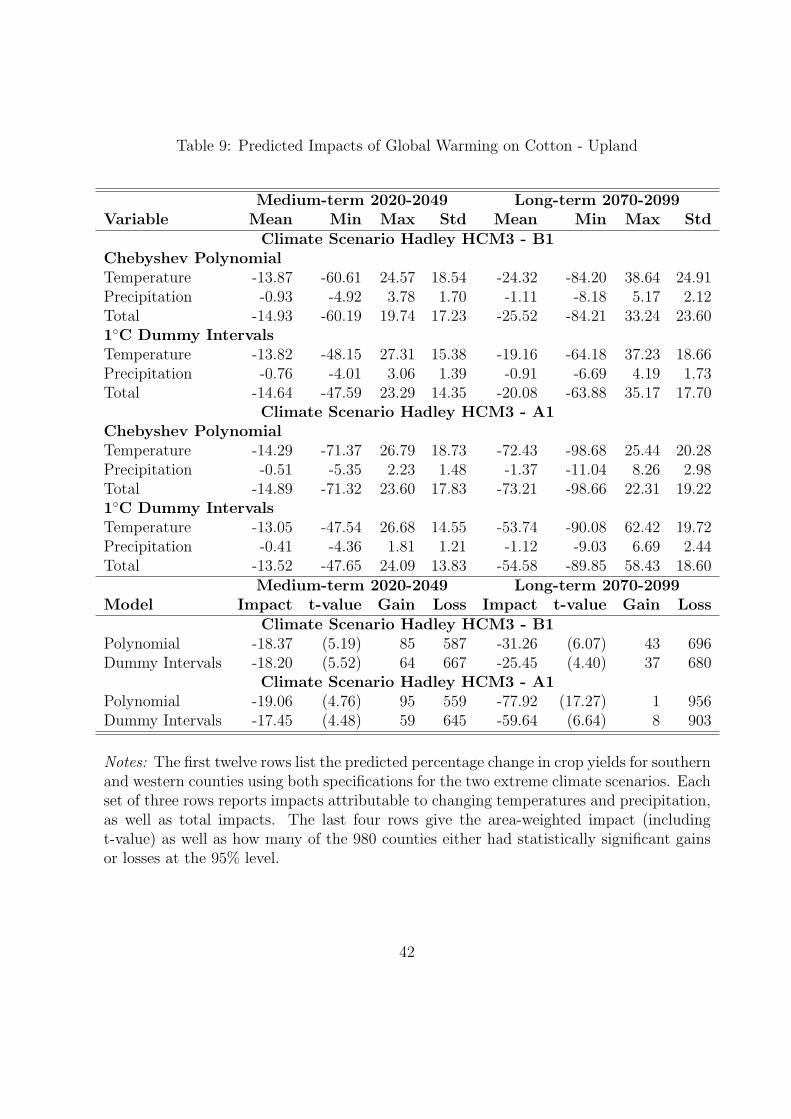
Table 9: Predicted Impacts of Global Warming on Cotton - Upland

Medium-term 2020-2049 Long-term 2070-2099Variable Mean Min Max Std Mean Min Max Std

Climate Scenario Hadley HCM3 - B1Chebyshev PolynomialTemperature -13.87 -60.61 24.57 18.54 -24.32 -84.20 38.64 24.91Precipitation -0.93 -4.92 3.78 1.70 -1.11 -8.18 5.17 2.12Total -14.93 -60.19 19.74 17.23 -25.52 -84.21 33.24 23.601◦C Dummy IntervalsTemperature -13.82 -48.15 27.31 15.38 -19.16 -64.18 37.23 18.66Precipitation -0.76 -4.01 3.06 1.39 -0.91 -6.69 4.19 1.73Total -14.64 -47.59 23.29 14.35 -20.08 -63.88 35.17 17.70

Climate Scenario Hadley HCM3 - A1Chebyshev PolynomialTemperature -14.29 -71.37 26.79 18.73 -72.43 -98.68 25.44 20.28Precipitation -0.51 -5.35 2.23 1.48 -1.37 -11.04 8.26 2.98Total -14.89 -71.32 23.60 17.83 -73.21 -98.66 22.31 19.221◦C Dummy IntervalsTemperature -13.05 -47.54 26.68 14.55 -53.74 -90.08 62.42 19.72Precipitation -0.41 -4.36 1.81 1.21 -1.12 -9.03 6.69 2.44Total -13.52 -47.65 24.09 13.83 -54.58 -89.85 58.43 18.60

Medium-term 2020-2049 Long-term 2070-2099Model Impact t-value Gain Loss Impact t-value Gain Loss

Climate Scenario Hadley HCM3 - B1Polynomial -18.37 (5.19) 85 587 -31.26 (6.07) 43 696Dummy Intervals -18.20 (5.52) 64 667 -25.45 (4.40) 37 680

Climate Scenario Hadley HCM3 - A1Polynomial -19.06 (4.76) 95 559 -77.92 (17.27) 1 956Dummy Intervals -17.45 (4.48) 59 645 -59.64 (6.64) 8 903

Notes: The first twelve rows list the predicted percentage change in crop yields for southernand western counties using both specifications for the two extreme climate scenarios. Eachset of three rows reports impacts attributable to changing temperatures and precipitation,as well as total impacts. The last four rows give the area-weighted impact (includingt-value) as well as how many of the 980 counties either had statistically significant gainsor losses at the 95% level.

42

Figure 1: Classification of States/Counties in Analysis

Notes: Graph displays the classification of counties used in various regressions. We label the union ofnorthern, interior, and southern states as eastern states.

43

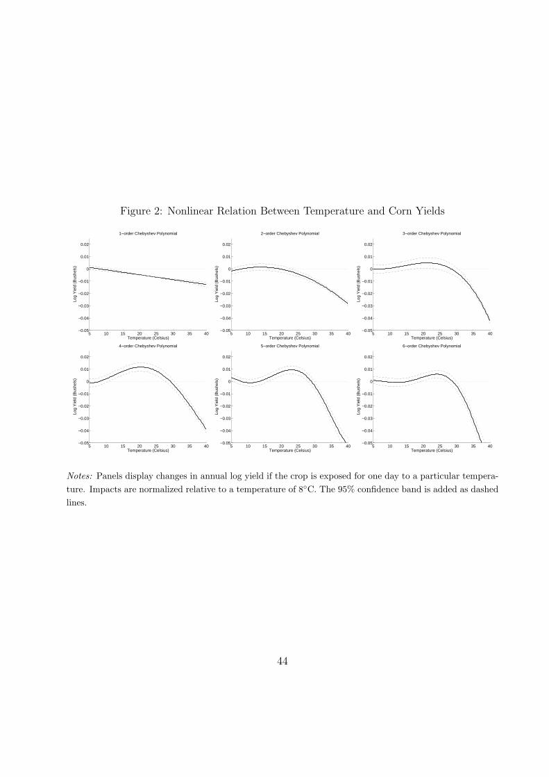
Figure 2: Nonlinear Relation Between Temperature and Corn Yields

5 10 15 20 25 30 35 40−0.05

−0.04

−0.03

−0.02

−0.01

0

0.01

0.02

Temperature (Celsius)

1−order Chebyshev Polynomial

Log

Yie

ld (

Bus

hels

)

5 10 15 20 25 30 35 40−0.05

−0.04

−0.03

−0.02

−0.01

0

0.01

0.02

Temperature (Celsius)

2−order Chebyshev Polynomial

Log

Yie

ld (

Bus

hels

)

5 10 15 20 25 30 35 40−0.05

−0.04

−0.03

−0.02

−0.01

0

0.01

0.02

Temperature (Celsius)

3−order Chebyshev Polynomial

Log

Yie

ld (

Bus

hels

)

5 10 15 20 25 30 35 40−0.05

−0.04

−0.03

−0.02

−0.01

0

0.01

0.02

Temperature (Celsius)

4−order Chebyshev Polynomial

Log

Yie

ld (

Bus

hels

)

5 10 15 20 25 30 35 40−0.05

−0.04

−0.03

−0.02

−0.01

0

0.01

0.02

Temperature (Celsius)

5−order Chebyshev Polynomial

Log

Yie

ld (

Bus

hels

)

5 10 15 20 25 30 35 40−0.05

−0.04

−0.03

−0.02

−0.01

0

0.01

0.02

Temperature (Celsius)

6−order Chebyshev Polynomial

Log

Yie

ld (

Bus

hels

)

Notes: Panels display changes in annual log yield if the crop is exposed for one day to a particular tempera-ture. Impacts are normalized relative to a temperature of 8◦C. The 95% confidence band is added as dashedlines.

44

Figure 3: County Fixed Effects

45

Figure 4: Nonlinear Relation Between Temperature and Corn, Soybean, and Cotton Yieldsfor Different Functional Forms

Corn

5 10 15 20 25 30 35 40−0.05

−0.04

−0.03

−0.02

−0.01

0

0.01

0.02

0

5

10

15

Exp

osur

e in

Day

s

Temperature (Celsius)

Year Fixed Effects

Log

Yie

ld (

Bus

hels

)

5 10 15 20 25 30 35 40−0.05

−0.04

−0.03

−0.02

−0.01

0

0.01

0.02

Temperature (Celsius)

Log

Yie

ld (

Bus

hels

)

Dummy Variable For Each 1−Degree Interval

5 10 15 20 25 30 35 40−0.05

−0.04

−0.03

−0.02

−0.01

0

0.01

0.02

Constant Temperature (Celsius)

Log

Yie

ld (

Bus

hels

)

Piecewise−linear Function

Soybeans

5 10 15 20 25 30 35 40−0.05

−0.04

−0.03

−0.02

−0.01

0

0.01

0.02

0

5

10

15

Exp

osur

e in

Day

s

Temperature (Celsius)

Log

Yie

ld (

Bus

hels

)

5−th order Chebyshev Polynomial

5 10 15 20 25 30 35 40−0.05

−0.04

−0.03

−0.02

−0.01

0

0.01

0.02

Temperature (Celsius)

Log

Yie

ld (

Bus

hels

)

Dummy Variable For Each 1−Degree Interval

5 10 15 20 25 30 35 40−0.05

−0.04

−0.03

−0.02

−0.01

0

0.01

0.02

Constant Temperature (Celsius)Lo

g Y

ield

(B

ushe

ls)

Piecewise−linear Function

Cotton

5 10 15 20 25 30 35 40−0.05

−0.04

−0.03

−0.02

−0.01

0

0.01

0.02

0

5

10

15

Exp

osur

e in

Day

s

Temperature (Celsius)

Log

Yie

ld (

Bus

hels

)

5−th order Chebyshev Polynomial

5 10 15 20 25 30 35 40−0.05

−0.04

−0.03

−0.02

−0.01

0

0.01

0.02

Temperature (Celsius)

Log

Yie

ld (

Bus

hels

)

Dummy Variable For Each 1−Degree Interval

5 10 15 20 25 30 35 40−0.05

−0.04

−0.03

−0.02

−0.01

0

0.01

0.02

Constant Temperature (Celsius)

Log

Yie

ld (

Bus

hels

)

Piecewise−linear Function

Notes: Panels display the impact of a given temperature for one day of the growing season on yearly logyields. The first row use corn yields, the second row soybean yields, and the last row cotton yields. Theleft column use a 5th-order Chebyshev polynomial (which are added in grey in the remaining columns),the middle column uses dummies for each 1-degree interval, and the right column uses a piecewise-linearfunction. The left column also displays a histogram of the average number of days a crop is exposed to each1-degree interval. The top left panel also displays the results if we use year fixed effects (black lines) insteadof quadratic time trends by state (grey lines). It also shows two confidence bands: the black dashed banduses Conley’s nonparametric approach, while the solid black band use 10000 bootstrap simulations wherewe resample years. Curves are relative to a temperature of 8◦C in the first two rows, and relative to 12◦Cin the last row.

46

Figure 5: Nonlinear Relation Between Temperature and Corn Yields for Subsets of Countiesor Years

5 10 15 20 25 30 35 40−0.05

−0.04

−0.03

−0.02

−0.01

0

0.01

0.02

Temperature (Celsius)

Northern Counties

Log

Yie

ld (

Bus

hels

)

5 10 15 20 25 30 35 40−0.05

−0.04

−0.03

−0.02

−0.01

0

0.01

0.02

Temperature (Celsius)

Interior Counties

Log

Yie

ld (

Bus

hels

)

5 10 15 20 25 30 35 40−0.05

−0.04

−0.03

−0.02

−0.01

0

0.01

0.02

Temperature (Celsius)

Southern Counties

Log

Yie

ld (

Bus

hels

)

5 10 15 20 25 30 35 40−0.05

−0.04

−0.03

−0.02

−0.01

0

0.01

0.02

Temperature (Celsius)

Years 1950−1977

Log

Yie

ld (

Bus

hels

)

5 10 15 20 25 30 35 40−0.05

−0.04

−0.03

−0.02

−0.01

0

0.01

0.02

Temperature (Celsius)

Years 1978−2004

Log

Yie

ld (

Bus

hels

)

5 10 15 20 25 30 35 40−0.05

−0.04

−0.03

−0.02

−0.01

0

0.01

0.02

Temperature (Celsius)

Using Years 1982, 1987, 1997, and 2002

Log

Yie

ld (

Bus

hels

)

Notes: Panels display changes in annual log yield if the crop is exposed for one day to a particular temper-ature. Impacts are normalized relative to a temperature of 8◦C. Results from the pooled model are addedin grey for comparison. The 95% confidence band, after adjusting for spatial correlation, is added as dashedlines.

47

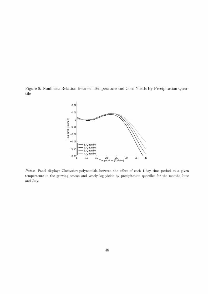
Figure 6: Nonlinear Relation Between Temperature and Corn Yields By Precipitation Quar-tile

5 10 15 20 25 30 35 40−0.05

−0.04

−0.03

−0.02

−0.01

0

0.01

0.02

Temperature (Celsius)

Log

Yie

ld (

Bus

hels

)

1. Quantile2. Quantile3. Quantile4. Quantile

Notes: Panel displays Chebyshev-polynomials between the effect of each 1-day time period at a giventemperature in the growing season and yearly log yields by precipitation quartiles for the months Juneand July.

48

Figure 7: Nonlinear Relation Between Temperature and Corn Yields for Various Definitionsof the Growing Seasons

5 10 15 20 25 30 35 40−0.05

−0.04

−0.03

−0.02

−0.01

0

0.01

0.02

Temperature (Celsius)

Growing Season March − August

Log

Yie

ld (

Bus

hels

)

5 10 15 20 25 30 35 40−0.05

−0.04

−0.03

−0.02

−0.01

0

0.01

0.02

Temperature (Celsius)

Growing Season April − August

Log

Yie

ld (

Bus

hels

)

5 10 15 20 25 30 35 40−0.05

−0.04

−0.03

−0.02

−0.01

0

0.01

0.02

Temperature (Celsius)

Growing Season May − August

Log

Yie

ld (

Bus

hels

)

5 10 15 20 25 30 35 40−0.05

−0.04

−0.03

−0.02

−0.01

0

0.01

0.02

Temperature (Celsius)

Growing Season March − September

Log

Yie

ld (

Bus

hels

)

5 10 15 20 25 30 35 40−0.05

−0.04

−0.03

−0.02

−0.01

0

0.01

0.02

Temperature (Celsius)

Growing Season April − September

Log

Yie

ld (

Bus

hels

)

5 10 15 20 25 30 35 40−0.05

−0.04

−0.03

−0.02

−0.01

0

0.01

0.02

Temperature (Celsius)

Growing Season May − September

Log

Yie

ld (

Bus

hels

)

5 10 15 20 25 30 35 40−0.05

−0.04

−0.03

−0.02

−0.01

0

0.01

0.02

Temperature (Celsius)

Growing Season March − May

Log

Yie

ld (

Bus

hels

)

5 10 15 20 25 30 35 40−0.05

−0.04

−0.03

−0.02

−0.01

0

0.01

0.02

Temperature (Celsius)

Growing Season June − August

Log

Yie

ld (

Bus

hels

)

Notes: Panels display changes in annual log yield if the crop is exposed for one day to a particular tem-perature. Impacts are normalized relative to a temperature of 8◦C. Columns of the first two rows differ bythe first month of the growing season: March, April, or May. The first two rows differ by the end of thegrowing season: August or September. The third row splits the six-months default growing season into twothree-months intervals to test time separability. The default relationship (March-August) is added as greybackground in the remaining graphs. The 95% confidence band, after adjusting for spatial correlation, isadded as dashed lines.

49

Figure 8: Geographic Distribution of Climate Impacts

Notes: Panels display predicted impacts under the B2 scenario for our preferred dummy variables approachusing the 55-year history of corn yields.

50