ESTIMATING THE FUTURE TRENDS IN

THE COST OF CO2 CAPTURE

TECHNOLOGIES

Technical Study

Report Number: 2006/6

Date: February 2006

This document has been prepared for the Executive Committee of the IEA GHG Programme. It is not a publication of the Operating Agent, International Energy Agency or its Secretariat.

INTERNATIONAL ENERGY AGENCY

The International Energy Agency (IEA) was established in 1974 within the framework of the Organisation for Economic Co-operation and Development (OECD) to implement an international energy programme. The IEA fosters co-operation amongst its 26 member countries and the European Commission, and with the other countries, in order to increase energy security by improved efficiency of energy use, development of alternative energy sources and research, development and demonstration on matters of energy supply and use. This is achieved through a series of collaborative activities, organised under more than 40 Implementing Agreements. These agreements cover more than 200 individual items of research, development and demonstration. The IEA Greenhouse Gas R&D Programme is one of these Implementing Agreements.

DISCLAIMER

This report was prepared as an account of work sponsored by the IEA Greenhouse Gas R&D Programme. The views and opinions of the authors expressed herein do not necessarily reflect those of the IEA Greenhouse Gas R&D Programme, its members, the International Energy Agency, the organisations listed below, nor any employee or persons acting on behalf of any of them. In addition, none of these make any warranty, express or implied, assumes any liability or responsibility for the accuracy, completeness or usefulness of any information, apparatus, product or process disclosed or represents that its use would not infringe privately owned rights, including any party’s intellectual property rights. Reference herein to any commercial product, process, service or trade name, trade mark or manufacturer does not necessarily constitute or imply an endorsement, recommendation or any favouring of such products.

COPYRIGHT

Copyright © IEA Greenhouse Gas R&D Programme 2006. All rights reserved.

ACKNOWLEDGEMENTS AND CITATIONS

This report describes research sponsored by the IEA Greenhouse Gas R&D Programme. This report was prepared by: Carnegie Mellon University Department of Engineering and Public Policy Center for Energy and Environmental Studies Pittsburgh Pennsylvania 15213 USA The principal researchers were:

• Edward Rubin • Matt Antes • Sonia Yeh • Michael Berkenpas

To ensure the quality and technical integrity of the research undertaken by the IEA Greenhouse Gas R&D Programme (IEA GHG) each study is managed by an appointed IEA GHG manager. The report is also reviewed by a panel of independent technical experts before its release. The IEA GHG manager for this report: John Davison The expert reviewers for this report:

• Rodney Allam, UK • Jon Gibbins, Imperial College, UK • Howard Herzog, MIT, USA • Keywan Riahi, IIASA, Austria • Leo Schrattenholzer, IIASA, Austria • Dale Simbeck, SFA Pacific, USA

The report should be cited in literature as follows: IEA Greenhouse Gas R&D Programme (IEA GHG), “Estimating future trends in the cost of CO2 capture technologies”, 2006/5, January 2006. Further information or copies of the report can be obtained by contacting the IEA GHG Programme at: IEA Greenhouse R&D Programme, Orchard Business Centre, Stoke Orchard, Cheltenham, Glos., GL52 7RZ, UK Tel: +44 1242 680753 Fax: +44 1242 680758 E-mail: mail@ieaghg.org www.ieagreen.org.uk

i

ESTIMATING FUTURE TRENDS IN THE COST OF CO2 CAPTURE TECHNOLOGIES

Background The IEA Greenhouse Gas R&D Programme (IEA GHG) has carried out studies to assess the performance and costs of various plants with CO2 capture and storage (CCS). These assessments have mostly been based on current technology and component cost data. This approach has the advantage of avoiding subjective judgements of what may or may not happen in the future. The disadvantage is that it does not take into account the potential for future improvements which could affect the long-term competitiveness of a technology. Reductions in the costs of technologies resulting from learning-by-doing and other factors have been systematically observed over many decades. Major factors contributing to cost reductions include, but are not limited to, improvements in technology design, materials, product standardisation, system integration or optimisation, economies of scale and reductions in input prices. This study analyses cost reductions that have been achieved for a range of process technologies and uses that information to predict possible future trends in the costs of power plants with CO2 capture. The study was carried out for IEA GHG by Carnegie Mellon University in the USA.

Study description Technologies analysed The study analyses historical cost trends for the following seven technologies which are in some ways analogous to technologies used in power plants with CO2 capture:

• Flue gas desulfurisation (FGD) in power plants • Selective catalytic reduction (SCR) in power plants • Pulverised coal boilers • Gas turbine combined cycle power plants • Liquefied natural gas (LNG) production plants • Oxygen production plants • Steam methane reforming (SMR) plants for hydrogen production

Average “learning rates” are derived for capital costs and operating and maintenance (O&M) costs. The learning rates represent the fractional reduction in cost associated with each doubling of cumulative total production or capacity of the technology. The learning rates for these technologies were used to estimate future reductions in costs of power plants with CO2 capture after 100GWe of capacity has been installed. This was achieved by breaking down the power plants into sub-systems, each of which was assumed to be analogous to one of the seven reference technologies. Future cost reductions for whole power plants with capture were then predicted, based on the learning rates for each of the sub-systems. The following power plants were assessed:

• Natural gas combined cycle plant with CO2 capture by post combustion amine scrubbing • Pulverised coal steam cycle plant with CO2 capture by post combustion amine scrubbing • Coal-based integrated gasification combined cycle (IGCC) plant with pre-combustion capture • Pulverised coal oxy-combustion steam cycle plant

ii

The study could, if required be extended in the future to other technologies such as natural gas combined cycles with pre-combustion capture. Learning curves and uncertainties Future costs predicted using learning curves are subject to various uncertainties, as discussed briefly below, and in more detail in the main report. Sensitivity studies were carried out to quantify the effects of some of the major uncertainties. Base capacities To calculate future cost reductions for power plants with CO2 capture it is necessary to define the current installed capacity of each sub-system. For example, in the case of oxyfuel plants, if the boilers are assumed to be very similar to conventional pulverised coal boilers it would be appropriate to assume that the ‘base capacity’ for oxyfuel boilers is the current installed capacity of conventional pulverised coal boilers. This results in only small future cost reductions. However, if oxyfuel boilers are assumed to be substantially different to conventional boilers, the base capacity could be assumed to be essentially zero, as there are currently no oxyfuel power plants. The resulting cost reductions would be much greater. Similar judgments have to be made for other power plant sub-systems, for example hydrogen-fired gas turbines used in IGCC plants. Cost increases for initial commercial plants Costs of initial commercial plants are often higher than those estimated in pre-commercial studies. It is assumed in this study that the learning rates will only be applied after a certain amount of initial capacity (between 3 and 10 GW, depending on the state of development of the technology) has been installed, at which point costs will have decreased to those given in pre-commercial studies. Use of technologies in other applications Some technologies will be used in applications other than power plants with CO2 capture. The installed capacity and learning achieved in these other applications can affect the costs for power plants with CO2 capture. Availability of cost data and the effects of commercial pricing The contractor for this study devoted much effort to obtaining and analysing cost data for existing technologies but it is inevitably difficult to obtain such information for some technologies over a number of years. The degree of commercial competition and variations in the profit margins of suppliers can have a significant effect on apparent cost trends. Inflation The historical data used to derive learning rates has to be converted to current money values by correcting for inflation. A variety of different inflation indices can be used to do this. The choice of inflation index can significantly affect the estimate of technology learning rate, particularly when the analysis covers a long period of time. The shape of learning curves The learning curve for a specific technology is not always best described by the classical log-linear function, but by more complex functions such as an S-shaped curve, in which costs initially stay relatively high, there is then a period of rapid cost reductions and finally a levelling off of costs. In this study, however, the log-linear model is retained for simplicity and consistency with other studies.

iii

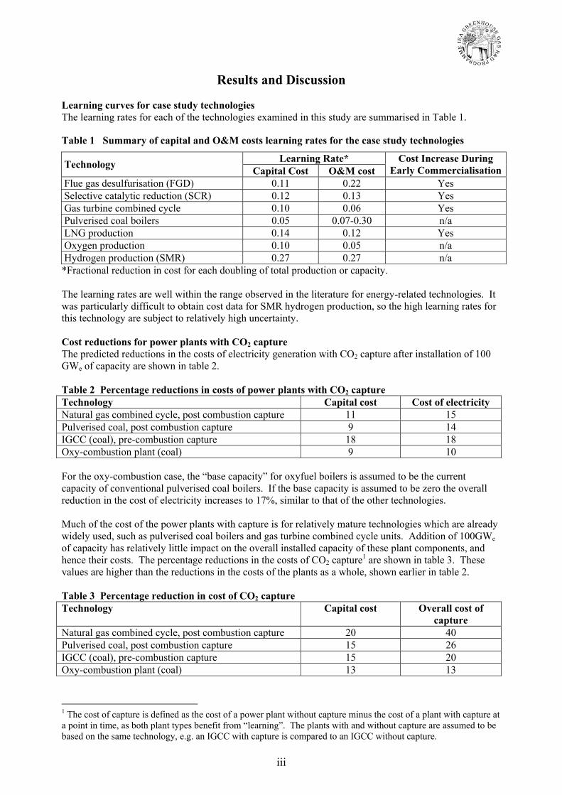
Results and Discussion Learning curves for case study technologies The learning rates for each of the technologies examined in this study are summarised in Table 1.

Table 1 Summary of capital and O&M costs learning rates for the case study technologies

Learning Rate* Technology Capital Cost O&M cost Cost Increase During

Early Commercialisation Flue gas desulfurisation (FGD) 0.11 0.22 Yes Selective catalytic reduction (SCR) 0.12 0.13 Yes Gas turbine combined cycle 0.10 0.06 Yes Pulverised coal boilers 0.05 0.07-0.30 n/a LNG production 0.14 0.12 Yes Oxygen production 0.10 0.05 n/a Hydrogen production (SMR) 0.27 0.27 n/a *Fractional reduction in cost for each doubling of total production or capacity. The learning rates are well within the range observed in the literature for energy-related technologies. It was particularly difficult to obtain cost data for SMR hydrogen production, so the high learning rates for this technology are subject to relatively high uncertainty. Cost reductions for power plants with CO2 capture The predicted reductions in the costs of electricity generation with CO2 capture after installation of 100 GWe of capacity are shown in table 2. Table 2 Percentage reductions in costs of power plants with CO2 capture Technology Capital cost Cost of electricity Natural gas combined cycle, post combustion capture 11 15 Pulverised coal, post combustion capture 9 14 IGCC (coal), pre-combustion capture 18 18 Oxy-combustion plant (coal) 9 10 For the oxy-combustion case, the “base capacity” for oxyfuel boilers is assumed to be the current capacity of conventional pulverised coal boilers. If the base capacity is assumed to be zero the overall reduction in the cost of electricity increases to 17%, similar to that of the other technologies. Much of the cost of the power plants with capture is for relatively mature technologies which are already widely used, such as pulverised coal boilers and gas turbine combined cycle units. Addition of 100GWe of capacity has relatively little impact on the overall installed capacity of these plant components, and hence their costs. The percentage reductions in the costs of CO2 capture1 are shown in table 3. These values are higher than the reductions in the costs of the plants as a whole, shown earlier in table 2. Table 3 Percentage reduction in cost of CO2 capture Technology Capital cost Overall cost of

capture Natural gas combined cycle, post combustion capture 20 40 Pulverised coal, post combustion capture 15 26 IGCC (coal), pre-combustion capture 15 20 Oxy-combustion plant (coal) 13 13

1 The cost of capture is defined as the cost of a power plant without capture minus the cost of a plant with capture at a point in time, as both plant types benefit from “learning”. The plants with and without capture are assumed to be based on the same technology, e.g. an IGCC with capture is compared to an IGCC without capture.

iv

It should be noted that the cost of capture is not just the cost of the capture section of the plant, but also takes into account the impacts of the addition of capture on the overall performance and cost of the power plant. Comparison with other IEA GHG studies The “current” costs of power plants with CO2 capture in this study are based on data from Carnegie Mellon University’s IECM modelling package. The overall IECM costs are broadly compatible with IEA GHG’s own recent studies. The main differences are due to differences in technical and economic input assumptions. In particular the IECM costs are based on a higher annual capital charge rate and a lower load factor, which result in higher electricity costs. However, these assumptions have little effect on the predicted percentage cost reductions due to learning, as illustrated by a sensitivity case employing IEA GHG assumptions for capital charge rate and load factor. IEA GHG’s recent studies on leading CO2 capture technologies2 include predictions of the performances and costs of power plants designed in the year 2020. These predictions were based on the contractors’ expectations of technology improvements and reductions in the costs of the plant components. Costs of electricity were predicted to decrease by between 20 and 25%. These are higher than the base case cost reductions predicted in this study, which are shown in table 1, but they are within the range of cost reductions for IGCC and NGCC plants predicted in the sensitivity cases in this study. The different studies use a different basis for estimating cost reductions, i.e. a total amount of plant installation in the case of this study and a date in the case of IEA GHG’s other studies, so the costs reductions should not necessarily be same.

Expert Reviewers’ Comments The draft study report was reviewed by various experts in power generation, process technologies and technology learning. IEA GHG is very grateful to all of those who contributed to this review. The comments from reviewers provided some significant information and helpful suggestions which contributed to the final report. Overall comments from the expert reviewers praised the study as a “significant contribution” to the field.

Major Conclusions Major factors which contribute to process technology cost reductions include, but are not limited to, improvements in technology design, materials, product standardisation, system integration or optimisation, economies of scale and reductions in input prices. Analysis of various process technologies indicates that in most cases capital costs have reduced by 10-15% for each doubling of installed capacity. The corresponding reduction in operating and maintenance costs is 5-30%. Based on learning rate data for analogous process technologies, the cost of electricity from power plants with CO2 capture is predicted to reduce by 10-18% after 100GWe of capacity has been installed. Much of the cost of a power plant with CO2 capture is for equipment which is already widely used, such as pulverised coal boilers and gas turbine combined cycles. Reductions in the incremental costs of CO2 capture are predicted to be 13-40%, i.e. greater than the reductions in the overall cost of electricity.

2 IEA GHG reports PH4/19 (IGCC) and PH4/33 (post-combustion capture).

v

IGCC with CO2 capture is estimated to have a higher overall cost reduction from learning than other coal-based power technologies because of greater cost reductions in the core power generation sections of the plant. However, the reduction in the incremental cost of capture in IGCC is lower than for plants with post combustion capture.

Recommendations A more extensive set of sensitivity analyses could provide a more detailed picture of the influence of alternative assumptions on cost reductions. A spreadsheet is provided with this report to enable users to assess further sensitivities if they wish to do so. However, no further work by IEA GHG on this topic is recommended at this time.

ESTIMATING FUTURE TRENDS

IN THE COST OF CO2 CAPTURE TECHNOLOGIES

Final Report to

International Energy Agency Greenhouse Gas R&D Programme (IEA GHG)

from

Carnegie Mellon University

Department of Engineering and Public Policy Center for Energy and Environmental Studies

Pittsburgh, Pennsylvania 15213

Principal Investigator: Edward S. Rubin Tel: (412) 268-5897 Fax: (412) 268-1089

E-mail: rubin@cmu.edu

Matt Antes The H. John Heinz III School of Public Policy and Management

Carnegie Mellon University

Sonia Yeh Office of Research and Development

U.S. Environmental Protection Agency

Michael Berkenpas Department of Engineering and Public Policy

Carnegie Mellon University

December 2005

i

Table of Contents

Acknowledgements................................................................................................................................ vi EXECUTIVE SUMMARY .................................................................................................................... 1 1. INTRODUCTION .............................................................................................................................. 4 2. STUDY APPROACH......................................................................................................................... 5 3. CASE STUDIES................................................................................................................................. 6

3.1 Flue Gas Desulfurization (FGD) and Selective Catalytic Reduction (SCR) Systems .................. 6 3.2 Pulverized Coal-Fired Boilers..................................................................................................... 10

3.2.1. Introduction......................................................................................................................... 10 3.2.2. Trends in Capacity and Performance .................................................................................. 10 3.2.3. Technological Progress of Coal-fired Boilers..................................................................... 14

3.3 Gas Turbine Combined Cycle (GTCC) Systems ........................................................................ 20 3.3.1. Introduction......................................................................................................................... 20 3.3.2. Cost Trends of GTCC and its Components ........................................................................ 22

3.4 Liquefied Natural Gas (LNG) Production .................................................................................. 23 3.4.1 Introduction.......................................................................................................................... 23 3.4.2 LNG Supply Chain .............................................................................................................. 26 3.4.3 Operating Costs.................................................................................................................... 35

3.5 Oxygen Production Technology ................................................................................................. 37 3.5.1 Current Air Separation Technologies .................................................................................. 38 3.5.2 Evolution of Oxygen Production ......................................................................................... 40 3.5.3 Oxygen Production Capacity ............................................................................................... 43 3.5.4 Cost Trend Analysis............................................................................................................. 45

3.6 Hydrogen Production by Steam Methane Reforming................................................................. 52 3.6.1 Introduction.......................................................................................................................... 52 3.6.2 Steam Methane Reforming Technology .............................................................................. 54 3.6.3 Difficulties of Cost Estimation for SMR ............................................................................. 55

3.7 Summary of Case Study Results................................................................................................. 58 4. APPLICATIONS TO CO2 CAPTURE SYSTEMS.......................................................................... 60

4.1 Overview of Power Plant Designs with CO2 Capture................................................................. 60 4.1.1 Post-combustion CO2 Capture ............................................................................................. 60 4.1.2 Pre-combustion CO2 Capture............................................................................................... 61 4.1.3 Oxyfuel Combustion for CO2 Capture................................................................................. 62 4.1.4 Current Status of Power Plant Systems................................................................................ 62

4.2 Methodological Approach to Cost Trend Projections................................................................. 63 4.3 Cost Estimates for Current Capture Plants ................................................................................. 65 4.4 Calculation of Plant-Level Cost Trends...................................................................................... 66

4.4.1 Sub-System Learning Rates ................................................................................................. 67 4.4.2 Current Sub-System Capacities ........................................................................................... 67 4.4.3 Effect of Non-CCS Experience............................................................................................ 69

4.5 Estimation of Future Cost Trends ............................................................................................... 70 4.5.1 Capital Cost Trends.............................................................................................................. 70 4.5.2 O&M Cost Trends ............................................................................................................... 74 4.5.3 Total Plant Cost Trends ....................................................................................................... 76

4.6 Sensitivity Analysis .................................................................................................................... 78 4.7 Concluding Remarks................................................................................................................... 80

5. REFERENCES ................................................................................................................................. 82 APPENDIX........................................................................................................................................... 87

ii

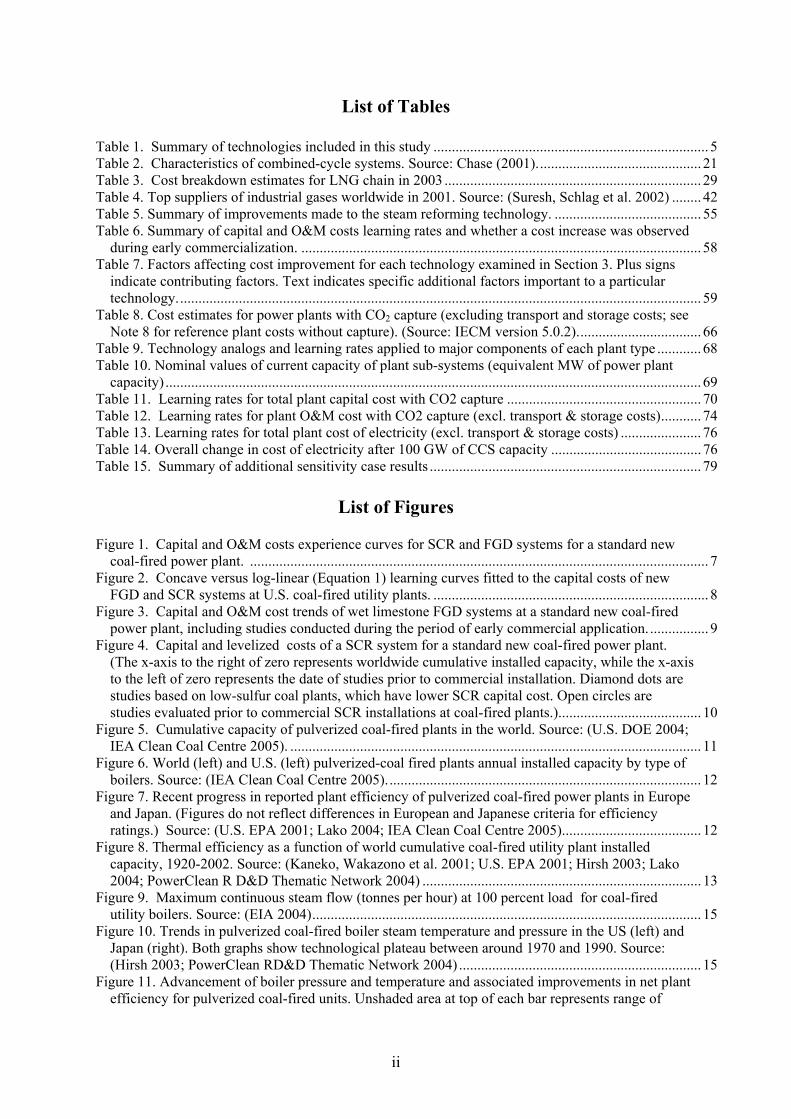
List of Tables

Table 1. Summary of technologies included in this study ........................................................................... 5 Table 2. Characteristics of combined-cycle systems. Source: Chase (2001)............................................. 21 Table 3. Cost breakdown estimates for LNG chain in 2003 ...................................................................... 29 Table 4. Top suppliers of industrial gases worldwide in 2001. Source: (Suresh, Schlag et al. 2002) ........ 42 Table 5. Summary of improvements made to the steam reforming technology. ........................................ 55 Table 6. Summary of capital and O&M costs learning rates and whether a cost increase was observed

during early commercialization. ............................................................................................................. 58 Table 7. Factors affecting cost improvement for each technology examined in Section 3. Plus signs

indicate contributing factors. Text indicates specific additional factors important to a particular technology............................................................................................................................................... 59

Table 8. Cost estimates for power plants with CO2 capture (excluding transport and storage costs; see Note 8 for reference plant costs without capture). (Source: IECM version 5.0.2).................................. 66

Table 9. Technology analogs and learning rates applied to major components of each plant type ............ 68 Table 10. Nominal values of current capacity of plant sub-systems (equivalent MW of power plant

capacity) .................................................................................................................................................. 69 Table 11. Learning rates for total plant capital cost with CO2 capture ..................................................... 70 Table 12. Learning rates for plant O&M cost with CO2 capture (excl. transport & storage costs)........... 74 Table 13. Learning rates for total plant cost of electricity (excl. transport & storage costs) ...................... 76 Table 14. Overall change in cost of electricity after 100 GW of CCS capacity ......................................... 76 Table 15. Summary of additional sensitivity case results .......................................................................... 79

List of Figures

Figure 1. Capital and O&M costs experience curves for SCR and FGD systems for a standard new

coal-fired power plant. ............................................................................................................................. 7 Figure 2. Concave versus log-linear (Equation 1) learning curves fitted to the capital costs of new

FGD and SCR systems at U.S. coal-fired utility plants. ........................................................................... 8 Figure 3. Capital and O&M cost trends of wet limestone FGD systems at a standard new coal-fired

power plant, including studies conducted during the period of early commercial application................. 9 Figure 4. Capital and levelized costs of a SCR system for a standard new coal-fired power plant.

(The x-axis to the right of zero represents worldwide cumulative installed capacity, while the x-axis to the left of zero represents the date of studies prior to commercial installation. Diamond dots are studies based on low-sulfur coal plants, which have lower SCR capital cost. Open circles are studies evaluated prior to commercial SCR installations at coal-fired plants.)....................................... 10

Figure 5. Cumulative capacity of pulverized coal-fired plants in the world. Source: (U.S. DOE 2004; IEA Clean Coal Centre 2005). ................................................................................................................ 11

Figure 6. World (left) and U.S. (left) pulverized-coal fired plants annual installed capacity by type of boilers. Source: (IEA Clean Coal Centre 2005)...................................................................................... 12

Figure 7. Recent progress in reported plant efficiency of pulverized coal-fired power plants in Europe and Japan. (Figures do not reflect differences in European and Japanese criteria for efficiency ratings.) Source: (U.S. EPA 2001; Lako 2004; IEA Clean Coal Centre 2005)...................................... 12

Figure 8. Thermal efficiency as a function of world cumulative coal-fired utility plant installed capacity, 1920-2002. Source: (Kaneko, Wakazono et al. 2001; U.S. EPA 2001; Hirsh 2003; Lako 2004; PowerClean R D&D Thematic Network 2004) ............................................................................ 13

Figure 9. Maximum continuous steam flow (tonnes per hour) at 100 percent load for coal-fired utility boilers. Source: (EIA 2004).......................................................................................................... 15

Figure 10. Trends in pulverized coal-fired boiler steam temperature and pressure in the US (left) and Japan (right). Both graphs show technological plateau between around 1970 and 1990. Source: (Hirsh 2003; PowerClean RD&D Thematic Network 2004) .................................................................. 15

Figure 11. Advancement of boiler pressure and temperature and associated improvements in net plant efficiency for pulverized coal-fired units. Unshaded area at top of each bar represents range of

iii

efficiencies for indicated steam conditions. Source: Modified from (Kitto 1996b) ............................... 16 Figure 12. Thermal efficiency (left) and boiler capacity (right) of 12 TVA plants compared with

overall trends in the U.S. The last three data points (square dots) are supercritical units....................... 17 Figure 13. Comparison of trended economic indexes, including gross domestic product (GDP)

implicit price deflators, Handy-Whitman Index of Public Utility Construction Costs, Labor Cost index (Bureau of Economic Analysis 2003), and Chemical Engineering construction cost index......... 17

Figure 14. Historical construction cost of PC boilers ($/kW) and the learning curve, subcritical boilers...................................................................................................................................................... 18

Figure 15. Experience curve of adjusted O&M costs for average AEP systems, 1929-1958..................... 19 Figure 16. Learning curves of coal steam plant O&M costs and boiler O&M costs, 1981-1997.

Source: Modified from Beamon and Leckey (1999). ............................................................................. 20 Figure 17. Diagram of a gas turbine combine cycle. Modified from Chase (2001). ................................. 21 Figure 18. Trend of selected combined cycle plant efficiency (LHV basis). Source: Chase (2001). ........ 21 Figure 19. Experience curve for the specific investment price of gas turbine combined cycle (GTCC)

technology (1981–1997). Source: Colpier and Cornland (2002). ........................................................... 22 Figure 20. Experience curve for the cost of generating electricity in a natural-gas-fired GTCC plant,

1981–1997. Curve A includes the change of natural gas price over the period studied. In curve B the natural gas price is held constant at 1.13 US$ (1990) per kWh. Source: (Colpier and Cornland 2002) ....................................................................................................................................................... 23

Figure 21. Global growth in baseload LNG production, 1970–2005 (anticipated). Sources: (Delano, Gulen et al. 2003; EIA 2003). ................................................................................................................. 24

Figure 22. Natural gas-to-market costs for various transport modes. Source: (Coyle 2003)..................... 24 Figure 23. Number of worldwide new LNG plants (greenfield) and construction of additional trains at

existing plants (expansion). Source: (EIA 2003) .................................................................................... 26 Figure 24. LNG base-loading flow scheme. ............................................................................................... 27 Figure 25. Natural gas/refrigerant cooling curve. Source:(Finn, Johnson et al. 2001) .............................. 28 Figure 26. Percentage of worldwide baseload LNG capacity for each liquefaction technology in use

as of December 2002. Source: (Bronfenbrenner 2004)........................................................................... 29 Figure 27. LNG Plant capital cost trends for greenfield facilities (US$2003 per tonne per year)............. 31 Figure 28. Worldwide LNG plant train capacity (million tonnes per year). Source: (EIA 2003) ............. 32 Figure 29. Percentage of anticipated worldwide baseload LNG capacity for each liquefaction

technology in 2010. Source:(Groothuis and Pek 2003) .......................................................................... 34 Figure 30. Experience curve of liquefaction unit cost based on adjusting for greenfield and expansion

trains and Chemical Engineering Plant Index, and cumulative capacity of worldwide LNG produced.................................................................................................................................................. 35

Figure 31. Liquefaction electricity requirements as a function of cumulative LNG produced. Source: (Bronfenbrenner 2004)............................................................................................................................ 37

Figure 32. Basic flow diagram of the cryogenic air separation process (courtesy of APCI). ..................... 39 Figure 33. Merchant consumers of oxygen in United States in 2001 (Suresh, Schlag et al. 2002). ........... 42 Figure 34. Merchant consumers of oxygen in Western Europe in 2001 (Suresh, Schlag et al. 2002)........ 43 Figure 35. Growth of a single train cryogenic train size in air separation units at Air Products (sTPD =

short tons per day). Source: (Smith 2001) .............................................................................................. 43 Figure 36. Worldwide production of oxygen and crude steel. Sources: (Scharle and Wilson 1981;

Petras, Mostello et al. 1987; CIR 1997; CIR 1998; Suresh, Schlag et al. 2002; Kato, Kubota et al. 2003; IISI 2004; AISI 2005) ................................................................................................................... 44

Figure 37. Experience curve for unit cost of oxygen production for trains larger than 1000 tpd as a function of cumulative worldwide oxygen production (1 Bcf = 2.83 million cubic meters) from 1980–2003. Data are adjusted for oxygen purity and pressure; costs adjusted using the Chemical Engineering Plant Index.......................................................................................................................... 47

Figure 38. Operating electricity requirements for trains larger than 1000 tpd, adjusted for oxygen purity (95%) and pressure (53 bar, 750 psig), for plants before and after structured packing technology was introduced...................................................................................................................... 48

Figure 39. Operating electricity requirements as a function of train size for air separation units producing 95% purity oxygen at 2.4 bar (20 psig). Source: (Queneau and Marcuson 1996) ................. 49

iv

Figure 40. Experience curve for oxygen production electricity requirement (as a measure of unit operating cost) as a function of cumulative worldwide oxygen production (1 Bcf = 2.83 million cubic meters) from 1980–2003, based on trains larger than 1000 tpd and adjusted for oxygen purity (95%) and pressure (53 bar, 750 psig). ................................................................................................... 50

Figure 41. ITM oxygen production development program goals for U.S. government and gas industry partnership. Source: (Armstrong and Foster 2004)................................................................................. 51

Figure 42. Annual world consumption of intentionally produced or merchant hydrogen in 1999 (1 Bcf = 2.83 million cubic meters). Source: (Suresh, Gubler et al. 2001) ................................................. 52

Figure 43. Annual U.S. production of hydrogen (1 Bcf = 2.83 million cubic meters). These data do not include all uses of hydrogen (see text). Source: (Suresh, Gubler et al. 2001) ........................................ 53

Figure 44. Estimated capital cost of hydrogen production using SMR technology in three plant sizes, current and possible future cases, with and without sequestration of CO2. Source: (National Research Council 2004) .......................................................................................................................... 54

Figure 45. Steam reforming of natural gas hydrogen plant with PSA (Fleshman, McEvoy et al. 1999). .. 55 Figure 46. U.S. unit shipments value for hydrogen, and average price of natural gas to the industrial

sector, 1971-2000. Source: (EIA 2001; Suresh, Gubler et al. 2001)....................................................... 56 Figure 47. Estimated natural gas fuel cost, capital charges, and non-fuel O&M costs for H2

production, 1971-1998. (1 cent per 100 cu ft = US$3.53 per 1000 cubic meters). ................................ 57 Figure 48. Experience curves for estimated capital cost and non-fuel O&M cost for H2 production via

steam methane reforming, 1971-1998. (1 Bcf = 2.83 million cubic meters; 1 cent per 100 cu ft = US$3.53 per 1000 cubic meters). Data source: (Suresh, Gubler et al. 2001).......................................... 57

Figure 49. Simplified process diagram for natural gas combined cycle (NGCC) power plant with an amine-based post-combustion CO2 capture system ................................................................................ 61

Figure 50. Simplified process diagram for pulverized coal (PC) power plant with an amine-based post-combustion CO2 capture system..................................................................................................... 61

Figure 51. Simplified process diagram for integrated gasification combined cycle (IGCC) power plant with pre-combustion CO2 capture system based on a water-gas shift reactor plus Selexol separation .. 62

Figure 52. Simplified process diagram for an oxyfuel PC power plant system with CO2 capture ............. 62 Figure 53. Capital cost trend for NGCC plant with CO2 capture assuming cost reductions after first

commercial installation. .......................................................................................................................... 71 Figure 54. Capital cost trend for PC plant with CO2 capture assuming cost reductions after first

commercial installation. .......................................................................................................................... 71 Figure 55. Capital cost trend for IGCC plant with CO2 capture assuming cost reductions after first

commercial installation. .......................................................................................................................... 71 Figure 56. Capital cost trend for Oxyfuel plant with CO2 capture assuming cost reductions after first

commercial installation. .......................................................................................................................... 71 Figure 57. Capital cost trend for NGCC plant with CO2 capture assuming cost reductions after 3 GW

of installed capacity. ............................................................................................................................... 72 Figure 58. Capital cost trend for PC plant with CO2 capture assuming cost reductions after 5 GW of

installed capacity..................................................................................................................................... 72 Figure 59. Capital cost trend for IGCC plant with CO2 capture assuming cost reductions after 7 GW of

installed capacity..................................................................................................................................... 72 Figure 60. Capital cost trend for oxyfuel plant with CO2 capture assuming cost reductions after 10

GW of installed capacity......................................................................................................................... 72 Figure 61. Effect of uncertainty in component-level learning rates on total capital cost uncertainty for

an NGCC plant with CO2 capture. .......................................................................................................... 73 Figure 62. Effect of uncertainty in component-level learning rates on total capital cost uncertainty for

a PC plant with CO2 capture. .................................................................................................................. 73 Figure 63. Effect of uncertainty in component-level learning rates on total capital cost uncertainty for

an IGCC plant with CO2 capture............................................................................................................. 73 Figure 64. Effect of uncertainty in component-level learning rates on total capital cost uncertainty for

an oxyfuel plant with CO2 capture. ......................................................................................................... 73 Figure 65. O&M cost trend for NGCC plant with CO2 capture (excluding CO2 transport and storage

costs). ...................................................................................................................................................... 75

v

Figure 66. O&M cost trend for PC plant with CO2 capture (excluding CO2 transport and storage costs). ...................................................................................................................................................... 75

Figure 67. O&M cost trend for IGCC plant with CO2 capture (excluding CO2 transport and storage costs). ...................................................................................................................................................... 75

Figure 68. O&M cost trend for oxyfuel plant with CO2 capture (excluding CO2 transport and storage costs). ...................................................................................................................................................... 75

Figure 69. Total cost of electricity for NGCC plant with CO2 capture (excluding CO2 transport and storage costs)........................................................................................................................................... 77

Figure 70. Total cost of electricity for PC plant with CO2 capture (excluding CO2 transport and storage costs)........................................................................................................................................... 77

Figure 71. Total cost of electricity for IGCC plant with CO2 capture (excluding CO2 transport and storage costs)........................................................................................................................................... 77

Figure 72. Total cost of electricity for oxyfuel plant with CO2 capture (excluding CO2 transport and storage costs)........................................................................................................................................... 77

vi

ACKNOWLEDGEMENTS

The authors wish to acknowledge the important contribution to this report of members of the Project Advisory Committee who helped guide and inform this research, and who served as reviewers of the midterm and final drafts of this report. They are Jon Gibbins (Imperial College), Howard Herzog (MIT), Keywan Riahi (IIASA), Leo Schrattenholzer IIASA) and Dale Simbeck (SFA Pacific). We are also grateful to Rodney Allam (Air Products) and John Davison (IEA GHG) for their insights and comments on the final draft report. We are especially indebted to John Davison for his critical role as the IEA GHG Project Manager for this effort.

1

EXECUTIVE SUMMARY

Because of growing worldwide interest in CO2 capture and storage (CCS) as a potential option for climate change mitigation, the expected future cost of CCS technologies also is of significant interest. Most studies of CO2 capture and storage costs have been based on currently available technology. This approach has the advantage of avoiding subjective judgments of what may or may not happen in the future, or what the cost will be of “advanced” technologies still in the early stages of development. On the other hand, reliance on current technology cost estimates has the disadvantage of not taking into account the potential for improvements that can affect the long-term competitiveness of CCS as a climate mitigation strategy.

Reductions in the cost of technologies resulting from learning-by-doing and other factors have been systematically observed over many decades. This study uses historical cost trends as a basis for estimating future costs of four types of large-scale electric power systems employing CO2 capture: pulverized coal (PC) and natural gas combined cycle (NGCC) plants using post-combustion CO2 capture systems; coal-based integrated gasification combined cycle (IGCC) plants with pre-combustion capture; and coal-fired oxyfuel combustion for new PC plants. We assess cost reductions that have been achieved by other process technologies in the past and, by analogy, estimate cost reductions that might be achieved by power plants with CO2 capture in the future.

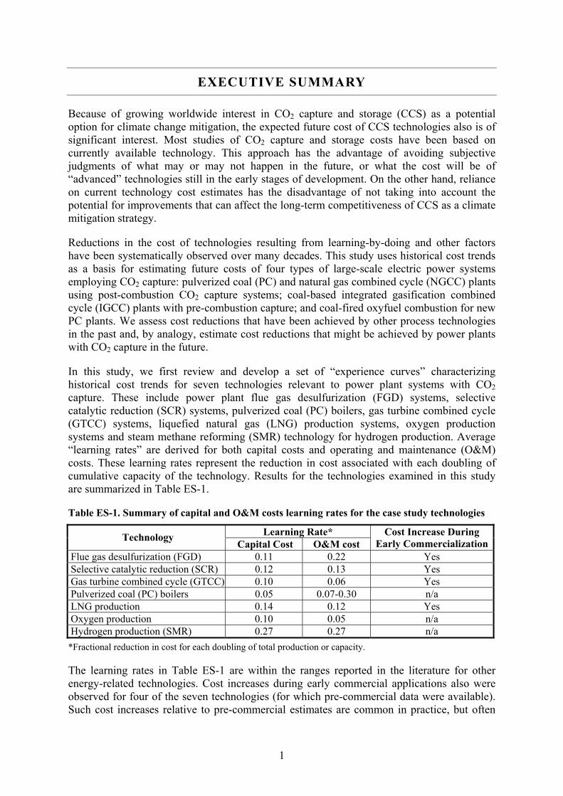
In this study, we first review and develop a set of “experience curves” characterizing historical cost trends for seven technologies relevant to power plant systems with CO2 capture. These include power plant flue gas desulfurization (FGD) systems, selective catalytic reduction (SCR) systems, pulverized coal (PC) boilers, gas turbine combined cycle (GTCC) systems, liquefied natural gas (LNG) production systems, oxygen production systems and steam methane reforming (SMR) technology for hydrogen production. Average “learning rates” are derived for both capital costs and operating and maintenance (O&M) costs. These learning rates represent the reduction in cost associated with each doubling of cumulative capacity of the technology. Results for the technologies examined in this study are summarized in Table ES-1.

Table ES-1. Summary of capital and O&M costs learning rates for the case study technologies

Learning Rate* Technology Capital Cost O&M cost

Cost Increase During Early Commercialization

Flue gas desulfurization (FGD) 0.11 0.22 Yes Selective catalytic reduction (SCR) 0.12 0.13 Yes Gas turbine combined cycle (GTCC) 0.10 0.06 Yes Pulverized coal (PC) boilers 0.05 0.07-0.30 n/a LNG production 0.14 0.12 Yes Oxygen production 0.10 0.05 n/a Hydrogen production (SMR) 0.27 0.27 n/a *Fractional reduction in cost for each doubling of total production or capacity.

The learning rates in Table ES-1 are within the ranges reported in the literature for other energy-related technologies. Cost increases during early commercial applications also were observed for four of the seven technologies (for which pre-commercial data were available). Such cost increases relative to pre-commercial estimates are common in practice, but often

2

are overlooked or excluded in the literature on learning curves. Major factors contributing to eventual cost reductions include, but are not limited to, improvements in technology design, materials, product standardization, system integration or optimization, economies of scale and reductions in input prices.

To estimate future cost trends for CO2 capture systems, we first decompose each plant design into several major sub-systems that include all equipment needed to carry out certain functions, such as power generation, air pollution control, or CO2 capture. We then apply a learning rate to each sub-system based on case study analogies. For any given level of total installed capacity, the estimated cost of the total plant is then calculated as the sum of all sub-system costs. Then, a classical learning curve (y = ax-b) is fitted to the total cost trend to yield a learning rate for the overall plant with CO2 capture.1 We also estimate the uncertainty of total capital cost, O&M cost, and cost of electricity production (COE) using a range of sub-system learning rates.

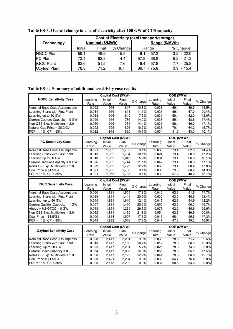
Table ES-2 shows the overall learning rates for each plant type from the onset of learning (a variable in the study) to the point where total installed capacity of each system reaches 100 GW. Nominal values range from 3% to 5%, with an overall range of about 1% to 8%. Based on these learning rates, Table ES-3 shows the overall change in COE. The largest overall cost reduction (18%) is seen for the IGCC system and the smallest (10%) for the oxyfuel system. The results with learning rate uncertainties show a broader range of cost reductions, varying from 3% to 26%. The sensitivity of results to other parameters of the analysis also was examined. These results are shown in Table ES-4. Key factors include the point at which learning (cost reductions) begin, the current capacity of each plant sub-system, and the magnitude of non-CCS applications contributing to future cost reductions. In general, combustion-based power plants, whose total cost is dominated by relatively mature components, showed lower overall learning rates than gasification-based plants. For similar reasons, the cost of CO2 capture technologies is projected to decline faster that the cost of the overall power plant. Results presented in this study can help to bound estimates of future CCS costs based on observed rates of change for other technologies.

Table ES-2. Learning rates for total plant cost of electricity (excl. transport & storage costs)

Nominal r 2

NGCC Plant 0.033 1.00 0.006 - 0.048PC Plant 0.035 0.98 0.015 - 0.054IGCC Plant 0.049 0.99 0.021 - 0.075Oxyfuel Plant 0.030 0.98 0.012 - 0.049

COE (excl transport/storage)Learning Rates for Total Plant

TechnologyRange

1 All results in this report exclude the additional costs (or credits) for CO2 transport and storage; however, the potential influence of these costs is discussed in Section 4.

3

Table ES-3. Overall change in cost of electricity after 100 GW of CCS capacity

Initial Final % ChangeNGCC Plant 59.1 49.9 15.5 46.1 - 57.2 3.2 - 22.0PC Plant 73.4 62.8 14.4 57.8 - 68.8 6.2 - 21.3IGCC Plant 62.6 51.5 17.6 46.4 - 57.8 7.7 - 25.8Oxyfuel Plant 78.8 71.2 9.7 66.7 - 75.8 3.9 - 15.4

TechnologyCost of Electricity (excl transport/storage)

Nominal ($/MWh) Range ($/MWh)Range % Change

Table ES-4. Summary of additional sensitivity case results

Learning Rate

Initial Value

Final Value % Change Learning

RateInitial Value

Final Value % Change

Nominal Base Case Assumptions 0.022 916 817 10.8% 0.033 59.1 49.9 15.5%Learning Starts with First Plant 0.014 916 811 11.5% 0.028 59.1 47.0 20.4%Learning up to 50 GW 0.018 916 849 7.3% 0.031 59.1 52.0 12.0%Current Capture Capacity = 0 GW 0.029 916 786 14.2% 0.037 59.1 48.8 17.4%Non-CSS Exp. Multipliers = 2.0 0.030 916 783 14.4% 0.036 59.1 49.0 17.1%Natural Gas Price = $6.0/GJ 0.022 925 826 10.7% 0.033 76.1 64.2 15.7%FCF = 11%, CF = 85% 0.022 918 820 10.7% 0.034 51.6 43.3 16.1%

Learning Rate

Initial Value

Final Value % Change Learning

RateInitial Value

Final Value % Change

Nominal Base Case Assumptions 0.021 1,962 1,783 9.1% 0.035 73.4 62.8 14.4%Learning Starts with First Plant 0.013 1,962 1,764 10.1% 0.024 73.4 60.8 17.2%Learning up to 50 GW 0.018 1,962 1,846 5.9% 0.031 73.4 66.0 10.1%Current Capture Capacity = 0 GW 0.026 1,962 1,744 11.1% 0.042 73.4 60.9 17.1%Non-CSS Exp. Multipliers = 2.0 0.029 1,962 1,723 12.2% 0.068 73.4 60.4 17.8%Coal Price = $1.5/GJ 0.021 1,965 1,786 9.1% 0.035 79.6 68.2 14.3%FCF = 11%, CF = 85% 0.021 1,963 1,785 9.1% 0.039 57.2 48.2 15.7%

Learning Rate

Initial Value

Final Value % Change Learning

RateInitial Value

Final Value % Change

Nominal Base Case Assumptions 0.050 1,831 1,505 17.8% 0.049 62.6 51.5 17.7%Learning Starts with First Plant 0.029 1,831 1,448 20.9% 0.032 62.6 48.6 22.4%Learning up to 50 GW 0.044 1,831 1,610 12.1% 0.045 62.6 54.9 12.2%Current Gasifier Capacity = 1 GW 0.057 1,831 1,460 20.3% 0.055 62.6 50.2 19.7%Above + H2-GTCC = 0 GW 0.088 1,831 1,285 29.8% 0.078 62.6 45.9 26.6%Non-CSS Exp. Multipliers = 2.0 0.062 1,831 1,432 21.8% 0.054 62.6 49.5 20.8%Coal Price = $1.5/GJ 0.050 1,834 1,507 17.8% 0.048 68.4 56.6 17.3%FCF = 11%, CF = 85% 0.048 1,832 1,516 17.2% 0.047 47.2 39.2 16.9%

Learning Rate

Initial Value

Final Value % Change Learning

RateInitial Value

Final Value % Change

Nominal Base Case Assumptions 0.028 2,417 2,201 9.0% 0.030 78.8 71.2 9.6%Learning Starts with First Plant 0.013 2,417 2,160 10.7% 0.017 78.8 68.6 12.9%Learning up to 50 GW 0.023 2,417 2,291 5.2% 0.025 78.8 74.3 5.8%Current Boiler Capacity = 0 0.054 2,417 2,008 16.9% 0.056 78.8 65.1 17.5%Non-CSS Exp. Multipliers = 2.0 0.038 2,417 2,122 12.2% 0.044 78.8 68.8 12.7%Coal Price = $1.5/GJ 0.028 2,421 2,204 9.0% 0.030 84.7 76.4 9.8%FCF = 11%, CF = 85% 0.028 2,418 2,202 9.0% 0.031 58.8 53.0 9.9%

COE ($/MWh)

COE ($/MWh)

COE ($/MWh)

COE ($/MWh)NGCC Sensitivity Case

Capital Cost ($/kW)

PC Sensitivity CaseCapital Cost ($/kW)

IGCC Sensitivity CaseCapital Cost ($/kW)

Oxyfuel Sensitivity CaseCapital Cost ($/kW)

4

1. INTRODUCTION

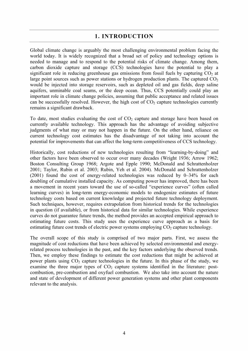
Global climate change is arguably the most challenging environmental problem facing the world today. It is widely recognized that a broad set of policy and technology options is needed to manage and to respond to the potential risks of climate change. Among them, carbon dioxide capture and storage (CCS) technologies have the potential to play a significant role in reducing greenhouse gas emissions from fossil fuels by capturing CO2 at large point sources such as power stations or hydrogen production plants. The captured CO2 would be injected into storage reservoirs, such as depleted oil and gas fields, deep saline aquifers, unminable coal seams, or the deep ocean. Thus, CCS potentially could play an important role in climate change policies, assuming that public acceptance and related issues can be successfully resolved. However, the high cost of CO2 capture technologies currently remains a significant drawback.

To date, most studies evaluating the cost of CO2 capture and storage have been based on currently available technology. This approach has the advantage of avoiding subjective judgments of what may or may not happen in the future. On the other hand, reliance on current technology cost estimates has the disadvantage of not taking into account the potential for improvements that can affect the long-term competitiveness of CCS technology.

Historically, cost reductions of new technologies resulting from “learning-by-doing” and other factors have been observed to occur over many decades (Wright 1936; Arrow 1962; Boston Consulting Group 1968; Argote and Epple 1990; McDonald and Schrattenholzer 2001; Taylor, Rubin et al. 2003; Rubin, Yeh et al. 2004). McDonald and Schrattenholzer (2001) found the cost of energy-related technologies was reduced by 0–34% for each doubling of cumulative installed capacity. As computing power has improved, there has been a movement in recent years toward the use of so-called “experience curves” (often called learning curves) in long-term energy-economic models to endogenize estimates of future technology costs based on current knowledge and projected future technology deployment. Such techniques, however, requires extrapolation from historical trends for the technologies in question (if available), or from historical data for similar technologies. While experience curves do not guarantee future trends, the method provides an accepted empirical approach to estimating future costs. This study uses the experience curve approach as a basis for estimating future cost trends of electric power systems employing CO2 capture technology.

The overall scope of this study is comprised of two major parts. First, we assess the magnitude of cost reductions that have been achieved by selected environmental and energy-related process technologies in the past, and the key factors underlying the observed trends. Then, we employ these findings to estimate the cost reductions that might be achieved at power plants using CO2 capture technologies in the future. In this phase of the study, we examine the three major types of CO2 capture systems identified in the literature: post-combustion, pre-combustion and oxyfuel combustion. We also take into account the nature and state of development of different power generation systems and other plant components relevant to the analysis.

5

2. STUDY APPROACH

This report develops historical experience curves for seven technologies relevant to power plant systems with CO2 capture. Experience curves for three selected technologies that have been studied in the past are summarized, and new experience curves are constructed for four additional technologies. Table 1 summarizes the seven technologies examined in this report and their relevance to CCS systems.

Table 1. Summary of technologies included in this study

Technology Relevance to CCS Systems Experience Curves Flue gas desulfurization (FGD) Post-combustion capture Summary of existing workSelective catalytic reduction (SCR) Post-combustion capture Summary of existing workPulverized coal (PC) boilers Oxyfuel combustion Developed in this study Gas turbine combined cycle (GTCC) Pre-combustion capture Summary of existing workLiquefied natural gas (LNG) production CO2 liquefaction Developed in this study Oxygen production Oxyfuels and pre-combustion Developed in this study Steam methane reforming (SMR) Pre-combustion Developed in this study

In Section 3 of this report we review and summarize a set of experience curves developed previously for flue gas desulfurization (FGD), selective catalytic reduction (SCR), and gas turbine combined cycle (GTCC) systems. We also present technology descriptions and results for newly-developed experience curves for pulverized coal (PC) boilers, liquefied natural gas (LNG) production systems, oxygen production systems, and steam methane reforming (SMR) technology for hydrogen production.

The analysis and discussion of each of these technologies includes the following steps:

• Determine how the installed capacity or cumulative production of each technology has changed over time. This includes a review of the historical context for how these technologies have been applied, and a description of the major driving forces (e.g., economic, technical, social, or political) for the diffusion of such technology.

• Determine how the costs of the technology (both the total capital cost and annual operating costs) have changed over time, in constant monetary values. We identify, qualitatively, technology-related and other reasons for the observed cost reductions.

• In some cases, observed cost trends showed increases rather than decreases. Such trends are documented and factors that may have caused such increases are discussed.

At the end of Section 3 we summarize and compare the learning rates for each of the technologies and the major factors affecting historical cost reductions. Then, in Section 4, the case study results are used to draw inferences for future cost trends of four power plant systems employing different types of CO2 capture options.

6

3. CASE STUDIES

The classical experience curve has been adopted in this report to characterize historical cost trends of technologies. The experience curve has the form:

Υ = ax-b (Equation 1)

where, Y is the specific cost of the xth unit; a is the direct person-hours (or cost) needed to produce the first unit; and b (b>0) is a parametric constant. The quantity 2–b is defined as the progress ratio (PR). It implies that each doubling of cumulative production results in a time or cost savings of (1 – 2–b). The latter quantity is defined as the learning rate (LR). Values of PR or LR commonly are reported in the literature as either a fraction or percentage for each doubling of cumulative production. While both measures are used in this report, greater emphasis is placed on the use of learning rates to quantify percentage cost reductions associated with a doubling of cumulative capacity.The following sections present background descriptions, study approaches and experience curve results for each of the seven technology case studies identified in Table 1.

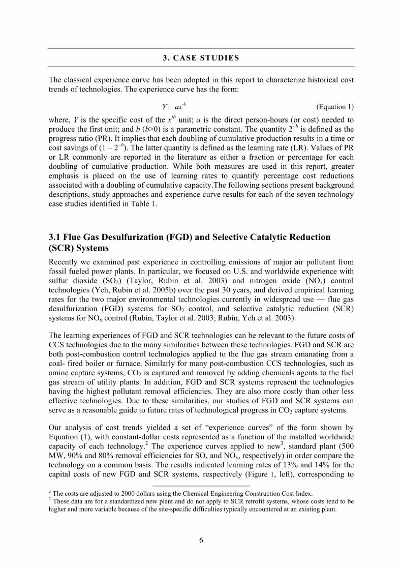
3.1 Flue Gas Desulfurization (FGD) and Selective Catalytic Reduction (SCR) Systems Recently we examined past experience in controlling emissions of major air pollutant from fossil fueled power plants. In particular, we focused on U.S. and worldwide experience with sulfur dioxide (SO2) (Taylor, Rubin et al. 2003) and nitrogen oxide (NOx) control technologies (Yeh, Rubin et al. 2005b) over the past 30 years, and derived empirical learning rates for the two major environmental technologies currently in widespread use — flue gas desulfurization (FGD) systems for SO2 control, and selective catalytic reduction (SCR) systems for NOx control (Rubin, Taylor et al. 2003; Rubin, Yeh et al. 2003).

The learning experiences of FGD and SCR technologies can be relevant to the future costs of CCS technologies due to the many similarities between these technologies. FGD and SCR are both post-combustion control technologies applied to the flue gas stream emanating from a coal- fired boiler or furnace. Similarly for many post-combustion CCS technologies, such as amine capture systems, CO2 is captured and removed by adding chemicals agents to the fuel gas stream of utility plants. In addition, FGD and SCR systems represent the technologies having the highest pollutant removal efficiencies. They are also more costly than other less effective technologies. Due to these similarities, our studies of FGD and SCR systems can serve as a reasonable guide to future rates of technological progress in CO2 capture systems.

Our analysis of cost trends yielded a set of “experience curves” of the form shown by Equation (1), with constant-dollar costs represented as a function of the installed worldwide capacity of each technology.2 The experience curves applied to new3, standard plant (500 MW, 90% and 80% removal efficiencies for SOx and NOx, respectively) in order compare the technology on a common basis. The results indicated learning rates of 13% and 14% for the capital costs of new FGD and SCR systems, respectively (Figure 1, left), corresponding to

2 The costs are adjusted to 2000 dollars using the Chemical Engineering Construction Cost Index. 3 These data are for a standardized new plant and do not apply to SCR retrofit systems, whose costs tend to be higher and more variable because of the site-specific difficulties typically encountered at an existing plant.

7

progress ratios of 0.87 and 0.86. These values were well within the range of learning rates found in the literature for a wide range of market-based technologies (Dutton and Thomas 1984), as well as a range of energy technologies (McDonald and Schrattenholzer 2001). Operating and maintenance (O&M) costs for FGD and SCR systems also declined significantly over the study period, with estimated learning rates of 23% for FGD systems and 42% for SCR systems (Figure 1). The observed steep reduction of SCR O&M cost is due to the facts of rapid catalyst price reductions and longer catalyst life that significantly reduced the variable O&M cost. In the U.S., historical catalyst prices dropped more than 70% in a 13-year period (1987-2000), while the expected catalyst lifetime has increased more than 5-fold in the same period (Yeh, Rubin et al. 2005b).

10%

100%

1 10 100 1000Worldwide Installed Capacity at Coal-Fired

Utility Plant (GWe)

Nor

mal

ized

Cap

ital C

os SCRy = 1.41x-0.22

PR = 0.86 FGDy = 1.60x-0.20

PR= 0.87

FGDy = 4.00x-0.37

PR = 0.77SCRy = 3.57x-0.79

PR = 0.58

1%

10%

100%

1 10 100 1000Worldwide Installed Capacity at Coal-Fired

Utility Plant (GWe)

Nor

mal

ized

O&

M C

osts

Figure 1. Capital and O&M costs experience curves for SCR and FGD systems for a standard new coal-fired power plant. 4

It is not clear whether the classic log-linear experience curve (as depicted in Equation 1) represents most accurately the cost improvements of a wide range of technologies. Historically, a number of authors have suggested alternative formulations of the learning curve based on empirical observations, especially deviations from log-linearity at the beginning and tail of the curve (Asher 1956; Conway and Schultz 1959; Boston Consulting Group 1968; Klepper and Graddy 1990). More often, when price is used as a surrogate for the manufactured cost of the technology or product (which is commonly the case, since only price data are usually available), structural changes and competition in the marketplace often lead to experience curves that deviate from log-linearity. The Boston Consulting Group (1968) proposed an S-shape experience curve based on the observed average unit price and cumulative industry output of 24 selected products. They hypothesized that at the development stage prices are set below cost to establish an initial market. As sales volume and experience reduce costs, these prices are maintained, gradually converting the negative margin to a positive one. However, if prices do not eventually decline as fast as costs, competitors are attracted to the market. Thus, at some point prices begin to decline faster than

4 For FGD system, a standard plant is sized 500 MWe, burning 3.5% sulfur coal, and achieve 90% SO2 removal efficiency. For SCR system, a standard plant is sized 500 MWe, burning medium sulfur coal, and achieving 80% NOx removal. For studies that used slightly different assumptions, a computer model (the Integrated Environmental Control Model or IECM) was used to adjust key design parameters to a consistent basis.

8

costs. Later, a reverse bend in the price curve is reached when the market become mature, and subsequently prices and costs change at the same rate.

In our study of FGD and SCR technologies, we also found that experience curves with initial concavity best fit the data for the two widely used environmental control technologies (Figure 2). In the case of FGD, the low initial learning rates resulted in part from the rapid and widespread deployment of “first-generation” technology in response to environmental regulatory requirements, with little time for learning. This was followed by improvements in succeeding generations of the technology based on factors including continued R&D and experience with the initial (and subsequent) installations.

10%

100%

1 10 100 1000

Worldwide Capacity of Wet FGD Systems (GWe)

Nor

mal

ized

FG

D C

apita

l Cos

t

19761980

1990

1995

1982

10%

100%

1 10 100Worldwide Capacity of SCR Systems

(GWe)

Nor

mal

ized

SC

R C

apita

l Cos

t

92.0,177.0,

2/

2

=−=

==

RaeyRaxy

xb

b

1983 1989

19931995

1996

2000

Figure 2. Concave versus log-linear (Equation 1) learning curves fitted to the capital costs of new FGD and SCR systems at U.S. coal-fired utility plants.

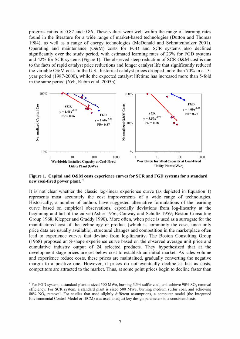
Given the interest in applying case study results such as those above to future power plants with CO2 capture, we also examined cost estimates of FGD and SCR technologies prior to and at the early stages of commercial application. This examination revealed significant increases in the capital cost of both systems during the early stages of commercial. The results are shown in Figure 3 and Figure 4.

For many advanced and complex technologies, especially large-scale technologies such as power plants and their environmental control systems, early cost estimates based on laboratory-scale projects and pilot plants are typically lower (more optimistic) than the actual costs subsequently realized for the initial set of full-scale commercial plants. Thus, costs often increase rather than decrease in the early phase of commercial deployment. The reasons for such increases are typically linked to shortfalls in performance and/or reliability that result from insufficient data or experience for scale-up and detailed design, or from new problems that arise during full-scale construction and operation. Although this phenomenon has been long recognized and often described qualitatively (Merrow, McDonnell et al. 1988), there are relatively few empirical studies that document such trends for energy and environmental technologies. One recent study, however (Claeson Colpier and Cornland 2002), reported a progress ratio (PR) above 100 percent for an experience curve for natural gas combined cycle (NGCC) systems in the period 1981-1991. This was followed by subsequent cost declines. Studies of British and Germany wind power (Ibenholt 2002) and photovoltaic (PV) technologies (Schaeffer 2003) also found progress ratios above 100

9

percent at the initial stages of deployment. Though no explanations were provided in the original studies, these rises were likely due to the general observation that the total cost of new technology cannot be reduced as quickly as costs are added through design changes and product performance improvements in the early stages of commercialization (Neij 1997).

For FGD system, cost estimates of the late 1960s proved to be considerably lower than actual costs due to the optimistic view of vendors and analysts that system unknowns would be controlled, and that inexpensive materials of construction could be utilized (Skopp 1969; The M.W. Kellogg Company 1971). In particular, early cost evaluation involved many design assumptions since technical data were limited. Equipment costs were sketchy, and very little corrosion data were available to properly select materials of construction for the service involved. In many cases, the “technological optimism” of process developers tended to maximize process potential and minimize problem areas such as corrosion, scaling, solids disposal, sulfite oxidation, mist elimination, gas reheat, operational turndown, and pH control. Cost estimates were also subject to further uncertainties in scale-up factors based on experimental and prototype installations. As a consequence, as time passed, and the results of pilot-plant and early installations became known, the magnitude of cost estimates was scaled up considerably (Spaite 1972; Battelle 1973).

196819721974

1975

19761980

1982

1990

1995

0

50

100

150

200

250

300

0 10 20 30 40 50 60 70 80 90 100Cumulative World Wet FGD Installed

Capacity (GW)

Cap

ital C

osts

($/k

W) i

n 19

97$

(1000 MW, eff =80-90%)

(200 MW, eff =87%) 1972

1975

1976

19801990

1995

1968

1974

1982

0

1

2

3

4

5

6

7

8

0 10 20 30 40 50 60 70 80 90 100Cumulative World Wet FGD Installed

Capacity (GW)

O&

M C

osts

(199

7$/M

Wh)

(1000 MW, eff =80-90%)

(200 MW, eff =87%)

Figure 3. Capital and O&M cost trends of wet limestone FGD systems at a standard new coal-fired power plant,5 including studies conducted during the period of early commercial application.

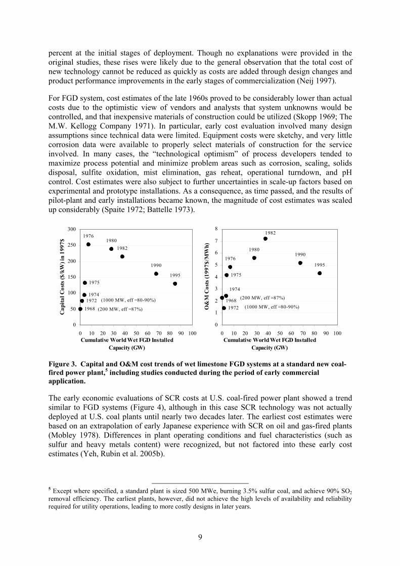
The early economic evaluations of SCR costs at U.S. coal-fired power plant showed a trend similar to FGD systems (Figure 4), although in this case SCR technology was not actually deployed at U.S. coal plants until nearly two decades later. The earliest cost estimates were based on an extrapolation of early Japanese experience with SCR on oil and gas-fired plants (Mobley 1978). Differences in plant operating conditions and fuel characteristics (such as sulfur and heavy metals content) were recognized, but not factored into these early cost estimates (Yeh, Rubin et al. 2005b).

5 Except where specified, a standard plant is sized 500 MWe, burning 3.5% sulfur coal, and achieve 90% SO2 removal efficiency. The earliest plants, however, did not achieve the high levels of availability and reliability required for utility operations, leading to more costly designs in later years.

10

1983

1989

1993

1995 2000

-20 -10 0 10 20 30 40 50 60 70 80

Cumulative World SCR Installed Capacity (GW)

SCR

Cap

ital C

osts

($/k

W),

1997

$ First Japan commercial installation on a coal-fired power plant

← First German commercial installation

↓ First US commercial installation

←

40

50

60

70

80

90

100

110

120

1977

1978

1979

1980

1980

1982

1982

1983

1989

1993

1995 20001996

-20 -10 0 10 20 30 40 50 60 70 80Cumulative World SCR Installed Capacity (GW)

SCR

Lev

eliz

ed C

osts

($/k

W),

1997

$

← First Japan coal plant

← First German coal plant

← First US coal plant

0

2

4

6

8

10

12

14

16

18

20

1977

1978

1979

SCR

Lev

eliz

ed C

osts

(199

7$ M

ills/k

Wh)

Figure 4. Capital and levelized 6 costs of a SCR system for a standard new coal-fired power plant. (The x-axis to the right of zero represents worldwide cumulative installed capacity, while the x-axis to the left of zero represents the date of studies prior to commercial installation. Diamond dots are studies based on low-sulfur coal plants, which have lower SCR capital cost. Open circles are studies evaluated prior to commercial SCR installations at coal-fired plants.)

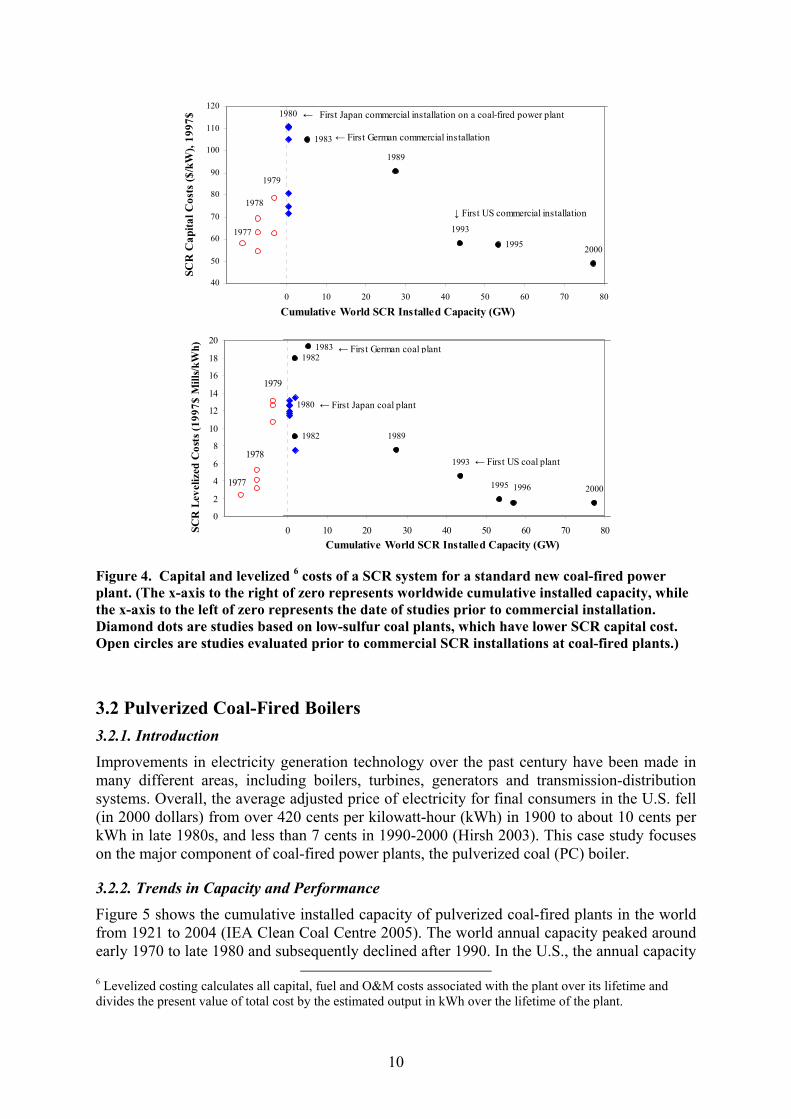
3.2 Pulverized Coal-Fired Boilers 3.2.1. Introduction Improvements in electricity generation technology over the past century have been made in many different areas, including boilers, turbines, generators and transmission-distribution systems. Overall, the average adjusted price of electricity for final consumers in the U.S. fell (in 2000 dollars) from over 420 cents per kilowatt-hour (kWh) in 1900 to about 10 cents per kWh in late 1980s, and less than 7 cents in 1990-2000 (Hirsh 2003). This case study focuses on the major component of coal-fired power plants, the pulverized coal (PC) boiler.

3.2.2. Trends in Capacity and Performance

Figure 5 shows the cumulative installed capacity of pulverized coal-fired plants in the world from 1921 to 2004 (IEA Clean Coal Centre 2005). The world annual capacity peaked around early 1970 to late 1980 and subsequently declined after 1990. In the U.S., the annual capacity

6 Levelized costing calculates all capital, fuel and O&M costs associated with the plant over its lifetime and divides the present value of total cost by the estimated output in kWh over the lifetime of the plant.

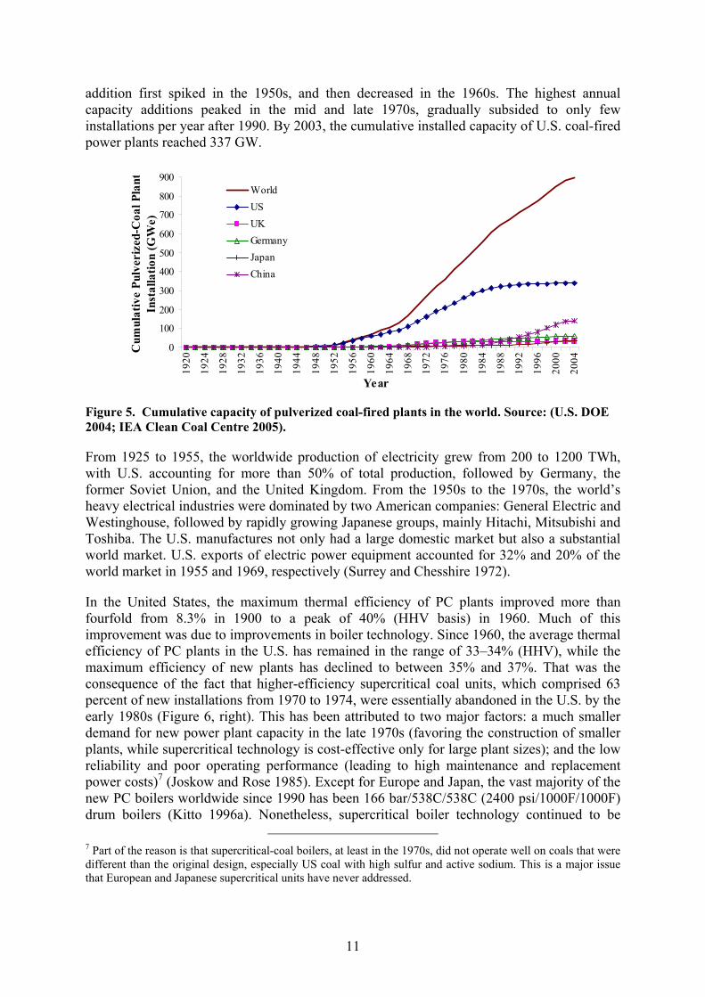
11

addition first spiked in the 1950s, and then decreased in the 1960s. The highest annual capacity additions peaked in the mid and late 1970s, gradually subsided to only few installations per year after 1990. By 2003, the cumulative installed capacity of U.S. coal-fired power plants reached 337 GW.

0

100

200

300

400

500

600

700

800

90019

20

1924

1928

1932

1936

1940

1944

1948

1952

1956

1960

1964

1968

1972

1976

1980

1984

1988

1992

1996

2000

2004

Year

Cum

ulat

ive

Pulv

eriz

ed-C

oal P

lant

Inst

alla

tion

(GW

e)

WorldUSUKGermanyJapanChina

Figure 5. Cumulative capacity of pulverized coal-fired plants in the world. Source: (U.S. DOE 2004; IEA Clean Coal Centre 2005).

From 1925 to 1955, the worldwide production of electricity grew from 200 to 1200 TWh, with U.S. accounting for more than 50% of total production, followed by Germany, the former Soviet Union, and the United Kingdom. From the 1950s to the 1970s, the world’s heavy electrical industries were dominated by two American companies: General Electric and Westinghouse, followed by rapidly growing Japanese groups, mainly Hitachi, Mitsubishi and Toshiba. The U.S. manufactures not only had a large domestic market but also a substantial world market. U.S. exports of electric power equipment accounted for 32% and 20% of the world market in 1955 and 1969, respectively (Surrey and Chesshire 1972).

In the United States, the maximum thermal efficiency of PC plants improved more than fourfold from 8.3% in 1900 to a peak of 40% (HHV basis) in 1960. Much of this improvement was due to improvements in boiler technology. Since 1960, the average thermal efficiency of PC plants in the U.S. has remained in the range of 33–34% (HHV), while the maximum efficiency of new plants has declined to between 35% and 37%. That was the consequence of the fact that higher-efficiency supercritical coal units, which comprised 63 percent of new installations from 1970 to 1974, were essentially abandoned in the U.S. by the early 1980s (Figure 6, right). This has been attributed to two major factors: a much smaller demand for new power plant capacity in the late 1970s (favoring the construction of smaller plants, while supercritical technology is cost-effective only for large plant sizes); and the low reliability and poor operating performance (leading to high maintenance and replacement power costs)7 (Joskow and Rose 1985). Except for Europe and Japan, the vast majority of the new PC boilers worldwide since 1990 has been 166 bar/538C/538C (2400 psi/1000F/1000F) drum boilers (Kitto 1996a). Nonetheless, supercritical boiler technology continued to be

7 Part of the reason is that supercritical-coal boilers, at least in the 1970s, did not operate well on coals that were different than the original design, especially US coal with high sulfur and active sodium. This is a major issue that European and Japanese supercritical units have never addressed.

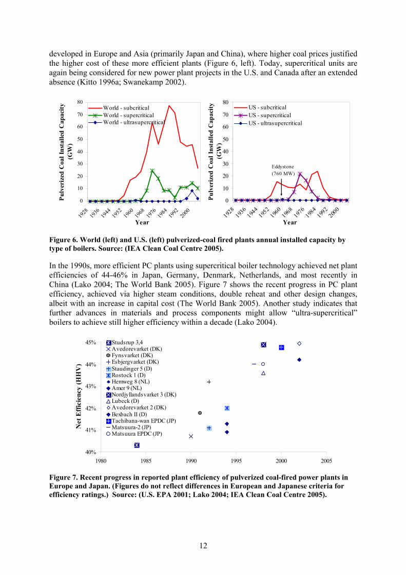
12

developed in Europe and Asia (primarily Japan and China), where higher coal prices justified the higher cost of these more efficient plants (Figure 6, left). Today, supercritical units are again being considered for new power plant projects in the U.S. and Canada after an extended absence (Kitto 1996a; Swanekamp 2002).

0

10

20

30

40

50

60

70

80

1928

1936

1944

1952

1960

1968

1976

1984

1992

2000

Year

Pulv

eriz

ed C

oal I

nsta

lled

Cap

acity

(G

W)

World - subcriticalWorld - supercriticalWorld - ultrasupercritical

0

10

20

30

40

50

60

70

80

1928

1936

1944

1952

1960

1968

1976

1984

1992

2000

Year

Pulv

eriz

ed C

oal I

nsta

lled

Cap

acity

(G

W)

US - subcriticalUS - supercriticalUS - ultrasupercritical

Eddystone(760 MW)

Figure 6. World (left) and U.S. (left) pulverized-coal fired plants annual installed capacity by type of boilers. Source: (IEA Clean Coal Centre 2005).

In the 1990s, more efficient PC plants using supercritical boiler technology achieved net plant efficiencies of 44-46% in Japan, Germany, Denmark, Netherlands, and most recently in China (Lako 2004; The World Bank 2005). Figure 7 shows the recent progress in PC plant efficiency, achieved via higher steam conditions, double reheat and other design changes, albeit with an increase in capital cost (The World Bank 2005). Another study indicates that further advances in materials and process components might allow “ultra-supercritical” boilers to achieve still higher efficiency within a decade (Lako 2004).

40%

41%

42%

43%

44%

45%

1980 1985 1990 1995 2000 2005

Net

Eff

icie

ncy

(HH

V)

Studsrup 3,4Avedorevarket (DK)Fynsvarket (DK)Esbjergvarket (DK)Staudinger 5 (D)Rostock 1 (D)Hemweg 8 (NL)Amer 9 (NL)Nordjyllandsvarket 3 (DK)Lubeck (D)Avedorevarket 2 (DK)Bexbach II (D)Tachibana-wan EPDC (JP)Matsuura-2 (JP)Matsuura EPDC (JP)

Figure 7. Recent progress in reported plant efficiency of pulverized coal-fired power plants in Europe and Japan. (Figures do not reflect differences in European and Japanese criteria for efficiency ratings.) Source: (U.S. EPA 2001; Lako 2004; IEA Clean Coal Centre 2005).

13

Experience Curves of Coal-Fired Plant Thermal Efficiency

A log-linear experience curve is fitted to the maximum thermal efficiency of U.S. PC plants between 1920 and 1985, and international PC plants between 1985 and 2005 (Figure 8). The data suggest a progress ratio of 103.5% from 1920 to 1972,8 i.e., thermal efficiency increases by 3.5% for every doubling of world cumulative installed capacity. The plateau of thermal efficiency in the U.S. after the 1970s also is apparent in this graph.9 However, more recent technology improvement, mainly supercritical and ultra-supercritical boilers in the European countries and Japan, has overcame the plateau and extended the learning curve to a higher level. A discontinuity in the experience curve is evident from Figure 8 due to technology structural change that shifts from subcritical technology to supercritical boiler technology. While the efficiency shown here applies to the overall plant, the improvement in boiler technologies accounts for the majority of progress.

y = 0.31x0.05

PR = 1.035

10%

100%

0 1 10 100 1,000World Cumulative Coal-Fired Utility Plant Installed Capacity (GW)

The

rmal

Eff

icie

ncy

(%)

US PlantsWorld Plants

1920

1985

2002

1972

Figure 8. Thermal efficiency as a function of world cumulative coal-fired utility plant installed capacity, 1920-2002. Source: (Kaneko, Wakazono et al. 2001; U.S. EPA 2001; Hirsh 2003; Lako 2004; PowerClean R D&D Thematic Network 2004)

Trends for Total Coal-Fired Plant Construction Cost

Joskow and Rose (1985) and a series of government reports, e.g., Energy Information Administration (1978) and Utility Data Institute (1993), compared U.S. coal–burning power plants historical construction cost and found that the real cost per kilowatt for constructing a power plant in the U.S. continued to decline during the early and mid-1960s, then stabilized in the late 1960s, and climbed substantially during the 1970s and 1980s. Their study controlled for scale effects, technological differences, input price changes, major environmental control technologies and other cross-sectional differences in real costs. Real construction costs increases were primarily due to new regulatory requirements such as environmental, health and safety standards, changes in work rules, improved design

8 The progress ratio remain the same (PR=1.035) when an experience curve is fitted to the data between 1920 to 2002. 9 Note that the progress ratio of PC plant thermal efficiency is not the only measure for technological improvement. The thermal efficiency of a PC plant, especially after 1970, is balanced between the economics of capital cost and fuel cost. However, the technology plateau between 1970 and 1990 suggests that the industry was not able to continuously improve the technology enough to produce more energy with less fuel while keeping the technology capital cost at the same level, as they did in 1920 − 1960.

14

standards, and increased labor costs as well as increased construction times and a decline in construction productivity. Nonetheless, the study by Joskow and Rose (1985) found significant learning effects in architect-engineering experience and utility experience for both subcritical and supercritical plants.

This study only examined the construction cost of the overall plants, which is subject to many factors not related to technological learning as we described above. In the next section, we will examine the cost trends for PC boilers alone, and estimate the associated experience curves for PC boiler capital and O&M costs.

3.2.3. Technological Progress of Coal-fired Boilers Prior to the 1940’s, major advances in boiler design came from increased steam pressure and temperature. The use of pulverized coal (grinding coal into fine powder rather than chunks of coal) increased the surface area of the fuel significantly, thus aiding the combustion. In addition, stronger metals (such as, “superalloy” steels) and other technology improvements allowed boilers to withstand higher temperature and pressures, yielding improvement in overall plant efficiency (Hirsh 2003). This increase in thermal efficiency allowed utilities to produce more energy with less fuel, thereby reducing capital and O&M costs per unit of product. The following sub-sections elaborate on some of the technology advancement of PC boilers.

Boiler Size

The principal factor in rapid unit cost reduction of a new generating plant has been attributed to economies of scale in all power plant components (Sporn 1968a; Surrey and Chesshire 1972; Joskow and Rose 1985; Hirsh 2003), including the generator, turbine and boiler. In the early 1900s, according to Hirsh (2003), large (50 MW) plants that housed five 10,000 kW steam turbines commonly required fifty or sixty boilers to power the turbines. By the 1920s, several boilers still served one or two steam turbines. The introduction of pulverized coal and continuous improvements in boiler design to raise steam temperatures contributed to increased boiler outputs that reduced the number of boilers per plant. The development of single-boiler, single-turbine systems contributed to faster improvements in thermal efficiency and cost reductions. Figure 9 shows the maximum steam flow of boilers increased 25-fold in 32 years, from 182 tonnes/hr (400,000 lbs/hr) in 1940 to 4545 tonnes/hr (10 million lbs/hr) in 1972.

Steam Temperature and Pressure

Advancement in steam temperature and steam pressure has been the major contributing factor for PC plant efficiency improvement. The maximum steam temperature and pressure of PC boilers increased from about 260°C (500°F) and 7 bar (100 psi) in 1900 to about 593°C (1100°F) and more than 275 bar (4000 psi) in the 1950s (Hirsh 2003) (Figure 10). The utility industry move toward higher capacity units in the early 1960s was accompanied by widespread adoption of the 242 bar (3500 psi) cycle for supercritical boilers. Of the nearly 11,000 MW in large units committed by U.S. utilities in 1962 and 1963, 70% were designed for supercritical steam pressure, with either single or double reheat (Sporn 1968) (Figure 6).

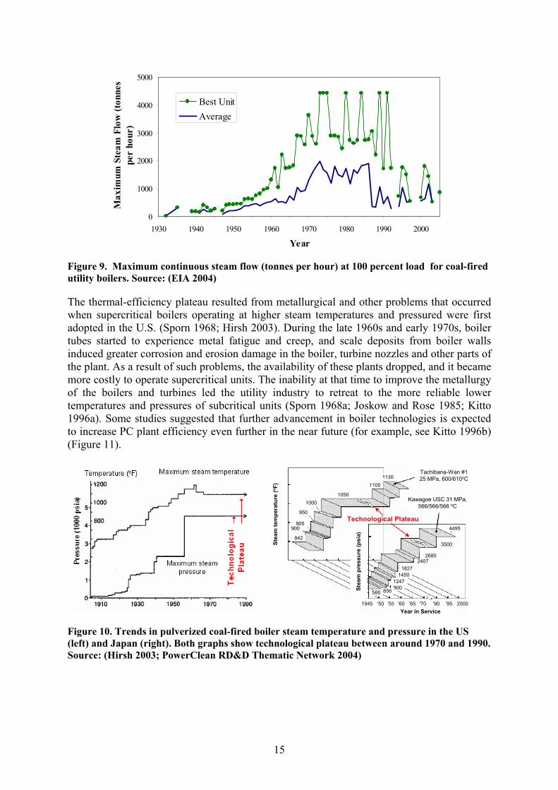
15

0

1000

2000

3000

4000

5000

1930 1940 1950 1960 1970 1980 1990 2000

Year

Max

imum

Ste

am F

low

(ton

nes

per

hour

)

Best UnitAverage

Figure 9. Maximum continuous steam flow (tonnes per hour) at 100 percent load for coal-fired utility boilers. Source: (EIA 2004)

The thermal-efficiency plateau resulted from metallurgical and other problems that occurred when supercritical boilers operating at higher steam temperatures and pressured were first adopted in the U.S. (Sporn 1968; Hirsh 2003). During the late 1960s and early 1970s, boiler tubes started to experience metal fatigue and creep, and scale deposits from boiler walls induced greater corrosion and erosion damage in the boiler, turbine nozzles and other parts of the plant. As a result of such problems, the availability of these plants dropped, and it became more costly to operate supercritical units. The inability at that time to improve the metallurgy of the boilers and turbines led the utility industry to retreat to the more reliable lower temperatures and pressures of subcritical units (Sporn 1968a; Joskow and Rose 1985; Kitto 1996a). Some studies suggested that further advancement in boiler technologies is expected to increase PC plant efficiency even further in the near future (for example, see Kitto 1996b) (Figure 11).

Stea

m te

mpe

ratu

re (o F

)

Stea

m p

ress

ure

(psi

a)

Kawagoe USC 31 MPa,566/566/566 oC

Tachibana-Wan #125 MPa, 600/610oC1130

1100

10501000

950

905900

842

4495

3500

26802407

18271450

1247900

566 856

1945 '50 '55 '60 '65 '70 '90 '95 2000Year in Service

Technological Plateau

Figure 10. Trends in pulverized coal-fired boiler steam temperature and pressure in the US (left) and Japan (right). Both graphs show technological plateau between around 1970 and 1990. Source: (Hirsh 2003; PowerClean RD&D Thematic Network 2004)

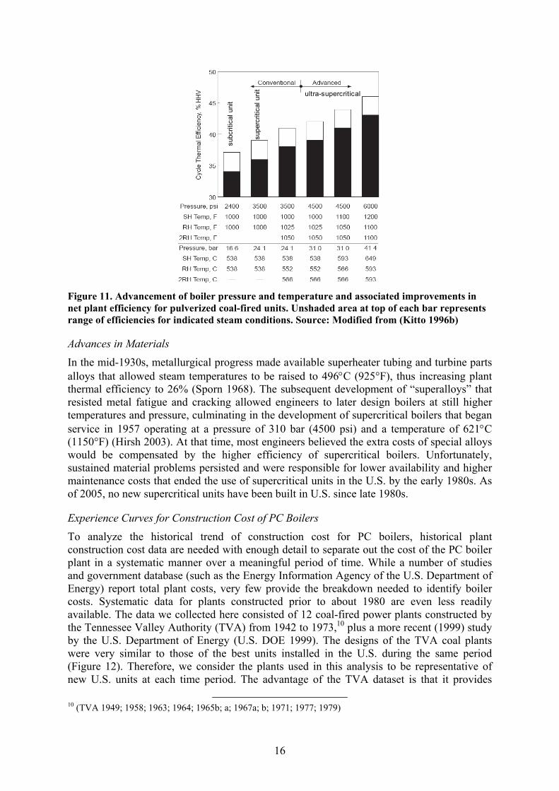
16

subc

ritic

al u

nit

supe

rcrit

ical

uni

t

ultra-supercritical

Figure 11. Advancement of boiler pressure and temperature and associated improvements in net plant efficiency for pulverized coal-fired units. Unshaded area at top of each bar represents range of efficiencies for indicated steam conditions. Source: Modified from (Kitto 1996b)

Advances in Materials

In the mid-1930s, metallurgical progress made available superheater tubing and turbine parts alloys that allowed steam temperatures to be raised to 496°C (925°F), thus increasing plant thermal efficiency to 26% (Sporn 1968). The subsequent development of “superalloys” that resisted metal fatigue and cracking allowed engineers to later design boilers at still higher temperatures and pressure, culminating in the development of supercritical boilers that began service in 1957 operating at a pressure of 310 bar (4500 psi) and a temperature of 621°C (1150°F) (Hirsh 2003). At that time, most engineers believed the extra costs of special alloys would be compensated by the higher efficiency of supercritical boilers. Unfortunately, sustained material problems persisted and were responsible for lower availability and higher maintenance costs that ended the use of supercritical units in the U.S. by the early 1980s. As of 2005, no new supercritical units have been built in U.S. since late 1980s.

Experience Curves for Construction Cost of PC Boilers

To analyze the historical trend of construction cost for PC boilers, historical plant construction cost data are needed with enough detail to separate out the cost of the PC boiler plant in a systematic manner over a meaningful period of time. While a number of studies and government database (such as the Energy Information Agency of the U.S. Department of Energy) report total plant costs, very few provide the breakdown needed to identify boiler costs. Systematic data for plants constructed prior to about 1980 are even less readily available. The data we collected here consisted of 12 coal-fired power plants constructed by the Tennessee Valley Authority (TVA) from 1942 to 1973,10 plus a more recent (1999) study by the U.S. Department of Energy (U.S. DOE 1999). The designs of the TVA coal plants were very similar to those of the best units installed in the U.S. during the same period (Figure 12). Therefore, we consider the plants used in this analysis to be representative of new U.S. units at each time period. The advantage of the TVA dataset is that it provides

10 (TVA 1949; 1958; 1963; 1964; 1965b; a; 1967a; b; 1971; 1977; 1979)

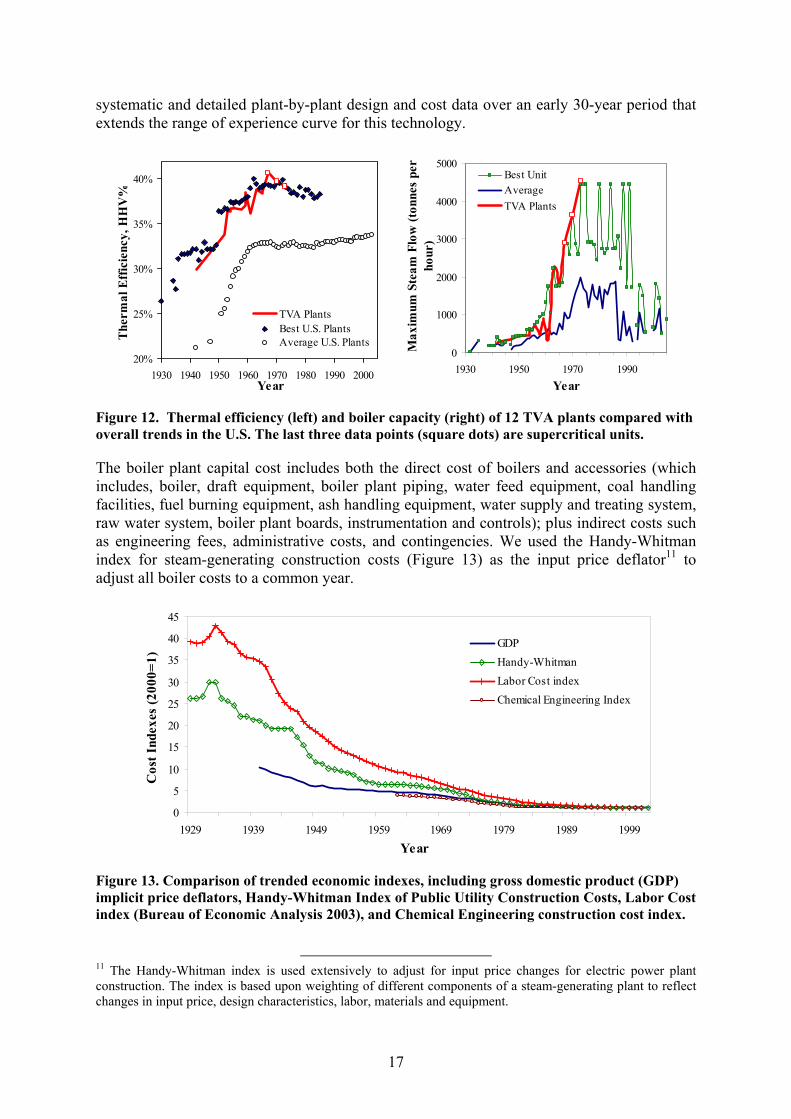
17

systematic and detailed plant-by-plant design and cost data over an early 30-year period that extends the range of experience curve for this technology.

20%

25%

30%

35%

40%

1930 1940 1950 1960 1970 1980 1990 2000Year

The

rmal

Eff

icie

ncy,

HH

V%

TVA PlantsBest U.S. PlantsAverage U.S. Plants

0

1000

2000

3000

4000

5000

1930 1950 1970 1990Year

Max

imum

Ste

am F

low

(ton

nes

per

hour

)

Best UnitAverageTVA Plants

Figure 12. Thermal efficiency (left) and boiler capacity (right) of 12 TVA plants compared with overall trends in the U.S. The last three data points (square dots) are supercritical units.

The boiler plant capital cost includes both the direct cost of boilers and accessories (which includes, boiler, draft equipment, boiler plant piping, water feed equipment, coal handling facilities, fuel burning equipment, ash handling equipment, water supply and treating system, raw water system, boiler plant boards, instrumentation and controls); plus indirect costs such as engineering fees, administrative costs, and contingencies. We used the Handy-Whitman index for steam-generating construction costs (Figure 13) as the input price deflator11 to adjust all boiler costs to a common year.

0

5

10

15

20

25

30

35

40

45

1929 1939 1949 1959 1969 1979 1989 1999Year

Cos

t Ind

exes

(200

0=1)

GDPHandy-WhitmanLabor Cost indexChemical Engineering Index

Figure 13. Comparison of trended economic indexes, including gross domestic product (GDP) implicit price deflators, Handy-Whitman Index of Public Utility Construction Costs, Labor Cost index (Bureau of Economic Analysis 2003), and Chemical Engineering construction cost index.

11 The Handy-Whitman index is used extensively to adjust for input price changes for electric power plant construction. The index is based upon weighting of different components of a steam-generating plant to reflect changes in input price, design characteristics, labor, materials and equipment.

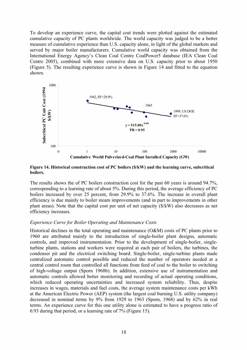
18

To develop an experience curve, the capital cost trends were plotted against the estimated cumulative capacity of PC plants worldwide. The world capacity was judged to be a better measure of cumulative experience than U.S. capacity alone, in light of the global markets and served by major boiler manufacturers. Cumulative world capacity was obtained from the International Energy Agency’s Clean Coal Centre CoalPower5 database (IEA Clean Coal Centre 2005), combined with more extensive data on U.S. capacity prior to about 1950 (Figure 5). The resulting experience curve is shown in Figure 14 and fitted to the equation shown.

y = 515.00x-0.08

PR = 0.95

100

1000

0 1 10 100 1000 10000Cumulative World Pulverized-Coal Plant Installed Capacity (GW)

Subc

ritic

al P

C U

nit C

ost (

1994

$/

kW)

1942, EF=29.9%

19651999, US DOEEF=37.6%

Figure 14. Historical construction cost of PC boilers ($/kW) and the learning curve, subcritical boilers.

The results shows the of PC boilers construction cost for the past 60 years is around 94.7%, corresponding to a learning rate of about 5%. During this period, the average efficiency of PC boilers increased by over 25 percent, from 29.9% to 37.6%. The increase in overall plant efficiency is due mainly to boiler steam improvements (and in part to improvements in other plant areas). Note that the capital cost per unit of net capacity ($/kW) also decreases as net efficiency increases.

Experience Curve for Boiler Operating and Maintenance Costs

Historical declines in the total operating and maintenance (O&M) costs of PC plants prior to 1960 are attributed mainly to the introduction of single-boiler plant designs, automatic controls, and improved instrumentation. Prior to the development of single-boiler, single-turbine plants, stations and workers were required at each pair of boilers, the turbines, the condenser pit and the electrical switching board. Single-boiler, single-turbine plants made centralized automatic control possible and reduced the number of operators needed at a central control room that controlled all functions from feed of coal to the boiler to switching of high-voltage output (Sporn 1968b). In addition, extensive use of instrumentation and automatic controls allowed better monitoring and recording of actual operating conditions, which reduced operating uncertainties and increased system reliability. Thus, despite increases in wages, materials and fuel costs, the average system maintenance costs per kWh at the American Electric Power (AEP) system (the largest coal burning U.S. utility company) decreased in nominal terms by 9% from 1929 to 1963 (Sporn, 1968) and by 62% in real terms. An experience curve for this one utility alone is estimated to have a progress ratio of 0.93 during that period, or a learning rate of 7% (Figure 15).

19

y = 75.39x-0.11

PR = 0.93

10

100

0 1 10 100World Cumulative Coal-Fired Utility Plant Installed Capacity (GW)

AE

P Sy

stem

, Per

cent

age

of 1

929

Ave

rage

1929

1958

Figure 15. Experience curve of adjusted O&M costs for average AEP systems, 1929-1958.

A study by the U.S. Energy Information Administration (EIA) also found that the total number of operating and maintenance employees for the average large plant has decreased significantly during 1920-1970. It was found that a new large coal-burning plant in the late 1970s required only one-fifth as many employees per megawatt of capacity as did the large coal-burning plants built during the period 1920 to about 1950 (EIA 1978).

Between 1980 and 2000, U.S. electricity markets underwent significant transformations from integrated power companies (controlling generation, transmission and distribution) to a more competitive and disaggregated market. Evidence suggests that power plant operators were under increasing pressure to reduce O&M costs. A report by the Energy Information Administration (EIA) examined changes in the operating cost of U.S. fossil-steam power plants form 1981 to 1997 and found that the non-fuel O&M costs12 per kWh for coal plants fell by 32 percent at existing plants (Beamon and Leckey 1999). In 1981 an average 300 MW coal plant had 75 employees. By 1997 the average had fallen to 53, a decline of 32% (Beamon and Leckey 1999)13. Increased plant utilization (a 20% increase from 51% to 61% over the period of 1981-1997) also contributes to O&M cost reductions between 1981 and 1997. This was largely due to increased competition after deregulation to reduce per kilowatt-hour O&M costs. Overall, boiler operation and maintenance accounted for over 74% of non-fuel O&M cost reductions between 1981-1997 (Beamon and Leckey 1999). An experience curve is fitted to both the plant O&M costs and boiler O&M costs14 between 1981-1997 based on the data in the Beamon and Leckey (1999) study (Figure 16). The O&M costs are adjusted to the same capacity factor of 51% since cost reduction due to increased utilization

12 Non-fuel operation and maintenance cost includes labor, plant operating supplies (including lubricants, chemicals, other miscellaneous materials, office and other incidental expenses), and maintenance renewal parts and material (EIA 1978). 13 Sources of Beamon and Leckey (1999) include FERC Form 1, “Annual Report of Major Electric Utilities, Licensees and Others,” and Form EIA-412, “Annual Report of Public Electric Utilities” (1981-1997). 14 It was difficult to judge from the report the definitions of the reported categories. Thus, we define non-fuel boiler O&M cost includes the maintenance of boiler plants, steam expenses, and miscellaneous steam power expenses. The overall plant non-fuel O&M cost includes boiler O&M plus operation supervision and engineering, coolants and water, steam from other sources, steam transferred, electric expenses, maintenance supervision and engineering, maintenance of structure, maintenance of electric plant, and maintenance of miscellaneous team plant.

20

is not related to technological change. The progress ratio of the PC boilers O&M costs is estimated to be 70% according to data reported in Beamon and Leckey (1999), corresponding to a learning rate of 30%. This is significantly higher than the rate shown earlier for the AEP dataset for plants operating from 1929–1963 (Figure 15).

y = 95.33x-0.51

PR = 0.70

y = 84.92x-0.42

PR = 0.75

1

10

100 1,000

World Cumulative Pulverized Coal Plant Installed Capacity (GW)

Non

-Fue

l O&

M C

ost (

2000

M

ills/

kWh)

Non-fuel Boiler O&M costs includes the maintenance of boiler plant, steam expenses, and miscellaneous steam power expenses.

Boiler O&M

Plant O&M

Figure 16. Learning curves of coal steam plant O&M costs and boiler O&M costs, 1981-1997. Source: Modified from Beamon and Leckey (1999).

3.3 Gas Turbine Combined Cycle (GTCC) Systems 3.3.1. Introduction Gas turbine combined cycle (GTCC) power systems play a critical role in the economics of CO2 capture and storage through their influence on the type of fuel used for power generation, and the specific emission rate per kilowatt-hour of electricity generated. GTCC units may be fueled directly by natural gas (with the option of post-combustion CO2 capture), or they may part of an IGCC system fueled by syngas or hydrogen (with the option of pre-combustion CO2 capture).

The GTCC system is composed mainly of three parts: gas turbine generator, heat recovery steam generator (HRSG), and steam turbine generator. The exhaust gas from the gas turbine is captured by the HRSG for steam production to supply a steam turbine (Figure 17). While the HRSG and steam turbine generator are relatively mature technologies, the commercial development of combined-cycle systems has proceeded in parallel with gas turbine development (Chase 2001).

Table 2 and Figure 18 summarize the evolution of GTCC systems since their first commercial application for electric generation.

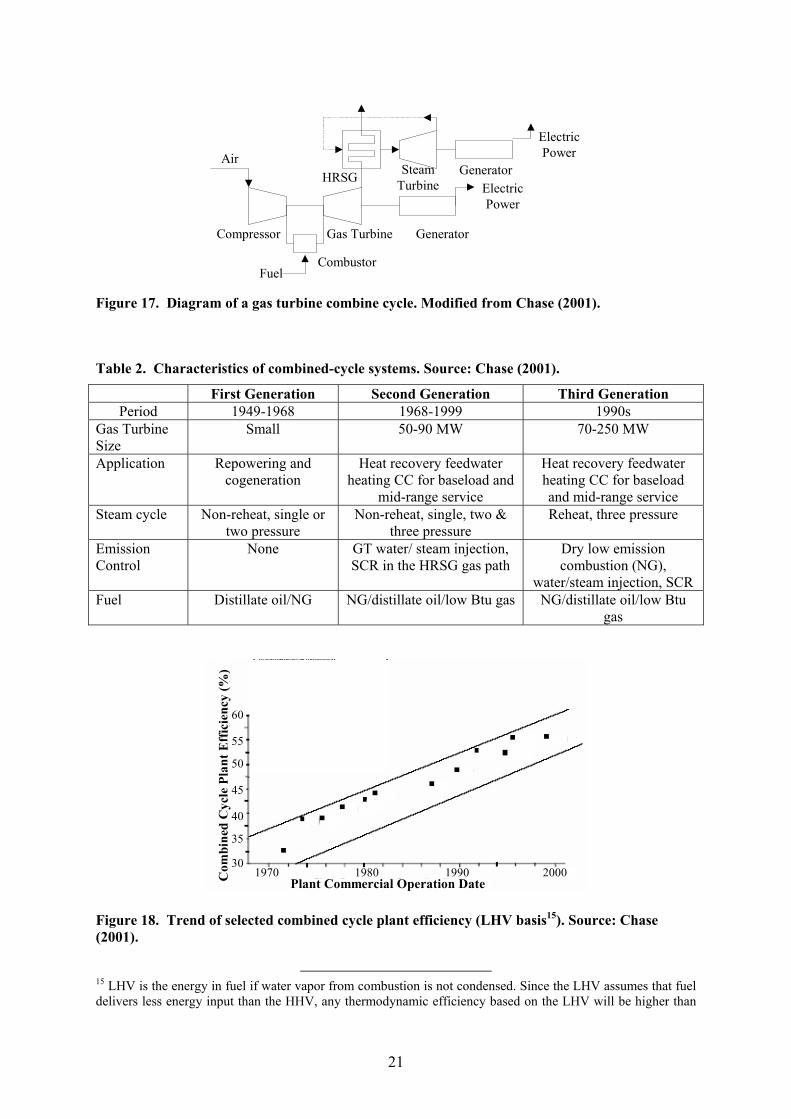
21

Air

Compressor

CombustorFuel

Gas Turbine Generator

ElectricPower

HRSG

ElectricPower

GeneratorSteamTurbine

Figure 17. Diagram of a gas turbine combine cycle. Modified from Chase (2001).

Table 2. Characteristics of combined-cycle systems. Source: Chase (2001).

First Generation Second Generation Third Generation Period 1949-1968 1968-1999 1990s

Gas Turbine Size

Small 50-90 MW 70-250 MW

Application Repowering and cogeneration

Heat recovery feedwater heating CC for baseload and

mid-range service

Heat recovery feedwater heating CC for baseload and mid-range service

Steam cycle Non-reheat, single or two pressure

Non-reheat, single, two & three pressure

Reheat, three pressure

Emission Control

None GT water/ steam injection, SCR in the HRSG gas path

Dry low emission combustion (NG),

water/steam injection, SCR Fuel Distillate oil/NG NG/distillate oil/low Btu gas NG/distillate oil/low Btu

gas

Plant Commercial Operation Date1970 1980 1990 2000C

ombi

ned

Cyc

le P

lant

Eff

icie

ncy

(%)

30

35

40

45

50

55

60

Figure 18. Trend of selected combined cycle plant efficiency (LHV basis15). Source: Chase (2001).

15 LHV is the energy in fuel if water vapor from combustion is not condensed. Since the LHV assumes that fuel delivers less energy input than the HHV, any thermodynamic efficiency based on the LHV will be higher than

22

3.3.2. Cost Trends of GTCC and its Components Cost trends and descriptions of this technology already have received considerable study by a number of investigators. According to Colpier and Cornland (2002), the efficiency for a state-of-the-art machine increased from 44 to 58 percent (LHV basis) between 1981 and 1997. An analysis by Colpier and Cornland (2002) examined the specific investment price for large GTCC power plants, and showed that increasing costs during 1981-1991 was followed by a period of rapidly falling costs during the 1990s (Figure 19). The subsequent price decreases (with a progress ratio of 75%, or LR of 25%), were attributed mainly to market developments and strategies as the GTCC market experienced a shakeout stage as several manufactures competed to gain market share. The price decline also was attributed to some real cost reductions from improved technology performance and a shift towards more standardized and modularized machines.

PR~75% (1991-1997)

PR>100% (1981-1991)

Cumulative installed capacity, MW

Inve

stm

ent P

rice

USD

(199

0$/k

W)

10000 100000

300

400

500

600

700800900

1000

Figure 19. Experience curve for the specific investment price of gas turbine combined cycle (GTCC) technology (1981–1997). Source: Colpier and Cornland (2002).

Other summaries of GTCC learning rates report similar results. For example, a learning rate of 34% is reported for the OECD countries during the period 1984–1994. GTCC also benefited from the learning experience of its various components, such as gas turbine. Gas turbine development improved combined-cycle efficiency primarily to the increase in firing temperature through the development of high temperature oxidation/corrosion resistant metals and coatings, advanced metal surface cooling techniques, advances in steam system technology (through new technology to weld continuous spiral fins on HRSG heat transfer tubes, the application of larger annulus area steam turbine designs for low exhaust pressure applications, and the application of reheat steam cycle). (Chase 2001). MacGregor et al. (1991) estimated that the cost of gas turbines achieved a 10% learning rate historically. Similarly, Rogner, (1998) found a learning rate of 19% for early gas turbines and a little below 7% for mature gas turbines. Advances in steam system technology through HRSG and the application of reheat steam cycle have also contributed to improved combined-cycle efficiency (Chase 2001).

one based on HHV. The numerical difference between LHV and HHV depends on the fuel, and is smallest for coal (LHV roughly 4% lower than HHV), and greatest for natural gas (LHV about 10% lower) (NRC 2000).

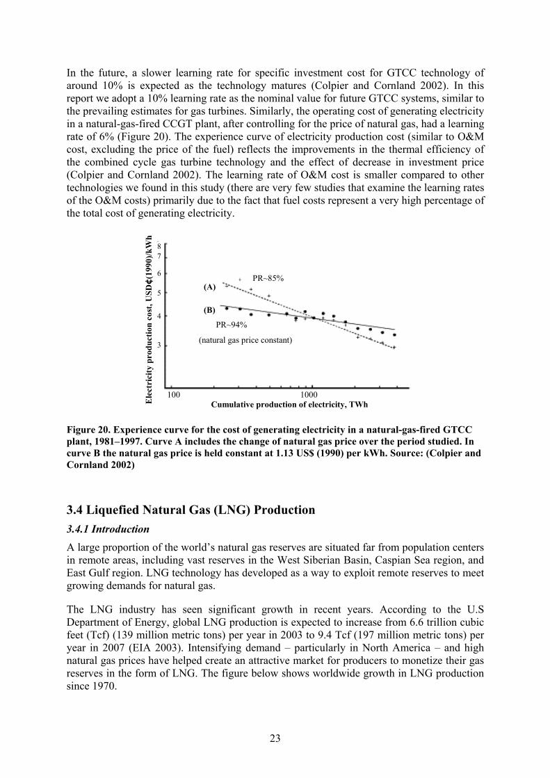
23

In the future, a slower learning rate for specific investment cost for GTCC technology of around 10% is expected as the technology matures (Colpier and Cornland 2002). In this report we adopt a 10% learning rate as the nominal value for future GTCC systems, similar to the prevailing estimates for gas turbines. Similarly, the operating cost of generating electricity in a natural-gas-fired CCGT plant, after controlling for the price of natural gas, had a learning rate of 6% (Figure 20). The experience curve of electricity production cost (similar to O&M cost, excluding the price of the fuel) reflects the improvements in the thermal efficiency of the combined cycle gas turbine technology and the effect of decrease in investment price (Colpier and Cornland 2002). The learning rate of O&M cost is smaller compared to other technologies we found in this study (there are very few studies that examine the learning rates of the O&M costs) primarily due to the fact that fuel costs represent a very high percentage of the total cost of generating electricity.

PR~85%

(natural gas price constant)

Cumulative production of electricity, TWhEle

ctri

city

pro

duct

ion

cost

, USD

¢(1

990)

/kW

h

100 1000

3

4

5

6

78

PR~94%

(A)

(B)

Figure 20. Experience curve for the cost of generating electricity in a natural-gas-fired GTCC plant, 1981–1997. Curve A includes the change of natural gas price over the period studied. In curve B the natural gas price is held constant at 1.13 US$ (1990) per kWh. Source: (Colpier and Cornland 2002)

3.4 Liquefied Natural Gas (LNG) Production 3.4.1 Introduction

A large proportion of the world’s natural gas reserves are situated far from population centers in remote areas, including vast reserves in the West Siberian Basin, Caspian Sea region, and East Gulf region. LNG technology has developed as a way to exploit remote reserves to meet growing demands for natural gas.

The LNG industry has seen significant growth in recent years. According to the U.S Department of Energy, global LNG production is expected to increase from 6.6 trillion cubic feet (Tcf) (139 million metric tons) per year in 2003 to 9.4 Tcf (197 million metric tons) per year in 2007 (EIA 2003). Intensifying demand – particularly in North America – and high natural gas prices have helped create an attractive market for producers to monetize their gas reserves in the form of LNG. The figure below shows worldwide growth in LNG production since 1970.

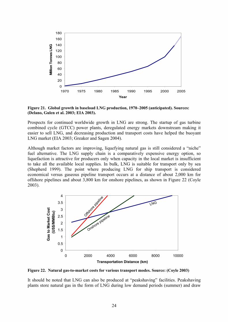
24

0

20

40

60

80

100

120

140

160

180

1970 1975 1980 1985 1990 1995 2000 2005

Year

Mill

ion

Tonn

es L

NG

Figure 21. Global growth in baseload LNG production, 1970–2005 (anticipated). Sources: (Delano, Gulen et al. 2003; EIA 2003).

Prospects for continued worldwide growth in LNG are strong. The startup of gas turbine combined cycle (GTCC) power plants, deregulated energy markets downstream making it easier to sell LNG, and decreasing production and transport costs have helped the buoyant LNG market (EIA 2003; Greaker and Sagen 2004).

Although market factors are improving, liquefying natural gas is still considered a “niche” fuel alternative. The LNG supply chain is a comparatively expensive energy option, so liquefaction is attractive for producers only when capacity in the local market is insufficient to take all the available local supplies. In bulk, LNG is suitable for transport only by sea (Shepherd 1999). The point where producing LNG for ship transport is considered economical versus gaseous pipeline transport occurs at a distance of about 2,000 km for offshore pipelines and about 3,800 km for onshore pipelines, as shown in Figure 22 (Coyle 2003).

0

0.5

1

1.5

2

2.5

3

3.5

4

0 2000 4000 6000 8000 10000Transportation Distance (km)

Gas

to M

arke

t Cos

t(U

S$/M

MB

tu)

LNG

Onshore pipelineOffsho

re pip

eline

0

0.5

1

1.5

2

2.5

3

3.5

4

0 2000 4000 6000 8000 10000Transportation Distance (km)

Gas

to M

arke

t Cos

t(U

S$/M

MB

tu)

LNG

Onshore pipelineOffsho

re pip

eline

Figure 22. Natural gas-to-market costs for various transport modes. Source: (Coyle 2003)

It should be noted that LNG can also be produced at “peakshaving” facilities. Peakshaving plants store natural gas in the form of LNG during low demand periods (summer) and draw

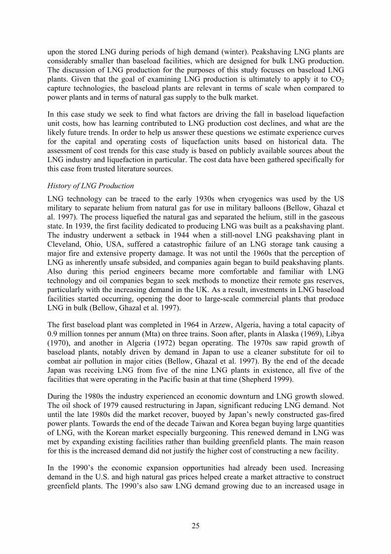
25

upon the stored LNG during periods of high demand (winter). Peakshaving LNG plants are considerably smaller than baseload facilities, which are designed for bulk LNG production. The discussion of LNG production for the purposes of this study focuses on baseload LNG plants. Given that the goal of examining LNG production is ultimately to apply it to CO2 capture technologies, the baseload plants are relevant in terms of scale when compared to power plants and in terms of natural gas supply to the bulk market.

In this case study we seek to find what factors are driving the fall in baseload liquefaction unit costs, how has learning contributed to LNG production cost declines, and what are the likely future trends. In order to help us answer these questions we estimate experience curves for the capital and operating costs of liquefaction units based on historical data. The assessment of cost trends for this case study is based on publicly available sources about the LNG industry and liquefaction in particular. The cost data have been gathered specifically for this case from trusted literature sources.

History of LNG Production

LNG technology can be traced to the early 1930s when cryogenics was used by the US military to separate helium from natural gas for use in military balloons (Bellow, Ghazal et al. 1997). The process liquefied the natural gas and separated the helium, still in the gaseous state. In 1939, the first facility dedicated to producing LNG was built as a peakshaving plant. The industry underwent a setback in 1944 when a still-novel LNG peakshaving plant in Cleveland, Ohio, USA, suffered a catastrophic failure of an LNG storage tank causing a major fire and extensive property damage. It was not until the 1960s that the perception of LNG as inherently unsafe subsided, and companies again began to build peakshaving plants. Also during this period engineers became more comfortable and familiar with LNG technology and oil companies began to seek methods to monetize their remote gas reserves, particularly with the increasing demand in the UK. As a result, investments in LNG baseload facilities started occurring, opening the door to large-scale commercial plants that produce LNG in bulk (Bellow, Ghazal et al. 1997).

The first baseload plant was completed in 1964 in Arzew, Algeria, having a total capacity of 0.9 million tonnes per annum (Mta) on three trains. Soon after, plants in Alaska (1969), Libya (1970), and another in Algeria (1972) began operating. The 1970s saw rapid growth of baseload plants, notably driven by demand in Japan to use a cleaner substitute for oil to combat air pollution in major cities (Bellow, Ghazal et al. 1997). By the end of the decade Japan was receiving LNG from five of the nine LNG plants in existence, all five of the facilities that were operating in the Pacific basin at that time (Shepherd 1999).

During the 1980s the industry experienced an economic downturn and LNG growth slowed. The oil shock of 1979 caused restructuring in Japan, significant reducing LNG demand. Not until the late 1980s did the market recover, buoyed by Japan’s newly constructed gas-fired power plants. Towards the end of the decade Taiwan and Korea began buying large quantities of LNG, with the Korean market especially burgeoning. This renewed demand in LNG was met by expanding existing facilities rather than building greenfield plants. The main reason for this is the increased demand did not justify the higher cost of constructing a new facility.

In the 1990’s the economic expansion opportunities had already been used. Increasing demand in the U.S. and high natural gas prices helped create a market attractive to construct greenfield plants. The 1990’s also saw LNG demand growing due to an increased usage in

26

producing electricity - nuclear suffered risk perception setbacks and environmental issues made coal-fired power plants less attractive (Aoki and Kikkawa 1995). As a result, between 1989 and 2000 five new greenfield plants started-up, as compared to only one greenfield facility in the previous ten years (Figure 23).

0

1

2

3

4

5

1964 1969 1974 1979 1984 1989 1994 1999 20040

20

40

60

80

100

120

140

Expansion

LNG Produced (Mta)

Greenfield Plants

Num

ber o

f Fac

ilitie

s C

onst

ruct

ed

Ann

ual P

rodu

ctio

n of

LN

G (M

ta)

0

1

2

3

4

5

1964 1969 1974 1979 1984 1989 1994 1999 20040

20

40

60

80

100

120

140

Expansion

LNG Produced (Mta)

Greenfield Plants

Num

ber o

f Fac

ilitie

s C

onst

ruct

ed

Ann

ual P

rodu

ctio

n of

LN

G (M

ta)

Figure 23. Number of worldwide new LNG plants (greenfield) and construction of additional trains at existing plants (expansion). Source: (EIA 2003)

Today the LNG market is rapidly growing. The current expansion of the LNG industry reflects a combination of factors, including a recent trend of decreased plant costs, the increased use of gas-fired power generation worldwide, and deregulation of downstream energy markets (Arthus-Bertrand 2004). Growth in the industry has also been buoyed by improved flexibility in long-term contracts, which have historically dominated the market. Short-term trading is expected to grow from 1% in 1992 up to 20% by 2010 (EIA 2003).

3.4.2 LNG Supply Chain

Capital Costs

The costs of the LNG chain can vary widely, primarily depending on the scale of the liquefaction plant, whether the liquefaction plant is built in a new location or an expansion of an existing facility, and the upstream costs of extracting gas from the field. Secondary factors affecting costs of the supply chain include the location of the facility (e.g., regulatory environment, geography, remoteness, shipping distance to market), and the composition of incoming gas (e.g., how much gas treatment is necessary) (DiNapoli 1986; Bellow, Ghazal et al. 1997; Cornot-Gandolphe, Appert et al. 2003).

The EIA reports that a new greenfield LNG installation typically costs between $1.5 and $2.0 billion for a typical 2-train facility that produces about 7 to 8 million tonnes per annum (Mta). Overall, LNG construction costs are generally higher than comparable energy projects. Costs for monetizing natural gas via LNG are elevated for a number of reasons, such as stringent safety standards (fallout from the Cleveland incident), necessity for cryogenic equipment and material, and a historic tendency to over-design to ensure supply security (EIA 2003).

27

Flow Scheme

In order to understand the capital costs associated with LNG production, it is helpful to be familiar with the flow scheme. The supply chain diagram is shown in Figure 24.

Figure 24. LNG base-loading flow scheme.

As outlined in Figure 24, there are four main parts to the value chain: gas field, LNG plant16, LNG shipping, and re-gasification. The gas field section includes operations from the gas reservoir to the LNG plant, including associated extraction equipment, piping and instrumentation. The next step in the process is the LNG plant, which includes gas treatment, liquefaction, LNG storage and loading. Gas arrives at the LNG plant from the gas field where contaminants such as water, mercury, acid gas, and heavier hydrocarbons are removed to avoid freezing up and damaging equipment when the gas is cooled. LNG plants typically have parallel trains consisting of integrated gas treating and liquefaction units in each train. The treatment process can be designed to purify the LNG to almost 100 percent methane before being liquefied. The natural gas is then cooled and liquefied for shipping, reducing its volume by a factor of 600 (Delano, Gulen et al. 2003). The third main part of the value chain is shipping the LNG from the LNG plant to a re-gasification terminal. The product is received at the terminal where it is vaporized, odorized, and metered for distribution.

Liquefaction Technology

Although there are a handful of different liquefaction technologies, all of the technologies are based on the common concept of reducing the temperature of natural gas until it is a liquid at ambient pressure, approximately –161°C (–258°F). The key difference lies in the method of cooling the natural gas (Sawchuk and Howard 2004). The methods entail cooling the natural gas by using a refrigeration cycle, where a refrigerant using consecutive expansion and compression transfers heat from a lower to a higher temperature. Refrigerants matching as closely as possible to the cooling/heating curves of the process gas and the refrigerant are

16 The LNG Plant section of the value chain is also known as the liquefaction plant in common literature references. However, to avoid confusing the liquefaction process of the LNG plant with the LNG plant as a whole (which includes gas treatment, LPG recovery, storage and loading in addition to liquefaction), we use the terminology “LNG plant” to refer to major section of the value chain that encompasses several operations, while “liquefaction unit” refers to the liquefaction process within the LNG plant.

28

used to produce the most efficient the thermodynamic process practicable, requiring less power per unit of LNG produced. Typical natural gas and refrigerant cooling curves are shown in Figure 25.

Natural gas cooling curve

Refrigerant cooling curve

Tem

pera

ture

Enthalpy

Natural gas cooling curve

Refrigerant cooling curve

Tem

pera

ture

Enthalpy Figure 25. Natural gas/refrigerant cooling curve. Source:(Finn, Johnson et al. 2001)

The means by which cooling is achieved and the equipment used play a major part in the overall efficiency, operability, reliability and cost of the plant. Since the first baseload LNG plant at Arzew, Algeria, the fundamental technology has remained the same. There have not been major breakthroughs in the liquefaction process, nor have there been vast differences in the thermodynamic efficiencies between processes (Troner 2001).

There are four distinct LNG liquefaction processes in operation today (plus two more processes to be utilized in plants currently under construction). The first two baseload LNG plants, constructed in the late 1960s, used a liquefaction flow scheme called the Cascade process developed by Phillips. Since then, Phillip’s Cascade process had not been installed in an LNG liquefaction facility until 1999 in Trinidad, when an updated version called Optimized Cascade process was constructed.

In 1970, a variation of the Cascade process was introduced by Air Products & Chemicals (APCI) called the Propane Mixed Refrigerant (C3MR) process. This process quickly became the prevailing liquefaction method for new plants starting-up in the industry from its introduction until competing methods were introduced in the late 1990s (Smaal 2003). In fact, with the exception of the plant in Skikda, Algeria which installed the Tealarc process in 1972 and Black & Veatch’s PRICO process for its three expansion units in 1981 and 1982, the C3MR process was the only liquefaction technology constructed until Trinidad in 1999 (Chiyoda 2003). During this period – from 1970 to 1998 – APCI’s C3MR process was used for 36 trains and only 4 trains, in Skikda in 1972, did not use APCI’s technology. The percent of annual LNG production of the technologies operating in 2002 is presented in Figure 26.

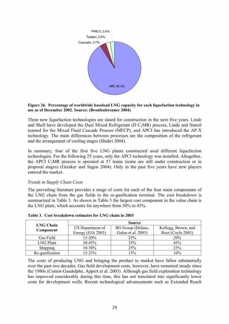
29

Cascade, 3.7%

Tealarc, 2.6%

PRICO, 2.6%

MR, 90.4%

Figure 26. Percentage of worldwide baseload LNG capacity for each liquefaction technology in use as of December 2002. Source: (Bronfenbrenner 2004)

Three new liquefaction technologies are slated for construction in the next five years. Linde and Shell have developed the Dual Mixed Refrigerant (D C3MR) process, Linde and Statoil teamed for the Mixed Fluid Cascade Process (MFCP), and APCI has introduced the AP-X technology. The main differences between processes are the composition of the refrigerant and the arrangement of cooling stages (Shukri 2004).

In summary, four of the first five LNG plants constructed used different liquefaction technologies. For the following 25 years, only the APCI technology was installed. Altogether, the APCI C3MR process is operated at 57 trains (some are still under construction or in proposal stages) (Greaker and Sagen 2004). Only in the past five years have new players entered the market.

Trends in Supply Chain Costs

The prevailing literature provides a range of costs for each of the four main components of the LNG chain from the gas fields to the re-gasification terminal. The cost breakdown is summarized in Table 3. As shown in Table 3 the largest cost component in the value chain is the LNG plant, which accounts for anywhere from 30% to 45%.

Table 3. Cost breakdown estimates for LNG chain in 2003

Source LNG Chain Component US Department of

Energy (EIA 2003) BG Group (Delano, Gulen et al. 2003)

Kellogg, Brown, and Root (Coyle 2003)

Gas Field 15-20% 25% 20% LNG Plant 30-45% 35% 45% Shipping 10-30% 25% 25%

Re-gasification 15-25% 15% 10%

The costs of producing LNG and bringing the product to market have fallen substantially over the past two decades. Gas field development costs, however, have remained steady since the 1980s (Cornot-Gandolphe, Appert et al. 2003). Although gas field exploration technology has improved considerably during this time, this has not translated into significantly lower costs for development wells. Recent technological advancements such as Extended Reach

30

Drilling (ERD) have justified tapping into new fields, but have not resulted in overall reduction of costs upstream of the LNG plant.

LNG plant construction costs have declined considerably, by approximately 20% to 35% since the 1980s with accelerated declines in the past five to ten years. This is discussed further in the section below on LNG plant cost trends.

Shipping costs have fallen anywhere from 5% to 30% over the same period, mainly depending on the number of shipments needed per unit of output. Fewer shipments decrease unit costs, although it requires greater storage capacity at the LNG plant. The large reductions in shipping cost have been accomplished mostly through economies of scale. LNG ship capacities have increased from about 40,000 m3 to approximately 140,000 m3 today (EIA 2003; Gower and Howard 2003).Current orders are being placed for ships with a capacity of over 200,000 m3, which should continue to reduce shipping unit costs.

The capital cost for re-gasification has only marginally declined compared to other parts of the LNG chain since the first re-gasification terminals were built in 1960s. LNG terminal construction costs typically accounts for less than 15% of the overall capital costs in the LNG chain. A large component of re-gas terminal construction stems from labor and land development costs, which generally have not declined over time. Slight cost reductions have been attributed to economies of scale in re-gas capacity (Cornot-Gandolphe, Appert et al. 2003).

Trends in LNG Plant Cost

During the first decade of baseload plants, from 1964 to 1972, the costs to construct an LNG Plant increased from about $400 per ton of annual liquefaction capacity to around $500 per ton (Figure 27). Since there were only five plants constructed during this period and the baseload LNG technology was quite new, it is difficult to draw trends with certainty in this time range. However, decreased competition and a tendency to over-design during this period helps explain this trend. Competition among liquefaction technology suppliers was strong during the initial years of plant construction, but had diminished to a single firm in the 1970s, possibly causing monopoly conditions of technology licensing and an increase in costs. In additions, the need to ensure supply security in the buoyant 1970s Asian LNG market caused new plants to build-in design redundancies into their plants.

While there were four liquefaction technologies during the early years of LNG production each supplied by a different company, only one company – APCI – remained for the next 25 years. This reduction in competition may have enticed APCI to raise mark-ups on the price of LNG liquefaction technology via monopoly power in this market (Greaker and Sagen 2004). However, simply being the only technology used for new plants after the initial plants started-up does not necessarily mean APCI enjoyed a monopoly. It is possible that it was continually being challenged by the Phillips Cascade process and other technologies. Shepherd (1999) interprets that a key contributing factor to LNG plant capital cost escalation was due to few contractors and liquefaction process licensors with proven expertise (Shepherd 1999).

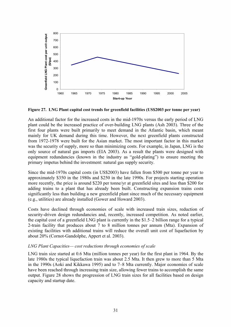
31

0

100

200

300

400

500

600

700

800

1960 1965 1970 1975 1980 1985 1990 1995 2000 2005

Start-up Year

Gre

enfie

ld L

NG P

lant

cos

t per

uni

t out

put

($/tp

a)

Figure 27. LNG Plant capital cost trends for greenfield facilities (US$2003 per tonne per year)

An additional factor for the increased costs in the mid-1970s versus the early period of LNG plant could be the increased practice of over-building LNG plants (Ash 2003). Three of the first four plants were built primarily to meet demand in the Atlantic basin, which meant mainly for UK demand during this time. However, the next greenfield plants constructed from 1972-1978 were built for the Asian market. The most important factor in this market was the security of supply, more so than minimizing costs. For example, in Japan, LNG is the only source of natural gas imports (EIA 2003). As a result the plants were designed with equipment redundancies (known in the industry as “gold-plating”) to ensure meeting the primary impetus behind the investment: natural gas supply security.

Since the mid-1970s capital costs (in US$2003) have fallen from $500 per tonne per year to approximately $350 in the 1980s and $250 in the late 1990s. For projects starting operation more recently, the price is around $220 per tonne/yr at greenfield sites and less than $200 for adding trains to a plant that has already been built. Constructing expansion trains costs significantly less than building a new greenfield plant since much of the necessary equipment (e.g., utilities) are already installed (Gower and Howard 2003).

Costs have declined through economies of scale with increased train sizes, reduction of security-driven design redundancies and, recently, increased competition. As noted earlier, the capital cost of a greenfield LNG plant is currently in the $1.5–2 billion range for a typical 2-train facility that produces about 7 to 8 million tonnes per annum (Mta). Expansion of existing facilities with additional trains will reduce the overall unit cost of liquefaction by about 20% (Cornot-Gandolphe, Appert et al. 2003).

LNG Plant Capacities— cost reductions through economies of scale

LNG train size started at 0.6 Mta (million tonnes per year) for the first plant in 1964. By the late 1980s the typical liquefaction train was about 2.5 Mta. It then grew to more than 5 Mta in the 1990s (Aoki and Kikkawa 1995) and to 7–8 Mta currently. Major economies of scale have been reached through increasing train size, allowing fewer trains to accomplish the same output. Figure 28 shows the progression of LNG train sizes for all facilities based on design capacity and startup date.

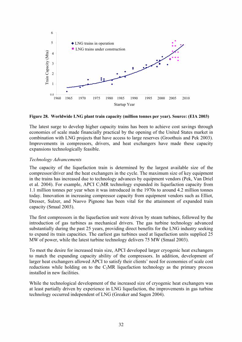
32

0.0

1.0

2.0

3.0

4.0

5.0

6.0

1960 1965 1970 1975 1980 1985 1990 1995 2000 2005 2010

Start up year

Tra

in c

apac

ity (M

tLNG trains in operationLNG trains under construc tion

Trai

n C

apac

ity (M

ta)

Startup Year1960 1965 1970 1975 1980 1985 1990 1995 2000 2005 2010

1

2

3

4

5

6

LNG trains in operationLNG trains under construction

Figure 28. Worldwide LNG plant train capacity (million tonnes per year). Source: (EIA 2003)

The latest surge to develop higher capacity trains has been to achieve cost savings through economies of scale made financially practical by the opening of the United States market in combination with LNG projects that have access to large reserves (Groothuis and Pek 2003). Improvements in compressors, drivers, and heat exchangers have made these capacity expansions technologically feasible.

Technology Advancements

The capacity of the liquefaction train is determined by the largest available size of the compressor/driver and the heat exchangers in the cycle. The maximum size of key equipment in the trains has increased due to technology advances by equipment vendors (Pek, Van Driel et al. 2004). For example, APCI C3MR technology expanded its liquefaction capacity from 1.1 million tonnes per year when it was introduced in the 1970s to around 4.2 million tonnes today. Innovation in increasing compressor capacity from equipment vendors such as Elliot, Dresser, Sulzer, and Nuovo Pignone has been vital for the attainment of expanded train capacity (Smaal 2003).

The first compressors in the liquefaction unit were driven by steam turbines, followed by the introduction of gas turbines as mechanical drivers. The gas turbine technology advanced substantially during the past 25 years, providing direct benefits for the LNG industry seeking to expand its train capacities. The earliest gas turbines used at liquefaction units supplied 25 MW of power, while the latest turbine technology delivers 75 MW (Smaal 2003).

To meet the desire for increased train size, APCI developed larger cryogenic heat exchangers to match the expanding capacity ability of the compressors. In addition, development of larger heat exchangers allowed APCI to satisfy their clients’ need for economies of scale cost reductions while holding on to the C3MR liquefaction technology as the primary process installed in new facilities.

While the technological development of the increased size of cryogenic heat exchangers was at least partially driven by experience in LNG liquefaction, the improvements in gas turbine technology occurred independent of LNG (Greaker and Sagen 2004).

33

Reduction of design redundancies

As described earlier, there was a historic tendency in the industry to over-design to ensure natural gas supply security. In the Asian market LNG plants in Australia and Malaysia routinely could produce 25 percent more than its stated capacity (Shepherd 1999). The degree of over-design has substantially reduced, but trains starting up in recent years still have the ability to operate at 10% above their stated capacity (EIA 2003). As experience with liquefaction increased, the perceived need to over-design waned, thus decreasing the design redundancy. This has contributed to steadily decreasing capital costs of LNG trains since the peak of supply security need in the mid-1970s (Ash 2003).

Competition among contractors

Competition plays a major role in the cost trends of LNG plants. As shown earlier (Figure 27), the capital costs increased from the first installations in the 1960s and early 1970s and peaked in the mid-1970s. Since the LNG market growth was primarily driven by Asia in the mid-1970s most plants built during this period serviced the Asian market. In addition to design redundancies being built into plants in the mid-1970s, there is less competition from pipeline gas in Asia. As a result, the first LNG plants constructed mainly for Atlantic basin customers who face pipeline gas competition (primarily in Europe during this period) were forced to lower costs as much as possible and compete on price, while the Asian LNG market did not face this competition (Shepherd 1999).

A similar rational explains the recent cost trends of new facilities. Plants in Nigeria (1999) and Trinidad (1999), which service the Atlantic market, are two of the lowest cost facilities that have completed construction. Expansion trains in Trinidad (2003) reportedly cost less than $200 per tonne (Troner 2001; Williams 2002).

Not only did the Trinidad plant need to reduce its costs because of pipeline gas competition for its product in the Atlantic basin, but it also received cost savings through competition due to renewed competition in liquefaction process technology. During the period Trinidad was obtaining bids Phillips, with Bechtel, was attempting to market an updated version of its cascade liquefaction technology that was last used in an LNG plant in 1969. The APCI C3MR process, therefore, was forced to compete for possibly the first time in about 25 years and enabled Trinidad to choose between competitive bids (Shepherd 1999). Subsequent projects in the Pacific basin have also seemed to benefit from increased competition. Recently, an expansion in Malaysia (2003) and greenfield project in Oman (2000) were able to construct facilities for $250 per tonne or less (Hagan 2000; Ash 2003; Yost and DiNapoli 2003).

Although the new projects in Trinidad, Malaysia and Oman all selected the APCI C3MR technology, the competitors are making inroads into the liquefaction technology market. Figure 29 illustrates the penetration of new technologies in the current market (compare this outlook to Figure 26).

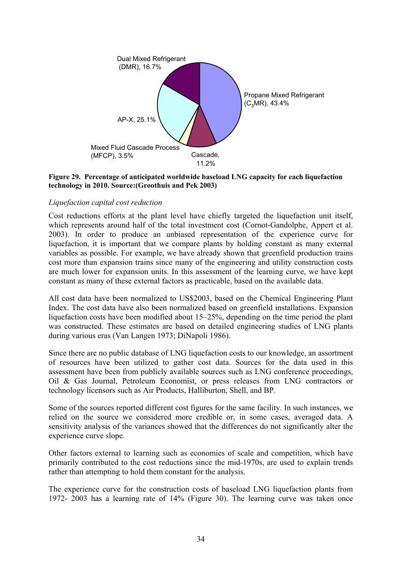
34

Propane Mixed Refrigerant (C3MR), 43.4%

Cascade, 11.2%

Mixed Fluid Cascade Process (MFCP), 3.5%

AP-X, 25.1%

Dual Mixed Refrigerant(DMR), 16.7%

Propane Mixed Refrigerant (C3MR), 43.4%

Cascade, 11.2%

Mixed Fluid Cascade Process (MFCP), 3.5%

AP-X, 25.1%

Dual Mixed Refrigerant(DMR), 16.7%

Figure 29. Percentage of anticipated worldwide baseload LNG capacity for each liquefaction technology in 2010. Source:(Groothuis and Pek 2003)

Liquefaction capital cost reduction

Cost reductions efforts at the plant level have chiefly targeted the liquefaction unit itself, which represents around half of the total investment cost (Cornot-Gandolphe, Appert et al. 2003). In order to produce an unbiased representation of the experience curve for liquefaction, it is important that we compare plants by holding constant as many external variables as possible. For example, we have already shown that greenfield production trains cost more than expansion trains since many of the engineering and utility construction costs are much lower for expansion units. In this assessment of the learning curve, we have kept constant as many of these external factors as practicable, based on the available data.

All cost data have been normalized to US$2003, based on the Chemical Engineering Plant Index. The cost data have also been normalized based on greenfield installations. Expansion liquefaction costs have been modified about 15–25%, depending on the time period the plant was constructed. These estimates are based on detailed engineering studies of LNG plants during various eras (Van Langen 1973; DiNapoli 1986).

Since there are no public database of LNG liquefaction costs to our knowledge, an assortment of resources have been utilized to gather cost data. Sources for the data used in this assessment have been from publicly available sources such as LNG conference proceedings, Oil & Gas Journal, Petroleum Economist, or press releases from LNG contractors or technology licensors such as Air Products, Halliburton, Shell, and BP.

Some of the sources reported different cost figures for the same facility. In such instances, we relied on the source we considered more credible or, in some cases, averaged data. A sensitivity analysis of the variances showed that the differences do not significantly alter the experience curve slope.

Other factors external to learning such as economies of scale and competition, which have primarily contributed to the cost reductions since the mid-1970s, are used to explain trends rather than attempting to hold them constant for the analysis.

The experience curve for the construction costs of baseload LNG liquefaction plants from 1972- 2003 has a learning rate of 14% (Figure 30). The learning curve was taken once

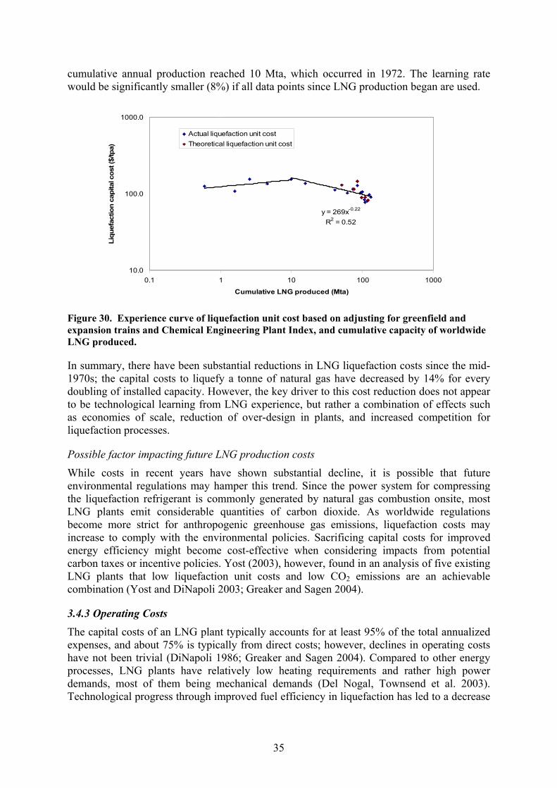
35

cumulative annual production reached 10 Mta, which occurred in 1972. The learning rate would be significantly smaller (8%) if all data points since LNG production began are used.

y = 269x-0.22

R2 = 0.52

10.0

100.0

1000.0

0.1 1 10 100 1000

Cumulative LNG produced (Mta)

Liqu

efac

tion

capi

tal c

ost (

$/tp

a)

Actual liquefaction unit costTheoretical liquefaction unit cost

Figure 30. Experience curve of liquefaction unit cost based on adjusting for greenfield and expansion trains and Chemical Engineering Plant Index, and cumulative capacity of worldwide LNG produced.

In summary, there have been substantial reductions in LNG liquefaction costs since the mid-1970s; the capital costs to liquefy a tonne of natural gas have decreased by 14% for every doubling of installed capacity. However, the key driver to this cost reduction does not appear to be technological learning from LNG experience, but rather a combination of effects such as economies of scale, reduction of over-design in plants, and increased competition for liquefaction processes.

Possible factor impacting future LNG production costs

While costs in recent years have shown substantial decline, it is possible that future environmental regulations may hamper this trend. Since the power system for compressing the liquefaction refrigerant is commonly generated by natural gas combustion onsite, most LNG plants emit considerable quantities of carbon dioxide. As worldwide regulations become more strict for anthropogenic greenhouse gas emissions, liquefaction costs may increase to comply with the environmental policies. Sacrificing capital costs for improved energy efficiency might become cost-effective when considering impacts from potential carbon taxes or incentive policies. Yost (2003), however, found in an analysis of five existing LNG plants that low liquefaction unit costs and low CO2 emissions are an achievable combination (Yost and DiNapoli 2003; Greaker and Sagen 2004).

3.4.3 Operating Costs The capital costs of an LNG plant typically accounts for at least 95% of the total annualized expenses, and about 75% is typically from direct costs; however, declines in operating costs have not been trivial (DiNapoli 1986; Greaker and Sagen 2004). Compared to other energy processes, LNG plants have relatively low heating requirements and rather high power demands, most of them being mechanical demands (Del Nogal, Townsend et al. 2003). Technological progress through improved fuel efficiency in liquefaction has led to a decrease

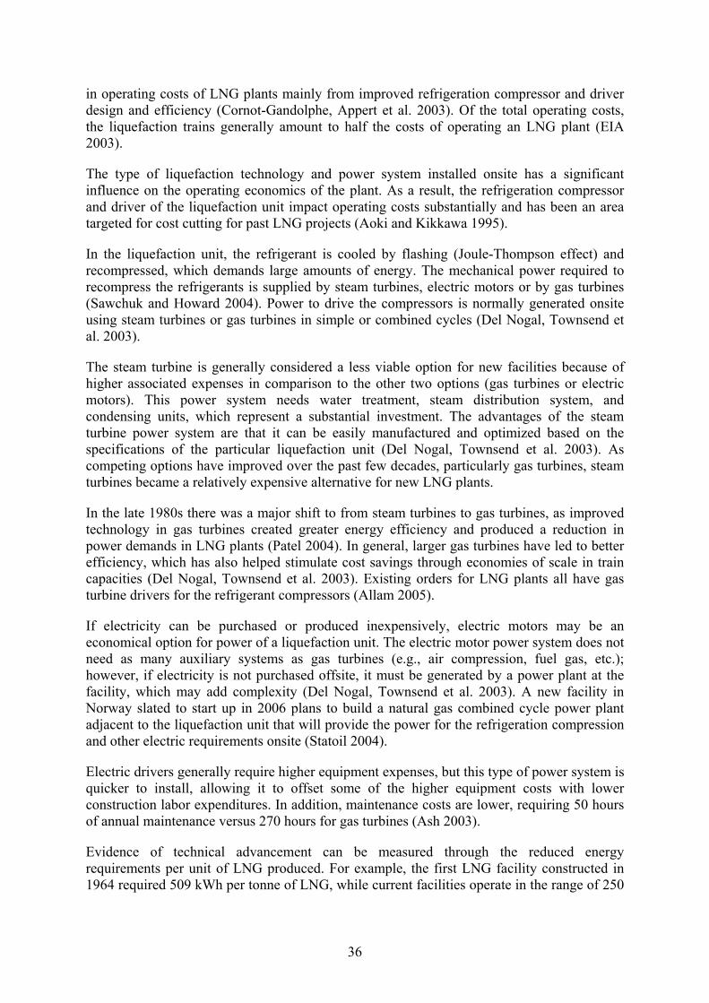
36

in operating costs of LNG plants mainly from improved refrigeration compressor and driver design and efficiency (Cornot-Gandolphe, Appert et al. 2003). Of the total operating costs, the liquefaction trains generally amount to half the costs of operating an LNG plant (EIA 2003).

The type of liquefaction technology and power system installed onsite has a significant influence on the operating economics of the plant. As a result, the refrigeration compressor and driver of the liquefaction unit impact operating costs substantially and has been an area targeted for cost cutting for past LNG projects (Aoki and Kikkawa 1995).

In the liquefaction unit, the refrigerant is cooled by flashing (Joule-Thompson effect) and recompressed, which demands large amounts of energy. The mechanical power required to recompress the refrigerants is supplied by steam turbines, electric motors or by gas turbines (Sawchuk and Howard 2004). Power to drive the compressors is normally generated onsite using steam turbines or gas turbines in simple or combined cycles (Del Nogal, Townsend et al. 2003).

The steam turbine is generally considered a less viable option for new facilities because of higher associated expenses in comparison to the other two options (gas turbines or electric motors). This power system needs water treatment, steam distribution system, and condensing units, which represent a substantial investment. The advantages of the steam turbine power system are that it can be easily manufactured and optimized based on the specifications of the particular liquefaction unit (Del Nogal, Townsend et al. 2003). As competing options have improved over the past few decades, particularly gas turbines, steam turbines became a relatively expensive alternative for new LNG plants.

In the late 1980s there was a major shift to from steam turbines to gas turbines, as improved technology in gas turbines created greater energy efficiency and produced a reduction in power demands in LNG plants (Patel 2004). In general, larger gas turbines have led to better efficiency, which has also helped stimulate cost savings through economies of scale in train capacities (Del Nogal, Townsend et al. 2003). Existing orders for LNG plants all have gas turbine drivers for the refrigerant compressors (Allam 2005).

If electricity can be purchased or produced inexpensively, electric motors may be an economical option for power of a liquefaction unit. The electric motor power system does not need as many auxiliary systems as gas turbines (e.g., air compression, fuel gas, etc.); however, if electricity is not purchased offsite, it must be generated by a power plant at the facility, which may add complexity (Del Nogal, Townsend et al. 2003). A new facility in Norway slated to start up in 2006 plans to build a natural gas combined cycle power plant adjacent to the liquefaction unit that will provide the power for the refrigeration compression and other electric requirements onsite (Statoil 2004).

Electric drivers generally require higher equipment expenses, but this type of power system is quicker to install, allowing it to offset some of the higher equipment costs with lower construction labor expenditures. In addition, maintenance costs are lower, requiring 50 hours of annual maintenance versus 270 hours for gas turbines (Ash 2003).

Evidence of technical advancement can be measured through the reduced energy requirements per unit of LNG produced. For example, the first LNG facility constructed in 1964 required 509 kWh per tonne of LNG, while current facilities operate in the range of 250

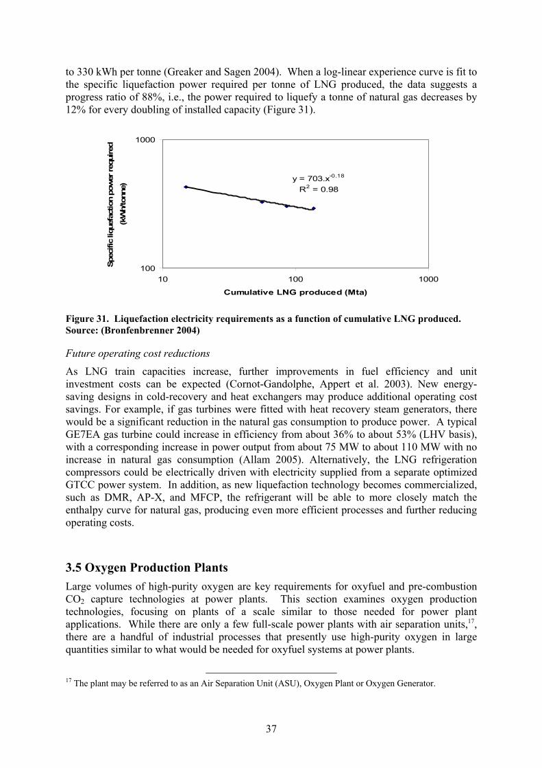
37

to 330 kWh per tonne (Greaker and Sagen 2004). When a log-linear experience curve is fit to the specific liquefaction power required per tonne of LNG produced, the data suggests a progress ratio of 88%, i.e., the power required to liquefy a tonne of natural gas decreases by 12% for every doubling of installed capacity (Figure 31).

y = 703.x-0.18

R2 = 0.98

100

1000

10 100 1000

Cumulative LNG produced (Mta)

Spec

ific

lique

fact

ion

pow

er re

quire

d (k

Wh/

tonn

e)

Figure 31. Liquefaction electricity requirements as a function of cumulative LNG produced. Source: (Bronfenbrenner 2004)

Future operating cost reductions

As LNG train capacities increase, further improvements in fuel efficiency and unit investment costs can be expected (Cornot-Gandolphe, Appert et al. 2003). New energy-saving designs in cold-recovery and heat exchangers may produce additional operating cost savings. For example, if gas turbines were fitted with heat recovery steam generators, there would be a significant reduction in the natural gas consumption to produce power. A typical GE7EA gas turbine could increase in efficiency from about 36% to about 53% (LHV basis), with a corresponding increase in power output from about 75 MW to about 110 MW with no increase in natural gas consumption (Allam 2005). Alternatively, the LNG refrigeration compressors could be electrically driven with electricity supplied from a separate optimized GTCC power system. In addition, as new liquefaction technology becomes commercialized, such as DMR, AP-X, and MFCP, the refrigerant will be able to more closely match the enthalpy curve for natural gas, producing even more efficient processes and further reducing operating costs.

3.5 Oxygen Production Plants Large volumes of high-purity oxygen are key requirements for oxyfuel and pre-combustion CO2 capture technologies at power plants. This section examines oxygen production technologies, focusing on plants of a scale similar to those needed for power plant applications. While there are only a few full-scale power plants with air separation units,17, there are a handful of industrial processes that presently use high-purity oxygen in large quantities similar to what would be needed for oxyfuel systems at power plants.

17 The plant may be referred to as an Air Separation Unit (ASU), Oxygen Plant or Oxygen Generator.

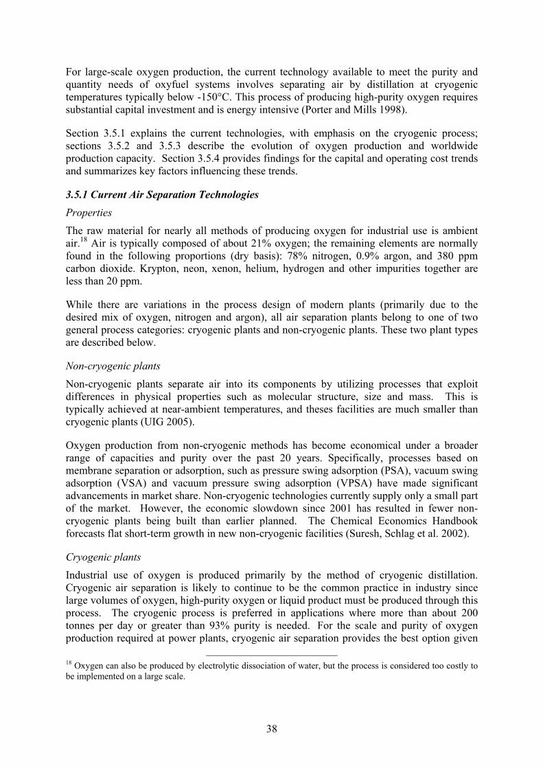
38

For large-scale oxygen production, the current technology available to meet the purity and quantity needs of oxyfuel systems involves separating air by distillation at cryogenic temperatures typically below -150°C. This process of producing high-purity oxygen requires substantial capital investment and is energy intensive (Porter and Mills 1998).

Section 3.5.1 explains the current technologies, with emphasis on the cryogenic process; sections 3.5.2 and 3.5.3 describe the evolution of oxygen production and worldwide production capacity. Section 3.5.4 provides findings for the capital and operating cost trends and summarizes key factors influencing these trends.

3.5.1 Current Air Separation Technologies

Properties

The raw material for nearly all methods of producing oxygen for industrial use is ambient air.18 Air is typically composed of about 21% oxygen; the remaining elements are normally found in the following proportions (dry basis): 78% nitrogen, 0.9% argon, and 380 ppm carbon dioxide. Krypton, neon, xenon, helium, hydrogen and other impurities together are less than 20 ppm.

While there are variations in the process design of modern plants (primarily due to the desired mix of oxygen, nitrogen and argon), all air separation plants belong to one of two general process categories: cryogenic plants and non-cryogenic plants. These two plant types are described below.

Non-cryogenic plants

Non-cryogenic plants separate air into its components by utilizing processes that exploit differences in physical properties such as molecular structure, size and mass. This is typically achieved at near-ambient temperatures, and theses facilities are much smaller than cryogenic plants (UIG 2005).

Oxygen production from non-cryogenic methods has become economical under a broader range of capacities and purity over the past 20 years. Specifically, processes based on membrane separation or adsorption, such as pressure swing adsorption (PSA), vacuum swing adsorption (VSA) and vacuum pressure swing adsorption (VPSA) have made significant advancements in market share. Non-cryogenic technologies currently supply only a small part of the market. However, the economic slowdown since 2001 has resulted in fewer non-cryogenic plants being built than earlier planned. The Chemical Economics Handbook forecasts flat short-term growth in new non-cryogenic facilities (Suresh, Schlag et al. 2002).

Cryogenic plants

Industrial use of oxygen is produced primarily by the method of cryogenic distillation. Cryogenic air separation is likely to continue to be the common practice in industry since large volumes of oxygen, high-purity oxygen or liquid product must be produced through this process. The cryogenic process is preferred in applications where more than about 200 tonnes per day or greater than 93% purity is needed. For the scale and purity of oxygen production required at power plants, cryogenic air separation provides the best option given

18 Oxygen can also be produced by electrolytic dissociation of water, but the process is considered too costly to be implemented on a large scale.

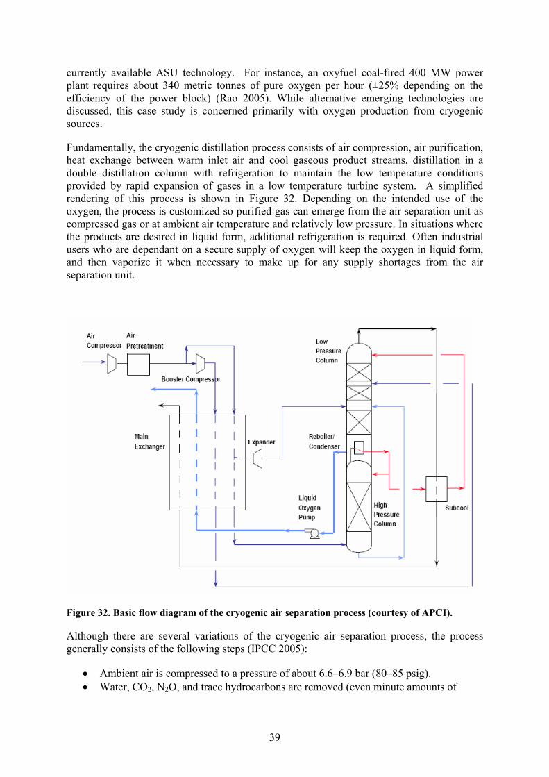
39

currently available ASU technology. For instance, an oxyfuel coal-fired 400 MW power plant requires about 340 metric tonnes of pure oxygen per hour (±25% depending on the efficiency of the power block) (Rao 2005). While alternative emerging technologies are discussed, this case study is concerned primarily with oxygen production from cryogenic sources.

Fundamentally, the cryogenic distillation process consists of air compression, air purification, heat exchange between warm inlet air and cool gaseous product streams, distillation in a double distillation column with refrigeration to maintain the low temperature conditions provided by rapid expansion of gases in a low temperature turbine system. A simplified rendering of this process is shown in Figure 32. Depending on the intended use of the oxygen, the process is customized so purified gas can emerge from the air separation unit as compressed gas or at ambient air temperature and relatively low pressure. In situations where the products are desired in liquid form, additional refrigeration is required. Often industrial users who are dependant on a secure supply of oxygen will keep the oxygen in liquid form, and then vaporize it when necessary to make up for any supply shortages from the air separation unit.

Figure 32. Basic flow diagram of the cryogenic air separation process (courtesy of APCI).

Although there are several variations of the cryogenic air separation process, the process generally consists of the following steps (IPCC 2005):

• Ambient air is compressed to a pressure of about 6.6–6.9 bar (80–85 psig). • Water, CO2, N2O, and trace hydrocarbons are removed (even minute amounts of

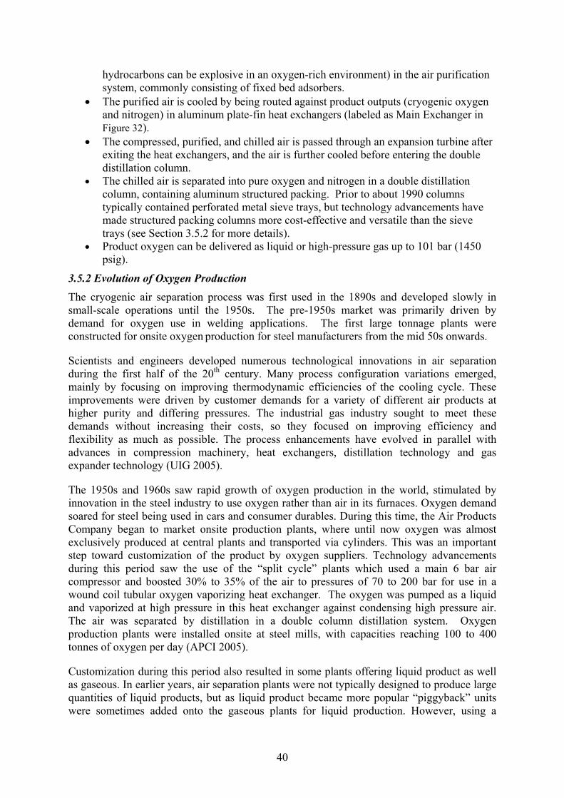
40

hydrocarbons can be explosive in an oxygen-rich environment) in the air purification system, commonly consisting of fixed bed adsorbers.

• The purified air is cooled by being routed against product outputs (cryogenic oxygen and nitrogen) in aluminum plate-fin heat exchangers (labeled as Main Exchanger in Figure 32).

• The compressed, purified, and chilled air is passed through an expansion turbine after exiting the heat exchangers, and the air is further cooled before entering the double distillation column.

• The chilled air is separated into pure oxygen and nitrogen in a double distillation column, containing aluminum structured packing. Prior to about 1990 columns typically contained perforated metal sieve trays, but technology advancements have made structured packing columns more cost-effective and versatile than the sieve trays (see Section 3.5.2 for more details).

• Product oxygen can be delivered as liquid or high-pressure gas up to 101 bar (1450 psig).

3.5.2 Evolution of Oxygen Production The cryogenic air separation process was first used in the 1890s and developed slowly in small-scale operations until the 1950s. The pre-1950s market was primarily driven by demand for oxygen use in welding applications. The first large tonnage plants were constructed for onsite oxygen production for steel manufacturers from the mid 50s onwards.

Scientists and engineers developed numerous technological innovations in air separation during the first half of the 20th century. Many process configuration variations emerged, mainly by focusing on improving thermodynamic efficiencies of the cooling cycle. These improvements were driven by customer demands for a variety of different air products at higher purity and differing pressures. The industrial gas industry sought to meet these demands without increasing their costs, so they focused on improving efficiency and flexibility as much as possible. The process enhancements have evolved in parallel with advances in compression machinery, heat exchangers, distillation technology and gas expander technology (UIG 2005).

The 1950s and 1960s saw rapid growth of oxygen production in the world, stimulated by innovation in the steel industry to use oxygen rather than air in its furnaces. Oxygen demand soared for steel being used in cars and consumer durables. During this time, the Air Products Company began to market onsite production plants, where until now oxygen was almost exclusively produced at central plants and transported via cylinders. This was an important step toward customization of the product by oxygen suppliers. Technology advancements during this period saw the use of the “split cycle” plants which used a main 6 bar air compressor and boosted 30% to 35% of the air to pressures of 70 to 200 bar for use in a wound coil tubular oxygen vaporizing heat exchanger. The oxygen was pumped as a liquid and vaporized at high pressure in this heat exchanger against condensing high pressure air. The air was separated by distillation in a double column distillation system. Oxygen production plants were installed onsite at steel mills, with capacities reaching 100 to 400 tonnes of oxygen per day (APCI 2005).

Customization during this period also resulted in some plants offering liquid product as well as gaseous. In earlier years, air separation plants were not typically designed to produce large quantities of liquid products, but as liquid product became more popular “piggyback” units were sometimes added onto the gaseous plants for liquid production. However, using a

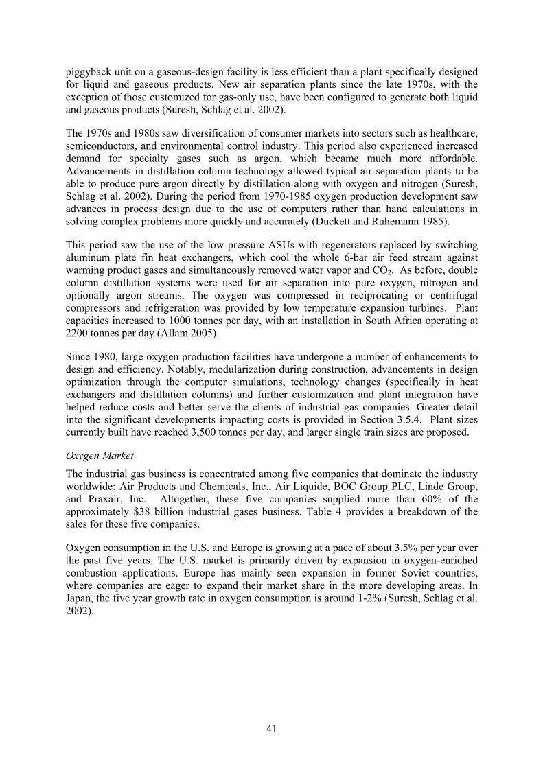
41

piggyback unit on a gaseous-design facility is less efficient than a plant specifically designed for liquid and gaseous products. New air separation plants since the late 1970s, with the exception of those customized for gas-only use, have been configured to generate both liquid and gaseous products (Suresh, Schlag et al. 2002).

The 1970s and 1980s saw diversification of consumer markets into sectors such as healthcare, semiconductors, and environmental control industry. This period also experienced increased demand for specialty gases such as argon, which became much more affordable. Advancements in distillation column technology allowed typical air separation plants to be able to produce pure argon directly by distillation along with oxygen and nitrogen (Suresh, Schlag et al. 2002). During the period from 1970-1985 oxygen production development saw advances in process design due to the use of computers rather than hand calculations in solving complex problems more quickly and accurately (Duckett and Ruhemann 1985).

This period saw the use of the low pressure ASUs with regenerators replaced by switching aluminum plate fin heat exchangers, which cool the whole 6-bar air feed stream against warming product gases and simultaneously removed water vapor and CO2. As before, double column distillation systems were used for air separation into pure oxygen, nitrogen and optionally argon streams. The oxygen was compressed in reciprocating or centrifugal compressors and refrigeration was provided by low temperature expansion turbines. Plant capacities increased to 1000 tonnes per day, with an installation in South Africa operating at 2200 tonnes per day (Allam 2005).

Since 1980, large oxygen production facilities have undergone a number of enhancements to design and efficiency. Notably, modularization during construction, advancements in design optimization through the computer simulations, technology changes (specifically in heat exchangers and distillation columns) and further customization and plant integration have helped reduce costs and better serve the clients of industrial gas companies. Greater detail into the significant developments impacting costs is provided in Section 3.5.4. Plant sizes currently built have reached 3,500 tonnes per day, and larger single train sizes are proposed.

Oxygen Market

The industrial gas business is concentrated among five companies that dominate the industry worldwide: Air Products and Chemicals, Inc., Air Liquide, BOC Group PLC, Linde Group, and Praxair, Inc. Altogether, these five companies supplied more than 60% of the approximately $38 billion industrial gases business. Table 4 provides a breakdown of the sales for these five companies.

Oxygen consumption in the U.S. and Europe is growing at a pace of about 3.5% per year over the past five years. The U.S. market is primarily driven by expansion in oxygen-enriched combustion applications. Europe has mainly seen expansion in former Soviet countries, where companies are eager to expand their market share in the more developing areas. In Japan, the five year growth rate in oxygen consumption is around 1-2% (Suresh, Schlag et al. 2002).

42

Table 4. Top suppliers of industrial gases worldwide in 2001. Source: (Suresh, Schlag et al. 2002)

Company 2000 Gas Sales

(million US$2000)

Air Liquide 7,159

Air Products and Chemicals, Inc 3,466

The BOC Group 4,681

Linde Group 4,106

Praxair, Inc 4,464

Others 14,100

TOTAL 37,976

The primary consumers of oxygen have shifted from welders in the first half of the 20th century to metals production (mostly steel) from about the 1940s to today. In the past 20 years a strong market for gasification and the use of oxygen in environmental technologies has proven to be a very strong growth area. Figure 33 and Figure 34 show consumption by sector and world region. Primary metals manufacture is still the largest market in all regions.

Clay, Glass, and Concrete Products

6%

Petroleum Refineries

6%

Welding/Cutting6%

Health Services4%

Pulp and Paper2%

Water Treatment1% Other

4%

Primary Metals Production

44%

Chemicals and Gasification

27%

Figure 33. Merchant consumers of oxygen in United States in 2001 (Suresh, Schlag et al. 2002).

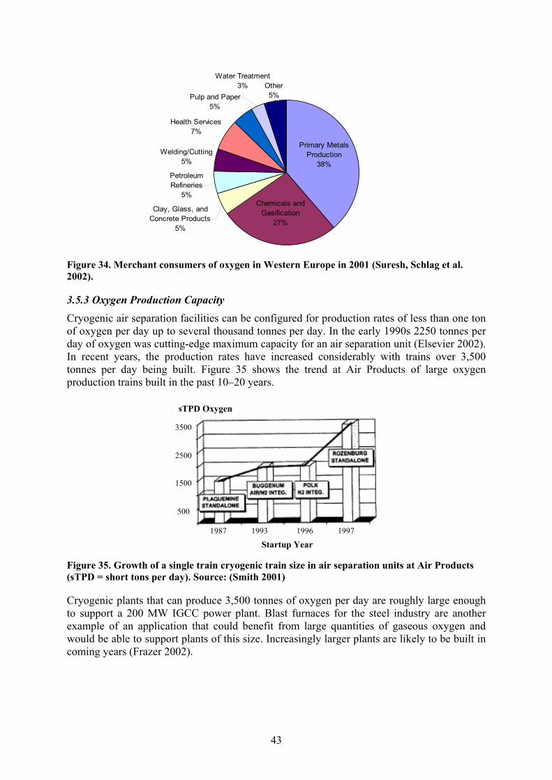
43

Clay, Glass, and Concrete Products

5%

Petroleum Refineries

5%

Welding/Cutting5%

Health Services7%

Pulp and Paper5%

Chemicals and Gasification

27%

Primary Metals Production

38%

Other5%

Water Treatment3%

Figure 34. Merchant consumers of oxygen in Western Europe in 2001 (Suresh, Schlag et al. 2002).

3.5.3 Oxygen Production Capacity Cryogenic air separation facilities can be configured for production rates of less than one ton of oxygen per day up to several thousand tonnes per day. In the early 1990s 2250 tonnes per day of oxygen was cutting-edge maximum capacity for an air separation unit (Elsevier 2002). In recent years, the production rates have increased considerably with trains over 3,500 tonnes per day being built. Figure 35 shows the trend at Air Products of large oxygen production trains built in the past 10–20 years.

Startup Year

sTPD Oxygen

1987 1993 1996 1997

500

1500

2500

3500

Figure 35. Growth of a single train cryogenic train size in air separation units at Air Products (sTPD = short tons per day). Source: (Smith 2001)

Cryogenic plants that can produce 3,500 tonnes of oxygen per day are roughly large enough to support a 200 MW IGCC power plant. Blast furnaces for the steel industry are another example of an application that could benefit from large quantities of gaseous oxygen and would be able to support plants of this size. Increasingly larger plants are likely to be built in coming years (Frazer 2002).

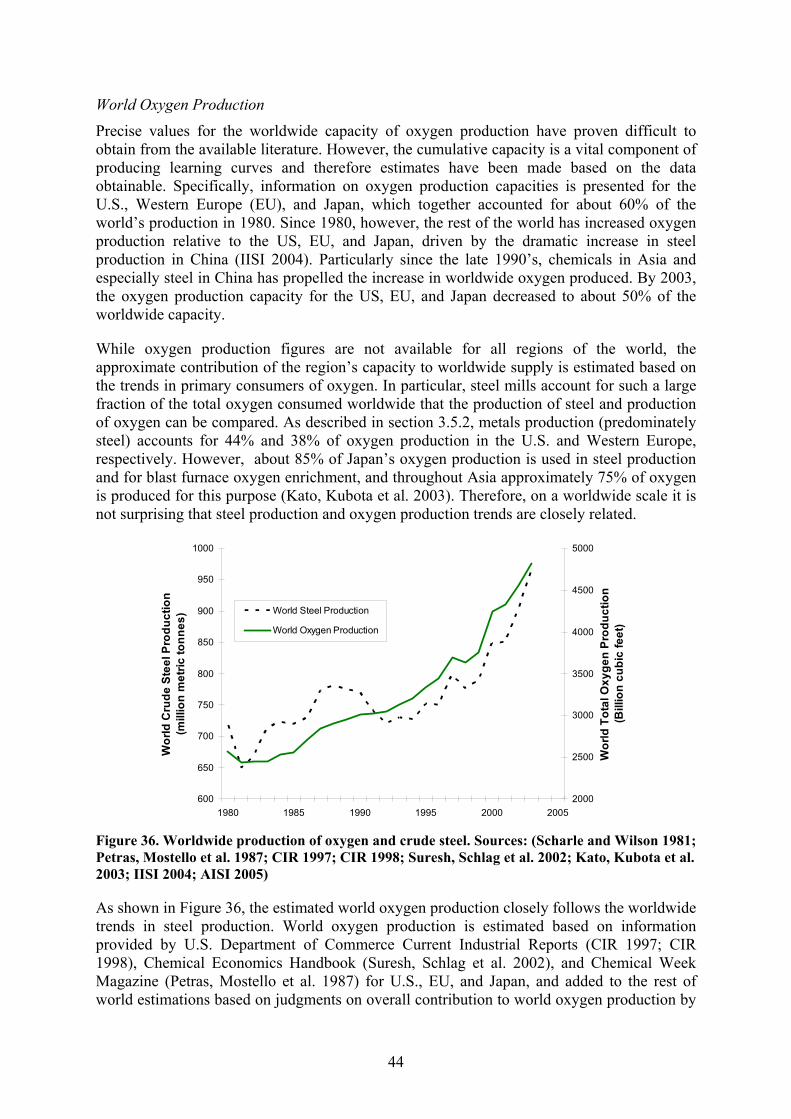
44

World Oxygen Production

Precise values for the worldwide capacity of oxygen production have proven difficult to obtain from the available literature. However, the cumulative capacity is a vital component of producing learning curves and therefore estimates have been made based on the data obtainable. Specifically, information on oxygen production capacities is presented for the U.S., Western Europe (EU), and Japan, which together accounted for about 60% of the world’s production in 1980. Since 1980, however, the rest of the world has increased oxygen production relative to the US, EU, and Japan, driven by the dramatic increase in steel production in China (IISI 2004). Particularly since the late 1990’s, chemicals in Asia and especially steel in China has propelled the increase in worldwide oxygen produced. By 2003, the oxygen production capacity for the US, EU, and Japan decreased to about 50% of the worldwide capacity.

While oxygen production figures are not available for all regions of the world, the approximate contribution of the region’s capacity to worldwide supply is estimated based on the trends in primary consumers of oxygen. In particular, steel mills account for such a large fraction of the total oxygen consumed worldwide that the production of steel and production of oxygen can be compared. As described in section 3.5.2, metals production (predominately steel) accounts for 44% and 38% of oxygen production in the U.S. and Western Europe, respectively. However, about 85% of Japan’s oxygen production is used in steel production and for blast furnace oxygen enrichment, and throughout Asia approximately 75% of oxygen is produced for this purpose (Kato, Kubota et al. 2003). Therefore, on a worldwide scale it is not surprising that steel production and oxygen production trends are closely related.

600

650

700

750

800

850

900

950

1000

1980 1985 1990 1995 2000 2005

Wor

ld C

rude

Ste

el P

rodu

ctio

n (m

illio

n m

etric

tonn

es)

2000

2500

3000

3500

4000

4500

5000

Wor

ld T

otal

Oxy

gen

Prod

uctio

n (B

illio

n cu

bic

feet

)World Steel Production

World Oxygen Production

Figure 36. Worldwide production of oxygen and crude steel. Sources: (Scharle and Wilson 1981; Petras, Mostello et al. 1987; CIR 1997; CIR 1998; Suresh, Schlag et al. 2002; Kato, Kubota et al. 2003; IISI 2004; AISI 2005)

As shown in Figure 36, the estimated world oxygen production closely follows the worldwide trends in steel production. World oxygen production is estimated based on information provided by U.S. Department of Commerce Current Industrial Reports (CIR 1997; CIR 1998), Chemical Economics Handbook (Suresh, Schlag et al. 2002), and Chemical Week Magazine (Petras, Mostello et al. 1987) for U.S., EU, and Japan, and added to the rest of world estimations based on judgments on overall contribution to world oxygen production by

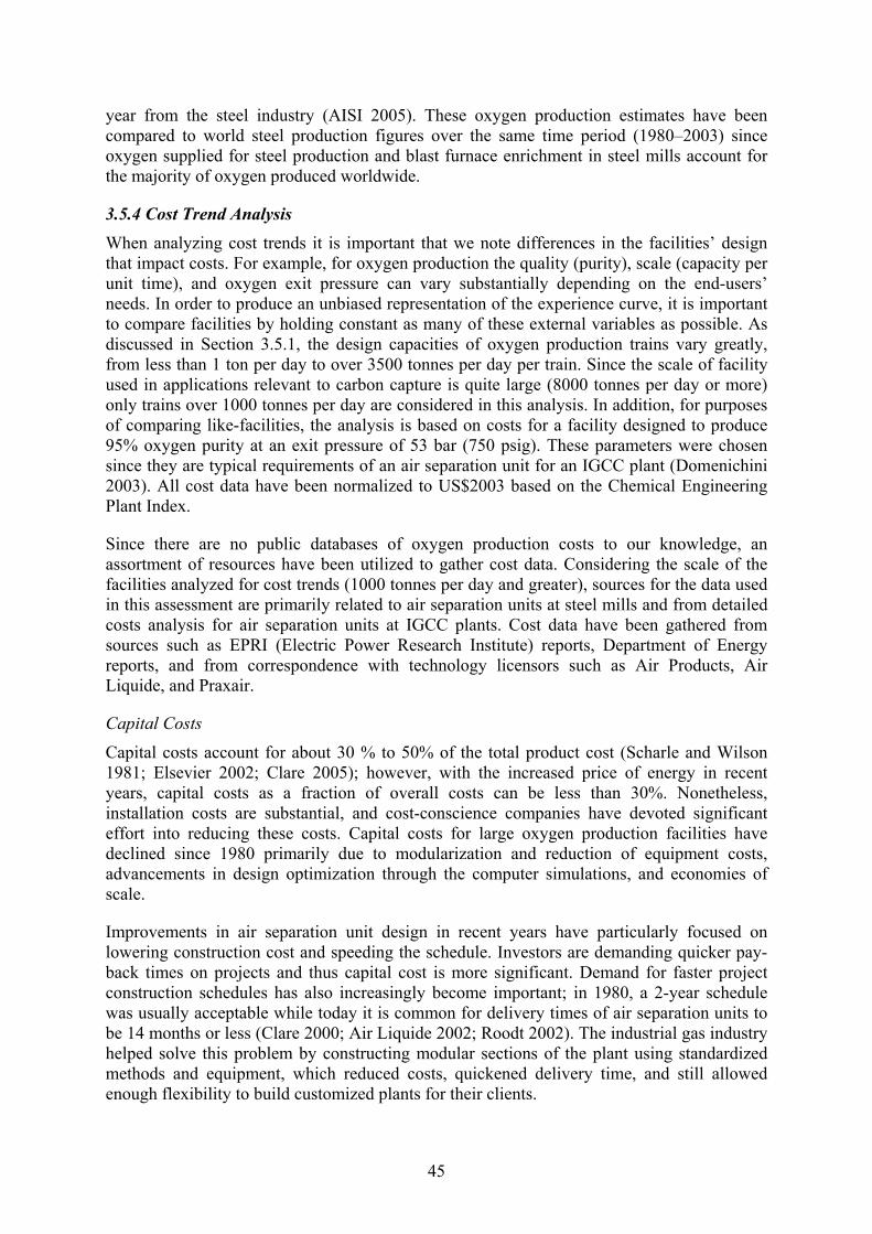
45

year from the steel industry (AISI 2005). These oxygen production estimates have been compared to world steel production figures over the same time period (1980–2003) since oxygen supplied for steel production and blast furnace enrichment in steel mills account for the majority of oxygen produced worldwide.

3.5.4 Cost Trend Analysis When analyzing cost trends it is important that we note differences in the facilities’ design that impact costs. For example, for oxygen production the quality (purity), scale (capacity per unit time), and oxygen exit pressure can vary substantially depending on the end-users’ needs. In order to produce an unbiased representation of the experience curve, it is important to compare facilities by holding constant as many of these external variables as possible. As discussed in Section 3.5.1, the design capacities of oxygen production trains vary greatly, from less than 1 ton per day to over 3500 tonnes per day per train. Since the scale of facility used in applications relevant to carbon capture is quite large (8000 tonnes per day or more) only trains over 1000 tonnes per day are considered in this analysis. In addition, for purposes of comparing like-facilities, the analysis is based on costs for a facility designed to produce 95% oxygen purity at an exit pressure of 53 bar (750 psig). These parameters were chosen since they are typical requirements of an air separation unit for an IGCC plant (Domenichini 2003). All cost data have been normalized to US$2003 based on the Chemical Engineering Plant Index.

Since there are no public databases of oxygen production costs to our knowledge, an assortment of resources have been utilized to gather cost data. Considering the scale of the facilities analyzed for cost trends (1000 tonnes per day and greater), sources for the data used in this assessment are primarily related to air separation units at steel mills and from detailed costs analysis for air separation units at IGCC plants. Cost data have been gathered from sources such as EPRI (Electric Power Research Institute) reports, Department of Energy reports, and from correspondence with technology licensors such as Air Products, Air Liquide, and Praxair.

Capital Costs

Capital costs account for about 30 % to 50% of the total product cost (Scharle and Wilson 1981; Elsevier 2002; Clare 2005); however, with the increased price of energy in recent years, capital costs as a fraction of overall costs can be less than 30%. Nonetheless, installation costs are substantial, and cost-conscience companies have devoted significant effort into reducing these costs. Capital costs for large oxygen production facilities have declined since 1980 primarily due to modularization and reduction of equipment costs, advancements in design optimization through the computer simulations, and economies of scale.

Improvements in air separation unit design in recent years have particularly focused on lowering construction cost and speeding the schedule. Investors are demanding quicker pay-back times on projects and thus capital cost is more significant. Demand for faster project construction schedules has also increasingly become important; in 1980, a 2-year schedule was usually acceptable while today it is common for delivery times of air separation units to be 14 months or less (Clare 2000; Air Liquide 2002; Roodt 2002). The industrial gas industry helped solve this problem by constructing modular sections of the plant using standardized methods and equipment, which reduced costs, quickened delivery time, and still allowed enough flexibility to build customized plants for their clients.

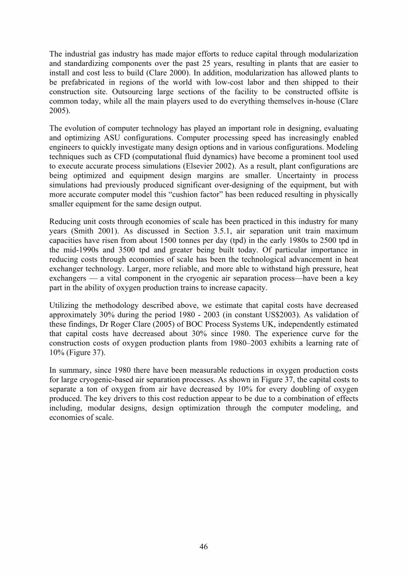
46

The industrial gas industry has made major efforts to reduce capital through modularization and standardizing components over the past 25 years, resulting in plants that are easier to install and cost less to build (Clare 2000). In addition, modularization has allowed plants to be prefabricated in regions of the world with low-cost labor and then shipped to their construction site. Outsourcing large sections of the facility to be constructed offsite is common today, while all the main players used to do everything themselves in-house (Clare 2005).

The evolution of computer technology has played an important role in designing, evaluating and optimizing ASU configurations. Computer processing speed has increasingly enabled engineers to quickly investigate many design options and in various configurations. Modeling techniques such as CFD (computational fluid dynamics) have become a prominent tool used to execute accurate process simulations (Elsevier 2002). As a result, plant configurations are being optimized and equipment design margins are smaller. Uncertainty in process simulations had previously produced significant over-designing of the equipment, but with more accurate computer model this “cushion factor” has been reduced resulting in physically smaller equipment for the same design output.

Reducing unit costs through economies of scale has been practiced in this industry for many years (Smith 2001). As discussed in Section 3.5.1, air separation unit train maximum capacities have risen from about 1500 tonnes per day (tpd) in the early 1980s to 2500 tpd in the mid-1990s and 3500 tpd and greater being built today. Of particular importance in reducing costs through economies of scale has been the technological advancement in heat exchanger technology. Larger, more reliable, and more able to withstand high pressure, heat exchangers — a vital component in the cryogenic air separation process—have been a key part in the ability of oxygen production trains to increase capacity.

Utilizing the methodology described above, we estimate that capital costs have decreased approximately 30% during the period 1980 - 2003 (in constant US$2003). As validation of these findings, Dr Roger Clare (2005) of BOC Process Systems UK, independently estimated that capital costs have decreased about 30% since 1980. The experience curve for the construction costs of oxygen production plants from 1980–2003 exhibits a learning rate of 10% (Figure 37).

In summary, since 1980 there have been measurable reductions in oxygen production costs for large cryogenic-based air separation processes. As shown in Figure 37, the capital costs to separate a ton of oxygen from air have decreased by 10% for every doubling of oxygen produced. The key drivers to this cost reduction appear to be due to a combination of effects including, modular designs, design optimization through the computer modeling, and economies of scale.

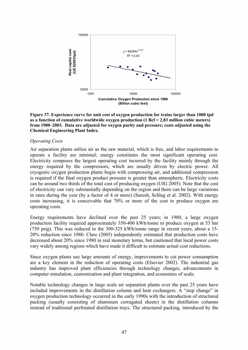
47

y = 94254x-0.157

R2 = 0.43

10000

100000

1000 10000 100000

Cumulative Oxygen Production since 1980(Billion cubic feet)

Rea

l cap

ital c

ost

(US

$200

3/tp

d)

Figure 37. Experience curve for unit cost of oxygen production for trains larger than 1000 tpd as a function of cumulative worldwide oxygen production (1 Bcf = 2.83 million cubic meters) from 1980–2003. Data are adjusted for oxygen purity and pressure; costs adjusted using the Chemical Engineering Plant Index.

Operating Costs

Air separation plants utilize air as the raw material, which is free, and labor requirements to operate a facility are minimal; energy constitutes the most significant operating cost. Electricity composes the largest operating cost incurred by the facility mainly through the energy required by the compressors, which are usually driven by electric power. All cryogenic oxygen production plants begin with compressing air, and additional compression is required if the final oxygen product pressure is greater than atmospheric. Electricity costs can be around two thirds of the total cost of producing oxygen (UIG 2005). Note that the cost of electricity can vary substantially depending on the region and there can be large variations in rates during the year (by a factor of 4 or more) (Suresh, Schlag et al. 2002). With energy costs increasing, it is conceivable that 70% or more of the cost to produce oxygen are operating costs.

Energy requirements have declined over the past 25 years; in 1980, a large oxygen production facility required approximately 350-400 kWh/tonne to produce oxygen at 53 bar (750 psig). This was reduced to the 300-325 kWh/tonne range in recent years, about a 15-20% reduction since 1980. Clare (2005) independently estimated that production costs have decreased about 20% since 1980 in real monetary terms, but cautioned that local power costs vary widely among regions which have made it difficult to estimate actual cost reductions.

Since oxygen plants use large amounts of energy, improvements to cut power consumption are a key element in the reduction of operating costs (Elsevier 2002). The industrial gas industry has improved plant efficiencies through technology changes, advancements in computer simulation, customization and plant integration, and economies of scale.

Notable technology changes in large scale air separation plants over the past 25 years have included improvements in the distillation column and heat exchangers. A “step change” in oxygen production technology occurred in the early 1990s with the introduction of structured packing (usually consisting of aluminum corrugated sheets) in the distillation columns instead of traditional perforated distillation trays. The structured packing, introduced by the

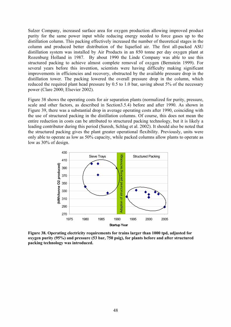
48

Sulzer Company, increased surface area for oxygen production allowing improved product purity for the same power input while reducing energy needed to force gases up to the distillation column. This packing effectively increased the number of theoretical stages in the column and produced better distribution of the liquefied air. The first all-packed ASU distillation system was installed by Air Products in an 850 tonne per day oxygen plant at Rozenburg Holland in 1987. By about 1990 the Linde Company was able to use this structured packing to achieve almost complete removal of oxygen (Bernstein 1999). For several years before this invention, scientists were having difficulty making significant improvements in efficiencies and recovery, obstructed by the available pressure drop in the distillation tower. The packing lowered the overall pressure drop in the column, which reduced the required plant head pressure by 0.5 to 1.0 bar, saving about 5% of the necessary power (Clare 2000; Elsevier 2002).

Figure 38 shows the operating costs for air separation plants (normalized for purity, pressure, scale and other factors, as described in Section3.5.4) before and after 1990. As shown in Figure 39, there was a substantial drop in average operating costs after 1990, coinciding with the use of structured packing in the distillation columns. Of course, this does not mean the entire reduction in costs can be attributed to structured packing technology, but it is likely a leading contributor during this period (Suresh, Schlag et al. 2002). It should also be noted that the structured packing gives the plant greater operational flexibility. Previously, units were only able to operate as low as 50% capacity, while packed columns allow plants to operate as low as 30% of design.

270

290

310

330

350

370

390

410

430

1975 1980 1985 1990 1995 2000 2005

Startup Year

(kW

h/to

nne

O2

prod

uced

)

Structured Packing

Adop

tion

of s

truct

ured

pac

king

tech

nolo

gy_

Sieve Trays

Figure 38. Operating electricity requirements for trains larger than 1000 tpd, adjusted for oxygen purity (95%) and pressure (53 bar, 750 psig), for plants before and after structured packing technology was introduced.

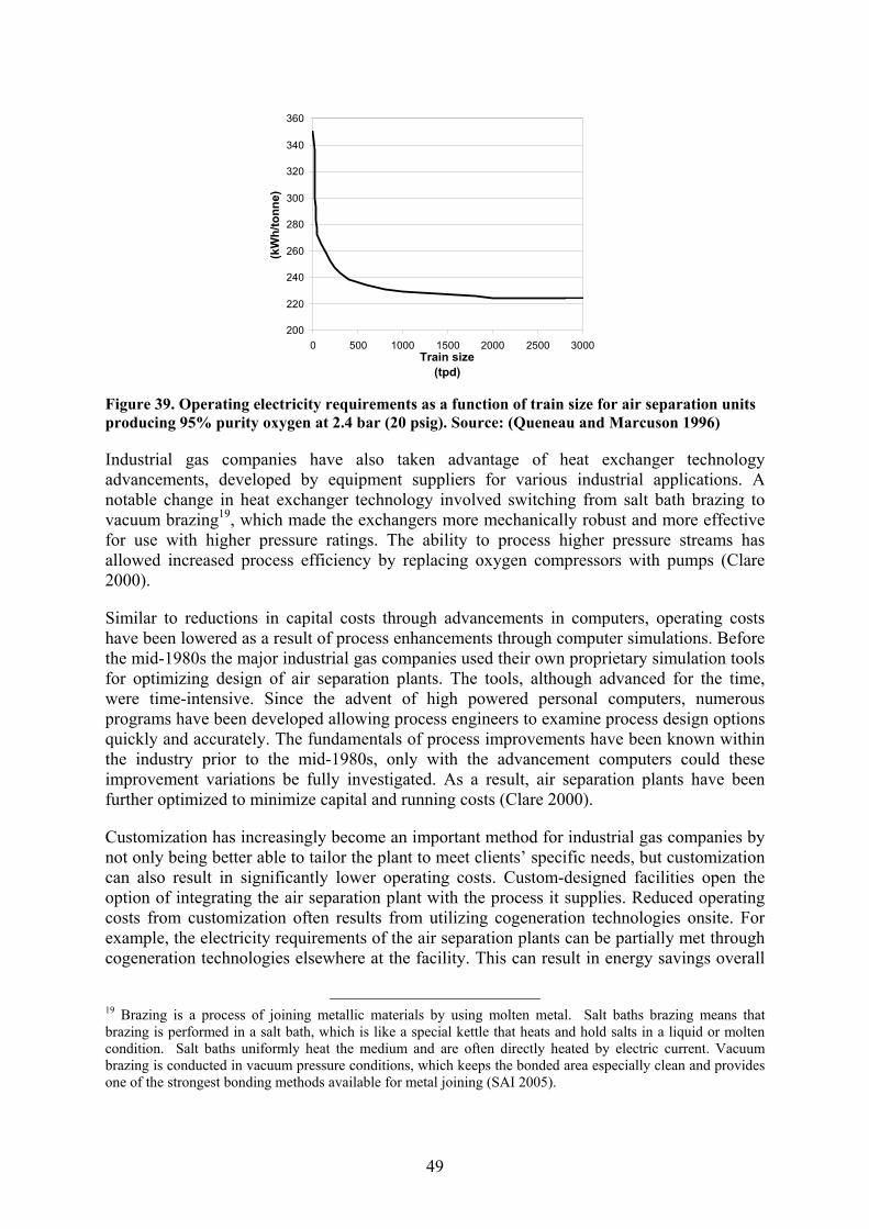
49

200

220

240

260

280

300

320

340

360

0 500 1000 1500 2000 2500 3000Train size

(tpd)

(kW

h/to

nne)

Figure 39. Operating electricity requirements as a function of train size for air separation units producing 95% purity oxygen at 2.4 bar (20 psig). Source: (Queneau and Marcuson 1996)

Industrial gas companies have also taken advantage of heat exchanger technology advancements, developed by equipment suppliers for various industrial applications. A notable change in heat exchanger technology involved switching from salt bath brazing to vacuum brazing19, which made the exchangers more mechanically robust and more effective for use with higher pressure ratings. The ability to process higher pressure streams has allowed increased process efficiency by replacing oxygen compressors with pumps (Clare 2000).

Similar to reductions in capital costs through advancements in computers, operating costs have been lowered as a result of process enhancements through computer simulations. Before the mid-1980s the major industrial gas companies used their own proprietary simulation tools for optimizing design of air separation plants. The tools, although advanced for the time, were time-intensive. Since the advent of high powered personal computers, numerous programs have been developed allowing process engineers to examine process design options quickly and accurately. The fundamentals of process improvements have been known within the industry prior to the mid-1980s, only with the advancement computers could these improvement variations be fully investigated. As a result, air separation plants have been further optimized to minimize capital and running costs (Clare 2000).

Customization has increasingly become an important method for industrial gas companies by not only being better able to tailor the plant to meet clients’ specific needs, but customization can also result in significantly lower operating costs. Custom-designed facilities open the option of integrating the air separation plant with the process it supplies. Reduced operating costs from customization often results from utilizing cogeneration technologies onsite. For example, the electricity requirements of the air separation plants can be partially met through cogeneration technologies elsewhere at the facility. This can result in energy savings overall

19 Brazing is a process of joining metallic materials by using molten metal. Salt baths brazing means that brazing is performed in a salt bath, which is like a special kettle that heats and hold salts in a liquid or molten condition. Salt baths uniformly heat the medium and are often directly heated by electric current. Vacuum brazing is conducted in vacuum pressure conditions, which keeps the bonded area especially clean and provides one of the strongest bonding methods available for metal joining (SAI 2005).

50

at the facility up to 30% compared to non-integrated air separation processes (Suresh, Schlag et al. 2002).

It should be noted that some process variants, such as using multiple reboilers for the distillation column or reflux enhancement equipment, can increase plant efficiency but at the expense of increasing capital costs. While these enhancements may decrease power requirements, it may not be the most economically desirable outcome. These sort of trade-offs are generally evaluated depending on the cost of electricity at the plant site (Clare 2000).

Economies of scale can provide energy savings per unit of oxygen produced. In general, the impact is greatest for small facilities (producing less than about 50 tonnes of oxygen per day). For the facilities considered in this analysis – those greater than 1000 tpd – the power savings through increased train size is substantially less. Queneau (1996) gives an estimate of the relationship between power used and oxygen production train size (Figure 39).

Evidence of technical advancement can be measured through the reduced energy requirements per unit of oxygen produced. As noted above, operating costs have declined about 15-20% over the past 25 years, similar to an industry expert’s estimation of 20% over the same time period (Clare 2005). In 1980, air separation units producing over 1000 tpd of 95% pure oxygen at 53 bar (750 psig) required about 350-400 kWh/tonne O2. In recent years, new plants are operating in the 300-325 kWh/tonne range. Plotting the energy requirements against the cumulative oxygen production gives the experience curve as shown in Figure 40. The operating costs of oxygen production plants from 1980–2003 has a progress ratio of 0.95, or a learning rate of 5%.

y = 731x-0.08

R2 = 0.42

100

1000

1000 10000 100000

Cumulative Oxygen Production since 1980(Billion cubic feet)

Ope

ratin

g El

ectr

icity

_(k

Wh/

tonn

e)

Figure 40. Experience curve for oxygen production electricity requirement (as a measure of unit operating cost) as a function of cumulative worldwide oxygen production (1 Bcf = 2.83 million cubic meters) from 1980–2003, based on trains larger than 1000 tpd and adjusted for oxygen purity (95%) and pressure (53 bar, 750 psig).

In summary, running costs have moderately declined since 1980. As shown in Figure 40, the operating costs have decreased by about 5% for every doubling of oxygen produced. The key drivers of operating cost reductions are multiple factors that include technology

51

improvements in the component equipment, technology advancements in computers, customization and plant integration, and economies of scale.

Taken together, capital costs and operating costs have declined about 1% per year over the past 25 years. Assuming that capital costs account for 40% of overall costs, and operating costs account for 60%, the overall reduction amounts to (0.3) x 40% (capital costs reduced 30% as stated above) plus (0.2) x 60% (operating costs decreased about 20%), which equates to about a 24% reduction over 25 years. A director of technology planning at Praxair, Inc. independently estimated that the industry normally expects to reduce costs by about 1% per year (Solomon 2005).

Future Prospects for Oxygen Production Cost Trends

After many years of enhancements in cryogenic air separation technology, oxygen production consists of an extremely efficient distillation process with few significant technical breakthroughs expected that would lead to a step change in costs (Suresh, Schlag et al. 2002; Armstrong and Foster 2004). However, research currently underway in non-cryogenic technology may dramatically change the process for producing oxygen in large-scale operations and greatly reduce costs. Companies such as Praxair and Air Products in collaboration with the U.S. Department of Energy are researching new methods for air separation, with the most promising of current research involving ceramic membranes that selectively separate oxygen from air in a process called Ion Transport Membrane (ITM). This technology could decrease the energy required per unit of oxygen by 35-50% and reduce capital costs by 25-35% (Frazer 2002; Armstrong and Foster 2004).

In the ITM process, ambient air is heated and compressed before contacting a ceramic membrane. The oxygen in the air becomes ionized on the surface of the ceramic, which allows the oxygen to selectively pass through the membrane while preventing impurities such as nitrogen from diffusing through. This technology currently is able to deliver only about 3 tonnes of oxygen product per day, but a U.S. government and gas industry partnership projects that large scale oxygen production ITM plants will be available towards the end of the decade. Figure 41 shows the ITM development program goals.

Figure 41. ITM oxygen production development program goals for U.S. government and gas industry partnership. Source: (Armstrong and Foster 2004)

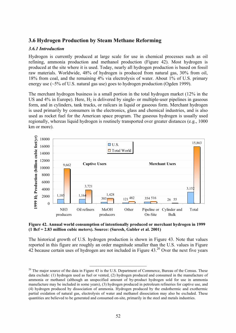
52

3.6 Hydrogen Production by Steam Methane Reforming 3.6.1 Introduction Hydrogen is currently produced at large scale for use in chemical processes such as oil refining, ammonia production and methanol production (Figure 42). Most hydrogen is produced at the site where it is used. Today, nearly all hydrogen production is based on fossil raw materials. Worldwide, 48% of hydrogen is produced from natural gas, 30% from oil, 18% from coal, and the remaining 4% via electrolysis of water. About 1% of U.S. primary energy use (~5% of U.S. natural gas use) goes to hydrogen production (Ogden 1999).

The merchant hydrogen business is a small portion in the total hydrogen market (12% in the US and 4% in Europe). Here, H2 is delivered by single- or multiple-user pipelines in gaseous form, and in cylinders, tank trucks, or railcars in liquid or gaseous form. Merchant hydrogen is used primarily by consumers in the electronics, glass and chemical industries, and is also used as rocket fuel for the American space program. The gaseous hydrogen is usually used regionally, whereas liquid hydrogen is routinely transported over greater distances (e.g., 1000 km or more).

1,185 1,164303 121 354 26

3,152

9,662

3,721

1,428482 516 55

15,863

0

2000

4000

6000

8000

10000

12000

14000

16000

18000

NH3producers

Oil refiners MeOHproducers

Other Pipeline orOn-Site

Cylinder andBulk

Total1999

H2 P

rodu

ctio

n (b

illio

n cu

bic

feet

/yr)

U.S.Total World

Captive Users Merchant Users

Figure 42. Annual world consumption of intentionally produced or merchant hydrogen in 1999 (1 Bcf = 2.83 million cubic meters). Source: (Suresh, Gubler et al. 2001)

The historical growth of U.S. hydrogen production is shown in Figure 43. Note that values reported in this figure are roughly an order magnitude smaller than the U.S. values in Figure 42 because certain uses of hydrogen are not included in Figure 43.20 Over the next five years

20 The major source of the data in Figure 43 is the U.S. Department of Commerce, Bureau of the Census. These data exclude: (1) hydrogen used as fuel or vented, (2) hydrogen produced and consumed in the manufacture of ammonia or methanol (although an unspecified amount of by-product hydrogen sold for use in ammonia manufacture may be included in some years), (3) hydrogen produced in petroleum refineries for captive use, and (4) hydrogen produced by dissociation of ammonia. Hydrogen produced by the endothermic and exothermic partial oxidation of natural gas, electrolysis of water and methanol dissociation may also be excluded. These quantities are believed to be generated and consumed on-site, primarily in the steel and metals industries.

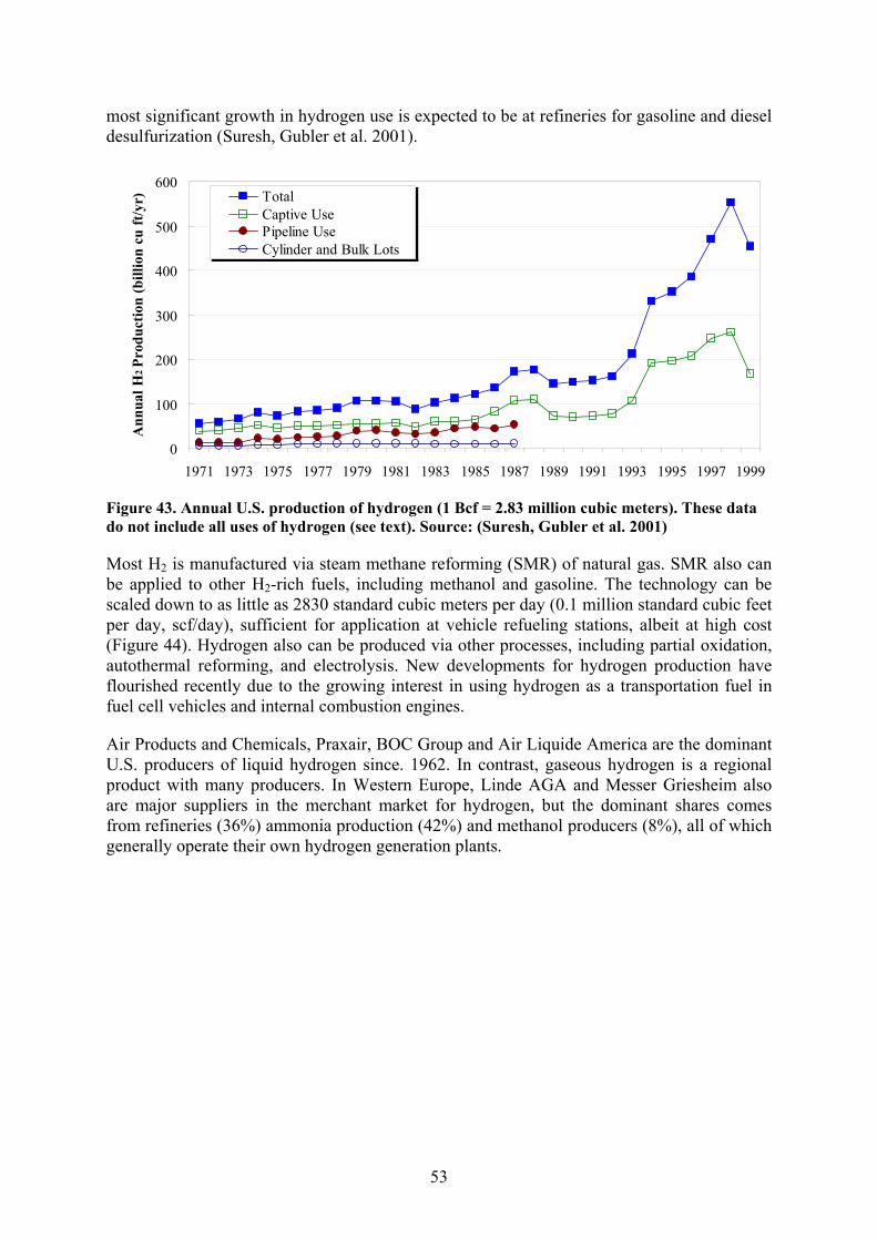
53

most significant growth in hydrogen use is expected to be at refineries for gasoline and diesel desulfurization (Suresh, Gubler et al. 2001).

0

100

200

300

400

500

600

1971 1973 1975 1977 1979 1981 1983 1985 1987 1989 1991 1993 1995 1997 1999

Ann

ual H

2 Pr

oduc

tion

(bill

ion

cu ft

/yr) Total

Captive UsePipeline UseCylinder and Bulk Lots

Figure 43. Annual U.S. production of hydrogen (1 Bcf = 2.83 million cubic meters). These data do not include all uses of hydrogen (see text). Source: (Suresh, Gubler et al. 2001)

Most H2 is manufactured via steam methane reforming (SMR) of natural gas. SMR also can be applied to other H2-rich fuels, including methanol and gasoline. The technology can be scaled down to as little as 2830 standard cubic meters per day (0.1 million standard cubic feet per day, scf/day), sufficient for application at vehicle refueling stations, albeit at high cost (Figure 44). Hydrogen also can be produced via other processes, including partial oxidation, autothermal reforming, and electrolysis. New developments for hydrogen production have flourished recently due to the growing interest in using hydrogen as a transportation fuel in fuel cell vehicles and internal combustion engines.

Air Products and Chemicals, Praxair, BOC Group and Air Liquide America are the dominant U.S. producers of liquid hydrogen since. 1962. In contrast, gaseous hydrogen is a regional product with many producers. In Western Europe, Linde AGA and Messer Griesheim also are major suppliers in the merchant market for hydrogen, but the dominant shares comes from refineries (36%) ammonia production (42%) and methanol producers (8%), all of which generally operate their own hydrogen generation plants.

54

$0$500

$1,000$1,500$2,000$2,500$3,000$3,500$4,000$4,500

100 1,000 10,000 100,000 1,000,000 10,000,000Size (kg/d H2)

Cap

ital C

ost (

2000

$/kg

/d H

2) Current TechnologyFuture technologyCurrent with CCSFuture with CCS

Figure 44. Estimated capital cost of hydrogen production using SMR technology in three plant sizes, current and possible future cases, with and without sequestration of CO2. Source: (National Research Council 2004)

3.6.2 Steam Methane Reforming Technology Catalytic steam reforming of methane (the main component of natural gas) is a well-known, commercially available process for hydrogen production (Rostrup-Nielsen 1984; Twigg 1989). In the United States, most hydrogen (~95%) is now manufactured via steam methane reforming (SMR) of natural gas. Other feedstocks, though less commonly used, include ethane, propane, butane and light and heavy naphtha. Steam reforming of hydrocarbons for ammonia production was introduced in 1930. The energy intensive nature of the process is the key driving force for improving the technology and reducing the overall cost of manufacturing. The energy consumption for ammonia production changed from an early level of 20 Gcal/tonne (79.4 MBtu/tonne) to about 7 Gcal/tonne (27.8 MBtu/tonne) in the last two decades (Worrell and Blok 1994; Agarwal 2004).

The SMR process produces a mixture of hydrogen and carbon monoxide commonly known as syngas. When hydrogen is the only desired product, the carbon monoxide is converted to carbon dioxide via the water-gas shift reaction. Subsequently, the hydrogen and CO2 are separated using either amine-based absorption or pressure swing adsorption (PSA) units (Figure 45). Traditional purification using amine-based absorption systems are capable of producing a by-product CO2 stream that is 99.8% pure by volume. Pressure swing adsorption (PSA) systems have been increasingly used for hydrogen purification since the late-1980s. This improves H2 purity to 99.999%, albeit at higher cost, but produces a by-product CO2 stream that is only 50% CO2 by volume, making that stream less attractive as a by-product source.

Over the years, the steam reforming process has undergone significant improvement, as shown in Table 5. Advanced engineering, more compact designs, shorter construction schedules and modular reformer construction have resulted in a significant reduction in plant cost, as discussed in the next section. Also note that recent increased concerns about NOx emissions in the fuel gas from the furnace has led to the inclusion of low-NOx burners and also catalytic NOx reduction units in the convection sections (Allam 2005).

55

Figure 45. Steam reforming of natural gas hydrogen plant with PSA (Fleshman, McEvoy et al. 1999).

Table 5. Summary of improvements made to the steam reforming technology.

Reforming Longer catalyst life time through better burner designs that produce more uniform heat flux

Higher operating pressure Improvements in reliability of hydrogen production Increase in reformer outlet temperature, which increases the yield of H2,

reduces methane slip in the flue gas, and reduces the energy demand of the PSA unit

Reduction in steam to carbon ratio Pre-reforming of the natural gas to reduce excess steam production Pre-heating of the air feed to the burners Reduce excess steam production

Modularization and

standardization

Standardization and modularization of plant components allows maximum shop assembly and reduces onsite labor and customization.

Shift conversion Better catalyst in the shift reactor increases the ease of operation, improves reliability, and reduces cost.

Heat recovery Increase in pressure drop reduces the size of air coolers

3.6.3 Difficulties of Cost Estimation for SMR

A systematic cost comparison of hydrogen production via steam methane reforming is difficult to estimate because hydrogen production cost depends on many factors, including the size of the plant, the type of feed gas, the purity of the hydrogen produced, and whether available export steam is desired. Most studies report only the total manufacturing cost of hydrogen, which combines the total capital cost with the costs of utilities, feedstock, cooling water, export steam, and labor—but with no explicit documentation of the specific assumptions or contribution of cost components. Due to lack of such data, it is impossible to adjust reported values to the same basis for comparisons. Other factors that affect the economics of SMR include the following:

Type of feedstock. A wide range of light hydrocarbon feedstocks can be used in the SMR process to produce hydrogen. Economics varies widely depending on the fuel composition.

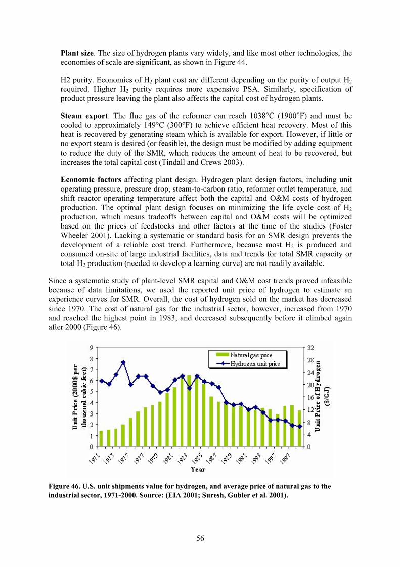
56

Plant size. The size of hydrogen plants vary widely, and like most other technologies, the economies of scale are significant, as shown in Figure 44.

H2 purity. Economics of H2 plant cost are different depending on the purity of output H2 required. Higher H2 purity requires more expensive PSA. Similarly, specification of product pressure leaving the plant also affects the capital cost of hydrogen plants.

Steam export. The flue gas of the reformer can reach 1038°C (1900°F) and must be cooled to approximately 149°C (300°F) to achieve efficient heat recovery. Most of this heat is recovered by generating steam which is available for export. However, if little or no export steam is desired (or feasible), the design must be modified by adding equipment to reduce the duty of the SMR, which reduces the amount of heat to be recovered, but increases the total capital cost (Tindall and Crews 2003).

Economic factors affecting plant design. Hydrogen plant design factors, including unit operating pressure, pressure drop, steam-to-carbon ratio, reformer outlet temperature, and shift reactor operating temperature affect both the capital and O&M costs of hydrogen production. The optimal plant design focuses on minimizing the life cycle cost of H2 production, which means tradeoffs between capital and O&M costs will be optimized based on the prices of feedstocks and other factors at the time of the studies (Foster Wheeler 2001). Lacking a systematic or standard basis for an SMR design prevents the development of a reliable cost trend. Furthermore, because most H2 is produced and consumed on-site of large industrial facilities, data and trends for total SMR capacity or total H2 production (needed to develop a learning curve) are not readily available.

Since a systematic study of plant-level SMR capital and O&M cost trends proved infeasible because of data limitations, we used the reported unit price of hydrogen to estimate an experience curves for SMR. Overall, the cost of hydrogen sold on the market has decreased since 1970. The cost of natural gas for the industrial sector, however, increased from 1970 and reached the highest point in 1983, and decreased subsequently before it climbed again after 2000 (Figure 46).

Figure 46. U.S. unit shipments value for hydrogen, and average price of natural gas to the industrial sector, 1971-2000. Source: (EIA 2001; Suresh, Gubler et al. 2001).

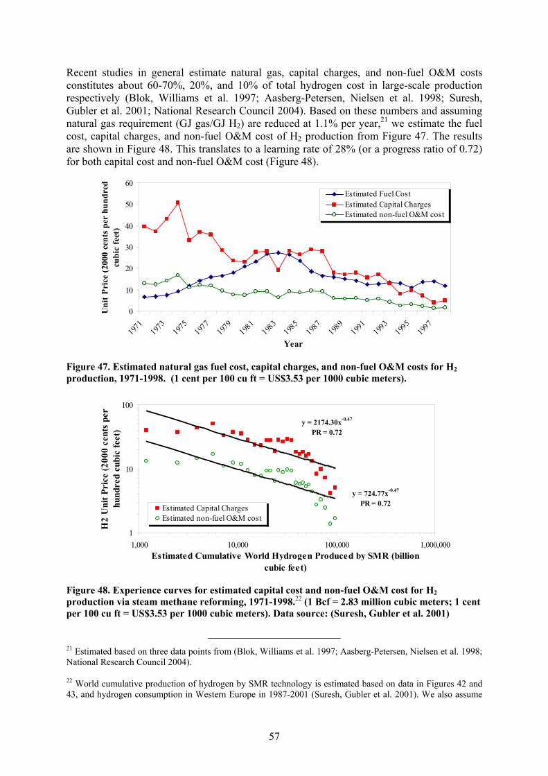
57

Recent studies in general estimate natural gas, capital charges, and non-fuel O&M costs constitutes about 60-70%, 20%, and 10% of total hydrogen cost in large-scale production respectively (Blok, Williams et al. 1997; Aasberg-Petersen, Nielsen et al. 1998; Suresh, Gubler et al. 2001; National Research Council 2004). Based on these numbers and assuming natural gas requirement (GJ gas/GJ H2) are reduced at 1.1% per year,21 we estimate the fuel cost, capital charges, and non-fuel O&M cost of H2 production from Figure 47. The results are shown in Figure 48. This translates to a learning rate of 28% (or a progress ratio of 0.72) for both capital cost and non-fuel O&M cost (Figure 48).

0

10

20

30

40

50

60

1971

1973

1975

1977

1979

1981

1983

1985

1987

1989

1991

1993

1995

1997

Year

Uni

t Pri

ce (2

000

cent

s per

hun

dred

cu

bic

feet

)

Estimated Fuel CostEstimated Capital ChargesEstimated non-fuel O&M cost

Figure 47. Estimated natural gas fuel cost, capital charges, and non-fuel O&M costs for H2 production, 1971-1998. (1 cent per 100 cu ft = US$3.53 per 1000 cubic meters).

y = 2174.30x-0.47

PR = 0.72

y = 724.77x-0.47

PR = 0.72

1

10

100

1,000 10,000 100,000 1,000,000Estimated Cumulative World Hydrogen Produced by SMR (billion

cubic feet)

H2

Uni

t Pri

ce (2

000

cent

s pe

r hu

ndre

d cu

bic

feet

)

Estimated Capital ChargesEstimated non-fuel O&M cost

Figure 48. Experience curves for estimated capital cost and non-fuel O&M cost for H2 production via steam methane reforming, 1971-1998.22 (1 Bcf = 2.83 million cubic meters; 1 cent per 100 cu ft = US$3.53 per 1000 cubic meters). Data source: (Suresh, Gubler et al. 2001)

21 Estimated based on three data points from (Blok, Williams et al. 1997; Aasberg-Petersen, Nielsen et al. 1998; National Research Council 2004).

22 World cumulative production of hydrogen by SMR technology is estimated based on data in Figures 42 and 43, and hydrogen consumption in Western Europe in 1987-2001 (Suresh, Gubler et al. 2001). We also assume

58

3.7 Summary of Case Study Results Table 6 summarizes the learning rates of capital costs and O&M costs for all technologies examined in this report. Overall, the learning rates in Table 6 are well within the range observed in the literature for energy-related technologies (McDonald and Schrattenholzer, 2001). The high learning rate for SCR O&M cost could be an artifact of overly conservative estimates by two early studies, where there was no SCR commercial experience in the U.S. and no technical data available about the applicability of the technology to U.S. coal-fired power plant. A separate analysis that looked only at studies after the first U.S. commercial experience has shown a much more modest learning rate of 0.13 for SCR O&M costs.

Table 6. Summary of capital and O&M costs learning rates and whether a cost increase was observed during early commercialization.

Learning Rate Technology Capital

Cost O&M Cost

Observed Cost Increase During Early

Commercialization Flue gas desulfurization (FGD) 0.11 0.22 Yes Selective catalytic reduction (SCR) 0.14 0.13 Yes Gas turbine combined cycle (GTCC) 0.10 0.06 Yes Pulverized coal (PC) boilers 0.05 0.07-0.30 n/a LNG production 0.14 0.12 Yes Oxygen production 0.10 0.05 n/a Hydrogen production (SMR) 0.27 0.27 n/a

Factors affecting the improvement of capital and O&M costs for each technology are summarized and tabulated in Table 7. The table gives a qualitative overview of factors that we found to influence the cost trends of each technology. Although some factors have a greater influence on cost trends than others, we do not make any attempt to quantify such influences in Table 7.

that 48% and 95% of hydrogen worldwide and in U.S., respectively, is produced from natural gas using SMR technology.

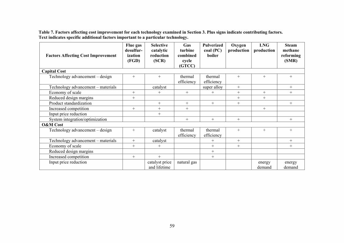
59

Table 7. Factors affecting cost improvement for each technology examined in Section 3. Plus signs indicate contributing factors. Text indicates specific additional factors important to a particular technology.

Factors Affecting Cost Improvement

Flue gas desulfur-

ization (FGD)

Selective catalytic

reduction (SCR)

Gas turbine

combined cycle

(GTCC)

Pulverized coal (PC)

boiler

Oxygen production

LNG production

Steam methane

reforming (SMR)

Capital Cost Technology advancement – design + + thermal

efficiency thermal

efficiency + + +

Technology advancement – materials catalyst super alloy + + Economy of scale + + + + + + + Reduced design margins + + + Product standardization + + + + + Increased competition + + + + Input price reduction + System integration/optimization + + + +

O&M Cost Technology advancement – design + catalyst thermal

efficiency thermal

efficiency + + +

Technology advancement – materials + catalyst + + + Economy of scale + + + + + Reduced design margins + Increased competition + + + Input price reduction catalyst price

and lifetime natural gas energy

demand energy demand

60

4. APPLICATIONS TO CO2 CAPTURE SYSTEMS

Here we utilize results of the Section 3 case studies to estimate the rates of technological change for four types of electric power systems employing different approaches for CO2 capture in addition to control of regulated air pollutants. Given the growing worldwide interest in CO2 capture and storage (CCS) as a potential option for climate change mitigation, the expected future cost of CCS technologies is of significant interest.

CO2 capture systems already are commercially deployed in a number of industrial processes, primarily in the petroleum and petrochemical industries. Current applications to electric power plants are limited to several coal- or gas-fired combustion units, where a relatively small volume of flue gas is treated for CO2 removal. In these cases, the captured CO2 is utilized in other industrial processes such as in the food industry. To date, there have been no applications of CO2 capture at the scale of a large (e.g., 500 MW) fossil-fuel power plant, which are the applications of interest for climate change mitigation.

In the absence of historical cost data for large power plants with CO2 capture, this study uses empirical cost trends for other analogous technologies to estimate learning curves for several types of power plants with CO2 capture. Additional technologies for CO2 transport and storage are outside the scope of this analysis, although they are clearly critical to a complete CCS system.

The next section briefly describes the types of power plants and CO2 capture systems examined in this study. Then we discuss the methods used to estimate future cost trends for each plant type.

4.1 Overview of Power Plant Designs with CO2 Capture Three general options for CO2 capture have been proposed for future power plant designs: post-combustion capture, pre-combustion capture, and oxyfuel combustion capture. Brief overviews of these systems are presented below.

4.1.1 Post-combustion CO2 Capture

Post-combustion systems separate CO2 from the flue gases produced by the combustion of a primary fuel (typically coal or natural gas) in air. Current commercial systems employ an organic solvent, such as monoethanolamine (MEA) or a mixture of amines, to capture the relatively small fraction of CO2 (typically 3–15% by volume) present in a flue gas stream (the main constituent being nitrogen from air). For a natural gas combined cycle (NGCC) power plant, a post-combustion capture system would be located downstream of the heat recovery steam generator (Figure 49). For a modern pulverized coal (PC) power plant the post-combustion capture unit would be located downstream of other air pollution control systems, as indicated in Figure 50. The capture process typically removes about 90% of the CO2 produced at the power plant. Once separated, the concentrated CO2 stream is compressed for transport and storage.

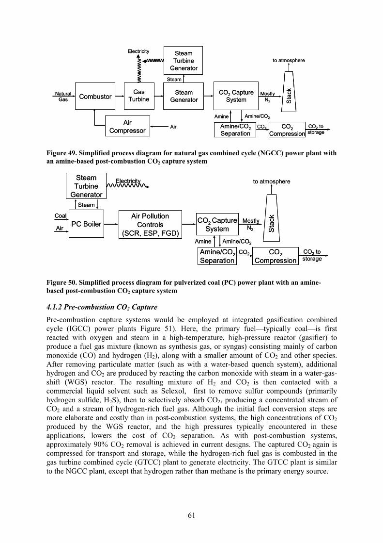
61

NaturalGas S

tack

Amine Amine/CO2

CO2 tostorage

Electricity SteamTurbine

Generator

CO2 CaptureSystem

Steam

GasTurbine

Amine/CO2Separation

MostlyN2

CO2Compression

CO2

SteamGenerator

AirCompressor

Combustor

Air

to atmosphere

NaturalGas S

tack

Amine Amine/CO2

CO2 tostorage

Electricity SteamTurbine

Generator

CO2 CaptureSystem

Steam

GasTurbine

Amine/CO2Separation

MostlyN2

CO2Compression

CO2

SteamGenerator

AirCompressor

Combustor

Air

to atmosphere

Figure 49. Simplified process diagram for natural gas combined cycle (NGCC) power plant with an amine-based post-combustion CO2 capture system

Coal

Air

Steam

Sta

ck

Amine/CO2

CO2

Steam Turbine

Generator

Electricity

Air PollutionControls

(SCR, ESP, FGD)

CO2 CaptureSystem

PC Boiler

Amine/CO2 Separation

MostlyN2

CO2Compression

Amine

CO2 tostorage

to atmosphere

Coal

Air

Steam

Sta

ck

Amine/CO2

CO2

Steam Turbine

Generator

Electricity

Air PollutionControls

(SCR, ESP, FGD)

CO2 CaptureSystem

PC Boiler

Amine/CO2 Separation

MostlyN2

CO2Compression

Amine

CO2 tostorage

to atmosphere

Figure 50. Simplified process diagram for pulverized coal (PC) power plant with an amine-based post-combustion CO2 capture system

4.1.2 Pre-combustion CO2 Capture Pre-combustion capture systems would be employed at integrated gasification combined cycle (IGCC) power plants Figure 51). Here, the primary fuel—typically coal—is first reacted with oxygen and steam in a high-temperature, high-pressure reactor (gasifier) to produce a fuel gas mixture (known as synthesis gas, or syngas) consisting mainly of carbon monoxide (CO) and hydrogen (H2), along with a smaller amount of CO2 and other species. After removing particulate matter (such as with a water-based quench system), additional hydrogen and CO2 are produced by reacting the carbon monoxide with steam in a water-gas-shift (WGS) reactor. The resulting mixture of H2 and CO2 is then contacted with a commercial liquid solvent such as Selexol, first to remove sulfur compounds (primarily hydrogen sulfide, H2S), then to selectively absorb CO2, producing a concentrated stream of CO2 and a stream of hydrogen-rich fuel gas. Although the initial fuel conversion steps are more elaborate and costly than in post-combustion systems, the high concentrations of CO2 produced by the WGS reactor, and the high pressures typically encountered in these applications, lowers the cost of CO2 separation. As with post-combustion systems, approximately 90% CO2 removal is achieved in current designs. The captured CO2 again is compressed for transport and storage, while the hydrogen-rich fuel gas is combusted in the gas turbine combined cycle (GTCC) plant to generate electricity. The GTCC plant is similar to the NGCC plant, except that hydrogen rather than methane is the primary energy source.

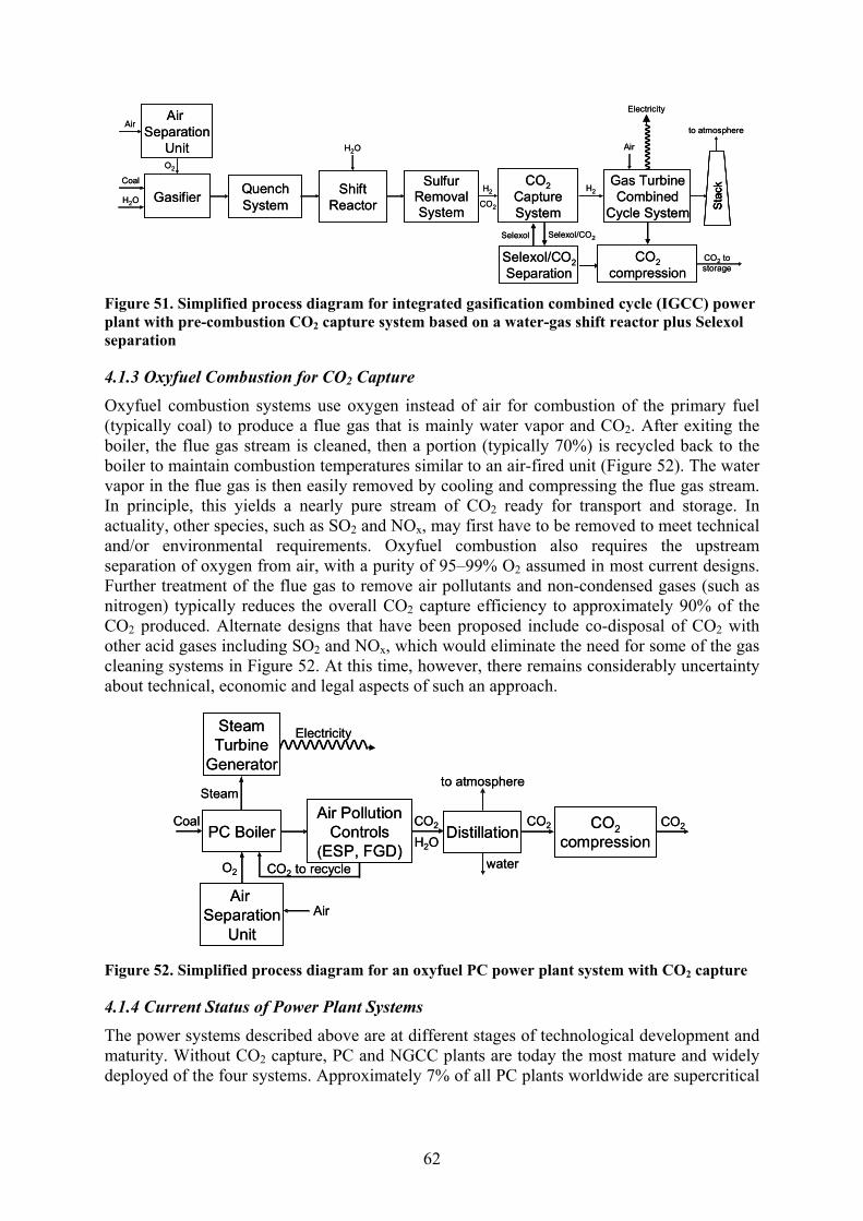
62

Gas TurbineCombined

Cycle SystemH2O St

ack

O2

Air

Coal

Gasifier

Stac

k

Air Separation

Unit

ShiftReactor CO2

Selexol/CO2Separation

Selexol Selexol/CO2

H2CO2

CaptureSystem

CO2compression

CO2 tostorage

Quench System

H2Sulfur

Removal System

to atmosphere

H2O

Electricity

Air

Gas TurbineCombined

Cycle SystemH2O St

ack

O2

Air

Coal

Gasifier

Stac

k

Air Separation

Unit

ShiftReactor CO2

Selexol/CO2Separation

Selexol Selexol/CO2

H2CO2

CaptureSystem

CO2compression

CO2 tostorage

Quench System

H2Sulfur

Removal System

to atmosphere

H2O

Electricity

Air

Figure 51. Simplified process diagram for integrated gasification combined cycle (IGCC) power plant with pre-combustion CO2 capture system based on a water-gas shift reactor plus Selexol separation

4.1.3 Oxyfuel Combustion for CO2 Capture Oxyfuel combustion systems use oxygen instead of air for combustion of the primary fuel (typically coal) to produce a flue gas that is mainly water vapor and CO2. After exiting the boiler, the flue gas stream is cleaned, then a portion (typically 70%) is recycled back to the boiler to maintain combustion temperatures similar to an air-fired unit (Figure 52). The water vapor in the flue gas is then easily removed by cooling and compressing the flue gas stream. In principle, this yields a nearly pure stream of CO2 ready for transport and storage. In actuality, other species, such as SO2 and NOx, may first have to be removed to meet technical and/or environmental requirements. Oxyfuel combustion also requires the upstream separation of oxygen from air, with a purity of 95–99% O2 assumed in most current designs. Further treatment of the flue gas to remove air pollutants and non-condensed gases (such as nitrogen) typically reduces the overall CO2 capture efficiency to approximately 90% of the CO2 produced. Alternate designs that have been proposed include co-disposal of CO2 with other acid gases including SO2 and NOx, which would eliminate the need for some of the gas cleaning systems in Figure 52. At this time, however, there remains considerably uncertainty about technical, economic and legal aspects of such an approach.

CoalDistillation

water

CO2

Air

H2O

O2

SteamTurbine

Generator

Electricity

Steam

PC Boiler CO2compression

Air Separation

Unit

CO2 to recycle

to atmosphere

Air PollutionControls

(ESP, FGD)

CO2CO2CoalDistillation

water

CO2

Air

H2O

O2

SteamTurbine

Generator

Electricity

Steam

PC Boiler CO2compression

Air Separation

Unit

CO2 to recycle

to atmosphere

Air PollutionControls

(ESP, FGD)

CO2CO2

Figure 52. Simplified process diagram for an oxyfuel PC power plant system with CO2 capture

4.1.4 Current Status of Power Plant Systems The power systems described above are at different stages of technological development and maturity. Without CO2 capture, PC and NGCC plants are today the most mature and widely deployed of the four systems. Approximately 7% of all PC plants worldwide are supercritical

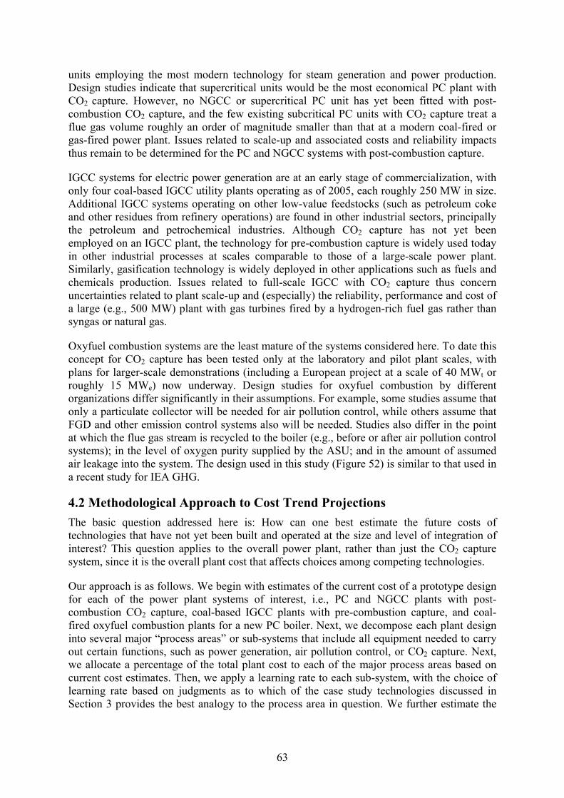
63

units employing the most modern technology for steam generation and power production. Design studies indicate that supercritical units would be the most economical PC plant with CO2 capture. However, no NGCC or supercritical PC unit has yet been fitted with post-combustion CO2 capture, and the few existing subcritical PC units with CO2 capture treat a flue gas volume roughly an order of magnitude smaller than that at a modern coal-fired or gas-fired power plant. Issues related to scale-up and associated costs and reliability impacts thus remain to be determined for the PC and NGCC systems with post-combustion capture.

IGCC systems for electric power generation are at an early stage of commercialization, with only four coal-based IGCC utility plants operating as of 2005, each roughly 250 MW in size. Additional IGCC systems operating on other low-value feedstocks (such as petroleum coke and other residues from refinery operations) are found in other industrial sectors, principally the petroleum and petrochemical industries. Although CO2 capture has not yet been employed on an IGCC plant, the technology for pre-combustion capture is widely used today in other industrial processes at scales comparable to those of a large-scale power plant. Similarly, gasification technology is widely deployed in other applications such as fuels and chemicals production. Issues related to full-scale IGCC with CO2 capture thus concern uncertainties related to plant scale-up and (especially) the reliability, performance and cost of a large (e.g., 500 MW) plant with gas turbines fired by a hydrogen-rich fuel gas rather than syngas or natural gas.

Oxyfuel combustion systems are the least mature of the systems considered here. To date this concept for CO2 capture has been tested only at the laboratory and pilot plant scales, with plans for larger-scale demonstrations (including a European project at a scale of 40 MWt or roughly 15 MWe) now underway. Design studies for oxyfuel combustion by different organizations differ significantly in their assumptions. For example, some studies assume that only a particulate collector will be needed for air pollution control, while others assume that FGD and other emission control systems also will be needed. Studies also differ in the point at which the flue gas stream is recycled to the boiler (e.g., before or after air pollution control systems); in the level of oxygen purity supplied by the ASU; and in the amount of assumed air leakage into the system. The design used in this study (Figure 52) is similar to that used in a recent study for IEA GHG.

4.2 Methodological Approach to Cost Trend Projections The basic question addressed here is: How can one best estimate the future costs of technologies that have not yet been built and operated at the size and level of integration of interest? This question applies to the overall power plant, rather than just the CO2 capture system, since it is the overall plant cost that affects choices among competing technologies.

Our approach is as follows. We begin with estimates of the current cost of a prototype design for each of the power plant systems of interest, i.e., PC and NGCC plants with post-combustion CO2 capture, coal-based IGCC plants with pre-combustion capture, and coal-fired oxyfuel combustion plants for a new PC boiler. Next, we decompose each plant design into several major “process areas” or sub-systems that include all equipment needed to carry out certain functions, such as power generation, air pollution control, or CO2 capture. Next, we allocate a percentage of the total plant cost to each of the major process areas based on current cost estimates. Then, we apply a learning rate to each sub-system, with the choice of learning rate based on judgments as to which of the case study technologies discussed in Section 3 provides the best analogy to the process area in question. We further estimate the

64

current cumulative capacity of each subsystem as the starting point for future learning. Then the component-level learning curve is applied to determine how the cost of each process area is reduced as additional power plants of a given type are constructed. Allowance also is made for additional experience in other (non-utility) applications. For any given level of total installed power plant capacity, the estimated cost of the total plant with CO2 capture is then the sum of all process area costs. Finally, a classical learning curve (y = ax-b) is fitted to the total cost trend to yield a learning rate for the overall plant with CO2 capture, based on an initial capacity Cmin and a final cumulative capacity, Cmax, for CCS plants of a given type.23 A regression analysis yields the parameter, b, for the overall plant. The learning rate is then calculated as: (1 – 2-b).

The procedure described above yields an overall learning rate that may vary with the choice of starting point (when does learning begin?) and end point (how long does learning persist?). In this project, we choose 100 GW as the nominal value of Cmax. This value is similar to the current deployment of FGD and SCR systems worldwide after 25–30 years. Methodologically, however, we establish Cmax as a parameter of the analysis and later use sensitivity analysis to examine the implication of alternative assumptions.

The cumulative CCS capacity at which learning (cost reduction) is assumed to begin also is a parameter of the analysis. The choice of a starting point for learning (Cmin) depends on whether one believes that current cost estimates for a large-scale plant with CO2 capture would indeed be accurate were such a plant actually built. Historical experience for other large-scale technologies indicates that cost estimates made prior to full-scale demonstration tend to underestimate the true costs of the first (and often several subsequent) generation of plants built at full scale. Only after several generations of new plants have been built and operated do costs eventually fall (as seen in Section 3 for four of the case studies). This means there is a reasonable chance that the actual cost of the first several large-scale plants with CO2 capture will exceed the costs currently reported in the literature.

The FGD and SCR case studies in Section 3 indicated that the actual capital cost of initial commercial installations in the U.S. exceeded early cost estimates by factors of two or more. At this time, however, we do not have a historical database adequate to quantitatively estimate the cost increases that might apply to initial installations of large plants with CO2 capture. Accordingly, we treat the problem parametrically. The most optimistic case assumes that current cost estimates for a large commercial plant are indeed accurate, and that further cost reductions are achieved after the first plant is completed. Nominally, however, we assume that additional large-scale plants must be designed, built and operated before the plant costs currently projected are actually achieved. In these cases, learning does not begin until the cumulative capacity has reached some critical level, Cmin (MW), a parameter of the analysis. Numerical estimates of Cmin are assumed to be 3 to 10 GW of installed capacity, based on historical experience for several of the technologies studied in Section 3. The higher value used for oxyfuel combustion systems because of its much earlier stage of development. For similar reasons, the onset of learning for IGCC systems is assumed to require more experience than more mature PC plants, while cleaner-burning NGCC plants with post-

23 The literature on experience curves indicates that classical learning rate for a particular technology often changes over time, and tends to “flatten out” as the technology matures. The result is that the shape of the experience curve for a specific technology is not always best described by the classical log-linear function, but by more complex functions such as an S-shaped curve [Yeh, Rubin, et. al., 2005]. In this study, however, we retain the log-linear model for simplicity and consistency with other studies.

65

combustion capture are assumed to require less additional experience than coal-based plants with capture, based on current levels of experience. Nominally, then, we assume Cmin is 3 GW for NGCC plants, 5 GW for PC plants, 7 GW for IGCC plants and 10 GW for oxyfuel plants.

Because of the many parameters and judgments inherent in the construction of a forward-looking learning curve, we have developed a computational tool in the form of an Excel spreadsheet to facilitate the calculation of learning curves for each of the four power plant systems of interest. The following sections elaborate on the specific assumptions used for each technology, and the results derived from those assumptions. In addition, we display the sensitivity of results to assumptions about key parameters. Readers wishing to explore other assumptions may do so using the computational models accompanying this report (see Appendix).

4.3 Cost Estimates for Current Capture Plants For the purposes of this study, current cost estimates for each plant configuration were obtained from the Integrated Environmental Control Model (IECM) developed at Carnegie Mellon University under sponsorship of the U.S. Department of Energy (USDOE). This model has been regularly updated, benchmarked and peer-reviewed as a tool for estimating the performance, emissions and cost of fossil fuel power plants for a user-specified set of assumptions. The most recent version of the model (IECM v.5.0.2), includes all four plant types of current interest (PC, NGCC, IGCC and oxyfuel), and provides a convenient method of obtaining systematic cost estimates for an overall plant as well as major plant components. A copy of the model and associated documentation accompany this report (see Appendix).

Table 8 summarizes the IECM cost estimates for each plant type based on a plant size of approximately 500 MW net output and a levelized capacity factor of 75%. All CO2 capture systems remove 90% of the CO2 produced and compress it to 13.8 MPa leaving the plant. All plants also are equipped with air pollution control systems that meet or exceed U.S. federal standards for new plants. The costs in Table 8 are similar to those in other recent studies based on similar assumptions (IPCC, 2005).

To estimate future cost trends, each power plant was divided into the major sub-sections shown in Table 8. For the CO2 capture section, the CO2 compressor was kept as a separate plant component in recognition of the fact that compression is a significant contributor to overall energy requirements, and that compressor technology is generally more mature than CO2 separation technologies at the scale of a large modern power plant. The contribution of each plant sub-section to the total plant cost is shown in Table 8.

The costs in Table 8 are intended to be representative of those found in the technical literature. However, the software described in the Appendix allows a user to easily change the total costs and/or percentage allocations if desired. The next section of this report illustrates the procedure and assumptions used to estimate overall plant cost trends.

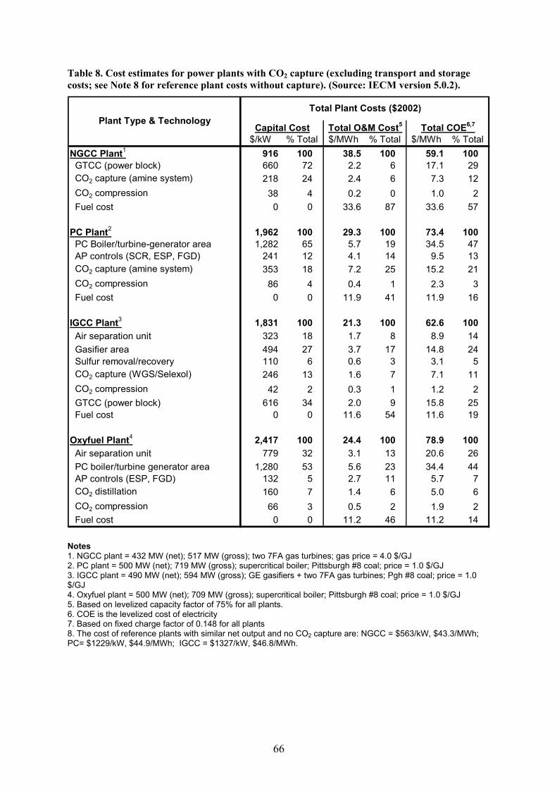
66

Table 8. Cost estimates for power plants with CO2 capture (excluding transport and storage costs; see Note 8 for reference plant costs without capture). (Source: IECM version 5.0.2).

$/kW $/MWh $/MWhNGCC Plant1 916 100 38.5 100 59.1 100 GTCC (power block) 660 72 2.2 6 17.1 29 CO2 capture (amine system) 218 24 2.4 6 7.3 12 CO2 compression 38 4 0.2 0 1.0 2 Fuel cost 0 0 33.6 87 33.6 57

PC Plant2 1,962 100 29.3 100 73.4 100 PC Boiler/turbine-generator area 1,282 65 5.7 19 34.5 47 AP controls (SCR, ESP, FGD) 241 12 4.1 14 9.5 13 CO2 capture (amine system) 353 18 7.2 25 15.2 21 CO2 compression 86 4 0.4 1 2.3 3 Fuel cost 0 0 11.9 41 11.9 16

IGCC Plant3 1,831 100 21.3 100 62.6 100 Air separation unit 323 18 1.7 8 8.9 14 Gasifier area 494 27 3.7 17 14.8 24 Sulfur removal/recovery 110 6 0.6 3 3.1 5 CO2 capture (WGS/Selexol) 246 13 1.6 7 7.1 11 CO2 compression 42 2 0.3 1 1.2 2 GTCC (power block) 616 34 2.0 9 15.8 25 Fuel cost 0 0 11.6 54 11.6 19

Oxyfuel Plant4 2,417 100 24.4 100 78.9 100 Air separation unit 779 32 3.1 13 20.6 26 PC boiler/turbine generator area 1,280 53 5.6 23 34.4 44 AP controls (ESP, FGD) 132 5 2.7 11 5.7 7 CO2 distillation 160 7 1.4 6 5.0 6 CO2 compression 66 3 0.5 2 1.9 2 Fuel cost 0 0 11.2 46 11.2 14

Plant Type & TechnologyTotal COE6,7

Total Plant Costs ($2002)

% Total % TotalTotal O&M Cost5

% TotalCapital Cost

Notes 1. NGCC plant = 432 MW (net); 517 MW (gross); two 7FA gas turbines; gas price = 4.0 $/GJ 2. PC plant = 500 MW (net); 719 MW (gross); supercritical boiler; Pittsburgh #8 coal; price = 1.0 $/GJ 3. IGCC plant = 490 MW (net); 594 MW (gross); GE gasifiers + two 7FA gas turbines; Pgh #8 coal; price = 1.0 $/GJ 4. Oxyfuel plant = 500 MW (net); 709 MW (gross); supercritical boiler; Pittsburgh #8 coal; price = 1.0 $/GJ 5. Based on levelized capacity factor of 75% for all plants. 6. COE is the levelized cost of electricity 7. Based on fixed charge factor of 0.148 for all plants 8. The cost of reference plants with similar net output and no CO2 capture are: NGCC = $563/kW, $43.3/MWh; PC= $1229/kW, $44.9/MWh; IGCC = $1327/kW, $46.8/MWh.

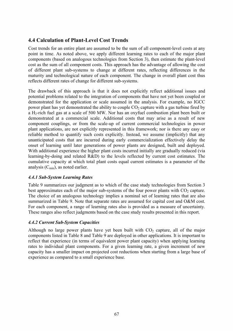
67

4.4 Calculation of Plant-Level Cost Trends Cost trends for an entire plant are assumed to be the sum of all component-level costs at any point in time. As noted above, we apply different learning rates to each of the major plant components (based on analogous technologies from Section 3), then estimate the plant-level cost as the sum of all component costs. This approach has the advantage of allowing the cost of different plant sub-systems to change at different rates, reflecting differences in the maturity and technological nature of each component. The change in overall plant cost thus reflects different rates of change for different sub-systems.

The drawback of this approach is that it does not explicitly reflect additional issues and potential problems related to the integration of components that have not yet been coupled or demonstrated for the application or scale assumed in the analysis. For example, no IGCC power plant has yet demonstrated the ability to couple CO2 capture with a gas turbine fired by a H2-rich fuel gas at a scale of 500 MW. Nor has an oxyfuel combustion plant been built or demonstrated at a commercial scale. Additional costs that may arise as a result of new component couplings, or from the scale-up of current commercial technologies in power plant applications, are not explicitly represented in this framework; nor is there any easy or reliable method to quantify such costs explicitly. Instead, we assume (implicitly) that any unanticipated costs that are incurred during early commercialization effectively delay the onset of learning until later generations of power plants are designed, built and deployed. With additional experience the higher plant costs incurred initially are gradually reduced (via learning-by-doing and related R&D) to the levels reflected by current cost estimates. The cumulative capacity at which total plant costs equal current estimates is a parameter of the analysis (Cmin), as noted earlier.

4.4.1 Sub-System Learning Rates Table 9 summarizes our judgment as to which of the case study technologies from Section 3 best approximates each of the major sub-systems of the four power plants with CO2 capture. The choice of an analogous technology implies a nominal set of learning rates that are also summarized in Table 9. Note that separate rates are assumed for capital cost and O&M cost. For each component, a range of learning rates also is provided as a measure of uncertainty. These ranges also reflect judgments based on the case study results presented in this report.

4.4.2 Current Sub-System Capacities Although no large power plants have yet been built with CO2 capture, all of the major components listed in Table 8 and Table 9 are deployed in other applications. It is important to reflect that experience (in terms of equivalent power plant capacity) when applying learning rates to individual plant components. For a given learning rate, a given increment of new capacity has a smaller impact on projected cost reductions when starting from a large base of experience as compared to a small experience base.

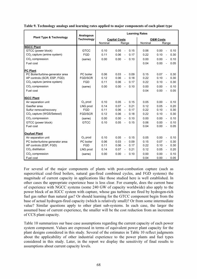
68

Table 9. Technology analogs and learning rates applied to major components of each plant type

Nominal NominalNGCC Plant GTCC (power block) GTCC 0.10 0.05 - 0.15 0.06 0.00 - 0.10 CO2 capture (amine system) FGD 0.11 0.06 - 0.17 0.22 0.10 - 0.30 CO2 compression (same) 0.00 0.00 - 0.10 0.00 0.00 - 0.10 Fuel cost 0.00 0.00 - 0.00 0.04 0.00 - 0.05

PC Plant PC Boiler/turbine-generator area PC boiler 0.06 0.03 - 0.09 0.15 0.07 - 0.30 AP controls (SCR, ESP, FGD) FGD/SCR 0.12 0.06 - 0.18 0.22 0.10 - 0.30 CO2 capture (amine system) FGD 0.11 0.06 - 0.17 0.22 0.10 - 0.30 CO2 compression (same) 0.00 0.00 - 0.10 0.00 0.00 - 0.10 Fuel cost 0.00 0.00 - 0.00 0.04 0.00 - 0.05

IGCC Plant Air separation unit O2 prod 0.10 0.05 - 0.15 0.05 0.00 - 0.10 Gasifier area LNG prod 0.14 0.07 - 0.21 0.12 0.05 - 0.20 Sulfur removal/recovery FGD 0.11 0.06 - 0.17 0.22 0.10 - 0.30 CO2 capture (WGS/Selexol) FGD/SCR 0.12 0.06 - 0.18 0.22 0.10 - 0.30 CO2 compression (same) 0.00 0.00 - 0.10 0.00 0.00 - 0.10 GTCC (power block) GTCC 0.10 0.05 - 0.15 0.06 0.00 - 0.10 Fuel cost 0.00 0.00 - 0.00 0.04 0.00 - 0.05

Oxyfuel Plant Air separation unit O2 prod 0.10 0.05 - 0.15 0.05 0.00 - 0.10 PC boiler/turbine generator area PC boiler 0.06 0.03 - 0.09 0.15 0.07 - 0.30 AP controls (ESP, FGD) FGD 0.11 0.06 - 0.17 0.22 0.10 - 0.30 CO2 distillation LNG prod 0.14 0.07 - 0.21 0.12 0.05 - 0.20 CO2 compression (same) 0.00 0.00 - 0.10 0.00 0.00 - 0.10 Fuel cost 0.00 0.00 - 0.00 0.04 0.00 - 0.05

Plant Type & Technology

Range Range

Learning Rates

Capital Costs O&M CostsAnalogous Technology

For several of the major components of plants with post-combustion capture (such as supercritical coal-fired boilers, natural gas-fired combined cycles, and FGD systems) the magnitude of current capacity in applications like those studied here is well established. In other cases the appropriate experience base is less clear. For example, does the current base of experience with NGCC systems (some 240 GW of capacity worldwide) also apply to the power block of an IGCC system with capture, whose gas turbines are fired by hydrogen-rich fuel gas rather than natural gas? Or should learning for the GTCC component begin from the base of actual hydrogen-fired capacity (which is relatively small)? Or from some intermediate value? Similar questions apply to other plant sub-systems. In each case, the larger the assumed base of current experience, the smaller will be the cost reduction from an increment of CCS plant capacity.

Table 10 summarizes our base case assumptions regarding the current capacity of each power system component. Values are expressed in terms of equivalent power plant capacity for the plant designs considered in this study. Several of the estimates in Table 10 reflect judgments about the applicability of other industrial experience to the power plants and fuel types considered in this study. Later, in the report we display the sensitivity of final results to assumptions about current capacity levels.

69

Table 10. Nominal values of current capacity of plant sub-systems (equivalent MW of power plant capacity)

CurrentPlant Type & Technology Capacity

(MW)NGCC Plant GTCC (power block) 240,000 CO2 capture (amine system) 10,000 CO2 compression 10,000

PC Plant PC Boiler/turbine-generator area 120,000 AP controls (SCR, ESP, FGD) 230,000 CO2 capture (amine system) 10,000 CO2 compression 10,000

IGCC Plant Air separation unit 50,000 Gasifier area 10,000 Sulfur removal/recovery 50,000 CO2 capture (WGS/selexol) 10,000 CO2 compression 10,000 GTCC (power block) 240,000

Oxyfuel Plant Air separation unit 50,000 PC boiler/turbine generator area 120,000 AP controls (ESP, FGD) 230,000 CO2 distillation 10,000 CO2 compression 10,000

4.4.3 Effect of Non-CCS Experience

Another factor affecting component-level cost projections is the experience that accrues from continued deployment in applications other than power plants with CO2 capture. For example, oxygen plants will continue to be used in a variety of industrial processes, and that additional capacity (experience) will contribute to future learning and associated cost reductions that benefit IGCC and oxyfuel systems. Other plant components also are likely to have additional applications that could accelerate component-level cost reductions. The scope of the current project, however, does not permit an analysis of future markets for all CCS system components. Nonetheless, to reflect the potential role of other industrial deployment, we introduce a new set of parameters (multipliers) that are applied to each increment of new CCS plant capacity to reflect additional capacity of a particular plant component in other applications. Thus, a multiplier of 2.0 applied to a particular component means that for every new 500 MW power plant with CO2 capture there is the equivalent of an additional 500 MW of capacity from other applications. This allows learning from non-CCS deployments to influence the cost trend of the power plants with capture, albeit in a simple way. As a practical matter, additional research is needed to quantify these multipliers for each plant component. Absent that information, the current study assumes (conservatively) no additional

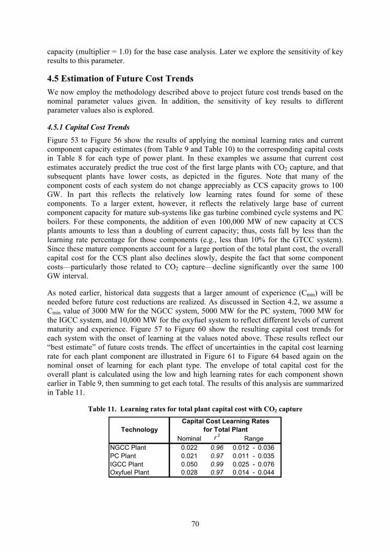
70

capacity (multiplier = 1.0) for the base case analysis. Later we explore the sensitivity of key results to this parameter.

4.5 Estimation of Future Cost Trends We now employ the methodology described above to project future cost trends based on the nominal parameter values given. In addition, the sensitivity of key results to different parameter values also is explored.

4.5.1 Capital Cost Trends Figure 53 to Figure 56 show the results of applying the nominal learning rates and current component capacity estimates (from Table 9 and Table 10) to the corresponding capital costs in Table 8 for each type of power plant. In these examples we assume that current cost estimates accurately predict the true cost of the first large plants with CO2 capture, and that subsequent plants have lower costs, as depicted in the figures. Note that many of the component costs of each system do not change appreciably as CCS capacity grows to 100 GW. In part this reflects the relatively low learning rates found for some of these components. To a larger extent, however, it reflects the relatively large base of current component capacity for mature sub-systems like gas turbine combined cycle systems and PC boilers. For these components, the addition of even 100,000 MW of new capacity at CCS plants amounts to less than a doubling of current capacity; thus, costs fall by less than the learning rate percentage for those components (e.g., less than 10% for the GTCC system). Since these mature components account for a large portion of the total plant cost, the overall capital cost for the CCS plant also declines slowly, despite the fact that some component costs—particularly those related to CO2 capture—decline significantly over the same 100 GW interval.

As noted earlier, historical data suggests that a larger amount of experience (Cmin) will be needed before future cost reductions are realized. As discussed in Section 4.2, we assume a Cmin value of 3000 MW for the NGCC system, 5000 MW for the PC system, 7000 MW for the IGCC system, and 10,000 MW for the oxyfuel system to reflect different levels of current maturity and experience. Figure 57 to Figure 60 show the resulting capital cost trends for each system with the onset of learning at the values noted above. These results reflect our “best estimate” of future costs trends. The effect of uncertainties in the capital cost learning rate for each plant component are illustrated in Figure 61 to Figure 64 based again on the nominal onset of learning for each plant type. The envelope of total capital cost for the overall plant is calculated using the low and high learning rates for each component shown earlier in Table 9, then summing to get each total. The results of this analysis are summarized in Table 11.

Table 11. Learning rates for total plant capital cost with CO2 capture

Nominal r 2

NGCC Plant 0.022 0.96 0.012 - 0.036PC Plant 0.021 0.97 0.011 - 0.035IGCC Plant 0.050 0.99 0.025 - 0.076Oxyfuel Plant 0.028 0.97 0.014 - 0.044

Capital Cost Learning Rates

Rangefor Total PlantTechnology

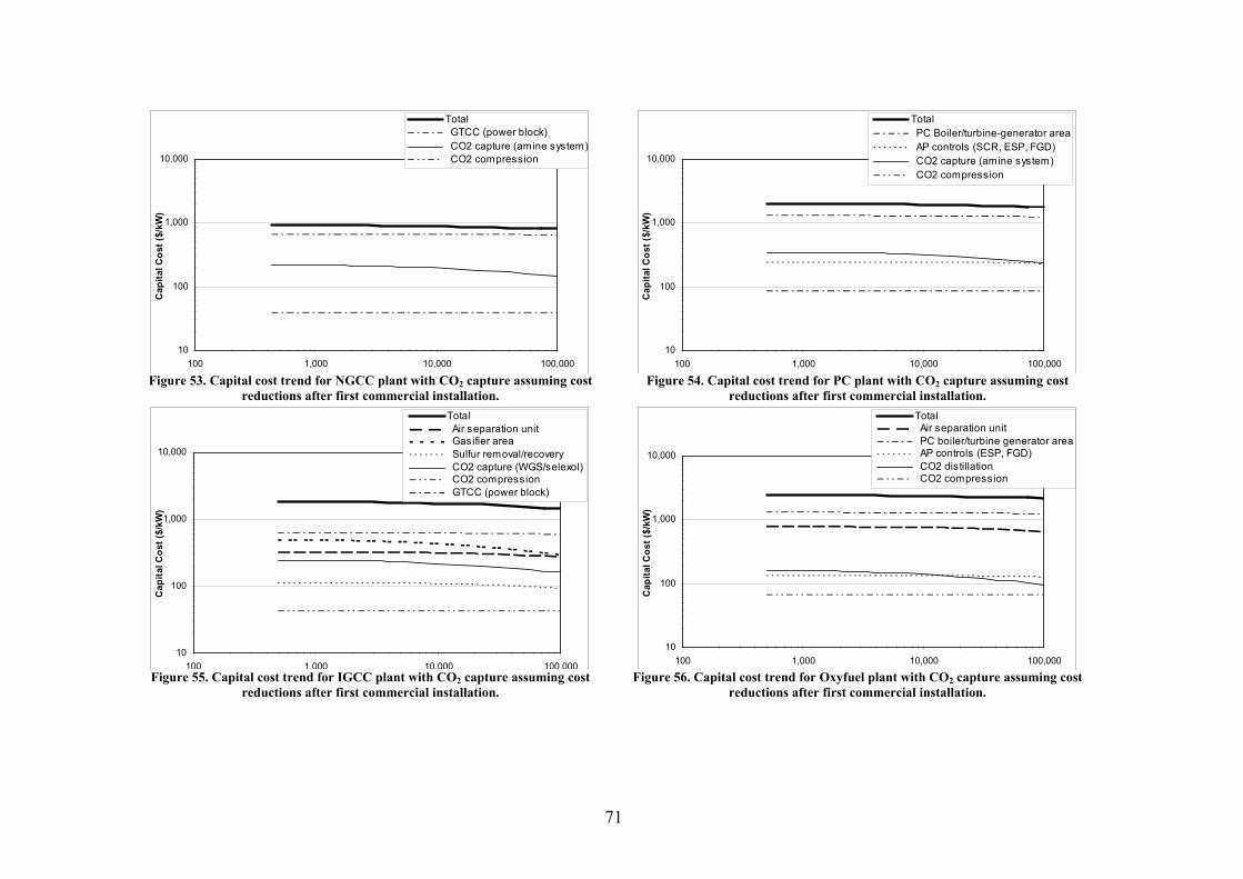
71

10

100

1,000

10,000

100 1,000 10,000 100,000

Cap

ital C

ost (

$/kW

)

Total GTCC (power block) CO2 capture (amine system) CO2 compression

10

100

1,000

10,000

100 1,000 10,000 100,000

Cap

ital C

ost (

$/kW

)

Total PC Boiler/turbine-generator area AP controls (SCR, ESP, FGD) CO2 capture (amine system) CO2 compression

Figure 53. Capital cost trend for NGCC plant with CO2 capture assuming cost reductions after first commercial installation.

Figure 54. Capital cost trend for PC plant with CO2 capture assuming cost reductions after first commercial installation.

10

100

1,000

10,000

100 1,000 10,000 100,000

Cap

ital C

ost (

$/kW

)

Total Air separation unit Gasifier area Sulfur removal/recovery CO2 capture (WGS/selexol) CO2 compression GTCC (power block)

10

100

1,000

10,000

100 1,000 10,000 100,000C

apita

l Cos

t ($/

kW)

Total Air separation unit PC boiler/turbine generator area AP controls (ESP, FGD) CO2 distillation CO2 compression

Figure 55. Capital cost trend for IGCC plant with CO2 capture assuming cost reductions after first commercial installation.

Figure 56. Capital cost trend for Oxyfuel plant with CO2 capture assuming cost reductions after first commercial installation.

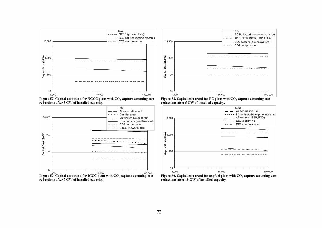
72

10

100

1,000

10,000

1,000 10,000 100,000

Cap

ital C

ost (

$/kW

)

Total GTCC (power block) CO2 capture (amine system) CO2 compression

10

100

1,000

10,000

1,000 10,000 100,000

Cap

ital C

ost (

$/kW

)

Total PC Boiler/turbine-generator area AP controls (SCR, ESP, FGD) CO2 capture (amine system) CO2 compression

Figure 57. Capital cost trend for NGCC plant with CO2 capture assuming cost reductions after 3 GW of installed capacity.

Figure 58. Capital cost trend for PC plant with CO2 capture assuming cost reductions after 5 GW of installed capacity.

10

100

1,000

10,000

1 000 10 000 100 000

Cap

ital C

ost (

$/kW

)

Total Air separation unit Gasifier area Sulfur removal/recovery CO2 capture (WGS/selexol) CO2 compression GTCC (power block)

10

100

1,000

10,000

1,000 10,000 100,000

Cap

ital C

ost (

$/kW

)

Total Air separation unit PC boiler/turbine generator area AP controls (ESP, FGD) CO2 distillation CO2 compression

Figure 59. Capital cost trend for IGCC plant with CO2 capture assuming cost reductions after 7 GW of installed capacity.

Figure 60. Capital cost trend for oxyfuel plant with CO2 capture assuming cost reductions after 10 GW of installed capacity.

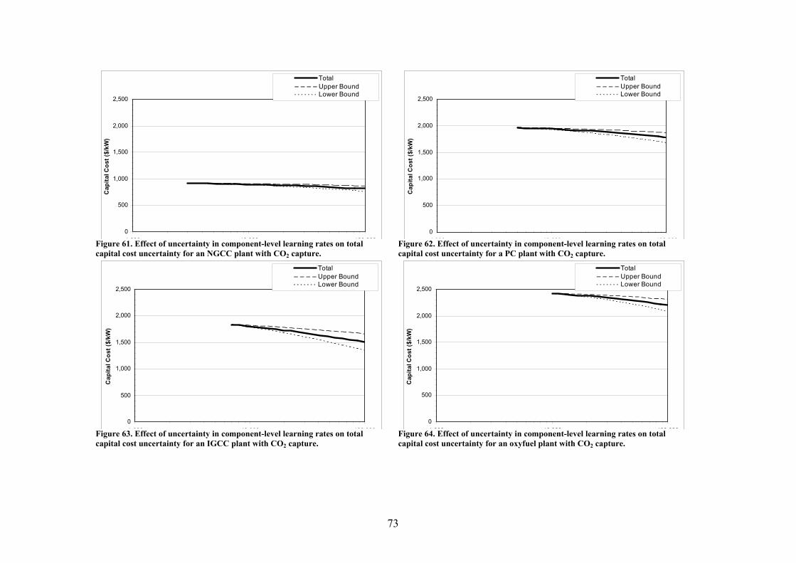
73

0

500

1,000

1,500

2,000

2,500

1 000 10 000 100 000

Cap

ital C

ost (

$/kW

)

TotalUpper BoundLower Bound

0

500

1,000

1,500

2,000

2,500

1 000 10 000 100 000

Cap

ital C

ost (

$/kW

)

TotalUpper BoundLower Bound

Figure 61. Effect of uncertainty in component-level learning rates on total capital cost uncertainty for an NGCC plant with CO2 capture.

Figure 62. Effect of uncertainty in component-level learning rates on total capital cost uncertainty for a PC plant with CO2 capture.

0

500

1,000

1,500

2,000

2,500

1 000 10 000 100 000

Cap

ital C

ost (

$/kW

)

TotalUpper BoundLower Bound

0

500

1,000

1,500

2,000

2,500

1 000 10 000 100 000

Cap

ital C

ost (

$/kW

)

TotalUpper BoundLower Bound

Figure 63. Effect of uncertainty in component-level learning rates on total capital cost uncertainty for an IGCC plant with CO2 capture.

Figure 64. Effect of uncertainty in component-level learning rates on total capital cost uncertainty for an oxyfuel plant with CO2 capture.

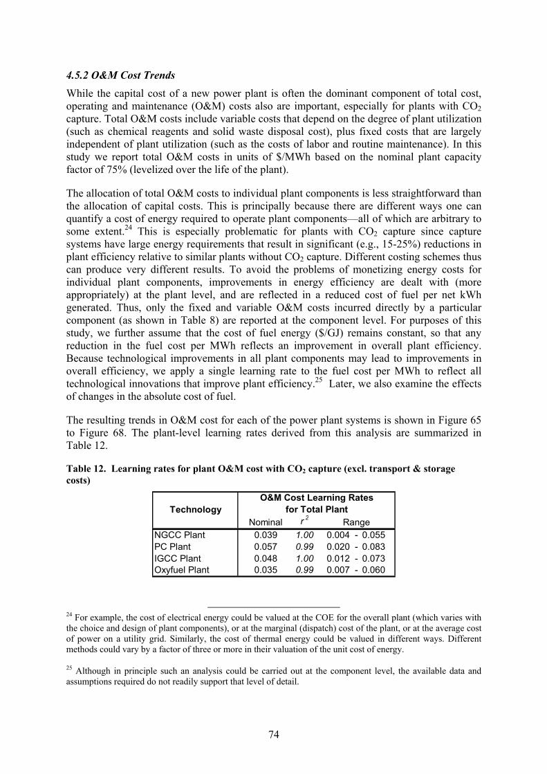
74

4.5.2 O&M Cost Trends While the capital cost of a new power plant is often the dominant component of total cost, operating and maintenance (O&M) costs also are important, especially for plants with CO2 capture. Total O&M costs include variable costs that depend on the degree of plant utilization (such as chemical reagents and solid waste disposal cost), plus fixed costs that are largely independent of plant utilization (such as the costs of labor and routine maintenance). In this study we report total O&M costs in units of $/MWh based on the nominal plant capacity factor of 75% (levelized over the life of the plant).

The allocation of total O&M costs to individual plant components is less straightforward than the allocation of capital costs. This is principally because there are different ways one can quantify a cost of energy required to operate plant components—all of which are arbitrary to some extent.24 This is especially problematic for plants with CO2 capture since capture systems have large energy requirements that result in significant (e.g., 15-25%) reductions in plant efficiency relative to similar plants without CO2 capture. Different costing schemes thus can produce very different results. To avoid the problems of monetizing energy costs for individual plant components, improvements in energy efficiency are dealt with (more appropriately) at the plant level, and are reflected in a reduced cost of fuel per net kWh generated. Thus, only the fixed and variable O&M costs incurred directly by a particular component (as shown in Table 8) are reported at the component level. For purposes of this study, we further assume that the cost of fuel energy ($/GJ) remains constant, so that any reduction in the fuel cost per MWh reflects an improvement in overall plant efficiency. Because technological improvements in all plant components may lead to improvements in overall efficiency, we apply a single learning rate to the fuel cost per MWh to reflect all technological innovations that improve plant efficiency.25 Later, we also examine the effects of changes in the absolute cost of fuel.

The resulting trends in O&M cost for each of the power plant systems is shown in Figure 65 to Figure 68. The plant-level learning rates derived from this analysis are summarized in Table 12.

Table 12. Learning rates for plant O&M cost with CO2 capture (excl. transport & storage costs)

Nominal r 2

NGCC Plant 0.039 1.00 0.004 - 0.055PC Plant 0.057 0.99 0.020 - 0.083IGCC Plant 0.048 1.00 0.012 - 0.073Oxyfuel Plant 0.035 0.99 0.007 - 0.060

O&M Cost Learning RatesTechnology

Rangefor Total Plant

24 For example, the cost of electrical energy could be valued at the COE for the overall plant (which varies with the choice and design of plant components), or at the marginal (dispatch) cost of the plant, or at the average cost of power on a utility grid. Similarly, the cost of thermal energy could be valued in different ways. Different methods could vary by a factor of three or more in their valuation of the unit cost of energy.

25 Although in principle such an analysis could be carried out at the component level, the available data and assumptions required do not readily support that level of detail.

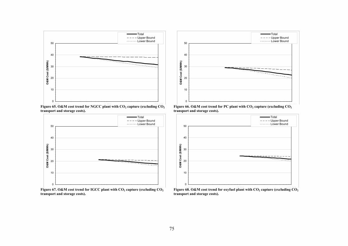
75

0

10

20

30

40

50

1 000 10 000 100 000

O&

M C

ost (

$/M

Wh)

TotalUpper BoundLower Bound

0

10

20

30

40

50

1 000 10 000 100 000

O&

M C

ost (

$/M

Wh)

TotalUpper BoundLower Bound

Figure 65. O&M cost trend for NGCC plant with CO2 capture (excluding CO2 transport and storage costs).

Figure 66. O&M cost trend for PC plant with CO2 capture (excluding CO2 transport and storage costs).

0

10

20

30

40

50

1 000 10 000 100 000

O&

M C

ost (

$/M

Wh)

TotalUpper BoundLower Bound

0

10

20

30

40

50

1 000 10 000 100 000

O&

M C

ost (

$/M

Wh)

TotalUpper BoundLower Bound

Figure 67. O&M cost trend for IGCC plant with CO2 capture (excluding CO2 transport and storage costs).

Figure 68. O&M cost trend for oxyfuel plant with CO2 capture (excluding CO2 transport and storage costs).

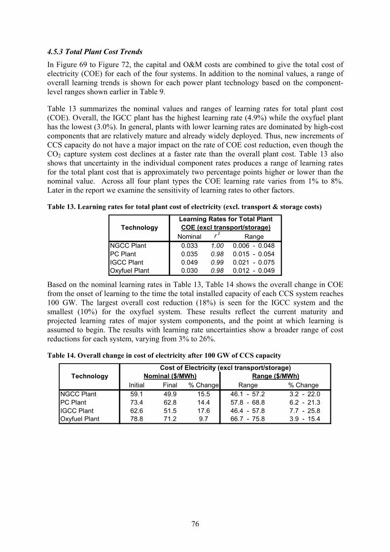
76

4.5.3 Total Plant Cost Trends In Figure 69 to Figure 72, the capital and O&M costs are combined to give the total cost of electricity (COE) for each of the four systems. In addition to the nominal values, a range of overall learning trends is shown for each power plant technology based on the component-level ranges shown earlier in Table 9.

Table 13 summarizes the nominal values and ranges of learning rates for total plant cost (COE). Overall, the IGCC plant has the highest learning rate (4.9%) while the oxyfuel plant has the lowest (3.0%). In general, plants with lower learning rates are dominated by high-cost components that are relatively mature and already widely deployed. Thus, new increments of CCS capacity do not have a major impact on the rate of COE cost reduction, even though the CO2 capture system cost declines at a faster rate than the overall plant cost. Table 13 also shows that uncertainty in the individual component rates produces a range of learning rates for the total plant cost that is approximately two percentage points higher or lower than the nominal value. Across all four plant types the COE learning rate varies from 1% to 8%. Later in the report we examine the sensitivity of learning rates to other factors.

Table 13. Learning rates for total plant cost of electricity (excl. transport & storage costs)

Nominal r 2

NGCC Plant 0.033 1.00 0.006 - 0.048PC Plant 0.035 0.98 0.015 - 0.054IGCC Plant 0.049 0.99 0.021 - 0.075Oxyfuel Plant 0.030 0.98 0.012 - 0.049

COE (excl transport/storage)Learning Rates for Total Plant

TechnologyRange

Based on the nominal learning rates in Table 13, Table 14 shows the overall change in COE from the onset of learning to the time the total installed capacity of each CCS system reaches 100 GW. The largest overall cost reduction (18%) is seen for the IGCC system and the smallest (10%) for the oxyfuel system. These results reflect the current maturity and projected learning rates of major system components, and the point at which learning is assumed to begin. The results with learning rate uncertainties show a broader range of cost reductions for each system, varying from 3% to 26%.

Table 14. Overall change in cost of electricity after 100 GW of CCS capacity

Initial Final % ChangeNGCC Plant 59.1 49.9 15.5 46.1 - 57.2 3.2 - 22.0PC Plant 73.4 62.8 14.4 57.8 - 68.8 6.2 - 21.3IGCC Plant 62.6 51.5 17.6 46.4 - 57.8 7.7 - 25.8Oxyfuel Plant 78.8 71.2 9.7 66.7 - 75.8 3.9 - 15.4

TechnologyCost of Electricity (excl transport/storage)

Nominal ($/MWh) Range ($/MWh)Range % Change

77

0

20

40

60

80

100

Cos

t of E

lect

ricity

($/M

Wh)

TotalUpper BoundLower Bound

0

20

40

60

80

100

Cos

t of E

lect

ricity

($/M

Wh)

TotalUpper BoundLower Bound

Figure 69. Total cost of electricity for NGCC plant with CO2 capture (excluding CO2 transport and storage costs).

Figure 70. Total cost of electricity for PC plant with CO2 capture (excluding CO2 transport and storage costs).

0

20

40

60

80

100

Cos

t of E

lect

ricity

($/M

Wh)

TotalUpper BoundLower Bound

0

20

40

60

80

100

Cos

t of E

lect

ricity

($/M

Wh)

TotalUpper BoundLower Bound

Figure 71. Total cost of electricity for IGCC plant with CO2 capture (excluding CO2 transport and storage costs).

Figure 72. Total cost of electricity for oxyfuel plant with CO2 capture (excluding CO2 transport and storage costs).

78

Because the COE values in this report do not include the additional costs of CO2 transport and storage, changes in the total system cost (including transport and storage) could be higher or lower than the values reported here. Based on a recent report of the Intergovernmental Panel on Climate Change (IPCC, 2005), inclusion of transport and storage costs would add up to roughly $10/MWh to the COE for plants using geological storage in saline formations, and could reduce total COE by up to $10/MWh for geological storage via enhanced oil recovery (EOR). The IPCC report also found that current pipeline-based technologies for CO2 transport and geological storage already are mature, with little if any potential for near-term cost reductions. The addition of constant transport and storage costs to the plant-level cost trends reported here would tend to further flatten the overall system cost trajectories and resulting learning rates.

4.6 Sensitivity Analysis The results presented above showed the effect of alternative component-level learning rates on capital, O&M and COE cost trends based on learning curve models. In this section we display the sensitivity of results to other key parameters. In particular, we analyze the following cases:

• Learning starts with first plant. This case assumes that current cost estimates for CCS plants are the true cost of building the first full-size units, with subsequent cost reductions given by the applicable learning rates.

• Learning up to 50 GW of capacity. This case extends the learning curve for cumulative capacity of CCS plants to 50 GW instead of 100 GW.

• Lower component capacity estimates. This case takes a more restrictive (bounding) view of the “current capacity” estimates for plant sub-systems in Table 10. Amine systems for post-combustion capture are assumed to have zero experience at a 500 MW power plant; coal gasifier experience for IGCC is reduced to 1000 MW; H2-fired GTCC experience at power plants is lowered to zero; and the current capacity of supercritical boilers with oxyfuel combustion and flue gas recycle also is set to zero.

• Additional non-CCS experience. A multiplier of 2.0 is assumed for all components of all plants in lieu of the nominal value of 1.0. This assumes that for every increment of CCS plant capacity there is an equal increment of other industrial capacity adding to the total cumulative experience for each component. The choice of a multiplier in this case is purely arbitrary and intended only for illustrative purposes.

• Higher fuel prices. This case assumes a natural gas price of $6.00/GJ and a coal price of $1.50/GJ (vs. nominal assumptions of $4/GJ and $1/GJ, respectively).

• Lower financing cost and higher utilization. This case assumes a fixed charge factor of 11% and a levelized plant capacity factor of 85%. These are the assumptions used in recent IEA GHG studies.

Table 15 shows the effects of these assumptions on results for capital cost and cost of electricity. In each case, only the parameter noted is changed; all others are kept at their nominal (base case) value. The first case shows the result of cost reductions that begin with the first plant installation (as in Figure 53 to Figure 56). This yields greater reductions in cost at the end of the simulation period. However, the average learning rates for capital cost and COE are lower than for the nominal case. This is because initially there is relative little change in total plant cost due to the “inertia” of relatively mature plant components whose costs change slowly with each increment of new CCS capacity.

79

Table 15. Summary of additional sensitivity case results

Learning Rate

Initial Value

Final Value % Change Learning

RateInitial Value

Final Value % Change

Nominal Base Case Assumptions 0.022 916 817 10.8% 0.033 59.1 49.9 15.5%Learning Starts with First Plant 0.014 916 811 11.5% 0.028 59.1 47.0 20.4%Learning up to 50 GW 0.018 916 849 7.3% 0.031 59.1 52.0 12.0%Current Capture Capacity = 0 GW 0.029 916 786 14.2% 0.037 59.1 48.8 17.4%Non-CSS Exp. Multipliers = 2.0 0.030 916 783 14.4% 0.036 59.1 49.0 17.1%Natural Gas Price = $6.0/GJ 0.022 925 826 10.7% 0.033 76.1 64.2 15.7%FCF = 11%, CF = 85% 0.022 918 820 10.7% 0.034 51.6 43.3 16.1%

Learning Rate

Initial Value

Final Value % Change Learning

RateInitial Value

Final Value % Change

Nominal Base Case Assumptions 0.021 1,962 1,783 9.1% 0.035 73.4 62.8 14.4%Learning Starts with First Plant 0.013 1,962 1,764 10.1% 0.024 73.4 60.8 17.2%Learning up to 50 GW 0.018 1,962 1,846 5.9% 0.031 73.4 66.0 10.1%Current Capture Capacity = 0 GW 0.026 1,962 1,744 11.1% 0.042 73.4 60.9 17.1%Non-CSS Exp. Multipliers = 2.0 0.029 1,962 1,723 12.2% 0.068 73.4 60.4 17.8%Coal Price = $1.5/GJ 0.021 1,965 1,786 9.1% 0.035 79.6 68.2 14.3%FCF = 11%, CF = 85% 0.021 1,963 1,785 9.1% 0.039 57.2 48.2 15.7%

Learning Rate

Initial Value

Final Value % Change Learning

RateInitial Value

Final Value % Change

Nominal Base Case Assumptions 0.050 1,831 1,505 17.8% 0.049 62.6 51.5 17.7%Learning Starts with First Plant 0.029 1,831 1,448 20.9% 0.032 62.6 48.6 22.4%Learning up to 50 GW 0.044 1,831 1,610 12.1% 0.045 62.6 54.9 12.2%Current Gasifier Capacity = 1 GW 0.057 1,831 1,460 20.3% 0.055 62.6 50.2 19.7%Above + H2-GTCC = 0 GW 0.088 1,831 1,285 29.8% 0.078 62.6 45.9 26.6%Non-CSS Exp. Multipliers = 2.0 0.062 1,831 1,432 21.8% 0.054 62.6 49.5 20.8%Coal Price = $1.5/GJ 0.050 1,834 1,507 17.8% 0.048 68.4 56.6 17.3%FCF = 11%, CF = 85% 0.048 1,832 1,516 17.2% 0.047 47.2 39.2 16.9%

Learning Rate

Initial Value

Final Value % Change Learning

RateInitial Value

Final Value % Change

Nominal Base Case Assumptions 0.028 2,417 2,201 9.0% 0.030 78.8 71.2 9.6%Learning Starts with First Plant 0.013 2,417 2,160 10.7% 0.017 78.8 68.6 12.9%Learning up to 50 GW 0.023 2,417 2,291 5.2% 0.025 78.8 74.3 5.8%Current Boiler Capacity = 0 0.054 2,417 2,008 16.9% 0.056 78.8 65.1 17.5%Non-CSS Exp. Multipliers = 2.0 0.038 2,417 2,122 12.2% 0.044 78.8 68.8 12.7%Coal Price = $1.5/GJ 0.028 2,421 2,204 9.0% 0.030 84.7 76.4 9.8%FCF = 11%, CF = 85% 0.028 2,418 2,202 9.0% 0.031 58.8 53.0 9.9%

COE ($/MWh)

COE ($/MWh)

COE ($/MWh)

COE ($/MWh)NGCC Sensitivity Case

Capital Cost ($/kW)

PC Sensitivity CaseCapital Cost ($/kW)

IGCC Sensitivity CaseCapital Cost ($/kW)

Oxyfuel Sensitivity CaseCapital Cost ($/kW)

The effect of shortening the cumulative experience level to 50 GW also results in lower learning rates, as well as lower overall cost reductions. In contrast, lower estimates of initial component capacity result in higher learning rates and greater overall cost reductions. Those results follow directly from the form of the learning curve equation, where each new increment of CCS capacity represents a greater fraction of total cumulative capacity when the initial capacity value is lowered. Quantitatively, the largest impact is seen for the IGCC plant, especially the case where current capacity of hydrogen-fired GTCC systems is lowered to zero. Because hydrogen-fired gas turbines are expected to be similar to current natural gas-fired designs, this case represents a bounding analysis to illustrate the influence of this parameter.

In a similar fashion, increasing the non-CCS experience multipliers for all plant components also significantly increases the learning rates and total cost reductions for all systems. As noted above, the choice of multiplier values in this case is arbitrary and for illustrative purposes only; further studies or scenarios would be needed to assign meaningful values to this parameter for each plant component.

80

Changes in the price of natural gas or coal can have a significant impact on the cost of electricity, as illustrated in Table 15. However, the table also shows that the impacts of higher fuel prices on learning rates and percent reductions in cost are small to negligible. The same is true for alternate assumptions about plant financing and utilization. Here, the cases in Table 15 show a significant impact on the initial cost of electricity, but small if any impacts on learning rates or the overall percentage reduction in cost after technology deployment.

Overall, the cases in Table 15 indicate learning rates and percentage cost reductions for plants with CO2 capture that are within the ranges shown earlier in Table 14 based on component-level learning rates alone. While other sets of assumptions may give different results, the sensitivity analysis presented here suggests that assumptions related to the learning curve formulation (e.g., when learning begins, the base of current experience, and the contribution of other applications) have a more pronounced effect on projected cost trends than assumptions related to initial plant cost (such as financing, fuel prices and utilization factor). The models accompanying this report (see Appendix) can be used to further explore and quantify the effects of alternate assumptions.

4.7 Concluding Remarks Projections of technological change are a critical factor in analyses of alternative futures, and the impacts of policy interventions to address societal issues such as global climate change. In this context, the current study attempts to advance the state of the art in estimating future cost trends for electric power systems with CO2 capture and storage (CCS). Based on empirical models of past experience, we first estimated historical rates of cost reduction (learning rates) for seven energy and environmental technologies with characteristics applicable to power plants with CO2 capture. We then applied these findings to estimate learning rates for the capital cost, O&M cost, and cost of electricity for four types of power plants with CO2 capture: three combustion-based systems (pulverized coal, natural gas combined cycle, and oxyfuel combustion), and one gasification-based system (integrated coal gasification combined cycle). These systems employ technologies that are at different stages of commercialization. The analysis therefore utilized differential rates of improvement for different plant components to reflect the historical evidence that mature technologies tend to improve more slowly than technologies at earlier stages of development.

Based on study assumptions, IGCC plants with capture were found to have the highest projected learning rates for cost of electricity (nominally about 5%, ranging from 3–8%), while combustion-based plants had lower rates of learning (nominally about 3%, ranging from 1–5%). These rates of cost reduction per doubling of installed capacity were based on a projected cumulative capacity of 100 GW for each system (about 200 CCS plants). At that level of deployment, total plant capital costs per net kilowatt are projected to decrease by approximately 10–20% while the cost of electricity production (excluding CO2 transport and storage costs) falls by approximately 15–25%. Capture plant learning rates and cost reduction results are sensitive to other assumptions, as discussed in the body of the report. The estimated learning rates and cost reductions for the CO2 capture technology components of each plant were higher than for the plants as a whole, as these components are at earlier stages of development and deployment.

A study of this nature also has important limitations that must be recognized. For one, while the concept of a constant learning rate is a convenient and widely used measure to characterize technological change, often it is an over-simplified representation of actual cost

81

trends for large-scale technologies. For example, cost trends for some technologies are better represented by an S-shaped curve, in which learning is initially slow, then accelerated, and then gradually slow again. Such trends were seen in several of the current case studies, and other examples have been reported in the literature. Alternative representations of technological learning, including models that account for additional factors such as R&D spending, are a subject of on-going research. Future developments in this area may provide insights that are beyond the scope of the present study. Within the current framework, a more extensive set of sensitivity analyses could provide a more detailed picture of the influence of alternative assumptions on reported results. Extensions of the current work that consider future improvements in CO2 capture efficiency together with reductions in cost also would enhance our understanding of the potential for reductions in cost-effectiveness and the cost of CO2 avoided. Toward these ends, the software accompanying this report can be used to further study projected process improvements, learning rates and costs of power plants employing CO2 capture as a climate change mitigation measure.

82

5. REFERENCES

Aasberg-Petersen, K., C. S. Nielsen, et al. (1998). "Membrane reforming for hydrogen." Catalysis Today 46(2-3): 193-201.

Agarwal, P. (2004). The Chemical Engineers' Resource Page. Ammonia: The Next Step. www.cheresources.com (July 2004)

Air_Liquide (2002). 100 Years of Inspiration: The Air Liquide Adventure. Paris, France, Air Liquide Group.

AISI (2005). SteelWorks. American Iron and Steel Institute. http://www.steel.org/ (April 12) Allam, R. (2005). Private communication, Air Products, Inc., August. Aoki, I. and Y. Kikkawa (1995). "Technical efforts focus on cutting LNG plant costs." Oil & Gas

Journal 93(27): 43-48. APCI (2005). Origins of Industrial Production. Air Products and Chemicals, Inc.

http://www.airproducts.com/Products/LiquidBulkGases/Oxygen/History/production.htm (March 23)

Argote, L. and D. Epple (1990). "Learning curves in manufacturing." Science 247( 4945): 920-924. Armstrong, P. and E. Foster (2004). ITM Oxygen for Gasification. Arrow, K. (1962). "The Economic Implications of Learning by Doing." Review of Economic Studies

29: 155-173. Arthus-Bertrand, Y. (2004). Liquefied Natural Gas. Courbevoie, France, Total S.A. Ash, N. (2003). "Taking the vast train." Petroleum Economist: 1. Asher, H. (1956). Cost-Quantity Relationships in the Airframe Industry. Santa Monica, CA, The

RAND Corporation. Battelle (1973). Stack Gas Treatment. Columbus, OH, Batelle Columbus Laboratory. Beamon, J. A. and T. J. Leckey (1999). Trends in power plant operating costs. Issues in Midterm

Analysis and Forecasting 1999. Report#: EIA/DOE-0607, Energy Information Administration.

Bellow, E. J., F. P. Ghazal, et al. (1997). "Technology advances keeping LNG cost-competitive." Oil & Gas Journal 95(22): 74-78.

Bernstein (1999). Cryogenic Argon Production. Modern Air Separation Plant Technology Conference, Chengdu, China.

Blok, K., R. H. Williams, et al. (1997). "Hydrogen production from natural gas, sequestration of recovered CO2 in depleted gas wells and enhanced natural gas recovery." Energy 22(2-3): 161-168.

BOC (2005). History of BOC. The BOD Group plc. http://www.boc.com/aboutus/history/1880s_1890s.asp (March 23)

Boston Consulting Group (1968). Perspectives on Experience, Boston Consulting Group Inc. Bronfenbrenner, J. (2004). Worldwide Baseload LNG Capacity. International Energy Agency

Working Party on Fossil Fuels Global Natural Gas Conference: Trends, Technologies & Investments, Houston, United States Energy Association.

Bureau of Economic Analysis (2003). Wage and Salary Accruals Per Full-Time Equivalent Employee by Industry: Utilities: electric and gas. http://www.econstats.com/nipa/NIPA6_6_6C_.htm (July 2005)

Chase, D. L. (2001). Combined-cycle development, evolution and future. GE Power Systems. GER-4206.

Chiyoda (2003). For Sustainable Growth. C. Corporation. Yokohama, Japan. CIR (1997). Industrial Gases - 1997. MA28C(97)-1. Washington, DC, U.S. Department of

Commerce. CIR (1998). Industrial Gases. MA325C(98)-1. Washington, DC, U.S. Deparment of Commerce. Claeson Colpier, U. and D. Cornland (2002). "The Economics of the Combined Cycle Gas Turbine -

an Experience Curve Analysis." Energy Policy 30(4): 309-316. Clare, R. (2000). Twenty Years of Innovation in Air Separation. AIChE National Meeting, Atlanta,

GA, USA, March 6-9, BOC Process Systems.

83

Clare, R. (2005). email correspondence. M. Antes. Colpier, U. C. and D. Cornland (2002). "The Economics of the Combined Cycle Gas Turbine - an

Experience Curve Analysis." Energy Policy 30(4): 309-316. Conway, R. W. and A. Schultz, Jr. (1959). "The manufacturing progress function." The Journal of

Industrial Engineering X(1): 39-54. Cornot-Gandolphe, S., O. Appert, et al. (2003). The Challenges of Further Cost Reductions for New

Supply Options (Pipeline, LNG, GTL), International Energy Agency. Coyle, D. (2003). The Gas to LNG Option. EFI Members Conference, San Francisco, CA, October

2003. Del Nogal, F., D. Townsend, et al. (2003). Synthesis of Power Systems for LNG Plants. Gas

Processors Association Spring Meeting, Bournemouth, UK, May 2003. Delano, F., G. Gulen, et al. (2003). Introduction to LNG. Houston, TX, Institute for Energy, Law &

Enterprise. DiNapoli, R. (1986). Evolution in LNG Project Costs and Estimation Techniques for New Projects.

8th LNG Conference, Los Angeles. Domenichini (2003). Gasification Power Generation Study, International Energy Agency Greenhouse

Gas R&D Programme. Duckett, M. and M. Ruhemann (1985). Cryogenic gas separation. The Chemical Engineer. Dutton, J. M. and A. Thomas (1984). "Treating Progress Functions as a Managerial Opportunity."

Academy of Management Review 9(2): 235-247. EIA (1978). Energy Data Reports: Steam-Electric Plant Construction Cost and Annual Production

Expenses. 1975. Twenty-Eighth Annual Supplement. Washington DC, U.S. Department of Energy, Energy Information Agency.

EIA (2001). Historical Natural Gas Annual: 1930 Through 2000. Washington, DC, Energy Information Administration, U.S. Department of Energy.

EIA (2003). The Global Liquefied Natural Gas Market: Status and Outlook. DOE/EIA-0637 (2003). Washington, DC, U.S. Department of Energy, Energy Information Administration.

EIA (2004). Annual Steam-Electric Plant Operation and Design Data (EIA-767 data file), 2002. Energy Information Administration, Department of Energy. http://www.eia.doe.gov/cneaf/electricity/page/eia767.html

Elsevier, A. T. (2002). It's in the Air. Metal Powder Report. 2. Finn, A., G. Johnson, et al. (2001). LNG Technology for Offshore and Mid-scale Plants. Manchester,

UK, Costain Oil, Gas & Process Limited. Fleshman, J., L. J. McEvoy, et al. (1999). New hydrogen plant design achieves low cost and high

efficiency. NPRA 1999 Annual Meeting, San Antonio, TX, Foster Wheeler. Foster Wheeler (2001). Hydrogen plants for the new millennium. Middle East PETROTECH 2001,

Octorber 29-31, 2001. Frazer, L. (2002). "The Gas is Greener..." Environmental Health Perspectives 110(1). Gower, S. and M. Howard (2003). Changing Economics of Gas Transportation. 22nd World Gas

Conference, Tokyo. Greaker, M. and E. L. Sagen (2004). Explaining experience curves for LNG liquefaction costs:

Compeition matter more than learning. Oslo, Norway. Groothuis, C. and B. Pek (2003). Larger LNG Plants, 5 to 8 Mtpa. Global Solutions International BV. Hagan, W. (2000). Kellogg Brown & Root Team will Execute Major Expansion of LNG Facility in

Malaysia. January 23, 2000, Halliburton Press Release. Hirsh, R. F. (2003). Technology and Transformation in the American Electric Utility Industry. New

York, NY, Cambridge University Press. Ibenholt, K. (2002). "Explaining Learning Curves for Wind Power." Energy Policy 30: 1181-1189. IEA Clean Coal Centre (2005). CoalPower5 (CD-ROM). London, UK. IISI (2004). World Steel in Figures. Brussels, Belgium, International Iron and Steel Institute. IPCC (2005). Special Report on Carbon Dioxide Capture and Storage, Intergovernmental Panel on

Climate Change, Cambridge University Press. Joskow, P. I. and N. L. Rose (1985). "The effects of technological change, experience, and

environmental regulation on the construction cost of coal-burning generating units." RAND

84

Journal of Economics 16(1): 1-27. Kaneko, S., O. Wakazono, et al. (2001). Large capacity power generation at high efficiency. 18th

World Energy Council Congress, Buenos Aire, World Energy Council. Kato, T., M. Kubota, et al. (2003). Effective Utilization of By-product Oxygen of Electrolysis

Hydrogen Production. Nagoya, Japan, Nagoya University. Kitto, J. B. (1996). Technology development for advanced pulverized coal-fired boilers. Orlando, FL,

Power-Gen International,. Kitto, J. B. (1996). Technology development for advanced pulverized coal-fired boilers. Power-Gen

International, Orlando, FL, December 4-6, 1996. Klepper, S. and E. Graddy (1990). "The Evolution of New Industries and the Determinants of Market

Structure." RAND Journal of Economics 21(1): 27-44. Lako, P. (2004). Coal-fired power technologies: coal-fired power options on the brink of climate

change. ECN-C-04-076. Netherlands, Energy research Centre of the Netherlands (ECN). MacGregor, P. R., C. E. Maslack, et al. (1991). The Market Outlook for Integrated Gasification

Combined Cycle Technology. Schenectady, NY, General Electric Company. McDonald, A. and L. Schrattenholzer (2001). "Learning rates for energy technologies." Energy Policy

29: 255-261. Merrow, E. W., L. McDonnell, et al. (1988). Understanding the Outcomes of Megaprojects : a

Quantitative Analysis of Very Large Civilian Projects. . Santa Monica, CA, RAND Corp. National Research Council (2004). The Hydrogen Economy: Opportunities, Costs, Barriers, and R&D

Needs. Washington, D.C., The National Academies Press. Neij, L. (1997). "Use of Experience Curves to Analyze the Prospects for Diffusion and Adoption of

Renewable Energy Technology." Energy Policy 23(13): 1099-1107. Ogden, J. M. (1999). "Prospects for building a hydrogen energy infrastructure." Annu. Rev. Energy

Environ. 24: 227-79. Patel, H. (2004). Gas Monetization - The LNG Chain. EFT Members Conference, Washington DC,

Sept 29 - Oct 1, 2004. Pek, J., A. Van Driel, et al. (2004). Large Capacity LNG Plant Development. 14th International

Conference on Liquefied Natural Gas (LNG-14), Doha, Qatar, March 21-24, 2004. Petras, R., R. Mostello, et al. (1987). Oxygen Plants for Coal Gasification: Experience at the Cool

Water GCC Power Plant. AP-5432 Project 2221-14. Murray Hill, NJ 07974, BOC Cryoplants. Porter, R. and O. Mills (1998). DOE Begins Research Effort to Revolutions Oxygen Production for

Future Energy, Industrial Processes. Washington, DC, U.S. Department of Energy, Federal Energy Technology Center.

PowerClean R D&D Thematic Network (2004). Fossil Fuel Power Generation State-of-the-art. Queneau, P. and S. Marcuson (1996). "Oxygen Pyrometallurgy at Copper Cliff - A Half Century of

Progress." JOM 48(1): 14-21. Rao, A. (2005). Oxygen required for coal-fired power plant. M. Antes. Pittsburgh, PA. Rogner, H. (1998). "Hydrogen technologies and the technology learning curve." International Journal

of Hydrogen Energy 23(9): 833-840. Roodt, M. (2002). World's largest air-separation plant. Engineering News. Rostrup-Nielsen, J. R. (1984). Catalytic Steam Reforming. New York, Springer-Verlag. Rubin, E. S., M. R. Taylor, et al. (2003). "Learning curves for environmental technology and their

importance for climate policy analysis." Energy: In Press. Rubin, E. S., S. Yeh, et al. (2003). "Experience curves for power plant emission control technologies."

International Journal of Energy Technology and Policy: In Press. Rubin, E. S., S. Yeh, et al. (2004). "Experience curves for power plant emission control technologies."

International Journal of Energy Technology and Policy 2(1/2): 52-69. SAI (2005). The Metal Processing Advantage. Solar Atmospheres, Inc.

http://www.solaratm.com/html/vb.html (April 14) Sawchuk, J. and M. Howard (2004). LNG Technology. BP.

http://www.bpenergy.com/news/pdf/GAS_ECONOMY_INSERTS.pdf (Sept) Schaeffer, G. J. (2003). Experience curves as policy tool - the case of PV. EXCETP-EXTOOL

workshop, Paris.

85

Scharle, W. and K. Wilson (1981). "Oxygen Facilities for Synthetic Fuel Projects." Journal of Engineering for Industry 103: 409-417.

Shepherd, R. (1999). Trends and Markets in Liquefied Natural Gas, The World Bank Group: 8. Shukri, T. (2004). LNG Technology Selection. Hydrocarbon Engineering: 71-74. Skopp, A. (1969). Fluid Bed Studies of the Limestone Based Flue Gas Desulfurization Process, Esso

Research and Engineering Company prepared under contract No. PH 86-67-130 for National Air Pollution Control Administration.

Smaal, A. (2003). Liquefaction Plants: Development of Technology and Innovation. 22nd World Gas Conference, Tokyo, 2003, Shell Global Solutions Int.

Smith, A. (2001). "A review of air separation technologies and their integration with energy conversion processes." Fuel Processing Technology 70(2): 115-134.

Solomon, J. (2005). personal communication. M. Antes, Praxair, Inc.: email. Spaite, P. W. (1972). SO2 control: status, cost and outlook. Power Engineering: October: 34-37. Sporn, P. (1968). Vistas in Electric Power. Volume I. London, UK, Pergamon Press Inc. Statoil (2004). Snohvit. http://www.snohvit.com/ (December) Suresh, B., R. Gubler, et al. (2001). Chemical Economics Handbook: Hydrogen. Menlo Park, CA,

SRI International. Suresh, B., S. Schlag, et al. (2002). CEH Marketing Research Report: Air Separation Gases. 743.1000

A. Menlo Park, CA, USA, SRI International. Surrey, A. J. and Chesshire (1972). World Market for Electric Power Equipment: Rationalisation and

Technical Change. Brighton, UK, The Science Policy Research Unit, University of Sussex. Swanekamp, R. (2002). "Return of the supercritical boiler." Power 146(4): 32-40. Taylor, M., E. S. Rubin, et al. (2003). "The effect of government actions on technological innovation

for SO2 control." Environmental Science & Technology 37(20): 4527 - 4534. The M. W. Kellogg Company (1971). Evaluation of SO2 - Control Processes. Task #5 Final Report.

Submitted to Environmental Protection Agency, Office of Air Programs. Contract No. CPA 70-68. Piscataway, NJ, The M. W. Kellogg Company.

The World Bank (2005). Pulverised Fuel Fired Boiler Plant. The World Bank. http://www.worldbank.org/html/fpd/em/power/EA/mitigatn/pcoalfpt.stm (April 2005)

Tindall, B. M. and M. A. Crews (2003). "Economics of export steam for hydrogen plants." Hydrocarbon Engineering 8(2).

Troner, A. (2001). Technology and Liquefied Natural Gas: Evolution of Markets, The Center for International Political Economy

The James A. Baker III Institute for Public Policy. TVA (1949). The Watts Bar Steam Plant: A comprehensive report on the planning, resign,

construction, and initial operation of the Watts Bar Steam Plant. Washington, DC, United States Government Printing Office.

TVA (1958). The Johnsonville Steam Plant: A comprehensive report on the planning, design, construction, costs and first power operations of the initial six-unit plant. Knoxville TN, Tennessee Valley Authority.

TVA (1963). The Colbert Steam Plant: A report on the planning, design, construction, costs and first power operations of the initial four-unit plant. Knoxville TN, Tennessee Valley Authority.

TVA (1964). The Paradise Steam Plant: A report on the planning, design, construction, costs and first power operations of the initial two-unit plant. Knoxville TN, Tennessee Valley Authority.

TVA (1965). The Kingston Steam Plant: A report on the planning, design, construction, costs and first power operations. Knoxville TN, Tennessee Valley Authority.

TVA (1965). The Widows Creek Steam Plant: A report on the planning, design, construction, costs and first power operations of the initial six-unit plant. Knoxville TN, Tennessee Valley Authority.

TVA (1967). The Bull Run Steam Plant: A report on the planning, design, construction, costs and first power operations of the initial one-unit plant. Knoxville TN, Tennessee Valley Authority.

TVA (1967). The Gallatin Steam Plant: A report on the planning, design, construction, costs and first power operations of the initial four-unit plant. Knoxville TN, Tennessee Valley Authority.

TVA (1971). The Widows Creek Steam Plant: A report on the planning, design, construction, costs

86

and first power operations of the two-unit addition. Knoxville TN, Tennessee Valley Authority.

TVA (1977). Final Cost of Cumberland Steam Plant Units 1 and 2. Chattanooga TN, Tennessee Valley Authority.

TVA (1979). The Paradise Steam Plant Unit 3: A report on the planning, design, construction, costs and first power operations of the one-unit addition. Knoxville TN, Tennessee Valley Authority.

Twigg, M. V., Ed. (1989). Catalyst Handbook. Frome, UK, Wolfe. U.S. DOE (1999). Market-Based Advanced Coal Power Systems. Final Report (DOE/FE-0400).

Washington, DC, Office of Fossil Energy, U.S. Department of Energy. U.S. DOE (2004). Form EIA-860. Annual Electric Generator Report, 2003. Washington, DC, U.S.

Department of Energy, Energy Information Administration. U.S. EPA (2001). Review of Potential Efficiency Improvements at Coal-Fired Power Plants. Clean

Air Markets, U.S. Environmental Protection Agency. http://www.epa.gov/airmarkets/fednox/126noda/heatrate_rpt_april17.pdf (July, 2005)

UIG (2005). Air Separation Technology Overview. Universal Industrial Gases, Inc. http://www.uigi.com/compair.html (February 1)

Utility Data Institute (1993). Electric Utility Power Plant Construction Costs, UDI-053-93. Washington, DC, Utility Data Institute.

Van Langen, J. (1973). LNG Liquefaction lants and Associated Shoreside Operations. MA-RD-900-75055. Kings Point, NY, The National Maritime Research Center.

Williams, B. (2002). "Trinidad and Tobago LNG follows initial success with aggressive expansion plans." Oil & Gas Journal.

Worrell, E. and K. Blok (1994). "Energy Savings in the Nitrogen Fertilizer Industry in the Netherlands." Energy 2(19): 195-209.

Wright, T. P. (1936). "Factors affecting the cost of airplanes." Journal of Aeronautical Sciences 3(2): 122-128.

Yeh, S., E. S. Rubin, et al. (2005). "Uncertainties in technology experience curves for integrated assessment models." International Journal of Energy Technology and Policy: Submitted.

Yeh, S., E. S. Rubin, et al. (2004). "Technology innovations and the experience curves for NOx control technology." Working Paper.

Yeh, S., E. S. Rubin, et al. (2005). "Technology innovations and the experience curves for NOx control technology." Journal of Air and Waste Management Association: In Print.

Yost, C. and R. DiNapoli (2003). "Benchmarking study compares LNG plant costs." Oil & Gas Journal 101(15): 56-59.

87

APPENDIX

Accompanying this report is a compact disc (CD) that includes two pieces of software to facilitate additional analysis of cost trends for power plants with CO2 capture.

The file labeled: “plant_cost_trend_analysis.xls” allows users to replicate or alter the data tables and resulting plant cost trend and learning rates given in Section 4 of this report. This spreadsheet model requires the Microsoft® Excel software program.

The second tool is the IECM-cs computer program and associated documentation. This is a plant-level performance and cost model that can be used to estimate the cost of alternative plant configurations with CO2 capture and storage. The model must first be installed using the software provided on the CD. Additional details are available at: www.iecm-online.com.