Estimating the Evaporative Cooling Bias of an …geerts/bart/wang_jtech.pdfEstimating the Evaporative Cooling Bias of an Airborne Reverse Flow Thermometer ... Evaporation from the

Estimating the Evaporative Cooling Bias of an Airborne Reverse Flow Thermometer

YONGGANG WANG AND BART GEERTS

University of Wyoming, Laramie, Wyoming

(Manuscript received 25 February 2008, in final form 24 June 2008)

ABSTRACT

Airborne reverse flow immersion thermometers were designed to prevent sensor wetting in cloud. Yet

there is strong evidence that some wetting does occur and therefore also sensor evaporative cooling as the

aircraft exits a cloud. Numerous penetrations of cumulus clouds in a broad range of environmental and

cloud conditions are used to estimate the resulting negative temperature bias. This cloud exit ‘‘cold spike’’

can be found in all cumulus clouds, even at subfreezing temperatures, both in continental and maritime

cumuli. The magnitude of the spike correlates most strongly with the dryness of the ambient air. A

temperature correction based on this relationship is proposed. More important than the cloud exit cold

spike, from a cumulus dynamics perspective, is the negative bias within cloud. Such bias is expected, due to

evaporative cooling as well. Evaporation from the wetted sensor in cloud is surmised because air decelerates

into the thermometer housing, and thus is heated and becomes subsaturated. Thus an in-cloud temperature

correction is proposed, based on the composite cloud exit evaporative cooling behavior. This correction

leads to higher and more realistic estimates of cumulus buoyancy and lower estimates of entrainment.

1. Introduction

Cumulus clouds are driven by buoyancy. Buoyancy is

notoriously difficult to measure (e.g., LeMone 1980),

and this hampers our understanding of cumulus dynam-

ics. Cloud buoyancy is affected by water loading, pres-

sure, and water vapor perturbations, but it is usually

dominated by temperature perturbations. Also, the ac-

curate measurement of temperature variations in cu-

muli is essential to understand entrainment (Paluch

1979; Jonas 1990; Blyth 1993).

Two types of temperature probes are used on air-

craft, radiometric, and immersion thermometers. The

latter type uses a sensor immersed in the airstream, for

instance the commonly used Rosemount thermometer.

The exposure of the sensing element, usually a plati-

num wire, to a stream of water droplets yields an

anomalously low temperature in cloud and mainly as

the aircraft exits the cloud (Heymsfield et al. 1979;

LeMone 1980). Rain below cloud base may also cause

instrument wetting and thus evaporative cooling below

the air temperature (Eastin et al. 2002). At subfreezing

temperatures, ice may accrete on the sensor, thus tem-

perature underestimation may occur long after exiting

the cloud, and in fact some immersion thermometer

sensors are intermittently heated to prevent ice accu-

mulation. The Rosemount probe has been used in sev-

eral cumulus dynamics studies, including McCarthy

(1974), LaMontagne and Telford (1983), and Jonas

(1990). Estimated typical magnitudes of the Rose-

mount temperature underestimate in cloud range from

0.5 (Nicholls et al. 1988) to 1.5 K (Eastin et al. 2002).

These errors led to the design of a reverse flow ther-

mometer (RFT), in which the sensor is shielded in a

housing through which the air flows in the direction

opposite to the airstream (Rodi and Spyers-Duran

1972). This reduces wetting or icing of the sensor

(Heymsfield et al. 1978). Yet there is evidence that re-

verse-flow immersion thermometers still become wet in

cumulus clouds (Lawson and Rodi 1987). This leads to

erroneously low temperatures upon exiting a cloud be-

cause of evaporative cooling (Lawson and Cooper

1990, hereafter referred to as LC90). This error does

not exclusively occur just outside cloud, where it is most

obvious, but also in cloud, because the airstream adja-

cent to the sensor has been dynamically heated during

its deceleration in the RFT housing (Lenschow and

Pennell 1974). The dynamic heating is a function of the

ratio of the decelerated flow speed to the true airspeed

(known as the ‘‘recovery factor’’) and can be accurately

Corresponding author address: Bart Geerts, Department of At-

mospheric Sciences, University of Wyoming, Laramie, WY 82071.

E-mail: [email protected]

VOLUME 26 J O U R N A L O F A T M O S P H E R I C A N D O C E A N I C T E C H N O L O G Y JANUARY 2009

DOI: 10.1175/2008JTECHA1127.1

� 2009 American Meteorological Society 3

corrected for. Cloudy air that is aerodynamically

heated is no longer saturated in the immediate vicinity

of the sensor, because the time scale for cloud droplets

to respond to changes in ambient humidity is much

larger than the travel time through the RFT housing

(Politovich and Cooper 1988). Thus if water is present

on the sensor, it will evaporate, cooling the sensor to-

ward the wet-bulb temperature of the heated air.

An RFT is currently used on the University of Wyo-

ming King Air (WKA), a National Science Foundation

research aircraft. Several other aircraft use or have

used an RFT as part of their instrument suite, including

the National Center for Atmospheric Research

(NCAR) Queen Airs, King Air, and Electra.

The purpose of this study is to quantify the RFT

evaporative cooling (EC) bias in cumulus clouds, de-

velop a correction for the EC error both inside and just

outside cumulus, and thus to obtain better estimates of

cumulus buoyancy and entrainment. The in-cloud cor-

rection is based on the much larger EC bias in the exit

region of cumulus clouds. We examine how this EC bias

is affected by ambient (out of cloud) and microphysical

(in cloud) conditions. The correction is empirical and

has become possible owing to a large number of cumu-

lus penetrations flown in recent years in a broad range

of ambient conditions.

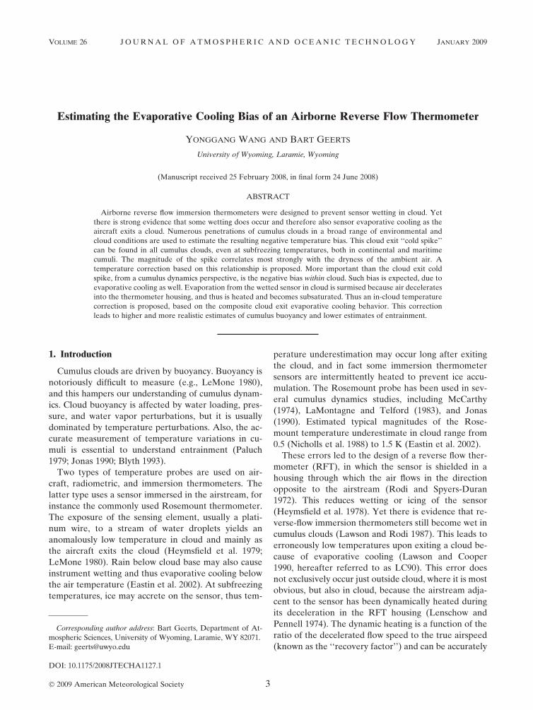
An example of a cloud exit EC error is shown in Fig.

1. The WKA penetrated a visibly growing tower with

sharp edges and with a 5 m s21 peak updraft (Fig. 1b).

The extent of the cumulus cloud can be inferred from

the cloud droplet number concentration No and the

liquid water content (LWC). The reverse flow tempera-

ture (TRF) trace shows a downward spike at the cloud

exit point, and a gradual recovery afterward. This evo-

lution is not related to changes in aircraft altitude (not

shown). The recovery appears to be exponential, sug-

gesting that most droplets on the temperature sensor

evaporate quickly in the dry airstream, while the larger

ones need more time. The negative TRF spike and ex-

ponential recovery are common features of cumulus

exit regions. We are aware that a real negative tem-

perature anomaly may occur along the cloud edges, for

example, due to the evaporation of cloud droplets in

detrained air (e.g., Jonas 1990). For instance, the cold

anomaly seen near the entrance of the cumulus in Fig.

1 (at x 5 0.78 km) may be real.

The analysis method and data sources are introduced

in section 2. The cloud exit EC bias is quantified and

related to cloud and ambient conditions in section 3.

The adaptation of the proposed cloud exit EC correc-

tion for use within clouds is presented in section 4, and

the impact of this correction on cumulus buoyancy and

entrainment is discussed in section 5.

2. Method and data sources

A large number of cumulus clouds were penetrated

by the WKA in three recent campaigns: 72 h were

flown in the High-Plains Cumulus (HiCu-03) campaign

in Wyoming in the summer of 2003, mostly in cumulus

congestus with a cloud base near the freezing level

(Damiani et al. 2006). A further 89 h were flown in the

Rain in Cumulus over the Ocean (RICO-04) campaign

(Rauber et al. 2007), conducted in shallow precipitating

trade wind cumuli over the tropical North Atlantic

Ocean in winter. And 60 h were flown in shallow–deep

orographic convection in Arizona in summer as part of

the Cumulus Photogrammetric, In-Situ and Doppler

Observations (CuPIDO-06) campaign (Damiani et al.

2008; Geerts et al. 2008). Typical conditions of the

sampled cumulus clouds in these three campaigns are

listed in Table 1. The cloud droplet number concentra-

tion No is obtained from the Forward Scattering Spec-

trometer Probe (FSSP). This count can, in theory, in-

clude ice crystals, but the ice crystal concentration is

FIG. 1. WKA measurements of a cumulus penetrated during

CuPIDO-06 at 1707 UTC 24 Jul 2006. (a) FSSP cloud droplet

number concentration (No) and LWC; (b) vertical air velocity and

TRF. The flight direction in this figure and all other transects

shown in this paper is from left to right.

4 J O U R N A L O F A T M O S P H E R I C A N D O C E A N I C T E C H N O L O G Y VOLUME 26

orders of magnitude smaller than the typical droplet

concentration. The cloud liquid water content is in-

ferred from the same probe, by integrating over all

droplet size bins (Brenguier et al. 1994). It does not

include drizzle or raindrops, but the FSSP LWC gener-

ally compared well (within 10%) with that from the

Gerber particle volume monitor (PVM-100) (Gerber et

al. 1994) and the DMT-100 (Droplet Measurement

Technologies) hotwire probe (King et al. 1981) for all

three field campaigns. Clearly, the HiCu-03 cumuli

were the most ‘‘continental,’’ with the highest No, the

lowest LWC, and the smallest mean droplet diameter.

CuPIDO-06 took place during the North American

monsoon; these cumuli had a remarkably high LWC

and, in terms of droplet size distribution and number

concentration, they were intermediate between the un-

polluted maritime cumuli east of the Lesser Antilles in

RICO-04 and the truly continental HiCu-03 cumuli.

Most clouds in the three campaigns were cumuli con-

gesti. Most clouds also contained some liquid or frozen

precipitation, according to cloud radar data collected

on all flights. All RICO-04 target clouds were relatively

shallow clouds with tops below the freezing level, while

the CuPIDO-06 cumuli ranged in size from cumulus

humilis to cumulonimbus. As will be shown later, the

combination of the three campaigns covers a broad

range of cloud microphysical and ambient temperature

and humidity conditions.

The instrument of primary interest in this study is the

reverse flow thermometer (Fig. 2). The dynamic heat-

ing from the free airstream to the platinum wire sensor

amounts to about 2.3 K for the typical WKA true air-

speed (;90 m s21) and the specific recovery factor of

the probe aboard the WKA. It is not clear how the

wetting of the sensor occurs. Wind tunnel observations

reported by LC90 indicate that drops are collected on

TABLE 1. Basic cloud properties and cloud exit EC parameters for all cumuli used in this study, in three campaigns. Cumulus depths

were estimated from the zenith antenna of the WCR and the lifting condensation level. The quality of fit is discussed in the text.

HiCu-03 RICO-04 CuPIDO-06

Environment Continental Maritime Continental

Number of clean cloud exit samples (T . 212.38C) 77 153 76

Number of clean cloud entrance samples (T . 212.38C) 291 188 162

Mean in-cloud temperature before EC correction (8C) 29.0 115.5 10.6

Approx range of cumulus depths (km) 1.0–3.8 0.8–2.7 0.7–10

Mean cloud droplet number concentration (cm23) 446 56 216

Mean droplet diameter (mm) 8.6 19.2 16.3

Mean cloud liquid water content (g m23) 0.35 0.43 0.83

Quality of cloud exit EC bias fit (K) 0.088 0.094 0.101

Mean cloud exit EC amplitude DTo (K) 20.77 21.07 21.75

Mean cloud exit EC time constant td (s) 2.20 2.33 1.88

Standard error of the regression estimate of DTo (K) 0.70 0.76 0.80

FIG. 2. Photo and schematic of the reverse-flow thermometer. Air enters through port (A)

and exits through any of several ports (B). Inside the housing, the air flows past a platinum

wire sensor (C) wound in a spiral, 25 mm in diameter. The reverse-flow design is intended to

separate hydrometeors (D) from the airstream that enters the probe. The schematic on the

right is from LC90.

JANUARY 2009 W A N G A N D G E E R T S 5

the outside of the RFT housing. This water then travels

rearward until reaching the round opening in the back

(‘‘A’’ in Fig. 2) and then accumulates just inside the

cylinder. The reverse airflow is very turbulent, and

some of this accumulated water is caught in the turbu-

lence and sprayed onto the sensor. Our measurements

indicate that this wetting happens quickly; even clouds

less than 100 m wide can produce a cloud exit EC sig-

nature, but stronger EC signatures occur at the exit of

clouds at least a few 100 m wide. Wind tunnel obser-

vations (LC90) suggest that at temperatures below

freezing, supercooled water accretes at the leading edge

of the thermometer housing and does not travel to the

trailing edge.1 Based on these observations, LC90 spec-

ulated that the cloud exit EC error should vanish at

temperatures below freezing. Heymsfield et al. (1978)

illustrate rime accumulation on the leading edge of the

RFT probe in a wind tunnel, and our own field obser-

vations during HiCu-03 and CuPIDO-06 confirm this.

But as will be shown later, the EC bias at the cloud exit

does occur below freezing, in fact even at air tempera-

tures well below 22.38C (corresponding with 08C

within the RFT housing). This suggests that at least

some sensor wetting results from droplets that never

contact the housing but remain embedded in the tur-

bulent reverse flow. Presumably only the smallest drop-

lets are not separated out at the RFT trailing edge.

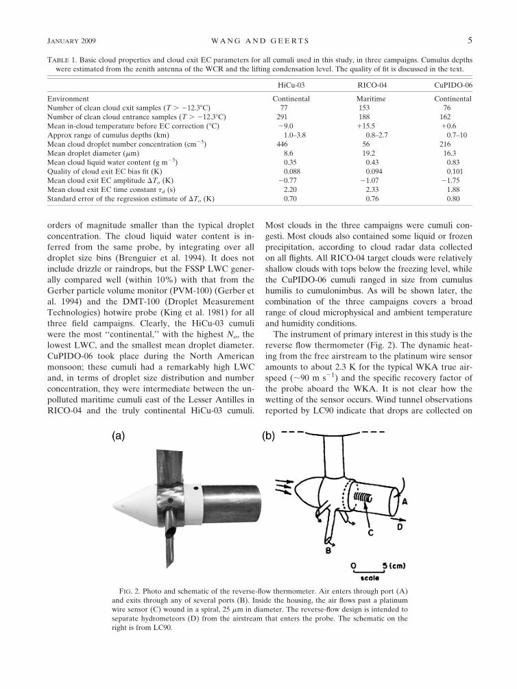
Cumulus clouds can be quite ragged, and clear defi-

nitions of a cloud and a cloud exit are needed. Only

(roughly) level aircraft penetrations through cumuli are

included. Cloud definitions are based on the FSSP No

measurements at 10 Hz, corresponding with a spatial

resolution of about 9 m. Data from all other probes are

measured at a higher frequency and are reduced to a

common frequency of 10 Hz. A cloud is defined as a

region at least 200 m wide with average No values ex-

ceeding a critical value No,c. For continental cumuli

(HiCu-03 and CuPIDO-06), No,c 5 100 cm23, and for

maritime cumuli (RICO-04), No,c 5 50 cm23. Pockets

of lower droplet concentrations (No, No,c) in cloud are

allowed, but their maximum width is 100 m, as is the

case for the cumulus in Fig. 1.

The resulting population of clouds then is used to

obtain a sample of ‘‘clean’’ cloud edges, defined as the

first point where No , 1 cm23 and No does not exceed

50 cm23 (20 cm23 for RICO-04) anywhere over a dis-

tance of at least 800 m in front of (for entrances) or

behind (for exits) the cloud. Only clean entrances and

exits are used in this study, because small patches of

cloud in the exit region can produce their own cloud

exit EC signal or at least contaminate the temperature

recovery following cloud exit from the main cloud (Fig.

3). Clearly only a fraction of clouds has clean exits. It is

worth noting that the number of clean exits is smaller

than the number of clean entrances (Table 1). The rea-

son for this probably is that the pilot tended to pen-

etrate a cumulus at a point where the cloud edge was

well defined, near the center of the cloud as judged

during the approach. The pilot cannot know what the

cloud exit region looks like.

3. Estimating the evaporative cooling bias in thecloud exit region

a. Composite temperature trace

The composite TRF traces for all entrances and all

exits for the three experiments are shown in Fig. 4. The

FIG. 3. Sample cloud exits from CuPIDO-06: (a) used and (b)

unused. The cloud edge in (b), at a distance of 1.0 km, is followed

by a thin cloud within 800 m; therefore, it is rejected. The cloud

edge in (a) is considered ‘‘clean’’ and is included in the study.

1 Note that no components of the RFT probe are heated to

remove accreted ice.


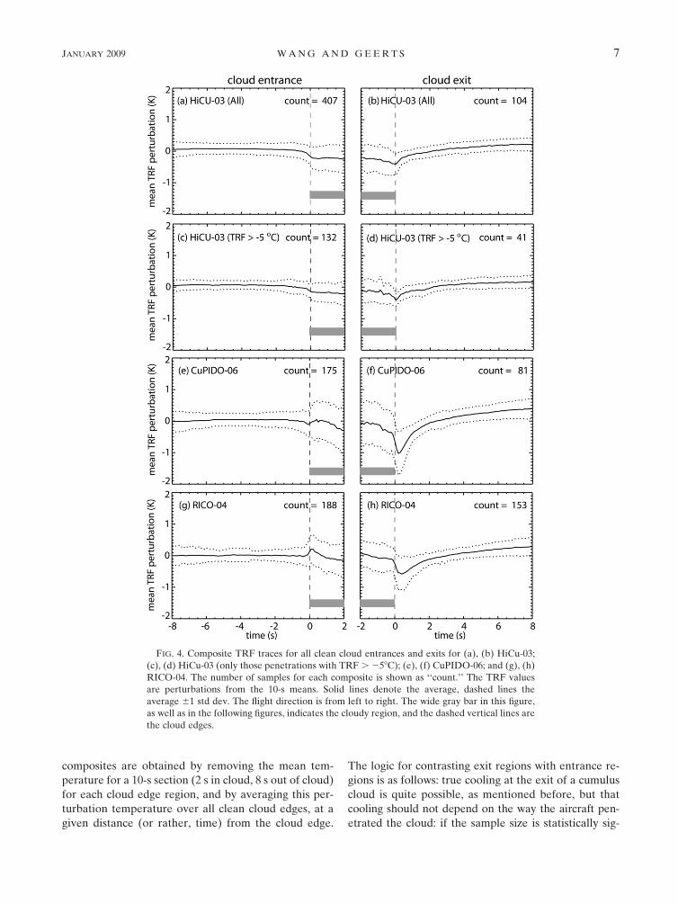
composites are obtained by removing the mean tem-

perature for a 10-s section (2 s in cloud, 8 s out of cloud)

for each cloud edge region, and by averaging this per-

turbation temperature over all clean cloud edges, at a

given distance (or rather, time) from the cloud edge.

The logic for contrasting exit regions with entrance re-

gions is as follows: true cooling at the exit of a cumulus

cloud is quite possible, as mentioned before, but that

cooling should not depend on the way the aircraft pen-

etrated the cloud: if the sample size is statistically sig-

FIG. 4. Composite TRF traces for all clean cloud entrances and exits for (a), (b) HiCu-03;

(c), (d) HiCu-03 (only those penetrations with TRF . 258C); (e), (f) CuPIDO-06; and (g), (h)

RICO-04. The number of samples for each composite is shown as ‘‘count.’’ The TRF values

are perturbations from the 10-s means. Solid lines denote the average, dashed lines the

average 61 std dev. The flight direction is from left to right. The wide gray bar in this figure,

as well as in the following figures, indicates the cloudy region, and the dashed vertical lines are

the cloud edges.


nificant, the difference in temperature trend between

exit and entrance regions should be entirely instrument

related. This is because in all three experiments, cumuli

were penetrated from various angles. Usually a pen-

etration was repeated in the opposite direction, or else

the cumulus was penetrated more than twice following

a rosette flight pattern (Damiani et al. 2008).

The composite TRF trace has a clear negative spike

just behind the cloud exit followed by a more gradual

recovery, at least for CuPIDO-06 (Fig. 4f) and RICO-

04 (Fig. 4h). This signature is not present near entrance

regions. Three explanations are offered: there are sys-

tematic variations in aircraft altitude associated with

cumulus drafts; the aircraft typically penetrated the cu-

mulus in the direction of the wind shear; and the EC of

a wetted sensor. The first and third explanation regard

the cold spike as an error, related to the instrument or

the platform; the second explanation regards the cold

spike as physically real.

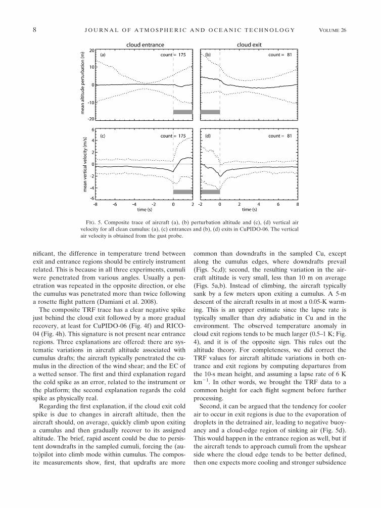
Regarding the first explanation, if the cloud exit cold

spike is due to changes in aircraft altitude, then the

aircraft should, on average, quickly climb upon exiting

a cumulus and then gradually recover to its assigned

altitude. The brief, rapid ascent could be due to persis-

tent downdrafts in the sampled cumuli, forcing the (au-

to)pilot into climb mode within cumulus. The compos-

ite measurements show, first, that updrafts are more

common than downdrafts in the sampled Cu, except

along the cumulus edges, where downdrafts prevail

(Figs. 5c,d); second, the resulting variation in the air-

craft altitude is very small, less than 10 m on average

(Figs. 5a,b). Instead of climbing, the aircraft typically

sank by a few meters upon exiting a cumulus. A 5-m

descent of the aircraft results in at most a 0.05-K warm-

ing. This is an upper estimate since the lapse rate is

typically smaller than dry adiabatic in Cu and in the

environment. The observed temperature anomaly in

cloud exit regions tends to be much larger (0.5–1 K; Fig.

4), and it is of the opposite sign. This rules out the

altitude theory. For completeness, we did correct the

TRF values for aircraft altitude variations in both en-

trance and exit regions by computing departures from

the 10-s mean height, and assuming a lapse rate of 6 K

km21. In other words, we brought the TRF data to a

common height for each flight segment before further

processing.

Second, it can be argued that the tendency for cooler

air to occur in exit regions is due to the evaporation of

droplets in the detrained air, leading to negative buoy-

ancy and a cloud-edge region of sinking air (Fig. 5d).

This would happen in the entrance region as well, but if

the aircraft tends to approach cumuli from the upshear

side where the cloud edge tends to be better defined,

then one expects more cooling and stronger subsidence

FIG. 5. Composite trace of aircraft (a), (b) perturbation altitude and (c), (d) vertical air

velocity for all clean cumulus: (a), (c) entrances and (b), (d) exits in CuPIDO-06. The vertical

air velocity is obtained from the gust probe.


on average in the exit region (i.e., usually on the down-

shear side). Indeed, clean edges are more common on

the entrance side than the exit side in all three cam-

paigns (Fig. 4), and the average exit region downdraft

(Fig. 5d) peaks at 22 m s21, which is stronger than the

entrance region downdraft (Fig. 5c). Cumuli were pen-

etrated from every angle, however, and the most com-

mon direction differed between the three campaigns

(Fig. 6). Overall, tailwind approaches (a surrogate for

an approach from the upshear side) are not significantly

more common than headwind approaches.

That leaves only the third explanation, that is, the

cloud exit cold spike is due to EC on the RFT sensor.

The composite TRF trace for HiCu-03 shows some

cooling at the exit (Fig. 4b), but not the clear spike seen

in the two other campaigns. The main reason for this is

that many HiCu-03 cumulus penetrations occurred at

temperatures below 258C (Table 1). The composite

TRF trace for the warmer HiCu-03 cases (.258C)

shows a cleaner negative spike and exponential recov-

ery in the exit region (Fig. 4d), although the cold spike

amplitude is smaller than for the two other campaigns,

and the cold spike location is closer to the cloud edge.

Several individual HiCu-03 penetrations do show a

clear cooling spike.

Another observation evident in Fig. 4 is that in all

three campaigns TRF tends to decrease as the aircraft

enters the cloud. This cooling tends to continue across

the cloud, not just in the first 2 s of cloud shown in Figs.

4a,c,e,g, but all the way to the exit point (i.e., between

22 and 0 s in Figs. 4b,d,f,h). This apparent cooling can

be seen also in the individual (noncomposite) com-

plete-cloud cumulus transects shown in Heymsfield et

al. (1979), in LC90, and in many CuPIDO cases (e.g.,

Fig. 1b). One expects cumulus towers to be warmer than

the surroundings, at least between the level of free

convection and the level where the entraining clouds

become neutrally buoyant. Penetrations were made at

all levels of the cumuli, always below anvils, and at all

stages of the lifetime of individual towers and of cumu-

lus clusters. In particular for the RICO-04 cumuli, the

RFT does register a higher temperature upon entrance

(Fig. 4g), but after less than 0.5 s in cloud, a cooling

trend sets in.

This cooling trend, or more generally the discordance

between the composite TRF trace in the first 200 m in

cloud and that in the last 200 m in cloud (Fig. 4), is the

strongest argument for the hypothesis that EC occurs at

the RFT sensor within cloud. The theoretical limit of

the TRF cooling due to evaporation is the wet-bulb

temperature depression of the dynamically heated air

(LC90). At the airspeed of the WKA, this depression

within cloud, where the air is assumed to be saturated

(Tr – Tw,cr in Fig. 7a), is about 1.4 K at an ambient

temperature of 208C and 0.6 K at 2108C (Fig. 8). The

theoretical limit of the cloud exit cold spike (i.e., the

wet-bulb depression of the ambient air) is much larger,

especially in warm, dry air (Fig. 8). This limit is rarely

reached in the exit region, however, because the sensor

is no longer actively wetted.

As mentioned in section 2, LC90 speculated that

cloud exit EC of the RFT should cease at temperatures

below 08C, because supercooled water freezes upon

contact with the RFT housing, building up rime on the

leading cone. The variation of the cloud exit cold spike

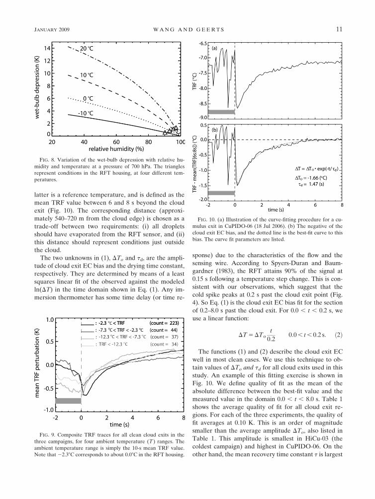
with ambient temperature is examined in Fig. 9. At

temperatures below 212.38C, the cloud exit cold spike

is weaker compared to that at higher temperatures, but

not absent. It is possible that under the high accretion

rate of supercooled water on the RFT housing, the heat

exchange is insufficient to freeze all the water, and that

some water still travels rearward and is shed from the

FIG. 6. Histogram of the angle between the flight-level wind direction and the aircraft

heading, for all cumulus penetrations in the three campaigns.


rear of the RFT cylinder. Many of the cloud exit cases

below 27.38C have a very low mean cloud LWC (0.1–

0.2 g m23), and they still show a minimum near the exit

point and a gradual TRF recovery. This suggests that at

any temperature at least some of the water reaching the

platinum wire is not shed from the RFT housing, but

rather remains suspended in the airstream as it travels

through the reverse flow tube. The higher latent heat of

sublimation (rather than the latent heat of evaporation)

and the lower vapor pressure deficit of the ambient air

relative to ice (compared to water) may explain the

longer recovery time for the two lowest temperature

ranges in Fig. 9 and for other cases shown below.

Given the gradual decrease in TRF cloud exit cold

spike magnitude with decreasing ambient temperature

below 22.38C (Fig. 9), we will implement the RFT EC

correction (discussed below) gradually between 212.38

and 22.38C.

b. Quantification of the TRF bias in the cloud exitregion

The TRF bias DT at cloud exit, due to evaporative

cooling at the surface of the wetted sensor, can be ap-

proached by an exponential decay curve:

DT 5 DTo exp � t

td

� �0:2 , t , 8:0 s; ð1Þ

where DT is the difference between the TRF at a par-

ticular time t and the temperature after recovery. The

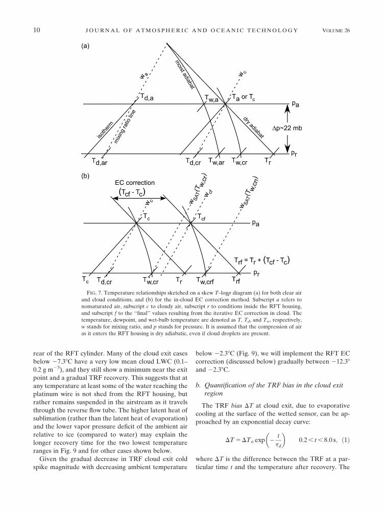
FIG. 7. Temperature relationships sketched on a skew T–logp diagram (a) for both clear air

and cloud conditions, and (b) for the in-cloud EC correction method. Subscript a refers to

nonsaturated air, subscript c to cloudy air, subscript r to conditions inside the RFT housing,

and subscript f to the ‘‘final’’ values resulting from the iterative EC correction in cloud. The

temperature, dewpoint, and wet-bulb temperature are denoted as T, Td, and Tw, respectively,

w stands for mixing ratio, and p stands for pressure. It is assumed that the compression of air

as it enters the RFT housing is dry adiabatic, even if cloud droplets are present.


latter is a reference temperature, and is defined as the

mean TRF value between 6 and 8 s beyond the cloud

exit (Fig. 10). The corresponding distance (approxi-

mately 540–720 m from the cloud edge) is chosen as a

trade-off between two requirements: (i) all droplets

should have evaporated from the RFT sensor, and (ii)

this distance should represent conditions just outside

the cloud.

The two unknowns in (1), DTo and td, are the ampli-

tude of cloud exit EC bias and the drying time constant,

respectively. They are determined by means of a least

squares linear fit of the observed against the modeled

ln(DT) in the time domain shown in Eq. (1). Any im-

mersion thermometer has some time delay (or time re-

sponse) due to the characteristics of the flow and the

sensing wire. According to Spyers-Duran and Baum-

gardner (1983), the RFT attains 90% of the signal at

0.15 s following a temperature step change. This is con-

sistent with our observations, which suggest that the

cold spike peaks at 0.2 s past the cloud exit point (Fig.

4). So Eq. (1) is the cloud exit EC bias fit for the section

of 0.2–8.0 s past the cloud exit. For 0.0 , t , 0.2 s, we

use a linear function:

DT 5 DTot

0:20:0 , t , 0:2 s: ð2Þ

The functions (1) and (2) describe the cloud exit EC

well in most clean cases. We use this technique to ob-

tain values of DTo and td for all cloud exits used in this

study. An example of this fitting exercise is shown in

Fig. 10. We define quality of fit as the mean of the

absolute difference between the best-fit value and the

measured value in the domain 0.0 , t , 8.0 s. Table 1

shows the average quality of fit for all cloud exit re-

gions. For each of the three experiments, the quality of

fit averages at 0.10 K. This is an order of magnitude

smaller than the average amplitude DTo, also listed in

Table 1. This amplitude is smallest in HiCu-03 (the

coldest campaign) and highest in CuPIDO-06. On the

other hand, the mean recovery time constant t is largest

FIG. 8. Variation of the wet-bulb depression with relative hu-

midity and temperature at a pressure of 700 hPa. The triangles

represent conditions in the RFT housing, at four different tem-

peratures.

FIG. 9. Composite TRF traces for all clean cloud exits in the

three campaigns, for four ambient temperature (T ) ranges. The

ambient temperature range is simply the 10-s mean TRF value.

Note that 22.38C corresponds to about 0.08C in the RFT housing.

FIG. 10. (a) Illustration of the curve-fitting procedure for a cu-

mulus exit in CuPIDO-06 (18 Jul 2006). (b) The negative of the

cloud exit EC bias, and the dotted line is the best-fit curve to this

bias. The curve fit parameters are listed.


in HiCu-03 and smallest in CuPIDO-06. In the next

section, we show that these differences in both DTo and

td can be interpreted mainly in terms of the relative

dryness of the environment, expressed in terms of the

wet-bulb depression.

c. Factors affecting the cloud exit evaporativecooling bias

We now examine what controls the two cloud exit

EC bias parameters, DTo and td. We consider two en-

vironmental factors, the temperature and a measure of

dryness outside the cloud. For the latter, we use the

wet-bulb depression (Tr 2 Tw,ar). (The symbols are ex-

plained in Fig. 7a.) We also consider four factors char-

acterizing the cloud that was penetrated: No, LWC, the

liquid water path (LWP, defined as the track-integrated

LWC, in units g m22), and the mean droplet diameter

(D). The latter is derived from the 15 FSSP drop-size

bins (5–50 mm). The cloud factors are averages or in-

tegrals over the entire cloud. The temperature is an

average over the entire cloud exit vicinity, from 2 s

inside cloud to 8 s outside cloud. The wet-bulb depres-

sion Tr 2 Tw,ar is an average between 0 and 2 s before

the cloud entrance (i.e., on the other side of the cloud).

The reason for this choice is not physical, but practical,

as explained below.

The wet-bulb depression (Tr 2 Tw,ar) applies to the

dynamically heated air inside the RFT housing, as illus-

trated in Fig. 7a. It is computed from the pressure (pr)

and the temperature (Tr) inside the RFT housing, and

the ambient mixing ratio wa. Both Tr and wa are mea-

sured. A LI-COR 6060 fast-rate wa sensor was available

in only two of the three campaigns (RICO-04 and

CuPIDO-06), and displayed wetting symptoms itself in

some cumulus penetrations. Therefore, we infer wa

from the slow-rate Cambridge chilled-mirror dewpoint

sensor. The chilled-mirror wa values in the entire exit

region, well beyond the (exit point 1 8 s), are contami-

nated by the cloud just penetrated, and they are in

essence a surrogate for cumulus width. In a composite

sense, the lowest chilled-mirror wa values (those best

representing the environment) occur just before the

cloud entrance point, thus the wet-bulb depression is

computed there. This solution is not ideal, because real

humidity differences may occur on opposite sides of a

cumulus, especially at a detrainment level.

The pressure pr is derived as follows:

pr 5 pa 1 Dp 5 pa 1rrU2

‘

2: ð3Þ

Here U‘ is the true airspeed of the aircraft, r is effective

recovery factor of the RFT housing and sensing ele-

ment (LC90) (r 5 0.625 for the RFT on the WKA), pa

is the static air pressure at flight level (Fig. 7), and r is

the air density. For the three field campaigns used in

this study, the compression into the RFT housing (Dp)

ranges between 20 and 24 hPa. The expression for wet-

bulb depression (K) is (e.g., Pruppacher and Klett 1996,

p. 490)

Tr � Tw;ar 5LeðTw;arÞ wSATðTw;arÞ � wa

� �cpa 1 cpvwa

: ð4Þ

Here LeðTw;arÞ is the latent heat of vaporization (J

kg21) at temperature Tw,ar, cpa is the specific heat of air

at constant pressure (J kg21 K21), and cpv is the specific

heat of water vapor at constant pressure (J kg21 K21).

The term wSAT in Eq. (4) is the saturation mixing ratio

(kg kg21) at Tw,ar:

wSATðTw;arÞ5eeSATðTw;arÞ

pr � eSATðTw;arÞ; ð5Þ

where eSATðTw;arÞ is the saturation vapor pressure (Pa)

at Tw,ar, and e is a constant (e 5 0.622). There is no

analytic solution for Eq. (4) for wet-bulb temperature,

so it needs to be solved iteratively.

The exponential fit parameters DTo and td are plot-

ted against the six factors for all clean cumulus exits in

the three campaigns in Fig. 11. The three campaigns

cover a broad spectrum of cumulus clouds, with a mean

LWC ranging between 0.1 and 2.1 g m23, a mean No

from 30 to 500 cm23, a mean D from 5 to 30 mm, and a

mean flight-level temperature from 212.38C (our thresh-

old temperature) to 1218C.

The magnitude of the correlation coefficients2 be-

tween LWP, No, and temperature on the one hand, and

either DTo or td on the other, are all very low, less than

0.1 (Fig. 11). Surprisingly, neither the LWP (g m22)

computed over the entire cloud (not shown) nor over

the last 2 s before the exit point (shown) show a signif-

icant correlation. There is no clear lower-limit LWC or

LWP for cloud exit EC to occur. This indicates that

RFT sensor wetting happens rather readily, even for

relatively thin or small liquid water clouds. With in-

creasing cloud LWC, the amplitude of the cold spike

(jDToj) does tend to increase, suggesting that the wet-

ting of the RFT sensor surface increases with LWC. In

fact, the cumuli in CuPIDO-06 have both the largest

LWC and the highest jDToj, compared to those in the

two other campaigns (Table 1). Still, the correlation

2 The linear regressions and correlation coefficients are com-

puted based on the minimization of the absolute differences (not

the square of the differences) between observations and the re-

gression line. This reduces the sensitivity to outliers.


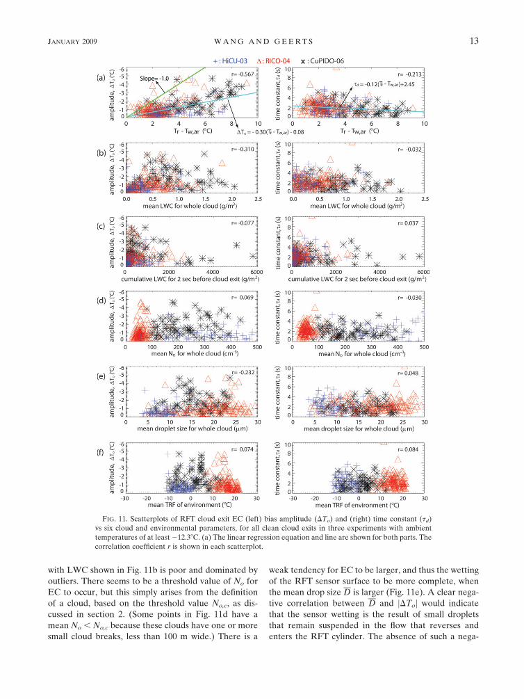
with LWC shown in Fig. 11b is poor and dominated by

outliers. There seems to be a threshold value of No for

EC to occur, but this simply arises from the definition

of a cloud, based on the threshold value No,c, as dis-

cussed in section 2. (Some points in Fig. 11d have a

mean No , No,c because these clouds have one or more

small cloud breaks, less than 100 m wide.) There is a

weak tendency for EC to be larger, and thus the wetting

of the RFT sensor surface to be more complete, when

the mean drop size D is larger (Fig. 11e). A clear nega-

tive correlation between D and jDToj would indicate

that the sensor wetting is the result of small droplets

that remain suspended in the flow that reverses and

enters the RFT cylinder. The absence of such a nega-

FIG. 11. Scatterplots of RFT cloud exit EC (left) bias amplitude (DTo) and (right) time constant (td)

vs six cloud and environmental parameters, for all clean cloud exits in three experiments with ambient

temperatures of at least 212.38C. (a) The linear regression equation and line are shown for both parts. The

correlation coefficient r is shown in each scatterplot.


tive correlation suggests that water shedding from the

RFT housing (an idea proposed by LC90) is important.

In short, no single cloud or environmental factor ex-

plains cloud exit EC. The wet-bulb depression Tr 2

Tw,ar is most strongly correlated: the drier the environ-

ment, the larger the cooling spike DTo and the smaller

td (i.e., the more rapidly the droplets evaporate from

the platinum wire). The linear regression between DTo

and the wet-bulb depression is as follows:

DTo 5 �0:30 Tr � Tw;ar

� �� 0:08 ðKÞ: ð6Þ

This means that upon exiting a cloud, TRF is cooled to

30% of its potential by evaporation [i.e., the ambient

wet-bulb depression (Fig. 8)]. The full wet-bulb depres-

sion can only be attained if the platinum wire spiral is

and remains fully wet. Only for a few cumulus penetra-

tions was this potential reached, according to Fig. 11a.

The standard error3 for linear regression (6) is 0.80 K.

This is a measure of uncertainty of the EC correction in

the cloud exit region. Similarly, the linear regression

between td and the wet-bulb depression is as follows:

td 5 �0:12 Tr � Tw;ar

� �1 2:45 ðsÞ: ð7Þ

Regression Eqs. (6) and (7) were evaluated for vari-

ous samples of the entire population of clean cloud

exits, in order to find contrasts and stronger correla-

tions. These samples included the three different cam-

paigns, maritime versus continental clouds, and cold

versus warm clouds. None of the regression equations

are substantially different, none of the correlation co-

efficients are substantially higher, and none of the re-

maining uncertainty is substantially lower. Compare,

for instance, the standard errors of DTo for each of the

campaigns (Table 1) with those for the three campaigns

combined. We also tried multiple regressions with the

top two and three variables, in terms of their correla-

tion with DTo (Fig. 11). These regressions are not sig-

nificantly better either. Therefore we propose that Eqs.

(1) and (2) are used to correct the TRF values for EC

in the cloud exit region, with the amplitude DTo given

by Eq. (6) and the drying time td given by Eq. (7). The

latter two equations represent the entire sample size

and the broadest parameter space. The full correction is

applied at mean temperatures above 22.38C, no cor-

rection is applied below 212.38C, and a fraction of the

correction increasing linearly between 0% and 100% is

applied between 212.38 and 22.38C.

To test this correction, a TRF composite for all en-

trances and all exits with TRF . 212.38C is shown in

Fig. 12. Here we focus on the correction outside of

cloud. The values plotted in Fig. 12 are departures from

the 10-s mean; thus what matters is the slope of the

curve, starting far away from the cloud. The composite

corrected temperature traces in the clear air are rather

flat in the cloud entrance and cloud exit cases, confirm-

ing the validity of the cloud exit EC bias correction. The

temperature decreases slightly toward cloud (;0.1 K)

in the cloud entrance region. Such cooling may be

present in the exit region also, near t 5 0.5 s in Fig. 12b,

but it is masked by the much larger EC correction. This

cloud edge cooling may well be real. It may be due to

the evaporative cooling of detrained cloudy parcels, or

to radial variation of adiabatic warming (e.g., subsi-

dence that peaks some distance away from the cloud

edge). In any event, the similarity of the exit and en-

trance TRF trends gives confidence in the EC correc-

FIG. 12. Composite TRF traces for all clean (a) cloud entrances and (b) cloud exits in

three campaigns. The values shown are perturbations from the 8-s mean for each entrance or

exit region. Gray lines denote the uncorrected, original TRF, black lines the TRF with a

correction for EC in the exit region. The black dotted lines are the mean corrected values 61

standard error.

3 The standard error is the standard deviation of the difference

between the linear regression values and the true values.


tion. The standard error, shown in Fig. 12b, reflects the

uncertainty in the EC correction only, not the overall

RFT instrument uncertainty. It is computed from the

standard errors of both the DTo and td estimates (i.e., it

is based on the scatter around the regression curves in

both parts of Fig. 11a).

4. Reverse flow temperature correction in cloud

Clearly, the true temperature in cumuli varies sub-

stantially, more than in the surrounding clear air, as is

evident in the larger standard deviations in cloud than

out of cloud in Fig. 4. But the dependence of the in-

cloud temperature trend within 200 m of the cloud edge

on the flight direction (into or out of the cloud) in a

large composite of cases (Fig. 4) is an indication of an

instrument bias. We now demonstrate that the EC cor-

rection proposed for cloud exit regions (section 3c) can

also be used to estimate the TRF bias within cumulus

clouds and to remove the erroneous cooling trend from

entrance point to exit point.

Within a cumulus cloud, the dynamically heated air in

the RFT housing is subsaturated, leading to EC of a

wetted surface. We make the following three assump-

tions:

1) The cloudy air is saturated, that is, the relative hu-

midity is precisely 100%. This implies that the vapor

pressure in cloud equals the saturation vapor pres-

sure at the best temperature estimate available (i.e.,

the EC-corrected TRF, denoted as TRFc).

2) The water vapor mixing ratio in the RFT housing

equals that in the cloudy-free airstream (i.e., drop-

lets do not have a chance to evaporate in the dy-

namically heated air). This implies that the wet-bulb

depression equals the difference between dynami-

cally heated temperature (Tr) and the wet-bulb tem-

perature Tw,cr (Fig. 7a), or successive corrections of

that difference (Fig. 7b).

3) Evaporative cooling of the RFT sensor in cloud oc-

curs at the same fraction of the wet-bulb depression

as observed just outside a cloud [i.e., Eq. (6) applies

in-cloud as well]. This assumption is rather conser-

vative, because the cloud exit cold spike magnitude

is constrained by sensor drying outside cloud, and

reaches only 30% of the wet-bulb depression,

whereas continuous sensor wetting occurs within

cloud.

More specifically, the third assumption applies every-

where in cloud except near the entrance. Individual

transects, and composites such as the one for the

RICO-04 entrance cases (Fig. 4g), suggest that the wet-

ting of the RFT sensor just beyond the cloud entrance

and the resulting cooling is a rapid process, but is not

instantaneous. The composite TRF signature at the en-

trance region shows some initial warming, followed by

cooling farther in the cumulus. We interpret the initial

warming as real and the follow-up cooling as dominated

by EC. Theoretically the composite TRF trace for all the

entrances should be very similar to that for all the

exits. Thus we choose the RTF ‘‘wetting time constant’’

tw as 0.7 s. This value is chosen by trial and error,

comparing the corrected composite TRF trace follow-

ing cloud entrance with that before cloud exit (shown

below). We use an exponential adjustment like Eq. (1),

with tw as the time constant and the full in-cloud cor-

rection derived below as the amplitude. The use of an

exponential rather than a linear curve is somewhat ar-

bitrary, and is motivated by the idea that the probability

of a new drop being collected by the platinum spiral

wire decreases with the number of droplets already

present on the wire.

The in-cloud correction is an iterative process, as fol-

lows: the initial guess for TRFc equals Tc, which is cor-

rected for dynamic heating (Fig. 7b) but not for EC.

The wet-bulb temperature Tw,cr then is calculated as

Tw;cr 5 Tr 1 TRFc� Tcð Þ

�LeðTw;crÞ wSATðTw;crÞ � wc

� �cpa 1 cpvwc

; ð8Þ

where wc is water vapor mixing ratio (kg kg21) in cloud,

computed as the saturation mixing ratio at the dew-

point temperature in cloud (TRFc),

wc 5eeSATðTRFcÞ

pa � eSATðTRFcÞ :

In Eq. (8), wSAT is the saturation mixing ratio at Tw,cr:

wSATðTw;crÞ5eeSATðTw;crÞ

pr � eSATðTw;crÞ:

The term Tr 1 TRFc� Tcð Þ in Eq. (8) is explained as

follows: the EC correction changes the estimate of the

free-airstream temperature from Tc to TRFc. This cor-

rection also applies inside the RFT housing; in other

words the estimate of the dynamically heated air

changes from Tr to Tr 1 TRFc� Tcð Þ (Fig. 7b). Fol-

lowing assumption (3) above, we obtain a new TRFc

based on Eq. (6):

TRFc 5 Tc 1 0:30 Tr 1 TRFc� Tcð Þ � Tw;cr

� �

3 1� exp�t

tw

� �� 1 0:08; ð9Þ

where t is time, computed from the cumulus entrance

point and increasing into the cloud. We then compare


TRFc from Eq. (9) with its initial guess (Tc), and iterate

through Eqs. (8) and (9) until the successive values of

TRFc differ by less than 0.001 K. At that point, TRFc 5

Tcf, and the temperature in the RFT housing is Trf,

following the notation in Fig. 7b. Note that the correc-

tion proposed herein is different for aircraft flying at

different operational speeds. Section 3 in LC90 can be

used as a guide to adapting our correction to different

airspeeds.

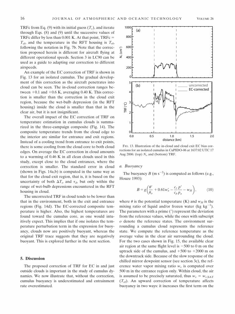
An example of the EC correction of TRF is shown in

Fig. 13 for an isolated cumulus. The gradual develop-

ment of this correction as the aircraft penetrates into

cloud can be seen. The in-cloud correction ranges be-

tween 10.1 and 10.6 K, averaging 0.40 K. This correc-

tion is smaller than the correction in the cloud exit

region, because the wet-bulb depression (in the RFT

housing) inside the cloud is smaller than that in the

clear air, but it is not insignificant.

The overall impact of the EC correction of TRF on

temperature estimation in cumulus clouds is summa-

rized in the three-campaign composite (Fig. 14). The

composite temperature trends from the cloud edge to

the interior are similar for entrance and exit regions.

Instead of a cooling trend from entrance to exit points,

there is some cooling from the cloud core to both cloud

edges. On average the EC correction in cloud amounts

to a warming of 0.46 K in all clean clouds used in this

study, except close to the cloud entrances, where the

correction is smaller. The standard error in cloud

(shown in Figs. 14a,b) is computed in the same way as

that for the cloud exit region, that is, it is based on the

uncertainty of both DTo and td, but only within the

range of wet-bulb depressions encountered in the RFT

housing in cloud.

The uncorrected TRF in cloud tends to be lower than

that in the environment, both in the exit and entrance

regions (Fig. 14d). The EC-corrected composite tem-

perature is higher. Also, the highest temperatures are

found toward the cumulus core, as one would intu-

itively expect. This implies that if one isolates the tem-

perature perturbation term in the expression for buoy-

ancy, clouds now are positively buoyant, whereas the

original TRF trace suggests that they are negatively

buoyant. This is explored further in the next section.

5. Discussion

The proposed correction of TRF for EC in and just

outside clouds is important in the study of cumulus dy-

namics. We now illustrate that, without the correction,

cumulus buoyancy is underestimated and entrainment

rate overestimated.

a. Buoyancy

The buoyancy B (m s22) is computed as follows (e.g.,

Houze 1993):

B 5 gu9

uo1 0:61w9y �

cv

cp

p9

po

� wH

� �; ð10Þ

where u is the potential temperature (K) and wH is the

mixing ratio of liquid and/or frozen water (kg kg21).

The parameters with a prime (9) represent the deviation

from the reference values, while the ones with subscript

o denote the reference states. The environment sur-

rounding a cumulus cloud represents the reference

state. We compute the reference temperature as the

average value in the clear air surrounding the cloud.

For the two cases shown in Fig. 15, the available clear

air region at the same flight level is 2500 to 0 m on the

uptrack side of the cumulus, and 1500 to 12000 m on

the downtrack side. Because of the slow response of the

chilled mirror dewpoint sensor (see section 3c), the ref-

erence water vapor mixing ratio wv is computed over

500 m in the entrance region only. Within cloud, the air

is assumed to be precisely saturated, thus wv 5 wv,SAT

(Tcf). An upward correction of temperature affects

buoyancy in two ways: it increases the first term on the

FIG. 13. Illustration of the in-cloud and cloud exit EC bias cor-

rections for an isolated cumulus in CuPIDO-06 at 1637:02 UTC 17

Aug 2006: (top) No and (bottom) TRF.


right and also the second term, because a higher tem-

perature implies a higher saturation mixing ratio. The

hydrometeor loading term wH is computed from the

water mass in the FSSP and the 2D optical array

probes. The pressure perturbation term [third on the

right in Eq. (10)] is ignored because the altitude of the

aircraft is not known with enough precision.

According to (10), 0.5 K of excess heat (u9) produces

the same buoyancy as ;3 g kg21 of excess water vapor

and ;1.6 g kg21 of water loading wH. (The latter is

negative buoyancy.) Thus, an in-cloud TRF correction

of 10.5 K is significant. To illustrate the impact of the

correction on buoyancy calculations, we examine two

penetrations of vigorous, growing cumuli in CuPIDO-

06 (Fig. 15). This illustration includes the reflectivity

and Doppler velocity transects from the Wyoming

Cloud Radar (WCR). The WCR operated in a vertical

plane above and below the aircraft (Damiani et al.

2008). The narrow horizontal black stripe in Figs.

15a,b,e,f indicates the radar blind zone (;100-m range,

both up and down). The flight level is centered in this

blind zone. The radar data provide a vertical slice of the

cumulus and assist in the interpretation of the flight-

level data. In both cases updrafts exceeded 10 m s21 at

and below flight level. The penetrations occurred about

1 km below cloud top but above the freezing level. An

older cumulus with strong downward motions (near x 5

0.5 km in Fig. 15b) is collapsing just to the left of the

first target cumulus. The high reflectivity below flight

level (Fig. 15a) is attributed to precipitation-size par-

ticles. Our interest is in the updraft plume at 1.0 , x ,

2.0 km, extending from near the cloud base to the top

(Fig. 15b). It is flanked by subsidence on both sides,

near x 5 2.5 and x 5 0.5 km (Figs. 15b,d). The EC bias

correction increases the in-cloud temperature, resulting

in a significant increase in cloud buoyancy. The uncor-

rected buoyancy values are negative on average, which

is difficult to reconcile with the updraft strength mea-

sured at flight level and over the depth of the cloud.

The corrected buoyancy is mostly positive across the

updraft plume (except for the right flank of the updraft,

near x # 2.0 km). The cumulus on the right (Fig. 15e)

probably is younger since its reflectivity is lower, but it

has an even stronger updraft plume bubbling up to

flight level (near 1.5 , x , 2.0 km in Figs. 15f,h). The

uncorrected buoyancy is slightly negative over the

width of this cloud. As a result of the EC correction,

this updraft plume again becomes mostly positively

buoyant, in particular in the updraft region (Fig. 15g).

The impact of the EC correction on the composite

buoyancy for all clean cloud edges is shown in Fig. 16.

Here the reference temperature and mixing ratio are

computed as the average over the 10 s shown (2 s in

cloud and 8 s out of cloud). The pressure perturbation

FIG. 14. (a), (b) As in Fig. 12, but with the EC correction applied both in cloud and cloud exit

regions. Again, the dotted lines are the mean corrected values 61 standard error. (c), (d) As in

(a), (b), but the actual average temperature is shown, rather than the average departure from

each individual 10-s mean.


term in (10) is ignored again, and the mixing ratio is

assumed to be saturated in cloud. This assumption af-

fects the water vapor term in (10) and explains the jump

in buoyancy at both cloud edges in Fig. 16. The uncor-

rected TRF yields negatively buoyant cloud cores on

average, inward from the entrance point (Fig. 16a).

This applies even for the subset of cases where the

average vertical velocity in cloud is positive (not

shown). The uncorrected composite buoyancy de-

creases from cloud entrance to exit, driven by the same

trend in the uncorrected TRF trace (Fig. 14). The buoy-

ancy discontinuity at the inner cloud (where Figs. 16a,b

meet) is simply due to the definition of buoyancy,

whose reference is just the average of the 10-s trace, for

convenience. In any event, the use of the EC-corrected

TRF yields higher buoyancy in the cloud’s core.

b. Entrainment

The impact of the EC correction on entrainment es-

timates is illustrated by means of a Paluch diagram

(Paluch 1979) (Fig. 17). The CuPIDO experiment ben-

efitted from excellent proximity soundings collected by

FIG. 15. An illustration of the impact of the TRF correction on buoyancy for two CuPIDO-06 cumuli, at (left) 1806:56 and (right)

1936:52 UTC 2 Aug 2006. (top colored panels) WCR profiles centered at flight level (black stripe): (top) reflectivity and (bottom)

vertical velocity. The aspect ratio of these cross sections is 3.6:1. (bottom graphs) Flight-level data with the vertical dashed lines indicate

the cumulus (left) entrance and (right) exit points, as determined from FSSP data: (top) buoyancy and (bottom) vertical air velocity.


a Mobile GPS Advanced Upper-Air Sounding (M-

GAUS) system. The radiosondes were released about

10 km upstream of the target orographic cumulus in

both examples in Fig. 17, and they ascended in clear air

within minutes of the aircraft cloud penetration. We

verified that the radiosonde did not penetrate the cloud

at any level. Two variables conserved under pseudo-

adiabatic moist processes are plotted: uq, the wet

equivalent potential temperature (defined in Paluch

1979), and wTOT, the total water mixing ratio. As be-

fore, the mixing ratio in cloud (i.e., the aircraft data) is

assumed to be its saturated value. Also shown in Fig. 17

are the cloud base (corresponding with the soundings’

lifting condensation level) and the cloud top (inferred

from WCR up-antenna reflectivity and photostereo-

grammetry; see Zehnder et al. 2007). Undiluted cloud

parcels ascending from below have the properties of the

air at cloud base; mixtures of undiluted boundary layer

air with air from above the cloud (i.e., vertical entrain-

ment) fall on the line connecting cloud base to cloud

top in Fig. 17. The closer the in-cloud measurements

are to the sounding curve at flight level, the stronger the

lateral entrainment at that level. The effect of the EC

correction is to increase uq by 1.6 K in the warm cloud

(Fig. 17a). In the colder cloud (Fig. 17b), the uq increase

is smaller, because of the temperature dependence of

the EC correction (section 3c). The total water wTOT

increases as well, since air in cloud is assumed to be

saturated. Thus the in-cloud measurements in Fig. 17

move slightly downward, and mainly to the right. In the

case of the deeper cloud (Fig. 17b) more vertical en-

trainment is apparent, and in the more shallow cumulus

(Fig. 17a) the sampled air is more similar to the cloud-

base air. In summary, the use of uncorrected TRF val-

ues tends to exaggerate lateral entrainment.

c. Further implications

Several studies have estimated cumulus buoyancy

and/or entrainment using a reverse-flow thermometer

FIG. 16. Composite buoyancy in (a) cloud entrance and (b) cloud exit regions.

FIG. 17. Paluch diagram for two cases during CuPIDO-06. The

lines represent M-GAUS sounding data; the triangle and 1 sym-

bols are aircraft data. The square symbol represents the sounding

data corresponding to the flight altitude. The mean change in wet

equivalent potential temperature (Duq) resulting from the EC cor-

rection and the mean temperature (TRF) are listed.


on an aircraft flying at about the same speed as the

WKA (;100 m s21); these include Boatman and Auer

(1983), Austin et al. (1985), Jensen et al. (1985), Blyth

et al. (1988), and Damiani et al. (2006). In some papers

other variables were derived from TRF, for instance,

equivalent potential temperature (Heymsfield et al.

1978). The EC correction proposed herein should be

applied to all those studies. Since most of the measure-

ments in the papers listed above occurred at tempera-

tures above 2128C, their analyses are affected and

some of their conclusions may be flawed. A further

investigation is worthwhile.

It should further be noted that while airborne radio-

metric thermometers avoid the issue of evaporative

cooling, they have their own problems near cloud and

precipitation (e.g., Nicholls et al. 1988; Jorgensen and

LeMone 1989). To illustrate this, we plotted the com-

posite temperature trace from the Ophir radiometric

thermometer on the NCAR C-130 aircraft in RICO-04

(Fig. 18). Clearly the C-130 did not penetrate the same

cumuli at the same time as the WKA, but it flew at

overlapping times, in the same region as the WKA, and

it also penetrated the cumuli from random directions,

often along great circles drifting with the wind. The

composite Ophir in-cloud temperature was about 0.2 K

lower than the ambient air temperature, while the cor-

rected RFT in-cloud temperature was about 0.3 K

higher than the surrounding clear air. The implications

for cumulus buoyancy are obvious. For the Ophir it is

likely that the in-cloud temperature measurement is

more accurate, because of the lower transmittance of

radiation in the Ophir CO2 infrared absorption band in

cloudy air.

6. Conclusions

There is strong evidence that the sensor of an air-

borne reverse-flow immersion thermometer (RFT) be-

comes partially wetted in cloud, notwithstanding the

reverse flow design. Aircraft data collected during nu-

merous penetrations of cumulus clouds in a broad

range of environmental and cloud conditions have been

used to estimate the bias of an RFT due to evaporative

cooling both in the cloud exit region and within cloud.

The following results have been reached:

1) A cold spike is commonly encountered as the air-

craft exits the cloud. Because such a spike is not

present in the cloud entrance region, it must be due

to evaporative cooling on a wetted sensor.

2) The amplitude of this cold bias varies much and

does not strongly correlate with cloud or environ-

mental conditions, but it is about 30% of the wet-

bulb depression of the ambient air.

3) This cloud exit temperature bias can be used to cor-

rect RFT values within clouds. This correction in-

creases the cloud temperatures by 0.4–0.5 K. Previ-

ous work using RFT measurements underestimated

the buoyancy and overestimated the entrainment in

cumulus clouds.

In further work we will use the proposed RFT cor-

rection for evaporative cooling to study buoyancy and

entrainment in the context of fundamental cumulus dy-

namics.

Acknowledgments. This work was supported by Na-

tional Science Foundation Grant ATM-0444254. We

appreciate the anonymous reviews and the insightful

discussions with Alfred R. Rodi, Jeffrey French, Gabor

Vali, Larry Oolman, and Perry Wechsler.

REFERENCES

Austin, P., M. Baker, A. Blyth, and J. Jensen, 1985: Small-scale

variability in warm continental cumulus clouds. J. Atmos.

Sci., 42, 1123–1138.

FIG. 18. Composite Ophir temperature for all clean cloud penetrations by the NCAR C-130

aircraft during RICO-04. The average and the average 61 std dev are shown. The bold gray

line is the composite corrected TRF trace for all RICO-04 cloud penetrations by the WKA,

shown for comparison.


Blyth, A. M., 1993: Entrainment in cumulus clouds. J. Appl. Me-

teor., 32, 626–641.

——, W. A. Cooper, and J. B. Jensen, 1988: A study of the source

of entrained air in Montana cumuli. J. Atmos. Sci., 45, 3944–

3964.

Boatman, J. F., and A. H. Auer, 1983: The role of cloud top en-

trainment in cumulus clouds. J. Atmos. Sci., 40, 1517–1534.

Brenguier, J., D. Baumgardner, and B. Baker, 1994: A review and

discussion of processing algorithms for FSSP concentration

measurements. J. Atmos. Oceanic Technol., 11, 1409–1414.

Damiani, R., G. Vali, and S. Haimov, 2006: The structure of ther-

mals in cumulus from airborne dual-Doppler radar observa-

tions. J. Atmos. Sci., 63, 1432–1450.

——, and Coauthors, 2008: The Cumulus, Photogrammetric, In

Situ, and Doppler Observations experiment of 2006. Bull.

Amer. Meteor. Soc., 89, 57–73.

Eastin, M. D., P. G. Black, and W. M. Gray, 2002: Flight-level

thermodynamic instrument wetting errors in hurricanes. Part

I: Observations. Mon. Wea. Rev., 130, 825–841.

Geerts, B., Q. Miao, and J. C. Demko, 2008: Pressure perturba-

tions and upslope flow over a heated, isolated mountain.

Mon. Wea. Rev., 36, 4272–4288.

Gerber, H., B. G. Arends, and A. S. Ackerman, 1994: New mi-

crophysics sensor for aircraft use. Atmos. Res., 31, 235–252.

Heymsfield, A. J., P. N. Johnson, and J. E. Dye, 1978: Observa-

tions of moist adiabatic ascent in northeast Colorado cumulus

congestus clouds. J. Atmos. Sci., 35, 1689–1703.

——, J. E. Dye, and C. J. Biter, 1979: Overestimates of entrain-

ment from wetting of aircraft temperature sensors in cloud. J.

Appl. Meteor., 18, 92–95.

Houze, R. A, Jr, 1993: Cloud Dynamics. Academic Press, 573 pp.

Jensen, J., P. Austin, M. Baker, and A. Blyth, 1985: Turbulent

mixing, spectral evolution and dynamics in a warm cumulus

cloud. J. Atmos. Sci., 42, 173–192.

Jonas, P. R., 1990: Observations of cumulus cloud entrainment.

Atmos. Res., 25, 105–127.

Jorgensen, D. P., and M. A. LeMone, 1989: Vertical velocity char-

acteristics of oceanic convection. J. Atmos. Sci., 46, 621–640.

King, W. D., C. T. Maher, and G. A. Hepburn, 1981: Further per-

formance tests on the CSIRO liquid water probe. J. Appl.

Meteor., 20, 195–202.

LaMontagne, R. G., and J. W. Telford, 1983: Cloud top mixing in

small cumuli. J. Atmos. Sci., 40, 2148–2156.

Lawson, R. P., and A. R. Rodi, 1987: Airborne tests of sensor

wetting in a reverse flow temperature probe. Proc. Sixth

Symp. on Meteorological Observation and Instrumentation,

New Orleans, LA, Amer. Meteor. Soc., 253–256.

——, and W. A. Cooper, 1990: Performance of some airborne

thermometers in clouds. J. Atmos. Oceanic Technol., 7, 480–

494.

LeMone, M. A., 1980: On the difficulty of measuring temperature

and humidity in cloud: Comments on ‘‘Shallow convection on

day 261 of GATE: Mesoscale arcs.’’ Mon. Wea. Rev., 108,

1702–1705.

Lenschow, D., and W. Pennell, 1974: On the measurement of

in-cloud and wet-bulb temperatures from an aircraft. Mon.

Wea. Rev., 102, 447–454.

McCarthy, J., 1974: Field verification of the relationship between

entrainment rate and cumulus cloud diameter. J. Atmos. Sci.,

31, 1028–1039.

Nicholls, S., E. L. Simmons, N. C. Atkins, and S. D. Rudman,

1988: A comparison of radiometric and immersion tempera-

ture measurements in water clouds. Proc. 10th Int. Conf. on

Cloud Physics, Hamburg, Germany, International Commis-

sion on Clouds and Precipitation, 322–324.

Paluch, I. R., 1979: The entrainment mechanism in Colorado cu-

muli. J. Atmos. Sci., 36, 2467–2478.

Politovich, M. K., and W. A. Cooper, 1988: Variability of the su-

persaturation in cumulus clouds. J. Atmos. Sci., 45, 1651–

1664.

Pruppacher, H. R., and J. D. Klett, 1996: Microphysics of Clouds

and Precipitation. Kluwer, 954 pp.

Rauber, R. M., and Coauthors, 2007: Rain in (shallow) Cumulus

over the Ocean—The RICO campaign. Bull. Amer. Meteor.

Soc., 88, 1912–1928.

Rodi, A. R., and P. A. Spyers-Duran, 1972: Analysis of time re-

sponse of airborne temperature sensors. J. Appl. Meteor., 11,

554–556.

Spyers-Duran, P. A., and D. Baumgardner, 1983: In flight estima-

tion of the time response of airborne temperature sensors.

Proc. Fifth Symp. on Meteorological Observation and Instru-

mentation, Toronto, ON, Canada, Amer. Meteor. Soc., 352–357.

Zehnder, J. A., J. Hu, and A. Razdan, 2007: A stereo photogram-

metric technique applied to orographic convection. Mon.

Wea. Rev., 135, 2265–2277.


Documents

Estimating the Evaporative Cooling Bias of an …geerts/bart/wang_jtech.pdfEstimating the Evaporative Cooling Bias of an Airborne Reverse Flow Thermometer ... Evaporation from the