ESTIMATING THE EFFECTS OF DE-SUPERHEATING SPRAY ON …

LAPPEENRANTA UNIVERSITY OF TECHNOLOGY

LUT School of Energy Systems

Energy Technology

Satu Tolvanen

ESTIMATING THE EFFECTS OF DE-SUPERHEATING

SPRAY ON MVR FAN PERFORMANCE USING CFD

Examiners: Associate Professor Teemu Turunen-Saaresti

Associate Professor Aki Grönman

FOREWORD

This thesis was done for Howden Turbo Fans Oy between November 2017 and May 2018.

I would like to thank Howden Turbo Fans Oy and my superior Samuli Mäntynen for this

amazing opportunity to work on this interesting topic and in an inspirational work

environment. I want to express my great gratitude towards my instructor Joni Tallgren for

guiding me through the wonders of Computational Fluid Dynamics and turbofans and for

providing me support and advice when I needed them. I want to also thank my instructors

Teemu Turunen-Saaresti and Aki Grönman from Lappeenranta University of Technology

for providing me comments and guidelines for this thesis.

In addition, I want to thank my family and friends, especially my mother, for the

unyielding support throughout my studies and during the process of finishing this thesis.

Espoo, May 25th

2018

Satu Tolvanen

ABSTRACT

Lappeenranta University of Technology


Energy Technology

Satu Tolvanen

Estimating the effects of de-superheating spray on MVR fan performance using CFD

Master’s thesis

2018

113 pages, 42 figures, 36 tables and 1 appendix

Examiners: Associate Professor Teemu Turunen-Saaresti

Associate Professor Aki Grönman

Keywords: De-superheating spray, multiphase flow, mechanical vapor recompression,

droplet evaporation, wet compression, turbofan, Computational Fluid Dynamics

This thesis was done for Howden Turbo Fans Oy. The goal was to investigate how de-

superheating spray affects the performance of a MVR fan by using Computational Fluid

Dynamics. Assumptions included neglecting temperature variation within droplets,

droplet-droplet interactions as well as radiation due to the limitations of the Lagrangian

Particle Tracking model.

Mechanical vapor recompression is a process where vapor from a falling film evaporator is

compressed using wet compression and recirculated back to heat the liquid in the

evaporator. In wet compression, liquid droplets are injected into a turbomachine which

reduces the work needed to achieve a desired pressure rise. Wet compression is used in gas

turbines as well as in industrial centrifugal compressors and fans.

The results of the modeling of multiphase flow in a turbofan stated that larger droplets

evaporate faster than smaller droplets due to secondary breakup and that the mass of

evaporated water is independent of the initial size of the droplets. In the simple pipe

simulations, the diameter of larger droplets decreased less than the diameter of smaller

droplets due to the absence of secondary breakup. In addition, less water evaporated with

larger droplets than with smaller droplets. The evaporation rate was high when steam’s

superheat temperature was high and flow velocity low because of high temperature

difference between the steam and the droplets and long residence time of the droplets in

the pipe. With high temperature difference between the phases the heat transfer between

the droplets and the steam was high and with long residence time, the droplets had a lot of

time to evaporate. The fluid temperature decreased more with smaller droplets than with

larger ones.

The turbofan performance improved with droplet injection. The pressure ratio, power

supplied to the impeller, work done on the fluid and impeller efficiency increased with

water injection. The increase in the total density of the fluid was the most influential factor

in the fan performance improvement.

TIIVISTELMÄ

Lappeenrannan teknillinen yliopisto


Energiatekniikka

Satu Tolvanen

Tulistuksenpoistosumutuksen vaikutusten arviointi MVR puhaltimen toiminta-

arvoihin laskennallista virtaustekniikkaa hyödyntäen

Diplomityö

2018

113 sivua, 42 kuvaa, 36 taulukkoa ja 1 liite

Tarkastajat: Apulaisprofessori Teemu Turunen-Saaresti

Tutkijaopettaja Aki Grönman

Hakusanat: Tulistuksenpoistosumutus, multifaasivirtaus, mekaaninen höyryn uudelleen

puristus, pisaran höyrystyminen, keskipakoispuhallin, laskennallinen virtaustekniikka

Tämä työ tehtiin Howden Turbo Fans Oy:lle. Työn tavoitteena oli tutkia

tulistuksenpoistosumutuksen vaikutusta MVR puhaltimen toiminta-arvoihin laskennallisen

virtaustekniikan avulla. Työssä ei huomioitu lämpötilavaihtelua pisaroiden sisällä,

pisaroiden välistä vuorovaikutusta ja lämpösäteilyä Lagrangian Particle Tracking -mallin

rajoitusten vuoksi.

Mekaanisessa höyryn uudelleen puristuksessa höyrystimestä tuleva höyry puristetaan

märkäkompressoinnilla ja johdetaan takaisin höyrystimeen lämmittämään siellä valuvaa

nestettä. Märkäkompressoinnissa nestepisaroita syötetään turbokoneeseen, mikä vähentää

vaadittua työtä, joka tarvitaan halutun paineen nousun saavuttamiseen.

Märkäkompressointia käytetään kaasuturbiineissa sekä keskipakoiskompressoreissa ja -

puhaltimissa.

Multifaasivirtauksen mallinnustulokset puhaltimessa osoittivat, että isommat pisarat

höyrystyvät nopeammin kuin pienemmät pisarat sekundaarihajoamisen johdosta ja että

höyrystyneen veden massa ei riipu pisaran alkuperäisestä koosta. Suoran putken

simulaatioissa puolestaan suuremmat pisarat pienenivät vähemmän kuin pienemmät

pisarat, koska sekundaarihajoamista ei tapahtunut. Lisäksi vettä höyrystyi vähemmän

suurien pisaroiden kanssa kuin pienien. Höyrystymisnopeus oli suuri korkean

tulistuslämpötilan ja pienen virtausnopeuden kanssa, koska tällöin lämpötilaero pisaroiden

ja höyryn välillä oli korkea ja koska pisarat olivat pitkään putkessa. Korkean lämpötilaeron

vuoksi lämmönsiirto pisaroiden ja höyryn välillä oli huomattavaa, ja pitkän putkessa

oleskelun aikana pisaroilla oli aikaa höyrystyä. Höyryn lämpötila pieneni enemmän

pienten pisaroiden kanssa kuin suurten.

Puhaltimen toiminta-arvot paranivat pisaroiden syötön kanssa. Paine-ero, mekaaninen

tehon syöttö, höyryyn tehty työ ja juoksupyörän hyötysuhde kasvoivat vesisumutuksen

kanssa. Suurin yksittäinen tekijä toiminta-arvojen paranemiseen oli höyryn

kokonaistiheyden kasvu.

TABLE OF CONTENTS

FOREWORD ......................................................................................................................... 2

ABSTRACT ........................................................................................................................... 3

TIIVISTELMÄ ...................................................................................................................... 4

TABLE OF CONTENTS ....................................................................................................... 5

NOMENCLATURE .............................................................................................................. 7

1 INTRODUCTION .......................................................................................................... 12

1.1 Howden Turbo Fans Oy as a company ...................................................................... 12 1.2 Scope of Work ............................................................................................................ 13 1.3 Assumptions and limitations ...................................................................................... 13

2 CENTRIFUGAL TURBOMACHINES ......................................................................... 15

2.1 Impeller ...................................................................................................................... 15 2.2 Diffuser and volute ..................................................................................................... 16

3 MECHANICAL VAPOR RECOMPRESSION ............................................................. 17

3.1 Mechanical Vapor Recompression in general ............................................................ 17 3.2 Wet compression ........................................................................................................ 19

3.2.1 Wet compression versus dry compression ........................................................ 20 3.2.2 Wet compression in centrifugal turbomachines ................................................ 22

4 MULTIPHASE FLOW ................................................................................................... 25

4.1 Numerical models of multiphase flow in CFX .......................................................... 25 4.2 Lagrangian Particle Tracking model .......................................................................... 25

4.2.1 Advantages and disadvantages of LPT model .................................................. 26

5 THERMODYNAMIC PROPERTIES AND EQUATIONS OF STATE ....................... 29

5.1 Dynamic viscosity and thermal conductivity ............................................................. 29 5.1.1 Real gas in continuous phase ............................................................................ 29

5.1.2 Ideal gas and liquid in dispersed phase ............................................................. 30 5.2 Specific heat capacity ................................................................................................. 30

5.2.1 Real gas in continuous phase ............................................................................ 30 5.2.2 Ideal gas and liquid in dispersed phase ............................................................. 31

5.3 Equation of state ......................................................................................................... 31 5.3.1 Real gas in continuous phase ............................................................................ 31 5.3.2 Ideal gas and liquid in dispersed phase ............................................................. 33

6 GOVERNING EQUATIONS ......................................................................................... 34

6.1 Continuous phase ....................................................................................................... 34 6.1.1 Conservation of mass ........................................................................................ 34 6.1.2 Conservation of momentum .............................................................................. 34 6.1.3 Conservation of energy ..................................................................................... 36

6.2 Dispersed phase .......................................................................................................... 37 6.2.1 Secondary breakup ............................................................................................ 37

6.3 Interphase transfer ...................................................................................................... 39 6.3.1 Momentum transfer ........................................................................................... 39

6.3.2 Heat transfer ...................................................................................................... 42 6.3.3 Mass transfer ..................................................................................................... 42

7 CFX MODEL .................................................................................................................. 46

7.1 Geometry .................................................................................................................... 46 7.2 Mesh ........................................................................................................................... 47

7.2.1 Mesh sensitivity analysis .................................................................................. 49 7.3 Number of Positions ................................................................................................... 50

7.3.1 Sensitivity analysis ............................................................................................ 51 7.4 Particle Number Rate ................................................................................................. 51 7.5 Materials ..................................................................................................................... 52 7.6 Analysis type .............................................................................................................. 53

7.7 Boundary conditions ................................................................................................... 53

7.7.1 Inlet ................................................................................................................... 53

7.7.2 Outlet ................................................................................................................. 54 7.7.3 Wall ................................................................................................................... 55 7.7.4 Interfaces ........................................................................................................... 56

7.8 Newton iteration method ............................................................................................ 56

7.9 Solver settings ............................................................................................................ 57

8 VALIDATION OF MODELS ........................................................................................ 59

8.1 Validation of the turbulence model ............................................................................ 59 8.2 Validation of the droplet evaporation model .............................................................. 62

9 RESULTS OF MODELING ........................................................................................... 67

9.1 Droplet evaporation in simple pipe ............................................................................ 67

9.1.1 Diameter change ............................................................................................... 67 9.1.2 Evaporated water mass ..................................................................................... 72 9.1.3 Fluid temperature decrease ............................................................................... 73

9.2 Droplet evaporation in turbofan ................................................................................. 77 9.2.1 Diameter change of droplets ............................................................................. 77

9.2.2 Evaporated water mass ..................................................................................... 80 9.2.3 Volume fraction and temperature of water droplets ......................................... 82

9.3 Turbofan performance ................................................................................................ 83

9.3.1 Pressure ratio ..................................................................................................... 86 9.3.2 Impeller power .................................................................................................. 91

9.3.3 Fan air power .................................................................................................... 95 9.3.4 Efficiency .......................................................................................................... 97

10 CONCLUSIONS ........................................................................................................... 103

10.1 Droplet evaporation in simple pipe ................................................................ 103

10.2 Droplet evaporation in turbofan ..................................................................... 104 10.3 Turbofan performance.................................................................................... 105

10.4 Recommendations for future work ................................................................ 106

11 SUMMARY .................................................................................................................. 108

REFERENCES .................................................................................................................. 110

APPENDICES

APPENDIX 1: Torque and total pressure variation in the last 500 iteration steps

7

NOMENCLATURE

Roman

𝐶D drag coefficient -

𝑐𝑝 specific heat capacity at constant pressure J/kgK

𝑐𝑣 specific heat capacity at constant volume J/kgK

�̇� mass flow rate kg/s

𝑞𝑣 volume flow m3/s

𝐴 constant -

𝐴 cross-sectional area m2

𝐵 constant -

𝐵𝑖 Biot number -

𝐶 constant, coefficient -

𝐷 diffusion coefficient m2/s

𝐸𝑜 Eotvos number -

𝐹 force N

𝐿 latent heat J/kg

𝑀 molecular weight kmol/kg

𝑁 number of something -

𝑁𝑢 Nusselt number -

𝑂ℎ Ohnesorge number -

𝑃 power W

𝑃𝑟 Prandtl number -

𝑄 heat transfer J

𝑅 gas constant J/kgK

𝑅𝑒 Reynolds number -

𝑆 source term kg/m3s, kg/m

2s

2, W/m

3

𝑆ℎ Sherwood number -

𝑆𝑐 Schmidt number -

𝑇 temperature °C, K

𝑈 factor -

𝑈 velocity m/s

𝑉 molar volume cm3/mol

8

𝑊𝑒 Weber number -

𝑋 comparison result %

𝑋 mole fraction -

𝑍 multiplier -

𝑎 acentric factor -

𝑎 constant -

𝑎 function of temperature -

𝑏 constant -

𝑐 absolute velocity m/s

𝑐 constant -

𝑑 diameter m

𝑔 gravitational acceleration m/s2

ℎ enthalpy J/kg

𝑘 compressibility coefficient -

𝑘 turbulence kinetic energy m2/s

2

𝑚 mass kg

𝑛 rotational speed 1/s

𝑛 exponent -

𝑝 pressure Pa, bar

𝑟 pressure ratio -

𝑡 time s

𝑣 specific volume m3/kg

𝑤 relative velocity m/s

𝑥 characteristic result W, Pa, -

𝑥 mass fraction -

𝑥 position -

Greek

∆𝑣 diffusion volume -

𝛤 diffusivity Pa s

𝛵 torque Nm

𝛺 angular velocity 1/s

𝛺(𝑇) collision function -

9

𝛽 angle between absolute and relative velocity °

𝛾 heat capacity ratio -

𝛿 Kronecker delta -

𝜂 efficiency -

𝜃 collision diameter Å

𝜆 thermal conductivity W/mK

𝜇 dynamic viscosity Pa s

𝜌 density kg/m3

𝜎 surface tension N/m

𝜏 normal and shear stress N/m

𝜔 turbulent frequency 1/s

Subscript

0 old timestep

00 total at the inlet of the machine

03 total at the outlet of the machine

1 static at the inlet of the impeller

2 static at the outlet of the impeller

A substance A

air air

all all

ambient ambient

ave average

B substance B

BA Basset

Bu buoyancy

C convective

CFX CFX software

c critical

ch characteristic

D drag

energy energy

evap evaporated

f fluid

10

F under relaxation

G gas

i, j, k indices

in inlet

ini initial

inj injection

liq liquid

mass mass

max maximum

min minimum

momentum momentum

multi multiphase

out outlet

p particle

r radial component

r impeller, fan

R rotational

rad radiation

ref reference

rel relative

sat saturation

single single phase

slip slip

software aerodynamic selection software

stat static

t turbulent, eddy

tot total

u fan air

v volume

VM virtual mass

vp vapor

w water

x axial component

𝜃 tangential component

11

Superscript

0 ideal gas, initial

G gas

n new timestep

S surface

Abbreviations

CFD Computational Fluid Dynamics

CO2 Carbon dioxide

DBT Dry bulb temperature

H2O Water

HTF Howden Turbo Fans Oy

MVC Mechanical Vapor Compression

MVR Mechanical Vapor Recompression

NoP Number of Positions

NoRP Number of Real Particles

PNR Particle Number Rate

PV Photovoltaic

WBT Wet bulb temperature

12

1 INTRODUCTION

This thesis was done for Howden Turbo Fans Oy (HTF). The purpose of this work was to

investigate how well and where water droplets injected into a turbofan evaporate, to

estimate the evaporation time of different droplet sizes and to calculate the effects of water

injection on the fan performance.

The motivation behind this work is that water injection into a centrifugal compressor or

centrifugal fan is used in a process called mechanical vapor recompression (MVR). This

technology is becoming more and more popular, for example, in the industry processing

food or in waste water treatment facilities because of the energy efficiency of the

technology. The medium handled in the industry often contains impurities which can stick

to the surfaces of the fan and deteriorate the performance of the machine. With water

injection, the surfaces of the turbomachine can be kept clean. Furthermore, because the

injected water evaporates inside the turbofan, it de-superheats the medium, which is also

often one of the main goals of water injection. However, the injected water can also be

detrimental to the fan performance, for example, because of erosion. Therefore, for the

optimization of the cleaning and de-superheating process, it is necessary to obtain more

knowledge of the evaporation of the water injected into the turbomachine and its effects on

the machine performance.

The reader should be noted that although this work investigates droplet injection into a

turbofan which is a centrifugal turbomachine most of the previous research on the subject

focus on water injection into a centrifugal compressor. Therefore, in the theory part of this

thesis, a centrifugal compressor term is used when discussing the theory behind MVR

process and wet compression. In the modeling and results part of the work, a turbofan term

is used since it is the machine that is the subject of this thesis. Nevertheless, the same

theory discussed in the theory part applies on all centrifugal turbomachines, compressors

and fans alike.

1.1 Howden Turbo Fans Oy as a company

Howden Turbo Fans Oy is a subsidiary of Howden which in turn is a subsidiary of Colfax

Corporation. Howden is a leading global player in engineering and producing industrial air

and gas handling equipment. The company’s products include fans, heat exchangers,

compressors and steam turbines. Howden was founded in 1854 by James Howden and it

13

became part of Colfax Corporation in 2012. The sales of Colfax were 3.3 billion in 2017

(Colfax 2018).

Howden Turbo Fans Oy provides energy efficient ExVel turbofans for wide range of

industries, for example, for MVR processes. The company offers tailor made products for

the customer’s process, focusing on the cost-effectiveness of the product investment as

well as on maintenance and operating costs over the fan’s lifetime. Customer support

segment offers an overall service concept which includes replacement fans, spare parts,

accessories, modernization as well as on-site repairs and measurements. (Howden 2014.)

1.2 Scope of Work

In this thesis, the research methodology includes familiarizing oneself with previous

studies about MVR process, wet compression and droplet evaporation inside a

turbomachine as well as studying the theory behind the evaporation of droplets and

multiphase flow. The geometry for the model is done with PTC Creo Parametric 2.0 and

the multiphase flow modeling is performed with ANSYS CFX 18.0.

The structure of the work is as follows. In Chapter 2, the basic information and equations

of centrifugal turbomachines are presented. In Chapter 3, the MVR process as well as wet

compression is introduced. In Chapter 4, the fundamentals of the chosen model used to

simulate multiphase flow are told. In Chapter 5 and Chapter 6, the governing equations

of multiphase flow modeling are introduced. In Chapter 7 and Chapter 8, the CFX model

and the validation of the used turbulence and droplet evaporation models are discussed,

respectively. In Chapter 9, simulation results are presented. Conclusions as well as

recommendations for future work are discussed in Chapter 10. The thesis is summarized

in Chapter 11 and the references used in this work are presented at the end of the paper.

1.3 Assumptions and limitations

The major assumptions made in this work stem from the limitations in the model used in

the simulation. The made assumptions and major limitations are listed below and they are

discussed in more detail in Chapter 4.2.1. Some assumptions are also made regarding the

variables in the governing equations used in the simulation but these assumptions are

presented when the equations are discussed in Chapters 5 and 6.

14

Assumptions:

- Droplet-droplet interactions are neglected.

- Temperature variation within droplets is neglected.

- Radiation is neglected.

Limitations:

- Flow has to be dilute.

- Particles do not affect the turbulence of the continuous phase.

- Particle material’s density, viscosity and conductivity have to be constant.

15

2 CENTRIFUGAL TURBOMACHINES

Centrifugal turbomachines include centrifugal compressors and centrifugal fans. In this

chapter, the basic characteristics of a centrifugal compressor are presented but the same

principles apply also to centrifugal fans and turbofans.

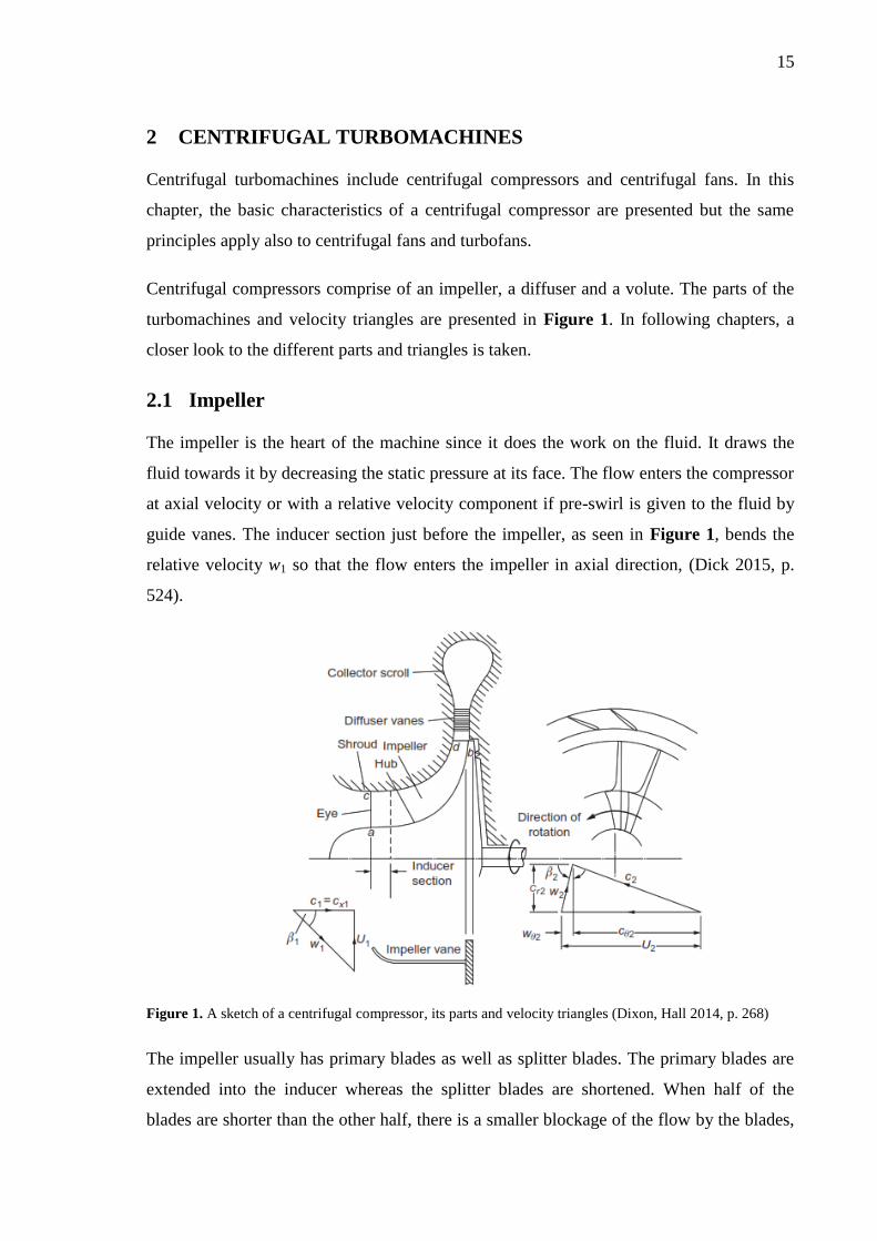
Centrifugal compressors comprise of an impeller, a diffuser and a volute. The parts of the

turbomachines and velocity triangles are presented in Figure 1. In following chapters, a

closer look to the different parts and triangles is taken.

2.1 Impeller

The impeller is the heart of the machine since it does the work on the fluid. It draws the

fluid towards it by decreasing the static pressure at its face. The flow enters the compressor

at axial velocity or with a relative velocity component if pre-swirl is given to the fluid by

guide vanes. The inducer section just before the impeller, as seen in Figure 1, bends the

relative velocity w1 so that the flow enters the impeller in axial direction, (Dick 2015, p.

524).

Figure 1. A sketch of a centrifugal compressor, its parts and velocity triangles (Dixon, Hall 2014, p. 268)

The impeller usually has primary blades as well as splitter blades. The primary blades are

extended into the inducer whereas the splitter blades are shortened. When half of the

blades are shorter than the other half, there is a smaller blockage of the flow by the blades,

16

thus a larger mass flow rate is allowed to pass through the impeller (Japikse 1996, p. 2-14).

The flow accelerates in the impeller and exits it in the direction following the blades. There

exists, however, a small slip velocity component, 𝑤𝜃2, at the impeller outlet because the

flow is not ideal and it slips against the direction of rotation (Japikse 1996, 2-4).

2.2 Diffuser and volute

The diffuser, or stator, is located after the impeller. Its main purpose is to convert the

kinetic energy of the flow into a static pressure rise so some of the work input can be

recovered. The static pressure can be increased by either increasing the area that the fluid

flows through which decreases the flow velocity of the fluid, or by changing the mean flow

path radius, thus recovering some of the angular velocity. (Japikse 1996, 3-1.)

There are two types of diffusers: vaneless and vaned. Vaneless diffusers are used when the

rotor work of the compressor and the velocity reduction are moderate. Vaned diffusers are

used with larger rotor works and stronger deceleration of the flow. Furthermore, the vaned

diffusers can be cascade diffusers or channel diffusers. The channel diffusers are more

efficient when a large pressure ratio and strong flow velocity reduction are needed,

whereas, the cascade diffuser is better with weaker flow velocity reduction. (Dick 2015,

527-528.)

The volute, or a collector, is located after the diffuser. It is a channel with increasing cross-

sectional area and shaped like a spiral that collects the fluid flow and guides it to a

tangential exit pipe. The volute can be of a symmetric or an overhung type, which are

shown in Figure 2. The overhung type volute is more popular because it takes less space to

install. (Dixon, Hall 2014, p. 300.)

Figure 2. Two types of centrifugal compressor volute (Dixon, Hall 2014, p. 301).

17

3 MECHANICAL VAPOR RECOMPRESSION

In this chapter, the basics of mechanical vapor recompression process and wet compression

are introduced.

3.1 Mechanical Vapor Recompression in general

Mechanical vapor recompression (MVR) or mechanical vapor compression (MVC) is an

energy saving process used in falling film evaporator plants in industries dealing with

products such as food, organic and inorganic solutions or waste water. In MVR process,

vapor from an evaporator is mechanically recompressed to higher pressure and temperature

by a centrifugal compressor or a high-pressure fan. After the compression, the vapor is fed

back to the evaporator where it condenses on the outside of the evaporator tubes where the

feed liquid is falling down. The condensation of the compressed vapor releases latent heat

which heats up the liquid inside the tubes. At the bottom of the evaporator, most of the

feed-in liquid has been vaporized and this vapor is then again fed to the turbomachine to be

recompressed. (Howden 2014.)

The reuse of the vapor makes the MVR process more energy efficient compared to

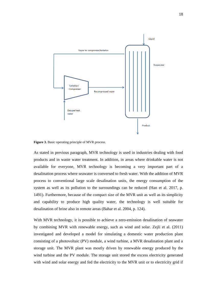
processes without heat recovery. The basic operating principle of the process is shown in

Figure 3. Usually, de-superheating water is fed to the MVR fan which helps to keep the

vapor saturated at the outlet of the turbomachine. This water is shown in the figure. The

benefits of MVR include energy savings, gentle evaporation due to low temperature

difference, simple technique and low specific operating costs. (GEA 2014, p. 4, 24.)

18

Figure 3. Basic operating principle of MVR process.

As stated in previous paragraph, MVR technology is used in industries dealing with food

products and in waste water treatment. In addition, in areas where drinkable water is not

available for everyone, MVR technology is becoming a very important part of a

desalination process where seawater is conversed to fresh water. With the addition of MVR

process to conventional large scale desalination units, the energy consumption of the

system as well as its pollution to the surroundings can be reduced (Han et al. 2017, p.

1491). Furthermore, because of the compact size of the MVR unit as well as its simplicity

and capability to produce high quality water, the technology is well suitable for

desalination of brine also in remote areas (Bahar et al. 2004, p. 124).

With MVR technology, it is possible to achieve a zero-emission desalination of seawater

by combining MVR with renewable energy, such as wind and solar. Zejli et al. (2011)

investigated and developed a model for simulating a domestic water production plant

consisting of a photovoltaic (PV) module, a wind turbine, a MVR desalination plant and a

storage unit. The MVR plant was mostly driven by renewable energy produced by the

wind turbine and the PV module. The storage unit stored the excess electricity generated

with wind and solar energy and fed the electricity to the MVR unit or to electricity grid if

19

necessary. The model was able to satisfy the domestic water demand of three different case

study cities in Morocco with a reasonable cost for the water. Furthermore, Karameldin et

al. (2002) proposed a wind driven MVR desalination system for Egypt’s rural areas near

the Red Sea where the land area is vast but population low and investments in, for

example, electrical grid are not profitable. They deduced that a wind driven MVR

desalination plant could provide fresh water for the residents effectively. The problem of

variable wind speed Karameldin and his colleagues solved by a proposition of an

interconnection between the desalination plant and the local electric grid.

MVR technology can also be used in conventional boiler power plants. In a recent study

performed by Tuan et al. (2013), the blow-down water and waste heat of a fire-tube boiler

system were recovered by a combination of a vacuum evaporator and MVR technology.

The study compared the traditional blow-down water system, system with the vacuum

evaporator addition and a system with the addition of the vacuum evaporator and the MVR

technology. It was shown that when the vacuum evaporator and the MVR technology were

added to the boiler system, the blow-down water and heat were recovered more than in the

other two cases. The study also evaluated the reduction in CO2 emissions and the value of

the investment. The results showed that the addition of the MVR technology could

decrease the yearly CO2 emissions significantly and that the investment would be

profitable.

From the studies presented above as well as other literature, it can be stated that the MVR

technology is well suited for a variety of purposes, from energy and food production to

providing fresh water for people. The technology is getting more and more attention since

the fight against global warming increases the need for more energy efficient processes.

Furthermore, as the world’s population increases year by year, the demand for electricity,

heat and domestic water rises but the energy consumption should not increase with the

same rate. Thus, processes incorporating MVR are becoming an essential part of the

energy and fresh water systems globally, in developing and developed countries alike.

3.2 Wet compression

The compression in the MVR process is, usually, based on wet compression where water

droplets are injected into the compressor or fan inlet. The droplets are vaporized in the

machine and the heat needed for the evaporation is absorbed from the working steam flow,

20

thus, the steam flow is cooled (Mohan et al. 2016, 5473). In this chapter, the difference

between wet and dry compression is introduced and some of the arguments and research

around the subject are discussed.

3.2.1 Wet compression versus dry compression

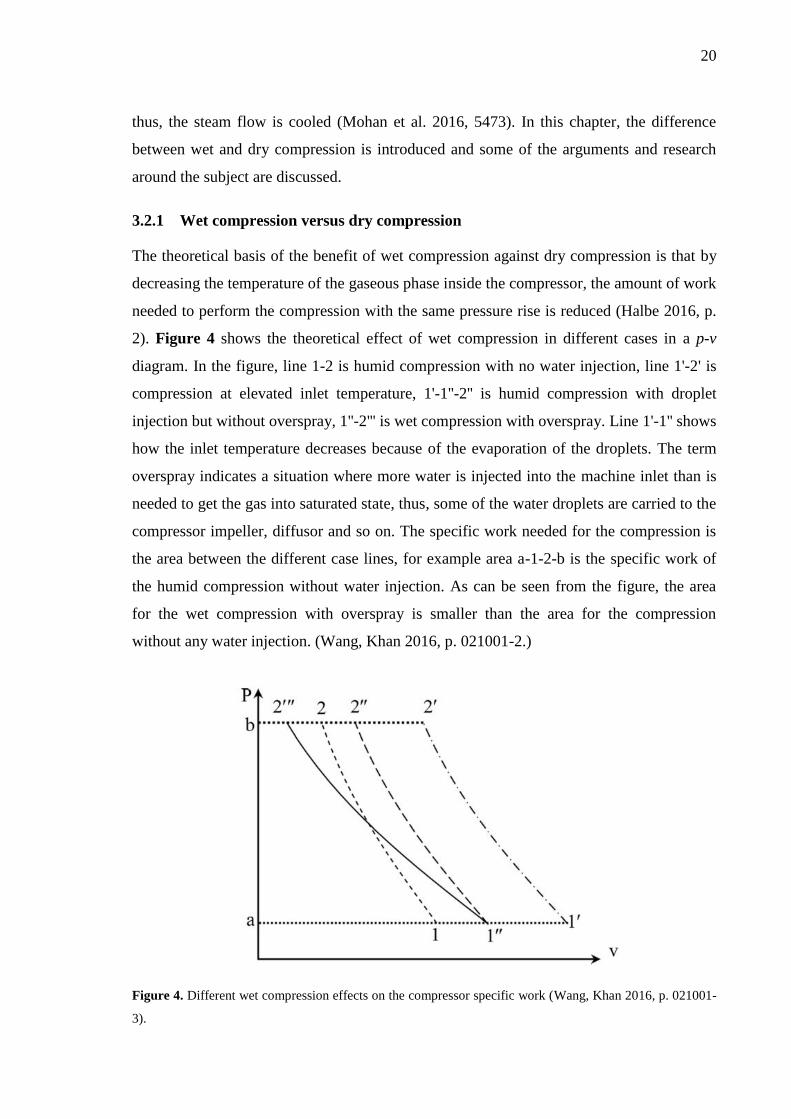
The theoretical basis of the benefit of wet compression against dry compression is that by

decreasing the temperature of the gaseous phase inside the compressor, the amount of work

needed to perform the compression with the same pressure rise is reduced (Halbe 2016, p.

2). Figure 4 shows the theoretical effect of wet compression in different cases in a p-v

diagram. In the figure, line 1-2 is humid compression with no water injection, line 1'-2' is

compression at elevated inlet temperature, 1'-1''-2'' is humid compression with droplet

injection but without overspray, 1''-2''' is wet compression with overspray. Line 1'-1'' shows

how the inlet temperature decreases because of the evaporation of the droplets. The term

overspray indicates a situation where more water is injected into the machine inlet than is

needed to get the gas into saturated state, thus, some of the water droplets are carried to the

compressor impeller, diffusor and so on. The specific work needed for the compression is

the area between the different case lines, for example area a-1-2-b is the specific work of

the humid compression without water injection. As can be seen from the figure, the area

for the wet compression with overspray is smaller than the area for the compression

without any water injection. (Wang, Khan 2016, p. 021001-2.)

Figure 4. Different wet compression effects on the compressor specific work (Wang, Khan 2016, p. 021001-

3).

21

Theoretically, the effects of wet compression are clear but in practice, the effects are more

complex. For example, Wang and Khan (2016) investigated the validity of three statements

involving wet compression in gas turbines: 1. the density of the air is increased with

fogging or overspray; 2. the power needed by the compressor is reduced with fogging or

overspray; 3. the efficiency of the gas turbine is increased with fogging or overspray. The

term fogging means that the amount of water injected into the flow is enough to get the gas

to saturated state without any overspray. Wang and Khan’s investigations concluded that

the first statement is valid for fogging but not always for overspray. Statement 1 fails with

overspray because water evaporation reduces the temperature of the gas significantly, thus

the pressure of the gas also gets reduced. The pressure decreases more than the temperature

according to the polytropic relation of temperature and pressure. According to ideal gas

law (𝜌~𝑝

𝑅𝑇), when pressure is reduced more than temperature, the density decreases

(Wang, Kahn 2016, p. 021001-5).

Statement 2 is not always valid for the specific power or power consumption of the

compressor but is true for compressor power per unit pressure ratio. One flaw of statement

2 is related to stating that only the exit temperature decreases when in reality, also the inlet

temperature decreases. In addition, if only air is considered and not humid air or a mixture

of air and water, the statement becomes false since the latent heat and heating of the

droplets increase the specific work of the compressor. (Ibid.)

Statement 3 has more to do with gas turbines than centrifugal compressors. Nevertheless,

Wang and Khan proved that the statement is not always true since all the factors that the

thermal efficiency of gas turbine depends on, increase, thus there are uncertainty in

determining the thermal efficiency. They concluded that in gas turbines, wet compression

should be used to increase the power output of the system, and not for increasing the

efficiency. (Ibid.)

It should be noted that Wang and Khan investigated wet compression only in gas turbines

which have an axial compressor in them and not centrifugal compressor or fan that is the

focus of this study. Furthermore, they did not present the effect of different water vapor

mass fractions on the validity of the statements, and they examined the statements only in

theory with general equations and not experimentally. Nevertheless, Wang and Khan

proved that not all claims regarding wet compression are 100 % true and their reasoning

should be kept in mind when considering wet compression in centrifugal compressors.

22

3.2.2 Wet compression in centrifugal turbomachines

Research around wet compression in gas turbines and axial compressors has been going on

for many years but the research of the usage of the technology in centrifugal machines has

got a boost only in recent years. Industries, such as oil and gas, have taken a step forward

in investigating wet compression in centrifugal compressors, especially in the use of

exploiting old gas fields.

How does wet compression then differ in centrifugal turbomachines compared to axial

machines? In gas turbines and axial compressors, the water vapor mass fraction is usually

limited to 2-3% but in industrial centrifugal compressors, especially in oil and gas industry,

the mass fraction of water vapor can be up to 50 or 60%. With such high mass fractions,

the efficiency of the compressor will be reduced compared to dry gas efficiency due to

very large density differences between the liquid and the gas at the inlet as well as large

internal losses inside the machine. The internal losses cause the required compression

power to surge and, consequently, the injected water droplets get overheated. (Fabbrizzi et

al. 2009, p. 2, 10-11.)

Another aspect of wet compression in industrial centrifugal compressors is that the

performance of a single stage of a centrifugal compressor is modified similarly as a whole

multistage axial compressor. In another words, one centrifugal compressor stage with wet

compression represents all stages of an axial compressor with wet compression in terms of

how the wet compression affects the performance of a stage or the whole machine. This

observation is due to the fact that the flow path length of a single stage centrifugal

compressor impeller and the flow path of an entire axial compressor typically used in gas

turbines can be in the same order of magnitude. Thus, the ratios between the droplet

evaporation time and the droplet residence time in the centrifugal compressor impeller and

in the entire multi-stage axial compressor are within a comparable order of magnitude.

(Abdelwahab 2006, p. 6.)

As stated before, wet compression can improve the performance of a turbomachine when

used correctly. The compressor power requirement can be reduced up to 5 % per stage

when the initial droplet diameter is less than 5 µm and when the maximum water mass

flow rate is 3 % of the dry gas mass flow rate (Abdelwahab 2006, p. 10). However, there

are also some detrimental effects on the performance characteristics. The increased mass

flow rate and the vaporization of the droplets shift the compressor to off-design flow

23

angles resulting in decrease of the aerodynamic efficiency (White, Meacock 2011, p. 1). In

addition, low inlet temperatures and high water rates can decrease the positive effects of

wet compression (Abdelwahab 2006, p. 10).

Taking into account all the positive and negative effects of wet compression, the

technology is well suitable for industrial centrifugal compressor purposes as it has been for

gas turbines. It is just important to use the right amount of water and the right initial

droplet diameter to get the best possible outcome of wet compression. In addition, in a case

of a compressor that is designed for dry flow, the implementation of wet compression

might be harder compared to a case with a compressor that is designed with wet

compression in mind (Ibid). For example, as stated before, increasing water mass flow rate

leads to off-design flow angles. The off-design flow angles can be seen from Figure 5

where the impeller exit flow angles of a wet compression case with different water mass

fractions are subtracted from the impeller exit flow angles of a dry compression case. The

flow angles are defined from radial direction. It can be seen that with increasing water

mass fraction, the flow angles start to derivate quite a lot from the dry compression case

angles (Jeong-Seek et al. 2006, p. 1479). Therefore, if a compressor which is designed for

dry gas flow is used with wet compression, the effects of the water injection can be

detrimental for the compressor performance as well as for different compressor parts via

erosion.

Figure 5. Deviation of wet compression impeller exit flow angle from a dry compression exit flow angle as a

function of water mass fraction (Jeong-Seek et al. 2006, p. 1479).

24

At least one comprehensive analysis using Computational Fluid Dynamics (CFD) of wet

compression in centrifugal compressors is done by Halbe (2016). In his research, Halbe

investigates the effects of two-phase flow of refrigerant R134a in a two-stage centrifugal

compressor using CFD with droplet sizes larger than 100 μm. The findings confirm that the

liquid injection can shift the compressor to operate at off-design conditions and that there

exists a high potential for erosion on the impeller blades and shroud. According to Halbe’s

simulations, the droplet injection results in fewer benefits compared to disadvantages

leading to overall performance degradation of the compressor. Halbe, however, simulated

only with droplets larger than 100 μm which do not evaporate completely inside the

compressor. As stated earlier, with smaller droplets, the advantages of liquid injection can

overrun the disadvantages.

25

4 MULTIPHASE FLOW

In a multiphase flow, there is at least two phases present in the flow, for example in the

case of this study, a vapor and a liquid phase. The vapor phase is called continuous phase

and the liquid phase is called dispersed phase or particle phase since it consists of discrete

elements, droplets in this case. (Crowe 2006, p. 1-1.)

This chapter introduces the governing equations and basic principle of modeling

multiphase flow in Ansys CFX simulation software.

4.1 Numerical models of multiphase flow in CFX

There are two main multiphase flow models in Ansys CFX: Eulerian-Eulerian model and

Lagrangian Particle Tracking model (LPT), also known as Eulerian-Lagrangian model.

(ANSYSb 2016, Ch. 5.)

1. Eulerian-Eulerian model: In this model, both the continuous and the dispersed

phase in the flow are tracked by Eulerian transport model. The phases share a

common flow field (Ibid). The properties of the particles are obtained by averaging

over a computational domain (Crowe 2006, p. 13-12).

2. Lagrangian Particle Tracking model: In this model, the dispersed phase is tracked

through the flow in a Lagrangian way and the continuous phase is modeled in an

Eulerian way. (ANSYSb 2016, Ch. 6.) The properties of particles are obtained by

updating the properties along the particle path (Crowe 2006, p. 13-12).

Taking into account the goal of this research as well as the advantages and disadvantages

of the two models, the Lagrangian Particle Tracking model is chosen to be used in this

work.

4.2 Lagrangian Particle Tracking model

As stated before, in Lagrangian Particle Tracking, the particles in the dispersed phase are

tracked in a Lagrangian way, thus, the properties of the particles are updated along their

flow path. The continuous phase is simulated with Eulerian approach so the properties of

the phase are averaged over the computational domain. Since it is not possible to track

every single particle injected into the computational domain, the Lagrangian approach

records and calculates a number of individual particles. Each individual tracked particle

26

represents a group of particles whose properties are equal to the properties of the tracked

particle. This way the properties of the whole dispersed phase can be determined. The

particles in the disperse phase interact and affect the surrounding fluid. The effects of the

particles on the fluid are included to the calculation via source terms that are calculated for

the mass, momentum and energy of the particles. These equations are discussed more in

Chapter 6. (ANSYSa 2016, Ch. 8.)

4.2.1 Advantages and disadvantages of LPT model

The advantages of LPT model compared to Eulerian-Eulerian model are that the model

simulates mass and heat transfer in better detail, the behavior and residence time of the

particles are tracked more accurately and the model can track better a wide range of

particle sizes (ANSYSa 2016, Ch. 8.2).

The disadvantages and limitations of LPT model for particle transport are that the model is

only for dilute flows with dispersed phase volume fraction below 1 %. In this study, the

maximum mass flow rate of the dispersed phase is 3 % of the continuous phase mass flow.

With the 3 % mass flow rate, the volume fraction of the dispersed phase is 0.000853 %

which validates that the flow is dilute. In addition, the very low volume fraction validates

assumption that droplet-droplet interactions are neglected in this work. (ANSYSa 2016,

Ch. 8.12.)

Another disadvantage for particle transport is that it cannot model turbulence for particles,

thus, the particles cannot affect the turbulence of the continuous phase. Particles can be

affected by the turbulence due to turbulent dispersion force. However, the turbulent

dispersion force increases the number of particles that has to be tracked, thus, increasing

the computational time needed for the simulation and making it harder to get the

simulation to converge. Therefore, the turbulent dispersion force is used as a post-process

method. (ANSYSa 2016, Ch. 8.5.2.3.)

The disadvantages for particle material are that the material’s density, viscosity and

conductivity have to be constant (ANSYSa 2016, Ch. 8.13). The restriction of constant

properties leads to the fact that ideal gas can only be used to model liquid-vapor phase

change in order to ensure that thermodynamic consistency is maintained during the phase

change process (Halbe 2016, p. 17). The reference properties for the ideal gas in the phase

change process are determined at the saturation temperature of the vapor at given pressure.

27

In addition, from the restriction of constant particle properties stems the assumption that

temperature variation within the particle is neglected in the calculation. This assumption

has to be checked via Biot number.

𝐵𝑖 =𝑁𝑢∙𝜆f

𝜆p (4-1)

where 𝐵𝑖 is Biot number [-]

𝑁𝑢 is Nusselt number [-]

𝜆f is thermal conductivity of fluid [W/mK]

𝜆p is thermal conductivity of particle [W/mK]

𝑁𝑢 = 2 + 0.6𝑅𝑒p

1

2𝑃𝑟f

1

3 (4-2)

where 𝑃𝑟f is fluid Prandtl number [-]

𝑅𝑒p is particle Reynolds number [-]

𝑅𝑒p =𝜌f𝑼slip𝑑p

𝜇f (4-3)

where 𝜇f is dynamic viscosity of the fluid [Pa s]

𝜌f is the continuous phase fluid density [kg/m3]

𝑑p is particle diameter [m]

𝑼slip is slip velocity [m/s]

𝑼slip = 𝑼f − 𝑼p (4-4)

where 𝑼f is continuous phase fluid velocity [m/s]

𝑼p is dispersed phase particle velocity [m/s]

𝑃𝑟f =𝜇f𝑐𝑝,f

𝜆f (4-5)

where 𝑐𝑝,f is specific heat capacity of the fluid at constant pressure

[J/kgK]

Biot number is determined with equation (4-1) Nusselt number is calculated with equation

(4-2) which is a correlation developed by Ranz and Marshall (Incropera et al. 2003, p.

465). Reynolds number for the particle is determined with equation (4-3), the slip velocity

28

between the particles in the dispersed phase and the fluid in the continuous phase with

equation (4-4) and Prandtl number for the continuous phase fluid with equation (4-5)

(Incropera et al. 2003, p. 409). In order for the assumption of constant temperature within

the particle to be valid, Biot number has to be smaller than 0.1. When the continuous phase

fluid is steam and the dispersed phase particles are water droplets, and when the particles

are injected to the continuous phase flow without slip velocity, Reynolds number becomes

zero and Nusselt number becomes two. In this situation, Biot number of the particle is

below 0.1 (Bi = 0.08) which validates the before made assumption. However, when the

particles are injected with different initial velocity than the velocity of the continuous

phase flow, Biot number can exceed the limit value. In this situation, the assumption of a

constant temperature inside the droplet would not be valid and there might be some errors

in the calculation. Nonetheless, because this research deals with a very dilute multiphase

flow, the possible errors that the assumption of constant temperature within the droplet

may bring are small. Therefore, variation of temperature within the droplet may be

neglected.

29

5 THERMODYNAMIC PROPERTIES AND EQUATIONS OF

STATE

In this chapter, the equations used to determine the thermodynamic properties and the

equation of state of the continuous and dispersed phase are presented.

5.1 Dynamic viscosity and thermal conductivity

The equations for dynamic viscosity and thermal conductivity for the real gas in the

continuous phase as well as for the ideal gas and liquid in the dispersed phase are

presented.

5.1.1 Real gas in continuous phase

Dynamic viscosity and thermal conductivity of the continuous phase are defined using

elementary kinetic gas theory which assumes that all the molecules are rigid non-

interacting spheres (Poling et al. 2001, p. 9.2).

𝜆f

𝜇f𝑐𝑣,f= 1.32 +

1.77𝑅G

𝑐𝑣,f (5-1)

where 𝑐𝑣,f is specific heat capacity of the fluid at

constant volume [J/kgK]

𝑅G is individual gas constant [J/kgK]

The thermal conductivity of the continuous phase is determined using modified Eucken

correlation which is presented in equation (5-1)

𝜇f = 26.69√𝑀𝑇

𝛺(𝑇)𝜃2 (5-2)

where M is molecular weight [kmol/kg]

𝛺(𝑇) is collision function [-]

𝜃 is collision diameter [Å]

𝜃 = 0.809√𝑉c3

(5-3)

where 𝑉c is critical molar volume [cm3/mol]

30

Dynamic viscosity for a rigid non-interacting sphere is presented in equation (5-2) (Poling

et al. 2001, p. 9.3). For gases at low pressure, it can be assumed that molecular collisions

do not affect viscosity, thus, the collision function 𝛺(𝑇) is unity (Poling et al. 2001, p.

10.43). CFX uses equation (5-2) to determine the dynamic viscosity of a real gas. Collision

diameter is calculated with equation (5-3).

5.1.2 Ideal gas and liquid in dispersed phase

For the components of the dispersed phase, such as the liquid and the evaporating vapor

component, constant values for dynamic viscosity and thermal conductivity are used

because of the limitations of LPT model as explained in Chapter 4.2.1. The use of the

constant values for the liquid phase should not affect the simulation results significantly

since the thermodynamic properties of liquids vary little when temperature or pressure is

changed. However, the use of constant values for the evaporating vapor component results

in the mandatory use of an ideal gas material as the vaporizing vapor component as

explained in Chapter 4.2.1. The use of ideal gas material can affect the validity of the

simulation results. However, the temperature and pressure ranges of the simulation are so

small that the variation of the thermodynamic properties is not significant. Therefore, the

use of constant values for the dynamic viscosity and thermal conductivity for the dispersed

phase should not affect the results significantly. The values are determined at the reference

state of the dispersed phase, 1 atmospheric pressure and 110 °C temperature.

5.2 Specific heat capacity

In this chapter, the equations for the specific heat capacity of the continuous phase’s real

gas and the dispersed phase’s ideal gas and liquid are discussed.


Specific heat capacity for the real gas of the continuous phase is based on the specific heat

for an ideal gas which is determined with a fourth order polynomial function.

𝑐𝑝0

𝑅G= 𝑎1 + 𝑎2𝑇 + 𝑎3𝑇2 + 𝑎4𝑇3 + 𝑎5𝑇4 (5-4)

where 𝑐𝑝0 is ideal gas specific heat capacity [J/kgK]

𝑎1 is constant [-]


31




𝑇 is temperature [K]

Equation (5-4) shows the fourth order polynomial function for determining the specific

heat capacity. The equation shows that the specific heat capacity for ideal gas is a function

of only temperature but in CFX when simulating real gas, the program allows the real gas

specific heat capacity to be dependent also on pressure (ANSYSa 2016, Ch. 1.4). The

constants for water used in the equation are obtained from Poling et al. (2001) and are

presented in Table 1.

Table 1. Constants of water for specific heat capacity equation (Poling et al. 2001, A.45).

𝑎1 [-] 4.395

𝑎2 [-] -4.186∙10-3

𝑎3 [-] 1.405∙10-5

𝑎4 [-] -1.564∙10-8

𝑎5 [-] 0.632∙10-11


As with the dynamic viscosity and thermal conductivity, because of the limitations of the

LPT model, a constant value approach is used when defining the specific heat capacity for

the dispersed phase components. The effects of this approach on the simulation results

should not be significant since the temperature and pressure ranges of the simulation cases

are small. The values of the specific heat capacity of the dispersed phase components are

determined at the reference state of the dispersed phase.

5.3 Equation of state

The equations of state for the two phases are presented below.


The equation of state of the real gas in the continuous phase is based on Aungier’s

modification to the Redlich-Kwong equation of state.

32

𝑝 =𝑅𝑇

𝑣−𝑏+𝑐−

𝑎(𝑇)

𝑣(𝑣+𝑏) (5-5)

where 𝑝 is pressure [Pa]

𝑅 is individual gas constant [J/kgK]

𝑣 is specific volume [m3/kg]

𝑎 is a function of temperature [-]

𝑏 is constant [-]

c is constant [-]

Equation (5-5) presents Aungier Redlich-Kwong equation of state for real gases. Aungier

added constant c to the equation to make the Redlich-Kwong equation more accurate near

the critical point of the gas (Aungier 1995, p. 278).

𝑏 = 0.08664 ∙ (𝑅𝑇c

𝑝c) (5-6)

where 𝑇c is critical temperature [K]

𝑝c is critical pressure [Pa]

𝑎(𝑇) = 𝑎0 (𝑇

𝑇𝑐)

−𝑛

(5-7)

where 𝑎0 is constant [-]

n is exponent [-]

Equations (5-6) and (5-7) show the equations for the parameter b and the temperature

dependent parameter a. Another modification from Aungier to the standard Redlich-

Kwong is the exponent n whose standard constant value is now replaced with an

experimental value or a correlation which is presented below.

𝑎0 = 0.42747 ∙𝑅2𝑇c

2

𝑝c (5-8)

𝑛 = 0.4986 + 1.1735𝛼 + 0.4754𝛼2 (5-9)

where 𝛼 is acentric factor [-]

Equations (5-8) and (5-9) show the equation for the constant 𝑎0 and the exponent n. The

acentric factor is tabulated for different substances and in this research, the value used is

33

0.344 (VDI 2010, p. 302). The correlation for the exponent is an empirical equation

developed by Aungier (1995).

𝑐 =𝑅𝑇c

𝑝c+𝑎0

𝑣c(𝑣c+𝑏)

+ 𝑏 − 𝑣c (5-10)

where 𝑣c is specific volume at critical point [m3/kg]

The additional constant c is presented in equation (5-10). According to Aungier (1995),

adding the constant c to the Redlich-Kwong equation may compromise the thermodynamic

stability condition. However, since c is usually much smaller than b, typically

approximately two orders of magnitude smaller, the addition does not affect the prediction

of the equation significantly (Aungier 1995, p. 278).


For the liquid component in the dispersed phase, the density is defined as a constant value

because of the material limitations of the LPT model. For the evaporating vapor

component, CFX uses ideal gas law to determine the density of the vapor. With the ideal

gas law, the thermodynamic properties of a real gas can be estimated to an acceptable limit

at low pressures (~ 1 bar), regardless of temperature or at high pressures (>> 1 bar) and

high temperatures (> 2 ∙ 𝑇c) (ANSYSa 2016, Ch. 14.3). In the case of this thesis, the

maximum pressure is below 1.5 bar and the temperature stays significantly below the

critical temperature of the water. Therefore, the use of ideal gas law as the equation of state

for the evaporating vapor component can lead to uncertainties in the simulation results.

However, the uncertainties could be limited to an acceptable level since the maximum

pressure of the simulations does not exceed 1.5 bar.

34

6 GOVERNING EQUATIONS

The governing equations for mass, momentum and energy for the continuous phase and

dispersed phase as well as for the interphase transfer between the phases are introduced in

this chapter. The equations are presented using Einstein notation.

6.1 Continuous phase

The conservation equations of mass, momentum and energy for the continuous phase are

based on Reynolds Averaged Navier Stokes equations for compressible flow, also known

as Favre Averaged Navier Stokes equations. The conservation equations along with the

equations that are used to determine the thermal properties of the continuous phase are

presented in this chapter.

6.1.1 Conservation of mass

Conservation of mass, also known as the continuity equation, states that mass of the fluid

is conserved. In multiphase flows, an additional mass source term is added to describe the

mass transfer between the phases.

𝜕𝜌

𝜕𝑡+

𝜕

𝜕𝑥𝑗(𝜌𝑈𝑖) = 𝑆mass (6-1)

where 𝜌 is fluid density [kg/m3]

𝑈𝑖 is velocity vector [m/s]

𝑡 is time [s]

𝑆mass is mass source from dispersed phase [kg/m3s]

Equation (6-1) introduces the continuity equation for the continuous phase. The mass

source term is defined later in Chapter 6.3.3.

6.1.2 Conservation of momentum

The conservation of momentum of the continuous phase is based on Newton’s second law,

which states that the rate of change of momentum is equal to the sum of forces acting on

the fluid. As earlier with the continuity equation, a source term is added to account for the

momentum transfer between the two phases and the term is defined in Chapter 6.3.1.

𝜕(𝜌𝑈𝑖)

𝜕𝑡+

𝜕

𝜕𝑥𝑗(𝜌𝑈𝑖𝑈𝑗) = −

𝜕𝑝

𝜕𝑥𝑖+

𝜕

𝜕𝑥𝑗(𝜏𝑖𝑗 − 𝜌𝑢𝑖𝑢𝑗̅̅ ̅̅ ̅) + 𝑆momentum (6-2)

35

where 𝑈𝑗 is velocity vector [m/s]

𝜏𝑖𝑗 is normal and shear stress [N/m]

−𝜌𝑢𝑖𝑢𝑗̅̅ ̅̅ ̅ is Reynolds stress term

𝑆momentum is momentum source from dispersed phase [kg/m2s

2]

The conservation of momentum is shown in equation (6-2). In a turbulent flow, the

Reynolds stress term has to be added to the equation to account for the velocity fluctuation

due to turbulence.

−𝜌𝑢𝑖𝑢𝑗̅̅ ̅̅ ̅ = 𝜇t (𝜕𝑈𝑖

𝜕𝑥𝑗+

𝜕𝑈𝑗

𝜕𝑥𝑖) −

2

3𝛿𝑖𝑗 (𝜌𝑘 + 𝜇𝑡

𝜕𝑈𝑘

𝜕𝑥𝑘) (6-3)

where 𝜇t is eddy viscosity [Pa s]

𝛿𝑖𝑗 is Kronecker delta function [-]

𝑘 is turbulence kinetic energy [m2/s

2]

𝑈𝑘 is velocity vector [m/s]

Equation (6-3) represents Reynolds stresses added to the conservation of momentum

equation. The Reynolds stress term is based on a hypothesis of eddy viscosity which

assumes that the stresses are proportional to the mean velocity gradient and eddy viscosity

(ANSYSb 2016, Ch. 2.2). The last term, 𝜇𝑡𝜕𝑈𝑘

𝜕𝑥𝑘, is neglected in ANSYS CFX, although this

assumption is perfectly valid only for incompressible flows (Ibid).

Eddy viscosity is determined with a turbulence model. The turbulence model chosen for

this research is 𝑘 − 𝜔 based Shear Stress Transport (SST) since it is accurate near the wall

as well as far away from the wall. SST combines turbulence models 𝑘 − 𝜖 and 𝑘 − 𝜔 and

uses 𝑘 − 𝜖 in the free stream and 𝑘 − 𝜔 near the wall. The model determines eddy

viscosity as a relation between turbulence kinetic energy and turbulent frequency (Ibid).

𝜇t = 𝜌𝑘

𝜔 (6-4)

where 𝜔 is turbulent frequency [1/s]

The SST eddy viscosity is shown in equation (6-4) (Ibid).

36

6.1.3 Conservation of energy

Conservation of energy for the continuous phase is based on the first law of

thermodynamics which states that the rate of change of energy is equal to the sum of heat

added to the fluid and work done on the fluid. In a turbulent flow, also turbulent diffusion

has to be accounted for in the equation. This is done by implementing an eddy diffusivity

hypothesis, which is similar to the eddy viscosity hypothesis used in the momentum

equation. The eddy diffusivity hypothesis assumes a linear relation between scalar

Reynolds fluxes and a mean scalar gradient (ANSYSb 2016, Ch. 2.2).

𝜕(𝜌ℎtot)

𝜕𝑡−

𝜕𝑝

𝜕𝑡+

𝜕(𝜌𝑈𝑗ℎtot)

𝜕𝑥𝑗=

𝜕

𝜕𝑥𝑗(𝜆

𝜕𝑇

𝜕𝑥𝑗− 𝜌𝑢𝑗ℎ̅̅ ̅̅ ) +

𝜕

𝜕𝑥𝑗[(𝑈𝑖(𝜏𝑖𝑗 − 𝜌𝑢𝑖𝑢𝑗̅̅ ̅̅ ̅)] + 𝑆energy (6-5)

where ℎtot is specific total enthalpy [J/kg]

𝜆 is thermal conductivity [W/mK]

−𝜌𝑢𝑗ℎ̅̅ ̅̅ is turbulent diffusion term [W/m2]

𝑆energy is energy source term from the dispersed phase [W/m3]

Conservation of energy for the continuous phase is shown in equation (6-5). The energy

source term from the dispersed phase is introduced more accurately in Chapter 6.3.2.

−𝜌𝑢𝑖ℎ̅̅ ̅̅ = 𝛤t𝜕ℎ

𝜕𝑥𝑖 (6-6)

where 𝛤t is eddy diffusivity [Pa s]

𝛤t =𝜇t

𝑃𝑟t (6-7)

where 𝑃𝑟t is turbulent Prandtl number [-]

Equation (6-6) presents the turbulent diffusion term and equation (6-7) shows the eddy

diffusivity term. Turbulent Prandtl number in equation (6-7) relates the eddy diffusivity of

heat to the eddy viscosity similarly as the regular Prandtl number (Srinivasan et al. 2011,

8881). In this research, it is assumed that the value of turbulent Prandtl number is constant

at 0.9 (ANSYSa 2016, Ch. 1.2).

37

6.2 Dispersed phase

In Eulerian-Lagrangian framework, the particle displacement is calculated with forward

Euler integration.

𝒙pn = 𝒙p

0 + 𝑼p0𝛿𝑡 (6-8)

where 𝑼p0 is initial particle velocity [m/s]

𝛿𝑡 is time step [s]

𝒙p0 is the old position of the particle [-]

𝒙pn is the new position of the particle [-]

The particle displacement in new time step is presented in equation (6-8). In the

calculation, it is assumed that the determined particle velocity is constant over the time

step and the new velocity at the end of the time step is calculated with analytical solution

for the particle momentum equation.

𝑚p𝑑𝑼p

𝑑𝑡= 𝑭all (6-9)

where 𝑚p is particle mass [kg]

𝑭all is all forces acting on a particle [N]

Equation (6-9) shows the momentum equation for the particle. Forces acting on particles

include forces such as buoyancy, drag and rotation, and are presented in Chapter 6.3.1.

6.2.1 Secondary breakup

In this thesis, the focus is on the effects of initial droplet diameter on the steam flow inside

a turbofan, so the droplets are injected into the steam flow uniformly with constant

diameter. Therefore, it is important to model the secondary breakup of the droplets in order

to get more accurate simulation results of the droplet evaporation and diameter change

inside the machine.

The secondary breakup of liquid jets occurs, for example, due to turbulence within the

liquid or due to aerodynamic forces acting on the liquid (ANSYSb. 2016, Ch. 6.5). These

mechanisms are present mainly because of the initial slip velocity between the liquid and

38

the gas phase and can be characterized with Weber number, Reynolds number and

Ohnesorge number. The equation for the Reynolds number is presented in equation (4-3).

𝑊𝑒 =𝜌f𝑼slip

2 𝑑p

𝜎 (6-10)

where 𝑊𝑒 is Weber number [-]

𝜎 is surface tension [N/m]

𝑂ℎ =√𝑊𝑒

𝑅𝑒=

𝜇p

√𝜌p𝜎𝑑p (6-11)

where 𝑂ℎ is Ohnesorge number [-]

𝜌p is particle density [kg/m3]

𝜇p is particle dynamic viscosity [Pa s]

Equations (6-10) and (6-11) present Weber and Ohnesorge number formulations. Weber

number shows the ratio of inertia to surface tension forces, and Ohnesorge number relates

Weber number and Reynolds number (Ashgriz 2011, p. 6). When Ohnesorge number is

low (Oh < 0.1), the flow has low viscosity or high surface tension and Weber number

dominates the droplet breakup process (Strotos et al. 2016, p. 96). When Weber number is

unity, deformation of the droplet begins to occur. The breakup process can be divided into

different regimes depending on the droplet Weber number presented in Table 2.

Table 2. Droplet breakup regimes determined by Weber number (ANSYSb 2016, Ch. 6.5.2).

Vibrational breakup We < 12

Bag breakup 12 < We <50

Bag-and-stamen breakup 50 < We <100

Sheet stripping 100 < We < 350

Catastrophic breakup 350 < We

When modeling droplet breakup, it is assumed that the decrease in the droplet radius is

determined by the used breakup model (Ibid). In this research, the used model is Cascade

Atomization and Breakup Model (CAB), in which the relation of the child droplet and the

parent droplet is assumed to be exponential. For more information about CAB model, the

reader is guided to the references of ANSYSb 2016, Ch. 6.5 and Tanner (2004).

39

6.3 Interphase transfer

As stated in earlier chapters, the continuous phase and the dispersed phase affect each

other, and this interaction is called two-way coupling. The effects of the particles on the

continuous phase are included in the calculation via source terms which are presented in

this chapter.

The interphase of liquid and vapor is determined through saturation vapor pressure, which

in turn is calculated with Antoine equation (Poling et al. 2001, p. 7.4).

log10 𝑝sat = 𝐴 −𝐵

𝑇+𝐶−273.15 (6-12)

where 𝑝sat is saturation vapor pressure [mmHg]

𝐴 is constant [-]

𝐵 is constant [-]

𝐶 is constant [-]

Equation (6-12) presents Antoine equation for the vapor pressure. Constants A, B and C are

tabulated in Table 3 for water and are valid for temperature range of 99 to 374 °C

(DDBST).

Table 3. Used Antoine equation constants (DDBST).

A 8.14019

B 1810.94

C 244.485

6.3.1 Momentum transfer

The momentum transferred from particles to the continuous phase fluid arises from the slip

velocity between the phases as well as from the displacement of the continuous phase by

the particles.

𝑚p𝑑𝑼p

𝑑𝑡= 𝑭D + 𝑭Bu + 𝑭R + 𝑭VM + 𝑭𝑃 + 𝑭BA (6-13)

where 𝑭D is drag force acting on the particle [N]

𝑭Bu is buoyancy force due to gravity [N]

𝑭R is forces due to domain rotation [N]

𝑭VM is virtual mass force [N]

40

𝑭𝑃 is pressure gradient force [N]

𝑭BA is Basset force [N]

Equation (6-13) shows the general form of the momentum equation for a particle. In CFX,

only drag force acting on the particle has an effect on the continuous phase.

𝑭D =1

8𝜋𝑑p

2𝜌f𝐶D|𝑼slip|(𝑼slip) (6-14)

where 𝐶D is drag coefficient [-]

𝜌f is fluid density [kg/m3]

The drag force on the particles is presented in equation (6-14). Different correlations for

the drag coefficient are presented in literature and modeled in CFX by different drag

models, for example, Schiller Naumann model or Ishii Zuber model. The Ishii Zuber

model is better for larger particle Reynolds numbers as well as for fluid particles, so it is

chosen to be used in this research (ANSYSb 2016, Ch. 5.5).

The drag coefficient is approximated in three regimes: viscous regime, distorted particle

regime and spherical cap regime. In the viscous regime, the fluid particles behave like solid

spheres, thus, the drag coefficient is calculated with the Schiller Naumann correlation

which determines the coefficient as a function of Reynolds number (Ibid).

𝐶D(sphere) =24

𝑅𝑒(1 + 0.15𝑅𝑒0.687) (6-15)

where 𝐶D(sphere) is drag coefficient for the viscous regime [-]

The Schiller Naumann correlation for the drag coefficient for a spherical particle is

presented in equation (6-15).

𝐶D(cap) =8

3 (6-16)

where 𝐶D(cap) is spherical cap regime drag coefficient [-]

In the spherical cap regime, the fluid particle is spherical cap shaped. The drag coefficient

in this regime is approximated with equation (6-16). In the distorted particle regime, before

the spherical cap regime, the droplet becomes shaped approximately as an ellipse and the

41

drag coefficient is estimated with Ishii-Zuber correlations. Now, the drag coefficient is not

dependent on Reynolds number and is almost constant.

𝐶D(ellipse) =2

3𝐸𝑜

1

2 (6-17)

where 𝐸𝑜 is Eotvos number [-]

𝐶D(ellipse) is ellipsoidal shaped particle’s

drag coefficient [-]

𝐸𝑜 =𝑔∆𝜌𝑑p

2

𝜎 (6-18)

where 𝑔 is gravitational acceleration [m/s2]

∆𝜌 is density difference between the

dispersed and the continuous phase [kg/m3]

The Ishii-Zuber correlation is shown in equation (6-17) in which the drag coefficient for

the ellipsoidal droplet is given as a function of Eotvos number (Ishii, Zuber 1979). The

Eotvos number is introduced in equation (6-18). In CFX, the different regimes are taken

into account by using the maximum drag coefficient chosen as presented below.

𝐶D(dist) = min(𝐶D(ellipse), 𝐶D(cap)) (6-19)

𝐶D = max(𝐶D(sphere), 𝐶D(dist)) (6-20)

where 𝐶D(dist) is the drag coefficient for the distorted

particle regime [-]

The way the final drag coefficient is determined in CFX is presented in equations (6-19)

and (6-20). The drag force calculated with equation (6-14) is multiplied by the number of

particles to obtain the momentum source term to the continuous phase momentum

equation.

𝑆momentum = −𝑁p𝑭D (6-21)

where 𝑁p is number of particles [-]

The source term to continuous phase momentum equation is given in equation (6-21).

42

6.3.2 Heat transfer

The interphase heat transfer happens via convective heat transfer, latent heat transfer

associated with mass transfer and radiative heat transfer. In this thesis, the radiative heat

transfer is neglected because of its small role in the interphase heat transfer and neglecting

it makes the simulation a lot simpler and less computational power requiring. The latent

heat transfer is presented in the next chapter, since it is associated with mass transfer.

Therefore, the interphase heat transfer is dominated by convection.

𝑄C = 𝜋𝑑p𝜆f𝑁𝑢(𝑇f − 𝑇p) (6-22)

where 𝑄C is convection heat transfer at interphase [J]

𝑇f is fluid temperature [K]

𝑇p is particle temperature [K]

The heat transfer from the droplet to the fluid is determined with equation (6-22)

(ANSYSb 2016, Ch. 6.3.1). With the calculated heat transfer, the source term to the

continuous phase energy equation can be now obtained.

𝑆energy = −𝑄C (6-23)

The energy source from dispersed phase to the continuous phase is presented in equation

(6-23).

6.3.3 Mass transfer

In CFX, mass transfer from the dispersed phase to the continuous phase is modeled with

Liquid Evaporation Model. In the model, the particle mass transfer is determined with two

correlations, one for the case when the temperature of the particle is equal to or above

boiling point, the other for the case when the particle temperature is below boiling point.

(ANSYSb 2016, Ch. 6.3.3.)

The boiling point is determined with Antoine equation presented earlier. It is assumed that

when the particle vapor pressure is above or equal to the ambient gas pressure, the particle

is boiling and the mass transfer to the continuous phase is as follows:

𝑑𝑚p

𝑑𝑡= −

𝑄C+𝑄rad

𝐿 (6-24)

43

where 𝑑𝑚p

𝑑𝑡 is particle mass change over time [kg/s]

𝑄rad is radiation heat transfer [J]

𝐿 is latent heat [J/kg]

As stated in the previous chapter, radiation is neglected in this thesis. Therefore, equation

(6-24) includes only convective heat transfer.

𝑑𝑚p

𝑑𝑡= −

𝑄C

𝐿 (6-25)

Equation (6-25) shows the mass transfer to the continuous phase when the particle is above

or equal to the boiling point. The latent heat for evaporation is specified indirectly in CFX

as the difference between the specific enthalpies of the liquid and the vapor phase

(ANSYSa 2016, Ch. 7.15.3.3.).

𝐿 = ℎvp,sat − ℎliq,sat (6-26)

where ℎvp,sat is specific enthalpy of vapor

at saturated state [J/kg]

ℎliq,sat is specific enthalpy of liquid

at saturated state [J/kg]

The latent heat is determined with equation (6-26). The saturated enthalpies of the vapor

and the liquid are determined at the saturation temperature.

When the vapor pressure is below the ambient pressure, the evaporation takes place in the

diffusion regime. The correlation for mass transfer in this regime is developed by

Abramzon and Sirignano (1989) and can be written as:

𝑑𝑚p

𝑑𝑡= 𝜋𝑑p𝜌f𝐷AB𝑆ℎ (

𝑀vp

𝑀G) ln (

1−𝑋vpS

1−𝑋vpG ) (6-27)

where 𝐷AB is binary diffusion coefficient [m2/s]

𝑆ℎ is Sherwood number [-]

𝑀vp is the molecular weight of the vapor in

the continuous phase [kmol/kg]

𝑀G is the molecular weight the gas

in the continuous phase [kmol/kg]

44

𝑋vpS is the equilibrium vapor mole

fraction at droplet surface [-]

𝑋vpG is the mole fraction of the evaporating component

vapor in the gas phase [-]

The mass transfer in the diffusion regime is determined with equation (6-27). The binary

diffusion coefficient in the equation determines the rate in which the mass of a substance is

transferred to another substance. The coefficient is determined by intermolecular forces

and is evaluated by estimation methods based on the kinetic gas theory. Fuller et al. (1969)

have developed a method for the binary diffusion coefficient at low pressures that can

estimate the coefficient with approximately 4 % accuracy. (VDI 2010, 149.)

𝐷AB =0.00143∙𝑇1.75[(

1

𝑀A)+(

1

𝑀B)]

12

𝑝∙√2∙[(∑ ∆𝑣A)13+(∑ ∆𝑣B)

13]

2 (6-28)

where 𝑀A is molecular weight of substance A [kmol/kg]

𝑀B is molecular weight of substance B [kmol/kg]

∆𝑣A is diffusion volume of substance A [-]

∆𝑣B is diffusion volume of substance B [-]

The binary diffusion coefficient between substances A and B is determined with equation

(6-28). The diffusion volumes are determined with group contributions of atoms and

simple molecules. In the case of this thesis, both A and B substances are water. The group

contribution of a water (H2O) molecule is 13.1. In the equation, temperature is in Kelvins

and pressure in bars. The resulting binary diffusion coefficient is in cm2/s. (VDI 2010,

150.)

𝑋vpS =

𝑝vp

𝑝ambient (6-29)

where 𝑝ambient is ambient pressure [Pa, bar]

𝑝vp is vapor pressure [Pa, bar]

The molar concentration of the evaporating component at the droplet surface is calculated

with equation (6-29) as the relation between the vapor pressure and the ambient pressure.

45

The molecular concentration of the vapor in the continuous phase is then evaluated as the

particle evaporates.

𝑆ℎ = 2 + 0.6𝑅𝑒p

1

2𝑆𝑐f

1

3 (6-30)

where 𝑆𝑐f is Schmidt number of fluid [-]

𝑆𝑐f =𝜇f

𝜌f𝐷AB (6-31)

Sherwood number for the mass transfer equation is analogous to Nusselt number for the

heat transfer equation but Prandtl number is replaced with Schmidt number. Sherwood

number is determined with equation (6-30) and Schmidt number with equation (6-31).

𝑆mass = −𝑑𝑚p

𝑑𝑡 (6-32)

The mass source from the dispersed phase particles to the continuous phase fluid is

determined with equation (6-32).

46

7 CFX MODEL

The modeling and simulating of the multiphase flow in a turbofan is done with ANSYS

CFX 18.0. First, a simple straight pipe is modeled in order to test the multiphase model and

to get an estimate of the evaporation time of the droplets in the steam flow. When the

model set up is tested and confirmed, turbofan geometry is coupled with multiphase flow.

In addition, the outlet duct of the turbofan is modeled with a simple pipe geometry that is

based on the geometry presented in Figure 6. In this pipe, the droplet evaporation time and

diameter change as well as fluid cooling is simulated the thought in mind whether it would

be efficient to inject the de-superheating water after the turbofan.

7.1 Geometry

The geometry for the modeling is produced with Creo Parametric 2.0. The geometry of the

first simple pipe is shown in Figure 6. The pipe is 30 meters long and one meter in

diameter.

Figure 6. The first simple pipe geometry.

The geometry of the fan is provided by Howden Turbo Fans Oy and is shown in Figure 7.

The whole inlet duct is generated by copying geometry with 1/3 of the components with a

rotation of 120°. The whole impeller is generated by copying geometry with 1/16 of the

components with a rotation of 22.5°. The geometry is a three body structure with interface

boundaries between each body.

47

Figure 7. Geometry of the turbofan.

7.2 Mesh

The meshes are generated with ICEM CFD 18.0. The pipe mesh is presented in Figure 8.

The mesh is a hexahedron grid with prism layer near the wall and a finer grid at the center

of the pipe. With the prism layer near the walls, the modeling of the flow in those areas is

more accurate than without the layer. The finer mesh in the center of the pipe is for the

accurate simulation of a water spray from a cone positioned to the pipe center. The cone

has been used in the earlier simulations but has been dropped from the final simulations of

this thesis because of how it makes the convergence of the simulations worse. Moreover, it

has been decided that the addition of the cone is not necessary to simulate the evaporation

of the droplets inside the turbofan and in the straight pipe. Although the simulation with

the cone has been dropped from this thesis, the mesh has been unchanged since the finer

mesh at the center does not affect the modeling results.

48

Figure 8. Mesh of the simple pipe with 1.9 million number of elements.

The fan mesh is shown in Figure 9 and is provided by Howden Turbo Fans Oy. The inlet

duct, the volute and the outlet duct all have tetrahedral mesh whereas the impeller body has

hexahedra mesh. In Figure 10, the hexahedra mesh in the impeller at one blade passage is

presented more closely. The mesh statistics are presented in Table 4.

Figure 9. Turbofan mesh provided by Howden Turbo Fans Oy.

49

Figure 10. Turbofan hexahedra mesh at one fan blade passage.

Table 4. Mesh statistics for turbofan geometry.

Inlet duct Impeller Volute and outlet duct

No. Of nodes 62 900 5 570 000 430 000

No. Of elements 265 000 5 150 000 1 620 000

- tetrahedra 243 000 - 1 270 000

- wedges 21 600 - 338 000

- hexahedra - 5 150 000 -

- pyramids - - 11 100

7.2.1 Mesh sensitivity analysis

Mesh sensitivity analysis is done in order to determine whether or not the results are

dependent on the grid size. For the simple pipe, two meshes in addition to the original one

in Figure 8 are generated so that the number of elements is approximately 1.5 times higher

than the previous one. The number of elements for the three grids and their y+ values on

the pipe walls are presented in Table 5. The y+ value is a dimensionless distance from the

wall. The value is determined with the distance from the wall to the first node of the mesh

and the wall shear stress. The y+ value is used to estimate the near wall resolution of the

mesh and it should be less than 20. (ANSYSa. 2016, Ch. 4.2.)

50

Table 5. Simple pipe mesh comparison with number of elements and y+ value.

Mesh Number of elements y+ value

Original 1.9 million 109

Finer 3.2 million 108

Finest 5.0 million 107

A multiphase simulation with constant parameters is run with each mesh and the values of

outlet temperature, droplet diameter at the end, static enthalpy of the flow at outlet and

water vapor mass fraction of the steam at outlet are compared between the finer meshes

and the original mesh. The differences of the results are shown in Table 6. As can be seen

from the table, the difference percentages of the finer meshes are practically zero.

Therefore, the mesh chosen to be used in the simple pipe simulation is the original one

with 1.9 million number of elements.

Table 6. Mesh sensitivity analysis results

Finer vs. original Finest vs. original

𝑇out 0.0014 % 0.0014 %

𝑑p,out 0.031 % 0.076 %

ℎstat,out 0.000 % 0.000 %

𝑥H2O,out 0.059 % 0.050 %

Mesh sensitivity analysis for the turbofan geometry has been performed previously by

Howden Turbo Fans Oy so it is not presented in this study.

7.3 Number of Positions

Number of Positions (NoP) is the number of tracked particles in the simulation. These

particles represent the total number of injected real particles. It is important to insert

enough particles to portray the real droplets to get good and valid results from the

simulation. In steady-state simulations, Number of Positions illustrates the total number of

particles that are injected, whereas in transient simulations, NoP represents particles

injected per unit time. In this study, Number of Positions is specified directly but it could

also be specified proportional to the liquid mass flow rate. (ANSYSa 2016, Ch. 8.6.1.)

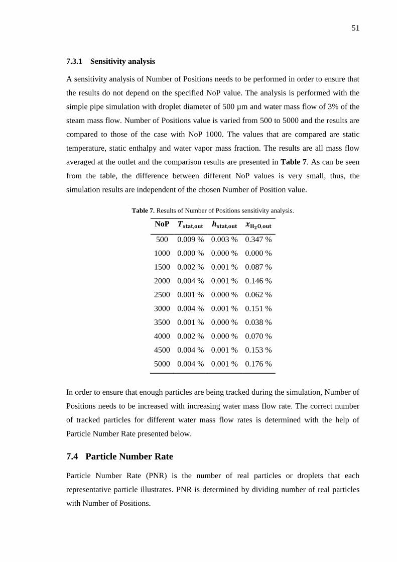
51

7.3.1 Sensitivity analysis

A sensitivity analysis of Number of Positions needs to be performed in order to ensure that

the results do not depend on the specified NoP value. The analysis is performed with the

simple pipe simulation with droplet diameter of 500 µm and water mass flow of 3% of the

steam mass flow. Number of Positions value is varied from 500 to 5000 and the results are

compared to those of the case with NoP 1000. The values that are compared are static

temperature, static enthalpy and water vapor mass fraction. The results are all mass flow

averaged at the outlet and the comparison results are presented in Table 7. As can be seen

from the table, the difference between different NoP values is very small, thus, the

simulation results are independent of the chosen Number of Position value.

Table 7. Results of Number of Positions sensitivity analysis.

NoP 𝑻𝐬𝐭𝐚𝐭,𝐨𝐮𝐭 𝒉𝐬𝐭𝐚𝐭,𝐨𝐮𝐭 𝒙𝐇𝟐𝐎,𝐨𝐮𝐭

500 0.009 % 0.003 % 0.347 %

1000 0.000 % 0.000 % 0.000 %

1500 0.002 % 0.001 % 0.087 %

2000 0.004 % 0.001 % 0.146 %

2500 0.001 % 0.000 % 0.062 %

3000 0.004 % 0.001 % 0.151 %

3500 0.001 % 0.000 % 0.038 %

4000 0.002 % 0.000 % 0.070 %

4500 0.004 % 0.001 % 0.153 %

5000 0.004 % 0.001 % 0.176 %

In order to ensure that enough particles are being tracked during the simulation, Number of

Positions needs to be increased with increasing water mass flow rate. The correct number

of tracked particles for different water mass flow rates is determined with the help of

Particle Number Rate presented below.

7.4 Particle Number Rate

Particle Number Rate (PNR) is the number of real particles or droplets that each

representative particle illustrates. PNR is determined by dividing number of real particles

with Number of Positions.

52

NoRP =�̇�p

4

3𝜋𝜌p

𝑑p3

6

(7-1)

where NoRP is number of real particles [1/s]

�̇�p is real particle mass flow rate [kg/s]

PNR =NoRP

NoP (7-2)

where PNR is Particle Number Rate [1/s]

NoP is Number of Positions [-]

Equation (7-1) shows how the number of real particles is determined, and with equation

(7-2) Particle Number Rate is calculated. The PNR is kept constant with different water

mass flow rates but when the droplet diameter is changed, the PNR changes also. For

example, with NoP 2500 and water mass flow rate of 3 % of the steam mass flow rate PNR

calculated for 10 µm and 100 µm droplets are 6.46∙108 1/s and 6.46∙10

5 1/s, respectively.

The smaller PNR for 100 µm droplets means that with larger droplet diameters, there needs

to be fewer particles injected in order to reach the same water mass flow rate. The case of

NoP 2500 and liquid carryover of 3 % is chosen to be the reference case for the PNR.

7.5 Materials

As explained in Chapter 4.2.1, the limitation of LPT model is that the dispersed or the

particle phase has to have constant properties and the vapor phase of the transferring

material has to be ideal gas. Therefore, the particle phase is set as water and the

evaporating vapor component as water ideal gas. In order to model the conditions at the

interphase of water and water ideal gas, a homogeneous binary mixture is created. In

homogeneous binary mixture, the Antoine equation, presented in Chapter 6.3, is defined.

The continuous phase is set to be real gas whose thermodynamic properties are determined

using Redlich-Kwong equations presented in Chapter 5. For the modeling of the transfer

of water ideal gas to the continuous phase, a variable composition mixture material is

created which includes the real gas and the water ideal gas materials. The reader should be

noted that, as will be explained in Chapter 7.7.1, the mass fraction of the water ideal gas

in the variable composition mixture is set to unity. Therefore, the real gas material in the

mixture is a dummy material that acts as a medium for the interphase mass transfer

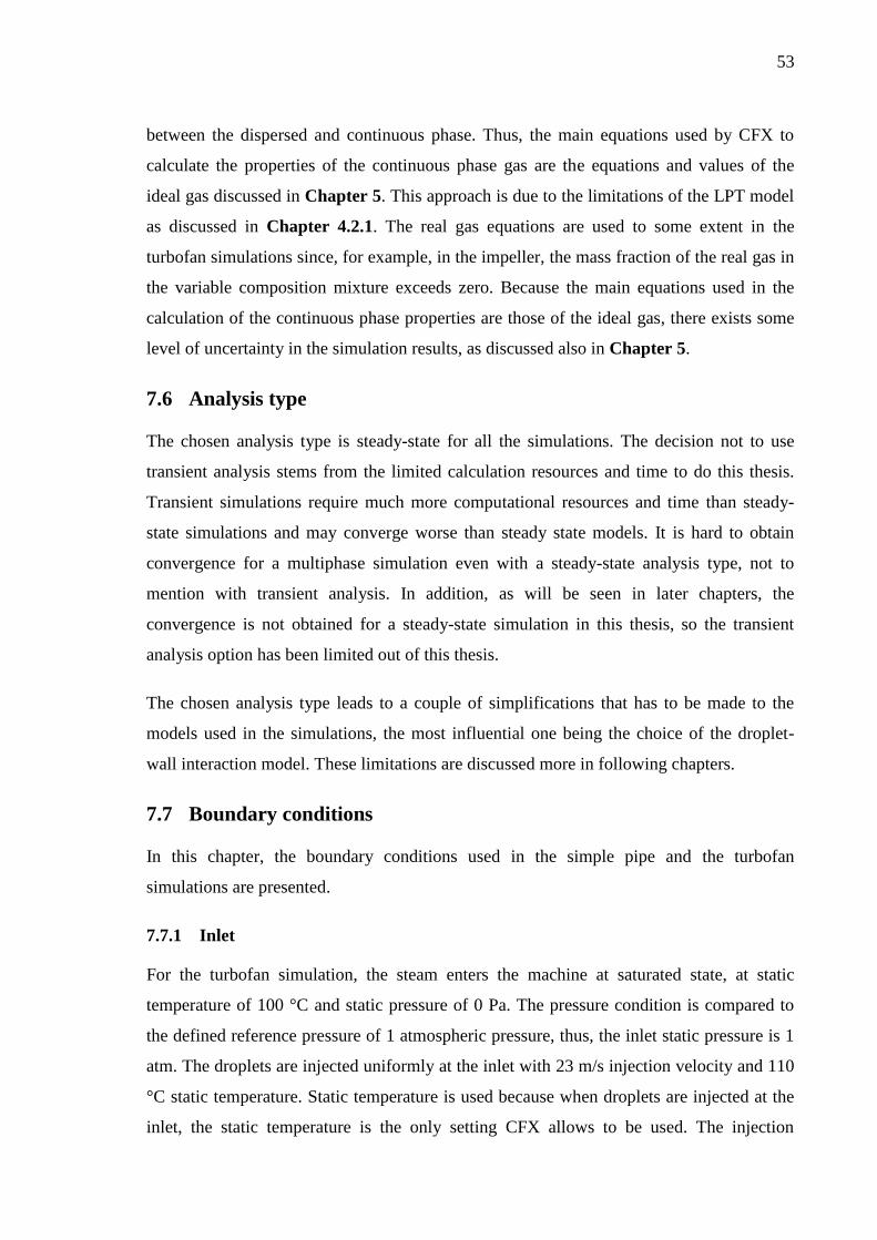
53

between the dispersed and continuous phase. Thus, the main equations used by CFX to

calculate the properties of the continuous phase gas are the equations and values of the

ideal gas discussed in Chapter 5. This approach is due to the limitations of the LPT model

as discussed in Chapter 4.2.1. The real gas equations are used to some extent in the

turbofan simulations since, for example, in the impeller, the mass fraction of the real gas in

the variable composition mixture exceeds zero. Because the main equations used in the

calculation of the continuous phase properties are those of the ideal gas, there exists some

level of uncertainty in the simulation results, as discussed also in Chapter 5.

7.6 Analysis type

The chosen analysis type is steady-state for all the simulations. The decision not to use

transient analysis stems from the limited calculation resources and time to do this thesis.

Transient simulations require much more computational resources and time than steady-

state simulations and may converge worse than steady state models. It is hard to obtain

convergence for a multiphase simulation even with a steady-state analysis type, not to

mention with transient analysis. In addition, as will be seen in later chapters, the

convergence is not obtained for a steady-state simulation in this thesis, so the transient

analysis option has been limited out of this thesis.

The chosen analysis type leads to a couple of simplifications that has to be made to the

models used in the simulations, the most influential one being the choice of the droplet-

wall interaction model. These limitations are discussed more in following chapters.

7.7 Boundary conditions

In this chapter, the boundary conditions used in the simple pipe and the turbofan

simulations are presented.

7.7.1 Inlet

For the turbofan simulation, the steam enters the machine at saturated state, at static

temperature of 100 °C and static pressure of 0 Pa. The pressure condition is compared to

the defined reference pressure of 1 atmospheric pressure, thus, the inlet static pressure is 1

atm. The droplets are injected uniformly at the inlet with 23 m/s injection velocity and 110

°C static temperature. Static temperature is used because when droplets are injected at the

inlet, the static temperature is the only setting CFX allows to be used. The injection

54

velocity of the droplets is determined with the parameters of the nozzle usually used by

HTF. The different mass flows of the water as well as the NoP of the droplets are presented

in Table 8. The different water mass flows correspond to the different steam mass flows of

80 %, 100 % and 120 % presented in the next chapter and are approximately 3 % of the

steam mass flow.

Table 8. Number of Positions for different water mass flow rates

�̇�𝐰 NoP

[kg/s] [-]

0.66 2022

0.81 2501

0.98 3034

For the simple pipe simulation, the inlet boundary condition is saturated steam and the

temperature of the steam is equal to the temperature at the outlet of the turbofan when de-

superheating is not used, 142 °C. Later, in Chapter 9.1, this temperature is changed to

130, 120 and 115 °C so different superheat temperatures are modeled. The inlet static

pressure condition is 0 bar compared to the defined reference pressure of 1.43 bar, which

results in inlet pressure of 1.43 bar. With this setting, an approximate value for the

evaporation rate and time for droplets with different initial size as well as the cooling of the

steam can be estimated. The droplets are injected with the same velocity and temperature

as with the turbofan simulation.

In order to get the steam to be saturated at the inlet of the simulations, the mass fraction of

water ideal gas at the inlet boundary is set to unity. This setting means that the real gas

material is a dummy material whose purpose is to be the medium for the interphase

transfer and evaporation phenomena as explained earlier in Chapter 7.5.

7.7.2 Outlet

The outlet boundary condition for both turbofan and simple pipe simulations is the mass

flow of the steam, 27.8 kg/s. Later this mass flow is changed to be 80 % and 120 % of the

original value in the turbofan simulation so the performance characteristics of the machine

can be obtained.

55

7.7.3 Wall

The walls in all simulations have smooth, adiabatic and no slip boundaries. For the

multiphase flow, the interaction of the droplets with the walls has to be defined. The

droplet interaction with the wall is chosen to be equation dependent with perpendicular and

parallel coefficient as unity. These values for the coefficients mean that when the droplet

interacts with the wall, it bounces off of the wall and does not lose its energy or

momentum. This method is chosen to be used because when the perpendicular coefficient

is set to zero, it is quickly noticed that when the droplet size is larger or equal to 10 µm,

most of the droplets hit the wall and get stuck to it, forming a wet film. The droplets

sticking to the walls can be seen from Figure 11, where droplets with initial size of 500

μm are injected into the fan with perpendicular coefficient set to zero. As seen from the

figure, the droplet tracks disappear at the inlet of the impeller while the droplet mean

diameter does not decrease to zero. The disappearance of the tracks when the droplet

diameter stays above zero millimeters implicates that the droplets have stuck to the wall.

Figure 11. 500 μm droplets getting stuck to the walls at the inlet of the impeller when perpendicular

coefficient for droplet wall interaction is set to zero.

The used Lagrangian Particle Tracking model in a steady-state simulation does not support

modeling of wet films so CFX stops following the water droplets when they hit the wall.

Simulating wet films would need its own model implemented to the simulation. CFX has a

built-in model for droplet interaction with walls and the formation of wet films but this

56

model is only supported in transient simulations. As explained earlier in Chapter 7.6,

transient simulations require more computational resources as well as time and may

converge worse than steady-state simulations. In addition, because the focus of this thesis

is on the evaporation of droplets and not wet films, the previously mentioned approach to

the droplet-wall interaction is used. The simulations would be more consistent with reality

if the modeling of wet films was implicated to the models, but, as has been mentioned, due

to the limited computational resources and time, the wet film model and transient analysis

is limited out of this thesis.

7.7.4 Interfaces

For the turbofan simulation, the interfaces of the impeller and other bodies have to be

specified since the impeller body is rotating and the other bodies are not. This setting is

done by selecting a general connection interface model and a frame change/mixing model.

The turbofan simulations are done with two frame change models. First, Frozen Rotor

model is used to obtain an approximate solution. The Frozen Rotor model assumes a fixed

relative orientation of the components across the interface while the frame of reference or

the pitch is changed. After the first solution is obtained, the interface model is changed to

Stage (Mixing Plane) model which calculates the circumferential average of the fluxes

through the bands on the interface. The Frozen Rotor solution is used as an initial guess for

the Stage (Mixing Plane) simulations. (ANSYSa 2016, Ch. 5.3.)

7.8 Newton iteration method

CFX solver uses Newton iteration to calculate the thermodynamic properties of the defined

materials using the equations presented in Chapter 5. This method can sometimes fail to

converge and stop the solver with an error message. The stopping of the CFX solver due to

Newton method’s error is observed to happen when the turbofan’s frame change model is

changed from Frozen Rotor to Stage (Mixing Plane) in a multiphase flow simulation. In

order for the Stage model to work with multiphase flow, changes have to be done to

Newton method’s parameters for the homogeneous binary mixture and mixture materials.

The iteration limit of Newton pressure parameter is increased and the under relaxation

factor of Newton pressure and Constitutive relation is decreased for both materials. The

iteration limit is increased from 100 to 300 and the under relaxation factors are decreased

from 1.0 to 0.75. With these changes, the Newton method obtains convergence in the CFX

solver and the simulation does not stop due to error.

57

7.9 Solver settings

The simulations are performed with High Resolution Advection Scheme and First Order

Turbulence Numerics. With the First Order setting for the turbulence equations, the

advection terms in those equations are first-order accurate. This setting is more robust than

the High Resolution option and often experiences numerical diffusion, but it is acceptable

to use the First Order setting for the turbulence calculation. The High Resolution option is

chosen to be used for the mass and energy equations since it is not acceptable to use a more

robust scheme for these equations. The High Resolution scheme varies the blend factor

used in the calculation throughout the domain in order to avoid the diffusion of the

equation parameters. (ANSYSa. 2016, Ch. 15.5.)

Timescale Factor is set to automatic and to a value four. Usually, the requirement is to

obtain convergence with timescale value five, but the value four is chosen to be used since

with multiphase flow and complex geometry, the convergence with value five would be

even worse than with a lower factor. The timescale in steady-state simulations is a false

time step which CFX uses to under-relax the equations while iterating to the final solution

(ANSYSa. 2016, Ch. 15.4).

The criteria for convergence is that the root mean square (RMS) residuals are smaller than

1 ∙ 10−4. The RMS residuals measure the local imbalance of each control volume equation.

The smaller the residual levels, the better the accuracy the equations are solved. The

residual levels can reach low values with very small timescale factors. In that case,

however, the convergence is not obtained since the under-relaxation of the equations is too

strong and the results are not trustworthy. (ANSYSa. 2016, Ch. 15.10.)

In addition to the residual levels, the convergence of the simulations should be monitored

by following the change of a couple of chosen variables. In the simple pipe simulations,

the variable chosen is the outlet temperature of the fluid, and in the turbofan simulations,

the chosen parameters are torque and total pressure at outlet. These variables are discussed

more in Chapter 9.1 and Chapter 9.3.

The first particle iteration is after 30 iterations, the particle iteration frequency is 5 and

particle source change target 0.03. The minimum diameter is set to be 1 ∙ 10-8

μm, after

which the droplet is assumed to be fully evaporated and CFX stops following it. Particle

under relaxation factors are set so that energy and mass relaxation factors are 0.5 and

58

velocity relaxation factor is 0.75. By reducing these factors the oscillation of the particle

source terms can be decreased (ANSYSa. 2016, Ch. 8.10).

𝑆f = (1 − 𝑈F)𝑆f + 𝑈F𝑆p (7-3)

Where 𝑆f is source term to the continuous phase fluid [-]

𝑈F is under relaxation factor [-]

𝑆p is source from particles [-]

Equation (7-3) shows how the CFX solver takes the particle under relaxation factors into

consideration in the simulation.

59

8 VALIDATION OF MODELS

In this chapter, the validations of the chosen turbulence model and the used droplet

evaporation model are presented.

8.1 Validation of the turbulence model

The chosen SST turbulence model is validated by simulating an experiment performed by

Bai et al. (2009). In their research, Bai and his colleagues injected water droplets from a

centrifugal spray nozzle into an air flow flowing in a rectangular duct. The duct is 95 × 95

mm in cross-section and its length is 1 m. The Reynolds number of the air flow varies

between 12 900 and 45 000. The droplets are injected with two nozzles positioned at the

top and bottom of the duct at 0.1 m distance from the inlet. The spray angle is 80°, the

operating pressure of the nozzle is 7 MPa and capacity 0.0226 m3/h. The Sauter Mean

Diameter of the droplets is 80 μm. The injection angle of the spray compared to the flow

direction is 90°. More information from the experimental setup can be found on Bai et al.

(2009).

The simulation with CFX is performed with air Reynolds numbers of 25 700 and 32 100

from which the inlet velocity of the air is calculated to be 4.1 and 5.1 m/s, respectively.

The droplet injection velocity and mass flow are approximated with the nozzle information

given on Bai et al. (2009) and the uniform initial diameter of the droplets is defined as 80

μm. The nozzle is simulated with a hollow cone. The simulation mesh is presented in

Figure 12. The mesh has 1.5 million hexahedra elements and finer grid near the walls. The

mesh sensitivity analysis is performed with two additional grids whose number of elements

are 1.0 million and 2.0 million. With the sensitivity analysis, it is concluded that the chosen

mesh with 1.5 million elements is accurate enough for the simulations.

Figure 12. Turbulence model validation mesh with 1.5 million number of elements.

60

In Figure 13, the comparison of velocity vectors between the experimental and CFX

simulation results for air Reynolds number of 25 700 is presented. The measurement

location is after the nozzle at 0.1 m along the duct. As can be seen, similar circulation of

the air flow is occurring in the CFX simulation results as is in the experimental ones. There

are four main vortices appearing in both figures and the direction of the flow is similar,

from the center towards the walls. In Figure 14, the comparison of the experimental and

CFX results for air Reynolds number of 32 100 is shown. The measurement location is

0.22 m from the nozzle. As with the lower Reynolds number flow, vortices are found to

appear in the corners of the duct because the water droplets disturb the flowing of the air

and give their momentum to the air flow. The two vortices at the top and bottom of the

duct stem from the positioning of the spray nozzles to the top and bottom of the duct.

Figure 13. Velocity vector comparison between a. experimental and b. CFX simulation results. Air Reynolds

number is 25 700 and x is 0.1 m from the nozzle. (Bai et al. 2009, p. 1017.)

Figure 14. Velocity vector comparison between a. experimental and b. CFX simulation results. Air Reynolds

number is 32 100 and x is 0.22 m from the nozzle. (Bai et al. 2009, p. 1017.)

61

The values of the average vorticity of the air flow with Re 45 000 at different distances

from the nozzles are compared between the experimental and CFX simulation results in

Figure 15. The experimental vorticity values are obtained from Bai et al. (2011) where Bai

and his colleagues performed a numerical study on how spray droplets mix in turbulent air

flow and validated their model based on their experiment in Bai et al. (2009). From Figure

15, it can be seen that there exists significant difference between the vorticity in the CFX

simulation and in the experiment. The difference is high near the nozzle as well as far

away from it, the highest value being 37 % when x is 0.18 m. In the middle measurement

locations, the difference is below 5 %. The difference curve and values are left out from

Figure 15 for clarity.

The reader should be noted that due to the limitations in computational resources and time,

the CFX simulations have not obtained full convergence, that is, the momentum residuals

are greater than 1 ∙ 10−4. The non-convergence can play a part in the high differences near

and far away from the nozzles. The experimental values can also have some uncertainty

given the uncertain elements of every experiment. Nevertheless, the differences near and

far away from the nozzles are not in acceptable limits, which could pose an uncertainty

factor on the results of this thesis.

Figure 15. Average vorticity along the duct for the experiment and CFX simulation with air Reynolds of 45

000.

62

It should be noted that even though the simulations are not fully converged, the velocity

profile of the air flow, in Figure 13 and Figure 14, as well as the tendency of decreasing

vorticity, in Figure 15, are similar to the ones in the experiment. In addition, when taking

into account that the SST model is a widely used built in model of CFX, the limitations of

turbulence modeling of the LPT model and the fact that the main focus of this thesis is on

the evaporation of droplets, the SST turbulence model could be used in this thesis.

8.2 Validation of the droplet evaporation model

The droplet evaporation model is validated by simulating an experiment found in literature

and comparing the modeling results with the experimental results. The experimental setup

and data is given by Sureshkumar et al. (2008). In the experiment, air at ambient conditions

is flowing to a rectangular duct with a cross-section of 585×585 mm. Water is injected into

the flow with a nozzle at different nozzle diameters and operating pressures. After a drift

eliminator, which stabilizes the flow and collects leftover water, the dry bulb temperature

(DBT) and wet bulb temperature (WBT) of the air are measured. The experimental setup is

shown in Figure 16. More details about the experiment can be found in Sureshkumar et al.

(2008).

Figure 16. Experimental setup and thermocouple locations at exit plane (Sureshkumar et al. 2008, p. 351)

The chosen test cases for the simulation are presented in Table 9. The chosen nozzle angle,

18°, is an assumed one and influenced by the study of Montazeri et al. (2015) who have

simulated the same experiment using ANSYS Fluent and made a sensitivity analysis of

spray angle as well. The simulated cases are all of hot-dry ambient conditions and the

relative humidity of the inlet air is assumed to be 12 % since it is not told precisely in

Sureshkumar et al (2008).

63

�̇�air = 𝜌air𝑈air𝐴 (8-1)

Where �̇�air is air mass flow rate [kg/s]

𝜌air is air density [kg/m3]

𝑈air is air velocity [m/s]

A is cross-sectional area [m2]

The mass flow rate of the inlet air is calculated with equation (8-1).

Table 9. Chosen experimental cases to be simulated.

Case Air Water Nozzle

Uair DBT WBT �̇�air 𝑇in 𝑇out �̇�w p d angle

[m/s] [°C] [°C] [kg/s] [°C] [°C] [l/min] [bar(g)] [mm] [°]

1 1 41.4 18.9 0.41 35.1 25.3 12.5 3 4 18

2 2 39.1 18.5 0.82 35 25.2 12.5 3 4 18

3 3 39.2 18.7 1.23 35.2 26.1 12.5 3 4 18

𝑈inj = 𝐶 ∙ √2∙𝑝rel

𝜌w (8-2)

where 𝑈inj is water injection velocity [m/s]

𝐶 is nozzle coefficient [-]

𝑝rel is relative pressure between nozzle and ambient [Pa]

𝜌w is water density [kg/m3]

The injection velocity of the water droplets is calculated with equation (8-2). The nozzle

coefficient is given by Surehkumar et al. as 0.9. The determined injection velocity is held

constant in all the simulations.

The grids used in the mesh sensitivity analysis are shown in Figure 17. The domain is

chosen to be longer than in the real experiment in order to let the inlet air flow develop

before and after the droplets are injected into it. The finer mesh in the center of the domain

is the part that corresponds to the experimental duct. In the experiment, carryover water is

collected by the drift eliminator before the thermocouples, so in the simulation, CFX stops

following the droplets just before the measuring locations at the end of the finer mesh part.

Case 3 is chosen to be simulated in the mesh sensitivity analysis and the results are shown

64

in Table 10. The static temperature of the air flow is mass averaged at the end of the

experimental part of the simulation domain. The different temperatures are compared to

the temperature of the mesh b. From the table, it can be seen that there are no significant

deviation in the results between the grids. Mesh b with 916 000 elements is chosen to be

used in the simulation.

Figure 17. Different mesh sizes used in grid sensitivity analysis: a. robust, b. finer and c. finest.

Table 10. Mesh sensitivity analysis results

Mesh No. of elements 𝑻𝐬𝐭𝐚𝐭,𝐨𝐮𝐭

a. 30 100 0.13 %

b. 916 000 0.00 %

c. 3 420 000 0.16 %

The droplet diameter distribution in the experiment is presented in Figure 18. From this

data, a Rosin Rammler distribution is developed. The distribution determined by Montazeri

et al. (2015) is used in this thesis. The mean diameter is 369 µm and the spread parameter

is 3.67 (Montazeri et al. 2015, 133).

Figure 18. Droplet diameter distribution of the experiment (Sureshkumar et al. 2008, p. 353).

65

The results of the simulation, dry bulb temperature, wet bulb temperature and enthalpy of

the air flow, are compared to those of the experimental ones. The comparison for the case

1, case 2 and case 3 are presented in Figure 19. From the figure, it can be seen that there

are some difference in the temperatures and enthalpy between the simulation and the

experiment. These differences can stem from many different aspects. The dominating

uncertainty is the drift eliminator used in the experiment. The eliminator is described

vaguely in the article and is hard to simulate accurately. In addition, in their work,

Sureshkumar and his coworkers state that there might be carryover mist in the air flow

after the eliminator due to its technical limitations. If any water is let to get to the

thermocouples, it might affect the temperature measurements resulting in errors in the

experiment. Another uncertainty factor is that the relative humidity is assumed in the

simulation and kept constant in different cases. In reality, the relative humidity of air can

change between the measurements. Furthermore, the assumptions and limitations of CFX

presented in Chapter 4.2.1 can lead to differences between experimental and simulation

results. Moreover, from the figures, it can be seen that the highest difference is usually

located only to one measurement point in the middle of the duct, thus, leading to higher

error only in small area in the domain.

Some uncertainties for the steam-water simulations in this thesis can stem from the fact

that the validation is done with an experiment where water droplets evaporate in air and

not in steam as is the case in this thesis. The used air-water experiment performed by

Sureshkumar et al. is chosen for the validation process since it is the best and most

accurate experimental research paper found in the literature that could be accessed by the

writer. Although, the equations and phenomena for the droplet evaporation are the same

regardless of the continuous phase gas and the liquid, there might be some uncertainties

posed on the usage of the LPT model for the simulation of steam-water combination.

Taking into account the factors of the droplet evaporation validation discussed above, it

can be concluded that the evaporation model used in this thesis could be validated more

and more accurately if a good and detailed experimental research paper of droplet

evaporation in steam flow was be found. Nevertheless, the phenomena and equations are

the same whether or not the continuous phase gas is air or steam. Therefore, the

evaporation model can be used in this thesis while keeping the uncertainties discussed

above in mind.

66

Figure 19. Comparison of the simulation and experimental results for case 1: a. DBT, b. WBT, c. enthalpy; case 2: d. DBT, e. WBT, f. enthalpy; case 3: g. DBT, h. WBT and

i. enthalpy

67

9 RESULTS OF MODELING

In this chapter, the results of the turbofan and the simple pipe multiphase modeling are

presented.

9.1 Droplet evaporation in simple pipe

In order to demonstrate and estimate the diameter change rate of different droplet sizes as

well as the time it takes for the steam to reach saturation temperature, simulations with 180

m long straight pipe with diameter of 0.75 m are performed. The pipe geometry is created

by scaling the previously presented shorter pipe geometry to the right diameter and to 45 m

in length and then copying this 45 m long pipe 3 times so that each copy starts at the end of

the previous one. In other words, the geometry of this longer pipe is the same as the

geometry of the simple pipe presented in Chapter 7.1, just scaled to a different size. In

addition, the mesh of the longer pipe is similar to the mesh of the shorter pipe but because

of the copying, the number of elements is approximately four times the number of

elements in the shorter pipe, 7.3 million elements. The boundary conditions are as

presented earlier and the droplet initial diameter varies from 10 μm to 500 μm. In addition

to the droplet diameter varying, the steam inlet velocity as well as superheat temperature is

changing. The values of the inlet velocity of the steam are 20, 50 and 80 m/s and the

superheat temperature values are 142, 130, 120 and 115 °C.

The chosen Number of Positions is 2500 for 10 μm droplet and 5000 for larger droplets.

Different number of NoP is chosen to be used for 10 μm droplets because the smaller the

droplet, the more demanding the simulation and with more NoP, the simulation becomes

even more demanding. With larger droplets, NoP does not affect the simulation time as

much as with smaller diameters, so 5000 NoP is to be used for larger droplets. It should be

kept in mind that as demonstrated in Chapter 7.3.1, NoP does not have an effect on the

results of the modeling. Furthermore, it should be mentioned that the simple pipe

simulations are fully converged so the results are trustworthy.

9.1.1 Diameter change

The diameter change of the droplets is determined by choosing a couple of samples of

particle tracks that continue to the outlet of the pipe and calculating the average diameter in

those tracks. The sample tracks are chosen from the tracks that continue to the outlet of the

68

pipe since some of the tracks disappear on the way because the particles reach the set

minimum diameter and CFX stops following them. However, for 10 μm droplets, the

tracks chosen for lower velocities are tracks that end on the way because with 10 μm

droplets, most of the water is evaporated in the pipe, thus, most of the particle tracks

disappear before reaching the outlet of the pipe. The tracks that reach the outlet are

positioned next to the pipe wall. Near the wall, the flow velocity of the steam and droplets

decrease because of the friction of the wall (ANSYSa. 2016, Ch. 2.7). Therefore, droplets

near the wall evaporate more slowly than droplets in the center of the pipe. The particle

tracks near the wall do not represent the overall droplet evaporation well and are, therefore,

excluded from the sample particle tracks. In addition, for larger droplets, most of the

chosen sample tracks are from the center section of the pipe, so, for a good comparison, the

sample tracks for the 10 μm droplets are also taken from the center section.

Normalized diameter change for different initial size droplets with steam superheat

temperature of 142 °C and different flow velocities is shown in Figure 20. As can be seen,

the larger the droplet, the less its diameter changes in the pipe. This phenomenon is

opposite to the diameter change in the turbofan where the diameter of larger droplets

changes more compared to the diameter of smaller droplets as will be presented in

Chapter 9.2. This difference is due to the fact that there is significantly less secondary

breakup in a straight pipe than in a turbomachine. Therefore, only evaporation and

diffusion decrease the droplet diameter. Because the water mass flow and Particle Number

Rate are constant but the initial droplet diameter changes with different cases, the total

number of real particles injected into the pipe with larger droplets is smaller compared to

the number with smaller droplets. Thus, the total surface area of smaller droplets is a lot

bigger than the total surface area of larger droplets. The higher the total surface area of

droplets, the higher the heat transfer between the particles and the fluid, hence, smaller

droplets evaporate faster and their diameter decreases more compared to larger droplets.

From Figure 20, it can also be noted that with lower flow velocities, the diameter of the

droplets decreases more than with higher velocities. This difference is due to the fact that

with a slower flowing flow, the droplets spend more time in the pipe and have more time to

transfer heat with the fluid. Therefore, they have more time to evaporate and, thus, the

droplet diameter at the end of the pipe is smaller. Furthermore, with smaller diameters,

such as 10 μm and 25 μm, it can be seen that the diameter change stops and the normalized

diameter stays constant. The droplets stay approximately at the same size when the steam

69

has reached the saturation temperature at given pressure. When the fluid is at saturation

temperature, it cannot take in anymore water vapor, thus, the liquid droplets stop

evaporating. It can be noted that the diameter of the droplets continue to decrease at a very

slow rate because of the pressure loss in the pipe. The pipe is so long that the pressure loss

between the inlet and outlet of the pipe has an effect on the saturation temperature of the

steam. When pressure decreases, so does the saturation temperature and, thus, the droplets

continue to cool the steam down as well as decrease in size at a very slow rate throughout

the pipe.

Figure 20. Normalized diameter change for different initial droplet diameters, superheat temperature is 142

°C and flow velocity is: a. 80 m/s, b. 50 m/s and c. 20 m/s.

In Figure 21, the normalized diameter change of droplets with superheat temperature of

130 °C and different flow velocities is shown. In the figure, there are similar phenomena as

in Figure 20 and the explanations are also the same as stated earlier. With lower superheat

temperature, the diameter change is smaller within the same timeframe and with same flow

velocity compared to a higher superheat temperature. The droplets are injected into the

pipe at same temperature, so, with lower superheat temperature of the steam, the

temperature difference between the steam and the droplets is smaller. Therefore, the heat

transfer rate between the steam and the particles is smaller resulting in lower decrease in

droplet diameter in the pipe.

70



In Figure 22 and Figure 23 the normalized droplet diameter change is shown for superheat

temperatures of 120 °C and 115 °C, respectively. From the figures, the same aspects as in

previous figures can be seen. As noted previously, as the superheat temperature decreases,

so does the diameter change rate of the droplets because of the lower temperature

difference between the steam and the droplets.

71





72

9.1.2 Evaporated water mass

In Figure 24, Figure 25 and Figure 26 the evaporated mass of water is shown for different

superheat temperatures and flow velocities of the steam and with initial droplet diameters

of 10, 50, 100, 300 and 500 μm. The evaporated mass of water is determined the same way

as earlier with the turbofan. As can be seen, the evaporated water mass is in correlation

with the earlier presented diameter change of the droplets. With droplet diameter of 10 μm

approximately all of the water is evaporated regardless of the superheat temperature of the

steam. Although there are some particle tracks left at the end of the pipe, the mass of the

particles is so small that it can be said that all of the water mass injected into the pipe gets

evaporated. As the initial diameter of the droplets increases, the evaporated water mass

decreases. As stated earlier, the evaporation rate of smaller droplets is higher because their

total surface area is a lot bigger compared to the total surface area of larger droplets

because of the total amount of real particles injected into the pipe. In addition, in

correlation with the diameter change, more water is evaporated with higher superheat

temperature and lower flow velocity than with lower temperature and higher flow velocity

because of the higher temperature difference between the droplets and the steam and

longer residence time of the droplets in the pipe.

Figure 24. Evaporated water mass percentage for different initial droplet diameters and steam superheat

temperatures, flow velocity is 80 m/s.

73





9.1.3 Fluid temperature decrease

The temperature decrease of the steam is determined in a center line that goes through the

pipe. The time is calculated with average steam velocity and the longitudinal position of

the steam in the pipe. The temperature decrease of the steam as a function of time is

presented in Figure 27, Figure 28, Figure 29 and Figure 30 for superheat temperatures

142, 130, 120 and 115 °C, respectively. Each superheat temperature has three figures with

different flow velocities and different initial droplet diameter. The target steam temperature

74

is 383 K which is the saturation temperature at given pressure. From Figure 27 and Figure

28, it can be noticed that with all velocities, droplets with initial diameter of 10 μm and 25

μm cool the steam to the desired temperature. The temperature difference between the

steam and the droplets is large enough to enable high enough evaporation rate of the water

to cool the steam to the saturation temperature. With flow velocity of 20 m/s, also the

droplets with 50 μm initial diameter are successful in cooling the steam to the desired

temperature. As stated earlier, with low velocities, the droplets spend more time in the

pipe, thus, they have more time to cool the temperature of the steam down. In Figure 29

and Figure 30 the temperature difference between the steam and the droplets is already so

small that the evaporation rate for droplets larger than 25 μm is not high enough to cool the

steam temperature down to the desired saturation temperature.

From all the figures, it can be clearly seen that the 10 μm droplet cools the steam

temperature to the desired value immediately after the inlet. This phenomenon is more

drastic the higher the superheat temperature of the steam is. High temperature difference

and large total surface area are the reasons for this fast evaporation of the droplets and cool

down of the steam, as is explained earlier in Chapter 9.1.1. The weird shape at the

beginning of the 10 μm line in the c. chart in the three first figures is there only because of

the drastic drop of the steam temperature and because the chart had to be made narrower so

the three charts, a, b and c, could be put next to each other for easier comparison. When

the line of 10 μm from Figure 27.c is shown in bigger size and the time range is limited

from 0 to 3 s in Figure 31, it can be seen that there are no weird shapes in the line.

75

Figure 27. Steam temperature decrease for superheat temperature 142 °C with different initial droplet

diameters and flow velocities: a. 80 m/s, b. 50 m/s, c. 20 m/s. The target steam saturation temperature is the

red line at 383 K.



red line at 383 K.

76



red line at 383 K.



red line at 383 K.

77

Figure 31. Fluid temperature change for 142 °C superheat temperature, 10 μm initial droplet diameter and 20

m/s fluid velocity. Time range is limited from 0 to 3 s.

9.2 Droplet evaporation in turbofan

The evaporation of droplets inside turbofan is investigated with different initial droplet

diameters. In this chapter, the results of the simulation are introduced and discussed. For

all the cases, the boundary conditions are the same and only the initial diameter of the

droplets is changing. The diameters investigated are 1.5, 10, 100, 300 and 500 μm.

It should be noted that the turbofan simulations are not fully converged so there is some

uncertainty in the results. In multiphase flow simulations, it is generally difficult to obtain

full convergence because the number of equations that need to be solved is high and the

phenomena that are simulated are so complicated. Moreover, a complex geometry and

mesh make it even harder to obtain full convergence. With more time and computational

power, fully converged results could probably have been obtained. Nevertheless, the

phenomena of multiphase flow and droplet evaporation inside a turbofan can be seen from

the results presented in this chapter.

9.2.1 Diameter change of droplets

The diameter change of droplets inside the fan is illustrated with 1.5 μm initial droplet size

in Figure 32, where the mean particle diameter of droplets is shown in the whole machine

for 250 particle tracks. As can be seen from the figure, the droplets do not decrease in size

in the inlet duct but their diameter starts to change when they reach the impeller of the fan.

78

This phenomenon is due to the fact that at the inlet duct, the steam is still at saturated state

so it cannot take in any more water. At the impeller, the impeller begins to do work on the

steam increasing the pressure and enthalpy of the steam. The steam starts to heat up and

heat as well as mass transfer between the steam and the droplets starts to take place.

Therefore, the droplets start to evaporate in the impeller and decrease in size. With droplet

diameter of 1.5 μm the diameter decrease is purely due to evaporation since the droplet

Weber number does not exceed unity as shown in Table 11.

The evaporation in the impeller is shown in Figure 33 where the 250 particle tracks are

limited by traveling time between 0.025 s and 0.035 s. The droplets evaporate quite

quickly when leaving the rotor due to the increase in pressure and temperature of the steam

as stated earlier. The water droplets reach their saturated state and start to evaporate and

cool the steam because the latent heat needed for the evaporation is taken from the

surrounding superheated steam.

Figure 32. Droplet mean diameter change inside the turbofan for 250 particle tracks. Initial droplet diameter

1,5 μm.

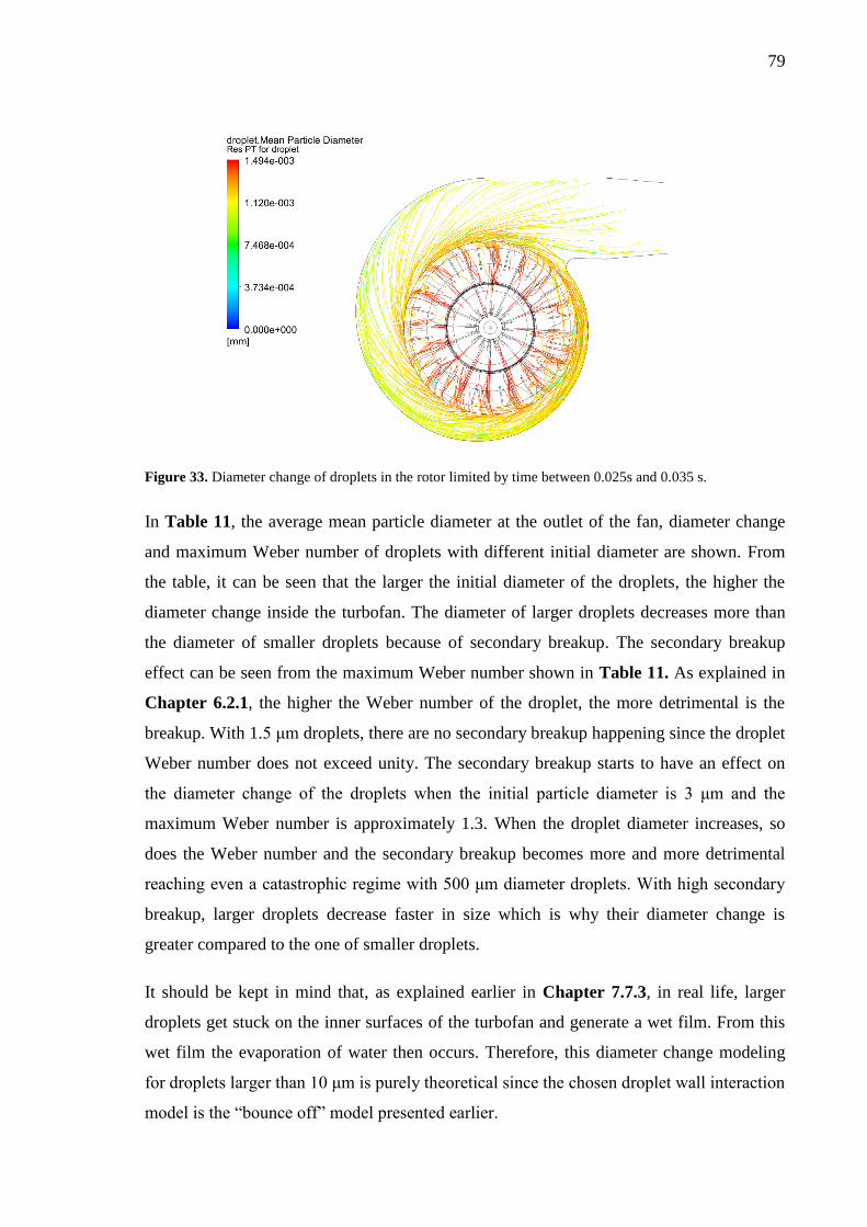
79

Figure 33. Diameter change of droplets in the rotor limited by time between 0.025s and 0.035 s.

In Table 11, the average mean particle diameter at the outlet of the fan, diameter change

and maximum Weber number of droplets with different initial diameter are shown. From

the table, it can be seen that the larger the initial diameter of the droplets, the higher the

diameter change inside the turbofan. The diameter of larger droplets decreases more than

the diameter of smaller droplets because of secondary breakup. The secondary breakup

effect can be seen from the maximum Weber number shown in Table 11. As explained in

Chapter 6.2.1, the higher the Weber number of the droplet, the more detrimental is the

breakup. With 1.5 μm droplets, there are no secondary breakup happening since the droplet

Weber number does not exceed unity. The secondary breakup starts to have an effect on

the diameter change of the droplets when the initial particle diameter is 3 μm and the

maximum Weber number is approximately 1.3. When the droplet diameter increases, so

does the Weber number and the secondary breakup becomes more and more detrimental

reaching even a catastrophic regime with 500 μm diameter droplets. With high secondary

breakup, larger droplets decrease faster in size which is why their diameter change is

greater compared to the one of smaller droplets.

It should be kept in mind that, as explained earlier in Chapter 7.7.3, in real life, larger

droplets get stuck on the inner surfaces of the turbofan and generate a wet film. From this

wet film the evaporation of water then occurs. Therefore, this diameter change modeling

for droplets larger than 10 μm is purely theoretical since the chosen droplet wall interaction

model is the “bounce off” model presented earlier.

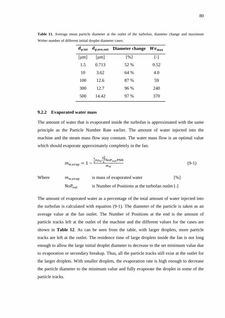
80

Table 11. Average mean particle diameter at the outlet of the turbofan, diameter change and maximum

Weber number of different initial droplet diameter cases.

𝒅𝐩,𝐢𝐧𝐢 𝒅𝐩,𝐚𝐯𝐞,𝐨𝐮𝐭 Diameter change 𝑾𝒆𝐦𝐚𝐱

[μm] [μm] [%] [-]

1.5 0.713 52 % 0.52

10 3.62 64 % 4.0

100 12.6 87 % 59

300 12.7 96 % 240

500 14.42 97 % 370

9.2.2 Evaporated water mass

The amount of water that is evaporated inside the turbofan is approximated with the same

principle as the Particle Number Rate earlier. The amount of water injected into the

machine and the steam mass flow stay constant. The water mass flow is an optimal value

which should evaporate approximately completely in the fan.

𝑚w,evap = 1 −4

3𝜋𝜌w

𝑑p3

6NoPoutPNR

�̇�w (9-1)

Where 𝑚w,evap is mass of evaporated water [%]

NoPout is Number of Positions at the turbofan outlet [-]

The amount of evaporated water as a percentage of the total amount of water injected into

the turbofan is calculated with equation (9-1). The diameter of the particle is taken as an

average value at the fan outlet. The Number of Positions at the end is the amount of

particle tracks left at the outlet of the machine and the different values for the cases are

shown in Table 12. As can be seen from the table, with larger droplets, more particle

tracks are left at the outlet. The residence time of large droplets inside the fan is not long

enough to allow the large initial droplet diameter to decrease to the set minimum value due

to evaporation or secondary breakup. Thus, all the particle tracks still exist at the outlet for

the larger droplets. With smaller droplets, the evaporation rate is high enough to decrease

the particle diameter to the minimum value and fully evaporate the droplet in some of the

particle tracks.

81

Table 12. Number of Positions left at the end of the turbofan for different initial droplet diameters.

𝒅𝐩,𝐢𝐧𝐢 Total NoP NoP at outlet

[μm] [-] [-]

1.5 2501 1692

10 2501 2334

100 2501 2501

300 2501 2501

500 2501 2501

The amount of evaporated water for the different cases is shown in Figure 34. As can be

seen from the figure, in all the cases the amount of evaporated water is above 90 % with a

slight increase when the initial droplet size becomes larger. This difference is probably due

to the approximation of PNR at the turbofan outlet. The value of PNR of larger droplets

changes throughout the fan because of secondary breakup. As explained in Chapter 7.4,

the smaller the particle diameter, the higher the PNR. When the particle diameter changes

rapidly because of the secondary breakup, so does the value of PNR. For example, with

500 μm initial diameter, the minimum PNR value is 5160 1/s and the maximum 1.07 ∙ 108

1/s. At the outlet, on different particle tracks, the PNR ranges between these minimum and

maximum values. Therefore, the chosen value for the calculation of the evaporated water

mass is an average value. As Figure 34 shows, regardless of the initial droplet diameter,

approximately the same amount of water is evaporated inside the turbofan.

Figure 34. The amount of evaporated water at the turbofan outlet for different initial droplet diameters.

82

9.2.3 Volume fraction and temperature of water droplets

As explained in Chapter 4.2.1, in order for the LPT model to be valid, the flow must be

dilute which means that the volume fraction of droplets has to be below 1 %. Because of

the chosen droplet wall interaction model, the particles are free to move inside the machine

with the fluid flow. Therefore, a phenomenon of a local gathering of water droplets is

noticed when modeling droplets with initial diameter equal to or larger than 10 μm. This

phenomenon is demonstrated in Figure 35, where the average volume fraction of 1.5 μm

and 10 μm droplets is shown. The value shown is the maximum limit of 1 %. The blue

colour in the right corner of the fan with 10 μm droplets indicates that the volume fraction

of water droplets is 1 % in those areas. In the left side of the figure, with 1.5 μm droplets,

there are no blue color to be seen, which indicates that there are no similar gathering of

water as is with 10 μm droplets. Because the maximum volume fraction value is exceeded

in the blue coloured regions, the LPT model begins to lose its validity in those regions. The

reduction of model validity results in extraordinary temperatures of droplets and fluid

along the particle tracks that have gathered in the right corner of the turbofan, as can be

seen in Figure 36.

In Figure 36, the droplet temperature along the particle tracks is shown for 1.5 and 10 μm

droplets. With 10 μm droplets there are a couple of cold areas in the particle tracks that

follow the corner in which the 1 % volume fraction limit is exceeded. However, tracks that

do not travel along the non-valid corner show temperature that makes sense, approximately

the saturation temperature at given pressure. These reasonable temperatures implicate that

the model validity problem is limited to a local volume and elements. This conclusion is

also supported by the fact that with smaller droplet size, the temperature along the tracks is

continuous throughout the fan. Therefore, the validity problem should not affect

significantly the results of the simulations. The problem could be solved by changing the

droplet wall interaction model so the particles would not move freely inside the machine

but interact with the wall as they do in reality. This change could be done in the future and,

as explained in Chapter 7.7.3, is not included in this thesis.

83

Figure 35. Average droplet volume fraction for 1.5 μm (left) and 10 μm (right), value shown is 1 %. Blue

colour in the right figure shows the 1 % droplet volume fraction.

Figure 36. Droplet temperature along particle tracks for 1.5 μm (left) and 10 μm (right).

9.3 Turbofan performance

The performance of the turbofan with water injection is determined with 1.5 μm droplets

because of the volume fraction limitations of larger liquid particles as explained in

Chapter 9.2.3. The simulations are done with the optimal mass flow rate of the steam,

27.8 kg/s, and water, 0.81 kg/s, as well as with 80 % and 120% mass flows in order to

obtain the performance characteristics. The pressure ratio, power and efficiency of the fan

are determined from the simulation results and compared to the ones of a single phase flow

with the same steam mass flow. In addition, the single phase flow simulation results are

compared to the performance characteristics of the same turbofan in HTF’s aerodynamic

selection software. The results should be as close to each other as possible.

84

The calculation procedure of the HTF’s software is based on standardized tests and fan

scaling laws. The software contains a set of non-dimensional aerodynamic performance

parameters for different fan types. These parameters are obtained from standardized model

performance tests. The performance values, in addition to the fan scaling laws, are then

used to select a proper fan for given operating parameters.

Because the turbofan CFX simulations are not fully converged, the comparisons are done

using the minimum and maximum values taken from CFX solver as well as with the

average values calculated from the ranges of the last 500 iterations. The variation of torque

and total pressure at outlet of the single and multiphase CFX simulations is presented in

APPENDIX 1. The torque and total pressure have different frequencies in their variation

and there seems not to be any distinguishable pattern in the fluctuation of the parameters

apart from the single phase flow simulations. Therefore, the minimum and maximum

values used in the calculation are example values chosen from the figures presented in

APPENDIX 1.

The steam mass flow used in the calculations is the mass flow determined at the outlet

boundary which is constant in all the simulations. However, with multiphase flow, CFX

lowers the steam mass flow at the inlet a bit since, due to the evaporation of the injected

water, the mass flow of the steam increases and this increase has to be taken into account

in the total mass flow at the outlet. Regardless, the constant steam mass flow is chosen to

be used in the calculations because the mass flow difference at the inlet between single and

multiphase flow simulations is small and the turbofan does work also to the liquid droplets,

meaning the total mass flow that is affected by the work done by the machine is the design

mass flow. In addition, with the design mass flow value, it is easier to compare the

simulation results with the results from the software.

For the calculation of the characteristic parameters, the total pressure at the inlet duct for

the CFX simulations has to be determined. Because of the static pressure boundary

condition at the inlet, the total pressure is calculated using the defined reference pressure as

well as the static and total pressure taken from CFX post. Moreover, for the comparison of

the simulation results to the performance characteristics of the software, the simulation

characteristic parameters have to be corrected with density. The density correction is done

because the total density of the fluid in CFX and the density used in the software are

different and this affects the characteristic values.

85

𝑝00 = 𝑝ref − 𝑝stat,in,CFX + 𝑝tot,in,CFX (9-2)

where 𝑝00 is total pressure at machine inlet [Pa]

𝑝ref is reference pressure [Pa]

𝑝stat,in,CFX is static pressure at inlet from CFX post [Pa]

𝑝tot,in,CFX is total pressure at inlet from CFX post [Pa]

The total pressure at inlet is determined using equation (9-2). CFX compares the values of

the static and total pressure to the defined reference pressure. At CFX post, the static

pressure is a negative value and the total pressure is a positive value. This means that the

absolute static pressure at inlet is lower than the reference pressure defined in CFX pre,

and that the absolute total pressure at inlet is higher than the reference pressure. In order to

obtain the absolute total pressure at inlet, the static pressure from CFX post has to be

subtracted from the reference pressure and the total pressure from CFX post has to be

summed to the reference pressure. The resulting pressure is then used in the calculation of

the performance characteristics of the turbofan. This procedure is needed when the

reference pressure and the inlet pressure condition are defined as in this thesis.

𝑥ch =𝜌software

𝜌CFX∙ 𝑥ini (9-3)

where 𝑥ch is characteristic result used in comparison [-]

𝑥ini is initial characteristic results [-]

𝜌software is total density used in software [kg/m3]

𝜌CFX is total density from CFX post [kg/m3]

Equation (9-3) presents how the density correction for the characteristic parameters is

done. The initial characteristic results are calculated with the total density taken from CFX

post and then these values are corrected with the total density used in the software. With

this correction, the results from CFX and the software can be compared.

𝑋 =𝑥ch,multi−𝑥ch,single

𝑥ch,single∙ 100 (9-4)

where 𝑋 is comparison result [%]

𝑥ch,multi is characteristic result of multiphase flow [-]

𝑥ch,single is characteristic result of single phase flow [-]

86

𝑋 =𝑥ch,single−𝑥ch,software

𝑥ch,software∙ 100 (9-5)

where 𝑥ch,software is characteristic result of the software [-]

Equation (9-4) shows how the pressure ratio and power of multiphase flow and single

phase flow simulations are compared. Equation (9-5) shows the comparison of pressure

ratio and power of single phase flow simulation and software. This kind of comparison

shows how much the injection of water increases the pressure ratio and power of the

turbofan and how much the single phase flow simulation differs from the software.

𝑋𝜂 = 𝜂multi − 𝜂single (9-6)

where 𝑋𝜂 is comparison result of efficiency [-]

𝜂single is turbofan efficiency of single phase flow simulation

[-]

𝜂multi is turbofan efficiency of multiphase flow simulation

[-]

𝑋𝜂 = 𝜂single − 𝜂software (9-7)

where 𝜂software is turbofan efficiency of software [-]

Equation (9-6) and (9-7) present how the comparison of the turbofan efficiency is done.

When the efficiency variation of different results is presented as percentage units, it is

easier to see the increase or decrease of the turbofan efficiency with water injection and

how much the single phase flow simulation differs from the software.

9.3.1 Pressure ratio

The pressure ratio of the turbofan is the relation of total pressure at inlet and total pressure

at outlet. The minimum and maximum values of the total pressure at outlet are obtained

from CFX solver and the average value is calculated from the range of the last 500

iteration time steps.

𝑟 =𝑝03

𝑝00 (9-8)

where 𝑝03 is total pressure at machine outlet [Pa]

87

𝑟 is pressure ratio [-]

The pressure ratio is determined with equation (9-8). Values of minimum, maximum and

average total pressure at outlet are used to calculate the corresponding pressure ratios. The

total pressure at inlet stays constant in the calculations and is determined with the earlier

presented equation (9-2).

The comparisons of the minimum, maximum and average pressure ratios for the

multiphase and single phase simulations are presented in Table 13, Table 14 and Table

15, respectively. From the tables, it can be seen that with all the values, the turbofan

pressure ratio increases with the injection of water. With higher mass flows, the pressure

ratio increases a bit more than with lower mass flows. The overall average increase in the

pressure ratio is approximately 1.6 %. The results are consistent with the theory of wet

compression and fogging as discussed in Chapter 3.2 and stem from the increase in the

total density of the fluid. According to the ideal gas law, (𝑝~𝜌𝑅𝑇), when the density of the

fluid increases the pressure increases if the temperature stays constant or when the

decrease in temperature is less than the increase of the density. The decrease of the

temperature is not large enough to overrun the benefits of the density rise, thus, the overall

result is that the outlet pressure increases with multiphase flow.

Table 13. Turbofan minimum pressure ratio comparison between single and multiphase flow simulations.

�̇� 𝒓𝐬𝐢𝐧𝐠𝐥𝐞,𝐦𝐢𝐧 𝒓𝐦𝐮𝐥𝐭𝐢,𝐦𝐢𝐧 Difference

[%] [-] [-] [%]

80 % 1.385 1.404 1.42 %

100 % 1.384 1.405 1.50 %

120 % 1.375 1.396 1.55 %

Table 14. Turbofan maximum pressure ratio comparison between single and multiphase flow simulations.

�̇� 𝒓𝐬𝐢𝐧𝐠𝐥𝐞,𝐦𝐚𝐱 𝒓𝐦𝐮𝐥𝐭𝐢,𝐦𝐚𝐱 Difference

[%] [-] [-] [%]

80 % 1.387 1.406 1.32 %

100 % 1.384 1.409 1.74 %

120 % 1.376 1.405 2.16 %

88

Table 15. Turbofan average pressure ratio comparison between single and multiphase flow simulations.

�̇� 𝒓𝐬𝐢𝐧𝐠𝐥𝐞,𝐚𝐯𝐞 𝒓𝐦𝐮𝐥𝐭𝐢,𝐚𝐯𝐞 Difference

[%] [-] [-] [%]

80 % 1.386 1.405 1.37 %

100 % 1.384 1.406 1.61 %

120 % 1.375 1.401 1.93 %

The minimum, maximum and average pressure ratios of the single phase flow simulation

are compared to the pressure ratios calculated in the software in Table 16, Table 17 and

Table 18, respectively. It can be seen, that the simulation pressure ratios are a bit less than

the pressure ratios in the software. The differences can stem from differences in the

calculation variables, for example specific heat capacity, that the two software use.

Nevertheless, the variation of the results is not significant so it can be stated that the

pressure ratios of the single phase flow simulations are consistent with the HTF’s software

pressure ratios.

Table 16. Turbofan minimum pressure ratio comparison between single phase simulation and software.

�̇� 𝒓𝐬𝐢𝐧𝐠𝐥𝐞,𝐦𝐢𝐧 𝒓𝐬𝐨𝐟𝐭𝐰𝐚𝐫𝐞 Difference

[%] [-] [-] [%]

80 % 1.385 1.420 -2.47 %

100 % 1.384 1.414 -2.13 %

120 % 1.375 1.393 -1.30 %

Table 17. Turbofan maximum pressure ratio comparison between single phase simulation and software.

�̇� 𝒓𝐬𝐢𝐧𝐠𝐥𝐞,𝐦𝐚𝐱 𝒓𝐬𝐨𝐟𝐭𝐰𝐚𝐫𝐞 Difference

[%] [-] [-] [%]

80 % 1.387 1.420 -2.28 %

100 % 1.384 1.414 -2.08 %

120 % 1.376 1.393 -1.23 %

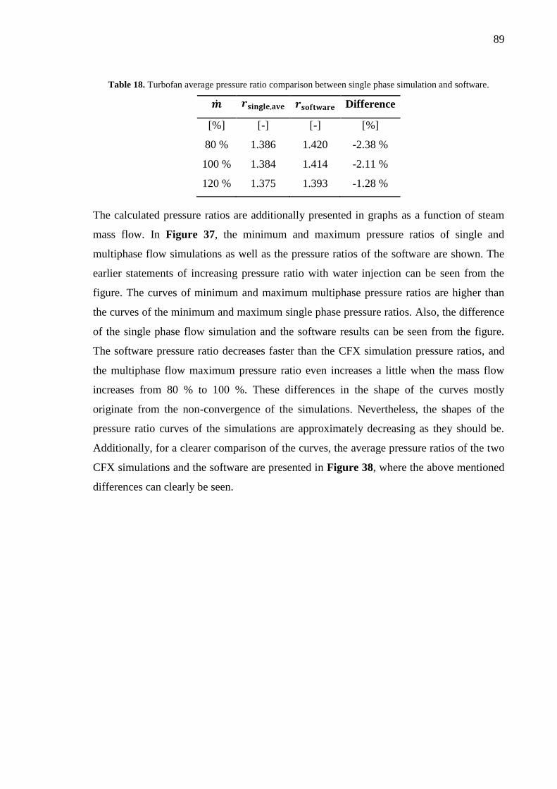
89

Table 18. Turbofan average pressure ratio comparison between single phase simulation and software.

�̇� 𝒓𝐬𝐢𝐧𝐠𝐥𝐞,𝐚𝐯𝐞 𝒓𝐬𝐨𝐟𝐭𝐰𝐚𝐫𝐞 Difference

[%] [-] [-] [%]

80 % 1.386 1.420 -2.38 %

100 % 1.384 1.414 -2.11 %

120 % 1.375 1.393 -1.28 %

The calculated pressure ratios are additionally presented in graphs as a function of steam

mass flow. In Figure 37, the minimum and maximum pressure ratios of single and

multiphase flow simulations as well as the pressure ratios of the software are shown. The

earlier statements of increasing pressure ratio with water injection can be seen from the

figure. The curves of minimum and maximum multiphase pressure ratios are higher than

the curves of the minimum and maximum single phase pressure ratios. Also, the difference

of the single phase flow simulation and the software results can be seen from the figure.

The software pressure ratio decreases faster than the CFX simulation pressure ratios, and

the multiphase flow maximum pressure ratio even increases a little when the mass flow

increases from 80 % to 100 %. These differences in the shape of the curves mostly

originate from the non-convergence of the simulations. Nevertheless, the shapes of the

pressure ratio curves of the simulations are approximately decreasing as they should be.

Additionally, for a clearer comparison of the curves, the average pressure ratios of the two

CFX simulations and the software are presented in Figure 38, where the above mentioned

differences can clearly be seen.

90

Figure 37. Minimum and maximum pressure ratio of single and multiphase flow simulations as well as

software pressure ratio.

Figure 38. Average pressure ratio of single and multiphase simulations as well as software pressure ratio.

91

9.3.2 Impeller power

The impeller power, which is the required mechanical power supplied to the impeller, is

determined with torque and angular velocity. Because of the non-convergence of the

simulations, the minimum and maximum values of torque have to be used in the

calculation of the impeller power. The torque values are obtained from CFX solver.

𝑃r = 𝛵𝛺 (9-9)

where 𝑃r is impeller power [W]

𝛵 is torque [Nm]

𝛺 is angular velocity [1/s]

𝛺 = 2𝜋𝑛 (9-10)

where 𝑛 is rotational speed [1/s]

The impeller power and angular velocity are determined with equations (9-9) and (9-10),

respectively. Minimum, maximum and average impeller powers are determined using the

corresponding values of torque. The rotational speed stays constant in all the calculations.

The comparisons of the minimum, maximum and average impeller power of the single and

multiphase flow simulations are presented in Table 19, Table 20 and Table 21,

respectively. It can be seen that with mass flows of 100 % and 120 %, the consumed power

increases with water injection and with 80 % mass flow, the power stays approximately the

same compared to the consumed power of the single phase flow simulations. As stated

before, the overall density of the fluid increases with droplet injection. According to the

affinity laws of fans, the density increase increases also the power consumption if all the

other parameters are held constant. The unchanged power of 80 % mass flow can stem

from the calculation of the optimal mass flow of water or from the fact that the simulations

are not fully converged.

In Table 20 with 120 % mass flow, there seems to be an 11.24 % increase in the power

consumption with multiphase flow. This result is not consistent with the other power

increase values. The jump is due to the non-convergence of the simulations. With higher

mass flows, the variance of the torque is significantly larger than the variance with smaller

mass flows. Therefore, there is a greater difference between the minimum and maximum

92

torque values that are taken from CFX solver and, thus, the rise in impeller power seems

abnormal.

Table 19. Turbofan minimum impeller power comparison between single and multiphase flow simulations.

�̇� 𝑷𝐫,𝐬𝐢𝐧𝐠𝐥𝐞,𝐦𝐢𝐧 𝑷𝐫,𝐦𝐮𝐥𝐭𝐢,𝐦𝐢𝐧 Difference

[%] [MW] [MW] [%]

80 % 1.753 1.740 -0.70 %

100 % 2.062 2.108 2.26 %

120 % 2.439 2.512 3.00 %

Table 20. Turbofan maximum impeller power comparison between single and multiphase flow simulations.

�̇� 𝑷𝐫,𝐬𝐢𝐧𝐠𝐥𝐞,𝐦𝐚𝐱 𝑷𝐫,𝐦𝐮𝐥𝐭𝐢,𝐦𝐚𝐱 Difference

[%] [MW] [MW] [%]

80 % 1.840 1.847 0.41 %

100 % 2.170 2.259 4.12 %

120 % 2.549 2.836 11.24 %

Table 21. Turbofan average impeller power comparison between single and multiphase flow simulations.

�̇� 𝑷𝐫,𝐬𝐢𝐧𝐠𝐥𝐞,𝐚𝐯𝐞 𝑷𝐫,𝐦𝐮𝐥𝐭𝐢,𝐚𝐯𝐞 Difference

[%] [MW] [MW] [%]

80 % 1.793 1.790 -0.20 %

100 % 2.120 2.187 3.17 %

120 % 2.505 2.618 4.52 %

In Table 22, Table 23 and Table 24, the minimum, maximum and average power of the

turbofan in the single phase flow simulation is compared to the power obtained in the

HTF’s software. The powers obtained from the simulations are a bit less than the power

from the software. The differences are smaller with the maximum impeller power values

than with the minimum values. The most influential aspect for the disparities is the non-

convergence of the simulations. If convergence was obtained, the differences could be

smaller. Nevertheless, the variance between the results of the two programs is in

acceptable limits.

93

Table 22. Turbofan minimum power comparison between single phase flow simulation and software.

�̇� 𝑷𝐫,𝐬𝐢𝐧𝐠𝐥𝐞,𝐦𝐢𝐧 𝑷𝐫,𝐬𝐨𝐟𝐭𝐰𝐚𝐫𝐞 Difference

[%] [MW] [MW] [%]

80 % 1.753 1.813 -3.33 %

100 % 2.062 2.196 -6.11 %

120 % 2.439 2.581 -5.49 %

Table 23. Turbofan maximum power comparison between single phase flow simulation and software.

�̇� 𝑷𝐫,𝐬𝐢𝐧𝐠𝐥𝐞,𝐦𝐚𝐱 𝑷𝐫,𝐬𝐨𝐟𝐭𝐰𝐚𝐫𝐞 Difference

[%] [MW] [MW] [%]

80 % 1.840 1.813 1.46 %

100 % 2.170 2.196 -1.19 %

120 % 2.549 2.581 -1.23 %

Table 24. Turbofan average power comparison between single phase flow simulation and software.

�̇� 𝑷𝐫,𝐬𝐢𝐧𝐠𝐥𝐞,𝐚𝐯𝐞 𝑷𝐫,𝐬𝐨𝐟𝐭𝐰𝐚𝐫𝐞 Difference

[%] [MW] [MW] [%]

80 % 1.793 1.813 -1.08 %

100 % 2.120 2.196 -3.47 %

120 % 2.505 2.581 -2.96 %

In Figure 39, the minimum and maximum impeller powers of the CFX simulations and

software are shown as functions of steam mass flow. The abnormal behavior of the

multiphase flow maximum impeller power with maximum mass flow can be clearly

noticed from the figure. The power curve should be approximately linear as, for example,

the software curve is, but the multiphase flow maximum power increases abnormally with

the maximum steam mass flow. As stated earlier, this behavior comes from the non-

convergence of the simulation and from the fact that with higher mass flows, the

convergence of multiphase flow simulations is worse than with lower mass flows. The

minimum power curve of the multiphase flow does not show similar abnormal behavior as

the maximum curve.

The average power curves are presented in Figure 40 where it can be seen that the

multiphase flow curve follows the software curve quite closely whereas the single phase

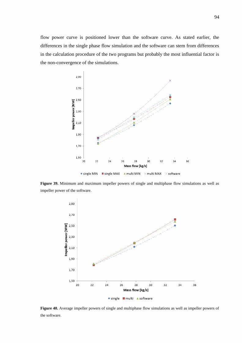
94

flow power curve is positioned lower than the software curve. As stated earlier, the

differences in the single phase flow simulation and the software can stem from differences

in the calculation procedure of the two programs but probably the most influential factor is

the non-convergence of the simulations.

Figure 39. Minimum and maximum impeller powers of single and multiphase flow simulations as well as

impeller power of the software.

Figure 40. Average impeller powers of single and multiphase flow simulations as well as impeller powers of

the software.

95

9.3.3 Fan air power

In addition to the mechanical power supplied to the impeller, the power or work which the

impeller does on the fluid is determined. This power is called fan air power and it is

calculated according to ISO 5801:2007 standard which provides standardized methods for

the determination of the performance of industrial fans (ISO 5801, 2007).

𝑍𝑘 =𝛾−1

𝛾∙

𝜌f,tot1𝑃r

�̇�(𝑝03−𝑝00) (9-11)

where 𝑍𝑘 is multiplier [-]

�̇� is boundary mass flow [kg/s]

𝜌f,tot1 is total density of steam at inlet [kg/m3]

𝛾 is heat capacity ratio =𝑐𝑝

𝑐𝑣 [-]

𝑐𝑝 is specific heat capacity at constant pressure [J/kgK]

𝑐𝑣 is specific heat capacity at constant volume [J/kgK]

𝑘 =𝑍𝑘 log10(𝑟)

log10[1+𝑍𝑘(𝑟−1)] (9-12)

where 𝑘 is compressibility coefficient [-]

𝑃u = 𝑞𝑣,f1𝑘(𝑝03 − 𝑝00) (9-13)

Where 𝑃u is fan air power [W]

𝑞𝑣,f1 is steam volume flow at inlet [m3/s]

The compressibility coefficient is determined with equation (9-12) and the multiplier in

that equation is calculated with equation (9-11). The fan air power is then determined with

equation (9-13). The comparisons of the minimum, maximum and average results between

single and multiphase flow simulations are presented in Table 25, Table 26 and Table 27,

respectively. As can be seen, the fan air power increases with the injection of the droplets.

This power increase is also due to the rise in the overall density of the fluid as explained

before. The increase of the fan air power is greater than the increase in the impeller power.

Thus, with a small increase in the input power, the pressure ratio and the power done to the

fluid can be increased.

96

Table 25. Turbofan minimum fan air power comparison between single and multiphase flow simulations.

�̇� 𝑷𝐮.𝐬𝐢𝐧𝐠𝐥𝐞,𝐦𝐢𝐧 𝑷𝐮,𝐦𝐮𝐥𝐭𝐢,𝐦𝐢𝐧 Difference

[%] [MW] [MW] [%]

80 % 1.307 1.360 4.09 %

100 % 1.639 1.710 4.31 %

120 % 1.944 2.030 4.44 %

Table 26. Turbofan maximum fan air power comparison between single and multiphase flow simulations.

�̇� 𝑷𝐮.𝐬𝐢𝐧𝐠𝐥𝐞,𝐦𝐚𝐱 𝑷𝐮,𝐦𝐮𝐥𝐭𝐢,𝐦𝐚𝐱 Difference

[%] [MW] [MW] [%]

80 % 1.318 1.368 3.82 %

100 % 1.645 1.729 5.11 %

120 % 1.952 2.082 6.68 %

Table 27. Turbofan average fan air power comparison between single and multiphase flow simulations.

�̇� 𝑷𝐮.𝐬𝐢𝐧𝐠𝐥𝐞,𝐚𝐯𝐞 𝑷𝐮,𝐦𝐮𝐥𝐭𝐢,𝐚𝐯𝐞 Difference

[%] [MW] [MW] [%]

80 % 1.312 1.364 3.95 %

100 % 1.642 1.719 4.68 %

120 % 1.947 2.057 5.65 %

The minimum, maximum and average fan air power of single phase flow simulations are

compared to the fan air power of the software in Table 28, Table 29 and Table 30. As can

be seen, with 80 % mass flow, CFX simulates the fan air power to be more than 5 % less

than the power in the software. This difference can stem from the differences in the

calculations of specific heat capacities and pressures in the two programs. Moreover, as

stated before, the non-convergence of the simulations can cause some uncertainties to the

results.

97

Table 28. Turbofan minimum fan air power comparison between single phase flow simulation and software.

�̇� 𝑷𝐮.𝐬𝐢𝐧𝐠𝐥𝐞,𝐦𝐢𝐧 𝑷𝐮,𝐬𝐨𝐟𝐭𝐰𝐚𝐫𝐞 Difference

[%] [MW] [MW] [%]

80 % 1.307 1.396 -6.39 %

100 % 1.639 1.719 -4.68 %

120 % 1.944 1.972 -1.43 %

Table 29. Turbofan maximum fan air power comparison between single phase flow simulation and software.

�̇� 𝑷𝐮.𝐬𝐢𝐧𝐠𝐥𝐞,𝐦𝐚𝐱 𝑷𝐮,𝐬𝐨𝐟𝐭𝐰𝐚𝐫𝐞 Difference

[%] [MW] [MW] [%]

80 % 1.318 1.396 -5.61 %

100 % 1.645 1.719 -4.32 %

120 % 1.952 1.972 -1.01 %

Table 30. Turbofan average fan air power comparison between single phase flow simulation and software.

�̇� 𝑷𝐮.𝐬𝐢𝐧𝐠𝐥𝐞,𝐚𝐯𝐞 𝑷𝐮,𝐬𝐨𝐟𝐭𝐰𝐚𝐫𝐞 Difference

[%] [MW] [MW] [%]

80 % 1.312 1.396 -6.02 %

100 % 1.642 1.719 -4.50 %

120 % 1.947 1.972 -1.25 %

9.3.4 Efficiency

The efficiency of the turbofan is determined using to the same ISO standard as with the fan

air power. In the standard, it is assumed that fan efficiency is equal to the impeller

efficiency. The fan efficiency is the ratio of power or work that the fan’s impeller does on

the fluid and the required mechanical supply power to the impeller. Because of the non-

convergence of the CFX simulations, the value of the efficiency depends on which power

values are used in the calculation.

𝜂r,min =𝑃u,min

𝑃r,max (9-14)

where 𝜂r,min is minimum fan efficiency [-]

𝑃u,min is minimum fan air power [W]

98

𝑃r,max is maximum impeller power [W]

𝜂r,max =𝑃u,max

𝑃r,min (9-15)

where 𝜂r,max is maximum fan efficiency [-]

𝑃u,max is maximum fan air power [W]

𝑃r,min is minimum impeller power [W]

𝜂r,avg =𝑃u,ave

𝑃r,ave (9-16)

where 𝜂r,ave is average fan efficiency [-]

𝑃u,ave is average fan air power [W]

𝑃r,ave is average impeller power [W]

The minimum, maximum and average fan efficiencies are calculated with equation (9-14),

(9-15) and (9-16), respectively. The comparisons of the corresponding values of single and

multiphase flow are presented in Table 31, Table 32 and Table 33. Apart from the

minimum efficiency with 120 % mass flow, the efficiency increases with the injection of

the droplets due to the greater rise in fan air power compared to the increase in the supplied

power, as presented earlier. In addition, because the cases simulated include fogging and

very small droplets the aerodynamic efficiency deprivation is limited. Therefore, the

efficiency of the fan is allowed to increase due to the increase in total density. The

decrease in the minimum efficiency with 120 % mass flow in Table 31 stems from the

abnormal increase in the maximum impeller power with maximum steam mass flow,

which in turn arises from the non-convergence of the simulation, as stated earlier.

Table 31. Turbofan minimum efficiency comparison between single and multiphase flow simulations.

�̇� 𝜼𝐫,𝐬𝐢𝐧𝐠𝐥𝐞,𝐦𝐢𝐧 𝜼𝐫,𝐦𝐮𝐥𝐭𝐢,𝐦𝐢𝐧 Difference

[%] [-] [-] [%]

80 % 0.710 0.736 2.61 %

100 % 0.755 0.757 0.14 %

120 % 0.762 0.716 -4.66 %

99

Table 32. Turbofan maximum efficiency comparison between single and multiphase flow simulations.

�̇� 𝜼𝐫,𝐬𝐢𝐧𝐠𝐥𝐞,𝐦𝐚𝐱 𝜼𝐫,𝐦𝐮𝐥𝐭𝐢,𝐦𝐚𝐱 Difference

[%] [-] [-] [%]

80 % 0.752 0.786 3.42 %

100 % 0.798 0.820 2.22 %

120 % 0.800 0.829 2.86 %

Table 33. Turbofan average efficiency comparison between single and multiphase flow simulations.

�̇� 𝜼𝐫,𝐬𝐢𝐧𝐠𝐥𝐞,𝐚𝐯𝐞 𝜼𝐫,𝐦𝐮𝐥𝐭𝐢,𝐚𝐯𝐞 Difference

[%] [-] [-] [%]

80 % 0.732 0.762 3.04 %

100 % 0.775 0.786 1.13 %

120 % 0.777 0.786 0.84 %

The single phase flow efficiencies and the software efficiency are compared in Table 34,

Table 35 and Table 36. As can be seen, the CFX simulation and the software efficiencies

differ a bit from each other. As with the comparisons before, also with this comparison, the

differences can arise from differences in the calculation procedure of the two programs as

well as from the non-convergence of the CFX simulation. Nevertheless, apart from the

minimum efficiency with 80 % mass flow, the differences are below 5 % so they are not

significant.

Table 34. Turbofan minimum efficiency comparison between single phase flow simulation and software.

�̇� 𝜼𝐫,𝐬𝐢𝐧𝐠𝐥𝐞,𝐦𝐢𝐧 𝜼𝐫,𝐬𝐨𝐟𝐭𝐰𝐚𝐫𝐞 Difference

[%] [-] [-] [%]

80 % 0.710 0.770 -5.96 %

100 % 0.755 0.783 -2.77 %

120 % 0.762 0.764 -0.15 %

100

Table 35. Turbofan maximum efficiency comparison between single phase flow simulation and software.

�̇� 𝜼𝐫,𝐬𝐢𝐧𝐠𝐥𝐞,𝐦𝐚𝐱 𝜼𝐫,𝐬𝐨𝐟𝐭𝐰𝐚𝐫𝐞 Difference

[%] [-] [-] [%]

80 % 0.752 0.770 -1.82 %

100 % 0.798 0.783 1.49 %

120 % 0.800 0.764 3.62 %

Table 36. Turbofan average efficiency comparison between single phase flow simulation and software.

�̇� 𝜼𝐫,𝐬𝐢𝐧𝐠𝐥𝐞,𝐚𝐯𝐞 𝜼𝐫,𝐬𝐨𝐟𝐭𝐰𝐚𝐫𝐞 Difference

[%] [-] [-] [%]

80 % 0.732 0.770 -3.84 %

100 % 0.775 0.783 -0.84 %

120 % 0.777 0.764 1.35 %

The minimum and maximum efficiencies of the CFX simulations and the software are

shown in Figure 41 as a function of steam mass flow. The differences between the two

CFX simulations as well as between the single phase flow simulation and the software can

be clearly seen. Moreover, the abnormal decrease of the minimum efficiency of multiphase

flow with 120 % mass flow can be noticed from the curves. As explained earlier, this

behavior comes from the abnormal increase of the impeller power. When the power needed

for the compression increases more than the work done to the fluid, the fan efficiency

decreases. Additionally, it can be seen that the shape of the CFX simulation curves are not

consistent with the shape of the software curve. The fan efficiency of the CFX simulations

increases longer with increasing mass flow compared to the efficiency of the software. As

with earlier parameters, the most influential factor in the comparison is the non-

convergence of the CFX simulations. The final results depend on when one stops CFX

solver, thus, the results vary a little.

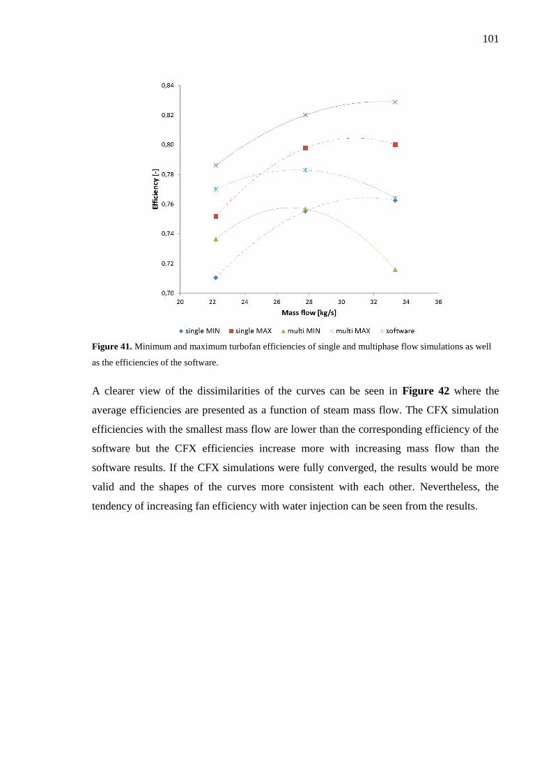
101

Figure 41. Minimum and maximum turbofan efficiencies of single and multiphase flow simulations as well

as the efficiencies of the software.

A clearer view of the dissimilarities of the curves can be seen in Figure 42 where the

average efficiencies are presented as a function of steam mass flow. The CFX simulation

efficiencies with the smallest mass flow are lower than the corresponding efficiency of the

software but the CFX efficiencies increase more with increasing mass flow than the

software results. If the CFX simulations were fully converged, the results would be more

valid and the shapes of the curves more consistent with each other. Nevertheless, the

tendency of increasing fan efficiency with water injection can be seen from the results.

102

Figure 42. Average turbofan efficiencies of single and multiphase flow simulations as well as efficiencies of

the software.

103

10 CONCLUSIONS

In this chapter, the results of the thesis are concluded and discussed as well as compared to

findings in literature. Recommendations for future work are also stated.

10.1 Droplet evaporation in simple pipe

The simulation of the droplet evaporation in the simple pipe show that the diameter change

and evaporation rate of larger droplets is significantly lower than the ones of smaller

droplets due to practically non-existent secondary breakup. Because there is no secondary

breakup, the total surface area of the droplets dominates the heat transfer between the

steam and the particles. Smaller droplets have larger total surface area compared to larger

droplets, thus, heat transfer between smaller droplets and steam is higher than with large

droplets and steam. Therefore, smaller droplets evaporate faster and more than larger

particles. Because of the larger total surface area and higher evaporation rate of smaller

droplets, the evaporated water mass is also greater with small diameter droplets than with

large ones.

The fluid temperature decrease in the simple pipe simulation is consistent with the

diameter change and evaporation rate of different droplet sizes. The smaller the initial

droplet diameter and the slower the flow velocity, the more and faster the temperature of

the fluid decreases. The desired saturation temperature is reached with 10 μm droplets with

all superheat temperatures and flow velocities as well as with 25 and 50 μm droplets when

the superheat temperature is high and velocity low.

From the results of the simple pipe simulation, it can be concluded that the positioning of

the de-superheating spray to the outlet duct of the turbofan would not be reasonable,

because it would require too much time and distance for the fluid temperature to decrease

to the wanted saturation temperature. If the de-superheating spray was placed to the outlet

duct, a very fine mist and small droplets should be used in order to obtain the wanted fluid

temperature decrease in a reasonable time and distance. However, this positioning choice

would need an approximation of costs since the sprays that generate very fine mist might

be more expensive than sprays that produce larger droplets.

104

10.2 Droplet evaporation in turbofan

The results of the modeling of droplet evaporation inside a turbofan show that the diameter

of the droplets does not change significantly in the inlet duct of the fan. The diameter does

not decrease in the inlet duct because the steam is still at saturated state, so, it cannot take

in more water vapor. In addition, in inlet duct, the Reynolds number and Weber number of

the droplets are small so no evaporation or secondary breakup is occurring. The droplet

diameter starts to decrease in the impeller of the turbofan due to the work that is done on

the fluid and the droplets. The impeller work increases the enthalpy, pressure and velocity

of the steam and the droplets, resulting in increase in the steam temperature as well as

evaporation and secondary breakup of the droplets.

The diameter change of larger droplets is greater than the diameter change of smaller

droplets at the outlet of the turbofan. Greater diameter change of larger particles is due to

significantly higher secondary breakup experienced by larger droplets. The higher

secondary breakup of larger droplets is due to the higher Weber number of the droplets

which, in turn, is higher because of the bigger diameter of the particles as well as because

the slip velocity between larger droplets and the steam is greater than the slip velocity

between smaller droplets and the steam. Large droplets have more mass than small

droplets, thus, they follow the flow of the steam worse than smaller droplets. Therefore, the

slip velocity between large droplets and steam is higher than the slip velocity between

smaller droplets and steam.

The evaporated mass of water in the turbofan is approximately the same regardless of the

initial diameter of the droplets when the injected water mass flow is constant. In other

words, the amount of water that evaporates inside the fan is independent of the diameter of

the droplets when the same amount of water is injected into the fan. The evaporation rate

can differ as seen with the diameter change of different droplet sizes, but the total mass of

evaporated water is approximately the same regardless of the initial size of the droplets.

There is, however, the uncertainty of the Particle Number Rate at the fan outlet with large

initial size droplets. Because the PNR changes due to the secondary breakup of larger

droplets, an average value of PNR is taken at the fan outlet and used in the calculation of

the evaporated mass of water. Average values pose some uncertainty on the evaporated

mass flow results but the approximate results are valid.

105

The results of the turbofan modeling are consistent with the results found in literature

about wet compression and, for example, with the results of Halbe (2016). Halbe’s results

of the simulation of refrigerant R134a state also that the diameter of the droplets starts to

decrease in the impeller, and that the diameter change as well as evaporation rate of larger

diameter droplets is higher than the ones of smaller droplets mostly due to secondary

breakup. In addition, Halbe’s findings on the evaporated liquid mass with different initial

droplet diameters are consistent with the results of this thesis, that is, that the evaporated

liquid mass is independent of the initial size of the droplets.

It should be kept in mind that, for the turbofan simulations, the chosen droplet-wall

interaction model poses an uncertainty. Because the droplets “bounce off” of the wall, they

move freely inside the fan but in reality, the droplets would impinge on the wall or splash

from it. Because of the chosen wall interaction model, with larger droplet diameters, the

LPT model loses its validity in one corner of the turbofan. However, this volume is small

compared to the total volume of the geometry, so the effects on the results should not be

significant. In addition, as mentioned previously, the turbofan simulations are not fully

converged, which could pose an uncertainty on the results. Nonetheless, the droplet

evaporation phenomenon and the diameter change of the droplets can be seen from the

results presented in this thesis.

10.3 Turbofan performance

The performance of the turbofan is better with droplet injection than without the injection.

The pressure ratio, power and efficiency of the fan increase with fogging mostly due to the

increase in the total density of the fluid. The efficiency of the fan increases with water

injection due to greater increase in the work done on the fluid compared to the increase in

the mechanical supply power. Furthermore, because the injection procedure is fogging and

not overspray, the aerodynamic efficiency deterioration is limited, which in turn allows the

overall efficiency of the fan to increase. The results are consistent with the information

found in literature regarding wet compression and fogging in turbomachines.

The results of the single phase flow simulations differ slightly from the results of HTF’s

aerodynamic selection software. These differences probably originate from differences in

the calculation equations used in the two programs as well as from the non-convergence of

106

the CFX simulations. Nevertheless, the dissimilarities are in an acceptable range at least

with higher mass flows.

In all the turbofan simulation results, there exists some uncertainty since the simulations

are not fully converged. Nonetheless, the phenomena of multiphase flow and its effects on

turbofan performance can be seen from the presented results and graphs.

10.4 Recommendations for future work

In the future, the work should be continued in order to obtain fully converged simulations

and more trustworthy results. In addition, the CFD modeling should be improved by

changing the droplet-wall interaction model to correspond reality better. With better wall

interaction model, the wet film created by large droplets that hit the walls of the fan could

be simulated and the local LPT model validity problems could be solved. Modeling with

more defined wall interaction model requires a transient simulation, which in turn requires

more time and computational power than steady state simulation and these aspects should

be considered when refining the wall interaction model. Furthermore, real gas

implementation to the interphase transfer simulation should be investigated. Currently, the

only option is to use ideal gas and constant property liquid when simulating the interphase

transfer phenomenon. If real gas could be included to this simulation, the results would be

more consistent with reality.

Simulations with different water mass percentages of the steam should be done so the

effects of the amount of water injected on compressor performance and droplet evaporation

could be obtained. In this thesis, the percentage of water is kept constant at 3 % of the

steam mass flow, so in the future, this percentage could be varied between 1 % and 5 %.

The optimal amount of injected water, which improves the turbofan performance the most,

could then be determined. Furthermore, simulations with spray nozzles should be done in

order to get a view of the effects of different types of nozzles and injection directions on

the droplet evaporation and performance of the turbofan. The nozzles could be positioned

in a way that the droplets are injected to the fluid in a parallel or a counter flow direction or

in different angles.

In future studies, the erosion of the blades of the turbomachine due to the injection of water

droplets should be investigated. There are some erosion models in CFX that could be used

in this kind of research. Erosion simulation could help to identify the most critical places

107

where the erosion is most likely to occur in turbomachines. In addition, some simplified

equations for the evaporation time and distance of different droplet sizes could be

generated to help determine fast and easily the evaporation time and distance of droplets as

well as the cooling time and distance of the fluid temperature. In addition, an economic

and technical analysis of sprays that produce very fine fog should be performed in order to

determine the financial sensibility of positioning the de-superheating spray in the outlet

duct of the turbofan. Also, experimental investigations and tests should be performed and

compared to the CFD simulations in order to validate the models and simulation results

more.

108

11 SUMMARY

This thesis is done for Howden Turbo Fans Oy with the objective of determining the

effects of de-superheating spray on a MVR fan using CFD. The motivation behind this

work is to improve the understanding of the phenomena of droplet evaporation inside a

turbofan and in MVR process. The CFD simulation is done with ANSYS CFX and the

simulations include modeling of multiphase flow inside a turbofan as well as in a straight

pipe. With the simulation results, the evaporation rate of droplets inside a turbofan and in a

straight pipe is obtained and the effects of droplet injection on the fan performance are

determined. The assumptions of neglecting droplet-droplet interaction, temperature

variation within droplets and radiation are made due to the limitations of the chosen model.

Mechanical vapor recompression is an energy efficient process for falling film evaporators

where evaporated vapor from the evaporator is compressed with a centrifugal

turbomachine and recirculated back to heat the liquid falling down in the evaporator. MVR

process is, usually, based on wet compression where liquid droplets are injected into the

turbomachine to improve its performance, for example, increase its pressure ratio.

Theoretically, the outlet temperature of the fluid is reduced with the liquid injection, thus,

reducing the amount of work needed to perform the same pressure rise as without the

liquid injection. There are many arguments for the use of wet compression in

turbomachines but some of those arguments are valid only for fogging and not for

overspray. Nevertheless, wet compression has its use in the industry where turbomachines

are used to handle humid flows or flows that contain impurities.

The modeling of multiphase flow is done using Lagrangian Particle Tracking model where

the dispersed or particle phase is modeled in Lagrangian way and the continuous phase is

modeled in Eulerian way. The benefits of LPT model include accurate modeling of mass

and heat transfer between the phases as well as detailed simulation of the particles in the

dispersed phase. The disadvantages of the model include requirement of a dilute flow and

constant particle properties as well as not being able to model turbulence for the particles.

The model simulates the continuous phase using Reynolds Averaged Navier Stokes

equations and takes the dispersed phase into account by adding source terms to the

continuous phase equations.

109

Droplet evaporation in a straight pipe is simulated with different steam temperatures and

flow velocities as well as with different initial droplet sizes. The diameter of the droplets

decreases faster with smaller droplets than with larger ones due to the absence of

secondary breakup. With higher superheat temperature and lower flow velocity, the

diameter decrease is greater than with lower superheat temperature and higher flow

velocity. When the superheat temperature is high, the temperature difference between the

droplets and the steam is larger than with low superheat temperature, thus, the heat transfer

between the phases is higher. With lower flow velocities the droplets spend more time in

the pipe and have more time to evaporate than with a faster flow. Additionally, the fluid

temperature decrease is analyzed in the straight pipe. The fluid cools down to the desired

saturation temperature faster with smaller droplets than with larger ones due to the faster

evaporation rate of the small droplets. Therefore, if the de-superheating spray was

positioned in the outlet duct of the turbofan, a very fine fog of water should be used. The

straight pipe simulation results are trustworthy since they are fully converged.

In the simulations of multiphase flow inside a turbofan, droplets with different initial

diameters are injected into the fan and their diameter change and evaporation rate as well

as effects on the fan performance are obtained. The diameter of larger droplets decreases

faster than the diameter of smaller droplets due to higher secondary breakup. The amount

of water that evaporates inside the turbofan is approximately constant regardless of the

initial droplet diameter. The performance of the turbofan is improved with water injection.

The pressure ratio, power supplied to the impeller, work done on the fluid and fan

efficiency increase with multiphase flow. The performance improvement is mostly due to

the increased total density of the fluid. There exists some uncertainty in the turbofan

simulation results since the simulations are not fully converged. Nonetheless, the

phenomena of the droplet evaporation as well as the effects of water injection on the fan

performance can be seen from the results.

Recommendations for future work include improving the convergence of the simulations,

refining the CFD model by selecting more appropriate droplet-wall interaction model and

investigating how to include real gas material to the interphase transfer simulation.

Furthermore, simulations with spray nozzles and erosion analysis as well as an economic

estimation of very fine fog sprays should be done in the future. Additionally, experimental

data should be obtained with experiments and tests in order to compare the simulation

results to them.

110

REFERENCES

Abdelwahab Ahmed. 2006. An Investigation of the Use of Wet Compression in Industrial

Centrifugal Compressors. ASME. Turbo Expo: Power for Land, Sea, and Air, Vol 4: Cycle

Innovations; Electric Power; Industrial and Cogeneration; Manufacturing Materials and

Metallurgy (2006). pp. 741-750. doi:10.1115/GT2006-90695.

Abramzon, B., Sirignano, W. A. 1989. Droplet Vaporization Model for Spray Combustion

Calculations. International Journal of Heat and Mass Transfer (1989), Vol.32(9). pp. 1605-

1618.

ANSYSa. 2016. Ansys CFX Modeling Guide. Release 18.0.

ANSYSb, 2016. Ansys CFX Theory Guide. Release 18.0.

Ashgriz, N. 2011. Handbook of Atomization and Sprays: Theory and Applications. Boston,

MA: Springer US. ISBN 978-7-4419-7263-7

Aungier, R. H. 1995. A Fast, Accurate Real Gas Equation of State for Fluid Dynamic

Analysis Applications. Journal of Fluids Engineering (1995), Vol. 117(2). pp. 277-281.

Bahar, R., Hawlader, M. N. A., Woei, L. S. 2004. Performance Evaluation of a

Mechanical Vapor Compression Desalination System. Desalination (2004), Vol. 166. pp.

123-127.

Bai, B., Zhang, H., Liu, L., Sun, H. 2009. Experimental Study on Turbulent Mixing of

Spray Droplets in Crossflow. Experimental Thermal and Fluid Science (2009), Vol. 33(6).

pp. 1012-1020.

Bai, B., Zhang, H., Liu, L., Sun, H. 2011. Numerical Study on Turbulent Mixing Spray

Droplets in Crossflow. Journal of Propulsion and Power (2011), Vol. 27(1). pp. 132-143.

Colfax. 2018. Colfax reports fourth quarter 2017 results. [Online document]. [Referred

26.4.2018]. Available at: http://ir.colfaxcorp.com/news-releases/news-release-

details/colfax-reports-fourth-quarter-2017-results

Crowe, C. T. 2006. Multiphase flow handbook. Boca Raton, FL: Taylor & Francis. ISBN

0-8493-1280-9.

111

DDBST. Dortmund Data Bank. [web page]. [Referred 7.5.2018]. Available at:

http://ddbonline.ddbst.de/AntoineCalculation/AntoineCalculationCGI.exe?component=Wa

ter

Dick, E. 2015. Fundamentals of Turbomachines. Dordrecht: Springer Netherlands. ISBN

978-94-017-9627-9 (e-book)

Dixon, S. L., Hall, C. A. 2014. Fluid mechanics and thermodynamics of turbomachinery.

Seventh edition. Oxford: Butterworth-Heinemann. ISBN 978-0-12-415954-9.

Fabbrizzi M., Cerretelli C., Del Medico F., D’Orazio M. 2009. An Experimental

Investigation of a Single Stage Wet Gas Centrifugal Compressor. ASME. Turbo Expo:

Power for Land, Sea, and Air, Vol 5: Microturbines and Small Turbomachinery; Oil and

Gas Applications (2009), pp. 443-453. doi:10.1115/GT2009-59548.

Fuller, E. N., Ensley, K., Giddings, J. C. 1969. Diffusion of Halogenated Hydrocarbons in

Helium. The Effect of Structure On Collision Cross Sections. The Journal of Physical

Chemistry (1969), Vol. 73(11). pp. 3679-3685.

GEA. 2014. Evaporation Technology using Mechanical Vapour Recompression. [online

document]. [Referred 27.11.2017]. Available at: http://www.dwa.nl/wp-

content/uploads/2014/09/Gea-Wiegand-MVR.pdf

Halbe, C. V. 2016. Effects of Two-Phase Flow in a Multistage Centrifugal Compressor.

Doctor of Philosophy. Faculty of the Virginia Polytechnic Institute and State University,

Mechanical Engineering. Blacksburg, Virginia. 140 pages.

Han, D., He, W. F., Yue, C., Pu, W. H. 2017. Study on desalination of zero-emission

system based on mechanical vapor compression. Applied Energy (2017), Vol. 185. pp.

1490-1496.

Howden. 2014. ExVel Turbo Fans. [Online document]. [Referred 19.4.2018]. Available at:

https://www.howden.com/Brochures/Exvel%20Turbo%20Fans.pdf

Incropera, F. P., DeWitt, D. P., Bergman, T. L., Lavine, A. S. 2003. Principles of heat and

Mass Transfer. 7th

edition. Delhi: Wiley India. ISBN 978-81-265-4273-4.

112

Ishii, M., Zuber, N. 1979. Drag Coefficient and Relative Velocity in Bubbly, Droplet or

Particulate Flows. AIChE Journal (1979), Vol.25(5). pp. 843-855.

ISO 5801. 2007. Industrial fans – Performance testing using standardized airways.

ISO/TC 117 Fans. 2nd

edition. Switzerland: International Organization for Standardization.

228 pages. Note: Revised by ISO 5801:2017.

Japikse, D. 1996. Centrifugal compressor design and performance. Wilder (VT): Concepts

ETI. ISBN 0-933283-03-2.

Kang, J.-S., Chang, B.-J., Yang, S.-S. 2006. Thermodynamic and aerodynamic meanline

analysis of wet compression in a centrifugal compressor. Journal of Mechanical Science

and Technology (2006), Vol. 20(9). pp. 1475-1482.

Karameldin, A., Lotfy, A., Mekhemar, S. 2003. The Red Sea area wind-driven mechanical

vapor compression desalination system. Desalination (2003), Vol. 153(1), pp. 47-53.

Mohan, A., Chidambaram, P. K., Suryan, A., Kim, H. D. 2016. Thermo-fluid dynamic

analysis of wet compression process. Journal of Mechanical Science and Technology

(2016), Vol. 30(12). 5473-5483. (Online) ISSN 1976-3824.

Montazeri, H., Blocken, B., Hensen, J. L. M. 2015. Evaporative cooling by water spray

systems: CFD simulation, experimental validation and sensitivity analysis. Building and

Environment (2015), Vol. 83. pp. 129-141.

Poling, B. E., Prausnitz, J. M. & O'Connell, J. P. 2001. The properties of gases and liquids.

5th ed. Boston: McGraw-Hill. ISBN 0-07-011682-2.

Srinivasan, C., Papavassiliou, D. V. 2011. Prediction of the turbulent Prandtl number in

wall flows with Lagrangian simulations. Industrial and Engineering Chemistry Research

(2011), Vol. 50(15). pp. 8881-8891.

Strotos, G., Malgarinos, I., Nikolopoulos, N., Gavaises, M. 2016. Predicting droplet

deformation and breakup for moderate Weber numbers. International Journal of

Multiphase Flow (2016), Vol. 85. pp. 96-109.

113

Sureshkumar, R., Kale, S. R., Dhar, P. L. 2008. Heat and mass transfer processes between

a water spray and ambient air – I. Experimental data. Applied Thermal Engineering

(2008), Vol. 28(5). pp. 349-360.

Tanner, F. X. 2004. Development and validation of a cascade atomization and drop

breakup model for high-velocity dense sprays. Atomization and sprays (2004), Vol. 14(3).

pp. 211-242.

Tuan, C.-I., Cheng, Y.-T., Yeh, Y.-L., Hsu, L.-F., Chen, T.-C. 2013. Performance

assessment of a combined vacuum evaporator – mechanical vapor re-compression

technology to recover boiler blow-down wastewater and heat. Sustainable Environment

Research (2013), Vol. 23(2). pp. 129-139.

VDI. 2010. VDI Heat Atlas. 2nd

edition. Berlin: Springer. ISBN 978-3-540-77876-9.

Wang, T., Khan, J. R. 2016. Discussion of some myths/features associated with gas turbine

inlet fogging and wet compression. Journal of Thermal Science and Engineering

Applications (2016), Vol. 8(2). p. 021001.

White, A. J., Meacock, A. J. 2011. Wet compression analysis including velocity slip effects.

Journal of Engineering for Gas Turbines and Power (2011), Vol. 133(8). Article number:

081701.

Zejli, D., Ouammi, A., Sacile, R., Dagdougui, H., Elmidaoui, A. 2011. An optimization

model for a mechanical vapor compression desalination plant driven by a wind/PV hybrid

system. Applied Energy (2011), Vol. 88(11). pp. 4042-4054.

APPENDIX 1, 1

APPENDIX 1: Torque and total pressure variation in the last 500 iteration steps

Figure 43. Single phase flow with 80 % mass flow torque and total pressure variation in 500 last iteration

steps.


steps.

APPENDIX 1, 2


steps.

Figure 46. Multiphase flow with 80 % mass flow torque and total pressure variation in 500 last iteration

steps.

APPENDIX 1, 3


steps.


steps.

Documents

ESTIMATING THE EFFECTS OF DE-SUPERHEATING SPRAY ON …