NBER WORKING PAPER SERIES

ESTIMATING THE EFFECT OF STUDENT AID ON COLLEGE ENROLLMENT:EVIDENCE FROM A GOVERNMENT GRANT POLICY REFORM

Helena Skyt NielsenTorben Sørensen

Christopher R. Taber

Working Paper 14535http://www.nber.org/papers/w14535

NATIONAL BUREAU OF ECONOMIC RESEARCH1050 Massachusetts Avenue

Cambridge, MA 02138December 2008

We appreciate comments from Ron Ehrenberg, Julien Grenet, Marieke Huysentruyt, Søren Leth-Petersen,from participants at ASSA 2007, ESPE 2007, SOLE 2008, TAPES 2008, and seminar participantsat the University of Amsterdam, University of Copenhagen, Aarhus University, University of Washington,and at AKF. The project has been supported by the Danish Research Agency (grant no. 2117-05-0076).The usual disclaimer applies. The views expressed herein are those of the author(s) and do not necessarilyreflect the views of the National Bureau of Economic Research.

NBER working papers are circulated for discussion and comment purposes. They have not been peer-reviewed or been subject to the review by the NBER Board of Directors that accompanies officialNBER publications.

© 2008 by Helena Skyt Nielsen, Torben Sørensen, and Christopher R. Taber. All rights reserved. Shortsections of text, not to exceed two paragraphs, may be quoted without explicit permission providedthat full credit, including © notice, is given to the source.

Estimating the Effect of Student Aid on College Enrollment: Evidence from a GovernmentGrant Policy ReformHelena Skyt Nielsen, Torben Sørensen, and Christopher R. TaberNBER Working Paper No. 14535December 2008JEL No. I22

ABSTRACT

In this paper, we investigate the responsiveness of the demand for college to changes in student aidarising from a Danish reform. We separately identify the effect of aid from that of other observed andunobserved variables such as parental income. We exploit the combination of a kinked aid schemeand a reform of the student aid scheme to identify the effect of direct costs on college enrollment. Toallow for heterogeneous responses due to borrowing constraints, we use detailed information on parents'assets. We find that enrollment is less responsive than found in other studies and that the presenceof borrowing constraints only deters college enrollment to a minor extent.

Helena Skyt NielsenUniversity of Aarhusand AKF, Institute for the Study of Labor (IZA)hnielsen@econ.au.dk

Torben SørensenDept. of Economics, University of AarhusBartholins Alle 4, Bld. 322DK-8000, Aarhus Ctosoerensen@econ.dk

Christopher R. Taber Department of Economics University of Wisconsin -Madison 1180 Observatory Dr Social Sciences Building #6448 Madison, WI 53706-1320 and NBER ctaber@ssc.wisc.edu

1 Introduction

An increase in educational subsidies is expected to increase college enrollment. Despite that

substantial educational subsidies are already in place, previous empirical work suggests the

elasticity is large. Empirical studies for the U.S. �nd that the magnitude of the e¤ect is such

that a $1,000 increase in the annual educational subsidy increases enrollment by roughly

3-5 percentage points (see e.g. Dynarski, 2003; Leslie and Brinkman, 1988; Manski and

Wise, 1983; McPherson and Shapiro, 1991). The purpose of this paper is to investigate the

responsiveness of the demand for college to changes in student aid by exploiting some useful

exogenous variation in Danish data.

The crucial issue in studies of the e¤ect of �nancial aid on enrollment is to separately

identify the e¤ect of aid from that of other observed and unobserved variables such as

parental background. First, student aid is often means tested against parental income and

other socioeconomic variables. Second, responsiveness of demand for college to changes in

student aid is likely to vary with parental background for many reasons. In particular, one

might expect college enrollment to be particularly responsive to educational subsidies among

families who are borrowing constrained (see e.g. Cameron and Taber, 2004). In this paper

we show how a combination of a kinked aid scheme and a reform of the student aid scheme

can be exploited to identify the e¤ect of direct costs on college enrollment accounting for

borrowing constraints. We show that, theoretically, the �rst characteristic is su¢ cient to

identify the e¤ect of interest.

The reform of the Danish student aid scheme was implemented for the college cohort

starting september 1988 and consisted of two major changes: it eliminated the means-testing

and �most importantly - it raised the level of grants by more than 25% for all students

above 19 years of age. The change in subsidy varied across parental background. After the

reform, educational subsidies universally covered almost all students throughout their college

education at a generous level.1

Children with poor parents (henceforth: poor kids) are often expected to be more re-

sponsive to educational subsidies than the children of rich parents (henceforth: rich kids).

This �nding may work through (at least) three di¤erent channels. (1) Poor kids are more

likely to be borrowing constrained, therefore, if increased subsidies reduce the extent of these

1We use the terms grant, stipend and student aid interchangeably.

1

constraints, poor kids may be more responsive to a policy change. (2) Poor kids may receive

lower schooling contingent transfers from their parents. If public transfers crowd out some

schooling contingent parental transfers, a policy change may have a smaller impact on rich

kids. (3) Poor kids receive less non-labor income transfers from their parents over their life

cycle than rich kids. That may be due to lower non-contingent transfers from their family

when they are young or due to less bequests. This implies that the marginal utility of income

is higher for poor kids than for rich kids who have higher non-labor income. As a result,

they are more sensitive to a reduction in costs. As is common in most of the literature, we

implicitly assume that children and their parents form a dynasty with common interests, and

hence we are not able to separately identify the e¤ect of (2) and (3). Our e¤orts are focused

on accounting appropriately for channel (1), namely, the e¤ect of borrowing constraints.

In a more direct approach we adopt the low liquid asset measure, which was suggested

by Zeldes (1989) and succesfully applied by Leth-Petersen (2006), to control for borrowing

constraints. They argue that the ratio of liquid assets to income is a powerful way to identify

the households who potentially face a binding credit constraint.

We use Danish register-based data for the cohorts graduating from high school in 1985 to

1990. In this way we have observations both before and after the reform. We rank individuals

according to the index of parental income which determines eligibility for student aid, and

match post-reform individuals with pre-reform individuals at the same place in the income

distribution.2 The fact that the relationship between this measure of parental income - and

hence the rank in the distribution of parental income - and the stipend is nonlinear, helps

us to identify the relationship of interest. We show formally that the relationship between

family income and college enrollment should jump at the kink point which allows us to

identify the e¤ect of the reform. Basically, we analyze whether the family income/college

enrollment relationship changed systematical di¤erently around the kink points.

We �nd that the subsidy did increase college enrollment, but to a smaller extent compared

to previous work on US data. The point estimates indicate that a $1,000 increase in the

yearly stipend increases college enrollment by 1.35 percentage points. This somewhat smaller

e¤ect might partly be caused by the fact that total subsidies were and still are larger in

2This avoids making restrictive untestable assumptions about income growth for the parents over the sixyear period. We are implicilty making the assumption that (counterfactual) eligibility for student aid forthe post-reform individuals had they graduated from high school before the reform, is determined by theirplace in the income distribution.

2

Denmark than it has ever been in the US. We �nd some evidence that borrowing constraints

deter enrollment. The reported results are conditional on an assumption that the supply is

completely �exible. If a supply constraint has been binding, a demand increase should show

up in �prices�which (in the Danish case) would be entry requirements in terms of GPA. We

argue that the demand response did not a¤ect prices signi�cantly.

To gain further insight and improve the interpretation of the reduced form results, we

set up and estimate a simple structural model. Simulating various policy counterfactuals,

the subsidy level is found to be important for college enrollment. Borrowing constraints do

not appear to be important in Denmark at this time, but this is in large part due to the

substantial subsidy already in place.

The remainder of this paper is organized as follows: Section 2 surveys the literature.

Section 3 describes the reform while section 4 documents the data. Section 5 presents the

empirical analysis and section 6 concludes the paper.

2 Existing Literature

The literature attempting to identify the e¤ect of costs on college attendance is long and

diverse. In an older review of the literature, Leslie and Brinkman (1988) conclude that the

estimated e¤ect on college attendance of a $1,000 dollar aid increase ranges from three to �ve

percentage points. The results from the earlier studies are, however, likely to be �awed by

poor identi�cation, as aid is correlated with numerous observable and unobservable variables.

Comparing enrollment rates across states, Kane (1995) �nds that a $1,000 dollar di¤er-

ence in costs of public 2-year college is associated with a 19-29% di¤erence in enrollment

rates (8-16 percentage points) among 18-19 year-olds. Conditioning on 2-year tuition, the

e¤ect of tuition in public 4-year college is positive, although insigni�cant, indicating that the

marginal price determining whether or not people attend college at all is public 2-year college

tuition and not 4-year college tuition. The major weakness of this cross-state comparison

is that identi�cation is based upon di¤erences between states which have been fairly stable

over time, making it di¢ cult to separate the e¤ect of tuition from other �xed inter-state dif-

ferences. Exploiting within-state di¤erences in public tuition increases since 1980, the same

study estimates a 3.5 percentage point drop in public undergraduate enrollment following a

$1,000 dollar increase in public 2-year tuition. Furthermore, the gap in enrollment between

3

high- and low-income youth grew the most in the states with the largest tuition increases,

hinting at the presence of borrowing constraints. Surprisingly, the study �nds no signi�cant

e¤ect of implementing the federal means-tested Pell Grant programme in the mid-seventies,

leading to the hypothesis of supply constraints muting the e¤ect of the supposedly increased

college demand on actual enrollment. This �nding is consistent with the in�uential study

of Hansen (1983). Later, Turner (1998) rationalized this missing e¤ect by large aid budget

institutions �undoing�the targeting of the federal grants.

Later, McPherson and Schapiro (1991) exploit more years of observations and �nd a

signi�cant e¤ect of changes of the Pell Grant. A $1,000 dollar increase in net costs (1978-

1979 dollars) is estimated to reduce the enrollment of low-income students by 6.8 percentage

points.

Exploiting annual micro-data from the CPS, Seftor and Turner (2002) examine the e¤ect

of changes in the Pell Grant programme on mature students, and �nd this group to be more

responsive to changes than traditional college-goers. More severe borrowing constraints for

the mature students might justify this.

The elimination of the Social Security Student Bene�t Program, which subsidized stu-

dents of deceased, disabled, or retired parents, provides Dynarski (2003) with a source of

exogenous variation in schooling costs. The e¤ect of a $1,000 dollar subsidy on the enroll-

ment probability is estimated to be 3.6 percentage points using a di¤erence-in-di¤erences

identi�cation strategy.

The previously mentioned results mainly apply to students from low-income families, in

that the youth subsidized by the Pell programme and to a large extent also those subsidized

by the Social Security Student Bene�t Program are from low-income families. Dynarski

(2000) studies the Georgia HOPE programme, which mainly a¤ected middle- and upper-

income students because any federal (means-tested) grants were deducted from the HOPE

stipends. This programme allowed free attendance at Georgia�s public colleges for state

residents with at least a B average in high school. Using out-of-state as well as in-state

control groups, Dynarski �nds that a $1,000 dollar subsidy increase raise enrollment rates

of middle- and upper-income students by 4-6 percentage points.

When focus shifts to the relationship between a single educational institution�s grant

and tuition scheme and enrollment into the institution, the results are mixed. Linsenmeir,

Rosen and Rouse (2006) �nd a small, insigni�cant e¤ect on low-income youth of converting

4

subsidized loans into pure grants, although there might be a signi�cant e¤ect on minori-

ties. Shin and Milton (2006) argue that the observed empirical anomaly that tuition and

enrollment have risen together over a time span is due to omitted variables. They perform

their analysis at the college level, including competitive institutions tuition level and the

wage premium as control variables, and �nd the enrollment changes during 1998-2002 to be

una¤ected by tuition and �nancial aid. Van der Klaauw (2002) exploits discontinuities in the

relation between a university�s �nancial aid o¤er and a continuous ability measure. Based

on the regression discontinuities, Van der Klaauw reveals an enrollment elasticity of 8.6% for

applicants who also �led for federal aid, whereas the elasticity for non-�lers is estimated to

be 1.3%. This di¤erence in responsiveness is taken as an indication of borrowing constraints.

In a European context, Baumgartner and Steiner (2006) implement a di¤erence-in-

di¤erences estimator in a discrete-time hazard rate model to evaluate the e¤ect of the German

student aid reform of 2001, which both increased the amount of subsidy received and the

coverage of the programme. Based on a fairly small sample, they �nd small and insigni�cant

e¤ects.

Changes of educational policy often a¤ect a signi�cant part of the population. Therefore,

it is crucial to consider the supply side of the sector and not only the demand side, and in

addition, general equilibrium e¤ects might �aw the results derived from a partial analysis.

Supply side considerations are rarely discussed explicitly in the studies, although e.g. Turner

(1998) and Kane (1995) point to supply side e¤ects as causing otherwise counter-intuitive

results. General equilibrium e¤ects are analyzed by Heckman, Lochner and Taber (1998),

who �nd that taking the tax �nancing of the college grant and the e¤ect on relative wages

into account, may reduce the e¤ect of tuition on enrollment by a factor 10.

There is a growing literature on borrowing constraints with no clear consensus on their

importance. Cameron and Heckman (1998, 2001) look at the e¤ect of income on college

completion. They �nd that after controlling for AFQT, the e¤ects of family income are quite

small. They argue that short run credit constraints do not seem to be a major component

determining schooling levels. Carneiro and Heckman (2002) follow up on this work that

credit constraints do not appear to be important, but claim that 8% of the population of

the united contraints may be subject to short run credit constraints. Belley and Lochner

(2007) extend this approach to consider both the NLSY79 and the NLSY97. They �nd much

stronger income e¤ects for the 1997 data. They argue that it is hard to reconcile these facts

5

without appealing to credit constraints.

Shea (2000) argues that borrowing constraints are not important. His approach is to �nd

family income variation that seems exogenous such as union status and job loss. He �nds

that these factors do not appear to be correlated with schooling. Keane and Wolpin (2001)

estimate a discrete dynamic programming model of schooling, work, and savings. They �nd

existence of borrowing constraints, but also �nd that relaxing them would have very little

e¤ect on college enrollment. Stinebrickner and Stinebrickner (2009) look at this issue by

asking students enrolled at Berea college directly about whether they would accept a fair

market loan and look at the relationship between the answer to this question and subsequent

drop out behavior. While there is a relationship, they conclude that credit constraints are

not a very important factor. Brown, Scholz, and Seshadri (2007) �nd quite di¤erent results.

They develop a model of parental transfers to children and test the implications of the

model. Speci�cally, they notice that �nancial aid decisions depend on the number of siblings

currently enrolled in college. They use this variation to show that credit constrained people

respond more strongly to this interaction than others leading them to conclude that the

credit constraints appear to be important.

Our contribution is twofold. First, since the reform of the student aid scheme is uni-

versial, we apply an identi�cation strategy which does not rely on the existence of a classic

control group not exposed to policy changes as many of the previous studies do. Second,

we introduce a new approach to deal with heteregenous responses due to credit constraints.

We exploit detailed information on the asset portfolios of the parents to directly identify

possible liquidity constraints among potential students.

3 The Reform

To identify the e¤ect of educational subsidies on enrollment into college, we exploit a reform

of the Danish Government Grant Policy which took place in 1988 and which in aggregate

numbers more than doubled the amount of study grants awarded.3 In Denmark, the avail-

able college educations can be grouped into three categories: short-cycle, medium-cycle and

long-cycle higher education programmes. Table 1 gives a brief overview of the three. In this

paper, we focus on enrollment into any college education. Exploiting the di¤erences between

3According to the Statistical Yearbooks (1984-1991) the amount of study grant awarded for higher edu-cation increased by 101% (after de�ation).

6

the three cycles of education is left as a natural, although not immediately straight forward,

extension of the paper. The reform may of course also have in�uenced, for instance, con-

sumption while in college, duration to completion and the extent of work while studying.4

In this paper, we focus on the e¤ect on college enrollment.

All colleges are public institutions and free of charge. Student grants are universal in

the sense that they are given to all students admitted to recognized educational institutions

independently of their quali�cations. There is an upper limit on the amount of wage income

allowed. The grant program is well known, the application procedure is simple, and therefore,

the take-up rate is close to 100%.5 Grants are means-tested for students below a certain age

limit, whereas students above the age limit receive grants independently of their parents�

income. For the present research project, we have access to the means-testing algorithm,

and the exact income measures needed to check for eligibility.

Before the reform the subsidy was means-tested based on the following index, X; for all

individuals below a certain age limit: �

X = Mother�s Income+ Father�s Income (1)

�a�Number of Siblings+ f(Parent�s Wealth); E

where Income is taxable income, Number of Siblings denotes the number of siblings below

the age limit who are undertaking a college education, a is annually adjusted to account

for in�ation, and f() is a nonlinear function of parents�wealth which also varies over time.

We disregard individuals with divorced parents. Until 1987, the subsidy was means-tested

for individuals below the age limit 22. That is, until age 22 the subsidy depended on the

index X; but all students age 22 and higher were eligible for the full subsidy. As a �rst step

before the major reform of the student aid system, the subsidy was means-tested only for

individuals below the age limit 20 in 1987.6

The actual reform was announced in 1987 and it was implemented for the cohort starting

at college September 1st, 1988.7 After the reform, educational subsidies universally covered

4Joensen (2008) and Arendt (2008) have found a negative e¤ect of grants on dropout from Danish data.Arendt (2008) explore this speci�c reform, he �nds no e¤ect of grant on completion.

5According to Danish Educational Support Agency (2000), 93% of students at institutions for highereducation received a state education grant for at least one month during their education. The residualconsists of older students who either earn high wages or are eligible for more favorable public income transfers.

6The 1987 change was �rst negotiated in February 1986 and it was passed in June 1986 in due time toin�uence the decisions of the 1986 cohort.

7According to the Parliament�s yearbooks the law was �rst proposed in Parliament on 18/11-1986, whereas

7

almost all students throughout their college education. The level of economic support was

high enough to su¢ ce for living. The reform consisted of two major changes: First, it

reduced the age limit of the means-testing to 19 years. This meant that only the very few

students who were born after August 1st and followed the fastest possible way through the

educational system were means-tested for the �rst one or two quarters of their studies.8

Second, the reform raised the levels of grants by more than 25% for all students above 19

years of age. The increase was largest for those who were not eligible for stipend before the

reform. Those with the largest parental incomes - and therefore the largest values of X -

went from no grant at all (as long as they were under the age of 22) to 48,968 DKK per year

(2001 prices), which roughly compared to $6,000 per year.9

In Figure 1, we sketch the in�uence of the reform on the aid scheme. The main content

of the reform was to universally increase the level of the stipend. The lower line (beginning

at s1) represents the initial stipend while the higher (at level s2) represents the post reform

stipend. One can see that prior to the reform individuals with X < x1 were eligible for the

maximum bene�t of s1: This bene�t started to phase out at level x1until level x2. Students

from families with X > x2 received no stipend. After the reform everyone was eligible for

the higher level. As a result, one can see that the net e¤ect of the reform was larger for

individuals for whom the pre-reform means-test was binding (i.e. X > x1) but that the

reform a¤ected everyone.

To exploit the variation provided by the reform, we predict the amount of stipend indi-

viduals who are observed post-reform would be eligible for had they graduated before the

reform. To avoid restrictive, untestable assumptions about income growth for the parents

over the six year period, we make the assumption that (counterfactual) eligibility for student

aid for the post-reform individuals had they graduated from high school before the reform, is

determined by their position in the income distribution. Hence, we rank individuals accord-

ing to the measure of parental income, Xi, which determines eligibility for student aid, and

predict the amount of aid an individual would have been eligible for before the reform by

assuming that his parents would have been at the same position in the income distribution

it was �nally agreed upon on 23/4-1987 (see the Parliament�s yearbook 1985-1986 and the Parliament�syearbook 1986-1987). Hence the 1987-cohort of high school graduates were the �rst ones to know about thereform when they made their career decisions.

8We exclude individuals who do not turn 19 in the year they graduate from high school. This group issmall and they are likely to have a systematically di¤erent behaviour.

9The average exchange rate during 2001 was 8.32 USD to one DKK.

8

at that time. Basically, we are controlling for the distribution of income and not allowing

it to determine the e¤ect of the reform. Using this approach, we implicitly assume that

the placement in the income distribution is una¤ected by the reform. As a consequence, we

estimate the e¤ect of the intention to treat rather than the actual treatment. Though, we

do not expect behaviour determining the income of the parents to be a¤ected considerably

by this reform.

Let Si be the stipend individual i would be eligible for if enrolling at high school grad-

uation. We de�ne the variable, Sprei to be the stipend for which the individual would be

eligible in 1985.10 Thus, for an individual from a pre-reform cohort, Sprei = Si: We have the

same administrative data used to determine the subsidy so we know this variable exactly.

For an individual post reform, we use the following procedure:

1. Calculate Xi

2. Determine the quantile of Xi for the current cohort

3. Obtain the corresponding quantile of Xi for the pre-reform cohort, call it xprei :

4. Calculate Sprei as the subsidy corresponding to X = xprei using the 1985 rule.

Given the design of the grant scheme and the reform, the basic task we face is to separate

the e¤ect of stipend from parental income and cohort e¤ects. Figure 1 illustrates that

we have three di¤erent sources of variation in the stipend which could potentially identify

the e¤ect of interest. Before the reform, the grant varied within each cohort across X.

Since the former is a function of the latter, using this source of variation for identi�cation

would, generally, require some strong functional form assumptions. The reform provides

variation over time. We are, however, excluding two high school graduation cohorts (1987

and 1988) to avoid announcement e¤ects, therefore, ending up with a considerable time span

between the treatment group (post-reform high school graduates) and the control group (pre-

reform graduates). Hence, directly comparing post-reform individuals to similar pre-reform

individuals is obviously not a tempting strategy due to inter cohort variation. Ideally, one

would like a control group not exposed to the reform to facilitate a di¤erence-in-di¤erence

10We take four years of grant as our measure of stipend. Due to the age limit, the total stipend receivedduring college is in general not just a scaling of the one-year stipend. Hence, the planning horizon of theindividual could be of relevance. In our present analysis, however, we lump the cycles together, so there areno natural measure for total stipend during education.

9

strategy to prevent cohort or year e¤ects from driving the results. However, the universal

nature of the grant system and the reform preclude such a control, since all potential students

are a¤ected by the reform. Although we have no group who are una¤ected by the reform,

we still have variation in the stipend change provided by the reform. As seen in Figure 1,

the change in stipend varies across individuals, and this is the source of variation we will

exploit for identi�cation.

4 A Simple Model

In this section we set up a simple model of the college going decision. The model is formulated

to provide a straightforward link between the identi�cation of the model and the variation

in the data. The model modi�es the model in Cameron and Taber (2004).

4.1 Basic Model

Individuals derive utility from consumption and tastes for non-pecuniary aspects of schooling.

These non-pecuniary tastes could represent the utility or disutility from school itself or

preferences for the menu of jobs available at each level of schooling. Assuming agents have

log utility over consumption in each period, lifetime utility for schooling level S is given by

Us =1Xt=0

�t log (ct) + �S

where ct is consumption at time t, vS represents non-pecuniary tastes for schooling level S,

� is the subjective rate of time preference. Note that we have abstracted from uncertainty

in the model.

We restrict the analysis to the binary choice of whether to go college or not. Individuals

choose schooling so that

S = argmax fUS j S 2 f0; 1gg ;

where 1 represents going to college, 0 represents not going to college.

Cameron and Taber (2004) assume that people borrow and lend at rate 1�after school,

but at rate R while in school. For borrowing constrained students R > 1�, whereas for non

borrowing constrained students R = 1�. In their model which approximated the U.S., income

is zero while is school so students must borrow while in school.

10

However, this model is not appropriate in the Danish case. Since students may be able

to subsist on the subsidy, they may not have to borrow while in school and may actually

save. We augment the Cameron-Taber model in a straightforward way. Following them,

we assume that the borrowing rate while in school is R: However if students save while in

school, they do so at the market rate rate 1�.

Let W1 and W0 be the present values of earnings discounted to the time of labor market

entry for college goers and non-college goers, respectively, and f is income during college.

There are three possibilities in this model depending on the level of f :

� If f is su¢ ciently low, students will borrow while in school at rate R

� If f is su¢ ciently high, students will save for the future while in school at rate 1=�

� For intermediate values, the student will neither borrow nor lend, but consume f whilein school.

Those who are not borrowing constrained can borrow and lend at rate 1=�. For the indi-

vidual who are potentially constrained, we assume that R is su¢ ciently large that borrowing

constrained people will not borrow during college. That is, for tractability, we assume that

only the second or third of the possibilities above actually occur.

Letting V1i be the utility from consumption if one goes to college. Then, for those that

can borrow at the market rate:

V1i =log (1� �)1� � +

�1

1� �

�log (�W1 + fi) :

For those that are potentially borrowing constrained

V1i =

(log(fi) + �

hlog(1��)1�� +

�11���log (W1)

iif fi < (�W1 + fi) (1� �)

log(1��)1�� +

�11���log (�W1 + fi) otherwise

:

The condition fi < (�W1 + fi) (1� �) denotes the cuto¤ for whether the individual is con-strained or not. If it holds then the individual is borrowing constrained in the sense that

if she were o¤ered a loan at the market interest rate, she would choose to take it. Note

that fi will consist, partly, of the educational subsidy received during college . Hence, the

subsidy in�uences the schooling decision through two channels. Directly, by a¤ecting the

return to college and, indirectly, by potentially altering the borrowing constraint status of

11

the individual. The importance of the subsidy for whether the individual is constrained or

not depends on the resources otherwise available to the student during college.

To see the main prediction from the model, consider two individuals with exactly the

same college lifetime income, W1, but that one individual is borrowing constrained while the

other is not. For the non-borrowing constrained student

@V1i@fi

=

�1

1� �

�1

�W1 + fi;

while for the borrowing constrained student

@V1i@fi

=1

fi:

Recall from above that the constraint binds when fi < (�W1 + fi) (1� �) in which caseborrowing constrained students will be more sensitive to changes in fi than will those that

are not constrained. Furthermore, it is important to keep in mind that fi consists of both

the subsidy and of other resources given to the parents while in school. This means that

even among families that are borrowing constrained, children from wealthier families will

have higher values of fi and thus lower values of @V1i@fi. Thus the theory yields the following

predictions:

1. All else equal, students from borrowing constrained families will be more sensitive to

the subsidy than students who are not constrained.

2. All else equal, among students from borrowing constrained households, those with

lower household resources will be more sensitive to the subsidy than those with more

resources, as long as wealthier families give larger transfers to their children.

5 Empirical Approach

The goal of our work is to evaluate the e¤ects of the reform. As should be clear from the

model, a major complication of the work will be to incorporate borrowing constraints. We

showed in the empirical section that individuals who are borrowing constrained will be par-

ticularly sensitive to changes in schooling subsidies. In this paper we evaluate the reform

using both a di¤erence-in-di¤erences type of approach and a structural model. We demon-

strate the close relationship between the two, and in particular, show that identi�cation in

12

the structural model is very closely linked to the di¤erence-in-di¤erences model. With this

goal in mind, we begin with a very simple model and add parts until we reach the structural

model.

From a glance at Figure 1, a natural simple estimation strategy appears. Prior to the

reform some students were receiving large subsidies, but after the reform subsidies were the

same across all groups. This has a simple prediction that we would expect to see a much

large e¤ect of the reform on those individuals who were previously receiving low subsidies

than those that were receiving high subsidies.

There are a number of di¤erent ways to implement such a di¤erence-in-di¤erences model,

but we �nd the following most convenient. It is easiest to think about identi�cation of this

model if income were binary. Assuming a probit model, we could estimate the model

Pr(Ci = 1) = �(�0 + �1Si + �2Ri + �3Xi); (2)

where Ci is a dummy variable indicating college enrollment and � is the c.d.f. of a Standard

Normal random variable. Si is the subsidy for which individual i is eligible, and Ri a

reform dummy. Before the reform, Si would take two values depending on whether family

income (Xi) were high or low. After the reform it would take a third and higher value but

be constant across individuals. The key parameter is �1 which represents the response of

college enrollment to a subsidy. Since prior to the reform Si is a function of Xi so with only

pre-reform data we can not separately identify �1 from �3. Furthermore, the reform dummy

(Ri) is like a time dummy in a standard di¤erence-in-di¤erences framework. Thus �1 is

identi�ed purely from the extent to which those who received a larger increase in stipend

due to the reform responded more strongly than those who experienced the smallest increase.

In practice Xi is not binary and we have other variables on which to condition. Our base

speci�cation is

Pr(Ci = 1) = �(�0 + �1Si + �2Ri + �3Xi + �4Sprei + �

0

5Zi); (3)

where Sprei is the pre-reform subsidy described in the previous speci�cation.

There is a major problem with this approach. Our economic model indicates that borrow-

ing constrained individuals will tend to be more sensitive to subsidies than non-borrowing

constrained individuals. Furthermore, within borrowing constrained families, those with

lower family resources will tend to be more responsive. This is problematic because the key

13

assumption justifying the di¤erence-in-di¤erences approach is that there is no interaction

between the reform and Xi: However, the theory tells us that one should expect such an

interaction. We address this problem in two separate ways.

Our �rst approach is apparent from again looking at �gure 1. The form of the subsidy

is far from smooth at the two kink points. By contrast, one would expect the relationship

between Xi and borrowing constraints to be smooth near the kink points. In the appendix

we formalize this form of nonparametric identi�cation near the kink point. In practice one

can implement this idea just by allowing an interaction between the reform and a smooth

function of Xi: That is one can estimate a model such as

Pr(Ci = 1) = �(�0 + �1Si + �2Ri + �3g1 (Xi) + �4Sprei + �5 (Ri � g2(Xi)) + �

0

6Zi); (4)

where g1 and g2 are �exible functional forms.

Our second approach is to make use of the low liquid asset indicator we described above.

It seems reasonable to believe that those individuals who have high liquid assets are not

borrowing constrained and those with low liquid assets are potentially constrained. We can

then look at both the e¤ects of the program on the non-constrained as well as examine the

importance of borrowing constraints by examining the di¤erence in the program on the two

di¤erent groups. To see the intuition for identi�cation, again consider the binary income

case. We could estimate the fully interacted model

Pr(Ci = 1) = �(�0 + �1Si + �2Ri + �3Xi + �4Di + �5 (Di � Si) (5)

+�6 (Di �Ri) + �7 (Di �Xi))

We have eight di¤erent groups and eight di¤erent parameters so the model is just identi�ed

and the source of the identi�cation is the same as in the simple model. In practice we have

a continuous model and the base speci�cation we use is the following:

Pr(Ci = 1) =�(�0 + �1Si + �2Ri + �3Xi + �4Sprei + �5Di + �6 (Di � Si)

+�7 (Di �Ri) + �8 (Di �Xi) + �09Zi) : (6)

Before discussing the structural model consider speci�cation (5) in terms of the model

we exposited in section 4. One insight from the model was that the borrowing constraint

should bind more tightly for poorer families. This means that for borrowing constrained

people the e¤ect of the subsidy should vary with family income. However, for non-borrowing

14

constrained it should not. Ideally we would want three treatment e¤ects, one for those who

are not borrowing constrained, a second for the high income borrowing constrained, and a

third for the low income borrowing constrained. However speci�cation (5) does not allow

for this. It allows for two �treatment e¤ects,� �1 for individuals who are not borrowing

constrained and �1+�6 for those who are. Ideally we would like to add a third possibility by

including a Si �Di �Xi interaction into the model. However that would require 9 di¤erent

parameters, but we only have 8 separate groups in the binary case so that model would not

be identi�ed. However, we can identify that model under one additional assumption. As

mentioned above, the key assumption justifying the di¤erence-in-di¤erences model is that

the time trend does not vary with Xi: It seems completely reasonable to us to also assume

that the time trend does not vary with Di. In that case, in the di¤erence-in-di¤erences

framework, we could think of estimating the model

Pr(Ci =1) = � (�0 + �1Si + �2Ri + �3Xi + �4Di + �5 (Di � Si) (7)

+�6 (Di � Si �Ri) + �7 (Di �Xi)) :

Again we have 8 parameters and 8 unknowns and it is straightforward to show that this model

is identi�ed. Identi�cation of this speci�cation will turn out to be analogous to identi�cation

of the structural model.

The problem with speci�cation (7) is that while it provides a clear description of the

data, it is di¢ cult to interpret the parameters. For example the parameters themselves have

little economic meaning so it is di¢ cult to say whether they are large or small. By using a

structural model we can present parameters that are interpretable and can use the model to

simulate policy counterfactuals. Of course, in doing so we are making stronger assumptions

in that we are taking the model as true, so this represents the standard tradeo¤ of stronger

assumptions but a more powerful model.

Next we describe the econometric implementation of the structural model presented in

section 4. To keep things simple we specify the �rst period income as

fi = Si + 0 + 1Xi;

where we allow students to have some other assets while young which can depend on family

resources proxied by Xi. We assume that these assets are not schooling dependent-that is

the family will provide the resources to the children whether they go to college or not. Let

15

W1i and W0i be our estimate of the present value of earnings of individual i as a high school

or college graduate. Given knowledge of W1i;W0i; fi, and �; one can calculate V0i and V1i.

We next assume that we can write the di¤erence in non-pecuniary tastes across schooling

levels as

�1i � �0i = T 0i��" + "i

"i � N�0; �2"

�where Ti contains a vast set of controls including the borrowing constraints indicator, parents�

income, and cohort indicators. Then the probability of going to college is

�

�1

�"[V1i � Voi] + T 0i�

�:

The di¤erence-in-di¤erences model (7) above was speci�ed in accordance with our struc-

tural model which is very similar except that we would replace the three parameters �1;�5;

and �6 with the three parameters �"; 0, and 1. The rest of the parameters would be

analogous to the taste parameters � so that we would estimate

Pr(Ci = 1) = �

��0 +

1

�"[V1i � Voi] + �1Ri + �2Xi + �3Di + �4[Di �Xi]

�: (8)

Thus identi�cation of the structural model comes in virtually the same way as that for the

di¤erence-in-di¤erences model. The advantage is that this model is easier to interpret and

it can be used for policy simulation.

In practice, we have continuous variables and estimate a model that is analogous to (8),

so we estimate the model

Pr(Ci = 1) =�

��0 +

1

�"[V1i � V0i] + �1Ri + �2Xi + �3S

prei + �4Di (9)

+�5[Di �Xi] + �06Zi) :

6 Data

6.1 Data source

We use a register-based data set covering the entire Danish population in the period 1983-

2005. To this data set, we add information about educational event histories of individuals

16

enrolled at educational institutions in the period 1973-2005. For the main part of the empiri-

cal analysis, we select a subsample consisting of high school students graduating in 1985-1990.

We use only individuals who graduate at �normal�ages, which we de�ne as 19-20 years.11

Furthermore, we select individuals who graduate from the ordinary high school track in order

to get a homogenous sample of individuals with observed GPA.12

We augment the data with a prediction of the amount of grant which each individual

would be eligible for, if they entered college immediately after high school graduation. We

exclude individuals with divorced parents at the time of graduation as it is complicated to

asses their eligibility status. We apply the algorithm which the authorities have used to

compute grants for the students (see Section 3).

In order to account for potential borrowing constraints, we add information about the

parents� liquid assets: the amount of assets held in cash, stocks, bonds, mortgage deeds

and other assets. For individuals with self-employed parents at the time of high school

graduation, accurate information about liquid assets is not available over the observation

period. We choose to treat them as non-constrained as they are likely to have access to

liquidity through their business. Our results are robust to this choice.

The resulting data set contains basic information about the individuals, grade point

average from high school (GPA), their parental background including the income needed for

means testing and the amount of liquid assets held at time of high school graduation.

6.2 Data description

In Table 2 we present enrollment rates at college for each of the high school graduation

cohorts 1983-1990 by year. One can see that delaying college enrollment in Denmark is

common. The table illustrates that roughly one half of the individuals who enroll within a

�ve year period do so within the �rst year of high school graduation (39% out of 73% for

all cohorts). In the empirical analysis, we focus on accumulated enrollment one year after

high school graduation such that pre-reform cohorts�enrollment decision occur prior to the

announcement of the reform. It is important to keep this restriction of the analysis in mind.

Strictly speaking, we cannot distinguish whether higher college enrollment within one year

11We do this to get a homogenous sample and to avoid interaction with the pre-reform means-testing ageof 22 years. Roughly 80% of the students graduate at age 19-20 years.12About 60% of the high school students attend the traditional academic track. The rest of the high school

students attend the business track, technical track, or another high school equivalent education.

17

of graduation is due to a higher general enrollment rate or people enrolling earlier. However,

this is what data allows, and it is nevertheless, a relevant policy parameter that we identify

as policy makers are interested in inducing enrolment early after high school graduation.13

In the empirical analysis, we disregard the 1986 and 1987 cohorts. The reform of 1988

was announced in time for the 1987 cohort to adjust their behavior, and it was preceeded

by a change in the age of eligibility for full grant independently of parental income (or more

precisely: independently of the variable X which was de�ned above) which was announced

in time for cohort 1986 to adjust their behavior.

Table 2 indicates that the reform of 1988 has in�uenced enrollment since enrollment of

cohorts graduating in years 1988-90 were systematically higher one year after high school

graduation and onwards. However, we notice that mean enrollment varies substantially

across the post-reform cohorts as well, indicating that it might be important to allow enroll-

ment to vary �exibly across cohorts. In the empirical analysis, we tried to impose a placebo

reform taking place one year later, and this experiment con�rmed that the variation due to

the actual reform is di¤erent from other cohort variation.

In Table 3, we present summary statistics by graduation year. We exclude the 7-8% of

individuals for whom information about the parents is unavailable. They are no di¤erent

than the rest of the sample in terms of high school graduation age and college enrollment

rates. Table 3 shows that the average high school graduation age is stable around 19.3 years,

and that the average GPA is just above 8 and slightly increasing over the cohorts, which

probably indicates grade in�ation.14

To implement our model, we need to identify which students are borrowing constrained.

We adopt a measure of borrowing constraints develped by Zeldes (1989) and used on Danish

data by Leth-Petersen (2006). We get a powerful test of the e¤ect of borrowing constraints by

adopting a sample split that divides the sample into a group who are de�nitely not borrowing

constrained versus a residual group who may be borrowing constrained. The assumption is

that households who have high liquid assets relative to income are de�nitely not borrowing

constrained, whereas households who have low liquid assets relative to income are potentially

13If we ignore the issue of borrowing constraints the data allow us to assess the e¤ect on accumulatedenrollment two and three years after high school graduation as well. Doing this we get similar estimates,indicating that the focus on accumulated enrollment one year after high school graduation does not limitthe interpretability of the analysis considerably.14At the relevant point in time, the Danish grade scale was as follows: 0, 3, 5, 6, 7, 8, 9, 10, 11, and 13.

The grades 6 and above are passed, and a medium performance is graded 8.

18

borrowing constrained. It is implicitly assumed that the low liquid assets households cur-

rently face a binding constraint because adverse income or consumption shocks have forced

them to run down liquid assets in the past. As a measure of borrowing constraints, this is

to be preferred over the measures that are usually applied: parents�income, parents�edu-

cation or race (Cameron and Taber, 2004; Carneiro and Heckman, 2001), because it more

accurately identi�es households who are potentially constrained.

We construct a basic and an extreme indicator for being potentially borrowing con-

strained: The basic indicator, D1, takes the value one if parents�liquid assets falls short of

one months�income, whereas the extreme indicator, D2, takes the value one if the parents�

liquid assets falls short of two months�income. However, for parents who are self-employed,

the amount of liquid assets is not registered and we set D1 = 0 and D2 = 0.

In Table 3, we report the two low liquid asset indicators, D1 and D2. Liquid assets

include all non-housing assets15, that is cash, shares, bonds, mortgage deeds, and other

assets. Roughly 30% of the sample have liquid assets below one months income, and roughly

40% have liquid assets below two months income. Those are the parents we regard as

potentially borrowing constrained.

In Table 4, we present the average composition of the parents�portfolio by high school

graduation cohort. The portfolios are dominated by cash and other assets (such as yachts,

cars, campers and other taxable assets). In Table 5, we present the average composition of

the parents�portfolio by the two low liquid asset indicators. It is seen that the potentially

borrowing constrained individuals - with D1=1 or D2=1 - hold a much lower proportion of

their wealth in stocks, bonds and mortgage deeds, and a higher proportion in other assets.

The parents who have liquid assets of less than one months�income, and thereby falls short

of the basic split, hold as much as 83% of their wealth in other assets. The parents who have

liquid assets of less than two months�income, and thereby falls short of the extreme split,

hold 72% of their wealth in other assets. The least constrained group with D2=0 hold 34%

in cash, only 33% in other assets and roughly 9% in mortgage deeds, 12% in bonds and 13%

in shares. It seems reasonable to us that a group with this portfolio composition would not

be borrowing constrained. In the empirical analysis, we try both D1 and D2 as measures

of being potential borrowing constrained. We report the results from using the basic split,

15Until a credit market reform in 1992, it was not possible to use the proceeds from mortgage loans forother purposes than �nancing real property.

19

D1, as this turns out to be statistically more signi�cant than D2.

7 Empirical Results

Our discussion of the results follows our discussion of our empirical approach in Section

5 very closely. The �rst speci�cation is analogous to the simple di¤erence-in-di¤erences

approach described in equation (3) above. These results are presented in the �rst three

columns of Table 6 for the full group, men, and women. Note that we do not present the

probit coe¢ cients but rather the average derivates so that the results are interpretable. One

can see from the table that the e¤ects are statistically signi�cant and that the magnitude

is larger for women than it is for men.16 The stipend is de�ned as the fraction of the full

stipend. That is an individual would have a value of Si = 1 if they were eligible for the

full stipend. Since the full stipend represents approximatley $6,000 per year the coe¢ cient

implies that the e¤ect of a $1,000 subsidy would be to change enrollment by 1.35% and the

con�dence interval around this value is tight. This is a substantially smaller e¤ect than the

magnitude typically found in the U.S.

Our next goal is to account for borrowing constraints by taking advantage of the kink in

the subsidy amount. In particular we implement the idea in speci�cation (4) by controlling

for a linear term in speci�cations (4)-(6) and a quadratic term in speci�cation (7). One can

see the basic result most clearly in column (4). The point estimates work as one might expect.

The coe¢ cient on the interaction between income percentile and the reform is negative which

implies that the reform has a stronger e¤ect on students from poorer families. Further this

leads the coe¢ cient on the stipend to increase substantially although the overall e¤ect is still

quite small compared to the previous literature. However, note that the key interaction term

is not statistically signi�cant and the estimate of the main e¤ect (coe¢ cient on Stipend) has

become considerably less precise. The coe¢ cient on Stipend is still statistically signi�cant,

but the con�dence interval now includes considerably higher values. In column (7) we include

a squared term (i.e. g(�) in (4) is now quadradic rather than linear). One can see that thepoint estimate changes very little although we lose a bit of precision. In terms of borrowing

constraints, the fact that the coe¢ cient on the interaction between income percentile and

the reform is not signi�cant means that we �nd no evidence of them. However, it is not clear

16The results from this speci�cation is in accordance with the �ndings by Angrist, Lang and Oreopoulos(2007).

20

at all whether this is due to small e¤ects or lack of power. Perhaps the main advantage of

the structural model to follow is that it helps to answer this question. The main thing we

learn from this exercise about the main e¤ect is not clear. The point estimate increased, but

the standard errors did as well. In order to get more precise estimates we turn to our second

method for dealing with borrowing constraints.

We �rst estimate the highly interacted model (6) in Table 7. The point estimates go the

opposite of what one would expect. The coe¢ cient on the interaction between the stipend

and the low asset indicator is actually negative suggesting that the stipend actually has a

smaller e¤ect on those likely to be borrowing constrained rather than a positive e¤ect as one

might expect. However, this negative interaction is not statistically signi�cant. Once again

the results suggest relatively small e¤ects of the subsidy (that is relative to the previous

literature) and also suggest that borrowing constraints do not appear to be important.

The speci�cation (7) is presented in Table 8 and is closer to what the model predicts. We

�nd a marginal e¤ect of 0.095 overall for the non-borrowing constrained individuals. The

e¤ect for borrowing constrained individuals can be seen from the interaction between the

stipend and low assets as well as the interaction between the stipend, low assets, and family

income. For low liquid asset/low income families the e¤ect of the stipend is substantially

higher. For example, for a low asset family at the tenth income percentile the e¤ect is

0:095 + 0:086� 0:125� 0:1 = 0:181

which is substantially larger than the main result. To get a better sense of whether these

e¤ects are large or not, we use our structural model.

The structural model is a nonlinear probit model represented in equation (9) and esti-

mation by maximum likelihood is straightforward. We estimate the model assuming that

students from families with low liquid asset holdings are potentially borrowing constrained.

In doing so, we control for family income, the interaction between family income and low

liquid assets, and for graduation cohorts. In this sense, identi�cation is analogous to the

di¤erence-in-di¤erences models presented above. The results from the structural model are

presented in Table 9. While not guaranteed, one can see that the 1=�" parameter is positive

and statistically signi�cant. Looking at the form of the probit model above, this results be-

cause our prediction of V1i�V0i does predict college enrollment. This is the key parameter inthe model, and we �nd it to be generally robust across di¤erent speci�cations of the model.

21

The main advantage of estimating the strucutural model is that we can use it to simulate

various policy counterfactuals. In Table 10 we present results that conform to two di¤erent

types of simulations. The �rst involves relaxing borrowing constraints while the second

involves changing the subsidy level. The middle row in Table 10 corresponds to the current

subsidy level. Looking at the columns to the right one can see that relaxing the borrowing

constraint would lead to only a slight increase in college going rates. Even for the low income

potentially constrained, eliminating the constraint would only increase education levels from

33.3% to 33.7%. However, the subsidy itself is important. Completely eliminating the

subsidy would reduce enrollment among all groups by more than 7 percentage points. One

should of course keep in mind that this is a very large subsidy so this is not surprising.17.

This e¤ect is a little smaller than the e¤ects estimated in the reduced form analysis and

substantially smaller than the ones estimated in the previous literature. An interesting result

is the importance of the borrowing constraint in the absence of the subsidy. In this case,

eliminating borrowing constraints would raise education levels for the low income potentially

constrained from 25.6% to 27.1%. This is a large e¤ect relative to the enrollment rate and

relative to the change for the current subsidy level, but it is still not huge.

One can also see in Table 10 that if we were to double the stipend one would see a

substantial increase in enrollment for all groups and a complete elimination of the importance

of borrowing constraints.

7.1 Analysis of capacity constraints

The e¤ect of a change in demand on the observed quantity depends crucially on the supply

side (that is the number of openings for students throughout the country). This is also

the case in the market for education. To derive the change in demand from changes in

observed college enrollment and attainment, we need to know something about the supply

side of the educational market or at least make our results conditional on assumptions about

supply. The existing literature have, most often, implicitly, assumed a totally �exible supply

of education, thereby equating demand changes to observed changes in quantities. This

approach seems reasonable when studying e¤ects on a limited subset of the population, but

when whole cohorts are a¤ected, as in our case, the supply of education might no longer

17The yearly stipend corresponds to 48,968 DKK (2001 prices) or approximately $6,000 US dollars usingthe exchange rate at that time.

22

adjust fully to match the increased demand.

Generally, if supply is not perfectly elastic, an increase in demand would lead to price

increases. In the Danish educational system, however, education is publicly provided, so there

are no direct price mechanism in the educational sector to observe. Thus, we need another

observable variable to somehow gauge the elasticity or �exibility of the supply. When the

demand for a particular education exceeds the study places supplied, the applicants are to a

large extent sorted by their high school GPA.18 When the net return to education increases,

we would expect the demand for education to increase for high school graduates with low

as well as high GPA. If the supply is totally elastic and follows demand, the composition

of those being induced to take further education determines whether the average GPA of

enrolled students goes up or down. However, if the supply is �xed we would expect the

average GPA of enrolled students to increase, as GPA is the main sorting instrument.

In Figure 3, which is based on a gross data set for a longer time period, we plot the

average high school GPA of �rst-year students for all colleges and for university college. We

do not see an unambiguous e¤ect of the reform on the average GPA of enrolled students, but

there seem to be a upward trend from 1984 with a slight drop in 1988 and a jump afterwards.

This observation might indicate an increased excess demand for education, and, therefore,

a wedge between the increase in demand and the increase in actual enrollment. However,

the increased average GPA of enrolled students in Figure 3 might just be a result of a time-

varying distribution of high school GPA as indicated by Tabel 3. To accommodate this

potential problem, we normalize each student�s GPA by the average in his or her high school

cohort. Still, the �gures are vulnerable to changes in other moments in the distribution

of high school GPA. In Figure 4 we plot the averages of these relative GPAs for �rst-year

students. Now the series seem more stationary - though, still with a slight drop in 1988 and

a jump up in 1989 - indicating that the increased enrollment following the reform was not

to a considerably extent dampened by an in�exible supply. To conclude, potential supply

constraints do not seem to have changed the composition of enrolled students with respect

to high school GPA. This analysis is, of course, not perfectly capable of identifying the

elasticity of the supply, but with these �gures in mind, we are more con�dent in directly

linking changes in observed enrollment to changes in demand for education.

18A (varying) fraction of the study places are reserved for so called second-quota-applicants, who cansupplement their GPA with e.g. work experience, folk high school.

23

8 Conclusion

Empirical studies across time and countries �nd a strong intergenerational correlation in

schooling, and more generally a strong relationship between family background and schooling.

To make the educational attainment less dependent of the parental background, educational

subsidies which are means-tested against parental income have been introduced all over the

world. We devote this paper to study how those subsidies in�uence the demand for college

education.

From a reduced form analysis taking potential borrowing constraints into account, we

�nd that college enrollment increases with increasing subsidy. A $1,000 increase in the

stipend increases college enrollment by 1.35 percentage points, which is a somewhat lower

response than found in the earlier literature. One reason might be that large subsidies

are already in place. Introducing a simple structural model allows us to simulate di¤erent

policy counterfactuals. These exercises show that borrowing constraints do not appear to be

particularly important in Denmark at this time.

A Appendix: A regression kink design

We control for the parents� �nancial situation by including their position in the income

distribution. If we believe that, for instance, borrowing constraints play a signi�cant role

in the schooling decision it would be misleading to restrict the responsiveness of stipend

to be constant across individuals. The variation in stipend over time is a direct function

of parental income, and therefore, strong functional form assumptions are needed to allow

the responsiveness to stipend to vary across income. However, the means-testing algorithm

provides us with a kink in the relationship between parents�income and the grant eligible

for. This kink could be exploited for non-parametric identi�cation.

Consider the following general speci�cation in which Yi represents a generic dependent

variable,

Yi = g(Xi; Si) + ui

where Xi is a continuous variable and Si is the treatment variable which we treat as contin-

uous here. The main issue for identi�cation is that Si is completely determined by Xi (i.e.

Si = S(Xi)): The standard problem one faces in this type of analysis is that ui is correlated

24

with Xi (and thus Si): However, suppose that there is a kink in the function S at some value

x�, but not in the function g(Xi; �) or the function E (ui j Xi). To simplify, we assume that

g(Xi; �) and E (ui j Xi) are continuous di¤erentiable. De�ne d0 and d1 such that

d0 � limx"x�

@S(x)

@x

d1 � limx#x�

@S(x)

@x

Then

limx#x�@E(YijXi=x)

@x� limx"x�

@E(YijXi=x)@x

d1 � d0

=limx#x�

�@g(x;S(x))

@x+ @g(x;S(x))

@s@S(x)@x

+ @E(uijXi=x)@x

�d1 � d0

�limx"x�

�@g(x;S(x))

@x+ @g(x;S(x))

@s@S(x)@x

+ @E(uijXi=x)@x

�d1 � d0

=@g(x�;S(x�))

@x+ @g(x�;S(x�))

@sd1 +

@E(uijXi=x�)@x

d1 � d0�@g(x�;S(x�))

@x� @g(x�;S(x�))

@sd0 � @E(uijXi=x�)

@x

d1 � d0=

@g(x�; S(x�))

@s

Hence, this treatment e¤ect is nonparametrically identi�ed at the kink points. In practice,

one must use more parameterized models to obtain reasonable precision. But still, the

di¤erence in sensitivity to income changes between those just to the left of the kink point

and those just to the right of it, can provide identi�cation. Thus, theoretically, the treatment

e¤ect is identi�ed even when we allow the e¤ect of parental income to be di¤erent after the

reform. This assumes, of course, that the kink points are known and that they are exogenous

to income formation. In practice, data will determine whether we have su¢ cient power to

separate Si from parental income Xi. This approach resembles the regression discontinuity

idea. Instead of a discontinuity of in the level of the stipend-income function, we have

a discontinuity in the slope of the function. Rothstein and Rouse (2007) apply a similar

approach in estimating the e¤ect of student debt on post-graduation behavior.

25

References

[1] Angrist, J., K. Lang, and P. Oreopoulos (2007), Incentives and Services for CollegeAchievement: Evidence from a Randomized Trial, IZA DP #3134. IZA, Bonn.

[2] Arendt, J. N. (2008), The Impact of Public Student Grants on Drop-out and Completionof Higher Education � Evidence from a Student Grant Reform. HE Paper 2008:10.University of Southern Denmark.

[3] Baumgartner, H. J. and V. Steiner (2006), Does More Generous Student Aid IncreaseEnrolment Into Higher Education? Evaluating the German Student Aid Reform of2001, IZA DP No. 2034.

[4] Becker, G. S. and N. Tomes (1986), Human Capital and the Rise and Fall of Families,Journal of Labor Econmics 4: S1-S39.

[5] Belley, P., and L. Lochner (2007), The Changing Role of Family Income and Ability inDetermining Educational Achievement, Journal of Human Capital, vol1. 1, no. 1, 37-89

[6] Blundell, R. A. Duncan, and C. Meghir (1998), Estimating Labor Supply ResponsesUsing Tax Reforms, Econometrica 66: 827-861.

[7] Brown, M., J.K. Sholz, and A. Seshadri (2007), �A New Test of Borrowing Constraintsfor Education,�unpublished manuscript, University of Wisconsin-Madison.

[8] Cameron, S. and C. Taber (2004), Estimation of Educational Borrowing ConstraintsUsing Returns to Schooling, Journal of Political Economy 112: 132-182.

[9] Carneiro, P. and J. J. Heckman (2002), The Evidence on Credit Constraints in Post-secondary Schooling, Economic Journal 112: 705-734.

[10] Card, D. (1999), The Causal E¤ect of Education on Earnings, in Handbook of LaborEconomics vol. 3A, edited by O. Ashenfelter and D. Card. Amsterdam: Elsevier.

[11] Card, D. (2001), Estimating the Returns to Schooling: Progress n Some PersistentEconometric Problems, Econometrica 69: 1127-60.

[12] Danish Educational Support Agency (2000), "Studerende i SU-uddannelse: Støtte ogstudiemæssig adfærd 1989-1997." (In English: Students eligible for State EducationGrants: Support and Behaviour). Report, SU Analyse.

[13] Dynarski, S. (2003), Does Aid Matter? Measuring the E¤ect of Student Aid on CollegeAttendance and Completion, American Economic Review 93: 279-288.

[14] Dynarski, S. (2000), Hope for Whom? Financial Aid for the Middle Class and Its Impacton College Attendace, National Tax Journal, 53: 629-661.

[15] Hansen, W. (1983). Impact of student �nancial aid on access. In Joseph Froomkin (Ed.).The crisis in higher education. New York: Academy of Political Science.

[16] Heckman, J. J., L. Lochner and C. Taber (1998), General EquilibriumTreatment E¤ects:A Study of Tuition Policy, American Economic Review, 88: 381-386.

[17] Joensen, J. S. (2008), Academic and Labor Market Success: The Impact of StudentEmployment, Abilities, and Preferences. Manuscript, Stockholm School of Economics.

26

[18] Kane, T. (1995), Rising Public College Tuition and College Entry: How Well do PublicSubsidies Promote Access to College?, NBER WP No. 5164.

[19] Keane, M. P. and K. I. Wolpin (2001), The E¤ect of Parental Transfers and BorrowingConstraints on Educational Attainment, Internatinal Economic Review 42: 1051-1103.

[20] Leslie, L. and P. Brinkman (1988), The Economic Value of Higher Education, NewYork: Macmillian.

[21] Leth-Petersen, S. (2006), Intertemporal Consumption and Credit Constraints: Does To-tal Expenditure Respond to An Exogenous Shock to Credit? Manuscript, U of Copen-hagen, Denmark.

[22] Linsenmeier, D. S., H. S. Rosen and C. E. Rouse (2006), Financial Aid Packages andCollege Enrolment Decisions: An Econometric Case Study, Review of Economics andStatistics 88:126-145.

[23] McPherson, M. S. and M. O. Schapiro (1991), Does Student Aid A¤ect College En-rolment? New Evidence on a Persistent Controversy, American Economic Review 81:309-318.

[24] Rothstein, J. and C. Rouse (2007), Constrained After College: Student Loans and EarlyCareer Occopational Choices, Unpublished working paper

[25] Seftor, N. S. and S. E. Turner (2002), Back to school: Federal Student Aid Policy andAdult College Enrolment, The Journal of Human Resources37: 336-352.

[26] Shea, J. (2000), Does Parents�Money Matter?, Journal of Public Economics 77: 155-84.

[27] Shin, J.-C. and S. Milton (2006), Rethinking Tuition E¤ects on Enrolment in PublicFour-Year Colleges and Universities, The Review of Higher Education 29:213-237.

[28] Stinebrickner, T. and R. Stinebrickner (2009), �The E¤ect of Credit Constraints on theCollege Drop-Out Decision: A Direct Approach Using a New Panel Study,�forthcomingAmerican Economic Review.

[29] Turner, S. E. (1998), The Vision and Reality of Pell Grants: Unforeseen Consequencesfor Students and Institutions. In L. Gladieux (Ed) Memory, Reason, Imagination: AQuarter Century of Pell Grants. Washington, D.C.: College Board.

[30] Van der Klaauw, W. (2002), Estimating the E¤ect of Financial Aid O¤ers on CollegeEnrolment: A Regression-Discontinuity Approach, International Economic Review 43:1249-1287.

[31] Zeldes, S. P. (1989), Consumption and Liquidity Constraints: An Empirical Investiga-tion, Journal of Political Economy 97: 305-346.

27

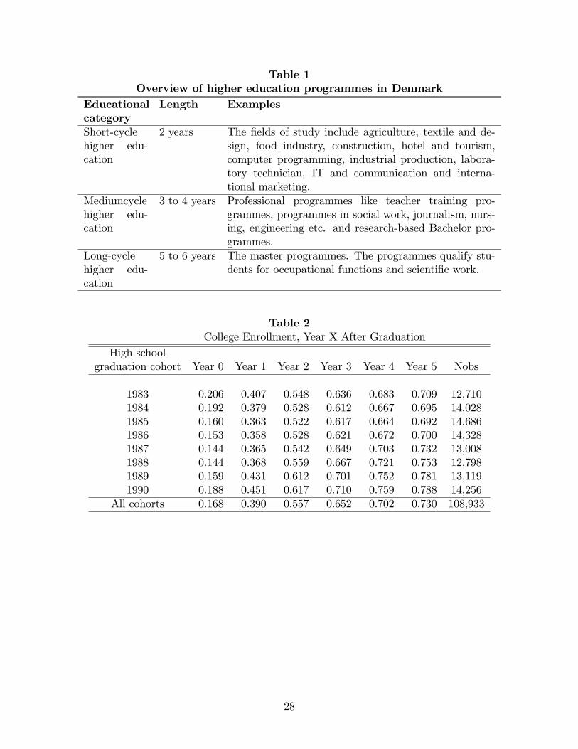
Table 1Overview of higher education programmes in Denmark

Educationalcategory

Length Examples

Short-cyclehigher edu-cation

2 years The �elds of study include agriculture, textile and de-sign, food industry, construction, hotel and tourism,computer programming, industrial production, labora-tory technician, IT and communication and interna-tional marketing.

Mediumcyclehigher edu-cation

3 to 4 years Professional programmes like teacher training pro-grammes, programmes in social work, journalism, nurs-ing, engineering etc. and research-based Bachelor pro-grammes.

Long-cyclehigher edu-cation

5 to 6 years The master programmes. The programmes qualify stu-dents for occupational functions and scienti�c work.

Table 2College Enrollment, Year X After Graduation

High schoolgraduation cohort Year 0 Year 1 Year 2 Year 3 Year 4 Year 5 Nobs

1983 0.206 0.407 0.548 0.636 0.683 0.709 12,7101984 0.192 0.379 0.528 0.612 0.667 0.695 14,0281985 0.160 0.363 0.522 0.617 0.664 0.692 14,6861986 0.153 0.358 0.528 0.621 0.672 0.700 14,3281987 0.144 0.365 0.542 0.649 0.703 0.732 13,0081988 0.144 0.368 0.559 0.667 0.721 0.753 12,7981989 0.159 0.431 0.612 0.701 0.752 0.781 13,1191990 0.188 0.451 0.617 0.710 0.759 0.788 14,256

All cohorts 0.168 0.390 0.557 0.652 0.702 0.730 108,933

28

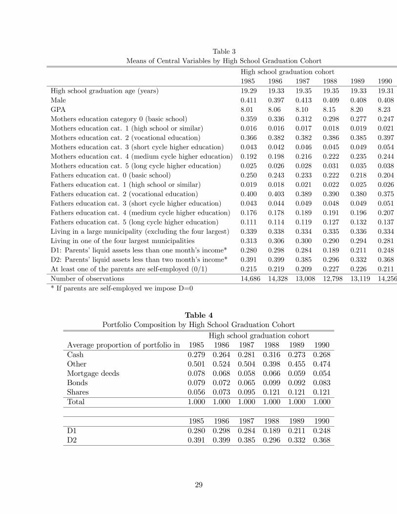
Table 3Means of Central Variables by High School Graduation Cohort

High school graduation cohort1985 1986 1987 1988 1989 1990

High school graduation age (years) 19.29 19.33 19.35 19.35 19.33 19.31Male 0.411 0.397 0.413 0.409 0.408 0.408GPA 8.01 8.06 8.10 8.15 8.20 8.23Mothers education category 0 (basic school) 0.359 0.336 0.312 0.298 0.277 0.247Mothers education cat. 1 (high school or similar) 0.016 0.016 0.017 0.018 0.019 0.021Mothers education cat. 2 (vocational education) 0.366 0.382 0.382 0.386 0.385 0.397Mothers education cat. 3 (short cycle higher education) 0.043 0.042 0.046 0.045 0.049 0.054Mothers education cat. 4 (medium cycle higher education) 0.192 0.198 0.216 0.222 0.235 0.244Mothers education cat. 5 (long cycle higher education) 0.025 0.026 0.028 0.031 0.035 0.038Fathers education cat. 0 (basic school) 0.250 0.243 0.233 0.222 0.218 0.204Fathers education cat. 1 (high school or similar) 0.019 0.018 0.021 0.022 0.025 0.026Fathers education cat. 2 (vocational education) 0.400 0.403 0.389 0.390 0.380 0.375Fathers education cat. 3 (short cycle higher education) 0.043 0.044 0.049 0.048 0.049 0.051Fathers education cat. 4 (medium cycle higher education) 0.176 0.178 0.189 0.191 0.196 0.207Fathers education cat. 5 (long cycle higher education) 0.111 0.114 0.119 0.127 0.132 0.137Living in a large municipality (excluding the four largest) 0.339 0.338 0.334 0.335 0.336 0.334Living in one of the four largest municipalities 0.313 0.306 0.300 0.290 0.294 0.281D1: Parents�liquid assets less than one month�s income* 0.280 0.298 0.284 0.189 0.211 0.248D2: Parents�liquid assets less than two month�s income* 0.391 0.399 0.385 0.296 0.332 0.368At least one of the parents are self-employed (0/1) 0.215 0.219 0.209 0.227 0.226 0.211Number of observations 14,686 14,328 13,008 12,798 13,119 14,256* If parents are self-employed we impose D=0

Table 4Portfolio Composition by High School Graduation Cohort

High school graduation cohortAverage proportion of portfolio in 1985 1986 1987 1988 1989 1990Cash 0.279 0.264 0.281 0.316 0.273 0.268Other 0.501 0.524 0.504 0.398 0.455 0.474Mortgage deeds 0.078 0.068 0.058 0.066 0.059 0.054Bonds 0.079 0.072 0.065 0.099 0.092 0.083Shares 0.056 0.073 0.095 0.121 0.121 0.121Total 1.000 1.000 1.000 1.000 1.000 1.000

1985 1986 1987 1988 1989 1990D1 0.280 0.298 0.284 0.189 0.211 0.248D2 0.391 0.399 0.385 0.296 0.332 0.368

29

Table 5Portfolio Composition by Low Liquid Asset Split: Basic vs. Extreme

Low liquid asset splitBasic Extreme

Average proportion of portfolio in D1=1 D1=0 D2=1 D2=0Cash 0.097 0.338 0.174 0.340Other 0.832 0.363 0.724 0.334Mortgage deeds 0.012 0.080 0.024 0.086Bonds 0.014 0.104 0.024 0.115Shares 0.045 0.116 0.054 0.125Total 1.000 1.000 1.000 1.000Number of students with observed liquid assets of parents 17,576 56,102 26,626 47,052

Table 6Probit Model for College Enrollment, Cohorts 1985, 1988-1990

Marginal E¤ects on College Enrollment(Standard Errors in Parentheses)

(1) (2) (3) (4) (5) (6) (7)All Men Women All Men Women All

Stipend 0.082 0.064 0.106 0.143 0.160 0.118 0.146(0.017) (0.028) (0.021) (0.043) (0.068) (0.054) (0.051)

Income Percentile 0.043 0.067 0.026 0.067 0.105 0.030 -0.009(0.017) (0.027) (0.022) (0.023) (0.037) (0.030) (0.060)

Income Percentile Squared 0.056(0.041)

Pre-Reform Stipend -0.005 0.061 -0.055 -0.036 0.012 -0.061 -0.070(0.025) (0.041) (0.032) (0.032) (0.052) (0.040) (0.039)

Income Percentile � Reform Dummy -0.049 -0.076 -0.009 -0.055(0.031) (0.049) (0.040) (0.082)

Income Percentile Squared 0.005� Reform Dummy (0.057)High School GPA included yes yes yes yes yes yes yesSex, age and geographical indicators yes yes yes yes yes yes yesIndicators for graduation cohort yes yes yes yes yes yes yesControls for parents�education yes yes yes yes yes yes yesLog-likelihood -48967 -20205 -28663 -48965 -20203 -28663 -48964Number of observations 81,581 33,383 48,198 81,581 33,383 48,198 81,581

30

Table 7Probit Model for College Enrollment With Controls for Borrowing Constraints

Cohorts 1985, 1988-1990Marginal E¤ects on College Enrollment(Standard Errors in Parentheses)

(1)Stipend 0.114

(0.032)Income Percentile 0.037

(0.022)Pre-Reform Stipend -0.011

(0.030)Low assets (0/1) 0.027

(0.027)Stipend � Low assets -0.077

(0.049)Reform � Low assets 0.049

(0.032)Income Percentile � Low assets -0.017

(0.020)High School GPA included yesSex, age and geographical indicators included yesIndicators for graduation cohort included yesControls for parents�education included yesInclude self-employed yesLog-likelihood -32,613Number of observations 54,843

31

Table 8Probit Model for College Enrollment, Cohorts 1985, 1988-1990

Marginal E¤ects on College Enrollment(Standard Errors in Parentheses)

(1) (2) (3)All Men Women

Stipend 0.095 0.113 0.092(0.026) (0.042) (0.033)

Income Percentile 0.033 0.037 0.029(0.021) (0.033) (0.027)

Pre-Reform Stipend -0.022 0.019 -0.050(0.030) (0.049) (0.038)

Low assets (0/1) -0.074 -0.157 -0.015(0.042) (0.065) (0.055)

Stipend � Low assets 0.086 0.168 0.024(0.038) (0.077) (0.061)

Stipend � Income Percentile � Low assets -0.125 -0.283 -0.003(0.060) (0.111) (0.090)

Income Percentile � Low assets 0.087 0.241 -0.029(0.062) (0.097) (0.079)

High School GPA included yes yes yesSex, age and geographical indicators included yes yes yesIndicators for graduation cohort included yes yes yesControls for parents�education included yes yes yesLog-likelihood -32,613 -13,391 -19,161Number of observations 54,843 22,438 32,405

32

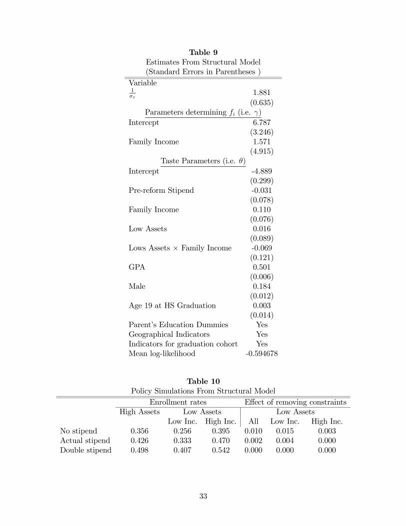
Table 9Estimates From Structural Model(Standard Errors in Parentheses )

Variable1�"

1.881(0.635)

Parameters determining fi (i.e. )Intercept 6.787

(3.246)Family Income 1.571

(4.915)Taste Parameters (i.e. �)

Intercept -4.889(0.299)

Pre-reform Stipend -0.031(0.078)

Family Income 0.110(0.076)

Low Assets 0.016(0.089)

Lows Assets � Family Income -0.069(0.121)

GPA 0.501(0.006)

Male 0.184(0.012)

Age 19 at HS Graduation 0.003(0.014)

Parent�s Education Dummies YesGeographical Indicators YesIndicators for graduation cohort YesMean log-likelihood -0.594678

Table 10Policy Simulations From Structural Model

Enrollment rates E¤ect of removing constraintsHigh Assets Low Assets Low Assets

Low Inc. High Inc. All Low Inc. High Inc.No stipend 0.356 0.256 0.395 0.010 0.015 0.003Actual stipend 0.426 0.333 0.470 0.002 0.004 0.000Double stipend 0.498 0.407 0.542 0.000 0.000 0.000

33

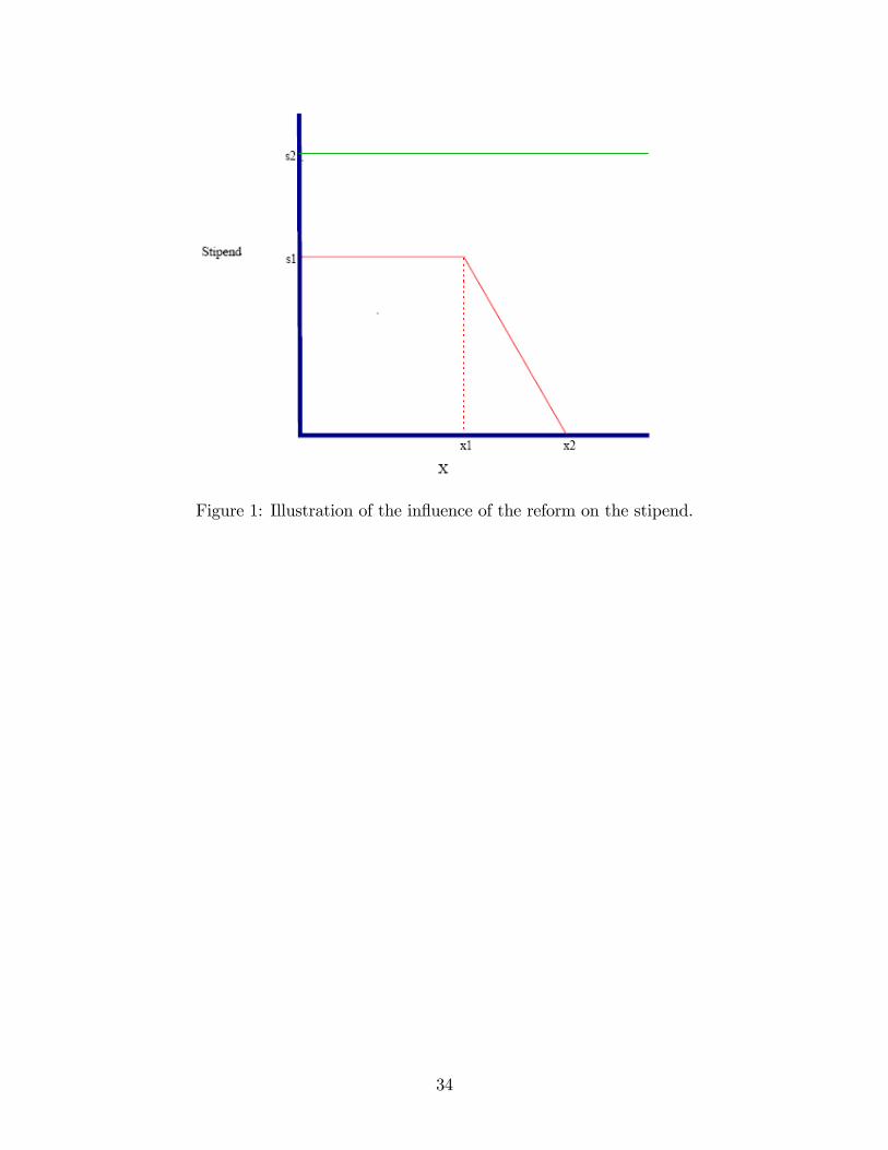
Figure 1: Illustration of the in�uence of the reform on the stipend.

34

Figure 2: The stipend rule and it�s relation to enrollment.

7,8

8

8,2

8,4

8,6

8,8

9

1982 1983 1984 1985 1986 1987 1988 1989 1990 1991 1992 1993 1994

Higher educationUniversities only

Figure 3: High school GPA of �rst-year students.

35

1

1,01

1,02

1,03

1,04

1,05

1,06

1,07

1,08

1,09

1982 1983 1984 1985 1986 1987 1988 1989 1990 1991 1992 1993 1994

Higher educationUniversities only

Figure 4: High school GPA of �rst-year students relative to high school cohort average.

36