Estimating the Complexity Function of Financial Time

Series: An Estimation Based on Predictive Stochastic

Complexity

Shu-Heng Chen(1)

Ching-Wei Tan(2)

(1)Departmen of Economics National Chengchi University Taipei, Taiwan. t

t(2)Departmen of Economics National Chengchi University Taipei, Taiwan.

ABSTRACT

Using the measure predictive stochastic complexity, this paper examines the complexity of

two types of financial time series of several Pacific Rim countries, including 11 series on

stock returns and 9 series on exchange rate returns. Motivated by Chaitin's application of

Kolmogorov complexity to the definition of "Life", we examine complexity as a function

of sample size, and call it the complexity function. By Chaitin (1979), if a time series is

truly random, then its complexity should increase at the same rate of sample size, which

means one would not gain or lose any information by finetuning sample size.

Geometrically speaking, this means that the complexity function is a 45 degree line. Based

on this criterion, we estimated the complexity function of the above 20 financial time

series and their iid normal surrogates. It is found that while the complexity functions of all

surrogates lie nearly to the 45 degree line, the ones of financial time series are steeper than

the 45-degree line except for the case of Indonesian stock return. Therefore, while the

complexity of most financial time series are initially low as opposed to that of the pseudo

random time series, it gradually catches up as sample size increases. The catching-up effect

indicates a short-lived property of financial signals. This property may lend support to the

hypothesis that financial time series are not random but are composed of a sequence of

structures, whose birth and death can be characterized by a jump process with an

embedded Markov chain. The significance of this empirical finding is also discussed in

light of the recent progress in financial econometrics. Further exploration of this property

may help data miners to select moderate sample size in either their data-preprocessing

procedure or active learning design.

Key words: Kolmogorov Complexity, Predictive Stochastic Complexity, Efficient Market

Hypothesis, IRS in Complexity, Jump Process, MATLAB.

1. Motivation and Introduction

The development of information theory can be roughly divided into two stages. The first

stage starting from 1948 is known as Shannon information theory, and the second stage

initialized around 1964-1966 can be entitled algorithmic information theory (Kolmogorov

complexity theory). The main difference between these two approaches lies in the

foundation of information theory. The former uses probability theory as the foundation of

information theory, whereas the latter asserts that information theory must precede

probability theory. As Kolmogorov (1983) stated:

From the general considerations that have been briefly developed it is not clear why information

theory should be based so essentially on probability theory, as the majority of text-books would

have it. It is my task to show that this dependence on previously created probability theory is not, in

fact, inevitable. (p.31)

The alternative foundation considered by Kolmogorov and many others is computation

theory. One of the most important concepts in algorithmic information theory is

Kolmogorov complexity. Kolmogorov complexity is a measure for the descriptive

complexity of an object. Roughly speaking, Kolmogorov complexity is defined to be the

length of the shortest algorithm (shortest string) fed to the universal Turing machine that

can output the object. However, as Rissanen (1989, p.i) pointed out, "the theory gives no

guidance to the practical construction of programs, let alone the shortest one, which in fact

turns out to be non-computable. Accordingly, the theory has had little or no direct impact

on statistical problems." What Rissanen suggests is to replace the universal Turing

machine by a class of probabilistic models. This modified version of Kolmogorov

complexity is called s ochastic complexity (Rissanen, 1989). t

The purpose of this paper is to show the relevance of Kolmogorov complexity to financial

data mining through Rissanen's modified version of Kolmogorov complexity. By "the

relevance of Kolmogorov complexity", we mean the two distinguishing features of

Kolmogorov complexity (Li and Vitanyi, 1990), namely, that

• it defines randomness from the perspective of individual objects.

• it defines randomness based on finite strings.

These two features motivate us to measure the stochastic complexity of financial time

series as a function of its locality and w ndow size; briefly, to denote the complexity of the

series of observations {x

i

i

i+1, xi+2, ..., xi+n} Ci(n), where i refers to locality and n refers to

window size. Suppose that Ci(n) is independent of i, and, by dropping the subscript i, call

C(n) the complexity function. Chaitin (1979), to our best knowledge, is the first that used

the mathematics of C(n) to distinguish structure (life) from randomness. More precisely, if

we graph the complexity function in a X-Y plane, Chaitin's notion of randomness can be

easily seen as a 45 degree line.

The central contribution of Chaitin (1979) is to provide a notion of randomness based on

the examination of the growth of an object. Theoretically, this notion of randomness

should be potentially useful for objects like time series. Unfortunately, since Chaitin's work

is based on Kolmogorov complexity, its direct impact on statistics has not been exploited

as Rissanen observed. In this paper, we would like to use Rissanen's modified version of

Kolmogorov complexity, known as predictive stochastic complexity (PSC), to apply

Chaitin's notion of randomness to financial time series. We use the surrogates of real

financial times series to show that this notion works quite well within the case of surrogate

data (pseudo random series), i.e., the complexity functions of all pseudo random series lie

close to the 45 degree line. However, the complexity functions of nearly all the financial

time series have a tendency to go above the 45 degree line as window size increases.

The main implication of this empirical finding is for the property of signals. It is now

well-known that financial time series is not iid (Pagan, 1996). As a result, signals can

hopefully be extracted. Recent studies of non-linear modeling in finance have, to some

extent, confirmed this (Chen, 1998a). On the other hand, the extensive inclusion of

relearning schemes in nonlinear modeling, such as ncremental learning or active learning,

also highlights the possibility that signals, while existent, can be brief (Fayyad,

Piatesky-Shapiro, Smyth and Uthurusamy, 1996). Our result confirms this property.

The rest of the paper is organized as follows. Section 2 gives a brief review of Chaitin's

notion of randomness and its application to a time series. Section 3 introduces the

complexity measure predictive stochastic complexity and its computation for the linear

ARMA (AutoRegressive and Moving-Average) model. Section 4 describes the financial

data used and presents the empirical results. Concluding remarks are given in Section 5.

2. A Chaitin's Version of Randomness

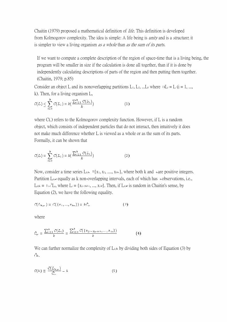
Chaitin (1979) proposed a mathematical definition of life. This definition is developed

from Kolmogorov complexity. The idea is simple: A life being is unity and is a structure; it

is simpler to view a living organism as a whole than as the sum of its parts.

If we want to compute a complete description of the region of space-time that is a living being, the

program will be smaller in size if the calculation is done all together, than if it is done by

independently calculating descriptions of parts of the region and then putting them together.

(Chaitin, 1979; p.85)

Consider an object L and its nonoverlapping partitions L1, L2, ...Lk where iLi = L (i = 1, ...,

k). Then, for a living organism L,

where C(.) refers to the Kolmogorov complexity function. However, if L is a random

object, which consists of independent particles that do not interact, then intuitively it does

not make much difference whether L is viewed as a whole or as the sum of its parts.

Formally, it can be shown that

Now, consider a time series Lk, {x1, x2, ...., xk }, where both k and are positive integers.

Partition Lk, equally as k non-overlapping intervals, each of which has observations, i.e.,

Lk, = i=1kLi, where Li = {x(i-1) +1, ..., xi }. Then, if Lk, is random in Chaitin's sense, by

Equation (2), we have the following equality.

where

We can further normalize the complexity of Lk, by dividing both sides of Equation (3) by

.

Call Equation (5) the normalized complexity function. Then the graph of the normalized

complexity function for a random time series, in Chaitin's sense, is, in effect, a 45 degree

line. In other words, the complexity function of a random time has a property known as

constant returns to scale (CRTS) in economics. Intuitively, this property says that if a time

series is random, then we cannot expect to extract any more information simply by scaling

up the size of the series.

However, if the time series is not random and has a structure, then implied by Equation (1),

we have the following inequality known as decreasing returns to scale (DRTS),

So, if a time series indeed has a structure, then as the number of observations get larger, we

are in a better position to extract high-quality information and to reduce complexity.

Roughly speaking, this is just an information-theoretic version of large sample theory.

After observing decreasing and constant returns to scale, one may wonder whether or not it

makes sense to see a complexity function with the property of increasing returns to scale

(IRTS). To motivate the discussion, let us consider the following jump process proposed

by Chen (1998b). A jump process is a continuous-time and discrete-state Markov process.

Let be the state space which is a collection of models (regimes) i.e.,

The model fi is corresponding to the state i. The cardinality of may be infinite. Now, let

w be the waiting time for regime switches or structural changes to occur, and w is

randomly distributed with the waiting time distribution (w). If at time t1, the "switch"

operator is on, the state at time [t1], say state j or (fj), will switch to state k (fk) ((fk) and

k j) at time [t1] + 1 where [.] is the Gauss symbol. The switch from j to k is randomly

determined by the embedded transition matrix T(j, k) where

If (w) is an exponential distribution function, then the jump process introduced above is

Markovian. However, in the light of the efficient market hypothesis, a memoryless

distribution may not be practical. If we consider fj a regularity of the stock price movement,

then the longer it survives the less likely it will continue to survive. In this case, a Weibull

distribution may serve better.

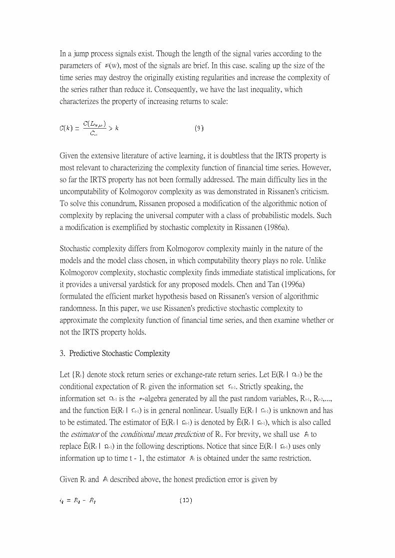
In a jump process signals exist. Though the length of the signal varies according to the

parameters of (w), most of the signals are brief. In this case. scaling up the size of the

time series may destroy the originally existing regularities and increase the complexity of

the series rather than reduce it. Consequently, we have the last inequality, which

characterizes the property of increasing returns to scale:

Given the extensive literature of active learning, it is doubtless that the IRTS property is

most relevant to characterizing the complexity function of financial time series. However,

so far the IRTS property has not been formally addressed. The main difficulty lies in the

uncomputability of Kolmogorov complexity as was demonstrated in Rissanen's criticism.

To solve this conundrum, Rissanen proposed a modification of the algorithmic notion of

complexity by replacing the universal computer with a class of probabilistic models. Such

a modification is exemplified by stochastic complexity in Rissanen (1986a).

Stochastic complexity differs from Kolmogorov complexity mainly in the nature of the

models and the model class chosen, in which computability theory plays no role. Unlike

Kolmogorov complexity, stochastic complexity finds immediate statistical implications, for

it provides a universal yardstick for any proposed models. Chen and Tan (1996a)

formulated the efficient market hypothesis based on Rissanen's version of algorithmic

randomness. In this paper, we use Rissanen's predictive stochastic complexity to

approximate the complexity function of financial time series, and then examine whether or

not the IRTS property holds.

3. Predictive Stochastic Complexity

Let {Rt} denote stock return series or exchange-rate return series. Let E(Rt | t-1) be the

conditional expectation of Rt given the information set t-1. Strictly speaking, the

information set t-1 is the -algebra generated by all the past random variables, Rt-1, Rt-2,...,

and the function E(Rt | t-1) is in general nonlinear. Usually E(Rt | t-1) is unknown and has

to be estimated. The estimator of E(Rt | t-1) is denoted by Ê(Rt | t-1), which is also called

the estimator of the conditional mean prediction of Rt. For brevity, we shall use t to

replace Ê(Rt | t-1) in the following descriptions. Notice that since E(Rt | t-1) uses only

information up to time t - 1, the estimator t is obtained under the same restriction.

Given Rt and t described above, the honest prediction error is given by

Furthermore, let us suppose that the model class provided for the selection of t is , and

the true prediction and its associated error due to any particular model ( ) are indexed

by , i.e., ,t and ,t. Then the model selection criterion in terms of the predictive

stochastic complexity (PSC) asserts that the model should be selected as that for which the

sum of the square of the true prediction errors is minimized, i.e.,

where

The predictive stochastic complexity is an information-theoretic measure of the complexity

of a string of data, relative to a model class and an estimation method. Although computing

PSC is time-consuming, an efficient algorithm for the linear autoregressive (AR) model

class was proposed and analyzed by Hannan et al. (1989) and Hemerly et al. (1989).

Furthermore, while computing predictive stochastic complexity for the linear

autoregressive and moving-average ARMA model class is significantly more difficult than

that of the AR case, a fixed-gain off-line prediction error estimation method, which is not

computationally expensive, is available in Gerencser and Rissanen (1991), Gerencser and

Baikovicius (1991) and Baikovicius and Gerencser (1992). A MATLAB code to

implement the recursive fixed-gain off-line prediction error estimation method is provided

by Ljung (1995).

In this paper we will only consider the class of linear ARMA, i.e., = {ARMA(p, q) | p =

1, 2, ..., P, q = 1, 2, ..., Q}.1 When the class of models is restricted to linear ARMA models,

each (p,q),t (p = 1, 2, ..., P; q = 1, 2, ..., Q) is simply the forecast made from

and

where

and {âi,t-1}i=1p and { j,t-1}j=1

q are the respective estimates for the unknown parameters {ai}i=1p

and {bj}j=1q by using only the information preceding the moment t. To estimate these

unknown parameters, three kinds of predictive stochastic complexities associated with

ARMA processes were established by Gerencser and Rissanen (1991). They are the

off-line estimation, the recursive prediction error method, and the off-line fixed-gain

prediction error method. The approach taken by this paper is the last one. As Gerencser

and Rissanen (1991) claimed: "A startling aspect of fixed gain estimators is that they

provide a more sensitive criterion for detection of overestimation than the standard

estimators of the previous section: the "badness" of the estimator increases the "badness"

of overestimation". This approach is briefly described as follows. Let 0 < < 1 and define

and = ({ai}i=1p, {bj}j=1

q). Let the estimator t-1 be defined as the solution to2

By this approach, the predictive stochastic complexity for the ARMA (p, q) of time series

{Rt}t=1N can be defined as the sum of the square of the recursive fixed-gain off-line

prediction errors, namely,

Furthermore, the predictive stochastic complexity of {Rt}t=1N under the model class

ARMA(p, q) (0 p P and 0 q Q) and the fixed gain is defined to be

Based on the definition above, to compute PSC ,N , one has to conduct an exhaustive

search over all (p, q)s in . However, as N is large enough, a sequential search based on

the asymptotic theory is given in Baikovicius and Gerencser (1992). In the following, we

shall summarize the major steps of this sequential search algorithm. To do so, a few more

notations are needed.

Define

and

Given these two notations, the sequential search algorithm for PSC ,N is mainly composed

of the following four steps.

1. Compute pN (0, 0). If pN (0, 0) > 0 then stop the search. The optimal model is

ARMA(0,0), and the PSC for the time series {Ri}i=1N is PSCN (0, 0). If instead p N

(0, 0) < 0, then continue the search as described in Step 2.

2. Compute pN (1, 0). If p N (1, 0) > 0 then stop search. The optimal model is

ARMA(1,0), and

If instead pN (1, 0) < 0 then continue the search according to Step 3.

3. Compute q N (0, 1). If q N (0, 1) > 0 then stop the search. The optimal model is

ARMA(0,1), and

If instead q N (0, 1) < 0 then set p = 1 and q = 1 and continue the search

according to Step 4.

4. Start moving from point (1,1) along the line {(p, q); p = q}, in the plane with the

axis given by the tentative model orders p and q, as long as pN (p, q) < 0 and

qN (p, q) < 0. Once pN (p, q) > 0 or qN (p, q) > 0, then compute pN (p - r, q)

(r=1,2...) and qN (p, q - s)(s = 1, 2, ...) until the first r where pN (p - r, q) < 0

and the first s where qN (p, q - s) < 0. When the condition is matched, the

optimal model is ARMA (p-r+1, q-s+1), and

The idea of the search for the minimum PSC and hence the true model ARMA(p*, q*) is

basically composed of two procedures. First, keep increasing p and q as long as these

increases result in the decrease of the associated stochastic complexities. Second, when

increasing p (q) increases the associated stochastic complexity, then q = q* (p = p*), and we

can start decreasing p (q), until an increase in the associated stochastic complexity is

obtained(see Figure 1). The first part of this idea is motivated by the following asymptotics

of pN (p, q) and qN (p, q). For any (p, q) Fp*,q* - Dp

*,q*,

and

where

and

As to the second part of the idea, the relevant asymptotic property is: under some

not-too-restrictive assumptions3 , for any (p, q) Dp*,q*,

and

where C is a non-random constant. Of course, these asymptotics of PSC per se are not

enough to justify the sequential search algorithm outlined above, because in some

applications, our data points (N) may not be large enough. In this case, we may get stuck in

the set Fp*,q* - Dp

*,q*. Thus, the suggestion made by Baikovicius and Gerencser (1992) is to

set small in Fp*,q* - Dp

*,q*, or try different values of so as to make sure that this does not

happen. In Ljung (1995), is suggested to be in the range [0.005, 0.03]. While is taken to

be 0.01 in this paper, as we shall see later, our concerns inspired by the real financial data

have little to do with the asymptotics of PSC. As a matter of fact, large samples are not

required for the use of PSC in terms of Kolmogorov complexity; PSC can be equally well

defined in large samples as well as small samples. As Rissanen (1986) stated: "This,

indeed, appears to be the case, and when corrected we do arrive at a criterion based on

prediction error, which is not only valid asymptotically like the previous ones but which is

also perfectly justified even for short samples." (p.56). However, when restricted on the

small sample, we may not be entitled to use the sequential search algorithm and there is no

known alternative except an exhaustive search. Nevertheless, for the sake of

computational-time complexity, this paper uses the sequential search algorithm for all sizes

of sample. However, since the results of all the samples are compared with those of

surrogate data (pseudo random series), the qualitative conclusion achieved in this paper is

not expected to change in any significant way.

This concludes our discussion of PSC. In the next section, PSC, being and information

theoretical measure of complexity, shall be used to approximate the complexity function of

financial time series.

4. The PSC of Financial Time Series

4.1. Data Description and Experimental Design

In this section, the PSC of 20 financial time series are computed. These 20 series are

described in Tables 1 and 2. The basic statistics are summarized in Tables 3 and 4. To

simplify notations, we would like to drop the fixed gain hereinafter, given that that it is

set to be 0.01.

Table 1: Stock Indices of 11 Asia-Pacific Countries

Country Index Period # of Observations

Australia All Ordinary Share 1/2/80 - 3/26/97 4320

Hong Kong Hang-Seng 2/1/73 - 3/26/97 6037

Indonesia Aktienkursindex 11/1/90 - 3/26/97 1620

Japan Nikkei 1/5/79 - 3/26/97 4452

Malaysia KLSE 5/1/92 - 3/26/97 1211

Philippines Manila Comp.Share 1/2/86 - 3/26/97 2873

South Korea Comp.Exchange 1/6/75 - 3/26/97 5724

Singapore Straits Times Industrials Share 1/2/70 - 3/26/97 7026

Taiwan TAIEX 1/5/71 - 3/26/97 7435

Thailand Bangkok SET 6/16/76 - 3/26/97 5326

U.S. S&P 500 1/2/68 - 3/26/97 7429

Data Source: AREMOS DATABASE

Table 2: Spot Exchange Rate (per U.S. Dollar) of Nine Asia-Pacific Countries

Country Currency Period # of Observations

Australia Australia Dollars 1/3/78 - 9/16/96 4725

Hong Kong HK Dollars 9/4/84 - 9/16/96 3044

Japan Japanese Yen 1/3/78 - 9/16/96 4765

Malaysia Malaysian Ringgit 5/19/86 - 9/16/96 2621

Philippines Philippine Pesos 5/19/86 - 9/16/96 2636

Singapore Singapore Dollars 9/4/84 - 9/16/96 3044

South Korea SK Yen 5/19/86 - 9/16/96 2640

Taiwan NT Dollars 1/4/88 - 9/16/96 2219

Thailand Thai Baht 1/4/88 - 9/16/96 2210

Data Source : AREMOS DATABASE

Table 3: Summary Statistics of Stock Return Series

COUNTRY MEAN(*10-4) MEDIAN(*10-4) STD(*10-3)

Australia 3.56 5.04 10.81

Hong Kong 4.27 2.94 19.52

Indonesia 2.84 0.00 8.87

Japan 2.51 5.56 11.76

The Philippines 11.14 0.00 19.63

Malaysia 6.02 6.09 11.65

Singapore 3.77 0.00 11.65

South Korea 4.03 0.00 12.33

Taiwan 5.62 6.41 16.31

Thailand 4.17 0.00 12.86

The U.S. 2.84 9.69 9.17

Table 4: Summary Statistics of Foreign Exchange Rate Series

COUNTRY MEAN(*10-5) MEDIAN(*10-5) STD(*10-3)

Australia 20.78 0.00 7.45

Hong Kong 27.54 0.00 7.38

Japan 5.15 23.89 7.94

Malaysia 11.12 3.34 6.77

Philippine 14.77 0.00 7.81

Singapore 6.35 0.00 6.87

South Korea 26.71 0.00 7.47

Taiwan 12.53 0.00 6.77

Thailand 10.69 0.00 7.10

As outlined in Section 2, what should be computed here is the normalized complexity

function C(k), (k = 1, 2, ...). The normalization requires a common denominator, . In

this paper, we choose 50 (set to 50) as the common denominator, and compute C(k) at k

= 2, 4, 10 and 20. All put together, five different window sizes are considered, i.e, k = 50,

100, 200, 500, and 1000. However, there are many k -consecutive-observation sequences

in each time series. Take S&P 500 for example. There are (7429 - k +1) such series, which

raises an inevitable question: which one should we pick? This, to some extent, is

equivalent to the selection of training and test samples when one tries to evaluate the

performance of a nonlinear model. In this paper, we decide to take all of them into account.

Precisely speaking, given a time series {Rt}, we consider each k -consecutive-observation

sequence Rk and number them as the original time series order Rki, where, i= 1,..., T-k

+1, and T is the number of observations of the whole time series {Rt}. In other words, we

are looking at a sliding window of observations Rik {Ri, ..., Ri+k }, where i = 1, 2, ..., T -

k , T - k + 1. We then compute the PSC of each Rki by using = {AR(p, q) | p = 1, 2, ...,

10, q = 1, 2, ..., 10} as our model class, and

The computation of PSC(p,q)(Rik ) is based on Equations (18)-(19) with = 0.01 and is

solved with the codes in MATLAB System Identification Toolbox provided by Ljung

(1995). Once we have the PSC for all Rik s, we take the robust estimator median as the

estimate of C(Lk,w), i.e.,

and

where k = 2, 4, 10 and 20. Since this is the first application of Chaitin's notion of

randomness to financial time series, we would like first to check whether or not it works

well with the random series. To do so, this paper uses the idea of surrogate data. The

surrogate data are generated as iid normal sequences by preserving the first and second

moment of the original time series.

4.2. Empirical Results

Based on the description above, the PSC of all iid normal surrogates are computed and the

results are summarized in Figures 2 and 3. What Figure 2 plots is the complexity functions

of all the surrogates as indicated in the box next to the figure. Since C(k) is only estimated

at four values of k, the graph is inevitably drawn by connecting points. However, it is clear

that C(k) increases as k increases. From Figure 2, we can see that lines of C(k) do not lie

exactly on the 45 degree line. Instead of CRTS, they are a little biased toward DRTS,

which means information can be further exploited as k increases. At first glance, this result

seems to be contrary to Chaitin's notion of randomness and in contradiction to what

intuition told us. It is not. Remember, while the series is random, its first moment and

second moment is constant. Therefore, according to large sample theory, the information

gained or the complexity reduced with a large k is from a better estimation of these

parameters. It is then interesting to see what will happen when the series is independent but

not identically distributed. . . Using the complexity function of those surrogates as

benchmarks, we will examine how financial time series behave. Are we gaining or losing

more information with a large sample? To answer this question, the PSC of 20 financial

time series are computed and the basic results are given in Tables 5 and 6. Using Equation

(33), these two tables are plotted in Figures 4 and 5 respectively.

Table 5: The Median of PSC (Lk,50) (*10-3): Stock Return

COUNTRY = 50 100 200 500 1000

Australia 3.44 6.83 14.55 38.18 83.21

Hong Kong 10.53 21.08 48.07 152.07 330.02

Indonesia 3.57 7.27 15.94 33.06 64.47

Japan 3.94 8.70 21.00 69.71 140.34

Malaysia 4.90 10.21 21.72 93.49 154.03

Philippines 11.82 25.44 55.35 148.95 313.53

Singapore 3.67 7.94 18.31 55.84 115.79

South Korea 6.40 13.75 28.38 78.27 164.13

Taiwan 8.64 18.06 40.61 108.16 227.22

Thailand 4.79 11.62 24.90 76.84 143.11

U.S. 3.17 6.57 13.51 38.02 82.63

Table 6: The Median of PSC (Lk,50) (*10-6): Foreign Exchange Markets

COUNTRY = 50 100 200 500 1000

Australia 1216.51 2636.28 5702.56 16176.79 35084.90

Hong Kong 5.84 13.60 30.21 96.80 189.08

Malaysia 174.13 381.80 837.92 2133.31 4008.86

Philippines 1048.57 2530.62 5765.62 21581.66 38469.22

Singapore 285.07 598.96 1105.53 2788.67 7591.05

South Korea 44.76 94.82 190.63 1371.43 4825.20

Japan 2260.25 4616.30 9995.44 24213.55 45727.70

Taiwan 119.03 271.24 694.30 1754.46 3606.22

Thailand 123.25 314.40 1081.45 4356.99 6483.82

From Figures 4 and 5, we can see that nearly all the financial time series share a common

feature in their complexity functions, namely, IRTS. Among these 20 financial time series,

the only one whose complexity function lies below the 45 degree line is the Indonesian

stock return. This result is a great contrast to the iid random normal series observed above.

Unlike the surrogate case, the complexity of financial time series is increasing rather than

decreasing with a larger value of k. This result also provides another evidence for the

non-stationary aspect of financial time series, for if financial time series are stationary, then

based on large sample theory, we can at least expect some minimum gain with large values

of k as we have seen from the surrogate data. Furthermore, if there exists a dependence

structure, we may expect more than this minimum. Unfortunately, we have got none of this

and it is the opposite that applies to our case.

5. Concluding Remarks

In this paper, we use Rissanen's PSC to estimate the complexity function of financial time

series. While the idea of the complexity function is originated from Chaitin in algorithmic

information theory, we find that, via Rissanen's modification, it can work well with the

financial time series. The complexity function of random series (the object without any

structure) is found to have the CRTS property, whereas the complexity function of

financial time series (the object with short-lived structures) is shown to have the IRTS

property. From the extensive study of those 20 financial time series, we conclude that the

IRTS property may be considered as an intrinsic part of financial time series. This result

can have further implications for financial data min ng.

i

f

The IRTS property implies that signals are brief, and we may not be able to learn more or

profit more from larger samples. It, therefore, lends support for the use of active learning

(Lanquillon, 1998; Nakhaeizadeh, Taylor, and Lanquillon, 1998). For example, upon

selecting the training sample, it favors the partial-memory design, i.e., the training sample

is chosen through a window with finite length, and data outside the window will be

automatically discarded. This design is expected to work because, by the IRTS property,

relearning with complete memory will not be beneficial. In literature, there are empirical

studies demonstrating some successful features of using partial-memory relearning

schemes (Jane and Lei, 1994). The IRTS property may provide a theoretical explanation

for the success of this style of learning schemes.

Also, the IRTS property implies that financial time series are not random but are composed

of a sequence of structures. Therefore, tools which are able to detect evolving patterns can

be very crucial for the success of financial data mining. This lends support to the use of

tools such as wavelets, k nearest neighbors, Kohonen's self-organizing maps and rule-based

regression models (Quinlan's cubist). The conventional econometric tools which are stuck

with a fixed structure or insensitive to the appearance of brief signals and evolving patterns

are not the best ones to deal with financial time series.

Acknowledgements

This paper was presented at the sixth conference on the theories and practices of security

and financial markets, Kaohsiung, December 13-14, 1997. the sixth international

conference on computational finance, New York, January 6-8, 1999. and the fifth

international conference o the Society for Computational Economics, Boston, June 24-26,

1999. The authors are grateful for participants' discussion well received in these

conferences. Special thanks go to Jorma Rissanen and Richard Roll. Of course, all

remaining errors are the authors' sole responsibility.

References:

[1]

Baikovicius, J. and L. Gerencser (1992), "Applications of Stochastic Complexity

and Related Computational Experiments," Proceeding of the 31st Conference of

Decision and Control, Tucson, Artzona. pp. 3311-3316.

t

[2]

Chaitin, G. J. (1979), "Toward a Mathematical Definition of `Life', " in R. D.

Levine and M. Tribus (eds.), The Maximal Entropy Formalism, pp. 447-498. MIT

Press.

[3]

Chen, S.-H. (1998a), "Evolutionary Computation in Financial Engineering: A

Roadmap of GAs and GP," Financial Engineering News, Vol. 2, No. 4.

[4]

Chen, S.-H. (1998b), "Modeling Volatility with Genetic Programming: A First

Report," Neural Network World-International Journal on Neural and Mass-Parallel

Computing and Information Systems, Vol. 8, No. 2, pp.181-190.

[5]

Chen, S.-H. and C.-W. Tan (1996), "Measuring Randomness by Rissanen's

Stochastic Complexity: Applications to the Financial Data," in D. Dowe, K. Korb

and J. Oliver (eds.), Information, Statistics and Induction in Science, World

Scientific, pp. 200-211.

[6]

Fayyad, U., G. Piatesky-Shapiro, P. Smyth and R. Uthurusamy (1996), Advances

in Knowledge Discovery and Data Mining, AAAI Press.

[7]

Haefke, C. and C. Helmenstein (1996), "Forecasting Stock Market Averages to

Enhance Profitable Trading Strategies," paper presented at the Second International

Conference on Computing in Economics and Finance, Geneva, Switzerland, June

26-28, 1996.

[8]

Hannan, A. J., E.J. McDougall and D. Poskitt (1989), "Recursive Estimation of

Autoregressions," Journal of the Royal Statistical Society, Series B, Vol. 51, No. 2,

pp.217-233.

[9]

Hemerley, E. and M. Davis (1989), " Recursive Order Estimation of

Autoregressions without Bounding the Model Set," Journal of the Royal Statistical

Socie y, Series B, Vol.53, No. 1, pp.201-210.

[10]

Gerencser, L. and J. Baikovicius (1991), "Model Selection, Stochastic Complexity

and Badness Amplification," Proceeding of the 30th Conference of Decision and

Control, Brighton, England. pp. 1999-2004.

[11]

Gerencser, L. and J. Rissanen (1991), "Asymptotics of Predictive Stochastic

Complexity," in E. Parzen, D. Brillinger, M. Rosenblatt, M. Taqqu, J. Geweke, and

C. Caines (eds.), New Directions in Time-Series Analysis, Institute of Mathematics

and its Applications, Minneapolis. pp.93-112.

[12]

Jang, G.-S. and F. Lai (1994), "Intelligent Trading of an Emerging Market," in

Deboeck, G. J. (ed.), Trading on the Edge: Neural, Genetic, and Fuzzy Systems for

Chaotic Financial Markets, Wiley.

[13]

Kolmogorov, A. N. (1983), "Combinatorila Foundations of Information Theory

and the Calculus of Probabilities," Russian Mathematical Surveys, Vol. 38, No. 4,

pp.29-40.

[14]

Kuan, C.-M. and T. Liu (1995), "Forecasting Exchange Rates Using Feedforward

and Recurrent Neural Networks," Journal of Applied Econometrics, Vol. 10,

pp.347-364.

[15]

Lanquillon, C. (1998), "Dynamic Aspects in Neural Classification," in G.

Nakhaeizadeh and E. Steurer (eds.), Proceedings Notes of the Workshop on

Application of Machine Learning and Data Mining in Finance, Chemnitzer

Informatik-Berichte. pp. 166-178.

[16]

Li, M. and P. Vitanyi (1990), "Kolmogorov Complexity and its Applications," in J.

van Leeuwen (eds.) Handbook of Theoretical Computer Science, Elsevier Science

Publishers.

[17]

Li, M. and P. Vitanyi (1997), An ntroduction to Kolmogorov Complexity AND Its

Applications, Revised and Expanded 2nd Edition, Springer-Verlag, New York.

I

[18]

Ljung, L. (1987), System Identification: Theory for the User, Prentice-Hall, Inc.

[19]

Ljung, L. (1995), "System Identification Toolbox," 3rd Printing, The MathWorks,

Inc.

[20]

Nakhaeizadeh, G., C. Taylor, and C. Lanquillon (1998), "Evaluating Usefulness for

Dynamic Classification," in R. Agrawal, P. Stolorz, and G. Piatetsky-Shapiro (eds.),

Proceedings of the Fourth International Conference on Knowledge Discovery and

Data Mining, AAAI Press. pp. 87-93.

[21]

Pagan, A. (1996), "The Econometrics of Financial Markets," Journal of Empirical

Finance, 3, pp. 15-102.

[22]

Rissanen, J. (1986), "Stochastic Complexity and Modeling," Annals of statistics,

Vol. 14, no. 3, pp.1080-1100.

[23]

Rissanen, J. (1989), Stochastic Complexity in Statistical Inquiry, World Scientific.