Estimating the Capitalization Effects of Harmful Algal Bloom Incidence, Intensity and

Duration? A Repeated Sales Model of Lake Erie Lakefront Property Values

Aneil Baron Doctoral Candidate, Department of Agricultural, Environmental and Development

Economics, the Ohio State University, baron.76@osu.edu

Wendong Zhang Assistant Professor, Department of Economics, Iowa State University,

wdzhang@iastate.edu

Elena Irwin Professor, Department of Agricultural, Environmental and Development Economics, the

Ohio State University, irwin.78@osu.edu

Selected Paper prepared for presentation at the 2016 Agricultural & Applied Economics

Association Annual Meeting, Boston, Massachusetts, July 31-August 2 Copyright 2016 by Aneil Baron, Wendong Zhang, and Elena Irwin. All rights reserved. Readers may make verbatim copies of this document for non-commercial purposes by any means, provided that this copyright notice appears on all such copies.

Abstract The goal of this paper is to observe whether and how harmful algal blooms are capitalized in home prices in several Ohio counties along Lake Erie. Harmful algal blooms have increased in severity and frequency, reducing the amenity value of the lake, posing health risks, and even threatening the drinking water supply. To address the problems of omitted variable bias due to unobserved emitter sites, we employ a repeat sales model. We find that a reduction of 1µg/L of chlorophyll-a yields a 2% increase in home prices, though the effect decays rapidly by distance. Secchi disk depth, while previous found to be significant in the literature, is statistically insignificant when utilizing repeat sales, and we find noticeable evidence of omitted variable bias when we do not control for emitter effects.

Introduction Excessive agricultural nutrient runoff is causing an increase in the incidence and intensity of

harmful algal blooms (HABs), an overgrowth of blue green algae that often produce toxins in

water bodies, both in the US and worldwide (Diaz and Rosenberg 2008). This poses significant

challenges for multiple valuable ecosystem services provided by many freshwater and marine

ecosystems. In the Great Lakes region, Lake Erie provides many high-valued ecosystem

services, including drinking water to over 11 million people in the US and Canada. It is the most

impacted lake, as evidenced by the unprecedented shut-off of Toledo, Ohio’s water supply in

2014. As the frequency and severity of HABs continues to increase with climate change, it is

important to accurately quantify the economic impact of HABs in terms of reduced recreational

opportunities, increased water treatment costs as well as potential negative impacts on lakefront

property values (Bingham et al. 2015).

There is comparatively little literature investigating the economic impact of water quality, due in

large part to data limitations and econometric challenges. Leggett and Bockstael (2000), provide

a model study, where they measure the valuation of fecal coliform oh home prices in Maryland.

Their main contribution is to control for emitter effects: otherwise omitted covariates which are

correlated both with water quality and home prices. Specifically in studyingf Lake Erie, Ara et

al.(2007) employ spatial econometrics, while Bingham et al. (2015) merely consider service

interruption.

The objective of this paper is to quantify the impacts of water quality and especially the presence

and intensity of HABs in Lake Erie on nearby housing values. The novelty of our study hinges

on the spatial and temporal extent of our water quality data sets and the large number of housing

transactions that allows us to employ a repeat sales approach. In addition, we use a direct

measure of HABs that is both temporally and spatially explicit. This measure is derived from

NOAA’s Medium Spectral Resolution Imaging Spectrometer (MERIS) imagery of Lake Erie,

which measures levels of chlorophyll-a, an indicator of algae levels and hence of HABs. In

addition to this new data source, we also include secchi depth readings, the most traditional

means of measuring water clarity.

The paper makes at least two contributions to the literature on water quality valuation. First, in

contrast to previous studies which often just relies on the levels of fecal coliform or secchi depth

readings, we use multiple measures of water quality to better understand their effects on housing

values. Second, while previous studies employ a hedonic framework, our large data set allows

us to also perform a repeat sales analysis. While hedonic regressions are an incredibly potent tool

for measuring how different characteristics are capitalized in home prices, hedonics may suffer

from omitted variable bias or other challenges which may alter the results that can be drawn from

them. Especially in the case of environmental characteristics such as air and water, unmeasured

neighborhood effect, and specifically emitter effects, may significantly bias results. This issue

was first addressed by Leggett and Bockstael (2000), but our approach is to deal with omitted

variables correlated with water clarity by utilizing repeat sales. A repeat sales model allows us to

hold the house, the neighborhood, and all the other observed and unobserved characteristics

fixed, only allowing time and water quality to vary. This study is the first instance to our

knowledge where repeat sales have been used in a paper analyzing water quality. We also vary

our measurements by distance and time, not only utilizing the reading at the time of sale, but the

value the previous year and the worst value that year and the year previous. We conclude that a

repeat sales model controls for omitted variable bias, without having to painstakingly measure

every potential emissions source, hydrological feature, and soil quality.

We find that reducing the concentration of chlorophyll-a by1 µg/L yield an increase in home

values by roughly 1.5-3%, though the effect is limited to houses very near the lake access points.

Specifically, the value at time of sale is not statistically important, but rather the maximum

chlorophyll level measured that year or the previous year. Water clarity measured by secchi disk

depth is found to have unbelievably positive coefficients in a hedonic model, but exhibits

evidence of omitted variable bias. When we employ a repeat sales model, secchi disk depth

becomes insignificant.

The remainder of the paper is as follows. Section 1introduces the problems of HABs in Lake

Erie, their cause, and prior efforts to analyze them. Section 2 presents previous econometric

techniques, advocates the employ of repeat sales, and discusses the potential challenges of

valuing HABs. Section 3 covers the different means of measuring water quality and our data

sources. Section 4 presents our results, while section 5 offers conclusions and policy

implications.

Background: Harmful Algae Blooms and Lake Erie

Harmful algae blooms are an environmental phenomenon of critical importance around the globe

(Diaz and Rosenberg 2008). While algae are an integral component of many water-based

ecosystems, there are two mechanisms by which a bloom may be detrimental to the environment.

First, an algae bloom may lead to a decrease in dissolved oxygen (hypoxia) due to the

breakdown of alga cells. Hypoxic conditions can lead to fish death and the unraveling of the

ecosystem. Of more immediate impact are blooms of toxic species of cyanobacteria, which

produce cyanotxins which can lead to illness or even death for animals or humans who come in

contact with it.

One of the most notable areas of recent HAB prevalence is Lake Erie. One of the Great Lakes, it

provides drinking water to over 11 million people in the US and Canada, and is a source of

recreation to millions in Ohio and Michigan. The lake been plagued with increasing HABs in

recent years, culminating in the unprecedented shutdown of Toledo, Ohio’s drinking water

supply in 2014. In Lake Erie, the most common cyanobacteria is Microcystis aeruginosa, a kind

of blue green algae, which causes both hypoxia and the spread of harmful toxins.

While temperature, wind, water depth, and other environmental factors play a significant role in

explaining the prevalence of HABs, the primary cause has been identified as nitrogen and

phosphorus loading from agricultural runoff (Kane et al. 2014, Watson et al. 2016, Bertani et al.

2016, Bridgeman et al. 2012). Lake Erie is fed by the Sandusky and Maumee rivers, both of

which are avenues of nitrogen and phosphorus loading. The Maumee river in particular is the

endpoint of runoff from 4.2 million acres of agricultural land. Due to the locations of these

rivers, the western part of the lake is most susceptible to HABs, though as the season progresses

the bloom spreads from west to east. It is for this reason that we focus our study to counties

along the western end of Lake Erie.

Farmers have an immediate and quantifiable cost associated with reducing phosphorus and

nitrogen loading, namely reducing their use of fertilizer, adopting mitigation mechanisms, or

employing different methods of cultivation. These are not insignificant costs, and thus before any

policy maker asks farmers to undertake such costs, they should attempt to determine the net

benefit of such mitigation. The state of Ohio believes the issue to be of critical importance,

making $100 million available for farmers at 0% interest rate in 2014 to adopt practices and

construct facilities to reduce fertilizer runoff. The state has also poured millions of dollars into

programs such as the Ohio Sea Grant, funding research projects at numerous universities.

From an economics perspective, there are multiple costs associated with HABs, many of which

are difficult to quantify. The first, most immediate cost is the increased costs to public water

systems to purify water. For instance, the city of Toledo in 2013 spent an extra $3,000 per day in

additional carbon filters and chemical treatment when algae levels were elevated (Dierkes, 2013)

There are also the direct costs due to illness, including medical treatment, lost productivity, and

distress. The CDC reported 61 illnesses nationally from 2009-2010 due to exposure from HABs,

though this number may underrepresent the number of those exposed. Individuals exposed

exhibited dermatological, gastrointestinal, respiratory and neurologic symptoms. They also find

that children may be more susceptible to such illnesses (CDC 2014).

There are also potential costs due to a decline in tourism or recreational value of the lake.

Tourists and locals are less likely to take trips to enjoy lake amenities when the water has an

unpleasant odor, is less aesthetically pleasing, or more importantly toxic. For example, Weicksel

and Lupi (2013) estimate the economic loss of the 2011 HAB to be $1.3 million due to beach

closures at Maumee Bay State Park, and $2.4 million in losses to recreational fishing. They also

estimate that the economic loss due to decreased tourism in Ohio ranges from $165,000-$20.79

million. Specifically concerning anglers, Sohngen et al. (2014) estimate the value of fishing

along the coast of Lake Erie to be $27.1 million annually. They also find in their survey that 96%

of respondents were aware of blooms, 84% had experienced a bloom, and half of respondents

had altered their behavior (selecting a different fishing site or not fishing at all) because of

HABs. While the goal of our study is not to measure the valuation of every resident in the state,

it is important to observe that the valuation of water quality is in no way limited to properties

directly abutting the lake.

Empirical Methodology

Hedonic pricing models estimate the effects of various independent variables such as house

characteristics, school quality, and other neighborhood characteristics, on the dependent variable,

traditionally the natural log of the house price. Hedonic theory suggests that, in market

equilibrium, we can determine the marginal value of various characteristics in or around the

home. Hedonic models, pioneered by Rosen (1974), have been used to value a host of

characteristics, ranging from school quality (e.g. Machin 2011), to Superfund sites (Greenstone

and Gallagher 2008), to noise pollution (e.g. Sunding and Swoboda 2010). In terms of water

quality, there have been hedonic analysis studying overall clarity (Young 1984), pH (Epp and

Al-Ani 1979) and Secchi disk depth readings (Steinnes 1992 and Michael, Boyle and Bouchard

1996). Geographically, studies have included Scotland (Pretty et al. 2003), Maryland (Poor et al.

2007), the Chesapeake Bay (Leggett and Bockstael 2000), Florida (Walsh et. al 2011), and Lake

Erie (Ara et al.2007).

However, most studies have failed to properly deal with the complications introduced by space

and the possibility of omitted variable bias due to emitter effects. As Small (1974) writes,

hedonics may suffer “empirical difficulties, especially correlation between pollution and

unmeasured neighborhood characteristics, [that] are so overwhelming as to render the entire

method useless.” As an illustrative example, suppose we are interested the relationship between

water quality, X, and house price Y. Our hedonic regression is of the following form:

! = #$ + #&' + ( (1)

We fail to observe a nearby toxic waste dump Z, which both negatively effects water quality and

home prices.

) = *$ + *&' + + (2)

Thus we are really estimating

! = #$ + #&' + #, *$ + *&' + + + ( (3)

! = #$ + #,*$ + #& + *&#, ' + (#,+ + () (4)

Which is unbiased only when #, = 0. If #, ≠ 0, the parameter will be biased. The direction of

bias depends on the circumstances. In our example, if the toxic waste dump has both a negative

effect on water quality and on home prices, the effect of water quality on home prices, #&, is

overestimated.

This challenge is addressed in the seminal work by Leggett and Bockstael (2000) that examines

the effect of fecal coliform in the Chesapeake Bay. Their main contribution was to adequately

control for sources of pollution, such as marinas and farm runoff. They correctly assert that if

one fails to account for an emission source, a measure of the air or water quality near that source

may over or understate the effect of water pollution, as it is highly correlated with the presence

of the source itself. The challenge that Leggett and Bockstael (2000) face is that it is difficult to

properly control for the presence of every emissions source and the specific hydrological and

topographical characteristics, especially when studying a large area.

Our solution to this conundrum is to employ a repeat sales model. Such a method is reliant upon

a sufficient temporal range of water quality measures, and a sufficiently large number of housing

transactions in order to conduct meaningful analysis. The strength of a repeat sales model is that

by holding the house, its characteristics, and the surrounding area constant, the only

characteristics which change over time, other than the age of the property and time itself, is the

water quality. It does, however, rely on the assumption that neither the house nor the

neighborhood characteristics change over time. One drawback of our data is that we are unable

to observe home improvements or additions, a consequence of county level records keeping

practices. For unobserved changes to neighborhood characteristics, we have little reason to

believe that there were major changes to the local communities that are not properly captured by

city and year fixed effects. Our area of study is relatively small, ranging from 30km-106km

outside of Toledo, Ohio, and we would suspect that any noticeable changes to crime rate or other

factors be captured by these fixed effects in such an area of study.

In terms of what measurements to use, it is not readily apparent how homeowners would value

chlorophyll-a or secchi disk depth readings directly, as it is highly doubtful that they would be

aware of the exact level. More likely, they only take notice when there is a noticeable change,

such as a water quality advisory, an algae bloom becomes visible, or water clarity dramatically

changes. Thus, a simple linear or logarithmic functional form potentially may not properly

capture a homeowner’s valuation, as it might if we were valuing crime or school quality. We

would also think that valuation of water quality would vary spatially. Most previous analysis, has

focused on houses very close to the body of water in question. For instance, Bingham et al.

(2015) only consider houses that are within 0.5 miles of Lake Erie. However, as Sohngen et al.

(2015) have found, many individuals much further inland value lake amenities and water quality

through fishing trips. Anglers surveyed are most likely value water clarity nearest their favored

boat ramps. In all likelihood, the valuation decays rapidly with distance, as investigated by

Walsh et. al (2011).

Simply measuring water quality at the time of sale may not not adequately capture any potential

effect either. Arguably, any characteristic’s price includes the implicit expectations of future

changes, which may or may not be adequately captured in current values. Bishop and Murphy

(2016) create a means of incorporating the trend of a particular variable, in their case a rising or

falling crime rate. However, HABs do not increase or decrease in a linear manner. Within a

given year HABs are highly cyclical, occurring most frequently towards the end of summer. We

would assume that a house sold in March would derive valuation not from the reading in March,

but from the severity of the bloom that year or the previous year.

When attempting to value future events such as HABs, we must invariably deal with the role of

expectations. There is little guidance in the economics literature on how to properly incorporate

expectations in such a valuation model. While there have been studies of the risk of hurricanes

and floods (e.g. Halstron and Smith 2004, and Daniel et al. 2009, Bin and Landry 2013) that

explore the impact and persistence of such events on insurance and valuation, each of these

events are relatively infrequent, dramatic events that have the potential to completely destroy a

home. Arguably, and increase in the prevalence of HABs is a less dramatic, persistent nuisance,

and may more likely to be properly priced into the housing market.

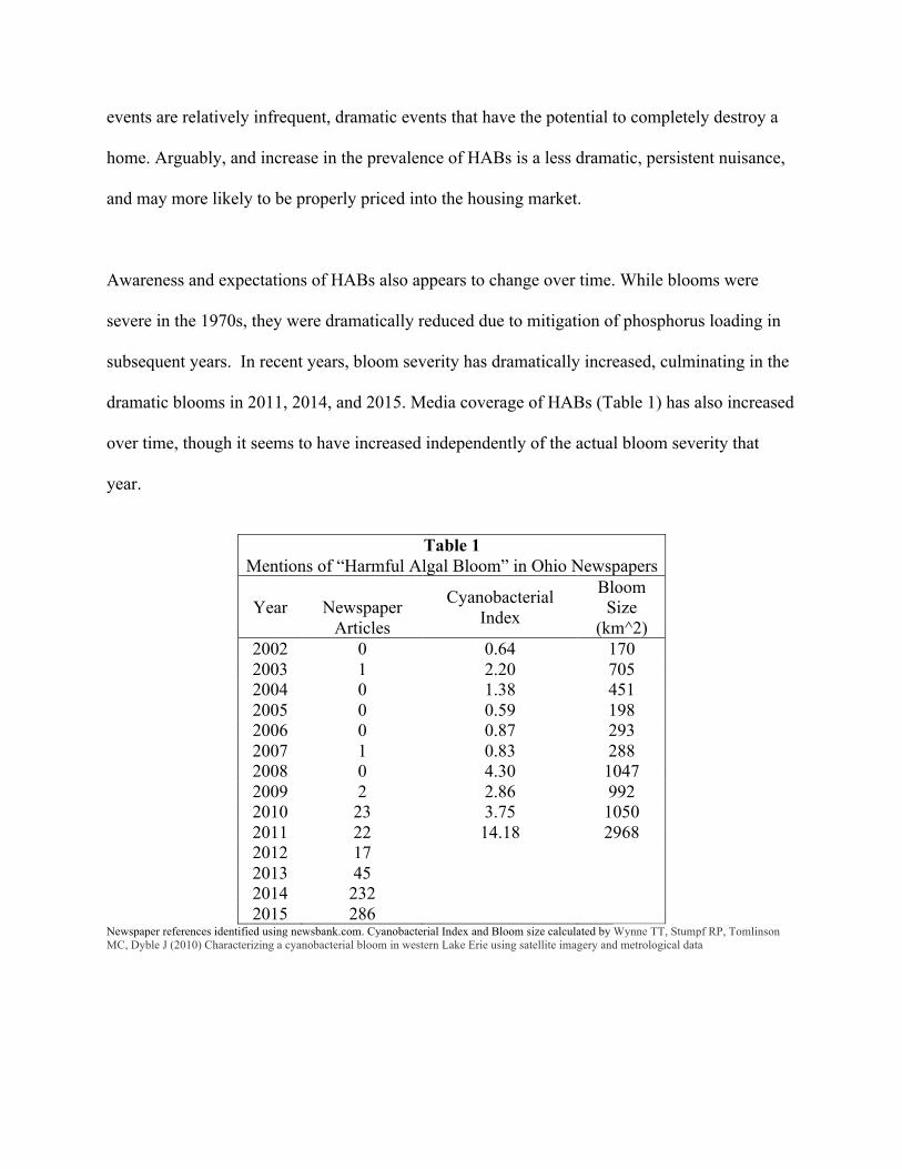
Awareness and expectations of HABs also appears to change over time. While blooms were

severe in the 1970s, they were dramatically reduced due to mitigation of phosphorus loading in

subsequent years. In recent years, bloom severity has dramatically increased, culminating in the

dramatic blooms in 2011, 2014, and 2015. Media coverage of HABs (Table 1) has also increased

over time, though it seems to have increased independently of the actual bloom severity that

year.

Table 1

Mentions of “Harmful Algal Bloom” in Ohio Newspapers

Year

Newspaper Articles

Cyanobacterial Index

Bloom Size

(km^2) 2002 0 0.64 170 2003 1 2.20 705 2004 0 1.38 451 2005 0 0.59 198 2006 0 0.87 293 2007 1 0.83 288 2008 0 4.30 1047 2009 2 2.86 992 2010 23 3.75 1050 2011 22 14.18 2968 2012 17 2013 45 2014 232 2015 286

Newspaper references identified using newsbank.com. Cyanobacterial Index and Bloom size calculated by Wynne TT, Stumpf RP, Tomlinson MC, Dyble J (2010) Characterizing a cyanobacterial bloom in western Lake Erie using satellite imagery and metrological data

Fortunately, during out timeframe of study of 2002-2011, it does not appear there is a dramatic

increase in awareness of HABs. Although there is an increase in 2010 and 2011, the increase

pales in comparison with the coverage in 2014 and 2015 following the 2014 HAB.

Data

There are several measures which have been employed to study the economic impact of water

quality. Most of the literature has focused on secchi disk depth or fecal coliform readings.

However, neither of these measurements are direct measures of the incidence and intensity of

HABs, and pose several challenges. First, they are only taken at a handful of sites on a quarterly

basis, so it is difficult to determine water quality in the areas between sites. Second, they only

measure water clarity, which may be due to a host of factors, such as sediment, other pollutants,

or hydrological fluctuations.

Recently environmental scientists have employed other means of measuring HABs. Water

samples are taken to count the level of harmful algae or the concentration of toxins. Visual

inspection at sites also plays a role. Another means of measuring HABs is by observing

chlorophyll-a readings from satellites, and either using them directly as a proxy for HABs, or

estimating the level of phycocyain. In particular, the Medium Resolution Imaging Spectrometer

(MERIS) onboard the Envisat satellite is used to measure chlorophyll-a readings in many bodies

of water around the world. In our data, the satellite provides chlorophyll-a readings for 2-km

squares through the lake. There has been little work relating chlorophyll-a readings to housing

values thus far. Of most relevance to our study is the report of Bingham et al (2015), which

creates a HAB severity index derived from MERIS chlorophyll-a readings for Lake Erie, and

find a negative relationship between HABs and home prices within 0.5 miles of the coast,

identified manually on Zillow.com. While an important first step, we believe that the economic

effects of HABs may well be felt by houses further inland, and their limited temporal window

and singular use of service interruption may not adequately capture valuation of HABs.

While for the purposes of our analysis we use chlorophyll-a readings as a proxy for harmful

algae, we should note that environmental scientists utilize spectral readings from MERIS to

calculate the cyanobacterial Index (CI), the spectral shape around the the 681nm band. This

method first was adapted to study Lake Erie by Wynne et al. (2010). The spectral shape is a

function of of the band and the second derivatives of neighboring spectral bands. Nevertheless,

chlorophyll-a readings are one of several criteria that are used to measure and predict HABs,

both in this equation, as well as a variable of interest in and of itself.

We utilize three data sources. Our first data source comprises a collection of secchi disk depth

readings from 1991-2012 at various sites along and in Lake Erie collected by the Ohio

Department of Natural Resources (ODNR). The principal drawback when relying on secchi disk

depth readings is that they are only observed at a handful of sites at specific time intervals. In

order to expand the number of observations of interest, we employ the technique of kriging.

Kriging is an optimal spatial interpolation based on regression against observed secchi depth

values of surrounding data points, weighted according to spatial covariance values. It has been

employed in several instances where there are a limited number of observations of a particular

environmental variable. For instance, Anselin (2006) and Beron et.al. (2003) employ kriging to

study the value of air quality. It has also been used by Ara et al. 2007 with secchi disk depth

readings in Lake Erie from 1991-1996. As we hypothesize that the primary means of valuation of

water quality is through recreation, we identify the location of public boat ramps and fishing

sites, again from ODNR, and identify what the secchi disk depth readings would be at each of

these 246 sites. These secchi disk depth values are quarterly, though they do not include

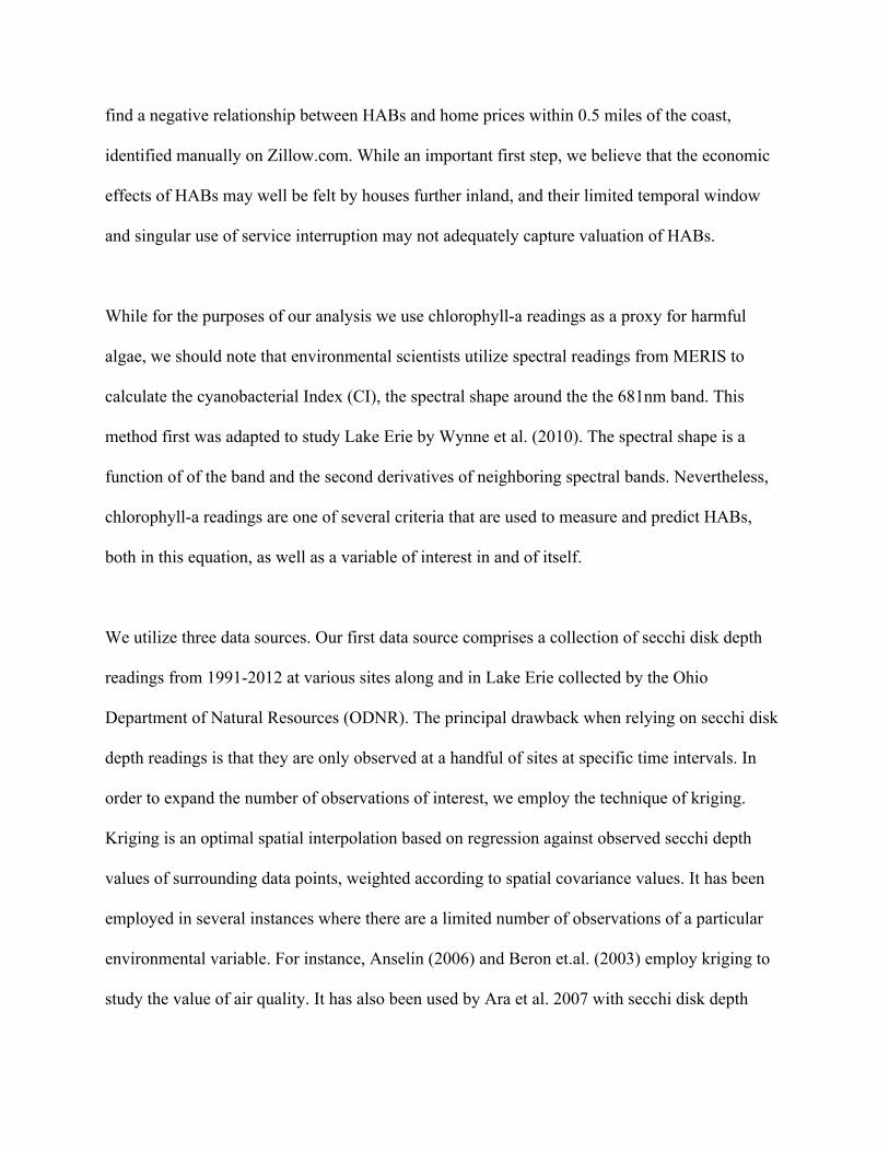
observations from the first quarter of each year. Overall from 2002-2011, secchi disk depth

readings at the 246 sites range from 0.267 meters to 7.764 meters, with and average of 1.795

meters of visibility.

Figure 1 Histogram of Secchi Disk Depth (Meters)

Figure 2 Secchi Disk Depth (Meters) Over Time

Our second source of data is the satellite chlorophyll-a readings from MERIS, which was active

from 2002-2011. The data provides a mesh grid with readings for each 2km block. While our

original data is bi-weakly, we aggregate to a quarterly average. There are several reasons for this

aggregation. First, we wish to compare results derived from chlorophyll-a readings with those

derived from quarterly secchi disk depth observations. Second, there is often significant

fluctuation between readings, and it is unlikely that an incredibly fine measurement scale is

valued by homeowners. There are also frequent missing observations due to cloud cover that

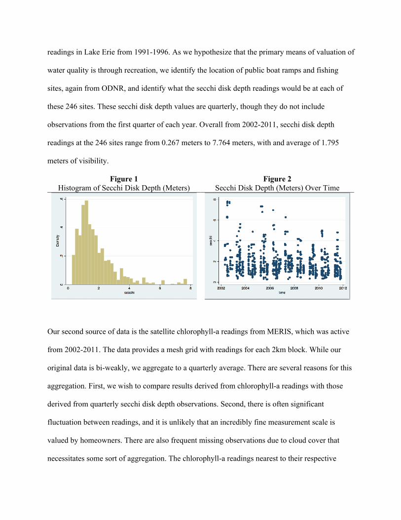
necessitates some sort of aggregation. The chlorophyll-a readings nearest to their respective

kriged site range from 0.166µg/L to 20.495µg/L. According to the Ohio EPA, a mild bloom algal

bloom occurs when chlorophyll-a levels are between 2µg/L and 5 µg/L, while a moderate bloom

occurs between 14µg/L and 50µg/L, and a severe bloom occurs when the chlorophyll-a readings

are above 50µg/L. These criteria are combined with cyanobacteria cell counts and visual

inspection measures, but provide a baseline for analysis.

Figure 3 Histogram of Chlorophyll-a (µg/L)

Figure 4 Chlorophyll-a (µg/L)Over Time

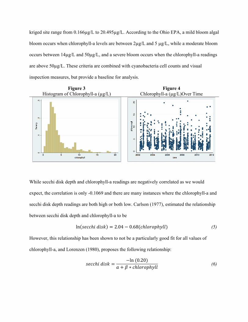
While secchi disk depth and chlorophyll-a readings are negatively correlated as we would

expect, the correlation is only -0.1069 and there are many instances where the chlorophyll-a and

secchi disk depth readings are both high or both low. Carlson (1977), estimated the relationship

between secchi disk depth and chlorophyll-a to be

ln 3455ℎ7973: = 2.04 − 0.68(5ℎABCBDℎEAA) (5)

However, this relationship has been shown to not be a particularly good fit for all values of

chlorophyll-a, and Lorenzen (1980), proposes the following relationship:

3455ℎ7973: = −ln(0.20)F + # ∗ 5ℎABCBDℎEAA (6)

Where F + # ∗ 5ℎABCBDℎEAA is the “extinction coefficient” and a the light-absorbing properties

other than chlorophyll. These properties will vary by the body of water being studied. Simulating

equation (2), Lorenzen (1980) graphs the theoretical relationship between chlorophyll and secchi

disk depth readings with different parameter values (replicated below), which mirrors our

observed results.

Figure 5 Observed Secchi Disk Depth and

Chlorophyll-a

Figure 6 Theoretical Secchi Disk Depth and

Chlorophyll-a

(beta held to be a constant 0.02)

Our final data source is comprised of parcel sales data of single family home from purchased

from CoreLogic. We utilize transactions from four lakefront counties in north western Ohio:

Lucas, Ottawa, Sandusky, and Erie. Combined there are 21,075 transactions within 30km of the

nearest access point that sold in Q2-Q4 from 2002-2011, and 8,547 within 10km. The data

includes the transaction price, sale date, and observed household characteristics such as square

footage, lot acreage, number of bedrooms, and construction material. We perform a basic

cleaning, removing the bottom 1% of sale prices, houses over $1 million dollars, and transactions

where the buyer and seller have the same last name.

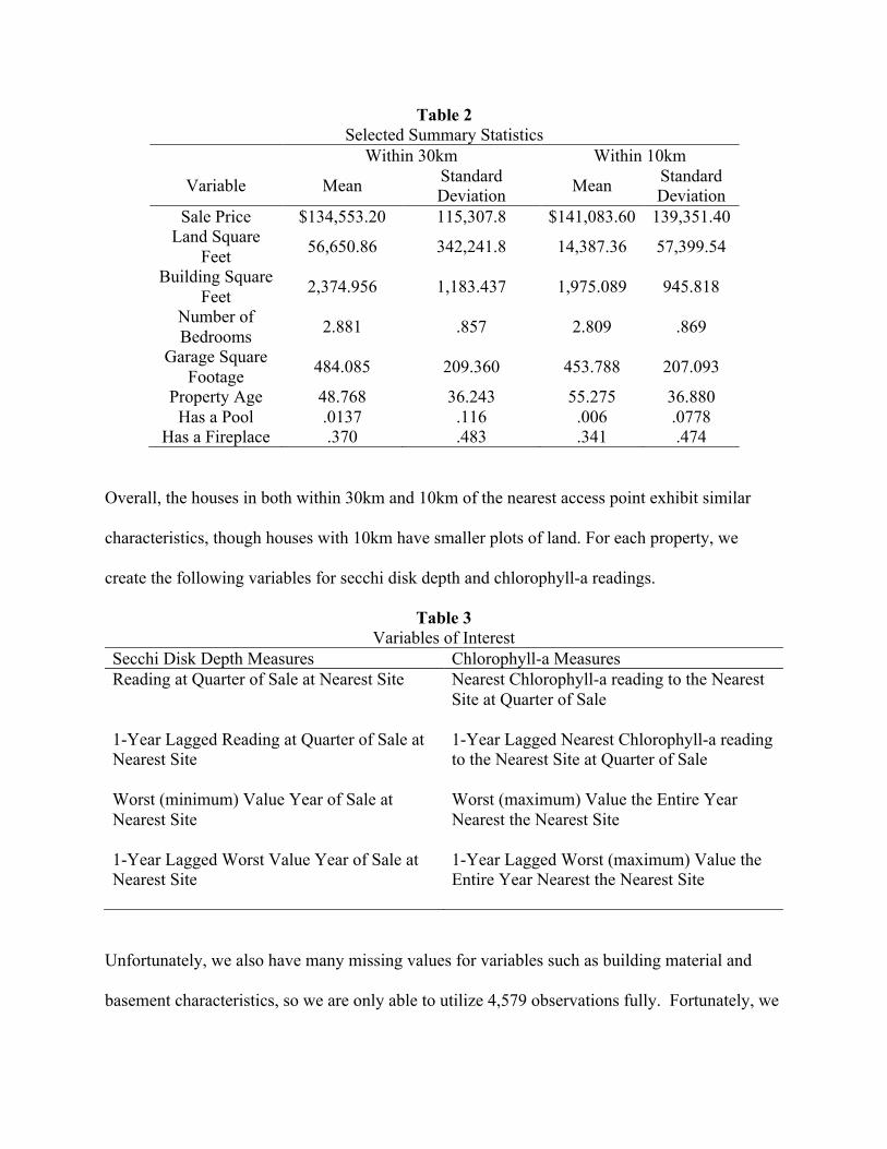
Table 2 Selected Summary Statistics

Within 30km Within 10km

Variable Mean Standard Deviation Mean Standard

Deviation Sale Price $134,553.20 115,307.8 $141,083.60 139,351.40

Land Square Feet 56,650.86 342,241.8 14,387.36 57,399.54

Building Square Feet 2,374.956 1,183.437 1,975.089 945.818

Number of Bedrooms 2.881 .857 2.809 .869

Garage Square Footage 484.085 209.360 453.788 207.093

Property Age 48.768 36.243 55.275 36.880 Has a Pool .0137 .116 .006 .0778

Has a Fireplace .370 .483 .341 .474

Overall, the houses in both within 30km and 10km of the nearest access point exhibit similar

characteristics, though houses with 10km have smaller plots of land. For each property, we

create the following variables for secchi disk depth and chlorophyll-a readings.

Table 3 Variables of Interest

Secchi Disk Depth Measures Chlorophyll-a Measures Reading at Quarter of Sale at Nearest Site

Nearest Chlorophyll-a reading to the Nearest Site at Quarter of Sale

1-Year Lagged Reading at Quarter of Sale at Nearest Site

1-Year Lagged Nearest Chlorophyll-a reading to the Nearest Site at Quarter of Sale

Worst (minimum) Value Year of Sale at Nearest Site

Worst (maximum) Value the Entire Year Nearest the Nearest Site

1-Year Lagged Worst Value Year of Sale at Nearest Site

1-Year Lagged Worst (maximum) Value the Entire Year Nearest the Nearest Site

Unfortunately, we also have many missing values for variables such as building material and

basement characteristics, so we are only able to utilize 4,579 observations fully. Fortunately, we

do not need complete characteristics when utilizing repeat sales, so we have 10,722 properties

which were sold at least twice.

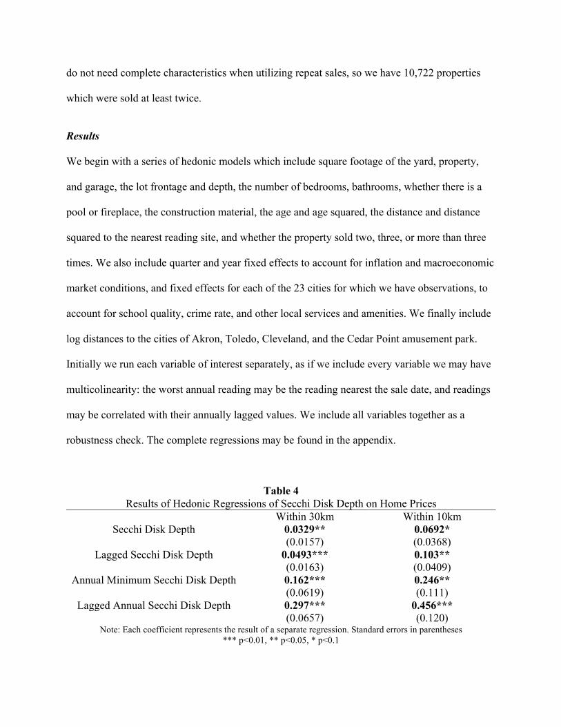
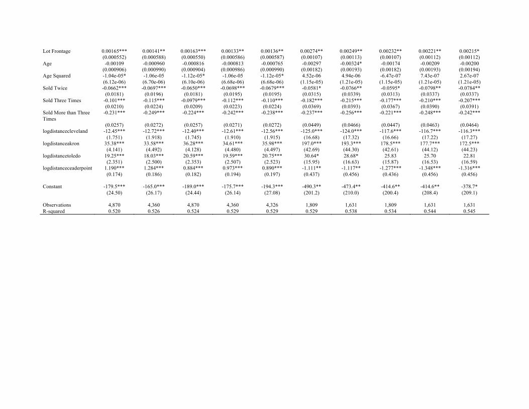
Results We begin with a series of hedonic models which include square footage of the yard, property,

and garage, the lot frontage and depth, the number of bedrooms, bathrooms, whether there is a

pool or fireplace, the construction material, the age and age squared, the distance and distance

squared to the nearest reading site, and whether the property sold two, three, or more than three

times. We also include quarter and year fixed effects to account for inflation and macroeconomic

market conditions, and fixed effects for each of the 23 cities for which we have observations, to

account for school quality, crime rate, and other local services and amenities. We finally include

log distances to the cities of Akron, Toledo, Cleveland, and the Cedar Point amusement park.

Initially we run each variable of interest separately, as if we include every variable we may have

multicolinearity: the worst annual reading may be the reading nearest the sale date, and readings

may be correlated with their annually lagged values. We include all variables together as a

robustness check. The complete regressions may be found in the appendix.

Table 4 Results of Hedonic Regressions of Secchi Disk Depth on Home Prices

Within 30km Within 10km Secchi Disk Depth 0.0329** 0.0692*

(0.0157) (0.0368) Lagged Secchi Disk Depth 0.0493*** 0.103**

(0.0163) (0.0409) Annual Minimum Secchi Disk Depth 0.162*** 0.246**

(0.0619) (0.111) Lagged Annual Secchi Disk Depth 0.297*** 0.456***

(0.0657) (0.120) Note: Each coefficient represents the result of a separate regression. Standard errors in parentheses

*** p<0.01, ** p<0.05, * p<0.1

We find that with a hedonic model, an increase in the water clarity is associated with higher

home prices. A one-meter increase in visibility is associated with a 3-45% increase in home

price, where the coefficient is larger for properties within 10km of the nearest access point. We

also find that the coefficients are larger for lagged values, perhaps suggesting that expectations

of water quality are based on prior observations. However, the incredibly large coefficients for

annual minimum readings are unreasonable, and in all likelihood this is due to omitted variable

bias in our hedonic: places with clearer water may have other unobserved characteristics, or be

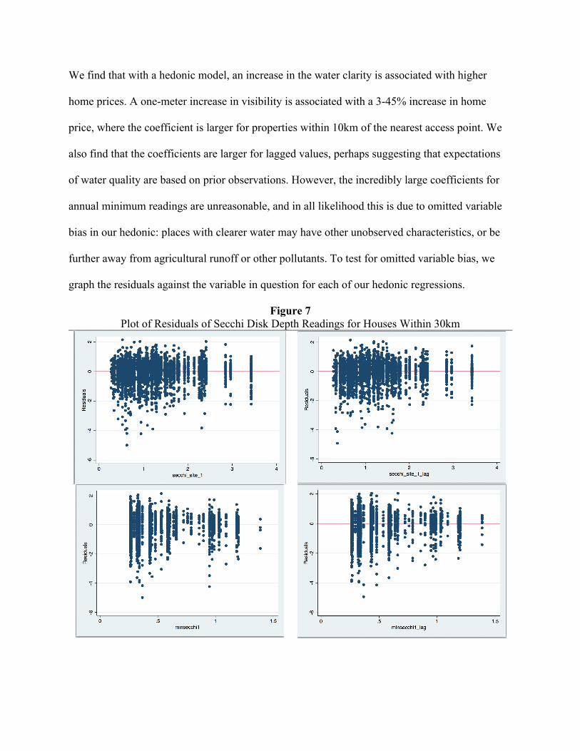
further away from agricultural runoff or other pollutants. To test for omitted variable bias, we

graph the residuals against the variable in question for each of our hedonic regressions.

Figure 7 Plot of Residuals of Secchi Disk Depth Readings for Houses Within 30km

Observing the residuals, we find that the the magnitude of the residuals increases at very low

secchi disk depth readings, which is the hallmark of omitted variable bias. We conclude that

there must be some omitted features that are correlated with low home prices and low water

clarity, and hence our parameter estimates are biased in the positive direction. We next repeat the

analysis, but employ a repeat sales model.

Table 5

Results of Repeat Sales Regressions of Secchi Disk Depth on Home Prices Within 30km Within 10km

Secchi Disk Depth 0.00835 0.0567 (0.0189) (0.0424)

Lagged Secchi Disk Depth 0.00292 0.00973 (0.0197) (0.0431)

Annual Minimum Secchi Disk Depth -0.00458 -0.131 (0.0540) (0.0883)

Lagged Annual Secchi Disk Depth 0.0291 -0.0655 (0.0639) (0.103)

Note: Each coefficient represents the result of a separate regression. Standard errors in parentheses *** p<0.01, ** p<0.05, * p<0.1

In a repeat sales model, secchi disk depth readings are entirely insignificant when regressed

independently, with one exception when all measures are included. This lack of significance may

suggest that the positive coefficients in the hedonic derive most of their significance from

unobserved emitter sites. When we plot the estimated residuals from the repeat sales regressions,

we find that there is a significant residual, but it does not exhibit any trend that would suggest

omitted variable bias.

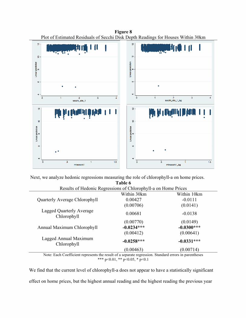
Figure 8 Plot of Estimated Residuals of Secchi Disk Depth Readings for Houses Within 30km

Next, we analyze hedonic regressions measuring the role of chlorophyll-a on home prices.

Table 6 Results of Hedonic Regressions of Chlorophyll-a on Home Prices

Within 30km Within 10km Quarterly Average Chlorophyll 0.00427 -0.0111

(0.00706) (0.0141) Lagged Quarterly Average

Chlorophyll 0.00681 -0.0138

(0.00770) (0.0149) Annual Maximum Chlorophyll -0.0234*** -0.0300***

(0.00412) (0.00641) Lagged Annual Maximum

Chlorophyll -0.0258*** -0.0331***

(0.00463) (0.00714) Note: Each Coefficient represents the result of a separate regression. Standard errors in parentheses

*** p<0.01, ** p<0.05, * p<0.1 We find that the current level of chlorophyll-a does not appear to have a statistically significant

effect on home prices, but the highest annual reading and the highest reading the previous year

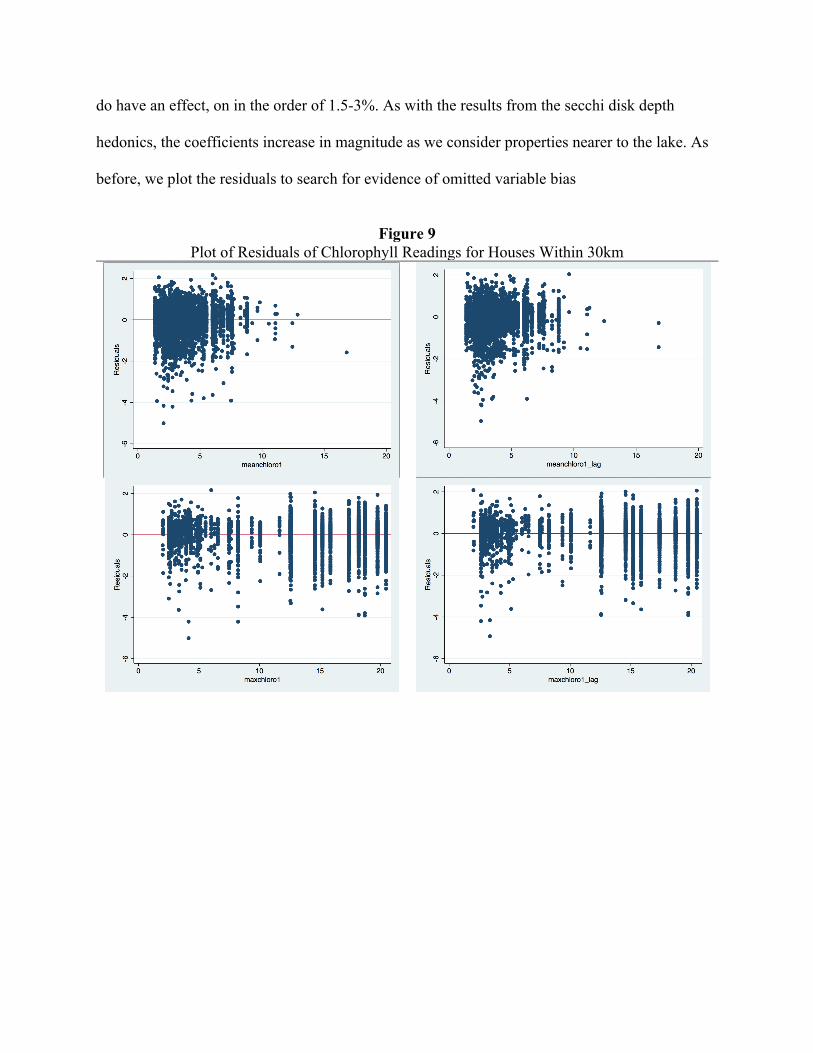
do have an effect, on in the order of 1.5-3%. As with the results from the secchi disk depth

hedonics, the coefficients increase in magnitude as we consider properties nearer to the lake. As

before, we plot the residuals to search for evidence of omitted variable bias

Figure 9

Plot of Residuals of Chlorophyll Readings for Houses Within 30km

When analyzing the residuals, there does appear to be omitted variable bias when considering the

reading at time of sale and that quarter in the previous year. However, the annual maximum and

previous year maximum do not appear to not appear to suffer from omitted variable bias, as the

residuals remain relatively constant for all values of chlorophyll-a. This may be because

chlorophyll-a levels are a better measure of HABs, which are large in scale and local

characteristics have much less of an immediate impact, as opposed to secchi disk depth readings

which may be more susceptible to local factors. We finally consider the role of chlorophyll-a on

home prices in a repeat sales model.

Table 7 Results of Repeat Sales Regressions Regressions of Chlorophyll-a on Home Prices

Within 30km Within 10km Quarterly Average Chlorophyll 0.00439 0.0167

(0.00743) (0.0120) Lagged Quarterly Average

Chlorophyll 0.0124 0.0125

(0.00841) (0.0135) Annual Maximum Chlorophyll -0.000802 -0.0219**

(0.00545) (0.00884) Lagged Annual Maximum

Chlorophyll 0.000435 -0.0192*

Quarterly Average Chlorophyll (0.00621) (0.0100) Note: Each coefficient represents the result of a separate regression. Standard errors in parentheses

*** p<0.01, ** p<0.05, * p<0.1

Our results from the repeat sales regressions are remarkably consistent with those from the

hedonics: the chlorophyll-a reading at time of sale is insignificant, while the worst readings the

year of sale and previous year yield a 2% lower price if chlorophyll-a readings increase by

1µg/L. Unlike the hedonic results, however, the effect is only significant with properties within

10km of the nearest readings site. As with the previous repeat sales analysis, we find a

significant residual, but no evidence of omitted variable bias, as the residuals remain constant for

the range of potential values of the variable in question.

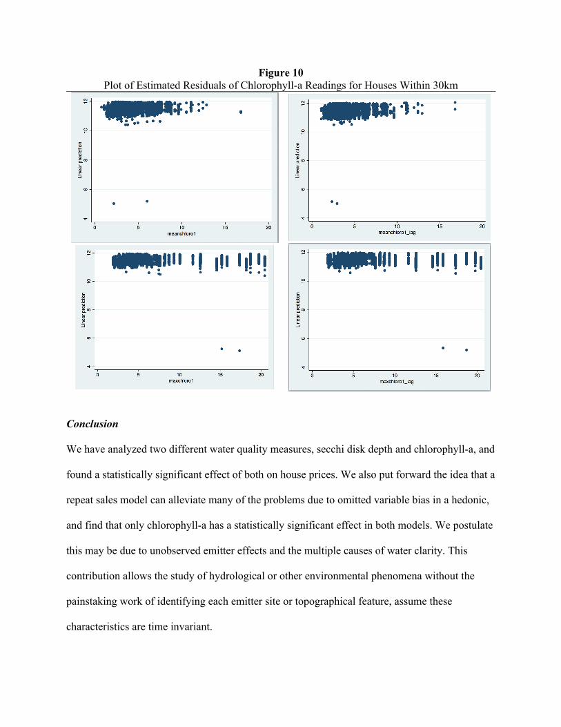
Figure 10 Plot of Estimated Residuals of Chlorophyll-a Readings for Houses Within 30km

Conclusion

We have analyzed two different water quality measures, secchi disk depth and chlorophyll-a, and

found a statistically significant effect of both on house prices. We also put forward the idea that a

repeat sales model can alleviate many of the problems due to omitted variable bias in a hedonic,

and find that only chlorophyll-a has a statistically significant effect in both models. We postulate

this may be due to unobserved emitter effects and the multiple causes of water clarity. This

contribution allows the study of hydrological or other environmental phenomena without the

painstaking work of identifying each emitter site or topographical feature, assume these

characteristics are time invariant.

We also find that statistical significance decays with distance. While we find a significant

negative result at 10km, it remains significant at the 5% level only as far as 15km, and becomes

becomes statistically insignificant at 18km. We also find that the worst readings of the year of

sale and the prior year, rather than measures at the time of sale are better readings when studying

the capitalization of HABs in home prices.

In terms of policy implications, using the median home price of $92,500 of houses within 10km,

we find the reduction of 1µg/L of chlorophyll-a yields a value of $1757-$2025 per house. With

7,588 homes that sold between 2002-2011 within 17km, that yields a benefit of $13-$15million

dollars for the reduction of 1µg/L of chlorophyll-a. This rough estimate invariably understates

the total capitalization as it does not includes homes that did not sell or in other counties and

states, but provides some indication of the overall magnitude. We should also note that these

estimates are significantly larger than the $9-$10 million dollar estimates of Bingham et al

(2015) for the entire HABs of 2011 and 2014. This difference is due both to our increased range

(0.5 miles compared with 17km), and their method of using service interruption, rather than a

hedonic framework.

We believe that there are several natural extensions of this work. While we suggest that perhaps

the valuation of water quality may be nonlinear, we obtain insignificant our counterintuitive

results when measuring polynomial, exponential, or kinked functions. We are exploring the role

of particular amenities such as boat ramps and beaches, though preliminary results merit more

careful analysis. Finally, we are also investigating open space, crime rate, and changes to

beachfront amenities overtime, which may be potential complications with a repeat sales

analysis. There is also the possibility of matching building permits with properties to help control

for otherwise unobserved home improvements.

References

Anselin, L. and J. Le Gallo. 2006. "Interpolation of Air Quality Measures in Hedonic House Price Models: Spatial Aspects". Spatial Economic Analysis 1(1):31-52.

Beron, K.J., Hanson, Y., Murdoch, J.C.,and Thayer, M.A. (2003),“Hedonic Price Functions and Spatial Dependence: Implications for the Demand for Urban Air Quality. ” In Advances in Spatial Econometrics: Methodology, Tools and Applications. Edited by Anselin, L., Florax,R.J.G.M, and Rey, S.J. Springer.

Bertani, I., D. Obenour, C. Steger, C. Stow, A. Gronewold, and D. Scavia. 2016. "Probabilistically assessing the role of nutrient loading in harmful algal bloom formation in western Lake Erie". Journal of Great Lakes Research.

Bin, O. and C. Landry. 2013. "Changes in implicit flood risk premiums: Empirical evidence from the housing market". Journal of Environmental Economics and Management 65(3):361-376.

Bingham, M., Sinha, S., and F. Lupi. 2015 “Economic Benefits of Reducing Harmful Algal Blooms in Lake Erie” Environmental Consulting & Technology, Inc., Report, 66 pp, October 2015.

Bishop, K. and A. Murphy. "Valuing Time-Varying Attributes Using the Hedonic Model: When is a Dynamic Approach Necessary?". SSRN Electronic Journal.

Bridgeman, T., J. Chaffin, D. Kane, J. Conroy, S. Panek, and P. Armenio. 2012. "From River to Lake: Phosphorus partitioning and algal community compositional changes in Western Lake Erie".Journal of Great Lakes Research 38(1):90-97.

CARLSON, R. 1977. "A trophic state index for lakes". Limnol. Oceangr. 22(2):361-369.

Centers for Disease Control and Prevention (CDC). Jaunary 10, 2014. “Algal Bloom–Associated Disease Outbreaks Among Users of Freshwater Lakes — United States, 2009–2010” MMWR. Morbidity and Mortality Weekly Reports. Retrieved from https://www.cdc.gov/mmwr/preview/mmwrhtml/mm6301a3.htm

Daniel, V., R. Florax, and P. Rietveld. 2009. "Flooding risk and housing values: An economic assessment of environmental hazard". Ecological Economics 69(2):355-365.

Diaz, R. and R. Rosenberg. 2008. "Spreading Dead Zones and Consequences for Marine Ecosystems".Science 321(5891):926-929.

Dierkes, Christina. 2014. “Harmful Algal Bloom Q&A and Updates.” Available at http://ohioseagrant.osu.edu/news/?article=697. Retrieved on October 6, 2014.

Epp, D. and K. Al-Ani. 1979. "The Effect of Water Quality on Rural Nonfarm Residential Property Values". American Journal of Agricultural Economics 61(3):529.

Graves, P., J. Murdoch, M. Thayer, and D. Waldman. 1988. "The Robustness of Hedonic Price Estimation: Urban Air Quality". Land Economics 64(3):220.

Greenstone, M. and J. Gallagher. 2008. "Does Hazardous Waste Matter? Evidence from the Housing Market and the Superfund Program *". Quarterly Journal of Economics 123(3):951-1003.

Hallstrom, D. and V. Smith. 2005. "Market responses to hurricanes". Journal of Environmental Economics and Management 50(3):541-561.

Kane, D., J. Conroy, R. Peter Richards, D. Baker, and D. Culver. 2014. "Re-eutrophication of Lake Erie: Correlations between tributary nutrient loads and phytoplankton biomass". Journal of Great Lakes Research 40(3):496-501.

LORENZEN, M. 1980. "Use of chlorophyll-Secchi disk relationships". Limnol. Oceangr. 25(2):371-372.

Machin, S. 2011. "Houses and schools: Valuation of school quality through the housing market".Labour Economics 18(6):723-729.

Michael, H, Boyle, K, and Ray Bouchard. 1996. “Water quality affects property prices: a case study of selected Maine Lake”, University of Maine. Miscellaneous Report Agricultural and Forest Experiment Station 398.

Poor, P., K. Pessagno, and R. Paul. 2007. "Exploring the hedonic value of ambient water quality: A local watershed-based study". Ecological Economics 60(4):797-806.

Pretty, J., C. Mason, D. Nedwell, R. Hine, S. Leaf, and R. Dils. 2003. "Environmental Costs of Freshwater Eutrophication in England and Wales". Environmental Science & Technology37(2):201-208.

Rosen, S. 1974. "Hedonic Prices and Implicit Markets: Product Differentiation in Pure Competition".Journal of Political Economy 82(1):34-55.

Small, K. 1975. "Air Pollution and Property Values: Further Comment". The Review of Economics and Statistics 57(1):105.

Sohngen, B., W. Zhang, J. Bruskotter, and B. Sheldon. 2015. Results from a 2014 Survey of Lake Erie Anglers. Columbus, OH: The Ohio State University, Department of Agricultural, Environmental and Development Economics and School of Environment & Natural Resources.

Steinnes, D. 1992. "Measuring the economic value of water quality". Ann Reg Sci 26(2):171-176.

Sunding, D. and A. Swoboda. 2010. "Hedonic analysis with locally weighted regression: An application to the shadow cost of housing regulation in Southern California". Regional Science and Urban Economics 40(6):550-573.

Walsh, P., J. Milon, and D. Scrogin. 2011. "The Spatial Extent of Water Quality Benefits in Urban Housing Markets". Land Economics 87(4):628-644.

Watson, S., C. Miller, G. Arhonditsis, G. Boyer, W. Carmichael, M. Charlton, R. Confesor, D. Depew, T. Höök, S. Ludsin, G. Matisoff, S. McElmurry, M. Murray, R. Peter Richards, Y. Rao, M. Steffen, and S. Wilhelm. 2016. "The re-eutrophication of Lake Erie: Harmful algal blooms and hypoxia".Harmful Algae 56:44-66.

Wynne, T., R. Stumpf, M. Tomlinson, and J. Dyble. 2010. "Characterizing a cyanobacterial bloom in Western Lake Erie using satellite imagery and meteorological data". Limnol. Oceangr. 55(5):2025-2036.

Young, C. 1984. "PERCEIVED WATER QUALITY AND THE VALUE OF SEASONAL HOMES".Journal of the American Water Resources Association 20(2):163-166.

Appendix

Table 4: Hedonic Regressions of Secchi Disk Depth on Home Prices Within 30km Within 10km (1) (2) (3) (4) (5) (6) (7) (8) (9) (10) VARIABLES logselleramount logselleramount logselleramount logselleramount logselleramount logselleramount logselleramount logselleramount logselleramount logselleramount Secchi Disk Depth 0.0329** 0.0174 0.0692* 0.0430 (0.0157) (0.0172) (0.0368) (0.0433) Lagged Secchi Disk Depth

0.0493*** 0.0365** 0.103** 0.0645

(0.0163) (0.0173) (0.0409) (0.0433) Annual Minimum Secchi Disk Depth

0.162*** -0.00443 0.246** -0.0480

(0.0619) (0.0762) (0.111) (0.156) Lagged Annual Secchi Disk Depth

0.297*** 0.269*** 0.456*** 0.431***

(0.0657) (0.0768) (0.120) (0.155) Distance to Site (km) -0.153*** -0.139** -0.123** -0.114** -0.108** -0.530** 0.278 0.312 0.251 0.268 (0.0510) (0.0542) (0.0494) (0.0529) (0.0547) (0.254) (0.339) (0.317) (0.325) (0.338) Distance to Site Squared (km)

0.00265*** 0.00231** 0.00223** 0.00188* 0.00172 0.0644*** 0.0346** 0.0351*** 0.0382*** 0.0349**

(0.00102) (0.00108) (0.000989) (0.00106) (0.00109) (0.0116) (0.0144) (0.0133) (0.0136) (0.0143) Land Square Feet -0.371 0.231 -0.650 0.908 0.402 8.428*** -2.389 -4.997 -4.080 -1.963 (3.063) (3.264) (2.976) (3.195) (3.260) (2.007) (6.067) (5.616) (5.820) (6.051) Building Square Feet 1.544*** 1.607*** 1.513*** 1.615*** 1.593*** 1.321*** 1.739*** 1.426*** 1.633*** 1.749*** (0.128) (0.138) (0.123) (0.132) (0.138) (0.218) (0.271) (0.226) (0.247) (0.271) Garage Square Feet 0.00947** 0.00696 0.0116*** 0.00836* 0.00694 0.00721 0.00448 0.0108 0.00700 0.00516 (0.00450) (0.00481) (0.00435) (0.00461) (0.00482) (0.00752) (0.00807) (0.00731) (0.00763) (0.00805) Number of Bedrooms 0.0145 0.0153 0.0155 0.0185 0.0170 0.0266 0.0202 0.0227 0.0245 0.0195 (0.0120) (0.0128) (0.0115) (0.0123) (0.0128) (0.0197) (0.0213) (0.0187) (0.0199) (0.0213) Number of Bathrooms 0.174*** 0.187*** 0.171*** 0.180*** 0.187*** 0.190*** 0.174*** 0.174*** 0.177*** 0.176*** (0.0145) (0.0156) (0.0139) (0.0150) (0.0157) (0.0272) (0.0305) (0.0260) (0.0283) (0.0304) Pool 0.129** 0.137** 0.126** 0.129** 0.143** 0.157 0.0778 0.0933 0.132 0.0986 (0.0566) (0.0632) (0.0550) (0.0597) (0.0631) (0.156) (0.168) (0.145) (0.158) (0.168) Fireplace 0.187*** 0.182*** 0.189*** 0.177*** 0.180*** 0.196*** 0.198*** 0.202*** 0.186*** 0.192*** (0.0184) (0.0198) (0.0177) (0.0190) (0.0198) (0.0347) (0.0381) (0.0332) (0.0357) (0.0381) Basement -0.0826*** -0.102*** -0.0800*** -0.0910*** -0.0939*** -0.0266 -0.00250 -0.0216 -0.0254 (0.0198) (0.0211) (0.0191) (0.0204) (0.0213) (0.0402) (0.0356) (0.0377) (0.0401) Brick 0.0353 0.0186 0.0412 0.0255 0.0214 0.0590 0.0216 0.0746 0.0331 0.0229 (0.0318) (0.0341) (0.0306) (0.0327) (0.0341) (0.0547) (0.0581) (0.0510) (0.0548) (0.0580) Concrete -0.0293 -0.0688 0.00945 0.00607 -0.0330 -0.287 -0.157 -0.219 -0.204 -0.148 (0.235) (0.266) (0.213) (0.236) (0.266) (0.333) (0.333) (0.321) (0.324) (0.332) Stucco 0.701* 0.384 0.499* 0.661* 0.397 0.449 0.0884 0.187 0.248 0.144 (0.373) (0.532) (0.301) (0.375) (0.530) (0.412) (0.577) (0.322) (0.402) (0.576) Metal -0.151 -0.137 -0.151 -0.136 -0.133 (0.524) (0.531) (0.521) (0.527) (0.530) Lot Depth 0.000783*** 0.000721** 0.000769*** 0.000682** 0.000692** 0.000405 0.000449 0.000347 0.000290 (0.000273) (0.000291) (0.000264) (0.000283) (0.000291) (0.000496) (0.000447) (0.000470) (0.000495)

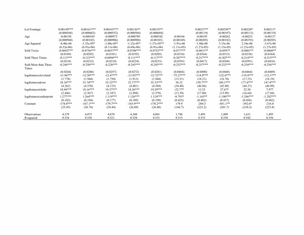
Lot Frontage 0.00149*** 0.00161*** 0.00165*** 0.00136** 0.00155** 0.00237** 0.00258** 0.00220* 0.00211* (0.000568) (0.000603) (0.000552) (0.000586) (0.000604) (0.00119) (0.00107) (0.00113) (0.00119) Age -0.00150 -0.000345 -0.000973 -0.000789 -0.000342 -0.00166 -0.00195 -0.00262 -0.00251 -0.00137 (0.000960) (0.00102) (0.000906) (0.000988) (0.00103) (0.00169) (0.00205) (0.00182) (0.00193) (0.00205) Age Squared -8.40e-06 -1.35e-05* -1.08e-05* -1.12e-05* -1.37e-05** -1.91e-06 -1.80e-06 3.15e-06 2.34e-06 -3.67e-06 (6.52e-06) (6.91e-06) (6.11e-06) (6.69e-06) (6.91e-06) (1.11e-05) (1.27e-05) (1.15e-05) (1.21e-05) (1.27e-05) Sold Twice -0.0692*** -0.0756*** -0.0657*** -0.0708*** -0.0752*** -0.0777** -0.0831** -0.0597* -0.0801** -0.0860** (0.0189) (0.0205) (0.0181) (0.0195) (0.0205) (0.0334) (0.0364) (0.0315) (0.0338) (0.0364) Sold Three Times -0.113*** -0.123*** -0.0994*** -0.111*** -0.117*** -0.207*** -0.217*** -0.182*** -0.214*** -0.215*** (0.0218) (0.0232) (0.0210) (0.0224) (0.0233) (0.0393) (0.0417) (0.0368) (0.0391) (0.0416) Sold More than Three Times

-0.244*** -0.250*** -0.228*** -0.245*** -0.245*** -0.252*** -0.257*** -0.232*** -0.254*** -0.256***

(0.0264) (0.0280) (0.0257) (0.0272) (0.0281) (0.0468) (0.0490) (0.0448) (0.0464) (0.0489) logdistancecleveland -11.96*** -12.50*** -12.47*** -12.92*** -12.72*** -75.27*** -114.9*** -122.6*** -119.4*** -112.1*** (1.778) (1.944) (1.750) (1.913) (1.944) (13.51) (18.21) (16.70) (17.23) (18.19) logdistanceakron 34.18*** 33.74*** 35.32*** 33.77*** 35.33*** 56.32 159.7*** 189.1*** 177.6*** 147.4*** (4.262) (4.570) (4.135) (4.481) (4.584) (34.40) (46.94) (42.80) (44.27) (46.99) logdistancetoledo 18.94*** 18.16*** 19.37*** 18.26*** 19.29*** -22.77* 13.23 27.67* 22.58 7.977 (2.446) (2.567) (2.347) (2.494) (2.578) (13.39) (17.80) (15.99) (16.64) (17.84) logdistanceceaderpoint 1.277*** 1.264*** 1.119*** 1.126*** 1.124*** -0.793* -1.165** -1.190*** -1.246*** -1.282*** (0.182) (0.194) (0.177) (0.189) (0.198) (0.425) (0.482) (0.437) (0.456) (0.482) Constant -174.8*** -167.1*** -179.7*** -165.9*** -178.2*** 179.9 -284.3 -451.1** -392.6* -216.8 (25.45) (26.76) (24.44) (26.09) (26.88) (166.7) (223.2) (201.7) (210.2) (223.8) Observations 4,579 4,075 4,870 4,360 4,041 1,746 1,495 1,809 1,631 1,495 R-squared 0.524 0.530 0.521 0.528 0.531 0.515 0.533 0.530 0.542 0.536

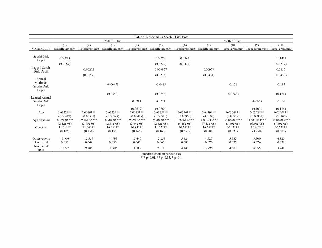
Table 5: Repeat Sales Secchi Disk Depth

Within 30km Within 10km (1) (2) (3) (4) (5) (6) (7) (8) (9) (10)

VARIABLES logselleramount logselleramount logselleramount logselleramount logselleramount logselleramount logselleramount logselleramount logselleramount logselleramount

Secchi Disk Depth 0.00835 0.00761 0.0567 0.114**

(0.0189) (0.0222) (0.0424) (0.0517) Lagged Secchi

Disk Depth 0.00292 0.000827 0.00973 0.0137

(0.0197) (0.0215) (0.0431) (0.0459) Annual

Minimum Secchi Disk

Depth

-0.00458 -0.0485 -0.131 -0.187

(0.0540) (0.0744) (0.0883) (0.121) Lagged Annual

Secchi Disk Depth

0.0291 0.0221 -0.0655 -0.136

(0.0639) (0.0764) (0.103) (0.116) Age 0.0152*** 0.0169*** 0.0153*** 0.0163*** 0.0165*** 0.0346*** 0.0439*** 0.0306*** 0.0392*** 0.0399***

(0.00417) (0.00505) (0.00395) (0.00478) (0.00511) (0.00860) (0.0102) (0.00778) (0.00935) (0.0105) Age Squared -8.89e-05*** -9.16e-05*** -8.98e-05*** -9.09e-05*** -9.20e-05*** -0.000235*** -0.000310*** -0.000207*** -0.000261*** -0.000285***

(2.42e-05) (2.79e-05) (2.31e-05) (2.64e-05) (2.82e-05) (6.16e-05) (7.43e-05) (5.60e-05) (6.60e-05) (7.69e-05) Constant 11.01*** 11.06*** 10.93*** 10.85*** 11.07*** 10.28*** 10.20*** 10.47*** 10.61*** 10.27***

(0.126) (0.154) (0.135) (0.166) (0.168) (0.253) (0.281) (0.233) (0.258) (0.300)

Observations 13,903 12,559 14,793 13,440 12,259 5,424 4,927 5,782 5,300 4,825 R-squared 0.050 0.044 0.050 0.046 0.043 0.080 0.070 0.077 0.074 0.079 Number of

fixid 10,722 9,785 11,305 10,389 9,611 4,148 3,798 4,380 4,055 3,741

Standard errors in parentheses *** p<0.01, ** p<0.05, * p<0.1

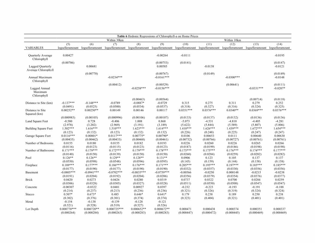
Table 6 Hedonic Regressions of Chlorophyll-a on Home Prices

Within 30km Within 10km (5) (6) (7) (8) (9) (10) (11) (12) (13) (14) VARIABLES logselleramount logselleramount logselleramount logselleramount logselleramount logselleramount logselleramount logselleramount logselleramount logselleramount

Quarterly Average Chlorophyll

0.00427 -0.00264 -0.0111 -0.0195

(0.00706) (0.00753) (0.0141) (0.0147) Lagged Quarterly

Average Chlorophyll 0.00681 0.00585 -0.0138 -0.0121

(0.00770) (0.00767) (0.0149) (0.0149) Annual Maximum

Chlorophyll -0.0234*** -0.0161*** -0.0300*** -0.0148

(0.00412) (0.00529) (0.00641) (0.0111) Lagged Annual

Maximum Chlorophyll

-0.0258*** -0.0156*** -0.0331*** -0.0207*

(0.00463) (0.00564) (0.00714) (0.0118) Distance to Site (km) -0.137*** -0.148*** -0.0789 -0.0887* -0.0729 0.315 0.275 0.311 0.279 0.252 (0.0491) (0.0525) (0.0500) (0.0534) (0.0537) (0.318) (0.327) (0.316) (0.324) (0.325) Distance to Site Squared (km)

0.00252** 0.00250** 0.00149 0.00146 0.00117 0.0351*** 0.0376*** 0.0340** 0.0369*** 0.0376***

(0.000983) (0.00105) (0.000996) (0.00106) (0.00107) (0.0133) (0.0137) (0.0132) (0.0136) (0.0136) Land Square Feet -0.580 0.728 -0.406 1.008 0.868 -5.073 -4.531 -4.810 -4.405 -4.281 (2.978) (3.202) (2.969) (3.191) (3.189) (5.622) (5.844) (5.589) (5.807) (5.806) Building Square Feet 1.502*** 1.616*** 1.510*** 1.623*** 1.614*** 1.410*** 1.626*** 1.439*** 1.672*** 1.654*** (0.123) (0.132) (0.123) (0.132) (0.132) (0.226) (0.248) (0.225) (0.247) (0.247) Garage Square Feet 0.0116*** 0.00801* 0.0117*** 0.00775* 0.00790* 0.0106 0.00653 0.0111 0.00640 0.00630 (0.00435) (0.00462) (0.00433) (0.00460) (0.00461) (0.00732) (0.00766) (0.00727) (0.00761) (0.00761) Number of Bedrooms 0.0155 0.0180 0.0155 0.0182 0.0193 0.0226 0.0260 0.0226 0.0265 0.0266 (0.0116) (0.0123) (0.0115) (0.0123) (0.0123) (0.0187) (0.0199) (0.0186) (0.0198) (0.0198) Number of Bathrooms 0.171*** 0.179*** 0.172*** 0.179*** 0.178*** 0.175*** 0.175*** 0.176*** 0.174*** 0.177*** (0.0140) (0.0150) (0.0139) (0.0150) (0.0150) (0.0260) (0.0284) (0.0259) (0.0282) (0.0282) Pool 0.126** 0.126** 0.129** 0.128** 0.131** 0.0906 0.123 0.105 0.137 0.137 (0.0550) (0.0598) (0.0548) (0.0596) (0.0595) (0.145) (0.159) (0.144) (0.158) (0.158) Fireplace 0.189*** 0.177*** 0.186*** 0.176*** 0.171*** 0.205*** 0.195*** 0.197*** 0.185*** 0.185*** (0.0177) (0.0190) (0.0177) (0.0190) (0.0190) (0.0332) (0.0357) (0.0330) (0.0356) (0.0356) Basement -0.0805*** -0.0941*** -0.0702*** -0.0835*** -0.0759*** -0.00566 -0.0250 0.000148 -0.0215 -0.0238 (0.0191) (0.0204) (0.0192) (0.0204) (0.0206) (0.0356) (0.0379) (0.0354) (0.0376) (0.0377) Brick 0.0420 0.0273 0.0426 0.0280 0.0319 0.0737 0.0322 0.0700 0.0284 0.0259 (0.0306) (0.0328) (0.0305) (0.0327) (0.0328) (0.0511) (0.0550) (0.0508) (0.0547) (0.0547) Concrete -0.00307 -0.0322 0.0401 0.00927 0.0397 -0.232 -0.223 -0.193 -0.191 -0.188 (0.214) (0.237) (0.213) (0.236) (0.236) (0.321) (0.326) (0.319) (0.324) (0.324) Stucco 0.507* 0.673* 0.485 0.646* 0.641* 0.179 0.238 0.189 0.250 0.238 (0.302) (0.376) (0.301) (0.374) (0.374) (0.323) (0.404) (0.321) (0.401) (0.401) Metal -0.154 -0.138 -0.139 -0.128 -0.121 (0.521) (0.528) (0.519) (0.527) (0.526) Lot Depth 0.000770*** 0.000720** 0.000725*** 0.000652** 0.000672** 0.000471 0.000438 0.000374 0.000351 0.000337 (0.000264) (0.000284) (0.000263) (0.000283) (0.000283) (0.000447) (0.000472) (0.000445) (0.000469) (0.000469)

Lot Frontage 0.00165*** 0.00141** 0.00163*** 0.00133** 0.00136** 0.00274** 0.00249** 0.00232** 0.00221** 0.00215* (0.000552) (0.000588) (0.000550) (0.000586) (0.000587) (0.00107) (0.00113) (0.00107) (0.00112) (0.00112) Age -0.00109 -0.000960 -0.000816 -0.000813 -0.000765 -0.00297 -0.00324* -0.00174 -0.00209 -0.00200 (0.000906) (0.000990) (0.000904) (0.000986) (0.000990) (0.00182) (0.00193) (0.00182) (0.00193) (0.00194) Age Squared -1.04e-05* -1.06e-05 -1.12e-05* -1.06e-05 -1.12e-05* 4.52e-06 4.94e-06 -6.47e-07 7.43e-07 2.67e-07 (6.12e-06) (6.70e-06) (6.10e-06) (6.68e-06) (6.68e-06) (1.15e-05) (1.21e-05) (1.15e-05) (1.21e-05) (1.21e-05) Sold Twice -0.0662*** -0.0697*** -0.0650*** -0.0698*** -0.0679*** -0.0581* -0.0766** -0.0595* -0.0798** -0.0784** (0.0181) (0.0196) (0.0181) (0.0195) (0.0195) (0.0315) (0.0339) (0.0313) (0.0337) (0.0337) Sold Three Times -0.101*** -0.115*** -0.0979*** -0.112*** -0.110*** -0.182*** -0.215*** -0.177*** -0.210*** -0.207*** (0.0210) (0.0224) (0.0209) (0.0223) (0.0224) (0.0369) (0.0393) (0.0367) (0.0390) (0.0391) Sold More than Three Times

-0.231*** -0.249*** -0.224*** -0.242*** -0.238*** -0.237*** -0.256*** -0.221*** -0.248*** -0.242***

(0.0257) (0.0272) (0.0257) (0.0271) (0.0272) (0.0449) (0.0466) (0.0447) (0.0463) (0.0464) logdistancecleveland -12.45*** -12.72*** -12.40*** -12.61*** -12.56*** -125.0*** -124.0*** -117.6*** -116.7*** -116.3*** (1.751) (1.918) (1.745) (1.910) (1.915) (16.68) (17.32) (16.66) (17.22) (17.27) logdistanceakron 35.38*** 33.58*** 36.28*** 34.61*** 35.98*** 197.0*** 193.3*** 178.5*** 177.7*** 172.5*** (4.141) (4.492) (4.128) (4.480) (4.497) (42.69) (44.30) (42.61) (44.12) (44.23) logdistancetoledo 19.25*** 18.03*** 20.59*** 19.59*** 20.75*** 30.64* 28.68* 25.83 25.70 22.81 (2.351) (2.500) (2.353) (2.507) (2.523) (15.95) (16.63) (15.87) (16.53) (16.59) logdistanceceaderpoint 1.190*** 1.284*** 0.884*** 0.973*** 0.890*** -1.111** -1.117** -1.277*** -1.348*** -1.316*** (0.174) (0.186) (0.182) (0.194) (0.197) (0.437) (0.456) (0.436) (0.456) (0.456) Constant -179.5*** -165.0*** -189.0*** -175.7*** -194.3*** -490.3** -473.4** -414.6** -414.6** -378.7* (24.50) (26.17) (24.44) (26.14) (27.08) (201.2) (210.0) (200.4) (208.4) (209.1) Observations 4,870 4,360 4,870 4,360 4,326 1,809 1,631 1,809 1,631 1,631 R-squared 0.520 0.526 0.524 0.529 0.529 0.529 0.538 0.534 0.544 0.545

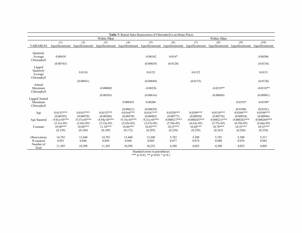
Table 7: Repeat Sales Regressions of Chlorophyll-a on Home Prices

Within 30km Within 10km (1) (2) (3) (4) (5) (6) (7) (8) (9) (10)

VARIABLES logselleramount logselleramount logselleramount logselleramount logselleramount logselleramount logselleramount logselleramount logselleramount logselleramount

Quarterly Average

Chlorophyll 0.00439 -0.00342 0.0167 0.00586

(0.00743) (0.00829) (0.0120) (0.0134) Lagged

Quarterly Average

Chlorophyll

0.0124 0.0125 0.0125 0.0133

(0.00841) (0.00849) (0.0135) (0.0138) Annual

Maximum Chlorophyll

-0.000802 -0.00226 -0.0219** -0.0218**

(0.00545) (0.00616) (0.00884) (0.00981) Lagged Annual

Maximum Chlorophyll

0.000435 0.00206 -0.0192* -0.0190*

(0.00621) (0.00629) (0.0100) (0.0101) Age 0.0153*** 0.0167*** 0.0152*** 0.0164*** 0.0161*** 0.0320*** 0.0399*** 0.0310*** 0.0394*** 0.0398***

(0.00395) (0.00479) (0.00396) (0.00478) (0.00482) (0.00777) (0.00938) (0.00776) (0.00934) (0.00944) Age Squared -9.01e-05*** -9.37e-05*** -8.94e-05*** -9.15e-05*** -9.21e-05*** -0.000217*** -0.000265*** -0.000213*** -0.000263*** -0.000269***

(2.31e-05) (2.65e-05) (2.32e-05) (2.65e-05) (2.67e-05) (5.59e-05) (6.62e-05) (5.57e-05) (6.59e-05) (6.66e-05) Constant 10.90*** 10.80*** 11.10*** 10.86*** 10.85*** 10.33*** 10.48*** 10.70*** 10.35*** 10.52***

(0.139) (0.169) (0.149) (0.172) (0.203) (0.238) (0.259) (0.243) (0.284) (0.334)

Observations 14,793 13,440 14,793 13,440 13,209 5,782 5,300 5,782 5,300 5,217 R-squared 0.051 0.046 0.050 0.046 0.045 0.077 0.074 0.080 0.076 0.082 Number of

fixid 11,305 10,389 11,305 10,389 10,252 4,380 4,055 4,380 4,055 4,005

Standard errors in parentheses *** p<0.01, ** p<0.05, * p<0.1

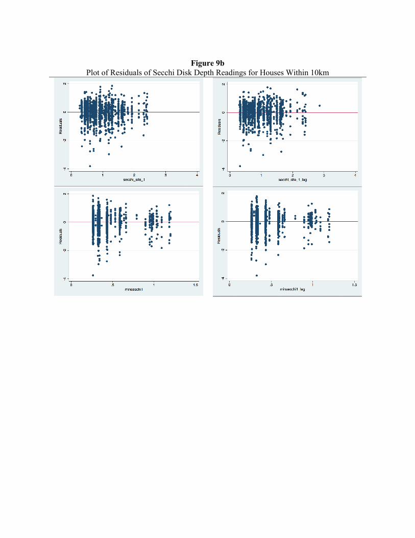
Figure 9b

Plot of Residuals of Secchi Disk Depth Readings for Houses Within 10km

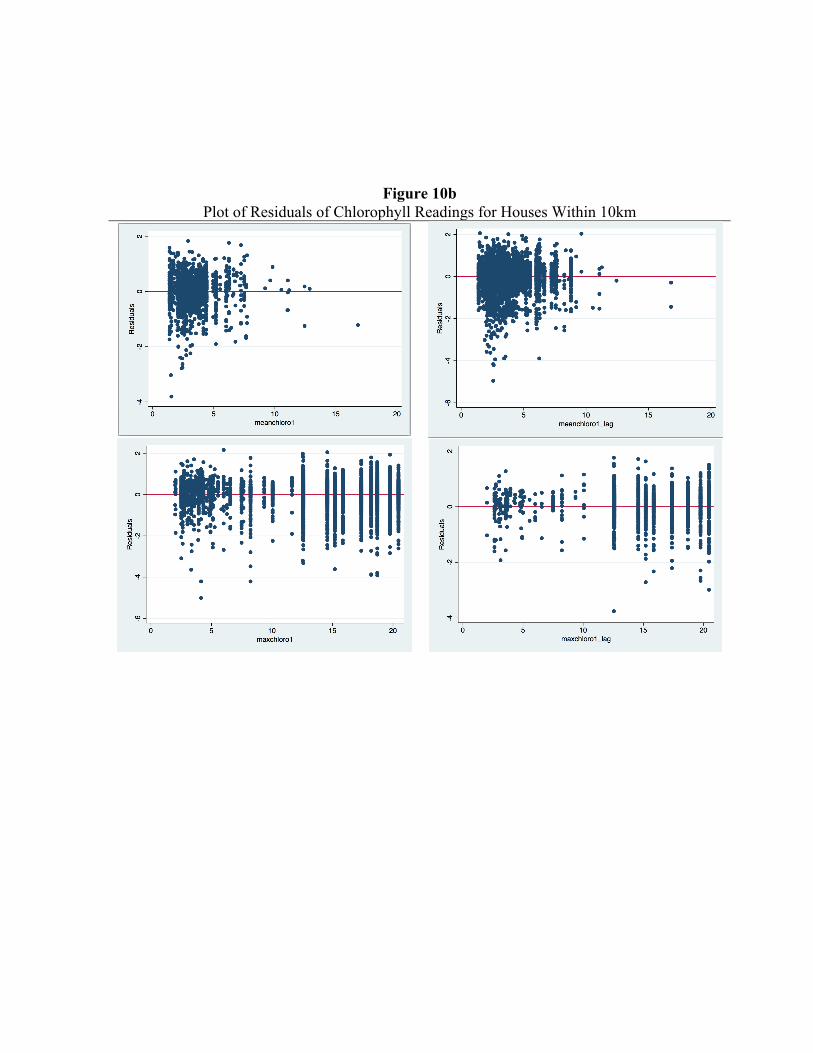
Figure 10b Plot of Residuals of Chlorophyll Readings for Houses Within 10km