Journal of Econometrics 13 (1980) 83-100. 0 North-Holland Publishing Company

ESTIMATING STOCHASTIC PRODUCTION AND COST FRONTIERS WHEN TECHNICAL AND

ALLOCATIVE INEFFICIENCY ARE CORRELATED*

Peter SCHMIDT

Michigan State University, East Lansing, MI 48824, USA

C.A. Knox LOVELL

University of North Carolina, Chapel Hill, NC 27514, USA

1. Introduction

In a recent paper [Schmidt and Love11 (1979) referred to hereafter as SL], we developed stochastic .frontier models of production, cost and factor

demand. The purpose of that paper was to show how such frontiers might be specified, to develop alternative estimation techniques for the stochastic

frontier models, and to show how to measure technical and allocative inefficiency, and their cost, relative to these stochastic frontiers.

However, SL assumed that there was no correlation between technical and

allocative inefficiency. The purpose of this paper is tosuggest why one might wish to relax that assumption, and to show how to do so in such a manner that one can test for the presence of such correlation. We are also interested in the effect of such correlation on estimates of frontier technology, and on the associated estimates of technical and allocative inefficiency and their cost.

The plan of the paper is as follows. Section 2 briefly reviews the salient features of the SL model and discusses the possible relationship between technical and allocative inefficiency. Section 3 develops a statistical model which allows correlated inefficiency. Section 4 presents an empirical illustration, and the last section gives our conclusions.

2. The relationship between technical and allocative inefficiency

We base our discussion on the model presented in sections 3 and 4 of SL,

*This paper is based upon work supported by the National Science Foundation under Grant No. Soc78-12447. We are indebted to E.R. Berndt and two referees of the Journal for their helpful comments. The usual caveat applies.

84 P. Schmidt and C.A.K. LoveIl, Stochastic production and cost,frontiers

which we summarize here. The production function is given by

lny=A+ i ccilnxi+v-u, (1) i=l

where y is output, the xi are inputs, v- N (0, CJ~), and u is the absolute value of a variable distributed as N (0, cr,“). The disturbances u and u are assumed

independent of each other; this seems reasonable since v represents the influence of factors outside the control of the firm, while u represents technical errors of the firm. Technical inefficiency relative to the stochastic

production frontier is given by u percent. For more discussion, see Aigner, Love11 and Schmidt (1977).

Assuming that output is exogenous to the firm, and that the firm attempts to minimize cost subject to the constraint (l), the first-order conditions are of

the form

lnxi-lnxi=ln(cc,pi/aip,)+ci, i=2,...,n, (2)

where pi are input prices and the ci represent allocative errors of the firm.

That is, ai measures the percent by which the chosen xi/xi ratio exceeds its cost minimizing value. It was assumed in SL that c= (Ed,. . .,a”)‘- N (I*, C), and that E is independent of v and u. SL showed how to estimate the system

consisting of (1) and (2), and showed how to use the associated cost function to make inferences about the costs of technical and allocative inefficiency.

Incidentally, we note that if output is not exogenous to the firm, and if profit maximization is the appropriate behavioral assumption, we can simply replace the set of n- 1 cost minimizing conditions (2) with a set of n profit

maximizing conditions, in which the disturbances would still represent allocative errors of the firm. This resulting system could then be estimated by simple modifications of the technique previously proposed. We state this explicitly to make it clear that the basic idea of both SL and this paper is applicable to a wider class of situations than those in which output is

exogenous to the firm. We now turn to the point of current interest, which is the relationship

among the disturbances v, u and E. In SL all three were assumed to be independent of each other. In as much as u represents the influence of factors outside the control of the firm, we feel that it is reasonable to assume that u is independent of u and E, which represent the influence of factors under the control of the firm. [This is consistent with the assumptions underlying most previous similar work; see, e.g., Zellner, Kmenta and Dreze (1966, p. 328).]

On the other hand, the assumed independence of u and E is much more questionable. The statistical question of whether or not the disturbances u

P. Schmidt and C.A.K. Lowell, Stochastic production and cost ,fronriers 85

and E are independently distributed is equivalent to the economic question of

whether or not technical and allocative inefficiency are independently distributed across firms. At first blush the question seems trivial and its

answer obvious. Well-managed firms operate close to their production frontiers and close to their least-cost expansion paths, while poorly managed firms do neither. There is little reason to expect to find firms whose managers perform one task well and the other poorly. Hence technical and allocative inefficiency might be expected to be positively correlated, and the statistical specification should permit a positive relationship between u and E.

Unfortunately the analogy between the two types of inefficiency and the

two disturbances is not that simple. As Farrell (1957) originally noted, and as Carlsson (1972), Johansen (1972) Forsund and Hjalmarsson (1974) and others have reiterated, the pursuit of technical and allocative efficiency is a

dynamic problem, while the representation of technical and allocative inefficiency by means of the disturbances u and E is static. As a result, even if

technical and allocative inefliciency are positively correlated over a period of time, in accordance with our reasoning above, the relationship between u and

E in any given year is unpredictable. To illustrate, consider an industry experiencing embodied technical

progress. Unless all firms invest at the same time and modernize at the same time, some firms must be technically inefficient relative to others on our static representation, even if all firms are following an efficient dynamic

investment program. Similarly, suppose that the industry’s technology is of the putty-clay variety, so that input substitution possibilities are severely limited once equipment is installed. In such a case, dynamically eflicient firms

will adjust factor proportions not to input prices prevailing at the time of

installation, but rather to some weighted average of discounted expected future input prices. Then if input prices do change over time, even perfect foresight must produce allocative inefficiency in most, if not all, years. Again, some firms must be allocatively inefficient on our static representation, even if all firms are following an efficient dynamic program.

Many other illustrations could be cited [Fuss and McFadden (1971) cite several], but by now two things should be apparent. First, the use of our static measures of technical and allocative inefficiency in a necessarily

dynamic setting requires careful interpretation, since measured static inefficiency may in fact be a planned part of an efficient dynamic program. Second, while we may continue to expect a positive correlation between technical and allocative inefficiency in a dynamic sense, it is not clear that we should expect such a relationship between our static measures of technical and allocative inefficiency. All of this is not to suggest that we necessarily believe strongly in the SL assumption that u and E are independent. Rather, we regard the issue as an empirical question, one which should and can be

tested. An if it turns out that u and F are not independent, we are of course

interested in the effect their correlation has on our estimates of frontier technology, and on our estimates of technical and allocative inefficiency.

3. Correlated inefficiencies: Statistical issues

We now wish to allow correlation between technical and allocative inefficiency. From a statistical point of view, this is an interesting problem since we want to permit u to be correlated not with q, i = 2,. . ., n, but with 1~~1. For example, suppose that input 1 is capital and input 2 is labor, so that

82 is the percentage mistake in choosing the capital-labor ratio. The assertion that u and s2 are positively correlated would be the assertion that technically inefficient firms have a higher capital-labor ratio, on average,

than do technically efficient firms, which is not what we have in mind. On the other hand, the assertion that u and 1~~1 are correlated in the assertion that technically inefficient firms have capital-labor ratios which are more in error (either too high or too low) than are the capital-labor ratios of

technically efficient firms, which is what we have in mind. In other words, we simply need to recognize that, as far as the extent of allocative inefficiency is concerned, what is relevant is not the size of q but the size of /ail.

This leads us to the following model: Let c -N(O,a:), as before. Let

where

(3)

(4)

and define

Ld=ILl*(. (5)

Finally, assume that r is independent of (~*,a’)‘. We note that L’ - N(0, u:), u is the absolute value of a variable distributed

as N(O,ai), and c-N(p,C,,); all of these facts are consistent with the specification of SL. Indeed if C,, #O then IA* and E are correlated. This implies, given u = lu*l, that u is uncorrelated with ai, i= 2,. . ., II, but is correlated positively with (~~1.

To substantiate the claim that u is uncorrelated with ci, let f’(u*,ci) be the

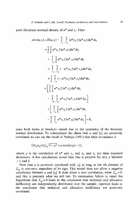
P. Schmidt and C.A.K. Love& Stochastic production and cost frontiers 87

joint (bivariate normal) density of u* and si. Then

COV(U,E~)=E(U,E~)= 4 7 l~*l~if(~*,~i)d~*d~i -30 -m

= $ % u* q f(u*, ei) du* dq

+ 7 Tu*sif(u*,ai)du*dq -co 0

+ j! j! (-u*)aif(u*,si)du*dai -m --ocI

+$ _yJ-u*)sJ(u*.si)du*dsi

= % [u*~J(u*.~-:~)du*di:~ 1

4 “s u* ai f (u*, si) du* dsi -03 -m 1

0 m

+ s 1 u*sif(u*,si)du*dsi -m 0

- 7 j! u*sif(u*,ai)du*dsi 1 =O, 0 -Cc

since both terms in brackets vanish due to the symmetry of the bivariate normal distribution. To substantiate the claim that u and 1.~~1 are positively correlated we can use the result of Nabeya (1951) that their covariance is

(2fr,~&) [Jm + p arcsin (p) - 11,

where p is the correlation of u* and si, and 6, and aE are their standard deviations. A few calculations reveal that this is positive for any p between

- 1 and 1. Note that u is positively correlated with /ai/ as long as the ith element of

C,, is non-zero, regardless of its sign. This model does not allow a negative

correlation between u and 1~~1. It does allow a zero correlation, when C,,=O, and this is precisely what we will test. To summarize, failure to reject the hypothesis that C,, =0 leads to the conclusion that technical and allocative inefficiency are independently distributed over the sample; rejection leads to the conclusion that technical and allocative inefficiency are positively correlated.

xx P. Schmidt und C.A.K. Lotell, Stochustic production und cost frontiers

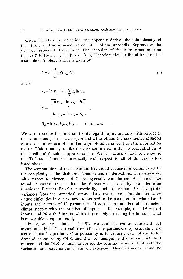
Given the above specification, the appendix derives the joint density of (r-u) and E. This is given by eq. (A.l) of the appendix. Suppose we let ,f(r --u,E) represent this density. The Jacobian of the transformation from (v--,E’)’ to [In x1,. .,lnx,]’ is r=cicq. Therefore the likelihood function for a sample of T observations is given by

where

w, = In y1 - A - C cli In xi,,

lnx,,-lnx,,-B,,

&= i

[ I> In XIr - In x,~ - B,,

Bi, = ln (a 1 PitIaiPl f L i=2,...,n.

We can maximize this function (or its logarithm) numerically with respect to

the parameters (A, or,. .,an, CT:, p and C) to obtain the maximum likelihood

estimates, and we can obtain their asymptotic variances from the information matrix. Unfortunately, unlike the case considered in SL, no concentration of the likelihood function appears feasible. We will actually have to maximize the likelihood function numerically with respect to all of the parameters listed above.

The computation of the maximum likelihood estimates is complicated by the complexity of the likelihood function and its derivatives. The derivatives

with respect to elements of C are especially complicated. As a result we found it easiest to calculate the derivatives needed by our algorithm

(DavidsonFletcher-Powell) numerically, and to obtain the asymptotic variances from the numerical second derivative matrix. This did not cause undue difftculties in our example (described in the next section), which had 3 inputs and a total of 13 parameters. However, the number of parameters climbs steeply with the number of inputs - for example, it is 19 with 4 inputs, and 26 with 5 inputs, which is probably stretching the limits of what

is reasonable computationally. Finally, we note that, as in SL, we could arrive at consistent but

asymptotically inefficient estimates of all the parameters by estimating the factor demand equations. One possibility is to estimate each of the factor demand equations by OLS, and then to manipulate the second and third moments of the OLS residuals to correct the constant terms and estimate the variances and covariances of the disturbances. These estimates would be

P. Schmidt and C.A.K. Lowll, Stochastic production und costjiiontirrs x9

messy since n estimates of cli would be obtained and since we might find 6;

~0 and/or 2 not positive definite, and are therefore not recommended. On

the other hand, since the disturbances in the various factor demand equations are correlated, and since the same parameters appear in each equation, a constrained GLS approach would be more reasonable. While these estimates would still not be as efficient as the MLE’s, they would be superior to the OLS estimates. The main problem with them is that it would

still be necessary to manipulate moments of the residuals to estimate ai, 0: and C (and to correct the estimated constant term), and thus we are still not guaranteed that 0: >O and that C is positive definite. As a result these estimates are reasonable mainly when one’s primary interest is in the technical parameters a,, . . ., cc,, and not in questions of efficiency. (And in such a case, there is frankly not much point in worrying about the ‘frontier’

aspects of the problem.)

4. Correlated inefficiencies: Empirical results

In this section we report the results of estimating the stochastic frontier

model given by eqs. (1) and (2) when technical and allocative inefficiencies are modelled by eqs. (3)-(5). The data set we use is the same as that used in SL. Briefly, the data set consists of a sample of 111 new privately owned

steam-electric generating plants constructed in the U.S. between 1947 and 1965. The sample contains observations on output, total cost, and prices and quantities of three inputs (capital, fuel and labor) for each plant. Output is

electricity generated (lo6 kWh) in the first year of operation, capital is the actual cost of the plant, fuel is the actual consumption (lo6 Btu) of fuel (coal, oil or gas) in the first year of operation, labor is the average number of

employees who worked at the plant during the year, measured in manhours (average number of employees x 2000) the price of capital is given by the firm’s bond rate prior to installation, the price of fuel is the actual price

($/lo6 Btu) of the dominant fuel used by the plant, averaged over the first three years of operation and the price of labor is the regional average industry wage rate ($/hour), averaged over the two years prior to plant installation.

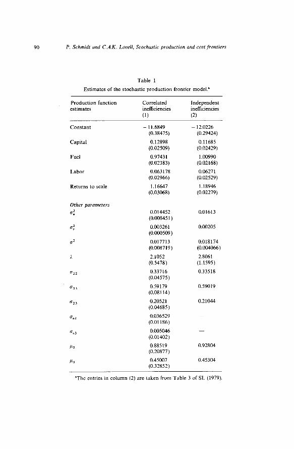
We report two sets of results in table 1. In column (1) we report maximum likelihood estimates of the stochastic frontier model that permits correlated inefficiencies, as given in eqs. (l)(5) above. In column (2) we report maximum likelihood estimates of the same model with independent inefficiencies; these results are taken from table 3 of SL. Numbers in parentheses in both columns are asymptotic standard errors.

Our interest in table 1 originates in the estimates of the two parameters 0 u2 and guJ, the only difference between the two models and the source of all

90 P. Schmidt and C.A.K. Looell, Stochastic production and cost frontiers

Table 1

Estimates of the stochastic production frontier model.”

Production function estimates

Correlated Independent inefficiencies inefficiencies

(1) (2)

Constant

Capital

-

Fuel

Labor

Returns to scale

Other parameters 2

0”

11.6849 (0.38475)

0.12898 (0.02509)

0.97431 (0.02383)

0.063178 (0.02966)

1.16647 (0.03068)

0.014452 (0.00845 1)

0.003261 (0.000509)

0.017713 (0.008719)

2.1052 (0.5478)

0.33716 (0.04575)

0.59179 (0.08114)

0.20521 (0.04685)

0.036529 (0.01186)

0.005046 (0.01402)

0.88519 (0.20877)

0.45007 (0.32852)

12.0226 (0.29424)

0.11685 (0.02429)

1.00990 (0.02168)

0.0627 1 (0.02529)

1.18946 (0.02279)

0.01613

0.00205

0.018174 (0.004066)

2.8061 (1.1595)

0.33518

0.59019

0.21044

0.92804

0.45304

“The entries in column (2) are taken from Table 3 of SL (1979).

P. Schmidt and C.A.K. Lowell, Stochastic production and cost frontiers 91

differences between columns (1) and (2). We do find some evidence that u

and 1.~1 are not distributed independently. The estimate of gU2 is significantly

different from zero at usual confidence levels although the estimate of gU3 is

not. The null hypothesis that crU2 = gU3 =0 is rejected with a joint test statistic

of 9.872, which is significant against x:(0.05). We conclude that technical and allocative inefficiency are not distributed independently across firms; technically efficient firms make smaller allocative errors than do technically inefficient firms, particularly with respect to their selection of capital-fuel ratios.

The finding that u and 1~1 are correlated leads to slight reductions in our

estimates of c(~ and p3, although we still find considerable overcapitalization relative to both fuel and labor on average over the sample. The likelihood ratio test statistic for testing the hypothesis pL2 =pL3 =0 is 120.055, which is still highly significant in x:. Correlation between u and 1~1 has a somewhat greater impact on our estimates of the magnitude and cost of technical and allocative inefficiency. The mean of the one-sided disturbance in the

production function (-u) is - 0.09592, indicating that 9.6 “/, technical inefficiency raises cost by 8.2 %. This compares with 10.1 y0 and 8.5 %,

respectively, with independent inefficiencies. In addition, the average cost of

allocative inefficiency is 8.1 %, compared with 9.2% with independent inefficiencies. The total cost of both types of inefficiency is therefore 16.3 y0 in the correlated inefficiencies case, compared with 17.7% in the independent inefficiencies case.

Finally, we note that the estimates of the production function parameters

are hardly affected by the generalization, although the small decline in the estimated fuel coefficient is sufficient to move it beneath unity. This strong

similarity in the two sets of estimates of frontier technology is comforting. It suggests that the way in which we model inefficiency relative to a stochastic frontier, and the nature of the inefficiency we find, has no appreciable effect on our inferences concerning the shape and placement of that frontier.

5. Conclusions

In this paper we have allowed for the possibility of positive correlation between technical and allocative inefficiency. A finding of such positive

correlation would be in accord with the intuitive supposition that poorly run firms will be poorly run both technically (operating far below their production frontiers) and allocatively (operating far from their least-cost expansion paths). On the other hand, we have presented some reasons why we might not find such a correlation, and which might therefore be used to defend the earlier SL assumption of independence of the two types of inefficiency.

92 P. Schmidt und C.A.K. Low& Stochastic production and cost frontiers

We have presented a model which allows for correlated inefficiencies, and

which contains the SL model as the special case corresponding to zero correlation. We have estimated the model using the same data set used in SL, consisting of data on 111 steam-electric generating plants. We do find evidence that technical and allocative inefficiency are correlated; and this correlation causes estimated magnitudes and costs of both technical and allocative inefficiency to decline relative to an estimated stochastic frontier

that remains essentially unaffected by the generalization. Whether this conclusion will hold in other empirical settings remains to be

seen, of course. If it does, it may be that allowing for correlation of technical

and allocative inefficiency is not always worth the extra bother. However, it should be stressed that there is no way to know this a priori; it is only by having techniques available to test the independence of the two sources of

inefficiency that we can obtain evidence on how reasonable the assumption of independence is.

Appendix

In this appendix we prove the following result:

Theorem. Suppose that

where t’ and u* are scalars and E is an N x 1 vector, and where v is

independent of u* and E. Define

u = Iu*l, w=v-u.

Then the joint density of w and E is

f(w,~)=[l-F(A)](2n)-‘~+‘)‘~[GI-~ ex p

x exp , (A.11

P. Schmidt and C.A.K. Louell, Stochastic production and cost frontiers 93

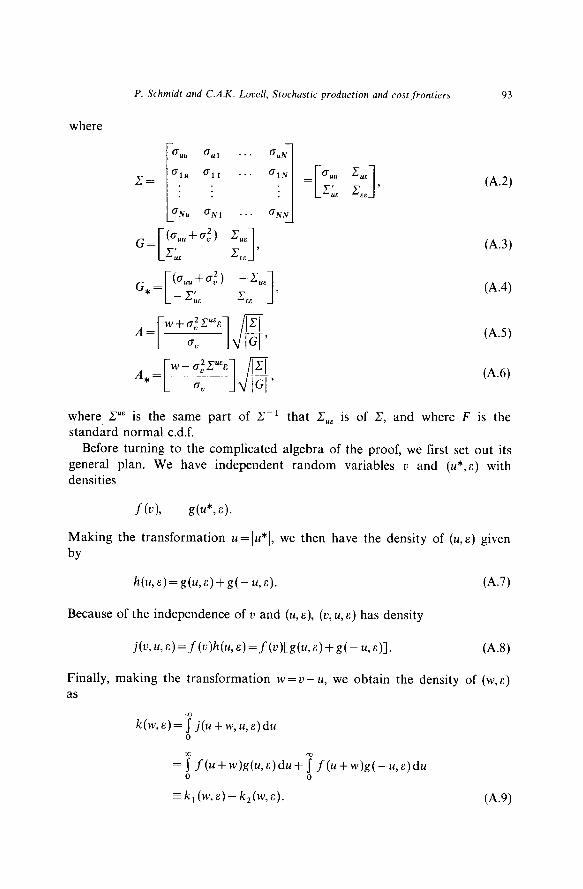
where

64.2)

(A.3)

64.4)

(A.5)

(A.6)

where C”” is the same part of C-l standard normal c.d.f.

that C,, is of C, and where F is the

Before turning to the complicated algebra of the proof, we first set out its general plan. We have independent random variables u and (u*,E) with densities

f(u), g(u*, 8).

Making the transformation u = Iu* 1, we then have the density of (~4,s) given

by

h(u,E)=g(u,&)+g(-u,&).

Because of the independence of u and (u, E), (u, U, E) has density

04.7)

j(u,u,&)=f(u)h(u,&)=f(u)Cg(u,&)+g(-u,&)l. WV

Finally, making the transformation w =u- u, we obtain the density of (w, E) as

k(w,s)=Tj(U+w,zq)du 0

=~f(ll+w)g(U,E)dlltTf(U+w)g(-U,E)dU 0

=k,(w,c)+k2(w,c). 64.9)

94 P. Schmidt urld C.A.K. Low/l, Stochustic production und cost ,fkmtiers

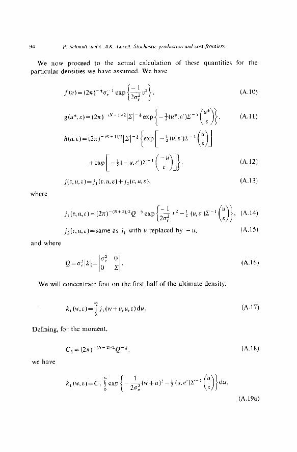
We now proceed to the actual calculation of these quantities for the particular densities we have assumed. We have

.f’(~)= (2x)-+0; ’ exp

,

(A.lO)

(A.1 1)

+exp ) (A.12)

j(v,u,&)=jl(U,U,E)+j2(Zi,U,E), (A.13)

where

jl(v,u,E)=(2n)m (N+WQ-fexp 2 &+ (U,E’)r l u 01 , (A.14)

12 E

j,(r, U,F:)=same as j, with u replaced by - U, (A.15)

and where

We will concentrate first on the first half of the ultimate density,

k,(w,c)=T j,(W+U,U,E)du. 0

Defining, for the moment,

cl = (,,)-(N+2)!2Q-f,

we have

(A.16)

(A.17)

(A.18)

du.

(A.19a)

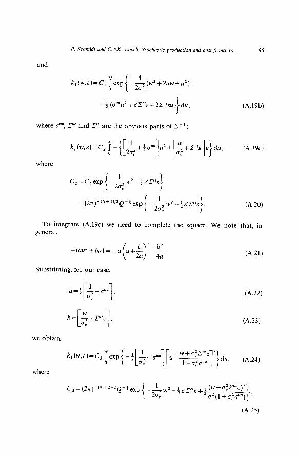
P. Schmidt and C.A.K. Lovell, Stochastic production and cost frontiers

and

k,(w,E)=Cl qexp 0 {

-&v~+2uw+u~) ”

- $ (d‘“u2 + E’CEEE + 2,Y’“&u) I

du,

where IS”‘, C”” and C”” are the obvious parts of C-l;

k,(w,e)=C2 T- 0

{[~+t~uu]~2+[~+=uE~]~)dv,

where

c, = c, exp i

- &v2 - )&‘.Y& ” I

= (2X)-‘N+2’/2 Q-*exp 1

--w2--$&‘CEE~

20;

95

(A.19b)

(A.19c)

(A.20)

To integrate (A.19~) we need to complete the square. We note that, in general,

-(au2+bu)=-a

Substituting, for our case,

we obtain

(A.21)

(A.22)

(A.23)

(A.24)

where

c, = (2n)-‘N+2)‘2Q-*exp -&w2_iE/pE ”

(A.25)

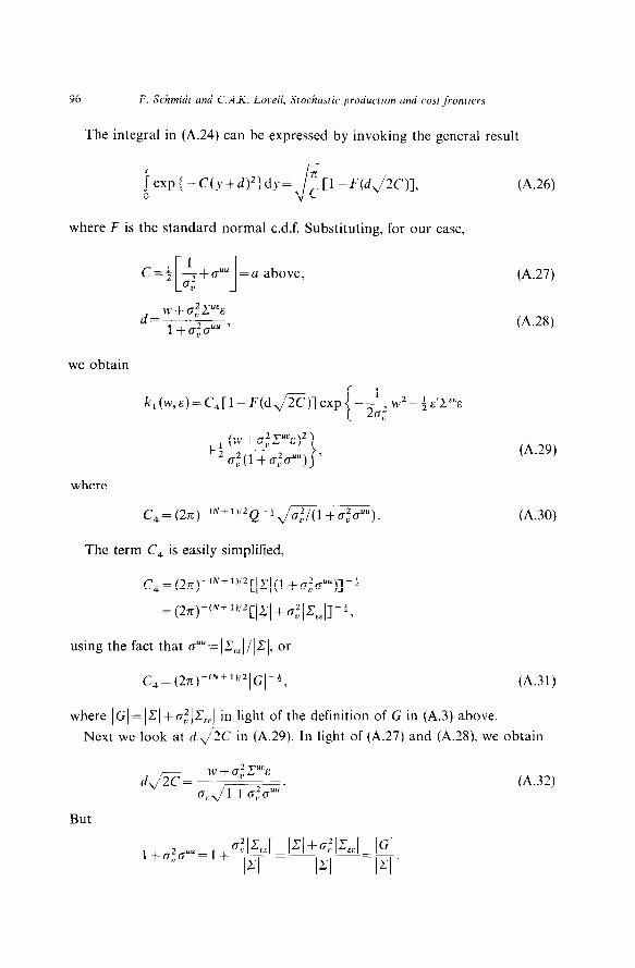
96 P. Schmidt and C.A.K. Louell, Stochastic production and costfrontiers

The integral in (A.24) can be expressed by invoking the general result

~exp(-C(y+d)z}d~= :[l-F(@C)], J

(A.26)

where F is the standard normal c.d.f. Substituting, for our case,

=u above, (A.27)

d= Wi-G2,Y&

l+o~cTuu ’ (A.28)

we obtain

k,(w,a)=C4[1-F(da)]exp -&w’-i~‘,Y% i L’

+’ (w+o;CUEE)2

2 cJ,z(l +D,2rY) I ’ (A.29)

where

Cq=(2+‘N+1)‘2Q-+&,Z/(1+&““). (A.30)

The term C, is easily simplified,

c,= (27L-‘N+1)‘2[~CJ(1 +U;cY)]-+

= (271)_ (N+1)‘2[(2_I+.tIC,,(]-f,

using the fact that c+‘“=~c,,~/~C(, or

c,= (27c_ (N+W[Gj-+, (A.31)

where \GI =jCl +olfIC,,l in light of the definition of G in (A.3) above.

Next we look at dfi in (A.29). In light of (A.27) and (A.28) we obtain

dm= w + G,‘PC

a,JiGp . (A.32)

But

I’. Schmidt und C.A.K. Loaell, Stochastic production und cost frontiers 97

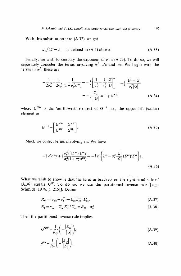
With this substitution into (A.32) we get

dfi=A, as defined in (AS) above. (A.33)

Finally, we wish to simplify the exponent of e in (A.29). To do so, we will

separately consider the terms involving w2, E’E and WE. We begin with the terms in w2, these are

(A.34)

where GNW is the ‘north-west’ element of G-l, i.e., the upper left (scalar)

element in

(A.35)

Next, we collect terms involving E’E. We have

(A.36)

What we wish to show is that the term in brackets on the right-hand side of

(A.36) equals GSE. To do so, we use the partitioned inverse rule [e.g.,

Schmidt (1976, p. 215)]. Define

R,= (CT,, +u;,- c,,c,‘c;,, (A.37)

R, = c,, - C,,C, 1 Z;, = R, - u;. (A.38)

Then the partitioned inverse rule implies

(A.39)

(A.40)

98 P. Schmidt and C.A.K. Love& Stochastic production and cost frontiers

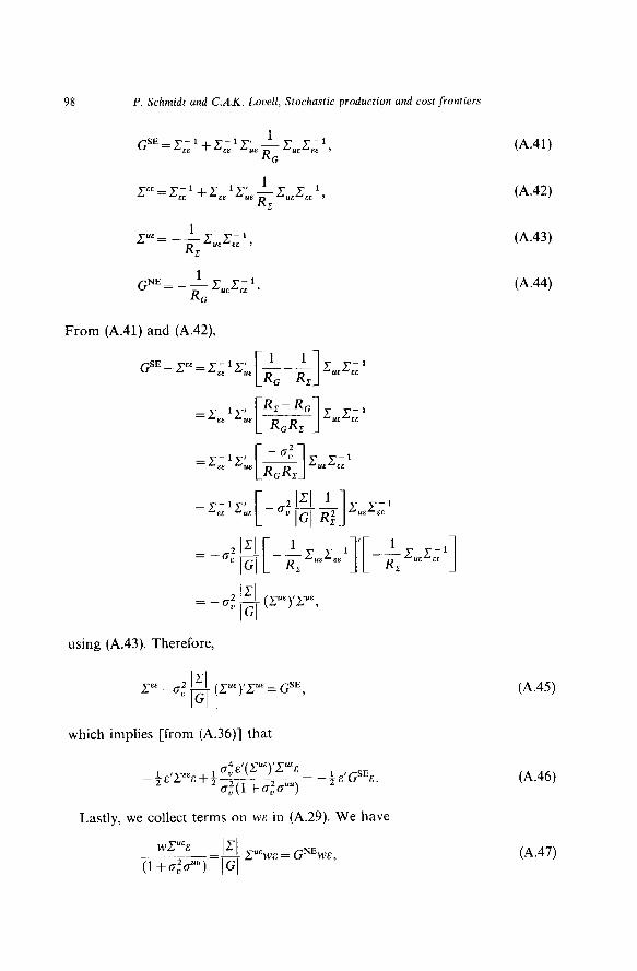
GSE = Z, ’ + C, ‘Z::, f C,,C, ‘, G

C”” = c, l + c, l c:, $ c,,c, l, ,?

C”” = - $ c,,c, l) r

GNE = - f C,,C, ‘. G

From (A.41) and (A.42),

1 1 G~E--==c-~CI ___ c C-1 EE UE [ 1 R, R, UC ='

2 ICI = - 0” IGI (CUE)‘CUE,

using (A.43). Therefore,

2 ICI C”“- 0” IGI (CUE)‘CUE= GSE,

which implies [from (A.36)] that

cT4&‘(CUE)‘CUE& _ *E’pEE+* ; O”(1 +O;C”“)

= - +c’GSEg.

Lastly, we collect terms on WE in (A.29). We have

WC”EE =H

P. Schmidt cmd C.A.K. Lowll, Stochastic production and cost frontiers 99

from (A.43) and (A.44),

(A.48)

We can now insert (A.31), (A.33) (A.34) (A.45) and (A.47) into (A.29) to obtain

.

(A.49)

This is the same as the first half of the right-hand side of (A.l), and completes the difficult part of the derivation.

The derivation of k2(w,c) follows the same lines as the derivation of

k, (w, a). Analogously to (A.19), we have

where

1 (A.51)

exactly the same as (A.19a) if we just replace C by C, throughout

replace C,, by -C,, throughout. (Note that Q is unaffected since As a result k, (w,E) is exactly the same as k, (w,E) with C,, and C””

But this is - that is,

ICI =M) replaced by - C,, and - P‘“. This gives

du

(A.50a)

du,

(ASOb)

k2(W,E)=[1-_(A*)](2~)-(N+1)!2 G, f exp-i(w,E’)G;l I I-{ .

(A.52)

loo P. Schmidt and C.A.K. Looell, Stochastic production and cost frontiers

Noting that ICI = IG*l, th’ IS is the same as the second half of the right-hand side of (A.l). This completes the derivation of (A.l).

We can also note that if the mean of E is p (rather than zero), we can just replace E everywhere in (A.l) by (E- ~0.

References

Aigner, D.J., C.A.K. Love11 and P. Schmidt, 1977, Formulation and estimation of stochastic frontier production function models, Journal of Econometrics 6, no. 1, July, 21-37.

Carlsson, B., 1972, The measurement of efficiency in production: An application to Swedish manufacturing industries, 1968, Unpublished Ph.D. dissertation (Department of Economics, Stanford University, Stanford, CA).

Farrell, M.J., 1957, The measurement of productive efficiency, Journal of the Royal Statistical Society A, General, 120, no. 3, 2533281.

Fdrsund, F.R. and L. Hjalmarsson, 1974, On the measurement of productive efficiency, Swedish Journal of Economics 72, no. 2, June, 141-154.

Fuss, M.A. and D.C. McFadden, 1971, Flexibility versus efficiency in ex ante plant design, Discussion paper no. 190 (Harvard Institute of Economic Research, Cambridge, MA).

Johansen, L., 1972, Production functions (North-Holland, Amsterdam). Nabeya, S., 1951, Absolute moments in two-dimensional normal distribution, Annals of the

Institute of Statistical Mathematics 3, 226. Schmidt, P., 1976, Econometrics (Marcel1 Dekker, New York). Schmidt, P. and C.A.K. Lovell, 1979, Estimating technical and allocative inefficiency relative to

stochastic production and cost frontiers, Journal of Econometrics 9, no. 4, Feb., 343-366. Zellner, A., J. Kmenta and J. D&e, 1966, Specification and estimation of Cobb-Douglas

production function models, Econometrica 34, no. 4, Oct., 784-795.