WP/14/40

Estimating Sri Lanka’s Potential Output

Ding Ding, John Nelmes, Roshan Perera, and Volodymyr Tulin

© 2014 International Monetary Fund WP/14/40

IMF Working Paper

Asia and Pacific Department

Estimating Sri Lanka’s Potential Output1

Prepared by Ding Ding, John Nelmes, Roshan Perera and Volodymyr Tulin

Authorized for distribution by Paul Cashin

March 2014

Abstract

In this paper we present various techniques to estimate Sri Lanka’s potential output and output gap, including statistical and model-based approaches. Compared to conventional statistical filters that rely exclusively on information in a single series, the model-based approaches allow potential output estimates to incorporate information contained in observable data series including inflation, actual output, unemployment and capacity utilization. The estimation results suggest that Sri Lanka’s potential output has risen slightly in the last few years.

JEL Classification Numbers:C32, C53, E31

Keywords: Potential Output, Output Gap, Multivariate Filter, Inflation Expectations, Capacity Utilization, Unemployment

Authors’ E-Mail Addresses: dding@imf.org; jnelmes@imf.org; roshan@cbsl.lk; vtulin@imf.org

1 We are grateful to Brian Aitken, Ben Bingham, Paul Cashin, Rahul Anand and our colleagues in the Asia and Pacific Department for helpful comments and discussions. We benefited from the feedback received from seminar participants at the Central Bank of Sri Lanka, in particular from Kosgallana Durage Ranasinghe.

This Working Paper should not be reported as representing the views of the IMF. The views expressed in this Working Paper are those of the author(s) and do not necessarily represent those of the IMF or IMF policy. Working Papers describe research in progress by the author(s) and are published to elicit comments and to further debate.

2

Contents Page I. Introduction ..........................................................................................................................3 II. Estimation Methodologies ...................................................................................................4 A. Univariate Statistical Filtering Methods ........................................................................4 B. The Multivariate Approach ............................................................................................4 C. The Production Function Approach ...............................................................................7 D. The Structural Vector Autoregression Approach ..........................................................8 III. The Data ...............................................................................................................................9 IV. Estimation Results .............................................................................................................11 A. Univariate Filters .........................................................................................................11 B. Multivariate Filter ........................................................................................................11 C. The Production Function..............................................................................................12 D. Structural VAR ............................................................................................................13 V. Conclusions and Policy Implications .................................................................................14 References ................................................................................................................................15

3

I. INTRODUCTION

Estimating the potential output of an economy is important, as it provides a useful benchmark for observable economic activity, and allows for the computation of the output gap.2 An economy that is operating above potential would often encounter capacity constraints that could lead to the buildup of inflation and, under certain circumstances, external balance of payments pressures. An economy with actual output below potential would often exhibit spare capacity, leading to a possible decline in those pressures. Potential output and output gap estimates are frequently used to calibrate macroeconomic policies, for example in determining the appropriate setting for monetary conditions, or in estimating structural fiscal balances and the growth impulse from the government budget. Because potential output is not directly observable, however, estimating it is subject to a degree of uncertainty.

This topic is particularly interesting for Sri Lanka because its economy grew rapidly over the two years following the end of the civil conflict in 2009, but thereafter reverted to around the average growth pace of the last decade. Did the growth spurt reflect faster potential output growth and thus a permanent upward shift in the country’s growth plane, or was it a transitory increase that may have pushed the economy up against capacity constraints? The answers to such questions are important from a longer-term perspective of Sri Lanka’s possible progression through the ranks of middle income status, and from a near-term perspective they would help to indicate whether using macroeconomic policy levers to stimulate a return to high growth could come at the cost of fostering macroeconomic imbalances. To date, however, there has been limited empirical work carried out to estimate Sri Lanka’s potential output.

This paper presents and compares estimates of Sri Lanka’s potential output and output gap from a number of filtering and model-based techniques. The simplest measures presented in the paper employ statistical univariate filters. The model-based approaches have the advantages of incorporating relevant information about the economy from observable data, and allow for a richer interpretation of the resulting estimates.

The paper is organized as follows. Section II describes the different methodologies used to estimate potential output and the output gap in Sri Lanka. Section III describes the data, and Section IV the compares the empirical estimation results. The final section provides concluding remarks.

2 Potential output is defined as the level of output that can be sustained over a period of time without generating inflation or deflation pressures. The output gap is defined as actual output minus potential output as a ratio of potential output (y-y*)/y*.

4

II. ESTIMATION METHODOLOGIES

The estimation techniques presented can be broadly categorized into four fields: (i) univariate statistical filters that attempt to distinguish between the permanent and cyclical components of output; (ii) a multivariate filtering approach that modifies the model presented in Benes et al (2010) for Sri Lanka, and incorporates information about the cyclical state of the economy from inflation, unemployment and capacity utilization; (iii) the standard Cobb-Douglas production function approach; and (iv) a structural vector autoregression (SVAR) approach based on the methodology developed by Blanchard and Quah (1989).

A. Univariate Statistical Filtering Methods

Four univariate methods are used to compute potential output. These include a Hodrick-Prescott filter, a piece-wise linear trend, a Baxter and King (1995) bandpass filter, and the Christiano-Fitzgerald (2003) filtering method:

The Hodrick-Prescott (HP) filter produces an estimate of potential output by minimizing the deviation of actual output from its trend, or potential, subject to a penalty on the maximum allowable change in trend growth between periods. The standard practice is to use a smoothness parameter equal to 1,600 for quarterly data and 100 for annual observations.

The piece-wise linear trend (LT) method fits a linear trend through the natural logarithm of GDP. Breaks in the series are tested using Chow and Quandt-Andrews tests.

The Baxter-King (BK) and Christiano-Fitzgerald (CF) band-pass filters accommodate business cycle dynamics using a range of business cycle frequencies to disentangle the cyclical from the trend components of output.

Univariate filters have the benefit of being widely used and understood, given their simplicity and ease of comparability. There are, however, several drawbacks. Because they rely on information from a single time series of data, one cannot attribute changes in potential growth to specific economic factors. Indeed, the choice of the smoothing parameter for the HP filter is not based on economic theory. As well, when the data to be filtered is integrated or nearly integrated, they can produce spurious cycles in de-trended data (Harvey and Jaeger 1993, Cogley and Nason 1995), and two-sided filters require manufactured data at the end of sample, resulting in biased end-sample estimates (Dupasquier et al 1997).

B. The Multivariate Approach

The multivariate (MV) approach used in this paper adapts the small macro model presented in Benes et al (2010) to Sri Lanka. Empirical estimates of theoretical relationships among actual and potential output, unemployment, inflation, and capacity utilization are used as conditioning information in a multivariate filter that captures long-run trends in the data. The multivariate approach is based on the conceptual definition of potential output as being the

5

level of output that may be sustained indefinitely without creating a tendency for inflation to rise or fall. In other words, a period in which inflation is stable would likely be a period in which actual output is equal to potential output. The key modeling adaptations for Sri Lanka involve incorporating service-sector capacity utilization and a generalized specification of the inflation-output trade-off.

Defining key variables

The model starts by defining three gaps: the output gap, the unemployment gap and the capacity utilization gap. The output gap is the log difference, in percent, between actual ( ) and potential ( ) GDP:

100 / (1)

The unemployment gap is the equilibrium unemployment rate, or non-accelerating inflation rate of unemployment (NAIRU), minus the actual unemployment rate :

(2)

The capacity utilization gap is the difference between the actual capacity utilization index and its equilibrium level :

(3)

Identifying relationships

The first identifying relationship is a Phillips curve-type of inflation equation linking inflation to the output gap:

(4)

where is the current annualized core inflation rate and is a shock term. The inflation equation incorporates the standard trade-off, where excess demand—a positive output gap—implies an increase in the rate of inflation. The lagged inflation rate, with the coefficient constrained to one, may be interpreted as a simple proxy for inflation expectations. It also entails that there is no long-run trade-off between inflation and output.

The second relationship is the standard Okun’s law that defines a simple relationship between the current unemployment rate and the output gap:

(5)

where the s are parameters and is a shock term. Lagged unemployment reflects links between lags of changes in employment and output identified in theory and data (Benes, 2010).

6

The third relationship links the capacity utilization gap with the output gap. This relationship implies that capacity utilization conveys important information that can help improve the estimates of potential output:

(6)

where the s are parameters and is a shock term. Capacity utilization of the manufacturing sector may entail fluctuations that fail to capture fully what one might expect from the overall economy. We therefore construct a broader measure of Sri Lanka’s capacity utilization that includes the service economy (see next section). It provides for less volatile dynamics and, in principle, is more informative for inferring the state of the overall economy.

The laws of motion for the equilibrium variables

The multivariate approach allows for the equilibrium values of output, unemployment and capacity utilization to vary over time, however their long-run steady-state levels are assumed to be constant. While the choice of the steady-state values matter conceptually, as the model’s endogenous estimates converge to these exogenous values in the very long run, from a practical point of view, the dynamics over the horizon of interest—the short term—are relatively unaffected by the choice of the long-term values.

The equilibrium unemployment rate follows the stochastic process:

(7)

This process includes both transitory shocks ( ) as well as persistent shocks ( ) to equilibrium unemployment, while the long-run steady state level of unemployment is assumed fixed. The inclusion of the output gap in the NAIRU represents a partial hysteresis effect from economy-wide demand fluctuations. This specification allows for a rather general description of unemployment developments in Sri Lanka. For example, post-conflict reconstruction activities and a broader growth base may have had a lasting impact on the dynamics of the equilibrium unemployment rate. The persistent shocks to the unemployment rate are modeled using an autoregressive process:

1 (8)

Potential output depends on the underlying potential growth trend and on changes in the equilibrium unemployment rate:

1 /19 /4 (9)

Changes in the equilibrium unemployment rate may cause both medium- and short-term potential growth to differ from long-run trend potential growth. The first difference term

reflects the impact of the change in the equilibrium unemployment rate on potential output growth through the Cobb-Douglas production function with the labor share

7

of . The second term—the 19-quarter difference in equilibrium unemployment—is intended to capture the effect of changes in the capital stock over a five-year period. Thus, the initial impact of a permanent one percentage point increase in is a decline in potential output of

percent. A negative impact continues for five years, such that the long-run decline in the level of potential output is 1 percent.

The underlying trend growth rate of potential output is not constant but follows serially

correlated deviations from the steady-state growth rate :

1 (10)

The equilibrium capacity utilization index follows an autoregressive process with persistent shocks:

(11)

where the persistent shocks follow: 1 (12)

The model also incorporates a generalized policy reaction relationship that links the output gap to deviations between observed inflation and the authorities’ long-term inflation objective:

(14)

This specification is consistent with both fixed and floating exchange rate regimes, which existed de facto in Sri Lanka over the estimation period. The equation suggests that if inflation exceeds the objective, tighter policy would generate excess supply, returning inflation back to target. Under a fixed exchange rate regime, higher inflation would cause an appreciation of the real exchange rate, generating an output gap and lower inflation over time.

The long-term inflation objective follows:

(13)

In this specification the inflation objective adapts to the changes from last period

expectations through the term . We use data on long-term inflation expectations for Sri Lanka from Consensus Economics.

C. The Production Function Approach

The production function is a traditional alternative approach to estimating potential output. Here we update Duma’s (2007) analysis of Sri Lanka’s potential output to account for developments over the last five years. The analysis follows the conventional two-factor Cobb-Douglas production function approach, with potential output estimated based on equilibrium capacity utilization rates for key inputs capital and labor. The relationship between actual and potential output of the economy can be described as:

8

∝ ∝

(15)

The notation for output, output gap, and capacity utilization variables is similar to the MV approach, i.e. equations (1) and (3), with actual and equilibrium capacity utilization denoted by

and , respectively. The superscripts and denote production function inputs: physical capital and labor. We incorporate data on capacity utilization for the whole economy into the analysis. For the calculation of NAIRU we rely on Okun’s law as outlined in Duma (2007).

D. The Structural Vector Autoregression Approach

The approach is based on the method developed by Blanchard and Quah (1989) to distinguish between the permanent and transitory components of output using a structural vector autoregression with long run restrictions. The restrictions assume that supply shocks have a permanent impact on output, while demand shocks have only a temporary impact. As such these assumptions aim to represent average dynamic effects of different shocks, although in reality, as Blanchard and Quah suggest, aggregate supply shocks might also create business cycle effects while demand shocks could have long-lasting impact on output.

We estimate a three variable SVAR system that includes real GDP growth, growth of real credit to the private sector, and inflation. Our approach is similar to Cerra and Saxena (2000), although we use real credit growth to infer demand factors. The long-run representation of the system can be written as the moving average structural representation ∆ , where is the lag operator. Specifically:

∆∆

∆∆

(16)

where ∆ , ∆ , and ∆ denote real GDP growth, change in real bank credit to the private sector, and the inflation rate, respectively. The vector denotes exogenous, unobserved structural residuals, while , d, and denote aggregate supply, aggregate demand, and aggregate nominal shocks, respectively. We also impose Clarida and Gali’s (1994) long-run identifying assumptions which make the matrix upper triangular which will allow us to recover structural shocks. Specifically:

Output is not affected in the long run by the demand and nominal shocks, which implies 0;

Nominal shocks have a permanent impact only on the price level in the long run, which implies 0. Nominal shocks are distinguished from demand shocks by allowing only the latter to impact real credit growth in the long run.

First, the VAR is estimated in its unrestricted form, after including the optimal number of lags. We then use the estimated parameters of to recover the unobserved structural shocks .

9

Since potential output corresponds to the permanent component of output in system (16), the equation for the change in potential output can be derived using the vector of supply shocks:

∆ (17)

where denotes a linear trend, which is implicitly omitted in the VAR representation. It should be noted that compared to the multivariate filtering techniques, this method relies on clear theoretical foundations and does not impose undue restrictions on the duration of the short-run dynamics of the permanent component of output.

III. THE DATA

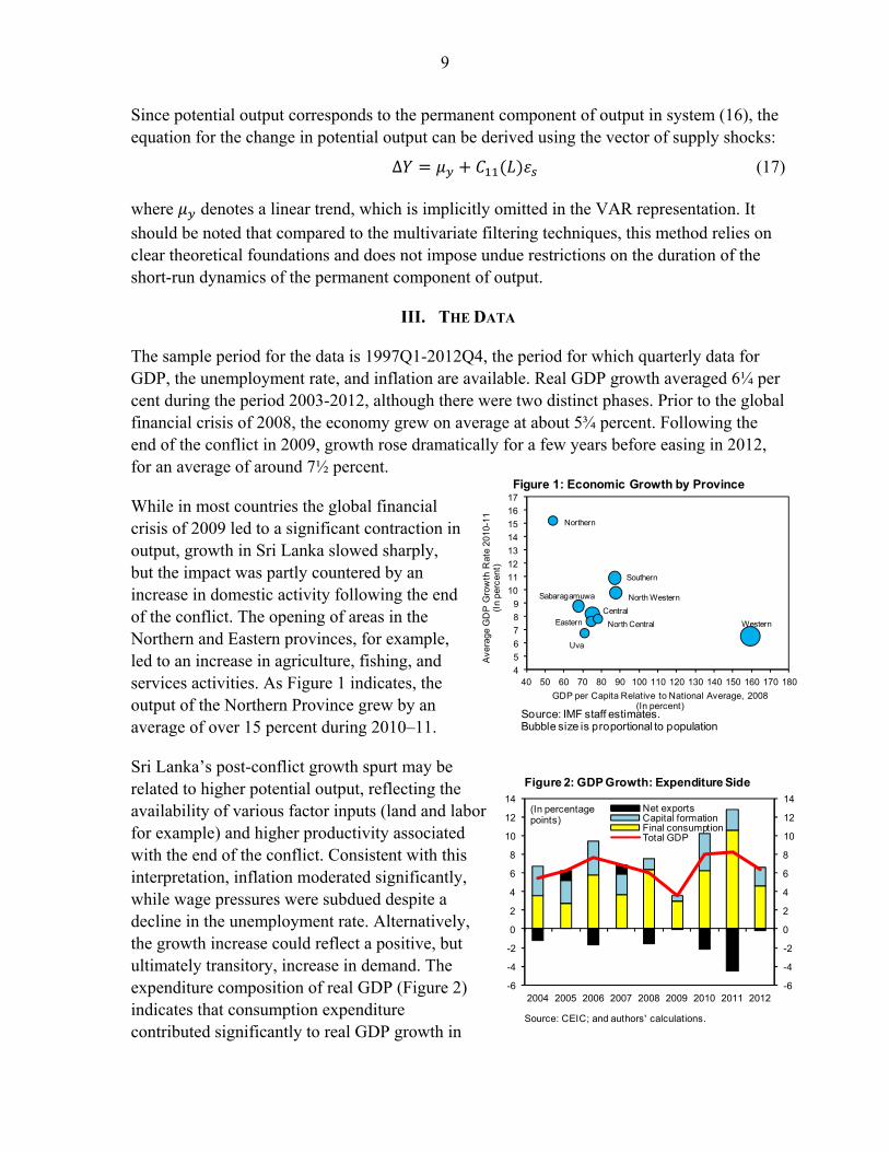
The sample period for the data is 1997Q1-2012Q4, the period for which quarterly data for GDP, the unemployment rate, and inflation are available. Real GDP growth averaged 6¼ per cent during the period 2003-2012, although there were two distinct phases. Prior to the global financial crisis of 2008, the economy grew on average at about 5¾ percent. Following the end of the conflict in 2009, growth rose dramatically for a few years before easing in 2012, for an average of around 7½ percent.

While in most countries the global financial crisis of 2009 led to a significant contraction in output, growth in Sri Lanka slowed sharply, but the impact was partly countered by an increase in domestic activity following the end of the conflict. The opening of areas in the Northern and Eastern provinces, for example, led to an increase in agriculture, fishing, and services activities. As Figure 1 indicates, the output of the Northern Province grew by an average of over 15 percent during 2010–11.

Sri Lanka’s post-conflict growth spurt may be related to higher potential output, reflecting the availability of various factor inputs (land and labor for example) and higher productivity associated with the end of the conflict. Consistent with this interpretation, inflation moderated significantly, while wage pressures were subdued despite a decline in the unemployment rate. Alternatively, the growth increase could reflect a positive, but ultimately transitory, increase in demand. The expenditure composition of real GDP (Figure 2) indicates that consumption expenditure contributed significantly to real GDP growth in

4

5

6

7

8

9

10

11

12

13

14

15

16

17

40 50 60 70 80 90 100 110 120 130 140 150 160 170 180

GDP per Capita Relative to National Average, 2008(In percent)

Ave

rag

e G

DP

Gro

wth

Rat

e 2

010-

11(I

n pe

rcen

t)

Sabaragamuwa

Southern

Central

Northern

Western

North Western

Uva

North CentralEastern

Figure 1: Economic Growth by Province

Source: IMF staff estimates.Bubble size is proportional to population

-6

-4

-2

0

2

4

6

8

10

12

14

-6

-4

-2

0

2

4

6

8

10

12

14

2004 2005 2006 2007 2008 2009 2010 2011 2012

Net exportsCapital formationFinal consumptionTotal GDP

(In percentagepoints)

Figure 2: GDP Growth: Expenditure Side

Source: CEIC; and authors' calculations.

10

2010–11, and was accompanied by a surge in imports that resulted in a large negative contribution from net exports. Capital formation’s contribution to growth did not increase markedly.

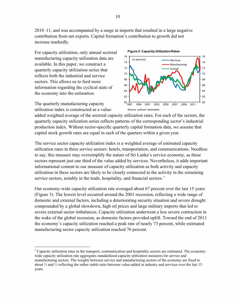
For capacity utilization, only annual sectoral manufacturing capacity utilization data are available. In this paper, we construct a quarterly capacity utilization series that reflects both the industrial and service sectors. This allows us to feed more information regarding the cyclical state of the economy into the estimation.

The quarterly manufacturing capacity utilization index is constructed as a value-added weighted average of the sectoral capacity utilization rates. For each of the sectors, the quarterly capacity utilization series reflects patterns of the corresponding sector’s industrial production index. Without sector-specific quarterly capital formation data, we assume that capital stock growth rates are equal in each of the quarters within a given year.

The service sector capacity utilization index is a weighted average of estimated capacity utilization rates in three service sectors: hotels, transportation, and communications. Needless to say, this measure may oversimplify the nature of Sri Lanka’s service economy, as these sectors represent just one third of the value added by services. Nevertheless, it adds important informational content to our measure of capacity utilization as both activity and capacity utilization in these sectors are likely to be closely connected to the activity in the remaining service sectors, notably in the trade, hospitality, and financial sectors. 3

Our economy-wide capacity utilization rate averaged about 67 percent over the last 15 years (Figure 3). The lowest level occurred around the 2001 recession, reflecting a wide range of domestic and external factors, including a deteriorating security situation and severe drought compounded by a global slowdown, high oil prices and large military imports that led to severe external sector imbalances. Capacity utilization underwent a less severe contraction in the wake of the global recession, as domestic factors provided uplift. Toward the end of 2011 the economy’s capacity utilization reached a peak rate of nearly 73 percent, while estimated manufacturing sector capacity utilization reached 76 percent.

3 Capacity utilization rates in the transport, communication and hospitality sectors are estimated. The economy-wide capacity utilization rate aggregates standardized capacity utilization measures for service and manufacturing sectors. The weights between service and manufacturing sectors of the economy are fixed to about ⅔ and ⅓ reflecting the rather stable ratio between value-added in industry and services over the last 15 years.

60

62

64

66

68

70

72

74

76

60

62

64

66

68

70

72

74

76

1997 1999 2001 2003 2005 2007 2009 2011

Services

Manufacturing

Overall

(In percent)

Figure 3: Capacity Utilization Rates

Source: authors' estimates.

11

IV. ESTIMATION RESULTS

A. Univariate Filters

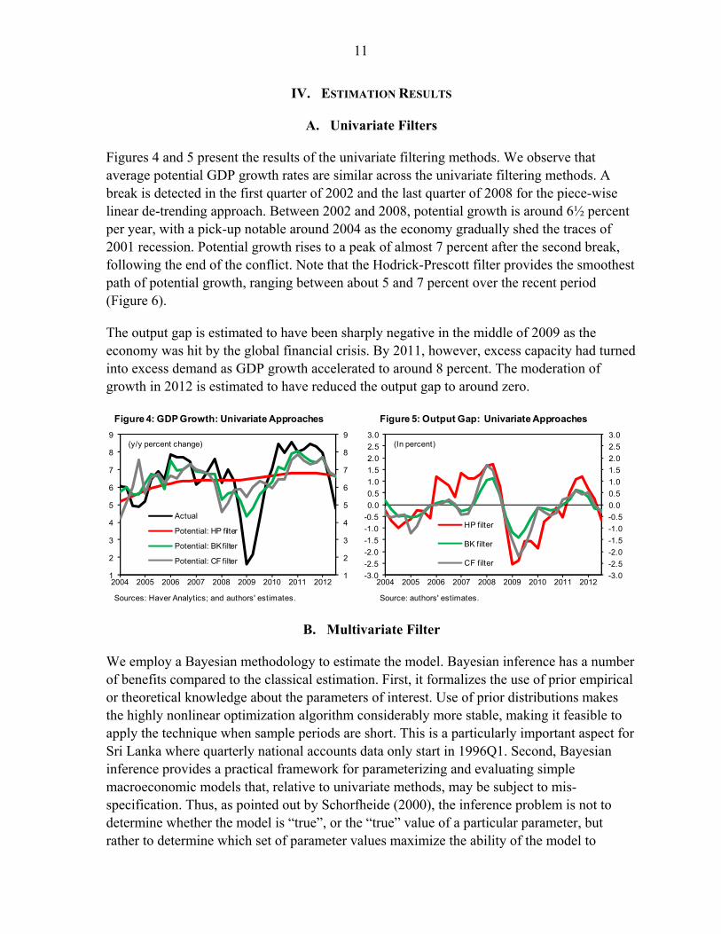
Figures 4 and 5 present the results of the univariate filtering methods. We observe that average potential GDP growth rates are similar across the univariate filtering methods. A break is detected in the first quarter of 2002 and the last quarter of 2008 for the piece-wise linear de-trending approach. Between 2002 and 2008, potential growth is around 6½ percent per year, with a pick-up notable around 2004 as the economy gradually shed the traces of 2001 recession. Potential growth rises to a peak of almost 7 percent after the second break, following the end of the conflict. Note that the Hodrick-Prescott filter provides the smoothest path of potential growth, ranging between about 5 and 7 percent over the recent period (Figure 6).

The output gap is estimated to have been sharply negative in the middle of 2009 as the economy was hit by the global financial crisis. By 2011, however, excess capacity had turned into excess demand as GDP growth accelerated to around 8 percent. The moderation of growth in 2012 is estimated to have reduced the output gap to around zero.

B. Multivariate Filter

We employ a Bayesian methodology to estimate the model. Bayesian inference has a number of benefits compared to the classical estimation. First, it formalizes the use of prior empirical or theoretical knowledge about the parameters of interest. Use of prior distributions makes the highly nonlinear optimization algorithm considerably more stable, making it feasible to apply the technique when sample periods are short. This is a particularly important aspect for Sri Lanka where quarterly national accounts data only start in 1996Q1. Second, Bayesian inference provides a practical framework for parameterizing and evaluating simple macroeconomic models that, relative to univariate methods, may be subject to mis-specification. Thus, as pointed out by Schorfheide (2000), the inference problem is not to determine whether the model is “true”, or the “true” value of a particular parameter, but rather to determine which set of parameter values maximize the ability of the model to

1

2

3

4

5

6

7

8

9

1

2

3

4

5

6

7

8

9

2004 2005 2006 2007 2008 2009 2010 2011 2012

Actual

Potential: HP filter

Potential: BK filter

Potential: CF filter

(y/y percent change)

Figure 4: GDP Growth: Univariate Approaches

Sources: Haver Analytics; and authors' estimates.

-3.0

-2.5

-2.0

-1.5

-1.0

-0.5

0.0

0.5

1.0

1.5

2.0

2.5

3.0

-3.0

-2.5

-2.0

-1.5

-1.0

-0.5

0.0

0.5

1.0

1.5

2.0

2.5

3.0

2004 2005 2006 2007 2008 2009 2010 2011 2012

HP filter

BK filter

CF filter

(In percent)

Figure 5: Output Gap: Univariate Approaches

Source: authors' estimates.

12

summarize the regular features of the data. Finally, Bayesian inference provides a simple method for comparing and choosing between different potentially mis-specified models that may not be nested on the basis of the marginal likelihood or the posterior probability of the model.

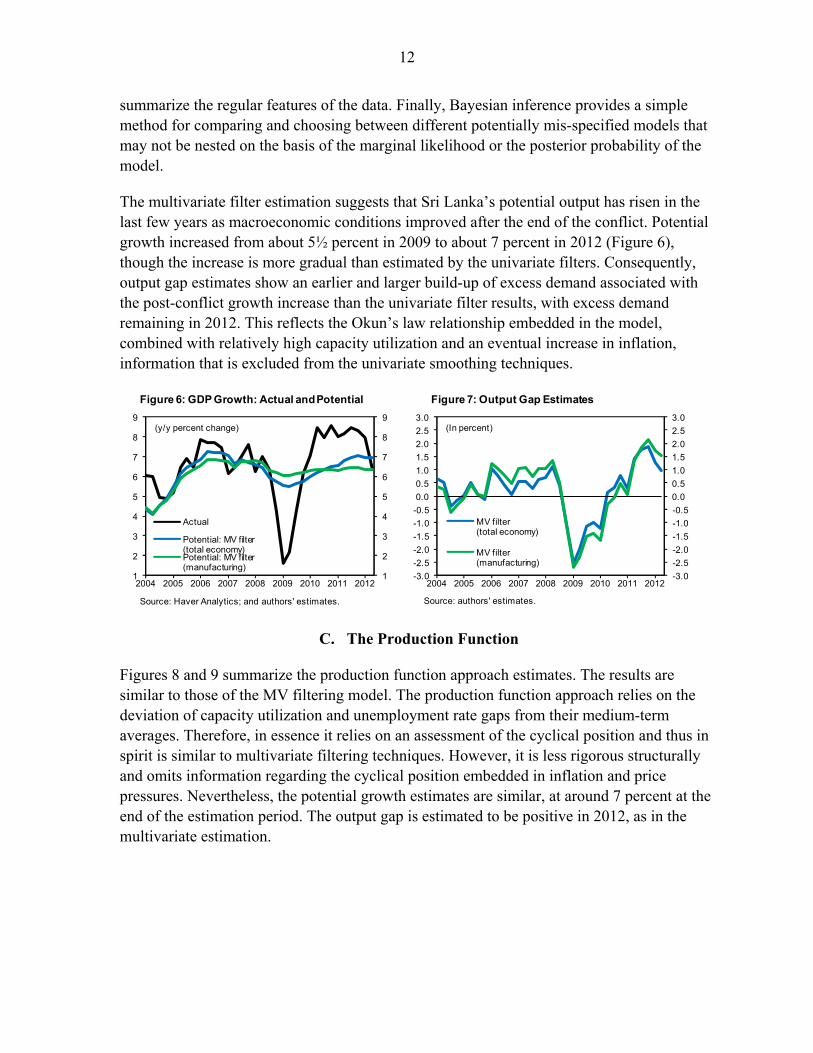
The multivariate filter estimation suggests that Sri Lanka’s potential output has risen in the last few years as macroeconomic conditions improved after the end of the conflict. Potential growth increased from about 5½ percent in 2009 to about 7 percent in 2012 (Figure 6), though the increase is more gradual than estimated by the univariate filters. Consequently, output gap estimates show an earlier and larger build-up of excess demand associated with the post-conflict growth increase than the univariate filter results, with excess demand remaining in 2012. This reflects the Okun’s law relationship embedded in the model, combined with relatively high capacity utilization and an eventual increase in inflation, information that is excluded from the univariate smoothing techniques.

C. The Production Function

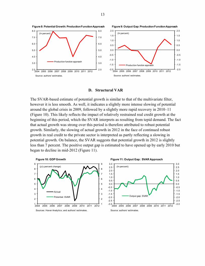
Figures 8 and 9 summarize the production function approach estimates. The results are similar to those of the MV filtering model. The production function approach relies on the deviation of capacity utilization and unemployment rate gaps from their medium-term averages. Therefore, in essence it relies on an assessment of the cyclical position and thus in spirit is similar to multivariate filtering techniques. However, it is less rigorous structurally and omits information regarding the cyclical position embedded in inflation and price pressures. Nevertheless, the potential growth estimates are similar, at around 7 percent at the end of the estimation period. The output gap is estimated to be positive in 2012, as in the multivariate estimation.

1

2

3

4

5

6

7

8

9

1

2

3

4

5

6

7

8

9

2004 2005 2006 2007 2008 2009 2010 2011 2012

Actual

Potential: MV filter (total economy)Potential: MV filter (manufacturing)

(y/y percent change)

Figure 6: GDP Growth: Actual and Potential

Source: Haver Analytics; and authors' estimates.

-3.0

-2.5

-2.0

-1.5

-1.0

-0.5

0.0

0.5

1.0

1.5

2.0

2.5

3.0

-3.0

-2.5

-2.0

-1.5

-1.0

-0.5

0.0

0.5

1.0

1.5

2.0

2.5

3.0

2004 2005 2006 2007 2008 2009 2010 2011 2012

MV filter (total economy)

MV filter (manufacturing)

(In percent)

Figure 7: Output Gap Estimates

Source: authors' estimates.

13

D. Structural VAR

The SVAR-based estimate of potential growth is similar to that of the multivariate filter, however it is less smooth. As well, it indicates a slightly more intense slowing of potential around the global crisis in 2009, followed by a slightly more rapid recovery in 2010–11 (Figure 10). This likely reflects the impact of relatively restrained real credit growth at the beginning of this period, which the SVAR interprets as resulting from tepid demand. The fact that actual growth was strong over this period is therefore attributed to robust potential growth. Similarly, the slowing of actual growth in 2012 in the face of continued robust growth in real credit to the private sector is interpreted as partly reflecting a slowing in potential growth. On balance, the SVAR suggests that potential growth in 2012 is slightly less than 7 percent. The positive output gap is estimated to have opened up by early 2010 but began to decline in mid-2012 (Figure 11).

-2.0

-1.5

-1.0

-0.5

0.0

0.5

1.0

1.5

2.0

-2.0

-1.5

-1.0

-0.5

0.0

0.5

1.0

1.5

2.0

2004 2005 2006 2007 2008 2009 2010 2011 2012

Production function approach

(In percent)

Figure 9: Output Gap: Production Function Approach

Source: authors' estimates.

2.0

3.0

4.0

5.0

6.0

7.0

8.0

2.0

3.0

4.0

5.0

6.0

7.0

8.0

2004 2005 2006 2007 2008 2009 2010 2011 2012

Production function approach

(In percent)

Figure 8: Potential Growth: Production Function Approach

Source: authors' estimates.

-3.0

-2.5

-2.0

-1.5

-1.0

-0.5

0.0

0.5

1.0

1.5

2.0

2.5

3.0

-3.0

-2.5

-2.0

-1.5

-1.0

-0.5

0.0

0.5

1.0

1.5

2.0

2.5

3.0

2004 2005 2006 2007 2008 2009 2010 2011 2012

Output gap: SVAR

(In percent)

Figure 11: Output Gap: SVAR Approach

Source: authors' estimates.

1

2

3

4

5

6

7

8

9

1

2

3

4

5

6

7

8

9

2004 2005 2006 2007 2008 2009 2010 2011 2012

Actual

Potential: SVAR

(y/y percent change)

Figure 10: GDP Growth

Sources: Haver Analytics; and authors' estimates.

14

V. CONCLUSIONS AND POLICY IMPLICATIONS

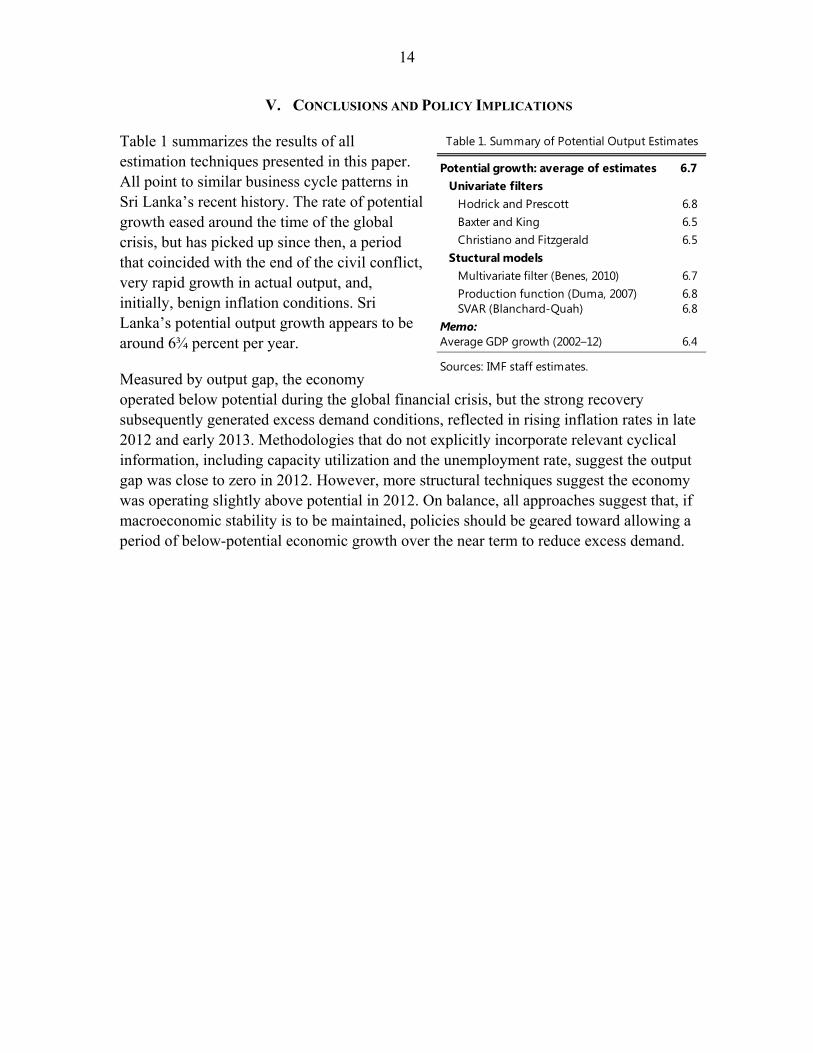
Table 1 summarizes the results of all estimation techniques presented in this paper. All point to similar business cycle patterns in Sri Lanka’s recent history. The rate of potential growth eased around the time of the global crisis, but has picked up since then, a period that coincided with the end of the civil conflict, very rapid growth in actual output, and, initially, benign inflation conditions. Sri Lanka’s potential output growth appears to be around 6¾ percent per year.

Measured by output gap, the economy operated below potential during the global financial crisis, but the strong recovery subsequently generated excess demand conditions, reflected in rising inflation rates in late 2012 and early 2013. Methodologies that do not explicitly incorporate relevant cyclical information, including capacity utilization and the unemployment rate, suggest the output gap was close to zero in 2012. However, more structural techniques suggest the economy was operating slightly above potential in 2012. On balance, all approaches suggest that, if macroeconomic stability is to be maintained, policies should be geared toward allowing a period of below-potential economic growth over the near term to reduce excess demand.

Potential growth: average of estimates 6.7Univariate filters

Hodrick and Prescott 6.8Baxter and King 6.5Christiano and Fitzgerald 6.5

Stuctural modelsMultivariate filter (Benes, 2010) 6.7Production function (Duma, 2007) 6.8SVAR (Blanchard-Quah) 6.8

Memo:Average GDP growth (2002–12) 6.4

Sources: IMF staff estimates.

Table 1. Summary of Potential Output Estimates

15

References

Anand, R., D. Ding, and S.J. Peiris, 2011, “Toward Inflation Targeting in Sri Lanka,” IMF Working Paper No. 11/81 (Washington: International Monetary Fund).

Baxter, M., and R.G. King, 1995, “Measuring Business Cycles: Approximate Band-Pass Filters for Economic Time Series,” NBER Working Paper No. 5022 (Cambridge, Massachusetts: National Bureau of Economic Research).

Benes, J., and P.N. Diaye, 2004, “A Multivariate Filter for Measuring Potential Output and the NAIRU; Application to The Czech Republic,” IMF Working Paper No. WP/04/45 (Washington: International Monetary Fund).

Benes, J., K. Clinton, R. Garcia-Saltos, M. Johnson, D. Laxton, P. Manchev, and T. Matheson, 2010, “Estimating Potential Output with a Multivariate Filter,” IMF Working Paper No. 10/285 (Washington: International Monetary Fund).

Cerra, V., and S. Saxena, 2000, “Alternative Methods of Estimating Potential Output and the Output Gap: An Application to Sweden” IMF Working Paper WP/00/59 (Washington: International Monetary Fund).

Clarida, R., and J. Gali, 1994, “Sources of Real Exchange Rate Fluxuations: How Important Are Nominal Shocks?” Carnegie-Rochester Conference Series on Public Policy 41.

Cogley, T., and J. Nason, 1995, “Effects of the Hodrick-Prescott Filter on Trend and Difference Stationary Time Series: Implications for Business Cycle Research,” Journal of Economic Dynamics and Control 19:253–78.

Duma, N., 2007, “Sri Lanka’s Sources of Growth,” IMF Working Paper No. 07/225 (Washington: International Monetary Fund).

Dupasquier, C., A. Guay, and P. St-Amant, 1997, “A Comparison of Alternative Methodologies for Estimating Potential Output and the Output Gap,” Working Paper 97-5 (Ottawa, Ontario, Canada: Bank of Canada).

Gupta, S., and M. Saxegaard, 2009, “Meaures of Underlying Inflation in Sri Lanka,” IMF Working Paper No. 09/167(Washington: International Monetary Fund).

Harvey, A.C., and A. Jaeger, 1993, “Detrending, Stylized Facts and the Business Cycle,” Journal of Applied Econometrics 8:231–47.

Schorfheide, F., 2000, “Loss Function-based Evaluation of DSGE Models,” Journal of Applied Econometrics 15, 645–67.