University of Nebraska - LincolnDigitalCommons@University of Nebraska - Lincoln

USGS Staff -- Published Research US Geological Survey

2015

Estimating Relative Sea-Level Rise andSubmergence Potential at a Coastal WetlandDonald R. CahoonU.S. Geological Survey, dcahoon@usgs.gov

Follow this and additional works at: http://digitalcommons.unl.edu/usgsstaffpub

Part of the Geology Commons, Oceanography and Atmospheric Sciences and MeteorologyCommons, Other Earth Sciences Commons, and the Other Environmental Sciences Commons

This Article is brought to you for free and open access by the US Geological Survey at DigitalCommons@University of Nebraska - Lincoln. It has beenaccepted for inclusion in USGS Staff -- Published Research by an authorized administrator of DigitalCommons@University of Nebraska - Lincoln.

Cahoon, Donald R., "Estimating Relative Sea-Level Rise and Submergence Potential at a Coastal Wetland" (2015). USGS Staff --Published Research. 992.http://digitalcommons.unl.edu/usgsstaffpub/992

PERSPECTIVES

Estimating Relative Sea-Level Rise and Submergence Potentialat a Coastal Wetland

Donald R. Cahoon

Received: 19 February 2014 /Revised: 22 July 2014 /Accepted: 14 August 2014 /Published online: 5 September 2014

Abstract A tide gauge records a combined signal of thevertical change (positive or negative) in the level of both thesea and the land to which the gauge is affixed; or relative sea-level change, which is typically referred to as relative sea-levelrise (RSLR). Complicating this situation, coastal wetlandsexhibit dynamic surface elevation change (both positive andnegative), as revealed by surface elevation table (SET) mea-surements, that is not recorded at tide gauges. Because theusefulness of RSLR is in the ability to tie the change in sealevel to the local topography, it is important that RSLR becalculated at a wetland that reflects these local dynamic sur-face elevation changes in order to better estimate wetlandsubmergence potential. A rationale is described for calculatingwetland RSLR (RSLRwet) by subtracting the SET wetlandelevation change from the tide gauge RSLR. The calculationis possible because the SET and tide gauge independentlymeasure vertical land motion in different portions of thesubstrate. For 89 wetlands where RSLRwet was evaluated,wetland elevation change differed significantly from zero for80 % of them, indicating that RSLRwet at these wetlandsdiffered from the local tide gauge RSLR. When compared totide gauge RSLR, about 39 % of wetlands experienced anelevation rate surplus and 58 % an elevation rate deficit (i.e.,sea level becoming lower and higher, respectively, relative tothe wetland surface). These proportions were consistent across

saltmarsh, mangrove, and freshwater wetland types.Comparison of wetland elevation change and RSLR isconfounded by high levels of temporal and spatial var-iability, and would be improved by co-locating tidegauge and SET stations near each other and obtaining long-term records for both.

Keywords Relative sea-level rise .Wetland elevation . Tidegauge . SET . Vertical accretion . Shallow subsidence .

Shallow expansion

Introduction

Determining the potential for wetland submergence by risingsea levels is an issue of critical importance to coastal resourcemanagers that requires knowledge of local changes in sealevel and wetland elevation. For nearly two centuries, high-resolution trends (mm/y) of relative sea-level change havebeen derived from long-term tide gauge records (IOC 2006).Because a tide gauge is affixed to the crust of the Earth, andthat crust may have its own vertical motion, it is impossible touse the tide gauge record by itself to separate out the absolutesea-level rise signal from the absolute vertical land motion(VLM) signal. Thus, this combined signal recorded at a tidegauge reflects relative sea-level change; or what is typicallyreferred to as relative sea-level rise (RSLR). Yet, it is highlyunlikely that RSLR measured in upland or built environments(e.g., the upland bench mark is attached to a building) at a tidegauge station fully represents the RSLR occurring at nearbywetlands. This is because coastal wetlands are typically locat-ed some distance from a tide gauge and its upland benchmarks, often in different hydrologic and geologic settings. Inaddition, global evaluations of wetland elevation trends usingthe high resolution (mm/y) surface elevation table–markerhorizon (SET–MH) method (Cahoon et al. 1995) reveal that

Communicated by Carolyn A. Currin

Electronic supplementary material The online version of this article(doi:10.1007/s12237-014-9872-8) contains supplementary material,which is available to authorized users.

D. R. Cahoon (*)US Geological Survey, Patuxent Wildlife Research Center,10300 Baltimore Avenue, c/o BARC-East, Building 308,Beltsville, MD 20705, USAe-mail: dcahoon@usgs.gov

Estuaries and Coasts (2015) 38:1077–1084DOI 10.1007/s12237-014-9872-8

# Coastal and Estuarine Research Federation (outside the USA) 2014

wetland elevation trends vary within and among wetlands,ranging from positive to negative slopes influenced by bothsurface vertical accretion and erosion, and subsurface subsi-dence and expansion processes (Cahoon et al. 1999, 2006).The SET–MHmethod is currently used in 29 countries on sixcontinents in both temperate and tropical coastal regionsto evaluate elevation dynamics in primarily salt marshand mangrove environments (Webb et al. 2013). Unlikethe upland habitats where tide gauges are located, saltmarshes and mangrove forests are able to alter theirsurface elevation by trapping sediments brought in bythe tide, and through belowground production and ac-cumulation of roots and rhizomes. In addition, thesesoft, unconsolidated sediments are subject to compactionand shrink-swell processes to a greater extent than up-land soils. Therefore, although RSLR as recorded by atide gauge provides an accurate estimate of the relation-ship between local uplands and sea level, it does notprovide an accurate estimate of the relationship betweenlocal wetlands and sea level. In order to determine wetlandsubmergence potential as sea level rises, one must considersurface elevation change in the wetland along with RSLRmeasured by the tide gauge.

This paper provides a brief review, from a methodo-logical perspective, of the approaches used to estimateRSLR by sea level scientists and wetland elevationchange by coastal wetland scientists, in order to deter-mine wetland submergence potential. The motivation be-hind this paper is to clarify how measures of RSLR by atide gauge and wetland surface elevation change by aSET are independent and complementary, how the twodatasets are used together to estimate local sea-level riseat a wetland site, and to propose a standard approach andterminology for quantifying and describing wetland vul-nerability to sea-level rise. Accounting for wetland sur-face elevation change in conjunction with tide gaugemeasures of RSLR allows for a direct calculation ofwetland elevation rate deficit or surplus relative to sea-level rise (Cahoon et al. 1995), for which the proposednew term is wetland RSLR (RSLRwet). The importanceof calculating RSLRwet is demonstrated from a literaturereview of the magnitude and direction of wetland eleva-tion change measured with the SET device. Furthermore,terms such as shallow and deep subsidence used by theSET–MH community (Cahoon et al. 1995), and howthese processes are measured, are clearly defined in thecontext of the long-established vocabulary for subsidenceused by the tide gauge community. Lastly, the influenceof high temporal and spatial variability in both the wetlandelevation and sea level trends on interpreting wetland submer-gence potential is described, as is the need for co-locating SETand tide gauge stations whenever practical, and obtaininglong-term records of both.

Complementarity of RSLR and Wetland ElevationChange Measures

Tide Gauge RSLR

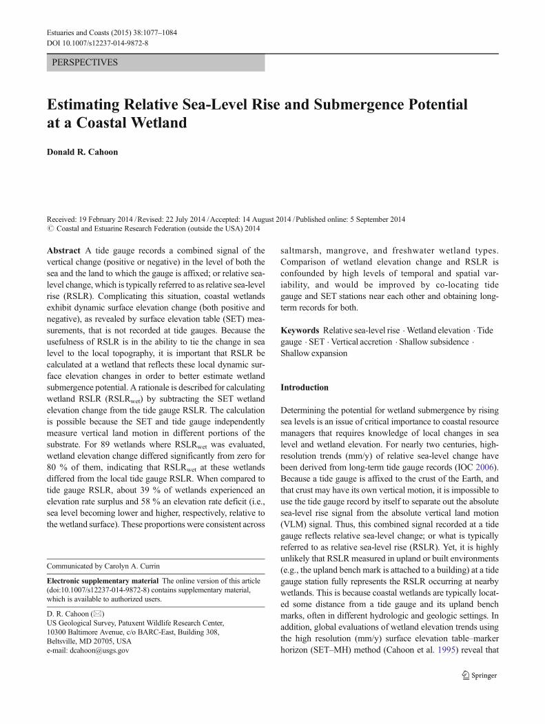
A tide gauge measures sea level in relation to a primaryreference point on land represented by a bench mark locatedon a stable surface such as exposed rock or a stainless steel roddriven to refusal, ideally to bedrock (Baker 1993; Bevis et al.2002; IOC 2006). Typically a network of 5–10 bench marks isestablished in the vicinity of each tide gauge, often at differentdepths in the substrate, and the most stable bench mark isdesignated the tide gauge bench mark (TGBM) or primaryreference point for sea level observations (Fig. 1). The primarybenchmark is connected to the tide gauge at its contact (sensor“0”) point by high-precision leveling repeated annually todetermine vertical stability of the gauge (IOC 2006), relativeto the surrounding bench marks. All bench marks in thenetwork are also connected to each other by high-precisionleveling repeated annually. Thus, a tide gauge records a rela-tive sea-level rise because it measures sea level change relativeto the bench marks attached to the crust, which is in motion.The crustal VLM, or VLMc, portion of the RSLR trend is thevelocity of the substratum at the base of the TGBM (Fig. 1).

Wetland Elevation Change

Nearly 50 years ago, Kaye and Barghoorn (1964) describedquantitatively the autocompaction of marsh soils that results ina change in level of the marsh surface. The implications of theirfindings are twofold. First, for a coastal marsh to maintain aconstant elevation, the accumulation rate of mineral and organ-ic material on or near the marsh surface must equal both the rateof crustal motion occurring below the marsh substrate as mea-sured at a tide gauge, plus the rate of autocompaction (i.e.,shallow subsidence, sensu Cahoon et al. 1995) of the marshsubstrate, the combination of which has been termed totalsubsidence (Cahoon et al. 1995). And if the marsh is to keeppace with a rising local sea level, then its rate of positive verticalchange from accumulation of material must equal or be greaterthan the rate of total subsidence plus the local sea-level trend.Second, the existence of autocompaction indicates that accre-tion measures that had been assumed to raise the level of themarsh by an equal amount, likely overestimate elevationchange, or underestimate it in the case of shallow expansion.Thus, assessing coastal wetland vulnerability to sea-level riserequires a quantitative understanding of not only RSLR but alsomarsh surface elevation change. To this end, the surface eleva-tion table–marker horizon (SET–MH) method was developed(Cahoon et al. 1995, 2002a, b; Callaway et al. 2013) to providesimultaneous, millimeter accuracy measures of vertical accre-tion and surface elevation change, from which shallow subsi-dence or expansion of the marsh substrate is calculated.

1078 Estuaries and Coasts (2015) 38:1077–1084

The SET is a portable, mechanical device that is attached toa pipe or rod mark driven into a wetland substrate (Boumansand Day 1993; Cahoon et al. 2002a, b; Callaway et al. 2013).The latest version of the SET attaches to a stainless steel roddriven typically 10–25m (up to 40m) into the substrate, and isknown as the Rod SET (Figs. 1 and 2), or RSET (Cahoon et al.2002b; Callaway et al. 2013). The RSET is designed withleveling mechanisms so that each time the device is attachedto a fixed position on the rod mark and leveled it will reoccupythe same reference plane in space (with respect to the rodmark) and remeasure the same point on the wetland surface atup to eight fixed positions around the mark. Surface elevation,relative to the base of the rod mark, is determined by loweringnine pins in the RSET arm to the wetland surface and mea-suring the height of each pin relative to the arm at each fixedposition (9 pins×8 positions=72 maximum number of read-ings). Wetland surface elevation change (VLMw) is deter-mined from repeat pin measurements of the marsh surface,and is the change in elevation relative to the base of therod mark (i.e., the subsurface datum) that incorporatesboth surface (i.e., vertical accretion) and subsurfaceprocess influences on elevation occurring above the base ofthe rod mark (Fig. 2). The RSET does not measure any VLMc

processes because they occur below the base of the rodmark (e.g., glacial isostatic adjustment and tectonics,Fig. 2), in what Cahoon et al. (1995) refer to as thedeep subsidence zone.

Measures of VLMw by the SET method and VLMc by aTGBM network connected to the global reference frame usingGPS are independent and from different portions of the substrateprofile. The SET method measures VLMw of the substrateoverlying the SET rod base, which ideally is set on bedrock,by direct measurement of thewetland surface relative to the SETrod base (Cahoon et al. 1995; Cahoon et al. 2002b; Webb et al.2013; Figs. 1 and 2). In contrast, the TGBM network connectedto GPS provides a measure of VLMc at the base of each benchmark (Fig. 1), but does not record any motion occurring in theless stable materials overlying the benchmark base (Bevis et al.2002). Thus, the VLMc measured at the TGBM network is notrepresentative of the shallow VLMw dynamics of a typicalwetland substrate. Thus, tide gauge RSLR can and usually doesinadequately describe wetland submergence potential.Estimates of wetland vulnerability to sea-level rise should bebased on the independent, high-resolution measures of bothwetland elevation change and tide gauge RSLR.

Subsurface Process Controls on Wetland Elevation

The SET device can be used to quantify subsurface processinfluences on elevation when used in conjunction with theartificial soil marker horizon method for measuring verticalaccretion. Wetland vertical accretion is the vertical accumula-tion of material related to soil development. Typically, 3 or 4

Fig 1 Conceptual diagram showing the relationship among measures ofvertical land motion as recorded by the tide gauge benchmark network ata coastal upland area (VLMc) and the rod surface elevation table (RSET)

method in a coastal wetland (VLMw). The double-headed arrows forVLMw and VLMc indicate that vertical motion can be up or down,depending on the local setting and conditions

Estuaries and Coasts (2015) 38:1077–1084 1079

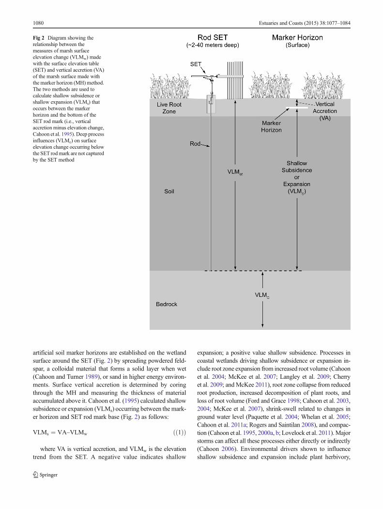
artificial soil marker horizons are established on the wetlandsurface around the SET (Fig. 2) by spreading powdered feld-spar, a colloidal material that forms a solid layer when wet(Cahoon and Turner 1989), or sand in higher energy environ-ments. Surface vertical accretion is determined by coringthrough the MH and measuring the thickness of materialaccumulated above it. Cahoon et al. (1995) calculated shallowsubsidence or expansion (VLMs) occurring between the mark-er horizon and SET rod mark base (Fig. 2) as follows:

VLMs ¼ VA–VLMw ðð1ÞÞ

where VA is vertical accretion, and VLMw is the elevationtrend from the SET. A negative value indicates shallow

expansion; a positive value shallow subsidence. Processes incoastal wetlands driving shallow subsidence or expansion in-clude root zone expansion from increased root volume (Cahoonet al. 2004; McKee et al. 2007; Langley et al. 2009; Cherryet al. 2009; and McKee 2011), root zone collapse from reducedroot production, increased decomposition of plant roots, andloss of root volume (Ford and Grace 1998; Cahoon et al. 2003,2004; McKee et al. 2007), shrink-swell related to changes inground water level (Paquette et al. 2004; Whelan et al. 2005;Cahoon et al. 2011a; Rogers and Saintilan 2008), and compac-tion (Cahoon et al. 1995, 2000a, b; Lovelock et al. 2011).Majorstorms can affect all these processes either directly or indirectly(Cahoon 2006). Environmental drivers shown to influenceshallow subsidence and expansion include plant herbivory,

Fig 2 Diagram showing therelationship between themeasures of marsh surfaceelevation change (VLMw) madewith the surface elevation table(SET) and vertical accretion (VA)of the marsh surface made withthe marker horizon (MH) method.The two methods are used tocalculate shallow subsidence orshallow expansion (VLMs) thatoccurs between the markerhorizon and the bottom of theSET rod mark (i.e., verticalaccretion minus elevation change,Cahoon et al. 1995). Deep processinfluences (VLMc) on surfaceelevation change occurring belowthe SET rodmark are not capturedby the SET method

1080 Estuaries and Coasts (2015) 38:1077–1084

prescribed fire, drought, river stage, tides, elevated atmosphericCO2 concentrations, and nitrogen and phosphorus enrichment(Cahoon et al. 2009).

Rates of Wetland Elevation Change

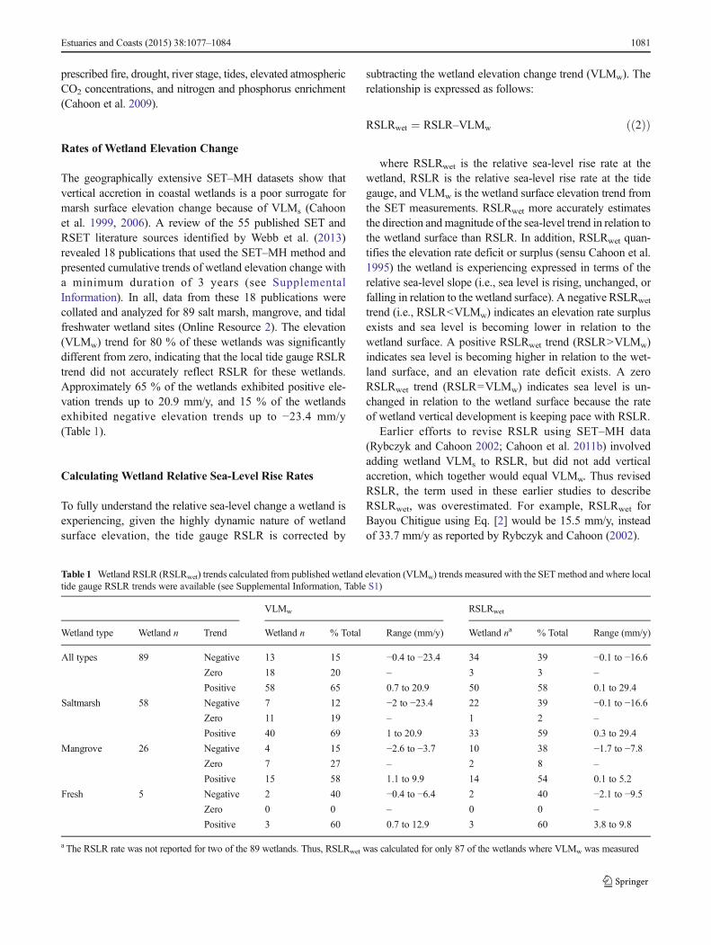
The geographically extensive SET–MH datasets show thatvertical accretion in coastal wetlands is a poor surrogate formarsh surface elevation change because of VLMs (Cahoonet al. 1999, 2006). A review of the 55 published SET andRSET literature sources identified by Webb et al. (2013)revealed 18 publications that used the SET–MH method andpresented cumulative trends of wetland elevation change witha minimum duration of 3 years (see SupplementalInformation). In all, data from these 18 publications werecollated and analyzed for 89 salt marsh, mangrove, and tidalfreshwater wetland sites (Online Resource 2). The elevation(VLMw) trend for 80 % of these wetlands was significantlydifferent from zero, indicating that the local tide gauge RSLRtrend did not accurately reflect RSLR for these wetlands.Approximately 65 % of the wetlands exhibited positive ele-vation trends up to 20.9 mm/y, and 15 % of the wetlandsexhibited negative elevation trends up to −23.4 mm/y(Table 1).

Calculating Wetland Relative Sea-Level Rise Rates

To fully understand the relative sea-level change a wetland isexperiencing, given the highly dynamic nature of wetlandsurface elevation, the tide gauge RSLR is corrected by

subtracting the wetland elevation change trend (VLMw). Therelationship is expressed as follows:

RSLRwet ¼ RSLR–VLMw ðð2ÞÞ

where RSLRwet is the relative sea-level rise rate at thewetland, RSLR is the relative sea-level rise rate at the tidegauge, and VLMw is the wetland surface elevation trend fromthe SET measurements. RSLRwet more accurately estimatesthe direction and magnitude of the sea-level trend in relation tothe wetland surface than RSLR. In addition, RSLRwet quan-tifies the elevation rate deficit or surplus (sensu Cahoon et al.1995) the wetland is experiencing expressed in terms of therelative sea-level slope (i.e., sea level is rising, unchanged, orfalling in relation to the wetland surface). A negative RSLRwet

trend (i.e., RSLR<VLMw) indicates an elevation rate surplusexists and sea level is becoming lower in relation to thewetland surface. A positive RSLRwet trend (RSLR>VLMw)indicates sea level is becoming higher in relation to the wet-land surface, and an elevation rate deficit exists. A zeroRSLRwet trend (RSLR=VLMw) indicates sea level is un-changed in relation to the wetland surface because the rateof wetland vertical development is keeping pace with RSLR.

Earlier efforts to revise RSLR using SET–MH data(Rybczyk and Cahoon 2002; Cahoon et al. 2011b) involvedadding wetland VLMs to RSLR, but did not add verticalaccretion, which together would equal VLMw. Thus revisedRSLR, the term used in these earlier studies to describeRSLRwet, was overestimated. For example, RSLRwet forBayou Chitigue using Eq. [2] would be 15.5 mm/y, insteadof 33.7 mm/y as reported by Rybczyk and Cahoon (2002).

Table 1 Wetland RSLR (RSLRwet) trends calculated from published wetland elevation (VLMw) trends measured with the SET method and where localtide gauge RSLR trends were available (see Supplemental Information, Table S1)

VLMw RSLRwet

Wetland type Wetland n Trend Wetland n % Total Range (mm/y) Wetland na % Total Range (mm/y)

All types 89 Negative 13 15 −0.4 to −23.4 34 39 −0.1 to −16.6Zero 18 20 – 3 3 –

Positive 58 65 0.7 to 20.9 50 58 0.1 to 29.4

Saltmarsh 58 Negative 7 12 −2 to −23.4 22 39 −0.1 to −16.6Zero 11 19 – 1 2 –

Positive 40 69 1 to 20.9 33 59 0.3 to 29.4

Mangrove 26 Negative 4 15 −2.6 to −3.7 10 38 −1.7 to −7.8Zero 7 27 – 2 8 –

Positive 15 58 1.1 to 9.9 14 54 0.1 to 5.2

Fresh 5 Negative 2 40 −0.4 to −6.4 2 40 −2.1 to −9.5Zero 0 0 – 0 0 –

Positive 3 60 0.7 to 12.9 3 60 3.8 to 9.8

a The RSLR rate was not reported for two of the 89 wetlands. Thus, RSLRwet was calculated for only 87 of the wetlands where VLMw was measured

Estuaries and Coasts (2015) 38:1077–1084 1081

Rates of Wetland RSLR

The historic, local RSLR rates were available for calculatingRSLRwet in all but one of the 18 studies and were compareddirectly to the VLMw values presented in Table 1. RSLRwet

was negative at 34 of the 87 wetlands (39 %), where sea levelwas becoming lower relative to the wetland surface at a rate of−0.1 to −16.6 mm/y (Table 1). These wetlands are experienc-ing an elevation rate surplus. RSLRwet was positive at 50 ofthe 87 wetlands (58 %), where sea level was becoming higherrelative to the wetland surface at a rate of 0.1 to29.4 mm/y. These wetlands are experiencing an eleva-tion rate deficit. The remaining three wetlands werekeeping pace with the local rate of sea-level rise. Theproportion of wetlands with negative and positive RSLRwet

was consistent (approximately 40 % and 60 %) acrosssaltmarsh, mangrove, and fresh wetland types (Table 1). Thehighest negative and positive VLMw trend and elevationrate surplus and deficit were reported from saltmarshwetlands. The range in negative and positive VLMw andelevation rate surplus and deficit was smaller in mangroveand fresh wetlands.

Caveats of Calculating RSLRwet

There are caveats to the RSLRwet approach related to thetemporal and spatial variability in wetland elevation andsea level data. High spatial variability in VLMw amongwetland sites requires that RSLRwet be calculated forevery wetland site, not extrapolated from nearby wet-lands. In addition, high spatial variability in sea levelindicates that distance from a wetland to a long-term tidegauge could be a drawback given that sea level recordedat the gauge does not necessarily transfer accurately overlong distances (Mossman et al. 2012). Yet, in manyregions, sea level trends and variations are highly corre-lated, thus suggesting some ability to extrapolate dependingon underlying geology.

Given the high variability in both trends, perhaps the mostimportant caveat is that comparisons of VLMw and RSLRtrends are confounded by the difference in record lengths. Thelongest SET data record available is near 20 years duration,but most are considerably shorter (<10 years). Relative sea-level trends from tide gauges should be a minimum of severaldecades, up to 60 to 70 years duration, to provide a meaning-ful trend, given the high level of noise in the sea level data(Peltier 2001). Ideally, both trends would be measured overthe same period of time and for several decades. Lackingwetland elevation trends of a similar long duration as tidegauge records, two approaches have been used to comparethese datasets of disparate length, each with its own shortcom-ings. First, the approach most often used is to assume that the

historic sea-level trend existed during the shorter durationwetland elevation trend, and the two trends are compareddirectly. This assumption may not be realistic in every in-stance. Alternatively, a short-term sea-level trend is calculatedfrom the tide gauge data for the same time period as thewetland elevation trend (e.g., 5 years), and the trendsare compared directly. This approach shows the short-term relationship of wetland elevation with recent sea-level change but not with the long-term sea-level trend.In addition, this approach can be confounded by highlevels of variability that typically occur in short durationrecords of both trends. Thus, calculations of RSLRwet mustbe interpreted and reported taking these caveats into account.See McIvor et al. (2013) for an excellent overview of theissues related to comparing surface elevation change data withsea-level rise data.

To address these caveats, efforts need to be made to co-locate tide gauges and SET–MH stations near each other, as isbeing done at the twenty-eight NOAA National EstuarineResearch Reserves (NERR) located in estuaries and associat-ed wetlands along the coasts of the USA (NERR 2012), and inLouisiana, USA, where each of the 390 wetland monitoringstations that make up the State of Louisiana Coast-wideReference Monitoring System (CRMS) includes a water levelgauge and a SET–MH station (Steyer et al. 2003). The CRMSand NERR long-term monitoring networks provide co-locat-ed, continuous records of local relative sea level change,vertical accretion, surface elevation change (VLMw), andVLMs across the range of ecological conditions in the coastalmarshes of Louisiana and the specific coastal setting whereeach NERR is located.

In sum, understanding the management and adaptationimplications of rising sea level on coastal wetlands requirescomplete knowledge of local RSLR rates with respect tocoastal habitats, specifically vertically dynamic shorelineand near-shore environments. Thus, coastal wetland managersneed high-resolution information on wetland elevation changerelative to local sea level change in order to improve assess-ments of submergence potential and to better manage thevaluable ecosystem services provided by coastal wetlands.To this end, this paper synthesized the current methodologyfor measuring wetland elevation dynamics and RLSR fromtide gauges, and provides a standard method and vocabularyfor estimating and describing the potential for wetlandsubmergence.

Acknowledgments K. Boone and J. Lynch drafted Fig. 1, and J. Lynchdrafted Fig. 2. I am deeply indebted to the following individuals forproviding critical reviews of earlier draft versions of this manuscript: S.Gill, P. Hensel, B. Horton, J. Lynch, K. Krauss, K. McKee, two anony-mous reviewers, and C. Currin. Any use of trade, product, or firm namesis for descriptive purposes only and does not imply endorsement by theUS Government. This research was funded by the U.S. GeologicalSurvey Climate and Land Use Research & Development program.

1082 Estuaries and Coasts (2015) 38:1077–1084

References

Baker, T.F. 1993. Absolute sea level measurements, climate change andvertical crustal movements. Global and Planetary Change 8: 149–159.

Bevis, M., W. Scherer, and M. Merrifield. 2002. Technical issues andrecommendations related to the installation of continuous GPSstations at tide gauges. Marine Geodesy 25: 87–99.

Boumans, R.M.J., and J.W. Day Jr. 1993. High precision measurements ofsediment elevation in shallow coastal areas using a sedimentation-erosion table. Estuaries 16: 375–380.

Cahoon, D.R. 2006. A review of major storm impacts on coastal wetlandelevation. Estuaries and Coasts 29(6A): 889–898.

Cahoon, D.R., and R.E. Turner. 1989. Accretion and canal impacts in arapidly subsiding wetland II: feldspar marker horizon technique.Estuaries 12(4): 260–268.

Cahoon, D.R., D.J. Reed, and J.W. Day Jr. 1995. Estimatingshallow subsidence in microtidal salt marshes of the south-eastern United States: Kaye and Barghoorn revisited. MarineGeology 128: 1–9.

Cahoon, D.R., J.W. Day Jr., and D.J. Reed. 1999. The influence of surfaceand shallow subsurface soil processes on wetland elevation: a syn-thesis. Current Topics in Wetland Biogeochemistry 3: 72–88.

Cahoon, D.R., J. French, T. Spencer, D.J. Reed, and I. Moller. 2000a.Vertical accretion versus elevational adjustment in UK saltmarshes:an evaluation of alternativemethodologies. InCoastal and estuarineenvironments: sedimentology, geomorphology and geoarchaeology,ed. K. Pye and J.R.L. Allen, 223–238. London: Geological Society,Special Publications. 175.

Cahoon, D.R., P.E. Marin, B.K. Black, and J.C. Lynch. 2000b. A methodfor measuring vertical accretion, elevation, and compaction of soft,shallow-water sediments. Journal of Sedimentary Research 70:1250–1253.

Cahoon, D.R., J.C. Lynch, P. Hensel, R. Boumans, B.C. Perez, B. Segura,and J.W. Day Jr. 2002a. High precision measurement of wetlandsediment elevation: I. recent improvements to the sedimentation-erosion table. Journal of Sedimentary Research 72(5): 730–733.

Cahoon, D.R., J.C. Lynch, B.C. Perez, B. Segura, R. Holland, C. Stelly,G. Stephenson, and P. Hensel. 2002b. High precision measurementof wetland sediment elevation: II. The rod surface elevation table.Journal of Sedimentary Research 72(5): 734–739.

Cahoon, D.R., P. Hensel, J. Rybczyk, K. McKee, C.E. Proffitt, and B.C.Perez. 2003. Mass tree mortality leads to mangrove peat collapse atBay Islands, Honduras after Hurricane Mitch. Journal of Ecology91: 1093–1105.

Cahoon, D.R., M.A. Ford, and P. Hensel. 2004. Ecogeomorphology ofSpartina patens-dominated tidal marshes: soil organic matter accu-mulation, marsh elevation dynamics, and disturbance. In Theecogeomorphology of tidal marshes, coastal estuarine studies, vol.59, ed. S. Fagherazzi, M. Marani, and L.K. Blum, 247–266.Washington: American Geophysical Union.

Cahoon, D.R., P. Hensel, T. Spencer, D.J. Reed, K.L. McKee, and N.Saintilan. 2006. Coastal wetland vulnerability to relative sea-levelrise: wetland elevation trends and process controls. InWetlands andnatural resource management, ecological studies, vol. 190, ed.J.T.A. Verhoeven, B. Beltman, R. Bobbink, and D. Whigham,271–292. Berlin: Springer.

Cahoon, D.R., D.J. Reed, A. Kolker, M. Brinson, J.C. Stevenson, S.Riggs, R. Christian, E. Reyes, C. Voss, and D. Kunz. 2009.Coastal wetland sustainability. In Coastal sensitivity to sea-levelrise: a focus on the mid-Atlantic region, a report by the US climatechange science program and the subcommittee on global changeresearch, ed. J.G. Titus, K.E. Anderson, D.R. Cahoon, S. Gill, E.R.Thieler, and S.J. Williams, 57–72. Washington: US EnvironmentalProtection Agency.

Cahoon, D.R., B.C. Perez, B. Segura, and J.C. Lynch. 2011a.Elevation trends and shrink-swell response of wetland soilsto flooding and drying. Estuarine, Coastal and Shelf Science91: 463–568.

Cahoon, D.R., D.A.White, and J.C. Lynch. 2011b. Sediment infilling andwetland formation dynamics in an active crevasse splay of theMississippi River delta. Geomorphology 131: 57–68.

Callaway, J.C., D.R. Cahoon, and J.C. Lynch. 2013. The surface eleva-tion table–marker horizon method for measuring wetland accretionand elevation dynamics. In Methods in Biogeochemistry ofWetlands. SSSA Book Series, vol. 10, ed. R.D. De Laune, K.R.Reddy, C.J. Richardson, J.P. Megonigal, 901–917. Madison: SoilScience Society of America.

Cherry, J.A., K.L. McKee, and J.B. Grace. 2009. Elevated CO2 enhancesbiological contributions to elevation change in coastal wetlands byoffsetting stressors associated with sea-level rise. Journal of Ecology97: 67–77.

Ford, M.A., and J.B. Grace. 1998. Effect of vertebrate herbivores on soilprocesses, plant biomass, litter accumulation and soil elevationchanges in a coastal marsh. Journal of Ecology 86: 974–982.

Intergovernmental Oceanographic Commission of UNESCO. 2006.Manual on Sea-level Measurements and Interpretation, Volume IV:an update to 2006, IOC Manuals and Guides No. 14, vol. IV;JCOMM Technical Report No. 31; WMO/TD No. 1339, Paris, 78pp.

Kaye, C.A., and E.S. Barghoorn. 1964. Late quaternary sea level changeand crustal rise at Boston, Massachusetts, with notes onautocompaction of peat. Geological Society of America Bulletin75: 63–80.

Langley, J.A., K.L. McKee, D.R. Cahoon, J.A. Cherry, and J.P.Megonigal. 2009. Elevated CO2 stimulates marsh elevation gain,counterbalancing sea-level rise. Proceedings of the NationalAcademy of Sciences 106: 6182–6186.

Lovelock, C.E., V. Bennion, A. Grinham, and D.R. Cahoon. 2011. Therole of surface and subsurface processes in keeping pace with sea-level rise in intertidal wetlands of Moreton Bay, Queensland,Australia. Ecosystems 14: 745–757.

McIvor, A., T. Spencer, I. Moller, andM. Spalding. 2013. The response ofmangrove soil surface elevation to sea level rise. Natural CoastalProtection Series: Report 3, Cambridge Coastal Research UnitWorking Paper 42. Published by The Nature Conservancy andWetlands International. 59 pages. ISSN 2050–7941. URL: http://coastalresilience.org/science/mangroves/surface-elevation-and-sea-level-rise

McKee, K.L. 2011. Biophysical controls on accretion and elevationchange in Caribbean mangrove ecosystems. Estuarine, Coastaland Shelf Science 91: 475–483.

McKee, K.L., D.R. Cahoon, and I.C. Feller. 2007. Caribbean mangrovesadjust to rising sea level through biotic controls on change in soilelevation. Global Ecology and Biogeography 16: 545–556.

Mossman, H., A. Davy, and A. Grant. 2012. Quantifying local variationin tidal regime using depth-logging fish tags.Estuarine, Coastal andShelf Science 96: 122–128.

NERR. 2012. Sentinel sites program guidance for climate change im-pacts, National Estuarine Research Reserve System, Office of Oceanand Coastal Resource Management. Silver Spring: NOAANationalOcean Service. 23 pp.

Paquette, C.H., K.L. Sundberg, R.M.J. Boumans, and G.L.Chmura. 2004. Changes in salt marsh surface elevation dueto variability in evapotranspiration and tidal flooding. Estuaries 27:82–89.

Peltier, W.R. 2001. Global glacial isostatic adjustment and modern in-strumental records of relative sea level history. In Sea level rise:history and consequences, vol. 75, ed. B.C. Douglas, M.S. Kearney,and S.P. Leatherman, 65–95. San Diego: Academic Press,International Geophysics Series.

Estuaries and Coasts (2015) 38:1077–1084 1083

Rogers, K., and N. Saintilan. 2008. Relationships betweensurface elevation and groundwater in mangrove forestsof southeast Australia. Journal of Coastal Research24: 63–69.

Rybczyk, J.M., and D.R. Cahoon. 2002. Estimating the potential forsubmergence for two subsiding wetlands in the Mississippi Riverdelta. Estuaries 25: 985–998.

Steyer, G.D., C.E. Sasser, J.M. Visser, E.M. Swenson, J.A.Nyman, and R.C. Raynie. 2003. A proposed coast-wide ref-erence monitoring system for evaluating wetland restoration

trajectories in Louisiana. Environmental Monitoring and Assessment81: 107–117.

Webb, E.L., D.A. Friess, K. Krauss, D.R. Cahoon, G.R. Guntenspergen,and J. Phelps. 2013. A global standard for monitoring coastalwetland vulnerability to accelerated sea-level rise. Nature ClimateChange 3: 458–465.

Whelan, K.R.T., T.J. Smith III, D.R. Cahoon, J.C. Lynch, and G.H.Anderson. 2005. Groundwater control of mangrove surface elevation:shrink-swell of mangrove soils varies with depth. Estuaries 28: 833–843.

1084 Estuaries and Coasts (2015) 38:1077–1084

Article title: Estimating relative sea-level rise and submergence potential at a coastal wetland

Donald R. Cahoon

US Geological Survey, Patuxent Wildlife Research Center, 10300 Baltimore Avenue, c/o BARC-East,

Building 308, Beltsville, MD 20705 USA, email: dcahoon@usgs.gov

SUPPLEMENTAL INFORMATION

DATA SOURCES FOR TABLE 1 and TABLE S1

The analyses of surface elevation table (SET) data presented in Table 1 were conducted on data found in

the 18 publications listed below. Only publications that contained SET data and presented cumulative

trends (3-year minimum duration) of surface elevation change for natural and restored salt marsh,

mangrove, and tidal freshwater wetland sites (i.e., excluding open water and mudflat sites, and

experimentally manipulated wetland sites) were included in the analyses presented in Table 1. The data

used in the analyses, and taken from these 18 publications, are listed in the Supplemental Information

Table S1.

REFERENCES

1. Baldwin, A. H., R. S. Hammerschlag, and D. R. Cahoon. 2009. Evaluation of restored tidal

freshwater wetlands. In Coastal Wetlands: an integrated ecosystem approach, ed. G. M. E. Perillo,

E. Wolanski, D. R. Cahoon, and M. Brinson, 801-831. Amsterdam: Elsevier

2. Boumans, R., M. Ceroni, D. Burdick, D. R. Cahoon, and C. Swarth. 2002. Sediment elevation

dynamics in tidal marshes: functional assessment of accretionary biofilters, CICEET Final Report

for the period August 15, 1999 through August 15, 2002, pp. 44.

3. Cahoon, D. R., J. French, T. Spencer, D. J. Reed, and I. Moller. 2000a. Vertical accretion versus

elevational adjustment in UK saltmarshes: an evaluation of alternative methodologies. In Coastal

and Estuarine Environments: Sedimentology, Geomorphology and Geoarchaeology, ed. K. Pye

and J. R. L. Allen, 223-238. London: Geological Society, Special Publications, 175.

4. Cahoon, D. R., D. A. White, and J. C. Lynch. 2011b. Sediment infilling and wetland formation

dynamics in an active crevasse splay of the Mississippi River delta. Geomorphology 131: 57-68.

5. Cornu, C. E., and S. Sadro. 2002. Physical and functional responses to experimental marsh

surface elevation manipulation in Coos Bay’s South Slough. Restoration Ecology 10: 474-486.

6. Day, J. W., Jr., J. Rybczyk, F. Scarton, A. Rismondo, D. Are, and G. Cecconi. 1999. Soil

accretionary dynamics, sea-level rise and the survival of wetlands in Venice Lagoon: a field and

modeling approach. Estuarine, Coastal and Shelf Science 49: 607-628.

7. Erwin, R. M., D. R. Cahoon, D. J. Prosser, G. M. Sanders, and P. Hensel. 2006. Surface elevation

dynamics in vegetated Spartina marshes versus unvegetated tidal ponds along the mid-Atlantic

coast, USA, with implications to waterbirds. Estuaries and Coasts 29: 96-106.

8. French, J. R., and H. Burningham. 2003. Tidal marsh sedimentation versus sea-level rise: a

southeast England estuarine perspective. Proceedings of the International Conference on

Coastal Sediments 2003. May 18-23, 2003, Clearwater Beach, FL, USA. CD-ROM

Published by World Scientific Publishing Corp. and East Meets West Productions,

Corpus Christi, Texas, USA. ISBN 981-238-422-7.

9. Hensel, P. F., J. W. Day, Jr., and D. Pont. 1999. Wetland vertical accretion and soil elevation

change in the Rhone River delta, France: the importance of riverine flooding. Journal of Coastal

Research 15(3): 668-681.

10. Ibanez, C., P. J. Sharpe, J. W. Day, Jr., J. N. Day, and N. Prat. 2010. Vertical accretion and

relative sea level rise in the Ebro delta wetlands (Catalonia, Spain). Wetlands 30: 979-988.

11. Krauss, K. W., D. R. Cahoon, J. A. Allen, K. C. Ewel, J. C. Lynch, and N. Cormier. 2010.

Surface elevation change and susceptibility of different mangrove zones to sea-level rise on

Pacific high islands of Micronesia. Ecosystems 13: 129-143.

12. Kroes, D. E., and C. R. Hupp. 2010. The effect of channelization on floodplain sediment

deposition and subsidence along the Pocomoke River, Maryland. Journal of the American Water

Resources Association 46(4): 686-699.

13. Lane, R. R., J. W. Day, Jr., and J. N. Day. 2006. Wetland surface elevation, vertical accretion,

and subsidence at three Louisiana estuaries receiving diverted Mississippi River water. Wetlands

26(4): 1130-1142.

14. Lovelock, C. E., V. Bennion, A. Grinham, and D. R. Cahoon. 2011. The role of surface and

subsurface processes in keeping pace with sea-level rise in intertidal wetlands of Moreton Bay,

Queensland, Australia. Ecosystems 14: 745-757.

15. McKee, K. L., D. R. Cahoon, and I. C. Feller. 2007. Caribbean mangroves adjust to rising sea

level through biotic controls on change in soil elevation. Global Ecology and Biogeography 16:

545-556.

16. McKee, K. L. 2011. Biophysical controls on accretion and elevation change in Caribbean

mangrove ecosystems. Estuarine, Coastal and Shelf Science 91: 475-483.

17. Rogers, K., K. M. Wilton, and N. Saintilan. 2006. Vegetation change and surface elevation

dynamics in estuarine wetlands of southeast Australia. Estuarine, Coastal and Shelf Science 66:

559-569.

18. Rybczyk, J. M., and D. R. Cahoon. 2002. Estimating the potential for submergence for two

subsiding wetlands in the Mississippi River delta. Estuaries 25: 985-998.

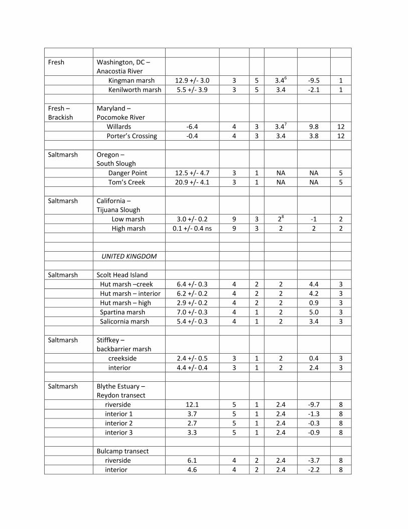
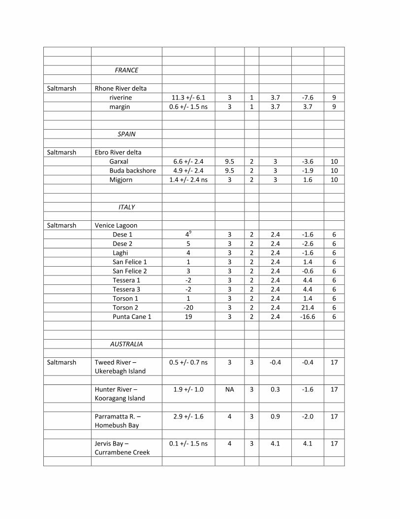
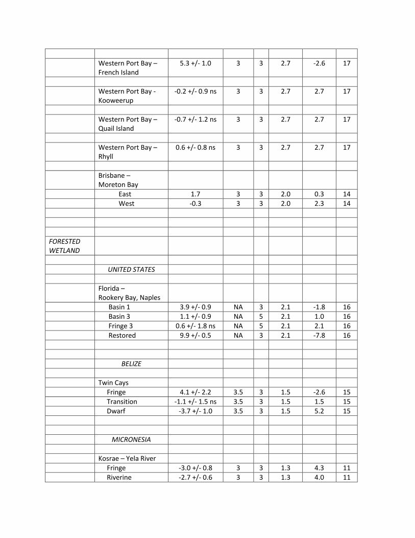
Table S1: Wetland elevation (VLMw) rate for 89 wetlands and wetland RSLR (RSLRwet) rate calculated for 87 of those wetlands. VLMw data taken from eighteen published studies using the SET method with a minimum record length of three years; RSLR was available for 17 of the published studies.

Wetland

Type

Location

Elevation Rate, VLMw

(mm/y)1

Record Length (years)

n2

RSLR

(mm/y)3

Wetland RSLR

(mm/y)4

Ref. No.5

HERBACEOUS MARSH

UNITED STATES

Saltmarsh Louisiana – Bayou Chitigue

2.2 +/- 0.6 8 3 13.3 11.1 18

Saltmarsh Louisiana – Old Oyster Bayou

3.6 +/- 0.8 8 3 9.0 5.4 18

Saltmarsh Louisiana – Caernarvon diversion

C-Near 4.2 +/- 0.2 4 2 3 -1.2 13

C-Mid 1.6 +/- 3.1 ns 4 2 3 3 13

C-Far 3.6 +/- 2.5 4 2 3 -0.6 13

W-Near 5.6 +/- 2.6 4 2 7 1.4 13

W-Mid 7.0 +/- 1.1 4 2 7 0 13

W-Far 2.7 +/- 0.9 4 2 7 4.3 13

V-Near -23.4 +/- 4.1 4 2 6 29.4 13

V-Mid -11.8 +/- 2.6 4 2 6 17.8 13

V-Far -11.0 +/- 2.4 4 2 6 17.0 13

Fresh-Brackish

Louisiana – Balize delta crevasse

Forest 0.7 +/- 0.6 4 2 10.0 9.3 4

Saltmarsh Massachusetts – Nauset Marsh

2.7 +/- 0.7 5 4 2.6 -0.1 7

Saltmarsh New Jersey – Little Beach

1.7 +/- 1.0 3 3 4.1 2.4 7

Saltmarsh Virginia - Wachapreague

High marsh 1.4 +/- 1.1 4 3 3.9 2.5 7

Mid marsh 0.7 +/- 1.1 ns 4 3 3.9 3.9 7

Virginia – Mockhorn

1.4 +/- 1.8 ns 4 2 3.9 3.9 7

Fresh Washington, DC – Anacostia River

Kingman marsh 12.9 +/- 3.0 3 5 3.46 -9.5 1

Kenilworth marsh 5.5 +/- 3.9 3 5 3.4 -2.1 1

Fresh – Brackish

Maryland – Pocomoke River

Willards -6.4 4 3 3.47 9.8 12

Porter’s Crossing -0.4 4 3 3.4 3.8 12

Saltmarsh Oregon – South Slough

Danger Point 12.5 +/- 4.7 3 1 NA NA 5

Tom’s Creek 20.9 +/- 4.1 3 1 NA NA 5

Saltmarsh California – Tijuana Slough

Low marsh 3.0 +/- 0.2 9 3 28 -1 2

High marsh 0.1 +/- 0.4 ns 9 3 2 2 2

UNITED KINGDOM

Saltmarsh Scolt Head Island

Hut marsh –creek 6.4 +/- 0.3 4 2 2 4.4 3

Hut marsh – interior 6.2 +/- 0.2 4 2 2 4.2 3

Hut marsh – high 2.9 +/- 0.2 4 2 2 0.9 3

Spartina marsh 7.0 +/- 0.3 4 1 2 5.0 3

Salicornia marsh 5.4 +/- 0.3 4 1 2 3.4 3

Saltmarsh Stiffkey – backbarrier marsh

creekside 2.4 +/- 0.5 3 1 2 0.4 3

interior 4.4 +/- 0.4 3 1 2 2.4 3

Saltmarsh Blythe Estuary – Reydon transect

riverside 12.1 5 1 2.4 -9.7 8

interior 1 3.7 5 1 2.4 -1.3 8

interior 2 2.7 5 1 2.4 -0.3 8

interior 3 3.3 5 1 2.4 -0.9 8

Bulcamp transect

riverside 6.1 4 2 2.4 -3.7 8

interior 4.6 4 2 2.4 -2.2 8

FRANCE

Saltmarsh Rhone River delta

riverine 11.3 +/- 6.1 3 1 3.7 -7.6 9

margin 0.6 +/- 1.5 ns 3 1 3.7 3.7 9

SPAIN

Saltmarsh Ebro River delta

Garxal 6.6 +/- 2.4 9.5 2 3 -3.6 10

Buda backshore 4.9 +/- 2.4 9.5 2 3 -1.9 10

Migjorn 1.4 +/- 2.4 ns 3 2 3 1.6 10

ITALY

Saltmarsh Venice Lagoon

Dese 1 49 3 2 2.4 -1.6 6

Dese 2 5 3 2 2.4 -2.6 6

Laghi 4 3 2 2.4 -1.6 6

San Felice 1 1 3 2 2.4 1.4 6

San Felice 2 3 3 2 2.4 -0.6 6

Tessera 1 -2 3 2 2.4 4.4 6

Tessera 3 -2 3 2 2.4 4.4 6

Torson 1 1 3 2 2.4 1.4 6

Torson 2 -20 3 2 2.4 21.4 6

Punta Cane 1 19 3 2 2.4 -16.6 6

AUSTRALIA

Saltmarsh Tweed River – Ukerebagh Island

0.5 +/- 0.7 ns 3 3 -0.4 -0.4 17

Hunter River – Kooragang Island

1.9 +/- 1.0 NA 3 0.3 -1.6 17

Parramatta R. – Homebush Bay

2.9 +/- 1.6 4 3 0.9 -2.0 17

Jervis Bay – Currambene Creek

0.1 +/- 1.5 ns 4 3 4.1 4.1 17

Western Port Bay – French Island

5.3 +/- 1.0 3 3 2.7 -2.6 17

Western Port Bay - Kooweerup

-0.2 +/- 0.9 ns 3 3 2.7 2.7 17

Western Port Bay – Quail Island

-0.7 +/- 1.2 ns 3 3 2.7 2.7 17

Western Port Bay – Rhyll

0.6 +/- 0.8 ns 3 3 2.7 2.7 17

Brisbane – Moreton Bay

East 1.7 3 3 2.0 0.3 14

West -0.3 3 3 2.0 2.3 14

FORESTED WETLAND

UNITED STATES

Florida – Rookery Bay, Naples

Basin 1 3.9 +/- 0.9 NA 3 2.1 -1.8 16

Basin 3 1.1 +/- 0.9 NA 5 2.1 1.0 16

Fringe 3 0.6 +/- 1.8 ns NA 5 2.1 2.1 16

Restored 9.9 +/- 0.5 NA 3 2.1 -7.8 16

BELIZE

Twin Cays

Fringe 4.1 +/- 2.2 3.5 3 1.5 -2.6 15

Transition -1.1 +/- 1.5 ns 3.5 3 1.5 1.5 15

Dwarf -3.7 +/- 1.0 3.5 3 1.5 5.2 15

MICRONESIA

Kosrae – Yela River

Fringe -3.0 +/- 0.8 3 3 1.3 4.3 11

Riverine -2.7 +/- 0.6 3 3 1.3 4.0 11

Interior 1.3 +/- 0.7 3 3 1.3 0 11

Kosrae – Utwe River

Fringe 1.2 +/- 0.3 3 3 1.3 0.1 11

Riverine 6.3 +/- 0.5 3 3 1.3 -5.0 11

Interior 1.3 +/- 0.2 3 3 1.3 0 11

AUSTRALIA

Moreton Bay

East 5.9 3 3 2.0 -3.9 14

West 1.4 3 3 2.0 0.6 14

Ukerebagh Island 2.4 +/- 1.4 3 3 -0.4 -2.8 17

Kooragang Island 2.0 +/- 0.5 NA 3 0.3 -1.7 17

-mixed w/ saltmarsh 2.1 +/- 0.6 NA 3 0.3 -1.8 17

Home Bush Bay 5.6 +/- 2.2 4 3 0.9 -4.7 17

-mixed w/ saltmarsh 4.7 +/- 1.2 4 3 0.9 -3.8 17

Currambene Creek 0.3 +/- 2.0 ns 4 3 4.1 4.1 17

-mixed w/ saltmarsh 0.1 +/- 1.5 ns 4 3 4.1 4.1 17

French Island -2.1 +/- 1.7 ns 3 3 2.7 2.7 17

Kooweerup -0.03 +/- 2.2 ns 3 3 2.7 2.7 17

Quail Island -2.6 +/- 2.1 3 3 2.7 2.7 17

Rhyll 0.9 +/- 1.9 ns 3 3 2.7 2.7 17

1Elevation trends not significantly different from zero are indicated by ns.

2n = the number of SET – MH stations at a wetland

3When RSLR is presented as a range, the mid-range value was used.

4RSLRwet is calculated as RSLR - VLMw

5See Supplemental Information for corresponding reference list.

6Source = NOAA tide gauge 8577330 at Solomons, Maryland; accessed at

<www.tidesandcurrents.noaa.gov> on January 19, 2014.

7Source = NOAA tide gauge 8571892 at Cambridge, Maryland; accessed at

<www.tidesandcurrents.noaa.gov> on January 19, 2014.

8Source = Cahoon, D., J. Lynch and A. Powell. 1996. Marsh vertical accretion in a southern California

estuary. Estuarine Coastal and Shelf Science 43:19-32

9Rates were estimated from Figure 6 in Day et al. (1999); reference 6 in Supplemental Information.

Article title: Estimating relative sea-level rise and submergence potential at a coastal wetland

Donald R. Cahoon

US Geological Survey, Patuxent Wildlife Research Center, 10300 Baltimore Avenue, c/o BARC-East,

Building 308, Beltsville, MD 20705 USA, email: dcahoon@usgs.gov