lable at ScienceDirect

Applied Geography 31 (2011) 251e258

Contents lists avai

Applied Geography

journal homepage: www.elsevier .com/locate/apgeog

Estimating reference evapotranspiration using remote sensing and empiricalmodels in a region with limited ground data availability in Kenya

Eduardo Eiji Maeda a,*, David A. Wiberg b, Petri K.E. Pellikka a

aDepartment of Geosciences and Geography, University of Helsinki, Gustaf Hällströmin katu 2, 00014, Helsinki, Finlandb Land Use Change and Agriculture Program at the International Institute for Applied Systems Analysis (IIASA), Laxenburg, Austria

Keywords:Reference evapotranspirationRemote sensingEmpirical modelsTaita HillsKenya

* Corresponding author. Tel.: þ358 44 2082876.E-mail address: eduardo.maeda@helsinki.fi (E.E. M

0143-6228/$ e see front matter � 2010 Elsevier Ltd.doi:10.1016/j.apgeog.2010.05.011

a b s t r a c t

Evapotranspiration is an important component of the hydrological cycle and its accurate quantification iscrucial for the design, operation and management of irrigation systems. However, the lack of meteoro-logical data from ground stations is a clear barrier to the proper management of water resources in poorcountries, increasing the risks of water scarcity and water conflicts. In the presented study, threetemperature based ET models are evaluated in the Taita Hills, Kenya, which is a particularly importantregion from the environmental conservation point of view. The Hargreaves, the Thornthwaite and theBlaneyeCriddle are the three tested methods, given that these are the most recommended approacheswhen only air temperature data are available. Land surface temperature data, retrieved from the MODIS/Terra sensor are evaluated as an alternative input for the models. One weather station with completeclimate datasets is used to calibrate the selected model using the FAO-56 PenmaneMonteith method asa reference. The results indicate that the Hargreaves model is the most appropriate for this particularstudy area, with an average RMSE of 0.47 mm d�1, and a correlation coefficient of 0.67. The MODIS LSTproduct was satisfactorily incorporated into the Hargreaves model achieving results that are consistentwith studies reported in the literature using air temperature data collected in ground stations.

� 2010 Elsevier Ltd. All rights reserved.

Introduction

Although global withdrawals of water resources are still belowthe critical limit, more than two billion people live in highly water-stressed areas due to the uneven distribution of this resource intime and space (Oki & Kanae, 2006). Simulated scenarios indicatethat up to 59% of the world population will face some sort of watershortage by 2050 (Rockstrom et al., 2009). In Kenya, currently over55% of the rural population do not have access to quality drinkablewater (FAO, 2005). In such regions, the accurate assessment ofwater demand and distribution is crucial to improve watermanagement and avoid scarcity.

Currently roughly 70% of freshwater withdraws are used foragriculture (FAO, 2005). In most sub-Saharan African countriesagriculture is themain economic activity, representing about 40% oftheir gross domestic product (Barrios, Ouattara, & Strobl, 2008) andit is estimated that between the years 1975 and 2000 the agricul-tural areas increased by 57% in sub-Saharan Africa (Brink & Eva,2009). Consequently, a careful control of the water used for

aeda).

All rights reserved.

irrigation is a key aspect to be considered in order to ensurea proper distribution of the available resources between residential,industrial and agricultural use.

Several studies have shown that careful irrigation managementcan considerably improve crops’ water use efficiency withoutcausing yield reduction (Du, Kang, Sun, Zhang, & Zhang, 2010,Hassanli, Ahmadirad, & Beecham, 2010). One of the fundamentalrequirements to estimating the amount of water necessary foroptimal agricultural production is to effectively understand therelationships between climatic conditions and evapotranspiration(ET). ET is defined as the combination of two separate processes, inwhich water is lost on the one hand from the soil surface byevaporation and on the other hand from the crop by transpiration(Allen, Pereira, Raes, & Smith, 1998). Reliable estimates of ET areessential to identify temporal variations on irrigation requirements,improve water resource allocation and evaluate the effect of landuse and management changes on the water balance (Ortega-Farias,Irmak, & Cuenca, 2009). Quantification of ET is a basic componentfor the design, operation and management of irrigation systems.

Given the fact that the direct measurement of ET is a difficulttask, the development of hydrometeorological models to estimate“reference ET” (ETo) resulted in important contributions for irri-gation management at global, regional and local scales. ETo is

E.E. Maeda et al. / Applied Geography 31 (2011) 251e258252

defined as the ET rate from a reference surface, where the referencesurface is a hypothetical grass with specific and well-known char-acteristics (Allen et al., 1998). The concept of ETo was introduced tostudy the evaporative demand of the atmosphere independently ofcrop type, crop phenology and management practices.

A great variety of ETo models have been developed during thepast decades. ETo models are typically based on physical principles,empirical equations or even a combination of physical and empir-ical approaches. Empirically based methods are establishedgrounded on observations and statistical analysis, and usually areappropriate for a specific region or climatic condition (e.g.Fooladmand & Ahmadi, 2009; Ahmadi & Fooladmand, 2008;Gavilán, Lorite, Tornero, & Berengena, 2006). On the other hand,physically based models aim to simulate fundamental principlessuch as energy balance and mass transfer. Although some disad-vantages and problems were reported, physically based modelshave proven to performwell in a great variety of climatic conditions(e.g. Liu & Luo, 2010; Villa Nova, Pereira, & Shock, 2007; Cancela,Cuesta, Neira, & Pereira, 2006).

Nevertheless, complex models developed to simulate thephysical processes involved in the ET frequently have many vari-ables and require a large amount of input data. For instance, solarradiation, relative humidity and wind speed are some of the vari-ables usually necessary to estimate ETo using physically basedmodels. Assembling and maintaining meteorological stationscapable of measuring such variables is very costly. In many devel-oping and poor countries, meteorological stations are often insuf-ficient to acquire the information necessary to represent thespatialetemporal variation of ETo. As a result, the irrigationmanagement in such areas is not optimal, increasing the risks ofwater scarcity and water conflicts.

Hence, intense efforts are necessary to search for alternativemethods and datasets to be used in poor regions highly affected byhunger and water scarcity. The combination of ET models withremote sensing data provides a feasible alternative to obtaintemporally and spatially continuous information about biophysicalvariables. According to Wagner, Kunstmann, Bárdossy, Conrad, andColditz. (2008), in poorly gauged catchments, remote sensing datacan significantly improve the availability of necessary information,for instance albedo, leaf area index and Land Surface Temperature(LST) (Wan, 2008).

This study evaluated three empirical ETo models in a regionparticularly important from the environmental conservation pointof view in Southeast-Kenya, where intense agricultural expansion istaking place. In order to overcome the low availability of meteo-rological data, LST data acquired by the MODIS/Terra sensor weretested as an alternative input for the evaluated models.

Study area

The Taita Hills are the northernmost part of the Eastern ArcMountains of Kenya and Tanzania, situated in the middle of theTsavo plains of the Taita-Taveta District in the Coast Province, Kenya(Fig. 1). The population of the whole Taita-Taveta district has grownfrom 90 146 (1962) persons to over 300 000 (Republic of Kenya,2001). The indigenous cloud forests have suffered substantial lossand degradation for several centuries as they have been convertedto agriculture, because of the abundant rainfall (annual 1100 mm)and rich soils (cambisols and humic nitosols) that provide goodconditions for agricultural production. Approximately half of thecloud forests have been cleared for agricultural lands and planta-tion forests since 1955 (Pellikka, Lötjönen, Siljander, & Lens, 2009).During the last 2 decades, the agricultural lands have increasedespecially in the surrounding foothills and lowlands (Clark &Pellikka, 2009).

Located in the inter-tropical convergence zone, the area hasa bimodal rainfall pattern, the long rains occurring in MarcheMayand short rains in NovembereDecember. The agriculture in the hillsis intensive small-scale subsistence farming. In the lower highlandzone and in uppermidland zone, the typical crops aremaize, beans,peas, potatoes, cabbages, tomatoes, cassava and banana. In theslopes and lower parts of the hills with average annual rainfallbetween 600 and 900 mm, early maturing maize species andsorghum and millet species are cultivated. In the lower midlandzones with average rainfall between 500 and 700 mm, drylandmaize types and onions are cultivated, among others. The twogrowing seasons, totaling to 150e170 days, coincide with the longand the short rains (Jaetzold & Schmidt, 1983). The land is preparedduring the dry season, and the crops are seeded prior to the shortrains and long rains. Harvesting takes place after the end of therainy seasons (Gachimbi et al., 2005).

The hills are surrounded by Tsavo national parks and sisal plan-tations leavingonly little land foragriculture to spreadover theplains.

Moreover, the Eastern Arc Mountains maintain some of therichest concentration of endemic animals and plants on Earth, andthus it is considered one of the 25 world’s biodiversity hotspots(Myers, Mittermeier, Mittermeier, Fonseca, & Kent, 2000). Althoughonly a small fraction of the indigenous cloud forests is preserved inthe Taita Hills, it continues to have an outstanding diversity of floraand fauna and high level of endemism. Hence, the area is consid-ered to have high scientific interest and there is a high potential forsucceeding in the connectivity development and community basednatural resource management (Himberg, Pellikka, & Luukkanen,2009).

Material and methods

Many empirically and physically based ETo models have beendeveloped during the past decades, varying in complexity and datarequirements. Generally, complex physically based models incor-porate a more comprehensive set of variables and parameters,which allows the model to perform well in a greater variety ofclimatic conditions. Unfortunately, such methods demand verydetailed meteorological data, which are frequently missing frommeteorological stations (Jabloun&Sahli, 2008).Moreover, settingupnew stations capable to record these data is in general expensive.

To overcome this problem, three empirical ETo models thatrequire only air temperature data were evaluated, namely theHargreaves, the Thornthwaite, and the BlaneyeCriddle methods.Each of these models, as well as the approach used for calibrationand error assessment, are described below.

Reference evapotranspiration (ETo) models

A) HargreavesThe Hargreaves method was developed by Hargreaves and

Samani (1985), using eight years of daily lysimeter data fromDavis, California, and tested in different locations such as Australia,Haiti and Bangladesh. Since then, the method has been successfullyapplied worldwide (e.g. Gavilán et al., 2006). The Hargreavesequation requires only daily mean, maximum and minimum airtemperature and extraterrestrial radiation. The equation can bewritten as:

ETo ¼ 0:0023� RA� ððTmax � TminÞÞ0:5�ðTmean þ 17:8Þ (1)

where ETo is the reference evapotranspiration given in mm day�1;RA is the extraterrestrial radiation; Tmean is mean temperature; Tminis the minimum temperature and Tmax is the maximumtemperature.

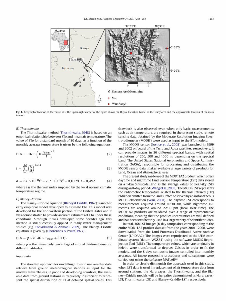
Fig. 1. Geographic location of the Taita Hills. The upper-right corner of the figure shows the Digital Elevation Model of the study area and the approximate location of the maintowns.

E.E. Maeda et al. / Applied Geography 31 (2011) 251e258 253

B) ThornthwaiteThe Thornthwaite method (Thornthwaite, 1948) is based on an

empirical relationship between ETo and mean air temperature. Thevalue of ETo for a standard month of 30 days, as a function of themonthly average temperature is given by the following equations:

ETo ¼ 16��10

Tmean

I

�a

(2)

I ¼X12i¼1

�ti5

�1;514(3)

a ¼ 67;5:10�8I3 � 7;71:10�6I2 þ 0;01791I þ 0;492 (4)

where I is the thermal index imposed by the local normal climatictemperature regime.

C) BlaneyeCriddleThe BlaneyeCriddle equation (Blaney & Criddle,1962) is another

early empirical model developed to estimate ETo. This model wasdeveloped for the arid western portion of the United States and itwas demonstrated to provide accurate estimates of ETo under theseconditions. Although it was developed some decades ago, thismethod is still successfully applied in many water managementstudies (e.g. Fooladmand & Ahmadi, 2009). The BlaneyeCriddleequation is given by (Doorenbos & Pruitt, 1977):

ETo ¼ p� ð0:46� Tmean þ 8:13ÞÞ (5)

where p is the mean daily percentage of annual daytime hours fordifferent latitudes.

Input data

The standard approach for modelling ETo is to use weather dataretrieve from ground meteorological stations as input for themodels. Nevertheless, in poor and developing countries, the avail-able data from ground stations is frequently insufficient to repre-sent the spatial distribution of ET at detailed spatial scales. This

drawback is also observed even when only basic measurements,such as air temperature, are required. In the present study, remotesensing data obtained by the Moderate Resolution Imaging Spec-troradiometer (MODIS) were used as input to the ETo models.

The MODIS sensor (Justice et al., 2002) was launched in 1999and 2002 on board of the Terra and Aqua satellites, respectively. Itcan provide images in 36 different spectral bands, with spatialresolutions of 250, 500 and 1000 m, depending on the spectralband. The United States National Aeronautics and Space Adminis-tration (NASA), responsible for processing and distributing theMODIS sensor data, makes available a large variety of products forLand, Ocean and Atmospheric uses.

Thepresentstudymadeuseof theMOD11A2product,whichoffersdaytime and nighttime Land Surface Temperature (LST) data storedon a 1-km Sinusoidal grid as the average values of clear-sky LSTsduring an8-day period (Wanget al., 2005). TheMODIS LST representsthe radiometric temperature related to the thermal infrared (TIR)radiation emitted from the land surface observedbyan instantaneousMODIS observation (Wan, 2008). The daytime LST corresponds tomeasurements acquired around 10:30 am, while nighttime LSTrecords are acquired around 22:30 pm (local solar time). TheMOD11A2 products are validated over a range of representativeconditions, meaning that the product uncertainties are well definedand has been satisfactorily used in a large variety of scientific studies.

In total, 368 LST images (8-day composite), corresponding to theentire MOD11A2 product dataset from the years 2001e2008, weredownloaded from the Land Processes Distributed Active ArchiveCenter (LP DAAC). The images were reprojected to the UTM coor-dinate system (datum WGS84) using the software MODIS Repro-jection Tool (MRT). The temperature values, which are originally inKelvin, were transformed to degrees Celsius in order to fit themodels, and the 8 days composite images compiled into monthlyaverages. All image processing procedures and calculations werecarried out using the software MATLAB�.

In order to clearly distinguish the approach used in this study,when LST data is used in replacement of air temperature data fromground stations, the Hargreaves, the Thornthwaite, and the Bla-neyeCriddle models will be hereafter denominated as Hargreaves-LST, Thornthwaite-LST, and BlaneyeCriddle-LST, respectively.

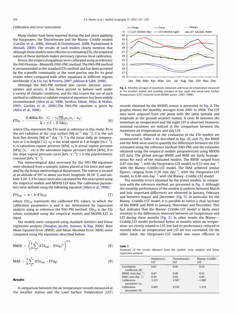
Fig. 2. Monthly averages of maximum, minimum and mean air temperature measuredat Voi weather station and monthly averages of day, night and mean Land SurfaceTemperatures (LST) retrieved from MODIS sensor (2001e2008).

Table 1Summary of the results obtained from the models’ error analysis and linearregression analysis.

Hargreaves-LST

Thornthwaite-LST

BlaneyeCriddle-LST

Correlationcoefficient (R)

0.67 0.66 0.55

RMSE (mm day�1) 0.47 0.49 0.53MAE (mm day�1) 0.39 0.42 0.46Calibration

parameter (a)3.221 3.507 �1.980

Calibrationparameter (b)

0.497 0.543 1.379

E.E. Maeda et al. / Applied Geography 31 (2011) 251e258254

Calibration and error assessment

Many studies have been reported during the last years applyingthe Hargreaves, the Thornthwaite and the BlaneyeCriddle models(Gavilán et al., 2006, Ahmadi & Fooladmand, 2008, Fooladmand &Ahmadi, 2009). The results of such studies clearly mention thatalthough thosemodelswereeffective inestimatingETo, theempiricalnature of these methods makes necessary rigorous local calibration.

Hence, theempirical equationswere calibratedusing as referencethe FAO PenmaneMonteith (FAO-PM)method. The FAO-PMmethodis recommended as the standard ETomethod and has been acceptedby the scientific community as the most precise one for its goodresults when compared with other equations in different regionsworldwide (Cai, Liu, Lei, & Pereira, 2007; Jabloun & Sahli, 2008).

Although the FAO-PM method also carries intrinsic uncer-tainties and errors, it has been proved to behave well undera variety of climatic conditions, and for this reason the use of suchmethod to calibrate or validate empirical equations has beenwidelyrecommended (Allen et al., 1998; Itenfisu, Elliott, Allen, & Walter,2003; Gavilán et al., 2006).The FAO-PM equation is given by(Allen et al., 1998):

EToR ¼ 0:408DðRn� GÞ þ g 900Tþ273u2ðes � eaÞ

Dþ gð1þ 0:34u2Þ(6)

where EToR represents the ETo used as reference in this study; Rn isthe net radiation at the crop surface [MJ m�2 day�1]; G is the soilheat flux density [MJ m-2 day�1]; T is the mean daily air tempera-ture at 2 m height [�C]; u2 is the wind speed at 2 m height [m s�1];es is saturation vapour pressure [kPa]; ea is actual vapour pressure[kPa]; (es e ea) is the saturation vapour pressure deficit [kPa]; D isthe slope vapour pressure curve [kPa �C�1]; g is the psychrometricconstant [kPa �C�1].

The meteorological data necessary for the FAO-PM equationswere obtained from a synoptic station placed at Voi town and oper-ated by the Kenya meteorological department. The station is locatedat an altitude of 597 m above sea level, longitude 38.34� E, and lati-tude3.24� S. ETovalueswere also calculated for this exact pointusingthe empirical models and MODIS LST data. The calibration parame-ters were defined using the following equation (Allen et al., 1998):

ETocal ¼ aþ b,EToLST (7)

where ETocal represents the calibrated ETo values, in which thecalibration parameters a and b are determined by regressionanalysis using as reference the FAO-PM method; ETolst is the ETovalues estimated using the empirical models and MODIS LST asinput.

The models were compared using standard statistics and linearregression analysis (Douglas, Jacobs, Sumner, & Ray, 2009). RootMean Squared Error (RMSE) and Mean Absolute Error (MAE) werecomputed using the equations described below:

RMSE ¼ 1n

Xn1

ðETocal � EToRÞ2!0:5

(8)

MAE ¼ 1n

Xn1

jETocal � EToRj (9)

Results

A comparison between the air temperature records measured atVoi weather station and the Land Surface Temperature (LST)

records obtained by the MODIS sensor is presented in Fig. 2. Thegraphic shows the monthly averages from 2001 to 2008. The LSTdata were acquired from one point with the same latitude andlongitude as the ground weather station. A close fit between theminimum air temperature and the night LST is observed. However,seasonal variations are noticed in the comparison between themaximum air temperatures and day LST.

The results obtained in the evaluation of the ETo models aresummarized in Table 1. As described in Eqs. (8) and (9), the RMSEand theMAEwere used to quantify the differences between the EToestimated using the reference method (FAO-PM) and the estimatesobtained using the empirical models parameterized using MODISLST data. The global average RMSE and MAE are fairly homoge-neous for each of the evaluated models. The RMSE ranged from0.47 mm day�1, with the Hargreaves-LST model, to 0.53 mm day�1,with the BlaneyeCriddle-LST model. The MAE achieved similarfigures, ranging from 0.39 mm day�1, with the Hargreaves-LSTmodel, to 0.46 mm day�1, with the BlaneyeCriddle-LST model.

The monthly errors obtained by the tested models, in compar-ison with the reference method, are presented in Fig. 3. Althoughthe monthly performance of the models is uniform between Marchand July, important differences are observed in January, Februaryand between August and December (Fig. 3). In particular for theBlaneyeCriddle-LST model, it is possible to notice a clear increaseof the RMSE and MAE in January, November and December. Thisfact indicates that the BlaneyeCriddle-LST model is likely moresensitive to the differences observed between air temperature andLST during these months (Fig. 2). In other words, the Blaneye-Criddle-LST model performed better in months when air temper-ature are closely related to LST, but had its performance reduced inmonths when air temperature and LST are less correlated. On theother hand, the Hargreaves-LST model was more efficient in

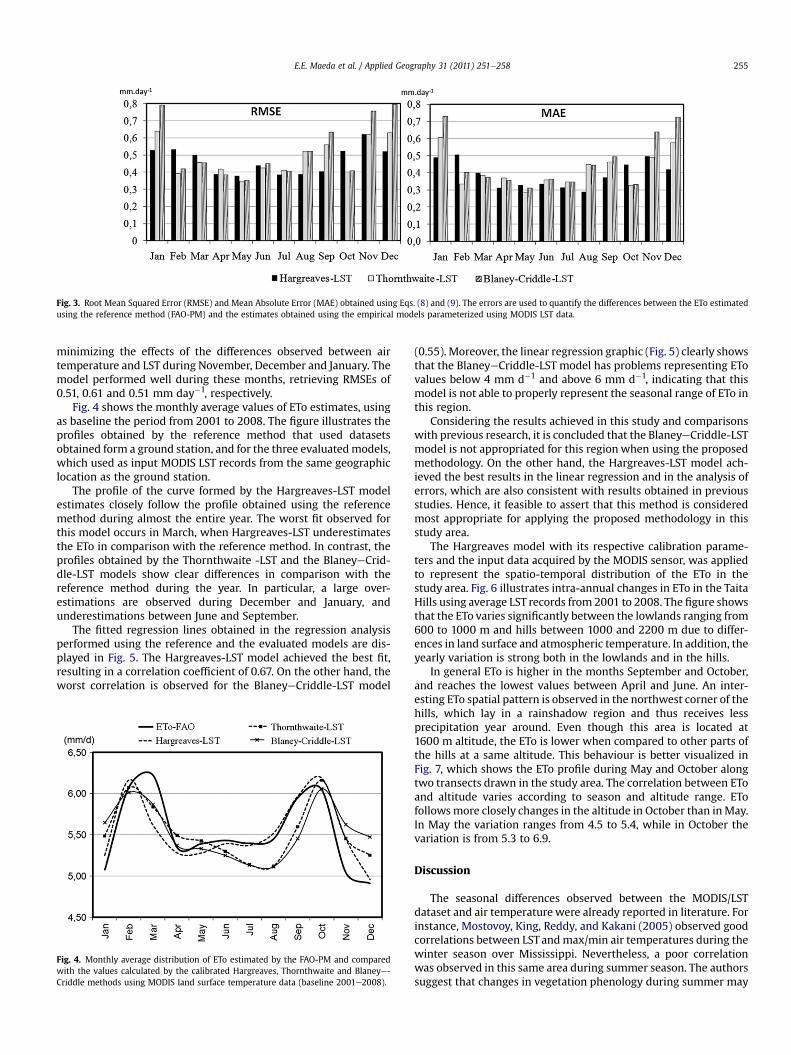
Fig. 3. Root Mean Squared Error (RMSE) and Mean Absolute Error (MAE) obtained using Eqs. (8) and (9). The errors are used to quantify the differences between the ETo estimatedusing the reference method (FAO-PM) and the estimates obtained using the empirical models parameterized using MODIS LST data.

E.E. Maeda et al. / Applied Geography 31 (2011) 251e258 255

minimizing the effects of the differences observed between airtemperature and LST during November, December and January. Themodel performed well during these months, retrieving RMSEs of0.51, 0.61 and 0.51 mm day�1, respectively.

Fig. 4 shows the monthly average values of ETo estimates, usingas baseline the period from 2001 to 2008. The figure illustrates theprofiles obtained by the reference method that used datasetsobtained form a ground station, and for the three evaluatedmodels,which used as input MODIS LST records from the same geographiclocation as the ground station.

The profile of the curve formed by the Hargreaves-LST modelestimates closely follow the profile obtained using the referencemethod during almost the entire year. The worst fit observed forthis model occurs in March, when Hargreaves-LST underestimatesthe ETo in comparison with the reference method. In contrast, theprofiles obtained by the Thornthwaite -LST and the BlaneyeCrid-dle-LST models show clear differences in comparison with thereference method during the year. In particular, a large over-estimations are observed during December and January, andunderestimations between June and September.

The fitted regression lines obtained in the regression analysisperformed using the reference and the evaluated models are dis-played in Fig. 5. The Hargreaves-LST model achieved the best fit,resulting in a correlation coefficient of 0.67. On the other hand, theworst correlation is observed for the BlaneyeCriddle-LST model

Fig. 4. Monthly average distribution of ETo estimated by the FAO-PM and comparedwith the values calculated by the calibrated Hargreaves, Thornthwaite and Blaneye-Criddle methods using MODIS land surface temperature data (baseline 2001e2008).

(0.55). Moreover, the linear regression graphic (Fig. 5) clearly showsthat the BlaneyeCriddle-LST model has problems representing ETovalues below 4 mm d�1 and above 6 mm d�1, indicating that thismodel is not able to properly represent the seasonal range of ETo inthis region.

Considering the results achieved in this study and comparisonswith previous research, it is concluded that the BlaneyeCriddle-LSTmodel is not appropriated for this region when using the proposedmethodology. On the other hand, the Hargreaves-LST model ach-ieved the best results in the linear regression and in the analysis oferrors, which are also consistent with results obtained in previousstudies. Hence, it feasible to assert that this method is consideredmost appropriate for applying the proposed methodology in thisstudy area.

The Hargreaves model with its respective calibration parame-ters and the input data acquired by the MODIS sensor, was appliedto represent the spatio-temporal distribution of the ETo in thestudy area. Fig. 6 illustrates intra-annual changes in ETo in the TaitaHills using average LST records from 2001 to 2008. The figure showsthat the ETo varies significantly between the lowlands ranging from600 to 1000 m and hills between 1000 and 2200 m due to differ-ences in land surface and atmospheric temperature. In addition, theyearly variation is strong both in the lowlands and in the hills.

In general ETo is higher in the months September and October,and reaches the lowest values between April and June. An inter-esting ETo spatial pattern is observed in the northwest corner of thehills, which lay in a rainshadow region and thus receives lessprecipitation year around. Even though this area is located at1600 m altitude, the ETo is lower when compared to other parts ofthe hills at a same altitude. This behaviour is better visualized inFig. 7, which shows the ETo profile during May and October alongtwo transects drawn in the study area. The correlation between EToand altitude varies according to season and altitude range. ETofollowsmore closely changes in the altitude in October than inMay.In May the variation ranges from 4.5 to 5.4, while in October thevariation is from 5.3 to 6.9.

Discussion

The seasonal differences observed between the MODIS/LSTdataset and air temperature were already reported in literature. Forinstance, Mostovoy, King, Reddy, and Kakani (2005) observed goodcorrelations between LST andmax/min air temperatures during thewinter season over Mississippi. Nevertheless, a poor correlationwas observed in this same area during summer season. The authorssuggest that changes in vegetation phenology during summer may

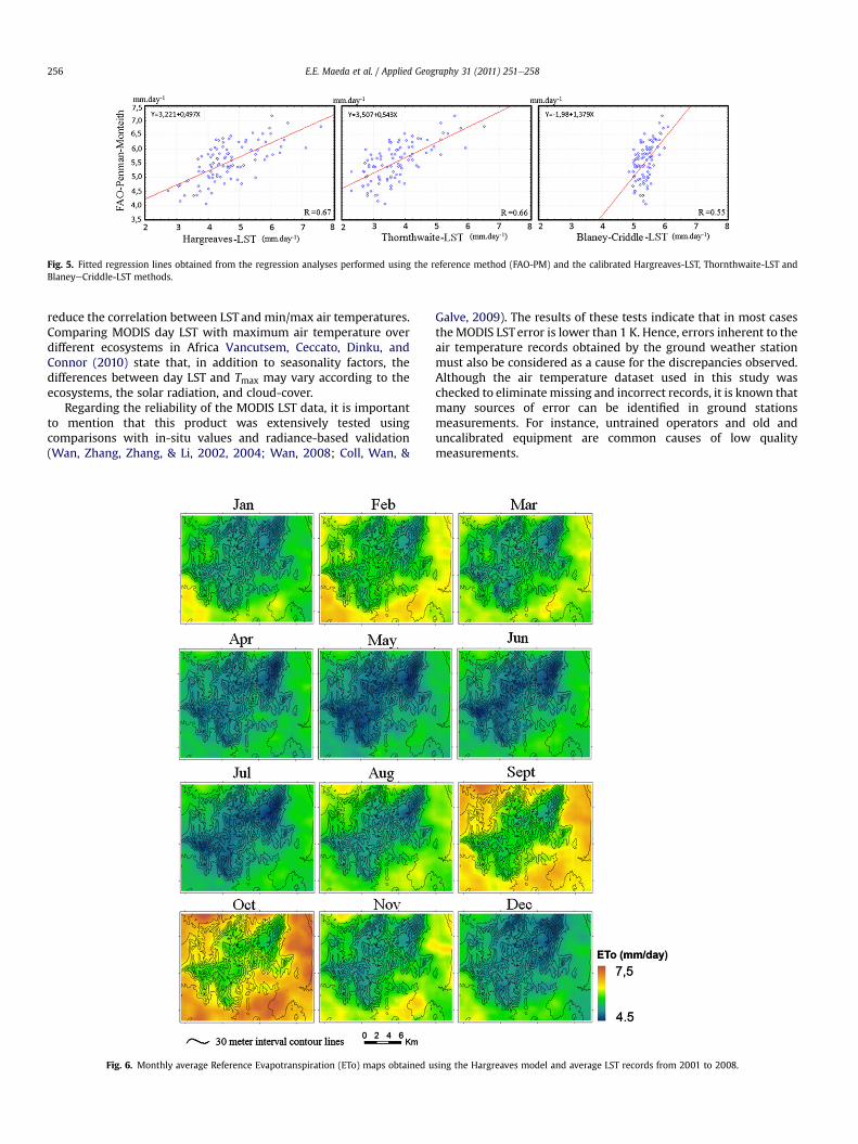
Fig. 5. Fitted regression lines obtained from the regression analyses performed using the reference method (FAO-PM) and the calibrated Hargreaves-LST, Thornthwaite-LST andBlaneyeCriddle-LST methods.

E.E. Maeda et al. / Applied Geography 31 (2011) 251e258256

reduce the correlation between LST and min/max air temperatures.Comparing MODIS day LST with maximum air temperature overdifferent ecosystems in Africa Vancutsem, Ceccato, Dinku, andConnor (2010) state that, in addition to seasonality factors, thedifferences between day LST and Tmax may vary according to theecosystems, the solar radiation, and cloud-cover.

Regarding the reliability of the MODIS LST data, it is importantto mention that this product was extensively tested usingcomparisons with in-situ values and radiance-based validation(Wan, Zhang, Zhang, & Li, 2002, 2004; Wan, 2008; Coll, Wan, &

Fig. 6. Monthly average Reference Evapotranspiration (ETo) maps obtained u

Galve, 2009). The results of these tests indicate that in most casestheMODIS LST error is lower than 1 K. Hence, errors inherent to theair temperature records obtained by the ground weather stationmust also be considered as a cause for the discrepancies observed.Although the air temperature dataset used in this study waschecked to eliminate missing and incorrect records, it is known thatmany sources of error can be identified in ground stationsmeasurements. For instance, untrained operators and old anduncalibrated equipment are common causes of low qualitymeasurements.

sing the Hargreaves model and average LST records from 2001 to 2008.

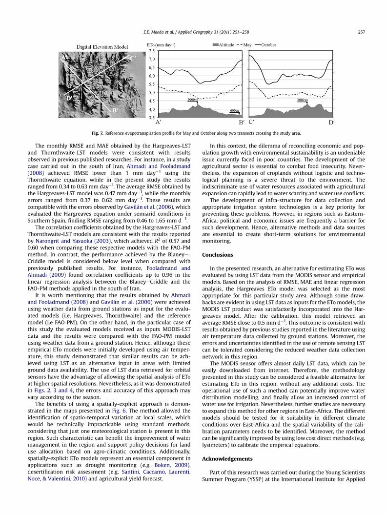
Fig. 7. Reference evapotranspiration profile for May and October along two transects crossing the study area.

E.E. Maeda et al. / Applied Geography 31 (2011) 251e258 257

The monthly RMSE and MAE obtained by the Hargreaves-LSTand Thornthwaite-LST models were consistent with resultsobserved in previous published researches. For instance, in a studycase carried out in the south of Iran, Ahmadi and Fooladmand(2008) achieved RMSE lower than 1 mm day�1 using theThornthwaite equation, while in the present study the resultsranged from 0.34 to 0.63 mm day�1. The average RMSE obtained bythe Hargreaves-LST model was 0.47 mm day�1, while the monthlyerrors ranged from 0.37 to 0.62 mm day�1. These results arecompatible with the errors observed by Gavilán et al. (2006), whichevaluated the Hargreaves equation under semiarid conditions inSouthern Spain, finding RMSE ranging from 0.46 to 1.65 mm d�1.

The correlation coefficients obtained by the Hargreaves-LST andThornthwaite-LST models are consistent with the results reportedby Narongrit and Yasuoka (2003), which achieved R2 of 0.57 and0.60 when comparing these respective models with the FAO-PMmethod. In contrast, the performance achieved by the Blaneye-Criddle model is considered below level when compared withpreviously published results. For instance, Fooladmand andAhmadi (2009) found correlation coefficients up to 0.96 in thelinear regression analysis between the BlaneyeCriddle and theFAO-PM methods applied in the south of Iran.

It is worth mentioning that the results obtained by Ahmadiand Fooladmand (2008) and Gavilán et al. (2006) were achievedusing weather data from ground stations as input for the evalu-ated models (i.e. Hargreaves, Thornthwaite) and the referencemodel (i.e FAO-PM). On the other hand, in the particular case ofthis study the evaluated models received as inputs MODIS-LSTdata and the results were compared with the FAO-PM modelusing weather data from a ground station. Hence, although theseempirical ETo models were initially developed using air temper-ature, this study demonstrated that similar results can be ach-ieved using LST as an alternative input in areas with limitedground data availability. The use of LST data retrieved for orbitalsensors have the advantage of allowing the spatial analysis of EToat higher spatial resolutions. Nevertheless, as it was demonstratedin Figs. 2, 3 and 4, the errors and accuracy of this approach mayvary according to the season.

The benefits of using a spatially-explicit approach is demon-strated in the maps presented in Fig. 6. The method allowed theidentification of spatio-temporal variation at local scales, whichwould be technically impracticable using standard methods,considering that just one meteorological station is present in thisregion. Such characteristic can benefit the improvement of watermanagement in the region and support policy decisions for landuse allocation based on agro-climatic conditions. Additionally,spatially-explicit ETo models represent an essential component inapplications such as drought monitoring (e.g. Boken, 2009),desertification risk assessment (e.g. Santini, Caccamo, Laurenti,Noce, & Valentini, 2010) and agricultural yield forecast.

In this context, the dilemma of reconciling economic and pop-ulation growth with environmental sustainability is an undeniableissue currently faced in poor countries. The development of theagricultural sector is essential to combat food insecurity. Never-theless, the expansion of croplands without logistic and techno-logical planning is a severe threat to the environment. Theindiscriminate use of water resources associated with agriculturalexpansion can rapidly lead towater scarcity andwater use conflicts.

The development of infra-structure for data collection andappropriate irrigation system technologies is a key priority forpreventing these problems. However, in regions such as Eastern-Africa, political and economic issues are frequently a barrier forsuch development. Hence, alternative methods and data sourcesare essential to create short-term solutions for environmentalmonitoring.

Conclusions

In the presented research, an alternative for estimating ETo wasevaluated by using LST data from the MODIS sensor and empiricalmodels. Based on the analysis of RMSE, MAE and linear regressionanalysis, the Hargreaves ETo model was selected as the mostappropriate for this particular study area. Although some draw-backs are evident in using LST data as inputs for the ETomodels, theMODIS LST product was satisfactorily incorporated into the Har-greaves model. After the calibration, this model retrieved anaverage RMSE close to 0.5 mm d�1. This outcome is consistent withresults obtained by previous studies reported in the literature usingair temperature data collected by ground stations. Moreover, theerrors and uncertainties identified in the use of remote sensing LSTcan be tolerated considering the reduced weather data collectionnetwork in this region.

The MODIS sensor offers almost daily LST data, which can beeasily downloaded from internet. Therefore, the methodologypresented in this study can be considered a feasible alternative forestimating ETo in this region, without any additional costs. Theoperational use of such a method can potentially improve waterdistribution modelling, and finally allow an increased control ofwater use for irrigation. Nevertheless, further studies are necessaryto expand thismethod for other regions in East-Africa. The differentmodels should be tested for it suitability in different climateconditions over East-Africa and the spatial variability of the cali-bration parameters needs to be identified. Moreover, the methodcan be significantly improved by using low cost direct methods (e.g.lysimeters) to calibrate the empirical equations.

Acknowledgements

Part of this research was carried out during the Young ScientistsSummer Program (YSSP) at the International Institute for Applied

E.E. Maeda et al. / Applied Geography 31 (2011) 251e258258

System Analysis (IIASA), Austria. The authors kindly thank Dr.MarekMakowski, from IIASA, and Luciana Kindl da Cunha, from theUniversity of Iowa, for their contribution. This study was funded bythe Academy of Finland, Council for Development Studies (TAITA-TOO project http://www.helsinki.fi/science/taita), Centre for Inter-national Mobility and the University of Helsinki.

References

Ahmadi, S. H., & Fooladmand, H. R. (2008). Spatially distributed monthly referenceevapotranspiration derived from the calibration of Thornthwaite equation:a case study, South of Iran. Irrigation Science, 26(4), 303e312.

Allen, R. G., Pereira, L. S., Raes, D., & Smith, M. (1998). Crop evapotranspiration eguidelines for computing crop water requirements e FAO irrigation and drainagepaper 56. Rome: FAO.

Barrios, S., Ouattara, B., & Strobl, E. (2008). The impact of climatic change on agri-cultural production: is it different for Africa? Food Policy, 33, 287e298.

Blaney, H. F., & Criddle, W. D. (1962). Determining consumptive use and irrigationwater requirements. USDA Technical Bulletin 1275. Beltsville: US Department ofAgriculture.

Boken, V. K. (2009). Improving a drought early warning model for an arid regionusing a soil-moisture index. Applied Geography, 29, 402e408.

Brink, A. B., & Eva, H. D. (2009). Monitoring 25 years of land cover change dynamics inAfrica:a samplebasedremotesensingapproach.AppliedGeography,29(4),501e512.

Cai, J., Liu, Y., Lei, T., & Pereira, L. S. (2007). Estimating reference evapotranspirationwith the FAO PenmaneMonteith equation using daily weather forecastmessages. Agricultural and Forest Meteorology, 145(1e2), 22e35.

Cancela, J. J., Cuesta, T. S., Neira, X. X., & Pereira, L. S. (2006). Modelling for improvedirrigation water management in a temperate region of Northern Spain. Bio-systems Engineering, 94(1), 151e163.

Clark,B. J. F.,&Pellikka,P.K.E. (2009). Landscapeanalysisusingmultiscale segmentationand object orientated classification. In A. Röder, & J. Hill (Eds.), Recent advances inremote sensing and geoinformation processing for land degradation assessment. ISPRSbook series in photogrammetry, remote sensing and spatial information sciences, Vol. 8(pp. 323e342). Taylor & Francis Group, ISBN 978-0-415-39769-8.

Coll, C., Wan, Z., & Galve, J. M. (2009). Temperature-based and radiance-basedvalidations of the V5 MODIS land surface temperature product. Journal ofGeophysical Research, 114, D20102. doi:10.1029/2009JD012038.

Doorenbos, J., & Pruitt, W. O. (1977). Guidelines for predicting crop water require-ments. FAO Irrigation and Drainage Paper, No. 56. Rome: FAO.

Douglas, E. M., Jacobs, J. M., Sumner, D. M., & Ray, R. L. (2009). A comparison ofmodels for estimating potential evapotranspiration for Florida land cover types.Journal of Hydrology, 373(3e4), 366e376.

Du, T., Kang, S., Sun, J., Zhang, X., & Zhang, J. (2010). An improved water use effi-ciency of cereals under temporal and spatial deficit irrigation in north China.Agricultural Water Management, 97(1), 66e74.

FAO e Food and Agriculture Organization of the United Nations, Land and WaterDevelopment Division. (2005). AQUASTAT information system on water andagriculture: Online database. Rome: FAO.

Fooladmand, H. R., & Ahmadi, S. H. (2009). Monthly spatial calibration of Bla-neyeCriddle equation for calculating monthly ETo in south of Iran. Irrigationand Drainage, 58(2), 234e245.

Gachimbi, L. N., Gicheru, P. T., Nyangw’ara, M. K., Lekasi, J. K., Sijali, I. V., & Kimigo, J.(2005). Agricultural productivity and sustainable land management in Kenya(APSLM): Smallholder farming, rural livelihoods, biodiversity and copping mecha-nisms in Taita Taveta district: Baseline survey report. Nairobi: Kenya AgriculturalResearch Institute. Technical Report No. 1.

Gavilán, P., Lorite, I. J., Tornero, S., & Berengena, J. (2006). Regional calibration ofHargreaves equation for estimating reference ET in a semiarid environment.Agriculture Water Management, 81, 257e281.

Hargreaves, G. H., & Samani, Z. A. (1985). Reference crop evapotranspiration fromtemperature. Applied Engineering in Agriculture, 1(2), 96e99.

Hassanli, A. M., Ahmadirad, S., & Beecham, S. (2010). Evaluation of the influence ofirrigation methods and water quality on sugar beet yield and water use effi-ciency. Agricultural Water Management, 97(2), 357e362.

Himberg, N. L. M. A. O., Pellikka, P., & Luukkanen, O. (2009). The benefits andconstraints of participation in forest management. The case of Taita Hills, Kenya.Fennia, 187, 61e76.

Itenfisu, D., Elliott, R. L., Allen, R. G., & Walter, I. A. (2003). Comparison of referenceevapotranspiration calculation as part of the ASCE standardization effort.Journal of Irrigation and Drainage Engineering ASCE, 129(6), 440e448.

Jabloun, M., & Sahli, A. (2008). Evaluation of FAO-56 methodology for estimatingreference evapotranspiration using limited climatic data. Application to Tunisia.Agricultural Water Management, 95(6), 707e715.

Jaetzold, R., & Schmidt, H. (1983)Farm management handbook of Kenya, Vol. II.. EastKenya, Kenya: Ministry of Agriculture.

Justice, C. O., Townshend, J. R. G., Vermote, E. F., Masuoka, E., Wolfe, R. E., Saleous, N.,et al. (2002). An overview of MODIS Land data processing and product status.Remote Sensing of Environment, 83, 3e15.

Liu, Y., & Luo, Y. (2010). A consolidated evaluation of the FAO-56 dual crop coeffi-cient approach using the lysimeter data in the North China Plain. AgriculturalWater Management, 97(1), 31e40.

Mostovoy, G. V., King, R., Reddy, K. R., & Kakani, V. G. (2005). Using MODIS LST datafor high-resolution estimates of daily air temperature over Mississippi. InProceedings of the 3rd international workshop on the analysis of multi-temporalremote sensing images (pp. 76e80). IEEE, CD Rom.

Myers, N., Mittermeier, R. A., Mittermeier, C. G., Fonseca, G. A. B., & Kent, J. (2000).Biodiversity hotspots for conservation priorities. Nature, 403(6772), 853e858.

Narongrit, C., & Yasuoka, Y. (2003). The use of terra-MODIS data for estimatingevapotranspiration and its change caused by global warming. EnvironmentalInformatics Archives, 1, 505e511.

Oki, T., & Kanae, S. (2006). Global hydrological cycles and world water resources.Science, 313(1068), 1068e1072.

Ortega-Farias, S., Irmak, S., & Cuenca, R. (2009). Special issue on evapotranspirationmeasurement and modeling. Irrigation Science, 28(1), 1e3.

Pellikka, P. K. E., Lötjönen, M., Siljander, M., & Lens, L. (2009). Airborne remotesensing of spatiotemporal change (1955e2004) in indigenous and exotic forestcover in the Taita Hills, Kenya. International Journal of Applied Earth Observationsand Geoinformation, 11(4), 221e232.

Republic of Kenya. (2001). The 1999 population & housing census. Kenya: CentralBureau of Statistics, Ministry of Planning and National Development.

Rockstrom, J., Falkenmark, M., Karlberg, L., Hoff, H., Rost, S., & Gerten, D. (2009).Future water availability for global food production: the potential of greenwater for increasing resilience to global change. Water Resources Research, 45,W00A12. doi:10.1029/2007WR006767.

Santini, M., Caccamo, G., Laurenti, A., Noce, S., & Valentini, R. (2010). A multi-component GIS framework for desertification risk assessment by an integratedindex. Applied Geography, 30(3), 394e415.

Thornthwaite, C. W. (1948). An approach toward a rational classification of climate.Geographical Review, 38, 55e94.

Vancutsem, C., Ceccato, P., Dinku, T., & Connor, S. J. (2010). Evaluation of MODIS landsurface temperature data to estimate air temperature in different ecosystemsover Africa. Remote Sensing of Environment, 114(2), 449e465.

Villa Nova, N. A., Pereira, A. B., & Shock, C. C. (2007). Estimation of referenceevapotranspiration by an energy balance approach. Biosystems Engineering, 96(4), 605e615.

Wagner, S., Kunstmann, H., Bárdossy, A., Conrad, C., & Colditz, R. R. (2008). Waterbalance estimation of a poorly gauged catchment in West Africa usingdynamically downscaled meteorological fields and remote sensing information.Physics and Chemistry of the Earth, 34(4e5), 225e235.

Wan, Z. (2008). New refinements and validation of the MODIS land-surfacetemperature/emissivity products. Remote Sensing of Environment, 112, 59e74.

Wan, Z., Zhang, Y., Zhang, Y. Q., & Li, Z.-L. (2002). Validation of the land-surfacetemperature products retrieved from Moderate Resolution Imaging Spectror-adiometer data. Remote Sensing of Environment, 83, 163e180.

Wan, Z., Zhang, Y., Zhang, Y. Q., & Li, Z.-L. (2004). Quality assessment and validationof the global land surface temperature. International Journal of Remote Sensing,25, 261e274.

Wang, K., Wan, Z., Wang, P., Sparrow, M., Liu, J., Zhou, X., et al. (2005). Estimation ofsurface long wave radiation and broadband emissivity using Moderate Reso-lution Imaging Spectroradiometer (MODIS) land surface temperature/emis-sivity products. Journal of Geophysical Research, 110, D11109.