Estimating Operational Risk Capital with Greater Accuracy .... Opdyke - UCE Presentation - Estimating... · Estimating Operational Risk Capital with Greater Accuracy, Precision, and

Estimating Operational Risk Capital with Greater Accuracy, Precision, and Robustness

J.D. Opdyke, Head of Operational Risk Modeling,

Quantitative Methods Group, GE Capital [email protected]

© J.D. Opdyke

1 of 63

© J.D. Opdyke

2 of 63

This work was completed by the sole author, J.D. Opdyke, when he was Senior Managing Director of DataMineit, LLC (aside from more recent reviews of the published journal paper). The views presented herein are the views of the sole author and do not necessarily reflect the views of DataMineit, LLC, GE Capital, or any other institution.

Disclaimer

© J.D. Opdyke

3 of 63

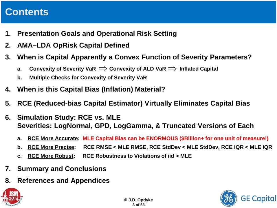
1. Presentation Goals and Operational Risk Setting 2. AMA–LDA OpRisk Capital Defined 3. When is Capital Apparently a Convex Function of Severity Parameters?

a. Convexity of Severity VaR Convexity of ALD VaR Inflated Capital b. Multiple Checks for Convexity of Severity VaR

4. When is this Capital Bias (Inflation) Material?

5. RCE (Reduced-bias Capital Estimator) Virtually Eliminates Capital Bias

6. Simulation Study: RCE vs. MLE Severities: LogNormal, GPD, LogGamma, & Truncated Versions of Each

a. RCE More Accurate: MLE Capital Bias can be ENORMOUS ($Billion+ for one unit of measure!) b. RCE More Precise: RCE RMSE < MLE RMSE, RCE StdDev < MLE StdDev, RCE IQR < MLE IQR c. RCE More Robust: RCE Robustness to Violations of iid > MLE

7. Summary and Conclusions 8. References and Appendices

Contents

⇒ ⇒

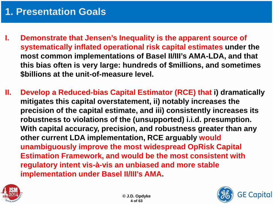
1. Presentation Goals

I. Demonstrate that Jensen’s Inequality is the apparent source of systematically inflated operational risk capital estimates under the most common implementations of Basel II/III’s AMA-LDA, and that this bias often is very large: hundreds of $millions, and sometimes $billions at the unit-of-measure level.

II. Develop a Reduced-bias Capital Estimator (RCE) that i) dramatically mitigates this capital overstatement, ii) notably increases the precision of the capital estimate, and iii) consistently increases its robustness to violations of the (unsupported) i.i.d. presumption. With capital accuracy, precision, and robustness greater than any other current LDA implementation, RCE arguably would unambiguously improve the most widespread OpRisk Capital Estimation Framework, and would be the most consistent with regulatory intent vis-à-vis an unbiased and more stable implementation under Basel II/III’s AMA.

© J.D. Opdyke

4 of 63

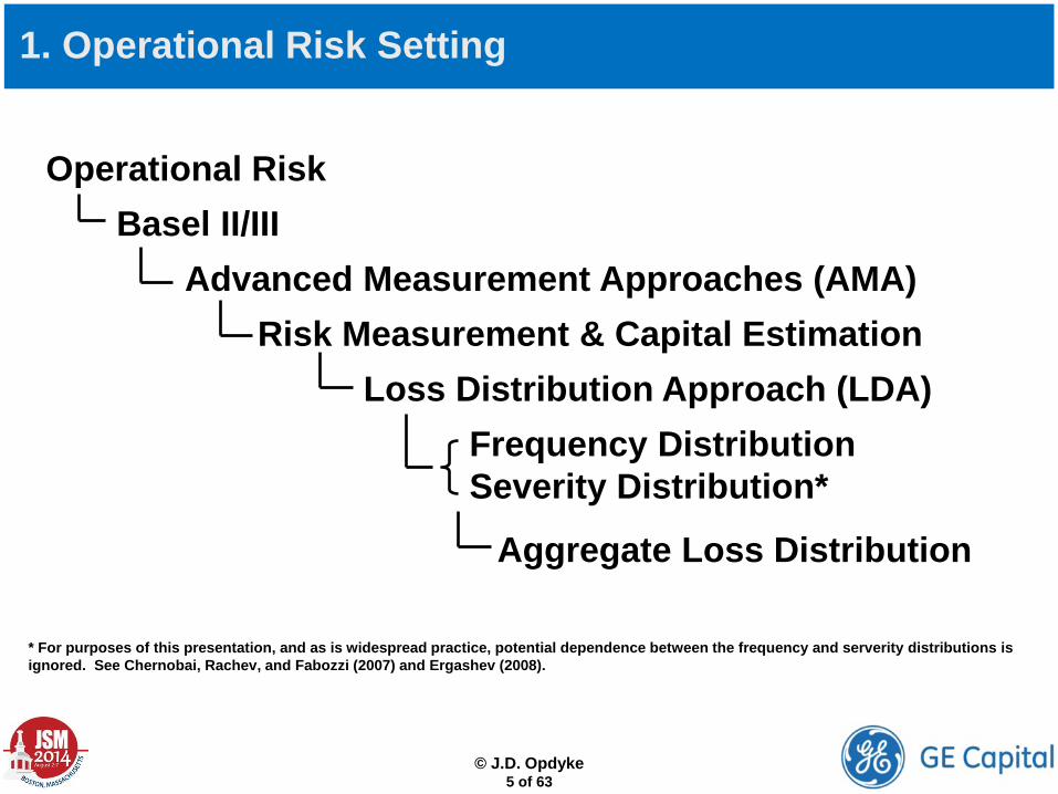
1. Operational Risk Setting

Operational Risk Basel II/III Advanced Measurement Approaches (AMA) Risk Measurement & Capital Estimation Loss Distribution Approach (LDA) Frequency Distribution

Severity Distribution*

Aggregate Loss Distribution

* For purposes of this presentation, and as is widespread practice, potential dependence between the frequency and serverity distributions is ignored. See Chernobai, Rachev, and Fabozzi (2007) and Ergashev (2008).

© J.D. Opdyke

5 of 63

2. AMA–LDA OpRisk Capital Defined

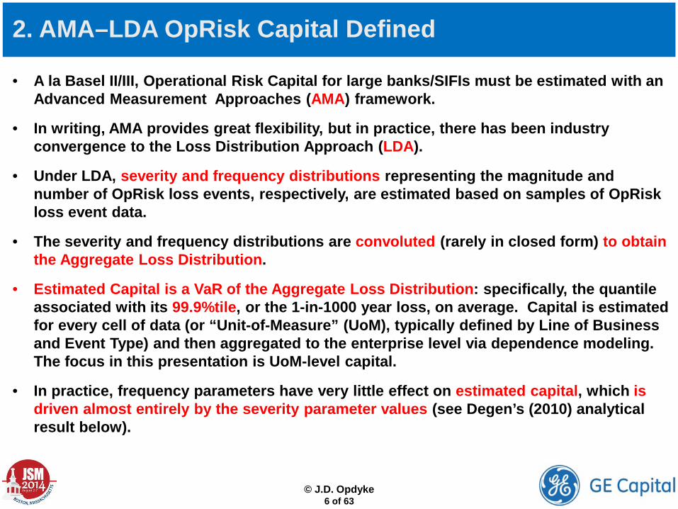
• A la Basel II/III, Operational Risk Capital for large banks/SIFIs must be estimated with an Advanced Measurement Approaches (AMA) framework.

• In writing, AMA provides great flexibility, but in practice, there has been industry convergence to the Loss Distribution Approach (LDA).

• Under LDA, severity and frequency distributions representing the magnitude and number of OpRisk loss events, respectively, are estimated based on samples of OpRisk loss event data.

• The severity and frequency distributions are convoluted (rarely in closed form) to obtain the Aggregate Loss Distribution.

• Estimated Capital is a VaR of the Aggregate Loss Distribution: specifically, the quantile associated with its 99.9%tile, or the 1-in-1000 year loss, on average. Capital is estimated for every cell of data (or “Unit-of-Measure” (UoM), typically defined by Line of Business and Event Type) and then aggregated to the enterprise level via dependence modeling. The focus in this presentation is UoM-level capital.

• In practice, frequency parameters have very little effect on estimated capital, which is driven almost entirely by the severity parameter values (see Degen’s (2010) analytical result below).

© J.D. Opdyke

6 of 63

2. AMA–LDA OpRisk Capital Defined

© J.D. Opdyke

7 of 63

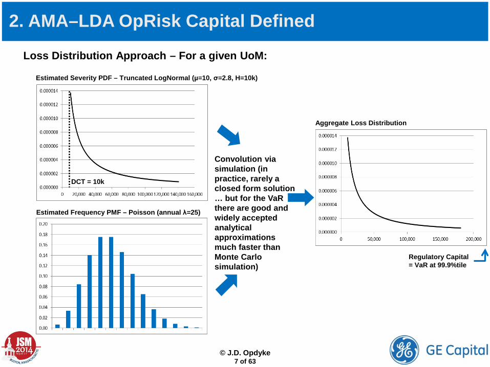
Loss Distribution Approach – For a given UoM:

DCT = 10k

Estimated Severity PDF – Truncated LogNormal (µ=10, σ=2.8, H=10k)

Estimated Frequency PMF – Poisson (annual λ=25)

Convolution via simulation (in practice, rarely a closed form solution … but for the VaR there are good and widely accepted analytical approximations much faster than Monte Carlo simulation)

Aggregate Loss Distribution

Regulatory Capital = VaR at 99.9%tile

© J.D. Opdyke

8 of 63

3.a. Apparent Convexity of Severity VaR Inflated Capital

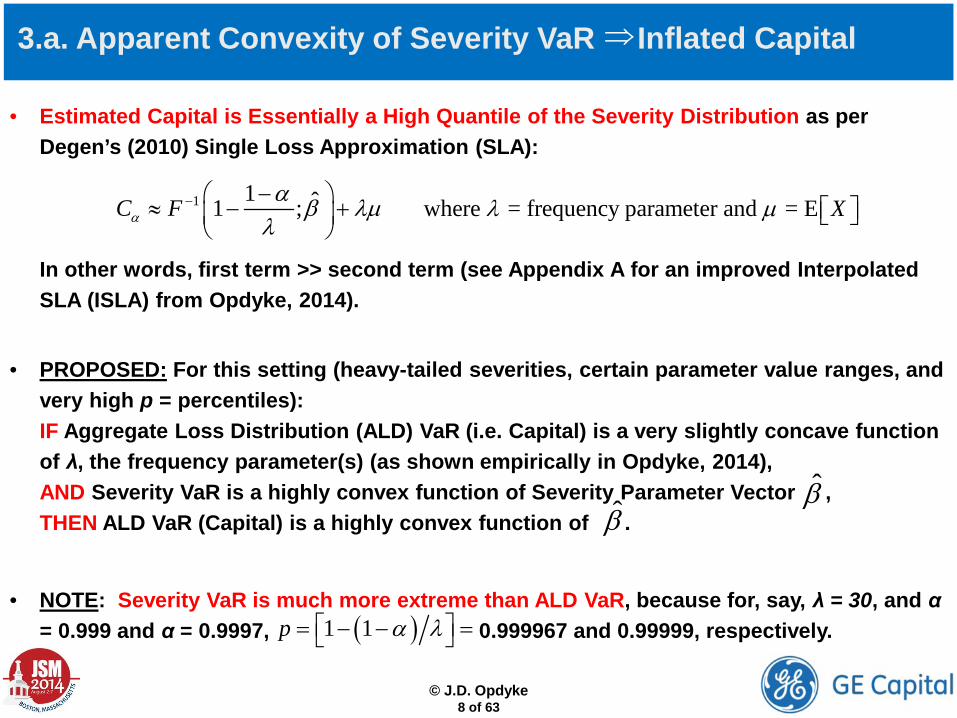
• Estimated Capital is Essentially a High Quantile of the Severity Distribution as per Degen’s (2010) Single Loss Approximation (SLA): In other words, first term >> second term (see Appendix A for an improved Interpolated SLA (ISLA) from Opdyke, 2014).

• PROPOSED: For this setting (heavy-tailed severities, certain parameter value ranges, and very high p = percentiles): IF Aggregate Loss Distribution (ALD) VaR (i.e. Capital) is a very slightly concave function of λ, the frequency parameter(s) (as shown empirically in Opdyke, 2014), AND Severity VaR is a highly convex function of Severity Parameter Vector , THEN ALD VaR (Capital) is a highly convex function of .

• NOTE: Severity VaR is much more extreme than ALD VaR, because for, say, λ = 30, and α = 0.999 and α = 0.9997, 0.999967 and 0.99999, respectively.

1 1 ˆ1 ;C Fαα β λµλ

− − ≈ − +

β̂β̂

⇒

where = frequency parameter and = E Xλ µ

( )1 1p α λ = − − =


( )ˆpdf β

( )Ê β β= β̂

sample2β̂ sample1β̂ sample3β̂

( )ˆPr β β= ± ∆

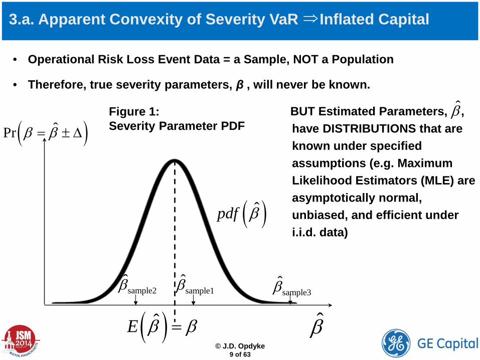
• Operational Risk Loss Event Data = a Sample, NOT a Population

• Therefore, true severity parameters, β , will never be known.

BUT Estimated Parameters, , have DISTRIBUTIONS that are known under specified assumptions (e.g. Maximum Likelihood Estimators (MLE) are asymptotically normal, unbiased, and efficient under i.i.d. data)

β̂Figure 1: Severity Parameter PDF

© J.D. Opdyke

9 of 63

⇒


© J.D. Opdyke

10 of 63

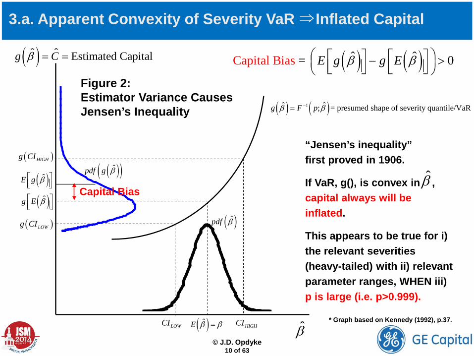
( ) ( )ˆ ˆ =Capital Bias 0E g g Eβ β − > ( )ˆ ˆ Estimated Capitalg Cβ = =

( ) ( )1ˆ ˆ; = presumed shape of severity quantile/VaRg F pβ β−=

( )Ê β β= β̂

( )ˆpdf β

( )( )ˆpdf g β

LOWCI HIGHCI

( )LOWg CI

( )HIGHg CI

( )ˆg E β

( )Ê g β

Capital Bias

* Graph based on Kennedy (1992), p.37.

“Jensen’s inequality” first proved in 1906.

If VaR, g(), is convex in , capital always will be inflated.

This appears to be true for i) the relevant severities (heavy-tailed) with ii) relevant parameter ranges, WHEN iii) p is large (i.e. p>0.999).

β̂

Figure 2: Estimator Variance Causes Jensen’s Inequality

⇒

• Severity VaR is NOT a convex function of the severity parameter vector globally, for all percentiles (p) and all severities. This is widely known and easily proved.

• However, Severity VaR appears always to be a convex function of under, concurrently, BOTH i) sufficiently high percentiles (p>0.999) AND ii) sufficiently heavy-tailed severities (amongst those used in OpRisk modeling). Both conditions hold in AMA–LDA OpRisk Capital Estimation (see Appendix B), and the very strong empirical evidence is exactly consistent with the effects of convexity in that we observe Jensen’s Inequality.

• Still, we would like to PROVE a) convexity in Severity VaR under these conditions, and b) convexity in VaR for all relevant severities.

β̂

3.b. Multiple Checks for Convexity of Severity VaR

β̂

© J.D. Opdyke

11 of 63


© J.D. Opdyke

12 of 63


• Re: a), we can examine three things: The shape of VaR as a function of the severity parameters…

i. individually (i.e. check for marginal convexity)

ii. jointly (i.e. mathematically determine the shape of the multidimensional VaR surface)

iii. jointly, based on extensive Monte Carlo simulation (i.e. examine the behavior of VaR as a function of joint parameter perturbation)


© J.D. Opdyke

13 of 63


i. individually (i.e. check for marginal convexity) Analytically this is straightforward for those severities with closed-form VaR functions. For the LogNormal, for example, However, this is not typically the case, especially for truncated distributions. But these marginal checks are easy to do graphically (NOTE that GPD also is straightforward analytically).

( )( )1exp , soVaR ICDF pµ σ −= = + Φ

2 2 0VaR VaRµ∂ ∂ = >

( )22 2 1 0VaR VaR pσ − ∂ ∂ = ⋅ Φ >


( )1 ;F p ξ−

Figure 3a:

© J.D. Opdyke

14 of 63


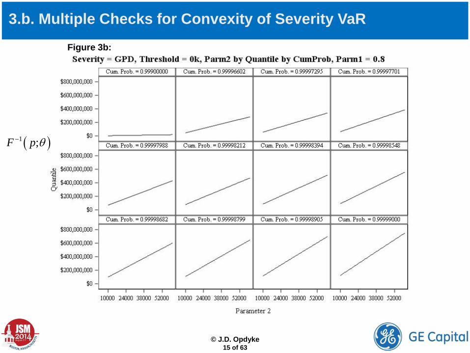
( )1 ;F p θ−

Figure 3b:

© J.D. Opdyke

15 of 63

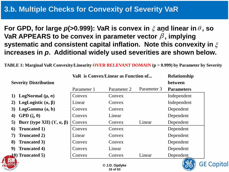
For GPD, for large p(>0.999): VaR is convex in and linear in , so VaR APPEARS to be convex in parameter vector , implying systematic and consistent capital inflation. Note this convexity in increases in p. Additional widely used severities are shown below. TABLE 1: Marginal VaR Convexity/Linearity OVER RELEVANT DOMAIN (p > 0.999) by Parameter by Severity

ξ θβ̂


Severity Distribution

VaR is Convex/Linear as Function of... Relationship between

Parameter 1 Parameter 2 Parameter 3 Parameters 1) LogNormal (µ, σ) Convex Convex Independent 2) LogLogistic (α, β) Linear Convex Independent 3) LogGamma (a, b) Convex Convex Dependent 4) GPD (ξ, θ) Convex Linear Dependent 5) Burr (type XII) (ϒ, α, β) Convex Convex Linear Dependent 6) Truncated 1) Convex Convex Dependent 7) Truncated 2) Linear Convex Dependent 8) Truncated 3) Convex Convex Dependent 9) Truncated 4) Convex Linear Dependent 10) Truncated 5) Convex Convex Linear Dependent

© J.D. Opdyke

16 of 63

ξ


© J.D. Opdyke

17 of 63


i. individually (i.e. check for marginal convexity) For all commonly used severities in this space, VaR always appears to be a convex function of at least one parameter, and a linear function of the rest. This would be consistent with convex, or “convex-dominant” (see below) behavior when VaR is examined as a function of the severity parameters jointly.


© J.D. Opdyke

18 of 63


ii. jointly (i.e. mathematically determine the shape of the multidimensional VaR surface) This can be done via examination of the signs and magnitudes of the eigenvalues of the shape operator (which define its principal curvatures). This turns out to be analytically nontrivial, if not intractable under truncation, and even numeric calculations for many of the relevant severities are nontrivial given the sizes of the severity percentiles that must be used in this setting (because most of the gradients are exceedingly large for such high percentiles).


© J.D. Opdyke

19 of 63

ii. jointly (i.e. mathematically determine the shape of the multidimensional VaR surface) So this research currently remains underway, and without this strict mathematical verification, attributions of capital inflation to Jensen’s inequality are deemed “apparent” and/or “preliminary,” as are those related to VaR’s (apparent) convexity. This scientifically conservative approach, however, belies the strong and consistent empirical evidence of capital inflation, and its behavior as being exactly consistent with the effects of Jensen’s inequality (in addition to findings of marginal convexity). In other words, just because the specific multidimensional shapes of high-percentile VaR under these severities are nontrivial to define mathematically, we should not turn a blind eye toward strong empirical evidence that convexity dominates VaR’s shapes as a joint function of severity parameters.


© J.D. Opdyke

20 of 63

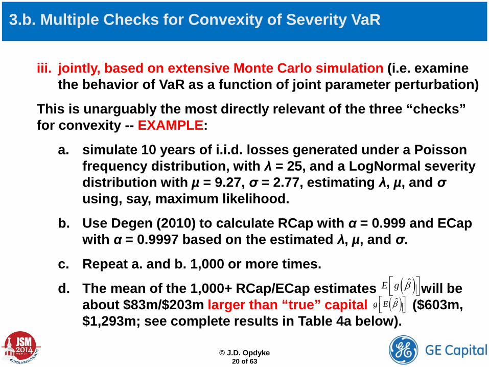
iii. jointly, based on extensive Monte Carlo simulation (i.e. examine the behavior of VaR as a function of joint parameter perturbation)

This is unarguably the most directly relevant of the three “checks” for convexity -- EXAMPLE:

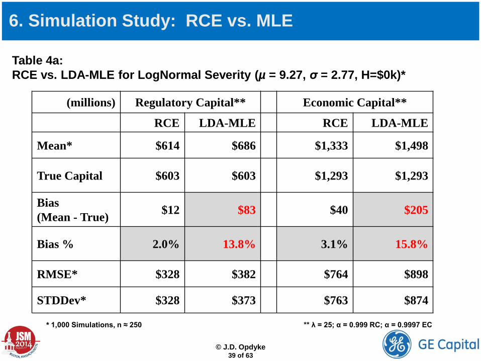
a. simulate 10 years of i.i.d. losses generated under a Poisson frequency distribution, with λ = 25, and a LogNormal severity distribution with µ = 9.27, σ = 2.77, estimating λ, µ, and σ using, say, maximum likelihood.

b. Use Degen (2010) to calculate RCap with α = 0.999 and ECap with α = 0.9997 based on the estimated λ, µ, and σ.

c. Repeat a. and b. 1,000 or more times.

d. The mean of the 1,000+ RCap/ECap estimates will be about $83m/$203m larger than “true” capital ($603m, $1,293m; see complete results in Table 4a below).

( )Ê g β ( )ˆg E β


© J.D. Opdyke

21 of 63

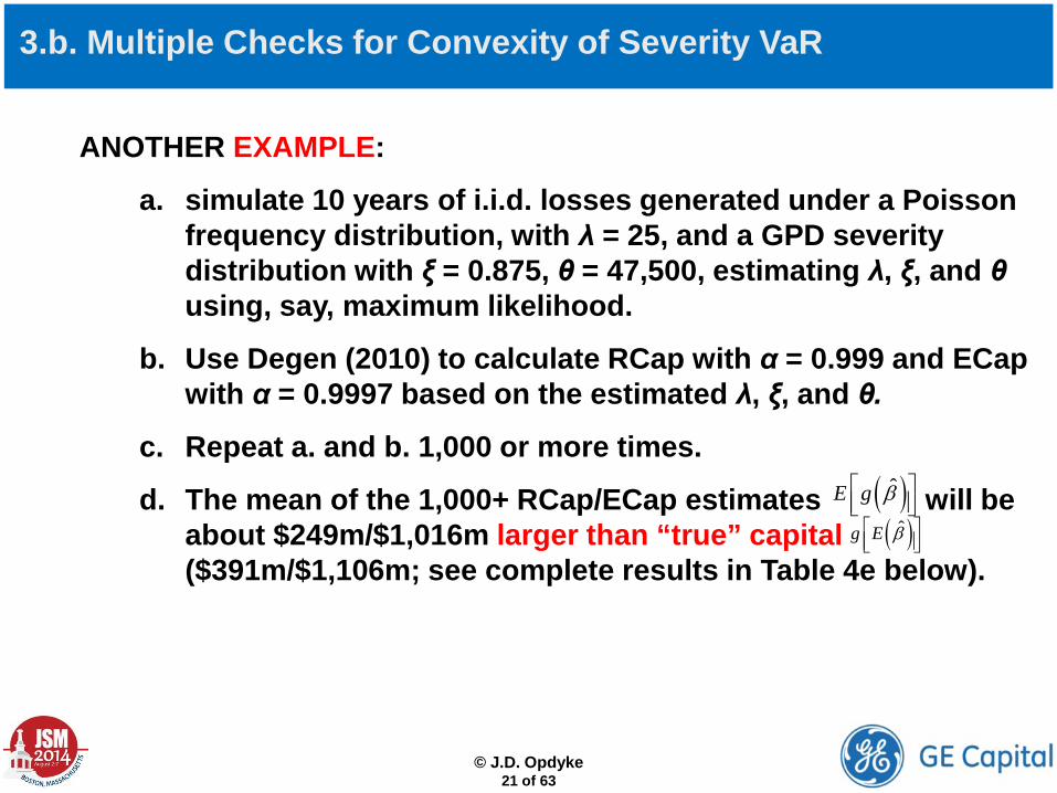
ANOTHER EXAMPLE:

a. simulate 10 years of i.i.d. losses generated under a Poisson frequency distribution, with λ = 25, and a GPD severity distribution with ξ = 0.875, θ = 47,500, estimating λ, ξ, and θ using, say, maximum likelihood.

b. Use Degen (2010) to calculate RCap with α = 0.999 and ECap with α = 0.9997 based on the estimated λ, ξ, and θ.

c. Repeat a. and b. 1,000 or more times.

d. The mean of the 1,000+ RCap/ECap estimates will be about $249m/$1,016m larger than “true” capital ($391m/$1,106m; see complete results in Table 4e below).

( )Ê g β

( )ˆg E β


© J.D. Opdyke

22 of 63

iii. jointly, based on extensive Monte Carlo simulation (i.e. examine the behavior of VaR as a function of joint parameter perturbation) As long as the percentiles examined are large enough (e.g. p > 0.999) and the severity parameter values large enough, the estimates of severity VaR and Rcap/ECap consistently, across all severities used in AMA-based operational risk capital estimation, are notably inflated. This inflation can be dramatic, not uncommonly into the hundreds of millions, and even billions of dollars, for each UoM (unit-of-measure) as shown below. So let us presume VaR convexity and design a capital estimator accordingly to mitigate the actual capital bias/inflation of which it is the presumed source…


• So we are presuming a) based on very strong empirical evidence and incomplete mathematical evidence.

• For b), tackling ALL potentially relevant severities is nontrivial (if possible), but arguably unnecessary as the number of severities used in this setting are quite finite, and we can satisfy a) for each individually. Note again that because capital (VaR of ALD) was shown empirically in Opdyke (2014) to be only a slightly concave function of the frequency parameter(s), the only source of capital inflation would appear to be strong convexity in severity VaR.


© J.D. Opdyke

23 of 63

© J.D. Opdyke

24 of 63

4. When is Capital Bias (Inflation) Material?

Convexity in Severity VaR Capital Bias is upwards … always! Magnitude of Capital Inflation is Determined by:

a) Variance of Severity Parameter Estimator: Larger Variance (smaller n<1,000) Larger Capital Bias

b) Heaviness of Severity Distribution Tail: Heavier More Capital Bias (so truncated distributions more bias, ceteris paribus)

c) Size of VaR Being Estimated: Higher VaR More Capital Bias (so Economic Capital Bias > Regulatory Capital Bias)

This demonstrable empirical behavior is exactly consistent with Jensen’s Inequality, and since most UoMs are heavy-tailed severities and typically n < 250, AMA–LDA OpRisk capital estimation is squarely in the bias zone!

⇒

⇒

⇒

⇒

⇒

© J.D. Opdyke

25 of 63

NOTE: LDA Capital Bias holds for most, if not all widely used severity parameter estimators (e.g. Maximum Likelihood Estimation (MLE), Robust Estimators (OBRE, CvM, QD, etc.), Penalized Likelihood Estimation (PLE), Method of Moments, all M-Class Estimators, Generalized Method of Moments, Probability Weighted Moments, etc.).

NOTE: Because CVaR is a (provably) convex function of severity parameter estimates (see Brown, 2007, Bardou et al., 2010, & Ben-Tal, 2005), switching from VaR to CVaR, even if allowed, does not avoid this problem (and in fact, appears to make it worse).

NOTE: Severities with E(x)=∞ also can exhibit such bias (see GPD with ξ = 1.1, θ = 40,000 in Opdyke, 2014), even though counterexamples exist.

4. When is Capital Bias (Inflation) Material?

5. RCE – Reduced-bias Capital Estimator

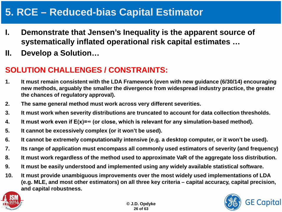
I. Demonstrate that Jensen’s Inequality is the apparent source of systematically inflated operational risk capital estimates …

II. Develop a Solution… SOLUTION CHALLENGES / CONSTRAINTS:

1. It must remain consistent with the LDA Framework (even with new guidance (6/30/14) encouraging new methods, arguably the smaller the divergence from widespread industry practice, the greater the chances of regulatory approval).

2. The same general method must work across very different severities. 3. It must work when severity distributions are truncated to account for data collection thresholds. 4. It must work even if E(x)=∞ (or close, which is relevant for any simulation-based method). 5. It cannot be excessively complex (or it won’t be used). 6. It cannot be extremely computationally intensive (e.g. a desktop computer, or it won’t be used). 7. Its range of application must encompass all commonly used estimators of severity (and frequency) 8. It must work regardless of the method used to approximate VaR of the aggregate loss distribution. 9. It must be easily understood and implemented using any widely available statistical software. 10. It must provide unambiguous improvements over the most widely used implementations of LDA

(e.g. MLE, and most other estimators) on all three key criteria – capital accuracy, capital precision, and capital robustness.

© J.D. Opdyke

26 of 63

© J.D. Opdyke

27 of 63

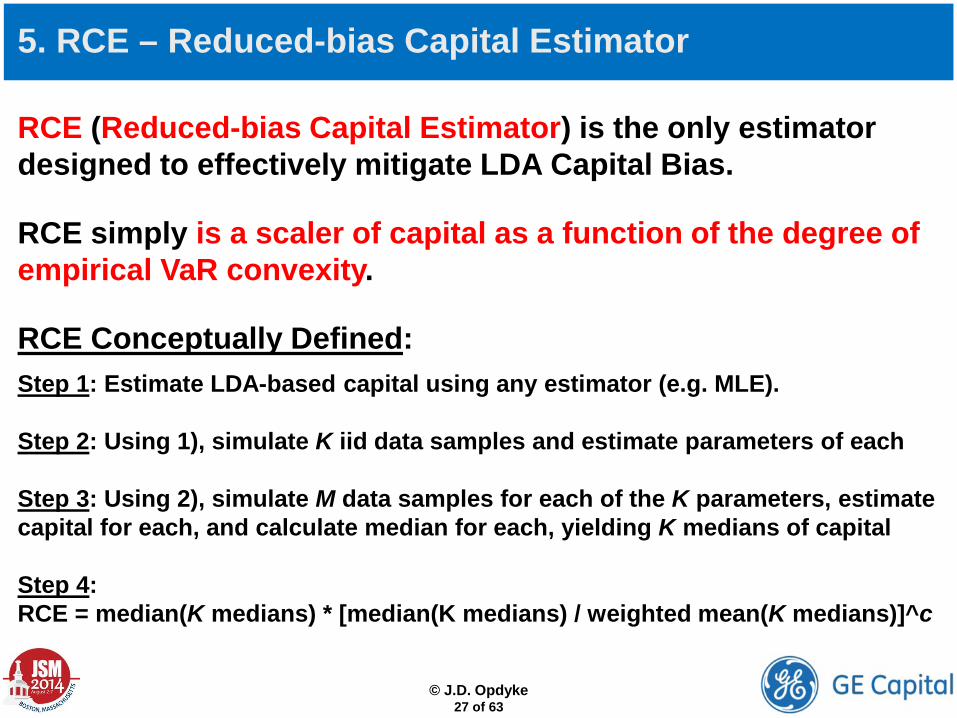
RCE (Reduced-bias Capital Estimator) is the only estimator designed to effectively mitigate LDA Capital Bias.

RCE simply is a scaler of capital as a function of the degree of empirical VaR convexity.

RCE Conceptually Defined:

Step 1: Estimate LDA-based capital using any estimator (e.g. MLE). Step 2: Using 1), simulate K iid data samples and estimate parameters of each Step 3: Using 2), simulate M data samples for each of the K parameters, estimate capital for each, and calculate median for each, yielding K medians of capital Step 4: RCE = median(K medians) * [median(K medians) / weighted mean(K medians)]^c


© J.D. Opdyke

28 of 63

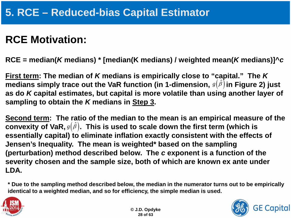
RCE Motivation:

RCE = median(K medians) * [median(K medians) / weighted mean(K medians)]^c

First term: The median of K medians is empirically close to “capital.” The K medians simply trace out the VaR function (in 1-dimension, in Figure 2) just as do K capital estimates, but capital is more volatile than using another layer of sampling to obtain the K medians in Step 3.

Second term: The ratio of the median to the mean is an empirical measure of the convexity of VaR, . This is used to scale down the first term (which is essentially capital) to eliminate inflation exactly consistent with the effects of Jensen’s Inequality. The mean is weighted* based on the sampling (perturbation) method described below. The c exponent is a function of the severity chosen and the sample size, both of which are known ex ante under LDA.


( )ˆg β

( )ˆg β

* Due to the sampling method described below, the median in the numerator turns out to be empirically identical to a weighted median, and so for efficiency, the simple median is used.

© J.D. Opdyke

29 of 63

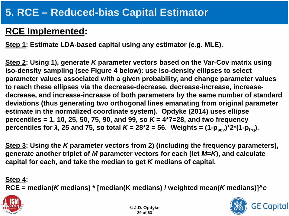
RCE Implemented:

Step 1: Estimate LDA-based capital using any estimator (e.g. MLE).

Step 2: Using 1), generate K parameter vectors based on the Var-Cov matrix using iso-density sampling (see Figure 4 below): use iso-density ellipses to select parameter values associated with a given probability, and change parameter values to reach these ellipses via the decrease-decrease, decrease-increase, increase-decrease, and increase-increase of both parameters by the same number of standard deviations (thus generating two orthogonal lines emanating from original parameter estimate in the normalized coordinate system). Opdyke (2014) uses ellipse percentiles = 1, 10, 25, 50, 75, 90, and 99, so K = 4*7=28, and two frequency percentiles for λ, 25 and 75, so total K = 28*2 = 56. Weights = (1-psev)*2*(1-pfrq).

Step 3: Using the K parameter vectors from 2) (including the frequency parameters), generate another triplet of M parameter vectors for each (let M=K), and calculate capital for each, and take the median to get K medians of capital.

Step 4: RCE = median(K medians) * [median(K medians) / weighted mean(K medians)]^c


© J.D. Opdyke

30 of 63

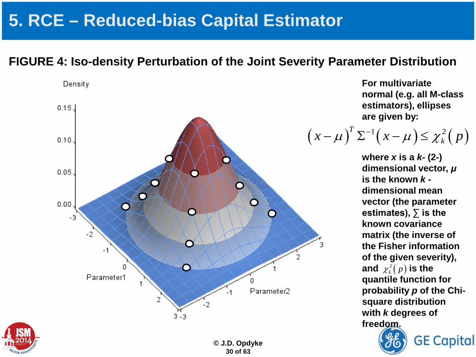
FIGURE 4: Iso-density Perturbation of the Joint Severity Parameter Distribution


For multivariate normal (e.g. all M-class estimators), ellipses are given by:

where x is a k- (2-) dimensional vector, μ is the known k -dimensional mean vector (the parameter estimates), ∑ is the known covariance matrix (the inverse of the Fisher information of the given severity), and is the quantile function for probability p of the Chi-square distribution with k degrees of freedom.

( )2k pχ

( ) ( ) ( )1 2Tkx x pµ µ χ−− Σ − ≤

© J.D. Opdyke

31 of 63

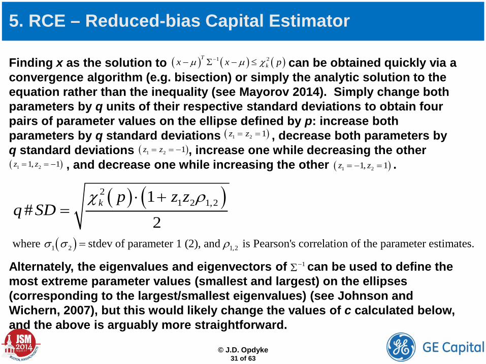
Finding x as the solution to can be obtained quickly via a convergence algorithm (e.g. bisection) or simply the analytic solution to the equation rather than the inequality (see Mayorov 2014). Simply change both parameters by q units of their respective standard deviations to obtain four pairs of parameter values on the ellipse defined by p: increase both parameters by q standard deviations , decrease both parameters by q standard deviations , increase one while decreasing the other , and decrease one while increasing the other . Alternately, the eigenvalues and eigenvectors of can be used to define the most extreme parameter values (smallest and largest) on the ellipses (corresponding to the largest/smallest eigenvalues) (see Johnson and Wichern, 2007), but this would likely change the values of c calculated below, and the above is arguably more straightforward.


( )1 2 1z z= =

( )1 2 1z z= = −

( )1 21, 1z z= = − ( )1 21, 1z z= − =

( ) ( ) ( )1 2Tkx x pµ µ χ−− Σ − ≤

( ) ( )21 2 1,21

#2

k p z zq SD

χ ρ⋅ +=

( )1 2 1,2where stdev of parameter 1 (2), and is Pearson's correlation of the parameter estimates.σ σ ρ=

1−Σ

© J.D. Opdyke

32 of 63

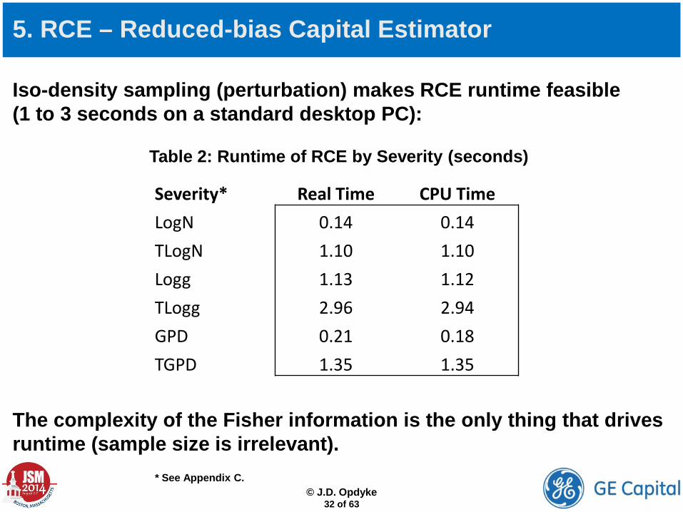
Iso-density sampling (perturbation) makes RCE runtime feasible (1 to 3 seconds on a standard desktop PC):


Severity* Real Time CPU Time LogN 0.14 0.14 TLogN 1.10 1.10 Logg 1.13 1.12 TLogg 2.96 2.94 GPD 0.21 0.18 TGPD 1.35 1.35

Table 2: Runtime of RCE by Severity (seconds)

The complexity of the Fisher information is the only thing that drives runtime (sample size is irrelevant).

* See Appendix C.

© J.D. Opdyke

33 of 63

Implementation NOTE: It is important to avoid bias when using iso-density sampling in cases of incalculably high capital. For example, say the initial MLE parameters happen to be large, and then the 99%tile of the joint parameter distribution, based on the initial estimates, is obtained in Step 2 of RCE’s implementation; and then the 99%tile of THIS Fisher information is obtained in Step 3, based on the joint parameter distribution of the Step 2 values. Capital calculated in Step 3 sometimes simply will be too large to calculate in such cases. If ignored, this could systematically bias RCE. A simple solution is to eliminate the entire ellipse of values – along with all “larger” ellipses – when any one value on an ellipse is too large to calculate.


© J.D. Opdyke

34 of 63

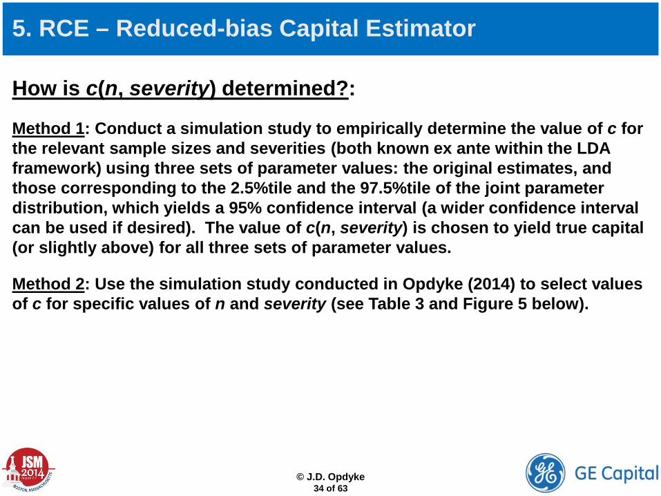
How is c(n, severity) determined?:

Method 1: Conduct a simulation study to empirically determine the value of c for the relevant sample sizes and severities (both known ex ante within the LDA framework) using three sets of parameter values: the original estimates, and those corresponding to the 2.5%tile and the 97.5%tile of the joint parameter distribution, which yields a 95% confidence interval (a wider confidence interval can be used if desired). The value of c(n, severity) is chosen to yield true capital (or slightly above) for all three sets of parameter values.

Method 2: Use the simulation study conducted in Opdyke (2014) to select values of c for specific values of n and severity (see Table 3 and Figure 5 below).


© J.D. Opdyke

35 of 63


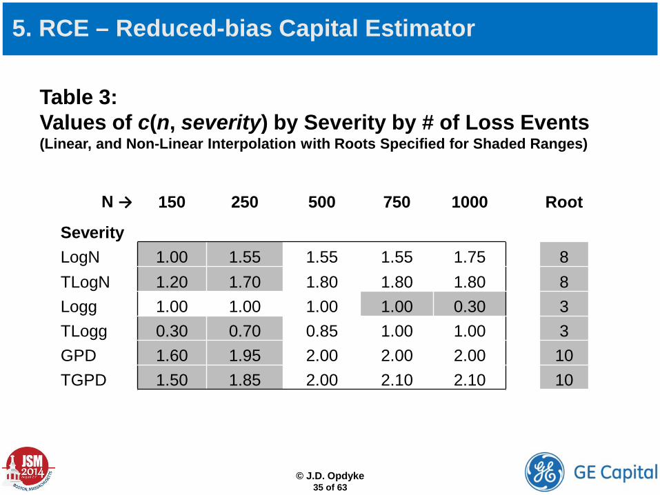
Table 3: Values of c(n, severity) by Severity by # of Loss Events (Linear, and Non-Linear Interpolation with Roots Specified for Shaded Ranges)

N → 150 250 500 750 1000 Root

Severity LogN 1.00 1.55 1.55 1.55 1.75 8 TLogN 1.20 1.70 1.80 1.80 1.80 8 Logg 1.00 1.00 1.00 1.00 0.30 3 TLogg 0.30 0.70 0.85 1.00 1.00 3 GPD 1.60 1.95 2.00 2.00 2.00 10 TGPD 1.50 1.85 2.00 2.10 2.10 10

© J.D. Opdyke

36 of 63


0.00

0.50

1.00

1.50

2.00

2.50

0 200 400 600 800 1,000 1,200

# Loss Events

c

LogNTLogNLoggTLoggGPDTGPD

X

+

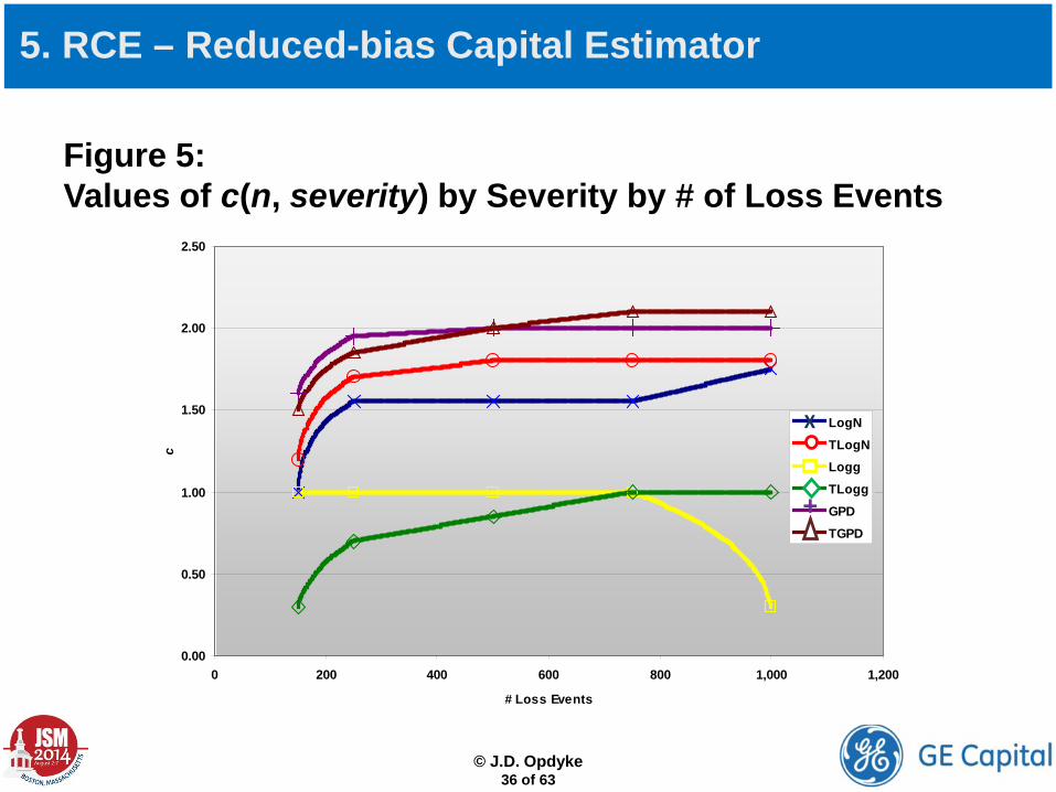
Figure 5: Values of c(n, severity) by Severity by # of Loss Events

© J.D. Opdyke

37 of 63

NOTE: Unfortunately, other Bias-reduction/elimination strategies in the literature, even for VaR (e.g. see Kim and Hardy, 2007), do not appear to work for this problem.* Most involve shifting the distribution of the estimator, often using some type of bootstrap distribution, which in this setting often results in negative capital estimates and greater capital instability. RCE-based capital is never negative, and is more stable than capital based on most, if not all other commonly used severity parameter estimators (e.g. MLE).

Also, given the very high percentiles being examined in this setting (e.g., Severity VaR = 0.99999 and higher), approaches that rely on the derivative(s) of VaR(s), perhaps via (taylor) series expansions, appear to run into numeric precision issues for some severities. So even when such solutions exist in tractable form, practical challenges may derail their application here.


* The only other work in the literature that appears to be similar in approach to RCE is the fragility heuristic (H) of Taleb et al. (2012) and Taleb and Douady (2013). Both RCE and H are measures of convexity based on perturbations of parameters: H measures the distance between the average of model results over a range of shocks and the model result of the average shock, while RCE is a scaling factor based on the ratio of the median to the mean of similar parameter perturbations. Both exploit Jensen’s inequality to measure convexity: in the case of the fragility heuristic, to raise an alarm about it, and in the case of RCE, to eliminate it (or rather, to effectively mitigate its biasing effects on capital estimation).

© J.D. Opdyke

38 of 63

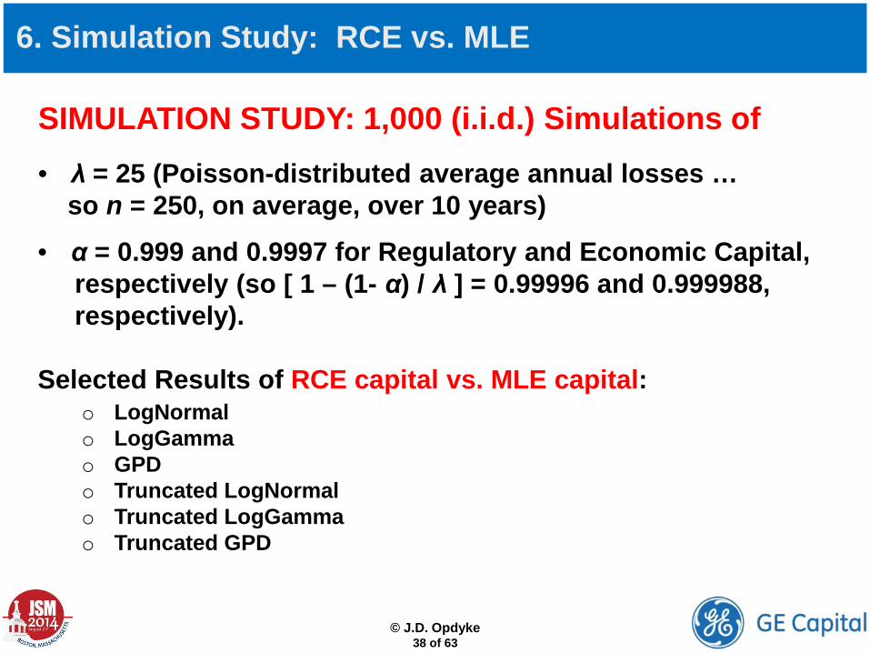
6. Simulation Study: RCE vs. MLE

SIMULATION STUDY: 1,000 (i.i.d.) Simulations of • λ = 25 (Poisson-distributed average annual losses … so n = 250, on average, over 10 years)

• α = 0.999 and 0.9997 for Regulatory and Economic Capital, respectively (so [ 1 – (1- α) / λ ] = 0.99996 and 0.999988, respectively). Selected Results of RCE capital vs. MLE capital:

o LogNormal o LogGamma o GPD o Truncated LogNormal o Truncated LogGamma o Truncated GPD

© J.D. Opdyke

39 of 63

Table 4a: RCE vs. LDA-MLE for LogNormal Severity (µ = 9.27, σ = 2.77, H=$0k)*

* 1,000 Simulations, n ≈ 250 ** λ = 25; α = 0.999 RC; α = 0.9997 EC


(millions) Regulatory Capital** Economic Capital**

RCE LDA-MLE RCE LDA-MLE

Mean* $614 $686 $1,333 $1,498

True Capital $603 $603 $1,293 $1,293

Bias (Mean - True) $12 $83 $40 $205

Bias % 2.0% 13.8% 3.1% 15.8%

RMSE* $328 $382 $764 $898

STDDev* $328 $373 $763 $874

© J.D. Opdyke

40 of 63

Table 4b: RCE vs. LDA-MLE for Truncated LogNormal Severity (µ = 10.7, σ = 2.385, H=$10k)*





Mean* $700 $847 $1,338 $1,678

True Capital $670 $670 $1,267 $1,267

Bias (Mean - True) $30 $177 $71 $411

Bias % 4.5% 26.4% 5.6% 32.4%

RMSE* $469 $665 $1,003 $1,521

STDDev* $468 $641 $1,000 $1,464

© J.D. Opdyke

41 of 63

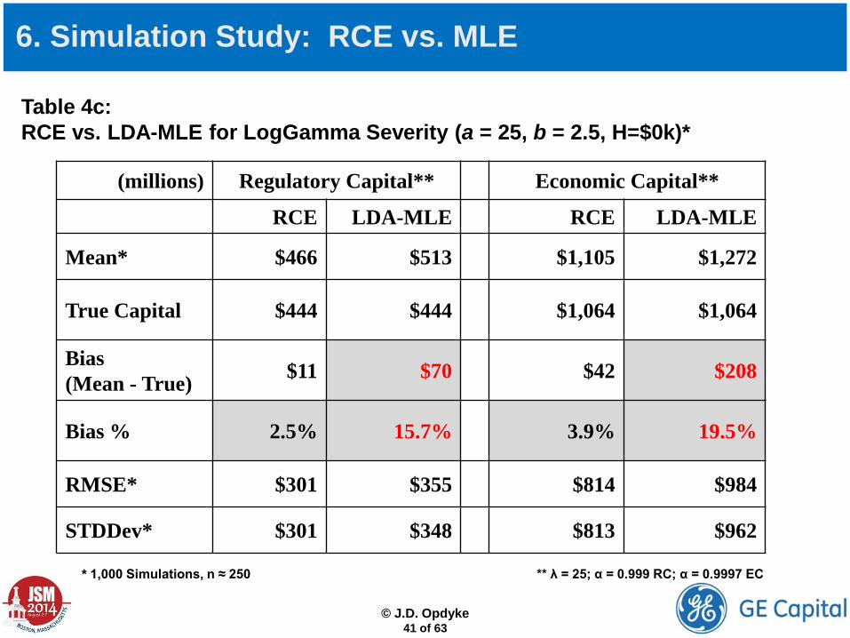
Table 4c: RCE vs. LDA-MLE for LogGamma Severity (a = 25, b = 2.5, H=$0k)*



Mean* $466 $513 $1,105 $1,272

True Capital $444 $444 $1,064 $1,064

Bias (Mean - True) $11 $70 $42 $208

Bias % 2.5% 15.7% 3.9% 19.5%

RMSE* $301 $355 $814 $984

STDDev* $301 $348 $813 $962



© J.D. Opdyke

42 of 63

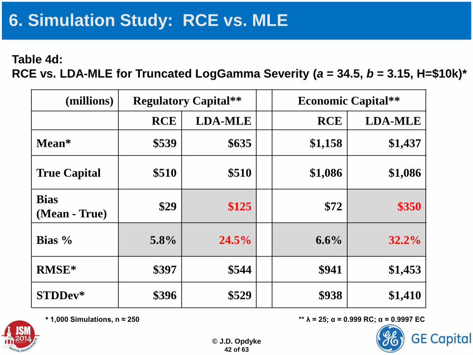
Table 4d: RCE vs. LDA-MLE for Truncated LogGamma Severity (a = 34.5, b = 3.15, H=$10k)*



Mean* $539 $635 $1,158 $1,437

True Capital $510 $510 $1,086 $1,086

Bias (Mean - True) $29 $125 $72 $350

Bias % 5.8% 24.5% 6.6% 32.2%

RMSE* $397 $544 $941 $1,453

STDDev* $396 $529 $938 $1,410



© J.D. Opdyke

43 of 63

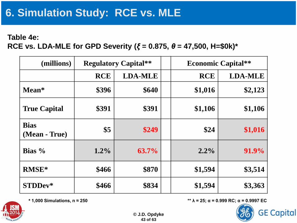
Table 4e: RCE vs. LDA-MLE for GPD Severity (ξ = 0.875, θ = 47,500, H=$0k)*



Mean* $396 $640 $1,016 $2,123

True Capital $391 $391 $1,106 $1,106

Bias (Mean - True) $5 $249 $24 $1,016

Bias % 1.2% 63.7% 2.2% 91.9%

RMSE* $466 $870 $1,594 $3,514

STDDev* $466 $834 $1,594 $3,363



© J.D. Opdyke

44 of 63

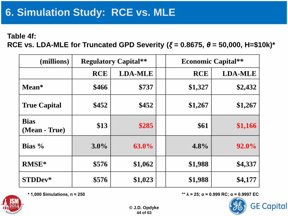
Table 4f: RCE vs. LDA-MLE for Truncated GPD Severity (ξ = 0.8675, θ = 50,000, H=$10k)*



Mean* $466 $737 $1,327 $2,432

True Capital $452 $452 $1,267 $1,267

Bias (Mean - True) $13 $285 $61 $1,166

Bias % 3.0% 63.0% 4.8% 92.0%

RMSE* $576 $1,062 $1,988 $4,337

STDDev* $576 $1,023 $1,988 $4,177



© J.D. Opdyke

45 of 63

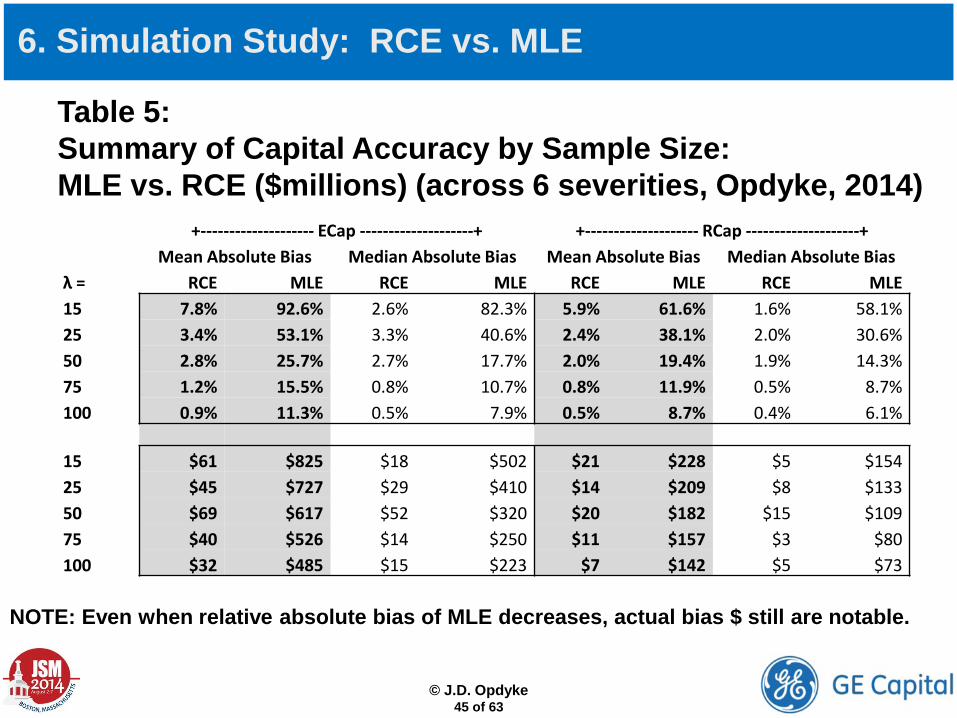
Table 5: Summary of Capital Accuracy by Sample Size: MLE vs. RCE ($millions) (across 6 severities, Opdyke, 2014) +-------------------- ECap --------------------+ +-------------------- RCap --------------------+

Mean Absolute Bias Median Absolute Bias Mean Absolute Bias Median Absolute Bias λ = RCE MLE RCE MLE RCE MLE RCE MLE 15 7.8% 92.6% 2.6% 82.3% 5.9% 61.6% 1.6% 58.1% 25 3.4% 53.1% 3.3% 40.6% 2.4% 38.1% 2.0% 30.6% 50 2.8% 25.7% 2.7% 17.7% 2.0% 19.4% 1.9% 14.3% 75 1.2% 15.5% 0.8% 10.7% 0.8% 11.9% 0.5% 8.7% 100 0.9% 11.3% 0.5% 7.9% 0.5% 8.7% 0.4% 6.1%

15 $61 $825 $18 $502 $21 $228 $5 $154 25 $45 $727 $29 $410 $14 $209 $8 $133 50 $69 $617 $52 $320 $20 $182 $15 $109 75 $40 $526 $14 $250 $11 $157 $3 $80 100 $32 $485 $15 $223 $7 $142 $5 $73

NOTE: Even when relative absolute bias of MLE decreases, actual bias $ still are notable.


© J.D. Opdyke

46 of 63

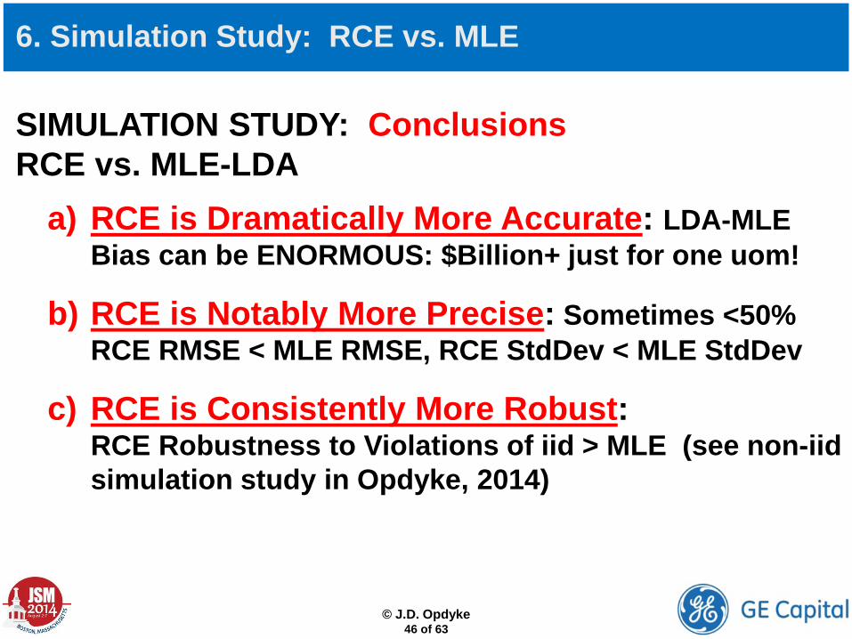
SIMULATION STUDY: Conclusions RCE vs. MLE-LDA

a) RCE is Dramatically More Accurate: LDA-MLE Bias can be ENORMOUS: $Billion+ just for one uom!

b) RCE is Notably More Precise: Sometimes <50% RCE RMSE < MLE RMSE, RCE StdDev < MLE StdDev

c) RCE is Consistently More Robust: RCE Robustness to Violations of iid > MLE (see non-iid simulation study in Opdyke, 2014)


© J.D. Opdyke

47 of 63

7. Summary and Conclusions

• Under an LDA framework, operational risk capital estimates based on the most commonly used estimators of severity parameters (e.g. MLE) and the relevant severity distributions are consistently systematically biased upwards, presumably due to Jensen’s inequality (Jensen, 1906).

• This bias is often material, sometimes inflating required capital by hundreds of millions, and even billions of dollars.

• RCE is the estimator MOST consistent with regulatory intent regarding a prudent, responsible implementation of an AMA–LDA framework in that it alone is not systematically and materially biased, let alone imprecise and non-robust.

• RCE is the only capital estimator that mitigates and nearly eliminates capital inflation under AMA-LDA. RCE also is notably more precise than LDA-based capital under most, if not all severity estimators, and consistently more robust to violations of i.i.d. data (which are endemic to operational risk loss data). Therefore, with greater capital accuracy, precision, and robustness, RCE unambiguously and notably improves LDA-based OpRisk Capital Estimation by all relevant criteria.

© J.D. Opdyke

48 of 63

8. References and Appendices • Bardou, O., Frikha, N., and Pages, G. (2010), “CVaR Hedging Using Quantization Based Stochastic Approximation,” working paper.

• Ben-Tal, A. (2007) “An Old-New Concept of Convex Risk Measures: The Optimized Certainty Equivalent,” Mathematical Finance, 17(3), 449-476.

• Brown, D., (2007) “Large Deviations Bounds for Estimating Conditional Value-at-Risk,” Operations Research Letters, 35, 722-730.

• Chernobai, A., Rachev, S., and Fabozzi, F. (2007), Operational Risk: A Guide to Basel II Capital Requirements, Models, and Analysis, John Wiley & Sons, Inc., Hoboken, New Jersey.

• Daníelsson, J., Jorgensen, B. N., Sarma, M., Samorodnitsky, G., and de Vries, C. G. (2005), “Subadditivity Re-examined: The Case for Value-at-Risk,” FMG Discussion Papers, www.RiskResearch.org.

• Daníelsson, J., Jorgensen, B. N., Sarma, M., Samorodnitsky, G., and de Vries, C. G. (2013), “Fat Tails, VaR and Subadditivity,” Journal of Econometrics, 172(2), 283-291.

• Degen, M. (2010), “The Calculation of Minimum Regulatory Capital Using Single-Loss Approximations,” The Journal of Operational Risk, Vol. 5, No. 4, 3-17.

• Degen, M., Embrechts, P., Lambrigger, D.D. (2007), “The Quantitative Modeling of Operational Risk: Between g-and-h and EVT,” Astin Bulletin, 37(2), 265-291.

• Embrechs, P., and Frei, M., (2009), “Panjer Recursion versus FFT for Compound Distributions,” Mathematical Methods of Operations Research, 69(3), 497-508.

• Ergashev B., (2008), “Should Risk Managers Rely on the Maximum Likelihood Estimation Method While Quantifying Operational Risk,” The Journal of Operational Risk, Vol. 3, No. 2, 63-86.

• Jensen, J. L. W. V. (1906), “Sur les fonctions convexes et les inégalités entre les valeurs moyennes,” Acta Mathematica, 30 (1), 175–193.

• Johnson, R., and Wichern, D., (2007), Applied Multivariate Statistical Analysis, 6th Ed., Pearson, Upper Saddle River, NJ.

• Kennedy, P. (1992), A Guide to Econometrics, The MIT Press, Cambridge, MA.

• Kim, J., (2010), “Conditional Tail Moments of the Exponential Family and its Related Distributions,” North American Actuarial Journal, Vol. 14(2), 198-216.

• Kim, J., and Hardy, M., (2007), “Quantifying and Correcting the Bias in Estimated Risk Measures,” Astin Bulletin, Vol. 37(2), 365-386.

• Mayorov, K., (2014), Email correspondence with the author, September, 2014.

© J.D. Opdyke

49 of 63

8. References and Appendices

• Opdyke, J.D., and Cavallo, A. (2012a), “Estimating Operational Risk Capital: The Challenges of Truncation, The Hazards of Maximum Likelihood Estimation, and the Promise of Robust Statistics,” The Journal of Operational Risk, Vol. 7, No. 3, 3-90.

• Opdyke, J.D. and Cavallo, A. (2012b), “Operational Risk Capital Estimation and Planning: Exact Sensitivity Analysis and Business Decision Making Using the Influence Function,” in Operational Risk: New Frontiers Explored, ed. E. Davis, Risk Books, Incisive Media, London.

• Opdyke, J.D. (2014), “Estimating Operational Risk Capital with Greater Accuracy, Precision, and Robustness,” forthcoming, The Journal of Operational Risk, Vol. 9, No. 4, Decmeber.

• Panjer, H. (2006), Operational Risk Modeling Analytics, Wiley Series in Probability and Statistics, John Wiley & Sons, Inc., Hoboken, NJ.

• Roehr, A., (2002), “Modelling Operational Losses”, Algo Research Quarterly, Vol.5, No.2, Summer 2002.

• Smith, J. (1987), “Estimating the Upper Tail of Flood Frequency Distributions,” Water Resources Research, Vol.23, No.8, 1657-1666.

• Taleb, N., Canetti, E., Kinda, T., Loukoianova, E., and Schmieder, C., (2012), “A New Heuristic Measure of Fragility and Tail Risks: Application to Stress Testing,” IMF Working Paper, Monetary and Capital Markets Department, WP/12/216.

• Taleb, N., and Douady, R., (2013), “Mathematical Definition, Mapping, and Detection of (Anti)Fragility,” Quantitative Finance, forthcoming.

© J.D. Opdyke

50 of 63

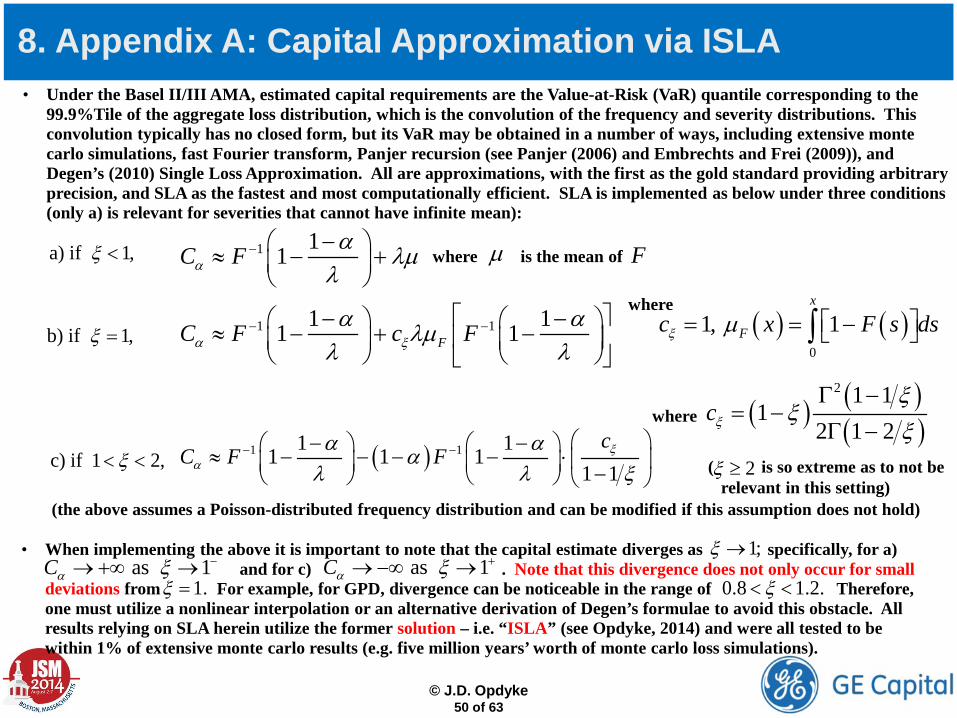
8. Appendix A: Capital Approximation via ISLA • Under the Basel II/III AMA, estimated capital requirements are the Value-at-Risk (VaR) quantile corresponding to the

99.9%Tile of the aggregate loss distribution, which is the convolution of the frequency and severity distributions. This convolution typically has no closed form, but its VaR may be obtained in a number of ways, including extensive monte carlo simulations, fast Fourier transform, Panjer recursion (see Panjer (2006) and Embrechts and Frei (2009)), and Degen’s (2010) Single Loss Approximation. All are approximations, with the first as the gold standard providing arbitrary precision, and SLA as the fastest and most computationally efficient. SLA is implemented as below under three conditions (only a) is relevant for severities that cannot have infinite mean):

1 11C Fαα λµλ

− − ≈ − +

1 11 11 1FC F c Fα ξα αλµλ λ

− − − − ≈ − + −

• When implementing the above it is important to note that the capital estimate diverges as specifically, for a) and for c) . Note that this divergence does not only occur for small deviations from For example, for GPD, divergence can be noticeable in the range of Therefore, one must utilize a nonlinear interpolation or an alternative derivation of Degen’s formulae to avoid this obstacle. All results relying on SLA herein utilize the former solution – i.e. “ISLA” (see Opdyke, 2014) and were all tested to be within 1% of extensive monte carlo results (e.g. five million years’ worth of monte carlo loss simulations).

( )1 11 11 1 11 1

cC F F ξα

α ααλ λ ξ

− − − − ≈ − − − − ⋅ − c) if 1 2,ξ< <

a) if 1,ξ <

b) if 1,ξ =

where

(the above assumes a Poisson-distributed frequency distribution and can be modified if this assumption does not hold)

( ) ( )( )

2 1 11

2 1 2cξ

ξξ

ξΓ −

= −Γ −

where

( ) ( )0

1, 1x

Fc x F s dsξ µ = = − ∫

where is the mean of µ F

1;ξ → as 1Cα ξ −→ +∞ → as 1Cα ξ +→ −∞ →

1.ξ = 0.8 1.2.ξ< <

( is so extreme as to not be relevant in this setting)

2ξ ≥

© J.D. Opdyke

51 of 63

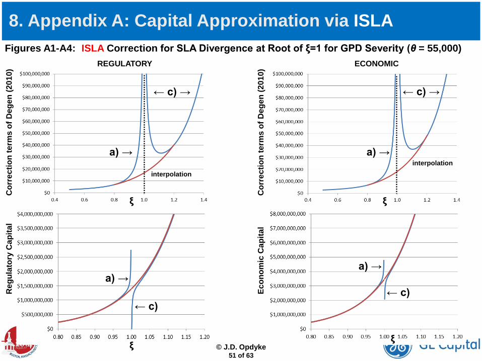
Figures A1-A4: ISLA Correction for SLA Divergence at Root of ξ=1 for GPD Severity (θ = 55,000)

ξ

Cor

rect

ion

term

s of

Deg

en (2

010)

a) →

← c) →

interpolation

REGULATORY

Reg

ulat

ory

Cap

ital

ξ

Cor

rect

ion

term

s of

Deg

en (2

010)

ξ

a) →

← c) →

interpolation

ECONOMIC

ξ

Econ

omic

Cap

ital

a) →

← c)

a) →

← c)

8. Appendix A: Capital Approximation via ISLA

© J.D. Opdyke

52 of 63

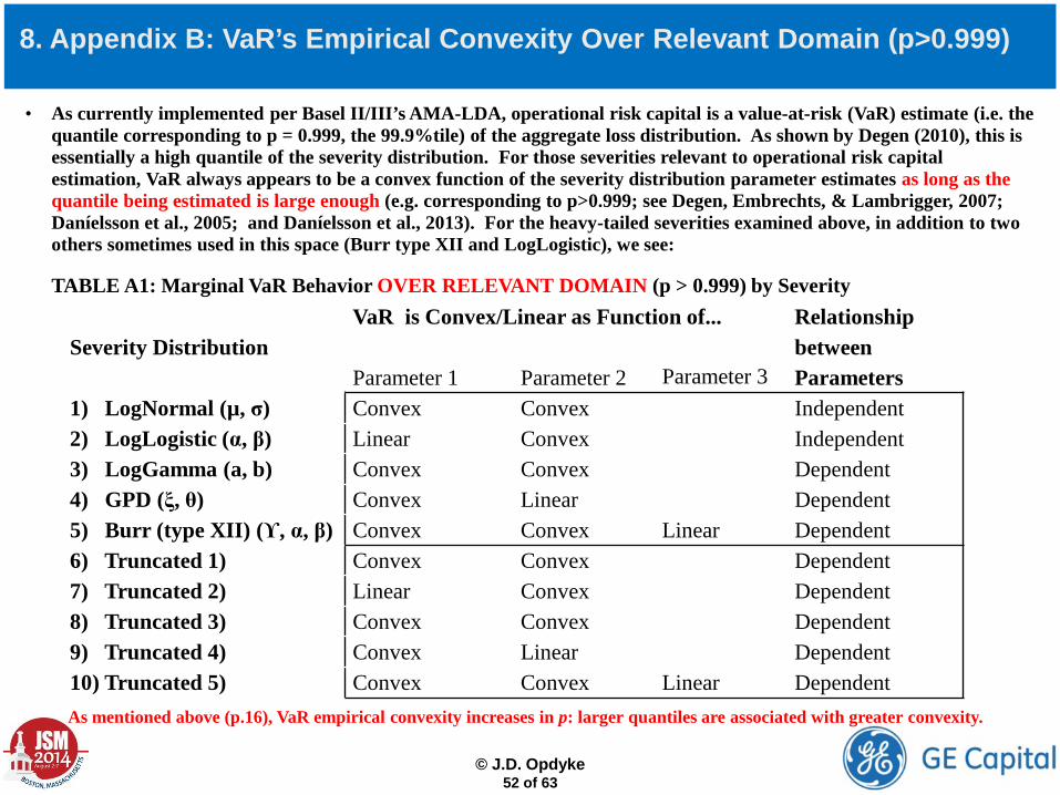
8. Appendix B: VaR’s Empirical Convexity Over Relevant Domain (p>0.999)

• As currently implemented per Basel II/III’s AMA-LDA, operational risk capital is a value-at-risk (VaR) estimate (i.e. the quantile corresponding to p = 0.999, the 99.9%tile) of the aggregate loss distribution. As shown by Degen (2010), this is essentially a high quantile of the severity distribution. For those severities relevant to operational risk capital estimation, VaR always appears to be a convex function of the severity distribution parameter estimates as long as the quantile being estimated is large enough (e.g. corresponding to p>0.999; see Degen, Embrechts, & Lambrigger, 2007; Daníelsson et al., 2005; and Daníelsson et al., 2013). For the heavy-tailed severities examined above, in addition to two others sometimes used in this space (Burr type XII and LogLogistic), we see: TABLE A1: Marginal VaR Behavior OVER RELEVANT DOMAIN (p > 0.999) by Severity As mentioned above (p.16), VaR empirical convexity increases in p: larger quantiles are associated with greater convexity.

Severity Distribution

VaR is Convex/Linear as Function of... Relationship between

Parameter 1 Parameter 2 Parameter 3 Parameters 1) LogNormal (µ, σ) Convex Convex Independent 2) LogLogistic (α, β) Linear Convex Independent 3) LogGamma (a, b) Convex Convex Dependent 4) GPD (ξ, θ) Convex Linear Dependent 5) Burr (type XII) (ϒ, α, β) Convex Convex Linear Dependent 6) Truncated 1) Convex Convex Dependent 7) Truncated 2) Linear Convex Dependent 8) Truncated 3) Convex Convex Dependent 9) Truncated 4) Convex Linear Dependent 10) Truncated 5) Convex Convex Linear Dependent

© J.D. Opdyke

53 of 63

• PDF and CDF of LogNormal:

• Mean of LogNormal:

• Inverse Fisher information of LogNormal:

8. Appendix C: Severity PDFs, CDFs, & Means for Capital Approximation

( ) ( )2 2E X e µ σ+=

( )( ) 2

ln121; ,

2

x

f x ex

µσµ σ

πσ

− − = ( ) ( )

2

ln1; , 12 2

xF x erf

µµ σ

σ

−= +

0 , 0x σ< < ∞ < < ∞

( )2

12 0

0 / 2A σθ

σ− =

© J.D. Opdyke

54 of 63

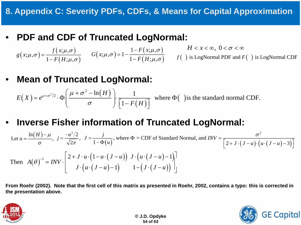
• PDF and CDF of Truncated LogNormal:

• Mean of Truncated LogNormal:

• Inverse Fisher information of Truncated LogNormal: From Roehr (2002). Note that the first cell of this matrix as presented in Roehr, 2002, contains a typo: this is corrected in the presentation above.


( ) ( )( ); ,

; ,1 ; ,

f xg x

F Hµ σ

µ σµ σ

=−

( ) ( )( )

1 ; ,; , 1

1 ; ,F x

G xF H

µ σµ σ

µ σ−

= −−

, 0H x σ< < ∞ < < ∞( ) ( ) is LogNormal PDF and is LogNormal CDFf F

( ) ( )( )

( )22

2 ln 1 where is the standard normal CDF.1

HE X e

F Hµ σ µ σ

σ+

+ −= ⋅Φ ⋅ Φ −

( )lnLet ,

Hu

µσ−

=2 2 ,2

ujπ

−=

( ), where = CDF of Standard Normal, and

1jJ

u= Φ

−Φ ( ) ( )( )2

2 3INV

J J u u J uσ

= + ⋅ − ⋅ ⋅ − −

( )( )( ) ( )( )

( )( ) ( )( )1 2 1 1

Then 1 1

J u u J u J u J uA INV

J u J u J J uθ −

+ ⋅ ⋅ − ⋅ − ⋅ ⋅ − − = ⋅ ⋅ ⋅ − − − ⋅ −

© J.D. Opdyke

55 of 63

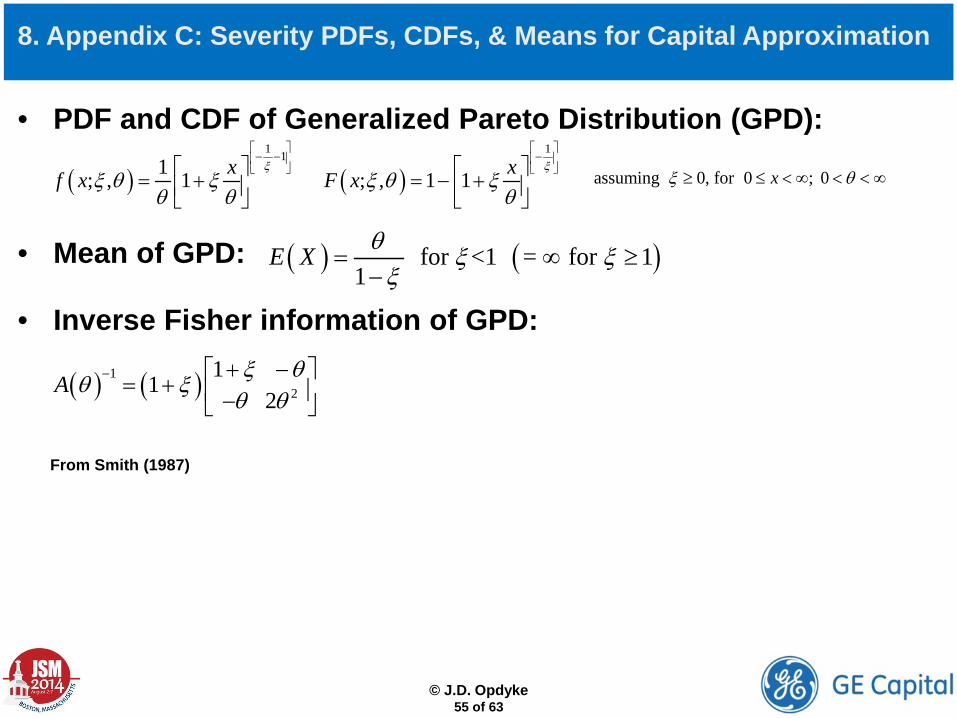
• PDF and CDF of Generalized Pareto Distribution (GPD):

• Mean of GPD:

• Inverse Fisher information of GPD: From Smith (1987)


( )1 11; , 1 xf xξ

ξ θ ξθ θ

− − = +

( )1

; , 1 1 xF xξ

ξ θ ξθ

− = − +

assuming 0, for 0 ; 0xξ θ≥ ≤ < ∞ < < ∞

( ) ( ) for <1 = for 11

E X θ ξ ξξ

= ∞ ≥−

( ) ( )12

1 1

2A

ξ θθ ξ

θ θ− + − = + −

© J.D. Opdyke

56 of 63

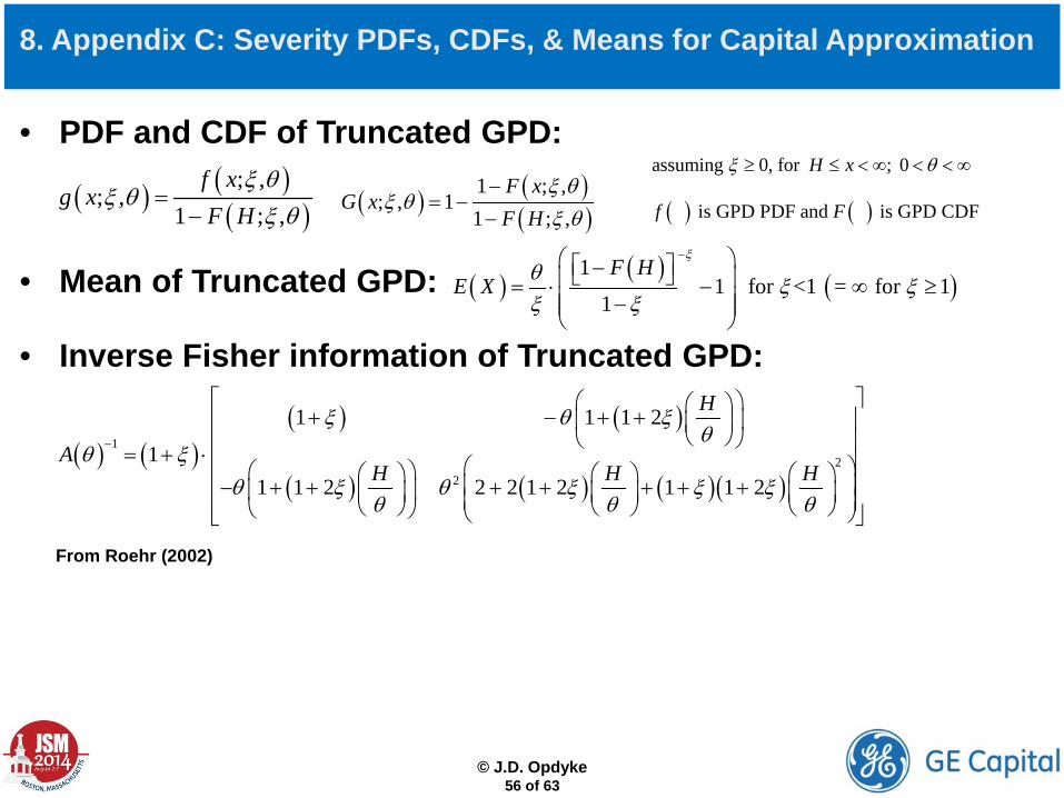
• PDF and CDF of Truncated GPD:

• Mean of Truncated GPD:

• Inverse Fisher information of Truncated GPD: From Roehr (2002)


( ) ( )( ); ,

; ,1 ; ,

f xg x

F Hξ θ

ξ θξ θ

=− ( ) ( )

( )1 ; ,

; , 11 ; ,

F xG x

F Hξ θ

ξ θξ θ

−= −

−

assuming 0, for ; 0H xξ θ≥ ≤ < ∞ < < ∞

( ) ( ) is GPD PDF and is GPD CDFf F

( ) ( )( ) ( )

( ) ( ) ( )( )

12

2

1 1 1 2

11 1 2 2 2 1 2 1 1 2

H

AH H H

ξ θ ξθ

θ ξθ ξ θ ξ ξ ξ

θ θ θ

−

+ − + +

= + ⋅ − + + + + + + +

( )( )

( )1

1 for <1 = for 11

F HE X

ξ

θ ξ ξξ ξ

− − = ⋅ − ∞ ≥ −

© J.D. Opdyke

57 of 63

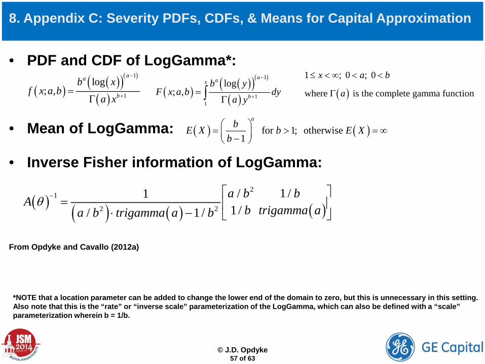
• PDF and CDF of LogGamma*:

• Mean of LogGamma:

• Inverse Fisher information of LogGamma: From Opdyke and Cavallo (2012a)


( )( )( )( )

( )

1

1

log; ,

aa

b

b xf x a b

a x

−

+=Γ

( )( )( )( )

( )

1

11

log; ,

aax

b

b yF x a b dy

a y

−

+=Γ∫

1 ; 0 ; 0x a b≤ < ∞ < <

( )where is the complete gamma functionaΓ

*NOTE that a location parameter can be added to change the lower end of the domain to zero, but this is unnecessary in this setting. Also note that this is the “rate” or “inverse scale” parameterization of the LogGamma, which can also be defined with a “scale” parameterization wherein b = 1/b.

( ) ( ) for 1; otherwise 1

abE X b E Xb

= > = ∞ −

( ) ( ) ( ) ( )2

1

2 2

/ 1 /11 / / 1 /a b b

Ab trigamma aa b trigamma a b

θ − =

⋅ −

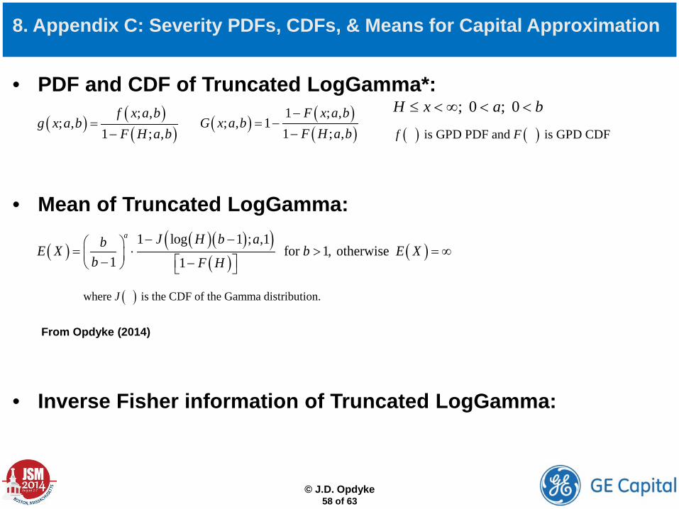
• PDF and CDF of Truncated LogGamma*:

• Mean of Truncated LogGamma: From Opdyke (2014)

• Inverse Fisher information of Truncated LogGamma:


( ) ( )( ); ,

; ,1 ; ,

f x a bg x a b

F H a b=

−( ) ( )

( )1 ; ,

; , 11 ; ,

F x a bG x a b

F H a b−

= −−

; 0 ; 0H x a b≤ < ∞ < <

( ) ( ) is GPD PDF and is GPD CDFf F

( )( )( )( )

( )( )

1 log 1 ; ,1 for 1, otherwise

1 1

a J H b abE X b E Xb F H

− − = ⋅ > = ∞ − −

( )where is the CDF of the Gamma distribution.J

© J.D. Opdyke

58 of 63

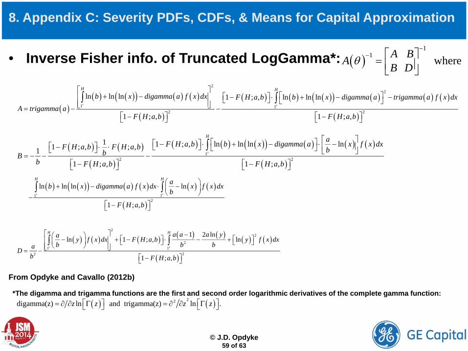
• Inverse Fisher info. of Truncated LogGamma*: From Opdyke and Cavallo (2012b)


( )1

1 where A BA B Dθ

−− =

( )( ) ( )( ) ( ) ( )

( )

( ) ( ) ( )( ) ( ) ( ) ( )

( )

22

1 12 2

ln ln ln 1 ; , ln ln ln

1 ; , 1 ; ,

H H

b x digamma a f x dx F H a b b x digamma a trigamma a f x dxA trigamma a

F H a b F H a b

+ +

+ − − ⋅ + − − = − −

− −

∫ ∫

( ) ( )

( )

( ) ( ) ( )( ) ( ) ( ) ( )

( )1

2 2

1 1 ; , ln ln ln ln1 ; , ; ,1

1 ; , 1 ; ,

H aF H a b b x digamma a x f x dxF H a b F H a b bbBb F H a b F H a b

+

− ⋅ + − ⋅ − − ⋅ ⋅ = − − − − −

∫

( ) ( )( ) ( ) ( ) ( ) ( )

( )1 1

2

ln ln ln ln

1 ; ,

H H ab x digamma a f x dx x f x dxb

F H a b

+ +

+ − ⋅ − −

−

∫ ∫

( ) ( ) ( ) ( ) ( ) ( ) ( )

( )

22

21 1

22

1 2 lnln 1 ; , ln

1 ; ,

H H a a a ya y f x dx F H a b y f x dxb b baD

b F H a b

+ +

− − + − ⋅ − + = − −

∫ ∫

*The digamma and trigamma functions are the first and second order logarithmic derivatives of the complete gamma function: ( ) ( )22digamma(z) ln and trigamma(z) ln .z z z z = ∂ ∂ Γ = ∂ ∂ Γ

© J.D. Opdyke

59 of 63

© J.D. Opdyke

60 of 63

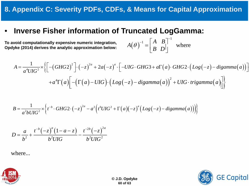
• Inverse Fisher information of Truncated LogGamma: To avoid computationally expensive numeric integration, Opdyke (2014) derives the analytic approximation below:


( )1

1 where A BA B Dθ

−− =

( ) ( ){ ( ) ( ) ( ) ( )( )2 2

4 2

1 2 2 3 2a aA GHG z a z UIG GHG a a GHG Log z digamma aa UIG

= × − ⋅ − + − ⋅ − ⋅ + Γ ⋅ ⋅ − −

( ) ( )( ) ( ) ( )( ) ( ) }24a a a UIG Log z digamma a UIG trigamma a + Γ − Γ − ⋅ − − + ⋅

( ) ( )( ) ( ) ( )( )( ){ }2 2 22 2

1 2 a ab bB t GHG z a t UIG a z Log z digamma aa bUIG

−= × ⋅ ⋅ − − + Γ − − −

( ) ( ) ( )22

2 2 2 2

1a ab bt z a z t zaDb b UIG b UIG

− −− − − −= + −

where...

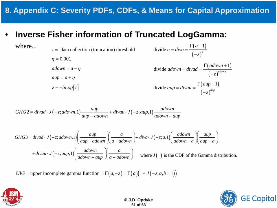
© J.D. Opdyke

61 of 63

• Inverse Fisher information of Truncated LogGamma:


0.001η =

adown a η= −

aup a η= +

z bLog t= −

( )( )

1divide a

aa diva

z

Γ += =

−

( )( )

1divide adown

adownadown divad

z

Γ += =

−

( )( )

1divide aup

aupaup divau

z

Γ += =

−

( ) ( )2 ; ,1 ; ,1aup adownGHG divad J z adown divau J z aupaup adown adown aup

= ⋅ − + ⋅ −− −

where...

( ) ( )3 ; ,1 ; ,1aup a adown aupGHG divad J z adown diva J z aaup adown a adown adown a aup a

= ⋅ − + ⋅ − − − − −

( ); ,1 adown adivau J z aupadown aup a adown

+ ⋅ − − − ( )where is the CDF of the Gamma distribution.J

( ) ( ) ( )( )upper incomplete gamma function , 1 ; , 1UIG a z a J z a b= = Γ − = Γ − − =

data collection (truncation) thresholdt =

© J.D. Opdyke

62 of 63

The largest US banks and Systemically Important Financial Institutions are required by regulatory mandate to estimate the operational risk capital they must hold using an Advanced Measurement Approach (AMA) as defined by the Basel II/III Accords. Most of these institutions use the Loss Distribution Approach (LDA) which defines the aggregate loss distribution as the convolution of a frequency distribution and a severity distribution representing the number and magnitude of losses, respectively. Capital is a Value-at-Risk estimate of this annual loss distribution (i.e. the quantile corresponding to the 99.9%tile, representing a one-in-a-thousand-year loss, on average). In practice, the severity distribution drives the capital estimate, which is essentially a very large quantile of the estimated severity distribution. Unfortunately, when using LDA with any of the widely used severity distributions (i.e. heavy-tailed, skewed distributions), all unbiased estimators of severity distribution parameters generate biased capital estimates apparently due to Jensen’s Inequality: VaR always appears to be a convex function of these severities’ parameter estimates because the (severity) quantile being estimated is so large and the severities are heavy-tailed. The resulting bias means that capital requirements always will be overstated, and this inflation is sometimes enormous (sometimes even billions of dollars at the unit-of-measure level). Herein I present an estimator of capital that essentially eliminates this upward bias when used with any commonly used severity parameter estimator. The Reduced-bias Capital Estimator (RCE), consequently, is more consistent with regulatory intent regarding the responsible implementation of the LDA framework than other implementations that fail to mitigate, if not eliminate this bias. RCE also notably increases the precision of the capital estimate and consistently increases its robustness to violations of the i.i.d. data presumption (which are endemic to operational risk loss event data). So with greater capital accuracy, precision, and robustness, RCE lowers capital requirements at both the unit-of-measure and enterprise levels, increases capital stability from quarter to quarter, ceteris paribus, and does both while more accurately and precisely reflecting regulatory intent. RCE is straightforward to explain, understand, and implement using any major statistical software package.

10. Abstract, Opdyke (2014)

Estimating Operational Risk Capital with Greater Accuracy, Precision, and Robustness

© J.D. Opdyke

63 of 63

J.D. Opdyke Head of Operational Risk Modeling, Quantitative Methods Group, GE Capital [email protected] 617-943-6463

CONTACT

mailto:[email protected]

Documents

Estimating Operational Risk Capital with Greater Accuracy .... Opdyke - UCE Presentation - Estimating... · Estimating Operational Risk Capital with Greater Accuracy, Precision, and