Estimating Neural Response Functions from fMRIwpenny/publications/nrf_third...Kumar et al. Estimating Neural Response Functions from fMRI 69 This paper extends the HDM formalism by

Frontiers in Neuroinformatics Research Article15 April 2014

1

Estimating Neural Response Functions fromfMRIS. Kumar 1,2 and W. Penny 1,∗

1Wellcome Trust Centre for Neuroimaging, University College London, UnitedKingdom2Institute of Neuroscience, Medical School, Newcastle University, United KingdomCorrespondence*:W. Penny12 Queen Square, London WC1N 3BG, United Kingdom, [email protected]

ABSTRACT2

This paper proposes a methodology for estimating Neural Response Functions (NRFs) from3fMRI data. These NRFs describe nonlinear relationships between experimental stimuli and4neuronal population responses. The method is based on a two-stage model comprising an5NRF and a Hemodynamic Response Function (HRF) that are simultaneously fitted to fMRI6data using a Bayesian optimisation algorithm. This algorithm also produces a model evidence7score, providing a formal model comparison method for evaluating alternative NRFs. The HRF8is characterised using previously established ‘Balloon’ and BOLD signal models. We illustrate9the method with two example applications based on fMRI studies of the auditory system. In the10first, we estimate the time constants of repetition suppression and facilitation, and in the second11we estimate the parameters of population receptive fields in a tonotopic mapping study.12

13

Keywords: Neural Response Function, Hemodynamic Response Function, Population Receptive Field, Parametric Modulation,14Neurometric Function, Bayesian Inference, Auditory Perception, Repetition Suppression, Tonotopic Mapping, Balloon Model15

1 INTRODUCTION

Functional Magnetic Resonance Imaging (fMRI) is a well established technique for the non-invasive16mapping of human brain function [13]. Analysis of fMRI data most often proceeds by modelling the17neuronal correlates of single events as delta functions or boxcars. These form event streams which are18then convolved with assumed Hemodynamic Response Functions (HRFs) to create regressors for General19Linear Models (GLMs). This forms the basis of the widely used Statistical Parametric Mapping (SPM)20approach [19].21

This paper proposes an alternative approach in which fMRI data is fitted using a nonlinear model22depicted in Figure 1. This comprises two mappings (i) a Neural Response Function (NRF) which maps23stimulus characteristics to neural responses and (ii) an HRF which maps neural responses to fMRI24data. Importantly, the HRF can accomodate variations across brain regions and subjects, and includes25nonlinearities associated with hemodynamic saturation effects. The parameters of the two mappings are26estimated together using a Bayesian optimisation algorithm that is widely used in neuroimaging [15].27This algorithm has the added benefit of producing a model evidence score which we will use to provide a28formal model comparison method [41] for evaluating alternative NRFs.29

1

Kumar et al. Estimating Neural Response Functions from fMRI

The goal of our approach is to make inferences about NRFs. These parametric models relate the activity30of a population of neurons within a single voxel or brain region to characteristics of experimental stimuli.31NRFs are similar, in principle, to those derived for individual neurons from single unit electrophysiology32but estimate population rather than single neuron responses [10]. In this paper we apply the NRF approach33to the auditory domain and provide two examples. The first is a Repetition Suppression paradigm in34which we estimate neural responses as a function of time since presentation of a similar stimulus. These35repetition suppression effects are an important marker of synaptic plasticity [49, 21]. The second is a36Tonotopic Mapping paradigm in which we model neural responses as Gaussian or Mexican-Hat functions37of stimulus frequency, and report the results of a formal Bayesian model comparison.38

This paper is based on a previous Hemodynamic Model (HDM) [16], which posited categorical relations39between stimuli and neural activation, and used a biophysically motivated differential equation model of40the HRF, which in turn was based on earlier physiological modelling [5]. This paper can be viewed as a41simple extension of that work which replaces the categorical neuronal model with a parametric one.42

A further perspective on this paper is that it presents an extension of linear models with ‘Parametric43Modulation’ terms, in which experimental variables of interest are used to modulate the height or duration44of boxcar functions representing neuronal activity [2, 25]. The work in this paper represents an extension45of this approach by allowing for nonlinear relations between fMRI signals and unknown parametric46variables. Nonlinear relationships can also be accomodated in the linear framework by using a Taylor47series approach, but this has a number of disadvantages which are described in the Material and Methods48section below.49

2 MATERIAL & METHODS

Figure 1 shows the structure of the model proposed in this paper. An NRF specifies how neuronal activity50is related to stimulus characteristics and an HRF specifies how fMRI data is related to neuronal activity.51The HRF is based on the Balloon model [5] which describes how blood deoxyhemoglobin, q, and volume,52v, are driven by neuronal activity, and a BOLD signal model which describes how the BOLD signal derives53from q and v. The hemodynamic and BOLD signal models are the same as those used in Dynamic Causal54Modelling (DCM) [46].55

The sub-sections below describe the above modules in more detail. We also briefly describe the56optimisation algorithm used to fit the model to fMRI data. This is a Bayesian estimation procedure which57also requires the specification of prior distributions over model parameters. We also provide a description58of the Taylor series approach for estimation of nonlinear parametric functions. In what follows N(x;m,S)59denotes a multivariate Gaussian distribution over variable x with mean m and covariance S, and U(x; l, u)60denotes a univariate uniform density with lower and upper bounds l and u.61

2.1 NEURAL RESPONSE FUNCTIONS

The original formulation of the Hemodynamic Model (HDM) [16] considered categorical relationships62between experimental manipulations and neuronal activity. For the kth experimental condition the63neuronal time series is modelled as64

zk(t) = βk

Nk∑j=1

δ[t− tk(j)] (1)

where tk(j) are the event times for condition k, Nk is the number of condition k events, and δ[] is a delta65function. The variable t denotes time in seconds since the beginning of the fMRI recording session, and66event times tk(j) are specified in the same units. The parameter βk is the ‘neuronal efficacy’ for condition67k and indicates the magnitude of the neural response.68

This is a provisional file, not the final typeset article 2


This paper extends the HDM formalism by also allowing for nonlinear parametric relationships. For69example, for the Repetition Suppression paradigm we use a model of the form70

zk(t) = βk

Nk∑j=1

δ[t− tk(j)] exp[−akrk(j)] (2)

with a parametric variable rk(j) denoting the time-lag (seconds) or item-lag (number of repeats)71associated with the jth event in condition k. The variable ak is the associated time constant that we72wish to estimate from data, with positive values indicating suppression and negative values facilitation.73The total neuronal activity is then given by74

z(t) =∑k

zk(t) + β0 (3)

where β0 is baseline neural activity. The incorporation of this baseline parameter is also novel to this paper75and we show in the results section that it can significantly improve model fit. Overall neuronal activity,76and the resulting BOLD signal (see below), are nonlinear functions of the parameter ak. This is therefore77an example of a nonlinear parametric response.78

For our repetition suppression experiment (see section 2.8) there are k = 1..4 experimental conditions79denoting the four different types of auditory stimulus . There are multiple trials, Nk, for each condition. In80our experiment the different conditions are presented in ‘pitch trains’. As the stimuli in the different trains81are presented several seconds apart, the linear summation in equation 3 merely combines the condition82specific neural responses, zk, into a single variable, z. Had the stimuli for the different categories been83interleaved in close temporal proximity this assumption would be questionable [18].84

For the Tonotopic Mapping paradigm we model neural responses as a Gaussian function of stimulus85frequency86

z(t) = βN∑j=1

δ[t− t(j)] exp

[−1

2

(fj − µσ

)2]

+ β0 (4)

where fj is the stimulus frequency (in Hz) for the jth event, µ is the centre frequency (of the population87receptive field), σ is the width and β is the magnitude. We also explore a Mexican-Hat wavelet parametric88form89

z(t) = β

N∑j=1

δ[t− t(j)]

[1−

(fj − µσ

)2]

exp

[−1

2

(fj − µσ

)2]

+ β0 (5)

This function, also referred to as a Ricker wavelet, is equivalent to the (negative, normalized) second90derivative of a Gaussian function [33]. The function corresponds to a Gaussian with surround suppression91and can also be produced using a Difference of Gaussians (DoG) functional form (with specific parameter92settings). Population receptive fields with surround suppression have been explored in the visual domain93[31]. Overall neuronal activity, and the resulting BOLD signal (see below), are nonlinear functions of94the parameters µ and σ. This is therefore another example of a nonlinear parametric response. For the95Tonotopic Mapping data we treat all stimuli as belonging to the same category, so have dropped the k96subscripts in equations 4 and 5.97

Although this paper focusses on the auditory system, we envisage that our approach may also be useful98for many other types of neuroimaging study. So, generally we allow for NRFs of the form99

z(t) = f(c1, c2, .., cK ; θn) (6)

where ck are stimulus characteristics for conditions k = 1..K and f is an arbitrary linear or nonlinear100function with parameters θn. For our Repetition Suppression example the neuronal parameters are θn =101

Frontiers in Neuroinformatics 3


{ak, βk, β0} and for the Tonotopic Mapping example they are θn = {µ, σ, β, β0} (here µ, σ and β are102specified indirectly by Gaussian latent variables to allow for an appropriately constrained optimization, as103described in section 2.3 below). More generally, the functional form is to be provided by the modeller and104the parameters are to be estimated, as described below. Different NRFs (eg Gaussian versus Mexican-Hat)105can then be evaluated in relation to each other using Bayesian Model Comparison [41].106

2.2 HEMODYNAMICS

Neuronal activity gives rise to fMRI data by a dynamic process described by an extended Balloon model107[4] and BOLD signal model [46] for each brain region. This specifies how changes in neuronal activity108give rise to changes in blood oxygenation that are measured with fMRI.109

The hemodynamic model involves a set of hemodynamic state variables, state equations and110hemodynamic parameters, θh. Neuronal activity z causes an increase in vasodilatory signal s that is subject111to autoregulatory feedback and inflow fin responds in proportion to this112

s = z − κs− γ(fin − 1) (7)

fin = s

Blood volume v and deoxyhemoglobin content q then change according to the Balloon model113

τ v = fin − fout (8)

τ q = finE(fin, ρ)− foutq

v

fout = v1/α (9)

where the first equation describes the filling of the venous ‘Balloon’ until inflow equals outflow, fout,114which happens with time constant τ . The proportion of oxygen extracted from the blood is a function of115flow116

E(f, ρ) =1− (1− ρ)1/f

ρ(10)

where ρ is resting oxygen extraction fraction. The free parameters of the model are the rate of signal decay117in each region, κ, and the transit time in each region, τ . The other parameters are fixed to γ = α = ρ =1180.32 in accordance with previous work [46].119

2.2.1 BOLD signal model The BOLD signal is given by a static nonlinear function of volume and120deoxyhemoglobin that comprises a volume-weighted sum of extra- and intra-vascular signals. This is121based on a simplified approach [46] (equation 12) that improves upon an earlier model [20]122

y = V0

[k1(1− q) + k2

(1− q

v

)+ k3(1− v)

](11)

k1 = 4.3θ0ρTE

k2 = εr0ρTE

k3 = 1− ε

where V0 is resting blood volume fraction, θ0 is the frequency offset at the outer surface of the magnetized123vessel for fully deoxygenated blood at 1.5T, TE is the echo time and r0 is the slope of the relation between124the intravascular relaxation rate and oxygen saturation [46]. In this paper we use the standard parameter125values V0 = 4, r0 = 25, θ0 = 40.3 and for our fMRI imaging sequence we have TE = 0.04. The only126free parameter of the BOLD signal model is ε, the ratio of intra- to extra-vascular signal.127



2.3 PRIORS

The overall model is fitted to data using the Variational Laplace (VL) optimisation algorithm [15]. This128is a Bayesian estimation procedure which requires the specification of prior distributions over model129parameters. The algorithm is widely used in neuroimaging, finding applications ranging from fitting of130Equivalent Current Dipole source models to DCMs [32]. Within VL, priors must be specified as Gaussians131(see section 2.5). However, priors of any unimodal form can in effect be specified over variables of interest132by using Gaussian latent variables and the appropriate nonlinear transform. For example, we use uniform133priors over parameters of the Tonotopic models (see below).134

2.3.1 Neural Response Function In the absence of other prior information about NRF parameters we135can initially use Gaussian priors with large variances, or uniform priors over a large range. Applying the136optimisation algorithm to selected empirical fMRI time series then provides us with ballpark estimates of137parameter magnitudes. The priors can then be set to reflect this experience [22]. Alternatively, one may138be able to base these values on published data from previous studies.139

For the Repetition Suppression models used in this paper, we use the following priors. The initial effect140size has a Gaussian prior141

p(βk) = N(βk; 1, σ2β) (12)

with σ2β = 10, and the decay coefficient also has a Gaussian prior142

p(ak) = N(ak; 0, σ2a) (13)

with σ2a = 1. The baseline neuronal activity also has a Gaussian prior143

p(β0) = N(β0; 0, σ2β) (14)

For the Tonotopic Mapping examples we used uniform priors over the centre frequency, width, and144amplitude as follows145

p(µ) = U(µ;µmin, µmax) (15)p(σ) = U(σ;σmin, σmax)

p(β) = U(β; βmin, βmax)

The minimum and maximum values were µmin = 0, µmax = 20, 000, σmin = 1, σmax = 5, 000, βmin =1460, βmax = 20. The centre frequency and width are expressed in Hz. These uniform priors were instantiated147in the VL framework by specifying a Gaussian latent variable and relating model parameters to latent148variables via the required nonlinearity. We used149

µ = (µmax − µmin)Φ(θµ) + µmin (16)

σ = (σmax − σmin)Φ(θσ) + σmin

β = (βmax − βmin)Φ(θβ) + βmin

The priors over the latent variables θµ, θσ and θβ were standard Gaussians (zero mean, unit variance). The150required nonlinearity Φ was therefore set to the standard cumulative Gaussian function [48]. The prior151over β0 was given by equation 14.152

In summary, for the Repetition Suppression example the neuronal parameters are θn = {ak, βk, β0} and153for the Tonotopic Mapping example they are θn = {θµ, θσ, θβ, β0}.154



2.3.2 Hemodynamic Response Function The unknown parameters are {κ, τ, ε}. These are represented155as156

κ = 0.64 exp(θκ) (17)τ = 2 exp(θτ )

ε = exp(θε)

and we have Gaussian priors157

p(θκ) = N(θκ; 0, 0.135) (18)p(θτ ) = N(θτ ; 0, 0.135)

p(θε) = N(θε; 0, 0.135)

where θh = {θκ, θτ , θε} are the hemodynamic parameters to be estimated. These priors are used for both158the applications in this paper and are identical to those used in DCM for fMRI.159

2.4 INTEGRATION

Our overall parameter vector θ = {θn, θh} comprises neurodynamic and hemodynamic parameters.160Numerical integration of the hemodynamic equations leads to a prediction of fMRI activity comprising a161single model prediction vector g(θ,m). This has dimension [T × 1] where T is the number of fMRI scans162(length of time series). The numerical integration scheme used in this paper is the ode15s stiff integrator163from Matlab’s ODE suite [45].164

2.5 OPTIMISATION

The VL algorithm can be used for Bayesian estimation of nonlinear models of the form165

y = g(θ,m) + e (19)

where y is the fMRI time series, g(θ,m) is a nonlinear function with parameters θ, and m indexes166assumptions about the NRF. For example, in the Repetition Suppression example below (see results167section) m indexes ‘item-lag’ or ‘time-lag’ models, and in the Tonotopic Mapping example m indexes168Gaussian or Mexican-Hat parametric forms.169

The term e denotes zero mean additive Gaussian noise. The likelihood of the data is170

p(y|θ, λ,m) = N(y; g(θ,m), exp(λ)−1IT ) (20)

with noise precision exp(λ) and p(λ|m) = N(λ;µλ, Sλ) with µλ = 0, Sλ = 1. Here IT denotes a171dimension T identity matrix. These values are used in DCM [41] and have been set so as to produce data172sets with signal to noise ratios that are typical in fMRI.173

The framework allows for Gaussian priors over model parameters174

p(θ|m) = N(θ;µθ, Cθ) (21)

where µθ and Cθ have been set as described in the previous section on priors.175



These distributions allow one to write down an expression for the joint log likelihood of data, parameters176and hyperparameters177

p(y, θ, λ|m) = p(y|θ, λ,m)p(θ|m)p(λ|m) (22)

The VL algorithm then assumes an approximate posterior density of the following factorised form178

q(θ, λ|y,m) = q(θ|y,m)q(λ|y,m) (23)q(θ|y,m) = N(θ;mθ, Sθ)

q(λ|y,m) = N(λ;mλ, Sλ)

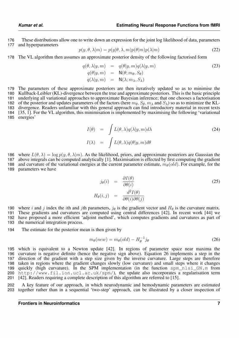
The parameters of these approximate posteriors are then iteratively updated so as to minimise the179Kullback-Leibler (KL)-divergence between the true and approximate posteriors. This is the basic principle180underlying all variational approaches to approximate Bayesian inference; that one chooses a factorisation181of the posterior and updates parameters of the factors (here mθ, Sθ,mλ and Sλ) so as to minimize the KL-182divergence. Readers unfamiliar with this general approach can find introductory material in recent texts183[35, 1]. For the VL algorithm, this minimisation is implemented by maximising the following ‘variational184energies’185

I(θ) =

∫L(θ, λ)q(λ|y,m)dλ (24)

I(λ) =

∫L(θ, λ)q(θ|y,m)dθ

where L(θ, λ) = log p(y, θ, λ|m). As the likelihood, priors, and approximate posteriors are Gaussian the186above integrals can be computed analytically [1]. Maximisation is effected by first computing the gradient187and curvature of the variational energies at the current parameter estimate, mθ(old). For example, for the188parameters we have189

jθ(i) =∂I(θ)

∂θ(i)(25)

Hθ(i, j) =d2I(θ)

∂θ(i)∂θ(j)

where i and j index the ith and jth parameters, jθ is the gradient vector and Hθ is the curvature matrix.190These gradients and curvatures are computed using central differences [42]. In recent work [44] we191have proposed a more efficient ‘adjoint method’, which computes gradients and curvatures as part of192the numerical integration process.193

The estimate for the posterior mean is then given by194

mθ(new) = mθ(old)−H−1θ jθ (26)

which is equivalent to a Newton update [42]. In regions of parameter space near maxima the195curvature is negative definite (hence the negative sign above). Equation 26 implements a step in the196direction of the gradient with a step size given by the inverse curvature. Large steps are therefore197taken in regions where the gradient changes slowly (low curvature) and small steps where it changes198quickly (high curvature). In the SPM implementation (in the function spm_nlsi_GN.m from199http://www.fil.ion.ucl.ac.uk/spm/), the update also incorporates a regularisation term200[42]. Readers requiring a complete description of this algorithm are referred to [15].201

A key feature of our approach, in which neurodynamic and hemodynamic parameters are estimated202together rather than in a sequential ‘two-step’ approach, can be illustrated by a closer inspection of203



equation 26. If we decompose the means, gradients and curvatures into neurodynamic and hemodynamic204parts205

mθ = [mn,mh]T (27)

jθ = [jn, jh]T

Hθ = [Hnn, Hnh;Hhn, Hhh]

then (using the Schur complement [1]) we can write the update for the neurodynamic parameters as206

mn(new) = mn(old)−[Hnn −HnhH

−1hhHhn

]−1jn (28)

whereas the equivalent second step of a two-step approach would use207

mn(new) = mn(old)−H−1nn jn (29)

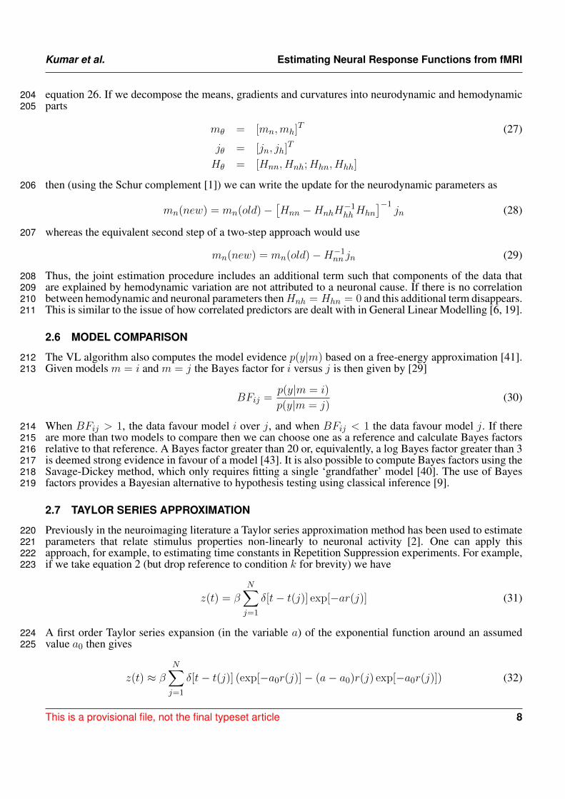
Thus, the joint estimation procedure includes an additional term such that components of the data that208are explained by hemodynamic variation are not attributed to a neuronal cause. If there is no correlation209between hemodynamic and neuronal parameters thenHnh = Hhn = 0 and this additional term disappears.210This is similar to the issue of how correlated predictors are dealt with in General Linear Modelling [6, 19].211

2.6 MODEL COMPARISON

The VL algorithm also computes the model evidence p(y|m) based on a free-energy approximation [41].212Given models m = i and m = j the Bayes factor for i versus j is then given by [29]213

BFij =p(y|m = i)

p(y|m = j)(30)

When BFij > 1, the data favour model i over j, and when BFij < 1 the data favour model j. If there214are more than two models to compare then we can choose one as a reference and calculate Bayes factors215relative to that reference. A Bayes factor greater than 20 or, equivalently, a log Bayes factor greater than 3216is deemed strong evidence in favour of a model [43]. It is also possible to compute Bayes factors using the217Savage-Dickey method, which only requires fitting a single ‘grandfather’ model [40]. The use of Bayes218factors provides a Bayesian alternative to hypothesis testing using classical inference [9].219

2.7 TAYLOR SERIES APPROXIMATION

Previously in the neuroimaging literature a Taylor series approximation method has been used to estimate220parameters that relate stimulus properties non-linearly to neuronal activity [2]. One can apply this221approach, for example, to estimating time constants in Repetition Suppression experiments. For example,222if we take equation 2 (but drop reference to condition k for brevity) we have223

z(t) = βN∑j=1

δ[t− t(j)] exp[−ar(j)] (31)

A first order Taylor series expansion (in the variable a) of the exponential function around an assumed224value a0 then gives225

z(t) ≈ β

N∑j=1

δ[t− t(j)] (exp[−a0r(j)]− (a− a0)r(j) exp[−a0r(j)]) (32)



This can be written as226

z(t) = β1z1(t) + β2z2(t) (33)β1 = β

β2 = β(a− a0)

z1(t) =N∑j=1

δ[t− t(j)] exp[−a0r(j)]

z2(t) = −N∑j=1

δ[t− t(j)]r(j) exp[−a0r(j)]

Convolution of this activity then produces the predicted BOLD signal227

g(t) = β1x1(t) + β2x2(t) (34)x1 = z1 ⊗ hx2 = z2 ⊗ h

where h is the hemodynamic response function (assumed known). This also assumes linear superposition228(that the response of a sum is the sum of responses). This linearised model can be fitted to fMRI data using229a standard GLM framework, with design matrix columns x1 and x2 and estimated regression coefficients230β1, β2. The estimated time constant is then given by231

a =β2

β1+ a0 (35)

The drawbacks of this approach are (i) it assumes that a reasonably accurate estimate of a can be provided232(a0, otherwise the Taylor series approximation is invalid), (ii) it assumes the hemodynamic response is233known and fixed across voxels, (iii) it assumes linear superposition (eg. neglecting possible hemodynamic234saturation effects) and (iv) inference is not straightforward as the parameter estimate is based on a ratio235of estimated quantities. However, the great benefit of this approach is that estimation can take place using236the GLM framework, allowing efficient application to large areas of the brain.237

2.8 REPETITION SUPPRESSION DATA

The experimental stimuli consisted of three pitch evoking stimuli with different ‘timbres’; Regular Interval238Noise (RIN), harmonic complex (HC), and regular click train (CT). Five different pitch values were used239having fundamental frequencies equally spaced on a log-scale from 100 to 300 Hz. The duration of each240stimulus was 1.5s.241

The RIN of a pitch value F0 was generated by first generating a sample of white noise, delaying it by2421/F0 sec and then adding it back to the original sample. This delay and add procedure was repeated 16243times to generate a salient pitch. The stimulus was then bandpass filtered to limit its bandwidth between2441000 and 4000 Hz. New exemplars of white noise were used to generate RIN stimuli that were repeated245within trials.246

The HC stimulus of fundamental frequency F0 was generated by adding sinusoids of harmonic247frequencies (multiples of F0) up to a maximum frequency (half the sampling rate) with phases chosen248randomly from a uniform distribution. The resulting signal was then Bandpass filtered between 1000 and2494000 Hz.250



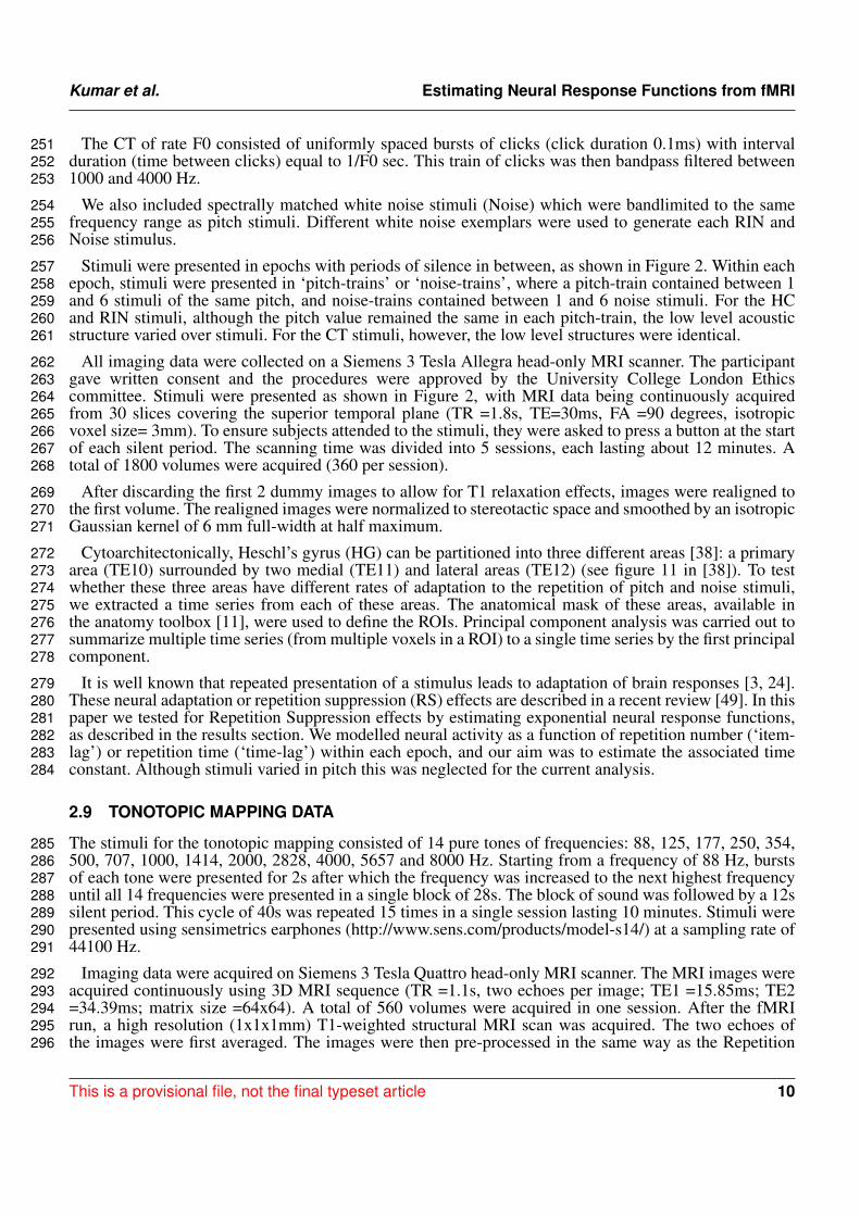
The CT of rate F0 consisted of uniformly spaced bursts of clicks (click duration 0.1ms) with interval251duration (time between clicks) equal to 1/F0 sec. This train of clicks was then bandpass filtered between2521000 and 4000 Hz.253

We also included spectrally matched white noise stimuli (Noise) which were bandlimited to the same254frequency range as pitch stimuli. Different white noise exemplars were used to generate each RIN and255Noise stimulus.256

Stimuli were presented in epochs with periods of silence in between, as shown in Figure 2. Within each257epoch, stimuli were presented in ‘pitch-trains’ or ‘noise-trains’, where a pitch-train contained between 1258and 6 stimuli of the same pitch, and noise-trains contained between 1 and 6 noise stimuli. For the HC259and RIN stimuli, although the pitch value remained the same in each pitch-train, the low level acoustic260structure varied over stimuli. For the CT stimuli, however, the low level structures were identical.261

All imaging data were collected on a Siemens 3 Tesla Allegra head-only MRI scanner. The participant262gave written consent and the procedures were approved by the University College London Ethics263committee. Stimuli were presented as shown in Figure 2, with MRI data being continuously acquired264from 30 slices covering the superior temporal plane (TR =1.8s, TE=30ms, FA =90 degrees, isotropic265voxel size= 3mm). To ensure subjects attended to the stimuli, they were asked to press a button at the start266of each silent period. The scanning time was divided into 5 sessions, each lasting about 12 minutes. A267total of 1800 volumes were acquired (360 per session).268

After discarding the first 2 dummy images to allow for T1 relaxation effects, images were realigned to269the first volume. The realigned images were normalized to stereotactic space and smoothed by an isotropic270Gaussian kernel of 6 mm full-width at half maximum.271

Cytoarchitectonically, Heschl’s gyrus (HG) can be partitioned into three different areas [38]: a primary272area (TE10) surrounded by two medial (TE11) and lateral areas (TE12) (see figure 11 in [38]). To test273whether these three areas have different rates of adaptation to the repetition of pitch and noise stimuli,274we extracted a time series from each of these areas. The anatomical mask of these areas, available in275the anatomy toolbox [11], were used to define the ROIs. Principal component analysis was carried out to276summarize multiple time series (from multiple voxels in a ROI) to a single time series by the first principal277component.278

It is well known that repeated presentation of a stimulus leads to adaptation of brain responses [3, 24].279These neural adaptation or repetition suppression (RS) effects are described in a recent review [49]. In this280paper we tested for Repetition Suppression effects by estimating exponential neural response functions,281as described in the results section. We modelled neural activity as a function of repetition number (‘item-282lag’) or repetition time (‘time-lag’) within each epoch, and our aim was to estimate the associated time283constant. Although stimuli varied in pitch this was neglected for the current analysis.284

2.9 TONOTOPIC MAPPING DATA

The stimuli for the tonotopic mapping consisted of 14 pure tones of frequencies: 88, 125, 177, 250, 354,285500, 707, 1000, 1414, 2000, 2828, 4000, 5657 and 8000 Hz. Starting from a frequency of 88 Hz, bursts286of each tone were presented for 2s after which the frequency was increased to the next highest frequency287until all 14 frequencies were presented in a single block of 28s. The block of sound was followed by a 12s288silent period. This cycle of 40s was repeated 15 times in a single session lasting 10 minutes. Stimuli were289presented using sensimetrics earphones (http://www.sens.com/products/model-s14/) at a sampling rate of29044100 Hz.291

Imaging data were acquired on Siemens 3 Tesla Quattro head-only MRI scanner. The MRI images were292acquired continuously using 3D MRI sequence (TR =1.1s, two echoes per image; TE1 =15.85ms; TE2293=34.39ms; matrix size =64x64). A total of 560 volumes were acquired in one session. After the fMRI294run, a high resolution (1x1x1mm) T1-weighted structural MRI scan was acquired. The two echoes of295the images were first averaged. The images were then pre-processed in the same way as the Repetition296



Suppression data. We restricted our data analysis to voxels from an axial slice (z = 6mm) covering the297superior temporal plane.298

3 RESULTS

3.1 REPETITION SUPPRESSION

We report results on an exponential ‘item-lag’ model, in which neuronal responses were modelled using299equation 2, k indexes the four stimulus types (HC, CT, RIN, Noise), and rk encodes the number of item300repeats since the first stimulus of that type in the epoch. We also fitted ‘time-lag’ models which used the301same equation but where rk encoded the elapsed time (in seconds) since the first stimulus of that type in302the epoch.303

We first report a model comparison of the item-lag versus time lag models. Both model types were fitted304to data from five sessions in six brain regions, giving a total of 30 data sets. The log model evidence was305computed using a free energy approximation described earlier. The difference in log model evidence was306then used to compute a log Bayes factor, with a value of 3 or greater indicating strong evidence.307

Strong evidence in favour of the ‘time-lag’ model was found in none out of 30 data sets, strong evidence308in favour of the ‘item-lag’ model was found in 22 out of 30 data sets. In the remaining 8 data sets, the309Bayes factors were not decisive but the item-lag model was preferred in 7 of them. We therefore conclude310that item-lags better capture the patterns in our data, and what follows below refers only to the item-lag311models.312

We now present results on the parametric responses of interest as captured by the βk (initial response)313and ak (decay) variables. These are estimated separately for each session of data using the model314fitting algorithm described earlier. We then combine estimates over sessions using precision weighted315averaging [28]. This is a Bayes-optimal procedure in which the overall parameter estimate is given by316a weighted average of individual session estimates. The weights are given by the relative precisions317(inverse variances) of the session estimates so that those with higher precision contribute more to the318final parameter estimate.319

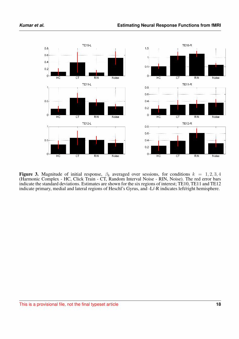
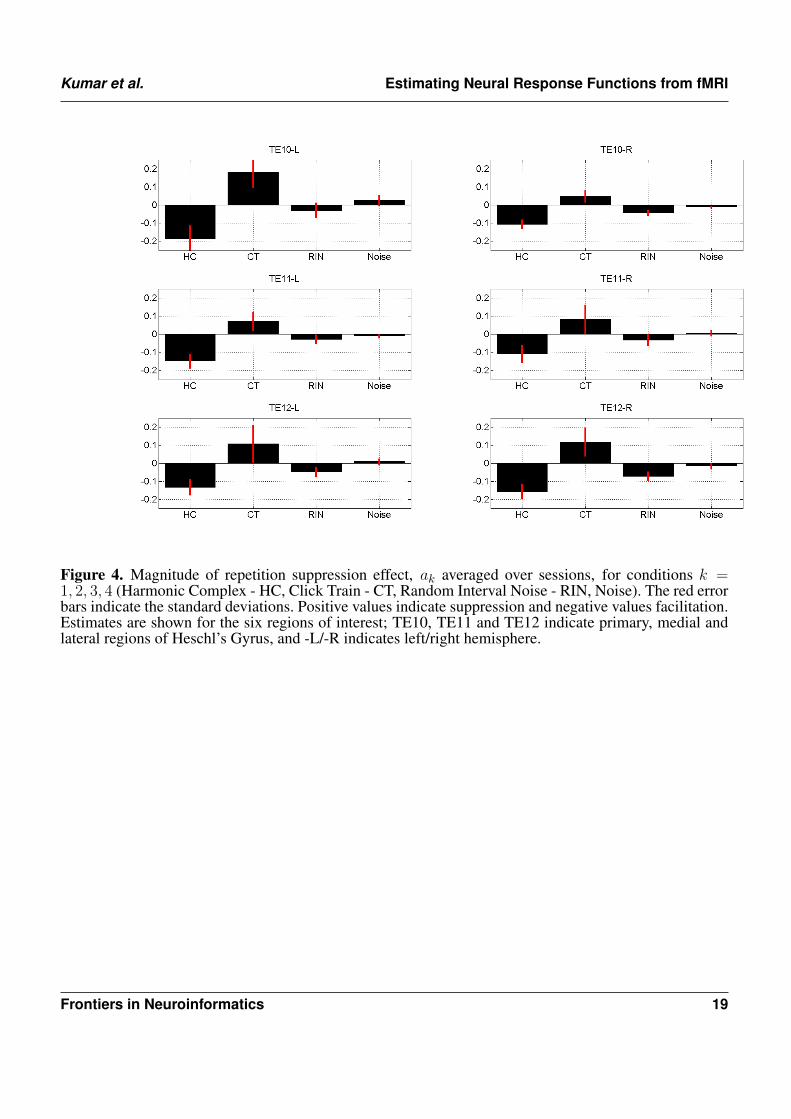
The estimates of the initial response magnitudes, βk, are shown in Figure 3 and the estimates of the320suppression effects, ak, are shown in Figure 4. Figure 3 shows that the pattern of initial responses321(responses at item lag 0) is similar over all regions with CT and RIN typically eliciting the largest322responses. Figure 4 shows that the noise stimulus does not elicit any repetition suppression effect in323any region. The CT stimulus elicits a suppression effect which is strongest in TE10-L whereas the HC324stimulus elicits a facilitation effect in all regions.325

3.2 TONOTOPIC MAPPING

This section describes the estimation of Neural Response Functions for the Tonotopic Mapping data. We326first focus on the Gaussian parametric form described in equation 4. The Full Width at Half Maximum327is given by FWHM = 2

√(2 ln 2)σ. Following [37] we define the Tuning Value as W = µ/FWHM328

where µ and FWHM are expressed in Hz. Larger tuning values indicate more narrowly tuned response329functions.330

We restricted our data analysis to a single axial slice (z =6) covering superior temporal plane. This slice331contained 444 voxels in the auditory cortex.332

Figure 5 shows the parameters of a Gaussian NRF as estimated over this slice. The main characteristics333are as follows. First, the centre frequency decreases and then increases again as one moves along the334posterior to anterior axis with high frequencies at y = −30, low frequencies at y = −10 and higher335frequencies again at y = 5. There is a single region of high amplitude responses that follows the length336



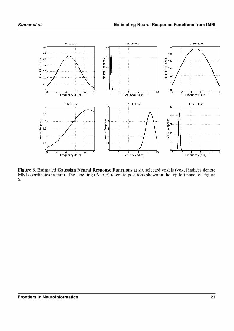
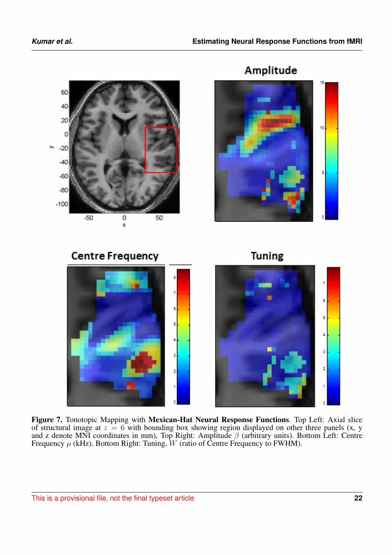
of Heschl’s Gyrus (the diagonal band in the top right panel of Figure 5). These responses have a low337centre frequency of between 200 and 300Hz. Finally the tuning values are approximately constant over338the whole slice, with a value of about W = 1, except for a lateral posterior region with a much higher339value of about W = 4. Figure 6 plots the estimated Gaussian response functions at six selected voxels.340

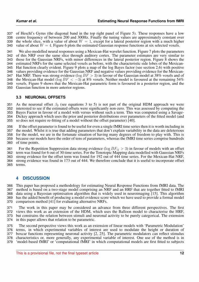
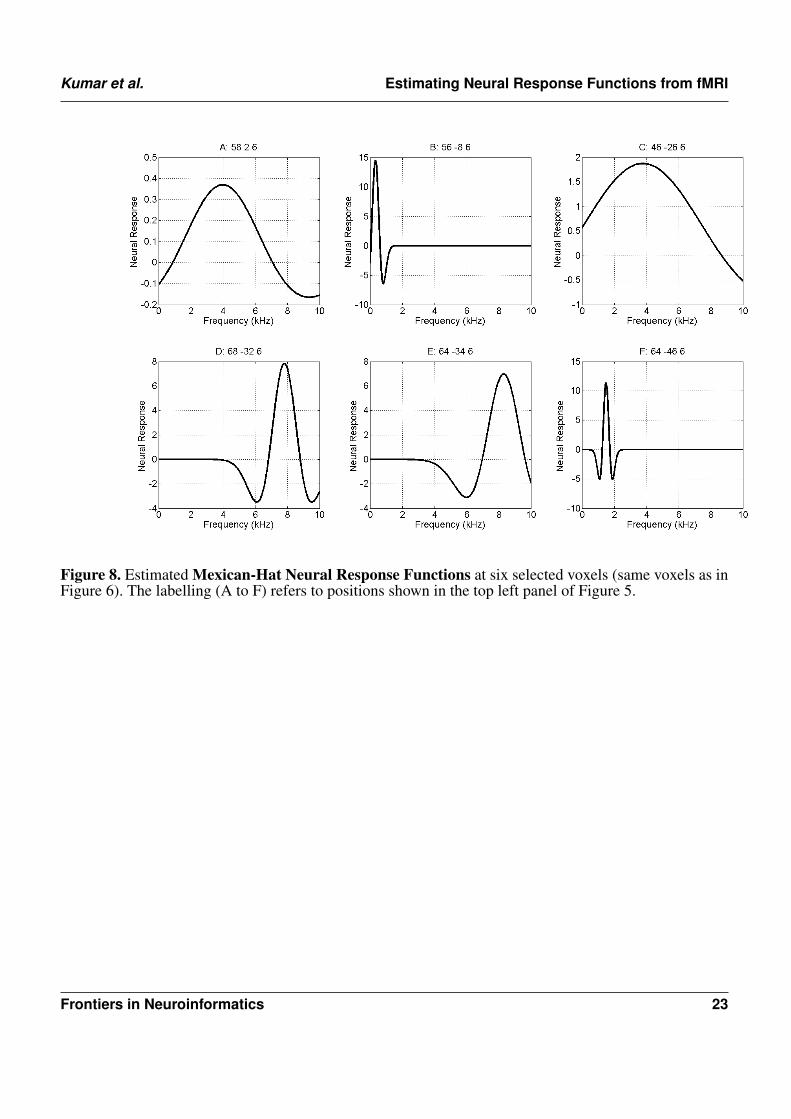
We also modelled neural responses using a Mexican-Hat wavelet function. Figure 7 plots the parameters341of this NRF over the same slice through auditory cortex. The parameter estimates are very similar to342those for the Gaussian NRFs, with minor differences in the lateral posterior region. Figure 8 shows the343estimated NRFs for the same selected voxels as before, with the characteristic side lobes of the Mexican-344Hat function clearly evident. Figure 9 plots a map of the log Bayes factor (see section 2.6) with positive345values providing evidence for the Gaussian NRF and negative values providing evidence for the Mexican-346Hat NRF. There was strong evidence (logBF > 3) in favour of the Gaussian model at 38% voxels and of347the Mexican-Hat model (logBF < −3) at 8% voxels. Neither model is favoured at the remaining 54%348voxels. Figure 9 shows that the Mexican-Hat parametric form is favoured in a posterior region, and the349Gaussian function in more anterior regions.350

3.3 NEURONAL OFFSETS

As the neuronal offset β0 (see equations 3 to 5) is not part of the original HDM approach we were351interested to see if the estimated offsets were significantly non-zero. This was assessed by computing the352Bayes Factor in favour of a model with versus without such a term. This was computed using a Savage-353Dickey approach which uses the prior and posterior distributions over parameters of the fitted model (and354so does not require re-fitting of a model without the offset parameter) [40].355

If the offset parameter is found to be useful for even a single fMRI time series then it is worth including in356the model. Whilst it is true that adding parameters that don’t explain variability in the data are deleterious357for the model, we are in the fortunate situation of having many degrees of freedom to play with. This is358because our models have the order of tens of parameters, whereas the fMRI time series comprise hundreds359of time points.360

For the Repetition Suppression data strong evidence (logBFij > 3) in favour of models with an offset361term was found for 6 out of 30 time series. For the Tonotopic Mapping data modelled with Gaussian NRFs362strong evidence for the offset term was found for 192 out of 444 time series. For the Mexican-Hat NRF,363strong evidence was found in 173 out of 444. We therefore conclude that it is useful to incorporate offset364terms.365

4 DISCUSSION

This paper has proposed a methodology for estimating Neural Response Functions from fMRI data. The366method is based on a two-stage model comprising an NRF and an HRF that are together fitted to fMRI367data using a Bayesian optimisation algorithm that is widely used in neuroimaging [15]. This algorithm368has the added benefit of producing a model evidence score which we have used to provide a formal model369comparison method [41] for evaluating alternative NRFs.370

The work in this paper may be considered an advance from three different perspectives. The first371views this work as an extension of the HDM, which uses the Balloon model to characterise the HRF,372but constrains the relation between stimuli and neuronal activity to be purely categorical. The extension373in this paper allows that relation to be parametric.374

The second perspective views this work as an extension of linear models with ‘Parametric Modulation’375terms, in which experimental variables of interest are used to modulate the height or duration of376boxcar functions representing neuronal activity [2, 25]. The parametric modulators can reflect stimulus377characteristics or, more generally, any experimental variable of interest. One use of the method is in378‘model-based fMRI’ or ‘computational fMRI’ in which computational models are first fitted to subjects379



behavioural data (reaction times and error rates) and the internal variables of these models are used as380parametric modulators [39, 14]. The work in this paper represents an extension of this approach by381allowing for nonlinear relations between fMRI signals and unknown parametric variables. Whilst it is382true that nonlinear relationships can be accommodated in the linear framework by using a Taylor series383approach, this has a number of disadvantages, as described in section 2.7.384

The third perspective views this work as a novel method for the estimation of Population Receptive385Fields (PRFs). These are similar, in principle, to receptive field functions derived for individual neurons386from single unit electrophysiology [7] but estimate population rather than single neuron responses [10].387In these studies parametric forms are derived for how neural responses depend on properties of sensory388stimuli, such as orientation and contrast, in addition to spatial and temporal characteristics [27, 10, 30].389

Previously, a two-step procedure has been proposed for NRF estimation [10]. The first step estimates390an HRF assuming known neural activity, and the second estimates an NRF based on the estimated391HRF. In this procedure the first step neglects the uncertainty in the assumed neural response and the392second step neglects the uncertainty in the estimated HRF. This can lead to over-confident inferences.393The simultaneous optimisation of NRF and HRF parameters proposed in this paper, however, does not394neglect these uncertainties. The conditional dependencies are captured in the relevant off-diagonal terms395in the posterior covariance matrix and this guides parameter estimates during the optimisation process396(see equations 27 and 28). Additionally, models with highly correlated parameters also have lower model397evidence [41], so this is also reflected in model comparison.398

In this paper, we applied our method to investigate repetition suppression in the auditory system. Our399model comparisons showed an exponential NRF based on item-lag was superior to one based on time-lag.400Intuitively, one might think that if the brain charges and discharges some dynamical system then the time-401lag model would be more likely than the item-lag model. However, it is well known that there are multiple402brain systems for supporting discrete representations, as indicated for example by studies of numerosity403[8]. Recent work in the visual domain has even characterised PRFs for numerosity [26]. Moreover, a404dominant paradigm in the repetition suppression literature has assumed an item-lag like model, in which405the number of repetitions is the key variable [23, 49]. This paper provides a methodology for testing such406assumptions.407

We found evidence of repetition suppression for the Click Train (CT) stimulus, facilitation for the408Harmonic Complex (HC) in all the areas, facilitation for RIN in some areas (e.g. TE12R) and no409suppression or facilitation for the noise stimulus. In our experiment the click trains (of a given pitch410value) were identical within a trial, whereas the acoustic structure of HC, RIN and Noise varied within a411trial (because of randomization of phase in the HC and use of a new exemplar of noise both for generation412of RIN and Noise). The identical acoustic structure of CT and variation in acoustic structure in HC, RIN413and Noise within trials may explain suppression of neural activity for CT and lack of it for HC, RIN and414Noise.415

We also applied our method to estimate tonotopic maps using two different functions: Gaussian416and Mexican-hat. The two functions produced maps which were similar. The results showed that low417frequencies activated HG whereas regions posterior to HG were activated by high frequencies. This is in418agreement with the tonotopic organization shown in previous works [12, 37, 47]. Bayesian comparison419of the two models using Gaussian and Mexican-hat functions showed that the former was preferred along420the HG whereas the latter was the preferred model in regions posterior to HG. This is in agreement with a421previous study [36] that showed spectral profiles with a single peak in the central part of HG and Mexican-422hat like spectral profiles lying posterior to HG. We also observed broad tuning curves along the HG and423narrow tuning curves posterior to HG. However, we did not observe the degree of variation in tuning width424in areas surrounding HG, as was found in [37]. This may be due to the fact that computations in our work425were confined to a single slice. Further empirical validation is needed to produce maps of the tuning width426covering wider areas of the auditory cortex.427

A disadvantage of our proposed method is the amount of computation time required. For our auditory428fMRI data (comprising 300 or 500 time points), optimization takes approximately 5 minutes per429



voxel/region on a desktop PC (Windows Vista, 3.2 GHz CPU, 12G RAM). One possible use of our430approach could therefore be to provide ‘ballpark’ estimates of NRF parameters, using data from selected431voxels, and then to derive estimates at neighbouring voxels using the standard Taylor series approach.432Alternatively, optimization with a computer cluster should deliver results overnight for large regions of433the brain (eg. comprising thousands of voxels).434

Our proposed method is suitable for modelling neural responses as simple parametric forms as assumed435in previous studies using parametric modulators or population receptive fields. It could also be extended436to simple nonlinear dynamical systems, for example of the sort embodied in nonlinear DCMs [34].437

Two disadvantages of our approach are that there is no explicit model of ongoing activity, and it is not438possible to model stochastic neural responses. Additionally, as the NRFs are identified solely from fMRI439data our neural response estimates will not capture the full dynamical range of neural activity available440from other modalities such as Local Field Potentials. On a more positive note, however, our approach441does inherit two key benefits of fMRI; that it is a noninvasive method with a large field of view.442

An additional finding of this paper is that model fits were significantly improved by including a neuronal443offset parameter. This offset could also be included in Dynamic Causal Models [17] by adding an extra444term to the equation governing vasodilation (equation 7).445

DISCLOSURE/CONFLICT-OF-INTEREST STATEMENT

The authors declare that the research was conducted in the absence of any commercial or financial446relationships that could be construed as a potential conflict of interest.447

ACKNOWLEDGEMENT

The authors would like to thank Guillaume Flandin, Karl Friston and Tim Griffiths for useful feedback on448this work.449

Funding: WP is supported by a core grant [number 091593/Z/10/Z] from the Wellcome Trust:450www.wellcome.ac.uk.451

REFERENCES[1]C.M. Bishop. Pattern Recognition and Machine Learning. Springer, New York, 2006.452[2]C. Buchel, A.P. Holmes, G. Rees, and K.J. Friston. Characterizing stimulus-response functions using453

nonlinear regressors in parametric fMRI experiments. NeuroImage, 8:140–148, 1998.454[3]R Buckner, J Goodman, M Burock, M Rotte, W Koutstaal, D Schacter, and B Rosen. Functional-455

anatomic correlates of object priming in humans revealed by rapid presentation event-related fMRI.456Neuron, 20:285–96, 1998.457

[4]R. Buxton, K. Uludag, D. Dubowitz, and T. Liu. Modelling the hemodynamic response to brain458activation. Neuroimage, 23:220–233, 2004.459

[5]R.B. Buxton, E.C. Wong, and L.R. Frank. Dynamics of blood flow and oxygenation changes during460brain activation: The Balloon Model. Magnetic Resonance in Medicine, 39:855–864, 1998.461

[6]R. Christensen. Plane answers to complex questions: the theory of linear models. Springer-Verlag,462New York, US., 2002.463

[7]P. Dayan and L.F. Abbott. Theoretical Neuroscience: Computational and Mathematical Modeling of464Neural Systems. MIT Press, 2001.465

[8]S Dehaene and E Brannon. Space, Time and Number in the Brain. Academic Press, 2011.466



[9]Z Dienes. Bayesian versus orthodox statistics: which side are you on? Perspectives on Pyschological467Science, 6:274–290, 2011.468

[10]S Dumoulin and B Wandell. Population receptive field estimates in human visual cortex. Neuroimage,46939:647–660, 2008.470

[11]S Eickhoff, K Stephan, H Mohlberg, C Grefkes, G Fink, K Amunts, and K Zilles. A new SPM471toolbox for combining probabilistic cytoarchitectonic maps and functional imaging data. Neuroimage,47225:1325–1335, 2005.473

[12]E Formisano, D Kim, F DiSalle, P van de Moortele, K Ugurbil, and R Goebel. Mirror-symmetric474tonotopic maps in human primary auditory cortex. Neuron, 40:859–869, 2003.475

[13]R.S.J. Frackowiak, K.J. Friston, C. Frith, R. Dolan, C.J. Price, S. Zeki, J. Ashburner, and W.D. Penny.476Human Brain Function. Academic Press, 2nd edition, 2003.477

[14]K Friston and R Dolan. Computational and dynamic models in neuroimaging. Neuroimage, 52:752–478765, 2009.479

[15]K. Friston, J. Mattout, N. Trujillo-Barreto, J. Ashburner, and W. Penny. Variational free energy and480the Laplace approximation. Neuroimage, 34(1):220–234, 2007.481

[16]K. J. Friston. Bayesian estimation of dynamical systems: an application to fMRI. Neuroimage,48216(2):513–530, Jun 2002.483

[17]K. J. Friston, L. Harrison, and W. Penny. Dynamic causal modelling. Neuroimage, 19(4):1273–1302,484Aug 2003.485

[18]K. J. Friston, O. Josephs, G. Rees, and R. Turner. Nonlinear event-related responses in fMRI. Magn486Reson Med, 39(1):41–52, 1998.487

[19]K.J. Friston, J. Ashburner, S.J. Kiebel, T.E. Nichols, and W.D. Penny, editors. Statistical Parametric488Mapping: The Analysis of Functional Brain Images. Academic Press, 2007.489

[20]K.J. Friston, L. Harrison, and W.D. Penny. Dynamic Causal Modelling. NeuroImage, 19(4):1273–4901302, 2003.491

[21]Marta I. Garrido, James M. Kilner, Stefan J. Kiebel, Klaas E. Stephan, Torsten Baldeweg, and Karl J.492Friston. Repetition suppression and plasticity in the human brain. Neuroimage, 48(1):269–279, Oct4932009.494

[22]A. Gelman, J.B. Carlin, H.S. Stern, and D.B. Rubin. Bayesian Data Analysis. Chapman and Hall,495Boca Raton, 1995.496

[23]K Grill-Spector, R Henson, and A Martin. Repetition and the brain: neural models of stimulus-specific497effects. Trends in cognitive sciences, 10:14–23, 2006.498

[24]K Grill-Spector, T Kushnir, S Edelman, G Avidan, Y Itzchak, and R Malach. Differential processing499of objects under various viewing conditions in the human lateral occipital complex. Neuron, 24:187–500203, 1999.501

[25]J Grinband, T Wager, M Lindquist, V Ferrera, and J Hirsch. Detection of time-varying signals in502event-related fMRI designs. Neuroimage, 43:509–520, 2008.503

[26]B Harvey, B Klein, N Petridou, and S Dumoulin. Topographic representation of numerosity in human504parietal cortex. Science, 341:1123–1126, 2013.505

[27]G Heckman, S Boivier, V Carr, E Harley, K Cardinal, and S Engel. Nonlinearities in rapid event-506related fMRI explained by stimulus scaling. Neuroimage, 34:651–660, 2007.507

[28]C Kasess, K Stephan, A Weissenbacher, L Pezawas, E Moser, and C Windischberger. Multi-subject508analyses with dynamic causal modelling. Neuroimage, 49:3065–3074, 2010.509

[29]R.E. Kass and A.E. Raftery. Bayes factors. Journal of the American Statistical Association, 90:773–510795, 1995.511

[30]K Kay, T Naselaris, R Prenger, and J Gallant. Identifying natural images from human brain activity.512Nature, 452:352–356, 2008.513

[31]S Lee, A Papanikolaou, N Logothetis, S Smirnakis, and G Keliris. A new method for estimating514population receptive field topography in visual cortex. Neuroimage, 81:144–157, 2013.515

[32]V Litvak, J Mattout, S Kiebel, C Phillips, R Henson, Kilner, G Barnes, R Oostenveld, J Daunizeau,516G Flandin, W Penny, and K Friston. EEG and MEG data analysis in SPM8. Comput Intell Neurosci,5172011:852961, 2011.518

[33]S. Mallat. A wavelet tour of signal processing. Academic Press, 1999.519



[34]A. C. Marreiros, S. J. Kiebel, and K. J. Friston. Dynamic causal modelling for fMRi: a two-state520model. Neuroimage, 39(1):269–278, Jan 2008.521

[35]T.S. Jaakola M.I. Jordan, Z. Ghahramani and L.K. Saul. An Introduction to Variational Methods for522Graphical Models. In M.I. Jordan, editor, Learning in Graphical Models. Kluwer Academic Press,5231998.524

[36]M Moerel, D DeMartino, R Santoro, K Ugurbil, R Goebel, E Yacoub, and E Formisano. Processing of525Natural Sounds: Characterization of Multipeak Spectral Tuning in Human Auditory Cortex. Journal526of Neuroscience, 33:11888–11898, 2013.527

[37]M. Moerel, F DeMartino, and E Formisano. Processing of Natural Sounds in Human Auditory528Cortex: Tonotopy, Spectral Tuning, and Relation to Voice Sensitivity. Journal of Neuroscience,52932:14205–14216, 2012.530

[38]P Morosan, J Rademacher, A Schleicher, K Amunts, T Schormann, and K Zilles. Human531primary auditory cortex: cytoarchitectonic subdivisions and mapping into a spatial reference system.532Neuroimage, 13:684–701, 2001.533

[39]J O’Doherty, A Hampton, and H Kim. Model-based fMRI and its application to reward learning and534decision making. Annals New York Academy of Sciences, 1104:35–53, 2007.535

[40]W Penny and G Ridgway. Efficient posterior probability mapping using Savage-Dickey ratios. PLOS536One, 8:e59655, 2013.537

[41]W. D. Penny. Comparing dynamic causal models using AIC, BIC and free energy. Neuroimage,53859(1):319–330, Jan 2012.539

[42]W. H. Press, S. A. Teukolsky, W. T. Vetterling, and B. P. Flannery. Numerical Recipes in C (Second540Edition). Cambridge, Cambridge, 1992.541

[43]A.E. Raftery. Bayesian model selection in social research. In P.V. Marsden, editor, Sociological542Methodology, pages 111–196. Cambridge, Mass., 1995.543

[44]B Sengupta, K Friston, and W Penny. Efficient Gradient Computation for Dynamical Systems.544Neuroimage, 2014. Accepted for Publication.545

[45]L Shampine and M Reichelt. The MATLAB ODE Suite. SIAM Journal on Scientific Computing,54618:1–22, 1997.547

[46]K Stephan, N Weiskopf, P Drysdale, P Robinson, and K Friston. Comparing hemodynamic models548with DCM. Neuroimage, 38(3):387–401, 2007.549

[47]T Talavage, M Sereno, J Melcher, P Ledden, B Rosen, and A Dale. Tonotopic organization in550human auditory cortex revealed by progressions of frequency sensitivity. Journal of Neurophysiology,55191:1282–1296, 2004.552

[48]D.D. Wackerley, W. Mendenhall, and R.L. Scheaffer. Mathematical statistics with applications.553Duxbury Press, 1996.554

[49]S Weigelt, L Muckli, and A Kohler. Functional Magnetic Resonance Adaptation in Visual555Neuroscience. Reviews in the Neurosciences, 29:363–380, 2008.556

FIGURES



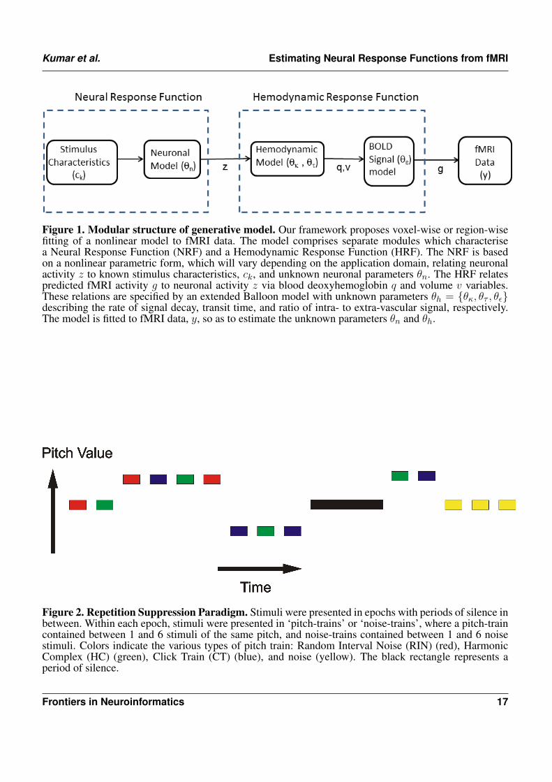
Figure 1. Modular structure of generative model. Our framework proposes voxel-wise or region-wisefitting of a nonlinear model to fMRI data. The model comprises separate modules which characterisea Neural Response Function (NRF) and a Hemodynamic Response Function (HRF). The NRF is basedon a nonlinear parametric form, which will vary depending on the application domain, relating neuronalactivity z to known stimulus characteristics, ck, and unknown neuronal parameters θn. The HRF relatespredicted fMRI activity g to neuronal activity z via blood deoxyhemoglobin q and volume v variables.These relations are specified by an extended Balloon model with unknown parameters θh = {θκ, θτ , θε}describing the rate of signal decay, transit time, and ratio of intra- to extra-vascular signal, respectively.The model is fitted to fMRI data, y, so as to estimate the unknown parameters θn and θh.

Figure 2. Repetition Suppression Paradigm. Stimuli were presented in epochs with periods of silence inbetween. Within each epoch, stimuli were presented in ‘pitch-trains’ or ‘noise-trains’, where a pitch-traincontained between 1 and 6 stimuli of the same pitch, and noise-trains contained between 1 and 6 noisestimuli. Colors indicate the various types of pitch train: Random Interval Noise (RIN) (red), HarmonicComplex (HC) (green), Click Train (CT) (blue), and noise (yellow). The black rectangle represents aperiod of silence.



Figure 3. Magnitude of initial response, βk averaged over sessions, for conditions k = 1, 2, 3, 4(Harmonic Complex - HC, Click Train - CT, Random Interval Noise - RIN, Noise). The red error barsindicate the standard deviations. Estimates are shown for the six regions of interest; TE10, TE11 and TE12indicate primary, medial and lateral regions of Heschl’s Gyrus, and -L/-R indicates left/right hemisphere.



Figure 4. Magnitude of repetition suppression effect, ak averaged over sessions, for conditions k =1, 2, 3, 4 (Harmonic Complex - HC, Click Train - CT, Random Interval Noise - RIN, Noise). The red errorbars indicate the standard deviations. Positive values indicate suppression and negative values facilitation.Estimates are shown for the six regions of interest; TE10, TE11 and TE12 indicate primary, medial andlateral regions of Heschl’s Gyrus, and -L/-R indicates left/right hemisphere.



Figure 5. Tonotopic Mapping with Gaussian Neural Response Functions. Top Left: Axial slice ofstructural image at z = 6 with bounding box showing region displayed on other three panels (x, y andz denote MNI coordinates in mm). The labelling (A to F) refers to plots in Figures 6 and 8. Top Right:Amplitude β (arbitrary units), Bottom Left: Centre Frequency µ (kHz). Bottom Right: Tuning, W (ratioof Centre Frequency to FWHM).This is a provisional file, not the final typeset article 20


Figure 6. Estimated Gaussian Neural Response Functions at six selected voxels (voxel indices denoteMNI coordinates in mm). The labelling (A to F) refers to positions shown in the top left panel of Figure5.



Figure 7. Tonotopic Mapping with Mexican-Hat Neural Response Functions. Top Left: Axial sliceof structural image at z = 6 with bounding box showing region displayed on other three panels (x, yand z denote MNI coordinates in mm), Top Right: Amplitude β (arbitrary units). Bottom Left: CentreFrequency µ (kHz). Bottom Right: Tuning, W (ratio of Centre Frequency to FWHM).



Figure 8. Estimated Mexican-Hat Neural Response Functions at six selected voxels (same voxels as inFigure 6). The labelling (A to F) refers to positions shown in the top left panel of Figure 5.



Figure 9. Top Right: Log Bayes Factor for Gaussian versus Mexican-Hat NRFs (full range of values). Positivevalues provide evidence for the Gaussian and negative values for the Mexican-Hat NRF. Bottom Left: As top rightbut scale changed to range logBFij > 3. Bottom Right: A plot of logBFji over range logBFji > 3 (ie in favourof Mexican-Hat). The Mexican-Hat is favoured in a posterior region, and the Gaussian more anteriorly.This is a provisional file, not the final typeset article 24

Documents

Estimating Neural Response Functions from fMRIwpenny/publications/nrf_third...Kumar et al. Estimating Neural Response Functions from fMRI 69 This paper extends the HDM formalism by