Estimating Item Response Theory Models Using Markov Chain

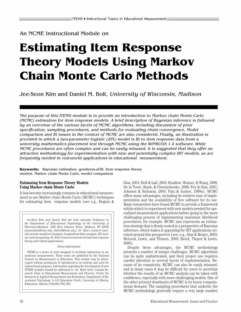
An NCME Instructional Module on

Estimating Item ResponseTheory Models Using MarkovChain Monte Carlo MethodsJee-Seon Kim and Daniel M. Bolt, University of Wisconsin, Madison

The purpose of this ITEMS module is to provide an introduction to Markov chain Monte Carlo(MCMC) estimation for item response models. A brief description of Bayesian inference is followedby an overview of the various facets of MCMC algorithms, including discussion of priorspecification, sampling procedures, and methods for evaluating chain convergence. Modelcomparison and fit issues in the context of MCMC are also considered. Finally, an illustration isprovided in which a two-parameter logistic (2PL) model is fit to item response data from auniversity mathematics placement test through MCMC using the WINBUGS 1.4 software. WhileMCMC procedures are often complex and can be easily misused, it is suggested that they offer anattractive methodology for experimentation with new and potentially complex IRT models, as arefrequently needed in real-world applications in educational measurement.

Keywords: Bayesian estimation, goodness-of-fit, item response theorymodels, Markov chain Monte Carlo, model comparison

Estimating Item Response Theory ModelsUsing Markov chain Monte CarloIt has become increasingly common in educational measure-ment to use Markov chain Monte Carlo (MCMC) techniquesfor estimating item response models (see e.g., Beguin &

Jee-Seon Kim and Daniel Bolt are both Associate Professors inthe Department of Educational Psychology at the University ofWisconsin-Madison, 1025 West Johnson Street, Madison, WI 53705([email protected], [email protected]). Dr. Kim’s research inter-ests include multilevel analysis, longitudinal data analysis, IRT mod-els, and test equating. Dr. Bolt’s research interests include item responsetheory and related applications.

Series Information

ITEMS is a series of units designed to facilitate instruction in ed-ucational measurement. These units are published by the NationalCouncil on Measurement in Education. This module may be photo-copied without permission if reproduced in its entirety and used forinstructional purposes. Information regarding the development of newITEMS modules should be addressed to: Dr. Mark Gierl, Canada Re-search Chair in Educational Measurement and Director, Centre forResearch in Applied Measurement and Evaluation, Department of Ed-ucational Psychology, 6–110 Education North, University of Alberta,Edmonton, Alberta, CANADA T6G 2G5.

Glas, 2001; Bolt & Lall, 2003; Bradlow, Wainer, & Wang, 1999;De la Torre, Stark, & Chernyshenko, 2006; Fox & Glas, 2001;Johnson & Sinharay, 2005; Patz & Junker, 1999a). MCMCoffers many advantages, including its relative ease of imple-mentation and the availability of free software for its use.Many researchers have found MCMC to provide a frameworkwithin which to experiment with new models needed for spe-cialized measurement applications before going to the morechallenging process of implementing maximum likelihoodprocedures, for example. MCMC also represents an estima-tion strategy that is firmly rooted in a perspective of Bayesianinference, which makes it appealing for IRT applications ori-ented around this perspective (see, e.g., Glas & Meijer, 2003;McLeod, Lewis, and Thissen, 2003; Zwick, Thayer & Lewis,2000).

Despite these advantages, the MCMC methodologypresents a number of unique challenges. MCMC algorithmscan be quite sophisticated, and their proper use requirescareful attention to several facets of implementation. Be-cause of its complexity, MCMC can also be easily misused,and in many cases it may be difficult for users to ascertainwhether the results of an MCMC analysis can be taken withconfidence, especially with more challenging models. One ofthe other primary drawbacks of MCMC is its heavy computa-tional demand. The sampling procedures that underlie theMCMC methodology generally require a very large number

38 Educational Measurement: Issues and Practice

of iterations before model parameters can be reliably esti-mated. It is not uncommon for a single estimation run totake several hours, or even a day or more, for more complexmodels or when analyzing large amounts of data.

The purpose of this module is to provide an introduc-tion to MCMC methods and to illustrate their applicationin estimating item response models. In that context, wealso discuss the WINBUGS software (Spiegelhalter, Thomas,Best, & Lunn, 2003; downloadable at http://www.mrc-bsu.cam.ac.uk/bugs/winbugs/contents.shtml), a computerprogram that allows for easy implementation of variousMCMC procedures. WINBUGS can be used to fit a host ofdifferent statistical models and has built in graphical andanalytical tools that help the user monitor the estimationprocess and evaluate results. Admittedly, the topic of MCMCis a difficult one to present in an introductory way in a singlepaper; as a result, we will frequently refer to some usefulreferences addressing different aspects of this topic to fill indetails. In addition, the reader may find it helpful to havea software package like WINBUGS at their disposal in ex-perimenting with certain aspects of MCMC. The WINBUGSpackage comes with several example models and data sets,including some specific to item response theory, that canhelp in learning the methodology. Clearly one of the bestways to learn MCMC techniques is to experiment with theprocedure using models and datasets that are already fa-miliar. Prior to discussing the specifics of MCMC, however,we review some basic principles of the Bayesian theoreticalframework, as this ultimately provides the foundation for theMCMC methodology.

Brief Overview of Bayesian Inference

Any attempt to understand MCMC requires familiarity withthe core principles of Bayesian inference. The centerpieceof this framework is Bayes’ theorem. (Readers previouslyunfamiliar with this topic may find it useful to study Congdon(2001) or similar sources before attempting to work MCMCmethods.) Bayes’ theorem is often portrayed in terms ofthe probabilities of discrete events, say an event “A” and anevent “B.” For example, in a medical context, event A couldrepresent the presence (or absence) of a particular type ofdisease, say the measles, and event B the outcome of a testfor the disease returning a result “positive” or “negative.”From Bayes’ theorem, we know that

P(A | B) = P(B | A)P(A)

/[∑A

P(B | A)P(A)

], (1)

where we refer to P(A | B) as the posterior probability of Agiven B (e.g., the probability of having the measles given theresult of the test); P(A) as the prior probability of A (e.g.,the prior probability of having measles), and P(B | A) as theconditional probability of B given A (e.g., the probability ofa particular test result given the presence or absence of themeasles).

The summation in the denominator of the right hand sideof (1) represents an accumulation across all possible out-comes of event A (e.g., has the measles, doesn’t have themeasles), and thus can also be taken as the probability of B,P(B) (i.e., the overall probability of a particular test result).Ultimately, Bayes’ theorem provides a representation of theconditional probability of one event given another (i.e., A

given B, or the probability of measles given the test result)in terms of the opposite conditional probability (i.e., B givenA, or the probability of a particular test result given the pres-ence or absence of the measles). For example, suppose it isknown that the probability of a positive test result given thatone truly has the measles is .95, the probability of a false pos-itive is .02, and the overall probability of having the measlesamong those tested is .10. Using Bayes’ theorem (as shown inequation 1) we can determine that the probability of havingthe measles given the positive test is (.95)(.10)/[.95(.10) +.02(.90)] = .84.

When fitting an item response model to item response data,practitioners are faced with a situation that reflects Bayes’theorem. Usually a primary goal in fitting an IRT model is toobtain information about parameters of the item responsemodel (e.g., item difficulty, item discrimination, examineeability) from the item response data. In terms of Bayes’theorem, this information is reflected in the relative likeli-hood(s) of particular parameter values for the model (“eventA”) given the observed item response data (“event B”). Thechosen IRT model (e.g., two-parameter logistic model; 2PL)provides a basis for describing the opposite conditional prob-ability, namely the probability of the item response data (B)given the model parameters (A).

Although at a conceptual level this idea fits, Bayes’ theoremas portrayed in (1) is inappropriate for most item responsetheory applications as item and ability parameters are gener-ally continuous values, not discrete events. Consequently wecannot consider the “probability” of their occurrence as wecan for finite discrete outcomes. It will therefore be more con-venient to portray Bayes’ theorem in the form of continuousprobability density functions, which represent the relativelikelihood of each outcome. Familiar examples of probabil-ity density functions include the normal density function,which takes the form of the familiar bell-shape curve. In theIRT context, Bayes’ theorem can be written with respect toprobability density functions as:

f(� | X) = f(X |�) ∗ f(�)

/∫

�

f (X |�) f (�) d�

(2)

where X denotes all of the item response data (i.e., thecorrect/incorrect scores of each examinee to each item),and � all of the unknown parameters, which in IRT generallyconsist of item and person parameters. The use of “f(·)” inplace of “P(·)” and “

∫” in place of “

∑” in (2) compared to (1)

accounts for the continuous nature of the parameter values.One other fundamental difference between (1) and (2) isthat � represents many parameters (i.e., multiple “events”),and X many observed outcomes, implying that the quantitiesin (2) should be thought of as multivariate outcomes ratherthan univariate ones. Consequently, we will view � as a setof hypothetical outcomes for all of the item and examineeparameters in the model.

The left hand side of (2), referred to as the joint posteriordensity (of the model parameters given the data), is used todetermine estimates of the model parameters. To evaluateit requires knowledge about the quantities on the right handside. The quantity f(X |�), which expresses the likelihood ofthe item response data given all of the model parameters, isdefined by the item response model (e.g., 2PL) along with its

Winter 2007 39

associated assumptions of local independence. The quantityf(�) is the prior density of the model parameters, and canbe thought of as indicating the relative likelihoods of partic-ular parameter values “prior to” data collection. The quantityin the denominator is now written in terms of integration (asopposed to discrete summation) of the conditional distribu-tion of the data given parameters over the parameter space,and is a constant for a fixed data set. It is often referred to as anormalizing constant as its value generally makes f(� | X )a proper density. Because this value is typically unknown(and often not easy to determine), we sometimes write:

f(� | X) ∝ f(X |�) ∗ f(�) (3)

to indicate that the joint posterior density is “proportionalto” the product of the quantities on the right hand side.This proportionality relationship is often the basis for sam-pling procedures that underlie MCMC, as it makes it pos-sible to evaluate (and sample with respect to) the rela-tive likelihoods of different sets of parameter values evenif the exact density of the posterior density cannot bedetermined.

The ultimate goal of MCMC is to reproduce the f(� | X )distribution. Although this distribution cannot often be de-termined analytically, as in our earlier example, it is oftenpossible to sample observations with respect to it (for de-tails, see Spiegelhalter, Thomas, Best, and Gilks, 1995). Bysampling enough observations, it becomes possible to deter-mine characteristics of the distribution, such as its meanand variance, that can be the basis for model parameter esti-mates. The precise mechanism by which sampling is best con-ducted varies depending on the known features of f(� | X );consequently, there are various different types of samplingalgorithms considered within MCMC. Once an appropriatesampling procedure is determined, aspects of the posteriorrelevant for determining parameter estimates, such as themean and standard deviation, become possible through com-puting corresponding characteristics of the generated sam-ple, such as its mean and standard deviation.

A fundamental difference between MCMC and other popu-lar estimation techniques such as maximum likelihood (ML)estimation is the emphasis in Bayesian inference on esti-mating distributions, as opposed to point estimates, whendescribing model parameters. On the one hand, this allowsa potentially richer description of the parameter estimatedistribution than is usually provided in ML estimation. How-ever, it is not uncommon to see MCMC methods used ina frequentist fashion, where point estimates (e.g., mean ofposterior) and standard errors (e.g., standard deviation ofposterior) are reported (see Rupp, Dey, and Zumbo, 2004 formore discussion of these issues).

Implementation of MCMC with IRT Models

Despite various approaches that can be applied in implemen-tation of MCMC methods, a common set of considerationsapply. Below, we outline some issues in the selection of pri-ors, sampling procedures, diagnostics for evaluating chainconvergence, and model comparison and fit issues underMCMC.

Specification of priorsIRT practitioners frequently use priors in ML estimation, es-pecially when using IRT estimation programs such as BILOG

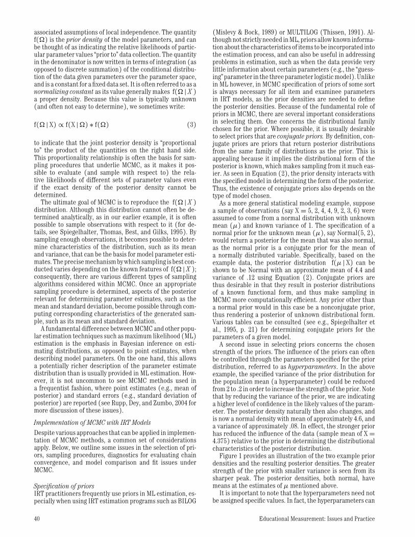
(Mislevy & Bock, 1989) or MULTILOG (Thissen, 1991). Al-though not strictly needed in ML, priors allow known informa-tion about the characteristics of items to be incorporated intothe estimation process, and can also be useful in addressingproblems in estimation, such as when the data provide verylittle information about certain parameters (e.g., the “guess-ing” parameter in the three parameter logistic model). Unlikein ML however, in MCMC specification of priors of some sortis always necessary for all item and examinee parametersin IRT models, as the prior densities are needed to definethe posterior densities. Because of the fundamental role ofpriors in MCMC, there are several important considerationsin selecting them. One concerns the distributional familychosen for the prior. Where possible, it is usually desirableto select priors that are conjugate priors. By definition, con-jugate priors are priors that return posterior distributionsfrom the same family of distributions as the prior. This isappealing because it implies the distributional form of theposterior is known, which makes sampling from it much eas-ier. As seen in Equation (2), the prior density interacts withthe specified model in determining the form of the posterior.Thus, the existence of conjugate priors also depends on thetype of model chosen.

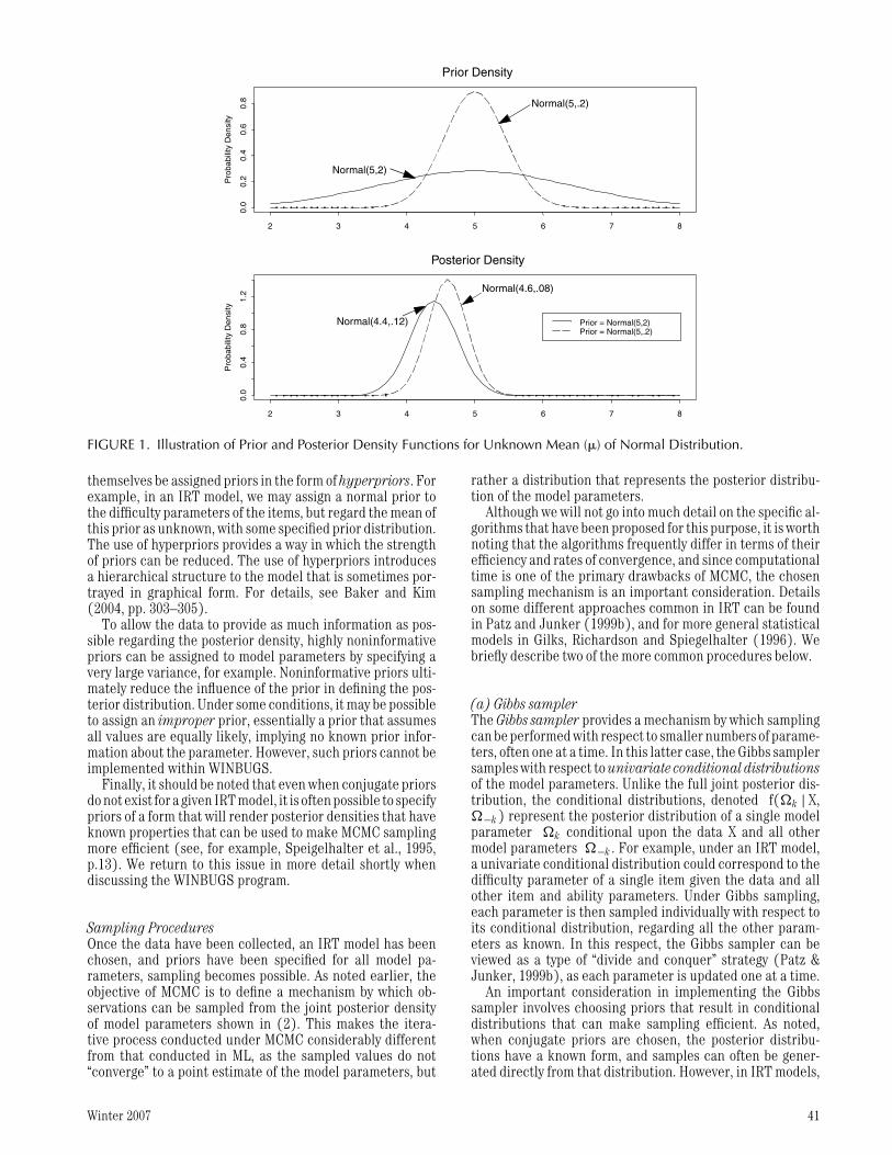
As a more general statistical modeling example, supposea sample of observations (say X = 5, 2, 4, 4, 9, 2, 3, 6) wereassumed to come from a normal distribution with unknownmean (µ) and known variance of 1. The specification of anormal prior for the unknown mean (µ), say Normal(5, 2),would return a posterior for the mean that was also normal,as the normal prior is a conjugate prior for the mean ofa normally distributed variable. Specifically, based on theexample data, the posterior distribution f(µ | X) can beshown to be Normal with an approximate mean of 4.4 andvariance of .12 using Equation (2). Conjugate priors arethus desirable in that they result in posterior distributionsof a known functional form, and thus make sampling inMCMC more computationally efficient. Any prior other thana normal prior would in this case be a nonconjugate prior,thus rendering a posterior of unknown distributional form.Various tables can be consulted (see e.g., Spiegelhalter etal., 1995, p. 21) for determining conjugate priors for theparameters of a given model.

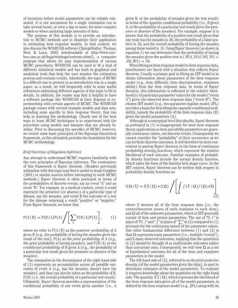
A second issue in selecting priors concerns the chosenstrength of the priors. The influence of the priors can oftenbe controlled through the parameters specified for the priordistribution, referred to as hyperparameters. In the aboveexample, the specified variance of the prior distribution forthe population mean (a hyperparameter) could be reducedfrom 2 to .2 in order to increase the strength of the prior. Notethat by reducing the variance of the prior, we are indicatinga higher level of confidence in the likely values of the param-eter. The posterior density naturally then also changes, andis now a normal density with mean of approximately 4.6, anda variance of approximately .08. In effect, the stronger priorhas reduced the influence of the data (sample mean of X =4.375) relative to the prior in determining the distributionalcharacteristics of the posterior distribution.

Figure 1 provides an illustration of the two example priordensities and the resulting posterior densities. The greaterstrength of the prior with smaller variance is seen from itssharper peak. The posterior densities, both normal, havemeans at the estimates of µ mentioned above.

It is important to note that the hyperparameters need notbe assigned specific values. In fact, the hyperparameters can


Pro

babi

lity

Den

sity

2 3 4 5 6 7 8

0.0

0.2

0.4

0.6

0.8

Prior Density

Pro

babi

lity

Den

sity

2 3 4 5 6 7 8

0.0

0.4

0.8

1.2

Prior = Normal(5,2)Prior = Normal(5,.2)

Posterior Density

Normal(5,2)

Normal(5,.2)

Normal(4.4,.12)

Normal(4.6,.08)

FIGURE 1. Illustration of Prior and Posterior Density Functions for Unknown Mean (�) of Normal Distribution.

themselves be assigned priors in the form of hyperpriors. Forexample, in an IRT model, we may assign a normal prior tothe difficulty parameters of the items, but regard the mean ofthis prior as unknown, with some specified prior distribution.The use of hyperpriors provides a way in which the strengthof priors can be reduced. The use of hyperpriors introducesa hierarchical structure to the model that is sometimes por-trayed in graphical form. For details, see Baker and Kim(2004, pp. 303–305).

To allow the data to provide as much information as pos-sible regarding the posterior density, highly noninformativepriors can be assigned to model parameters by specifying avery large variance, for example. Noninformative priors ulti-mately reduce the influence of the prior in defining the pos-terior distribution. Under some conditions, it may be possibleto assign an improper prior, essentially a prior that assumesall values are equally likely, implying no known prior infor-mation about the parameter. However, such priors cannot beimplemented within WINBUGS.

Finally, it should be noted that even when conjugate priorsdo not exist for a given IRT model, it is often possible to specifypriors of a form that will render posterior densities that haveknown properties that can be used to make MCMC samplingmore efficient (see, for example, Speigelhalter et al., 1995,p.13). We return to this issue in more detail shortly whendiscussing the WINBUGS program.

Sampling ProceduresOnce the data have been collected, an IRT model has beenchosen, and priors have been specified for all model pa-rameters, sampling becomes possible. As noted earlier, theobjective of MCMC is to define a mechanism by which ob-servations can be sampled from the joint posterior densityof model parameters shown in (2). This makes the itera-tive process conducted under MCMC considerably differentfrom that conducted in ML, as the sampled values do not“converge” to a point estimate of the model parameters, but

rather a distribution that represents the posterior distribu-tion of the model parameters.

Although we will not go into much detail on the specific al-gorithms that have been proposed for this purpose, it is worthnoting that the algorithms frequently differ in terms of theirefficiency and rates of convergence, and since computationaltime is one of the primary drawbacks of MCMC, the chosensampling mechanism is an important consideration. Detailson some different approaches common in IRT can be foundin Patz and Junker (1999b), and for more general statisticalmodels in Gilks, Richardson and Spiegelhalter (1996). Webriefly describe two of the more common procedures below.

(a) Gibbs samplerThe Gibbs sampler provides a mechanism by which samplingcan be performed with respect to smaller numbers of parame-ters, often one at a time. In this latter case, the Gibbs samplersamples with respect to univariate conditional distributionsof the model parameters. Unlike the full joint posterior dis-tribution, the conditional distributions, denoted f(�k | X,�−k) represent the posterior distribution of a single modelparameter �k conditional upon the data X and all othermodel parameters �−k . For example, under an IRT model,a univariate conditional distribution could correspond to thedifficulty parameter of a single item given the data and allother item and ability parameters. Under Gibbs sampling,each parameter is then sampled individually with respect toits conditional distribution, regarding all the other param-eters as known. In this respect, the Gibbs sampler can beviewed as a type of “divide and conquer” strategy (Patz &Junker, 1999b), as each parameter is updated one at a time.

An important consideration in implementing the Gibbssampler involves choosing priors that result in conditionaldistributions that can make sampling efficient. As noted,when conjugate priors are chosen, the posterior distribu-tions have a known form, and samples can often be gener-ated directly from that distribution. However, in IRT models,

Winter 2007 41

direct Gibbs sampling has only been implemented for normalogive IRT models, and even then requires use of a processreferred to as data augmentation. Details are provided inAlbert (1992), Baker (1998), and Bradlow et al. (1999).

Due to its use of known conditional distributions for sam-pling, implementation of Gibbs sampling is often straightfor-ward as standard statistical software can be used to generatethe samples. Details on the generation of these samples areprovided shortly.

(b) Metropolis HastingsAlternative procedures to Gibbs sampling are needed whenthe conditional distributions are not of a known distribu-tional form. This is generally the case when logistic IRT mod-els (e.g., two-parameter or three-parameter logistic models)are estimated. Patz and Junker (1999b) discuss the use ofMetropolis Hastings sampling in such contexts. The Metropo-lis Hastings method makes use of the proportionality rela-tionship established in Equation (3). In effect, the samplesare indirectly taken from the joint posterior by generatingcandidate observations from proposal distributions. For ex-ample, the proposal distribution might be a normal distribu-tion, with mean determined by current state of the parameterin the chain, and a specified variance. These candidate ob-servations are then chosen as a new state for the chain inproportion to their relative likelihood (based on Equation3) compared against the current state of sampled parametervalues in the Markov chain. If the candidate state is rejected,the previous state is retained as the new state. Key issues inimplementing a Metropolis Hastings strategy revolve aroundconstruction of the proposal distributions, as the frequencywith which the candidate observations are retained affectsthe efficiency of the algorithm (see Patz and Junker, 1999bfor further discussion of this issue). For example, the valueof the constant variance chosen in the above example willlikely have a substantial influence on how frequently the pro-posal distributions return values that are accepted as newstates for the chain.

Monitoring the Markov chainOnce a sampling mechanism has been determined, observa-tions are randomly and repeatedly sampled in an iterativefashion producing a series of observations that representstates in a Markov chain. To begin the sampling process, itis necessary to specify an initial set of values for the modelparameters. These values can be randomly generated, or insome other way be systematically defined, such as educatedguesses as to point estimates of the model parameters. Re-gardless of the method used, we refer to this first state as thestarting state of the chain. However, the sequence of valuesproduced in this chain will not be independent; new stateswill likely be affected by previous states, as the conditionaldistributions of parameters are defined at least in part bythe values of the previous state. This is particularly true un-der Metropolis Hastings which, as noted, has the potentialto retain the previous state as its current state. As a result,there will typically be a positive correlation between param-eter values sampled at successive states in the chain. Thisnot only makes it inappropriate to view a small number ofstates as a random sample from the posterior, but also makesthe initial sampled states of questionable value, as they willlikely be influenced by the starting state. It is therefore com-

mon to dismiss a number of the initial states (referred toas “burn-in” states) and to estimate the posterior only fromobservations sampled after the burn-in period. For example,with IRT models, it has been common to dismiss the first 500or so states as burn-in iterations.

Another critical issue in monitoring the simulated states ofthe Markov chain involves evaluating chain convergence. Thesequence of states for the Markov chain should theoreticallyconverge to a stationary distribution such that the sampledobservations can be viewed as a sample from the posteriordistribution of the model parameters. The rate at which thisconvergence occurs can vary depending on several factors.First, high correlations between adjacent states imply a slowrate of convergence, thus requiring a very large numberof iterations before the sampled states can be viewed as asample from the posterior. Second, the sampling algorithmused can also affect the rate of convergence. For example,under Metropolis Hastings, if the candidate states generatedfrom proposal distributions are rarely selected, longer chainswill be needed. Other causes of nonconvergence may relateto identification problems with the model.

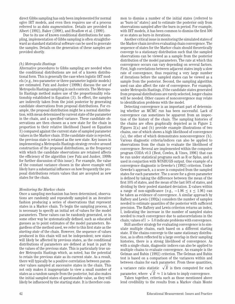
Detecting convergence is an important part of determin-ing whether an MCMC run has been successful. Lack ofconvergence can sometimes be apparent from an inspec-tion of the history of the chain. The sampling histories ofthe chains are often graphically depicted as in Figure 2.Figures 2(a) and (b) provide example illustrations of twochains, one of which shows a high likelihood of convergence(a), the other of which demonstrates nonconvergence (b).Various diagnostic criteria/indices can also be applied toobservations from the chain to evaluate the likelihood ofconvergence. Several are implemented within the computerprogram CODA v0.3 (Best, Cowles, & Vines, 1996) that canbe run under statistical programs such as R or Splus, and isused in conjuction with WINBUGS output. One example of aconvergence diagnostic is Geweke’s (1992) criterion. UnderGeweke’s approach, a z score is computed from the sampledstates for each parameter. The z-score for a given parameteris defined by taking the difference between the mean of thefirst 10% of states, and the mean of the last 50% of states, anddividing by their pooled standard deviation. Z-values withina range of non-significance (e.g., −1.96 ≤ z ≤ 1.96) canbe taken as evidence of convergence. A similar approach byRaftery and Lewis (1992a) considers the number of samplesneeded to estimate quantiles of the posterior with sufficientprecision. The Raftery and Lewis criterion returns an index,I, indicating the increase in the number of sampled statesneeded to reach convergence due to autocorrelations in thechain; values of I > 5.0 indicate problems with convergence.

Still another strategy for evaluating convergence is to sim-ulate multiple chains, each based on a different startingstate. If the chains converge to the same stationary distribu-tion, as is often reflected by a large overlap in their samplinghistories, there is a strong likelihood of convergence. Aswith a single chain, diagnostic indices can also be applied tomultiple chains to evaluate convergence. An example is theGelman and Rubin (1992) criterion. The Gelman and Rubintest is based on a comparison of the variances within andbetween chains for each parameter. From these quantities,a variance ratio statistic

√R is then computed for each

parameter, where√

R ≈ 1 is taken to imply convergence.Taken together, criteria such as those mentioned above

lend credibility to the results from a Markov chain Monte


(a)a

iteration

1 250 500 750 1000

0.3

0.4

0.5

0.6

0.7

(b)a

iteration

1 250 500 750 1000

0.0

0.25

0.5

0.75

1.0

FIGURE 2. Examples of Sampling Histories Associated with Markov Chains Displaying Evidence of Convergence (a) andNonconvergence (b).

Carlo analysis as a basis for approximating the joint posterior.Various other criteria also exist for evaluating convergence,as described in Best, Cowles and Vines (1996). It is importantto note, however, that even satisfaction of the above criteriashould not be taken as a guarantee of convergence. Foradditional information on the issue of convergence underMCMC within psychometric models, see Sinharay (2004).

Constructing posterior distributionsOnce sufficient evidence of convergence has been obtained,the simulated chain can be used to construct the marginalposterior distributions that are the basis for model parameterestimates. Several additional issues are considered in thisprocess. The first concerns the number of burn-in states todismiss. Raftery and Lewis (1992b) recommend basing thisdecision in part on the estimated autocorrelations (i.e., thecorrelations between adjacent states) in the chain, whichcan be estimated using CODA. The length of the burn-inshould naturally be at least as large as the distance betweensamples needed to achieve an autocorrelation of 0. However,because the actual burn-in usually involves a relatively smallnumber of iterations (<1% of the total), the effect of someinaccuracy is generally of minimal significance.

A second consideration involves the possibility of thinningthe chain. For example, rather than including all states of thechain, it is possible to choose only every fifth or tenth state, forexample, if substantial autocorrelations are present. Whenthinning is not used, CODA also has procedures that canappropriately adjust the standard errors of the parameterestimates to account for the autocorrelations.

Finally, in determining how many sampled states of thechain are necessary, it is important to recognize the influ-ence of Monte Carlo standard errors on the results (Patzand Junker, 1999b). Because the posterior distributions areconstructed from samples, they are imprecise due to sam-pling error. Consequently, when computing moments of theposterior distributions, such as their means, error in the es-timates can be attributed not only to the standard error of

the point estimate (as reflected by the standard deviationof the posterior), but also to sampling error, referred to asMonte Carlo error. As a rule of thumb, the simulation shouldbe run until the Monte Carlo error for each parameter ofinterest is less than about 5% of the sample standard devia-tion (Spiegelhalter et al., 2003). The Monte Carlo error canalways be reduced by lengthening the chain. More on the dis-tinction between these two forms of error will be describedin the real data example.

Evaluating model fitBecause of the emphasis in Bayesian inference on poste-rior distributions as opposed to point estimates of modelparameters, MCMC methods are also generally associatedwith different procedures for evaluating model fit than whenusing ML methods. One general strategy involves the use ofposterior predictive checks. Sinharay (2005) and Sinharay,Johnson, and Stern (2006) provide good illustrations of waysin which posterior predictive checks can be used with itemresponse models. A posterior predictive distribution refersto the distribution for a replicate set of observations (e.g., anew item response data set) conditional on the distributionof model parameters given the observed data. Such replicateobservations can be easily generated within WINBUGS evenin the process of estimating the model parameters. Fromthese generated replicate observations, a discrepancy statis-tic is chosen that can be evaluated both for the observed itemresponse data as well as each of the replicate data sets. Thediscrepancy statistic for the actual data is compared againstthe distribution of discrepancy statistics across the replicatedata sets to evaluate model fit. For example, if the discrep-ancy statistic for the real data exceeds (in magnitude) alarge percentage of the discrepancy statistics observed forthe replicated datasets (say 95%), the model is said not tofit (at α = .05). Different types of deviance statistics can bechosen depending on the aspect of model misfit of greatestconcern. For example, if local dependence among item pairsis of concern, a deviance statistic such as an item-pair odds

Winter 2007 43

ratio can be used to identify item pairs that fail to satisfy thiscondition. Other deviance statistics might attend to featuresof the test score distribution, or item proportion correctionstatistics. We consider an application of posterior predictivechecks using odds ratios in a real data example introducedshortly.

Model comparisonBeyond studies of absolute model fit, other approaches canbe used for model comparison. Unlike statistical tests ofmodel fit, these criteria identify which of one or more modelsprovides a better fit to the data, without evaluating the de-gree of fit in an absolute sense. We consider two possibilities,the Pseudo-Bayes Factor criterion, and the Deviance Infor-mation Criterion (DIC). To introduce the former index, itis first necessary to define the Bayes factor, a fundamen-tal concept for model comparison under Bayesian inference(see Raftery, 1996). A Bayes Factor (BF) is an index forcomparing models that is defined as the ratio of the marginallikelihoods of the data under each model. In other words,

BF = Likelihood(Data|Model1)Likelihood(Data | Model2)

(4)

where the preferred model is the model returning the higherlikelihood. Based on (4), Model 1 is preferred when BF>1,and Model 2 is preferred when BF<1. The relative magnitudeof BF also can be used in evaluating the relative weight ofevidence in support of either model, with BF >12 implyingstrong evidence in favor of Model 1, and BF>150 implyingvery strong evidence in favor of Model 1 (Jeffreys, 1961), forexample.

In practice, it is common to approximate this compari-son using the conditional predictive ordinate (CPO), a so-called pseudo-Bayes factor comparison (Geisser & Eddy,1979; Gelfand, Dey & Chang, 1992). The CPO can be com-puted at the level of an individual item response as

CPO−1 = 1T

T∑1

1/f(x |�t ) (5)

where T is the total number of sampled states in a chain,and f(x | �t ) is the likelihood of the observed item response(x = 0 or 1) based on the sampled parameter values at statet.

In IRT modeling, a separate CPO index can be computedfor each item response. A summary of the index valuesacross item responses can be computed by taking the logof the product of the CPOs. The preferred model is theone returning the higher log product. In the WINBUGSprogram, computation of the CPO is straightforward, as itonly requires tracing the inverse probability of each ob-served item response over the MCMC sampled states, andthen tabulating the average of their logs when the chain isfinished.

A second index for model comparison is the DevianceInformation Criterion (DIC; Spiegelhalter, Best, Carlin &van der Linde, 2002). The DIC is an index similar to theAkaike Information Criterion (AIC; Akaike, 1973) and theBayesian Information Criterion (BIC; Schwartz, 1978) oftenused under ML in that it weighs both model fit and modelcomplexity in identifying the preferred model. The DIC is

based on the posterior distribution of the deviance (i.e.,−2 x log likelihood) and a term representing “the effectivenumber of parameters” that accounts for the expected de-crease in deviance attributable to the added parameters ofthe more complex model. Estimation of the DIC index canbe requested within the WINBUGS program. As with AIC andBIC, the smaller the value of DIC, the better the model. Foran illustration of model fit comparison involving IRT models,the reader is referred to Sahu (2002).

Practical Illustration: Fit of 2PL model to UniversityMath Placement Data using WINBUGS 1.4

To provide an example illustration of the above procedures,we consider an item response dataset from a 36-item math-ematics placement test. The test is administered each fallto entering freshmen in the University of Wisconsin systemto assist with course placement decisions. All items are fiveoption multiple choice items. In this illustration we considerthe application of a two-parameter logistic model (2PL),although other models, such as a three-parameter logistic(3PL), may also be appropriate.

Under the 2PL, the probability of a correct response forexaminee i to item j is modeled as

Prob(Xij = 1) = exp[aj(θi−bj)]

1 + exp[aj(θi−bj)], (6)

where Xij denotes the item response (0 = incorrect; 1 =correct), θ i is an examinee ability parameter, and item pa-rameters a j indicate the item discrimination and b j the itemdifficulty. A random sample of 1000 examinees was used forestimation of the model. Consistent with common IRT prac-tice, we focus here on the estimation of the item parameters,where the ability parameters are viewed as nuisance param-eters (Patz & Junker, 1999b). However, it is important tonote that ability parameters could also be estimated in asimilar fashion.

Specification of priorsTo estimate the 2PL using MCMC, priors must first be spec-ified for all item and person parameters. We assume θ i∼Normal (0,1) for all persons i, and aj ∼LogNormal(0,.5)and bj ∼Normal (0,2) for all items j. These are similar topriors commonly used in BILOG. Less or more informativepriors and/or priors of different distributional forms couldnaturally also have been chosen. Each item response is as-sumed to be a Bernoulli outcome with probability of correctresponse determined by the 2PL model and correspondingperson and item parameters.

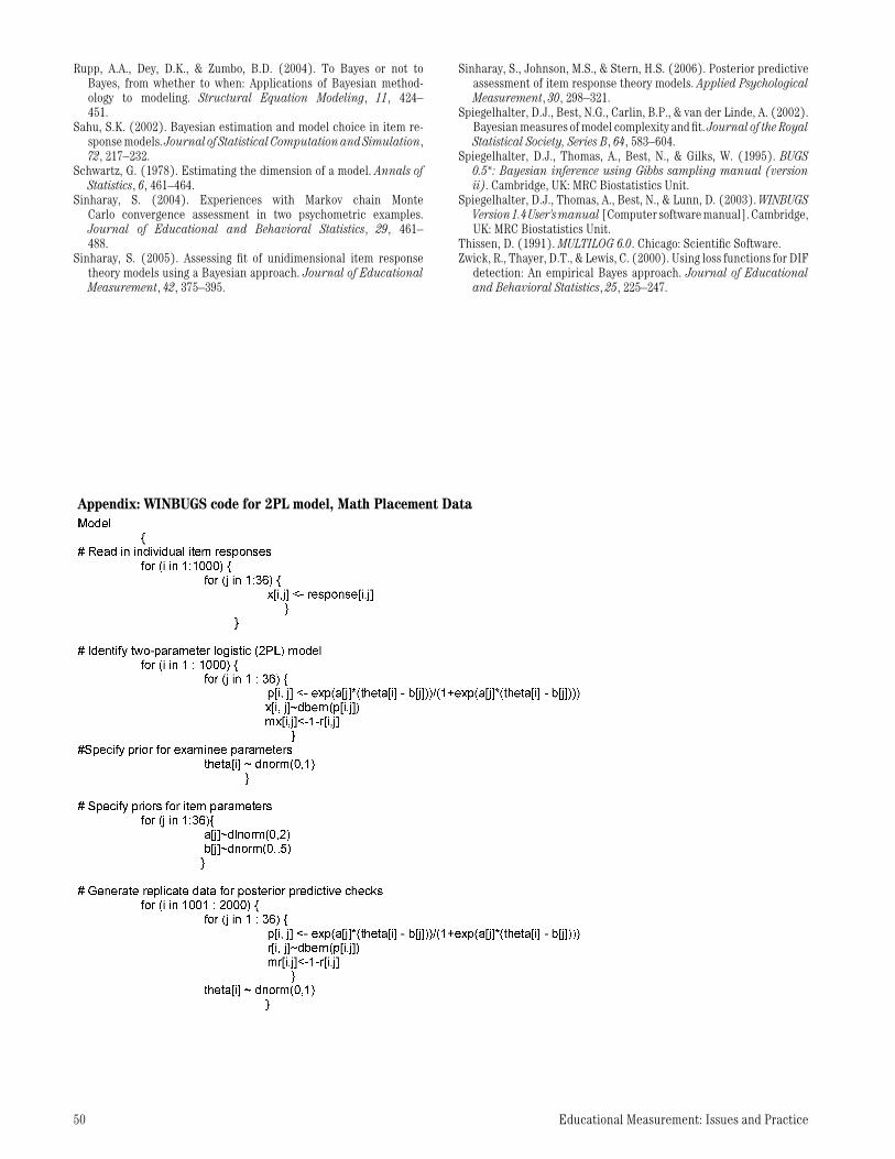
Sampling procedureAs noted, the program WINBUGS has the potential to im-plement several different sampling algorithms depending onwhich method is most efficient for a given application. Theappendix displays WINBUGS code for the current analysis.The model and priors selected are not conjugate priors andthus do not lead to conditional distributions that would per-mit direct Gibbs sampling. In addition, the characteristicsof the conditional distributions vary depending on the typeof parameter. Consequently, different forms of sampling willbe implemented for different parameter types. As normalpriors were assumed for both the ability (θ) and difficulty(b) parameters, each of these parameter types results in a


conditional distribution that is log concave, allowing WIN-BUGS 1.4 program to implement an adaptive rejection sam-pling (ARS) algorithm. (For details on this procedure, seeGilks & Wild, 1992). However, the conditional distributionsfor the item discrimination parameters (a) do not possessthis property. Nevertheless, a more efficient algorithm thanMetropolis Hastings is also available due to the restrictedrange of values for these parameters (due to the log-normalprior, they must always be positive). WINBUGS implements aslice sampling algorithm in which observations are sampleduniformly from the domain of its conditional probability den-sity. Details of this procedure are provided by Neal (2003). Itshould be noted that the selection of each of these algorithmsoccurs through a process internal to WINBUGS, and so neednot be specified by the user.

Despite the use of different methods of sampling for dif-ferent parameters in the model, both approaches seek toproduce chains that provide observations that reproduce the

a[1]

iteration

1 5000 10000

0.0

0.2

0.4

0.60.8

1.0

a[2]

iteration

1 5000 10000

0.0

0.5

1.0

1.52.0

2.5

b[1]

iteration

1 5000 10000

-1.5

-1.0

-0.5

0.0

0.5

b[2]

iteration

1 5000 10000

0.5

1.0

1.5

2.0

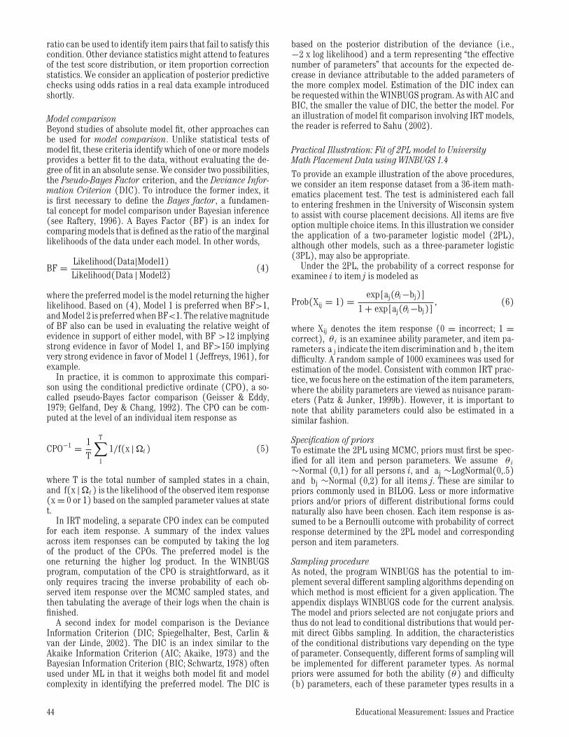
FIGURE 3. Chains for Discrimination and Difficulty Parameters, Items 1 and 2 of Math Placement Data.

joint posterior distribution of the model parameters. Conse-quently, the general process by which the chain is monitoredand estimates determined is not affected by these differentsampling appraoches.

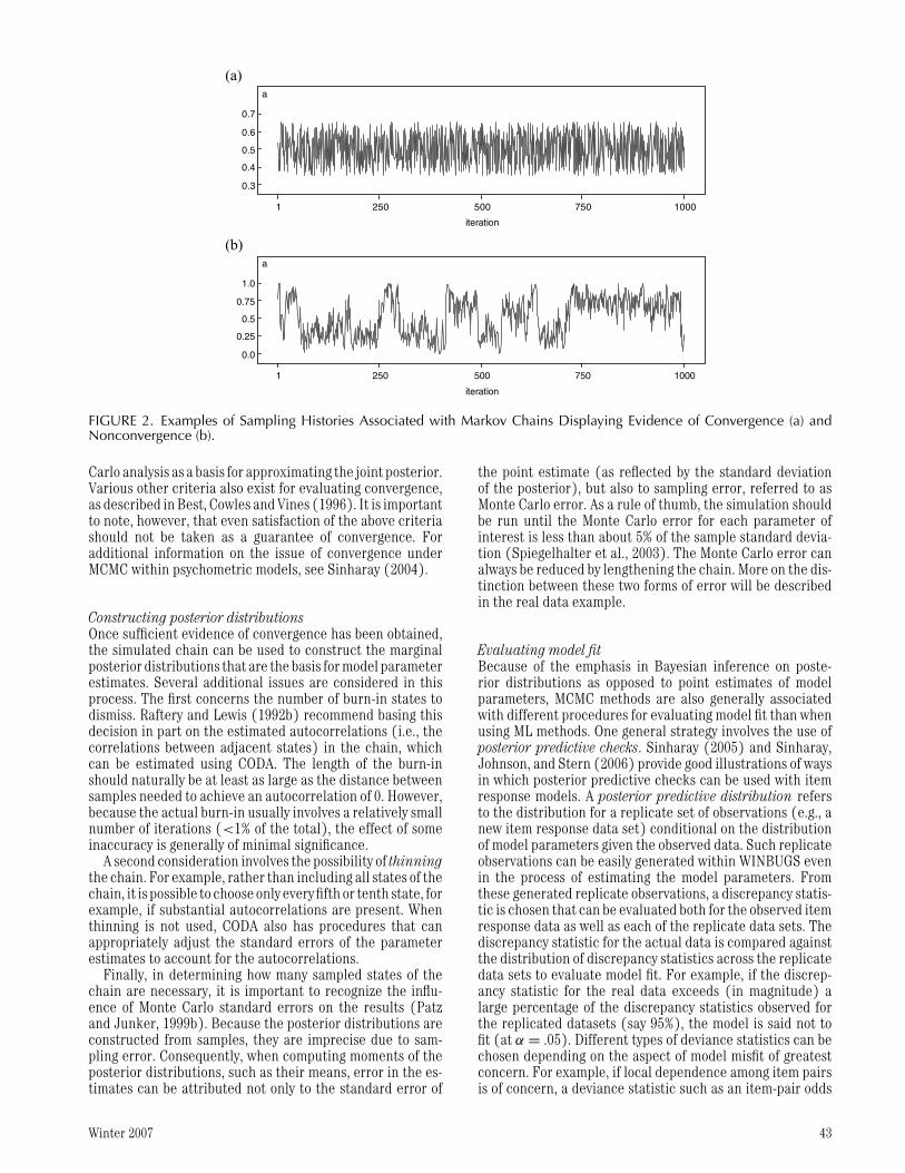
Monitoring the chainUsing a randomly generated starting state, A Markov chainfor the 2PL was run out to 10,000 states for five differentchains. Convergence was examined both through visual in-spection of the sampling histories of the chains as well ascomputation of convergence diagnostics. Figure 3 illustratesthe state histories for the discrimination and difficulty pa-rameters of items 1 and 2 from chain 1, both of which appearto display relatively quick convergence to a stationary dis-tribution (Similar results were observed for the other itemsand chains). Similarly, an overlay of the sampling histories ofparameters for the five chains (not shown here) further sup-ported convergence, as between-chain variability relative to

Winter 2007 45

within-chain variability appeared minimal. Each chain tookapproximately 3 hours to complete.

Further confirmation of convergence was obtained fromconvergence diagnostics. The Geweke (1992) criterion re-turned z-scores between ±2 for all but one of the discrim-ination parameters (item 20: −2.03), and for the difficultyparameters was always between ±2. Similarly, the Rafteryand Lewis (1992a) diagnostic returned I indices less than5 for all discrimination and difficulty parameters, with amaximum value of 3.16 for the difficulty parameters (Item22), and a maximum value of 3.34 for the discrimination pa-rameters (Item 10). Lastly, the Gelman and Rubin (1992)criterion returned point estimates of

√R = 1.0 for each of

the 72 difficulty and discrimination parameters, suggestinghigh similarity across chains. Overall, it therefore appearsthere is good evidence for the convergence of the chain.

Inspecting posterior distributionsBased on the Raftery and Lewis diagnostics and autocorre-lation estimates, a conservative burn-in of 500 was used forall parameters. The Raftery and Lewis (1992b) diagnosticreturned a maximum burn-in recommendation of 21 (for thea parameter of item 10), while the largest autocorrelationfor samples 10 states apart was.16 (for the b parameter ofitem 36) and essentially 0 for all samples 50 states apart. Dueto the overall length of the chain, the use of 500 as burn-in,although conservative, comes at little cost.

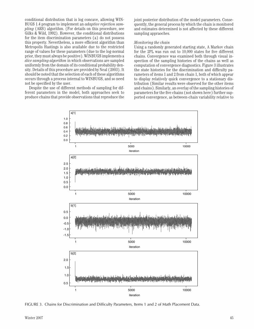
Figure 4 illustrates the resulting marginal posterior distri-butions from the 10,000 iterations of chain 1 for the difficultyand discrimination parameters of items 1 and 2. The uni-modal, symmetric shape of the posteriors suggests that theposterior mean likely provides a good point estimate of themodel parameters. The standard deviations of the marginalposterior distributions provide standard errors for these esti-mates. Table 2 shows the final estimates of model parametersfor the 36 items, as well as the corresponding ML estimatescomputed using the program BILOG and the same priors.The MCMC columns also provide an estimate of the MonteCarlo error based on the number of iterations of each chain.As can be seen from Table 1, the MCMC and MML estimatesare virtually identical across items. For a detailed review ofstudies comparing ML versus MCMC-based point estimationof IRT model parameters, see Rupp, Dey and Zumbo (2004).

Model fit and comparisonTo examine issues related to model comparison and fit, aposterior predictive check was applied using an odds ratio(OR) discrepancy statistic. As noted earlier, such a statisticpermits inspection of local independence at the item pairlevel. For a given pair of items, the index is defined as

OR = n11n00

n10n01, (7)

where the “n”s denote the number of examinees obtaining agiven sequence of scores for a given item pair, and the sub-scripts identify the pattern (e.g., n10 indicates the numberof examinees answering the first item in the pair correctlyand the second item incorrectly). As this test statistic isdefined for any item pair, there exist a total of 36×35/2 =630 different OR statistics that can be studied using thisposterior predictive check. In the current analysis, 24 of

a[1] sample: 10000

0.0 0.2 0.4 0.6

0.0

2.0

4.0

6.0

a[2] sample: 10000

1.0 1.5 2.0

0.01.02.03.04.0

b[1] sample: 10000

-1.5 -1.0 -0.5 0.0

0.0

1.0

2.0

3.0

b[2] sample: 10000

0.4 0.6 0.8 1.0

0.0

2.0

4.0

6.0

FIGURE 4. Marginal Posterior Density for Item Discrimina-tion and Difficulty Parameters, Items 1 and 2, Math Place-ment Data

the statistics displayed a p-value less than .05, 15, of whichproduce values more positive than expected. For example,one such item pair was items 3 and 6, where the observedOR = 2.52, while a 95% confidence interval (CI) based onreplicate data had lower and upper bounds of 1.36 and 2.44,respectively. For items 16 and 20, the OR = 1.37, with 95%CI = 1.38, 2.50. So overall in terms of local independence, thefit of the 2PL seems to be reasonably good, with significantpairs generally falling just outside the region of nonsignifi-cance. As noted earlier, there are many other aspects of fitthat could be evaluated using different discrepancy statis-tics.

To evaluate the 2PL in comparison to the one-parameterlogistic model (1PL), the 1PL model was also fit to the samedata, essentially following the same process used above inestimating the 2PL. The 1PL models the probability of correctresponse as

Prob(Xij = 1) = exp[a(θi−bj)]1 + exp[a(θi−bj)]

, (8)

with the primary difference from the 2PL being the applica-tion of a common discrimination parameter across all items.In estimating the model, the same priors as for the 2PL wereimposed for the difficulty parameters and the one discrimi-nation parameter.

As in the 2PL, an “a” parameter was estimated, but wasassumed equal across all items.


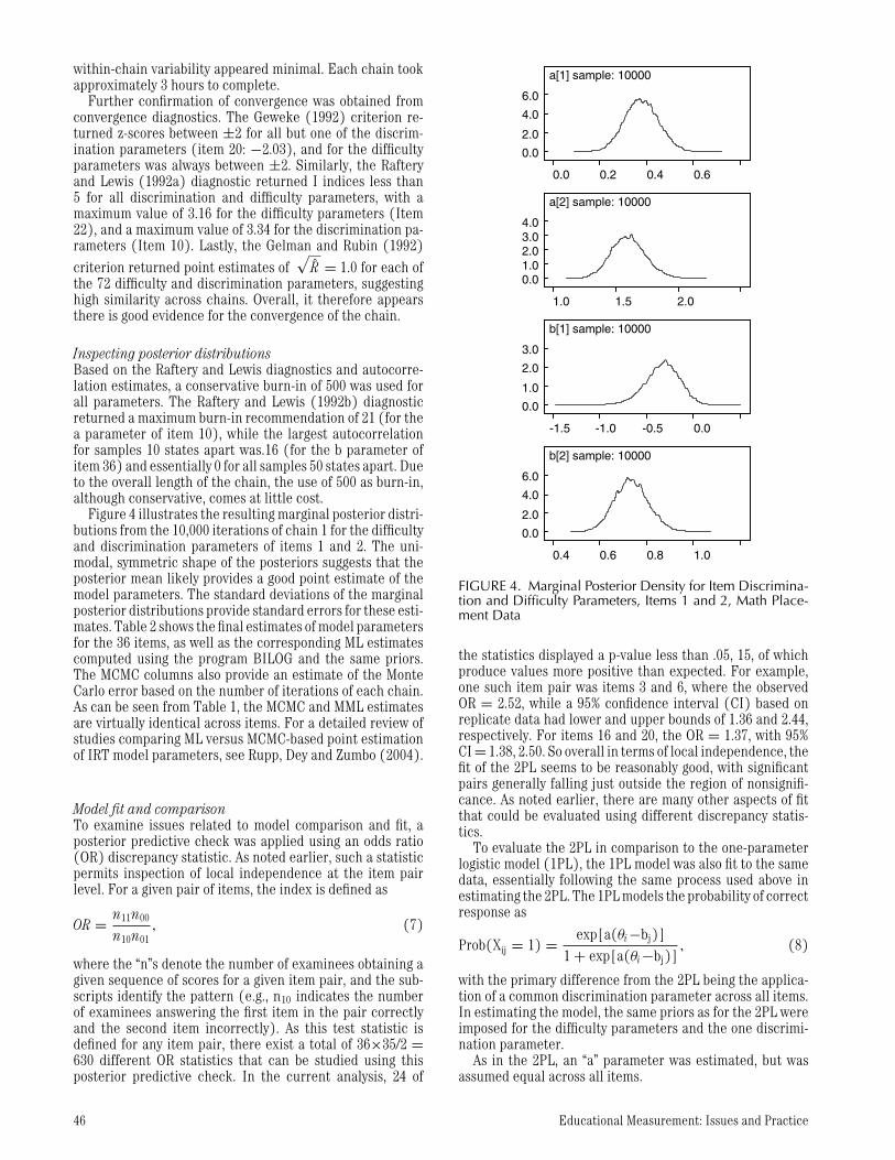
Table 1. Markov Chain Monte Carlo (MCMC) and Marginal Maximum Likelihood(MML) 2PL Model Parameter Estimates, Math Placement Data

MCMC Estimates MML Estimates

Item a se mcse b se mcse a se b se

1 .38 .07 .001 -.34 .19 .002 .41 .06 -.30 .162 1.60 .14 .002 .74 .07 .001 1.57 .13 .75 .073 .88 .10 .002 -.62 .10 .002 .87 .09 -.61 .094 .54 .08 .001 .24 .13 .002 .56 .07 .23 .125 .40 .07 .001 1.16 .27 .006 .42 .07 1.09 .236 .92 .09 .001 .19 .08 .001 .92 .09 .20 .087 .99 .10 .002 .18 .08 .001 .98 .09 .19 .078 .70 .09 .001 -.31 .11 .001 .71 .08 -.29 .109 1.34 .12 .002 -.27 .06 .001 1.32 .12 -.26 .06

10 .52 .08 .002 2.11 .32 .009 .52 .08 2.10 .3111 .89 .10 .003 1.94 .20 .005 .87 .10 1.97 .2012 .72 .09 .002 1.05 .15 .003 .72 .08 1.06 .1413 .73 .09 .001 -.71 .12 .002 .74 .09 -.69 .1114 .94 .09 .001 .64 .10 .002 .93 .09 .65 .0915 .97 .10 .001 .30 .08 .001 .97 .09 .31 .0816 .66 .08 .001 .60 .13 .002 .67 .08 .59 .1217 .46 .07 .001 -.34 .16 .002 .49 .07 -.31 .1418 .81 .10 .003 2.07 .24 .007 .80 .09 2.07 .2219 .60 .08 .001 .60 .14 .003 .61 .08 .59 .1320 1.38 .12 .002 .38 .07 .001 1.36 .11 .40 .0621 .53 .08 .002 1.68 .26 .007 .54 .07 1.65 .2422 .59 .08 .002 1.54 .24 .006 .60 .08 1.52 .2123 .90 .10 .002 -.99 .12 .002 .89 .10 -.98 .1124 .51 .07 .001 .82 .18 .003 .53 .07 .80 .1625 .69 .08 .002 1.10 .16 .003 .69 .08 1.10 .1426 .82 .09 .001 .52 .10 .002 .82 .08 .53 .1027 .96 .10 .002 .86 .11 .002 .95 .09 .87 .1028 1.11 .10 .001 .29 .08 .001 1.10 .10 .30 .0729 1.00 .10 .002 -.82 .10 .002 1.00 .10 -.81 .0930 .73 .09 .001 .60 .12 .002 .74 .08 .60 .1131 .95 .10 .002 1.17 .13 .002 .94 .09 1.18 .1232 .86 .10 .002 1.66 .18 .004 .85 .09 1.68 .1833 .75 .09 .001 -.42 .10 .002 .76 .08 −.40 .1034 1.33 .12 .002 .16 .07 .001 1.31 .12 .17 .0635 .70 .08 .001 .53 .12 .002 .71 .08 .53 .1136 1.06 .10 .002 1.24 .12 .003 1.04 .10 1.25 .12

a = item discrimination estimate.b = item difficulty estimate.se = standard error.mcse = Markov chain standard error.

Both the DIC and Pseudo-Bayes factor criteria were eval-uated for the 2PL and 1PL. In both cases, the 2PL is shown tobe preferred to the 1PL. For the DIC index, the 2PL returnedDIC = 42,578 (the effective number of parameters, pD =901) while the 1PL returned DIC = 42,921 (pD = 847). Interms of the Pseudo-Bayes factor criterion, the 1PL returneda log(CPO) = −21,463 across item responses, while the 2PLreturned a log(CPO) = −21,294. Consequently, the criteriaagree in the selection of the 2PL over the 1PL model for thesedata.

Concluding Comments

Models such as the 2PL can usually be easily fit using MCMCmethods. As noted in the introduction, however, the MCMC

methodology perhaps finds its greatest appeal in its abilityto accommodate more complex IRT models for which ML-based IRT estimation software (like BILOG) is unavailable.Such applications often present new challenges, however; wemention a couple of common problems from our experience.One is the occurrence of sampling “traps.” A trap occurswhen a state in the chain is encountered from which thepossible domain from which a new state can be sampled isso restricted that no eligible sample is produced, even aftera large number of attempts. The occurrence of a trap causesWINBUGS to terminate, and often requires restarting thechain from a new starting state. Other challenges are relatedto the frequent need for stricter identifiability constraintsthan are applied when using other estimation procedures.For example, use of MCMC with multidimensional and/or

Winter 2007 47

mixture IRT models can lead to dimension/class “identityswitching” over the course of a simulated chain. Identityswitching refers to the situation where one dimension orclass comes to represent another, making the estimation ofdimension-specific parameters problematic. For example, ina two-dimensional item response model, it can happen that atsome point in the chain, what was originally ability dimension1 assumes the role of ability dimension 2, thus creating aninconsistency in how the item discrimination values shouldbe interpreted over the course of the chain.

For these and other reasons, practitioners new to theMCMC methodology may find it useful to experiment withsimple models in the context of MCMC before attemptingmore complex ones. A “model-building” strategy that beginswith a simplified version of the IRT model of interest may,where possible, provide a better starting point for implement-ing MCMC procedures to ensure identifiability of individualparameters. Readers are encouraged also to examine a vari-ety of different MCMC applications, including those outsideof IRT, for a better understanding of the methodology, as wellas potential challenges in implementing MCMC. For exam-ple, the uses of MCMC methods for de-convolving mixtures(Robert, 1997) or in fitting hierarchical models (Clayton,1997) have been frequently studied, and in ways that wouldlikely be informative for IRT models generalized to accom-modate similar types of structure.

Finally, we note that while this paper has focused on theWINBUGS software for estimating MCMC models, a variety ofdifferent packages can also be used. Essentially any statisti-cal software that can be used to simulate data from specifieddistributions can be used. Patz and Junker (1999b) providecode for implementing MCMC procedures with IRT modelsusing the program S-plus. Such applications often help con-siderably in reducing the computational time in conductingMCMC, but demand a little more in terms of programmingon the part of the user.

Self-test1. Suppose that a drug screening test used to disqualify

riders in a long-distance bicycle race is 95% accurate indetecting users of the illegal drug, and is 99% accurate indetecting nonusers of the drug. Suppose it is furtherknown that 3% of the cyclists use the drug. FollowingBayes’ theorem, identify

(a) the prior distribution for use of the drug(b) the posterior probability that a cyclist is actually

a user if the test is positive(c) the posterior probability that a cyclist is not a

user if the test is negative

2. Which of the potential priors for the difficultyparameters in an IRT model: N(−1, 1), N(−1, 20) orN(−1,.2) would likely have the greatest influenceon the final item difficulty estimates?

3. True/False questions

(a) In MCMC estimation, the Markov chain for agiven parameter should eventually converge toa single point value.

(b) A primary advantage of MCMC methods with IRTmodels is that they are easier to implement than

ML methods, although generally take a long timeto run.

(c) The distributional form selected for the prior(s)matters little in determining an appropriateMCMC sampling algorithm.

(d) If an MCMC algorithm fails to converge for agiven model and data set, there must be some-thing wrong with how the sampling procedurewas programmed.

(e) A fundamental difference between Bayesianapproaches (like MCMC) and frequentist ap-proaches (like ML) to model estimation is theemphasis in Bayesian estimation on estimatingposterior distributions rather than point esti-mates of model parameters.

(f) It is possible to study different aspects of IRTmodel fit through the use of different dis-crepancy statistics using posterior predictivechecks.

(g) If after a single MCMC runs a second MCMC chainwere run using a different starting value andproduced a different sampling history than theoriginal chain, the original chain has not con-verged.

4. In evaluating the fit of the 2PL model to his item responsedata set, test practitioner Phil approximates the Bayesfactor for the 2PL versus 1PL to be 1340. Is Phil correct inassuming that the 2PL therefore provides a close fit tohis item response data?

5. Suppose that after 1,000 iterations an MCMC run hasconverged. If the number of MCMC iterations were thenincreased by 100 times to 100,000, which should de-crease, the Monte Carlo standard error (MCSE) or thepoint estimate standard error (SE)? By how much is itexpected to decrease?

6. Suppose test practitioner Janet estimates a model usingMCMC and ML, and finds noticeable differences in thefinal point estimates of the model despite having usedthe same priors in both estimation runs. She rechecks theMCMC algorithm, and is confident of convergence. Whatmight explain the difference in the results?

Answers to Self-Test1. (a) Because the distribution is only defined over a do-

main of two events, the prior can be expressed asP(user) =.03; P(nonuser) = .97.

(b) Using Bayes’ theorem, P(user | test = positive) =. P(test = positive | user) P(user)/[P(test = positive

| user) P(user)+ P(test = positive | nonuser) -P(nonuser)] = .95 ×.03 / (.95×.03 +.01×.97) =

.75(c) Using Bayes theorem, P(nonuser | test = neg-

ative) = P(test = negative | nonuser)P(nonuser)/[P(test=negative | user) P(user)+P(test = negative | nonuser)−P(nonuser)] =.99 ×.97 / (.05×.03 +.99×.97) >.99

2. The N(−1,.2) prior would have the strongest effect, as ithas the smallest variance. It would generally also pro-duce parameter estimates with the smallest standarderrors.

3. (a) F, the chain should converge to a stationary dis-tribution of values, not a single value.


(b) T, many MCMC algorithms take only minutes toprogram, but when used in practice can takehours or more to run.

(c) F, the form of the prior defines characteristicsof the posterior that can often permit moreefficient MCMC sampling techniques.

(d) F, model misspecification and/or a lack of infor-mation in the data could also be responsible.

(e) T, in MCMC we estimate marginal posterior dis-tributions for the model parameters; in MLwe determine point estimates of the modelparameters.

(f) T, posterior predictive checks provide a very flex-ible set of techniques for investigating anyform of misfit that can be captured by a dis-crepancy statistic.

(g) F, the two chains should converge to a commondistribution, but their sampling histories willlikely be different.

4. No, the Bayes factor criterion, and approximations to it,provide a criterion for model comparison, not the eval-uation of model fit in an absolute sense. Phil would becorrect in claiming the 2PL provides a better relativefit than the 1PL, but that does not necessarily meanthat the 2PL model provides a close fit to the data.

5. The Monte Carlo standard error (MCSE) should de-crease, not the point estimate standard error (SE).Only the MCSE is systematically affected by thesize of the sample (i.e., the number of MCMC itera-tions). Because the MCSE reflects the standard errorof the sample mean, we can use the standarderror of the mean formula in approximating the ex-pected reduction in the MCSE: σ /

√1,000 =√

100 × σ/√

100,000, implying a 10 times smallerMCSE.

6. When point estimates are derived from an MCMC run,they are generally based on a characteristic of theposterior distributions of the model parameters,often the posterior mean. The posterior mean may not bethe value producing the maximum likelihood, especiallywhen the posterior distribution is asymmetric. So theestimates likely differ because they reflect differentcharacteristics of the posterior distributions.

References

Akaike, H. (1973). Information theory and an extension of the maxi-mum likelihood principle. In B.N. Petrov & F. Csaki (Eds.), Proceed-ings, 2nd International Symposium on Information Theory (pp.267–281). Budapest: Akademiai Kiado.

Albert, J.H. (1992). Bayesian estimation of normal ogive item responsecurves using Gibbs sampling. Journal of Educational Statistics, 17,251–269.

Baker, F.B. (1998). An investigation of the item parameter recoverycharacteristics of a Gibbs sampling approach. Applied PsychologicalMeasurement, 22, 153–169.

Baker, F.B., & Kim, S-H. (2004). Item response theory: Parameterestimation techniques (2nd ed.). New York: Marcel Dekker.

Beguin, A.A., & Glas, C.A.W. (2001). MCMC estimation and some model-fit analysis of multidimensional IRT models. Psychometrika, 66,541–562.

Best, N., Cowles, M.K., & Vines, K. (1996). CODA∗: Convergence di-agnosis and output analysis software for gibbs sampling output,version 0.30. Cambridge, UK: MRC Biostatistics Unit.

Bolt, D.M., & Lall, V.F. (2003). Estimation of compensatory andnoncompensatory multidimensional item response models usingMarkov chain Monte Carlo. Applied Psychological Measurement,29, 395–414.

Bradlow, E.T., Wainer, H., & Wang, X. (1999). A Bayesian randomeffects model for testlets. Psychometrika, 64, 153–168.

Clayton, D.G. (1997). Generalized linear mixed models. In W.R. Gilks,S. Richardson, & D.J. Spiegelhalter (Eds.), Markov chain MonteCarlo in practice (pp. 275–302). London: Chapman & Hall.

Congdon, P. (2001). Bayesian statistical modeling. Chichester, Eng-land: John Wiley & Sons.

De la Torre, J., Stark, S., & Chernyshenko, O. (2006). Markov ChainMonte Carlo estimation of item parameters for the generalizedgraded unfolding model. Applied Psychological Measurement, 30,216–232.

Fox, J.-P., & Glas, C.A.W. (2001). Bayesian estimation of multilevel IRTmodels using Gibbs sampling. Psychometrika, 66, 271–288.

Geisser, S., & Eddy, W. (1979). A predictive approach to model selec-tion. Journal of the American Statistical Association, 74, 153–160.

Gelfand, A.E., Dey, D.K., & Chang, H. (1992). Model determinationusing predictive distributions with implementation via samplingmethods. In J.M. Bernardo, J.O. Berger, A.P. Dawid, & A.F.M. Smith(Eds.), Bayesian statistics (Vol. 4, pp. 147–167). Oxford, UK: OxfordUniversity Press.

Gelman, A., & Rubin, D.B. (1992). Inference from iterative simulationusing multiple sequences (with discussion). Statistical Science, 7,457–511.

Geweke, J. (1992) Evaluating the accuracy of sampling-based ap-proaches to calculating posterior moments. In J.M. Bernardo, J.O.Berger, A.P. Dawid, & A.F.M. Smith (Eds.), Bayesian statistics (Vol.4, pp. 169–193). Oxford, UK: Oxford University Press.

Gilks, W.R., & Wild, P. (1992). Adaptive rejection sampling for Gibbssampling. Applied Statistics, 41, 337–348.

Gilks, W.R., Richardson, S., & Spiegelhalter, D.J. (1996). Markov chainMonte Carlo in practice. Boca Raton, FL: Chapman & Hall.

Glas, C. A. W., & Meijer, R. R. (2003). A Bayesian approach to personfit analysis in item response theory models. Applied PsychologicalMeasurement, 27, 217–233.

Jeffreys, H. (1961). Theory of probability. London: Oxford UniversityPress.

Johnson, M.S., & Sinharay, S. (2005). Calibration of polytomous itemfamilies using Bayesian hierarchical modeling. Applied Psychologi-cal Measurement, 29, 369–400.

McLeod, L., Lewis, C, & Thissen, D. (2003). A Bayesian method for thedetection of item preknowledge in computerized adaptive testing.Applied Psychological Measurement, 27, 121–137.

Mislevy, R.J., & Bock, R.D. (1989). BILOG 3: Item analysis and testscoring with binary logistic models. Mooresville, IN: Scientific Soft-ware.

Neal, R.M. (2003). Slice sampling. Annals of Statistics, 31, 705–767.Patz, R., & Junker, B. (1999a). Applications and extensions of MCMC in

IRT: Multiple item types, missing data, and rated responses. Journalof Educational and Behavioral Statistics, 24, 342–366.

Patz, R., & Junker, B. (1999b). A straightforward approach to Markovchain Monte Carlo methods for item response models. Journal ofEducational and Behavioral Statistics, 24, 146–178.

Raftery, A.E. (1996). Hypothesis testing and model selection. In W.R.Gilks, S. Richardson, & D.J. Spiegelhalter (Eds.), Markov chainMonte Carlo in practice (pp. 115–130). London: Chapman & Hall.

Raftery, A.E., & Lewis, S.M. (1992a). How many iterations in the Gibbssampler? In J.M. Bernardo, J.O. Berger, A.P. Dawid, & A.F.M. Smith(Eds.), Bayesian statistics (Vol. 4, pp. 765–776). Oxford, UK: OxfordUniversity Press.

Raftery, A.E., & Lewis, S.M. (1992b). One long run with diagnostics:implementation strategies for Markov chain Monte Carlo. StatisticalScience, 7, 493–497.

Robert, C.P. (1997). Mixtures of distributions: Inference and estima-tion. In W.R. Gilks, S. Richardson, & D.J. Spiegelhalter (Eds.),Markov chain Monte Carlo in practice (pp. 441–464). London:Chapman & Hall.

Winter 2007 49

Rupp, A.A., Dey, D.K., & Zumbo, B.D. (2004). To Bayes or not toBayes, from whether to when: Applications of Bayesian method-ology to modeling. Structural Equation Modeling, 11, 424–451.

Sahu, S.K. (2002). Bayesian estimation and model choice in item re-sponse models. Journal of Statistical Computation and Simulation,72, 217–232.

Schwartz, G. (1978). Estimating the dimension of a model. Annals ofStatistics, 6, 461–464.

Sinharay, S. (2004). Experiences with Markov chain MonteCarlo convergence assessment in two psychometric examples.Journal of Educational and Behavioral Statistics, 29, 461–488.

Sinharay, S. (2005). Assessing fit of unidimensional item responsetheory models using a Bayesian approach. Journal of EducationalMeasurement, 42, 375–395.

Sinharay, S., Johnson, M.S., & Stern, H.S. (2006). Posterior predictiveassessment of item response theory models. Applied PsychologicalMeasurement, 30, 298–321.

Spiegelhalter, D.J., Best, N.G., Carlin, B.P., & van der Linde, A. (2002).Bayesian measures of model complexity and fit. Journal of the RoyalStatistical Society, Series B, 64, 583–604.

Spiegelhalter, D.J., Thomas, A., Best, N., & Gilks, W. (1995). BUGS0.5∗: Bayesian inference using Gibbs sampling manual (versionii). Cambridge, UK: MRC Biostatistics Unit.

Spiegelhalter, D.J., Thomas, A., Best, N., & Lunn, D. (2003). WINBUGSVersion 1.4 User’s manual [Computer software manual]. Cambridge,UK: MRC Biostatistics Unit.

Thissen, D. (1991). MULTILOG 6.0. Chicago: Scientific Software.Zwick, R., Thayer, D.T., & Lewis, C. (2000). Using loss functions for DIF

detection: An empirical Bayes approach. Journal of Educationaland Behavioral Statistics, 25, 225–247.

Appendix: WINBUGS code for 2PL model, Math Placement Data


Winter 2007 51

Documents

Estimating Item Response Theory Models Using Markov Chain