Embed Size (px)
Citation preview

ORNL/TM-2002/225
Estimating Impacts of Diesel FuelReformulation with Vector-basedBlending
December 2002
Prepared by
G. R. HadderOak Ridge National Laboratory
R.W. CrawfordR.W. Crawford Energy Systems
H. T. McAdamsAccaMath Services
B. D. McNuttU.S. Department of Energy
DOCUMENT AVAILABILITY
Reports produced after January 1, 1996, are generally available free via the U.S. Department ofEnergy (DOE) Information Bridge:
Web site: http://www.osti.gov/bridge
Reports produced before January 1, 1996, may be purchased by members of the public from thefollowing source:
National Technical Information Service5285 Port Royal RoadSpringfield, VA 22161Telephone: 703-605-6000 (1-800-553-6847)TDD: 703-487-4639Fax: 703-605-6900E-mail: [email protected] site: http://www.ntis.gov/support/ordernowabout.htm
Reports are available to DOE employees, DOE contractors, Energy Technology Data Exchange(ETDE) representatives, and International Nuclear Information System (INIS) representativesfrom the following source:
Office of Scientific and Technical InformationP.O. Box 62Oak Ridge, TN 37831Telephone: 865-576-8401Fax: 865-576-5728E-mail: [email protected] site: http://www.osti.gov/contact.html
This report was prepared as an account of work sponsored by an agency ofthe United States Government. Neither the United States government norany agency thereof, nor any of their employees, makes any warranty,express or implied, or assumes any legal liability or responsibility for theaccuracy, completeness, or usefulness of any information, apparatus,product, or process disclosed, or represents that its use would not infringeprivately owned rights. Reference herein to any specific commercial product,process, or service by trade name, trademark, manufacturer, or otherwise,does not necessarily constitute or imply its endorsement, recommendation,or favoring by the United States Government or any agency thereof. Theviews and opinions of authors expressed herein do not necessarily state orreflect those of the United States Government or any agency thereof.
ORNL/TM-2002/225
Engineering Science and Technology Division
ESTIMATING IMPACTS OF DIESEL FUEL REFORMULATIONWITH VECTOR-BASED BLENDING
G. R. HadderTransportation Technology Group
Oak Ridge National LaboratoryOak Ridge, Tennessee
R.W. CrawfordR.W. Crawford Energy Systems
Tucson, Arizona
H.T. McAdamsAccaMath ServicesCarrollton, Illinois
B.D. McNuttU.S. Department of Energy
Office of Policy and International AffairsWashington, DC
December 2002
Prepared for U.S. Department of Energy Offices of
Policy and International AffairsEnergy Efficiency and Renewable Energy
Fossil Energy
Prepared by theOAK RIDGE NATIONAL LABORATORY
P.O. Box 2008Oak Ridge, Tennessee 37831-6285
managed byUT-Battelle, LLC
for theU.S. DEPARTMENT OF ENERGY
under contract DE-AC05-00OR22725


iii
TABLE OF CONTENTS
Page
LIST OF TABLES . . . . . . . . . . . . . . . . . . . . . . . . . . . . . . . . . . . . . . . . . . . . . . . . . . . . . . . . . . . . . . . vii
LIST OF FIGURES . . . . . . . . . . . . . . . . . . . . . . . . . . . . . . . . . . . . . . . . . . . . . . . . . . . . . . . . . . . . . . xi
ACRONYMS AND ABBREVIATIONS . . . . . . . . . . . . . . . . . . . . . . . . . . . . . . . . . . . . . . . . . . . . . xiii
ABSTRACT . . . . . . . . . . . . . . . . . . . . . . . . . . . . . . . . . . . . . . . . . . . . . . . . . . . . . . . . . . . . . . . . . . . xvii
EXECUTIVE SUMMARY . . . . . . . . . . . . . . . . . . . . . . . . . . . . . . . . . . . . . . . . . . . . . . . . . . . . . . . . ES-1ES.1 OBJECTIVES AND KEY FINDINGS . . . . . . . . . . . . . . . . . . . . . . . . . . . . . . . . . . . . . ES-1ES.2 PREMISES AND CASES . . . . . . . . . . . . . . . . . . . . . . . . . . . . . . . . . . . . . . . . . . . . . . . ES-1ES.3 EMISSIONS MODELING . . . . . . . . . . . . . . . . . . . . . . . . . . . . . . . . . . . . . . . . . . . . . . . ES-4ES.4 RFD STUDY FINDINGS . . . . . . . . . . . . . . . . . . . . . . . . . . . . . . . . . . . . . . . . . . . . . . . ES-5
PART I: THE REFINERY STUDY
I-1. INTRODUCTION . . . . . . . . . . . . . . . . . . . . . . . . . . . . . . . . . . . . . . . . . . . . . . . . . . . . . . . . . . . I-1
I-2. THE ORNL REFINERY YIELD MODEL . . . . . . . . . . . . . . . . . . . . . . . . . . . . . . . . . . . . . . . . I-5I-2.1 ORNL-RYM2002 . . . . . . . . . . . . . . . . . . . . . . . . . . . . . . . . . . . . . . . . . . . . . . . . . . . . . . . . I-5I-2.2 MODEL UPDATE . . . . . . . . . . . . . . . . . . . . . . . . . . . . . . . . . . . . . . . . . . . . . . . . . . . . . . I-5
I-3. PREMISES . . . . . . . . . . . . . . . . . . . . . . . . . . . . . . . . . . . . . . . . . . . . . . . . . . . . . . . . . . . . . . . I-7I-3.1 POLICY ISSUES . . . . . . . . . . . . . . . . . . . . . . . . . . . . . . . . . . . . . . . . . . . . . . . . . . . . . . . I-7I-3.2 STUDY PERIOD AND GEOGRAPHIC AREA . . . . . . . . . . . . . . . . . . . . . . . . . . . . . . . I-8I-3.3 TECHNICAL PREMISES . . . . . . . . . . . . . . . . . . . . . . . . . . . . . . . . . . . . . . . . . . . . . . . . I-8
I-3.3.1 Refinery Production Rates . . . . . . . . . . . . . . . . . . . . . . . . . . . . . . . . . . . . . . . . . . I-11I-3.3.2 Distillate Quality . . . . . . . . . . . . . . . . . . . . . . . . . . . . . . . . . . . . . . . . . . . . . . . . . I-11I-3.3.3 Gasoline Quality . . . . . . . . . . . . . . . . . . . . . . . . . . . . . . . . . . . . . . . . . . . . . . . . . I-13I-3.3.4 Refinery Raw Materials . . . . . . . . . . . . . . . . . . . . . . . . . . . . . . . . . . . . . . . . . . . . I-14I-3.3.5 Refinery Capacity and Investment . . . . . . . . . . . . . . . . . . . . . . . . . . . . . . . . . . . I-14I-3.3.6 Product Revenue and Raw Material Costs . . . . . . . . . . . . . . . . . . . . . . . . . . . . . I-14I-3.3.7 Study Cases . . . . . . . . . . . . . . . . . . . . . . . . . . . . . . . . . . . . . . . . . . . . . . . . . . . . . I-14
I-4. EMISSIONS MODELING . . . . . . . . . . . . . . . . . . . . . . . . . . . . . . . . . . . . . . . . . . . . . . . . . . . . I-17I-4.1 GASOLINE . . . . . . . . . . . . . . . . . . . . . . . . . . . . . . . . . . . . . . . . . . . . . . . . . . . . . . . . . . . I-17I-4.2 DIESEL FUEL . . . . . . . . . . . . . . . . . . . . . . . . . . . . . . . . . . . . . . . . . . . . . . . . . . . . . . . . . I-17I-4.3 DIESEL FUEL EMISSIONS MODELING CONCERNS . . . . . . . . . . . . . . . . . . . . . . . I-18
I-5. CALIBRATION AND DEMONSTRATION . . . . . . . . . . . . . . . . . . . . . . . . . . . . . . . . . . . . . . I-21I-5.1 CALIBRATION CRITERIA . . . . . . . . . . . . . . . . . . . . . . . . . . . . . . . . . . . . . . . . . . . . . . I-21I-5.2 CALIBRATION ADJUSTMENTS . . . . . . . . . . . . . . . . . . . . . . . . . . . . . . . . . . . . . . . . . I-21I-5.3 CALIBRATION RESULTS . . . . . . . . . . . . . . . . . . . . . . . . . . . . . . . . . . . . . . . . . . . . . . I-22
iv
I-6. IMPACTS OF DIESEL FUEL REFORMULATION IN PADD II REFINERIES . . . . . . . . . . I-27I-6.1 BASE CASE 1: LOW SULFUR DIESEL FUEL . . . . . . . . . . . . . . . . . . . . . . . . . . . . . . I-27I-6.2 CASE 1.1: PARALLEL INVESTMENT AND VEHICLE PERFORMANCE RFD . . . I-54I-6.3 CASE 1.2: PARALLEL INVESTMENT AND EMISSIONS REDUCTION RFD . . . . I-54I-6.4 BASE CASE 2: ULSD . . . . . . . . . . . . . . . . . . . . . . . . . . . . . . . . . . . . . . . . . . . . . . . . . . I-55I-6.5 CASE 2.1: SEQUENTIAL INVESTMENT AND VEHICLE
PERFORMANCE RFD . . . . . . . . . . . . . . . . . . . . . . . . . . . . . . . . . . . . . . . . . . . . . . . . . . I-56I-6.6 CASE 2.2: SEQUENTIAL INVESTMENT AND EMISSIONS
REDUCTION RFD . . . . . . . . . . . . . . . . . . . . . . . . . . . . . . . . . . . . . . . . . . . . . . . . . . . . . I-57I-6.7 EMISSIONS SPECIFICATION BENEFITS . . . . . . . . . . . . . . . . . . . . . . . . . . . . . . . . . . I-57I-6.8 OFF-ROAD SULFUR . . . . . . . . . . . . . . . . . . . . . . . . . . . . . . . . . . . . . . . . . . . . . . . . . . . I-61
I-7. IMPACT OF DIESEL FUEL REFORMULATION ON DEMAND FOR CANADIANSYNTHETIC CRUDE . . . . . . . . . . . . . . . . . . . . . . . . . . . . . . . . . . . . . . . . . . . . . . . . . . . . . . . . I-63
I-8. CONCLUSIONS . . . . . . . . . . . . . . . . . . . . . . . . . . . . . . . . . . . . . . . . . . . . . . . . . . . . . . . . . . . . I-69
REFERENCES . . . . . . . . . . . . . . . . . . . . . . . . . . . . . . . . . . . . . . . . . . . . . . . . . . . . . . . . . . . . . . . I-73
APPENDIX I-A: ENSYS ENERGY & SYSTEMS, INC., PROGRESS REPORT NUMBER 1TECHNOLOGY AND FEATURES ENHANCEMENTS TO THE ORNLRYM MODEL . . . . . . . . . . . . . . . . . . . . . . . . . . . . . . . . . . . . . . . . . . . . . . . . . . . I-77
APPENDIX I-B: ENSYS ENERGY & SYSTEMS, INC., PROGRESS REPORT NUMBER 2TECHNOLOGY AND FEATURES ENHANCEMENTS TO THE ORNLRYM MODEL . . . . . . . . . . . . . . . . . . . . . . . . . . . . . . . . . . . . . . . . . . . . . . . . . . . I-83
APPENDIX I-C: API COMMENTS ON RESEARCH PROPOSAL “ESTIMATING IMPACTSOF DIESEL FUEL REFORMULATION WITH VECTOR-BASEDBLENDING” . . . . . . . . . . . . . . . . . . . . . . . . . . . . . . . . . . . . . . . . . . . . . . . . . . . . I-95
APPENDIX I-D: API COMMENTS ON DOE RFD STUDY . . . . . . . . . . . . . . . . . . . . . . . . . . . . I-105
PART II: DIESEL FUEL EMISSIONS MODELSFOR THE ORNL REFINERY YIELD MODEL
II-1. INTRODUCTION . . . . . . . . . . . . . . . . . . . . . . . . . . . . . . . . . . . . . . . . . . . . . . . . . . . . . . . . . . II-1II-1.1 BACKGROUND . . . . . . . . . . . . . . . . . . . . . . . . . . . . . . . . . . . . . . . . . . . . . . . . . . . . . II-1II-1.2 PURPOSE OF THIS WORK . . . . . . . . . . . . . . . . . . . . . . . . . . . . . . . . . . . . . . . . . . . . II-2II-1.3 SUMMARY . . . . . . . . . . . . . . . . . . . . . . . . . . . . . . . . . . . . . . . . . . . . . . . . . . . . . . . . . II-2II-1.4 ORGANIZATION OF THE REPORT . . . . . . . . . . . . . . . . . . . . . . . . . . . . . . . . . . . . . II-3
II-2. METHODOLOGY AND DATA . . . . . . . . . . . . . . . . . . . . . . . . . . . . . . . . . . . . . . . . . . . . . . . II-5II-2.1 DIESEL FUEL AND EMISSIONS DATABASE . . . . . . . . . . . . . . . . . . . . . . . . . . . . II-5II-2.2 FUEL VARIABLE SPACE . . . . . . . . . . . . . . . . . . . . . . . . . . . . . . . . . . . . . . . . . . . . . II-5II-2.3 METHODOLOGY FOR MODEL DEVELOPMENT . . . . . . . . . . . . . . . . . . . . . . . . . II-7
v
II-3. EIGENVECTOR EMISSIONS MODELS . . . . . . . . . . . . . . . . . . . . . . . . . . . . . . . . . . . . . . . II-11II-3.1 NOX EMISSIONS MODEL . . . . . . . . . . . . . . . . . . . . . . . . . . . . . . . . . . . . . . . . . . . . . II-11II-3.2 PM EMISSIONS MODEL . . . . . . . . . . . . . . . . . . . . . . . . . . . . . . . . . . . . . . . . . . . . . . II-13
II-4. EMISSIONS RESPONSE MODELS . . . . . . . . . . . . . . . . . . . . . . . . . . . . . . . . . . . . . . . . . . . II-15II-4.1 INTRODUCTION . . . . . . . . . . . . . . . . . . . . . . . . . . . . . . . . . . . . . . . . . . . . . . . . . . . . II-15II-4.2 NOX RESPONSE MODEL . . . . . . . . . . . . . . . . . . . . . . . . . . . . . . . . . . . . . . . . . . . . . . II-16II-4.3 PM RESPONSE MODEL . . . . . . . . . . . . . . . . . . . . . . . . . . . . . . . . . . . . . . . . . . . . . . II-21
II-5. IMPLEMENTATION IN RYM . . . . . . . . . . . . . . . . . . . . . . . . . . . . . . . . . . . . . . . . . . . . . . . . II-29II-5.1 REPRESENTING TECHNOLOGICAL CHANGE . . . . . . . . . . . . . . . . . . . . . . . . . . . II-29II-5.2 IMPLEMENTATION IN RYM . . . . . . . . . . . . . . . . . . . . . . . . . . . . . . . . . . . . . . . . . . II-32
REFERENCES . . . . . . . . . . . . . . . . . . . . . . . . . . . . . . . . . . . . . . . . . . . . . . . . . . . . . . . . . . . . . . . II-33
APPENDIX II-A: STATISTICAL RESULTS FOR NOX EMISSIONS MODEL . . . . . . . . . . . . . . II-35
APPENDIX II-B: STATISTICAL RESULTS FOR PM EMISSIONS MODEL . . . . . . . . . . . . . . II-41
APPENDIX II-C: PEER REVIEW COMMENTS AND REPLY . . . . . . . . . . . . . . . . . . . . . . . . . . II-47

vii
LIST OF TABLES
Table Page
ES-1 On-road No. 2 diesel fuel regulations and timing . . . . . . . . . . . . . . . . . . . . . . . . . . . . . . . . . . ES-2
ES-2 Diesel fuel reformulation case studies for U.S. Midwestern refineries in summer 2010 . . . . . . . . . . . . . . . . . . . . . . . . . . . . . . . . . . . . . . . . . . . . . . . . . . . . . . . . . . . . ES-4
ES-3 Diesel fuel reformulation study findings . . . . . . . . . . . . . . . . . . . . . . . . . . . . . . . . . . . . . . . . . ES-6
PART I: THE REFINERY STUDY
1.1 On-road No. 2 diesel fuel regulations and timing . . . . . . . . . . . . . . . . . . . . . . . . . . . . . . . . . . I-2
3.1 PADD II raw materials and products for year 2010 summer . . . . . . . . . . . . . . . . . . . . . . . . . . I-9
3.2 PADD II pre-investment process capacity for year 2010 summer . . . . . . . . . . . . . . . . . . . . . . I-10
3.3 Diesel fuel reformulation case studies for summer 2010 . . . . . . . . . . . . . . . . . . . . . . . . . . . . . I-12
5.1 Crude oil quality calibration demonstration for PADD II summer . . . . . . . . . . . . . . . . . . . . . I-22
5.2 Process unit utilization calibration demonstration for PADD II summer . . . . . . . . . . . . . . . . I-22
5.3 Reformulated gasoline calibration demonstration for PADD II summer . . . . . . . . . . . . . . . . . I-23
5.4 Conventional gasoline calibration demonstration for PADD II summer . . . . . . . . . . . . . . . . . I-24
5.5 Distillate calibration demonstration for PADD II summer . . . . . . . . . . . . . . . . . . . . . . . . . . . I-25
6.1 Diesel fuel reformulation case studies for PADD II in summer 2010 . . . . . . . . . . . . . . . . . . . I-27
6.2 Refinery costs in PADD II summer 2010 . . . . . . . . . . . . . . . . . . . . . . . . . . . . . . . . . . . . . . . . I-29
6.3 Properties of diesel fuels in PADD II summer 2010 . . . . . . . . . . . . . . . . . . . . . . . . . . . . . . . . I-30
6.4 Properties of on-road diesel fuels, by desulfurization (DeS) technology, in PADD II summer 2010 . . . . . . . . . . . . . . . . . . . . . . . . . . . . . . . . . . . . . . . . . . . . . . . . . . . . . . . . . . . . . . I-33
6.5 Blendstocks of diesel fuels in PADD II summer 2010 . . . . . . . . . . . . . . . . . . . . . . . . . . . . . . . I-34
6.6 Properties of gasolines in PADD II summer 2010 . . . . . . . . . . . . . . . . . . . . . . . . . . . . . . . . . . I-40
6.7 Blendstocks of gasolines in PADD II summer 2010 . . . . . . . . . . . . . . . . . . . . . . . . . . . . . . . . I-43
6.8 Pooled gasoline blendstocks in PADD II summer 2010 . . . . . . . . . . . . . . . . . . . . . . . . . . . . . I-46
6.9 Refinery volume balance in PADD II summer 2010 . . . . . . . . . . . . . . . . . . . . . . . . . . . . . . . . I-47
viii
6.10 Hydrogen balance for PADD II refineries . . . . . . . . . . . . . . . . . . . . . . . . . . . . . . . . . . . . . . . . I-48
6.11 Process capacity expansions and additions in PADD II summer 2010 . . . . . . . . . . . . . . . . . . I-50
6.12 Cost of process capacity expansions and additions in PADD II summer 2010 . . . . . . . . . . . . I-51
6.13 Components of refinery cost changes in PADD II summer 2010 . . . . . . . . . . . . . . . . . . . . . . I-52
6.14 Quality of crude oil processed in PADD II summer 2010 . . . . . . . . . . . . . . . . . . . . . . . . . . . . I-52
6.15 Refinery energy use changes in PADD II summer 2010 . . . . . . . . . . . . . . . . . . . . . . . . . . . . . I-53
6.16 Refinery costs in PADD II summer 2010 with average specifications . . . . . . . . . . . . . . . . . . I-59
6.17 Properties of RFD, with average specifications, in PADD II summer 2010 . . . . . . . . . . . . . . I-60
6.18 Sulfur content of PADD II off-road diesel fuels . . . . . . . . . . . . . . . . . . . . . . . . . . . . . . . . . . . I-62
7.1 Comparison of crude oils in RFD study . . . . . . . . . . . . . . . . . . . . . . . . . . . . . . . . . . . . . . . . . . I-64
7.2 Comparison of fraction properties in crude oils of RFD study Fraction: 68-175oF . . . . . . . . . . . . . . . . . . . . . . . . . . . . . . . . . . . . . . . . . . . . . . . . . . . . . . . . . . I-64
7.3 Comparison of aggregated fraction properties in crude oils of RFD studyFraction: 175-375oF . . . . . . . . . . . . . . . . . . . . . . . . . . . . . . . . . . . . . . . . . . . . . . . . . . . . . . . . . I-65
7.4 Comparison of aggregated fraction properties in crude oils of RFD studyFraction: 375-650oF . . . . . . . . . . . . . . . . . . . . . . . . . . . . . . . . . . . . . . . . . . . . . . . . . . . . . . . . . I-65
7.5 Comparison of fraction properties in crude oils of RFD studyFraction: 650-690oF . . . . . . . . . . . . . . . . . . . . . . . . . . . . . . . . . . . . . . . . . . . . . . . . . . . . . . . . . I-65
7.6 Comparison of fraction properties in crude oils of RFD studyFraction: 690-800oF . . . . . . . . . . . . . . . . . . . . . . . . . . . . . . . . . . . . . . . . . . . . . . . . . . . . . . . . . I-66
7.7 Comparison of fraction properties in crude oils of RFD studyFraction: 800-1050oF+ . . . . . . . . . . . . . . . . . . . . . . . . . . . . . . . . . . . . . . . . . . . . . . . . . . . . . . . I-66
8.1 Diesel fuel reformulation study findings . . . . . . . . . . . . . . . . . . . . . . . . . . . . . . . . . . . . . . . . . I-71
PART II: DIESEL FUEL EMISSIONS MODELSFOR THE ORNL REFINERY YIELD MODEL
2.1 Diesel Fuel Properties . . . . . . . . . . . . . . . . . . . . . . . . . . . . . . . . . . . . . . . . . . . . . . . . . . . . . . . II-6
2.2 Terms Contained in Emission Models . . . . . . . . . . . . . . . . . . . . . . . . . . . . . . . . . . . . . . . . . . . II-9
ix
3.1 Sum of Squares Contributions by Fuel Property for the NOx Emissions Model . . . . . . . . . . . II-12
3.2 Sum of Squares Contributions by Fuel Property for the PM Emissions Model . . . . . . . . . . . . II-14
4.1 Relevant Range of Fuel Property Values . . . . . . . . . . . . . . . . . . . . . . . . . . . . . . . . . . . . . . . . . II-16
4.2 Reduced-Form NOx Response Model . . . . . . . . . . . . . . . . . . . . . . . . . . . . . . . . . . . . . . . . . . . II-17
4.3 Magnitude of Predicted NOx Emissions Response . . . . . . . . . . . . . . . . . . . . . . . . . . . . . . . . . . II-21
4.4 Reduced-Form PM Response Model . . . . . . . . . . . . . . . . . . . . . . . . . . . . . . . . . . . . . . . . . . . . II-22
4.5 Magnitude of Predicted PM Emissions Response . . . . . . . . . . . . . . . . . . . . . . . . . . . . . . . . . . II-27
5.1 Fraction of Diesel Highway NOx Inventory by EGR System Type . . . . . . . . . . . . . . . . . . . . . II-30
5.2 Assumptions for the Effect of Advanced Technology Engines on FleetwideEmissions Response to Fuels . . . . . . . . . . . . . . . . . . . . . . . . . . . . . . . . . . . . . . . . . . . . . . . . . . II-31

xi
LIST OF FIGURES
Figure Page
PART I: THE REFINERY STUDY
4.1 Comparative Performance of Regression Models . . . . . . . . . . . . . . . . . . . . . . . . . . . . . . . . . . I-19
7.1 ULS Diesel Increases Demand for Synthetic Crude . . . . . . . . . . . . . . . . . . . . . . . . . . . . . . . . I-67
7.2 RFD Reduces Demand for Synthetic Crude at Recent Prices: Parallel Investment . . . . . . . . . I-67
7.3 Synthetic Crude Demand Comparisons . . . . . . . . . . . . . . . . . . . . . . . . . . . . . . . . . . . . . . . . . . I-68
7.4 Hydroprocessing Capacity Is Related to Synthetic Crude Demand Outlook:Parallel Investment with Vehicle Performance RFD . . . . . . . . . . . . . . . . . . . . . . . . . . . . . . . . I-68
PART II: DIESEL FUEL EMISSIONS MODELSFOR THE ORNL REFINERY YIELD MODEL
2.1 Distribution of Fuel Sulfur Content . . . . . . . . . . . . . . . . . . . . . . . . . . . . . . . . . . . . . . . . . . . . . II-6
3.1 Sum of Squares Contributions to NOx Model . . . . . . . . . . . . . . . . . . . . . . . . . . . . . . . . . . . . . II-11
3.2 Sum of Squares Contributions to PM Model . . . . . . . . . . . . . . . . . . . . . . . . . . . . . . . . . . . . . . II-13
4.1 NOx Emissions Response to Total Cetane Number . . . . . . . . . . . . . . . . . . . . . . . . . . . . . . . . . II-18
4.2 NOx Emissions Response to Natural and Additized Cetane . . . . . . . . . . . . . . . . . . . . . . . . . . . II-18
4.3 NOx Emissions Response to Aromatics Content . . . . . . . . . . . . . . . . . . . . . . . . . . . . . . . . . . . II-18
4.4 NOx Emissions Response to Sulfur Content . . . . . . . . . . . . . . . . . . . . . . . . . . . . . . . . . . . . . . II-19
4.5 NOx Emissions Response to Oxygen Content . . . . . . . . . . . . . . . . . . . . . . . . . . . . . . . . . . . . . II-19
4.6 PM Emissions Response to Cetane Effects . . . . . . . . . . . . . . . . . . . . . . . . . . . . . . . . . . . . . . . II-23
4.7 PM Emissions Response to Natural and Additized Cetane . . . . . . . . . . . . . . . . . . . . . . . . . . . II-24
4.8 PM Emissions Response to Cetane Improvement . . . . . . . . . . . . . . . . . . . . . . . . . . . . . . . . . . II-24
4.9 PM Emissions Response to Sulfur and Aromatics Content . . . . . . . . . . . . . . . . . . . . . . . . . . . II-25
4.10 PM Emissions Response to Sulfur Content and Specific Gravity . . . . . . . . . . . . . . . . . . . . . . II-25
4.11 PM Emissions Response to Sulfur Content and Cetane Improvement . . . . . . . . . . . . . . . . . . II-26


xiii
ACRONYMS AND ABBREVIATIONS
AEO Annual Energy Outlook
API American Petroleum Institute
ASTM American Society for Testing and Materials
bbl Barrel
BGY Billion gallons per year
CARB California Air Resources Board
CG Conventional gasoline
cpg Cents per gallon
cSt Centistokes
DeS Desulfurization
DOE Department of Energy
EGR Exhaust gas recirculation
EIA Energy Information Administration
EP End point
EPA Environmental Protection Agency
EtOH Ethanol
E200 The cumulative volume percent evaporated at 200oF in ASTM test D86-87: Distillation of Petroleum Products
E300 The cumulative volume percent evaporated at 300oF in ASTM test D86-87: Distillation of Petroleum Products
F Fahrenheit
FBP Final boiling point
FCC Fluid catalytic cracking
FOE Fuel oil equivalent
IBP Initial boiling point

xiv
LL Lower limit
LPG Liquefied petroleum gas
LSD Low sulfur diesel
LSG Low sulfur gasoline
M Motor octane number
max Maximum
MBCD Thousand barrels per calendar day
MBD Thousand barrels per day
MBPD Thousand barrels per day
MBSD Thousand barrels per stream day
mg/mi Milligrams per mile
min Minimum
MM Million
mpg Miles per gallon
MST/D Thousand short tons per day
MTBE Methyl tertiary butyl ether
NOx Oxides of nitrogen
NPC National Petroleum Council
NPRA National Petroleum Refiners Association or National Petrochemical & Refiners Association
ORNL Oak Ridge National Laboratory
PADD Petroleum Administration for Defense District
PM Particulate matter
ppm Part per million
psi Pounds per square inch
R Research octane number
xv
RFD Reformulated diesel fuel
RFG Reformulated gasoline
ROI Return on investment
RVP Reid vapor pressure
RYM2002 Refinery Yield Model, updated in 2002
ST/CD Short tons per calendar day
TAP Toxic air pollutant
Txx The temperature at which xx (0<xx<100) percent of a test volume of fuel is evaporated in ASTM test D86-87: Distillation of Petroleum
Products
UL Upper limit
ULSD Ultra low sulfur diesel
UrL Upper regulatory limit
VOC Volatile organic compound
vol Volume
wt Weight
WTI West Texas Intermediate


xvii
ABSTRACT
The Oak Ridge National Laboratory Refinery Yield Model has been used to study the refining cost,investment, and operating impacts of specifications for reformulated diesel fuel (RFD) produced in refineriesof the U.S. Midwest in summer of year 2010. The study evaluates different diesel fuel reformulationinvestment pathways. The study also determines whether there are refinery economic benefits for producingan emissions reduction RFD (with flexibility for individual property values) compared to a vehicleperformance RFD (with inflexible recipe values for individual properties). Results show that refining costsare lower with early notice of requirements for RFD. While advanced desulfurization technologies (with lowhydrogen consumption and little effect on cetane quality and aromatics content) reduce the cost of ultra lowsulfur diesel fuel, these technologies contribute to the increased costs of a delayed notice investment pathwaycompared to an early notice investment pathway for diesel fuel reformulation. With challenging RFDspecifications, there is little refining benefit from producing emissions reduction RFD compared to vehicleperformance RFD. As specifications become tighter, processing becomes more difficult, blendstock choicesbecome more limited, and refinery benefits vanish for emissions reduction relative to vehicle performancespecifications. Conversely, the emissions reduction specifications show increasing refinery benefits overvehicle performance specifications as specifications are relaxed, and alternative processing routes andblendstocks become available. In sensitivity cases, the refinery model is also used to examine the impact ofRFD specifications on the economics of using Canadian synthetic crude oil. There is a sizeable increase insynthetic crude demand as ultra low sulfur diesel fuel displaces low sulfur diesel fuel, but this demandincrease would be reversed by requirements for diesel fuel reformulation.

ES-1
EXECUTIVE SUMMARY
ES.1 OBJECTIVES AND KEY FINDINGS
The Oak Ridge National Laboratory Refinery Yield Model (ORNL-RYM2002), updated in 2002, has been usedto study the refining cost, investment, operating, and crude oil impacts of specifications for reformulateddiesel fuel (RFD) in case studies required by the U.S. Department of Energy (DOE) Offices of Policy andInternational Affairs, Energy Efficiency and Renewable Energy, and Fossil Energy. Key findings of thisstudy include the following:
C Refining costs are lower with early notice of product quality requirements for RFD. With early noticeof RFD requirements, refinery capital investment has not yet been made to satisfy the ultra low sulfurdiesel fuel (ULSD) requirement of year 2006, and there is greater flexibility for investment planning.With delayed notice of requirements, investment flexibility is less because capital investment has beensunk to satisfy the ULSD sulfur requirement.
C While advanced desulfurization technologies reduce the cost of ULSD, these technologies cancontribute to the increased costs of a delayed notice compared to an early notice investment pathwayto RFD. With relatively small impact on cetane and aromatics quality, these technologies are on asuboptimal pathway for RFD production.
C There is little refining economic benefit from using flexible emissions reduction specifications ratherthan vehicle performance recipe specifications, when recipe specifications are challenging. This isbecause processing options and blendstocks are very limited for achieving challenging recipespecifications.
C Emissions reduction specifications show increasing refinery benefits over vehicle performance recipespecifications, as those recipe specifications are relaxed, and alternative processing routes andblendstocks become available.
C There is a sizeable increase in synthetic crude oil demand as ULSD displaces low sulfur diesel fuel, butthis demand increase would be reversed by a requirement for diesel fuel reformulation.
ES.2 PREMISES AND CASES
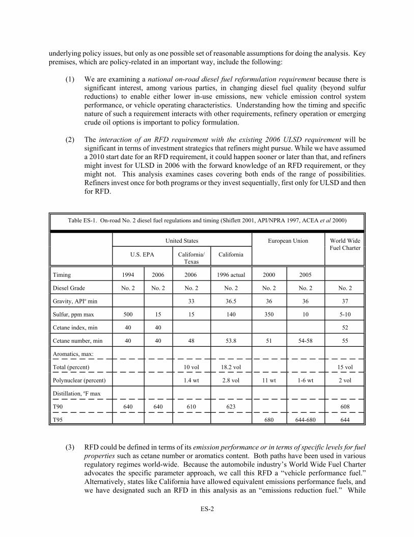
Table ES-1 shows on-road No. 2 diesel fuel regulations and timing for several regulatory authorities and forthe World Wide Fuel Charter. Given that the diesel fuel requirements for California and Texas will belargely satisfied by alternative performance-based specifications, the most challenging requirements for on-road diesel fuel are those specifications recommended by the European Union and the World Wide FuelCharter, particularly specifications for cetane number and total aromatics. Global vehicle and enginemanufacturing associations support the World Wide Fuel Charter on the basis that “Consistent fuel qualityworld-wide is necessary to market high-quality automotive products matching world-wide customerperformance and environmental needs.”
The examination of challenging RFD specifications and their impacts on refinery investment requirementsand operating costs inevitably raises a wide range of policy issues. In establishing specific premises for thisstudy, we must make assumptions about the resolution of a number of currently unresolved issues. Oneshould not interpret these premises as ORNL or DOE views regarding the appropriate resolution of the
ES-2
underlying policy issues, but only as one possible set of reasonable assumptions for doing the analysis. Keypremises, which are policy-related in an important way, include the following:
(1) We are examining a national on-road diesel fuel reformulation requirement because there issignificant interest, among various parties, in changing diesel fuel quality (beyond sulfurreductions) to enable either lower in-use emissions, new vehicle emission control systemperformance, or vehicle operating characteristics. Understanding how the timing and specificnature of such a requirement interacts with other requirements, refinery operation or emergingcrude oil options is important to policy formulation.
(2) The interaction of an RFD requirement with the existing 2006 ULSD requirement will besignificant in terms of investment strategics that refiners might pursue. While we have assumeda 2010 start date for an RFD requirement, it could happen sooner or later than that, and refinersmight invest for ULSD in 2006 with the forward knowledge of an RFD requirement, or theymight not. This analysis examines cases covering both ends of the range of possibilities.Refiners invest once for both programs or they invest sequentially, first only for ULSD and thenfor RFD.
Table ES-1. On-road No. 2 diesel fuel regulations and timing (Shiflett 2001, API/NPRA 1997, ACEA et al 2000)
United States European Union World WideFuel Charter
U.S. EPA California/Texas
California
Timing 1994 2006 2006 1996 actual 2000 2005
Diesel Grade No. 2 No. 2 No. 2 No. 2 No. 2 No. 2 No. 2
Gravity, APIo min 33 36.5 36 36 37
Sulfur, ppm max 500 15 15 140 350 10 5-10
Cetane index, min 40 40 52
Cetane number, min 40 40 48 53.8 51 54-58 55
Aromatics, max:
Total (percent) 10 vol 18.2 vol 15 vol
Polynuclear (percent) 1.4 wt 2.8 vol 11 wt 1-6 wt 2 vol
Distillation, oF max
T90 640 640 610 623 608
T95 680 644-680 644
(3) RFD could be defined in terms of its emission performance or in terms of specific levels for fuelproperties such as cetane number or aromatics content. Both paths have been used in variousregulatory regimes world-wide. Because the automobile industry’s World Wide Fuel Charteradvocates the specific parameter approach, we call this RFD a “vehicle performance fuel.”Alternatively, states like California have allowed equivalent emissions performance fuels, andwe have designated such an RFD in this analysis as an “emissions reduction fuel.” While

ES-3
emissions performance will be set equal, vehicle operational impacts and refining cost impactscould be different for vehicle performance RFD compared to emissions reduction RFD. Weanalyze both RFDs in terms of refinery impacts.
(4) Changes to off-road diesel fuel quality are quite likely in the time frame of this analysis, but thespecifics are not known. ULSD (15 ppm maximum sulfur content) may become the needed fuelfor some portion of the off-road market while some low sulfur diesel fuel (500 ppm maximumsulfur content) may remain in the diesel fuel pool due to phase-in of the ULSD requirement. Forthis analysis, a volume of diesel equal to off-road volume is assumed to be at 500 ppm and therest at 15 ppm (i.e., ULSD), but the actual end use markets for the two sulfur levels may be moremixed than that. The critical implied assumption is that all high sulfur (greater than 500 ppm)diesel fuel disappears from the refinery slate by 2010.
(5) Changes to gasoline requirements are likely in the time frame relevant to this analysis. We havepremised the requirements contained in current proposed legislation (U.S. Senate Bill S.517,subsequently amended into U.S. House of Representatives Bill H.R.4) as a plausible set of newrequirements. Despite significant changes in that legislation (e.g., MTBE ban, elimination of thereformulated gasoline oxygenate requirement and mandated ethanol use), the actual impact onrefinery operations in our study region, the U.S. Midwest, is relatively small because of pre-existing ethanol use and the almost total absence of MTBE use in that region, and the limitedinteractions between gasoline quality and diesel fuel reformulation.
(6) Finally, we examine the interaction between greater use of Canadian synthetic crude oils andthese tighter diesel fuel quality specifications, with the implicit assumptions that there will be asignificant growth in the volume of that synthetic crude production and that U.S. Midwesternrefineries are a natural market for that crude. The need for effective integration of refinerychanges in the U.S. (driven by changing product quality requirements) and expanded syntheticcrude production in Canada is a possible use of this part of the analysis.
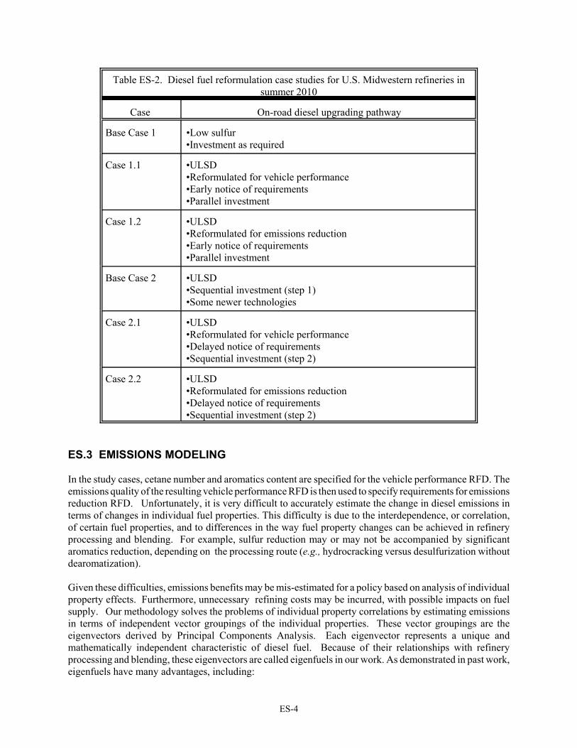
Based on these premises, the study case design is summarized in Table ES-2. For each of the two differentreformulation pathways (vehicle performance and emissions reduction), two different investment pathwaysare investigated in the study cases, in order to understand the refinery benefits of early notice of requirementsfor more stringent specifications. With early notice of RFD requirements, refinery capital investment wouldnot yet be made to satisfy the ULSD sulfur requirement of year 2006, giving greater flexibility for investmentplanning. With delayed notice of requirements, capital investment would have been sunk to satisfy the ULSDsulfur requirement, resulting is less investment flexibility.
ES-4
Table ES-2. Diesel fuel reformulation case studies for U.S. Midwestern refineries insummer 2010
Case On-road diesel upgrading pathway
Base Case 1 •Low sulfur•Investment as required
Case 1.1 •ULSD•Reformulated for vehicle performance•Early notice of requirements•Parallel investment
Case 1.2 •ULSD•Reformulated for emissions reduction•Early notice of requirements•Parallel investment
Base Case 2 •ULSD•Sequential investment (step 1)•Some newer technologies
Case 2.1 •ULSD•Reformulated for vehicle performance•Delayed notice of requirements•Sequential investment (step 2)
Case 2.2 •ULSD•Reformulated for emissions reduction•Delayed notice of requirements•Sequential investment (step 2)
ES.3 EMISSIONS MODELING
In the study cases, cetane number and aromatics content are specified for the vehicle performance RFD. Theemissions quality of the resulting vehicle performance RFD is then used to specify requirements for emissionsreduction RFD. Unfortunately, it is very difficult to accurately estimate the change in diesel emissions interms of changes in individual fuel properties. This difficulty is due to the interdependence, or correlation,of certain fuel properties, and to differences in the way fuel property changes can be achieved in refineryprocessing and blending. For example, sulfur reduction may or may not be accompanied by significantaromatics reduction, depending on the processing route (e.g., hydrocracking versus desulfurization withoutdearomatization).
Given these difficulties, emissions benefits may be mis-estimated for a policy based on analysis of individualproperty effects. Furthermore, unnecessary refining costs may be incurred, with possible impacts on fuelsupply. Our methodology solves the problems of individual property correlations by estimating emissionsin terms of independent vector groupings of the individual properties. These vector groupings are theeigenvectors derived by Principal Components Analysis. Each eigenvector represents a unique andmathematically independent characteristic of diesel fuel. Because of their relationships with refineryprocessing and blending, these eigenvectors are called eigenfuels in our work. As demonstrated in past work,eigenfuels have many advantages, including:

ES-5
Simplification of the analysis, because the mathematical independence of eigenfuels eliminatescorrelations among the variables and the associated complications.
Economy of representation, because a smaller number of such vector variables may effectively replacea larger number of original variables.
Greater understanding of the patterns of variation that are important to emissions, and how thesepatterns relate to refinery processing and blending.
New insight into the optimal economic formulation of fuels to reduce emissions.
Given limitations of the available diesel engine test data, we find that the eigenfuel method leads to newperspectives on diesel fuel-emissions relationships:
Fuel properties are only surrogate variables for underlying causal factors. Much of the emissionsreduction seen in past testing comes from reducing highly aromatic cracked stocks in diesel fuel.Because these stocks are low in cetane number and high in density, researchers have tended to attributethe emissions reductions to the increase in cetane number or reduction in density associated with theirremoval, rather than to the compositional change itself.
How one varies a fuel property can be the most important factor in determining the emissions response.A given fuel property can be changed in many ways, and a unit change in that property can producemarkedly different effects on emissions depending on how that change is introduced.
ES.4 RFD STUDY FINDINGS
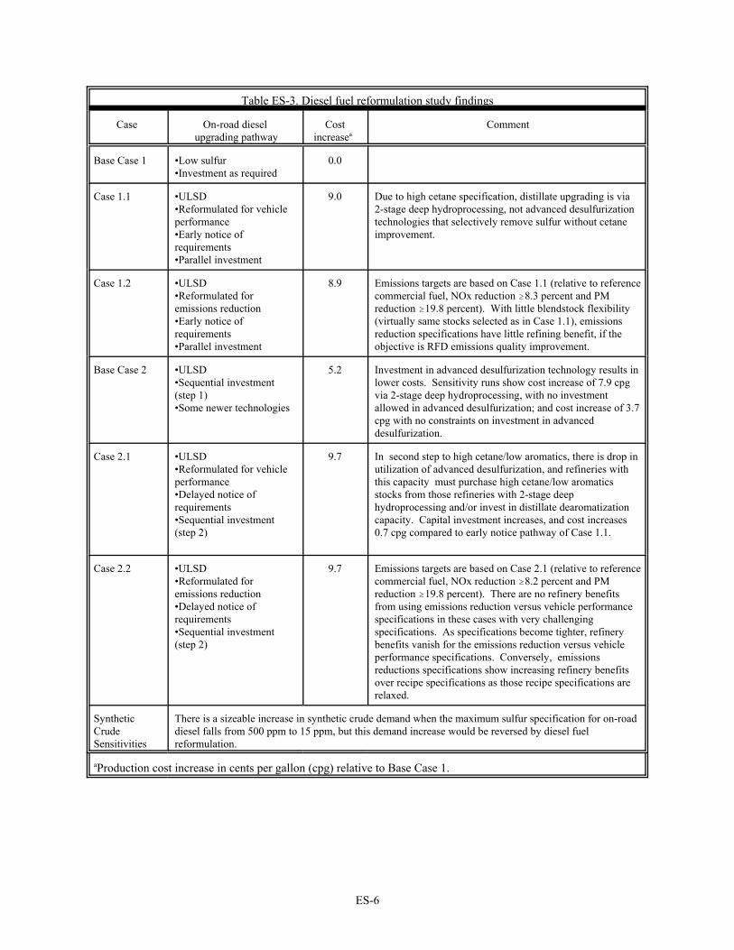
With its eigenfuel-based representation of emissions, ORNL-RYM2002 produced the RFD study findingssummarized in Table ES-3. The table shows that refining costs are lower with early notice (parallelinvestment) of product quality requirements for on-road diesel fuel. While advanced desulfurizationtechnologies (with low hydrogen consumption and little effect on cetane quality and aromatics content)reduce the cost of ULSD, these technologies contribute to the increased costs of a sequential investmentpathway compared to a parallel investment pathway to RFD. In the sequential investment pathway, advanceddesulfurization unit utilization and the associated cash margin fall. The sequential investments includesubstantial conversion of second-stage hydrodesulfurization capacity to second stage dearomatizationcapacity.
ES-6
Table ES-3. Diesel fuel reformulation study findings
Case On-road diesel upgrading pathway
Costincreasea
Comment
Base Case 1 •Low sulfur•Investment as required
0.0
Case 1.1 •ULSD•Reformulated for vehicleperformance•Early notice ofrequirements•Parallel investment
9.0 Due to high cetane specification, distillate upgrading is via2-stage deep hydroprocessing, not advanced desulfurizationtechnologies that selectively remove sulfur without cetaneimprovement.
Case 1.2 •ULSD•Reformulated foremissions reduction•Early notice ofrequirements•Parallel investment
8.9 Emissions targets are based on Case 1.1 (relative to referencecommercial fuel, NOx reduction $8.3 percent and PMreduction $19.8 percent). With little blendstock flexibility(virtually same stocks selected as in Case 1.1), emissionsreduction specifications have little refining benefit, if theobjective is RFD emissions quality improvement.
Base Case 2 •ULSD•Sequential investment(step 1)•Some newer technologies
5.2 Investment in advanced desulfurization technology results inlower costs. Sensitivity runs show cost increase of 7.9 cpgvia 2-stage deep hydroprocessing, with no investmentallowed in advanced desulfurization; and cost increase of 3.7cpg with no constraints on investment in advanceddesulfurization.
Case 2.1 •ULSD•Reformulated for vehicleperformance•Delayed notice ofrequirements•Sequential investment(step 2)
9.7 In second step to high cetane/low aromatics, there is drop inutilization of advanced desulfurization, and refineries withthis capacity must purchase high cetane/low aromaticsstocks from those refineries with 2-stage deephydroprocessing and/or invest in distillate dearomatizationcapacity. Capital investment increases, and cost increases0.7 cpg compared to early notice pathway of Case 1.1.
Case 2.2 •ULSD•Reformulated foremissions reduction•Delayed notice ofrequirements•Sequential investment(step 2)
9.7 Emissions targets are based on Case 2.1 (relative to referencecommercial fuel, NOx reduction $8.2 percent and PMreduction $19.8 percent). There are no refinery benefitsfrom using emissions reduction versus vehicle performancespecifications in these cases with very challengingspecifications. As specifications become tighter, refinerybenefits vanish for the emissions reduction versus vehicleperformance specifications. Conversely, emissionsreductions specifications show increasing refinery benefitsover recipe specifications as those recipe specifications arerelaxed.
SyntheticCrudeSensitivities
There is a sizeable increase in synthetic crude demand when the maximum sulfur specification for on-roaddiesel falls from 500 ppm to 15 ppm, but this demand increase would be reversed by diesel fuelreformulation.
aProduction cost increase in cents per gallon (cpg) relative to Base Case 1.
ES-7
With the objective of RFD emissions quality improvement, there is little refining economic benefit from usingthe flexible emissions reduction specifications rather than the vehicle performance recipe specifications inthese cases, which have very challenging specifications. As specifications become tighter, processingbecomes more difficult, blendstock choices become more limited, and refinery benefits vanish for emissionsreduction relative to vehicle performance specifications.
Conversely, emissions reduction specifications show increasing refinery benefits over vehicle performancerecipe specifications as those recipe specifications are relaxed, and alternative processing routes andblendstocks become available. For example, using average specifications rather than cap specifications inour study reduces investment and RFD production costs for emissions reduction compared to vehicleperformance.
In sensitivity cases, ORNL-RYM2002 is used to examine the impact of RFD specifications on the economicsof using Canadian synthetic crude oil. There is a sizeable increase in synthetic crude demand as ULSD fueldisplaces low sulfur diesel fuel, but this demand increase would be reversed by a requirement for diesel fuelreformulation.


I-1
PART I. THE REFINERY STUDY
I-1. INTRODUCTION
The Oak Ridge National Laboratory Refinery Yield Model (ORNL-RYM2002), updated in 2002, has been usedto study the refining cost, investment, operational, and crude oil impacts of specifications for reformulateddiesel fuel (RFD) in case studies required by the U.S. Department of Energy (DOE) Offices of Policy andInternational Affairs, Energy Efficiency and Renewable Energy, and Fossil Energy.
Table 1.1 shows No. 2 on-road diesel fuel regulations and timing for several regulatory authorities and forthe World Wide Fuel Charter. Given that the diesel fuel requirements for California and Texas will belargely satisfied by alternative performance-based specifications, the most challenging requirements for on-road diesel fuel are those specifications recommended by the European Union and the World Wide FuelCharter, particularly specifications for cetane number and total aromatics.
Global vehicle and engine manufacturing associations support the World Wide Fuel Charter on the basis that“Consistent fuel quality world-wide is necessary to market high-quality automotive products matching world-wide customer performance and environmental needs.” In its “Technical Background for Harmonised FuelRecommendations,” the World Wide Fuel Charter discusses its views of the emissions reduction potentialof changes in individual diesel fuel properties. In fact, it is very difficult to accurately estimate the changein diesel emissions in terms of changes in individual fuel properties. This difficulty is due to theinterdependence, or correlation, of certain fuel properties, and to differences in the way fuel property changescan be achieved in refinery processing and blending. For example, sulfur reduction may or may not beaccompanied by significant aromatics reduction, depending on the processing route (e.g., hydrocrackingversus desulfurization without dearomatization).
Given these difficulties, emissions benefits may be mis-estimated for a regulation based on analysis ofindividual property effects. Furthermore, unnecessary refining costs may be incurred, with possible impactson fuel supply. Our eigfenfuel methodology, described in PART II of this report, solves the problems ofindividual property correlations by estimating emissions in terms of independent vector variables. Eigenfuels,which are related to underlying refinery and blending processes, provide an unambiguous method for cost-effective blending of refinery stocks.
I-2
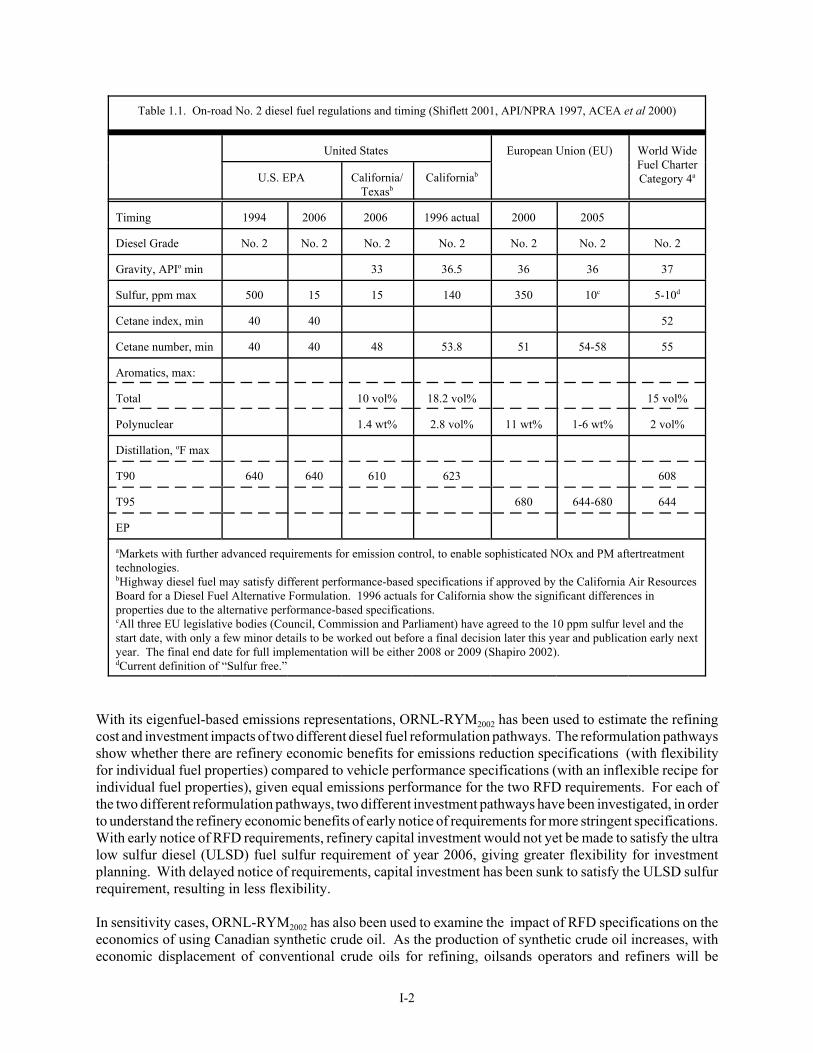
Table 1.1. On-road No. 2 diesel fuel regulations and timing (Shiflett 2001, API/NPRA 1997, ACEA et al 2000)
United States European Union (EU) World WideFuel CharterCategory 4aU.S. EPA California/
TexasbCaliforniab
Timing 1994 2006 2006 1996 actual 2000 2005
Diesel Grade No. 2 No. 2 No. 2 No. 2 No. 2 No. 2 No. 2
Gravity, APIo min 33 36.5 36 36 37
Sulfur, ppm max 500 15 15 140 350 10c 5-10d
Cetane index, min 40 40 52
Cetane number, min 40 40 48 53.8 51 54-58 55
Aromatics, max:
Total 10 vol% 18.2 vol% 15 vol%
Polynuclear 1.4 wt% 2.8 vol% 11 wt% 1-6 wt% 2 vol%
Distillation, oF max
T90 640 640 610 623 608
T95 680 644-680 644
EP
aMarkets with further advanced requirements for emission control, to enable sophisticated NOx and PM aftertreatmenttechnologies. bHighway diesel fuel may satisfy different performance-based specifications if approved by the California Air ResourcesBoard for a Diesel Fuel Alternative Formulation. 1996 actuals for California show the significant differences inproperties due to the alternative performance-based specifications.cAll three EU legislative bodies (Council, Commission and Parliament) have agreed to the 10 ppm sulfur level and thestart date, with only a few minor details to be worked out before a final decision later this year and publication early nextyear. The final end date for full implementation will be either 2008 or 2009 (Shapiro 2002). dCurrent definition of “Sulfur free.”
With its eigenfuel-based emissions representations, ORNL-RYM2002 has been used to estimate the refiningcost and investment impacts of two different diesel fuel reformulation pathways. The reformulation pathwaysshow whether there are refinery economic benefits for emissions reduction specifications (with flexibilityfor individual fuel properties) compared to vehicle performance specifications (with an inflexible recipe forindividual fuel properties), given equal emissions performance for the two RFD requirements. For each ofthe two different reformulation pathways, two different investment pathways have been investigated, in orderto understand the refinery economic benefits of early notice of requirements for more stringent specifications.With early notice of RFD requirements, refinery capital investment would not yet be made to satisfy the ultralow sulfur diesel (ULSD) fuel sulfur requirement of year 2006, giving greater flexibility for investmentplanning. With delayed notice of requirements, capital investment has been sunk to satisfy the ULSD sulfurrequirement, resulting in less flexibility.
In sensitivity cases, ORNL-RYM2002 has also been used to examine the impact of RFD specifications on theeconomics of using Canadian synthetic crude oil. As the production of synthetic crude oil increases, witheconomic displacement of conventional crude oils for refining, oilsands operators and refiners will be

I-3
technically challenged by requirements to improve diesel fuel cetane number, jet fuel smoke point, and heavygas oil quality for fluid catalytic cracking feed (Yui 2000; Yui and Chung 2001).

I-5
I-2. THE ORNL REFINERY YIELD MODEL
I-2.1 ORNL-RYM2002
ORNL-RYM2002 is a linear program representing over 75 refining processes which can be used to produceup to 50 different products from more than 180 crude oils. An investment module provides for the additionof processing capacity (DOE 1984a,b; Tallett and Dunbar 1988; Tallett, Dunbar and Leather 1992).ORNL-RYM2002 tracks gravity, cetane index, aromatics, sulfur, flash point, pour point, viscosity, hydrogencontent, heat of combustion, distillation temperatures, and pollutant emissions on all diesel componentstreams. In separate data tables in ORNL-RYM2002, diesel blending components are identified; blendingvalues are assigned to these components; and specifications are set for diesel products. ORNL-RYM2002incorporates diesel fuel blending using the vector-based eigenfuel concept to satisfy emissions specificationsfor oxides of nitrogen (NOx) and particulate matter (PM) (McAdams, Crawford, and Hadder 2002; Crawford2002).
Properties for other distillates and for gasolines are handled in a similar fashion. ORNL-RYM2002incorporates gasoline blending to satisfy formula and emissions standards mandated by the Clean Air ActAmendments of 1990 and described by the EPA Complex Model, which predicts gasoline pollutant emissionsin terms of gasoline properties (Korotney 1993). ORNL-RYM2002 also represents requirements of the toxicsanti-backsliding rulemaking of 2001 (EPA 2001).
Overoptimization can occur as a result of the ORNL-RYM2002 use of a modeling concept in which refinerystreams with identical distillation cut points are kept separate through different refining processes. Ratioconstraints on refinery streams can be used to avoid unrealistic separation of streams with identical distillationcut points. With ratio constraints, the proportions of streams entering a process are constrained to equal theproportions of those streams produced at a source process. This study makes use of ratio constraints ingasoline production, based on calibration results. Ratio constraints are also used for distillate deepdesulfurization and dearomatization processes.
It is important to recognize that refineries within a region can vary widely in technical capability, and thatrefineries are subject to temporal variations in complex operations. A refining outcome (e.g., investment cost)can span a range, and this range has uncertainty.
I-2.2 MODEL UPDATE
Specifically for this study, ORNL-RYM2002 was updated to include:
The most recent process configuration and revamp cost information for distillate desulfurization units.
Representations of advanced desulfurization technologies that selectively remove sulfur, with lowhydrogen consumption.
Representation of the most recent catalyst developments.
Representation of revamping of existing steam reforming hydrogen production units to increasecapacity and reduce energy consumption and operating costs.
Representation of a debottlenecking feature to enable capacity addition on selected units at a fractionof new unit costs.

I-6
Representation of process unit capital cost trending over time to reflect the potential benefits of laterprocess unit additions.
A number of other technology and features enhancements, discussed in Appendices I-A and I-B(Dunbar and Tallett 2002a,b).
I-7
I-3. PREMISES
I-3.1 POLICY ISSUES
The examination of the impacts of an RFD requirement on refinery investment and operating costs inevitablyraises a wide range of policy issues. These issues have to be addressed in order to establish the frameworkfor the subject. In establishing specific premises for this study, we must make assumptions about theresolution of a number of currently unresolved issues. One should not interpret these premises as ORNL orDOE views as to the appropriate resolution of the underlying policy issues, but only as one possible set ofreasonable assumptions for doing the analysis. We have highlighted below some of the key premises thatare policy-related in an important way:
(1) We are examining a national on-road diesel fuel reformulation requirement because there issignificant interest, among various parties, in changing diesel fuel quality (beyond sulfurreductions) to enable either lower in-use emissions, new vehicle emission control systemperformance, or vehicle operating characteristics (e.g., cold startability, noise, idle quality).Understanding how the timing and specific nature of such a requirement interacts with otherrequirements, refinery operation or emerging crude oil options is important to policy formulation.
(2) The interaction of such an RFD requirement with the existing 2006 ULSD requirement will besignificant in terms of investment strategics that refiners might pursue. While we have assumeda 2010 start date for an RFD requirement, it could happen sooner or later than that, and refinersmight invest for ULSD in 2006 with the forward knowledge of an RFD requirement, or theymight not. This analysis examines cases covering both ends of the range of possibilities.Refiners invest once for both programs (effectively) in 2006 or they invest sequentially, first onlyfor ULSD and then for RFD.
(3) RFD could be defined in terms of its emission performance or in terms of specific levels for fuelproperties such as cetane number or aromatics content. Both paths have been used in variousregulatory regimes world-wide. Because the auto industry’s World Wide Fuel Charter advocatesthe specific parameter approach, we call this RFD a “vehicle performance fuel.” Alternatively,states like California have allowed equivalent emissions reduction fuels, and we have specifiedsuch an RFD in this analysis as an “emissions reduction fuel.” While emissions performancewill be set equal, vehicle operational impacts and refining cost impacts could be different forvehicle performance RFD compared to emissions reduction RFD. We analyze both RFDs interms of refinery impacts.
(4) Changes to off-road diesel fuel quality are quite likely in the time frame of this analysis, but thespecifics are not known. ULSD (at 15 ppm maximum sulfur) may become the needed fuel forsome portion of the off-road market while some low sulfur diesel fuel (at 500 ppm maximumsulfur) may remain in the diesel fuel pool due to the phase-in of the ULSD requirement. For thisanalysis, a volume of diesel equal to off-road volume is assumed to be at 500 ppm and the restat 15 ppm (i.e., ULSD), but the actual end use markets for the two sulfur levels may be moremixed than that. The critical implied assumption is that all high sulfur (greater than 500 ppm)diesel fuel disappears from the PADD II (Petroleum Administration for Defense District II, theU.S. Midwest) refinery slate by 2010.
(5) Changes to gasoline requirements are likely in the time frame relevant to this analysis. We havepremised the requirements contained in current proposed legislation (U.S. Senate Bill S.517,subsequently amended into U.S. House of Representatives Bill H.R.4) as a plausible set of new
I-8
requirements. Despite the significant changes in that legislation (MTBE ban, elimination of thereformulated gasoline [RFG] oxygenate requirement and mandated ethanol use), the actualimpact on PADD II refinery operations for the purposes of our analysis is relatively smallbecause of pre-existing ethanol use and the almost total absence of MTBE use in that region, andthe limited interactions between gasoline quality and diesel fuel reformulation.
(6) Finally, we examine the interaction between greater use of Canadian synthetic crude oils andthese tighter diesel fuel quality specifications, with the implicit assumption that there will be asignificant growth in the volume of that synthetic crude production and that PADD II refineriesare a natural market for that crude. The need for effective integration of refinery changes in theU.S. (driven by changing product quality requirements) and expanded synthetic crude productionin Canada is a possible use of this part of the analysis.
I-3.2 STUDY PERIOD AND GEOGRAPHIC AREA
The study period is summer of year 2010. The study area is PADD II, a 15 state area in the U.S. Midwest with27 operable refineries, annually producing 22 percent of all gasoline and 25 percent of all on-road diesel fuelproduced in the U.S. With the exception of PADD IV (the U.S. Rocky Mountain area), PADD II has thehighest percentage production of on-road diesel fuel (relative to refinery net production of finished petroleumproducts). Also with the exception of PADD IV, PADD II has the highest percentage of imports of Canadiancrude oil (relative to total refinery input of crude oil), which is a consideration for the sensitivity case studyof the impact of RFD specifications on the economics of using Canadian synthetic crude oil. PADD IV wasnot selected because of its relatively small refining capacity and low complexity.
Of the 27 PADD II refineries, 13 have distillate hydrotreating, and we assume that these refineries arecurrently producers of low sulfur diesel fuel. Different studies have focused on a range of possibilities forrefinery participation in on-road diesel fuel production for 2006-2007. Baker & O’Brien (2001) believes thatonly current low sulfur diesel fuel producers are likely to continue in the ULSD market. On the other hand,MathPro (2002) concludes that some refineries that do not now produce low sulfur diesel fuel may haveincentives to produce ULSD. For our more distant outlook of year 2010 (with a 24 percent increase in on-road diesel fuel production, compared to year 2000), we assume that ULSD/RFD production can be spreadamong all refineries in PADD II.
I-3.3 TECHNICAL PREMISES
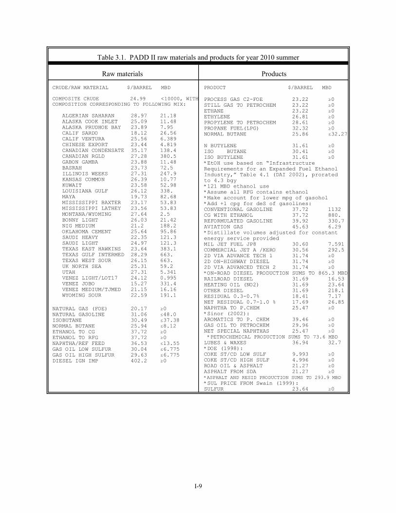
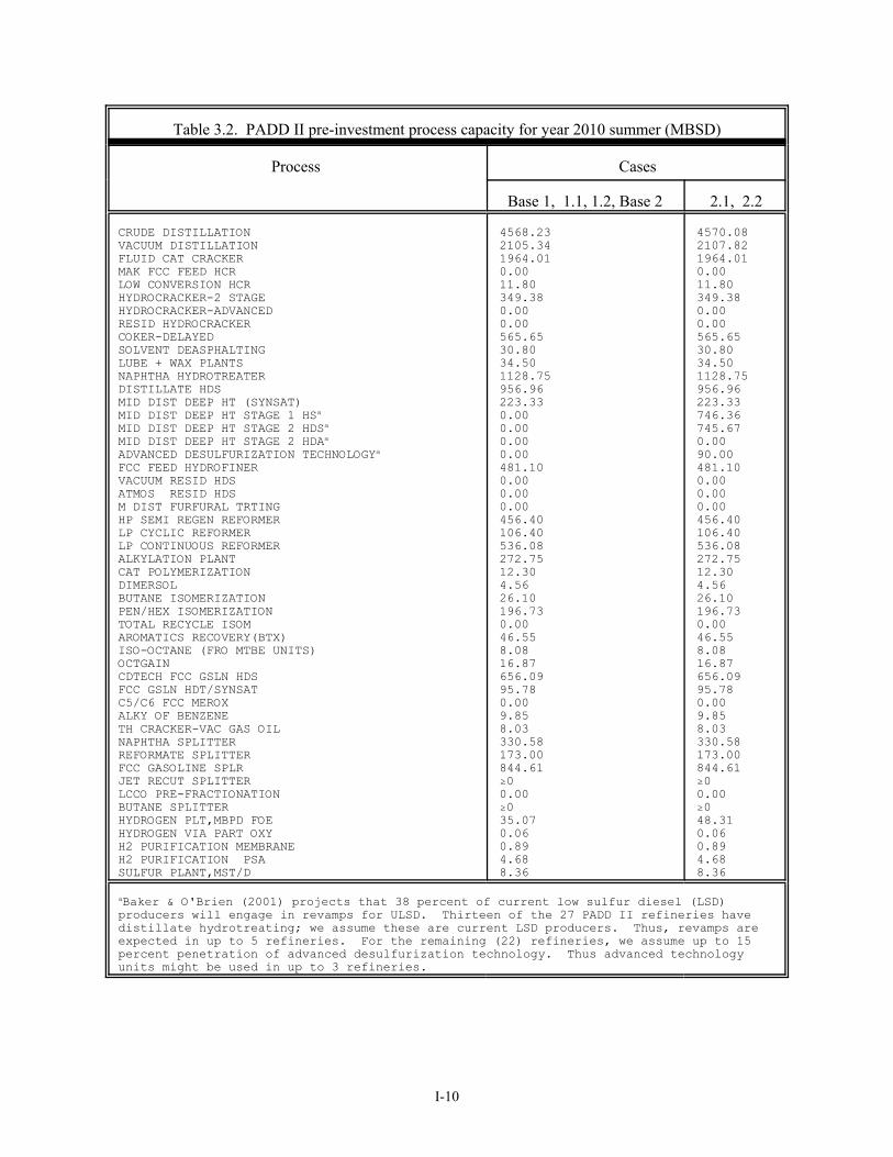
Technical premises for product slates and revenues, raw materials and costs, and process capacity data -as loaded in ORNL-RYM2002 - are shown in Table 3.1 and Table 3.2. These modeling data are based oninformation sources discussed in the following paragraphs.
I-9
Table 3.1. PADD II raw materials and products for year 2010 summer
Raw materials Products
CRUDE/RAW MATERIAL $/BARREL MBD
COMPOSITE CRUDE 24.99 <10000, WITHCOMPOSITION CORRESPONDING TO FOLLOWING MIX: ALGERIAN SAHARAN 28.97 21.18 ALASKA COOK INLET 25.09 11.48 ALASKA PRUDHOE BAY 23.89 7.95 CALIF SARDO 18.12 26.56 CALIF VENTURA 25.56 6.389 CHINESE EXPORT 23.44 4.819 CANADIAN CONDENSATE 35.17 138.4 CANADIAN RGLD 27.28 380.5 GABON GAMBA 23.88 11.48 BASRAH 23.73 72.5 ILLINOIS WEEKS 27.31 247.9 KANSAS COMMON 26.39 10.77 KUWAIT 23.58 52.98 LOUISIANA GULF 26.12 338. MAYA 19.73 82.68 MISSISSIPPI BAXTER 23.17 53.83 MISSISSIPPI LATHEY 23.56 53.83 MONTANA/WYOMING 27.64 2.5 BONNY LIGHT 26.03 21.42 NIG MEDIUM 21.2 188.2 OKLAHOMA CEMENT 25.64 95.86 SAUDI HEAVY 22.35 121.3 SAUDI LIGHT 24.97 121.3 TEXAS EAST HAWKINS 23.64 383.1 TEXAS GULF INTERMED 28.29 663. TEXAS WEST SOUR 26.15 663. UK NORTH SEA 25.31 59.2 UTAH 27.31 5.341 VENEZ LIGHT/LOT17 24.12 0.995 VENEZ JOBO 15.27 331.4 VENEZ MEDIUM/TJMED 21.15 16.16 WYOMING SOUR 22.59 191.1
NATURAL GAS (FOE) 20.17 $0NATURAL GASOLINE 31.06 #48.0ISOBUTANE 30.49 #37.38NORMAL BUTANE 25.94 #8.12ETHANOL TO CG 37.72 $0ETHANOL TO RFG 37.72 $0NAPHTHA/REF FEED 36.53 #13.55GAS OIL LOW SULFUR 30.04 #6.775GAS OIL HIGH SULFUR 29.63 #6.775DIESEL IGN IMP 402.2 $0
PRODUCT $/BARREL MBD PROCESS GAS C2-FOE 23.22 $0 STILL GAS TO PETROCHEM 23.22 $0 ETHANE 23.22 $0 ETHYLENE 26.81 $0 PROPYLENE TO PETROCHEM 28.61 $0 PROPANE FUEL(LPG) 32.32 $0NORMAL BUTANE 25.86 #32.27
N BUTYLENE 31.61 $0ISO BUTANE 30.41 $0 ISO BUTYLENE 31.61 $0*EtOH use based on “InfrastructureRequirements for an Expanded Fuel EthanolIndustry,” Table 4.1 (DAI 2002), proratedto 4.3 bgy *121 MBD ethanol use *Assume all RFG contains ethanol *Make account for lower mpg of gasohol *Add +1 cpg for deS of gasolines: CONVENTIONAL GASOLINE 37.72 1132 CG WITH ETHANOL 37.72 880. REFORMULATED GASOLINE 39.92 330.7 AVIATION GAS 45.63 6.29 *Distillate volumes adjusted for constantenergy service provided MIL JET FUEL JP8 30.60 7.591 COMMERCIAL JET A /KERO 30.56 292.5 2D VIA ADVANCE TECH 1 31.74 $02D ON-HIGHWAY DIESEL 31.74 $0 2D VIA ADVANCED TECH 2 31.74 $0 *ON-ROAD DIESEL PRODUCTION SUMS TO 865.3 MBD RAILROAD DIESEL 31.69 16.53 HEATING OIL (NO2) 31.69 23.64 OTHER DIESEL 31.69 218.1 RESIDUAL 0.3-0.7% 18.41 7.17 NET RESIDUAL 0.7-1.0 % 17.69 26.85 NAPHTHA TO P.CHEM 25.47 $0 *Sinor (2002):AROMATICS TO P. CHEM 39.46 $0 GAS OIL TO PETROCHEM 29.96 $0 NET SPECIAL NAPHTHAS 25.47 $0 *PETROCHEMICAL PRODUCTION SUMS TO 73.6 MBD LUBES & WAXES 36.94 32.7 *DOE (1998):COKE ST/CD LOW SULF 9.993 $0COKE ST/CD HIGH SULF 4.996 $0ROAD OIL & ASPHALT 21.27 $0 ASPHALT FROM SDA 21.27 $0*ASPHALT AND RESID PRODUCTION SUMS TO 293.9 MBD *SUL PRICE FROM Swain (1999):SULFUR 23.64 $0
I-10
Table 3.2. PADD II pre-investment process capacity for year 2010 summer (MBSD)
Process Cases
Base 1, 1.1, 1.2, Base 2 2.1, 2.2
CRUDE DISTILLATION VACUUM DISTILLATION FLUID CAT CRACKER MAK FCC FEED HCR LOW CONVERSION HCR HYDROCRACKER-2 STAGE HYDROCRACKER-ADVANCEDRESID HYDROCRACKER COKER-DELAYED SOLVENT DEASPHALTING LUBE + WAX PLANTS NAPHTHA HYDROTREATER DISTILLATE HDS MID DIST DEEP HT (SYNSAT) MID DIST DEEP HT STAGE 1 HSa MID DIST DEEP HT STAGE 2 HDSa
MID DIST DEEP HT STAGE 2 HDAa
ADVANCED DESULFURIZATION TECHNOLOGYa
FCC FEED HYDROFINER VACUUM RESID HDS ATMOS RESID HDS M DIST FURFURAL TRTING HP SEMI REGEN REFORMER LP CYCLIC REFORMER LP CONTINUOUS REFORMER ALKYLATION PLANT CAT POLYMERIZATION DIMERSOL BUTANE ISOMERIZATION PEN/HEX ISOMERIZATION TOTAL RECYCLE ISOM AROMATICS RECOVERY(BTX) ISO-OCTANE (FRO MTBE UNITS)OCTGAIN CDTECH FCC GSLN HDS FCC GSLN HDT/SYNSAT C5/C6 FCC MEROX ALKY OF BENZENE TH CRACKER-VAC GAS OIL NAPHTHA SPLITTER REFORMATE SPLITTER FCC GASOLINE SPLR JET RECUT SPLITTER LCCO PRE-FRACTIONATION BUTANE SPLITTER HYDROGEN PLT,MBPD FOE HYDROGEN VIA PART OXY H2 PURIFICATION MEMBRANEH2 PURIFICATION PSASULFUR PLANT,MST/D
4568.232105.341964.010.0011.80349.380.000.00565.6530.8034.501128.75956.96223.330.000.000.000.00481.100.000.000.00456.40106.40536.08272.7512.304.5626.10196.730.0046.558.0816.87656.0995.780.009.858.03330.58173.00844.61$00.00$035.070.060.894.688.36
4570.082107.821964.010.0011.80349.380.000.00565.6530.8034.501128.75956.96223.33746.36745.670.0090.00481.100.000.000.00456.40106.40536.08272.7512.304.5626.10196.730.0046.558.0816.87656.0995.780.009.858.03330.58173.00844.61$00.00$048.310.060.894.688.36
aBaker & O'Brien (2001) projects that 38 percent of current low sulfur diesel (LSD) producers will engage in revamps for ULSD. Thirteen of the 27 PADD II refineries have distillate hydrotreating; we assume these are current LSD producers. Thus, revamps are expected in up to 5 refineries. For the remaining (22) refineries, we assume up to 15 percent penetration of advanced desulfurization technology. Thus advanced technology units might be used in up to 3 refineries.
I-11
I-3.3.1 Refinery Production Rates
Refinery summer production rates are based on the Petroleum Supply Annual 2000 (DOE 2001b). Refineryproduction is projected to year 2010, using the Reference Case growth rates published in Table A11 of theAnnual Energy Outlook 2002 with Projections to 2020 (DOE 2001a).
I-3.3.2 Distillate Quality
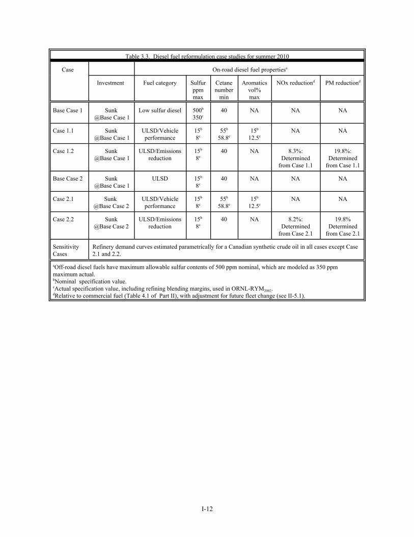
On-road diesel fuel has sulfur, cetane number, aromatics content and emissions specifications (nominal andactual) as shown in Table 3.3. The actual specifications for cetane number and aromatics content are basedon refiner guidance that the lowest reasonable blending margins should be based on the reproducibility oftests that determine property values. Reproducibility is the variability of the average values obtained byseveral test operators while measuring the same item. We assume a 3.8 number margin for our cetane numberspecifications, based roughly on the reproducibility of ASTM D613. For aromatics, the reproducibility ofASTM D1319 is 2.5 vol percent when total aromatics content is approximately 15 vol percent. We have nobasis for assumptions for additional margins that may be needed for pipeline degradation of product quality. Off-road diesel fuels (including No. 2 home heating oil) have maximum allowable sulfur contents of 500 ppmnominal, which is modeled as 350 ppm maximum actual. As discussed in Section I-3.1, a volume of dieselfuel equal to the off-road volume is assumed to be at a sulfur content of 500 ppm (nominal) and the rest at15 ppm sulfur (i.e., ULSD) in year 2010, but the actual end use markets for the two sulfur levels may be moremixed than that. The critical implied assumption is that all high sulfur (greater than 500 ppm) diesel fueldisappears from the refinery slate by 2010, in PADD II. Otherwise, specifications for diesel fuels, distillatesand products other than gasoline are based on API/NPRA (1997) and NPC (1993). On-road diesel-equivalent miles-per-gallon (mpg) are held constant across cases.
I-12
Table 3.3. Diesel fuel reformulation case studies for summer 2010
Case On-road diesel fuel propertiesa
Investment Fuel category Sulfurppmmax
Cetanenumber
min
Aromaticsvol%max
NOx reductiond PM reductiond
Base Case 1 Sunk @Base Case 1
Low sulfur diesel 500b
350c40 NA NA NA
Case 1.1 Sunk @Base Case 1
ULSD/Vehicleperformance
15b
8c55b
58.8c15b
12.5cNA NA
Case 1.2 Sunk @Base Case 1
ULSD/Emissionsreduction
15b
8c40 NA 8.3%:
Determinedfrom Case 1.1
19.8%:Determined
from Case 1.1
Base Case 2 Sunk @Base Case 1
ULSD 15b
8c40 NA NA NA
Case 2.1 Sunk @Base Case 2
ULSD/Vehicleperformance
15b
8c55b
58.8c15b
12.5cNA NA
Case 2.2 Sunk @Base Case 2
ULSD/Emissionsreduction
15b
8c40 NA 8.2%:
Determinedfrom Case 2.1
19.8%Determined
from Case 2.1
SensitivityCases
Refinery demand curves estimated parametrically for a Canadian synthetic crude oil in all cases except Case2.1 and 2.2.
aOff-road diesel fuels have maximum allowable sulfur contents of 500 ppm nominal, which are modeled as 350 ppmmaximum actual. bNominal specification value.cActual specification value, including refining blending margins, used in ORNL-RYM2002.dRelative to commercial fuel (Table 4.1 of Part II), with adjustment for future fleet change (see II-5.1).

I-13
I-3.3.3 Gasoline Quality
To the extent possible, gasoline properties are consistent with key provisions of proposed U.S. Senate BillS.517 (subsequently amended into U.S. House of Representatives Bill H.R.4.) which, among other initiatives:
1. Specifies the Renewable Fuels Standard requirement (4.3 billion gallons for the U.S. in year 2010).
2. Ensures that 35 percent or more of the quantity of the renewable fuels requirement is used duringeach of two specified seasons. We assume uniform use of ethanol across the seasons.
3. Prohibits the use of MTBE, not later than four years after the date of enactment.
4. Eliminates the oxygen content requirement for RFG.
5. Maintains Toxic Air Pollutant emission reductions for RFG at 1999-2000 baseline levels.
6. Consolidates the Volatile Organic Compound (VOC) emissions specification for all RFG to themore stringent requirement for southern RFG.
For those areas not otherwise specified by S.517:
RFG satisfies Phase II Federal recipe and emissions requirements for PADD II.
There are no VOC offset allowances for RFG in the summer of 2010. (For example, RFG blended with10 percent ethanol and sold in Chicago and Milwaukee has had a 2 percent offset in the VOCrequirement, based on carbon monoxide reduction benefits).
Conventional gasoline (CG) without oxygenates satisfies requirements for Phase II Reid vapor pressure(RVP) volatility control and antidumping.
CG with 10 vol percent ethanol has a 1 psi RVP waiver and satisfies requirements for antidumping.For this study, we assume that governors of PADD II states will not exercise the S.517 option to repealthe 1 psi RVP waiver.
RFG and CG satisfy the toxics anti-backsliding rulemaking of 2001 (EPA 2001). Incremental RFGsatisfies one of two possible toxics standards. If incremental RFG is produced by refineries currentlyproducing RFG, then the standard for incremental production is 21.5 percent toxics reduction. Ifincremental RFG is from refineries not currently producing RFG, then the standard for incrementalproduction is 25.3 percent toxics reduction.
All gasolines contain no more than 30 ppm sulfur, on average.
Ethanol usage patterns are based on Infrastructure Requirements for an Expanded Fuel EthanolIndustry (DAI 2002).
Gasoline properties are weighted to reflect the market requirements (e.g., Class splits) implied in recentdata provided by EPA (Weihrauch 2001).
The production share of RFG is based on monthly production shares reported in the Petroleum SupplyAnnual 2000 (DOE 2001b). Gasoline-equivalent mpg are held constant across cases. Where required,gasolines are pooled to combine volumes and properties of regular, mid-grade, and premium grades. The
I-14
source data for octane estimates and for pooling are the 1996 American Petroleum Institute/NationalPetroleum Refiners Association Survey of Refining Operations and Product Quality (API/NPRA 1997) andthe NPRA Survey of U.S. Gasoline Quality and U.S. Refining Industry Capacity to Produce ReformulatedGasolines (NPRA 1991).
I-3.3.4 Refinery Raw Materials
Refinery inputs of crude oil and raw materials are based on Petroleum Supply Annual 2000 (DOE2001b). Refinery inputs are projected to year 2010, using the Reference Case growth rates published in Table A11of the Annual Energy Outlook 2002 with Projections to 2020 (DOE 2001a). The crude oil mix is basedon the regional mixes reported by NPC (1993).
I-3.3.5 Refinery Capacity and Investment
Refinery capacity is based on in-place capacity and construction as reported in Refinery Capacity Data asof January 1, 2001 (DOE 2002b), NPC (1993), NPRA (1991), the Oil & Gas Journal (Stell 2001a,b), orAmerican Petroleum Institute and NPRA (API/NPRA 1997). Capacities for reformate splitter, fluid catalyticcracker (FCC) naphtha splitter, and straight run naphtha splitter are set at the greatest of capacity reportedin NPRA (1991); or NPC (1993); or unconstrained Base Case 1 capacity (see Table 3.2). The loss ofhydrogen to fuel gas is based on API/NPRA (1997).
Process capacity investment is based on a nominal 15 percent after-tax discounted cash flow rate of returnon investment (ROI), and actual investment cost is based on an actual 10 percent after-tax discounted cashflow ROI. For existing capacity, typical investment costs are used for up to 20 percent expansion in capacity. For capacity greater than the defined expansion limit, investment is subject to economies of scale, accordingto the "six-tenths factor" relationship:
CostNew = (CapacityNew/CapacityTypical Size)n*CostTypical Size, with n between 0.6 and 0.7
New capacity is averaged over the affected refineries. Investment options include established technologies,plus the new process options described in Section I-2.2.
I-3.3.6 Product Revenue and Raw Material Costs
Revenues and costs are expressed in year 2000 U.S. dollars. Raw material and crude oil costs are based onthe Annual Energy Outlook 2002 with Projections to 2020 (DOE 2001a), NPC (1993), Petroleum MarketingAnnual (DOE 2002a), and guidance from the Energy Information Administration (EIA). Product prices arebased on the Annual Energy Outlook 2002 with Projections to 2020 (DOE 2001a), Petroleum MarketingAnnual (DOE 2002a), historical price differentials, price ratios, heating values, estimates reported by NPC(1993), and EIA guidance.
I-3.3.7 Study Cases
The two different on-road diesel fuel reformulation pathways, with equal emissions performancerequirements, are defined as follows:
Cetane number (55 minimum) and aromatics specifications (15 vol percent maximum) are thoserecommended by the World Wide Fuel Charter. We categorize this RFD as a “vehicle performance

I-15
fuel,” as discussed in Section I-3.1. The NOx and PM emissions properties of this fuel are estimatedwith an eigenfuel model.
Emissions are specified not to exceed the NOx and PM emissions of the vehicle performance fuel. Wecategorize this RFD as an “emissions reduction fuel,” as discussed inn Section I-3.1. This fuel otherwiseconforms to nominal ASTM D975 specifications for No. 2-D, with a minimum cetane number of 40and with no specification for aromatics content. These nominal specifications are converted to actualspecifications according to Section I-3.3.2.
For each of the two different reformulation pathways, two different investment pathways are investigated,in order to understand the refinery economic benefits of early notice of requirements for more stringent cetanenumber and aromatics specifications. The two different investment pathways are:
Parallel pathway: There is early notice of requirements for RFD, and capital investments have not yetbeen made to satisfy the ULSD requirement of year 2006.
Sequential pathway: There is delayed notice of requirements for RFD, and capital investments havealready been sunk to satisfy the ULSD requirement.
The study cases are summarized in Table 3.3, which also shows sensitivity cases to estimate the refinerydemand curves for a Canadian synthetic crude oil. The ORNL-RYM2002 analysis focuses on refinery costchanges, diesel fuel oil blend stocks, diesel fuel oil properties, and process capacity investment. This reportcontains tabulated results and discussions for:
Overall model results for calculation of cost changeProperties of diesel fuels (on road and off road)Blendstocks for diesel fuels Properties of gasolinesBlendstocks for gasolineRaw material and product volume balanceHydrogen balance and utilization of key process unitsProcess investmentsComponents of cost changeQuality of crude oil processedEnergy use


I-17
I-4. EMISSIONS MODELING
I-4.1 GASOLINE
ORNL-RYM2002 represents gasoline blending to satisfy both formula and emissions standards for gasolines.Emissions modeling provides a means for predicting the emissions performance of a gasoline, given otherproperties of the gasoline. The EPA Complex Model is a set of non-linear equations that predicts emissionsof VOCs, toxic air pollutants (TAPs), and NOx in terms of gasoline properties including RVP, E200, E300,benzene, oxygen, sulfur, aromatics, and olefins contents (Korotney 1993). The non-linear Complex Modelpresents difficult adaptation problems for use in refinery linear programs. Each gasoline blending componenthas VOC, TAP, and NOx blending values that vary with overall gasoline composition. The Complex Modelis represented in ORNL-RYM2002 by a linear delta method in which off-line software computes coefficientsof change in emissions with changes in a gasoline property. These coefficients are then used in the off-linesoftware to compute emissions blending values for the gasoline blending components. ORNL-RYM2002 issolved iteratively, until convergence of the objective function value is achieved.
I-4.2 DIESEL FUEL
PART II of this report provides a detailed discussion of the implementation of eigenfuel-based diesel fuelemissions models for ORNL-RYM2002. The eigenfuel method overcomes the deficiencies of emissionsmodels derived from multiple regression analysis. Multiple regression analysis is widely used for expressingthe dependence of a response variable on several predictor variables. In spite of its evident success in manyapplications, multiple regression analysis can face serious difficulties when the predictor variables are to anyappreciable extent covariant (McAdams, Crawford and Hadder 2002) . Efforts to evaluate the separate effectsof fuel variables on the emissions from heavy-duty diesel engines are often frustrated by the close associationof fuel properties.
Most heavy-duty diesel engine research has been conducted with test fuels “concocted” in the laboratory tovary selected fuel properties in isolation. While it might eliminate the confounding effect caused by naturallycovarying fuel properties, this approach departs markedly from the real world, where reformulation of fuelsto reduce emissions will naturally and inevitably lead to changes in a series of interrelated properties. Toaddress these concerns, we have implemented the alternative eigenfuel-based approach to modeling theeffects of fuel characteristics on emissions.
The eigenfuel approach is based on the use of Principal Components Analysis to describe fuels in terms ofeigenvectors. Each eigenvector represents a unique and mathematically independent characteristic of dieselfuel. Because of their relationships with refinery processing and blending, these eigenvectors are calledeigenfuels in our work. As demonstrated in McAdams, Crawford and Hadder (2000a,b and 2002), eigenfuelshave many advantages, including:
Simplification of the analysis, because the mathematical independence of eigenfuels eliminatescorrelations among the variables and the complications introduced by multi-collinearity.
Economy of representation, because a smaller number of such vector variables may effectively replacea larger number of original variables.
Greater understanding of the patterns of variation that are important to emissions, and how thesepatterns relate to refinery processing and blending.

I-18
New insight into the optimal economic formulation of fuels to reduce emissions.
Knowing the extent of interdependence among fuel variables, we should not be surprised by the difficultyof selecting an “optimal” set of variables for a regression model. We may believe that cetane number ordensity has an important influence on emissions, but either may be nearly replaced by a combination of othervariables. Stepwise regression, a commonly used multiple regression analysis technique, searches througha sequence of differing model formulations to find one that is “optimum.” With diesel fuel test data, therecan be many different sets of variables that perform nearly as well as the one set ultimately chosen.
Fig. 1 brings this point into focus. There are 4,095 different regression models that can be formed fromtwelve fuel properties, and these models form the universe among which stepwise regression searches. It willtake all twelve properties to place a model at the very end of the curve. Forty-five different models populatethe last two percent of fuels-related variance in NOx, and these models typically involve 7 to 9 fuel propertyvariables. The coefficients of the fuel property variables can be significantly different among these models,leading to uncertainty about their relative importance in testing and in the cost-effective blending of refinerystocks. However, models based on a small number of eigenfuels perform well, with five eigenfuelsexplaining nearly 97 percent of the fuels-related variance in NOx. The eigenfuel coefficients provide anunambiguous basis for cost-effective blending of refinery stocks.
We recognize that the existing test data for heavy-duty diesel engines are inadequate to answer fully the manyquestions related to the effect of fuels on emissions. Given this limitation, however, we find that the eigenfuelapproach leads to new perspectives on diesel fuel-emissions relationships:
Fuel properties are only surrogate variables for underlying causal factors. Much of the emissionsreduction seen in past testing comes from reducing highly aromatic cracked stocks in diesel fuel.Because these stocks are low in cetane number and high in density, researchers have tended to attributethe emissions reductions to the increase in cetane number or reduction in density associated with theirremoval, rather than to the compositional change itself.
How one varies a fuel property can be the most important factor in determining the emissions response.A given fuel property can be changed in many ways, and a unit change in that property can producemarkedly different effects on emissions depending on how that change is introduced.
I-4.3 DIESEL FUEL EMISSIONS MODELING CONCERNS
During the diesel fuel reformulation study, premises and progress were reviewed with the AmericanPetroleum Institute Economics Work Group and the Diesel Issues Subcommittee. With regard to emissionsmodeling, API raised the following concerns: data are insufficient and inappropriate for estimation of anemissions model; it is inappropriate to assume that percent reductions of emissions in the current fleet willapply equally to future engine-aftertreatment systems; diesel engines with exhaust gas recirculation may havea NOx response to cetane that is directionally different from the data used in eigenfuel-based modeldevelopment; lube oil slippage could have significant effects on emissions.
Appendices I-C and I-D include API comments and our responses to API concerns. Part II of this reportexplains our resolution of some of the API concerns.
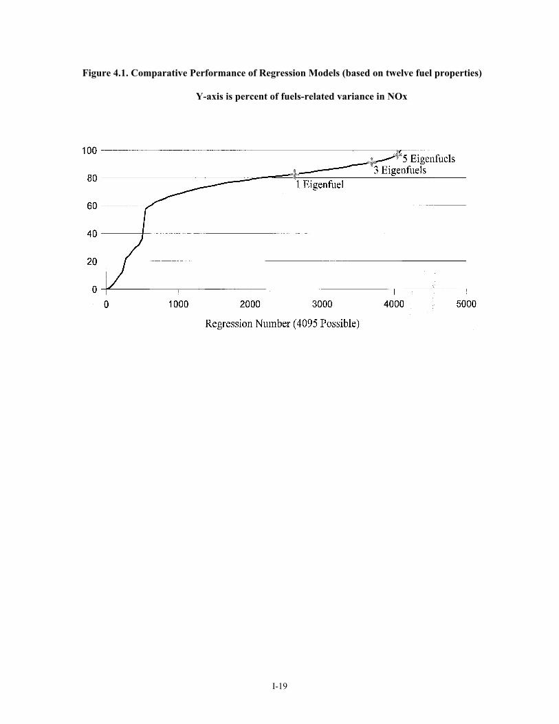
I-19
Figure 4.1. Comparative Performance of Regression Models (based on twelve fuel properties)
Y-axis is percent of fuels-related variance in NOx

I-21
I-5. CALIBRATION AND DEMONSTRATION
I-5.1 CALIBRATION CRITERIA
Prior to executing the study cases, we calibrated ORNL-RYM2002 for approximate replication of PADD II year2000 summer data for gasoline and distillate production and process utilization. These model adjustmentswere then used in the study cases themselves. The calibration criteria included the following:
Crude Oil: Model-derived crude oil sulfur content and gravity were to be within 10 percent of the year2000 data source (DOE 2001b).
Process Utilization: The NPC (1993) criterion of “maximum variance of ±8 percent” was used forutilization of the four process types reported in the year 2000 data source (DOE 2001b).
Gasoline: Model-derived gasoline volume and property values were to be either (1) within 10 percentof the data source (EPA 2002), or (2) within the calibration criteria percentages reported by MathProin “U.S. Petroleum Refining” (NPC 2000).
Distillates: API/NRPA (1997) distillate quality information may be outdated for a year 2000 distillateproperty calibration. However, shadow values for distillate products were evaluated, based on the NPC(1993) criterion of a maximum variance of ±20 percent, in comparison with refiner prices for productsreported for year 2000 (DOE 2002a).
I-5.2 CALIBRATION ADJUSTMENTS
Data sources and inputs (without extrapolation to a future year) for the calibration are listed in the SectionI-3 premises. The required adjustments in ORNL-RYM2002 were determined to be:
Fix distillation properties of gasolines to approximate historical values. This adjustment objective issimilar to distillation curve calibration performed by MathPro in NPC (2000).
Scale aromatics blending values of gasoline blendstocks by 0.93 (except for high aromaticsblendstocks). ORNL-RYM2002 blendstock property values are primarily based on PADD III (U.S. GulfCoast) data, and adjustments are required for modeling other regions. API/NRPA (1997) reported thatthe gasoline pool aromatics content for PADD II was 0.92 of the gasoline pool aromatics content forPADD III.
Scale olefin blending values of gasoline blendstocks by 0.65 (except for high olefin blendstocks).ORNL-RYM2002 blendstock property values are primarily based on PADD III data, and adjustments arerequired for modeling other regions. API/NRPA (1997) reported that the gasoline pool olefins contentfor PADD II was 0.81 of the gasoline pool olefins content for PADD III.
Apply blending ratio controls to FCC gasoline blendstocks. In the year 2000 calibration, ratio controlsare also applied to FCC gasoline feed to the FCC gasoline splitter and to light and heavy FCC gasolineblended to finished gasolines. These ratios result in a reasonable distribution of olefins over differentgasoline types.
In the year 2000 calibration, production constraints were relaxed by targeting product outputs (gasolines anddiesel fuels) at ±5 percent of the observed year 2000 levels.
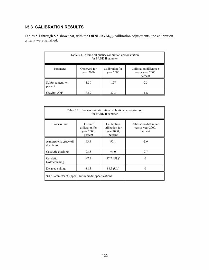
I-22
I-5.3 CALIBRATION RESULTS
Tables 5.1 through 5.5 show that, with the ORNL-RYM2002 calibration adjustments, the calibrationcriteria were satisfied.
Table 5.1. Crude oil quality calibration demonstrationfor PADD II summer
Parameter Observed foryear 2000
Calibration foryear 2000
Calibration differenceversus year 2000,
percent
Sulfur content, wtpercent
1.30 1.27 -2.3
Gravity, APIo 32.9 32.3 -1.8
Table 5.2. Process unit utilization calibration demonstrationfor PADD II summer
Process unit Observedutilization for
year 2000,percent
Calibrationutilization for
year 2000,percent
Calibration differenceversus year 2000,
percent
Atmospheric crude oildistillation
93.4 90.1 -3.6
Catalytic cracking 93.5 91.0 -2.7
Catalytichydrocracking
97.7 97.7 (UL)a 0
Delayed coking 88.5 88.5 (UL) 0
aUL: Parameter at upper limit in model specifications.
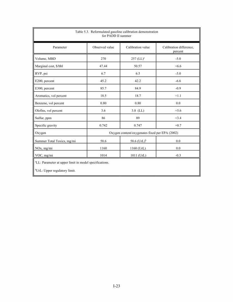
I-23
Table 5.3. Reformulated gasoline calibration demonstrationfor PADD II summer
Parameter Observed value Calibration value Calibration difference,percent
Volume, MBD 270 257 (LL)a -5.0
Marginal cost, $/bbl 47.44 50.57 +6.6
RVP, psi 6.7 6.5 -3.0
E200, percent 45.2 42.2 -6.6
E300, percent 85.7 84.9 -0.9
Aromatics, vol percent 18.5 18.7 +1.1
Benzene, vol percent 0.80 0.80 0.0
Olefins, vol percent 3.6 3.8 (LL) +5.6
Sulfur, ppm 86 89 +3.4
Specific gravity 0.742 0.747 +0.7
Oxygen Oxygen content/oxygenates fixed per EPA (2002)
Summer Total Toxics, mg/mi 58.6 58.6 (UrL)b 0.0
NOx, mg/mi 1160 1160 (UrL) 0.0
VOC, mg/mi 1014 1011 (UrL) -0.3
aLL: Parameter at upper limit in model specifications.
bUrL: Upper regulatory limit.
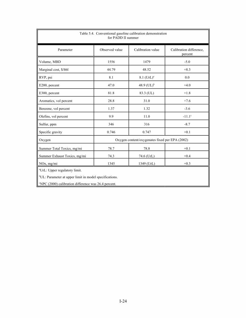
I-24
Table 5.4. Conventional gasoline calibration demonstrationfor PADD II summer
Parameter Observed value Calibration value Calibration difference,percent
Volume, MBD 1556 1479 -5.0
Marginal cost, $/bbl 44.79 48.52 +8.3
RVP, psi 8.1 8.1 (UrL)a 0.0
E200, percent 47.0 48.9 (UL)b +4.0
E300, percent 81.8 83.3 (UL) +1.8
Aromatics, vol percent 28.8 31.0 +7.6
Benzene, vol percent 1.37 1.32 -3.6
Olefins, vol percent 9.9 11.0 -11.1c
Sulfur, ppm 346 316 -8.7
Specific gravity 0.746 0.747 +0.1
Oxygen Oxygen content/oxygenates fixed per EPA (2002)
Summer Total Toxics, mg/mi 78.7 78.8 +0.1
Summer Exhaust Toxics, mg/mi 74.3 74.6 (UrL) +0.4
NOx, mg/mi 1345 1349 (UrL) +0.3aUrL: Upper regulatory limit.bUL: Parameter at upper limit in model specifications. cNPC (2000) calibration difference was 26.4 percent.

I-25
Table 5.5. Distillate calibration demonstrationfor PADD II summer
Parameter Observed value2000
Calibration valuefor year 2000
Calibration differenceversus year 2000,
percent
Jet A
Volume, MBD 235.5 223.7 -5.0
Marginal cost, $/bbl 36.70 40.86 +11.3
On-road diesel fuel
Volume, MBD 680.2 688.8 +1.3
Marginal cost, $/bbl 38.11 38.11 0.0
Home heating oil
Volume, MBD 19.3 20.28 +5.0
Marginal cost, $/bbl 38.05 33.48 -12.0
Railroad diesel fuel
Volume, MBD 13.5 14.14 +4.7
Marginal cost, $/bbl 38.05 30.45 -20.0
Other off-road diesel fuel
Volume, MBD 177.0 185.9 +5.0
Marginal cost, $/bbl 38.05 31.30 -17.7


I-27
I-6. IMPACTS OF DIESEL FUEL REFORMULATION IN PADD II REFINERIES
The diesel fuel reformulation study estimates the refining impacts of different pathways for reformulation andrefinery investment in PADD II, for summer operations in year 2010. Cost, product quality, operational, andinvestment impacts are determined for the different pathways provided by the cases listed in Table 6.1. Thissection presents detailed refinery modeling results for the cases.
Table 6.1. Diesel fuel reformulation case studies for PADD II in summer 2010
Case On-road diesel upgrading pathway
Base Case 1 •Low sulfur•Investment as required
Case 1.1 •ULSD•Reformulated for vehicle performance•Early notice of requirements•Parallel investment
Case 1.2 •ULSD•Reformulated for emissions reduction•Early notice of requirements•Parallel investment
Base Case 2 •ULSD•Sequential investment (step 1)•Some newer technologies
Case 2.1 •ULSD•Reformulated for vehicle performance•Delayed notice of requirements•Sequential investment (step 2)
Case 2.2 •ULSD•Reformulated for emissions reduction•Delayed notice of requirements•Sequential investment (step 2)
I-6.1 BASE CASE 1: LOW SULFUR DIESEL FUEL
Base Case 1 is one of two base cases used as references to show comparative and cumulative impacts ofdifferent reformulation and investment pathways. In Base Case 1, on-road diesel fuel must satisfy current(year 2002) requirements for sulfur content (500 ppm maximum) and cetane number (40 minimum), and thereare no requirements for aromatics and emissions quality. However, Base Case 1 is not representative ofcurrent quality requirements for off-road diesel fuels (with home heating oil included), which have premisedsulfur specifications of 500 ppm maximum. By using this off-road sulfur specification in all cases, we haveintentionally removed a variable from the study. Key results for Base Case 1 and all other cases aresummarized in Tables 6.2 through 6.15, which show:
I-28
Overall model results for calculation of cost change (Table 6.2)Properties of diesel fuels (Table 6.3)Properties of diesel fuels, by desulfurization technology (Table 6.4)Blendstocks for diesel fuels (Tables 6.5)Properties of gasolines (Table 6.6)Blendstocks for gasoline (Table 6.7)Pooled blendstocks for gasoline (Table 6.8)Raw material and product volume balance (Table 6.9)Hydrogen balance and utilization of key process units (Table 6.10)Process investments (Tables 6.11and 6.12)Components of cost changes (Table 6.13)Quality of crude oil processed (Table 6.14)Energy use changes (Table 6.15)
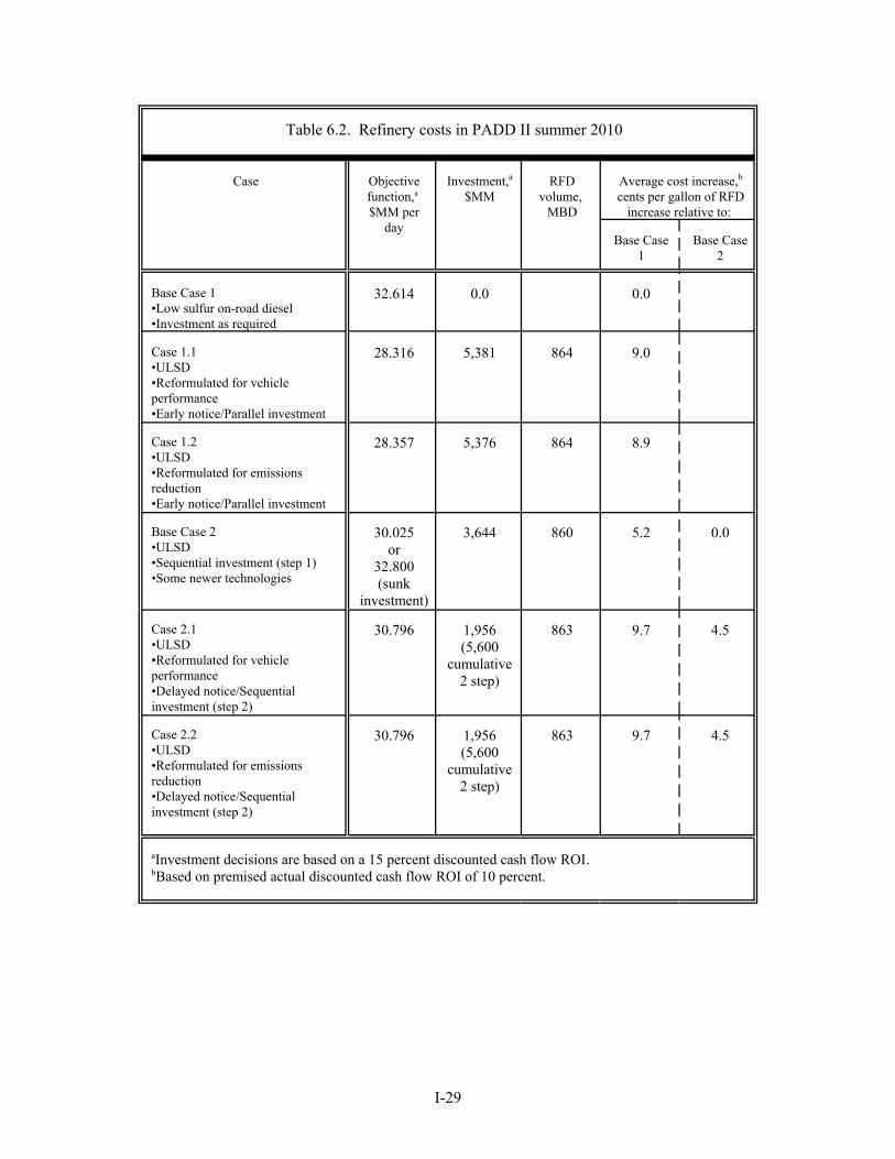
I-29
Table 6.2. Refinery costs in PADD II summer 2010
Case Objectivefunction,a $MM per
day
Investment,a$MM
RFDvolume,
MBD
Average cost increase,bcents per gallon of RFD
increase relative to:
Base Case1
Base Case2
Base Case 1•Low sulfur on-road diesel•Investment as required
32.614 0.0 0.0
Case 1.1•ULSD•Reformulated for vehicleperformance•Early notice/Parallel investment
28.316 5,381 864 9.0
Case 1.2•ULSD•Reformulated for emissionsreduction•Early notice/Parallel investment
28.357 5,376 864 8.9
Base Case 2•ULSD•Sequential investment (step 1)•Some newer technologies
30.025or
32.800(sunk
investment)
3,644 860 5.2 0.0
Case 2.1•ULSD•Reformulated for vehicleperformance•Delayed notice/Sequentialinvestment (step 2)
30.796 1,956(5,600
cumulative2 step)
863 9.7 4.5
Case 2.2•ULSD•Reformulated for emissionsreduction•Delayed notice/Sequentialinvestment (step 2)
30.796 1,956(5,600
cumulative2 step)
863 9.7 4.5
aInvestment decisions are based on a 15 percent discounted cash flow ROI.bBased on premised actual discounted cash flow ROI of 10 percent.

I-30
Table 6.3. Properties of diesel fuels in PADD II summer 2010
Property Base Case 1•Low sulfur on-road diesel•Investment as required
Case 1.1•ULSD•Reformulated for vehicleperformance•Parallel investment
On-road
Rail-road
OtherOff-road
HeatingOil
On-road
Rail-road
OtherOff-road
HeatingOil
Volume, MBD 844 17 221 24 864 17 218 24
API Gravity, oAPI 35.9 37.5 35.7 37.1 39.2 34.6 33.9 33.0
Specific gravity .8450 .8291
Sulfur, ppm 350 350 350 350 8 260 330 350
Cetane Index 48.5 53.5
Cetane Number, clear 44.9 51.5
Cetane Improver,vol%
.000 .122
Cetane Improver,number increase
0.0 7.3
Cetane Number, total 44.9 58.8
Aromatics, vol% 26.8 21.6 24.6 22.4 12.5 23.1 29.9 28.3
Viscosity, cSt 2.65 2.76
ASTM IBP, oFa 377 375
T10 436 421 442 437 434 421 440 439
T30 463 453 475 468 463 453 473 466
T50 499 494 512 499 492 493 508 504
T70 549 538 556 538 539 539 554 550
T90 589 585 593 588 591 611 612 591
FBPa 633 635
NOx change, %b -0.7 -8.3
PM change, %b -2.4 -19.8aIBP and FBP are based on survey reports of differences relative to T10 and T90 (NIPER 1994).bRelative to commercial fuel (Table 4.1 of Part II), with adjustment for future fleet change (see II-5.1).
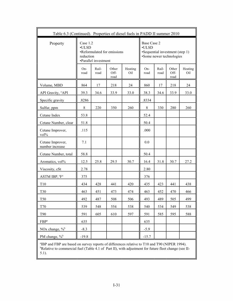
I-31
Table 6.3 (Continued). Properties of diesel fuels in PADD II summer 2010
Property Case 1.2•ULSD•Reformulated for emissionsreduction•Parallel investment
Base Case 2•ULSD•Sequential investment (step 1)•Some newer technologies
On-road
Rail-road
OtherOff-road
HeatingOil
On-road
Rail-road
OtherOff-road
HeatingOil
Volume, MBD 864 17 218 24 860 17 218 24
API Gravity, oAPI 39.3 34.6 33.9 33.0 38.3 34.6 33.9 33.0
Specific gravity .8286 .8334
Sulfur, ppm 8 220 350 260 8 330 280 260
Cetane Index 53.8 52.4
Cetane Number, clear 51.8 50.4
Cetane Improver,vol%
.115 .000
Cetane Improver,number increase
7.1 0.0
Cetane Number, total 58.8 50.4
Aromatics, vol% 12.5 25.8 29.5 30.7 16.4 31.8 30.7 27.2
Viscosity, cSt 2.78 2.80
ASTM IBP, oFa 375 376
T10 434 428 441 420 435 423 441 438
T30 463 451 473 474 463 452 470 466
T50 492 487 508 506 493 489 505 499
T70 539 548 554 538 540 534 549 538
T90 591 605 610 597 591 585 595 588
FBPa 635 635
NOx change, %b -8.3 -5.9
PM change, %b -19.8 -15.7aIBP and FBP are based on survey reports of differences relative to T10 and T90 (NIPER 1994).bRelative to commercial fuel (Table 4.1 of Part II), with adjustment for future fleet change (see II-5.1).
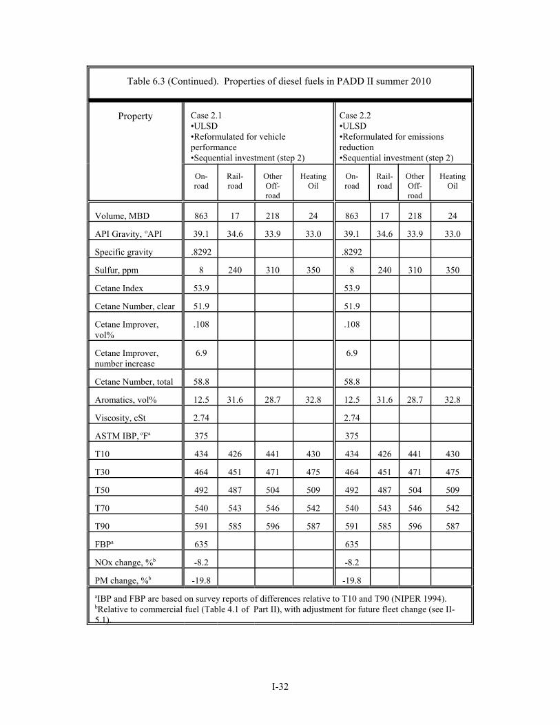
I-32
Table 6.3 (Continued). Properties of diesel fuels in PADD II summer 2010
Property Case 2.1•ULSD•Reformulated for vehicleperformance•Sequential investment (step 2)
Case 2.2•ULSD•Reformulated for emissionsreduction•Sequential investment (step 2)
On-road
Rail-road
OtherOff-road
HeatingOil
On-road
Rail-road
OtherOff-road
HeatingOil
Volume, MBD 863 17 218 24 863 17 218 24
API Gravity, oAPI 39.1 34.6 33.9 33.0 39.1 34.6 33.9 33.0
Specific gravity .8292 .8292
Sulfur, ppm 8 240 310 350 8 240 310 350
Cetane Index 53.9 53.9
Cetane Number, clear 51.9 51.9
Cetane Improver,vol%
.108 .108
Cetane Improver,number increase
6.9 6.9
Cetane Number, total 58.8 58.8
Aromatics, vol% 12.5 31.6 28.7 32.8 12.5 31.6 28.7 32.8
Viscosity, cSt 2.74 2.74
ASTM IBP, oFa 375 375
T10 434 426 441 430 434 426 441 430
T30 464 451 471 475 464 451 471 475
T50 492 487 504 509 492 487 504 509
T70 540 543 546 542 540 543 546 542
T90 591 585 596 587 591 585 596 587
FBPa 635 635
NOx change, %b -8.2 -8.2
PM change, %b -19.8 -19.8aIBP and FBP are based on survey reports of differences relative to T10 and T90 (NIPER 1994).bRelative to commercial fuel (Table 4.1 of Part II), with adjustment for future fleet change (see II-5.1).
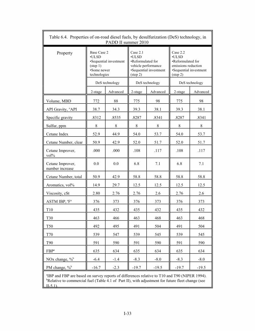
I-33
Table 6.4. Properties of on-road diesel fuels, by desulfurization (DeS) technology, inPADD II summer 2010
Property Base Case 2•ULSD•Sequential investment(step 1)•Some newertechnologies
Case 2.1•ULSD•Reformulated forvehicle performance•Sequential investment(step 2)
Case 2.2•ULSD•Reformulated foremissions reduction•Sequential investment(step 2)
DeS technology DeS technology DeS technology
2-stage Advanced 2-stage Advanced 2-stage Advanced
Volume, MBD 772 88 775 98 775 98
API Gravity, oAPI 38.7 34.3 39.3 38.1 39.3 38.1
Specific gravity .8312 .8535 .8287 .8341 .8287 .8341
Sulfur, ppm 8 8 8 8 8 8
Cetane Index 52.9 44.9 54.0 53.7 54.0 53.7
Cetane Number, clear 50.9 42.9 52.0 51.7 52.0 51.7
Cetane Improver,vol%
.000 .000 .108 .117 .108 .117
Cetane Improver,number increase
0.0 0.0 6.8 7.1 6.8 7.1
Cetane Number, total 50.9 42.9 58.8 58.8 58.8 58.8
Aromatics, vol% 14.9 29.7 12.5 12.5 12.5 12.5
Viscosity, cSt 2.80 2.76 2.76 2.6 2.76 2.6
ASTM IBP, oFa 376 373 376 373 376 373
T10 435 432 435 432 435 432
T30 463 466 463 468 463 468
T50 492 495 491 504 491 504
T70 539 547 539 545 539 545
T90 591 590 591 590 591 590
FBPa 635 634 635 634 635 634
NOx change, %b -6.4 -1.4 -8.3 -8.0 -8.3 -8.0
PM change, %b -16.7 -2.3 -19.7 -19.5 -19.7 -19.5aIBP and FBP are based on survey reports of differences relative to T10 and T90 (NIPER 1994).bRelative to commercial fuel (Table 4.1 of Part II), with adjustment for future fleet change (seeII-5.1).
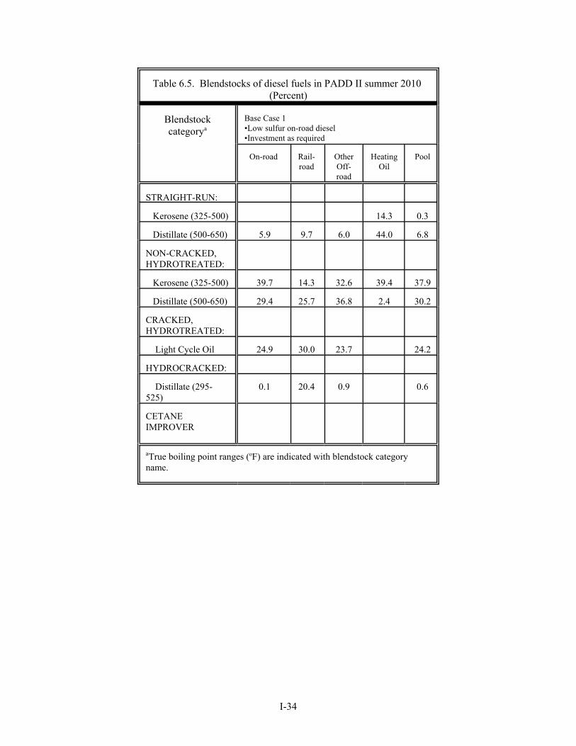
I-34
Table 6.5. Blendstocks of diesel fuels in PADD II summer 2010 (Percent)
Blendstockcategorya
Base Case 1•Low sulfur on-road diesel•Investment as required
On-road Rail-road
OtherOff-road
HeatingOil
Pool
STRAIGHT-RUN:
Kerosene (325-500) 14.3 0.3
Distillate (500-650) 5.9 9.7 6.0 44.0 6.8
NON-CRACKED,HYDROTREATED:
Kerosene (325-500) 39.7 14.3 32.6 39.4 37.9
Distillate (500-650) 29.4 25.7 36.8 2.4 30.2
CRACKED,HYDROTREATED:
Light Cycle Oil 24.9 30.0 23.7 24.2
HYDROCRACKED:
Distillate (295-525)
0.1 20.4 0.9 0.6
CETANEIMPROVER
aTrue boiling point ranges (oF) are indicated with blendstock categoryname.

I-35
Table 6.5 (Continued). Blendstocks of diesel fuels in PADD II summer 2010 (Percent)
Blendstockcategorya
Case 1.1•ULSD•Reformulated for vehicle performance•Parallel investment
On-roadfrom
2-stage
On-road fromadvanced
DeS
Rail-road
OtherOff-road
HeatingOil
Pool
STRAIGHT-RUN:
Kerosene (325-500)
Distillate (500-650)
NON-CRACKED,HYDROTREATED:
Kerosene (325-500) 45.7 14.3 25.4 34.4 41.0
Distillate (500-650) 39.4 35.4 40.0 35.6 39.4
CRACKED,HYDROTREATED:
Light Cycle Oil 14.7 30.0 30.0 30.0 18.2
HYDROCRACKED:
Distillate (295-525)
20.4 4.6 1.2
CETANEIMPROVER
0.12 0.09
aTrue boiling point ranges (oF) are indicated with blendstock category name.
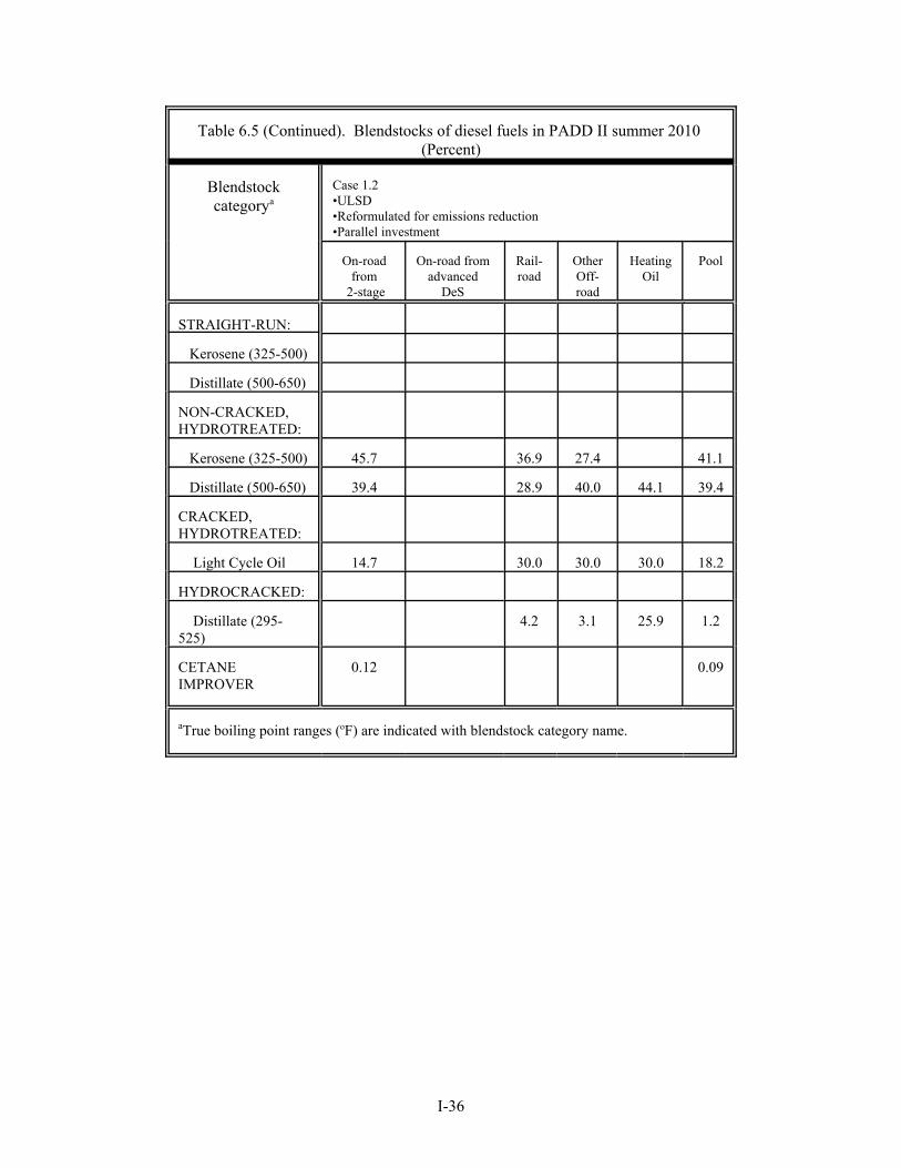
I-36
Table 6.5 (Continued). Blendstocks of diesel fuels in PADD II summer 2010 (Percent)
Blendstockcategorya
Case 1.2•ULSD•Reformulated for emissions reduction•Parallel investment
On-roadfrom
2-stage
On-road fromadvanced
DeS
Rail-road
OtherOff-road
HeatingOil
Pool
STRAIGHT-RUN:
Kerosene (325-500)
Distillate (500-650)
NON-CRACKED,HYDROTREATED:
Kerosene (325-500) 45.7 36.9 27.4 41.1
Distillate (500-650) 39.4 28.9 40.0 44.1 39.4
CRACKED,HYDROTREATED:
Light Cycle Oil 14.7 30.0 30.0 30.0 18.2
HYDROCRACKED:
Distillate (295-525)
4.2 3.1 25.9 1.2
CETANEIMPROVER
0.12 0.09
aTrue boiling point ranges (oF) are indicated with blendstock category name.
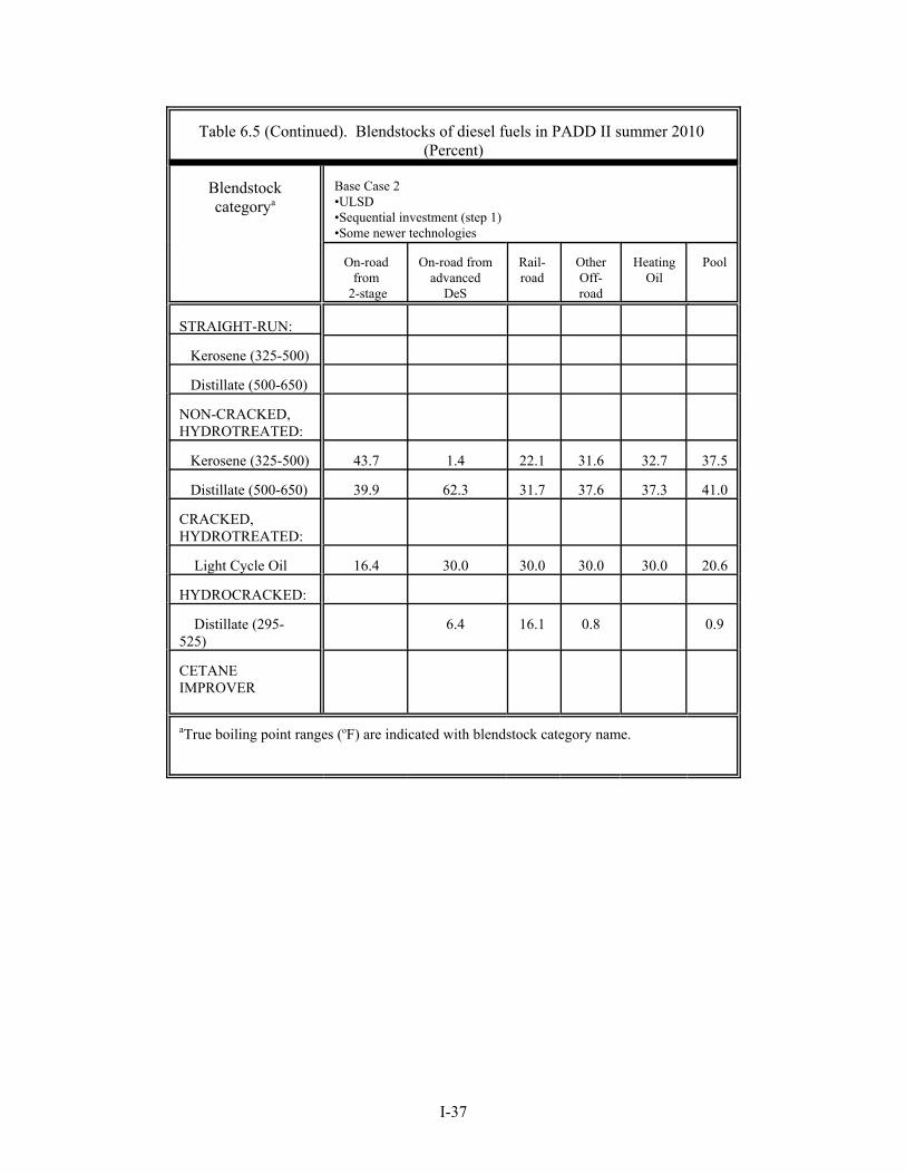
I-37
Table 6.5 (Continued). Blendstocks of diesel fuels in PADD II summer 2010 (Percent)
Blendstockcategorya
Base Case 2•ULSD•Sequential investment (step 1)•Some newer technologies
On-roadfrom
2-stage
On-road fromadvanced
DeS
Rail-road
OtherOff-road
HeatingOil
Pool
STRAIGHT-RUN:
Kerosene (325-500)
Distillate (500-650)
NON-CRACKED,HYDROTREATED:
Kerosene (325-500) 43.7 1.4 22.1 31.6 32.7 37.5
Distillate (500-650) 39.9 62.3 31.7 37.6 37.3 41.0
CRACKED,HYDROTREATED:
Light Cycle Oil 16.4 30.0 30.0 30.0 30.0 20.6
HYDROCRACKED:
Distillate (295-525)
6.4 16.1 0.8 0.9
CETANEIMPROVER
aTrue boiling point ranges (oF) are indicated with blendstock category name.
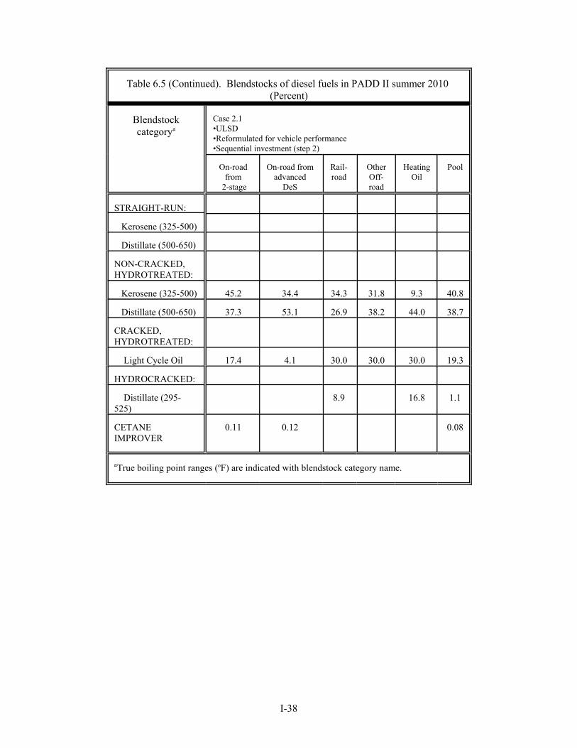
I-38
Table 6.5 (Continued). Blendstocks of diesel fuels in PADD II summer 2010 (Percent)
Blendstockcategorya
Case 2.1•ULSD•Reformulated for vehicle performance•Sequential investment (step 2)
On-roadfrom
2-stage
On-road fromadvanced
DeS
Rail-road
OtherOff-road
HeatingOil
Pool
STRAIGHT-RUN:
Kerosene (325-500)
Distillate (500-650)
NON-CRACKED,HYDROTREATED:
Kerosene (325-500) 45.2 34.4 34.3 31.8 9.3 40.8
Distillate (500-650) 37.3 53.1 26.9 38.2 44.0 38.7
CRACKED,HYDROTREATED:
Light Cycle Oil 17.4 4.1 30.0 30.0 30.0 19.3
HYDROCRACKED:
Distillate (295-525)
8.9 16.8 1.1
CETANEIMPROVER
0.11 0.12 0.08
aTrue boiling point ranges (oF) are indicated with blendstock category name.

I-39
Table 6.5 (Continued). Blendstocks of diesel fuels in PADD II summer 2010 (Percent)
Blendstockcategorya
Case 2.2•ULSD•Reformulated for emissions reduction•Sequential investment (step 2)
On-roadfrom
2-stage
On-road fromadvanced
DeS
Rail-road
OtherOff-road
HeatingOil
Pool
STRAIGHT-RUN:
Kerosene (325-500)
Distillate (500-650)
NON-CRACKED,HYDROTREATED:
Kerosene (325-500) 45.2 34.4 34.3 31.8 9.3 40.8
Distillate (500-650) 37.3 53.1 26.9 38.2 44.0 38.7
CRACKED,HYDROTREATED:
Light Cycle Oil 17.4 4.1 30.0 30.0 30.0 19.3
HYDROCRACKED:
Distillate (295-525)
8.9 16.8 1.1
CETANEIMPROVER
0.11 0.12 0.08
aTrue boiling point ranges (oF) are indicated with blendstock category name.

I-40
Table 6.6. Properties of gasolines in PADD II summer 2010
Property Base Case 1•Low sulfur on-road diesel•Investment as required
Case 1.1•ULSD•Reformulated for vehicleperformance•Parallel investment
CG CG/EtOH
RFG CG CG/EtOH
RFG
Volume, MBD 1132 880 330.7 1132 880 330.7
Octane, (R+M)/2 88.1 88.1 88.7 88.1 88.1 88.7
RVP, psi 8.3 9.3 6.6 8.3 9.3 6.5
Aromatics, vol % 32.4 29.8 30.6 31.8 29.5 31.0
Benzene, vol % 1.68 2.44 0.90 1.74 2.41 0.90
Olefins, vol % 5.1 3.8 6.9 4.6 4.9 4.3
Sulfur, ppm 30 30 30 30 30 30
E200, % 42.6 61.2 50.9 43.1 59.2 50.9
E300, % 81.1 85.1 87.5 81.1 85.5 88.8
Oxygen, wt % 0.00 3.48 3.47 0.00 3.47 3.47
Specific gravity .7546 .7552 .7581 .7519 .7573 .7587
Summer total TAP,mg/mi
63.1a 63.1a
Summer exhaust TAP,mg/mi
73.4a 73.5a 73.4a 73.2a
NOx, mg/mi 1176 1189 1172 1176 1186 1168
VOC, mg/mi 1302 1432 993a 1299 1429 994a
aBinding emissions constraint.

I-41
Table 6.6 (Continued). Properties of gasolines in PADD II summer 2010
Property Case 1.2•ULSD•Reformulated for emissionsreduction•Parallel investment
Base Case 2•ULSD•Sequential investment (step 1)•Some newer technologies
CG CG/EtOH
RFG CG CG/EtOH
RFG
Volume, MBD 1132 880 330.7 1132 880 330.7
Octane, (R+M)/2 88.1 88.1 88.7 88.1 88.1 88.7
RVP, psi 8.3 9.3 6.6 8.3 9.3 6.6
Aromatics, vol % 32.4 28.9 30.9 33.3 26.8 30.5
Benzene, vol % 1.70 2.50 0.90 1.62 2.63 0.90
Olefins, vol % 4.5 4.9 4.7 4.6 5.0 6.8
Sulfur, ppm 30 30 30 30 30 30
E200, % 43.0 61.7 50.9 42.9 60.9 51.0
E300, % 80.7 85.3 88.8 80.8 85.4 88.0
Oxygen, wt % 0.00 3.47 3.47 0.00 3.49 3.47
Specific gravity .7522 .7569 .7587 .7530 .7538 .7587
Summer total TAP,mg/mi
63.1a 63.0a
Summer exhaust TAP,mg/mi
73.4 a 73.3a 73.2a 73.3a
NOx, mg/mi 1176 1188 1168 1177 1182 1172
VOC, mg/mi 1305 1427 993 1307 1421 993a
aBinding emissions constraint.
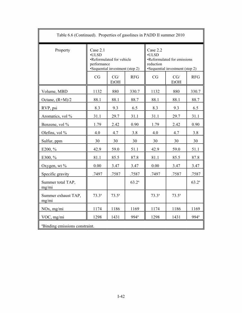
I-42
Table 6.6 (Continued). Properties of gasolines in PADD II summer 2010
Property Case 2.1•ULSD•Reformulated for vehicleperformance•Sequential investment (step 2)
Case 2.2•ULSD•Reformulated for emissionsreduction•Sequential investment (step 2)
CG CG/EtOH
RFG CG CG/EtOH
RFG
Volume, MBD 1132 880 330.7 1132 880 330.7
Octane, (R+M)/2 88.1 88.1 88.7 88.1 88.1 88.7
RVP, psi 8.3 9.3 6.5 8.3 9.3 6.5
Aromatics, vol % 31.1 29.7 31.1 31.1 29.7 31.1
Benzene, vol % 1.79 2.42 0.90 1.79 2.42 0.90
Olefins, vol % 4.0 4.7 3.8 4.0 4.7 3.8
Sulfur, ppm 30 30 30 30 30 30
E200, % 42.9 59.0 51.1 42.9 59.0 51.1
E300, % 81.1 85.5 87.8 81.1 85.5 87.8
Oxygen, wt % 0.00 3.47 3.47 0.00 3.47 3.47
Specific gravity .7497 .7587 .7587 .7497 .7587 .7587
Summer total TAP,mg/mi
63.2a 63.2a
Summer exhaust TAP,mg/mi
73.3a 73.5a 73.3a 73.5a
NOx, mg/mi 1174 1186 1169 1174 1186 1169
VOC, mg/mi 1298 1431 994a 1298 1431 994a
aBinding emissions constraint.
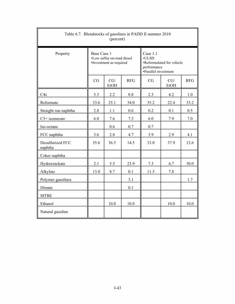
I-43
Table 6.7. Blendstocks of gasolines in PADD II summer 2010(percent)
Property Base Case 1•Low sulfur on-road diesel•Investment as required
Case 1.1•ULSD•Reformulated for vehicleperformance•Parallel investment
CG CG/EtOH
RFG CG CG/EtOH
RFG
C4s 3.3 2.2 0.8 2.3 4.2 1.0
Reformate 33.6 25.1 34.0 35.2 22.4 33.2
Straight run naphtha 2.8 1.1 0.6 0.2 0.1 0.5
C5+ isomerate 6.0 7.6 7.5 6.0 7.9 7.0
Iso-octane 0.6 0.7 0.7
FCC naphtha 3.6 2.8 4.7 3.9 2.9 4.1
Desulfurized FCCnaphtha
35.6 36.5 14.5 33.0 37.9 12.6
Coker naphtha
Hydrocrackate 2.1 5.5 23.9 7.3 6.7 30.0
Alkylate 13.0 8.7 0.1 11.5 7.8
Polymer gasolines 3.1 1.7
Dimate 0.1
MTBE
Ethanol 10.0 10.0 10.0 10.0
Natural gasoline

I-44
Table 6.7 (Continued). Blendstocks of gasolines in PADD II summer 2010 (percent)
Property Case 1.2•ULSD•Reformulated for emissionsreduction•Parallel investment
Base Case 2•ULSD•Sequential investment (step 1)•Some newer technologies
CG CG/EtOH
RFG CG CG/EtOH
RFG
C4s 2.7 3.9 1.0 3.2 2.8 0.8
Reformate 31.9 26.5 33.7 31.8 22.3 37.5
Straight run naphtha 0.2 0.4 4.1 1.1
C5+ isomerate 7.7 5.8 6.7 9.1 3.6 7.7
Iso-octane 0.7 0.7
FCC naphtha 4.5 2.1 4.2 5.5 1.5 5.0
Desulfurized FCCnaphtha
33.6 40.0 12.6 32.3 38.7 11.5
Coker naphtha
Hydrocrackate 9.8 0.9 29.4 7.8 4.2 23.3
Alkylate 9.0 10.9 9.6 12.9
Polymer gasolines 2.1 3.1
Dimate
MTBE
Ethanol 10.0 10.0 10.0 10.0
Natural gasoline
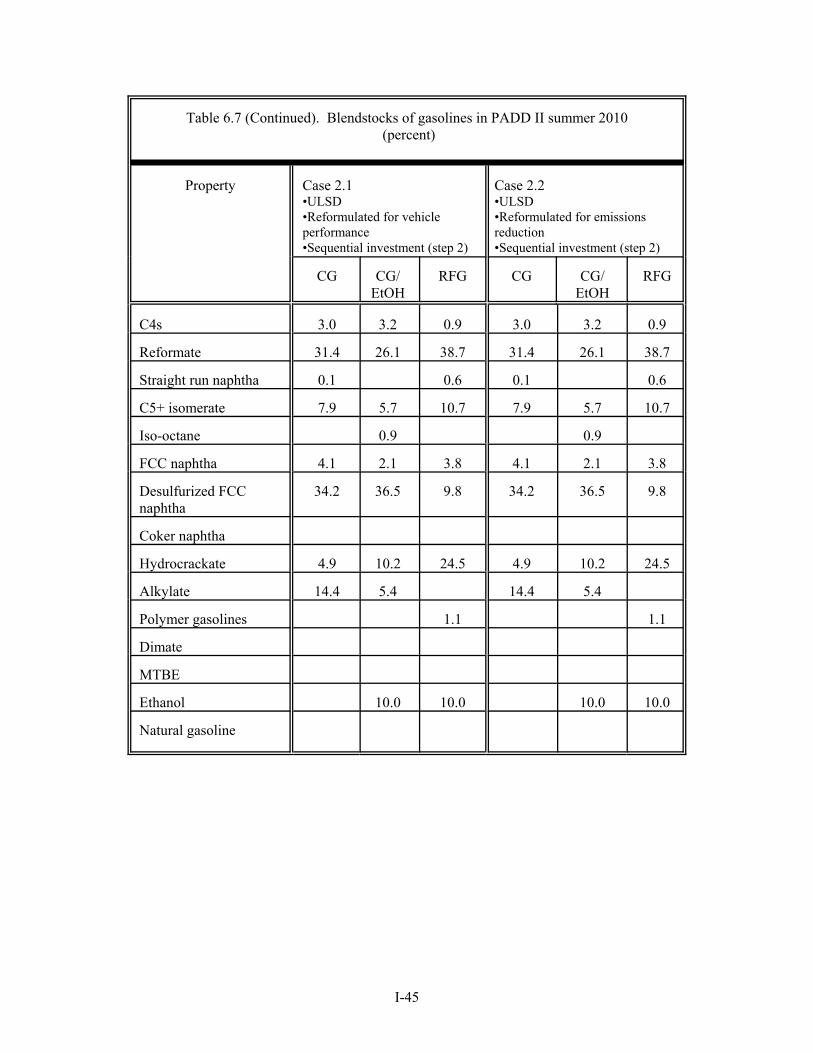
I-45
Table 6.7 (Continued). Blendstocks of gasolines in PADD II summer 2010 (percent)
Property Case 2.1•ULSD•Reformulated for vehicleperformance•Sequential investment (step 2)
Case 2.2•ULSD•Reformulated for emissionsreduction•Sequential investment (step 2)
CG CG/EtOH
RFG CG CG/EtOH
RFG
C4s 3.0 3.2 0.9 3.0 3.2 0.9
Reformate 31.4 26.1 38.7 31.4 26.1 38.7
Straight run naphtha 0.1 0.6 0.1 0.6
C5+ isomerate 7.9 5.7 10.7 7.9 5.7 10.7
Iso-octane 0.9 0.9
FCC naphtha 4.1 2.1 3.8 4.1 2.1 3.8
Desulfurized FCCnaphtha
34.2 36.5 9.8 34.2 36.5 9.8
Coker naphtha
Hydrocrackate 4.9 10.2 24.5 4.9 10.2 24.5
Alkylate 14.4 5.4 14.4 5.4
Polymer gasolines 1.1 1.1
Dimate
MTBE
Ethanol 10.0 10.0 10.0 10.0
Natural gasoline
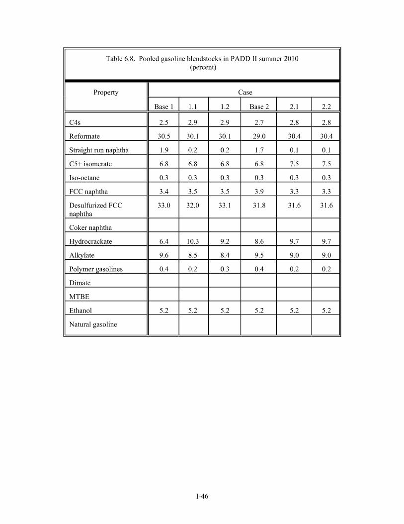
I-46
Table 6.8. Pooled gasoline blendstocks in PADD II summer 2010 (percent)
Property Case
Base 1 1.1 1.2 Base 2 2.1 2.2
C4s 2.5 2.9 2.9 2.7 2.8 2.8
Reformate 30.5 30.1 30.1 29.0 30.4 30.4
Straight run naphtha 1.9 0.2 0.2 1.7 0.1 0.1
C5+ isomerate 6.8 6.8 6.8 6.8 7.5 7.5
Iso-octane 0.3 0.3 0.3 0.3 0.3 0.3
FCC naphtha 3.4 3.5 3.5 3.9 3.3 3.3
Desulfurized FCCnaphtha
33.0 32.0 33.1 31.8 31.6 31.6
Coker naphtha
Hydrocrackate 6.4 10.3 9.2 8.6 9.7 9.7
Alkylate 9.6 8.5 8.4 9.5 9.0 9.0
Polymer gasolines 0.4 0.2 0.3 0.4 0.2 0.2
Dimate
MTBE
Ethanol 5.2 5.2 5.2 5.2 5.2 5.2
Natural gasoline
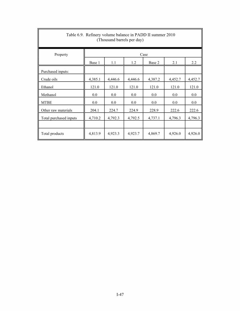
I-47
Table 6.9. Refinery volume balance in PADD II summer 2010(Thousand barrels per day)
Property Case
Base 1 1.1 1.2 Base 2 2.1 2.2
Purchased inputs:
Crude oils 4,385.1 4,446.6 4,446.6 4,387.2 4,452.7 4,452.7
Ethanol 121.0 121.0 121.0 121.0 121.0 121.0
Methanol 0.0 0.0 0.0 0.0 0.0 0.0
MTBE 0.0 0.0 0.0 0.0 0.0 0.0
Other raw materials 204.1 224.7 224.9 228.9 222.6 222.6
Total purchased inputs 4,710.2 4,792.3 4,792.5 4,737.1 4,796.3 4,796.3
Total products 4,813.9 4,923.3 4,923.7 4,869.7 4,926.0 4,926.0

I-48
Table 6.10. Hydrogen balance for PADD II refineriesEntry at top of cell is fuel oil equivalent barrels of hydrogen per day
(minus sign indicates consumption)Entry at bottom of cell is process unit utilization
(calendar rate divided by stream day capacity x 100 percent)
ProcessCase
Base 1a
•Low sulfur on-roaddiesel•Investment as required
1.1a
•ULSD•Reformulated forvehicle performance•Parallel investment
1.2a
•ULSD•Reformulated foremissions reduction•Parallel investment
Naphtha hydrotreating -3,277 -2,308 -2,323
(87.0) (83.1) (83.1)
FCC gasolinedesulfurization
-5,639 -5,654 -5,653
(87.9) (87.9) (87.9)
Distillate desulfurization -10,680 -20,915 -20,545
(86.6) (175) (174)
Distillate dearomatization -2,309 -2,759
(New capacity) (New capacity)
FCC feed hydrofining -8,514 -8,529 -8,529
(87.0) (87.0) (87.0)
Gas oil hydrocracking -31,412 -37,228 -37,189
(80.3) (97.4) (97.3)
Reforming +38,186 +37,796 +37,845
(79.8) (80.3) (80.4)
C4 isomerization -44 -44 -44
(84.0) (84.0) (84.0)
C5/C6 isomerization -330 -330 -330
(84.0) (84.0) (84.0)
Iso-octane -316 -316 -316
(93.0) (93.0) (93.0)
Hydrogen production +33,482 +51,175 +51,199
(85.5) (129) (129)
Hydrogen to fuel andlosses
-11,456 -11,339 -11,354
aWith investment sunk per Base Case 1.

I-49
Table 6.10 (Continued). Hydrogen balance for PADD II refineriesEntry at top of cell is fuel oil equivalent barrels of hydrogen per day
(minus sign indicates consumption)Entry at bottom of cell is process unit utilization
(calendar rate divided by stream day capacity x 100 percent)
ProcessCase
Base 2 a
•ULSD•Sequential investment(step 1)•Some newertechnologies
2.1b
•ULSD•Reformulated forvehicle performance•Sequential investment(step 2)
2.2b
•ULSD•Reformulated foremissions reduction•Sequential investment(step 2)
Naphtha hydrotreating -3,409 -2,795 -2,795
(84.4) (87.0) (87.0)
FCC gasolinedesulfurization
-5,420 -5,681 -5,681
(87.9) (86.8) (86.8)
Distillate desulfurization -21,666 -20,026 -20,026
(185) (82.1) (82.1)
Distillate dearomatization -5,295 -5,295
(New capacity) (New capacity)
FCC feed hydrofining -8,484 -8,421 -8,421
(87.0) (87.0) (87.0)
Gas oil hydrocracking -30,743 -36,212 -36,212
(81.1) (94.1) (94.1)
Reforming +36,867 +38,187 +38,187
(77.3) (81.2) (81.2)
C4 isomerization -44 -45 -45
(84.0) (86.6) (86.6)
C5/C6 isomerization -330 -360 -360
(84.0) (91.6) (91.6)
Iso-octane -316 -316 -316
(93.0) (93.0) (93.0)
Hydrogen production +44,605 +52,422 +52,422
(113) (99.6) (99.6)
Hydrogen to fuel andlosses
-11,060 -11,456 -11,456
aWith investment sunk per Base Case 1.bWith investment sunk per Base Case 2.
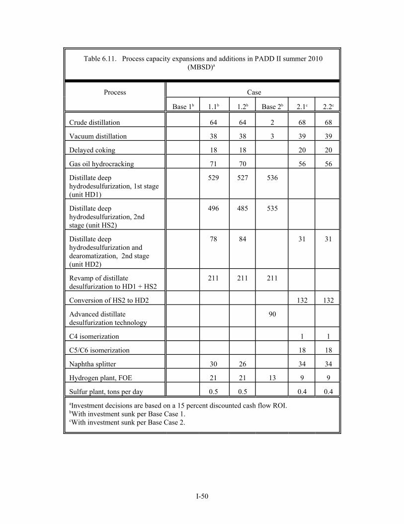
I-50
Table 6.11. Process capacity expansions and additions in PADD II summer 2010(MBSD)a
Process Case
Base 1b 1.1b 1.2b Base 2b 2.1c 2.2c
Crude distillation 64 64 2 68 68
Vacuum distillation 38 38 3 39 39
Delayed coking 18 18 20 20
Gas oil hydrocracking 71 70 56 56
Distillate deephydrodesulfurization, 1st stage(unit HD1)
529 527 536
Distillate deephydrodesulfurization, 2ndstage (unit HS2)
496 485 535
Distillate deephydrodesulfurization anddearomatization, 2nd stage(unit HD2)
78 84 31 31
Revamp of distillatedesulfurization to HD1 + HS2
211 211 211
Conversion of HS2 to HD2 132 132
Advanced distillatedesulfurization technology
90
C4 isomerization 1 1
C5/C6 isomerization 18 18
Naphtha splitter 30 26 34 34
Hydrogen plant, FOE 21 21 13 9 9
Sulfur plant, tons per day 0.5 0.5 0.4 0.4aInvestment decisions are based on a 15 percent discounted cash flow ROI.bWith investment sunk per Base Case 1.cWith investment sunk per Base Case 2.
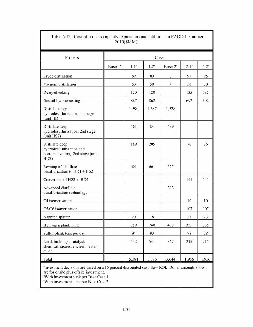
I-51
Table 6.12. Cost of process capacity expansions and additions in PADD II summer2010($MM)a
Process Case
Base 1b 1.1b 1.2b Base 2b 2.1c 2.2c
Crude distillation 89 89 3 95 95
Vacuum distillation 50 50 4 50 50
Delayed coking 120 120 135 135
Gas oil hydrocracking 867 862 692 692
Distillate deephydrodesulfurization, 1st stage(unit HD1)
1,590 1,587 1,528
Distillate deephydrodesulfurization, 2nd stage(unit HS2)
461 451 489
Distillate deephydrodesulfurization anddearomatization, 2nd stage (unitHD2)
189 205 76 76
Revamp of distillatedesulfurization to HD1 + HS2
601 601 575
Conversion of HS2 to HD2 141 141
Advanced distillatedesulfurization technology
202
C4 isomerization 10 10
C5/C6 isomerization 107 107
Naphtha splitter 20 18 23 23
Hydrogen plant, FOE 759 760 477 335 335
Sulfur plant, tons per day 94 93 78 78
Land, buildings, catalyst,chemical, spares, environmental,other
542 541 367 215 215
Total 5,381 5,376 3,644 1,956 1,956aInvestment decisions are based on a 15 percent discounted cash flow ROI. Dollar amounts shownare for onsite plus offsite investment.bWith investment sunk per Base Case 1.cWith investment sunk per Base Case 2.
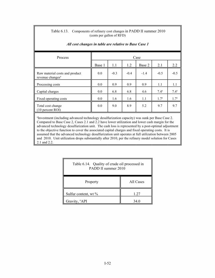
I-52
Table 6.13. Components of refinery cost changes in PADD II summer 2010(cents per gallon of RFD)
All cost changes in table are relative to Base Case 1
Process Case
Base 1 1.1 1.2 Base 2 2.1 2.2
Raw material costs and productrevenue changesa
0.0 -0.3 -0.4 -1.4 -0.5 -0.5
Processing costs 0.0 0.9 0.9 0.9 1.1 1.1
Capital charges 0.0 6.8 6.8 4.6 7.4a 7.4a
Fixed operating costs 0.0 1.6 1.6 1.1 1.7a 1.7a
Total cost change(10 percent ROI)
0.0 9.0 8.9 5.2 9.7 9.7
aInvestment (including advanced technology desulfurization capacity) was sunk per Base Case 2. Compared to Base Case 2, Cases 2.1 and 2.2 have lower utilization and lower cash margin for theadvanced technology desulfurization unit. The cash loss is represented by a post-optimal adjustmentto the objective function to cover the associated capital charges and fixed operating costs. It isassumed that the advanced technology desulfurization unit operates at full utilization between 2005and 2010. Unit utilization drops substantially after 2010, per the refinery model solution for Cases2.1 and 2.2.
Table 6.14. Quality of crude oil processed inPADD II summer 2010
Property All Cases
Sulfur content, wt % 1.27
Gravity, oAPI 34.0

I-53
Table 6.15. Refinery energy use changes in PADD II summer 2010
Daily energy use changes relative to Base Case 1
Purchased electricity, 1000 Kwh
Plant fuel,FOE-MBD
Base Case 1•Low sulfur on-road diesel•Investment as required
0 0
Case 1.1•ULSD•Reformulated for vehicleperformance•Parallel investment
3,893 26
Case 1.2•ULSD•Reformulated for emissionsreduction•Parallel investment
3,883 26
Base Case 2•ULSD•Sequential investment (step 1)•Some newer technologies
2,852 20
Case 2.1•ULSD•Reformulated for vehicleperformance•Sequential investment (step 2)
3,878 27
Case 2.2•ULSD•Reformulated for emissionsreduction•Sequential investment (step 2)
3,828 27
I-54
I-6.2 CASE 1.1: PARALLEL INVESTMENT AND VEHICLE PERFORMANCE RFD
In Case 1.1, ULSD is reformulated for vehicle performance. Given early notice of diesel fuel qualityrequirements, refiners follow a parallel investment pathway. Key results for Case 1.1 and results of all othercases are summarized in Tables 6.2 through 6.15.
Due to the high cetane number specification for vehicle performance RFD, distillate upgrading is via two-stage deep hydroprocessing (Table 6.11). There is no investment in advanced technologies that selectivelyremove sulfur (with low hydrogen consumption and without significant cetane improvement). Five existingdistillate desulfurization units are revamped into two-stage units. For new two-stage installations, 14 percentof second-stage capacity is for units with 70 percent dearomatization capability. Lesser dearomatizationoccurs in the first- and second-stage distillate desulfurization units: 20 percent and 35 percentdearomatization, respectively.
Cetane improver is important in satisfying the on-road diesel cetane number specification. Table 6.3 showsthat the cetane improver treat rate is 0.122 vol percent. This rate is substantially higher than current regionalaverages. For example, in the API/NPRA (1997) survey, the cetane improver treat rate for CARB diesel was0.027 vol percent.
Table 6.2 shows that the average cost increase for RFD in Case 1.1 is 9.0 cents per gallon (cpg). The majorcomponent of this cost increase is capital charges (Table 6.13). Cetane improver (in the raw material categoryof Table 6.13) contributes 1.2 cpg to the cost increase.
Tighter on-road specifications cause an increase in aromatics in the off-road diesel pool in Case 1.1. The off-road diesel pool has an aromatics content of 29.3 vol percent, compared with 24.2 vol percent in Base Case1. A comparison of off-road diesel blendstocks for the two cases (Table 6.5) shows a decline in straight-runblendstocks (higher sulfur content, lower aromatics content) and an increase in hydrotreated light-cycle oil(lower sulfur content, higher aromatics content) in Case 1.1 compared to Base Case 1. The decline in sulfurcontent for the off-road diesel pool (327 ppm compared to 350 ppm for Base Case 1) is discussed in SectionI-6.8.
RFD in Case 1.1 has much-improved emissions characteristics, relative to the commercial reference fuel.NOx emissions are reduced by 8.3 percent, and PM emissions are reduced by 19.8 percent (Table 6.3). Table6.15 shows that diesel fuel reformulation requires a sizeable increase in refinery energy use. Changes inrefinery energy and the associated pollutant emissions need to be included in a complete evaluation of theenvironmental impacts of RFD.
I-6.3 CASE 1.2: PARALLEL INVESTMENT AND EMISSIONS REDUCTION RFD
In Case 1.2, ULSD is reformulated for emissions reduction. Given early notice of diesel fuel qualityrequirements, refiners follow a parallel investment pathway. Key results for Case 1.2 and results of all othercases are summarized in Tables 6.3 through 6.15.
Emissions specifications for Case 1.2 are based on Case 1.1, in which NOx is reduced by 8.3 percent, andPM is reduced by 19.8 percent. In both cases, virtually the same blendstocks are used for RFD (Table 6.5).
Because there is little blendstock flexibility to exploit in achieving the challenging emissions requirements,the eigenfuel-based emissions reduction specifications offer little refining economic benefit over the vehicleperformance specifications, and refining impacts are about the same in both cases.
I-55
In Case 1.2, distillate upgrading is via two-stage deep hydroprocessing (Table 6.11). There is no investmentin advanced technologies that selectively remove sulfur. Five existing distillate desulfurization units arerevamped into two-stage units. For new two-stage installations, 15 percent of second-stage capacity is forunits with 70 percent dearomatization capability.
Table 6.3 shows that the cetane improver treat rate is 0.115 volume percent, slightly lower than with vehicleperformance specifications, but still substantially higher than current regional averages.
Table 6.2 shows that the average cost increase for RFD in Case 1.1 is 8.9 cpg, slightly lower than in Case 1.1.The major component of this cost increase is capital charges (Table 6.13). Cetane improver (in the rawmaterial category of Table 6.13) contributes 1.1 cpg to the cost increase.
In Case 1.2, the off-road diesel pool has an aromatics content of 29.3 vol percent, compared with 24.2 volpercent in Base Case 1. A comparison of off-road diesel blendstocks for the two cases (Table 6.5) shows adecline in straight-run blendstocks (higher sulfur content, lower aromatics content) and an increase inhydrotreated light-cycle oil (lower sulfur content, higher aromatics content) in Case 1.2 compared to BaseCase 1. The decline in sulfur content for the off-road diesel pool (333 ppm compared to 350 ppm for BaseCase 1) is discussed in Section I-6.8.
Table 6.15 shows that diesel fuel reformulation requires a sizeable increase in refinery energy use. Changesin refinery energy and the associated pollutant emissions need to be included in a complete evaluation of theimpacts of RFD.
I-6.4 BASE CASE 2: ULSD
Base Case 2 is one of two base cases used as references to show comparative and cumulative impacts ofdifferent reformulation and investment pathways. Base Case 2 is the first step of a sequential investmentpathway in which refiners do not have early notice of diesel fuel reformulation requirements. In this firststep, ULSD must satisfy future requirements for sulfur content (15 ppm maximum) and cetane number (40minimum), but there are no requirements for reformulation to satisfy vehicle performance or emissionsreduction specifications. The second sequential step involves refiner investments for diesel fuelreformulation, given that investments for ULSD production have already been made in the first step.
Like Base Case 1, Base Case 2 is not representative of current quality requirements for off-road diesel fuels,which have premised sulfur specifications of 500 ppm maximum. By using this off-road sulfur specificationin all cases, we have intentionally removed a variable from the study. Key results for Base Case 2 and allother cases are summarized in Tables 6.2 through 6.15.
We premise limited market penetration of advanced technologies that selectively remove sulfur, with lowhydrogen consumption. Of the 27 PADD II refineries, 13 refineries currently have distillate hydrotreating,and we assume that these refineries produce low sulfur diesel fuel. Given the Baker & O’Brien (2001)projection that thirty-eight percent of current low sulfur diesel producers will engage in revamps of distillatehydrotreating units, we allow revamping in up to five refineries. For the remaining 22 refineries, wearbitrarily assume that up to three refineries (i.e., almost 15 percent technology penetration) can invest inadvanced desulfurization technologies.
In Base Case 2, five existing distillate desulfurization units are revamped into two-stage units (Table 6.11).Investment in advanced technologies lowers the cost of ULSD production. Relative to Base Case 1, the costincrease for ULSD is 5.2 cpg (Table 6.2). Sensitivity runs show a ULSD cost increase of 7.9 cpg via two-stage deep hydrotreating, with no investment allowed in advanced technologies; and a cost increase of 3.7
I-56
cpg with no constraints on investment in advanced technologies. These results have similarities with the“ULSD Supply and Cost” curve in Baker & O’Brien (2001). For the purposes of illustration only, re-scalingthe numbers in the Baker & O’Brien curve to approximately match our study: 7.9 cpg falls to 5.7 cpg at 85percent volume. With advanced technology costs at 3.7 cpg: (5.7 cpg)*(.85) + (3.7 cpg)*(0.15) = 5.4 cpgfor the overall average cost increase.
ULSD product quality is dramatically different for different desulfurization technologies. Table 6.4 showsthat ULSD produced with advanced technologies has substantially lower cetane quality, higher aromaticscontent, and poorer emissions quality. While the advanced technologies are attractive for sulfur reduction,these technologies have little impact on those properties (e.g., cetane quality and aromatics content) whichdefine “reformulation” in this study.
For new two-stage installations, all of the second-stage capacity is for units with deep desulfurization, with35 percent dearomatization. With 20 percent dearomatization in the first-stage, dearomatization across thetwo stages explains a large part of the on-road diesel aromatics reduction (to 16.4 vol percent) relative to BaseCase 1. There is also a shift of aromatics into the off-road diesel pool, relative to Base Case 1. In Base Case2, the off-road diesel pool has an aromatics content of 30.4 vol percent, compared with 24.2 vol percent inBase Case 1. A comparison of off-road diesel blendstocks for the two cases (Table 6.5) shows a decline instraight-run blendstocks (higher sulfur content, lower aromatics content) and an increase in hydrotreated light-cycle oil (lower sulfur content, higher aromatics content) in Base Case 2. The decline in sulfur content forthe off-road diesel pool (281 ppm compared to 350 ppm for Base Case 1) is discussed in Section I-6.8.
Table 6.15 shows that ULSD production requires a sizeable increase in refinery energy use, relative to BaseCase 1. Changes in refinery energy and the associated pollutant emissions need to be included in a completeevaluation of the impacts of ULSD.
I-6.5 CASE 2.1: SEQUENTIAL INVESTMENT AND VEHICLE PERFORMANCE RFD
Case 2.1 represents a second sequential step along an investment pathway in which refiners do not have earlynotice of diesel fuel reformulation requirements. Given that the investments for ULSD production havealready been made in the first step, Case 2.1 is the second sequential step for diesel fuel reformulation tosatisfy vehicle performance specifications. Key results for Case 2.1 and results of all other cases aresummarized in Tables 6.2 through 6.15.
In the Case 2.1 step to RFD with high cetane number and low aromatics, there is drop in utilization ofadvanced technologies that selectively remove sulfur. Refiners who invested in advanced technologycapacity in step one of the investment pathway must either purchase high cetane/low aromatics stocks fromthose refineries with two-stage deep hydroprocessing capacity, or they must invest in distillatedearomatization capacity (in our premises, this subset of refineries does not have the option of changing thedistillate product mix). Tables 6.11 and 6.12 show that gas oil hydrocracking, distillate dearomatization, andhydrogen production are among the investments made in Case 2.1. There is substantial conversion ofsecond-stage hydrodesulfurization capacity to second stage dearomatization capacity. These investments areadded to the Base Case 2 investments to derive total investments for the two-step sequential investmentpathway.
Investment (including advanced technology desulfurization capacity) was sunk per Base Case 2. The sunkinvestment approach assumes that the advanced technology desulfurization unit operates at full utilizationbetween 2005 and 2019. However, for Case 2.1, unit utilization drops substantially after 2010. With itslower utilization, the advanced technology desulfurization unit has a lower cash margin, which is contrary
I-57
to the sunk investment assumptions. Objective function adjustments have been made to cover the associatedcapital charges and fixed operating costs.
Cetane improver is important in satisfying the on-road diesel cetane number specification. Table 6.3 showsthat the cetane improver treat rate is 0.108 volume percent, which is substantially higher than current regionalaverages.
Table 6.2 shows that the average cost increase for RFD in Case 2.1 is 9.7 cpg. The major component of thiscost increase is capital charges (Table 6.13). Cetane improver (in the raw material category of Table 6.13)contributes 1.0 cpg to the cost increase. Compared to the early notice pathway of Case 1.1, capital investmentincreases in Case 2.1 (by 4.1 percent), and the per gallon cost increases by 0.7 cents.
In Case 2.1, the off-road diesel pool has an aromatics content of 29.1 vol percent, compared with 24.2 volpercent in Base Case 1. A comparison of off-road diesel blendstocks for the two cases (Table 6.5) shows adecline in straight-run blendstocks (higher sulfur content, lower aromatics content) and an increase inhydrotreated light-cycle oil (lower sulfur content, higher aromatics content) in Case 2.1. The decline in sulfurcontent for the off-road diesel pool (309 ppm compared to 350 ppm for Base Case 1) is discussed in SectionI-6.8.
RFD in Case 2.1 has much-improved emissions characteristics, relative to the commercial reference fuel.NOx emissions are reduced by 8.2 percent, and PM emissions are reduced by 19.8 percent (Table 6.3). Because cetane quality and aromatics content are controlled, emissions quality is about the same for RFDproduced by different desulfurization technologies. However, cetane and aromatics control is more expensivefor refiners using advanced desulfurization technologies. Compared with RFD produced with two-stagetechnologies, the marginal cost of RFD produced with advanced technologies is 1.7 cpg higher.
Table 6.15 shows that diesel fuel reformulation requires a sizeable increase in refinery energy use. Changesin refinery energy and the associated pollutant emissions need to be included in a complete evaluation of theenvironmental impacts of RFD.
I-6.6 CASE 2.2: SEQUENTIAL INVESTMENT AND EMISSIONS REDUCTION RFD
Instead of using cetane number and aromatics specifications for RFD, Case 2.2 uses emissions specificationsbased on results of Case 2.1. NOx emissions are to be reduced by 8.2 percent, and PM emissions are to bereduced by 19.8 percent In spite of these specification changes, refinery operations and investments are thesame for both Case 2.1 and Case 2.2. Thus, there are no refinery economic benefits from using the emissionsreduction specifications versus the vehicle performance recipe specifications in these cases, which have verychallenging specifications. As specifications become tighter, the processing routes and blendstock choicesbecome more limited. The emissions reduction specifications thus have little refining flexibility to exploit,and refinery benefits vanish for the flexible emissions reduction specifications relative to the vehicleperformance recipe specifications.
I-6.7 EMISSIONS SPECIFICATION BENEFITS
It has been assumed that the maximum vehicle performance specifications are cap specifications whichrequire safety margins to assure that the specifications are not violated. Therefore, the 55 minimum cetanenumber for RFD is represented in ORNL-RYM2002 as a refinery target of 58.8 minimum cetane number, andthe 15 vol percent maximum aromatics content is represented as a refinery target of 12.5 vol percentmaximum aromatics content. As discussed in prior Section I-6.6, there are no refinery economic benefits
I-58
from using the emissions reduction specifications in Case 2.2 when the vehicle performance recipespecifications are at these very challenging levels, which limit processing and blendstock options.
Sensitivity cases have been examined to determine if there are emissions modeling benefits for refining withless challenging specifications in Cases 2.1 and 2.2. In these sensitivity cases, the vehicle performancespecifications are assumed to be average specifications. For example, the 15 vol percent maximum aromaticsspecification can be exceeded occasionally during the production season, as long as the seasonal average forthe region is not greater than 15 vol percent. Therefore, the 55 minimum cetane number for RFD isrepresented in ORNL-RYM2002 as a refinery target of 55 minimum cetane number, and the 15 vol percentmaximum aromatics content is represented as a refinery target of 15 vol percent maximum aromatics content.As shown in Table 6.16, emissions reduction specifications for the sequential investment pathway in PADDII reduce RFD production costs by 0.2 cpg and investment (over the total sequential pathway) by 6.4 percent,compared to vehicle performance specifications. Table 6.17 shows that, with the increased blendingflexibility of emissions reduction specifications for RFD, there are increases in API gravity, cetane numberand aromatics content, while the same emissions quality is achieved for both emissions reduction and vehicleperformance RFDs.
Emissions reduction specifications would show increasing refinery economic benefits over vehicleperformance recipe specifications in circumstances where increasing numbers of processing routes andblendstocks can be used to achieve the objective of emissions quality improvement.
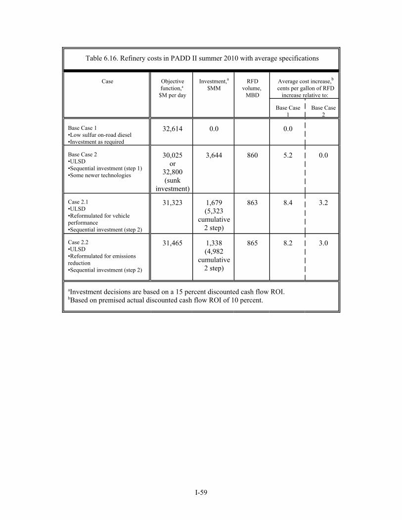
I-59
Table 6.16. Refinery costs in PADD II summer 2010 with average specifications
Case Objectivefunction,a
$M per day
Investment,a
$MMRFD
volume, MBD
Average cost increase,b
cents per gallon of RFDincrease relative to:
Base Case1
Base Case2
Base Case 1•Low sulfur on-road diesel•Investment as required
32,614 0.0 0.0
Base Case 2•ULSD•Sequential investment (step 1)•Some newer technologies
30,025or
32,800(sunk
investment)
3,644 860 5.2 0.0
Case 2.1•ULSD•Reformulated for vehicleperformance•Sequential investment (step 2)
31,323 1,679(5,323
cumulative2 step)
863 8.4 3.2
Case 2.2•ULSD•Reformulated for emissionsreduction•Sequential investment (step 2)
31,465 1,338(4,982
cumulative2 step)
865 8.2 3.0
aInvestment decisions are based on a 15 percent discounted cash flow ROI.bBased on premised actual discounted cash flow ROI of 10 percent.
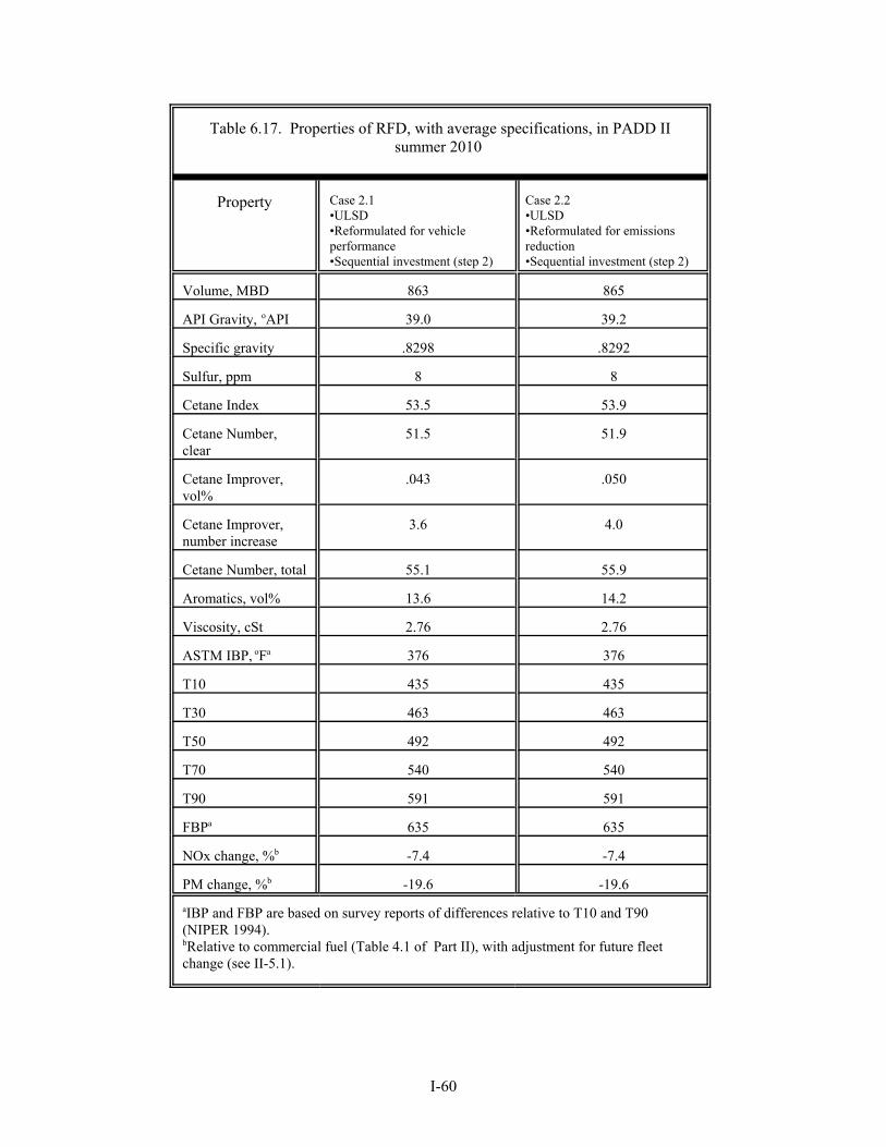
I-60
Table 6.17. Properties of RFD, with average specifications, in PADD IIsummer 2010
Property Case 2.1•ULSD•Reformulated for vehicleperformance•Sequential investment (step 2)
Case 2.2•ULSD•Reformulated for emissionsreduction•Sequential investment (step 2)
Volume, MBD 863 865
API Gravity, oAPI 39.0 39.2
Specific gravity .8298 .8292
Sulfur, ppm 8 8
Cetane Index 53.5 53.9
Cetane Number,clear
51.5 51.9
Cetane Improver,vol%
.043 .050
Cetane Improver,number increase
3.6 4.0
Cetane Number, total 55.1 55.9
Aromatics, vol% 13.6 14.2
Viscosity, cSt 2.76 2.76
ASTM IBP, oFa 376 376
T10 435 435
T30 463 463
T50 492 492
T70 540 540
T90 591 591
FBPa 635 635
NOx change, %b -7.4 -7.4
PM change, %b -19.6 -19.6aIBP and FBP are based on survey reports of differences relative to T10 and T90(NIPER 1994).bRelative to commercial fuel (Table 4.1 of Part II), with adjustment for future fleetchange (see II-5.1).

I-61
I-6.8 OFF-ROAD SULFUR
The off-road sulfur quality giveaway (i.e., exceeding the required sulfur quality) shown in Table 6.18 wouldbe unlikely if off-road quality requirements were coordinated with on-road requirements. In Base Case 1,investments are made for production of low sulfur (500 ppm nominal; 350 ppm actual) off-road diesel, beforenotice of requirements for ULSD or RFD. This approach was used to remove or diminish the effects of avariable (off-road sulfur content) in our study.
As previously discussed, we have used the Baker & O’Brien (2001) projection that up to thirty-eight percentof current on-road low sulfur diesel producers will engage in revamps of distillate hydrotreating units forproduction of ULSD. Of the remaining hydrotreating capacity for on-road low sulfur diesel, some capacitycould be used to produce feedstocks for new deep hydrotreating units for RFD, some capacity could be usedto support off-road diesel production, or there could be a reduction in capacity utilization. We have assumedthat the remaining hydrotreating capacity continues to operate at Base Case utilization levels. There wouldbe no giveaway of sulfur quality if the utilization of low sulfur hydrotreating capacity were allowed to fall. Other product specifications (e.g., the allowable percentage of light cycle oil) are related to sulfur qualitygiveaway. For example, if the light cycle oil constraint is removed, there is no sulfur giveaway in any of theproducts.
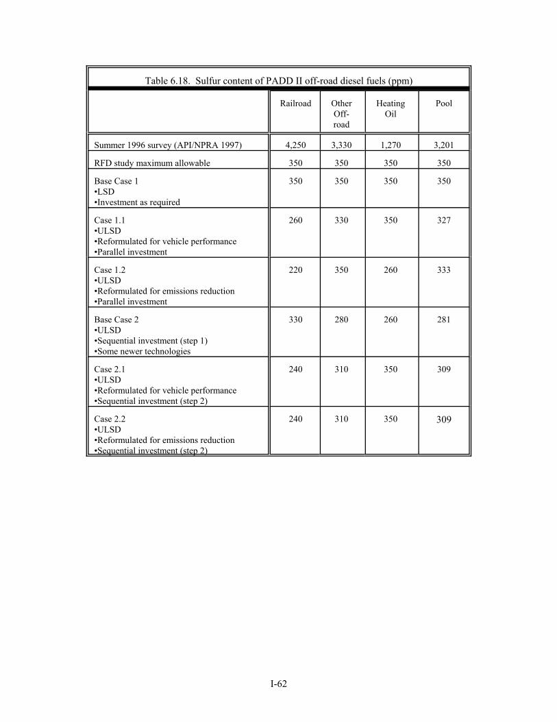
I-62
Table 6.18. Sulfur content of PADD II off-road diesel fuels (ppm)
Railroad OtherOff-road
HeatingOil
Pool
Summer 1996 survey (API/NPRA 1997) 4,250 3,330 1,270 3,201
RFD study maximum allowable 350 350 350 350
Base Case 1•LSD•Investment as required
350 350 350 350
Case 1.1•ULSD•Reformulated for vehicle performance•Parallel investment
260 330 350 327
Case 1.2•ULSD•Reformulated for emissions reduction•Parallel investment
220 350 260 333
Base Case 2•ULSD•Sequential investment (step 1)•Some newer technologies
330 280 260 281
Case 2.1•ULSD•Reformulated for vehicle performance•Sequential investment (step 2)
240 310 350 309
Case 2.2•ULSD•Reformulated for emissions reduction•Sequential investment (step 2)
240 310 350 309
I-63
I-7. IMPACT OF DIESEL FUEL REFORMULATION ON DEMANDFOR CANADIAN SYNTHETIC CRUDE
In sensitivity cases, ORNL-RYM2002 has been used to examine the impacts of RFD on the PADD II refinerydemand for Canadian synthetic crude oil. As the production of synthetic crude oil increases, with economicdisplacement of conventional crude oils, oilsands operators and refiners will face technical challenges withimproved quality requirements for diesel fuel, jet fuel, and heavy gas oil for fluid catalytic cracking feed (Yui2000; Yui and Chung 2001). The cetane quality, aromatics content, and emissions specifications for RFDin our case studies would increase these challenges. Tables 7.1 through 7.7 show fractions and selectedproperties for the PADD II crude oil used in the case studies; for a Canadian synthetic crude; and for anORNL-RYM2002 approximation of that Canadian synthetic crude. For the distillate fractions, the syntheticcrude and its approximation have substantially lower cetane indices (375-690oF fraction), and higheraromatics contents (375-650oF fraction), compared to the PADD II crude oil. However, with much lowersulfur levels, the value of synthetic crude should increase in the production of low sulfur products. The sensitivity cases illustrate impacts of changes in diesel product quality requirements, given the premisedsynthetic crude quality and the PADD II refinery configurations. These cases do not address the issues of(1) modifying the quality of synthetic crude to meet the requirements of crude purchasers; (2) modifyingrefinery hardware to accommodate higher levels of synthetic crude use; or (3) impacts on product properties(e.g., jet fuel and diesel lubricity) other than those specified in the case studies. Demand curves are estimated with the ORNL-RYM2002 parametric feature, which is not appropriate forlinking the two steps of the delayed notice, sequential investment pathway. Therefore, demand curves arenot presented for sequential Cases 2.1 and 2.2. For the early notice cases, Fig. 7.1 through Fig. 7.3 showthe PADD II refinery demand for Canadian synthetic crude for various differentials in its price relative tothe price of West Texas Intermediate (WTI) crude.
Fig. 7.1 shows the PADD II refinery demand for Canadian synthetic crude, given production of low sulfurdiesel (Base Case 1) and ULSD (Base Case 2). At the actual price differential of -$0.27 per barrel in years2000 and 2001 (Syncrude 2002), the Fig. 7.1 demand for synthetic crude for production of low sulfur diesel(Base Case 1) is 122 MBD, or about 2.8 percent of the total PADD II crude run. This synthetic crudepercentage is nearly the same as the current actual 2.6 percent (NRC 2002b). With production of low sulfurdiesel, the demand for synthetic crude is 0.3 percent of the total PADD II crude run at a price premium toWTI of $2.00 per barrel, and 8.5 percent of the total PADD II crude run at a price discount $2.00 per barrel. There is a sizeable increase in synthetic crude demand when the maximum sulfur specification for on-roaddiesel falls from 500 ppm (Base Case 1) to 15 ppm (Base Case 2). This demand increase is expected, giventhe low sulfur levels of synthetic crude.
Fig. 7.2 shows that diesel fuel reformulation, with challenging specifications for vehicle or emissionsreduction, substantially reduces the demand for synthetic crude at recent prices (i.e., in the price differentialneighborhood of -$0.27 per barrel in years 2000 and 2001), compared with demand under ULSD production.The demand effect increases as price differentials drop below $0.50 per barrel. The consolidated Fig. 7.3shows that diesel fuel reformulation can reverse the synthetic crude demand increase that resulted from thetransition from low sulfur diesel to ULSD.
The relationship between desulfurization capacity and synthetic crude demand is illustrated in Fig. 7.4. Asexpected prices for synthetic crude fall, the expected demand for that crude increases, and investment in first-and second stage deep desulfurization capacity declines. Due to the higher aromatics content of syntheticcrude, investment in second stage deep desulfurization/dearomatization capacity increases as the expecteddemand for synthetic crude increases.
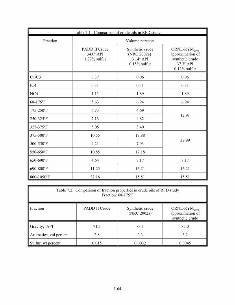
I-64
Table 7.1. Comparison of crude oils in RFD study
Fraction Volume percents
PADD II Crude34.0o API
1.27% sulfur
Synthetic crude(NRC 2002a)
31.4o API0.15% sulfur
ORNL-RYM2002approximation ofsynthetic crude
37.3o API0.12% sulfur
C1/C3 0.37 0.06 0.06
IC4 0.31 0.31 0.31
NC4 1.11 1.89 1.89
68-175oF 5.63 6.94 6.94
175-250oF 6.73 4.6912.91
250-325oF 7.13 4.82
325-375oF 5.05 3.40
375-500oF 10.55 13.8838.99
500-550oF 4.21 7.93
550-650oF 10.85 17.18
650-690oF 4.64 7.17 7.17
690-800oF 11.25 16.21 16.21
800-1050oF+ 32.16 15.51 15.51
Table 7.2. Comparison of fraction properties in crude oils of RFD studyFraction: 68-175oF
Fraction PADD II Crude Synthetic crude(NRC 2002a)
ORNL-RYM2002approximation ofsynthetic crude
Gravity, oAPI 71.5 83.1 85.0
Aromatics, vol percent 2.8 2.3 3.2
Sulfur, wt percent 0.015 0.0032 0.0045

I-65
Table 7.3. Comparison of aggregated fraction properties in crude oils of RFD studyFraction: 175-375oF
Fraction PADD II Crude Synthetic crude (NRC 2002a)
ORNL-RYM2002approximation ofsynthetic crude
Gravity, oAPI 54.1 52.0 56.9
Aromatics, vol percent 14.0 17.0 17.0
Sulfur, wt percent 0.048 0.0037 .00037
Table 7.4. Comparison of aggregated fraction properties in crude oils of RFD studyFraction: 375-650oF
Fraction PADD II Crude Synthetic crude(NRC 2002a)
ORNL-RYM2002approximation ofsynthetic crude
Gravity, oAPI 36.8 29.5 31.8
Cetane index 50.4 38.3 42.5
Aromatics, vol percent 26.6 34.6 34.1
Sulfur, wt percent 0.586 0.0391 0.0391
Table 7.5. Comparison of fraction properties in crude oils of RFD studyFraction: 650-690oF
Fraction PADD II Crude Synthetic crude (NRC 2002a)
ORNL-RYM2002approximation ofsynthetic crude
Gravity, oAPI 29.9 21.0 23.0
Cetane index 58.0 41.7 44.4
Sulfur, wt percent 1.221 0.204 0.203

I-66
Table 7.6. Comparison of fraction properties in crude oils of RFD studyFraction: 690-800oF
Fraction PADD II Crude Synthetic crude (NRC 2002a)
ORNL-RYM2002approximation ofsynthetic crude
Gravity, oAPI 26.2 19.9 26.1a
Sulfur, wt percent 0.949a 0.298 0.298a Relative to 650-690oF fraction, these property trends are implausible.
Table 7.7. Comparison of fraction properties in crude oils of RFD studyFraction: 800-1050oF+
Fraction PADD II Crude Synthetic crude (NRC 2002a)
ORNL-RYM2002approximation ofsynthetic crude
Gravity, oAPI 15.5 17.9 17.1
Sulfur, wt percent 2.03 0.363 0.320

I-67
Fig. 7.1. ULS Diesel Increases Demand for Synthetic Crude(PADD II Summer 2010)
-$2.50
-$2.00
-$1.50-$1.00
-$0.50
$0.00
$0.50
$1.00$1.50
$2.00
$2.50
0 100 200 300 400 500 600 700
Synthetic crude demand, MBD
Sync
rude
- W
TI, p
er b
b
Low Sulfur DieselULS Diesel
Fig. 7.2. RFD Reduces Demand for Synthetic Crude at Recent Prices: Parallel Investment
(PADD II Summer 2010)
-$2.50
-$2.00
-$1.50
-$1.00
-$0.50
$0.00
$0.50
$1.00
$1.50
$2.00
$2.50
0 100 200 300 400 500 600 700
Synthetic crude demand, MBD
Sync
rude
- W
TI, p
er b
bl
VehiclePerformance RFDEmissionsReduction RFDULS Diesel

I-68
Fig. 7.3. Synthetic Crude Dem and Com parisons(PADD II Sum m er 2010)
-$2.50
-$2.00
-$1.50
-$1.00
-$0.50
$0.00
$0.50
$1.00
$1.50
$2.00
$2.50
0 100 200 300 400 500 600 700
Synthetic crude demand, MBD
Sync
rude
- W
TI, p
er b
b
Low Sulfur Diesel
VehiclePerformance RFD -Parallel Investment
EmissionsReduction RFD -Parallel Investment
ULS Diesel
Fig. 7.4. Hydroprocess ing C apac ity Is Related to Synthetic C rude Dem and O utlook: Parallel Inves tm ent w ith Vehic le Perform ance
RFD (PADD II Sum m er 2010)
150
200
250
300
350
400
450
500
550
100 200 300 400 500Synthetic c rude dem and, MBD
Proc
ess
unit
inve
stm
ent c
apac
ity,
MBS
D
1st Stage DeepDesulfu riza tion
2nd Stage DeepDesulfu riza tion
2nd Stage DeepDesulfu riza tion /Dearomatiza tion
I-69
I-8. CONCLUSIONS
ORNL-RYM2002 has been used to estimate the refining cost and investment impacts of different diesel fuelreformulation pathways, to determine if there are refinery economic benefits for producing an emissionsreduction RFD (with eigenfuel-based flexibility for individual property values) compared to a vehicleperformance RFD (with recipe values for individual properties). These RFDs are premised to have equalemissions performance.
Table 8.1 shows that refining costs are lower with early notice of product quality requirements for RFD.While advanced desulfurization technologies (with low hydrogen consumption and little effect on cetanequality and aromatics content) reduce the cost of ULSD, these technologies contribute to the increased costsof a delayed-notice sequential investment pathway compared to an early-notice parallel investment pathwayto RFD.
Given the objective of RFD emissions quality improvement, there is little refining economic benefit fromusing the flexible emissions reduction specifications rather than the vehicle performance recipe specificationsin these cases, which have very challenging specifications. As specifications become tighter, processingbecomes more difficult, and blendstock choices become more limited, refinery benefits vanish for emissionsreduction relative to vehicle performance specifications.
Conversely, the emissions reduction specifications show increasing refinery benefits over vehicleperformance recipe specifications as those recipe specifications are relaxed, and alternative processing routesand blendstocks become available. For example, using average specifications rather than cap specificationsin our study reduces investment and RFD production costs for emissions reduction compared to vehicleperformance. With the increased blending flexibility of emissions reduction specifications for RFD, thereare changes in API gravity, cetane number and/or aromatics content, while the same emissions quality isachieved for both emissions reduction and vehicle performance RFDs.
In sensitivity cases, ORNL-RYM2002 indicates that there is a sizeable increase in synthetic crude demand asULSD displaces low sulfur diesel fuel, but this demand increase would be reversed by a requirement for RFD.
In summary:
C Refining costs are lower with early notice of product quality requirements for RFD. With early noticeof RFD requirements, refinery capital investment has not yet been made to satisfy the ULSDrequirement of year 2006, and there is greater flexibility for investment planning. With delayed noticeof requirements, investment flexibility is less because capital investment has been sunk to satisfy theULSD sulfur requirement.
C While advanced desulfurization technologies reduce the cost of ULSD, these technologies cancontribute to the increased costs of a delayed notice compared to an early notice investment pathwayto RFD. With relatively small impact on cetane and aromatics quality, these technologies are on asuboptimal pathway for RFD production.
C There is little refining economic benefit from using flexible emissions reduction specifications ratherthan the vehicle performance recipe specifications, when recipe specifications are challenging. This isbecause processing options and blendstocks are very limited for achieving challenging recipespecifications.

I-70
C Emissions reduction specifications show increasing refinery benefits over vehicle performance recipespecifications, as those recipe specifications are relaxed, and alternative processing routes andblendstocks become available.
C There is a sizeable increase in synthetic crude oil demand as ULSD displaces low sulfur diesel fuel, butthis demand increase would be reversed by a requirement for diesel fuel reformulation.

I-71
Table 8.1. Diesel fuel reformulation study findings
Case On-road diesel upgrading pathway
Costincreasea
Comment
Base Case 1 •Low sulfur•Investment as required
0.0
Case 1.1 •Ultra low sulfur•Reformulated forvehicle performance•Early notice ofrequirements•Parallel investment
9.0 Due to high cetane specification, distillate upgrading isvia 2-stage deep hydroprocessing, not advanceddesulfurization technologies that selectively removesulfur without cetane improvement.
Case 1.2 •Ultra low sulfur•Reformulated foremissions reduction•Early notice ofrequirements•Parallel investment
8.9 Emissions targets are based on Case 1.1 (relative toreference commercial fuel, NOx reduction $8.3 percentand PM reduction $19.8 percent). With littleblendstock flexibility (virtually same stocks selected asin Case 1.1), emissions reduction specifications havelittle refining benefit, given equal emissions for the twoRFDs.
Base Case 2 •Ultra low sulfur•Sequential investment(step 1)•Some newertechnologies
5.2 Investment in advanced desulfurization technologyresults in lower costs. Sensitivity runs show costincrease of 7.9 cpg via 2-stage deep hydroprocessing,with no investment allowed in advanced desulfurization;and cost increase of 3.7 cpg with no constraints oninvestment in advanced desulfurization.
Case 2.1 •Ultra low sulfur•Reformulated forvehicle performance•Delayed notice ofrequirements•Sequential investment(step 2)
9.7 In second step to high cetane/low aromatics, there isdrop in utilization of advanced desulfurization, andrefineries with this capacity must purchase highcetane/low aromatics stocks from those refineries with2-stage deep hydroprocessing and/or invest in distillatedearomatization capacity. Capital investment increases,and cost increases 0.7 cpg compared to early noticepathway of Case 1.1.
Case 2.2 •Ultra low sulfur•Reformulated foremissions reduction•Delayed notice ofrequirements•Sequential investment(step 2)
9.7 Emissions targets are based on Case 2.1 (relative toreference commercial fuel, NOx reduction $8.2 percentand PM reduction $19.8 percent). There are no refinerybenefits from using emissions versus vehicleperformance specifications in these cases with verychallenging specifications. As specifications becometighter, refinery benefits vanish for emissionsreduction versus vehicle performance specifications. Conversely, emissions reduction specification benefitsfor refining increase as vehicle performancespecifications are relaxed.
SyntheticCrudeSensitivities
There is a sizeable increase in synthetic crude demand when the maximum sulfur specification foron-road diesel falls from 500 ppm to 15 ppm, but this demand increase would be reversed bydiesel fuel reformulation.
aCost increase, in cpg, relative to Base Case 1.

I-73
REFERENCES
American Petroleum Institute and National Petroleum Refiners Association (API/NPRA). 1997. 1996American Petroleum Institute/National Petroleum Refiners Association Survey of Refining Operations andProduct Quality, API Publishing Services, 1220 L. Street, N.W., Washington DC, July.
Clark, Dale (NRC). 2002a. Data on synthetic crudes and Canadian heavy crudes, Natural ResourcesCanada, Ottawa, Ontario.
Crawford, R.W. 2002. “Development of NOx Emissions Model for Heavy-Duty Diesel Engines,”RWCrawford Energy Systems, under contract with Oak Ridge National Laboratory, April 16.
Dickson, Cheryl L. and Gene P. Sturm, Jr. (NIPER). 1994. Diesel Fuels, 1994, NIPER-187 PPS 94/5,National Institute for Petroleum and Energy Research, Bartlesvillle, OK, December.
Downstream Alternatives, Inc (DAI). 2002. Infrastructure Requirements for an Expanded Fuel EthanolIndustry, Oak Ridge National Laboratory Ethanol Project, Subcontract No. 4500010570, South Bend, IN46680-2587, January 15, http://www.afdc.doe.gov/pdfs/6235.pdf
Dunbar, Daniel N. and Martin R. Tallett. 2002a. “Progress Report Number 1 - Technology andFeatures Enhancements to ORNL RYM,” EnSys Energy & Systems, Inc., Flemington, NJ.
Dunbar, Daniel N. and Martin R. Tallett. 2002b. “Progress Report Number 2 - Technology and FeaturesEnhancements to ORNL RYM,” EnSys Energy & Systems, Inc., Flemington, NJ, April 7.
European Automobile Manufacturers Association, Alliance of Automobile Manufacturers, EngineManufacturers Association, Japan Automobile Manufacturers Association (ACEA et al). 2000. “World-wideFuel Charter,” April, http://www.engine-manufacturers.org/about/Final%20WWFC%204%2000.pdf
Hadder, G.R. 1997. Re-estimation of the Refining Cost of Reformulated Gasoline NOx Control, draftreport, Oak Ridge National Laboratory, Oak Ridge, TN, February 26.
Korotney, D. 1993. “Revised Complex Model for Conventional and Reformulated Gasoline,” EPAAir Docket A-92-12, Environmental Protection Agency, Fuels and Standards Branch, Ann Arbor MI.
MathPro Inc. 2002. Prospects for Adequate Supply of Ultra Low Sulfur Diesel Fuel in the TransitionPeriod (2006-2007), Prepared for The Alliance of Automobile Manufacturers and The Engine ManufacturersAssociation, West Bethesda, MD, February 26.
McAdams, H.T., R.W. Crawford, and G.R. Hadder. 2000a. “A Vector Approach to Regression Analysisand Its Application to Heavy-Duty Diesel Emissions,” SAE 2000-01-1961, Society of Automotive EngineersInternational Spring Fuels & Lubricants Meeting & Exposition, Paris, France, June 19-22.
McAdams, H.T., R.W. Crawford, and G.R. Hadder. 2000b. A Vector Approach to Regression Analysisand Its Application to Heavy-Duty Diesel Emissions, ORNL/TM-2000/5, Oak Ridge National Laboratory,Oak Ridge, TN 37831, November.
McAdams, H.T., R.W. Crawford, and G.R. Hadder. 2002. PCR+ in Diesel Fuels and EmissionsResearch, ORNL/TM-2002-16, Oak Ridge National Laboratory, Oak Ridge, TN 37831, March.
I-74
National Petroleum Council (NPC). 1993. U.S. Petroleum Refining, Washington, DC, August.
National Petroleum Council (NPC). 2000. U.S. Petroleum Refining, Assuring the Adequacy andAffordability of Cleaner Fuels, Washington, DC, June.
National Petroleum Refiners Association (NPRA). 1991. NPRA Survey of U.S. Gasoline Quality andU.S. Refining Industry Capacity to Produce Reformulated Gasolines, Part A, Suite 1000, 1899 L Street, NW,Washington, DC, January.
Natural Resources Canada (NRC). 2002b. “Canadian Oil Sands,” TRB Summer Meeting, Port Huron,MI, July.
Ory, Raymond E., Jr (Baker & O’Brien). 2001. “Potential Impacts of Sulfur Regulation on Cost andSupply of Diesel Fuels in the United States,” National Petrochemical & Refiners Association, AM-01-32,Washington, DC.
Shapiro, Ellen. 2002. “Comment on Draft DOE Study Protocol,” Alliance of AutomobileManufacturers, e-mail to Gerald Hadder, May 29.
Shiflett, Woody. 2001. “The Drive to Lower and Lower Sulfur: Criterion’s New Catalysts HelpRefiners Tackle Sulfur,” National Petrochemical & Refiners Association, AM-01-29, Washington, DC.
Sinor, J.E. 2000. Review of Market for Octane Enhancers, J.E. Sinor Consultants, Inc., Niwot, CO,May, http://www.afdc.doe.gov/pdfs/4747.pdf
Stell, Jeannie. 2001a. “Worldwide Construction,” Oil & Gas Journal, October 29,http://downloads.pennnet.com/pnet/surveys/ogj/ogj_99447295.pdf
Stell, Jeannie. 2001b. “2001 Worldwide Refining Survey,” Oil & Gas Journal, December 24,http://downloads.pennnet.com/pnet/surveys/ogj/ogj_9952jp082-124.pdf
Swain, Edward J. 1999. “U.S. refinery-sulfur production peaked in 1996,” Oil & Gas Journal,March 8.
Syncrude Canada LTD (Syncrude). 2002. Syncrude Canada LTD 2001 Annual Report. Fort McMurray,Alberta, http://www.syncrude.com/investors/ar01/pdf/FinRev.pdf
Tallett, M.R., and D.N. Dunbar. 1988. Enhancement of EIA Refinery Yield Model: Extension andDemonstration on Gasoline and Diesel Quality Issues, Oak Ridge National Laboratory Contract No.DE-AC05-840R21400, EnSys Energy & Systems, Inc., Flemington, NJ, August.
Tallett, M.R. and D.N. Dunbar. 2001. “Proposal for Technology and Features Enhancements to theORNL RYM Model,” EnSys Energy & Systems, Inc., Flemington, NJ, December 4.
Tallett, M.R., D.N. Dunbar, and J. Leather. 1992. “Summary Documentation of Oak Ridge RefineryYield Model Reformulated Gasoline Update,” EnSys Energy & Systems, Inc., Flemington, NJ, March 16.
U.S. Department of Energy (DOE). 1984a. Refinery Evaluation Modeling System (REMS)Documentation, DOE/EIA-0460, Energy Information Administration, Washington, DC, October.

I-75
U.S. Department of Energy (DOE). 1984b. Refinery Evaluation Modeling System (REMS)Documentation, DOE/EIA-0461, Energy Information Administration, Washington, DC, October.
U.S. Department of Energy (DOE), Energy Information Administration. 2001a. Annual Energy Outlook2002 with Projections to 2020, DOE/EIA-0383(2002), Washington, DC, December 21,http://www.eia.doe.gov/oiaf/aeo/pdf/appa.pdf
U.S. Department of Energy (DOE), Energy Information Administration. 1998. Challenges of ElectricPower Industry Restructuring for Fuel Suppliers, DOE/EIA-0623, Washington, DC, September,http://www.eia.doe.gov/pub/electricity/chg_str_fuel.pdf
U.S. Department of Energy (DOE), Energy Information Administration. 2002a. PetroleumMarketing Annual, DOE/EIA-0380(2001),http://www.eia.doe.gov/oil_gas/petroleum/data_publications/petroleum_marketing_annual/pma.html
U.S. Department of Energy (DOE), Energy Information Administration. 2001b. Petroleum SupplyAnnual 2000, DOE/EIA-0340(00)/1 and 2, Washington, DC, June,http://www.eia.doe.gov/oil_gas/petroleum/data_publications/petroleum_supply_annual/psa_volume1/psa_volume1.html andhttp://www.eia.doe.gov/oil_gas/petroleum/data_publications/petroleum_supply_annual/psa_volume2/psa_volume2.html
U.S. Department of Energy (DOE), Energy Information Administration. 2002b. Refinery Capacity Dataas of January 1, 2001, DBF file containing petroleum refinery capacity data by refinery. Energy InformationA d m i n i s t r a t i o n ( E I A ) , F o r m E I A - 8 2 0 , " B i e n n i a l R e f i n e r y R e p o r t , "http://www.eia.doe.gov/oil_gas/petroleum/data_publications/refinery_capacity_data/refcapacity.html.
U.S. Environmental Protection Agency (EPA). 2001. Control of Emissions of Hazardous Air Pollutantsfrom Mobile Sources, 40 CFR Parts 80, and 86.
U.S. Environmental Protection Agency (EPA). 2002. “Toxics baselines,” e-mail memorandum andspreadsheet attachment from John Weihrauch to Gerald Hadder, June 27.
Weihrauch, John. 2001. “Revised PADD Data,” tables provided to G.R. Hadder.
Yui, Sok. 2000. “Athabasca oilsands produce quality diesel and jet fuels,” Oil & Gas Journal,November 20.
Yui, Sok and Keng Chung. 2001. “Processing oilsands is Syncrudes’s R&D focus,” Oil & Gas Journal,April 23.


APPENDIX I-A
ENSYS ENERGY & SYSTEMS, INC., PROGRESS REPORT NUMBER 1TECHNOLOGY AND FEATURES ENHANCEMENTS
TO THE ORNL RYM MODEL

I-79
EnSys ORNL Contract: 4000013512 – ORNL Refinery Yield Model Update
Progress Report Number 1- Technology and Features Enhancementsto the ORNL RYM Model
I. Hydrocracking/FCC Feed Pretreating
The RYM structure as now used provides for:
Unit FDS FCC Feed pretreatingUnit HCL Mild to moderate hydrocrackingHCR Severe hydrocrackingHCV Residuum hydrocracking
The above correspond to the Oil and Gas Journal annual refining survey categories.
The Exxon Mobil MAK process table MAK is retained as a separate unit. In using the model, the abovecategories suffice since they cover the range of hydrocracking severity reflected in Table MAK. Howeversince the MAK table exists, the table values are being reviewed and updated based on the latest NPRA papers.Its structure will not be expanded.
Although the current structure holds, some table vectors are being moved from Table FDS to HCL. A totalof 20 additional process unit vectors have been defined to fit in the above structure based on vendor dataappearing in Hydrocarbon Processing for UOP and Chevron, a Texaco NPRA Paper, a NPRA Paperdescribing the UOP process and data from Handwerk, Maples and Meyers. A (spreadsheet) document willbe supplied detailing the precise sources.
Hydrogen consumptions range from 650 to 2500 SCF/bbl (before allowing for hydrogen losses) and productmiddle distillate sulfur contents range from 10 to 400 ppm. There are vectors which correspond to LCO andlight FCC and coker gas oils hydrocracking. The LCO data indicate hydrogen consumption of the order of2000 scf/bbl or greater and a conversion range from 30 to 60 percent. Undercutting of the LCO will not befurther considered since both FCC distillate and light gas oil feed are represented and undercutting appearsto fall within the realm of refinery operations sub-optimization.
The existing approach of hydrocracker vectors corresponding to a gasoline versus a jet/distillate operationis being reviewed and will be maintained.
II. Hydrogen Plant Revamp
Three NPRA papers were reviewed – AM-01-19, Air Products/Tecnip, AM-01-27, Haldor Topsoe and AM-01-27, Foster Wheeler, AM-01-36. We estimate that a 30% increase in capacity can be achieved for 25%of the ISBL and 10% of the OSBL investment costs, with a marginal increase in energy efficiency of 8%.
There are other options aside from de-bottlenecking:
I-80
Retirement and replacement - According to Air Products, during the period 1991 through 2000, refinersadded approximately 300 MMSCFD of new capacity and retired 130 MMSCFD. Although FosterWheeler states that the tighter new plant designs offer less revamp potential than the older plants, onthe other hand they note many of the older plants have been revamped at least once. From the abovefigure for outright hydrogen plant retirement, the revamp potential is definitely limited.
Across the fence hydrogen purchase. During the same 1991-2000 period, industrial gas companies added 850MMSCFD of capacity for sale to refiners. This option is becoming attractive to refiners because theytend to avoid the (now near catastrophic) consequences of a sudden hydrogen plant shutdown, theyavoid expending investment capital and they have greater refinery operations flexibility.
Hydrogen Recovery and Purification – this is discussed below.
The modeling challenges for representing the important cost of hydrogen appear to lie less in estimating thecost of the various supply options than in estimating their likely adoption. We are considering the best optioncould be to represent plant “revamp” in fact as a debottleneck with controlled upper limits.
III. Hydrogen Purification and Recovery
Two units are being considered – the existing HPM unit for membrane purification and a new RYM TablePSA to represent pressure swing absorption. The latter is gaining ground in spite of a higher investment costsince higher purity hydrogen is produced at a higher pressure. Investment cost data has been assembled fromHydrocarbon Processing, UOP NPRA Paper AM-99-08 and European Union data available from the Internet.
If both units are allowed to ride free, the validity of the relative selection may be in question. The higherpurity of the PSA hydrogen facilitates middle distillate desulfurization to lower sulfur levels (one reason forits selection), but we do not represent different hydrogen purity levels in RYM. A disadvantage of themembrane process is the need for hydrogen recompression and we do not represent different hydrogenpressure levels in RYM, although we can make an adjustment to the HPM investment cost. Also, totalhydrogen purification may exceed reasonable values since site specific limitations are a reality.
We propose to put in Table POL constraints to limit both total hydrogen purification capacity and PSA versusHPM – current OGJ refinery survey data indicate the hydrogen purification capacity accounts for 38% ofhydrogen plant production and the survey shows HPM versus PSA (cryogenic separation is relatively minor).
IV. Hydrogen Consumption Consistency Across Process Units
Based on published data, the RDS and ARD units show reasonable hydrogen consumption values. However,the residuum hydrocracker is low by an estimated factor of 1.75 based on data from Hydrocarbon Processingan Handwerk. The middle distillate hydrogen consumption data are being reviewed separately as a part ofthe following task

I-81
V. Middle Distillate Deep Desulfurization and Aromatics Saturation
Building on the recent model development work for API, two NPRA Papers were reviewed in depth: AM-01-22 by Mustang Engineers and Constructors, Inc and AM-01-28 by Haldor Topsoe and San Joaquin RefiningCompany.
These papers address revamp potential and the incremental steps required to achieve less than 10 ppm productsulfur. The Mustang paper gives ULSD revamp cost estimates. The requirements for aromatics saturation arealso addressed in these papers.
The two papers essentially agree on the revamp steps required to achieve ULSD:
the addition of a second reactor or a new second stage hydrotreater to lower space velocity by providingincreased catalyst volume
more active catalyst directed at desulfurizing sterically hindered sulfur compounds (look at NiMo versusCoMo).
higher hydrogen purity from hydrogen purificationscrubbing of the recycle gas to provide higher hydrogen purityhigher reactor pressure to be considered in addition to the above to increase the hydrogen partial pressure in
the reactor
The reactor internals must also be examined since a one percent bypassing of the feed can contribute 50 to150 ppm sulfur content to the diesel product.
In order to saturate aromatics to the 4 weight percent level, increase feed cetane by 10 numbers and API by6, a second high pressure noble catalyst stage is required, along with an intermediate stripper column toremove dissolved H2S and NH3 from the first stage effluent
Revamp Potential
Both NPRA papers state that units built since the early 1990s may be revamped according to the abovescheme and that additional revamps of the type above to already revamped units may not be feasible. Torevamp an earlier generation hydrocracker (1970’s and 1980’s) may require up to three times the catalystvolume, as opposed to an increase of 100 percent in the catalyst volume for the post 1990 units.
Revamp Cost
For a 30,000 BPD unit with 1/3 LCO feed, Mustang estimates 8.6 million dollars for the above sequence fora 100% catalyst volume increase. This is an ISBL figure with an accuracy stated of 20 percent up or down.An offsites cost range of 30-100 percent onsite investment is quoted. The Mustang paper indicates a 0.9million dollar ISBL increase in going from a 50 to 100 percent catalyst volume increase. Applying economiesof scale, this provides a basis for estimating the revamp cost of a pre-1990s hydrotreater requiring three timesthe catalyst volume.
Implementation
Through EnSys’ work for the API, we have established limits and cost factors for revamping existing LSDunits (Table SYD) and existing conventional DDS units into ULSD units. We are using the above publishedupdates to tune the revamp cost factors we have in the model.

I-82
VI. Next Steps
With the above steps now undertaken, we are moving into the second stage of the tasks namely to build inthe changes and to implement the other RYM feature updates.
Daniel DunbarMartin Tallett
APPENDIX I-B
ENSYS ENERGY & SYSTEMS, INC., PROGRESS REPORT NUMBER 2TECHNOLOGY AND FEATURES ENHANCEMENTS
TO THE ORNL RYM MODEL


EnSys Energy & Systems, Inc.
I-85
EnSys ORNL Contract: 4000013512 – ORNL Refinery Yield ModelUpdate
Progress Report Number 2 - Technology and Features Enhancements to the ORNL RYM Model
Additions and changes to RYM, including Table INVUNT have been completed, i.e. all themodifications reviewed below have been built in to the RYM master Excel workbook. Ashakedown test run during Task B is planned to reveal the need for any corrections.
The existing middle distillate streams proved adequate to accomplish the enhancements listedbelow. This will not be true for the next stage where the RYM enhancements are to be extendedto very low sulfur gasoline. The updates and additions include the following:
I. Hydrocracking/FCC Feed Pretreating
The RYM structure has been established to correspond to:
Unit FDS FCC Feed pretreatingUnit HCL Mild to moderate hydrocrackingHCR Moderate to Severe hydrocrackingHCU New generation hydrocracking, capable of producing naphtha and distillate streams at the10 ppm sulfur level.
The above correspond to the Oil and Gas Journal annual refining survey categories, howeverpremise judgement will have to be exercised in specifying the extent of HCU units. While thehydrocracker representation maintains the flexibility to operate in a gasoline versus jet versusdistillate mode, all of the RYM process tables have been reworked to reflect the growingimportance of this unit in a low sulfur world.
Table HCR Moderate to Severe Hydrocracking
This is based on pre-2000 technology and with product qualities approximating the July 1997"API Survey of Refining Operations and Product Quality". A new Table HCU representsadvanced state of the art hydrocracking designed to attain 10 ppm sulfur level middle distillateand naphtha sulfur levels, accompanied by de-aromatization and cetane boosting. The existingtable HCR has been completely revised - data are based primarily on UOP Unicracking
EnSys Energy & Systems, Inc.
I-86
published in the November 2000 issue of Hydrocarbon Processing, page 118. Table HCRcontains an option to hydrocrack light cycle oil with data based on Mobil NPRA paper AM-95-39 with an LCO conversion of 60%.
Table HCU New Generation Hydrocracking Technology
This new table is for advanced hydrocracking technology claimed to increase middle distillateyield by 5 to 15% with middle distillate 10 ppm sulfur level products, 5 - 15 percent aromaticscontent and at the 60 cetane number level. The process employs an efficient means of recyclingunconverted oil to the cracking reactor, an enhanced hot separator and back-staged reactors. Theprocess is claimed to economize on hydrogen consumption. Data are based primarily on a UOPdescription published in NPRA paper AM-01-30 and IFP process data published in Hydrocarbonprocessing, November 2000, page 116. These high product qualities are attained with ArabMedium crude oil, with 3.0 % sulfur gas oil
Table HCU also contains an option to hydrocrack light cycle oil to a sub 10 ppm level distillatesulfur level.
An option that can now be considered is to allow revamping of existing HCR units to HCU. Wedo not currently have an assessment of the extent to which this is feasible.
Table HCL Mild/Low Conversion Hydrocracking
Data are based on a Hydrocarbon Processing article, November 1999, p 43, Tables 10 and 11 forpartial (low) conversion operations. Also on the Texaco T-Star mild hydrocracking process asdescribed in AM-6-60 corresponding to 32 percent gas oil conversion. By comparison, RYMTable FDS to hydrotreat FCC feed is now structured to accomplish desulfurization, with anoptional hydrocracking conversion function limited to 15% gas oil conversion.
Table MAK Exxon Mobil Makfining
The Exxon Mobil MAK process MAK remains in RYM as a hydrocracking alternative andreflects 55 percent gas oil conversion. In using the model, the above categories suffice since theycover the range of hydrocracking severity reflected in Table MAK. Since Table MAK remains,the MAK table values and investment cost have been reviewed against Exxon Mobil/KelloggBrown &Root NPRA Papers AM-97-64 and AM-00-18.
EnSys Energy & Systems, Inc.
I-87
In addition to the sources cited above, process and investment cost estimates have been reviewedand incorporated from vendor data appearing in Hydrocarbon Processing for UOP and Chevronand from Handwerk, Maples and Meyers. Specific reference detail will be provided in thedocumentation product to be delivered. The above process unit tables contain process vectors which are for virgin light and heavy gasoils, coker gas oil and FCC LCO. Undercutting of the LCO will not be further considered sinceit appears to fall within the realm of refinery operations sub-optimization.
II FCC Yield and Product Quality Effects
The input of hydrotreated and hydrocracked feed to the FCC unit of course lower the sulfur levelof the FCC naphtha and distillate products, while increasing FCC gas oil conversion. Theseeffects were reviewed and also updated to reflect the changes made to RYM as described above.The data were based on Hydrocarbon Processing, November 1999, page 43 (UOP), Harts FuelTechnology & management, November/December 1999, page 59 (Azko Nobel Chemicals) andCriterion Catalyst NPRA paper AM-01-29.
III. Hydrogen Consumption Consistency Across Process Units
Based on published data, the hydrogen consumption values have been updated. The hydrogenconsumption levels of ARD, RDS and HCV have been raised by factors of 1.8, 1.5 and 1.2respectively.
A comparative summary of process unit hydrogen consumption levels as they stand now inRYM is given below:
Hydrogen Consumption SCF/bbl Virgin Feed LCO or LCGO
ARD –Atmospheric Resid Desul 900 -RDS – Residuum Desulfurization 1200 -HCV- Residuum Hydrocracking 1450 -
FDS – FCC Feed Desulfurization 450 550HCL- Mild Hydrocracking 600-900 -HCR- Moderate to Severe Hydrocracking 1200-2000 2100-2500HCU- New Generation Technology 2500 2800
MAK- Exxon Mobil Makfining 1150-1400 1700SYD – Synsat for Diesel 400-500 1370
EnSys Energy & Systems, Inc.
I-88
HD1 – First Stage Deep Desulfurization 110 (1) 300-500HS2 – Second Stage Deep Desulfurization 350 300-500HD2 – Stage 2-Dearomatization 700 900-1700
DDS – Low Severity Distillate Desulfur 100 280
(1) On review, the hydrogen consumption for HD1 virgin feed appears low. Actual HD1hydrogen consumptions vary depending on the type of feedstock (kero, heavy kero, diesel B) andthe feed sulfur level. We will check whether this effectively is a typo or whether the hydrogenconsumption range needs to be altered.
IV. Review of Investment Costs
The capital investment estimates of all RYM process units involved in the production of ultralow sulfur diesel fuel were reviewed, with the results shown below and as in Table INVUNT. Inaddition to the specific references cited in the sections below, the principal sources were Garyand Handwerk, 4th Edition and Robert E. Maples, 2nd Edition. Detailed source pages will beprovided in the documentation to be provided. The deep desulfurization/dearomatization capitalcosts were thoroughly reviewed in connection with a recent ULSD study for API and an EnSysreport in conjunction with Dr. Richard Foley for EIA.
Size ISBL InvestmentBpd MM Dollars
ARD –Atmospheric Resid Desul 40000 122.0RDS – Residuum Desulfurization 40000 151.0
HCV- Residuum Hydrocracking 40000 265.0FDS – FCC Feed Desulfurization 40000 100.0
HCL- Mild Hydrocracking 40000 124.0 -HCR- Moderate to Severe Hydrocracking 40000 195.0HCU- New Generation Technology* 40000 242.0MAK- Exxon Mobil Makfining 40000 184.0
FCC Catalytic Cracker 40000 160.0
SYD – Synsat for Diesel 30000 43.3**HD1 – First Stage Deep Desulfurization 30000 38.5HS2 – Second Stage Deep Desulfurization 30000 12.3HD2 – Stage 2- Dearomatization 30000 32.1
EnSys Energy & Systems, Inc.
I-89
DDS – Low Severity Distillate Desulfur 30000 30.3
*** – Advanced Desulfurization Type 1 30000 36.0*** – Advanced Desulfurization Type 2 30000 32.2BID Diesel Bio Desulfurization 30000 35.0
MMSCFD million dollars
H2P Natural gas Steam Reforming 60 53.4HPM Hydrogen Membrane Purification 40 10.0PSA Hydrogen Purif – Swing Adsorption * 40 9.5* New process unit additions to RYM ** Capital cost for SYD is high because based on 32% hydro-dearomatization versus 17% forHD1 unitThe above hydrogen purification units HPM and PSA contain a 1.33 CAP row entry to reflect25% downtime for regeneration. A scale factor of 0.9 is recommended given the modular natureof the units.
V. Distillate Properties Review and Corrections
All distillate stream properties were reviewed and corrected where necessary. The attached Excelspreadsheet summarizes the effort and results. The properties review included sulfur, aromaticsspecific/API gravity, cetane number and kerosene smoke point (where required). The RYMmodel properties updates are shown in red, predominantly for aromatics content and cetanenumber. The Synsat unit aromatics contents were adjusted to a less severe operation consistentwith hydrogen usage and all cetane number values were checked against an API correlationsupplied by Exxon Mobil. A few API gravity corrections were also made.
Note, the SynSat unit effectively equates to the LSD unit and the HD1/HS2/HD2 complex to theULSD processes.
VI. Hydrogen Plant Revamp/Debottleneck
The natural gas fed steam reforming plant hydrogen plant represented in Table H2P was updatedfor natural gas and utilities consumptions to reflect current Foster Wheeler performance. Sourcesare Meyers, Second Edition, page 6.61 and Technip NPRA paper AM-01-19, page 9, Table 2.The latter was for an Air Products and Chemicals plant and involved a comparison of thevariable cost of hydrogen production with the updated Table H2P values. The ISBL capitalinvestment cost is from Gary and Handwerk, 4th Edition, page 264. The overall result is to lowerthe cost of producing hydrogen versus the previous RYM representation.

EnSys Energy & Systems, Inc.
I-90
Three NPRA papers were reviewed for hydrogen plant revamp potential – AM-01-19, AirProducts and Chemicals/Tecnip, AM-01-27, Haldor Topsoe and AM-01-27, Foster Wheeler,AM-01-36. It is estimated that a 30% increase in capacity can be achieved for 25% of the ISBLand 10% of the OSBL investment costs, with a marginal increase in energy efficiency of 8%.
There are two other primary options aside from de-bottlenecking:
Retirement and replacement - According to Air Products, during the period 1991 through 2000,refiners added approximately 300 MMSCFD of new capacity and retired 130 MMSCFD. Although Foster Wheeler states that the tighter new plant designs offer less revamp potentialthan the older plants, on the other hand they note many of the older plants have been revampedat least once. From the above figure for outright hydrogen plant retirement, the revamp potentialis definitely limited.
Across the fence hydrogen purchase. During the same 1991-2000 period, industrial gascompanies added 850 MMSCFD of capacity for sale to refiners. This option is becomingattractive to refiners because they tend to avoid the (now near catastrophic) consequences of asudden hydrogen plant shutdown, they avoid expending investment capital and they provideincreased refinery operations flexibility.
The modeling challenges for representing the important cost of hydrogen appears to lie less inestimating the cost of the various supply options than in estimating their likely adoption.
VII. Hydrogen Purification and Recovery
Two units have been modeled – the existing HPM unit for membrane purification and a newRYM Table PSA to represent pressure swing absorption. The latter is gaining ground sincehigher purity hydrogen is produced at a higher pressure.
Table HPM representing hydrogen membrane purification is based on data published inHydrocarbon Processing, April 2000, p72 for the Medal process and on UOP NPRA Paper AM-99-08. Investment cost is also based on European Union data available from the Internet.
Table PSA investment cost for swing absorption is based on investment cost based oncomparisons from Gary and Handwerk, Fourth Edition, Meyers, Second Edition, WorldRefining, October 2001 and current Oil and Gas Journal Construction Survey costs.
If both units are allowed to ride free, the validity of the relative selection may be in question. Thehigher purity of the PSA hydrogen facilitates middle distillate desulfurization to lower sulfurlevels (one reason for its selection), but we do not represent different hydrogen purity levels inRYM. A disadvantage of the membrane process is the need for hydrogen recompression and wedo not represent different hydrogen pressure levels in RYM, although we can make an

EnSys Energy & Systems, Inc.
I-91
adjustment to the HPM investment cost. Also, total hydrogen purification may exceed reasonablevalues since site specific limitations are a reality.
It is proposed to insert Table POL constraints to limit both total hydrogen purification capacityand PSA versus HPM – current Oil and Gas Journal Refining Survey data indicates thathydrogen purification capacity accounts for 38% of hydrogen plant production and the surveyshows PSA to dominate over HPM and cryogenic separation, which is relatively minor.
VIII. Middle Distillate Deep Desulfurization and Aromatics Saturation
A. Existing RYM Process Units
Building on the recent model development work for API, two NPRA Papers were reviewed indepth: AM-01-22 by Mustang Engineers and Constructors, Inc and AM-01-28 by Haldor Topsoeand San Joaquin Refining Company.
These papers address hydrotreater revamp potential and the incremental steps required to achieveless than 10 ppm product sulfur. The Mustang paper gives ULSD revamp cost estimates. Therequirements for aromatics saturation are also addressed in these papers.
The two papers essentially agree on the revamp steps required to achieve ULSD:
the addition of a second reactor or a new second stage hydrotreater to lower space velocity by providing increased catalyst volume
more active catalyst directed at desulfurizing sterically hindered sulfur compounds (look atNiMo versus CoMo).
higher hydrogen purity from hydrogen purification
scrubbing of the recycle gas to provide higher hydrogen purity
higher reactor pressure to be considered in addition to the above to increase the hydrogen partial pressure in the reactor.
The reactor internals must also be examined since a one percent bypassing of the feed cancontribute 50 to 150 ppm sulfur content to the diesel product.
In order to saturate aromatics to the 4 weight percent level, increase feed cetane by 10 numbersand API by 6, a second high pressure noble catalyst stage is required, along with an intermediatestripper column to remove dissolved H2S and NH3 from the first stage effluent

EnSys Energy & Systems, Inc.
I-92
Revamp Potential
Both NPRA papers state that units built since the early 1990s may be revamped according to theabove scheme and that additional revamps of the type above to already revamped units may notbe feasible. To revamp an earlier generation hydrotreater (1970’s and 1980’s) may require up tothree times the catalyst volume, as opposed to an increase of 100 percent in the catalyst volumefor the post 1990 units.
Revamp Cost
For a 30,000 BPD unit with 1/3 LCO feed, Mustang estimates 8.6 million dollars for the abovesequence for a 100% catalyst volume increase. This is an ISBL figure with an accuracy stated of20 percent up or down. An offsites cost range of 30-100 percent onsite investment is quoted. The Mustang paper indicates a 0.9 million dollar ISBL increase in going from a 50 to 100percent catalyst volume increase. Applying economies of scale, this provides a basis forestimating the revamp cost of a pre-1990s hydrotreater requiring three times the catalyst volume.
B. New RYM Distillate Desulfurization Process Units
Two new units were selected and added to represent prospective distillate desulfurizationprocesses under development:
1. Advanced Desulfurization Type 1
This process is claimed to reduce product sulfur to 10 ppm and lower using a sorption process.The process is in the pilot plant stage with the possibility of commercialization to follow in theshort term. (Commercial gasoline units are in operation and the licensor maintains there is littledifficulty in extending the process to diesel.) Both virgin and LCO feed streams are representedwith low hydrogen consumption in the 40 to 170 SCF/bbl range. Cetane improvement andaromatics reduction does not occur to any marked degree. This process is described in *****,giving process data and estimated variable and investment costs.
2. Advanced Desulfurization Type 2
This process claims to reduce the sulfur content of virgin distillate and LCO to the 10-20 ppmsulfur content level. There is no hydrogen consumption reported, however there is a 9 to 15cetane number increase claimed, along with a reduction in aromatics content. The process claimsa novel approach, using kinetic ultrasonic waves targeted at sulfur atoms to raise local pressuresto 10,000 psi accompanied by hydrogen transfer from water. The sulfones that are formed in theprocess are extracted with a solvent. This process is described in *****, giving process data and
EnSys Energy & Systems, Inc.
I-93
estimated variable and investment costs. . After earlier promising tests, questions remain aboutthe consistent performance of the process, with the need for more R&D indicated. The Unipure ASR-2 Diesel Desulfurization process is described in NPRA paper AM-01-10. Thisprocess is also based on employing a liquid catalyst and the removal of sulfur via sulfones, butlike ***** does not claim significant cetane improvement or dearomatization. While using adifferent process than *****, the Unipure ASR-2 process description gives similar estimates forproduct sulfur content and investment and operating costs. Therefore this duplicative processwas not modeled. However, future developments will be tracked – the process is in the pilotplant stage and a commercial application is projected. The process may be modelled in thefuture.
The Englehard-Washington REDAR process for upgrading light cycle oil was also not modeledat this point. The hydrocracker and deep desulfurization/dearomatization process units describedabove provide ample avenues for up grading light cycle oil. NPRA paper AM-01-23 describesthe REDAR process and while it may produce a lower sulfur than HD2 (4 versus 10 ppm), it isstill in the pilot plant stage. The process may be modelled in the future.
Daniel N. DunbarMartin R. Tallett


APPENDIX I-C
API COMMENTS ON RESEARCH PROPOSAL “ESTIMATING IMPACTS OF DIESEL FUEL REFORMULATION WITH
VECTOR-BASED BLENDING”

I-97
API Economics Work Group and Diesel Issues Subcommittee: Thanks very much for yourhelpful comments on the Scenario Document. DOE responses are inserted in the text. Asnoted, we welcome further guidance. Barry McNutt and Jerry Hadder
Date: May 21, 2002
To: Barry McNutt, U.S. Department of Energy, Office of Policy and InternationalAffairs; Jerry Hadder, Oak Ridge National Laboratory
From: API Economics Work Group and Diesel Issues Subcommittee
Re: Comments on Research Proposal “Estimating Impacts of Diesel FuelReformulation with Vector-Based Blending”
The API Economics Work Group and the Diesel Issues Subcommitteeappreciate the opportunity to comment on the DOE researchproposal entitled “Estimating Impacts of Diesel FuelReformulation with Vector-Based Blending”. As you know, wesupport the high quality research on the economics of fuelregulation that the DOE undertakes, and value DOE's input on someof the similar efforts that API undertakes. During this processof constructive engagement, there are times when DOE may disagreewith an assumption or study premise utilized in an API study, orat times we may disagree on a particular DOE study’s timingand/or premises. It is in this spirit of constructive engagementthat the following comments are offered for your consideration.We also suggest that a meeting with you to discuss the DOEproposal may improve the mutual understanding of the overalleffort and result in an improved work product. In this light, theAPI Economics Work Group is scheduled to meet in Washington onJune 18 and, if you concur, would be available to meet with youon that day. We will follow up with you shortly regarding thispotential meeting.
Proposed DOE Study is Premature: Definitive Studies of EmissionBenefits of RFD Needed First
The proposed study is based on the initial premise that controlson diesel fuel quality (beyond the reduction of sulfur) will benecessary “to enable either lower in-use emissions, new vehicleemissions control system performance or vehicle operatingcharacteristics…” This premise is both unfounded and untested[See DOE Reply 1]. There have not been any definitive studiesthat have assessed the need for (or evaluated the costs andbenefits of) such controls. In particular, we are aware of nodata that reliably captures the impact of changes in fuelparameters on emissions from the new engines and after-treatment
I-98
technology that manufacturers plan to introduce either incompliance with the Tier 2 standards for light-duty vehicles andlight-duty trucks or in response to the 2004/2007 standards forheavy-duty engines. In fact, as API noted in recent commentspertaining to the EPA draft diesel fuel effects model, data onthe impacts of fuel properties on emissions from model year 1996and newer diesel trucks are extremely sparse. Furthermore, thereis insufficient information in the existing literature toadequately separate the emissions effects of individual changesin fuel properties. [See DOE Reply 2] Taken together, this makes projections of emissions (and associated benefits) for 2010 andbeyond highly uncertain. Until these technologies becomeavailable and are adequately tested, there is no way to determinebenefits from further highway diesel reformulation past the 15ppm sulfur cap requirement.
It also is important to note that even if diesel fuelreformulation does provide some quantifiable benefit in the shortterm (i.e., 2010) by reducing emissions from the current in-usefleet, these benefits will decline over time, particularly inrelation to those derived from the introduction of advancedtechnology to meet more stringent emissions standards[See DOEReply 3]. For example, the EPA has estimated that the 2007 NOxstandard for new heavy-duty diesel engines will ultimately resultin about a 90% reduction in in-use heavy-duty diesel vehiclefleet emissions over the next 30 years due to fleet turnover andthe expanded penetration of cleaner technologies into the fleet. Clearly, when measured against a backdrop of diminishing in-useemissions in the future, any benefits from fuel reformulationwill become increasingly marginal. This suggests thatimprovements in vehicle engine and after-treatment technology arelikely to be significantly more cost-effective than fuelreformulation. It may also pose less of a risk to fuel supplythan fuel reformulation.
Until these assessments have been made and validated, it isdifficult to justify a study that focuses on the timing andinteraction of additional diesel fuel quality controls beyondsulfur reductions with existing diesel regulations. Nor, in ouropinion, could the results of such a study be considered reliablegiven the deficiencies in existing data as explained above.
DOE Reply
1. The premise document should not be interpreted as a DOE proposal or support forchanges in diesel fuel specifications. DOE’s interest is transportation fuel supply. Givensupport of the World Wide Fuel Charter by global vehicle and manufacturing associations,DOE needs to understand the potential Charter implications for transportation fuelsupply.
I-99
2. DOE understands that there are data limitations. Recognizing the difficulties in separatingthe emissions effects of individual changes in fuel properties, DOE developed the eigenfuelapproach, which correctly separates the emissions effects of changes in groups of properties.
3. An analysis based on existing data is appropriate for projecting emission changes in theexisting on-road fleet of conventional engines. The analysis will be applied on a"percentage or relative basis" in estimating emission changes from newer engines, so thatthe emissions effect possible through fuel reformulation will decline as the baselineemission levels of engines decline.
Model of Emission Reductions to Assess Refining Flexibility hasnot been adequately Defined or Reviewed
Part of DOE's assessment will be to determine if refiningflexibility can be provided by regulating via the establishmentof an "emissions performance” standard versus specific "parametercontrol". Any conclusions regarding this flexibility will behighly dependent upon the emissions model utilized to perform theevaluation. Yet, the DOE proposal provides inadequate detailconcerning the methodology, assumptions and approach that isintended for use in this regard [See DOE Reply 4].
The DOE proposal appears to suggest that conventional analyticaltools that correlate changes in diesel fuel properties withexhaust emissions (similar to the draft model recently proposedby EPA) are fraught with statistical issues relating to thecorrelation of individual fuel properties. We agree with thisassessment. In fact, API submitted extensive public comments onthe draft EPA diesel fuel property effects model. Our primaryconcern was that severe limitations in the emissions databaseunderlying the model (particularly relating to fuel impacts for1996 and newer heavy-duty diesel engines) made it impossible toadequately separate individual fuel property effects no matterwhat statistical procedure was used let alone reliably predictfuel emission impacts in 2010. In addition, API was concernedthat the draft EPA model over-predicted future fuel effectsbecause it relied on data from older engines that were notrepresentative of the future fleet of heavy-duty highway dieselvehicles. The DOE proposal indicates that an “eigenfuels methodology” willbe used to estimate emissions in terms of independent vectorvariables. However, the proposed DOE approach has not beenadequately peer reviewed and it is unclear that it will overcomefundamental limitations in the underlying database of availablestudies [See DOE Reply 5]. In fact, the EPA assessed the DOEeigenfuels methodology using the database that supported itsdraft model fuel effects NOx model and concluded that the DOEapproach “… did not assist in eliminating unimportant fuel terms,and therefore did not appear to offer an advantage over moretraditional regression analyses” [See DOE Reply 6].
Finally, while by no means experts on the creation and use ofeigenfuels, we are not convinced that such an approach canadequately represent unique technologies (such as adsorption) or
I-100
feeds (syncrude, GTL, Bio,etc.). We question the proclamationthat Eigenfuels provide an "unambiguous and theoretically correctmethod for cost-effective blending". DOE Reply
4. The eigenfuel methodology is described in detail in our report provided to Mike Leister(PCR+in Diesel Fuels and Emissions Research). A copy of the report will be mailed to ArtWeise. Please advise us if additional copies are needed.
5. The following peer-reviewed reports have been published:
H.T. McAdams, R.W. Crawford, G.R. Hadder. 2000a. A Vector Approach toRegression Analysis and Its Application to Heavy-Duty Diesel Emissions, SAE 2000-01-1961, Society of Automotive Engineers International Spring Fuels & LubricantsMeeting & Exposition, Paris, France, June 19-22.
H.T. McAdams, R.W. Crawford, G.R. Hadder. 2000b. A Vector Approach toRegression Analysis and Its Application to Heavy-Duty Diesel Emissions, ORNL/TM-2000/5, Oak Ridge National Laboratory, Oak Ridge, TN 37831, November.
McAdams, H.T., R.W. Crawford, G.R. Hadder. 2002. PCR+in Diesel Fuels andEmissions Research, ORNL/TM-2002-16, Oak Ridge National Laboratory, OakRidge, TN 37831, Mar
In addition, Robert Crawford presented “Issues & Concerns in Development of DieselFuel Emissions Models” at the EPA Diesel Fuel Effects Analysis Workshop. Crawfordpresented “Multi-Property Vector Approach to Fuels and Emissions Analysis” at the DOEOffice of Transportation Technologies CIDI Review. We also distributed, with request forcomments from several industry contacts, “Eigenvectors of Commercial Diesel Fuels.”
6. EPA made only a limited effort in assessing eigenfuels as an alternative method duringtheir 2001 study on diesel emissions, and they ended their effort with an incorrectapplication of the eigenfuel technique for screening out unimportant fuel terms.
Focus on PADD 2 Only Not Comprehensive Enough
DOE's study is focused only on PADD II. Presumably this is toallow the further evaluation of Canadian syncrude on the outcome. It allows the investigation to avoid some convolution of S.517due to the high use of ethanol and low RFG production. However,this may not provide a realistic picture of overall impacts. Other PADDs should be considered if this effort is to yield validresults representative of a significant share of U.S. refiningcapacity. PADD II may represent a particularly challenged regionin terms of cetane quality, aromatics content, and alternative(non-diesel) distillate markets, and thus may not berepresentative of what refiners in other regions would face [SeeDOE Reply 7].
I-101
DOE Reply
7. DOE did not intend to imply that PADD 2 was selected as representative of the nation. Future work may examine other PADDs.
Assumption that 500ppm S non-road fuel will be 360 ppm S actualOpen to Question
It is not at all clear that a 500ppm S non-road fuel will be 360ppm S actual. Logic suggests that LSD will not have as muchsulfur "giveaway" in a post ULSD world - particularly if highsulfur non-road goes away. LSD will be made from the harder totreat diesel streams while virgin streams that currently go toLSD will be used for ULSD. While these factors might suggesthigher actual sulfur levels well above 360 ppm, the big unknownis the impact that downgraded (contaminated/interfaces) ULSD willhave? High levels of downgrading could tend to bring the actualsulfur level back down some.
In addition, DOE's reference case assumes that all non-roaddiesel fuel (inclusive of home heating oil) will be at 500 ppmsulfur or less in 2010. Imposing such a constraint on thereference case may distort the basis such that additionalparameter controls on cetane and aromatics are less thanotherwise would have been the case had a more realistic referencecase been assumed [See DOE Reply 8].
DOE Reply
8. DOE welcomes specific guidance from API on these questions.
Assumption that the Chicago/Milwaukee VOC offset goes away Opento Question
We are not aware of the reason for this assumption, and wouldappreciate further explanation as to the basis for it [See DOEReply 9]
DOE Reply
9. The VOC assumption is made in a post-Senate Energy Bill context. With an end to theoxygen requirement, more stringent VOC requirements, etc., DOE believes that theScenario Document makes a plausible assumption for the VOC offset.
DOE's Table 1 should exclude Sweden Class 1
DOE's Table 1 should exclude Sweden Class 1 as this is more of akerosine than a diesel fuel [See DOE Reply 10].
DOE Reply
10. For clarity, the table will be so-revised.

I-102
Use of Ratio-Free RYM Model can yield Unrealistic Results
The API Econ WG has earlier questioned the use of the ratio-freeRYM model as unrealistic yielding results, i.e. is notrepresentative of the lower end of the range [See DOE Reply 11].
DOE Reply
11. The uncomposited updated refinery model will be used because the composited modelhas not yet been updated. In its case studies (supporting DOE comments in response tothe EPA’s May 16, 2000 Notice of Proposed Rulemaking on Heavy-Duty Engine andVehicle Emission Standards and Highway Diesel Fuel Sulfur Control), EnSys observed thatthe uncomposited model allows the analysis to fully differentiate between deephydrotreating of easy versus difficult streams.
Updated RYM Model not Transparent
The RYM has undergone some updates that have not been widelyreviewed. It would be helpful if DOE would present details of themodel updates for our better understanding of capabilities andassumptions [See DOE Reply 12].
DOE Reply
12. EnSys’ progress reports on the updating tasks are in Appendices I-A and I-B.
Assumption to hold On-Road Diesel-Equivalent MPG Constant acrossall cases Open to Question
DOE plans to hold on-road diesel-equivalent mpg constant acrossall cases. This may not be realistic as reformulation throughhydrogenation will effect energy density.
In addition, under the study methodology it is stated that costchanges will not account for the consumer fuel economy effect. At a minimum, refinery out-turns should be adjusted toaccommodate lower energy density resulting from reformulation[See DOE Reply 13].
DOE Reply
13. The Scenario Document statement on constant mpg means that refinery out-turns willbe adjusted to accommodate consumer demand.
If incremental RFG is from refineries not currently producingRFG, then the standard for that RFG production is 25.3 percenttoxics reduction and not 26.7.
EPA's MSAT rule at 80.855(b)(1)(ii) has a default toxics standardfor RFG as 26.71% reduction; this is applicable if a refinery did

I-103
not produce RFG between 1998 and 2000. EPA has admitted thatthis value was calculated incorrectly and should be 25.3%. EPAhas not officially corrected its mistake because it will issue arevised value based on three years (1998-2000), not just the twoyears (1998-1999). The 26.71 was meant as an interim value untilEPA could review/include data for 2000.
The DOE proposal states on p.7: "RFG and CG will satisfy thetoxics anti-backsliding rulemaking of 2001(EPA 2001). Incremental RFG will satisfy one of two possible toxicsstandards. If incremental RFG is produced by refineries currently producing RFG, then the standard for incrementalproduction is 21.5 percent toxics reduction. If incremental RFGis from refineries not currently producing RFG, then the standardfor incremental production is 26.7 percent toxics reduction."
The last sentence of this paragraph should read: "If incrementalRFG is from refineries not currently producing RFG, then thestandard for that RFG production is 25.3 percent toxicsreduction" [See DOE Reply 14].
DOE Reply
14. The toxics specification for incremental RFG will be so-revised.
Other Comments/Questions:
Grade split document for gasoline by Weihrauch 2001 should bereviewed [See DOE Reply 15].
DOE Reply
15. The Weirauch data imply Class splits, rather than grade splits. The document will bemailed to Art Weise.
How are Jet and Kero handled within the study. Are they also atthe 500 ppm max? [See DOE Reply 16].
DOE Reply
16. Jet A and kerosene are in a pool assumed to have Jet A quality. The target sulfurcontent (863 ppm) is based on the 1996 American Petroleum Institute/National PetroleumRefiners Association Survey of Refining Operations and Product Quality. DOE welcomesalternative guidance from API on this question.


APPENDIX I-D
API COMMENTS ON DOE RFD STUDY

An equal opportunity employerI-107
Date: September 16, 2002
To: Barry McNutt, U.S. Department of Energy, Office of Policy and InternationalAffairs; Jerry Hadder, Oak Ridge National Laboratory
From: API Economics Work Group and Diesel Issues Subcommittee
Re: Comments on DOE RFD study
Art:
Thanks very much for API comments on the DOE RFD study. Please see bold text for ourreply. If additional information would be helpful, please call me at (865) 483-9287.
Jerry HadderOak Ridge National Laboratory
The API Economics Work Group and the Diesel Issues Subcommitteeappreciate the opportunity to comment on the DOE RFD study. Beloware comments based on the DOE output dated August 19, 2002. Weapologize for the delayed response but between holidays and amyriad of other issues, plates here have been pretty full. Thanksagain for keeping us up-to-date, and we would welcome theopportunity for further input as the study continues.
DOE Study is Premature: Reliable Emissions Data Needed First
The reliability of the NOx and PM results remain open toquestion. It appears that the sulfur/cetane/aromatics controlcase is driving PM and NOx to very high performance values. Thissuggests serious problems with the underlying data. This reflectsthe fact that no data exist that reliably capture the impact ofchanges in fuel parameters on emissions from the new engines andafter-treatment technology that manufacturers plan to introduceeither in compliance with the Tier 2 standards for light-dutyvehicles and light-duty trucks or in response to the 2004/2007standards for heavy-duty engines.
We understand DOE’s interest in assessing the economic and supplyimpacts of fuel reformulation given global vehicle manufacturingsupport of the World Wide Fuel Charter, but we continue to

An equal opportunity employerI-108
question the value of quantitative analysis given theinsufficiency of the underlying data. Indeed, the potential formisguided proposals and policy (e.g., proliferation of boutiquediesel fuels) stemming from such premature estimates is notinsignificant. A strong case can be made for refraining from thepublication of such analyses until reliable supporting databecome available.
The DOE RFD study should not be viewed as a prelude for DOE policy proposals orsupport for changes in diesel fuel specifications. DOE is studying diesel fuel reformulationbecause of the Department’s interest in transportation fuel supply. Given support of theWorld Wide Fuel Charter by global vehicle and manufacturing associations, DOE needs tounderstand the potential Charter implications for transportation fuel supply. DOE alsoneeds to understand the implications of API’s view that “it would be preferable to setmore general in-use performance specifications for fuels that allow flexibility informulation as opposed to arbitrary limitations on major fuel components that yieldlimited benefits at high cost” (Murphy letter to Hodac et al, September 3, 2002).
With regard to emissions data, API raised the following concerns in our June 18 meeting.DOE is taking the action noted:
1. Data are insufficient and inappropriate for estimation of emissions model. Action: Cite concern in final report.
2. It is inappropriate to assume that percent reductions of emissions in the currentfleet will apply equally to future engine-aftertreatment systems. Action: Citeconcern in final report. Our premise will be retained because we nor API Committeecan suggest a better alternate premise.
3. Diesel engines with EGR may have a NOx response to cetane that is directionallydifferent from the data used in eigenfuel-based model development. Action: RobertCrawford will test performance of eigenfuel-based emissions model on EGR datathat were not used in emissions model estimation. We will acknowledge concern infinal report; include Crawford’s findings; include comments from EPA420-S-02-012(EPA claims "no discernable effect" of cetane on NOx emissions from EGRequipped engines, whereas API said cetane increases "increased NOx".")
DOE understands that there are data limitations and uncertainties and will considerupdates of the RFD study as data uncertainties are resolved. Nevertheless, DOE willcomplete and publish the present study in order to develop an understanding of thedirectional implications of RFD on transportation fuel supply.
Characterization of New Technology

An equal opportunity employerI-109
DOE inappropriately is referencing **** in its text. This is notan ***** study but rather an advanced technology studyconsidering technologies that have high capability to selectivelyremove sulfur without affecting other properties. DOE shouldremove its references to ***** utilization and refer to advancetechnologies or maybe more appropriately, to low H2 consumptiontechnologies that selectively remove sulfur.
DOE will do so.
Market Penetration of New Technology
The DOE study assumes a 15% market penetration of new technologyin base case 2. What is the basis for this assumption? While thismarket penetration rate does not seem unreasonable, it will behighly dependent upon the technology premises imposed. Presumablythis new technology includes greater sulfur selectivity ofconventional HDT catalyst and greater reactivity or otheradvanced technology besides just *****. It is not clear whattechnology premises DOE is considering but the assumptions shouldbe explicitly laid out in the report.
Technology premises will be detailed in the report by including the Ensys progress reportson the ORNL-RYM technology updating tasks. These progress reports were included asresponse No. 12 to the API letter of May 21, 2002. The market penetration rates areassumptions that we believe (as you state) are not unreasonable. We also receivedindependent consultation that the market penetration assumption is not unreasonable.
Cost Impacts of New Technology
The DOE results indicate a significant cost reduction attributedto new technology in base case 2, i.e., 5.2 cpg vs 7.9 cpg if itwere all hydrotreating. Based on a presentation at the July 2002meeting of the Clean Diesel Independent Review Panel, ***** hason-site capital costs similar to hydrotreating, but gains itssavings through reduced operational costs and offsiterequirements, e.g.,hydrogen. Hence, does it make sense that a 15%penetration of this technology could reduce overall ULSD cost bya third? Or stated differently, the absence of the 15%penetration increases ULSD cost by half?
Backing down the steep end of the cost curve will have a substantial effect on reducingaverage costs. For example, the DOE results may be consistent with the Baker & O’BrienULSD Supply and Cost curve from NPRA Paper AM-01-32, page 20. For the purposes ofillustration only, re-scaling the numbers in the Baker & O’Brien curve to approximatelymatch the DOE study: 7.9 cpg falls to 5.7 cpg at 85 percent volume. With new technologycosts at 3.7 cpg: (5.7 cpg)*.85 + (3.7 cpg)*(0.15) = 5.4 cpg for the overall average.
I-110
Inadequate Basis for DOE Preliminary Finding related to NewTechnology
There is inadequate basis for the preliminary DOE finding that“newer technologies contribute to increased costs of sequentialinvestment pathway compared to parallel investment pathway”. Thisconclusion is dependant upon the assumed rate of new technologyadoption, a parameter with high uncertainty. At the least,qualification of the DOE finding is necessary. It is suggestedthat additional sensitivity cases in 2.1 and 2.2 would be neededto further investigate the robustness of this conclusion. Also,differentials between parallel and sequential investments aredriven by factors other than new technology (configuration, size,pressure, timing, H2 capacity, etc.). It is not clear the extentto which the model can capture the cost savings associated withparallel investment vs sequential investment. This should beclearly laid out and discussed in the report.
For the purposes of understanding directional impacts of new technology, DOE hasassumed a technology adoption rate which does not seem unreasonable (see abovediscussion of “Market Penetration of New Technology.”). We do not believe there is a need,at this time, to perform additional sensitivity studies. However, we will include your letterin our report, as a record of your concern. We understand that the differentials betweenparallel and sequential investments are driven by a set of complex inter-related factors. Wewill discuss some of these factors in our report. DOE including Sulfur Reductions in Home Heating Oil?
Based on the footnote on page 4 (labeled "Case Study Summary") ofits output, DOE appears to be including sulfur reductions forhome heating oil in its modeling. We are unsure of the reason forthis as we are not aware of any discussions to date to regulatehome heating oil (HHO), and such regulation does not fall underthe purview of the EPA. We suggest that the cases be rerunwithout desulfurization of HHO to 360 ppm.
Heating oil sulfur was specified to be consistent with prior EnSys studies used as the basisfor DOE comment on EPA proposals for ULSD. Given heating oil’s relatively smallvolume (less than 10 percent of the total off-road production volume) in our study, anduncertainty about future requirements of pipelines and end-use customers, DOE will notrerun the cases at this time.
PART II
DIESEL FUEL EMISSIONS MODELS FOR THE ORNL REFINERY YIELD MODEL
July 2002
Prepared by:
RWCrawford Energy SystemsTucson Arizona
Prepared for:
Oak Ridge National LaboratoryOak Ridge, Tennessee
managed byUT-Battelle, LLC
for theU.S. DEPARTMENT OF ENERGY
under contract DE-AC05-00OR22725


II-1
II-1. INTRODUCTION
II-1.1 BACKGROUND
The potential for reformulating diesel fuel to reduce emissions is of considerable current interest. In 1993the State of California established a reformulation program with emissions performance standards for dieselfuel in an effort to reduce emissions of nitrogen oxides (NOx), particulate matter (PM) and air toxics. Morerecently, the State of Texas proposed a similar diesel fuel program, and other states have considered suchprograms.
The attractiveness of diesel fuel reformulation to state authorities stems from the potential for achievingemissions reductions from the in-use vehicle fleet – predominantly heavy-duty diesel (HDD) engines – in ashort to intermediate time frame. Beginning in this period and continuing over a longer time frame, newadvanced-technology diesel engines with much lower exhaust emission levels will enter the fleet andsubstantially reduce the HDD contribution to fleetwide emissions. Other parties, including engine and vehiclemanufacturers, may have interest in diesel fuel reformulation (beyond sulfur reductions) to enable newemission control technologies or improve vehicle operating characteristics.
In response to the interest in diesel fuel reformulation, the U.S. Environmental Protection Agency (EPA)initiated a research effort to relate diesel fuel characteristics to HDD emissions. Relying on the compilationof emissions test data already published in the technical literature, the agency developed statistical modelsfor exhaust emissions as functions of fuel properties such as aromatics content, specific gravity, and cetanenumber. The EPA work is summarized in two publications (EPA 2001, SwRI 2001) and was presented ata public workshop in August 2001. Although recognized for contributions to the understanding of theseissues, the results of the EPA effort were greeted with considerable discussion and some controversy in termsof data adequacy, statistical methodology, selection of variables, and model predictions. EPA subsequentlyconcluded the work without adopting an approved statistical model of emissions for regulatory use.
Oak Ridge National Laboratory (ORNL) has been involved in the analysis of diesel fuel and emissions issuessince 1998 on behalf of the U.S. Department of Energy (DOE). This work is been motivated by theunderstanding that diesel fuel reformulation could have substantial impacts on U.S. fuel supply and shouldbe undertaken only on the most reliable technical assessment of benefits and costs. The ORNL work hasinvolved refinery impact studies, emissions test data analysis, and the development of improved statisticalmethodologies for assessing the diesel fuel / emissions relationship.
One outcome of this work has been the development of the eigenfuel methodology for diesel fuels andemissions research as an alternative to the conventional research paradigm in which:
• Experimental fuels are blended in an effort to vary selected diesel fuel properties in isolationfrom each other, and
• Stepwise regression is used as the primary technique to select among competing statisticalmodels of the resulting emissions test data.
Diesel fuels are strongly affected by naturally-occurring relationships among the individual fuel properties,as are all diesel fuel and emissions data in which the relationships have not been artificially eliminated. Inthis realm, ORNL has concluded that the influential factors for emission are better described by eigenfuels– vector variables representing combinations of the fuel properties. The eigenfuel methodology and its
II-2
application in diesel fuels and emissions research are described more fully in two recent ORNL publications(McAdams 2000a,b and McAdams 2002).
II-1.2 PURPOSE OF THIS WORK
During 2002 ORNL will conduct a series of assessments of the impacts of a reformulated diesel fuelrequirement on refinery investment and operating costs using the Refinery Yield Model (ORNL-RYM2002)as updated in 2002. Case studies will be conducted as required by the DOE Offices of Policy andInternational Affairs, Energy Efficiency and Renewable Energy, and Fossil Energy to focus on the refineryimplications of issues such as the following:
• A national on-road diesel fuel reformulation requirement
• The interaction of such a requirement with the existing 2006 Ultra-Low Sulfur Dieselrequirement
• How diesel reformulation is specified in terms of emissions performance or specific levelsfor fuel properties
• Changes to off-road diesel fuel quality
• Changes to gasoline requirements
• Greater use of Canadian synthetic crude oils.
The work described in this report was designed to support the planned case studies through the developmentof statistical models that can be used within RYM to estimate the emissions impacts of finished diesel fuels.The work and the resulting statistical models should be understood as an analytical tool to help advance thetechnical understanding of the diesel fuel / emissions relationship and to support the assessment of how dieselfuel reformulation could impact the refining sector. It should not be taken as a conclusive assessment of howdiesel fuel characteristics influence emissions in HDD engines, because R&D in this area remains at acomparatively early stage. Indeed, the structure and coefficients of the models may change over time as newdata and improved methodology become available.
II-1.3 SUMMARY
Statistical models of the relationship between HDD engine emissions and the physical, chemical, andcompositional properties of diesel fuels are developed using the ORNL eigenfuel methodology. Thesemodels predict the fractional (percentage) change in emissions for a fuel relative to the emissions level forthe average diesel fuel currently sold in the U.S. For the first time, nonlinear terms have been incorporatedin the eigenfuel methodology, including both quadratic (X2) terms representing saturation phenomenon andinteraction terms among properties.
The database compiled by EPA in its 2001 work has been employed to estimate the statistical models. TheEPA database is the result of the most comprehensive effort to date to compile the diesel fuels and HDDemissions test data that has been published. Notwithstanding imperfections and criticisms regarding dataadequacy, the database fairly represents the state-of-knowledge in HDD emissions testing as of 2001.Nevertheless, it characterizes in numbers sufficient for statistical analysis only the engine technologies thatpredominate in the current on-road vehicle fleet, and provides little or no information on newer technologyengines equipped with EGR, exhaust after-treatment catalysts and particulate traps, or designed withadvanced engine combustion controls.

II-3
EGR-equipped engines will soon enter the vehicle fleet and more advanced engines with exhaust after-treatment and combustion controls are expected to be introduced in 2004 and later years in response to more-stringent emission standards. As a result, the statistical models developed from the existing database mustbe adjusted for the effects of new technology in order to estimate fleetwide emissions impacts in future years.The following adjustment process is adopted:
• The statistical models are treated as functions that predict an emissions response benchmarkedto the technology level and fuel-responsiveness of current on-road HDD engines. Thesefunctions, without further adjustment, are representative of the emissions response for currenton-road engines that survive to future years.
• The fleetwide response of NOx emissions to cetane number is adjusted downward over timeto account for the portion of engines equipped with EGR. NOx emissions from EGR-equipped engines are assumed to be unresponsive to cetane number based on the one studythat has examined this issue. The adjustment varies by calendar year based on EPA estimatesof the fleetwide proportion of EGR-equipped engines.
• Once adjusted for EGR, and in the absence of advanced engine combustion controls, thepredictive functions are assumed to be representative of future engines that will be equippedwith exhaust after-treatment devices. That is, the percentage response of engine-outemissions to fuel changes as predicted by the EGR-adjusted functions are assumed to passthrough to an equal percentage response in exhaust emissions, although the percentage isreferenced to a much lower baseline level.
It is reasonable to expect that future engine designs will have reduced emissions sensitivity to fuels as a resultof advances in engine combustion controls. Modifications in combustion chamber design, sophisticatedcomputerized control of injector operation, and similar advances are expected to modify the in-cylindercombustion process to reduce emissions. These advances may exploit pathways to combustion change thatare similar to the ones by which fuel reformulation reduces emissions in current engines, and thereby reducethe sensitivity of emissions to fuel reformulation. Because there is no test information on which to base ananalysis of this effect, a scenario approach has been taken in which bounding assumptions are made for thesensitivity to fuels in future, advanced engines. For the portion of the fleet having advanced combustioncontrols, the fuel sensitivity is assumed to range from one-third less than current engines to the limit of zeroresponse to fuels.
II-1.4 ORGANIZATION OF THE REPORT
Section 2 of this report presents a summary of the analytical methodology and the database used in the study.The discussion emphasizes the incorporation of nonlinear (quadratic and interactive) terms in the variablespace used in the eigenfuel analysis. Additional, more detailed information on the eigenfuel methodologycan be found in previously referenced ORNL publications, while further information on the database can befound in the previously referenced EPA and SwRI publications. Section 3, and the related Appendices A andB, present a summary of the statistical results for the eigenfuel emission models. The emphasis in this sectionis the overall composition of the vector models and the contributions made by the nonlinear terms.
To accommodate implementation within RYM, the eigenvector models are transformed to a mathematically-equivalent form in terms of fuel property variables. Section 4 describes this process and presents the resultingRYM emission response models. The coefficients of the model terms are presented and the predicted effectsof fuel properties on emissions are displayed. Section 5 then describes the process by which the models areadjusted for technology effects and implemented with RYM.


1 The dominant technology groups are Groups T and F, consisting of low-speed turbocharged engines below500 horsepower with electronic fuel injection (Group T) and mid-speed turbocharged engines of any horsepower ratingwith mechanical fuel injection (Group F). Engines in these groups are not equipped with EGR systems, oxidationscatalysts, or particulate traps.
II-5
II-2. METHODOLOGY AND DATA
II-2.1 DIESEL FUEL AND EMISSIONS DATABASE
One result of the 2001 work by EPA on diesel fuel characteristics and engine emissions was the creation ofa database containing more detailed information on a wider range of heavy-duty diesel engines and fuels thanhad been previously available. A full description of the database can be found in EPA 2001, pp. 6-22.
A subset of the EPA database, consisting of approximately 70 percent of its tests, was used in the prior ORNLwork on this topic. The subset spans ten different engine technology groups, including the dominanttechnology types on the road1, which were found in the EPA work to share a common emissions responseto fuels. The subset contains 906 emissions tests, out of the 1315 tests in the entire database, for which NOxand PM emissions and a minimum of nine different fuel properties had been measured. When reduced toeliminate test data on very high-sulfur fuels (discussed below), the data set used here contains a total of 707tests.
The sulfur content of fuels in the EPA database follows a bi-model distribution. A majority of the fuels arebelow the current federal standard for on-road fuels of 500 ppm sulfur, although a substantial number havesulfur contents in excess of 1000 ppm. EPA retained all of the data, arguing that high-sulfur fuels were stillpermitted in off-road applications. For this work, test data for fuels of 750 ppm sulfur or less have beenretained, so that the analysis better represents the lower sulfur levels of current and future diesel fuels.
As shown in Figure 2.1, a majority of the data are clustered in the range of 350-500 ppm sulfur. A smaller,but still substantial, number of tests have been conducted at reduced sulfur levels in the ranges of 200 ppm,100 ppm, and below 50 ppm. Overall, the data average 322 ppm sulfur, which is very near the 350 ppmaverage for current commercial fuels, and represent reasonably well the very low sulfur levels that will becharacteristic of future fuels.
The statistical models developed from the data subset can be used directly to represent the emissions responseto fuels in the engines of the current on-road fleet and in that portion of future fleets that survive from today.Because there is inadequate (or no) data to support statistical analysis on engines with EGR, exhaust after-treatment, or advanced engine combustion controls, the statistical models developed for current technologieshave been adjusted in an effort to account for possible differences in the fuels-emissions response of futureengines. The statistical models are treated as emissions response functions that are benchmarked to currenttechnology levels and fuel-responsiveness and can, therefore, be re-calibrated by the adjustment process torepresent future technologies.
II-2.2 FUEL VARIABLE SPACE
Past ORNL work used twelve primary physical, chemical, and compositional properties to describe dieselfuels. Twelve primary properties are still used to describe fuels in this work (see Table 2.1), but therepresentation of cetane number has changed. Total cetane number and cetane improvement are now usedin place of natural cetane number and cetane improvement, in recognition of the belief that natural and
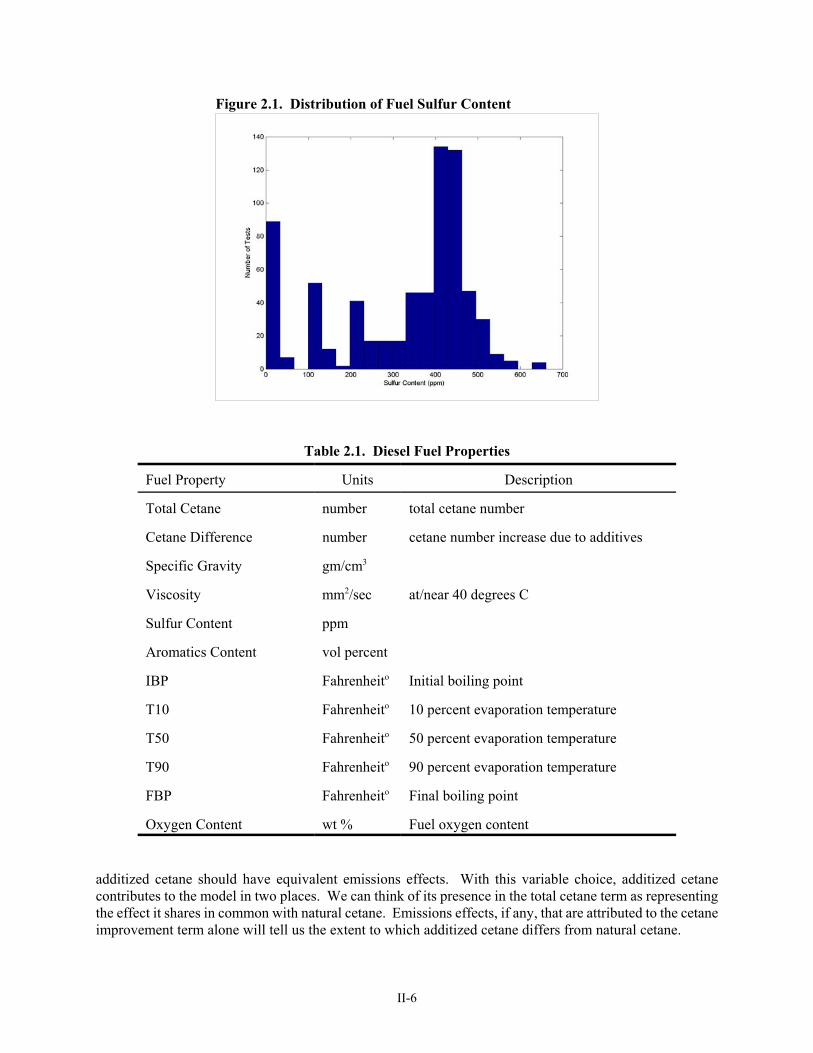
II-6
Figure 2.1. Distribution of Fuel Sulfur Content
Table 2.1. Diesel Fuel Properties
Fuel Property Units Description
Total Cetane number total cetane number
Cetane Difference number cetane number increase due to additives
Specific Gravity gm/cm3
Viscosity mm2/sec at/near 40 degrees C
Sulfur Content ppm
Aromatics Content vol percent
IBP Fahrenheito Initial boiling point
T10 Fahrenheito 10 percent evaporation temperature
T50 Fahrenheito 50 percent evaporation temperature
T90 Fahrenheito 90 percent evaporation temperature
FBP Fahrenheito Final boiling point
Oxygen Content wt % Fuel oxygen content
additized cetane should have equivalent emissions effects. With this variable choice, additized cetanecontributes to the model in two places. We can think of its presence in the total cetane term as representingthe effect it shares in common with natural cetane. Emissions effects, if any, that are attributed to the cetaneimprovement term alone will tell us the extent to which additized cetane differs from natural cetane.
II-7
Prior ORNL work also examined emission models based solely on linear fuel property variables. For the firsttime, this work takes the step of considering nonlinear (quadratic and interactive) terms in the variable spaceused in the eigenfuel analysis. Quadratic (X2) terms are used to represent saturation effects, in which theemission response slows and then ends as a fuel characteristic is varied to an ultimate value. Interactive termsare used to represent effects by which changes in two fuel properties tend to potentiate or offset each other.With twelve variables, as many as twelve quadratic (squared) terms and 12*11/2 = 66 interaction terms arepossible, for a total of 78 second order terms that could be considered.
For this work, quadratic and interactive terms were constructed for the six fuel properties that previousresearch had found to be important predictors for emissions (total cetane, cetane improvement, specificgravity, sulfur content, aromatics content, and oxygen content). Nonlinear terms were not considered forviscosity and the distillation temperatures, because these properties are thought to be most useful asdescriptors of the fuels, rather than emissions. Thus, 6 quadratic and 6*5/2 = 15 interaction terms wereconsidered for a total of 21 nonlinear terms. Much of the work in model development is related todetermining which of the nonlinear terms make a useful contribution.
II-2.3 METHODOLOGY FOR MODEL DEVELOPMENT
The process of model development follows the methodology laid out in prior ORNL publications (McAdams,Crawford and Hadder 2000a,b and 2002). The dependent variable is the logarithm of emissions after theeffects of individual engines have been removed from the data. The variable space is defined by the choiceof the twelve linear fuel property variables and one or more nonlinear terms. The linear fuel properties areused in all cases, while the number of nonlinear terms varies throughout the analysis.
Having chosen a variable space containing N total linear and nonlinear terms, Principal Components Analysis(PCA) is used to define the N eigenvectors that form an orthogonal basis for the space. In this approach, thenonlinear terms are incorporated directly in the vectors. The property-based description of fuels istransformed to eigenvector terms, and the eigenvector weights become the independent fuel variables in anotherwise conventional linear regression analysis. The effect of engines on emissions is removed in a firststage regression that essentially re-expresses the emissions test data to the mean emissions levels for eachengine. The effect of fuels is assessed in a second stage regression conducted on the re-expressed emissionsvalues. A full description of the regression methodology can be found in McAdams 2000b, pp. 9-32.
There are two basic methods to incorporate nonlinear terms in a regression model. In the “postnormalization” method, variables X and X2 are formed and then independently normalized to mean 0 andstandard deviation 1. This method is computationally simple, but one should recognize that X and X2 willtypically exhibit a strong linear correlation when computed over a range of positive values. In the “pre-normalization” method, variable X is first normalized and squared to form X2, which is then renormalized.This method is computationally more complex, but substantially reduces the correlation between linear andnonlinear terms that would otherwise be present. The “pre-normalization” method was chosen here over thecompeting “post-normalization” approach because it greatly reduces the linear dependence among terms.
The resulting emission models are of the form:
log( E ) = A0 + SUM( Ai * Wi ) (1)
where Ai are linear regression coefficients and Wi is the fuel weight for eigenvector I. This model formimplies that mass emissions are an exponential function of the summation term:
E = E0 * EXP( SUM( Ai * Wi) ) (2)

II-8
As shown in the ORNL publications, any eigenvector model can be transformed into a mathematicallyequivalent model in terms of the original fuel property variables:
log( E ) = SUM( Bi * Pi ), or
E = EXP( SUM( Bi * Pi) ) (3)
where Bi are emissions coefficients and Pi is the value for fuel property I.
While the models are exponential when stated in terms of mass emissions, the degree of non-linearityintroduced by the transformation is small in all cases, because the summation term is, itself, relatively small.A greater degree of nonlinear behavior can be introduced by the presence of quadratic terms, although thisis found to be modest in most circumstances.
The process of model development is a sequential search to find the most efficient set of variables forpredicting emissions. The search is done independently in developing the NOx and PM emission models, sothat the terms included in the variable space will differ for the two pollutants. A decision was made at theoutset of the study to retain all twelve linear fuel properties. Thus, the emphasis in the search is to identifynonlinear terms that make useful contributions to prediction.
Starting with a variable space containing only the twelve linear fuel property variables, an eigenvector modelis developed using the methods previously described. The 21 quadratic and interactive terms are testedindividually against the residuals from the best eigenvector model to identify terms that may add predictivepower. Quadratic and interactive terms appearing to contribute to predictive power are then added to thelinear terms to create an augmented variable space.
The process then follows the following steps until all of the nonlinear terms that make useful contributionsare identified:
1. A new set of eigenvectors is defined for the augmented variable space, which now includes bothlinear and nonlinear variables, and a new eigenvector model is selected, considering thesignificance and substantiality of terms. Typically, the retained terms account for 92-94 percentof the total effect associated with fuels.
2. The non-linear fuel property term making the weakest contribution to the model is identified usingthe simplify.m algorithm that has been developed for use in variable selection (see McAdams 2002,Appendix D). The algorithm provides a means to attribute the eigenvector model sums of squares(SS) to the individual fuel properties and to conduct an F test of their significance.
3. When a non-linear term is dropped from consideration, the eigenvectors are redefined and a revisedeigenvector model is selected. The nonlinear terms not present in the model are then re-testedindividually against the residuals from the current model to identify terms that may add predictivepower. One such term can be introduced to the model at each step. We then return to step 1 aboveand repeat the model estimation, simplification and testing process.
When the model development process came to an end, the final eigenvector models for NOx and PM werebased on variable spaces of 17 and 19 terms, respectively. As shown in Table 2.2, the variable spaces containall twelve linear terms plus five and seven nonlinear terms.

II-9
Table 2.2. Terms Contained in Emission Models
NOx Model PM Model
12 linear fuel properties
Total Cetane2
Sulfur2
Aromatics2
Cetane Improvement x Specific Gravity Cetane Improvement x Aromatics
12 linear fuel properties
Total Cetane2
Sulfur2
Oxygen2
Cetane Improvement x Total Cetane Sulfur x Cetane Improvement Sulfur x Specific Gravity Sulfur x Aromatics

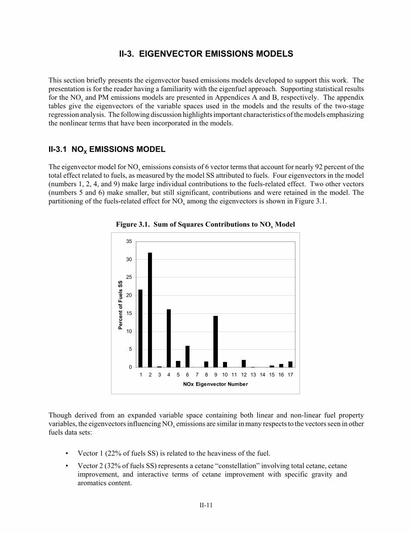
II-11
0
5
10
15
20
25
30
35
1 2 3 4 5 6 7 8 9 10 11 12 13 14 15 16 17
NOx Eigenvector Number
Perc
ent o
f Fue
ls S
S
Figure 3.1. Sum of Squares Contributions to NOx Model
II-3. EIGENVECTOR EMISSIONS MODELS
This section briefly presents the eigenvector based emissions models developed to support this work. Thepresentation is for the reader having a familiarity with the eigenfuel approach. Supporting statistical resultsfor the NOx and PM emissions models are presented in Appendices A and B, respectively. The appendixtables give the eigenvectors of the variable spaces used in the models and the results of the two-stageregression analysis. The following discussion highlights important characteristics of the models emphasizingthe nonlinear terms that have been incorporated in the models.
II-3.1 NOX EMISSIONS MODEL
The eigenvector model for NOx emissions consists of 6 vector terms that account for nearly 92 percent of thetotal effect related to fuels, as measured by the model SS attributed to fuels. Four eigenvectors in the model(numbers 1, 2, 4, and 9) make large individual contributions to the fuels-related effect. Two other vectors(numbers 5 and 6) make smaller, but still significant, contributions and were retained in the model. Thepartitioning of the fuels-related effect for NOx among the eigenvectors is shown in Figure 3.1.
Though derived from an expanded variable space containing both linear and non-linear fuel propertyvariables, the eigenvectors influencing NOx emissions are similar in many respects to the vectors seen in otherfuels data sets:
• Vector 1 (22% of fuels SS) is related to the heaviness of the fuel.
• Vector 2 (32% of fuels SS) represents a cetane “constellation” involving total cetane, cetaneimprovement, and interactive terms of cetane improvement with specific gravity andaromatics content.
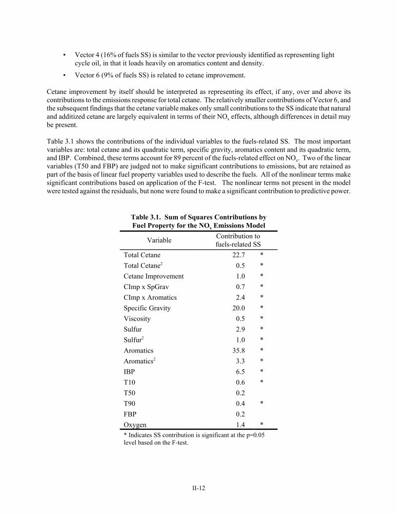
II-12
• Vector 4 (16% of fuels SS) is similar to the vector previously identified as representing lightcycle oil, in that it loads heavily on aromatics content and density.
• Vector 6 (9% of fuels SS) is related to cetane improvement.
Cetane improvement by itself should be interpreted as representing its effect, if any, over and above itscontributions to the emissions response for total cetane. The relatively smaller contributions of Vector 6, andthe subsequent findings that the cetane variable makes only small contributions to the SS indicate that naturaland additized cetane are largely equivalent in terms of their NOx effects, although differences in detail maybe present.
Table 3.1 shows the contributions of the individual variables to the fuels-related SS. The most importantvariables are: total cetane and its quadratic term, specific gravity, aromatics content and its quadratic term,and IBP. Combined, these terms account for 89 percent of the fuels-related effect on NOx. Two of the linearvariables (T50 and FBP) are judged not to make significant contributions to emissions, but are retained aspart of the basis of linear fuel property variables used to describe the fuels. All of the nonlinear terms makesignificant contributions based on application of the F-test. The nonlinear terms not present in the modelwere tested against the residuals, but none were found to make a significant contribution to predictive power.
Table 3.1. Sum of Squares Contributions byFuel Property for the NOx Emissions Model
Variable Contribution tofuels-related SS
Total Cetane 22.7 *Total Cetane2 0.5 *Cetane Improvement 1.0 *CImp x SpGrav 0.7 *CImp x Aromatics 2.4 *Specific Gravity 20.0 *Viscosity 0.5 *Sulfur 2.9 *Sulfur2 1.0 *Aromatics 35.8 *Aromatics2 3.3 *IBP 6.5 *T10 0.6 *T50 0.2T90 0.4 *FBP 0.2Oxygen 1.4 ** Indicates SS contribution is significant at the p=0.05level based on the F-test.

II-13
0
5
10
15
20
25
30
1 2 3 4 5 6 7 8 9 10 11 12 13 14 15 16 17 18 19
PM Eigenvector Number
Perc
ent o
f Fue
ls S
SFigure 3.2. Sum of Squares Contributions to PM Emissions
II-3.2 PM EMISSIONS MODEL
The eigenvector model for PM emissions consists of 7 vector terms that account for 95 percent of the totaleffect of fuels as measured by the sum of squares. Five of the eigenvectors in the model (1, 3, 5, 7, and 9)make large individual contributions to the fuels-related effect. Two other vectors (11 and 12) make smaller,but still significant, contributions and were retained in the model. The partitioning of the fuels-related effectfor PM is shown in Figure 3.2.
Because the variable space used for the PM model differs from that used in the NOx model in terms of thenonlinear variables included, the composition and interpretation of the eigenvectors will also differ. In spiteof this difference, and the inclusion of nonlinear terms, the eigenvectors influencing PM emissions are similarin many respects to the features seen in other fuels data sets:
• Vector 1 (14% of fuel SS) is related to the heaviness of the fuel.
• Vector 3 (27% of fuel SS) is related to oxygen content.
• Vector 5 (14% of fuel SS) is similar to the vector previously identified as representing lightcycle oil.
• Vector 7 (9% of fuel SS) is a feature loading on IBP in conjunction with aromatics and sulfurcontent.
• Vector 9 (25% of fuel SS) is related to cetane improvement.
These five vector terms account for 89 percent of the fuels-related effect. The two remaining terms in themodel appear to describe interactions among fuel properties.
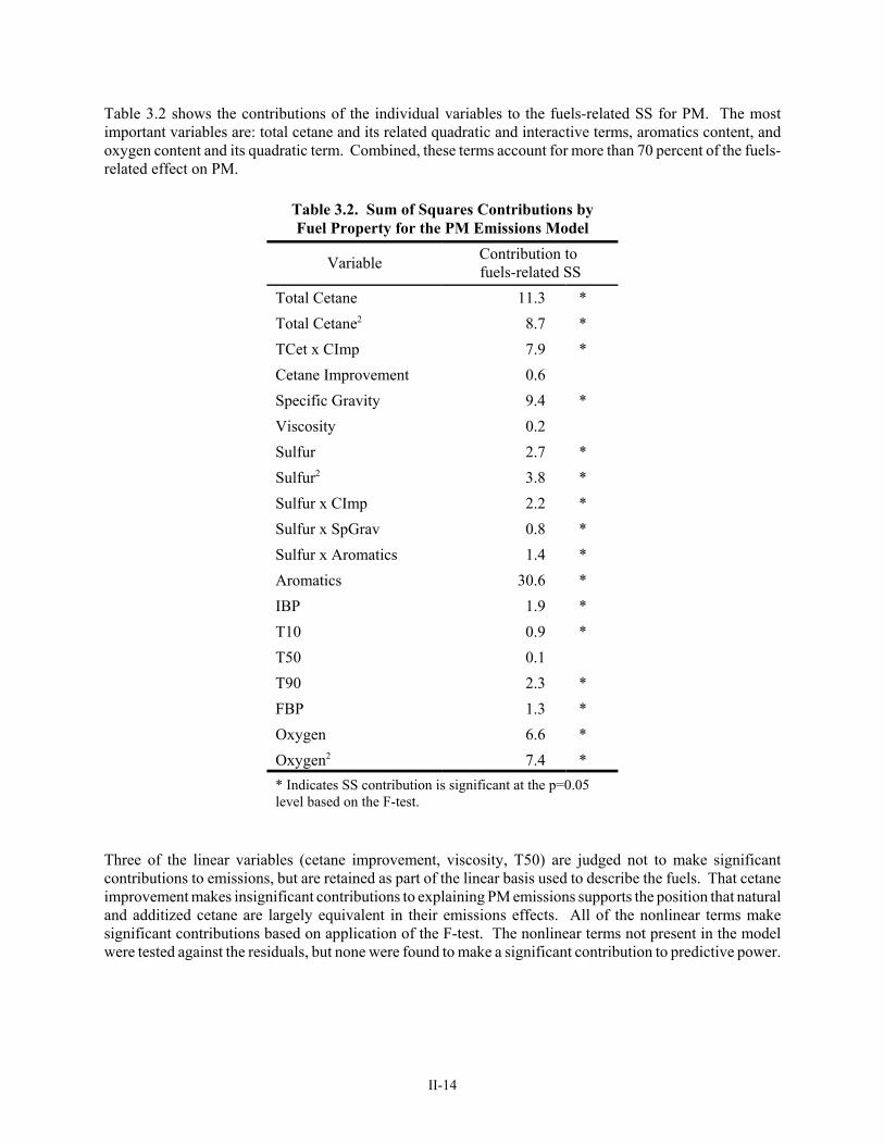
II-14
Table 3.2 shows the contributions of the individual variables to the fuels-related SS for PM. The mostimportant variables are: total cetane and its related quadratic and interactive terms, aromatics content, andoxygen content and its quadratic term. Combined, these terms account for more than 70 percent of the fuels-related effect on PM.
Table 3.2. Sum of Squares Contributions byFuel Property for the PM Emissions Model
Variable Contribution to fuels-related SS
Total Cetane 11.3 *Total Cetane2 8.7 *TCet x CImp 7.9 *Cetane Improvement 0.6 Specific Gravity 9.4 *Viscosity 0.2 Sulfur 2.7 *Sulfur2 3.8 *Sulfur x CImp 2.2 *Sulfur x SpGrav 0.8 *Sulfur x Aromatics 1.4 *Aromatics 30.6 *IBP 1.9 *T10 0.9 *T50 0.1 T90 2.3 *FBP 1.3 *Oxygen 6.6 *Oxygen2 7.4 ** Indicates SS contribution is significant at the p=0.05level based on the F-test.
Three of the linear variables (cetane improvement, viscosity, T50) are judged not to make significantcontributions to emissions, but are retained as part of the linear basis used to describe the fuels. That cetaneimprovement makes insignificant contributions to explaining PM emissions supports the position that naturaland additized cetane are largely equivalent in their emissions effects. All of the nonlinear terms makesignificant contributions based on application of the F-test. The nonlinear terms not present in the modelwere tested against the residuals, but none were found to make a significant contribution to predictive power.

II-15
II-4. EMISSIONS RESPONSE MODELS
II-4.1 INTRODUCTION
As has been noted, an eigenvector model can be transformed into a mathematically equivalent expression interms of the original fuel property variables. An equivalent expression of this kind will give the sameemissions predictions as the eigenvector model and may be easier to implement for predictive purposes inmany applications. RYM is such an application, and the emissions models are therefore implemented as theirequivalent fuel property expressions. An eigenvector model can be translated to its fuel property equivalent by an analytical process of algebraicexpansion and manipulation. The eigenvector weights in the regression equation would be replaced by theiralgebraic calculation in terms of fuel property values, and the resulting terms then re-organized into a similarequation in terms of fuel property variables. The process is cumbersome, however, and would be complicatedby the two levels of variable standardization involved in the pre-normalization approach to modelingnonlinear terms.
A regression technique has been used as a curve fitting tool as an alternative to the analytical process fortransforming an eigenfuel model to its equivalent in fuel property terms. The curve fitting process generatessynthetic emission tests data and fits a regression model containing linear and quadratic terms in the originalfuel variables, as appropriate. The result of this process is a reduced form version of the original eigenvectormodel that, for all practical purposes, gives equivalent predictions of emissions changes.
To develop the reduced form models, N=10,000 synthetic diesel fuels were generated by sampling randomlyfrom the range of fuel properties that might be encountered in refinery analyses. The range (see Table 4.1)was selected to bracket the maximum change in finished fuel properties likely to be relevant to emissions,based on the following considerations:
• The end of the range most favorable to emissions reduction was taken from the largestproperty changes, in the direction of reduced emissions, found in experimental fuels used inHDD emissions testing. This choice assumes that past research has identified the maximumextent that each property is likely to be modified in an effort to reduce emissions.
• The end of the range most adverse to emissions was taken from the end of the range ofproperty values, in the direction opposite to reduced emissions, found in commercial fuels.This choice assumes that RYM need not consider finished fuels that are more adverse toemissions than those at the end of the range of current commercial fuels.
In both cases, the endpoints of the range of data (experimental or commercial) were taken as the limits of theinterval that contained 95 percent of the fuels.
Having generated the fuels, the eigenfuel-based emission models were evaluated to generate a predictedemissions response. The predicted responses were then referenced to the emissions level of the averagecommercial fuel by expressing the predicted response as a fractional difference from the emissions valuepredicted for the average commercial fuel. A fractional difference of -0.050 for a fuel would mean that itreduces emissions by 5 percent compared to the average commercial fuel.
The reduced form models are estimated by regressing the synthesized fractional emissions response valuesagainst the linear, quadratic, and interaction terms found in the variable space of the eigenfuel-based models.The regression approach fits a fuel property equation to the emissions response surface of the eigenfuel

II-16
Table 4.1. Relevant Range of Fuel Property Values
Low Emissions
AverageCommercial
Fuel
High Emissions
TotCetane number 60.0 45.4 40.0CetImprv number 15.0 0 0.0Density gm/cm3 0.814 0.850 0.864Viscosity mm2/sec 1.66 2.67 3.26Sulfur ppm 5 352 500Aromatics vol percent 5.0 33.2 42.0IBP deg F 175 349 400T10 deg F 354 429 463T50 deg F 427 513 542T90 deg F 522 607 631FBP deg F 590 653 679Oxygen wt percent 5 0 0
model, and it also reduces the response surface from one stated in terms of log(emissions) to one in termsof mass emissions. The functions are of the form:
E = Ao + Sum ( Ai * Pi ) (4)
where E represents the predicted mass emissions (gm/bhp-hr), Ai are the reduced-form regression coefficients,and Pi represents the series of fuel property values including linear, quadratic, and interactive terms in thephysical units shown in the table above.
The reduced-form models created by this process are excellent representations of the eigenfuel-basedemissions models. The R2 statistics are 0.999 for NOx and 0.994 for PM, and the correlation coefficientsbetween the synthetic data and the predictions of the reduced-form models are similarly high. The use ofN=10,000 synthetic fuels assures that the estimated coefficient values are influenced by sampling fluctuationsto only a very small degree. The smallest t-statistic in the NOx model was 67 for the FBP term. The smallestt-statistic in the PM model was 14 for the T10 term.
The following sections present the NOx and PM response models, in turn, including the coefficient values andthe magnitudes of predicted emissions effects. Although we show predictions for the fuel propertiesindividually, it must be remembered that the properties generally do not vary independently in real-worldfuels. The predictions seen here for individual properties should be understood as vector emission effects thathave been distributed to the individual properties. In the case of a typical fuel change, several (or many)properties will change simultaneously, and the resulting emissions response will be the sum of contributionsthat are attributed to the properties.
II-4.2 NOX RESPONSE MODEL
Table 4.2 presents the reduced-form NOx response model. The equations predict the fractional emissionschange relative to the average commercial fuel as a function of the fuel property values (in physical units).The equations for total cetane, sulfur content, and aromatics content include both linear and quadraticcontributions. Cetane improvement appears in five places in the equation, including its participation in total

II-17
Table 4.2. Reduced-Form NOx Response Model(coefficients in physical units)
Model TermLinear
CoefficientQuadraticCoefficient
InflectionPoint
Intercept -0.29436Total Cetane -0.0050089 0.00003002 83.4Cetane Improvement -0.044716
CImp x Sp Gravity 0.054009CImp x Aromatics -0.00005762
Specific Gravity 0.37573Viscosity -0.0023846Sulfur 0.00007831 -0.08262 E-6 473.9Aromatics 0.0043869 -0.00004791 45.8IBP 0.00014618T10 -0.00002595T50 -0.00005585T90 0.00002215FBP 0.00001847Oxygen 0.0093568
cetane (linear and quadratic terms), its own linear term, and two interactive terms with specific gravity andaromatics.
The three properties with quadratic terms will reach a maximum when the property value equals the inflectionpoints shown in the table. Past practice in emissions modeling, as in the Complex Model for ReformulatedGasoline (DOE 1994), has been to “straight-line” the emissions response for values beyond the inflectionpoint. That approach is adopted here, although as a practical matter, all current and future fuels will lie belowthe inflection points, so that the straight-line portion of the curves will not be encountered.
Figures 4.1 through 4.5 illustrate the predicted NOx responses to the fuel properties found to have the largesteffects:
• NOx emissions are predicted to decrease by 2.7 percent when total cetane number is raised15 points from the commercial average of 45.4 to a total of 60 cetane (Figure 4.1), assumingthat other fuel property values would remain constant. There is a modest curvature to therelationship. A slowing of the emissions response begins to appear at total cetane values inthe mid-50s, and the response continues to slow as higher cetane numbers are approached.The maximum predicted reduction is 4.3 percent at the inflection point of 83.4 total cetane.This high cetane level is very unlikely to be encountered in either analytical exercises or inreal-world practice.

II-18
-8.0-7.0-6.0-5.0-4.0-3.0-2.0-1.00.01.02.0
5 10 15 20 25 30 35 40 45
Arom atics Conte nt (volum e pe rce nt)
NO
x Em
issi
ons
Cha
nge
(per
cent
)
Figure 4.3. NOx Emissions to Atomatics Content
-5.0
-4.0
-3.0
-2.0
-1.0
0.0
1.0
2.0
40 45 50 55 60 65 70 75 80 85Tota l Cetane Number
NO
x Em
issi
ons
Cha
nge
(Per
cent
)
Figure 4.1. NOx Emissions Response to Total Cetane Number
-4.5-4.0-3.5-3.0-2.5-2.0-1.5-1.0-0.50.0
0 5 10 15Cetane Number Increase
NO
x Em
issi
ons
Cha
nge
(Per
cent
)
Cetane Improvement Natural Cetane Increase
Figure 4.2. NOx Emissions Response to Natural and Additized Cetane
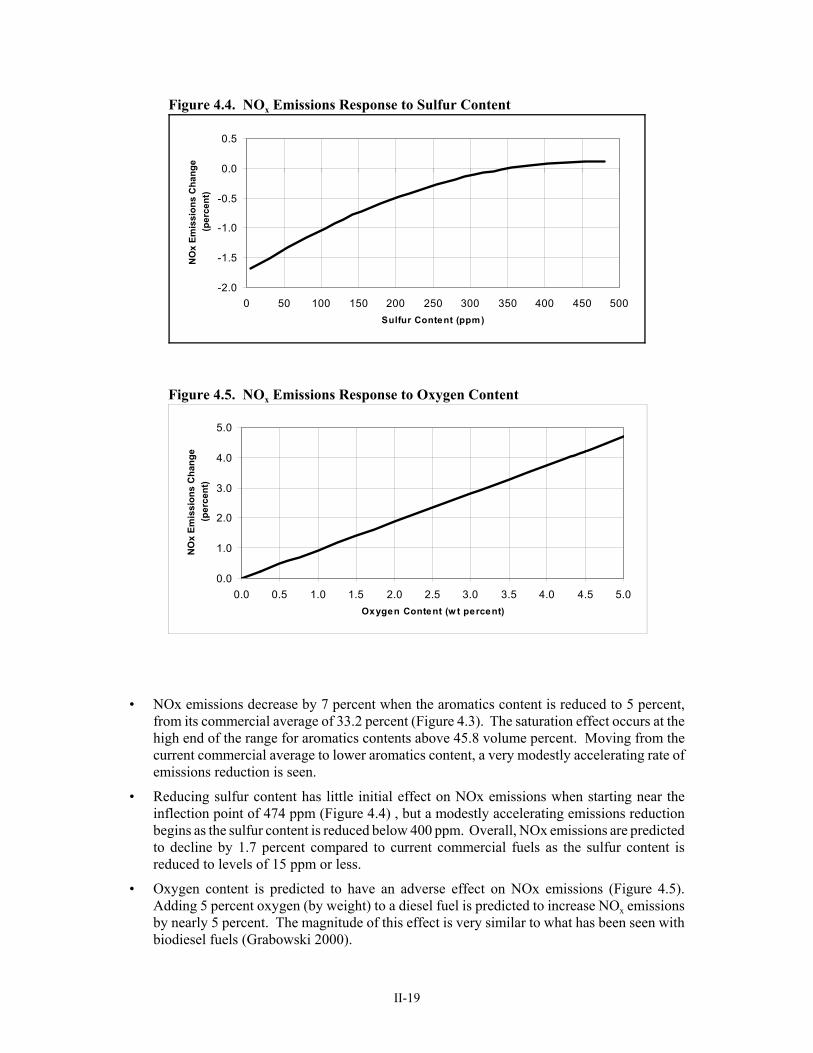
II-19
0.0
1.0
2.0
3.0
4.0
5.0
0.0 0.5 1.0 1.5 2.0 2.5 3.0 3.5 4.0 4.5 5.0Oxygen Content (w t percent)
NO
x Em
issi
ons
Cha
nge
(per
cent
)
Figure 4.5. NOx Emissions Response to Oxygen Content
-2.0
-1.5
-1.0
-0.5
0.0
0.5
0 50 100 150 200 250 300 350 400 450 500Sulfur Content (ppm)
NO
x Em
issi
ons
Cha
nge
(per
cent
)
Figure 4.4. NOx Emissions Response to Sulfur Content
• NOx emissions decrease by 7 percent when the aromatics content is reduced to 5 percent,from its commercial average of 33.2 percent (Figure 4.3). The saturation effect occurs at thehigh end of the range for aromatics contents above 45.8 volume percent. Moving from thecurrent commercial average to lower aromatics content, a very modestly accelerating rate ofemissions reduction is seen.
• Reducing sulfur content has little initial effect on NOx emissions when starting near theinflection point of 474 ppm (Figure 4.4) , but a modestly accelerating emissions reductionbegins as the sulfur content is reduced below 400 ppm. Overall, NOx emissions are predictedto decline by 1.7 percent compared to current commercial fuels as the sulfur content isreduced to levels of 15 ppm or less.
• Oxygen content is predicted to have an adverse effect on NOx emissions (Figure 4.5).Adding 5 percent oxygen (by weight) to a diesel fuel is predicted to increase NOx emissionsby nearly 5 percent. The magnitude of this effect is very similar to what has been seen withbiodiesel fuels (Grabowski 2000).
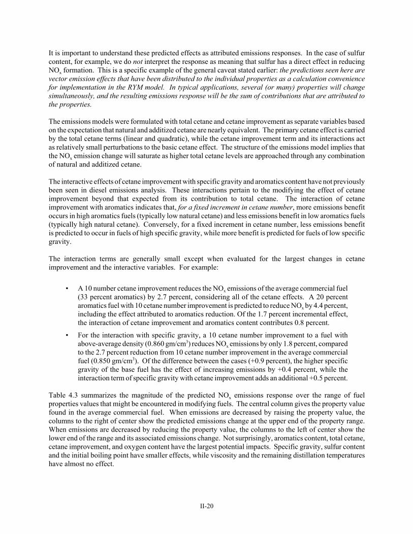
II-20
It is important to understand these predicted effects as attributed emissions responses. In the case of sulfurcontent, for example, we do not interpret the response as meaning that sulfur has a direct effect in reducingNOx formation. This is a specific example of the general caveat stated earlier: the predictions seen here arevector emission effects that have been distributed to the individual properties as a calculation conveniencefor implementation in the RYM model. In typical applications, several (or many) properties will changesimultaneously, and the resulting emissions response will be the sum of contributions that are attributed tothe properties.
The emissions models were formulated with total cetane and cetane improvement as separate variables basedon the expectation that natural and additized cetane are nearly equivalent. The primary cetane effect is carriedby the total cetane terms (linear and quadratic), while the cetane improvement term and its interactions actas relatively small perturbations to the basic cetane effect. The structure of the emissions model implies thatthe NOx emission change will saturate as higher total cetane levels are approached through any combinationof natural and additized cetane.
The interactive effects of cetane improvement with specific gravity and aromatics content have not previouslybeen seen in diesel emissions analysis. These interactions pertain to the modifying the effect of cetaneimprovement beyond that expected from its contribution to total cetane. The interaction of cetaneimprovement with aromatics indicates that, for a fixed increment in cetane number, more emissions benefitoccurs in high aromatics fuels (typically low natural cetane) and less emissions benefit in low aromatics fuels(typically high natural cetane). Conversely, for a fixed increment in cetane number, less emissions benefitis predicted to occur in fuels of high specific gravity, while more benefit is predicted for fuels of low specificgravity.
The interaction terms are generally small except when evaluated for the largest changes in cetaneimprovement and the interactive variables. For example:
• A 10 number cetane improvement reduces the NOx emissions of the average commercial fuel(33 percent aromatics) by 2.7 percent, considering all of the cetane effects. A 20 percentaromatics fuel with 10 cetane number improvement is predicted to reduce NOx by 4.4 percent,including the effect attributed to aromatics reduction. Of the 1.7 percent incremental effect,the interaction of cetane improvement and aromatics content contributes 0.8 percent.
• For the interaction with specific gravity, a 10 cetane number improvement to a fuel withabove-average density (0.860 gm/cm3) reduces NOx emissions by only 1.8 percent, comparedto the 2.7 percent reduction from 10 cetane number improvement in the average commercialfuel (0.850 gm/cm3). Of the difference between the cases (+0.9 percent), the higher specificgravity of the base fuel has the effect of increasing emissions by +0.4 percent, while theinteraction term of specific gravity with cetane improvement adds an additional +0.5 percent.
Table 4.3 summarizes the magnitude of the predicted NOx emissions response over the range of fuelproperties values that might be encountered in modifying fuels. The central column gives the property valuefound in the average commercial fuel. When emissions are decreased by raising the property value, thecolumns to the right of center show the predicted emissions change at the upper end of the property range.When emissions are decreased by reducing the property value, the columns to the left of center show thelower end of the range and its associated emissions change. Not surprisingly, aromatics content, total cetane,cetane improvement, and oxygen content have the largest potential impacts. Specific gravity, sulfur contentand the initial boiling point have smaller effects, while viscosity and the remaining distillation temperatureshave almost no effect.
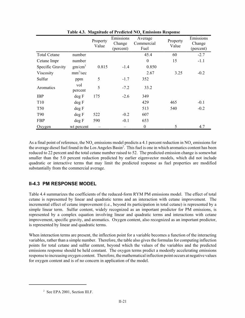
2 See EPA 2001, Section III.F.
II-21
Table 4.3. Magnitude of Predicted NOx Emissions Response
PropertyValue
EmissionsChange
(percent)
AverageCommercial
Fuel
PropertyValue
EmissionsChange
(percent)Total Cetane number 45.4 60 -2.7Cetane Impr number 0 15 -1.1Specific Gravity gm/cm3 0.815 -1.4 0.850Viscosity mm3/sec 2.67 3.25 -0.2Sulfur ppm 5 -1.7 352
Aromatics volpercent 5 -7.2 33.2
IBP deg F 175 -2.6 349T10 deg F 429 465 -0.1T50 deg F 513 540 -0.2T90 deg F 522 -0.2 607FBP deg F 590 -0.1 653Oxygen wt percent – – 0 5 4.7
As a final point of reference, the NOx emissions model predicts a 4.1 percent reduction in NOx emissions forthe average diesel fuel found in the Los Angeles Basin2. This fuel is one in which aromatics content has beenreduced to 22 percent and the total cetane number raised to 52. The predicted emission change is somewhatsmaller than the 5.0 percent reduction predicted by earlier eigenvector models, which did not includequadratic or interactive terms that may limit the predicted response as fuel properties are modifiedsubstantially from the commercial average.
II-4.3 PM RESPONSE MODEL
Table 4.4 summarizes the coefficients of the reduced-form RYM PM emissions model. The effect of totalcetane is represented by linear and quadratic terms and an interaction with cetane improvement. Theincremental effect of cetane improvement (i.e., beyond its participation in total cetane) is represented by asimple linear term. Sulfur content, widely recognized as an important predictor for PM emissions, isrepresented by a complex equation involving linear and quadratic terms and interactions with cetaneimprovement, specific gravity, and aromatics. Oxygen content, also recognized as an important predictor,is represented by linear and quadratic terms.
When interaction terms are present, the inflection point for a variable becomes a function of the interactingvariables, rather than a simple number. Therefore, the table also gives the formulas for computing inflectionpoints for total cetane and sulfur content, beyond which the values of the variables and the predictedemissions response should be held constant. The oxygen terms predict a modestly accelerating emissionsresponse to increasing oxygen content. Therefore, the mathematical inflection point occurs at negative valuesfor oxygen content and is of no concern in application of the model.

II-22
Table 4.4. Reduced-Form PM Response Model(coefficients in physical units)
Model TermLinear
CoefficientQuadraticCoefficient
InflectionPoint
Intercept -0.20469
Total Cetane -0.046802 0.00041817 Eq. 1
TCet x CImp 0.00051441
Cetane Improvement -0.031423
Specific Gravity 0.78127
Viscosity -0.0057629
Sulfur 0.0012166 -0.00000047 Eq. 2
Sulfur x Cimp 0.00001302
Sulfur x Sp Grav -0.00096997
Sulfur x Aromatics -0.00000446
Aromatics 0.0046396
IBP 0.00009756
T10 -0.00003778
T50 -0.00010789
T90 0.00023096
FBP 0.00019213
Oxygen -0.024834 -0.0046336 < 0
Equ. 1. Compute inflection point in cetane space as follows, where notation for coefficients isdefined by the equation E = a TCet + b TCet2 + c CImp + d TCet*CImp + e Sulf*CImp. (a) Resolve total cetane into its components TCet = NCet + CImp. (b) Limit CImp to not greater than: -[ a + c + (2b+d)NCet + e*Sulf ] / (2b+2d). © Limit NCet to not greater than: -[ a + (2b+d)CImp ] / (2b). (d) Recompute TCet = NCet + CImp after limitations are applied.
Equ 2. Compute inflection point for sulfur as follows, where notation for coefficients isdefined by the equation E = a S + b S2 + c S*SpGrav + d S*Arom + e S*CImp. Limit sulfur tonot greater than: -[ a + c SpGrav + d Arom + e CImp ] / (2b)
The cetane terms in the model – total cetane, its quadratic, cetane improvement and its interaction with totalcetane – produce the emissions surface shown in Figure 4.6. The axes in the figure are natural cetane andcetane improvement; therefore, total cetane number increases as one moves into the figure from theforeground point at natural cetane=40 and cetane improvement=0. The PM emissions surface declines rapidlyfrom the foreground point (40, 0), whether moving along the axis of increasing natural cetane, the axis of

II-23
Figure 4.6. PM Emissions Response to Cetane Effects
increasing cetane improvement, or diagonally through the figure. One sees that the emissions responsequickly saturates as higher total cetane numbers are approached. The maximum PM emissions reduction is-5.0 percent at a total cetane number of 56 or higher.
Figure 4.7 shows the trend in PM emissions with increasing total cetane. The solid line represents the effectof increasing natural cetane without use of cetane improvers. The dashed line represents cetane improvementof up to 15 numbers, by the use of additives with a base fuel of 45 natural cetane. PM emissions are reducedby approximately 5 percent when natural cetane number is raised to a total of 56 from the commercial averageof 45, and is flat thereafter. Cetane improvement produces a somewhat more rapid reduction in PM emissionsup to a saturation point at 52 total cetane (7 additized cetane numbers), but less total emissions reduction athigher numbers. The PM emissions effect of cetane improvers is largest in fuels with a natural cetane numberbelow 50 as seen in Figure 4.8. Almost no effect remains when cetane additives are used in base fuels withnatural cetane of 52 numbers or higher.
The PM emissions response to sulfur content is a 4-dimensional surface involving sulfur (linear and quadraticterms) and its interactions with aromatics content, specific gravity, and cetane improvement. Of these, theterms involving sulfur and aromatics content, shown in Figure 4.9, have the largest effects. Reducing thesulfur content of the average commercial fuel, with aromatics content of 33 percent, to below 15 ppm ispredicted to reduce PM emissions by only 3 percent (top line in the figure). The interaction with aromaticscontent potentiates this effect, however, increasing the emissions reduction as sulfur is removed from fuelsof reduced aromatics content. As seen in the bottom line of the figure, decreasing the aromatics content to5 percent, at constant sulfur content, is predicted to reduce PM emissions by nearly 10 percent. Removingsulfur from 5 percent aromatics fuel adds an additional 6 percent PM emissions reduction when 15 ppm sulfuris reached, for a total of 16 percent reduction.
A similar, although smaller, effect occurs in the terms involving sulfur content and specific gravity, as shownin Figure 4.10. At a specific gravity of 0.850 gm/cm3 that is typical of current commercial fuels, PMemissions begin to decline when sulfur content is reduced below 250 ppm. The maximum reduction is 3percent when sulfur content is decreased to 15 ppm. Decreasing the density of fuels to as low as 0.815gm/cm3 is predicted to reduce PM emissions by 1.8 percent, and the subsequent removal of sulfur to the levelof 15 ppm adds an additional 4 percent.
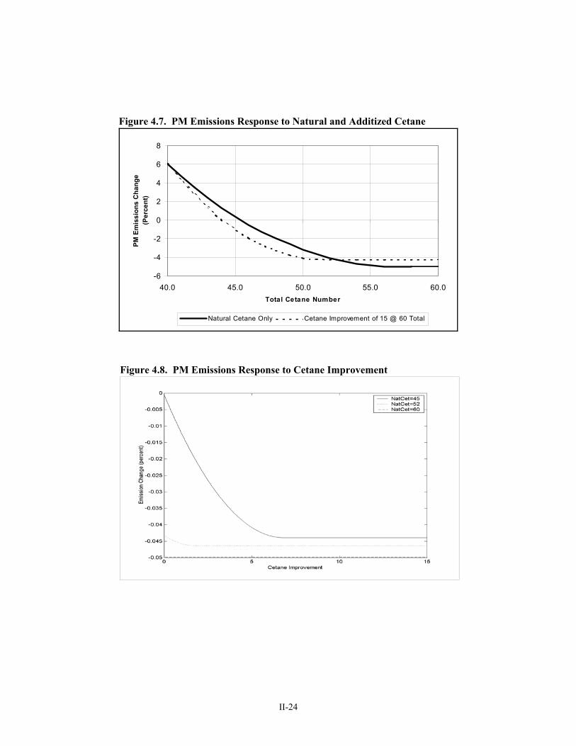
II-24
-6
-4
-2
0
2
4
6
8
40.0 45.0 50.0 55.0 60.0Total Cetane Number
PM E
mis
sion
s C
hang
e (P
erce
nt)
Natural Cetane Only Cetane Improvement of 15 @ 60 Total
Figure 4.7. PM Emissions Response to Natural and Additized Cetane
Figure 4.8. PM Emissions Response to Cetane Improvement

II-25
Figure 4.9. PM Emissions Response to Sulfur and Aromatics Content
Figure 4.10. PM Emissions Response to Sulfur Content and Specific Gravity
A similar potentiation of the benefit of reducing sulfur content also occurs in conjunction with cetaneimprovement, as shown in Figure 4.11. In current commercial fuels (top line of the figure), the benefit ofreducing sulfur content to 15 ppm is approximately 3 percent. An additional 4 percent PM reduction can beachieved by raising the cetane number 10 points through additives (lower line of the figure). Reducing sulfurcontent of the additized fuel to 15 ppm then reduces PM emissions by an additional 7 percent, to reach a totalof 11 percent reduction.

II-26
Figure 11. PM Emissions Response to Sulfur Content and CetaneImprovement
In general, one sees that the sulfur terms in the PM emissions model indicate increased benefits from sulfurreduction in fuels that have been improved, compared to current commercial fuels, in terms of aromaticscontent, specific gravity, or additized cetane. To our knowledge, such effects have not been explored in priorresearch and are not well-understood in terms of combustion processes. Nevertheless, the effects clearlyindicate that multi-property fuel improvements along these axes tend to potentiate each other in reducing PMemissions.
In addition to cetane and sulfur content, oxygen is predicted to have a large effect on PM emissions. PMemissions are predicted to decline by 25 percent when oxygen content reaches 5 percent (by weight). Thetrend shows a modest degree of acceleration as oxygen content increases.
Table 4.5 summarizes the sensitivity of emissions to changes in the fuel property values. If emissions aredecreased by raising the property value, the columns to the right of center show the maximum PM reductionwhen the property is moved to the upper end of the relevant range. If emissions are decreased by reducingthe property value, the columns to the left of center show the maximum PM reduction when the property ismoved to the lower end of the relevant range.
Clearly, the path to PM emissions reduction lies in adding oxygen to fuels and in reducing sulfur content inconjunction with aromatics. Total cetane and cetane improvement make smaller, but still substantialcontributions to PM emissions reductions, while other properties and the distillation curve appear to havemuch smaller effects.
The RYM model predicts an 11.3 percent reduction in PM emissions for the average diesel fuel found in theLos Angeles Basin. This fuel is one in which aromatics content has been reduced to 22 percent, the sulfurcontent cut to 130 ppm, and the total cetane number raised to 52. The predicted emission change is nearlytwice the 6.9 percent reduction estimated using a simple, linear eigenvector model in McAdams 2002. ThatPM estimate was caveated, however, because the prior eigenfuel model did not consider interaction terms thatEPA’s analysis had indicated were important. Now that quadratic and interaction terms are considered, the
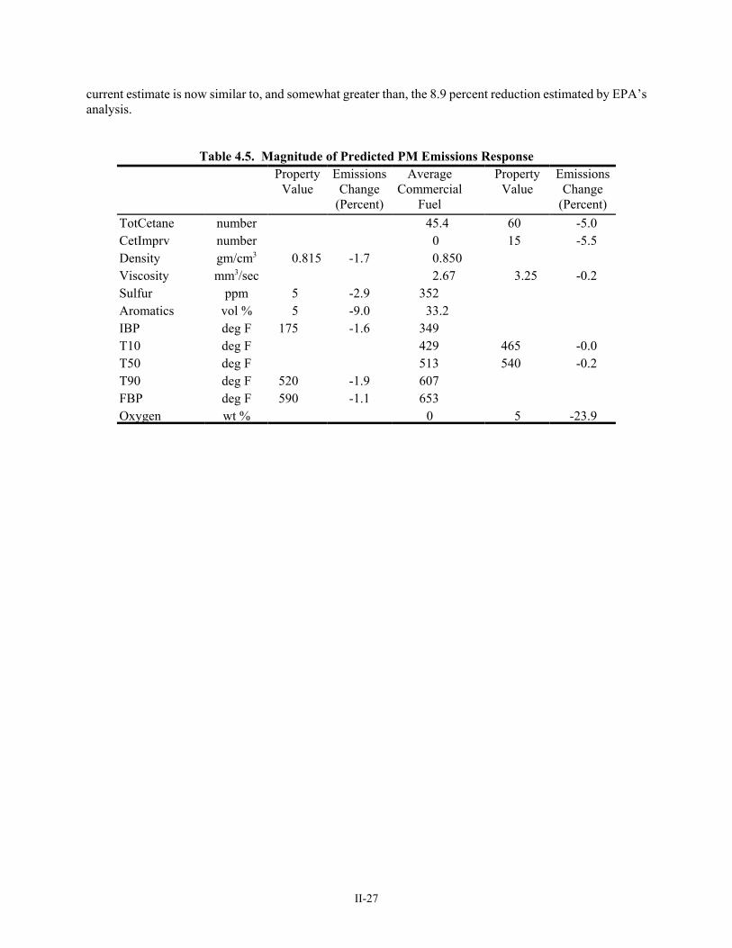
II-27
current estimate is now similar to, and somewhat greater than, the 8.9 percent reduction estimated by EPA’sanalysis.
Table 4.5. Magnitude of Predicted PM Emissions ResponseProperty
ValueEmissions
Change(Percent)
AverageCommercial
Fuel
PropertyValue
EmissionsChange
(Percent)TotCetane number 45.4 60 -5.0CetImprv number 0 15 -5.5Density gm/cm3 0.815 -1.7 0.850Viscosity mm3/sec 2.67 3.25 -0.2Sulfur ppm 5 -2.9 352Aromatics vol % 5 -9.0 33.2IBP deg F 175 -1.6 349T10 deg F 429 465 -0.0T50 deg F 513 540 -0.2T90 deg F 520 -1.9 607FBP deg F 590 -1.1 653Oxygen wt % 0 5 -23.9

II-29
II-5. IMPLEMENTATION IN RYM
II-5.1 REPRESENTING TECHNOLOGICAL CHANGE
At any point in time, the emissions effect of reformulating diesel fuel will depend on the mix of enginetechnologies on the road, the baseline exhaust emissions of each technology type, and the response ofemissions to changes in fuel properties, which could vary by technology type. There will soon be substantialchanges in diesel engines and fuels as the 2004 exhaust emission standards are implemented. After that point,new engines are expected to have EGR systems, oxidation catalysts, and particulate traps, and the sulfurcontent of diesel fuel will be cut to 10-15 ppm as an enabling measure to protect emission control systems.A key issue in this analysis is how a database that pertains almost entirely to current engines, without EGRor exhaust after-treatment, can be used to develop emission models representing the progressively changingfleet of vehicles between now and 2010.
As a starting point, differences in the emissions response to fuels, measured on a percentage basis, amongengine technology groups in the current on-road fleet appear to be small. The EPA analysis detected modestdifferences in the response to fuels for several groups, but the sales-weighted influence of these groups wasseen to be of essentially no importance. EPA’s conclusion was that, for the current population of on-roadengines, the emissions response to fuel changes appeared to be homogeneous. Therefore, we may treat thecurrent fleet of on-road engines as a single group, as in the statistical models presented in the prior section.
The emissions responses estimated through the statistical analysis are used here as benchmark functions thatare tied to the technology level and fuel-responsiveness of current on-road engines. These functions aredirectly representative of the emissions response for current engines that survive to future years, and they areused with adjustments to estimate the emissions response in newer technology engines equipped with EGR,exhaust after-treatment devices, or advanced engine combustion controls.
EPA estimates that EGR-equipped engines will account for 45 percent of the diesel on-road NOx inventoryby 2010 and 64 percent by 2020 (see Table 5.1). Only one study (HDEWG 1999) has tested an EGR-equipped engine on a range of fuels. Its conclusion was that fuel cetane appears to have little or no effect onNOx emissions, at least for the engine configuration tested. This result could be understood as suggesting thatEGR reduces peak combustion temperatures and pressures in a way that is similar to the combustion changesintroduced by increasing the cetane number. Having modified combustion characteristics through the useof EGR, there appears to remain essentially no additional benefit that can be achieved by increasing cetane.
To represent this effect, the cetane terms in the NOx model are adjusted downward over time in proportionto the declining number of non-EGR engines operating in fleet. By 2010, the most distant time period to beconsidered in RYM studies, the NOx benefit of increasing cetane number will be reduced to 55 percent of itscurrent value to reflect the proportion of the year 2010 fleet without EGR. The emissions response to otherfuel property changes, and of PM emissions to fuels, remain the same, in relative terms, as for the currentfleet.
The implication of measuring emission changes on a relative basis is that the absolute change in massemissions – whether measured as grams per mile or grams per brake-horsepower-hour – will be smaller inthe future as the baseline emission factors for the overall fleet decline. That is, although we assume that theemission changes on a fractional or percentage basis predicted for current engines will apply equally to futureengines, the lower baseline emission rate of the future engines will translate into a smaller total effect of massemissions.
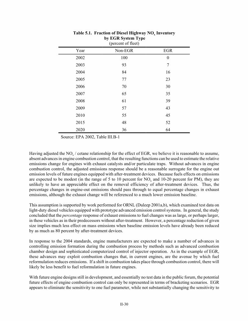
II-30
Table 5.1. Fraction of Diesel Highway NOx Inventory by EGR System Type
(percent of fleet)Year Non-EGR EGR2002 100 02003 93 72004 84 162005 77 232006 70 302007 65 352008 61 392009 57 432010 55 452015 48 522020 36 64
Source: EPA 2002, Table III.B-1
Having adjusted the NOx / cetane relationship for the effect of EGR, we believe it is reasonable to assume,absent advances in engine combustion control, that the resulting functions can be used to estimate the relativeemissions change for engines with exhaust catalysts and/or particulate traps. Without advances in enginecombustion control, the adjusted emissions response should be a reasonable surrogate for the engine outemission levels of future engines equipped with after-treatment devices. Because fuels effects on emissionsare expected to be modest (in the range of 5 to 10 percent for NOx and 10-20 percent for PM), they areunlikely to have an appreciable effect on the removal efficiency of after-treatment devices. Thus, thepercentage changes in engine-out emissions should pass through to equal percentage changes in exhaustemissions, although the exhaust change will be referenced to a much lower emission baseline.
This assumption is supported by work performed for ORNL (Duleep 2001a,b), which examined test data onlight-duty diesel vehicles equipped with prototype advanced emission control systems. In general, the studyconcluded that the percentage response of exhaust emissions to fuel changes was as large, or perhaps larger,in these vehicles as in their predecessors without after-treatment. However, a percentage reduction of givensize implies much less effect on mass emissions when baseline emission levels have already been reducedby as much as 80 percent by after-treatment devices.
In response to the 2004 standards, engine manufacturers are expected to make a number of advances incontrolling emission formation during the combustion process by methods such as advanced combustionchamber design and sophisticated computerized control of injector operation. As in the example of EGR,these advances may exploit combustion changes that, in current engines, are the avenue by which fuelreformulation reduces emissions. If a shift in combustion takes place through combustion control, there willlikely be less benefit to fuel reformulation in future engines.
With future engine designs still in development, and essentially no test data in the public forum, the potentialfuture effects of engine combustion control can only be represented in terms of bracketing scenarios. EGRappears to eliminate the sensitivity to one fuel parameter, while not substantially changing the sensitivity to
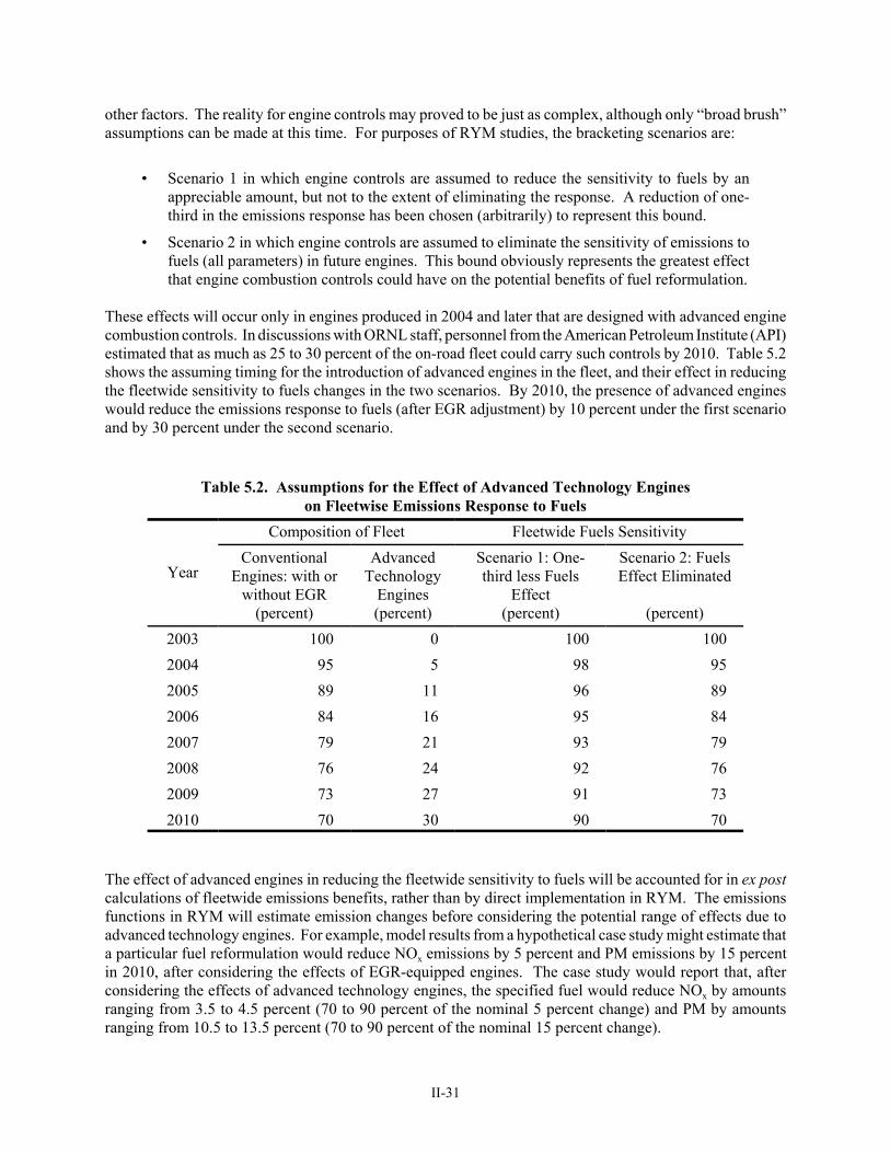
II-31
other factors. The reality for engine controls may proved to be just as complex, although only “broad brush”assumptions can be made at this time. For purposes of RYM studies, the bracketing scenarios are:
• Scenario 1 in which engine controls are assumed to reduce the sensitivity to fuels by anappreciable amount, but not to the extent of eliminating the response. A reduction of one-third in the emissions response has been chosen (arbitrarily) to represent this bound.
• Scenario 2 in which engine controls are assumed to eliminate the sensitivity of emissions tofuels (all parameters) in future engines. This bound obviously represents the greatest effectthat engine combustion controls could have on the potential benefits of fuel reformulation.
These effects will occur only in engines produced in 2004 and later that are designed with advanced enginecombustion controls. In discussions with ORNL staff, personnel from the American Petroleum Institute (API)estimated that as much as 25 to 30 percent of the on-road fleet could carry such controls by 2010. Table 5.2shows the assuming timing for the introduction of advanced engines in the fleet, and their effect in reducingthe fleetwide sensitivity to fuels changes in the two scenarios. By 2010, the presence of advanced engineswould reduce the emissions response to fuels (after EGR adjustment) by 10 percent under the first scenarioand by 30 percent under the second scenario.
Table 5.2. Assumptions for the Effect of Advanced Technology Engineson Fleetwise Emissions Response to Fuels
Year
Composition of Fleet Fleetwide Fuels SensitivityConventional
Engines: with orwithout EGR
(percent)
AdvancedTechnology
Engines(percent)
Scenario 1: One-third less Fuels
Effect(percent)
Scenario 2: FuelsEffect Eliminated
(percent)2003 100 0 100 1002004 95 5 98 952005 89 11 96 892006 84 16 95 842007 79 21 93 792008 76 24 92 762009 73 27 91 732010 70 30 90 70
The effect of advanced engines in reducing the fleetwide sensitivity to fuels will be accounted for in ex postcalculations of fleetwide emissions benefits, rather than by direct implementation in RYM. The emissionsfunctions in RYM will estimate emission changes before considering the potential range of effects due toadvanced technology engines. For example, model results from a hypothetical case study might estimate thata particular fuel reformulation would reduce NOx emissions by 5 percent and PM emissions by 15 percentin 2010, after considering the effects of EGR-equipped engines. The case study would report that, afterconsidering the effects of advanced technology engines, the specified fuel would reduce NOx by amountsranging from 3.5 to 4.5 percent (70 to 90 percent of the nominal 5 percent change) and PM by amountsranging from 10.5 to 13.5 percent (70 to 90 percent of the nominal 15 percent change).
II-32
II-5.2 IMPLEMENTATION IN RYM
The emissions models are implemented in RYM by pre-evaluating the equations for each blendstock in themodel to create NOx and PM “blending values”. The blending values are, in concept, estimated contributionsof each blendstock to the emissions level of finished fuels in which the blendstocks are used. The RYMsolution process will assume that the blending values combine linearly according to the volume fractions inthe final fuel. The full emission equations will be evaluated after the model’s solution and the precise valueof the predicted emissions response compared with that estimated by RYM under linear blending. If thedifference is large, the RYM case will be re-run.
The degree of nonlinearity in the equations is generally small across the range of fuel modifications that arelikely to be encountered in case studies. The primary exception to this generality is the cetane surface for PMemissions, in which the emissions response slows rapidly as total cetane number is increased and reachessaturation at a total cetane of 56. A Monte Carlo simulation was conducted to put bounds on the likelihoodof divergence. A total of 1000 synthetic fuels was generated by uniform, random sampling within the rangeof relevant fuel property values identified in Table 4.1. NOx and PM blending value were computed for eachfuel using the emissions equations in Tables 4.2 and 4.4. The 1000 fuels were then treated as blendstocksto create new fuels.
The blendstock simulation selected 2 fuels at random and blended them according to random weights thattotaled 100 percent. The individual fuel properties were blended linearly, as were the NOx values, to producea simulated final fuel. A total of 100 such “final fuels” were generated. Some fuel properties, such asaromatics, will blend linearly, while other properties will not. The greatest non-linearity in blending may liein the distillation temperatures. However, these properties have relatively little effect on emissions and effortsto obtain nonlinear blending algorithms did not yield reliable relationships. Thus, linear blending was usedas a reasonable approximation, but it will tend to understate the degree of divergence to be encountered inRYM.
The results of the simulation give us reason to believe that pre-evaluating the equations for all blendstockswill be a satisfactory approach for implementing the equations in RYM. Of 100 cases generated, most ofthe errors in estimate are within 1 part in 10 of the precisely calculated emission response. This means thata 5 percent in reduction in NOx would be estimated to within +/- 0.5 percent by the model (4.5 to 5 .5percent), while a 20 percent reduction in PM would be estimated to within +/- 2 percent by the model (18 to22 percent).
It must be recognized that the actual degree of divergence between the RYM solution and the preciselycalculated value are likely to be greater than shown in the simulation. First, RYM employs nonlinearblending algorithms for properties such as sulfur content and the distillation curve that do not blend inaccordance with volume weights. The divergence estimated in the simulation would increase if nonlinearblending were allowed. Second, the actual blendstocks in the RYM model span a wider range in fuelproperties than was considered in the simulation. For example, a series of blendstocks will represent non-aromatic feeds and, therefore, have zero aromatics content; other blendstocks may represent aromatic feedsand, therefore, have 100 percent aromatics content. In the simulation, the hypothetical “blendstocks” rangedbetween 5 and 42 percent. As a result, blendstocks in the model are more likely to fall in the range of valueswhere the emissions response saturates, thereby increasing the divergence between RYM solution and theprecise emissions response. Nevertheless, the divergence can be reduced whenever necessary by rerunninga case.
II-33
REFERENCES
Department of Energy. 1994. Estimating the Costs and Effects of Reformulated Gasoline. DOE/PO-0030. December.
Duleep, K.G. 2001. Diesel Technology and Fuel Requirements for Low Emissions: Phase I, Energyand Environmental Analysis, Inc., under contract with ORNL, May.
Duleep, K.G. 2001. Diesel Technology and Fuel Requirements for Low Emissions, Energy andEnvironmental Analysis, Inc., under contract with ORNL, May.
Environmental Protection Agency. 2001. Strategies and Issues in Correlating Diesel Fuel Propertieswith Emissions: Staff Discussion Document. EPA420-P-01-001. July.
Environmental Protection Agency. 2002. The Effect of Cetane Number Increase Due to Additives onNOx Emissions from Heavy-Duty Highway Engines. EPA420-S-02-012. June.
Grabowski, M.S., R.L. McCormick, T.L. Alleman, A.M. Herring. 2000. The Effect of BiodieselComposition on Engine Emissions From a DDC Series 60 Diesel Engine. Colorado Institute for Fuels andEngine Research, Colorado School of Mines, under contract with NREL, June.
Heavy Duty Engine Working Group (HDEWG). 1999. Phase II Briefing for Meeting of the MobileSources Technical Review Subcommittee. Clean Air Act Advisory Committee. Washington, D.C. January13.
McAdams, H.T., R.W. Crawford and G.R. Hadder. 2000. A Vector Approach to Regression Analysisand Its Application to Heavy-Duty Diesel Emissions. SAE 2000-01-1961.
McAdams, H.T., R.W. Crawford and G.R. Hadder. 2000. A Vector Approach to Regression Analysisand Its Application to Heavy-Duty Diesel Emissions. ORNL/TM-2000/5.
McAdams, H.T., R.W. Crawford and G.R. Hadder. 2001. PCR+ in Diesel Fuels and EmissionsResearch. ORNL/TM-2002/16.
Southwest Research Institute. 2001. Diesel Fuel Impact Model Data Analysis Plan Review. SwRI08.04075.


APPENDIX II-A
STATISTICAL RESULTS FOR NOX EMISSIONS MODEL


II-37
PCA Eigen variables 1 2 3 4 5 6 7 8 9 10 11 12 13 14 15 16 17 TotCetane 0.107 -0.474 0.175 -0.200 0.057 -0.426 0.141 -0.080 0.123 -0.129 0.225 -0.159 0.140 -0.241 0.253 -0.350 0.332CetImprv 0.029 -0.242 0.418 0.414 -0.025 -0.406 0.075 -0.145 0.120 -0.290 -0.193 0.128 -0.006 0.287 -0.143 0.294 -0.246Density 0.312 0.176 0.048 0.443 -0.080 0.081 0.049 0.039 0.067 -0.001 -0.358 -0.030 -0.426 -0.032 0.439 -0.351 0.156Viscosity 0.395 -0.099 -0.154 0.053 0.042 0.001 0.073 0.182 0.202 0.173 -0.038 0.007 -0.030 0.102 -0.212 0.487 0.634Sulfur 0.268 0.045 0.191 -0.217 0.285 0.272 0.135 -0.449 -0.196 -0.189 -0.278 -0.529 -0.002 -0.000 -0.188 0.043 0.005Aromatics 0.210 0.182 0.106 0.494 -0.272 0.114 -0.028 -0.298 -0.290 0.026 0.403 0.032 0.400 -0.236 -0.093 -0.019 0.138IBP 0.223 -0.025 -0.365 0.081 0.322 -0.118 0.016 0.330 -0.510 -0.461 0.045 0.038 0.163 0.144 0.223 0.072 -0.061T10 0.362 -0.091 -0.178 0.159 0.264 -0.109 0.062 0.148 0.128 0.195 0.098 0.019 -0.068 -0.032 -0.578 -0.454 -0.294T50 0.394 -0.124 -0.028 -0.044 -0.052 0.076 0.121 0.039 0.203 0.261 0.252 -0.217 0.012 -0.112 0.410 0.354 -0.525T90 0.306 -0.119 -0.078 -0.244 -0.460 0.029 -0.218 -0.103 -0.044 0.075 -0.082 0.010 0.235 0.648 0.047 -0.253 -0.017FBP 0.299 -0.128 -0.105 -0.270 -0.394 -0.044 -0.209 -0.069 -0.108 -0.298 -0.211 0.311 -0.224 -0.508 -0.172 0.111 -0.113Oxygen -0.011 0.004 0.300 -0.104 -0.367 0.219 0.647 0.474 -0.142 -0.134 0.047 -0.051 -0.016 0.027 -0.153 -0.071 -0.016Tot Cet ^ 2 -0.155 -0.213 -0.360 0.072 -0.106 -0.232 0.450 -0.267 -0.357 0.437 -0.350 0.061 0.057 -0.064 0.033 0.045 -0.035Sulfur ^ 2 -0.221 -0.035 -0.417 0.238 -0.356 -0.108 -0.091 0.113 0.234 -0.256 -0.078 -0.636 0.062 -0.084 -0.132 0.019 -0.031Aromatics^2 -0.081 -0.281 -0.343 0.095 0.046 0.450 0.309 -0.351 0.313 -0.342 0.194 0.289 -0.084 0.128 0.042 -0.056 0.012CImp x Dens -0.127 -0.498 0.088 0.140 -0.055 0.172 -0.255 0.032 -0.410 0.136 0.292 -0.185 -0.529 0.117 -0.071 0.047 0.045CImp x Arom -0.058 -0.461 0.139 0.174 0.112 0.424 -0.218 0.260 0.047 0.096 -0.403 0.051 0.455 -0.196 0.045 -0.051 -0.032 Eigenvalues 5.322 2.422 1.805 1.532 1.210 1.058 0.967 0.793 0.542 0.493 0.260 0.216 0.141 0.089 0.069 0.060 0.021 Pct Variance 31.307 14.247 10.618 9.012 7.119 6.222 5.690 4.666 3.187 2.900 1.529 1.270 0.827 0.525 0.407 0.351 0.121Cumulative Pct 31.307 45.554 56.172 65.184 72.303 78.525 84.214 88.881 92.067 94.967 96.497 97.767 98.595 99.120 99.528 99.879 100.000
PCA Eigen variables in physical units
1 2 3 4 5 6 7 8 9 10 11 12 13 14 15 16 17 TotCetane 0.674 -2.971 1.097 -1.257 0.356 -2.673 0.885 -0.499 0.771 -0.809 1.413 -0.994 0.879 -1.508 1.583 -2.194 2.080CetImprv 0.130 -1.085 1.874 1.857 -0.111 -1.821 0.338 -0.651 0.540 -1.301 -0.865 0.573 -0.028 1.286 -0.641 1.318 -1.102Density 0.005 0.003 0.001 0.007 -0.001 0.001 0.001 0.001 0.001 -0.000 -0.005 -0.000 -0.006 -0.000 0.007 -0.005 0.002Viscosity 0.249 -0.062 -0.097 0.033 0.026 0.001 0.046 0.115 0.127 0.109 -0.024 0.004 -0.019 0.064 -0.133 0.307 0.399Sulfur 43.943 7.390 31.388 -35.671 46.711 44.631 22.222 -73.622 -32.088 -30.944 -45.658 -86.757 -0.323 -0.016 -30.775 7.083 0.866Aromatics 1.716 1.488 0.865 4.040 -2.220 0.931 -0.228 -2.432 -2.368 0.214 3.294 0.258 3.268 -1.926 -0.759 -0.159 1.124IBP 12.321 -1.366 -20.173 4.504 17.827 -6.516 0.891 18.253 -28.221 -25.512 2.483 2.079 9.013 7.977 12.309 3.964 -3.373T10 14.016 -3.506 -6.896 6.172 10.225 -4.208 2.391 5.741 4.943 7.536 3.802 0.732 -2.641 -1.235 -22.374 -17.556 -11.385T50 13.363 -4.214 -0.944 -1.493 -1.761 2.590 4.095 1.325 6.891 8.862 8.556 -7.355 0.404 -3.813 13.915 12.029 -17.830T90 10.685 -4.161 -2.722 -8.515 -16.066 1.028 -7.611 -3.606 -1.525 2.615 -2.879 0.362 8.209 22.651 1.650 -8.846 -0.589FBP 9.986 -4.267 -3.502 -9.016 -13.137 -1.452 -6.961 -2.290 -3.614 -9.930 -7.032 10.384 -7.471 -16.937 -5.733 3.717 -3.754Oxygen -0.005 0.002 0.136 -0.047 -0.166 0.099 0.293 0.215 -0.064 -0.061 0.021 -0.023 -0.007 0.012 -0.069 -0.032 -0.007Tot Cet ^ 2 -0.244 -0.336 -0.567 0.113 -0.166 -0.365 0.708 -0.420 -0.562 0.688 -0.551 0.096 0.089 -0.101 0.051 0.071 -0.056Sulfur ^ 2 -0.251 -0.040 -0.473 0.271 -0.404 -0.122 -0.103 0.128 0.266 -0.291 -0.089 -0.722 0.071 -0.095 -0.150 0.021 -0.035Aromatics^2 -0.114 -0.393 -0.480 0.133 0.065 0.629 0.432 -0.491 0.438 -0.479 0.272 0.405 -0.117 0.179 0.059 -0.079 0.016CImp x Dens -0.105 -0.410 0.072 0.115 -0.045 0.141 -0.210 0.026 -0.338 0.112 0.241 -0.152 -0.436 0.097 -0.059 0.039 0.037CImp x Arom -0.052 -0.414 0.125 0.156 0.101 0.382 -0.196 0.233 0.042 0.086 -0.362 0.046 0.409 -0.176 0.041 -0.046 -0.029
Table A.1. PCA Decomposition of Experimental Fuels for NOx Model

II-38
Stage 1: Regression against engine dummy variables SS DF Mean Sq Mean 1695.1658 1.0000 1695.1658Model 11.0749 35.0000 0.3164 F Value: 176.46Error 1.2032 671.0000 0.0018 R-square: 0.9020Total 1707.4439 707.0000 2.4151 Stage 2(a): Regression against PCA coefficients (eigenfuels) SS DF Mean Sq Mean 0.0000 1.0000 0.0000Model 0.7546 17.0000 0.0444 F Value: 68.17Error 0.4486 689.0000 0.0007 R-square: 0.6271Total 1.2032 707.0000 0.0017 Predictive correlation to dependent variable: 0.7919
Estimate Std Err t-value Intercept -0.00000 0.00096 0.00000EigVec 1 0.00658 0.00042 15.81274EigVec 2 0.01185 0.00062 19.20768EigVec 3 -0.00105 0.00071 1.46568EigVec 4 0.01062 0.00078 13.68153EigVec 5 -0.00399 0.00087 4.57070EigVec 6 0.00771 0.00093 8.25964EigVec 7 0.00005 0.00098 0.05454EigVec 8 -0.00465 0.00108 4.30955EigVec 9 -0.01680 0.00130 12.87233EigVec 10 0.00554 0.00137 4.04847EigVec 11 0.00125 0.00188 0.66115EigVec 12 0.00985 0.00207 4.76842EigVec 13 -0.00325 0.00256 1.26737EigVec 14 -0.00247 0.00321 0.76727EigVec 15 0.00878 0.00365 2.40492EigVec 16 -0.01297 0.00393 3.29939EigVec 17 -0.02891 0.00669 4.32367 SS contributions by eigenvector Reg Coeff Model SS Pct SS F Ratio EigVec 1 0.0066 0.1628 21.58 250.04*EigVec 2 0.0119 0.2402 31.84 368.93*EigVec 3 -0.0010 0.0014 0.19 2.15 EigVec 4 0.0106 0.1219 16.15 187.18*EigVec 5 -0.0040 0.0136 1.80 20.89*EigVec 6 0.0077 0.0444 5.89 68.22*EigVec 7 0.0001 0.0000 0.00 0.00 EigVec 8 -0.0046 0.0121 1.60 18.57*EigVec 9 -0.0168 0.1079 14.30 165.70*EigVec 10 0.0055 0.0107 1.41 16.39*EigVec 11 0.0012 0.0003 0.04 0.44 EigVec 12 0.0099 0.0148 1.96 22.74*EigVec 13 -0.0032 0.0010 0.14 1.61 EigVec 14 -0.0025 0.0004 0.05 0.59 EigVec 15 0.0088 0.0038 0.50 5.78*EigVec 16 -0.0130 0.0071 0.94 10.89*EigVec 17 -0.0289 0.0122 1.61 18.69*
Table A.2. PCR+ Regression Model for NOx Emissions
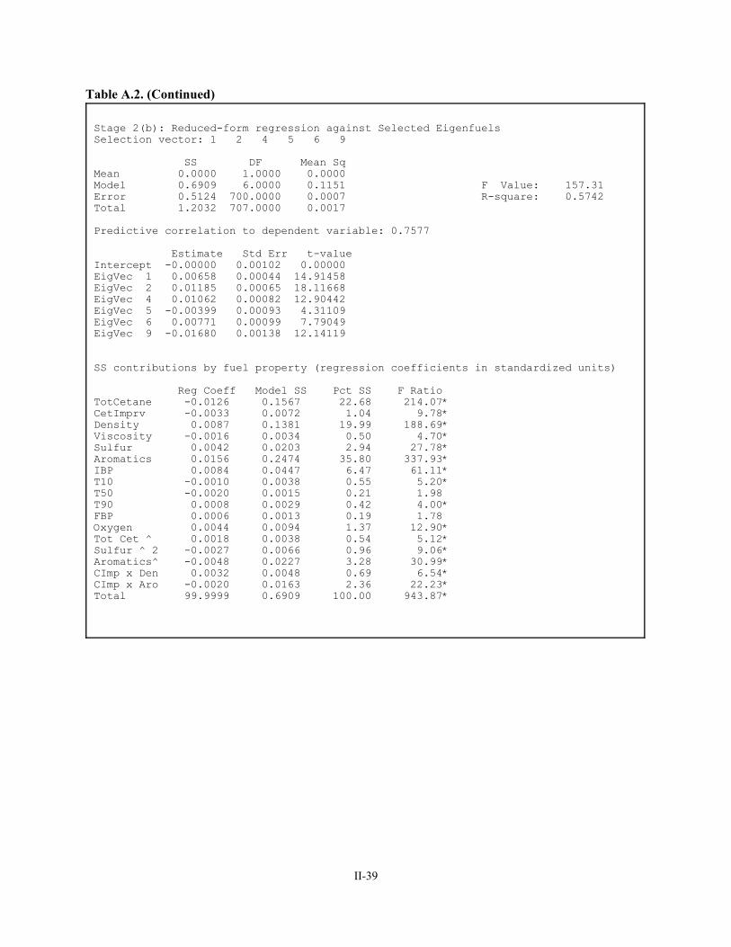
II-39
Stage 2(b): Reduced-form regression against Selected EigenfuelsSelection vector: 1 2 4 5 6 9 SS DF Mean Sq Mean 0.0000 1.0000 0.0000Model 0.6909 6.0000 0.1151 F Value: 157.31Error 0.5124 700.0000 0.0007 R-square: 0.5742Total 1.2032 707.0000 0.0017 Predictive correlation to dependent variable: 0.7577 Estimate Std Err t-value Intercept -0.00000 0.00102 0.00000EigVec 1 0.00658 0.00044 14.91458EigVec 2 0.01185 0.00065 18.11668EigVec 4 0.01062 0.00082 12.90442EigVec 5 -0.00399 0.00093 4.31109EigVec 6 0.00771 0.00099 7.79049EigVec 9 -0.01680 0.00138 12.14119 SS contributions by fuel property (regression coefficients in standardized units) Reg Coeff Model SS Pct SS F Ratio TotCetane -0.0126 0.1567 22.68 214.07*CetImprv -0.0033 0.0072 1.04 9.78*Density 0.0087 0.1381 19.99 188.69*Viscosity -0.0016 0.0034 0.50 4.70*Sulfur 0.0042 0.0203 2.94 27.78*Aromatics 0.0156 0.2474 35.80 337.93*IBP 0.0084 0.0447 6.47 61.11*T10 -0.0010 0.0038 0.55 5.20*T50 -0.0020 0.0015 0.21 1.98 T90 0.0008 0.0029 0.42 4.00*FBP 0.0006 0.0013 0.19 1.78 Oxygen 0.0044 0.0094 1.37 12.90*Tot Cet ^ 0.0018 0.0038 0.54 5.12*Sulfur ^ 2 -0.0027 0.0066 0.96 9.06*Aromatics^ -0.0048 0.0227 3.28 30.99*CImp x Den 0.0032 0.0048 0.69 6.54*CImp x Aro -0.0020 0.0163 2.36 22.23*Total 99.9999 0.6909 100.00 943.87*
Table A.2. (Continued)

APPENDIX II-B
STATISTICAL RESULTS FOR PM EMISSIONS MODEL


II-43
PCA Eigen variables 1 2 3 4 5 6 7 8 9 10 11 12 13 14 15 16 17 18 19 TotCetane 0.125 -0.080 0.169 -0.144 0.664 -0.059 0.014 -0.169 0.098 -0.003 -0.126 -0.157 0.028 0.271 0.129 -0.378 0.183 -0.117 -0.353CetImprv 0.048 0.212 -0.175 -0.462 0.381 -0.027 0.171 -0.219 0.259 0.115 -0.193 -0.014 -0.141 -0.281 -0.215 0.348 -0.129 0.084 0.280Density 0.308 0.121 -0.207 -0.226 -0.331 -0.002 -0.004 -0.057 0.028 -0.069 0.042 -0.194 -0.413 -0.368 -0.013 -0.355 0.394 0.087 -0.207Viscosity 0.392 -0.158 -0.012 -0.054 -0.025 -0.066 -0.166 -0.080 0.037 -0.190 0.242 -0.001 0.032 -0.096 -0.044 0.502 -0.092 -0.506 -0.394Sulfur 0.270 0.096 0.098 0.150 0.034 -0.305 0.356 0.467 -0.134 0.182 -0.112 -0.572 0.128 -0.115 -0.025 0.047 -0.151 -0.029 0.015Aromatics 0.206 0.113 -0.203 -0.251 -0.372 0.123 0.347 -0.080 0.013 -0.091 -0.514 0.140 0.203 0.393 0.169 -0.013 -0.114 -0.136 -0.111IBP 0.215 -0.233 -0.137 0.051 -0.082 -0.265 -0.500 -0.001 -0.033 0.546 -0.367 0.062 -0.030 0.176 -0.219 0.079 0.145 0.075 0.023T10 0.358 -0.172 -0.151 -0.046 0.014 -0.257 -0.195 -0.104 0.086 -0.190 0.132 0.082 0.079 -0.078 0.132 -0.401 -0.612 0.141 0.224T50 0.396 -0.081 0.102 -0.038 0.026 -0.001 -0.029 -0.019 0.006 -0.357 0.149 -0.135 0.113 0.332 0.063 0.250 0.423 0.333 0.420T90 0.305 -0.148 0.185 0.051 0.033 0.481 0.168 -0.033 -0.163 0.046 0.026 0.114 0.161 -0.061 -0.682 -0.208 -0.070 0.028 0.002FBP 0.298 -0.154 0.170 0.052 0.082 0.441 0.083 -0.041 -0.170 0.413 0.020 0.101 -0.214 -0.156 0.579 0.115 -0.077 0.048 0.096Oxygen -0.014 0.179 0.521 -0.349 -0.166 -0.069 -0.161 0.012 -0.029 0.029 0.020 0.015 0.076 0.011 0.000 0.144 -0.209 0.525 -0.410Tot Cet ^ 2 -0.165 -0.336 -0.031 -0.263 0.128 -0.044 -0.066 0.127 -0.682 -0.347 -0.290 -0.026 -0.253 -0.078 -0.017 0.064 -0.064 -0.005 0.038Oxygen ^ 2 -0.017 0.177 0.517 -0.341 -0.179 -0.059 -0.203 0.018 -0.017 0.074 -0.005 -0.032 0.010 -0.001 0.007 -0.196 0.055 -0.529 0.423TCet x CImp -0.011 0.189 -0.382 -0.396 0.087 -0.010 -0.013 0.110 -0.402 0.297 0.476 0.073 0.363 0.110 0.042 -0.065 0.093 -0.008 -0.024Sulfur ^ 2 -0.230 -0.251 -0.150 -0.162 -0.143 0.412 -0.245 -0.163 0.144 0.038 0.009 -0.695 0.150 0.072 0.023 0.018 -0.155 0.009 0.019CImp x Sulf -0.094 -0.211 0.136 0.073 -0.183 -0.356 0.373 -0.703 -0.238 0.178 0.150 -0.120 0.007 0.016 -0.042 0.024 0.027 0.010 0.031Dens x Sulf -0.096 -0.505 0.065 -0.200 -0.051 -0.097 0.132 0.152 0.234 -0.001 -0.113 0.170 0.499 -0.448 0.136 -0.039 0.269 0.039 -0.010Sulf x Arom -0.085 -0.420 0.020 -0.283 -0.092 -0.069 0.287 0.322 0.280 0.147 0.296 0.074 -0.431 0.369 -0.117 -0.009 -0.092 -0.010 -0.002 Eigenvalues 5.317 2.713 2.173 1.888 1.645 1.143 0.953 0.785 0.548 0.527 0.461 0.260 0.175 0.163 0.096 0.064 0.048 0.023 0.017 Pct Variance 27.985 14.281 11.439 9.939 8.659 6.018 5.014 4.131 2.884 2.772 2.425 1.366 0.919 0.860 0.504 0.339 0.250 0.124 0.092Cumulative Pct 27.985 42.266 53.706 63.645 72.304 78.322 83.336 87.467 90.350 93.122 95.547 96.913 97.832 98.692 99.195 99.534 99.785 99.908 100.000 PCA Eigen variables in physical units: Deltas 1 2 3 4 5 6 7 8 9 10 11 12 13 14 15 16 17 18 19 TotCetane 0.781 -0.503 1.059 -0.903 4.165 -0.371 0.088 -1.056 0.616 -0.019 -0.791 -0.985 0.174 1.700 0.807 -2.367 1.146 -0.733 -2.210CetImprv 0.216 0.952 -0.785 -2.069 1.706 -0.120 0.766 -0.982 1.159 0.518 -0.867 -0.064 -0.634 -1.259 -0.963 1.561 -0.577 0.377 1.256Density 0.005 0.002 -0.003 -0.003 -0.005 -0.000 -0.000 -0.001 0.000 -0.001 0.001 -0.003 -0.006 -0.006 -0.000 -0.005 0.006 0.001 -0.003Viscosity 0.247 -0.099 -0.008 -0.034 -0.016 -0.041 -0.105 -0.051 0.023 -0.119 0.152 -0.001 0.020 -0.061 -0.028 0.316 -0.058 -0.319 -0.248Sulfur 44.286 15.732 16.088 24.640 5.603 -49.988 58.499 76.567 -22.046 29.876 -18.319 -93.863 21.046 -18.833 -4.138 7.750 -24.706 -4.714 2.490Aromatics 1.681 0.924 -1.657 -2.050 -3.038 1.004 2.840 -0.651 0.108 -0.742 -4.205 1.143 1.659 3.211 1.380 -0.105 -0.931 -1.115 -0.906IBP 11.868 -12.880 -7.587 2.813 -4.507 -14.670 -27.668 -0.072 -1.851 30.170 -20.282 3.403 -1.642 9.736 -12.119 4.358 8.014 4.167 1.246T10 13.843 -6.645 -5.844 -1.770 0.540 -9.947 -7.543 -4.017 3.346 -7.352 5.128 3.158 3.045 -3.030 5.106 -15.505 -23.705 5.441 8.669T50 13.442 -2.745 3.469 -1.285 0.892 -0.050 -0.991 -0.653 0.187 -12.106 5.046 -4.575 3.824 11.256 2.134 8.491 14.354 11.310 14.248T90 10.659 -5.177 6.449 1.772 1.163 16.821 5.880 -1.170 -5.707 1.608 0.918 3.968 5.627 -2.138 -23.825 -7.272 -2.463 0.979 0.054FBP 9.948 -5.137 5.656 1.722 2.734 14.693 2.780 -1.372 -5.664 13.785 0.655 3.384 -7.138 -5.190 19.310 3.837 -2.572 1.594 3.218Oxygen -0.006 0.081 0.236 -0.158 -0.075 -0.031 -0.073 0.006 -0.013 0.013 0.009 0.007 0.035 0.005 0.000 0.065 -0.094 0.238 -0.186Tot Cet ^ 2 -0.259 -0.529 -0.049 -0.414 0.202 -0.070 -0.104 0.200 -1.074 -0.547 -0.456 -0.040 -0.398 -0.123 -0.027 0.101 -0.100 -0.007 0.059Oxygen ^ 2 -0.133 1.417 4.145 -2.732 -1.437 -0.477 -1.626 0.146 -0.134 0.592 -0.042 -0.256 0.080 -0.009 0.052 -1.573 0.442 -4.234 3.392TCet x CImp -0.010 0.180 -0.365 -0.378 0.083 -0.009 -0.012 0.105 -0.384 0.284 0.455 0.070 0.346 0.105 0.040 -0.062 0.089 -0.008 -0.023Sulfur ^ 2 -0.261 -0.286 -0.171 -0.184 -0.162 0.468 -0.279 -0.185 0.163 0.044 0.011 -0.790 0.171 0.082 0.027 0.020 -0.176 0.010 0.021CImp x Sulf -0.096 -0.217 0.140 0.075 -0.188 -0.367 0.383 -0.723 -0.245 0.184 0.154 -0.124 0.008 0.016 -0.043 0.024 0.028 0.010 0.032Dens x Sulf -0.120 -0.632 0.082 -0.250 -0.063 -0.121 0.166 0.190 0.293 -0.001 -0.142 0.213 0.624 -0.560 0.170 -0.049 0.336 0.049 -0.013Sulf x Arom -0.102 -0.506 0.024 -0.341 -0.110 -0.083 0.346 0.389 0.338 0.178 0.356 0.089 -0.520 0.445 -0.141 -0.011 -0.111 -0.012 -0.003
Table B.1. PCA Decomposition of Experimental Fuels for PM Model
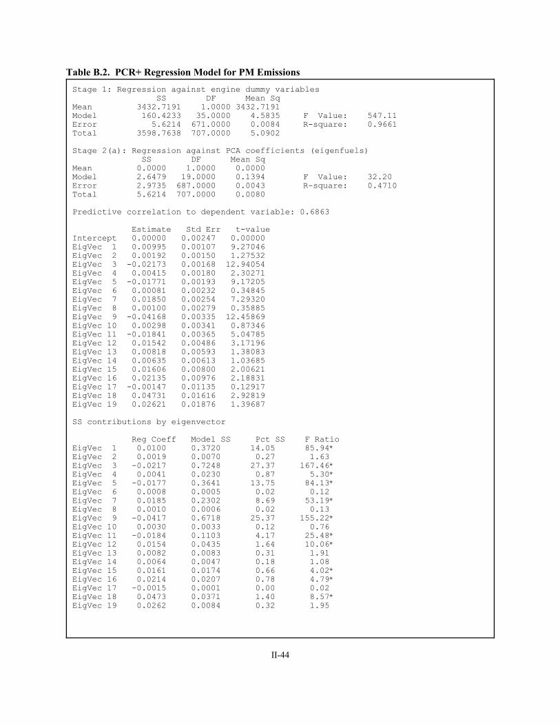
II-44
Stage 1: Regression against engine dummy variables SS DF Mean Sq Mean 3432.7191 1.0000 3432.7191Model 160.4233 35.0000 4.5835 F Value: 547.11Error 5.6214 671.0000 0.0084 R-square: 0.9661Total 3598.7638 707.0000 5.0902
Stage 2(a): Regression against PCA coefficients (eigenfuels) SS DF Mean Sq Mean 0.0000 1.0000 0.0000Model 2.6479 19.0000 0.1394 F Value: 32.20Error 2.9735 687.0000 0.0043 R-square: 0.4710Total 5.6214 707.0000 0.0080
Predictive correlation to dependent variable: 0.6863
Estimate Std Err t-value Intercept 0.00000 0.00247 0.00000EigVec 1 0.00995 0.00107 9.27046EigVec 2 0.00192 0.00150 1.27532EigVec 3 -0.02173 0.00168 12.94054EigVec 4 0.00415 0.00180 2.30271EigVec 5 -0.01771 0.00193 9.17205EigVec 6 0.00081 0.00232 0.34845EigVec 7 0.01850 0.00254 7.29320EigVec 8 0.00100 0.00279 0.35885EigVec 9 -0.04168 0.00335 12.45869EigVec 10 0.00298 0.00341 0.87346EigVec 11 -0.01841 0.00365 5.04785EigVec 12 0.01542 0.00486 3.17196EigVec 13 0.00818 0.00593 1.38083EigVec 14 0.00635 0.00613 1.03685EigVec 15 0.01606 0.00800 2.00621EigVec 16 0.02135 0.00976 2.18831EigVec 17 -0.00147 0.01135 0.12917EigVec 18 0.04731 0.01616 2.92819EigVec 19 0.02621 0.01876 1.39687
SS contributions by eigenvector
Reg Coeff Model SS Pct SS F Ratio EigVec 1 0.0100 0.3720 14.05 85.94*EigVec 2 0.0019 0.0070 0.27 1.63 EigVec 3 -0.0217 0.7248 27.37 167.46*EigVec 4 0.0041 0.0230 0.87 5.30*EigVec 5 -0.0177 0.3641 13.75 84.13*EigVec 6 0.0008 0.0005 0.02 0.12 EigVec 7 0.0185 0.2302 8.69 53.19*EigVec 8 0.0010 0.0006 0.02 0.13 EigVec 9 -0.0417 0.6718 25.37 155.22*EigVec 10 0.0030 0.0033 0.12 0.76 EigVec 11 -0.0184 0.1103 4.17 25.48*EigVec 12 0.0154 0.0435 1.64 10.06*EigVec 13 0.0082 0.0083 0.31 1.91 EigVec 14 0.0064 0.0047 0.18 1.08 EigVec 15 0.0161 0.0174 0.66 4.02*EigVec 16 0.0214 0.0207 0.78 4.79*EigVec 17 -0.0015 0.0001 0.00 0.02 EigVec 18 0.0473 0.0371 1.40 8.57*EigVec 19 0.0262 0.0084 0.32 1.95
Table B.2. PCR+ Regression Model for PM Emissions
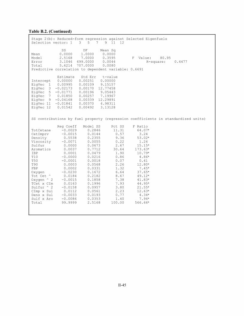
II-45
Stage 2(b): Reduced-form regression against Selected EigenfuelsSelection vector: 1 3 5 7 9 11 12 SS DF Mean Sq Mean 0.0000 1.0000 0.0000Model 2.5168 7.0000 0.3595 F Value: 80.95Error 3.1046 699.0000 0.0044 R-square: 0.4477Total 5.6214 707.0000 0.0080Predictive correlation to dependent variable: 0.6691 Estimate Std Err t-value Intercept 0.00000 0.00251 0.00000EigVec 1 0.00995 0.00109 9.15157EigVec 3 -0.02173 0.00170 12.77458EigVec 5 -0.01771 0.00196 9.05443EigVec 7 0.01850 0.00257 7.19967EigVec 9 -0.04168 0.00339 12.29891EigVec 11 -0.01841 0.00370 4.98311EigVec 12 0.01542 0.00492 3.13128 SS contributions by fuel property (regression coefficients in standardized units) Reg Coeff Model SS Pct SS F Ratio TotCetane -0.0029 0.2846 11.31 64.07*CetImprv -0.0015 0.0144 0.57 3.24 Density 0.5538 0.2355 9.36 53.02*Viscosity -0.0071 0.0055 0.22 1.24 Sulfur 0.0000 0.0673 2.67 15.15*Aromatics 0.0037 0.7712 30.64 173.63*IBP 0.0001 0.0479 1.90 10.79*T10 -0.0000 0.0216 0.86 4.86*T50 -0.0001 0.0018 0.07 0.41 T90 0.0003 0.0568 2.26 12.80*FBP 0.0002 0.0331 1.32 7.45*Oxygen -0.0230 0.1672 6.64 37.65*Tot Cet ^ 0.0184 0.2182 8.67 49.12*Oxygen ^ 2 -0.0015 0.1858 7.38 41.83*TCet x CIm 0.0163 0.1996 7.93 44.95*Sulfur ^ 2 -0.0158 0.0957 3.80 21.55*CImp x Sul 0.0112 0.0561 2.23 12.63*Dens x Sul -0.0033 0.0193 0.77 4.34*Sulf x Aro -0.0086 0.0353 1.40 7.94*Total 99.9999 2.5168 100.00 566.66*
Table B.2. (Continued)


APPENDIX II-C
PEER REVIEW COMMENTS AND REPLY

II-49
Review of DRAFT Estimating Impacts of Diesel Fuel Reformulation with Vector-Based Blending,ORNL/TM-2002/225
Reviewer: David AndressDavid Andress & Associates, Inc.1108 Harriet LaneKensington, MD 20895November 6, 2002
To formulate policy recommendations and comment on proposed regulations concerning reformulateddiesel fuels, the Department of Energy requires high quality analyses of cost and produceability impactsassociated with potential diesel fuel reformulations. The ORNL report does an excellent job of meetingthat objective. The study premises and expository material are well laid out, and the conclusions arepresented in a straightforward and coherent manner. The authors did a good job of the describing thestudy limitations, which are inevitable given the current limitations in emissions data and the early stageof the public debate on reformulated diesel fuels.
The study consists of two separate research activities: a set of refinery analyses and estimates of NOx andPM emission models for diesel fuels. The ORNL-RYM model, which was used for the refinery analyses,has been used in many important DOE and EPA studies and has been extensively peer reviewed byindustry and other stakeholders. On the other hand, the eigenfuel approach to estimating emission modelsis relatively new and still evolving. Accordingly, most of our comments pertain to the eigenfuel analysisand include some suggestions for additional exploratory data analysis.
Developing an emissions model for diesel fuels is a challenging effort for a number of reasons includingthe acknowledged limitations in the available data. An earlier EPA attempt, for example, was concludedafter receiving public comments without a producing a model recommendation. The eigenfuel modeldescribed in the ORNL study presents a viable candidate for public review. We note that API commentedon the fact that the EPA database used to develop the emissions model did not include emissions data fordiesel engines with advanced emission controls. In particular, API noted that the correlation of NOxemissions with cetane was different in engines equipped with exhaust gas recirculation (EGR) from thosewithout EGR. The EPA database did not contain data on engines with EGR. Although the API commentis true, we believe the ORNL approach is correct. If the EPA data base had included emissions data onboth engines with and without EGR, they would have to be separated prior to performing a regressionanalysis. Comparison can be made to the California Predictive Model in which separate regressionmodels are fit to different vehicle technology classes.
One of the report’s conclusions is that the eigenfuel-based emissions approach shows increasing benefitsas recipe specifications are relaxed. However, the economic benefit for the sensitivity case that wasanalyzed was comparatively small. We offer the following observations:
4. California prescribes a recipe for diesel fuel properties, but allows the refiners to use alternativeformulations provided independent testing verifies the emissions from the alternativeformulation are equal to or less than those of the reference fuel. According to material on theCARB web site, most refiners in California use alternative diesel formulations that are certifiedto meet emission standards through independent emissions tests. This suggests an economicbenefit exists for blending flexibility, and the eigenfuel-based emissions methodology couldconfirm this for existing diesel fuel standards. Whether there is an economic benefit of anysignificance for the stricter 2006 California diesel fuel regulations has not been investigated. Since California tends to lead the nation in adopting environmental standards, a future studycould examine this issue. Such a study could provide input for establishing a diesel emissions

II-50
model for use in California and Texas. Using an emissions model to certify diesel fuels, ratherthan having to subject alternative diesel fuel formulations to independent testing, would bevaluable to refiners.
5. It is not surprising that “vehicle performance” and “emissions reduction” specifications in RYMproduce similar results. Cetane control, aromatics reduction, and specific gravity are key fuelcomponents that contribute to emissions reductions of both NOx and PM. The contribution toemissions reduction from specific gravity is small. As noted in the ORNL report, specificgravity is correlated with aromatic content and cetane. We can infer that not much leewaybeyond aromatic and cetane control exists in the current RYM representation to reduce NOxand PM emissions. Given the way the emission equations are represented in RYM, it wouldappear that even with somewhat less stringent requirements on NOx and PM emissions,increases in cetane and reductions in aromatic content would still be needed.
6. The ORNL study only considered NOx and PM emissions, which are the primary emissions ofconcerns for diesel fuels. A complete analysis would also include HC, CO, and toxic emissions. The Auto Alliance World Wide Fuel Charter includes data that show that substantial reductionsin HC and CO emissions occur as cetane increased, and that the percentage reductions in HCand CO emissions are greater than those of NOx and PM emissions. This could further constrainrefiner flexibility in meeting emission reductions in the existing diesel fleet that are equivalentto the Auto Alliance recipe proposal.
7. As the ORNL study notes, cetane has an effect on cold startability. As emissions are higher when engines are cold, cold startability could have a significant effect on diesel emissions. Therelative difference between emissions from hot and cold engines may be greater for engineswith advanced emission control technologies.
8. Finally, we note the ongoing tussle between the auto and oil industries about how to implementtechnologies to reduce vehicular emissions and how to divide up the responsibility between theauto and oil industries. The auto industry would like greater control in setting fuel recipestandards. The following quote from the World Wide Fuel Charter illustrates their argument:
Production diesel engines are set to a standard density which determines the amount of fuelinjected. The (volumetric) injection quantity is a control parameter for other emission controlsystems like the exhaust gas recirculation (EGR). Variations in fuel density therefore result innon-optimal EGR-rates for a given load and speed point in the engine map and, as a consequence,influence the exhaust emission characteristics.
Part II of the report, which describes the derivation of eigenfuels, explains that a conventional regressionanalysis was used to estimate the emission equations that are input to ORNL-RYM. The methodologywas: (1) apply an eigenvalue analysis to the full data set; (2) use the results of Step (1) to generate asynthetic data set limited to the domain of interest (upper and lower value constraints on fuel parameters);and (3) apply a standard regression analysis to the synthetic data step generated in Step (2). The use ofthe synthetic data set appears similar to a technique called random balancing. The reason for usingrandom balancing is to simplify the regression model, since some of the quadratic or interactive that werestatistically significant in the original regression may not be in the new regression. Nonetheless, wewonder why a standard regression analysis was applied to the synthetic data in lieu of using anothereigenfuel analysis and/or what the advantage was in using the eigenfuel approach for the first regression.

II-51
Part II notes the eigenvector and regression analyses are mathematically equivalent, i.e., onerepresentation can be transformed into the other. This raises the obvious question of the advantage ofusing one approach over the other. We believe that a comparison between a pure eigenfuel approach anda pure regression approach would be useful to assess whether the eigenfuel approach described in Part IIprovides additional benefit.
In reviewing documentation describing how regression models were selected for regulatory compliancemodels, we observed cases where a final regression model was selected from a set of regression modelswith similar R squares. This situation occurs when collinearity among some of the variables is present. We note that the selection process can appear somewhat arbitrary at times. However, a “good” selectionprocess should incorporate an understanding of the physical processes.
We suggest exploring the use of a mixed effect regression model, as there seems to be a growingacceptance in the regulatory arena for this approach. California used a mixed effect regression analysis toestimate the Predictive Model equations. The California approach treats the fuels as the fixed effects andthe vehicles as the random effects. The recently released EPA biodiesel emissions analysis also used amixed effect model. EPA used a fixed effect regression analysis to estimate the Complex Modelequations, and California has identified this as one the reasons why emission estimates produced by thePredictive and Complex models are not consistent.
On Pages S-5 and 1-2, a statement is made to the effect that the eigenfuel methodology results ineconomy of representation. However, the characterization used in ORNL-RYM is based on the originalfuel properties (from page II-4 “to accommodate RYM, eigenvector models are transformed to fuelproperty models”), and so no economy of representation occurs in the context of the study.
Pages S-1 and 1-2, state that the eigenfuels provide a greater understanding of the patterns of variationneeds to be explained in the text. In Part II, the eigenfuels are loosely interpreted in terms of the originalfuel parameters, but no new insights are provided. For example, does a particular eigenfuel correspond toa group of fuel properties that are commonly controlled in the refinery proportionate to their coefficientsin the eigenfuel? Part II notes that the analysis uncovered the statistical significance of some interactiveterms, which was not previously recognized. Jerry noted that the EPA proposed model did not contain acetane term. (I find this hard to understand considering the emphasis place on the relationship betweencetane and emissions in the World Fuels Charter.) A comparison with the discontinued EPA effort andother studies would be useful in identifying insights gained from the eigenvector approach.
Page 1-1 states that emission benefits may be misrepresented if based on analysis of individual fuelproperties. While this statement is true, it is not clear how the eigenfuel approach contributes to a betterunderstanding of the problem. The eigenfuel representation in RYM is based on individual fuelproperties.
An advantage that is claimed for the eigenfuel approach is that is provides a non arbitrary way of dealingwith collinearity in the independent variables. However, the eigenvector approach merely shifts thecollinearity problem from regression analysis to principle component analysis. Just as there can beseveral regression models with similar R squares using different subsets of the original variables, differentorthogonal bases can be selected with much the same result. For example, the orthogonal basis in which asingle vector explains all the regression variance is the one determined by a regression analysis. (Theremaining orthogonal basis vectors can be selected arbitrarily.)
The eigenfuel methodology applied to estimate NOx and PM emissions is an interesting adaptation to thetheoretical principal component analysis. Quadratic and interactive terms are introduced because of apositive correlation with NOx or PM emissions, not to explain patterns in the underlying fuel property

II-52
space. Another avenue that might be interesting to explore is to perform a principle component analysiswithout added quadratic and interactive terms, and then determine if any quadratic and interactiveeigenfuels need to be added.
Page 1-13 says the “most important eigenfuels are clearly related to refinery processing and blending”. Part II does not fully support this assertion. The interpretation of the eigenfuels was in terms of theoriginal fuel components, i.e., those physical components with the largest contribution to the eigenfuels. Although the eigenfuels may provide additional physical insights, the document did not identify any. Itshould be noted that the choice of the eigenfuels is related to both component scaling and whethernormalization transformations (e.g., differences from mean) are used. This is an area for further research,as the choice of scaling can help in formulating a physical or economic interpretation of the eigenfuels.
The application of the eigenfuels in Part II was to estimate NOx and PM emissions, i.e., to gain insightsinto the relationship between refinery processing and blending and NOx and PM emissions. In thatprocess, the selection of which quadratic and interactive terms to include in each analysis depends ontheir respective correlation with NOx or PM emissions. The following table lists the eigenvector numbersfor the NOx and PM emissions with the greatest contributions to the respective regression analyses.
Eigenvectornumber
NOx Emissions PM Emissions
Pct. variancecontribution ofeigenvector
Pct. variancecontribution forregression (partexplained byregressionanalysis)
Pct. variancecontribution ofeigenvector
Pct. variancecontribution forregression (partexplained byregression analysis
1 31 22 28 14
2 14 32 14 0
3 11 0 11 27
4 9 16 10 0
5 7 2 9 14
9 3 14 4 25
As can be seen in the above table, an argument can be made that the most significant eigenvectors are (forthe most part) most correlated to NOx emissions, but not for PM emissions.
The statement about the economy of representation for the eigenvectors may be true, but needs to bedemonstrated. For example, how many eigenfuels are needed to explain X percent of the regressionvariation versus how many fuel properties are needed. As the regression analysis in Part II used all theeigenfuels, there was no economy of representation in that analysis. In addition, we wonder why termswhose coefficients were not statistically significant were retained in the final regression models. Table4.2, for example, shows regression coefficients for T50 and FBD although they are not statisticallysignificant at the 0.05 level (Table 3.1).
Fig. 1 (1-15) does not present a balanced comparison between regressions using the fuel properties andthe eigenfuels. In both cases, there are 12 variables that can be used in the regression analysis. That is,
II-53
there 4,095 different regression models for cases. For the eigenvector regressions, only one of thepossible 4,095 different regression models was selected using a standard stepwise regression approach (looking at the sequential improvement in the R-square statistic). The same methodology should beapplied to the used for regressions based on the fuel properties. This would provide a more balancedcomparison between regression analyses based on fuel properties versus eigenfuels. It should also benoted that the discussion on page I-13 and the analysis in Part II differ in that quadratic and cross productterms are included in Part II. It appears that the discussion in Part I is based on an earlier eigenfuelanalysis.
Statistical model building is an art, and different analytic representations may lend themselves in varyingdegrees to understanding the underlying physical phenomena. To this extent, the use of the eigenfuelsapproach may show patterns that were not previously understood. The value may be in understandinghow fuel properties are jointly varied in the refinery blending operation, i.e., as a pattern recognition tool. However, we note that a recognized weakness in principle component analysis is in interpreting theeigenvectors, and the interpretations can be affected by component scaling. Other papers by the authorshave explored this concept in more detail, and they may have provided additional insights in this area. Nonetheless, we endorse the eigenfuel approach as a useful tool for exploratory analysis and haveprovided some thoughts for additional explanatory research. We want to acknowledge the quality of thepresentation in Part II, which included a good list of caveats and discussion of data limitations.
II-54
Author Reply to Review of DRAFT Estimating Impacts of Diesel Fuel Reformulation with Vector-Based Blending, ORNL/TM-2002/225
Dave Andress:
Thanks very much for your careful and thoughtful review of our RFD report. We will revise the report toaddress your comments and incorporate your editorial suggestions. We believe that several of yourquestions are answered in our previous publications (which I mailed to you last week) on the eigenfuelmethodology, and we may need to use more specific literature citations in our RFD report. Regardingyour specific comments:
Your page 3: “... we believe that a comparison between a pure eigenfuel approach and a pure regressionapproach would be useful to assess whether the eigenfuel approach described in Part II providesadditional benefit.” See ORNL/TM-2002/16, Section 3.4, among others.
Your page 3: “... we wonder why a standard regression analysis was applied to the synthetic data in lieuof using another eigenfuel analysis and/or what the advantage was in using the eigenfuel approach for thefirst regression.” This is done solely as a “curve fitting” tool to give us an equivalent model stated interms of the individual fuel properties that could be implemented within RYM. That is, the emissionanalysis was conducted in the vector space using eigenfuels as the explanatory variables. Havingdeveloped the models, we needed to transform to equations written using the fuel properties. This canactually be done algebraically (with some effort); the random balance regression approach was chosen asa practical approach for making the transformation.
Your page 3:”... This raises the obvious question of the advantage of using one approach over the other.” The advantage of the eigenfuel approach is that it will not be “fooled” by the aliasing existing among theindividual properties, while conventional methods can misidentify the influential variables. SeeORNL/TM-2002/16, Section 3 for a full discussion of this.
Your page 3: “ ... a statement is made to the effect that the eigenfuel methodology results in economy ofrepresentation. However, the characterization used in ORNL-RYM is based on the original fuelproperties, and so no economy of representation occurs in the context of the study.” And your page 5: “...The statement about economy of representation may be true, but needs to be demonstrated.” In acomputational sense -- counting the number of variables -- this is true, but computational power is cheaptoday. The reduction in dimensionality comes in the fact that we identified 6 (vector) fuel factorsinfluencing NOx emissions and 7 (vector) fuel factors influencing PM emissions, out of variable spacesthat encompassed 17 and 19 terms, respectively. We need all of the properties to describe the vectors, butthere are only 6 and 7 vector features influencing NOx and PM emissions.
Your page 4: “ ... does a particular eigenfuel correspond to a group of fuel properties that are commonlycontrolled in the refinery to proportionate to their coefficients in the eigenfuel?” See ORNL/TM-2002/16,Section 5. Eigenfuels are related (some more clearly than others) to blendstocks, implying a “macro”level of control using blendstock proportions, rather than property controls. We are not suggestingabandonment of property controls needed for trimming product quality.
Your page 4: “A comparison with the discontinued EPA effort and other studies would be useful inidentifying insights gained from the eigenvector approach.” See ORNL/TM-2002/16, Table 5.1,Sections 2.2 through 3.5.
Your page 4: “ Page 1-13 says the ‘most important eigenfuels are clearly related to refinery processingand blending.’” See ORNL/TM-2002/16, Table 5.1
II-55
Your page 4: “ ... emission benefits may be misrepresented if based on analysis of individual fuelproperties.” While the emission model in RYM is written in terms of individual fuel properties, as amatter of computation convenience, it was not developed using an analysis based on individual fuelproperties. It was developed from an analysis that used eigenvectors and therefore avoided the problemsthat aliasing of variables can introduce.
Your page 4: “However, the eigenvector approach merely shifts the collinearity problem from regressionanalysis to principal component analysis.” The collinearity problem is dealt with and resolved in PCA,which is something that conventional regression analysis cannot really achieve. When the number andidentity of the explanatory variables is constant, there is only one orthogonal basis for the data set andthat is the one identified by PCA. As you noted, the work did undertake a novel effort to identify vectorbases that are efficient for describing fuel effects on emissions.
Your page 4: “It should be noted that the choice of eigenfuels is related to both component scaling andwhether normalization transformations are used.” See ORNL/TM-2002/16, Section 5 for support on theinterpretation of eigenfuels in refining terms. Additional work on formulating physical interpretations ofthe eigenfuels would be beneficial.
Your page 5: “As can be seen in the above table, an argument can be made that the most significanteigenvectors are (for the most part) most correlated to NOx emissions, but not for PM emissions.” Youcannot safely draw the conclusion from the table. The variables spaces differed for the NOx and PMmodels, so that the nth eigenvector of the NOx space is not necessarily related to the nth eigenvector of thePM space.
Your page 5: “As the regression analysis in Part II used all the eigenfuels, there was no economy ofrepresentation in that analysis.” The procedure is to use all of the eigenfuels initially, and then to dropthose that do not contribute to the regression explanatory power. Therein lies the economy. (In fact, youmust retain all of the vectors initially, or you risk excluding features that could be important in theregression.) As to Table 4.2, you must remember that the final regression of synthetic data is done onlyfor curve-fitting purposes and is not a statistical analysis that purports to identify the influential factors. Thus, T50 is needed in the reduced-form model because it is a component of eigenfuels that hadsignificant influences on emissions. This is not to say that T50 by itself has a statistically significantinfluence on emissions. We don’t believe that the fuel properties have individual causal relationships toemissions.
If you would like to discuss this further, perhaps we could have a three-way conference call. Let us knowif additional clarification would be helpful.
Thanks again for your excellent review.
G.R. Hadder and R.W. Crawford