Embed Size (px)
Citation preview
IntroductionA model for canopy height
Evaluation and testsDiscussion and conclusions
Estimating forest attributes using observations of canopyheight: a model-based approach
Lauri Mehtatalo1
1 University of Joensuu
September 29, 2009Kvantitatiivisten menetelmien seminaari
Joensuu, FinlandBased on Mehtatalo, L. and Nyblom, J. 2009. Estimating forest attributes
using observations of canopy height: a model-based approach. ForestScience 55(5): 411-422.
Lauri Mehtatalo1 Estimating forest attributes using observations of canopy height: a model-based approach
IntroductionA model for canopy height
Evaluation and testsDiscussion and conclusions
Outline of the presentation
IntroductionForest inventory and laser scanningOur question
A model for canopy heightGeneral assumptionsA model for single tree crownA model for a standA model for random tree locationsEstimation
Evaluation and testsDataResultsExamples with real data
Discussion and conclusions
Lauri Mehtatalo1 Estimating forest attributes using observations of canopy height: a model-based approach
IntroductionA model for canopy height
Evaluation and testsDiscussion and conclusions
Forest inventory and laser scanningOur question
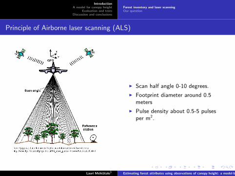
Principle of Airborne laser scanning (ALS)
I Scan half angle 0-10 degrees.
I Footprint diameter around 0.5meters
I Pulse density about 0.5-5 pulsesper m2.
Lauri Mehtatalo1 Estimating forest attributes using observations of canopy height: a model-based approach
IntroductionA model for canopy height
Evaluation and testsDiscussion and conclusions
Forest inventory and laser scanningOur question
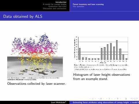
Data obtained by ALS
Observations collected by laser scanner.
Histogram of laser height observationsfrom an example stand.
Lauri Mehtatalo1 Estimating forest attributes using observations of canopy height: a model-based approach
IntroductionA model for canopy height
Evaluation and testsDiscussion and conclusions
Forest inventory and laser scanningOur question
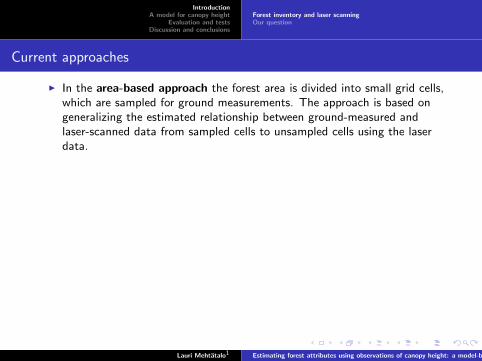
Current approaches
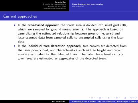
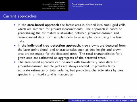
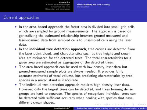
I In the area-based approach the forest area is divided into small grid cells,which are sampled for ground measurements. The approach is based ongeneralizing the estimated relationship between ground-measured andlaser-scanned data from sampled cells to unsampled cells using the laserdata.
I In the individual tree detection approach, tree crowns are detected fromthe laser point cloud, and characteristics such as tree height and crownarea are estimated for the detected trees. The total characteristics for agiven area are estimated as aggregates of the detected trees.
I The area-based approach can be used with low-density laser data butground-measured sample plots are always needed. It provides fairlyaccurate estimates of total volume, but predicting characteristics by treespecies in a mixed stand is inaccurate.
I The individual tree detection approach requires high-density laser data.However, only the largest trees can be detected, and trees forming densegroups are hard to separate. The species of recognized individual trees canbe detected with sufficient accuracy when dealing with species that havedifferent crown shapes.
Lauri Mehtatalo1 Estimating forest attributes using observations of canopy height: a model-based approach
IntroductionA model for canopy height
Evaluation and testsDiscussion and conclusions
Forest inventory and laser scanningOur question
Current approaches
I In the area-based approach the forest area is divided into small grid cells,which are sampled for ground measurements. The approach is based ongeneralizing the estimated relationship between ground-measured andlaser-scanned data from sampled cells to unsampled cells using the laserdata.
I In the individual tree detection approach, tree crowns are detected fromthe laser point cloud, and characteristics such as tree height and crownarea are estimated for the detected trees. The total characteristics for agiven area are estimated as aggregates of the detected trees.
I The area-based approach can be used with low-density laser data butground-measured sample plots are always needed. It provides fairlyaccurate estimates of total volume, but predicting characteristics by treespecies in a mixed stand is inaccurate.
I The individual tree detection approach requires high-density laser data.However, only the largest trees can be detected, and trees forming densegroups are hard to separate. The species of recognized individual trees canbe detected with sufficient accuracy when dealing with species that havedifferent crown shapes.
Lauri Mehtatalo1 Estimating forest attributes using observations of canopy height: a model-based approach
IntroductionA model for canopy height
Evaluation and testsDiscussion and conclusions
Forest inventory and laser scanningOur question
Forest inventory using laser scanning
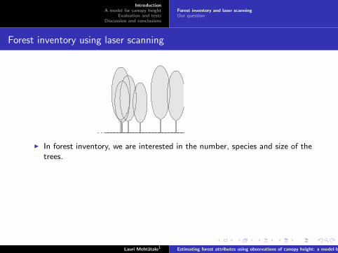
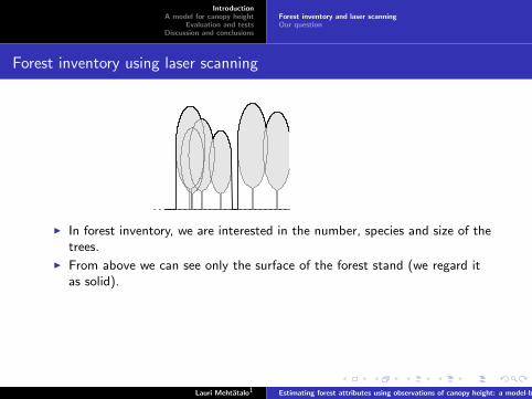
I In forest inventory, we are interested in the number, species and size of thetrees.
I From above we can see only the surface of the forest stand (we regard itas solid).
I Observation obtained by a laser scanner can be taken as observed canopyheight if the footprint is small and observations are taken from the nadir.
I These observations are random because their location, tree heights, andtree locations may be random.
I Several observations provide data of measured canopy heights.
Lauri Mehtatalo1 Estimating forest attributes using observations of canopy height: a model-based approach
IntroductionA model for canopy height
Evaluation and testsDiscussion and conclusions
Forest inventory and laser scanningOur question
Forest inventory using laser scanning
v
z((v))
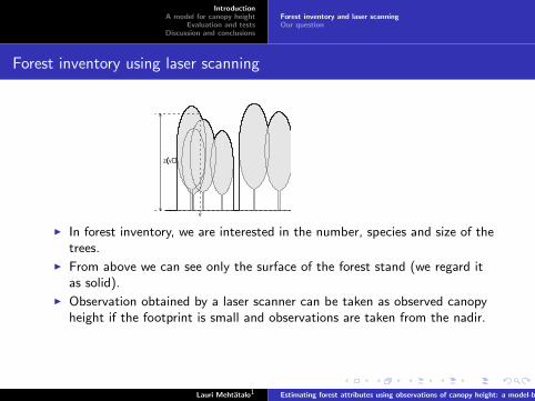
I In forest inventory, we are interested in the number, species and size of thetrees.
I From above we can see only the surface of the forest stand (we regard itas solid).
I Observation obtained by a laser scanner can be taken as observed canopyheight if the footprint is small and observations are taken from the nadir.
I These observations are random because their location, tree heights, andtree locations may be random.
I Several observations provide data of measured canopy heights.
Lauri Mehtatalo1 Estimating forest attributes using observations of canopy height: a model-based approach

IntroductionA model for canopy height
Evaluation and testsDiscussion and conclusions
Forest inventory and laser scanningOur question
Forest inventory using laser scanning
v
z((v))
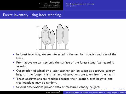
I In forest inventory, we are interested in the number, species and size of thetrees.
I From above we can see only the surface of the forest stand (we regard itas solid).
I Observation obtained by a laser scanner can be taken as observed canopyheight if the footprint is small and observations are taken from the nadir.
I These observations are random because their location, tree heights, andtree locations may be random.
I Several observations provide data of measured canopy heights.
Lauri Mehtatalo1 Estimating forest attributes using observations of canopy height: a model-based approach
IntroductionA model for canopy height
Evaluation and testsDiscussion and conclusions
Forest inventory and laser scanningOur question
Forest inventory using laser scanning
v
z((v))
I In forest inventory, we are interested in the number, species and size of thetrees.
I From above we can see only the surface of the forest stand (we regard itas solid).
I Observation obtained by a laser scanner can be taken as observed canopyheight if the footprint is small and observations are taken from the nadir.
I These observations are random because their location, tree heights, andtree locations may be random.
I Several observations provide data of measured canopy heights.
Lauri Mehtatalo1 Estimating forest attributes using observations of canopy height: a model-based approach
IntroductionA model for canopy height
Evaluation and testsDiscussion and conclusions
Forest inventory and laser scanningOur question
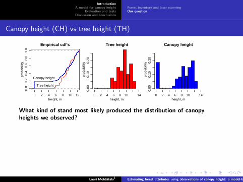
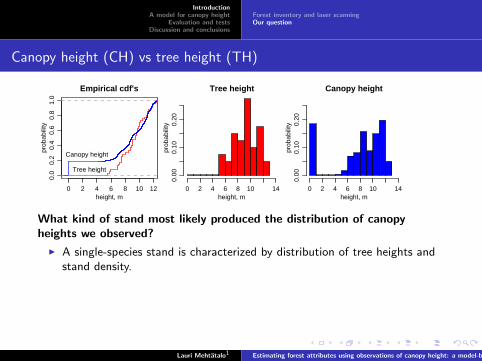
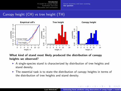
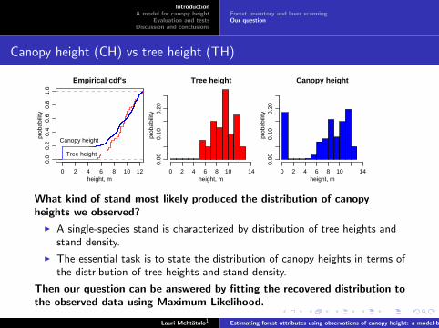
Canopy height (CH) vs tree height (TH)
0 2 4 6 8 10 12
0.0
0.2
0.4
0.6
0.8
1.0
Empirical cdf's
height, m
prob
abili
ty
Tree height
Canopy height
Tree height
height, m
prob
abili
ty
0 2 4 6 8 10 14
0.00
0.10
0.20
Canopy height
height, m
prob
abili
ty
0 2 4 6 8 10 14
0.00
0.10
0.20
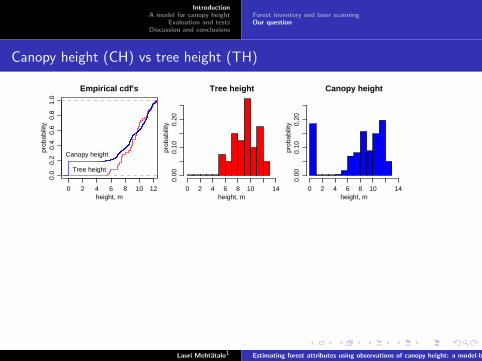
What kind of stand most likely produced the distribution of canopyheights we observed?
I A single-species stand is characterized by distribution of tree heights andstand density.
I The essential task is to state the distribution of canopy heights in terms ofthe distribution of tree heights and stand density.
Then our question can be answered by fitting the recovered distribution tothe observed data using Maximum Likelihood.
Lauri Mehtatalo1 Estimating forest attributes using observations of canopy height: a model-based approach
IntroductionA model for canopy height
Evaluation and testsDiscussion and conclusions
Forest inventory and laser scanningOur question
Canopy height (CH) vs tree height (TH)
0 2 4 6 8 10 12
0.0
0.2
0.4
0.6
0.8
1.0
Empirical cdf's
height, m
prob
abili
ty
Tree height
Canopy height
Tree height
height, m
prob
abili
ty
0 2 4 6 8 10 14
0.00
0.10
0.20
Canopy height
height, m
prob
abili
ty
0 2 4 6 8 10 14
0.00
0.10
0.20
What kind of stand most likely produced the distribution of canopyheights we observed?
I A single-species stand is characterized by distribution of tree heights andstand density.
I The essential task is to state the distribution of canopy heights in terms ofthe distribution of tree heights and stand density.
Then our question can be answered by fitting the recovered distribution tothe observed data using Maximum Likelihood.
Lauri Mehtatalo1 Estimating forest attributes using observations of canopy height: a model-based approach
IntroductionA model for canopy height
Evaluation and testsDiscussion and conclusions
General assumptionsA model for single tree crownA model for a standA model for random tree locationsEstimation
General assumptions
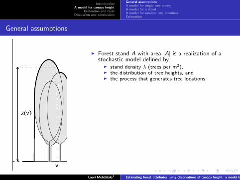
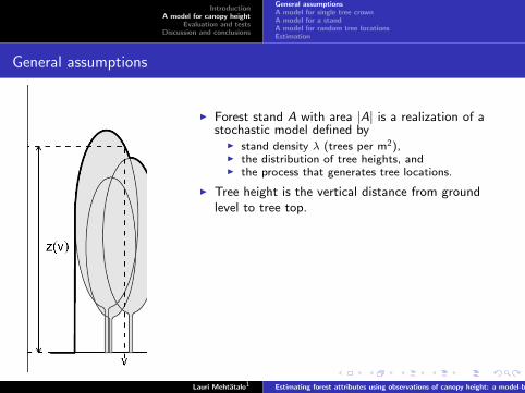
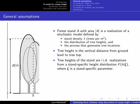
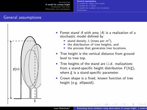
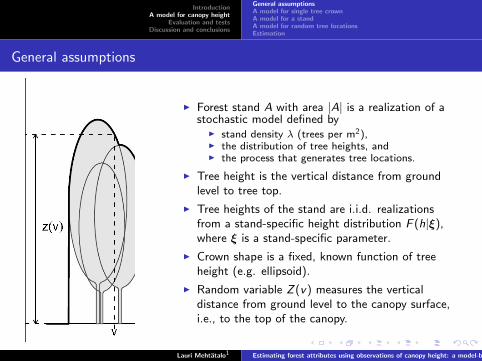
I Forest stand A with area |A| is a realization of astochastic model defined by
I stand density λ (trees per m2),I the distribution of tree heights, andI the process that generates tree locations.
I Tree height is the vertical distance from groundlevel to tree top.
I Tree heights of the stand are i.i.d. realizationsfrom a stand-specific height distribution F (h|ξ),where ξ is a stand-specific parameter.
I Crown shape is a fixed, known function of treeheight (e.g. ellipsoid).
I Random variable Z(v) measures the verticaldistance from ground level to the canopy surface,i.e., to the top of the canopy.
Lauri Mehtatalo1 Estimating forest attributes using observations of canopy height: a model-based approach
IntroductionA model for canopy height
Evaluation and testsDiscussion and conclusions
General assumptionsA model for single tree crownA model for a standA model for random tree locationsEstimation
General assumptions
I Forest stand A with area |A| is a realization of astochastic model defined by
I stand density λ (trees per m2),I the distribution of tree heights, andI the process that generates tree locations.
I Tree height is the vertical distance from groundlevel to tree top.
I Tree heights of the stand are i.i.d. realizationsfrom a stand-specific height distribution F (h|ξ),where ξ is a stand-specific parameter.
I Crown shape is a fixed, known function of treeheight (e.g. ellipsoid).
I Random variable Z(v) measures the verticaldistance from ground level to the canopy surface,i.e., to the top of the canopy.
Lauri Mehtatalo1 Estimating forest attributes using observations of canopy height: a model-based approach
IntroductionA model for canopy height
Evaluation and testsDiscussion and conclusions
General assumptionsA model for single tree crownA model for a standA model for random tree locationsEstimation
A model for a single tree crown
a(h)
b(h)
z
h
Y(z,h)
u
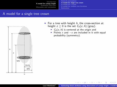
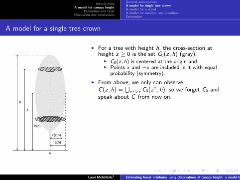
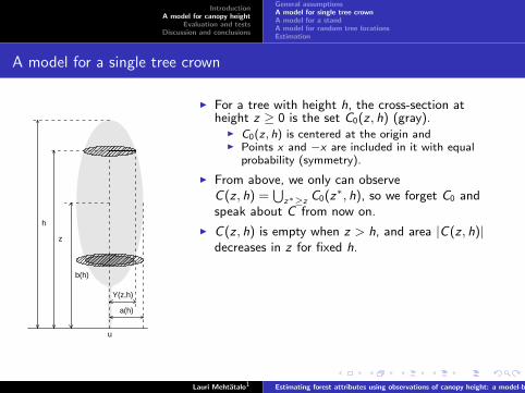
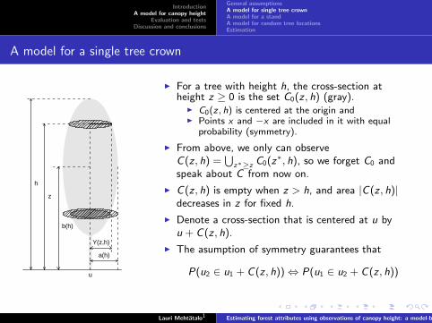
I For a tree with height h, the cross-section atheight z ≥ 0 is the set C0(z , h) (gray).
I C0(z, h) is centered at the origin andI Points x and −x are included in it with equal
probability (symmetry).
I From above, we only can observeC(z , h) =
⋃z∗≥z C0(z∗, h), so we forget C0 and
speak about C from now on.
I C(z , h) is empty when z > h, and area |C(z , h)|decreases in z for fixed h.
I Denote a cross-section that is centered at u byu + C(z , h).
I The asumption of symmetry guarantees that
P(u2 ∈ u1 + C(z , h))⇔ P(u1 ∈ u2 + C(z , h))
Lauri Mehtatalo1 Estimating forest attributes using observations of canopy height: a model-based approach
IntroductionA model for canopy height
Evaluation and testsDiscussion and conclusions
General assumptionsA model for single tree crownA model for a standA model for random tree locationsEstimation
A model for a single tree crown
a(h)
b(h)
z
h
Y(z,h)
u
I For a tree with height h, the cross-section atheight z ≥ 0 is the set C0(z , h) (gray).
I C0(z, h) is centered at the origin andI Points x and −x are included in it with equal
probability (symmetry).
I From above, we only can observeC(z , h) =
⋃z∗≥z C0(z∗, h), so we forget C0 and
speak about C from now on.
I C(z , h) is empty when z > h, and area |C(z , h)|decreases in z for fixed h.
I Denote a cross-section that is centered at u byu + C(z , h).
I The asumption of symmetry guarantees that
P(u2 ∈ u1 + C(z , h))⇔ P(u1 ∈ u2 + C(z , h))
Lauri Mehtatalo1 Estimating forest attributes using observations of canopy height: a model-based approach
IntroductionA model for canopy height
Evaluation and testsDiscussion and conclusions
General assumptionsA model for single tree crownA model for a standA model for random tree locationsEstimation
A model for a stand
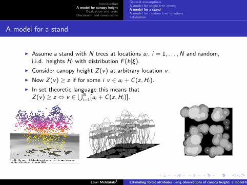
I Assume a stand with N trees at locations ui , i = 1, . . . ,N and random,i.i.d. heights Hi with distribution F (h|ξ).
I Consider canopy height Z(v) at arbitrary location v .
I Now Z(v) ≥ z if for some i v ∈ ui + C(z ,Hi ).
I In set theoretic language this means thatZ(v) ≥ z ⇔ v ∈
⋃Ni=1[ui + C(z ,Hi )].
Lauri Mehtatalo1 Estimating forest attributes using observations of canopy height: a model-based approach
IntroductionA model for canopy height
Evaluation and testsDiscussion and conclusions
General assumptionsA model for single tree crownA model for a standA model for random tree locationsEstimation
A model for a stand
I Assume a stand with N trees at locations ui , i = 1, . . . ,N and random,i.i.d. heights Hi with distribution F (h|ξ).
I Consider canopy height Z(v) at arbitrary location v .
I Now Z(v) ≥ z if for some i v ∈ ui + C(z ,Hi ).
I In set theoretic language this means thatZ(v) ≥ z ⇔ v ∈
⋃Ni=1[ui + C(z ,Hi )].
Lauri Mehtatalo1 Estimating forest attributes using observations of canopy height: a model-based approach

IntroductionA model for canopy height
Evaluation and testsDiscussion and conclusions
General assumptionsA model for single tree crownA model for a standA model for random tree locationsEstimation
A model for a stand
I For the complement event, we get by De Morgans’s lawZ(v) ≤ z ⇔ v ∈
⋂Ni=1[ui + C(z ,Hi )]
I Because of the symmetry of cross-sections and mutual independence oftree heights, we finally get
P(Z(v) < z) = P[ui ∈ v + C(z ,Hi ), for all i = 1, . . . ,N
]=
N∏i=1
P[ui ∈ v + C(z ,Hi )
],
Lauri Mehtatalo1 Estimating forest attributes using observations of canopy height: a model-based approach
IntroductionA model for canopy height
Evaluation and testsDiscussion and conclusions
General assumptionsA model for single tree crownA model for a standA model for random tree locationsEstimation
A model for random tree locations
I Assume that tree locations are generated by a spatial Poisson process withdensity λ. Then N ∼ Poisson(λ|A|) and locations ui are uniformlydistributed over A.
I We proceed in three steps:
I First we condition on N and Hi , i = 1, . . . ,N.I Then we continue to condition on N but take the expectation over Hi ,
i = 1, . . . ,N.I Finally, the expectation over N yields the result.
Lauri Mehtatalo1 Estimating forest attributes using observations of canopy height: a model-based approach
IntroductionA model for canopy height
Evaluation and testsDiscussion and conclusions
General assumptionsA model for single tree crownA model for a standA model for random tree locationsEstimation
A model for random tree locations
I Assume that tree locations are generated by a spatial Poisson process withdensity λ. Then N ∼ Poisson(λ|A|) and locations ui are uniformlydistributed over A.
I We proceed in three steps:I First we condition on N and Hi , i = 1, . . . ,N.
I Then we continue to condition on N but take the expectation over Hi ,i = 1, . . . ,N.
I Finally, the expectation over N yields the result.
Lauri Mehtatalo1 Estimating forest attributes using observations of canopy height: a model-based approach

IntroductionA model for canopy height
Evaluation and testsDiscussion and conclusions
General assumptionsA model for single tree crownA model for a standA model for random tree locationsEstimation
A model for random tree locations
I Assume that tree locations are generated by a spatial Poisson process withdensity λ. Then N ∼ Poisson(λ|A|) and locations ui are uniformlydistributed over A.
I We proceed in three steps:I First we condition on N and Hi , i = 1, . . . ,N.I Then we continue to condition on N but take the expectation over Hi ,
i = 1, . . . ,N.
I Finally, the expectation over N yields the result.
Lauri Mehtatalo1 Estimating forest attributes using observations of canopy height: a model-based approach
IntroductionA model for canopy height
Evaluation and testsDiscussion and conclusions
General assumptionsA model for single tree crownA model for a standA model for random tree locationsEstimation
A model for random tree locations
I Assume that tree locations are generated by a spatial Poisson process withdensity λ. Then N ∼ Poisson(λ|A|) and locations ui are uniformlydistributed over A.
I We proceed in three steps:I First we condition on N and Hi , i = 1, . . . ,N.I Then we continue to condition on N but take the expectation over Hi ,
i = 1, . . . ,N.I Finally, the expectation over N yields the result.
Lauri Mehtatalo1 Estimating forest attributes using observations of canopy height: a model-based approach
IntroductionA model for canopy height
Evaluation and testsDiscussion and conclusions
General assumptionsA model for single tree crownA model for a standA model for random tree locationsEstimation
A model for random tree locations
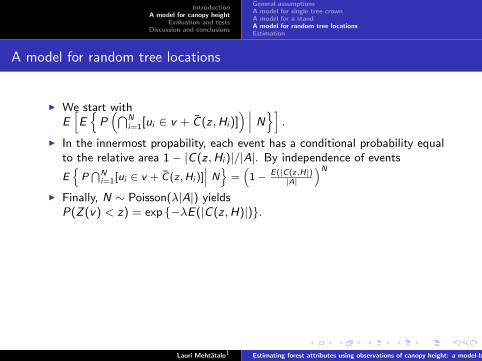
I We start withE[E{
P(⋂N
i=1[ui ∈ v + C(z ,Hi )]) ∣∣∣ N
}].
I In the innermost propability, each event has a conditional probability equalto the relative area 1− |C(z ,Hi )|/|A|. By independence of events
E{
P⋂N
i=1[ui ∈ v + C(z,Hi )]∣∣∣ N}
=(
1− E(|C(z,H|)|A|
)N
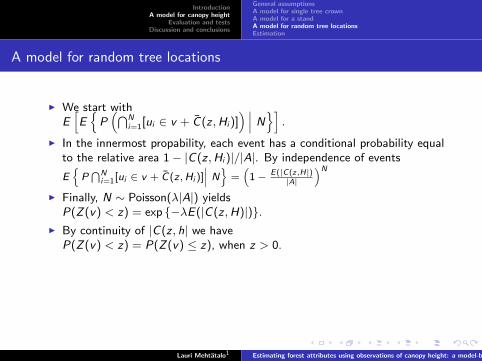
I Finally, N ∼ Poisson(λ|A|) yieldsP(Z(v) < z) = exp {−λE(|C(z ,H)|)}.
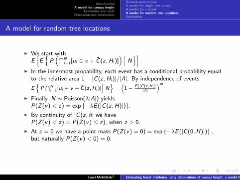
I By continuity of |C(z , h| we haveP(Z(v) < z) = P(Z(v) ≤ z), when z > 0.
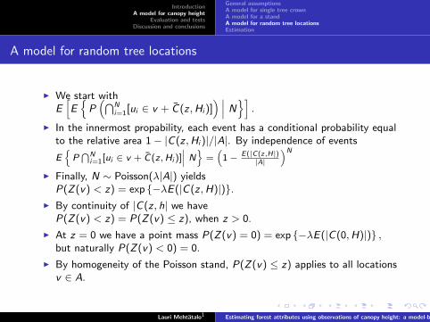
I At z = 0 we have a point mass P(Z(v) = 0) = exp {−λE(|C(0,H)|)} ,but naturally P(Z(v) < 0) = 0.
I By homogeneity of the Poisson stand, P(Z(v) ≤ z) applies to all locationsv ∈ A.
Lauri Mehtatalo1 Estimating forest attributes using observations of canopy height: a model-based approach
IntroductionA model for canopy height
Evaluation and testsDiscussion and conclusions
General assumptionsA model for single tree crownA model for a standA model for random tree locationsEstimation
A model for random tree locations
I We start withE[E{
P(⋂N
i=1[ui ∈ v + C(z ,Hi )]) ∣∣∣ N
}].
I In the innermost propability, each event has a conditional probability equalto the relative area 1− |C(z ,Hi )|/|A|. By independence of events
E{
P⋂N
i=1[ui ∈ v + C(z,Hi )]∣∣∣ N}
=(
1− E(|C(z,H|)|A|
)N
I Finally, N ∼ Poisson(λ|A|) yieldsP(Z(v) < z) = exp {−λE(|C(z ,H)|)}.
I By continuity of |C(z , h| we haveP(Z(v) < z) = P(Z(v) ≤ z), when z > 0.
I At z = 0 we have a point mass P(Z(v) = 0) = exp {−λE(|C(0,H)|)} ,but naturally P(Z(v) < 0) = 0.
I By homogeneity of the Poisson stand, P(Z(v) ≤ z) applies to all locationsv ∈ A.
Lauri Mehtatalo1 Estimating forest attributes using observations of canopy height: a model-based approach
IntroductionA model for canopy height
Evaluation and testsDiscussion and conclusions
General assumptionsA model for single tree crownA model for a standA model for random tree locationsEstimation
Distribution function and density
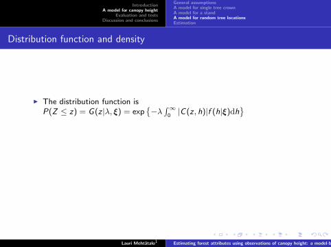
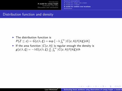
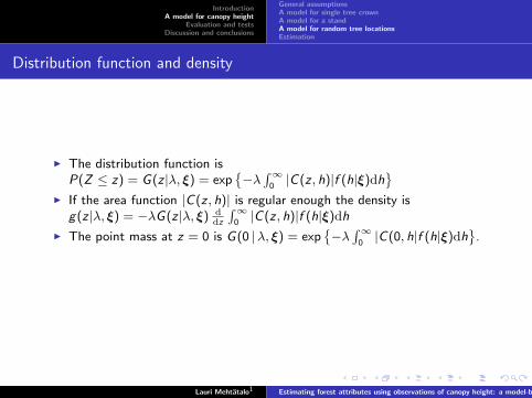
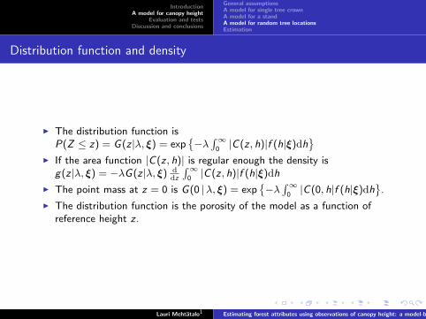
I The distribution function isP(Z ≤ z) = G(z |λ, ξ) = exp
{−λ∫∞
0|C(z , h)|f (h|ξ)dh
}
I If the area function |C(z , h)| is regular enough the density isg(z |λ, ξ) = −λG(z |λ, ξ) d
dz
∫∞0|C(z , h)|f (h|ξ)dh
I The point mass at z = 0 is G(0 |λ, ξ) = exp{−λ∫∞
0|C(0, h|f (h|ξ)dh
}.
I The distribution function is the porosity of the model as a function ofreference height z .
Lauri Mehtatalo1 Estimating forest attributes using observations of canopy height: a model-based approach
IntroductionA model for canopy height
Evaluation and testsDiscussion and conclusions
General assumptionsA model for single tree crownA model for a standA model for random tree locationsEstimation
Distribution function and density
I The distribution function isP(Z ≤ z) = G(z |λ, ξ) = exp
{−λ∫∞
0|C(z , h)|f (h|ξ)dh
}I If the area function |C(z , h)| is regular enough the density is
g(z |λ, ξ) = −λG(z |λ, ξ) ddz
∫∞0|C(z , h)|f (h|ξ)dh
I The point mass at z = 0 is G(0 |λ, ξ) = exp{−λ∫∞
0|C(0, h|f (h|ξ)dh
}.
I The distribution function is the porosity of the model as a function ofreference height z .
Lauri Mehtatalo1 Estimating forest attributes using observations of canopy height: a model-based approach
IntroductionA model for canopy height
Evaluation and testsDiscussion and conclusions
General assumptionsA model for single tree crownA model for a standA model for random tree locationsEstimation
Estimation
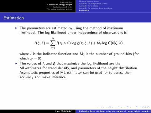
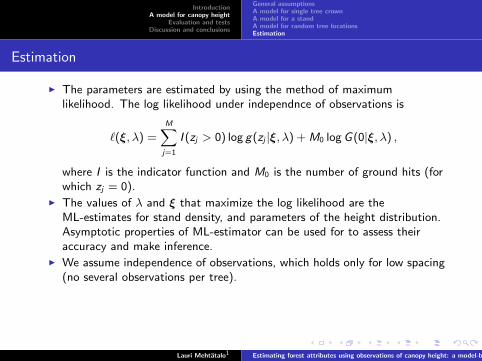
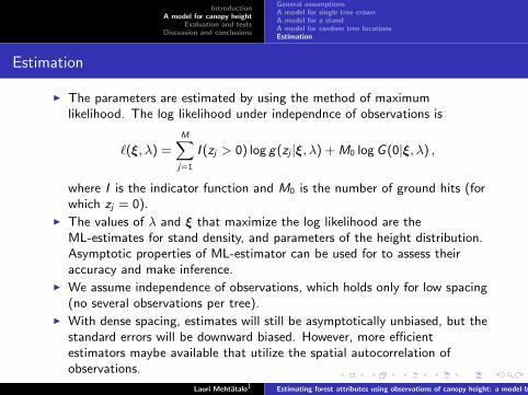
I The parameters are estimated by using the method of maximumlikelihood. The log likelihood under independnce of observations is
`(ξ, λ) =M∑
j=1
I (zj > 0) log g(zj |ξ, λ) + M0 log G(0|ξ, λ) ,
where I is the indicator function and M0 is the number of ground hits (forwhich zj = 0).
I The values of λ and ξ that maximize the log likelihood are theML-estimates for stand density, and parameters of the height distribution.Asymptotic properties of ML-estimator can be used for to assess theiraccuracy and make inference.
I We assume independence of observations, which holds only for low spacing(no several observations per tree).
I With dense spacing, estimates will still be asymptotically unbiased, but thestandard errors will be downward biased. However, more efficientestimators maybe available that utilize the spatial autocorrelation ofobservations.
Lauri Mehtatalo1 Estimating forest attributes using observations of canopy height: a model-based approach
IntroductionA model for canopy height
Evaluation and testsDiscussion and conclusions
General assumptionsA model for single tree crownA model for a standA model for random tree locationsEstimation
Estimation
I The parameters are estimated by using the method of maximumlikelihood. The log likelihood under independnce of observations is
`(ξ, λ) =M∑
j=1
I (zj > 0) log g(zj |ξ, λ) + M0 log G(0|ξ, λ) ,
where I is the indicator function and M0 is the number of ground hits (forwhich zj = 0).
I The values of λ and ξ that maximize the log likelihood are theML-estimates for stand density, and parameters of the height distribution.Asymptotic properties of ML-estimator can be used for to assess theiraccuracy and make inference.
I We assume independence of observations, which holds only for low spacing(no several observations per tree).
I With dense spacing, estimates will still be asymptotically unbiased, but thestandard errors will be downward biased. However, more efficientestimators maybe available that utilize the spatial autocorrelation ofobservations.
Lauri Mehtatalo1 Estimating forest attributes using observations of canopy height: a model-based approach
IntroductionA model for canopy height
Evaluation and testsDiscussion and conclusions
DataResultsExamples with real data
Simulated data
Ab(h)
a(h)
h00 z
y
Y((z,, h))
z
y
h0
0b−−1((z))
a(h)
B
Y((z,, h))
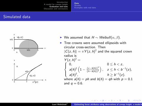
I We assumed that H ∼Weibull(α, β).
I Tree crowns were assumed ellipsoids withcircular cross-section. Then|C(z , h)| = πY (z , h)2 and the squared crownradius isY (z , h)2 =
0, 0 ≤ h < z ,
a(h)2(
1− {z−b(h)}2
{h−b(h)}2
), z ≤ h < b−1(z),
a(h)2, h ≥ b−1(z).where a(h) = ph and b(h) = qh with p = 0.1and q = 0.6.
Lauri Mehtatalo1 Estimating forest attributes using observations of canopy height: a model-based approach

IntroductionA model for canopy height
Evaluation and testsDiscussion and conclusions
DataResultsExamples with real data
Simulated data
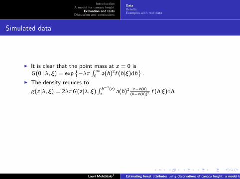
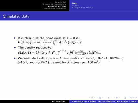
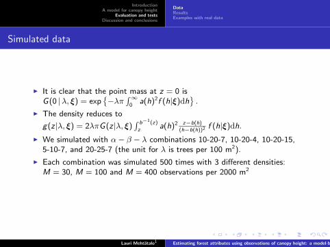
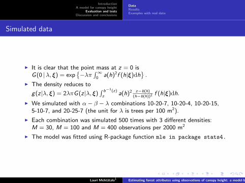
I It is clear that the point mass at z = 0 isG(0 |λ, ξ) = exp
{−λπ
∫∞0
a(h)2f (h|ξ)dh}.
I The density reduces to
g(z |λ, ξ) = 2λπG(z |λ, ξ)∫ b−1(z)
za(h)2 z−b(h)
(h−b(h))2 f (h|ξ)dh.
I We simulated with α− β − λ combinations 10-20-7, 10-20-4, 10-20-15,5-10-7, and 20-25-7 (the unit for λ is trees per 100 m2).
I Each combination was simulated 500 times with 3 different densities:M = 30, M = 100 and M = 400 observations per 2000 m2
I The model was fitted using R-package function mle in package stats4.
Lauri Mehtatalo1 Estimating forest attributes using observations of canopy height: a model-based approach
IntroductionA model for canopy height
Evaluation and testsDiscussion and conclusions
DataResultsExamples with real data
Simulated data
I It is clear that the point mass at z = 0 isG(0 |λ, ξ) = exp
{−λπ
∫∞0
a(h)2f (h|ξ)dh}.
I The density reduces to
g(z |λ, ξ) = 2λπG(z |λ, ξ)∫ b−1(z)
za(h)2 z−b(h)
(h−b(h))2 f (h|ξ)dh.
I We simulated with α− β − λ combinations 10-20-7, 10-20-4, 10-20-15,5-10-7, and 20-25-7 (the unit for λ is trees per 100 m2).
I Each combination was simulated 500 times with 3 different densities:M = 30, M = 100 and M = 400 observations per 2000 m2
I The model was fitted using R-package function mle in package stats4.
Lauri Mehtatalo1 Estimating forest attributes using observations of canopy height: a model-based approach
IntroductionA model for canopy height
Evaluation and testsDiscussion and conclusions
DataResultsExamples with real data
Example fits
00.
1fr
eque
ncy
10−
20−
4
00.
6
= 4.71
= 19.51
= 7.31
λλββαα
00.
2fr
eque
ncy
10−
20−
7
00.
5
= 6.08
= 19.65
= 9.19
λλββαα
00.
2fr
eque
ncy
10−
20−
15
00.
2
= 13.42
= 20.12
= 10.18
λλββαα
00.
1fr
eque
ncy
3−10
−7
00.
8
= 10.25
= 8.79
= 2.54
λλββαα
h, meters
00.
6
0 10 20 30
freq
uenc
y20
−25
−7
z, meters
00.
3
0 10 20 30
= 5.9= 25.32= 40.68
λλββαα
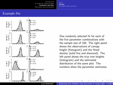
One randomly selected fit for each ofthe five parameter combinations withthe sample size of 100. The right panelshows the observations of canopyheight (histogram) and the fitteddensity (solid line and diamond). Theleft panel shows the true tree heights(histogram) and the estimateddistribution of the same plot. Thenumbers show the parameter estimates.
Lauri Mehtatalo1 Estimating forest attributes using observations of canopy height: a model-based approach
IntroductionA model for canopy height
Evaluation and testsDiscussion and conclusions
DataResultsExamples with real data
Simulation results
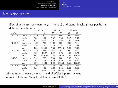
Bias of estimates of mean height (meters) and stand density (trees per ha) indifferent simulations.
M=30 M=100 M=400α-β-λ H N H N H N10-20-4 true mean 19.03 400 19.03 400 19.03 400
bias% 0.84 2.26 0.62 0.09 0.12 0.30s.d. 1.21 148.53 0.67 78.16 0.36 53.56
10-20-7 true mean 19.03 700 19.03 700 19.03 700bias% 0.89 2.42 0.45 -1.66 0.07 0.43s.d. 1.03 235.62 0.56 125.15 0.31 79.85
10-20-15 true mean 19.03 1500 19.03 1500 19.03 1500bias% 0.02 13.27 -0.05 2.76 -0.07 0.70s.d. 1.08 2698.26 0.53 263.39 0.29 145.76
3-10-7 true mean 8.93 700 8.93 700 8.93 700bias% 6.65 1.76 1.45 3.20 0.65 -0.57s.d. 2.27 480.08 1.24 238.60 0.66 122.87
20-25-7 true mean 24.34 700 24.34 700 24.34 700bias% 0.23 1.28 -0.08 2.12 0.02 0.40s.d. 0.78 205.81 0.43 112.24 0.22 73.31
M=number of observations, α and β Weibull parms, λ truenumber of stems. Sample plot area was 2000m2
Lauri Mehtatalo1 Estimating forest attributes using observations of canopy height: a model-based approach
IntroductionA model for canopy height
Evaluation and testsDiscussion and conclusions
DataResultsExamples with real data
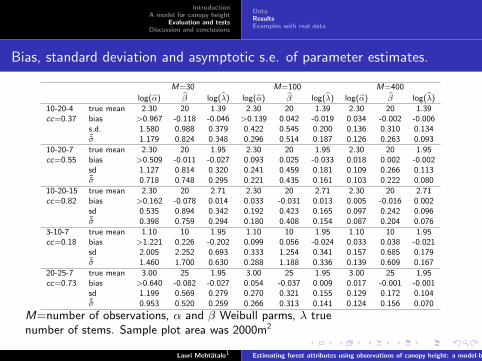
Bias, standard deviation and asymptotic s.e. of parameter estimates.
M=30 M=100 M=400
log(α) β log(λ) log(α) β log(λ) log(α) β log(λ)10-20-4 true mean 2.30 20 1.39 2.30 20 1.39 2.30 20 1.39cc=0.37 bias >0.967 -0.118 -0.046 >0.139 0.042 -0.019 0.034 -0.002 -0.006
s.d. 1.580 0.988 0.379 0.422 0.545 0.200 0.136 0.310 0.134¯σ 1.179 0.824 0.348 0.296 0.514 0.187 0.126 0.263 0.093
10-20-7 true mean 2.30 20 1.95 2.30 20 1.95 2.30 20 1.95cc=0.55 bias >0.509 -0.011 -0.027 0.093 0.025 -0.033 0.018 0.002 -0.002
sd 1.127 0.814 0.320 0.241 0.459 0.181 0.109 0.266 0.113¯σ 0.718 0.748 0.295 0.221 0.435 0.161 0.103 0.222 0.080
10-20-15 true mean 2.30 20 2.71 2.30 20 2.71 2.30 20 2.71cc=0.82 bias >0.162 -0.078 0.014 0.033 -0.031 0.013 0.005 -0.016 0.002
sd 0.535 0.894 0.342 0.192 0.423 0.165 0.097 0.242 0.096¯σ 0.398 0.759 0.294 0.180 0.408 0.154 0.087 0.204 0.076
3-10-7 true mean 1.10 10 1.95 1.10 10 1.95 1.10 10 1.95cc=0.18 bias >1.221 0.226 -0.202 0.099 0.056 -0.024 0.033 0.038 -0.021
sd 2.005 2.252 0.693 0.333 1.254 0.341 0.157 0.685 0.179¯σ 1.460 1.700 0.630 0.288 1.188 0.336 0.139 0.609 0.167
20-25-7 true mean 3.00 25 1.95 3.00 25 1.95 3.00 25 1.95cc=0.73 bias >0.640 -0.082 -0.027 0.054 -0.037 0.009 0.017 -0.001 -0.001
sd 1.199 0.569 0.279 0.270 0.321 0.155 0.129 0.172 0.104¯σ 0.953 0.520 0.259 0.266 0.313 0.141 0.124 0.156 0.070
M=number of observations, α and β Weibull parms, λ truenumber of stems. Sample plot area was 2000m2
Lauri Mehtatalo1 Estimating forest attributes using observations of canopy height: a model-based approach
IntroductionA model for canopy height
Evaluation and testsDiscussion and conclusions
DataResultsExamples with real data
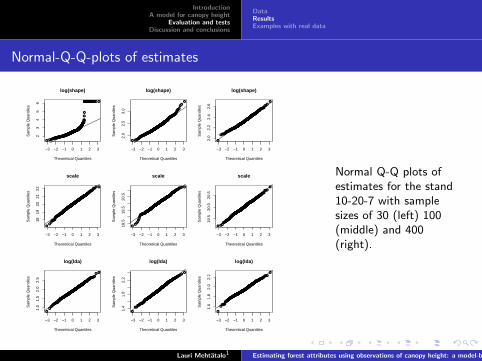
Normal-Q-Q-plots of estimates
●
●
●●
●●
●●●
●
●
●
●●
●●●
●
●● ●
●
●
●
●●●
●●
●
●
●●
●
●
●●
●
●
●
●●
●
●
●
●
●
●
●
●
●
●●
●●●●●
●●
●
●
●
●
●●
●
●
●
●
●
●●
●●
●●
●
●●
●
●
●●●
●
●
●●
●
●
●
●
●
●●●
●●
● ●●
● ●
●
●
●
●
●
●
●
●
●●
●
● ●●
●
●●●●●
●
●●
●
●●●
●●
●●
●
●●●
●●
●●●
●
●
●●
●●
●●
●●●
●●
●
●
●
●
●
●
●
●●
●●●
●
●
●●●●
●●
●
●
●
●●●
●
● ●
●
●
●●●
●●
●● ●●
●
●
●
●
●●
●●●●
●
●
●
●
●
●
●●
●
●
●●
●●
●●
●
●
●●
●
●
●
●
●
●●●●
●
●
●
●
●●
●
●●
●●
●
●●
●
●
●●
●
●
●
●●
●
●
●
●
●
●●●●
●
●
●
●
●●●
●●
●
●●
●
●● ●●●●●●
●
●
●
●●
●●
●●●
●●
●●
●
●
●
●
●
●
●
●
●
●
●
●
●
●
●
●
●
●
●●●●
●
●●
●
●
●
●
●
●
●●●●
●●
●
●
●●
●
●
●●
●●
●●●
●
●
●
●●●
●
●
●●●
●
●●
●
●
●●
●
●
●
●
●
●
●●
●
●
●●
●
●
●
●
●
●
●●
●
●
●
●
●
●
●
●
●
●
●●
●●
● ●
●●
●●
●●
●
●
●
●●
●
●●
●
●
●
●
●
●
●
●
●
●●
●●
●
●●
●●
●●●
●
●
●
●
●
●
●●
●
●●●●●
●
●●
●
●
●
●
●
●●
●●
●
●
●
●●
●●
●
●
●
●●●●
●●
●
●
●●
●
●
●
●
●●●
●●
●
●
●
−3 −2 −1 0 1 2 3
23
45
6
log(shape)
Theoretical Quantiles
Sam
ple
Qua
ntile
s
●
●
●
●
●
●
●●
●
●
●
●
●
●●
●
●●
●
●
●●
●●
●
●●●
●
●
●
●
●
●
●
●
●●
●
●
●●
●
●●
●●●
●●
●●●
●
●●
●
●●
●
●
●
●●
●
●
●●●
●
●●
●
●
●
●
●
●
●●●
●●●
●
●
●
●
●
●
●●●
●
●●
●
●●
●
●
●
●●●●
●
●
●
●●
●
●
●●
●●
●
●
●
●●
●
●
●●
●
●
●
●
●●●
●●
●
●
●
●
●
●
●
●●
●
●
●
●●
●
●●
●
●
●●
●
●
●
●
●
●
●
●
●●
●
●●
●
●●
●
●
●●
●
●
●
●●●●
●
●
●
●
●
●
●
●
●
●
●
●
●
●●
●
●
●
●●
●
●
●●
●
●●●
●
●
●
●
●
●
●●
●
●●●
●
●●
●●
●
●●●
●●
●●●
●
●●
●
●
●
●●
●
●●
●●
●●
●●
●
●
●●
●
●
●
●
●
●
●
●●●
●
●
●●●
●
●
●
●
●
●
●
●●
●
●
●
●
●
●●
●●
●
●
●
●
●
●
●
●
●●
●
●
●
●
●
●
●
●
●●
●●
●
●●
●
●
●●
●
●
●●
●●
●●
●
●
●
●
●
●●
●●
●
●
●●
●
●
●
●
●
●
●
●
●●
●
●
●●
●●
●●
●
●
●●
●
●
●
●
●
●
●
●●
●
●
●
●
●●
●
●
●
●
●
●
●
●
●
●
●
●
●
●●
●
●
●
●
●
●
●●
●●
●
●
●●
●
●
●●
●
●
●●
●
●
●
●
●
●
●
●●
●
●●
●
●
●
●●
●
●
●●
●
●
●●
●
●
●
●
●●
●
●●
●
●
●
●
●
●
●●
●
●
●●
●
●
●
●
●
●●
●●
●
●
●
●
●
●
●●●
●
●
●
●
●
●
●
●●
●
●
●
●●
●
●
●●
●●
●
−3 −2 −1 0 1 2 3
1819
2021
22
scale
Theoretical Quantiles
Sam
ple
Qua
ntile
s
●
●
●
●●
●
●
●●
●
●
●
●
●●
●
●
●●
●●
●
●
●
●●●●
●●
●
●
●
●
●
●●
●
●●
●●
●
●
●
●
●●
●
●●
●
●
●
●
●●
●
●
●●
●
●
●
●
●
●●
●
●
●
●●
●●
●●
●
●
●●
●
●●●●
●
●
●
●●
●
●
●●
●
●●●
●
●●
●
●
●
●
●●
●●
●
●
●●
●
●
●
●
●
●
●●
●
●
●
●
●●
●
●
●
●
●
●
●
●
●●
●●
●●
●●
●
●
●●
●●●
●
●
●
●●
●
●
●
●
●
●
●●
●●
●
●
●
●
●●
●●
●●●●
●
●
●
●
●
●●
●
●
●
●
●●
●
●
●
●●
●
●
●
●
●
●
●
●●
●
●●●●
●
●
●●●
●
●●
●●●
●
●
●
●
●●
●
●
●●
●
●
●
●●
●●
●●●
●
●●
●
●
●
●●●
●
●●
●
●
●
●
●
●●●
●
●
●●
●
●●
●
●
●●●
●●●
●●
●
●
●
●
●
●
●●
●
●
●
●
●
●
●●
●
●●
●●●
●
●
●●
●
●
●
●
●
●
●
●
●
●
●
●●
●
●
●●
●
●
●
●●●
●
●
●
●
●●
●●
●
●
●
●●
●
●
●
●
●
●
●
●
●
●
●●
●
●
●
●
●●●
●
●
●
●●
●
●●
●
●
●●●
●
●
●
●●
●
●
●
●
●●
●
●
●
●
●
●
●
●
●
●●
●●
●
●●
●
●
●
●●●●
●
●
●●
●
●
●
●
●●
●●●
●
●
●
●
●
●●
●
●
●
●●●
●●●
●●
●
●
●
●
●
●
●
●
●
●
●
●
●
●
●
●
●
●
●
●
●●
●
●
●
●●
●
●
●
●
●●
●
●●
●
●
●
●
●
●
●
●●
●
●
●●●●
●
●
●
●
●●
●
●
●
●
●
●
−3 −2 −1 0 1 2 3
1.0
1.5
2.0
2.5
log(lda)
Theoretical Quantiles
Sam
ple
Qua
ntile
s
●
●
●
●●●
●
●
●
●
●
●
●●
●
●●
●
●
●●
●
●
●●
●
●
●
●
●●
●●
●
●
●
●●
●
●
●
●
●
●
●
●
●
●
●
●
●
●
●
●
●
●
●
●
●
●
●●●
●
●
●
●●
●●
●
●●●
●
●
●
●
●●
●
●
●
●
●
●
●
●
●●
●
●●
●●
●●
●●
●
●
●
●
●●●
●●
●
●●
●
●
●
●
●
●
●
●
●
●
●
●●
●●●
●
●●
●
●
●
●
●
●
●
●
●
●
●
●
●
●●
●●
●
●●●
●●●●
●
●
●
●
●
●●
●
●
●●
●●
●
●●●
●●
●
●
●●
●
●
●
●●
●
●●
●●
●●
●●
●●
●
●
●
●
●
●
●●
●
●
●●
●●
●
●●●
●●
●
●●
●●●
●
●
●
●
●
●
●●●
●
●
●●
●●●
●●
●●
●
●
●
●
●
●●
●
●●●
●●
●
●
●●
●
●
●
●●●
●●
●
●
●●
●
●
●●●
●
●●●
●
●●
●
●
●
●
●●
●
●
●
●
●
●●
●
●
●
●
●
●
●
●
●●
●
●●
●
●
●
●●
●
●
●
●
●
●
●
●
●
●●
●
●
●
●
●
●
●
●
●
●
●
●
●
●
●
●●
●
●
●
●
●
●
●●
●
●
●●
●●
●●
●
●
●●
●●●
●●
●
●
●
●●
●
●
●●
●
●●
●
●
●
●●
●
●●
●
●
●
●
●
●●
●
●
●
●
●●
●●
●
●●
●
●●
●
●●
●●
●
●
●
●
●
●
●●
●●
●
●●
●●
●●
●
●
●
●●
●
●●
●
●●
●
●
●●●
●
●
●●
●
●
●
●
●
●●
●
●
●
●
●●●
●●
●
●●
●
●
●
●
●
●●
●
●
●
●●
●
●
●●
●●
●
●
●●
●
●
●
●
●
●●
●
●
●
●
−3 −2 −1 0 1 2 3
2.0
2.5
3.0
log(shape)
Theoretical Quantiles
Sam
ple
Qua
ntile
s
●●
●
●
●
●
●
●
●
●
●
●
●
●
●
●●
●●
●
●
●
●
●●
●●●●●
●
●
●
●
●
●
●
●●
●●
●●
●
●
●
●
●
●
●
●●
●●●
●
●
●
●
●
●●●
●●
●
●
●
●●
●
●
●
●
●
●
●●●
●
●●
●
●●
●
●
●
●
●●
●●●
●●
●
●●
●
●
●
●
●
●
●●●
●
●●
●
●
●
●●
●●
●
●
●
●
●
●●
●
●●
●●
●
●●●
●●
●●●
●
●
●
●
●
●●
●
●
●●
●●
●●
●●
●
●
●
●
●
●●●
●
●●●
●
●
●●
●
●
●
●
●
●
●
●
●●
●●
●
●●
●
●●
●
●
●●
●
●●
●
●●●
●
●●●
●
●●
●
●●
●●
●
●●
●
●
●
●
●
●●
●●
●
●●
●●
●
●
●
●●●
●
●
●●
●
●
●
●
●
●●
●●
●
●
●
●
●●
●●
●
●
●●
●●●
●●
●
●
●
●
●
●
●●
●
●●●
●
●
●
●
●
●
●
●
●
●
●
●●
●
●
●
●
●●●
●
●
●●
●●
●
●
●
●
●●
●
●
●●
●
●
●
●
●
●
●●
●
●
●
●
●
●●
●
●●
●
●
●
●
●
●
●
●
●●
●
●
●
●
●
●
●
●
●●
●●
●
●●
●
●
●
●
●
●
●
●●
●
●
●
●●
●
●
●
●
●
●
●
●
●●
●
●
●
●●●
●
●
●
●
●
●●
●
●●●
●●
●●
●●●
●
●
●
●
●●●
●
●
●
●
●
●
●
●
●
●
●
●
●
●
●
●●
●
●●
●
●
●
●
●
●
●●
●●
●●
●
●
●
●
●
●
●
●
●
●
●
●
●
●
●
●
●
●
●
●
●●
●
●
●
●●
●
●
●●
●
●
●●
●
●●
●●
●
●
●
●
●
●
●
●●
●
●
●
●
●
●
●
−3 −2 −1 0 1 2 3
18.5
19.5
20.5
scale
Theoretical Quantiles
Sam
ple
Qua
ntile
s
●●
●
●
●
●●
●
●
●
●●
●●
●
●
●
●
●
●●
●
●
●
●
●●
●
●
●
●
●
●
●
●
●
●
●
●
●
●●
●
●
●●
●
●
●
●
●
●
●
●●
●
●
●●
●
●●●
●
●
●
●
●
●
●
●
●
●
●
●●●
●
●
●●
●
●
●
●●
●
●●
●
●
●
●
●
●
●●
●
●
●
●
●
●
●
●
●
●
●
●
●
●
●
●●●
●●●
●
●
●
●
●●
●●
●
●
●
●●
●
●
●
●
●
●●
●
●●
●
●
●
●
●
●
●
●●●
●
●●
●
●
●
●
●●
●●●
●
●●
●
●
●
●
●
●
●
●
●
●
●
●●
●●●
●●●
●●
●
●
●
●
●●●
●
●
●
●●
●●
●●
●
●
●●
●
●
●
●
●●
●
●●
●
●
●
●●●
●●
●●
●
●
●
●●
●●●
●
●
●
●●
●
●
●
●
●●
●
●
●
●●
●●
●
●
●
●●
●
●
●
●●
●●
●
●
●●
●
●
●
●
●●
●
●
●
●
●
●
●
●
●
●
●●
●
●●
●●
●●●●
●
●
●●●
●
●
●●
●
●●
●
●●
●
●●
●
●●●
●
●
●
●●
●
●
●
●
●
●
●
●
●
●
●
●
●
●
●
●
●
●
●
●●
●
●
●
●
●●
●
●
●
●
●●
●
●
●
●
●
●●
●
●
●
●●●
●
●
●
●
●
●
●●
●●
●
●
●
●
●
●●
●
●
●
●
●
●
●●●
●●●
●
●●
●
●
●
●●
●●
●●
●●
●
●
●
●
●
●
●
●
●●
●
●●●
●
●
●
●
●
●
●●
●
●
●●●
●
●
●
●
●
●
●●
●●
●
●
●
●●
●●●
●●●
●
●
●
●
●
●
●
●
●
●
●●●
●●
●
●
●
●
●●●●
●●
●
●●
●
●
●
●
●●
●
●
●●
●
●
●
−3 −2 −1 0 1 2 3
1.4
1.8
2.2
log(lda)
Theoretical Quantiles
Sam
ple
Qua
ntile
s
●●
●●●
●
●
●
●
●
●●
●●
●
●
●
●
●
●
●
●
●●
●
●
●●
●
●
●
●●
●●●
●
●●
●●●
●
●
●
●
●
●
●
●
●
●
●●
●●
●
●●●●
●●●
●
●●
●
●●
●
●
●●
●●
●
●●
●
●
●
●
●
●
●●
●
●●
●●●
●
●
●●●●
●●●
●
●
●
●
●
●●
●
●
●
●
●
●
●
●
●
●●
●
●
●●●●
●
●
●●
●
●
●●
●
●
●
●
●
●
● ●
●
●●
●
●
●●●
●
●
●
●
●
●
●●
●
●
●
●
●
●●
●
●●
●
●
●
●
●
●
●
●
●
●●
●●
●
●
●
●●
●●
●
●
●
●●●
●●
●●●
●
●●
●
●●
●
●
●●
●
●●
●
●
●●●
●
●
●
●●
●●
●
●●
●●
●
●●●
●●
●
●
●
●●
●●●
●
●
●
●
●
●
●●
●
●
●
●
●
●
●
●
●
●●
●
●
●
●●●
●●
●
●
●
●●
●
●
●
●●
●
●
●
●●
●
●●●
●●
●
●●
●
●
●
●
●●●
●
●
●
●
●
●
●●
●
●
●
●
●
●
●
●●
●
●
●●
●●
●
●
●
●
●
●
●
●●●
●
●
●
●
●●
●●
●
●
●
●
●
●
●
●
●
●●●
●
●
●●
●
●
●
●
●●
●
●
●
●
●
●
●
●
●
●●
●
●●
●
●●
●
●
●●
●
●
●●
●
●
●●
●
●●
●
●
●
●
●
●●
●
●
●
●
●
●●
●
●
●
●●
●
●●
●●
●
●
●
●
●
●
●●
●
●●
●
●
●
●●
●●
●●
●
●
●
●
●●
●●
●
●
●●●
●●●
●●
●
●●
●
●
●●
●●●
●●
●
●
●●
●
●
●●●
●
●●●
●
●
●
●
●
●
●
●
●
●
●
●●
●●
●
●
−3 −2 −1 0 1 2 3
2.0
2.2
2.4
2.6
log(shape)
Theoretical Quantiles
Sam
ple
Qua
ntile
s
●●
●●
●
●
●●
●
●
●
●
●
●
●
●
●
●
●
●
●
●
●
●
●
●●
●
●
●
●●●
●●
●●
●
●●
●
●
●
●
●●
●
●
●
●
●
●
●
●
●
●
●
●
●●
●
●
●
●
●
●
●
●
●
●
●●
●
●●
●
●
●●
●
●
●
●
●
●
●●
●
●
●
●
●
●
●●
●
●
●
●●
●
●
●●
●
●
●●
●
●●
●●
●
●
●
●●
●
●
●
●●
●
●●
●
●
●
●●●●●
●●
●●
●
●
●●
●
●
●
●
●
●
●
●
●
●
●
●
●
●●
●●●
●
●●
●
●
●
●
●
●
●●
●
●
●
●
●
●
●
●
●
●
●
●●
●
●
●
●●
●
●
●●
●
●
●
●●
●
●●
●
●
●●
●
●
●
●●
●●
●
●
●
●●●●●
●
●●
●●
●
●
●
●
●
●●
●●
●●
●
●
●
●●
●
●
●
●
●
●
●
●
●
●
●
●●
●
●
●
●●
●●
●
●
●●
●
●
●
●
●●
●
●
●●
●
●
●
●
●
●
●
●●
●
●●
●
●
●●
●●●
●
●●
●
●
●
●●
●
●●
●●●
●
●
●
●
●
●
●●
●●
●
●●
●
●
●
●●●●
●
●
●
●●
●
●
●
●
●
●
●
●
●
●
●
●
●●
●
●
●
●
●
●
●
●
●
●●
●
●●
●
●
●
●
●●
●
●●●
●●
●
●
●●
●
●●
●
●
●
●
●
●
●
●
●
●
●●
●●
●●
●●●
●
●●
●
●
●
●
●●
●
●●●
●
●
●
●
●●
●●
●●
●
●
●
●
●
●
●
●●
●
●
●
●
●
●●●
●●
●
●
●
●
●
●●
●
●
●●
●
●●●●
●
●
●
●
●
●●
●
●●
●●
●
●
●●
●
●
●
●●
●
●
●●●
●
●
●
●●
●
●
●
●
●
●
●
●
●●
●●
−3 −2 −1 0 1 2 3
19.5
20.0
20.5
scale
Theoretical Quantiles
Sam
ple
Qua
ntile
s
●
●●
●
●
●
●
●●
●
●●
●
●●
●●
●●
●
●
●
●
●●
●
●
●
●
●
●●
●
●●●
●●
●
●
●
●
●●
●
●
●
●
●
●
●●
●
●
●
●●
●
●●
●●
●
●
●
●
●
●●●
●●
●
●●
●
●
●
●
●
●
●
●
●
●
●
●
●
●
●
●
●
●●
●
●●
●●
●
●
●
●
●●
●
●●
●●●●
●
●●
●
●
●
●
●
●
●
●
●●●
●
●●
●
●●
●●
●
●●●●●●
●●
●●
●
●●
●
●●
●
●●
●
●
●
●
●●
●
●
●
●
●
●
●
●
●
●
●
●
●
●
●
●
●
●●
●●●
●
●
●
●
●
●
●●
●
●
●
●●●
●●
●
●●●
●
●
●
●
●●
●
●
●
●
●
●
●●
●●●
●
●●
●●
●
●
●
●●
●●
●●
●
●●
●
●
●
●●
●
●
●●
●
●
●
●
●
●
●
●●
●●
●
●
●
●
●
●●
●●
●●
●
●
●●
●
●
●
●
●●
●
●
●
●●
●
●
●
●
●
●
●
●
●
●
●
●●
●
●●
●●●
●
●
●
●
●
●
●
●
●
●
●●
●
●●
●●●
●
●
●●●
●
●
●●
●
●●
●
●
●
●●
●
●●
●
●
●
●
●●
●
●●
●
●
●
●●
●●
●
●
●●
●
●●
●
●
●
●
●
●●
●
●
●
●●
●●●●
●●●●
●
●●
●
●
●●●
●
●
●
●
●
●
●
●
●●
●
●
●
●●
●
●
●
●
●●●
●
●
●
●
●
●●●
●
●●●
●
●●
●
●
●
●
●
●●
●
●
●●
●●
●
●
●●●
●●
●●
●
●
●●
●●
●●
●●●
●
●
●●
●●●
●
●
●
●●
●●
●
●●
●●
●
●
●●
●●
●
●
●●
●
●
●
●
●
●
●
●●●●
−3 −2 −1 0 1 2 3
1.6
1.8
2.0
2.2
log(lda)
Theoretical Quantiles
Sam
ple
Qua
ntile
s
Normal Q-Q plots ofestimates for the stand10-20-7 with samplesizes of 30 (left) 100(middle) and 400(right).
Lauri Mehtatalo1 Estimating forest attributes using observations of canopy height: a model-based approach
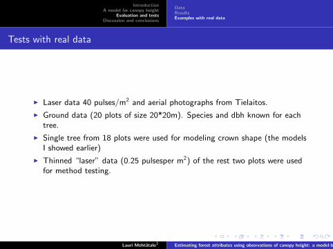
IntroductionA model for canopy height
Evaluation and testsDiscussion and conclusions
DataResultsExamples with real data
Tests with real data
I Laser data 40 pulses/m2 and aerial photographs from Tielaitos.
I Ground data (20 plots of size 20*20m). Species and dbh known for eachtree.
I Single tree from 18 plots were used for modeling crown shape (the modelsI showed earlier)
I Thinned “laser” data (0.25 pulsesper m2) of the rest two plots were usedfor method testing.
Lauri Mehtatalo1 Estimating forest attributes using observations of canopy height: a model-based approach
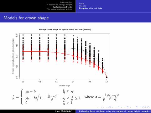
IntroductionA model for canopy height
Evaluation and testsDiscussion and conclusions
DataResultsExamples with real data
Models for crown shape
●
●
●
●
●
●
●
●●
●●
●
●
●
●
●
●
●
●
●●
●
●
●
●
●
●
●
●●
●
●
●
●
●
●
●
●
●
●
●
●
●
●
●
●
●
●
●●
●
●●
●
●
●
●
●
●
●
●●
●●
●
●
●
●
●
●
●
●
●●
●
●
●
●
●
●
●
●●
●
●
●
●
●
●
●
●
●
●
●
●
●
●
●
●
●
●
●●
●
●●
●
●
●
●
●
●
●
●●
●●
●
●
●
●
●
●
●
●
●●
●
●
●
●
●
●
●
●●
●
●
●
●
●
●
●
●
●
●
●
●
●
●
●
●
●
●
●●
●
●●
●
●
●
●
●
●
●
●●
●●
●
●
●
●
●
●
●
●
●●
●
●
●
●
●
●
●
●●
●
●
●
●
●
●
●
●
●
●
●
●
●
●
●
●
●
●●●
●
●●
●
●
●
●
●
●
●
●●
●●
●
●
●
●
●
●
●
●
●●
●
●
●
●
●
●
●
●●
●
●
●
●
●
●
●
●
●
●
●
●
●
●
●
●
●
●●●
●
●●
●
●
●
●
●
●
●
●
●
●
●
●
●
●
●
●
●
●
●
●●
●
●
●
●
●
●
●
●●
●
●
●
●
●
●
●
●
●
●
●
●
●
●
●
●
●
●●●
●
●●
●
●
●
●
●
●
●
●
●
●●
●
●
●
●
●
●
●
●
●●
●
●
●
●
●
●
●
●
●
●
●
●
●
●
●
●
●
●
●
●●
●
●
●
●
●●●●●
●●
●
●
●
●
●
●
●
●●
●
●
●
●
●
●
●
●
●
●
●●
●
●
●
●
●
●
●
●
●
●
●
●
●
●
●
●
●
●
●
●
●
●
●
●
●
●●●●●
●●
●
●
●
●
●●
●
●●
●
●
●
●
●●
●
●
●
●
●●
●
●
●
●
●
●
●●
●
●
●
●
●
●
●
●
●
●
●
●
●
●
●
●
●
●
●
●
●●
●
●
●
●
●
●
●●
●
●
●
●
●
●
●
●
●
●
●
●
●
●
●
●
●
●
●
●
●
●●
●●
●●
●
●●
●
●
●
●
●
●
●
●
●
●
●●●
●●
●
●
●
●
●
●
●●
●
●
●
●
●
●
●
●●●
●
●
●
●
●
●
●
●
●
●
●
●
●
●
●
●
●
●
●
●
●
●
●
●
●
●
●
●●
●
●●●
●●●
●
●
●
●
●
●
●
●
●●
●
●
●
●
●●
●
●
●
●
●
●
●
●
●
●
●
●
●
●
●●
●
●
●
●
●
●
●
●●
●
●
●
●
●
●
●
●
●
●●
●
●
●
●
●
●
●●
●
●●●
●
●
●
●●
●
●
●
●
●
●
●
●
●
●
●
●
●
●
●
●
●
●
●●●
●
●
●●
●
●
●
●
●
●●
●
●
●●
●
●
●
●
●
●
●
●
●
●
●
●
●
●
●
●●
●
●
●
●
●
●
●
●
●
●
●
●
●
●●
●●
●
●
●●
●
●
●
●
●
●
●
●
●
●
●
●●●
●
●●
●●●●●●●●●●●●●●●●●●●●●●●●●●●●●●●●●●●●●●●●●●●●●●●●●●●●●
0.0 0.2 0.4 0.6 0.8 1.0
0.00
0.05
0.10
0.15
0.20
Average crown shape for Spruce (solid) and Pine (dashed)
Relative height
Rel
ativ
e cr
own
radi
us (
Cro
wn
radi
us /
tree
hei
ght)
rH
=
y0 + b h
H≤ x0
y0 + b
√1− ( h
H−x0)2
a2 x0 <hH≤ 1
0 hH> 1
where a =
√b2(1−x0)2
b2−y20
Lauri Mehtatalo1 Estimating forest attributes using observations of canopy height: a model-based approach
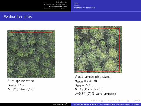
IntroductionA model for canopy height
Evaluation and testsDiscussion and conclusions
DataResultsExamples with real data
Evaluation plots
8
Pure spruce standH=17.77 mN=700 stems/ha
28
Mixed spruce-pine stand¯Hspruce=9.87 m
¯Hpine=15.66 mN=1350 stems/haρ=0.70 (70% were spruces)
Lauri Mehtatalo1 Estimating forest attributes using observations of canopy height: a model-based approach
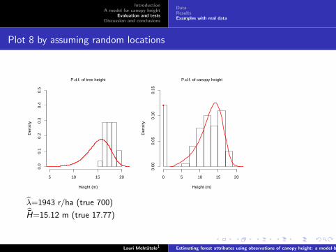
IntroductionA model for canopy height
Evaluation and testsDiscussion and conclusions
DataResultsExamples with real data
Plot 8 by assuming random locations
Height (m)
Den
sity
5 10 15 20
0.0
0.1
0.2
0.3
0.4
0.5
P.d.f. of tree height
Height (m)
Den
sity
0 5 10 15 20
0.00
0.05
0.10
0.15
P.d.f. of canopy height
λ=1943 r/ha (true 700)H=15.12 m (true 17.77)
Lauri Mehtatalo1 Estimating forest attributes using observations of canopy height: a model-based approach
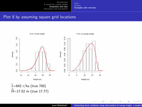
IntroductionA model for canopy height
Evaluation and testsDiscussion and conclusions
DataResultsExamples with real data
Plot 8 by assuming square grid locations
Height (m)
Den
sity
12 14 16 18 20
0.0
0.1
0.2
0.3
0.4
0.5
P.d.f. of tree height
Height (m)
Den
sity
0 5 10 15 20
0.00
0.02
0.04
0.06
0.08
0.10
0.12
P.d.f. of canopy height
λ=642 r/ha (true 700)H=17.52 m (true 17.77)
Lauri Mehtatalo1 Estimating forest attributes using observations of canopy height: a model-based approach
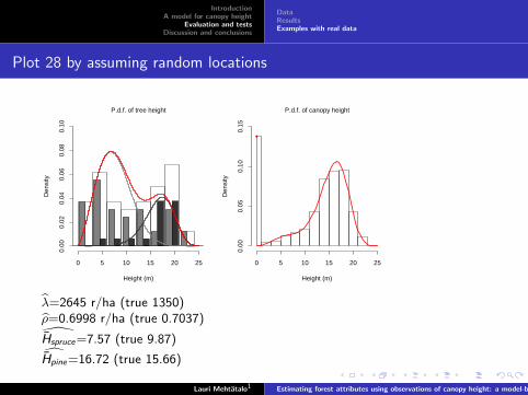
IntroductionA model for canopy height
Evaluation and testsDiscussion and conclusions
DataResultsExamples with real data
Plot 28 by assuming random locations
Height (m)
Den
sity
0 5 10 15 20 25
0.00
0.02
0.04
0.06
0.08
0.10
P.d.f. of tree height
Height (m)
Den
sity
0 5 10 15 20 25
0.00
0.05
0.10
0.15
P.d.f. of canopy height
λ=2645 r/ha (true 1350)ρ=0.6998 r/ha (true 0.7037)Hspruce=7.57 (true 9.87)Hpine=16.72 (true 15.66)
Lauri Mehtatalo1 Estimating forest attributes using observations of canopy height: a model-based approach
IntroductionA model for canopy height
Evaluation and testsDiscussion and conclusions
Discussion and conclusions
I First trials to derive stand characteristics by utilizing assumptions oncrown shape, and a spatial model for the stand.
I ML-estimation for the model seems to be quite stable and produces quitereliable estimates with simulated datasets
I Comutationally intensive method as it needs nested application ofnumerical methods
I Seems to be quite vulnerable to violation of asumptions on spatial patternof tree locations
I Could be a way to integrate the research on single tree crowns with themodels of stand structure.
I Could provide a theoretical basis for the so-callet area-based approach.
Lauri Mehtatalo1 Estimating forest attributes using observations of canopy height: a model-based approach
IntroductionA model for canopy height
Evaluation and testsDiscussion and conclusions
Publications
Mehtatalo, L. and Nyblom, J. Estimating forest parameters using observationsof canopy height: a model-based approach. Forest Science 55(5): 411-422.Hello WordMehtatalo, L. 2006. Eliminating the effect of overlapping crowns from aerialinventory estimates. Canadian Journal of Forest Research 36(7): 1649-1660.(Reprints available upon request)
Lauri Mehtatalo1 Estimating forest attributes using observations of canopy height: a model-based approach