Embed Size (px)
Citation preview
Do not
distrib
ute or
copy
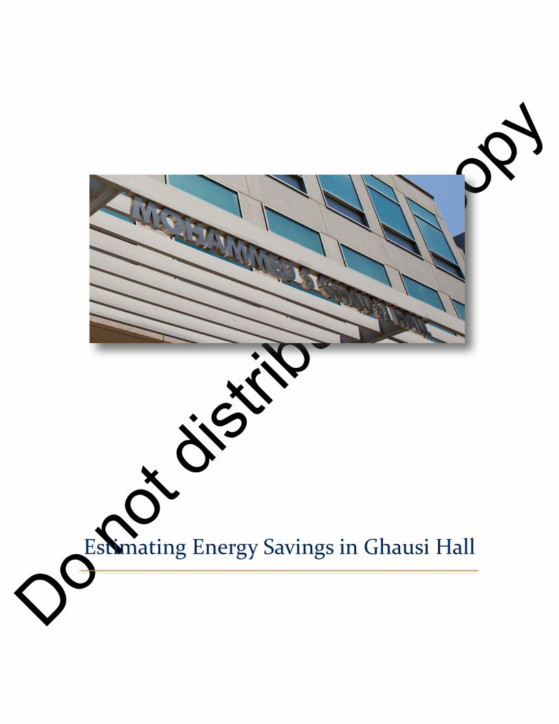
Estimating Energy Savings in Ghausi Hall
Do not
distrib
ute or
copy
Estimating Energy Savings in Ghausi Hall
PAGE 1
Table of Contents Executive Summary ..................................................................................................... 2
1. Introduction ............................................................................................................. 3
2. Data Characteristics ................................................................................................ 4 2.1. Outside Air Temperature ............................................................................................... 4 2.2. Electricity Usage ............................................................................................................ 5 2.3. Chilled Water Usage ...................................................................................................... 7 2.4. Steam Usage Characteristics ......................................................................................... 9
3. Model Selection, Forecasts, and Interpretations ................................................. 10 3.1. Electricity Model ........................................................................................................... 10
3.1.1. Electricity Model Selection ..................................................................................................... 10 3.1.2. Electricity Forecasts ................................................................................................................. 11 3.1.3. Electricity Results Interpretation .......................................................................................... 12
3.2. Chilled Water Model ..................................................................................................... 12 3.2.1. Chilled Water Model Selection ............................................................................................. 12 3.2.2. Chilled Water Forecasts ......................................................................................................... 13 3.2.3. Chilled Water Results Interpretation ................................................................................... 14
3.3. Steam Model .................................................................................................................. 14 3.3.1. Steam Model Selection ........................................................................................................... 14 3.3.2. Steam Forecasts ....................................................................................................................... 15 3.3.3. Steam Results Interpretation ................................................................................................ 16
4. Conclusions and Recommendations .................................................................... 16
Appendix A: Installed Energy Conservation Measures ............................................. 18
Appendix B: Detailed Data Characteristics .............................................................. 19
Appendix C: Electricity Model Selection Details ...................................................... 20
Appendix D: Chilled Water Model Selection Details ............................................... 22
Appendix E: Steam Model Selection Details ............................................................ 23
References ................................................................................................................. 26
Do not
distrib
ute or
copy
Estimating Energy Savings in Ghausi Hall
PAGE 2
Executive Summary The University of California, Davis (UC Davis) Energy Conservation Office
develops and implements energy projects and initiatives across the campus that include retrofit projects in campus buildings, engaging the campus community in energy conservation, promoting student involvement, and overseeing the energy operations and maintenance for existing buildings across the campus.1 The Energy Conservation Office recently implemented several energy conservation measures (ECMs) in buildings on campus and needs to assess their effectiveness. As a team of MBA students at the UC Davis Graduate School of Management, we used data from the Energy Conservation Office to estimate the effectiveness of ECMs implemented in Ghausi Hall. Our goal of this project is to find predictive models for three different sources of energy that can be used to estimate Ghausi Hall’s annual energy and financial savings.
Using time series forecasting techniques, multiple linear regression, and various statistical techniques, we performed an analysis of Ghausi Hall’s energy use data from January 2015 to May 2016. We identified several variables such as cooling degree hours (CDH) and heating degree hours (HDH) that can potentially explain the variation of energy usage. By predicting energy usage for the year of 2016, we estimated that the ECMs will save $7,400 in electricity costs, $1,322 for chilled water costs, and $3,733 for steam costs for a total of $12,455 per year. This represents a total savings of 8% of Ghausi Hall’s annual energy costs. Based on our models and predictions, we concluded that the ECMs are effective at saving energy; however, we don’t know the total cost of the ECMs therefore we are unable to determine if the measures are cost effective.
We are confident that our models and methods can be used to predict energy savings from ECMs in other buildings on campus. We do, however, acknowledge the limitations of our models. There is a significant level of uncertainty in the estimating daily CDH and HDH in the future from historical data. Although this method can and should be improved, at the end of the year the actual daily CDH and HDH can be calculated using the measured outside air temperature on campus. Using the actual daily CDH and HDH at the end of the year will make the energy and financial savings estimate more accurate. Another issue we found is the high variation within the chilled water usage data and the relatively large errors from the model. One possible model improvement is to include an independent variable which captures the effects of solar irradiation on chilled water use to cool the building.
1 See the UC Davis Energy Conservation Office website: http://facilities.ucdavis.edu/energy_conservation/index.html
Do not
distrib
ute or
copy
Estimating Energy Savings in Ghausi Hall
PAGE 3
1. IntroductionAccording to the University of California Davis (UC Davis) Energy Conservation
Office, the campus currently spends more than $25 million each year on energy.2 There are numerous energy inefficient buildings on the UC Davis campus and many opportunities to reduce energy use, save money, and reduce greenhouse gas emissions. Our project focuses on one building, Ghausi Hall, which houses the Department of Civil and Environmental Engineering and was constructed in 1999. Between December 2015 and April 2016, Facilities Management at UC Davis implemented various energy conservation measures (ECMs) in Ghausi Hall, which are expected to immediately save a significant amount of energy.3
The primary goal for our project is to estimate the annual energy and financial savings from the ECMs implemented in Ghausi Hall by forecasting energy use for pre-ECM and post-ECM levels. Our secondary goal is to develop a robust, extensible model for forecasting energy usage that can be used to estimate savings from energy retrofits for other buildings on campus.
From our analysis of the energy use data in Ghausi Hall, we estimated the annual energy savings for 2016 from recently implemented ECMs. Using the latest utility rates for UC Davis,4 we estimated the annual financial savings from our calculated energy savings (see Table 1). According to the Campus Energy Education Dashboard (CEED), Ghausi Hall’s annual energy cost is $158,285.5 Therefore, the estimated annual savings of $12,455 represents a savings rate of approximately 8%.
Table 1: Summary of Energy and Financial Savings from Implemented ECMs
Energy Source Estimated Annual Energy Saved Estimated Annual Savings
Electricity 95,846 kWh (9%) $7,400
Chilled Water 13,828 ton-hours (3%) $1,322
Steam 372,962 kBTU (8%) $3,733
Total $12,455
This report is organized into four main sections including the introduction. Section two explores the characteristics of the energy usage data in Ghausi Hall from
2 See the UC Davis Financial Stability Action Plan website: http://fsap.ucdavis.edu/projects/index.html 3 See Appendix A for the list of Energy Conservation Measures (ECMs) implemented in Ghausi Hall. 4 UC Davis Utilities Rates: http://utilities.ucdavis.edu/rates/index.html 5 UC Davis Campus Energy Education Dashboard (CEED) http://ceed.ucdavis.edu/

Do not
distrib
ute or
copy
Estimating Energy Savings in Ghausi Hall
PAGE 4
January 2015 until May 2016. Section three presents the models that we developed to forecast building energy use for each energy source and our calculations of energy and financial savings for 2016. Section four provides a summary of our findings and recommendations for future exploration and analysis. The appendix provides the detailed statistical analysis of the methods presented in this report.
2. Data Characteristics
The UC Davis Energy Conservation Office provided us with energy consumption data for Ghausi Hall from January 1st, 2015 to May 10, 2016. Ghausi Hall is comprised of 67% engineering labs; the remaining space is used for offices.6 The building uses three different sources for energy: electricity, chilled water, and steam. Electricity is used for lighting, operating the heating, ventilating, and air conditioning (HVAC) units, and for plug-loads such as laboratory and office equipment. Chilled water is used to cool the building and steam is used to heat the building as well as provide hot water for the building.
Ghausi Hall has meters that take readings of each energy source every fifteen minutes. This level of granularity is not necessary for our purposes so we used readings every twenty-four hours to calculate daily energy consumption.7 Electricity is measured in kilowatt hours (kWh),8 chilled water is measured in ton-hours,9 and steam is measured in British thermal units (BTU).10
We proceed with a discussion of data characteristics of outside air temperature as well as the three measures of energy consumption: electricity, chilled water, and steam.
2.1. OUTSIDE AIR TEMPERATURE
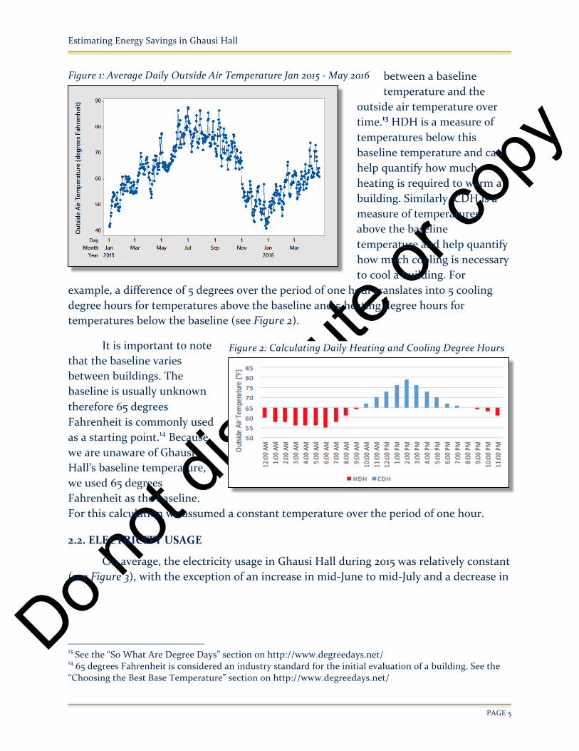
The time series plot11 of outside air temperature shows high seasonality12 as expected (see Figure 1). In order to study the effects of the outside air temperature on building energy use, we calculated two variables: heating degree hours (HDH) and cooling degree hours (CDH). Each variable is defined as the integral of the difference
6 UC Davis Campus Energy Education Dashboard (CEED) http://ceed.ucdavis.edu/ 7 To calculate daily energy consumption we used the difference between meter readings at 12:00 am. 8 The kilowatt-hour (kWh) is an International System of Units (SI) derived unit used to measure energy. It is used by utilities for electricity billing and is defined as delivering 1,000 watts of power for one hour. 9 The ton-hour is a measure of refrigeration energy that is approximately equal to 3.5 kWh. 10 The British Thermal Unit (BTU) is a traditional unit of energy defined as the amount of energy required to raise the temperature of 1 pound of water by 1 degree Fahrenheit. 11 A time series is a continuous set of observations that are ordered in equally spaced intervals (DeLurgio, 1998, p. 13). 12 Seasonality refers to cycles that occur over short repetitive calendar periods and, by definition, have a duration of less than 1 year (Keller, 2014, p. 832).
Do not
distrib
ute or
copy
Estimating Energy Savings in Ghausi Hall
PAGE 5
between a baseline temperature and the
outside air temperature over time.13 HDH is a measure of temperatures below this baseline temperature and can help quantify how much heating is required to warm a building. Similarly, CDH is a measure of temperatures above the baseline temperature and help quantify how much cooling is necessary to cool a building. For
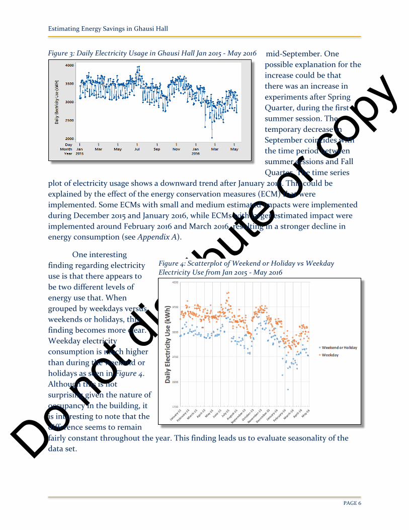
example, a difference of 5 degrees over the period of one hour translates into 5 cooling degree hours for temperatures above the baseline and 5 heating degree hours for temperatures below the baseline (see Figure 2).
It is important to note that the baseline varies between buildings. The baseline is usually unknown therefore 65 degrees Fahrenheit is commonly used as a starting point.14 Because we are unaware of Ghausi Hall’s baseline temperature, we used 65 degrees Fahrenheit as the baseline. For this calculation we assumed a constant temperature over the period of one hour.
2.2. ELECTRICITY USAGE
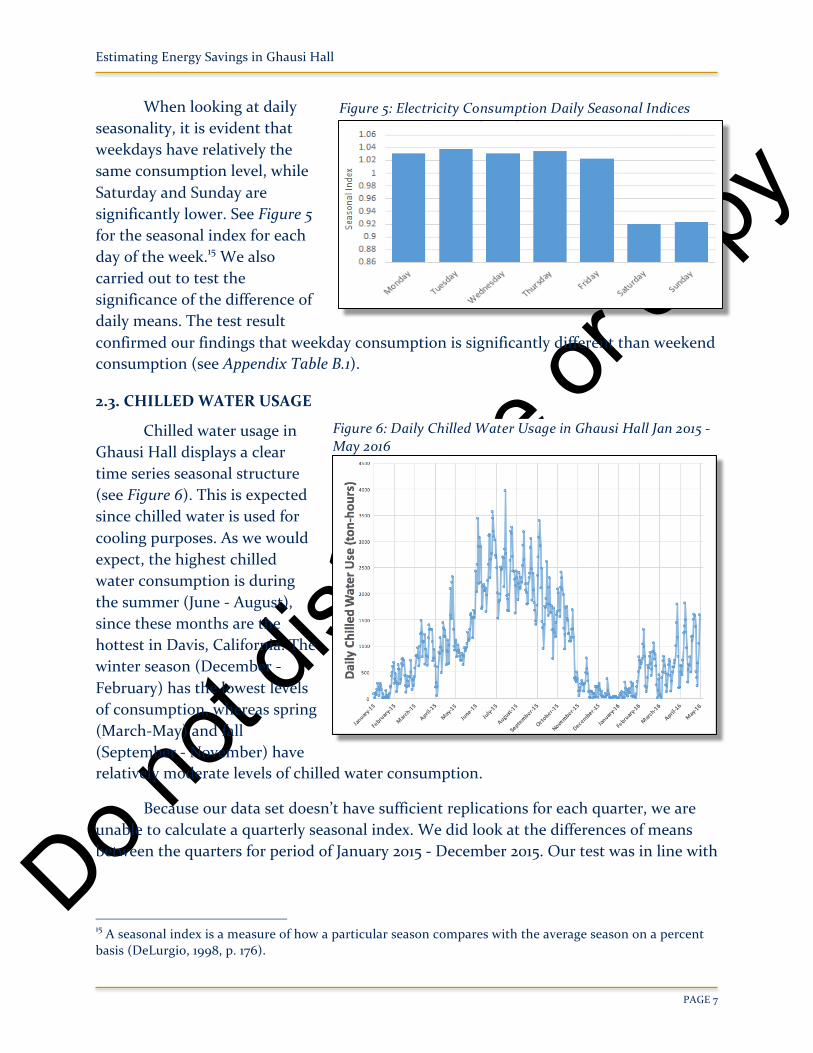
On average, the electricity usage in Ghausi Hall during 2015 was relatively constant (see Figure 3), with the exception of an increase in mid-June to mid-July and a decrease in
13 See the “So What Are Degree Days” section on http://www.degreedays.net/ 14 65 degrees Fahrenheit is considered an industry standard for the initial evaluation of a building. See the “Choosing the Best Base Temperature” section on http://www.degreedays.net/
Figure 2: Calculating Daily Heating and Cooling Degree Hours
Figure 1: Average Daily Outside Air Temperature Jan 2015 - May 2016
Do not
distrib
ute or
copy
Estimating Energy Savings in Ghausi Hall
PAGE 6
mid-September. One possible explanation for the increase could be that there was an increase in experiments after Spring Quarter, during the first summer session. The temporary decrease in September coincides with the time period between summer sessions and Fall Quarter. The time series
plot of electricity usage shows a downward trend after January 2016. This could be explained by the effect of the energy conservation measures (ECM) that were implemented. Some ECMs with small and medium estimated impacts were implemented during December 2015 and January 2016, while ECMs with larger estimated impact were implemented around February 2016 and March 2016, resulting in a stronger decline in energy consumption (see Appendix A).
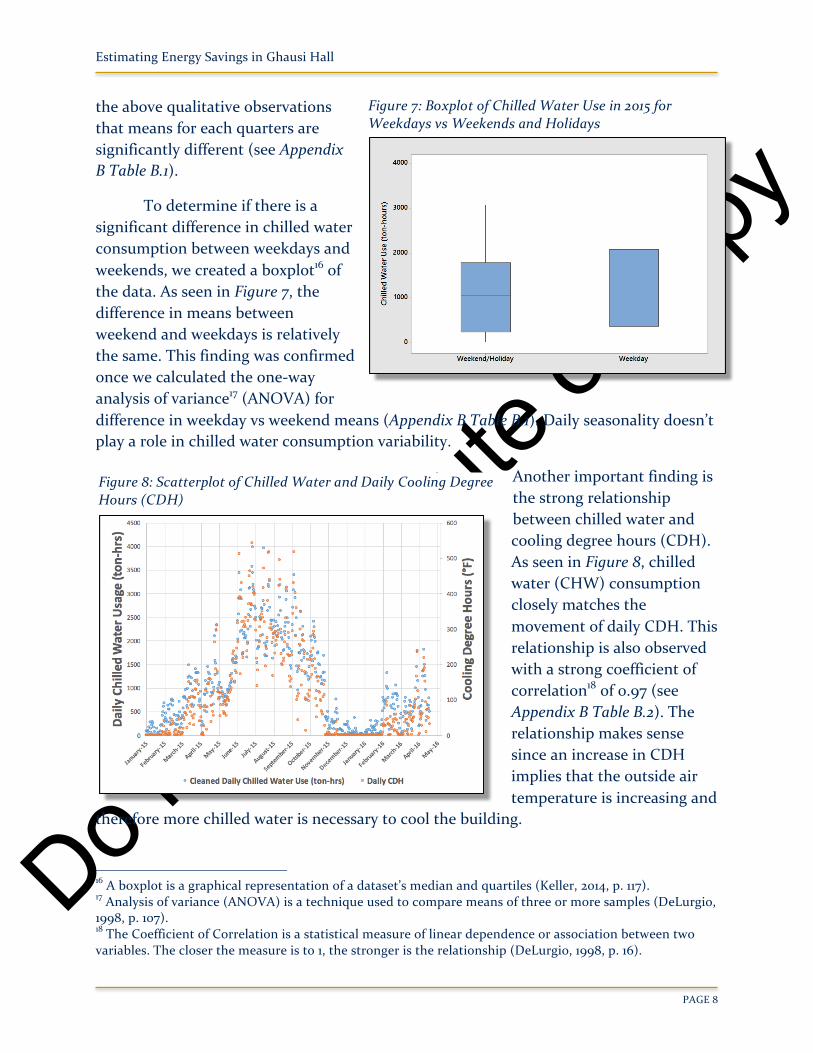
One interesting finding regarding electricity use is that there appears to be two different levels of energy use that. When grouped by weekdays versus weekends or holidays, this finding becomes more clear. Weekday electricity consumption is much higher than during the weekend or holidays as seen in Figure 4. Although this is not surprising given the nature of occupancy in the building, it is interesting to note that the difference seems to remain fairly constant throughout the year. This finding leads us to evaluate seasonality of the data set.
Figure 4: Scatterplot of Weekend or Holiday vs WeekdayElectricity Use from Jan 2015 - May 2016
Figure 3: Daily Electricity Usage in Ghausi Hall Jan 2015 - May 2016
Do not
distrib
ute or
copy
Estimating Energy Savings in Ghausi Hall
PAGE 7
When looking at daily seasonality, it is evident that weekdays have relatively the same consumption level, while Saturday and Sunday are significantly lower. See Figure 5 for the seasonal index for each day of the week.15 We also carried out to test the significance of the difference of daily means. The test result confirmed our findings that weekday consumption is significantly different than weekend consumption (see Appendix Table B.1).
2.3. CHILLED WATER USAGE
Chilled water usage in Ghausi Hall displays a clear time series seasonal structure (see Figure 6). This is expected since chilled water is used for cooling purposes. As we would expect, the highest chilled water consumption is during the summer (June - August), since these months are the hottest in Davis, California. The winter season (December - February) has the lowest levels of consumption, whereas spring (March-May) and fall (September - November) have relatively moderate levels of chilled water consumption.
Because our data set doesn’t have sufficient replications for each quarter, we are unable to calculate a quarterly seasonal index. We did look at the differences of means between the quarters for period of January 2015 - December 2015. Our test was in line with
15 A seasonal index is a measure of how a particular season compares with the average season on a percent basis (DeLurgio, 1998, p. 176).
Figure 5: Electricity Consumption Daily Seasonal Indices
Figure 6: Daily Chilled Water Usage in Ghausi Hall Jan 2015 - May 2016
Do not
distrib
ute or
copy
Estimating Energy Savings in Ghausi Hall
PAGE 8
the above qualitative observations that means for each quarters are significantly different (see Appendix B Table B.1).
To determine if there is a significant difference in chilled water consumption between weekdays and weekends, we created a boxplot16 of the data. As seen in Figure 7, the difference in means between weekend and weekdays is relatively the same. This finding was confirmed once we calculated the one-way analysis of variance17 (ANOVA) for difference in weekday vs weekend means (Appendix B Table B.1). Daily seasonality doesn’t play a role in chilled water consumption variability.
Another important finding is the strong relationship between chilled water and cooling degree hours (CDH). As seen in Figure 8, chilled water (CHW) consumption closely matches the movement of daily CDH. This relationship is also observed with a strong coefficient of correlation18 of 0.97 (see Appendix B Table B.2). The relationship makes sense since an increase in CDH implies that the outside air temperature is increasing and
therefore more chilled water is necessary to cool the building.
16 A boxplot is a graphical representation of a dataset’s median and quartiles (Keller, 2014, p. 117). 17 Analysis of variance (ANOVA) is a technique used to compare means of three or more samples (DeLurgio, 1998, p. 107). 18 The Coefficient of Correlation is a statistical measure of linear dependence or association between two variables. The closer the measure is to 1, the stronger is the relationship (DeLurgio, 1998, p. 16).
Figure 8: Scatterplot of Chilled Water and Daily Cooling Degree Hours (CDH)
Figure 7: Boxplot of Chilled Water Use in 2015 for Weekdays vs Weekends and Holidays
Do not
distrib
ute or
copy
Estimating Energy Savings in Ghausi Hall
PAGE 9
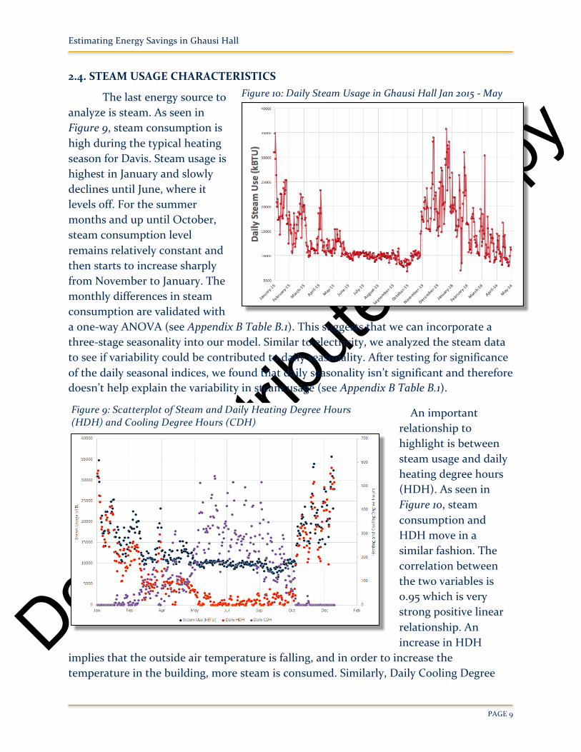
2.4. STEAM USAGE CHARACTERISTICS
The last energy source to analyze is steam. As seen in Figure 9, steam consumption is high during the typical heating season for Davis. Steam usage is highest in January and slowly declines until June, where it levels off. For the summer months and up until October, steam consumption level remains relatively constant and then starts to increase sharply from November to January. The monthly differences in steam consumption are validated with a one-way ANOVA (see Appendix B Table B.1). This suggests that we can incorporate a three-stage seasonality into our model. Similar to electricity, we analyzed the steam data to see if variability could be contributed to daily seasonality. After testing for significance of the daily seasonal indices, we found that daily seasonality isn’t significant and therefore doesn’t help explain the variability in steam usage (see Appendix B Table B.1).
An important relationship to highlight is between steam usage and daily heating degree hours (HDH). As seen in Figure 10, steam consumption and HDH move in a similar fashion. The correlation between the two variables is 0.95 which is very strong positive linear relationship. An increase in HDH
implies that the outside air temperature is falling, and in order to increase the temperature in the building, more steam is consumed. Similarly, Daily Cooling Degree
Figure 9: Scatterplot of Steam and Daily Heating Degree Hours (HDH) and Cooling Degree Hours (CDH)
Figure 10: Daily Steam Usage in Ghausi Hall Jan 2015 - May 2016
Do not
distrib
ute or
copy
Estimating Energy Savings in Ghausi Hall
PAGE 10
Hours (CDH) is negatively correlated with daily steam usage. CDH refers to cooling and steam is not used for cooling. Therefore, when there is a high CDH, we observe a low steam usage. Also, we do see that there is daily steam usage over the summer, even when there is high CDH and almost no HDH. This is because that steam is also used to heat water in Ghausi Hall.
After providing an overview of the characteristics of our data set, we proceed by developing models to forecast electricity, steam, and chilled water consumption for 2016 and estimating the cost savings from the energy conservation measures.
3. Model Selection, Forecasts, and Interpretations
3.1. ELECTRICITY MODEL
3.1.1. Electricity Model Selection
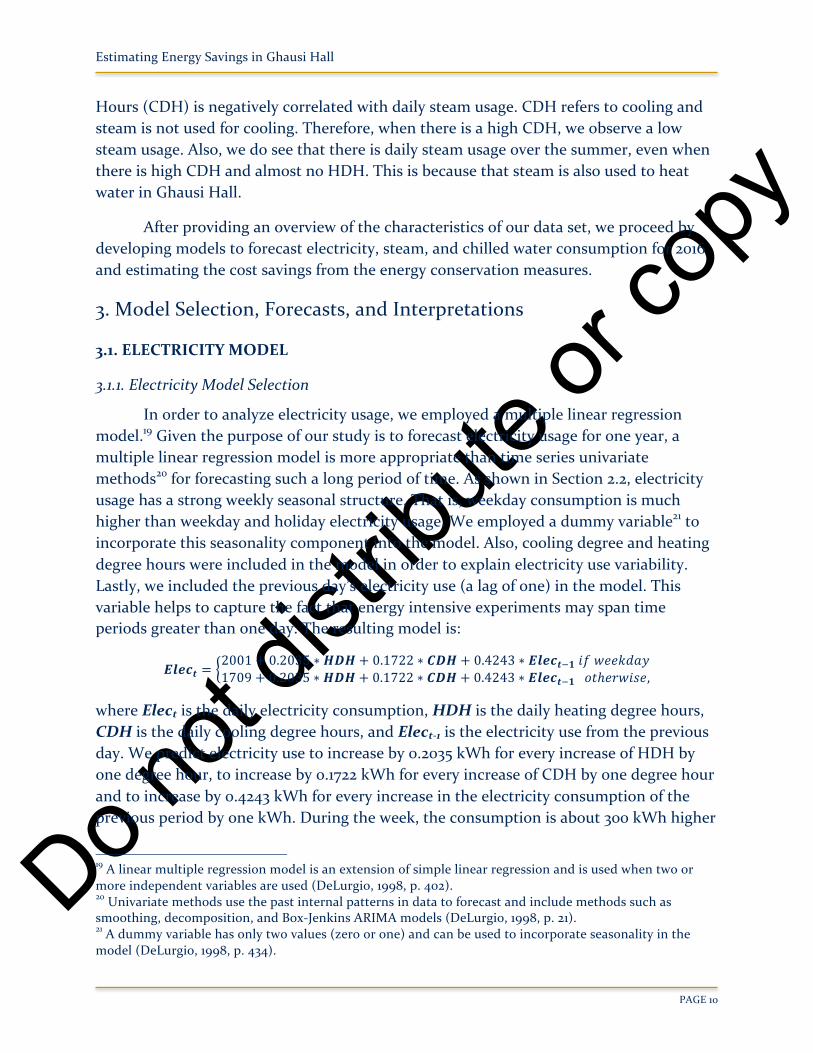
In order to analyze electricity usage, we employed a multiple linear regression model.19 Given the purpose of our study is to forecast electricity usage for one year, a multiple linear regression model is more appropriate than time series univariate methods20 for forecasting such a long period of time. As shown in Section 2.2, electricity usage has a strong weekly seasonal structure. That is, weekday consumption is much higher than weekday and holiday electricity usage. We employed a dummy variable21 to incorporate this seasonality component into the model. Also, cooling degree and heating degree hours were included in the model in order to explain electricity use variability. Lastly, we included the previous day’s electricity use (a lag of one) in the model. This variable helps to capture the fact that energy intensive experiments may span time periods greater than one day. The resulting model is:
𝑬𝒍𝒆𝒄𝒕 =2001 + 0.2035 ∗ 𝑯𝑫𝑯 + 0.1722 ∗ 𝑪𝑫𝑯 + 0.4243 ∗ 𝑬𝒍𝒆𝒄𝒕4𝟏𝑖𝑓𝑤𝑒𝑒𝑘𝑑𝑎𝑦1709 + 0.2035 ∗ 𝑯𝑫𝑯 + 0.1722 ∗ 𝑪𝑫𝑯 + 0.4243 ∗ 𝑬𝒍𝒆𝒄𝒕4𝟏𝑜𝑡ℎ𝑒𝑟𝑤𝑖𝑠𝑒,
where Elect is the daily electricity consumption, HDH is the daily heating degree hours, CDH is the daily cooling degree hours, and Elect-1 is the electricity use from the previous day. We predict electricity use to increase by 0.2035 kWh for every increase of HDH by one degree hour, to increase by 0.1722 kWh for every increase of CDH by one degree hour and to increase by 0.4243 kWh for every increase in the electricity consumption of the previous period by one kWh. During the week, the consumption is about 300 kWh higher
19 A linear multiple regression model is an extension of simple linear regression and is used when two or more independent variables are used (DeLurgio, 1998, p. 402). 20 Univariate methods use the past internal patterns in data to forecast and include methods such as smoothing, decomposition, and Box-Jenkins ARIMA models (DeLurgio, 1998, p. 21). 21 A dummy variable has only two values (zero or one) and can be used to incorporate seasonality in the model (DeLurgio, 1998, p. 434).
Do not
distrib
ute or
copy
Estimating Energy Savings in Ghausi Hall
PAGE 11
than on weekends or holidays, holding all other variables constant. Overall, the model helps explain over 70 percent of the variability in electricity use (see Appendix C Table C.1).
In order to validate the fit of the model as well its forecasting ability, we performed fitting and internal forecasting analysis by using the first 11 months of data and forecasting for the following month (see Appendix C Table C.2). On average, the model forecasts were within five percent difference from the actual observed electricity usage. Therefore, we conclude that our model has a fairly accurate forecasting ability (see Appendix C Figure C.1).
The multiple linear regression model has underlying assumptions of normality, linearity, constant variance, and others. We performed various qualitative and quantitative tests to verify the validity of these assumptions. All of the assumptions hold in the model, except autocorrelation.22
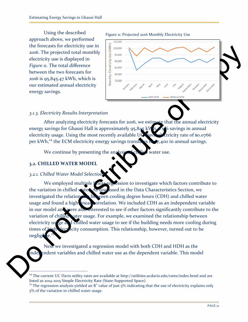
3.1.2. Electricity Forecasts
Given that we want to analyze the impact of the ECMs, we need to create two models for each energy source: one to estimate what energy use would have been in 2016 if the ECMs had not been implemented and one to estimate what energy use will be in 2016 with the ECMs. The model described in the previous section uses data from 2015 and can be used to forecast what energy consumption levels would have been had the ECMs were not implemented. By using the energy consumption data for January 2016 to May 2016 and comparing it with our forecasted values without ECM updates, we calculated an average percent savings. We applied this average savings rate for our forecasted consumption levels with ECM updates for May 2016 to December 2016. In order to estimate the CDH and HDH for May to December 2016, we referenced historical monthly averages for HDH and CDH.23 Finally, we compared the forecasted values of the two models to calculate the impact of the ECMs.
22 Autocorrelation occurs when the value of a series in one time period is related to the value of itself in previous period. The introduction of the previous day’s electricity use variable in the model decreases the autocorrelation problem, but does not resolve the problem completely. See Appendix C Table C.3 for more details. 23 The website http://www.degreedays.net/ calculates average monthly HDH and CDH using the last five years of weather data. We used the weather data from Sacramento Executive Airport as the closest, most reliable data source that is readily available.
Do not
distrib
ute or
copy
Estimating Energy Savings in Ghausi Hall
PAGE 12
Using the described approach above, we performed the forecasts for electricity use in 2016. The projected total monthly electricity use is displayed in Figure 11. The total difference between the two forecasts for 2016 is 95,845.47 kWh, which is our estimated annual electricity energy savings.
3.1.3. Electricity Results Interpretation
After analyzing electricity forecasts for 2016, we estimate that the annual electricity energy savings for Ghausi Hall is approximately 95,845 kWh, a 9% savings in annual electricity usage. Using the most recently available UC Davis electricity rate of $0.0766 per kWh,24 the ECM electricity energy savings translates to $7,400 in annual savings.
We continue by presenting the analysis of chilled water use.
3.2. CHILLED WATER MODEL
3.2.1. Chilled Water Model Selection
We employed multiple linear regression to investigate which factors contribute to the variation in chilled water. As discussed in the Data Characteristics Section, we investigated the relationship between cooling degree hours (CDH) and chilled water usage and found a high linear correlation. We included CDH as an independent variable in our model and were also interested to see if other factors significantly contribute to the variation of chilled water usage. For example, we examined the relationship between electricity usage and chilled water usage to see if the building needs more cooling during times of high electricity consumption. This relationship, however, turned out to be negligible.25
Next we investigated a regression model with both CDH and HDH as the independent variables and chilled water use as the dependent variable. This model
24 The current UC Davis utility rates are available at http://utilities.ucdavis.edu/rates/index.html and are listed as 2014-2015 Simple Electricity Rate (State-Supported Space). 25 The regression analysis yielded an R2 value of just 5% indicating that the use of electricity explains only 5% of the variation in chilled water usage.
Figure 11: Projected 2016 Monthly Electricity Use
Do not
distrib
ute or
copy
Estimating Energy Savings in Ghausi Hall
PAGE 13
yielded an adjusted-R2 value26 of 97% which initially suggested the model was a good fit. We discovered however, that this model produced negative values for chilled water use during cold seasons, an outcome we consider not to be meaningful. We therefore removed heating degree hours from the model and continued investigating the regression model with CDH as the only independent variable.
𝑪𝒉𝒊𝒍𝒍𝒆𝒅𝑾𝒂𝒕𝒆𝒓 = 321.2 + 6.5870 ∗ 𝑫𝒂𝒊𝒍𝒚𝑪𝑫𝑯,
where Chilled Water is daily chilled water consumption measured in ton-hours and Daily CDH is daily cooling degree hours measured in degree Fahrenheit. The model can be interpreted as follows: for a one degree Fahrenheit increase in daily CDH, we predict the chilled water use to increase by 6.5870 ton-hours. This model still explains 94% of the variation in the use of chilled water and fits the data well.27 However, we found the model has large error measures.28 We attribute these larger error measures to the high variation of the chilled water usage data. Part of this variation could be explained through the varying intensity of direct sunshine, Ghausi Hall receives. We expect solar irradiation to add significantly to the amount of cooling needed.
The scatter plot of CDH versus chilled water use shows an interesting pattern for the cold seasons from November through March (see Figure 8 above). With the baseline temperature of 65 degrees Fahrenheit, there are zero daily CDH for this time period. However, the actual usage data of chilled water shows that the building in fact had been cooled during this period. This suggests, that we could adjust the baseline temperature and re-evaluate the model fit with the new daily CDH values.
As with our model for electricity use, the model assumptions for chilled water are met except for a high autocorrelation of the data. As a result, created a model which included time as a second independent variable, however, the R2 value did not improve significantly.29 Additionally, this did not solve the problem with autocorrelation. For the sake of simplicity, we continued our analysis with the simpler model.
3.2.2. Chilled Water Forecasts
As with electricity, we forecasted what the chilled water use would have been for January to May 2016 had no ECMs been implemented. We took the difference between the forecasted values and the actual values for these months and calculated the average
26 The adjusted R2 is the coefficient of determination adjusted for degrees of freedom. It explains the amount of variance in the dependent variable that can be explained by the included independent variables (Keller, 2014, p. 692). 27 See Appendix D Table D.1 and Figure D.1. 28 See Appendix D Table D.2 for further reference. 29 The alternative model yielded an adjusted R2 value of 97% compared to 94% for the model without time.
Do not
distrib
ute or
copy
Estimating Energy Savings in Ghausi Hall
PAGE 14
savings.30 In the next step, we took the model and forecasted what the chilled water usage for the rest of the year would have been, had no ECM been implemented. We then subtracted the savings and obtained the forecast for the chilled water use for the rest of the year, including the already implemented ECM.
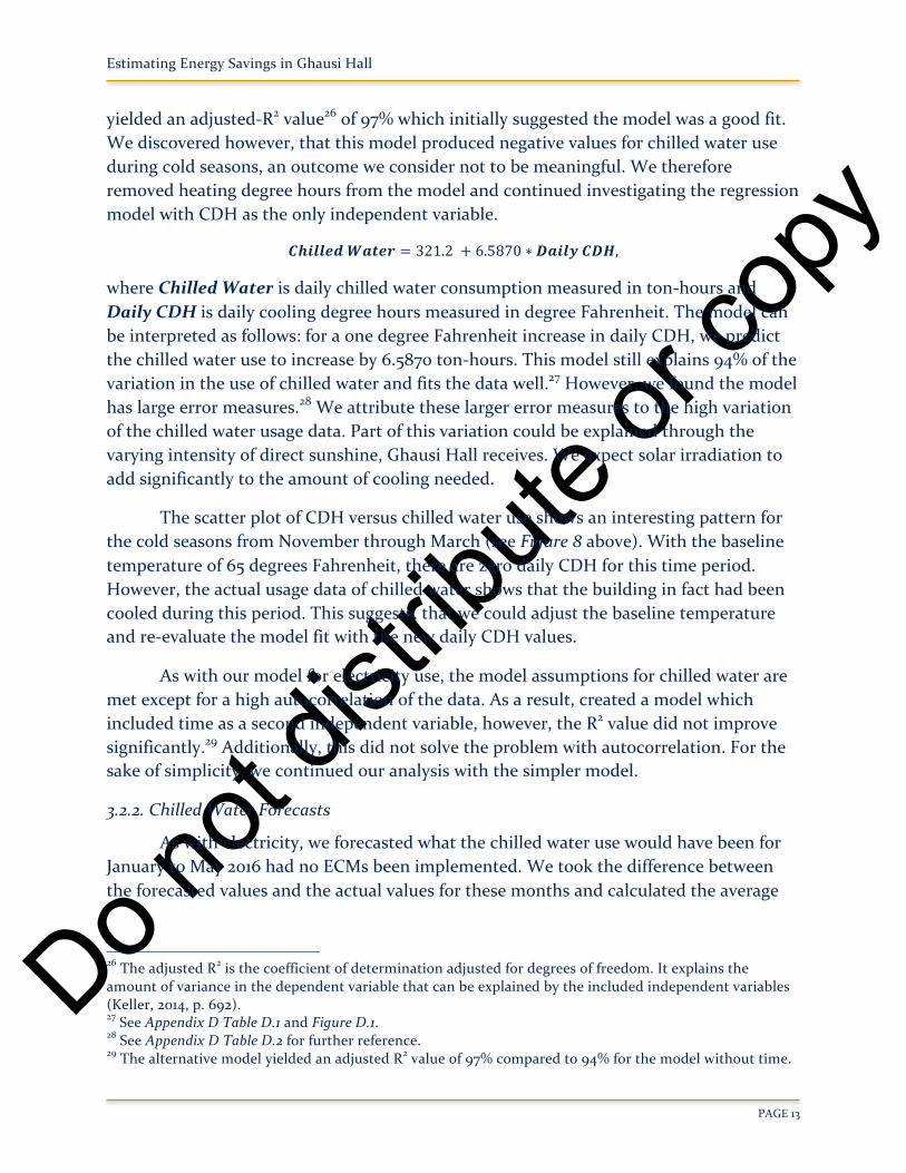
Figure 12 depicts the actual and predicted chilled water use for 2016. From January to May 2016, we used the actual daily CDH to forecast the chilled water use without ECM. For the rest of the year, we used historical monthly average daily CDH (hence the stepped function).
3.2.3. Chilled Water Results Interpretation
Our predicted chilled water energy savings over the year 2016 is 13,828 ton-hours. Assuming a price of $0.0965 per ton-hour31 this leads to an estimated annual savings of $1,322 for 2016. Interestingly, these savings are the smallest savings among the three energy categories, both in terms of percentage savings as well as in terms of absolute dollar amounts. The relatively low percentage of energy savings might suggest that there is still room for further improvement in reducing chilled water use in Ghausi Hall.
We will continue our analysis by looking into the model selection process for steam usage.
3.3. STEAM MODEL
3.3.1. Steam Model Selection
In order to estimate the effectiveness of steam reduction for Ghausi Hall after implementing the ECMs, we must first determine the appropriate model for the forecasting. We employed a multiple linear regression analysis using a logarithmic
30 The average monthly chilled water savings for our model is 3.77%. 31 The current UC Davis utility rates are 2014-2015 Simple Chilled Water Rate (State-Supported Space).
Figure 12: Actual and Forecasted Daily Chilled Water Use in Ghausi Hall for 2016
Do not
distrib
ute or
copy
Estimating Energy Savings in Ghausi Hall
PAGE 15
transformation32 of the dependent variable (daily steam usage for Ghausi Hall) and several explanatory independent variables:
𝐿𝑜𝑔10 𝑺𝒕𝒆𝒂𝒎 = 3.94349 + 0.001037 ∗ 𝑫𝒂𝒊𝒍𝒚𝑯𝑫𝑯 + 0.03720 ∗ (𝑱𝒂𝒏𝒕𝒐𝑨𝒑𝒓𝒊𝒍) + 0.04181 ∗ (𝑴𝒂𝒚𝒕𝒐𝑨𝒖𝒈),
where Log10(Steam) is the log base 10 transformed daily steam usage in kBTU, Daily HDH is the daily heating degree hours in degrees Fahrenheit, Jan to April is the dummy variable for the months from January to April, and May to Aug is the dummy variable for the months from May to August. The baseline for the dummy variable is September to December (see Appendix E Table E.1 for the details of the regression analysis). Daily steam usage and daily HDH have high correlation of 0.95.
As seen in Figure 9 above, we do observe a difference in usage of steam due to seasonality, therefore, we incorporate seasonality dummy variables. This model has a coefficient of determination adjusted for degrees of freedom (adjusted R2) greater than 90 percent and a very low Mean Square Error (MSE).33 After performing all of the tests, we conclude that the regression model assumptions were not violated (see Appendix E Table E.4). We conclude that the model does a good job explaining the variation in steamusage.
The next section applies this model to forecast steam usage in Ghausi Hall for 2016.
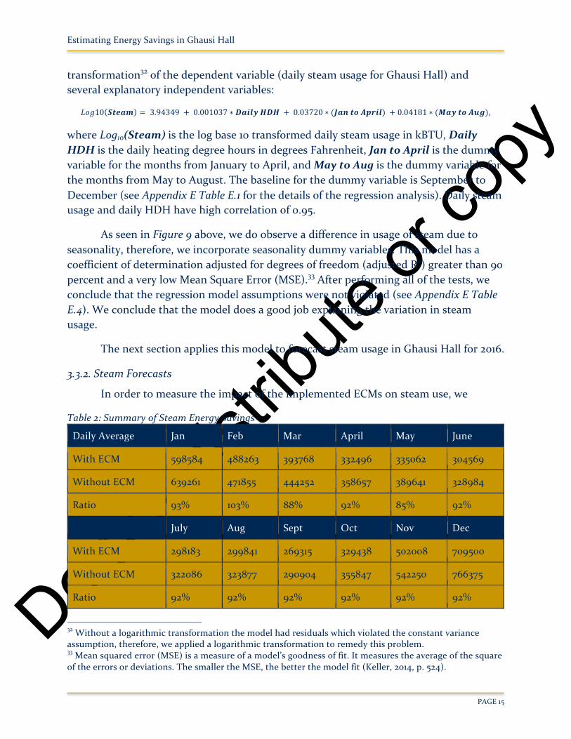
3.3.2. Steam Forecasts
In order to measure the impact of the implemented ECMs on steam use, we
Table 2: Summary of Steam Energy Savings
Daily Average Jan Feb Mar April May June
With ECM 598584 488263 393768 332496 335062 304569
Without ECM 639261 471855 444252 358657 389641 328984
Ratio 93% 103% 88% 92% 85% 92%
July Aug Sept Oct Nov Dec
With ECM 298183 299841 269315 329438 502008 709500
Without ECM 322086 323877 290904 355847 542250 766375
Ratio 92% 92% 92% 92% 92% 92%
32 Without a logarithmic transformation the model had residuals which violated the constant variance assumption, therefore, we applied a logarithmic transformation to remedy this problem. 33 Mean squared error (MSE) is a measure of a model’s goodness of fit. It measures the average of the square of the errors or deviations. The smaller the MSE, the better the model fit (Keller, 2014, p. 524).
Do not
distrib
ute or
copy
Estimating Energy Savings in Ghausi Hall
PAGE 16
forecasted what the steam use would have been for January to May 2016 had no ECMs been implemented. We took the difference between the forecasted values and the actual values for these months and calculated the average savings. Next we took the model and forecasted what the steam usage for the rest of the year would have been, had no ECM been implemented. We then subtracted the savings and obtained the forecast for the steam use for the rest of the year, including the already implemented ECM.
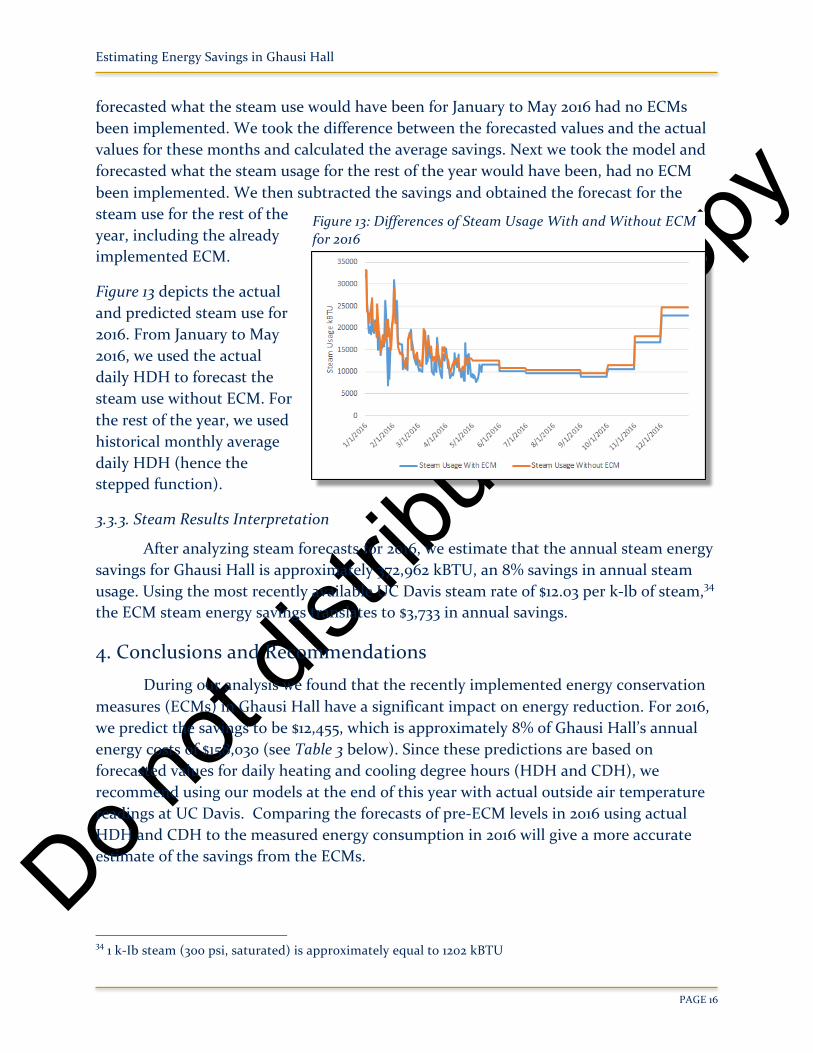
Figure 13 depicts the actual and predicted steam use for 2016. From January to May 2016, we used the actual daily HDH to forecast the steam use without ECM. For the rest of the year, we used historical monthly average daily HDH (hence the stepped function).
3.3.3. Steam Results Interpretation
After analyzing steam forecasts for 2016, we estimate that the annual steam energy savings for Ghausi Hall is approximately 372,962 kBTU, an 8% savings in annual steam usage. Using the most recently available UC Davis steam rate of $12.03 per k-lb of steam,34 the ECM steam energy savings translates to $3,733 in annual savings.
4. Conclusions and Recommendations
During our analysis we found that the recently implemented energy conservation measures (ECMs) in Ghausi Hall have a significant impact on energy reduction. For 2016, we predict the savings to be $12,455, which is approximately 8% of Ghausi Hall’s annual energy costs of $158,030 (see Table 3 below). Since these predictions are based on forecasted values for daily heating and cooling degree hours (HDH and CDH), we recommend using our models at the end of this year with actual outside air temperature readings at UC Davis. Comparing the forecasts of pre-ECM levels in 2016 using actual HDH and CDH to the measured energy consumption in 2016 will give a more accurate estimate of the savings from the ECMs.
34 1 k-Ib steam (300 psi, saturated) is approximately equal to 1202 kBTU
Figure 13: Differences of Steam Usage With and Without ECMfor 2016
Do not
distrib
ute or
copy
Estimating Energy Savings in Ghausi Hall
PAGE 17
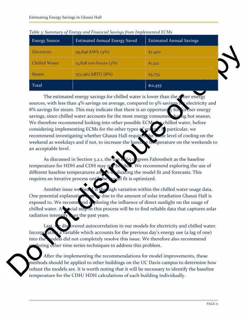
Table 3: Summary of Energy and Financial Savings from Implemented ECMs
Energy Source Estimated Annual Energy Saved Estimated Annual Savings
Electricity 95,846 kWh (9%) $7,400
Chilled Water 13,828 ton-hours (3%) $1,322
Steam 372,962 kBTU (8%) $3,733
Total $12,455
The estimated energy savings for chilled water is lower than the other energy sources, with less than 4% savings on average, compared to 9% savings for electricity and 8% savings for steam. This may indicate that there is an opportunity for further energy savings, since chilled water accounts for the most energy consumed during hot season. We therefore recommend looking into other possible ECMs for chilled water, before considering implementing ECMs for the other types of energy. In particular, we recommend investigating whether Ghausi Hall requires the same level of cooling on the weekend as weekdays and if not, to increase the baseline temperature on the weekends to an acceptable level.
As discussed in Section 3.2.1, the use of 65 degrees Fahrenheit as the baseline temperature for HDH and CDH may not be ideal. We recommend exploring the use of different baseline temperatures and re-evaluating the model fit and forecasts. This requires an iterative process until the model fit is optimized.
Another issue we found is the high variation within the chilled water usage data. One potential explanation may be due to the amount of solar irradiation Ghausi Hall is exposed to. We recommend exploring the influence of direct sunlight on the usage of chilled water. A crucial step in this process will be to find reliable data that captures solar radiation intensity over the past years.
Last, we discovered autocorrelation in our models for electricity and chilled water. Incorporating a variable which accounts for the previous day’s energy use (a lag of one) into the models did not completely resolve this issue. We therefore also recommend exploring other time series techniques to address this problem.
After the implementing the recommendations for model improvements, these methods should be applied to other buildings on the UC Davis campus to determine how robust the models are. It is worth noting that it will be necessary to identify the baseline temperature for the CDH/ HDH calculations of each building individually.
Do not
distrib
ute or
copy
Estimating Energy Savings in Ghausi Hall
PAGE 18
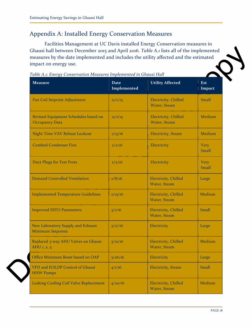
Appendix A: Installed Energy Conservation Measures Facilities Management at UC Davis installed Energy Conservation measures in
Ghausi hall between December 2015 and April 2016. Table A.1 lists all of the implemented measures by the date implemented and includes the utility affected and the estimated impact on energy use.
Table A.1: Energy Conservation Measures Implemented in Ghausi Hall
Measure Date Implemented
Utility Affected Est Impact
Fan Coil Setpoint Adjustment 12/1/15 Electricity, Chilled Water, Steam
Small
Revised Equipment Schedules based on Occupancy Data
12/1/15 Electricity, Chilled Water, Steam
Medium
Night Time VAV Reheat Lockout 1/13/16 Electricity, Steam Medium
Combed Condenser Fins 2/2/16 Electricity Very Small
Duct Plugs for Test Ports 2/2/16 Electricity Very Small
Demand Controlled Ventilation 2/8/16 Electricity, Chilled Water, Steam
Large
Implemented Temperature Guidelines 2/15/16 Electricity, Chilled Water, Steam
Medium
Improved SSTO Parameters 3/1/16 Electricity, Chilled Water, Steam
Small
New Laboratory Supply and Exhaust Minimum Setpoints
3/17/16 Electricity Large
Replaced 3-way AHU Valves on Ghausi AHU 1, 2, 5
3/21/16 Electricity, Chilled Water, Steam
Medium
Office Minimum Reset based on OAP 3/26/16 Electricity Large
VFD and EOLDP Control of Ghausi HHW Pumps
4/1/16 Electricity, Steam Small
Leaking Cooling Coil Valve Replacement 4/20/16 Electricity, Chilled Water, Steam
Medium
Do not
distrib
ute or
copy
Estimating Energy Savings in Ghausi Hall
PAGE 19
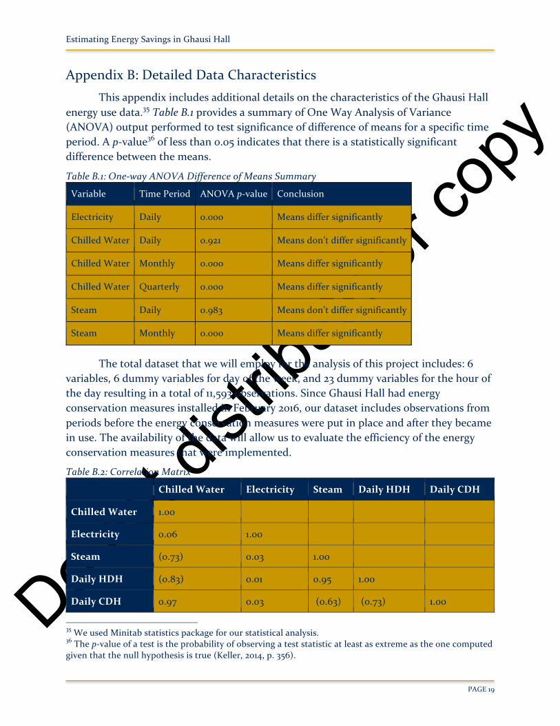
Appendix B: Detailed Data Characteristics
This appendix includes additional details on the characteristics of the Ghausi Hall energy use data.35 Table B.1 provides a summary of One Way Analysis of Variance (ANOVA) output performed to test significance of difference of means for a specific time period. A p-value36 of less than 0.05 indicates that there is a statistically significant difference between the means.
Table B.1: One-way ANOVA Difference of Means Summary
Variable Time Period ANOVA p-value Conclusion
Electricity Daily 0.000 Means differ significantly
Chilled Water Daily 0.921 Means don’t differ significantly
Chilled Water Monthly 0.000 Means differ significantly
Chilled Water Quarterly 0.000 Means differ significantly
Steam Daily 0.983 Means don’t differ significantly
Steam Monthly 0.000 Means differ significantly
The total dataset that we will employ for the analysis of this project includes: 6 variables, 6 dummy variables for day of the week, and 23 dummy variables for the hour of the day resulting in a total of 11,593 observations. Since Ghausi Hall had energy conservation measures installed in February 2016, our dataset includes observations from periods before the energy conservation measures were put in place and after they became in use. The availability of the data will allow us to evaluate the efficiency of the energy conservation measures that were implemented.
Table B.2: Correlation Matrix
Chilled Water Electricity Steam Daily HDH Daily CDH
Chilled Water 1.00
Electricity 0.06 1.00
Steam (0.73) 0.03 1.00
Daily HDH (0.83) 0.01 0.95 1.00
Daily CDH 0.97 0.03 (0.63) (0.73) 1.00
35 We used Minitab statistics package for our statistical analysis. 36 The p-value of a test is the probability of observing a test statistic at least as extreme as the one computed given that the null hypothesis is true (Keller, 2014, p. 356).
Do not
distrib
ute or
copy
Estimating Energy Savings in Ghausi Hall
PAGE 20
Figure B.1 and Figure B.2 are boxplots of electricity use and chilled water use (respectively) that compare the weekday energy usage to the weekend or holiday energy usage.
Appendix C: Electricity Model Selection Details
This appendix contains the details for the electricity model, explores the fit of the model, and provides more information on the regression assumptions. Table C.1 summarizes the multiple regression model for electricity use.
Table C.1: Regression Analysis of Electricity Use
Term Coefficient T-Value p-Value VIF
Constant 1709 16.62 0.000
Daily HDH 0.2035 3.02 0.003 2.18
Daily CDH 0.1722 2.48 0.013 2.18
Weekday vs Weekend and Holiday Variable 292.4 19.92 0.000 1.09
Electricityt-1 0.4243 13.94 0.000 1.09
Model Summary S37 R2 Adjusted R2
124.978 69.48% 69.14%
37 S is the Standard Error of the Estimate and is a measure of model fit. S represents the average distance the observations are away from the fitted regression line (DeLurgio, 1998, p. 96).
Figure B.2: Boxplot of Electricity Use in 2015 for Weekdays vs Weekends and Holidays
Figure B.1: Boxplot of Chilled Water Use in 2015 for Weekdays vs Weekends and Holidays
Do not
distrib
ute or
copy
Estimating Energy Savings in Ghausi Hall
PAGE 21
Table C.2 shows the common error measures for the model-fitting process as well as for the internal forecast. Both categories show satisfying results.
Table C.2: Internal Forecasting Analysis for Electricity
Fitting Internal Forecast
MSE 14,429.17 40,691.77
MAD 94.33 174.92
MAPE 2.79% 5.43%
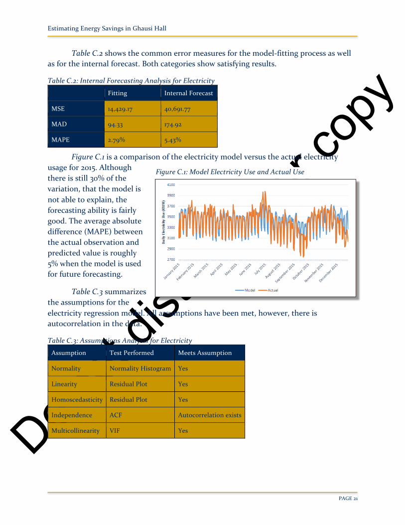
Figure C.1 is a comparison of the electricity model versus the actual electricity usage for 2015. Although there is still 30% of the variation, that the model is not able to explain, the forecasting ability is fairly good. The average absolute difference (MAPE) between the actual observation and predicted value is roughly 5% when the model is used for future forecasting.
Table C.3 summarizes the assumptions for the electricity regression model. All assumptions have been met, however, there is autocorrelation in the data.
Table C.3: Assumptions Analysis for Electricity
Assumption Test Performed Meets Assumption
Normality Normality Histogram Yes
Linearity Residual Plot Yes
Homoscedasticity Residual Plot Yes
Independence ACF Autocorrelation exists
Multicollinearity VIF Yes
Figure C.1: Model Electricity Use and Actual Use
Do not
distrib
ute or
copy
Estimating Energy Savings in Ghausi Hall
PAGE 22
Appendix D: Chilled Water Model Selection Details This appendix contains the details for the chilled water model, explores the fit of
the model, and provides more information on the regression assumptions. Table D.1 summarizes the simple linear regression model for chilled water usage. We used the data from 2015 to fit the model.
Table D.1: Regression analysis of chilled water
Term Coefficient T-Value p-Value VIF
Constant 321.2 19.72 0.000
Daily CDH 6.5870 78.81 0.000 1.00
Model Summary S R2 Adjusted R2
222.294 94.49% 94.48%
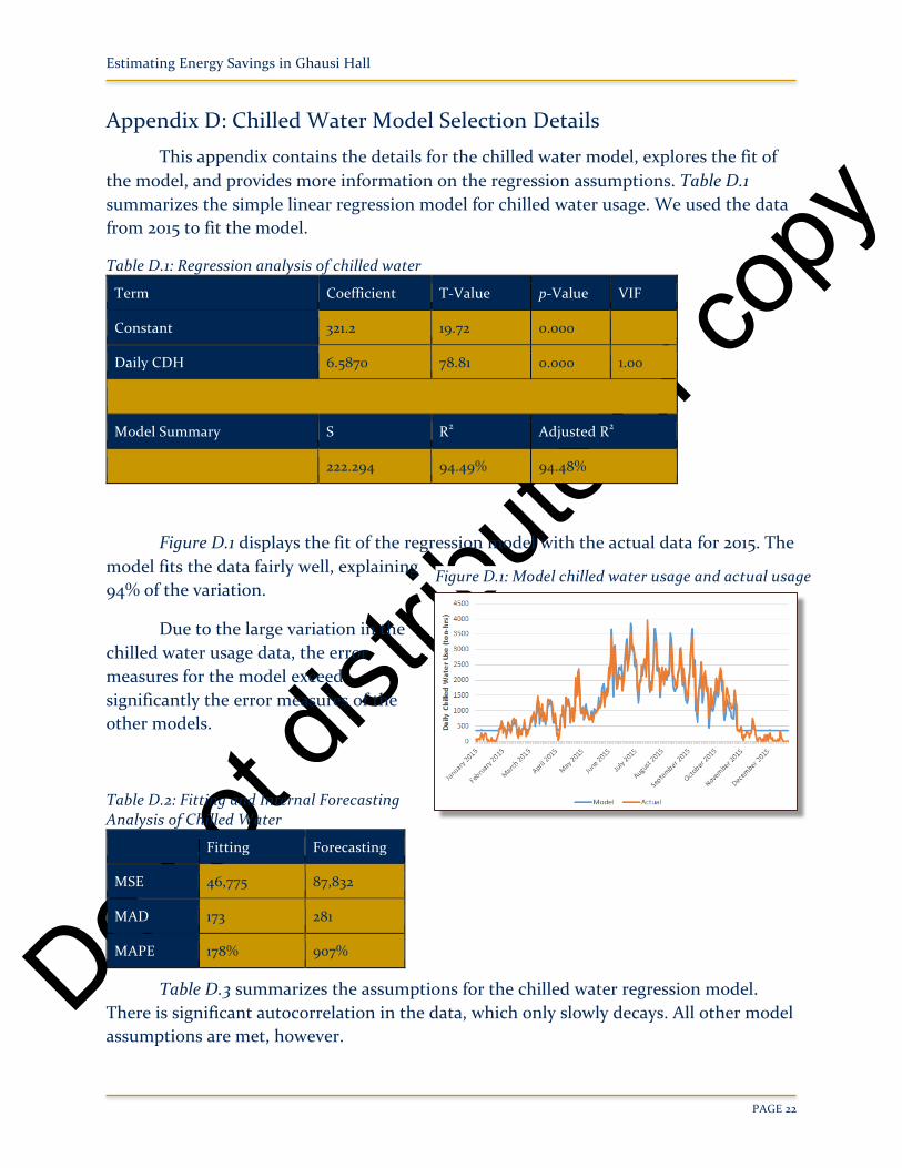
Figure D.1 displays the fit of the regression model with the actual data for 2015. The model fits the data fairly well, explaining 94% of the variation.
Due to the large variation in the chilled water usage data, the error measures for the model exceed significantly the error measures of the other models.
Table D.2: Fitting and Internal Forecasting Analysis of Chilled Water
Fitting Forecasting
MSE 46,775 87,832
MAD 173 281
MAPE 178% 907%
Table D.3 summarizes the assumptions for the chilled water regression model. There is significant autocorrelation in the data, which only slowly decays. All other model assumptions are met, however.
Figure D.1: Model chilled water usage and actual usage
Do not
distrib
ute or
copy
Estimating Energy Savings in Ghausi Hall
PAGE 23
Table D.3: Assumptions Analysis for Chilled Water
Assumption Test Performed Meets Assumption
Normality Normality Histogram Yes
Linearity Residual Plot Yes
Homoscedasticity Residual Plot Yes
Independence ACF Autocorrelation exists.
Multicollinearity VIF Yes
Appendix E: Steam Model Selection Details
This appendix contains the details for the steam model, explores the fit of the model, and provides more information on the regression assumptions. Table E.1 summarizes the regression model for steam.
Table E.1: Regression Analysis of Steam
Term Coefficient T-Value p-Value VIF
Constant 3.94330 72361 0.000
Daily HDH 0.001037 53.96 0.000 1.37
Jan to April 0.03782 6.46 0.000 1.34
May to Aug 0.04159 6.35 0.000 1.69
Model Summary S R2 Adjusted R2
0.04551 91.24% 91.17%
The independent attributes are all significant, with p-values less than a significance level of 0.0538. The VIF39 are less than 10, showing that independent variables are independent of each other. We removed CDH from our model as it becomes not significant with p-value larger than 0.05 and its multicollinearity issue with HDH. This model has a high R2 value of 91.24%. This indicates that 91.24% of variance of log(steam usage) can be explained by our model.
38 Significance level is the probability of rejecting the null hypothesis given that it is true (type I error). 39 The variance inflation factor (VIF) quantifies the severity of multicollinearity in an ordinary least squares regression analysis. Usually, attribute VIF larger than 10 indicates there is possible multicollinearity.
Do not
distrib
ute or
copy
Estimating Energy Savings in Ghausi Hall
PAGE 24
In terms of considering seasonality in our selected model, we conducted seasonality analysis. By comparing values of R2, MSE and MAPD, model with three stages components improves the model, we obtained a higher R2 and lower error measures (see Table E.2).
Table E.2: Steam Seasonality Analysis
R2 MSE MAPE
With Seasonality 91.24% 0.0109 0.852%
Without Seasonality 89.86% 0.0126 0.892%
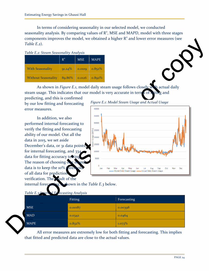
As shown in Figure E.1, model daily steam usage follows closely with actual daily steam usage. This indicates that our model is very accurate in terms of fitting and predicting, and this is confirmed by our low fitting and forecasting error measures.
In addition, we also performed internal forecasting to verify the fitting and forecasting ability of our model. Out all the data in 2015, we set aside December’s data, or 31 data points, for internal forecasting, and 334 data for fitting accuracy testing. The reason of choosing one month data is to keep the 10% threshold of all data for prediction verification. The result of the internal forecasting is shown in the Table E.3 below.
Table E.3:Internal Forecasting Analysis
Fitting Forecasting
MSE 0.00187 0.00398
MAD 0.0342 0.0464
MAPE 0.832% 1.073%
All error measures are extremely low for both fitting and forecasting. This implies that fitted and predicted data are close to the actual values.
Figure E.1: Model Steam Usage and Actual Usage
Do not
distrib
ute or
copy
Estimating Energy Savings in Ghausi Hall
PAGE 25
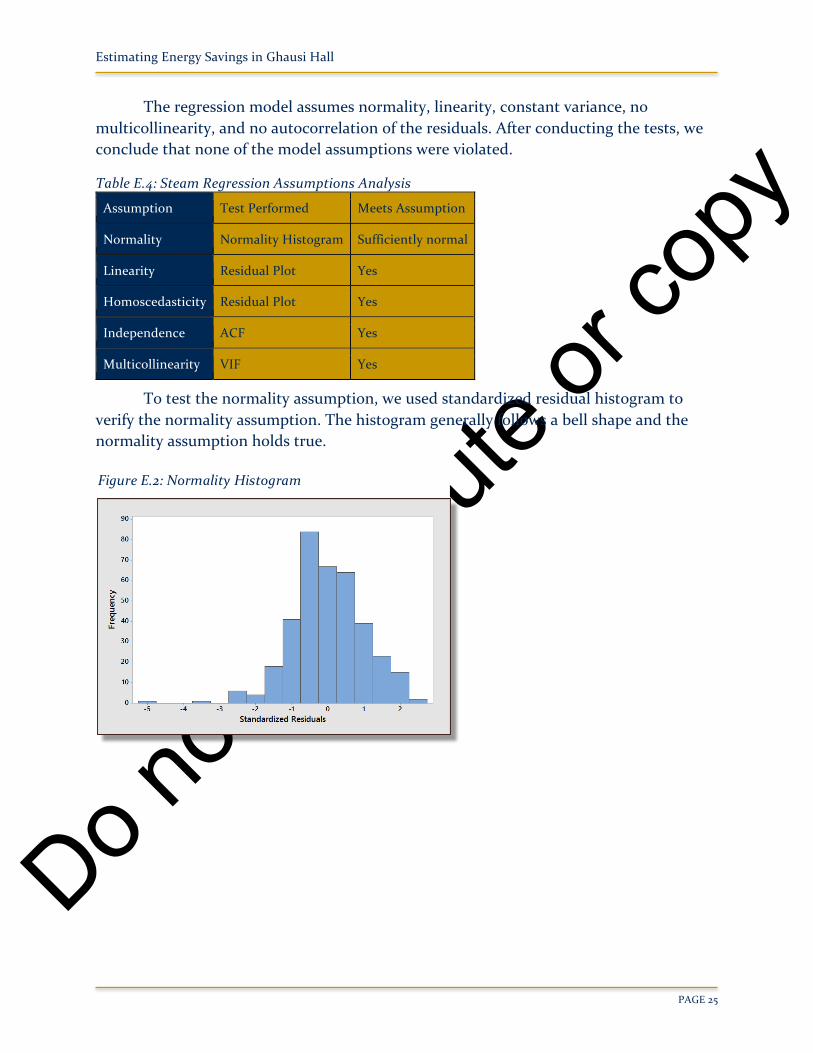
The regression model assumes normality, linearity, constant variance, no multicollinearity, and no autocorrelation of the residuals. After conducting the tests, we conclude that none of the model assumptions were violated.
Table E.4: Steam Regression Assumptions Analysis
Assumption Test Performed Meets Assumption
Normality Normality Histogram Sufficiently normal
Linearity Residual Plot Yes
Homoscedasticity Residual Plot Yes
Independence ACF Yes
Multicollinearity VIF Yes
To test the normality assumption, we used standardized residual histogram to verify the normality assumption. The histogram generally follows a bell shape and the normality assumption holds true.
Figure E.2: Normality Histogram
Do not
distrib
ute or
copy
Estimating Energy Savings in Ghausi Hall
PAGE 26
References1. DeLurgio, S. A. (1998). Forecasting Principles and Applications. University of Missouri-Kansas
City: McGraw-Hill.
2. Keller, G. (2014). Statistics for Management and Economics. Cengage Learning.
3. Tsai, C.-L. (2016). MGT/MGP 285 Time Series Analysis and Forecasting Notes.
4. Tsai, C.-L. (2016). MGT/MGP 285 Time Series Analysis and Forecasting Numerical Handouts.