Embed Size (px)
Citation preview
ESTIMATING DESIGN-FLOOD DISCHARGES FOR STREAMS IN IOWA USING DRAINAGE-BASIN AND CHANNEL-GEOMETRY CHARACTERISTICS
U.S. GEOLOGICAL SURVEY Water-Resources Investigations Report 93-4062
Prepared in cooperation with the , IOWA HIGHWAY RESEARCH BOARD
and the HIGHWAY DIVISION of the IOWA DEPARTMENT OF TRANSPORTATION (IOWA DOT Research Project HR-322)
ESTIMATING DESIGN-FLOOD DISCHARGES FOR STREAMS IN IOWA USING DRAINAGE-BASIN AND CHANNEL-GEOMETRY CHARACTERISTICS
Bv David A. Eash
U.S. GEOLOGICAL SURVEY Water-Resources Investigations Report 93-4062
Prepared in cooperation with the IOWA HIGHWAY RESEARCH BOARD and the HIGHWAY DIVISION of the IOWA DEPARTMENT OF TRANSPORTATION (Iowa DOT Research Project HR-322)
Iowa City, Iowa 1993
U.S. DEPARTMENT OF THE INTERIOR
BRUCE BABBITT, Secretary
U.S. GEOLOGICAL SURVEY
Robert M. Hirsch, Acting Director
For additional information write to:
District Chief U.S. Geological Survey Rm. 269, Federal Building 400 South Clinton Street Iowa City, Iowa 52244
ii ESTIMATlNCi DESIGN-FLOOD DISCHARGES FOR STREAMS IN IOWA
Copies of this report can be purchased from:
U.S. Geological Survey Books and Open-File Reports Federal Center, Bldg. 810 Box 25425 Denver, Colorado 80225
CONTENTS
Page
...... Abstract ......................... 1
...... Introductio 1
............................................................................................................. Purpose and scope 2
............................................................................................................ Acknowledgments 3
Flood-frequency analyses of streamflow-gaging stations in Iowa ............................................... 3 Development of multiple-regression equations ............................................................................ 6
................................................................................... Ordinary least-squares regression 6 Weighted least-squares regression ................................................................................. 8
Estimating design-flood discharges using drainage-basin characteristics ................................. 9
................................................................... Geographic-information-system procedure 10 Verification of drainage-basin characteristics ...................... .. .................................... 13 Drainage-basin characteristic equations .................................................................. 16 Example of equation use.. example 1 ............................................................................. 18
Estimating design-flood discharges using channel-geometry characteristics .......................... 19
Channel-geometry data collection .................................................................................. 19 .................................................................. Channel-geometry characteristic equations 22
Analysis of channel-geometry data on a statewide basis ................................. 22 Analysis of channel-geometry data by selected regions ................................... 22 Comparison of regional and statewide channel-geometry equations .............. 24
....................................................................... Examples of equation use.. examples 2-4 27
Application and reliability of flood-estimation methods ............................................................ 32
Limitations and accuracy of equations .......................................................................... 32 Weighting design-flood discharge estimates ................... .. ....................................... 34
Calculation of estimates .................................................................................... 35 . . Example of welghtmg.. example 5 ..................................................................... 35
Weighting design-flood discharge estimates for gaged sites ........................................ 35
Calculation of estimates ................................................................................... 36 Examples of weighting.. examples 6-7 ........................................................ 36
Estimating design-flood discharges for an ungaged site on a gaged stream ............... 37
Calculation of estimates ................................................................................... 37 ...................................................... Example of estimation method-. example 8 38
........................................................................................................... Summary and conclusions 41 References ................................................................................................................................ 42
Page
Appendix A. Selected drainage-basin characteristics quantified using a geographic- .............................................................................. information-system procedure 45
Appendix B. Techniques for manual, topographic-map measurements of primary ....................... drainage-basin characteristics used in the regression equations 49
Appendix C. Procedure for conducting channel-geometry measurements .............................. 53
ILLUSTRATIONS
Page
Figure 1. Map showing location of streamflow-gaging stations used to collect drainage-basin data ............................................................................................. 4
2. Map showing location of streamflow-gaging stations used to collect ......................................... channel-geometry data and regional transition zone 5
........................................... 3. Graph showing example of a flood-frequency curve 7
4. Map showing four geographic-information-system maps that constitute a ........................ digital representation of selected aspects of a drainage basin 11
5. Map showing distribution of 2-year, 24-hour precipitation intensity for Iowa and southern Minnesota ........................................................................... 13
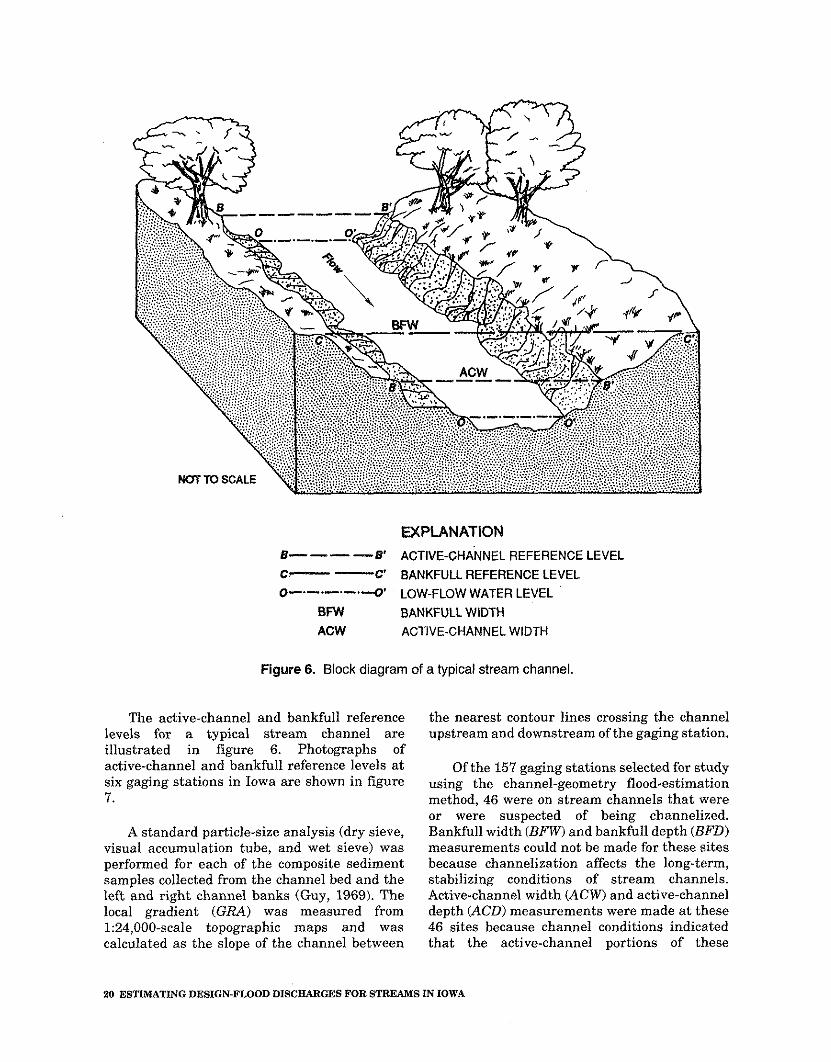
6. Block diagram of a typical stream channel ...................................................... 20
7. Photographs showing active-channel and bankfull reference levels a t six streamflow-gaging stations in Iowa .................................................................. 21
8. Graphs showing relation between 2-year recurrence-interval discharge and channel width for bankfull and active-channel width regression
............................................................................................................. equations 28
9. Graphs showing relation between 100-year recurrence-interval discharge and channel width for bankfull and active-channel width regression equations .......................................................................................................... 29
10. Graph showing bankfull cross section for Black Hawk Creek at Grundy Center ................................................................................................................. 31
iv ESTIMATING DESIGN-FLOOD DISCHARGES FOR STREAMS IN IOWA
TABLES
Page
Table 1. Comparisons of manual measurements and geographic-information- system-procedure measurements of selected drainage-basin characteristics a t selected streamflow-gaging stations ................................... 14
Statewide drainage-basin characteristic equations for estimating design- flood discharges in Iowa ..................................................................................... 17
Statewide channel-geometry characteristic equations for estimating design-flood discharges in Iowa ......................................................................... 23
Region I channel-geometry characteristic equations for estimating design- flood discharges in Iowa outside of the Des Moines Lobe landfonn region .................................................................................................................. 25
Region I1 channel-geometry characteristic equations for estimating design- flood discharges in Iowa within the Des Moines Lobe landform region ......... 26
Statistical summary for selected statewide drainage-basin and channel- geometry characteristics, and for selected regional channel-geometry characteristics a t streamflow-gaging stations in Iowa .................................... 33
Comparisons of manual measurements made from different scales of topographic maps of primary drainage-basin characteristics used in the regression equations .......................................................................................... 50
Flood-frequency data for streamflow-gaging stations in Iowa ........................ 57
Selected drainage-basin and channel-geometry characteristics for streamflow-gaging stations in Iowa ................................................................. 80
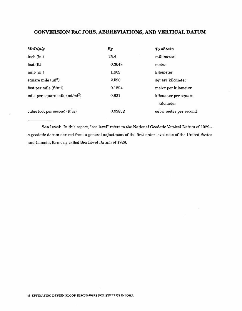
CONVERSION FACTORS, ABBREVIATIONS, AND VERTICAL DATUM
Multiply
inch (in.)
foot (ft)
mile (mi)
square mile (mi2)
foot per mile (ft'mi)
mile per square mile (mi/mi2)
cubic foot per second (ft31s)
To obtain
millimeter
meter
kilometer
square kilometer
meter per kilometer
kilometer per square
kilometer
cubic meter per second
Sea level: In this report, "sea level" refers to the National Geodetic Vertical Datum of 1929-
a geodetic datum derived from a general adjustment of the first-order level nets of the United States
and Canada, formerly called Sea Level ~ a t u m of 1929.
vi ESTIMATING DESIGN-FLOOD DISCHARGES FOR STREAMS IN IOWA
ESTIMATING DESIGN-FLOOD DISCHARGES FOR STREAMS IN IOWA USING DRAINAGE-BASIN AND CHANNEL-GEOMETRY
CHARACTERISTICS
By David A. Eash
ABSTRACT
Drainage-basin and channel-geometry multiple-regression equations are presented for estimating design-flood discharges having recurrence intervals of 2, 5, 10, 25, 50, and 100 years at stream sites on rural, unregulated streams in lowa. Design-flood discharge estimates determined by Pearson Type-Ill analyses using data collected through the 1990 water year are reported for the 188 streamflow-gaging stations used in either the drainage-basin or channel-geometry regression analyses. Ordinary least-squares multiple-regression techniques were used to identify selected drainaqe-basin and
onsite and on topographic maps. Statewide and regional channel-geometry regression equations that are dependent on whether a stream has been channelized were developed on the basis of bankfull and active-channel characteristics. The significant channel-geometry characteristics identified for the statewide and regional regression equations included bankfull width and bankfull depth for natural channels unaffected by channel- ization, and 'active-channel width for stabilized channels affected by channelization. The average standard errors of prediction ranged from 41.0 to 68.4 percent for the statewide channel-geometry equations and from 30.3 to 70.0 percent for the regional channel-geometry equations.
channel-geometry characteristics andto delineate two channel-geometry regions. Weighted least- Procedures provided for applying the squares multiple-regression techniques, which drainage-basin and channel-geometry regression account for differences in the variance of flows at depend on whether the design-flood different gaging stations and for variable lengths in estimate is a site On an ungaged station records, were used to estimate the Stream, an ungaged site on a gaged stream, or a regression parameters. gaged site. When both a drainage-basin and a
channel-geometry regression-equation estimate
Statewide drainage-basin equations were developed from analyses of 164 streamflow- gaging stations. Drainage-basin characteristics were quantified using a geographic-information- system procedure to process topographic maps and digital cartographic data. The significant characteristics identified for the drainage-basin equations included contributing drainage area, relative relief, drainage frequency, and 2-year, 24-hour precipitation intensity. The average standard errors of prediction for the drainage- basin equations ranged from 38.6 to 50.2 percent. The geographic-information-system procedure expanded the capability to quantitatively relate drainage-basin characteristics to the magnitude and frequency of floods for stream sites in lowa and provides a flood-estimation method that is independent of hydrologic regionalization.
Statewide and regional channel-geometry regression equations were developed from analyses of 157 streamflow-gaging stations. Channel-geometry characteristics were measured
are available for a stream site, a procedure is presented for determining a weighted average of the two flood estimates. The drainage-basin regression equations are applicable to unregu- lated rural drainage areas less than 1,060 square miles, and the channel-geometry regression equations are applicable to unregulated rural streams in lowa with stabilized channels.
INTRODUCTION
Knowledge of the magnitude and frequency of floods is essential fo r the effective manage- ment of flood plains and for the economical planning and safe design of bridges, culverts, levees, and other structures located along streams. Long-term flood data collected from a network of streamflow-gaging stations operated in Iowa are available for hydrologic analysis to compute design-flood discharge estimates for the gaged sites as well as for ungaged sites on the gaged streams. Techniques are needed to estimate design-flood discharges for sites on all
INTRODUCTION 1
ungaged streams in Iowa because most such stream sites in the State have no flood data available, particularly sites on smaller streams.
Flood runoff is a function of many interrelated factors that include, but are not limited to climate, soils, land use, and the physiography of drainage basins. Previous investigations for Iowa (Schwob, 1953, 1966; Lara, 1973,1987) have been limited to the types of basin characteristics that can be investigated as potential explanatory variables for the development of multiple-regression flood- estimation equations because many of the flood-runoff factors are difficult to measure. Previous investigations defined hydrologic regions to account for factors affecting flood runoff that were difficult to measure directly. The hydrologic regions were delineated on the basis of physiographic differences of broad geographic landform regions. However, two major limitations are encountered when using the hydrologic-region method to estimate flood discharges for ungaged sites. First, i t is difficult to weight flood estimates for drainage basins located in more than one hydrologic region or located near the boundaries of hydrologic regions because the boundaries are not well defined. Regional boundaries are transitional zones where the physiographic characteristics of one hydrologic region gradually merge into another. Second, because large hydrologic regions may contain drainage basins with physiographies that are anomalous to the region in which they are located, it is difficult to correlate their physiographic differences to another hydrologic region, or to weight their flood estimates. Quantitative measurements of basin morphology to determine appropriate regional equations for drainage basins are not applicable for resolving these regional limitations. As a result, flood estimates for some ungaged sites become very subjective.
To address the need to minimize the subjectivity encountered in applying regional flood-estimation methods, a study using two different flood-estimation methods was made by the U.S. Geological Survey in cooperation with the Iowa Highway Research Board and the Highway Division of the Iowa Department of Transportation. Two new flood-estimation methods for Iowa, which are presumed to be independent from each other, were used in this
study. An advantage in developing flood- frequency equations using two independent flood-estimation methods is that each method canbe used to verify the results of the other, and the estimates obtained from each method can be used to calculate a weighted average.
Methods are now available to more easily quantify selected morpbologic and climatic characteristics for a large number of drainage basins. A geographic-information-system (GIs) procedure developed by the U.S. Geological Survey uses topographic maps and digital cartographic data to quantify several basin characteristics that typically were not quantified previously. This GIs procedure expands the capability to relate drainage-basin characteristics to the magnitude and frequency of floods for stream sites in Iowa and provides a flood-estimation method that is independent of hydrologic regionalization.
Measurements of channel-geometry characteristics have been used to estimate the magnitude and frequency of floods in investigations conducted by Fields (19751, Webber and Roberts (1981), Parrett and others (19871, Hedman and Kastner (19771, and Osterkamp and Hedman (1982). These investigations have shown that measurements of specific channel-geometry characteristics provide a reliable method [or estimating flood discharges because channel cross-sectional characteristics are assumed to be a function of flow volume and sediment-load transport (Pickup and Rieger, 1979, p. 41; Osterkamp, 1979, p. 2).
Purpose and Scope
The purpose of this report is to: (1) define equations for Iowa that relate measurable drainage-basin characteristics to design-flood discharges having recurrence intervals of 2, 5, 10, 25, 50, and 100 years that are independent of hydrologic regionalization; (2) define corroborative equations for Iowa that relate channel-geometry characteristics to the same design-flood recurrence intervals; and (3) define application and reliability of drainage-basin and channel-geometry flood-estimation methods.
Both the drainage-basin and channel- geometry flood-estimation methods described in
2 ESTIMATING DESIGN-FLOOD DISCHARGES FOR STREAMS IN IOWA
this report are applicable to unregulated rural streams located within the State. The drainage-basin flood-estimation method is limited to streams with drainage areas less than 1,060 mi2. The channel-geometry flood- estimation method is applicable to stabilized stream channels in Iowa.
The U.S. Army Corps of Engineers, Omaha and Rock Island Districts, contributed to the funding of the sediment-sample analyses. James J. Majure, formerly with the U.S. Geological Survey, Iowa City, Iowa, and now with the Iowa State University, GIS Support and Research Facility, Ames, 'Iowa, developed the computer software used to quantify the drainage-basin characteristics and the software used to integrate the overall GIS procedure.
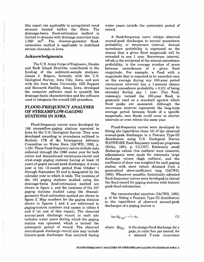
FLOOD-FREQUENCY M a Y S E S OF STREAMFLOW-GAGING STATIONS IN IOWA
Flood-frequency curves were developed for 188 streamflow-gaging stations operated in Iowa by the U.S. Geological Survey. They were developed according to procedures outlined in Bulletin 17B of the Interagency Advisory Committee on Water Data (IACWD, 1982, p. 1-28). These flood-frequency curves include data collected through the 1990 water year for both active and discontinued continuous-record and crest-stage gaging stations having a t least 10 years of gaged annual-peak discharges. A water year is the 12-month period from October 1 through September 30 and is designated by the calendar year in which i t ends. The locations of the 164 gaging stations studied using the drainage-basin flood-estimation method are shown in figure 1, and the locations of the 157 gaging stations studied using the channel- geometry flood-estimation method are shown in figure 2. Map numbers for the gaging stations shown in figures 1 and 2 are referenced to gaging-station numbers and names in tables 8 and 9 (at end of this report). The observed annual-peak discharge record a t each site includes water years during which the gaging station was operated, which is termed the systematic period of record. The observed annual-peak discharge record also may include historic-peak discharges that occurred during
water years outside the systematic period of record.
A flood-frequency curve relates observed annual-peak discharges to annual exceedance probability or recurrence interval. Annual exceedance probability is expressed as the chance that a given flood magnitude will he exceeded in any 1 year. Recurrence interval, which is the reciprocal of the annual exceedance probability, is the average number of years between exceedances of a given flood magnitude. For example, a flood with a magnitude that is expected to be exceeded once on the average during any 100-year period (recurrence interval) has a 1-percent chance (annual exceedance probability = 0.01) of being exceeded during any 1 year. This flood, commonly termed the 100-~ear flood, is generally used as a standard against which flood peaks are measured. Although the recurrence interval represents the long-term average period between floods of a specific magnitude, rare floods could occur a t shorter intervals or even within the same year.
Flood-frequency curves were developed by fitting the logarithms (base 10) of the observed annual-peak discharges to a Pearson Type-111 distribution using U.S. Geological Survey WATSTORE flood-frequency analysis programs (Kirby, 1981, p. C1-(357). Extremely small discharge.values (low outliers) were censored, adjustments were made for extremely large discharge values (high outliers), and the coefficient of skew was weighted for each gaging station with skew values obtained from a generalized skew-coefficient map (IACWD, 1982). Whenever possible, historically adjusted flood-frequency curves were developed to extend the flood record for gaging stations with historic peak-flood information.
The recommended equation (IACWD, 1982, p. 9) for fitting a Pearson Type-I11 distribution to the logarithms of observed annual-peak discharges of a gaging station is
where QT(g) is the design-flood discharge for a gage, in cubic feet per second, for a selected T-year recurrence
FLOOD-FREQUENCY ANALYSES OF STREAMFLOW-GAGING STATIONS IN IOWA 3
VMOI NI SYW3MLS Bod S338YH3SIa aOO'Id-N3IS3a 3NUWLS3 P
i
I - South Dakota
FLOOD-FREQUENCY ANALYSES OF STREAMFLOW-GAGING STATIONS IN IOWA 6
interval; - x is the mean of the logarithms
(base 10) of the observed annual-peak discharges;
k is the standardized Pearson Type-I11 deviate for a selected T-year recurrence interval and weighted skew coefficient; and
s is the standard deviation of the logarithms (base 10) of the observed annual-peak dis- charges.
Results of the Pearson Type-I11 flood- frequency analyses are presented in table 8 (listed as method B17B, a t end of this report) for the 188 streamflow-gaging stations analyzed using either the drainage-basin or channel- geometry flood-estimation techniques. Included in table 8 is information about the type of gage operated, the effective record length of the gage, whether a systematic or historical analysis was performed, the observed annual-peak discharge record (listed as flood period), and the maximum known flood-peak discharge and its recurrence interval. An example flood-frequency curve is shown in figure 3.
DEVELOPMENT OF MULTIPLE-REGRESSION EQUATIONS
Multiple linear-regression techniques were used to independently relate selected drainage- basin and channel-geometry characteristics to design-flood discharges having recurrence intervals of 2, 5, 10, 25, 50, and 100 years. A general overview of the ordinary least-squares and weighted least-squares multiple linear- regression techniques used to develop the equations is presented in the following two sections. Specific information on the multiple- regression analyses for either flood-estimation method is presented in later sections entitled "Drainage-Basin Characteristic Equations" and "Channel-Geometry Characteristic Equations."
Ordinary Least-Squares Regression
Ordinary least-squares (OLS) multiple linear-regression techniques were used to
develop the initial multiple-regression equations, or models, for both the drainage- basin and channel-geometry flood-estimation methods. In OLS regression, a design-flood discharge (termed the response variable) is estimated on the basis of one or more significant drainage-basin or channel-geometry character- istics (termed the explanatory variables) in which each observation is given an equal weight. The response variable is assumed to be a linear function of one or more of the explanatory variables. Logarithmic transforma- tions (base 10) were performed for both the response and explanatory variables used in all of the OLS regression analyses. Data transformations were used to obtain a more constant variance of the residuals about the regression line and to linearize the relation between the response variable and explanatory variables. The general form of the OLS regres- sion equations developed in these analyses is
log,, (QT) = loglO (C) +blloglo (XI) + (2)
where QT is the response variable, the estimated design-flood discharge, in cubic feet per second, for a selected T-year recurrence interval;
C is a constant;
bi is the regression coefficient for the ith explanatory variable (i = 1, ... ,PI;
Xi is the value of the ith explanatory variable, a drainage-basin or channel-geometry characteristic (i = I , ... ,p); and
P is the total number of explanatory variables in the equation.
Equation 2, when untransformed, is algebraically equivalent to
6 ESTIMATING DESIGN.FLOOD DISCHARGES FOR STREAMS IN IOWA
EX
CE
ED
AN
CE
PR
OB
AB
ILITY, IN
PE
RC
EN
7
Pearson Type-111 flood-frequency estim
ate for streamflow
-gaging station 05494300 F
OX
RIV
ER
AT
BLO
OM
FIE
LD (m
ap
number 133, figure 1)
Figure 3. E
xample of a flood-frequency cuw
e.

streamflow-gaging stations in Iowa (fig. 1). The drainage-network digital map (fig. 48) Drainage-basin characteristics were quantified is created by extracting the drainage network using a GIS procedure to process topographic for the basin from 1:100,000-scale USGS digital maps and digital cartographic data. An line graph (DLG) data. The extraction process overview of the GIS procedure is provided in the uses GIS software to select and append together following section. the DLG data contained within the
drainage-divide polygon.
Geographic-Information-System Procedure The elevation-contour digital map (fig. 4C)
is created from 1:250.000-scale DMA dieital
The GIS procedure developed by the U.S. Geological Survey (USGS) quantifies for each drainage basin the 26 basin characteristics listed in Appendix A (at end of this report). These characteristics were selected for the GIS procedure on the basis of their hypothesized applicability in flood-estimation analysis and their general acceptability as measurements of drainage-basin morphology and climate. Techniques for making manual measurements of selected drainage-basin characteristics from topographic maps are outlined in Appendix B (at end of this report). The GIS procedure uses ARCIINFO com~uter software and other . - software developed specifically to integrate with ARCIINFO (Majure and Soenksen, 1991; Eash, 1993).
The GIS procedure entails four main steps: (1) creation of four GIS digital maps (ARCIINFO coverages) from three cartographic data sources, (2) assignment of attribute information to three of the four GIS digital maps, (3) quantification of 24 morphologic basin characteristics from the four GIS digital maps, and (4) quantification of two climatic basin characteristics from two precipitation data sources.
The first step creates four GIS digital maps representing selected aspects of a drainage basin. Examples of these maps are shown in figure 4. The drainage-divide digital map (fig. 4A) is created by delineating the surface-water drainage-divide boundary for a streamflow- gaging station on 1:250,000-scale U.S. Defense Mapping Agency (DMA) topographic maps. This drainage-divide delineation is manually digitized into a polygon digital map using GIS software. If noncontributing drainage areas are identified within the drainage-divide boundary, then each noncontributing drainage area also is delineated and digitized.
elevation model (DEM) data that are referenced to sea level (in meters). GIS software is used to convert the DEM data to a lattice file of point elevations for an area slightly larger than the drainage-divide polygon. This lattice file of point elevations is contoured with a 12-meter (39.372-ft) or smaller contour interval using ARCIINFO software. The contour interval is chosen to provide at least five contours for each drainage basin. GIS software selects the contours contained within the drainage-divide polygon to create the elevation-contour digital map. Elevation contours then are converted to units of feet.
The basin-length digital map (fig. 4D) is created by delineating and digitizing the basin length from 1:250,000-scale DMA topographic maps. The basin length characteristic is delineated by first identifying the main channel for the drainage basin on 1:100,000-scale topographic maps. The main channel is identified by starting at the basin outlet and proceeding upstream, repetitively selecting the channel that drains the greater area a t each stream junction. The most upstream channel is extended to the drainage-divide boundary defined for the drainage-divide digital map. This main channel identified on 1:100,000-scale topographic maps is used to define the main channel on 1:250,000-scale topographic maps. The basin length is centered along the main-channel, flood-plain valley from basin outlet to basin divide and digitized with as straight a line as possible from the 1:250,000-scale maps. When comparing the basin length shown in figure 40 to those stream segments corresponding to the main channel in figure 4B, it can be seen that the basin length does not include all the sinuosity of the stream segments.
The second step assigns attributes to specific polygon, line-segment, and point
10 ESTIMATING DESIGN-PLOOD DISCHARGES FOR STREAMS IN IOWA

A. Drainage-divide digital map digitized from Waterloo topographic map.
Base from U.S. Defense Mapping Agency, 1 :250,000, 1976 Universal Transverse Mercalor projection, Zone 15
B. Drainage-network digital map extracted from Marshalltown-West digital line graph data, with stream-order numbers.
C. Elevation-contour digital map created from Waterloo-East digital elevation model. from Waterloo topographic map. sea-level data, with contour intervals at 39.372 feet.
L ~ .. Base from U.S. Defense Mapping Agency, Base from U.S. Defense Mapping Agency, 1:250,000, 1976 1 :250.000, 1976 Universal Transverse Mercator projection, Universal Transverse Mercator projection. Zone 15 Zone 15
0 5 MILES 2;5 0 2.5 5 KILOMETERS
EXPLANATION A STREAMFLOW-GAGING STATION
Figure 4. Four geographic-information-system maps that constitute a digital representation of selected aspects of a drainage basin.
ESTIMATING DESIGN-FLOOD DISCHARGES USING DRAINAGE-BASIN CHARACTERISTICS 11
features in the first three of the four GIS digital maps shown in figure 4. As a prerequisite, the digital maps are edited to ensure that drainage-divide boundaries, stream segments, and the basin-length line segments are connected properly. If noncontributing drainage areas are identified, they are assigned attributes with separate polygon designations so that the basin-characteristic programs can distinguish between contributing and noncontributing areas. Each line segment in the drainage-network digital map is assigned a Strahler stream-order number (Strahler, 1952) and a code indicating whether the line segment represepts part of the main channel or a secondary channel. Specific GIs programs have been developed to assign the proper stream- order number to each line segment and to code those line segments representing the main channel. Figure 4B shows the Strahler stream-order numbers for streams in the Black Hawk Creek at Grundy Center (station number 05463090; map number 73, fig. 1) drainage basin. A description on how to order streams using Strahler's method is included in Appendix B (at end of this report).
The line segments in the elevation-contour digital map were assigned elevations from the processing of the DEM data. Line segments overlain by noncontributing drainage-area polygons are assigned attributes designating noncontributing contour segments. Two point attributes are added to the elevation-contour digital map to represent the maximum and minimum elevations of the drainage basin. The maximum basin elevation is defined from the highest DEM-generated contour elevation within the contributing drainage area. The minimum basin elevation is defined at the basin outlet as an interpolated value between the first elevation contour crossing the main channel upstream of the basin outlet and the first elevation contour crossing the main channel downstream of the basin outlet.
The third step uses the four GIs digital maps shown in figure 4 and a set of programs developed by the USGS (Majure and Soenksen, 1991) to quantify the 24 morphologic basin characteristics listed in Appendix A (at end of this report). These basin characteristics include selected measurements of area, length, shape, and topographic relief that define selected
aspects of basin morphology, and several channel characteristics. The programs access the information automatically maintained by the GIS for each of the four digital maps, such as the length of line segments and the area of polygons, as well as the previously described attribute information assigned to the polygon, line-segment, and point features of three of the four GIs digital maps. The GIS programs then use this information to automatically quantify the 24 morphologic basin characteristics.
The fourth step uses a software program developed to quantify the remaining two basin characteristics listed in Appendix A (at end of this report). These two climatic characteristics are quantified using GIS digital maps representing the distributions of mean annual precipitation and 2-year, 24-hour precipitation intensity for the area contributing to all surface-water drainage in Iowa. This area includes a portion of southern Minnesota. The mean annual precipitation digital map was digitized from a contour map for Iowa, supplied by the Iowa Department of Agriculture and Land Stewardship, State Climatology Office (Des Moines), and from a contour map for Minnesota (Baker and Kuehnast, 1978). The 2-year, 24-hour precipitation intensity digital map was digitized from a contour map for Iowa (Waite, 1988, p. 31) and interpolated contours for southern Minnesota that were digitized from a United States contour map (Hershfield, 1961, p. 95). The digital map representing the distribution of 2-year, 24-hour precipitation intensity for Iowa and southern Minnesota is shown in figure 5. The weighted average for each climatic characteristic is computed for a drainage basin by calculating the mean of the area-weighted precipitation values that are within the drainage-divide polygon.
Of the 26 drainage-basin characteristics listed in Appendix A, 12 are referred to as primary drainage-basin characteristics because they constitute specific GIS procedure or manual topographic-map measurements. They are listed under headings containing the word "measurement." The remaining characteristics are calculated from the primary drainage-basin characteristics; they are listed in Appendix A under headings containing the word "computation." Each drainage-basin character- istic listed in Appendix A is footnoted with a
12 ESTIMATING DESIGN-FLOOD DISCHARGES FOR S T R W S IN IOWA
EXPLANATION
1 AREA OF EQUAL 2-YEAR, 24-HOUR PRECIPITATION INTENSITY--Number is precipitation intensity, in inches
Figure 5. Distribution of 2-year, 24-hour precipitation intensity for Iowa and southern Minnesota.
reference and the cartographic data source used for both GIS procedure and manual measurements.
Verification of Drainage-Basin Characteristics
To verify that the drainage-basin characteristics quantified using the GIs procedure are valid, manual topographic-map measurements of selected drainage-basin characteristics were made for 12 of the
streamflow-gaging stations used in the drainage-basin flood-estimation method. These comparison measurements were made for those primary drainage-basin characteristics identified as being significantly related to flood runoff in the multiple-regression equations presented in the following section entitled "Drainage-Basin Characteristic Equations." Comparison measurements were made from topographic maps of the same scales as were used in the GIS procedure. The results of the comparisons are shown in table 1.
ESTIMATING DESIGN-FLOOD DISCHARGES USING DRAINAGE-BASIN CHARACTERISTICS IS
Table 1. Comparisons of manual measurements and geographic-information-system-procedure measurements of selected drainage-basin characteristics at selected streamflow-gaging stations
[TDA, total drainage area, in square miles; BP, basin perimeter, in miles; BR, basin relief, in feet; FOS, number of first-order streams; TTF, 2-year, 24-hour precipitation intensity, in inches; MAN,
manual measurement; G I s , geographic-information-system procedure; % DIFF, percentage difference between MAN and GZS]
Measure- Selected drainage-basin characteristics Station ment number technique T D A ~ BP BR FOS TTF
05411600 MAN 177 73.3 297 84 3.05 G I s 178 73.9 274 84 3.05 % DIFF +0.6 +0.8 -7.7 0 0
05414450 MAN 21.6 21.9 444 10 3.05 G I s 22.3 21.3 394 10 3.05 % DZFF +3.2 -2.7 -11.3 0 0
05414600 MAN 1.54 5.32 280 1 3.05 G I s 1.53 5.97 291 1 3.05 % DIFF -0.6 +12.2 +3.9 0 0
05462750 MAN 11.6 15.0 160 6 3.05 G I s 11.9 15.5 129 6 3.05 % DIFF +2.6 +3.3 -19.4 0 0
05463090 MAN 56.9 33.5 181 28 3.15 G I s 57.0 33.1 160 28 3.15 % DZFF +0.2 -1.2 -11.6 0 0
05470500 MAN 204 69.8 318 60 3.15 G I s 208 67.7 292 51 3.15 % DIFF +2.0 -3.0 -8.2 -15.0 0
05481000 MAN 844 139 303 152 3.05 G I s 852 139 300 155 3.05 % DIFF +0.9 0 -1.0 +2.0 0
05489490 MAN 22.9 24.8 280 10 3.25 GZS 22.2 26.2 263 10 3.25 % DZFF -3.1 +5.6 -6.1 0 0
06483430 MAN 29.9 28.8 198 12 2.85 GIS 30.0 28.9 182 12 2.85 % DIFF +0.3 c0.3 -8.1 0 0
06609500 MAN 871 206 582 477 3.05 G I s 869 210 550 475 3.05 % DIFF -0.2 +1.9 -5.5 -0.4 0
14 ESTIMATING DESIGN-FLOOD DISCHARGkS FOR STREAMS IN IOWA
Table 1. Comparisons of manual measurements and geographic-information-system-procedure measurements of selected drainage-basin characteristics a t selected streamflow-gaging
stations--Continued
Measure- Selected drainage-basin characteristics Station ment number techniaue T D A ~ BP BR FOS TTF
06807780 MAN 42.7 47.4 268 18 3.05 G I s 42.8 48.8 280 19 3.05 % DIFF ~ 0 . 2 +3.0 +4.5 +5.6 0
06903400 MAN 182 79.0 224 80 3.25 G I s 184 79.6 256 80 3.25 % DIFF +1.1 +0.8 +14.3 0 0
WILCOXON SIGNED-RANKS TEST STATISTIC^ -1.726 -1.334 -1.843 -0.365 NO TEST^ p-VALUE STATISTIC 0.0844 0.1823 0.0653 0.7150
Manual TDA measurements are streamflow-gaging-station drainage areas published by the U.S. Geological Survey in annual streamflow reports. Noncontributing drainage areas (NCDA) are not listed because none were identified for these drainage basins.
Using a 95-percent level of significance, the T-value statistic = 2.2010 (Irnan and Conover, 1983, p. 438).
All values for % DIFF = 0
Comparison measurements for total drainage area (TDA) indicate that the GIs procedure was within about 1 percent of the drainage areas published by the USGS in annual streamflow reports for 8 of the 12 selected gaging stations. This comparison indicates that delineations of drainage areas used in the GIs procedure, made from 1:250,000-scale topographic maps, were generally valid. The Wilcoxon signed-ranks test was applied to four of the five drainage-basin characteristics listed in table 1 using STATIT procedure SGNRNK (Statware, Inc., 1990, p. 3-25 - 3-26). Results (table 1) indicate that GIs procedure measurements of total drainage area, basin perimeter (BP), basin relief (BR), and number of first-order streams (FOS) were not significantly different from manual topographic-map measurements at the 95-percent level of significance. The greater
variation in measurement comparisons of basin relief are believed to be due to limitations in the 1:250,000-scale DEM data. Results of the comparison tests (table 1) indicate that GIs procedure measurements are generally valid for the primary drainage-basin characteristics used in the regression equations presented in the following section.
Basin slope (BS) is another drainage-basin characteristic that was quantified using DEM data. It is hypothesized that basin slope may have a significant effect on surface-water runoff. Basin slope was indicated as being a significant characteristic in a few of the initial multiple-regression analyses. Comparison measurements indicated that the GIs procedure greatly underestimated basin slope. Measure- ment differences for basin slope were between minus 9 and 66 percent, with an average
ESTIMATING DES1GN.FLOOD DISCHARGES USING DRAINAGE-BASIN CHARACTERISTICS 15
underestimation of 40 percent for the 10 drainage basins tested (Eash, 1993, p. 180-181). For this reason, the basin-slope characteristic was deleted from the drainage-basin characteristics data set during the initial multiple-regression analyses. Basin-slope comparisons appear to indicate that the 1:250,000-scale DEM data used to create the elevation-contour digital maps are not capable of reproducing all the sinuosity of the elevation contours depicted on the 1:250,000-scale DMA topographic maps. The elevation contours generated using the GIs procedure are much more generalized than the topographic-map contours; thus, the total length of the elevation contours are undermeasured when using the "contour-band" method of calculating basin slope (BS) (Appendix A). A comparison of the elevation contours shown in figure 4C for the Black Hawk Creek a t Grundy Center (station number 05463090; map number 73, fig. 1) drainage basin to those depicted on the DMA 1:250,000-scale Waterloo topographic map showed a significant difference in the sinuosity of the elevation contours depicted.
Drainage-Basin Characteristic Equations
The 26 drainage-basin characteristics listed in Appendix A were quantified for 164 streamflow-gaging stations (fig. 1) and investigated as potential explanatory variables in the development of multiple-regression equations for the estimation of design-flood discharges. Because of the previously described problems concerning measurement verification of basin slope and because of the difficulty associated with manual measurements of total stream length, six basin characteristics were deleted from the regression data set. The excluded characteristics were basin slope (BS), total stream length (TSL), stream density (SD), constant of channel maintenance (CCM), ruggedness number (RN), and slope ratio (SR).
Several other drainage-basin characteristics also were deleted from the data set because of multicollinearity. Multicollinearity is the condition where a t least one explanatory variable is closely related to (that is, not independent of) one or more other explanatory variables. Regression models that include variables with multicollinearity may be
unreliable because coefficients in the models may be unstable. Output from the ALLREG analysis and a correlation matrix of Pearson product-moment correlation coefficients: were used as guides in identifying the variables with multicollinearity. The hydrologic validity of variables with multicollinearity in the context of flood runoff was the principal criterion used in determining which drainage-basin character- istics were deleted from the data set. Upon completion of the ALLREG analyses, any remaining multicollinearity problems were identified with the SREGRES procedure by checking each explanatory variable for variance inflation factors greater than 10.
Statewide flood-estimation equations were developed from analyses of the drainage-basin characteristics using the ordinary least-squares and weighted least-squares multiple-regression techniques previously described. The best equations developed in terms of PRESS statistics, coefficients of determination, and standard errors of estimate are listed in table 2. The characteristics identified as most significant in the drainage-basin equations are contributing drainage area (CDA), relative relief (RR), drainage frequency (DF), and 2-year, 24-hour precipitation intensity (TTF). Table 9 (at end of this report) lists these significant drainage-basin characteristics, as quantified by the GIs procedure, for 164 streamflow-gaging stations in Iowa.
Three of the four characteristics listed in the drainage-basin equations (table 2) are calculated from primary drainage-basin characteristics. The drainage-basin equations are comprised of six primary drainage-basin characteristics. Contributing drainage area (CDA) is a measure of the total area that contributes to surface-water runoff at the basin outlet. The primary drainage-basin characteristics used to calculate contributing drainage area are total drainage area (TDA) and noncontributing drainage .area (NCDA). Relative relief (RR) is a ratio of two primary drainage-basin characteristics, basin relief (BR) and basin perimeter (BPI. Drainage frequency (DF) is a measure of the average number of first-order streams per unit area and is an indication of the spacing of the drainage network. The primary drainage-basin characteristics used to calculate drainage
16 ESTIMATING DESIGN.FLOOD DISCHARGES FOR STREAMS IN IOWA
Table 2. Statewide drainage-basin characteristic equations for estimating design-flood discharges in Iowa
[Q, peak discharge, in cubic feet per second, for a given recurrence interval, in years; CDA, contributing drainage area, in square miles; RR, relative relief, in feet per mile; DF, drainage frequency, in number of first-order streams per square mile; TTF, 2-year, 24-hour precipitation
intensity, in inches]
Average Average Standard standard error equivalent
error of estimate of prediction years of Estimation equation Loglo Percent (percent) record
Number of streamflow-gaging stations = 164
Qz = 53.1 C D A ~ . ~ ~ ~ R R ~ . ~ ~ ~ D F ~ . ~ ~ ~ (TTF - 0.171 41.0 42.2 3.9
Q5 = 98.8 R R ~ . ~ ~ ~ ~ f l . ~ ~ ~ (TTF - 2.5)0.s85 ,156 37.2 38.6 5.4
Q,, = 136 C D A ~ . ~ ~ ~ R R ~ . ~ ~ ~ D @ . ~ ~ ~ (TTF - 2.5)0.801 ,160 38.2 39.8 6.5
Q50 = 231 c D A ~ . ~ ~ ~ R R ~ . ~ ~ ~ (TTF - 2.5)0.491 .I85 44.5 46.5 9.5
Note: Basin characteristics are map-seale dependent. See Appendix A and Appendix B for basin-characteristic descriptions, computations, and acales of maps to use for manual measureinents.
frequency are the number of first-order streams (FOS) and contributing drainage area (CDA). The value of FOS is determined by using Strahler's method of ordering streams (Strahler, 1952). A description of Strahler's stream-ordering method is included in Appendix B. The 2-year, 24-hour precipitation intensity (TTF) is a primary drainage-basin- characteristic measurement of the maximum 24-hour precipitation expected to be exceeded on the average once every 2 years.
Additional information pertaining to the characteristics used in the drainage-basin equations (table 2) is included in Appendix A. Techniques on how to make manual measurements from topographic maps for the primary drainage-basin characteristics used in the equations are outlined in Appendix B. Several of the primary drainage-basin
characteristics are map-scale dependent. Use of maps of scales other than the scales used to develop the equations may produce results that do not conform to the range of estimation accuracies listed for the equations in table 2. The scale of map to use for manual measurements of each primary drainage-basin characteristic is outlined in Appendix A and Appendix B.
Examination of residuals, the difference between the Pearson Type-111 and multiple- regression estimates of peak discharge for the drainage-basin equations, indicated no evidence of geographic bias. The drainage-basin equations thus were determined to be independent of hydrologic regionalization within the State.
ESTIMA'lTNG DESIGN-FLOOD DISCHARGES USING DRAINAGE-BASIN CHARACTERISTICS 17
The drainage-basin flood-estimation method developed in this study is similar to the regional flood-estimation method developed by Lara (1987) because both methods estimate flood discharges on the basis of morphologic relations. While the standard errors of estimate appear to be higher for the drainage-basin equations than for Lara's equations (Lara, 1987, p. 281, a direct comparison cannot he made because of the different methodologies used to develop the equations. Lara's method is based on the physiography of broad geographic landform regions defined for the State, whereas the drainage-basin method presented in this report is based on specific measurements of basin morphology. The drainage-basin equations are independent of hydrologic regionalization. The application of regional equations often requires that subjective judgments be made concerning basin anomalies and the weighting of regional discharge estimates. This subjectivity may introduce additional unmeasured error to the estimation accuracy of the regional discharge estimates. The drainage-basin regression equations presented in this report provide a flood-estimation method that minimizes the subjectivity in its application to the ability of the user to measure the characteristics.
Example of Equation Use-- Example 1
Examule 1.--An application of the drainage- basin flood-estimation method can be illustrated by using the equation (listed in table 2) to estimate the 100-year peak discharge for the discontinued Black Hawk Creek at Grundy Center crest-stage gaging station (station number 05463090; map number 73, fig. I), located in Grundy County, a t a bridge crossing on State Highway 14, a t the north edge of Grundy Center, in the NW114, see. 7, T. 87 N., R. 16 W. Differences between manually computed values (table 1) and values computed using the GIs procedure (tables 1 and 9) are due to differences in applying the techniques.
Step 1. The characteristics used in the drainage-basin equation (table 2) are contributing drainage area (CDA), relative relief (RR), drainage frequency (DF), and 2-year, 24-hour precipitation intensity (TTF). The primary drainage-basin characteristics used in this equation are total drainage area (TDA),
noncontributing drainage area (NCDA), basin relief (BR), basin perimeter (BP), number of first-order streams (FOS), and 2-year, 24-hour precipitation intensity (TTF). These primary drainage-basin characteristic measurements and the scale of maps to use for each manual measurement are described in Appendix A and Appendix B.
Step 2. The topographic maps used to delineate the drainage-divide boundary for this gaging station are the DMA 1:250,000-scale Waterloo topographic map and the USGS 1:100,000-scale Grundy County map. Figure 4A shows the drainage-divide boundary that was delineated for this gaging station. on the 1:250,000-scale map. Contributing drainage area (CDA) is calculated from the primary drainage-basin characteristics total drainage area (TDA) and noncontributing drainage area (NCDA). The total drainage area published for this gaging station in the annual streamflow reports of the U.S. Geological Survey is 56.9 mi2 (table 9). Inspection of the 1:100,000-scale map does not show any noncontributing drainage areas within the drainage-divide boundary of this basin. The contributing drainage area (CDA) is calculated as
Step 3. Relative relief (RR) is calculated from the primary drainage-basin characteristics basin relief (BR) and basin perimeter (BP). The difference between the highest elevation contour and the lowest interpolated elevation in the basin measured from the 1:250,000-scale topographic map gives a basin relief of 181 ft (table 1). Figure 4C shows an approximate representation of the topography for this drainage basin. The drainage-divide boundary delineated on the 1:250,000-scale topographic map (fig. 4A) is used to measure the basin perimeter, which is 33.5 mi (table 1). Relative relief (RR) is calculated as
18 ESTIMATING DESIGN-FLOOD DISCHARGES FOR STREAMS IN IOWA
= 5.40 ft/mi.
Step 4. Drainage frequency (DF) is calculated from the primary drainage-basin characteristics number of first-order streams (FOS) and contributing drainage area (CDA). A total of 28 first-order streams are counted within the drainage-divide delineation for this gaging station on the 1:100,000-scale topographic map (table 1). These first-order streams are shown in figure 4B. Drainage frequency (DF) is calculated as
FOS DF = - CDA '
2 =0.492 first-order streamslmi
Step 5. The 2-year, 24-hour precipitation intensity (TTF) for the drainage basin is determined from figure 5. Because the drainage-divide boundary for this gaging station is completely within the polygon labeled as 3.15 in., the 2-year, 24-hour precipitation
intensity is given a value of 3.15 in. (table 1).
ESTIMATING DESIGN-FLOOD
The channel-geometry flood-estimation method uses selected channel-geometry characteristics to estimate the magnitude and frequency of floods for stream sites in Iowa. The channel-geometry method is based on measure- ments of channel morphology, which are assumed to be a function of streamflow discharges and sediment-load transport. Multiple-regression equations were developed by relating significant channel-geometry characteristics to Pearson Type-111, design-flood discharges for 157 streamflow-gaging stations in Iowa (fig. 2).
Channel-Geometry Data Collection
The channel-geometry parameters that were measured for each of the gaging stations are as follows:
ACW - average width of the active channel, in feet;
ACD - average depth of the active channel, in feet;
BFW - average width of the bankfull channel, in feet;
Step 6. The 100-year flood estimate using BFD - average depth of the bankfull channel, in feet;
the drainage-basin equation (table 2) is calculated as SCbd - silt-clay content of channel-bed
material, in percent;
Qloo= 277 (cDAIO.~'~ ( R R ) ~ . ~ ~ ~ ( D F ) ~ . ~ ~ ~ (TTF- SCIbk - silt-clay content of left channel-bank
= 277 (56.9)G.s81 ( 5 . 4 0 ) ~ ~ ~ ~ (0.492)~-~O~ (3.15 - 2.5)0.389, material, in percent;
SCrbk - silt-clay content of right channel-bank material, in percent;
Discharge estimates listed in this report are Dso - diameter size of channel-bed particles
rounded to three significant figures. The for which the total weight of all particles
difference between the above estimate of with diameters greater than D50 is equal to the total weight of all particles with
8,310 ft3/s and the estimate of 7,740 ft3/s listed diameters less than or equal to D50, in in table 8 (method GISDB) is due to millimeters; and measurement differences between manual measurement and GIs procedure techniques GRA - local gradient of channel, in feet per (table 1). mile.
ESTIMATING DESIGN.FLOOD DISCHARGES USING CHANNEL-GEOMETRY CHARACTERISTICS 19
---
NOT TO SCALE
EXPLANATION @---- 8' ACTIVE-CHANNEL REFERENCE LEVEL
Ci------ C ' BANKFULL REFERENCE LEVEL 0 -.-.-.-. 4, LOW-FLOW WATER LEVEL
B W BANKFULL WIDTH ACW ACTIVE-CHANNEL WIDTH
Figure 6. Block diagram of a typical stream channel.
The active-channel and bankfull reference levels for a typical stream channel are illustrated in figure 6. Photographs of active-channel and bankfull reference levels at six gaging stations in Iowa are shown in figure ..
A standard particle-size analysis (dry sieve, visual accumulation tube, and wet sieve) was performed for each of the composite sediment samples collected from the channel bed and the left and right channel banks (Guy, 1969). The local gradient (GRA) was measured from 1:24,000-scale topographic maps and was calculated as the slope of the channel between
the nearest contour lines crossing the channel upstream and downstream of the gaging station.
Of the 157 gaging stations selected for study using the channel-geometry flood-estimation method, 46 were on stream channels that were or were suspected of being channelized. Bankfull width (BFW) and bankfull depth (BFD) measurements could not be made for these sites because channelization affects the long-term, stabilizing conditions of stream channels. Active-channel width (ACW) and active-channel depth (ACD) measurements were made a t these 46 sites because channel conditions indicated that the active-channel portions of these
20 ESTIMATING DESIGN.PL00D DISCHARGES FOR STREAMS IN IOWA
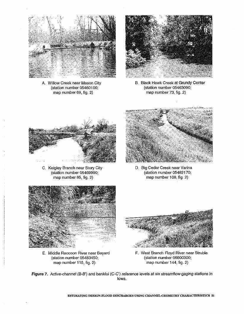
A. Willow Creek near Mason City (station number 05460100; map number 69, fig. 2)
B. Black Hawk Creek at Grundy Center (station number 05463090; map number 73, fig. 2)
C. Keigley Branch near Story City (station number 05469990; map number 85, fig. 2)
D. Big Cedar Creek near Varina (station number 05482170;
map number 108, fig. 2)
E. Middle Raccoon River near Bayard F. West Branch Floyd River near Struble (station number 05483450; (station number 06600300; map number 115, fig. 2) map number 144, fig. 2)
Figure 7. Active-channel (8-B') and banMul (C-C') reference levels at six streamflow-gaging stations in Iowa.
ESTIMATING DESIGN-FLOOD DISCHARGES USING CHANNEL.GEOMETRY CHARACTERISTICS 21
channels had stabilized. Commonly, the active-channel portion of the channel will adjust back to natural or stable conditions within approximately 5 to 10 years after channelization occurs (Waite Osterkamp, U.S. Geological Survey, oral commun., October 1992). Two data sets thus were compiled for the channel-geometry multiple-regression analyses: a 157-station data set that did not include bankfull measurements and a ill-station data set (a subset of the 157-station data set) that included both the active-channel and bankfull measurements.
Channel-Geometry Characteristic Equations
Analysis of Charnel-Geometry Data on a Statewide Basis
Multiple-regression analyses initially were performed on both data sets. Statewide equations were developed for each data set using the ordinary least-squares (OLS) and weighted least-squares (WLS) multiple- regression techniques previously described. The best equations developed in terms of PRESS statistics, coefficients of determination, and standard errors of estimate for each data set are listed in table 3. The channel-geometry characteristics identified as most significant for the ill-station data set were hankfull width (BFW1 and bankfull depth (BFD). The channel-geometry characteristic identified as most significant in the 157-station data set was active-channel width (ACW). Table 9 (at end of this report) lists the average values for BFW, BFD, and ACW for the streamflow-gaging stations analyzed in the 111- and 157-station data sets. Appendix C (at end of this report) outlines the procedure for conducting channel- geometry measurements of these characteristics.
Comparison of the average standard errors of prediction listed in table 3 indicate that the data set that included bankfull measurements provided better estimation accuracy for the design-flood discharges investigated in this study than did the active-channel measure- ments in thk other data set. The size and shape of the channel cross section is assumed to be a function of streamflow discharge and sediment- load transport. The bankfull channel is a longer
term geomorphic feature predominately sculptured by larger magnitude discharges, whereas the active channel is a shorter term geomorphic feature that is sculptured by continuous fluctuations in discharge. Because the design-flood discharge equations developed in this study estimate larger magnitude discharges, a multiple regression relation with better estimation accuracy was defined using bankfull characteristics.
In an attempt to further improve the estimation accuracy of the equations, each gaging station was classified into one of six channel types for which separate multiple- regression analyses were performed. Gaging stations were classified according to channel- type classifications described by Osterkamp and Hedman (1982, p. 8). This classification is based on the results of the sediment-sample analyses of percent silt-clay content (SCbd) and diameter size (D5*) of the channel-bed particles, and the percent silt-clay content of the left (SClbk)and right bank (SCrbk) material. The channel- geometry flood-estimation equations developed using this procedure were inconclusive because the estimation accuracy of some channel-type equations improved while the estimation accuracy of other equations decreased. An analysis of covariance procedure described by W.O. Thomas, Jr., (U.S. Geological Survey, written commun., 19821, wherein each channel- type classification was identified as a qualitative variable, was used to test whether there was a statistical difference due to channel-type classifications. Based on the results of this analysis, there was no significant difference between the channel-type equations and the equations developed without channel-type classification. Because of the results of these two channel-type analyses, statewide channel-geometry equations classi- fied according to sediment-sample analyses were determined to not significantly improve the estimates of design-flood discharges for streams in Iowa.
Analysis of Channel-Geometry Data by Selected Regions
Examination of residuals for both sets of statewide channel-geometry equations listed in table 3 indicated evidence of geographic bias with respect to the Des Moines Lobe landform
22 ESTIMATING DESIGN-FLOOD DISCHARGES FOR STREAMS EN IOWA
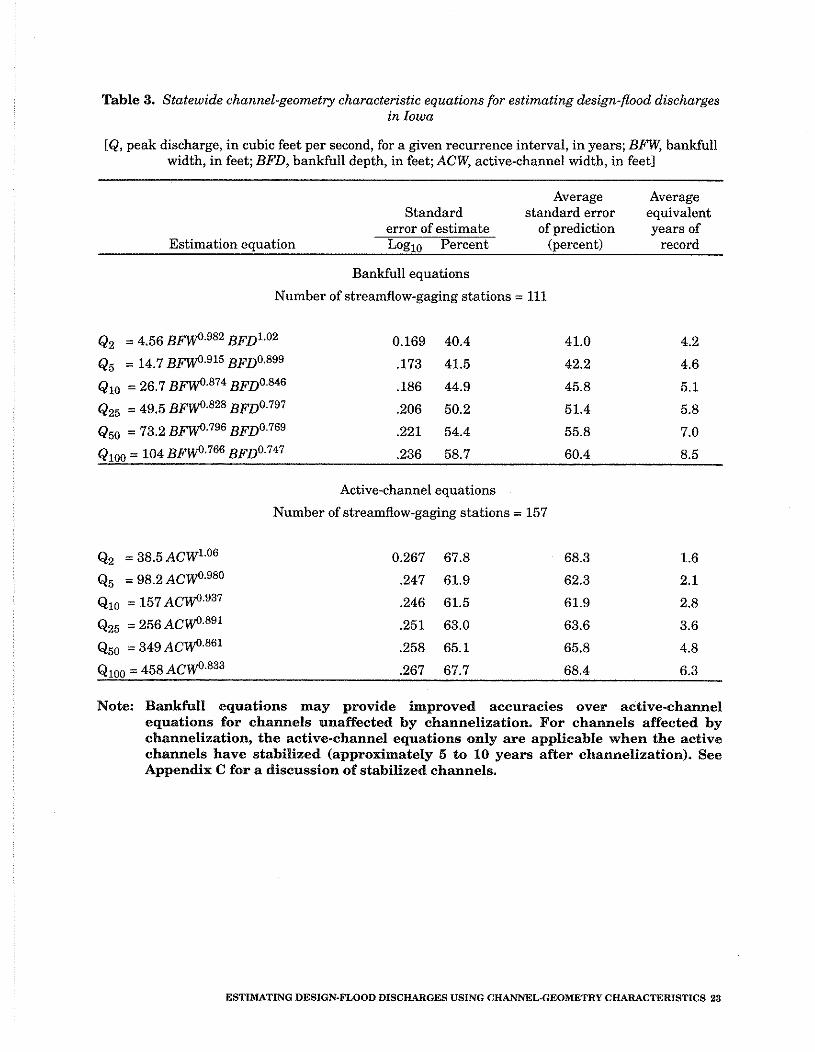
Table 3. Statewide channel-geometry characteristic equations for estimating design-flood discharges in Iowa
[Q, peak discharge, in cubic feet per second, for a given recurrence interval, in years; BFW, bankfull width, in feet; BFD, bankfull depth, in feet;ACW, active-channel width, in feet]
Average Average Standard standard error equivalent
error of estimate of prediction years of Estimation equation Loglo Percent (percent) record
Bankfull equations
Number of streamflow-gaging stations = 111
Active-channel equations
Number of streamflow-gaging stations = 157
Note: Bankfull equations may provide improved accuracies over active-channel equations for channels unaffected by channelization. For channels affected by channelization, the active-channel equations only are applicable when the active channels have stabilized (approximately 5 to 10 years after channelization). See Appendix C for a discussion of stabilized channels.
ESTIMATING DESIGN.FLOOD DISCHARGES USING CHANNEL-GEOMETRY CHARACTERISTICS 23
region (fig. 2). Consequently, both data sets were split into regional data sets, and additional multiple-regression analyses were performed for two regions in Iowa.
The State was divided into two hydrologic regions using information on areal trends of the residuals for the statewide regression equations, the Des Moines Lobe landform region, and topography as guides. The delineation of channel-geometry Regions I and 11 is shown in figure 2. The topography of the Des Moines Lobe landform region (Region 11) is characteristic of a young, postglacial landscape that is unique with respect to the topography of the rest of the State (Region I) (Prior, 1991, p. 30-47). The region generally comprises low-relief terrain, accentuated by natural lakes, potholes, and marshes, where surface-water drainage typically is poorly defined and sluggish. The shaded area between hydrologic Regions I and I1 (fig. 2) represents a transitional zone where the channel morphology of one region gradually merges into the other. This regionalization process served to compensate for the geographic bias observed in the statewide residual plots, which was not accounted for otherwise in the 111- and 157-station channel- geometry regression equations listed in table 3.
Using the OLS and WLS multiple- regression techniques previously described, two sets of flood-estimation equations were developed for each channel-geometry region. Of the lll-station data set, 78 stations were in Region I and 33 stations were in Region 11. Of the 157-station data set, 120 stations were in Region I and 37 stations were in Region 11. Gaging stations located within the regional transition zone (fig. 2) were compiled into either Region I or Region I1 data sets on the basis of residuals from the statewide regression equations and on the regional locations of their stream channels. The best equations developed in terms of PRESS statistics, coeff~cient of determination, and standard errors of estimate for the Region I data sets are listed in table 4 and the best equations developed for the Region I1 data sets are listed in table 5.
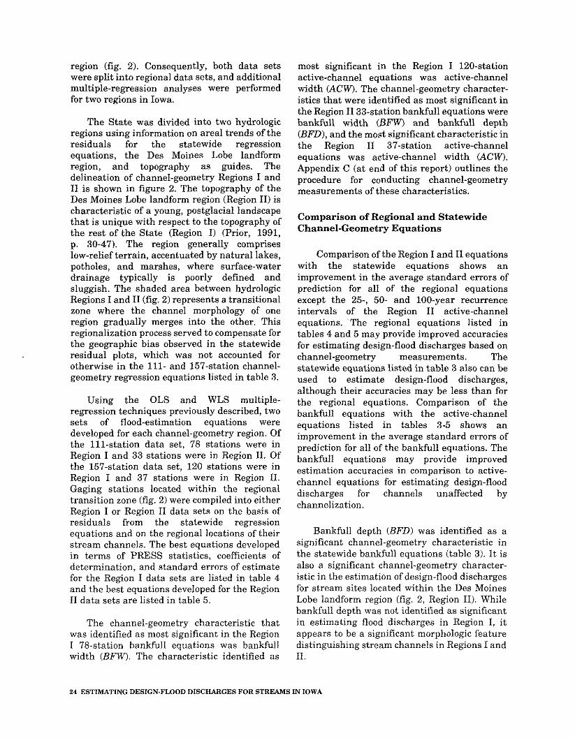
The channel-geometry characteristic that was identified as most significant in the Region I 78-station bankfull equations was bankfull width (BFW). The characteristic identified as
most significant in the Region I 120-station active-channel equations was active-channel width (ACW). The channel-geometry character- istics that were identified as most significant in the Region I1 33-station bankfull equations were bankfull width (BFW) and bankfull depth (BFD), and the most significant characteristic in the Region I1 37-station active-channel equations was active-channel width (ACW). Appendix C (at end of this report) outlines the procedure for conducting channel-geometry measurements of these characteristics.
Comparison of Regional and Statewide Channel-Geometry Equations
Comparison of the Region I and I1 equations with the statewide equations shows an improvement in the average standard errors of prediction for all of the regional equations except the 25-, 50- and 100-year recurrence intervals of the Region I1 active-channel equations. 'The regional equations listed in tables 4 and 5 may provide improved accuracies for estimating design-flood discharges based on channel-geometry measurements. The statewide equations listed in table 3 also can be used to estimate design-flood discharges, although their accuracies may be less than for the regional equations. Comparison of the bankfull equations with the active-channel equations listed in tables 3-5 shows an improvement in the average standard errors of prediction for all of the bankfull equations. The bankfull equations may provide improved estimation accuracies in comparison to active- channel equations for estimating design-flood discharges for channels unaffected by channelization.
Bankfull depth (BFD) was identified as a significant channel-geometry characteristic in the statewide bankfull equations (table 3). I t is also a significant channel-geometry character- istic in the estimation of design-flood discharges for stream sites located within the Des Moines Lobe landform region (fig. 2, Region 11). While bankfull depth was not identified as significant in estimating flood discharges in Region I, it appears to be a significant morphologic feature distinguishing stream channels in Regions I and 11.
24 ESTIMATING DESWN.FLOOD DISCHARGES FOR STREAMS IN IOWA
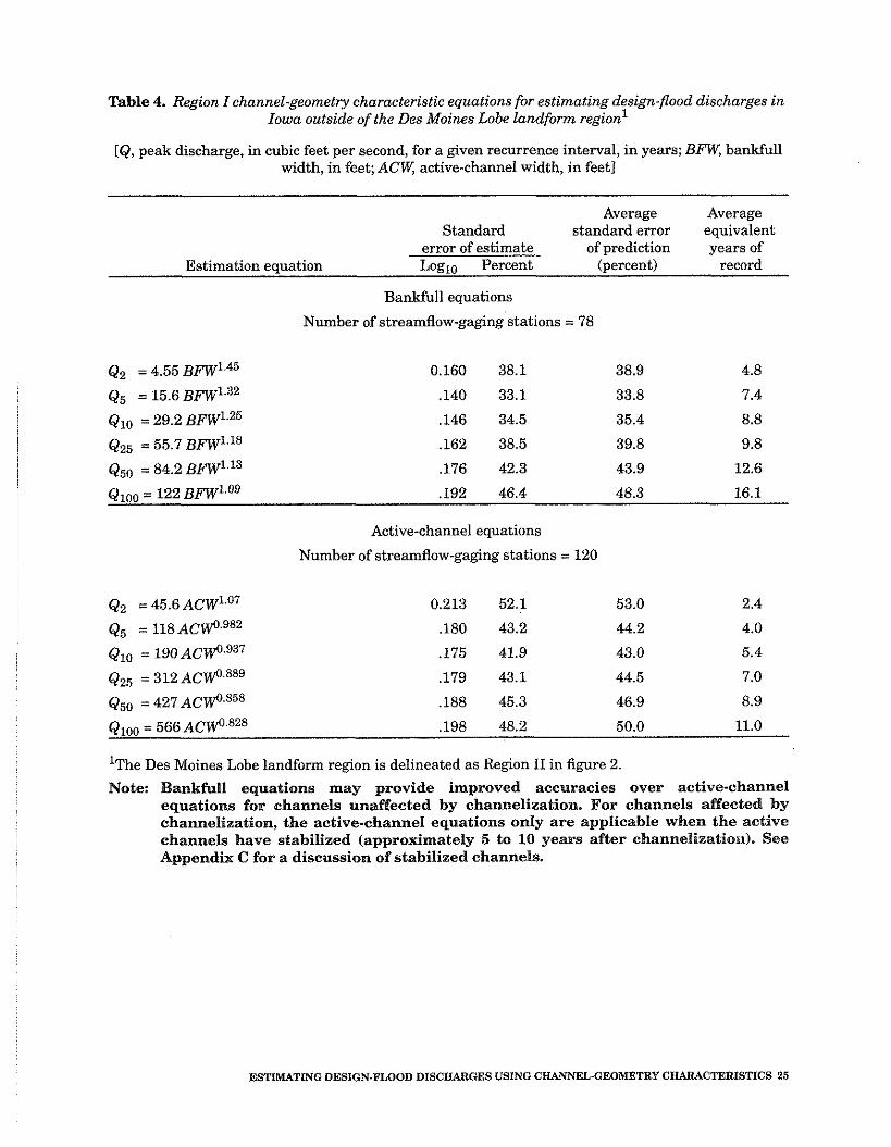
Table 4. Region I channel-geometry characteristic equations for estimating design-flood discharges in Iowa outside of the Des Moines Lobe landform region1
[Q, peak discharge, in cubic feet per second, for a given recurrence interval, in years; BFW, bankfull width, in feet; ACW, active-channel width, in feet1
Average Average Standard standard error eauivalent
error of estimate of prediction years of Estimation equation Loglo Percent (percent) record
Bankfull equations
Number of streamflow-gaging stations = 78
Active-channel equations
Number of streamflow-gaging stations = 120
he Des Moines Lobe landform region is delineated as Region I1 in figure 2.
Note: Bankfull equations may provide improved accuracies over active-channel equations for channels unaffected by channelization. For channels affected by channelization, the active-channel equations only are applicabIe when the active channels have stabilized (approximately 5 to 10 years after channelization). See Appendix C for a discussion of stabilized channels.
ESTIMATING DESIGN-FLOOD DISCHARGES USING CHANNEL-GEOMETRY CHARACTERISTICS 25
Table 5. Region TI channel-geometry characteristic equations for estimating design-flood discharges in Iowa within the Des Moines Lobe landform region1
[Q, peak discharge, in cubic feet per second, for a given recurrence interval, in years; BFN, bankfull width, in feet; BFD, bankfull depth, in feet;ACW, active-channel width, in feet]
Average Average Standard standard error equivalent
error of estimate of prediction years of Estimation equation Loglo Percent (percent) record
Bankfull equations
Number of streamflow-gaging stations = 33
Active-channel equations
Number of streamflow-gaging stations = 37
l ~ h e Des Moines Lobe landform region is delineated as Region I1 in figure 2
Note: Bankfull equations may provide improved accuracies over active-channel equations for channels unaffected by channelization. For channels affected by channelization, the active-channel equations only are applicable when the active channels have stabilized (approximately 5 to 10 years after channelization). See Appendix C for a discussion of stabilized channels.
26 ESTIMATING DESIGN-FLOOD DISCHARGES FOR STREAMS IN IOWA
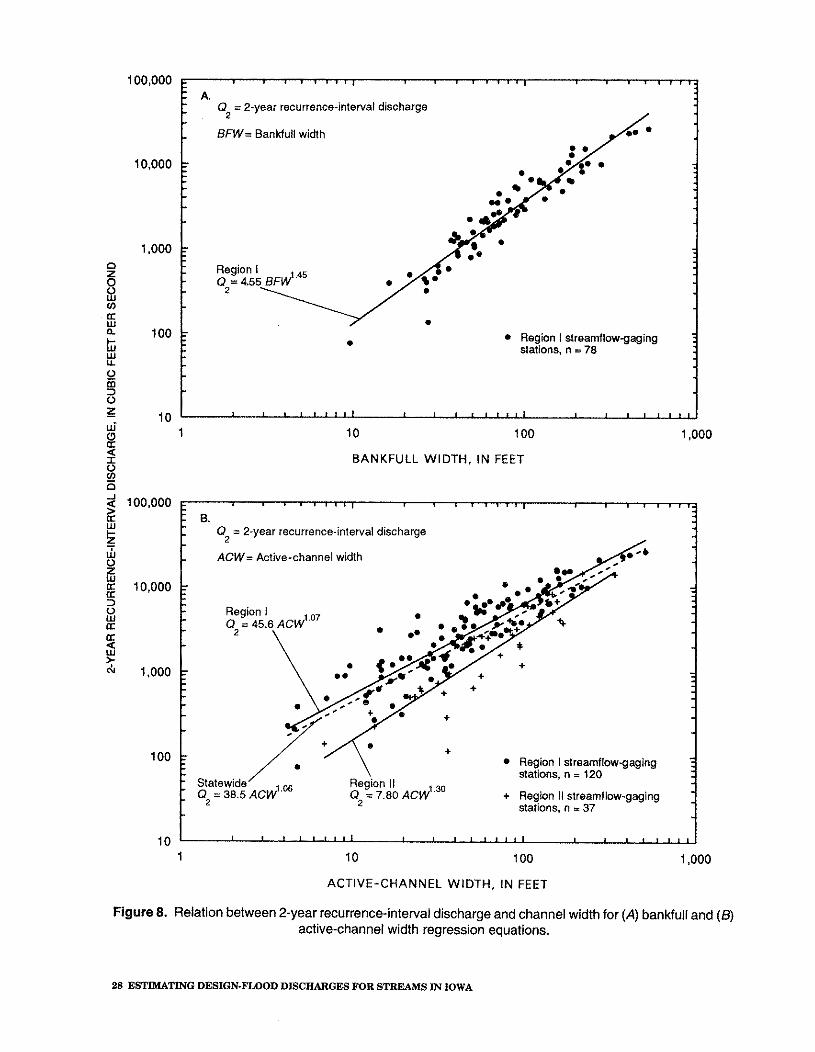
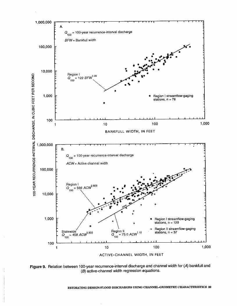
The differences in peak-discharge estimation between regional and statewide active-channel width (ACW) equations are shown in figures 8B and 9B for the 2- and 100-year recurrence intervals, respectively. Figures 8B and 9B illustrate the higher estimated peak discharges obtained from the Region I equations relative to those obtained from the Region I1 equations for a specified active-channel width. The slopes of the Region I regression lines are parallel to those of the statewide regression lines at a higher estimated discharge. The Region I1 regression lines have steeper slopes relative to the Region I and statewide regression lines but at a lower estimated discharge. Figures 8.4 and 9A illustrate the relation of the Region I, bankfull regression equations for 2- and 100-year recurrence-interval discharges, respectively. Tests performed using STATIT procedure REGGRP (Statware, Inc., 1990, p. 6-32 - 6-36) indicated that there were statistically significant differences in the slopes and intercepts of the Region I and Region I1 regression lines for both the bankfull and active-channel equations.
The paired-t test was used to test whether design-flood discharge estimates obtained by both the bankfull and active-channel regression equations for the same gaging station were significantly different a t the 95-percent level of significance. The paired-t test was applied using STATIT procedure HYPOTH (Statware, Inc., 1990, p. 3-21 - 3-23). For table 3, discharge estimates for 111 stations were not significantly different for all design-flood recurrence intervals. For table 4, discharge estimates for 78 stations were significantly different for the 2-year recurrence interval, but estimates were not significantly different for the 5-year to 100-year recurrence intervals. For table 5, discharge estimates for 33 stations were not significantly different for all design-flood recurrence intervals.
The application of the channel-geometry regression equations listed in tables 4 and 5 for a stream site are determined by two factors, and the application of the channel-geometry equations listed in table 3 are determined only by the second factor. First, the stream site is located in figure 2 to determine whether Region I or Region I1 equations apply. The user may be
faced with a dilemma if design-flood discharges are to be estimated for a stream site located within the shaded transitional zone or for a stream that crosses regional boundaries. The discharges could be estimated using both the Region I and I1 equations and hydrologic judgment used to select the most reasonable design-flood estimate, or a weighted average based on the proportion of drainage area within each region could be applied. The most reasonable alternative to resolving this dilemma may be to use the statewide equations listed in table 3 because they preclude regional subjectivity and the majority of statewide design-flood estimates calculate between Region I and Region I1 estimates.
Second, the stream site is inspected to determine whether the stream was channelized. If evidence of channelization is not found, then the bankfull equations are applicable (the first set of equations listed in tables 3, 4, and 5); if evidence of channelization is found, then the active-channel equations may be applicable for stabilized channels (the second set of equations listed in tables 3, 4, and 5). Appendix C (at end of this report) outlines a procedure for identifying channelized streams and describes the stabilization conditions for which channel- geometry measurements of channelized streams are applicable.
Examples of Equation Use--Examples 2-4
Examule 2.--Use a regional, channel- geometry equation to estimate the 100-year peak discharge for the discontinued Black Hawk Creek a t Grundy Center crest-stage gaging station (station number 05463090; map number 73, fig. 21, located in Grundy County, a t a bridge crossing on State Highway 14, at the north edge of Grundy Center, in the NW114 sec. 7, T. 87 N., R. 16 W.
Step 1. The appropriate regional equation is determined on the basis of which hydrologic region the stream site is located in and whether the stream has been channelized. This gaging station is located in Region I, and an inspection of the USGS 1:100,000-scale Grundy County map and a visit to the site show no evidence of channelization. Therefore the 100-year bankfull equation for Region I, listed in the first set of
ESTIMATING DESIGN.FL0OD DISCHARGES USING CHANNEL-GEOMETRY CHARACTERISTICS 27
! A. I I i
- Q = 2-year recurrence-interval discharge 2
BFW= BanMull width
- - - - - - -
- . Region I streamflowgaging stations, n = 78
*
I I
1 0 100
BANKFULL W I D T H , I N FEET
! B. I I 1 -
Q = Pyear recurrence-interval discharge
ACW= Active-channel width
- - -
-
* Region I streamflow-gaging - stations, n = 120
+ Region I1 streamflow-gaging stations, n = 37
I I
10 100
ACTIVE-CHANNEL WIDTH, I N FEET
Figure 8. Re la t ion b e t w e e n P y e a r recurrence-interval d i s c h a r g e a n d c h a n n e l width for (A) bankfull a n d (6) ac t ive -channe l width r e g r e s s i o n e q u a t i o n s .
28 ESTIMATING DESIGN-FLOOD DISCHARGES FOR STREAMS IN IOWA
l,OOO.OOO [i A. I I 4 - - 0 = loo-year recurrence-interval discharge
100
BFW= BanMull width
,000,000 I 3 6.
0 = 100-year recurrence-interval discharge 1W -
ACW= Active channel width - - -
- - -
e Region 1 streamflowgaging - stations, n = 120
+ Region II streamflow-gaging stations, n = 37
100 I I
1 10 100 1,000
ACTIVE-CHANNEL WIDTH, IN FEET
100,000
10,000
8 V)
% a e 1,000 W W U.
2 m 3 0 z ui 100
Figure 9. Relation between 100-year recurrence-interval discharge and channel width for (A) bankfull and (6) active-channel width regression equations.
5
- : Region I - o = 122 BFW'
100
r e Region I streamflow-gaging stations, n = 78 - 0
I 1
ESTIMATING DESIGN-FLOOD DISCHARGES USING CHANNEL-GEOMETRY CHARACTERISTICS 29
g 1 10 100 1,000 a I 0 BANKFULL WIDTH. IN FEET v, (11
equations in table 4, is determined to be the most applicable. The only channel-geometry characteristic used for the Region I bankfull equation is the bankfull width (BFW). Appendix C describes the procedure for conducting this channel-geometry measurement.
Step 2. Three bankfull widths measuring 52, 50, and 52 ft, measured along a straight channel reach about 0.75-1.0 mi downstream of the gaging station, were used to calculate an average bankfull width (BFW) of 51 ft. Figure 7B shows the bankfull reference level a t one of these channel measurement sections.
Step 3. The 100-year flood estimate for the Region I bankfull equation (table 4) is calculated as
Exam~le 3.--Use a regional channel- geometry equation to estimate the 50-year peak discharge for the Big Cedar Creek near Varina continuous-record gaging station (station number 05482170; map number 108, fig. 2), located in Pocahontas County, a t a bridge crossing on County Highway N33, 5.5 mi northeast of Varina, in the NE114 sec. 24, T. 91 N., R. 34 W.
Step 1. This gaging station is located in Region 11, and an inspection of the USGS 1:100,000-scale Pocahontas County map and a visit to the site show evidence of channelization. Therefore, the 50-year active-channel equation for Region 11, listed in the second set of
(ACW) of 25.0 ft. Figure 7 0 shows the approximate active-channel reference level for the channel reach measured to calculate an average active-channel width.
Step 3. The 50-year flood estimate for the Region I1 active-channel equation (table 5) is calculated as
Example 4.--Use a statewide channel- geometry equation in table 3 to estimate the 100-year peak discharge for the gaging station used in example 2.
Step 1. Because a statewide equation is to be used and no evidence of channelization is evident, as determined in example 2, the 100-year bankfull equation listed in the first set of equations in table 3 is applicable. Bankfull width (BFW) and bankfull depth (BFD) are the channel-geometry characteristics used for this equation. Appendix C describes the procedure for conducting these channel-geometry measurements.
Step 2. The average bankfull width (BFW) calculation of 51 ft for this stream channel is outlined in example 2.
Step 3. The average bankfull depth (BFD) for this stream channel was calculated to be 6.0 ft. The bankfull depth measurements used to determine this average are listed in the "Bankfull-Depth (BFD) Measurements" section ofAppendix C, and they are illustrated in figure - -
esuatiois in table 5, is determined to be the 10.
mist applicable. ~ e i t u r e s that are character- istic of channelized streams are illustrated in figure 70, which shows the straightened and leveed channel reach downstream of the gage. The only channel-geometry characteristic used for the Region I1 active-channel equation is the active-channel width (ACW). Appendix C describes the procedure for conducting this cbannel-geometry measurement.
Step 2. Three active-channel widths measuring 25.6, 25.3, and 24.2 ft, measured along a straight channel reach about 0.25-0.5 mi downstream of the gaging station, were used to calculate an average active-channel width
Step 4. The 100-year flood estimate for the statewide bankfull equation (table 3) is calculated as
Examples 2 and 4 illustrate the use of bankfull measurements in computing 100-year flood estimates for this gaging station using regional and statewide multiple-regression equations. The regional estimate was determined to be 8,860 ft3/s, and the statewide estimate was determined to be 8,060 ft3/s.
30 ESTIMATING DESIGN-FLOOD DISCHARGES FOR STREAMS IN IOWA
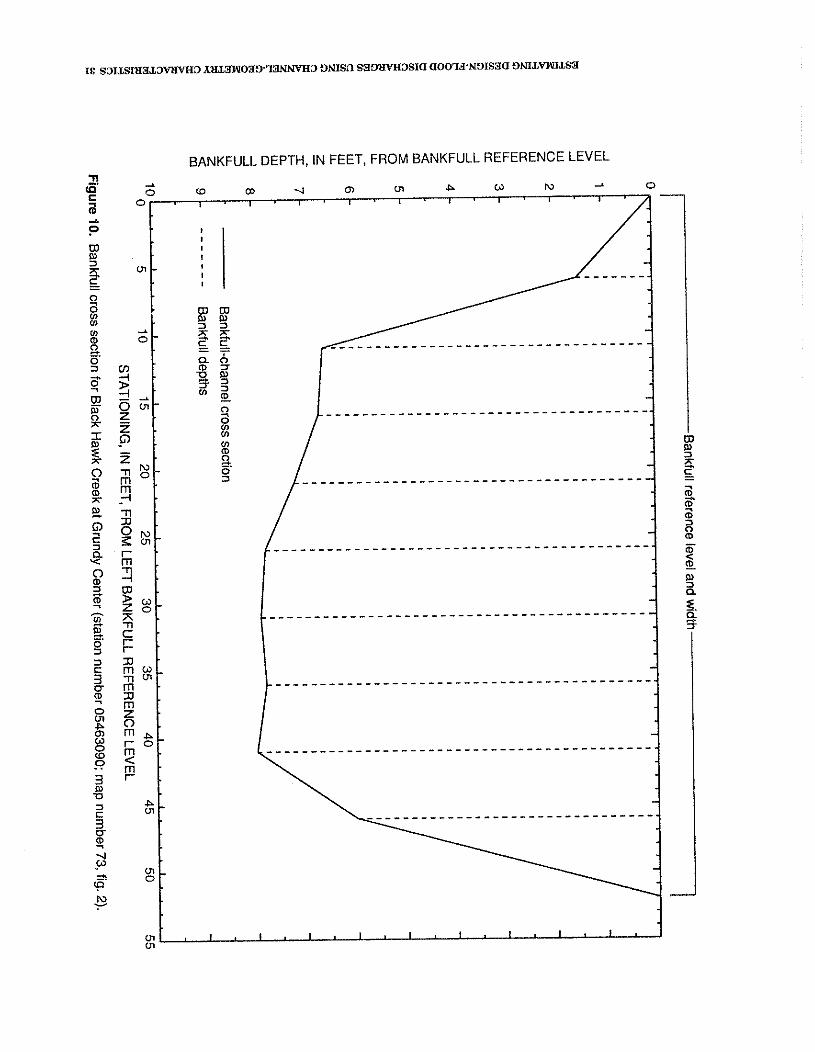
Bankfull reference level and w
idth
APPLICATION AND RELIABILITY will be within one standard error approximately OF FLOOD-ESTIlkWTION two-thirds of the time.
METHODS
The regression equations developed in this study for both the drainage-basin and channel-geometry flood-estimation methods apply only to streams in Iowa where peak streamflow is not affected substantially by stream regulation, diversion, or other human activities. The drainage-basin method does not apply to basins in urban areas unless the effects of urbanization on surface-water runoff are negligible. The channel-geometry method does not apply to channels that have been altered substantially from their stabilized conditions by human activities, as outlined in Appendix C.
Limitations and Accuracy of Equations
The applicability and accuracy of the drainage-basin and channel-geometry flood- estimation methods depend on whether the drainage-basin or channel-geometry character- istics measured for a stream site are within the range of the characteristic values used to develop the regression equations. The acceptable range for each of the drainage-basin characteristics used to develop the statewide equations (table 2) are tabulated as maximum and minimum values in table 6. Likewise, the acceptahle range for each of the channel- geometry characteristics used to develop the statewide and regional equations (tables 3-5) also are tabulated as maximum and minimum values in table 6. The applicability of the drainage-basin and channel-geometry equations is unknown when the characteristic values associated with a stream site are outside of the acceptahle ranges.
The standard errors of estimate and average standard errors of prediction listed in tables 2-5 are indexes of the expected accuracy of the regression-equation estimates in that they provide measures of the difference between the regression estimate and the Pearson Type-I11 estimate for a design-flood recurrence interval. If all assumptions for applying regression techniques are met, the difference between the regression estimate and the Pearson Type-I11 estimate for a design-flood recurrence interval
The standard error of estimate is a measure of the distribution of the observed annual-peak discharges about the regression surface (Jacques and Lorenz, 1988, p. 17). The average standard error of prediction inciudes the error of the regression equation as well as the scatter about the equation (Hardison, 1971, p. C228). Although the standard error of estimate of the regression gives an approximation of the standard error of peak discharges, the average standard error of prediction provides more precision in the expected accuracy with which estimates of peak discharges can be made. The average standard error of prediction is estimated by taking the square root of the. PRESS statistic mean. Because the standard errors of estimate and average standard errors of prediction are expressed as logarithms (base 101, they are converted to percentages by methods described by Hardison (1971, p. C230).
The average standard errors of prediction for the regression models ranged as follows: statewide drainage-basin equations, 38.6 to 50.2 percent (table 2); statewide channel-geometry bankfull equations, 41.0 to 60.4 percent (table 3); statewide channel-geometry active-channel equations, 61.9 to 68.4 percent (table 3); Region I channel-geometry bankfull equations, 33.8 to 48.3 percent (table 4); Region I channel- geometry active-channel equations, 43.0 to 53.0 percent (table 4); Region I1 channel-geometry bankfull equations, 30.3 to 52.1 percent (table 5); and Region I1 channel-geometry active- channel equations, 59.7 to 70.0 percent (table 5).
The average equivalent years of record represents an estimate of the number of years of actual streamflow record required a t a stream site to achieve a n accuracy equivalent to each respective drainage-basin or channel-geometry design-flood discharge estimate. The average equivalent years of record as described by Hardison (1971, p.C231-C233) is a function of the standard deviation and skew of the observed annual-peak discharges at the gaging stations analyzed for each respective regression equation, the accuracy of the regression equation, and the recurrence interval of the design flood. The average equivalent years of record for a design flood with a recurrence
82 ESTIMATING DESIGN-FLOOD DISCHARGES FOR STREAMS IN IOWA
Table 6. Statistical summary for selected statewide drainage-basin and channel-geometry characteristics, and for selected regional channel-geometry characteristics at streamflow-gaging
stations in Iowa
[CDA, contributing drainage area, in square miles; RR, relative relief, in feet per mile; DF, drainage frequency, in number of first-order streams per square mile; TTF, Zyear, 24-hour precipitation inten- sity, in inches; BFW, bankfull width, in feet; BFD, bankfull depth, in feet; ACW, active-channel width,
in feet]
Statewide drainage-basin characteristics
Statistic CDA RR DF TTF
Maximum 1,060 48.7 2.95 3.26 Minimum .338 1.57 ,043 2.82 Mean 209 6.48 .520 3.11 Median 80.7 4.45 ,510 3.14 No. of sites 164 164 164 164
Statewide channelgeometry characteristics
Statistic BFW BFD ACW
Maximum 523 17.1 510 Minimum 9.6 1.7 4.2 Mean 110 7.0 77.0 Median 82.7 6.7 49.8 No. of sites 111 111 157
Regional channel-geometry characteristics
Region I Region I1
Statistic BFW ACW BFW BFD ACW
Maximum 523 510 361 12.5 339 Minimum 9.6 4.2 19.3 2.0 6.9 Mean 106 73.7 120 6.6 87.4 Median 71.0 46.1 106 6.6 73.3 No. of sites 78 120 33 33 37
interval of T-years is calculated as (Hardison, mean weighted skew coefficient 1971, p. C231) of the logarithms (base 10) of the
observed annual-peak discharges
2 S (13) a t the gaging stations used in
~ = r (GF each respective regression-model
data set and the recurrence
where E is the average equivalent years of interval relating the standard record, in years; error of a T-year peak discharge
to the index of variability (i) and r is a factor that is a function of the the number of observed annual-
APPLICATION AND RELLABILITY OF FLOOD.ESTIMATM1N METHODS 33
peak discharges; 100-year flood bankfull equation (table 4) and
- assuming the standard errors for measuring s is an index of variability equal to channel width reported by Wahl(1976), the
the mean standard deviation of the logarithms (base 10) of the observed annual-peak discharges a t the gaging stations used in each respective regression-model data set; and
SE, is the average standard error of prediction, in log units (base 101, estimated using the Press statistic.
Several of the primary drainage-basin characteristics used in the regression equations listed in table 2 are map-scale dependent. Use of maps of scales other than the scales used to develop the equations may produce results that do not conform to the range of estimation accuracies listed for the equations in table 2. The scale of map to use for manual measurements of each primary drainage-basin characteristic is outlined in Appendix A and Appendix B.
An additional constraint in the application and reliability of the channel-geometry characteristic equations is the requirement to obtain onsite measurements of bankfull or active-channel width, and possibly bankfull depth. Training and experience are required to properly identify the bankfull and active- channel features in order to make these measurements. The variability in making these measurements can be large, even among experienced individuals. As reported by Wahl (19761, based on a test conducted in northern Wyoming, the standard error in estimated discharge due to variation in width measure-
true standard error = [ ( 0 . 1 ~ 2 ) ~ + (0.13)~ + (0.06)~l 06, = 0.240.
This yields an average standard error of 59.6 percent compared to 46.4 percent for the regression equation alone. Wahl (1984, p. 64) notes that the variability of the measurements collected in the Wyoming test probably is greater than normally would be encountered in applying channel-geometry measurements in a particular hydrologic area. Sites in the Wyoming test were chosen for their diversity, and they ranged from ephemeral streams in a nearly desert environment to perennial streams in a high mountain environment.
Despite the limitations associated with the channel-geometry method, the equations presented in this report are considered to be useful as a corroborative flood-estimation method with respect to the drainage-basin method. The channel-geometry equations are applicable to all unregulated, stabilized stream channels in the State, whereas the drainage- basin equations are applicable only to stream sites with drainage areas less than 1,060 mi2. Although the error of measurement may be larger for channel-geometry characteristics than for drainage-basin characteristics, the variability of channel-geometry measurements made in Iowa are assumed to be not as great as reported by Wahl (1984) for the Wyoming test. An additional advantage in utilizing the channel-geometry method is that design-flood discharge estimates obtained from each flood-estimation method can be used to calculate a weighted average as described in the following section.
ments alone was about 30 percent (0.13 log unit). Variation in bankfull-depth measure- Weighting Design-Flood Discharge ments probably would increase this standard error in estimated discharge. Wahl (1976) also noted an average bias with respect to the mean channel width of about 14 percent (0.06 log unit). A truer total standard error, in log units, for a channel-geometry discharge estimate is calculated by Wahl (1984, p. 63) as the square root of the sums of the squares of the errors of the regression equation and of the variation and average bias in width measurements. Using the standard error of estimate for the Region I,
Design-flood discharges determined using both the drainage-basin and channel-geometry flood-estimation methods are presumed to be independent from each other. Each flood- estimation method thus can be used to verify results from the other; when design-flood discharge estimates are independent, the independent estimates can be used to obtain a weighted average (IACWD, 1982, p. 8-11,
34 ESTIMATING DESIGN.FL0OD DISCHARGES FOR STREAMS IN IOWA
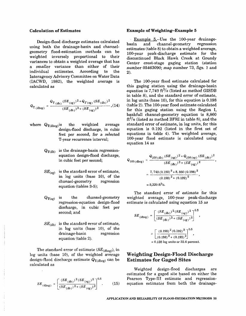
Calculation of Estimates Example of Weighting--Example 6
Design-flood discharge estimates calculated using both the drainage-basin and cbannet- geometry flood-estimation methods can be weighted inversely proportional to their variances to obtain a weighted average that has a smaller variance than either of their individual estimates. According to the Interagency Advisory Committee on Water Data (IACWD, 19821, the weighted average is calculated as
where QTCdbcg)is the weighted average design-flood discharge, in cubic feet per second, for a selected T-year recurrence interval;
QT(dbj is the drainage-basin regression- equation design-flood discharge, in cubic feet per second;
SE(cg) is the standard error of estimate, in log units (base lo), of the channel-geometry regression equation (tables 3-5);
QT(cg) is the channel-geometry regression-equation design-flood discharge, in cubic feet per second; and
SEcdh) is the standard error of estimate, in log units (base 101, of the drainage-basin regression equation (table 2).
The standard error of estimate (SE(dbcg)), in log units (base lo), of the weighted average design-flood discharge estimate QT(,jbcgj can be calculated as
F x a m ~ l e 5.--Use the 100-year drainage- basin and channel-geometry regression estimates (table 8) to obtain a weighted average, 100-year peak-discharge estimate for the discontinued Black Hawk Creek a t Grundy Center crest-stage gaging station (station number 05463090; map number 73, figs. 1 and 2).
The 100-year flood estimate calculated for this gaging station using the drainage-basin equation is 7,740 ft3/s (listed as method GISDB in table 8), and the standard error of estimate, in log units (base 101, for this equation is 0.198 (table 2). The 100-year flood estimate calculated for this gaging station using the Region I, bankfull channel-geometry equation is 8,860 ft3/s (listed as method BFRI in table 8), and the standard error of estimate, in log units, for this equation is 0.192 (listed in the first set of equations in table 4). The weighted average, 100-year flood estimate is calculated using equation 14 as
The standard error of estimate for this weighted average, 100-year peak-discharge estimate is calculated using equation 15 as
= 0.138 lag units or 32.6 percent
Weighting Design-Flood Discharge Estimates for Gaged Sites
Weighted design-flood discharges are estimated for a gaged site based on either the Pearson Type-111 estimate and regression- equation estimates from both the drainage-
APPLICATION AND RELIABILITY OF FLOOD.ESTIMAT1ON METHODS 36
basin and channel-geometry flood-estimation methods or on the Pearson Type-I11 estimate and only one of the regression-equation estimates. The design-flood discharge estimate is a weighted average of these values in which the Pearson Type-I11 estimate for the gaged site is weighted by the effective record length (ERL) a t the gaged site, and the regression-equation estimates are weighted by the average equivalent years of record associated with their respective regression equations.
Calculation of Estimates
The weighted design-flood discharge estimate for a gaged site as outlined by the Interagency Advisory Committee on Water Data (IACWD, 1982, p. 8-1 - 8-2) is calculated as
where QT(T(wg) is the weighted design-flood discharge for a gaging station, in cubic feet per second, for a selected T-year recurrence internal;
Q T ( ~ ) is the Pearson Type-I11 design-flood discharge for a gaging station, in cubic feet per second, as determined by the analysis of the observed annual-peak discharge record (listed as method B17B in table 8);
ERL is the effective record length for a gaging station, in years, representing the QT(g) analysis (table 8);
QT(gdb) is the drainage-basin regression- equation design-flood discharge for a gaging station, in cubic feet per second, (listed as method GISDB in table 8);
E(db) is the average equivalent years of record for the drainage-basin regression equation used to determine QT(gdb) (table 2);
Q T ~ ) is the channel-geometry
regression-equation design-flood discharge for a gaging station, in cubic feet per second, (listed as either method BFRI, ACRI, ACRII, or BFRII in table 8); and
E(cg) is the average equivalent years of record for the channel-geometry regression equation used to determine QT(gcg) (table 4 or 5).
If both the drainage-basin regression- equation estimate QT(gdb), and the channel- geometry regression-equation estimate QT(gcg) are not available for a gaged site, then equatlon 16 used to calculate the weighted design-flood discharge estimate QT(wgl is simplified to the
weighting of two estimates based on QT(g) and ERL and either QT(gdb), and E(db) or QT(gcg) and E(,g). An example of weighting a gaged site with only one regression-equation estimate is illustrated in "Example 7."
By including both the drainage-basin and channel-geometry regression-equation esti- mates, or only one of these estimates, with the computed Pearson Type-I11 estimate for a gaged site, design-flood histories for a relatively long period of time are incorporated into the weighted estimate for the gaged site and tend to decrease the time-sampling error (Choquette, 1988, p. 41). Climatic conditions during a short gaged period of record often are not indicative of the longer term climatic variability associated with a particular gaging station. Such time-sampling error may be particularly large when the observed gaged period of record represents an unusually wet or dry climatic cycle compared to the longer term average climatic conditions. Time-sampling error thus is minimized for a gaging station by weighting the design-flood discharge estimate QT(wg)
Examples of Weighting--Examples 6-7
Exam~le 6.--Calculate a weighted 100-year peak-discharge estimate for the discontinued Black Hawk Creek a t Grundy Center crest-stage gaging station (station number
$6 ESTIMATING DESIGN-FLOOD DISCHARGES FOR STREAMS IN IOWA
05463090; map number 73, figs. 1 and 2). An Estimating Desim-Flood - - inspection of table 8 lists regression-equation J-J~~~.~~~~~ for an ungaged site on a estimates for both the drainage-basin and channel-ge0metr.y flood-estimation methods. Gaged Stream The 10Gyear Pearson Type-I11 estimate is 8,320 ft3/s, and the effective record length is 24 Design-flood discharges for an ungaged site
years (table 8). The 100-year drainage-basin on a gaged stream can be estimated if the total regression estimate is 7,740 ft3/s (tabIe 8), and drainage area of the ungaged site is between 50 the average equivalent years of record for this and 150 percent of the total drainage area of the regression equation is 11.5 (table 2). The gaged site by an adjustment procedure 100-year Region I, bankfull channel-geometry described by Choquette (1988, p. 42-45) and regression estimate is 8,860 ft3/s (table 8), and Koltun and Roberts (1990, p. 6-8). This the average equivalent years of record for this procedure uses flood-frequency information regression equation is 16.1 (listed in the first set from the Pearson Type-111 and of equations in table 4). The weighted 100-year egression-equation estimates a t the gaged site flood estimate for this gaging station is to adjust the regression-equation estimate at calculated using equation 16 as the ungaged site.
- (Q1OO(g) ) (ERL) + (QlOO (gdb)) ( E ( d b ) ) + ( Q l O ~ g c g ) ) ( E ( c g ) ) Q100(,) -
E R L f E ( d b ) +*(cg)
Exam~le 7.--Calculate a weighted 50-year peak-discharge estimate for the discontinued Fox River at Bloomfield gaging station (station number 05494300; map number 133, fig. 11, located in Davis County, a t a bridge crossing on a county highway, about 0.5 mi north of Bloomfield, in the SE114 sec. 13, T. 69 N., R. 14 W. Table 8 lists a regression-equation estimate for only the drainage-basin flood-estimation method. The 50-year Pearson Type-I11 estiniate is 10,600 ft3/s, and the effective record length is 21 years (table 8). 'The flood-frequency curve developed from the Pearson Type-111 analysis for this gaging station is shown in figure 3. The 50-year drainage-basin regression estimate is 7,600 ft3/s (table 81, and the average equivalent years of record for this regression equation is 9.5 (table 2). The weighted 50-year flood estimate for this gaging station is calculated using a simplified version of equation 16 as
Calculation of Estimates
The regression-equation estimate for the ungaged site is determined as one of the following: (1) the weighted average QT(dbeg)
calculated from both the drainage-basin and channel-geometry regression-equation esti- mates using equation 14 or (2) the regression- equation estimate of QT(db) or QT(cg) calculated from either one of these flood-estimation methods. The calculation for this adjustment procedure is
where QT(au) is the adjusted design-flood discharge for the ungaged site, in cubic feet per second, for a selected T-year recurrence interval;
- ( Q ~ o ( ~ ) ) ( E R L ) + (Q50(gdb)) ( E ( d b ) ) Q50(wg) - is the regression design-flood
E R L + E ( d b ) discharge for the ungaged site, in cubic feet per second, determined as one of the following: (1) the weighted average of both the drainage-basin and channel-
APPLICATION ANP) RELLABILZTY OF FLOOD-ESTM4TION METWODS 87
geometry regression-equation estimates QT(dbcg) (equation 14); (21 only the drainage-basin regression-equation estimate QT(db); or (3) only the channel- geometry regression-equation estimate QT(cg);
AF is the adjustment factor for the gaged site and is calculated as
where QT(wg) is the weighted design-flood discharge for the gaged site, in cubic feet per second, as defined by equation 16;
QT(,.~) is the regression design-flood discharge for the gaged site, in cubic feet per second, determined as one of the following: (1) the weighted average of both the drainage-basin and channel- geometry regression-equation estimates QT(dbcg), as defined by equation 14; (2) only the drainage-basin regression- equation estimate QT(db); or (3) only the channel-geometry regression-equation estimate Q~(cg);
ATDA is the absolute value of the difference between the total drainage area of the gaged site (TDAg) and the total drainage area of the ungaged site; and
TDAg is the total drainage area of the gaged site, in square miles, listed as the published drainage area in table 9.
This procedure (1) adjusts the regression-equation estimate for the ungaged site QT(ru) by the ratio A F when the total drainage area of the ungaged site equals the total drainage area of the gaged site TDAg and (2) prorates the adjustment to 1.0 as the difference in total drainage area between the gaged site and the ungaged site approaches
either 0.5 or 1.5 of the total drainage area of the gaged site. In other words, when the total drainage area of the ungaged site is 50 percent larger or 50 percent smaller than the total drainage area of the gaged site, no adjustment is applied to the regression-equation estimate for the ungaged site Q T ( ~ ) .
Example of Estimation Method--Example 8
Exam~le 8.--Determine the 50-year peak- discharge estimate for an ungaged site on Otter Creek, located on the Osceola and Lyon County line, a t a bridge crossing on County Highway L26,4.75 mi southwest of Ashton, in the $W1/4 sec. 31, T. 98 N., R. 42 W. Because a crest-stage gaging station is located on this stream, Otter Creek near Ashton (station number 06483460; map number 139, fig. 11, the 50-year recurrence interval regression-equation estimate calculated for the ungaged site can be adjusted by the weighted 50-year flood-discharge estimate calculated for the gaged site. Estimating the adjusted 50-year peak discharge for the ungaged site Q50(au) (equation 17) involves four steps.
Step 1. A regression-equation estimate Q50(ru) (equation 17) is calculated for the ungaged site. Both drainage-basin and channel- geometry flood-estimation methods could be used to calculate a weighted average estimate Q50(dbcg) (equation 14) for the regression estimate (Qso(,,)) or only one of these flood-estimation methods could be used to calculate the regression-equation estimate (Q50(ru)). For this example, only the statewide drainage-basin estimate (Q50(db)) (table 2) will be used for the 50-year recurrence interval regression-equation estimate (Qso(,,)) a t the ungaged site because channel-geometry measurements were not collected for calculating a channel-geometry estimate (Q50(cg)).
(A). The characteristics used in the drainage-basin equation (table 2) are contributing drainage area (CDA), relative relief (RR), drainage frequency (DF), and 2-year, 24-hour precipitation intensity (TTF). The primary drainage-basin characteristics used in this equation are total drainage area (TDA), noncontributing drainage area (NCDA), basin relief (BR), basin perimeter (BP), number of first-order streams (FOS), and 2-year, 24-hour
38 ESTIMATING DESIGN-FLOOD DISCHARGES FOR STREAMS IN IOWA
Step 2. The weighted 50-year peak discharge for the gaged site Q50(wg) (equation 16) is estimated next. Because table 8 lists both the drainage-basin and channel-geometry regression-equation estimates for this gaged site, Otter Creek near Ashton (station number 06483460, map number 139, fig. I), the weighted estimate will be based on the Pearson Type-111 estimate and both of these regression-equation estimates.
The 50-year Pearson Type-I11 estimate is 11,100 ft3/s, and the effective record length is 39 years (table 8). The 50-year drainage-basin regression estimate is 6,710 ft3/s (listed as method GISDB in table 8), and the average equivalent years of record for this regression equation is 9.5 (table 2). The 50-year Region I, active-channel channel-geometry regression estimate is 9,260 ft3/s (listed as method ACRI in table 8), and the average equivalent years of record for this regression equation is 8.9 (listed in the second set of equations in table 4). The weighted 50-year flood estimate for the gaged site is calculated using equation 16 as
9,260 ft3/s (listed as method ACRI in table 8), and the standard error of estimate, in log units, for this equation is 0.188 (listed in the second set of equations in table 4). The weighted average, 50-year flood estimate for the gaged site is calculated using equation 14 as
Because Q50(dbcgS= Q50(rg) in this example, then Q50(rg) = 7,960 ft IS.
Step 4. The final step adjusts the 50-year recurrence interval regression-equation est- imate of 8,550 ft3/s calculated for the ungaged site by the 50-year recurrence interval information determined for the gaged site. The adjusted 50-year flood estimate for the ungaged site Q50(au) is calculated using equations 17 and 18 as
Step 3. The regression-equation estimate for the gaged site Q50(rg) (equation 18) is determined next. Because table 8 lists both the drainage-basin and channel-geometry regression estimates for this gaged site, Otter Creek near Ashton, the weighted average of these regression estimates Q60(dbcg) (equation 14) is calculated to determine the regression estimate Q50(rg).
The 50-year flood estimate calculated for this gaging station using the drainage-basin equation is 6,710 ft3/s (listed as method GISDB in table 8), and the standard error of estimate, in log units (base 101, for this equation is 0.185 (table 2). The 50-year flood estimate calculated for this gaging station using the Region I, active-channel channel-geometry equation is
ATDA is the absolute value of the difference between the total drainage area of the gaged site (88.0 mi2) and the total drainage area of the ungaged site (120 mi2),
ATDA = 32.0 mi2; TDA, = 88.0 mi2;
This adjustment procedure has increased the 50-year recurrence interval regression- equation estimate for the ungaged site &50(ru) by
40 ESTIMATING DESIGN-FLOOD DISCHARGES FOR STREAMS IN IOWA
107.4 percent based on the 50-year recurrence interval information determined for the gaged site upstream of this ungaged site.
SUM CONCLUSIONS
Drainage-basin and channel-geometry equations are presented in this report for estimating design-flood discharges having recurrence intervals of 2, 5, 10, 25, 50, and 100 years at stream sites on rural, unregulated streams in Iowa. The equations were developed using ordinary least-squares and weighted least-squares multiple-regression techniques. Statewide equations were developed for the drainage-basin flood-estimation method and statewide and regional equations were developed for the channel-geometry flood- estimation method. The drainage-basin equations are applicable to stream sites with drainage areas less than 1,060 mi2, and the channel-geometry equations are applicable to stabilized stream channels in Iowa.
Flood-frequency curves were developed for 188 continuous-record and crest-stage gaging stations on unregulated rural streams in Iowa. Pearson Type-I11 estimates of design-flood discharges are reported for these gaging stations.
Regression analyses of Pearson Type-I11 design-flood discharges and selected drainage- basin characteristics, quantified using a geographic-information-system (GIs) proce- dure, were used to develop the statewide drainage-basin flood-estimation equations. The significant characteristics identified for the drainage-basin equations included contributing drainage area; relative relief; drainage frequency; and 2-year, 24-hour precipitation intensity. The regression coefficients for these equations indicated an increase in design-flood discharges with increasing magnitude in the values of each drainage-basin characteristic. The average standard errors of prediction for the drainage-basin equations ranged from 38.6 to 50.2 percent.
Techniques on how to make manual measurements from topographic maps for the primary drainage-basin characteristics used in the regression equations are presented along with examples. Several of the primary
drainage-basin characteristics used in the regression equations are map-scale dependent. Use of maps of scales other than the scales used to develop the equations may produce results that do not conform to the range of estimation accuracies listed for the equations.
Regression analyses of Pearson Type-I11 design-flood discharges and selected channel-geometry characteristics were used to develop both statewide and regional channel- geometry equations. On the basis of a geographic bias identified from the statewide regression residuals, two channel-geometry hydrologic regions were defined for Iowa relative to the Des Moines Lobe landform region. The significant channel-geometry characteristics identified for the statewide and regional regression equations included bankfull width and bankfull depth for natural channels unaffected by channelization, and active- channel width for stabilized channels affected by channelization. The regression coefficients for the statewide and regional channel- geometry equations indicated an increase in design-flood discharges with increasing magnitude in the values of each channel- geometry characteristic. The average standard errors of prediction for the statewide regression equations ranged from 41.0 to 68.4 percent and for the regional regression equations from 30.3 to 70.0 percent. The regional channel-geometry regression equations provided an improved estimation accuracy compared to the statewide regression equations, with the exception of the Region I1 active-channel regression equations developed for design floods having recurrence intervals of 25,50, and 100 years. Guidelines for measuring the channel-geometry character- istics used in the statewide and regional regression equations are presented along with examples.
Procedures for applying the drainage-basin and channel-geometry regression equations vary and depend on whether the design-flood discharge estimate is for a site on an ungaged stream, an ungaged site on a gaged stream, or a gaged site. When both a drainage-basin and a channel-geometry regression-equation estimate are available for a stream site, a procedure is presented for determining a weighted average of the two flood estimates. The procedure for estimating a design-flood discharge for an
SUMMARY AND CONCLUSIONS 41
ungaged site on a gaged stream is based on information from the Pearson Type-I11 estimate for the gaged site, and on information from either both flood-estimation methods, or from only one of the methods. At a gaged site, a weighted design-flood discharge is estimated from the Pearson Type-I11 estimate, and from either both flood-estimation methods, or from only one of the methods. Examples are provided for each of these procedures.
The drainage-basin and channel-geometry flood-estimation methods presented in this report each measure characteristics that are presumed to be independent of each other. The drainage-basin flood-estimation method is based on measurements of morphologic and climatic characteristics that are related to how water flows off the land. The drainage-basin method measures the varying flood potential a t stream sites as defined by differences in basin size, topographic relief, stream development, and ureciuitation. The channel-eeometrv - flood-estimation method, in contrast, is based on measurements of channel morphology that are assumed to be a function of streamflow discharges and sediment-load transport. The channel-geometry method measures the variability of floods that have actually occurred as defined by differences in channel width and depth.
The drainage-basin flood-estimation method developed in this study is similar to the regional flood-estimation method developed in a previous study because both methods estimate flood discharges on the basis of morphologic relations. While the standard errors of estimate for the drainage-basin equations in this study appear to be higher, a direct comparison cannot be made because of the different methodologies used to develop the equations.
The statewide drainage-basin and statewide channel-geometry regression equations presented in this report provide flood- estimation methods that minimize the subjectivity in their application to the ability of the user to measure the characteristics. Although the user of the regional channel- geometry equations may still encounter a dilemma when a stream site is located within the transitional zone or when a stream crosses regional boundaries, application of the
statewide channel-geometry equations may be utilized to preclude the regional subjectivity associated with estimating a design-flood discharge in this situation. Despite the greater variability in the error of measurement associated with the channel-geometry characteristics, the channel-geometry equations presented in this report are considered to be useful as a corroborative flood-estimation method with respect to the drainage-basin method.
The estimation accuracy of the drainage- basin regression equations possibly could be improved if drainage-basin characteristics were quantified from larger scale data. The drainage-basin characteristics quantified by the GIs procedure were limited to the 1:250,000- and 1:100,000-scale digital cartographic data currently available for Iowa.
REFERENCES
Allen, D.M., 1971, Mean square error of prediction as a criterion for selecting prediction variables: Technometrics, v. 13, p. 469-475.
Baker, D.G., and Kuehnast, E.L., 1978, Climate of Minnesota, part X--Precipitation normals for Minnesota, 1941-1970: Minnesota Agricultural Experiment' Station Technical Bulletin 314, 15 p.
Choquette, A.F., 1988, Regionalization of peak discharges for streams in Kentucky: U.S. Geological Survey Water-Resources Investigations Report 87-4209,105 p.
Dempster, G.R., Jr., 1983, Instructions for streamflowhasin characteristics file: U.S. Geological Survey National Water Data Storage and Retrieval System (WATSTORE), v. 4, chap. 11, sec. A, 34 p.
Eash, D.A., 1993, A geographic information system procedure to quantify physical basin characteristics, in Harlin, J.M., and Lanfear, K.J., eds., Proceedings of the Symposium on Geographic Information Systems and Water Resources: American Water Resources Association Technical Publication Series TPS-93-1, p. 173-182.
42 ESTIMATING DESIGN-FLOOD DISCHARGES FOR STREAMS IN IOWA
Fields, F.K., 1975, Estimating streamflow characteristics for streams in Utah using selected channel-geometry parameters: U.S. Geological Survey Water-Resources Investigations 34-74,19 p.
Guy, H.P., 1969, Laboratory theory and methods for sediment analysis: U.S. Geological Survey Techniques of Water- Resources Investigations, book 5, chap. C-I, 58 p.
Hardison, C.H., 1971, Prediction error of regression estimates of streamflow characteristics at ungaged sites: U.S. Geological Survey Professional Paper 7504, p. C228-C236.
Hedman, E.'R., and Kastner, W.M., 1977, Streamflow characteristics related to channel geometry in the Missouri River basin: U.S. Geological Survey Journal of Research, v. 5, no. 3, p. 285-300.
Hershfield, D.M., 1961, Rainfall frequency atlas of the United States: Washington, D.C., U.S. Department of Commerce, Weather Bureau Technical Paper No. 40,115 p.
Iman, R.L., and Conover, W.J., 1983, A modern approach to statistics: New York, Wiley and Sons, 497 p.
Interagency Advisory Committee on Water Data (IACWD), 1982, Guidelines for determining flood flow frequency: Hydrology Subcom- mittee Bulletin 17B, 28 p. and appendices.
Jacques, J.E., and Lorenz, D.L., 1988, Techniques for estimating the magnitude and frequency of foods in Minnesota: U.S. Geological Survey Water-Resources Investigations Report 87-4170,48 p.
Kirby, W.H., 1981, Annual flood frequency analysis using U.S. Water Resources Council guidelines (Program 5407): U.S. Geological Survey National Water Data Storage and Retrieval System (WATSTORE), v. 4, chap. I, sec. C, 57 p.
Koltun, G.F., and Roberts, J.W., 1990, Techniques for estimating flood-peak discharges of rural, unregulated streams in Ohio: U.S. Geological Survey Water-
Resources Investigations Report 89-4126, 68 p.
Lara, O.G., 1973, Floods in Iowa--Technical manual for estimating their magnitude and frequency: Iowa Natural Resources Council Bulletin 13, 56 p.
-1987, Method for estimating the magnitude and frequency of floods at ungaged sites on unregulated rural streams in Iowa: U.S. Geological Survey Water-Resources Investigations Report 87-4132,34 p.
Larimer, O.J., 1957, Drainage areas of Iowa streams: Iowa Highway Research Board Bulletin No. 7 (reprinted 1974), 439 p.
Majure, J.J., and Soenksen, P.J., 1991, Using a geographic information system to determine physical basin characteristics for use in flood-frequency equations, in Balthrop, B.H., and Terry, J.E., eds., U.S. Geological Survey National Computer Technology Meeting--Proceedings, Phoenix, Arizona, November 14-18, 1988: U.S. Geological Survey Water-Resources Investigations Report 90-4162, p. 31-40.
Mallows, C.L., 1973, Some comments on Cp: Technometrics, v. 15, p. 661-675.
Marquardt, D.W., 1970, Generalized inverses, ridge regression, biased linear estimation, and nonlinear estimation: Technometrics, v. 12, p. 591-612.
Melton, M.A., 1957, An analysis of the relations among elements of climate, surface properties, and geomorphology: Office of Naval Research, Geography Branch, Columbia Univ. Dept. of Geology, New York, Technical Report 11, Project NR 389-042, 102 p.
Montgomery, D.C., and Peck, E.A., 1982, Introduction to linear regression analysis: New York, Wiley and Sons, 504 p.
Office of Water Data Coordination, 1978, Physical basin characteristics for hydrologic analysis, in National handbook of recom- mended methods for water-data acquisition: U.S. Geological Survey, Reston, Va., chap. 7, 38 p.
REFERENCES 43
Osterkamp, W.R., 1979, Variation of alluvial- channel width with discharge and character of sediment: U.S. Geological Survey Water-Resources Investigations 79-15,ll p.
Osterkamp, W.R., and Hedman, E.R., 1977, Variation of width and discharge for natural high-gradient stream channels: Water Resources Research, v. 13, no. 2, p. 256-258.
- 1982, Perennial-streamflow characteristics related to channel geometry and sediment in the Missouri ~ i v e i s as in: U.S. Geological Survey Professional Paper 1242,37 p.
Stedinger, J.R., and Cohn, T.A., 1986, Flood frequency analysis with historical and paleoflood information: Water Resources Research, v. 22, no. 5, p. 785-793.
Strahler, A.N., 1952, Dynamic basis of geomorphology: Bulletin of the Geological Society of America, v. 63, p. 923-938.
-1958, Dimensional analysis applied to fluvially eroded landforms: Bulletin of the Geological Society of America, v. 69, p. 279-300.
- 1964, Quantitative geomorphology of Parrett, Charles, Hull, J.A., and Omang, R.J., drainage basins and channel networks. in -
1987, Revised techniques for estimating Chow, V.T., ed., Handbook of applied peak discharges from channel width in hydrology: New York, McGraw-Hill, Montana: U.S. Geological Survey Water- p. 4-39-4-76. Resources Investigations Report 87-4121, 34 p. Tasker. G.D.. 1980. Hvdrolonic renression with
weighted' least' squares:- water Resources Pickup, G., and Rieger, W.A., 1979, A conceptual Research, v. 16, no. 6, p. 1107-1113.
model of the relationship between channel characteristics and discharge: Earth ~ ~ ~ k ~ ~ , G.D., and ~ h ~ ~ ~ ~ , w,o,, 1978, ~ l ~ ~ d Surface Processes, v. 4, p. 37-42. frequency analysis with pre-record
infirmation: ~ o u r n a l of ~ydraul ics Division, Prior, J.C., 1991, Landforms of Iowa: Iowa City, American Society of Civil Engineers, v. 104, Iowa Department of Natural Resources, no. 12, p. 249-259. University of Iowa Press, 153 p.
Riggs, H.C., 1974, Flash flood potential from Wahl, K.L., 1976, Accuracy of channel
channel measurements: International measurements and the implications in
Association of Scientific Hydrology estimating streamflow characteristics, in
Publication 112, Proceedings of Paris Modern Developments in Hydrometry:
Symposium, p. 52-56. Padua, Italy, World Meteorological Organization, v. 2, p. 311-319.
Robbins, C.H., 1986, Techniques for simulating flood hvdromauhs and estimating flood - 1984, Evolution of the use of channel
" - . - volumes for ungaged basins in central cross-section properties for estimating Tennessee: U.S. Geological Survey streamflow characteristics, in Meyer, E.L., Water-Resources Investigations Report ed., Selected papers in the hydrologic 86-4192, 32 p. sciences 1984: U.S. Geological Survey
Water-Supply Paper 2262, p. 53-66. Schwob, H.H., 1953, Iowa floods--Magnitude
and frequency: Iowa Highway Research Board Bulletin 1, 171 p.
- 1966, Magnitude and frequency of Iowa floods: Iowa Highway Research Board Bulletin 28, parts I and 11,423 p.
Statware, Inc., 1990, Statit statistics reference manual, release 2.3X: Corvallis, Oregon, Statware, Inc., chap. 6,50 p.
Waite, Paul, 1988, Iowa precipitation frequencies: Iowa Department of Agriculture and Land Stewardship, State Climatology Office, Climatology of Iowa Series 2, revised, 42 p.
Webber, E.E., and Roberts, J.W., 1981, Floodflow characteristics related to channel geometry in Ohio: U.S. Geological Survey Open-File Report 81-1105,28 p.
44 ESTIMATING DESIGN-FLOOD DISCHARGES FOR STREAMS IN IOWA
Selected Drainage-Basin Characteristics Quantified Using a Geographic- Information-System Procedure
[*, A primary drainage-basin characteristic used in the regression equations (table 2); superscripts a-n, footnotes at end of the appendix reference the literary and data source for
each drainage-basin characteristic and list topographic-map scales to use for manual measurements of primary drainage-basin characteristics used in the regression equations1
Basin-Area Measurements
TDA* - Total drainage areaa, in square milesb, includes noncontributing areas.
NCDA* - Noncontributing drainage areaa, in square milesb, total area that does not contribute to surface-water runoff at the basin outlet.
Basin-Length Measurements
BL - Basin lengthc, in milesb, measured along the main-channel, flood-plain valley from basin outlet to basin divide.
BP* b - Basin perimetera, in miles , measured along entire drainage-basin divide.
Basin-Relief Measurements
BS -Average basin slopea, in feet per milebsd, measured by the "contour-band" method, within the contributing drainage area (CDA),
(total length of all selected elevation contours) (contour interval) BS =
CDA
BR* - Basin reliefe, in feetdzf, measured as the sea-level elevation difference between the highest contour elevation and the lowest interpolated elevation at basin outlet within the CDA.
Basin Computations
CL)A - Contributing drainage areaa, in square miles, defined as the total area that contributes to surface-water runoff at the basin outlet,
CDA = TDA - NCDA
BW - Effective basin widtha, in miles,
CDA B W = - BL
SF - Shape factora, dimensionless, ratio of basin length to effective basin width,
ER - Elongation ratioa, dimensionless, ratio of(1) the diameter of a circle of area equal to that of
APPENDIX A 45
the basin to (2) the length of the basin,
RB - Rotundity of basina, dimensionless,
n (BL) RB = - = 0.785 SF.
4CDA
CR - Compactness ratioa, dimensionless, is the ratio of the perimeter of the basin to the circumference of a circle of equal area,
RR - Relative reliefe, in feet per mile,
Channel- (Stream-) Length Measurements
MCL - Main-channel lengtha, in mile@, measured along the main channel from the basin outlet to the basin divide.
TSL - Total stream lengthe, in milesg, computed by summing the length of all stream segments within the CDA.
Channel-Relief Measurement
MCS - Main-channel slopea, in feet per mile, an index of the slope of the main channel computed from the difference in streambed elevationd a t points 10 percent and 85 percent of the distance& along the main channel from the basin outlet to the basin divide,
MCS = ( E 8 5 - E 1 ~ ) 0.75 MCL '
Channel (Stream) Computations
MCSR - Main-channel sinuosity ratioa, dimensionless,
MCL MCSR = -
BL '
SD - Stream densitya, in miles per square mile, within the CDA,
TSL SD = -
CDA
CCM - Constant of channel maintenancea, in square miles per mile, within the CDA,
46 ESTIMATING DESIGN-FLOOD DISCHARGES fOR SlXEAMS IN IOWA
CDA - 1 CCM = - T S L - a'
MCSP - Main-channel slope proportionh, dimensionless,
MCSP = MCL
( M C S ) 0.5 '
RN - Ruggedness numberi, in feet per mile,
RN = ( T S L ) ( B E )
= ( S D ) ( B R ) . CDA
S R - Slope ratio of main-channel slope to basin slopee, dimensionless, within the CDA,
MCS S R = -
B S '
First-Order Streams Measurement
FOS* - Number of first-order streams within the C D A ~ S ~ S ~ , using Strahler's method of ordering streams.
Drainage-Frequency Computation
DF - Drainage frequencye, in number of first-order streams per square mile, within the CDA,
FOS DF = -
CDA
Climatic Measurements
AP - Mean annual precipitationc, in inches1, computed as a weighted average within the TDA.
T T - 2-year, 24-hour precipitation intensityc, in inchesm,", defined as the maximum 24-hour precipitation expected to be exceeded on the average once every 2 years, computed as a weighted average within the TDA.
-
aModified from Office of Water Data Coordination (1978, p. 7-9 - 7-16).
b ~ e a s u r e d from 1:250,000-scale U.S. Defense Mapping Agency topographic maps.
Wodified from National Water Data Storage and Retrieval System (Dempster, 1983, p. A-24--A-26).
d ~ e a s u r e d from 1:250,000-scale U.S. Defense Mapping Agency digital elevation model sea-level data.
eModified from Strahler (1958, p. 282-283).
1:250,000-scale U.S. Defense Mapping Agency topographic maps for manual measurements.
Weasured from 1:100,000-scale U.S. Geological Survey digital line graph data.
h~odif ied from Robbins (1986, p. 12).
'~odified from Melton (1957)
j~odified from Strahler (1952).
k ~ s e 1:100,000-scale U.S. Geological Survey topographic maps (County Map Series) for manual measurements.
'Determined from Iowa Department of Agriculture and Laud Stewardship, State Climatology Office (Des Moines), and from Baker and Kuehnast (1978); mean annual precipitation maps.
mDetermined from Waite (1988, p. 31) and Hershfield (1961, p. 95); 2-year, 24-hour precipitation intensity maps.
"Use figure 5 for manual measurements,
48 ESTIMATING DESIGN-FLOOD DISCHARGES FOR STREAMS IN IOWA
Techniques for Manual, Topographic-Map Measurements of Primary Drainage-Basin Characteristics Used in the Regression Equations
The drainage-basin flood-estimation method is applicable to unregulated rural stream sites in Iowa with drainage areas less than 1,060 mi2. Specific information concerning techniques for making manual measurements is outlined for the six primary drainage-basin characteristics that are used to calculate the four basin characteristics listed in the regression equations in table 2. Comparisons between manual measurements made from different scales of topographic maps are shown in table 7 for four of these six primary drainage-basin characteristics. Table 7 demonstrates that several of these primary drainage-basin characteristics are map-scale dependent. Map-scale dependency refers to a condition whereby a drainage-basin characteristic value is affected substantially by the scale of topographic map used in the measurement. The comparisons in table 7 list the percentage differences between manual measurements made a t the same scale used for geographic- information-system (CIS) measurements (the base scale) and manual measurements made a t different scales. Use of maps of scales other than the scales used to develop the equations may produce results that do not conform to the range of estimation accuracies listed for the equations in table 2. The scale of map to use for manual measurements of each primary drainage-basin characteristic is outlined in this section and in the footnotes a t the end of Appendix A.
Total Drainage Area (TDA)
The stream site is located and the drainage-divide boundary upstream of the site is delineated on 1:250,000-scale U.S. Defense Mapping Agency (DMA) topographic maps. The drainage-divide boundary is delineated along the topographic divide that directs surface-water runoff from precipitation to the basin outlet located at the stream site. The drainage-divide boundary is an irregular line that traces the perimeter of the drainage area and is perpendicular to each elevation contour that it crosses (Ofice of Water Data Coordination, 1*8, p. 7-9 - 7-10). In some cases it may be difficult to delineate the drainage-divide boundary on 1:250,000-scale topographic maps, particularly for small drainage basins or for drainage basins located in areas of low relief. In such cases it may be necessary to use larger scale topographic maps, such as 1:100,000-scale or 1:24,000-scale maps, to facilitate the delineation. Figure 4A shows the drainage-divide boundary for the Black Hawk Creek at Grundy Center streamflow-gaging station (station number 05463090; map number 73, fig. 1).
Because GIS measurements of total drainage area were quantified from 1:250,000-scale topographic maps, the appropriate scale for manual measurements of total drainage area is 1:250,000. Total drainage areas for many Iowa stream sites are listed in "Drainage Areas of Iowa Streams" (Larimer, 1957). The total drainage areas listed in this publication can be used to calculate contributing drainage area (CDA) once any necessary adjustments for noncontributing drainage areas (NCDA) are accounted for. Manual measurements of total drainage area for stream sites typically are planimetered or digitized from topographic maps if drainage areas are not listed in Larimer's (1957) publication.
Noncontributing Drainage Area (NCDA)
Noncontributing drainage areas usually are identified as either an area of internal drainage or as an area draining into a disappearing stream. Internal drainage areas drain into depressions, which are represented by hachured contour lines on topographic maps. Internal drainage areas may include potholes or marshes, which are common within the Des Moines Lobe landform region in north-central Iowa (Region 11, fig. 2). Disappearing streams do not connect with the drainage network that reaches the basin outlet. In the karst topography of northeast Iowa, sinkholes are a common cause of disappearing streams.
APPENDIX B 49
e7 o
Tab
le 7
. C
ompa
riso
ns o
f m
anu
al m
easu
rem
ents
mad
e fr
om d
iffe
rent
sca
les
of t
opog
raph
ic m
aps
ofpr
imar
y dr
aina
ge-b
asin
cha
ract
eris
tics
m
U)
used
in
the
regr
essi
on e
quat
ions
1 3
-
ITD
A, t
otal
dra
inag
e ar
ea, i
n s
quar
e m
iles
; B
P, b
asin
per
imet
er, i
n m
iles
; BR
, bas
in re
lief
, in
feet
; F
OS
, num
ber
of f
irst
-ord
er s
trea
ms;
250
K,
8 m
anua
l mea
sure
men
ts m
ade
from
1:2
50,0
00-s
cale
U.S
. D
efen
se M
appi
ng A
genc
y to
pogr
aphi
c m
aps;
*, b
ase
scal
e us
ed f
or g
eogr
aphi
c-
0
u
info
rmat
ion-
syst
em m
easu
rem
ents
; lo
OK
, man
ual
mea
sure
men
ts m
ade
from
1:1
00,0
00-s
cale
U.S
. G
eolo
gica
l Sur
vey
Cou
nty
Map
Ser
ies
f to
pogr
aphi
c m
aps;
24K
, man
ual
mea
sure
men
ts m
ade
from
1:2
4,00
0-sc
ale
U.S
. G
eolo
gica
l Sur
vey
topo
grap
hic
map
s; %
DIF
F, p
erce
ntag
e di
ffer
ence
bet
wee
n ba
se-s
cale
an
d c
ompa
riso
n-sc
ale m
anua
l mea
sure
men
ts]
2 r u S
tati
on n
umbe
rs o
f th
ree
stre
amfl
ow-g
apin
g st
atio
ns r
e~
rese
nti
n~
sm
all.
int
erm
edia
te.
and
larg
e dr
aina
ee b
asin
s. r
es~
ecti
vel
y
9
in I
0541
4450
06
9034
00
0660
9500
(m
ap n
umbe
r 11
, fig
. 1)
(map
num
ber
183,
fig.
1)
(map
num
ber
157,
fig.
1)
@ U) B
asin
i2
char
ac-
3 te
rist
ics
250K
* lO
OK
%
DIF
F
24K
%
DIF
F
250K
* lO
OK
%
DIF
F
24K
%
DIF
F
250K
X lO
OK
%
DIF
F
a s
250K
lo
OK
* %
DIF
F
24K
%
DIF
F
250K
lo
OK
* %
DIF
F
24K
%
DIF
F
250K
lo
OK
* %
DIF
F
FO
S
1
10
-90.
0 4
1
+31
0.0
7 8
0
-91.
2 27
2 +
240.
0 32
47
7 -9
3.3
egr
essi
on e
quat
ions
are
lis
ted
in t
able
2.
Com
pari
son
mea
sure
men
ts
for
2-ye
ar,
24-h
our
prec
ipit
atio
n in
tens
itie
s (T
TF
) wer
e no
t ap
plic
able
.
'A
plan
imet
er w
as u
sed
for
man
ual
mea
sure
men
ts o
f T
DA
. Non
cont
ribu
ting
dra
inag
e ar
eas-
(NC
DA
) are
not
lis
ted
beca
use
no s
igni
fica
nt
NC
DA
wer
e id
enti
fied
for
thes
e dr
aina
ge b
asin
s.
Noncontributing drainage areas are delineated on 1:250,000-scale topographic maps. When questionable noncontributing drainage areas are encountered, hydrologic judgment is required to determine whether to delineate these areas as noncontributing. Larger scale topographic maps facilitate the delineation of questionable noncontributing areas.
Basin perimeter (BP)
The basin perimeter is measured along the drainage-divide boundary delineated on 1:250,000-scale topographic maps. Because GIs measurements of basin perimeter were quantified from 1:250,000-scale topographic maps, the appropriate scale for manual measurements is 1:250,000.
Basin Relief (BR)
Basin relief is the difference between the maximum elevation contour and the minimum interpolated elevation within the contributing drainage area delineated on 1:250,000-scale topographic maps. The minimum basin elevation is defined a t the basin outlet as an interpolated elevation between the first elevation contour crossinn the main channel u~s t r eam of the basin outlet ', and the first elevation contour crossing the main channel downstream of the basin outlet. Because GIs measurements of basin relief were quantified from 1:250,000-scale digital elevation model (DEM) data, the appropriate scale for manual measurements is 1:250,000. Figure 4C shows the elevation contours created from DEM data for the Black Hawk Creek a t Grundy Center drainage basin.
Number of First-Order Streams (FOS)
The number of first-order streams is a count of all the stream segments defined as being a first-order drainage using Strahler's method of ordering streams (Strahler, 1952). First-order streams are defined for contributing drainage areas on 1:100,000-scale topographic maps. Figure 48 shows the stream ordering for the Black Hawk Creek at Grundy Center drainage basin. As shown in figure 4B, a stream segment with no tributaries is defined as a first-order stream. Where two first-order streams join, they form a second-order stream; where two second-order streams join, they form a third-order stream; and so forth. Because GIs measurements of the number of first-order streams were quantified from 1:100,000-scale digital line graph data, the appropriate scale for manual measurements is 1:100,000. Comparison measurements listed in table 7 indicate that the number of first-order streams is clearly map-scale dependent and use of map scales other than 1:100,000 may produce results that do not conform to the range of estimation accuracies listed for the equations in table 2.
%Year, 24-Hour Precipitation Intensity (TTF)
The map shown in figure 5 is used to calculate 2-year, 24-hour precipitation intensities for drainage basins in Iowa and for basins that extend into southern Minnesota. This map shows polygon areas that represent averages for maximum 24-hour precipitation intensities, in inches, that are expected to be exceeded on the average once every 2 years. These polygons were created from the precipitation contours depicted on 2-year, 24-hour precipitation intensity maps for Iowa (Waite, 1988, p. 31) and the United States (Hershfield, 1961, p. 95). The polygon areas for southern Minnesota were interpolated from the precipitation contours depicted on the United States map. The polygons shown in figure 5 represent the average value, in inches, of rainfall between the precipitation contours and are not intended to represent interpolated values between the contours. Figure 5 was used to compute a weighted average of the 2-year, 24-hour precipitation intensity for each drainage basin processed by the GIS procedure. A manual measurement. of 2-year, 24-hour precipitation intensity can be made by delineating the approximate location of the drainage-divide boundary for a stream site in figure 5. The approximate percentage of the total drainage area for the
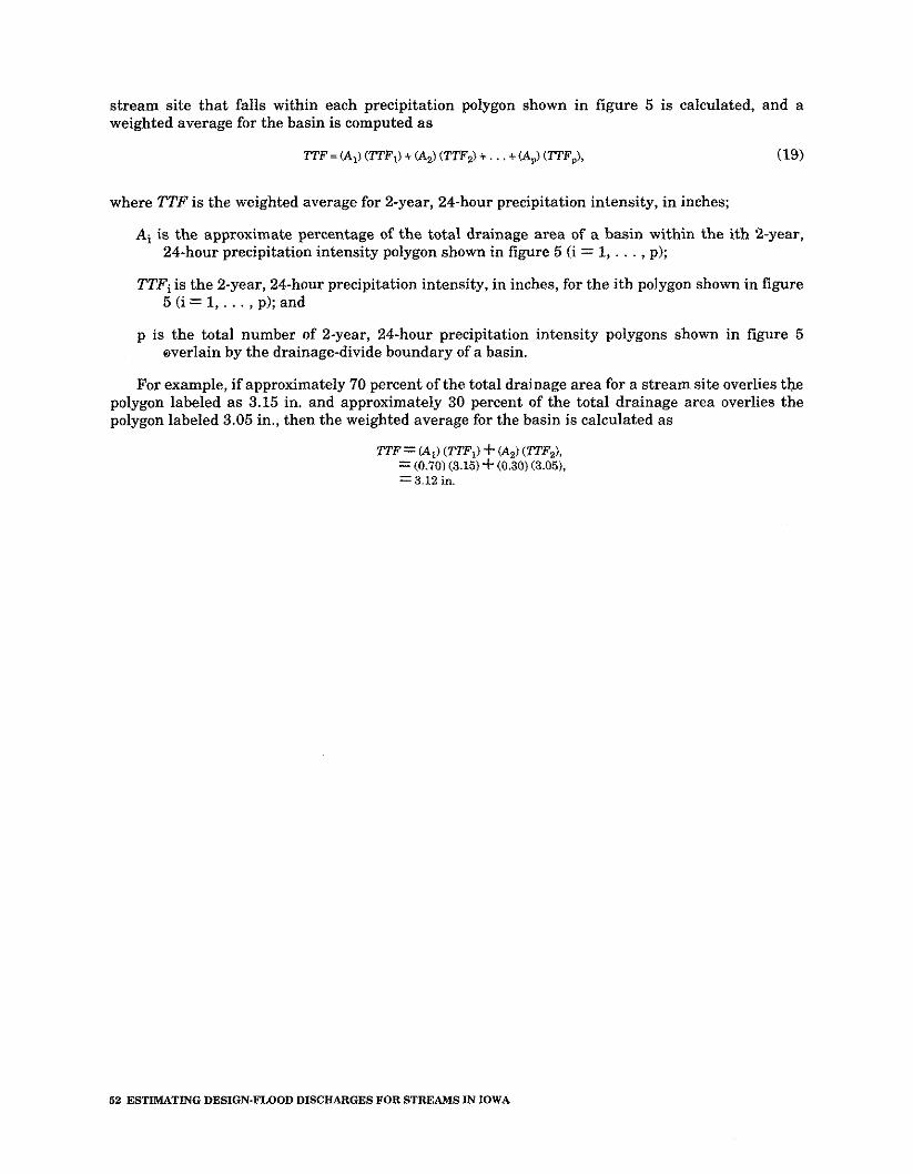
stream site that falls within each precipitation polygon shown in figure 5 is calculated, and a weighted average for the basin is computed as
TTF = (A,) (ITF,) + (Az) (TTF2) + . . . +(A> (TTFJ, (19)
where TTF is the weighted average for 2-year, 24-hour precipitation intensity, in inches;
Ai is the approximate percentage of the total drainage area of a basin within the ith 2-year, 24-hour precipitation intensity polygon shown in figure 5 (i = 1, . . . , p);
TTFi is the 2-year, 24-hour precipitation intensity, in inches, for the ith polygon shown in figure 5 (i = 1, . . . , p); and
p is the total number of 2-year, 24-hour precipitation intensity polygons shown in figure 5 overlain by the drainage-divide boundary of a basin.
For example, if approximately 70 percent of the total drainage area for a stream site overlies the polygon labeled as 3.15 in. and approximately 30 percent of the total drainage area overlies the polygon labeled 3.05 in., then the weighted average for the basin is calculated as
TTF= (A,) (TTF,) + (A,) (IT&), = (0.70) (3.15) f (0.30) (3.03, = 3.12 in.
52 ESTIMATING DESIGN-FLOOD DISCHARGES FOR STREAMS IN IOWA
APPENDIX C
Procedure for Conducting Channel-Geometry Measurements
The channel-geometry flood-estimation method is applicable to stream sites in Iowa with unregulated and stabilized stream channels. The following discussion outlines the procedure for conducting channel-geometry measurements.
Selection of Channel-Geometry Measurement Reaches
An inspection of 1:100,000- or 1:24,000-scale topographic maps is made to evaluate the channel reach both upstream and downstream of the stream site. Channel-geometry measurements are made along a straight channel reach, and an inspection of topographic maps is helpful in determining whether to start searching upstream or downstream of the site for a measurement reach. If the channel for some distance upstream and downstream of the stream site is very sinuous, unnaturally wide, or in an area that may be affected by development, topographic maps can be inspected to locate more suitable channel reaches a t nearby bridges upstream or downstream of the stream site.
Channel-geometry measurements can be made a t some distance away from the stream site, either upstream or downstream, as long as the drainage area upstream of the measurement reach does not change by more than about 5 percent from the drainage area of the stream site. The 5-percent change in drainage area is an approximate limitation to ensure that channel-geometry measurements are representative of the streamflow discharges that occur a t the stream site.
Topographic maps are useful in identifying linear channels that are usually indicative of channelization. Channels that appear to be channelized are noted because application of the channel-geometry equations listed in tables 3-5 are dependent on whether a stream has been channelized. A visual inspection of the channel also is made upon visiting the stream site to check for evidence of channelization. Features that are characteristic of channelized streams are illustrated in figure 70, which shows the straightened and leveed channel reach downstream of the Big Creek near Varina gaging station (station number 05482170; map number 108, fig. 2). If evidence of channelization is not found, then the bankfull equations (the first set of equations listed in tables 3-5) are applicable; if evidence of channelization is found, then the active-channel equations (the second set of equations listed in tables 3-5) may be applicable.
The channel-geometry method may not be applicable to poorly drained or pooled streams that have extremely low, local gradients (less than approximately 0.1 ft/mi.). A local gradient is measured from 1:24,000-scale topographic maps and is calculated as the slope of the channel between the nearest contour lines crossing the channel upstream and downstream of a stream site. This slope measurement is performed only for those stream sites that are suspected of having extremely low, local gradients and typically is not required for channel-geometry measurements.
Selection of Channel-Geometry Measurement Sections
Measurements of channel-geometry characteristics are made at channel cross sections that represent stable and self-formed channel-bank conditions. Self-formed channels are natural channels or channels that have been affected by channelization for which a t least the active-channel portion of the channel has had time to adjust back to natural conditions. Commonly, the active-channel portion of the channel will adjust back to natural or self-formed conditions within approximately 5 to 10 years after channelization occurs.
Measurements are made far enough away from bridges or other structures crossing the stream channel to avoid any alterations to the channel caused by construction. More distance is allowed downstream of bridges to avoid the effects of the channel constriction and more distance is allowed upstream of culverts to avoid the effects of backwater. Ideally, measurements are made in a
APPENDMC 53
generally straight stream reach where channel widths and flow velocities are relatively uniform across the channel (Osterkamp and Hedman, 1982, p. 3 and 6). A desirable channel reach narrows slightly in width in the downstream direction and has channel-bank surfaces that are depositional and stable, as evidenced by permanent vegetation. A relatively trapezoidal cross section is ideal for making width and depth measurements. Channel cross sections to avoid are those that (1) show evidence of bank instability such as extensive deposition, erosion indicated by cut or scalloped banks, or bank sloughing; (2) include apparent bedrock in the channel bed or banks; or (3) are altered by riprap or other types of natural or unnatural linings or obstructions, such as logjams, fallen trees, or large rocks that cause local changes in channel width. If possible, avoid a channel section that crosses sandbars. If a channel has a pool-and-riffle sequence, select measurement sections a short distance upstream or downstream from a riffle.
Bankfull Width (BFW) Measurements
Bankfull width measurements are applicable if channelization is not apparent. Bankfull width measurements are used in the first set of equations listed in tables 3-5. Riggs (1974) describes the bankfull channel width as the horizontal distance between the tops of the banks of the main channel. The top of the bank typically is defined as the place where the flood plain and the channel intersect and usually is distinguished by an abrupt change in slope from near vertical to horizontal. The bankfull reference level shown in figure 6 may not always be found a t the flood-plain elevation. Because some channels have developed terraces, the bankfull reference level may be found a t an elevation lower than the flood-plain elevation. If the channel is deeply incised or the bankfull reference level is not readily identified, active-channel width (ACW) measurements are made, and the second set of equations listed in tables 3-5 are used.
An average bankfull-width measurement is determined as the average of a t least three bankfull-width measurements that are made at channel sections separated by a t least twice the bankfull width. For example, if the first bankfull section measured has a width of 50 ft, the next bankfull section is selected at least 100 ft upstream or downstream of the first bankfull section. A tagline or tape is staked a t either side of the channel a t the bankfull reference level perpendicular to the channel. The tagline is staked horizontally and stretched taut for an accurate width measurement. Elevations can be measured from the water surface on either side of the channel up to the tagline to check that it is staked horizontally. The width is measured to at least two significant figures. For width measurements at larger channels, a hand level or automatic level that permits stadia readings can be used to read a surveying rod held on the opposite bank.
At least three bankfull width measurements that are within 10 percent of the average are collected. For example, if width measurements of 50,55, and 60 ft are collected a t three sections, the average is 55 ft. Ten percent of this average is 5.5 ft. In this example, all three width measurements are within 10 percent of the average of 55 ft. If three width measurements do not fall within 10 percent of the average, due to low- or high-outlier bankfull width measurements, then a fourth bankfull width measurement is collected. A new average for all of the bankfull width measurements then is calculated and checked to see if any three of the width measurements are within 10 percent of the new average. Additional bankfull width measurements are collected until a t least three of the width measurements are found to be within 10 percent of the average for all of the bankfull width measurements. Those width measurements that fall within 10 percent of the average are used to calculate an average bankfull width (BFW). Figures 7B, 7C, and 7F show photographs at three stream sites where a surveying rod was held at the bankfull reference level used to measure hankfull widths.
Bankfull Depth (BFD) Measurements
The bankfull channel-geometry equations listed in the first set of equations in tables 3 and 5, require that bankfull depth measurements be made in addition to bankfull width (BFW) measurements. A bankfull depth measurement is made at one of the bankfull measurement sections
54 ESTIMATING DESIGN-FLOOD DISCHARGES FOR STREAMS IN IOWA
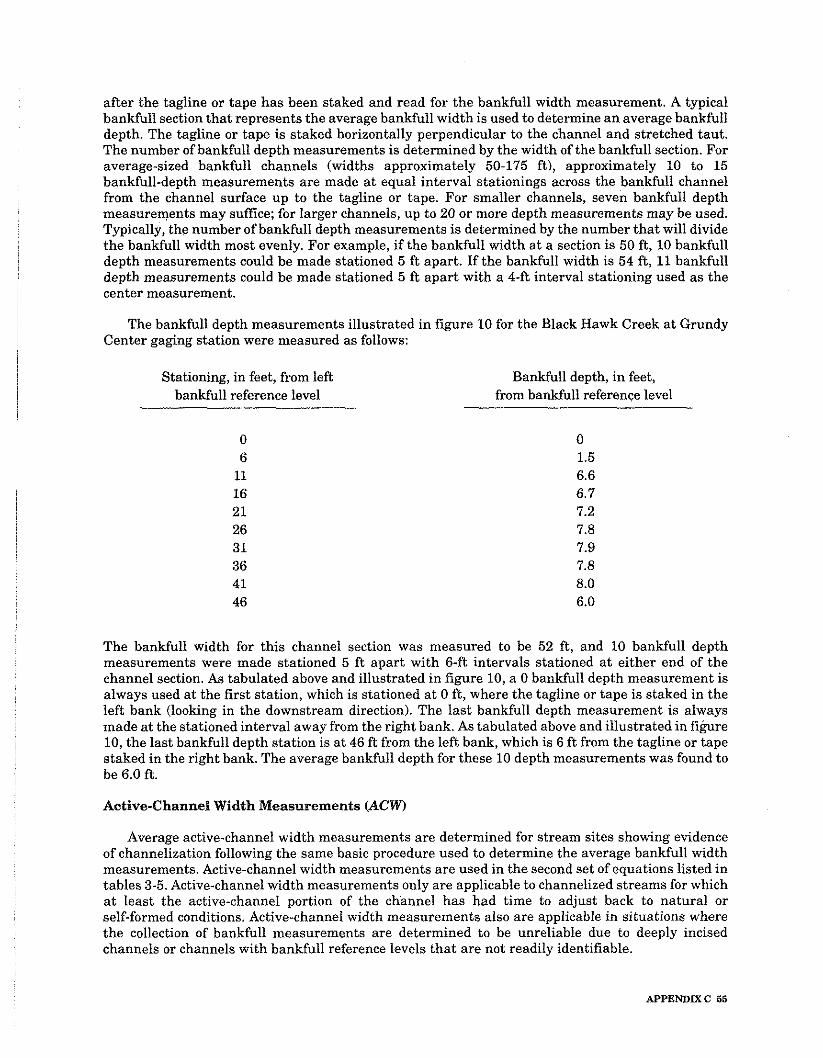
after the tagline or tape has been staked and read for the bankfull width measurement. A typical bankfull section that represents the average bankfull width is used to determine an average bankfull depth. The tagline or tape is staked horizontally perpendicular to the channel and stretched taut. The number of bankfull depth measurements is determined by the width of the bankfull section. For average-sized bankfull channels (widths approximately 50-175 ft), approximately 10 to 15 bankfull-depth measurements are made a t equal interval stationings across the bankfull channel from the channel surface up to the tagline or tape. For smaller channels, seven bankfull depth measurements may suffice; for larger channels, up to 20 or more depth measurements may be used. Typically, the number of bankfull depth measurements is determined by the number that will divide the bankfull width most evenly. For example, if the bankfull width at a section is 50 ft, 10 bankfull depth measurements could be made stationed 5 ft apart. If the bankfull width is 54 ft, 11 bankfull depth measurements could be made stationed 5 ft apart with a 4-ft interval stationing used as the center measurement.
The bankfull depth measurements illustrated in figure 10 for the Black Hawk Creek a t Grundy Center gaging station were measured as follows:
Stationing, in feet, from left bankfull reference level
Bankfull depth, in feet, from bankfull reference level
The bankfull width for this channel section was measured to he 52 fk, and 10 bankfull depth measurements were made stationed 5 ft apart with 6-ft intervals stationed at either end of the channel section. As tabulated above and illustrated in figure 10, a 0 bankfull depth measurement is always used at the first station, which is stationed at 0 ft, where the tagline or tape is staked in the left bank (looking in the downstream direction). The last bankfull depth measurement is always made at the stationed interval away from the right bank. As tabulated above and illustrated in f i b r e 10, the last bankfull depth station is a t 46 ft from the left bank, which is 6 ft from the tagline or tape staked in the right bank. The average bankfull depth for these 10 depth measurements was found to be 6.0 ft.
Aotive-Channel Width Measurements (ACW)
Average active-channel width measurements are determined for stream sites showing evidence of channelization following the same basic procedure used to determine the average bankfull width measurements. Active-channel width measurements are used in the second set of equations listed in tables 3-5. Active-channel width measurements only are applicable to channelized streams for which a t least the active-channel portion of the channel has had time to adjust back to natural or self-formed conditions. Active-channel width measurements also are applicable in situations where the collection of bankfull measurements are determined to be unreliable due to deeply incised channels or channels with bankfull reference levels that are not readily identifiable.
APPENDIX C 66
As shown in figure 6, the active-channel reference level is identified a t a lower channel-bank elevation. At least three active-channel width measurements are made that are within 10 percent of the average, and active-channel measurement sections are separated by at least twice the active-channel width. The tngline or tape is staked in a similar manner as previously described, and width measurements are read to a t least two significant figures. As defined by Osterkamp and Hedman (1977, p. 256),
"The active channel is a short-term geomorphic feature subject to change by prevailing discharges. The upper limit is defined by a break in the relatively steep bank slope of the active channel to a more gently sloping surface beyond the channel edge. The break in slope normally coincides with the lower limit of permanent vegetation so that the two features, individually or in combination, define the active channel reference level. The section beneath the reference level is that portion of the stream entrenchment in which the channel is actively, if not totally, sculptured by the normal process of water and sediment discharge."
Figures 7A and 7E show photographs a t two stream sites where a tape and a tagline, respectively, were staked at the active-channel reference level used to measure active-channel widths.
66 ESTIMATING DESIGN-FLOOD DISCHARGES FOR STREAMS IN IOWA
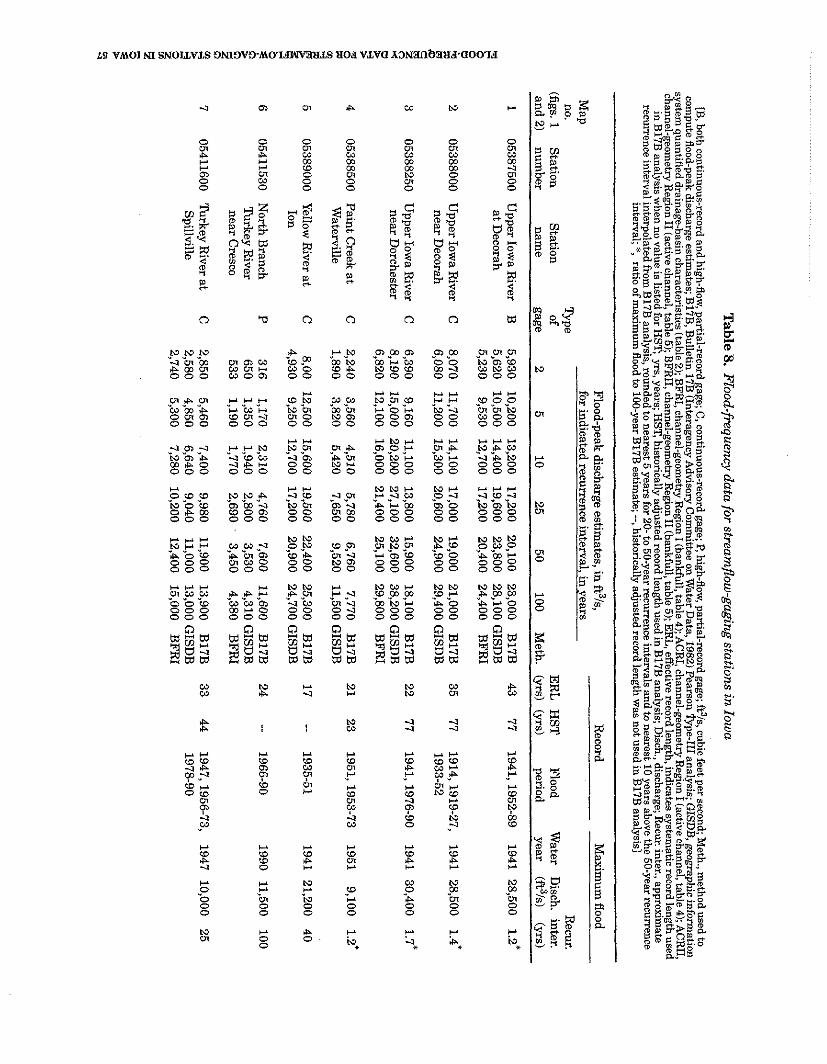
Tab
le 8. Flood-frequency d
ata for stream
flow
-gag
ing
station
s in Io
wa
[B, both wntinuous-record and high-flow
, partial-record gage; C, continuous-rew
rd gage; P, high-flow, partial-record gage; R
3/s, cubic feet per second; Meth., m
ethod used eom
oute flood-oeak discharee estimates: B
17B. B
ulletin 178 (Interaeenev Advisorv C
omm
ittee on Water D
ata. 1982) Pearson %ve-111 analvs~s: GISD
B, geom
aphic informat~on
inter;& I, ratio of m
aximu&
fldod to 100-year BI~
B
&tim
ite; --, historiially adjusted record length was not used in ~
17
~
analysis]
Flood-peak discharge estim
ates, in ft3/s, R
ecord M
aximum
flood M
ap for indicated recurrence interval, in years
no. 'h
e
Recur.
(figs. 1
Station
Station
of E
RL
H
ST
F
lood W
ater D
isch. inter.
and
21
num
ber nam
e gage
2 5
10 25
50 100
Meth.
(yrs) (yrs)
period year
(ft3/s) (y
rs)
1
05387500 U
pper Iowa R
iver B
5,930
10,200 13,200
17,200 20,100
23,000 B
17B
43
77
1941,1952-89 1941 28,500
1.2*
3 a
t Decorah
5,620 10,500
14,400 19,600
23,800 28,100 G
ISD
B
P
5,230 9,530
12,700 17,200
20,400 24,400
BF
RI
0
i 2
05388000 U
pper IowaR
iver C
8,070
11,700 14,100
17,000 19,000
21,000 B
17B
35 77
1914,1919-27, 1941
28,500 1.4*
near D
ecorah 6,080
11,200 15,300
20,600 24,900
29,400 GIS
DB
1933-52
e 2 8 3
05388250 U
pper Iowa R
iver C
6,390
9,160 11,100
13,800 15,900
18,100 B
17B
22 77
1941,1976-90 1941
30,400 1.7*
e
near Dorchester
u 8,190
15,000 20,200
27,100 32,600
38,200 GIS
DB
?; 6,820
12,100 16,000
21,400 25,100
29,800 B
FR
I s
0" 4
05388500 P
aint C
reek at
C
2,240 3,560
4,510 5,780
6,760 7,770
B17B
2
1
23 1951, 1953-73
1951 9,100
1.2' 0
Waterville
1,890 3,820
5,420 7,650
9,520 11,500 G
ISD
B
3 5
05389000 Y
ellow R
iver at
C
8,00 12,500
15,600 19,500
22,400 25,300
B17B
17
-- 1935-51
1941 21,200 40
Ion 4,930
9,250 12,700
17,200 20,900
24,700 GIS
DB
2 6
05411530 N
orth Branch
P
316 1,170
2,310 4,760
7,600 11,600
B17B
24
-- 1966-90
1990 11,500
100 h
%
Turkey R
iver 650
1,350 1,940
2,800 3,530
4,310 GIS
DB
n
ear Cresco
533 1,190
1,770 2,690
- 3,450
4,380 B
FR
I 3 3
7 05411600
Turkey R
iver at
C
2,850 5,460
7,400 9,980
11,900 13,900
B17B
3
3
44 1947,1956-73,
1947 10,000
25
5 S
pillville 2,580
4,850 6,640
9,040 11,000
13,000 GIS
DB
1978-90
2,740 5,300
7,280 10,200
12,400 15,000
BF
RJ
z
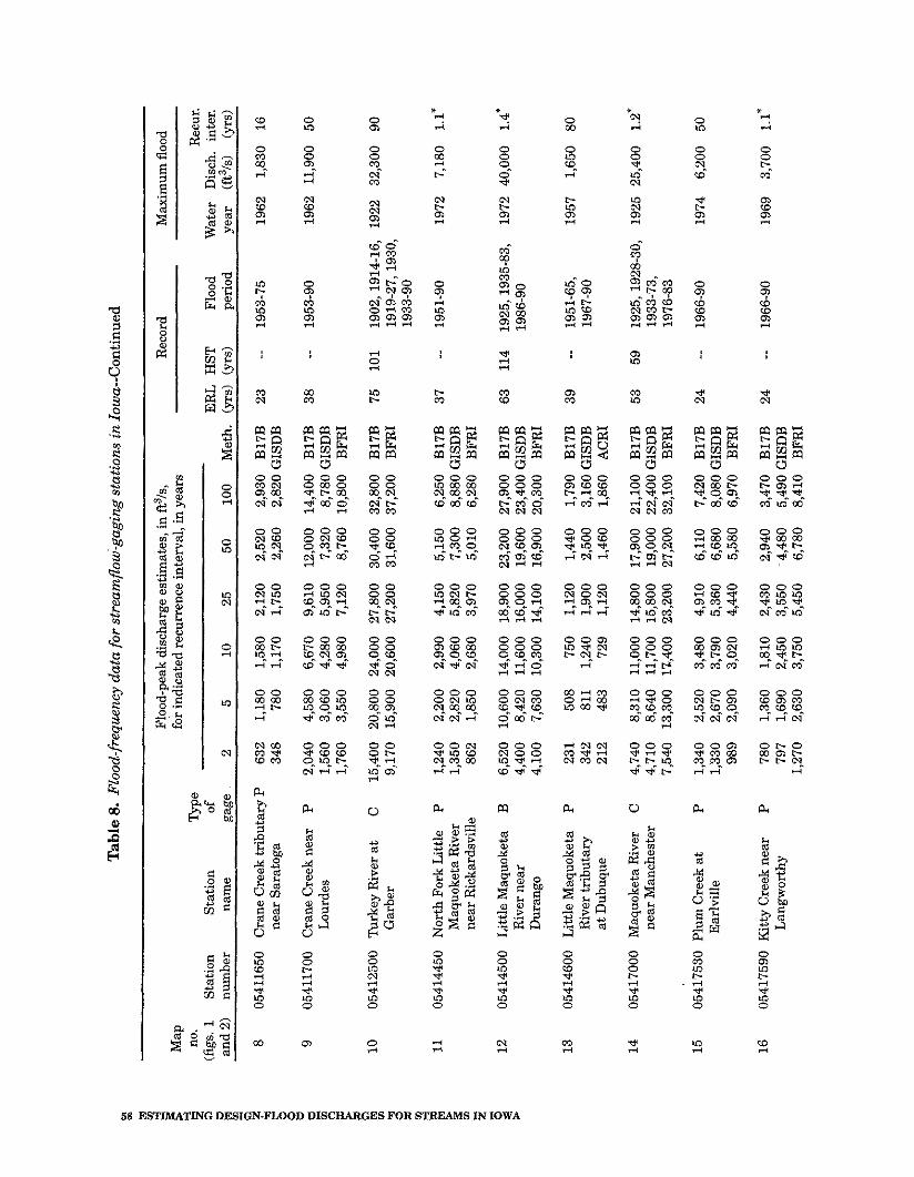
n
Tab
le 8
. F
lood
-fre
quen
cy d
ata
for
stre
amfl
ow
-gag
ing
sta
tio
ns
in Io
wa-
-Co
nti
nu
ed
m
m
V1
Flo
od-p
eak
disc
harg
e es
tim
ates
, in
ft3
/s,
Rec
ord
Max
imum
floo
d M
ap
for i
ndic
ated
rec
urre
nce
inte
rval
. in
vea
rs
* , .
3 no
. w
e
Rec
ur.
o
(fig
s. 1
S
tati
on
Sta
tion
of
E
RL
H
ST
Floo
d W
ater
D
isch
. in
ter.
an
d2
1
num
ber
nam
e ga
ge
2 5
10
25
50
100
Met
h.
(yrs
) (y
rs)
peri
od
year
(ft31s)
(~rs)
3 ki 8 8
0541
1650
C
rane
Cre
ek t
rib
uta
ryP
63
2 1,
180
1,58
0 2,
120
2,52
0 2,
930
B17
B
23
-- 19
53-7
5 19
62
1,83
0 16
n
near
Sar
atog
a 34
8 78
0 1,
170
1,75
0 2,
260
2,82
0 G
ISD
B
$ 9
0541
1700
C
ran
eCre
ekn
ear
P
2,04
0 4,
580
6,67
0 9,
610
12,0
00
14,4
00
B17
B
38
-- 19
53-9
0 19
62
11,9
00
50
Lou
rdes
1,
560
3,06
0 4,
280
5,95
0 7,
320
8,78
0 G
ISD
B
1,76
0 3,
550
4,98
0 7,
120
8,76
0 10
,800
B
FR
I
e E
10
0541
2500
T
urke
y R
iver
at
C
15,4
00
20,8
00
24,0
00
27,8
00
30,4
00
32,8
00
B17
B
75
101
1902
,191
4-16
, 19
22
32,3
00
90
Gar
ber
9,17
0 15
,900
20
,600
27
,200
31
,600
37
,200
B
FR
I 3
1919
-27,
1930
, 19
33-9
0 3 E
11
0541
4450
N
orth
For
k L
ittl
e P
1,
240
2,20
0 2,
990
4,15
0 5,
150
6,25
0 B
17B
37
--
1951
-90
1972
7,
180
1.1.
Maq
uoke
ta R
iver
1,
350
2,82
0 4,
060
5,82
0 7,
300
8,88
0 G
ISD
B
V1
near
Ric
kard
svil
le
4
862
1,85
0 2,
680
3,97
0 5,
010
6,28
0 B
FR
I - 6 5
12
0541
4500
L
ittl
eMaq
uoke
ta
B
6,52
0 10
,600
14
,000
18
,900
23
,200
27
,900
B
17B
63
11
4 19
25,1
935-
83,
1972
40
,000
1.
4'
Riv
er n
ear
4,40
0 8,
420
11,6
00
16,0
00
19,6
00
23,4
00 G
ISD
B
1986
-90
Dur
ango
4,
100
7,63
0 10
,300
14
,100
16
,900
20
,300
B
FR
I
13
0541
4600
L
ittl
e M
aquo
keta
P
23
1 50
8 75
0 1,
120
1,44
0 1,
790
B17
B
39
-- 19
51-6
5,
1957
1,
650
80
Riv
er t
ribu
tafy
34
2 81
1 1,
240
1,90
0 2,
500
3,16
0 G
ISD
B
1967
-90
at D
ubuq
ue
212
483
729
1,12
0 1,
460
1,86
0 A
CR
I
14
0541
7000
M
aquo
keta
Riv
er
C
4,74
0 8,
310
11,0
00
14,8
00
17,9
00
21,1
00
B17
B
53
59
1925
,192
8-30
, 19
25 2
5,40
0 1.
2.
near
Man
ches
ter
4,71
0 8,
640
11,7
00
15,8
00
19,0
00
22,4
00 G
ISD
B
1933
-73,
7,
540
13,3
00
12,4
00
23,2
00
27,2
00
32,1
00
BF
RI
1976
-83
15
05
4175
30 P
lum
Cre
ek a
t P
1,
340
2,52
0 3,
480
4,91
0 6,
110
7,42
0 B
17B
24
--
1966
-90
1974
6,
200
50
Ear
lvil
te
1,33
0 2,
670
3,79
0 5,
360
6,68
0 8,
080
GIS
DB
98
9 2,
090
3,02
0 4,
440
5,58
0 6,
970
BF
RI
16
0541
7590
K
itty
Cre
ek n
ear
P
780
1,36
0 1,
810
2,43
0 2,
940
3,47
0 B
17B
24
--
1966
-90
1969
3,
700
1.1*
L
angw
orth
y 79
7 1,
690
2,45
0 3,
550
4,48
0 5,
490
GIS
DB
1,
270
2,63
0 3,
750
5,45
0 6,
780
8,41
0 B
FR
I
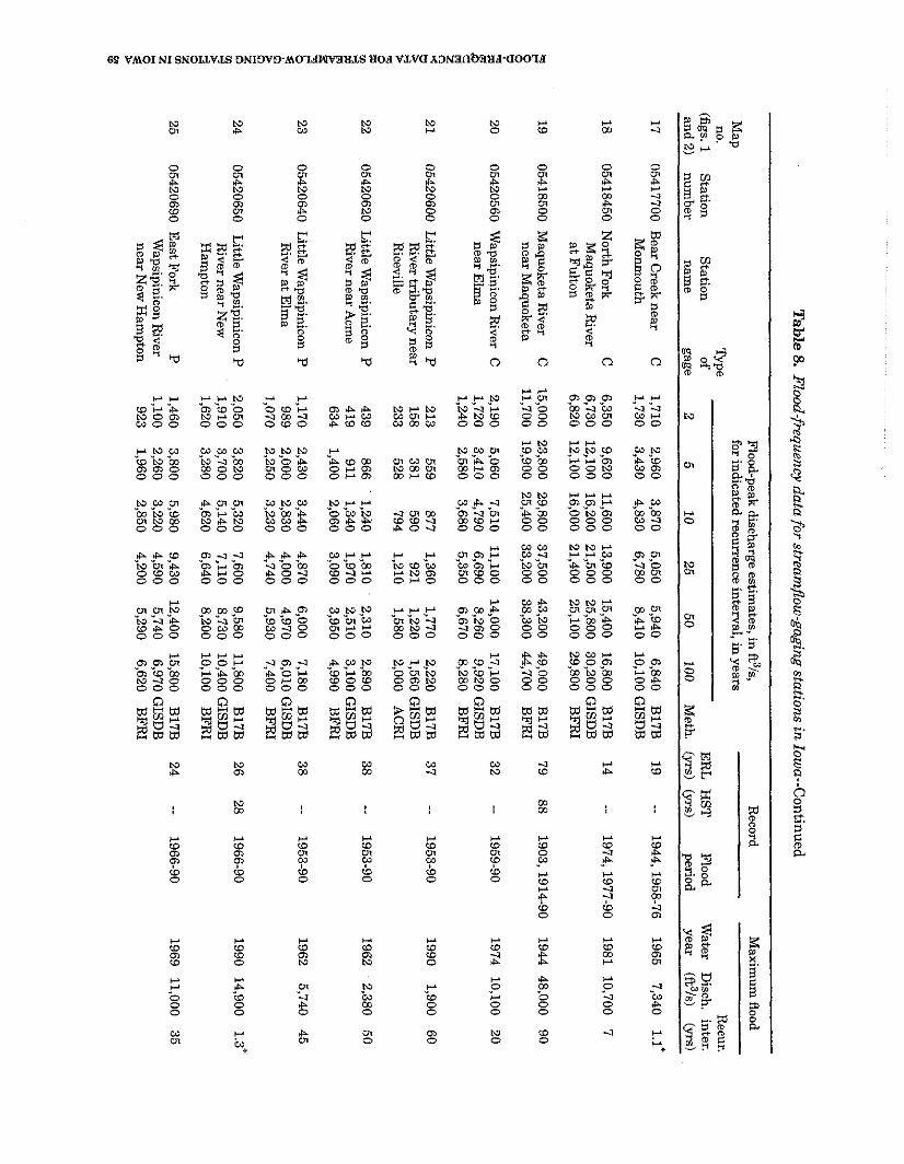
Table 8. F
lood-frequency data for streamflow
-gaging stations in Iow
a--Continued
Flood-peak discharge estim
ates, in fi3/s,
Record
Maxim
um flood
for indicated recurrence interval, in years
no. m
e
Recur.
(figs. 1
Station
Station
of E
RL
H
ST
F
lood W
ater D
isch. inter.
and 2) num
ber nam
e gage
2 5
10
25
50 100
Meth.
+s)
(yrs) period
year (fi3/s)
(yrs)
17 05417700 B
ear Creek near
C
1,710 2,960
3,870 5,050
5,940 6,840
B17B
19
-- 1944,1958-76
1965 7,340
1.1' M
onmouth
1,730 3,430
4,830 6,780
8,410 10,100 G
ISD
B
18 05418450 N
orth Fork
C
6,350 9,620
11,600 13,900
15,400 16,800
B17B
14
-- 1974,1977-90
1981 10,700 7
Maquoketa R
iver 6,730
12,100 16,200
21,500 25,800
30,200 GISD
B
at F
ulton 6,820
12,100 16,000
21,400 25,100
29,800 B
FR
I
i! 19
05418500 Maquoketa R
iver C
near M
aquoketa 8
20 05420560 W
apsipinicon River
C
near Elm
a s 8 *
21
05420600 L
ittle Wapsipinicon P
g
River tributary near
2 - R
iceville
14,000 17,100
B17B
32
-- 1959-90
1974 10,100
20 8,260
9,920 GIS
DB
6,670
8,280 B
FR
I
1,770 2,220
B17B
37
-- 1953-90
1990 1,900
60 1,220
1,560 GIS
DB
1,580
2,000 A
CR
I
05420620 Little W
apsipinicon P
439 R
iver near Acm
e 419 634
2,890 B
17B
38 --
1953-90 1962
2,380 50
3,100 GIS
DB
4,990
BF
RI
05420640 Little W
apsipinicon P
1,170 R
iver at E
lma
989 1,070
7,180 B
17B
38 --
1953-90 1962
5,740 45
6,010 GIS
DB
7,400
BF
RI
05420650 L
ittle Wapsipinicon P
2,050
River n
ear New
1,910
Ham
pton 1,620
11,800 B
17B
26 28
1966-90 1990
14,900 1.3*
10,400 GIS
DB
10,100
BF
RI
V
3 25
05420690 East F
ork P
1,460
3,800 5,980
9,430 12,400
15,800 B
17B
24 --
1966-90 1969
11,000 3
5
% W
apsipinicon River
1,100 2,260
3,220 4,590
5,740 6,970 G
ISD
B
5 s near N
ew H
ampton
923 1,960
2,850 4,200
5,290 6,620
BF
RI
%
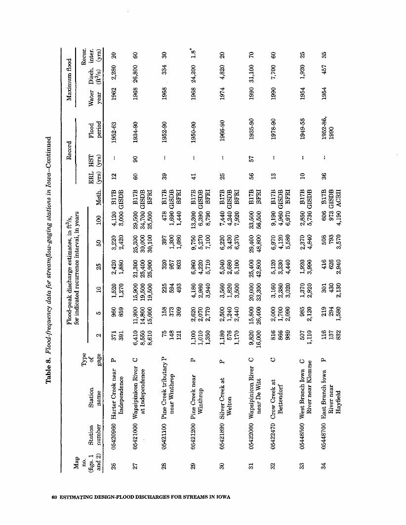
Table
8.
Flo
od-f
requ
ency
dat
a fo
r st
ream
flow
-gag
ing
stat
ion
s in
Io
wa-
-Co
nti
nu
ed
Flo
od-p
eak
disc
harg
e es
tim
ates
, in
fls
, R
ecor
d fo
r in
dica
ted
recu
rren
ce in
terv
al, i
n y
ears
M
axim
um fl
ood Rec
ur.
Wat
er
Dis
ch.
inte
r.
year
(f
t3/s
) (y
rs)
no.
Typ
e (f
igs.
1
Sta
tion
S
tati
on
of
ER
L
HS
T
Floo
d 2
5 10
25
50
10
0 M
eth.
(y
rs)
(yrs
) pe
riod
an
d 2)
nu
mbe
r na
me
gage
26
0542
0960
Har
ter
Cre
ek n
ear
P
Inde
pend
ence
3,
220
4,12
0 B
17B
12
--
1952
-63
2,42
0 3,
000
GIS
DB
27
0542
1000
Wap
sipi
nico
n R
iver
C
a
t Ind
epen
denc
e 25
,300
29
,500
B
17B
60
90
19
34-9
0 30
,000
34
,700
GIS
DB
30
,100
35
,500
B
FR
I
28
0542
1100
P
ine
Cre
ek tr
ibut
ary
P
near
Win
thro
p 39
7 47
8 B
17B
39
--
1952
-90
1,30
0 1,
690
GIS
DB
1,
080
1,44
0 B
FR
I
29
0542
1200
Pin
e C
reek
nea
r P
W
inth
rop
1,10
0 2,
620
4,18
0 6,
960
9,75
0 13
,300
B
17B
4
1
-- 19
50-9
0 1,
010
2,07
0 2,
960
4,22
0 5,
270
6,39
0 G
ISD
B
1,35
0 2,
770
3,94
0 5,
710
7,10
0 8,
790
BF
RI
30
0542
1890
Sil
ver C
reek
at
P
Wel
ton
1,18
0 2,
500
3,56
0 5,
040
6,22
0 7,
440
B17
B
25
-- 19
66-9
0 57
6 1,
240
1,82
0 2,
680
3,43
0 4,
240
GIS
DB
1,
170
2,44
0 3,
500
5,10
0 6,
370
7,92
0 B
FR
I
31
05
4220
00 W
apsi
pini
con
Riv
er
C
near
De
Wit
t 9,
820
15,8
00
20,0
00
25,4
00
29,4
00
33,5
00
B17
B
56
57
1935
-90
16,0
00
26,4
00
33,3
00
42,8
00
48,8
00
56,5
00
BF
RI
32
0542
2470
Cro
w C
reek
at
C
Bet
tend
orf
816
2,00
0 3,
160
5,12
0 6,
970
9,19
0 B
17B
1
3
-- 19
78-9
0 86
6 1,
700
2,38
0 3,
330
4,12
0 4,
960
GIS
DB
98
9 2,
090
3,02
0 4,
440
5,58
0 6,
970
BF
RI
33
05
4485
00 W
est B
ranc
h Io
wa
C
Riv
er n
ear
Mem
me
507
985
1,37
0 1,
920
2,37
0 2,
850
B17
B
10
-- 19
49-5
8 1,
110
2,12
0 2,
920
3,99
0 4,
840
5,73
0 G
ISD
B
34
0544
8700
Eas
t Bra
nch
Iow
a P
R
iver
nea
r H
ayfi
eld
116
219
301
416
508
606
B17
B
36
-- 19
52-8
6,
137
294
430
626
793
973
GIS
DB
19
90
832
1,58
0 2,
130
2,94
0 3,
570
4,19
0 A
CR
II
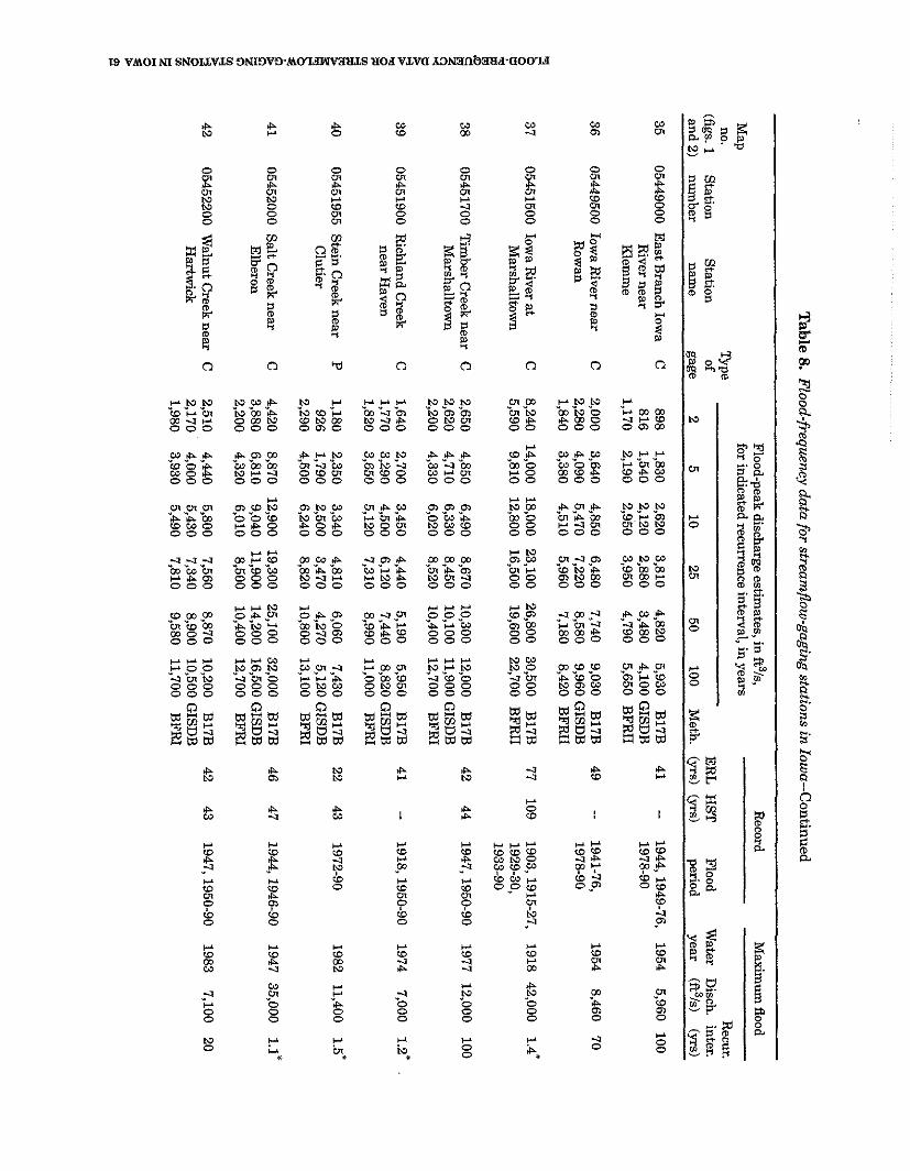
Table 8. F
lood-frequency data for stream
flow-gaging statio
ns in
Iowa--C
ontinued
Flood-peak discharge estim
ates, in ft3/s,
Record
Maxim
um flood
for indicated recurrence interval, in years no.
Type
Recur.
(figs. 1
Station
Station
of E
RL
H
ST
Flood
Water
Disch.
inter. and 2)
number
name
gage 2
5 10
25 50
100 M
eth. (y
rs) 01.s) period
year (ft3/s)
(yrs)
35 05449000 E
ast Branch Iow
a C
898
1,830 2,620
3,810 4,820
5,930 B
17B
41 --
1944,1949-76, 1954
5,960 100
River near
816 1,540
2,120 2,880
3,480 4,100 G
ISDB
1978-90
Klem
me
1,170 2,190
2,950 3,950
4,790 5,650
BF
RII
36 05449500 Iow
a Rivernear
C
2,000 3,640
4,850 6,480
7,740 9,030
B17B
49
-- 1941-76,
1954 8,460
70 R
owan
2,280 4,090
5,470 7,220
8,580 9,960 G
ISDB
1978-90
1,840 3,380
4,510 5,960
7,180 8,420
BF
RII
37 05451500 Iow
a River a
t C
8,240
14,000 18,000
23,100 26,800
30,500 B
17B
77 109
1903,1915-27, 1918 42,000
1.4* M
arshalltown
5,590 9,810
12,800 16,500
19,600 22,700
BF
RII
1929-30, 1933-90
38 05451700 T
imber C
reek near C
2,650
4,850 6,490
8,670 10,300
12,000 B
17B
42 44
1947,1950-90 1977
12,000 100
Marshalltow
n 2,620
4,710 6,330
8,450 10,100
11,900 GISD
B
2,200 4,330
6,020 8,520
10,400 12,700
BFR
I
39 05451900 R
ichland Creek
C
1,640 2,700
3,450 4,440
5,190 5,950
B17B
41
-- 1918,1950-90
1974 7,000
1.2' near H
aven 1,770
3,290 4,500
6,120 7,440
8,820 GISD
B
1,820 3,650
5,120 7,310
8,990 11,000
BF
RI
40 05451955 S
tein Creek
near
P
1,180 2,350
3,340 4,810
6,060 7,430
B17B
22
43 1972-90
1982 11,400
1.5
~
Clutier
926 1,790
2,500 3,470
4,270 5,120 G
ISDB
2,290
4,500 6,240
8,820 10,800
13,100 B
FR
I
41 05452000 S
alt Creek near
C
4,420 8,870
12,900 19,300
25,100 32,000
B17B
46
47 1944, 1946-90
1947 35,000
1.1
*
Elbem
n 3,880
6,810 9,040
11,900 14,200
16,500 GISD
B
2,200 4,320
6,010 8,500
10,400 12,700
BF
RI
42 05452200 W
alnut Creek
near
C
2,510 4,440
5,800 7,560
8,870 10,200
B17B
42
43 1947,1950-90
1983 7,100
20 H
artwick
2,170 4,000
5,430 7,340
8,900 10,500 G
ISDB
1,980
3,930 5,490
7,810 9,580
11,700 B
FR
I
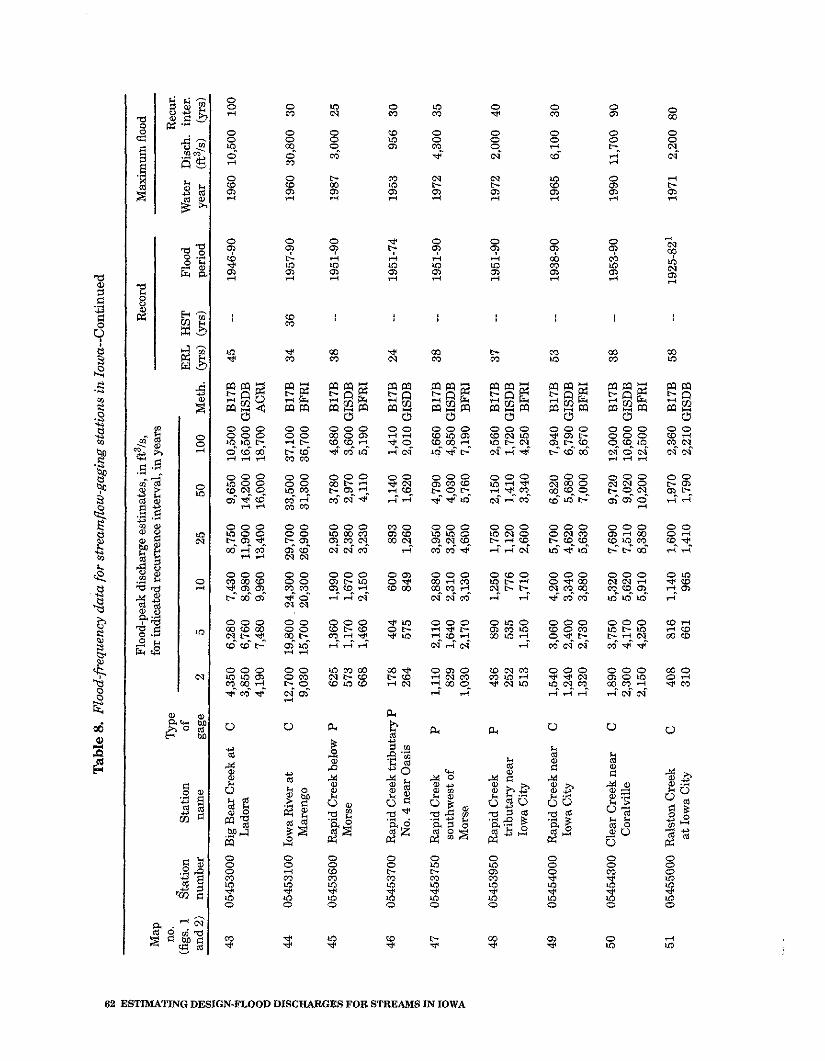
m
Tab
le 8
. F
lood
-fre
quen
cy d
ata
for
stre
amfl
ow-g
agin
g st
atio
ns
in I
ow
a-G
on
tin
ued
N I
Flo
od-p
eak
disc
harg
e es
tim
ates
, in
ft3/
s,
Rec
ord
Max
imum
floo
d M
ap
for i
ndic
ated
recu
rren
ce in
terv
al, i
n y
ears
$ no
. T
ype
Rec
ur.
(fig
s. 1
S
tati
on
Sta
tion
of
E
RL
H
ST
Fl
ood
Wat
er
Dis
ch.
inte
r.
8 an
d 2)
nu
mbe
r na
me
gage
2
5 10
25
50
10
0 M
eth.
(y
rs)
(yrs
) pe
riod
ye
ar
(&s)
(y
rs)
s n $
43
0545
3000
Big
Bea
r C
reek
at
C
4,35
0 6,
280
7,43
0 8,
750
9,65
0 10
,500
B
17B
45
--
1946
-90
1960
10
,500
10
0 L
ador
a 3,
850
6,76
0 8,
980
11,9
00
14,2
00
16,5
00 G
ISD
B
8 C( 4,
190
7,48
0 9,
960
13,4
00
16,0
00
18,7
00
AC
RI
w B 44
05
4531
00
Iow
a R
iver
at
C
12,7
00
19,8
00 . 2
4,30
0 29
,700
33
,500
37
,100
B
17B
34
36
19
57-9
0 19
60
30,8
00
30
Mar
engo
9,
030
15,7
00
20,3
00
26,9
00
31,3
00
36,7
00
BF
RI
n 8
45
0545
3600
R
apid
Cre
ek b
elow
P
62
5 1,
360
1,99
0 2,
950
3,78
0 4,
680
B17
B
38
-- 19
51-9
0 19
87
3,00
0 25
3 M
orse
57
3 1,
170
1,67
0 2,
380
2,97
0 3,
600
GIS
DB
z rn
66
8 1,
460
2,15
0 3,
230
4,11
0 5,
190
BF
RI
E 46
05
4537
00
Rap
idC
reek
trib
uta
ryP
17
8 40
4 60
0 89
3 1,
140
1,41
0 B
17B
24
--
1951
-74
1953
95
6 30
N
o. 4
nea
r O
asis
26
4 57
5 84
9 1,
260
1,62
0 2,
010
GIS
DB
V
) z 47
05
4537
50
Rap
id C
reek
P
1,
110
2,11
0 2,
880
3,95
0 4,
790
5,66
0 B
17B
38
--
8 19
51-9
0 19
72
4,30
0 35
3 so
uthw
est o
f 82
9 1,
640
2,31
0 3,
250
4,03
0 4,
850
GIS
DB
M
orse
1,
030
2,17
0 3,
130
4,60
0 5,
760
7,19
0 B
FR
I
48
0545
3950
R
apid
Cre
ek
P
436
890
1,25
0 1,
750
2,15
0 2,
560
B17
B
37
-- 19
51-9
0 19
72
2,00
0 40
tr
ibut
ary
near
25
2 53
5 77
6 1,
120
1,41
0 1,
720
GIS
DB
Io
wa
Cit
y 51
3 1,
150
1,71
0 2,
600
3,34
0 4,
250
BF
RI
49
0545
4000
R
apid
Cre
ek n
ear
C
1,54
0 3,
060
4,20
0 5,
700
6,82
0 7,
940
B17
B
53
-- 19
38-9
0 19
65
6,10
0 30
Io
wa
Cit
y 1,
240
2,40
0 3,
340
4,62
0 5,
680
6,79
0 G
ISD
B
1,32
0 2,
730
3,88
0 5,
630
7,00
0 8,
670
BF
RI
50
0545
4300
Cle
ar C
reek
nea
r C
1,
890
3,75
0 5,
320
7,69
0 9,
720
12,0
00
B17
B
38
-- 19
53-9
0 19
90
11,7
00
90
C
oral
vitl
e 2,
300
4,17
0 5,
620
7,51
0 9,
020
10,6
00 G
ISD
B
2,15
0 4,
250
5,91
0 8,
380
10,2
00
12,5
00
BF
RI
51
05
4550
00 R
alst
onC
reek
C
40
8 81
6 1,
140
1,60
0 1,
970
2,36
0 B
17B
58
--
1925
-82'
19
71
2,20
0 80
a
t Iow
a C
ity
310
661
965
1,41
0 1,
790
2,21
0 G
ISD
B
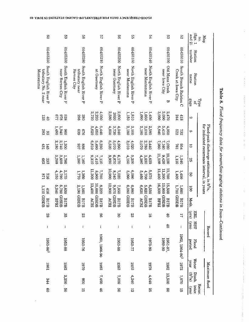
Ta
ble 8. F
lood-frequency data for streamflow
-gaging stations in Iowa-C
ontinued
~~
~~p
Flood-peak discharge estim
ates, in ft3/s, R
ecord M
aximum
flood for indicated recurrence interval, in years
no. 'b
e
Recur.
(figs. 1
Station
Station
of E
RL
H
ST
Flood
Water
Disch.
inter. an
d2
) num
ber nam
e gage
2 5
10 25
50 100
Meth.
(yrs) (yrs)
period year
(ft3/s) (yrs)
52 05455010 S
outh Branch R
alston C
418 732
954 1,240
1,450 1,660
B17B
17
-- 1962,1964-80'
1972 1,070
15 C
reek at Iowa C
ity 244
522 761
1,110 1,400
1,710 GIS
DB
53 05455100 O
ld Mans C
reek B
near Iow
a City
54 05455140 N
orth English R
iver P
near Montezum
a
55 05455150 N
orth English R
iver P
near Montezum
a
56 05455200 N
orth English R
iver P
near Guernsey
57 05455210 N
orth English R
iver P
at Guernsey
12,700 15,500
B17B
40
40 1951-87,
1982 13,500
60 11,200
13,000 GIS
DB
1989-90
13,400 16,300
BF
RI
5,570 6,550
B17B
18
-- 1973-90
1978 4,640
25 4,700
5,620 GIS
DB
5,460
6,620 A
CR
I
6,090 6,980
B17B
23
-- 1953-77
1953 4,240
12 5,090
6,080 GISD
B
7,020 7,850
B17B
30
-- 1953-88
1953 7,000
50 8,340
9,870 GIS
DB
10,900
12,900 A
CR
I
7,700 8,220
B17B
'
26 --
1960,1966-90 1982
7,460 40
8,960 10,600 G
ISD
B
11,300 13,400
AC
RI
g 58
05455280 South E
nglish River P
380
676 886
1,160 1,360
1,560 B
17B
23 --
1953-76 1970
900 11
s h
tributary near
298 639
937 1,380
1,770 2,190 G
ISDB
k B
arnes City
m. - 2
0
U,
59 05455300 S
outh English R
iver P
528 960
1,300 1,780
2,170 2,600
B17B
35
-- 1953-88
1982 2,200
50 *
near Barnes C
ity 978
1,940 2,740
3,850 4,790
5,780 GIS
DB
$
677 1,480
2,180 3,260
4,150 5,240
BF
RI
$ i2 5 60
05455350 S
outh English R
iver P
40 93
145 233
316 416
B17B
28
-- 1953-80'
1961 344
60
5
tributary No. 2 near
123 283
431 662
871 1,110 G
ISD
B
3 M
ontezuma
0)
W
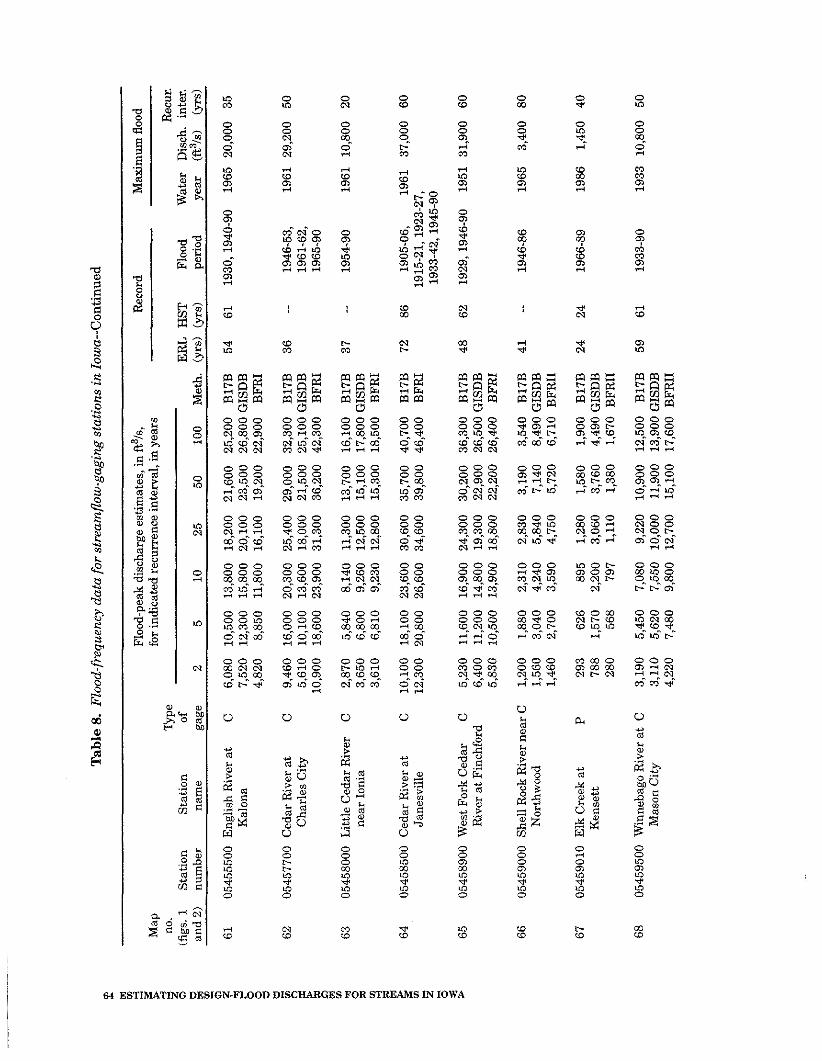
Tab
le 8
. F
lood
-fre
quen
cy d
ata
for
stre
amfl
ow-g
agin
g st
atio
ns
in I
ow
a--C
on
tin
ued
:: m
m 8
Flo
od-p
eak
disc
harg
e es
tim
ates
, in
ft3/
s,
Rec
ord
Max
imum
flo
od
Map
fo
r ind
icat
ed r
ecur
renc
e in
terv
al, i
n ye
ars
3 no
. T
ype
Rec
ur.
0
(fig
s. 1
S
tati
on
Sta
tion
of
E
RL
H
ST
Fl
ood
Wat
er
Dis
ch.
inte
r.
u an
d2
) nu
mbe
r na
me
gage
2
5 10
25
50
10
0 M
eth.
(y
rs)
bs
)
peri
od
year
(f
t3/s
) (PS
I 8 3 ;t
61
0545
5500
Eng
lish
Riv
er a
t C
6,
080
10,5
00
13,8
00
18,2
00
21,6
00
25,2
00
B17
B
54
61
1930
,194
0-90
19
65 2
0,00
0 35
5 K
alon
a 7,
520
12,3
00
15,8
00
20,1
00
23,5
00
26,8
00 G
ISD
B
% 4,
820
8,85
0 11
,800
16
,100
19
,200
22
,900
B
FR
I - z
62
0545
7700
Ced
ar R
iver
at
C
9,46
0 16
,000
20
,300
25
,400
29
,000
32
,300
B
17B
36
--
1946
-53,
19
61 2
9,20
0 50
1 C
harl
es C
ity
5,61
0 10
,100
13
,600
18
,000
21
,500
25
,100
GIS
DB
19
61-6
2,
10,9
00
18,6
00
23,9
00
31,3
00
36,2
00
42,3
00
BF
RI
1965
-90
8 3 63
05
4580
00 L
ittl
e C
edar
Riv
er
C
2,87
0 5,
840
8,14
0 11
,300
13
,700
16
,100
B
17B
37
--
1954
-90
1961
10
,800
20
8
ne
ar I
onia
3,
650
6,80
0 9,
260
12,5
00
15,1
00
17,8
00 G
ISD
B
3 3,
610
6,81
0 9,
230
12,8
00
15,3
00
18,5
00
BF
RI
L! 2 64
05
4585
00
Ced
ar R
iver
at
C
10,1
00
18,1
00
23,6
00
30,6
00
35,7
00
40,7
00
B17
B
72
86
1905
-06,
19
61
37,0
00
60
m
Jane
svil
le
12,3
00
20,8
00
26,6
00
34,6
00
39,8
00
46,4
00
BF
RI
1915
-21,
192
3-27
, !2 -
1933
-42,
194
5-90
0 3
65
0545
8900
Wes
t For
k C
edar
C
5,
230
11,6
00
16,9
00
24,3
00
30,2
00
36,3
00
B17
B
48
62
1929
,194
6-90
19
51 3
1,90
0 60
R
iver
at F
inch
ford
6,
400
11,2
00
14,8
00
19,3
00
22,9
00
26,5
00 G
ISD
B
5,83
0 10
,500
13
,900
18
,800
22
,200
26
,400
B
FR
I
66
0545
9000
She
ll R
ock
Riv
er n
ear
C
1,20
0 1,
880
2,31
0 2,
830
3,19
0 3,
540
B17
B
41
--
1946
-86
1965
3,
400
80
Nor
thw
ood
1,56
0 3,
040
4,24
0 5,
840
7,14
0 8,
490
GIS
DB
1,
460
2,70
0 3,
590
4,75
0 5,
720
6,71
0 B
FR
II
67
0545
9010
E
lk C
reek
at
P
293
626
895
1,28
0 1,
580
1,90
0 B
17B
24
24
19
66-8
9 19
86
1,45
0 40
K
ense
tt
788
1,57
0 2,
200
3,06
0 3,
760
4,49
0 G
ISD
B
280
568
797
1,11
0 1,
380
1,67
0 B
FR
II
68
0545
9500
Win
neba
go R
iver
at
C
3,19
0 5,
450
7,08
0 9,
220
10,9
00
12,5
00
B17
B
59
61
19
33-9
0 19
33
10,8
00
50
Mas
on C
ity
3,11
0 5,
620
7,55
0 10
,000
11
,900
13
,900
GIS
DB
4,
220
7,48
0 9,
800
12,7
00
15,1
00
17,6
00 B
FR
II
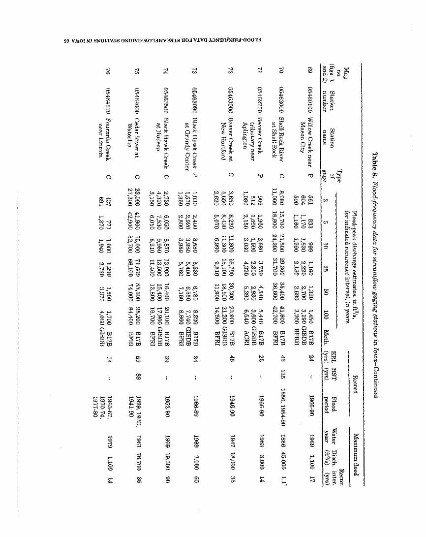
Tab
le 8. Flood-frequency d
ata
for streamflo
w-g
agin
g statio
ns in
Iow
a--Co
ntin
ued
Flood-peak discharge estim
ates, in ft3/s,
Record
Maxim
um flood
for indicated recurrence interval, in years
no. T
me
Recur.
(figs. 1
Station
Station
of E
RL
H
ST
Flood
Water
Disch.
inter. and 2)
number
name
gage 2
5 10
25 50
100 M
eth. (yrs)
(yrs) period
year (ft3/s)
(yrs)
69 05460100 W
illow C
reek near P
561
833 999
1,190 1,320
1,450 B
17B
24 --
1966-90 1969
1,100 17
Mason C
ity 604
1,170 1,630
2,220 2,700
3,190 GIS
DB
590
1,160 1,590
2,180 2,680
3,200 B
FR
II
70 05462000 S
hellRockR
iver C
8,080
15,700 21,500
29,300 35,400
41,600 B
17B
43 135
1856, 1954-90 1856 45,000
1.1
- a
t Shell R
ock 11,000
18,800 24,200
31,700 36,600
42,700 B
FR
I
71 05462750
Beaver C
reek P
905
1,900 2,680
3,750 4,540
5,440 B
17B
25 --
1966-90 1983
3,000 1
4
tributary near 512
1,090 1,590
2,310 2,930
3,600 GIS
DB
A
plington 1,080
2,150 3,030
4,320 5,390
6,540 A
CR
I
72 05463000 B
eaver Creek a
t C
3,650
8,230 11,800
16,700 20,300
23,900 B
17B
45 --
1946-90 1947
18,000 35
New
Hartford
4,650 8,430
11,300 15,100
18,100 21,200 G
ISD
B
2,620 5,070
6,990 9,810
11,900 14;500
BF
RI
73 05463090
Black H
awk C
reek P
1,030
2,400 3,580
5,330 6,780
8,320 B
17B
24 --
1966-89 1969
7,000 60
at G
rundy Center
1,570 2,920
3,980 5,400
6,550 7,740 G
ISD
B
1,360 2,800
3,980 5,760
7,160 8,860
BF
RI
74 05463500 B
lack Haw
kCreek
C
2,730 6,050
8,870 13,000
16,400 20,100
B17B
39
-- 1952-90
1969 19,300
90 at H
udson 4,320
7,530 9,950
13,000 15,400
17,900 GIS
DB
3,150
6,010 8,210
11,400 13,800
16,700 B
FR
I
75 05464000 C
edar River a
t C
23,000
41,900 55,000
71,600 83,600
95,200 B
17B
59 88
1929,1933, 1961 76,700
35
W
aterloo 27,300
42,900 52,700
66,100 74,000
84,400 B
FR
I 1941-90
76 05464130
Fourm
ile Creek
C
437 771
1,000 1,290
1,500 1,700
B17B
1
4
-- 1963-67,
1979 1,100
14
near L
incoln 691
1,370 1,940
2,720 3,370
4,060 GIS
DB
1970-74, 1977-80
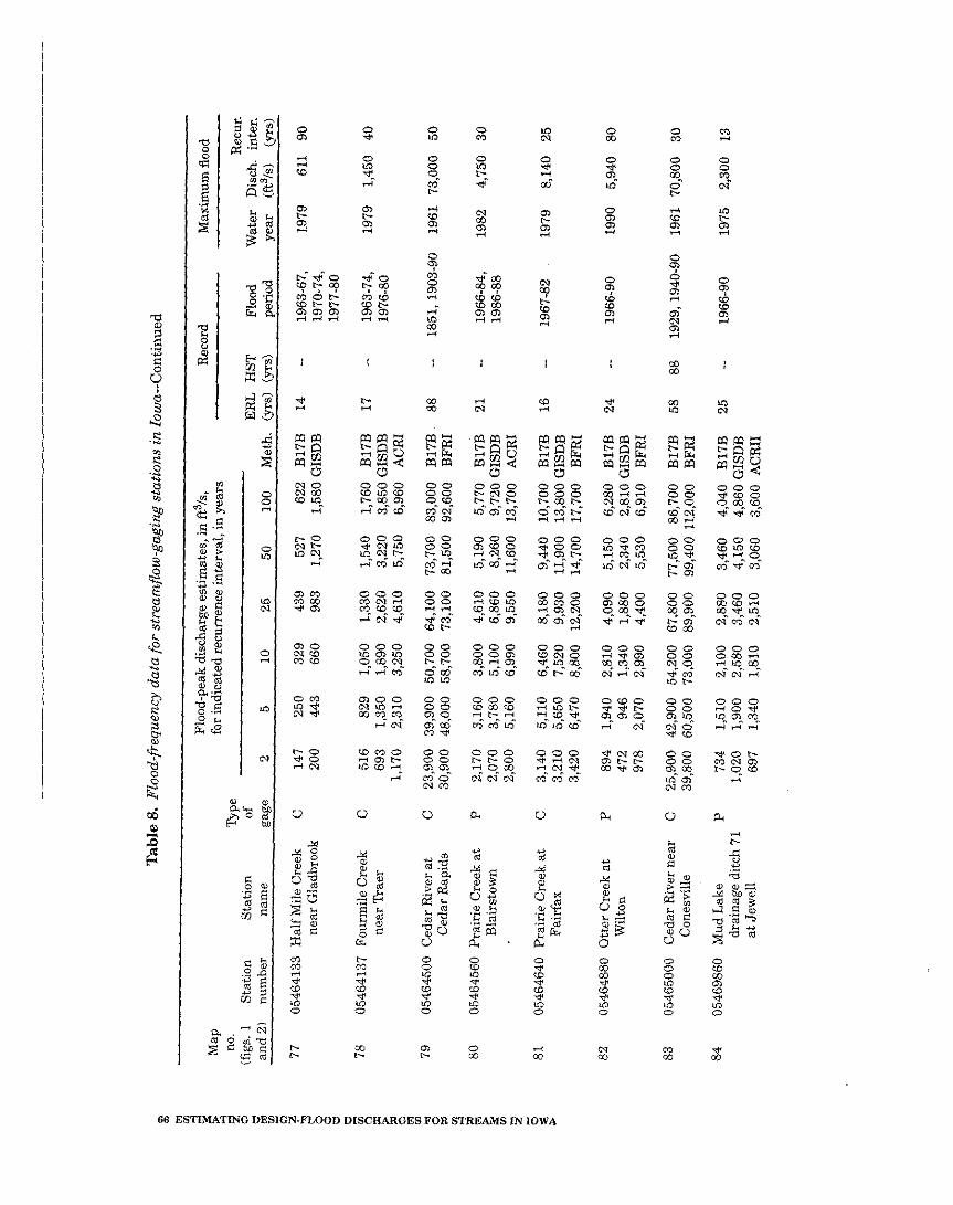
Tab
le 8
. F
lood
-fre
quen
cy d
ata
for
stre
amfl
ow
-gag
ing
sta
tio
ns
in Io
wa-
-Co
nti
nu
ed
2 !2 c! F
lood
-pea
k di
scha
rge
esti
mat
es, i
n fi
3/s,
R
ecor
d M
axim
um f
lood
g M
ap
for i
ndic
ated
rec
urre
nce
inte
rval
, in
year
s 2
no.
n T
ype
Rec
ur.
(fig
s. 1
S
tati
on
Sta
tion
of
E
RL
H
ST
Floo
d W
ater
D
isch
. in
ter.
G
and
21
nu
mbe
r na
me
gage
2
5 10
25
50
10
0 M
eth.
(y
rs)
(yrs
) pe
riod
ye
ar
(fi3
/s)
(yrs
) z 9
77
0546
4133
Hal
f M
ile C
reek
C
14
7 25
0 32
9 43
9 52
7 62
2 B
17B
1
4
-- 19
63-6
7,
1979
61
1 90
3 0
ne
ar G
ladb
rook
20
0 44
3 66
0 98
3 1,
270
1,58
0 G
ISD
B
1970
-74,
0 u
1977
-80
u ! 78
05
4641
37
Fou
rmil
e C
reek
C
51
6 82
9 1,
050
1,33
0 1,
540
1,76
0 B
17B
17
--
1963
-74,
19
79
1,45
0 40
ne
ar T
raer
69
3 1,
350
1,89
0 2,
620
3,22
0 3,
850
GIS
DB
19
76-8
0 1,
170
2,31
0 3,
250
4,61
0 5,
750
6,96
0 A
CR
I $ m
*I 0
79
0546
4500
C
edar
Riv
er a
t C
23
,900
39
,900
50
,700
64
,100
73
,700
83
,000
B
17B
. 88
--
1851
,190
3-90
19
61 7
3,00
0 50
E C
edar
Rap
ids
30,9
00
48,0
00
58,7
00
73,1
00
81,5
00
92,6
00
BF
RI
80
0546
4560
Pra
irie
Cre
ek a
t P
2,
170
3,16
0 3,
800
4,61
0 5,
190
5,77
0 B
17B
2
1
-- 19
66-8
4,
1982
4,
750
30
Bla
irst
own
m 2,
070
3,78
0 5,
100
6,86
0 8,
260
9,72
0 G
ISD
B
1986
-88
2 2,
800
5,16
0 6,
990
9,55
0 11
,600
13
,700
A
CR
I
3 5
81
05
4646
40 P
rair
ie C
reek
at
C
3,14
0 5,
110
6,46
0 8,
180
9,44
0 10
,700
B
17B
1
6
-- 19
67-8
2 *
1979
8,
140
25
Fai
rfax
3,
210
5,65
0 7,
520
9,93
0 11
,900
13
,800
GIS
DB
3,
420
6,47
0 8,
800
12,2
00
14,7
00
17,7
00
BF
RI
82
0546
4880
O
tter
Cre
ek a
t P
89
4 1,
940
2,81
0 4,
090
5,15
0 6,
280
B17
B
24
-- 19
66-9
0 19
90
5,94
0 80
W
ilton
47
2 94
6 1,
340
1,88
0 2,
340
2,81
0 G
ISD
B
978
2,07
0 2,
990
4,40
0 5,
530
6,91
0 B
FR
I
83
0546
5000
C
edar
Riv
er n
ear
C
25,9
00
42,9
00
54,2
00
67,8
00
77,5
00
86,7
00
B17
B
58
88
1929
,194
0-90
19
61 7
0,80
0 30
C
ones
vill
e 39
,800
60
,500
73
,000
89
,900
99
,400
112
,000
B
FR
I
84
0546
9860
M
udL
ake
P
734
1,51
0 2,
100
2,88
0 3,
460
4,04
0 B
17B
25
--
1966
-90
1975
2,
300
13
dr
aina
ge d
itch
71
1,02
0 1,
900
2,58
0 3,
460
4,15
0 4,
860
GIS
DB
a
t Jew
el1
697
1,34
0 1,
810
2,51
0 3,
060
3,60
0 A
CR
II
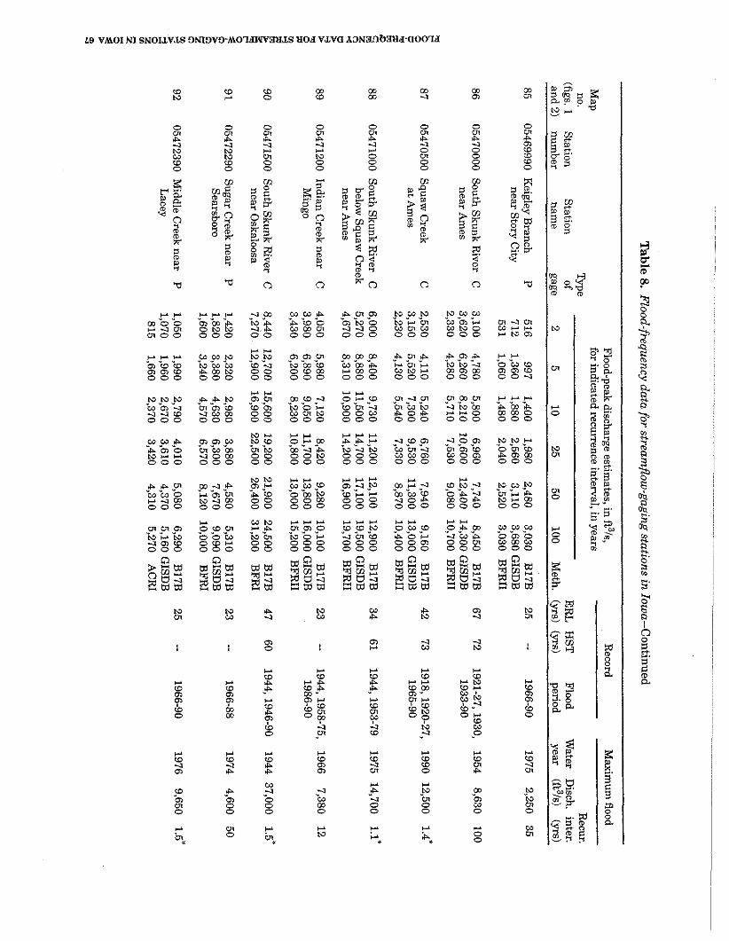
Table 8. R
oo
d-freq
uen
cy d
ata
for streamflo
w-g
agin
g statio
ns in
Iow
a--Co
ntin
ued
Man
Flood-peak discharge estim
ates, in ft3/s, R
ecord M
aximum
fiood for indicated recurrence interval, in years
. .
no. 'b
e
Recur.
(figs. 1
Station
Station
of E
RL
H
ST
Flood
Water
Disch.
inter. and 2)
number
name
gage 2
5 10
25 50
100 M
eth. (yrs) (yrs)
period year
(ft3/s) (~
rs)
85 05469990
KeigIey B
ranch P
516
997 1,400
1,980 2,480
3,030 B
17B
25 --
1966-90 1975
2,250 3
5
near Story C
ity 712
1,360 1,880
2,560 3,110
3,680 GIS
DB
531
1,060 1,480
2,040 2,520
3,030 B
FR
II
86 05470000
South S
kunk River
C
3,100 4,780
5,800 6,960
7,740 8,450
B17B
67
72 1921-27,1930,
1954 8,630
100 near A
mes
3,620 6,260
8,210 10,600
12,400 14,300 G
ISD
B
1933-90 2,330
4,280 5,710
7,530 9,080
10,700 BF
RII
05470500 S
quaw C
reek C
a
t Am
es
05471000 S
outh Skunk R
iver C
below
Squaw
Creek
near Am
es
05471200 Indian C
reek near C
M
ingo
05471500 South S
kunk River
C
near Oskaloosa
05472290 Sugar C
reek near P
S
earsboro
05472390 M
iddle Creek n
ear P
L
aces
2,530 4,110
5,240 6,760
7,940 9,160
B17B
3,150
5,520 7,300
9,530 11,300
13,000 GIS
DB
2,230
4,130 5,540
7,330 8,870
10,400 BF
RII
6,000 8,400
9,730 11,200
12,100 12,900
B17B
5,270
8,880 11,500
14,700 17,100
19,500 GIS
DB
4,670
8,310 10,900
14,200 16,900
19,700 B
FR
II
4,050 5,980
7,120 8,420
9,280 10,100
B17B
3,980
6,890 9,050
11,700 13,800
16,000 GIS
DB
3,430
6,200 8,230
10,800 13,000
15,200 BF
RII
8,440 12,700
15,600 19,200
21,900 24,500
B17B
7,270
12,900 16,900
22,500 26,400
31,200 B
FR
I
1,420 2,320
2,980 3,880
4,580 5,310
B17B
1,820
3,380 4,630
6,300 7,670
9,090 GIS
DB
1,600
3,240 4,570
6,570 8,120
10,000 B
FR
I
1,050 1,990
2,790 4,010
5,080 6,290
B17B
1,070
1,960 2,670
3,610 4,370
5,160 GISD
B
815 1,660
2,370 3,420
4,310 5,270
AC
RI
Tab
le 8
. F
lood
-fre
quen
cy d
ata
for
stre
amfl
ow-g
agin
g st
atio
ns
in I
owa-
-Con
tinu
ed
%
m rn
Flo
od-p
eak
disc
harg
e es
tim
ates
, in
fL3/
s, R
ecor
d M
axim
um f
lood
M
ap
for i
ndic
ated
rec
urre
nce
inte
rval
, in
year
s no
. T
ype
Rec
ur.
n (f
igs.
1.
Sta
tion
S
tati
on
of
ER
L
HS
T
Floo
d W
ater
D
isch
. in
ter.
0
M
and
2)
num
ber
nam
e ga
ge
2 5
10
25
50
100
Met
h.
(yrs
) (y
rs)
peri
od
year
(ft"/s)
(yrs
)
41 ?:
93
0547
2445
Roc
k C
reek
at
P
870
1,65
0 2,
270
3,15
0 3,
870
4,65
0 B
17B
22
--
1966
-88
1970
4,
100
60
z 0 S
igou
rney
1,
370
2,51
0 3,
390
4,55
0 5,
480
6,44
0 G
ISD
B
8 1,
100
2,19
0 3,
090
4,40
0 5,
490
6,65
0 A
CR
I a B
94
05
4725
00 N
orth
Sku
nk R
iver
C
5,67
0 10
,500
14
,000
18
,700
22
,300
26
,000
B
17B
48
60
19
44,1
946-
90
1960
27
,500
1.1.
i ne
ar S
igou
rney
9,
240
14,9
00
19,0
00
24,0
00
27,8
00
31,7
00 G
ISD
B
5,16
0 9,
050
11,9
00
15,9
00
18,9
00
22,0
00
AC
RI
2 tj 2
95
0547
3300
Ced
ar C
reek
nea
r P
5,
310
9,13
0 12
,200
16
,500
20
,200
24
,200
B
17B
23
--
1965
-89
1965
26,
000
1.1
*
Z
Bat
avia
4,
240
6,96
0 8,
940
11,4
00
13,3
00
15,2
00 G
ISD
B
rn +
3,00
0 5,
750
7,87
0 11
,000
13
,300
16
,100
B
FR
I E g
96
0547
3400
C
edar
Cre
ek n
ear
C
6,40
0 7,
870
8,64
0 9,
470
9,99
0 10
,500
B
17B
12
--
1979
-90
1983
8,
560
9 V
) O
akla
nd M
ills
6,84
0 10
,800
13
,700
17
,100
19
,700
22
,300
GIS
DB
5
x 4,
820
8,85
0 11
,800
16
,100
19
,200
22
,900
B
FR
I
5 97
05
4735
00 B
igC
reek
nea
r C
1,
980
3,76
0 5,
110
6,95
0 8,
400
9,88
0 B
17B
26
32
19
48,1
956-
79
1973
10
,500
1.
1"
Mou
nt P
leas
ant
2,56
0 4,
390
5,75
0 7,
460
8,80
0 10
,200
GIS
DB
2,
230
4,38
0 6,
080
8,60
0 10
,500
12
,800
B
FR
I
98
0547
4000
Sku
nk R
iver
at
C
20,9
00
31,0
00
37,1
00
44,2
00
48,9
00
53,3
00
B17
B
81
13
9 19
03, 1
915-
90
1973
66,
800
1.2'
A
ugus
ta
19,7
00
31,9
00
39,8
00
50,7
00
57,4
00
66,1
00
BF
RI
99
0547
6500
Des
Moi
nes
Riv
er
C
2,12
0 4,
470
6,55
0 9,
790
12,7
00
15,9
00
B17
B
41
52
1952
-90
1969
16
,000
10
0 a
t Est
herv
ille
2,
370
4,34
0 5,
790
7,63
0 9,
200
10,8
00 B
FR
II
100
0547
6750
Des
Moi
nes
Riv
er
C
4,12
0 7,
720
10,3
00
13,6
00
16,1
00
18,4
00
B17
B
51
52
19
40-9
0 19
69
18,0
00
90
at H
umbo
ldt
3,64
0 6,
480
8,49
0 11
,000
13
,100
15
,300
BF
RII
Tab
le 8. Flood-frequency d
ata
for stream
flow
-gag
ing
station
s in Io
wa--C
on
tinu
ed
Flood-peak discharge estim
ates, in ft3/s, R
ecord M
aximum
flood M
ap for indicated recurrence interval, in
years no.
me
R
ecur. (figs. 1
S
tation S
tation of
ER
L
HST
Flood
Water
Disch.
inter. an
d 2)
number
name
gage 2
5 10
25 50
100 M
eth. (yrs) (yrs)
period year
(ft3/s) (yrs)
101 05479000
East F
ork Des
C
3,780 7,600
10,700 15,300
19,100 23,200
B17B
54
72 1938, 1940-90
1938 22,000 80
Moines R
iver at 3,570
6,340 8,300
10,700 12,800
14,900 BF
RII
Dakota C
ity
102 05480000
Lizard C
reek near C
1,590
3,350 4,710
6,560 7,990
9,420 B
17B
42 --
1940-81 1947
10,000 1.1*
Clare
1,920 3,540
4,780 6,370
7,620 8,880 G
ISD
B
2,080 3,830
5,120 6,770
8,180 9,610
BF
RII
+ 0 103
05480500 D
es Moines R
iver C
a
t Fort D
odge
0
g 104
05481000 Bm
ne River n
ear C
a
Webster C
ity Le
E k- "! 105
05481300 D
es Moines R
iver C
% n
ear Stratford
I 106
05481680 B
eaver Creek a
t P
B
eaver
S 9 - 107
05481950 Beaver C
reek near C
G
rimes
-- ro ji
108 05482170 B
ig Cedar C
reek C
8
n
ear Varina
0
Zi
9,930 i6,700
21,500 28,000
33,000 38,200
BI
~B
7,760
13,300 17,100
21,800 25,700
29,600 B
FR
II
5,090 8,840
11,500 15,100
17,800 20,500
B17B
4,430
7,730 10,200
13,200 15,600
17,900 GIS
DB
4,750
8,380 10,900
14,100 16,800
19,600 B
FR
II
14,000 23,800
30,900 40,400
47,700 55,200
B17B
16,800
27,600 34,900
43,300 50,600
57,700 B
FR
II
594 1,080
1,430 1,880
2,210 2,530
B17B
638
1,210 1,650
2,230 2,690
3,160 GIS
DB
674
1,320 1,820
2,500 3,070
3,670 B
FR
II
2,770 4,570
5,800 7,340
8,460 9,550
B17B
3,940
6,720 8,770
11,300 13,300
15,300 GIS
DB
2,120
3,910 5,240
6,940 8,380
9,860 B
FR
II
640 1,260
1,720 2,330
2,780 3,240
B17B
691
1,350 1,860
2,540 3,080
3,630 GIS
DB
512
1,000 1,360
1,910 2,330
2,760 A
CR
II
i-l i-l
I-' i-l
v I-' I-' I-' i-l
i-l I-' m a j: I-' I-'
W N I-' 0 $ ; k ? Z Z - ? o g NI-'
8 0 8 0 a 8 0 0
e a a e a
e e e 8 w E 8 E m m
W m
N N N m W 0 w N 0 8i e m a w W E 0
0 0 w 0 0 0 o o o o 8 g w
a a .W "a $0 "I-' "I-'
PNOl "2 "2 "2 "G "g 2% 3W2 8 % 8 %EW Z 8 $ w - a O W N
0 0 0 0 0 m a m o w + o o m N ~ W 0 0 o o o
I-' i-l I-' .g "E 9 "a "4 Y "I-' m e w %Z*G m a w C .N "- "5' "-
O N 8 2 Y % % P a I - ' m e o w w w w 4 P 0 0 0 0 0 0 0 0 m m ~ o o o O N N
0 0 % % % 0 0 0 0 0
i-l I-' i-l I-' i-l i-l C g 3-2-g g"2-g "$ "2 "; "L "2 -s "; "$ "2 "i 0 0 - 0 0 e - w N - U ~ e m w a w m 0 0 0 0 0 0 0 0 N a W 0 0 0 O N 0
0 0 w m o 0 0 0 0 0
I-'+ i-1i-1i-1 I-'N CLi -1 i -1 "2 "2 "E "Z "g .!! "N "N "I-' C" "W "N "I-' "i-1 "I-' O W N N e w W-IW - a r m "$ "; *: "E -2
0 0 0 0 0 - a ~ w w m - a - w e m r 0 0 0 0 0 0 0 0 O W N 0 0 0 0 0 0
0 0 0 0 0 0 0 0 0 0
N r V N V .o"m " a p N W N I-'
N N I-'-- me^ ~ i - 1 ~ va+vm
g g 2 8 g "m "4 "w w m "N " ~ 1 "m "i-1 "P "w I- 'W N e - o o o o o 8 8 $ 8 5 3 a N e
0 0 0 0 0 0 O 0 O o O
0 0 0 0 0
NI-' i-1NN N N ClrI-' "g g g "g "g ?' "* "W "i-1 i-l -I a w N "I-' .N m w -4 "m .w e m - "A "W m 4 -a
0 0 0 0 0 *"4N g g p ,,, 8 8 % " m b - m a
0 0 0 0 0 0 0 0 0 0 0 0 0 0 0 0 0 0
N
U1
i-l 0
N a
::
I-' 0 0
z
g g j.&
DL ;;t 8 8 g i $ 8 f 2 g PJ
j' X, 2 e
m "? a
W I-' N W P W a P a w o 3 Z " W m G I W - I-' i-l
w i-l
s? -2 i-l I-' I-' W W w G I-' 8
"P I-' ? a 8 s? 2
t; Y 2 2 E r a 3 8 w o o o o 8 2 w 0 0
Cb 0
I-' I-' I-' t; s (0 t; w t; t; 8 m m a 5' m w m o 8 P 2 w I-' i-l a e w N ,.'
N N w W "to k "W 5' b 0 I-' i 0 0
a a 4 o o P o o 8 0 0
0
p. W 4 0 0
W W i-l 0 E 0 0 0
0 z
$ 2 F
2 g, E PL
9 8 I F
99 I*
x 2 3. g&X
% G 8 %
- 0 %50;; '0
I T
-j.g 2 3 2 - 7 7
2 0
%.
Z B. g D
g
Table 8. F
lood-frequency da
ta for stream
flow
-gag
ing
station
s in Io
wa--C
on
tinu
ed
Flood-peak discharge estim
ates, in ft3/s, R
ecord M
aximum
flood M
ap for indicated recurrence interval, in
years no.
Type
Recur.
(figs. 1
Station
Station
of E
RL
H
ST
Flood
Water
Disch.
inter. and 2)
number
name
gage 2
5 1
0
25 50
100 M
eth. (yrs) (yrs)
period year
(ft3/s) (yrs)
117 05484000 S
outhRaccoon
C
10,400 16,400
20,400 25,400
29,000 32,500
B17B
5
1
-- 1940-90
1958 35,000 1.1'
River at R
edfield 12,000
20,000 25,800
33,000 38,500
44,100 GIS
DB
8,480
14,800 19,300
25,500 29,800
35,000 B
FR
I
118 05484500
Raccoon R
iver C
14,400
23,400 a
t Van M
eter 10,600
17,900
119 05484800 W
alnut Creek a
t C
2,270
4,890 D
es Moines
1,950 3,580
1,880 3,520
120 05485640 F
ourmile C
reek at
C
2,510 4,190
Des M
oines 1,710
3,120 1,310
2,430
49,700 B
17B
76 --
1915-90 1947
41,200 40
39,200 B
FR
II
18,100 B
17B
19 --
1972-90 1986
12,500 3
5
9,220 GIS
DB
9,140
BF
RII
8,860 B
17B
18 --
1972-79, 1977
5,380 10
7,840 GIS
DB
1981-90
6,190 A
CR
II
121 05486000
North R
iver near C
3,420
6,990 10,100
14,900 19,200
23,900 B
17B
51
--
1940-90 1947
32,000 1.3'
Norw
alk 7,140
12,200 16,100
20,900 24,700
28,500 GIS
DB
2,680
4,960 6,730
9,200 11,200
13,200 A
CR
I
122 05486490
Middle R
iver near C
7,140
11,100 13,700
17,000 19,300
21,600 B
17B
51
--
1940-90 1947
34,000 1.6'
Indianola 10,100
16,600 21,300
27,100 31,600
36,200 GIS
DB
5,020
8,830 11,700
15,500 18,500
21,500 A
CR
I
123 05487470 S
outh River n
ear C
10,700
17,900 22,700
28,600 32,700
36,600 B
17B
54 61
1930,1940-90 1990 88,100
100 A
ckworth
9,520 15,300
19,400 24,300
28,100 31,900 G
ISDB
4,820
8,500 11,200
15,000 17,900
20,800 A
CR
I
124 05487600 S
outh White B
reast P
2,230 4,070
5,410 7,190
8,550 9,910
B17B
29
-- 1953-81
1981 11,800
1.2' C
reek near
1,940 3,560
4,810 6,460
7,800 9,170 G
ISD
B
Osceola
1,700 3,430
4,830 6,910
8,520 10,500
BF
RI
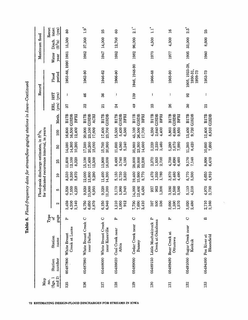
<
Tab
le 8
. F
lood
-fre
quen
cy d
ata
for
stre
amfl
ow-g
agin
g st
atio
ns i
n Io
wa-
-Con
tinu
ed
N
Flo
od-p
eak
disc
harg
e es
tim
ates
, in
ft3/
s,
Rec
ord
Max
imum
floo
d M
ap
for i
ndic
ated
rec
urre
nce
inte
rval
, in
year
s no
. T
ype
Rec
ur.
(fig
s. 1
S
tati
on
Sta
tion
of
E
RL
HST
Floo
d W
ater
D
isch
. in
ter.
an
d 2
) nu
mbe
r na
me
gage
2
5 10
25
50
10
0 M
eth.
(y
rs)
(yrs
) pe
riod
ye
ar
(&s)
(y
rs)
125
0548
7800
Whi
te B
reas
t P
3,
450
6,32
0 8,
530
11,6
00
14,0
00
16,6
00
B17
B
37
-- 19
53-8
8, 1
990
1981
15
,500
80
C
reek
at L
ucas
4,
200
7,15
0 9,
330
12,1
00
14,3
00
16,5
00 G
ISD
B
2,14
0 4,
220
5,87
0 8,
320
10,2
00
12,4
00
BF
RI
126
0548
7980
W
hite
Bre
ast C
reek
C
6,75
0 9,
820
12,0
00
15,1
00
17,5
00
20,0
00
B17
B
32
46
1962
-90
1982
37,
300
1.9'
ne
ar D
alla
s 6,
650
10,8
00
13,8
00
17,4
00
20,2
00
23,1
00 G
ISD
B
3,87
0 6,
950
9,29
0 12
,500
15
,000
17
,600
A
CR
I
ii,
127
0548
8000
W
hite
Bre
ast
Cre
ek C
6,
150
9,32
0 11
,400
g
near
Kno
xvill
e 6,
940
11,2
00
14,3
00
I 12
8 05
4886
20
Coa
l Cre
ekn
ear
P
1,21
0 3,
170
5,15
0 A
lbia
1,
050
1,99
0 2,
730
V1 L?
912
1,94
0 2,
820
8 12
9 05
4890
00
Ced
ar C
reek
nea
r C
7,
790
14,0
00
19,4
00
$ B
usse
y 7,
690
12,4
00
15,9
00
3,41
0 6,
450
8,77
0
130
0548
9150
L
ittl
e M
ucha
kino
ck P
39
7 C
reek
at O
skal
oosa
50
0 53
6
131
0548
9490
B
ear
Cre
ek a
t P
2,
090
Ott
umw
a 1,
390
1,57
0
132
0549
1000
S
ugar
Cre
ek n
ear
C
3,02
0 K
eoku
k 2,
480
13,9
00
15,7
00
17,4
00
B17
B
21
36
19
46-6
2 19
47
14,0
00
25
18,0
00
20,9
00
23,7
00 G
ISD
B
8,49
0 11
,600
15
,300
B
17B
24
--
1966
-90
1982
12
,700
60
3,
740
4,56
0 5,
420
GIS
DB
4,
160
5,24
0 6,
560
BF
RI
28,0
00
35,8
00
45,1
00
B17
B
49
139
1946
,194
8-90
19
82 9
6,00
0 2.
1'
20,0
00
23,3
00
26,5
00 G
ISD
B
12,2
00
14,6
00
17,7
00
BF
RI
3,22
0 4,
250
B17
B
23
-- 19
66-8
8 19
70
4,50
0 1.
1*
2,23
0 2,
640
GIS
DB
3,
460
4,40
0 B
FR
I
5,29
0 5,
860
B17
B
26
-- 19
65-9
0 19
77
4,30
0 16
5,
670
6,68
0 G
ISD
B
7,99
0 9,
850
BF
RI
11,2
00
13,4
00
B17
B
30
92
1905
, 192
3-28
, 19
05 3
3,00
0 2.
5*
8,42
0 9,
720
GIS
DB
19
30-3
1,
1959
-73
133
0549
4300
Fo
x R
iver
at
B
2,71
0 4,
970
6,65
0 8,
890
10,6
00
12,4
00
B17
B
21
--
1953
-73
1960
8,
600
25
Blo
omfi
eld
2,16
0 3,
730
4,91
0 6,
410
7,60
0 8,
810
GIS
DB
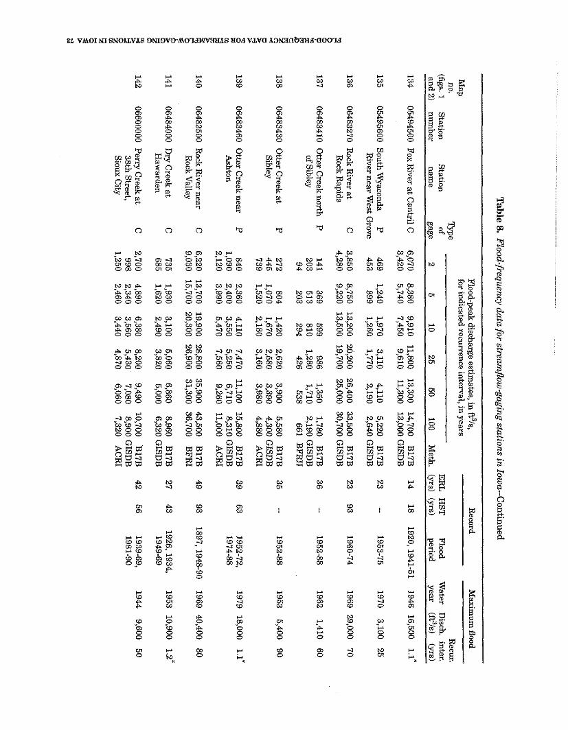
Table 8. F
lood-frequency da
ta for stream
flow
-gag
ing
station
s in Iow
a--Continued
Flood-peak discharge estimates, in ft3/s,
Record
Maxim
um flood
Map
for indicated recurrence interval, in years no.
we
R
ecur. (figs. 1
S
tation S
tation of
ER
L
HS
T
Flood W
ater D
isch. inter.
and 2) num
ber nam
e gage
2 5
10 25
50 100
Meth.
@rs)
(yrs) period
year (ft3/s)
(yrs)
134 05494500
FoxR
iver at C
antril C
6,070 8,380
9,910 11,800
13,300 14,700
B17B
1
4
18 1920,1941-51
1946 16,500
1.1.
3,420 5,740
7,450 9,610
11,300 13,000 G
ISDB
135 05495600
South W
yaconda P
469
1,240 1,970
3,110 4,110
5,220 B
17B
23 --
1953-75 1970
3,100 25
River near W
est Grove
453 899
1,260 1,770
2,190 2,640 G
ISDB
136 06483270
Rock R
iver at
C
3,850 8,750
13,200 20,200
26,400 33,500
B17B
23
93 1960-74
1969 29,000
70 Z
Rock R
apids 4,280
9,220 13,500
19,700 25,000
30,700 GISD
B
b 0
0
137 06483410 O
tter Creek north
P
141 369
599 986
1,350 1,780
B17B
36
-- 1952-88
1962 1,410
60
3 of S
ibley 203
513 810
1,280 1,710
2,190 GISD
B
9
94 203
294 426
538 661
BF
RII
2 3 138
06483430 O
tter Creek a
t P
272
804 1,420
2,620 3,900
5,580 B
17B
35
--
1952-88 1953
5,400 90
4
a S
ibley 445
1,070 1,670
2,580 3,390
4,300 GISD
B
5 739
1,520 2,180
3,160 3,980
4,880 A
CR
I
$ 139
06483460 Otter C
reek near P
840
2,360 4,110
7,470 11,100
15,800 B
17B
39 6
3
1952-72, 1979
18,000 1.1"
Ashton
1,090 2,400
3,550 5,250
6,710 8,310 G
ISDB
1974-88
2,120 3,990
5,470 7,560
9,260 11,000
AC
RI
140 06483500
Rock R
iver near C
6,220
13,700 19,900
28,800 35,900
43,500 B
17B
49 93
1897,1948-90 1969 40,400
80 S
Rock V
alley 9,030
15,700 20,300
26,900 31,300
36,700 B
FR
I s
6 $ 1
41
06484000
Dry C
reek at
C
735 1,930
3,100 5,060
6,860 8,960
B17B
27
43 1926,1934,
1953 10,900
1.2*
3 H
awarden
685 1,620
2,490 3,820
5,000 6,320 G
ISDB
1949-69
? 142
06600000 P
eny
Creek
at C
2,700
4,890 6,380
8,200 9,490
10,700 B
17B
42 56
1939-69, 1944
9,600 50
2
38th Street,
998 2,340
3,560 5,430
7,080 8,900 G
ISDB
1981-90
0
% S
ioux City
1,250 2,460
3,440 4,870
6,060 7,320
AC
RI
* 7
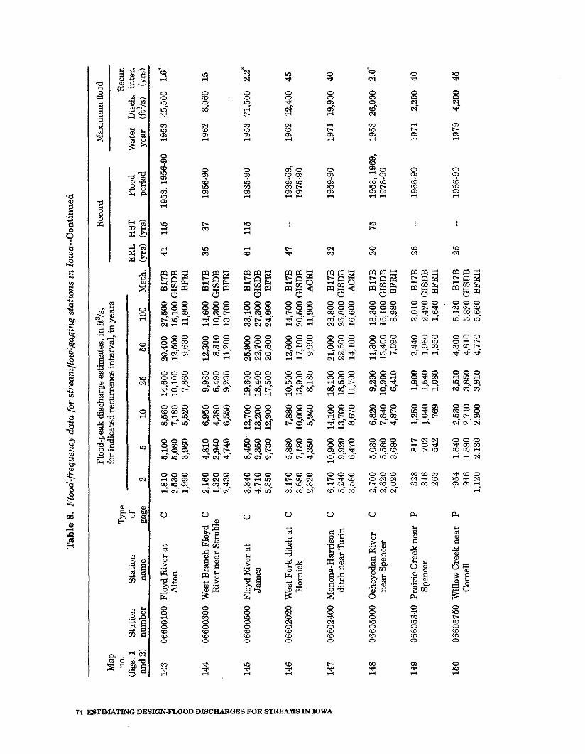
Tab
le 8
. F
lood
-fre
quen
cy d
ata
for
stre
amfl
ow-g
agin
g st
atio
ns
in Io
wa-
-Con
tinu
ed
Flo
od-p
eak
disc
harg
e es
tim
ates
, in
ft3/
s,
Rec
ord
Max
imum
floo
d fo
r ind
icat
ed re
curr
ence
inte
rval
. in
vea
rs
, .
no.
Typ
e R
ecur
. (f
igs.
1
Sta
tion
S
tati
on
of
ER
L
HST
Fl
ood
Wat
er
Dis
ch.
inte
r.
and
2)
num
ber
nam
e ga
ge
2 5
10
25
50
100
Met
h.
(yrs
) (y
rs)
peri
od
year
(
~~
1s
)
(YT
S)
143
0660
0100
Flo
yd R
iver
at
C
1,81
0 5,
100
8,56
0 14
,600
20
,400
27
,500
B
17B
41
11
5 19
53,1
956-
90
1953
45,
500
1.6'
A
lton
2,
530
5,08
0 7,
180
10,1
00
12,5
00
15,1
00 G
ISD
B
1,99
0 3,
960
5,52
0 7,
860
9,63
0 11
,800
B
FR
I
144
0660
0300
Wes
t B
ranc
h Fl
oyd
C
2,16
0 4,
810
6,95
0 9,
930
12,3
00
14,6
00
B17
B
35
37
1956
-90
1962
8,
060
15
Riv
er n
ear
Str
nble
1,
320
2,94
0 4,
380
6,49
0 8,
310
10,3
00 G
ISD
B
2,43
0 4,
740
6,55
0 9,
230
11,2
00
13,7
00
BF
RI
145
0660
0500
Flo
ydR
iver
at
C
3,84
0 8,
450
12,7
00
19,6
00
25,9
00
33,1
00
B17
B
61
11
5 19
35-9
0 19
53 7
1,50
0 2.
2"
Jam
es
4,71
0 9,
350
13,2
00
18,4
00
22,7
00
27,3
00 G
ISD
B
5,35
0 9,
730
12,9
00
17,5
00
20,8
00
24,8
00
BF
RI
146
0660
2020
Wes
t For
kdit
ch a
t C
3,
170
5,88
0 7,
880
10,5
00
12,6
00
14,7
00
B17
B
47
-- 19
39-6
9,
1962
12
,400
45
H
orni
ck
3,68
0 7,
180
10,0
00
13,9
00
17,1
00
20,5
00 G
ISD
B
1975
-90
2 R
2,32
0 4,
350
5,94
0 8,
180
9,99
0 11
,900
A
CR
I
$ 14
7 06
6024
00 M
onon
a-H
arri
son
C
6,17
0 10
,900
14
,100
18
,100
21
,000
23
,800
B
17B
32
19
59-9
0 19
71 1
9,90
0 40
di
tch
near
Tur
in
5,24
0 9,
920
13,7
00
18,6
00
22,6
00
26,8
00 G
ISD
B
3,58
0 6,
470
8,67
0 11
,700
14
,100
16
,600
A
CR
I
148
0660
5000
Och
eyed
an R
iver
C
2,
700
5,03
0 6,
820
9,29
0 11
,300
13
,300
B
17B
20
75
19
53,1
969,
19
53 2
6,00
0 2.
0' ne
ar S
penc
er
2,82
0 5,
580
7,84
0 10
,900
13
,400
16
,100
GIS
DB
19
78-9
0 2,
020
3,68
0 4,
870
6,41
0 7,
690
8,98
0 B
FR
II
149
0660
5340
Pra
irie
Cre
ek n
ear
P
328
817
1,25
0 1,
900
2,44
0 3,
010
B17
B
25
-- 19
66-9
0 19
71
2,20
0 40
S
penc
er
316
702
&,0
40
1,54
0 1,
960
2,42
0 G
ISD
B
263
542
769
1,08
0 1,
350
1,64
0 B
FR
II
150
0660
5750
Will
ow C
reek
nea
r P
-9
54
1,84
0 2,
530
3,51
0 4,
300
5,13
0 B
17B
25
--
1966
-90
1979
4,
200
45
Cor
nell
91
6 1,
890
2,71
0 3,
850
4,81
0 5,
820
GIS
DB
1,
120
2,13
0 2,
900
3,91
0 4,
770
5,66
0 B
FR
II
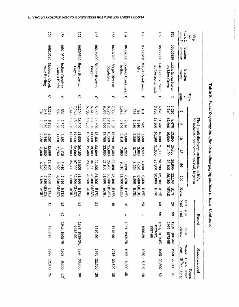
Tab
le 8. Flood-frequency d
ata for streamflo
w-g
agin
g statio
ns in
Iow
a--Co
ntin
ued
- -
-
Flood-peak discharge estim
ates, in ft3/s, R
ecord M
aximum
flood for indicated recurrence interval. in vears
. .
no. m
e
Recur.
(figs. 1
Station
Station
of E
RL
H
ST
F
lood W
ater D
isch. inter.
and
2)
number
name
gage 2
5 10
25 50
100 M
eth. (yrs) (yrs)
period Y
ear (ft3/s)
(~
$1
15
1
06605850 L
ittle Sioux R
iver C
4,520
9,470 13,800
20,300 25,900
32,100 B
17B
28 99
1953, 1961-62 1953 22,500
35
a
t Linn G
rove 7,240
12,600 16,500
21,100 25,100
29,100 B
FR
II 1965,1973-90
152 06606600
Little S
ioux River
C
6,470 11,700
15,800 21,800
26,700 32,100
B17B
69
99 1891, 1919-25,
1965 29,800 80
at C
orrectionville 6,890
12,200 16,100
21,600 25,300
30,000 B
FR
I 1929-32, 1937-90
8 153
06606790 Maple C
reek near P
134
702 1,580
3,630 6,090
9,560 B
17B
24 --
1966-89 1969
5,300 40
8 A
lta 828
1,740 2,530
3,660 4,620
5,660 GIS
DB
553
1,230 1,830
2,770 3,550
4,500 B
FR
I k
4 e 154
06607000 Odebolt C
reek near C
990
2,010 2,880
4,220 5,380
6,670 B
17B
18 --
1951, 1958-75 1962
5,200 45
g A
rthur 1,880
3,800 5,410
7,690 9,610
11,700 GIS
DB
3 2 u
155
06607200 M
aple River a
t C
7,030
11,900 15,200
19,400 22,400
25,400 B
17B
49 --
1942-90 1978 20,800
35 %
M
apleton 6,720
12,100 16,300
21,800 26,200
30,700 GIS
DB
$
8,060 13,600
17,700 23,000
27,100 31,000
AC
RI
5
156 06608500 S
oldier River a
t C
8,450
14,300 18,400
23,600 27,500
31,200 B
17B
51
--
1940-90 1950 22,500
20 P
isgah 5,920
10,900 14,800
19,900 24,000
28,400 GIS
DB
5,760
10,000 13,200
17,400 20,700
23,900 A
CR
I
2 157
06609500 B
oyer River a
t C
12,100
18,300 21,900
26,100 28,900
31,400 B
17B
61
--
1881,1918-25, 1990 30,800
90
h
Logan
7,750 13,500
17,900 23,500
27,900 32,300 G
ISD
B
1938-90 7,990
13,500 17,500
22,800 26,900
30,800 A
CR
I 5 i 0 V,
158 06610500 Indian C
reek at
C 561
1,520 2,480
4,110 5,640
7,440 B
17B
25 35
1942,1955-76 1942
9,200 1.2'
2 C
ouncil Bluffs
583 1,280
1,880 2,760
3,520 4,340 G
ISD
B
g 159
06610520 Mosquito C
reek C
3,110
6,170 8,590
12,000 14,700
17,500 B
17B
15
--
1965-79 1972
12,000 25
2 9 n
ear Earling
946 1,930
2,740 3,880
4,820 5,830 G
ISD
B
3 797
1,630 2,330
3,360 4,240
5,180 A
CR
I
s 2
-3
Table
8. F
lood
-fre
quen
cy d
ata
for
stre
amfl
ow-g
agin
g st
atio
ns
in Io
wa-
-Con
tinu
ed
m
Floo
d-pe
ak d
isch
arge
est
imat
es, i
n ft
3/s
, R
ecor
d M
axim
um fl
ood
Map
fo
r ind
icat
ed r
ecur
renc
e in
terv
al, i
n ye
ars
no.
'be
R
ecur
. (f
igs.
1
Sta
tion
S
tati
on
of
ER
L
HST
Fl
ood
Wat
er
Dis
ch.
inte
r.
and
2)
num
ber
nam
e ga
ge
2 5
10
25
50
100
Met
h.
(yrs
) (y
rs)
peri
od
year
(f
t3/s
) b
s)
160
0661
0600
Mos
quito
Cre
ekat
P
4,
540
7,90
0 10
,500
14
,300
17
,400
20
,800
B
17B
39
--
1952
-90
1958
17,
300
50
Neo
la
2,60
0 4,
950
6,84
0 9,
380
11,5
00
13,6
00 G
ISD
B
1,37
0 2,
690
3,75
0 5,
280
6,55
0 7,
890
AC
RI
161
0680
6000
W
aubo
nsie
Cre
ek
C
2,87
0 5,
780
8,17
0 11
,700
14
,600
17
,700
B
17B
24
--
1946
-69
1950
14
,500
50
ne
ar B
artl
ett
1,18
0 2,
270
3,13
0 4,
310
5,26
0 6,
250
GIS
DB
E 16
2 06
8074
10
Wes
t Nis
hnab
otna
C
9,
410
15,5
00
19,5
00
24,3
00
27,7
00
31,0
00
B17
B
31
--
1960
-90
1972
26,
400
40
Riv
er a
t Han
cock
6,
520
11,6
00
15,4
00
20,4
00
24,4
00
28,5
00 G
ISD
B
2 6,
700
11,5
00
15,0
00
19,7
00
23,3
00
26,9
00
AC
RI
I 16
3 06
8074
70
Indi
an C
reek
nea
r P
85
8 2,
240
3,72
0 6,
420
9,17
0 12
,700
B
17B
25
--
1966
-90
1982
15
,800
1.
2'
Em
erso
n 1,
310
2,49
0 3,
420
4,67
0 5,
680
6,73
0 G
ISD
B
vi
1;49
0 3,
050
4,31
0 6,
220
7,70
0 9,
510
BF
RI
4: - 8 16
4 06
8077
20
Mid
dle
Sil
ver
Cre
ek P
38
7 67
9 87
9 1,
130
1,31
0 1,
480
B17
B
32
-- 19
53-8
4,
1976
1,
200
35
3
near
Avo
ca
285
646
970
1,46
0 1,
890
2,36
0 G
ISD
B
1986
-88
258
616
949
1,49
0 1,
960
2,54
0 B
FR
I
165
0680
7760
Mid
dle
Sif
ver C
reek
P
882
1,26
0 1,
510
1,82
0 2,
050
2,27
0 B
17B
38
--
1953
-90
1973
2,
110
60
near
Oak
land
84
9 1,
740
2,50
0 3,
570
4,47
0 5,
430
GIS
DB
43
3 93
2 1,
360
2,03
0 2,
600
3,23
0 A
CR
I
166
0680
7780
M
iddl
e S
ilve
r C
reek
P
1,32
0 1,
960
2,41
0 2,
980
3,42
0 3,
870
B17
B
37
-- 19
53-5
5,
1973
3,
700
80
at T
reyn
or
1,07
0 2,
150
3,04
0 4,
280
5,31
0 6,
400
GIS
DB
19
57-9
0 82
1 1,
670
2,39
0 3,
440
4,34
0 5,
300
AC
RI
167
0680
8000
M
ule
Cre
ek n
ear
C
762
1,84
0 2,
730
3,98
0 4,
950
5,93
0 B
17B
16
--
1954
-69
1954
2,
070
6 M
alve
rn
704
1,42
0 2,
010
2,84
0 3,
520
4,25
0 G
ISD
B
168
0680
8500
Wes
t Nis
hnab
otna
C
15
,300
25
,700
32
,200
39
,800
44
,900
49
,600
B
17B
42
43
19
47,1
949-
90
1987
40,
800
30
Riv
er a
t Ran
dolp
h 12
,200
20
,000
25
,400
32
,500
87
,800
42
,900
A
CR
I
Table 8. Flood-frequency d
ata
for stream
flow-gaging statio
ns in
Iowa--C
ontinued
Flood-peak discharge estimates, in
ft3/s, R
ecord M
aximum
flood for indicated recurrence interval, in
years no.
Typ
e R
ecur. (figs. 1
S
tation S
tation of
ER
L
HS
T
Flood W
ater D
isch. inter.
and 2) num
ber nam
e gage
2 5
10 25
50 100
Meth.
(yrs) (yrs)
period year
(ft3/s) (yrs)
169 06809000
Davids C
reek near C
892
2,140 3,400
5,590 7,710
10,300 B
17B
22 --
1952-73 1958 22,700
2.2' H
amlin
1,320 2,540
3,530 4,890
6,020 7,200 G
ISD
B
170 06809210
EastN
ishnabotna C
8,910
15,600 20,400
26,500 31,000
35,400 B
17B
32 43
1958,1961-90 1958 34,200
80 R
iver near Atlantic
6,570 11,200
14,800 19,200
22,800 26,400 G
ISD
B
8,400 14,200
18,300 23,800
28,000 32,100
AC
RI
*1
171 06809500
East N
ishnahotna C
9,330
16,100 20,700
26,200 30,100
33,700 B
17B
69 87
1917-25, 1972
38,000 1.1
*
6 0 R
iver at R
ed Oak
10,800 18,000
23,200 29,700
34,700 39,800 G
ISDB
1936-90
u a& 8,540
14,400 18,600
24,100 28,400
32,500 A
CR
I
@ 172
06810000 Nishnabotna R
iver C
15,900
23,900 28,600
33,800 37,200
40,300 B
17B
69 139
1917,1922-23, 1947
55,500 1.4*
s above H
amburg
10,100 16,800
21,600 27,800
32,500 37,000
AC
RI
1929-90 ?: a u
173 06811760
Tarkio R
iver near
P
573 1,220
1,760 2,540
3,170 3,850
B17B
33
-- 1952-90
1987 3,210
50
E E
lliot 629
1,270 1,800
2,540 3,170
3,830 GIS
DB
,. 825
1,770 2,580
3,830 4,850
6,080 B
FR
I
06811840 T
arkio River a
t C
2,920
6,490 9,290
13,100 S
tanton 1,500
2,820 3,870
5,270 1,360
2,660 3,720
5,240
06811875 S
nake Creek near
P
1,170 2,010
2,580 3,280
Yorktow
n 837
1,630 2,270
3,140 519
1,100 1,600
2,350
06817000 N
odaway R
iver at
C
10,800 19,300
24,900 31,600
Clarinda
11,500 18,800
24,200 30,900
10,600 17,500
22,500 28,900
15,900 18,800
B17B
37
-- 1952,1954-56,
1967 22,500
1.2* 6,410
7,600 GIS
DB
1958-90
6,500 7,840
AC
RI
3,780 4,250
B17B
25
-- 1966-90
1987 3,080
20 3,850
4,600 GISD
B
3,000 3,710
AC
RI
36,200 40,400
B17B
66
87
1903,1918-25,
1947 31,100
25 36,100
41,300 GIS
DB
1936-90
33,800 38,400
AC
RI
Z
m
177 06818598 P
latte River near
P
1,440 2,110
2,560 3,110
3,510 3,910
B17B
23
-- 1966-88
1974 3,120
25 !2
Stringtow
n 1,550
2,740 3,650
4,830 5,770
6,740 GIS
DB
8 5
1,730 3,320
4,590 6,400
7,880 9,430
AC
RI
4
4
Table
8. F
lood
-fre
quen
cy d
ata
for
stre
amfl
ow-g
agin
g st
atio
ns
in Io
wa-
-Con
tinu
ed
2
DO
. 'h
e
(fig
s. 1
S
tati
on
Sta
tion
of
- and
2)
num
ber
nam
e ga
ge
178
0681
8750
P
latt
e R
iver
nea
r C
D
iago
nal
179
0681
9190
Eas
t For
k O
ne
C
Hun
dred
and
Tw
o R
iver
nea
r B
edfo
rd
180
0689
7950
Elk
Cre
ek n
ear
C
Dec
atur
City
181
0689
8000
T
hom
pson
Riv
er a
t C
D
avis
City
182
0689
8400
Wel
don
Riv
er n
ear
C
Leo
n
183
0690
3400
C
hari
ton
Riv
er
C
near
Cha
rito
n
184
0690
3500
Hon
ey C
reek
nea
r C
R
usse
ll
185
0690
3700
Sou
th F
ork
Cha
rito
n C
R
iver
nea
r Pr
omis
e C
ity
186
0690
3900
C
hari
ton
Riv
er
C
near
Rat
hbun
Floo
d-pe
ak d
isch
arge
est
imat
es, i
n ft
3/s,
R
ecor
d M
axim
um fl
ood
for i
ndic
ated
rec
urre
nce
inte
rval
, in
year
s R
ecur
. E
RL
H
ST
Floo
d . W
ater
D
isch
. in
ter.
2
5 10
25
50
10
0 M
eth.
(y
rs)
(yrs
) pe
riod
ye
ar
(ft3
/s)
(yrs
)
5,00
0 6,
760
7,76
0 8,
850
9,56
0 10
,200
B
17B
24
25
19
67-9
0 19
89
8,63
0 20
3,
880
6,42
0 8,
280
10,6
00
12,4
00
14,2
00 G
ISD
B
3,20
0 5,
830
7,86
0 10
,700
12
,900
15
,200
A
CR
I
4,21
0 6,
460
7,96
0 9,
820
11,2
00
12,5
00
B17
B
24
-- 19
60-8
3 19
74
9,98
0 25
2,
880
4,96
0 6,
520
8,51
0 10
,100
11
,700
GIS
DB
2,
720
5,02
0 6,
810
9,31
0 11
,300
13
,400
A
CR
I
30,2
00
36,0
00
B17
B
24
-- 19
59,1
967-
90
1990
18
,000
11
11
,600
13
,500
GIS
DB
13
,800
16
,700
B
FRI
22,1
00
25,0
00
B17
B
68
106
1885
,189
7,
1885
30,
000
1.2'
32
,500
36
,800
GIS
DB
19
03,1
909,
26
,300
30
,200
A
CR
I 19
14-1
5,19
18-2
4,
1926
, 194
2-90
17,8
00
20,4
00
B17
B
37
72
1959
-90
1959
48
,600
2.
4%
12,9
00
14,9
00 G
ISD
B
16,6
00
19,3
00
AC
RI
3,48
0 6,
050
8,04
0 10
,900
13
,200
15
,600
B
17B
30
4
4
1947
,196
0,
1981
16
,600
1.
1'
3,58
0 5,
970
7,71
0 9,
880
11,6
00
13,2
00 G
ISD
B
1966
-90
1,91
0 3,
810
5,33
0 7,
590
9,32
0 11
,400
B
FRI
609
1,35
0 2,
010
3,05
0 3,
980
5,03
0 B
17B
11
--
1952
-62
1959
4,
100
50
847
1,59
0 2,
190
2,99
0 3,
650
4,34
0 G
ISD
B
5,80
0 9,
320
11,9
00
15,4
00
18,2
00
21,1
00
B17
B
23
-- 19
68-9
0 19
81 2
8,00
0 1.
3'
3,10
0 5,
180
6,71
0 8,
620
10,1
00
11,6
00 G
ISD
B
3,15
0 5,
760
7,76
0 10
,500
12
,800
15
,000
A
CR
I
5,57
0 12
,000
17
,600
25
,800
32
,700
40
,300
B
17B
1
3
-- 19
57-6
9l
1960
21
,800
17
7,
040
11,1
00
14,0
00
17,5
00
20,2
00
22,8
00 G
ISD
B
6L VMOI NI SNOILVLS O N I O V 3 . M O ' I ~ L S llOd VLVa h3N3IlbFI&IWIOO'I.B
CL m -a
8
2 8
0 0,
0
w 0
3 0 W w w 0
m < % F; 0 * % % a ., m S
% F9 e n v
.mm rrr W P CLm01
0 e w 6
5 2 $ a X g: :: E9 2 $, 2 9 $,
6: g R 8 2 R m a -. 3
r p p "0 "N "N W 8 8 $?2G 0 0 0 0 0
z:: W W P "m "w "P "w "P 0 0 W W N 0 0 0 0 0
N N r "+ "?' "01 p. m o ON^ 0 0 w r 4 0 0 0 0 0
% % m m - a "0 - t "W "N "?' 0 0 m w m 0 0 0 0 0
"% "Z .-a "-a "W N O W N W 0 0 o m m 0 0 0 0 0
0 0 G ; g3G; 8; ~ 8 2
% N P
W +-
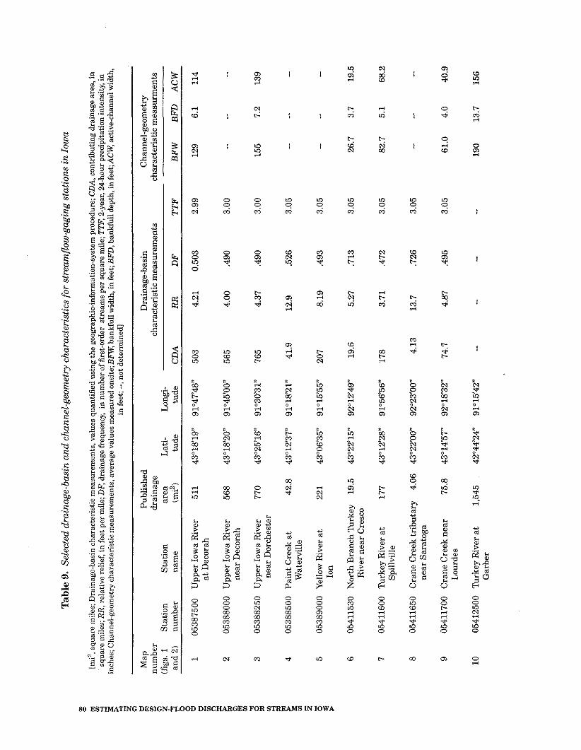
Tab
le 9
. Se
lect
ed d
rain
age-
basi
n an
d ch
anne
l-ge
omet
ry ch
arac
teri
stic
s for
str
eam
flow
-gag
ing
stat
ions
in
Iow
a m 0
m (m
i2, s
quar
e m
iles;
Dra
inag
e-ba
sin
char
acte
rist
ic m
easu
rem
ents
, val
ues
quan
tifi
ed u
sing
the geographic-information-system p
roce
dure
; CD
A, c
ontr
ibut
ing
drai
nage
are
a, in
V1
!! sq
uare
mile
s; R
R, r
elat
ive
reli
ef, i
n fe
et p
er m
ile; D
F, d
rain
age
freq
uenc
y, i
n nu
mbe
r of
firs
t-or
der
stre
ams
per
squa
re m
ile; I
TF
, 2-y
ear,
24-h
our p
reci
pita
tion
inte
nsit
y, in
in
ches
; Cha
nnel
-geo
met
ry e
hara
cter
isti
c m
easu
rem
ents
, ave
rage
val
ues
mea
sure
d on
site
; BFW
, ban
kful
l wid
th, i
n fe
et; B
FD
, ban
kful
l dep
th, i
n fe
et; A
CW
, act
ive-
chan
nel w
idth
, in
fee
t; --,
not d
eter
min
ed]
z 0 D
m M
ap
Pu
bli
shed
D
rain
age-
bas
in
Ch
ann
el-g
eom
etry
n
um
ber
d
rain
age
char
acte
rist
ic m
easu
rem
ents
ch
arac
teri
stic
mea
surm
ents
2 (f
igs.
1
Sta
tio
n
Sta
tio
n
are
a
Lat
i-
Lon
gi-
P
an
d 21
n
um
ber
n
ame
(mi2
) tu
de
tu
de
CD
A
RR
DF
TTF
BFW
BFD
AC
W
0
0
u 1
0538
7500
U
pp
er I
ow
a R
iver
51
1 43
"18'
19"
91°4
7'48
" 50
3 4.
21
0.50
3 2.
99
129
6.1
114
i2 a
t Dec
ora
h
X
2 05
3880
00
Up
per
Iow
a R
iver
56
8 43
°18'
20"
91°4
5'00
" 56
5 4.
00
,490
3.
00
-- .-
.-
'8 n
ear
Dee
ora
h
rn
-. 3 ii
) 3
0538
8250
U
pp
er I
ow
a R
iver
77
0 43
"25'
16"
91°3
0'31
" 76
5 4.
37
.490
3.
00
155
7.2
139
3
nea
r D
orc
hes
ter
4 05
3885
00
Pai
nt
Cre
ek a
t 42
.8
43"1
2'37
" 91
°18'
21"
41.9
12
.9
,526
3.
05
-- --
-.
v1
Wat
ervi
lle
5 - 3
5 05
3890
00
Yel
low
Riv
er a
t 22
1 43
"06'
35"
91°1
5'55
" 20
7 8.
19
.493
3.
05
-- ..
-.
3 Io
n
6 05
4115
30
No
rth
Bra
nch
Tu
rkey
19
.5
43'2
2'15
" 92
°12'
49"
19.6
5.
27
,713
3.
05
26.7
3.
7 19
.5
Riv
er n
ear
Cre
sw,
7 05
4116
00
Tu
rkey
Riv
er a
t 17
7 43
"12'
28"
91°5
6'56
" 17
8 3.
71
,472
3.
05
82.7
5.
1 68
.2
Spi
llvi
lle
8 05
4116
50
Cra
ne
Cre
ek t
rib
uta
ry
4.06
43
"22'
00"
92"2
3'0O
S 4.
13
13.7
,7
26
3.05
.-
-- -.
nea
r S
arat
og
a
9 05
4117
00
Cra
ne
Cre
ek n
ear
75.8
43
'14'
57"
92"1
8'32
" 74
.7
4.87
.4
95
3.05
61
.0
4.0
40.9
L
ou
rdes
10
0541
2500
T
urk
ey R
iver
at
1,54
5 42
'44'
24"
91°1
5'42
" .-
-.
-- --
190
13.7
15
6 G
arb
er
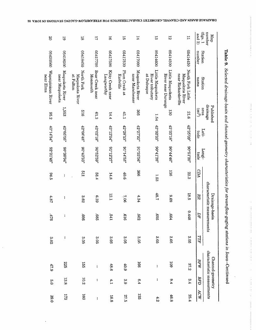
I8 VMOI N1 SNOILVLS 3N13V3-MO7dNV3XJ.S UOd S31LS1H3L3WWH3 hU.L3YUO33'73NNVH3 (INV N I W B - 3 W N I V X a
c3 e,
? I"
N I-' ,- ,- I-' ,- I-' +- I-' o w m 4 m Cn P w N I-' I-'
0 0 0 0 0 0 0 =: cn cn Cn cn cn cn 01 % :: " ;f: P ;f: m m 4 4
" 5 +- ;f: I-' -J
;f: 4
;f: =: cn 4 -J Cn cn 0
E * 01 *
m 0 cn 0 w W 0 8 0 & 0 0 0 0 0 0 0 0 0 0
~ 2 2 ~ a i ~ g g N I-' $ - S c n
5 " v g $ 9
m
I-' 2 "Ln 01 W +-
w Ln I-' m w 0 cn W W m r r 0 E G 2 i-' cn a
P P P P P P P P P P % Y ,- 2 2 0 % I-' X X 2 2 2
2 2 2 % 2 2 % ? 2 m 51 m, P, W, Y U: m, '0, P, ? m,
w w w w w w w 8 2 +- % 2 Z g K I-' I-' G I-' m N. 4 H
Ct H 3
d 0 % 2 N Ln 2 W 2 t.3 o? 0, m, P, W, '0, -2 W, o? m,
a
zr g.F
w S E Y e?,
% 2 a 3 z 2 3
3 % i:
"7 W I-' w I-' Cn +- P 0 k? ,- m r % I ; 2 c z Cn W
8, ID 2. 8. E $ e
P + W F .g 2 2 c 2 w
I-' m c P (0
m In In $ m m k m 5 m k m % ;f: m N Ln P
W W 2 N g Ln g g g g % Cn Ln Ln Cn
5'
N I-' ,- I-' P m 0 " % Ln cn m % z w 2
I-' I-' I % R z 2 2 E
I-' +- I-' N I-' W N C1 23 8 E Z Cn a E $
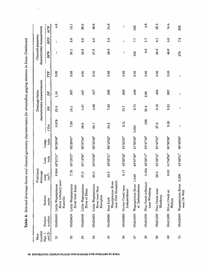
Tab
le 9
. S
elec
ted
dra
inag
e-b
asin
an
d c
hann
el-g
eom
etry
cha
ract
eris
tics
for
str
eam
flow
-gag
ing
stat
ion
s in
Iow
a--C
onti
nued
%
Map
P
ubli
shed
D
rain
age-
basi
n C
hann
el-g
eom
etry
nu
mbe
r dr
aina
ge
char
acte
rist
ic m
easu
rem
ents
ch
arac
teri
stic
mea
surm
ents
(f
igs.
1
Sta
tion
S
tati
on
area
L
ati-
L
ongi
- an
d 2)
nu
mbe
r na
me
(mi2
) tu
de
tude
C
DA
R
R
DF
TTF
BFW
BFD ACW
21
0542
0600
L
ittl
e W
apsi
pini
con
0.90
0 43
"21'
31n
92°2
9'08
" 0.
879
21.0
1.
14
3.05
--
-- 4.
6 R
iver
tri
buta
ry n
ear
Ric
evill
e
22
0542
0620
L
ittl
e W
apsi
pini
con
7.76
43
"19'
37"
92"2
9'07
" 7.
90
10.1
,5
07
3.05
30
.1
2.8
12.1
R
iver
nea
r Acm
e
23
0542
0640
L
ittl
e W
apsi
pini
con
37.3
43
"14'3
OS
92"2
7'04
" 38
.0
5.87
,4
47
3.05
43
.2
2.8
26.3
R
iver
at E
lma
24
0542
0650
L
ittl
e W
apsi
pini
con
95.0
43
-03'
58"
92"2
3'38
" 94
.7
4.88
5
07
3.
05
57.5
4.
0 46
.6
Riv
er n
ear
New
H
ampt
on
25
0542
0690
E
ast F
ork
30.3
43
'05'
11"
92"1
8'22
" 30
.2
7.83
.5
95
3.05
39
.0
3.9
21.6
W
apsi
pini
con
Riv
er
near
New
Ham
pton
26
0542
0960
H
arte
r C
reek
nea
r 6.
17
42"2
9'52
" 91
°53'
27"
6.11
10
.7
,655
3.
05
.-
-- --
Inde
pend
ence
27
0542
1000
W
apsi
pini
con
Riv
er
1,04
8 42
°27'
49"
91'5
3'42
" 1,
050
2.71
.4
49
3.05
18
2 7.
7 14
2 a
t In
depe
nden
ce
28
0542
1100
P
ine
Cre
ek tr
ibut
ary
0.33
4 42
'29'
17"
91°4
7'10
" ,3
38
35.4
2.
95
3.05
9.
6 1.
7 4.
8 ne
ar W
inth
rop
29
0542
1200
P
ine
Cre
ek n
ear
28.3
42
O28
'11"
91'4
7'01
" 27
.6
9.15
,4
35
3.05
50
.6
4.1
35.1
W
inth
rop
30
0542
1890
S
ilve
r Cre
ek a
t 9.
03
41°5
4'54
" 90
°36'
00"
9.30
9.
21
,967
3.
05
46.0
4.
8 14
.4
Wel
ton
31
0542
2000
W
apsi
pini
con
Riv
er
2,33
0 41
°46'
01"
90°3
2'05
" --
-- --
-- 27
9 7.
2 23
5 ne
ar D
e W
itt
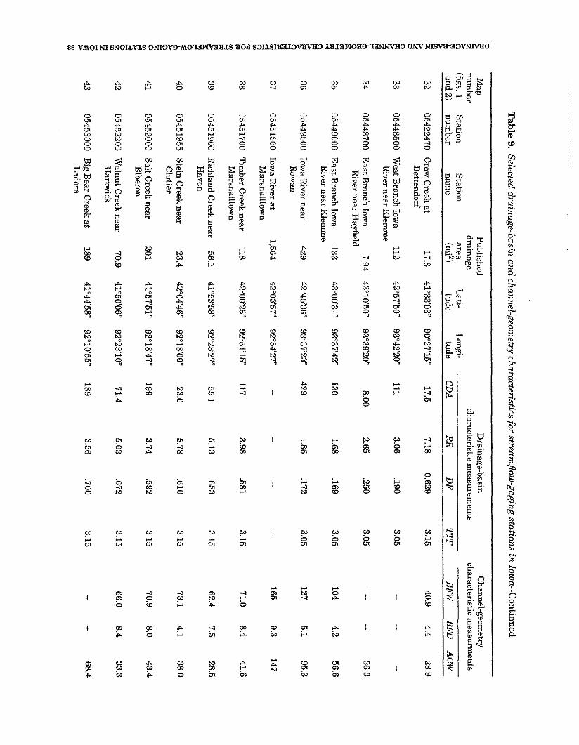
Tab
le 9. Selected d
rainag
e-basin
an
d channel-geom
etry characteristics for stream
flow-gaging statio
ns in
Iowa--C
ontinued
M~
P
Published
Drainage-basin
Channel-geom
etry z
number
drainage characteristic m
easurements
characteristic measurm
ents $
(figs. 1
Station
Station
area L
ati- L
ongi- I"
and
21
num
ber nam
e (m
i2) tude
tude C
DA
R
R
DF
P
F
BFW
B
FD
A
CW
m, k i
32 05422470
Crow
Creek at
17.8 41°33'03"
90°27'15" 17.5
7.18 0.629
3.15 40.9
4.4 28.9
Bettendorf
33 05448500
West B
ranch Iowa
112 42"57'50m
93'42'20"
111 3.06
,190 3.05
-- --
-- R
iver near Klem
me
34 05448700
East B
ranch Iowa
7.94 43°10'50"
93"39'20" 8.00
2.65 .250
3.05 --
-- 8
36.3 o
River near H
ayfield a 3
35
05449000
East B
ranch Iowa
133 43"00'31"
93'37'42" 130
1.68 ,169
3.05 104
4.2 56.6
z R
iver near Klem
me
D 36
05449500 Iow
a River near
429 4Z
045'36" 93"37'23"
429 1.86
,172 3.05
127 5.1
95.3 I!
Row
an kd g
37 05451500
Iowa R
iver at 1,564
42'03'57" 9Z
054'27" -.
-- --
-. 165
9.3 147
3
Marshalltow
n a -. $
38 05451700
Tim
ber Creek near
118 42"00'25"
9Z051'15"
117 3.98
.581 3.15
71.0 8.4
41.6 m
M
arshalltown
8 e 39
05451900 R
ichland Creek n
ear 56.1
4153'58" 92'28'27"
55.1 5.13
,653 3.15
62.4 7.5
28.5 H
aven
$ ti 40
05451955 S
tein Creek near
23.4 4Z
004'46" 92"18'O
Om
23.0
5.78 ,610
3.15 73.1
4.1 38.0
2; C
lutier
3 m
41 05452000
Salt C
reek near 201
41°57'51" 9Z
018'47" 199
3.74 ,592
3.15 70.9
8.0 43.4
-I
Elberon
2 s 0 3
42 05452200
Walnut C
reek near 70.9
41°50'06" 92"23'1O
X
71.4 5.03
67
2
3.15 66.0
8.4 33.3
9 H
artwick
5 43
05453000 B
ig Bear C
reek at 189
41°44'58" 9Z
010'55" 189
3.56 ,700
3.15 --
-- 5
68.4
rn L
adora i)
m
Tab
le 9
. Se
lect
ed d
rain
age-
basi
n an
d ch
anne
l-ge
omet
ry ch
arac
teri
stic
s for
str
eam
flow
-gag
ing
stat
ions
in
Iow
a--C
onti
nned
P
Map
P
ubli
shed
D
rain
age-
basi
n C
hann
el-g
eom
etry
nu
mbe
r dr
aina
ge
char
acte
rist
ic m
easu
rem
ents
ch
arac
teri
stic
mea
surm
ents
(f
igs.
1
Sta
tion
S
tati
on
area
L
ati-
L
ongi
- an
d2
1
num
ber
nam
e (m
i2)
tude
tu
de
CD
A
RR
D
F
TTF
BF
W
BF
D
AC
W
44
0545
3100
Io
wa
Riv
er a
t 2,
794
41°4
8'48
" 9Z
003'
51"
-- *-
-- --
188
11.8
16
0 M
aren
go
45
0545
3600
R
apid
Cre
ek b
elow
8.
12
41a4
3'45
" 91
'25'
38"
7.94
11
.5
0.50
4 3.
15
31.2
3.
8 14
.3
Mor
se
46
0545
3700
R
apid
Cre
ek tr
ibut
ary
1.95
41
°42'
53"
91°2
4'52
" 1.
89
13.2
1.
06
3.15
--
-- --
No.
4 n
ear
Oas
is
47
0545
3750
R
apid
Cre
ek
15.2
41
°43'
23"
91°2
6'16
" 14
.7
8.46
,6
13
3.15
42
.1
5.1
27.5
so
uthw
est o
f Mor
se
48
0545
3950
R
apid
Cre
ek tr
ibut
ary
3.43
41
°41'
56"
91'2
8'39
" 3.
48
12.5
,2
87
3.15
26
4.
5 12
ne
ar Io
wa
Cit
y m
.. e 8
49
0545
4000
R
apid
Cre
ek n
ear
25.3
41
'41'
19"
91°2
9'15
" 25
.2
8.58
.5
55
3.15
50
6.
8 34
S Io
wa
Cit
y
50
0545
4300
C
lear
Cre
ek n
ear
98.1
41
°40'
36"
91°3
5'55
" 97
.4
4.85
,4
31
3.15
70
7.
6 44
C
oral
vill
e
51
05
4550
00
Ral
ston
Cre
ek a
t 3.
01
41"3
9'50
m
91'3
0'48
" 2.
98
12.6
,6
71
3.15
--
-- --
Iow
a C
ity
52
0545
5010
S
outh
Bra
nch
Ral
ston
2.
94
41'39
'05"
91'3
0'27
" 2.
92
13.3
,3
43
3.15
--
-- .-
Cre
ek a
t Iow
a C
ity
53
0545
5100
O
ld M
ans
Cre
ek
201
41°3
6'23
" 91
°36'
56"
200
2.88
,5
00
3.15
89
9.
5 49
.0
near
Iow
a C
ity
54
0545
5140
N
orth
Eng
lish
Riv
er
31.0
41
'38'
45"
92'3
4'20
- 31
.3
4.43
,7
03
3.15
--
-- 19
.5
near
Mon
tezu
ma
55
0545
5150
N
orth
Eng
lish
Riv
er
34.0
41
"39'
0OZ
92
°33'
00"
33.8
4.
47
,739
3.
15
-- --
-- ne
ar M
onte
zum
a
Table 9. S
elected drain
age-b
asin a
nd
channel-geometry ch
aracteristics for streamflow
-gaging station
s in Iow
a--Continued
Map
number
Published
drainaee D
rainage-basin C
hannel-geometry
characteristic measurem
ents characteristic m
easurments
- (figs. 1
S
tation S
tation area
Lati-
Longi-
and 2) num
ber nam
e (m
i2) tude
tude C
DA
R
R
DF
TT
F
BFW
BF
D
AC
W
56 05455200
North E
nglish River
68.7 41°38'47"
92"23'4In 68.1
4.38 0.778
3.15 --
-- 43.5
near Guernsey
57 05455210
North E
nglish River
81.5 41°38'42"
92O21'28"
80.7 4.12
.I68
3.15
-- -
45.6 a
t Guernsey
58 05455280
South E
nglish River
2.51 41°33'00"
92°28'00" 2.53
10.4 1.18
3.15 --
-- --
tributary near B
arnes City
59 05455300
South E
nglish River
11.5 41°31'26"
92"27'56" 11.6
12.0 ,773
3.17 31.5
4.9 12.1
near Barnes C
ity
60 05455350
South E
nglish River
0.523 41°34'02" 92'27'01"
53
7
13.8 1.86
3.15 --
-. --
tributary No.2 near
Montezum
a
61 05455500
English R
iver at 573
41°27'59" 91°42'56"
584 2.59
.556 3.18
Kalona
62 05457700
Cedar R
iver at
1,054 43O
03'45" 92"40'23"
1,060 2.27
.297 2.99
Charles C
ity
63 05458000
Little C
edar River
306 43"02'05"
92"30'05" 305
3.95 ,390
3.03 near Ionia
64 05458500
Cedar R
iver at
1,661 4Z
038'54" 92"27'54"
-- --
-- -.
Janesville
65 05458900
West F
ork cedar
846 42"37'50"
92"32'24" 842
2.65 ,346
3.05 R
iver at F
inchford
66 05459000
Shell R
ock River
300 43'24'51"
93"13'14" 300
2.16 ,197
2.96 near N
orthwood
Table
9.
Sele
cted
dra
inag
e-ba
sin
and
chan
nel-
geom
etry
char
acte
rist
ics f
or s
trea
mfl
ow-g
agin
g st
atio
ns i
n Io
wa-
-Con
tinue
d 8
Map
P
ubli
shed
D
rain
age-
basi
n C
hann
el-g
eom
etry
nu
mbe
r dr
aina
ge
char
acte
rist
ic m
easu
rem
ents
ch
arac
teri
stic
mea
surm
ents
$ (f
igs.
1
Sta
tion
S
tati
on
area
L
ati-
L
ongi
- an
d 2)
nu
mbe
r na
me
(mi2
) tu
de
tude
CDA
RR
DF
TTF
i! BFW
BFD
ACW
,-> 8 67
05
4590
10
Elk
Cre
ek a
t Ken
sett
58
.1
43"2
2'18
" 93
"12'
37"
58.7
4.
18
0.18
7 3.
04
41.5
2.
7 35
.7
Z
68
0545
9500
W
inne
bago
Riv
er a
t 52
6 43
O09
'54"
93'1
1'33
" 52
0 2.
17
,229
3.
03
161
7.8
91.3
8 M
ason
Cit
y 8
69
0546
0100
W
illow
Cre
ek n
ear
78.6
43
"08'
55"
93°1
6'07
" 80
.2
2.62
,1
00
3.05
57
.9
3.7
34.3
M
ason
Cit
y
m
00
70
0546
2000
S
hell
Roc
k R
iver
1,
746
4Z04
2'42
" 92
'34'58
" --
-- --
-- 21
6 6.
5 1
91
a
at S
hell
Roc
k % .-
m
71
05
4627
50
Bea
ver
Cre
ek
11.6
42
"34'
40n
92"5
0'49
" 11
.9
8.31
,5
05
3.05
-.
--
I 19
.2
trib
utar
y ne
ar
m
Apl
ingt
on
Z 5 72
05
4630
00
Bea
ver
Cre
ek a
t 34
7 42
'34'
22"
92'37
'04"
352
4.05
.4
29
3.06
80
5.
6 70
.1
s N
ew H
artf
ord
73
0546
3090
B
lack
Haw
k C
reek
at
56.9
42
°22'
10"
92"4
6'05
" 57
.0
4.84
.4
92
3.15
51
6.
0 34
.7
Gru
ndy
Cen
ter
74
0546
3500
B
lack
Haw
k C
reek
30
3 42
"24'
28"
92"2
7'47
" 29
9 3.
45
,428
3.
13
91
5.7
73.9
at
Hud
son
75
0546
4000
C
edar
Riv
er a
t 5,
146
4Z02
9'44
" 92
'20'
03"
-- --
-- --
403
8.6
377
Wat
erlo
o
76
0546
4130
F
ourm
ile
Cre
ek n
ear
13.7
8 42
'13'
32"
92"3
6'39
" 13
.5
7.83
,5
18
3.15
--
-- --
Lin
coln
77
0546
4133
H
alf
Mile
Cre
ek n
ear
1.33
42
"12'
40n
92"3
6'39
" 1.
33
16.3
.7
50
3.15
--
-- --
Gla
dbro
ok
78
0546
4137
F
ourm
ile
Cre
ek n
ear
19.5
1 42
"12'
07"
92'33
'44"
19.3
6.
22
,363
3.
15
-- --
20.7
T
raer
Table 9. S
elected drain
age-b
asin a
nd
channel-geometry ch
aracteristics for streamflow
-gaging station
s in Iow
a--Continned
M~
P
Published
Drainage-basin
Channel-geom
etry Z
num
ber drainaae
characteristic measurem
ents characteristic m
easurments
(figs. 1
Station
- S
tation area
Lati-
Longi-
and 2) num
ber nam
e (m
i3
tude tude
CD
A
RR
D
F W
F
BFW
BFD
AC
W
t 79
05464500 C
edar River at
6,510 41°58'14"
91°40'01" --
-- --
-- 439
12.5 413
Cedar R
apids - P
80 05464560
Prairie C
reek at 87.0
41°54'42" 92O
05'03" 86.5
4.18 0.543
3.15 --
.-
46.9
Blairstow
n
81
8
05464640 P
rairie Creek at
178 41°55'22"
91°47'02" 175
3.35 .566
3.15 96.2
7.0 79.6
o F
airfax 3 ,-' 3
82 05464880
Otter C
reek at Wilton
10.7 41°36'17"
91'02'08" 10.9
6.91 ,368
3.15 40.6
6.2 9.1
0
83
05465000
Cedar R
iver near 7,785
41°24'36" 91°17'06"
-- --
-- -.
523 10.6
510 C
onesville
84 05469860
Mud L
ake drainage 65.4
42-18'52" 93'38'23"
65.4 4.60
,138 3.14
-- --
31.7 E un
ditch 71 at Jewel1
2 0 ~1
85 05469990
Keigley B
ranch near 81.0
42"09'01" 93°37'13"
30.5 5.28
,197 3.15
37.7 4.4
23.8 z $a
Story C
ity
86 05470000
South S
kunk River
815 42'04'05"
93"37'02" 322
4.12 ,161
3.14 104
6.7 83.4
near Am
es
87 05470500
Squaw
Creek
204 42"01'21n
93"37'45" 208
4.31 ,245
3.15 87.2
7.2 62.1
zi at A
mes
k 6 -
88 05471000
South S
kunk River
556 42"00'31"
93'35'37" 558
3.29 ,199
3.14 131
9.4 106
3 below
Squaw
Creek
% near A
mes
2; 3 89
05471200 Indian C
reek near 276
41°48'17" 93"18'36"
278 4.00
,280 3.15
106 8.6
83.3
5 M
ingo
3
90 05471500
South S
kunk River
1,635 41°21'19"
92'39'31" .-
-- --
-- s
162 10.9
138 near O
skaloosa %
Tab
le 9
. S
elec
ted
dra
inu
ge-
bas
in a
nd
cha
nnel
-geo
met
ry c
har
acte
rist
ics
for
stre
amfl
ow-g
agin
g st
atio
ns
in Io
wa-
-Con
tinu
ed
s
Map
P
ubli
shed
D
rain
age-
basi
n C
hann
el-g
eom
etry
nu
mbe
r dr
aina
ge
char
acte
rist
ic m
easu
rem
ents
ch
arac
teri
stic
mea
surm
ents
(f
igs.
1
Sta
tion
S
tati
on
area
L
ati-
L
ongi
- an
d2
) nu
mbe
r na
me
(mi2
) tu
de
tude
C
DA
R
R
DF
TT
F
BFW
B
FD
AC
W
91
05
4722
90
Sug
ar C
reek
nea
r 52
.7
41°3
4'26
" 92
"44'
20*
54.0
5.
24
0.70
3 3.
15
57
7.7
34.7
S
ears
boro
92
0547
2390
M
iddl
e C
reek
nea
r 23
.0
42O
43'55
" 93
O42
'26"
22.5
5.
21
,667
3.
25
-- --
14.8
L
acey
93
0547
2445
R
ock
Cre
ek a
t 26
.3
41°2
0'12
" 92
"13'
20"
26.1
8.
84
,383
3.
25
-- --
19.6
S
igou
rney
94
0547
2500
N
orth
Sku
nk R
iver
73
0 41
°18'
03"
92"1
2'16
" 72
8 2.
44
.631
3.
19
-- --
83.0
ne
ar S
igou
rney
95
0547
3300
C
edar
Cre
ek n
ear
252
41°0
0'34
" 92
°07'
06"
247
2.52
,5
54
3.25
88
11
.6
55.5
B
atav
ia
96
0547
3400
C
edar
Cre
ek n
ear
530
40°5
5'20
" 91
°40'
10"
527
2.26
.4
76
3.25
12
2 12
.7
75.7
O
akla
nd M
ills
97
0547
3500
B
ig C
reek
nea
r 10
6 41
°00'
52"
91°3
4'49
" 10
1 4.
25
,397
3.
25
71.6
9.
3 57
.4
Mou
nt P
leas
ant
98
0547
4000
S
kunk
Riv
er
4,30
3 40
°45'
13"
91°1
6'40
" --
-.
-- --
322
17.1
27
5 at
Aug
usta
99
0547
6500
D
es M
oine
s R
iver
1,
372
43O
23'51
" 94
O50
'38"
-- --
-- --
106
6.7
95
at E
sth
e~
lle
100
0547
6750
D
es M
oine
s R
iver
2,
256
42-4
3'12
" 94
"13'
06"
-.
-- --
-- 17
2 6.
8 16
3 at
Hum
bold
t
101
0547
9000
E
ast F
ork
Des
1,
308
42O
43'26
" 94
"11'
30n
-- --
-- --
187
6.4
170
Moi
nes
Riv
er
at D
akot
a C
ity
Table 9. S
elected drain
age-b
asin a
nd
channel-geometry ch
aracteristics for streamflow
-gaging station
s in Iow
a--Continued
Map
Published
Drainage-basin
Channel-geom
etry num
ber drainage
characteristic measurem
ents characteristic rneasurm
ents -
(figs. 1
Station
Station
area L
ati- L
ongi- and21
number
name
(mi2)
tude tude
CDA
RR
DF
TT
F
BF
W
BF
D ACW
102 05480000
Lizard C
reek near 257
42"32'35" 94'20'45"
263 3.09
0.130 3.05
101 6.3
73.3 C
lare
103 05480500
Des M
oines River
4,190 42'30'22"
94"12'04" -.
-- --
-- 239
9.4 219
at Fort D
odge
104 05481000
Boone R
iver near 844
42"26'01" 93'48'12"
852 2.16
.I82 3.05
166 8.3
148 W
ebster City
105 05481300
Des M
oines River
5,452 42'15'04"
9359'52" --
-- --
-- 361
12.5 339
near Stratford
106 05481680
Beaver C
reek at 38.5
42"02'04" 94O
08'46" 38.8
4.24 .I29
3.15 49.4
4.4 25.5
Beaver
107 05481950
Beaver C
reek near 358
4P41'18"
93"44'08" 358
2.66 ,319
3.15 95.5
6.6 85.9
Grim
es
108 05482170
Big C
edar Creek near
80.0 4Z
041'16" 94"47'52"
80.7 3.83
,074 3.05
.-
-- 25.0
Varina
109 05482300
North R
accoon River
700 4Z
021'16" 94"59'26"
700 2.76
,140 3.05
150 8.1
108 near S
ac City
110 05482500
North R
accoon 1,619
41°59'17" 94"22'36"
-- --
-- .-
178 10.1
157 R
iver near Jefferson
111 ' 05482600
Hardin C
reek at 43.7
42°16'01" 94O
25'10" 42.3
1.57 .I4
2
3.05 32.9
4.2 21.8
Farnham
ville
112 05482900
Hardin C
reek near 1
01
42O
05'34" 9425'39"
97.8 3.03
,205 3.06
71.0 6.2
51.0 F
arlin
113 05483000
East F
ork Hardin
24.0 42"06'27"
94O22'12"
23.3 2.97
.043 3.13
36.6 3.2
13.5 C
reek near Churdan
Tab
le 9
. S
elec
ted
dra
inag
e-b
asin
an
d c
hann
el-g
eom
etry
ch
arac
teri
stic
s fo
r st
ream
flow
-gag
ing
stat
ion
s in
Iow
a--C
onti
nued
Map
P
ubli
shed
D
rain
age-
basi
n C
hann
el-g
eom
etry
nu
mbe
r dr
aina
ge
char
acte
rist
ic m
easu
rem
ents
ch
arac
teri
stic
mea
surm
ents
(f
igs.
1
Sta
tion
S
tati
on
area
L
ati-
L
ongi
- an
d21
num
ber
nam
e (m
i2)
tude
tu
de
CD
A
RR
D
F
TT
F
BFCV
B
FD
A
CW
114
0548
3349
M
iddl
e R
acco
on R
iver
6.
58
4290
2'30
" 94
"52'4
3"
6.53
17
.7
0.76
6 3.
05
21.4
3.
2 7.
1 tr
ibut
ary
at C
arro
ll
115
0548
3450
M
iddl
e R
acco
on
375
41°4
6'43
" 94
'29'
33"
370
4.01
%
511
3.09
10
2 7.
4 8
8
Riv
er n
ear
Bay
ard
116
0548
3600
M
iddl
e R
acco
on
440
41°4
1'14
" 94
"22'
15"
423
3.63
.4
94
3.09
--
-- *-
Riv
er a
t Pan
ora
117
0548
4000
S
outh
Rac
coon
99
4 41
°35'
22"
94"0
9'04
" 1,
000
3.41
.5
39
3.12
18
0 10
.7
139
Riv
er a
t Red
fiel
d 11
8 05
4845
00
Rac
coon
Riv
er
3,44
1 41
°32'
02"
93"5
6'59
" --
-- --
-- 25
0 11
.3
220
at V
an M
eter
119
0548
4800
W
alnu
t Cre
ek a
t 78
.4
41°3
5'14
" 93
'42'
11"
77.2
5.
35
,388
3.
15
66.0
7.
5 46
.8
Des
Moi
nes
120
0548
5640
F
ourm
ile
Cre
ek a
t 92
.7
41°3
6'50
" 93
'32'
43"
92.2
4.
14
,293
3.
15
-- --
51.4
D
es M
oine
s
121
0548
6000
N
orth
Riv
er n
ear
349
41°2
7'25
" 93
'39'
10"
349
4.82
,5
38
3.15
--
-- 45
.0
Nor
wal
k
122
0548
6490
M
iddl
e R
iver
nea
r 50
3 41
"25'
27"
93'3
5'09
" 49
2 4.
22
,686
3.
20
-- .-
81.0
In
dian
ola
123
0548
7470
S
outh
Riv
er n
ear
460
41°2
0'14
" 93
"29'
10"
462
4.08
,5
52
3.25
--
.-
77.9
A
ckw
orth
124
0548
7600
S
outh
Whi
te B
reas
t 28
.0
40'5
7'36
" 93
O41
'28"
27.5
12
.0
,510
3.
25
59.5
7.
9 38
.5
Cre
ek n
ear
Osc
eola
125
0548
7800
W
hite
Bre
ast C
reek
12
8 41
°01'
24"
9327
'56"
12
8 5.
35
,603
3.
25
69.6
8.
4 33
.0
at L
ucas
Tab
le 9. S
elected drain
age-b
asin a
nd
channel-geometry ch
aracteristics for streamflow
-gaging station
s in Iow
a--Continued
Map
Published
Drainage-basin
Channel-geom
etry num
ber drainage
characteristic measurem
ents characteristic m
easurments
(figs. 1
Station
Station
area L
ati- L
ongi- and 2)
number
name
(mi2)
tude tude
CD
A
RR
D
F
VF
B
FW
B
FD
A
CW
k E
126 05487980
White B
reast Creek
342 41°14'41"
93"16'08" 341
3.32 0.577
3.25 --
-- 63.5
near Dallas
-
127 05488000
White B
reast Creek
380 41°19'25"
93'08'55" 379
3.09 .583
3.25 --
*-
-- near K
noxville
d
128 05488620
Coal C
reek 13.5
41°01'02* 92'50'46"
13.4 10.3
,597 3.25
38.7 5.0
17.2 8
near Albia
%
3 129
05489000 C
edar Creek near
374 41°13'09"
92'54'38" 370
3.49 .654
3.25 96
10.9 52.3
.e B
ussey
I 130
05489150 L
ittle Muchakinock
9.12 41'15'58"
92"38'33" 8.69
9.78 ,230
3.25 26.8
3.7 17.2
Creek a
t Oskaloosa
n
131 05489490
Bear C
reek 22.9
41°00'43" 92'27'54"
22.2 10.0
.450 3.25
56.2 6.3
29.9 e B
at O
ttumw
a 2
Z: 132
05491000 S
ugar Creek near
105 40°2633"
91°28'24" 106
3.07 :547
3.26 .-
-- --
'=I
8 K
eokuk
05494300 Fox R
iver at
87.7 40°46'10"
92"25'05" 85.1
3.37 .541
3.25 --
-- --
Bloom
field
05494500 Fox R
iver at C
antril 161
40"39'20n 92'0330"
158 2.96
.615 3.25
-- --
--
05495600 S
outh Wyaconda R
iver 4.69
40Q43'00"
92"30'00n 4.58
12.7 ,437
3.25 -.
-- --
near West G
rove
06483270 R
ock River a
t Rock
788 43'26'13''
96O09'58"
790 3.76
,528 2.82
-- --
-- R
apids
06483410 O
tter Creek north of
11.9 43°2T
41" 95'4'29"
11.8 6.59
,338 2.85
19.3 2.0
6.9 S
ibley
06483430 O
tter Creek a
t Sibley
29.9 43'24'14"
95°46'10" 30.0
6.30 ,401
2.85 --
- 13.5
(0
Table
9.
Sel
ecte
d d
rain
age-
bas
in a
nd
cha
nnel
-geo
met
ry c
har
acte
rist
ics
for
stre
amfl
ow-g
agin
g st
atio
ns
in Io
wa-
-Con
tinu
ed
N
Map
P
ubli
shed
D
rain
age-
basi
n C
hann
el-g
eom
etry
nu
mbe
r dr
aina
ge
char
acte
rist
ic m
easu
rem
ents
ch
arac
teri
stic
mea
surm
ents
(f
igs.
1
Sta
tion
S
tati
on
area
L
ati-
L
ongi
- an
d2
) nu
mbe
r na
me
(mi2
) tu
de
tude
C
DA
R
R
DF
TTF
BF
W
BF
D
ACW
139
0648
3460
O
tter
Cre
ek n
ear
88.0
43
"20'
07"
95"4
5'43
" 89
.2
4.78
0.
460
2.89
--
-- 36
.1
Ash
ton
140
0648
3500
R
ock
Riv
er n
ear
1,59
2 43
"12'
52"
96"1
7'39
" .-
-- --
-- 18
8 5.
9 10
0 R
ock
Val
ley
14
1
0648
4000
D
ry C
reek
48
.4
42'5
9'48
" 96
O28
'10"
48.2
5.
28
,622
2.
85
-- --
-- at
Haw
arde
n
142
0660
0000
P
erry
Cre
ek a
t 65
.1
42'3
2'08
" 96
"24'
3gn
64.3
7.
30
32
8
2.85
--
-- 22
.0
38th
Str
eet,
Sio
ux C
ity
143
0660
0100
Fl
oyd
Riv
er a
t Alto
n 26
8 42
O58
'55"
96°0
0'03
" 26
7 3.
56
.456
2.
94
66.3
7.
9 49
.8
144
0660
0300
W
est B
ranc
h Fl
oyd
180
42'55
'25"
96'"1
0'34
" 18
0 3.
69
,405
2.
85
76.0
8.
1 48
.5
Riv
er n
ear
Str
uble
145
0660
0500
Fl
oyd
Riv
er a
t Jam
es 8
86
42'3
4'36
" 96
'18'
43"
886
2.74
.4
50
2.89
13
1 7.
6 97
.2
146
0660
2020
W
est F
ork
ditc
h at
40
3 42
O13
'37"
96'0
4'40
" 40
4 3.
41
,507
2.
95
-- --
39.4
H
orni
ck
147
0660
2400
M
onon
a-H
anis
on
900
41°5
7'52
" 95
"59'
30"
902
2.59
.4
09
2.94
--
-- 59
di
tch
near
Tur
in
148
0660
5000
O
chey
edan
Riv
er
426
43"0
7'44
" 95
"12'
37"
424
3.03
,3
27
2.93
15
8 4.
8 57
.1
near
Spe
ncer
149
0660
5340
P
rair
ie C
reek
nea
r 22
.3
43'05
'16"
95'09
'40"
22.4
4.
43
,223
2.
95
27.1
3.
3 12
.8
Spe
ncer
150
0660
5750
W
illow
Cre
ek n
ear
78.6
42
"58'
21n
95"0
9'40
n 80
.9
3.62
.2
97
2.97
67
.8
5.2
36.8
C
orne
ll
Table 9. S
elected drain
age-b
asin a
nd
channel-geometry ch
aracteristics for stream
flow
-gag
ing
station
s in Iow
a--Continued
Map
Published
Drainage-basin
Channel-geom
etry num
ber drainage
characteristic measurem
ents characteristic m
easurments
(figs. 1
Station
Station
area L
ati- L
ongi- and 2)
number
name
(mi2)
tude tude
CDA
R
R
DF
n?i.
BF
W
BF
D
AC
W
15
1
06605850 L
ittle Sioux R
iver 1,548
42'53'24" 95°14'30"
-- -.
-- --
150 11.7
123 a
t Linu G
rove
152 06606600
Little S
ioux River
2,500 42°28'20"
95"47'49" --
-- -.
-- 156
12.9 142
at Correctionville
153 06606790
Maple C
reek 15.5
42O44'56"
95°22'16" 16.0
10.7 0.624
3.05 27.4
3.4 12.8
near Alta
154 06607000
Odebolt C
reek near 39.3
42°20'10" 95°22'52"
38.6 10.6
,856 3.05
-- --
-- A
rthur
i? 155
06607200 M
aple River at
0
3 M
apleton
2 156
06608500 S
oldier River a
t P
isgah :: 21
157 06609500
Boyer R
iver a
t Logan
158 06610500
Indian Creek at
Council B
luffs b
159 06610520
Mosquito C
reek
i5 near E
arling
8 160
06610600 M
osquito Creek a
t !!
Neola
2 0 3
16
1
06806000 W
aubonsie Creek
5! near B
artlett - 8 S
162
06807410 W
est Nishuabotna
>
River a
t Hancock
8
(0
Table
9.
Sel
ecte
d d
rain
age-
bas
in a
nd
chan
nel-
geom
etry
ch
arac
teri
stic
s for
str
eam
fto
w-g
agin
g st
atio
ns
in I
owa-
-Con
tinu
ed
P
m B M
ap
Pub
lish
ed
Dra
inag
e-ba
sin
Cha
nnel
-geo
met
ry
num
ber
drai
nage
ch
arac
teri
stic
mea
sure
men
ts
char
acte
rist
ic m
easu
rmen
ts
$ (f
igs.
1
Sta
tion
S
tati
on
area
L
ati-
L
ongi
- an
d2
) nu
mbe
r na
me
(mi2
) tu
de
tude
C
DA
R
R
DF
TT
F
BF
W
BF
D
AC
W
;
163
0680
7470
In
dian
Cre
ek n
ear
37.3
41
°01'
50"
95"2
2'51
" 38
.6
7.09
0.
363
3.15
54
.4
4.4
14.8
3 E
mer
son
0
0
u 16
4 06
8077
20
Mid
dle
Sil
ver C
reek
3.
21
41°2
8'33
" 95
"28'
06"
3.28
14
.8
,610
3.
05
16.2
2.
8 4.
8
z ne
ar A
voca
2
165
0680
7760
M
iddl
e S
ilve
r Cre
ek
25.7
41
°19'
28"
95'3
3'19
" 25
.8
6.67
,5
43
3.05
--
-- 8.
2 ne
ar O
akla
nd
Om V) 16
6 06
8077
80
Mid
dle
Sil
ver C
reek
42
.7
41°1
4'37
" 95
'365
3"
42.8
5.
74
,444
3.
05
-.
-- 3
14.9
at
Tre
ynor
U
1
167
0680
8000
M
ule
Cre
ek n
ear
10.6
40
"56'
40m
95
'35'
40"
10.6
13
.1
,378
3.
15
.-
-- .-
Mal
vern
9 16
3 06
8085
00
Wes
t Nis
hnab
otna
1,
326
40°5
2'23
" 95
O34
'48"
-- --
.-
-- --
-.
186
a < R
iver
at R
ando
lph
i2=
169
0680
9000
D
avid
s C
reek
nea
r 26
.0
41'4
0'25
" 94
'48'
20"
26.5
8.
14
64
1
3.15
--
.-
-- H
amli
n
170
0680
9210
E
ast
Nis
hnab
otna
43
6 41
°20'
46"
95"0
4'36
" 42
9 3.
10
,721
3.
13
-- --
131
Riv
er n
ear
Atl
anti
c
171
0680
9500
E
ast N
ishn
abot
na
894
41"0
0'31
n 95
"14'
29"
886
2.84
,6
79
3.13
--
-- 13
3 R
iver
at R
ed O
ak
172
0681
0000
N
ishn
abot
na R
iver
2,
806
40°3
7'57
" 95
"37'
3Z0
-- --
.-
-- .-
-- 15
6 ab
ove
Ham
burg
173
0681
1760
T
arki
o R
iver
nea
r 10
.7
41°0
6'06
" 95
O06
09"
10.2
9.
93
.488
3.
15
36.1
5.
4 12
.6
Ell
iot
174
0681
1840
T
arki
o R
iver
at
49.3
40
-58'
52"
95"O
6'3Zn
47
.0
5.62
.5
10
3.15
.-
-- 23
.9
Sta
nton
Tab
le 9. Selected drainage-basin and channel-geometry characteristics for stream
flow-gaging stations in
Iowa--C
ontinued
Map
Published
Drainage-basin
Channel-geom
etry
5 num
ber drainage
characteristic measurem
ents characteristic m
easurments
d
(figs. 1
Station
Station
area L
ati- L
ongi- ?
m and21
number
name
(mi2)
tude tnde
CD
A
RR
D
F
TTF BFW
BFD
AC
W
t 1
75
06811875
Snake C
reek near 9.10
40°44'33" 95O
07'46" 9.34
14.6 0.428
3.23 --
-- 9.7
Yorktow
n - ti
176 06817000
Nodaw
av River a
t 762
40'44'19" 95'00'47"
758 3.08
.810 3.16
.-
-- 1
63
3 C
lariida m
r
177 06818598
Platte R
iver near 51.7
4038'44" 94'29'39"
51.5 3.68
,56
3
3.25 --
-*
29.9 8
Stringtow
n Ei 3
178 06818750
Platte R
iver near 217
40°46'02" 94"24'46"
210 2.79
,520 3.25
-- --
53
.1
Diagonal
179 06819190
East F
ork One
92.1 40°38'01"
9b
44
'41
" 92.6
4.69 ,550
3.25 --
-- 45.6
Hundred and T
wo
3 R
iver near Bedford
E
,* 5 o
180 06897950
Elk C
reek near 52.5
40°43'18" 93'56'12"
54.1 8.93
68
4
3.25 91.0
8.5 58.7
m
'Ii D
eeatur City
0
0
3 1
81
06898000
Thom
pson River a
t 701
40°38'25" 93'48'29"
702 2.88
,692 3.24
-- .-
122
k! D
avis City
*I
182 06898400 W
eldon River near
104 40n41'45"
93O38'07"
108 5.83
54
7
3.25 --
-- 71.1
Leon
e 183
06903400 C
hariton River near
182 40'57'12"
93'15'37'' 184
3.22 ,436
3.25 64.4
9.3 5
1.1
2 3
Chariton
3 1
84
06903500
Honey C
reek near 13.2
40e55'25" 93'07'55"
13.7 7.27
,582 3.25
-- .-
-- z 7
Russell
0
?J 185
06903700 S
outh Fork C
hariton 168
40948'02" 93"11'32"
169 2.60
,514 3.25
-- -.
i: 52.4
- R
iver near Prom
ise C
ity
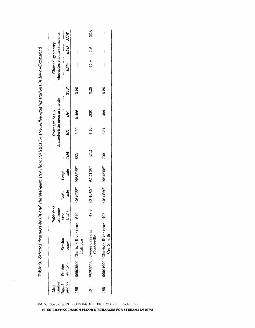
* :: T
able
9.
Sel
ecte
d d
rain
age-
bas
in a
nd
cha
nnel
-geo
met
ry c
har
acte
rist
ics
for
stre
amft
ow-g
agin
g st
atio
ns
in I
owa-
-Con
tinu
ed
x w
m
.
0
* 9
Map
P
ubli
shed
D
rain
age-
basi
n C
hann
el-g
eom
etry
%
num
ber
drai
nage
ch
arac
teri
stic
mea
sure
men
ts
char
acte
rist
ic m
easu
rmen
ts
(fig
s. 1
S
tati
on
Sta
tion
ar
ea
Lat
i-
Lon
gi-
and
2)
num
ber
nam
e (m
i2)
tude
tu
de
CD
A
RR
D
F
TZ
F
BF
W
BF
D
AC
W
8 w
'D
a
0 2
186
0690
3900
C
hari
ton
Riv
er n
ear
549
40'4
9'22
" 92
"53'
22"
553
2.20
0.
486
3.25
--
-- --
?
3 R
athb
un
g i5
0 0
187
0690
3990
C
oope
r Cre
ek a
t u
l;r
47.8
40
'45'
02"
92O
51'3
6"
47.2
4.
70
53
0
3.25
45
.9
7.9
35.6
2 24
Cen
tem
ille
8
3
g g
188
0690
4000
C
hari
ton
Riv
er n
ear
708
40°4
4'20
" 92
-48'
05"
709
2.31
,4
99
3.25
--
-- --
:: ':
Cen
tem
ille
m:
3 Y
s%
3~
s 2
0
g ?, 2 5 $