Embed Size (px)
Citation preview

Estimating Base Layers and Subgrade Modulii for ME Pavement Design in Manitoba
Maria Elena Oberez, P. Eng.
Pavement Research Engineer
Manitoba Infrastructure and Transportation
Email: [email protected]
Said Kass, P.Eng. M.Eng.
Director, Materials Engineering Branch
Email: [email protected]
Stan Hilderman, P. Eng.
Senior Pavement/Geotechnical Engineer
Email: [email protected]
M. Alauddin Ahammed, P. Eng. Ph.D.
Pavement Design Engineer
Email: [email protected]
William Tang, P. Eng.
Pavement Analysis Engineer
Email: [email protected]
Paper prepared for presentation
at the New Developments in ME Pavement Design Session
of the 2015 Conference of the
Transportation Association of Canada
Charlottetown, PEI
2
ABSTRACT
The assessment of the structural adequacy of an existing pavement scheduled for rehabilitation
is an important aspect of pavement rehabilitation design. Non-destructive testing (NDT) has
been widely used to determine the design inputs for existing pavement layers in rehabilitation
design. The Falling Weight Deflectometer (FWD) is used by different agencies for the non-
destructive evaluation of existing pavement layers and subgrade properties. In addition, the
deflection basin from the FWD can be applied to select an appropriate rehabilitation strategy.
The backcalculated elastic properties of each layer in the pavement and the subgrade from the
FWD testing are required for Level 1 and 2 inputs in rehabilitation design when using the
AASHTOWare Pavement ME Design program.
This paper focuses on the backcalculation of pavement layers and subgrade modulii using
various methods. The backcalculated resilient modulii (MR) of the base and subgrade from
these procedures are compared with modulii from the forward calculation method. This forward
calculation method was developed under the Federal Highway Administration’s project for
reviewing Long-Term Pavement Performance (LTPP) backcalculation data. The calculated
modulii are also compared to the laboratory determined resilient modulus for similar materials.
The highway sections used in the study are the same test sections proposed to be used to
calibrate the Pavement ME distress models in Manitoba. The selected modulii of the pavement
layers and subgrade will be used as inputs in the calibration process.
INTRODUCTION
With the recent release of the AASHTOWare Pavement ME design program, the calibration and
implementation efforts of Pavement ME design by many highway agencies, the need to
accurately characterize the many parameters of existing pavement for design and rehabilitation
has increased. Since 1999, Manitoba Infrastructure and Transportation (MIT) have invested in
the mechanistic characterization of pavement materials that includes dynamic modulus testing
of different bituminous mixes and resilient modulus testing for typical subgrade and granular
base materials with varying fines and moisture contents. MIT has also been collecting deflection
data using FWD for its network and project level surveys.
The FWD applies a dynamic load onto the pavement surface to simulate traffic loads. The
surface deflections at various distances from the load center are recorded by geophone sensors.
The MIT’s FWD testing program uses 9 sensors placed at 0, 200, 300, 450, 600, 900, 1200,
1500, and 1800 mm from the center of the load plate. For this study, all deflection
measurements were taken in the outer wheel path.
The FWD data used in this study were obtained from test sections that are well distributed
throughout the Province of Manitoba to capture the various types of subgrade, base materials
and asphalt mixes used in Manitoba. Table I lists the location of the test sections, thicknesses of
the asphalt and individual base layers, soil classification and description of the subgrade from
soil survey and laboratory tests.
3
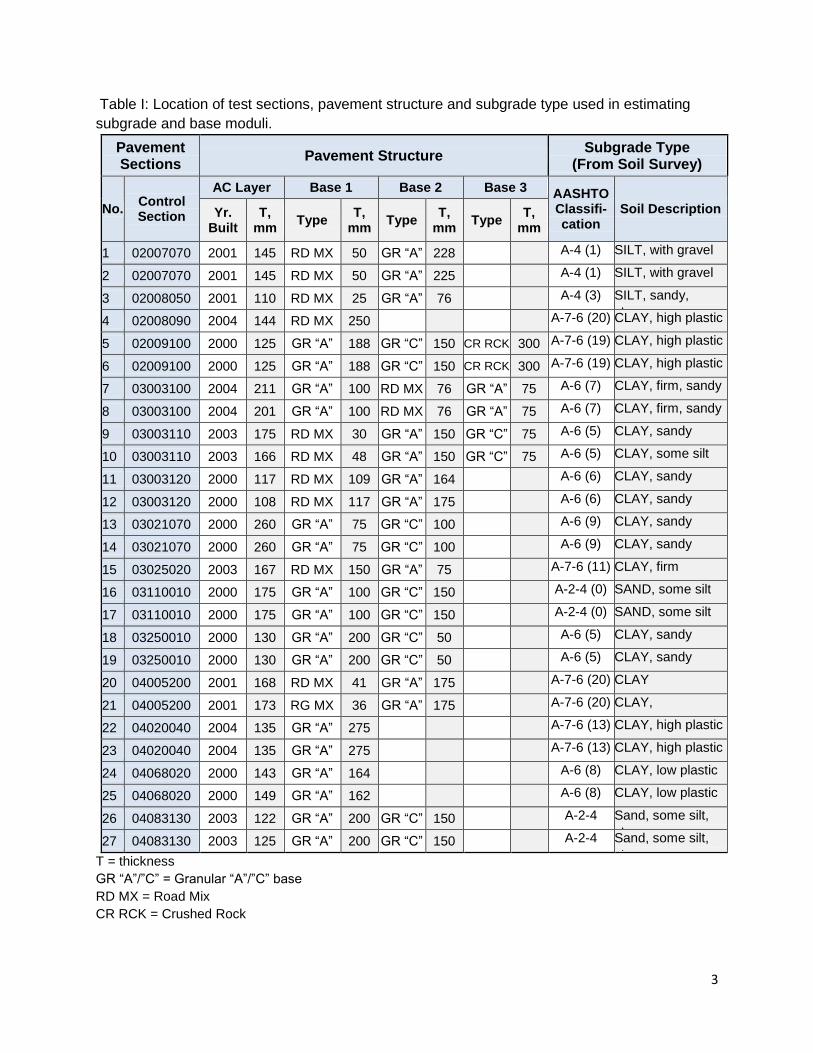
Table I: Location of test sections, pavement structure and subgrade type used in estimating
subgrade and base moduli.
Pavement Sections
Pavement Structure Subgrade Type
(From Soil Survey)
No. Control Section
AC Layer Base 1 Base 2 Base 3 AASHTO Classifi-cation
Soil Description Yr. Built
T, mm
Type T,
mm Type
T, mm
Type T,
mm
1 02007070 2001 145 RD MX 50 GR “A” 228
A-4 (1) SILT, with gravel
2 02007070 2001 145 RD MX 50 GR “A” 225
A-4 (1) SILT, with gravel
3 02008050 2001 110 RD MX 25 GR “A” 76
A-4 (3) SILT, sandy,
clayey 4 02008090 2004 144 RD MX 250
A-7-6 (20) CLAY, high plastic
5 02009100 2000 125 GR “A” 188 GR “C” 150 CR RCK 300 A-7-6 (19) CLAY, high plastic
6 02009100 2000 125 GR “A” 188 GR “C” 150 CR RCK 300 A-7-6 (19) CLAY, high plastic
7 03003100 2004 211 GR “A” 100 RD MX 76 GR “A” 75 A-6 (7) CLAY, firm, sandy
8 03003100 2004 201 GR “A” 100 RD MX 76 GR “A” 75 A-6 (7) CLAY, firm, sandy
9 03003110 2003 175 RD MX 30 GR “A” 150 GR “C” 75 A-6 (5) CLAY, sandy
10 03003110 2003 166 RD MX 48 GR “A” 150 GR “C” 75 A-6 (5) CLAY, some silt
11 03003120 2000 117 RD MX 109 GR “A” 164
A-6 (6) CLAY, sandy
12 03003120 2000 108 RD MX 117 GR “A” 175
A-6 (6) CLAY, sandy
13 03021070 2000 260 GR “A” 75 GR “C” 100
A-6 (9) CLAY, sandy
14 03021070 2000 260 GR “A” 75 GR “C” 100
A-6 (9) CLAY, sandy
15 03025020 2003 167 RD MX 150 GR “A” 75
A-7-6 (11) CLAY, firm
16 03110010 2000 175 GR “A” 100 GR “C” 150
A-2-4 (0) SAND, some silt
17 03110010 2000 175 GR “A” 100 GR “C” 150
A-2-4 (0) SAND, some silt
18 03250010 2000 130 GR “A” 200 GR “C” 50
A-6 (5) CLAY, sandy
19 03250010 2000 130 GR “A” 200 GR “C” 50
A-6 (5) CLAY, sandy
20 04005200 2001 168 RD MX 41 GR “A” 175
A-7-6 (20) CLAY
21 04005200 2001 173 RG MX 36 GR “A” 175
A-7-6 (20) CLAY,
22 04020040 2004 135 GR “A” 275
A-7-6 (13) CLAY, high plastic
23 04020040 2004 135 GR “A” 275
A-7-6 (13) CLAY, high plastic
24 04068020 2000 143 GR “A” 164
A-6 (8) CLAY, low plastic
25 04068020 2000 149 GR “A” 162
A-6 (8) CLAY, low plastic
26 04083130 2003 122 GR “A” 200 GR “C” 150
A-2-4 Sand, some silt,
clayey 27 04083130 2003 125 GR “A” 200 GR “C” 150
A-2-4 Sand, some silt,
clayey T = thickness
GR “A”/”C” = Granular “A”/”C” base
RD MX = Road Mix
CR RCK = Crushed Rock
4
- Equation 1
- Equation 2
Objectives and Scope
The objectives of the study are:
a) Identify the backcalculation method that will provide reasonably accurate resilient
modulus of the base and subgrade for use in Pavement ME design for flexible pavement
rehabilitation.
b) Investigate the accuracy of calculated resilient modulus of the base layers and subgrade
from static linear analysis using: (a) Boussinesq-Odemark model (ELMOD software); (b)
Boussinesq model (AASHTO 1993 procedure); (c) Hogg model; and (d) Dorman and
Metcalf model. The Hogg model and Dorman and Metcalf model are forward calculation
methods used to screen the back calculated resilient modulii in the FHWA’s LTPP
database.
c) Provide any modifications to the existing guidelines in the use of backcalculated resilient
modulus of the base and the subgrade in Pavement ME design. These guidelines
include the use of factors to convert field modulus to laboratory modulus.
d) Investigate the use of the combined modulus of the base layers for Pavement ME design.
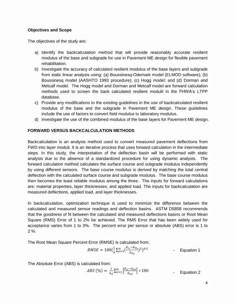
FORWARD VERSUS BACKCALCULATION METHODS
Backcalculation is an analysis method used to convert measured pavement deflections from
FWD into layer moduli. It is an iterative process that uses forward calculation in the intermediate
steps. In this study, the interpretation of the deflection basin will be performed with static
analysis due to the absence of a standardized procedure for using dynamic analysis. The
forward calculation method calculates the surface course and subgrade modulus independently
by using different sensors. The base course modulus is derived by matching the total central
deflection with the calculated surface course and subgrade modulus. The base course modulus
then becomes the least reliable modulus among the three. The inputs for forward calculations
are: material properties, layer thicknesses, and applied load. The inputs for backcalculation are
measured deflections, applied load, and layer thicknesses.
In backcalculation, optimization technique is used to minimize the difference between the
calculated and measured sensor readings and deflection basins. ASTM D5858 recommends
that the goodness of fit between the calculated and measured deflections basins or Root Mean
Square (RMS) Error of 1 to 2% be achieved. The RMS Error that has been widely used for
acceptance varies from 1 to 3%. The percent error per sensor or absolute (ABS) error is 1 to
2 %.
The Root Mean Square Percent Error (RMSE) is calculated from:
The Absolute Error (ABS) is calculated from:
5
- Equation 3
- Equation 4
Where: n = Number of sensors used to measure basin
dmi = Measured deflection at point i
dci = Calculated at point i
The Odemark-Boussinesq Method (ELMOD Software)
ELMOD is an acronym for Evaluation of Layer Moduli and Overlay Design. It is a program
developed by Dynatest that can be used for a 5-layer system. It considers the depth to bedrock
and non-linear behaviour of the subgrade in the analysis. Using the Odemark Model, the
pavement layers are transformed to a semi-infinite half space following the Method of
Equivalent Thickness (MET). For the stiffness to remain the same, the following expression
must remain constant:
. The Method of Equivalent Thickness (MET) equation to convert
the equivalent thickness of each layer is
. After converting all layers to their
equivalent thickness, the vertical displacement/deflection per layer is then calculated using
Boussinesq’s Equation:
Where:
dz = Displacement
v = Poisson’s ratio
o = Stress applied on the pavement
a = Radius of plate
E = Elastic modulus of the layer
z = Depth from the surface
The Boussinesq Model (AASHTO Method)
The AASHTO methodology computes the resilient modulus of the subgrade based on
Boussinesq’s equation (AASHTO 1993). Boussinesq developed a closed-form equation for a
semi-infinite, linear elastic median half-space based on a point load. The AASHTO-based MR is
computed using the following simplified equation:
Where: MR = Resilient Modulus
C = Correction Factor
P = Plate load (lb)
µ = Poisson’s ratio
dr = Deflection measured at r distance from the plate
r = Distance from the load

6
- Equation 5
- Equation 6
- Equation 7
The Poisson’s ratio is recommended to fall within the range of 0.30 to 0.50 (AASHTO, 1993). A
Poisson’s ratio of 0.40 was used in the calculation of the subgrade resilient modulus. The
correction factor is applied to adjust the backcalculated resilient modulus to those obtained from
laboratory testing. The Manual for MEPDG recommends a value of 0.33 for all subgrade soils.
The AASHTO 1993 design manual recommends using the last sensor deflection for calculating
the resilient modulus of the subgrade. In this study, the sensor at 1200 mm is used.
The Hogg Model (Forward Calculation Method)
The Hogg model simplifies the typical multilayered elastic system to an equivalent two-layer
model consisting of a thin plate on an elastic foundation. It uses the deflection at the center of
the load and one of the offset deflections. The Hogg model considers variations in pavement
thickness and the ratio of the pavement stiffness to subgrade stiffness. The equation used to
calculate the Hogg subgrade modulus is:
Hogg showed that the offset distance to the point where the deflection is approximately one-half
of that under the center of the load plate was effective in removing biases in the estimation. To
calculate this offset distance where deflection is half of center deflection, the equation below is
used:
The characteristic length of the deflection basin is calculated from:
Where:
Eo = Subgrade modulus
µo = Poisson’s ratio for subgrade
So = Theoretical point load stiffness
S = Pavement stiffness = p/o (area loading)
P = Applied load
o = Deflection at the center of load plate
r = Deflection at offset distance r
R = Distance from center of load plate
R50 = Offset distance where r/o = 0.5

7
- Equation 8
l = Characteristic length
h = Thickness of the subgrade
I = Influence factor
α = Curve fitting coefficient
β = Curve fitting coefficient
B = Curve fitting coefficient
yo = Characteristic length coefficient
m = Stiffness ratio coefficient
Compared to any backcalculation approach, the Hogg model of forward calculation gives less
variability in resilient modulus between test points. The Hogg model is effective and very easy to
use when deriving relatively accurate subgrade modulus.
Dorman and Metcalf (Forward Calculation Method for Intermediate Layers)
The modulus relationship developed by Dorman and Metcalf between two adjacent layers of
unbound materials can be used to forward calculate the modulus of the intermediate base layer
using Hogg subgrade modulus. The intermediate modulus is calculated using the Equation:
Where: EBase = Dorman and Metcalf base modulus, MPa
h2 = Thickness of the intermediate base layer, mm
Ssub = Subgrade modulus, MPa
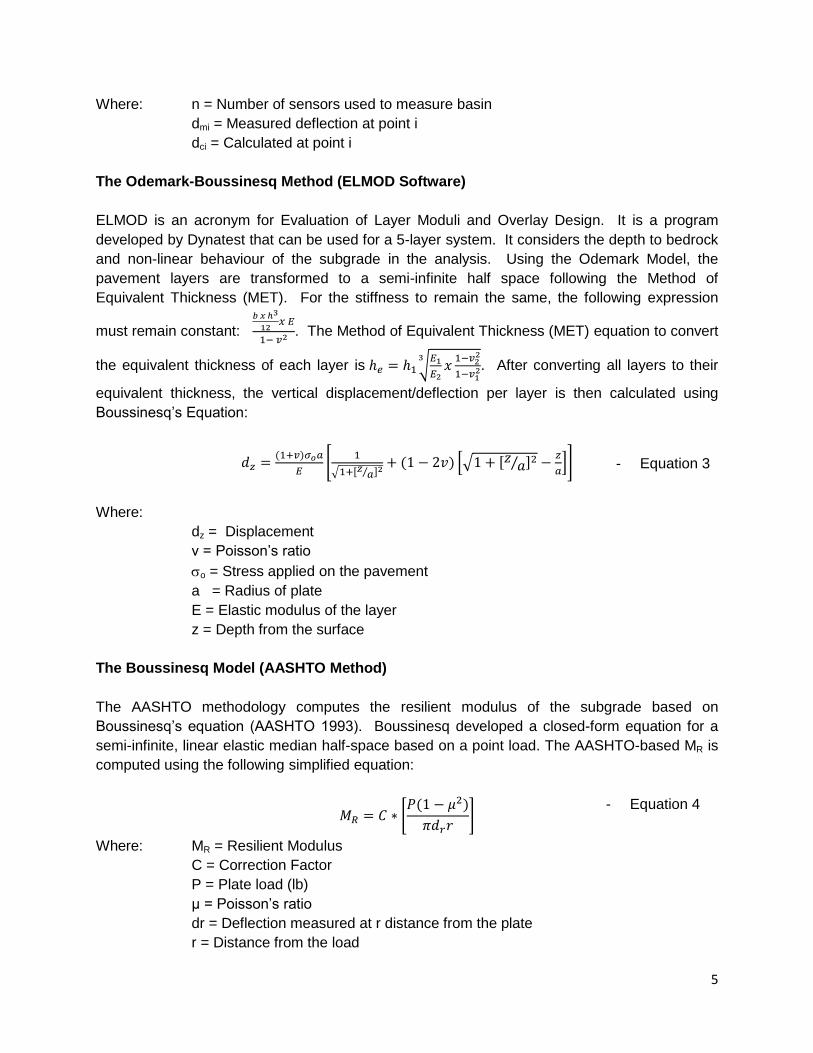
Sensitivity of the Subgrade to Repeated Stress
Deflection measurements from FWD can be used to evaluate the sensitivity of the pavement
and subgrade materials to repeated loadings. This is done by comparing the trend of the load
versus the estimated modulus of the material. The subgrade and base materials undergo either
strain softening or strain hardening during the cycle of FWD loadings. The strain softening in
fine-grained soil such as clay and silty clay can be due to the contraction of the soil as the load
is repeatedly applied. It then generates negative pore pressure as it dilates. The strain
hardening of granular soils such as sandy or gravelly soil can be due to the particles locking up
into a denser arrangement during the cycle of loading. This feature can be used to verify the
type of material in-situ and the effects of loads on the performance of the materials.
A similar procedure can be used to determine the stress sensitivity of the base and AC
pavement to repeated stress. Figures 1a and 1b show the stress sensitivity of the subgrade at
various test locations. It is expected that the base materials will exhibit strain hardening during
the cycle of loading.
8
.
ANALYSIS AND DISCUSSION
Backcalculation of the Subgrade Modulus
Six test sections with known subgrade type, gradation and moisture content were used in the
analyses. The laboratory resilient modulus of each section was estimated using the values
provided in Table II. The Least Square Method and Standard Error of Estimate (SEE) were used
to assess which of the models investigated gives a subgrade resilient modulus that best fits with
the laboratory resilient modulus. Figure II shows that the resilient modulus estimated from the
Hogg model provide the best fit with the laboratory resilient modulus while the Boussinesq and
Odemark-Boussinesq models overestimates the resilient modulus of the subgrade.
Table II: Laboratory determined resilient modulus of typical subgrade in Manitoba based on
varying moisture contents.
SOIL TYPE AASHTO Classification
Moisture Content, % Resilient Modulus, MPa
Silty Sand A-2-4 (GI=0) 7.7, 9.5, 12.4, 14 58.4, 51.9, 49.7, 39.5
Sandy Silt A-4 (GI=4) 8.5, 10.9, 12.6, 14.9 66.6, 62.8, 67.5, 56.9
Sandy Clay A-6 (GI=7) 12.4, 13.6, 15.4, 16.9 101.9, 63.2, 32.3, 15.4
Sandy Clay A-6 (GI=8) 10.6, 12.5, 14.0, 15.2 105.4, 73.1, 43.5, 20.9
High Plastic Clay A-7-6 (GI=17) 18.8, 20.4, 23.0, 23.8 108.0, 78.7, 42.1, 34.8
High Plastic Clay A-7-6 (GI=20) 28.0, 28.3, 31.2, 32.6 63.9, 62.4, 39.7, 31.5
The Manual for MEPDG provides recommended values for C Factor to reduce the
backcalculated resilient modulus of the subgrade and base layers to their equivalent laboratory
resilient modulus before they can be used in Pavement ME Design. For the subgrade, the
20
40
60
80
100
120
140
160
180
20 40 60 80
Bac
kcal
cula
ted
Su
bgr
ade
Mo
du
lus,
Mp
a
FWD Load, kN
02007070HU
03003100HU
03003100HU
03003120HU
03025020HU
03110010HU
03110010HU
03250010HU
04068020HU
04068020HU
04083130HU
04083130HU
20
40
60
80
100
120
140
160
180
20 40 60 80
Bac
kcal
cula
ted
Su
bgr
ade
Mo
du
lus,
MP
a
FWD Load, kN
02008050HU
02008090HU
02009100HU
03021070HU
03021070HU
03250010HU
04020040HU
04020040HU
Figure I-A: Strain hardening of the subgrade
soil indicating presence of coarse aggregates
in the soil.
Figure I-B: Strain softening of subgrade soil
indicating clayey and silty soil.

9
recommended C Factor is 0.33. This factor was only applied to the calculated modulus using
the Boussinesq and the Boussinesq-Odemark models. Figure III shows that the recommended
MEPDG C-Factor of 0.33 underestimates the resilient modulus of the subgrade when compared
to laboratory resilient modulus. To reduce the error of estimate, simple iterations were made to
determine the C Factor that will give the least square error and Standard Error of Estimate (SEE)
of the backcalculated resilient modulii from each model. The C Factors that produced the least
error of estimates are 0.69 for the Boussinesq model and 0.75 for the Boussinesq-Odemark
model.
Figure II: Graphical illustration of the laboratory resilient modulus versus calculated resilient
modulus of the six test sections using different models.
Figure III: Graphical illustration of the laboratory resilient modulus versus the adjusted resilient
modulus using MEPDG recommended C Factor of 0.33.
Table III provides the SEE using the MEPDG recommended C Factor of 0.33 and the C Factors
determined from this study (MIT). The subgrade resilient modulus calculated from ELMOD
gives the lowest SEE after a C factor of 0.75 was applied to the back-calculated resilient
modulus. Finally, Figure IV shows the graphical comparison between the laboratory resilient
modulus versus the resilient modulus adjusted using the appropriate C Factors as determined in
this analysis.
0
50
100
150
0 50 100 150
Cal
cula
ted
Res
ilien
t M
od
ulu
s, M
pa
Laboratory-determined Resilient mModulus, MPa
Hogg Model (Forward Calculation)
Boussinesq Model (AASHTO 1993 Method)
Boussinesq-Odemark Model (ELMOD Software)
0
50
100
150
0 50 100 150
Cal
cula
ted
Res
ilien
t M
od
ulu
s, M
pa
Laboratory-determined Resilient Modulus, MPa
Hogg Model (Forward Calculation)
Boussinesq Model (AASHTO 1993 Method)
Boussinesq-Odemark Model (ELMOD Software)
10
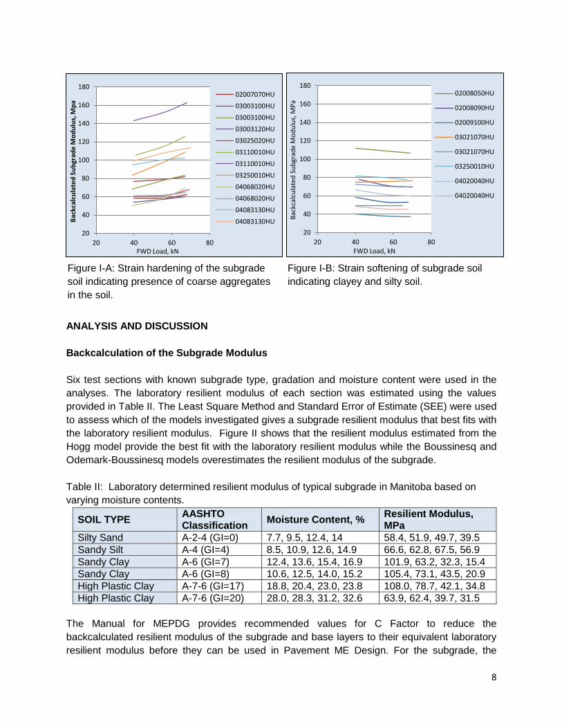
Table III: Statistics for Unadjusted and Adjusted Resilient Modulus of the Subgrade Using
Boussinesq, Boussinesq-Odemark and Hogg Models.
Analysis Method
Boussinesq Model
(AASHTO 1993)
Boussinesq-Odemark
Model (ELMOD)
Hogg Model (Forward
Calculation)
Parameter MEPDG MIT MEPDG MIT Unadjusted
C Factor 0.33 0.69 0.33 0.75 -
Least Square 7078 964 7650 299 1005.59
SEE 42.07 15.5 43.73 8.65 15.86
Figure IV: Graphical illustration of the laboratory determined resilient modulus versus adjusted
resilient modulus of the subgrade using the C Factors that produce the least Standard Error of
Estimate (SEE).
Effect of Subgrade Modulus in Pavement ME Design
To assess the sensitivity of the predicted distresses to changes in subgrade modulus, several
runs of the Pavement ME software were done using the maximum and minimum values of
laboratory resilient modulus of the subgrade. Refer to Table II. The subgrade material properties
such as gradation and plasticity index as determined from soil survey and the typical maximum
moisture content and dry density for a similar subgrade material from the Department’s material
database were used as inputs for analysis. In the analysis, the pavement structure and
properties, weather and traffic data were kept constant. Tables IV-A and IV-B show the results
of the analysis. In this table, if a range of numbers is given, it indicates an increased predicted
distress due to lower resilient modulus of the subgrade. A single number indicates no change in
the predicted distress.
For all subgrade types, the predicted terminal IRI varies from 1.88 to 1.94 m/km for a 10-year
design and 2.36 to 2.54 m/km for a 20-year design. Based on these results, it appears that the
predicted terminal IRI is not sensitive to the subgrade type and resilient modulus. Similar
results were observed with the predicted total permanent deformation or total rutting. The
difference in the results for all subgrade types and resilient modulii is 0.33 mm for a 10-year
design life and 0.83 mm for a 20-year design life and the maximum predicted total rutting in all
0
50
100
150
0 50 100 150
Cal
cula
ted
Res
ilien
t M
od
ulu
s, M
pa
Laboratory-determined Resilient Modulus, MPa
Hogg Model (Forward Calculation)
Boussinesq Model (AASHTO 1993 Method)
Boussinesq-Odemark Model (ELMOD Software)

11
cases is only 10 percent of the target total rutting after 20 years. The difference in the predicted
rutting or permanent deformation can be considered insignificant.
The predicted AC bottom-up fatigue cracking remained at 1.17% for the 10-year design and
1.45% for the 20-year design for all subgrade types investigated. This indicates that the AC
bottom-up fatigue cracking is insensitive to the subgrade type and modulus. The predicted total
cracking (reflective and alligator) also shows insensitivity to the subgrade stiffness with only a
0.04% difference in prediction for a 10-year design and 0.22% for a 20-year design.
For the 10-year design, the subgrade consisting of silty sand and sandy clay induced the
highest AC thermal cracking of 568.68 m/km while sandy silt resulted to lowest thermal cracking
of 555.56 m/km. It appears that AC thermal cracking is slightly affected by subgrade type but
insensitive to resilient modulus of the subgrade in a 10-year design life. The predicted AC
thermal cracking for a 20-year design remained at 608.57 m/km for all types.
The predicted AC top-down cracking showed to have the highest sensitivity to subgrade type
and stiffness. Sandy clay subgrade showed the highest sensitivity to changes in resilient
modulus compared to other types. Subgrade consisting of silty sand and sandy silt appeared to
be the least affected by the change in resilient modulus.
Table IV-A. MEPDG predicted distresses using maximum and minimum values of laboratory-
determined subgrade resilient modulus using 10-year design life.
SOIL TYPE Terminal
IRI (m/km)
Total Permanent
Deformation (mm)
Total Cracking (Reflective
+Alligator) (%)
AC Thermal Cracking (m/km)
AC Bottom-up
fatigue cracking
(%)
AC top-down fatigue
cracking (m/km)
Silty Sand 1.88 1.04-1.14 50.01-49.99 568.68 1.17 165.16-170.58
Sandy Silt 1.89 1.05-1.10 50.01-50.00 555.56 1.17 182.39-184.52
Sandy Clay 1.92-1.93 1.10-1.45 50.00-50.03 567.13 1.17 76.14-183.1
Sandy Clay 1.92 1.10-1.19 50.00-50.02 568.68 1.17 106.57-182.39
High Plastic Clay 1.93-1.94 1.02-1.11 50.00-50.01 567.52 1.17 154.89-181.69
High Plastic Clay 1.94 1.01-1.06 50.01 564.81 1.17 142.31-185.21
Table IV-B. MEPDG predicted distresses using maximum and minimum values of laboratory-
determined subgrade resilient modulus using 20-year design life.
SOIL TYPE Terminal
IRI (m/km)
Total Permanent
Deformation (mm)
Total Cracking (Reflective
+Alligator) (%)
AC Thermal Cracking (m/km)
AC Bottom-up fatigue cracking
(%)
AC top-down fatigue cracking
(m/km)
Silty Sand 2.36 1.84-1.95 50.19-50.08 608.57 1.45 326.97-402.43
Sandy Silt 2.42 1.82-1.85 50.16-50.11 608.57 1.45 387.23-401.19
Sandy Clay 2.48-2.50 1.85-2.65 50.11-50.33 608.57 1.45 215.95-386.16
Sandy Clay 2.49 1.85-2.17 50.11-50.27 608.57 1.45 289.22-384.01
High Plastic Clay 2.52-2.53 1.80-1.85 50.11-50.20 608.57 1.45 371.70-382.53
High Plastic Clay 2.53-2.54 1.78-1.83 50.15-50.22 608.57 1.45 353.35-402.17
12
Backcalculation of the Base Layer Modulus
The ELMOD software was used to backcalculate the resilient modulus of the base. The
calculated resilient modulus of the subgrade using AASHTO 1993 method was used as a seed
modulus for the subgrade. Several iterations were made before reasonable resilient modulus
values were obtained. The backcalculated resilient modulii of the base with RMS less than 3%
that give reasonable resilient modulus values for the material were selected. These modulii
were then averaged and used for further analysis.
The laboratory resilient modulus for the base of the test sections investigated was estimated
from the results of the laboratory testing done on various base materials. The aggregate type,
fines and moisture contents of the existing base material in the test sections are used to
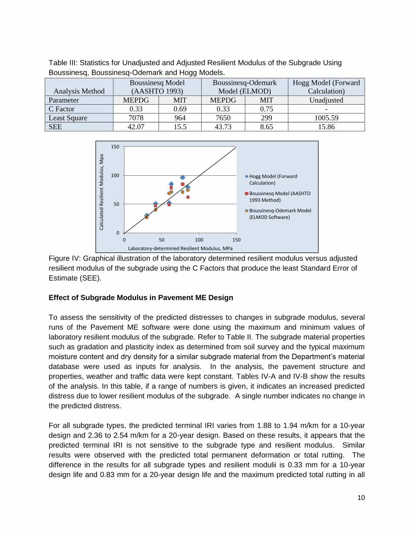
estimate the resilient modulus of the base from laboratory results. The overall results show that
the backcalculated resilient modulus of the base is consistently higher than the laboratory
determined resilient modulus (See Figure V). The Standard Error of Estimate (SEE) for
unadjusted modulus of the base using ELMOD is 182.5. The MEPDG Manual of Practice
recommends reducing the backcalculated resilient modulus of the base by a factor equal to 0.62
for base layers below the AC layer. Using this factor, the SEE was reduced to 51.5. The plots of
the adjusted backcalculated base resilient modulus compared to unadjusted resilient modulus
are shown in Figure V.
Figure V: Graphical comparison of adjusted and unadjusted backcalculated versus laboratory
determined resilient modulus of the base estimated from similar materials.
Combined Modulus of the Base
Some of the challenges in backcalculating the individual base modulus are the variability of field
conditions such as thickness of the different layers of the base, the presence of sandwich and
stabilized layers, and the insufficient laboratory test data of resilient modulus of base layer
materials used. To address these issues, a simplified and practical method is developed to
0
100
200
300
400
0 100 200 300 400
Bac
kcal
cula
ted
Res
ilien
t M
od
ulu
s o
f th
e B
ase,
M
Pa
Laboratory Resilient Modulus of the Base, MPa
Resilient Modulus of the Base Using ELMOD Software
Unadjusted Backcalculated Resilient Modulus of Base
Adjusted Backcalculated Resilient Modulus of the Base

13
assess the structural condition of base with layers consisting of variable materials. This method
combines all the different layers in the base into one layer and backcalculating the effective
resilient modulus of the base. This effective resilient modulus represents the combined resilient
modulus of the base. The combined resilient modulii of the base for test sections identified for
this analysis were backcalculated using the ELMOD software and verified using the Dorman
and Metcalf forward calculation equation. The comparison is presented in Figure VI.
In Figure VI, a good correlation between back and forward calculated combined modulii for
typical base layers consisting of Granular A over Granular C is observed. For pavement
sections with road mix over granular base, including sandwich construction, the base modulus
from forward calculation method provides unreasonably low values. Road mix is a base
material stabilized with emulsified asphalt. It appears that the forward calculation method used
in the study is insensitive to the presence of bound layers in the base. The backcalculated
combined resilient modulus of the base using the ELMOD software consistently gives higher
values for both sandwich construction and base layers topped with road mix. This indicates that
ELMOD takes into account the presence of stiff layers in the base. The results of the
backcalculated combined modulus of the base using ELMOD were then used to investigate the
possibility of using combined modulus in Pavement ME analysis.
Figure VI: Back versus forward calculated combined resilient modulus of the base layer.
Several runs using Pavement ME Design software were carried out to compare the predicted
distresses using combined modulus of the base versus individual modulii of the base layers.
For the combined resilient modulus, the material properties of the top layer of the base were
used in the analysis. In Table V-A, Columns (i) and (ii) are typical pavement structures
consisting of AC layer underlain by Granular “A” and Granular “C”. The results presented in
Table V-A show that there is no significant difference in the predicted terminal IRI and total
cracking for all cases. The rutting of the subgrade remained at 0.01 mm for all cases. Although
the rutting of the base resulting from factored combined modulus is significantly higher
100
150
200
250
300
350
400
450
100 150 200 250 300 350 400 450
Mo
du
lus
fro
m F
orw
ard
Cal
cula
tio
n
(Do
rman
an
d M
etc
alf)
, Mp
a
ELMOD Backcalculated Modulus, Mpa
Composite Modulus (ELMOD VS. Dorman and Metcalf Model)
Sandwich Construction
RD MX over GB
GB "A" over GB "C"

14
compared to the predicted rutting of the total of individual base layers, the difference in the
predicted total rutting is insignificant for all cases.
Table V-B gives the predicted distresses for a pavement with base layer consisting of granular
“A” and granular “C” over crush rock (Column iii). The base layer sits on the top of a soft high
plastic clay subgrade. The results show small variations in the predicted terminal IRI and total
cracking. The subgrade rutting remained at 0.01 mm for all cases. The factored combined
modulus gives the highest base and total rutting/deformation. The rutting at the asphalt
concrete is affected by the variability of the base layer modulii. In Table V-B, Section (iv)
represents a sandwich construction. In this case, the predicted terminal IRI and rutting did not
show any significant difference among all cases. Although Pavement ME provide predicted top-
down and bottom-up cracking where individual layers were used, it gave predicted total cracking
as zero (0.0) for both factored and unfactored backcalculated modulus. Also, the predicted total
rutting/deformation do not consider the rutting at the base and subgrade layers.
Table V-A: Pavement ME predicted pavement and subgrade distresses using combined and
individual layer moduli of the base layer.
Pavement
Distress
i. AC, Gran A, Gran C ii. AC, Gran A, Gran C
A b C d a B c d
Terminal IRI 2.54 2.54 2.51 2.51 2.6 2.57 2.59 2.57
Total Cracking 50.03 50.03 50.03 50 50.17 50.1 50.16 50.1
Rutting AC only 2.11 2.17 2.14 2.18 2.06 2.06 2.04 2.04
Rutting Subgrade 0.01 0.01 0.01 0.01 0.01 0.01 0.01 0.01
Rutting Base 0.21 0.06 0.09 0.01 2.02 1.01 1.81 1.01
Total Rutting 2.33 2.24 2.24 2.2 4.09 3.08 3.86 3.06
Table V-B: Pavement ME predicted pavement and subgrade distresses using combined and
individual layer modulus of the base layer.
Pavement
Distress
iii. AC, Gran A, Gran C, Cr Rck iv. AC, Gran A, RD MX, Gran A
a b C d a B c d
Terminal IRI 2.77 2.69 2.71 2.67 2.55 2.55 2.52 2.52
Total Cracking 50.56 50.33 50.45 50.31 50 50.02 0.00 0.00
Rutting AC only 3.14 3.04 3.04 2.98 3.1 3.03 2.67 2.63
Rutting Subgrade 0.01 0.01 0.01 0.01 0.01 0.01 0 0
Rutting Base 7.14 4.4 5.22 3.94 0.01 0.05 0 0
Total Rutting 10.29 7.45 8.27 6.93 3.12 3.09 2.67 2.63
Where:
a = Pavement ME prediction using adjusted backcalculated combined resilient
modulus of the base layers
b = Pavement ME prediction using unadjusted backcalculated combined resilient
modulus of the base layers

15
- Eq. 9
- Eq. 10
- Eq. 11
c = Pavement ME prediction using adjusted backcalculated resilient modulus of
individual layers of the base
d = Pavement ME prediction using unadjusted backcalculated resilient modulus of
the individual layers of the base
Seasonal Variation of Resilient Modulus of the Base and Subgrade
The Pavement ME design software gives an option to input the monthly resilient modulus of the
subgrade soil. For MIT to be able to use this option, the seasonal variation of the resilient
modulus was included in the study. From 2011 to 2013, pavement deflections were measured in
8 different test sites in different seasons of the year using FWD. The FWD tests were done in
the summer, fall, start and end of winter and spring seasons. These data were used originally to
determine the start and end dates of the winter weight premium and spring restrictions in
Manitoba. The same data were used in this study to evaluate the changes in the resilient
modulus of the subgrade for Pavement ME design. Due to the large number of data requirement
for this analysis, the resilient modulus of the subgrade was calculated using AASHTO 1993
method. The results are plotted in Figures VII-A and VII-B.
The seasonal trend of the backcalculated resilient modulus of the subgrade was compared to
the maximum compressive strain on top of the subgrade. In estimating the maximum
compressive strain on top of the base and subgrade, a mechanistic relationship between FWD
deflections and layer conditions was used. These equations are independent from
backcalculated modulii of the base and the subgrade.
The prediction models for critical strains for pavements with unbound aggregate base are:
tensile strain at the bottom of asphalt pavement (ac), critical strain at the top of the base (abc),
and critical strain at the top of the subgrade (sg). In this study, these critical strains were
calculated using the regression equations developed in the study on relationships between
FWD deflections and asphalt pavement layer condition indicators by Xu, B. Et.al 2002. These
relationships incorporate the complicated dynamic effect of FWD loading and nonlinear
behaviour of unbound materials. These equations are:
Where:
= Tensile strain at the bottom of AC
= Compressive strain on top of the base layer
= Compressive strain on of the subgrade
SCI = Surface Curvature Index, calculated from equation:
BDI = Base Damage Index, calculated from equation:
16
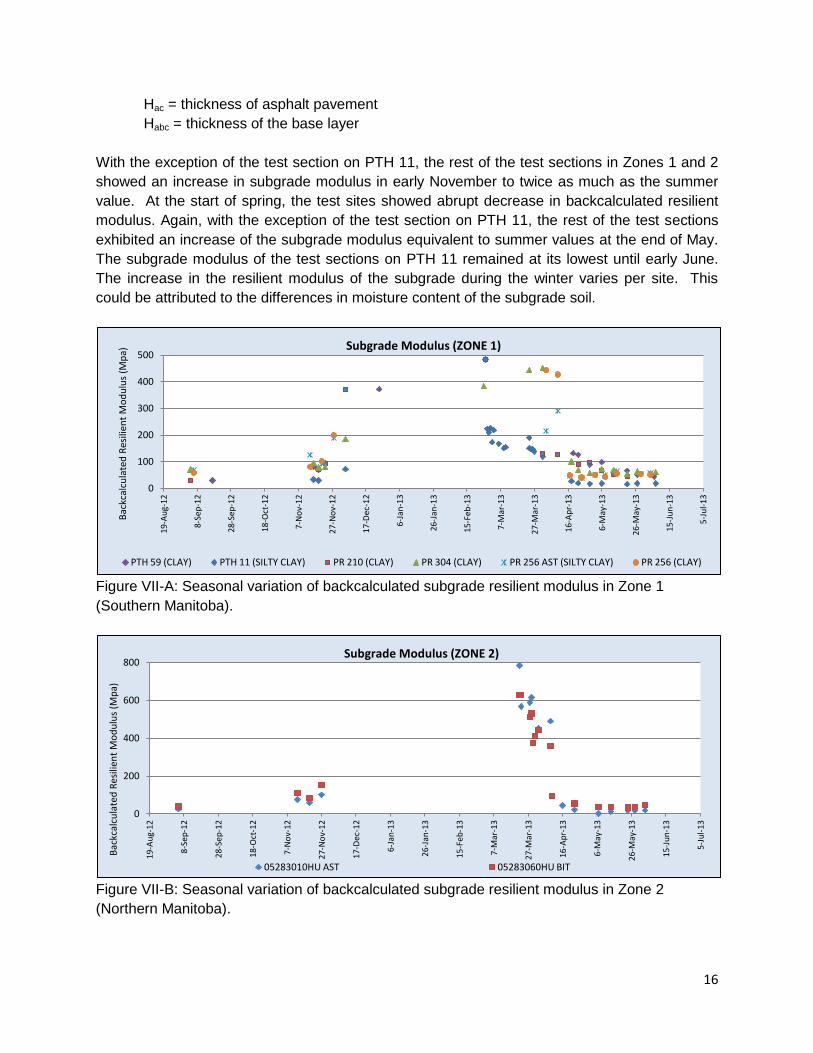
Hac = thickness of asphalt pavement
Habc = thickness of the base layer
With the exception of the test section on PTH 11, the rest of the test sections in Zones 1 and 2
showed an increase in subgrade modulus in early November to twice as much as the summer
value. At the start of spring, the test sites showed abrupt decrease in backcalculated resilient
modulus. Again, with the exception of the test section on PTH 11, the rest of the test sections
exhibited an increase of the subgrade modulus equivalent to summer values at the end of May.
The subgrade modulus of the test sections on PTH 11 remained at its lowest until early June.
The increase in the resilient modulus of the subgrade during the winter varies per site. This
could be attributed to the differences in moisture content of the subgrade soil.
Figure VII-A: Seasonal variation of backcalculated subgrade resilient modulus in Zone 1
(Southern Manitoba).
Figure VII-B: Seasonal variation of backcalculated subgrade resilient modulus in Zone 2
(Northern Manitoba).
0
100
200
300
400
500
19-A
ug-
12
8-Se
p-1
2
28-S
ep-1
2
18-O
ct-1
2
7-N
ov-
12
27-N
ov-
12
17-D
ec-1
2
6-Ja
n-1
3
26-J
an-1
3
15-F
eb-1
3
7-M
ar-1
3
27-M
ar-1
3
16-A
pr-
13
6-M
ay-1
3
26-M
ay-1
3
15-J
un
-13
5-Ju
l-13
Bac
kcal
cula
ted
Res
ilien
t M
od
ulu
s (M
pa)
Subgrade Modulus (ZONE 1)
PTH 59 (CLAY) PTH 11 (SILTY CLAY) PR 210 (CLAY) PR 304 (CLAY) PR 256 AST (SILTY CLAY) PR 256 (CLAY)
0
200
400
600
800
19-
Au
g-12
8-S
ep-1
2
28-S
ep-1
2
18-
Oct
-12
7-N
ov-
12
27-
No
v-1
2
17-
Dec
-12
6-Ja
n-1
3
26-
Jan
-13
15-F
eb-1
3
7-M
ar-1
3
27-
Mar
-13
16-
Ap
r-1
3
6-M
ay-1
3
26-
May
-13
15-J
un
-13
5-Ju
l-1
3
Bac
kcal
cula
ted
Res
ilien
t M
od
ulu
s (M
pa)
Subgrade Modulus (ZONE 2)
05283010HU AST 05283060HU BIT
17
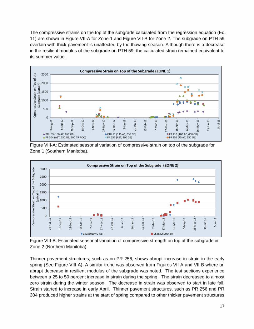
The compressive strains on the top of the subgrade calculated from the regression equation (Eq.
11) are shown in Figure VII-A for Zone 1 and Figure VII-B for Zone 2. The subgrade on PTH 59
overlain with thick pavement is unaffected by the thawing season. Although there is a decrease
in the resilient modulus of the subgrade on PTH 59, the calculated strain remained equivalent to
its summer value.
Figure VIII-A: Estimated seasonal variation of compressive strain on top of the subgrade for
Zone 1 (Southern Manitoba).
Figure VIII-B: Estimated seasonal variation of compressive strength on top of the subgrade in
Zone 2 (Northern Manitoba).
Thinner pavement structures, such as on PR 256, shows abrupt increase in strain in the early
spring (See Figure VIII-A). A similar trend was observed from Figures VII-A and VII-B where an
abrupt decrease in resilient modulus of the subgrade was noted. The test sections experience
between a 25 to 50 percent increase in strain during the spring. The strain decreased to almost
zero strain during the winter season. The decrease in strain was observed to start in late fall.
Strain started to increase in early April. Thinner pavement structures, such as PR 256 and PR
304 produced higher strains at the start of spring compared to other thicker pavement structures
0
500
1000
1500
2000
2500
19-A
ug-
12
8-Se
p-1
2
28-S
ep-1
2
18-O
ct-1
2
7-N
ov-
12
27-
No
v-1
2
17-D
ec-1
2
6-Ja
n-1
3
26-J
an-1
3
15-F
eb-1
3
7-M
ar-1
3
27-M
ar-1
3
16-
Ap
r-1
3
6-M
ay-1
3
26-M
ay-1
3
15-J
un
-13
5-Ju
l-13
Cp
mp
ress
ive
Stra
in o
n T
op
of
the
Sub
grad
e (µ
stra
in)
Compressive Strain on Top of the Subgrade (ZONE 1)
PTH 59 (150 AC, 650 GB) PTH 11 (130 AC, 335 GB) PR 210 (100 AC, 400 GB) PR 304 (AST, 150 GB, 300 CR RCK)) PR 256 (AST, 200 GB) PR 256 (75 AC, 150 GB)
0
500
1000
1500
2000
2500
3000
19-
Au
g-1
2
8-Se
p-1
2
28-
Sep
-12
18-O
ct-1
2
7-N
ov-
12
27-
No
v-1
2
17-D
ec-1
2
6-J
an-1
3
26-
Jan
-13
15-
Feb
-13
7-M
ar-1
3
27-
Mar
-13
16-
Ap
r-1
3
6-M
ay-1
3
26-M
ay-1
3
15-
Jun
-13
5-Ju
l-13
Co
mp
ress
ive
Stra
in o
n T
op
of
the
Sub
grad
e (µ
stra
in)
Compressive Strain on Top of the Subgrade (ZONE 2)
05283010HU AST 05283060HU BIT
18
such as PTH 11 and PR 210. Similar observations were made for compressive strains
developed on top of the subgrade in Zone 2 (Northern Manitoba). See Figure VIII-B.
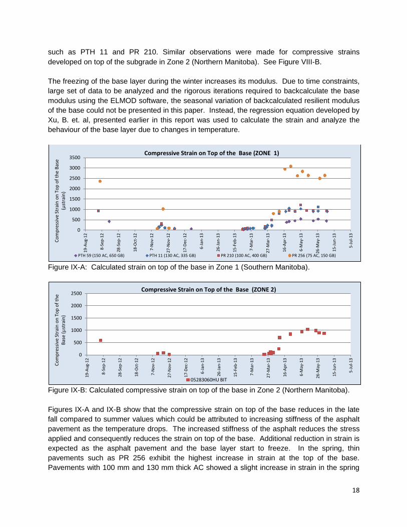
The freezing of the base layer during the winter increases its modulus. Due to time constraints,
large set of data to be analyzed and the rigorous iterations required to backcalculate the base
modulus using the ELMOD software, the seasonal variation of backcalculated resilient modulus
of the base could not be presented in this paper. Instead, the regression equation developed by
Xu, B. et. al, presented earlier in this report was used to calculate the strain and analyze the
behaviour of the base layer due to changes in temperature.
Figure IX-A: Calculated strain on top of the base in Zone 1 (Southern Manitoba).
Figure IX-B: Calculated compressive strain on top of the base in Zone 2 (Northern Manitoba).
Figures IX-A and IX-B show that the compressive strain on top of the base reduces in the late
fall compared to summer values which could be attributed to increasing stiffness of the asphalt
pavement as the temperature drops. The increased stiffness of the asphalt reduces the stress
applied and consequently reduces the strain on top of the base. Additional reduction in strain is
expected as the asphalt pavement and the base layer start to freeze. In the spring, thin
pavements such as PR 256 exhibit the highest increase in strain at the top of the base.
Pavements with 100 mm and 130 mm thick AC showed a slight increase in strain in the spring
0
500
1000
1500
2000
2500
3000
3500
19-
Au
g-1
2
8-Se
p-1
2
28-S
ep-1
2
18-O
ct-1
2
7-N
ov-
12
27-N
ov-
12
17-D
ec-1
2
6-Ja
n-1
3
26-J
an-1
3
15-F
eb-1
3
7-M
ar-1
3
27-M
ar-1
3
16-A
pr-
13
6-M
ay-1
3
26-M
ay-1
3
15-J
un
-13
5-Ju
l-13
Co
mp
ress
ive
Stra
in o
n T
op
of
the
Bas
e (µ
stra
in)
Compressive Strain on Top of the Base (ZONE 1)
PTH 59 (150 AC, 650 GB) PTH 11 (130 AC, 335 GB) PR 210 (100 AC, 400 GB) PR 256 (75 AC, 150 GB)
0
500
1000
1500
2000
2500
19-
Au
g-1
2
8-Se
p-1
2
28-
Sep
-12
18-O
ct-1
2
7-N
ov-
12
27-
No
v-1
2
17-
Dec
-12
6-J
an-1
3
26-
Jan
-13
15-
Feb
-13
7-M
ar-1
3
27-
Mar
-13
16-
Ap
r-1
3
6-M
ay-1
3
26-M
ay-1
3
15-
Jun
-13
5-Ju
l-1
3
Co
mp
ress
ive
Stra
in o
n T
op
of
the
Bas
e (µ
stra
in)
Compressive Strain on Top of the Base (ZONE 2)
05283060HU BIT
19
while thick pavements such as PTH 59 showed insignificant increase in the strain in the spring
compared to summer value.
Summary of Findings and Recommendations
1. The stress sensitivity analysis of the subgrade may be used to identify change in the in-
situ material type. This information can be used to determine the required number of
boreholes and laboratory testing during the soil survey. This can result in considerable
savings to the department where the frequency/extent of change in soil type is less than
the standard sampling protocol.
2. The backcalculated layer modulus using ELMOD may vary widely from one load drop to
another, or from one location to another. Good judgment should be used when using the
backcalculated modulii. The backcalculated layer modulii of the base and subgrade
using ELMOD are found to be within the range of values determined from laboratory
triaxial tests.
3. There is a close agreement between the laboratory-determined modulus of the subgrade
and the modulus calculated using the Hogg model. The comparison of the subgrade
modulii between the laboratory resilient modulus and AASHTO 1993 method showed
close agreement when a C Factor of 0.69 is used instead of 0.33 in the AASHTO
method. The AASHTO 1993 method can be used to estimate a reasonably accurate
subgrade resilient modulus when mass calculations are being performed. The
recommended backcalculation using the ELMOD software provides a better estimate of
the subgrade modulus compared to AASHTO 1993 when a C Factor of 0.75 is used.
ELMOD should be used when more accuracy is desired.
4. The modulus of the subgrade could potentially increase by as much as twice the
summer value during the months of November and December as the subgrade starts to
freeze and in March before the subgrade starts to thaw. The increase in subgrade
modulus during the winter season from January to February can be greater than five (5)
times the summer value. Due to the thawing of the subgrade in the spring, the
backcalculated modulus may decrease by as much as 50% of the summer value
between the months of April and July. The modulus does not change significantly from
August to October. The trend of the calculated compressive strain at the top of the
subgrade also supports this finding.
5. For HMA overlay, the subgrade type and resilient modulus showed very little influence in
the predicted rutting, IRI and total fatigue cracking.
6. For pavements with base layers constructed with an A-Base over C-Base, the
backcalculated combined modulus of the base using ELMOD can be used in pavement
analysis using Pavement ME Design with negligible difference in the predicted total
rutting, IRI and total fatigue cracking compared to inputs for individual base layers.
Additional case studies are required for a 3-layer base system where crushed rocks are
underlain by the C-Base layer. Initial results suggest that the estimated combined layer
modulus of a 3-layer base system without applying applying the MEPDG recommended
C Factor can be used in the current Pavement ME distress models with minor difference
20
in the predicted distresses. For sandwich construction, Pavement ME does not provide
or gives erroneous prediction for total cracking when individual layer modulus is used.
7. The seasonal trend of the calculated compressive strain at the top of the base is similar
to the trend of the calculated strain for the subgrade. Further analysis is required to
determine the seasonal variation in the base modulus backcalculations using the
ELMOD software.
References:
1. AASHTO Guide for Design of Pavement Structure. AASHTO, 1996.
2. B. Xu, S.R. Ranjithan, and Y.S. Kim. New Relationships Between the Falling Weight
Deflectometer Deflections and Asphalt Pavement Layer Indicators. In Transportation
Research Record 1806, TRB, Washington D.C. 2002.
3. Soliman, H., Shalaby, A. Evaluation of Subgrade Resilient Modulus for Typical Soils in
Manitoba. March 2012.