Estimating and Optimizing the Impact of Inventoryon Consumer Choices in a Fashion Retail Setting

Pol Boada Collado • Victor Martınez-de-Albeniz1

IESE Business School, University of Navarra, Av. Pearson 21, 08034 Barcelona, Spain

pboada@iese.edu • valbeniz@iese.edu

Abstract

In fashion retailing, the display of product inventory at the store is important to captureconsumers’ attention. Higher inventory levels might allow more attractive displays and thusincrease sales, in addition to avoiding stock-outs. We develop a choice model where productdemand is indeed affected by inventory, and controls for product and store heterogeneity, sea-sonality, promotions and potential unobservable shocks in each market. We empirically test themodel with daily traffic, inventory and sales data from a large retailer, at the store-day-productlevel. We find that the impact of inventory level on sales is positive and highly significant, evenin situations of extremely high service level. The magnitude of this effect is large: each 1%increase in product-level inventory at the store increases sales of 0.58% on average. This sup-ports the idea that inventory has a strong role in helping customers choose a particular productwithin the assortment. We finally describe how a retailer should optimally decide its inventorylevels within a category and describe the properties of the optimal solution. Applying suchoptimization to our data set yields consistent and significant revenue improvements, of morethan 10% for any date and store compared to current practices.

Submitted: April 6, 2016. Revised: May 17, 2017

Keywords: fashion retailing, choice models, inventory management, assortment planning.

1. Introduction

Managing store inventory is a key process in retailing. It is necessary to maintain sufficient inventory

depth so as to convert potential demand into sales. Yet, carrying high levels of inventory is costly,

as working capital needs to be financed, and it may create significant obsolescence risks, especially

for innovative products (Fisher 1997, Caro and Martınez-de-Albeniz 2014, 2015).

The academic literature has usually suggested that higher inventories lead to higher sales, e.g.,

under the newsvendor model. This positive relationship between the inventory decision and the

sales realization has usually been modeled in the literature through an increasing concave curve.

In practical settings, the inventory-sales relationship may be quite complex. There are at least

three reasons why higher inventories should lift sales. First, when inventory level is zero, potential

1IESE Business School, University of Navarra, Av. Pearson 21, 08034 Barcelona, Spain, email: valbeniz@iese.edu.V. Martınez-de-Albeniz’s research was supported in part by the European Research Council - ref. ERC-2011-StG283300-REACTOPS and by the Spanish Ministry of Economics and Competitiveness (Ministerio de Economıa yCompetitividad) - ref. ECO2014-59998-P.

1

customers may leave the store empty-handed, thereby reducing sales. The effect of stock-outs has

been widely documented, e.g., in Campo et al. (2003), Musalem et al. (2010) or Che et al. (2012).

Second, when inventory level is positive but close to zero, the items in the store may not fit perfectly

the potential customer taste. For example, for fresh food products, the quality of the few items left

on the shelf may not be as good as it usually is. For apparel goods, the few available products may

not cover all possible sizes, leading to the broken assortment effect (Smith and Achabal 1998, Caro

and Gallien 2010). Third, when inventory level is high, in certain contexts higher inventory may

still drive sales up. For instance, in fashion apparel retailing, ‘better’ displays are usually associated

with higher inventory level requirements. Indeed, products with high inventory are candidates for

premium high-traffic space at the entrance, while products with low inventory cannot be displayed

with the same level of quality and are typically pushed to the back walls of the store. Finally, note

that there may be alternative reasons for a decreasing relationship between inventory and sales,

namely that scarcity may encourage customers to procrastinate less and buy as soon as possible,

thereby lifting sales when inventory levels are low (Su and Zhang 2008, Liu and van Ryzin 2008,

Aviv and Pazgal 2008, Cachon and Swinney 2009).

Precise knowledge of the impact of inventory on sales is important to retailers to optimize store

operations, in particular in fashion apparel retailing, which is the focus of this paper. In this

industry, merchandizers have a prominent role in making stores look ‘attractive’ by displaying the

product in the best possible way, so as to extract the maximum possible revenue out of store space.

To support such objective, we seek to answer the two following research questions. First, from an

empirical perspective, can we measure the effect of inventory on sales, from store data (as opposed

to randomly experimenting with store inventory)? To provide an answer, we need an approach that

should take into account that demand is highly volatile and subject to seasonal variations, that

there may be heterogeneity across products and stores and that customers may substitute across

products. Second, from a decision-making perspective, we are interested in deciding how to take

inventory decisions, and in particular how to balance inventories across products in limited store

space.

To deal with the first question, we develop an empirical model to identify the shape of the

inventory-sales relationship. Specifically, we propose a choice model where store visitors choose

whether to buy one of the existing options, or nothing. In this model, the main difficulty is to

separate the effect of inventory on sales from co-movement of inventory and sales due to retailer

planned decisions. Indeed, sales and inventory may be positively associated because there is a

common driver that increases or decreases both at the same time. For example, larger stores would

carry higher inventory levels and sell more, but this is because of higher traffic. More generally, if

the retailer expects higher sales in a particular product, store or week, it will plan higher inventory

2

levels, so from an empirical perspective we will need to be careful in distinguishing this type of

relationship from a direct, causal effect. Hence, inventory endogeneity may be a concern. The

literature has handled this issue in different ways, depending on the context of study. Most of the

existing studies have focused on functional consumer goods such as groceries (e.g., Campo et al.

2003, Musalem et al. 2010, Che et al. 2012). As opposed to fashion goods, planned inventory is fixed

and variations over the target inventory can be taken as exogenous (see discussion in p. 1187 of

Musalem et al. 2010 for details). Other studies have looked at the retail distribution of automobiles.

Given the nature of such purchases, the sales process is typically long so that dealers may order

inventory for a particular customer before the actual purchase has been made, so inventory is highly

influenced by local demand forecasts (Olivares and Cachon 2009). Taking into account endogeneity

becomes a central concern for this industry, and one can use supply shocks to measure the direct

effect of inventory (Cachon et al. 2013). Fashion apparel resembles groceries more than automobiles

because it does not customize inventories for individual customers. However, in contrast with

groceries, seasonality and promotions at the store level may create endogeneity problems. To

eliminate them, we control for seasonality and price discounts; we also add instrumental variables

that capture the drivers of the inventory decision for the retailer, such as planned promotions and

predicted local events. By doing so, we can isolate the direct effect of inventory on sales.

We apply our model to a data set from a large European fashion retailer. We use daily traffic

at the store, and inventory and sales data at the store-product level (products are a combination

of model and color, but do not differentiate between sizes), for 85 stores in 13 different cities,

during the 2013-2014 period (two spring-summer and fall-winter collections). We find that the

impact of inventory on sales is positive and highly significant, even in situations of extremely high

service level. The magnitude of this effect is large: a 1% increase in product-level inventory at

the store increases sales of 0.58% on average. The results are robust across product categories,

seasons and model specifications (definition of inventory level variable, interactions in the controls,

nesting in choice model). This suggests that in fashion apparel retailing, inventory is a key lever to

push product sales. Indeed, in contrast with functional consumer goods such as groceries, fashion

products are usually not well-known by customers, so inventory levels (beyond pure availability)

should have a strong influence in the discovery process, through the association of inventory and

display.

Our empirical results provide the opportunity for a further examination of how inventory de-

cisions should be taken at the store, i.e., our second research question. Using our choice model,

we formulate an optimization problem where inventory levels are decision variables, within a set of

constraints, including total inventory maximum levels (to consider limited store space) and mini-

mum product inventory levels (to avoid changes in the assortment). This problem is a variation of

3

assortment planning (Kok et al. 2009). We analytically characterize the optimal solution to this

problem. We find that it is optimal to introduce products with the largest margins but the optimal

distribution of inventory can vary depending on margin and attractiveness. We then numerically

optimize inventory levels using the actual data and show that redistributing properly inventory

across products within the same family would lift revenues by 18.9% on average, from the current

practice. Furthermore, using our demand model we also estimate the cost of ignoring the inventory

effect: we find that choosing inventory levels based on product attractiveness and price only reduces

profits by more than 15% compared to the optimum.

This work makes two main contributions to the literature. First, it documents and provides

quantitative measurements of the inventory-sales relationship in the fashion industry, which com-

plement other studies (Smith and Achabal 1998, Caro and Gallien 2010, Ramakrishnan 2012). To

the best of our knowledge, our results are the first to report that inventory may still have an influ-

ence on demand even when service level is close to 100%. We interpret this influence through the

association of higher inventories with better displays, that suggest that higher inventory provides

better visibility to the products, and this is critical in a setting where purchases are the outcome

of a product discovery process. Second, we formulate an inventory balancing optimization problem

from our choice model that we solve when decisions are continuous or integer variables. In both

cases, we provide an algorithm to find the optimal solution. Our approach combines in a single

model features from assortment planning (Anderson et al. 1992) and decreasing returns when a

product’s inventory level is large (Corstjens and Doyle 1981).

The rest of the paper is organized as follows. §2 describes the relevant literature. We present our

model and describe the estimation strategy in §3. §4 applies the model to a data set from a fashion

retailer and obtains empirical estimates. We then formulate the inventory optimization problem in

§5. We finally conclude in §6. Supporting tables and proofs are contained in the Appendix.

2. Literature Review

Our work is related to analytical models and empirical studies that connect inventory (or more

generally, product offering) to sales.

There are numerous papers that develop models where demand directly increases with inventory

availability, see Urban (2005) for a review. Early papers in the marketing literature find that better

product visibility, mainly through display, increases sales, see e.g., Corstjens and Doyle (1981)

among others. In the recent operations literature, Balakrishnan et al. (2004) optimize inventory

ordering, through the economic order quantity (EOQ), when the demand rate varies with inventory

level. Balakrishnan et al. (2008) coordinate inventory level and pricing in a newsvendor setting

when demand is increasing in inventory. These papers model the ‘demand-enhancing’ value of

4

inventory, included in the direct effect that we discuss in this paper. Another factor included in

the direct effect is the censoring that inventory introduces on demand, to translate them into sales.

Conrad (1976) first highlighted the differences between potential demand and censored sales, due

to out-of-stocks, using a Poisson distribution. The role of display is analyzed by Smith and Achabal

(1998), where a dependency of demand and inventory is introduced. This is the broken assortment

effect also discussed in Caro and Gallien (2010), Caro et al. (2010) or Caro and Gallien (2012), due

to availability of a generic product but unavailability of certain sizes.

Most of the literature above ignores substitution across products, and hence usually presents

a single-product analysis. In contrast, there are models that precisely focus on this substitution

aspect, and study the optimal combination of products that a retail point should carry. These are

assortment planning models, which typically consider whether an item should be introduced or not,

hence using binary variables. Anderson et al. (1992) provides a comprehensive textbook while Kok

et al. (2009) reviews more recent work, including demand modelling and estimation. Most of the

many papers written on the subject use a logit demand specification (for an exception, see Smith

and Agrawal 2000 that use an exogenous linear demand model). When margins are identical, van

Ryzin and Mahajan (1999) show that carrying a popular set made of the most attractive items is

optimal. Talluri and van Ryzin (2004) show that, when margins are different, the optimal set is

revenue-ordered, i.e., made of the highest-margin items. Some work jointly considers assortment

and inventory/shelf-space decisions, see Hubner and Kuhn 2012 for a recent review. Gaur and

Honhon (2006) use a locational model a la Hotelling, and Maddah and Bish (2007) use a logit

model but only price and assortment directly influence the demand. Furthermore, there are several

papers that also incorporate inventory effects over time, by considering stock-out-based substitution

from products which inventory has been depleted into available ones, e.g., Mahajan and van Ryzin

(2001), Hopp and Xu (2008), Honhon et al. (2010), Honhon and Seshadri (2013). In this paper, our

formulation of inventory optimization can be cast as a variation of assortment planning (adding

inventory can be interpreted as adding variety), and in particular extends the revenue-ordered result

of Talluri and van Ryzin (2004): it is optimal to carry the highest-margin items, but the amount

of inventory depends on how attractive products are.

In addition, there is significant empirical work that is related to this paper. The impact of

stock-outs on grocery sales has been studied in Campo et al. (2000, 2003), Musalem et al. (2010)

and Che et al. (2012) among others. We borrow from these studies the use of the choice model (see

Train 2009 for details on the empirical methodology), with the difference that product attractiveness

may vary with inventory level, when strictly positive. Other related works that estimate the impact

of unavailable products are Kok and Fisher (2007), who estimate the degree of substitution and

determine how much space (facings) should be given to each product, and Fisher and Vaidyanathan

5

(2014), who combine estimation of substitution probabilities with assortment optimization and

show implementation results at three retailers. Koschat (2008) study the effect of inventory on

magazine sales in a newsvendor setting, and find that inventory increases sales even when the

available quantity is higher than demand. The previously mentioned papers introduce controls so

that inventory is exogenous in their estimation, as we do in this paper. In contrast, studies in

automotive distribution cannot use the same approach, due to the nature of the sales process, as

mentioned in the introduction. Olivares and Cachon (2009) analyze how inventory is determined

by sales forecasts and competition in automobile dealerships. They run a cross-sectional analysis

with population instrumental variables and generalized moments method to estimate the relation

between inventory, sales and competing market characteristics. Cachon et al. (2013) look at the

reverse relationship, the impact of inventory on sales. They control inventory endogeneity by

considering weather shocks to the supply of cars at the dealers. They find that raising inventory

directly decreases sales but indirectly increases them because of higher submodel variety. Finally,

it is worth mentioning that Craig et al. (2016) estimate the role of inventory fill-rate on sales in

fashion apparel as we do, but in a business-to-business setting where sales are wholesale orders to

the manufacturer where there can be no display effects. Finally, there are also empirical papers

that document customer strategic behavior, e.g., Nair (2007) or Li et al. (2014). In those settings,

product abundance decreases demand rates, which is not the case here.

3. Model Development

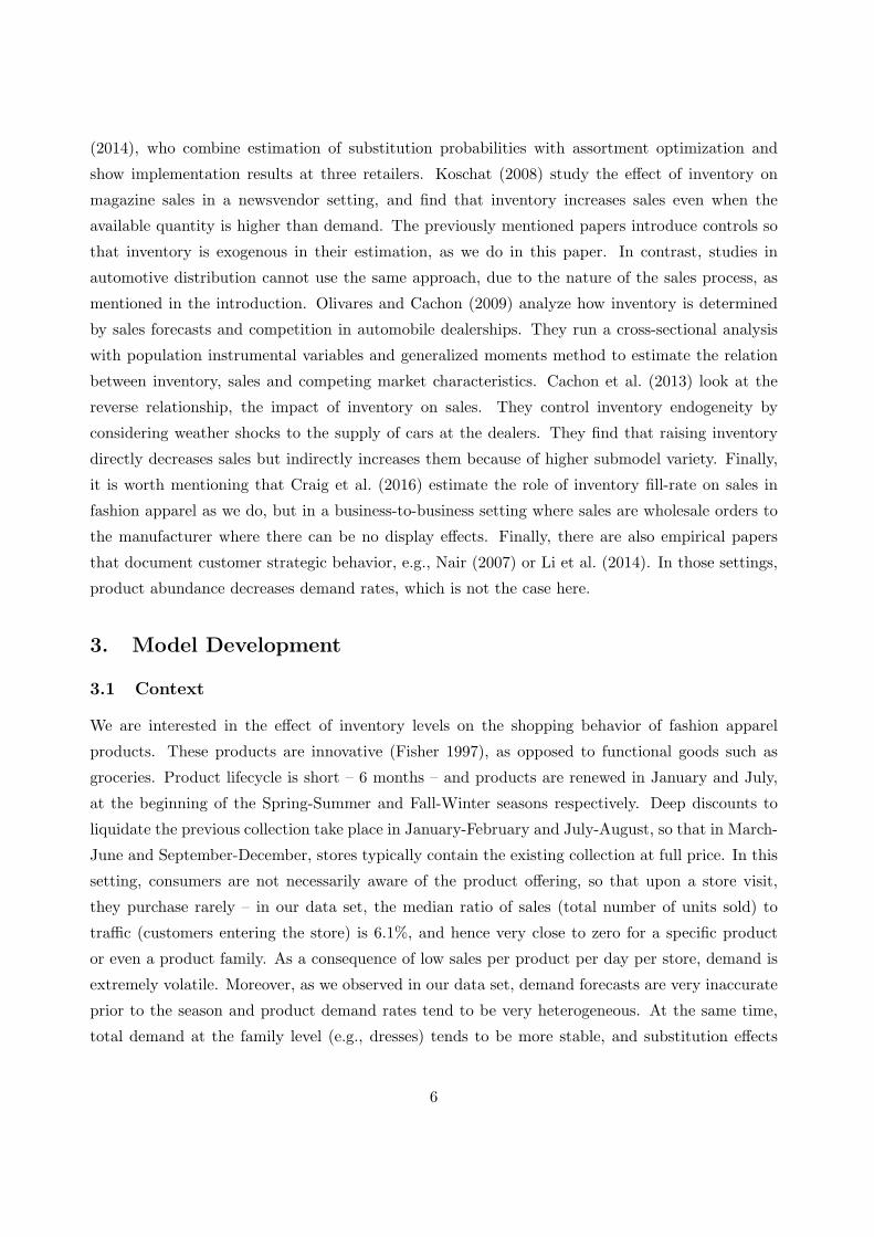
3.1 Context

We are interested in the effect of inventory levels on the shopping behavior of fashion apparel

products. These products are innovative (Fisher 1997), as opposed to functional goods such as

groceries. Product lifecycle is short – 6 months – and products are renewed in January and July,

at the beginning of the Spring-Summer and Fall-Winter seasons respectively. Deep discounts to

liquidate the previous collection take place in January-February and July-August, so that in March-

June and September-December, stores typically contain the existing collection at full price. In this

setting, consumers are not necessarily aware of the product offering, so that upon a store visit,

they purchase rarely – in our data set, the median ratio of sales (total number of units sold) to

traffic (customers entering the store) is 6.1%, and hence very close to zero for a specific product

or even a product family. As a consequence of low sales per product per day per store, demand is

extremely volatile. Moreover, as we observed in our data set, demand forecasts are very inaccurate

prior to the season and product demand rates tend to be very heterogeneous. At the same time,

total demand at the family level (e.g., dresses) tends to be more stable, and substitution effects

6

seem strong across products in the same family.

Stores in which the products are sold may be very different from each other. However, some of

them are located in the same city and are affected by the same promotional activity and marketing

effort: we call each of these cities a market.

3.2 Model Structure

In this setting, we develop a model for the behavior of a customer (she) visiting a store and shopping

within a given product family. Because of the innovative nature of the products and the low visit

frequency of shoppers, she goes through a discovery process of the different products on display.

In the spirit of Musalem et al. (2010), at store s, located in a market m(s), at time t, the utility

provided by purchasing product j with inventory Ijst > 0 to customer i can be written as:

Uijst = βXjst + ϕ(Ijst) + εijst. (1)

Xjst contains any covariates that may directly influence demand. In our study, we include

several demand drivers as covariates. We first create fixed effects αj and αs for product and

store intrinsic attractiveness (independent terms in our base model or interacted through a fixed

effect αjs in our robustness study), and αt for seasonality (identical across markets in our base

model or market-dependent through a fixed effect αm(s)t in our robustness study). We then take

into consideration the effect of discounts through a term βddst, where dst denotes the percentage

discount with respect to the list price, offered in store s at time t. This discount is taken as the

average discount in the category, because in our setting all discounts were planned to be equal, at

the category level; but it is straightforward to extend it to product-specific discounts. To take care

of potential endogeneity of Ijst, we also include instrumental variables through an additional term

βIV IVjst (described in detail at the end of this section). In addition, ϕ a function that reflects

the impact of inventory depth on the customer’s discovery process. When Ijst = 0, the customer

cannot see the product or buy it, so she obtains Uijst = −∞. Hence, this formulation takes care of

censoring by directly internalizing product unavailability in the utility function. εijst is a Gumbel-

distributed random variable (Anderson et al. 1992). Finally, not buying any product generates a

Gumbel utility εi0st.

Given this utility structure, when the customer chooses the product (including the outside

option, i.e., not buying anything) that provides the highest utility, the probability that product j

within the assortment set Ast is purchased can be written as

pjst =eβXjst+ϕ(Ijst)

1 +∑

k∈AsteβXkst+ϕ(Ikst)

(2)

The underlying assumptions of the model are worth discussing. First, we recognize that there

is product and store heterogeneity. This is captured via fixed effects αj and αs. Our formulation

7

thus allows the conversion of traffic into sales by store to be very different, even in the same

market and the same product. That is, a store at a train station might have a much higher

conversion than another one located in the street, for a given product. Similarly, we capture

product popularity differences, which are quite important in the fashion industry. Note that we do

not include product features in our model, such as price, because they are directly incorporated in

the product parameter.

Second, shopping behavior might be different on a weekday vs. the week-end, so that we need

a control for seasonality. We introduce common seasonal variation through a fixed effect αt. Note

that with our specification,we are implicitly assuming that the response to external market shocks

is the same in all the stores, an assumption that has been done before in the literature (Olivares

and Cachon 2009). Furthermore, we explicitly control for local promotions through the term βddst.

Moreover, the impact of inventory is captured via the function ϕ, such that ϕ(0) = −∞, so

that there can be no sales when the product is unavailable. In contrast with most of the operations

management literature, we do not assume there is a ‘true’ demand that is censored by low inventory:

we rather assume that sales are a function of product, store and time factors together with a retail

inventory effect. Observe that when the inventory effect is constant, i.e., ϕ(0) = −∞ and ϕ(I) = ϕ

for I > 0, then our model recovers the standard model where a stochastic demand independent

of the inventory level can be defined and demand is censored when there is no inventory. In our

analysis, we will mainly consider two forms for ϕ: ϕ(I) = γ log(I), which has been considered

often before in single-product settings (Corstjens and Doyle 1981, Balakrishnan et al. 2004); or

ϕ(I) piecewise-constant, which we will exploit to isolate effects at low inventory levels, due to

availability and broken assortment concerns, vs. at high levels. Regardless of the specific form of

ϕ, it is assumed that the impact of inventory is independent of j, s, t. Note that we also evaluate a

model where the inventory effect may depend on the product price and find that these interactions

are weak.

Writing ϕks the average of ϕ(Ikst) across all times and vkst = eβXkst+ϕks , Equation (2) can be

cast as

pjst =vjste

ϕ(Ijst)−ϕjs

1 +∑

k∈Astvksteϕ(Ikst)−ϕks

.

Our model structure will thus exploit inventory variations across time within the same store, and

link them to sales variations. Figure 1 illustrates the evolution of inventory and sales for several

products and stores. We observe that inventory variations do not follow any clear pattern, and in

particular it is apparent that when inventory levels are lower than average, it is because of past sales

and lack of replenishment: this variation does not seem planned by the retailer and we interpret it

as exogenous random variation.

Despite the lack of clear inventory patterns, one may wonder whether ϕ(Ijst) − ϕjs may be

8

Units in stock Units sold

0

10

20

30

40

50

Mar Apr May Jun Jul

Date

Units

Product a in store 1

0

10

20

30

40

Mar Apr May Jun Jul

Date

Units

Product a in store 2

0

5

10

15

20

25

Mar Apr May Jun Jul

Date

Units

Product a in store 3

0

10

20

30

Mar Apr May Jun Jul

Date

Units

Product b in store 1

0

5

10

15

20

25

Mar Apr May Jun Jul

Date

Units

Product b in store 2

0

5

10

15

Mar Apr May Jun Jul

Date

Units

Product b in store 3

0

10

20

30

40

Mar Apr May Jun Jul

Date

Units

Product c in store 1

0

10

20

30

Mar Apr May Jun Jul

Date

Units

Product c in store 2

0

5

10

15

20

25

Mar Apr May Jun Jul

Date

Units

Product c in store 3

Figure 1: Evolution of number of inventory (dashed) and sales (solid) for three stores and three

products (dresses of Spring-Summer 2014).

positively associated with εijst. This might create an endogeneity problem: even though we may

find that ϕ has an increasing shape (higher inventory leads to higher sales), it may be because

the retailer was anticipating higher sales and increased inventory at that store on that date. This

requires discussing how this retailer (as most in this industry) takes inventory decisions. Inventory

levels are decided centrally at this firm, so they are not subject to the intervention of store managers.

Specifically, headquarters collects sales data for a particular product, builds a forecast for future

sales, sets a service level and organizes weekly shipments to the stores. The target inventory level

is calculated as the current demand forecast times a factor (coverage of demand measured in days).

Given the heterogeneity in products and stores, and the existing seasonality within the category,

target inventory level should be expressed as

Itargetjst = γjγsγtγ0

for some parameters γj , γs, γt, forecast factors for product j, store s and time t respectively; and

γ0 (safety factor, independent of j, s, t because product margins are quite similar within a product

9

family). As a result, by introducing controls αj , αs, αt, the estimation of ϕ should not be subject

to any bias.

Nevertheless, to avoid any doubt, we still include an instrumental variable. This variable should

be directly related to any unobservable planned events for product j in store s at time t and

correlated with Ijst, but not driving the utility of the consumer in the store. We specifically

use the average inventory for product j at time t in the rest of stores in the same market, i.e.,

IVjst = log(1 +

∑s′ =s|m(s′)=m(s) Ijs′t

), to account for planned spikes of demand in that market.

3.3 Estimation Procedure

To estimate the model parameters, we maximize the likelihood function. For this purpose, consider

store s at time t. Conditional on receiving a total of Nst visitors, the units sold of products within

the assortment j ∈ Ast, denoted {Sjst}, follow a multinomial distribution:

f({Sjst}|Nst) =Nst!∏

j∈AstSjst!

∏j∈Ast

pSjst

jst

1−∑j∈Ast

pjst

Nst−∑

j∈AstSjst

. (3)

Denote g(Nst) the probability of observing traffic Nst. Since stores and periods are assumed to be

independent, the total likelihood is expressed as∏s

∏t

g(Nst)f({Sjst}|Nst).

The log-likelihood is thus equal to a constant plus

L({pjst}) =∑s

∑t

∑j∈Ast

Sjst log(pjst) +

Nst −∑j∈Ast

Sjst

log

1−∑j∈Ast

pjst

. (4)

Using our model specification, we obtain

L =∑s

∑t

∑j∈Ast

Sjst(βXjst + ϕ(Ijst))

−Nst log

1 +∑k∈Ast

eβXkst+ϕ(Ikst)

. (5)

This function is concave in the model parameters (McFadden 1974) so it is straightforward to

maximize. Unfortunately, the large number of observations (more than 370,000) and the large

number of parameters (more than 40,000 in our robustness study) make estimation challenging,

and standard statistical packages (in R for example) are not useful even in a powerful computer,

because extremely large matrices have to be inverted. For this reason, we develop a gradient-based

procedure to find the estimators, which converges in reasonable time.

10

To provide a measure of goodness-of-fit of our model, we compare it to the null model, character-

ized by a constant expected utility, i.e., Uijst = α0+εijst. We let Lnull the associated log-likelihood

of this model. We also compare it to the full model, where there is one parameter for each observa-

tion. In this case, the best estimator is pfulljst =Sjst

Nstand we let Lfull = L(pfulljst ). The goodness-of-fit

metric we use is the likelihood-ratio index LRI = (L− Lnull)/(Lfull − Lnull) ∈ [0, 1].

Finally, our empirical study will compare the model that includes the inventory effect ϕ(·)against one where the inventory effect is absent ϕ(x) ≡ 0 for x > 0. Recall however that ϕ(0) = −∞,

so this benchmark model incorporates the effect of stock-outs.

4. Empirical Application

4.1 Data

To apply our model, we worked with a large fashion retailer with revenues of several hundred

millions of euros. This chain directly operates its own stores all over the world, but in this study

we focused on 85 stores in four European countries. These stores are located in one of 13 different

European cities (that we call markets), in which there are at least 4 stores. Each of the stores only

carries products from the retailer’s unique brand, distributed across 13 main product families, in

different numbers depending on the store size and market. There were store openings during the

period of interest, which means that in different seasons the number of active stores may vary.

In our study, a product is defined as a distinct combination of model and color, and may include

several sizes (so that a product is the aggregate of SKUs over all the available sizes), which is the

most disaggregate level that the retailer uses. This set-up implies that the estimated inventory

effect combines both a broken assortment effect when inventory level is low (due to missing sizes)

and a display effect when inventory level is high (due to more advantageous placement in the store).

We collected daily measurements over 2013 and 2014 of the following variables:

• Number of visitors for each store and day Nst. The data was generated from traffic counters

at the entrance of each store. Note that there were stores where the counting sensors were

not operational (typically smaller and older stores), but they were removed from our sample.

• Number of units sold for each product in each store in each day Sjst. The data was provided

from the company’s ERP system and had 1.8 million records.

• Number of units stocked for each product in each store in each day Ijst. The data had 12.9

million records for the stores under consideration. In contrast with other retailers (DeHoratius

and Raman 2008), inventory records were found to be quite complete (only 2.9% of sales

records had missing inventory data) and reliable (no suspicious jumps in inventory levels that

11

could not be traced back to sales or replenishment). It is worth highlighting that the service

level was generally extremely high, as only in 0.1% of the product-store-day triplets there was

a stock-out event, i.e., ending inventory was zero.

• Average discount per product family in each store in each day dst. Operationalizing this

variable was quite challenging, because we did not observe the posted price of products that

were not sold on a given store and time. To still be able to obtain the discount variable, we

exploited the fact that promotions were planned to be the same across all products within a

product family, day and store, e.g., today 20% off on dresses in a given store, so we set dst to

be the average discount across the products within a product family on that store and day.

From these data, we removed the sales data where traffic or inventory data was missing (e.g., in

days where a store was closed), which resulted in a final count of 11.2 million traffic, inventory and

sales records, each corresponding to a triplet product-store-day.

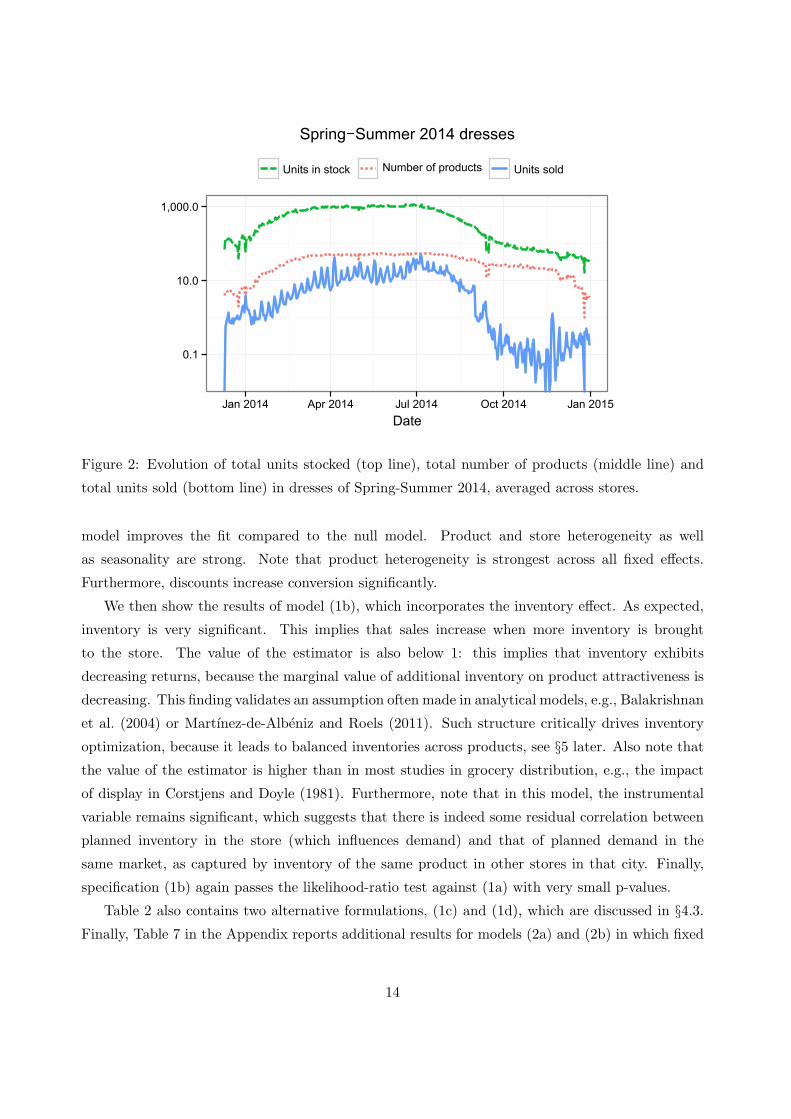
We focus our application on the firm’s top two product families: T-shirts and dresses. Figure

2 illustrates the totals of the relevant variables across the 85 stores for the dresses belonging to

the Spring-Summer 2014 collection. As we can see, products are continuously introduced until

mid-February, then stay stable during the regular season until end of June, and finally go through

liquidation starting in July. To focus on the regular season, we apply our model to the regular

season: February 15 to June 30 for the Spring-Summer collection and September 15 to December

31 for the Fall-Winter collection. Thus we consider 2.6 million records in total, for 1,349 products

within the dress and T-shirt families (note that we removed 255 products that never reached a

total stock of 50 units across all stores during 2013-14, which is an indication that they were not

mass-distributed as the rest of the sample).

During those periods, we report in Table 1 the average traffic Nst, average number of products

carried at the store |Ast|, average units sold at product level Sjst, average units stocked at product

level Ijst, for the two families during each of the four seasons under consideration.

4.2 Estimation Results

We present our results in Table 2, for the dress product family in Spring-Summer 2014. As described

in §3.3, we obtain the estimators through a gradient method. We also obtain standard errors

by inverting Fisher’s information matrix, which allow us to calculate p-values for the estimated

coefficients.

The table compares different specifications of the main model, where simple fixed effects without

interactions are used. The first specification tested is model (1a), which includes controls for for

products, stores and days, as well as discounts and the instrumental variable. We see that the

12

2013 2014

Spring-Summer Fall-Winter Spring-Summer Fall-Winter

Dress Visitors 1,031 991 938 824

Products available 45.2 58.2 77.1 66.1

Units stocked 20.0 19.0 19.9 18.7

Units sold 0.36 0.25 0.29 0.20

T-shirt Visitors 1,031 991 938 824

Products available 68.7 77.7 84.4 91.4

Units stocked 18.7 16.8 18.4 17.1

Units sold 0.33 0.30 0.37 0.28

Table 1: Sample descriptive statistics (averages across stores and days).

Model

(1a) (1b) (1c) (1d)

Fixed effects Product, store, day

Discount 0.249*** 0.300*** 0.303*** 0.309***

IV 0.192*** 0.0861*** 0.104*** 0.0813***

log(I) 0.592*** Inventory as factor 0.479***

p× log(I) 0.00103***

Number of observations 371,712 371,712 371,712 371,712

Number of variables 1,512 1,513 1,527 1,514

Log-likelihood -908,127 -904,397 -903,922 -904,354

LRI 20.1% 22.3% 22.6% 22.3%

Table 2: Estimation results for dresses in Spring-Summer 2014 (*** = significant at the 1% level).

13

0.1

10.0

1,000.0

Jan 2014 Apr 2014 Jul 2014 Oct 2014 Jan 2015

Date

Spring Summer 2014 dresses

Number of productsUnits in stock Units sold

Figure 2: Evolution of total units stocked (top line), total number of products (middle line) and

total units sold (bottom line) in dresses of Spring-Summer 2014, averaged across stores.

model improves the fit compared to the null model. Product and store heterogeneity as well

as seasonality are strong. Note that product heterogeneity is strongest across all fixed effects.

Furthermore, discounts increase conversion significantly.

We then show the results of model (1b), which incorporates the inventory effect. As expected,

inventory is very significant. This implies that sales increase when more inventory is brought

to the store. The value of the estimator is also below 1: this implies that inventory exhibits

decreasing returns, because the marginal value of additional inventory on product attractiveness is

decreasing. This finding validates an assumption often made in analytical models, e.g., Balakrishnan

et al. (2004) or Martınez-de-Albeniz and Roels (2011). Such structure critically drives inventory

optimization, because it leads to balanced inventories across products, see §5 later. Also note that

the value of the estimator is higher than in most studies in grocery distribution, e.g., the impact

of display in Corstjens and Doyle (1981). Furthermore, note that in this model, the instrumental

variable remains significant, which suggests that there is indeed some residual correlation between

planned inventory in the store (which influences demand) and that of planned demand in the

same market, as captured by inventory of the same product in other stores in that city. Finally,

specification (1b) again passes the likelihood-ratio test against (1a) with very small p-values.

Table 2 also contains two alternative formulations, (1c) and (1d), which are discussed in §4.3.Finally, Table 7 in the Appendix reports additional results for models (2a) and (2b) in which fixed

14

effects include interactions products-stores and markets-days. There are no qualitative differences

between them, which suggests that controls for potential behaviors such as store-dependent product

success (interaction product-store) or inventory planning based on local events (market-dependent

shocks through interaction market-day) do not influence the impact of inventory much. That is,

although the coefficient for log(I) is slightly reduced, the sign remains positive and the value highly

significant.

4.3 Robustness

We validate in this section the conclusions from Table 2, by providing some robustness checks.

First, to check that the logarithmic specification ϕ(I) = γ log(I) is valid, we estimated the

model using a piecewise-constant function. That is, ϕ(I) = ϕk when I ∈ {Ik, . . . , Ik+1 − 1}, fork = 1, . . . ,K. Specifically, we use 15 different intervals, with Ik = 1, . . . , 10, 15, 20, 30, 40, 50. This

is shown as model (1c) in Table 2. This alternative estimation indicates whether the inventory

effect seen so far is driven more for low inventory situations, i.e., because of broken assortment, or

whether it is also strong for high inventory situations, i.e., because of display effects. We illustrate

the results of this piecewise-constant function for dresses in Spring-Summer 2014 (the base case of

Table 2) in Figure 3. Note that we have centered the piecewise-constant function to the same level

to the logarithmic function so as to make comparison easier (this is without loss of generality).

−1

0

1

2

0 20 40

Inventory level

Inventory as factor Logarithmic

Figure 3: ϕ(I) estimated as a logarithmic function in model (1b) or with 15 factors respectively in

model (1c), for dresses of Spring-Summer 2014 .

15

We see that the piecewise-constant function penalizes inventory levels close to zero much more

than the logarithmic function. This suggests that broken assortments indeed have a high impact

on sales. Moreover, we see that for the function remains increasing even for high inventory levels,

e.g., in the right figure it jumps up by 0.15 (implying an increase of about 15% in sales) when

inventory moves from the interval [30,39] to [40,49]. At this level of inventory, the probability of a

stock-out is zero, given an average sale below 0.4 units per day. Hence, all indicates that indeed

inventory display must be responsible for this increase. Finally, one may wonder if at high levels of

inventory (as shown in the retailer’s ERP system), all of it is on display. The results suggest that

even a fraction of that inventory may be in the backroom, displays must be more visible when the

total inventory in the store is higher.

Second, we examine whether the inventory effect is homogeneous across products. For this

purpose, we introduce the interacted covariate Pj log(Ijst), where Pj is the list price of product

j, computed as the largest price used across all stores and days. This is shown as model (1d) in

Table 2. We see that the inventory effect tends to be larger for more expensive items, because the

interaction of price with log(I) is estimated to be 0.001. Although this interaction is significant

at the 1% level, the variation across products remains relatively homogeneous, and the coefficient

for the inventory effect only varies between 0.52 (for the cheapest item) and 0.73 (for the most

expensive one).

Third, we ran the same analysis for other seasons and product families. We obtained similar

goodness-of-fit improvements and estimates of the inventory effect in model (1b), all of them signif-

icant at the 1% level. We report in Table 3 the estimates for covariate log(I) in model (1b), which

are on average 0.58. This implies that increasing inventory by 1% increases product attractiveness

by 0.58 log(1.01) ≈ 0.58%. Notice from these additional scenarios that T-shirts are slightly more

sensitive to inventory (average of 0.62) compared to dresses (average of 0.53). This is despite similar

size structures, which suggests that the broken assortment effect should be similar. One possible

explanation is that they offer higher variety, cf. Table 1, which should make the display effect more

important.

Finally, we may wonder whether the MNL structure may have an influence on the estimated

strength of the inventory effect. For instance, if the choice process involves a more complex

structure, would we see a similar inventory influence? To answer this question, we considered

a nested version of the choice model, where products belong to product subfamilies (e.g., the

dress category is broken down into 6 subcategories: sleeveless, straps, swimmer, short sleeve, 3/4

sleeve and long sleeve). In this alternative choice model, the probability of choosing product j in

store s at time t can be written as pinjst × pnestn(j)st where n(j) denotes the nest to which j belongs,

wnst =∑

k∈Ast|n(k)=n eβXkst+ϕ(Ikst), pinjst = eβXjst+ϕ(Ijst)

wn(j)stand pnestnst =

wµnst

1+∑

n′ wµ

n′stwith µ a nesting

16

Season Dresses T-shirts

Spring-Summer 2013 0.458*** 0.636***

Fall-Winter 2013 0.532*** 0.636***

Spring-Summer 2014 0.592*** 0.648***

Fall-Winter 2014 0.577*** 0.563***

Table 3: Estimate of the inventory effect, i.e., coefficient γ in the estimation of ϕ(I) = γ log(I) in

model (1b), for different seasons and product families.

Season Dresses T-shirts

Spring-Summer 2013 0.468*** 0.645***

Fall-Winter 2013 0.538*** 0.637***

Spring-Summer 2014 0.581*** 0.648***

Fall-Winter 2014 0.579*** 0.557***

Table 4: Estimate of the inventory effect with demand nesting, i.e., coefficient γ in the estimation

of ϕ(I) = γ log(I) in model (1b), for different seasons and product families.

parameter (note that when µ = 1 we recover the original model). Kok and Xu (2011) discusses such

a nested formulation. Table 4 reports the estimated inventory effect in this more general choice

model. Interestingly, the nesting parameter µ in model (1b) falls within 0.86 and 1.12 across all

eight scenarios, which suggests that our original model (which assumes µ = 1) does an adequate

job at capturing substitution across products. As we can see, even in this more general case the

estimated value of the inventory effect remains positive with similar values to those reported in

Table 3.

5. Inventory optimization

Our empirical analysis has shown that inventory at the product level strongly influences sales. In

this section, we are interested in quantifying the potential improvement on family-level revenues

that a store manager can achieve by modifying store inventory levels in a given date. Indeed, we

can obtain estimates of demand from data of the first days of the season, and use the demand

choice model in (2); note that since this requires out-of-sample forecasting, we use our specification

(1b), so we present here the results for this model. For this purpose, we investigate the impact of

rebalancing inventory across products, within a certain family, store and date. In our analysis, we

17

keep total inventory across the product family unchanged. Since total inventory level is the same,

the increase in revenues is driven by shifting inventory (and thus sales) from some products with

excessive inventory, to others with more limited inventory.

5.1 Integer Formulation

Consider a store s and a particular date t (indices removed for simplicity). At this moment and

place, the total inventory at the store is I. The store manager can modify the inventory mix across

products in the assortment A:∑

j∈A Ij ≤ I. Product j = 1, . . . , n = |A| is sold at a price pj in that

specific date and store. Without loss of generality, we sort the products such that p1 ≥ . . . ≥ pn.

To keep high variety or perception of it in the category, the store may want to set a fixed minimum

inventory level for each product. We call the minimum amount ILj . Furthermore, there may be a

maximum amount of inventory in store, IHj , to account for the shelf space constraints for example.

Letting vj = eαj+αs+αt+βddst+βIV IVjst , the basic problem can be formulated as follows:

(IP) maxIj∈N

n∑j=1

pjvjeϕ(Ij)

1 +n∑

j=1

vjeϕ(Ij)

subject to ILj ≤ Ij ≤ IHj , j = 1, . . . , n,

n∑j=1

Ij ≤ I .

(6)

This is an integer optimization problem that could potentially be hard to solve, because of (i)

the non-linear nature of product attractiveness and (ii) the existence of constraints. Fortunately,

under certain conditions on ϕ(·), we can transform it into a tractable one.

Proposition 1. [Transformation into a binary problem]. When eϕ(I) is concave in I, then

(IP ) is equivalent to the following assortment planning problem (IP ′)

(IP ′) maxxjk

p0 +

n∑j=1

IHj −ILj∑k=1

pjvjkxjk

v0 +n∑

j=1

IHj −ILj∑k=1

vjkxjk

subject to xjk ∈ {0, 1}, for j = 1, . . . , n and k = 1, . . . , IHj − ILj ,

n∑j=1

IHj −ILj∑k=1

xjk ≤ X,

(7)

18

where v0 = 1+∑n

j=1 vjeϕ(ILj ), p0 =

∑nj=1 pjvje

ϕ(ILj ), X = I−∑n

j=1 ILj , vjk = vj

(eϕ(I

Lj +k) − eϕ(I

Lj +k−1)

).

Proposition 1 shows an equivalent formulation of (IP ) when ϕ is well-behaved. In particular,

it applies when ϕ(I) = γ log(I) with β ∈ [0, 1], as we have obtained in §4. The next question

is whether (IP ′) is any easier than (IP ). It turns out that it is a standard assortment planning

problem with MNL demand and a cardinality constraint: Rusmevichientong et al. (2010) provide

an algorithm to solve it in polynomial time.

5.2 Continuous Formulation

Given the typically large value of I, of the order of hundreds if not thousands, then an alternative

to (IP ) is to take Ij as a continuous variable, expressed as

(CP) maxIj∈R

n∑j=1

pjvjeϕ(Ij)

1 +

n∑j=1

vjeϕ(Ij)

subject to ILj ≤ Ij ≤ IHj , j = 1, . . . , n,

n∑j=1

Ij ≤ I .

(8)

To obtain strong analytical results, we assume in the rest of this section that ϕ(I) = γ log(I) with

γ ∈ [0, 1]. Assume moreover that ILj = 0 and IHj = ∞ (we explain later how to incorporate their

respective constraints again). In this case, letting xj = Ij/I we can define

Jk =maxxj≥0

ϕk :=

∑kj=1 pjvjx

γj

1 +∑k

j=1 vjxγj

subject to

k∑j=1

xj ≤ 1.

(9)

We let x∗j|k, j = 1, . . . , k, denote the optimal solution (we prove later that it is uniquely defined).

One should note the similarities between (9) and traditional assortment planning models with

capacity constraints (Rusmevichientong et al. 2010). Indeed, here we control a continuous variable

xj ≥ 0 that can take any amount of the existing capacity, while in standard assortment planning

models, the decision variable is whether item j should be introduced: xj = 0, 1/k (to keep total

capacity equal to 1). It is known that there, when capacity constraints are non-binding, it is optimal

to carry the products with the highest revenues (Talluri and van Ryzin 2004). This similarity

will carry over to our setting, i.e., the products with the highest prices will be introduced, and

19

the optimal quantities will depend on both price pj , base attractiveness vj and the sensitivity of

attractiveness to quantity γ, as shown next.

Proposition 2. [Revenue-ordered sets are optimal]. Consider problem Jk. At optimality, for

j ≤ k, if pj > Jk, x∗j|k > 0; if pj < Jk, x

∗j|k = 0.

This property can be exploited to characterize the optimal solution as follows.

Theorem 1. [Characterization of optimum] Consider problem Jk. There exists a revenue-

ordered set Ak ∈{{1}, {1, 2}, . . . , {1, . . . , k}

}such that the optimal solution is uniquely character-

ized by x∗j|k = 0 if j /∈ Ak and

x∗j|k =[(pj − Jk)vj ]

11−γ∑

l∈Ak[(pl − Jk)vl]

11−γ

(10)

if j ∈ Ak, where Jk is uniquely defined by

Jk =

∑j∈Ak

[(pj − Jk)vj ]1

1−γ

1−γ

. (11)

The theorem thus provides a numerical scheme to quickly identify the optimal solution: one

must try k candidates (each one corresponding to one Ak) and search for the corresponding Jk

using the fixed point equation (11), which is straightforward numerically because the fixed-point

mapping is monotonic. Such monotone one-dimensional mappings have been used elsewhere in the

assortment planning literature (Li and Huh 2011, Gallego and Wang 2014).

Furthermore, we can use this result further to provide a greedy algorithm to find the solution.

For this purpose, we use from (9) that Jk+1 ≥ Jk, because a feasible solution of the problem with

k variables is also feasible in the problem with k+ 1 variables. This property implies the following

proposition.

Proposition 3. [Introducing products greedily] If pk > Jk−1, then pk > Jl for any l = 0, . . . , n.

As a result, we can find the optimal solution by applying the following procedure.

Corollary 1. [Solution algorithm] The following algorithm yields the optimal solution for Jk.

1. Initialize J0 = 0 and set j = 1.

2. If pj ≤ Jj−1, then for all l ≥ j, Jl = Jj−1 and x∗j|l = 0. The optimal solution is thus such

that Aj−1 = {1, . . . , j − 1}.

3. Otherwise, then Aj = {1, . . . , j} and x∗m|j > 0 for m = 1, . . . , j. From Theorem 1, we obtain

Jj > Jj−1. Move to the next item j + 1.

20

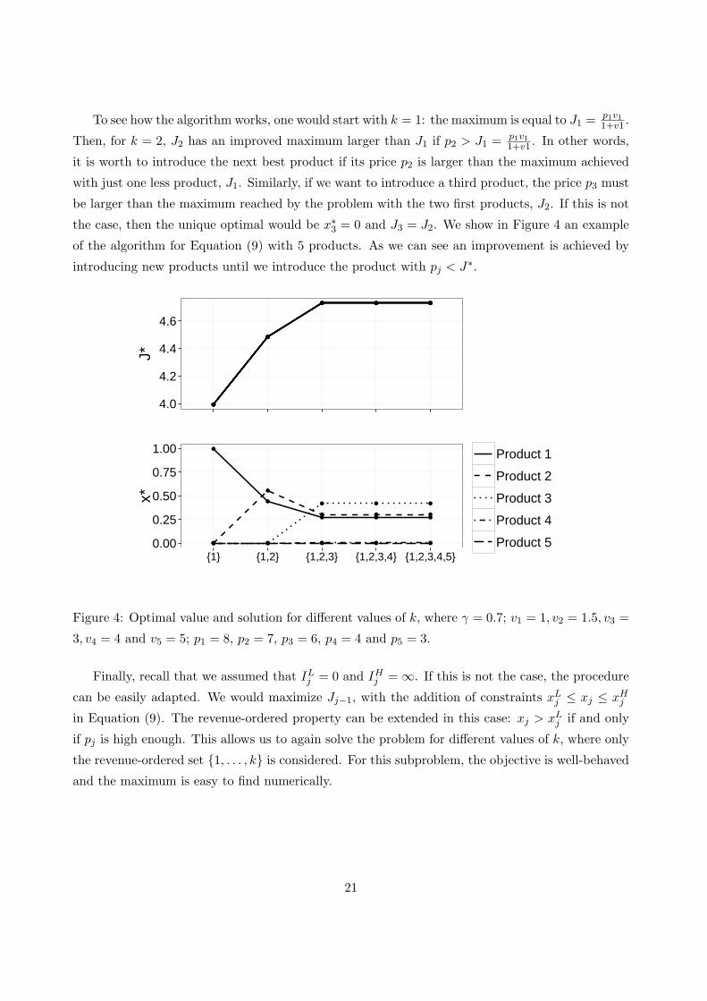
To see how the algorithm works, one would start with k = 1: the maximum is equal to J1 =p1v11+v1 .

Then, for k = 2, J2 has an improved maximum larger than J1 if p2 > J1 = p1v11+v1 . In other words,

it is worth to introduce the next best product if its price p2 is larger than the maximum achieved

with just one less product, J1. Similarly, if we want to introduce a third product, the price p3 must

be larger than the maximum reached by the problem with the two first products, J2. If this is not

the case, then the unique optimal would be x∗3 = 0 and J3 = J2. We show in Figure 4 an example

of the algorithm for Equation (9) with 5 products. As we can see an improvement is achieved by

introducing new products until we introduce the product with pj < J∗.

4.0

4.2

4.4

4.6

J*

0.00

0.25

0.50

0.75

1.00

{1} {1,2} {1,2,3} {1,2,3,4} {1,2,3,4,5}

x*

Product 1

Product 2

Product 3

Product 4

Product 5

Figure 4: Optimal value and solution for different values of k, where γ = 0.7; v1 = 1, v2 = 1.5, v3 =

3, v4 = 4 and v5 = 5; p1 = 8, p2 = 7, p3 = 6, p4 = 4 and p5 = 3.

Finally, recall that we assumed that ILj = 0 and IHj = ∞. If this is not the case, the procedure

can be easily adapted. We would maximize Jj−1, with the addition of constraints xLj ≤ xj ≤ xHj

in Equation (9). The revenue-ordered property can be extended in this case: xj > xLj if and only

if pj is high enough. This allows us to again solve the problem for different values of k, where only

the revenue-ordered set {1, . . . , k} is considered. For this subproblem, the objective is well-behaved

and the maximum is easy to find numerically.

21

5.3 Application

To evaluate the impact of the results of the previous section, we compared the predicted performance

of the actual inventory levels with that of the optimized integer inventory levels suggested by our

model. We kept store traffic unchanged.

Counterfactual: inventory optimization. We tested the improvement potential for different

stores and days, within the dress product family during Spring-Summer 2014, for which the demand

model was estimated in Table 2. Specifically, for a particular store and day, we let I be the sum

of inventory. We assumed IHj was the highest level of inventory carried over the season of that

product within that store; and ILj to be the least of 20% of that maximum and 50% of the average

inventory over the season (to avoid assortment reductions). Table 5 reports the percentage increase

in revenue.

Store

A B C D E F G H Average

Date

2014-03-01 13.7% 15.0% 16.4% 18.8% 23.1% 15.5% 32.1% 38.2% 21.6%

2014-03-08 12.1% 12.8% 12.9% 15.2% 14.2% 16.3% 32.0% 36.0% 18.9%

2014-03-15 13.1% 14.1% 11.6% 17.2% 18.7% 17.2% 28.6% 30.3% 18.8%

2014-03-22 9.1% 13.6% 15.2% 20.1% 17.9% 16.4% 27.5% 32.9% 19.1%

2014-03-28 15.2% 12.2% 14.5% 17.5% 16.0% 12.8% 25.8% 30.2% 18.0%

2014-04-04 14.6% 12.9% 13.9% 14.5% 16.1% 11.4% 25.8% 30.8% 17.5%

2014-04-11 24.7% 12.5% 18.0% 19.0% 20.1% 2.8% 20.6% 30.4% 18.5%

2014-04-17 20.0% 14.7% 12.7% 18.6% 14.0% 12.8% 24.9% 29.0% 18.4%

Average 15.3% 13.5% 14.4% 17.6% 17.5% 13.2% 27.2% 32.2% 18.9%

Table 5: Improvement of revenue by rebalancing inventory of dresses, for 8 stores and 8 selected

days in Spring-Summer 2014.

Table 5 shows the potential improvements of rebalancing inventory. We observe that the aver-

age increase over the current inventory policy is 18.9%. Improvement varies in the range 2-38%,

although for any store or date, it is at least 13%. This is quite high given that (i) there are no

changes in the assortment; (ii) the total inventory is the same; and (iii) the only improvement

lever is a more balanced inventory across products. Interestingly, the improvement is achieved by

modifying the inventory of products slightly: for instance, in store D (a median store) on March

22, 2014, in the optimal solution 11 products out of 40 are set to their maximum inventory level,

and none to the minimum. Indeed, optimization tends to increase inventory of the most profitable

and popular items (as in most assortment planning models), but also maintain a higher quantity

of inventory of the items with low popularity, to avoid the broken assortment effect; on the other

22

hand, inventory of the medium-popularity items is decreased. Hence, these results suggest that

taking into account the impact of inventory depth on sales may lift revenues significantly for a

retailer, without major variations on assortments nor inventory levels.

In addition, the optimal inventory levels do not vary much over time. Over the dates shown

in Table 5, the coefficient of variation of the optimal inventory levels is 14%, which suggests that

variation is small. Moreover, the variation is minimal for high-selling items: the top five selling

products in store D over the eight dates for which optimization was carried out have suggested

inventory levels (min-max) of 45-46, 42-43, 34-34, 25-33 and 20-26 respectively. This suggests that

implementing the optimal solution in a store essentially requires a one-time intervention early in

the season, to bring the inventory to an “ideal” target level; from that moment on, inventory levels

are just replenished when sales occur, through an order-up-to policy.

Furthermore, to verify that optimization is not pushing higher-priced items and removing lower-

priced items to achieve the aforementioned improvements, we reran the optimization in (8) assuming

that all products carried the same price. In other words, we maximized expected units sold instead

of revenue. Table 6 shows the results. We observe that the average improvement is lower – 8.3% –

yet qualitatively the improvements are similar.

Store

A B C D E F G H Average

Date

2014-03-01 6.3% 7.5% 8.2% 7.8% 10.4% 7.6% 9.8% 12.5% 8.8%

2014-03-08 6.0% 7.0% 7.1% 9.0% 8.5% 7.9% 10.4% 11.1% 8.4%

2014-03-15 7.0% 6.6% 7.8% 7.8% 8.2% 8.6% 8.5% 11.6% 8.3%

2014-03-22 6.1% 6.9% 8.1% 9.4% 7.3% 8.9% 8.8% 10.6% 8.3%

2014-03-28 8.5% 5.8% 7.0% 8.6% 7.6% 6.5% 8.7% 8.2% 7.6%

2014-04-04 9.5% 7.0% 7.6% 7.0% 7.6% 6.3% 8.7% 8.8% 7.8%

2014-04-11 16.6% 7.0% 8.5% 8.4% 8.6% 6.3% 8.3% 9.3% 9.1%

2014-04-17 14.1% 7.0% 5.6% 7.4% 6.9% 5.5% 8.8% 9.7% 8.1%

Average 9.3% 6.8% 7.5% 8.2% 8.1% 7.2% 9.0% 10.2% 8.3%

Table 6: Improvement of expected units sold by rebalancing inventory of dresses, for 8 stores and

8 selected days in Spring-Summer 2014.

Finally, the potential of optimization reported here is based on an analytical demand model

based on our empirical results. Of course, a randomized experiment with an intervention on inven-

tory levels would be useful to validate the conclusions.

The cost of ignoring the inventory effect. It is also worth comparing the optimal solution

to heuristic solutions that ignore the dependency of sales on inventory. To estimate how such

23

heuristics perform, we compare the current solution to two simple heuristic policies:

• The first policy sets inventory levels proportional to sales. This implies that the retailer

keeps the same assortment and provides a similar service level for all items. Specifically, such

heuristic would set Ij/I =vj∑

l∈Akvl.

• The second policy discriminates across products so as to prioritize products with higher

margins, but ignores the inventory effect. Specifically, such heuristic would set Ij > 0 in

a demand model with γ = 0 (instead of 0.592 in dresses for Spring-Summer 2014), i.e.,

Ij/I =(pj−Jk)vj∑

l∈Ak(pl−Jk)vl

.

We compare the profits derived from using these heuristics (with the same minimum and max-

imum display quantities as before), with the optimal solution. We find that heuristic 1 delivers

on average 17.6% less profit than the optimal solution (minimum 6.5%, maximum 28.6%), while

heuristic 2 yields 15.5% less profit than optimal (minimum 2.7%, maximum 27.3%). This suggests

that ignoring the inventory effect, i.e., setting γ = 0 in heuristic 2, is expensive: significant value is

left on the table. In fact, the loss of profit is almost as large as ignoring product margins (as done

in heuristic 1), and the results achieved are not very different from the current policy applied at

the retailer.

6. Conclusions and Further Research

In this paper, we studied the effect of inventory level on demand for fashion products. For these

products, customers do not necessarily know what they want, and as a result, higher inventories,

through better displays, may increase sales. We develop a choice model that incorporates the

impact of inventory level. We control for store and product heterogeneity, seasonality, promotions

and also introduce instrumental variables to avoid biases due to potential inventory endogeneity.

We estimate the model empirically with highly disaggregate data from a large retailer. We find that

inventory availability strongly drives sales, at both low inventory levels (broken assortment) and

high inventory levels (display). Finally, given the direct effect identified in our empirical findings,

we study how a retailer could rebalance inventory across a product family to maximize revenue.

We characterize the structure of the optimal solution and provide a simple algorithm to find it.

Using the parameters from our estimation and the actual inventory policy, we find that revenues

can be improved significantly (+18.9% on average), without any change in assortment and only

minor adjustments in inventory levels. High improvements can also be achieved if the retailer wants

to maximize the number of units sold (+8.3%).

Our work opens a number of directions for future research. From an empirical perspective, we

have identified inventory as a key driver of demand. Our results can be confirmed through other

24

methods: namely, it would be interesting to run a controlled experiment where the inventory of

some products is reduced on purpose, to estimate the impact on demand for all products. This

would be similar to Caro and Gallien (2010) but on inventory planning rather than replenishment

optimization. Another necessary further study is to detail why demand increases with inventory.

In this paper, we argued that the impact of inventory on sales is due to broken assortment when

inventories are low, and display when they are high. To further separate the different channels, it

would be interesting to obtain data on where inventory is located, and explain sales through display

variables. From a modelling standpoint, there are also some interesting models to study. We have

developed a simple mathematical program to optimize inventory in the store. Several extensions

can be explored, that include real features that we have overlooked, such as multiple stores using a

common limited inventory in the warehouse, multiple periods, fixed costs for replenishing inventory,

etc. This requires for example studying dynamic programs where inventory of an attractive product

has to be rationed across stores and periods.

Acknowledgements

The authors would like to thank three anonymous referees and an associate editor for their helpful

comments and insights.

References

Anderson, S. P., A. De Palma, and J.-F. Thisse. 1992. Discrete choice theory of product differentiation. MIT

Press.

Aviv, Y., and A. Pazgal. 2008. Optimal Pricing of Seasonal Products in the Presence of Forward-Looking

Consumers. Manufacturing & Service Operations Management 10 (3): 339–359.

Balakrishnan, A., M. Pangburn, and E. Stavrulaki. 2004. Stack Them High, Letem Fly: Lot-Sizing Policies

When Inventories Stimulate Demand. Management Science 50 (5): 630–644.

Balakrishnan, A., M. S. Pangburn, and E. Stavrulaki. 2008. Integrating the promotional and service roles

of retail inventories. Manufacturing & Service Operations Management 10 (2): 218–235.

Cachon, G., S. Gallino, and M. Olivares. 2013. Does adding inventory increase sales? evidence of a scarcity

effect in us automobile dealerships. Working paper, Columbia Graduate School of Business.

Cachon, G. P., and R. Swinney. 2009. Purchasing, pricing, and quick response in the presence of strategic

consumers. Management Science 55 (3): 497–511.

Campo, K., E. Gijsbrechts, and P. Nisol. 2000. Towards understanding consumer response to stock-outs.

Journal of Retailing 76 (2): 219–242.

Campo, K., E. Gijsbrechts, and P. Nisol. 2003. The impact of retailer stockouts on whether, how much, and

what to buy. International Journal of Research in Marketing 20 (3): 273–286.

25

Caro, F., and J. Gallien. 2010. Inventory Management of a Fast-Fashion Retail Network. Operations

Research 58 (2): 257–273.

Caro, F., and J. Gallien. 2012. Clearance pricing optimization for a fast-fashion retailer. Operations re-

search 60 (6): 1404–1422.

Caro, F., J. Gallien, M. Dıaz, J. Garcıa, J. Corredoira, M. Montes, J. Ramos, and J. Correa. 2010. Zara

uses operations research to reengineer its global distribution process. Interfaces 40 (1): 71–84.

Caro, F., and V. Martınez-de-Albeniz. 2014. How Fast Fashion Works: Can It Work for You, Too? IESE

Insight Review 21:58–65.

Caro, F., and V. Martınez-de-Albeniz. 2015. Fast fashion: Business model overview and research opportu-

nities. In Retail Supply Chain Management: Quantitative Models and Empirical Studies, 2nd Edition,

ed. N. Agrawal and S. A. Smith, 237–264. Springer, New York.

Che, H., X. Chen, and Y. Chen. 2012. Investigating effects of out-of-stock on consumer stockkeeping unit

choice. Journal of Marketing Research 49 (4): 502–513.

Conrad, S. 1976. Sales data and the estimation of demand. Journal of the Operational Research Society 27

(1): 123–127.

Corstjens, M., and P. Doyle. 1981. A model for optimizing retail space allocations. Management Science 27

(7): 822–833.

Craig, N., N. DeHoratius, and A. Raman. 2016. The impact of supplier inventory service level on retailer

demand. Manufacturing & Service Operations Management 18 (4): 461–474.

DeHoratius, N., and A. Raman. 2008. Inventory Record Inaccuracy: An Empirical Analysis. Management

Science 54 (4): 627–641.

Fisher, M., and R. Vaidyanathan. 2014. A demand estimation procedure for retail assortment optimization

with results from implementations. Management Science 60 (10): 2401–2415.

Fisher, M. L. 1997. What is the right supply chain for your product? Harvard Business Review 75:105–117.

Gallego, G., and R. Wang. 2014. Multiproduct price optimization and competition under the nested logit

model with product-differentiated price sensitivities. Operations Research 62 (2): 450–461.

Gaur, V., and D. Honhon. 2006. Assortment Planning and Inventory Decisions Under a Locational Choice

Model. Management Science 52 (10): 1528–1543.

Honhon, D., V. Gaur, and S. Seshadri. 2010. Assortment planning and inventory decisions under stockout-

based substitution. Operations Research 58 (5): 1364–1379.

Honhon, D., and S. Seshadri. 2013. Fixed vs. random proportions demand models for the assortment planning

problem under stockout-based substitution. Manufacturing & Service Operations Management 15 (3):

378–386.

Hopp, W. J., and X. Xu. 2008. A static approximation for dynamic demand substitution with applications

in a competitive market. Operations Research 56 (3): 630–645.

Hubner, A. H., and H. Kuhn. 2012. Retail category management: State-of-the-art review of quantitative

research and software applications in assortment and shelf space management. Omega 40 (2): 199–209.

26

Kok, A. G., and M. L. Fisher. 2007. Demand estimation and assortment optimization under substitution:

Methodology and application. Operations Research 55 (6): 1001–1021.

Kok, A. G., M. L. Fisher, and R. Vaidyanathan. 2009. Assortment planning: Review of literature and

industry practice. In Retail supply chain management, 99–153. Springer.

Kok, A. G., and Y. Xu. 2011. Optimal and competitive assortments with endogenous pricing under hierar-

chical consumer choice models. Management Science 57 (9): 1546–1563.

Koschat, M. A. 2008. Store inventory can affect demand: Empirical evidence from magazine retailing.

Journal of Retailing 84 (2): 165–179.

Li, H., and W. T. Huh. 2011. Pricing multiple products with the multinomial logit and nested logit models:

Concavity and implications. Manufacturing & Service Operations Management 13 (4): 549–563.

Li, J., N. Granados, and S. Netessine. 2014. Are consumers strategic? structural estimation from the

air-travel industry. Management Science 60 (9): 2114–2137.

Liu, Q., and G. van Ryzin. 2008. Strategic capacity rationing to induce early purchases. Management

Science 54 (6): 1115–1131.

Maddah, B., and E. K. Bish. 2007. Joint pricing, assortment, and inventory decisions for a retailer’s product

line. Naval Research Logistics (NRL) 54 (3): 315–330.

Mahajan, S., and G. van Ryzin. 2001. Stocking retail assortments under dynamic consumer substitution.

Operations Research 49 (3): 334–351.

Martınez-de-Albeniz, V., and G. Roels. 2011. Competing for shelf space. Production and Operations Man-

agement 20 (1): 32–46.

McFadden, D. 1974. Conditional Logit Analysis of Qualitative Choice Behavior. In Frontiers in Econometrics,

ed. P. Zarembka. Academic Press, New York.

Musalem, A., M. Olivares, E. Bradlow, C. Terwiesch, and D. Corsten. 2010. Structural Estimation of the

Effect of Out-of-Stocks. Management Science 56 (7): 1180–1197.

Nair, H. 2007. Intertemporal price discrimination with forward-looking consumers: Application to the US

market for console video-games. Quantitative Marketing and Economics 5 (3): 239–292.

Olivares, M., and G. P. Cachon. 2009. Competing retailers and inventory: An empirical investigation of

General Motors’ dealerships in isolated US markets. Management Science 55 (9): 1586–1604.

Ramakrishnan, R. 2012. Markdown Management. In The Oxford handbook of pricing management, ed.

O. Ozer and R. Phillips. Oxford University Press, Oxford, United Kingdom.

Rusmevichientong, P., Z.-J. M. Shen, and D. B. Shmoys. 2010. Dynamic assortment optimization with a

multinomial logit choice model and capacity constraint. Operations research 58 (6): 1666–1680.

Smith, S., and D. Achabal. 1998. Clearance Pricing and Inventory Policies for Retail Chains. Management

Science 44 (3): 285–300.

Smith, S. A., and N. Agrawal. 2000. Management of multi-item retail inventory systems with demand

substitution. Operations Research 48 (1): 50–64.

Su, X., and F. Zhang. 2008. Strategic Customer Behavior, Commitment, and Supply Chain Performance.

Management Science 54 (10): 1759–1773.

27

Talluri, K., and G. J. van Ryzin. 2004. Revenue management under a general discrete choice model of

consumer behavior. Management Science 50 (1): 15–33.

Train, K. 2009. Discrete choice methods with simulation. Cambridge university press.

Urban, T. L. 2005. Inventory models with inventory-level-dependent demand: A comprehensive review and

unifying theory. European Journal of Operational Research 162 (3): 792–804.

van Ryzin, G., and S. Mahajan. 1999. On the relationship between inventory costs and variety benefits in

retail assortments. Management Science 45 (11): 1496–1509.

Appendix

Model

(2a) (2b)

Fixed effects Product-store, market-day

Discount -0.200*** -0.224***

IV 0.344*** 0.158***

log(I) 0.489***

Number of observations 371,712 371,712

Number of variables 41,920 41,921

Log-likelihood -892,785 -891,317

LRI 29.2% 30.0%

Table 7: Estimation results for dresses in Spring-Summer 2014 (*** = significant at the 1% level).

Proofs

Proof of Proposition 1. The transformation relies on writing Ij = ILj +∑Ij−ILj

k=1 xjk. To prove

equivalence, one must establish that a solution of (IP’) can always be implemented in (IP). This

requires that there is an optimal solution such that, for all j, xjk is decreasing in k. To prove this,

assume that there is an optimal solution with j, k such that (xjk, xj,k+1) = (0, 1). Let us show that,

when eϕ(I) is concave, then (xj,k, xj,k+1) = (1, 0) provides a solution that is at least as good.

The objective of (IP’) can be written as

π∗ =p0 + pj(vjkxjk + vj,k+1xj,k+1)

v0 + vjkxjk + vj,k+1xj,k+1

28

Since (xjk, xj,k+1) = (0, 1) is optimal, then it must be true that

π∗ =p0 + pjvj,k+1

v0 + vj,k+1≥ p0

v0,

i.e., pj v0 ≥ p0. But then

π∗ =p0 + pjvj,k+1

v0 + vj,k+1≥

p0 + pjvj,kv0 + vj,k

(12)

is equivalent

(v0pj − p0)(vj,k+1 − vj,k) ≥ 0.

But when eϕ(I) is concave, vj,k+1 ≤ vj,k, so it must be that (12) is an equality.

Proof of Proposition 2. We can reformulate conditions of Jk as follow:

Jk = maxx1,...,xk−1≥0,

∑k−1j=1 xj≤1

Φ(x1, . . . , xk−1) =

∑k−1j=1 pjvjx

γj + pkvk(1−

∑k−1j=1 xj)

γ

1 +∑k−1

j=1 vjxγj + vk(1−

∑k−1j=1 xj)

γ

Note that we wrote xk = 1 −∑k−1

j=1 xj to work with just k − 1 non-negative variables. Then,

taking the first derivative for each j = 1, . . . , k − 1 we obtain:

1

γ

∂Φ

∂xj=

vjxγ−1j (pj − Φ)− vkx

γ−1k (pk − Φ)

1 +∑k

l=1 vlxγl

At an optimal solution x∗1, . . . , x∗k, where Φ(x

∗) = Jk, consider products i, j where x∗i , x∗j > 0. From

first-order conditions, it must be true that ∂Φ∂xi

= ∂Φ∂xj

and thus vixγ−1i (pi − Φ) = vjx

γ−1j (pj − Φ).

Hence either pi, pj > Φ or pi, pj ≤ Φ. Suppose that the latter case holds. Then Jk ≤ Φ∑k

l=1 vlxγl

1+∑k

l=1 vlxγl

<

Φ: this is a contradiction. Hence x∗i > 0 if and only if pi > Jk.

Proof of Theorem 1. From the proof of Proposition 2, we know that for all i, j such that x∗i , x∗j > 0,

∂Φ∂xi

= ∂Φ∂xj

. Moreover, at such point, it is simple to verify that this is a maximum. This implies that

x∗i =

[(pi − Jk)vi(pj − Jk)vj

] 11−γ

x∗j .

Using again the condition∑k

j=1 xj = 1 we obtain the following implicit relation, Equation (10):

x∗j =[(pj − Jk)vj ]

11−γ∑

l∈Ak[(pl − Jk)vl]

11−γ

where Ak is the set of indices l for which x∗l > 0.

29

Since Jk(1 +∑

l∈Akvlx

γl ) =

∑l∈Ak

plvlxγl , we find that

Θ(J) := J −

∑j∈Ak

[(pj − J)vj ]1

1−γ

1−γ

is such that Θ(Jk) = 0. Θ is a strictly increasing one-variable function, so Jk is uniquely obtained

by finding the root of Θ(J) = 0. In summary, at optimality, we have that, from Proposition 2,

there exists Ak made of the indices with the highest prices, and the optimal solution is obtained

by combining Equations (10) and (11).

Proof of Proposition 3. First, it is clear from the monotonicity of Jk that pk > Jk−1 ≥ Jk−2 ≥. . . ≥ J0. Second, for l ≥ k, for any x1, . . . , xl, recalling that pk ≥ pi for i ≥ k,∑l

j=1 pjvjxjγ

1 +∑l

j=1 vjxjγ=

( ∑k−1j=1 pjvjxj

γ

1 +∑k−1

j=1 vjxjγ

)(1 +

∑k−1j=1 vjxj

γ

1 +∑l

j=1 vjxjγ

)+

∑lj=k pjvjxj

γ

1 +∑l

j=1 vjxjγ

< pk

(1 +

∑k−1j=1 vjxj

γ

1 +∑l

j=1 vjxjγ

)+

∑lj=k pjvjxj

γ

1 +∑l

j=1 vjxjγ

≤ pk

(1 +

∑k−1j=1 vjxj

γ

1 +∑l

j=1 vjxjγ

)+ pk

( ∑lj=k vjxj

γ

1 +∑l

j=1 vjxjγ

)= pk.

Thus the maximum over x1, . . . , xk (within a compact set) is also strictly smaller than pk: Jl <

pk.

30