Embed Size (px)
Citation preview

Estimating an Ordinary Differential Equation Model
With Partially Observed Data
Kwang Woo Ahn
Division of Biostatistics
Medical College of Wisconsin, Milwaukee, WI 53226
email: [email protected]
Michael Kosoy
Centers for Disease Control and Prevention
Fort Collins, CO 80521
email: [email protected]
Kung–Sik Chan
Department of Statistics and Actuarial Science
The University of Iowa, Iowa City, Iowa 52242
email: [email protected]
July 22, 2011
Abstract
Ordinary differential equation (ODE) models, e.g. the susceptible-infected-recovered
model, are widely used in engineering, ecology, and epidemiology. Many ODE models
1

specify the state process as driven by a system of nonlinear differential equations. In
practice, ODE models may be observed partially in that only a proper subset of the
state vector is observed with measurement errors over discrete time. While there are
several methods for estimating ODE models with partially observed data, they are
invariably subject to several problems including high computational cost, sensitivity to
initial values or large sampling variability. We propose a new computationally efficient
two-step method for estimating a differential equation model with partially observed
data. We derive the consistency and large-sample distribution of the proposed method.
The efficacy of the new method is illustrated by simulations and a real epidemiological
time-series data on the prevalence of Bartonella in a wild population of cotton rats.
——————————————
Keywords: Asymptotic normality; Bartonella; Consistency; Local polynomial regression;
Nonlinear state-space model; SIR model
1. INTRODUCTION
State-space models whose state process is driven by some system of nonlinear ordinary
differential equation (ODE) are widely used to study dynamics in science (Farlow 1993;
Diekmann and Heesterbeek 2000); such models are referred to as differential equation models
below. For example, a variant of the susceptible-infected-recovered (SIR) model is driven by
the following system of nonlinear differential equations:
dS
dt= −αSI
N+ bN − µS, dR
dt= γI − µR,
dI
dt= α
SI
N− γI − µI, dN
dt= −µN + bN,
(1)
where S, I, R, and N are the sizes of susceptibles, infectives, recovered individuals, and total
population, respectively, and α, µ, γ, b are the force of infection, death rate, recovery rate,
and birth rate, respectively. If the proportions of the susceptible, infective and recovered are
of main interest, equation (1) can be further reduced in dimension and simplified as follows:
2
d
dt
( SN
)= −α S
N
I
N+(
1− S
N
)b,
d
dt
( IN
)= α
S
N
I
N− (b+ γ)
I
N,
d
dt
(RN
)= γ
I
N− bR
N,
(2)
where S/N , I/N , and R/N represent the proportions of susceptibles, infectives, and re-
covered individuals. Below, besides d/dt, we shall freely use several notations standing for
the derivative operator including ′, the superscript (1), and their higher order counterparts,
for notational convenience and clarity. The third equation of (2) is redundant because
(S + I + R)/N = 1 and µ is eliminated from equation (1). In practice, the state pro-
cess (S/N, I/N)T is often partially observed in that only I/N is observed at discrete time
with measurement errors. For example, Kosoy, Mandel, Green, Marston, Jones and Childs
(2004a) monitored the prevalence of Bartonella infection in a wild population of cotton rats
over a period of about 2 years. They reported monthly number of infected rats based on
marked-capture-recapture study, but no information on the susceptibles is available; we shall
return to this example below. Indeed, the problem of estimation with partially observed data
from a process driven by a nonlinear ODE arises frequently in practice.
Consider the general case with the state equation driven by the following ODE:
dX0(t)
dt= Z(X0(t),β), (3)
where X0(t) = (X1(t), . . . , Xk(t))T is the true state vector, β = (β1, . . . , βm)T is an unknown
parameter vector, and Z(·) = (Z1(·), . . . , Zk(·))T is a nonlinear vector function. Let y(t) =
a(X0(t)) be a vector function of the state that is observable with additive measurement
error:
Y (t) = y(t) + ε(t), (4)
where the errors ε(t) are independent and ε(t) is independent of X0(s), s ≤ t. The
case of fully observed state corresponds to a being the identity function or some bijective
function. For simplicity, we shall mainly consider the case of scalar-valued y.
3
Parameter estimation of an ODE model has been extensively studied in the literature.
The state-space models using the extended Kalman filter (EKF) and the unscented Kalman
filter (UKF) have been investigated from a Bayesian perspective; see Simon (2006). EKF
approximates a nonlinear system by its first order Taylor expansion. However, the approxi-
mation error becomes non-negligible for strongly nonlinear systems. UKF partly overcomes
this drawback by using unscented transformation, but it lacks theoretical justification.
The second approach to solving an ODE model is the collocation method which approxi-
mates the solution by some finite-dimensional basis-function expansion; see Ramsay, Hooker,
Campbell and Cao (2007) who proposed the generalized profile estimation method. Some
asymptotic properties of the latter method have been obtained recently by Brunel (2008)
and Qi and Zhao (2010). The generalized profile estimation method works for both fully and
partially observed data. However, the method is computationally expensive as it requires
profiling out the generally high-dimensional coefficient in the functional expansion. Also, the
associated optimization method appears to be quite sensitive to initial values; see simulation
results in Section 5.
The third approach is the two-step approach that consists of (i) estimating the derivatives
of the state process from data at the sampling epochs, via some nonparametric smoothing
methods, and then (ii) estimating the model parameters by minimizing the sum of squared
deviations between the left and right side of the defining ODE, with the derivatives replaced
by their nonparametric estimates from (i); see Liang and Wu (2008) and Brunel (2008) where
kernel smoothing and spline smoothing were used to implement (i), respectively. Brunel
(2008) extended the two-step method for handling partially observed data for a class of
models, the derivative of whose unobserved state component is partly linear in the unobserved
state. Wu, Zhu, Miao and Perelson (2008) pointed out that the problem of partially observed
data may be circumvented by deriving an equivalent ODE model in terms of the observed
state components, assuming some Jacobian conditions. They proposed to estimate the ODE
model by optimizing some criterion function based on the fit of the solution of the ODE to
observed data, which results in a more complex objective function that is, also, sensitive to
4
the estimation of the initial states of the ODE.
Here, our contributions are twofold. First, we provide in Section 2 a set of sufficient
conditions, and necessary conditions, under which we can derive an ODE equivalent to
(A.1) and whose state, known as derivate coordinates (Kantz and Schreiber 2003, p. 152),
comprises an observed component of the state vector of (A.1) and its ith derivatives, i =
1, . . . , k − 1. Assuming the existence of such an equivalent ODE, we may then estimate the
new state vector with discrete-time data on the observed component, via local polynomial
regression, which can then be fed into the second step of estimation via least squares. In
Section 3, we propose a new two-step method for estimating an ODE model with partially
observed data, and derive the consistency and large-sample distribution of the proposed
estimation method. In Section 4, we discuss conditions on the validity of the proposed
method for estimating the SIR model with discrete-time data on the proportions of infectives.
Empirical performance of the proposed method is studied by simulations in Section 5. We
illustrate the efficacy of the proposed method by estimating an SIR model with seasonal
birth rate, using the Bartonella data, in Section 6. We briefly conclude in Section 7.
2. VALIDITY OF THE METHOD OF DERIVATIVE COORDINATES
In this section, we study some sufficient conditions for the existence of an ODE that is
equivalent to (A.1) and whose state vector comprises the derivative coordinates based on an
observable function of the original state vector of (A.1). Since the derivative coordinates can
be estimated by local polynomial regression, we can employ a two-step estimation scheme
using the equivalent ODE.
Let y(j) be a function of x such that it equals the jth derivative of y(t) = a(X0(t)) with
respect to t, evaluated at t with X0(t) = x, for x in the state space X ⊆ Rk, an open subset.
Since the ODE defined by (A.1) is autonomous, the preceding derivatives are invariant with
respect to t and they can be evaluated at t = 0. Write y for y(0). Clearly, y = a(x). Let
yk−1 = (y(j), j = 0, . . . , k − 1)T , which can be interpreted as the observable y and its first
k− 1 derivatives along the solution of (A.1). The basic idea of our approach is based on the
5

fact that the ODE defined by (A.1) is equivalent to an ODE with yk−1 as the state vector,
i.e. there exists a bijective, differentiable map H such that yk−1 = H(x), under some mild
regularity conditions. Assume for the moment that this is true and that (A.1) is equivalent
to a k-order ODE in y:
y(k)(t) = G(yk−1(t);β). (5)
Suppose, furthermore, that we observe Y (ti) = y(ti)+ε(ti), i = 1, . . . , n. Denote the estima-
tor by y(j)(ti), j = 0, . . . , k, i = 1, . . . , n. In particular, yk−1(ti) = (y(ti), . . . y(k−1)(ti))
T . Let
|·| be the Euclidean norm of the enclosed expression. Then we can estimate β by the following
two-step estimation procedure. First, estimate y and its derivatives, i.e. y(j)(ti), j = 0, . . . , k,
via local polynomial fitting based on the observations Y (ti), i = 1, . . . , n. Next we estimate
β by minimizing the objective function
S(β) =n∑i=1
|y(k)(ti)−G(yk−1(ti);β)|2. (6)
This approach circumvents the difficulties of being unable to observe the entire original state
vector X0 up to some additive measurement error. The theoretical and empirical properties
of the proposed estimation scheme will be developed in the following sections.
In the remainder of this section, we discuss when yk−1 provides an equivalent state vector
for the ODE defined by (A.1). A similar problem in the context of a controlled ODE has
been extensively studied, see Hunter, Su and Meyer (1983), Terrell (1999) and the references
therein. However, these results do not apply to our setting without control. First, define
some notations. Let q = q(x) be a differentiable real-valued function of x ∈ Rk, with as
many derivatives as needed in subsequent discussion. Define the Lie derivative LZ(q) whose
value at x ∈ Rk equals < Z(x),∇q(x) >= Z(x)T∇q(x) where Z is as defined in (A.1),
< · > denotes taking the inner product, and ∇q(x) is the gradient of q evaluated at x, i.e. if
x = (x1, . . . , xk)T , ∇q(x) = (∂q(x)/∂x1, . . . , ∂q(x)/∂xk)
T ; we often suppress the parameter
β for clarity. Let Q(x) = (a(x), LZ(a)(x), . . . , Lk−1Z (a)(x))T , where LjZ denotes composition
of the function LZ with itself j times. It can be shown by chain rule that yk−1 = Q(x). The
dependence of Q on β is suppressed for clarity. Let Q : X → Y , with both X and Y being
6

open subsets of Rk. The following main result of this section concerns when the function Q
is globally invertible, in which case y provides an equivalent state vector for the ODE driven
by (A.1). (This result is likely “known” among experts but we cannot find it stated in the
literature.)
Theorem 1 For the ODE defined by (A.1), y is an equivalent state vector with the param-
eter space Ωβ if, for any fixed β ∈ Ωβ, (i) Q is proper, i.e. for any compact set K ⊆ Y, its
pre-image Q−1(K) is a compact set, (ii) the Jacobian matrix J(x) = ∂Q/∂xT is of full-rank,
i.e. of non-zero determinant, for all x ∈ X , (iii) X is a connected set and Y is a simply
connected set, i.e. any two points in Y can be connected by a continuous curve lying entirely
inside Y. Conversely, if Q is globally invertible, then condition (ii) holds.
The sufficiency part of the preceding theorem follows from the Hadamard global inverse
function theorem, see Theorem 6.2.8 of Krantz and Parks (2002). The necessity part is
trivial since an invertible Q must have an invertible Jacobian matrix.
Now, we illustrate this result with the SIR model defined by (2). We shall drop the last
equation there as it is redundant since S + I +R = N . Write s for S/N and i for I/N . Let
x = (s, i)T . The state space X = (s, i) : 0 < s < 1, 0 < i < 1, 0 < s + i < 1. Here, the
boundary si = 0 or 1 = s+ i is excluded. Then, the state equation is given by
x′= Z(x) =
−αsi+ b(1− s)
αsi− (b+ γ)i
.
Suppose we observe i up to some additive measurement errors. Hence, y = a(x) = i. Then,
LZ(a)(x) = Z(x)T (0, 1)T = αsi− (b+ γ)i because ∇a(x) = (0, 1)T . So,
Q(x) =
i
αsi− (b+ γ)i
.
Hence, y1 ∈ Y = (0, 1)× R. The parameter space Ωβ = (α, γ, b)T ∈ R3 : α > 0, γ > 0, b >
0. In this case, the global inversion of y = Q(x) can be shown with ease as i = y and
s = y(1)/y + (b+ γ)/α.
7

Alternatively, we now show the global invertibility of Q by checking the conditions of
Theorem 1. We first verify condition (i). Let K ⊆ Y be a compact set. Clearly Q−1(K) is
the intersection of a closed set and X , because Q is a continuous function. It remains to show
that Q−1(K) is bounded away from the boundary of X so that it is closed and bounded, and
hence compact. The compactness of K implies that for any y1 = (y, y(1))T ∈ K, y is strictly
bounded away from 0 and 1 and y(1) is bounded, hence i = y is bounded away from 0 and
1 and so is s = y(1)/y + (b+ γ)/α. That s+ i does not approach 1 follows from the third
equation of the SIR model and the fact that i is bounded away from 0. Therefore condition
(i) holds. The Jacobian matrix of Q equals
J(x) =
0 1
αi αs− (b+ γ)
.
J is of full-rank at x if and only if its determinant at x is non-zero. Now, det(J(x)) = −αi,
which is non-zero for α 6= 0 and i = I/N 6= 0, so condition (ii) holds. Finally, condition (iii)
holds trivially.
3. A NEW TWO-STEP ESTIMATION METHOD
Without loss of generality, assume that the original ODE under study can be equivalently
formulated as a pth order ODE in terms of a scalar process X1(t) which admits as many
derivatives as required below and is observable with additive measurement errors over a set
of epochs. The case of a vector process and how to determine p are briefly discussed at the
end of this section. Specifically, let the pth order differential equation be
X(p)1 (t) = F (X(t),β), (7)
where X(t) = (X(0)1 (t), . . . , X
(p−1)1 (t))T with X
(0)1 (t) = X1(t). For simplicity, we assume
a(X0) = (1, 0, . . . , 0)X0, i.e., the observation equation equals
Y (ti) = X1(ti) + ε(ti), i = 1, . . . , n, (8)
8

where ε(ti)’s are independent with covariance matrix diag(σ2(t1), . . . , σ2(tn)). The smooth-
ness of the X-process and Taylor expansion imply that
X1(tj) ≈ω∑i=0
X(i)1 (t)
i!(tj − t)i ≡
ω∑i=0
αi(t)(tj − t)i.
We can then estimate α(t) = (α0(t), . . . , αω(t))T or (X(0)1 (t), . . . , X
(ω)1 (t))T via local polyno-
mial regression by minimizing
n∑i=1
Yi −
ω∑j=0
αj(t)(ti − t)j2
Khn(ti − t),
where K(·) is a symmetric kernel function, Khn(·) = K(·/hn)/hn, and hn > 0 is the band-
width. The derivatives at t can then be estimated as X(i)(t) = i!αi(t). For estimating the
qth derivative, Fan and Gijbels (1996, Section 3.3) recommended setting the degree of the
local polynomial to be larger than q by 1, i.e., ω = q + 1, which will be adopted henceforth
below .
For estimating the ODE model defined by (7) and (8), the parameter β can be estimated
by minimizing the following objective function:
S(β) =n∑i=1
X(p)1 (ti)− F (X(ti),β)2.
This generalizes the approach by Liang and Wu (2008) who derived the large-sample prop-
erties of the estimator for the case of a vector differential equation with p = 1, which is
appropriate when the state vector is fully observable. For the case of partially observable
state vector, we now derive the large-sample properties of the proposed method. Define
Dn(β1,β2) =n∑i=1
F (X(ti),β1)− F (X(ti),β2)2.
The functionDn(β1,β2)/n converges to a functionD(β1,β2) = EF (X(t),β1)−F (X(t),β2)2
as n→∞ by the uniform law of large numbers, under some regularity conditions. For sim-
plicity, we suppress t in F (X(t),β) in the following regularity assumptions.
Assumption 2
9
(i) The function X(j)1 (t) is continuous on T , the compact support of t, for j = 0, 1, . . . , p+2.
(ii) The kernel function K is symmetric about 0 and supported over [−1, 1]. In addition,
K(x1 + x2/hn) = O(hn) uniformly for x1 ∈ [−1, 1] and x2 6= 0 where hn → ∞ as n → ∞.
This condition is satisfied by most kernel functions practically used including the Gaussian
kernel function, the triangular kernel function, and the following kernel functions for j ≥ 1,
K(x) =(1− x2)j
22j+1B(j + 1, j + 1)1|x|≤1,
where B(a, b) = Γ(a)Γ(b)/Γ(a + b). The kernel functions of j = 1, 2, 3 are Epanechnikov,
biweight, and triweight kernel functions, respectively.
(iii) The bandwidth hn is a sequence of positive numbers such that hn → 0 but nh2p+1n →∞
as n→∞.
(iv) The sampling epochs ti’s are independent and identically distributed with a compact
support T ; the common density function, f(t), is bounded away from 0 and has continuous
second derivatives; the variance σ2(t) is bounded away from 0 and ∞ for t ∈ T .
Assumption 3
(i) The function F (X,β) is a continuous function of X and β for X ∈ X and β ∈ Ωβ, a
compact subset of Rm in whose interior lies the true parameter value β0.
(ii) Equation D(β1,β2) = 0 if and only if β1 = β2.
Assumption 4
(i) The derivatives, ∂F (X,β)/∂β, ∂F (X,β)/∂X, ∂2F (X,β)/(∂X∂βT ), and ∂2F (X,β)/(∂β∂βT )
exist and are continuous functions of β ∈ Ωβ, X ∈ X . Also, there exist two positive con-
stants d and 0 < ζ ≤ 1 such that for all Xν1 ,Xν2 ∈ X∣∣∣∂F (Xν1 ,β)
∂β− ∂F (Xν2 ,β)
∂β
∣∣∣ ≤ d|Xν1 −Xν2|ζ .
10
(ii) The partial derivative ∂F (X,β)/∂X is a continuous function of X ∈ X and satisfies
supX∈X
∣∣∣∂F (X,β)
∂X
∣∣∣ ≤M,
for some constant M <∞.
Assumption 1 imposes standard regularity conditions on the kernel and the density of the
sampling epochs in order to ensure standard asymptotic properties of the kernel estimators
of the derivatives of the state process. Assumption 2 is related to the identifiability of the
ODE model, see Xia and Moog (2003). Assumption 3 imposes some smoothness conditions
on the ODE. For the case p = 1, these assumptions are similar to those used in Liang and
Wu (2008).
Let
µj =
∫ujK(u)du, νj =
∫ujK2(u)du.
Define two (p+2)× (p+2) matrices Sp+1 and S∗p+1 with their (i, j)th entries equal to µi+j−2
and νi+j−2, respectively. Let cp+1 = (µp+2, . . . , µ2p+3)T . Let ξp+1 be the (p + 2) × 1 unit
vector having 1 in the (p + 1)th entry and β0 be the true parameter vector; the subscript
p + 1 in cp+1 and ξp+1 refers to the degree of the local polynomial employed in estimating
X(p)1 . We now state the main results on the consistency and the large-sample distribution
of the proposed estimation method, where p, the order of the differential equation, is an
arbitrary but fixed positive integer. The proof can be found in Appendix.
Theorem 5 Under Assumptions 1-3, βn is consistent, i.e. βn converges to β0 in probability
as n→∞. In addition, nh(2p+1)/2n (βn−β0 +Ch2
n) converges weakly to a normal distribution
with mean 0 and covariance matrix Σβ, where
C =ξTp+1S
−1p+1cp+1
p+ 1E(X(p+2)(t)
∂F (X(t),β0)
∂β
),
Σβ = p!2ξTp+1S−1p+1S
∗p+1S
−1p+1ξp+1
[E∂F (X(t),β0)
∂β
∂F (X(t),β0)
∂β
T]−1
× E[σ(t)∂FX(t),β0√
f(t)∂β
σ(t)∂FX(t),β0√f(t)∂β
T]×[E∂F (X(t), β0)
∂β
∂F (X(t),β0)
∂β
T]−1
.
11
Remark 6 Although Theorem 5 concerns the case of random design in the sampling scheme,
Fan and Gijbels (1996, Section 3.2.4) pointed out that local polynomial estimators adapt to
both random and fixed designs. Especially, the bias and variance expressions in Appendix
remain valid for both designs, so the asymptotic properties stated in Theorem 5 hold for fixed
design as well, assuming the uniform convergence of Dn(β1,β2)/n→ D(β1,β2) as n→∞.
Remark 7 For bandwidth selection, one may use the optimal bandwidth hopt given in Section
3.2.3 of Fan and Gijbels (1996), with the unknown quantity there replaced by estimates from
data using some initial bandwidth value. Indeed, we adopted this approach in the simulations
and real application below. The optimal bandwidth hopt is of order n−1/(2p+5), which satisfies
Assumption 1(iii). We observed this simple optimal bandwidth worked well in our simulation
study.
Remark 8 Theorem 5 implies that the convergence rate may be faster than the root-n con-
vergence rate, which was also observed and justified by Liang and Wu (2008) for p = 1. The
convergence rate generally does not exceed the root-n rate for regular models. However, the
faster convergence rate in our case obtains because the variance of X(p)1 (ti)−F (X(ti),β) in
S(β) is proportional to 1/(nh2p+1n ), which converges to zero under the regularity conditions.
Although so far we have considered the case that only a univariate component of the
original state vector is observable, the method extends readily to the case when more than
one component of the state vector are observable, see Appendix.
4. SIR MODEL REVISITED
We now illustrate the new method using the SIR model. Consider the SIR model defined by
the first two equations of (2) because the third equation is redundant. Letting S(t)/N(t) =
s(t) and I(t)/N(t) = i(t) and suppressing t for simplicity, these two equations become
s′= −αsi+ (1− s)b,
i′= αsi− (b+ γ)i.
(9)
12
Furthermore, the birth rate b is relaxed to be some smooth function of t, up to some pa-
rameters that are included in the vector parameter β. For illustration, we shall consider the
following simple seasonal birth rate model:
b = b(t) = q sin(π
6t) + r cos(
π
6t) + v, (10)
where the period is 12. In practice, we may only have information on the proportion of
infectives, i.e. only i is observed at epochs t1, . . . , tn ∈ T ⊂ R. It follows from the discussions
in Section 2 that (i, i′)T is an equivalent state vector. Indeed, s can be solved from the second
equation of (A.4) as follows:
s =1
α
(i′i
+ b+ γ). (11)
and hence we can also compute s′
from the first equation of (A.4) as follows:
s′= −αsi+ (1− s)b = −(i
′+ bi+ γi) +
1− 1
α
(i′i
+ b+ γ)b. (12)
In order to construct the second-order differential equation in terms of i and i′, we dif-
ferentiate the second equation of (A.4) with respect to t. Using (11) and (12), we obtain
i′′
= αs′i+ αsi
′ − b′i− (b+ γ)i′
= (i′+ bi+ γi)(−αi− b) +
i′2
i+ (αb− b′)i ≡ F (X,β),
(13)
where X = (i, i′)T .
Based on local polynomial fitting, we can estimate the higher derivatives of i. Denoting
the estimators of the first and second derivatives by i′
and i′′
respectively, the proposed
method then estimates the unknown parameter vector β by minimizing the following objec-
tive function:
S(β) =n∑i=1
i′′(ti)− F (X(ti),β)2. (14)
We show in Appendix that Assumptions 1-3 for the SIR model with seasonal birth rate are
valid under very general conditions.
13

Table 1: Empirical performance of the proposed estimation method. Data were simulated
from a state-space model whose state is driven by the ODE defined by equations (1) and
(12). The parameter n denotes the sample size and ∆ the time interval. Average parameter
estimates are reported with their standard deviation in the row with title ‘SD’ just below it,
whereas the corresponding coverage rate of the nominal 95% confidence interval reported in
the row with heading ‘CR’ two rows below it.Simulation Study I
b known q, r known r known all parameters unknown
n ∆ α γ α γ v α γ q v α γ q r v
(1) (0.15) (1) (0.15) (0.15) (1) (0.15) (0.06) (0.15) (1) (0.15) (0.06) (−0.10) (0.15)
[0.5] [0.5] [0.5] [0.5] [0.5] [0.5] [0.5] [0] [0.5] [0.5] [0.5] [-2] [0] [0.5]
17 1 0.969 0.147 0.984 0.150 0.145 0.987 0.151 0.065 0.149 0.857 0.143 0.057 −0.047 0.161
SD 0.335 0.038 0.533 0.079 0.127 0.649 0.096 0.082 0.176 0.501 0.065 0.061 0.062 0.089
CR 88.2 96.0 85.5 94.3 94.2 90.7 95.6 90.4 95.7 99.5 98.5 93.2 95.2 99.5
100 1 0.969 0.151 0.961 0.151 0.151 1.027 0.152 0.044 0.147 0.884 0.151 0.057 −0.061 0.164
SD 0.079 0.009 0.104 0.018 0.032 0.194 0.038 0.017 0.045 0.267 0.078 0.027 0.030 0.050
CR 91.3 98.8 90.8 98.3 98.6 98.7 92.1 99.0 96.8 99.1 97.1 96.3 95.1 99.8
200 1 0.970 0.150 0.959 0.151 0.150 1.027 0.155 0.046 0.148 0.889 0.151 0.057 −0.063 0.163
SD 0.054 0.006 0.070 0.012 0.021 0.077 0.015 0.010 0.025 0.262 0.032 0.025 0.028 0.047
CR 91.3 99.5 91.1 99.1 99.6 97.1 90.7 99.7 98.2 96.9 91.2 95.4 92.5 99.9
400 1 0.971 0.151 0.964 0.152 0.152 1.029 0.156 0.045 0.148 0.873 0.149 0.061 −0.064 0.161
SD 0.037 0.004 0.049 0.009 0.015 0.061 0.011 0.008 0.018 0.177 0.023 0.019 0.020 0.033
CR 89.9 99.9 90.2 99.5 99.7 99.1 96.3 99.8 99.6 96.3 90.7 96.7 90.6 99.5
Simulation Study II
100 1 0.969 0.151 0.961 0.151 0.151 1.027 0.152 0.044 0.147 0.884 0.151 0.057 −0.061 0.164
SD 0.079 0.009 0.104 0.018 0.032 0.194 0.038 0.017 0.045 0.267 0.078 0.027 0.030 0.050
CR 91.3 98.8 90.8 98.3 98.6 98.7 92.1 99.0 96.8 99.1 97.1 96.3 95.1 99.8
200 0.5 0.982 0.152 0.963 0.152 0.148 1.025 0.154 0.047 0.145 0.922 0.147 0.057 −0.066 0.167
SD 0.057 0.007 0.080 0.015 0.028 0.187 0.032 0.022 0.041 0.210 0.024 0.027 0.022 0.032
CR 94.8 98.4 93.5 98.2 98.8 98.4 94.4 98.2 96.8 95.2 95.3 90.3 88.5 99.9
400 0.25 0.989 0.152 0.972 0.154 0.150 1.027 0.154 0.049 0.147 0.922 0.147 0.062 −0.071 0.170
SD 0.042 0.005 0.063 0.013 0.025 0.190 0.034 0.023 0.041 0.213 0.025 0.028 0.024 0.033
CR 93.2 98.8 94.2 98.1 98.7 97.5 92.0 97.1 96.1 88.6 92.8 84.4 90.1 99.5
14

Table 2: Comparison of three methods of estimation, with data simulated as in part of simu-
lation study II. Averages and standard deviations of the parameters estimates of the proposed
method, the methods of Wu et al. (2008) and Ramsay et al. (2007) were reported in rows
with headings ‘Two-Step’, ‘Nonlinear Least Squares’ and ‘Generalized Profile Estimation’,
respectively.Initial Values Set at True Values Initial Values Different from True Values
b known r known b known r known
n ∆ α γ α γ q v α γ α γ q v
(1) (0.15) (1) (0.15) (0.06) (0.15) (1) (0.15) (1) (0.15) (0.06) (0.15)
[1] [0.15] [1] [0.15] [0.06] [0.15] [0.5] [0.5] [0.5] [0.5] [0] [0.5]
200 0.5 Two- 0.981 0.152 1.025 0.156 0.047 0.145 0.981 0.152 1.016 0.153 0.046 0.143
SD Step 0.059 0.007 0.084 0.015 0.015 0.025 0.059 0.007 0.229 0.036 0.023 0.041
400 0.25 0.985 0.152 1.026 0.157 0.049 0.148 0.985 0.152 1.028 0.155 0.048 0.147
SD 0.043 0.005 0.078 0.013 0.014 0.024 0.043 0.005 0.169 0.029 0.021 0.037
200 0.5 Nonlinear 1.126 0.162 1.476 0.205 0.028 0.251 1.127 0.162 1.445 0.185 0.082 0.458
SD Least 0.059 0.005 0.362 0.048 0.059 0.172 0.060 0.005 0.312 0.050 0.052 0.342
400 0.25 Squares 1.059 0.156 1.283 0.176 0.049 0.239 1.060 0.156 1.241 0.181 0.107 0.408
SD 0.040 0.004 0.250 0.030 0.051 0.177 0.042 0.004 0.115 0.014 0.029 0.136
200 0.5 Generalized 1.018 0.144 1.016 0.146 0.048 0.146 0.535 0.145 2.313 0.020 -0.010 1.509
SD Profile 0.036 0.007 0.054 0.005 0.014 0.009 0.010 0.005 0.168 0.005 0.022 0.085
400 0.25 Estimation 1.003 0.145 1.002 0.147 0.051 0.148 0.534 0.162 0.783 0.205 0.010 0.652
SD 0.018 0.006 0.006 0.006 0.012 0.008 0.012 0.006 0.006 0.007 0.006 0.017
15

5. SIMULATION STUDIES
In this section, we study the empirical performance of the proposed method for estimat-
ing an ODE model via simulation. We simulated data from the SIR model defined by (1)
with seasonal birth rate defined by (10). Given the population size N(t), the sample size
m(t) was randomly drawn from the binomial distribution Bin(N(t),a) where a is the cap-
ture probability. Since the asymptotic results remain valid for the case of fixed sampling
design that often occurs in practice, we simulated observations at equally-spaced epochs
t = t1, . . . , tn where tj − tj−1 ≡ ∆, j = 2, . . . , n; at time t, w(t) is drawn from the bino-
mial distribution Bin(m(t), i(t)) where i(t) = I(t)/N(t); y(t) = w(t)/m(t) = i(t) + ε(t)
is the observed sample proportion of infectives at time t. The w’s are conditionally inde-
pendent given m(t), It/Nt, t = t1, t2, . . . , tn. Thus, ε(tj), j = 1, . . . , n are independent, of
zero mean and variance σ2(tj) = i(tj)1 − i(tj)/m(t) which is bounded away from 0 and
infinity if the i’s are bounded away from 0. The true parameter vector (α, µ, γ, q, r, v)T =
(1, 0.15, 0.15, 0.06,−0.1, 0.15)T , with the initial proportion of susceptibles being 0.25 and that
of infectives equal to 0.55. The capture probability a is set to be 0.2. The fourth-order Runge-
Kutta method was employed to generate the underlying continuous-time process. The dis-
cretization step size is set to 1/30 corresponding to 1 day, whereas the proportion of infectives
was measured as the sample proportion of infected subjects, once per month, twice a month,
or four times a month. Given the observations y(tj), we estimated β = (α, γ, q, r, v)T by
minimizing (14) with F there given by (13). We used the triweight kernel function for local
polynomial smoothing. Two kinds of simulation studies were performed. All experiments
were replicated 1000 times, unless stated otherwise:
1. Simulation Study I: We fix the time interval between two consecutive observations as
1, i.e. a month, and try various sample sizes including 17, 100, 200, and 400. Since
our real data example in Section 6 has 17 observations, n = 17 is considered in the
simulations.
2. Simulation Study II: The study period is fixed to be [0, 100] with the equal time interval
16
between two consecutive observations being either 1, 0.5 or 0.25. The sample size equals
100 with time interval 1, 200 with time interval 0.5, and 400 with time interval 0.25.
We summarize in Table 1 the simulation results for the proposed estimation method based on
four scenarios: (i) known birth rate b; (ii) known r; and (iii) all parameters unknown. Initial
values for the optimization are enclosed by square brackets. Table 1 reports the averages
of the estimates, their standard deviations, and the empirical coverage rates of the nominal
95% confidence interval constructed based on the limiting distribution given in Theorem 5.
Simulation study I concerns the case of increasing sampling domain asymptotic framework
whereas simulation study II concerns the case of infill asymptotic framework for which sam-
pling is increasingly dense over a fixed domain. Strictly speaking, the theoretical results
in Section 3 hold only under the infill asymptotic framework in which the consistency of
the derivative estimates from the local polynomial regression obtains. Nevertheless, it is of
practical interest to examine the performance of the proposed method under the increas-
ing domain asymptotic framework as monitoring studies on prevalence of infectious disease
generally take place over equally-spaced epochs.
In preliminary simulation studies, we observed that the high variability in the deriva-
tive estimates close to the boundaries significantly drive up the variability and bias of the
proposed estimation method. Consequently, we restricted the summation in the objective
function (14) to summands with 3.5 ≤ t ≤ n − 2.5 based on our experience. This is con-
sistent with the finding in Brunel (2008) showing that excluding the derivative estimates
on the boundaries improves the convergence rate in the two-step method with spline-based
derivative estimates. Table 1 shows that the bias and sample standard deviation of the
estimators generally decrease with increasing sample size. It is harder to estimate the birth
rate function because the observations consist of percents of infectives which yield indirect
information about the birth rate. Nevertheless, if the parameter r is fixed, the other shape
parameter (q) and the overall birth rate (v) appear to be well estimated with reasonable bias
and variability. The empirical coverage rates generally get closer to the nominal level with
17
increasing sample size.
We also compare the proposed method with the methods of Wu et al. (2008) and Ramsay
et al. (2007) by repeating part of simulation study II, which is reported in Table 2. Since the
generalized profile method of Ramsay et al. (2007) is computationally expensive, all results
in Table 2 are based on 200 replications. In order to explore the effects of the initial values
on optimization, we implemented two sets of initial values for the parameters of the ODE,
namely, the true parameter values and values different from the true values. For the method
of Wu et al. (2008), the differential equation (13) is numerically solved via the Euler scheme
with the initial values of the state vector estimated by local polynomial at t = 3.5 because
we observed that (i) a more accurate numerical solver, Runge-Kutta scheme, induces a more
complex objective function, which causes severe initial value problems on optimization and
high variability; (ii) using the initial values of the state vector estimated at boundary points
leads to more variability and bias as in the case of the proposed method. Parameter estimates
were then obtained by the least squares method based on estimates from t = 3.5 to t = 100.
We implemented the generalized profile estimation method of Ramsay et al. (2007) via the
R-package CollocInfer, following the computer code for fitting an example given in Ramsay
et al. (2007). The performance of the generalized profile estimation method is very sensitive
to initial values. For true initial values, it generally enjoys the smallest bias and variability
among the three methods although the proposed method compares well with it. On the other
hand, with non-true initial values, it incurs much larger bias and slightly higher variability.
Both the proposed method and the method of Wu et al. (2008) are more robust to initial
values, although the proposed method consistently outperforms the latter method in terms
of smaller bias and variability. Moreover, the computation time for the methods of Wu
et al. (2008) and Ramsay et al. (2007) were, respectively, 15–40 times and ≥ 2000 times
higher than that of the proposed method. In sum, these simulation results suggest that the
proposed method is a computationally quick and yet relatively efficient, robust method for
estimating an ODE model with partially observed data.
18
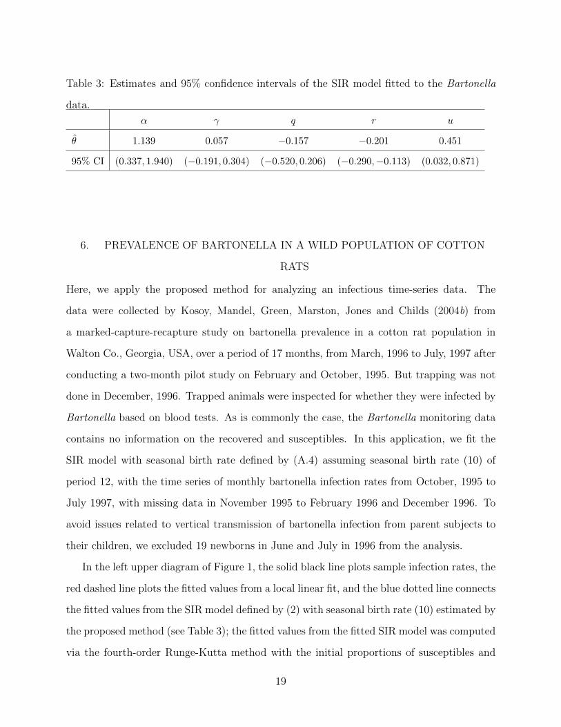
Table 3: Estimates and 95% confidence intervals of the SIR model fitted to the Bartonella
data.
α γ q r u
θ 1.139 0.057 −0.157 −0.201 0.451
95% CI (0.337, 1.940) (−0.191, 0.304) (−0.520, 0.206) (−0.290,−0.113) (0.032, 0.871)
6. PREVALENCE OF BARTONELLA IN A WILD POPULATION OF COTTON
RATS
Here, we apply the proposed method for analyzing an infectious time-series data. The
data were collected by Kosoy, Mandel, Green, Marston, Jones and Childs (2004b) from
a marked-capture-recapture study on bartonella prevalence in a cotton rat population in
Walton Co., Georgia, USA, over a period of 17 months, from March, 1996 to July, 1997 after
conducting a two-month pilot study on February and October, 1995. But trapping was not
done in December, 1996. Trapped animals were inspected for whether they were infected by
Bartonella based on blood tests. As is commonly the case, the Bartonella monitoring data
contains no information on the recovered and susceptibles. In this application, we fit the
SIR model with seasonal birth rate defined by (A.4) assuming seasonal birth rate (10) of
period 12, with the time series of monthly bartonella infection rates from October, 1995 to
July 1997, with missing data in November 1995 to February 1996 and December 1996. To
avoid issues related to vertical transmission of bartonella infection from parent subjects to
their children, we excluded 19 newborns in June and July in 1996 from the analysis.
In the left upper diagram of Figure 1, the solid black line plots sample infection rates, the
red dashed line plots the fitted values from a local linear fit, and the blue dotted line connects
the fitted values from the SIR model defined by (2) with seasonal birth rate (10) estimated by
the proposed method (see Table 3); the fitted values from the fitted SIR model was computed
via the fourth-order Runge-Kutta method with the initial proportions of susceptibles and
19
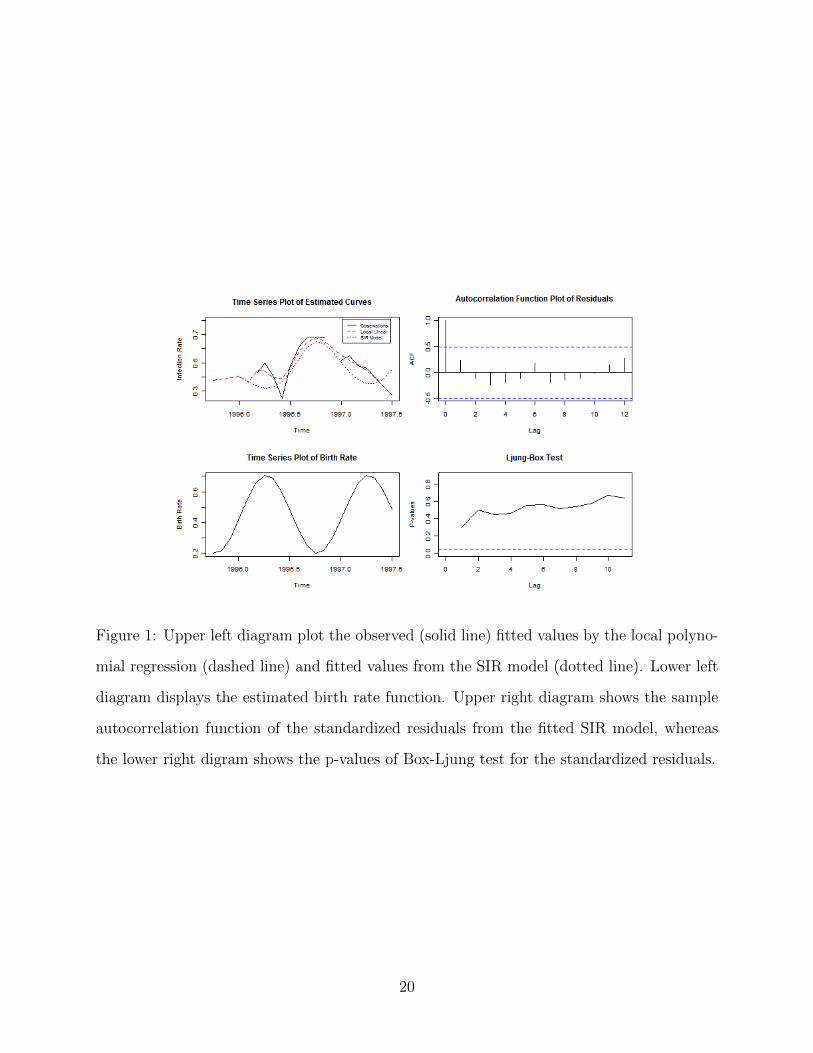
Figure 1: Upper left diagram plot the observed (solid line) fitted values by the local polyno-
mial regression (dashed line) and fitted values from the SIR model (dotted line). Lower left
diagram displays the estimated birth rate function. Upper right diagram shows the sample
autocorrelation function of the standardized residuals from the fitted SIR model, whereas
the lower right digram shows the p-values of Box-Ljung test for the standardized residuals.
20

infectives on January, 1996 calculated by formulas given in Section 4. The estimated birth
rate curve in the left lower diagram of Figure 1 shows that as the birth rate increases, the
infection rate decreases and vice versa, which is consistent with intuition.
Table 3 reports the parameter estimates with their 95% confidence intervals obtained
by the asymptotic results derived in Theorem 5. For interpretation, 5.7% (γ) of infectives
recovered a month after infection on average. The estimate α = 1.139 is the product of the
transmission probability and the number of contacts per month. The birth rate b attained
maximum in April and minimum in October. We now assess the goodness of fit of the fitted
SIR model, by checking whether or not the standardized residuals are approximately white
noise, i.e. uncorrelated and of constant variance. The residuals are defined as the observed
values minus the fitted values. The residuals are standardized by normalizing them by their
standard deviations. The right upper diagram of Figure 1 plots the autocorrelation function
of the standardized residuals; none of them are significantly different from 0 at 5% level.
The white-noise assumption can be further tested by checking whether the first k residual
autocorrelations all equal to zero by the Ljung-Box test. The right lower diagram of Figure
1 reports the the p-values of the Ljung-Box tests for k = 1, . . . , 11, showing that the white-
noise assumption cannot be rejected at 5% significance level. These plots suggest that there
are no residual autocorrelations, and hence the model fits the data well.
7. CONCLUSION
We show that, under some conditions, an ODE model may admit an equivalent state vector in
terms of the observed state component and its higher derivatives; this observation forms the
basis of our proposed method for estimating an ODE model by conditional least squares with
the higher derivatives first estimated via local polynomial regression. The proposed method
enjoys desirable large-sample properties. Both simulation studies and the real application
demonstrate the usefulness of the proposed method.
Here, we mention several interesting future research directions. While we consider the
case of ODE, the proposed method may be readily extended to the case when the state
21
process is driven by some partial differential equation. It is of interest to study the the-
oretical properties of such extension. Second, in practice, the choice of the bandwidth is
of importance. The limiting distribution obtained in Section 3 may be useful for studying
a more rigorous optimal choice of the bandwidth. For the Bartonella data, the observed
monthly counts of infectives are binomially distributed, but this information is not explicitly
used in the estimation of the derivatives via local polynomial regression. It is of interest to
study possible gain by estimating the derivatives via local generalized linear models using
Fan, Heckman and Wand (1995). Furthermore, simulations suggest that omitting several
derivative estimates around the sampling boundaries improved the empirical convergence
rate of the proposed estimation scheme. Although this observation is consistent with the
theoretical result of Brunel (2008) that omitting the two extreme boundary derivative esti-
mates, from spline smoothing, improves the convergence rate of the two-step method, it is
of interest to investigate the impact of omitting multiple boundary derivative estimates on
the convergence rate of the proposed method.
ACKNOWLEDGEMENTS
This work was partially supported by the U.S. National Science Foundation.
REFERENCES
Brunel, N. J.-B. (2008), “Parameter estimation of ODE’s via nonparametric estimators,”
Electronic Journal of Statistics, 2, 1242–1267.
Diekmann, O., and Heesterbeek, J. A. P. (2000), Mathematical Epidemiology of Infectious
Diseases: Model Building, Analysis and Interpretation, West Sussex: John Wiley &
Sons Ltd.
Fan, J., and Gijbels, I. (1996), Local Polynomial Modeling and Its Applications, London:
Chapman & Hall.
22
Fan, J., Heckman, N. E., and Wand, M. P. (1995), “Local polynomial kernel regression for
generalized linear models and quasi-likelihood functions,” Journal of American Statis-
tical Association, 90, 141–150.
Farlow, S. J. (1993), Partial Differential Equations for Scientists and Engineers, New York:
Dover Publications.
He, D., and Earn, D. J. D. (2007), “Epidemiological effects of seasonal oscillations in birth
rates,” Theoretical Population Biology, 72(2), 274 – 291.
Hunter, L. R., Su, R., and Meyer, G. (1983), “Global transformations of nonlinear systems,”
IEEE Transactions on Automatic Control, 28, 24–31.
Ireland, J. M., Mestel, B. D., and Norman, R. A. (2007), “The effect of seasonal host birth
rates on disease persistence,” Mathematical Biosciences, 206(1), 31 – 45. Alcala Special
Issue.
Kantz, H., and Schreiber, T. (2003), Nonlinear Time Series Analysis (2nd ed.), Cambridge:
Cambridge University Press.
Kosoy, M., Mandel, E., Green, D., Marston, E., Jones, D., and Childs, J. (2004a), “Prospec-
tive studies of bartonella of rodents. Part II. Diverse infections in a single rodent com-
munity,” Vector-Borne and Zoonotic Diseases, 4, 296–305.
Kosoy, M. Y., Mandel, E. L., Green, D. C., Marston, E. L., Jones, D. C., and Childs,
J. E. (2004b), “Prospective studies of Bartonella of rodents. Part I. Demographic and
temporal patterns in population dynamics,” Vector-Borne and Zoonotic Disease, 4, 285–
295.
Krantz, S. G., and Parks, H. R. (2002), The Implicit Function Theorem: History, Theory,
and Applications, Boston: Birkhauser.
23
Liang, H., and Wu, H. (2008), “Parameter estimation for differential equation models using a
framework of measurement error in regression models,” Journal of American Statistical
Association, 103, 1570–1583.
Qi, X., and Zhao, H. (2010), “Asymptotic efficiency and finite-sample properties of the
generalized profiling estimation of parameters in ordinary differential equations,” Annals
of Statistics, 38, 435–481.
Ramsay, J. O., Hooker, G., Campbell, D., and Cao, J. (2007), “Parameter estimation for
differential equations: A generalized smoothing approach (with discussion),” Journal of
the Royal Statistical Society, Series B, 69, 741–796.
Simon, D. (2006), Optimal State Estimation: Kalman, H∞, and Nonlinear Approaches, New
Jersey: John Wiley and Sons, Inc.
Terrell, W. J. (1999), “Some Fundamental Control Theory II: Feedback Linearization of
Single Input Nonlinear Systems,” The American Mathematical Monthly, 106, 812–828.
van der Vaart, A. W. (1998), Asymptotic Statistics, Cambridge: Cambridge University Press.
Wu, H., Zhu, H., Miao, H., and Perelson, A. S. (2008), “Parameter Identifiability and
Estimation of HIV/AIDS dynamic Models,” Bulletin of Mathematical Biology, 70, 785–
799.
Xia, X., and Moog, C. H. (2003), “Identifiability of Nonlinear Systems With Application to
HIV/AIDS Models,” IEEE Transactions on Automatic Control, 48, 330–336.
Zhang, J., Jin, Z., Xue, Y., and Li, Y. (2009), “The Dynamics of the Pulse Birth in an SIR
Epidemic Model with Standard Incidence,” Discrete Dynamics in Nature and Society,
p. doi:10.1155/2009/490437.
24
APPENDIX A. EXTENSION TO THE CASE OF OBSERVING MULTIPLE
COMPONENTS OF THE STATE PROCESS
The basic idea is to augment the observable components with enough number of their higher
derivatives to make an equivalent state vector. Consider the general case with the state
equation driven by the following ODE:
dX0(t)
dt= Z(X0(t),β), (A.1)
Let the original state vector be X0(t) = (X1(t), . . . , Xk(t))T , some of whose components
are unobservable. Without loss of generality, assume that Xobs(t) = (X1(t), . . . , Xu(t))T is
observed up to some additive error, but Xmis(t) = (Xu+1(t), . . . , Xk(t))T is unobservable,
where 1 ≤ u < k. Partition (A.1) according to Xobs and Xmis, and let Zobs(X0,β) be the
right hand side of (A.1) corresponding to Xobs so that X′
obs(t) = Zobs(X0(t),β). To solve
Xmis(t) in terms of Xobs(t), its derivatives, and β, we set up the following equations:
X(1)obs(t) = Zobs(X0(t),β), . . . ,X
(`)obs(t) = Z
(`−1)obs (X
(i)0 (t), i = 0, . . . , `− 1,β), (A.2)
where X(i) denotes the ith derivative vector of X at time t. To determine `, notice that
all derivatives of X0(t) is a function of X0(t) given β. For example, it follows from the
chain rule that X(2)0 (t) is a function of X0(t) and X
(1)0 (t), and since X
(1)0 (t) is a function
of X0(t), X(2)0 (t) is a function of X0(t). Consequently, the right side of each equation in
(A.2) depends only on X0(t) and β. Because u components of X0 are observable while the
remaining k − u components are unobservable, hence k − u equations are generally needed
to solve for the k − u unknowns, resulting in
` =⌈k − u
u
⌉,
where dxe represents the ceiling function of x. We assume that the first k − u equations
in (A.2) uniquely determine Xmis, given β, and hence also all its higher derivatives. Then
write the solutions Xmis(t) = R(X(i)obs(t), i = 0, . . . , `,β) for some function R. Differentiate
the last equation of (A.2) followed by substituting in it the preceding expression for Xmis(t)
25
to yield
X(`+1)obs (t) = Z
(`)obs(X
(i)obs(t), i = 0, . . . , `,β) ≡ F (X
(i)obs(t), i = 0, . . . , `,β). (A.3)
Finally, we propose to estimate β by minimizing the total conditional sum of squared errors:
S(β) =n∑i=1
|X(`+1)
obs (ti)− F (X(j)
obs(ti), j = 0, . . . , `,β)|2,
where X(j)
obs(ti), j = 0, . . . , `+ 1 are obtained from local polynomial fitting based on data at
epochs ti, i = 1, . . . , n.
APPENDIX B. VALIDITY OF ASSUMPTIONS 1-3 FOR THE SIR MODEL
Consider
s′= −αsi+ (1− s)b,
i′= αsi− (b+ γ)i.
(A.4)
For Assumption 1, (i) is clearly satisfied whereas (ii) generally holds with a suitable kernel
function. The bandwidth condition in (iii) can be readily implemented and the density
condition in (iv) refers to the sampling protocol. Part (i) of Assumption 2 is clearly satisfied
if we restrict the parameter space is a sufficiently large, relatively compact set. Part (ii) there
presupposes the existence of an ergodic stationary solution; this is a difficult problem, but see
Ireland, Mestel and Norman (2007) and He and Earn (2007) for conditions under which the
SIR model with seasonal birth rate admits a chaotic solution and hence an ergodic stationary
solution. We now show that Assumption 3 holds, under some regularity conditions. We
assume that i admits a positive lower bound, see Zhang, Jin, Xue and Li (2009) for relevant
discussion. We verify Assumption 3(i) first. Let β = (α, γ, q, r, v)T and recall X = (i, i′)T ,
and that
F (X,β) = (i′+ bi+ γi)(−αi− b) +
i′2
i+ (αb− b′)i.
26

Then,
∂F (X,β)
∂β=
−(i′+ bi+ γi)i+ bi
−αi2 − bi
−α sin(π6t)i2 +
(−2b− γ + α) sin
(π6t)− π
6cos(π6t)i− sin
(π6t)i′
−α cos(π6t)i2 +
(−2b− γ + α) cos
(π6t)
+ π6
sin(π6t)i− cos
(π6t)i′
−αi2 + (−2b− γ + α)i− i′
.
Thus,∣∣∣∂F (Xν1 ,β)
∂β− ∂F (Xν2 ,β)
∂β
∣∣∣≤ d1|iν1 − iν2|+ d2|i
′
ν1− i′ν2|+ d3|i2ν1 − i
2ν2| = d1|iν1 − iν2|+ d2|i
′
ν1− i′ν2|+ d3(iν1 + iν2)|iν1 − iν2|,
where
d1 = |i′ν1|+ 2b+∣∣∣(−2b− γ + α) sin
(π6t)
+π
6cos(π
6t)∣∣∣
+∣∣∣(−2b− γ + α) cos
(π6t)− π
6sin(π
6t)∣∣∣+ | − 2b− γ + α|,
d2 = |iν2|+∣∣∣ sin(π
6t)
+ cos(π
6t)
+ 1∣∣∣,
d3 = (b+ γ + 2α) +∣∣∣α sin
(π6t)∣∣∣+
∣∣∣α cos(π
6t)∣∣∣.
From (A.4), i′
is a function of s and i, and s and i are bounded, so i′
is bounded. Thus, d1,
d2, and d3(iν1 + iν2) are bounded, so Assumption 3(i) is satisfied. Now,
∂F (X,β)
∂X=
(b+ γ)(−αi− b)− α(i′+ bi+ γi)− i
′2
i2+ (αb− b′)
−αi− b+ 2 i′
i
.
Since i has a positive lower bound, Assumption 3(ii) is also satisfied.
APPENDIX C. PROOF OF THEOREM 2
For simplicity, we assume that ti’s are independent and identically distributed and σ21 =
· · · = σ2n ≡ σ2
ε , in the following proofs.
27
C.1 Proof of Consistency
Let δ(ti) = X(p)(ti)−X(p)(ti) = X(p)(ti)− F (X(ti),β0). First, we have
n∑i=1
X(p)(ti)− F (X(ti),β)2
=n∑i=1
F (X(ti),β0) + δ(ti)− F (X(ti),β)2
=n∑i=1
F (X(ti),β0)− F (X(ti),β)2 +n∑i=1
δ2(ti)
+ 2n∑i=1
F (X(ti),β0)− F (X(ti),β)δ(ti).
(A.5)
From Theorem 3.1 of Fan and Gijbels (1996), we have, for any t0 ∈ T
E(X(j)(t0))−X(j)(t0) = ξTj+1S−1j+1cj+1
X(j+1)(t0)
j + 1h2n + op(h
2n),
Var(X(j)(t0)) = ξTj+1S−1j+1S
∗j+1S
−1j+1ξj+1
j!2σ2(t0)
f(t0)nh2j+1n
+ op
( 1
nh2j+1n
),
(A.6)
where the op(·) terms hold uniformly for t0 ∈ T . Thus, X(j)(t0) − X(j)(t0) = Op(h2n +
1/√nh2j+1
n ) = Op(h2n + 1/
√nh2p+1
n ) ≡ Op(bn) uniformly over T for j = 0, . . . , p, which is
op(1) provided that hn → 0 and nh2j+1n → ∞, j = 0, . . . , p. The second term of the last
equation of (A.5) is hence Op(nb2n). Consider the first term there, which can be decomposed
asn∑i=1
F (X(ti),β0)− F (X(ti),β)2
=n∑i=1
F (X(ti),β0)− F (X(ti),β)2 +n∑i=1
F (X(ti),β)− F (X(ti),β)2
+ 2n∑i=1
F (X(ti),β0)− F (X(ti),β)F (X(ti),β)− F (X(ti),β).
By Assumption 3(i) and the mean value theorem, the second term of the preceding equation
can be bounded as follows:
n∑i=1
F (X(ti),β)− F (X(ti),β)2 =n∑i=1
|X(ti)− X(ti)|2∣∣∣∂F (xi,β)
∂x
∣∣∣2≤M2
n∑i=1
|X(ti)− X(ti)|2 = Op(nb2n),
(A.7)
28
where xi lies between X(ti) and X(ti). Due to the continuity of F and the compactness of
T and Ωβ, F (X(ti),β0)−F (X(ti),β) is uniformly bounded. Thus, similar to the derivation
of (A.7), we have
n∑i=1
[F (X(ti),β0)− F (X(ti),β)F (X(ti),β)− F (X(ti),β)]
= Op(nbn) = op(n).
(A.8)
Finally, the third term of (A.5) can be similarly shown to be Op(nbn).
Note that Assumptions 1(i), 2(i) and 3(i) imply that ∀t ∈ T ,∀β1,β2 ∈ Ωβ, there exists
a constant K such that
|F (X(t),β1)− F (X(t),β2)| ≤ K|β1 − β2|. (A.9)
Hence the class of functions F (X(t),β),β ∈ Ωβ is P-Glivenko-Cantelli so that that the
uniform law of large numbers hold; c.f. van der Vaart (1998, Example 19.7). The uniform
law of large numbers then entails the almost sure convergence of
1
n
n∑i=1
F (X(ti),β0)− F (X(ti),β)2 → D(β0,β), (A.10)
uniformly in β, where D(β0,β) = EF (X(t),β0)−F (X(t),β)2. Consistency then follows
from (A.7)-(A.10) and Assumption 2(ii).
C.2 Proof of the Asymptotic Distribution
Note that, under the assumptions of continuous derivatives and using the mean-value theo-
rem, we have
0 =∂S(β)
∂β=∂S(β0)
∂β+∂2S(β)
∂β∂βT(β − β0),
where ∂S(β∗)/∂β equals ∂S(β)/∂β evaluated at β = β∗ and β lies between β and β0.
Then, we have
β − β0 = −∂2S(β)
∂β∂βT
−1∂S(β0)
∂β. (A.11)
29

Consider ∂S(β)/∂β, which can be expressed as
∂S(β)
∂β= −2
n∑i=1
F (X(ti),β)− F (X(ti),β)∂F (X(ti),β)
∂β− 2
n∑i=1
δ(ti)∂F (X(ti),β)
∂β
≡ I1n + I2n.
Due to the continuity of ∂F (X(ti),β)/∂β and the compactness of T and Ωβ, |∂F (X(ti),β)/∂β|
is bounded by some constant, say, d0. Using the mean value theorem and Assumption 3(i),
we obtain
I1n = −2n∑i=1
F (X(ti),β)− F (X(ti),β)∂F (X(ti),β)
∂β
= −2n∑i=1
F (X(ti),β)− F (X(ti),β)∂F (X(ti),β)
∂β− ∂F (X(ti),β)
∂β+∂F (X(ti),β)
∂β
≤ 2dM
n∑i=1
|X(ti)− X(ti)|1+ζ + 2d0
n∑i=1
|X(ti)− X(ti)|
= Op(nb1+ζn ) +Op(nbn) = Op(nbn),
where recall 0 < ζ ≤ 1. Define
T j,t =
1 (t1 − t) · · · (t1 − t)j...
......
1 (tn − t) · · · (tn − t)j
.
Write Ki for Khn(ti − t) and let Y = (Y1, . . . , Yn)T . Then, the n × n matrix of weights W
becomes
W = diagK1, . . . , Kn.
It can be readily seen that I2n can be expressed as
−2n∑i=1
∂F (X(ti),β)
∂β− ∂F (X(ti),β)
∂β
δ(ti)− 2
n∑i=1
∂F (X(ti),β)
∂βδ(ti). (A.12)
By Assumption 3(i), the first term is Op(nbn1+ζ). Write F
′
p−1,i = ∂FX(ti),β/∂β for
i = 1, . . . , n, and F p−1 = (F′p−1,1, . . . , F
′p−1,n)T . The second term of (A.12) can be ex-
pressed as F Tp−1δ(t1), . . . , δ(tn)T . Recall ξp+1 stands for the (p + 2) × 1 unit vector hav-
ing 1 in the (p + 1)th entry. Let ξp+1,t = p!ξTp+1(T Tp+1,tW tT p+1,t)
−1T Tp+1,tW t and Ξp+1 =
30

(ξTp+1,t1, . . . , ξTp+1,tn)T . Letting X
(p)t = (X(p)(t1), . . . , X(p)(tn))T , X t = (X(t1), . . . , X(tn))T
and ε = (ε(t1), . . . , ε(tn))T , we have
δ(t1), . . . , δ(tn)T = Ξp+1Y −X(p)t = Ξp+1X t −X(p)
t + Ξp+1ε.
From (A.6), we have
F Tp−1Ξp+1X t −X(p)
t = Cnh2n + op(nbn), (A.13)
where
C =ξTp+1S
−1p+1cp+1
p+ 1E(X(p+1)(t)
∂FX(t),β∂β
).
Furthermore, 2F Tp−1Ξp+1ε is a sum of weighted independent variables εi, i = 1, . . . , n with
mean 0 and covariance matrix of the form
4F Tp−1Ξp+1Cov(ε)ΞT
p+1F p−1.
Let H = diag(1, hn, . . . , hp+1n ). Noting Cov(ε) = σ2
ε I, consider the (i, j)th entry of Ξp+1ΞTp+1
denoted by ηij:
ηij = p!2ξTp+1(T Tp+1,ti
W tT p+1,ti)−1T T
p+1,tiW tiW tjT p+1,tj(T
Tp+1,tj
W tT p+1,tj)−1ξp+1.
When i = j, from Section 3.7 of Fan and Gijbels (1996), we have
(T Tp+1,ti
W tiT p+1,ti)−1T T
p+1,tiW tiW tiT p+1,ti(T
Tp+1,ti
W tiT p+1,ti)−1
=1
f(ti)nhnH−1S−1
p+1S∗p+1S
−1p+1H
−1(1 + op(1)).
Thus, we have
ηii =p!2
f(ti)nh2p+1n
ξTp+1S−1p+1S
∗p+1S
−1p+1ξp+1(1 + op(1)),
which holds uniformly over T . When i 6= j, the (r, s)th entry of T Tp+1,ti
W tiW tjT p+1,tj equals
Grs =1
h2n
n∑k=1
K(tk − ti
hn
)(tk − ti)r−1K
(tk − tjhn
)(tk − tj)s−1.
Without loss of generality, assume ti 6= tj if i 6= j. Upon substituting (tk − ti)/hn by u, we
get
E(Grs) = nhr+s−3n
∫K(u)ur−1K
(u+
ti − tjhn
)(u+
ti − tjhn
)s−1
f(ti + hnu)du.
31
Using Taylor expansion and the fact that hn → 0 as n→∞, we have
f(ti + hnu) = f(ti) + o(1). (A.14)
Consider ∫K(u)ur−1K
(u+
ti − tjhn
)(u+
ti − tjhn
)s−1
du.
Since the support of K is [−1, 1], ∣∣∣(u+ti − tjhn
)s−1∣∣∣ ≤ 1. (A.15)
In addition, by Assumption 1(i), K(u+(ti−tj)/hn) = O(hn). Combining (A.14) and (A.15),
we have
E(Grs) = O(nhr+s−2n ).
Applying similar arguments yields
√V ar(Grs) = O(nhr+s−2
n ).
Then,
Grs = E(Grs) +Op(√V ar(Grs)) = Op(nh
r+s−2n ).
Therefore, for some matrix S∗∗ independent of hn and n,
T Tp+1,ti
W tiW tjT p+1,tj = Op(nHS∗∗H) = op(
n
hnHS∗∗H). (A.16)
It follows from Section 3.7 of Fan and Gijbels (1996) that
T Tp+1,ti
W tiT p+1,ti = nf(ti)HSH(1 + op(1)). (A.17)
Combining (A.16) and (A.17),
ηij = op(1
nh2p+1n
),
uniformly over T . Thus, we have
Ξp+1Cov(ε)ΞTp+1 =
p!2σ2ε
nh2p+1n
ξTp+1S−1p+1S
∗p+1S
−1p+1ξp+1Af (1 + op(1)),
32
where Af = diag(1/f(t1), . . . , 1/f(tn)). Consequently,
F Tp−1Ξp+1Cov(ε)ΞT
p+1Fp−1
=p!2σ2
ε
h2p+1n
ξTp+1S−1p+1S
∗p+1S
−1p+1ξp+1E
[(∂F (X(t),β)√f(t)∂β
)(∂F (X(t),β)√f(t)∂β
)T]+ op(
1
h2p+1n
).
(A.18)
On the other hand, we have
1
n
∂2S(β)
∂β∂βT= − 2
n
n∑i=1
[X(p)(ti)− F (X(ti), β)]∂2F (X(ti), β)
∂β∂βT
+2
n
n∑i=1
∂F (X(ti), β)
∂β
[∂F (X(ti), β)
∂β
]T.
Using an argument similar to that for deriving (A.5) and Assumption 1 and 3, it can be
checked that the first term on the right side of the preceding equation is op(1), while the sec-
ond term converges to 2E[∂F (X,β0)/∂β∂F (X,β0)/∂βT ]. Combining (A.11) - (A.18)
and recalling Assumption 1(iii) on the bandwidth hn, we apply the Lindeberg-Feller central
limit theorem to obtain the desirable result:
nh(2p+1)/2n (β − β0 +Ch2
n)→ N(0,Σβ)
in distribution, where
C =ξTp+1S
−1p+1cp+1
p+ 1E(X(p+2)(t)
∂F (X(t),β0)
∂β
),
Σβ = p!2σ2εξ
Tp+1S
−1p+1S
∗p+1S
−1p+1ξp+1
[E∂F (X(t),β0)
∂β
∂F (X(t),β0)
∂β
T]−1
× E[∂F (X(t),β0)√
f(t)∂β
∂F (X(t),β0)√f(t)∂β
T]×[E∂F (X(t),β0)
∂β
∂F (X(t),β0)
∂β
T]−1
.
33


![Partial Di erential Equation - YIN S CAPITAL 殷氏资本Notes in Partial Di erential Equation [Instructor: Ovidiu Savin] x1 Remark 1.2.7. Burgers’ Equation. It is a fundamental](https://img.pdfslide.us/doc/110x75/610241b86dc5ce6a4214ffbe/partial-di-erential-equation-yin-s-capital-eoe-notes-in-partial-di-erential.jpg)