Estimating a Tail Exponent by Modelling Departure from … · Estimating a Tail Exponent by Modelling Departure from a Pareto ... DEPARTURE FROM A PARETO DISTRIBUTION ... (1982, 1990)

Estimating a Tail Exponent by Modelling Departure from a Pareto DistributionAuthor(s): Andrey Feuerverger and Peter HallSource: The Annals of Statistics, Vol. 27, No. 2 (Apr., 1999), pp. 760-781Published by: Institute of Mathematical StatisticsStable URL: http://www.jstor.org/stable/120112Accessed: 12/06/2009 09:53

Your use of the JSTOR archive indicates your acceptance of JSTOR's Terms and Conditions of Use, available athttp://www.jstor.org/page/info/about/policies/terms.jsp. JSTOR's Terms and Conditions of Use provides, in part, that unlessyou have obtained prior permission, you may not download an entire issue of a journal or multiple copies of articles, and youmay use content in the JSTOR archive only for your personal, non-commercial use.

Please contact the publisher regarding any further use of this work. Publisher contact information may be obtained athttp://www.jstor.org/action/showPublisher?publisherCode=ims.

Each copy of any part of a JSTOR transmission must contain the same copyright notice that appears on the screen or printedpage of such transmission.

JSTOR is a not-for-profit organization founded in 1995 to build trusted digital archives for scholarship. We work with thescholarly community to preserve their work and the materials they rely upon, and to build a common research platform thatpromotes the discovery and use of these resources. For more information about JSTOR, please contact [email protected].

Institute of Mathematical Statistics is collaborating with JSTOR to digitize, preserve and extend access to TheAnnals of Statistics.

http://www.jstor.org

http://www.jstor.org/stable/120112?origin=JSTOR-pdf

http://www.jstor.org/page/info/about/policies/terms.jsp

http://www.jstor.org/action/showPublisher?publisherCode=ims

The Annals of Statistics 1999, Vol. 27, No. 2, 760-781

ESTIMATING A TAIL EXPONENT BY MODELLING DEPARTURE FROM A PARETO DISTRIBUTION

BY ANDREY FEUERVERGER AND PETER HALL

University of Toronto and University of Toronto and Australian National University

We suggest two semiparametric methods for accommodating departures from a Pareto model when estimating a tail exponent by fitting the model to extreme-value data. The methods are based on approximate likelihood and on least squares, respectively. The latter is somewhat

simpler to use and more robust against departures from classical extreme-value approximations, but produces estimators with approximately 64% greater variance when conventional extreme-value approximations are appropriate. Relative to the conventional assumption that the sampling population has exactly a Pareto distribution beyond a threshold, our methods reduce bias by an order of magnitude without inflating the order of variance. They are motivated by data on extrema of community sizes and are illustrated by an application in that context.

1. Introduction. Estimating the tail exponent, or shape parameter, of a distribution is motivated by a particularly wide variety of practical problems, in areas ranging from linguistics to sociology and from hydrology to insur- ance. See, for example, Zipf (1941, 1949), Todorovic (1978), Smith (1984, 1989), NERC (1985), Hosking and Wallis (1987) and Rootzen and Tajvidi (1997). Many models and estimators have been proposed, including those of Hill (1975), Pickands (1975), de Haan and Resnick (1980), Teugels (1981), Csorgo, Deheuvels and Mason (1985) and Hosking, Wallis and Wood (1985). The goodness of fit of a Pareto model to the tail of a distribution can often be explored visually by simply plotting the logarithms of extreme order-statistics against the logarithms of their ranks. The plot should be approximately linear if the Pareto model applies over the range of those order statistics, and in this case the negative value of the slope of the line is an estimate of the Pareto exponent. More efficient estimators are available, however, and those in use today are generally of two types, based on likelihood and the method of moments, respectively.

Both these approaches are susceptible to errors in the assumed model for the distribution tail. As Rootzen and Tajvidi (1997) point out, none of the standard approaches is "robust against departures from the assumption that the tail of the distribution is approximated by a GP [generalized Pareto]

Received November 1997; revised February 1999. Key words and phrases. Bias reduction, extreme-value theory, log-spacings, maximum likeli-

hood, order statistics, peaks-over-threshold, regression, regular variation, spacings, Zipf's law.

760

ESTIMATING A TAIL EXPONENT

distribution. If there are marked deviations from a GP tail, the results will be misleading." On the other hand, if one confines attention to data that are so far out in the tail that the Pareto assumption is valid, then the effective sample size can be small and the estimator of tail exponent may have relatively large variance.

Moreover, in some applications of the Pareto model, data that provide evidence of departure from the model are of greater interest than those to which the model fits well. A case in point is Zipf's (1941, 1949) classic study of the dynamics of community sizes. A linear plot of the logarithm of community size against the logarithm of rank, as in the case of U.S. cities during most of the twentieth century [see, e.g., Zipf (1941), Chapter 10; Hill (1975)] has been suggested as evidence of "stable intranational equilibrium"; while nonlinear plots, for example in the context of Austrian and Australian communities 60 to 80 years ago, have been interpreted as implying instability [Zipf (1949)]. As Zipf argues, it can be of greater sociological interest to analyze data from countries or eras that depart from the benchmark of "intranational equilibrium," than it is to analyze those which achieve the benchmark.

In this paper we propose a simple and effective way of reducing the bias that arises if one uses extreme-value data relatively deeply into the sample. We show that the main effects of bias may be accommodated by modelling the scale of log-spacings of order statistics. With this result in mind, we suggest two bias-reduction methods, both developed from a simple scale-change model for log-spacings, and based on likelihood and on least squares, respectively. In the first method, a three-parameter approximation to likelihood is suggested for the distribution of log-spacings. One of the parameters is the desired tail exponent. In our least-squares approach, log-log spacings play the role of response variables, the explanatory variables are ranks of order statistics and the regression "errors" have a type-3 extreme-value distribution, with exponentially light tails.

These techniques reduce bias by an order of magnitude, without affecting the order of variance. Therefore, they can lead to significant reductions in mean squared error. Moreover, they allow us to model extreme-value data that depart markedly from the standard asymptotic regime. This advantage will be illustrated in Section 3 by application to highly non-Pareto data on Australian community sizes. We are not aware of kernel or moment methods that are competitive with our approach; they would be awkward to construct in the context of a flexible and practicable class of distributions that represent departures from the Pareto model.

Statistical properties of estimators of tail exponents in Pareto models (sometimes referred to as models for Zipf's law) have been studied exten- sively. Early work in a parametric setting includes that of Hill (1970, 1974), Hill and Woodroofe (1975) and Weissman (1978). Smith (1985) points out the anomalous behaviour of estimators of certain exponents in the context of generalized Pareto distributions. Hall (1982, 1990) and Csorgo, Deheuvels and Mason (1985), among others, consider the effect of choice of threshold on

761

A. FEUERVERGER AND P. HALL

performance of tail-exponent estimators. Rootzen and Tajvidi (1997) compare the performances of different approaches to tail-parameter estimation.

Davison (1984) and Smith (1984) provide statistical accounts of peaks- over-threshold, or POT, methods. Those techniques are of course not identical to methods based on extreme-order statistics, but the strong duality between the two approaches means, as Smith (1984) notes, that virtually all methods for one context have versions for the other. Our bias-correction methods are no exception. However, for the sake. of brevity we shall discuss them only in the case of extreme order-statistics. Section 2 will introduce our methods, and Section 3 will describe their numerical properties. Theoretical performance will be outlined in Section 4, and technical arguments behind that work will be summarized in Section 5.

2. Methodology.

2.1. Modelling the source of bias. We shall introduce methodology in the case where the tail that is of interest is at the origin. Our methods extend immediately from there to the case of a tail at infinity. Suppose the distribution function F admits the approximation F(x) Cxa as x I 0, or more explicitly,

(2.1) F(x) = Cxa{1 + 8(x)),

where C, a are positive constants and 8 denotes a function that converges to O as x I 0. We wish to estimate a from a random sample Z= {X1,..., Xn} drawn from the distribution F. Often, one would proceed by assuming the particular Pareto model

(2.2) Fo(x) = Cx&,

assumed for 0 < x < r, say, rather than (2.1), and alleviating bias problems caused by discrepancies between (2.1) and (2.2) by using only particularly small order-statistics from X. However, this approach can have a detrimental effect on performance, since it ignores information about a that lies further into the sample. That information would be usable if we knew more about the function 8. In later work we shall refer to the model at (2.1) as a "perturbed" Pareto distribution, when it is necessary to distinguish it from the Pareto distribution at (2.2).

One approach to accessing the information is to model 8, for example in the fashion

(2.3) 8(x) = Dx + o(x )

as x -> 0, where / > 0 and -oo < D < oo are unknown constants. In principle we could drop the "small oh" remainder term at (2.3), substitute the resulting formula into (2.1) and estimate the four parameters C, D, a, ,3 by maximum likelihood. This means, in effect, working with the model

F,(x) = Clxal + C2xa2,

762

(2.4)


assumed for 0 < x < r, say, where C1, a,, a2 are all positive and the model is made identifiable by insisting that a = a1 < a2. The type of departure from a Pareto model suggested by (2.3) or (2.4) argues that the true distribution is, to a first approximation, a mixture of two Pareto distributions. This is sometimes implicitly assumed in accounts of departures from the Pareto. See for example Zipf's (1949), page 423 discussion of the contributions made by distinct urban and rural communities to the overall distribution of community sizes, and the remarks in the Appendix in this paper on data from countries that have been formed from mergers of autonomous states.

2.2. Likelihood and least-squares approaches. Our methods are based on the observation that, to a good approximation, the normalized log-spacings of small order-statistics in the sample r are very nearly rescaled exponential variables, where the scale change may be simply represented in terms of the model at (2.1). Specifically, let Xnl < -* < X_ denote the order statistics from X and define

Ui = i(log X,i1 - log Xn).

Then, for a function 81 that can be expressed in terms of the 8 of (2.1), it may be shown that

(2.5) Ui Zi 0{1 + 8,(i/n)} = Zi exp{61(i/n)},

where 0 = 1/a and the variables Z1, Z2,... are independent and exponentially distributed with unit mean. It can be proved that if 8 satisfies (2.1) and (2.3) then

(2.6) (y) = D y1 + o(y1)

as y 0, where ,1 = 13/a and D1 = -(3/aa)C-,/tD. In view of (2.5), this suggests regarding the variables Ui as exponential with mean 0 exp{Dj(i/n)P1}, and estimating 0, D1, ,8 by maximum likelihood. In this case the negative log-likelihood is

r r

(2.7) r log 0 + D (i/n)1 + 0 1 U exp-D1(i/n) 1}. i=l i=l

(Here, r is the threshold or smoothing parameter, about which we shall say more in Section 2.4.) Differentiating with respect to 0, equating to zero and solving for 0, we obtain 0 = T(D1, f,), say. Substituting back into (2.7) we conclude that (D1, ,1) should be chosen to minimize

(2.8) L(D1, B1) = Dlr-1 (i/n)1 + log[r-1 E U exp{-Dl(i/n)f11 i= 1 = J

An alternative approach to inference may be based on the fact that, by (2.5), the log-log spacings Vi = log Ui satisfy

Vi ( ,t + 5l(i/n) + ei,

763

(2.9)


where /uc = log 0 + LO, UO is the mean of the distribution of log Z, (thus, fJu = -0.5772..., the negative of the value of Euler's constant), and ei =

log Zi - /u-t (for 1 < i < n) may be interpreted as an error in the approximate regression model (2.9). Given that 86 may be expressed by (2.6), we may (for fixed 8,3) compute explicit estimators (( ,31), D,( 13) of the unknowns Au, DI that minimize

(2.10) S( , Dl, /31) Vi - - D,(i/n)1}2

i==l

Despite their having larger asymptotic variance than maximum likelihood methods (see Section 4), we found in numerical studies that the least-squares approaches were sometimes less biased and so could have superior overall performance (Section 3).

The case where 13 is known, or is a known function of a (see Section 3.1), is of major interest. If we can reduce the number of unknown parameters, then the variances of our estimates of those that remain should also be reduced. Two canonical cases deserve special mention. In the first, one may think of X as being generated in the fashion X = IY1/a, where Y has a density that is nonzero and differentiable at the origin. Here, a = 3 and so ,13 = 1. The second example is generated in the form F(x) = G(x)a, where the distribution function G is supported on the positive half-line and (confined to that domain) has a density that is nonzero and differentiable at the origin. Here, 3 = 1 and so ,1 = l/a. In practice one may obtain empirical evidence for either of these cases by computing pilot estimates of D1, a, ,1. See Section 3.1 for an example.

2.3. An exploratory least-squares approach. To obtain a preliminary approximation to ,3 it is sometimes helpful to fit the semiparametric model at (2.1) and (2.3) directly to log-spacings, as follows. Observe from (2.5) and (2.6) that

log X, i 1 - log Xni + i Zi f{l1 + D,(i/n) 1}.

Hence, for i >j and with xij = log{i/(j - 1)1 and yij = log Xn i+ - log X"j,

(2.11) Yij Oxij + D2 exp( 1 )xij) + D3,

where the "constants" D2, D3 depend on j and n. (The approximation is generally good, at least for i sufficiently greater than j, if D3 is omitted. We do, however, need j moderately large in order to neglect the stochastic component.) We may fit the model at (2.11) by ordinary or weighted least- squares for values i satisfying j < i < r, say.

2.4. Estimators of a. The analysis in Section 2.2 suggests three estimators of a, of which the first is based on maximum likelihood and the others on least-squares. The likelihood-based estimator is found by taking (D1, ,31) to

764


minimize L(D1, S3), defined at (2.8), and putting

(2.12) al = T(D1,1) = [r-1 E Uiexp{-D,(i/n)l)].

To derive the least-squares estimators, let Vi = log Ui = log (log X, i+ -

log Xni) + log i, choose ( DJ, j/3, D1) to minimize S( ,u, D1, j1) [defined at (2.10)] and let

(2.13) W, = i(log X, i +- log Xni)exp -Dj1(i/n) 1},

W = r-1 i r Wi and ,-o = Jf>o(log x)e-x dx = - 0.5772157. Then two least- squares estimators of a are a2 = exp( ,pu - j,) and 03 = 1/W. When ,1 is

known, or estimated separately, we replace ,1 by that value at all its appearances, for example at (2.12) and (2.13). If we take 0, = I/a (see Sections 2.2 and 3.1), then we should again make the obvious changes to the algorithm, maximizing the likelihood or minimizing the sum of squares under the constraint.

Given an estimator a of a, one may obtain an estimator of C quite simply, by substituting into the formula C = r(Xnr)_-/n. As expected, the estimators of a do not require the value of n, while those of C do. In practice, when only extreme-order statistics are recorded, the value of n is usually unknown.

The value of r at (2.8) and (2.10) plays the role of a threshold, or smoothing parameter, determining the depth into the data that we are prepared to go when fitting the model defined by (2.1) and (2.3). For conventional estimators, such as those of Hill (1975) and also for our estimators aj, increasing r results in an increase in bias, owing to departure of (2.1) from its "ideal" form (2.2), but this is accompanied by a decrease in variance. One virtue of our approach is that for it, bias does not increase so rapidly with increasing r, and so r may be chosen an order of magnitude larger, producing an improvement in mean-square performance by an order of magnitude. These properties will be demonstrated numerically in Section 3 and theoretically in Section 4; see, for example, Remark 4.4.

3. Numerical properties.

3.1. Example: community sizes. Zipf [(1949), page 139], showed graphically that data on large Australian community sizes in 1921 departed markedly from a Pareto distribution with regularly varying tail at infinity. He neither tabulated his data nor gave a source, but they were apparently taken from Wickens (1921). See the Appendix of the present paper for details. Figure 1 graphs the logarithm of community size against the logarithm of rank for these data for all 256 Australian communities that had 2000 or more inhabitants in 1921. (Zipf considered only communities of more than 3000 people.) The graph would of course be linear if the sampling distribution were Pareto.

765


Li

sFIG. *.* * ..

CD t

CN

o \

0

0.0 0.5 1.0 1.5 2.0 2.5 Log 10 of Rank

FIG. 1. Logarithms of Australian community sizes, I. Plot of logarithm of community size against logarithm of rank for all 256 Australian communities having 2000 or more inhabitants in 1921.

Nevertheless, it is plausible that the data were generated as X = Y-l, where X denotes the population of a randomly chosen Australian community and Y has the perturbed Pareto distribution modelled by (2.1) and (2.3). We analyzed the data from that viewpoint and also as though they were from a perturbed Pareto distribution with an upper bound at a fixed number No, say. That is, we subtracted each population size from No and regarded the new data Z = No - X as coming from a population whose distribution function had the form described by (2.1) and (2.3). This approach has apparently not been used before with community-size data and would be inimical to Zipf's ideas, but there are nevertheless good empirical reasons for adopting it. We shall report here only this type of analysis, since it produced residuals whose empirical distribution was closer to the exponential than was that of residuals obtained using the first approach.

Figure 2 shows a plot of values of the negative of the logarithm of Z against the logarithm of rank. It represents the analogue of Figure 1 in this context and would be linear if the single-component Pareto distribution at (2.2) were an appropriate model for departures of community size from an upper bound.

When applying the exploratory least-squares approach suggested in Sec- tion 2.3, we found that if we took j > 5 then a plot of y,j against exp( 31xij), for j < i < 256 and with 3, chosen by least-squares, gave very nearly a

766


0 * C,,O

0

0*

*.

0.0 0.5 1.0 1.5 2.0

Log10 of 'I'

FIG. 2. Logarithms of Australian community sizes, II. Plot of negative value of the logarithm of the difference between size of 10th largest community and size of the (10 + i)th largest community, for 1 < i < 245, against the logarithm of i.

straight line with negative slope. This suggests that for some No > 0, the distribution function G of city size has very nearly the property,

1 - G( No - x) = A I log(l - A2 x)ja

= AiA x{l + aA2x + 0(x2)},

for positive constants a, A1, A2 and small positive values of x. This is the perturbed Pareto model suggested by (2.1) and (2.3), with ,8 = 1. To appreciate why (3.1) follows from linearity of the plot, note that linearity suggests that to a good approximation, Xni?+ = B1 exp(-B2i)1) for constants B1, B2 > 0. Taking X,,i+1 = G-'1 - (i/n)} and writing x for i/n, we obtain 1 - x = G{B1 exp(-B3x'31)}. This gives (3.1) exactly, with a = 1/31.

Therefore, in our subsequent analysis, we took /B = 1 at (2.3), or equiva- lently, 8,3 = 1/a at (2.6). (Of course, this ,1 differs from that in the para- graph immediately above.) We used the maximum likelihood (ML) and least- squares (LS) methods suggested in Sections 2.2 and 2.4, with ,81 there constrained to equal 1/a. For brevity we took the LS estimator to be a2; results for a3 are similar. For the sake of simplicity we took No to equal the population of the smallest community that was not used in the analysis. That is, if attention was confined to communities whose size ranked in the range k + 1 < i < k + r + 1, then we took No to equal the size of the kth largest community. Removal of large community sizes was necessary to avoid errors

767


0-

N 0/

_F.

) /

3 C\O - C: O

(0 0:

0 1 2 3 4 5 - Log ( 1-i/r)

FIG. 3. Residual q-q plot. Ranked values of the residuals Zi, defined by (3.2), plotted against corresponding quantiles of the exponential distribution with unit mean. The line "y = x" is

superimposed on the plot. Raw data were those used to generate Figure 2.

due to arbitrariness of community boundaries in large Australian cities. The definitions of Sydney and Sydney North, and Melbourne and Melbourne South as distinct communities are among the obvious examples of this problem.

The goodness-of-fit of the exponential distribution to residuals is apparent from q-q plots, of which Figure 3 is typical. There we graph log Z( + k +1) against -log{1l - (i/r)} for 1 < i < r, where

(3.2) Zi = U/[(1/a^)exp(D( i/n)1/)}

is our estimate of the quantity Zi appearing at (2.5), the parameter estimates on the right-hand side of (3.2) were obtained by maximum likelihood under the constraint that / = 1 and Z(j) denotes the ith largest value of Zi. For Figure 3 we took No to be the size of the 10th largest community (so that k = 10) and used all remaining communities of size 2000 or more (so that r = 256 - 11 = 245). We do not of course know the value of n in (3.2), but that is of no concern since it is absorbed into the estimator of D1.

The resulting estimates of a, for different values of r and the cut-off k, range from about 0.9 to 1.2 and are given in Table 1. The ML estimates are a little less variable than those based on LS and also tend to be a little larger. Not much can be read into this, however, since all estimates were computed from the same data. Both ML and LS estimates are strikingly resistant to

768


substantial changes in r. The main source of variation appears to be random fluctuation, rather than systematic variation with r. This reflects the very low bias arising from the excellent fit of the model when /3 is constrained to equal 1; see Figure 3. By way of contrast, the Hill (1975) estimate of a increases virtually monotonically with increasing r, and more than doubles in size (from 1.57 to 3.53) within the range of Table 1. This substantial systematic error reflects the very poor fit to data offered by the single-component Pareto model at (2.2). The poor fit is exemplified by a highly nonlinear q-q plot (analogous to that of Figure 3 and not given here) for residuals under the single-component model.

In the same setting as Figure 3, the "full" (i.e., without /8 constrained) ML estimate of a equals 0.64, and the estimate of /3 is 0.54. To assess the significance of these results we conducted a simulation study using data generated from the distribution at (3.3), with a = 8 = 1, n = 20,000 and r = 250 and values of B that produced "Zipf plots" having moderate curvatures, as in Figure 2. (The case of higher curvature will be treated in Sec- tion 3.2.) These values of n and r were chosen because they lead to Zipf plots broadly similar to that in Figure 2. For the sake of simplicity we shall continue to use the same n and r in Section 3.2.

TABLE 1

Estimates of a for different values of k and r*

r + k

k 256 200 150 100

6 ML 1.215 1.051 1.053 1.157 LS 1.152 0.910 0.873 0.980 Hill 3.531 3.007 2.458 1.921

8 ML 1.149 0.986 0.964 0.993 LS 1.097 0.874 0.811 0.865 Hill 3.146 2.666 2.165 1.669

10 ML 1.166 1.001 0.981 1.017 LS 1.212 0.883 0.839 0.891 Hill 3.173 2.693 2.188 1.687

12 ML 1.211 1.043 1.043 1.149 LS 1.152 0.918 0.851 1.004 Hill 3.353 2.861 2.337 1.821

15 ML 1.165 0.997 0.980 1.026 LS 1.125 0.892 0.846 0.935 Hill 3.073 2.616 2.125 1.638

20 ML 1.167 0.995 0.974 1.007 LS 1.134 0.901 0.853 0.952 Hill 2.968 2.529 2.051 1.573

* In each cell in the table, the maximum likelihood estimate (denoted by ML, and computed under the constraint 18 = 1) is listed above the corresponding least-squares estimate (LS), which in turn is listed above the Hill (1975) estimate.

769


We found that (1) the "full" ML and LS estimators of a have much higher variance than the "constrained" estimators (i.e., with ,3 constrained to equal 1); (2) the differences in bias are relatively minor; (3) the "constrained" ML estimator of a is substantially more accurate than the Hill (1975) estimator; and (4) the "full" ML estimator of ,3 is biased downwards by a factor close to 2, with variance being less of a problem. This bias appears to be due to third-order effects, which are not captured by second-order models such as the combination of (2.1) and (2.3). In view of this bias, we do not find the value /3 = 0.54, obtained using the "full" ML method, to be problematical. Overall, the "full" ML estimator does not perform well for these data, since departure from a single Pareto distribution is not sufficiently great; but the "constrained" ML method is effective.

We conclude that the true value of a is close to 1. This is the value claimed by Zipf (1949) for countries such as the United States that satisfy his law of "intranational equilibrium," although of course he was concerned with regular variation at infinity, not at an upper bound to city size.

3.2. Summary of numerical properties. When fitting mixture models, it is generally found that a multicomponent model produces improved performance only if there is clear evidence that more than one component is necessary. When a single component is adequate, fitting a mixture of two or more components typically leads to poor performance, because (1) the addi- tional nuisance parameters use up information that would otherwise be available for estimating the main parameters of interest, and (2) there are problems of identifiability when the components are close. This gives rise to relatively poor performance of the "full" ML and LS methods, noted in Section 3.1, when the Zipf curve has only moderate curvature.

However, when fitting a single Pareto distribution to data such as those on which Figure 2 is based, it is relatively important to determine the threshold, r, by empirical means. It has been observed previously that, in a range of settings, empirical choice of r can increase root mean squared error by a factor of about 2 when /3 is unknown; see, for example, Hall and Welsh (1985). As shown in Section 3.1 (Table 1), when fitting a Pareto mixture the estimator of a is relatively robust against systematic effects resulting from choice of r. Therefore, even if "full" or "constrained" ML or LS methods, for fixed values of r, produce estimates that perform similarly to Hill's estimator when the latter is computed at an optimal threshold, the ML or LS methods can be superior to the Hill estimator in practice. Analysis of threshold-choice methods for Hill's estimator is beyond the scope of this paper.

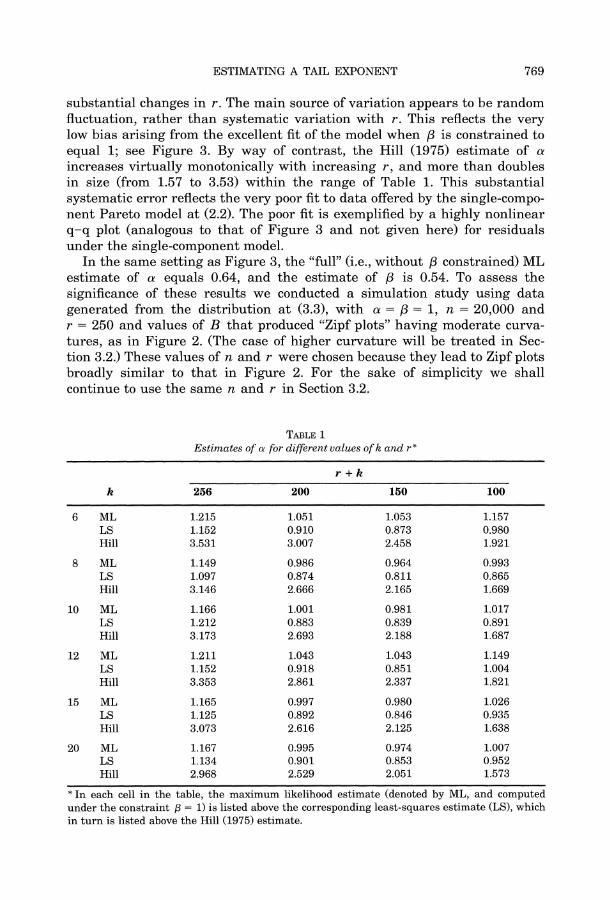
Since /, is the parameter of a high-order term in the model, the likelihood surface is relatively flat near the maximizing value of /3,. Figure 4 depicts a typical graph of -L(D1, /,), defined at (2.8), and shows this property clearly. Similar behavior may be observed for the function S( JL, D1, 8/), defined at (2.10), and in this case one must also take care that the estimate of /3B is not taken to be a pathological extremum at infinity. These problems are not as

770


LCd -

FIG. 4. Likelihood surface. Typical plot of -L(D, ,1) for data generated in the simulation study in Section 3.2.

serious when data sets are analyzed individually, however. In our simulation study we used grid search to approximate the minimum, but due to the flatness of L and S it sometimes happened that the value we obtained was a long way from the true minimum. Additionally, in some samples where the Zipf plot was approximately linear, despite the average Zipf curve being nonlinear, the estimate of ,1 was a large distance from the true value of ,1. For these reasons we use median absolute deviation (MAD) instead of mean squared error to describe performance.

We simulated data from the distribution

(3.3) X= U1/ exp(BUO/"),

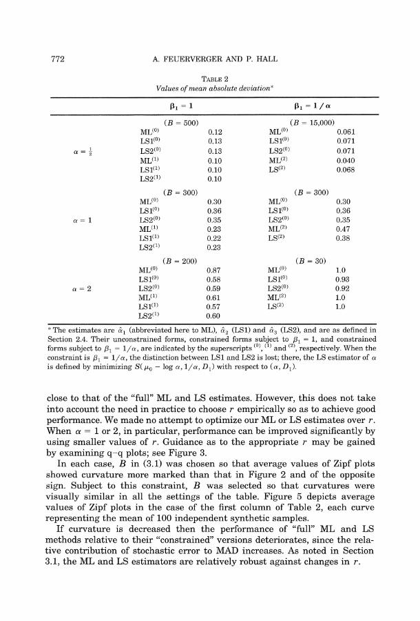
where a, 8 > 0, B = -D/a, -oo < D < oo and U had a Uniform distribution on the interval [0, 1]. The parameters a, ,3, D have the meanings ascribed to them in Section 2, and the value of C there is now 1. In particular, the perturbed Pareto model defined at (2.1) and (2.3) is valid. In the context of (3.3), and for n = 20,000 and r = 250, Table 2 gives median absolute deviations of estimates computed by "full" or "constrained" ML and LS methods. The "constrained" estimators are generally slightly superior, and the ML and LS methods perform similarly. Throughout this section, the results reported represent averages over 100 simulated independent samples.

The MAD of estimators suggested by Hill (1975), for r = 250, exceeds that of "full" ML estimators by a factor of between 1.3 and 3.6 across the range of Table 2. If the Hill estimator is computed at the value of r that gave it optimal MAD performance in the simulation study, then its MAD is generally

771


TABLE 2 Values of mean absolute deviation*

P1 =

(B = 500) ML(?> LS1(?) LS2(0) ML(') LS11) LS2(1)

(B = 300)

0.12 0.13 0.13 0.10 0.10 0.10

0.30 0.36 0.35 0.23 0.22 0.23

(B = 200) ML(O?> LS1(?) LS2(0) ML(W) LS()1 LS2(1)

0.87 0.58 0.59 0.61 0.57 0.60

* The estimates are a' (abbreviated here to ML), &2 (LS1) and &3 (LS2), and are as defined in Section 2.4. Their unconstrained forms, constrained forms subject to ,38 = 1, and constrained forms subject to ,3 = 1/a, are indicated by the superscripts (0), (1) and (2), respectively. When the constraint is i81 = 1/a, the distinction between LS1 and LS2 is lost; there, the LS estimator of a is defined by minimizing S( ikO - log a, 1/a, D1) with respect to (a, Di).

close to that of the "full" ML and LS estimates. However, this does not take into account the need in practice to choose r empirically so as to achieve good performance. We made no attempt to optimize our ML or LS estimates over r. When a = 1 or 2, in particular, performance can be improved significantly by using smaller values of r. Guidance as to the appropriate r may be gained by examining q-q plots; see Figure 3.

In each case, B in (3.1) was chosen so that average values of Zipf plots showed curvature more marked than that in Figure 2 and of the opposite sign. Subject to this constraint, B was selected so that curvatures were visually similar in all the settings of the table. Figure 5 depicts average values of Zipf plots in the case of the first column of Table 2, each curve representing the mean of 100 independent synthetic samples.

If curvature is decreased then the performance of "full" ML and LS methods relative to their "constrained" versions deteriorates, since the relative contribution of stochastic error to MAD increases. As noted in Section 3.1, the ML and LS estimators are relatively robust against changes in r.

PI = l/o:

ML(O LS1(0? LS2(0: ML(2)

LS(2)

(B = 15,000

(B = 300)

a= 1

a= 2

0.061 0.071 0.071 0.040 0.068

0.30 0.36 0.35 0.47 0.38

1.0 0.93 0.92 1.0 1.0

ML(?) LS 1(O LS2(0) ML(2) LS(2>

(B = 30)

772

=i a

(a) (b) (c)

C,

0

a-

I,

0

a

a,

44

0.0 0.5 1.0 1.5 2.0

LoglO (I)

0.0 0.5 1.0 1.5 2.0

Log10 (I)

0.0 0.5 1.0 1.5 2.0

Log1O (1)

FIG. 5. Average Zipfplots. Plot of expected value of the negative of the logarithm of the ith smallest simulated data value, against the logarithm of i. The parameter values for panels (a), (b) and (c) are those of the first three blocks, respectively, in the first column of Table 2.

= )

I

C12

z

0

tt~

3,3 z-~ zP

0 n

o 8

I . I o


4. Theoretical properties. Assume that (2.1) holds, where a > 0 and the function 8 is twice-differentiable on (0, oo) and satisfies

(4.1) si()(x) = (d/dx)1(Dx ) + O(x7it) for i = 0, 1,2

as x I0, with 0 < 3 < y < oo and -oo < D < o00. Put ,1 = /3/a and yi = y/a, and let a1,..., o-6 denote positive constants. (In Remark 4.1 we shall give the values of cj2 for j = 1, 2, 4, 5.) Define the estimators a,, a2, a3 as in Sec- tion 2.4.

THEOREM. Assume condition (4.1), and that r = r(n) -> oo at a rate such that r1' + (r/n) = O(n-8) for some E > 0. If 81 is estimated as part of the likelihood or least-squares procedure then, for j = 1, 2, 3,

(4.2) a, = a[1 + r-1/ N, + Op((r/n)mi(2 l)(log n)3}

as n -> oo, where the random variable Nnj is asymptotically Normal N(O, ofj2). If, in the estimation procedure, we substitute for /11 a random variable that is within Op(rG) of its true value, where 0 < qr = O(n-8) for some e > 0, then (4.2) remains true provided (1) we interpret N,j as an asymptotically Normal N(0, rj2 3) random variable, and (2) we replace the remainder term

by Op{(r/n) min(2 1, 71) + I log n}.

REMARK 4.1 (Values of j2). For integers j > 1 and k > 0, define

Kijk | fxj P(log x)k dx,

and put AO = (K20 - K1O)(K22 - 11) - (21 - KKll), A1 K20 K22 -2D

A2 = K11K21 - K10 K22 and A3 = K10 K21 - K11K20. Then,

o2 == AA2f (A i + A23x1' log x) dx ITZ 0 X 3 10 0

= AO2{A + A2 K2O + A3K22 + 2(A1A2 K10 + A1A3K11 + A2A3K21)},

and cr22 = (02r2, where -cr2 = Tr2/6 = 1.644934 is the variance of the logarithm of an exponential random variable. There is no such elementary relationship in the cases of o32 or o-62, for which the formulas are particularly complex and, for brevity, are not given here. More simply, however, 0(2 =

(K20 - K2 ) 1 and = oO2

REMARK 4.2 (Bias reduction). Condition (4.1) asks that to first order, 8 decrease like x1 as x 10, and to second order, decrease like x7. In these circumstances the biases of more conventional estimators of a are asymptotic to a constant multiple of (r/n) 1; see for example Hall (1982) and Cs6rgo, Deheuvels and Mason (1985). Our theorem shows that this level of bias has been eliminated completely from the estimators a^ and a2 and that the new bias is of order only (r/n)min(2 1 Yl), multiplied by a logarithmic factor. This

represents an improvement by an order of magnitude.

774


REMARK 4.3 (Variance). The variance of conventional estimators is of size r-1 [Hall (1982); Csorgo, Deheuvels and Mason (1985)]. It follows from the theorem that this level of variance is preserved by our bias-reduced estimators. Moreover, it may be proved that under the assumption that the model at (2.4) holds exactly for x in some interval [0, s], the estimator a, has asymptotic minimum variance among all estimators based on X"1,.. , Xnr.

REMARK 4.4 (Mean squared error reduction). The theoretically smallest order of mean squared error is achieved by selecting the threshold, r, so that squared asymptotic bias is of the same size as asymptotic variance. In view of the results noted in Remarks 4.2 and 4.3, this will produce a mean squared error that is an order of magnitude less for our estimators a,, a2 and 03 than in cases of conventional methods. In the conventional cases mentioned in Remarks 4.2 and 4.3, this balance would be achieved with a value r of the same size as (n/r)211, but for our estimators, the optimal r is an order of magnitude larger.

REMARK 4.5 (Estimators of C, D1 and j1). ABy extending arguments in Section 5 it may be shown that the estimator Cj = r(Xnr)ji/n has asymptotic variance of size r (log n)2 and asymptotic bias of size (r/n)m"i(21l1 l) multiplied by a power of log n (the latter depending on j). Our estimators of D1 and 1,( derived by either maximum likelihood or least squares, have variances of size r-(r/n)-2Pl(log n)2 and r- l(r/n)-2Il1, respectively. There-

fore, these estimators will not be consistent unless r(r/n)2P1 -> oo. In view of Remark 4.4, this requires r to be an order of magnitude larger than would typically be used for conventional estimators of a. Note, however, that despite our likelihood and least-squares estimators being derived as functions of estimators of D1 and 1,3 consistent estimation of these quantities is not required for consistent estimation of a.

5. Derivation of theorem. For brevity we treat only the case of al, in the setting where a, 83, D1 are estimated together. Let Z1, Z2,... be independent exponential random variables with unit mean and define

n -i+ 1

Si= E Z,_j+,/(n -j + 1) j=1

and Ti = exp(-Si). By Renyi's representation for order statistics [e.g., David (1970), page 18], we may choose the Zi's so that Xni = F-'(T,) for 1 < i < n. Observe too that

(5.1) Si = log(n/i) + O? (i-1/2)

uniformly in 1 < i < r and that the representation of F at (2.1) may equiva- lently be written as

logF-l(x) = Ologx + Cl + 82(x),

775

(5.2)


where 0 = a-1, C1 - 0 log C, and by (4.1), defining ( = min(2,/3, yl),

52 = -OC-1Dx ' + O(x")

as x It0. Furthermore, Si, - Si = -ilZi. It follows from the latter result and (5.2) that

Ui i(log X, i + - log X) = X Zi + i{2(Ti) - (T)}

whence, defining ,uO = E(log Z1), gU = log 0 + o?, ei = log Zi - Ao and

A, = log[l + (OZ)-1i{2(Ti+1) - 2(T)}],

we have

(5.3) Ui = 0Zi exp( + Ai).

Put 63(z) = 82(e-z). Then by (4.1), (Si)(z) = O{exp(-/31z)} for i = 1,2, as z -- oa. In view of(5.1), exp(-Si) = (i/n){l + Op(i-1/2)} uniformly in 1 < i <

r, and so, defining pi = (i/n)/1, we have

2(Ti+l) - M2(Ti) = 63(Si+l) - 83(Si)

(5.4) = -i1 (S) + o

Moreover, by (5.1),

(5.5) 83(Si) = 8%{log(n/i)} + 0,(i-12pi).

Define ai = - 6(log(n/i)} = (i/n)8 (i/n). Combining (5.4) and (5.5), we deduce that

82((T7i) - 8,(Ti) = i-1Ziai + Oi-3/2Zi(Zi + 1)pi).

Therefore, 0Ai = a, + Op{i-1/2(Zi + l)pi + (i/n) }, uniformly in 1 < i < r. Now, ai = -( ?/ca2)C-/aD(i/n) + O{(fi/7n)}. Hence,

(5.6) Ai D1 ,,(i/n)3 + O(i-1/2(Z + l)pi + (i/n)

uniformly in 1 < i < r, where D1 = -( P/a)C-,/aD. Substituting (5.6) into (5.3) we see that

(5.7) Ui = 6Zi exp{D,(i/n)8 l} + Op{i- /2Zi(Zi + l)pi + (i/n)?,

uniformly in 1 < i < r. From this point it is convenient to write Au, D?, 1,8 rather than 7/, D1, P3

for the true values of ,t, D1, 81 and to write AJ, D,, ,8 for general candidates for /J?, Do, 38. In this notation, put A, = y - ?0, AD = (D1 - DO)/D? and A= - 13 , and note that Pi = (i/n)6 and ^ = min(2 3, 1). Now,

D(i/n)P' = {Do + (D - D?)}(i/n)'l exp{(, 1 - 132)log(i/n))

= D?(i/n) ?

+ D (i/n) {AD + A,, log(i/n)}

+ O[(i/n)12{AD + (A,i log n)2}],

776


uniformly in 1 < i < r. Therefore, by (5.7),

(5.8) Vi - Ui expf{-D,(i/n) 1}

= OZ,{1 - D p,(AP + Ali,)} + Op{Qi(D1, pi)},

Vi(i/n) 1 = OZi Pipl - p(A + i)} + OZ,i{(i/n)1 - Pij + OptpiQi(D1, 8P)}

uniformly in 1 < i < r, where ii = log(i/n) and

Qi(D1, 8) = -1/2Zi(Z + l)Pi + (i/n) + p ?i + (A log n)2

For j = 1, 2, let Bj equal the average over 1 < i < r of the left-hand sides of (5.8) and (5.9), respectively, and let B3 equal the average over 1 < i < r of the left-hand side of (5.9) multiplied by li. Let Z, pZ and pmZ equal the averages of Zi, PiZi and p,m,Zi, respectively, over the same range. Put I = 1, and mi = log(i/r), and observe that li = 1 + mi. For nonnegative integers k, define Tjk= r- i p/mt, and let q = r- 12p + (r/n)6 + p{A2 + (A^ log n)2}. In this notation we have, by (5.8) and (5.9),

r0 B = Z - DT{rioAD + (711 + 17lo)A,} + Op(q),

0-1B, = pZ - D1T20oAD + (T21 + 1720)A

+ r-1 Zi{(i/n)P1 - Pi} + Op( Pq),

(5.10) (5.10) 0-1B = pmZ + IpZ - {(T2 + 20) AD

+ (22 + 21T21 + 1T20) Ap}

+ r~1 Zi{(i/n)1 - p,i}l, + OP, pq log n). i=l

Also, r r

b1 r-1 I (i/n)3 = 10 + r1 E (i/n1 - p}, i=1 i=l

r r

b2 r- 1 E (i/n) 3 log(i/n) = rll + lrT + r- 1 {(i/n)31 - pil,. i1= i=l

Consequently,

r1bBj = Tio[Z - D{lT0oAD + (T11 + T10o)Ap}]

+ Zr- 1 E {(i/n) 1- Pi} + OP( pq), i=l

-lb2B = (11 + [ + (lT1o)[ - Dot l7O D 711 + 17io)Ap}]

+ Zr-1 E {(i/n)31 - pi,li + O,( pq log n),

i=1

777


whence

0-1 (bB B) = Z - PZ + D?,[(To - To)AD

(5.11) +{721 + i20 - T10(T11 + lT10o)}A]

+ O(pq + r-1/2pI\ log n),

0-1(b2B, - B3) = (711 + 1T10)Z - (pmZ + IpZ)

+ Do[{721 +

1720 - 710(T11 + Tlo0)}AD

(5.12) + ({22 + 21721 + l20 - (11 + I10) 2AJ

+ Op{pq log n + r-1/2PAl (log n)2}.

Here we have used the fact that, for j = 0, 1,

(Z - 1)r-1 E {(i/n)P1 -pi ll =- O{r- l/2plAI(log n)i+1} t=l1

Let M= (mjk) denote the 2 x 2 symmetric matrix with mi1 = T20 - 1Lo,

m12 = 7T21- T10T11 + 1(720 - T20) and

m22 = 72 - 711 + 21(721 - T710oT) + 12(20 - 2 711)

Then, det M = (720 - 710)( 22 -r1) - (21 - To7)2 Define (Wl, W2, 3) =

E(Z, pZ, pmZ), (WI, W22 W3) = (Z - w, PZ - 2, pmZ - 3), A1 = -ToW - W2 and A2 = (11 + 110o)W1 - (W3 + IW2). Let R1, R2,... denote generic random variables each of which equals 1 + op(l). In this notation,

T W (det M)(710, ~T 1+ lr10)M-'(A1, A2)

(5.13) [T10{To(22 -

Tl) -

711(T21 -

TlOT11)J

+ Tll(Tll20 -

T10T21)Wil

- ('Tl(22- l)

- 7ll(&21

- 10711))W2

- (711T20

- T107T21)W3

Hence,

W1 + (det M) 1W

(5.14) -(det M)- 1{(20722 -7 21

+(711721 -

710722)W2

+(T10o21- 7-11720)W3)

Since rj pJKjk as n - oo then the quantity at (5.14) is asymptotically Normal with zero mean and variance r-lo12, where (r2 is as defined in Remark 4.1.

778


Let p = r-1/2p + (r/n)Y denote the part of q that does not involve AD or A,. If, in the quantity on the far left-hand side of (5.13), we replace (A1, A2) by

(A1, A'2) = (A1 + Op(pp), A2 + Op(pp log n)),

then the net change to the far right-hand side of (5.13) is to add a term Op(t), where t = p4p(log n). Hence, the net change to (5.14) is to add a term of size (r/nz)(log n)3. We claim that this gives the claimed limit theorem in the case of a'. To appreciate why, let AD, A denote the versions of AD, A in which Dl, ,81 are replaced by D1, /1, respectively. Note that the function L(D1, /,), defined at (2.13), is minimized when b1Bl - B2 = 0 and b2B1 - B3 = 0. Therefore, D1, /31 are given asymptotically by the equations formed by setting the right-hand sides of (5.11) and (5.12) equal to zero. This shows that (A, ,A)T equals -(D)-'1M-l(Al, A2)T [note the appearance of M-1(A, A2)T on the left in (5.13)], plus terms that are either negligible or of size p-(r/n)A(log n)2. Moreover, our likelihood-based estimator 0 = a-1 of 0

equals B1 = B1(D, /3), evaluated at (D1, /1). Using the expansion (5.10) of B1 we see that 0- 1 equals

Dl(7o,17T11 + Tlo)(AD,A),

plus terms that are either negligible or of size (r/n)6(log n)3. [Note the appearance of (r10, T11 + r1o) on the left in (5.13).] Hence, by (5.13) (modified as suggested earlier), we deduce that 0-1 equals the quantity at (5.14), plus a term of size t. The desired central limit theorem for a' follows.

APPENDIX

Notes on the data. The data analyzed in Section 3.1 were extracted from tables prepared following the census of the Commonwealth of Australia on the nights of 3 and 4 April, 1921. See Wickens (1921). As definitions of communities we took "Municipalities" for New South Wales, Western Aus- tralia and Tasmania, "Cities, Towns and Boroughs" for Victoria, "Cities and Towns" for Queensland, and "Corporations" for South Australia. Alternative definitions, incorporating sparser communities in rural districts, would include data on "Shire" populations in New South Wales, Victoria and Queens- land, "District Councils" for South Australia, and "Road Districts" for West- ern Australia. However, our choice appears to reproduce exactly the data presented graphically by Zipf [(1949), page 439].

The populations of the two internal territories in 1921, the Federal Capital Territory and the Northern Territory, were not tabulated by Wickens (1921) in a form which is readily comparable with that for the states, although detailed geographic distributions were given. We judged from the latter that the territories did not include any communities with populations exceeding 2000 and so did not include them in our data set.

779


Explanations alternative to those of Zipf (1941, 1949) are possible for nonlinear plots of log-community size against log-rank. They include the hypothesis that the data are drawn from mixtures of Pareto distributions. For example, the distribution of Australian community sizes in 1921 would have reflected the strictures of development in six largely autonomous British colonies, which had been federated into a "mixture" only 20 years previously.

Acknowledgment. We are particularly grateful to Ms. R. Boyce for obtaining the Australian population data used in Section 3.

REFERENCES

CS6RG6, S., DEHEUVELS, P. and MASON, D. (1985). Kernel estimates of the tail index of a distribution. Ann. Statist. 13 1050-1077.

DAVID, H. A. (1970). Order Statistics. Wiley, New York. DAVISON, A. C. (1984). Modelling excesses over high thresholds, with an application. In Statisti-

cal Extremes and Applications (J. Tiago de Oliveira, ed.) 461-482. Reidel, Dordrecht. DE HAAN, L. and RESNICK, S. I. (1980). A simple asymptotic estimate for the index of a stable

distribution. J. Roy. Statist. Soc. Ser. B 42 83-88. HALL, P. (1982). On some simple estimates of an exponent of regular variation. J. Roy. Statist.

Soc. Ser. B 44 37-42. HALL, P. (1990). Using the bootstrap to estimate mean squared error and select smoothing

parameter in nonparametric problems. J. Multivariate Anal. 32 177-203. HALL, P. and WELSH, A. H. (1985). Adaptive estimates of parameters of regular variation. Ann.

Statist. 13 331-341. HILL, B. M. (1970). Zipf's law and prior distributions for the composition of a population.

J. Amer. Statist. Assoc. 65 1220-1232. HILL, B. M. (1974). The rank frequency form of Zipf's law. J. Amer. Statist. Assoc. 69 1017-1026. HILL, B. M. (1975). A simple general approach to inference about the tail of a distribution. Ann.

Statist. 3 1163-1174. HILL, B. M. and WOODROOFE, M. (1975). Stronger forms of Zipf's law. J. Amer. Statist. Assoc. 70

212-229. HOSKING, J. R. M. and WALLIS, J. R. (1987). Parameter and quantile estimation for the general-

ized Pareto distribution. Technometrics 29 339-349. HOSKING, J. R. M., WALLIS, J. R. and WOOD, E. F. (1985). Estimation of the generalized

extreme-value distribution by the method of probability-weighted moments. Techno- metrics 27 251-261.

NERC (1975). Flood Studies Report 1. Natural Environment Research Council, London. PICKANDS, J. III (1975). Statistical inference using extreme order statistics. Ann. Statist. 3

119-131. ROOTZEN, H. and TAJVIDI, N. (1997). Extreme value statistics and wind storm losses: a case

study. Scand. Actuar. J. 70-94. SMITH, R. L. (1984). Threshold methods for sample extremes. In Statistical Extremes and

Applications (J. Tiago de Oliveira, ed.) 621-638. Reidel, Dordrecht. SMITH, R. L. (1985). Maximum likelihood estimation in a class of nonregular cases. Biometrika

72 67-90. SMITH, R. L. (1989). Extreme value analysis of environmental time series: an application to trend

detection in ground-level ozone. Statist. Sci. 4 367-393. TEUGELS, J. L. (1981). Limit theorems on order statistics. Ann. Probab. 9 868-880. TODOROVIC, P. (1978). Stochastic models of floods. Water Resource Research 14 345-356. WEISSMAN, I. (1978). Estimation of parameters and large quantiles based on the k largest

observations. J. Amer. Statist. Assoc. 73 812-815.

780

ESTIMATING A TAIL EXPONENT 781

WICKENS, C. H. (1921). Census of the Commonwealth of Australia, 1921 1. H. J. Green, Govern- ment Printer, Melbourne.

ZIPF, G. K. (1941). National Unity and Disunity: the Nation as a Bio-Social Organism. Principia Press, Bloomington, IN.

ZIPF, G. K. (1949). Human Behavior and the Principle of Least Effort: an Introduction to Human

Ecology. Addison-Wesley, Cambridge, MA.

DEPARTMENT OF STATISTICS

UNIVERSITY OF TORONTO

100 ST. GEORGE STREET

TORONTO, ONTARIO

CANADA M55 3G3

CENTRE FOR MATHEMATICS

AND ITS APPLICATIONS

AUSTRALIAN NATIONAL UNIVERSITY

CANBERRA ACT 0200 AUSTRALIA E-MAIL: [email protected]

Documents

Estimating a Tail Exponent by Modelling Departure from … · Estimating a Tail Exponent by Modelling Departure from a Pareto ... DEPARTURE FROM A PARETO DISTRIBUTION ... (1982, 1990)