Estimating a System's Mean Time-to-Compromise

Security Metrics

52 PublishedbytheieeeComPutersoCietyn1540-7993/08/$25.00©2008ieeenieeeseCurity&PrivaCy

estimatingasystem’smeantime-to-Compromise

DaviD John Leversage British Columbia Institute of Technology

eric James Byres

Byres Security

Mean time-to-compromise is a comparative security

metric that applies lessons learned from physical security.

Security architects and managers can use MTTC intervals

to intelligently compare systems and determine where

resources should be focused to achieve the most effective

cost/MTTC ratio.

O ne of the challenges network security professionals face is providing a simple yet meaningful estimate of a system or network’s security preparedness to man-

agement, who typically aren’t security professionals. Although enumerating system flaws can be relatively easy, seemingly simple questions such as, “How much more secure will our system be if we invest in this technology?” or “How does our security prepared-ness compare to other companies in our sector?” can prevent a security project from moving forward.

This has been particularly true for our area of re-search—the security of Supervisory Control and Data Acquisition (SCADA) and industrial automation and control systems (IACS) used in critical infrastructures such as petroleum production and refining, electricity generation and distribution, and water management. Companies operating these systems must invest sig-nificant resources toward improving their systems’ se-curity, but upper management’s understanding of the risks and benefits is often vague. Furthermore, com-peting interests for the limited security dollars often leave many companies basing decisions on the best sales pitch rather than a well-reasoned security program.

The companies operating in these sectors aren’t unso-phisticated. Most have many years of experience making intelligent business decisions on a large variety of mul-tifaceted issues on a daily basis. For example, to be prof-itable, refining and chemical companies must optimize hundreds (or thousands) of process feedback loops, an extremely complex process. Yet, models based on key performance indicators (KPI) have simplified the prob-lem to the point where upper management can make

wel l-rea soned decisions on glob-al operations without getting mired in the details.1

In our discussions with management and security administrators at these companies, they repeatedly pointed out those similar types of performance indi-cators could be useful for making corporate security decisions. What these companies wanted wasn’t proof of absolute security, but rather a measure of relative security. To address this need in the SCADA world specifically and the corporate IT security world more generally, we propose a mean time-to-compromise (MTTC) interval as an estimate of the time it will take for an attacker with a specific skill level to success-fully impact a target system (see the “A brief history of MTTC” sidebar). We also propose a state-space mod-el (SSM) and algorithms for estimating attack paths and state times to calculate these MTTC intervals for a given target system. Although we use SCADA as an example, we believe our approach should work in any IT environment.

Lessons learned from physical securityDetermining a safe’s burglary rating is similar to de-termining a network’s security rating. Both involve a malicious agent attempting to compromise the system and take action resulting in loss. Safes in the US are as-signed a burglary and fire rating based on well-known Underwriters Laboratory testing methodologies such as UL Standard 687.2

The UL rating system is based on the concept of net working time (NWT)—that is, the time spent at-

Security Metrics

www.computer.org/security/nieeeseCurity&PrivaCy 53

tempting to break into the safe by testers using speci-fied sets of tools, such as diamond-grinding tools and high-speed carbide-tip drills. TL-15 means that the safe has been tested for an NWT of 15 minutes us-ing high-speed drills, saws, and other sophisticated penetrating equipment. TL-30 means that the safe has been tested for an NWT of 30 minutes. The UL testing procedure also categorizes the sets of tools al-lowed into levels: TRTL-30 indicates that the safe has been tested for an NWT of 30 minutes, but with an extended range of tools such as torches.

UL testing engineers confirmed that they use de-sign-level knowledge about a safe when planning and executing attacks. They also confirmed that although attackers can use perhaps dozens of strategies to access a safe, they actually only try a few. Finally, each of the safe’s surfaces represents an attack zone, which might alter the attacker’s strategies.

A few observations about this process merit mention:

It implies that given the proper resources and enough time, any safe can eventually be broken into.A safe receives a burglary rating based on its ability to withstand a focused attack by a team of knowl-

•

•

edgeable safe crackers following a well-defined set of rules and testing procedures. The rules include using well-defined sets of com-mon resources for safe cracking. The resources available to the testers are organized into well-defined levels that represent increasing cost and complexity and decreasing availably to the average attacker.Although other possibilities for attack might exist, testers will use only a limited set of strategies based on their detailed knowledge of the safe.

Most important, the UL rating doesn’t promise that the safe is secure from all possible attack strate-gies. An attacker could quite possibly uncover a design flaw that would let him or her break into a given safe in a time under the rated period. However, from a statistical viewpoint, we can reasonably assume that as a group, TL-30 safes are more secure than TL-15 safes. This ability to efficiently estimate a comparative security level for a given system is the core objective of our proposed methodology.

Learning from the philosophy of rating safes, we developed a methodology for rating a target network.

•

•

•

Breach

Internet

Workstation 1

Network 1Ethernet

Network 2Ethernet

Breach

Breach Strikeavailability

Launch machine

Firewall

Strikeintegrity

PenetrateBreach

Zone 1: Process control network

Zone 2: Enterprise network

Zone 3: Internet

Server 1

Workstation 1

Workstation 2 Workstation 3

Workstation 2 Workstation 3

Server 2

Server 1 Server 2target machine

Penetrate

Firewall

Figure 1. An example of attack zones and attacker movement through the zones to strike a target device on the target network. The blue and red lines represent two possible attack paths.

Security Metrics

54 ieeeseCurity&PrivaCynJanuary/February2008

Our methodology makes the following assumptions.

Given proper resources and enough time, an agent skilled in electronic warfare can successfully attack any network.A target network or device must be capable of sur-viving an attack for some minimally acceptable benchmark period (the MTTC).Most attackers will use a limited set of strategies based on their expertise and knowledge of the target.We can statistically group attackers into levels, each with a common set of resources, such as access to popular attack tools or a level of technical knowl-edge and skill.

These assumptions let us calculate the MTTC using various methods.

Attack zonesJust like a safe has different sides requiring their own attack strategies, a complex network consists of several generally homogeneous zones. Thus, we begin by divid-ing a topological map of the target network into attack zones, as Figure 1 shows. Each zone represents a network or network of networks separated from other zones by boundary devices. In our example, the system of interest is layered into three zones: zone 1 is the process-control network (PCN, the target of interest), zone 2 is the en-terprise network (EN), and zone 3 is the Internet.

We assume that consistent security practices (such as operating system deployment, patching prac-tices, and communications protocol usage) are in ef-fect within a zone. These practices could be good or bad (that is, users perform patching randomly), but are consistent within the zone.

•

•

•

•

The concept of zones is important for two reasons. First, when staging an attack from within the target network, attackers will likely use a different set of strategies than they would when attacking from the Internet. Dividing the topological map into zones lets us represent each zone with its own SSM. Second, assuming a consistent practice within a zone lets us simplify the model to keep it manageable.

Predator modelSean Gorman3 and Erland Jonsson4 provided the mo-tivation and insight to pursue a predator-prey-based SSM. For this article, our proposed SSM (see Figure 2) is for attacks launched remotely from the Internet. It consists of three general states:

Breaching occurs when the attacker circumvents a boundary device to gain user or root access to a node on the other side of the boundary. Penetration is when the attacker gains user or root ac-cess to a node without crossing a boundary device. Striking is impacting the target system’s or device’s confidentiality, integrity (take unauthorized con-trol), or availability (deny authorized access).

Although we could hypothesize many more states, our experimentation indicates that having more than five states adds little to the model’s output yet greatly increases the calculations’ complexity. For example, Miles McQueen and others suggest reconnaissance states. However, reconnaissance states can add signifi-cant complexity to the process because virtually all states will require some reconnaissance to be transit-ed. So, we could consider reconnaissance as a substate and include it in a primary state’s calculations.

The attacker compromises one or more nodes while moving toward the target, as Figure 1 shows. With layered network architectures, the resulting sequence of states—a Markov chain—betrays the attacker’s path and strategy.

Attack-path modelWe use the state-space predator model to map the attack-path model—an SSM of all possible attack paths from the launch node to the target device, accounting for network topology and security policies. Consider the network in Figure 1. If we make three simplifying assumptions—that the attacker only moves forward toward the target, that the attacker can’t compro-mise the firewalls (that is, the attacker can penetrate them, but not take them over completely), and that the attacker can’t compromise the target device from a device outside of the target zone—we get the attack-path model shown in Figure 3.

The assumption that the attacker only moves

•

•

•

L

A

C

SB P I

A = Strike availabilityB = BreachC = Strike confidentialityI = Strike integrityL = LaunchP = PenetrateS = Success

Figure 2. State-space predator model for attacks launched from the Internet. Our proposed SSM consists of three general states: breach, penetrate, and strike.

Security Metrics


forward toward the target reflects our philosophy that motivated attackers won’t deliberately increase their attack time with unnecessary actions and en-sures that each analysis produces a consistent at-tack-path model. The second and third assumptions might not be typical of most networks and could be removed. However, for this article’s purpose, they simplify the attack-path model to clearly illustrate its salient features.

Estimating state timesThe next step is to estimate state times. Numerous methodologies exist for this purpose. We use a statisti-cal algorithm based on a modified version of McQueen and colleagues’ time-to-compromise model.5 This al-gorithm lets us estimate the duration of the breach, penetrate, and strike states. Elsewhere, we present a simple attack-tree-based technique that we can use to obtain a formalized estimate for the state times in sys-tems in which algorithms are unavailable.6

To differentiate between McQueen and colleagues’ TTCM and our modified version, we call our version the state-time estimation algorithm (STEA).

We divide the attacker’s actions into three statisti-cal processes:

Process 1—when the attacker has identified one or more known vulnerabilities and has one or more exploits on hand. Process 2—when the attacker has identified one or more known vulnerabilities but doesn’t have an ex-ploit on hand. Process 3—when no known vulnerabilities or ex-ploits are available.

Equation 1 shows the time-to-compromise (T )—that is, the total time of all three processes:

T = t1P1 + t2(1 – P1 )(1 – u ) + t3u(1 – P1). (1)

Process 1We hypothesize process 1 to have a mean time of one day (t1 = 1 day). We expect this time to change with experience and defer to McQueen and colleagues7 for supporting arguments.

Equation 2 shows the probability that the attacker is in process 1:

P1 = 1 – e–V × M/K, (2)

where V is the average number of vulnerabilities per node within a zone, M is the number of exploits read-ily available to the attacker, and K is the total number of nonduplicate software vulnerabilities in the Na-tional Vulnerability Database.

•

•

•

In the absence of statistical data, we hypothesize that the distribution of attackers versus skill levels is normal and introduce a skills indicator that represents the attacker’s percentile rating and can take on any value from 0 (absolute beginner) to 1 (highly skilled attacker). To get M, we multiply the skills indicator and the total number of exploits readily available to all attackers (m). McQueen and colleagues chose m to be 450 based on exploit code publicly available over the Internet through sites such as Metasploit (www.metasploit.com). We use the same value for m.

We hypothesize that we can extend K to represent other classes of vulnerabilities, such as nonduplicate vulnerabilities in the protocol used to strike the tar-get device.

Process 2We hypothesize process 2 to have a mean time of 5.8 days (t2 = 5.8 days × ET, where ET is the expect-ed number of tries). Again, we expect this time to change with experience, and we defer to McQueen and colleagues for supporting arguments.7 Equation 3 shows how we calculate ET:

ET �

AMV

� 1� tries �NM � i � 2

V � i � 1�

��

��i � 2

tries�

�

��

�

��tries � 2

V � AM � 1�

�

��

�

��

, (3)

where AM is the average number of the vulnerabilities for which an exploit can be found or created by the attacker given their skill level, and NM is the number of vulnerabilities that an attacker with this skill level won’t be able to use.

Process 3This process hypothesizes that the rate of new vulner-abilities or exploits becomes constant over time.8 To

L

A

C

SB2B1 P2

P1

I

Figure 3. Attack-path model for the network shown in Figure 1 with simplifying assumptions. The blue and red paths correspond to the same-colored paths in Figure 1. We omit the dashed transitions from the simplified attack-path model.

Security Metrics


calculate this, we need a probability variable u that indicates that process 2 is unsuccessful:

u = (1 – s)V (4)

t3 = ((1/s) – 0.5) × 30.42 + 5.8 days (5)

Equations 4 and 5 differ from McQueen and col-leagues’ equations in that we use s (the skills indicator) in place of AM/V.

The STEA model’s strength is that we can modify it to include other time for substates (such as recon-naissance) and adapt it to incorporate environmental variables that affect the state times (such as patching intervals). To illustrate this flexibility, we included a rather abstract variable in the calculation—namely, the frequency of access-control list rule reviews. To do this, we first assumed that boundary devices such as routers and firewalls offer security by reducing the number of vulnerabilities that are visible to the at-tacker. That is, only a portion of the network’s attack surface is visible to the attacker.9 We then assume that a boundary device’s effectiveness decays if a network administrator doesn’t regularly review its rule sets. We incorporated this relationship into Equations 2 and 4 to produce equations 6 and 7:

P1 = 1 – e–a×V×M/K (6)

u = (1 – s)a×V, (7)

where a is visibility (a = 1 when estimating penetra-tion state times).

Finally, we worked with a firewall expert at the British Columbia Institute of Technology to deter-

mine a possible correlation between visibility and up-date/review frequency. He estimated that

no reviews, a = 1.00; semi-annual reviews, a = 0.30; quarterly reviews, a = 0.12; andmonthly reviews, a = 0.05.

We need further research to support these estimations, but they’re sufficient as a proof of concept.

This is just one example of the opportunity to add environmental variables that might eventually prove to be important indicators of relative security perfor-mance. Other factors we’ve experimented with in-clude patch intervals, operating system diversity, and password policies. If industrial control-loop-optimi-zation research is any indication, considerable future research will explore which indicators are truly im-portant and how they affect the MTTC.

Attacker skill levelsAttacker skill levels are based on capabilities. Attack-ers are classified as beginners (that is, script kiddies) if they’re only capable of using existing code, tools, and attacks to exploit known vulnerabilities. An interme-diate attacker can also modify existing code, tools, and attacks to exploit known vulnerabilities. An expert attacker can also create new code, tools, and attacks and identify previously unknown vulnerabilities. The Venn diagram in Figure 4 shows the relationship be-tween attacker skill levels.

We quantify an attacker’s skill level as s for use in the STEA. In the absence of meaningful statistical data, we base s on learning curves, with s = 1.0 for an expert, s = 0.9 for an intermediate, and s = 0.5 for a beginner attacker. In each of these cases, s actually represents the top of the skills group. We need further research to support these estimations, but they suffice as a proof of concept.

Building MTTC intervalsWe use the predator model to create an attack-path model of each system being measured. Using the STEA, we estimate each state time for each attacker skill level and tabulate the results in a first set of tables (one for each system). We calculate the mean time for each attack path and each attacker skill level using the attack-path model and state times and tabulate the results in a second set of tables (three for each system). We then use the attack-path model to estimate each attack path’s probability.

Presently, we give each attack path an equal prob-ability. In practice, we expect this won’t be true; however, it provides a metric letting us compare two or more systems until reliable statistical data is avail-

••••

Intermediate

All Internet users

Beginner Expert

Figure 4. Venn diagram of capabilities-based attacker skills levels. Beginner attackers are only capable of using existing exploit code, tools, and attacks. Intermediate users are capable of both using and modifying existing exploit code, tools, and attacks. In addition to these capabilities, expert users can identify new vulnerabilities and create novel tools and attacks.

Security Metrics


able. Markov chains of variable length represent the collection of attack paths, and the attack-path model becomes a variable-length Markov chain model. We add the product of each attack path probability and its mean time to the second set of tables and then sum the products to produce a mathematical expectation for the MTTC. The leftmost boundary of each MTTC interval (the shortest attack path), the rightmost boundary (the longest attack path), and the MTTC itself are read directly from the second set of tables.

Choosing the appropriate attack paths for the MTTC calculation is pivotal. The full attack-path model, shown in Figure 3, has 140 attack paths. In-cluding all of these paths would result in an artifi-cially high MTTC because most attack paths include one or more penetration states. We can’t completely ignore penetration because attackers use it to escalate privileges or strengthen a distributed DoS attack. A motivated attacker won’t spend an unnecessary amount of time penetrating a network and tends to choose the shortest attack paths. We therefore only allow a single penetration of each network when cal-culating the MTTC. The attack-path model is the same as is shown in Figure 3 except we omit the

dashed transitions, reducing the total number of at-tack paths to 28.

Case studyA utility company wants to compare systems in two facilities to determine how to focus its resources. Both systems have topologies identical to the system in Fig-ure 1 (the framework doesn’t require identical to-pologies; we use them only for illustrative purposes). Both facilities have limited manpower and financial resources for security, but have different priorities. Staff at facility 1 believes it should review its firewall rules only on an annual basis, and focus on patching systems on the primary EN (zone 2). As is common in the SCADA world, facility 1’s staff largely ignores patching on the PCN (zone 1). Consequently, it aver-ages 2 and 10 vulnerabilities per node on the EN and PCN, respectively.

In contrast, facility 2 reviews its firewall rules on a quarterly basis, but as a result has less time for patch management. Furthermore, it tries to patch both the EN and PCN with the same team. Thus, it averages 4 and 6 vulnerabilities per node on the EN and PCN, respectively.

T he concept of mean time-to-compromise (MTTC) isn’t new—for example, Erland Jonsson and Tomas Olovsson

use mean-time-to-breach to analyze attacker behaviors1 and the Honeynet community uses MTTC to measure a system’s ability to survive Internet exposure. These works, however, view MTTC as an observable variable rather than a calcu-lated indicator of relative security. Miles McQueen and his colleagues2,3 move toward the latter. Their methodology uses directed graphs to calculate an expected time-to-com-promise for differing attacker skill levels. Other works look at probabilistic models to estimate security. However, as McQueen and colleagues point out, many of the techniques proposed for estimating cybersecurity require significant detail about the target system, making them unmanageable as a comparative tool for multiple systems.

To address this issue, our model focuses on being a com-parative tool for attacks launched remotely from the Internet. We also propose several averaging techniques to make it a more generally applicable methodology while still allowing meaningful comparisons. We developed our model, along with its support-ing methodology, with emerging industrial security standards in mind—specifically those the International Electrotechnical Com-mission (IEC)4 and the International Society for Measurement and Control (ISA)5,6 are developing.

We ignored some security aspects in the MTTC framework because we developed it to be part of a Hierarchical Holographic Model (HHM), which will include models for attacks exploiting

additional failure mechanisms such as social engineering and compromising emanations (Tempest). To quote Yacov Haimes, “the basic philosophy of HHM is to build a family of models that address different aspects of the system.”7

References

E. Jonsson and T. Olovsson, “A Quantitative Model of the Security In-

trusion Process Based on Attacker Behaviour,” IEEE Trans. Software Eng.,

vol. 23, no. 4, Apr. 1997, pp. 235–245.

M.A. McQueen et al., “Time-to-Compromise Model for Cyber Risk Re-

duction Estimation,” Quality of Protection: Security Measurements and

Metrics, Springer, 2005.

M.A. McQueen et al., “Quantitative Cyber Risk Reduction Estimation

Methodology for a Small SCADA Control System,” Proc. 39th Ann. Ha-

waii Int’l Conf. System Sciences (HICSS 06), track 9, 2006, p. 226.

Int’l Electrotechnical Commission, “Power System Control and Asso-

ciated Communications—Data and Communication Security,” IEC TR

62210, May 2003.

Int’l Soc. for Measurement and Control, “Security for Industrial Auto-

mation and Control Systems Part 1: Concepts, Terminology and Mod-

els (Draft),” ISA-99.00.01, ISA, Spring 2006.

Int’l Soc. for Measurement and Control, “Security for Industrial Auto-

mation and Control Systems Part 2: Establishing an Industrial Automa-

tion and Control System Security Program” (draft), ISA-99.00.02, ISA,

Spring 2006.

Y.Y. Haimes, Risk Modeling, Assessment, and Management, 2nd ed., John

Wiley & Sons, 2004.

1.

2.

3.

4.

5.

6.

7.

A brief history of mean time-to-compromise

Security Metrics


Corporate management wishes to know which fa-cility has the best philosophy so they can deploy it across the corporation.

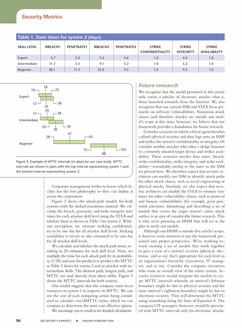
Figure 3 shows the attack-path models for both systems with the dashed transitions omitted. We cal-culate the breach, penetrate, and strike integrity state times for each attacker skill level using the STEA and tabulate them as shown in Table 1 for system 2. With-out encryption, we estimate striking confidential-ity to be one day for all attacker skill levels. Striking availability is trivial, so also estimated to be one day for all attacker skill levels.

We calculate and tabulate the attack path times, re-sulting in 28 estimates for each skill level. Next, we multiply the time for each attack path by its probabili-ty (1/28) and sum the products to produce the MTTC as Table 2 shows for system 2 and an attacker with in-termediate skills. The shortest path, longest path, and MTTC are read directly from these tables. Figure 5 shows the MTTC intervals for both systems.

Our model suggests that the company must focus resources on system 1 to improve its MTTC. We can use the cost of each mitigating action being consid-ered to calculate cost/DMTTC ratios, which we can compare to determine the most cost-effective option.

We encourage you to email us for detailed calculations.

Future researchWe recognize that the model presented in this article only covers a subclass of electronic attacks—that is, those launched remotely from the Internet. We also recognize that our current SSM and STEA focus pri-marily on software vulnerabilities. Numerous attack classes (and therefore attacks) are outside our mod-el’s scope at this time; however, we believe that our framework provides a foundation for future research.

Consider scenarios in which a threat agent breaches a plant’s physical security and then logs onto an HMI and strikes the system’s confidentiality or integrity. Or consider another attacker who takes a sledge hammer to a remotely situated target device and strikes avail-ability. These scenarios involve four states: breach, strike confidentiality, strike integrity, and strike avail-ability—remarkably similar to the states in the SSM we present here. We therefore expect that security ar-chitects can modify our SSM to identify attack paths for other attack classes, such as social engineering or physical attacks. Similarly, we also expect that secu-rity architects can modify the STEA to estimate state times for other vulnerability classes, such as protocol and human vulnerabilities (for example, poor pass-word selection). Identifying and describing a set of models that covers the target system’s entire attack surface is an area of considerable future research. This is why we’re pursuing an HHM that will act as the glue to unify our models.

Although our HHM is outside this article’s scope, it deserves some mention to put the framework pre-sented into proper perspective. We’re working to-ward creating a set of models that work together to give a view of a system’s security (physical, elec-tronic, and so on) that’s appropriate for each level in an organization’s hierarchy (executives, IT manag-ers, and so on). Consider the company executives who want an overall view of the entire system. Se-curity architects would integrate the models to cre-ate MTTC intervals whereby an interval’s leftmost boundary might be due to physical security and the same interval’s rightmost boundary might be due to electronic security. They will determine the MTTC using something along the lines of Equation 8. The company’s IT managers, however, would be present-ed with MTTC intervals only for electronic attacks,

Table 1. State times for system 2 (days).

Skill level BReach1 PeneTRaTe1 BReach2 PeneTRaTe2 STRike confidenTialiTy

STRike inTegRiTy

STRike availaBiliTy

Expert 5.7 5.0 5.6 4.6 1.0 4.6 1.0

Intermediate 11.7 5.5 9.1 5.2 1.0 5.2 1.0

Beginner 38.1 11.3 33.0 9.5 1.0 9.5 1.0

Expert

Intermediate

Beginner

10 2518

......

12 2820

28 6547

22 3930

1912 28

10388

72

... ...

... ...

Figure 5. Example of MTTC intervals (in days) for our case study. MTTC intervals are shown in pairs with the top interval representing system 1 and the bottom interval representing system 2.

Security Metrics


whereby an interval’s leftmost boundary might be due to compromising emanations (Tempest) and the same interval’s rightmost boundary might be due to software vulnerabilities.

MTTCOVERALL = (C1 * MTTC1) + (C2 * MTTC2) + ... + (CN * MTTCN), (8)

where C is the weighting or probability coefficient, and MTTCN is the attack class (electronic, physical, and so on).

We should also be able to extend our model to ac-count for numerous environmental factors, such as patch intervals, operating system diversity, and pass-

word policies. Determining which indicators are truly important and how they affect the MTTC is also an area for considerable research. Our next endeavor will be to improve our estimates and will focus on vis-ibility (a) versus firewall update/review frequency. We’re researching the use of common vulnerability scanners such as Nessus (www.nessus.org) and Nmap (insecure.org/nmap) to identify how many vulner-abilities are visible behind the firewall to obtain mea-sured values for a.

In the long term, we need to collect relevant sta-tistical data to set the MMTC intervals confidence levels. Promising sources for this statistical data are the Honeynet Project (www.honeynet.org) and the

Table 2. attack path times and MTTc calculation for system 2 and for an attacker with intermediate skills.

aTTack PaTh PRoBaBiliTy PaTh TiMe PRoducT

L, B1, B2, C, S 1/28 21.8 0.78

L, B1, B2, I, S 1/28 26.0 0.93

L, B1, B2, A, S 1/28 21.8 0.78

L, B1, B2, C, I, S 1/28 27.0 0.96

L, B1, B2, C, A, S 1/28 22.8 0.81

L, B1, B2, I, A, S 1/28 27.0 0.96

L, B1, B2, C, I, A, S 1/28 28.0 1.00

L, B1, P1, B2, C, S 1/28 27.3 0.98

L, B1, P1, B2, I, S 1/28 31.5 1.13

L, B1, P1, B2, A, S 1/28 27.3 0.98

L, B1, P1, B2, C, I, S 1/28 32.5 1.16

L, B1, P1, B2, C, A, S 1/28 28.3 1.01

L, B1, P1, B2, I, A, S 1/28 32.5 1.16

L, B1, P1, B2, C, I, A, S 1/28 33.5 1.20

L, B1, B2, P2, C, S 1/28 27.0 0.96

L, B1, B2, P2, I, S 1/28 31.2 1.11

L, B1, B2, P2, A, S 1/28 27.0 0.96

L, B1, B2, P2, C, I, S 1/28 32.2 1.15

L, B1, B2, P2, C, A, S 1/28 28.0 1.00

L, B1, B2, P2, I, A, S 1/28 32.2 1.15

L, B1, B2, P2, C, I, A, S 1/28 33.2 1.19

L, B1, P1, B2, P2, C, S 1/28 32.5 1.16

L, B1, P1, B2, P2, I, S 1/28 36.7 1.31

L, B1, P1, B2, P2, A, S 1/28 32.5 1.16

L, B1, P1, B2, P2, C, I, S 1/28 37.7 1.35

L, B1, P1, B2, P2, C, A, S 1/28 33.5 1.20

L, B1, P1, B2, P2, I, A, S 1/28 37.7 1.35

L, B1, P1, B2, P2, C, I, A, S 1/28 38.7 1.38

MTTC (intermediate) 30.3

Note: L = launch, B = breach, P = penetrate, C = strike confidentiality, I = strike integrity, A = strike availability, and S = success.

Security Metrics


results of penetration team testing in the field. Both will help us to improve our state time estimations and to identify predominant attacker strategies. Our expe-rience with the Industrial Security Incident Database leads us to believe that this might even help identify how an attacker’s strategies are modified according to environmental conditions (such as network topology and defenses) and attacker skill levels.

Finally, we hypothesize that the distribution of attackers with skills ranging from beginner to ex-pert will be normal. Our recent research pursues key risk indicators to identify the key skills and resources used for each of the three attacker levels and to relate these to the attacker’s skill level through learning-curve theory.

T he findings of this preliminary research indicate that MTTC could be an efficient and powerful

tool for comparative analysis of security environ-ments and solutions. By deliberately restricting the variety of possible states (and nodes on attack trees) and selecting marker strategies rather than exhaus-tive lists, the model allows reasonable comparisons for decision-making purposes.

The selection of time as the unit of measurement is paramount to the model’s strength. Time intervals are useful for intelligently comparing and selecting from a broad range of mitigating actions. We can compare and choose among two or more entirely different mitigating solutions based on which solution has the lowest cost in dollars per day and yet meets or exceeds a benchmark MTTC.

The MTTC framework can also identify how hard or weak a system is as seen by the attacker compared with peer systems in the same industry. MTTC indus-try averages (and other averages) can be collected over time and used to make peer comparisons. Above-average MTTC intervals would likely encourage an opportunistic attacker to move to another target, whereas below-average MTTC intervals would en-courage the opposite.

ReferencesL. Desborough and R. Miller, “Increasing Customer Value of Industrial Control Performance Monitoring—Honeywell’s Experience,” Proc. 6th Int’l Conf. Chemical Process Control (CPC VI), John Wiley & Sons, 2002, pp. 172–192.Underwriters Laboratories, Standard for Safety Burglary-Resistant Safes, UL 687, UL, 2005.S.P. Gorman et al., “A Predator Prey Approach to the Network Structure of Cyberspace,” ACM Int’l Conf. Proc. Series, vol. 58, Trinity College Dublin, 2004, pp. 1–6.E. Jonsson and T. Olovsson, “A Quantitative Model of

1.

2.

3.

4.

the Security Intrusion Process Based on Attacker Be-haviour,” IEEE Trans. Software Eng., vol. 23, no. 4, Apr. 1997, pp. 235–245.M.A. McQueen et al., “Quantitative Cyber Risk Re-duction Estimation Methodology for a Small SCADA Control System,” Proc. 39th Ann. Hawaii Int’l Conf. Sys-tem Sciences (HICSS 06), track 9, 2006, p. 226. D. Leversage and E.J. Byres, “Comparing Electronic Battlefields: Using Mean Time-to-Compromise as a Comparative Security Metric,” Comm. Computer and Information Science—Computer Network Secu-rity, Proc. 4th Int’l Conf. Mathematical Methods, Models, and Architectures for Computer Network Security, Springer, 2007, pp. 213–227.M.A. McQueen et al., “Time-to-Compromise Model for Cyber Risk Reduction Estimation,” First Workshop on Quality of Protection, Quality of Protection: Security Mea-surements and Metrics, Springer, 2005.E. Rescorla, “Is Finding Security Holes a Good Idea?” IEEE Security & Privacy, vol. 3, no. 1, Jan./Feb. 2005, pp. 14–19.P. Manadhata and J.M. Wing, Measuring a System’s At-tack Surface, tech. report CMU-CS-04-102, School of Computer Science, Carnegie Mellon Univ., 2004.

David John Leversage is a faculty member with the Depart-ment of Electrical and Computer Engineering Technology at the British Columbia Institute of Technology (BCIT) and a se-nior research scientist for security analysis and modeling of critical infrastructures at Byres Research. His research focuses on the application of risk and attack models for identifying vulnerabilities in SCADA systems and protocols. Leversage has a BS in electrical engineering from Lakehead University. He is a professional engineer with the Association of Professional Engineers and Geoscientists of British Columbia. Contact him at [email protected].

Eric James Byres is the founder of the BCIT Critical Infrastruc-ture Security Center, one of North America’s leading aca-demic facilities in the field of Supervisory Control and Data Acquisition (SCADA) cybersecurity. His main research interest is cyberprotection for critical infrastructure, and he has been responsible for numerous standards, best practices, and in-novations for data communications and controls systems se-curity in industrial environments. Byres has a BS in applied science from the University of British Columbia. He is a profes-sional engineer with the Association of Professional Engineers and Geoscientists of British Columbia. Contact him at [email protected].

For more information on this or any other computing topics, please visit the IEEE Computer Society’s Digital Library at http://computer.org/publications/dlib.

5.

6.

7.

8.

9.

Documents

Estimating a System's Mean Time-to-Compromise