Estimating a combined Moho model for marine areas via

Stud. Geophys. Geod., 64 (2020), 125, DOI: 10.1007/s11200-019-1067-0 1 © 2020 The Authors

Estimating a combined Moho model for marine areas via satellite altimetric - gravity and seismic crustal models

MAJID ABREHDARY1 AND LARS E. SJÖBERG1,2

1 Division of Mathematics, Computer and Surveying Engineering, University West (HV),

SE-461 86 Trollhättan, Sweden ([email protected]) 2 Division of Geodesy and Satellite Positioning, Royal Institute of Technology (KTH),

SE-100 44 Stockholm, Sweden

Received: August 13, 2019; Revised: October 3, 2019; Accepted: October 23, 2019

ABSTRACT

Isostasy is a key concept in geoscience in interpreting the state of mass balance between the Earth’s lithosphere and viscous asthenosphere. A more satisfactory test of isostasy is to determine the depth to and density contrast between crust and mantle at the Moho discontinuity (Moho). Generally, the Moho can be mapped by seismic information, but the limited coverage of such data over large portions of the world (in particular at seas) and economic considerations make a combined gravimetric-seismic method a more realistic approach. The determination of a high-resolution of the Moho constituents for marine areas requires the combination of gravimetric and seismic data to diminish substantially the seismic data gaps. In this study, we estimate the Moho constituents globally for ocean regions to a resolution of 1 1° by applying the Vening Meinesz-Moritz method from gravimetric data and combine it with estimates derived from seismic data in a new model named COMHV19. The data files of GMG14 satellite altimetry-derived marine gravity field, the Earth2014 Earth topographic/bathymetric model, CRUST1.0 and CRUST19 crustal seismic models are used in a least-squares procedure. The numerical computations show that the Moho depths range from 7.3 km (in Kolbeinsey Ridge) to 52.6 km (in the Gulf of Bothnia) with a global average of 16.4 km and standard deviation of the order of 7.5 km. Estimated Moho density contrasts vary between 20 kg m3 (north of Iceland) to 570 kg m3 (in Baltic Sea), with a global average of 313.7 kg m3 and standard deviation of the order of 77.4 kg m3. When comparing the computed Moho depths with current knowledge of crustal structure, they are generally found to be in good agreement with other crustal models. However, in certain regions, such as oceanic spreading ridges and hot spots, we generally obtain thinner crust than proposed by other models, which is likely the result of improvements in the new model. We also see evidence for thickening of oceanic crust with increasing age. Hence, the new combined Moho model is able to image rather reliable information in most of the oceanic areas, in particular in ocean ridges, which are important features in ocean basins.

M. Abrehdary and L.E. Sjöberg

2 Stud. Geophys. Geod., 64 (2020)

Ke y wo rd s : Vening Meinesz-Moritz, satellite altimetry, Moho depth, Moho density contrast, uncertainty

1. INTRODUCTION

The Mohorovičić discontinuity (or Moho) is the interface, which marks the boundary between both the oceanic crust and continental crust from underlying mantle. The study of the Moho has become a vital topic for investigating the dynamics of the Earth’s interior, such as understanding the processes of continental rifting, breakup and the evolution of petroleum systems within passive margins (Sutra and Manatschal, 2012). In general, there are two main methods for determining the Moho: gravimetric and seismic ones, which do not deliver the same result due to their different geological and geophysical hypotheses in addition to different qualities and spatial distributions of the required data (e.g., Sjöberg, 2009). In case of the gravimetric method, gravity data are employed under a certain isostatic hypothesis, implying that the Moho model is characterized by some simplified hypothesis to guarantee the uniqueness of the solution of the inverse gravitational problem (Reguzzoni et al., 2013), while in the seismic studies, Moho models are mostly determined from refracted and reflected waves, and sometimes by receiver functions and the ambient noise technique (Kind et al., 2012; Shapiro and Campillo, 2004). Although, the global crust models based on seismic methods are locally very accurate, they are typically sparse, particularly over areas without adequate seismic data, where they could yield unrealistic results with large uncertainties. Accordingly, over large parts of the world with a limited coverage of seismic data, in particular in marine areas, the combination of seismic and gravimetric data (i.e combined approach) is essential.

Different attempts to estimate a global crust model using either seismic or gravimetric method have been made on global scale during the years, and it is far from clear to get and compare their accuracies. Overviews of existing studies on seismic Moho determination can be found in the literature. The first model, named CRUST5.1, dates back to Mooney et al. (1998), and it was based on seismic refraction data, and later on its updated version, called CRUST2.0 (Bassin et al., 2000), was compiled with 2 2 resolution. Zhou et al. (2006) produced a model by constraining shear velocity structure in the crust and upper mantle from phase and group velocity measurements of fundamental mode of Rayleigh and Love waves, while Meier et al. (2007) directly used surface wave data to globally infer the crust thickness. CRUST1.0 (Laske et al., 2013) is the most frequently used crustal model, which is based on a database of crustal thickness data from active source seismic studies as well as from receiver function studies. More recently, Szwillus et al. (2019) developed a global crustal thickness model and velocity structure from geostatistical analysis of seismic data, and we hereafter call this model that of CRUST19.

For gravimetric and combined gravimetric-seismic methods different models have been proposed during the last decade. Chappell and Kusznir (2008) described a method for determining Moho depth (MD), lithosphere thinning factor and the location of the ocean-continent transition at rifted continental margins using 3-D gravity inversion, which includes a correction for the large negative lithosphere thermal gravity anomaly within the continental margin lithosphere. Sjöberg (2009) defined the so-called Vening Meinesz-Moritz (VMM) problem, and provided some solutions for estimating the MD. This

Estimating a combined Moho model for marine areas …

Stud. Geophys. Geod., 64 (2020) 3

approach was later proceeded by some additional theoretical studies for recoverying also the Moho density contrast (MDC) (Sjöberg and Bagherbandi, 2011) and improved for isolating the Bouguer gravity anomaly from non-isostatic effects (Bagherbandi and Sjöberg, 2012). Eshagh et al. (2011) presented a Moho model from a combination of the EGM2008 and seismic model based on the VMM method. Wang et al. (2011) released gravity‐derived crustal thickness models for the North Atlantic Ocean and the Chain Fracture Zone, which are calibrated using seismically determined crustal thickness, and he concluded that about 7% of the ocean crust is less than 4 km thick, 58% is 47 km thick, and the remaining 35% is more than 7 km thick. Tenzer and Bagherbandi (2012) stated that the VMM MD from gravity disturbance can better fit to the seismic Moho model than those from the gravity anomaly. This argument was also theoretically proved by Sjöberg (2013). Reguzzoni et al. (2013) compiled both the MD and MDC using the combination of the CRUST2.0 and gravity data from the GOCE model. Bai et al. (2014) mapped a model of crustal thickness using marine gravity data corrected for the sediment thickness, thermal expansion, and pressure compression in the South China Sea and showed the influence of these factors on gravity-derived estimates of the MD. Tenzer and Chen (2014) applied a new method to estimate the MD using the gravimetric forward and inverse modeling in the spectral domain, and Hamayun (2014) produced the MD using gravity disturbance together with two seismic models. Tenzer et al. (2015a) used the CRUST1.0 model to estimate the average densities of crustal structures, and compile the gravity field quantities derived by the Earth’s crustal structures and investigate their spatial and spectral characteristics and their correlation with the crustal geometry in context of the gravimetric Moho determination. Sjöberg et al. (2015) showed that the application of the Bouguer gravity disturbance and the no-topography gravity anomaly in the VMM model to determine the MD deliver similar results, emphasising the importance of not using the traditional Bouguer gravity anomaly for gravity inversion. Tenzer et al. (2015b) formulated the gravimetric inverse problem for recovering the Moho geometry based on adopting the generalized compensation model by considering the variable depth and density of compensation. Reguzzoni and Sampietro (2015) applied a new iterative strategy to estimate the MD and the crustal density by exploiting gravity data coming from the GOCE satellite weakly combined with CRUST2.0 mean MD. Abrehdary et al. (2015, 2017) computed a combined Moho parameters model according to the VMM method. Abrehdary et al. (2018) estimated a new MDC model named MDC2018, using the marine gravity field from satellite altimetry in combination with a seismic-based crustal model and Earth’s topographic/bathymetric data. Bai et al. (2019) applied temperature-based and velocity-based methods to model the lithospheric/upper mantle density, taking the Atlantic Ocean as a case study region and showed that the temperature-based method performs well in reproducing Moho geometry in the main part of the Atlantic Ocean, especially in the central basin.

In this study we aim at attenuating the afformentioned drawbacks in using either seismic- or gravimetric-only techniques in ocean areas by combining the altimeter-derived GMG14 global marine gravity field model (Sandwell et al., 2014) with the seismic models of CRUST1.0 and CRUST19. For our investigation of crustal structure, we apply a combined approach to simultaneously estimate the MD and MDC (or Moho constituents) by the VMM hypothesis and available seismic models to a resolution of



1 1. The study, resulting in a Moho model called COMHV19, therefore incorporates three steps. The first step is to define our technique of combining the gravimetric and seismic data by estimating the Moho constituents based on least-squares adjustment by elements from the GMG14 along with CRUST1.0 and CRUST19. The second step is to model the uncertainty of the Moho constituents, which plays a major role in the accuracy of the final Moho model, and the last step is to compare our resulting Moho constituents with other global and regional Moho models.

2. METHODOLOGY

2 . 1 . A l t i m e t r y - g r a v i m e t r y m e t h o d

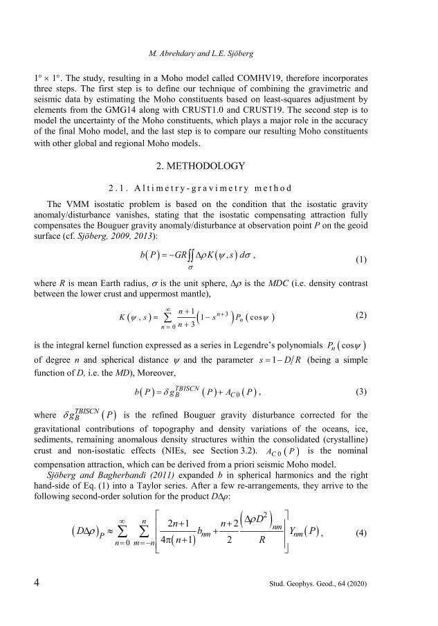
The VMM isostatic problem is based on the condition that the isostatic gravity anomaly/disturbance vanishes, stating that the isostatic compensating attraction fully compensates the Bouguer gravity anomaly/disturbance at observation point P on the geoid surface (cf. Sjöberg, 2009, 2013):

,b P GR K s d

, (1)

where R is mean Earth radius, is the unit sphere, is the MDC (i.e. density contrast between the lower crust and uppermost mantle),

3

0

1, 1 cos

3n

nn

nK s s P

n

(2)

is the integral kernel function expressed as a series in Legendre’s polynomials cosnP of degree n and spherical distance and the parameter 1s D R (being a simple function of D, i.e. the MD), Moreover,

0TBISCNB Cb P g P A P , (3)

where TBISCNBg P is the refined Bouguer gravity disturbance corrected for the

gravitational contributions of topography and density variations of the oceans, ice, sediments, remaining anomalous density structures within the consolidated (crystalline) crust and non-isostatic effects (NIEs, see Section 3.2). 0CA P is the nominal compensation attraction, which can be derived from a priori seismic Moho model.

Sjöberg and Bagherbandi (2011) expanded b in spherical harmonics and the right hand-side of Eq. (1) into a Taylor series. After a few re-arrangements, they arrive to the following second-order solution for the product D∆ρ:

2

0

2 1 24 1 2

nnm

nm nmPn m n

Dn nD b Y P

n R

, (4)



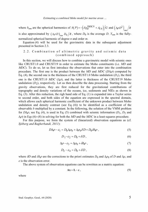
where bnm are the spherical harmonics of 0TBISCNB Cb P g A G and 2

nmD R

is also approximated by 0nmD D R , where D0 is the average D. Ynm is the fully-normalized spherical harmonic of degree n and order m.

Equation (4) will be used for the gravimetric data in the subsequent adjustment presented in Section 2.3.

2 . 2 . C o m b i n a t i o n o f a l t i m e t r i c g r a v i t y a n d s e i s m i c d a t a ( c o m b i n e d a p p r o a c h )

In this section, we will discuss how to combine a gravimetric model with seismic ones like CRUST1.0 and CRUST19 in order to estimate the Moho constituents (i.e. MD and MDC). To do so, let us first introduce the observations that enter into the combination procedure. The first one is the product between the MD and MDC (D) computed by Eq. (4), the second one is the thickness of the CRUST1.0 Moho undulation (D1), the third one is the CRUST1.0 MDC (), and the latter is thickness of the CRUST19 Moho undulation (D2), respectively. Let us then describe the data processing. Starting from the gravity observations, they are first reduced for the gravitational contributions of topography and density variations of the oceans, ice, sediments and NIEs as shown in Eq. (3). After this reduction, the righ hand side of Eq. (1) is expanded into a Taylor series to second order, and both sides of the equation are expressed in the spectral domain, which allows each spherical harmonic coefficient of the unknown product between Moho undulation and density contrast (see Eq. (4)) to be identified as a coefficient of the observable b multiplied by a constant. In the following, the solution of the VMM problem for D, see Eq. (4), is used in Eq. (5) combined with seismic information (D1, D2 and ) in Eqs (6)(8) in solving for both the MD and the MDC in a least-squares procedure.

For this purpose, we form the system of (linearized) observation equations as (cf. Sjöberg and Bagherbandi, 2011):

1 0 0 0 0D D D D , (5)

1 2 0D D D , (6)

3 0 , (7)

2 4 0D D D , (8)

where D and are the corrections to the priori estimates D0 and 0 of D and ∆ρ, and is the observation error.

The above system of observation equations can be rewritten as a matrix equation:

εAx L , (9)

where



0 01 00 11 0

D

A , D

x , and

1 0 0

2 0

3 0

4 0

l Dl Dll D

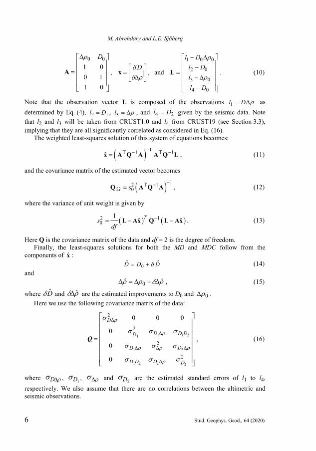
L . (10)

Note that the observation vector L is composed of the observations 1l D as determined by Eq. (4), 2 1l D , 3l , and 4 2l D given by the seismic data. Note that l2 and l3 will be taken from CRUST1.0 and l4 from CRUST19 (see Section 3.3), implying that they are all significantly correlated as considered in Eq. (16).

The weighted least-squares solution of this system of equations becomes:

1T 1 T 1ˆ x A Q A A Q L , (11)

and the covariance matrix of the estimated vector becomes

12 T 1ˆˆ 0sxx

Q A Q A , (12)

where the variance of unit weight is given by

2 10

1ˆ ˆTs

df L Ax Q L Ax . (13)

Here Q is the covariance matrix of the data and df = 2 is the degree of freedom. Finally, the least-squares solutions for both the MD and MDC follow from the

components of x̂ : 0ˆ ˆD D D (14) and 0ˆ ˆ , (15)

where D̂ and ˆ are the estimated improvements to D0 and 0 . Here we use the following covariance matrix of the data:

1 1 21

1 2

1 2 2 2

2

2

2

2

0 0 0

0

0

0

D

D D DD

D D

D D D D

Q , (16)

where D , 1D , and 2D are the estimated standard errors of l1 to l4, respectively. We also assume that there are no correlations between the altimetric and seismic observations.



3. THE DATA

3 . 1 . M a r i n e g r a v i t y d i s t u r b a n c e

Marine gravity measurments are powerful tools for mapping tectonic structures, especially in the deep ocean basins, where the topography remains unmapped by ships or is buried by thick sediment (Sandwell et al., 2014). Acordingly, we use refined Bouguer gravity disturbances derived from the GMG14 altimetry-derived marine gravity and Earth2014 topographic models (Hirt and Rexer, 2015) to degree and order 180 as an input data to constract a global map of Moho model. In details a grid with a resolution of 1 1 on a global scale is synthesized.

The GMG14 is a combined new radar altimeter measurements from satellites CryoSat-2 and Jason-1 that is two times more accurate than previous models with an accuracy of about 2 mGal. The Earth2014 is a global relief model, which comprises five different layers of height data, including Earth’s surface (lower interface of the atmosphere), topography and bathymetry of the oceans and major lakes, topography, bathymetry and bedrock, ice-sheet thicknesses and rock-equivalent topography.

3 . 2 . A d d i t i v e c o r r e c t i o n s t o g r a v i t y d i s t u r b a n c e

Despite the advantages in using satellite altimetric gravity disturbance described in this paper, these gravity data contain signals from the topography and density heterogeneities related to bathymetry, ice, sediments and also from those in the mantle and core/mantle topography variations as well as the remaining consolidated crust. In order to strip the gravity disturbances caused only by the geometry of the Moho interface, all aforementioned nuisance signals must be suppressed by applying the so-called stripping gravity corrections, which these corrections were derived from the ESCM180 Earth’s spectral crustal model (Tenzer et al., 2015a). The global crustal model of CRUST1.0 was also used to obtain both 0 and D0 for each block. In the CRUST1.0 model, the difference between the lower crust density and uppermost mantle density describes the MDC that we used as the observation vector in our least-squares adjustment.

An additional additive correction is for the non isostatic effect (NIE), which is a way to filter out some remaining signals in the gravity data caused by disturbing effects in the Earth’s interior by comparing the gravimetric and seismic data in the frequency domain (see Bagherbandi and Sjöberg, 2012).

3 . 3 . S e i s m i c c r u s t a l m o d e l s

The seismic methods are most effective for investigating the structure of the Earth’s crust, where the base of the crust is defined as the Moho. The most common seismic method is deep seismic sounding, in which the MD is determined from refracted or reflected seismic waves (Prodehl and Mooney, 2012). Receiver functions (Kind et al., 2012) and the ambient noise technique (Shapiro and Campillo, 2004) are two other most popular techniques, which are quite limited at global scale due to the lack of informations in oceanic areas (Hello et al., 2011). A review on the use of passive seismic methods can be found in the work of Lebedev et al. (2013).

The most common global crustal models are those based primarily on seismic information. For instance, the CRUST1.0 Moho model is based on a database of crustal



thickness data from active source seismic studies as well as from receiver function studies. The model has a resolution of 1 1 and incorporates 35 key crustal types that contain the thickness, density and velocity of compressional (Vp) and shear waves (Vs) for eight layers (ice, water, upper, middle, and lower sediments, upper, middle, and lower crust). The Vp values are based on field measurements, while Vs and density are estimated by using empirical Vp-Vs and Vp-density relationships, respectively. For regions lacking field measurements, the seismic velocity structure of the crust is extrapolated from the average crustal structure for regions with similar crustal age and tectonic setting. The topography and bathymetry are adopted from ETOPO1 (Amante and Eakins, 2009). The sediment cover is based on the sediment model by Laske and Masters (1997) with some near-coastal updates. Under oceans the widely used CRUST1.0 model is greatly restricted by a low coverage of seismic data.

The CRUST19 model presents global maps of MD and average P-wave velocity of the crystalline crust with a resolution of 1 1 using a nonstationary kriging algorithm. The model is derived from a database of seismic points (i.e. the U.S. Geological Survey [USGS] Global Seismic Catalog [GSC] database) as in CRUST1.0, including some additional information (i.e. the age of the ocean floor), following a design philosophy that tries to respect the data as much as possible. In addition to the inclusion of additional data and the kriging interpolation machinery, an advantage of CRUST19 is that it is published with its corresponding uncertainty, which can be helpful for any geophysical application that relies on such models. It is also helpful in the combined approach to be used below.

4. UNCERTAINTY MEASURES IN THE MOHO CONSTITUENTS

In this section, we try to present a reasonable method to estimate the uncertainty in those observations of the VMM and seismic models to secure the quality of the Moho results.

4 . 1 . U n c e r t a i n t y i n t h e V M M m o d e l

The variance of DΔρ can be computed by the following formula (see Sjöberg and Bagherbandi, 2011):

2 2

2 2 2

, , , ,2

4 4D nm nm nm kl nmkln m n m k l n m

N N NG G

, (17)

where is normal gravity, 2 1nmN n , 2nm and nmkl are the potential coefficient

error degree and order variances and covariances, respectively. The latter quantities are usually available from the least-squares solution of the potential coefficients (Abrehdary et al., 2017).

4 . 2 . U n c e r t a i n t y i n t h e s e i s m i c c r u s t a l m o d e l s

It should be noted that, the uncertainties are different in various seismic methods and can be different even for the same methods in different experiments and areas. Actually, the uncertainties can be arisen from several factors such as the survey method, the spatial resolution of the survey, and the analytical techniques used to process the data



(Christensen and Mooney, 1995; Chulick et al., 2013). It is difficult to estimate the uncertainties related to seismic crustal models, as their qualities are not specified, and they vary a lot from place to place due to the accuracy as well as the quantity of available seismic observations, in particular on ocean. For example, Grad et al. (2009) demonstrated that the MD uncertainties estimated using seismic data in Europe regionally exceed 10 km, with an average error of about 4 km. The best horizontal Moho resolution is typically inferred from reflection profiles (cf. Kanao et al., 2011), but such technique is expensive, thus not widely used. The Moho detection from a two-way travel time might also be affected by a weak reflectivity. An intermediate spatial resolution could be obtained from a deep seismic sounding based on using refracted and wide-angle reflected waves. The uncertainties of detecting the MD from the wide-angle reflection and refraction methods are typically about 12 km. Another technique, that became quite common during the last two decades, is based on inverting the P- or S-wave receiver functions (e.g., Zhu and Kanamori, 2000; Hansen et al., 2009). An estimated uncertainty of this method is about 3 km. The intermediate-period surface waves are quite sensitive to the crustal thickness, but are not able to discriminate it from the mantle velocity structure, thus cannot be inverted uniquely (cf. Danesi and Morelli, 2001; Kobayashi and Zhao, 2004; Ritzwoller et al., 2001). A wide station spacing and absence of intra-plate earthquakes in Antarctica does not generally allow inverting the short-period surface waves which have a better sensitivity to a shallower density structure. However, surface waves are useful for studying areas where other types of seismic data are not available. MD uncertainties under oceanic crust are typically considered at the level of 12 km, and 34 km for volcanic rises, plateaus. However, here we make an effort to assess the crustal model standard errors of the CRUST1.0 MD, CRUST1.0 MDC and of the CRUST19 MD, which are used in this study. As for the former, i.e. the uncertainty of the CRUST19 MD the problem is quite simple since the expected accuracy has already been computed by Szwillus et al. (2019), which we use in the present work. As for the CRUST1.0 data, since no formal error standard deviations are provided, they have to be empirically defined for MD. In particular, large MD errors have been assigned to oceans, where there are no data or they are of poor quality (Reguzzoni et al., 2013). These errors have been additionally weighted according to the depth of the CRUST1.0 Moho as stated in Christensen and Mooney (1995); finally a smoothing operator has been applied to the resulting grid of error standard deviations in order to remove discontinuities. Different is the situation for the CRUST1.0 MDC, where no estimate is given for the expected accuracy by the authors and even the literature on how the model has been computed is quite limited. In absence of better information we estimate the MDC accuracy simply as the density accuracy of the crystalline crust, disregarding the density accuracy of the upper mantle. In oceanic regions the estimated accuracy has been fixed according to Carlson and Raskin (1984) to 0.4 kg m3. Basically starting from the seismic velocities reported in Table 3 of Christensen and Mooney (1995) and considering the equation reported in Table 8 of the same paper, it has been possible to propagate the error in terms of seismic velocity to error in terms of crustal density. Moreover, since both the seismic velocity accuracy and the coefficients for the equation in Table 8 of Christensen and Mooney (1995) depends on the depth, the CRUST1.0 MD has been used for computing the CRUST1.0 MDC.



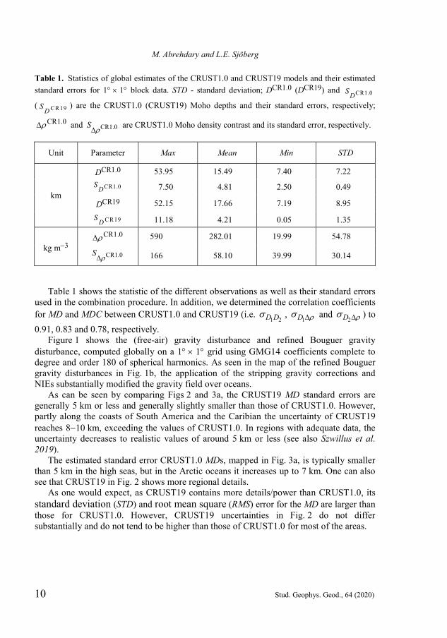
Table 1 shows the statistic of the different observations as well as their standard errors used in the combination procedure. In addition, we determined the correlation coefficients for MD and MDC between CRUST1.0 and CRUST19 (i.e.

1 2D D , 1D and

2D ) to 0.91, 0.83 and 0.78, respectively.

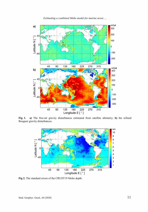
Figure 1 shows the (free-air) gravity disturbance and refined Bouguer gravity disturbance, computed globally on a 1 1 grid using GMG14 coefficients complete to degree and order 180 of spherical harmonics. As seen in the map of the refined Bouguer gravity disturbances in Fig. 1b, the application of the stripping gravity corrections and NIEs substantially modified the gravity field over oceans.

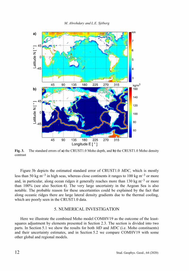
As can be seen by comparing Figs 2 and 3a, the CRUST19 MD standard errors are generally 5 km or less and generally slightly smaller than those of CRUST1.0. However, partly along the coasts of South America and the Caribian the uncertainty of CRUST19 reaches 810 km, exceeding the values of CRUST1.0. In regions with adequate data, the uncertainty decreases to realistic values of around 5 km or less (see also Szwillus et al. 2019).

The estimated standard error CRUST1.0 MDs, mapped in Fig. 3a, is typically smaller than 5 km in the high seas, but in the Arctic oceans it increases up to 7 km. One can also see that CRUST19 in Fig. 2 shows more regional details.

As one would expect, as CRUST19 contains more details/power than CRUST1.0, its standard deviation (STD) and root mean square (RMS) error for the MD are larger than those for CRUST1.0. However, CRUST19 uncertainties in Fig. 2 do not differ substantially and do not tend to be higher than those of CRUST1.0 for most of the areas.

Table 1. Statistics of global estimates of the CRUST1.0 and CRUST19 models and their estimated standard errors for 1 1 block data. STD - standard deviation; DCR1.0 (DCR19) and CR1.0DS

( CR19DS ) are the CRUST1.0 (CRUST19) Moho depths and their standard errors, respectively;

CR1.0 and CR1.0S are CRUST1.0 Moho density contrast and its standard error, respectively.

Unit Parameter Max Mean Min STD

km

DCR1.0 53.95 15.49 7.40 7.22

CR1.0DS 7.50 4.81 2.50 0.49

DCR19 52.15 17.66 7.19 8.95

CR19DS 11.18 4.21 0.05 1.35

kg m3 CR1.0 590 282.01 19.99 54.78

CR1.0S 166 58.10 39.99 30.14



Fig. 1. a) The free-air gravity disturbances estimated from satellite altimetry; b) the refined Bouguer gravity disturbances.

Fig 2. The standard errors of the CRUST19 Moho depth.



Figure 3b depicts the estimated standard error of CRUST1.0 MDC, which is mostly less than 50 kg m3 in high seas, whereas close continents it ranges to 100 kg m3 or more and, in particular, along ocean ridges it generally reaches more than 130 kg m3 or more than 100% (see also Section 4). The very large uncertainty in the Aegean Sea is also notable. The probable reason for these uncertainties could be explained by the fact that along oceanic ridges there are large lateral density gradients due to the thermal cooling, which are poorly seen in the CRUST1.0 data.

5. NUMERICAL INVESTIGATION

Here we illustrate the combined Moho model COMHV19 as the outcome of the least-squares adjustment by elements presented in Section 2.3. The section is divided into two parts. In Section 5.1 we show the results for both MD and MDC (i.e. Moho constituents) and their uncertainty estimates, and in Section 5.2 we compare COMHV19 with some other global and regional models.

Fig. 3. The standard errors of a) the CRUST1.0 Moho depth, and b) the CRUST1.0 Moho density contrast



5 . 1 . C O M H V 1 9 r e s u l t s

The new Moho model is named COMHV19. Its constituents and their uncertainties are determined with a resolution of 1 1 using the altimeter-derived GMG14 global marine gravity field, Earth2014 topographic model and seismic models of CRUST1.0 and CRUST19 in the weighted least-squares procedure presented in Section 2.3. This combination allows us to create a fully coherent and consistent Moho model over the oceanic blocks with no data voids.

Let us first express the observations that enter into the combination procedure. The first set is the product between the MD and MDC (D) estimated from Eq. (4) and the second ones are CRUST1.0 MD (DCR1.0), CRUST1.0 MDC (CR1.0) and CRUST19 MD (DCR19), respectively. Basically D is combined with independent a priori estimates D0 and 0 of those parameters, with the goal of getting separate improved estimates of each parameter.

In Table 2 and Figs 4a5b we present the results of COMHV19. By comparing Tables 1 and 2 one can observe that our mean standard errors have

significantly decreased in the new model. In the following, we provide the geophysical interpretations of the estimated MD

(Fig. 4) and MDC (Fig. 5) along with their uncertainties estimated by our adjustment model.

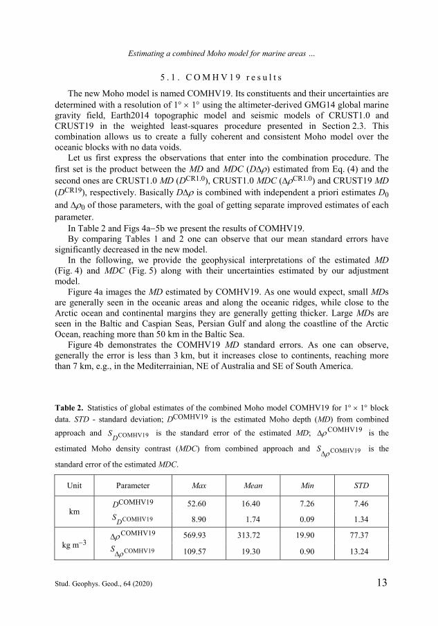
Figure 4a images the MD estimated by COMHV19. As one would expect, small MDs are generally seen in the oceanic areas and along the oceanic ridges, while close to the Arctic ocean and continental margins they are generally getting thicker. Large MDs are seen in the Baltic and Caspian Seas, Persian Gulf and along the coastline of the Arctic Ocean, reaching more than 50 km in the Baltic Sea.

Figure 4b demonstrates the COMHV19 MD standard errors. As one can observe, generally the error is less than 3 km, but it increases close to continents, reaching more than 7 km, e.g., in the Mediterrainian, NE of Australia and SE of South America.

Table 2. Statistics of global estimates of the combined Moho model COMHV19 for 1 1 block data. STD - standard deviation; DCOMHV19 is the estimated Moho depth (MD) from combined approach and COMHV19DS is the standard error of the estimated MD; COMHV19 is the

estimated Moho density contrast (MDC) from combined approach and COMHV19S is the

standard error of the estimated MDC.

Unit Parameter Max Mean Min STD

km DCOMHV19 52.60 16.40 7.26 7.46

COMHV19DS 8.90 1.74 0.09 1.34

kg m3 COMHV19 569.93 313.72 19.90 77.37

COMHV19S 109.57 19.30 0.90 13.24



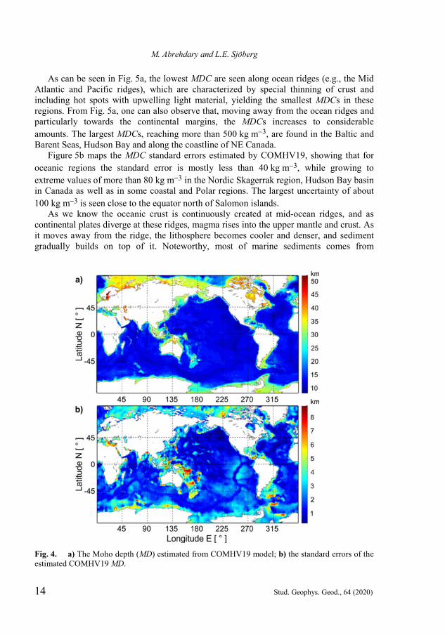
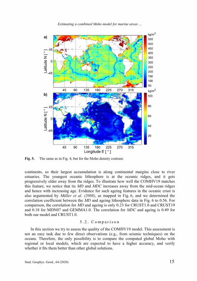
As can be seen in Fig. 5a, the lowest MDC are seen along ocean ridges (e.g., the Mid Atlantic and Pacific ridges), which are characterized by special thinning of crust and including hot spots with upwelling light material, yielding the smallest MDCs in these regions. From Fig. 5a, one can also observe that, moving away from the ocean ridges and particularly towards the continental margins, the MDCs increases to considerable amounts. The largest MDCs, reaching more than 500 kg m3, are found in the Baltic and Barent Seas, Hudson Bay and along the coastline of NE Canada.

Figure 5b maps the MDC standard errors estimated by COMHV19, showing that for oceanic regions the standard error is mostly less than 40 kg m3, while growing to extreme values of more than 80 kg m3 in the Nordic Skagerrak region, Hudson Bay basin in Canada as well as in some coastal and Polar regions. The largest uncertainty of about 100 kg m3 is seen close to the equator north of Salomon islands.

As we know the oceanic crust is continuously created at mid-ocean ridges, and as continental plates diverge at these ridges, magma rises into the upper mantle and crust. As it moves away from the ridge, the lithosphere becomes cooler and denser, and sediment gradually builds on top of it. Noteworthy, most of marine sediments comes from

Fig. 4. a) The Moho depth (MD) estimated from COMHV19 model; b) the standard errors of the estimated COMHV19 MD.



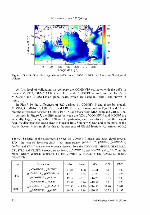
continents, so their largest accumulation is along continental margins close to river estuaries. The youngest oceanic lithosphere is at the oceanic ridges, and it gets progressively older away from the ridges. To illustrate how well the COMHV19 matches this feature, we notice that its MD and MDC increases away from the mid-ocean ridges and hence with increasing age. Evidence for such ageing features in the oceanic crust is also argumented by Müller et al. (2008), as mapped in Fig. 6, and we determined the correlation coefficient between the MD and ageing lithosphere data in Fig. 6 to 0.56. For comparison, the correlation for MD and ageing is only 0.23 for CRUST1.0 and CRUST19 and 0.18 for MDN07 and GEMMA1.0. The correlation for MDC and ageing is 0.49 for both our model and CRUST1.0.

5 . 2 . C o m p a r i s o n

In this section we try to assess the quality of the COMHV19 model. This assessment is not an easy task due to few direct observations (e.g., from seismic techniques) on the oceans. Therefore, the only possibility is to compare the computed global Moho with regional or local models, which are expected to have a higher accuracy, and verify whether it fits them better than other global solutions.

Fig. 5. The same as in Fig. 4, but for the Moho density contrast.



At first level of validation, we compare the COMHV19 estimates with the MDs in models MDN07, GEMMA1.0, CRUST1.0 and CRUST19 as well as the MDCs in MDC2018 and CRUST1.0 on global scale, which are listed in Table 3 and shown in Figs 712.

In Figs 710 the differences of MD derived by COMHV19 and those by models MDN07, GEMMA1.0, CRUST1.0 and CRUST19 are shown, and in Figs 11 and 12 we plot the differences between COMHV19 MDC and those from MDC2018 and CRUST1.0.

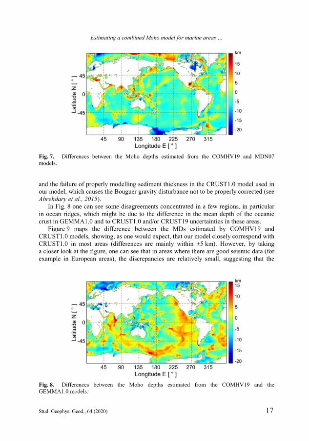
As seen in Figure 7, the differences between the MDs of COMHV19 and MDN07 are generally large, being within ±20 km. In particular, one can observe that the largest negative discrepancies occur near to Hudson Bay, Southern Ocean and some parts of the Arctic Ocean, which might be due to the presence of Glacial Isostatic Adjustment (GIA)

Table 3. Statistics of the differences between the COMHV19 model and other global models. STD - the standard deviation; RMS - root mean square. DCOMHV19, DMDN07, DGEMMA1.0, DCR1.0 and DCR19 are the Moho depths derived from the COMHV19, MDN07, GEMMA1.0, CRUST1.0 and CRUST19 model, respectively; COMHV19, MDC2018 and CR1.0 are the Moho density contrasts estimated by the COMHV19, MDC2018 and CRUST1.0 model, respectively.

Unit Parameters Max Mean Min STD RMS

km

DCOMHV19 DMDN07 21.23 1.38 23.41 4.17 4.40 DCOMHV19 DGEMMA1.0 17.16 0.63 21.23 3.71 3.76

DCOMHV19 DCR1.0 19.17 0.91 14.75 2.05 2.38 DCOMHV19 DCR19 25.57 0.74 18.57 3.11 3.20

kg m3 COMHV19 MDC2018 202.50 14.29 214.56 32.40 35.41 COMHV19 CR19 184.24 19.84 236.87 36.25 41.32

Fig. 6. Oceanic lithosphere age (from Müller et al., 2008, © 2008 the American Geophysical Union).



and the failure of properly modelling sediment thickness in the CRUST1.0 model used in our model, which causes the Bouguer gravity disturbance not to be properly corrected (see Abrehdary et al., 2015).

In Fig. 8 one can see some disagreements concentrated in a few regions, in particular in ocean ridges, which might be due to the difference in the mean depth of the oceanic crust in GEMMA1.0 and to CRUST1.0 and/or CRUST19 uncertainties in these areas.

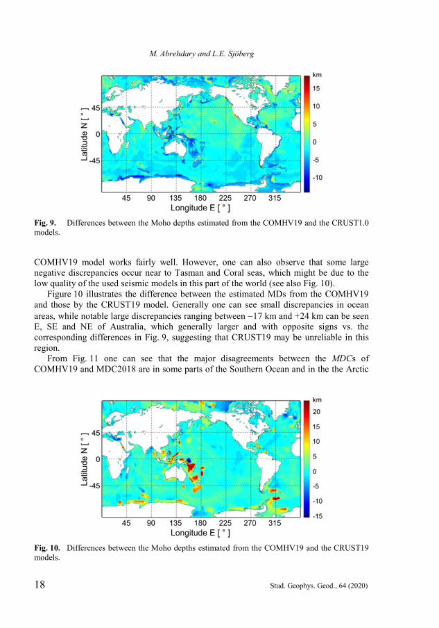
Figure 9 maps the difference between the MDs estimated by COMHV19 and CRUST1.0 models, showing, as one would expect, that our model closely correspond with CRUST1.0 in most areas (differences are mainly within ±5 km). However, by taking a closer look at the figure, one can see that in areas where there are good seismic data (for example in European areas), the discrepancies are relatively small, suggesting that the

Fig. 7. Differences between the Moho depths estimated from the COMHV19 and MDN07 models.

Fig. 8. Differences between the Moho depths estimated from the COMHV19 and the GEMMA1.0 models.



COMHV19 model works fairly well. However, one can also observe that some large negative discrepancies occur near to Tasman and Coral seas, which might be due to the low quality of the used seismic models in this part of the world (see also Fig. 10).

Figure 10 illustrates the difference between the estimated MDs from the COMHV19 and those by the CRUST19 model. Generally one can see small discrepancies in ocean areas, while notable large discrepancies ranging between 17 km and +24 km can be seen E, SE and NE of Australia, which generally larger and with opposite signs vs. the corresponding differences in Fig. 9, suggesting that CRUST19 may be unreliable in this region.

From Fig. 11 one can see that the major disagreements between the MDCs of COMHV19 and MDC2018 are in some parts of the Southern Ocean and in the the Arctic

Fig. 9. Differences between the Moho depths estimated from the COMHV19 and the CRUST1.0 models.

Fig. 10. Differences between the Moho depths estimated from the COMHV19 and the CRUST19 models.



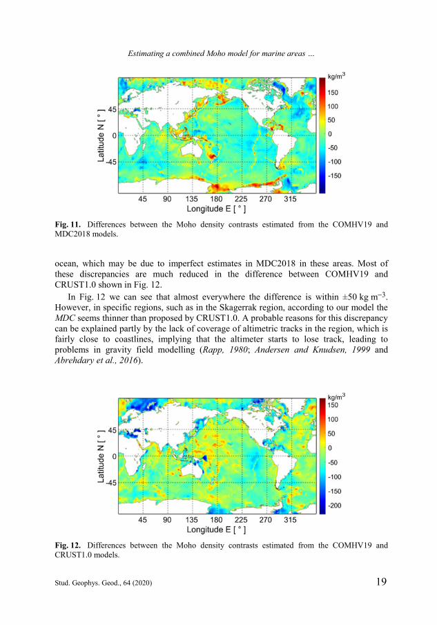
ocean, which may be due to imperfect estimates in MDC2018 in these areas. Most of these discrepancies are much reduced in the difference between COMHV19 and CRUST1.0 shown in Fig. 12.

In Fig. 12 we can see that almost everywhere the difference is within ±50 kg m3. However, in specific regions, such as in the Skagerrak region, according to our model the MDC seems thinner than proposed by CRUST1.0. A probable reasons for this discrepancy can be explained partly by the lack of coverage of altimetric tracks in the region, which is fairly close to coastlines, implying that the altimeter starts to lose track, leading to problems in gravity field modelling (Rapp, 1980; Andersen and Knudsen, 1999 and Abrehdary et al., 2016).

Fig. 11. Differences between the Moho density contrasts estimated from the COMHV19 and MDC2018 models.

Fig. 12. Differences between the Moho density contrasts estimated from the COMHV19 and CRUST1.0 models.



A second level of comparison is performed with respect to regional MD models of SAM10, NAM02, AFR07, EUP09, ASA03, AUS11 and ANT13 as well as MOHV19 MDC as listed in Table 4.

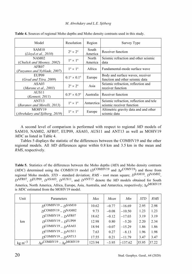
Tables 5 displays the statistic of the differences between the COMHV19 and the other regional models. All MD differences agree within 0.8 km and 3.5 km in the mean and RMS, respectively.

Table 5. Statistics of the differences between the Moho depths (MD) and Moho density contrasts (MDC) determined using the COMHV19 model (DCOMHV19 and COMV19) and those from regional Moho models. STD - standard deviation; RMS - root mean square; DSAM10, DNAM02, DAFR07, DEUP09, DASA03, DAUS11, and DANT13 denote the MD models obtained for South America, North America, Africa, Europe, Asia, Australia, and Antarctica, respectively; MOHV19 is MDC estimated from the MOHV19 model.

Unit Parameters Max Mean Min STD RMS

km

DCOMHV19 DSAM10 10.62 0.77 16.69 2.95 2.98 DCOMHV19 DNAM02 9.73 0.08 10.50 1.23 1.23 DCOMHV19 DAFR07 18.62 0.12 17.03 3.19 3.19 DCOMHV19 DEUP09 12.98 0.80 5.20 2.20 2.34 DCOMHV19 DASA03 18.94 0.07 15.29 1.86 1.86 DCOMHV19 DAUS11 7.63 0.27 8.13 1.96 1.98 DCOMHV19 DANT13 17.55 0.21 11.79 3.47 3.47

kg m3 COMHV19 MOHV19 123.94 3.95 137.62 35.95 37.22

Table 4. Sources of regional Moho depths and Moho density contrasts used in this study.

Model Resolution Region Survey Type

SAM10 (Lloyd et al., 2010) 2 2 South

America Receiver function

NAM02 (Chulick and Mooney, 2002) 1 1 North

America Seismic refraction and other seismic data

AFR07 (Pasyanos and Nyblade, 2007) 1 1 Africa Fundamental-mode surface wave

EUP09 (Grad and Tiira, 2009) 0.1 0.1 Europe Body and surface waves, receiver

function and other seismic data ASA03

(Marone et al., 2003) 2 2 Asia Seismic refraction, reflection and receiver function

AUS11 (Kennett, 2011) 0.5 0.5 Australia Receiver function

ANT13 (Baranov and Morelli, 2013) 1 1 Antarctica Seismic refraction, reflection and tele

seismic receiver function MOHV19

(Abrehdary and Sjöberg, 2019) 1 1 Europe Altimetric gravity data and and other seismic data



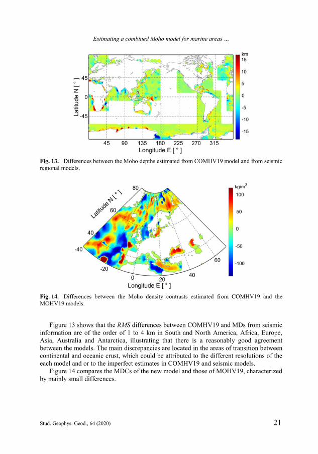
Figure 13 shows that the RMS differences between COMHV19 and MDs from seismic information are of the order of 1 to 4 km in South and North America, Africa, Europe, Asia, Australia and Antarctica, illustrating that there is a reasonably good agreement between the models. The main discrepancies are located in the areas of transition between continental and oceanic crust, which could be attributed to the different resolutions of the each model and or to the imperfect estimates in COMHV19 and seismic models.

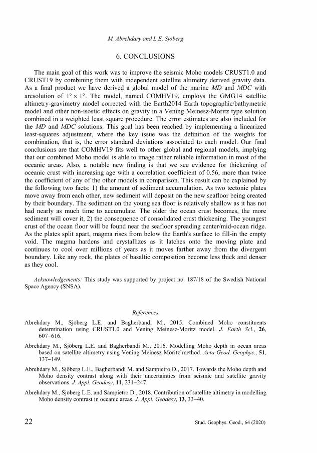
Figure 14 compares the MDCs of the new model and those of MOHV19, characterized by mainly small differences.

Fig. 13. Differences between the Moho depths estimated from COMHV19 model and from seismic regional models.

Fig. 14. Differences between the Moho density contrasts estimated from COMHV19 and the MOHV19 models.



6. CONCLUSIONS

The main goal of this work was to improve the seismic Moho models CRUST1.0 and CRUST19 by combining them with independent satellite altimetry derived gravity data. As a final product we have derived a global model of the marine MD and MDC with aresolution of 1 1. The model, named COMHV19, employs the GMG14 satellite altimetry-gravimetry model corrected with the Earth2014 Earth topographic/bathymetric model and other non-isostic effects on gravity in a Vening Meinesz-Moritz type solution combined in a weighted least square procedure. The error estimates are also included for the MD and MDC solutions. This goal has been reached by implementing a linearized least-squares adjustment, where the key issue was the definition of the weights for combination, that is, the error standard deviations associated to each model. Our final conclusions are that COMHV19 fits well to other global and regional models, implying that our combined Moho model is able to image rather reliable information in most of the oceanic areas. Also, a notable new finding is that we see evidence for thickening of oceanic crust with increasing age with a correlation coefficient of 0.56, more than twice the coefficient of any of the other models in comparison. This result can be explained by the following two facts: 1) the amount of sediment accumulation. As two tectonic plates move away from each other, new sediment will deposit on the new seafloor being created by their boundary. The sediment on the young sea floor is relatively shallow as it has not had nearly as much time to accumulate. The older the ocean crust becomes, the more sediment will cover it, 2) the consequence of consolidated crust thickening. The youngest crust of the ocean floor will be found near the seafloor spreading center/mid-ocean ridge. As the plates split apart, magma rises from below the Earth's surface to fill-in the empty void. The magma hardens and crystallizes as it latches onto the moving plate and continues to cool over millions of years as it moves farther away from the divergent boundary. Like any rock, the plates of basaltic composition become less thick and denser as they cool.

Acknowledgements: This study was supported by project no. 187/18 of the Swedish National

Space Agency (SNSA).

References

Abrehdary M., Sjöberg L.E. and Bagherbandi M., 2015. Combined Moho constituents determination using CRUST1.0 and Vening Meinesz-Moritz model. J. Earth Sci., 26, 607616.

Abrehdary M., Sjöberg L.E. and Bagherbandi M., 2016. Modelling Moho depth in ocean areas based on satellite altimetry using Vening Meinesz-Moritz’method. Acta Geod. Geophys., 51, 137149.

Abrehdary M., Sjöberg L.E., Bagherbandi M. and Sampietro D., 2017. Towards the Moho depth and Moho density contrast along with their uncertainties from seismic and satellite gravity observations. J. Appl. Geodesy, 11, 231247.

Abrehdary M., Sjöberg L.E. and Sampietro D., 2018. Contribution of satellite altimetry in modelling Moho density contrast in oceanic areas. J. Appl. Geodesy, 13, 3340.



Abrehdary M. and Sjöberg L.E., 2019. Recovering Moho constituents from satellite altimetry and gravimetric data for Europe and surroundings. J. Appl. Geodesy, 13, 291303.

Amante C. and Eakins B.W. 2009. ETOPO1 1 Arc-Minute Global Relief Model: Procedures, Data Sources and Analysis. NOAA Technical Memorandum NESDIS NGDC-24. NOAA, National Geophysical Data Center, Boulder, CO.

Andersen O.B., Knudsen P. and Berry P.A., 2010. The DNSC08GRA global marine gravity field from double retracked satellite altimetry. J. Geodesy, 84, 191199.

Bagherbandi M. and Sjöberg L.E., 2012. Non-isostatic effects on crustal thickness: a study using CRUST2.0 in Fennoscandia. Phys. Earth Planet. Inter., 200201, 3744.

Bai Y., Williams S.E., Müller R.D., Liu Z. and Hosseinpour M., 2014. Mapping crustal thickness using marine gravity data: Methods and uncertainties. Geophysics, 79, G27G36.

Bai Y., Li M., Wu S., Dong D., Gui Z., Sheng J. and Wang Z., 2019. Upper mantle density modelling for large-scale Moho gravity inversion: case study on the Atlantic Ocean. Geophys. J. Int., 216, 21342147.

Bassin C., Laske G. and Masters T.G., 2000. The current limits of resolution for surface wave tomography in North America. Eos Trans. AGU, 81, F897.

Baranov A. and Morelli A, 2013. The Moho depth map of the Antarctica region. Tectonophysics, 609, 299313.

Carlson R.L. and Raskin G.S., 1984. Density of the ocean crust. Nature, 311, 555558. Chappell A.R. and Kusznir N.J., 2008. Three-dimensional gravity inversion for Moho depth at rifted

continental margins incorporating a lithosphere thermal gravity anomaly correction. Geophys. J. Int., 174, 113.

Christensen N. and Mooney W., 1995. Seismic velocity structure and composition of the continental crust: A global view. J. Geophys. Res.-Atmos., 100, 97619788.

Chulick G. and Mooney W., 2002. Seismic structure of the crust and uppermost mantle of North America and adjacent ocean basins: A synthesis. Bull. Seismol. Soc. Amer., 92, 24782492.

Chulick G.S., Detweiler S. and Mooney W.D., 2013. Seismic structure of the crust and uppermost mantle of South America and surrounding oceanic basins. J. South Am. Earth Sci., 42, 260276.

Danesi S. and Morelli A., 2001. Structure of the upper mantle under the Antarctic Plate from surface wave tomography. Geophys. Res. Lett., 28, 43954398.

Eshagh M., Bagherbandi M. and Sjöberg L., 2011. A combined global Moho model based on seismic and gravimetric data. Acta Geod. Geophys. Hung., 46, 2538.

Grad M. and Tiira T., 2009. The Moho depth map of the European Plate. Geophys. J. Int., 176, 279292.

Hamayun H., 2014. Global Earth Structure Recovery from State-of-the-Art Models of the Earth’s Gravity Field and Additional Geophysical Information. PhD Thesis. Delft University of Technology, Delft, The Netherlands.

Hansen S.E., Nyblade A.A., Heeszel D.S., Wiens D.A., Shore P. and Kanao M., 2010. Crustal structure of the Gamburtsev Mountains, East Antarctica, from S-wave receiver functions and Rayleigh wave phase velocities. Earth Planet. Sci. Lett., 300, 395401.

Hello Y., Ogé A., Sukhovich A. and Nolet G., 2011. Modern mermaids: New floats image the deep Earth. Eos Trans. AGU, 92(40), 337338.



Hirt C. and Rexer M., 2015., Earth2014: 1 arc-min shape, topography, bedrock and ice-sheet models - Available as gridded data and degree-10,800 spherical harmonics. Int. J. Appl. Earth Obs. Geoinf., 39, 103112.

Kanao M., Fujiwara A., Miyamachi H., Toda S., Ito K., Tomura M., Ikawa T. and Group T.S.G., 2011. Reflection imaging of the crust and the lithospheric mantle in the Lützow-Holm complex, Eastern Dronning Maud Land, Antarctica, derived from the SEAL transects. Tectonophysics, 508, 7384.

Kennett B.L.N., Salmon M. and Saygin E., 2011. AusMoho: the variation of Moho depth in Australia. Geophys. J. Int., 187, 946958.

Kind R., Yuan X. and Kumar P., 2012. Seismic receiver functions and the lithosphere-asthenosphere boundary. Tectonophysics, 536, 2543.

Kobayashi R. and Zhao D., 2004. Rayleigh-wave group velocity distribution in the Antarctic region. Phys. Earth Planet. Inter., 141, 167181.

Laske G., Ma Z., Masters G. and Pasyanos M.E., 2013. A New Global Crustal Model at 1 1 Degrees (CRUST1.0). http://igppweb.ucsd.edu/~gabi/crust1.html.

Laske G. and Masters G., 1997. A global digital map of sediment thickness. Eos Trans. AGU, 78(F483).

Lebedev S., Adam J.M.C. and Meier T., 2013. Mapping the Moho with seismic surface waves: a review, resolution analysis, and recommended inversion strategies. Tectonophysics, 609, 377394.

Lloyd S., van der Lee S., Franca G.S., Assumpcao M. and Feng M., 2010. Moho map of South America from receiver functions and surface waves. J. Geophys. Res.-Solid Earth, 115, B11315.

Marone F., Van Der Meijde M., Van Der Lee S. and Giardini D., 2003. Joint inversion of local, regional and teleseismic data for crustal thickness in the Eurasia-Africa plate boundary region. Geophys. J. Int., 154, 499514.

Meier U., Curtis A. and Trampert J., 2007. Global crustal thickness from neural network inversion of surface wave data. Geophys. J. Int., 169, 706722.

Mooney W.D., Laske G. and Masters T.G., 1998. CRUST5.1: A global crustal model at 5 5. J. Geophys. Res.-Solid Earth, 103, 727747.

Müller R.D., Sdrolias M., Gaina C. and Roest W.R., 2008. Age, spreading rates, and spreading asymmetry of the world's ocean crust. Geochem. Geophys. Geosyst., 9, Q04006.

Pasyanos M.E. and Nyblade A.A., 2007. A top to bottom lithospheric study of Africa and Arabia. Tectonophysics, 444, 2744.

Prodehl C. and Mooney W.D. (Eds), 2012. Exploring the Earth’s Crust - History and Results of Controlled-Source Seismology. GSA Memoir 208. Geological Society of America, Boulder, CO.

Rapp R.H., 1980. A comparison of altimeter and gravimetric geoids in the Tonga Trench and Indian Ocean areas. Bull. Geod., 54, 149163.

Reguzzoni M. and Sampietro D., 2015. GEMMA: An Earth crustal model based on GOCE satellite data. Int. J. Appl. Earth Obs. Geoinf., 35, 3143.

Reguzzoni M., Sampietro D. and Sansò F., 2013. Global Moho from the combination of the CRUST2.0 model and GOCE data. Geophys. J. Int., 195, 222237.



Ritzwoller M.H., Shapiro N.M., Levshin A.L. and Leahy G.M., 2001. Crustal and upper mantle structure beneath Antarctica and surrounding oceans. J. Geophys. Res.-Solid Earth, 106, 3064530670.

Sandwell D.T., Müller R.D., Smith W.H., Garcia E. and Francis R., 2014. New global marine gravity model from CryoSat-2 and Jason-1 reveals buried tectonic structure. Science, 346, 6567.

Shapiro N.M. and Campillo M., 2004. Emergence of broadband Rayleigh waves from correlations of the ambient seismic noise. Geophys. Res. Lett., 31, L07614.

Sjöberg L.E., 2009. Solving Vening Meinesz-Moritz inverse problem in isostasy. Geophys. J. Int., 179, 15271536.

Sjöberg L.E., 2013. On the isostatic gravity anomaly and disturbance and their applications to Vening Meinesz-Moritz gravimetric inverse problem. Geophys. J. Int., 193, 12771282.

Sjöberg L.E. and Bagherbandi M., 2011. A method of estimating the Moho density contrast with a tentative application of EGM08 and CRUST2.0. Acta Geophys., 59, 502525.

Sjöberg L.E., Bagherbandi M. and Tenzer R., 2015. On gravity inversion by no-topography and rigorous isostatic gravity anomalies. Pure Appl. Geophys., 172, 26692680.

Szwillus W., Afonso J.C., Ebbing J. and Mooney W.D., 2019. Global crustal thickness and velocity structure from geostatistical analysis of seismic data. J. Geophys. Res.-Solid Earth, 124, 16261652.

Sutra E. and Manatschal G., 2012. How does the continental crust thin in a hyperextended rifted margin? Insights from the Iberia margin. Geology, 40, 139142.

Tenzer R. and Bagherbandi M., 2012. Reformulation of the Vening Meinesz-Moritz inverse problem of isostasy for isostatic gravity disturbances. Int. J. Geosci., 3, 918929.

Tenzer R. and Chen W., 2014. Expressions for the global gravimetric Moho modeling in spectral domain. Pure Appl. Geophys., 171, 18771896.

Tenzer R., Chen W., Tsoulis D., Bagherbandi M., Sjöberg L.E., Novák P. and Jin S., 2015a. Analysis of the refined CRUST1.0 crustal model and its gravity field. Surv. Geophys., 36, 139165.

Tenzer R., Chen W. and Jin S., 2015b. Effect of upper mantle density structure on Moho geometry. Pure Appl. Geophys., 172, 15631583.

Wang T., Lin J., Tucholke B. and Chen Y.J., 2011. Crustal thickness anomalies in the North Atlantic Ocean basin from gravity analysis. Geochem. Geophys. Geosyst., 12, Q0AE02.

Zhu L. and Kanamori H., 2000. Moho depth variation in southern California from teleseismic receiver functions. J. Geophys. Res.-Solid Earth, 105(B2), 29692980.

Zhou Y., Nolet G., Dahlen F.A. and Laske G., 2006. Global upper‐mantle structure from finite‐frequency surface‐wave tomography. J. Geophys. Res.-Solid Earth, 111(B4), B04304.

Documents

Estimating a combined Moho model for marine areas via