Estimates of species-area power law parameters vary

Estimates of species-area power law parameters

vary strongly by scale and location. DRAFT OF

SUBMISSION TO EvolEcolResearch

Henri Laurie∗

Mathematics and Applied Mathematics, University of Cape Town

Rondebosh

7701

South Africa Tony Rebelo

Protea Atlas Project, National Botanical Institute

Private Bag X7

Kirstenbosch

7730

John A. Silander, Jr

Ecology and Evolutionary Biology, University of Connecticut

Storrs CT 06268-3042

Walter Smit

Protea Atlas Project, National Botanical Institute

Private Bag X7

Kirstenbosch

7730

October 18, 2006

∗To whom correspondence should be addressed.

1

Abstract

Question: How much do parameter estimates of power-law species-area

relationships depend on sampling?

Data description: From the Protea Atlas data we use > 250 000 records

of the 372 known species of Proteaceae that occur in the 9 426 1′× 1′ cells

that cover the Fynbos biome in the Cape Floristic Region.

Methods: The species-area relationship is assumed to be N = cAz, where

N is the species count in a region of area A. log(c) and z were estimated by

linear regression of log(S) on log(A). Samples of A were constructed to vary

by location but not by scale, or to vary by scale but not by location, or to

vary by both. Some samples were terminated when they included the whole

CFR, and some when they included a whole sub-region. One sub-region not

formally part of the CFR is included in some subregional estimates.

Conclusion: When sample A varies by scale as well as location, z ≈ 0.47

and log(c) ≈ 0.64. When sample A varies by location but not by scale, z ≈ 1.

When sample A varies by scale but not by location, z and log(c) are approxi-

mately normally distributed with means E[z] ≈ 0.4611 and E[log(c)] ≈ 0.6664

and variances Var[z] ≈ 0.0061 and Var[log(c)] ≈ 0.0860. In this case the quan-

tities log(c), z and N1/×1′ for a given location are pairwise strongly correlated.

The residuals of these correlations show evidence of spatial pattern.

Keywords: species-area curve, spatial variation, species richness, Protea

Atlas, Fynbos, Proteaceaee, Cape Floristic Region

2

Introduction

Species-area curves are widely considered to be of fundamental ecological

significance (Rosenzweig 1995; Lomolino 2001; Ney-Nifle and Mangel 2000;

Driver et al. 2003). This significance is typically interpreted as follows: the

parameters of a species-area curve fitted to data from some coherent ecological

entity are a property of that entity. In that sense, a simple curve summarises

the spatial pattern of species richness. In particular, one should be able to

predict species richness simply from area. This would be very useful in con-

servation management (Driver et al. 2003). The areas in question span the

range from landscapes (< 102 km2) to continents(> 106 km2).

We report here that detailed analysis of fine-grained data on species oc-

curence does not support such an ambitious interpretation.

We studied at a large data set for the distribution of all Proteaceae that

occur in the entire Cape Floristic Region (CFR henceforth). We use the

Arrhenius formula N = cAz, where N is the number of species and A is

the area. We expect other two-parameter functions to give similar results

(see Connor and McCoy (1979) and Matter et al. (2002) for other possible

formulae). If the curve were a property of the entire area, applicable to all

sub-areas inside it, then any representative set of data pairs (Ai, Ni) should

yield satisfactory estimates of the parameters c and z. This is not the case;

instead, the estimates depend strongly on how the data pairs (Ai, Ni) are

selected. Indeed, it is possible to select Ai that have a common location

(thus getting estimates at many locations), or that have a common scale

(thus getting estimates for several scales) or that vary across both scale and

location. We report surprising variability and a mixture of compatibility and

incompatibility between the resulting estimates.

Methods

Our data come from the Protea Atlas Project (http://protea.worldonline.

co.za) records of Proteaceae. The basic Protea Atlas site record sheet gives a

census of all species of Proteaceae present in a centrally geo-referenced area of

uniform habitat up to 500 m in diameter (Rebelo 1991). Data were collected

by professionals and by amateurs under professional supervision. We limited

ourselves to the Fynbos biome (Cowling 1992) which is endemic to the Cape

3

Floristic Region, the smallest of the worlds six floristic regions (Takhtajan

1986). Thus our study concerns all species of a clade occuring in all of one

vegetation type endemic to an entire biome. Moreover, the species in this

study are all endemic to Fynbos. Our final data set contained 252 513 records

of 374 species at 61 591 record localities.

The analyses below were based on counts constructed as follows. We

started with a raster of 1′× 1′ cells (roughly 28 000 of them). From this

we amalgamated adjacent cells to obtain larger units of sizes 3′× 3′, 7′

× 7′,

15′×15′, 31′

×31′, 63′×63′, 127′

×127′, 255′×255′, 511′

×511′ and 1023′×1023′.

Thus this study is at ten levels of focus, in the sense of Scheiner et al. (2000).

The larger units overlap to some extent. Each of the larger units was cen-

tred on a 1′× 1′ cell, called its “focal cell” henceforth. Every focal cell is at

the centre of a full sequence of associated larger units. These are similar to

the nested sequences used in Koleff and Gaston (2002), where the units are

termed “tetrads”.

For the purposes of this study, a cell was regarded as a Fynbos cell if it

contained a Protea Atlas record, which is acceptable at these scales. Our

database contains 9 426 Fynbos cells for the entire CFR. For the sub-regional

analyses, we included cells from the Alexandria sub-region of the Protea Atlas

(see Figure 1), which although not part of the CFR is adjacent to it.

We counted the number N of Proteaceae species present in each unit. We

also found the area A occupied by Fynbos in a unit as the count of Fynbos

cells in that unit. At the largest scale, each one of the 1023′× 1023′ units

contains all of the Fynbos cells.

For each of the estimates below, we assembled an appropriate data series

of the form (Ai, Ni). Upon taking logarithms, the Arrhenius equation be-

comes log(N) = log(c) + z log(A). We obtained estimates of intercept log(c)

and slope z by least-squares fits to (log(Ai), log(Ni)). We used the following

software packages: ARC-GIS, ARC-INFO, ARC-MAP, MS-Excel, gnumeric

and Octave.

The Cape Floristic Region has been divided into several sub-regions in

the past. Here we use sub-regions based on centres of endemism for the

Proteaceae (modified from Cowling, Holmes, and Rebelo 1992) (see Figure 1).

All but two of the sub-regions are simply connected and also contiguous with

another, so that they form a simply connected whole. The twe exceptions are

4

the Karoo Islands and Swartberg Islands subregions, each of which comprise

several isolated pockets of Fynbos within other vegetation types.

[Figure 1 about here.]

For each sub-region, we classified a cell as in the sub-region if more than

50% of the cell’s area falls in the sub-region.

Samples that vary by location and by scale

When all units of all sizes are considered, one gets a data set with approxi-

mately 100 000 (Ai, Ni) pairs. This set gives a single estimate of the intercept

log(c) and slope z of the Arrhenius line in log-log space.

We also constructed for each sub-region a data set from the counts of all

units of all sizes in that sub-region. This gives 29 estimates of the Arrhenius

parameters, one for each sub-region.

The subregions themselves were also considered as areal units. This yields

a shorter data set, of 29 (Ai, Ni) pairs, where each Ai is the number of

Fynbos cells of a sub-region and Ni the corresponding species count. Only

one estimate of parameters comes from this data set.

Samples that vary by location but not by scale

Consider all units of a given size, for example 7′× 7′. It is obvious that they

will vary in the number of species they contain. However, at all sizes except

1′× 1′ and 1023′

× 1023′, they also contain different amounts of Fynbos cells.

So by using all units of a given size, we may construct data sets where the

counts vary by location but not by scale. “Scale” in this sense is very similar

to “focus” Scheiner et al. (2000).

We did this for the entire CFR, which gave 8 single-scale estimates of the

parameters log(c) and slope z.

We repeated this for each sub-region. The results were similar, and we do

not report them here.

Samples that vary by scale by not by location

For each focal cell, we considered the 10 units centred on that cell (for a similar

nested sampling method, see Preston 1960 and Rosenzweig 1995). Since the

5

units in such a sample have a common centre but different sizes, they vary by

scale but not location.

For the whole CFR, these data sets yielded 9 426 pairs of Arrhenius pa-

rameters, one for each 1′× 1′ cell. We refer to this as the “nested series, full

CFR” parameter estimates.

For sub-regions, each nested series was terminated at the first unit in which

the entire sub-region was contained (of course cells from outside the sub-region

were ignored). Locations in different sub-regions have different sample sizes,

determined by the unit area encompassing the entire sub-region; the largest

unit varied from 15′× 15′ to 511′

× 511′. We refer to parameter estimates

from these data sets as “nested series, sub-regional” values.

Thus each of the Fynbos cells in the CFR yielded two curves: one for

the entire CFR and one for its sub-region and correspondingly two pairs of

Arrhenius parameters. Additionally, the cells in the Alexandria sub-region

each yielded a pair of parameter estimates. Because each estimate has a

geographic reference, namely the central cell, maps of a given parameter (may)

reveal spatial variation.

For each sub-region we constructed a nested series with that sub-region at

its centre. Adjacent subregions were added until the full CFR was reached.

This yielded 29 estimates of Arrhenius parameter pairs, each of them spatially

referenced to a particular sub-region.

Results

Variation across location and scale

The species-area relationships across all units in the entire CFR is shown as

pair of scatter-plots in Figure 2. The Arrhenius parameters are log(c) ≈ 0.64

and z ≈ 0.47. The latter value is rather high compared to traditionally ex-

pected values (Rosenzweig 1995; Preston 1960) and reported values (Cowling

et al. 1992; Driver et al. 2003; Proches et al. 2004).


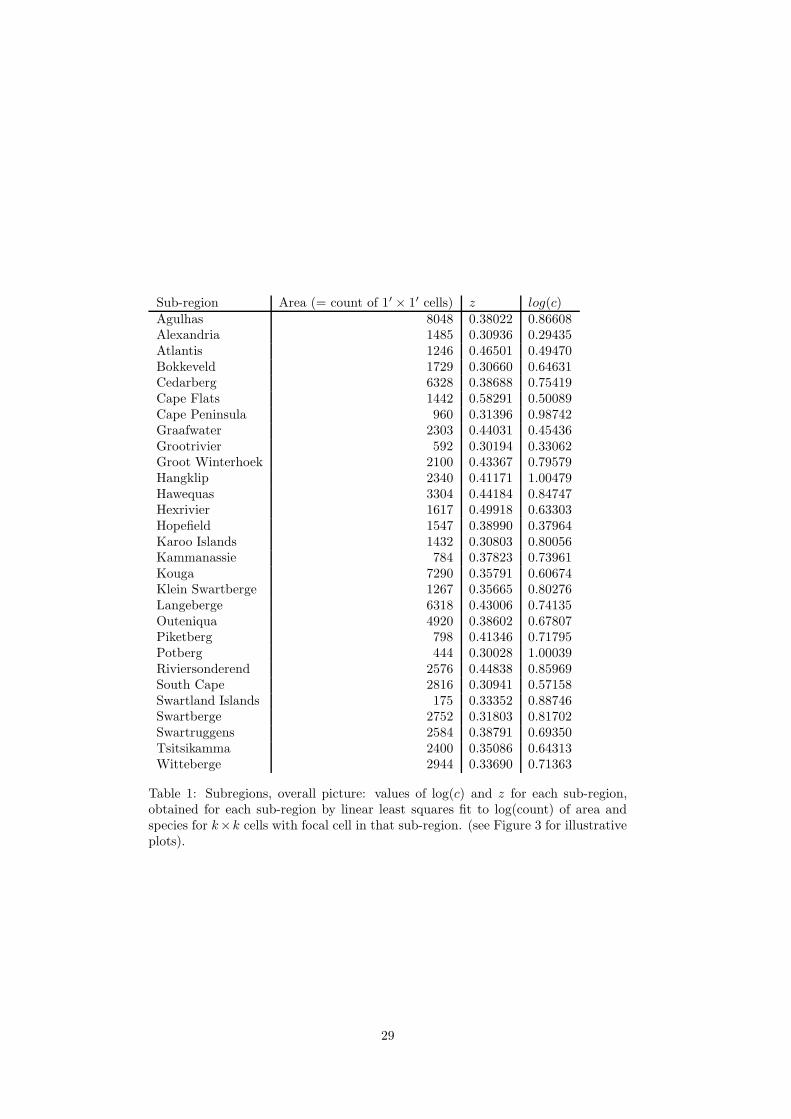
Subregional data are exemplified by the four scatterplots in Figure 3. The

29 estimated parameter values for all cells at all relevant focus levels (i.e. the

largest scale is the smallest at which the entire region is included for every

focal cell) for each sub-region are given in Table 1.

6


[Table 1 about here.]

Across the subregions, the estimates are log(c) = 0.40 and z = 0.50 (see

Figure 4)


Variation by location but not by scale

At a single focus, the estimates for the Arrhenius slopes are far higher than

over the entire data set (Figure 2). Single-focus slopes (z) show a decrease

from 1.22 (3′× 3′) to 0.88 (31′

× 31′) over smaller scales, but then increase to

1.25 (127′×127′) and decrease to 1.08 (511′

×511′) at the largest relevant focus

level. Note that 63′× 63′ to 127′

× 127′ are the focus levels that correspond

best to the area of the sub-regions, so that the increase over intermediate

scales might be a sub-regional effect.

Intercept (log(c)) is positive only for the smallest focus level (the estimate

at 3′× 3′ is about 1.4 species per cell). It goes down to log(c) = −2.05 at

127′× 127′, which is about 0.006 species per cell, and then increases slightly.

These unrealistic values are explained as follows. At the larger scales, none

of the units contain only one cell. Estimates of log(c) at these levels are

extrapolations beyond the data, and there is no reason to expect them to be

realistic. In contrast, the overall estimate of log(c) ≈ 0.64 of the previous

section gives around 4 species per 1′× 1′ cell. This matches the data, which

gives a mean of 6.86 species per cell, with a standard deviation of 5.09.

At the larger scales, the units overlap substantially. The resultant correla-

tion decreases the apparent variance in both log(A) and log(N). In principle,

this could be corrected by calculating the effective sample size, but since no

statistical inference was attempted in this paper, we did not do so.

Variation by scale but not by location

We now turn to nested data, where all the units in a given data set have

a common centre but different scales. This gives a spatial reference to the

resulting estimates of log(c) and z. Each data set contains at most 10 pairs,

but there are very many of them. In fact, for each of the approximately

10 000 cells in the CFR, there are two data sets and two pairs of Arrhenius

7

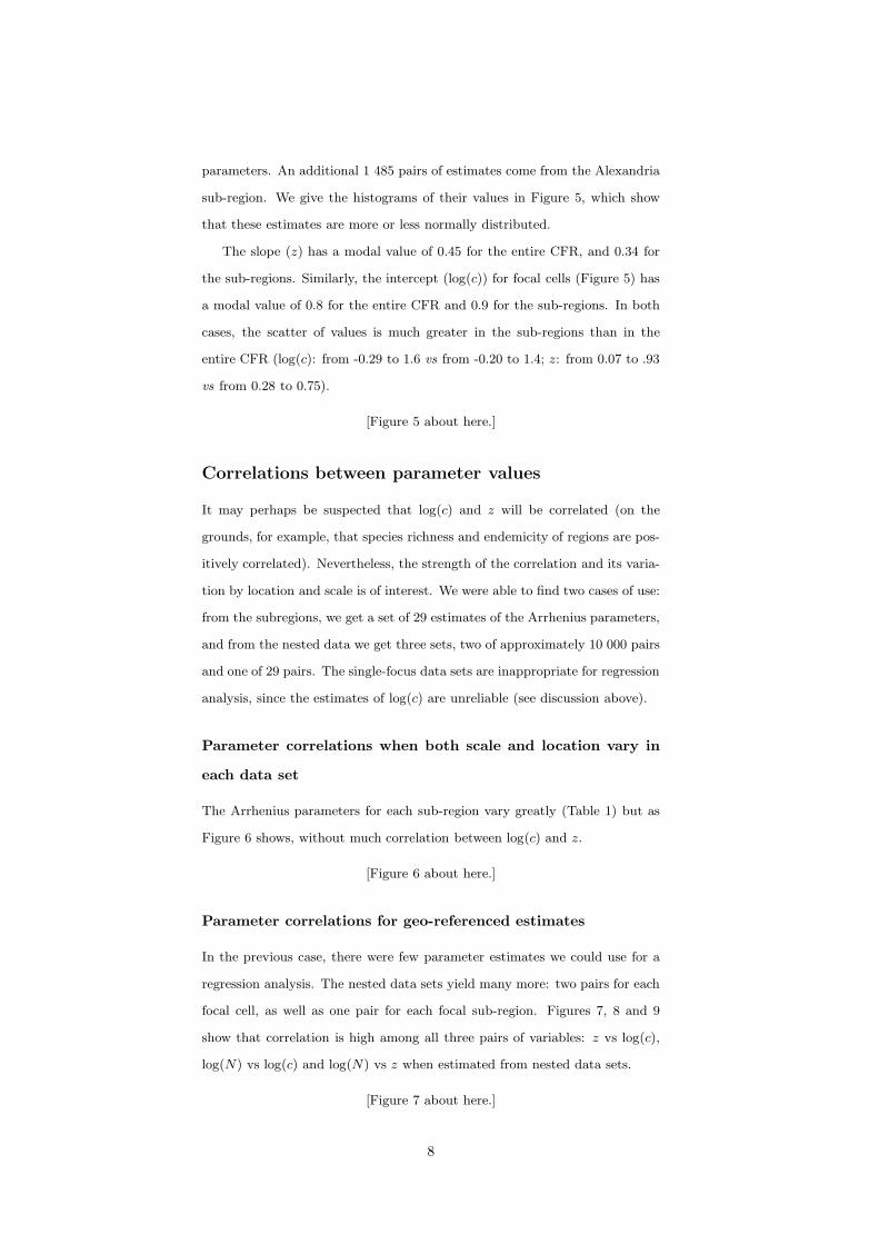
parameters. An additional 1 485 pairs of estimates come from the Alexandria

sub-region. We give the histograms of their values in Figure 5, which show

that these estimates are more or less normally distributed.

The slope (z) has a modal value of 0.45 for the entire CFR, and 0.34 for

the sub-regions. Similarly, the intercept (log(c)) for focal cells (Figure 5) has

a modal value of 0.8 for the entire CFR and 0.9 for the sub-regions. In both

cases, the scatter of values is much greater in the sub-regions than in the

entire CFR (log(c): from -0.29 to 1.6 vs from -0.20 to 1.4; z: from 0.07 to .93

vs from 0.28 to 0.75).


Correlations between parameter values

It may perhaps be suspected that log(c) and z will be correlated (on the

grounds, for example, that species richness and endemicity of regions are pos-

itively correlated). Nevertheless, the strength of the correlation and its varia-

tion by location and scale is of interest. We were able to find two cases of use:

from the subregions, we get a set of 29 estimates of the Arrhenius parameters,

and from the nested data we get three sets, two of approximately 10 000 pairs

and one of 29 pairs. The single-focus data sets are inappropriate for regression

analysis, since the estimates of log(c) are unreliable (see discussion above).

Parameter correlations when both scale and location vary in

each data set

The Arrhenius parameters for each sub-region vary greatly (Table 1) but as

Figure 6 shows, without much correlation between log(c) and z.


Parameter correlations for geo-referenced estimates

In the previous case, there were few parameter estimates we could use for a

regression analysis. The nested data sets yield many more: two pairs for each

focal cell, as well as one pair for each focal sub-region. Figures 7, 8 and 9

show that correlation is high among all three pairs of variables: z vs log(c),

log(N) vs log(c) and log(N) vs z when estimated from nested data sets.


8



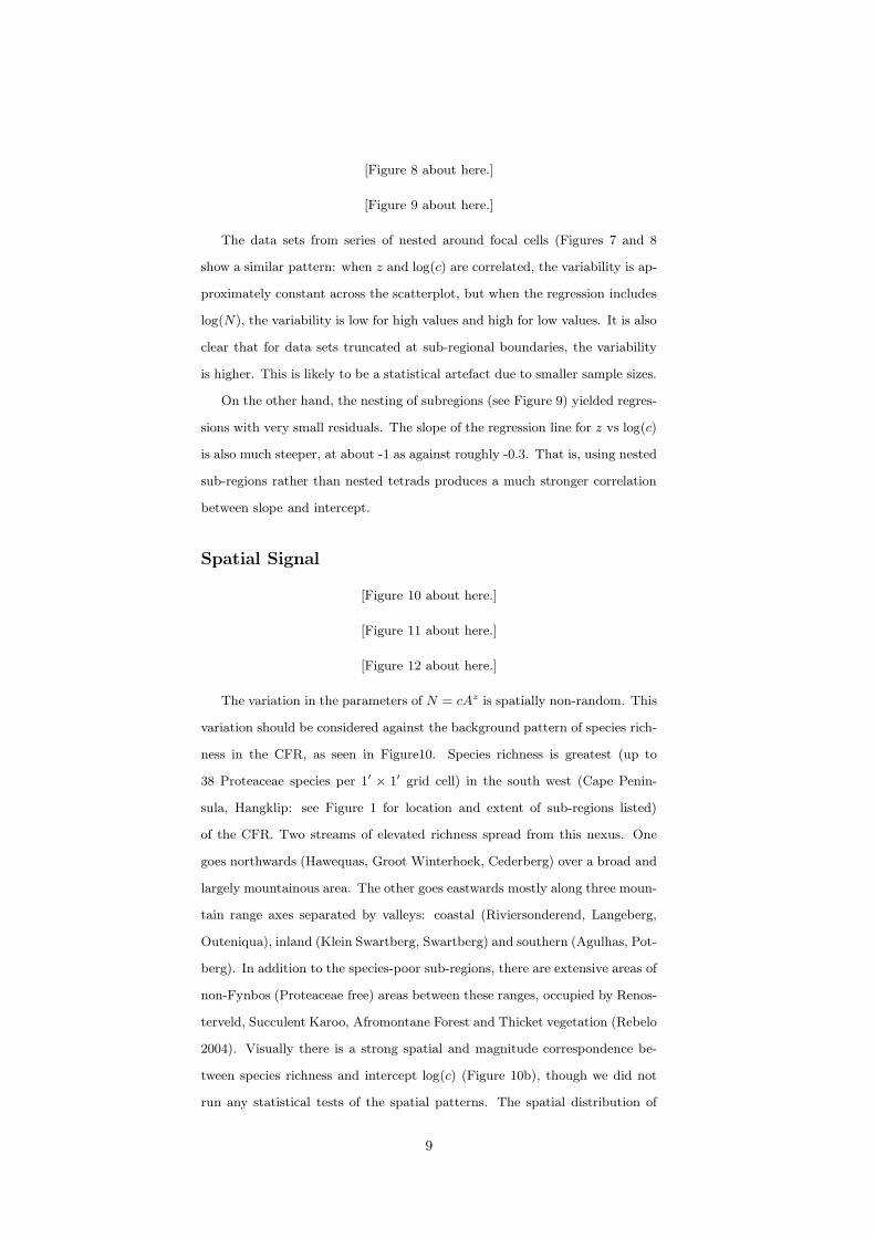
The data sets from series of nested around focal cells (Figures 7 and 8

show a similar pattern: when z and log(c) are correlated, the variability is ap-

proximately constant across the scatterplot, but when the regression includes

log(N), the variability is low for high values and high for low values. It is also

clear that for data sets truncated at sub-regional boundaries, the variability

is higher. This is likely to be a statistical artefact due to smaller sample sizes.

On the other hand, the nesting of subregions (see Figure 9) yielded regres-

sions with very small residuals. The slope of the regression line for z vs log(c)

is also much steeper, at about -1 as against roughly -0.3. That is, using nested

sub-regions rather than nested tetrads produces a much stronger correlation

between slope and intercept.

Spatial Signal




The variation in the parameters of N = cAz is spatially non-random. This

variation should be considered against the background pattern of species rich-

ness in the CFR, as seen in Figure10. Species richness is greatest (up to

38 Proteaceae species per 1′× 1′ grid cell) in the south west (Cape Penin-

sula, Hangklip: see Figure 1 for location and extent of sub-regions listed)

of the CFR. Two streams of elevated richness spread from this nexus. One

goes northwards (Hawequas, Groot Winterhoek, Cederberg) over a broad and

largely mountainous area. The other goes eastwards mostly along three moun-

tain range axes separated by valleys: coastal (Riviersonderend, Langeberg,

Outeniqua), inland (Klein Swartberg, Swartberg) and southern (Agulhas, Pot-

berg). In addition to the species-poor sub-regions, there are extensive areas of

non-Fynbos (Proteaceae free) areas between these ranges, occupied by Renos-

terveld, Succulent Karoo, Afromontane Forest and Thicket vegetation (Rebelo

2004). Visually there is a strong spatial and magnitude correspondence be-

tween species richness and intercept log(c) (Figure 10b), though we did not

run any statistical tests of the spatial patterns. The spatial distribution of

9

the intercept (log(c)) mirrors the species richness patterns, but smooths the

data to some degree, with values of up to 1.436 (or 27 species per cell) and as

low as -0.29 (or 0.51 species per cell). Slope z shows a similar pattern (Fig-

ure 10c), except that the relationship is inverted and there is a proportionally

lower z for some of the eastern peripheral sub-regions (Kouga, Tsitsikamma).

The inverted relationship between log(c) and z is expected because they are

negatively correlated (see above).

However, even the residuals show a strong spatial signal (Figure 11). The

residual of the slope z as predicted by the intercept log(c) (Figure 11a), shows

a very strong southwestern over-prediction, with a radial decrease outwards

towards a strong under-prediction in the north and especially the east. The

residual of richness as predicted from the intercept log(c) (Figure 11b) shows

an over-prediction on the species-poor periphery of the CFR, with an under-

prediction in the southwest. By contrast, the residual of richness as predicted

from the slope z (Figure 11c), shows an under-prediction in the species-poor

eastern portion of the CFR and an over-prediction on the species-poor western

and northern regions.

Apart from the broad patterns, a fine-scale signal also exists. An inspection

of the contiguous areas (blocks) of Fynbos shows that the residual of slope z

as predicted by intercept log(c) (Figure 11a), is greater on the edges in the

south-west and northwards, but lower on the edges in the east. The residual

of species richness predicted log(N) from the intercept log(c) (Figure 11b)

also shows that the edges of the blocks are under-predicted in the south-

west, and over-predicted in the east, although the pattern is not as distinct

as previously. However, the residual of species richness as predicted by slope

z (Figure 11c), shows a consistent pattern of over-prediction on the edges of

blocks, and under-prediction at their centres.

Comparison with the spatial signal for data series truncated at the edges

of subregions (Figure 12) reveals that these patterns are not a feature of the

CFR. Instead, they are determined by the termination of the data sets (i.e.

whether at sub-region or CFR boundary). In each case, we find exactly the

same patterns of over-prediction and under-prediction, both regional and fine-

scale and for each parameter.

10

Discussion

Almost every point we wish to make in discussing these results can be illus-

trated by reference to Figure 2. What is seen very clearly is that the (A,N)

data pairs fill a clearly delineated region, more or less triangular, on the log-log

plot. Two points stand out:

1. the tendency of species number to increase with area is apparent from

upper and lower boundaries of the scatterplot, which both have positive

slope, and

2. the variance in S is large for small A and small for large A.

Figure 3 illustrates similar data for counts internal to the sub-regions; they

exhibit the same two features noted above. The 29 (A, N) pairs for the area

and number of species of each sub-region plotted in Figure 4 again repeats

this pattern.

A species-area curve for Proteaceae in Fynbos would summarise all these

scatterplots in a single formula; if we use S = cAz then Figure 2 leads us

to z = 0.47 via a least-squares fit. This value has independent support from

the sub-regional counts in Figure 4, where z = 0.50 is obtained. We note that

the nested tetrad z values in Figure 5, while also consistent with Figure 2, do

not amount to an independent confirmation, as Figure 2 is the superposition

of these nested data sets, which are pair-wise disjoint and each contain one

(A,N) pair from each focus level.

So is the CFR characterised by z ≈ 0.47? Unfortunately, our data give

conflicting values. First, if we use all tetrads internal to the sub-regions, we

get the distinctly lower estimates of Table 1. On the other hand, for (A,N)

pairs taken from a single focus level, the values of z are very much higher,

quite inconsistent with z ≈ 0.5. Nevertheless, they are consistent with each

other, and support a value of z ≈ 1, on k′× k′ tetrads for a fixed k. These

inconsistencies appear to reflect differences in the sampling schemes: in the

cases where z ≈ 0.5, the values of A span much larger intervals than in the

cases where z ≈ 1. However, this cannot be the full explanation, since a simple

vertical slice over a relatively narrow range [A, A+δA] in Figure 2 would yield

an estimate of z consistent with z ≈ 0.5. Instead, it appears that the data for

such an [A, A + δA] slice comes from several focus levels, and that the higher

values of N come from focus levels with smaller k. Thus within focus levels

11

there is a strong bias against tetrads with small A and large N ; we are unable

to suggest an explanation for this bias.

The foregoing tends to undermine our confidence in the validity of esti-

mates of z. The huge variance in N at low A makes things no better. It causes

variability in the nested tetrad estimates, as follows. Every nested tetrad data

set in Figure 2 starts with a 1′× 1′ cell with an (A, N) pair that lies on the

log(c) axis, and then moves along a non-decreasing line to a 1023′× 1023′

tetrad containing the whole Fynbos. They all end at the same (A,N) pair,

and therefore lines that start with high N must climb more slowly than lines

that start at low N . Thus the high variance of N at low A not only means

that N = cAz is subject to large error at low A, but also that nested sam-

pling schemes will yield negatively correlated estimates of log(c) and z, as is

reported in Figures 7 and 9. Moreover, the wider the range of richness at low

A, the wider will be the range of estimates of log(c) and z.

The correlation of log(c) and z with log(S) accounts for the similarity in

their spatial variation displayed in Figure 10. But since the residual is not

random, as shown in Figures 11 and 12, there is an additional, purely spatial

effect. It appears to make a difference whether the focal cell of nested tetrads

is near or far from an extremity of Fynbos. This is true at the relatively small

scale of transitions between Fynbos and other vegetation types within the

CFR as well as the larger scale of the CFR as a whole. We noted above that

at a given A, the larger values of N tend to come from tetrads with smaller k.

Now, for two tetrads of different k to have similar A it is necessary for the

Fynbos cells to fill the larger tetrad less densely; this is often the case near

the boundaries of the Fynbos biome at small and large scale. It seems that

the relation between log(c) and z near the edges of the Fynbos biome differs

from how these parameters interact away from edges.

We conclude that parameter estimates of the Arrhenius curve for Pro-

teaceae in Fynbos strongly varies in space and is subject to large sampling

error. Let us briefly reflect on what this uncertainty may imply.

The classical use of S = cAz in theoretical ecology is in the comparison of

otherwise very different spatial domains (Rosenzweig 1995; Lomolino 2001).

We note first of all that the full, set-valued species-area relationship, as shown

for example in Figure 2, could in principle be used for these comparisons. It

would be cumbersome but rigorous. The data requirements for such compar-

12

isons are so onerous that in many cases the available data would not suffice, as

they do not get anywhere near being exhaustive. Moreover, sampling schemes

often differ among data sets. Nevertheless, the full, i.e. set-valued, species-

area relationship would enable comparisons of the classical kind and even

support statistical inference. In the absence of representative and comparable

set-valued species-area data, one must be cautious about conclusions based

on Arrhenius parameters.

When N = cAz is to be used in conservation (as in for instance Driver

et al. (2003)), there is an additional cause for caution. Reserves, by definition,

have relatively small A. In species-area terms, this means that the included N

may well be of high variance. It is highly unlikely that the Arrhenius formula

is a good predictor of A at the scale of a typical reserve, and it will be even

less so at the even smaller scale of extensions to existing reserves.

Acknowledgments: Partly funded by NSF (Grant # DEB008901) and

as a part of the Bayesian Macro-Ecology Working Group supported by the

National Center for Ecological Analysis and Synthesis, a Center funded by

NSF (Grant #DEB-94-21535), the University of Santa Barbara, and the State

of California.

References

Arita, H. and Rodrıguez, P. 2002. Geographic range, turnover rate and the

scaling of species diversity. Ecography 25, 541–550.

Azovsky, A. 2002. Size-dependent species-area relationships in benthos: is

the world more diverse for microbes? Ecography 25, 273–282.

Banavar, J., Green, J., Harte, J., and Maritan, A. 1999. Finite size scaling

in ecology. Physical Review Letters 83, 4212–4214.

Borda-de Agua, L., Hubbell, S., and McAllister, M. 2002. Species-area

curves, diversity indices, and species abundance distributions: a multi-

fractal analysis. The American Naturalist 159, 138–155.

Connor, E. and McCoy, E. 1979. The statistics and biolgogy of the species-

area relationship. The American Naturalist 113, 791–833.

Cowling, R., ed. 1992. The Ecology of Fynbos: Nutrients, Fire and Diver-

sity. Cape Town: Oxford University Press.

Cowling, R., Holmes, P., and Rebelo, A. 1992. Plant diversity and en-

13

demism. In The Ecology of Fynbos: Nutrients, Fire and Diversity (R.

Cowling, ed), pp. 62–112. Cape Town: Oxford University Press.

Driver, A., Desmet, P., Rouget, M., Cowling, R., and Maze, K. 2003. Suc-

culent Karoo Ecosystem Plan. Technical Report CCU 1/03, Cape Con-

servation Unit of the Botanical Society of South Africa, Cape Town.

Hanski, I. and Gyllenberg, M. 1997. Uniting two general patterns in the

distribution of species. Science 275, 397–400.

Harte, J., Blackburn, T., and Ostling, A. 2001. Self-similarity and the re-

lationship between abundance and range size. The American Natural-

ist 157, 374–386.

Harte, J. and Kinzig, A. 1997. On the implications of species-area relation-

ships for endemism, spatial turnover, and food web patterns. Oikos 80,

417–427.

Harte, J., Kinzig, A., and Green, J. 1999. Self-similarity in the distribution

and abundance of species. Science 284, 334–336.

Harte, J., McCarthy, S., Taylor, K., Kinzig, A., and Fischer, M. 1999.

Estimating species-area relationships from plot to landscape scale using

species turnover data. Oikos 86, 45–54.

Koleff, P. and Gaston, K. 2002. The relationship between local and re-

gional species richness and spatial turnover. Global Ecology and Bio-

geography 11, 363–375.

Leitner, W. and Rosenzweig, M. 1997. Nested species-area curves and

stochastic sampling: a new theory. Oikos 79, 503–512.

Lomolino, M. 2001. The species-area relationship: new challenges for an

old pattern. Progress in Physical Geography 25, 1–21.

Lomolino, M. and Weiser, M. 2001. Towards a more general species-area

relationship: diversity on islands, great and small. Journal of Biogeog-

raphy 28, 431–445.

Matter, S., Hanski, I., and Gyllenberg, M. 2002. A test for the metapopula-

tion model of the species-area relationship. Journal of Biogeography 29,

977–983.

Ney-Nifle, M. and Mangel, M. 2000. Habitat loss and changes in the species-

area relationship. Conservation Biology 14, 893–898.

Plotkin, J., Potts, M., Leslie, N., Manokaran, N., LaFrankie, J., and Ashton,

14

P. 2000. Species-area curves, spatial aggregation, and habitat speciali-

sation in tropical forests. Journal of Theoretical Biology 207, 81–99.

Preston, F. 1960. Time and space in the variation of species. Ecology 41,

611–627.

Preston, F. 1962. The canonical distribution of commonness and rarity.

Ecology 43, 185–215 and 410–432.

Proches, S., Cowling, R., and Mucina, L. 2004. Species-area curves based

on releve data for Cape Floristic Region. South African Journal of Sci-

ence 99, 474–476.

Rosenzweig, M. 1995. Species diversity in space and time. Cambridge: Cam-

bridge University Press.

Rebelo, A. 1991. Protea Atlas Manual: instruction booklet to the Protea

Atlas Project. Cape Town: Protea Atlas Project.

Rebelo, A. 2004. Fynbos vegetation. In The Vegetaation of South Africa,

Lesotho and Swaziland (L. Mucina and M. Rutherford, eds), Cape Town:

Strelitzia.

Scheiner, S., Cox, S., Willig, M., Mittelbach, G., Osenberg, C., and Kaspari,

M. 2000. Species richness, species-area curves and Simpson’s paradox.

Evolutionary Ecology Research 2, 791–802.

Takhtajan, A. 1986. Floristic Regions of the World. Berkeley, CA: Univer-

sity of California Press.

Whittaker, R., Willis, K., and Field, R. 2001. Scale and species richness:

towards a general, hierarchical theory of species diversity. Journal of

Biogeography 28, 453–470.

15

KOU

LAN

ALEGRO

AGU

WIT

SC

SWA

CEDGRA

OUTRIV

HOP

KI

TSICF

KSB

GW

SWR

ATLKMNHAW

BOK

PIK

HEX

HANPOT

CP

KIKI

SISI

BOK

SWA

0 50 100 150 20025Kilometres

Total richness per subregion 8 − 17

18 − 26

27 − 35

36 − 44

45 − 54

55 − 69

70 − 90

91 − 109

Figure 1: Subregions of the Fynbos biome, based on centres of endemism for Pro-teaceae (based on Cowling et al., 1992). Fynbos areas are not shown. Boundariesare arbitrarily drawn in non-Fynbos vegetation between sub-regions. Colour subre-gional species richness. The sub-regions are AGU = Agulhas Plain, ALE = Alexan-dria, ATL = Atlantis, BOK = Bokkeveld, CED = Cedarberg, CF = Cape Flats, CP= Cape Peninsula, GRA = Graafwater, GRO = Grootrivier, GW = Groot Winter-hoek, HAN = Hangklip, HAW = Hawequas, HEX = Hex River, HOP = Hopefield,KI = Karoo Islands, KMN = Kammanassie, KOU = Kouga, KSB = Klein Swart-berge, LAN = Langeberg, OUT = Outeniqua, PIK = Piketberg, POT = Potberg,RIV = Riviersonderend, SC = Southern Cape, SI = Swartland Islands, SWA =Swartberge, SWR = Swartruggens, TSI = Tsitsikamma and WIT = Witteberge.

16

(a)

0

0.5

1

1.5

2

2.5

3

0 0.5 1 1.5 2 2.5 3 3.5 4

log(

#spe

cies

)

log(#fynbos cells)

Proteaceae species versus fynbos area in k’ by k’ cells, whole CFR, thinned data

0

0.5

1

1.5

2

2.5

3

0 0.5 1 1.5 2 2.5 3 3.5 4

log(

#spe

cies

)

log(#fynbos cells)

Proteaceae species versus fynbos area in k’ by k’ cells, whole CFR, thinned data

(b)

0

0.5

1

1.5

2

2.5

3

0 0.5 1 1.5 2 2.5 3 3.5 4

log(

#spe

cies

)

log(#fynbos cells)

Proteaceae species versus fynbos area in k’ by k’ cells, whole CFR

0

0.5

1

1.5

2

2.5

3

0 0.5 1 1.5 2 2.5 3 3.5 4

log(

#spe

cies

)

log(#fynbos cells)

Proteaceae species versus fynbos area in k’ by k’ cells, whole CFR

Figure 2: All the counts of k × k cells, where k = 2l− 1 (a) focus levels with odd

l (k = 1, 7, 31, 127, 511) (b) focus levels with even l (k = 3, 15, 63, 255, 1023). Forease of interpretation, only every 20th datum is plotted.

17

0

0.5

1

1.5

2

2.5

0 0.2 0.4 0.6 0.8 1 1.2 1.4 1.6 1.8

log(

Num

ber

of S

peci

es)

log(Area) (count of 1 min by 1 min cells)

Cape Peninsula subregion

0

0.2

0.4

0.6

0.8

1

1.2

1.4

1.6

1.8

2

0 0.2 0.4 0.6 0.8 1 1.2 1.4 1.6

log(

Num

ber

of S

peci

es)


Potberg subregion

0

0.5

1

1.5

2

2.5

3

0 0.5 1 1.5 2 2.5

log(

Num

ber

of S

peci

es)


Hangklip subregion

0

0.5

1

1.5

2

2.5

3

3.5

0 0.5 1 1.5 2 2.5

log(

Num

ber

of S

peci

es)


Agulhas subregion

Figure 3: Representative plots, subregions: species count versus area in all k × k

tetrads centred in the subregions Cape Peninsula, Potberg, Hangklip and Agulhas.Data limited to the 1′

× 1′ cells of the sub-region. Slope of least-squares fits arereported separately, see Table 1.

18

0

0.5

1

1.5

2

2.5

0 0.5 1 1.5 2 2.5 3 3.5

log(

#spe

cies

)

log(#protea cells)

Subregional species versus area

0

0.5

1

1.5

2

2.5

0 0.5 1 1.5 2 2.5 3 3.5

log(

#spe

cies

)

log(#protea cells)

Subregional species versus area

Figure 4: Species-area curve for the 29 sub-regions within the Cape Floristic Region,South Africa (the data are in Table 1). For codes and locations of sub-regions, seeFigure 1. Area is the number of Fynbos cells within the sub-region (note thatboundaries of sub-regions tend to lie in non-Fynbos vegetation).

19

Figure 5: The distribution of slope (z) and intercept (log(c)) of straight line log-logleast squares fits of N = cAz to nested species-area data for Proteaceae, with focal1′× 1′ cells:

(a) each series extends to entire CFR,(b) each series is confined to one of the 29 sub-regions (Figure 1) of the Fynbosbiome.The estimates of z and log(c) are from 9 426 regression lines. In each case, a nestedseries of tetrads concentric to a 1′

× 1′ cell was used. The tetrads sizes were k′× k′,

where k = 1, 3, 7, 15, 31, 63, 127, 255, 511 and 1023. Area is the number Fynbos cellsin the tetrad. For series confined to a sub-region, only cells in the sub-region werecounted, and the series terminated at the smallest tetrad enclosing the sub-region.

20

0

0.2

0.4

0.6

0.8

1

0 0.2 0.4 0.6 0.8 1 1.2

log(

c)

z

Subregional fits, all k by k counts

0

0.2

0.4

0.6

0.8

1

0 0.2 0.4 0.6 0.8 1 1.2

log(

c)

z

Subregional fits, all k by k counts

Figure 6: Correlation and variability of sub-regional log(c) and z, as estimatedfrom all tetrads per sub-region. These values are from linear regression to the dataillustrated in Figure 3.

21

(a)

0.3 0.4 0.5 0.6 0.7

0.00.5

1.01.5

interc

ept

slope

(b)

0.0 0.5 1.0 1.5

0.00.5

1.01.5

interc

ept

#species in 1’ by 1’ cell

(c)

0.0 0.5 1.0 1.5

0.30.4

0.50.6

0.7

slope


Figure 7: Slope, intercept and observed local Proteaceae richness relationships fornested species-area curves of all Fynbos focal cells. All data series extend to theentire CFR. The pair-wise correlations are: (a) z vs log(c); (b) log(N) vs log(c); (c)log(N) vs z.

22

(a)

0.0 0.5 1.0 1.5

0.20.4

0.60.8

local_intercept

local_

slope

(b)

0.0 0.5 1.0 1.5

0.00.5

1.01.5

local_

interc

ept


(c)

0.0 0.5 1.0 1.5

0.20.4

0.60.8

local_

slope


Figure 8: Slope, intercept and observed Proteaceae richness relationships for nestedspecies-area curves of all Fynbos focal cells within the Cape Floristic Region. Eachdata series is confined to a single sub-region (Figure 1); Alexandria sub-region wasnot used. The pair-wise correlations are: (a) z vs log(c); (b) log(N) vs log(c); (c)log(N) vs z.

23

(a)

0

0.5

1

1.5

2

0 0.5 1 1.5 2

log(

c)

z

Paramaters of least squares fits to subregional focus nested series

0

0.5

1

1.5

2

0 0.5 1 1.5 2

log(

c)

z

Paramaters of least squares fits to subregional focus nested series

(b)

(c)

Figure 9: Slope, intercept and observed Proteaceae richness relationships for species-area curves of 29 focal sub-regions within the Fynbos biome. Estimates from nestedseries constructed for each sub-region by accumulation of adjacent sub-regions. TheAlexandria sub-region was included in all series. The pair-wise correlations are: (a)z vs log(c); (b) log(N) vs log(c); (c) log(N) vs z.

24

(a)0 50 100 150 20025

Kilometres

1

1.1 − 3

3.1 − 4

4.1 − 5

5.1 − 7

7.1 − 9

9.1 − 11

12 − 13

14 − 17

18 − 38

Total richness per cell in CFR

(b)0 50 100 150 20025

Kilometres

Spatial distribution of intercept in CFR

−0.292894 − 0.106410

0.106411 − 0.285123

0.285124 − 0.426588

0.426589 − 0.549545

0.549546 − 0.659585

0.659586 − 0.766149

0.766150 − 0.874257

0.874258 − 0.990582

0.990583 − 1.133493

1.133494 − 1.436183

(c)0 50 100 150 20025

Kilometres

Spatial distribution of slope in CFR

0.273965 − 0.351716

0.351717 − 0.383800

0.383801 − 0.411970

0.411971 − 0.440384

0.440385 − 0.470754

0.470755 − 0.503653

0.503654 − 0.539791

0.539792 − 0.579839

0.579840 − 0.628590

0.628591 − 0.723616

Figure 10: Spatial distribution of (a) observed Proteaceae species richness, andcomputed (b) intercept log(c) and (c) slope z for Proteaceae species-area curvescompiled from and shown for geo-referenced data sets of the Fynbos biome. Eachdata set comprises all tetrads centred on the focal cell. Non-Fynbos cells are blank.

25

0 50 100 150 20025Kilometres

Observed slope minus slope predicted from intercept

−0.10 − −0.064

−0.063 − −0.044

−0.043 − −0.028

−0.027 − −0.015

−0.014 − −0.0036

−0.0035 − 0.0068

0.0069 − 0.016

0.017 − 0.026

0.027 − 0.039

0.040 − 0.067

0 50 100 150 20025Kilometres

Observed log richness minus log richness predicted from intercept

−0.737042 − −0.432408

−0.432407 − −0.302122

−0.302121 − −0.196506

−0.196505 − −0.107922

−0.107921 − −0.035368

−0.035367 − 0.029829

0.029830 − 0.095788

0.095789 − 0.168268

0.168269 − 0.255755

0.255756 − 0.490906

0 50 100 150 20025Kilometres

Observed log richness minus log richness predicted from slope

−0.728259 − −0.336446

−0.336445 − −0.221023

−0.221022 − −0.135851

−0.135850 − −0.065421

−0.065420 − −0.004200

−0.004199 − 0.053329

0.053330 − 0.111661

0.111662 − 0.176877

0.176878 − 0.259692

0.259693 − 0.490646

Figure 11: Spatial signal in parameter estimates of richness, slope and interceptfor Proteaceae species-area curves compiled from and shown for focal cells in theentire Fynbos biome. The spatial signal is determined by yobs − ypred, whereypred = k1x + k2 as a least squares fitted line, and x and y are defined as: (a)slope observed - slope predicted from the intercept: x = intercept log(c), y = slopez; (b) observed log richness - predicted log richness from the intercept: x = log(c),y = log(observed richness); (c) observed log richness - predicted log richness fromthe slope: x = z, y = log(observed richness). Non-Fynbos cells are blank. Colourramping is from red (underestimated) to blue (overestimated) in all cases.

26

−0.308969 − −0.189843

−0.189842 − −0.115774

−0.115773 − −0.073278

−0.073277 − −0.041802

−0.041801 − −0.009780

−0.009779 − 0.022440

0.022441 − 0.056325

0.056326 − 0.093708

0.093709 − 0.140213

0.140214 − 0.265892

Observed slope minus slope predicted from intercept (based on sub−regions)

−0.543973 − −0.319999

−0.319998 − −0.202523

−0.202522 − −0.120622

−0.120621 − −0.057118

−0.057117 − −0.005416

−0.005415 − 0.041113

0.041114 − 0.090791

0.090792 − 0.150306

0.150307 − 0.230812

0.230813 − 0.432738

Observed log richness minus log richness predicted from intercept (based on sub−regions)

−0.843715 − −0.498254

−0.498253 − −0.333160

−0.333159 − −0.222649

−0.222648 − −0.128599

−0.128598 − −0.041875

−0.041874 − 0.041923

0.041924 − 0.129551

0.129552 − 0.217581

0.217582 − 0.310591

0.310592 − 0.475204

Observed log richness minus log richness predicted from slope (based on sub−regions)

Figure 12: Spatial signal in parameter estimates of richness, slope and intercept forProteaceae species-area curves compiled from and shown for focal cells in the sub-regions of the Cape Floristic Region, South Africa. The spatial signal is determinedby yobs−ypred, where ypred = k1x+k2 as a least squares fitted line, and x and y aredefined as: (a) slope observed - slope predicted from the intercept: x = interceptlog(c), y = slope z; (b) observed log richness - predicted log richness from the inter-cept: x = log(c), y = log(observed richness); (c) observed log richness - predictedlog richness from the slope: x = z, y = log(observed richness). Non-Fynbos cellsare blank. Sub-regions are shown. Colour ramping is from red (underestimated) toblue (overestimated) in all cases.

27

List of Tables

1 Subregions, overall picture: values of log(c) and z for eachsub-region, obtained for each sub-region by linear leastsquares fit to log(count) of area and species for k × k

cells with focal cell in that sub-region. (see Figure 3 forillustrative plots). . . . . . . . . . . . . . . . . . . . . . . . 29

28

Sub-region Area (= count of 1′× 1′ cells) z log(c)

Agulhas 8048 0.38022 0.86608Alexandria 1485 0.30936 0.29435Atlantis 1246 0.46501 0.49470Bokkeveld 1729 0.30660 0.64631Cedarberg 6328 0.38688 0.75419Cape Flats 1442 0.58291 0.50089Cape Peninsula 960 0.31396 0.98742Graafwater 2303 0.44031 0.45436Grootrivier 592 0.30194 0.33062Groot Winterhoek 2100 0.43367 0.79579Hangklip 2340 0.41171 1.00479Hawequas 3304 0.44184 0.84747Hexrivier 1617 0.49918 0.63303Hopefield 1547 0.38990 0.37964Karoo Islands 1432 0.30803 0.80056Kammanassie 784 0.37823 0.73961Kouga 7290 0.35791 0.60674Klein Swartberge 1267 0.35665 0.80276Langeberge 6318 0.43006 0.74135Outeniqua 4920 0.38602 0.67807Piketberg 798 0.41346 0.71795Potberg 444 0.30028 1.00039Riviersonderend 2576 0.44838 0.85969South Cape 2816 0.30941 0.57158Swartland Islands 175 0.33352 0.88746Swartberge 2752 0.31803 0.81702Swartruggens 2584 0.38791 0.69350Tsitsikamma 2400 0.35086 0.64313Witteberge 2944 0.33690 0.71363

Table 1: Subregions, overall picture: values of log(c) and z for each sub-region,obtained for each sub-region by linear least squares fit to log(count) of area andspecies for k×k cells with focal cell in that sub-region. (see Figure 3 for illustrativeplots).

29

Documents

Estimates of species-area power law parameters vary