Estimates of Grizzly Bear Population Size and Density › ... › files › GBP_2015_10_Report_PopulationSiz… · Estimates of Grizzly Bear Population Size and Density for the 2014

Estimates of Grizzly Bear Population Size and Density for the 2014 Alberta Yellowhead Population Unit (BMA 3) and South Jasper National Park Inventory Project

fRI Research Grizzly Bear Program Report

October 2015

Prepared forWeyerhaeuser Ltd., West Fraser Mills Ltd, Alberta Environment and Parks, and Jasper National Park

Citation : Stenhouse, G.B.1, Boulanger, J.2, Efford, M.3, Rovang, S.1, McKay, T.1, Sorensen, A.1, and Graham, K. 1 2015. Estimates of Grizzly Bear population size and density for the 2014 Alberta Yellowhead Population Unit (BMA 3) and south Jasper National

Park. Report prepared for Weyerhaeuser Ltd., West Fraser Mills Ltd, Alberta Environment and Parks, and Jasper National Park. 73 pages.

1 fRI Research, Grizzly Bear Program, 1176 Switzer Drive, Hinton, Alberta

2 Integrated Ecological Research, Nelson, B.C.

3 Dept. of Mathematics and Statistics, University of Otago, P.O. Box 56, Dunedin, New Zealand


2

AbstractThe first provincial grizzly bear DNA population inventory assessment was conducted in Bear Management Area 3 (BMA 3) within the

Yellowhead population unit in 2004. Ten years after this first inventory, funding and support were provided by provincial and federal government

agencies along with two forest management tenure holders to repeat and expand the second grizzly bear population inventory in 2014.

The area studied in 2014 included BMA 3, along with an expansion into the White Goat Wilderness Area to the south. In addition, for the first

time, the southern portion of JNP (JNP) was inventoried. The study design for this project incorporated our current knowledge of the study

areas, applied spatially explicit capture recapture (SECR) methods, and used DNA hair samples collected using non-invasive approaches.

The goals of this study were to:

1. Apply a study design that would allow direct comparison of 2014 results with 2004 data in BMA 3,

2. Provide an estimate of the current population size within BMA 3,

3. Compare the spatial distribution of grizzly bears on the current landscape, and determine how this distribution relates to that

found in 2004, and

4. Conduct a DNA inventory of south JNP (adjacent to provincial BMA 3) to gain information on grizzly bear occupancy and density

for this area.

Overall, 108 unique bears were detected within the 2014

sampling area, including 63 bears in BMA 3, 16 bears in the

White Goat Wilderness Area, and 29 bears in south JNP. The SECR

population estimate indicates that the population estimate for

BMA 3 is 74.2 grizzly bears (CI = 56.2 - 98.0) while the south JNP

population estimate is 54.0 grizzly bears (CI = 39.8 – 73.2). An

additional 10.4 (CI=7.6-14.2) bears are estimated in the White

Goat and surrounding area. When viewed as a single ecosystem,

the population estimate would be 138.6 grizzly bears, with a

confidence interval of 114.6 to 167.7 animals.

These new population estimates indicate the population of bears in

BMA 3 has increased since the previous population inventory work

was completed in 2004. Estimates for the 2004 DNA sampling

grid based on SECR analysis was 36 bears (CI 28.6- 45.3) in 2004

compared to 71.3 bears (CI 53.9-94.2) in 2014. Our findings

represent an annual population rate of increase of approximately

7%, which is higher than commonly seen in most interior grizzly

bear populations in North America. The reasons for this observed

rate of population increase are unclear and require additional

investigation and analysis to determine whether current and past

management actions are contributing to this rate of increase.

In 2008, a DNA-based population estimate was completed in the

northern half of JNP. Combining the north JNP population estimate

with current data results in an estimated total of 113 grizzly bears

residing within the boundaries of JNP. However, this estimate is

based on the assumption that grizzly bear densities in north Jasper

have remained constant since 2008.

Results from this inventory indicate that spatially explicit methods

obtain robust estimates with less sampling effort through the use

of sampling stratification. These techniques can be employed

in future population inventory work in other provincial BMAs to

reduce overall project costs.


3

AcknowledgementsAppreciation is extended to all who helped out during this project.

Many thanks for the work of our field crews, who drove and hiked

many kilometers in all weather, including: Leonie Brown, Amy

Stenhouse, Cam McClelland, Brent Rutley, Audrey Lorincz, Natasha

Mackintosh, Kelly Mulligan, Lisa Card, and Sean O’Donovan. Jasper

DNA crews hiked hundreds of kilometers during the summer, TJ

Gooliaff, Ed Healy, Sarah Fassina, and Theresa Westhaver. Terry

Larsen, John Saunders, Terry Winkler and Bryan MacBeth assisted

in grizzly bear capture and collaring efforts and collected biological

samples that supported this inventory effort. We appreciate Paul

Stenhouse for volunteering his time in the field. Many thanks to

Mark Bradley and John Wilmshurst at Parks Canada and Jim Allen

Alberta Environment and Sustainable Resource Development

(AESRD) for having the foresight regarding the opportunity this

project represents for grizzly bear conservation and recovery in

Alberta, and for making this project happen. We also appreciated

the fieldwork help from fRI Research staff members Karen Graham,

Kevin Myles, Karine Pigeon, and Bill Tinge, along with Penny

Bayfield, Heidi Fengler, Geoff Skinner, and Mike Wesbrook from

Parks Canada. A number of brave volunteers also assisted in this

project, including Emily Blythe, Hailey Deptuck, Marie-Helene

Hamel, Julie Hewlett, Paula Klassen, Jason Lynds, Matt Reynolds,

and Krista Russell. We greatly appreciate the cooperation of Parks

Canada during this project, including the use of backcountry cabins

and facilities, and logistical support.

Thanks to Jay Cowen and Steve Wotton of Peregrine Helicopters

for excellent aerial support as well as assistance in the field. As

always, thanks to Julie Duval for her extensive assistance with data

management for this project. GIS support was provided by both

Kevin Myles and Josh Crough at fRI Research.

DNA laboratory analysis was performed by Wildlife Genetics

International in Nelson, B.C., who continue to contribute to ongoing

analysis to support our broader research program and grizzly bear

conservation in Alberta.

We greatly appreciate the cooperation and safety training provided

by Centrica Energy (Robb Hanlan and Stolberg Gas Plants), Sherritt

Coal, and Teck Coal. We are also grateful for the accommodation

provided by AESRD at the Shunda Fire Base.

This project would not have been possible without funding

provided by Weyerhaeuser, West Fraser, the Government of

Alberta, Parks Canada and fRI Research. Administrative support

and guidance were provided by Cemil Gamas and Risa Croken at fRI

Research.

We also wish to thank the many other partners of fRI Research

Grizzly Bear Program, for contributing to the many data sets that

have been assembled over the past 15 years, which proved valuable

in the undertaking and completion of this report.

Many thanks also to Amy MacLeod for the valuable advice she

provided us regarding logistics and approaches for field work in

park settings.

We also want to thank Sean Kinney, Fran Hanington, and Ben

Williamson for handling pubic communication and notifications

related to this project, and release and communication efforts for

the final report for the program partners.

Lastly, it is important to note that this rather large undertaking

represents an important shift in provincial grizzly bear recovery

efforts, with a consortium of land and resource managers joining

forces to work together to gather important data for the long term

conservation of this species. A truly great team achievement.


4

ContentsAbstract ...........................................................................................2

Acknowledgements .....................................................................3

Table of Contents ..........................................................................4

List of Tables ..................................................................................5

List of Figures ................................................................................6

Introduction ....................................................................................7

Study Area(s) .................................................................................8

Methods...........................................................................................10

BMA 3 Site Selection....................................................................10

JNP Site Selection .........................................................................11

BMA 3 Field Methods and Sampling ..................................13

Wildlife Cameras .....................................................................13

JNP Field Methods and Sampling .......................................14

Sub-Selection of Samples for DNA Analysis ...................16

DNA Analysis ............................................................................16

Population Analysis ......................................................................17

1. Introduction .....................................................................17

2. Methods ............................................................................17

2.1. Defining Strata ................................................................18

2.2. Estimates of Abundance and Density .......................20

2.3. Adjustment of Sessions ................................................21

3. Results ...............................................................................23

3.1. Summary ...........................................................................23

3.2. Spatially Explicit Analyses ............................................25

3.2.1. Females (2014) ...............................................................25

3.2.2. Males (2014) ...................................................................30

3.2.3. Combined estimates for Males and Female Bears. .........................................................................35

3.2.4. An Estimate for the Entire Jasper National Park ....35

3.3. Reanalysis of 2004 DNA BMA 3 Population Inventory Data Using Spatially Explicit Methods ......................36

3.3.1. Females .............................................................................38

3.3.2. Males ..................................................................................41

3.3.3. Combined Estimates for Males and Females in 2004 .....................................................44

3.3.4. Comparison of 2004 SECR Estimates with 2004 Closed Model/Telemetry Estimates. .........................44

3.4. Comparison of 2014 and 2004 Estimates ..............44

3.4.1. Spatially Explicit Estimates of Expected (Average) Number of Bears on the Sampling Grid ....................44

3.4.2. Comparison of Spatial Distribution Between 2004 and 2014 ...........................................................................47

3.5. Wildlife Camera Results ................................................49

4. Discussion .........................................................................49

5. Literature Cited ...............................................................51

Appendix A : Design for the Yellowhead Unit 3 and Southern Jasper National Park 2014 Grizzly Bear DNA Inventory Project. ............................................................................................55

Some Important Background on Spatially Explicit Mark-Recapture Models .............................................................56

1. Methods (Abridged) ......................................................57

2. Results and Discussion ..................................................57

2.1. Analysis of 2004 Data ...................................................57

2.2. Design of 2014 Survey ..................................................59

2.3. A Proposed Sampling Grid Layout. ............................61

2.4. Potential Challenges with this Survey Design ..............................................................62

Appendix B : Description of Pilot Simulations for 2014 Yellowhead/JNP Survey ..............................................................63

Appendices A & B Literature Cited ..........................................65


5

List of TablesTable 1. Site habitat and sampling covariates used to describe scale

of movement and detection of bears. .......................................... 18

Table 2. Strata used in spatially explicit capture-recapture analysis. Habitat area is defined by the total area minus area of barren landcover of greater than 2000 meters elevation. ................18

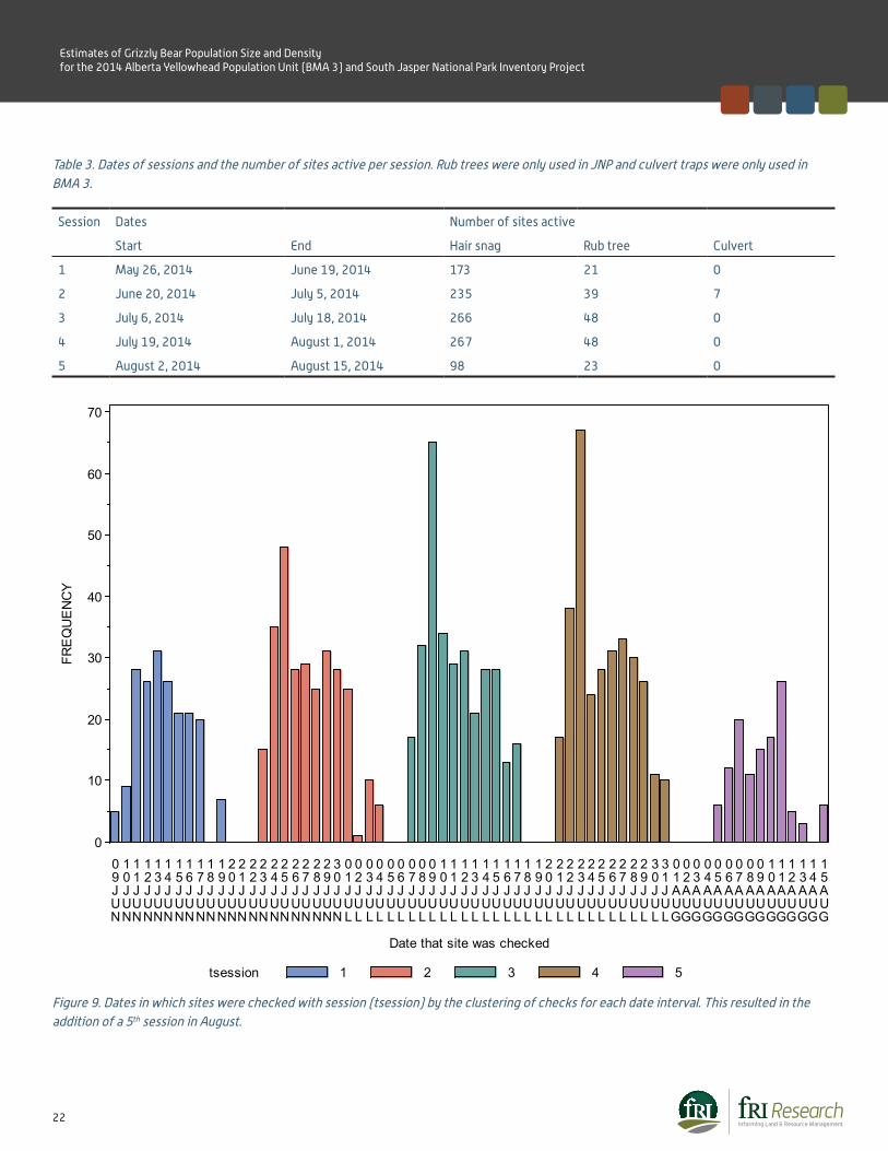
Table 3. Dates of sessions and the number of sites active per session. Rub trees were only used in Jasper National Park and culvert traps were only used in BMA 3. .....................................22

Table 4. Numbers of individual bears detected in each stratum and stratum membership based upon mean detection locations. ............................................................................................23

Table 5. Summary statistics for detections of females in the Yellowhead Ecosystem 2014 sampling grid. ...........................26

Table 6. Female SECR model selection results. Site covariate acronyms are listed in Table 1. AICc = sample size adjusted Akaike Information Criterion, ΔAICc = the difference in AICc between the model and the most supported model, AICc weight = wi, K = the number of model parameters, and log-likelihood (LL) are given. Baseline constant models are shaded for reference with covariate models. ........................................27

Table 7. Estimates of expected population size and density for females on the 2014 Yellowhead Ecosystem sampling grid. Estimates are from model 1 (D(strata) g0(CC+RT+t5) σ(.)) in Table 6. Estimates were not possible for the secondary stratum since no female bears were detected. .......................................29

Table 8. Summary statistics for detections of males in the Yellowhead Ecosystem 2014 sampling grid. Detections were pooled across detector types. ......................................................30

Table 9. Male SECR model selection results. Site acronyms are given in Table 1. AICc = sample size adjusted Akaike Information Criterion, ΔAICc = the difference in AICc between the model and the most supported model, AICc weight = wi, K = the number of model parameters, and log-likelihood (LL) are given. Baseline constant models are shaded for reference with covariate models. ............................................................................33

Table 10. Estimates of expected population size and density for males on the 2014 Yellowhead Ecosystem sampling grid. Estimates are from model 1 (D(strata) g0(CC) σ (.)) in Table 9. ...........................................................................................34

Table 11. Combined estimates of male and female bears on the Yellowhead Ecosystem DNA sampling unit based on estimates in Tables 7 and 10. ...........................................................................35

Table 12. Comparison of expected population size and density estimates from the 2014 and spatially explicit analysis of the 2008 BMA 2/Jasper inventory (Boulanger 2015a). .........................................................................36

Table 13. Summary statistics for detections of females in the 2004 BMA 3 sampling grid. . .............................................39

Table 14. Female SECR model selection results for the 2004 BMA 3 Inventory. AICc = sample size adjusted Akaike Information Criterion, ΔAICc = the difference in AICc between the model and the most supported model, AICc weight = wi, K = the number of model parameters, and log-likelihood (LL) are given. Baseline constant models are shaded for reference with covariate models. ...................................................................40

Table 15. Female expected population size and density estimates from spatially explicit mark-recapture analysis of the 2004 BMA 3 data. Estimates are from model 1 in Table 14. ...........41

Table 16. Summary statistics for males detected in the 2004 BMA 3 Inventory. .......................................................................................41

Table 17. Male SECR model selection results for the 2004 BMA 3 3 Inventory. AICc = sample size adjusted Akaike Information Criterion, ΔAICc = the difference in AICc between the model and the most supported model, AICc weight = wi, K = the number of model parameters, and log-likelihood (LL) are given. Baseline non-covariate models are shaded for reference with covariate models. ..................43

Table 18. Male abundance and density estimates from spatially explicit mark-recapture analysis of the 2004 BMA 3 data. .......................................................................................43

Table 19. Combined sex abundance and density estimates from spatially explicit mark-recapture analysis of the 2004 BMA 3 data. .....................................................................................................44

Table 20. Comparison of spatially explicit estimates of expected (average) number of bears on the 2004 BMA 3 DNA sampling grid between 2004 and 2014. .....................................................45

Table 21. Estimates of gross change (ratio of estimates in 2014 and 2010) and yearly change based on spatially explicit estimates of average population size. .......................................46

Table 22. The number of cameras operating, the total number of photos taken, and the number of photos containing a black bear and grizzly bear for each DNA session. ............................49


6

List of FiguresFigure 1. The Yellowhead population unit, including provincial lands

and the southern portion of Jasper National Park. .................9

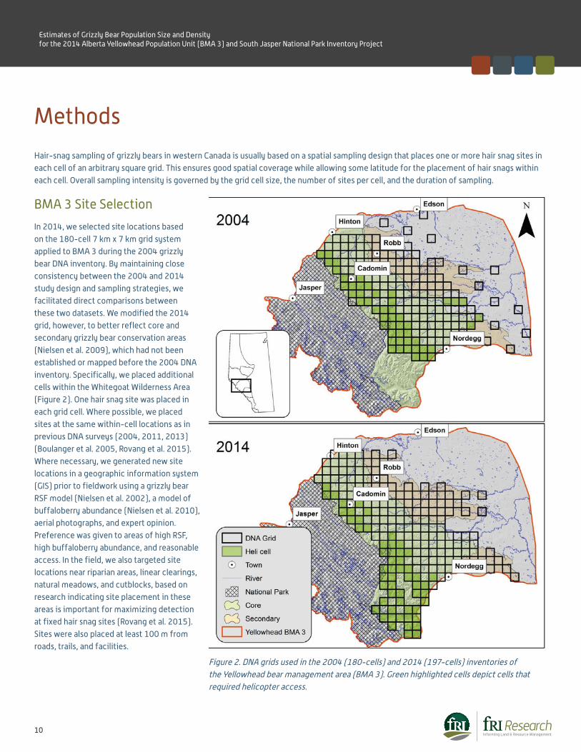
Figure 2. DNA grids used in the 2004 (180-cells) and 2014 (197-cells) inventories of the Yellowhead bear management area (BMA 3). Green highlighted cells depict cells that required helicopter access. ............................................................................10

Figure 3. South JNP with 7 km x 7 km grid cells, hair snag sites, and rub trees. Cells that were not sampled either had centroids which fell in non-habitat or presented logistical constraints. ........................................................................................12

Figure 4. Grid cells that have a wildlife camera located at the DNA hair snag site. ....................................................................................14

Figure 5. Grid cells sampled by access type: backcountry, boat, day hike, heli, or road. .............................................................................15

Figure 6. Spatially explicit (SECR) strata used in the analysis based upon management objectives and design of the study. Hair snag sites, rub trees, and culvert sites are also shown for reference. Areas shaded in green are protected areas (National or Provincial parks). ......................................................19

Figure 7. SECR strata with non-habitat defined as barren areas at elevations of 2000m or higher. Also indicated is the number of sessions each site was sampled. ............................................20

Figure 8. Dates in which sites were checked with session defined as the number of checks each individual site had received during the inventory. ......................................................................21

Figure 9. Dates in which sites were checked with session (tsession) by the clustering of checks for each date interval. This resulted in the addition of a 5th session in August. ......22

Figure 10. Mean detection locations of male and female bears on the sampling grid based on cumulative detections at hair snag, rub tree, and culvert sites. Multiple mean detections at DNA sites are delineated by a concentric ring of locations with a * denoting the central location. ......................................................24

Figure 11. Number of detections as a function of hair snag (HS), rub tree (RT), and culvert traps (CT). .........................................25

Figure 12. Approximate movement paths of females based on detections during the DNA inventory. The actual path is approximate, given that the sequence of detections is not known. Symbols for multiple detections at single sites are offset to facilitate interpretation. ..............................................26

Figure 13. Detection functions for detection at hair snags in session 5 (black line), detections at hair snags in sessions 1-4 (red line), and rub trees averaged across sessions (green line) from Model 2 (Table 6). Canopy cover was set at mean levels. Dashed lines are confidence limits on predictions. ...............28

Figure 14. Detection function for model 2 (Table 6) at various levels of canopy cover (left). Green line is for highest observed canopy closure (81%); red line is for mean canopy closure (43%) and black line is for lowest canopy cover (1%, black line). The distribution of canopy cover by site type is given on the right graph. .................................................................................29

Figure 15. Approximate movement paths of males based on detections during the DNA inventory. The actual path is approximate given that the sequence of detections is not known. Symbols for multiple detections at single sites are offset to facilitate interpretation. A movement of 127 kilometers is highlighted with a hashed green line. ..............31

Figure 16. Effect of inclusion and exclusion of outlier 127 kilometer movement on spatially explicit detection function estimates. Male detection functions are indicated by the blue line. Female detection function lines are in red for reference purposes. ............................................................................................32

Figure 17. Detection function on highest observed canopy closure (81%); green line, mean canopy closure (43%, brown line) and minimal canopy closure (1%, black line). .................................34

Figure 18. Locations of hair snag sites sampled during the 2004 BMA 3 DNA mark-recapture inventory. Moved sessions were only in place for a single session whereas fixed sites were in place for all 4 sessions. ..................................................................37

Figure 19. Mean detection locations of bears for the 2004 BMA 3 DNA mark-recapture inventory with the 2004 grid and 2014 SECR strata shown in reference. Not shown are locations of transect sites in 2004 that did detect one male bear in the southwest corner of the sampling grid. Multiple mean detection locations at single locations are offset with a * denoting the central location. ......................................................38

Figure 20. Approximate movement paths of females based on detections during the 2004 BMA 3 DNA inventory. The actual path is approximate given that the sequence of detections is not known. Symbols for multiple detections at single sites are offset to facilitate interpretation. ..............................................39

Figure 21. Approximate movement paths of males based on detections during the 2004 BMA 3DNA inventory. The actual path is approximate given that the sequence of detections is not known. Symbols for multiple detections at single sites are offset to facilitate interpretation. ..............................................42

Figure 22. Comparison of spatially explicit estimates of expected (average) population size for the 2004 BMA 3 DNA sampling grid area in 2004 and 2014. .........................................................45

Figure 23. Annual rates of population change in comparison to the estimate rate of change (1.07). The estimate of estimated rate of change of 1.04 pertains to estimated rates of increase for the Northern Continental Divide Ecosystem (2004-9; (Mace et al. 2011)) as well as Banff National Park and Kananaskis (1994-2002; (Garshelis et al. 2004)). .......................................46

Figure 24. Comparison of mean detections of bears from the 2004 and 2014 inventory of BMA 3. Multiple mean detections at single sites are indicated by a concentric ring with the site location denoted by a *. ................................................................47


7

IntroductionInventory of wildlife populations is often the first step needed to determine the appropriate conservation status of species and to develop

or improve the management of those species (Martin et al. 2007). For threatened and endangered species, population monitoring is a

critical step to developing effective recovery plans intended to stop or reverse the decline of a listed species (Martin et al. 2007). Recovery

plans should be designed with the intent and ability to monitor the species throughout the recovery process as it serves to estimate trend

in abundance and distribution and aids in understanding the ecological and human factors that influence those changes in time and space

(Campbell et al. 2002). Thus, it also serves to track the response of the species to recovery efforts and to inform, in a timely manner,

appropriate management responses (Gibbs et al. 1999, Campbell et al. 2002). However, often recovery plans face multifaceted ecological,

political, economic, and social obstacles and are initiated without population estimates or other complete biological knowledge (Campbell et

al. 2002).

These are the challenges faced by grizzly bear recovery and conservation efforts in Alberta, where the species is listed as Threatened

(Festa-Bianchet 2010). Grizzly bears are a high profile and charismatic species often held with long-standing cultural value as a symbol of

wilderness, ecological value as a top predator and umbrella species, and economic value for ecotourism (Kellert 1994, Kellert et al. 1996,

Noss et al. 1996). Despite many values, the social tolerance of grizzly bears varies widely (Kellert et al. 1996) and grizzly bears have suffered

dramatic range reductions and suspected population declines due to over-exploitation and habitat loss (Mattson and Merrill 2002, Ross

2002). These issues, and the continued threat of human-caused mortality rates (Festa-Bianchet 2010), have spurred conservation efforts

in Alberta over the past decade. A province-wide hunting moratorium was instituted in 2006 and an extensive DNA-based capture-mark-

recapture (CMR) study was conducted from 2004-2008. This CMR study provided the first population estimates for the majority (five out

of seven) of the Bear Management Areas (BMAs) in the province. Baseline population estimates from these provincial DNA inventories were

used, along with other information, to change the status of grizzly bears in Alberta to Threatened (Festa-Bianchet 2010).

DNA-based sampling techniques are a non-invasive adaptation of capture-mark-recapture (CMR) methods – the most frequently employed

approach for estimating wildlife population size across a wide variety of wildlife species (Nichols 1992, Pradel 1996, Long 2008). A number of

authors have concluded that noninvasive genetic sampling using hair is ideally suited for monitoring rare or hard-to-capture species like grizzly

bears because the hair can be collected remotely without having to catch or disturb the animal (Taberlet et al. 1999, Mills et al. 2000). As a

result, numerous projects outside of Alberta have also used this technique to estimate grizzly bear population size, including projects in British

Columbia (Woods et al. 1999, Mowat and Strobeck 2000, Poole et al. 2001, (Boulanger et al. 2002), Apps et al. 2004, (Proctor et al. 2010)), the

U.S.A. (Romain-Bondi et al. 2004, Kendall et al. 2008), and Europe (Gervasi et al. 2010, Schregel et al. 2012).

Due to the low densities and wide provincial distribution of grizzly bears, combined with habitats that are often difficult to access, it is likely

that monitoring grizzly bears in Alberta will continue to require some form of genetic hair sampling methods, either alone or in combination

with other sources of genetic materials and movement data from grizzly bears. The Alberta Grizzly Bear Recovery Plan (Alberta Grizzly Bear

Recovery Team 2008) recommended that population inventories be repeated on a 5-year return interval to assist managers in understanding

demographic trends and aid in evaluating ongoing land management and recovery efforts. Timely data and decision making is particularly

important for grizzly bears given their low reproductive potential (Weaver et al. 1996), which makes them sensitive to anthropogenic

impacts and vulnerable to further population decline and range contraction (Mattson and Merrill 2002). However, due to the high cost of

population inventories and a desire to modify and improve inventory techniques, repeat inventories at the BMA scale have not occurred in

any Alberta BMA, prior to 2014.

Fortunately, numerous research activities designed to improve our understanding of population monitoring techniques have been supported

in Alberta and elsewhere. This includes research into new spatially explicit capture recapture (SECR) analysis methods (Efford 2011), new

Resource Selection Function (RSF) models and habitat mapping (White et al. 2011), and improved design, methodology, and analysis of

DNA inventory techniques (Boulanger 2015b, Boulanger et al. 2006, Rovang et al. 2015). The accumulation of new knowledge from this

research has resulted in an improved ability to design more cost-effective population inventory methods, to analyse inventory data, and

to interpret the results. In addition to the scientific progress since the first provincial DNA population inventory in 2004, current research

and public opinion appears to suggest that there may be an increasing grizzly bear population in at least two provincial BMAs. A small scale


8

DNA inventory project using a fixed-site hair snag design suggested an increasing population trend between 2004 and 2011 in the north-

west portion of BMA 3 (Rovang et al. 2015), while an on-going large scale DNA project in BMA 6 using un-baited hair snags, rub trees, and

opportunistic samples also suggests an increasing grizzly bear population (Andrea Morehouse pers. comm.). Neither project, however, is able

to determine population trend across an entire BMA. As a result, complete, precise, and defensible data upon which management decisions

can be confidently based is still lacking for these two areas, and in fact all provincial grizzly bear management areas. Given that more than a

decade has passed since the first DNA inventory in Alberta (BMA 3 in 2004), current and complete grizzly bear inventory data is needed to

evaluate and adapt recovery and management efforts.

To address this need, we repeated the BMA 3 population inventory in 2014. Results from the 2004 inventory estimated 42 grizzly bears

(CI=36 to 55) in the surveyed portion of BMA 3, and a density of only 5 bears per 1000 km2 (Boulanger et al. 2005). This low density was

likely due to historic human-bear conflict, hunting, habitat loss, and high levels of industrial activity (AESRD 2010). The superpopulation

of bears (including dependent offspring) for the 2004 grid and surrounding area was 53, with a confidence interval of 44 to 80 bears. It

is important to recognize that the 2004 inventory in BMA 3 did not include any of the adjacent federal lands which are considered as part

of the same ecosystem (i.e. JNP). Estimates of grizzly bear populations in south Jasper have previously been based on expert opinion and

extrapolations from adjacent DNA surveys, applying RSF habitat selection models (Boulanger et al. 2011). However, a DNA-based population

inventory has never been completed for JNP south of Highway 16, making south Jasper the only section of the national parks within Alberta

where inventory data does not exist.

The goals of this study were to:

1. Apply a study design that would allow direct comparison of 2014 results with 2004 data for BMA 3,

2. Provide an estimate of the current population size within BMA 3,

3. Assess the spatial distribution of grizzly bears on the current landscape, and determine how this distribution relates to that found in 2004, and

4. Conduct a DNA inventory of south Jasper National Park (JNP) (adjacent to provincial BMA 3) to gain information on grizzly bear

occupancy and density for this area.

As a result, this project will also provide the first DNA-based population estimate for south Jasper.

Study AreaThis project had two study areas both within the Yellowhead grizzly bear population unit (BMA 3), and encompasses both provincial lands and

the southern portion of JNP. We designated these two adjacent areas as separate study areas for the purposes of field planning, sampling and

study design. However, we conducted an integrated data analysis that included each study area as a separate unit but acknowledging them as

part of the same ecosystem, and allowing for movement by bears across the boundary between the two areas.

The DNA inventory of BMA 3 consisted of a 197-cell grid covering 9,650 km2 of the eastern foothills area of Alberta’s Rocky Mountains

(Figure 1). The study area included almost all habitat designated as core and secondary grizzly bear conservation zones and was bordered by

Highway 16 in the north, Highway 11 in the south, and JNP to the west.

The south JNP study area consisted of 7,063 km2, including the region south of Highway 16 from the British Columbia border in the west to

the JNP park boundary in the east, and south to Highway 11 at the Banff National Park boundary (Figure 1).


9

Elevation ranged from 880 m to 3,365 m, and included a diversity of habitats. Sub-alpine areas consisted primarily of Engelmann spruce

(Picea engelmannii) and sub-alpine fir (Abies lasiocarpa) whereas upland forests consisted of aspen (Populus tremuloides), white spruce

(Picea glauca), and open stands of lodgepole pine (Pinus contorta). Lowland forests were characterized by mixed forests of black spruce

(Picea mariana), tamarack (Larix laricina), and lodgepole pine, while wetlands and riparian areas were dominated by willow (Salix spp.) and

shrub-graminoid communities. Important bear foods occurring in the study area include buffaloberry (Shepherdia canadensis), alpine sweet

vetch (Hedysarum alpinum), cow parsnip (Heracleum lanatum), and various blueberry species (Vaccinum spp.) (Munro et al. 2006). Other

large predators found here are black bears (Ursus americanus), wolf (Canis lupus), and cougar (Puma concolor). Ungulate prey species within

the study area include elk (Cervus canadensis), moose (Alces alces), white-tailed deer (Odocoileus virginianus), mule deer (O. hemionus),

and bighorn sheep (Ovis canadensis).

Several different types of land-use activities occur within BMA 3, including forestry, open pit coal mining, oil and gas exploration and

development, and outdoor recreation. Linear features such as roads, pipelines, seismic lines, and all terrain vehicle (ATV) trails are widespread

on the landscape, making most of the study area accessible by vehicle and/or by foot, though some areas required helicopter support for access.

JNP has a number of recreation activities that take place along the two major highway corridors (Highways 16 and 93), and the town site of

Jasper occurs along Highway 16 in the Athabasca valley. The vast majority of the park is not accessible by either road or trail.

Figure 1. The Yellowhead population unit, including provincial lands and the southern portion of JNP.


10

Methods

Hair-snag sampling of grizzly bears in western Canada is usually based on a spatial sampling design that places one or more hair snag sites in

each cell of an arbitrary square grid. This ensures good spatial coverage while allowing some latitude for the placement of hair snags within

each cell. Overall sampling intensity is governed by the grid cell size, the number of sites per cell, and the duration of sampling.

BMA 3 Site Selection

In 2014, we selected site locations based

on the 180-cell 7 km x 7 km grid system

applied to BMA 3 during the 2004 grizzly

bear DNA inventory. By maintaining close

consistency between the 2004 and 2014

study design and sampling strategies, we

facilitated direct comparisons between

these two datasets. We modified the 2014

grid, however, to better reflect core and

secondary grizzly bear conservation areas

(Nielsen et al. 2009), which had not been

established or mapped before the 2004 DNA

inventory. Specifically, we placed additional

cells within the Whitegoat Wilderness Area

(Figure 2). One hair snag site was placed in

each grid cell. Where possible, we placed

sites at the same within-cell locations as in

previous DNA surveys (2004, 2011, 2013)

(Boulanger et al. 2005, Rovang et al. 2015).

Where necessary, we generated new site

locations in a geographic information system

(GIS) prior to fieldwork using a grizzly bear

RSF model (Nielsen et al. 2002), a model of

buffaloberry abundance (Nielsen et al. 2010),

aerial photographs, and expert opinion.

Preference was given to areas of high RSF,

high buffaloberry abundance, and reasonable

access. In the field, we also targeted site

locations near riparian areas, linear clearings,

natural meadows, and cutblocks, based on

research indicating site placement in these

areas is important for maximizing detection

at fixed hair snag sites (Rovang et al. 2015).

Sites were also placed at least 100 m from

roads, trails, and facilities.

Figure 2. DNA grids used in the 2004 (180-cells) and 2014 (197-cells) inventories of the Yellowhead bear management area (BMA 3). Green highlighted cells depict cells that required helicopter access.


11

JNP Site Selection

For south JNP, we also applied the 7 km x 7 km grid system previously used for BMA 3 during the 2004 DNA survey, and extended this grid

westward to cover the southern portion of the park. We used a spatially explicit capture recapture (SECR) approach to assist in the sampling

design for the JNP inventory. SECR models the movement of grizzly bears on the sampling grid as well as the layout of sites within the

sampling grid. Therefore, this approach is robust to heterogeneity of detection rates caused by trap layout relative to bear home ranges, and

as a result, “holes” in trap coverage are allowed (Efford and Fewster 2013). In addition, edge effects and closure violation are not a biasing

factor; therefore, radio-collar based corrections of estimates are not required [adapted from Boulanger and Efford AB 2014 JNP Design draft

4-28-2014 - see Appendix A].

SECR relies on estimating average density across a known region of interest; therefore, every part of the study area should have a known,

non-zero chance of being sampled with a hair snag site. However, sampling “non-habitat” areas (barren areas of rock, snow or ice, above

2000 m) was not undertaken, based on the near-zero likelihood of detecting bears in these areas. In JNP, the majority of grid cells included

both habitat and non-habitat areas; therefore, we chose to select a cell for sampling only if its centroid fell within ‘habitat’ areas. We note

that this selection favours cells with higher quality habitat compared to cells with a larger area of rock and ice.

The exclusion of cells with centroids within non-habitat resulted in the dropping of 91 of 179 cells, leaving 88 cells selected for sampling

in the original design. Eighteen of these cells were subsequently dropped due to lack of access, and 4 alternate cells were added, for a total

of 74 cells sampled (Figure 3). Where substitutions were made, alternate cells were based on adjacency and similarity of habitat quality

between the cells (as estimated by RSF values) in order to maintain a representative range of habitat quality.

Once the grid cells to be sampled were determined, potential hair snag sites for each cell were generated in a GIS. At the grid cell scale, site

selection was focused on areas of high RSF values in order to maximize detection probability within the selected cells, and sites were placed

as close to the center of the cell as possible, within the constraints of accessibility. To minimize the risk of bear-human encounters and to

address public safety concerns, hair snags were at least 200 m from roads and trails, and 500 m from facilities such as campgrounds, picnic

sites, or viewpoints. In the field, all hair snags were set up in locations that included a visual barrier between roads/trails/facilities and the

site, such as trees or topographic features. To focus on areas of bear movement and foraging, site placement also targeted areas near riparian

zones and natural meadows.


12

Figure 3. South JNP with 7 km x 7 km grid cells, hair snag sites, and rub trees. Cells that were not sampled either had centroids which fell in non-habitat or presented logistical constraints.


13

BMA 3 Field Methods and Sampling

We built hair snag sites using approximately 50 m of barbed wire strung around 3-6 trees at a height of 50 cm following protocols adapted

from previous studies (Woods et al. 1999, Boulanger et al. 2005, 2006). We constructed a lure pile in the center of the corral using branches,

rotten wood, and other forest debris, topped with a thick layer of moss or other absorbent material. Corrals were large enough so that

the scent lure pile could be reached only when a bear crossed the barbed wire, and uneven ground (e.g. low or high spots) was filled or

obstructed. During site setup and every two weeks thereafter, we baited the site with 2 L of scent lure (aged cattle blood) mixed with 500

mL of canola oil, and topped with conifer branches to protect the lure from rain. Use of a scent lure (instead of bait) attracts bears to the site

without providing a food reward. Sites were not moved throughout the field season, since spatially explicit methods are theoretically more

robust to heterogeneity caused by site placement relative to home range centers. Due to late snowmelt, we set up sites (n=56) in alpine

habitat requiring helicopter access two weeks later than sites (n=141) accessed by motor vehicle. We sampled most sites (n=172) for 4

sessions, while sites (n=25) in White Goat Wilderness Area were sampled for 3 sessions as a result of late spring snow conditions.

We checked sites for hair every two weeks. Hair samples were collected into paper envelopes using tweezers or gloves. We also collected

data regarding sample location, adjacency to other samples, and sample quality to facilitate the final sub-selection of hair samples for DNA

analysis. Following collection of samples, we removed (burned) any remaining hair from the wire to ensure that hair found during subsequent

visits was from the correct session. Throughout the field season, hair samples were stored with silica desiccant packs both in the field and in

the office.

As part of ongoing research there were also some (n=7) active culvert trapping sites where grizzly bear capture and radio collaring work was

underway during the DNA inventory data collection period. Bears captured or recorded at these sites (barb wire and cameras) also provided

hair samples that were incorporated into the appropriate sampling period, to provide additional data on unique individuals present.

Wildlife Cameras

In 2004, grizzly bear habitat towards the eastern boundary was sampled using 17 isolated (non-contiguous) cells to investigate grizzly bear

occurrence in these areas. At that time, no bears were detected in these eastern boundary cells using DNA hair snags, no bears were detected

by hair snags in the southeastern portion of the main grid, and very few bears were detected in the northeast. Nonetheless, grizzly bear

sightings have been reported in these areas. This raised the concern that bears were present towards the eastern boundary, but were not

being detected by hair snag sites.

In response to this concern, during the 2014 survey we set up a total of 54 wildlife cameras along the eastern-most portion of the BMA 3

DNA grid, overlapping secondary grizzly bear habitat (Figure 4). Our goal was to investigate if and/or how many grizzly bears approached

a DNA hair snag site but were not detected via a hair sample(s). We set up 43 cameras in session 1 during the first sampling session of the

hair snag sites; 4 additional cameras were set up in session 2 (n=47); and 7 additional cameras were set up in session 3 (n=54). However,

four cameras were removed following sampling in session 3, leaving a total of 50 cameras operating in session 4. Each camera was placed

at a location that captured the entire hair snag site to ensure any bears approaching the site were detected by the camera. We downloaded

camera data on the same 14-day sampling schedule as the DNA hair snag sites and removed the cameras following the last DNA sampling

session (session 4). No cameras were used within JNP as part of our study.


14

Figure 4. Grid cells that have a wildlife camera located at the DNA hair snag site.

JNP Field Methods and Sampling

The presence of naturally occurring bear rub trees along hiking trails in the national parks provides an opportunity for a non-invasive method

of obtaining grizzly bear hair samples with relatively easy access. In south JNP, we sampled hair from 50 naturally occurring bear rub trees

found along trails. Rub tree locations were either previously mapped by Parks Canada staff (n=25) or found during the 2014 field season by

fRI Research staff (n=25). Rub trees were set up with a zig-zag “Z” formation of barb wire on the rubbed surface using 4 strands of barb wire

with 3 barbs each, positioning the first three wires to cover as much of the rubbing surface as possible. The fourth strand was placed below

the zig-zag at a height of approximately 25 cm as a “cub rub”. Rub trees were not baited with scent lure. To exclude samples that may have

been left from the previous year, we removed (burned) all hair present during setup.

While rub trees provide a relatively low-cost method of obtaining hair samples for DNA analysis, research suggests that using rub trees alone

may result in an under-representation of females and family groups in the population inventory, as these groups may not use rub trees as

often as male bears (Kendall et al. 2008). This appears to hold true in our study area; individuals identified from rub trees in JNP in 2013


15

included 14 males, but only 4 females (Mark Bradley, pers. comm.). Therefore, in addition to sampling rub trees, barb wire corrals were set up

at 74 sites in south JNP including: 31 road accessible sites, 6 day hiking sites, 24 sites accessed by multi-day backcountry travel, 8 helicopter

sites, and 5 sites accessed by boat (Figure 5). Corrals and lure piles were built using the same methods as in BMA 3. During site setup and

every two weeks thereafter with 2 L of scent lure (aged cattle blood) mixed with 500 mL of canola oil. Due to late snowmelt, backcountry

and high elevation sites were set up two weeks later than sites accessed by motor vehicle. Most sites (n = 62) were sampled for 4 sessions,

while 13 sites were sampled for 3 sessions.

Figure 5. Grid cells sampled by access type: backcountry, boat, day hike, heli, or road.


16

Hair snags and rub tree sites were checked every two weeks for

hair. Occasionally, samples were also collected opportunistically

from bear scrapings on trees located near established hair snag and

rub tree sites. Hair samples were collected into paper envelopes

using tweezers or gloves. Data were collected regarding sample

location, adjacency to other samples, and sample quality to

facilitate the final sub-selection of hair samples for DNA analysis.

Following collection of samples, any remaining hair was removed

(burned) from hair snag and rub tree sites, to ensure that hair found

during subsequent visits was from the correct session. Throughout

the field season, hair samples were stored with silica desiccant

packs both in the field and in the office.

Sub-Selection of Samples for DNA Analysis

As is the case in most large scale grizzly bear inventory projects,

recognizing budget constraints, it was not possible to genotype

all hair samples collected during 2014. To select a subsample of

hair for DNA analysis, we followed a series of sub-selection criteria

based on those previously used for DNA surveys in both Alberta and

British Columbia. These sub-sampling criteria have been shown

to result in a minimal reduction in the number of individual bears

identified (Proctor et al 2012). Initial screening of hair samples

excluded those identified as non-bear species, and those with a

high confidence of species identified as black bear. In some cases,

it was possible to confirm bear species using wildlife camera data

from the hair snag site. Previous research (David Paetkau, pers.

comm.) indicates that for successful genotyping, bear hair samples

must include either 1) at least one guard hair, or 2) five or more

underfur hairs. Samples that did not meet these minimum criteria

were excluded based on the likelihood that they did not contain

sufficient genetic material.

For hair snag sites, we reviewed each site and session separately,

and applied further criteria to all samples not excluded in the

initial screening. At a minimum, we selected the best sample for

each site/session, as indicated by field data, hair sample size,

and probability of grizzly bear species. In addition, we selected 1

in every 3 from adjacent samples, starting with the best sample

in each barb group. If there were more than 3 samples in a barb

group, for the remaining samples, greater preference was given

to samples with a greater number of guard hairs and samples with

greater confidence in grizzly bear species identification. Less

preference was given to samples with unknown species, samples

with black bear and grizzly bear hair on the same barb, and directly

adjacent samples.

For rub tree sites, each rub tree and session was reviewed

separately, and further criteria were applied to all samples not

excluded in the initial screening. At a minimum, we selected the

best sample for each rub tree/session. Barbs 1-3, 4-6, 7-9, and 10-

12 (see site setup) were considered as groupings, based on their

adjacency and height on the tree. Samples from the bark or from

the ground were considered as separate groupings, unless samples

on the bark were known to be immediately adjacent to each other.

Samples on the wire (but not on a barb) were also considered as a

separate grouping, unless known to be immediately adjacent to a

barb. Based on these designated groupings, we selected the best

sample in each grouping. Greater preference was given to samples

with a greater number of guard hairs and samples with greater

confidence in grizzly bear species identification. Less preference

was given to samples with unknown species, samples with black

bear and grizzly bear hair on the same barb, and directly adjacent

samples.

DNA Analysis

Hair samples were sent to Wildlife Genetics International in

Nelson, British Columbia, Canada for genotyping analysis. DNA

was extracted using QiaGEN DNeasy Tissue kits following standard

protocols (Paetkau 2003). Samples were examined under a

dissecting microscope, and those with the visual appearance

characteristics of black bears hair(jet black from root to tip) were

removed. Samples that passed the visual examination underwent

a prescreen using a species-specific marker (G10J) to distinguish

grizzly bear from black bear samples (Paetkau 2003). Individual

grizzly bears were genotyped to 7 loci (markers G10J, G1A, G10B,

G1D, G10H, G10M, G10P) and sex was assigned using a ZFX/

ZFY gender marker (Paetkau et al. 2003). To determine parent-

offspring relationships within BMA 3, samples were genotyped

to 21 loci (markers G1D, G10H, G10M, G10P, G10C, G10L, G10U,

G10X, CXX20, CXX110, MU50, MU59, REN145P07, CPH9, Msut2,

Mu51, Mu23). Error checking protocols included selective

reanalysis of similar genotypes (those matching at 1, 2, or 3 loci) to

confirm the genotype or resolve errors, thus eliminating genotypes

created through genotyping error (Paetkau 2003, Waits and

Paetkau 2005, Kendall et al. 2009).


17

Population AnalysisJohn Boulanger and Murray Efford.

1. Introduction

This section of the report provides an outline of spatially explicit

mark-recapture estimation of grizzly bear DNA mark-recapture

projects that occurred in BMA 3 and southern JNP in 2014. In

addition, where possible these analysis approaches and results are

compared to previous population inventory results from 2004.

Recent advances in spatially explicit mark-recapture methods

(SECR) potentially produce a more robust population estimate of

these areas (Efford and Fewster 2013) and also allow inference

about variation in density within the study areas through stratified

sampling and density surface modelling (Royle et al. 2013, Efford

2014a).

These studies were designed to take advantage of the benefits

of spatially explicit modelling (Boulanger and Efford 2014). In

particular, sampling intensity was varied by geographic area based

on management objectives, habitat, and logistic challenges. In

addition, areas of non-habitat (as defined by barren habitat at

greater than 2000 m) were not sampled in order to optimize

efforts to areas of most contiguous habitat.

This exercise had the following objectives:

1. Fit parsimonious models to describe detection probability

variation and scale of movements of bears in the Yellowhead

population unit.

2. Use a stratified model to estimate density and regional

population size for each region of interest (BMA 3 and

southern JNP).

3. Compare estimates to previous estimates from 2004

(Boulanger et al. 2005) including the re-analysis of the 2004

data set using spatially explicit methods.

Other analyses, such as density surface modelling of the

distribution of bears on the sampling grid, will be detailed in future

reports.

2. Methods

Spatially explicit capture-recapture (SECR) methods (Efford

2004, Efford et al. 2004, Borchers and Efford 2008, Efford et al.

2009, Efford 2011, Royle et al. 2014) estimate population density

allowing for the spatial scale of movement, estimated from the

detection sites of bears that are detected repeatedly. Unlike closed

models that pool data from multiple hair snag sites within each

session for each bear, the SECR method used multiple detections

of bears at unique hair snag sites within a session to model bear

movements and detection probabilities. Using this information, the

detection probabilities of grizzly bears at their home range center

(g0), spatial scale of grizzly bear movements (s) around the home

range center, and bear density were estimated.

An assumption of this method is that grizzly bear home range

can be approximated by a circular symmetrical distribution of

use (Efford 2004), but the method is robust to deviations from

circularity (M. G. Efford unpubl. results). The configuration of the

sampling sites is used in the process of estimating the scale of

movements and density, and lack of geographic closure (incursion

of bears centered outside the grid) is modeled directly. There

is therefore no need to adjust for study-area size and closure

violation as with previous closed models.

SECR models detections of bears with home ranges centered either

directly on the sampling grid or in adjoining habitat; the grid and

adjoining habitat together comprise the habitat ‘mask’. Considering

too little adjoining habitat as the potential source of detected bears

can cause positive bias in density estimates. An initial analysis

was conducted with sexes combined to determine the size of the

mask (relative to study area size) needed to control bias in density

estimates. The esa.plot and suggest.buffer functions of the R

package ‘secr’ were run for a g0(sex) σ (sex) conditional likelihood

model. These suggested a buffer width of 35 km would give

unbiased estimates; estimation is also expected to be unbiased

with a wider buffer, but computation is then slower for a given

spatial resolution.

Subsequent analyses were run separately for male and female

grizzly bears to test for variation in detection probability at the

home range center and scale of movements. Models were run

separately for males and females.

Spatially explicit capture re-capture model fitting had three phases:

1. Baseline tests for temporal, behavioural, and heterogeneity

variation in g0 and σ to establish a baseline model of detection.

2. Addition of site covariates to baseline model to describe

heterogeneity induced by site placement

3. Using the most supported model from step 2, strata-specific

models were fit under the assumption that relationships

between site covariates and g0/σ were similar across strata.


18

Site covariates such as a terrain ruggedness index and canopy

closure were evaluated at two spatial scales as potential predictors

of the detection probability parameters (g0 and σ) (Table 1)

(Boulanger et al. 2009). The two scales (‘site’ and ‘home-range’)

corresponded respectively to the distance at which bears

encountered (responded to) hair snags and the typical home-range

radius. We used 1.96 km as the site scale, based on estimates

by Boulanger et al. (2004), and 10 km as the home range scale,

corresponding to bear home range areas (Nielsen et al. 2004b).

Humans often plan and influence land use activities approximately

on the scale of bear home ranges (i.e., the township). In most

cases site scale was used as a covariate for detection probabilities

(g0) and home range scale was used as a covariate for the σ scale

parameter. For this phase of the analysis it was assumed that

density was constant across the extent of the survey area.

Table 1. Site habitat and sampling covariates used to describe scale of movement and detection of bears.

Habitat variable Description

TRI Terrain ruggedness index (Riley et al. 1999)

dstream

Negative exponential decay (500m

parameter) distance to stream

CC Percent canopy cover

Rub tree (RT)

A binary covariate to indicate that site was

a rub tree

Hair snag (HS)

A binary covariate to indicate a site was a

hair snag site

Models were evaluated in terms of relative support information

theoretic model selection methods Sample size adjusted AICc

scores were used to define the best model as determined by the

lowest AICc score (Burnham and Anderson 1998).

2.1. Defining Strata

Strata were defined based on a-priori boundaries of management

interest, as well as likely difference in density and sampling

intensity (Table 2 and Figure 6). White Goat Wilderness Area

(hereafter White Goat) and the immediate area to the east, as well

as JNP were primarily unroaded and/or protected areas and were

therefore grouped as a single stratum. The eastern boundary of the

White Goat Area boundary was partially also based upon the extent

of sampling that occurred during the 2004 DNA mark-recapture

inventory. However, population estimates were derived for JNP and

White Goat separately.

Table 2. Strata used in spatially explicit capture-recapture analysis. Habitat area is defined by the total area minus area of barren landcover of greater than 2000 meters elevation.

Strata Defined by Sampling

design

Area

(km2)

Habitat

Total

BMA 3

Core

AB BMA 3

grizzly bear

zone

One site per

7x7 km cell

4 sessions 6738.8 6353.2

BMA 3

Secondary

AB BMA 3

grizzly bear

zone

One site per

10x10 km cell

4 sessions 3509.4 3509.4

Jasper/

White Goat

Mountainous/

protected

areas

One site per

7x7 km cell

2-4 sessions

7898.5

(JNP)

1707.6

(WG)

4342.9

(JNP)

770.2

(WG)

The SECR model uses actual hair snag locations, so no special action

was needed to represent spatial differences in sampling intensity

between strata beyond using strata as a covariate for density when

producing population estimates (Table 2). Some sites were not

sampled in all sessions (see also ‘Adjustment of sessions’ below),

and the resulting temporal variation was represented with a binary

‘usage’ matrix – a series of 1’s and 0’s for each site indicating the

sessions in which it was active (1) or non-active (0).


19

Figure 6. Spatially explicit (SECR) strata used in the analysis based upon management objectives and design of the study. Hair snag sites, rub trees, and culvert sites are also shown for reference. Areas shaded in green are protected areas (national or provincial parks).

The habitat mask for the SECR analysis used a discrete cell size (mask spacing) of 3 km for all analyses. A sensitivity analysis of mask spacing

suggested 3 km was a good compromise between processing time and minimizing bias in estimates (no change in D with spacing of 3.5–2.5

km). Mask cells were categorized according the stratum of their centroid. Centroids outside the Yellowhead unit (where no sites were

sampled) were assigned to the stratum of the nearest Yellowhead cell. Many of the sampling grids contained substantial areas of barren rock

and ice which was not considered suitable habitat for grizzly bears (Figure 7). Cells received a single site if the centroid of the cell fell within

grizzly habitat defined as non-barren landcover with an elevation less than 2000 meters. The main reduction of the number of sites sampled

occurred in Jasper and White Goat that had higher proportions of non-habitat. Barren land cover above 2000 m was excluded from the

habitat mask in the SECR analysis, as in previous habitat analyses using DNA mark-recapture data (Boulanger 2015) and in the design of the

BMA 3 and JNP study (Boulanger and Efford 2014).


20

Figure 7. SECR strata with non-habitat defined as barren areas at elevations of 2000m or higher. Also indicated is the number of sessions each site was sampled.

2.2. Estimates of Abundance and Density

Expected population size and density estimates were derived from the most supported models for each sex and stratum combination.

Estimates of grizzly bears on the entire sampling grid, and estimates for each stratum (Table 2) were produced. Expected population size

is the expected number of bears that would be contained within the study area or regional area at one time (Efford and Fewster 2013). It is

analogous to the average number of bears on the sampling grid given in previous survey reports. Density is then estimated as the expected

number of grizzly bears divided by the entire area of the grid, or the habitat area within the grid. Log based confidence intervals on expected

population size and density were generated using formulas from Efford and Fewster (2013). All spatially explicit analyses were done in

package SECR (Efford 2014b) in R statistical software (R_Development_Core_Team 2009). In addition, data were screened using program

DENSITY (Efford et al. 2004). Map figures were produced using program QGIS (QGIS_Foundation 2015).


21

2.3. Adjustment of Sessions

Due to a late spring, many higher elevation mountain sites were not sampled initially until late June or July. The sessions for each site were

initially numbered sequentially, which led to a large degree of variation in session number among sites re-visited in the same week (Figures 7

and 8).

Session 0 1 2 3 4 5

FRE

QU

EN

CY

0

10

20

30

40

50

60

70

Date that site was checked

09JUN

10JUN

11JUN

12JUN

13JUN

14JUN

15JUN

16JUN

17JUN

18JUN

19JUN

20JUN

21JUN

22JUN

23JUN

24JUN

25JUN

26JUN

27JUN

28JUN

29JUN

30JUN

01JUL

02JUL

03JUL

04JUL

05JUL

06JUL

07JUL

08JUL

09JUL

10JUL

11JUL

12JUL

13JUL

14JUL

15JUL

16JUL

17JUL

18JUL

19JUL

20JUL

21JUL

22JUL

23JUL

24JUL

25JUL

26JUL

27JUL

28JUL

29JUL

30JUL

31JUL

01AUG

02AUG

03AUG

04AUG

05AUG

06AUG

07AUG

08AUG

09AUG

10AUG

11AUG

12AUG

13AUG

14AUG

15AUG

Figure 8. Dates in which sites were checked with session defined as the number of checks each individual site had received during the inventory.

This created a potential issue for modelling of temporal change in detection probabilities based on seasonality as well as behavioural

responses. In addition, some sites were sampled into August which is usually considered as the berry season. It can be seen from Figure 8 that

the sites were sampled in distinct temporal clusters. To resolve this, the sessions for each site were adjusted to be defined in each cluster

(Table 3) which also meant a 5th session was added. This created synchronized sessions for each site (Figure 9). The trap usage matrix of the

SECR trap file was used to inform the SECR model as to when each site was active.


22

Table 3. Dates of sessions and the number of sites active per session. Rub trees were only used in JNP and culvert traps were only used in BMA 3.

Session Dates Number of sites active

Start End Hair snag Rub tree Culvert

1 May 26, 2014 June 19, 2014 173 21 0

2 June 20, 2014 July 5, 2014 235 39 7

3 July 6, 2014 July 18, 2014 266 48 0

4 July 19, 2014 August 1, 2014 267 48 0

5 August 2, 2014 August 15, 2014 98 23 0

tsession 1 2 3 4 5

FRE

QU

EN

CY

0

10

20

30

40

50

60

70

Date that site was checked

09JUN

10JUN

11JUN

12JUN

13JUN

14JUN

15JUN

16JUN

17JUN

18JUN

19JUN

20JUN

21JUN

22JUN

23JUN

24JUN

25JUN

26JUN

27JUN

28JUN

29JUN

30JUN

01JUL

02JUL

03JUL

04JUL

05JUL

06JUL

07JUL

08JUL

09JUL

10JUL

11JUL

12JUL

13JUL

14JUL

15JUL

16JUL

17JUL

18JUL

19JUL

20JUL

21JUL

22JUL

23JUL

24JUL

25JUL

26JUL

27JUL

28JUL

29JUL

30JUL

31JUL

01AUG

02AUG

03AUG

04AUG

05AUG

06AUG

07AUG

08AUG

09AUG

10AUG

11AUG

12AUG

13AUG

14AUG

15AUG

Figure 9. Dates in which sites were checked with session (tsession) by the clustering of checks for each date interval. This resulted in the addition of a 5th session in August.


23

3. Results

3.1. Summary

Overall, 108 unique bears were detected in the entire Yellowhead ecosystem DNA sampling area with 63 bears detected on provincial lands

in BMA 3, 16 bears in the White Goat, and 29 bears in south JNP (Table 4). In many cases, bears were detected in more than one of these

three strata; therefore, the number of bears detected based on detection location (116) was higher than that based on mean detection

location (the mean of the x and y coordinates of DNA sites where a bear was detected across all sessions) (Table 4). Spatially explicit model

estimates of population size and density account for detections across multiple strata by estimating density based upon home range centers,

as well as likely movements of bears on the sampling grid.

Table 4. Numbers of individual bears detected in each stratum and stratum membership based upon mean detection locations.

Strata Detections Mean locations

BMA 3 Males Females Total Males Females Total

Core 34 27 61 33 26 59

Secondary 5 0 5 4 0 4

Jasper National Park/White Goat

Jasper National

Park

20 12 32 17 12 29

White Goat 9 9 18 9 7 16

Site outside of

White Goat

1 0 1

Total 69 48 117 63 45 108

Mean detection locations (Figure 10) illustrate that many bears in BMA 3 were detected along the border with JNP. We note that these

detection locations are only based upon sampling conducted within the survey area, and therefore may not reflect the true home range

centers of bears.


24

Figure 10. Mean detection locations of male and female bears on the sampling grid based on cumulative detections at hair snag, rub tree, and culvert sites. Multiple mean detections at a single DNA site are delineated by a concentric ring of locations with a * denoting the central location.

The majority of detections occurred with hair snag sampling which was presumably due to the fact the hair snags occurred throughout the

study area whereas rub tree and culvert sampling were restricted to smaller areas and in the case of culverts for a limited and shorter time

frame. (Table 3 and Figure 11).


25

Sample type CT HS RT

Num

ber o

f det

ectio

ns a

t uni

que

site

s

0

10

20

30

40

50

SECR sessionSexF M

1 2 3 4 5 1 2 3 4 5

Figure 11. Number of detections as a function of hair snag (HS), rub tree (RT), and culvert traps (CT).

3.2. Spatially Explicit Analyses

Spatially explicit analyses were conducted separately for females and males, given the likelihood of sex-specific parameters as well as sex-

specific distributions of bears on the sampling grid. This approach was simpler than attempting a pooled analysis with sex-specific terms for

each parameter.

3.2.1. Females (2014)

Detections of females were lowest in the first session, then approximately constant until the last session, when detections increased (Table

5). The number of active sites (detectors) was lower in the first session, which may have contributed to the lower number of detections.

However, the number of detectors was also lower in the fifth session, which had the highest number of detections. The number of unmarked

bears detected decreased with each session, suggesting that sampling was relatively efficient. The number of new bears detected during

session 5 in August was only 5 also suggesting that there was minimal immigration into the grid during the initial part of the August berry

season.


26

Table 5. Summary statistics for detections of females in the Yellowhead Ecosystem 2014 sampling grid.

Statistic Session(j)

1 2 3 4 5 Total

Detections (nj) 4 16 16 12 21 68

Unmarked (uj) 4 15 13 8 5 45

Cumulative marked (Mt+1) 4 19 32 40 45 45

Frequencies (fsessions) 24 18 3 0 0 45

Total site visitsA 4 20 18 14 22 78

Detectors visited 4 18 16 12 19 69

Detectors available 194 281 314 315 121 1225AIncludes multiple visits to different sites within single sessions.

Detections and movements occurred mainly in mountainous areas with only a few detections in the eastern part of the core stratum and no

detections in the secondary stratum (Figure 12). There were no detections of female bears in the Athabasca River Valley of JNP.

Figure 12. Approximate movement paths of females based on detections during the DNA inventory. The actual path is approximate, given that the sequence of detections is not known. Symbols for multiple detections at single sites are offset to facilitate interpretation.


27

Model selection efforts initially focused on identifying base

variation in detection at home range center (g0) and scale of

movement (σ). From the suite of models considered , the model

with temporal variation in detection probabilities (g0) in session

5 (denoted as t5) was most supported (model 12). Models with

behavioural response due to habituation to fixed hair snag sites

(termed bHS in models 18-20) were not supported. In the second

phase, site covariate models were considered. Of these, the model

where g0 varied with canopy cover, whether a site was a rub tree or

hair snag (model 2) was substantially more supported than other

site covariates such as terrain ruggedness (model 5) and distance

from stream (model 8). In the last phase of model selection, the

strata-specific density model was more supported than models

which assumed homogenous density across the sampling grid

(model 1). The strata-specific model assumed similar responses of

detection probabilities to canopy closure across all strata.

Table 6. Female SECR model selection results. Site covariate

acronyms are listed in Table 1. AICc = sample size adjusted

Akaike Information Criterion, ΔAICc = the difference in

AICc between the model and the most supported model,

AICc weight = wi, K = the number of model parameters, and

log-likelihood (LL) are given. Baseline constant models are

shaded for reference with covariate models.

No Model AICc ΔAICc wi K LL

Strata-specific density

1 g0(CC+RT+t5A) σ (.) 708.0 0.00 1.00 7 -344.0

Site covariate models (uniform density)

2 g0(CC +RT+t5) σ (.) 719.8 11.81 0.00 6 -352.8

3 g0(CC +t5) σ (.) 723.1 15.03 0.00 5 -355.8

4 g0 (CC) σ (.) 731.4 23.38 0.00 4 -361.2

5 g0 (TRI+t5) σ (.) 743.1 35.09 0.00 5 -365.8

6 g0 (RT+t5) σ (.) 741.8 33.80 0.00 5 -365.1

7 g0 (t5) σ (dstream) 747.9 39.89 0.00 5 -368.2

8 g0 (t5+dstream) σ(.) 747.4 39.34 0.00 5 -367.9

9 g0 (t5) σ (.) 748.3 40.24 0.00 4 -369.6

10 g0 (t5) σ (CC) 750.8 42.76 0.00 5 -369.6

11 g0 (t5) σ (TRI) 750.7 42.66 0.00 5 -369.6

Base models (uniform density)

12 g0 (t5) σ (.) 748.3 40.28 0.00 4 -369.6

13 g0 (t) σ (.) 750.3 42.28 0.00 7 -366.6

14 g0 (T) σ (.) 755.6 47.58 0.00 4 -373.3

15 g0 (.) σ (h2) 760.9 52.88 0.00 3 -377.2

16 g0 (.) σ (.) 763.2 55.18 0.00 4 -377.1

17 g0 (b) σ (.) 763.3 55.28 0.00 4 -377.1

18 g0 (RT+bHSB) σ (.) 766.0 57.98 0.00 6 -375.9

19g0(RT+bHS)

σ(RT+bHS) 766.3 58.28 0.00 9 -371.6

20 g0(.) σ(RT+bHS) 767.7 59.68 0.00 6 -376.7Adenotes specific detection rates for session 5Bdenotes a behavioural response specific to hair snag sites


28

The detection function from model 2 suggested that bears were the most detectable in session 5 (Figure 13, black line) compared to other

sessions (red line) for hair snags. Females were the least detectable at rub trees (green line).

0 5000 10000 15000 20000 25000

0.00

0.05

0.10

0.15

0.20

Distance (m)

Det

ectio

n pr

obab

ility

Figure 13. Detection functions for detection at hair snags in session 5 (black line), detections at hair snags in sessions 1-4 (red line), and rub trees averaged across sessions (green line) from model 2 (Table 6). Canopy cover was set at mean levels. Dashed lines are confidence limits on predictions.

A plot of the detection function at various canopy cover levels (Figure 13a) suggest that bears were had lower detection probabilities in sites

with high canopy cover (Figure 14a, green line) compared to areas of low canopy cover (black line). The distribution of sites relative to canopy

cover (Figure 14b) suggests that most sites were in moderate canopy cover with detection rates indicated by the red line in Figure 14a.


29

a)Predicted detection probabilites by canopy cover classes

0 5000 10000 15000 20000 25000

0.00

0.05

0.10

0.15

0.20

Distance (m)

Det

ectio

n pr

obab

ility

b)Distribution of canopy cover by detector type

Sample type: CT HS RTN

umbe

r of s

ites

0

10

20

30

40

50

60

70

80

Canopy cover

0 8 16 24 32 40 48 56 64 72 80

Figure 14. Detection function for model 2 (Table 6) at various levels of canopy cover (a). Green line is for highest observed canopy closure (81%); red line is for mean canopy closure (43%) and black line is for lowest canopy cover (1%, black line). The distribution of canopy cover by site type is given on the right graph (b).

Expected population size and density estimates were produced for the strata specific density model (Table 6, model 1). Estimates were not

possible for the secondary stratum, given that no female bears were detected in this stratum. Estimates for individual stratum were not very

precise, however, the overall estimate for the entire Yellowhead area had acceptable precision as defined by a coefficient of variation of less

than 20% (Pollock et al 1990) (Table 7).

Table 7. Estimates of expected population size and density for females on the 2014 Yellowhead Ecosystem sampling grid. Estimates are from model 1 (D(strata) g0(CC+RT+t5) σ(.)) in Table 6. Estimates were not possible for the secondary stratum since no female bears were detected.

Strata/area Expected population size Density

Estimate SE Conf. Limit CV Estimate SE Conf. Limit

BMA 3

Core 34.4 8.5 21.4 55.4 24.6% 5.45 1.34 3.39 8.77

Secondary

Total 34.4 8.2 21.7 54.5 24.6% 3.48 0.83 2.20 5.53

Jasper 28.0 6.7 17.6 44.4 23.9% 6.55 1.57 4.13 10.40

White Goat 5.4 1.3 3.4 8.5 23.9% 6.55 1.57 4.13 10.40

Entire population

unit 67.7 11.0 49.3 93.0 16.3% 4.53 0.74 3.30 6.23


30

3.2.2. Males (2014)

For male grizzly bears, lower numbers were detected in sessions 1 and 5 (Table 8); however, this could have been due to the lower number

of active detectors in sessions 1 and 5. The number of new bears detected declined as the sessions progressed, and only 3 new males were

detected in session 5 suggesting minimal immigration of new bears during the August (session 5) berry season. Capture frequencies, or the

number of sessions in which individual males were detected, suggested reasonable detection rates with males being detected in up to 4

different sessions.

Table 8. Summary statistics for detections of males in the Yellowhead Ecosystem 2014 sampling grid. Detections were pooled across detector types.


1 2 3 4 5 Total

Detections (nj) 14 31 27 21 13 106

Unmarked (uj) 14 26 10 10 3 63

Cumulative marked (Mt+1) 14 40 50 60 63 63

Frequencies (fsessions) 33 21 5 4 0 63

Total site visitsA 18 42 32 25 15 131

Detectors visited 15 35 26 19 13 107

Detectors available 194 281 314 315 121 1225AIncludes multiple visits to different sites within single sessions.

Movements of males based upon detections and redetections demonstrated extensive movement and movements across stratum

boundaries (Figure 15). Most notable were the movements on the boundary of the core and Jasper/White Goat strata. Most movements were

less than 50 kilometers in total, across all sampling sessions.


31

Figure 15. Approximate movement paths of males based on detections during the DNA inventory. The actual path is approximate given that the sequence of detections is not known. Symbols for multiple detections at single sites are offset to facilitate interpretation. A movement of 127 kilometers is highlighted with a hashed green line.

One movement (by male id 343-1A-2) of 127 kilometers occurred between sessions 3 and 4; genotypes for these detections were

confirmed based on analysis to a larger number of loci for each sample. This movement is denoted by a hashed line in Figure 14. This

movement was an outlier compared to all other movements, as illustrated by plotted detection functions with and without this movement

included (Figure 16). The density estimates with the outlier movement data included was 3.46 bears per 1000 km2 (SE=0.4, CI=2.77-4.22),

versus an estimate of 3.85 (SE=0.44, CI=3.07-4.83) when the outlier data were included (baseline g0(.) σ(.) model). We therefore excluded

this movement from the spatially explicit model analysis, given the sensitivity of SECR estimates to movement distances. Spatially explicit

models, as well as most mark-recapture methods, assume that the “target population” of bears have stationary home ranges, and that the

sample of bears does not include a large proportion of “transient” bears. This assumption allows a defined population and density estimate.

By incorporating movement data, spatially explicit models allow further assessment of this assumption and how it might affect estimates.


32

127 km movement included 127 km movement excluded

Figure 16. Effect of inclusion and exclusion of outlier 127 kilometer movement on spatially explicit detection function estimates. Male detection functions are indicated by the blue line. Female detection function lines are in red for reference purposes.

Model selection for male grizzly bear data was conducted in three stages. In the first stage, a base model was fitted which tested for general

forms of detection probability and σ variation. Behavioural response and time variation in detection probabilities were not supported. A

model with constant detection probabilities at home range center and linear trends in scale of movement (Table 9: model 13). Site covariate

models were fitted in the second stage. Many of the site covariate models were more supported than the baseline model (models 8 and

15), including models with terrain ruggedness (model 8),canopy closure (models 2-4), and rub trees (models 3 and 5) affecting detection

probabilities (g0). Terrain ruggedness (models 5 and 6) and canopy closure (model 7) affected scale of movement (σ). Of these, a model

with canopy closure influencing g0 with linear trends in scale of movement (σ) was more supported (model 2) . Strata was then added as

a covariate for density; this variable also increased the overall support as indicated by a lower AICc score (model 1), further suggesting

stratum-specific densities within the Yellowhead sampling grid.


33

Table 9. Male SECR model selection results. Site acronyms are given in Table 1. AICc = sample size adjusted Akaike Information Criterion, ΔAICc = the difference in AICc between the model and the most supported model, AICc weight = wi, K = the number of model parameters, and log-likelihood (LL) are given. Baseline constant models are listed twice and shaded for reference with covariate models.

No Model AICc ΔAICc wi, K LL

Strata-specific density

1 g0(CC) σ (T) 1245.2 0 0.96 7 -615.7

Site covariates models (uniform density)

2 g0 (CC) σ (T) 1252.8 7.6 0.02 5 -620.9

3 g0 (CC+RT) σ (T) 1254.7 9.5 0.01 6 -620.6

4 g0 (CC) σ (.) 1255.6 10.4 0.01 4 -623.5

5 g0 (RT) σ (TRI+T) 1257.6 12.3 0.00 6 -622.0

6 g0 (.) σ (TRI+T) 1259.1 13.9 0.00 5 -624.0

7 g0 (.) σ (CC+T) 1266.7 21.5 0.00 5 -627.8

8 g0 (TRI) σ (T) 1275.8 30.5 0.00 5 -632.4

9 g0 (.) σ (T) 1276.7 31.5 0.00 4 -634.0

10 g0 (RT) σ (T) 1277.5 32.2 0.00 5 -633.2

11 g0 (dstream) σ (T) 1278.7 33.4 0.00 5 -633.8

12 g0 (.) σ (dstream+T) 1279.0 33.7 0.00 5 -634.0

13 g0 (RT+bhs) σ (T) 1281.5 36.3 0.00 8 -631.4

Baseline models (uniform density)

14 g0 (.) σ (T) 1276.7 31.5 0.00 4 -634.0

15 g0 (.) σ (.) 1278.1 28.9 0.00 3 -635.8

16 g0 (T) σ (T) 1278.6 33.4 0.00 5 -633.8

17 g0 (.)σ (t) 1280.4 35.1 0.00 7 -632.2

18 g0 (t) σ (.) 1280.9 35.6 0.00 7 -632.4

19 g0 (t) σ (t) 1284.1 38.9 0.00 11 -628.5

Plots of the detection function from model 2 (Figure 17) revealed that detection probabilities of bears were highest at sites with low canopy

closure, a similar result to females (Figure 14). Scale of movement decreased slightly over the sampling sessions.


34

a)Canopy closure (g0)

0 5000 10000 15000 20000 25000

0.00

0.05

0.10

0.15

Distance (m)

Det

ectio

n pr

obab

ility

b)Temporal variation (σ)

0 5000 10000 15000 20000 250000.

000.

010.

020.

030.

040.

050.

06Distance (m)

Det

ectio

n pr

obab

ility

Figure 17. a) Detection function on highest observed canopy closure (81%); green line, mean canopy closure (43%, brown line) and minimal canopy closure (1%, black line). B) Temporal variation in σ in session 1 (black line) and session 5 (red line) with canopy closure at mean levels.

Estimates of expected population size were reasonably precise (CV<20%) for most strata with the exception of the secondary stratum

(Table 10).

Table 10. Estimates of expected population size and density for males on the 2014 Yellowhead Ecosystem sampling grid. Estimates are from model 1 (D(strata) g0(CC) σ (T)) in Table 9.

Strata/area Expected population size Density (bears per 1000 km2)


BMA 3

Core 35.8 6.38 25.3 50.6 17.8% 5.66 1.01 4.00 8.02

Secondary 4.1 2.4 1.4 11.9 58.8% 1.15 0.68 0.39 3.34

Total 39.9 6.65 28.8 55.2 16.7% 4.04 0.67 2.92 5.59

Jasper 26.0 5.18 17.7 38.3 19.9% 6.10 1.21 4.15 8.98

White Goat 5.0 0.99 3.4 7.4 19.8% 6.11 1.21 4.15 8.99

Entire

population unit 70.9 7.78 57.2 87.8 11.0% 4.74 0.52 3.83 5.88


35

3.2.3. Combined Estimates for Males and Female Bears

Table 11 provides combined estimates for male and female bears for the 2014 Yellowhead population unit (from Tables 7 and 10). Precision was better for combined estimates, compared to sex-specific estimates, with all coefficients of variation < 20%, other than the secondary stratum.

Table 11. Combined estimates of male and female bears on the Yellowhead Ecosystem DNA sampling unit based on estimates in Tables 7 and 10.

Strata/area Detected Expected population size Density (bears per 100 km2)


BMA 3

Core 61 70.2 10.6 52.3 94.3 15.1% 11.12 1.68 8.28 14.92

Secondary 5 4.1 2.4 1.4 11.9 58.8% 1.15 0.68 0.40 3.35

Total 66 74.2 10.6 56.2 98.0 14.2% 7.53 1.07 5.70 9.93

Jasper 29 54.0 8.5 39.8 73.2 15.7% 12.66 1.98 9.33 17.17

White Goat 18 10.4 1.6 7.6 14.1 15.6% 12.66 1.98 9.34 17.16

Entire unit 108 138.6 13.5 114.6 167.7 9.7% 9.28 0.90 7.67 11.22

3.2.4. An Estimate for the Entire Jasper National Park

We also completed a spatially explicit analysis for the north JNP, reanalyzing data that was collected during the DNA inventory in 2008

(Boulanger 2015). The analysis of Boulanger (2015a) used density surface modelling to partition and estimate density and expected

population size in sub-regions of the 2008 BMA 2/JNP sampling grid (Alberta Grizzly Bear Inventory Team 2009). A model that predicted

density of the 2008 DNA grid using resource selection function based habitat scores and RISK scores (Nielsen et al. 2004, Nielsen et al.

2006) was used for this analysis. This model, combined with spatially explicit detection models, estimated 34 females and 26 males for

North Jasper (Table 12). Under the assumption that densities have remained constant in northern Jasper since 2008, a total of 113 bears was

estimated for the entire area of JNP. However, this estimate should be interpreted with caution, given the uncertainty in status of the grizzly

bear population in north JNP since 2008. For example, this estimate will be biased if the population in north JNP experienced a decline or

increase in abundance since 2008. Given this, it is not appropriate to estimate a confidence limit on the overall estimate since it would not

include the statistical uncertainty in trend between 2008 and 2014.


36

Table 12. Comparison of expected population size and density estimates from the 2014 and spatially explicit analysis of the 2008 BMA 2/Jasper inventory (Boulanger 2015).

Sex SECR model Expected population size Density (bears per 1000 km2)

Density Detection Estimate SE Conf. Int. CV Estimate SE Conf. Int.

North JNP (2008)

females RSF*Risk g0(CC) σ (TRI) 34 3.5 27.5 41.3 10.4% 11.89 1.24 9.69 14.58

males RSF g0(TRI ) σ(.) 26 2.0 22.0 30.0 7.9% 9.07 0.71 7.77 10.58

South JNP (2014)

females Stratum g0(CC+RT+t5) σ (.) 28 6.7 17.6 44.4 23.9% 6.55 1.57 4.13 10.40

males Stratum g0(CC) σ (T) 26 5.2 17.7 38.3 19.9% 6.10 1.21 4.15 8.98

A previous estimate for JNP was based on extrapolation of reference area densities using RSF modelling (Boulanger et al. 2011); results from

the 2004-2008 DNA inventory projects were used to derive RSF models, which were then applied to extrapolate densities from the DNA

grids to adjoining park areas. The extrapolation produced an estimate of 109 (CI=64-173) bears for JNP.

3.3. Reanalysis of 2004 DNA BMA 3 Population Inventory Data Using Spatially Explicit Methods

The 2004 BMA 3 inventory employed an intensive sampling design: each cell included a fixed sampling site which was sampled for four

sessions, along with a site that was moved to a new location during each of sessions 2 through 4 (Boulanger et al. 2005, Boulanger et al.

2006). This entire data set was considered in the SECR reanalysis of the 2004 data, since SECR models consider site location as well as

whether or not a session was active (Figure 18). A ‘fix’ covariate was used to test for differences in detection between fixed and moved sites.

Sampling in 2004 overlapped much of the 2014 core strata and the western section of the 2014 secondary strata.


37

Figure 18. Locations of hair snag sites sampled during the 2004 BMA 3 DNA mark-recapture inventory. Moved sessions were only in place for a single session whereas fixed sites were in place for all 4 sessions.

Overall, 44 bears (24 females and 20 males) were detected during the 2004 DNA Inventory (Figure 19). Of these, mean locations for 3 males

and 2 females fell within the 2014 secondary stratum, with the rest occurring in the core stratum. In the 2014 reanalysis of 2004 data, 23

females and 35 males were detected within the core 2004 grid. Sampling intensity in 2014 was lower, especially in the secondary area

(Figure 6); therefore, the best comparison is of spatially explicit estimates rather than numbers of bears detected.


38

Figure 19. Mean detection locations of bears for the 2004 BMA 3 DNA mark-recapture inventory with the 2004 grid and 2014 SECR strata shown in reference. Not shown are locations of transect sites in 2004 that did detect one male bear in the southwest corner of the sampling grid. Multiple mean detection locations at single locations are offset with a * denoting the central location.

3.3.1. Females

Detections of females were lowest in the first and last sampling sessions. Low detections in the first session may have been due to a lower

number of active sites (Table 13). The number of new bears detected declined with session, suggesting that sampling was effective in

detecting most of the bears on the sampling grid. In addition, as indicated by detection frequencies, the majority of bears were detected at

least twice during sampling.


39

Table 13. Summary statistics for detections of females in the 2004 BMA 3 sampling grid.


1 2 3 4 Total

Detections (nj) 7 16 16 9 48

Unmarked (uj) 7 11 4 2 24

Cumulative marked (Mt+1) 7 18 22 24 24

Frequencies (fsessions) 10 7 4 3 24

Total site visitsA 13 23 18 15 69

Detectors visited 12 21 14 15 62

Detectors available 188 365 349 360 1262AIncludes multiple visits to different sites within single sessions.

Detections and movements were primarily distributed on the western edge of the sampling grid with a few movements into the secondary

strata (Figure 20). There was also a single detection in the central part of the secondary strata.

Figure 20. Approximate movement paths of females based on detections during the 2004 BMA 3 DNA inventory. The actual path is approximate given that the sequence of detections is not known. Symbols for multiple detections at single sites are offset to facilitate interpretation.


40

Base model selection did not detect any variation in detection at home range center or scale of movement (Table 14, Model 11). Of site

covariate models, a model with detection probability at home range center being positively associated with terrain ruggedness was most

supported (Model 2). A model with fixed sites displaying lower detection rates also showed some support compared to a constant parameter

model (Models 3 and 5). A model with strata-specific densities (Model 1) was most supported further demonstrating different densities

between core and secondary strata.

Table 14. Female SECR model selection results for the 2004 BMA 3 Inventory. AICc = sample size adjusted Akaike Information Criterion, ΔAICc = the difference in AICc between the model and the most supported model, AICc weight = wi, K = the number of model parameters, and log-likelihood (LL) are given. Baseline constant models are shaded for reference with covariate models.


Strata model

1 g0(TRI) σ (.) 645.7 0.00 0.64 5 -316.2

Site covariate models

2 g0 (TRI) σ (.) 648.1 2.38 0.19 4 -319.0

3 g0(fix+TRI) σ (.) 649.7 4.00 0.09 5 -318.2

4 g0 (TRI) σ (TRI) 649.8 4.14 0.08 4 -318.3

5 g0 (fix) σ (.) 663.8 18.14 0.00 4 -326.8

6 g0 (.) σ (.) 664.4 18.75 0.00 3 -328.6

7 g0 (.) σ (CC) 664.6 18.89 0.00 4 -327.2

8 g0 (CC) σ (.) 666.3 20.57 0.00 4 -328.1

9 g0 (stream) σ (.) 667.2 21.50 0.00 4 -328.5

10 g0 (.) σ (CC) 667.2 21.54 0.00 4 -328.6

Base model

11 g0 (.) σ (.) 664.4 18.75 0.00 3 -328.6

12 g0 (T) σ (.) 664.9 19.21 0.00 4 -327.4

13 g0 (.) σ (T) 666.6 20.88 0.00 4 -328.2

14 g0 (b) σ (.) 667.2 21.47 0.00 4 -328.5

15 g0 (.) σ (t) 667.2 21.54 0.00 6 -325.1

16 g0 (T) σ (T) 667.5 21.78 0.00 5 -327.1

17 g0 (t) σ (.) 671.6 25.93 0.00 6 -327.3

The 2014 SECR reanalysis of the 2004 data resulted in an estimate of expected population size of 21.6 females for the 2004 sampling grid.

This estimate for the entire 2004 grid was close to the sum of the separate estimates for the core and secondary strata (Table 15). The

terrain ruggedness covariate for g0 had minimal effect on estimates.


41

Table 15. Female expected population size and density estimates from spatially explicit mark-recapture analysis of the 2004 BMA 3 data. Estimates are from model 1 in Table 14.

Strata Expected population size Density


2004 sampling grid 21.6 3.5 15.7 29.6 16.2% 2.53 0.41 1.85 3.47

SECR strata

core 19.3 3.4 13.8 27.1 17.4% 3.05 0.53 2.18 4.28

secondary 2.5 1.8 0.7 8.7 70.0% 0.71 0.50 0.21 2.46

Total 21.8 3.6 15.9 30.0 16.3% 2.21 0.36 1.61 3.04

3.3.2. Males

Summary statistics indicate that detections were relatively even across sampling sessions, however, the number of active detectors was less

for the first session. The number of marked bears declined for each session suggesting that sampling was relatively effective (Table 16).

Table 16. Summary statistics for males detected in the 2004 BMA 3 Inventory.


1 2 3 4 Total

Detections (nj) 13 10 10 8 41

Unmarked (uj) 13 4 1 2 20

Cumulative marked (Mt+1) 13 17 18 20 20

Frequencies (fsessions) 9 2 8 1 20

Total site visitsA 20 21 17 9 67

Detectors visited 17 18 15 7 57

Detectors available 188 365 349 360 1262

Distributions of detections and movements demonstrated that most males were detected on the western part of the sampling grid with only

single detections of bears in the secondary strata (Figure 21). If compared with the 2014 spatial data (Figure 10), it is apparent that many of

the bears detected on the 2004 sampling grid may have had home ranges that overlapped Jasper and White Goat in the west.


42

Figure 21. Approximate movement paths of males based on detections during the 2004 BMA 3DNA inventory. The actual path is approximate given that the sequence of detections is not known. Symbols for multiple detections at single sites are offset to facilitate interpretation.Baseline model selection revealed linear trends (symbolized by T) in scale of movement (σ; Table 17, model 9) as with the 2014 data (Table

9). Terrain ruggedness influenced scale of movement with substantially more support than baseline models (model 2). A strata (core and

secondary strata) model was most supported (model 21).


43

Table 17. Male SECR model selection results for the 2004 BMA 3 3 Inventory. AICc = sample size adjusted Akaike Information Criterion, ΔAICc = the difference in AICc between the model and the most supported model, AICc weight = wi, K = the number of model parameters, and log-likelihood (LL) are given. Baseline non-covariate models are shaded for reference with covariate models.


Strata model

1 g0 (.) σ(T+TRI) 628.5 0.00 0.62 6 -305.54

Site covariate models

2 g0 (.) σ(T+TRI) 629.5 1.01 0.37 5 -307.12

3 g0 (TRI) σ(T) 639.0 10.51 0.00 5 -312.37

4 g0 (.) σ(T+CC) 640.6 12.06 0.00 5 -313.15

5 g0 (.) σ(T) 646.9 18.39 0.00 4 -318.12

6 g0 (CC) σ(T) 647.5 18.97 0.00 5 -316.6

7 g0 (.)

σ(T+dstream) 650.1 21.60 0.00 5 -317.92

8 g0 (dstream)

σ(T) 650.5 22.01 0.00 5 -318.12

Baseline models

9 g0 (.) σ (T) 646.9 18.39 0.00 4 -318.1

10 g0 (T) σ(.) 657.9 29.34 0.00 4 -323.6

11 g0 (.) σ (T+fix) 649.5 21.00 0.00 5 -315.5

12 g0 (fix+T) σ (.) 660.4 31.89 0.00 5 -323.1

13 g0 (.) σ (t) 654.5 25.96 0.00 6 -321.3

14 g0 (b) σ (.) 661.7 33.16 0.00 4 -325.5

15 g0 (t) σ (.) 664.9 36.36 0.00 6 -323.2

16 g0 (t) σ (t) 666.8 38.26 0.00 9 -315.4

17 g0 (.) σ (.) 669.2 40.72 0.00 3 -330.8

The estimate of expected or average population size was 14.4 for male bears for the Alberta 2004 grid area (Table 18).

Table 18. Male abundance and density estimates from spatially explicit mark-recapture analysis of the 2004 BMA 3 data.

Strata Expected population size Density (bears per 100 km2)

estimate SE Conf. Limit CV Estimate SE Conf. Limit

AB04 DNA grid 14.4 2.4 10.4 19.9 16.7% 1.69 0.28 1.22 2.34

SECR strata

core 13.2 2.5 9.2 19.1 18.8% 2.09 0.39 1.45 3.02

secondary 2.0 1.6 0.5 8.0 82.7% 0.55 0.46 0.14 2.27

Total 15.2 2.6 10.9 21.1 16.9% 1.54 0.26 1.11 2.14


44

3.3.3. Combined Estimates for Males and Females in 2004

The combined estimate of bears for reanalysis of the 2004 data set was 37 bears for the core and secondary area and 36 bears for the DNA sampling grid (Table 19).

Table 19. Combined sex abundance and density estimates from spatially explicit mark-recapture analysis of the 2004 BMA 3 data from estimates of females (Table 15) and males (Table 18).

Strata Abundance Density (bears per 100 km2)

estimate SE Conf. Limit CV Estimate SE Conf. Limit

AB04 DNA grid 36.0 4.2 28.6 45.3 11.8% 4.22 0.50 3.36 5.32

SECR strata

core 32.5 4.2 25.3 41.8 12.9% 5.14 0.66 4.00 6.61

secondary 4.5 2.4 1.7 12.0 53.5% 1.26 0.68 0.47 3.38

Total 37.0 4.4 29.3 46.6 11.9% 3.75 0.45 2.97 4.73

3.3.4. Comparison of 2004 SECR Estimates with 2004 Closed Model/Telemetry Estimates.

The SECR estimate for the 2004 DNA grid area was 36 bears (males and females, CI=29-45). This is lower than the previous estimate of 42

bears (CI=36-55), which was derived from closed models corrected by proportion points on the grid (using radio collared bears) (Boulanger

et al. 2005). However, the confidence intervals of these two estimates overlap; therefore, this difference should be interpreted with caution.

3.4. Comparison of 2014 and 2004 Estimates

3.4.1. Spatially Explicit Estimates of Expected (average) Number of Bears on the Sampling Grid.

Estimates from spatially explicit models for the 2004 sampling grid (Figure 16) were compared to assess the relative change in expected or

average number of bears on the sampling grid between 2004 and 2014 (Table 20).


45

Table 20. Comparison of spatially explicit estimates of expected (average) number of bears on the 2004 BMA 3 DNA sampling grid between 2004 and 2014.

Year/sex Bears

detected

Expected

NSE Conf. Limit CV

2004

females 24 21.6 3.5 15.7 29.6 16.2%

males 20 14.4 2.4 10.4 19.9 16.3%

pooled 44 36.0 4.2 28.6 45.3 11.8%

2014

females 23 33.7 8.1 21.1 53.7 24.1%

males 35 37.6 6.2 27.3 51.8 16.4%

pooled 58 71.3 10.2 53.9 94.2 14.3%

A graphical representation of the estimates and confidence intervals from Table 20 is given in Figure 22.

0.0

10.0

20.0

30.0

40.0

50.0

60.0

70.0

80.0

90.0

100.0

females males pooled

Expe

cted

pop

ulat

ion

size

Group

2004 2014

Figure 22. Comparison of spatially explicit estimates of expected (average) population size for the 2004 BMA 3 DNA sampling grid area in 2004 and 2014.


46

Estimates from the ratio of the 2014 and 2004 estimates (gross change) were scaled for a yearly interval to estimate yearly rates of change.

Yearly rates of population change were estimated at 1.05 and 1.11 for females and males respectively, for a pooled average rate of change of

1.07 (Table 21).

Table 21. Estimates of gross change (ratio of estimates in 2014 and 2004) and yearly change based on spatially explicit estimates of average population size.

Sex Gross change Yearly change

Estimate SE Estimate SE Conf. Limit

females 1.56 0.45 1.05 0.14 0.76 1.33

males 2.61 0.61 1.10 0.19 0.72 1.48

pooled 1.98 0.37 1.07 0.12 0.84 1.30

The pooled rate of change is compared to previously published estimates, as well as other hypothetical rates of change in Figure 23. The

estimate of lambda of 1.04 pertains to estimated rates of increase for the Northern Continental Divide Ecosystem (2004-9; (Mace et al.

2011)) as well as Banff National Park and Kananaskis (1994-2002; (Garshelis et al. 2004)). The estimated rate of change calculated in

our analysis was higher than most previously published bear studies. As discussed later, one factor that most likely influenced the rate of

change was the addition of at least 30 relocated bears to the Yellowhead BMA over the last 10 years. Future analyses will consider factors

influencing the observed trend including relocated bears, known mortalities, and radio collar-based survival rates.

20

30

40

50

60

70

80

90

100

110

2002 2004 2006 2008 2010 2012 2014 2016

Expe

cted

pop

ulat

ion

size

Year

1.10

1.07

1.04

Figure 23. Annual rates of population change in comparison to the estimate rate of change (1.07). The estimate of estimated rate of change of 1.04 pertains to estimated rates of increase for the Northern Continental Divide Ecosystem (2004-9; (Mace et al. 2011)) as well as Banff National Park and Kananaskis (1994-2002; (Garshelis et al. 2004)).


47

3.4.2. Comparison of Spatial Distribution Between 2004 and 2014

Figure 24 provides a comparison of the spatial distribution of detections in 2004 and 2014. This comparison should be interpreted cautiously

given the higher degree of sampling effort, especially in secondary areas, in 2004. The main differences in distribution between 2004 and

2014 are an increase in bears in the central and southeast core area, and around the Cadomin mine in 2014 as compared to 2004.

2004 distribution of mean detections

2014 distribution of mean detections

Figure 24. Comparison of mean detections of bears from the 2004 and 2014 inventory of BMA 3. Multiple mean detections at single sites are indicated by a concentric ring with the site location denoted by a *.

An upcoming density surface modelling exercise will provide further inference on differences in distribution and factors influencing

distribution.


48

3.5. Wildlife Camera Results

Results from wildlife cameras in selected grid cells indicated that

we were successful in gathering samples from bears visiting these

sites. The majority of photos within these cells were of black bears,

and grizzly bear hair was collected at all sites and sessions where

photos showed a grizzly bear had visited the hair snag site.

Table 22. The number of cameras operating, the total number of photos taken, and the number of photos containing a black bear and grizzly bear for each DNA session.

DNA

Session

No.

Cameras

Set Up

No.

Cameras

Sampled

Total

Photos

Black

Bear

Photos

Grizzly

Bear

Photos

0 - - - - -

1 43 - - - -

2 +4 43 630 491 12

3 +3 47 401 260 1

4 - 50 290 145 5

4. Discussion

Estimates from the 2014 grid suggests the population of grizzly

bears in BMA 3 has increased between 2004 and 2014, with an

estimated rate of population increase of approximately 7% (CI=-

16%-30%), which is higher than commonly seen in most interior

grizzly bear populations in North America (Garshelis et al. 2004,

Schwartz et al. 2005, Mace et al. 2011). The reasons for population

increase are unclear, and additional investigation is required to

determine whether management actions have contributed to this

rate of increase. The provincial grizzly bear hunting moratorium

that was put in place in 2006 has played a role in reducing overall

human caused mortalities over the past 8 years.

There are a number of additional pieces of information (datasets)

that need to be considered when evaluating the observed increase

in population size within BMA 3. First it should be recognized

that as a result of management actions related to “problem

bear management”, enforcement officers have relocated 30

bears to this BMA during the period 2004-2014. This represents

approximately 3 bears per year over this 10 year period. At this

time we have not pursued further analysis to determine what

role this population augmentation may have played in population

increase, however, we recommend that this analysis be undertaken

in order to make refinements in management practices to support

recovery efforts. In addition, new DNA data sets obtained from a

scat collection project undertaken within BMA 3 in the fall of 2014

may further refine DNA-based estimates. Further analysis of these

datasets is now underway.

Other studies, have also suggested an increasing population within

BMA 3, including results from a smaller sampling grid in the vicinity

of Hinton (Rovang 2013). The 2013 analysis estimated a yearly

rate of increase of 1.06 (CI=0.93-1.19), using a Pradel trend model

that compared bears detected on the 2011 grid with those from

the 2004 grid. A similar analysis combining detections of individual

bears on DNA grids each year between 2004 and 2014 collaring

effort, and translocated bear data, will provide a more precise and

definitive estimate of trend.

Spatially explicit methods provided a way to obtain robust

population estimates with less sampling effort, through the use of

fixed rather than moved sites and by allowing a stratified sampling

approach. For example, precision of estimates for bears on the BMA

3 grid were similar (Table 20) in 2004 and 2014, even though the

2014 grid used only fixed sites, as well as reduced trap density in

secondary areas (Figures 6 and 18). This type of stratification can

be employed in future population inventory work to reduce overall

project costs.

The use of site covariates in spatially explicit analyses provides

a new way to model heterogeneity variation in individual bear

detection probabilities caused by placement of site in various

habitats. In general, it may be easier to select site locations in non-

homogenous forest (lower canopy cover) or in mountainous areas

(higher terrain ruggedness), since a heterogeneous landscape is

more likely to contain features or micro-habitats optimal for site

placement. Not surprisingly, detection of bears is associated with

these site covariates given the relative ease of finding optimal

areas for site placement . In addition, in some analyses, scale

of movement is influenced by terrain ruggedness, as indicated

by smaller grizzly bear home range sizes in mountainous areas

(Schwab 2003).


49

Spatially explicit analysis resulted in lower estimates of abundance

for the 2004 sampling grid as compared with the original closed

model approaches used in 2004, however, this difference could be

due to sampling variation. Of particular note, the SECR reanalysis

suggested that the expected population size of male bears was only

14 bears, even though 20 bears were detected on the grid in 2004.

This was due to the fact that many bears were detected on the

eastern edge of the grid, resulting in many bears with partial home

ranges on the grid. The 2004 data also included many detections

on the eastern border, resulting in uncertainty in male residency on

the grid. The closure correction estimate for 2004 was based upon

a limited sample size of bears. A potential analysis that could refine

the 2004 estimate would be the use of the cumulative sample

size of bear locations to provide a better closure-corrected 2004

estimate which could be compared with the 2004 SECR estimates.

The current analysis assumes that densities in each stratum are

homogenous. It is more likely that densities vary as a function of

habitats and proximity of roads (which influence survival rates)

(Boulanger and Stenhouse 2014). Spatially explicit estimates

are robust to variation in densities across sampling grids (Efford

2014a); therefore it is likely that strata-specific estimates of

density and expected population size will also be robust. Future

analyses will utilize density surface modelling (Royle et al. 2013,

Efford 2014a, Boulanger 2015) to explore factors that affect

larger-scale density across the sampling grid and provide a spatial

representation of density variation.

This report has provided the first documented example of an

expanding grizzly bear population in Alberta through the use of

DNA inventory techniques and SECR methodologies, showing the

value and importance of well designed, repeat inventory efforts.

These data will be essential in discussions on population recovery

targets and review of the provincial status assessment for this

species. In addition, the estimate for south Jasper represents the

first population estimate for this area, and forms a strong and

important foundation for status monitoring and genetic databases.


50

5. Literature Cited

Alberta Grizzly Bear Recovery Team. 2008. Alberta grizzly bear

recovery plan 2008-2013. Alberta Species at Risk Recovery

Plan No. 15. Alberta Sustainable Resource Development, Fish

and Wildlife Division, Edmonton, Alberta. Edmonton, AB.

Alberta Grizzly Bear Inventory Team. 2009. Grizzly bear population

size and density estimates for the 2008 DNA Inventory of

the Grande Cache Bear Management Area (BMA 2). Alberta

Sustainable Resource Development, Fish and Wildlife Division.

Apps, C. D., B. N. Mclellan, J. G. Woods, and M. F. Proctor. 2004.

Estimating grizzly bear distribution and abundance relative to

habitat and human influence. Journal of Wildlife Management

68:138–152.

Borchers, D. L., and M. G. Efford. 2008. Spatially explicit

maximum likelihood methods for capture-recapture studies.

Biometrics:377-385.

Boulanger, J. 2015a. Spatially explicit mark-recapture estimates of

grizzly bear population density in DNA grid and protected areas

in Alberta (Draft Report). Department of Environment and

Sustainable Resource Development, Govt. of Alberta.

Boulanger, J. 2015b. Strategies for monitoring of grizzly bear

populations in Alberta: A summary of the Grizzly Bear

Monitoring Workshop, Edmonton, Alberta, April 21-22, 2015.

Alberta Department Environment and Sustainable Resource

Development, Government of Alberta.

Boulanger, J., J. Cranston, S. E. Nielsen, and G. Stenhouse. 2009.

Estimation of grizzly bear population size for the Swan

Hills management unit using DNA sampling and habitat-

relative occupancy models. Alberta Sustainable Resource

Development.

Boulanger, J., and M. Efford. 2014. Design for the Yellowhead Unit

3 and Southern Jasper National Park 2014 Grizzly Bear DNA

Inventory project. fRI Research and Integrated Ecological

Research.

Boulanger, J., S. E. Nielsen, J. Cranston, and G. Stenhouse. 2011.

Estimation of grizzly bear population size for Jasper and

Banff National Parks using DNA sampling and habitat-relative

occupancy models.

Boulanger, J., M. Proctor, S. Himmer, G. Stenhouse, D. Paetkau, and

J. Cranston. 2006. An empirical test of DNA mark – recapture

sampling strategies for grizzly bears. Ursus 17:149–158.

Boulanger, J., and G. B. Stenhouse. 2014. The impact of roads on the

demography of grizzly bears in Alberta. PLoS One 9:e115535.

Boulanger, J., G. Stenhouse, and R. Munro. 2004. Sources of

heterogeneity bias when DNA mark-recapture sampling

methods are applied to grizzly bear (Ursus arctos) populations.

Journal of Mammalogy 85:618-624.

Boulanger, J., G. Stenhouse, M. Proctor, S. Himmer, D. Paetkau, and

J. Cranston. 2005. 2004 population inventory and density

estimates for the Alberta 3B and 4 B grizzly bear management

area. Report prepared for Alberta Sustainable Resources

Development, Fish and Wildlife Division. 28 pp.

Boulanger, J., G. C. White, B. N. McLellan, J. G. Woods, M. F. Proctor,

and S. Himmer. 2002. A meta-analysis of grizzly bear DNA

mark-recapture projects in British Columbia. Ursus 13:137-

152.

Burnham, K. P., and D. R. Anderson. 1998. Model selection and

inference: A practical information theoretic approach.

Springer, New York, New York, USA.

Campbell, S. J., A. J. Clark, L. H. Crampton, A. D. Guerry, L. T. Hatch,

P. R. Hosseini, J. J. Lawler, and R. J. O’Connor. 2002. An

Assessment Of Monitoring Efforts In Endangered Species

Recovery Plans. Ecological Applications 12:674–681.

Efford, M. 2004. Density estimation in live-trapping studies. Oikos

106:598-610.

Efford, M., D. L. Borchers, and A. E. Byrom. 2009. Density estimation

by spatially explicit capture–recapture: likelihood-based

methods. Pages 255-269 in D. L. Thompson, E. G. Cooch,

andM. J. Conroy, editors. Modelling demographic processes in

marked populations. Springer, New York.

Efford, M., D. K. Dawson, and C. S. Robbins. 2004. DENSITY:

software for analysing capture-recapture data from passive

detector arrays. Animal Biodiversity and Conservation 27:217-

228.


51

Efford, M. G. 2011. Estimation of population density by spatially

explicit capture-recapture analysis of data from area searches.

Ecology 92:2202–2207.

Efford, M. G. 2014a. Bias from heterogeneous usage of space in

spatially explicit capture-recapture analyses. Methods in

Ecology and Evolution 5:599-602.

Efford, M. G. 2014b. secr spatially explicit capture recapture

models. R package version 2.8.1, http://CRAN.R-project.org/

package=secr.

Efford, M. G., and R. M. Fewster. 2013. Estimating population size

by spatially explicit capture-recapture. Oikos 122:918-928.

Festa-Bianchet, M. 2010. Status of the Grizzly Bear (Ursus arctos

) in Alberta : Update 2010. Alberta Sustainable Resource

Development, Alberta Conservation Association, Alberta

Wildlife Status Report No.37 (Upadate 2010). Volume 37.

Garshelis, D. L., M. L. Gibeau, and S. Herrero. 2004. Grizzly bear

demographics in and around Banff National Park and Kannaskis

Country, Alberta. Journal of Wildlife Management 69:277-297.

Gervasi, V., P. Ciucci, F. Davoli, J. Boulanger, L. Boitani, and E.

Randi. 2010. Addressing challenges in non invasive capture-

recapture based estimates of small populations: a pilot study

on the Apennine brown bear. Conservation Genetics 11:2299–

2310. <http://link.springer.com/10.1007/s10592-010-0115-

7>. Accessed 17 Mar 2015.

Gibbs, J. P., H. L. Snell, and C. E. Causton. 1999. Effective

monitoring for adaptive wildlife management: Lessons from

the Galapagos Islands. The Journal of Wildlife Management

63:1055–1065.

Kellert, S. R., M. Black, C. R. Rush, and A. J. Bath. 1996. Human

culture and large carnivore conservation in North America.

Conservation Biology 10:977–990.

Kellert, S. R. 1994. Public attitudes toward bears and their

conservation. International Conference on Bear Research and

Management 9:43–50.

Kendall, K. C., J. B. Stetz, J. Boulanger, and A. Macleod. 2009.

Demography and Genetic Structure of a Recovering Grizzly

Bear Population. The Journal of Wildlife Managment 73:3–16.

Kendall, K. C., J. B. Stetz, D. a. Roon, L. P. Waits, J. B. Boulanger, and

D. Paetkau. 2008. Grizzly Bear Density in Glacier National Park,

Montana. Journal of Wildlife Management 72:1693–1705.

<http://www.bioone.org/doi/abs/10.2193/2008-007>.

Accessed 9 May 2014.

Long, R. A. 2008. Designing effective noninvasive carnivore

surveys. Pages 8–45 in. Noninvasive Survey Methods For

Carnivores.

Mace, R. D., D. W. Carney, T. Chilton-Radandt, S. A. Courville, M. A.

Haroldson, R. B. Harris, J. Jonkel, B. McLellan, M. Madel, T. L.

Manley, C. C. Schwartz, C. Servheen, G. Stenhouse, J. S. Waller,

and E. Wenum. 2011. Grizzly bear population vital rates and

trend in the Northern Continental Divide Ecosystem, Montana.

The Journal of Wildlife Management 76:119-128.

Martin, J., W. M. Kitchens, and J. E. Hines. 2007. Importance of

Well-Designed Monitoring Programs for the Conservation of

Endangered Species: Case Study of the Snail Kite. Conservation

Biology 21:472–481. <http://www.wec.ufl.edu/faculty/

kitchensw/Martin, Kitchens, Hines 2007a.pdf>. Accessed 6

Jan 2015.

Mattson, D. J., and T. Merrill. 2002. Extirpations of grizzly bears

in the contiguous United States, 1850-2000. Conservation

Biology 16:1123–1136.

Mills, L. S., M. K. Schwartz, and D. A. Tallmon. 2000. Estimating

Animal Abundance Using Noninvasive DNA Sampling: Promise

and Pitfalls. Ecological Applications 10:283–294.

Mowat, G., and C. Strobeck. 2000. Estimating population size of

grizzly bears using hair capture, DNA profiling, and mark-

recapture analysis. Journal of Wildlife Management 64:183–

193.

Munro, R. H. M., S. E. Nielsen, M. H. Price, G. B. Stenhouse, and M.

S. Boyce. 2006. Seasonal and diel patterns of grizzly bear diet

and activity in west-central Alberta. Journal of Mammalogy

87:1112–1121.

Nichols, J. D. 1992. Capture-Recapture Models. BioScience

42:94–102.

Nielsen, S. E., M. S. Boyce, G. B. Stenhouse, and R. H. M. Munro.

2002. Modeling grizzly bear habitats in the Yellowhead

ecosystem of Alberta: taking autocorrelation seriously. Ursus

13:45–56.


52

Nielsen, S. E., J. Cranston, and G. B. Stenhouse. 2009. Identification

of priority areas for grizzly bear conservation and recovery in

Alberta, Canada. Journal of Conservation Planning 5:38–60.

Nielsen, S., S. Herrero, M. Boyce, R. Mace, B. Benn, M. Gibeau,

and S. Jevons. 2004a. Modelling the spatial distribution of

human-caused grizzly bear mortalities in the Central Rockies

ecosystem of Canada. Biol Conserv 120:101 - 113.

Nielsen, S. E., S. Herrero, M. S. Boyce, R. D. Mace, B. Benn, M. L.

Gibeau, and S. Jevons. 2004b. Modeling the spatial distribution

of human-caused grizzly bear mortalities in the Central

Rockies ecosystem of Canada. Biological Conservation

120:101-113.

Nielsen, S. E., G. McDermid, G. B. Stenhouse, and M. S. Boyce. 2010.

Dynamic wildlife habitat models: Seasonal foods and mortality

risk predict occupancy-abundance and habitat selection in

grizzly bears. Biological Conservation 143:1623–1634.

Noss, R. F., H. B. Quigley, M. G. Hornocker, T. Merrill, C. Paul, and

P. C. Paquett. 1996. Conservation Biology and Carnivore

Conservation in the Rocky Mountains. Conservation Biology

10:949–963.

Nielsen, S., G. Stenhouse, and M. Boyce. 2006. A habitat-based

framework for grizzly bear conservation in Alberta. Biol

Conserv 130:217 - 229.

Paetkau, D. 2003. An empirical exploration of data quality in

DNA-based population inventories. Molecular Ecology

12:1375–1387. <http://doi.wiley.com/10.1046/j.1365-

294X.2003.01820.x>. Accessed 17 Dec 2014.

Poole, K. G., G. Mowat, and D. A. Fear. 2001. DNA-based population

estimate for grizzly bears Ursus arctos in northeastern British

Columbia, Canada. Wildlife Biology 2:105–115.

Pollock, K. H., J. D. Nichols, C. Brownie, and J. E. Hines. 1990.

Statistical inference for capture-recapture experiments. Wildl.

Monographs 107:1-97.Pradel, R. 1996. Utilization of capture-

mark-recapture for the study of recruitment and population

growth rate. Biometrics 52:703–709.

Proctor, M., B. N. McLellan, J. Boulanger, C. D. Apps, G. Stenhouse,

D. Paetkau, and G. Mowat. 2010. Ecological investigations of

grizzly bears in Canada using DNA from hair: 1995-2005: a

review of methods and progress. Ursus 21:169-188.

QGIS_Foundation. 2015. QGIS: A free and open geographic

information system (www.qgis.org).

R_Development_Core_Team. 2009. R Foundation for Statistical

Computing, Vienna, Austria.

Riley, S. J., S. D. DeGloria, and R. Elliot. 1999. A terrain ruggedness

index that quantifies topographic heterogeneity,.

Intermountain Journal of Sciences 5:1-4.

Romain-Bondi, K., R. B. Wielgus, L. Waits, W. F. Kasworm, M. A.

Austin, and W. L. Wakkinen. 2004. Density and population size

estimates for North Cascade grizzly bears using DNA hair-

sampling techniques. Molecular Ecology 117:417–428.

Ross, P. I. 2002. Update COSEWIC status report on the grizzly bear

Ursus arctos in Canada, in COSEWIC assessment and update

status report on the Grizzly Bear Ursus arctos in Canada.

Committee on the Status of Endangered Wildlife in Canada,

Ottawa 91 pp.

Rovang, S. B. 2013. Factors affecting the detectability and eastern

distribution of grizzly bears in Alberta, Canada. University of

Alberta.

Rovang, S., S. Nielsen, and G. Stenhouse. 2015. In the trap:

detectability of fixed hair trap DNA methods in grizzly bear

population monitoring. Journal of Wildlife Management (In

Press).

Royle, J. A., R. B. Chandler, C. C. Sun, and A. K. Fuller. 2013.

Integrating resource selection information with spatial

capture–recapture. Methods in Ecology and Evolution 4:520-

530.

Schregel, J., A. Kopatz, S. B. Hagen, H. Brøseth, M. E. Smith, S.

Wikan, I. Wartiainen, P. E. Aspholm, J. Aspi, J. E. Swenson, O.

Makarova, N. Polikarpova, M. Schneider, P. M. Knappskog, M.

Ruokonen, I. Kojola, K. F. Tirronen, P. I. Danilov, and H. G. Eiken.

2012. Limited gene flow among brown bear populations in far

Northern Europe? Genetic analysis of the east-west border

population in the Pasvik Valley. Molecular ecology 21:3474–

88. <http://www.ncbi.nlm.nih.gov/pubmed/22680614>.

Accessed 23 Jan 2015.

Schwab, B.L. 2003. Graph Theoretic Methods for Examining

Landscape Connectivity and Spatial Movement Patterns:

Application to the FMF Grizzly Bear Research. MSc Thesis.

Department of Geography, University of Calgary, Calgary AB.


53

Schwartz, C. C., M. A. Haroldson, G. C. White, R. B. Harris, S. Cherry,

K. A. Keating, D. Moody, and C. Serveen. 2005. Temporal,

spatial, and environmental influences on the demographics of

grizzly bears in the Greater Yellowstone Ecosystem. Wildlife

Monographs 161.

Taberlet, P., L. P. Waits, and G. Luikart. 1999. Non-invasive energetic

sampling: look before you leap. Trends in Ecology and

Evolution 14:323–327.

Waits, L. P., and D. Paetkau. 2005. Noninvasive genetic sampling

tools for wildlife biologists: a review of applications and

recommendations for accurate data collection. The Journal of

Wildlife Management 69:1419–1433.

Weaver, J. L., P. C. Paquet, and L. F. Ruggiero. 1996. Resilience

and conservaton of large carnivores in the rocky mountains.

Conservation Biology 10:964–976.

White, J. C., M. A. Wulder, C. Gomez, and G. Stenhouse. 2011. A

history of habitat dynamics: Characterizing 35 years of stand

replacing disturbance. Canadian Journal of Remote Sensing

37:234–251.

Woods, J. G., D. Paetkau, D. Lewis, B. N. McLellen, M. Proctor, and

C. Strobeck. 1999. Genetic tagging of free-ranging black and

brown bears. Wildlife Society Bulletin 27:616–627.


54

Appendix A : Design for the Yellowhead Unit 3 and Southern Jasper National Park 2014 Grizzly Bear DNA Inventory project.April 27, 2014

John Boulanger, Integrated Ecological Research, 924 Innes, Nelson, BC, V1L 5T2, Canada, [email protected] 250-352-2605.

Murray Efford, 60 Helensburgh Road, Dunedin 9010, New Zealand.

This short report details the proposed study design for the Alberta Grizzly Bear Management Unit 3 and JNP grizzly bear DNA mark-recapture

project that will be conducted in the spring and summer of 2014. The region of interest for this survey is the Yellowhead population unit

(Proctor and Paetkau 2004) which contains provincial land and federal parks (Figure A1).

Figure A1. The Yellowhead population unit with core, secondary, and parks areas delineated. In addition, hair snag sites and frequencies of detections of grizzly bears are noted.


55

The main objectives of this inventory are as listed:

1. Obtain a population size and density estimate for Unit 3 that

can be compared to the DNA mark-recapture survey estimate

from 2004 (Boulanger et al. 2005) (Figure A1). This design

should be optimized to reduce costs of field sampling while

still providing a robust estimate.

2. Obtain a robust population estimate that extends to core and

secondary areas (Nielsen et al. 2009) that were formulated

subsequent to the 2004 survey that extend to the east and

south of the original 2004 sampling grid (Figure A1). This

will assist in assessment of recovery strategies for this

management unit.

3. Obtain a population size and density estimate for the portion

of JNP that lies directly to the west of the Yellowhead DNA

grid.

4. Obtain an overall population size and density estimate for the

entire Yellowhead population unit (Proctor and Paetkau 2004).

This will provide a baseline population estimate for the best

demographically and geographically bounded population in the

area.

Since 2004, there have been further developments in spatially

explicit mark-recapture estimation methodology (Efford 2004,

Borchers and Efford 2008, Efford et al. 2009, Royle and Gardner

2011, Efford and Fewster 2013, Royle et al. 2014) that could

possibly provide refined estimates for the 2004 study and further

optimize the 2014 sampling design. Other studies have suggested

that spatial explicit methods provide both robust density estimates

as well as population estimates for larger study area extents (Efford

and Fewster 2013).

The design in 2004 was intended to ensure a robust population

estimate from closed mark-recapture models. For example, sites

were moved between sessions to ensure that all bears had an

opportunity to be detected. While this effort did increase detection

of bears (Boulanger et al. 2006), it also led to increased field costs.

One question in terms of study design is whether spatially explicit

capture–recapture (SECR) methods, which model site location,

might reduce the need to move sites between sessions.

The main objectives of the study design exercise were:

1. Determine whether moving of sites was needed for robust

estimates when spatially explicit mark-recapture methods are

used for analysis. This was explored using the 2004 data set that

contained both fixed and moved sites (Boulanger et al. 2006).

2. Suggest spatial sampling design and analysis methods for Unit

3 to account for likely lower density in eastern sections while

providing estimates that extend to the core and secondary

areas.

3. Determine the best way to sample JNP given difficulties in

access and large amounts of non-habitat within the survey

area.

4. Ensure the overall design can provide an estimate for

the entire Yellowhead population unit as well as the sub-

jurisdictionally bounded units (Unit 3 (core and secondary)

and JNP).

Some Important Background on Spatially Explicit Mark-Recapture Models

In past designs that used closed mark-recapture models, one of

the primary objectives of sampling designs was to ensure that

every bear on the sampling grid had a reasonable probability of

detecting a hair snag each session. To facilitate this, sites were

moved between sessions, and the density of sites relative to bear

home range size was relatively high therefore ensuring bears

encountered multiple sites over the course of sampling (Boulanger

et al. 2004). In addition, covariates such as distance of mean

capture from the sampling grid edge were used to parameterize

heterogeneity caused by edge bears not encountering as many hair

snags as resident bears (Boulanger and McLellan 2001).

Spatially explicit mark-recapture models parameterize the

movement of grizzly bears on the sampling grid as well as the

layout of sites within the sampling grid. Therefore, this approach

is robust to heterogeneity of detection rates caused by trap

layout relative to bear home ranges and as a result “holes” in trap

coverage are allowed (Efford and Fewster 2013). In addition, edge

effects and closure violation are not a biasing factor and therefore

radio-collar based corrections of estimates are not needed (which

is a very noteworthy advantage of SECR methods). However,

the SECR approach relies on estimating average density across a

known region of interest (in our case, the Yellowhead population

unit). Therefore, every part of this region should have a known,

non-zero chance of being sampled with a hair snag. As a result,

site placement needs to ensure a representative sample of habitat

types and ranges of density in the region of interest. An approach

that “high grades” by sampling only areas of high density will

result in a biased estimate of population size and density since

this area will not typify the entire survey extent. This basic survey

requirement is not unique to SECR, SECR simply provides a more


56

focused method to define the “target population” in terms of spatial extent. However, sampling non-habitat areas (barren areas above 2000

meters which has been confirmed through the extensive use of GPS collar data from bears utilizing mountainous habitats) is not required and

we therefore develop a design that focuses on potential bear habitat in the Yellowhead population unit and stratifies sampling based on core

and secondary areas.

1. Methods (Abridged)

The 2004 data set was re-analyzed using spatially explicit mark-recapture methods. The prime objective of this analysis was to assess

the relative level of precision that could be obtained by SECR methods and use trap-covariates within SECR to determine if there was

a difference in detection probabilities of fixed versus moved sites. In addition spatial variation in density across the 2004 data set was

assessed using food model covariates as well as polynomial based trends in density.

A data set was collected in 2013 that sampled the southern portion of the 2004 grid in the core habitat areas (Figure A1). This data set was

analyzed to assess if densities of bears had increased in the core areas. This was used to further inform the SECR-based design.

Using the results of the 2004 analysis the design was adjusted to accommodate likely spatial variation in density. The main challenges

addressed were as follows:

i. Non-habitat areas in JNP as delineated by the barren landcover class above 2000m. These areas were very unlikely to have resident

grizzly bears. Therefore, sampling designs were adjusted to not sample non-habitat, including areas in White Goat Wilderness Area.

ii. Likely gradients in density based on core and secondary areas. An estimate of density was desired for the entire region but it was likely

that bear density was lower in the secondary areas and therefore intensive sampling was less justifiable.

Spatial simulations were conducted to assess bias and precision of the proposed survey design.

2. Results and Discussion

2.1. Analysis of 2004 Data

We present a synopsis of results of the analysis of the 2004 data set highlighting results that apply to the design of the 2014 survey. The

2014 survey report will provide detailed results of the 2004 SECR analysis in unison with the 2014 survey analysis.

2.1.1. Fixed Versus Moved Sites

Spatially explicit models allow testing of variation in the detection probabilities of hair snag sites. Therefore it was possible to test whether

detection probabilities of sites that were fixed were similar to those that were moved. The general result from the analysis of the 2004 data

set was that fixed and moved sites had similar detection rates. In addition, estimates from the 2 design types (sites fixed for all 4 sessions vs

sites moved each of 4 sessions) were similar. This overall result suggested that the heterogeneity in detection probabilities and subsequent

reduced estimates from closed model analyses (Boulanger et al. 2006) was accounted for by spatially explicit methods.

2.1.2. Precision of Estimates for the 2004 Using SECR Methods

In general, precision was marginal (CV approximately 17%) for both SECR and closed model analyses (Boulanger et al. 2005) for the 2004

data set. These estimates suggest that low densities of bears and subsequent low numbers of individual detected limited the precision

of estimates. If we assume similar densities for 2014 then substantial sampling effort may still be required to obtain precise estimates.

Increasing the study area to include the White Goat Wilderness Area and JNP should increase the number of detected bears therefore

increasing estimate precision.


57

2.1.3. Analysis of 2013 Survey Data

The 2013 survey occurred in the southern core area of the 2004 DNA grid (Figure A2). For this survey 1 site was placed in a 49 km2 that was

sampled for 4 sessions. In total, 16 bears (5 females and 11 males) were detected compared to 4 bears (2 males and 2 females) that were

detected in the 2004 survey.

Figure A2. DNA sampling that occurred in the Unit 3 area in 2011 and 2013. Two HS sites and one rub tree was sampled per hexagon in the 2011 grid (Rovang 2013).

Estimates of density for the 2013 grid area from SECR (using a g0(sex) σ(sex) model) was 5.4 (CI=3.2-9.2) bears per 1000 km2. Sample sizes

were too low to obtain density estimates for the comparable 2004 survey area. The 2013 density estimate was similar to the estimate of the

entire grid area in 2004 of 4.79 (CI=4.1-6.3) (Boulanger et al 2005). Because few bears were detected in this area in 2004 it could be argued

that density has increased relative to 2004.

In 2011, Rovang (2013) surveyed a grid in the northern section of the original 2004 grid. Boulanger (unpublished) used Pradel robust design

models to estimate trend and superpopulation size for this grid and found an overall increasing trend (σ=1.05, CI=0.93-1.2) and an increase

in superpopulation size from 16 (CI=8-24) to 25 (CI=15-35) from 2004 to 2011 also suggesting that the bear population was increasing.

Both these studies suggest a moderate increase in bears on the original 2004 sampling grid with increased occurrence of bears in areas that

did not detect high densities in 2004 (Figure A1). In both cases the majority of sampling occurred in the core zone. These results argue for

relatively systematic sampling in core areas to further document potential increases in bears of these areas.


58

2.2. Design of 2014 Survey

The following general strategies were employed to optimize the survey design. In all designs we recommend fixed rather than moved sites

given the results of the 2004 analysis. We assumed that 4 2-week sampling sessions would be conducted in all regions of the study area.

2.2.1. Ensuring a Representative Sampling of the Landscape.

We advocate a systematic sampling grid which is a similar approach to previous surveys. However, sampling within the grid will be stratified

by core and secondary areas, with reduced sampling effort in likely areas of lower density within the secondary zones. Unlike the 2004

grid, and previous proposals, we advocate sampling the entire Yellowhead population unit including all secondary zones and the White Goat

Wilderness Area. This will allow a robust estimate that applies to the entire regional study area. Estimates can still be compared with the 2004

grid by constraining the SECR model to estimate density for just the area of the 2004 grid (for comparison).

2.2.2. Accommodating Non-Habitat in Jasper National Park

One challenge with the design was to ensure a representative sample while accommodating non-habitat. This was achieved by dropping

points from the systematic grid that fall in non-habitat. Exactly how to achieve this with grid cells is problematic, as 7-km x 7-km grid cells

in JNP usually include both habitat and non-habitat. The approach we used was to place a hair snag in a cell only if its centroid lies in ‘habitat’

areas. We used the grid cells and their associated centroids generated by fRI Research for selection of cells.

Effectively, the centroids form a systematic grid, with latitude to place the snag elsewhere according to logistical criteria. Sites would be

placed within a specific radius of the centroid or within the enclosing grid square. There has always been an element of expert knowledge

in the placement of hair snags, and this can continue under the proposed systematic design. Rovang (2013) concluded “grizzly bear

[occupancy] detection is maximized when sites are placed in areas with abundant buffaloberry and clover cover and near pipelines, wellsites,

cutblocks, and streams”. We suggest hair snags be placed at the best location within 3 km of the nominal location on the systematic grid.

We note that this selection will favor cells with more habitat compared to cells with a large area of rock and ice. In this context, probability of

a centroid being selected will be weighted by the proportion of habitat in a cell. A plot of percent habitat per cell in comparison with cell RSF

score illustrates that the main factor determining RSF-based habitat of a cell is the percentage of rock and ice within the cell (Figure A3).


59

Aver

age

cell

RSF

sco

re

0.00 1.00 2.00 3.00 4.00 5.00 6.00 7.00 8.00 9.00 10.00

Percent non-habitat in cell0 20 40 60 80 100

Figure A3. Percent non-habitat (barren > 2000m) in a 49 km2 cell versus RSF score for JNP.

2.2.3. Stratifying the Secondary Zone

We suggest halving the sampling intensity in the eastern secondary habitat by dropping alternate sites, leaving a checkerboard pattern. This

increases average spacing from 7 km to nearly 10 km and results in about 34 ‘secondary’ sites. A further saving might be gained by surveying

only alternate sites in the core area NE of a line between Hinton and Nordegg. Few bears were detected in this zone in 2004, but there are 50

sites in this part of the core (i.e. 25 could be saved). The argument for retaining all sites in this zone is that they are relatively cheap to survey

and bear density may have increased.

We eliminated cells from the 2004 grid with centroids that fell outside of the secondary zone under the assumption that these do not apply

to the Yellowhead population unit.

Bears in the area with lower sampling intensity (secondary habitat) will have fewer opportunities for detection than in the core habitat, and

some may be missed that would otherwise be detected, but this is accommodated by a SECR analysis that allows for stratification (Efford in

prep.).


60

2.3. A proposed Sampling Grid Layout.

We formulated an overall design for the Yellowhead (Figure A4) and conducted simulations of the layout (using spatially explicit parameters

from the 2004 analysis) to test for potential biases and levels of precision. As detailed in Appendix B, the design provided both precise and

unbiased estimates when confronted with gradients in density and heterogeneity caused by non-habitat in JNP.

This design employs 88 sites in Jasper and 190 sites in the Unit 3 area (Figures A4 and A5). For Unit 3, of the 190 sites, 35 are in the

secondary habitat zone, 25 in the southern White Goat Wilderness Area, and 130 in the core Unit 3 area. This compares with 194 cells in the

original 2004 survey, and 176 in the recent scaled down design for the Unit 3 area. We note that this design should be less costly than the

original 2004 design since all sites are fixed, however, the increased efficiency will be offset by the higher cost of sampling 24 cells White

Goat Wilderness Area.

Figure A4. Proposed sampling grid as delineated by cell centroids. The actual locations of sites would be based on the best habitat placement within the proximity of the centroid.

For Jasper, systematic coverage occurs in most of the larger valleys with less coverage in areas that contain a high degree of non-habitat (for

example the eastern section of JNP). Eleven of the 88 sites are in areas with no road or trail access so presumably these areas would need to

be accessed by helicopter. An additional 5 cells to the south were not part of the original survey area and are actually in Banff National Park

and therefore the access status of these cells is not known. Given that an objective of the survey is to sample the entire population unit, we

suggest these cells are considered for the survey.


61

Figure A5. Proposed design as delineated by access type and original proposed designs.

2.4. Potential Challenges with this Survey Design

The following is a list of potential challenges with suggested methods to confront the challenges.

2.4.1. Difficult to Synchronize and Ensure all Sessions are 14 Days Long for Sites in JNP.

Spatially explicit methods allow different session lengths and asynchronous sampling (Efford et al. 2013) and therefore this will not be an

issue for the analysis. However, we suggest that session length not extend too much beyond 2 weeks due to potential degradation of DNA

samples.

2.4.2. Joint Use of Rub Trees and Hair Snags

Both rub trees and hair snags will be employed in JNP. We suggest that both methods are used rather than just rub trees given likely

differences in target populations from the 2 methods of sampling (Boulanger et al. 2008) when sampling is conducted in June and July only.

2.4.3. Difficult to Sample Remote Areas for all Four Sessions

Spatial mark-recapture allows sites to be active or not active for a given set of sessions. If this is expected for many sites then simulations

should be used to assess changes in levels of precision. For example, it may be possible to sample some of the more remote White Goat sites

for less than 4 sessions as a means of reducing costs. Simulations could be used to assess this strategy. It would be useful to know the relative

cost of site access for proposed White Goat sites to better determine the best sampling strategy.

2.4.4. Difficult to Sample the Entire Set of Proposed Survey Cells


62

This design is based on the Yellowhead population unit which is the best demographic representation of bears (Proctor and Paetkau 2004)

therefore we suggest that the entire area should be sampled if at all possible. Otherwise, the region of interest should be re-specified based

on other criteria. Alternatively, sampling effort could be reduced for the most expensive (least accessible) sites by reducing the number of

sessions or reducing the number of sites. For example, a 50% checkerboard could be applied as in the secondary habitat, to define a third

stratum. However, the NW-SE trending valleys and ridges happen to match diagonals of the checkerboard, which may result in artifacts. The

‘generalized random tessellation stratified’ method (GRTS) (Olsen et al. 2012) is another way to select a spatially balanced subsample of

sites, allowing a fraction other than 50% in this stratum and avoiding the checkerboard diagonal problem.

Appendix B : Description of Pilot Simulations for 2014 Yellowhead/JNP SurveySimulations were done to verify the overall effectiveness of the proposed sampling design.

A bear population was simulated across the entire region (Yellowhead, JNP, White Goat Wilderness Area, Banff NP), excluding areas mapped

as barren (Figure B1). No allowance was made for bears with home range centers outside the region that may have encountered hair snags

inside, because for most of its length the boundary is real (highways and barrens) or adjoins an area of very low bear density. Three strata

were defined for the density of the simulated population: ‘secondary’ habitat and ‘core’ habitat NE of a line approximately between Hinton

and Nordegg (area 6068 km2), ‘core’ habitat between that line and one 30 km to the SW (area 3916 km2; essentially the rest of the 2004

survey area), and valley habitat in the mountains of JNP, Banff NP and White Goat, including the remainder of the ‘core’ habitat (area 4991

km2).

The three strata were assigned grizzly bear densities of 2, 10 and 15 per 1000 km2 respectively. This results in an average density in

non-barren habitat of 8.425 per 1000 km2, or an expected bear population of 126. Although the density is about twice the estimate for

Yellowhead in 2004 (Boulanger et al. 2005), it includes a large area of prime habitat not surveyed then.

Figure B1. Three examples of simulated bear populations based on the three habitat strata described in the text.

Notional detectors were placed according to the systematic grid, dropping alternate sites in secondary habitat. Sampling scenarios were


63

i. “Optimistic” – four sampling intervals with detection parameters g0 = 0.2, sigma = 6500

ii. “Pessimistic” – three intervals with detection parameters g0 = 0.1, sigma = 6500

Data were generated for 100 replicates using the ‘IHP’ option in function sim.popn of the R package secr (Efford 2014) with 1-km2 pixels.

Each dataset was analysed by fitting a spatially explicit capture–recapture with ‘secr.fit’ using a habitat mask with 4-km2 pixels. Variance

calculations assumed a fixed number of bears in the region (i.e. distribution = ‘binomial’ in ‘secr.fit’).

Estimates were unbiased from both sampling scenarios (relative bias of estimated density < 1%). Precision of the density estimates was

very good with the “optimistic” scenario (relative SE 3%) because under this scenario the majority of bears were detected. Precision was

predictably poorer for the “pessimistic” scenario, but nevertheless adequate (RSE 9%). Note that these values for RSE apply to estimates of

both density and population size as the area is fixed (14975 km2).

Placement of hair snags more centrally in fingers of habitat (rather than up against the edge where that is the nominal position) will tend to

increase the number of bear detections, which may marginally improve the precision of density estimates.

Appendices A & B Literature Cited


64

Borchers, D. L., and M. G. Efford. 2008. Spatially explicit maximum likelihood methods for capture-recapture studies. Biometrics:377-385.

Boulanger, J., K. C. Kendall, J. B. Stetz, D. A. Roon, L. P. Waits, and D. Paetkau. 2008. Multiple data sources improve DNA-based mark-recapture

population estimates of grizzly bears. Ecological Applications

18:577-589.

Boulanger, J., and B. McLellan. 2001. Closure violation in DNA-

based mark-recapture estimation of grizzly bear populations.

Canadian Journal of Zoology 79:642-651.

Boulanger, J., M. Proctor, S. Himmer, G. Stenhouse, D. Paetkau, and

J. Cranston. 2006. An empirical test of DNA mark-recapture

sampling strategies for grizzly bears. Ursus 17:149-158.

Boulanger, J., G. Stenhouse, and R. Munro. 2004. Sources of

heterogeneity bias when DNA mark-recapture sampling

methods are applied to grizzly bear (Ursus arctos) populations.

Journal of Mammalogy 85:618-624.

Boulanger, J., G. Stenhouse, M. Proctor, S. Himmer, D. Paetkau, and

J. Cranston. 2005. Population inventory and density estimates

for the Alberta 3B and 4B Grizzly Bear Management Area.

Alberta Sustainable Resource Development.

Efford, M. 2004. Density estimation in live-trapping studies. Oikos

106:598-610.

Efford, M., D. L. Borchers, and A. E. Byrom. 2009. Density estimation

by spatially explicit capture–recapture: likelihood-based

methods. Pages 255-269 in D. L. Thompson, E. G. Cooch,

andM. J. Conroy, editors. Modelling demographic processes in

marked populations. Springer, New York.

Efford, M. G. 2014. secr spatially explicit capture recapture

models. R package version 2.8.1, http://CRAN.R-project.org/

package=secr.

Efford, M. G., D. L. Borchers, and G. Mowat. 2013. Varying effort in

capture–recapture studies. Methods in Ecology and Evolution.

Efford, M. G., and R. M. Fewster. 2013. Estimating population size

by spatially explicit capture-recapture. Oikos 122:918-928.

Nielsen, S., J. Cranston, and G. Stenhouse. 2009. Identification of

priority areas for grizzly bear conservation and recovery in

Alberta, Canada. J of Conserv Plann 5:38 - 60.

Olsen, A. R., T. M. Kincaid, and Q. Payton. 2012. Spatially balanced

survey designs for natural resources. in R. Gitzen, A., andJ.

J. Millspaugh, editors. Design and analysis of long-term

ecological monitoring studies.

Proctor, M., and D. Paetkau. 2004. A genetic- based spatial analysis

of grizzly bears in Alberta. Alberta Sustainable Resource

Development.

Rovang, S. B. 2013. Factors affecting the detectability and eastern

distribution of grizzly bears in Alberta, Canada. University of

Alberta.

Royle, J. A., R. B. Chandler, R. Sollman, and B. Gardner. 2014. Spatial

capture recapture. Academic Press, Watham, Massachusetts.

Royle, J. A., and B. Gardner. 2011. Hierarchical spatial capture–

recapture models for estimating density from trapping arrays.

in A. F. O’Connell, J. D. Nichols, andK. U. Karanth, editors.

Camera Traps in Animal Ecology: Methods and Analyses.

Springer, Tokyo.

Documents

Estimates of Grizzly Bear Population Size and Density › ... › files › GBP_2015_10_Report_PopulationSiz… · Estimates of Grizzly Bear Population Size and Density for the 2014