Estimates of Future Water Demand for Selected ... of Future Water Demand for Selected Water-Service Areas in the Upper Duck River Basin, Central Tennessee By SUSAN S. HUTSON With a

Estimates of Future Water Demand for Selected Water-Service Areas in the Upper Duck River Basin, Central Tennessee

By SUSAN S. HUTSON

With a section on Methodology Used to Develop Population Forecasts for Bedford, Marshall, and Maury Counties, Tennessee, From 1993 Through 2050

By GREGORY E. SCHWARZ___________________

U.S. GEOLOGICAL SURVEY

Water-Resources Investigations Report 96-4140

Prepared in cooperation with theDUCK RIVER DEVELOPMENT AGENCY

Memphis, Tennessee 1996

U.S. DEPARTMENT OF THE INTERIOR BRUCE BABBITT, Secretary

U.S. GEOLOGICAL SURVEY Gordon P. Eaton, Director

Any use of trade, product, or firm name in this report is for identification purposes only and does not constitute endorsement by the U.S. Geological Survey.

For additional information write to: Copies of this report may be purchased from:

District Chief U.S. Geological SurveyU.S. Geological Survey Branch of Information Services810 Broadway, Suite 500 Box 25286Nashville, Tennessee 37203 Denver, Colorado 80225-0286

CONTENTS

Glossary................................................................................................................................................................................. viAbstract.............................................................................................................................................^ 1Introduction ........................................................................................................................................................................... 1

Purpose and scope ....................................................................................................................................................... 3Approach..................................................................................................................................................................... 4

Hydrologic setting................................................................................................................................................................. 4Water use ............................................................................................................................................................................... 4Water-demand simulation...................................................................................................................................................... 5

Institute for Water Resources-Municipal and Industrial Needs System...................................................................... 5Model description.............................................................................................................................................. 7

Demand models....................................................................................................................................... 7Single-coefficient requirement models.................................................................................................... 10

Data preparation/model input............................................................................................................................ 10Housing data............................................................................................................................................ 11

Base- and calibration-year data..................................................................................................... 11Future-year data............................................................................................................................. 13

Employment data..................................................................................................................................... 13Base- and calibration-year data..................................................................................................... 14Future-year data............................................................................................................................. 15

Model calibration............................................................................................................................................... 16Model reliability................................................................................................................................................ 16Model results..................................................................................................................................................... 18

Single-coefficient requirement model.......................................................................................................................... 18Summary................................................................................................................................................................................ 20Methodology used to develop population forecasts for Bedford, Marshall, and Maury Counties,

Tennessee, from 1993 through 2050 by Gregory E. Schwarz................................................................................. 23The data....................................................................................................................................................................... 23Method of estimation................................................................................................................................................... 23Method of forecasting.................................................................................................................................................. 24Model estimation and population forecasts................................................................................................................. 25

Box-Cox model.................................................................................................................................................. 25Linear and log-linear models............................................................................................................................. 26

Summary and conclusions........................................................................................................................................... 43Selected References.............................................................................................................^^ 43Appendix A. Derivation of the confidence intervals for the log-linear model...................................................................... 45Appendix B. SAS computer code used to generate the results ............................................................................................. 47

FIGURES

1. Map showing location of the upper Duck River study area and the Maury/southernWilliamson, Marshall, and Bedford water-service areas............................................................................................ 2

2. Schematic describing the Institute for Water Resources-Municipal and IndustrialNeeds System architecture.......................................................................................................................................... 8

3. Schematic relating the calibration and simulation processes of the Institute for Water Resources-Municipal and Industrial Needs System to data, computationalsubroutine, library, and result modules....................................................................................................................... 9

4. Actual and projected populations for Bedford County, Tennessee, for the linear, log-linear,maximum likelihood, and nonlinear instrumental variables models.......................................................................... 27

Contents Hi

5. Actual and projected populations for Marshall County, Tennessee, for the linear, log-linearmaximum likelihood, and nonlinear instrumental variables models.......................................................................... 28

6. Actual and projected populations for Maury County, Tennessee, for the linear, log-linear,maximum likelihood, and nonlinear instrumental variables models.......................................................................... 29

7. Actual and projected populations for Bedford County, Tennessee, using census-year data onlyfor the linear, log-linear, maximum likelihood, and nonlinear instrumental variables models.................................. 30

8. Actual and projected populations for Marshall County, Tennessee, using census-year data onlyfor the linear, log-linear, maximum likelihood, and nonlinear instrumental variables models.................................. 31

9. Actual and projected populations for Maury County, Tennessee, using census-year data onlyfor the linear, log-linear, maximum likelihood, and nonlinear instrumental variables models.................................. 32

10. Actual and projected populations for Bedford County, Tennessee, for the linear and log-linearmodels, with confidence intervals.............................................................................................................................. 33

11. Actual and projected populations for Marshall County, Tennessee, for the linear and log-linearmodels, with confidence intervals.............................................................................................................................. 34

12. Actual and projected populations for Maury County, Tennessee, for the linear and log-linearmodels, with confidence intervals.............................................................................................................................. 35

13. Actual and projected populations for Bedford County, Tennessee, using census-year data onlyfor the linear and log-linear models, with confidence intervals................................................................................. 36

14. Actual and projected populations for Marshall County, Tennessee, using census-year data onlyfor the linear and log-linear models, with confidence intervals................................................................................. 37

15. Actual and projected populations for Maury County, Tennessee, using census-year data onlyfor the linear and log-linear models, with confidence intervals................................................................................. 38

TABLES

1. Total surface- and ground-water withdrawals by water-service area......................................................................... 42. Public-supply deliveries of water to various water-use sectors by water-service area in 1993................................. 63. Public-supply systems and source(s) of supply in 1993 ............................................................................................ 64. Socioeconomic parameters input to the Institute for Water Resources-Municipal

and Industrial Needs System...................................................................................................................................... 75. Climatological variables for the water-service areas ................................................................................................. 96. Summary of housing data input to the Institute for Water Resources-Municipal and Industrial

Needs System for the residential model by water-service area and by modeling scenario........................................ 127. Marginal price and bill difference for water and wastewater, in 1980 dollars,

for the metered housing category............................................................................................................................... 138. Estimated metered occupied-housing units by value range....................................................................................... 149. Median household income ......................................................................................................................................... 15

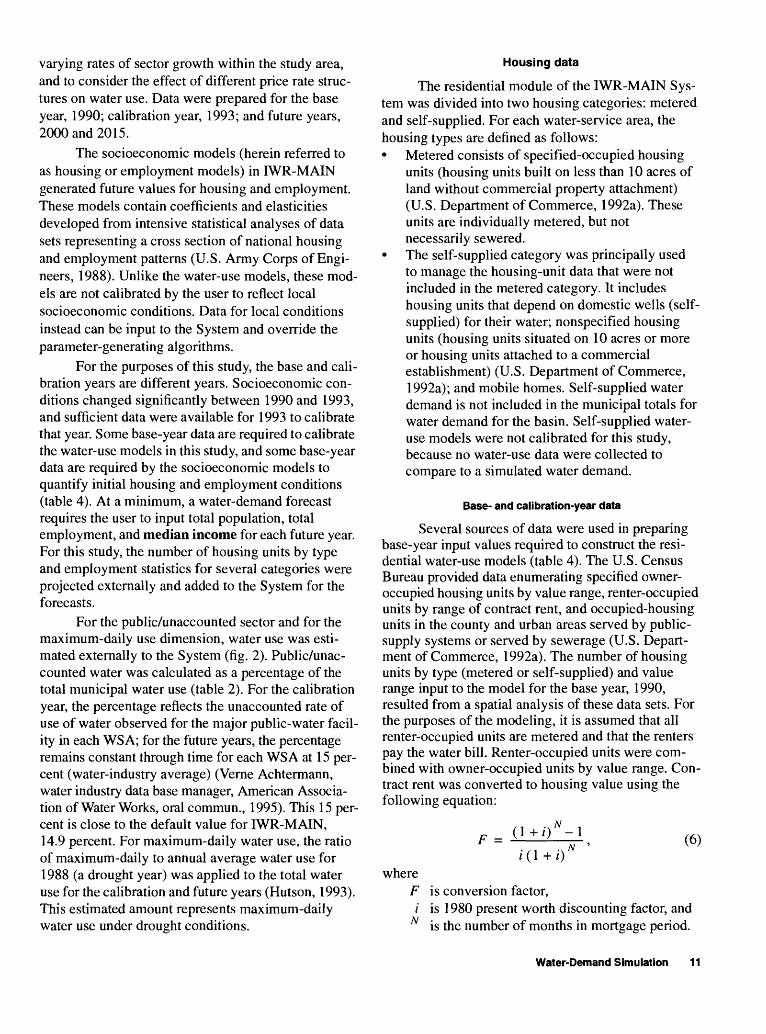
10. Observed and simulated average annual water demand for metered housing for 1993............................................. 1711. Model and calibration constants for the metered housing models............................................................................. 1712. Per capita use for the residential sector...................................................................................................................... 1813. Simulated water demand for Bedford, Marshall, and Maury/southern Williamson water-service

areas for 1993, 2000, 2015, 2025, 2035, and 2050.................................................................................................... 1914. Populations of Bedford, Marshall, and Maury Counties, Tennessee, 1960-92.......................................................... 2415. Maximum likelihood and nonlinear instrumental variables estimates of the Box-Cox

transformation parameter........................................................................................................................................... 2616. Maximum likelihood and nonlinear instrumental variables estimates of the Box-Cox

transformation parameter using census year data only .............................................................................................. 2617. Parameter estimates for the linear and log-linear models for Bedford, Marshall,

and Maury Counties, Tennessee................................................................................................................................. 3918. Parameter estimates for the linear and log-linear models for Bedford, Marshall, and

Maury Counties, Tennessee, using census year data only.......................................................................................... 3919. Projected populations and 95-percent confidence intervals for Bedford County, Tennessee,

1993-2050, results from the linear model.................................................................................................................. 4020. Projected populations and 95-percent confidence intervals for Marshall County, Tennessee,

1993-2050, results from the linear model.................................................................................................................. 40

iv Estimates of Future Water Demand for Selected Water-Service Areas in the Upper Duck River Basin, Central Tennessee

21. Projected populations and 95-percent confidence intervals for Maury County, Tennessee, 1993-2050, results from the linear model...............................................................................

22. Projected populations and 95-percent confidence intervals for Bedford County, Tennessee, 1993-2050, results from the log-linear model.........................................................................

23. Projected populations and 95-percent confidence intervals for Marshall County, Tennessee, 1993-2050, results from the log-linear model.........................................................................

24. Projected populations and 95-percent confidence intervals for Maury County, Tennessee, 1993-2050, results from the log-linear model .........................................................................

41

41

42

42

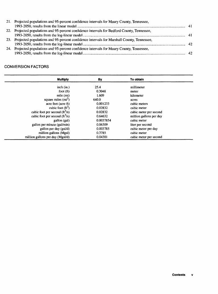
CONVERSION FACTORS

Multiply By To obtain

inch (in.)foot (ft)

mile (mi)square miles (mi )

acre feet (acre ft)cubic foot (ft3)

cubic foot per second (ft3/s)cubic foot per second (ft3/s)

gallon (gal)gallon per minute (gal/min)

gallon per day (gal/d)million gallons (Mgal)

million gallons per day (Mgal/d)

25.40.30481.609

640.00.0012330.028320.028320.646320.00378540.063090.0037850.37850.04381

millimetermeterkilometeracrescubic meterscubic metercubic meter per secondmillion gallons per daycubic meterliter per secondcubic meter per daycubic metercubic meter per second

Contents

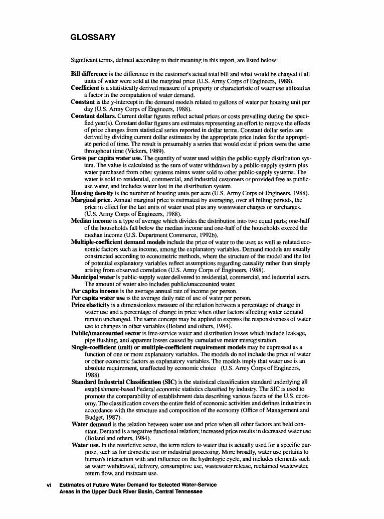
GLOSSARY

Significant terms, defined according to their meaning in this report, are listed below:

Bill difference is the difference in the customer's actual total bill and what would be charged if all units of water were sold at the marginal price (U.S. Army Corps of Engineers, 1988).

Coefficient is a statistically derived measure of a property or characteristic of water use utilized as a factor in the computation of water demand.

Constant is the y-intercept in the demand models related to gallons of water per housing unit per day (U.S. Army Corps of Engineers, 1988).

Constant dollars. Current dollar figures reflect actual prices or costs prevailing during the speci fied year(s). Constant dollar figures are estimates representing an effort to remove the effects of price changes from statistical series reported in dollar terms. Constant dollar series are derived by dividing current dollar estimates by the appropriate price index for the appropri ate period of time. The result is presumably a series that would exist if prices were the same throughout time (Vickers, 1989).

Gross per capita water use. The quantity of water used within the public-supply distribution sys tem. The value is calculated as the sum of water withdrawn by a public-supply system plus water purchased from other systems minus water sold to other public-supply systems. The water is sold to residential, commercial, and industrial customers or provided free as public- use water, and includes water lost in the distribution system.

Housing density is the number of housing units per acre (U.S. Army Corps of Engineers, 1988).Marginal price. Annual marginal price is estimated by averaging, over all billing periods, the

price in effect for the last units of water used plus any wastewater charges or surcharges. (U.S. Army Corps of Engineers, 1988).

Median income is a type of average which divides the distribution into two equal parts; one-half of the households fall below the median income and one-half of the households exceed the median income (U.S. Department Commerce, 1992b).

Multiple-coefficient demand models include the price of water to the user, as well as related eco nomic factors such as income, among the explanatory variables. Demand models are usually constructed according to econometric methods, where the structure of the model and the list of potential explanatory variables reflect assumptions regarding causality rather than simply arising from observed correlation (U.S. Army Corps of Engineers, 1988).

Municipal water is public-supply water delivered to residential, commercial, and industrial users. The amount of water also includes public/unaccounted water.

Per capita income is the average annual rate of income per person.Per capita water use is the average daily rate of use of water per person.Price elasticity is a dimensionless measure of the relation between a percentage of change in

water use and a percentage of change in price when other factors affecting water demand remain unchanged. The same concept may be applied to express the responsiveness of water use to changes in other variables (Boland and others, 1984).

Public/unaccounted sector is free-service water and distribution losses which include leakage, pipe flushing, and apparent losses caused by cumulative meter misregistration.

Single-coefficient (unit) or multiple-coefficient requirement models may be expressed as a function of one or more explanatory variables. The models do not include the price of water or other economic factors as explanatory variables. The models imply that water use is an absolute requirement, unaffected by economic choice (U.S. Army Corps of Engineers, 1988).

Standard Industrial Classification (SIC) is the statistical classification standard underlying all establishment-based Federal economic statistics classified by industry. The SIC is used to promote the comparability of establishment data describing various facets of the U.S. econ omy. The classification covers the entire field of economic activities and defines industries in accordance with the structure and composition of the economy (Office of Management and Budget, 1987).

Water demand is the relation between water use and price when all other factors are held con stant. Demand is a negative functional relation; increased price results in decreased water use (Boland and others, 1984).

Water use. In the restrictive sense, the term refers to water that is actually used for a specific pur pose, such as for domestic use or industrial processing. More broadly, water use pertains to human's interaction with and influence on the hydrologic cycle, and includes elements such as water withdrawal, delivery, consumptive use, wastewater release, reclaimed wastewater, return flow, and instream use.

vi Estimates of Future Water Demand for Selected Water-Service Areas in the Upper Duck River Basin, Central Tennessee

Estimates of Future Water Demand for Selected Water-Service Areas in the Upper Duck River Basin, Central TennesseeBy Susan S. Hutson

Abstract

Estimates of future water demand were determined for selected water-service areas in the upper Duck River basin in central Tennessee through the year 2050. The Duck River is the principal source of publicly-supplied water in the study area providing a total of 15.6 million gal lons per day (Mgal/d) in 1993 to the cities of Columbia, Lewisburg, Shelbyville, part of south ern Williamson County, and several smaller com munities. Municipal water use increased 19 percent from 1980 to 1993 (from 14.5 to 17.2 Mgal/d). Based on certain assumptions about socioeconomic conditions and future development in the basin, water demand should continue to increase through 2050.

Projections of municipal water demand for the study area from 1993 to 2015 were made using econometric and single-coefficient (unit- use) requirement models of the per capita type. The models are part of the Institute for Water Resources-Municipal and Industrial Needs Sys tem, IWR-MAIN. Socioeconomic data for 1993 were utilized to calibrate the models.

Projections of water demand in the study area from 2015 to 2050 were made using a single- coefficient requirement model. A gross per capita use value (unit-requirement) was estimated for each water-service area based on the results gen erated by IWR-MAIN for year 2015. The gross per capita estimate for 2015 was applied to popu lation projections for year 2050 to calculate water demand. Population was projected using the log- linear form of the Box-Cox regression model.

Water demand was simulated for two sce narios. The scenarios were suggested by various planning agencies associated with the study area. The first scenario reflects a steady growth pattern based on present demographic and socioeconomic conditions in the Bedford, Marshall, and Maury/southern Williamson water-service areas. The second scenario considers steady growth in the Bedford and Marshall water-service areas and additional industrial and residential development in the Maury/southern Williamson water-service area beginning in 2000.

For the study area, water demand for sce nario one shows an increase of 121 percent (from 17.2 to 38 Mgal/d) from 1993 to 2050. In scenario two, simulated water demand increases 150 per cent (17.2 to 43 Mgal/d) from 1993 to 2050.

INTRODUCTION

Water use for municipal purposes is increasing in the upper Duck River basin (fig. 1). Water for domestic, industrial, and commercial uses (municipal purposes) from public-supply systems increased 19 percent, from 14.5 million gallons per day (Mgal/d) in 1980 to 17.2 Mgal/d in 1993. Projected residential, industrial, and commercial developments in the basin suggest that water use is likely to continue to increase. Uncertainty exists among officials from local agencies in the basin about the adequacy of existing water sup plies to meet future demands. Long-term forecasts can help decision-makers determine if the Duck River, the principal source of publicly-supplied water in the basin, can supply the future demands.

In 1989, the U.S. Geological Survey (USGS) conducted an investigation to document trends in water availability, use, and future demand in the upper

Introduction

87° 22' 30'

36° 00'86° 37' 30 85° 52' 30'

35° 15'

-WILLIAMSON

Normandy y Manchester Dam

10 20 MILES

10 20 KILOMETERS

TENNESSEE

Ridge

Sequatchie Volley

Study areaModified from R.A. Milter (1974)

EXPLANATION

STUDY-AREA BOUNDARY

- - WATER-SERVICE-AREA BOUNDARY--Each county water-service area is consistent with that county's political boundary, except for the Maury County water-service area that includes part of southern Williamson County

BEDFORD COUNTY NAMEVolley and PHYSIOGRAPHIC PROVINCE

Kiage

Figure 1. Upper Duck River study area and the Maury/southem Williamson, Marshall, and Bedford water-service areas.

2 Estimates of Future Water Demand for Selected Water-Service Areas in the Upper Duck River Basin, Central Tennessee

Duck River basin (Hutson, 1993) 1 . The study provided estimates of future water demand through 2015. The study concluded that increases in withdrawals from the Duck River downstream of the city of Shelbyville would reduce minimum flows at the public water- supply intakes for the cities of Lewisburg and Columbia (fig. 1).

The effect of reduced flows on water quality was not addressed in the Hutson (1993) study. How ever, discharge permits that affect water quality are based on current minimum flows. Reduced minimum flows along the Duck River would reduce the carrying capacity of the river which would necessitate further costly treatment by municipalities and industry (such as tertiary treatment of effluent). Otherwise, deteriora tion of water quality in the river would ensue. Adverse water-quality conditions would be further exacerbated by any additional loadings of treated effluent that would emanate from economic development associ ated with increased water use (Larry M. Richardson, Manager, Water Resources Operations, Tennessee Val ley Authority, written commun., 1992).

In 1994, the USGS began an investigation to reassess municipal water demand in the basin using more recent (1990 and 1993) socioeconomic and demographic data and to extend the water demand projections to 2050. The investigation was conducted in cooperation with the Duck River Development Agency (DRDA). Part of the mission of the USGS is to assess the water use of the nation. In addition to col lecting water-use data, this study evaluated and devel oped methodologies and techniques for estimating water use and for projecting future water demand that may be applied nationwide.

Purpose and Scope

The purpose of this report is to provide esti mates of future municipal water demand for the year 2050. Municipal water demand is publicly-supplied water delivered to residential, industrial, and commer cial users and includes conveyance losses in the distri bution systems. The study area is comprised of Bedford, Marshall, and Maury Counties, and part of southern Williamson County (fig. 1). The investigation was limited to this area because municipal water demand from the upper Duck River will most proba-

1 References begin on page 43.

bly increase as a result of growth primarily in these counties (Steve Parks, Director, Duck River Develop ment Agency, oral commun., 1994). The investigation includes an inventory of the municipal water use in the study area and excludes any assessment of the effect of withdrawals on streamflow or of the availability of streamflow for waste assimilation.

Estimates of municipal water demand for 2015 were made with the Institute for Water Resources- Municipal and Industrial Needs System (IWR-MAIN or System) water-use models. These models were designed by Planning and Management Consultants, Ltd., under the auspices of the U.S. Army Corps of Engineers, Institute for Water Resources (U.S. Army Corps of Engineers, 1988).

The structure of the IWR-MAIN System limits projections to 25 years, for example, 1990 to 2015. A single-coefficient requirement model, therefore, was devised to extend the forecast to 2050. Estimates of municipal water-use demand for 2050 were calculated as the product of the gross per capita water use derived from the IWR-MAIN forecasts for 2015 and a popula tion estimate for 2050 for each water-service area.

Three types of models for projecting population over a long period of time (58 years, 1993 to 2050) were evaluated. The projections of population pro duced by the log-linear case of the Box-Cox model were used in the single-requirement models because the log-linear case yields the more reasonable and sim ilar estimates.

The terms water use, water demand, and water requirement are commonly interchanged. Technically the terms are distinct. Water use refers to the water that is actually used for a specific purpose (See Glossary). Water demand is the relation between water use and price when all other factors are held constant. Water requirement is water use as an abso lute requirement unaffected by economic choice.

Water-use values are expressed in the text as three-significant figures and in the tables as three- significant figures or as two decimal places. Percent ages appear in the text and tables as integers. Simu lated water demand for the calibration year, 1993, is expressed as three-significant figures or as two deci mal places. Simulated water demand for years 2000 through 2050 is expressed as two-significant figures or as one decimal place to reflect the uncertainty of the accuracies of the projections over the length of time. Values may not add to totals shown because of inde pendent rounding.

Introduction

Approach

The following tasks were designed to accom plish the project objectives:

Collect municipal water-use data for each public- supply system in the water-service areas for 1980, 1985,1989, 1990, and 1993.

Calibrate the IWR-MAIN water-demand models using demographic, economic, and water-use data for 1993. Estimate municipal water demand for 2015 using the calibrated models. Calculate gross per capita use for each water-service area.

Project population to 2050 using the log-linear form of the Box-Cox statistical model.

Input gross per capita use and populationprojections to a single-coefficient requirement model to forecast water demand for 2050.

HYDROLOGIC SETTING

The upper Duck River basin drains parts of the Highland Rim and Central Basin physiographic regions of Tennessee (Miller, 1974) (fig. 1). The cli mate of the area is moderate, with annual rainfall aver aging 46 inches per year. The river flows from the dissected limestone highlands in northern Coffee County into Normandy Reservoir, which was com pleted by the Tennessee Valley Authority (TVA) in 1976 (fig. 1). The reservoir, with a capacity of 117,000 acre-feet at normal maximum headwater elevation of 875 feet, is used for flood control, water supply, water- quality enhancements, and recreation. The study area begins downstream from Normandy Dam in Bedford County, and includes Marshall, Maury, and southern Williamson Counties. The study area ends at the west ern Maury County line and, including southern Will iamson County, is about 1,500 square miles.

Since the construction of Normandy Reservoir, the 3-day 20-year low-flow discharge in the upper

Duck River as it flows through Bedford, Marshall, and Maury Counties has increased. As a result, the river has become a more reliable source of supply of water during low flows. The 3-day 20 year (3Q20) minimum flow represents the lowest mean daily flow for a con secutive 3-day period with a recurrence interval of 20 years. The period of record is based on the climatic year which extends from April 1 through March 31 and is designated by the year in which it ends (B ing- ham, 1985). Estimated values of 3Q20 at Shelbyville and Columbia before and after completion of the dam site are as follows (Outlaw and Weaver, 1996):

Before 1976

Location

Shelbyville Columbia

Cubic feet per

second

53.8 68.6

Million gallons

per day

34.8 44.3

Period of

record

1949-1976 1961-1976

After 1976Cubic feet per

second

73.5 97.9

Million gallons

per day

47.5 63.3

Period of

record

1977-1993 1977-1993

WATER USE

The study area in the upper Duck River basin is divided into three municipal water-service areas (WSA's), whose boundaries closely coincide with their respective county boundaries (fig. 1). The three WSA's are Bedford, Marshall, and Maury/southern Williamson. The Duck River is the main source of water for municipal use in the study area, supplying 91 percent of the municipal water used. Springs and wells supplement the municipal water supply from the Duck River. Ground water supplies about 9 percent of the municipal water used in the study area.

Withdrawals for municipal use in the basin increased 19 percent from 1980 to 1993 from 14.5 to 17.2 Mgal/d (Alexander and others, 1984; Tennessee Division of Water Supply files, 1990 and 1993; USGS files, 1985,1988, and 1990) (table 1). Most of the increase has occurred in recent years. The

Table 1 . Total surface- and ground-water withdrawals by water-service area

Water-service area

BedfordMarshallMaury/

southernWilliamson.

Study area totals

Withdrawals, in million gallons per day1980

3.812.278.43

14.5

1985

3.622.518.75

14.9

1988

3.992.618.94

15.5

1989

4.362.829.41

16.6

1990

4.202.859.93

17.0

1993

4.592.52

10.1

17.2


Maury/southern Williamson WSA, for example, increased water use 1.16 Mgal/d between 1988 and 1993, the largest increase in the study area. Total water use in the study area in the same period increased 1.70 Mgal/d. These increases in water use are mainly due to increased demands by the residential and indus trial sectors (table 2). However, recent dry weather (drought of 1988) also affected water demand in the area by creating a need for additional water for outside usage in the summer (Hutson, 1993).

Municipal water use in the study area for 1993 was estimated from an inventory of public-supply sys tems. The inventory was conducted in 1994 in cooper ation with the Duck River Development Agency. Data from 14 public-supply systems provided information on the source of supply; daily average-annual amount of water withdrawn or purchased (table 3); and, amounts distributed to residential, commercial, and industrial users; conveyance losses; and free service. Conveyance losses and free water is referred to as public/unaccounted. Self-supplied water for indus trial and residential purposes was not inventoried. The inventory showed that: Municipal withdrawals in 1993 totaled

17.2 Mgal/d (table 1). Surface water accounted for 91 percent of the

withdrawals (15.6 Mgal/d); the remaining 9 percent or 1.66 Mgal/d was withdrawn from springs and wells (table 3). Water was withdrawn downstream of Normandy Reservoir at four public-supply intakes on the Duck River (Shelbyville Water System, Bedford County Utility District, Lewisburg Water System, and Columbia Water Department).

Residential water use accounted for 40 percent (6.86 Mgal/d); commercial use, 15 percent (2.60 Mgal/d); industrial use, 25 percent (4.34 Mgal/d); and, public/unaccounted water, 20 percent (3.41 Mgal/d) of the total withdrawals (table 2).

WATER-DEMAND SIMULATION

Water demand in the upper Duck River basin downstream of Normandy Dam was simulated to 2050 for two scenarios. Scenario 1 reflects a steady growth pattern based on present demographic and socioeconomic conditions in the Bedford, Marshall, and Maury/southern Williamson WSA's. Scenario 2 con siders steady growth in the Bedford and Marshall

WSA's and additional industrial and residential devel opment in the Maury/southern Williamson WSA beginning in 2000.

The combined use of the IWR-MAIN System and the population estimates was necessary to forecast water demand to 2050. The econometric and single- coefficient requirement models of the IWR-MAIN System were used to forecast water demand to 2015 for each WSA. The IWR-MAIN System limits water- use projections to 25 years (1990-2015). To forecast water demand to 2050, the IWR-MAIN results for 2015 were combined with population estimates for 2050 in a single-coefficient requirement (SCR) model. The gross per capita water use for scenario 1 (steady growth) and for scenario 2 (steady growth with increased growth in Maury/southern Williamson WSA) was determined from estimates produced by IWR-MAIN for each WSA for 2015. The gross per capita water use for each scenario and the projected population for 2050 were multiplied to estimate water use for each scenario in 2050. The methodology used for projecting population over a long period of time was developed for this study by G.E. Schwarz. The methodology and the results for the study area are detailed in a separate section by Schwarz.

Institute for Water Resources-Municipal and Industrial Needs System

The IWR-MAIN System (herein referred to as IWR-MAIN or System) was used to estimate future municipal water demand. Econometric demand and single-coefficient requirement (usually of the unit-use type) models calculated water demand as a function of socioeconomic parameters. A value for each of these parameters was projected for the years for which water demand was estimated.

IWR-MAIN is used primarily to test assump tions and the effect various assumptions or changes would have on water use in the basin rather than as a predictive tool to generate absolute amounts of water use in the future. This fact and basic assumptions about growth, land use, population, and technology drive the results. If the assumptions are changed (for example, population decreases in the area), the model's water-demand results will change. The accu racy of the results depends on the validity of the assumptions.

Water-Demand Simulation

Table 2. Public-supply deliveries of water to various water-use sectors by water-service area in 1993[Values, in million gallons per day]

SectorWater-service area

BedfordMarshallMaury/southern WilliamsonStudy area totals

Residential

1.75.96

4.156.86

Commercial

0.72.50

1.382.60

Industrial

1.08.45

2.814.34

Public/unaccounted

1.04.61

1.763.41

Table 3. Public-supply systems and source(s) of supply in 1993[Mgal/d, million gallons per day; WSA, water-service area; --, no transaction; gw, ground water; WS, Water System; UD, Utility District; MCBPU, Marshall County Board of Public Utilities; and, WD, Water Department]

Public-supply system

Source of supply

(river mile)Withdrawals

(Mgal/d)

Purchasedwater

(Mgal/d)

Shelbyville Water System Bedford County UD #1 and #2

Bell Buckle Water System Wartrace Water System Flat Creek Cooperative

Chapel Hill Water System

Marshall County Board of Public Utilities.

Cornersville Water Department Petersburg Water System 1 Lewisburg Water System

Henry Horton State Park2

Columbia Water Department Mount Pleasant Water System Spring Hill Water Department Maury County Water System Hillsboro and Thompson Station

Utility District.

Bedford WSA

Duck River (227.0) 3.28Duck River (202.4) .77Shelbyville WSWartrace WSCascade Spring (gw) .54Shelbyville WS

Marshall WSA

MCBPU #1Town well (gw) . 11Lewisburg WSCornersville WDChapel Hill WSLewisburg WSFayetteville WSDuck River (181.0) 2.41(metered at City Lake)MCBPU #1Chapel Hill WS

Maury/southern Williamson WSA

0.00 .16

.09

.00

.37

.02

.03

.11

.05

.02

Duck River (133.7) Spring (gw) Columbia WD Columbia WD Spring Hill WD

9.091.01

.23

.69

.36

1 Water purchased by this public water-supply system is not included in the study area total. Water is withdrawn from the Elk River watershed.2 Facility is a non-community public-water supplier. For the purposes of the model, the transfer of water from MCBPU #1 is handled as if it were a delivery to a commercial user.


Model Description

IWR-MAIN is a water-demand forecasting sys tem that contains a range of water-use models, socioeconomic-parameter generating procedures, and data-management techniques (U.S. Army Corps of Engineers, 1988). Nonmunicipal (self-supplied) or rural water demand is not simulated by IWR-MAIN. The architecture of IWR-MAIN allows for the separa tion of the study area into smaller study units (spatial disaggregation) and the analysis of the smaller units by sector and by season (fig. 2).

The Duck River study area was separated in IWR-MAIN into study units that correspond with the water-service areas. The IWR-MAIN divides munici pal water users within each WSA into four major sec tors: residential, commercial, industrial, and public/unaccounted. Each sector is further divided into a number of categories for simulation purposes. The seasonal dimensions of the System consider any one of the elements of annual average water use, summer or winter season water use, or maximum daily water use for each sector and category.

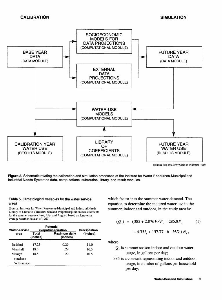
The relation between the calibration and the simulation processes of the System is displayed graph ically in figure 3. The schematic illustrates how the data modules relate to the computational modules and to the results. The base-year data are used to produce future-year data by means of internal models (compu tational module) that project growth for the various socioeconomic parameters. The growth in socioeconomic parameters (future data) also may be projected externally by the user and added to the model. Base (or calibration) year data are incorporated into the water-use models to simulate base (or calibration) year water use. If the base and calibration year are different years, selected future-year data also are incorporated into the model. The water-use models are calibrated by adjusting the library values to reflect local socioeco nomic and climatic conditions. The libraries contain the model constants, parameter coefficients, and cli matic values. Base-year and future-year data are used by the water-use models to calculate water demand for future years.

Version 5.1 of IWR-MAIN used in this study was prepared by Planning and Management Consult ants, Ltd., in cooperation with the U.S. Army Corps of Engineers, Water Resources Support Center, Institute for Water Resources (U.S. Army Corps of Engineers, 1988). The user's manual and system description for

IWR-MAIN provides additional details for much of the discussion presented in this section of the report.

Demand models

The econometric water-demand models relate socioeconomic parameters to water use for the resi dential, industrial, and commercial sectors (table 4). For the purposes of this study, these models were applied to only the residential sector. For the purposes of this study the residential sector was divided into two categories: metered and self-supplied. The num ber of housing units in each category is the variable driving the residential models. Housing value and price of water are the primary economic variables.

Water demand for the metered water category is calculated for each housing value range for the sum mer and winter seasons by applying multiple- coefficient demand models. Only the equation for the summer metered water category includes weather con ditions as a factor for influencing water demand. Pre cipitation and evapotranspiration values read from the IWR-MAIN Library of Climatic Variables produce values for the moisture deficit parameter. Precipitation and evaporation values are retrieved from the library using the latitude and longitude for each WSA (table 5).

Summer water demand includes indoor and out door usage. Indoor usage is related to the drinking, cooking, bathing, cleaning, and similar activities inside a household. Outdoor usage is related to lawn or garden sprinkling, car washing, or other similar activ ity. Irrigable land and moisture-deficit are variables

Table 4. Socioeconomic parameters input to the Institute for Water Resources-Municipal and Industrial Needs System[SIC, Standard Industrial Classification groups]

Required base-year parameters Future-year parameters

Number of residences by Number of residences by type and value range. type and value range.

Commercial and industrial Commercial and industrial employment by SIC. employment by SIC.

Number of persons per household Total employment 1Median household income Median household incomeResident population Resident population 1Water and sewer rate structureComposite Construction Cost IndexBill differenceClimatic conditionsTotal population

1 Required model input.

Water-Demand Simulation

INPUT DATA

Number of housing units by type, density and market-value range; average lot size; persons per household; and Composite Construction Cost Index

Number of employees by 3-digit Standard Industrial Classification (SIC) groups

Water and wastewater prices and rate structures; marginal price; bill difference

Climatic/weather conditions (moisture deficit)

Residential population, income and employment

WATER-USE MODELS

Econometric equations Unit-use requirement equations

LIBRARY DATA

DISAGGREGATED WATER USES

DIMENSIONS SECTORS CATEGORIES

AverageAnnual

Use

WinterSeason

Use

SummerSeason

Use

Maximum Daily Use

Residential

Commercial/ Institutional

Industrial

Public/ Unaccounted

Housing units by value metered and sewered flat rate with septic tank flat rate and sewered apartments up to 100 value ranges

Hotels, restaurants Hospitals Other 48 categories

Other products SIC 202 Mining machinery SIC 353 Other 198 categories

Distribution system losses Parks and public areas Other 28 categories

Modified from U.S. Army Corps of Engineers (1988)

Figure 2. Schematic describing the Institute for Water Resources-Municipal and Industrial Needs System architecture.


CALIBRATION SIMULATION

BASE YEAR DATA

(DATA MODULE)

SOCIOECONOMICMODELS FOR

DATA PROJECTIONS(COMPUTATIONAL MODULE)

EXTERNALDATA

PROJECTIONS(COMPUTATIONAL MODULE)

FUTURE YEAR DATA

(DATA MODULE)

WATER-USE MODELS

(COMPUTATIONAL MODULE)

CALIBRATION YEARWATER USE

(RESULTS MODULE)

ILIBRARY

OF COEFFICIENTS

(COMPUTATIONAL MODULE)

FUTURE YEARWATER USE

(RESULTS MODULE)

Modified from U.S. Army Corps of Engineers (1988)

Figure 3. Schematic relating the calibration and simulation processes of the Institute for Water Resources-Municipal and Industrial Needs System to data, computational subroutine, library, and result modules.

Table 5. Climatological variables for the water-service areas[Source: Institute for Water Resources-Municipal and Industrial Needs Library of Climatic Variables; rain and evapotranspiration measurements for the summer season (June, July, and August) based on long-term average weather data as of 1967]

Water-servicePotential

evapotranspiration Precipitationarea Total

(inches)

Bedford 17.25

Marshall 18.5Maury/ 18.5

southernWilliamson.

Maximum daily (inches)

0.29.29.29

(inches)

11.010.510.5

which factor into the summer water demand. The equation to determine the metered water use in the summer, indoor and outdoor, in the study area is:

(65) = (385 + 2.876 V/Fa -2S5.SPs (1)

-4.351 s + 157.77 -B-MD)Nr ,

wherereQs is summer season indoor and outdoor water

usage, in gallons per day; 385 is a constant representing indoor and outdoor

usage, in number of gallons per householdper day;

Water-Demand Simulation 9

V is average house value, in a range of value per1,000 dollars;

Fa is assessment factor; Ps is effective summer marginal price of water, in

dollars per 1,000 gallons; Is is effective summer bill difference variable, in

dollars per billing period; B is irrigable land per dwelling unit, in acres per

unit; MD is summer-season moisture deficit, in inches;

andNr is number of residences, in value range r.

Irrigable land is a function of housing density and is derived from the following equation:

B = 0.803 Hd,-1.26

(2)

whereB is irrigable land per dwelling unit, in acres per

unit, andHd is housing density, in number of units per acre.

Summer-season moisture deficit, MD, is calculated as follows:

MD = E-0.6R, (3)

whereE is summer-season potential evaporation, in

inches, andR is summer-season precipitation, in inches. Winter water demand includes only indoor

water usage. Winter usage is calculated as follows:

(QD) = (234+ 1.451 V/Fa (4)

-45.9Pa -2.59Ia )Nr ,

whereV, Fa, and Nr are as defined in equation (1);

QD is winter or indoor water use, in gallons perday;

234 is y-intercept, number of gallons per house hold per day;

Pa is effective annual marginal price of water, indollars per 1,000 gallons; and

Ia is effective annual marginal price of water, indollars per billing period.

Summer and winter season water demand are calculated. The model then aggregates the water use and produces a seasonally weighted residential rate of

use for the WSA, including maximum daily and aver age annual. In the model, housing value acts as a proxy for income. Marginal price and bill difference variables capture the effects of change in the water- rate structure on disposable income. The model assumes that the higher the disposable income, the greater the water use.

Single-coefficient requirement models

The single-coefficient requirement (unit-use) models estimate future water demand as a product of projected WSA commercial or industrial employment and a projected value of per-employee water use. Price of water is not a factor in these models. The unit-use coefficient is assumed to be fixed through time, that is, new technology is not a factor the model recognizes. Industrial and commercial water use were estimated as follows:

(5)

where<2 is water usage, in gallons per day; a is average annual use; n is industrial (commercial) use category; C is industrial (commercial) water-use coeffi

cient, in gallons per employee per day; and P is number of employees.

Data Preparation/Model Input

Housing and employment data were prepared as input to the water-use and socioeconomic models con tained in IWR-MAIN. Several assumptions (about the character of the data for the base and the calibration years, and about the structure of socioeconomic condi tions in future years) were necessary to model the basin. These assumptions are detailed within the respective data sections.

The water-use models of the IWR-MAIN Sys tem utilized demographic and economic data provided externally by the user as well as parameter values gen erated internally by socioeconomic models in the Sys tem. Actual values of these parameters are required for a base, or beginning year, and projected values of selected parameters for specified future years. The data were developed for each WSA (Bedford, Mar shall, and Maury/southern Williamson) for the resi dential, commercial, and industrial sectors. This spatial separation allowed the System to consider


varying rates of sector growth within the study area, and to consider the effect of different price rate struc tures on water use. Data were prepared for the base year, 1990; calibration year, 1993; and future years, 2000 and 2015.

The socioeconomic models (herein referred to as housing or employment models) in IWR-MAIN generated future values for housing and employment. These models contain coefficients and elasticities developed from intensive statistical analyses of data sets representing a cross section of national housing and employment patterns (U.S. Army Corps of Engi neers, 1988). Unlike the water-use models, these mod els are not calibrated by the user to reflect local socioeconomic conditions. Data for local conditions instead can be input to the System and override the parameter-generating algorithms.

For the purposes of this study, the base and cali bration years are different years. Socioeconomic con ditions changed significantly between 1990 and 1993, and sufficient data were available for 1993 to calibrate that year. Some base-year data are required to calibrate the water-use models in this study, and some base-year data are required by the socioeconomic models to quantify initial housing and employment conditions (table 4). At a minimum, a water-demand forecast requires the user to input total population, total employment, and median income for each future year. For this study, the number of housing units by type and employment statistics for several categories were projected externally and added to the System for the forecasts.

For the public/unaccounted sector and for the maximum-daily use dimension, water use was esti mated externally to the System (fig. 2). Public/unac counted water was calculated as a percentage of the total municipal water use (table 2). For the calibration year, the percentage reflects the unaccounted rate of use of water observed for the major public-water facil ity in each WS A; for the future years, the percentage remains constant through time for each WSA at 15 per cent (water-industry average) (Verne Achtermann, water industry data base manager, American Associa tion of Water Works, oral commun., 1995). This 15 per cent is close to the default value for IWR-MAIN, 14.9 percent. For maximum-daily water use, the ratio of maximum-daily to annual average water use for 1988 (a drought year) was applied to the total water use for the calibration and future years (Hutson, 1993). This estimated amount represents maximum-daily water use under drought conditions.

Housing data

The residential module of the IWR-MAIN Sys tem was divided into two housing categories: metered and self-supplied. For each water-service area, the housing types are defined as follows: Metered consists of specified-occupied housing

units (housing units built on less than 10 acres of land without commercial property attachment) (U.S. Department of Commerce, 1992a). These units are individually metered, but not necessarily sewered.

The self-supplied category was principally used to manage the housing-unit data that were not included in the metered category. It includes housing units that depend on domestic wells (self- supplied) for their water; nonspecified housing units (housing units situated on 10 acres or more or housing units attached to a commercial establishment) (U.S. Department of Commerce, 1992a); and mobile homes. Self-supplied water demand is not included in the municipal totals for water demand for the basin. Self-supplied water- use models were not calibrated for this study, because no water-use data were collected to compare to a simulated water demand.

Base- and calibration-year data

Several sources of data were used in preparing base-year input values required to construct the resi dential water-use models (table 4). The U.S. Census Bureau provided data enumerating specified owner- occupied housing units by value range, renter-occupied units by range of contract rent, and occupied-housing units in the county and urban areas served by public- supply systems or served by sewerage (U.S. Depart ment of Commerce, 1992a). The number of housing units by type (metered or self-supplied) and value range input to the model for the base year, 1990, resulted from a spatial analysis of these data sets. For the purposes of the modeling, it is assumed that all renter-occupied units are metered and that the renters pay the water bill. Renter-occupied units were com bined with owner-occupied units by value range. Con tract rent was converted to housing value using the following equation:

F = (6)

whereF is conversion factor,/ is 1980 present worth discounting factor, and

N is the number of months in mortgage period.


For the study area,/ is 0.006 (7.20 percent annual rate), Harry

Slingerland, Credit Officer, Federal Reserve Bank, St.Louis, Missouri, written commun., 1994)and

N is 360.Equivalent housing value expressed in 1980 dollars is as follows:

V = R-F, (7)

whereF is conversion factor as defined in equation (6).V is equivalent housing value, andR is monthly rent.For the calibration year (1993), estimates of the

total number of occupied-housing units by WSA were provided by the Tennessee Housing Development Agency (Kimberly Clark, Senior Housing Research Analyst, written commun., 1994) (table 6). The type of

data (U.S. Department of Commerce, 1992a) used to separate the housing units by type (metered or self- supplied) for 1990 were not available for 1993, there fore, the same proportion of housing unit by type as determined for the base year was used for 1993.

The housing density (fig. 2; table 4) for the cen tral part of the City of Columbia was used as the hous ing density value for each WSA for the base, calibration, and future years. This density value is six units per acre (David Holderfield, Director of Grants and Planning, City of Columbia, oral commun., 1994). The model uses housing density to calculate the rate of use of water for irrigable land and, ultimately, summer demand (indoor use plus outdoor use) (equations 1, 2, and 3). In preliminary model runs, this housing density closely approximated the amount of water used on an average lot in 1993 in each WSA and, therefore, was used for each WSA to calibrate the expected summer usage.

The model is structured so that only one value for the housing density variable for the base,

Table 6. Summary of housing data input to the Institute for Water Resources-Municipal and Industrial Needs System for the residential model by water-service area and by modeling scenario[--, no data input; scenario 1, steady growth from year to year; and scenario 2, selected higher growth in the residential sectors for the Maury/southern Williamson water-service area only]

Water-service area

Housing type

Occupied-housing units

1990 1993 2000 2015

Scenario 1 and 2Bedford

Metered Self-supplied Total

Marshall Metered Self-supplied Total

Maury/southern Williamson.


Maury/southern Williamson.


9,809 9,8541,704

11,653

10,0542,107

12,705

Scenario 1 and 2

6,333

18,732

18,732

6,5522,0028,554

20,9312,284

23,125

20,9312,284

23,215

Scenario 1

Scenario 2

6,6952,0029,086

21,3812,284

24,929

21,3822,284

26,614

10,7541,951

14,487

7,5841,501

10,360

23,1471,781

29,218

24,8331,781

32,164


calibration, and future years can be specified for each model run. This housing density value can change with time. However, changing the housing density value creates an alternative water-use scenario by changing summer demand. Model input for the pricing and the climate variables have the same limits, wherein each pricing and climate specification repre sents a new set of model conditions and an alternative water-use scenario.

The U.S. Census Bureau provided statistics for resident population (U.S. Department of Commerce, 1992b) for each WSA for the base year (1990). Cali bration and future-year projections of population resulted from the application of a log-linear type regression model to census data. See section by G.E Schwarz in this report for an explanation of the meth odology and the population projections for Bedford, Marshall, and Maury Counties.

The water and wastewater price-rate structures for each system in each WSA (data collected as part of this study) were used to specify annual and summer- season marginal price and to calculate bill difference for the base year. Rate structure information for the period 1993 was compiled and the rates were expressed in 1980 constant dollars (table 7).

Table 7. Marginal price and bill difference for water and wastewater, in 1980 dollars, for the metered housing category

Water- service

area


southernWilliamson.

Marginal price per thousand

gallons

3.463.851.93

Bill difference per thousand

gallons

1.08.52

4.29

The rate structure imposed by the largest public supplier in each WSA was adopted as the determining rate structure for water demand in that WSA. This technique was justified because, either this public sup plier served most of the connections in the WSA, or it distributed water to other systems, influencing their rate structure. The selected systems were Columbia Water Department (Maury/southern Williamson WSA), Lewisburg Water System (Marshall WSA), and Shelbyville Water System (Bedford WSA).

Future-year data

For future years (2000 and 2015) the number of total housing units was generated externally to IWR-

MAIN (fig. 2; table 4). The external method utilizes the projected resident population for each future year and the number of persons per household in 1990 (Bedford 2.59; Marshall, 2.57; and Maury, 2.62 per sons per household) (U.S. Department of Commerce, 1992b) (table 8). The rate of expansion of public- supply service also was factored into future estimates of housing units.

For the calibration and future years, the number of housing units within a selected value range for a specified housing type was generated by an internal econometric housing model (table 7). In calculating the percentage of housing units for a selected value range, this housing model considered the rate of change in median income and in population from the base year to the future year (U.S. Army Corps of Engi neers, 1988).

The only complete assessment of median house hold income in Tennessee occurs in each decennial census. The 1990 census provided base year (1990) median household income (U.S. Department of Com merce, 1992c) (table 9). For the calibration and future years, median household income was estimated using a multiplier derived from the average of the rate of change in per capita income in constant 1972 dollars from 1980 to 2015 as projected by the U.S. Depart ment of Commerce, Bureau of Economic Analysis (Duanne Hackman, Regional Economic Office, writ ten commun., 1992). The six rates of change that were projected for per capita income by the Bureau of Eco nomic Analysis were used in conjunction with the 1989 median household income for each county as reported by the U.S. Department of Commerce, U.S. Census Bureau in 1990; and, with the 1993 median household income as reported by the Columbia Power System (Linsay Boyd, General Manager, Columbia Power System, written commun., 1994). For the pur poses of the model input, the dollars are expressed as 1980 constant dollars.

Employment data

For the commercial sector, several Standard Industrial Classification (SIC) categories are grouped together because the water-use coefficients for the categories are similar. For industry, a more comprehensive data base (results from the inventory of the public-supply systems) and a greater range of coefficients for the categories resulted in more


Table 8. Estimated metered occupied-housing units by value range[Scenario 1, steady growth from year to year; scenario 2, higher growth in the residential sector for the Maury/southem Williamson water-service area]

Water-service area

Value range (1,000 dollars) Housing units

(1980 constant dollars) 1990 1993

Bedford0.0

14.121.128.135.242.249.256.363.370.487.9

105.5123.1140.7175.9211.1281.4351.8

- 14.1- 21.1- 28.1- 35.2- 42.2- 49.2- 56.3- 63.3- 70.4- 87.9- 105.5- 123.1- 140.7- 175.9- 211.1- 281.4- 351.8- 703.5

Total

1,2251,0531,8122,1061,2748875533031991639279251615412

9,809

1,128970

1,6692,0761,256874670367241198112163523331824

9,854

Marshall0.0

14.121.128.135.242.249.256.363.370.487.9

105.5123.1140.7175.9211.1281.4351.8

- 14.1- 21.1- 28.1- 35.2- 42.2- 49.2- 56.3- 63.3- 70.4- 87.9- 105.5- 123.1- 140.7- 175.9- 211.1- 281.4- 351.8- 703.5

Total

886725

1,1171,379734502335204121171754015207101

6,333

828678

1,0441,3957435084322631562209790344516202

6,552

2000

Scenario 1 and 2981843

1,4512,0191,22185087247831425714573723314914037919

10,754


1,4287605205883582123001324601732308112012

7,802

2015

500430740

2,0021,211843

1,500822540442249

2,1006654253991062753

13,054

357292450

1,485790541

1,070651386546239

1,391521695243350

359,975

division of the industrial categories than of the com mercial categories.

Base- and calibration-year data

The employment model requires total employ ment data for each WSA for 5 years before the base year (1985), the base year (1990), the calibration year (1993), and each future year (2000 and 2015). The

State Labor Force Summary provided total employment statistics from 1985 (5 years before the base year) to 1993 (Michael Ballard, Tennessee Department of Employment Security, written commun., 1994). For the base and calibration years, the Directory of Manufactur ers (White, 1994) and the Tennessee labor force estimates from Tennessee Department of Employment Security (1990) provided a means of separating the employment


Table 8. Estimated metered occupied-housing units by value range Continued

Water-service area

Value range (1,000 dollars) Housing units

(1980 constant dollars)

Maury/southern Williamson0.0 - 14.1

14.1 - 21.121.1 - 28.128.1 - 35.235.2 - 42.242.2 - 49.249.2 - 56.356.3 - 63.363.3 - 70.470.4 - 87.987.9 - 105.5

105.5 - 123.1123.1 - 140.7140.7 - 175.9175.9 - 211.1211.1 - 281.4281.4 - 351.8351.8 - 703.5

Total

Maury/southern Williamson 20.0 - 14.1

14.1 - 21.121.1 - 28.128.1 - 35.235.2 - 42.242.2 - 49.249.2 - 56.356.3 - 63.363.3 - 70.470.4 - 87.987.9 - 105.5

105.5 - 123.1123.1 - 140.7140.7 - 175.9175.9 - 211.1211.1 - 281.4281.4 - 351.8351.8 - 703.5

Total

Table 9. Median household income

1990

2,1021,4082,0553,3962,3602,5021,441

90673384648022810488501977

18,732

2,1021,4082,0553,3962,3602,5021,441

90673384648022810488501977

18,732

Water- Median household incomeservice expressed in 1980 constant dollars

area 1990 1993 2000

Bedford 14,887 16,077 18,090Marshall 15,039 16,417 18,473Maury/ 16,542 18,065 20,128

southernWilliamson.

2015

22,26322,73424,311

1993 2000 2015

Scenario 11,978 1,669 3801,325 1,118 2551,934 1,632 3723,626 3,561 3,4712,520 2,475 2,4122,671 2,624 2,5571,947 2,477 4,1251,224 1,557 2,594

991 1,260 2,0981,143 1,454 2,422

649 825 1,374419 1,131 2,832191 516 1,292162 436 1,09392 248 62135 94 23613 35 8713 35 87

20,931 24,473 29,849

Scenario 21,978 1,755 4141,325 1,176 2771,934 1,716 4053,626 3,813 3,8112,520 2,650 2,6482,671 2,809 2,8081,947 2,629 4,4981,224 1,653 2,828

991 1,337 2,2881,143 1,543 2,641

649 876 1,498419 1,304 3,235191 595 1,476162 503 1,24992 286 71035 109 27013 40 9913 40 99

20,931 26,254 32,920

statistics for 2-digit SIC classifications into statisticsfor three-digit SIC categories.

Future-year data

Projected rates of growth by two-digit SICgroup from year 1993 inventoried to 2005 were prepared by the Tennessee Labor Market Unit, Researchand Statistics Unit, Tennessee Department of Employment and Security for the Middle Tennessee Substate

ofooc ^QoroVi /"'olrKi/oll \i/fittt»i-» r-rvmmnn Te»r«r«e»ee£»£»


Department of Employment Security, 1994). Individ ual county statistics cannot be officially disclosed because of the confidentiality of the information. Employment projections for the study area, therefore, were based on the growth projected for the substate area.

For a scenario of steady growth in the commer cial and industrial sectors in each WSA, the model input for the total number of employees for the study area is as follows: year 1985, 34,659; 1990, 45,310; 1993, 51,445; 2000, 56,453; and 2015, 67,853. For a scenario of higher growth in selected industrial cate gories for the Maury/southern Williamson WSA for years 2000 and 2015, the estimated number of employees for the study area is 58,803 and 70,203, respectively.

Model Calibration

Model calibration consists of using actual socioeconomic data for a period of time and simulating water use for various sectors of the municipal system such as residential, commercial, and industrial cus tomers. Actual water-use data are compared to simu lated results to determine calibration accuracy. Two major steps comprise the calibration process:1. Initial simulation using all the default parameters

ofIWR-MAIN;and2. Analysis of the pattern of errors resulting when

the simulated water demand is compared to the actual values, then adjusting equations as needed.

The year 1993 was selected for calibration because water use was inventoried for the public- supply systems and industries in the study area for that year. The water-use inventory provided a guide to adjusting the residential, commercial, and industrial constants and coefficients of the water-use models. Industrial activity and the resulting water-use patterns were sufficiently different between 1990 and 1993 so that a model using the 1993 calibration data is more reliable for estimating future use.

For this study, IWR-MAIN estimates of the residential-water demand exhibit systematic errors of predicting actual water use in the calibration year. This pattern of prediction error indicates that residential water use in the study area is characterized by a lower (or higher) base use than that observed in the data that were used to derive the IWR-MAIN demand models. The simulated residential water demand for the Bed ford and Marshall WSA's was lower and for the Maury/southern Williamson WSA, water demand was higher (table 10).

The winter and summer model constants repre senting gallons of water per household per day were adjusted to calibrate the seasonal models (table 11). The coefficients for the effective marginal price vari able for summer and winter usage also were adjusted using regional (State of Kentucky) coefficients for the Bedford and Marshall WSA's (Eva Opitz, Director of Research, Planning and Management Consultants, Ltd., oral commun., 1994). The combined water and wastewater rates in these two WSA's exceeded the rates in the national data sets that were used to develop the System's price coefficients. The coefficient applied to the effective summer marginal price of water was changed from 285.5 to 160.9 as defined in equation (1). The effect in the equation is, for each 1.00 dollar increase in the price, water use is reduced 160.9 gallons for the summer season for each residen tial unit.

The coefficient applied to the effective annual marginal price of water was changed from 45.9 to 37.55 as defined in equation (4). The effect in the equation is, that for each 1.00 dollar increase in the price, water use is reduced 37.55 gallons for the winter season for each residential unit. Changing the elastic ity reduces the effect of the rate of change on the amount of water used.

Summer and annual water usage for each WSA was calibrated to yield ratios of 1.06 (Bedford), 1.03 (Marshall), and 1.07 (Maury/southern Williamson) of summer to annual use to agree with the summer (June- August) use to annual use ratio for the largest public- supplies in each WSA in 1993. These systems closely mirrored the seasonal water use of the other major water systems in the respective WSA.

For the industrial and commercial single- coefficient requirement models (water-use per employee) the results of the initial calibration revealed the need to adjust IWR-MAIN default coefficients from the Library of Coefficients (U.S. Army Corps of Engineers, 1988). The commercial sector required the greatest adjustments. Per employee rates of use for the largest utility customers were verified using the data compiled from the inventory of 1993 usage. These included industries with high employment, high pro jected rate of growth, or large quantity users. Changes to the coefficients reflect local per employee use for a specific SIC or represent average employee use for combined SIC categories.

Model Reliability

The constants and coefficients in the water-use models were generally reliable in estimating residential


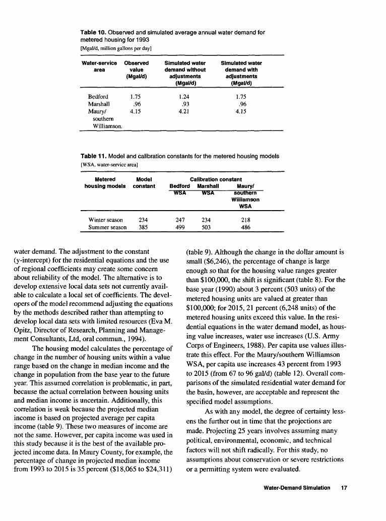
Table 10. Observed and simulated average annual water demand for metered housing for 1993[Mgal/d, million gallons per day]

Water-servicearea


southernWilliamson.

Observedvalue

(Mgal/d)

1.75.96

4.15

Simulated waterdemand without

adjustments(Mgal/d)

1.24.93

4.21

Simulated waterdemand withadjustments

(Mgal/d)

1.75.96

4.15

Table 11 . Model and calibration constants for the metered housing models[WSA, water-service area]

Metered Model housing models constant

Winter season 234 Summer season 385

Calibration constant Bedford Marshall Maury/

WSA

247 499

WSA

234 503

southern Williamson

WSA

218 486

water demand. The adjustment to the constant (y-intercept) for the residential equations and the use of regional coefficients may create some concern about reliability of the model. The alternative is to develop extensive local data sets not currently avail able to calculate a local set of coefficients. The devel opers of the model recommend adjusting the equations by the methods described rather than attempting to develop local data sets with limited resources (Eva M. Opitz, Director of Research, Planning and Manage ment Consultants, Ltd, oral commun., 1994).

The housing model calculates the percentage of change in the number of housing units within a value range based on the change in median income and the change in population from the base year to the future year. This assumed correlation is problematic, in part, because the actual correlation between housing units and median income is uncertain. Additionally, this correlation is weak because the projected median income is based on projected average per capita income (table 9). These two measures of income are not the same. However, per capita income was used in this study because it is the best of the available pro jected income data. In Maury County, for example, the percentage of change in projected median income from 1993 to 2015 is 35 percent ($18,065 to $24,311)

(table 9). Although the change in the dollar amount is small ($6,246), the percentage of change is large enough so that for the housing value ranges greater than $100,000, the shift is significant (table 8). For the base year (1990) about 3 percent (503 units) of the metered housing units are valued at greater than $100,000; for 2015, 21 percent (6,248 units) of the metered housing units exceed this value. In the resi dential equations in the water demand model, as hous ing value increases, water use increases (U.S. Army Corps of Engineers, 1988). Per capita use values illus trate this effect. For the Maury/southern Williamson WSA, per capita use increases 43 percent from 1993 to 2015 (from 67 to 96 gal/d) (table 12). Overall com parisons of the simulated residential water demand for the basin, however, are acceptable and represent the specified model assumptions.

As with any model, the degree of certainty less ens the further out in time that the projections are made. Projecting 25 years involves assuming many political, environmental, economic, and technical factors will not shift radically. For this study, no assumptions about conservation or severe restrictions or a permitting system were evaluated.


Table 12. Per capita use for the residential sector[Scenario 1, steady growth; scenario 2 , higher growth in the residential sector in the Maury/southern Williamson water-service area; --, no data]

Water- service

area

BedfordMarshall

Maury/

Per capita use, in gallons per person per day1993

(actual)

5742

67

2000 (simulated)


Scenario 179

2015 (simulated)

8781

96southern Williamson.

Maury/ southern Williamson.

Scenario 279 98

Model Results

The IWR-MAIN models that were calibrated for the Bedford, Marshall, Maury/southern Williamson water-service areas were used to simulate water demand for years 2000 and 2015. The estimates for each water-service area are aggregated to yield basin totals for the upper Duck River. The results of the sim ulation for scenario 1 (table 13) show that: Simulated average water demand in the basin

could increase 10 percent by 2000 and 57 percent by 2015.

Residential water demand could increase 24 percent by 2000 and 90 percent by 2015.

Commercial water demand could increase 23 percent by 2000 and 58 percent by 2015.

Industrial water demand could increase13 percent by 2000 and 41 percent by 2015.

The results of the simulation for scenario 2 show that average water demand could increase 16 percent by 2000 and 71 percent by 2015.

Single-Coefficient Requirement Model

Water demand for the Bedford, Marshall, and Maury/southern Williamson WSA's for years 2025, 2035, and 2050 was estimated using a single- coefficient requirement model expressed as

Q = C P, (8)

where

Q is average annual water use, in gallons per day;C is a water-use coefficient (gross per capita

use); andP is population.

This single-coefficient requirement model was devised to extend the forecast to 2050. The mathematical structure of the IWR-MAIN System limits projections of the socioeconomic parameters to 25 years, for example, 1990 to 2015.

Gross per capita use for each WSA for year 2015 was multiplied by a projected population to cal culate water demand (table 13). The gross per capita values for 2015 were derived from sector estimates of water demand produced by the IWR-MAIN System. For the Bedford WSA, the gross per capita value is 205; Marshall, 176; Maury/southern Williamson sce nario one, 225; and Maury/southern Williamson sce nario two, 219 gallons per person per day.

Population projections for Bedford, Marshall and Maury counties for 2025, 2035, and 2050 are based on published census data for the years 1960 to 1992. Population data for census years 1960, 1970, 1980, and 1990 are based on census count data. Data for intercensus years 1961-68, 1971-78, 1981-88, and 1991-1992 are estimated by the Bureau of Census on the basis of ancillary data, such as birth and death rates and migration statistics. No population data are avail able for the years preceding the decennial census for 1969, 1979, and 1989. Population projections for southern Williamson County for a steady and higher rate of growth for 2025, 2035, and 2050 were provided by the Williamson County Planning Commission (Joseph Home, Director, written commun., 1994).


Table 13. Simulated water demand for Bedford, Marshall, and Maury/southern Williamson water-service areas for 1993, 2000, 2015, 2025, 2035, and 2050

[WSA, water-service area; --, not simulated]

Sector 1993 2000 2015 2025 2035in million gallons per day

Percent 2050 increase

from 1993

Bedford WSA scenario 1 and 2

ResidentialCommercialIndustrialPublic/unaccountedTotal water demandMaximum daily use

1.75.72

1.081.044.596.75

2.21.01.2

.85.27.8

3.31.31.31.06.9 7.6 8.2

10 11 12

_ 9.4 105

14 107

Marshall WSA scenario 1 and 2


0.96.50.45.61

2.523.83

1.3.6.5.4

2.84.2

2.1.8.9.7

4.5 4.8 5.26.8 7.2 7.8

_..._..6.0 1389.0 135

Maury/southern Williamson WSA scenario 1


4.151.382.811.76

10.115.6

5.01.63.21.7

1218

7.32.03.92.3

16 17 1924 26 29

__

22 11833 112

Maury/southern Williamson WSA scenario 2


4.151.382.811.47

10.115.6

5.51.63.41.9

1219

8.12.04.22.5

17 20 2326 30 35

__..

27 16740 156

Upper Duck River study area scenario 1


6.862.604.342.44

17.225.8

8.53.24.92.9

1929

13.04.16.14.0

27 30 3340 45 50

__.. ._

38 12157 121

Upper Duck River study area scenario 2


6.862.604.342.43

17.225.8

9.03.25.13.1

2030

14.04.16.44.2

29 33 3644 50 54

_._...

43 15064 148


Regression analysis was used to relate the popu lation data to time. The choice of a functional form of regression analysis for relating population to time is important because the projections are carried out for a long period of time (58 years, 1993 to 2050). Three types of regression models were evaluated. When graphed, the Box-Cox model yields projections that show a large negative curvature so that out-of-sample projections quickly go to infinity. The large negative curvature is partially a consequence of using ancillary data to estimate population between census years. Special cases of the Box-Cox model (the linear and log-linear models) yield more reasonable and similar projections. In the final analysis, the projections gener ated by the log-linear model were used (see section by G.E. Schwarz).

The population projection for each WSA was modified to reflect the number of persons (households) served by public supply. The percentage of the popula tion served for 2025, 2035, and 2050 is the same per centage as determined for 2015. For Bedford, 90 percent; Marshall, 94 percent; and Maury/southern Williamson WSA, 97 percent. For scenario two, addi tional population is added to the log-linear projection of population for Maury County to account for addi tional industrial growth.

The results of the simulation for the upper Duck River basin study area for 2050 (table 13) show that: For scenario one (steady growth), average water

demand could increase 121 percent to 38 Mgal/d. For scenario two (higher growth in selected

sectors for the Maury/southern Williamson WSA), average water demand could increase 150 percent to 43 Mgal/d.

SUMMARY

Municipal water use in the upper Duck River basin study area increased 19 percent from 1980 to 1993 (14.5 Mgal/d to 17.2 Mgal/d). Socioeconomic data for the area suggest that water demand will con tinue to increase in response to residential, industrial, and commercial development. Officials from the Duck River Development Agency are concerned whether the capacity of the river can meet future water demands. In an attempt to address this concern, an investigation was conducted during 1994 by the USGS in cooperation with the Duck River Development Agency to determine potential future water demands. Methods used in this study can be applied nationwide to estimate water use and project water demand.

The study area includes about 1,500 square miles of the Duck River basin, extending from Nor mandy Dam to the western Maury County line.

Included in the study area are Bedford County, Mar shall County, and Maury/southern Williamson Coun ties. The 3-day 20-year low-flow discharge of the upper Duck River has increased as a result of con trolled releases since the construction of Normandy Reservoir.

Public-water systems withdrawing from the Duck River supplied an average of 15.6 Mgal/d (about 91 percent of the total water demand) in 1993 to utili ties in the Bedford, Marshall, and Maury/southern Williamson water-service areas (WSA's). The balance (about 9 percent or 1.66 Mgal/d) was supplied from springs and wells. The public-water systems delivered water for residential, commercial, and industrial uses to the cities of Lewisburg, Shelbyville, Columbia, Mount Pleasant, and several smaller communities in the basin.

Water demand in the basin for the year 2050 was estimated using the Institute for Water Resources- Municipal And Industrial Needs System (IWR- MAIN) and a single-coefficient requirement model. Water demand was projected based on steady growth throughout the study area (scenario 1) and increased growth starting in 2000 in the Maury/southern Will iamson WSA (scenario 2).

The IWR-MAIN was calibrated to 1993 condi tions and was used to estimate water demand for 2015. Gross per capita use was derived from the water- demand estimate for 2015 for each water-service area. For the Bedford WSA, the gross per capita use is 205; Marshall, 176; Maury/southern Williamson scenario 1, 225; and Maury/southern Williamson scenario 2, 219 gallons per person per day.

Census data for each WSA were used in a log- linear regression analysis to project population in each WSA to 2050. A single-coefficient model was devised to combine water use with projected population and extend the water-use forecast to 2050. Gross per capita use for each WSA for year 2015 was multiplied by a projected population to calculate water demand. Water demand for each water-service area was combined to yield a total for the basin.

Results from the water-use models indicate that water demand for the upper Duck River study area for the years indicated could increase as follows:

Scenario 1Year

199320152050

Totaldemand(Mgal/d)

17.22738

Percentincrease

from 1993

..57

121

Scenario 2Total

demand(Mgal/d)

17.22943

Percentincrease

from 1993

..69

150


Methodology Used to Develop Population Forecastsfor Bedford, Marshall, and Maury Counties,

Tennessee, From 1993 Through 2050

by

Gregory E. Schwarz

Methodology Used to Develop Population Forecasts for Bedford, Marshall, and Maury Counties, Tennessee, From 1993 Through 2050By Gregory E. Schwarz

This section describes the methods used to develop population forecasts for Bedford, Marshall, and Maury Counties, Tennessee, from 1993 through 2050. Three approaches for estimating the relation between population and time are compared. These approaches include the Box-Cox, the log-linear, and the linear regression methods. The Box-Cox model allows for a general nonlinear relation between popula tion and time and includes, as special cases, the linear and log-linear models. The results from the three approaches indicate that the best model for forecasting population into the distant future is the log-linear model.

The Data

The forecasts are based on published census data for the years 1960 to 1992. Population data for census years 1960,1970,1980, and 1990 are based on census count information. Data for the intercensus years from 1961 through 1968, 1971 through 1978, 1981 through 1988, and 1991 through 1992 are estimated by the cen sus on the basis of ancillary data. No population data are available for the years 1969, 1979, and 1989. Cen sus estimates of population for the three counties between 1960 and 1992 are presented in table 14.

Method of Estimation

Regression analysis was used to relate the popu lation data to time. Because the forecast is carried out over a long period (58 years), the choice of a functional form relating population to time is critical. To facilitate the estimation of a correct functional form, a Box-Cox transformation (Davidson and MacKinnon, 1993, p. 483-507) of the population variable is used. The

functional form with the Box-Cox transformation applied to the dependent variable is

(1)

where Pt is the population for observation t; Tt is the year corresponding to observation t\ et is an unob served error term, assumed independent and normally distributed with mean of 0 and variance of a e; and A, P0, and P! are constants to be estimated.

There are two approaches to estimating the coef ficients A, Po, and Pi in equation 1 maximum likeli hood (ML) and nonlinear instrumental variables (NLIV). In practice, ML estimates can be obtained by rescaling the population variable. This is accomplished by dividing population by the geometric mean of pop ulation for the sample and estimating the resulting equation using nonlinear least squares (NLLS). The resulting estimate of A is identical to the ML estimate, although its estimated standard error is not (the coeffi cients Po and Pi in the rescaled model are transformed by the scale change and, thus, must be retransformed to obtain ML estimates). To calculate the standard error of the ML estimate of A, we use the method of double- length artificial regression (DLR) (Davidson and MacKinnon, 1993, p. 498-500). An alternative approach to ML (or NLLS) estimation is to estimate the rescaled version of the model using NLIV (Amemiya, 1985, p. 249-252). Under this approach, DLR is not needed because the standard error of A, is consistently estimated.

The form of equation 1 permits a number of commonly used functional forms. The linear and log- linear models are simply restricted versions of the equation. For the linear model, A is set equal to 1, and

Method of Estimation 23

Table 14. Populations of Bedford, Marshall, and Maury Counties, Tennessee, 1960-92

[N.A., not available. Sources: U.S. Bureau of the Census, (1967), (1968), (1969), (1973), (1974), (1975), (1976), (1978), (1979), (1988a), (1988b), (1990), and (1994)]

Year

196019611962196319641965196619671968196919701971197219731974197519761977197819791980198119821983198419851986198719881989199019911992

Bedford County

23,22323,53423,41223,92324,28224,39425,05225,38326,581N.A.25,03924,70025,10025,60025,70025,80026,00025,90026,390N.A.27,91627,90028,20028,20028,60028,90029,20029,30029,500N.A.30,41 131,05331,738

Number

Marshall County

16,91416,53416,61417,50117,72217,97317,77418,09118,489N.A.17,31917,40017,50017,70017,90018,10018,00018,30018,312N.A.19,69819,80019,80019,70020,40020,60020,80021,20021,300N.A.21,53922,46922,974

Maury County

41,78941,86243,35643,77044,16045,01945,27545,75344,807N.A.44,02843,60044,20044,80045,20045,20046,40047,50047,895N.A.51,09551,60051,60051,50052,30053,30054,10055,00055,300N.A.54,81258,13159,740

Conversely, the log-linear model can be obtained by taking the limit of equation 1 as A, goes to infinity to obtain

(3)

where In(-) denotes the natural logarithm. To under-<\

stand this derivation, take the limit of (P,-1)A, as A, goes to zero using L'hospital's rule from elementary calculus. This model, too, can be estimated by ordinary least squares.

Method of Forecasting

Population forecasts from the Box-Cox model were estimated by the equation

p,= [1 1] i/x(4)

where P, is the forecast of population for period r; and 1, po» and Pi are ML or NLIV estimates of A,, PQ, anc* PJ. This form of the forecast equation is technically incorrect because it does not fully account for the effects of random error arising from the et term and error in the parameter estimates. However, the forecast should be relevant for indicating the general perfor mance of the Box-Cox transformation.

Projections for the linear and log-linear models are based on the following equations

Linear model: Pt = (5)

the intercept term is used to absorb the -1 appearing in the left-hand side of the equation. The estimated modelis

and

Log-Linear model: Pt = expl P (6)

p, = (2) where po and pj are estimated values of P0 and pj. The term a,, appearing in equation 6, is the variance of the forecast error. This variance is observation-

This model can be estimated by ordinary least squares. dependent and is given by


= a. 1 +NV(T)

(7)

2.where oe is the estimated variance of the regression residual; N is the sample size; V(TS) is the variance of T for in-sample observations (that is, observations used to estimate the regression); and 7^ is the average of the in-sample Ts. Note that the variance given in equation 7 is for out-of-sample forecasts only. For in-sample forecasts, the variance is equal to 2d^ minus the quan tity expressed in the righthand side of the equals sign in equation 7. Note also that the forecast equation for the log-linear model given in equation 6 is biased in small

2samples due to the use of an estimated value for Ge (as opposed to a known value). However, given the small value of this variance in practice (see below), the mag nitude of the bias is small and can reasonably be ignored.

Confidence intervals for the linear-model fore cast are given by

Confidence Interval Upper Bound:~2

and (8)

Confidence Interval Lower Bound:

where Pt is forecasted population as given by equation 5; ta/2 (N- 2) is the critical level for a t statistic with N- 2 degrees of freedom at significance level a; and 6^ is the forecast variance as given in equation 7 using the d^ estimated from the linear model.

The confidence interval for the log-linear model is derived in a more complicated manner. Observation- dependent bounds Lt and Ut are needed such that the difference Ut -Lt is minimized subject to the constraint that the probability of the event Lt <Pt < Ut equals 1 - a. Due to the skewed nature of the log-normal dis tribution for the error term, the forecasted value will not necessarily lie halfway between the lower and

2upper bounds. For the case where Ge is known, the lower and upper bounds satisfy the relations

Confidence Interval Lower Bound:L2( 5 U2

and (9)

Confidence Interval Upper Bound:

where 6^ is given in equation 7 and Zt solves the equation

'ft -e /2 , tJ e dz = 1 - a. (10)

A derivation of these equations is given in Appendix A.

Model Estimation and Population Forecasts

This section presents the results from estimating the Box-Cox, linear, and log-linear models. The esti mated models are used to generate population forecasts for Bedford, Marshall, and Maury Counties, Tennessee.

Box-Cox Model

Table 15 gives ML and NLIV estimates of X and associated standard errors for Bedford, Marshall, and Maury Counties. Instruments used for the NLIV proce dure are a constant, time, and time-squared. Estimated values of K are consistently negative and, in most cases, significantly different from 0. All the estimates are sig nificantly different from 1.0, implying systematic rejection of the linear model.

Population forecasts for the ML and NLIV mod els for the three counties are shown in figures 4 to 6. For comparison, the population projections for the lin ear and log-linear models also are shown (see below for details on these projections), as well as projections for 1995, 2000, 2005, 2008, and 2010 from a study by the University of Tennessee (Economic and Community Staff, 1992). The figures show clear problems with the Box-Cox model. All projections, regardless of the

Model Estimation and Population Forecasts 25

Table 15. Maximum likelihood and nonlinear instrumental variables estimates of the Box-Cox transformation parameter

[X, Box-Cox transformation parameter. Asymptotic standard errors in parentheses]

Table 16. Maximum likelihood and nonlinear instrumental variables estimates of the Box-Cox transformation parameter using census year data only (N = 4)

[X, Box-Cox transformation parameter. Asymptotic standard errors in parentheses]

Maximum likelihood County estimate of X

Nonlinear instrumental variables estimate of X

Maximum likelihood County estimate of X

Nonlinear instrumental variables estimate of X

Bedford

Marshall

Maury

-1.809fl

(0.978)

-2.900° *

(1.266)

-2.931" ^

(1.095)

-3.088fl *

(1.212)

-7.507" *

(2.390)

-6.195* *

(1.852)

a Significantly different from 1 at 5-percent level of significance. b Significantly different from 0 at 5-percent level of significance.

estimation method, reach an asymptote early in the forecast horizon. A possible cause of this problem is the use of intercensus year data to estimate the model. Unlike census year data, which are determined from a full count of the population, intercensus year data are estimated from ancillary data such as birth rates, death rates, and so forth. The use of ancillary data implies the intercensus year population estimates are not as accu rate as the census year estimates, with larger errors occurring in the years just before a census year. This is demonstrated in the data as large changes in population between a census year and the preceding year (see the graphs labeled "Actual data" in figures 4 to 6). It is pos sible that in trying to fit the large curvature in the data between census years, the Box-Cox model generates large negative estimates for X.

To assess the importance of the intercensus year estimates, the Box-Cox model was reestimated using only the four census year population estimates. The resulting estimates of A, are presented in table 16, and population projections are shown in figures 7 to 9. With the exception of Marshall County, the estimates of A, are much less negative. None of the estimates are sig nificantly different from 0 or from 1, which is probably due to the smaller estimated values of \ and the fewer number of data points entering the regressions. With the exception of Marshall County, the projections are much more stable and do not attain an asymptote within the forecast period. Also, the Box-Cox forecasts

Bedford

Marshall

Maury

-0.633 (1.177)

-2.886 (4.656)

-0.326 (3.637)

-0.679 (1.690)

-7.261 (11.081)

-1.413 (6.302)

do not differ significantly from those of the log-linear model.

Linear and Log-Linear Models

The unrealistically large curvatures generated by the Box-Cox model suggest that attention should be focused on the linear and log-linear models. The nega tive values for A, obtained from the models estimated using only census year data tend to support a model with curvature, such as the log-linear model. Table 17 presents results for the linear and log-linear models using all the data. Results based only on census year data are reported in table 18. All the results show the time trend variable to be significantly different from 0, and the coefficients of correlation (R2) indicate good regression fits.

Projections and 95-percent confidence intervals for Bedford, Marshall, and Maury Counties, using the linear and log-linear models and estimated using all the data, are given in figures 10 to 12. Projections and 95-percent confidence intervals for models estimated from only census year data are given in figures 13 to 15. Generally, the forecasts of the linear and log-linear models are very similar. All show an upper trend in population with a characteristic widening of the confi dence intervals for forecasts further into the future. With the exception of later year forecasts for Bedford County, the confidence interval of the linear model overlaps the confidence interval of the log-linear


60 50

-

w Q w 3 I

40

o I o.

O Q.

30

-

20

-]

i i

i i

i i

i i

i I

i i

i r

i i

i i

i |

i i

i i

i i

i i

i |

r r, ,,,,,,

| ,,,,,,,,,,,,,,,,,,,,,,

1960

19

70

1980

19

90

2000

20

10

2020

YE

AR

1 '

' '

I '

' '

' '

' '

' '

I '

'

2030

20

40

1 '

' '

I

2050

B> a o O oO

O O

A

ctua

l dat

a

Lin

ear f

orec

ast

_

M

L f

orec

ast

EX

PLA

NA

TIO

N

D

D

D

Uni

vers

ity o

f Ten

ness

ee f

orec

ast

_ _

_ _

Log

-lin

ear f

orec

ast

NLI

V f

orec

ast

Figu

re 4

. Act

ual a

nd p

roje

cted

pop

ulat

ions

for

Bed

ford

Cou

nty,

Ten

ness

ee, f

or th

e lin

ear,

log-

linea

r, m

axim

um l

ikel

ihoo

d (M

L),

and

nonl

inea

r in

stru

men

tal v

aria

bles

(N

LIV

) m

odel

s.

50 J

> m

S S2.

<a

5-

= »

* o

£ -

n

1 |

H S

30

?<'

E?

00 o

u

aw

a

2 a » I

40-

CO a CO o3

0-

20-

10- 1960

1970

19

80

1990

20

00

2010

YEAR

EX

PLA

NA

TIO

N

2020

2030

2040

20

50

O O

O

Act

ual d

ata

Lin

ear

fore

cast

_

M

L f

orec

ast

n

Uni

vers

ity o

f Ten

ness

ee f

orec

ast

- -

Log

-lin

ear

fore

cast

NL

IV f

orec

ast

Fig

ure

5.

Act

ual a

nd p

roje

cted

pop

ulat

ions

for

Mar

shal

l Cou

nty,

Ten

ness

ee,

for

the

linea

r, lo

g-lin

ear,

max

imum

lik

elih

ood

(ML)

, an

d no

nlin

ear

inst

rum

enta

l var

iabl

es (

NLI

V)

mod

els.

CO

Q O

110-

100- 90-^

80-

70-

60-

50-

40- 1960

1970

1980

1990

2000

2010

2020

2030

2040

1 '

' '

I

2050

YEAR

O o 5

o' -n

o

O O

O

Act

ual d

ata

Lin

ear f

orec

ast

ML

for

ecas

t

EX

PLA

NA

TIO

N

D D

D

Uni

vers

ity o

f Ten

ness

ee f

orec

ast

_ _

_ _

Log

-lin

ear f

orec

ast

NL

IV f

orec

ast

Figu

re 6

. Act

ual a

nd p

roje

cted

pop

ulat

ions

for

Mau

ry C

ount

y, T

enne

ssee

, fo

r the

line

ar,

log-

linea

r, m

axim

um li

kelih

ood

(ML)

, an

d no

nlin

ear

inst

rum

enta

l var

iabl

es (

NLI

V)

mod

els.

60-

> m

3 2.

B) 5

*. I

= sr

~ (0

a ?* 3D

-«

<* O

B) 3

(0 Q.

(D (0

3

(D (D

O. i

co Q CO O I z O D a. O

a.

50-

20-

I ' '

' '

1960

1 ' '

' I '

' ' '

' ' '

' ' I

' ' '

' ' '

' ' '

I '

1970

1980

1990

2000

20

10

YE

AR

1 I

' '

' '

2020

2030

1 ' '

' I '

' ' '

' ' '

' ' I

2040

2050

EX

PLA

NA

TIO

N

O O

O

Act

ual d

ata

Lin

ear f

orec

ast

ML

for

ecas

t

D D

D

Uni

vers

ity o

f Ten

ness

ee f

orec

ast

_ _

_ _

Log

-lin

ear f

orec

ast

NL

IV f

orec

ast

Figu

re 7

. Act

ual a

nd p

roje

cted

pop

ulat

ions

for

Bed

ford

Cou

nty,

Ten

ness

ee,

usin

g ce

nsus

-yea

r da

ta o

nly

for t

he li

near

, lo

g-lin

ear,

max

imum

like

lihoo

d (M

L),

and

nonl

inea

r in

stru

men

tal v

aria

bles

(N

LIV

) m

odel

s.

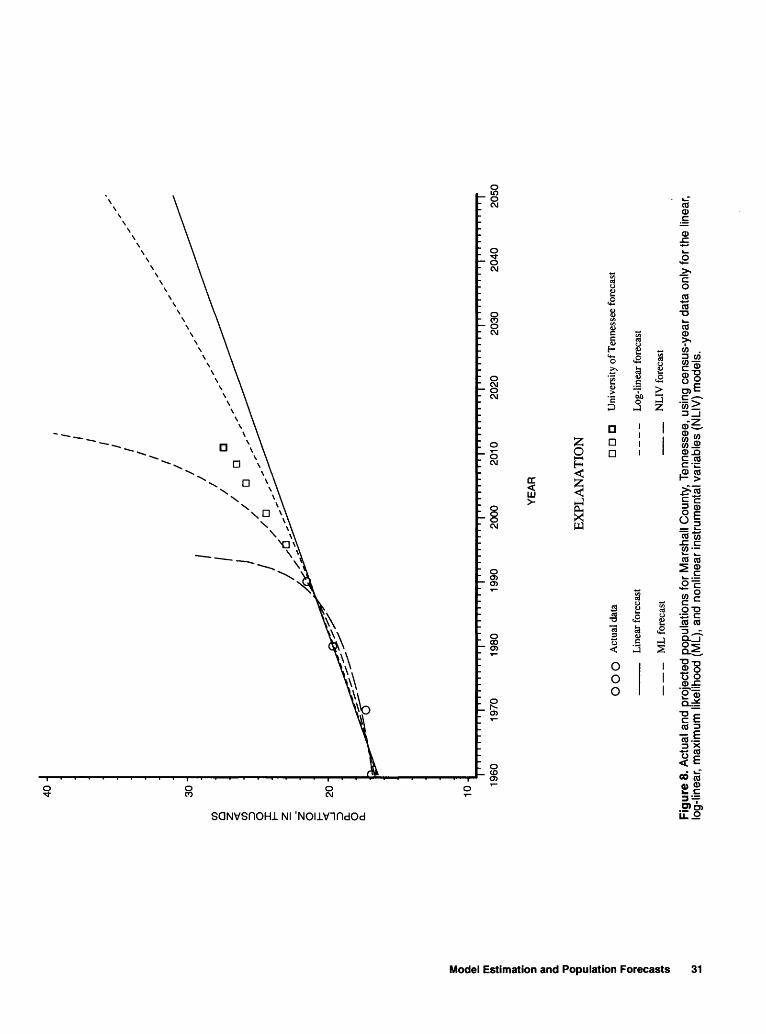
40-

o Q. 2. m

~. 0) B> Q. o

30-

20-

10- 1960

1970

1 ' '

I ' '

1980

1990

2000

2010

2020

2030

1 '

' '

I '

' '

' '

' '

' '

I

2040

2050

YEAR

EX

PLA

NA

TIO

N

O O

O

Act

ual d

ata

Lin

ear f

orec

ast

ML

for

ecas

t

DD

D

Uni

vers

ity o

f Ten

ness

ee f

orec

ast

_ _

_ _

Log

-lin

ear f

orec

ast

__ _

N

LIV

for

ecas

t

Figu

re 8

. Act

ual a

nd p

roje

cted

pop

ulat

ions

for

Mar

shal

l Cou

nty,

Ten

ness

ee,

usin

g ce

nsus

-yea

r dat

a on

ly fo

r the

line

ar,

log-

linea

r, m

axim

um li

kelih

ood

(ML)

, an

d no

nlin

ear

inst

rum

enta

l var

iabl

es (

NLI

V)

mod

els.

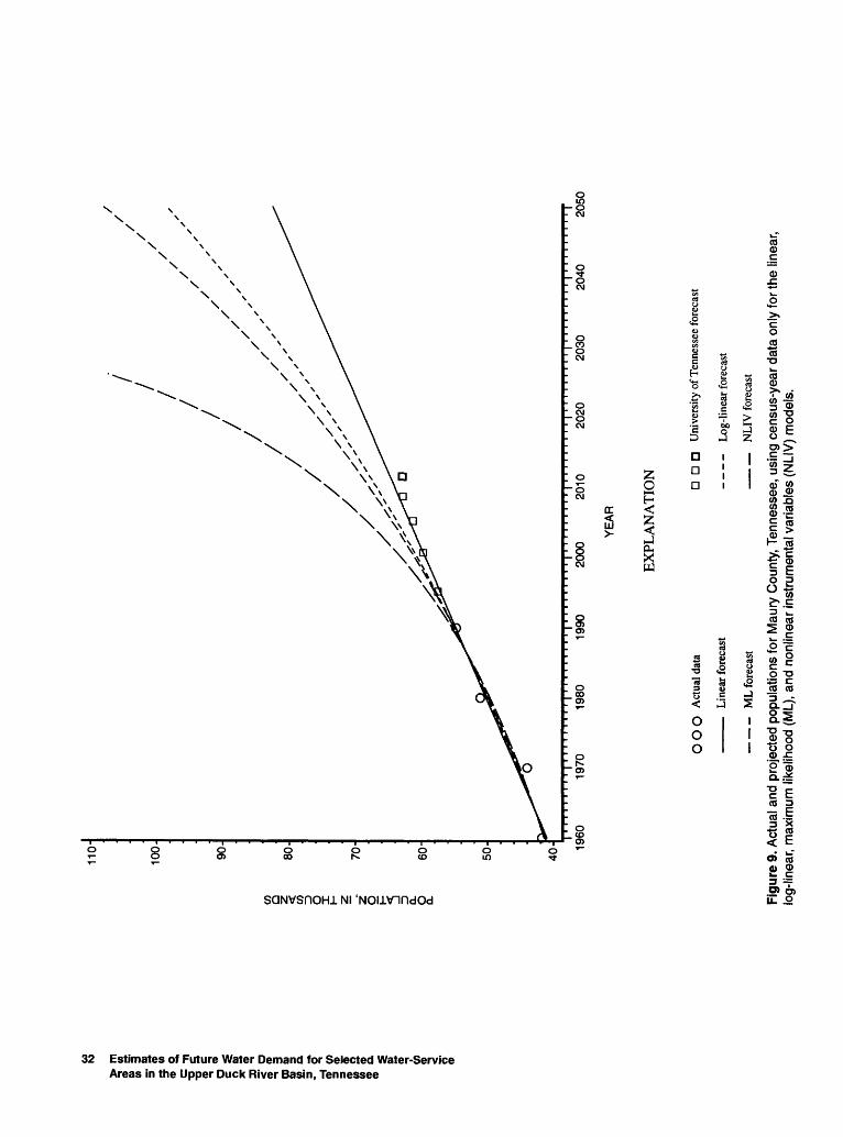
> m i& 0) a

2.1

=

J?

- o» 1 1 CD

0)

8 I

CO o z

< CO o z

o

110

100 90 80-

70-

60-

50-

40- 19

6019

7019

8019

9020

0020

1020

2020

30

YE

AR

EX

PLA

NA

TIO

N

2040

2050

O O

O

Act

ual d

ata

Line

ar fo

reca

st

ML

fore

cast

D D

D

Uni

vers

ity o

f Ten

ness

ee fo

reca

st

- - - -

Log-

linea

r for

ecas

t

_

N

LIV

for

ecas

t

Figu

re 9

. Act

ual a

nd p

roje

cted

pop

ulat

ions

for

Mau

ry C

ount

y, T

enne

ssee

, us

ing

cens

us-y

ear

data

onl

y fo

r the

line

ar,

log-

linea

r, m

axim

um li

kelih

ood

(ML)

, an

d no

nlin

ear

inst

rum

enta

l var

iabl

es (

NLI

V)

mod

els.

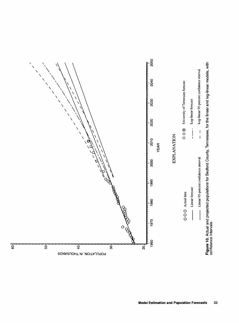
60-

50-

40-

30-

20-

I ' '

' '

1960

1970

1980

1990

2000

2010

2020

YE

AR

2030

2040

2050

o> Q. n

o

O O

O

Act

ual d

ata

Lin

ear f

orec

ast

Lin

ear

95-p

erce

nt c

onfi

denc

e in

terv

al

EX

PLA

NA

TIO

N

D D

DU

nive

rsity

of T

enne

ssee

for

ecas

t

Log

-lin

ear f

orec

ast

Log

-lin

ear 9

5-pe

rcen

t con

fide

nce

inte

rval

Figu

re 1

0. A

ctua

l and

pro

ject

ed p

opul

atio

ns fo

r B

edfo

rd C

ount

y, T

enne

ssee

, fo

r the

line

ar a

nd l

og-li

near

mod

els,

with

co

nfid

ence

inte

rval

s.

50-

8 I

=>

<?

~« » a II ^

<D

3D *

P0) n>

0)

3w

a

is W

(D

(D

Q.

40

O a.

O

a.

30

-

20

-

10- 19

6019

7019

8019

902000

2010

2020

2030

1 '

' '

I '

' '

' '

' '

' '

I 20

40

2050

YE

AR

EX

PLA

NA

TIO

N

O O

O

Act

ual d

ata

____

Line

ar fo

reca

st

Line

ar 9

5-pe

rcen

t con

fiden

ce in

terv

al

OD

D

Uni

vers

ity o

f Ten

ness

ee fo

reca

st

- -

Log-

linea

r for

ecas

t

_ _

Log-

linea

r 95-

perc

ent c

onfid

ence

inte

rval

Figu

re 1

1. A

ctua

l and

pro

ject

ed p

opul

atio

ns fo

r M

arsh

all C

ount

y, T

enne

ssee

, for

the

linea

r an

d lo

g-lin

ear

mod

els,

with

co

nfid

ence

inte

rval

s.

SC siseoajoj uojieindod pue uojieuijisg \apow

o 3!<§Q. 2 (D *

S F»

Q. o5

(D Q.

T3c_COo'

V)

O O

I

(D £0

£0

Q. 5"

to5'(D £0

O Q.jo"

i.Er

POPULATION, IN THOUSANDS

O O O

r. >

§

_i O8

s- o

m

60

-

> m

3

«>

3 <S ti If II ? «> a

' </>

20- 19

601 I

' ' '

' ' '

' ' '

I ' '

' ' '

19

70

1980

1990

2000

20

10

YE

AR

2020

2030

2040

1 '

' '

I

2050

EX

PLA

NA

TIO

N

OO

O

Act

ual d

ata

Lin

ear f

orec

ast

Lin

ear 9

5-pe

rcen

t con

fide

nce

inte

rval

OD

D

Uni

vers

ity o

f Ten

ness

ee f

orec

ast

- -

Log

-lin

ear

fore

cast

_ _

L

og-l

inea

r 95

-per

cent

con

fide

nce

inte

rval

Figu

re 1

3. A

ctua

l and

pro

ject

ed p

opul

atio

ns fo

r B

edfo

rd C

ount

y, T

enne

ssee

, us

ing

cens

us-y

ear d

ata

only

for t

he li

near

an

d lo

g-lin

ear m

odel

s, w

ith c

onfid

ence

inte

rval

s.

50

-

i 2. m

w 3 51

o o> a o o 5T

5'

40-

D

O

x

30

z D a.

O

a.2

0-

10- 19

6019

7019

8019

902000

2010

YE

AR

EX

PLA

NA

TIO

N

2020

2030

2040

1 '

' I

2050

O O

O

Act

ual d

ata

Lin

ear f

orec

ast

Lin

ear 9

5-pe

rcen

t con

fide

nce

inte

rval

Uni

vers

ity o

f Ten

ness

ee f

orec

ast

Log

-lin

ear f

orec

ast

Log

-lin

ear 9

5-pe

rcen

t con

fide

nce

inte

rval

Figu

re 1

4. A

ctua

l and

pro

ject

ed p

opul

atio

ns f

or M

arsh

all C

ount

y, T

enne

ssee

, us

ing

cens

us-y

ear

data

onl

y fo

r th

e lin

ear

and

log-

linea

r m

odel

s, w

ith c

onfid

ence

inte

rval

s.

> m

<5 2* f?

5* <' o

a, A

00 0

)8 g

.

120

110

100-

co

90

Q CO O Q_ 2

80 70-

60-

50-

40- 19

601970

1980

1990

2000

YEAR

2010

2020

I '

I

2030

2040

1 ' '

' I

2050

EX

PLA

NA

TIO

N

O O

O

Act

ual d

ata

Line

ar fo

reca

st

Line

ar 9

5-pe

rcen

t con

fiden

ce in

terv

al

DD

D

Uni

vers

ity o

f Ten

ness

ee f

orec

ast

_ .

Log-

linea

r for

ecas

t

Log-

linea

r 95-

perc

ent c

onfid

ence

inte

rval

Figu

re 1

5. A

ctua

l and

pro

ject

ed p

opul

atio

ns fo

r M

aury

Cou

nty,

Ten

ness

ee, u

sing

cen

sus-

year

dat

a on

ly fo

r the

line

ar

and

log-

linea

r mod

els,

with

con

fiden

ce in

terv

als.

Table 17. Parameter estimates for the linear and log-linear models for Bedford, Marshall, and Maury Counties, Tennessee

[Standard errors in parentheses; p0 and pj, estimated parameters; R2, coefficient of correlation]

County

Bedford

Marshall

Maury

Po

23.001°

(0.224)

16.299°

(0.236)

40.679°

(0.595)

Linear model

Pi If

0.235° 0.930 (0.012)

0.169° 0.861 (0.013)

0.494° 0.893 (0.032)

Po

3.143°

(0.008)

2.800°

(0.012)

3.718°

(0.011)

Log-linear model

Pi

0.00875° (0.00043)

0.00874° (0.00064)

0.01003°

(0.00062)

ff

0.937

0.871

0.903

° Significantly different from 0 at the 5-percent level of significance.

Table 18. Parameter estimates for the linear and log-linear models for Bedford, Marshall, and Maury Counties, Tennessee, using census-year data only (N = 4)

[Standard errors in parentheses; p0 and Pj, estimated parameters; R2, coefficient of correlation]

County

Bedford

Marshall

Maury

Po

22.981°

(0.277)

16.429°

(0.539)

41.011°

(1.167)

Linear model

Pi fl2

0.244° 0.993

(0.015)

0.163° 0.941

(0.029)

0.461° 0.965

(0.062)

Po

3.140°

(0.008)

2.805°

(0.027)

3.719°

(0.024)

Log-linear model

Pi

0.00918°

(0.00043)

0.00854°

(0.00146)

0.00963°

(0.00127)

ff

0.996

0.945

0.966

° Significantly different from 0 at the 5-percent level of significance.

model. The forecast from the University of Tennessee study (Economic and Community Staff, 1992) gener ally lies within the confidence interval for the log- linear model. The smaller confidence interval for the log-linear model projections is misleading because the method for estimating the confidence interval assumes

2Ge is known. A corrected confidence interval would include additional spread due to inherent uncertainty in the estimated value of the variance term. This correc tion would be particularly large in the case of regres sions estimated with census-year data because of the

few number of observations (N = 4) used to estimate the variance.

Tables 19 to 21 list population projections and confidence intervals for the three counties for the case where the model is linear and all available data are used in the regression. Tables 22 to 24 give projections and confidence intervals for the log-linear model, also using all available data. With the exception of the last 5 years for Bedford County, the confidence intervals for the linear models overlap with those for the log- linear models.


Table 19. Projected populations and 95-percent confidence intervals for Bedford County, Tennessee, 1993-2050, results from the linear model

Table 20. Projected populations and 95-percent confidence intervals for Marshall County, Tennessee, 1993-2050, results from the linear model

Year

1993199419951996199719981999200020012002200320042005200620072008200920102011201220132014201520162017201820192020202120222023202420252026202720282029203020312032203320342035203620372038203920402041204220432044204520462047204820492050

Projected population30,77231,00731,24231,47831,71331,94932,18432,42032,65532,89133,12633,36233,59733,83334,06834,30434,53934,77535,01035,24635,48135,71735,95236,18836,42336,65936,89437,12937,36537,60037,83638,07138,30738,54238,77839,01339,24939,48439,72039,95540,19140,42640,66240,89741,13341,36841,60441,83942,07542,31042,54642,78143,01743,25243,48743,72343,95844,194

95-percent confidence

intervalLower bound

29,37029,59829,82530,05230,27830,50430,73030,95531,18031,40531,62931,85332,07732,30032,52332,74632,96833,19033,41233,63433,85534,07634,29734,51834,73834,95835,17835,39835,61735,83636,05536,27436,49336,71136,93037,14837,36637,58437,80138,01938,23638,45338,67038,88739,10439,32039,53739,75339,96940,18540,40140,61740,83341,04941,26441,48041,69541,910

Upper bound32,17332,41632,66032,90433,14933,39433,63933,88434,13034,37734,62334,87035,11835,36535,61335,86236,11036,35936,60836,85737,10737,35737,60737,85738,10838,35938,61038,86139,11339,36539,61639,86940,12140,37340,62640,87941,13241,38541,63841,89242,14642,39942,65342,90743,16243,41643,67143,92544,18044,43544,69044,94545,20045,45545,71145,96646,22246,477

Year

1993199419951996199719981999200020012002200320042005200620072008200920102011201220132014201520162017201820192020202120222023202420252026202720282029203020312032203320342035203620372038203920402041204220432044204520462047204820492050

Projected population

21,86622,03522,20322,37222,54122,71022,87823,04723,21623,38423,55323,72223,89024,05924,22824,39724,56524,73424,90325,07125,24025,40925,57825,74625,91526,08426,25226,42126,59026,75826,92727,09627,26527,43327,60227,77127,93928,10828,27728,44628,61428,78328,95229,12029,28929,45829,62629,79529,96430,13330,30130,47030,63930,80730,97631,14531,31331,482


intervalLower bound

20,39320,55420,71420,87321,03221,19121,35021,50821,66521,82321,98022,13622,29222,44822,60422,75922,91423,06923,22323,37723,53123,68523,83823,99124,14424,29624,44924,60124,75324,90425,05625,20725,35825,50925,65925,81025,96026,11026,26026,41026,56026,70926,85827,00727,15627,30527,45427,60327,75127,89928,04828,19628,34428,49228,63928,78728,93529,082

Upper bound

23,33923,51623,69323,87124,04924,22824,40724,58624,76624,94625,12725,30725,48925,67025,85226,03426,21626,39926,58226,76526,94927,13327,31727,50127,68627,87128,05628,24128,42728,61328,79928,98529,17129,35829,54529,73129,91930,10630,29330,48130,66930,85731,04531,23331,42231,61031,79931,98832,17732,36632,55532,74432,93433,12333,31333,50333,69233,882


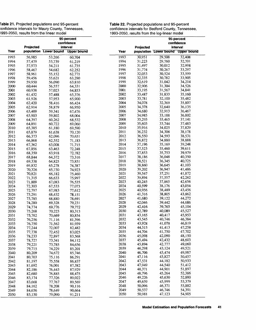
fable 21. Projected populations and 95-percent confidence intervals for Maury County, Tennessee, 1993-2050, results from the linear model

Table 22. Projected populations and 95-percent confidence intervals for Bedford County, Tennessee, 1993-2050, results from the log-linear model

Year

1993199419951996199719981999200020012002200320042005200620072008200920102011201220132014201520162017201820192020202120222023202420252026202720282029203020312032203320342035203620372038203920402041204220432044204520462047204820492050


56,98557,47957,97358,46758,96159,45659,95060,44460,93861,43261,92662,42062,91463,40963,90364,39764,89165,38565,87966,37366,86867,36267,85668,35068,84469,33869,83270,32670,82171,31571,80972,30372,79773,29173,78574,28074,77475,26875,76276,25676,75077,24477,73878,23378,72779,22179,71580,20980,70381,19781,69282,18682,68083,17483,66884,16284,65685,150

95-percent confidence interval

Lower bound

53,26653,73954,21154,68255,15255,62156,09056,55757,02357,48857,95358,41658,87959,34159,80260,26260,72261,18061,63862,09662,55263,00863,46363,91864,37264,82565,27865,73066,18266,63367,08367,53367,98368,43268,88069,32869,77670,22370,66971,11671,56272,00772,45272,89773,34173,78574,22974,67275,11675,55876,00176,44376,88577,32677,76778,20878,64979,090

Upper bound

60,70461,21961,73562,25262,77163,29063,81064,33164,85365,37665,90066,42466,95067,47668,00468,53269,06069,59070,12070,65171,18371,71572,24872,78273,31673,85174,38774,92375,46075,99776,53577,07377,61278,15178,69179,23179,77280,31380,85481,39681,93982,48283,02583,56884,11284,65685,20185,74686,29186,83787,38287,92988,47589,02289,56990,11690,66491,211

Year

1993199419951996199719981999200020012002200320042005200620072008200920102011201220132014201520162017201820192020202120222023202420252026202720282029203020312032203320342035203620372038203920402041204220432044204520462047204820492050


30,95131,22331,49731,77432,05332,33532,61932,90633,19533,48733,78134,07834,37834,68034,98535,29335,60335,91636,23236,55036,87237,19637,52337,85338,18638,52138,86039,20239,54739,89440,24540,59940,95641,31641,68042,04642,41642,78943,16543,54543,92844,31544,70445,09845,49445,89446,29846,70647,11647,53147,94948,37148,79649,22649,65950,09650,53750,981


intervali Lower bound

29,50829,76030,01230,26730,52430,78231,04231,30431,56731,83332,10032,36932,64032,91333,18833,46533,74434,02534,30834,59334,88035,16935,46035,75336,04836,34536,64536,94737,25137,55737,86538,17638,48938,80539,12239,44239,76540,08940,41740,74641,07841,41341,75042,09042,43242,77743,12443,47443,82744,18244,54044,90145,26445,63045,99946,37146,74647,123

Upper bound

32,40832,70132,99833,29733,59933,90534,21434,52634,84135,16035,48235,80736,13536,46736,80237,14137,48337,82938,17838,53138,88839,24839,61139,97940,35040,72541,10341,48641,87242,26242,65643,05443,45643,86244,27244,68645,10445,52745,95346,38446,81947,25847,70248,15048,60349,06049,52149,98750,45750,93351,41251,89752,38652,88053,37953,88254,39154,905


Table 23. Projected populations and 95-percent confidence intervals for Marshall County, Tennessee, 1993-2050, results from the log-linear model

Table 24. Projected populations and 95-percent confidence intervals for Maury County, Tennessee, 1993-2050, results from the log-linear model

Year

1993199419951996199719981999200020012002200320042005200620072008200920102011201220132014201520162017201820192020202120222023202420252026202720282029203020312032203320342035203620372038203920402041204220432044204520462047204820492050


21,96322,15622,35122,54722,74522,94523,14723,35023,55523,76223,97124,18224,39424,60924,82525,04325,26325,48525,70925,93526,16326,39326,62626,86027,09627,33427,57427,81728,06228,30828,55728,80929,06229,31829,57629,83630,09830,36330,63030,90031,17231,44631,72332,00232,28432,56832,85433,14433,43533,73034,02734,32634,62834,93335,24135,55135,86436,180


intervalLower bound

20,43820,60920,78120,95421,12821,30321,47921,65621,83422,01322,19422,37522,55722,74122,92623,11123,29823,48723,67623,86624,05824,25124,44524,64024,83725,03525,23425,43425,63625,83926,04326,24926,45626,66426,87427,08527,29827,51227,72727,94428,16228,38228,60328,82629,05029,27629,50329,73229,96230,19430,42830,66330,90031,13831,37831,62031,86432,109

Upper bound

23,51223,72823,94624,16624,38924,61424,84225,07225,30525,54025,77826,01926,26226,50826,75727,00827,26227,51927,77928,04128,30728,57528,84629,12029,39729,67729,96030,24530,53430,82631,12131,41931,72132,02532,33332,64332,95733,27533,59533,91934,24734,57734,91235,24935,59035,93536,28336,63536,99037,34937,71138,07838,44838,82239,19939,58139,96640,356

Year

1993199419951996199719981999200020012002200320042005200620072008200920102011201220132014201520162017201820192020202120222023202420252026202720282029203020312032203320342035203620372038203920402041204220432044204520462047204820492050


57,34557,92458,50859,09859,69460,29560,90461,51862,13862,76563,39864,03764,68365,33665,99566,66167,33368,01268,69969,39270,09270,79971,51472,23572,96473,70174,44475,19675,95576,72177,49678,27879,06879,86680,67381,48782,31083,14183,98084,82885,68586,55087,42488,30789,19990,10091,01091,92992,85793,79594,74395,70096,66797,64398,63099,626100,633101,650


intervalLower bound

53,46653,98454,50555,03055,55956,09256,62957,17057,71658,26558,81959,37759,93960,50661,07761,65362,23362,81763,40664,00064,59865,20165,80966,42267,04067,66268,29068,92269,56070,20370,85071,50472,16272,82673,49574,17074,85075,53676,22776,92477,62778,33579,05079,77080,49681,22881,96782,71183,46284,21984,98285,75286,52887,31088,10088,89589,69890,507

Upper bound

61,28361,92362,57263,22863,89264,56465,24565,93466,63167,33768,05168,77369,50570,24570,99571,75372,52073,29774,08274,87775,68276,49677,32078,15378,99679,85080,71381,58682,47083,36484,26985,18486,10987,04687,99388,95289,92190,90291,89492,89893,91394,94095,97997,03098,09399,168100,255101,355102,467103,593104,731105,882107,046108,223109,414110,619111,837113,069


Summary and Conclusions

Three types of models are used to estimate the relation between population and time for Bedford, Marshall, and Maury Counties. The Box-Cox model yields projections with a large negative curvature so large that out-of-sample projections quickly go to infin ity. The large curvature is partially a consequence of using ancillary data to estimate population between census years. More reasonable and similar projections are obtained for the linear and log-linear models. Gen erally, the confidence intervals around the forecasts show some degree of overlap between these two mod els. Given the curvature indicated by the Box-Cox model, which includes the linear and log-linear models as special cases, the log-linear model appears to best forecast populations of Bedford, Marshall, and Maury Counties into the future.

SELECTED REFERENCES

Alexander, P.M., Keck, L.A., Conn, L.G., and Wentz, S.J., 1984, Drought-related impacts on municipal and major self-supplied industrial water withdrawals in Tennes see Part B: U.S. Geological Survey Water-Resources Investigations Report 84-4074, 398 p.

Amemiya, Takeshi, 1985, Advanced econometrics: Cam bridge, Harvard University Press, 521 p.

Bingham, R.H., 1985, Low flows and flow duration of Ten nessee streams through 1981: U.S. Geological Survey Water-Resources Investigations Report 84-4347, 325 p.

Boland, J.J., Dziegielewski, B., Baumann, D.D., Opitz, E.M., 1984, Influence of price and rate structures on municipal and industrial water use: Fort Belvoir, Vir ginia, U.S. Army Corps of Engineers Institute for Water Resources, Contract Report 84-Industrial Water Use: Fort Belvoir, Virginia, U.S. Army Corps of Engi neers Institute for Water Resources, Contract Report 84-C-2, 187 p.

Burchett, C.R., 1977, Water resources of the upper Duck River basin, central Tennessee: Tennessee Division of Water Resources, Tennessee Water Resources Series no. 12, 103 p.

Davidson, Russell, and MacKinnon, J.G., 1993, Estimation and inference in econometrics: New York, Oxford Uni versity Press, 874 p.

Economic and Community Staff, South Central Tennessee Development District, comp., 1992, Population esti mates for the State of Tennessee, in 1994 data profile: Knoxville, Tennessee, University of Tennessee, 25 p.

Howe, C.W., Linaweaver, P.P., Jr., 1967, The impact of price on residential water demand and its relation to system design and price structure: Water Resources Research 3 (1st Quarter), p. 12-32.

Hutson, S.S., 1993, Water availability, use, and estimated future water demand in the upper Duck River basin, middle Tennessee: U.S. Geological Survey Water- Resources Investigations Report 92-4179, 39 p.

Kindler, J., and Russell, C.S., 1984, Modelling waterdemands: Orlando, Florida, Academic Press (Harcourt, Brace, Jovanovich, Inc), 248 p.

Miller, R.A., 1974, The geologic history of Tennessee: Ten nessee Division of Geology Bulletin 74, 63 p.

Office of Management and Budget, 1987, Standard indus trial classification manual 1987: 705 p.

Outlaw, G.S., and Weaver, J.D., 1996, Flow duration and low flows of Tennessee streams through 1992: U.S. Geological Survey Water-Resources Investigations Report 95-4293, 245 p.

Tennessee Department of Employment Security, 1990, Annual averages Tennessee labor force estimates 1985-1989: Nashville, Tennessee, Labor Market Infor mation Unit, Research and Statistics Division, Tennes see Department of Employment Security, 87 p.

1991, Annual averages labor force and nonagricul- tural employment estimates 1986-1990: Nashville, Tennessee, Labor Market Information Research and Statistics Division, Tennessee Department of Employ ment Security, 87 p.

U.S. Army Corps of Engineers, 1988, IWR-MAIN water use forecasting system, version 5.1: Fort Belvoir, Vir ginia, Water Resources Support Center, Institute for Water Resources, 324 p.

U.S. Bureau of the Census, 1967, Estimates of the popula tion of states, July 1, 1966, in Current Population Reports, Population Estimates: Bureau of the Census, Series P-25, No. 380.

1968, Estimates of the population of states, July 1,1966 and July 1, 1967, in Current Population Reports, Population Estimates: Bureau of the Census, Series P-25, No. 414.

1969, Estimates of the population of states, July 1,1967 and July 1, 1968, in Current Population Reports, Population Estimates: Bureau of the Census, Series P-25, No. 436 and 437.

1973, Estimates of the population of Tennessee coun ties, July 1, 1971 and July 1, 1972, in Current Popula tion Reports, Population Estimates: Bureau of the Census, Series P-26, No. 47.

1974, Estimates of the population of Tennessee coun ties and metropolitan areas, July 1, 1972 and 1973, in Current Population Reports, Population Estimates: Bureau of the Census, Series P-26, No. 83.

1975, Estimates of the population of Tennessee coun ties and metropolitan areas, July 1, 1973 and 1974, in

Selected References 43

Current Population Reports, Population Estimates: Bureau of the Census, Series P-26, No. 133. 1976, Estimates of the population of Tennessee coun ties and metropolitan areas, July 1, 1974 and 1975, in Current Population Reports, Population Estimates: Bureau of the Census, Series P-26, No. 75-42. 1978, Estimates of the population of Tennessee coun ties and metropolitan areas, July 1, 1976 (revised) and 1977 (provisional), in Current Population Reports, Pop ulation Estimates: Bureau of the Census, Series P-26, No. 77-42. 1979, Estimates of the population of Tennessee coun ties and metropolitan areas, July 1, 1977 (revised) and 1978 (provisional), in Current Population Reports, Population Estimates: Bureau of the Census, Series P-26, No. 78-42. 1988a, Estimates of the Population of Tennessee counties and metropolitan areas, July 1,1981, to 1985, in Current Population Reports, Local Population Esti mates: Bureau of the Census, Series P-26, No. 85-TN-C. 1988b, South, 1986 Population and 1985 per capita income estimates for counties and incorporated places, in Current Population Reports, Local Population Esti mates: Bureau of the Census, Series P-26, No. 86-S-SC. 1990, South, 1988 Population and 1987 per capita income estimates for counties and incorporated places, in Current Population Reports, Local Population Esti mates: Bureau of the Census, Series P-26, No. 88-S-SC.

1994, Population estimates for counties and metro politan areas, July 1, 1991, in Current Population Reports, Population Estimates and Projections: Bureau of the Census, P25-1108.

U.S. Department of Commerce, 1988, Climatological data annual summary, Tennessee 1988: Asheville, North Carolina, National Oceanic and Atmospheric Adminis tration, 17 p.

1989, Climatological data annual summary, Tennes see 1989: Asheville, North Carolina, National Oceanic and Atmospheric Administration, 17 p.

1992a, 1990 Census of housing, general housing characteristics, Tennessee: U.S. Government Printing Office, 270 p.

1992b, 1990 Census of population, general population characteristics, Tennessee: U.S. Government Printing Office, 353 p. 1992c, 1990 Census of population and housing,summary social, economic, and housing characteris tics, Tennessee: U.S. Government Printing Office, 203 p.

Vickers, B.B., ed., 1989, Tennessee statistical abstract 1989, Center for Business and Economic Research: Knox- ville, Tennessee, University of Tennessee, 755 p.

White, J.L., ed., 1994, 1994 Directory of Tennessee manu facturers: geographic section, Nashville, Tennessee: M. Lee Smith Publishers & Printers, section B, 297 p.


Appendix A. Derivation of the Confidence Intervals for the Log-Linear Model

This appendix derives the relations necessary to determine minimal confidence limits for the log-linear model. The derivation assumes that the standard error of the residuals is known.

We seek to minimize the difference Ut - Lt subject to the constraint

Prob(Lt <Pt <Ut) = 1-a, (11)

where Lt is the lower bound on the confidence interval; Ut is the upper bound; and a is the significance level (for a 95-percent confidence interval, a equals 0.05). The probability expressed in equation 11 is conditioned on the information contained in the sample used to estimate the log-linear model.

It is convenient at this point to adopt some matrix notation. Let xt represent the row vector [1 Tt]; let Xs rep resent the N by 2 matrix consisting of ones in the first column and the sample values of Tin the second column; let P be the 2 by 1 vector [(30 Pi]', with |3 being the P vector evaluated at the sample estimates; and let es correspond to the N vector of residuals for the sample values of P. The population Pt appearing in equation 11 can then be writ ten as

Pt = exp (xfi + e t)

(12)

The term et - x^X^s)'JX^s represents the forecast error and is given by the sum of independent, normally distrib uted random variables with a mean of 0. As such, it is itself normally distributed with mean of 0 and variance equal to the variance of the forecast error G( (see equation 7). Let ut represent this forecast error. By substituting equation 12 into equation 11, taking natural logarithms, and dividing by the square root of d/ we obtain

n(L) -x p u Prob - ' r ^ r = 1-a. (13)

2 / 2If G e is known, then the term u/ ̂ dt is normally distributed with a mean of 0 and variance of 1. Define

(L} = (tafi ,1-^P)/ and z(u\ = (inftf Vjc^/d ' The minimization problem can be

stated as

Appendix A 45

The first-order conditions for minimization (in addition to equation 11) are

(15)

and

(16)

These conditions define a unique solution for Lt and Ut. Since the second-order conditions for a minimum are sat isfied, the solution obtained is a global minimum.

Dividing equation 15 by equation 16 and taking natural logarithms, we obtain

-Z2 (U)-j-1 l- = In (I/,) -In (I,) (17)

Upon simplifying equation 17, we obtain

t t * t *

Thus, the solution to the minimization problem is

L,=

and (19)

",=

where Zt solves the equation

1 A -e2/2, 1 //vv. f e £/e = I-a. (20)/^ J » 7^2

A solution for Zt can be obtained using the Newton method. Note that if a is less than 0.5, then Zt must be positive (if Zt is less than zero, then the probability defined by the left-hand side of equation 20 would be less than 0.5). Because the first derivative of the left-hand side of equation 20 is positive and the second derivative is nega tive for all positive values of Zt, the Newton method converges quickly and uniformly on the solution if the starting value for Zt is 0.


Appendix B. SAS Computer Code Used to Generate the Results

The following is the SAS computer code used to generate the tables and figures appearing in the text.

/* This program estimates the lambda coefficient for the simple one-sided Box-Cox transformation of the dependent variable. The lambda coefficient and standard error correspond to the maximum likelihood esti mates (the beta coefficients on the explanatory variables are wrong (as are the standard errors)). See my notes for transforming these values into the correct values. The method of estimation is maximum likeli hood, using the concentrated log likelihood function and rescaling the dependent variable by its geometric mean. */

%lettol= IE-10; %let cutoff = 2.25 ;

%let popl = bedpop ; %let pop2 = marpop ; %let pop3 = maupop ;

%let tpopl = tbedpop ; %let tpop2 = tmarpop ; %let tpopS = tmaupop ;

%let apopl = abedpop ; %let apop2 = amarpop ; %let apopS = amaupop ;

%let Ipopl = Ibedpop ; %let Ipop2 = Imarpop ; %let IpopS = Imaupop ;

%let ppopl = pbedpop ; %let ppop2 = pmarpop ; %let ppop3 = pmaupop ;

%let ctitlel 1 = Results for Bedford County ; %let ctitle21 = Results for Marshall County ; %let ctitle31 = Results for Maury County ;

%let ctitlel2 = Results for Bedford County (census years only); %let ctitle22 = Results for Marshall County (census years only); %let ctitle32 = Results for Maury County (census years only);

%let headll 1 = 'Bedford' / 'County, 1993-2050' / / '[Results from the linear model] 1 ; %let head!21 = 'Marshall' / 'County, 1993-2050' // '[Results from the linear model]'; %let head!31 = 'Maury' / 'County, 1993-2050' / / '[Results from the linear model]';

%let headl!2 = 'Bedford' / 'County, 1993-2050' / / '[Results from the linear model using census year data]'; %let head!22 = 'Marshall' / 'County, 1993-2050' / / '[Results from the linear model using census year data]'; %let head!32 = 'Maury' / 'County, 1993-2050' / / '[Results from the linear model using census year data]';

Appendix B 47

%let headllll = 'Bedford' / 'County, 1993-2050' / / '[Results from the log-linear model] 1 ; %let headl!21 = 'Marshall' / 'County, 1993-2050' / / '[Results from the log-linear model]'; %let head!131 = 'Maury' / 'County, 1993-2050' / / '[Results from the log-linear model]';

%let headl!12 = 'Bedford' / 'County, 1993-2050' / / '[Results from the log-linear model using census year data] 1 ; %let headl!22 = 'Marshall' / 'County, 1993-2050' / / '[Results from the log-linear model using census year data]'; %let headl!32 = 'Maury' / 'County, 1993-2050' / / '[Results from the log-linear model using census year data]';

libname dir";filename indata '-/tenn/popdat.dat';filename indata2 '-/tenn/proj.dat';

/* Read the data */

data one ;infile indata;input year time bedpop marpop maupop ;bedpop = bedpop/1000 ;marpop = marpop/1000 ;maupop = maupop/1000 ;time = time - 60 ;dep = 0 ;

/* if year A= 1960 and year A= 1970 and year A= 1980 and year A= 1990 then do ;*/

if year = 1969 or year = 1979 or year = 1989 then do ;bedpop =.;marpop =.;maupop =. ;dep =.;

end;Ibedpop = log(bedpop); Imarpop = log(marpop); Imaupop = log(maupop); time2 = time*time;

data two;do i = 93 to 150;time = i - 60 ;year = 1900 + time + 60 ;output;

end ;

data three;infile indata2 ;input year time pbedpop pmarpop pmaupop ;pbedpop = pbedpop/1000 ;pmarpop = pmarpop/1000 ;pmaupop = pmaupop/1000 ;


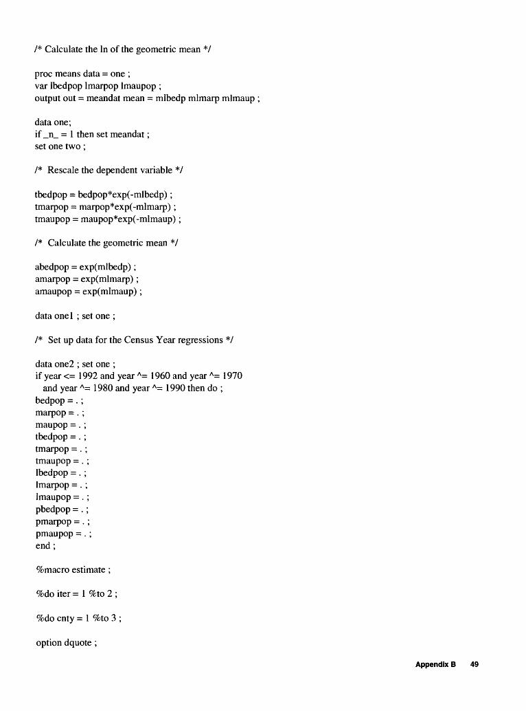
/* Calculate the In of the geometric mean */

proc means data = one ;var Ibedpop Imarpop Imaupop ;output out = meandat mean = mlbedp mlmarp mlmaup ;

data one;if _n_ = 1 then set meandat;set one two;

/* Rescale the dependent variable */

tbedpop = bedpop*exp(-mlbedp); tmarpop = marpop*exp(-mlmarp); tmaupop = maupop*exp(-mlmaup);

/* Calculate the geometric mean */

abedpop = exp(mlbedp); amarpop = exp(mlmarp); amaupop = exp(mlmaup);

data onel ; set one ;

/* Set up data for the Census Year regressions */

data one2 ; set one ;if year <= 1992 and year A= 1960 and year A= 1970

and year A= 1980 and year A= 1990 then do ; bedpop =.; marpop = . ; maupop =.; tbedpop =.; tmarpop = . ; tmaupop =.; Ibedpop =. ; Imarpop =. ; Imaupop =.; pbedpop = . ; pmarpop =.; pmaupop = .; end;

%macro estimate ;

%do iter = 1 %to 2 ;

%do cnty = 1 %to 3 ;

option dquote ;

Appendix B 49

filename resoutl "~/tenn/linres&cnty&iter..dat"; filename resout2 "~/tenn/llnres&cnty&iter..dat";

/* Set up dataset of actual data (for display purposes) */

title 1 &&&ctitle&cnty&iter; title2; title3 ;

data outdatO ; set one&iter ;pophat = &&&pop&cnty ;if pophat A= .;disp = 0;

keep pophat year disp ;

data outdat5 ; set three ;pophat = &&&ppop&cnty;disp = 5 ;

keep pophat year disp ;

/* Here's a linear model */

proc reg data = one&iter ;model &&&pop&cnty = time ;output out = outdatl p = pophat 195 = cilo u95 = cihi;

data outdatl ; set outdatl ;disp = 1 ;if year <= 1992 then do ;

cilo =. ;cihi = .;

end ; keep pophat year disp cilo cihi;

data results ; set outdatl ; if year > 1992; pophat = pophat* 1000 ; cilo = cilo* 1000; cihi = cihi* 1000; file resoutl ; if year = 1993 then putTable . Projected populations and 95-percent confidence intervals for

&&&headl&cnty&iter / / / /1 95-percent 95-percent1 / 1 confidence confidence1 / 1 interval interval1 /

Projected Projected1 / /'Year population Lower bound Upper bound Year population Lower bound

Upper bound1 / / / @ ;


if year <= 2021 thenput year " pophat commaT.O ' ' cilo commaT.O " cihi commaT.O ";

elseput year " pophat commaT.O ' ' cilo comma?.0 " cihi comma?.0 ;

/* Here's a log-linear model */

proc reg data = one&iter ;model &&&lpop&cnty = time ;output out = outdat2 p = pophat stdi = sdfore stdr = sdres ;

/* These statements calculate the upper and lower bounds of the 95% confidence interval for the log linear model, assuming the standard deviation of the forecast is known. This allows us to simplify the estimation and use the normal distribution. The assumption also simplifies the estimation of the un-logged forecast. */

data outdat2 ; set outdat2 ; disp = 2 ; dif=l ;if year > 1992 then do;

do until(dif < &tol); if x = . then x = 0 ;pdif = .95 - (probnorm(x + 2* sdfore) - probnorm(-x));dfx = ((2*3.141592654)**(-.5))*(exp(-((x+2*sdfore)**2)/2) + exp(-(x**2)/2)); xn = x + (pdif/dfx); dif = abs(xn - x); x = xn;

end;cilo = exp(pophat - sdfore*(x + 2* sdfore)); cihi = exp(pophat + sdfore*x); pophat = exp(pophat + ((sdfore**2)/2));

end; else do;

cilo =.; cihi =.;if sdres = . then sdres = sdfore ; pophat = exp(pophat + ((sdres**2)/2));

end; keep pophat year disp cilo cihi;

data results ; set outdat2 ;if year > 1992;pophat = pophat* 1000 ;cilo = cilo* 1000;cihi = cihi* 1000;file resout2 ;if year = 1993 then putTable . Projected populations and 95-percent confidence intervals for '

&&&headll&cnty&iter / / / /95-percent 95-percent1 /

Appendix B 51

' confidence confidence' / ' interval interval' /

Projected Projected' / /'Year population Lower bound Upper bound Year population Lower bound

Upper bound' / / / @ ;

if year <= 2021 thenput year" pophat comma?.0 ' ' cilo commaV.O" cihi commaV.O ";

elseput year" pophat commaV.O ' ' cilo commaV.O" cihi commaV.O ;

/* These are the ML estimates for lambda */

proc model data = one&iter ;dep = (bO + bl*time) - (((&&&tpop&cnty**lambda)-l)/lambda);Imbda = lambda;betaO = (&&&apop&cnty**lmbda)*(bO + (1/lmbda)) - (1/lmbda);betal =bl*(&&&apop&cnty**lmbda);e = (&&&apop&cnty**lmbda)*(-((bO + bl*time) - (((&&&tpop&cnty**lmbda)-l)/lmbda)))pophat = &&&apop&cnty*((lmbda*(bO + bl*time) + !)**( 1/lmbda));blambda = (((&&&pop&cnty**lmbda)*(lmbda*&&&lpop&cnty - 1)) + l)/(lmbda**2);Inpop = &&&lpop&cnty ;fit dep start = (lambda 2 bO 0 bl 0) / maxiter = 200

out = outdatS ;outvars pophat year time Imbda betaO betal e blambda Inpop &&&apop&cnty ; run;

data outdatS ; set outdatS ;disp = 3 ;if pophat > &cutoff*&&&apop&cnty then pophat = . ;drop __type_ &&&apop&cnty ;

data correct; set outdatS ; ife A=.;

proc means data = correct; var e; output out = sigma n = nobs uss = sse ;

data temp ;if _n_ = 1 then set sigma ; set correct; if_n_= 1 ;sigma = (sse/nobs)**.5 ; keep Imbda betaO betal sigma ;

proc print data = temp ;

data correct; if _n_ = 1 then set sigma ;


set correct;sigma = (sse/nobs)**.5 ;Ir = e/sigma;Ir2 = l ;rl = 1/sigma ;r!2 = 0;r2 = time/sigma;r22 = 0;r3 = -blambda/sigma;r32 = Inpop;r4 = e/(sigma**2);r42 = -1/sigma ;

data correct2 ; set correct; Ir = lr2; rl=r!2;r2 = r22 ; r3 = r32 ; r4 = r42 ;

data correct; set correct correct2 ; keep Ir rl r2 r3 r4 ;

proc model data = correct;Ir = rl*bO + r2*bl + r3*lambda + r4*sigma ;fit Ir start = (bO 0 bl 0 lambda 0 sigma 0);

run ;

/* Try an instrumental variables estimator */

proc model data = one&iter ;

endogenous dep &&&pop&cnty ; exogenous time; instruments _exog_ time2;

dep = (bO + bl*time) - (((&&&tpop&cnty**lambda)-l)/lambda);Imbda = lambda;betaO = (&&&apop&cnty**lmbda)*(bO + (1/lmbda)) - (1/lmbda);betal = bl*(&&&apop&cnty**lmbda);e = (&&&apop&cnty**lmbda)*(-((bO + bl*time) - (((&&&pop&cnty**lmbda)-l)/lmbda)));pophat = &&&apop&cnty*((lmbda*(bO + bl*time) + !)**( 1/lmbda));fit dep start = (lambda 2 bO 0 bl 0) / n2sls maxiter = 200

out = outdat4;outvars pophat year Imbda betaO betal e &&&apop&cnty ; run ;

data outdat4 ; set outdat4 ;disp = 4;if pophat > &cutoff*&&&apop&cnty then pophat = . ;

Appendix B 53

drop _type_ &&&apop&cnty ;

data temp ; set outdat4 ;ife A=.;

keep Imbda betaO betal e ;

proc means data = temp ; vare; output out = sigma n = nobs uss = sse ;

data temp ;if _n_ = 1 then set sigma ;set temp;if_n_=l ;sigma = (sse/nobs)**.5 ;

keep Imbda betaO betal sigma ;

proc print data = temp ;

data outdat; set outdatO outdatl outdat2 outdatS outdat4 outdatS ; keep pophat year disp ;

data outdatb ; set outdatO outdatl outdat2 outdatS ; keep pophat year disp ;

data outdat6 outdat? ; set outdatl ;pophat = cilo ;disp = 6;output outdat6;pophat = cihi;output outdat? ;keep pophat year disp ;

data outdatS outdat9 ; set outdat2 ;pophat = cilo ;disp = 7 ;output outdatS ;pophat = cihi;output outdat9;keep pophat year disp ;

data outdatb ; set outdatb outdat6 outdat? outdatS outdat9 ; proc sort; by disp ;

option dquote ;filename gsafilel "-/tenn/graph.l&cnty&iter"; filename gsafile2 "~/tenn/graph.2&cnty&iter"; filename gsafilla "-/tenn/graphwp.l&cnty&iter"; filename gsafi!2a "~/tenn/graphwp.2&cnty&iter";

/* Set up commands for graphing the ML, NLIV, Linear and Log-linear models */


goptions reset=global device=pslmono interpol=join gaccess='sasgaedt' gsfmode=replace rotate=landscape gprolog='25210A'X ;

axislcolor=BLACK width=2.0label=(font=centx 'YEAR') value=(font=centx height=l)*

axis2color=BLACK width=2.0label=(justify=r a=90 font=centx 'POPULATION, IN THOUSANDS') value=(font=centx height=l)

symbol 1v = plusinterpol=none;

symbo!2interpol = joinline = 1 ;

symboBinterpol = joinline = 2;


symbolsinterpol = joinline = 4;

symbo!6v = starinterpol = none ;

proc gplot data=OUTDAT ; plot pophat*year = disp /

haxis=axisl vaxis=axis2 nolegend ;

goptions gsfname = gsafilel ;

run;

Appendix B 55

goptions device=hpljgll gsfmode=replace rotate=landscape gprolog=";

axislcolor=BLACKwidth=2.0label=(font=centx 'YEAR')value=(font=centx height=l)»

axis2color=BLACKwidth=2.0label=(justify=r a=90 font=centx 'POPULATION, IN THOUSANDS')value=(font=centx height=l)


symbol!interpol =joinline = 1 ;


symbo!4interpol =joinline = 3 ;

symbolsinterpol = joinline = 4;

symbo!6v = starinterpol = none;

proc gplot data=OUTDAT; plot pophat*year = disp /

haxis=axisl vaxis=axis2 nolegend;

goptions gsfname = gsafilla;

run;

/* Set up code for graphing linear and log-linear models with confidence intervals */


goptions reset=global device=pslmono interpol=join gaccess='sasgaedt' gsfmode=replace rotate=landscape gprolog='25210A'X;

axislcolor=BLACK width=2.0label=(font=centx 'YEAR') value=(font=centx height=l)»

axis2color=BLACK width=2.0label=(justify=r a=90 font=centx 'POPULATION, IN THOUSANDS') value=(font=centx height=l)

symbol 1v = plusinterpol=none ;


symboBinterpol = joinline = 8 ;

symboWv = starinterpol = none ;

symbol5line = 2 ;

symbo!6line = 20;

proc gplot data=OUTDATB ; plot pophat*year = disp /

skipmiss haxis=axisl vaxis=axis2 nolegend;

goptions gsfname=gsafile2 ;

run;

goptions device=hpljgll

Appendix B 57

gsfmode=replace rotate=landscape gprolog=";

axislcolor=BLACKwidth=2.0label=(font=centx 'YEAR')value=(font=centx height=l)»

axis2color=BLACKwidth=2.0label=(justify=r a=90 font=centx 'POPULATION, IN THOUSANDS')value=(font=centx height=l)




symbo!4v = starinterpol = none;

symbolsline = 2;

symbo!6line = 20;

proc gplot data=OUTDATB ; plot pophat*year = disp /

skipmiss haxis=axisl vaxis=axis2 nolegend;

goptions gsfname=gsafi!2a;

run;

%end;

%end;

%mend estimate ;

%estimate;

AZ


Documents

Estimates of Future Water Demand for Selected ... of Future Water Demand for Selected Water-Service Areas in the Upper Duck River Basin, Central Tennessee By SUSAN S. HUTSON With a