ESTIMATED AND OPTIMIZED MONETARY POLICY RULES FOR …epubs.surrey.ac.uk/844884/1/PhD_Thesis_Iklaga_Fred_Economics_D… · ESTIMATED AND OPTIMIZED MONETARY POLICY RULES FOR RESOURCE-RICH

ESTIMATED AND OPTIMIZED

MONETARY POLICY RULES FOR

RESOURCE-RICH EMERGING ECONOMIES

by

Fred Ogli Iklaga

SUBMITTED FOR THE DEGREE OF DOCTOR OF PHILOSOPHY

AT

THE SCHOOL OF ECONOMICS

FACULTY OF ARTS AND SOCIAL SCIENCES

UNIVERSITY OF SURREY

DECEMBER 2016

Supervisors: Paul Levine and Vasco Gabriel

c⃝Fred Ogli Iklaga, 2016

Declaration

This thesis and the work to which it refers are the results of my own

efforts. Any ideas, data, images or text resulting from the work of others

(whether published or unpublished) are fully identified as such within the

work and attributed to their originator in the text, bibliography or in

footnotes. This thesis has not been submitted in whole or in part for

any other academic degree or professional qualification. I agree that the

University has the right to submit my work to the plagiarism detection

service TurnitinUK for originality checks. Whether or not drafts have

been so-assessed, the University reserves the right to require an electronic

version of the final document (as submitted) for assessment as above.

Signature of Author

ii

UNIVERSITY OF SURREY

SCHOOL OF

ECONOMICS

The undersigned hereby certify that they have read and

recommend to the Faculty of Arts and Social Sciences for acceptance

a thesis entitled “Estimated and Optimized Monetary

Policy Rules for Resource-rich Emerging Economies”

by Fred Ogli Iklaga in partial fulfillment of the requirements for

the degree of Doctor of Philosophy.

Dated: December 2016

External Examiner:Alexander Mihailov

Research Supervisors:Paul Levine

Vasco Gabriel

Examining Committee:

iii

Table of Contents

Table of Contents iv

List of Tables vii

List of Figures ix

Abstract i

Dedication iii

Acknowledgements iv

1 Introduction 1

2 Signal Extraction Issues in Monetary Policy Rules: An Estimated

Taylor rule for a Resource-rich Emerging Economy 14

2.1 Introduction . . . . . . . . . . . . . . . . . . . . . . . . . . . . . . . . 15

2.2 Different Measures of Potential Output . . . . . . . . . . . . . . . . . 21

2.3 Model Specification . . . . . . . . . . . . . . . . . . . . . . . . . . . . 25

2.3.1 Standard Taylor Rule . . . . . . . . . . . . . . . . . . . . . . . 25

2.3.2 Forward-looking Taylor Rule . . . . . . . . . . . . . . . . . . . 26

2.4 Estimation and Analysis of Results . . . . . . . . . . . . . . . . . . . 29

2.4.1 Data . . . . . . . . . . . . . . . . . . . . . . . . . . . . . . . . 29

2.4.2 Estimates of the Forward-Looking Taylor rule 2000Q1-2016Q3 30

2.5 Conclusions . . . . . . . . . . . . . . . . . . . . . . . . . . . . . . . . 32

3 A DSGE Model for an Oil- Producing Small Open Emerging Econ-

omy 34

3.1 Introduction . . . . . . . . . . . . . . . . . . . . . . . . . . . . . . . . 35

3.2 Small Open Economy DSGE Oil-producer

Model . . . . . . . . . . . . . . . . . . . . . . . . . . . . . . . . . . . 42

3.2.1 Dynamic Model . . . . . . . . . . . . . . . . . . . . . . . . . . 42

3.3 Calibration and Estimation . . . . . . . . . . . . . . . . . . . . . . . 56

3.3.1 Bayesian Estimation . . . . . . . . . . . . . . . . . . . . . . . 56

iv

3.3.2 Data . . . . . . . . . . . . . . . . . . . . . . . . . . . . . . . . 56

3.3.3 Identification Issues . . . . . . . . . . . . . . . . . . . . . . . . 61

3.3.4 Posterior Estimates . . . . . . . . . . . . . . . . . . . . . . . . 62

3.3.5 Model Validation . . . . . . . . . . . . . . . . . . . . . . . . . 65

3.4 Conclusions . . . . . . . . . . . . . . . . . . . . . . . . . . . . . . . . 72

4 Optimized Monetary Policy Rules in an Oil Producing Emerging

Economy 74

4.1 Introduction . . . . . . . . . . . . . . . . . . . . . . . . . . . . . . . . 75

4.2 Augmented DSGE Model for Oil Producer . . . . . . . . . . . . . . . 80

4.3 Model Calibration . . . . . . . . . . . . . . . . . . . . . . . . . . . . . 84

4.4 Stability Test . . . . . . . . . . . . . . . . . . . . . . . . . . . . . . . 84

4.5 Welfare-Optimal Monetary Policy . . . . . . . . . . . . . . . . . . . 88

4.5.1 Optimized Simple Rules . . . . . . . . . . . . . . . . . . . . . 88

4.5.2 Optimized Simple Rules for the Oil Producer . . . . . . . . . 91

4.6 Conclusions . . . . . . . . . . . . . . . . . . . . . . . . . . . . . . . . 101

5 Policy Implications, Recommendations and Future Research 103

5.1 Policy Implications and Recommendation . . . . . . . . . . . . . . . . 103

5.2 Future Research . . . . . . . . . . . . . . . . . . . . . . . . . . . . . . 105

A Full-Information Two-Stage Approach Test Results 109

A.1 Limited-Information Approach . . . . . . . . . . . . . . . . . . . . . . 110

A.1.1 Model . . . . . . . . . . . . . . . . . . . . . . . . . . . . . . . 110

A.1.2 Identifying the Monetary Policy Function in the Canonical

New Keynesian Model . . . . . . . . . . . . . . . . . . . . . . 112

A.1.3 Identification-Robust Inference . . . . . . . . . . . . . . . . . 114

A.2 Full-Information Two-Stage Approach . . . . . . . . . . . . . . . . . 117

A.2.1 Analysis of Results . . . . . . . . . . . . . . . . . . . . . . . . 123

A.3 Conclusions . . . . . . . . . . . . . . . . . . . . . . . . . . . . . . . . 124

A.4 Forward-Looking Taylor Rule Statistics . . . . . . . . . . . . . . . . . 125

B Step-by-Step Description of the DSGE Model for the Emerging

Economy Oil-producer 126

B.1 A Standard NK Closed Economy Model . . . . . . . . . . . . . . . . 126

B.1.1 The RBC Core . . . . . . . . . . . . . . . . . . . . . . . . . . 127

B.1.2 From RBC to NK . . . . . . . . . . . . . . . . . . . . . . . . . 130

B.1.3 The Central Bank . . . . . . . . . . . . . . . . . . . . . . . . . 132

B.1.4 Shock processes . . . . . . . . . . . . . . . . . . . . . . . . . . 132

B.2 A Closed Economy NK Model with Credit-

Constrained Consumers . . . . . . . . . . . . . . . . . . . . . . . . . 133

B.3 A Standard Open-Economy NK Model . . . . . . . . . . . . . . . . . 134

B.4 Incomplete Exchange Rate Pass-Through . . . . . . . . . . . . . . . 140

B.4.1 Exchange Rate Pass-through and Imports . . . . . . . . . . . 144

B.5 An Oil Sector and Oil Price Changes . . . . . . . . . . . . . . . . . . 145

v

B.5.1 Zero-Growth Steady State . . . . . . . . . . . . . . . . . . . . 146

B.5.2 A Balanced-Non-Zero-Growth Steady State . . . . . . . . . . 150

C Summary of the Full Open Economy Model 153

C.1 Dynamic Model . . . . . . . . . . . . . . . . . . . . . . . . . . . . . . 153

D Data Plots and Some Descriptive Statistics 159

E Identification Diagnostics 165

F Bayesian Estimation Output 168

F.1 Univariate and Multivariate Convergence Diagnostic . . . . . . . . . . 168

F.2 Priors and Posteriors . . . . . . . . . . . . . . . . . . . . . . . . . . . 174

vi

List of Tables

2.1 Pairwise Correlation between Proxies of the Output Gap . . . . . . . 25

2.2 Descriptive Statistics . . . . . . . . . . . . . . . . . . . . . . . . . . . 29

2.3 Estimation Results . . . . . . . . . . . . . . . . . . . . . . . . . . . . 31

3.1 Calibrated Parameters . . . . . . . . . . . . . . . . . . . . . . . . . . 60

3.2 Priors and Posterior Estimates using Standard HP Filter for Con-

sumption and Investment . . . . . . . . . . . . . . . . . . . . . . . . . 63

3.3 Priors and Posterior Estimates using Modified HP Filter for Con-

sumption and Investment . . . . . . . . . . . . . . . . . . . . . . . . . 64

3.4 Selected Second Moments for Standard HP Filter Estimates . . . . . 66

3.5 Selected Second Moments for Modified HP Filter Estimates . . . . . 66

4.1 Optimized Current Inflation, Exchange Rate & Real Wage Rules (Exoge-

nous Fiscal Policy) . . . . . . . . . . . . . . . . . . . . . . . . . . . . . 93

4.2 Optimized Current Inflation, Exchange Rate & Real Wage Rules (Fiscal

Policy with Debt Rule) . . . . . . . . . . . . . . . . . . . . . . . . . . . 94

A.1 Stage 1: Estimates of the Structural Parameters with Projected 90

per cent Confidence Intervals of the Identification-Robust Test . . . . 121

vii

A.2 Stage 2: Estimates of the Structural Parameters with Projected 90

per cent Confidence Intervals of the Identification-Robust Test . . . . 122

A.3 Augmented Dickey-Fuller Test Results . . . . . . . . . . . . . . . . . 125

D.1 Descriptive Statistics . . . . . . . . . . . . . . . . . . . . . . . . . 160

viii

List of Figures

2.1 Comovement in Output Gap Proxies . . . . . . . . . . . . . . . . . . . . 24

3.1 A Technology Shock without (Model 1) and with (Model 2) Rule of

Thumb Consumers . . . . . . . . . . . . . . . . . . . . . . . . . . . . 69

3.2 A Gov Spending Shock without (Model 1) and with (Model 2) Rule

of Thumb Consumers . . . . . . . . . . . . . . . . . . . . . . . . . . . 69

3.3 A Monetary Shock without (Model 1) and with (Model 2) Rule of

Thumb Consumers . . . . . . . . . . . . . . . . . . . . . . . . . . . . 70

3.4 Oil Price Shock without (Model 1) and with (Model 2) Rule of Thumb

Consumers . . . . . . . . . . . . . . . . . . . . . . . . . . . . . . . . . 70

3.5 Historical Decomposition of Consumption . . . . . . . . . . . . . . . 71

3.6 Historical Decomposition of Inflation . . . . . . . . . . . . . . . . . . 71

3.7 Historical Decomposition of Exchange Rate . . . . . . . . . . . . . . . 72

3.8 Historical Decomposition of Interest Rate . . . . . . . . . . . . . . . . 72

4.1 Rule of Thumb Consumers and the Inverted Taylor Principle . . . . 86

4.2 Rule of Thumb Consumers and CPI Inflation Targeting . . . . . . . 86

4.3 Rule of Thumb Consumers and Deflator Inflation . . . . . . . . . . . . 87

ix

4.4 Real Wage Target with 70 per cent Rule of Thumb Consumers . . . . . 87

4.5 Debt/GDP ratio and Indeterminacy . . . . . . . . . . . . . . . . . . . . 96

4.6 Oil Producer economyModel with Exogenous Government Spending: IRFs

to Technology Shock . . . . . . . . . . . . . . . . . . . . . . . . . . . 97


to Markup Shock . . . . . . . . . . . . . . . . . . . . . . . . . . . . . 98


to Government Shock . . . . . . . . . . . . . . . . . . . . . . . . . . . 98


to Monetary Shock . . . . . . . . . . . . . . . . . . . . . . . . . . . . 99

4.10 Oil Producer economy Model with Endogenous Government Spending

Rule: IRFs to Technology Shock . . . . . . . . . . . . . . . . . . . . . 99


Rule: IRFs to Markup Shock . . . . . . . . . . . . . . . . . . . . . . . 100


Rule: IRFs to Government Shock . . . . . . . . . . . . . . . . . . . . . 100


Rule: IRFs to Monetary Shock . . . . . . . . . . . . . . . . . . . . . . 101

A.1 Computed based on the CBO’s estimates for potential output . . . . . . . 115

A.2 Computed based on the HP filter estimates for potential output . . . . . . 115

A.3 Computed based on the quadratic trend estimates for potential output . . 116

A.4 Computed based on the Real-Time HP filter estimates for potential output 116

A.5 Computed based on the BK filter estimates for potential output . . . . . 117

x

A.6 Computed based on the CF filter estimates for potential output . . . . . . 117

D.1 Investment Standard HP Filter . . . . . . . . . . . . . . . . . . . . . 161

D.2 Investment Modified HP Filter . . . . . . . . . . . . . . . . . . . . . . 162

D.3 Consumption Standard HP Filter . . . . . . . . . . . . . . . . . . . . 162

D.4 Consumption Modified HP Filter . . . . . . . . . . . . . . . . . . . . 163

D.5 Real Effective Exchange Rate . . . . . . . . . . . . . . . . . . . . . . 163

D.6 Consumer Price Index . . . . . . . . . . . . . . . . . . . . . . . . . . 164

D.7 Three-month Deposit Rate . . . . . . . . . . . . . . . . . . . . . . . . 164

E.1 Pairwise Collinearity Patterns in DSGE Model . . . . . . . . . . . . . 165



E.4 Identification of Prior Means . . . . . . . . . . . . . . . . . . . . . . . 167

E.5 Identification of Prior Means Sensitivity Test . . . . . . . . . . . . . . 167

F.1 Univariate convergence diagnostic . . . . . . . . . . . . . . . . . . . . 168









xi


F.11 Multivariate convergence diagnostic . . . . . . . . . . . . . . . . . . . 173

F.12 Multivariate convergence diagnostic . . . . . . . . . . . . . . . . . . . 174





xii

Abstract

Emerging economies are largely influenced by their vulnerability to domestic and ex-

ternal shocks with the effect on economic prosperity usually more pronounced when

driven by volatile factors. Given country specifics, macroeconomists in emerging

economies implement policies to alleviate the impact of these disturbances on the

economy, considering the ensuing implications of supply side constraints that may

hamper the transmission and efficacy of monetary policy initiatives. This task is

however compounded when the economy is highly dependent on resource exports.

Therefore, central banks in such jurisdictions require comprehensive and reli-

able tools to conduct monetary policy. In view of the foregoing, this thesis makes

distinct contributions building on existing research on monetary policy rules in

resource-rich emerging economies developing a non-zero growth and inflation two-

bloc open economy Smets-Wouters type Dynamic Stochastic General Equilibrium

(DSGE) model suitable for optimal policy analysis. The DSGE model incorporates

liquidity-constrained consumers, incomplete exchange rate pass-through (ERPT) to

import and export prices as well as Oil revenue for a nonindustrial Oil-producer

economy. Undertaking optimal monetary policy simulations, we propose alternative

monetary policy rules for the effective management of competing and sometimes

i

ii

conflicting macroeconomic policy objectives in resource-rich emerging economies.

Following the thesis introduction, the second chapter assesses from a general

perspective a common challenge confronted by central banks in the conduct of mon-

etary policy. Estimating Taylor-type monetary policy rules a test of robustness is

undertaken by applying different measures of potential output to highlight signal

extraction issues faced by policy makers when considering business cycle dynamics.

This is important when there are considerable data challenges and issues of identi-

fication and indeterminacy. The DSGE model developed to fit the dynamics of an

oil-producer emerging economy is presented in the third chapter following which we

carry out optimal monetary policy simulations in the fourth chapter.

Dedication

This thesis is dedicated to my Heavenly Father and Almighty God, for indeed His

thoughts toward me are thoughts of peace, to give me an expected end.

iii

Acknowledgements

I wish to thank several individuals and establishments for supporting me through

this doctoral programme at the University of Surrey. Although it has being quite

challenging, this 4 years of postgraduate study has culminated into this doctoral

thesis. It is on this note that I would first like to express my immense appreciation

and thanks to Professor Paul Levine, my principal supervisor, for his many sug-

gestions and unwavering support during my PhD programme. Working alongside

Professor Levine pushed my frontier of knowledge far beyond my expectations as an

economist. I look forward to our extending this relationship into the future.

I am also very grateful to Dr Vasco Gabriel for his supervision, guidance and kind

support throughout my studies at the University of Surrey. Vasco offered me invalu-

able intellectual suggestions that was instrumental to cohesively bringing the thesis

together. I would also like to take this opportunity to thank all other colleagues

and friends at the School of Economics, University of Surrey, who contributed to

my doctoral studies.

I am also hugely indebted to my mother and siblings for the encouragement and

kind support through a very challenging period of my career.

Finally, but most importantly, my thanks and gratitude go to my wonderful

iv

v

wife, Mrs Ella Iklaga for being with me through the study. I am also grateful to my

children King, Praise, Olohikowoicho and Ehikowoicho for their understanding.

Guildford, Surrey Fred Ogli Iklaga December 30, 2016

Chapter 1

Introduction

The wealth of emerging and developing nations, particularly for nonindustrial economies

is largely influenced by their vulnerability to macroeconomic shocks. Moreover, the

effects of economic disturbances on prosperity is usually more pronounced when they

are driven by volatile: climatic conditions, aid flows, price developments in interna-

tional commodity markets and private capital flows. If inadequately managed, the

associated costs of economic shocks could be high and may inadvertently affect the

achievement of long-term macroeconomic goals including full-employment, poverty

reduction and sustainable development.

In addition to the debilitating factors identified above, many emerging economies1

are confronted with other inherent country specifics and peculiar endogenous ‘supply-

side’ constraints that imping on the effective implementation of macroeconomic

policy. Some of these constraints include inadequate infrastructure, high energy

costs, poor quality of economic and social infrastructure, low labour quality and

productivity, untapped economies of scale, lack of support services, and existence of

administrative pricing regimes and subsidies.

1For reading convenience emerging economies as used in this thesis includes both emergingmarkets and developing economies.

1

2

Reflecting upon the highlighted challenges, it is commonplace to find research

centred on analysing macroeconomic volatility in emerging and developing economies

through the lens of the ‘business cycle phenomenon’. From a theoretical perspec-

tive, some studies adopt a neoclassical view on the factors that drive macroeconomic

disturbances in such economies. Departing from the view that macroeconomic pol-

icy has a significant role to play, Aguiar and Gopinath (2007) as well as Kydland

and Zarazaga (2002) for instance, while acknowledging that diverse shocks affect

the economy, strongly propound that aggregate economic fluctuations in emerging

economies are mainly explained by shocks to total factor productivity. By adopting

this line of thought which suggests a single source of shocks to the economy,there

are limitations to the stabilization role of monetary policy.

From the viewpoint of an economist who keenly observed the contribution of

monetary and fiscal policy towards restoring macroeconomic stability in resource-

rich small open emerging economies through the global financial and economic crises

of 2007/8 and the 2014 plunge in oil prices, I find the concept of aggregating macroe-

conomic shocks on the economy to be quite simplistic and restrictive for analysis

and policy formulation. Certainly, a critical assessment of these two episodes clearly

shows that macroeconomic policy has an ameliorating effect on the economy. This

view is duly supported by Garca-Cicco et al. (2010) findings that shows macroeco-

nomic shocks are driven by a combination of both permanent and transitory shocks

in emerging economies.

Therefore, the foregoing serves as a key motivation to further expound on the role

and efficacy of monetary policy in emerging economies. Specifically, for economists

3

in resource-rich emerging economies with significant exposure to external shocks it

is imperative that there is a need to establish a clear understanding of the sources

and impact of different shocks. For effective management of the economy, different

sources of economic disturbances should be identified and the channels of shock

propagation appropriately analysed when a relatively large proportion of income

and total exports is from commodity exports. Policy makers in emerging economies

need to develop comprehensive processes that factor-in prevailing realities in the

conduct of monetary policy. Effective decision making requires a consistent and

reliable assessment of economic developments that incorporates the likely impact

of macroeconomic shocks while at the same time identifying constraints that may

impede monetary policy.

To that end, this thesis focuses on the conduct of monetary policy in resource-

rich emerging economies. I analyse the optimal setting of monetary policy in a non-

industrial resource-rich emerging economy that depends largely on oil exports for

sustenance. Given the structure of the economy, decision-makers deal with a rather

complex task of selecting the operating targets of monetary policy towards con-

trolling prices, real growth and employment in resource-rich emerging economies.2

Therefore, central bankers and academics diligently seek optimal strategies towards

setting the operating targets of monetary policy by focusing only on a few relevant

variables, thus applying monetary policy rules. Ultimately, efforts to influence the

economic process need to be set in such a way that economic welfare is maximised.

2It should also be noted that the incidence of supply-side constraints on the economy has ensuingimplications on the transmission mechanism and the efficacy of monetary policy. In this regard,it is typical for central banks in such jurisdictions to pursue policies that promote in additionto the core mandate of maintaining price stability, initiatives that can stimulate real growth anddevelopment (see, Vasudevan (2014)). Thus, the analyses in this thesis underscores these realitieswithout discounting the existence of bottlenecks to the transmission of monetary policy.

4

In commencing this study, a general investigation into issues related to estimated

monetary policy rules is addressed before proceeding to develop and estimate a

Dynamic Stochastic General Equilibrium (DSGE) model for a small open economy

nonindustrial oil-exporter. Thereafter, an assessment of optimal monetary policy

rules that are welfare enhancing is undertaken and policy options are proffered for

the emerging economy oil-producer.

DSGE models remain a workhorse tools for macroeconomic analyses undertaken

by academics and practitioners for both theoretical and practical reasons. Theoret-

ically, DSGE models confront the Lucas (1976) critique by explicitly incorporating

forward-looking mechanisms that improve the model applicability for policy anal-

ysis, discussion and forecasting.3 In addition, these models are typically built on

microfoundations that describe the optimizing behaviour of economic agents which

provides a more representative structure of the economy. Thus, economist can on

this basis make more precise interpretation of structural parameters as well as the

evolution of different variables in response to fundamental shocks over time. Lastly,

rational expectations which are essential features of modern macroeconomic analysis

and models are also captured within the framework.

From a practical perspective, DSGE models are useful for carrying out policy

experiments since nominal and real frictions such as price and wage rigidities are

modelled to account for non-competitive market structures which produces greater

economic realism. This feature enhances the new-Keynesian DSGE framework and

provides for amongst others, the monopolistic competitive behaviour of firms, habit

3This is with respect to when DSGE models are compared to econometric models that are basedon systems of ad-hoc Keynesian behavioural equations and computed on aggregated historical dataand are as such ‘policy invariant’.

5

formation and other measures of persistence. On the contrary, while the strengths

of DSGE models mentioned above are veritable, it is also useful to acknowledge that

after the global financial crisis of 2007/8 many economists have challenged certain

aspects of the foundations as well as the predictive abilities of DSGE models (see,

for example, (Caballero (2010)).

Background and Justification

Nigeria is a price-taking oil-producing nation similar to Algeria, Indonesia and

Venezuela. With a population of about 180 million people, the country depends

heavily on crude-oil exports since the commercial discovery in 1956. Proceeds from

Oil sales forms a significant proportion of government financing and continues to

be the major export earner for Nigeria (Central Bank of Nigeria (2014)). Notwith-

standing its dominant place in fiscal and external sectors of the economy, the Oil

industry remains an enclave sector, employing only a relatively small proportion of

Nigerian workforce.4 On the other hand, agriculture occupies a significant place in

the economy, accounting for 39 per cent of Real Gross Domestic Product (GDP)

and employing over 65 per cent of the population (see, World Bank (1998)). It

should however be mentioned that agricultural production is predominantly subsis-

tent with approximately 90 per cent of agricultural output being produced by small

farm holders who reside in the rural areas and account for over 70 per cent of the

population (see, World Bank (1998)). This depicts the existence of a huge informal

4Due to the capital intensive nature of the Oil sector the employment generation capacity ofthe sector is low

6

sector as many farmers are unregistered. Besides the economic susceptibility to de-

velopments in the Oil sector, Nigeria also suffers from huge supply side constraints

driven mainly by deficiencies in physical, social infrastructure and the existence of

administrative price regimes in several sectors including the downstream oil sector

(Business Monitor International (2010)).

Collier et al. (2008), describes the Nigerian economy as relatively very volatile

and that evidence shows the adverse effects of volatility on real GDP growth rate in

Nigeria as it hinders investment and reduces productivity in the public and private

sectors. The study, however, stressed that oil price fluctuations was only a partial

driver of the volatility in the system and that past policy choices had also played

a significantly role in the current predicament. The study recommends that for

Nigeria to attain sustained growth in the future and reduce the level of poverty

which are necessary prerequisites for economic development, a stable macroeconomic

environment is imperative.

Consequently, given the structure of the Nigerian economy and prevailing eco-

nomic challenges, there is a need to define coherent policy choices that would provide

a conducive and favourable economic environment for the achievement of macroeco-

nomic goals and aspirations. Whereas it is evident that there is a need to implement

a suitable fiscal rule along with proper finance-management framework to mitigate

the impact of ‘boom-and-bust-type’ fiscal policy cycles, developing optimal monetary

policy rules that guide decision-making by the monetary authorities to minimise the

economic costs associated with episodes of instability is absolutely required. Such

monetary policy rules should reflect the awareness that while evaluating alternative

7

policy rules, uncertainties about the structure of the economy need to be considered

and incorporated in policy formulation. The proper policy-mix should be capable

of supporting efficient macroeconomic management of emerging risks and volatility

continually.

The Research Questions

Resource-rich emerging economies as the one highlighted above have peculiar eco-

nomic features such as having primary commodity exports account for a significant

ratio of total export earnings; extractive industrial sector being a major contributor

to GDP; government fiscal operations that depend on revenues from earnings on

finite resource exploitation; and in some cases, the main export earner remains an

enclave sector, directly employing only a relatively small proportion of the popula-

tion.

Recent developments, particularly in the last three decades, have further high-

lighted the level of vulnerability of commodity exporting economies to external

shocks as international commodity markets have witnessed considerable levels of

volatility. Therefore, stability oriented policies are required to ensure that resource-

rich economies are better insulated from the substantial fluctuations that emanate

from external developments and the vagaries of price developments in commodity

markets. Against this background, this thesis extends the body of knowledge in

macroeconomic modelling, by constructing a model for nonindustrial commodity

exporting emerging economies applying a DSGE framework. Understanding the

8

economic interactions and dynamics in these economies is key to improving macroe-

conomic management and ultimately enhance economic welfare. My research con-

tributes to this endeavour by focusing on the assessment of optimal monetary policy

rules under this framework.

Specifically, my thesis addresses questions such as how do oil price fluctuations

affect the economy? Is monetary policy key to mitigate the impact of these fluc-

tuations? Could fiscal and monetary policy coordination improve macroeconomic

performance? Under what policy regime and rule would a central bank in a resource-

rich economy optimally achieve its core mandate of maintaining price stability?

These are some of the policy-relevant questions the research addresses. The re-

search draws on earlier works to build a fully operational dynamic macroeconomic

model of a resource-rich emerging economy for policy analysis and the conduct of

monetary policy. It involves establishing stylized facts about the economy; con-

structing a DSGE model that accounts for peculiarities of the economy in view; and

adopting an optimal policy approach to the design of monetary policy rules.

Related Literature

In an attempt to show that monetary policy can alleviate the allocation problem

caused by immediate responses to foreign resource revenue changes, Aliyev (2012)

constructs a small open economy (SOE) DSGE model. The model simulations

indicate foreign exchange interventions by the monetary authority can dampen the

negative effects of the ‘Dutch Disease and promote macroeconomic stability when

future resource revenues are volatile in the short run. The author emphasises the

9

role of foreign exchange interventions in a natural resource abundant economy.

Villarreal (2007), studies an Oil-producing economy and estimates a DSGE

model employing a Bayesian estimation method. The results of the study shows

that the presence of the Oil sector plays a significant role in economic performance.

The author considers and incorporates certain features peculiar to the Mexican and

other emerging market economies.

Similarly, Gabriel et al. (2010) estimates a DSGE model for India an emerging

economy incorporating new features such as the informal sector and financial devel-

opment that fit the stylised facts of the Indian economy. The study shows that policy

makers should trade-off between maintaining price and financial stability for high

growth, trade and financial liberalisation. The model was estimated using Bayesian

maximum likelihood methods and the authors propose future developments.

Contribution to Existing Body of Knowledge

A key novelty of this thesis is that it incorporates the distinctive features of emerging

economies in DSGE modelling paradigm proffering optimal monetary policy rules

for resource-rich nonindustrial oil-producers. This thesis proffers optimized sim-

ple monetary policy rules that are robust across large fractions of non-Ricardian

consumers in the Oil-producer economy. DSGE models have been widely used by

central banks with impressive achievements as revealed in (Blanchard (2008)) and

are suitable when central banks encounter issues related to limitations of economic

data, rapid economic changes, unobservable parts of the economy and macroeco-

nomic variables. Evidently, these are all challenges to economic policy making in

10

many resource-rich emerging economies.

Yang (2008), asserts that there is a need for an increase in the body of knowledge

on emerging countries to build modelling mechanisms that allows for the transmis-

sion of external shocks. Such mechanisms are essential when models are designed

for resource-rich economies. Furthermore, the thesis aims to build on the advances

on formulating and estimating (a combination of calibration and estimation) by ap-

plying new-Keynesian DGSE framework for developing economies through incorpo-

rating consistent assumptions on the structure of a nonindustrial emerging economy

Oil producer. The thesis contributes to the body of knowledge by developing ana-

lytical tools and capabilities in macroeconomic analysis that is specifically designed

for resource-rich emerging economies. The research also contributes to the theoret-

ical and empirical literature on policy design options for Oil-producer economies in

terms of the monetary policy instruments and targets that would be suitable for use

by monetary authorities in such jurisdictions.

Research Design and Methodology

Methodology

The thesis essentially applies Bayesian techniques for empirical appraisal of macroe-

conomic models to develop optimal policy rules for resource-rich emerging economies

in an uncertain environment. The DSGE framework is used for the model develop-

ment, estimations and to evaluate policy options. As highlighted by Canova (2007),

the need for robustness is considered crucial in evaluating the quality of DSGE mod-

els. The approach allows for a complete characterization of uncertainties, and is a

11

well-designed way to incorporate prior information about parameters, that facilitates

a direct link for calibration purposes and policy analysis. My thesis applies advanced

macroeconometric techniques to estimate and assess optimal monetary policy rules

in DSGE models. I draw from the literature on data issues in the estimation of new-

Keynesian models using different estimates of the output gap to assess monetary

policy rules. This provides a useful empirical account of the accuracy of estimated

model parameters in monetary policy rules particularly in the context of structural

macroeconomic models. The estimation of monetary policy rules applying different

estimation techniques of the output gap and inflation is a first stage of the empirical

study and provides useful initial insights into the role of monetary policy.

From a broad perspective, I develop and estimate by Bayesian methods a novel

DSGE small open-economy model of a resource-rich oil-exporting economy with

some distinctive features of the Nigerian economy. This serves as the strategy for

the rest of the work and will build on the fairly standard Smets and Wouters (2003)

type SOE model drawing from some of the open economy features in Gali and

Monacelli (2005) and Gali (2008). Following the presentation of the core RBC

model, I proceed by introducing an Oil-producing sector, imperfect capital mobility

and financial frictions. This builds on work done in Gabriel (2010) and thereafter

Bayesian estimation methodology is used to assess the relative importance of the

additional features that are incorporated.

Once the SOE model is developed, an evaluation of various policy regimes and

rules is undertaken to assess performance and possibly recommend those that are

best suited to achieve the mandates of the monetary authority. The current regime

12

serves as a benchmark on which others forms of monetary arrangements are as-

sessed. A comprehensive analysis will be undertaken between the various regime

types though all regimes may be viewed in the context of generalized Taylor rules

with interest rate responding to the policy targets and the preceding period interest

rate. Rules are computed to maximize welfare from a micro-founded perspective for

the representative household. The optimized Taylor rules are robustly designed with

respect to the uncertainties facing the policymaker, this is a novel feature. Govern-

ment finances play a significant role in an Oil-exporting economy as revenues from

oil and gas are used to finance government expenditure. Therefore, fiscal and mon-

etary policy coordination is required for the achievement of stabilisation objectives.

The role of coordination is underscored in modelling the Oil-exporting economy.

Data and Data Sources

The research employs macroeconomic data set for Nigeria. The study explores sec-

ondary data from national bureau of statistics, government institutions and the

monetary authorities. Additional secondary sources include, International Journals,

books and publications from IMF and World Bank including the International Fi-

nancial Statistics (IFS).

Structure of the Thesis

The second chapter assesses some data issues in the estimation of forward-looking

monetary policy reaction functions in a resource-rich emerging economy. In a test of

robustness, I estimate these models applying different measures of potential output

to produce the output gap including the Hodrick Prescott filtering technique and a

13

band-pass filter to characterize the business cycle dynamics. The study highlights

some important data issues related to linear approximation models in the new-

Keynesian framework.

In the third chapter a DSGE model is developed to fit the dynamics of a resource-

rich oil exporting economy. This chapter builds on Villarreal (2007) and Gabriel

et al. (2010) by incorporating additional features that are peculiar to resource-rich

emerging economies similar to the one presented earlier in the background to this

study. The model development and estimation takes a cue from recent research work

on the Indian economy (Gabriel et al. (2016)).

The fourth chapter focuses on extending the model for actual policy application

by introducing optimal monetary policy analysis to assess the welfare implications.

The role of monetary policy in the model is emphasised by comparing the efficacy of

various types of optimized simple monetary policy rules within the DSGE modelling

framework.

Chapter 2

Signal Extraction Issues inMonetary Policy Rules: AnEstimated Taylor rule for aResource-rich Emerging Economy

Policy makers encounter several challenges in the process of establishing a fair view

of business cycle dynamics. Amongst these issues is a need to extract satisfactorily

from real output data, a measure of potential output which is an unobservable

variable to serve as the basis for computing the output gap. Revisiting issues of

signal extraction from output data, I examine how different proxies of potential

output affects computed monetary policy rules and analyse the likely effects on new-

Keynesian models in this chapter. In data sparse environment, the effectiveness of

monetary policy may depend largely on data quality when assessing the business

cycle. An important implication of the results in this chapter is that linear rational

expectations models including Taylor-type monetary policy rules are useful tools in

new-Keynesian models and can be applied in analyzing the monetary policy stance

in resource-rich emerging economies.

14

15

2.1 Introduction

The application of linear rational expectations (LRE) models lie at the core of char-

acterizing economic agents’ expectations in many macroeconomic models. Whereas

the literature links the foundations of rational expectations models to the early works

of Muth (1961), it is evident and also well documented that data, identification and

issues of indeterminacy beguile the use of LREs as proxies representing the forward-

looking behaviour of economic agents and their responses to policy in macroeco-

nomics. Invariably, significant scrutiny show that these models are susceptible to

solutions with multiple equilibria. Wherefore, the application of the new-Keynesian

Phillips curves (NKPC); Taylor-type monetary policy reaction functions; and Euler

equations all incorporated in simultaneous equation models, structural vector au-

toregression (SVAR) and dynamic stochastic general equilibrium models has come

under criticism in recent studies as highlighted in Dufour et al. (2013). However,

LRE models are mainly applied because of the relative ease of implementation and

computational convenience. 1

In view of the aforementioned pitfalls, the reliability of inferences made from ap-

plying LREs as local approximation in macroeconomic models becomes contentious

to the extent that issues indeterminacy may possibly result in the alteration of the

transmission of shocks within an estimated system of equations. Furthermore, inde-

terminacy is undesirable in new-Keynesian (NK) models as it may induce business

cycle fluctuations that are not present when parameters are uniquely determined.

1Taylor (1983) presents a useful survey of its uses in macroeconomics.

16

Hence, a system of equations that is not uniquely determined may lead to consid-

erable welfare loses and should be of concern to the conservative policymaker (see,

Christiano and Harrison (1999)). Accordingly, the limitations related to using LRE

models provides incentive for research on viable procedures for testing indeterminacy

and the impact of sunspot fluctuations on estimated model parameters.

There is quite an extensive literature analyzing Taylor rules to evaluate the stance

and impact of monetary policy in advanced economies. In a standard forward-

looking sticky price model, Clarida et al. (2000) (hereinafter referred as CGG) ex-

amine the impact of the conduct of monetary policy by the United States’ Federal

Reserve Bank system (FED) through two distinctive periods between 1960 and 1997.

Evaluating the effects of the estimated reaction functions on steady state dynamics

of the economy, determinacy conditions were tested using a generalisation of the

‘Taylor (1993) principle’ as a necessary condition for determinacy.2 The authors

conclude that prior to 1979 US monetary policy passed through a phase that could

be referred to as ‘passive’, while post 1979 during the administrations of Paul Volker

and Alan Greenspan as Chairmen of the FED, monetary policy was more ‘active’

mode.

In CGG’s view, active monetary policy of the Federal Reserve significantly damp-

ened price volatility and led to inflation stabilisation therefore ushering-in the period

regarded as the era of ‘the Great Moderation’. Determinacy in the estimated pa-

rameters of the Taylor rule is in the authors’ view strong evidence that monetary

policy post 1979 was more responsive to deviations in consumer price inflation from

2In addition, the Taylor-rule principle stipulates interest rate must be raised by a fractiongreater than one-for-one with inflation to foster price stability and maintain the credibility of thecentral bank.

17

its target. In other words, inflation in the model is determined in the latter period

of the sample from late 1979 as the US central bank systematically raises nominal

interest rates in conformity to the Taylor principle of more than a one-for-one with

inflation (see, Cochrane (2011)). As highlighted earlier, Clarida et al. (2000) main

conclusions are well critiqued because the model applied in the study includes LREs

which are susceptible to identification and indeterminacy issues (see, Kleibergen and

Mavroeidis (2009)).3

In addition to the issue of identification and indeterminacy highlighted above,

other uncertainties pervade the specification of local approximation models that

should be considered when testing the validity of estimated parameters of the mon-

etary policy rule. An ideal case includes misspecification of trend components used

to compute unobserved variables such as the output gap. In linear rational expecta-

tions models this may pose significant challenges to macroeconomists and introduce

data issues (see, Cogley (2001)). Lubik and Schorfheide (2004) allude to a scenario

in which a central bank may encounter issues of signal extraction in capturing the

unobserved trends in potential output. Thus, apart from the earlier issues raised on

the use LREs, specifying Taylor-type rules in new-Keynesian models also requires

that the derivation of model-consistent concepts of the business cycle should be

cautiously considered. This chapter focuses on how typical data issues related to

business cycle dynamics may affect the results of estimated Taylor rules for Nigeria.

3To support this conclusions further, I also apply a single and then two-stage identification-robust test procedure consisting of a full and limited information test that produces acceptableresults irrespective of how well the structural parameters are identified or if there is dynamicmisspecification of the estimated new-Keynesian model on US data. The test and estimationresults when compared to results in previous studies show with a few trivial differences, that themain inferences indicating a null hypothesis of indeterminacy cannot be rejected thus, remain validin the same post-1979 period for United States all in Appendix A.

18

Typically, economists employ either statistical filters or explicitly model low fre-

quency processes to capture business cycle dynamics. Invariably, this implies that

the choice of filters applied in the computation of potential output would affect the

economist’s view about the business cycle. Consequently, Canova (1998) reiterates

how variations in filtering and computation techniques may produce heterogeneous

representations of potential output and therefore, the business cycle dynamics which

will influence results of macroeconomic models. Similarly, Orphanides (1999) con-

trast the application of real-time and final data noting important consequences this

poses when analysing monetary policy rules. It is therefore rational to ascertain

how different proxies of the potential output may impact on shock propagation in

a new-Keynesian model and within the context of the present monologue, and par-

ticularly how it would affect estimates of monetary policy rules in a resource-rich

emerging economy.

To this end, this chapter examines the implication of using different methods to

extract potential output from real GDP data applied in computing the output gap

has on the parameter estimates of Taylor type monetary policy rules. I assess the

estimates using different statistical filters including the HP filter analyzing the effect

of different settings of the smoothing parameter λ on the estimated parameters of

the Taylor rule. In addition, I apply quadratic detrending to construct the output

gap series akin to Clarida et al. (1998) and then the Christiano and Fitzgerald (2003)

filter.

Batini (2004) discusses alternative monetary policy strategies that could be

19

adopted by the Central Bank of Nigeria (CBN) to achieve and maintain price sta-

bility. The author highlights the merits of several possible options for conducting

monetary policy in Nigeria, commencing with a historical analysis of monetary pol-

icy outcomes. The paper proposes alternative strategies that the CBN could adopt

to improve the effectiveness of monetary policy and suggests ultimately that a long-

run target for inflation alongside a free float of the exchange rate would be the most

favoured regime. As a caveat, however, Batini (2004) notes that the effectiveness of

monetary in Nigeria depends on the ability of authorities to resolve operational issues

while also bearing in mind the external and fiscal environment (See, Tolulope and

Ajilore (2013) for additional insight on the need for fiscal-monetary coordination).

The CBN is mandated to formulate and implement monetary policy in Nigeria.

In pursuant of its legal statutes, it is obligatory for the institution to ensure that

its policies foster the maintenance of price and monetary stability in Nigeria. In

addition to this core objective, the developmental role of the CBN implores the

Bank to promote non-inflationary growth via the conduct of monetary policy. It

is well known that there exist several monetary policy strategies through which set

macroeconomic objectives can be achieved. Over time, the CBN has relied more

on the application of indirect transmission channels to conduct monetary policy. In

practice, this features targeting the monetary base using open market operations

(OMO) and various other policy tools to achieve the ultimate objective of price

stability. Although the effectiveness of such an approach may be debatable, one

thing is certain and that is the Bank has for a long period of time depended on policy

interest rates to signal the stance of monetary policy. The Bank which transited

20

from direct to indirect monetary instruments uses a transactional interest rate the

monetary policy rate (MPR) for conducting monetary policy.4

Similar to the framework mentioned above, the use of a policy interest rate to

signal the monetary policy stance is an integral feature of the policy framework

in many emerging economies. These anchor interest rates are usually adopted as

indicative targets of monetary policy irrespective of whether or not the subsisting

monetary policy framework is an explicit form of inflation targeting. In this regard,

Mankiw (2002) investigates the Federal Reserve Bank monetary policy through a

substantial part of the ‘Great Moderation’ and shows that although the institution

had no formal inflation targeting framework in place, the decisions of the Board

of Governors largely follows a simple Taylor Rule. Questions comparable to this

may be raised about the CBN’s conduct of monetary policy to ascertain whether its

policy stance follows a forward-looking Taylor type rule over time. The application

of such a framework makes it possible for economist and analyst to evaluate the

view of the CBN on prevailing and future economic via the use of monetary policy

rules such as the Taylor-type rules. There is no claim however, that policy makers

at the CBN actually adhere to a forward-looking Taylor rule though the estimated

rules can characterize developments in Nigeria.

In line with the discussions above, in this chapter I estimate a forward looking

Taylor rule for Nigeria using different methods to compute the output gap in the

model. The estimates of the parameters are consistent with prior conclusions in

the literature on Taylor rules in emerging economies and reaffirm the role of ‘active’

4The actual policy rate applied by the CBN had been the minimum rediscount rate (MRR) forpolicy signalling prior to the introduction of a new framework which replaced it with the MPR.

21

monetary policy in the effective management inflation. Although the results indicate

some discrepancies in the estimates when different filters are used to compute the

output gap, most of the selected filters produce similar results.

The rest of the chapter is structured as follows. Section 2.2 presents an insight

into the measurement of different proxies of the potential output as applied in this

study. Section 2.3 focuses on the specification of the Taylor rule estimated in the

chapter, while the estimates of the Taylor rule is analysed in Section 2.4. Section

2.5 concludes.

2.2 Different Measures of Potential Output

The concept of potential output and the output gap are central to analytic work

and recommendations in macroeconomics. Basically, assessing the economy from

the supply side, potential output is described as the maximum level of output an

economy is capable of sustaining without a persistent rise in domestic prices. The

output gap is particularly useful when formulating monetary policy vis-a-vis the

management of aggregate demand since it is the basis for steering the economy

towards achieving set goals. It should be restated that because potential output is an

unobserved variable, it is a challenge to estimating potential output in a completely

satisfactory manner. Thus, given the prevalent use of the measure in assessing the

optimal level of aggregate economic activity, there are numerous techniques as well

as refinements developed to capture a fair view of the trend in macroeconomics.5

From a general perspective extracting the potential output follows:

5See, Cogley and Nason (1995), Harvey and Jaeger (1993) for a survey on output gap measures.

22

yt = µt + ct (2.1)

ct = yt − µt (2.2)

alternatively,

ct = a(L)yt

where yt is a macroeconomic variable decomposed into the trend µt and cyclical ct

components. Hence, the signal extraction procedure results in data that represents

a trend and cycle component.

Although there are no definitive methodology for computing business cycle dy-

namics, there are three major approaches6. The first group of methods are termed

as the classical cycles methods that separates periods of relative expansion from

contractions of the economic activity. Developed by Burns and Mitchell (1946) the

technique mainly identifies turning points and was further improved on by Bry and

Boschan (1971).

The second approach involves identifying deviation from cycles including the

Hodrick-Prescott (HP) filter that produces a stationary stochastic time series (see,

Hodrick and Prescott (1997)). Others in the category of statistical derived stochastic

variables are the Baxter-King band-pass and Christiano-Fitzgerald filters.

6While the conduct of monetary policy requires central banks to minimise the communicationof multiple messages to economic agents on the institutions view on economic developments, it isintuitive that monetary authorities should extract information from as many relevant sources aspossible in the process of policy making.

23

Finally, model-based methods, including the SVAR analysis (Du Plessis et al.

(2007)) and (Moolman (2004)) method of applying Markov-switching models, are

used to derive the business cycle using theoretical prior information of the series.

As noted in Massman et al. (2003) exposition on business cycles and turning points,

depending on whether a statistical parametric model is employed or not, the process

of extracting a cycle could be termed as either parametric or non-parametric. How-

ever, Harvey and Koopman (2000) rationale assess the two approaches as basically

taking weighted averages of the time series.

It should be emphasised that researchers are not obliged to follow a standardised

methodology in computing potential output, but are rather guided by economy

and data- specific circumstances to influence the methodology used in terms of

the general approach, the specific details of the approach, and the extent to which

judgement is brought to bear on the results. The various filters applied in this study

display the level of heterogeneity required for the analysis. Notably, the different

business cycle proxies are heterogeneous with regard to amplitude, average length

and persistence of the cycle. Five standard proxies of the potential output for the

Nigerian economy are used to capture business cycle fluctuations in this study. The

HodrickPrescott (HP) filter is the first transformation and is obtained by applying

the default standard weight lambda at 1,600, and two other settings of 1,200 and

500. Fourth a quadratic trend measure of potential output QT obtained through a

trend cycle decomposition. The fifth is constructed using the frequency filter from

Christiano and Fitzgerald (2003) and applying them to log-real GDP. The band-

pass and random walk filters are extracted using cyclical setting of [6, 32] quarters

24

with leads/lags. All transformations are made using data from 1981:Q1 2016:Q4

compensating for initial and post filtering conditions.

Chart 2.1 display the business cycle proxies using the five filters mentioned. A

cursory assessment of the business cycle measures indicates contrasting characteris-

tics of the proxies. The chart shows positive correlations of the proxies, as shown in

Table 2.1, though there are variations in the relationships when assessed on a pair-

wise basis. The highest correlation is 0.99 between the pair (HP1600, HP1200) over

the entire sample. On the other hand, the lowest is 0.41 between the Christiano-

Fitzgerald random walk and quadratic trend filters. Overall, the cross correlations

reveal that the quadratic trend is least correlated with the other estimates of poten-

tial output.

Figure 2.1: Comovement in Output Gap Proxies

It should be noted that the CBO and QT measures have the highest variance

amongst the group of filters and similar to the others the variation reduces as we

approach the end of the sample.

25

Table 2.1: Pairwise Correlation between Proxies of the Output GapQT HP1600 HP1200 HP500 CFRW

QT 1.00 0.61 0.57 0.47 0.41HP1600 0.61 1.00 0.99 0.96 0.79HP1200 0.57 0.99 1.00 0.98 0.79HP500 0.47 0.96 0.98 1.00 0.75CFRW 0.41 0.79 0.79 0.75 1.00

It is important to examine the reliability of the measures in capturing the turning

points of the business cycle as we move along the entire sample. It is clear that the

different proxies are heterogeneous in terms of dating the business cycle. All filters

indicate a deep contraction during the early-1980s and a similar dynamic in the

business cycle beginning 2015Q3 as supported by real output data.

2.3 Model Specification

2.3.1 Standard Taylor Rule

In this section, we first describe the original rule introduced by John Taylor and

then the forward-looking version of the monetary policy rule. The central bank is

concerned with keeping inflation low and stable and also with smoothing the business

cycle which informs the composition of the Taylor rule. Thus, the equation written

for the interest rate is as follows:

Rt = R + πt + c1(πt − π) + c2yt + εt (2.3)

where Rt is a central bank or short-term interest rate at time t, R is a short-term

trend real interest rate. π is actual inflation, while π is target inflation rate. yt is

the output gap and the monetary policy shock is captured in the model as εt. Based

26

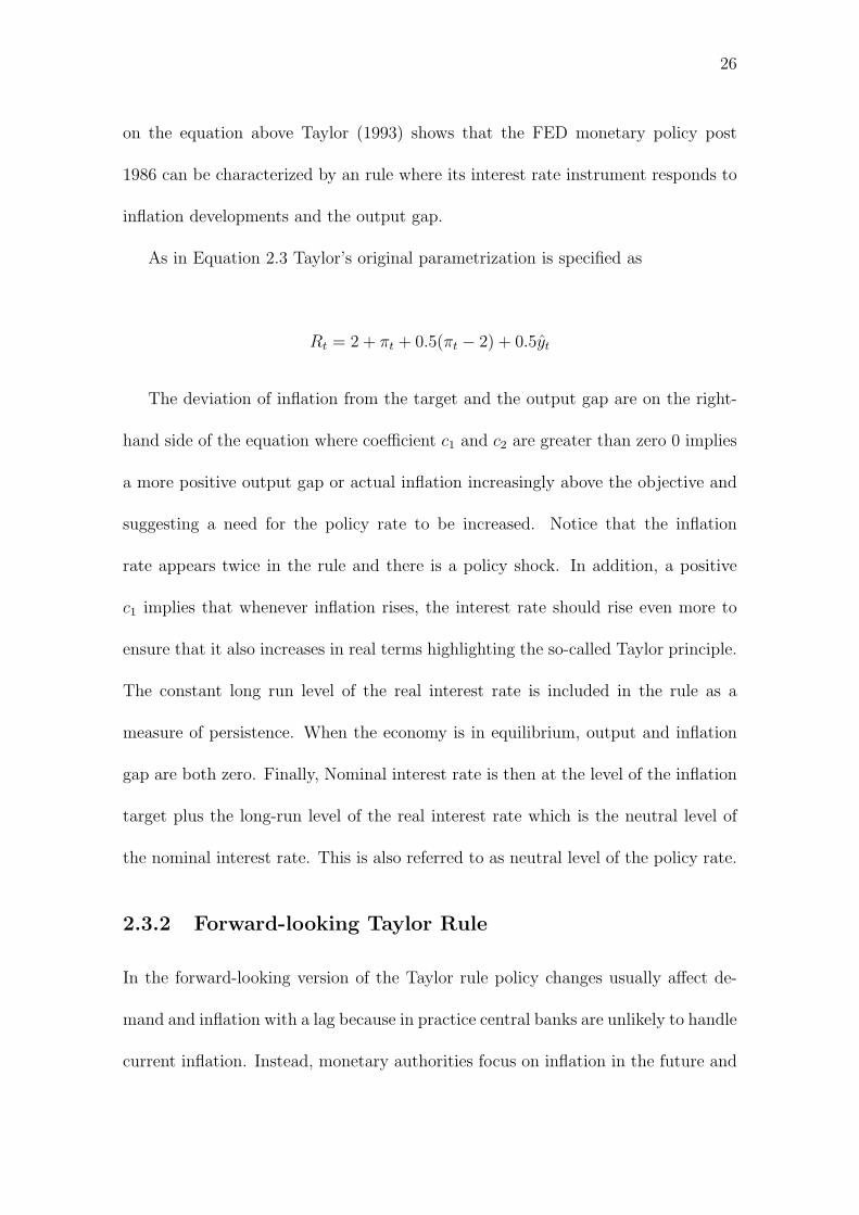
on the equation above Taylor (1993) shows that the FED monetary policy post

1986 can be characterized by an rule where its interest rate instrument responds to

inflation developments and the output gap.

As in Equation 2.3 Taylor’s original parametrization is specified as

Rt = 2 + πt + 0.5(πt − 2) + 0.5yt

The deviation of inflation from the target and the output gap are on the right-

hand side of the equation where coefficient c1 and c2 are greater than zero 0 implies

a more positive output gap or actual inflation increasingly above the objective and

suggesting a need for the policy rate to be increased. Notice that the inflation

rate appears twice in the rule and there is a policy shock. In addition, a positive

c1 implies that whenever inflation rises, the interest rate should rise even more to

ensure that it also increases in real terms highlighting the so-called Taylor principle.

The constant long run level of the real interest rate is included in the rule as a

measure of persistence. When the economy is in equilibrium, output and inflation

gap are both zero. Finally, Nominal interest rate is then at the level of the inflation

target plus the long-run level of the real interest rate which is the neutral level of

the nominal interest rate. This is also referred to as neutral level of the policy rate.

2.3.2 Forward-looking Taylor Rule

In the forward-looking version of the Taylor rule policy changes usually affect de-

mand and inflation with a lag because in practice central banks are unlikely to handle

current inflation. Instead, monetary authorities focus on inflation in the future and

27

thus conduct monetary policy based on expected future outcomes. Assuming that

the central bank applies flexible inflation targeting framework for the conduct of

monetary policy, it is given that the inflation forecast becomes the intermediate

target of monetary policy or nominal anchor. Flexibility of the rule means that the

central bank allows for temporary deviations of inflation from the target and does

not solely focus on inflation but still cares about smoothing the economic business

cycle. The specification of the forward-looking version of the Taylor rule follows

Rt = g1Rt−1 + (1− g1)[Rnt + g2(π

et+N − πt) + g3yt

]+ εt (2.4)

Observe that the forward-looking version is similar to the earlier stated original

version of the rule. It is also an equation for the nominal interest rate and the output

gap is a variable on the right-hand side of the model. However, some important

differences include interest rates adjustments are now based on expected or predicted

inflation changes and not actual inflation. Such expectations may be obtained from

surveys or through a variety of approaches to estimate expected inflation.7 The

first lag of the interest rate is also in the rule showing that the central bank has a

preference of the central bank to smooth changes in the policy rate. It is also clear

that in equilibrium the policy interest rate is at the neutral level which is a sum of

equilibrium real interest rate and expected inflation n periods ahead.

In practice, the equilibrium real rate might not be constant and might be higher

in less developed and fast growing economies because marginal rate of return to

capital is higher. As economies convey to a higher income level, it is expected

7An example, is to calculate the weighted average of past inflation and inflation objectives anduse it as a proxy or us a general equilibrium model with rational expectations.

28

that the equilibrium real rate would decline. Also, the equilibrium real interest

rate might decline as countries get access to international capital markets. So, to

estimate equilibrium we need to estimate a non-stationary trend in the real interest

rate.

The coefficient g1 is usually lies between 6.0 and 0.9 to capture persistence, g2 is

set relative to g3 which signifies the importance of the inflation gap relative to the

output gap. g3 greater that zero and g2 greater that zero means the interest rate

should be higher when expected inflation exceeds the target or when the economy

operates above capacity. Also, note that positive g2 is just enough to satisfy the

Taylor principle. It is generally accepted that indeterminacy occurs when a central

bank implements a regime that follows a Taylor-type interest rate rule but fails

to respond adequately and timely to inflation deviations from target.8 Thus, the

implication is that passive monetary policy may fail to subdue self-fulfilling inflation

expectations. Clearly the values of the parameters may vary from one central bank

to the other. Hence, there is a need to use data and judgment to estimate or calibrate

the coefficients of the Taylor rule. Moreover, the Taylor rule may be specified in

general equilibrium models to consistently describe the economy and how the central

bank steers the interest rate. This is beyond the scope of our present discussion and

our analysis in this chapter is based only on the estimates of the single equation

forward-looking version Taylor rule for Nigeria.

8Woodford (2003) for example shows that indeterminacy may arise were the central bank tofail to adopt an aggressive policy stance against inflation.

29

2.4 Estimation and Analysis of Results

2.4.1 Data

Time series data from 2000Q1 to 2016Q4 was used to estimate the forward-looking

Taylor rule for Nigeria. The variables include Gross Domestic Product (GDP) at

constant basic prices, Composite Consumer Price Index (CPI) and the 3 months

deposit rate (3MDR). The data for the Nigerian economy were source from publi-

cations of the Central Bank of Nigeria and the National Bureau for Statistics. The

CPI and GDP are seasonally adjusted and Augmented Dickey-Fuller (ADF) test for

unit roots were undertaken for all variables indicating that the computed time series

are stationary at level implying the estimation is carried out at I(0) (see, A.3. The

descriptive statistics for the data is presented in Table 2.2 below:

Table 2.2: Descriptive StatisticsR P i Y (1) Y (2) Y (3) Y (4) Y (5)

Mean 10.52 -0.66 0.00 0.02 0.05 0.14 -0.39Median 10.29 -0.67 0.23 0.24 0.02 -0.03 1.37Maximum 20.02 19.63 2.82 2.59 1.94 3.36 9.45Minimum 4.63 -28.16 -4.36 -4.06 -3.20 -4.18 -17.23Std. Dev. 3.25 8.09 1.80 1.68 1.34 1.90 7.30Skewness 0.49 -0.35 -0.55 -0.50 -0.36 -0.19 -0.50Kurtosis 3.24 4.33 2.41 2.32 2.18 2.11 1.91

Jarque-Bera 3.33 7.40 5.13 4.76 3.89 3.10 7.13Probability 0.19 0.02 0.08 0.09 0.14 0.21 0.03

Sum 830.97 -52.06 -0.20 1.40 3.78 11.28 -30.84Sum Sq. Dev. 823.55 5100.19 252.29 220.28 139.08 280.58 4158.26

Observations 79 79 79 79 79 79 79

Notes: Y (1) = HP Filter λ 1600, Y (2) = HP Filter λ 1200, Y (3) = HP Filter λ 500,Y (4) = Christiano Fitzgerald Filter and Y (5) = Quadratic Trend.

30

2.4.2 Estimates of the Forward-Looking Taylor rule 2000Q1-

2016Q3

This section reports estimates of the forward looking Taylor rule for the period

2000Q1-2016Q3. Table 2.3 presents results of the estimated Taylor rule using dif-

ferent statistical filters and the quadratic trend to obtain potential output. The

results show for all estimated models that the autoregressive variable Rt−1 is highly

persistent. This is indicative of the significant weight policy makers place on past

interest rate developments before effecting any policy decisions. Based on the 5 per

cent significance level, Πt−1 is not statistically significant. Given the negative re-

lationship between interest rates and inflation, a significant Πt−1 would imply that

policy makers would reduce rates if the inflation rate in the previous quarter were

to increase which is counter-intuitive. Estimates for the parameter Πt−3 indicates

that policy decisions are influenced by inflation outcomes three previous quarters.

Thus, policy makers give strong consideration to inflation developments t− 3 in the

decision making process. The results suggest that a 1 per cent increase in inflation

t− 3 results in 0.16 per cent increase in interest rates.

In addition, the results show that considerable attention is given to inflation

expectations of economic agents. Thus, the inflation gap estimates shows that a 1

per cent increase in six quarter ahead inflation above the inflation target level results

in a 0.08 per cent increase in interest rates. So, this implies monetary authorities are

mindful of achieving the single-digit inflation target.9 Furthermore, the results also

suggest that the MPC members are quite cautious of output developments in Nigeria

9Nigeria subscribes to maintaining a single digit target for inflation in accordance with the WestAfrican Monetary Zone convergence criteria.

31

placing a relatively large weight on business cycles dynamics. The estimates show

a 1 per cent increase in the output gap would result in a 0.34 per cent decrease in

interest rates consistent with the developmental objectives of the CBN. The results

also reveals that the estimates of the output gap computed using a quadratic trend

is only significant at 10 per cent.

R2 suggests that 86 per cent changes in the interest rate decision can be explained

by changes in Rt−1, Πt−3, P it−2 and Yt−1. The F-statistics suggests that the model

coefficients are statistically different from zero. Thus, the model is robust enough

to explain the variations in Rt.

Table 2.3: Estimation Results

Filters(1) (2) (3) (4) (5)

Variables (HP λ 1600) (HP λ 1200) (HP λ 500) (CF) (QT)Constant 0.753133 0.750118 0.787141 0.712284 0.945123

(1.24) [0.6091] (1.24) [0.6065] (1.32) [0.5976] (1.19) [0.5978] (1.43) [0.66080]Rt−1 0.861093 0.863368 0.869189 0.855820 0.870816

(17.0) [0.05074] (17.2) [0.05024] (17.7) [0.04902] (17.2) [0.04987] (15.4) [0.05647]Πt−1 -0.103646* -0.105033* -0.110465* -0.103315* -0.116575*

(-1.83) [0.05668] (-1.86) [0.05636] (-2.00) [0.05030] (-1.86) [0.05554] (-1.93) [0.06055]Πt−3 0.161421 0.160753 0.157228 0.166629 0.151638

(2.91) [0.05548] (2.91) [0.05523] (2.89) [0.00530] (3.06) [0.05454] (2.56) [0.05915]

P it−2 0.0803369 0.0809904 0.0826681 0.0862225 0.0906986(2.08) [0.03857] (2.11) [0.03835] (2.20) [0.03190] (2.30) [0.03752] (2.19) [0.041330]

Yt−1 -0.335851 -0.364127 -0.479292 -0.364015 -0.0476839*(-3.42)[0.09735] (-3.54)[0.10290] (-3.84)[0.12480] (-3.83)[0.09494] (-1.71)[0.02783]

Observations 67 67 67 67 67R2 0.866043 0.867166 0.871075 0.870996 0.847258Adjusted R2 0.855063 0.856278 0.860507 0.860442 0.834738F-test 78.87** 79.64** 82.43** 82.37** 67.67**log (likelihood) -108.018 -107.736 -106.735 -106.756 -112.414*p< 0.10

Notes: T-statistics in parentheses and standard errors in brackets. P i is computedusing expected inflation 4 quarters ahead. All estimates are significant at 5.0 per centwith exceptions as indicated.

32

2.5 Conclusions

The chapter estimates forward-looking monetary policy rules for Nigeria using Or-

dinary Least Squares (OLS). I estimate forward-looking Taylor rules using different

proxies of potential output to assess how this affects the results in this chapter. The

results show that interest rate changes are influenced by developments to inflation

and the output gap in Nigeria. However, output gap developments influence in-

terest rate decisions more than the level of inflation and its target. Discrepancies

in the point estimates from applying different filters to compute potential output,

highlights the implicit data issues that policy makers encounter in the assessment

of business cycle dynamics. In the absence of a clear view on the state of the econ-

omy, policy makers may use other variants of Taylor-type monetary policy reaction

functions to guide decisions.

In data sparse environment, the effectiveness of monetary policy may depend

largely on data quality when assessing the business cycle. Although data accuracy,

timeliness and frequency remain a challenge for emerging economies, the estimation

procedure produces consistent estimates of the coefficients though there are expected

differences depending on the statistical approach applied to filter potential output. A

useful lesson for emerging economies that are confronted with data challenges includ-

ing the presence of structural breaks in output data is that new-Keynesian model

estimates and test results can be impaired by the filtering technique and length

of observations used to derive model consistent data. Consequently, economist in

resource-rich emerging economies such as the focus of this thesis need to carefully

consider and account for data constraints when adopting a methods to extract the

33

business cycle dynamics as well as data applied in the estimation of new-Keynesian

models.

Chapter 3

A DSGE Model for an Oil-Producing Small Open EmergingEconomy

1

A small open economy DSGE model for a heavily dependent nonindustrial oil-

producer is developed in this chapter. In the sections that follow we build a DSGE

model designed for estimation via Bayesian Maximum Likelihood methods. The

modelling approach adopted incorporates features that are important to capture the

dynamics of an emerging economy oil-producer. These include adding large frac-

tions of non-Ricardian consumers, incomplete exchange rate pass-through (ERPT)

to import and export prices and oil revenue. Taking the model to data, we apply

model consistent methods to filter and demean components of aggregate demand,

consumption and investment for Nigeria. Other observable variables transformed for

the Bayesian estimation are consumer price inflation, a short-term deposit rate and

trade weighted real effective exchange rate. We find that the incorporated features

provide a good fit for the economy.

1This Chapter was co-authored by Dr. Cristiano Cantore, Dr. Vasco Gabriel and ProfessorPaul Levine, University of Surrey

34

35

3.1 Introduction

Recent developments in the international commodity markets have stimulated re-

newed interest in the study of the impact of large external shocks on resource-rich

economies. In particular, a huge price swing saw crude oil prices drop from as high

as USD115 a barrel in June 2014 to a low of USD45 in January 2015 marking the

second such event of a huge oil price fall in six years following the global financial

and economic crises of 2007/8. Although oil prices made a remarkable rebound after

the first episode of a huge price drop, it should be noted that at the time, many

oil exporters were well- insulted from the impact of the shock by sufficient ‘fiscal

buffers’ and adequate international reserves. On the contrary, a simple assessment

of the second incidence in 2014 shows less optimism of a consecutive scenario of

rapid price recovery to levels before the plunge. As a result and in the absence of

ample buffers, the ability of some oil exporters to effectively manage the impact of

the oil price shock on the economy is in doubt(see, International Monetary Fund

(2012)). Against this perspective and inherent uncertainties, it is evident that the

determination of crude oil prices exhibit a volatile process which poses considerable

challenges to macroeconomic stability and management particularly in heavily de-

pendent oil exporting economies. Indeed, the aforementioned scenario highlights a

fundamental feature of small open economies which is their exposure to fluctuations

in foreign markets and international business cycles.

The Nigerian economy is heavily dependent on revenues from oil exports and

36

is therefore considerably vulnerable to oil price fluctuations. Over the past four

decades, oil and gas revenues have accounted for about 80.0 per cent of total gov-

ernment financing and earned around 90.0 per cent of total exports. With proven

crude oil reserves estimated at 37 billion barrels and a production output of approx-

imately only 2.5 million barrels of crude daily (OPEC Annual Statistical Bulletin

2015), Nigeria remains a ‘price-taker’ subject to the interplay of market forces which

are determined by the dictates of dominant producers and the global demand for

oil and gas. Consequently, the mono-product nature of exports and fiscal revenue

makes macroeconomic outcomes susceptible to the vagaries of oil prices.1 It is also

important to highlight that, even though Nigeria has a projected relatively long

horizon of income stream from oil and gas revenues due to its estimated reserves

and current levels of production, a major challenge before policy makers remains the

need to maintain macroeconomic stability and a stable fiscal profile while discount-

ing volatile oil sector developments so that its resource wealth can be transformed

into development gains.

There is a large body of research on examining the effects of foreign shocks on

domestic macroeconomic developments. These studies vary between empirical and

theoretical founded research focusing on generic, cross-sectional or country specific

issues that are related to the effects and channels through which foreign shocks are

propagated in open economies. Although empirically skewed analytical methods

including the use of vector autoregressions (VAR) and dynamic factor models (see,

1Beyond price developments, oil revenue is volatile in Nigeria because of incessant productionshut-downs and supply disruptions. In addition, oil revenue is affected by peculiar market demandconditions associated with the shale oil and gas revolution which has made traditional consumersof Nigerian crude reduce patronage of the Bonny light and other streams of crude oil from Nigeria.In response, Nigeria has had to find alternative markets for crude by discounting sales to attractbuyers.

37

Kose et al. (2008)) provide some useful explanations of the degree of co-movement

between the international business cycle and domestic macro-variables, a comparison

shows that theoretical based approaches have properties that make them better

suited for policy analysis.

Most prominent among the theoretical based approaches are new-Keynesian dy-

namic stochastic general equilibrium (DSGE) models. These models have become

benchmark tools in macroeconomics; having micro-foundations with optimising eco-

nomic agents and endogenous forward looking expectations make them particularly

suitable for policy analysis, as well as useful for forecasting. Built on the real busi-

ness cycle (RBC) framework embedded at the core, a broad array of nominal and real

frictions may be incorporated to emphasize economic reality in order to investigate

or answer research questions based on specific theoretical underpinnings (see, Gali

(2008)). Against this background, DSGE models have been tailored successively

to incorporate unique economic features by adding necessary ‘bells and whistles’

that are required to characterise the economic structure, frictions and agents’ con-

straints to answer macroeconomic research questions including those related to this

current narrative on how specific economies or group of economies should respond

to external shocks.

In line with themes covered in the literature on open economies, several authors

use DSGE models to analyse savings, investment and spending behaviour in response

to oil price shocks assessing how alternative macroeconomic policies affect these

variables. Proposing the means by which open economies should conduct monetary

and fiscal policy, a few papers characterize the interaction between the domestic

38

oil economy and non-oil sectors of the economy predicated on the assumption that

domestic output is influenced by the oil price (a proxy for the cost of petroleum

products or energy) on account that oil serves as an important production input

(see, Catao and Chang (2013) and Vasconez (2014) among other papers). A common

policy recommendation inferred from the conclusions of these studies is indicative

of a need to curtail aggregate demand whenever there is a negative oil price shock.

Although this is a logical point of view in the management of inflation, evaluating

the relationship between the oil and other sectors solely from a cost-push perspective

may negate the impact of oil price shocks on aggregate demand when substantial

demand for domestic inputs are from the oil industry or oil sales constitute a major

source of exports earnings and government financing. Thus, when the converse

holds as above different policy options may have to be considered to ensure the

effectiveness of policy initiatives.

Following this line of reasoning, Bergholt (2014) focusing on the role of sectoral

trade interdependence assumes that the oil sector uses non-oil sector output as in-

termediate input, then sets up a sticky wage- and price DSGE model for analysing

inefficiencies in the conduct of monetary policy associated with the impact of oil

price shocks to the economy. Attempting to improve the model fit, the author in-

corporates both the interactions in production networks between the domestic oil

and non-oil firms, and how frictions in the model affect resource allocation and wage

and price dispersion along business cycle dynamics. Assessing the welfare implica-

tions, Bergholt (2014) finds that any attempt to stabilise the effects of developments

39

from the oil sector produces volatility elsewhere in the industrialised economy. In-

variably, the contradicting conclusions relative to the cost-push approach earlier

mentioned alludes to the importance and need to ascertain the appropriate trans-

mission channel(s) through which oil price shocks affect all sectors of the economy

in order to proffer optimal policies using open economy DSGE models as well as

from a general perspective in modelling.

Extending the literature on oil exporters to economies with less developed indus-

trial sectors, recent works by Richmond et al. (2013), Berg et al. (2013), assess the

implications of public investment strategies and management of windfalls in a three

sector model setting consisting of tradable, non-tradable and oil sectors. Similarly,

building on Buffie et al. (2012) and Berg et al. (2013), Melina et al. (2014) develops

a consistent model-based framework to analyse debt sustainability and the public

investment-growth nexus for a sub-Saharan African(SSA) economy. A prevalent

proposal made by these authors is that appropriate policies should be implemented

to insulate resource-rich economies from the volatility of resource price shocks by

saving a part of volatile windfalls, maintaining sustainable fiscal buffers and having

a sufficient pool of funds for investment over a period of time.

Devarajan et al. (2015) apply a similar framework to analyze and derive simple

budget rules when public revenue from oil exports in a capital constrained economy

is volatile. The authors asserts that “when a resource price change is positive and

temporary, the best strategy is to save the revenue windfall in a sovereign fund,

then use the interest income from the fund to raise citizens consumption” for en-

hanced welfare. Combining the savings in the wealth fund with transfers made to

40

households, serves as a means to moderate the impact of shocks as incorporated in

the model by Devarajan et al. (2015). In addition, the authors assert that public

investment stimulated growth in output remains a veritable protection to smooth

consumption in response to resource price shocks. It should be noted, however,

that these works focus more on the policies for sustaining a sufficient stream of

income from the finite extractive resource rather than achieving the objectives of

macroeconomic stability in these economies.

As highlighted by the conclusions in the literature on SSA economies, the effects

of terms of trade shocks on oil producers could be substantial and is of special

interest particularly where the shock is strongly positively correlated with domestic

output and capital inflows. Capital flows may witness a sharp reversal or even a

dramatic “sudden stop” during a negative oil price shock as emphasized by Calvo

(1998) and evident for some oil exporters as a result of the ‘second round effects’ of

the 2007/8 crises. Output developments, on the other hand may vary depending on

the structure of the sectoral contributions to overall output. This implies that the

debilitating effects of such reversals on the financial system may sometimes be more

amplified than the somewhat transient impact of oil price shocks on output.

It may suffice to state, that when the resource production sector is relatively

an enclave one, the moderate impact of external shocks may support conventional

wisdom of the existence of a ‘dual-economy’, that is, a huge informal sector which

plays a stabilizing role on the economy of commodity exporters. In addition, it is ex-

pected that the inclusion of a significant proportion of credit-constrained consumers

who depend on current income and have limited access to formal financial services

41

will improve the model fit for the emerging economy. Similarly, incorporating an

informal sector should stylize the nature of productive activity in these economies.

In this chapter, we incorporate important features for an emerging economy oil-

producer to a two-bloc open economy Smets-Wouters type model: a large proportion

of non-Ricardian consumers2, incomplete exchange rate pass-through to import and

export prices, and oil revenue. Thereafter, a Bayesian estimation approach is used

to estimate the model using five macroeconomic variables for Nigeria. As a result

of data limitations, we calibrate some structural parameters which would otherwise

would not be estimated sufficiently precise. Other assumptions at this stage of the

model development include specifying government spending as an exogenous pro-

cess (AR1) which depends solely on historic data on government spending to GDP

ratio. Therefore, oil price developments affect the model through the trade balance.

This assumption can however be relaxed as found in other small open economy

(SOE) models by incorporating a detailed specification of government activity as

an endogenous process with the government raising taxes and spending based on a

budget rule. This would certainly have implications for the estimated results. It

should also be highlighted here that long-run growth and inflation in the steady

state are non-zero in the DSGE model for the emerging economy oil-exporter.

The chapter is organised as follows. Section 3.2 presents the basic SOE DSGE

oil-producer model employed in this thesis. In Section 3.3, estimations and analysis

of the model are undertaken for the Nigerian economy. Section 3.4 concludes.

2The new-Keynesian DSGE model presented in this thesis consist of two types of households.Firstly, we have Ricardian households maximizing expected utility from leisure and consumptionwith full access to financial markets and thus smooth consumption over time. In other words, thesehouseholds are optimizing agents in the model. Secondly, non-Ricardian households depend onwages to consume every period (see, Gali et al. (2007)). We also refer to non-Ricardian householdsinterchangeably as liquidity-constrained or rule-of-thumb households in this thesis.

42

3.2 Small Open Economy DSGE Oil-producer

Model

This section presents a summary of the two-bloc open economy Smets-Wouters type

model analysed in this Chapter. The small open economy model developed here fea-

tures nominal price rigidities in the form of staggered prices a la Calvo (1983) and

imperfect competition. Other attributes incorporated that are common to emerg-

ing economy oil-producers includes liquidity-constrained consumers, international

financial frictions, incomplete ERPT to import and export prices and oil revenue.

At this stage of the model development, a simplified version of the oil sector is in-

troduced with proceeds from sales of crude oil impacting on the trade balance. Our

model specification closely follows Gabriel et al. (2010). For descriptive purposes an

elaborate presentation of the model in stages of its development is in Appendix B.

3.2.1 Dynamic Model

Households

Assume consumers in the economy are represented by an identical infinitely lived

household that obtains utility from consumption and leisure. Then our representa-

tive household will maximize the objective function at time t given value function

as follows

Ωt = Et

[∞∑s=0

βsU(Ct+s, Lt+s)

](3.1)

where E is the operator for expectations, the subjective discount factor, β, U stands

for marginal utility, with consumption, Ct, and leisure, Lt. Total hours worked and

43

available time for leisure is normalized to one (1) that is, ht = 1−Lt. The households

objective at time t is to optimize it’s position by choosing consumption Ct and

leisure Lt from its state-contingent plans as well as financial holdings to maximize

Ωt in a stochastic environment.

Including habit formation by adopting external habits χ ∈ [0, 1] as a price per-

sistence mechanism in the household utility function, the single period utility and

the marginal utilities of consumption and leisure is written respectively as,

UC,t = (1− ϱ)C(1−ϱ)(1−σ)−1t (1− ht)

ϱ(1−σ) ; for Ct = C1,t, C2,t; ht = h1,t, h2,t(3.2)

UL,t = −ϱC(1−ϱ)(1−σ)t (1− ht)

ϱ(1−σ)−1 ; for Ct = C1,t, C2,t; ht = h1,t, h2,t (3.3)

where the subscript 1 and 2 in consumption and hours denotes Ricardian and

non-Ricardian consumers respectively. The relative weight of agents on consumption

is ϱ ∈ (0, 1) which is a compatible utility function given a balanced non-zero growth

in the steady state when σ ≥ 1 the risk-aversion parameter also equivalent to the

inverse of the intertemporal rate of substitution.3 Given the world long run growth

rate, we specify 1 + gt as the stochastic steady state growth rate which is a salient

feature in the emerging economy SOE model rather than the commonly assumed

zero growth rate in some models.4 Non-Ricardian consumers C1,t of proportion λ

are subject to consume

C1,t = Wth1,t (3.4)

3See, Chapter 9 Barro and Sala-i-Martin (2004) for details.4See appendix B.5.2 for the detailed set up for the balanced-exogenous-growth steady state

44

In Nigeria, non-Ricardian consumers, denoted above as C1,t constitute a signif-

icant proportion of households and this category of consumers typify those who do

not smooth consumption due to limited access to financial services (see, Kama and

Adigun (2013) and EFInA (2010)). Invariably, this implies that a substantial num-

ber of households do not have access to credit. Inaccessibility to formal financial

services and dependence on informal financial arrangements also impacts the effi-

cacy of monetary policy in Nigeria as revealed in a recent paper by Mbutor and Uba

(2013). Furthermore, in a relatively volatile output environment such as Nigeria, the

presence of a significant fraction of households being non-Ricardian should amplify

the propagation of government spending shocks on the system. These agents do not

participate in asset markets, consuming entirely disposable income in the period.

Non-Ricardian consumers choose C1,t and L1,t = 1−h1,t to maximize U1(C1,t, L1,t)

subject to (B.35). Real wage is equivalent to the marginal rate of substitution

between consumption and leisure.

The first-order conditions, total consumption Ct and hours ht are

1

Rn,t

= βEt

[UC2,t+1

UC2,tΠt+1

](3.5)

Ct = λC1,t + (1− λ)C2,t (3.6)

UL1,t

UC1,t

=UL2,t

UC2,t

=Wt (3.7)

ht = λh1,t + (1− λ)h2,t (3.8)

Rn,t signifies the gross nominal interest rate during the period [t, t+ 1].

Introducing the open economy features of the model, interaction between house-

holds and the rest of world takes place in the goods market and access to foreign

45

finance implying these agents face a risk premium from developments in the in-

ternational capital markets. Following the Dixit-Stiglitz (DS) indices for domestic

consumption of home (H) and foreign (F) goods summarized here for both consump-

tion and investment goods5

Pi,t =[wi(PH,t)

1−µi + (1− wi)(PF,t)1−µi

] 11−µi ; for i = C, I (3.9)

The intra-temporal optimization for home consumption is

1 =

[wC

(PH,tPC,t

)1−µC+ (1− wC)

(PF,tPC,t

)1−µC] 1

1−µC

(3.10)

PH,tPC,t

=1

[wC + (1− wC)T 1−µCt ]

11−µC

(3.11)

where Tt ≡ PF,tPH,t

CH,t = wC

(PH,tPC,t

)−µCCt (3.12)

CF,t = (1− wC)

(PF,tPC,t

)−µCCt (3.13)

CH,t∗ = (1− ω∗

C)

(PH,t

PC,tRERC,t

(θ + (1− θ)

StP∗ ℓH,t

PH,t

))−µ∗C

Ct∗ (3.14)

Real exchange rate is specified in terms of relative aggregate price RERi,t ≡P ∗i,tSt

Pi,t

5Weights in the consumption baskets in the two blocs are then defined by

wC = 1− (1− ν)(1− ωC) ; w∗C = 1− ν(1− ω∗

C)

In (B.44), ωC , ω∗C ∈ [0, 1] consists of parameters that describes the extent of ‘bias’ in both blocs.

On assumption ωC = ω∗C = 1 we have wC = w∗

C = 1, i.e., autarky, while ωC = ω∗C = 0 is equivalent

to a case of perfect integration with wC = ν and w∗C = 1− ν, i.e., weight according to proportions

of produced goods in the two blocs. The home economy shrinks as ν → 0 which is the limit. HencewC → ωC and w∗

C → 1, implying a closed foreign bloc. However, so long as ωC > 0, some foreign-produced goods would be consumed in the home economy. Variables with asterisk superscript arefor the foreign economy. Proportions for respective domestic and foreign blocs are ν and 1 − νrespectively.

46

for consumption and similarly for investment (for i = C, I) where St above stands

for nominal exchange rate.

Incorporating additional financial frictions to the households module, we intro-

duce two non-contingent one-period bonds BH,t and B∗F,t expressed in the respective

currency units of each bloc and paid in period t (see, Benigno (2001)). The bond

prices are specified as

PB,t =1

Rn,t

; P ∗B,t =

1

R∗n,tϕ(

StB∗F,t

PH,tYt)

(3.15)

where B∗F,t constitutes the total sum of foreign assets held by domestic residents in

foreign currency, ϕ(·) is the risk premium paid by domestic households on foreign

bonds assuming ϕ(0) = 0 and ϕ′ < 0 and PH,tYt is nominal output. R∗n,t denotes the

gross foreign nominal interest rate.

The budget constraint for the representative household at period t is expressed

nominally as:

PC,tCt + PB,tBH,t + P ∗B,tStB

∗F,t + PC,tTLt = PC,tWtLt +BH,t−1 + StB

∗F,t−1 + PC,tΓt(3.16)

where the real wage rate is Wt, lump-sum taxes less government transfer payments

are TLt and households receive Γt, dividends for owning firms. Consumption, taxes,

real wages and dividends are multiplied by the DS price index PC,t described in

(B.42). Defining Πt our consumer price inflation as Πt ≡ PC,t

PC,t−1the households

47

intertemporal and labour supply decisions will then be

PB,t = βEt

[UC,t+1

UC,tΠt+1

](3.17)

P ∗B,t = βEt

[UC,t+1St+1

UC,tΠt+1St

](3.18)

Wt =UL,tUC,t

= −Uh,tUC,t

(3.19)

Firms

A Cobb-Douglas type function below depicts the process of production by firms.

Output Yt is formed using hours, ht from households and capital Kt at beginning-

of-period t given the production technology parameter At

Yt = F (At, ht, Kt) = (Atht)αK1−α

t (3.20)

In (3.20) Yt, ht and Kt are in per-capita units. Firms build up capital as determined

by

Kt = (1− δ)Kt−1

1 + gt+ (1− S(Xt))It (3.21)

implying capital producing firms face a convex investment curve as they convert It

of production into new capital (1−S(Xt))It traded at Qt a real price and an affixed

cost of S(Xt) at time t.6

The necessary condition for maximizing profit is

Qt(1− S(Xt)−XtS′(Xt)) + Et

[1

(Rt+1)Qt+1S

′(Xt+1)I2t+1

I2t

]= 1 (3.22)

6Investment costs are therefore convex and dissipate since, Xt ≡ ItIt−1

and since S(·) fulfills theconditions for S′, S′′ ≥ 0 ; S(1 + g) = S′(1 + g) = 0.

48

It is required for capital demand by firms to satisfy

Et[(Rt+1)RPSt+1] =Et

[(1− α)

PWt+1Yt+1

Kt+1+ (1− δ)Qt+1

]Qt

(3.23)

The right-hand-side of (3.23) represents the gross return to holding one unit of

capital through successive periods (t to t+ 1). On the other hand, the ratio on the

left side of the equation (3.23) is gross returns on bond holdings, foregone cost on

capital and an exogenously determined shock on the risk-premium RPSt, which is

modelled later. The functional form for the investment costs with g as the balanced

growth rate in the model so far, will be

S(X) = ϕX(Xt − (1 + g))2 (3.24)

Thereafter, utilizing a homogenous wholesale good to produce differentiated con-

sumption output, a retail sector is introduced in the model as

Ct =

(∫ 1

0

Ct(m)(ζ−1)/ζdk

)ζ/(ζ−1)

(3.25)

given that ζ stands for elasticity of substitution. Intermediate good m sells at Pt(m)

depicted in the demand equation of the form

Ct(m) =

(Pt(m)

Pt

)−ζ

Ct (3.26)

where Pt =[∫ 1

0Pt(m)1−ζdm

] 11−ζ

. Pt represents the index of aggregate price.

49

The cost of converting m to retail output equals cY Wt (m) employing the produc-

tion technology (3.20). Hence

Yt(m) = (1− c)Y Wt (m) (3.27)

Y Wt =

(Atht)αK1−α

t−1

∆t

(3.28)

∆t describes price dispersion as follows

∆t ≡1

n

n∑j=1

(Pt(j)/Pt)−ζ = ξΠζ

t∆t−1 + (1− ξ)

(JtHt

)−ζ

(3.29)

Price stickiness is introduced next by assuming a probability 1 − ξ each period

that intermediate good prices m are optimally set at P 0t (m). Prices are left fixed

if not re-optimized.7 Intermediate producers m objective every period is to choose

P 0t (m) so that discounted profits are maximized subject to (B.20) solved as

Et

∞∑k=0

ξkDt,t+kYt+k(m)

[P 0t (m)− 1

(1− 1/ζ)Pt+kMCt+kMSt+k

]= 0 (3.30)

where Dt,t+k ≡ βΛC,t+k

ΛC,tbecomes the nominal stochastic discount factor from [t, t+k].

MSt a mark-up shock with steady state 1(1−1/ζ)

is introduced in (B.24).

The law of large numbers implies an evolution in prices that follows

P 1−ζt+1 = ξP 1−ζ

t + (1− ξ)(P 0t+1)

1−ζ (3.31)

Difference equations describe the inflation dynamics in order to set the model up

in non-linear form for simulation and estimation. Now specifying nominal discount

7Thus, on an average 11−ξ can be interpreted as the duration firms leave prices unchanged.

50

factor by Dt,t+k ≡ βUC,t+k/Pt+k

UC,t/Pt, 8 inflation dynamics for both producer currency

pricers (PCP) and local currency pricers (LCP) are given by

1 PCP Price Setters in Home Currency

Ht − ξHβEt[Πζ−1H,t+1Ht+1βg,t+1(1 + gt+1)] = YtUC,t (3.32)

Jt − ξHβEt[ΠζH,t+1Jt+1βg,t+1(1 + gt+1)] =

1

1− 1ζ

MStYtUC,tMCt (3.33)

MCt =PWH,t

PH,t=PWH,t/PC,t

PH,t/PC,t=

Wt

PC,tht

αYtPH,t

PC,t

(3.34)

1 = ξHΠζ−1H,t + (1− ξH)

(JtHt

)1−ζ

(3.35)

2 LCP Price Setters in Foreign Currency

Hℓt − ξHβEt[(Π

∗ ℓH,t+1)

ζ−1Hℓt+1βg,t+1(1 + gt+1)] = Y ∗

t StUC,t (3.36)

J ℓt − ξHβEt[(Π∗ ℓH,t+1)

ζJ ℓt+1βg,t+1(1 + gt+1)] =1

1− 1ζ

MSt Y∗t StUC,tMCℓ

t (3.37)

MCℓt =

MCtStP ∗ ℓ

H,t

PH,t

(3.38)

1 = ξH(Π∗ ℓH,t)

ζ−1 + (1− ξH)

(J ℓtHℓt

)1−ζ

(3.39)

Define the LoP gap for LCPers as

Ψt ≡StP

∗ ℓH,t

PH,t(3.40)

8Using the summation St ≡∑∞

k=0 βkXt+k, we write

St = Xt +∞∑k=1

βkXt+k = Xt +∞∑

k′=0

βk′+1Xt+k′+1 putting k′ = k + 1

= Xt + βSt+1

51

Then

Ψt

Ψt−1

=StSt−1

Π∗ ℓH,t

ΠH,t

(3.41)

Aggregate export inflation in foreign currency is then

Π∗H,t = θ

ΠH,t

St+ (1− θ)Π∗ ℓ

H,t (3.42)

Exchange Rate Pass-through and Imports

Supported by empirical literature on Nigeria, incomplete ERPT to import prices is

incorporated into the model.9 To incorporate the partial exchange rate pass-through

to imports, assume only a proportion θ∗ of importers set prices on producer basis.

Then the 1− θ∗ will have incomplete exchange rate pass-through and as similar to

the set up for exports we have

RERi,t ≡PF,tPi,t

= θ∗StP

∗i,t

Pi,t+ (1− θ∗)

P ∗F,t

Pi,t; for i = C, I (3.43)

for consumption and investment goods. Ψi,t ≡P ∗F,t

Pi,tis an AR1 process with a steady

state Ψi ≡P ∗F

Pi=

SP ∗i

Pi= 1.

Real marginal costs are given by

MCt =PWt

Pt(3.44)

and (B.32) must be modified to

RK,t =(1− α)MCt+1Yt

Kt−1+ (1− δ)Qt

Qt−1

(3.45)

Note that as ξ → 0 and ζ → ∞, MCt → 1, ∆t → 1 and the NK model reduces to a

9Various studies have estimated the ERPT for Nigeria (see Adebiyi and Mordi (2012), Oyinlolaand Adetunji (2009) and Oladipo (2007) among others. From the conclusions of these studies, itis therefore justifiable to introduce a mechanism that captures the process of incomplete exchangerate pass-through to import and export prices in the small open economy model.

52

flexi-price RBC core model.

Corresponding interactions of firms with the rest of the world are set up as

IH,t = wI

(PH,t/PC,tPI,t/PC,t

)−µIIt (3.46)

IF,t = (1− wI)

(PF,t/PC,tPI,t/PC,t

)−µIIt (3.47)

I∗H,t = (1− ω∗I )

(PH,t/PC,t

PI,t/PC,tRERI,t

(θ + (1− θ)

StP∗ ℓH,t

PH,t

))−ρ∗I

I∗t (3.48)

PI,tPC,t

=

[wI

(PH,tPC,t

)1−µI+ (1− wI)

(PF,tPC,t

)1−µI] 1

1−µI

(3.49)

StSt−1

=RERC,tΠt

RERC,t−1 Π∗t

(3.50)

TtTt−1

=ΠF,t

ΠH,t

(3.51)

RERC,t =1[

1− wC + wCT µC−1t

] 11−µC

(3.52)

RERI,t =1[

1− wI + wIT µI−1t

] 11−µI

(3.53)

Πt = [wC(ΠH,t)1−µC + (1− wC)(ΠF,t)

1−µC ]1

1−µC (3.54)

Foreign aggregate consumption and investment in the small open economy are

53

exogenous processes and denoted by C∗t and I∗t respectively10. Then foreign equiv-

alent demand for the export of the home goods as specified above is written as

C∗H,t = (1− w∗

C)

(P ∗H,t

P ∗C,t

)−µ∗C

C∗t = (1− w∗

C)

(PH,t

PC,tRERC,t

)−µ∗CC∗t (3.55)

I∗H,t = (1− w∗I)

(P ∗H,t

P ∗I,t

)−µ∗I

I∗t = (1− w∗I)

(PH,t

PI,tRERI,t

)−µ∗II∗t (3.56)

where P ∗H,t, P

∗C,t and P

∗I,t refer to the prices of consumption in the home bloc, and

aggregate consumption and investment goods denominated in units of the foreign

economy currency is equivalent to StP∗H,t = PH,t.

11

RERrt =

U∗C,t

UC,t(3.57)

R∗t =

R∗n,t−1

Π∗t

(3.58)

1

R∗n,tϕ(

StB∗F,t

PH,tYt)StB

∗F,t = StB

∗F,t−1 + TBt (3.59)

ϕ(StB

∗F,t

PH,tYt) = exp

(ϕBStB

∗F,t

PH,tYt

); ϕB < 0 (3.60)

(3.61)

Then the real exchange rate is given by

RERC,t = RERdtRER

rt (3.62)

0 = Et

UC,t+1

UC,t

RERrt+1

RERrt

1

Π∗t+1

1

ϕ(StB∗

F,t

PH,tYt) exp(ϵUIP,t+1)

−RERd

t+1

RERdt

(3.63)

10Aggregate variables such as Ct and C∗t are in per capital terms and aggregated across varieties

with the two blocs consuming a relative total expressed as νCt

(1−ν)C∗t.

11This is based on the ‘law of one price’ for converted goods.

54

An alternative to (A.51) which uses an exogenous process for R∗n,t rather than U

∗C,t

(which drives RERrt ) is

1

ϕ(StB∗

F,t

PH,tYt

)exp(ϵUIP,t)R∗

n,t

= Et

[UC,t+1St+1

UC,tΠt+1St

](3.64)

Oil Sector

Oil output Y O is treated as exogenous in the model. Oil production is incorporated

into the model as an enclave sector which leaves output developments in the oil

industry determined by the long run oil to real GDP ratio. Likewise, oil price

follows an AR(1) process with a random walk without a drift following Hamilton

(1983)12, thus

logpO∗t = logpO∗

t−1 + εpot ,

where (εpot ∼ i.i.d.N(0, σ2po) is the oil price shock.

The trade balance is then equivalent to

TBt = StP∗O,tY

O + PH,tYt − PC,tCt − PI,tIt − PH,tGt (3.65)

The Central Bank

The gross nominal and ex post real interest rates are related by

Rt =Rn,t−1

Πt

(3.66)

given that nominal interest rates represents a policy term as commonly specified.

The central bank policy function for the resource-rich oil exporter includes a target

for the exchange rate expressed as:

12The issue of determination of oil prices is also extensively elucidated upon in Bernanke et al.(1997)

55

logRn,t/Rn = ρr logRn,t−1/Rn + (1− ρr)(θπEt[log Πt+j]/Π

+ θs logSt/S) + ϵMPS,t (3.67)

(3.67) is an ‘implementable’ rule that does not require knowledge of the output

gap.

Market clearing equation is therefore

Yt = CH,t + IH,t + C∗H,t + I∗H,t +Gt (3.68)

Shocks Five domestic shocks for technology, mark-up, UIP, consumption and in-

vestment conclude the home module:

logAt+1

A= ρa log

AtA

+ ϵa,t+1 (3.69)

logMSt+1

MS= ρms log

MStMS

+ ϵms,t+1 (3.70)

logUIPt+1

UIP= ρUIP log

UIPtUIP

+ ϵuip,t+1 (3.71)

ϵr,t+1 = ρeϵr,t + νr,t+1 (3.72)

logΨC,t+1

ΨC

= ρψc logΨC,t

ΨC

+ ϵψc,t+1 (3.73)

logΨI,t+1

ΨI

= ρψilog

ΨI,t

ΨI

+ ϵψi,t+1 (3.74)

The rest of the world processes are exogenously determined by AR1 shocks

logR∗n,t/R

∗n = ρ∗r log(R

∗n,t−1/R

∗n) + ϵ∗r,t+1 (3.75)

logΠ∗t+1

Π∗ = ρ∗π logΠ∗t

Π∗ + ϵ∗π,t+1 (3.76)

logC∗t+1

C∗ = ρ∗c logC∗t

C∗ + ϵ∗c,t+1 (3.77)

logI∗t+1

I∗= ρ∗i log

I∗tI∗

+ ϵ∗i,t+1 (3.78)

56

and

U∗C,t = U (3.79)

h∗t = h (3.80)

Y ∗ = C∗ + I∗ (3.81)

3.3 Calibration and Estimation

3.3.1 Bayesian Estimation

The Bayesian estimation of DSGE models is now routine and has been carried out

with some success by Adebiyi and Mordi (2010), Adebiyi and Mordi (2012) and CBN

(2013) for Nigeria. As is usual these estimations were carried out using a linearized

model. But it is now recognised that estimation to capture non-linearities are

important, especially where linearization removes the contribution of risk in agents’

decisions (see, Fernandez-Villaverde (2009), Fernandez-Villaverde et al. (2012) and

Kollman (2015), for example). We estimate the non-linear DSGE model presented

earlier using Bayesian methods in this section

3.3.2 Data

Our data set to estimate the system contains five macroeconomic observable vari-

ables including measures of investment, consumption, inflation rate, real effective

exchange rate (REER) and nominal interest rate. The set of variables for Nigeria

are at quarterly frequency obtained from the NBS, CBN Statistical Bulletin and the

International Financial Statistics (IFS) of the International Monetary Fund. Hav-

ing considered the likely impact of structural breaks on the system, we apply the

sample period 2002:3-2015:4 for the estimation. We reconcile available vintage of

57

data for 2007:1-2015:4 ‘backcasting’13 using quarterly growth rates for real invest-

ment and consumption to obtain the full quarterly series from 2000:1 - 2015:4. We

use TRAMO-SEATS throughout for seasonal adjustments. As noted Aguiar and

Gopinath (2007), most cyclical fluctuations in developing countries are driven by

trends. In view of this, we employ the Hodrick-Prescott filter in order to obtain

stationary data for the real investment(INV) and consumption(CONS). Choosing

between the ‘flexible-HP’ filtered data and bog-standard filtered data with lambda

= 1600, we apply both approaches in two different estimations to assess which works

well for the Nigerian economy (see, Choudhary et al. (2013)). The inflation rate is

calculated on the composite measure of the Consumer Price Index (CPI). For nomi-

nal interest rate, we apply the 3-month deposit rate an intermediate rate to capture

the effects of the Monetary Policy Rate (MPR), the CBN’s policy rate and liquidity

conditions. The trade-weighted REER from the IFS is a proxy for the real exchange

rate in the estimation (see, Appendix D).

The corresponding measurement equations of the model are specified as:

log(INVt)/INV t)

log(CONSt)/CONSt)

log(CPIt − CPIt−1)− log(Π)

3MDRt/4− 3MDR/4

log(REERt/REER)

=

log(INVtINV

)+mect

log(CONSt

CONS

)+meit

log(Πt

Π

)log(Rn,t

Rn

)log(REERt

REER

)

A brief review of the Modified Hodrick Prescott Filter

In order to address issues related to economy specific differences in the ratio of vari-

ances for both the generated cyclical series as well as fraction of growth differentials

of trend components when the HP filter is employed, the modified HP filter extends

the conventional concept of decomposing time series by selecting an optimal value

13So we use the available growth rates to compute backwards earlier observations prior to 2007:1.

58

for λ. The first step towards selecting λ involves obtaining a spline from the solution

of the minimizing

mingt

[T∑t=1

(yt − gt)2 + λ

T∑t=1

[(gt+2 − gt+1)− (gt+1 − gt)]2

]

which solves for gt

gt = [I + λA]−1yt = Byt

where A = K ′K is such that K = kij is a (T − 2) x T matrix. The next step

employs the leave-one-out technique developed in Craven and Wahba (1979) and

also adopted in McDermott (1997). The notion is to exclude individual data points

each time period, and then isolating the λ which best replicates the data point.

From a practical point of view, we plug in an arbitrary value for λ which produces a

new spline from gt above for each left out data point applying the mean square sum

of the predicted as well as left out points as follows in cross-validation function14

CV | λ =

∑Tk=1(yk − gkT,λ(tk))

2

T

Thus, the ability of the spline produced from gt to mimic the left out data points

determines the suitability of λ. Invariably, the λ minimizing the function CV | λ

is the assumed optimal smoothing parameter and is simplified in the generalised

versions below:

GCV (λ) = T−1

T∑k=1

(yk − gt,k(λ))2

(1− 1TtrA(λ))2

Calibrated Parameters

The next step in the estimation procedure involves keeping a number of parameter

values fixed. This includes some structural parameters which are set to match

the corresponding data sample mean. The outcome of this process ensures all the

14Choudhary et al. (2013) provides a full description of the methodology.

59

calibrated parameters are consistent with the observed steady state values. For the

Bayesian estimation in this chapter, the discount factor β is fixed at 0.99 and for the

firms behaviour and price setting, the depreciation rate of non-resource capital δ is

10 per cent which is computed to be 0.025 on a quarterly basis this as commonly

fixed in the literature. The debt-elastic interest rate parameter χB is set at 0.05 also

consistent with the estimates in the literature (see, McKnight et al. (2016)).

Finally we calibrate ωC and ωI using trade data. From (B.136) we have

csimp ≡ C-imports

GDP=PFCFPCY

= cy(1− wC)

(PFPC

)−µC

isimp ≡ I-imports

GDP=PF IFPCY

= iy(1− wI)

(PFPI

)−µI

csexp ≡ C-exports

GDP= (1− ω∗

C)

(PH

PCRERC

)−µ∗Cc∗yY ∗

Y=C∗H

Y

isexp ≡ I-exports

GDP= (1− ω∗

I )

(PH

PIRERI

)−µ∗Ii∗yY ∗

Y=I∗HY

tb ≡ TB

PCY= oil + csexp + isexp − csimp − isimp

where oil ≡ TBPCY

Hence using data for shares csimp, isimp, csexp, isexp and oil, we

can calibrate ωC and ωI making these variables to be solved in the steady state.

Using data for Nigeria foreign trade statistics for 2014 (see, NBS (2015b)) we obtain

csimp = 0.10, isimp = 0.15, csexp = 0.23 and isexp = 0.02 for TB = 0.

We can choose units of home and foreign output so that PH = PF = 1. Then

PC = PI = 1. The remaining calibration is k = Y ∗

Y, c∗y and i∗y.

Prior Distribution of Estimated Parameters

We estimate parameters for the Nigerian economy based on the theoretical under-

pinnings of the model and findings from previous studies on small open economies

and natural resource producers. To estimate these remaining parameters which are

related to exogenous processes, and nominal and real frictions in the model, we first

set prior distributions as provided by fore knowledge. However, due to a paucity of

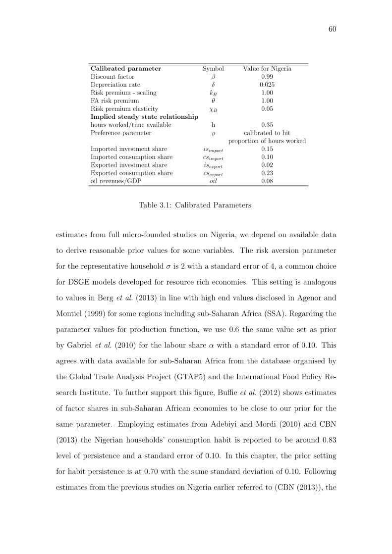
60

Calibrated parameter Symbol Value for NigeriaDiscount factor β 0.99Depreciation rate δ 0.025Risk premium - scaling kB 1.00FA risk premium θ 1.00Risk premium elasticity χB 0.05Implied steady state relationshiphours worked/time available h 0.35Preference parameter ϱ calibrated to hit

proportion of hours workedImported investment share isimport 0.15Imported consumption share csimport 0.10Exported investment share isexport 0.02Exported consumption share csexport 0.23oil revenues/GDP oil 0.08

Table 3.1: Calibrated Parameters

estimates from full micro-founded studies on Nigeria, we depend on available data

to derive reasonable prior values for some variables. The risk aversion parameter

for the representative household σ is 2 with a standard error of 4, a common choice

for DSGE models developed for resource rich economies. This setting is analogous

to values in Berg et al. (2013) in line with high end values disclosed in Agenor and

Montiel (1999) for some regions including sub-Saharan Africa (SSA). Regarding the

parameter values for production function, we use 0.6 the same value set as prior

by Gabriel et al. (2010) for the labour share α with a standard error of 0.10. This

agrees with data available for sub-Saharan Africa from the database organised by

the Global Trade Analysis Project (GTAP5) and the International Food Policy Re-

search Institute. To further support this figure, Buffie et al. (2012) shows estimates

of factor shares in sub-Saharan African economies to be close to our prior for the

same parameter. Employing estimates from Adebiyi and Mordi (2010) and CBN

(2013) the Nigerian households’ consumption habit is reported to be around 0.83

level of persistence and a standard error of 0.10. In this chapter, the prior setting

for habit persistence is at 0.70 with the same standard deviation of 0.10. Following

estimates from the previous studies on Nigeria earlier referred to (CBN (2013)), the

61

parameters for the investment adjustment cost ϕi is set to 4.0, while the Calvo-

pricing parameter ξ is specified as 0.75 and ζ is set at 7.0 with standard deviations

of 3.00, 0.15 and 0.50, respectively. The prior setting for the ξ implies assumes a

contract duration of less than 2 quarters for monopolistic competitive firms in the

model. The proportion of liquidity constrained consumers λ is set at 0.40 with stan-

dard error of 0.10 on the grounds that survey report show about that around 40 per

cent of the total population in Nigeria do not have access to financial services (see

EFInA (2010).

Regarding the policy parameters, estimates from the posterior estimates of the

monetary policy reaction function in CBN (2013) indicates that the Bank is conser-

vative in its management of inflation. However, we apply less informative priors for

the set of feedback parameters θp and θs at 2.00 and 0.001 with standard deviation

of 1.00 and 0.01. We keep the smoothing parameter ρr at 0.70 the mid-point of the

divergence between estimates in the findings for the CBN reaction function in Garcia

(2010) and Adebiyi and Mordi (2010). Large priors are set for the shock processes

following Adolfson et al. (2008), that argues for this in the analysis of small open

develop economies. In the case of Nigeria, it is expected as an oil exporter economy

that larger swings in observed data would imply much wider standard errors using

setting between 2 and 3 for the prior and an inverted gamma distribution.

We present the full list of prior distributions and parameters settings in Table

3.2 as well as Table 3.3.

3.3.3 Identification Issues

As a precondition for taking the DSGE model developed in this chapter to the

data and subsequently for effective policy analysis, we address some issues with

identification of the parameters. To help pinpoint and resolve identification issues

related to collinearity amongst the parameters, we first perform a straight forward

check on the rank of columns JT and HT via a Monte Carlo exploration of the priors

62

and observable variables. Figures E.1 to E.3 in the appendices presents the pairwise

collinearity patterns of estimated parameters in the new-Keynesian DSGE Model.

In addition, procedures to assess the identification strength based on the Fisher

information matrix are undertaken for the estimated parameters relative to the

parameter values and prior standard deviations in Figures E.4 and E.5 of Appendix

C. The diagnostics results reveal that some parameters are weakly identified as larger

absolute values of the bars implies stronger identification.

3.3.4 Posterior Estimates

A two-step procedure is adopted for Bayesian estimation of the joint posterior distri-

bution for the estimated parameters. The first step, obtains the the Hessian matrix

applying a standard numerical optimization algorithm. Secondly, the Hessian ma-

trix from the first stage is used to recover the posterior distribution of the model

via Metropolis-Hastings algorithm (MCMC-MH). Thereafter, univariate and mul-

tivariate diagnostic statistics from running two parallel chains of the MCMC-MH

algorithm are used to assess convergence for all estimations in this chapter by ana-

lyzing ‘between and within’ moments of the MCMC chains (see, Brooks and Gelman

(1998)).

Thirty per cent of the first draws are discarded out of a total of 200,000 random

draws obtained from the MCMC-MH. A reasonable acceptance rate for two MCMC

chains is achieved by adjusting the variance-covariance matrix of the perturbation

term which produces an acceptance rate ranging between 27.77% and 34.26% for the

estimation using the standard HP filter and 29.83% and 31.07% for the modified HP

filter which are close to acceptable rates of about a third according to the literature.15

Posterior means are reported for all estimated parameters in Table 3.2 and Table

3.3 with confidence intervals for the models.

The results in Table 3.2 and Table 3.3 for the emerging economy oil- exporter

15See Schorfheide (2000) for more details.

63

Parameter Notation Prior distribution Posterior distribution

Density Mean S.D/df No RT RTInvestment adjustment ϕi Inv. gamma 4.00 3.00 1.43 [1.03:1.82] 1.40 [1.03:1.77]Risk aversion σ Inv. gamma 2.00 4.00 1.57 [0.51:2.79] 1.07 [0.55:1.57]Consumption habit hC Beta 0.70 0.10 0.68 [0.49:0.86] 0.70 [0.53:0.88]Calvo prices ξ Beta 0.75 0.15 0.55 [0.40:0.73] 0.63 [0.50:0.76]Labour share α Beta 0.60 0.10 0.78 [0.76:0.80] 0.79 [0.77:0.80]Import Pass-through parameter θ Beta 0.50 0.20 0.36 [0.21:0.51] 0.36 [0.21:0.51]Substitution elasticity (H/F goods) µ Normal 1.50 0.20 1.41 [1.07:1.73] 1.37 [1.06:1.70]Substitution elasticity (varieties) ζ Normal 7.00 0.50 6.98 [6.17:7.78] 6.98 [6.20:7.83]Financial frictionsProportion of RT consumers λ Beta 0.40 0.10 - 0.38 [0.22:0.53]Interest rate ruleInterest rate smoothing ρr Beta 0.50 0.10 0.82 [0.78:0.87] 0.83 [0.79:0.88]Feedback from expected inflation θph Normal 1.50 0.01 1.498 [1.482:1.515] 1.499 [1.483:1.516]Feedback from X-rate θsh Inv. gamma 0.005 0.001 0.005 [0.004:0.007] 0.005 [0.004:0.007]AR(1) coefficientTechnology ρA Beta 0.85 0.10 0.78 [0.64:0.92] 0.73 [0.60:0.87]Government spending ρG Beta 0.85 0.10 0.85 [0.71:0.99] 0.85 [0.72:0.99]Price mark-up ρMS Beta 0.50 0.10 0.50 [0.34:0.66] 0.50 [0.33:0.66]Foreign Interest rate ρr∗ Beta 0.50 0.10 0.49 [0.34:0.65] 0.49 [0.35:0.64]Foreign inflation rate ρπ Beta 0.50 0.10 0.47 [0.33:0.62] 0.48 [0.33:0.62]Foreign consumption ρc∗ Beta 0.50 0.10 0.51 [0.36:0.69] 0.51 [0.35:0.68]Standard deviation of AR(1) innovations/I.I.D. shocksTechnology sd(ϵA) Inv. gamma 2.00 4.00 3.03 [0.64:5.27] 4.76 [2.23:7.74]Government spending sd(ϵG) Inv. gamma 3.00 4.00 3.14 [0.82:5.47] 2.74 [0.86:4.96]Price mark-up sd(ϵMS) Inv. gamma 2.00 3.00 2.06 [0.51:4.32] 1.76 [0.55:3.18]Monetary policy sd(ϵmps) Inv. gamma 3.00 4.00 0.79 [0.62:0.96] 0.77 [0.60:0.94]Foreign Interest rate sd(ϵr) Inv. gamma 3.00 4.00 2.19 [1.14:3.16] 2.40 [1.39:3.37]Foreign inflation rate sd(ϵpie) Inv. gamma 3.00 4.00 1.37 [0.89:1.83] 1.14 [0.76:1.54]Foreign consumption sd(ϵc) Inv. gamma 2.00 3.00 11.69 [0.51:27.67] 3.24 [0.47:8.09]Oil Price sd(ϵoil) Inv. gamma 3.00 4.00 2.67 [0.80:4.69] 2.39 [0.76:4.03]LL -684.24 -684.77

Table 3.2: Priors and Posterior Estimates using Standard HP Filter forConsumption and Investment

Notes: we report posterior means and 90% probability intervals (in parentheses) basedon the output of the Metropolis-Hastings Algorithm. Sample period: 2003:IIto 2015:IV.

shows posterior estimates for the DSGE model with and without Ricardian agents

with a monetary policy rule which has inflation and nominal exchange rate feedbacks.

Log marginal likelihood at the bottom of both tables indicate marginal differences

between the model with and without non-Ricardian consumers. Although there

are no significant improvements, the estimation outcomes show that including this

feature fits the structure of the base model well. However, a cursory perusal of the

90% probability intervals shows that the model with non-Ricardian consumers has

more informative estimates with tighter confidence sets for most of the estimated

variables.

64

Parameter Notation Prior distribution Posterior distribution

Density Mean S.D/df No RT RTInvestment adjustment ϕi Inv. gamma 4.00 3.00 2.29 [1.33:3.26] 2.44 [1.31:3.46]Risk aversion σ Inv. gamma 2.00 4.00 1.94 [0.44:3.59] 1.31 [0.59:2.01]Consumption habit hC Beta 0.70 0.10 0.69 [0.51:0.86] 0.71 [0.55:0.89]Calvo prices ξ Beta 0.75 0.15 0.66 [0.41:0.92] 0.75 [0.59:0.91]Labour share α Beta 0.60 0.10 0.76 [0.71:0.80] 0.74 [0.67:0.80]Import Pass-through parameter θ Beta 0.50 0.20 0.37 [0.21:0.52] 0.37 [0.21:0.52]Substitution elasticity (H/F goods) µ Normal 1.50 0.20 1.45 [1.13:1.78] 1.47 [1.13:1.80]Substitution elasticity (varieties) ζ Normal 7.00 0.50 6.94 [6.11:7.76] 6.96 [6.11:7.80]Financial frictionsProportion of RT consumers λ Beta 0.40 0.10 - 0.39 [0.23:0.55]Interest rate ruleInterest rate smoothing ρr Beta 0.50 0.10 0.83 [0.79:0.88] 0.84 [0.79:0.89]Feedback from expected inflation θph Normal 1.50 0.01 1.499 [1.483:1.516] 1.499 [1.483:1.516]Feedback from X-rate θsh Inv. gamma 0.005 0.001 0.005 [0.004:0.007] 0.005 [0.004:0.007]AR(1) coefficientTechnology ρA Beta 0.85 0.10 0.82 [0.70:0.94] 0.84 [0.71:0.97]Government spending ρG Beta 0.85 0.10 0.85 [0.71:0.99] 0.88 [0.77:0.99]Price mark-up ρMS Beta 0.50 0.10 0.50 [0.34:0.66] 0.50 [0.34:0.67]Foreign Interest rate ρr∗ Beta 0.50 0.10 0.48 [0.33:0.63] 0.49 [0.34:0.64]Foreign inflation rate ρπ Beta 0.50 0.10 0.47 [0.33:0.61] 0.47 [0.33:0.62]Foreign consumption ρc∗ Beta 0.50 0.10 0.51 [0.34:0.67] 0.51 [0.34:0.68]Standard deviation of AR(1) innovations/I.I.D. shocksTechnology sd(ϵA) Inv. gamma 2.00 4.00 4.13 [0.67:6.90] 2.26 [0.55:4.50]Government spending sd(ϵG) Inv. gamma 3.00 4.00 4.32 [0.71:8.20] 15.89 [0.77:36.99]Price mark-up sd(ϵMS) Inv. gamma 2.00 3.00 2.27 [0.56:5.06] 1.68 [0.58:2.90]Monetary policy sd(ϵmps) Inv. gamma 3.00 4.00 0.78 [0.60:0.95] 0.77 [0.59:0.93]Foreign Interest rate sd(ϵr) Inv. gamma 3.00 4.00 2.40 [1.30:3.39] 2.16 [1.13:3.11]Foreign inflation rate sd(ϵpie) Inv. gamma 3.00 4.00 2.00 [0.88:3.16] 2.06 [0.95:3.17]Foreign consumption sd(ϵc) Inv. gamma 2.00 3.00 2.18 [0.49:4.28] 6.55 [0.52:21.17]Oil Price sd(ϵoil) Inv. gamma 3.00 4.00 2.44 [0.87:4.26] 3.90 [0.70:7.51LL -700.74 -700.78

Table 3.3: Priors and Posterior Estimates using Modified HP Filter forConsumption and Investment

Notes: we report posterior means and 90% probability intervals (in parentheses) basedon the output of the Metropolis-Hastings Algorithm. Sample period: 2003:IIto 2015:IV.

These estimates are generally plausible. The reported results indicate that prices

are a lot stickier in model 2 with financial frictions which is consistent with other

studies on similar economies (see, Gabriel et al. (2010)). We find that firms in the

model with only Ricardian consumers adjust prices more frequently 1.7 - 3.7 quar-

ters than the model with non-Ricardian consumers at 2.0 - 4.2 quarters, implying a

greater level of price stickiness. In addition, results from the estimation are indica-

tive of slightly higher levels of habit persistence in the model with credit constrained

consumers.

Both estimated models produce higher estimates of α, suggesting a labour share

65

about three-quarters of total factor input in the resource-rich emerging economy.

There is a huge deviation in the structural parameter σ from the prior for both

models. On the other hand, ζ deviate little from its prior mean overlapping prior and

posterior distributions suggesting uninformative data on the parameter. Estimated

value for substitution elasticity µ for home and foreign goods suggests identification

issues as these are quite imprecise. The posterior estimates for λ is remarkable

depicting a similar proportion of non-Ricardian consumers in the Nigerian economy

when compared with statistics showing that close to 40% of households are liquidity

constrained. Thus, there are some important inferences that may be implied for the

conduct of monetary and fiscal policy.

From our estimates, we may infer that the CBN is aggressive in managing infla-

tionary pressures given the inflation feedback, with θph while responding to move-

ments in the foreign exchange rate. The degree of policy inertia parameter ρr esti-

mated at 0.83 is highly persistent and signifies the Central Bank of Nigeria signifi-

cantly smooths of its interest rate decisions. However, it worth noting that the prior

standard deviations are relatively tight.

The estimated shock processes indicate some level of persistence, while the stan-

dard deviations are large compared to values commonly found in the literature for

industrialised economies. This level of volatility is consistent with emerging and oil

exporting economies as verified from stylized facts. Generally the results for the

standard deviations of the AR(1) innovations and shocks are close to the priors al-

though foreign consumption shock in the model with only Ricardian agents is huge

relative to the model with credit-constrained consumers.

3.3.5 Model Validation

For empirical applications we further address the questions whether the model cap-

tures the underlying characteristics of the actual data and what the impact of struc-

tural shocks are on the main macroeconomic time series. We assess the model

66

properties using standard moments criteria, impulse response analysis and shock

decomposition of shocks which are presented in the following subsections.

Standard Moment Criteria

Standard Deviation

Model Consumption Investment Inflation Interest rate Exchange rate

Data 15.63 20.91 2.68 0.68 3.89

Model no RT 4.54 20.59 2.79 0.81 7.17

Model RT 4.69 20.17 2.87 0.84 7.19

Cross-correlation with Consumption

Data 1.00 0.10 -0.004 0.10 -0.11

Model no RT 1.00 0.49 -0.03 -0.70 -0.18

Model RT 1.00 0.49 0.10 -0.68 -0.02

Table 3.4: Selected Second Moments for Standard HP Filter Estimates

Based on the posterior distribution of the model, theoretical moments are computed in

the order approximately equal to 1.

Standard Deviation

Model Consumption Investment Inflation Interest rate Exchange rate

Data 16.81 23.92 2.68 0.68 3.89

Model no RT 4.99 16.61 2.80 0.94 7.43

Model RT 6.15 13.57 2.65 0.86 6.89

Cross-correlation with Consumption

Data 1.00 -0.15 -0.08 0.09 -0.13

Model no RT 1.00 0.58 0.02 -0.70 -0.65

Model RT 1.00 0.60 0.19 -0.56 -0.19

Table 3.5: Selected Second Moments for Modified HP Filter Estimates

Based on the posterior distribution of the model, theoretical moments are computed in

the order approximately equal to 1.

Note that with exception of consumption and the exchange rate, both models repli-

cate closely the data with regards to the standard deviations. It is clear that the

67

models successfully mimic the actual data on inflation and interest rate well. Al-

though investment is more volatile than consumption, the results show that in-

vestment is better replicated by the model. The failure to replicate the stylized

fact on investment by these models is not uncommon in the literature on emerging

economies. Similarly, the cross-correlation with consumption is closer for the first

model.

Impulse Responses

In this section, an assessment of the impact of four estimated shocks on some vari-

ables of interest is undertaken to gain some useful insight on the transmission mecha-

nism and how these innovations and model uncertainties may affect policy decisions.

Figures 3.1–3.4 compares the impulse responses to technology, government spending

and monetary policy shocks for λ = 0.0, 0.38 (no credit-constrained households and

38% constrained respectively). Computed in percentage terms as deviations from

the steady state values, the figures show impulse response functions for 40 period

(10 years horizon).

Comparing the two models, we observe that the inclusion of non-Ricardian agents

magnifies the impact of a Technology shock on most variables plotted in figure 3.1.

Although we find that the contemporaneous effects of the Technology shock on

output, consumption and investment are similar or even somewhat muted in the

case of consumption, comparing both models reveals a higher level of persistence in

the model with credit-constrained consumers. For most variables we find that the

impact of the ϵA shock lasts between 10 to 15 quarters, while the impact on output

and consumption is last about 20 quarters. We find that the impact on inflation

and real interest rate dies out relatively rapidly. However, the contemporary impact

on hours worked and real wage is rather more visible on model 2.

Figure 3.2 shows that a shock to government spending has a relatively pro-

nounced positive impact on output 0.3 per cent, while having a negative impact on

68

consumption 20 quarters. Nonetheless, the figure shows an initial positive impact a

government spending shock on consumption for the model with credit constrained

consumers. This indicates that there are implications for fiscal policy when we have

non-Ricardian agents in the model. Thus, fiscal policy may be applied to boost con-

sumption. On a contemporaneous basis, while we find that consumption in model

1 declines marginally by -0.02 per cent the converse is the case for model 2 as the

consumption increases when there are non-Ricardian agents included in the model.

Hours worked increases as well as real wages, with real wage for the model with

credit constrained higher by about a third. However, the impact of the shock on

real wages declines out rapidly only after 5 quarters. The immediate impact of a

government spending shock on real wage is relatively higher for model 2. Nominal

interest rate rises as a result of a government spending shock, even though the effect

is muted by the presence of rule of thumb consumers in line with the new-Keynesian

foundations of the model. Higher nominal interest rates may also be indicative of

fiscal dominance and some crowding out the private sector. Prices go increase and

there is considerable real exchange rate appreciation.

The effects of a monetary policy shock is generally transient on the selected

variables declining rapidly in about 5 quarters. A monetary policy shock has a

greater impact on consumption in model 2. The efficacy of a monetary policy

shock in curtailing the level of consumption in the model is approximately twice the

magnitude for the model with non-Ricardian consumers in comparison to the model

1. The impact of the shock is also transmitted to aggregate output, hours worked

and real wage. Therefore, the estimated results indicate that monetary authorities

have a greater leverage on the management of inflation when there are significant

proportions of non-Ricardian consumers. Increased nominal interest rates impacts

on the hours worked and real wage which has an impact on consumption. Inflation

and output falls, while there is real and nominal exchange rate appreciation.

A positive Oil price shock has leads to considerable appreciation of the real

69

and nominal exchange rates. a positive effect on leads to increases in consumption,

investment and real wages. On the other hand, aggregate output declines as a result

to a shock in oil price. Lower hour worked and the rent seeking behaviour during an

Oil boom is a common trend for many oil exporter economies, while income levels

increase as more oil revenue is available for spending.

5 10 15 20 25 30 35 40

Quarters

0.5

1

1.5

% d

ev fr

om S

S

Output

5 10 15 20 25 30 35 40

Quarters

0

0.2

0.4

0.6

0.8

% d

ev fr

om S

S

Consumption

5 10 15 20 25 30 35 40

Quarters

-0.20

0.20.40.60.8

% d

ev fr

om S

S

Investment

5 10 15 20 25 30 35 40

Quarters

-3

-2

-1

0

% d

ev fr

om S

S

Hours worked

5 10 15 20 25 30 35 40

Quarters

-2

-1

0

1

% d

ev fr

om S

S

Real wage

5 10 15 20 25 30 35 40

Quarters

0

0.5

1

% d

ev fr

om S

S

Real interest rate

5 10 15 20 25 30 35 40

Quarters

-0.3

-0.2

-0.1

0

% d

ev fr

om S

S

Nominal interest rate

5 10 15 20 25 30 35 40

Quarters

0.5

1

1.5

% d

ev fr

om S

S

Tobin Q

5 10 15 20 25 30 35 40

Quarters

-1

-0.5

0

% d

ev fr

om S

S

Inflation

5 10 15 20 25 30 35 40

Quarters

0.5

1

1.5

% d

ev fr

om S

S

Real Ex rate

5 10 15 20 25 30 35 40

Quarters

-0.1

0

0.1

0.2

0.3

% d

ev fr

om S

S

LoP gap

5 10 15 20 25 30 35 40

Quarters

-0.8-0.6-0.4-0.2

00.2

% d

ev fr

om S

S

Nominal Ex Rate

Model 1 Model 2

Figure 3.1: A Technology Shock without (Model 1) and with (Model 2) Rule of

Thumb Consumers

5 10 15 20 25 30 35 40

Quarters

0

0.1

0.2

0.3

% d

ev fr

om S

S

Output

5 10 15 20 25 30 35 40

Quarters

-0.08-0.06-0.04-0.02

00.02

% d

ev fr

om S

S

Consumption

5 10 15 20 25 30 35 40

Quarters

-0.04

-0.02

0

0.02

% d

ev fr

om S

S

Investment

5 10 15 20 25 30 35 40

Quarters

0

0.2

0.4

% d

ev fr

om S

S

Hours worked

5 10 15 20 25 30 35 40

Quarters

0

0.1

0.2

0.3

% d

ev fr

om S

S

Real wage

5 10 15 20 25 30 35 40

Quarters

-0.1

-0.05

0

% d

ev fr

om S

S

Real interest rate

5 10 15 20 25 30 35 40

Quarters

0

0.01

0.02

0.03

% d

ev fr

om S

S


5 10 15 20 25 30 35 40

Quarters

-0.12-0.1

-0.08-0.06-0.04-0.02

% d

ev fr

om S

S

Tobin Q

5 10 15 20 25 30 35 40

Quarters

0

0.05

0.1

% d

ev fr

om S

S

Inflation

5 10 15 20 25 30 35 40

Quarters

-0.14-0.12-0.1

-0.08-0.06-0.04-0.02

% d

ev fr

om S

S

Real Ex rate

5 10 15 20 25 30 35 40

Quarters

-0.01

0

0.01

% d

ev fr

om S

S

LoP gap

5 10 15 20 25 30 35 40

Quarters

0.020.040.060.08

0.10.120.14

% d

ev fr

om S

S

Nominal Ex Rate

Model 1 Model 2

Figure 3.2: A Gov Spending Shock without (Model 1) and with (Model 2) Rule of

Thumb Consumers

70

5 10 15 20 25 30 35 40

Quarters

-1

-0.5

0

% d

ev fr

om S

S

Output

5 10 15 20 25 30 35 40

Quarters

-0.8

-0.6

-0.4

-0.2

% d

ev fr

om S

S

Consumption

5 10 15 20 25 30 35 40

Quarters

-1

-0.8

-0.6

-0.4

% d

ev fr

om S

S

Investment

5 10 15 20 25 30 35 40

Quarters

-1.5

-1

-0.5

0

% d

ev fr

om S

SHours worked

5 10 15 20 25 30 35 40

Quarters

-3

-2

-1

% d

ev fr

om S

S

Real wage

5 10 15 20 25 30 35 40

Quarters

0

1

2

% d

ev fr

om S

S

Real interest rate

5 10 15 20 25 30 35 40

Quarters

0.05

0.1

0.15

0.2

0.25

% d

ev fr

om S

S


5 10 15 20 25 30 35 40

Quarters

-1

-0.5

0

% d

ev fr

om S

S

Tobin Q

5 10 15 20 25 30 35 40

Quarters

-2

-1

0

% d

ev fr

om S

S

Inflation

5 10 15 20 25 30 35 40

Quarters

-1

-0.5

0

% d

ev fr

om S

S

Real Ex rate

5 10 15 20 25 30 35 40

Quarters

-2

-1.5

-1

-0.5

% d

ev fr

om S

S

LoP gap

5 10 15 20 25 30 35 40

Quarters

-3

-2.5

-2

% d

ev fr

om S

S

Nominal Ex Rate

Model 1 Model 2

Figure 3.3: A Monetary Shock without (Model 1) and with (Model 2) Rule of Thumb

Consumers

5 10 15 20 25 30 35 40

Quarters

-0.1

-0.08

-0.06

-0.04

-0.02

% d

ev fr

om S

S

Output

5 10 15 20 25 30 35 40

Quarters

0.080.1

0.120.140.160.18

% d

ev fr

om S

S

Consumption

5 10 15 20 25 30 35 40

Quarters

0.2

0.4

0.6

% d

ev fr

om S

S

Investment

5 10 15 20 25 30 35 40

Quarters

-0.12

-0.11

-0.1

-0.09

% d

ev fr

om S

S

Hours worked

5 10 15 20 25 30 35 40

Quarters

0.12

0.14

0.16

% d

ev fr

om S

S

Real wage

5 10 15 20 25 30 35 40

Quarters

-0.01

0

0.01

% d

ev fr

om S

S

Real interest rate

5 10 15 20 25 30 35 40

Quarters

-4

-2

0

2

4

% d

ev fr

om S

S

×10-3 Nominal interest rate

5 10 15 20 25 30 35 40

Quarters

-0.2

-0.18

-0.16

-0.14

-0.12

% d

ev fr

om S

S

Tobin Q

5 10 15 20 25 30 35 40

Quarters

-0.01

0

0.01

% d

ev fr

om S

S

Inflation

5 10 15 20 25 30 35 40

Quarters

-0.24

-0.22

-0.2

-0.18

% d

ev fr

om S

S

Real Ex rate

5 10 15 20 25 30 35 40

Quarters

-0.1

-0.05

0

% d

ev fr

om S

S

LoP gap

5 10 15 20 25 30 35 40

Quarters

-0.22

-0.2

-0.18

-0.16

% d

ev fr

om S

S

Nominal Ex Rate

Model 1 Model 2

Figure 3.4: Oil Price Shock without (Model 1) and with (Model 2) Rule of Thumb

Consumers

71

Shock Decomposition

The figures below show the shock decomposition for consumption, inflation, ex-

change rate and interest rates.

Figure 3.5: Historical Decomposition of Consumption

Figure 3.6: Historical Decomposition of Inflation

72

Figure 3.7: Historical Decomposition of Exchange Rate

Figure 3.8: Historical Decomposition of Interest Rate

3.4 Conclusions

A two-bloc open economy Smets-Wouters type model with credit-constrained con-

sumers, an oil sector, and imperfect exchange-rate pass-through to exports and

imports is set out and estimated in this chapter. The Bayesian estimation results

reveal useful insight to the role of non-Ricardian agents in the SOE DSGE model

73

framework which would be explored further in the next chapter to examine optimal

monetary policy alternatives.

The impulse response functions reveal that a technology shock has relatively long

term effect on the selected macroeconomic variables. Technological advancement

fosters growth over the long run but having a short-lived impact on inflation and real

interest rates in the model. The implication is that alongside a growth enhancing

technological process for the oil exporter economy, effective monetary and fiscal

policies is required to ensure the maintenance of macroeconomic stability over the

long run. Based on the analysis on the model credit constrained consumers, we

also find that, government spending has the efficacy to boost consumption in the

short-run and thereby could be a veritable tool for enhancing economic welfare

when there is dwindling aggregate demand in the oil-exporter emerging economy.

Oil price shocks leads to rapid appreciation of the exchange rate that may lead to

a misalignment in the RER limiting the lever of monetary policy. Foreign exchange

interventions on the other hand, may be applied to manage the currency appreciation

when the Oil price shock is not a structural shift in prices. Introducing financial

frictions such as liquidity constrained consumers produces a structural model that is

well-suited for the study of policy options in the resource-rich oil-producer economy.

Chapter 4

Optimized Monetary Policy Rulesin an Oil Producing EmergingEconomy

1

This chapter examines optimal monetary policy rules in a nonindustrial oil-

producer economy. For this purpose, we set up a model with non-Ricardian house-

holds (liquidity-constrained consumers), international financial frictions, incomplete

exchange rate pass-through to import and export prices and oil revenue. We cali-

brate the small open economy model for the policy simulations for Nigeria. Optimal

policy exercises for different proportions of liquidity-constrained consumers reveal

that an optimized simple rule with a real wage target outperforms the other policy

alternatives. We also observe from the simulations a trade-off between the govern-

ment’s ability to borrow from domestic households and implementing a welfare max-

imizing policy rule that is saddle path stable for large proportions of non-Ricardian

consumers. This has important policy implications for the heavily-dependent oil-

producer emerging economy especially if policymakers choose to pursue an expan-

sionary fiscal policy through borrowing from domestic financial markets alongside

implementing monetary policy that involves targeting real wages.

1This chapter was co-authored by Professor Paul Levine, University of Surrey

74

75

4.1 Introduction

It is well known that uncertainty is a defining characteristic of the macroeconomic

management landscape.2 For this reason, central banks need to identify, to a feasi-

ble extent, the different sources of uncertainty and volatility confronting the econ-

omy. Furthermore, policymakers should endeavour to distinguish between perma-

nent shocks that may demand significant macroeconomic adjustment to the economy

from those that are transient and require only smoothing when formulating policies.

Hence, a proper evaluation of the type of macroeconomic shocks, the magnitude

and how these shocks are propagated through the economy is required in order to

effectively implement policy initiatives.

Besides holding a reasonable view on the transmission mechanism of exogenous

shocks to the economy, central banks as well as fiscal authorities also need to have

a clear understanding of the policy space so that the appropriate policy mix will be

implemented in a bid to achieve broad macroeconomic objectives.

In view of the above, whereas macroeconomic policy design and implementation

in many resource-rich emerging economies tend to focus mainly on long-term con-

cerns such as the distribution and exhaustibility of natural resource endowments

as highlighted in a survey by van der Ploeg and Venables (2012), the conduct of

monetary and fiscal policy should transcend this common practice. Macroeconomic

policymakers in resource-rich economies (RRE) should be obliged to take into cog-

nisance the effects of factors such as volatility in the price, production output and

revenue derived from commodity exports on short- to medium term policy initia-

tives.3 In particular, it is suggested that heavily resource-dependent oil producers

2Regarding monetary policy - Alan Greenspan stated: ‘Uncertainty is not just an importantfeature of the monetary policy landscape; it is the defining characteristic of that landscape.” FederalReserve Bank of Kansas (2003), Opening Remarks.

3Recent survey by van der Ploeg and Venables (2012) reveal academic work on natural resource-rich economies has focused more on medium- to long-term fiscal policy. In addition, the literaturerecognises the role of fiscal policy as a regulator of oil income pass-through to the economy, witha standard recommendation that resource-rich economies should save a proportion of income inorder to smooth expenditure when resources are discovered.

76

should constantly assess how large and unpredictable swings in oil prices that are

usually driven by exogenous factors4 affect overall macroeconomic performance. In-

deed, it should be stated from the onset of this study, that the conduct of monetary

policy in some major oil producing economies have been quite challenging in the

last four and a half decades.

How should monetary policy respond in an economy when crude oil and gas

exports constitute a dominant part of exports and fiscal revenue? In which direc-

tion and to what magnitude should policymakers at the central bank adjust interest

rates that will promote the achievement of its primary mandate of maintaining price

stability while being consistent with the achievement of other broad macroeconomic

objectives? Are alternative sources of financing the government in conflict with mon-

etary policy goals? These amongst numerous similar questions are usually explored

in the optimal monetary policy literature for resource-rich emerging economies.

Clarida et al. (2001) considering optimal monetary policy in the context of an

open economy, acknowledges that openness complicates monetary management and

necessitates central banks to account for the exchange rate effects on the real econ-

omy and inflation. The authors develop an open economy monetary model with im-

perfect competition, staggered price-setting with labour market frictions and reveal

that under specific circumstances, the challenges of monetary policy formulation

is ‘isomorphic’ to the case of a closed economy (that is, qualitatively similar but

showing that openness has quantitative implications). Undertaking optimal mone-

tary policy simulations using the open economy model, the results in Clarida et al.

(2001) indicate that the central bank in pursuant of its price stability objective

should be relatively more aggressive in its response to inflationary pressures unlike

the case of a closed economy.5 The authors findings suggest that the policy stance of

4From 1973 to 2014, there has been 5 distinct periods where crude oil prices dropped by over50%. Factors that influenced such episodes of significant oil price fluctuations include supply anddemand conditions, technical production issues, geopolitical risks as well as cartel decisions.

5The conclusion presupposes the monetary authorities actions with respect to the timing andmagnitude of adjustment of the policy interest rate.

77

the monetary authorities should be contingent upon the ‘degree of openness’ of the

economy. Although the paper maintains that the same optimal interest rate feed-

back rule holds in both cases, the findings indicate that the introduction of the open

economy features into the framework engenders a clear distinction of the domes-

tic inflation from the consumer price inflation and recommends that the monetary

authority target the domestic inflation index while allowing for an exchange rate

determination via a floating regime if there is perfect exchange rate pass-through.

This position is recommended by the authors regardless of the effects of resulting

variability in the exchange rate on the consumer price index (CPI). Therefore, rec-

ommendations in the paper are in line with conclusions in Kosuki (2001). Clarida

(2014) under similar economic settings shows that optimal monetary policy can only

deliver good macroeconomic outcomes and stable domestic price level in an inflation

targeting regime via a Taylor rule when there is a commitment device.

Focusing our discourse specifically on resource-rich oil producing economies,

Wills (2013) evaluates optimal monetary policy rules from a contextual view of

managing real exchange rate appreciation. The paper examines how new discover-

ies of oil affect agents expectations by influencing the non-resource terms of trade

and government demand.6 The author shows that in comparison to other monetary

policy rules, an optimal monetary policy in the form of a Taylor-type rule which

responds to the natural level of output can significantly improve welfare. To ac-

complish the welfare objectives, the paper concludes that the central bank needs to

take pro-active measures to stabilize inflation, as well as close the output and fiscal

gaps that emerge before actual exploitation of the resource endowment. Thus, Wills

(2013) conclusions imply that monetary policy in heavily dependent RREs would

be more effective with a clear foresight on fiscal operations which requires sound

monetary and fiscal coordination.

6Wills (2013) concludes that oil discoveries causes the real exchange rate to appreciate becauseof the forward-looking behaviour of households and the government which increases spending inanticipation of future earnings.

78

Similarly, Ferrero and Seneca (2015) examine optimal monetary policy for resource-

rich economies employing an augmented version of the canonical small open economy

(SOE) dynamic stochastic general equilibrium (DSGE) model of Gali and Monacelli

(2005). The paper abstract from a number of features and frictions in the standard

framework to consider closely the implications of introducing a reliance on the com-

modity exports. To this end, the authors link productivity in the endogenous oil

sector in the model to domestic intermediate non-oil firms upon which the oil sector

sources inputs. The model specifies a fiscal rule which dampens the contempora-

neous effects of oil price shocks to the economy, thereby smoothening government

spending.7. Ferrero and Seneca (2015) assess optimal monetary policy in a linear

quadratic framework for the industrialised economy and show that optimal policy

requires a reduction of the policy interest rate when there is a fall in crude oil

prices. On the other hand, the authors recommend that the policy interest rate

may be raised by the central bank if it has an overriding consumer price inflation

stabilisation mandate so that the inflationary impact of an exchange rate depreci-

ation will be limited. The preceding findings corroborate those in Bergholt (2014)

that emphasizes the importance of identifying the proper path of transmission of oil

shocks and its spillovers to the rest of the economy. The later study indicates that

the weight on stabilization of real activity increases proportionately with the size of

the oil sector.

In this chapter, we study how the monetary authority in a heavily-dependent

resource-rich emerging economy should respond to developments in inflation and

exchange rate. We use a small open economy DSGE model of an oil producer with

non-zero output growth and inflation, a significant proportion of non-Ricardian con-

sumers, partial exchange rate pass-through to imports and export prices, and eval-

uate the welfare implications of different monetary policy rules. As precedence, we

7Government spending in the model is strictly according to an endogenous fiscal policy rulethat is financed through a sovereign wealth fund. This is analogous to the structural fiscal surplustype rule implemented by some commodity exporters including Chile (see, Medina and Soto (2007)

79

first establish stability conditions of the model with respect to the proportion of

liquidity-constrained consumers. A foreknowledge of this is vital to the analysis of

how this agents affect the results from the optimal policy exercises we undertake

for the small open emerging economy. The specification of fiscal policy is simpli-

fied as it is assumed government finances its operations only from oil revenue and

borrowing from the domestic markets. Although we adopt a parsimonious fiscal

regime, it sufficiently captures the effects of the transmission of oil price shocks

to the nonindustrial oil producer economy for the optimal policy exercises in this

chapter.8

From the initial stability analysis for the small open emerging economy oil-

producer, we find that the inverted aggregate demand logic (IADL) holds for Taylor

type policy rules with feedback on inflation and the exchange rate which is in agree-

ment with the work by Bilbiie (2008). The result is also consistent with Boerma

(2014) that suggests similar outcomes for nonindustrial emerging economies. More-

over, stability tests reveals that a rule which includes a real wage target is robust

across large fractions of non-Ricardian consumers. Thereafter, simulation results

from the optimal policy exercises show that the same rule outperforms other simple

optimized monetary policy rules according to the welfare calculations. However, the

central bank’s implementation of the rule with a real wage target comes with in-

creased interest rate volatility. In view of the foregoing analysis, there are important

policy implications for the Nigerian economy which is heavily-dependent on crude

oil as its main export earner and source for financing fiscal operations. Volatile oil

prices affects exchange rate stability, the current account, government fiscal deficit

and the conduct monetary policy.

The findings in this chapter contributes to the optimal monetary policy literature

for RREs. The purpose of this study is to analyze optimal monetary policy by

8We adopt a passive fiscal policy regime with the fiscal authorities setting its instrument tostabilize the government’s stock of debt. Leeper (1991) classifies passive fiscal policy as one inwhich fiscal instrument is adjusted to stabilize the government debt stock.

80

employing a suitable model for a nonindustrial emerging oil-producer and assesses

the short to medium term policy implications. Whereas, several papers analyse

optimal monetary policy rules for RREs, relatively few address nonindustrialised

RRE with sparsely any spillovers to industrial sector. This scope of this paper is

limited to optimal monetary policy experiments employing optimized simple rules

when the central bank with commitment and agents have perfect information. This

work does not study the effects of implementing alternative fiscal policy regimes in

the model for the resource rich emerging economy. Furthermore, we do not study the

impact of having a rigourously modelled financial sector by incorporating a ‘financial

accelerator’ mechanism as in Gertler et al. (2003) and Gabriel et al. (2010) which

would be insightful to assess its effects on real and nominal shocks in the small open

economy model.

The rest of the chapter is structured as follows. We set out the augmented model

for the policy analysis in Section 2 and then present a brief summary of the model

calibration and results in Section 3. Section 4 shows initial stability analysis of our

model. In Section 5 optimal policy exercises are undertaken. Section 6 concludes.

4.2 Augmented DSGE Model for Oil Producer

Fiscal Policy

For simplification government revenue from oil exports is aggregated as τOt a proxy

for both royalties and profit taxes9 and paid each period as

TOt = τOt pO∗t yOt .

9Resource production is subject to royalties at a rate of τ royt and profit taxes at a rate of τdiv

determined by existing oil fiscal regime.

81

We assume this is the only source of tax revenue to pay for government spending

Gt. Then the government debt accumulates according to

Dt = RtDt−1 +Gt − TOt (4.1)

where the net real and nominal interest rates are connected through the Fischer

equation (4.6) below.

Now define debt, government spending and tax to GDP ratios, that is dt ≡ Dt

Yt,

gt ≡ Gt

Ytand dOt ≡ TO

t

Ytrespectively. Then in terms of these ratios (4.1) becomes

dt = Rtdt−1Yt−1

Yt+ gt − tOt =

Rt

1 + ∆Ytdt−1 + gt − tOt (4.2)

where ∆Yt ≡ Yt−Yt−1

Yt−1is the real GDP growth rate. Hence government spending

as a proportion of GDP is given by

gt = tOt + dt −Rt

1 + ∆Ytdt−1 (4.3)

We close the fiscal side of the model with a rule for the debt-GDP ratio which

returns the target steady-state debt-GDP ratio d at a rate that depends on ρd and

an exogenous random shock that captures political and implementation uncertainty

regarding the rule.

In a balanced growth steady state we have

g = tO + d+R

1 + ∆Yd (4.4)

Thus for R > ∆Y, g < tO. In the model calibrate tO to be consistent with

observed long-run values for d and g and 4.4.

82

Alternatively, in absent of a fiscal rule government spending is specified as an

AR(1) process

logGt+1

G= ρg log

Gt

G+ ϵg,t+1

The trade balance is then equivalent to

TBt = StP∗O,tY

O + PH,tYt − PC,tCt − PI,tIt − PH,tGt (4.5)

The Central Bank

The relationship between the gross nominal interest and the ex post real interest

rates is

Rt =Rn,t−1

Πt

(4.6)

and following the conventional Taylor-type policy rule we have Rn,t the policy vari-

able specified as:

log

(Rn,t

Rn

)= ρ log

(Rn,t−1

Rn

)+ θπ log

(Πt

Π

)+ θy log

(YtY

)+ ϵMPS,t (4.7)

log

(Rn,t

Rn

)= ρ log

(Rn,t−1

Rn

)+ θπ log

(Πt

Π

)+ θs log

(StS

)+ ϵMPS,t (4.8)

logRn,t/Rn = ρr logRn,t−1/Rn + (1− ρr)(θπEt[log Πt+j]/Π

+ θs logSt/S) + ϵMPS,t+1 (4.9)

(4.9) is an ‘implementable’ rule that does not require knowledge of the output

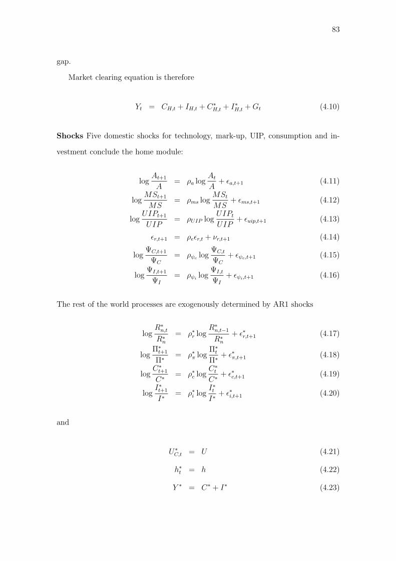
83

gap.

Market clearing equation is therefore

Yt = CH,t + IH,t + C∗H,t + I∗H,t +Gt (4.10)

Shocks Five domestic shocks for technology, mark-up, UIP, consumption and in-

vestment conclude the home module:

logAt+1

A= ρa log

AtA

+ ϵa,t+1 (4.11)

logMSt+1

MS= ρms log

MStMS

+ ϵms,t+1 (4.12)

logUIPt+1

UIP= ρUIP log

UIPtUIP

+ ϵuip,t+1 (4.13)

ϵr,t+1 = ρeϵr,t + νr,t+1 (4.14)

logΨC,t+1

ΨC

= ρψc logΨC,t

ΨC

+ ϵψc,t+1 (4.15)

logΨI,t+1

ΨI

= ρψilog

ΨI,t

ΨI

+ ϵψi,t+1 (4.16)

The rest of the world processes are exogenously determined by AR1 shocks

logR∗n,t

R∗n

= ρ∗r logR∗n,t−1

R∗n

+ ϵ∗r,t+1 (4.17)

logΠ∗t+1


Π∗ + ϵ∗π,t+1 (4.18)

logC∗t+1


C∗ + ϵ∗c,t+1 (4.19)

logI∗t+1

I∗= ρ∗i log

I∗tI∗

+ ϵ∗i,t+1 (4.20)

and

U∗C,t = U (4.21)

h∗t = h (4.22)

Y ∗ = C∗ + I∗ (4.23)

84

4.3 Model Calibration

Simulations in this chapter are undertaken using the priors in Table 3.2. As a

conventional in the literature some of the setting of the structural parameters are

standard. The subjective discount factor β is set at 0.99 implies an annual real

rate of interest of 4 per cent, the capital depreciation rate δ = 0.025 corresponds to

an annual depreciation of 10 per cent; while the Cobb-Douglas production function

parameter α = 0.6 and entails a labor share of income is close to 2/3. Oil sector

contribution to real GDP is set a 0.08 approximately the long run ratio. Debt ratio

is 1.3 equivalent to an annual target of 30 per cent of GDP. A detailed description

of the calibration is presented in the third chapter of this thesis.

4.4 Stability Test

Turning to stability analysis we consider two general forms of rules that include the

Taylor rule (4.9) and those with nominal exchange rate growth and real wage growth

targeting. Figure 4.1 examines the stability properties of the calibrated model in

the space of (θπ, λ). The figure confirms the important policy implication of having

a large λ (that is, the proportion of credit-constrained consumers) as highlighted in

Bilbiie (2008) and subsequently from an open economy perspective as in Boerma

(2014); namely that for the ‘Taylor Principle’ the feedback parameter in the rule

thetaπ must exceed unity for the economy to have a unique stable equilibrium.

Re-parameterizing feedback coefficients θπ, θw and θs by setting απ = (1−ρr)θπ,

αw = (1−ρr)θw and αs = (1−ρr)θs allows the possibility for ρr = 1 when optimizing

for ρr, απ, αw and αs. In order to maximize efficiently with respect to feedback

parameters we introduce the re-parametrization απ ≡ (1−ρr)θπ and αy ≡ (1−ρr)θy.

Notice that the special case of an integral rule (ρr = 1), αy = 0 with a zero-inflation

steady state (Π = 1) is logRn,t = απ logPt which is a price level rule.

In (4.26) this is accompanied by domestic inflation targeting and in (4.24) by

85

CPI inflation targeting.

logRn,t/Rn = ρr log (Rn,t−1/Rn) + (1− ρr)(θπ log (Πt/Π)

+ θs log (St/S) + θ∆s log (St/St−1) + θw log(Wt

PC,t)− log(

Wt−1

PC,t−1

))+ ϵr,t

(4.24)

logRn,t/Rn = ρr log (Rn,t−1/Rn) + (1− ρr)(θπ log (Πt/Π)

+ θs log (St/S) + θ∆s log (St/St−1))+ ϵr,t (4.25)

which we parameterize as

logRn,t/Rn = ρr log (Rn,t−1/Rn) + απ log (Πt/Π)

+ αs log (St/S) + α∆s log (St/St−1) + ϵr,t (4.26)

Figures 4.2 and 4.3 put θ∆s = θw = 0 so suppressing exchange rate growth and

real wage growth targeting. In the space of (λ, θπ) with ρr = 0.7 and see instability

or indeterminacy for high values of λ ≥ 0.6.

86

0 0.1 0.2 0.3 0.4 0.5 0.6 0.7 0.8 0.9λ

0

0.5

1

1.5

2

2.5

3

θπ

Indeterminacy NK

DeterminacyIndeterminacyInstability

Figure 4.1: Rule of Thumb Consumers and the Inverted Taylor Principle

0 0.1 0.2 0.3 0.4 0.5 0.6 0.7 0.8 0.9λ

0

0.5

1

1.5

2

2.5

3

θπ

Indeterminacy NK


Figure 4.2: Rule of Thumb Consumers and CPI Inflation Targeting

Figure 4.1 shows there exist a policy rule that is robust with a saddle-path

stability for a large proportion of credit-constrained consumers.

87

0 0.1 0.2 0.3 0.4 0.5 0.6 0.7 0.8 0.9λ

0

0.5

1

1.5

2

2.5

3

θπ

Indeterminacy NK


Figure 4.3: Rule of Thumb Consumers and Deflator Inflation

0 0.25 0.5 0.75 1 1.25 1.5 1.75 2 2.25 2.5 2.75 3 3.25 3.5 3.75 4 θ

w

0

0.25

0.5

0.75

1

1.25

1.5

1.75

2

2.25

2.5

2.75

3

θπ

Indeterminacy NK


Figure 4.4: Real Wage Target with 70 per cent Rule of Thumb Consumers

In Figure 4.4 with θw ≥ 1.5 such a rule results in saddle-path stability. This

suggests that a combination of domestic or CPI inflation targeting along-side suffi-

ciently aggressive real wage growth targeting will be robust across models with low

88

and high proportions of credit-constrained consumers.

4.5 Welfare-Optimal Monetary Policy

In this section we analyze optimal monetary and fiscal policy rules for the oil pro-

ducer economy. In line with the literature, we focus on Taylor-type optimized simple

rules that proxy the well-known Ramsey solution. Alongside, comparison between

the exogenous determined government spending and a passive fiscal rule that targets

debt as a percentage of GDP as set out earlier in section 3.2 are made to analyse

monetary-fiscal interaction. The optimal policy exercises we undertake assume that

the central bank has several instruments at its disposal to maximize a general dis-

counted welfare criterion subject to constraints set out and estimates from the small

open economy DSGE model for the Nigeria. First, we briefly describe below the

optimal policy analysis approach implemented in this study. Thereafter, optimal

policy simulations for different proportions of λ credit constrained consumers, are

assessed for the different optimized simple rules. Applying the CPI inflation target-

ing rules (4.24) and (4.25) we verify the effects of this source of financial frictions

on the model. As highlighted Batini et al. (2007), nonindustrial economies may use

welfare analysis to compare the effects of financial frictions on different monetary

policy regimes. Furthermore, we simulate simple forward-looking rules to verify if

the anticipatory actions of the central bank at targeting forecast inflation results in

substantial welfare loses.

4.5.1 Optimized Simple Rules

First consider the general and time-consistent solution to the Ramsey problem set

to maximize at time 0, Ω0 = E0 [∑∞

t=0 βtu(yt, yt−1,wt)] given initial values Z0 which

89

is subject to

Et[f(yt, yt+1, yt−1,wt, ϵt+1)] = 0 (4.27)

Et[ϵt+1] = 0

Et[ϵt+1ϵ′t+1] = Σϵ

where Zt,Xt are (n−m)× 1 and m× 1 vectors of both variables that are backward

and forward-looking, respectively, ϵt is a ℓ× 1 i.i.d shock variable and wt is an r× 1

vector of instruments. Under perfect information all variables dated t or earlier are

observed at time t including shocks and which implies yt can be enlarged to include

lagged and forward-looking variables.

From the above, the general solution to the Ramsey solution can be expressed

as wt = f(Zt, λ2,t). However, due to complexity and challenges with observability

of variables such as the technology shock At (that is, elements of Zt in the model)

and more importantly λ2,t, actual implementation of the Ramsey solution is limited.

Hence, we limit our analysis in our study on optimal policy with respect to the

oil producer economy to optimized simple rules, using the Ramsey solution as a

benchmark.

Accordingly, optimized simple rule in which the vector of instruments wt respond

to an observed subset of macroeconomic variables in a prescribed (for example log-

linear) fashion are utilized to address general optimal policy problems. We use the

log-linear form of the rules written as

logwt = D log yt (4.28)

where we define logwt ≡ [logw1,t logw2,t, · · ·, logwr,t]′ over r instruments, and simi-

larly for log yt, and the matrix D selects a subset of yt from which to feedback. Again

this is quite general in that yt can be enlarged to include lagged and forward-looking

90

variables.

The optimized simple rules then defines the inter-temporal welfare loss at time

t according to the time-consistent (discretionary) policy expected loss for observed

Zt in Bellman form as10

Ωt(Zt) = Et

[∞∑τ=t

βτ−tu(yt, yt−1,wt)

]= u(yt, yt−1,wt) + βEt [Ωt+1(Zt+1)] (4.29)

Define the value function

V (Zt) = maxwt

u(yt, yt−1,wt) + βEt [Vt+1(Zt+1)] (4.30)

Then Bellman’s equation is

Vt(Zt) = maxwt

Et u(yt, yt−1,wt) + βEt [Vt+1(Zt+1)] (4.31)

In other words Ωt is maximized at time t, given the model constraints, knowin

a similar approach would be applied to minimize at time t+ 1, Ωt+1. The dynamic

programming solution solves for aMarkov Perfect stationary solution as wt = F (Zt),

and Xt = G(Zt).11

Setting the steady-state values for the preferred instruments wt, denoted by w,

the optimized simple rule computes a second-order solution for a particular setting

of w and solves the maximization problem at t = 0,

maxw,D

Ω0(Z0,Σ,w, D) (4.32)

given initial values Z0 and the variance-covariance matrix of shocks Σ (a diagonal

matrix in all the codes). In a purely stochastic problem we put Z0 = Z, the steady

10This applies only to the zero-growth steady state.11See Currie and Levine (1993) and Levine et al. (2008a) for a treatment of the linear quadratic

approach solutions.

91

state of Zt, maximizing the conditional welfare at the steady state. In a purely de-

terministic problem there is no exogenous uncertainty and the optimization problem

is driven by the need to return from Z0 to its steady state, Z.

In the optimal policy experiments that follow, we adopt the Covariance Matrix

Adaptation Evolution Strategy (CMA-ES) optimization routine for the simulations.

The CMA-ES algorithm is a second order procedure to non-linear optimisation which

estimates a positive definite matrix for simulations associated with discontinuities,

local optima and outliers. This method minimises the level of the simulation out-

comes on the starting values for X0.

4.5.2 Optimized Simple Rules for the Oil Producer

We now examine optimal policy for Nigeria in terms of the implementable, price

level, sub-optimal and real wage target rules which are special instances of the

policy rule (4.28). Proceeding, we compare the simulation results of the optimized

monetary policy rules for 5, 25, 35, and 50 per cent of rule-of-thumb consumers.

Table 4.1 show simulation results for the models with an AR1 process for government

spending, while Table 4.2 presents corresponding results for the model with an

endogenous spending rule with debt-GDP ratio of 30 per cent as presented in Section

4.2. In both cases, the rule with a real wage target serve as the benchmark against

which the welfare loses on the implementable, price level and sub-optimal rules are

quantified.

Calculations of the welfare is computed based on the consumption equivalent as

12

CEt ≡ Ut(1.01Ct, 1.01Ct−1, Ht)− Ut(Ct, Ct−1, Ht)

To compute CE(%) we apply CEt, CE = 0.00309801 and CE = 0.00423638 from

12For every equilibrium of Ct and Ht, we compute increases in single-period utility as Ut =Ut(Ct, Ct−1,Ht) following a percentage growth in consumption

92

the deterministic steady state of the models with exogenous and endogenous fiscal

policies, respectively as the basis for welfare comparisons.13 Results in Table 4.1

and 4.2 reveals that in general non-trivial welfare gains associated with the choice of

optimized rules adopted by the central bank in pursuit of its mandates. Moreover,

the percentage consumption-equivalent loss for the sub-optimal rule is considerably

large and suggesting that it is possible for the monetary authority to conduct its

stabilization policy badly by implementing non-optimized rules.

13The welfare loss is reported as a consumption equivalent percentage increase above the rulethat includes a real wage target.

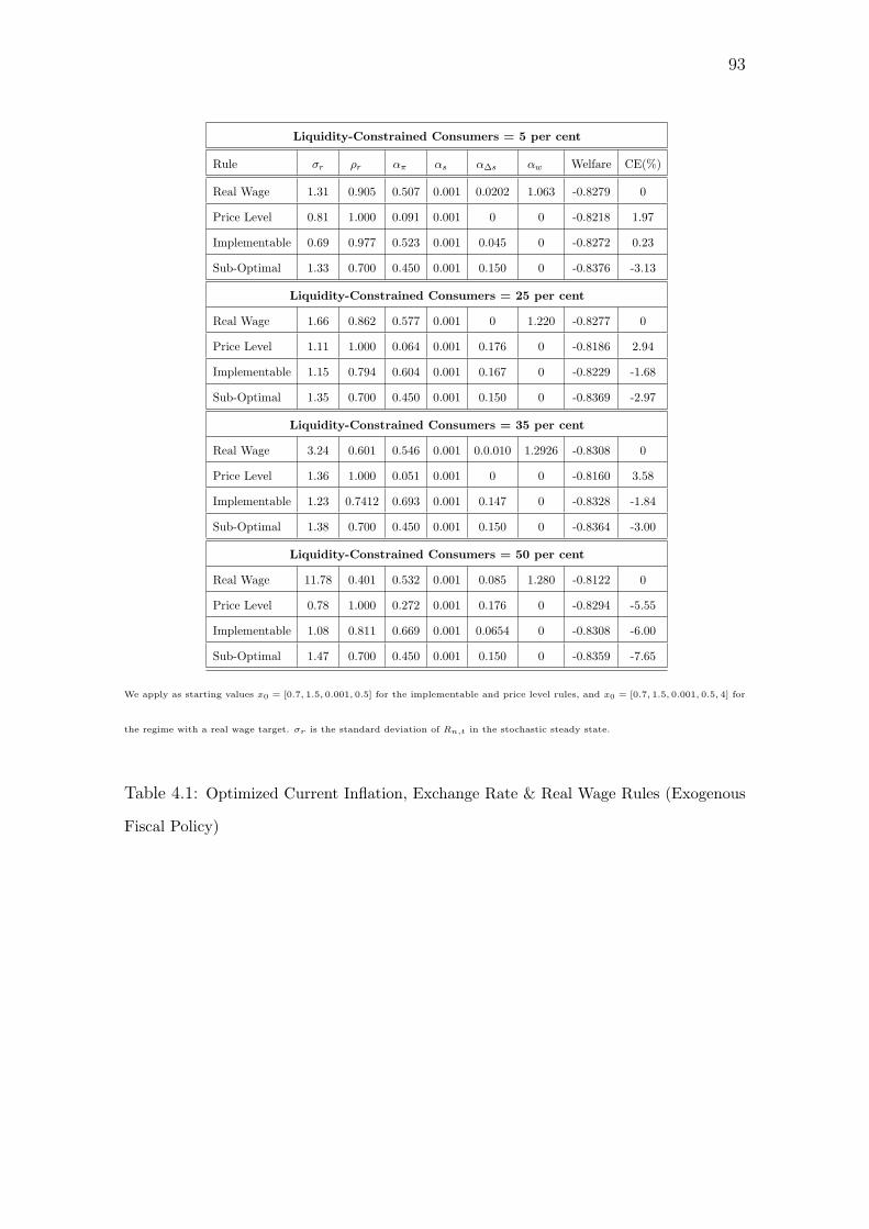
93

Liquidity-Constrained Consumers = 5 per cent

Rule σr ρr απ αs α∆s αw Welfare CE(%)

Real Wage 1.31 0.905 0.507 0.001 0.0202 1.063 -0.8279 0

Price Level 0.81 1.000 0.091 0.001 0 0 -0.8218 1.97

Implementable 0.69 0.977 0.523 0.001 0.045 0 -0.8272 0.23

Sub-Optimal 1.33 0.700 0.450 0.001 0.150 0 -0.8376 -3.13


Real Wage 1.66 0.862 0.577 0.001 0 1.220 -0.8277 0

Price Level 1.11 1.000 0.064 0.001 0.176 0 -0.8186 2.94

Implementable 1.15 0.794 0.604 0.001 0.167 0 -0.8229 -1.68

Sub-Optimal 1.35 0.700 0.450 0.001 0.150 0 -0.8369 -2.97


Real Wage 3.24 0.601 0.546 0.001 0.0.010 1.2926 -0.8308 0

Price Level 1.36 1.000 0.051 0.001 0 0 -0.8160 3.58

Implementable 1.23 0.7412 0.693 0.001 0.147 0 -0.8328 -1.84

Sub-Optimal 1.38 0.700 0.450 0.001 0.150 0 -0.8364 -3.00


Real Wage 11.78 0.401 0.532 0.001 0.085 1.280 -0.8122 0

Price Level 0.78 1.000 0.272 0.001 0.176 0 -0.8294 -5.55

Implementable 1.08 0.811 0.669 0.001 0.0654 0 -0.8308 -6.00

Sub-Optimal 1.47 0.700 0.450 0.001 0.150 0 -0.8359 -7.65

We apply as starting values x0 = [0.7, 1.5, 0.001, 0.5] for the implementable and price level rules, and x0 = [0.7, 1.5, 0.001, 0.5, 4] for

the regime with a real wage target. σr is the standard deviation of Rn,t in the stochastic steady state.

Table 4.1: Optimized Current Inflation, Exchange Rate & Real Wage Rules (Exogenous

Fiscal Policy)

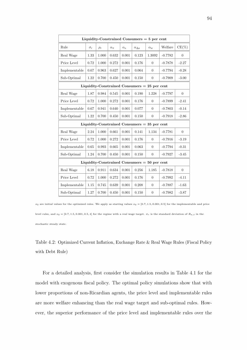
94


Rule σr ρr απ αs α∆s αw Welfare CE(%)

Real Wage 1.33 1.000 0.632 0.001 0.123 1.3092 -0.7782 0

Price Level 0.72 1.000 0.272 0.001 0.176 0 -0.7878 -2.27

Implementable 0.67 0.963 0.627 0.001 0.064 0 -0.7794 -0.28

Sub-Optimal 1.22 0.700 0.450 0.001 0.150 0 -0.7909 -3.00


Real Wage 1.87 0.984 0.545 0.001 0.190 1.228 -0.7797 0

Price Level 0.72 1.000 0.272 0.001 0.176 0 -0.7899 -2.41

Implementable 0.67 0.941 0.640 0.001 0.077 0 -0.7803 -0.14

Sub-Optimal 1.22 0.700 0.450 0.001 0.150 0 -0.7918 -2.86


Real Wage 2.24 1.000 0.661 0.001 0.141 1.134 -0.7781 0

Price Level 0.72 1.000 0.272 0.001 0.176 0 -0.7916 -3.19

Implementable 0.65 0.993 0.665 0.001 0.063 0 -0.7794 -0.31

Sub-Optimal 1.24 0.700 0.450 0.001 0.150 0 -0.7927 -3.45


Real Wage 6.18 0.911 0.634 0.001 0.256 1.185 -0.7818 0

Price Level 0.72 1.000 0.272 0.001 0.176 0 -0.7992 -4.11

Implementable 1.15 0.745 0.639 0.001 0.208 0 -0.7887 -1.63

Sub-Optimal 1.27 0.700 0.450 0.001 0.150 0 -0.7982 -3.87

x0 are initial values for the optimized rules. We apply as starting values x0 = [0.7, 1.5, 0.001, 0.5] for the implementable and price

level rules, and x0 = [0.7, 1.5, 0.001, 0.5, 4] for the regime with a real wage target. σr is the standard deviation of Rn,t in the

stochastic steady state.

Table 4.2: Optimized Current Inflation, Exchange Rate & Real Wage Rules (Fiscal Policy

with Debt Rule)

For a detailed analysis, first consider the simulation results in Table 4.1 for the

model with exogenous fiscal policy. The optimal policy simulations show that with

lower proportions of non-Ricardian agents, the price level and implementable rules

are more welfare enhancing than the real wage target and sub-optimal rules. How-

ever, the superior performance of the price level and implementable rules over the

95

real wage target rule with respect to welfare levels achieved decline with progressive

increases in the proportions of rule-of-thumb (RT) consumers. The deteriorating

performance of these rules at maintaining welfare is linked to the decline in the

number of households that participate in asset markets and are thus able to smooth

consumption. Hence, the price level and implementable are less effective tools for

central banks to maintain welfare when non-Ricardian consumers are predominant

in the economy. On the other hand, although it seems that implementing a real

wage target rule is preferable from a welfare perspective, it comes with a trade-off

of higher levels of volatility in the stochastic standard deviations of the nominal

interest rate.

These results are reflective of findings in the literature highlighting the impli-

cations of having rule-of-thumb consumers in DSGE models given the role these

agents play in boosting aggregate consumption especially in response to a govern-

ment spending shock.

Table 4.2 shows results for the model with endogenous fiscal policy. Given the

stability constraints of the model(see, Figure 4.5), the policy simulations indicate

that irrespective of the proportion of RT consumers, welfare outcomes are better-

off when the central bank implements a policy rule with a real wage target. The

results show significant welfare gains from implementing the real wage target rule

which increases with additional proportions of liquidity-constrained consumers. We

note however that akin to the results in Table 4.1, implementing the rule with a

real wage target comes with considerably higher levels of volatility to the nominal

interest rate. The optimal monetary policy exercises also show rapid fall in welfare

which is driven by increasing proportions of credit constrained consumers for the

price level rule. The price level rule turns out to be the worst performing rule when

non-Ricardian agents constitute a large proportion of consumers in the model for

the oil-producer.

96

Figure 4.5: Debt/GDP ratio and Indeterminacy

Figures 4.6–4.13 show the impulse response functions (irfs) to a 1% increase in

technology, mark-up, government spending and monetary shocks respectively for

the implementable, price level and real wage target rules. A cursory examination of

responses of selected macroeconomic variables to the shocks for both models with

exogenous and endogenous fiscal policy are consistent with literature on small open

emerging economies.14 Figure 4.6 show that a technology shock impacts positively

on output which rises immediately. On the other hand, a productivity shock results

in a fall in inflation, while both consumption and leisure rise, and hours fall. We

observe that although real wages fall instantly for all the optimized policy rules,

the real wage target rule is more effective at reducing the impact of a productivity

shock and at bringing real wages back to its steady state. Figure 4.7 and 4.11 depict

negative responses of output, consumption and real wages to a price shock. We

also note that there are substantial differences between the real wage rule and the

other rules when the impact of a government spending shock is assessed. It should

be noted that a government spending shock should rather boost investment in the

model with endogenous fiscal policy. A monetary policy shock in Figure 4.9 show

strong similarities between the performance of the real wage and implementable

14The impulse responses are present for models with 35 per cent liquidity-constrained consumerswhich is close to the estimated parameter λ

97

rules with exception of the impact on nominal interest rates. It is observed that a

government spending shock has positive influences though transient on output but

with dire implications for consumer prices. Overall, the figures evidently show that

the real wage rule performs better with regards to its ability at ensuring that welfare

is sustained, however the implementation of a real wage rule results in increases in

price volatility.

10 20 30 40

Quarters

0.5

1

1.5

2

2.5

3

3.5

4

4.5

% d

ev fr

om S

S

×10-3 Output

10 20 30 40

Quarters

-2

-1.5

-1

-0.5

0

0.5

1

1.5

% d

ev fr

om S

S

×10-3 Consumption

10 20 30 40

Quarters

-1

0

1

2

3

4

5

6

7

% d

ev fr

om S

S

×10-3 Investment

10 20 30 40

Quarters

-8

-7

-6

-5

-4

-3

-2

-1

0

% d

ev fr

om S

S

×10-3 Hours worked

10 20 30 40

Quarters

-12

-10

-8

-6

-4

-2

0

2

% d

ev fr

om S

S

×10-3 Real wage

10 20 30 40

Quarters

-6

-5

-4

-3

-2

-1

0

% d

ev fr

om S

S


10 20 30 40

Quarters

0.5

1

1.5

2

2.5

3

3.5

4

% d

ev fr

om S

S

×10-3 Real Exchange Rate

10 20 30 40

Quarters

-4

-3.5

-3

-2.5

-2

-1.5

-1

-0.5

0

% d

ev fr

om S

S

×10-3 Inflation

Implementable Rule Price Level Rule Real Wage Targeting Rule

Figure 4.6: Oil Producer economy Model with Exogenous Government Spending: IRFs

to Technology Shock

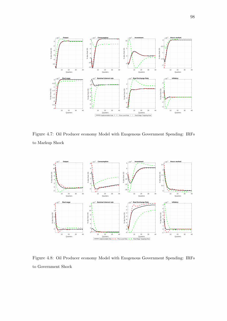
98

10 20 30 40

Quarters

-10

-8

-6

-4

-2

0

% d

ev fr

om S

S

×10-4 Output

10 20 30 40

Quarters

-12

-10

-8

-6

-4

-2

0

% d

ev fr

om S

S

×10-4 Consumption

10 20 30 40

Quarters

-5

0

5

10

% d

ev fr

om S

S

×10-4 Investment

10 20 30 40

Quarters

-2

-1.5

-1

-0.5

0

% d

ev fr

om S

S

×10-3 Hours worked

10 20 30 40

Quarters

-4

-3.5

-3

-2.5

-2

-1.5

-1

-0.5

0

% d

ev fr

om S

S

×10-3 Real wage

10 20 30 40

Quarters

-6

-5

-4

-3

-2

-1

0

1

% d

ev fr

om S

S


10 20 30 40

Quarters

-8

-6

-4

-2

0

2

% d

ev fr

om S

S


10 20 30 40

Quarters

-4

-2

0

2

4

6

% d

ev fr

om S

S

×10-4 Inflation



to Markup Shock

10 20 30 40

Quarters

-2

0

2

4

6

8

10

12

% d

ev fr

om S

S

×10-4 Output

10 20 30 40

Quarters

-2

0

2

4

6

8

% d

ev fr

om S

S

×10-4 Consumption

10 20 30 40

Quarters

-20

-15

-10

-5

0

5

% d

ev fr

om S

S

×10-4 Investment

10 20 30 40

Quarters

0

0.5

1

1.5

2

2.5

% d

ev fr

om S

S

×10-3 Hours worked

10 20 30 40

Quarters

0

1

2

3

4

% d

ev fr

om S

S

×10-3 Real wage

10 20 30 40

Quarters

0

2

4

6

8

10

12

% d

ev fr

om S

S


10 20 30 40

Quarters

-9

-8

-7

-6

-5

-4

-3

-2

-1

% d

ev fr

om S

S


10 20 30 40

Quarters

-1

0

1

2

3

4

5

6

7

% d

ev fr

om S

S

×10-4 Inflation



to Government Shock

99

10 20 30 40

Quarters

-0.04

-0.03

-0.02

-0.01

0

% d

ev fr

om S

S

Output

10 20 30 40

Quarters

-0.04

-0.02

0

0.02

0.04

0.06

0.08

% d

ev fr

om S

S

Consumption

10 20 30 40

Quarters

-0.12

-0.1

-0.08

-0.06

-0.04

-0.02

0

% d

ev fr

om S

S

Investment

10 20 30 40

Quarters

0

0.05

0.1

0.15

0.2

% d

ev fr

om S

S

Hours worked

10 20 30 40

Quarters

0

0.1

0.2

0.3

0.4

% d

ev fr

om S

S

Real wage

10 20 30 40

Quarters

-8

-6

-4

-2

0

2

4

% d

ev fr

om S

S


10 20 30 40

Quarters

-0.06

-0.05

-0.04

-0.03

-0.02

-0.01

0

0.01

% d

ev fr

om S

S

Real Exchange Rate

10 20 30 40

Quarters

-0.08

-0.07

-0.06

-0.05

-0.04

-0.03

-0.02

-0.01

0

% d

ev fr

om S

S

Inflation



to Monetary Shock

10 20 30 40

Quarters

0.5

1

1.5

2

2.5

3

3.5

% d

ev fr

om S

S

×10-3 Output

10 20 30 40

Quarters

-0.5

0

0.5

1

1.5

2

2.5

3

% d

ev fr

om S

S

×10-3 Consumption

10 20 30 40

Quarters

0

2

4

6

8

% d

ev fr

om S

S

×10-3 Investment

10 20 30 40

Quarters

-8

-7

-6

-5

-4

-3

-2

-1

0

% d

ev fr

om S

S×10-3 Hours worked

10 20 30 40

Quarters

-6

-4

-2

0

2

4

% d

ev fr

om S

S

×10-3 Real wage

10 20 30 40

Quarters

-3.5

-3

-2.5

-2

-1.5

-1

-0.5

0

0.5

% d

ev fr

om S

S


10 20 30 40

Quarters

1

2

3

4

5

6

7

% d

ev fr

om S

S


10 20 30 40

Quarters

-20

-15

-10

-5

0

5

% d

ev fr

om S

S

×10-4 Inflation


Figure 4.10: Oil Producer economy Model with Endogenous Government Spending Rule:

IRFs to Technology Shock

100

10 20 30 40

Quarters

-7

-6

-5

-4

-3

-2

-1

0

% d

ev fr

om S

S

×10-4 Output

10 20 30 40

Quarters

-10

-8

-6

-4

-2

% d

ev fr

om S

S

×10-4 Consumption

10 20 30 40

Quarters

-12

-10

-8

-6

-4

-2

0

% d

ev fr

om S

S

×10-4 Investment

10 20 30 40

Quarters

-10

-5

0

5

% d

ev fr

om S

S

×10-4 Hours worked

10 20 30 40

Quarters

-2.5

-2

-1.5

-1

-0.5

0

% d

ev fr

om S

S

×10-3 Real wage

10 20 30 40

Quarters

-6

-4

-2

0

2

4

6

8

% d

ev fr

om S

S


10 20 30 40

Quarters

-20

-15

-10

-5

0

% d

ev fr

om S

S


10 20 30 40

Quarters

-2

0

2

4

6

8

10

12

% d

ev fr

om S

S

×10-4 Inflation



IRFs to Markup Shock

10 20 30 40

Quarters

-2

-1

0

1

2

3

4

% d

ev fr

om S

S

×10-3 Output

10 20 30 40

Quarters

0

0.5

1

1.5

2

2.5

% d

ev fr

om S

S

×10-3 Consumption

10 20 30 40

Quarters

0

5

10

15

20

% d

ev fr

om S

S

×10-4 Investment

10 20 30 40

Quarters

-4

-2

0

2

4

6

% d

ev fr

om S

S×10-3 Hours worked

10 20 30 40

Quarters

-4

-2

0

2

4

6

8

10

12

% d

ev fr

om S

S

×10-3 Real wage

10 20 30 40

Quarters

-4

-2

0

2

4

6

% d

ev fr

om S

S


10 20 30 40

Quarters

-3

-2

-1

0

1

2

3

4

% d

ev fr

om S

S


10 20 30 40

Quarters

-8

-6

-4

-2

0

2

4

6

% d

ev fr

om S

S

×10-4 Inflation



IRFs to Government Shock

101

10 20 30 40

Quarters

-12

-10

-8

-6

-4

-2

0

% d

ev fr

om S

S

×10-3 Output

10 20 30 40

Quarters

-10

-8

-6

-4

-2

% d

ev fr

om S

S

×10-3 Consumption

10 20 30 40

Quarters

-2

-1

0

1

2

% d

ev fr

om S

S

×10-3 Investment

10 20 30 40

Quarters

-0.02

-0.015

-0.01

-0.005

0

% d

ev fr

om S

S

Hours worked

10 20 30 40

Quarters

-0.03

-0.025

-0.02

-0.015

-0.01

-0.005

0

% d

ev fr

om S

S

Real wage

10 20 30 40

Quarters

-4

-3

-2

-1

0

1

% d

ev fr

om S

S


10 20 30 40

Quarters

-8

-6

-4

-2

0

2

4

% d

ev fr

om S

S


10 20 30 40

Quarters

-16

-14

-12

-10

-8

-6

-4

-2

0

% d

ev fr

om S

S

×10-3 Inflation



IRFs to Monetary Shock

4.6 Conclusions

This chapter examines optimal monetary policy for a nonindustrial oil-producer

economy. We employ a small open economy DSGE model that incorporates nominal

price rigidities, imperfect competition, international financial frictions, incomplete

exchange rate pass-through, non-Ricardian agents in form of credit-constrained con-

sumers and oil revenue relevant features for the policy evaluation for the commodity

exporter. Bayesian estimates of the small open economy DSGE model for Nigeria

are used for the optimal policy computations which reveals the welfare implica-

tions of the selected optimized simple rules for different fractions of non-Ricardian

agents. The policy experiments are undertaken for models with exogenous govern-

ment spending and alternatively for a model with government spending determined

by a debt-GDP rule.

102

The model results show that overall, the rule with a real wage target outper-

forms the other optimized and the sub-optimal rules when assessed from a welfare

perspective. In terms of the welfare analysis, we also find that the gains from im-

plementing a particular form of optimized simple rule are non-trivial in comparison

to the real wage target rule. On the contrary, the results show that implementing

a rule that includes a real wage target in the context of the model setup results in

relatively higher levels of volatility in nominal interest rates.

From a modeling perspective, we observe that for the model to be saddle path

stable, the government needs to constrain borrowing in order to accommodate large

fractions of liquidity-constrained consumers, particularly if a rule that includes a

real wage target is implemented using the model with a debt-GDP spending rule.

Thus, we find that the ability of government to borrow from domestic sources to

finance its budget hinges on the level of asset market participation.

Chapter 5

Policy Implications,

Recommendations and Future

Research

Finally I discuss some important policy implications of the conclusions in this thesis

and make suggestions on how these these could aid policy decisions. Subsequently,

some directions for future research are suggested.

5.1 Policy Implications and Recommendation

There are important policy implications from the findings from the policy simula-

tions in this thesis. Firstly, given considerable welfare loses that occur due to the

choice of optimized simple rule, it is expected that the central bank should under-

take rigorous evaluation of its policy options before adopting and implementing a

specific monetary policy regime. Undertaking this is task has to be a priority since

the ultimate goal of macroeconomic policy is to improve economic welfare. In addi-

tion, the monetary authority ought to be mindful of the likely impact of its choice

policy regime would have on nominal interest rate as well as the term structure of

103

104

interest rates. Although it may be common for fast growing emerging or developing

economies to witness high levels of inflation and interest rates, central banks should

be cautious in selecting a suitable monetary policy regime as certain policy rules

could further increase the level of volatility in interest rates. Interest rate volatility

could bolster market uncertainty, adversely affecting the spread between deposit and

lending rates, and thus the cost of borrowing.

Secondly, the optimized policy simulations reveals the government’s borrow-

ing limitation due to interactions between the government spending rule and non-

Ricardian agents in the model. As a consequence, the ability of fiscal authorities to

borrow from domestic households to finance budget requirements when monetary

policy is conducted using a rule that targets prices alongside real wages is capped

to a specific debt-GDP ratio. For a mono-economy where a huge portion of rev-

enues come from oil and gas exports, policymakers urgently need to diversify its

sources revenue in order to mitigate the negative impact of occasional huge swings

in oil prices. Government needs to expand its tax base by accessing viable options

including widening coverage of the sales tax regime, property and company income

taxes. Most importantly the government should foster an environment conducive

for investment by providing the adequate security, good infrastructure and stability

which attracts foreign investments into domestic debt and equity markets. This is

preferable to outright borrowing from abroad to finance the budget because of the

cost of borrowing from international capital markets and repayment uncertainties

that depends on oil price performance. Simultaneously, financial and banking re-

forms should deliberately promote the increased participation of households in asset

markets by adopting a financial inclusion strategy to boost the percentage of the

banked population and number of persons with access to credit.

Finally, while the simulations in this paper are undertaken assuming normal

times, there are critical implications for the conduct of monetary and fiscal policy

105

during adverse times. For example, it could be inferred from the results, struc-

ture of the model with a large proportions of credit-constrained consumers and the

monetary-fiscal interactions that the only option available to finance the short fall in

government revenue during a recession driven by a huge decline in oil prices would

be either to spend from savings or borrow abroad for the non-industrial oil-producer

economy. Although this is mainly due to the model restrictions of having a large

fraction of non-Ricardian consumers, marginal propensity to save also declines dur-

ing a recession as unemployment rises. Ultimately, proper monetary and fiscal policy

coordination is required to ensure both aspects of macroeconomic policy work pro-

gressively towards restoring the economic back on the path of growth. Government’s

counter-cyclical fiscal stimulus spending should be consistent with the central banks

monetary policy regime.

5.2 Future Research

Future research will utilize the model to study welfare-optimal monetary policy

rules, comparing inflation-targeting pure float with a managed float and allow-

ing foreign reserve intervention as a second monetary instrument. Fiscal rules and

monetary-fiscal interactions will also be examined as in Batini et al. (2009). Fi-

nally our studies will attempt to identify robust rules under different information

assumptions on the part of economic agents such as bounded versus full rational-

ity. The general methodology will follow Batini et al. (2006), Levine et al. (2008b),

Levine and Pearlman (2010) and Levine et al. (2012).

On the modelling side future research will incorporate a banking sector with

micro-founded financial frictions, foreign reserves allowing for intervention as a sec-

ond monetary instrument and a formal-informal two-sector domestic economy. We

consider the latter two in detail before going on to discuss the estimation of the

model and its use for policy analysis.

106

Foreign Reserves and Intervention

First we will introduce Foreign reserves intervention as a second monetary instru-

ment. Widely acknowledged as a monetary policy instrument, the use of foreign

exchange (FX) interventions by central banks to dampen currency appreciation or

depreciation has become common place in not just emerging economies but also in

some developed economies post the financial crisis of 2008/09. Formalising such in-

terventions as an additional monetary policy instrument in macroeconomic models

should further epitomize the actions of central banks when faced with the two-

pronged effects of volatile developments in international financial markets and oil

price shocks. In particular, monetary authorities may undertake regular interven-

tions in FX market to moderate supply or demand pressures by sterilizing the surplus

proceeds from oil exports to control liquidity in the system or conversely intervene

by providing FX from its international reserves in order to maintain exchange rate

stability when there is a deficit of inflows to the market as it is the case for oil

producers. We follow research by Benes et al. (2015) to introduce sterilized inter-

ventions in the DSGE model for Nigeria. This would involve a study of various

hybrid monetary policy rules and managed exchange rate regimes to analyse their

implications for inflation, output and the exchange rate in the presence of various

domestic and external shocks. The results should be indicative of how a mixed

regime may insulate the economy from external shocks as well as its impact on

misalignment of the national currency in the presence of trade shocks.

Formal/informal Sectors

Introducing a two-sector formal/informal division will characterize the dual struc-

ture of the Nigeria Economy model. The next stage in the model development

involves the introduction of a sparsely researched aspect in the literature, that is

the inclusion of the informal sector. Acknowledging the paucity of DSGE models

107

that reflect the dual nature of some emerging economies, Anand et al. (2015) develop

an open-economy model with a shadow economy to analyse the macroeconomic im-

pacts of labour and product market deregulation on output and employment. In

addition to other findings, it is notable the paper concludes that the unofficial econ-

omy is a major determinant of the sign and, in particular, the magnitude of impulse

responses relative to the open economy features of the model. Following the fall

in oil price, information such as this may be quite instructive for policy decision

making, particularly were it regards implementation of structural reforms used to

enhance growth and employment. As it is prevalent in many developing and emerg-

ing economies, the informal sector epitomises an important segment of the Nigerian

economy and plays a significant role in employment creation, production and income

generation.

According to CBN (2010) informal economic sector commonly refers to all eco-

nomic activities which are currently unregistered and operates outside official regula-

tory ambit. From a different perspective, the informal sector is described as market

based production of goods and services whether legal or illegal that escapes detec-

tion in the official estimates of gross domestic products (GDP). The NBS (2015a)

refers to the informal sector employment in Nigeria as ‘those generated by individ-

uals not officially or formally recognized in the system or businesses employing less

than 10 or those businesses operating with little or no structures e.g. those in rural

and subsistence Agriculture, Light Manufacturing, Wholesale and Retail Trade, and

personal services like those of barbers and hairdressers mechanics, repair of electron-

ics, and other household goods, plumbers among others.’ The same report which

recorded a remarkable increase in the number of jobs created in the informal sector

for that quarter, also shows that about 90 per cent of the employed are engaged

informally. Although there are diverse opinions and views on the precise definition

of what type of activities consists the informal sector, it is clear that it includes un-

reported incomes from production, whether through barter exchange or monetary

108

transactions which may become taxable when duely reported to the government.

From a general perspective, some broad characteristics of the informal sector can be

can be incorporated into the DSGE model as summarized in the Table below.1

Lab. Market Credit Market Taxation Lab. Share

Formal Sector frictions lower frictions taxed lower

Informal Sector no frictions higher frictions untaxed higher

Table 1. Characterizing Informality in the Nigerian DSGE Model

1See Batini et al. (2010) for a survey of the literature on informality.

Appendix A

Full-Information Two-Stage

Approach Test Results

Weak instrument robust tests in Generalised Methods of Moments (GMM) unlike

conventional GMM tests functions well irrespective of whether identification of es-

timated parameters is weak or strong (see, Canova and Sala (2009) and Cochrane

(2007)). In line with the conclusions of CGG, applying identification robust limited-

and full-information methods following of Mavroeidis (2010) as developed in Stock

and Wright (2000) and Kleibergen (2005) and the novel approach of by Castelnuovo

and Fanelli (2014) which I is annexed to this chapter. I use different proxies of the

output gap to capture business cycle dynamics in the Taylor rule as specified by

CGG in order to ascertain whether or not earlier inferences made hold. On the one

hand, while this serves as a further check of robustness, it is also a validation exer-

cise of the use of Taylor-type monetary policy rules in the new-Keynesian framework

addressing the challenges of signal extraction and data for policy decision making.

109

110

A.1 Limited-Information Approach

A.1.1 Model

The new-Keynesian model as presented by CGG consists of a forward-looking policy

rule:

r∗t = r∗ + ψπEt(πt+1 − π∗) + ψxxt (A.1)

where r∗t represents the target nominal policy rate, πt is inflation and xt denotes

the output gap. Et stands for conditional expectation of the inflation dynamics

obtained from information at time t, π∗ signifies an inflation target, while r∗ is long-

run stable interest rate. Actual rt may vary from the target interest rate due to

exogenous developments leaving the central bank with the responsibility of having

to smooth rt. Thus, there is a partial adjustment between the actual and target

rates given by equation (A.1).

rt = ρ1ρr∗t−1 + ρr∗t−1 + (1− ρ)r∗t + εr,t

Parameter ρ = ρ1 + ρ2 signifies policy inertia, or smoothing of the interest rate,

while εr,t is a monetary policy shock based on the assumption the innovation is driven

by information that is available to the public at t− 1, implying Et−1 , εr,t = 0. The

baseline specification of the rule (A.1) is written as:

rt = α + ρ1rt−1 + ρ2r∗t−2 + (1− ρ)(ψπEtπt+1 + ψxxt) + εr,t (A.2)

where, α = (1 − ρ)(r∗ − ψππ∗). When ρ2 = 0, it becomes the model equivalent

as extensively discussed by Woodford (2003, ch 4). Replace expected values by

realizations in equation (A.2) rewrite as

rt = α + ρ1rt−1 + ρ1rt−2 + (1− ρ)(ψππt+1 + ψxxt) + et (A.3)

111

et = εr,t − (1− ρ)ψπ(πt+1 − Etπt+1) (A.4)

et which is the residual term could possibly an AR(1) process. Assuming rational

expectations with the expected error Et−1εr,t = 0 we have EZtet = 0 as moment

conditions for all predetermined variables Zt.

A model of monetary transmission is specified to discuss how monetary pol-

icy affects macroeconomic fluctuations in the same form as CGG and Lubik and

Schorfheide (2004). The log-linearised equilibrium conditions in the steady state

are specified as

πt = βEtπt+1 + λ(yt − zt) (A.5)

yt = Etyt+1 − σ(rt − Etπt+1) + gt (A.6)

Equation (A.5) which is forward-looking, represents the Phillips curve, while

yt is a derivative of households intertemporal optimization and denotes the Euler

equation for output. The discount factor parameter lies between 0 <β <1 and

captures nominal rigidities in the slope λ >0 given a process for zt that signifies

exogenous shifts in production costs. On the other hand, Euler equation (A.6) is

driven by a parameter σ which stands for the intertemporal elasticity of substitution.

Government spending and preferences are captured as an exogenous process as gt

that captures exogenous processes.1 The model solution consist of the equations

above and xt = yt− zt an identity determining the path of the endogenous variables

πt, xt and rt which are conditional on zt, gt and εr,t the exogenous forcing variables.

The existence of a unique stable solution, show the model equilibrium is determinate,

while multiple stable solutions indicates indeterminacy in the model. Determinacy

1These equations can be obtained for DSGE models as log linear approximations with respectto the steady state (see Woodford (2003), ch. 4). Note omissions of constants for the inflationtarget and equilibrium real rate in the long-run.

112

in the model is dependent on the fulfilment of the necessary condition:

ψπ +1− β

λψx − 1 ≥ 0 (A.7)

The condition (A.7) generalized as Taylor (1993) ‘principle’ requiring nominal inter-

est rates to be raised above proportionately with inflation to prevent self-fulfilling

cycles. This condition would still remain sufficient for determinacy even when a

forward-looking rule as in (A.1) were to substituted using contemporaneous πt for

Etπt + 1 (again as the proposition (4.4) found in Woodford (2003), similarly in Lu-

bik and Schorfheide (2004)). It is necessary for rule (2) the forward-looking Taylor

rule to also ensure the inflation response is not excessive. Empirically, this second

condition is typically not binding for the structural parameter values β, λ, σ (used

in CCG) and the confidence sets for ψπ, ψx as derived below. Thus, it suffices that

the condition specified as equation (A.7) covers our discussions on indeterminacy.

A.1.2 Identifying the Monetary Policy Function in the Canon-

ical New Keynesian Model

Based on the canonical new Keynesian model above, issues of identification are dis-

cussed in this section. Mavroeidis (2010) argue that provided other factors remain

the same, sunspot fluctuations enhance the identification monetary policy rule coef-

ficients. Specifically, identification is shown to depend on the gradient of the Phillips

curve, the prevalence of sunspot fluctuations, and dynamics of shocks.

For simplicity sake and clarity of discussions, it is assumed that there are no

policy inertia, as in the model above. For convenience the policy reaction function

is rewritten thus,

rt = α+ ψπEt−1πt+1 + ψπEt−1xt + et (A.8)

where et is driven by changes to expected inflation and output and the note that

113

expectations are unobserved. Presuming our optimal instruments in our case above

Et−1πt+1 and Et−1xt+1 are actually observed variables. An absence of perfect mul-

ticollinearity among regressors Et−1πt+1, Et−1xt yields the rank condition for iden-

tification. Besides, as emphasized in Clarida et al. (1999) exogenous variation in

Et−1πt+1 and Et−1xt is higher given more accurate estimates of the coefficients and

strong identification. Wheras β <1, solving forward the Phillips curve (A.5) we

obtain non-explosive solutions

π = λ

∞∑j=0

βEtxt+j (A.9)

Thus, λ = 0 becomes a necessary condition for identification hence the slope

Phillips curve ought not to flatten out completely. If that were to occur, Et−1πt+1

becomes a constant and negligibly collinear with the intercept for the monetary

policy rule. From a different perspective it can be likened to a fixed price scenario

since inflation expectations would not vary. Thus, it is empirically significant to note

that weaker identification of the monetary policy function coefficients is expected

if the Phillips curve is relatively flat (see, for example, Kleibergen and Mavroeidis

(2009)). It is also relevant to highlight that, for any case λ = 0, identification

is determined by the output gap equilibrium dynamics. Specifically, as described

in Mavroeidis (2010) the output gap dynamics can be depicted as equations xt =

Gst + vt and st = Qst1 + φt, where st represents vector of state variables, ut and ρt

a innovations, whereas G and Q are a combination of the values determined by the

structural parameters and equation (A.9), implies that Et−1πt+1 = λG(IβQ)1Qst1,

and Et−1xt = GQst1. Assume the vector st1 represents all significant instruments

for endogenous regressors for policy rule (A.2), that is πt+1 and x− t, in the policy

rule, clearly identification failure occurs when st is a scalar. Given that zt and gt

are autoregressive processes defined as: zt = ρzzt1 + ϵz,t and gt = ρggt1 + ϵg,t , and

ϵz,t and ϵg,t are shocks to the exogenous variables. Equation (A.6) the Euler, viewed

114

in terms of xt can be represented as follows:

xt = Etxt+1 − σ(rt − Etπt+1) + gt − (1− ρz)zt (A.10)

The equilibrium dynamics of the model depends on the Phillips curve (A.5), the

output gap equation (A.10), and monetary policy rule rt = ψπEtπt+1 + ψxxt + εr,t

being determinate.

A.1.3 Identification-Robust Inference

This section is follows the approach of Mavroeidis (2010) in implementing of the

identification-robust method. In its simplest form, the method is analogous to Stock

andWright (2000) provisions used to obtain the identification-robust confidence sets.

Given the S statistic which is equivalent to the objective function of the GMM, the

coefficient values are assessed based on the null hypothesis that validates the moment

conditions. This abstraction of Anderson and Rubin (1949) GMM test procedure for

linear instrumental variables models (referred to as AR-S statistic), is not as effective

as a Wald test in a case were identification is strong. Hence, Kleibergen (2005)

conditional score statistic abbreviated as K-LM solves the weakness by exclusively

implementing an optimal choice of instruments.

The figures below are generated applying 90 per cent confidence levels for ψπ

and ψx in equation (A.2) using the K-LM test with a test range of 0 to 10 and 0 to

2 for the parameters, respectively . So that improvement in the test power is made,

the results are a combination of both the K-LM and JKLM test in a ratio 9:1 as

proposed by Kleibergen (2005). The test is presented for the six different measures

of output gap with a fitted Wald ellipse superimposed on the figure for comparison

purposes.

A cursory examination of the charts above indicates that prior to 1979:Q3, Fed

monetary policy remained inconsistent with equilibrium determinacy with respect to

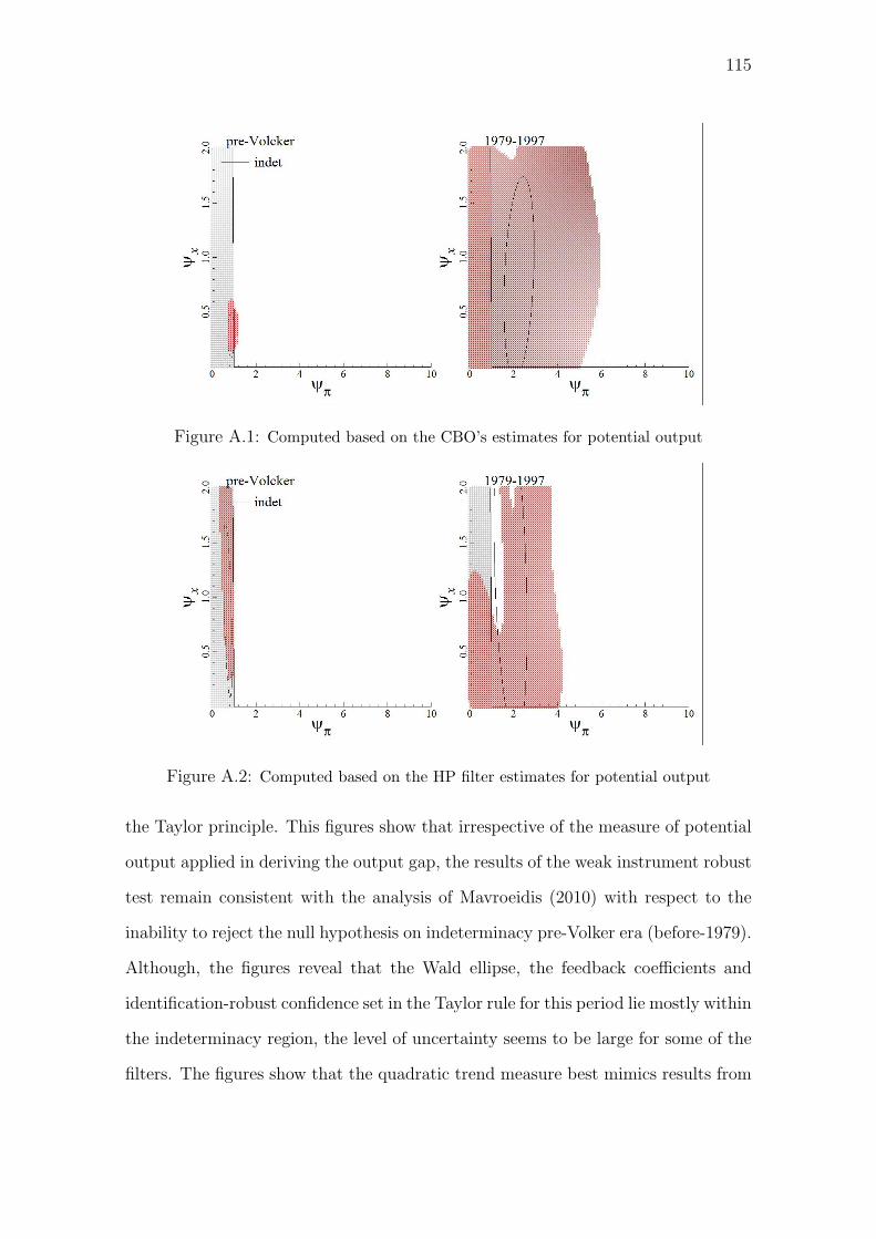
115

Figure A.1: Computed based on the CBO’s estimates for potential output

Figure A.2: Computed based on the HP filter estimates for potential output

the Taylor principle. This figures show that irrespective of the measure of potential

output applied in deriving the output gap, the results of the weak instrument robust

test remain consistent with the analysis of Mavroeidis (2010) with respect to the

inability to reject the null hypothesis on indeterminacy pre-Volker era (before-1979).

Although, the figures reveal that the Wald ellipse, the feedback coefficients and

identification-robust confidence set in the Taylor rule for this period lie mostly within

the indeterminacy region, the level of uncertainty seems to be large for some of the

filters. The figures show that the quadratic trend measure best mimics results from

116

Figure A.3: Computed based on the quadratic trend estimates for potential output

Figure A.4: Computed based on the Real-Time HP filter estimates for potential output

the CBO estimates, while the level of uncertainty is higher for measures derived

using the statistical filters such as the HP, BK and CF filters. Much wider range of

outcomes and policy options.

The tests in this section reveal that in line with Mavroeidis (2010) conclusions,

the monetary policy rule cannot also be precisely estimated during the post 1979

sample when the limited-information method is used for the identification-robust

test. This conclusion is similar irrespective of the output gap measure applied in the

Taylor rule. Although, CGG suggests that the this may be due to possible differences

117

Figure A.5: Computed based on the BK filter estimates for potential output

Figure A.6: Computed based on the CF filter estimates for potential output

in the case of sunspot fluctuations during both samples and the increase in policy

inertia, or the smoothing of interest rate fluctuations across the two periods, a full-

information approach is applied next to ascertain whether new-Keynesian system of

equations are identified.

A.2 Full-Information Two-Stage Approach

In this section, the two-stage approach proposed by Castelnuovo and Fanelli (2014)

is applied to test indeterminacy and identification failures in US monetary policy.

118

The procedure entails a strategy which first involves a full-information test of the

cross-equation restrictions (CER) to ascertain consistency between the reduced form

of the model and its unique stable solution. Establishing this rules out the possibil-

ity of sunspot driven expectations. Secondly, where the CER are rejected, a limited

information test of the orthogonality restrictions is undertaken to validate if the ini-

tial outcome from the first stage of testing is contingent on misspecification linked to

omitting useful propagation mechanisms in the system of structural Euler equations

or whether it is because of incidence of multiple equilibria.

As an empirical test of robustness, the HP filter rather than the CBO estimates

is applied to derive the potential output for US quarterly data from 1954Q3 2008Q3

matching the sample in Castelnuovo and Fanelli (2014). Accordingly, the output

gap is computed as log-deviation of the real GDP from the smoothed series of the

HP filter. Other observable variables include inflation derived as the quarterly rate

of growth of the US GDP deflator; and quarterly effective Fed funds rate (obtained

using monthly averages). I start by briefly presenting the structural small scale New

Keynesian business cycle model from Benati and Surico (2009) which features three

equations in order to understand the testing mechanism and a brief summary of the

test procedure as in the reference paper:

yt = γEtyt+1 + (1− γ) ˜yt−1 − δ(Rt − Etπt+1) + ωy,t (A.11)

πt =β

1 + βαEtπt+1 +

α

1 + βαπt−1 + κyt + ωπ,t (A.12)

Rt = ρRt−1 + (1− ρ)(φππt + φy ˜yt) + ωR,t (A.13)

where

ωx,t = ρxωx,t−1 + εx,t − 1≺ρx ≮ 1, εx,t ∼ WN(0, σ2), x = y, π, R (A.14)

119

and information set

Ft, thatisEt· : = E(· |Ft)

where γ stands for the forward-looking variable weight in the IS curve; α inflation

indexation for price setting; the households intertemporal elasticity of substitution

is δ; κ the Phillips curve gradient; regarding the policy function, ρ, ϕπ and ϕy denote

smoothing parameter for the interest rate, the long-run coefficient on inflation and

that on the output gap. Finally, ωx,t in the fourth equation are mutually independent

autoregressive first order disturbances while the εx,t, are the fundamental shocks.

The system composed by equations (A.11) to (A.14) is compacted in the repre-

sentation

Γ0Xt = ΓfEtXt+1 + ΓbXt−1 + ωt

ω = Ξωt + εt, εt ∼ WN(0,∑

ε)

Ξ := dg(ρy, ρπ, ρR),∑

ε := dg(σ2y, σ

2π, σ

2R)

where

Xt := (yt, πt, Rt)′, ωt := (ωy,t, ωπ,t, ωR,t)′, εt := (εy,t, επ,t, εR,t)′

and

Γ0:=

1 0 δ

−κ 1 0

−(1− ρ)φy −(1− ρ)φπ 1

,Γf :=

γ δ 0

0 β1+βα

0

0 0 0

,Γb:=

1− γ 0 0

0 α1+βα

0

0 0 ρ

,

Take θs := (γ, δ, α, κ, ρ, φπ, φy, ρy, ρπ, ρR, σ2y, σ

2π, σ

2R)′ be the m x 1 vector of struc-

tural parameters (m:=dim(t)). Elements of the matrices above have a nonlinear

dependence on θ then without losing the generalization, are assumed non-singular.

Testing Strategy and Results

The summarised test strategy for the identification-robust test adopted from Castel-

nuovo and Fanelli (2014) is as follows:

120

Step 1

LR test for the CER that yields the identification-robust confidence set

H0,cer

C∗LR1−η1 :=

θs ∈ G∗

θs, LRT (ϕθs) <c

η1χ2d1

and

Step 2

Conditional on the confidence set above being empty, an AndersonRubin test for

the orthogonality restrictions

H0,spec

C∗AR1−η1 :=

θs ∈ D∗

θs, ART (θs) <c

η2χ2d2

121

Tab

leA.1:Stage

1:Estim

ates

oftheStructuralParam

eterswithProjected

90per

centCon

fidence

Intervalsof

theIdentification

-Rob

ust

Test

1954:Q

3-1979:Q

2‘pre-Volker’

1985:Q

1-2008:Q

3‘G

reat

Moderation’

CBO

Estim

ates

HPfilter

Estim

ates

CBO

Estim

ates

HPfilter

Estim

ates

Param

.Interpretation

θ s,M

Lproj.

90%

c.i.

θ s,M

Lproj.

90%

c.i.

θ s,M

Lproj.

90%

c.i.

θ s,M

Lproj.

90%

c.i.

γIS:forw

ard-look

ingterm

--

--

0.729

0.652-0.772

0.795

0.681-0.844

δIS:inter.

elast.

ofsubstitution

--

--

0.082

0.082-0.154

0.092

0.080-0.154

αNKPC:indexationpastinflation

--

--

0.02

0.020-0.059

0.04

0.020-0.082

κNKPC:slop

e-

--

-0.048

0.042-0.098

0.063

0.043-0.095

ρRule,sm

oothingterm

--

--

0.666

0.569-0.697

0.687

0.640-0.698

φy

Rule,reaction

toou

tputgap

--

--

0.339

0.127-0.479

0.434

0.074-0.892

φπ

Rule,reaction

toinflation

--

--

5.439

2.318-5.445

4.775

2.796-5.477

ϕy

Outputgapshock,persistence

--

--

0.92

0.720-0.978

0.961

0.726-0.978

ρπ

Inflationshock,persistence

--

--

0.925

0.748-0.970

0.807

0.807-0.979

ρR

Policyrate

shock,persistence

--

--

0.794

0.730-0.806

0.76

0.713-0.830

Identification

-rob

ust

c.s.

Empty

Non

-empty

122

Tab

leA.2:Stage

2:Estim

ates

oftheStructuralParam

eterswithProjected

90per

centCon

fidence

Intervalsof

theIdentification

-Rob

ust

Test

1954:Q

3-1979:Q

2‘pre-Volker’

1985:Q

1-2008:Q

3‘G

reat

Moderation’

CBO

Estim

ates

HPfilter

Estim

ates

CBO

Estim

ates

HPfilter

Estim

ates

Param

.Interpretation

θ s,LI

proj.

90%

c.i.

θ s,LI

proj.

90%

c.i.

θ s,LI

proj.

90%

c.i.

θ s,LI

proj.

90%

c.i.

γIS:forw

ard-look

ingterm

0.841

0.660-0.845

0.843

0.650-0.850

0.821

0.650-0.850

0.802

0.700-0.844

δIS:inter.

elast.

ofsubstitution

0.088

0.084-0.160

0.152

0.080-0.160

0.132

0.080-0.160

0.092

0.080-0160

αNKPC:indexationpastinflation

0.025

0.020-0.070

0.036

0.020-0.100

0.097

0.020-0.099

0.032

0.021-0.097

κNKPC:slop

e0.042

0.040-0.058

0.054

0.040-0.100

0.087

0.040-0.100

0.093

0.041-0.099

ρRule,sm

oothingterm

0.52

0.500-0.698

0.697

0.500-0.700

0.699

0.500-0.700

0.685

0.606-0.699

φtildey

Rule,reaction

toou

tputgap

0.138

0.050-0.325

0.821

0.050-1.500

0.295

0.050-1.043

0.468

0.050-1.132

φpi

Rule,reaction

toinflation

0.687

0.500-0.906

0.507

0.500-5.499

2.123

0.500-5.499

3.793

0.507-5.491

ρtildey

Outputgapshock,persistence

0.9

0.620-0.964

0.846

0.400-0.980

0.911

0.400-0.980

0.911

0.751-0.979

ρpi

Inflationshock,persistence

0.578

0.414-0.793

0.594

0.400-0.980

0.907

0.400-0.980

0.949

0.752-0.980

ρR

Policyrate

shock,persistence

0.798

0.565-0.916

0.897

0.672-0.980

0.795

0.674-0.980

0.79

0.746-0.954

Identification

-rob

ust

c.s.

Non

-Empty

Non

-empty

123

A.2.1 Analysis of Results

Tables A.1 and A.2 in the appendix show projected 90 per cent confidence interval of

the identification-robust test with point estimates of the structural parameters fol-

lowing the test on the new-Keynesian model described in the system (A.11) through

(A.14). A Numeric inversion of the full information test is used to obtain the set

of empty or non-empty parameter estimates. As in Castelnuovo and Fanelli (2014)

5,000,000 points of θs selected from random test of the uniform distribution from

the Cartesian product of set intervals. The p-values indicate that similar to the

test results for the CBO potential output measure, the HP filter derived measure

show that the pre-Volcker sample is empty, so we cannot rule out the incidence of

indeterminacy for this period. The estimates firmly shows that the case of deter-

minacy is rejected for the the pre-Volcker sample between 1954Q3 - 1979Q2, while

Table A.2 of the grid-test indicates the converse for the post-Volcker from 1985Q1

- 2008Q3. The p-value for the estimates is 0.36 and 0.23 for the non-empty C∗LRθs

which is 19.54 and 22.15 for the CBO and HP filter estimates, respectively. The

identification robust test results do not reject the correct specification of the system

for the later sample. Hence, we accept the new-Keynesian system of equations for

the post Volcker period.

In comparison to conclusions drawn from the single equation approach in Section

A.1.3 for the policy reaction function, the incidence of sunspot expectations can be

ruled out as a factor driving the business cycle since the cross equation restrictions

of the new-Keynesian model is not rejected for the null hypothesis of determinacy

of the system.

The estimates for both the CBO and HP filter measures show tight confidence

intervals for the Taylor rule parameters.

Table A.2 in appendix A presents results for the second stage limited-information

method. The results are non-empty for both sample periods which supports the

earlier LR test outcome in the full information approach for the. Reported test

124

statistics from the inverted Anderson-Rubin test for the second stage show that

the associated test statistics for the estimated parameter values for both sample to

be significant. The new-Keynesian model is not rejected for the earlier period for

the periods. A combination of the two tests using the limited and full information

methods confidence interval for phiπ is quite accurately specified according of the

confidence sets.

A.3 Conclusions

This study re-examines the conclusions of Clarida et al. (2000) using different stan-

dard measures of the potential output and real time data releases. I apply a single

and then two-stage identification-robust test procedures which performs well irre-

spective of the strength of identification of the structural parameters or issues related

to dynamic misspecification of the estimated new Keynesian model. Regarding the

two-stage test, the procedure firstly involves a full information test of the cross-

equation restrictions (CER) to ascertain whether the reduced form of the model

is consistent with the unique stable solution in order to rule out the occurrence

of sunspot driven expectations. Secondly, where the CER are rejected, a limited

information test of the orthogonality restrictions is undertaken to validate if the

initial outcome from the first stage of testing is contingent on misspecification due

to omission of relevant propagation mechanisms from the system of structural Euler

equations or whether it is because of incidence of multiple equilibria.

125

A.4 Forward-Looking Taylor Rule Statistics

Table A.3: Augmented Dickey-Fuller Test ResultsNull Hypothesis: Variable has a unit root

Variables Exogenous t-Statistics Prob*Rt Constant, Linear Trend -3.491577 0.04870

P it Constant -2.731659 0.07500

Y λ1600 Constant -3.751965 0.00550

Y λ1200 Constant -3.849190 0.00420

Y λ500 Constant -4.093631 0.00200

*Mackinnon (1996) one-side p-values

Appendix B

Step-by-Step Description of the

DSGE Model for the Emerging

Economy Oil-producer

B.1 A Standard NK Closed Economy Model

This section presents the detailed development of the NK DSGE model for the

nonindustrial resource-rich emerging economies. Thereafter, additional features are

incorporated that are typical of an emerging economy oil producer. In Section

B.1 we proceed from an RBC flexi-price to an NK sticky-price model. Then in

Section B.2 we now introduce our first financial friction, non-Ricardian consumers.

The NK model becomes open is Section B.3 where a second financial friction a

risk premium on foreign bond holdings of households. Up to now the open economy

model maintains the assumption of perfect pass-through of exchange rate to domestic

and export prices. This assumption is relaxed in section B.4. Finally in Section B.5

we add an oil production sector.

126

127

B.1.1 The RBC Core

First, single-period utility of households consumption, Ct, external habit χCt−1 and

leisure, Lt, is defined as

Ut = U(Ct, Lt) =((Ct − χCt−1)

(1−ϱ)Lϱt )1−σ − 1

1− σ(B.1)

where, σ ≥ 1 the risk-aversion parameter, also stands for inverse of the intertem-

poral rate of substitution. ϱ ∈ (0, 1) expresses relative weight on consumption by

households compatible with the steady state growth σ ≥ 1. Marginal utilities for

both leisure and consumption are,

UC,t = (1− ϱ)(Ct − χCt−1)(1−ϱ)(1−σ)−1L

ϱ(1−σ)t (B.2)

UL,t = ϱ(Ct − χCt−1)(1−ϱ)(1−σ)L

ϱ(1−σ)−1t (B.3)

Household value function is expressed as

Ωt = Et

[∞∑s=0

βsU(Ct+s, Lt+s)

](B.4)

where β = discount factor. Household’s choice at t is state-contingent between con-

suming Ct, its leisure, Lt and financial holdings when maximizing Ωt dependent

on its budget constraint at time t

Bt+1 = BtRt−1 +Wtht − Ct + Γt − TLt (B.5)

where Bt = net stock of real financial riskless assets, Wt = real wage rate, Γt =

dividends, TLt = lump-sum taxes, and Rt = real interest rate paid on assets. Hours

worked are ht = 1 − Lt ∈ (0, 1) and the total amount of time available for work or

leisure is normalized at unity. Government spending financing is through lump-sum

128

non-distortionary taxes. First-order conditions are

UC,t = RtβEt [UC,t+1] (B.6)

UL,tUC,t

= Wt (B.7)

An equivalent representation of the Euler consumption equation (B.6) is

1 = RtEt [Λt,t+1] (B.8)

where Λt,t+1 ≡ βUC,t+1

UC,tis the real stochastic discount factor over the interval [t, t+1]

and (B.6) or (B.8) is the Euler consumption functions.

Output Yt is a product of hours, ht and capital Kt at the beginning of each

period given the Cobb-Douglas production function

Yt = F (At, ht, Kt−1) = (Atht)αK1−α

t−1 (B.9)

where At is a technology parameter and Yt, ht and end-of-period capital, Kt, per-

capita units for households.With Rt + δ, then

Fh,t = αYtht

= Wt (B.10)

FK,t = (1− α)YtKt−1

= Rt + δ (B.11)

It is investment at t. Capital accumulation is

Kt+1 = (1− δ)Kt + It (B.12)

The RBC model is then completed with an output equilibrium equating supply and

demand

Yt = Ct + It +Gt (B.13)

129

where Gt = government spending and Bt = Kt. Capital producing firms convert

It a part of output to (1 − S(Xt))It sold of new capital sold at a real price Qt and

at a cost (that was absent before) of S(Xt). Investment costs are convex Xt ≡ ItIt−1

and S(·) satisfies S ′, S ′′ ≥ 0 ; S(X) = S ′(X) = 0. Expected discounted profits is

maximized

Et

∞∑k=0

Dt,t+k [Qt+k(1− S (It+k/It+k−1))It+k − It+k]

where Dt,t+k ≡ βUC,t+k

UC,trate for the real stochastic discount

Kt = (1− δ)Kt−1 + (1− S(Xt))It (B.14)

First-order conditions are

Qt(1− S(Xt)−XtS′(Xt)) + Et

[Λt,t+1Qt+1S

′(Xt+1)I2t+1

I2t

]= 1 (B.15)

Arbitrage between returns on capital and bonds given by

Et[Λt,t+1RK,t+1] = Et[Λt,t+1Rt+1] = 1 (B.16)

where RK,t is its gross return given by

RK,t =(1− α) Yt

Kt−1+ (1− δ)Qt

Qt−1

(B.17)

In (B.32) the right-hand-side is the gross return to holding a unit of capital in from t

to t+1. The left-hand-side is the gross return from holding bonds, the opportunity

cost of capital. The set-up is completed with the functional form of the investment

costs as

S(X) = (ϕX(Xt −X))2 (B.18)

130

B.1.2 From RBC to NK

Introducing a retail sector which applies a homogeneous products to derive differ-

entiated consumption goods

Ct =

(∫ 1

0

Ct(m)(ζ−1)/ζdk

)ζ/(ζ−1)

(B.19)

where ζ equals elasticity of substitution and then implies there are demand equations

for every intermediate good m priced as Pt(m) of form

Ct(m) =

(Pt(m)

Pt

)−ζ

Ct (B.20)

where Pt =[∫ 1

0Pt(m)1−ζdm

] 11−ζ

. Pt is the aggregate price index.

Good m is converted at the cost cY Wt (m) where production of wholesale goods

apply the technology for production (B.97). Hence

Yt(m) = (1− c)Y Wt (m) (B.21)

Y Wt =

(Atht)αK1−α

t−1

∆t

(B.22)

where ∆t is price dispersion given below.

Price stickiness is introduced by assuming a probability of 1− ξ for which prices

of intermediate good m are optimally set at P 0t (m). These are fixed when not re-

optimized.1 The objective for m producers is to choose P 0t (m) at any time t in

order to maximize discounted profits

Et

∞∑k=0

ξkDt,t+kYt+k(m)[P 0t (m)− Pt+kMCt+k

](B.23)

subject to (B.20), where Dt,t+k is now the nominal stochastic discount factor over

1Thus we can interpret 11−ξ as the average duration for which prices are left unchanged.

131

the interval [t, t+ k]. The solution to this is

Et

∞∑k=0

ξkDt,t+kYt+k(m)

[P 0t (m)− 1

(1− 1/ζ)Pt+kMCt+kMSt+k

]= 0 (B.24)

In (B.24) we have introduced a mark-up shock MSt to the steady state mark-up

1(1−1/ζ)

. The price index would evolve according to the law of large numbers as in

P 1−ζt+1 = ξP 1−ζ

t + (1− ξ)(P 0t+1)

1−ζ (B.25)

The model is then set up as difference equations. For summation St ≡∑∞

k=0 βkXt+k,

we can write

St = Xt +∞∑k=1

βkXt+k = Xt +∞∑k′=0

βk′+1Xt+k′+1 putting k′ = k + 1

= Xt + βSt+1 (B.26)

and the nominal discount factor as Dt,t+k ≡ βUC,t+k/Pt+k

UC,t/Pt, inflation dynamics are

given by

Ht − ξβEt[Πζ−1t+1Ht+1] = YtUC,t (B.27)

Jt − ξβEt[Πζt+1Jt+1] =

(1

1− 1ζ

)YtUC,tMCtMSt (B.28)

1 = ξΠζ−1t + (1− ξ)

(JtHt

)1−ζ

(B.29)

and price dispersion is given by

∆t ≡1

n

n∑j=1

(Pt(j)/Pt)−ζ = ξΠζ

t∆t−1 + (1− ξ)

(JtHt

)−ζ

(B.30)

Real marginal costs are no longer fixed and are given by

MCt =PWt

Pt(B.31)

132

and (B.32) must be modified to

RK,t =(1− α)MCt+1Yt

Kt−1+ (1− δ)Qt

Qt−1

(B.32)

Note that as ξ → 0 and ζ → ∞, MCt → 1, ∆t → 1 and the NK model reduces to

the flexi-price RBC core model.

B.1.3 The Central Bank

The gross nominal and ex post real interest rates are related by

Rt =Rn,t−1

Πt

(B.33)

where the nominal interest rate is a policy variable, typically given in the literature

by a standard Taylor-type rule:

log

(Rn,t

Rn

)= ρ log

(Rn,t−1

Rn

)+ θπ log

(Πt

Π

)+ θy log

(YtY

)+ ϵMPS,t (B.34)

B.1.4 Shock processes

The structural shock processes in log-linearised form are assumed to follow AR(1)

processes

logAt − log At = ρA(logAt−1 − log At−1) + ϵA,t

logGt − log Gt = ρG(logGt−1 − log Gt−1) + ϵG,t

logMSt − logMS = ρMS(logMSt−1 − logMS) + ϵMS,t

where MS = RPS = 1 in the steady state (so logMS = logRPS = 0), while the

monetary policy shock ϵMPS,t is assumed to be i.i.d with zero mean. This completes

133

the specification of the benchmark NK model.

B.2 A Closed Economy NK Model with Credit-

Constrained Consumers

We introduce a financial friction in the form of liquidity constrained ‘rule of thumb’

consumers which is widely accepted in the literature on emerging economies as an

important transmission channel of shocks.

Suppose that a proportion λ of consumers are credit constrained and have no

income from monopolistic retail firms. They must consume out of wage income and

their consumption is given by

C1,t = Wth1,t (B.35)

The remaining Ricardian consumers are modelled as before and consume C2,t. Total

consumption and hours are then

Ct = λC1,t + (1− λ)C2,t (B.36)

ht = λh1,t + (1− λ)h2,t (B.37)

Liquidity constrained consumers now choose C1,t and L1,t = 1−h1,t to maximize

U1(C1,t, L1,t) subject to (B.35). The first order conditions are now the same for both

types

UL1,t

UC1,t

=UL2,t

UC2,t

= Wt (B.38)

Together with (B.35) and the functional form U1,t = U(C1,t, L1,t) =(C

(1−ϱ)1,t Lϱ

1,t)1−σ−1

1−σ

this leads to the foc for the liquidity constrained consumers

ρ(1− L1,t)

(1− ρ)L1,t

= 1 ⇒ L1,t = 1− h1,t = ρ (B.39)

134

In other words hours worked by liquidity constrained consumers are constant.

B.3 A Standard Open-Economy NK Model

Composite Dixit-Stiglitz (D-S) consumption and investment are for home and foreign

goods:

Ct =

[w

1µCC C

µC−1

µCH,t + (1− wC)

1µC C

µC−1

µCF,t

] µCµC−1

(B.40)

It =

[w

1µII I

µI−1

µIH,t + (1− wI)

1µI I

µI−1

µIF,t

] µIµI−1

(B.41)

The corresponding D-S price indices are

PC,t =[wC(PH,t)

1−µC + (1− wC)(PF,t)1−µC

] 11−µC (B.42)

PI,t =[wI(PH,t)

1−µI + (1− wI)(PF,t)1−µI

] 11−µI (B.43)

Proportions for home and foreign produced goods are ν and 1−ν. Consumption

basket weights for both blocs are

wC = 1− (1− ν)(1− ωC) ; w∗C = 1− ν(1− ω∗

C) (B.44)

In (B.44), ωC , ω∗C ∈ [0, 1] are a parameters that captures the degree of ‘bias’ in the

two blocs. If ωC = ω∗C = 1 we have wC = w∗

C = 1, i.e., autarky, while ωC = ω∗C = 0

gives us the case of perfect integration with wC = ν and w∗C = 1 − ν, i.e., weights

are in proportion to the proportions of goods produced in the two countries. In the

limit, as the home country becomes small ν → 0. Hence wC → ωC and w∗C → 1.

Thus the foreign bloc becomes closed, but as long as there is a degree of home bias

and ωC > 0, the home country continues to consume foreign-produced consumption

goods. Exactly the same applies to the investment baskets where we define ωI and

135

ω∗I by

wI = 1− (1− ν)(1− ωI) ; w∗I = 1− ν(1− ω∗

I ) (B.45)

Then standard intra-temporal optimizing decisions for home consumers and firms

lead to

CH,t = wC

(PH,tPC,t

)−µCCt (B.46)

CF,t = (1− wC)

(PF,tPC,t

)−µCCt (B.47)

IH,t = wI

(PH,tPI,t

)−µIIt (B.48)

IF,t = (1− wI)

(PF,tPI,t

)−µIIt (B.49)

(B.50)

In the small open economy we take foreign aggregate consumption and invest-

ment, denoted by C∗t and I∗t respectively, as exogenous processes2 Define one real

exchange rate as the relative aggregate consumption price RERC,t ≡P ∗C,tSt

PC,twhere

St is the nominal exchange rate. Similarly define RERI,t ≡P ∗I,tSt

PI,tfor investment.

Then foreign counterparts of the above defining demand for the export of the home

goods are

C∗H,t = (1− w∗

C)

(P ∗H,t

P ∗C,t

)−µ∗C

C∗t = (1− w∗

C)

(PH,t

PC,tRERC,t

)−µ∗CC∗t (B.51)

I∗H,t = (1− w∗I)

(P ∗H,t

P ∗I,t

)−µ∗I

I∗t = (1− w∗I)

(PH,t

PI,tRERI,t

)−µ∗II∗t (B.52)

where P ∗H,t, P

∗C,t and P

∗I,t denote the price of home consumption, aggregate consump-

tion and aggregate investment goods in foreign currency and we have used the law

2Aggregate variables such as Ct and C∗t are aggregates over varieties and in fact per capita

measures. Relative total consumption in the two blocs is then given by νCt

(1−ν)C∗t.

136

of one price for differentiated good, namely StP∗H,t = PH,t.

We incorporate financial frictions facing households as in Benigno (2001). There

are two non-contingent one-period bonds denominated in the currencies of each bloc

with payments in period t, BH,t and B∗F,t respectively in (per capita) aggregate. The

prices of these bonds are given by

PB,t =1

Rn,t

; P ∗B,t =

1

R∗n,tϕ(

StB∗F,t

PH,tYt)

(B.53)

where ϕ(·) captures the cost in the form of a risk premium for home households

to hold foreign bonds, B∗F,t is the aggregate foreign asset position of the economy

denominated in foreign currency and PH,tYt is nominal GDP. We assume ϕ(0) = 0

and ϕ′ < 0. Rn,t and R∗n,t denote the nominal interest rate over the interval [t, t+1].

The representative household must obey a budget constraint expressed in nom-

inal terms:

PC,tCt + PB,tBH,t + P ∗B,tStB

∗F,t + PC,tTLt = PC,tWtLt +BH,t−1 + StB

∗F,t−1 + PC,tΓt(B.54)

where PC,t is a Dixit-Stiglitz price index defined in (B.42),Wt is the real consumption

wage rate, TLt are lump-sum taxes net of transfers and Γt are dividends from

ownership of firms. The intertemporal and labour supply decisions of the household

are then

PB,t = βEt

[UC,t+1

UC,tΠt+1

](B.55)

P ∗B,t = βEt

[UC,t+1St+1

UC,tΠt+1St

](B.56)

Wt =UL,tUC,t

= −Uh,tUC,t

(B.57)

137

where

UC,t = (1− ϱ)(Ct − χCt−1)(1−ϱ)(1−σ)−1(1− ht)

ϱ(1−σ) (B.58)

λh,t = −(Ct − χCt−1)(1−ϱ)(1−σ)ϱ(1− ht)

ϱ(1−σ)−1 (B.59)

Πt ≡ PC,tPC,t−1

(B.60)

Note that now in the open economy Πt is consumer price inflation.

Then combining (B.55) and (B.56) we arrive at the modified UIP condition

PB,tP ∗B,t

=Et

[UC,t+1

Pt

Pt+1

]Et

[UC,t+1

St+1Pt

StPt+1

] (B.61)

In the absence of an international risk premium, ϕ(·) → 1 and (B.61) reduces to the

standard UIP condition.3

The retailer’s and wholesaler’s decisions are as before for the closed economy

except Πt is replaced with domestic price inflation ΠH,t ≡ PH,t

PH,t−1which differs from

consumer price inflation.

Equilibrium and Foreign asset accumulation is given by

Yt = CH,t + IH,t +1− ν

ν

[C∗H,t + I∗H,t

]+Gt

≡ CH,t + IH,t + EX∗t +Gt (B.62)

EXt =1− ν

ν(1− w∗

C)

(PH,t

PC,tRERC,t

)−µ∗CC∗t

+1− ν

ν(1− w∗

I)

(PH,t

PI,tRERI,t

)−µ∗II∗t (B.63)

StSt−1

=RERC,tΠt

RERC,t−1Π∗t

(B.64)

3In log-linearized form this becomes log(1 +Rn,t)− log(1 +Rn,t) = Et[logSt+1]− St.

138

TtTt−1

=ΠF,t

ΠH,t

(B.65)

RERC,t =

[w∗C + (1− w∗

C)Tµ∗C−1t

] 11−µ∗

C[1− wC + wCT µC−1

t

] 11−µC

(B.66)

RERI,t =

[w∗I + (1− w∗

I)Tµ∗I−1t

] 11−µ∗

I[1− wI + wIT µI−1

t

] 11−µI

(B.67)

Πt = [w(ΠH,t)1−µC + (1− w)(ΠF,t)

1−µC ]1

1−µC (B.68)

logRn,t/Rn = ρr logRn,t−1/Rn + (1− ρr)(θπEt[log Πt+1]/Π

+ θs logSt/S) + ϵr,t+1 (B.69)

For the small open economy (SOE) ν → 0, wC → ωC and w∗C → 1; but 1−ν

ν(1−

w∗C) → 1 − ω∗

C so a large ‘closed’ economy imports consumption goods from the

SOE. Similarly wI → ωI and w∗I → 1; but 1−ν

ν(1 − w∗

I) → 1 − ω∗I and the same

applies to investment goods.

The foreign Euler and Fischer equations are

1

R∗n,t

= βEt

[U∗C,t+1

U∗C,tΠ

∗t+1

](B.70)

R∗t =

R∗n,t−1

Π∗t

(B.71)

Then add a risk premium shock in period t−1, exp(ϵUIP,t) and use (B.56) and (B.70)

to obtain

1

ϕ(StB∗

F,t

PH,tYt

)exp(ϵUIP,t)

Et

[U∗C,t+1

U∗C,tΠ

∗t+1

]=

1

ϕ(StB∗

F,t

PH,tYt

)exp(ϵUIP,t)R∗

n,t

= Et

[UC,t+1St+1

UC,tΠt+1St

](B.72)

Noting that St+1

Πt+1St= St+1Pt

Pt+1St=

RERC,t+1

RERC,tΠ∗t+1

, and using (B.74), we then obtain the

consumption real exchange rate as

RERC,t = RERdtRER

rt (B.73)

139

where

RERrt ≡ U∗

C,t

UC,t(B.74)

and RERdt , the deviation of the real consumption exchange rate from its risk-sharing

value RERrt , is given by

Et

UC,t+1

UC,t

RERrt+1

RERrt

1

Π∗t+1

1

ϕ(StB∗

F,t

PH,tYt) exp(ϵUIP,t)

−RERd

t+1

RERdt

= 0 (B.75)

Equation (B.72) is one form of the modified UIP condition that treats R∗n,t as

exogenous. Equations (B.73)–(B.75) is an alternative form of the modified UIP

condition that treats U∗C,t as exogenous and highlights the deviation from risk sharing

under complete international financial markets.

Current account dynamics are given by

1

R∗n,tϕ(

StB∗F,t

PH,tYt)StB

∗F,t = StB

∗F,t−1 + TBt (B.76)

ϕ(StB

∗F,t

PH,tYt) = exp

(ϕBStB

∗F,t

PH,tYt

); χB < 0 (B.77)

TBt = PH,tYt − PC,tCt − PI,tIt − PH,tGt (B.78)

Exogenous shocks are assumed to follow AR1 processes:

logAt+1

A= ρa log

AtA

+ ϵa,t+1 (B.79)

logGt+1

G= ρg log

Gt

G+ ϵg,t+1 (B.80)

logMSt+1

MS= ρms log

MStMS

+ ϵms,t+1 (B.81)

logUIPt+1

UIP= ρUIP log

UIPtUIP

+ ϵuip,t+1 (B.82)

ϵr,t+1 = ρeϵr,t + νr,t+1 (B.83)

There are now two ways to close the model. First, as is standard for models of

140

the small open economy (SOE), we can assume processes for foreign variables R∗n,t,

Π∗t , C

∗t , I

∗t and U∗

t are exogenous and independent. Then assuming AR1 processes

for these as well the model is closed with

logR∗n,t/R

∗n = ρ∗r logR

/n,t−1R

∗n + ϵ∗r,t+1 (B.84)

logΠ∗t+1


Π∗ + ϵ∗π,t+1 (B.85)

logC∗t+1


C∗ + ϵ∗c,t+1 (B.86)

logI∗t+1

I∗= ρ∗I log

I∗tI∗

+ ϵ∗i,t+1 (B.87)

logh∗t+1

h∗= ρ∗h log

h∗tI∗

+ ϵ∗h,t+1 (B.88)

and

U∗C,t = (1− ϱ∗)(C∗

t − χ∗C∗t−1)

(1−ϱ∗)(1−σ∗)−1(1− h∗t )ϱ∗(1−σ∗) (B.89)

(B.90)

The second approach is to use data for world variables to estimate a VAR. The

final most satisfactory approach is to acknowledge that the foreign variables are

interdependent and part of a model driven by the same form of shocks and policy

rules as for the SOE. This model can be the closed economy of section B.1 fitted to

World or US data.

B.4 Incomplete Exchange Rate Pass-Through

Incomplete exchange rate pass-through in the model follow similar the processes

described below for both pass-through to exports and imports.

141

Exchange Rate Pass-through and Exports

We first consider exchange rate pass-through to exports. We provide a more general

set-up in which a fixed proportion θ of retailers set export prices P ∗ pH,t in the Home

currency (producer currency pricers, PCP) and a proportion 1− θ set export prices

P ∗ ℓH,t in the dollars (local currency pricers, LCP). Then the price of exports in foreign

currency is given by

P ∗H,t = θP ∗ p

H,t + (1− θ)P ∗ ℓH,t (B.91)

Putting θ = 0 gets us back to the previous model with complete exchange rate

pass-through.

PCP Exporters

Assume that there is a probability of 1 − ξH at each period that the price of each

good f is set optimally to PH,t(f). If the price is not re-optimized, then it is held

constant.4 For each producer f the objective is at time t to choose PH,t(f) to

maximize discounted profits

Et

∞∑k=0

ξkHDt,t+kYt+k(f)[PH,t(f)− PH,t+kMCt+k

]

where Dt,t+k is the discount factor over the interval [t, t + k], subject to a com-

mon5 downward sloping demand from domestic consumers and foreign importers of

elasticity ζ and MCt =PWH,t

PH,tare marginal costs. The solution to this is

Et

∞∑k=0

ξkHDt,t+kYt+k(f)

[PHt(f)−

ζ

(ζ − 1)PH,t+kMCt+k

]= 0 (B.92)

4Thus we can interpret 11−ξH

as the average duration for which prices are left unchanged.5Recall that we have imposed a symmetry condition ζ = ζ∗ at this point; i.e., the elasticity of

substitution between differentiated goods produced in any one bloc is the same for consumers inboth blocs.

142

and by the law of large numbers the evolution of the price index is given by

P 1−ζH,t+1 = ξH (PH,t)

1−ζ + (1− ξH)(PH,t+1(f))1−ζ (B.93)

Monopolistic profits as a proportion of GDP are given by

ΓtPH,tYt

≡PH,tYt − PW

H,tYWt

PH,tYt= 1−MCt

(1 +

F

Y

)(B.94)

For good f imported by the home country from PCP foreign firms the price

P pF,t(f), set by retailers, is given by P p

F,t(f) = StP∗F,t(f). Similarly P ∗ p

H,t(f) =PH,t(f)

St.

LCP Exporters

Price setting in export markets by domestic LCP exporters follows is a very similar

fashion to domestic pricing. The optimal price in units of domestic currency is

P ∗ ℓH,tSt, costs are as for domestically marketed goods so (B.92) and (B.93) become

Et

∞∑k=0

ξkHDt,t+kY∗t+k(f)

[PH,t(f)

∗ ℓSt+k −ζ

(ζ − 1)PH,t+kMCt+k

]= 0 (B.95)

and by the law of large numbers the evolution of the price index is given by

(P ∗ ℓH,t+1)

1−ζ = ξH(P∗ ℓH,t)

1−ζ+ (1− ξH)(P

∗ ℓH,t+1(f))

1−ζ (B.96)

Foreign exporters from the large ROW bloc are PCPers so we have

PF,t = StP∗F,t (B.97)

Table 1 summarizes the notation used.

143

Origin of Good Domestic Market Export Market (PCP) Export Market(LCP)

Home PH P ∗ pH = PH

StP ∗ ℓH = PH

St

Foreign P ∗F P p

F = StP∗F non-existent

Table 1. Notation for Prices

To obtain the non-linear dynamics for LCPers, rewrite (B.95) as

Et

∞∑k=0

ξkHDt,t+kY∗t+k(f)St+k

[PH,t(f)

∗ ℓ − ζ

(ζ − 1)P ∗ ℓH,t+kMCℓ

t+k

]= 0 (B.98)

where

MCℓt ≡

MCt PH,tStP ∗ ℓ

H,t

(B.99)

As before define the terms of trade for the home bloc (import/export prices in one

currency) as Tt ≡ PF,t

PH,t. Define the terms of trade for the foreign bloc as T ∗

t ≡ P ∗H,t

P ∗F,t

.

With PCPers only the law of one price holds and T ∗t =

StP ∗H,t

StP ∗F,t

=PH,t

PF,t= 1

Tt , but with

LCPers this no longer is the case. Now we have that

T ∗t ≡

P ∗H,t

P ∗F,t

=θP ∗ p

H,t + (1− θ)P ∗ ℓH,t

P ∗F,t

=θPH,t

St+ (1− θ)P ∗ ℓ

H,t

PF,t

St

(B.100)

It follows that

TtT ∗t = θ + (1− θ)

StP∗ ℓH,t

PH,t(B.101)

and hence from (B.99) and (B.101)

MCℓt =

(1− θ)MCtTtT ∗

t − θ(B.102)

The system is completed with

Π∗H,t = θΠ∗ p

H,t + (1− θ)Π∗ ℓH,t (B.103)

From StP∗ pH,t = PH,t and RERt ≡ StP ∗

t

Ptwe have that

Π∗ pH,t =

RERt−1ΠH,tΠ∗t

RERtΠt

(B.104)

144

Exporters from the foreign bloc are PCPers so StP∗F,t = PF,t. Therefore by analogy

with (B.104) we have

ΠF,t =RERt

RERt−1

Πt

Π∗t

Π∗F,t (B.105)

and

Πt =[w(ΠH,t)

1−µ + (1− w)(ΠF,t)1−µ] 1

1−µ (B.106)

From the definitions of Tt and T ∗t we have that

TtTt−1

=ΠF,t

ΠH,t

(B.107)

T ∗t

T ∗t−1

=Π∗H,t

Π∗F,t

(B.108)


∗ ℓH,t+1)

ζ−1Hℓt+1] = Y ∗

t StUC,t (B.109)


ζJ ℓt+1] =1

1− 1ζ


t (B.110)


ζ−1 + (1− ξH)

(J ℓtHℓt

)1−ζ

(B.111)

Equations (B.102) – (A.20) give us the new equations to describe imperfect

exchange rate pass-though for exports. As θ → 1 we get back to the previous model

with complete exchange rate pass-through.

B.4.1 Exchange Rate Pass-through and Imports

Up to now it has been assumed that there is complete exchange rate pass-through

for imports, i.e., PF,t = StP∗F,t. Hence RERC,t ≡ PF,t

PC,t=

StP ∗F,t

PC,t. But the rest of

the world is closed in its own view of the small open economy, so P ∗F,t = P ∗

C,t and

RERC,t =StP ∗

C,t

PC,t.

Now assume only a proportion θ∗ of importers are producer price setters with

complete exchange rate pass-through. Then by analogy with the case of exports we

145

how put

RERC,t ≡PF,tPC,t

= θ∗StP

∗C,t

PC,t+ (1− θ∗)

P ∗F,t

PC,t(B.112)

for consumption goods, where ΨC,t ≡P ∗F,t

PC,tis an exogenous process with a determin-

istic steady state ΨC ≡ P ∗F

PC=

SP ∗C

PC= 1.

Similarly for imports of investment goods

RERI,t ≡PF,tPI,t

= θ∗StP

∗F,t

PI,t+ (1− θ∗)

P ∗F,t

PI,t(B.113)

and we define another exogenous process ΨI,t ≡P ∗F,t

PI,twith ΨI ≡

P ∗F

PI=

SP ∗C

PI= 1.

B.5 An Oil Sector and Oil Price Changes

We introduce an oil sector treating oil output as an exogenous endowment Y O.

Revenues is then driven only by the price of oil P ∗O,t denominated in foreign currency

which is a exogenous process as for the other shock processes in the model. The

only change to the model is in the trade balance which now becomes

TBt = StP∗O,tY

O + PH,tYt − PC,tCt − PI,tIt − PH,tGt (B.114)

146

B.5.1 Zero-Growth Steady State

First assume zero growth in the steady state: g = g∗ = 0 and non-negative

inflation Π = Π∗ = Π∗H = Π∗

F > 0. Then we have

Rn = R∗nϕ

(SB

P

)C1 = Wh1

1

Rn

= β

C = λC1 + (1− λ)C2

UL1

UC1

=UL2

UC2

=W

h = λh1 + (1− λ)h2

UC = (1− ϱ)C(1−ϱ)(1−σ)−1(1− h)ϱ(1−σ) ; for C = C1, C2; h = h1, h2

UL = −ϱC(1−ϱ)(1−σ)(1− h)ϱ(1−σ)−1 ; for C = C1, C2; h = h1, h2

147

1 =

[wC

(PHPC

)1−µC+ (1− wC)

(PFPC

)1−µC] 1

1−µC

PHPC

=1

[wC + (1− wC)T 1−µC ]1

1−µC

CH = wC

(PHPC

)−µCC

CF = (1− wC)

(PFPC

)−µCC

CH∗ = (1− ω∗

C)

(PH

PCRERC

)−µ∗CC∗

∆ =(1− ξ)

11−ζ (1− ξΠζ−1)

ζ1−ζ

1− ξΠζ

J

H=

(1− ξΠζ−1

1− ξ

) 11−ζ

MC =PW

P=

(1− 1

ζ

)J(1− βξΠζ)

H(1− βξΠζ−1)

H(1− ξHβΠζ−1) = Y UC

J(1− ξHβΠζ) =

1

1− 1ζ

Y UCMC

Hℓ = H

J ℓ = J

MCℓ =MC

Ψ = 1

148

PWH

PC= MC

PHPC

(B.115)

K =(1− α)MC PH

PCY

(R + δ)Q(B.116)

(B.117)

Y W = (AH)αK1−α (B.118)

Y =(1− c)Y W

∆(B.119)

R =Rn

Π(B.120)

I = (g + δ)K (B.121)

X = 1 (B.122)

S(X) = S ′(X) = 0 (B.123)

Q =PIPC

(B.124)

149

IH = wI

(PH/PCPI/PC

)−µII (B.125)

IF = (1− wI)

(PF/PCPI/PC

)−µII (B.126)

I∗H = (1− ω∗I )

(PH

PRER

)−µ∗II∗ (B.127)

PIPC

=

[wI

(PHPC

)1−µI+ (1− wI)

(PFPC

)1−µI] 1

1−µI

(B.128)

Y = CH + IH + EXC + EXI +Gt (B.129)

EXC = C∗H,t = (1− ω∗

C,t)

(PH

PCRERC

)−µ∗CC∗ (B.130)

EXI = I∗H,t = (1− ω∗I,t)

(PH

PIRERI

)−µ∗II∗ (B.131)

RERC =1

[1− wC + wCT µC−1]1

1−µC

(B.132)

RERI =1

[1− wI + wIT µI−1]1

1−µI

(B.133)

1 = βR∗n (B.134)

R∗ =R∗n

Π∗ (B.135)

The problem now there are 31 variables but only 30 SS equations! The model is

only complete if we pin down the steady state of the foreign assets or equivalently

the trade balance. In other words there is a unique model associated with any choice

of the long-run assets of our SOE.6.

Our missing equation is therefore the trade balance

TB = P ∗OSY

O+PHY−PCC−PII−PHG = PHEXC − (PCC − PHCH)︸︷︷︸Net Exports of C-goods

+PHEXI − (PII − PHIH)︸︷︷︸Net Exports of I-goods

(B.136)

using Y = CH + IH + EXC + EXI +Gt, for some choice of TB, say zero.

6The same point applies to government debt when we introduce fiscal policy

150

B.5.2 A Balanced-Non-Zero-Growth Steady State

We can easily set up the model with a balanced-exogenous-growth steady state.

Now the process for At is replaced with

At = AtAct

At = (1 + g)At−1 exp(ϵA,t) ⇒ log At = µ+ log At−1 + ϵtrend,t

logAct − logAc = ρA(logAct−1 − logAc) + ϵA,t

where µ = log(1 + g) ≈ g and At is a labour-augmenting technical progress param-

eter which we decompose into a cyclical component, Act , modelled as a temporary

AR1 process, a stochastic trend, a random walk with drift, At. Thus the balanced

growth deterministic steady state path (bgp) is driven by labour-augmenting tech-

nical change growing at a net rate g. If we put g = ϵtrend,t = 0 and At = 1, we arrive

at our previous formulation with Act = At.

Now stationarize variables by defining cyclical and stationary components:

Y ct ≡ Yt

At=

(atHt)α(Kt−1

At

)1−α∆t

=(atHt)

α(Kc

t−1

(1+gt)

)1−α∆t

Kct ≡ Kt

At

Cct ≡ Ct

At

Ict ≡ ItAt

W ct ≡ Wt

At

for all non-stationary variables. Then dynamic equation in cyclical components

151

involving a lead or lag needs modifying as follows:

U ct =

((Cct − χCc

t−1/(1 + gt))(1−ϱ)(1− ht)

ϱ)1−σc − 1

1− σc

U cC,t ≡ UC,t

A(1−ϱ)(1−σc)−1t

= (1− ϱ)(Cct − χCc

t−1/(1 + gt))(1−ϱ)(1−σc)−1(1− ht)

ϱ(1−σc)

Λt,t+1 = βUC,t+1

UC,t= β(1 + gt+1)

(1−ϱ)(1−σc)−1U cC,t+1

U cC,t

≡ βg,t+1

U cC,t+1

U cC,t

Kct = (1− δ)

Kct−1

1 + gt+ (1− S(Xc

t ))Ict

Xct = (1 + gt)

IctIct−1

S(Xct ) = ϕX(X

ct − 1− g)2

S ′(Xct ) = 2ϕX(X

ct − 1− g)

where the growth-adjusted discount rate is defined as

βg,t ≡ β(1 + gt)(1−ϱ)(1−σc)−1, (E.1)

the Euler equation is still

Et [Λt,t+1Rt+1] (E.2)

and

Hct − ξEt[Π

ζ−1t+1H

ct+1βg,t+1(1 + gt+1)] = Y c

t UcC,t

Jct − ξEt[Πζt+1J

ct+1βg,t+1(1 + gt+1)] = Y c

t UcC,tMCtMSt

where

gt ≡(At − At−1)

At= (1 + g) exp(ϵA,t)− 1

is the stochastic steady state growth rate.

The steady state for the rest of the system is the same as the zero-growth one

152

except for the following relationships:

R =(1 + g)1+(σc−1)(1−ϱ)

β≡ 1

βg=Rcn

Π

Rn = ΠR (E.3)

Λ =1

R

Ic =(δ + g)Kc

1 + g

Xc = 1 + g

J c

Hc=

(1− ξΠζ−1

1− ξ

) 11−ζ

MC =

(1− 1

ζ

)J(1− βg(1 + g)ξΠζ)

H(1− βg(1 + g)ξΠζ−1)(E.4)

where R and Rn are the real and nominal steady state interest rates and Π is

inflation.

Appendix C

Summary of the Full Open

Economy Model

We now bring together all the features in the context of an open economy - credit-

constrained consumers, international financial frictions, incomplete exchange rate

pass-through and oil revenue.

C.1 Dynamic Model

C1,t = Wth1,t (A.1)

1

Rn,t

= βEt

[UC2,t+1

UC2,tΠt+1

)(A.2)

Ct = λC1,t + (1− λ)C2,t (A.3)

UL1,t

UC1,t

=UL2,t

UC2,t

=Wt (A.4)

ht = λh1,t + (1− λ)h2,t (A.5)

UC,t = (1− ϱ)C(1−ϱ)(1−σ)−1t (1− ht)

ϱ(1−σ) ; for Ct = C1,t, C2,t; ht = h1,t, h2,t(A.6)

UL,t = −ϱC(1−ϱ)(1−σ)t (1− ht)

ϱ(1−σ)−1 ; for Ct = C1,t, C2,t; ht = h1,t, h2,t (A.7)

153

154

1 =

[wC

(PH,tPC,t

)1−µC+ (1− wC)

(PF,tPC,t

)1−µC] 1

1−µC

(A.8)

PH,tPC,t

=1

[wC + (1− wC)T 1−µCt ]

11−µC

(A.9)

where Tt ≡ PF,tPH,t

CH,t = wC

(PH,tPC,t

)−µCCt (A.10)

CF,t = (1− wC)

(PF,tPC,t

)−µCCt (A.11)

CH,t∗ = (1− ω∗

C)

(PH,t

PC,tRERC,t

(θ + (1− θ)

StP∗ ℓH,t

PH,t

))−µ∗C

Ct∗ (A.12)

PCP Price Setters in Home Currency

Ht − ξHβEt[Πζ−1H,t+1Ht+1] = YtUC,t (A.13)

Jt − ξHβEt[ΠζH,t+1Jt+1] =

1

1− 1ζ

MStYtUC,tMCt (A.14)

MCt =PWH,t

PH,t=PWH,t/PC,t

PH,t/PC,t=

Wt

PC,tht

αYtPH,t

PC,t

(A.15)

1 = ξHΠζ−1H,t + (1− ξH)

(JtHt

)1−ζ

(A.16)

LCP Price Setters in Foreign Currency


∗ ℓH,t+1)

ζ−1Hℓt+1] = Y ∗

t StUC,t (A.17)


ζJ ℓt+1] =1

1− 1ζ


t (A.18)

MCℓt =

MCtStP ∗ ℓ

H,t

PH,t

(A.19)


ζ−1 + (1− ξH)

(J ℓtHℓt

)1−ζ

(A.20)

155

Define the LoP gap for LCPers as

Ψt ≡StP

∗ ℓH,t

PH,t(A.21)

Then

Ψt

Ψt−1

=StSt−1

Π∗ ℓH,t

ΠH,t

(A.22)

Aggregate export inflation in foreign currency is then

Π∗H,t = θ

ΠH,t

St+ (1− θ)Π∗ ℓ

H,t (A.23)

but this is not an input into the rest of the model.

Y Wt = (Atht)

αK1−αt (A.24)

Yt =(1− c)Y W

t

∆t

(A.25)

∆t = ξΠζt∆t−1 + (1− ξ)

(JtHt

)−ζ

(A.26)

PWH,t

PC,t= MCt

PH,tPC,t

(A.27)

Et [Λt,t+1Rt+1] =EtΛt,t+1

[PWH,t+1

Pt+1(1− α)

YWt+1

Kt+ (1− δ)Qt+1

]Qt

(A.28)

Rt =Rn,t−1

Πt

(A.29)

Kt = (1− δ)Kt−1 + (1− S(Xt))It

S ′, S ′′ ≥ 0 ; S(1 + g) = S ′(1 + g) = 0 (A.30)

Xt =ItIt−1

(A.31)

S(Xt) =ϕI2(Xt − (1 + g))2 (A.32)

PI,tPC,t

= Qt(1− S(Xt)−XtS′(Xt)) + Et

[Λt,t+1Qt+1S

′(Xt+1)I2t+1

I2t

](A.33)

156

IH,t = wI

(PH,t/PC,tPI,t/PC,t

)−µIIt (A.34)

IF,t = (1− wI)

(PF,t/PC,tPI,t/PC,t

)−µIIt (A.35)

I∗H,t = (1− ω∗I )

(PH,t/PC,t

PI,t/PC,tRERI,t

(θ + (1− θ)

StP∗ ℓH,t

PH,t

))−ρ∗I

I∗t (A.36)

PI,tPC,t

=

[wI

(PH,tPC,t

)1−µI+ (1− wI)

(PF,tPC,t

)1−µI] 1

1−µI

(A.37)

Yt = CH,t + IH,t + C∗H,t + I∗H,t +Gt (A.38)

StSt−1

=RERC,tΠt

RERC,t−1Π∗t

(A.39)

TtTt−1

=ΠF,t

ΠH,t

(A.40)

RERC,t =1[

1− wC + wCT µC−1t

] 11−µC

(A.41)

RERI,t =1[

1− wI + wIT µI−1t

] 11−µI

(A.42)

Πt = [wC(ΠH,t)1−µC + (1− wC)(ΠF,t)

1−µC ]1

1−µC (A.43)

logRn,t/Rn = ρr logRn,t−1/Rn + (1− ρr)(θπEt[log Πt+1]/Π

+ θs logSt/S) + ϵr,t+1 (A.44)

RERrt =

U∗C,t

UC,t(A.45)

R∗t =

R∗n,t−1

Π∗t

(A.46)

1

R∗n,tϕ(

StB∗F,t

PH,tYt)StB

∗F,t = StB

∗F,t−1 + TBt (A.47)

ϕ(StB

∗F,t

PH,tYt) = exp

(ϕBStB

∗F,t

PH,tYt

); ϕB < 0 (A.48)

TBt = StP∗O,tY

O + PH,tYt − PC,tCt − PI,tIt − PH,tGt (A.49)

157

Then the real exchange rate is given by

RERC,t = RERdtRER

rt (A.50)

0 = Et

UC,t+1

UC,t

RERrt+1

RERrt

1

Π∗t+1

1

ϕ(StB∗

F,t

PH,tYt) exp(ϵUIP,t+1)

−RERd

t+1

RERdt

(A.51)

An alternative to (A.51) which uses an exogenous process for R∗n,t rather than U

∗C,t

(which drives RERrt ) is

1

ϕ(StB∗

F,t

PH,tYt

)exp(ϵUIP,t)R∗

n,t

= Et

[UC,t+1St+1

UC,tΠt+1St

](A.52)

Shocks There are 7 domestic shocks:

logAt+1

A= ρa log

AtA

+ ϵa,t+1 (A.53)

logGt+1

G= ρg log

Gt

G+ ϵg,t+1 (A.54)

logMSt+1

MS= ρms log

MStMS

+ ϵms,t+1 (A.55)

logMPSt+1

MPS= ρmps log

MPStMPS

+ ϵmps,t+1 (A.56)

logUIPt+1

UIP= ρUIP log

UIPtUIP

+ ϵuip,t+1 (A.57)

ϵr,t+1 = ρeϵr,t + νr,t+1 (A.58)

logΨC,t+1

ΨC

= ρψc logΨC,t

ΨC

+ ϵψc,t+1 (A.59)

logΨI,t+1

ΨI

= ρψilog

ΨI,t

ΨI

+ ϵψi,t+1 (A.60)

158

If the ROW is not modelled explicitly we close the model with 4 exogenous AR1

shocks

logR∗n,t/R

∗n = ρ∗r log(R

∗n,t−1/R

∗n + ϵ∗r,t+1 (A.61)

logΠ∗t+1


Π∗ + ϵ∗π,t+1 (A.62)

logC∗t+1


C∗ + ϵ∗c,t+1 (A.63)

logI∗t+1

I∗= ρ∗i log

I∗tI∗

+ ϵ∗i,t+1 (A.64)

and

U∗C,t = (1− ϱ∗)(C∗

t − χ∗C∗t−1)

(1−ϱ∗)(1−σ∗)−1(1− h∗t )ϱ∗(1−σ∗) (A.65)

h∗t = h (A.66)

Y ∗ = C∗ + I∗ (A.67)

Appendix D

Data Plots and Some Descriptive

Statistics

159

160

Tab

leD.1:DescriptiveStatistics

Con

sumption(standa

rdHP)

Investmen

t(standa

rdHP)

Con

sumption(M

odified

HP)

Investmen

t(M

odified

HP)

Inflation

Interest

Rate

Excha

nge

Rate

Mean

-0.02

4.82

-0.31

2.63

-0.05

-0.22

0.02

StandardError

2.21

2.96

2.38

3.38

0.38

0.10

0.55

Median

1.65

2.78

-0.48

0.26

-0.26

-0.26

0.17

StandardDeviation

15.63

20.91

16.81

23.92

2.68

0.68

3.89

Sam

ple

Variance

244.40

437.09

282.52

572.22

7.16

0.46

15.14

Kurtosis

0.02

3.42

-0.33

2.71

3.23

-0.41

5.42

Skewness

-0.62

1.64

-0.31

-0.40

-0.43

-0.11

-0.96

Ran

ge67.16

103.42

73.10

150.26

16.52

2.75

26.07

Minim

um

-38.53

-27.35

-40.38

-82.72

-8.97

-1.58

-15.66

Max

imum

28.64

76.06

32.71

67.55

7.56

1.17

10.41

Sum

-0.93

241.21

-15.33

131.34

-2.47

-11.22

1.00

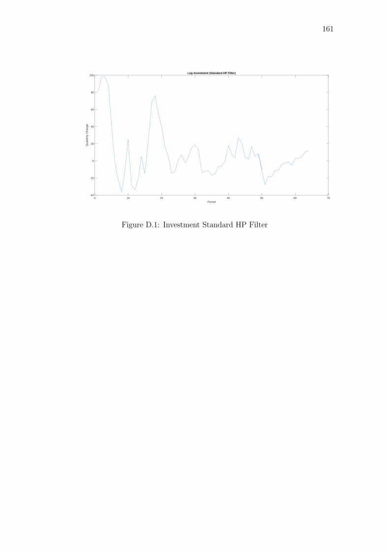
161

0 10 20 30 40 50 60 70

Period

-40

-20

0

20

40

60

80

100

Qua

rter

ly C

hang

e

Log Investment (Standard HP Filter)

Figure D.1: Investment Standard HP Filter

162

0 10 20 30 40 50 60 70

Period

-100

-80

-60

-40

-20

0

20

40

60

80

Qua

terly

Cha

nge

Log Investment (Modified HP Filter)

Figure D.2: Investment Modified HP Filter

0 10 20 30 40 50 60 70

Period

-40

-30

-20

-10

0

10

20

30

Qua

rter

ly C

hang

e

Log Consumption (Standard HP Filter)

Figure D.3: Consumption Standard HP Filter

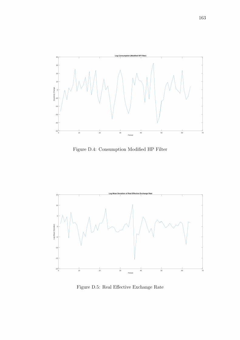
163

0 10 20 30 40 50 60 70

Period

-50

-40

-30

-20

-10

0

10

20

30

40

Qua

rter

ly C

hang

eLog Consumption (Modified HP Filter)

Figure D.4: Consumption Modified HP Filter

0 10 20 30 40 50 60 70

Period

-20

-15

-10

-5

0

5

10

15

Log

Mea

n D

evia

tion

Log Mean Deviation of Real Effective Exchange Rate

Figure D.5: Real Effective Exchange Rate

164

0 10 20 30 40 50 60 70

Period

-10

-8

-6

-4

-2

0

2

4

6

8

Per

cen

tConsumer Price Inflation

Figure D.6: Consumer Price Index

0 10 20 30 40 50 60 70

Period

-2

-1.5

-1

-0.5

0

0.5

1

1.5

2

2.5

Qua

terly

Cha

nge

Three- Month Deposit Rate

Figure D.7: Three-month Deposit Rate

Appendix E

Identification Diagnostics

eps_

gh

eps_gh

eps_

ah

eps_ah

eps_

msh

eps_msh

eps_

r

eps_r

eps_

pie

eps_pie

eps_

c

eps_c

eps_

mps

h

eps_mpsh

eps_

oil

eps_oil

eps_

psiC

eps_psiC

eps_

psiI

eps_psiI

eps_

mec

eps_mec

eps_

mei

eps_mei

rho_

ah

rho_ah

rho_

gh

rho_gh

rho_

msh

rho_msh

rho_

r

rho_r

rho_

c

rho_c

rho_

pie

rho_pie

rhoI

rhoI

rho_

rh

rho_rh

rho_

psiC

rho_psiC

rho_

psiI

rho_psiI

muh

muh

phi_

ih

phi_ih

sigm

ah

sigmah

habh

habh

xih

xih

lam

h

lamhth

eta

theta

alph

ahalphah

zeta

h

zetah

thet

aph

thetaph

thet

ash

thetash

prior_mean - Collinearity patterns with 1 parameter(s)0

0.1

0.2

0.3

0.4

0.5

0.6

0.7

0.8

0.9

1

Figure E.1: Pairwise Collinearity Patterns in DSGE Model

165

166

eps_

gheps_gh

eps_

ah

eps_ah

eps_

msh

eps_msh

eps_

r

eps_r

eps_

pie

eps_pie

eps_

c

eps_c

eps_

mps

h

eps_mpsh

eps_

oil

eps_oil

eps_

psiC

eps_psiC

eps_

psiI

eps_psiI

eps_

mec

eps_mec

eps_

mei

eps_mei

rho_

ah

rho_ah

rho_

gh

rho_gh

rho_

msh

rho_msh

rho_

r

rho_r

rho_

c

rho_c

rho_

pie

rho_pie

rhoI

rhoI

rho_

rh

rho_rh

rho_

psiC

rho_psiC

rho_

psiI

rho_psiI

muh

muh

phi_

ih

phi_ih

sigm

ah

sigmah

habh

habh

xih

xih

lam

h

lamh

thet

a

theta

alph

ah

alphah

zeta

h

zetah

thet

aph

thetaph

thet

ash

thetash


0.1

0.2

0.3

0.4

0.5

0.6

0.7

0.8

0.9

1


eps_

gh

eps_gh

eps_

ah

eps_ah

eps_

msh

eps_msh

eps_

r

eps_r

eps_

pie

eps_pie

eps_

c

eps_c

eps_

mps

h

eps_mpsh

eps_

oil

eps_oil

eps_

psiC

eps_psiC

eps_

psiI

eps_psiI

eps_

mec

eps_mec

eps_

mei

eps_mei

rho_

ah

rho_ah

rho_

gh

rho_gh

rho_

msh

rho_msh

rho_

r

rho_r

rho_

c

rho_c

rho_

pie

rho_pie

rhoI

rhoI

rho_

rh

rho_rh

rho_

psiC

rho_psiC

rho_

psiI

rho_psiI

muh

muh

phi_

ih

phi_ih

sigm

ah

sigmah

habh

habh

xih

xih

lam

h

lamh

thet

a

theta

alph

ah

alphah

zeta

h

zetah

thet

aph

thetaph

thet

ash

thetash


0.1

0.2

0.3

0.4

0.5

0.6

0.7

0.8

0.9

1


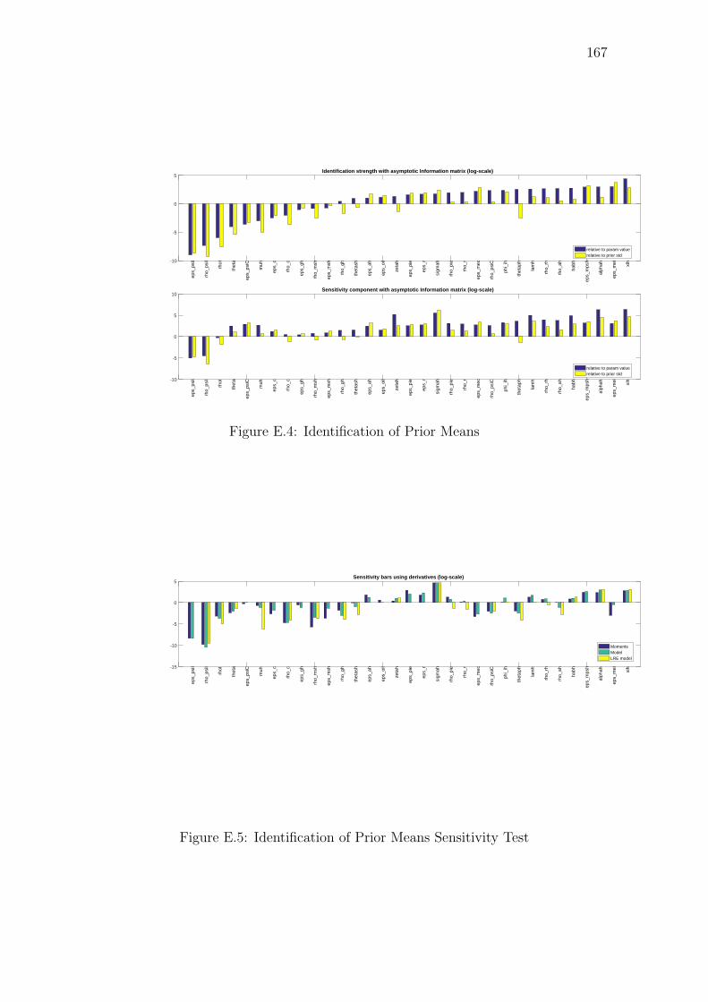
167

-10

-5

0

5Identification strength with asymptotic Information matrix (log-scale)

eps_

psiI

rho_

psiI

rhoI

thet

a

eps_

psiC

muh

eps_

c

rho_

c

eps_

gh

rho_

msh

eps_

msh

rho_

gh

thet

ash

eps_

ah

eps_

oil

zeta

h

eps_

pie

eps_

r

sigm

ah

rho_

pie

rho_

r

eps_

mec

rho_

psiC

phi_

ih

thet

aph

lam

h

rho_

rh

rho_

ah

habh

eps_

mps

h

alph

ah

eps_

mei xih

relative to param valuerelative to prior std

-10

-5

0

5

10Sensitivity component with asymptotic Information matrix (log-scale)

eps_

psiI

rho_

psiI

rhoI

thet

a

eps_

psiC

muh

eps_

c

rho_

c

eps_

gh

rho_

msh

eps_

msh

rho_

gh

thet

ash

eps_

ah

eps_

oil

zeta

h

eps_

pie

eps_

r

sigm

ah

rho_

pie

rho_

r

eps_

mec

rho_

psiC

phi_

ih

thet

aph

lam

h

rho_

rh

rho_

ah

habh

eps_

mps

h

alph

ah

eps_

mei xih

relative to param valuerelative to prior std

Figure E.4: Identification of Prior Means

-15

-10

-5

0

5Sensitivity bars using derivatives (log-scale)

eps_

psiI

rho_

psiI

rhoI

thet

a

eps_

psiC

muh

eps_

c

rho_

c

eps_

gh

rho_

msh

eps_

msh

rho_

gh

thet

ash

eps_

ah

eps_

oil

zeta

h

eps_

pie

eps_

r

sigm

ah

rho_

pie

rho_

r

eps_

mec

rho_

psiC

phi_

ih

thet

aph

lam

h

rho_

rh

rho_

ah

habh

eps_

mps

h

alph

ah

eps_

mei xih

MomentsModelLRE model

Figure E.5: Identification of Prior Means Sensitivity Test

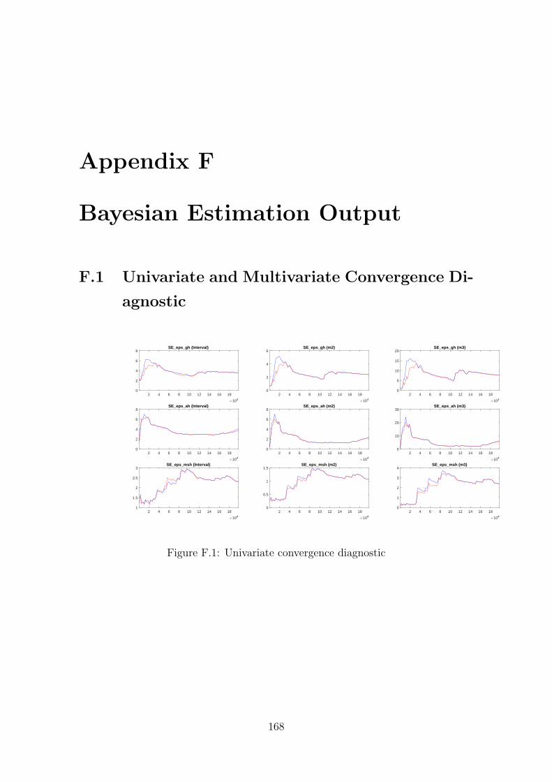
Appendix F

Bayesian Estimation Output

F.1 Univariate and Multivariate Convergence Di-

agnostic

2 4 6 8 10 12 14 16 18

×104

0

2

4

6

8SE_eps_gh (Interval)

2 4 6 8 10 12 14 16 18

×104

0

2

4

6SE_eps_gh (m2)

2 4 6 8 10 12 14 16 18

×104

0

5

10

15

20SE_eps_gh (m3)

2 4 6 8 10 12 14 16 18

×104

0

2

4

6

8SE_eps_ah (Interval)

2 4 6 8 10 12 14 16 18

×104

0

2

4

6

8SE_eps_ah (m2)

2 4 6 8 10 12 14 16 18

×104

0

10

20

30SE_eps_ah (m3)

2 4 6 8 10 12 14 16 18

×104

1

1.5

2

2.5

3SE_eps_msh (Interval)

2 4 6 8 10 12 14 16 18

×104

0

0.5

1

1.5SE_eps_msh (m2)

2 4 6 8 10 12 14 16 18

×104

0

1

2

3

4SE_eps_msh (m3)

Figure F.1: Univariate convergence diagnostic

168

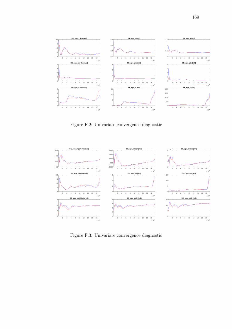
169

2 4 6 8 10 12 14 16 18

×104

1.4

1.6

1.8

2

2.2SE_eps_r (Interval)

2 4 6 8 10 12 14 16 18

×104

0.2

0.4

0.6

0.8SE_eps_r (m2)

2 4 6 8 10 12 14 16 18

×104

0

0.5

1

1.5SE_eps_r (m3)

2 4 6 8 10 12 14 16 18

×104

1

2

3

4

5SE_eps_pie (Interval)

2 4 6 8 10 12 14 16 18

×104

0

1

2

3SE_eps_pie (m2)

2 4 6 8 10 12 14 16 18

×104

0

2

4

6

8SE_eps_pie (m3)

2 4 6 8 10 12 14 16 18

×104

0

2

4

6

8SE_eps_c (Interval)

2 4 6 8 10 12 14 16 18

×104

0

5

10

15SE_eps_c (m2)

2 4 6 8 10 12 14 16 18

×104

0

50

100

150

200SE_eps_c (m3)


2 4 6 8 10 12 14 16 18

×104

0.2

0.25

0.3

0.35SE_eps_mpsh (Interval)

2 4 6 8 10 12 14 16 18

×104

0.008

0.01

0.012

0.014

0.016SE_eps_mpsh (m2)

2 4 6 8 10 12 14 16 18

×104

1

2

3

4×10-3 SE_eps_mpsh (m3)

2 4 6 8 10 12 14 16 18

×104

1.5

2

2.5

3

3.5SE_eps_oil (Interval)

2 4 6 8 10 12 14 16 18

×104

0

1

2

3SE_eps_oil (m2)

2 4 6 8 10 12 14 16 18

×104

0

5

10

15SE_eps_oil (m3)

2 4 6 8 10 12 14 16 18

×104

3

4

5

6SE_eps_psiC (Interval)

2 4 6 8 10 12 14 16 18

×104

1

2

3

4

5SE_eps_psiC (m2)

2 4 6 8 10 12 14 16 18

×104

0

5

10

15SE_eps_psiC (m3)


170

2 4 6 8 10 12 14 16 18

×104

2

4

6

8

10SE_eps_psiI (Interval)

2 4 6 8 10 12 14 16 18

×104

0

5

10

15SE_eps_psiI (m2)

2 4 6 8 10 12 14 16 18

×104

0

20

40

60SE_eps_psiI (m3)

2 4 6 8 10 12 14 16 18

×104

3

4

5

6SE_eps_mec (Interval)

2 4 6 8 10 12 14 16 18

×104

1

2

3

4

5SE_eps_mec (m2)

2 4 6 8 10 12 14 16 18

×104

0

5

10

15SE_eps_mec (m3)

2 4 6 8 10 12 14 16 18

×104

0

5

10

15SE_eps_mei (Interval)

2 4 6 8 10 12 14 16 18

×104

0

10

20

30SE_eps_mei (m2)

2 4 6 8 10 12 14 16 18

×104

0

50

100

150

200SE_eps_mei (m3)


2 4 6 8 10 12 14 16 18

×104

0.1

0.2

0.3

0.4rho_ah (Interval)

2 4 6 8 10 12 14 16 18

×104

0

0.005

0.01

0.015

0.02rho_ah (m2)

2 4 6 8 10 12 14 16 18

×104

0

1

2

3

4×10-3 rho_ah (m3)

2 4 6 8 10 12 14 16 18

×104

0.1

0.2

0.3

0.4rho_gh (Interval)

2 4 6 8 10 12 14 16 18

×104

0

0.005

0.01

0.015

0.02rho_gh (m2)

2 4 6 8 10 12 14 16 18

×104

0

1

2

3

4×10-3 rho_gh (m3)

2 4 6 8 10 12 14 16 18

×104

0.2

0.22

0.24

0.26

0.28rho_msh (Interval)

2 4 6 8 10 12 14 16 18

×104

6

8

10

12×10-3 rho_msh (m2)

2 4 6 8 10 12 14 16 18

×104

0.5

1

1.5

2×10-3 rho_msh (m3)


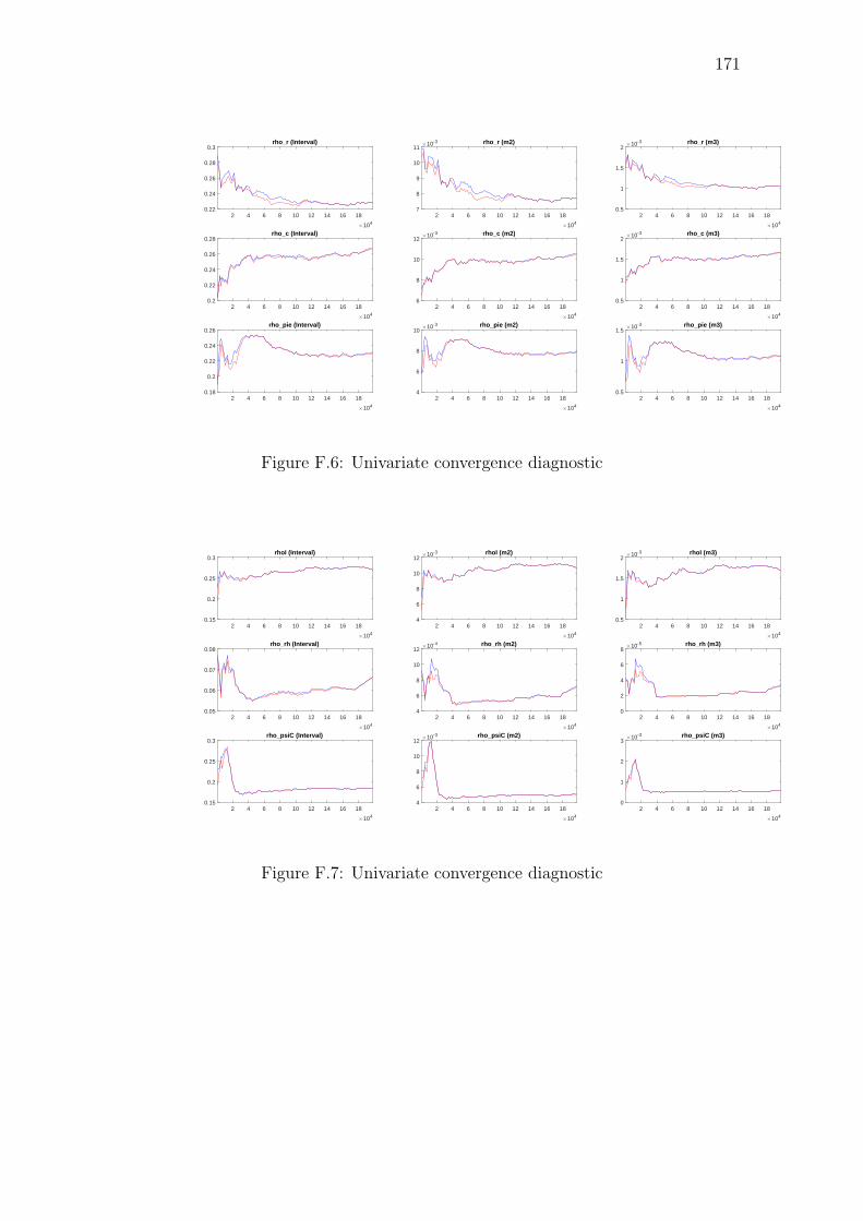
171

2 4 6 8 10 12 14 16 18

×104

0.22

0.24

0.26

0.28

0.3rho_r (Interval)

2 4 6 8 10 12 14 16 18

×104

7

8

9

10

11×10-3 rho_r (m2)

2 4 6 8 10 12 14 16 18

×104

0.5

1

1.5

2×10-3 rho_r (m3)

2 4 6 8 10 12 14 16 18

×104

0.2

0.22

0.24

0.26

0.28rho_c (Interval)

2 4 6 8 10 12 14 16 18

×104

6

8

10

12×10-3 rho_c (m2)

2 4 6 8 10 12 14 16 18

×104

0.5

1

1.5

2×10-3 rho_c (m3)

2 4 6 8 10 12 14 16 18

×104

0.18

0.2

0.22

0.24

0.26rho_pie (Interval)

2 4 6 8 10 12 14 16 18

×104

4

6

8

10×10-3 rho_pie (m2)

2 4 6 8 10 12 14 16 18

×104

0.5

1

1.5×10-3 rho_pie (m3)


2 4 6 8 10 12 14 16 18

×104

0.15

0.2

0.25

0.3rhoI (Interval)

2 4 6 8 10 12 14 16 18

×104

4

6

8

10

12×10-3 rhoI (m2)

2 4 6 8 10 12 14 16 18

×104

0.5

1

1.5

2×10-3 rhoI (m3)

2 4 6 8 10 12 14 16 18

×104

0.05

0.06

0.07

0.08rho_rh (Interval)

2 4 6 8 10 12 14 16 18

×104

4

6

8

10

12×10-4 rho_rh (m2)

2 4 6 8 10 12 14 16 18

×104

0

2

4

6

8×10-5 rho_rh (m3)

2 4 6 8 10 12 14 16 18

×104

0.15

0.2

0.25

0.3rho_psiC (Interval)

2 4 6 8 10 12 14 16 18

×104

4

6

8

10

12×10-3 rho_psiC (m2)

2 4 6 8 10 12 14 16 18

×104

0

1

2

3×10-3 rho_psiC (m3)


172

2 4 6 8 10 12 14 16 18

×104

0.22

0.24

0.26

0.28rho_psiI (Interval)

2 4 6 8 10 12 14 16 18

×104

7

8

9

10

11×10-3 rho_psiI (m2)

2 4 6 8 10 12 14 16 18

×104

1

1.2

1.4

1.6×10-3 rho_psiI (m3)

2 4 6 8 10 12 14 16 18

×104

0.2

0.4

0.6

0.8muh (Interval)

2 4 6 8 10 12 14 16 18

×104

0.02

0.04

0.06

0.08muh (m2)

2 4 6 8 10 12 14 16 18

×104

0

0.01

0.02

0.03

0.04muh (m3)

2 4 6 8 10 12 14 16 18

×104

0

2

4

6phi_ih (Interval)

2 4 6 8 10 12 14 16 18

×104

0

1

2

3

4phi_ih (m2)

2 4 6 8 10 12 14 16 18

×104

0

5

10phi_ih (m3)


2 4 6 8 10 12 14 16 18

×104

0.4

0.6

0.8

1sigmah (Interval)

2 4 6 8 10 12 14 16 18

×104

0

0.05

0.1

0.15

0.2sigmah (m2)

2 4 6 8 10 12 14 16 18

×104

0

0.05

0.1

0.15sigmah (m3)

2 4 6 8 10 12 14 16 18

×104

0.25

0.3

0.35

0.4habh (Interval)

2 4 6 8 10 12 14 16 18

×104

0.005

0.01

0.015

0.02habh (m2)

2 4 6 8 10 12 14 16 18

×104

1

2

3

4×10-3 habh (m3)

2 4 6 8 10 12 14 16 18

×104

0

0.1

0.2

0.3

0.4xih (Interval)

2 4 6 8 10 12 14 16 18

×104

0

0.005

0.01

0.015xih (m2)

2 4 6 8 10 12 14 16 18

×104

0

0.5

1

1.5

2×10-3 xih (m3)


173

2 4 6 8 10 12 14 16 18

×104

0.15

0.2

0.25

0.3lamh (Interval)

2 4 6 8 10 12 14 16 18

×104

4

6

8

10

12×10-3 lamh (m2)

2 4 6 8 10 12 14 16 18

×104

0

0.5

1

1.5

2×10-3 lamh (m3)

2 4 6 8 10 12 14 16 18

×104

0.15

0.2

0.25

0.3theta (Interval)

2 4 6 8 10 12 14 16 18

×104

6

7

8

9

10×10-3 theta (m2)

2 4 6 8 10 12 14 16 18

×104

0.8

1

1.2

1.4×10-3 theta (m3)

2 4 6 8 10 12 14 16 18

×104

0

0.1

0.2

0.3

0.4alphah (Interval)

2 4 6 8 10 12 14 16 18

×104

0

0.005

0.01

0.015

0.02alphah (m2)

2 4 6 8 10 12 14 16 18

×104

0

1

2

3×10-3 alphah (m3)


2 4 6 8 10 12 14 16 18

×104

0.8

1

1.2

1.4zetah (Interval)

2 4 6 8 10 12 14 16 18

×104

0.1

0.15

0.2

0.25

0.3zetah (m2)

2 4 6 8 10 12 14 16 18

×104

0.05

0.1

0.15

0.2

0.25zetah (m3)

2 4 6 8 10 12 14 16 18

×104

0.015

0.02

0.025

0.03

0.035thetaph (Interval)

2 4 6 8 10 12 14 16 18

×104

6

8

10

12×10-5 thetaph (m2)

2 4 6 8 10 12 14 16 18

×104

0.5

1

1.5

2×10-6 thetaph (m3)

2 4 6 8 10 12 14 16 18

×104

2

2.5

3

3.5×10-3 thetash (Interval)

2 4 6 8 10 12 14 16 18

×104

0.8

1

1.2

1.4

1.6×10-6 thetash (m2)

2 4 6 8 10 12 14 16 18

×104

1

2

3

4×10-9 thetash (m3)

Figure F.11: Multivariate convergence diagnostic

174

2 4 6 8 10 12 14 16 18

×104

0

10

20

30

40Interval

2 4 6 8 10 12 14 16 18

×104

0

50

100

150m2

2 4 6 8 10 12 14 16 18

×104

0

1000

2000

3000m3

Figure F.12: Multivariate convergence diagnostic

F.2 Priors and Posteriors

-2 0 2 4 6 8 10 12 140

0.2

0.4

SE_eps_gh

-2 0 2 4 6 8 10 120

0.2

0.4

0.6

SE_eps_ah

0 2 4 6 80

0.2

0.4

0.6

SE_eps_msh

0 2 4 6 8 10 12 140

0.2

0.4

0.6

SE_eps_r

0 2 4 6 8 10 12 140

0.2

0.4

0.6

0.8SE_eps_pie

-5 0 5 10 15 20 25 30 350

0.2

0.4

0.6

SE_eps_c

2 4 6 8 10 12 140

1

2

3

4

SE_eps_mpsh

0 5 10 150

0.2

0.4

0.6SE_eps_oil

0 5 10 15 200

0.2

0.4

SE_eps_psiC

Figure F.13: Priors and Posteriors

175

-2 0 2 4 6 8 10 12 140

0.2

0.4

SE_eps_psiI

5 10 15 20 250

0.5

1

1.5SE_eps_mec

2 4 6 8 10 12 14 160

0.5

1

1.5SE_eps_mei

0.3 0.4 0.5 0.6 0.7 0.8 0.9 1 1.10

2

4

rho_ah

0.2 0.4 0.6 0.8 1 1.20

2

4

rho_gh

0 0.2 0.4 0.6 0.8 10

1

2

3

4

rho_msh

0 0.2 0.4 0.6 0.8 10

1

2

3

4

rho_r

0 0.2 0.4 0.6 0.8 10

1

2

3

4

rho_c

0 0.2 0.4 0.6 0.80

1

2

3

4

rho_pie


0 0.2 0.4 0.6 0.8 10

1

2

3

4

rhoI

0.3 0.4 0.5 0.6 0.7 0.8 0.90

5

10

15

rho_rh

0.4 0.5 0.6 0.7 0.8 0.9 1 1.10

2

4

6rho_psiC

0.2 0.4 0.6 0.8 1 1.20

1

2

3

4

rho_psiI

0.5 1 1.5 2 2.50

0.5

1

1.5

2

muh

0 2 4 6 8 10 12 140

0.5

1

1.5

2phi_ih

0 2 4 6 8 100

0.5

1

sigmah

0.2 0.4 0.6 0.8 1 1.20

1

2

3

4

habh

0.2 0.3 0.4 0.5 0.6 0.7 0.8 0.90

2

4

xih


176

0 0.2 0.4 0.6 0.80

1

2

3

4

lamh

0 0.2 0.4 0.6 0.80

1

2

3

4

theta

0.3 0.4 0.5 0.6 0.7 0.80

20

40

alphah

4 5 6 7 8 9 100

0.2

0.4

0.6

0.8

zetah

1.44 1.46 1.48 1.5 1.52 1.54 1.560

10

20

30

40

thetaph

0 2 4 6 8 10 12

×10-3

0

200

400

thetash


Bibliography

Adebiyi, M. and Mordi, C. (2010). Estimating a Small Scale Macroeconometric

Model (SSMM) for Nigeria. CBN Occasional Paper, (39), 1–45.

Adebiyi, M. and Mordi, C. (2012). A Dynamic Stochastic General Equilibrium

(DSGE) Model of Exchange Rate Pass-Through to Domestic Inflation in Nigeria.

ECOMOD Conference 2012.

Adolfson, M., Laseen, S., Linde, J., and Villani, M. (2008). Evaluating an Estimated

New Keynesian Small Open Economy Model. Journal of Economic Dynamics and

Control, 32(8), 2690–2721.

Agenor, R. and Montiel, P. (1999). Development Macroeconomics. 2 edition.

Aguiar, M. and Gopinath, G. (2007). Emerging Market Business Cycles: The Cycle

is the Trend. Journal of Political Economy, 115(1).

Aliyev, R. (2012). Monetary Policy in Resource-Rich Developing Economies.

CERGE-EI Prague.

Anand, R., Khera, P., Munkacsi, Z., and Saxegaard, M. (2015). Structural Reforms,

Openness and the Informal Economy. IMF Working Paper.

Anderson, T. W. and Rubin, H. (1949). Estimation of the Parameters of a Single

Equation in a Complete System of Stochastic Equations. Annals of Mathematical

Statistics, 20(1), 46–63.

177

178

Barro, R. and Sala-i-Martin, X. (2004). Economic Growth. Second Edition, McGraw-

Hill.

Batini, N. (2004). Achieving and Maintaining Price Stability in Nigeria. IMF

Working Paper, WP/04/97.

Batini, N., Justiniano, A., Levine, P., and Pearlman, J. (2006). Robust Inflation-

Forecast-Based Rules to Shield against Indeterminacy. Journal of Economic Dy-

namics and Control, 30, 1491–1526.

Batini, N., Levine, P., and Pearlman, J. (2007). Monetary Rules in Emerging

Economies with Financial Market Imperfections. Presented to the NBER Confer-

ence on International Dimensions of Monetary Policy, S’Agaro, Catalonia, Spain,

June 11-13, 2007 and NBER Conference Volume, International Dimensions of

Monetary Policy, ed. J. Gali and M. Gertler.

Batini, N., Levine, P., and Pearlman, J. (2009). Monetary and Fiscal Rules in an

Emerging Small Open Economy. IMF Working Paper, WP/09/22.

Batini, N., Kim, Y.-B., Levine, P., and Lotti, E. (2010). Informal Labour and Credit

Markets: A Survey. IMF Working Paper, WP/10/42.

Benati, L. and Surico, P. (2009). VAR Analysis and the Great Moderation. American

Economic Review, 99(4), 1636–1652.

Benes, J., Berg, A., Portillo, R., and Vavra, D. (2015). Modeling Sterilized In-

terventions and Balance Sheet Effects of Monetary Policy in a New-Keynesian

Framework. Open Economies Review, 26(1), 81–108.

Benigno, P. (2001). Price Stability with Imperfect Financial Integration. CEPR

Discussion Paper no. 2854.

Berg, A., Portillo, R., Yang, S., and Zanna, L. (2013). Public Investment in

179

Resource-Abundant Developing Countries. IMF Economic Review, 61(1), 92–

129.

Bergholt, D. (2014). Monetary Policy in Oil Exporting Economies. Working paper,

CAMP Working Paper Series No 5.

Bernanke, B., Gertler, M., and Watson, M. (1997). Systematic Monetary Policy and

the Effects of Oil Price Shocks. Brookings Papers on Economic Activity, 28(1),

91–157.

Bilbiie, F. (2008). Limited Asset Markets Participation, Monetary Policy and (In-

verted) Aggregate Demand Logic. Journal of Economic Theory, 140(1), 162–196.

Blanchard, O. J. (2008). The State of Macro. National Bureau of Economic Research

Working Paper 14259.

Boerma, J. (2014). Openness and the (Inverted) Aggregate Demand Logic. De

Nederlandsche Bank Working Papers No. 436.

Brooks, P. and Gelman, A. (1998). General Methods for Monitoring Convergence of

Iterative Simulations. Journal of Computational and Graphical Statistics,, 7(4),

434–455.

Bry, G. and Boschan, C. (1971). Interpretation and Analysis of Time Series Scatters.

The American Statistician, 25(2), 29–33.

Buffie, E., Berg, A., Pattillo, C., Portillo, R., and Zanna, F. (2012). Public In-

vestment, Growth, and Debt Sustainability: Putting Together the Pieces. IMF

Working Paper 12/144, International Monetary Fund,Washington, D.C.

Burns, A. F. and Mitchell, W. C. (1946). Measuring Business Cycles. New York,

New York: National Bureau of Economic Research.

Business Monitor International (2010). Nigeria infrastructure report q3. Technical

report.

180

Caballero, R. J. (2010). Macroeconomics after the Crisis: Time to Deal with the

Pretense-of-Knowledge Syndrome. Journal of Economic Perspectives, 24(4), 85–

102.

Calvo, G. A. (1983). Staggered Contracts in a Utility-Maximizing Framework. Jour-

nal of Monetary Economics, 12, 383–398.

Calvo, G. A. (1998). Capital Flows and Capital-Markets Crises. Journal of Applied

Econometrics, 1(1), 35–54.

Canova, F. (1998). Detrending and Business Cycle Facts. Journal of Monetary

Economics, 41(3), 533–540.

Canova, F. (2007). Methods for Applied Macroeconomic Research. Princeton Uni-

versity Press New Jersey, 2 edition. Pg. 370.

Canova, F. and Sala, L. (2009). Back to Square One: Identification issues in DSGE

models. Journal of Monetary Economics, 56(4), 431–449.

Castelnuovo, E. and Fanelli, L. (2014). Monetary Policy, Indeterminacy and Iden-

tification Failures in the U.S.: Results from a Robust Test. Journal of Applied

Econometrics.

Catao, L. and Chang, R. (2013). Monetary Policy Rules for Commodity Traders.

IMF Economic Review, 61(1), 52–91.

CBN (2010). The Changing Structure of the Nigerian Economy. Central Bank of

Nigeria, 2 edition.

CBN (2013). Dynamic Stochastic General Equilibrium (DSGE) Model for Monetary

Policy Analysis in Nigeria. CBN.

Central Bank of Nigeria (2014). Statistical Bullentin, Golden Jubilee Edition. Tech-

nical report.

181

Choudhary, A., Hanif, N., and Iqbal, J. (2013). On Smoothing Macroeconomic

Time Series using HP and Modified HP Filter. Munich Personal RePEc Archive,

45630, 1–15.

Christiano, L. J. and Fitzgerald, T. J. (2003). The Band Pass Filter. International

Economic Review, 44, 435–465.

Christiano, L. L. and Harrison, S. G. (1999). Chaos, Sunspots and Automatic

Stabilizers. Journal of Monetary Economics, 44(1), 3–31.

Clarida, R. (2014). Monetary Policy in Open Economies: Practical Perspectives for

Pragmatic Central Bankers. NBER Working Paper No. 20545.

Clarida, R., Gali, J., and Gertler, M. (1998). Monetary Policy Rules in Practice:

Some International Evidence. European Economic Review, 42(6), 1033–1067.

Clarida, R., Galı, J., and Gertler, M. (1999). The Science of Monetary Policy: A

New Keynesian Perspective. Journal of Economic Literature, 37(4), 1661–1707.

Clarida, R., Galı, J., and Gertler, M. (2000). Monetary Policy Rules and Macroe-

conomic Stability: Evidence and Some Theory. Quarterly Journal of Economics,

115(1), 147–80.

Clarida, R., Gali, J., and Gertler, M. (2001). Optimal Monetary Policy in Open

versus Closed Economies: An Integrated Approach. AEA Papers and Proceedings,

4, 248–252.

Cochrane, J. H. (2007). Identification with Taylor Rules: A Critical Review. Na-

tional Bureau of Economic Research(NBER) Working Paper 13410.

Cochrane, J. H. (2011). Determinacy and Identification with Taylor Rules. Journal

of Political Economy, 119(3), 565–615.

182

Cogley, T. (2001). Estimating and Testing Rational Expectations Models when the

Trend Specification is Uncertain. Journal of Economic Dynamics and Control,

25, 1485–1525.

Cogley, T. and Nason, J. M. (1995). Effects of the Hodrick-Prescott Filter on Trend

and Difference Stationary Time Series: Implications for Business Cycle Research.

Journal of Economic Dynamics and Control, 19(1-2), 253–278.

Collier, P., Soludo, C., and Pattillo, C. (2008). Economic Policy Options for a

Prosperous Nigeria. Palgrave Macmillan.

Craven, P. and Wahba, G. (1979). Smoothing noisy data with spline functions:

estimating the correct degree of smoothing by the method of generalized cross-

validation. Numerische Mathematik, 31, 377–403.

Currie, D. and Levine, P. L. (1993). Rules, Reputation and Macroeconomic Policy

Coordination. Cambridge University Press.

Devarajan, S., Dissou, Y., Go, D., and Robinson, S. (2015). Budget Rules and

Resource Booms and Busts: A Dynamic Stochastic General Equilibrium Analysis.

CSAE Conference 2015: Economic Development in Africa.

Du Plessis, S., Smit, B., and Sturzenegger, F. (2007). The Cyclicality of Monetary

and Fiscal Policy in South Africa Since 1994. Journal of Money, Credit and

Banking, 75(3), 391–411.

Dufour, J.-M., Khalaf, L., and Kichian, M. (2013). Identification-Robust Analysis of

DSGE and Structural Macroeconomic Models. Journal of Monetary Economics,

60, 340–350.

EFInA (2010). Access to Financial Services in Nigeria. Survey by Enhancing Fi-

nancial Innovation and Access (EFInA).

183

Fernandez-Villaverde, J. (2009). The Econometrics of DSGE Models. CEPR Dis-

cussion Paper No. 7159.

Fernandez-Villaverde, J., Gordon, G., Guerron-Quintana, P. A., and Rubio-Ramırez,

J. (2012). Nonlinear Adventures at the Zero Lower Bound. NBERWorking Papers

18058, National Bureau of Economic Research, Inc.

Ferrero, A. and Seneca, M. (2015). Monetary Policy in Resource-Rich Economiess.

Norges Bank Research Working Paper.

Gabriel, V., Levine, P., Pearlman, J., and Yang, B. (2010). An Estimated Model

of the Indian Economy . University of Surrey Discussion Paper DP 12/10 and

forthcoming in the “Handbook of the Indian Economy”, edited by Chetan Ghate,

Oxford University Press .

Gabriel, V., Levine, P., and Yang, B. (2016). An Estimated DSGE Open-economy

Model of the Indian Economy with Financial Frictions. Discussion Paper in Eco-

nomics, DP 03/16, School of Economics University of Surrey Guildford.

Gali, J. (2008). Monetary Policy, Inflation and the Business Cycle. Princeton

University Press.

Gali, J. and Monacelli, T. (2005). Monetary Policy and Exchange Rate Volatility

in a Small Open Economy. Review of Economic Studies, 72, 707 – 734.

Gali, J., Lopez-Salido, J., and Valles, J. (2007). Understanding the Effects of Govern-

ment Spending on Consumption. Journal of the European Economic Association,

5(1), 227–270.

Garca-Cicco, J., Pancrazi, R., and Uribe, M. (2010). Real Business Cycles in Emerg-

ing Countries? American Economic Review, 100(5), 2510–2531.

Garcia, C. (2010). Is the Phillips Curve Useful for Monetary Policy in Nigeria?

CBN Occasional Paper, (38), 1–36.

184

Gertler, M., Gilchrist, S., and Natalucci, F. M. (2003). External Constraints on

Monetary Policy and the Financial Accelerator. NBER Working Paper No. 10128.

Hamilton, J. D. (1983). Oil and the Macroeconomy Since World War II. Journal of

Political Economy, 91(2), 1103–1123.

Harvey, A. C. and Jaeger, A. (1993). Detrending, Stylized Facts and the Business

Cycle. Journal of Applied Econometrics, 8, 231–247.

Harvey, A. C. and Koopman, S. J. (2000). Signal Extraction and the Formulation

of Unobserved Components Models. Econometrics Journal, 3(1), 87–107.

Hodrick, R. J. and Prescott, E. C. (1997). Postwar U.S. Business Cycle: An Em-

pirical Investigation. Journal of Money, Credit and Banking, 29, 1–16.

International Monetary Fund (2012). Commodity price swings and commodity ex-

porters. World Economic Outlook, International Monetary Fund.

Kama, U. and Adigun, M. (2013). Financial Inclusion in Nigeria: Issues and Chal-

lenges. Central Bank of Nigeria Occasional Papers, (45).

Kleibergen, F. (2005). Testing Parameters in GMM without Assuming That They

are Identified. Econometrica, 73(4), 1103–1123.

Kleibergen, F. and Mavroeidis, S. (2009). Weak Instrument Robust Tests in GMM

and the New Keynesian Phillips Curve. Journal of Business and Economic Statis-

tics, 27(3), 293–311.

Kollman, R. (2015). Tractable Latent State Filtering for Non-Linear DSGE Models

Using a Second-Order Approximation and Pruning. Computational Economics,

45(2), 239–260.

Kose, M., Otrok, C., and Prasad, E. (2008). Global Business Cycles: Convergence

or Decoupling? Working paper, International Monetary Fund.

185

Kosuki, A. (2001). Optimal Monetary Policy Response to Relative-Price Changes.

Journal of Monetary of Economics, 48(1), 55 – 80.

Kydland, F. and Zarazaga, C. (2002). Argentina’s Lost Decade. Review of Economic

Dynamics, 5(1).

Leeper, E. M. (1991). Equilibria under ‘Active’ and ‘Passive’ Monetary and Fiscal

Policies. Journal of Monetary Economics, 27, 129–147.

Levine, P. and Pearlman, J. (2010). Robust Monetary Rules under Unstructured

and Structured Uncertainty. Journal of Economic Dynamics and Control, 34(3),

456–471.

Levine, P., Pearlman, J., and Pierse, R. (2008a). Linear-Quadratic Approximation,

Efficiency and Target-Implementability. Journal of Economic Dynamics and Con-

trol, 32, 3315–3349.

Levine, P., McAdam, P., and Pearlman, J. (2008b). Quantifying and Sustaining

Welfare Gains from Monetary Commitment. Journal of Monetary Economics,

55(7), 1253–1276.

Levine, P., McAdam, P., and Pearlman, J. (2012). Probability Models and Robust

Policy Rules. European Economic Review, 56(2), 246 – 262.

Lubik, T. A. and Schorfheide, F. (2004). Testing for Indeterminacy: An Application

to U.S. Monetary Policy. American Economic Review, 94, 190–217.

Lucas, Jr., R. E. (1976). Econometric Policy Evaluation: A Critique. In K. Brun-

ner and A. Meltzer, editors, The Phillips Curve and Labor Markets. Carnegie-

Rochester Conf. Series on Public Policy.

Mankiw, N. G. (2002). American Economic Policy in the 1990s, chapter US Mone-

tary Policy During the 90s. Cambridge, MA: MIT Press.

186

Massman, M., Mitchell, J., and Weale, M. (2003). Business Cycles and Turning

Points: A Survey of Statistical Techniques. National Institute Economic Review,

183(1), 90–106.

Mavroeidis, S. (2010). Monetary Policy Rules and Macroeconomic Stability: Some

New Evidence. American Economic Review, 100(1), 491–503.

Mbutor, M. O. and Uba, I. A. (2013). The Impact of Financial Inclusion on Monetary

Policy in Nigeria. Journal of Economics and International Finance, 5(8), 318–326.

McDermott, C. J. (1997). An Automatic Method for Choosing the Smoothing Pa-

rameter in the HP filter. Unpublished, International Monetary Fund, Washington,

DC.

McKnight, S., Mihailov, A., and Pompa Rangel, A. (2016). What Do Latin American

Inflation Targeters Care About? A Comparative Bayesian Estimation of Central

Bank Preferences. Economics & Management Discussion Paper 129, University

of Reading.

Medina, J. P. and Soto, C. (2007). Copper Price, Fiscal Policy and Business Cycle

in Chile. Central Bank of Chile, Working Paper no. 458.

Melina, G., Yang, S., and Zanna, L. (2014). Debt Sustainability, Public Investment,

and Natural Resources in Developing Countries: the DIGNAR Model. Working

paper, International Monetary Fund.

Moolman, E. (2004). A Markov Switching Regime Model of the South African

Business Cycle. Economic Modelling, 21(4), 631–646.

Muth, J. F. (1961). Rational Expectations and the Theory of Price Movements.

Econometrica, 29(3), 315–335.

NBS (2015a). Employment (Job) Creation Survey, 3rd Quarter. National Bureau

of Statistics Nigeria - Survey.

187

NBS (2015b). Foreign Trade Statistics Quarter One. National Bureau of Statistics

Nigeria - Survey.

Oladipo, O. (2007). Exchange Rate Pass-Through: A Case Study of a Small Open

Economy. Global Economy Journal, 7(3).

Orphanides, A. (1999). The quest for prosperity without inflation. mimeo, Federal

Reserve Board.

Oyinlola, M. and Adetunji, M. (2009). A Bound Testing Analysis of Exchange

Rate Pass-Through to Aggregate Import Prices in Nigeria: 1980-2006. Journal of

Economic Development, 34(2).

Richmond, C., Yackovlev, I., and Yang, S. (2013). Investing Volatile Oil Revenues

in Capital-Scare Economies: An Application to Angola. Working paper, Interna-

tional Monetary Fund.

Schorfheide, F. (2000). Loss Function-Based Evaluation of DSGE Models. Journal

of Applied Econometrics, 15(6), 645–670.

Smets, F. and Wouters, R. (2003). An Estimated Stochastic Dynamic General Equi-

librium Model of the Euro Area. Journal of the European Economic Association,

1(5), 1123–1175.

Stock, J. H. and Wright, J. H. (2000). GMM with Weak Identification. Economet-

rica, 68(5), 1055–1096.

Taylor, J. B. (1983). Rational Expectations Models in Macroeconomics. National

Bureau of Economic Research(NBER) Working Paper 1224.

Taylor, J. B. (1993). Discretion versus Policy Rules in Practice. Carnegie-Rochester

Conference Series on Public Policy, 39, 195–214.

188

Tolulope, A. O. and Ajilore, T. (2013). Inflation Targeting Monetary Policy Rule

in Nigeria: Estimates of the Policy Reaction Function. International Journal of

Economics and Finance, 5(7), http://dx.doi.org/10.5539/ijef.v5n7p139.

van der Ploeg, F. and Venables, A. J. (2012). Natural Resource Wealth: The

Challenge of Managing a Windfall. Annual Review of Economics, 4, 315–337.

Vasconez, V. (2014). What if Oil is les Substitutable? A New-Keynesian Model with

Oil, Price and Wage Stickiness including Capital Accumulation. CIMS Conference

Proceeding.

Vasudevan, A. (2014). Central Banking for Emerging Market Economies: A Relook

in the Context of the Global Financial Crisis. Academic Foundation, 2 edition.

Villarreal, R. (2007). Essays on Monetary Policy in Oil-Producing Economies. Ph.d.

thesis, Princeton University.

Wills, S. (2013). Optimal Monetary Responses to Oil Discoveries. OxCarre Research

Paper, 121, 248–252.

Woodford, M. (2003). Foundations of a Theory of Monetary Policy. Princeton

University Press.

World Bank (1998). Human Development Report. Technical report, The World

Bank, Washington DC.

Yang, B. (2008). Dynamic Stochastic General Equilibrium Modelling: Applications

to Developed and Developing Economies. Ph.d. thesis, University of Surrey.

Documents

ESTIMATED AND OPTIMIZED MONETARY POLICY RULES FOR …epubs.surrey.ac.uk/844884/1/PhD_Thesis_Iklaga_Fred_Economics_D… · ESTIMATED AND OPTIMIZED MONETARY POLICY RULES FOR RESOURCE-RICH