ESTIMATED AND ANALYSIS OF THE ... - Science …thescipub.com/PDF/ajassp.2014.1542.1552.pdf · ... 21030 Kuala Terengganu, Terengganu, Malaysia Science ... 21030 Kuala Terengganu,

American Journal of Applied Sciences 11 (9): 1542-1552, 2014 ISSN: 1546-9239 © 2014 L. MuhamadSafiih et al., This open access article is distributed under a Creative Commons Attribution (CC-BY) 3.0 license doi:10.3844/ajassp.2014.1542.1552 Published Online 11 (9) 2014 (http://www.thescipub.com/ajas.toc)

Corresponding Author: L. MuhamadSafiih, School of Informatics and Applied Mathematics, Institute of Marine Biotechnology, University Malaysia Terengganu, 21030 Kuala Terengganu, Terengganu, Malaysia

1542 Science Publications

AJAS

ESTIMATED AND ANALYSIS OF THE RELATIONSHIP BETWEEN THE ENDOGENOUS AND EXOGENOUS

VARIABLES USING FUZZY SEMI-PARAMETRIC SAMPLE SELECTION MODEL

1L. MuhamadSafiih, 2A.A. Kamil and 3M.T. Abu Osman

1School of Informatics and Applied Mathematics, Institute of Marine Biotechnology, University Malaysia Terengganu, 21030 Kuala Terengganu, Terengganu, Malaysia

2School of Distance Education, University Sains Malaysia, 11800 USM Penang, Malaysia 3Department of Computer Sceince, Kulliayyah Information and Communication Technology,

International Islamic University Malaysia, P.O.Box 10, 50728 Kuala Lumpur, Malaysia

Received 2014-02-10; Revised 2014-07-08; Accepted 2014-07-15

ABSTRACT

An important progress within the last decade in the development of the selectivity model approach to overcome the inconsistent results if the distributional assumptions of the errors terms are made this problem is through the use of semi-parametric method. However, the uncertainties and ambiguities exist in the models, particularly the relationship between the endogenous and exogenous variables. A new framework of the relationship between the endogenous and exogenous variables of semi-parametric sample selection model using the concept of fuzzy modelling is introduced. Through this approach, a flexible fuzzy concept hybrid with the semi-parametric sample selection models known as Fuzzy Semi-Parametric Sample Selection Model (FSPSSM). The elements of vagueness and uncertainty in the models are represented in the model construction, as a way of increasing the available information to produce a more accurate model. This led to the development of the convergence theorem presented in the form of triangular fuzzy numbers to be used in the model. Besides that, proofs of the theorems are presented. An algorithm using the concept of fuzzy modelling is developed. The effectiveness of the estimators for this model is investigated. Monte Carlo simulation revealed that consistency depends on bandwidth parameter. When bandwidth parameters, c are increased from 0.1, 0.5, 0.75 and 1 as the numbers of N increased (from 100 to 200 and increased to 500), the values of mean approaches (closed to) the real parameter. Through the bandwidth parameter also reveals that the estimated parameter is efficient, i.e., the S.D, MSE and RMSE values become smaller as N increased. In particular, the estimated parameter becomes consistent and efficient as the bandwidth parameters approaches to infinity, c→∞ as the number of observations, n tend to infinity, n→∞. Keywords: Selectivity Model, Semi-Parametric, Fuzzy Concept, Bandwidth, Monte Carlo

1. INTRODUCTION

The sample selection model or the selectivity model introduced by Heckman (1979) is one of the most successful regression models if applied together with other models. This model is a combination of the probit and regression models. The earlier studies on this model focused

on the parametric approach. However, the standard approach of estimating sample selection model shows inconsistent results if the distributional assumptions of the errors terms are made. Hence, an important progress within the last decade in the development of an alternative approach to overcome this problem is through the use of semi-parametric method (Andrews (1991; Cosslett, 1990;

L. MuhamadSafiih et al. / American Journal of Applied Sciences 11 (9): 1542-1552, 2014


AJAS

Gerfin, 1996; Ichimura and Lee, 1991; Khan and Powell, 2001; Klein and Spady, 1993; Lee and Vella, 2006; Martins, 2001; Powell, 1987; Powell et al., 1989).

Although semi-parametric method of selectivity model is established, there still exist a basic problem of intrinsic features, such as uncertainty and ambiguity particularly in the relationship between the endogenous and exogenous variables. Therefore, it will disrupt the ability and effectiveness of the model proceeded to give the estimated value that can explain the actual situation of a phenomenon. These are questions and problems that have yet to be explored and the main pillar of this study. A new framework of the relationship between the endogenous and exogenous variables of semi-parametric sample selection model using the concept of fuzzy modelling by Zadeh (1965) is introduced. Through this approach, a flexible fuzzy concept hybrid with the semi-parametric sample selection models known as Fuzzy Semi-Parametric Sample Selection Model (FSPSSM). Hence, an alternative way to deal with this uncertainty and ambiguity is to use fuzzy concepts introduced by Zadeh (1965).

The purpose of this chapter is twofold; firstly, to provide a better understanding of the magnitude of consistency as well as efficiency, when the new modeling of FSPSSM is implemented under normality assumption. It is then extended to verify the inconsistency of the model when it does not follow the assumption of the normal distribution. Secondly, is to provide the magnitude of the consistency under FSPSSM. For this purpose, the bandwidth parameter of Powell (1987) model is used. To achieve these aims, Monte Carlo simulations using R language programming by Safiih (2013) and as well as the estimator introduced by (Powell et al., 1989; Powell, 1987) which are hybrid with fuzzy concept is developed.

2. MATRIALS AND METHODS

2.1. The Semi-parametric Sample Selection Model (SPSSM)

The semi-parametric sample selection model is a hybrid between the two sides of the semi-parametric approach, i.e., it combines some advantages of both fully parametric and the completely nonparametric approaches. The first model, i.e., participation equation is estimated by the parametric method, while the outcome equation is estimated by the nonparametric method. For instance, (Newey et al., 1990; Martins, 2001) used a two-step semi-parametric approach of model (1). The Semi-Parametric Sample Selection Model (SPSSM) can be written as:

* '

* '

*

1 0

0

; 1,...,

sp spi i

i i isp sp sp

ispisp

i i isp sp sp

z w

if d x ud

otherwise

z z d i N

γ ε

β

= +

= + >=

= =

(1)

where,

ispd and

ispz are dependent variables

ispx and

ispw are

vectors of remaining exogenous variablesγandβare unknown parameter vectors

ispε and

ispu are error terms. It

generalises the Heckman’s two-step procedure, i.e., in the first step, the participation equation is estimated semi-parametrically using the estimator proposed by Klein and Spady (1993). The results from this first step are used to construct a nonparametric correction term for selectivity of wage equation in the second step. The difference between parametric and semi-parametric approaches comes in the form of weaker assumption of the error term. The two-step estimation procedure refers to the estimation of the participant and the outcome equations as mention in Lola et al. (2009). Consider the binary selection model and proceeds by specifying the parametric part of the model. Order the N observations such that the first 1,...,n observations represent participants with di = 1 and yiobserved. The remaining observations were the non-participants with di = 0 and yi unobserved.

In this study, the semi-parametric method in Equation 1 is considered. As with the Safiih (2013) paper of FPSSM, this method involves two steps. In the first step, the parameter, β in the participation equation is estimated using Density Weighted Average Derivative Estimator (DWADE) and in the second step, Powell (1987) estimator in the outcome equation is used to estimate the parameter, γ. The DWADE which was proposed by Powell et al. (1989) is used to estimate parameter βin the first step of Equation 1. This estimator is based onsample analogues of the product moment representation of the average derivations and is constructed using nonparametrickernel estimators of the density of the regressors. However, a practical interest of weighted average derivatives is that they are proportional to coefficients vector βin the index function. Powell estimatorproposed by Powell (1987) is used to estimate parameter γin the second step of Equation 1. Powell (1987) considered asemi-parametric selection model that combines the two-equation structure with the following weak distribution alas sumption about the joint distribution of the error terms with the form:

( )'( , | ) , |i i i i i if u w f u wε ε γ= (2)



AJAS

It is assumed that the joint density of εi, ui (conditional on wi) is smooth but with unknown function f(.). Hence it depends on wionly through the linear model, i.e., 'iwγ .

Based on these assumptions, the regression function for the observed outcome zi takes the following form:

* *

' '

' '

( | ) ( | , 0)

( | , )

( )

i i i i i

i i i i i

i i

E z x E z w d

w E u w x

w x

γ β εγ λ β

= >

= + > −

= +

where, λ(.) is an known smooth function. Ideally, given two observations i and j with wi ≠ wj and the condition of ' '

i jw wγ = γ the unknown function λ(.) canbe differentiated

by subtracting the regression functions for i and j:

* *

' '

( ) ( )

( ) ' ( ) ( )

( ) '

i i j j

i j i j

i j

E z w w E z w w

w w x x

w w

γ λ β λ β

γ

= − = =

= + −

= −

This is the basic idea underlying the estimator of γ as

proposed by Powell (1987):

1

1 1

1

1 1

ˆ ˆ ( )( )`2

ˆ. ( ) ( )2

N N

powell ij i j i ji j i

N N

ij i j i ji j i

nN w w w w

nN w w z z

γ ϖ

ϖ

−

= = +

−

= = +

= − −

− −

∑ ∑

∑ ∑

(3)

These weights of ˆ ijϖ

are calculated, γ̂

can be

estimated by a weighted least-squares estimator, where ' 'ˆ ˆ1

ˆ i jij

x xN k

c c

β βϖ

− =

with symmetric kernel function

k(.), bandwidth c. and the estimate parameter β̂ has

already obtained previously, as an estimate of β. Under Equation 2, we obtain a single index model for the decision equation in place of the probit model (probit step) in the parametric case Equation 4:

' '( ( 0 | ) 1) ( )i i iP d d x g x β> = = (4)

where, g(.) is unknown but a smooth function. Estimators for β̂

in this model have been discussed in section 2.5, as

the first step of the semi-parametric procedure. Given γ̂ , the second step of the semi-parametric procedure consists of estimating γ using Equation 3.

Powell (1987) proved that the ̂powellγ estimator in

Equation 3 is n -consistent and asymptotically normal under an appropriate chosen Kernel (or bandwidth c). This result provided a n -consistent and asymptotically normal distribution as Equation 5:

ˆ( ) (0, )dpowell powelln N Vγ γ− → (5)

where, d→ denotes convergence in distribution. The Powell procedure takes the data as input from the outcome equation (x and y, where may not contain a vector of ones). The first-step, index ' ˆ

spix β

is estimated which

involved the vector id and bandwidth vector, c. Both id and c are DWADE which are multiply by an i.i.d. random sample and the k threshold parameter, respectively. The first element of c is used to estimate the intercept coefficient. The bandwidth c from the second element is used for estimating the slope coefficients.

2.2. Fuzzy Modelling

In this study, we used the fuzzy set definition that is related to the existing fuzzy set theory introduced by Zadeh (1965). The Definition 1 of fuzzy numbers is followed from Yen et al. (1999). The definition is as follows:

Definition 1

The fuzzy function is defined by : ; ( , )f X A Y Y f x A× → =% %% % where:

• A⊂X;X is a crisp set • A% is a fuzzy set • Y% is the codomain of x associated withthe fuzzy

setA% • Some properties of fuzzy set where A⊂F (ℜ) is

called a fuzzy number if: • There exist x∈ℜsuch that µA (x) = 1 • αA = [x, µαA(x)≥ a] is a closed interval for every α∈

(0,1] • where,R is the set of real numbers

The membership function for Triangular Fuzzy Number (TFN), µA (x): ℜ→ [0,1] is described as below Equation 6:

( 1)[ , ]

( 1)

1( )

( )[ , ]

( )

0

A

xif x I m

m

if x mx

u xif c m u

u m

otherwise

µ

− ∈ − =

= − ∈ −

(6)



AJAS

where, 1≤m≤u, x is a value of real number I and u, the lower and upper bound of the support of A, respectively. Then the TFN is denoted by (l, m,n). The support of is the set elements {x∈ℜ|l<x<u}. A non-fuzzy number by convention occurs when l = m = u.

Definition 2

Let X be a space of point and x∈X, ∀x∈D⊂X s.t. ∃µD: X→ [0,1]. Then DD {(x, (x))}= µ% is called a fuzzy data.

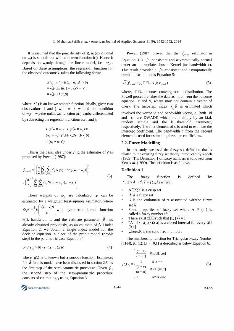
The process for getting fuzzy data is illustrated in Fig.1. In this figure, x is original data (Fig. 1a) which involves uncertainty. Hence, it is called crisp uncertainty data (Fig. 1b) which is assigned the value of 1 or 0. In order to get a fuzzy data, the process of fuzzification (Fig. 1c) with the membership function between (0,1] and defuzzification (Fig. 1d) will be implemented.

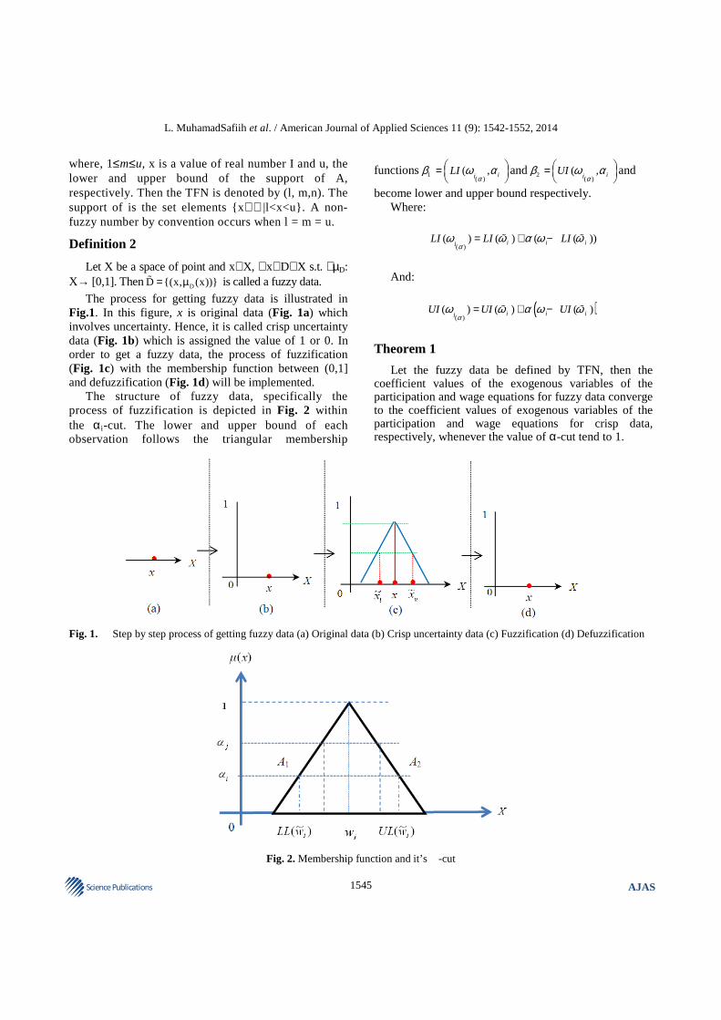
The structure of fuzzy data, specifically the process of fuzzification is depicted in Fig. 2 within the αi-cut. The lower and upper bound of each observation follows the triangular membership

functions 1( )

( , iiLI

αβ ϖ α =

and 2

( )( , ii

UIα

β ϖ α =

and

become lower and upper bound respectively. Where:

( )( ) ( ) ( ( ))i i ii

LI LI LIα

ϖ ϖ α ϖ ϖ= + −% %

And:

( )( )

( ) ( ) ( )i i iiUI UI UI

αϖ ϖ α ϖ ϖ= + −% %

Theorem 1

Let the fuzzy data be defined by TFN, then the coefficient values of the exogenous variables of the participation and wage equations for fuzzy data converge to the coefficient values of exogenous variables of the participation and wage equations for crisp data, respectively, whenever the value of α-cut tend to 1.

Fig. 1. Step by step process of getting fuzzy data (a) Original data (b) Crisp uncertainty data (c) Fuzzification (d) Defuzzification

Fig. 2. Membership function and it’s �-cut



AJAS

Proof

In order to get the crisp value, the centroid method is used. Then, the fuzzy number for all observations of ϖiis given as:

( )( )1( ) ( )

3ci i ii

W LI UIϖ ϖ ϖ= + +

If α→1, then the values of ( ) 1

Axαµ = , where the

lower bound and upper bound for each observation is based on Equation 2. Applying the α-cut into the triangular membership function, the fuzzy number that is obtained depends on the given value of the α-cut over the range 0 and 1 and is as follows:

( ) ( )

( )

( ) ( ( )) ( ( ))

31

( ( ) ( ))3

i i i i i i

i i i

ic

LI LI UI UIW

LI UIα α

α

ϖ α ϖ ϖ ϖ ϖ ϖ

ϖ ϖ ϖ

+ − + + −=

= + +

When α approaches 1, then:

( ) i(a)( ) ( )i i iLl andUlαϖ ϖ ϖ ϖ→ →

Further, we obtained:

( )( )

1

3 uil i iiic a

W ϖ ϖ ϖ ϖ→ + + =%

Hence:

( )icW i

αϖ→ (7)

Equation 7 stated that when α approaches 1, then

( )icW

αapproaches crisp, ϖi. In general, any observation of

the real fuzzy data is crisp for all observations such that xi and zi,

( )iic

X xα

→ and( )

iicZ z

α→ respectively, as αtends to

1. This implies that the fuzzy data values of the participation and structural equations converge to the values of the participation and structural equations for crisp data, respectively whenever the value of α-cuts tend to 1.

2.3. Development of Fuzzy Semi-Parametric Sample Selection Model

In order to formulate a fuzzy SPSSM, the SPSSM in Equation 1 is reconsidered. Towards the development of FSPSSM, the same procedure in Lola et al. (2009) is

used which involved 3 stage i.e., (1) fuzzification, (2) fuzzy environment and (3) defuzzification. In the first stage, the elements of real-valued input variables or crisp uncertainty values are converted into fuzzy data using a particular value of membership function. A triangular fuzzy number with α-cut method is used for all observations. In this study, the same α-cuts method as in Equation 7 is considered. Hence, lower and upper

bounds for each observation ( )*, , , ,i i i i isp sp sp sp sp

w x z uε is

obtained which is defined respectively as:

,

*

( , , ), ( , )

( , , ), ( , , )

( , , )i

i i i i i i i isp m u sp ml l usp sp sp sp sp sp

i i i i i i i isp m u sp sp m ul lsp sp sp sp sp

i i isp m ul sp sp sp

w w w w x x x x

z z z z and

u u u u

ε ε ε ε

= =

= =

=

According to Equation 2, their respective

membership functions are defined as:

1,2,3,4,5

( )[ , ]

( )

1( )

( )[ , [

( )

0

lsp

K splKlsp

Aksp Kuspi

KuspKusp

x Kif x

a

if xx

xif x

a

otherwise

αα α

α

αµ

αα α

α=

− ∈ − ==

−∈

−

(8)

Based on Equation 8, 5 types of membership

functionAk sp

µ , can be generated by Ksp

A taking on the

values of K = 1, 2, 3, 4 and 5, where K = 1, 2, 3, 4 and 5 represents *, , ,sp sp sp sp spw x z and uε respectively.

For the second step, the α-cuts method is proceeded for all the exogenous variables and error terms. While for the third stage, the fuzzy values are converted to output of the crisp value as in the following formula Equation 9:

11,..,

( , , )k

i

Kl Ksp usp

Kspi k

AK

α α α

==

=∑ (9)

where,

Klsp

α andKusp

α represents lower and upper bounds,

respectively. Again, 5 types of defuzzified can be generated in this stage where KA takes values of K = 1, 2,

3, 4 and 5. The values of 1, 2, 3, 4 and 5 representing



AJAS

, , *,w x z and uε respectively. Hence, the FSPSSM is of

the form as Equation 10:

* '

* *

*

1 0

0

; 1,...,

sp

sp

i

i

i

i ii

i isp sp

i isp sp

Z w

if d x ud

otherwise

z z d i N

γ ε

β

= +

= + >=

= =

% %%

% % %

% %

(10)

The terms *, , ,

i i i isp sp sp spw x z ε% % %

and

ispu%

are fuzzy

numbers with the membership functions

*, , ,w x zi i iisp sp spsp

εµ µ µ µ

and uisp

µ respectively.

2.4. The Monte Carlo Simulation

2.4.1. Consistency and Efficiency of FSPSSM

To obtain a consistent estimator of FSPSSM in Equation 1, the error terms is assumed to follow a normal distribution. The hybrid of the model proposed by Nawata (1994) with fuzzy concept is considered. Then, the Monte Carlo simulation technique (Kabadayi, 2004; Rana et al., 2008; 2009; Witchakul el al., 2008) is used to illustrate the developed model. Adversely, the estimators are inconsistent if the error terms does not satisfy normal distribution (Chamberlain, 1986; Robinson, 1988; Powell et al., 1989; Cosslett, 1990; Ichimura and Lee, 1991; Newey et al., 1990; Vella, 1992; Ichimura, 1993; Schafgans, 1996; Markus, 1998). For the development of SPSSM, one of the elements used to measure the consistency or efficiency of the parameter is through the usage of bandwidth parameter, c(for instance, Chamberlain, 1986; Powell et al., 1989; Andrews, 1991; Cosslett, 1990; Ahn and Powell, 1993; Klein and Spady, 1993; Schafgans, 1996; Das et al., 2003; Bellemare et al., 2002). According to Hardle (1990), the bandwidth parameter is a scalar argument to the kernel function that determines what range of the nearby data points will be heavily weighted in making an estimate. The choice of bandwidth represents a trade-off between bias (which is intrinsic to a kernel estimator and which increases with bandwidth) and variance of the estimates from the data (which decreases with bandwidth). An estimator is efficient if the RMSE values become smaller as the bandwidth parameter, c values increases as the number of N increased.

2.5. The Monte Carlo Simulation of Fuzzy Semi- Parametric Sample Selection Model

As mentioned earlier to achieve the second aim of this study i.e., consistency under FSPSSM, the Monte Carlo simulation developed by Nawata (1994) with α-cuts of 0.2, 0.4, 0.6 and 0.8 are also considered. In this section, the effectiveness of the proposed model is focused on the usage of bandwidth parameter, c. Therefore, the form of FSPSSM with DWADE and Powell estimators are hybrid with Nawata (1994) can be rewritten according to Equation 1 as follows:

0 1

0 11( 0), 1,2,3,..,i

i i isp sp sp

i isp sp

y b b w

d x u i N

ε

α α

= + +

= + + > =

%% %

% %

(11)

The values of

ispw% and

ispx% in the participationand

selection equation are independently, identically distributed (i.i.d) random variablehaving uniform distribution with the meansvalue of 0 and variance of 20. ρis thecorrelation coefficient between fuzzyexogenous variables, ( )

i isp spw and x% % . In Equation 11, the exogenous

variables, i isp sp

x and w% %

which involve bandwidth

parameter, care followed from DWADE and Powell procedures, respectively.

The fuzzy error terms of i isp sp

and uε% % arei.i.d normal

random variables. For isp

ε% theestimated parameters of the

means is zero andvariance is 1. Meanwhile, for isp

u%

theestimated parameter of the mean is zero andstandard deviation is 10.ϑ0 is the correlationcoefficient between fuzzy error terms, ( )

i isp spand uε% % . The performance of the

FSPSSM under consistency with bandwidth parameters,c, due to tables reduction, we show only thevalues of ρand 0 ϑ0 is 0, i.e., representing parameter of no correlation between ,

i i i isp sp sp spw and x and uε%% % % ,

respectively. As per section 5.3, the value of ϑ belongs to set [-1,1] and 0 is chosen as the middle value of itsset. The sample size of N = 100, 200 500 and the bandwidth parameter, c = 0.1, 0.5, 0.75, 1 are considered. The bandwidths parameters, cgoverns the degree of “smoothness” imposedon the estimated function f (.) as in section 2.5, with large values of c corresponding to asmoother function estimate (Newey et al., 1990). For all cases, the number ofreplications is 1,000. The true parameters value of γ1 is 1.



AJAS

3. RESULTS

3.1. The Monte Carlo Simulation Result: The Fuzzy Semi-Parametric Sample Selection Model

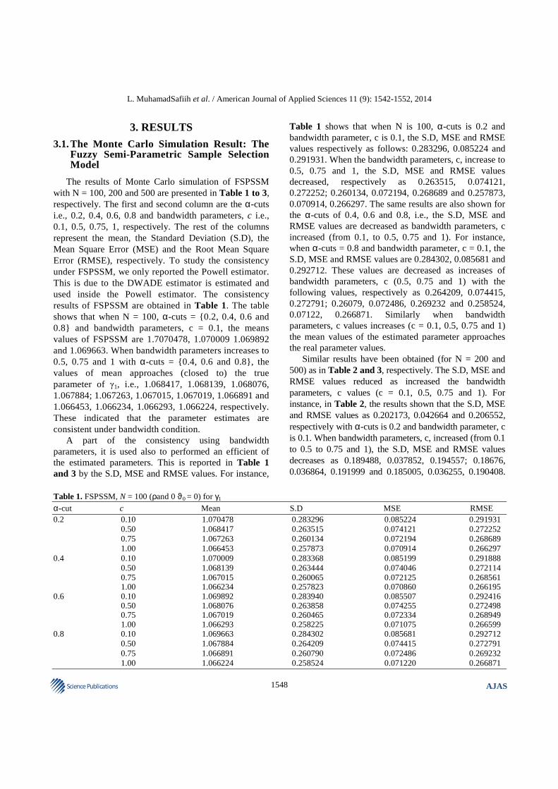
The results of Monte Carlo simulation of FSPSSM with N = 100, 200 and 500 are presented in Table 1 to 3, respectively. The first and second column are the α-cuts i.e., 0.2, 0.4, 0.6, 0.8 and bandwidth parameters, c i.e., 0.1, 0.5, 0.75, 1, respectively. The rest of the columns represent the mean, the Standard Deviation (S.D), the Mean Square Error (MSE) and the Root Mean Square Error (RMSE), respectively. To study the consistency under FSPSSM, we only reported the Powell estimator. This is due to the DWADE estimator is estimated and used inside the Powell estimator. The consistency results of FSPSSM are obtained in Table 1. The table shows that when N = 100, α-cuts = {0.2, 0.4, 0.6 and 0.8} and bandwidth parameters, c = 0.1, the means values of FSPSSM are 1.7070478, 1.070009 1.069892 and 1.069663. When bandwidth parameters increases to 0.5, 0.75 and 1 with α-cuts = {0.4, 0.6 and 0.8}, the values of mean approaches (closed to) the true parameter of γ1, i.e., 1.068417, 1.068139, 1.068076, 1.067884; 1.067263, 1.067015, 1.067019, 1.066891 and 1.066453, 1.066234, 1.066293, 1.066224, respectively. These indicated that the parameter estimates are consistent under bandwidth condition.

A part of the consistency using bandwidth parameters, it is used also to performed an efficient of the estimated parameters. This is reported in Table 1 and 3 by the S.D, MSE and RMSE values. For instance,

Table 1 shows that when N is 100, α-cuts is 0.2 and bandwidth parameter, c is 0.1, the S.D, MSE and RMSE values respectively as follows: 0.283296, 0.085224 and 0.291931. When the bandwidth parameters, c, increase to 0.5, 0.75 and 1, the S.D, MSE and RMSE values decreased, respectively as 0.263515, 0.074121, 0.272252; 0.260134, 0.072194, 0.268689 and 0.257873, 0.070914, 0.266297. The same results are also shown for the α-cuts of 0.4, 0.6 and 0.8, i.e., the S.D, MSE and RMSE values are decreased as bandwidth parameters, c increased (from 0.1, to 0.5, 0.75 and 1). For instance, when α-cuts = 0.8 and bandwidth parameter, c = 0.1, the S.D, MSE and RMSE values are 0.284302, 0.085681 and 0.292712. These values are decreased as increases of bandwidth parameters, c (0.5, 0.75 and 1) with the following values, respectively as 0.264209, 0.074415, 0.272791; 0.26079, 0.072486, 0.269232 and 0.258524, 0.07122, 0.266871. Similarly when bandwidth parameters, c values increases (c = 0.1, 0.5, 0.75 and 1) the mean values of the estimated parameter approaches the real parameter values.

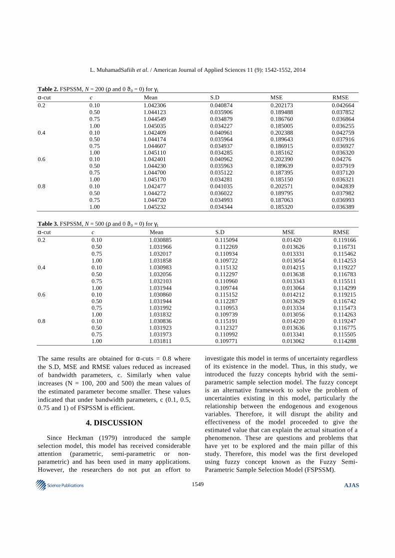
Similar results have been obtained (for N = 200 and 500) as in Table 2 and 3, respectively. The S.D, MSE and RMSE values reduced as increased the bandwidth parameters, c values (c = 0.1, 0.5, 0.75 and 1). For instance, in Table 2, the results shown that the S.D, MSE and RMSE values as 0.202173, 0.042664 and 0.206552, respectively with α-cuts is 0.2 and bandwidth parameter, c is 0.1. When bandwidth parameters, c, increased (from 0.1 to 0.5 to 0.75 and 1), the S.D, MSE and RMSE values decreases as 0.189488, 0.037852, 0.194557; 0.18676, 0.036864, 0.191999 and 0.185005, 0.036255, 0.190408.

Table 1. FSPSSM, N = 100 (ρand 0 ϑ0 = 0) for γ1

α-cut c Mean S.D MSE RMSE 0.2 0.10 1.070478 0.283296 0.085224 0.291931 0.50 1.068417 0.263515 0.074121 0.272252 0.75 1.067263 0.260134 0.072194 0.268689 1.00 1.066453 0.257873 0.070914 0.266297 0.4 0.10 1.070009 0.283368 0.085199 0.291888 0.50 1.068139 0.263444 0.074046 0.272114 0.75 1.067015 0.260065 0.072125 0.268561 1.00 1.066234 0.257823 0.070860 0.266195 0.6 0.10 1.069892 0.283940 0.085507 0.292416 0.50 1.068076 0.263858 0.074255 0.272498 0.75 1.067019 0.260465 0.072334 0.268949 1.00 1.066293 0.258225 0.071075 0.266599 0.8 0.10 1.069663 0.284302 0.085681 0.292712 0.50 1.067884 0.264209 0.074415 0.272791 0.75 1.066891 0.260790 0.072486 0.269232 1.00 1.066224 0.258524 0.071220 0.266871



AJAS

Table 2. FSPSSM, N = 200 (ρ and 0 ϑ0 = 0) for γ1


Table 3. FSPSSM, N = 500 (ρ and 0 ϑ0 = 0) for γ1


The same results are obtained for α-cuts = 0.8 where the S.D, MSE and RMSE values reduced as increased of bandwidth parameters, c. Similarly when value increases (N = 100, 200 and 500) the mean values of the estimated parameter become smaller. These values indicated that under bandwidth parameters, c (0.1, 0.5, 0.75 and 1) of FSPSSM is efficient.

4. DISCUSSION

Since Heckman (1979) introduced the sample selection model, this model has received considerable attention (parametric, semi-parametric or non-parametric) and has been used in many applications. However, the researchers do not put an effort to

investigate this model in terms of uncertainty regardless of its existence in the model. Thus, in this study, we introduced the fuzzy concepts hybrid with the semi-parametric sample selection model. The fuzzy concept is an alternative framework to solve the problem of uncertainties existing in this model, particularly the relationship between the endogenous and exogenous variables. Therefore, it will disrupt the ability and effectiveness of the model proceeded to give the estimated value that can explain the actual situation of a phenomenon. These are questions and problems that have yet to be explored and the main pillar of this study. Therefore, this model was the first developed using fuzzy concept known as the Fuzzy Semi-Parametric Sample Selection Model (FSPSSM).



AJAS

5. CONCLUSION

In this study, we studied the consistency for FSPSSM under normality assumption. Subsequent of this assumption, the effect of the correlation between fuzzy variables (wand x% % ) and the effect of the correlation

between error terms (i iand uε% % ) are investigated. As a

continuation from that, consistency in FSPSSM using the bandwidth parameter as introduced by Powell (1987) is also studied. A Monte Carlo simulation is used to examine the consistency for FSPSSM under normality assumption. The Monte Carlo simulation results reveal that consistency depends on bandwidth parameter. When bandwidth parameters, c are increased from 0.1, 0.5, 0.75 and 1 as the numbers of N increased (from 100 to 200 and increased to 500), the values of mean approaches (closed to) the real parameter. According to Schafgans (1996), this indicated that the FSPSSM is consistent. Through the bandwidth parameter also reveals that the estimated parameter is efficient, i.e., the S.D, MSE and RMSE values become smaller as N increased. In particular, the estimated parameter becomes consistent and efficient as the bandwidth parameters approaches to infinity, c→∞ as the number of observations, n tend to infinity, n→∞. In this study, we are focusing only for two area which are fuzzy concept particullarly on fuzzy number of semi-parametric Sample Selection Model coins as fuzzy semi-parametric Sample Selection Model (FSPSSM) and to see the effectiveness of the proposed model, the simulation using monte carlo is used.

This paper developed of this proposed modeling approach, future research work could be emphasized in several directions. Apparently, the fuzzy concepts defined in this study consider the TFN and α-cut method. Therefore, future study could consider other fuzzy numbers which are more advanced such as S-shaped, bell-shaped. Since the relationship between explanatory variables exists in the models, the concept of linear programming-based method introduced by Tanaka et al. (1982) and Amri and Tularam (2012) could be explored. By doing so, perhaps a deeper understanding of the underlying structure of the models could be obtained. Thus, some other mathematical tools such as optimization theory could be explored.

The most significant idea of this research was to bring the concept of fuzzy into the selectivity model. In general, this concept is considered as a platform to discover a new dimension using these models. Further

research could consider development of fuzzy perspective on a new paradigm of selection model, such as nonparametric and semi-nonparametric methods, the properties and theoretical parts of selection model, handling a weaker assumption and investigating “a curse of dimensionality” using fuzzy concept.

In the development of FSPSSM, fuzzy logic using rules based method can also be considered. This concept will lead to produce an output based on linguistics variables and linguistics modifier. Hence, the proposed model would be useful in order to compute the uncertainties in the models. Thus, it would be interesting to find whether it is possible to determine the percentages to which any specific uncertain parameters of the models contribute to the overall uncertainty of the models.

In this study, we have developed Monte Carlo simulations using R language programming. These simulations could be improved. Babuska and Verbruggen (1996; Chandramohan and Kamalakkannan, 2014; Hussein and Nordin, 2014; Kareem, et al., 2014; Kahtan et al., 2014; Sridharan and Chitra, 2014) mentioned that modeling of complex systems will always remain an interactive approach. Thus, future study could consider the usage of other software packages or programming languages and incorporate graphic interface. In this way, information such as parameter estimate could be easily utilized and would be beneficial to the decision makers as well as others interested parties. These methods could be useful in data mining, e.g., in credit default analysis, healthcare analysis, security analysis and agriculture analysis.

6. ACKNOWLEDGMENT

The author wishesto thank theMinistry of Higher Education, Malaysia for sponsoring studies and University Malaysia Terengganu (UMT) for the support and encouragement of study at the PhD level

7. REFERENCES

Ahn, H. and J. Powell, 1993. Semi-parametric estimation of censored selection models with a nonparametric selection mechanism. J. Econometr., 58: 3-29. DOI: 10.1016/0304-4076(93)90111-H

Amri, S. and G.A. Tularam, 2012. Performance of mulitple linear regression and nonlinear neural networks and fuzzy logic techniques in modelling house prices. J. Math. Stat., 8: 419-434. DOI: 10.3844/jmssp.2012.419.434



AJAS

Andrews, D.W.K., 1991. Asymptotic normality of series estimation for nonparametric and semi-parametric regression models. Econometrica, 59: 307-345. DOI: 10.2307/2938259

Babuska, R. and H.B. Verbruggen, 1996. An overview of fuzzy modeling for control. Control Eng. Pract., 4: 1593-1606.

Bellemare, C., B. Melenberg and A. Soest, 2002. Semi-parametric models for satisfaction with income. Portuguse Economic J., 1: 181-203. DOI: 10.1007/s10258-002-0006-z

Chamberlain, G., 1986. Asymptotic efficiency in semi-parametric models with censoring. J. Econometr., 32: 189-218. DOI: 10.1016/0304-4076(86)90038-2

Chandramohan, K. and P. Kamalakkannan, 2014. Traffic controlled-dedicated short range communication: A secure communication using traffic controlled dedicated short range communication model in vehicular ad hoc networks for safety related services. J. Comput. Sci., 10: 1315-1323. DOI: 10.3844/jcssp.2014.1315.1323

Cosslett, S., 1990. Semi-Parametirc Estimation of a Regression Models with Sample Selectivity. In: Nonparametric and Semi-Parametric Estimation Methods in Econometrics and Statistics, Barnett, W.A., J. Powell and G.E. Tauchen (Eds.), Cambridge University Press. pp: 175-198.

Das, M., W.K. Newey and F. Vella, 2003. Nonparametric estimation of sample selection models. Rev. Econom. Stud., 70: 33-58. DOI: 10.1111/1467-937X.00236

Gerfin, M., 1996. Parametric and semi-parametric estimation of the binary response model of labour market participation. J. Applied Econometr., 11: 321-339. DOI: 10.1002/(SICI)1099-1255(199605)11:3<321::AID-JAE391>3.0.CO;2-K

Hardle, W., 1990. Applied Nonparametric Regression. 1st Edn., Cambridge University Press, Econometric Society Monograph.

Heckman, J.J., 1979. Sample selection bias as a specification error. Econometrica, 47: 153-161. DOI: 10.2307/1912352

Hussein, I.S.H. and M.J. Nordin, 2014. Palmprint verification using invariant moments based on wavelet transform. J. Comput. Sci., 10: 1389-1396.DOI:10.3844/jcssp.2014.1389.1396

Ichimura, H. 1993. Semi-Parametric Least Square (SLS) and Weighted SLS Estimation of Single-Index Model. J. Econometr., 58: 71-120

Ichimura, H. and L.F. Lee, 1991. Semi-parametirc Least Square Estimation of Multiple Index Models: Single Equation Estimation. In: Nonparametric and Semi-Parametric Estimation Methods in Econometrics and Statistics, Barnett, W.A., J. Powell and G.E. Tauchen (Eds.), Cambridge University Press, Cambridge.

Kabadayi, O., 2004. Range of medium and high energy protons and alpha particles in NaI scintillator. Am. J. Applied Sci., 1: 33-35. DOI: 10.3844/ajassp.2004.33.35

Kareem, S.H., I.H. Ali and M.G. Jalhoom, 2014. Synthesis and characterizationof organic functionalized mesoporous silica and evaluate their adsorptive behavior for removal of methylene blue from aqueous solution. Am. J. Environ. Sci., 10: 48-60.DOI:10.3844/ajessp.2014.48.60

Khan, S. and J.L. Powell, 2001. Two-step estimation of semi-parametric censored regression models. J. Econometr., 103: 73-110. DOI: 10.1016/S0304-4076(01)00040-9

Kahtan, H., N.A. Bakar and R. Nordin, 2014. Dependability attributes for increased security in component-based software development. J. Comput. Sci., 10: 1298-1306. DOI: 10.3844/jcssp.2014.1298.1306

Klein, R. and R. Spady, 1993. An efficient semi-parametric estimator of the binary response model. Econometrica, 61: 387-423. DOI: 10.2307/2951556

Lee, M.J. and F. Vella, 2006. A semi-parametric estimator for censored selection models with endogeneity. J. Econometr., 130: 235-252. DOI: 10.1016/j.jeconom.2004.11.001

Lola, M.S., A.A. Kamil and M.T.A. Osman, 2009. Fuzzy Parametric of Sample Selection Model Using Heckman Two-Step Estimation Models. Am. J. Applied Sci., 6: 1845-1853. DOI: 10.3844/ajassp.2009.1845.1853

Markus, F., 1998. Semi-parametric estimation of selectivity models. Ph.D. Thesis, Konstanz University, Konstanz.

Martins, M.F.O., 2001. Parametric and semi-parametric estimation of sample selection models: An empirical application to the female labor force in portugal. J. Applied Econometr., 16: 23-39. DOI: 10.1002/jae.572



AJAS

Safiih, L.M., 2013. Fuzzy parametric sample selection model: Monte carlo simulation approach. J. Stat. Comput. Simulat., 83: 992-1006. DOI: 10.1080/00949655.2011.646277

Nawata, K., 1994. Estimation of sample selection bias models by maximum likelihood estimator and heckman’s two-step estimator. Econometr. Lett., 45: 33-40. DOI: 10.1016/0165-1765(94)90053-1

Newey, W.K., J.L. Powell and J.R. Walker, 1990. Semi-parametric estimation of selection models: Some empirical results. Am. Economic Rev., 2: 324-328.

Powell, J. J.H. Stock and T.M. Stoker, 1989. Semi-parametric estimation of index coefficients. Econometrica, 57: 1403-1430.

Powell, J.L., 1987. Semi-parametric estimation of bivariate latent variable models. Social Systems Research Institute. University of Wisconsin-Madison.

Rana, M.S., H. Midi and A.H.M.R. Imon, 2008. A robust modification of the goldfeld-quandt test for the detection of heteroscedasticity in the presence of outliers. J. Math. Stat., 4: 277-283.DOI:10.3844/jmssp.2008.277.283

Rana, M.S., H. Midi and A.H.M.R. Imon, 2009. A robust rescaled moment test for normality in regression. J. Math. Stat., 5: 54-62.DOI:10.3844/jmssp.2009.54.62

Robinson, P.M., 1988. Root-N consistent semi-parametric regression. Econometrica, 56: 931-954. DOI: 10.2307/1912705

Schafgans, M., 1996. Semi-parametric estimation of a sample selection model: estimation of the intercept; theory and applications. Ph.D. Thesis, Yale University, New Haven.

Sridharan, K. and M. Chitra, 2014. Trust based automatic query formulation search on expert and knowledge users systems. J. Comput. Sci., 10: 1174-1185.DOI:10.3844/jcssp.2014.1174.1185

Tanaka, H., S. Hayashi and K. Asai, 1982. Linear regression analysis with fuzzy model. IEEE Trans. Syst. Man Cybernet., 12: 903-907.

Vella, F., 1992. Simple tests for sample selection bias in censored and discrete choice models. J. Applied Econometr., 7: 413-421. DOI: 10.1002/jae.3950070407

Witchakul, S., P.S.N. Ayudhaya and P. Charnsethikul, 2008. A stochastic knapsack problem with continuous random capacity. J. Math. Stat., 4: 269-276. DOI:10.3844/jmssp.2008.269.276

Yen, K.K., S. Ghoshray and G. Roig, 1999. A linear regression model using triangular fuzzy number coefficients. Fuzzy Sets Syst., 106: 167-177.

Zadeh, L.A., 1965. Fuzzy sets. Inform. Control, 8: 338-358. DOI: 10.1016/S0019-9958(65)90241-X

Documents

ESTIMATED AND ANALYSIS OF THE ... - Science …thescipub.com/PDF/ajassp.2014.1542.1552.pdf · ... 21030 Kuala Terengganu, Terengganu, Malaysia Science ... 21030 Kuala Terengganu,