arX

iv:2

102.

0902

3v1

[cs

.LG

] 1

7 Fe

b 20

21

Estimate Three-Phase Distribution Line Parameters

With Physics-Informed Graphical Learning Method

Wenyu Wang, Student Member, IEEE, Nanpeng Yu, Senior Member, IEEE,

Abstract—Accurate estimates of network parameters are essen-tial for modeling, monitoring, and control in power distributionsystems. In this paper, we develop a physics-informed graphicallearning algorithm to estimate network parameters of three-phase power distribution systems. Our proposed algorithm usesonly readily available smart meter data to estimate the three-phase series resistance and reactance of the primary distributionline segments. We first develop a parametric physics-based modelto replace the black-box deep neural networks in the conventionalgraphical neural network (GNN). Then we derive the gradient ofthe loss function with respect to the network parameters and usestochastic gradient descent (SGD) to estimate the physical param-eters. Prior knowledge of network parameters is also consideredto further improve the accuracy of estimation. Comprehensivenumerical study results show that our proposed algorithm yieldshigh accuracy and outperforms existing methods.

Index Terms—Power distribution network, graph neural net-work, parameter estimation, smart meter.

I. INTRODUCTION

Accurate modeling of three-phase power distribution sys-

tems is crucial to accommodating the increasing penetration

of distributed energy resources (DERs). To monitor and coor-

dinate the operations of DERs, several key applications such as

three-phase power flow, state estimation, optimal power flow,

and network reconfiguration are needed. All of these depend

on accurate three-phase distribution network models, which

include the network topology and parameters [1]. However,

the distribution network topology and parameters in the geo-

graphic information system (GIS) often contain errors because

the model documentation usually becomes unreliable during

the system modifications and upgrades [2].

Although topology estimation for distribution networks has

been studied extensively [3], [4], the estimation of distribution

network parameters such as line impedances still needs further

development. It is more challenging to estimate parameters

of power distribution networks than that of transmission

networks. This is because the distribution lines are rarely

transposed, which lead to unequal diagonal and off-diagonal

elements in the impedance matrix. Thus, three-phase line

models need to be developed instead of single-phase equivalent

models. Specifically, the elements of the 3×3 phase impedance

matrix need to be estimated for each three-phase line segment.

Many methods have been proposed to estimate transmission

network parameters. However, very few of them can be applied

to the three-phase distribution networks using readily available

W. Wang and N. Yu are with the Department of Electrical and ComputerEngineering, University of California, Riverside, CA 92521, USA. Email:nyu@ece.ucr.edu.

sensor data. The existing parameter estimation literature can

be roughly classified into three groups based on the type of

sensor data used.

In the first group of literature, supervisory control and

data acquisition (SCADA) system data such as power and

current injections are used to estimate transmission network

parameters of a single-phase model. Most of the algorithms

in this group perform joint state and parameter estimation

by residual sensitivity analysis and state vector augmentation

[5]. Parameter errors are detected using identification indices

[6], [7], enhanced normalized Lagrange multipliers [8], and

projection statistics [9]. Adaptive data selection [10] is used

to improve parameter estimation accuracy.

In the second group of literature, phasor measurement unit

(PMU) data such as voltage and current phasors are used

to estimate line parameters of transmission and distribution

systems [11]–[17]. Although these methods achieve highly ac-

curate parameter estimates, they require costly and widespread

installation of PMUs. Linear least squares is used to estimate

transmission line parameters [11]. Parallel Kalman filter for

a bilinear model is used to estimate both states and line

parameters of the transmission system [12]. With single-

phase transmission line models, nonlinear least squares is

used to estimate line parameters and calibrate remote meters

[13]. Traveling waves are used to estimate parameters of

series compensated lines [14]. An augmented state estimation

method is developed to estimate three-phase transmission line

parameters [15]. Maximum likelihood estimation (MLE) is

used to estimate single-phase distribution line parameters [16].

Lasso is adopted to estimate three-phase admittance matrix in

distribution systems [17].

In the third group of literature, smart meter data such as

voltage magnitude and complex power consumption are used

to estimate distribution line parameters [18]–[22]. Particle

swarm [18] and linear regression [20], [23] are used to

estimate single-phase line parameters. Linear approximation of

voltage drop [19] is used to estimate the parameters of single-

phase and balanced three-phase distribution lines. Multiple

linear regression model is used to estimate three-phase line

impedance in [21], but it does not work with delta-connected

smart meters with phase-to-phase measurement. In [22], three-

phase line parameters are estimated through MLE based on a

linearized physical model.

The existing methods for parameter estimation either as-

sume a single-phase equivalent distribution network model or

require widespread installation of micro-PMUs, which are cost

prohibitive. To fill the knowledge gap, this paper develops

a physics-informed graphical learning algorithm to estimate

the 3× 3 series resistance and reactance matrices of three-

phase distribution line model using readily available smart

meter measurements. Our proposed method is inspired by the

emerging graph neural network (GNN), which is designed

for estimation problems in networked systems. We develop

three-phase power flow-based physical transition functions

to replace the ones based on deep neural networks in the

GNN. We then derive the gradient of the voltage magnitude

loss function with respect to the line segments’ resistance

and reactance parameters with an iterative method. Finally,

the estimates of distribution network parameters can be up-

dated with the stochastic gradient descent (SGD) approach to

minimize the error between the physics-based graph learning

model and the smart meter measurements. Prior estimates and

bounds of network parameters are also leveraged to improve

the estimation accuracy. To improve computation efficiency,

partitions can be introduced so that parameter estimations are

executed in parallel in sub-networks.

The main technical contributions of this work are:

• A physics-informed graphical learning method is devel-

oped to estimate line parameters of three-phase distribu-

tion networks.

• Our proposed algorithm only uses readily available smart

meter data and can be easily applied to real-world distri-

bution circuits.

• By preserving the nonlinearity of three-phase power

flows in the graphical learning framework, our proposed

approach yields more accurate parameter estimates on test

feeders than the state-of-the-art benchmark.

The rest of the paper is organized as follows. Section

II describes the problem setup and assumptions. Section III

presents the overall framework of the proposed method and

briefly introduces the GNN. Section IV provides the technical

methods for construction and parameter estimation based on

the physics-informed graphical model. Section V evaluates the

performance of the proposed algorithm with a comprehensive

numerical study. Section VI states the conclusion.

II. PROBLEM SETUP AND ASSUMPTIONS

A. Problem Setup

The objective of this work is to estimate the series resistance

and reactance in the 3×3 phase impedance matrix of three-

phase primary lines of a distribution feeder. The impedance

matrix of a line l can be written as, Zl=Rl+jXl, where

Rl ,

raal rabl raclrabl rbbl rbclracl rbcl rccl

, Xl , j

xaal xab

l xacl

xabl xbb

l xbcl

xacl xbc

l xccl

. (1)

Since Zl is symmetric, for each line segment there are 6

resistance and 6 reactance parameters. The network contains

L lines and N + 1 nodes, indexed as node 0 to N . Node 0is the source node (e.g., a substation). In total, there are 12Lparameters to estimate. M loads are connected to the primary

lines through the non-source nodes. The loads can be single-

phase, two-phase, or three-phase.

B. Assumptions

The assumptions of measurement data and the network

model are summarized below. First, for a single-phase load

on phase i, the smart meter records real and reactive power

injections and voltage magnitude of phase i. Second, for a

two-phase delta-connected load between phase i and j, the

smart meter records the power injection and voltage magnitude

across phase i and j. Third, for a three-phase load, the smart

meter records total power injection and voltage magnitude

of a known phase i. Fourth, SCADA system records the

voltage measurements at the source node. Fifth, it is assumed

that the phase connections of all loads are known. Sixth,

the topology of the primary three-phase feeder is known.

Seventh, we assume that the GIS contains rough estimates

of the network parameters. Assumptions one to four are based

on the typical measurement configurations of smart meters and

SCADA. Assumptions five to seven are based on the available

information in GIS.

III. OVERALL FRAMEWORK AND REVIEW OF THE GNN

A. Overall Framework of the Proposed Method

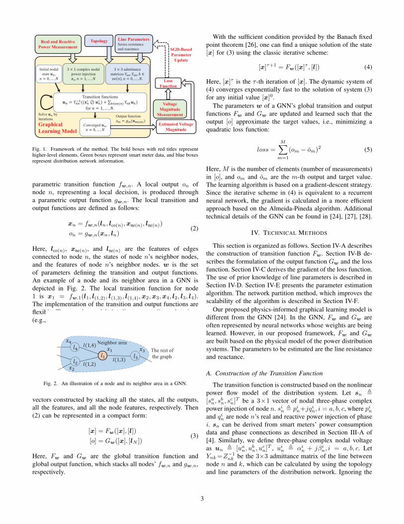
The overall framework of the proposed graphical learning

method for distribution line parameter estimation is illustrated

in Fig. 1. As shown in the figure, a physics-informed graphical

learning engine is constructed based on nonlinear power flow.

The inputs to the graphical learning engine include power in-

jection measurements from smart meters, distribution network

topology, and distribution line parameters. In the graphical

learning engine, each node corresponds to a physical bus

in the distribution network. The nodal states, i.e., the three-

phase complex voltage are iteratively updated by a set of

transition functions. The graphical learning engine’s outputs

are the estimated smart meter voltage magnitudes, which are

used to calculate the graphical learning engine’s loss function.

The gradient of the line parameters is computed from the loss

function and subsequently used to update the line parameters

using stochastic gradient descent. The technical details of the

proposed method will be explained in IV.

B. A Brief Overview of the GNN

A GNN is a neural network model, which uses a graph’s

topological relationships between nodes to incorporate the

underlying graph-structured information in data [24]. GNNs

have been successfully applied in many different domains,

such as social networks, image processing, and chemistry

[25]. Our proposed physics-informed graphical learning model

is developed by embedding physics of power distribution

networks into the standard GNN.

The GNN is comprised of nodes connected by edges. The

nodes represent objects or concepts, and the edges represent

the relationships between nodes. Two vectors are attached

to a node n: the state vector xn and the feature vector

ln. A feature vector l(m,n) is attached to edge (m,n). The

state xn, which embeds information from its neighborhood

with arbitrary depth, is naturally defined by the features of

itself and the neighboring nodes and edges through a local

2

Topology Line ParametersSeries resistance

and reactance

admittance

matrices

Transition functions

for .

Real and Reactive

Power Measurement

complex nodal

power injection

Graphical

Learning Model

Initial nodal

state ,

Converged ,

Solve by

iterationsOutput function

Estimated Voltage

Magnitude

Voltage

Magnitude

Measurement

Loss

Function

SGD-Based

Parameter

Update

Fig. 1. Framework of the method. The bold boxes with red titles representhigher-level elements. Green boxes represent smart meter data, and blue boxesrepresent distribution network information.

parametric transition function fw,n. A local output on of

node n, representing a local decision, is produced through

a parametric output function gw,n. The local transition and

output functions are defined as follows:

xn = fw,n(ln, lco(n),xne(n), lne(n))

on = gw,n(xn, ln)(2)

Here, lco(n), xne(n), and lne(n) are the features of edges

connected to node n, the states of node n’s neighbor nodes,

and the features of node n’s neighbor nodes. w is the set

of parameters defining the transition and output functions.

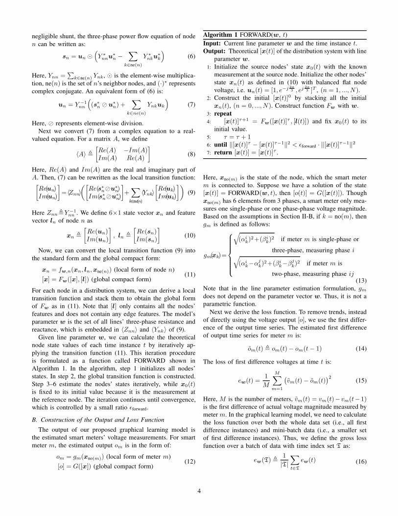
An example of a node and its neighbor area in a GNN is

depicted in Fig. 2. The local transition function for node

1 is x1 = fw,1(l1, l(1,2), l(1,3), l(1,4),x2,x3,x4, l2, l3, l4).The implementation of the transition and output functions are

flexible. They can be modeled as linear or nonlinear functions

(e.g., neural networks). Let [x], [o], [l], and [lN ] represent the

The rest of

the graph

Neighbor area

Fig. 2. An illustration of a node and its neighbor area in a GNN.

vectors constructed by stacking all the states, all the outputs,

all the features, and all the node features, respectively. Then

(2) can be represented in a compact form:

[x] = Fw([x], [l])

[o] = Gw([x], [lN ])(3)

Here, Fw and Gw are the global transition function and

global output function, which stacks all nodes’ fw,n and gw,n,

respectively.

With the sufficient condition provided by the Banach fixed

point theorem [26], one can find a unique solution of the state

[x] for (3) using the classic iterative scheme:

[x]τ+1 = Fw([x]τ , [l]) (4)

Here, [x]τ is the τ -th iteration of [x]. The dynamic system of

(4) converges exponentially fast to the solution of system (3)

for any initial value [x]0.

The parameters w of a GNN’s global transition and output

functions Fw and Gw are updated and learned such that the

output [o] approximate the target values, i.e., minimizing a

quadratic loss function:

loss =

M∑

m=1

(om − om)2 (5)

Here, M is the number of elements (number of measurements)

in [o], and om and om are the m-th output and target value.

The learning algorithm is based on a gradient-descent strategy.

Since the iterative scheme in (4) is equivalent to a recurrent

neural network, the gradient is calculated in a more efficient

approach based on the Almeida-Pineda algorithm. Additional

technical details of the GNN can be found in [24], [27], [28].

IV. TECHNICAL METHODS

This section is organized as follows. Section IV-A describes

the construction of transition function Fw. Section IV-B de-

scribes the formulation of the output function Gw and the loss

function. Section IV-C derives the gradient of the loss function.

The use of prior knowledge of line parameters is described in

Section IV-D. Section IV-E presents the parameter estimation

algorithm. The network partition method, which improves the

scalability of the algorithm is described in Section IV-F.

Our proposed physics-informed graphical learning model is

different from the GNN [24]. In the GNN, Fw and Gw are

often represented by neural networks whose weights are being

learned. However, in our proposed framework, Fw and Gw

are built based on the physical model of the power distribution

systems. The parameters to be estimated are the line resistance

and reactance.

A. Construction of the Transition Function

The transition function is constructed based on the nonlinear

power flow model of the distribution system. Let sn ,

[san, sbn, s

cn]

T be a 3×1 vector of nodal three-phase complex

power injection of node n. sin , pin+jqin, i = a, b, c, where pinand qin are node n’s real and reactive power injection of phase

i. sn can be derived from smart meters’ power consumption

data and phase connections as described in Section III-A of

[4]. Similarly, we define three-phase complex nodal voltage

as un , [uan, u

bn, u

cn]

T , uin , αi

n + jβin, i = a, b, c. Let

Ynk=Z−1nk be the 3×3 admittance matrix of the line between

node n and k, which can be calculated by using the topology

and line parameters of the distribution network. Ignoring the

3

negligible shunt, the three-phase power flow equation of node

n can be written as:

sn = un ⊙(

Y ∗nnu

∗n −

∑

k∈ne(n)

Y ∗nku

∗k

)

(6)

Here, Ynn =∑

k∈ne(n) Ynk, ⊙ is the element-wise multiplica-

tion, ne(n) is the set of n’s neighbor nodes, and (·)∗ represents

complex conjugate. An equivalent form of (6) is:

un = Y −1nn

(

(s∗n ⊘ u∗n) +

∑

k∈ne(n)

Ynkuk

)

(7)

Here, ⊘ represents element-wise division.

Next we convert (7) from a complex equation to a real-

valued equation. For a matrix A, we define

〈A〉 ,

[

Re(A) −Im(A)Im(A) Re(A)

]

(8)

Here, Re(A) and Im(A) are the real and imaginary part of

A. Then, (7) can be rewritten as the local transition function:[

Re(un)Im(un)

]

=〈Znn〉

([

Re(s∗n⊘u∗n)

Im(s∗n⊘u∗n)

]

+∑

k∈ne(n)

〈Ynk〉

[

Re(uk)Im(uk)

])

(9)

Here Znn,Y −1nn . We define 6×1 state vector xn and feature

vector ln of node n as

xn ,

[

Re(un)Im(un)

]

, ln ,

[

Re(sn)Im(sn)

]

(10)

Now, we can convert the local transition function (9) into

the standard form and the global compact form:

xn = fw,n(xn, ln,xne(n)) (local form of node n)

[x] = Fw([x], [l]) (global compact form)(11)

For each node in a distribution system, we can derive a local

transition function and stack them to obtain the global form

of Fw as in (11). Note that [l] only contains all the nodes’

features and does not contain any edge features. The model’s

parameter w is the set of all lines’ three-phase resistance and

reactance, which is embedded in 〈Znn〉 and 〈Ynk〉 of (9).

Given line parameter w, we can calculate the theoretical

node state values of each time instance t by iteratively ap-

plying the transition function (11). This iteration procedure

is formulated as a function called FORWARD shown in

Algorithm 1. In the algorithm, step 1 initializes all nodes’

states. In step 2, the global transition function is constructed.

Step 3–6 estimate the nodes’ states iteratively, while x0(t)is fixed to its initial value because it is the measurement at

the reference node. The iteration continues until convergence,

which is controlled by a small ratio ǫforward.

B. Construction of the Output and Loss Function

The output of our proposed graphical learning model is

the estimated smart meters’ voltage measurements. For smart

meter m, the estimated output om is in the form of:

om = gm(xno(m)) (local form of meter m)

[o] = G([x]) (global compact form)(12)

Algorithm 1 FORWARD(w, t)

Input: Current line parameter w and the time instance t.Output: Theoretical [x(t)] of the distribution system with line

parameter w.

1: Initialize the source nodes’ state x0(t) with the known

measurement at the source node. Initialize the other nodes’

state xn(t) as defined in (10) with balanced flat node

voltage, i.e. un(t) = [1, e−j 2π3 , ej

2π3 ]T , (n = 1, ..., N).

2: Construct the initial [x(t)]0 by stacking all the initial

xn(t), (n = 0, ..., N). Construct function Fw with w.

3: repeat

4: [x(t)]τ+1 = Fw([x(t)]τ , [l(t)]) and fix x0(t) to its

initial value.

5: τ = τ + 16: until ‖[x(t)]τ − [x(t)]τ−1‖2 < ǫforward · ‖[x(t)]

τ−1‖2

7: return [x(t)] = [x(t)]τ .

Here, xno(m) is the state of the node, which the smart meter

m is connected to. Suppose we have a solution of the state

[x(t)] = FORWARD(w, t), then [o(t)] = G([x(t)]). Though

xno(m) has 6 elements from 3 phases, a smart meter only mea-

sures one single-phase or one phase-phase voltage magnitude.

Based on the assumptions in Section II-B, if k = no(m), then

gm is defined as follows:

gm(xk)=

√

(αik)

2+(βik)

2 if meter m is single-phase or

three-phase, measuring phase i√

(αik−αj

k)2+(βi

k−βjk)

2 if meter m is

two-phase, measuring phase ij(13)

Note that in the line parameter estimation formulation, gmdoes not depend on the parameter vector w. Thus, it is not a

parametric function.

Next we derive the loss function. To remove trends, instead

of directly using the voltage output [o], we use the first differ-

ence of the output time series. The estimated first difference

of output time series for meter m is:

om(t) , om(t)− om(t− 1) (14)

The loss of first difference voltages at time t is:

ew(t) =1

M

M∑

m=1

(

vm(t)− om(t))2

(15)

Here, M is the number of meters, vm(t) = vm(t)− vm(t− 1)is the first difference of actual voltage magnitude measured by

meter m. In the graphical learning model, we need to calculate

the loss function over both the whole data set (i.e., all first

difference instances) and mini-batch data (i.e., a smaller set

of first difference instances). Thus, we define the gross loss

function over a batch of data with time index set T as:

ew(T) ,1

|T|

∑

t∈T

ew(t) (16)

4

Here, |T| is the size of T. Suppose we have measurement data

over t = 0, ..., T , and define Tfull , {t|t = 1, ..., T } as the

full batch for first difference time series. Then the gross error

of the model over all first difference instances is ew(Tfull).

C. Gradient of the Loss Function With Respect to the Line

Parameters

We design a new algorithm to calculate the gradient of the

loss function (16) of first difference voltage time series with

respect to the line parameters w. The gradient calculation

formula in the GNN cannot be directly applied because it is

derived for the data of a particular time instance, and not for

time series. To derive the gradient of the loss function (16),

we define an equivalent graphical learning model, with new

state and feature vectors as follows:

xn(t) ,

[

xn(t− 1)xn(t)

]

, ln(t) ,

[

ln(t− 1)ln(t)

]

(17)

The corresponding equivalent transition function is:

xn(t) = fw,n(x(t)n, l(t)n, x(t)ne(n))

,

[

fw,n(xn(t− 1), ln(t− 1),xne(n)(t− 1))fw,n(xn(t), ln(t),xne(n)(t))

]

(18)

The compact form of (18) is:

[x(t)]= Fw([x(t)], [l(t)]),

[

Fw([x(t− 1)], [l(t− 1)])Fw([x(t)], [l(t)])

]

(19)

Here,

[x(t)] ,

[

[x(t− 1)][x(t)]

]

, [l(t)] ,

[

[l(t− 1)][l(t)]

]

(20)

The output function of first difference voltage time series for

meter m is:

om(t)= gm(xno(m)(t)),gm(xno(m)(t))−gm(xno(m)(t−1)) (21)

The compact form of (21) is:

[o(t)] = G([x(t)]),G([x(t)])−G([x(t− 1)]) (22)

Using the equivalent graphical learning model defined in

(17)-(22), we can calculate the gradient of ew(T) over any

batch of data T with respect to w using an efficient function

BACKWARD shown in Algorithm 2. The iterative FORWARD

function can be represented as a recurrent neural network.

Thus, ew(T)’s gradient is difficult to calculate in the conven-

tional way. To evaluate the gradient more efficiently, we design

Algorithm 2 following the same backpropagation principle

in [24] based on the Almeida-Pineda algorithm [27], [28].

Algorithm 2 calculates the gradient by using an intermediate

variable z(t) through iterative applications of steps 5–10. The

theoretical details of designing such algorithms can be found

in [24], [27], [28]. In Algorithm 2, the lengthy derivations

of A(t), b(t), and∂Fw([x(t)],[l(t)])

∂ware omitted. Please refer to

the detailed derivations in Appendix A, B, and C, respectively.

ǫbackward is a small ratio controlling the convergence threshold

and T is the backward shift batch index defined as:

T , {t− 1|t ∈ T} (23)

Algorithm 2 BACKWARD(w, T)

Input: Current line parameter w and the first difference

instance batch index T.

Output: Gradient∂ew(T)

∂w.

1: [x(t)]=FORWARD(w, t), t ∈ T ∪ T.

2: Construct [x(t)] as (20), t ∈ T.

3: Calculate [o(t)] = G([x(t)]), A(t) = ∂Fw([x(t)],[l(t)])∂[x(t)] ,

b(t) = ∂ew(t)∂[o(t)] ·

∂G([x(t)])∂[x(t)] , for t ∈ T.

4: for t ∈ T do

5: Initialize z(t)0 = 01×12N , τ = 0.

6: repeat

7: z(t)τ+1 = z(t)τ · A(t) + b(t)8: τ = τ + 19: until ‖z(t)τ − z(t)τ−1‖2 < ǫbackward · ‖z(t)

τ−1‖2

10:∂ew(t)∂w

= z(t)τ · ∂Fw([x(t)],[l(t)])∂w

, for t ∈ T.

11: end for

12:∂ew(T)

∂w= 1

|T|

∑

t∈T

∂ew(t)∂w

13: return∂ew(T)

∂w

D. Utilization of Prior Distribution of Line Parameters

Through MAP and Constraints

Electric utilities often have reasonable estimates of distri-

bution systems’ line impedance in GIS, which serve as key

statistics for the prior distributions of the line parameters. This

subsection describes how to use these information to improve

estimates of line parameters using maximum a posteriori

probability (MAP) and parameter constraints.

1) Use of Prior Line Parameter Distribution in MAP Es-

timate: The posterior distribution of the line parameters is:

P (w | [v(t)]Tt=1) =P ([v(t)]Tt=1 | w)P (w)

P ([v(t)]Tt=1)(24)

Here [v(t)] represents a stack of vm(t), (m = 1, ...,M), and

[v(t)]Tt=1 represents [v(t)] of t = 1, ...,M , i.e., the observed

first difference voltage time series over the entire time period.

Maximizing (24) is equivalent to the minimization in (25):

minw

− logP ([v(t)]Tt=1 | w)− logP (w) (25)

We assume vm(t) ∼ N(om(t), σ2vm

) and are independent

across smart meters m=1, ...,M and time steps t=1, ..., T .

We also assume a Gaussian prior of the line parameters

wi ∼ N(µi, σ2wi), i = 1, ..., |w|. om(t) is the output of the

graphical learning model with parameter w, i.e., the theoretical

vm(t) with parameter w. For simplification, we further assume

σvm ≈σv , ∀m, so that (25) can be approximated by:

minw

T∑

t=1

M∑

m=1

(vm(t)− om(t))2

σ2v

+

|w|∑

i=1

(wi − µi)2

σ2wi

(26)

5

By scaling (26), we have:

minw

1

TM

T∑

t=1

M∑

m=1

(vm(t)− om(t))2+σ2v

TM

|w|∑

i=1

(wi − µi)2

σ2wi

=minw

ew(Tfull) +R(w)

(27)

where R(w) ,σ2v

TM

∑|w|i=1

(wi−µi)2

σ2wi

. The prior distribution of

line parameters specifies, µi and σ2wi

. The only unknown term

in R(w) is σ2v , which needs to be estimated. With the Gaussian

assumption vm(t) ∼ N(om(t), σ2v), σ

2v can be estimated from

data samples by:

σ2v≈

1

M(T−1)

T∑

t=1

M∑

m=1

(vm(t)−om(t))2=T

T−1ew(Tfull)

(28)

The approximation in (28) holds when w is close to the

true parameter value. The MAP estimation of line parameters

consists of two steps. First, we estimate w by minimizing

ew(Tfull) without prior knowledge and calculate σ2v with (28).

Second, we obtain the MAP estimate with (27).

Since we work with both the entire dataset and mini-batches,

we define the loss function over a data batch T as:

Jw(T) = ew(T) + γR(w) (29)

where γ is the regularization factor that controls the weight

of prior. (24)-(27) corresponds to MAP with γ = 1. Note that

R(w) does not depend on |T|, because R(w) is defined on

the full batch size T = |Tfull|. This definition ensures that

when Tfull is split into mini-batches, the average Jw(T) over

all mini-batches equals Jw(Tfull).The gradient of R(w) can be calculated as follows:

∂R(w)

∂wi

=2σ2

v(wi − µi)

TMσ2wi

, i = 1, ..., |w| (30)

2) Constraints on Line Parameter Estimates: We can

also add constraints to the line parameter estimates if we

know their upper and lower limits. Assume that we know

wmin,i ≤ wi ≤ wmax,i, i,= 1, ..., |w|. Then we can ap-

ply projected gradient descent to ensure that the learned

parameters from the SGD-based estimation procedure stays

within the allowable range. Here we denote the projec-

tion as wproj = CONS(w,wmin,wmax), in which wproj,i =min(wmax,i,max(wi, wmin,i)) for i,= 1, ..., |w|.

E. SGD-Based Line Parameter Estimation Algorithm

Our proposed SGD-based line parameters estimation

method is summarized in Algorithm 3. In step 1, the parameter

set witer is initialized with its original value in the GIS. The

initial values for the parameters are assumed to be not far

from the correct ones. In steps 2 to 20, we iteratively update

witer by descending Jwiter(Tbatch)’s gradient over a small group

of samples (i.e., a mini-batch) of size nbatch. We use patience

npatience to decide when to stop the iterative update process.

That is to say, the algorithm will be stopped if Jbest is not

improved in npatience epochs (an epoch goes through all T

samples in mini-batches). Steps 5 to 15 show the procedure

of updating witer over each mini-batch, in which we use

the backtracking line search of parameters sinitial, α, and βto determine the step size in each move. In step 21, the

parameters wbest, which has the lowest loss value Jwbest(Tfull)

is selected as the output. The use of prior distribution of

the distribution line parameters is controlled by µi, σ2wi

,

i = 1, ..., |w|, γ, wmin, and wmax.

Algorithm 3 SGD-Based Line Parameter Estimation

Input: First difference of smart meter voltage magnitude

[v(t)] and three-phase nodal power injection [l(t)], t ∈Tfull; prior distribution information µi, σ2

wiof line pa-

rameters, i = 1, ..., |w|, regularization factor γ, parameter

constraints wmin, wmax; hyperparameters nbatch, npatience,

sinitial, α, β and ǫstop; an initial estimate winitial of w for

the 12L line parameters.

Output: Updated estimate of w.

1: Initialize witer =wbest =winitial and Jbest = Jwbest(Tfull) as

(29). nepoch = 0. Jhistory(nepoch) = Jbest.

2: repeat

3: nepoch = nepoch + 14: Randomly split Tfull into mini-batches of size nbatch.

5: for each mini-batch Tbatch do

6: Calculate∂R(witer)∂witer

as (30).

7: ∇Jwiter=BACKWARD(witer, Tbatch)+γ ∂R(witer)

∂witer

8: Set s = sinitial and ∆w = −∇Jwiter.

9: wtemp=CONS(witer + s∆w, wmin, wmax)

10: while Jwtemp(Tbatch)>Jwiter

(Tbatch)+αs∇JTwiter

∆w do

11: s = βs12: wtemp=CONS(witer+s∆w,wmin,wmax)13: end while

14: witer = wtemp

15: end for

16: if Jwiter(Tfull) < Jbest then

17: Jbest = Jwiter(Tfull),wbest = witer.

18: end if

19: Jhistory(nepoch) = Jbest

20: until 1−Jhistory(nepoch)

Jhistory(nepoch−npatience)< ǫstop

21: return wbest.

F. Distributed Parameter Estimation With Network Partition

For large-scale networks, the FORWARD function takes a

larger number iterations to converge and is thus more time

consuming. To solve this problem, we propose a network

partitioning method to enable parallel computing over smaller

sub-networks. The proposed approach works as follows. First,

we identify a few edges of the network, which partition the

network into sub-networks with similar sizes Second, for each

selected edge, one end of it is used as a quasi-source. The

quasi-source’s three-phase power injection, voltage magnitude

of each phase, and the voltage angle difference between phases

are measured. Now, each sub-network contains at least one

quasi-source node or substation. Third, each sub-network is

treated as an independent network and one quasi-source node

6

or substation is selected as the source node; the other quasi-

source nodes or substations in this sub-network are treated

as ordinary nodes with three additional single-phase pseudo-

loads in phase A, B, and C respectively, whose voltage and

power injections are measured. Fourth, we execute Algorithm

3 for all sub-network in parallel.

We can take the IEEE 37-bus test feeder shown in Fig. 3

as an example of the network partition method. The feeder is

partitioned into three sub-networks with similar size by edge

702-703 and 708-733. Node 702 and 708 are used as quasi-

sources. Sub-network 1’s source node is 799, and node 702

has 3 additional pseudo loads. Sub-network 2’s source node

is 702, and node 708 has 3 additional pseudo loads. Sub-

network 3’s source node is 708. Since sub-network 3 has no

other quasi-source nodes, it does not contain any pseudo loads.

Fig. 3. Schematic of the modified IEEE 37-bus test feeder.

V. NUMERICAL STUDY

A. Setup for Numerical Tests

We evaluate the performance of our proposed graphical

learning-based parameter estimation algorithm and a few state-

of-the-art algorithms on the modified IEEE 13-bus and 37-bus

test feeders. We modify these two test feeders by introducing

loads with all 7 types of phase connections, AN , BN , CN ,

AB, BC, CA, and ABC. The basic information of the two

modified IEEE test feeders are shown in Table I. The modified

37-bus test feeder is shown in Fig. 3 and the modified 13-bus

feeder is described in [22].

TABLE ITHE BASIC INFORMATION OF THE IEEE TEST FEEDERS

FeederNo. ofLoads

No. ofEdges

PeakLoads

Level ofUnbalance

13-bus 10 6 3 MW 0.037637-bus 25 21 2.4 MW 0.0270

The hourly real power consumptions on the test feeders are

calculated based on the real power consumption time series

from the smart meters of a real-world distribution feeder in

North America. The length of the real power consumption time

series is 2160, which corresponds to 90 days of measurements.

The reactive power time series are calculated by assuming

a lagging power factor, which follows a uniform distribution

U(0.9, 1). The peak loads of the 13-bus and 37-bus test feeders

are 3MW and 2.4MW respectively. The nodal voltages are

calculated by power flow analysis using OpenDSS. To simulate

the smart meter measurement noise, we use a zero-mean

Gaussian distribution with three standard deviation matching

0.1% to 0.2% of the nominal values. The 0.1 and 0.2 accuracy

class smart meters established in ANSI C12.20-2015 repre-

sent the typical noise levels in real-world advanced metering

infrastructure. We assume that the initial estimates for the

distribution line parameters, winitial, are randomly sampled

from a uniform distribution within ±50% of the correct values.

When generating simulated time series data, the power

consumptions are allocated relatively evenly to each phase

so that the test feeders are close to balance. Following [29],

the level of unbalance of a feeder at time interval t can be

measured as

u(t) =|IA(t)−Im(t)|+ |IB(t)−Im(t)|+ |IC(t)−Im(t)|

3Im(t)(31)

where Im(t) = 13 (IA(t) + IB(t) + IC(t)) is the mean of the

distribution substation line current magnitudes of the three

phases at time interval t. We use the 90-day average of u(t)to measure the level of unbalance of the test feeders, which

are shown in Table I.

The hyperparameters for SGD of the proposed graphical

learning model is set up as follows. nbatch=10, npatience =10,

sinitial =1000, α=0.3, β=0.5, and ǫstop = 0.01. The ǫforward

in the FORWARD function and ǫbackward in the BACKWARD

function are set to be 1e−20. These values are set empirically

so that the algorithm updates Jwiter(T) adequately and stops

when it saturates.

The setup corresponding to the prior distribution component

of the proposed algorithm is set up as follows. winitial is

assumed to be within ±50% of the correct values. Thus, the

lower and upper bounds of the parameter wi are selected to

bewinitial,i

1+50% = 23winitial,i and

winitial,i

1−50% = 2winitial,i, where winitial,i

is the ith element in winitial. For the MAP estimation of each

parameter wi, we set µi=winitial,i and σwi=winitial,i×50%×1

3 ,

which represents a Gaussian distribution centered at winitial,i

and its three standard deviation matching ±50% of winitial,i.

Though this Gaussian assumption is different from the actual

uniform distribution of winitial, simulation results show the

MAP is still effective.

The proposed graphical learning model uses SGD to update

line parameter estimates. To reliably evaluate the performance

of the proposed model, we execute the algorithm multiple

times with different random seeds and calculate the aver-

age performance. The numerical tests are implemented using

MATLAB on a DELL workstation with two 3.0 GHz Intel

Xeon 8-core CPUs and 192 GB RAM.

B. Performance Measurement

We use the mean absolute deviation ratio (MADR) to

measure the estimation error of distribution line parameters.

7

The MADR between the estimated w and the correct value

w† is defined as:

MADR ,

12L∑

i=1

|wi − w†i | ÷

12L∑

i=1

|w†i | × 100% (32)

The performance of a distribution line parameter estimation

algorithm is evaluated by the percentage of MADR improve-

ment, which is defined as:

MADR improvement ,MADRinitial−MADRfinal

MADRinitial

× 100%

(33)

where MADRinitial and MADRfinal represent the MADR of

the initial and the final line parameter estimates. The maximum

possible MADR improvement is 100%, which corresponds to

a perfect estimation (i.e., MADRfinal=0%).

C. Performance Comparison of the Proposed Graphical

Learning Method and State-of-the-Art Algorithms

The performance of our proposed graphical learning algo-

rithm (GL) with MAP and parameter constraints (abbreviated

as CON) is compared with the state-of-the-art algorithm, lin-

earized power flow model based maximum likelihood estima-

tion (LMLE) [22]. In addition, we perform an ablation study

to evaluate the relative importance of the MAP and parameter

constraints modules in our proposed graphical learning model.

These methods are tested with three smart meter accuracy

class: noiseless (0%), 0.1%, and 0.2%. Due to the randomness

of the SGD component of the proposed and comparison

algorithms, the combination of each algorithm and smart meter

class are tested 20 times with different random seeds. The

average MADR improvement of the proposed and comparison

algorithms are reported in Table II.

TABLE IIAVERAGE MADR IMPROVEMENT OF PARAMETER ESTIMATION METHODS

FeederMeterClass

LMLE GLGL+CON

GL+MAP

GL+CON&MAP

13-bus0% 59.9% 69.2% 74.7% 69.5% 75.0%

0.1% 59.3% 68.0% 70.0% 70.3% 73.4%0.2% 56.4% 64.7% 66.4% 68.0% 70.2%

37-bus0% 35.8% 40.5% 41.7% 40.5% 41.7%

0.1% 17.0% 22.0% 25.2% 25.4% 25.6%0.2% -10.9% 10.7% 18.7% 20.3% 20.9%

54 56 58 60 62 64 66 68 70 72MADR Improve (%)

LMLE

GL

GL+CON

GL+MAP

GL+CON&MAP

Fig. 4. Box plot of 20 random tests for each different algorithms in the 13-bustest feeder, 0.2% noise level.

From Table II, we can see that the MADR improvement of

the GL algorithm is significantly higher than that of LMLE

in both test feeders under all meter classes. The increase in

MADR improvement ranges from 8.3% to 9.3% in the 13-

bus feeder and 4.7% to 21.6% in the 37-bus feeder. The

estimation accuracy of both GL and LMLE increases as the

meter noise level decreases. In the 37-bus feeder under 0.2%

meter class, the LMLE has negative MADR improvement,

which means the LMLE fails to obtain a more accurate

parameter estimation from the initial parameters. On the other

hand, the GL algorithm still obtains a more accurate parameter

estimation under the same condition. These results show that

by preserving the nonlinearity of three-phase power flows, the

GL algorithm is significantly more accurate than the LMLE.

In addition to the advantage of GL algorithm, Table II shows

the benefit of CON and MAP. Compared with GL algorithm,

using only CON has a higher MADR improvement by 1.7%

to 5.5% in the 13-bus feeder, and 1.2% to 8% in the 37-bus

feeder. Compared with GL algorithm, using only MAP has

a higher MADR improvement by 0.3% to 3.3% in the 13-

bus feeder, and 0% to 9.6% in the 37-bus feeder. The GL

algorithm using both CON and MAP has the highest MADR

improvement, which is higher than LMLE by 13.8% to 15.1%

in the 13-bus feeder, and 5.9% to 31.8% in the 37-bus feeder.

The box plot of Fig. 4 compares the accuracy of different

algorithms in the 13-bus test feeder, 0.2% meter class. These

results show that both MAP and CON are effective in utilizing

the prior distribution of line parameters to further improve the

parameter estimation accuracy.

The estimation accuracy of all algorithms increases as the

meter noise level decreases, with one exception. In Table II,

we note that under meter class 0%, the MAP’s improvement

over the GL algorithm is not as significant as 1% and 2%

meter classes. This is because under the noiseless 0% meter

class, the σ2v for MAP is much smaller than 1% and 2% meter

classes. The smaller σ2v put less weight on R(w) in (27) and

thus the MAP is less effective under the 0% meter class.

In Table II, we also note that the overall accuracy of 13-

bus feeder is higher than 37-bus. This is because the 37-bus

feeder has lower meter number to line number ratio and longer

average node-to-node distances (in terms of number of line

segments). The material of line segments, configurations, and

load profiles are also different between the two feeders.

D. Performance on Unbalanced Distribution Feeders

We test our proposed method with higher unbalance levels

by adjusting the load levels in each phase of the test feeders.

The result shows that our proposed method is very accurate

even if the feeder is severely unbalanced. Table III shows the

average MADR improvement of different parameter estimation

methods when the feeder’s unbalance level is 0.1, which is

deemed as severely unbalanced. From Table III, We can draw

similar conclusions as in Table II. The GL algorithm and its

combination with CON and MAP significantly outperform

LMLE. Compared with the LMLE, the GL algorithm has

a higher MADR improvement by 8.4% to 8.7% in the 13-

bus feeder, and 4.5% to 19.7% in the 37-bus feeder. The

GL+CON&MAP has the most accurate estimation result. Its

8

MADR improvement is higher than LMLE by 14.7% to 16.1%

in the 13-bus feeder, and 6.6% to 29.5% in the 37-bus feeder.

TABLE IIIAVERAGE MADR IMPROVEMENT OF PARAMETER ESTIMATION METHODS

IN HIGHLY UNBALANCED FEEDERS(UNBALANCE LEVEL=0.1)

FeederMeterClass

LMLE GLGL+CON

GL+MAP

GL+CON&MAP

13-bus0% 58.2% 66.6% 73.1% 67.7% 73.8%

0.1% 57.6% 66.3% 68.8% 69.6% 72.3%0.2% 54.2% 62.9% 65.2% 67.4% 70.3%

37-bus0% 35.0% 40.4% 41.6% 40.3% 41.6%

0.1% 17.5% 22.0% 25.3% 25.5% 25.7%0.2% -8.4% 11.3% 19.2% 20.7% 21.1%

VI. CONCLUSION

In this paper, we develop a physics-informed graphical

learning algorithm to estimate line parameters of three-

phase power distribution networks. Our proposed algorithm

is broadly applicable as it uses only readily available smart

meter data to estimate the three-phase series resistance and re-

actance of the primary line segments. We leverage the domain

knowledge of power distribution systems by replacing the deep

neural network-based transition functions in the graph neural

network with three-phase power flow-based physical transition

functions. A rigorous derivation of the gradient of the loss

function for first difference voltage time series with respect

to line parameters is provided. The network parameters are

estimated through iterative application of stochastic gradient

descent. The prior distribution of the line parameters is also

considered to further improve the accuracy of the proposed pa-

rameter estimation algorithm. Comprehensive numerical study

results on IEEE test feeders show that our proposed algorithm

significantly outperforms the state-of-the-art algorithm. The

relative advantage of the proposed algorithm becomes more

pronounced when smart meter measurement noise level is

higher.

REFERENCES

[1] W. Wang, N. Yu, B. Foggo, J. Davis, and J. Li, “Phase identification inelectric power distribution systems by clustering of smart meter data,”in 2016 15th IEEE International Conference on Machine Learning and

Applications (ICMLA). IEEE, Dec. 2016, pp. 259–265.[2] B. Foggo and N. Yu, “Improving supervised phase identification through

the theory of information losses,” IEEE Transactions on Smart Grid,vol. 11, no. 3, pp. 2337–2346, 2019.

[3] Y. Liao, Y. Weng, G. Liu, Z. Zhao, C.-W. Tan, and R. Rajagopal,“Unbalanced multi-phase distribution grid topology estimation and busphase identification,” IET Smart Grid, vol. 2, no. 4, pp. 557–570, 2019.

[4] W. Wang and N. Yu, “Maximum marginal likelihood estimation of phaseconnections in power distribution systems,” IEEE Transactions on Power

Systems, vol. 35, no. 5, pp. 3906–3917, 2020.[5] P. Zarco and A. G. Exposito, “Power system parameter estimation: A

survey,” IEEE Transactions on Power Systems, vol. 15, no. 1, pp. 216–222, 2000.

[6] N. Logic and G. T. Heydt, “An approach to network parameter estimationin power system state estimation,” Electric Power Components and

Systems, vol. 33, no. 11, pp. 1191–1201, 2005.[7] M. R. Castillo, J. B. London, N. G. Bretas, S. Lefebvre, J. Prevost,

and B. Lambert, “Offline detection, identification, and correction ofbranch parameter errors based on several measurement snapshots,” IEEE

Transactions on Power Systems, vol. 26, no. 2, pp. 870–877, 2010.

[8] Y. Lin and A. Abur, “Enhancing network parameter error detectionand correction via multiple measurement scans,” IEEE Transactions on

Power Systems, vol. 32, no. 3, pp. 2417–2425, 2016.

[9] J. Zhao, S. Fliscounakis, P. Panciatici, and L. Mili, “Robust parameterestimation of the french power system using field data,” IEEE Transac-

tions on Smart Grid, vol. 10, no. 5, pp. 5334–5344, 2018.

[10] C. Li, Y. Zhang, H. Zhang, Q. Wu, and V. Terzija, “Measurement-based transmission line parameter estimation with adaptive data selectionscheme,” IEEE Transactions on Smart Grid, vol. 9, no. 6, pp. 5764–5773, 2017.

[11] M. Asprou and E. Kyriakides, “Estimation of transmission line parame-ters using pmu measurements,” in 2015 IEEE Power & Energy Society

General Meeting. IEEE, July 2015, pp. 1–5.

[12] R. Kumar, M. G. Giesselmann, and M. He, “State and parameterestimation of power systems using phasor measurement units as bilinearsystem model,” International Journal of Renewable Energy Research,vol. 6, no. 4, pp. 1373–1384, 2016.

[13] K. V. Khandeparkar, S. A. Soman, and G. Gajjar, “Detection andcorrection of systematic errors in instrument transformers along withline parameter estimation using PMU data,” IEEE Transactions on Power

Systems, vol. 32, no. 4, pp. 3089–3098, 2016.

[14] S. Gajare, A. K. Pradhan, and V. Terzija, “A method for accurateparameter estimation of series compensated transmission lines usingsynchronized data,” IEEE Transactions on Power Systems, vol. 32, no. 6,pp. 4843–4850, 2017.

[15] P. Ren, H. Lev-Ari, and A. Abur, “Tracking three-phase untransposedtransmission line parameters using synchronized measurements,” IEEE

Transactions on Power Systems, vol. 33, no. 4, pp. 4155–4163, 2017.

[16] J. Yu, Y. Weng, and R. Rajagopal, “Patopaem: A data-driven parameterand topology joint estimation framework for time-varying system indistribution grids,” IEEE Transactions on Power Systems, vol. 34, no. 3,pp. 1682–1692, 2018.

[17] O. Ardakanian, V. W. S. Wong, R. Dobbe, S. H. Low, A. von Meier,C. J. Tomlin, and Y. Yuan, “On identification of distribution grids,” IEEE

Transactions on Control of Network Systems, vol. 6, no. 3, pp. 950–960,2019.

[18] S. Han, D. Kodaira, S. Han, B. Kwon, Y. Hasegawa, and H. Aki,“An automated impedance estimation method in low-voltage distributionnetwork for coordinated voltage regulation,” IEEE Transactions on

Smart Grid, vol. 7, no. 2, pp. 1012–1020, 2015.

[19] J. Peppanen, M. J. Reno, R. J. Broderick, and S. Grijalva, “Distributionsystem model calibration with big data from AMI and PV inverters,”IEEE Transactions on Smart Grid, vol. 7, no. 5, pp. 2497–2506, 2016.

[20] J. Zhang, Y. Wang, Y. Weng, and N. Zhang, “Topology identificationand line parameter estimation for non-PMU distribution network: Anumerical method,” IEEE Transactions on Smart Grid, vol. 11, no. 5,pp. 4440–4453, 2020.

[21] V. C. Cunha, W. Freitas, F. C. Trindade, and S. Santoso, “Automateddetermination of topology and line parameters in low voltage systemsusing smart meters measurements,” IEEE Transactions on Smart Grid,vol. 11, no. 6, pp. 5028–5038, 2020.

[22] W. Wang and N. Yu, “Parameter estimation in three-phase power dis-tribution networks using smart meter data,” in 2020 International Con-

ference on Probabilistic Methods Applied to Power Systems (PMAPS).IEEE, Aug. 2020, pp. 1–6.

[23] M. Lave, M. J. Reno, and J. Peppanen, “Distribution system parameterand topology estimation applied to resolve low-voltage circuits on threereal distribution feeders,” IEEE Transactions on Sustainable Energy,vol. 10, no. 3, pp. 1585–1592, 2019.

[24] F. Scarselli, M. Gori, A. C. Tsoi, M. Hagenbuchner, and G. Monfardini,“The graph neural network model,” IEEE Transactions on Neural

Networks, vol. 20, no. 1, pp. 61–80, 2008.

[25] J. Zhou, G. Cui, Z. Zhang, C. Yang, Z. Liu, L. Wang, C. Li, and M. Sun,“Graph neural networks: A review of methods and applications,” arXiv

preprint arXiv:1812.08434, 2018.

[26] M. A. Khamsi and W. A. Kirk, An Introduction to Metric Spaces and

Fixed Point Theory. John Wiley & Sons, 2011, vol. 53.

[27] F. J. Pineda, “Generalization of back-propagation to recurrent neuralnetworks,” Physical Review Letters, vol. 59, no. 19, pp. 2229–2232,1987.

[28] L. B. Almeida, “A learning rule for asynchronous perceptrons withfeedback in a combinatorial environment,” in Artificial Neural Networks:

Concept Learning, 1990, pp. 102–111.

9

[29] W. Wang and N. Yu, “Advanced metering infrastructure data drivenphase identification in smart grid,” in The Second International Con-

ference on Green Communications, Computing and Technologies, Sep.2017, pp. 16–23.

[30] D. Zwillinger, CRC Standard Mathematical Tables and Formulas,33rd ed. Chapman and Hall/CRC, 2018.

10

APPENDIX A

DERIVATION OF A(t)

The 12N×12N matrix A(t) is defined as

A(t) ,∂Fw([x(t)], [l(t)])

∂[x(t)]

=

[

∂Fw([x(t−1)],[l(t−1)])∂[x(t−1)] 06N×6N

06N×6N∂Fw([x(t)],[l(t)])

∂[x(t)]

] (34)

∂Fw([x(t)],[l(t)])∂[x(t)] is derived by calculating each 6× 6 local

Jacobian matrix defined as

∂fw,n(t)

∂xk(t),

∂fw,n(xn(t), ln(t),xne(n)(t))

∂xk(t), 1≤n, k≤N (35)

The calculation of (35) depends on n and k. If k /∈ne(n) and

k 6=n, then∂fw,n(t)

∂xk(t)= 06×6 (36)

If k ∈ ne(n), then

∂fw,n(t)

∂xk(t)= 〈Znn〉 · 〈Ynk〉 (37)

which is a function of line impedance parameters. If k = n,

then

∂fw,n(t)

∂xk(t)= 〈Znn〉 ·

∂

[

Re(s∗n(t)⊘ u∗n(t))

Im(s∗n(t)⊘ u∗n(t))

]

∂

[

Re(un(t))Im(un(t))

] (38)

To calculate (38), we simplify the notations and define

Iin(t) ,

pin(t)− jqin(t)

αin(t)− jβi

n(t), i = a, b, c. (39)

By rules of the function derivative, each element in the second

term of the RHS of (38) can be calculated as in (40) and (41):

∂Re(Iin(t))

∂αin(t)

=pin(t)[(β

in(t))

2−(αin(t))

2]−2qin(t)αin(t)β

in(t)

[(αin(t))

2 + (βin(t))

2]2

∂Re(Iin(t))

∂βin(t)

=qin(t)[(α

in(t))

2−(βin(t))

2]−2pin(t)αin(t)β

in(t)

[(αin(t))

2 + (βin(t))

2]2

∂Im(Iin(t))

∂αin(t)

=∂Re(Iin(t))

∂βin(t)

∂Im(Iin(t))

∂βin(t)

= −∂Re(Iin(t))

∂αin(t)

(40)

For i 6= j, we have:

∂Re(Iin(t))

∂αjn(t)

=∂Re(Iin(t))

∂βjn(t)

=∂Im(Iin(t))

∂αjn(t)

=∂Im(Iin(t))

∂βjn(t)

=0

(41)

Thus, given the features [l(t − 1)] and [l(t)], the line

parameter w, and the theoretical states [x(t−1)] and [x(t)] on

current w estimation, we can calculate A(t) following (34)-

(41).

APPENDIX B

DERIVATION OF b(t)

The 1×12N vector b(t) is defined by

b(t) ,∂ew(t)

∂[o(t)]·∂G([x(t)])

∂[x(t)](42)

In (42), calculating∂ew(t)∂[o(t)] is equivalent to calculating

∂ew(t)∂om(t) ,

m=1, ...,M . From (15), we have:

∂ew(t)

∂om(t)=

2

M

(

om(t)− vm(t))

, m=1, ...,M (43)

By the definition of (22), the second term of RHS of (42) can

be calculated as an M×12N matrix:

∂G([x(t)])

∂[x(t)]=

[

−∂G([x(t−1)])∂[x(t−1)]

∂G([x(t)])∂[x(t)]

]

(44)

∂G([x(t)])∂[x(t)] is derived by calculating each 1 × 6 vector

(∂gm(xno(m)(t))

∂xn(t)

)T, m = 1, ...,M , n = 1, ..., N . Depending on

m and n,∂gm(xno(m)(t))

∂xn(t)is calculated in three cases.

1) Case 1: If n 6=no(m), then:

∂gm(xno(m)(t))

∂xn(t)= 06×1 (45)

2) Case 2: If n = no(m) and meter m measures voltage

magnitude of phase i (i.e., meter m is a single-phase meter

on phase i or a three-phase meter measuring phase i’s voltage),

then each element of∂gm(xno(m)(t))

∂xn(t)can be calculated as

follows:

∂gm(xno(m)(t))

∂αin(t)

=αin(t)

√

(αin(t))

2 + (βin(t))

2

∂gm(xno(m)(t))

∂βin(t)

=βin(t)

√

(αin(t))

2 + (βin(t))

2

∂gm(xno(m)(t))

∂αjn(t)

=∂gm(xno(m)(t))

∂βjn(t)

= 0 (j 6= i)

(46)

3) Case 3: If n = no(m) and meter m is a two-phase meter

measuring phase ij’s voltage magnitude, then each element of∂gm(xno(m)(t))

∂xn(t)can be calculated as follows:

∂gm(xno(m)(t))

∂αin(t)

=αin(t)− αj

n(t)√

(αin(t)− αj

n(t))2 + (βin(t)− βj

n(t))2

∂gm(xno(m)(t))

∂βin(t)

=βin(t)− βj

n(t)√

(αin(t)− αj

n(t))2 + (βin(t)− βj

n(t))2

∂gm(xno(m)(t))

∂αjn(t)

= −∂gm(xno(m)(t))

∂αin(t)

∂gm(xno(m)(t))

∂βjn(t)

= −∂gm(xno(m)(t))

∂βin(t)

∂gm(xno(m)(t))

∂αkn(t)

=∂gm(xno(m)(t))

∂βkn(t)

= 0, (k 6= i, j)

(47)

Thus, given the theoretical output time difference om(t), the

measured output time difference vm(t), and the theoretical

11

states [x(t − 1)] and [x(t)] on current w estimation, we can

calculate b(t) following (42)-(47).

APPENDIX C

DERIVATION OF∂Fw([x(t)],[l(t)])

∂w

From (19), we have the 12N×12L matrix

∂Fw([x(t)], [l(t)])

∂w=

[

∂Fw([x(t−1)],[l(t−1)])∂w

∂Fw([x(t)],[l(t)])∂w

]

(48)

∂Fw([x(t)],[l(t)])∂w

is derived by calculating∂fw,n(t)∂wm

for each n=1, ..., N and m=1, ....|w|, in which

fw,n(t) , fw,n(xn(t), ln(t),xne(n)(t)) (49)

For easier derivation, here we introduce a new set of parame-

ters ξ of size 12L, which is the set of w’s corresponding line

conductance and susceptance. Then∂fw,n(t)∂wm

is derived by

∂fw,n(t)

∂wm

=∂fw,n(t)

∂ξ·

∂ξ

∂wm

(50)

∂fw,n(t)∂ξ

is calculated by calculating each∂fw,n(t)

∂ξm, m =

1, ..., |ξ|. From (9), we have

∂fw,n(t)

∂ξm=

∂〈Znn〉

∂ξm

([

Re(s∗n(t)⊘ u∗n(t))

Im(s∗n(t)⊘ u∗n(t))

]

+∑

k∈ne(n)

〈Ynk〉

[

Re(uk(t))Im(uk(t))

])

+ 〈Znn〉∑

k∈ne(n)

∂〈Ynk〉

∂ξm

[

Re(uk(t))Im(uk(t))

]

(51)

(50) and (51) can be calculated given current parameter

estimate w, corresponding ξ, and the theoretical state [x(t)] on

current w estimation. The derivation of∂〈Znn〉∂ξm

and∂〈Ynk〉∂ξm

in

(51) will be explained in Appendix section C-A. The derivation

of ∂ξ∂wm

in (50) will be explained in Appendix section C-B.

A. Derivation of∂〈Znn〉∂ξm

and∂〈Ynk〉∂ξm

From (8), we have

∂〈Znn〉

∂ξm=

[

∂Re(Znn)∂ξm

−∂Im(Znn)∂ξm

∂Im(Znn)∂ξm

∂Re(Znn)∂ξm

]

(52)

By the definition in (6) and (9), we have

Znn = Y −1nn = (Gnn + jBnn)

−1 (53)

Here, Gnn =∑

k∈ne(n) Gnk and Bnn =∑

k∈ne(n) Bnk. Gnk

and Bnk are the real and imaginary part of Ynk. For a

complex square matrix (A + jB), if A and (A + BA−1B)are nonsingular, then by the Woodbury matrix identity, we

can prove the following:

(A+jB)−1=(A+BA−1B)−1−j(A+BA−1B)−1BA−1 (54)

Under normal conditions, the Gnn and Bnn satisfy the condi-

tion for (54), which is also verified by numerical tests. Thus,

we have

∂Re(Znn)

∂ξm=

∂(Gnn +BnnG−1nnBnn)

−1

∂ξm∂Im(Znn)

∂ξm= −

∂(Gnn +BnnG−1nnBnn)

−1BnnG−1nn

∂ξm

(55)

The 3 × 3 matrix∂Re(Znn)

∂ξmis derived by calculating

∂Re(Znn(i,j))∂ξm

for each i, j, in which Znn(i, j) is the ij-th

element of Znn. By the chain rule, we have

∂Re(Znn(i, j))

∂ξm=Tr

([

∂Re(Znn(i, j))

∂(Re(Znn))−1

]T

×∂(Re(Znn))

−1

∂ξm

)

(56)

We define E(i,j)m×n as an m × n matrix, in which the ij-th

element is 1 and the rest of elements are all 0. Using the rules

of matrix derivatives [30], we have

∂Re(Znn(i, j))

∂(Re(Znn))−1= −Re(Znn)

TE(i,j)3×3Re(Znn)

T (57)

The second term of RHS of (56) is calculated following (55):

∂(Re(Znn))−1

∂ξm=

∂(Gnn +BnnG−1nnBnn)

∂ξm

=∂Gnn

∂ξm+∂Bnn

∂ξmG−1

nnBnn+Bnn

∂G−1nn

∂ξmBnn

+BnnG−1nn

∂Bnn

∂ξm

(58)

Here ∂Gnn

∂ξm=

∑

k∈ne(n)∂Gnk

∂ξmand ∂Bnn

∂ξm=

∑

k∈ne(n)∂Bnk

∂ξm.

Calculating ∂Gnk

∂ξmand ∂Bnk

∂ξmis straight forward as in (59) and

(60).

∂Gnk

∂ξm=

03×3 if ξm is not line nk’s conductance parameter

E(i,i)3×3 if ξm is the ii-th diagonal element in Gnk

E(i,j)3×3 +E

(j,i)3×3 if ξm is the ij-th and ji-th

off-diagonal elements in Gnk

(59)

∂Bnk

∂ξm=

03×3 if ξm is not line nk’s susceptance parameter

E(i,i)3×3 if ξm is the ii-th diagonal element in Bnk

E(i,j)3×3 +E

(j,i)3×3 if ξm is the ij-th and ji-th

off-diagonal elements in Bnk

(60)

The 3× 3 matrix∂G−1

nn

∂ξmis derived by calculating

∂G−1nn(i,j)∂ξm

for

each i, j, in which G−1nn(i, j) is the ij-th element of G−1

nn . By

the chain rule, we have

∂G−1nn(i, j)

∂ξm= Tr

([

∂G−1nn(i, j)

∂Gnn

]T

×∂Gnn

∂ξm

)

(61)

We have shown how to calculate ∂Gnn

∂ξm. And similar to (57),

we have∂G−1

nn(i, j)

∂Gnn

= −G−Tnn E

(i,j)3×3 G

−Tnn

(62)

12

From (55), we have

∂Im(Znn)

∂ξm= −

∂Re(Znn)

∂ξmBnnG

−1nn −Re(Znn)

∂Bnn

∂ξmG−1

nn

−Re(Znn)Bnn

∂G−1nn

∂ξm(63)

Every term in (63) has been solved by (56)-(62).

The∂〈Ynk〉∂ξm

in (51) can be calculated as

∂〈Ynk〉

∂ξm=

[

∂Re(Ynk)∂ξm

−∂Im(Ynk)∂ξm

∂Im(Ynk)∂ξm

∂Re(Ynk)∂ξm

]

=

[

∂Gnk

∂ξm−∂Bnk

∂ξm∂Bnk

∂ξm

∂Gnk

∂ξm

]

(64)

Here, every element in (64) can be calculated by (59) and (60).

B. Derivation of∂ξ

∂wm

Since ξ is the set of 12L lines’ conductance and sus-

ceptance, we have ξ = {gijl , bijl | l = 1, ..., 12L, ij =

aa, ab, ac, bb, bc, cc}, in which gijl and bijl are line l’s conduc-

tance and susceptance in phase ij. Thus, we need to calculate∂g

ij

l

∂wmand

∂bij

l

∂wm. Let Gl and Bl be the 3×3 conductance and

susceptance matrix of line l. From (54), we know

Gl = (Rl +XlR−1l Xl)

−1

Bl = −GlXlR−1l

(65)

By the chain rule, we have

∂gijl∂wm

= Tr

([

∂gijl∂G−1

l

]T

×∂G−1

l

∂wm

)

∂bijl∂wm

= Tr

([

∂bijl∂B−1

l

]T

×∂B−1

l

∂wm

)

(66)

Suppose gijl and bijl are the hk-th element of Gl and Bl,

(h ≤ k). Similar to (57), we have

∂gijl∂G−1

l

= −GTl E

(h,k)3×3 GT

l

∂bijl∂B−1

l

= −BTl E

(h,k)3×3 BT

l

(67)

From (65), we have:

∂G−1l

∂wm

=∂Rl

∂wm

+∂Xl

∂wm

R−1l Xl

+Xl

∂R−1l

∂wm

Xl +XlR−1l

∂Xl

∂wm

∂B−1l

∂wm

= −∂Gl

∂wm

XlR−1l −Gl

∂Xl

∂wm

R−1l

−GlXl

∂R−1l

∂wm

(68)

Here,

∂Rl

∂wm

=

03×3 if wm is not line l’s resistance parameter

E(d,d)3×3 if wm is the dd-th diagonal element in Rl

E(d,e)3×3 +E

(e,d)3×3 if wm is the de-th and ed-th

off-diagonal elements in Rl

(69)

∂Xl

∂wm

=

03×3 if wm is not line l’s reactance parameter

E(d,d)3×3 if wm is the dd-th diagonal element in Xl

E(d,e)3×3 +E

(e,d)3×3 if wm is the de-th and ed-th

off-diagonal elements in Xl

(70)∂R

−1l

∂wmis derived by calculating

∂R−1l

(d,e)

∂wmfor each d and e,

where R−1l (d, e) is the de-th element of R−1

l .

∂R−1l (d, e)

∂wm

= Tr

([

∂R−1l (d, e)

∂Rl

]T

×∂Rl

∂wm

)

(71)

And similar to (57), we have

∂R−1l (d, e)

∂Rl

= −R−Tl E

(d,e)3×3 R−T

l(72)

Thus, following (65)-(72), we derive ∂ξ∂wm

. Plugging it into

(50), we calculate∂fw,n(t)∂wm

and thus obtain∂Fw([x(t)],[l(t)])

∂w.

13