ESTABLISHMENT HARWELL LA. 73 M ImEEEEEEEE,.,hEEE C … · U.K.(excluding VAT) £20 for the first two subroutines plus £2 for each subroutine in excess of two. ... into the column

r~AO-.09Q 33 TOM C ENERY RESEARCH ESTABLISHMENT HARWELL (ENGLAND) F/G 12/1

HARWELL SUBROUTINE LIBRARY. A CATALOGUE OF SUBROUTINES (1973),(U)LA. 73 M J HOPPER

UNCLASSIFIED ,ERE-A71177 M"ImEEEEEEEE,.,hEEEEEl~llhllEEEEI

E-llEElllEEEEEE-l///lEEEEEE

UNCLASSIFIED H.S.L.(77)N.2

HARWELL SUBROUTINE LIBRARYORDER FORM

EXTERNAL USE OF THEHARWELL SUBROUTINE LIBRARY

We wish the subroutine library to be of use to many people and we are willing to provide copies in source codeof individual routines or of the whole library to external users on request. Charges are made (see below) to externalusers to cover the cost of handling, postage and documentation involved in fulfilling their requests for copies.

The charges cover only the copying and despatching of library routines. Therefore we do not undertake toprovide any assistance that may be needed to use a subroutine successfully, and we do not guarantee the efficacyof any subroutine or documentation. However we hope that deficiences in subroutines and the documentation willbe brought to our attention, in order that we can improve the Harwell library.

Except for a small number of subroutines obtained from elsewhere, the subroutines in the Harwell SubroutineLibrary are the property of the United Kingdom Atomic Energy Authority and a potential user must accept andabide by the conditions listed below. All communication with the library by external users should be madethrough Mr.S.Marlow, Building 8.9, AERE Harwell, Didcot, Oxon, OX I1 ORA, (Tel. Abingdon 24141 ext.2930), who is the liaison officer for the library's external affairs.

The conditions attached to external use are as follows:

(i) the subroutines may only be used for research purposes by the person or organisation to whom they aresupplied. They may not be copied for use by other persons or organisations, except with the writtenpermission of the liaison officer.

(ii) due acknowledgement is made of the use of subroutines in any research publications resulting from their use.

(iii) the subroutines may be modified for use in research applications by external users. The nature of suchmodifications should be indicated in writing for information to the liaison officer. At no time however, shallthe subroutines or modifications thereof become the property of the external user.

(iv) the use of the subroutines in commercial applications must be agreed in writing with AERE Harwell and onterms and conditions to be negotiated. In the first instance, anyone considering such commercialapplications should write to the liaison officer.

The charges for library material are listed below. Overseas customers are charged on a different scale than thatused for U.K. customers to cover the extra costs in meeting their requirements and all items are despatched by airmail. Charges to customers in the United Kingdom are subject to VAT. All prices given are valid to the 1stAugust 1977, and subject to review thereafter.

(1) Listings of subroutinesU.K.(excluding VAT) £5 eachOverseas £20 each

(2) Card decks of subroutinesU.K.(excluding VAT) £5 per 400 cards (minimum order £10)Overseas £15 per 400 cards (minimum order £30)

(3) Subroutines on magnetic tape (including the cost of the tape which we supply)U.K.(excluding VAT) £20 for the first two subroutines plus £2 for each subroutine in excess of two.Overseas £40 for the first two subroutines plus £2 for each subroutine in excess of two.

(4) Complete library on tape (including the cost of the tape which we supply and one set of specification sheets)U.K.(excluding VAT) £75Overseas £150

(5) Additional complete sets of specification sheetsU.K.(excluding VAT) £17 each setOverseas £30 each set

N.B. We require payment with order for orders up to £50. Cheques should be made payable to AERE, Harwell.Please complete the form opposite by filling in the sections appropriate to the library material you require. Enterinto the column on the right the cost of the items and fill in the total at the bottom of the form. To avoid anyconfusion we advise you to cross out the whole of each section that is not relevant to your order.

2

To: Mr. S. Marlow, Building 8.9, A.E.R.E., Harwell, Didcot, Oxon, OXI I ORA, England.

Please send me a copy of the following material from the Harwell Subroutine Library.

Name, title and mailing address (BLOCK CAPITALS please) ............................................................

I. Listings Please send listings of the following subroutines ............................................................

...............................................................................................

2. Card decks Please send card decks of the following subroutines .........................................

Normally these are punched in EBCDIC card code, see table of codes overleaf. However we will use the

BCD card code if you m ark this box..........................................................................................

3. Subroutines on magnetic tape Please send me copies of the following subroutines on magnetic tape

4. Complete library If you wish to receive a copy of the complete library on magnetic tape and. ad~inlcmlt eso uruiese~iains I o iht eev diinlcpe fst

complete set of subroutine specifications, mark this box ............................................................ D3. Additional complete sets of subroutine specifications If you wish to receive additional copies of sets

of subroutine specification sheets for the complete library enter the number required in this box ........

6. Magnetic tape parameters We prefer to write magnetic tapes in EBCDIC 8-bit code on 9-track tape,see table of codes overleaf, at a density of 800 bits per inch. However if you wish to receive EBCDIC6-bit code on 7-track tape at a density of 556 bits per inch mark this box ........................................The material is blocked in fixed length records, each block containing 40 card images. If you require adifferent number of card images per block, write the number here ................................ N.B. To get the complete library on to one tape the blocking must be at least 4. If the options offered arenot suitable then we will try and meet your requirements. You will receive full details of the labelling,blocking and character codes of any magnetic tapes that we send you.

7. Library publications If you wish to receive free of charge library bulletins, giving information aboutnew subroutines and modifications to the library, then mark this box ............................... ]If you wish to receive free of charge new issues of the Subroutine Library's catalogue and supplementsm ark this box ....................................................................................................................... D8. The computer It would help us if you write down the name and model number of the computer onwhich you are going to use our library .................. ..............................................................

VAT (UK only)............

TOTAL COST

A cheque for £ ......... made payable to AERE, Harwell is enclosed for my order (orders up to £50) / I agree to paythe charges indicated for my order (orders over £50). JPlease delete whichever does not applyl.

I agree to abide by the conditions given opposite.

D ate ............................... ................... Signature ......................................................................Name (BLOCK CAPITALS please) .....................................................................

for and on behalf of (BLOCK CAPITALS please) ........................................

3i

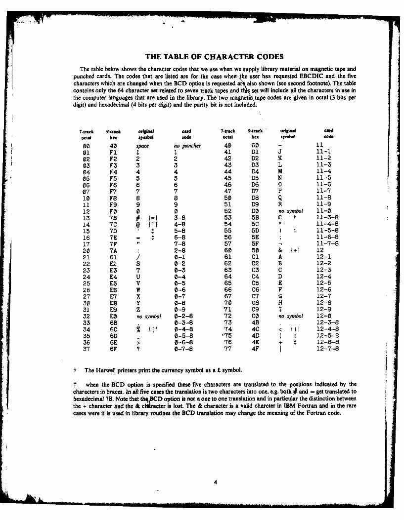
THE TABLE OF CHARACTER CODES

The table below shows the character codes that we use when wve supply library material on magnetic tape andpunched cards. The codes that are listed are for the case when -the user has requested EBCDIC and the fivecharacters which are changed when the BCD option is requested ar also shown (see second footnote). The tablecontains only the 64 character set related to seven track tapes and th set will include all the characters in use inthe computer languages that are used in the library. The two magneti tape codes are given in octal (3 bits perdigit) and hexadecimal (4 bits per digit) and the parity bit is not included,

T-track 9-track orilal card 7-track 9-track orisinal card

octal hel symbol code octal hex symbol code

00 40 space no punches 40 60 - 1101 F1 1 1 41 D1 J 11-102 F2 2 2 42 D2 K 11-203 F3 3 3 43 D3 L 11-304 F4 4 4 44 D4 M 11-405 F5 5 5 45 D5 N 11-506 F6 6 6 46 D6 0 11-607 F7 7 7 47 D7 P 11-710 F8 8 8 50 D8 Q 11-811 F9 9 9 51 D9 R 11-912 FO 0 0 52 DO no symbol 11-013 7B # l: 3-8 53 5B E t 11-3-814 7C @ 1') 4-8 54 5C * 11-4-815 7D ' 5-8 55 5D ) t 11-5-816 7E t 6-8 56 5E 11-6-817 7F " 7-8 57 5F -' 11-7-820 7A 2-8 60 50 & 1+1 1221 61 / 0-1 61 C1 A 12-122 E2 S 0-2 62 C2 B 12-223 E3 T 0-3 63 C3 C 12-324 E4 U 0-4 64 C4 D 12-425 E5 V 0-5 65 C5 E 12-526 E6 W 0-6 66 C6 F 12-627 E7 X 0-7 67 C7 G 12-730 E8 Y 0-8 70 C8 H 12-831 E9 Z 0-9 71 C9 I 12-932 EO no symbol 0-2-8 72 C0 no symbol 12-033 6B 0-3-8 73 4B 12-3-834 6C % (1 0-4-8 74 4C < M1 12-4-835 6D 0-5-8 '75 4D ( 1 12-5-336 6E > 0-6-8 76 4E + 12-6-837 6F ? 0-7-8 77 4F I 12-7-8

t The Harwell printers print the currency symbol as a £ symbol.

when the BCD option is specified these five characters are translated to the positions indicated by the

characters in braces. In all five cases the translation is two characters into one, e.g. both # and = get translated tohexadecimal 7B. Note that thQCD option is not a one to one translation and in particular the distinction betweenthe + character and the & clhracter is lost. The & character is a valid charcter in IBM Fortran and in the rarecases were it is used in library routines the BCD translation may change the meaning of the Fortran code.

4

ARE R.7477

VARWELLSUBROUTINE

LIBRARY.A CATALOGUE OF -

SUBROUTINES (1973)j

piledby[PM.jfiopjer I

This report contains a complete list of all the subroutines currently in the Harwell

Subroutine Library and gives for each one a brief outline of purpose, method, origin,

language and other attributes. Also included are contributions by members of the Numerical

Analysis Group on topics of general interest to library users. One of these is on how to

use the library and the others cover data fitting, optimization, linear algebra and

quadrature.

This di ion of the catalogue supersedes the previous issue (1971) R.6912.

Acknowledgements

I wish to thank Messrs. M.J.D. Powell, R. Fletcher, J.K. Reid and A.R. Curtis for

contributing the sections on Data Fitting, Optimization, Linear Algebra and quadrature.

KI

Accession For

NITS GRA&IDTIC TA F]unannouniced

Theoretical Physics Division, jutf C'toU.K.A.E.A. Research Group,Atomic Energy Research Establishment, BYHARWELL. Dist1iut .

July, 1973 . - AV3il; itY -

I..-- Av i,11Ib4 o

HL,.73 /2891, (C13) " 'Av 'DiHM.Dist Sp ia

II$/L/ . .

NOMA:

CONTENTS AM SUBROUTINE CLASSIFICATION

Page

Introduction .................................................................. 1

Part I: A list of subroutines 5

D. Differential equations 6

DA . Runge-Kutta methods for ordinary differential equation initialvalue problems .................................................. 6

DC ..... Linear multistep methods, predictor corrector mcthods forordinary differential equation initial value problems ........... 6

D) ..... Two-point boundary value ordinary differential equation problems 7DP . Parabolic partial differential equation problems ................ 8

E. Algebraic eigenvalue and eigenvector problems, i.e. diagonalization ofmatrices and latent roots and vectors 9

EA ..... Eigenvalues and eigenvectors of real symmetric matrices ......... 9EB ..... Eigenvalues and eigenvectors of real general matrices ........... 11EC ..... Eigenvalues and eigenvectors of Hermitian matrices .............. 13

F. Mathematical functions, random numbers and Fourier transforms 14

FA ..... Random numbers .................................................. 14FB ..... Elliptic integrals .............................................. 15F. ..... Error function, gamma function, exponential integrals and related

functions ........................................... ........ 16FD ..... Simple functions ........................................... .. 19FF ..... Bessel functions .............................................. 19Fr .... Functions associated with Quantum Physics ...................... .. 21FT ..... Fourier transforms ............................................ 21

G. Geometrical problems 21

GA ..... Transformation of co-ordinates and areas of contours ............ 21

I. Integer valued functions and integer valued system functions 23

IA ..... Integer functions offering system facilities .................... 23IC . Character string manipulation functions ......................... 23ID .... Simple integer functions ........................................ 23

K. Sorting and using sorted information 24

KA ..... Referencing ordered tables, located entries in ordered tables ... 24KB ..... Sorting arrays of numbers into order ............................ 24KC ..... Sorting and merging intervals on the real line .................. 25

L. Linear and dynamic programming 26

LA ..... Linear programming, i.e. minimization of a linear functionsubject to linear constraints ................................... 26

SBN 7058 0183 7

Page

V. Optimization and nonlinear data fitting problems 63

VA ..... Minimization of general functions and sums of squares offunctions of several variables ................................... 63

VB ..... Nonlinear data fitting and minimization of sums of squares offunctions and data fitting by spline functions .................. 68

VC ..... Data fitting by polynomials and spline functions ................ 70VD ..... Minimization of a function of one variable ...................... 71

VE . Minimization of a general function subject to linear constraints 72

Z. Non-FORTRAN system facilities 74

ZA ..... Time of day, date, program timing, dummy read and write, PAWAinformation, character code translation, message to operator,swop data set names, obtain TIOT and DCB information etc ......... 74

ZE ..... Estimation of rounding errors ................................... 78ZR . Debugging aids on ABENDs, completion codes, copies of system

control blocks ................................................. 78ZV ..... Accessing DD card information ................................... 79

A.E.R.E. reports describing library routines .................................. 80

Part II: Topics of general interest to users of the Harwell Subroutine Library 83

Using the Harwell Subroutine Library - naming conventions, write ups,using library routines in programs, library information sources, computergenerated index, obtaining copies of library routines in source form -listings, and decks and HUW files, SSP library, external users, enquiries 84

Data fitting and approximation ........................................... 97

Optimization ............................................... ..... 102

Linear algebra .......................................................... 106

Quadrature .............................................................. ill

General index ................................................................ 118

Page

M. Problems in linear algebra (excluding eigenvalue problems) 27

MAL..Solution of linear equations, also inverses and determinants ... 27MB..Inverses of matrices, also determinants, adjoints and generalized

inverses......................................................... 35.C...Computations with real matrices and vectors ........................ 37

MD . Determinants of matrices ....................... o....... 41ME . Computations with complex matrices and vectors ..o...................41

.X...Minitmum andi maximum elements of vectors ......................... 43

N. Nonlinear equation problems 43

NB..Solution of a single nonlinear equation in one unknown ... ........... 43NS..Solution of systems of nonlinear equations in sever-al unknowns .. 44

0., Input and output facilities 4

OA..Printing of arrays in tabular form...............................45GB . Subroutines generating output to the graph plotter .......o..... ..... 45OC . Graphical output on the line printer or teletype terminal .... 460D..Paper tape and Dectape data handling ............................... 46OE..Source and text editing facilities ................................. 47ON..Free form input facilities ........... o.........1...... o............47

P. Polynomial and rational function problems 48

PA..Zeros of polynomials .............. o................................48PB..Evaluation of polynomials .......... o............o...................49PC . Generating coefficients of polynomials ............................. 49PD..Functions of polynomials.......................................... 50PE..Polynomial and rational approximations, orthogonal polynomials 51

Q. Numerical integration 54

QA..Integrals of functions of one variable .......o......................54QB..Multi-dimensional integration of functions of sever-al variables 56QD . Integration of trigonometric and related functions ................. 57

.Estimation of integrals by Monte Carlo methods ..................... 57

S. Functions of statistics 58

SA..Probability functions ............................ ................. 58SV..Extraction of statistical information from data fitting routines 59

T. Interpolation and general approximation of functions 59

TA ... Generating and printing finite differences ......................... 59TB ... Interpolation by polynomials and spline functions...................60TD. .Estimation of derivatives by finite differences .................... 62TG .. Evaluation of spline functions .................. o..................62TS .... o Approximation of functions by spline functions....................63

Introduction

1. The Harwell Subroutine LibraryIThe Harwell Subroutine Library is maintained by the Numerical Analysis Group of

Theoretical Physics Division, A.E.R.E. Harwell. It is strictly a library of subprograms

which must be called by a user written program. Complete programs are not included inI

the library although some of the library 'routines' are in fact packages of more than onesubprogram. The principle language is FORTRAN but a few of the routines are written in

the machine code for the current Harwell computer - an IBM~ model 370/165.

The library is composed mainly of mathematical and numerical analysis routines. These

have in the main been written by members of the Numerical Analysis Group, past and present,

and are usually of a high standard. A few of the routines have been derived from sources

outside Harwell and acknowledgements are made to that effect in the catalogue entries.

The principle function of the library is to provide Harwell computer users with good

an eprovide copies of the library, and listings and card decks of individual routines

frasmall handling charge, see section A subsection 6 in part II.

Telibr-ary started life in 1963 and was first used on an IBM~ 7030 (STRETCH) computer.

I197the whole libr-ary was converted to be used on an IEh1 360 and at that time the

mciecoded routines were rewritten and the concept of having both single and double

precision versions of routines was introduced.

2. The catalogue

This catalogue of the Harwell subroutine library stands as a precise definition of

the library. It serves as a reference document for library facilities for users of the

Harwell computer. New users of the library will find the section A in part II 'how to

use the library' useful as an introduction to library facilities. Also useful, the

general index at the back of this report which has been extended in scope to provide a

general cross reference index to all library facilities.

This is a new issue of the catalogue and it supersedes the 1971 issue R.6912 and its

two supplements. All the new library routines introduced since 1971 have been included

and a few that have been discontinued have been removed. A new external users section

giving details of the charges for library material has been included, this was previously

published in the first supplement to R.6912. There is a new subsection of section A on

library information sources and a complete list of all A.E.R.E. reports which cover

library routines and include listings. The three sections on data fitting, optimization

and linear algebra have been brought up to date and a new section on quadrature has been

added. In the general list of routines we now give for each routine a list of any other

library or user routines which are called by that routine. There is no section on the

Harwell graphical package this time as this is now the responsibility of the Central

Computer Group at Harwell and is covered in, R. Jones and W. Prior, 'GHOST users manual' ,

TP 484.

The catalogue consists of two parts. Part I contains the complete list of routines

that make up the library giving details of purpose, method and attributes. The details

given are brief and only intended to be sufficient for a potential user to decide which of

the routines, if any, are suitable for his particular problem. The routines are listed in

* alphabetical order and the classification used for routine names is such that the list

falls naturally into sections associated with different classes of problem. There are

some exceptions and general topics, such as data fitting, are covered by routines spread

throughout the list. The general index provided at the end of the report can be used to

help the user locate routines associated with his particular problem. At the end of

part I you will find the list of A.E.R.E. reports which cover library routines.

Part 11 consists of sections contributed by members of the Numerical Analysis Group

on topics of general interest. They are intended to cover the situation which often

arises when there appears to be more than one routine in the library which could be used

to solve a particular problem. The sections give guidance as to best methods and point

to the routines which should be used. The sections also serve an educational purpose in

showing ways of setting up problems so that best use is made of the facilities available.

It is hoped that these contributions will grow in number and content with each new re-

issue of the catalogue.

The first section in part II is on how to use the library. Because this report is

primarily a reference document it has been placed after the list of subroutines and not

at the beginning where it logically should be. Anyone unfamiliar with the library should

make a point of reading that section, particularly the sections on naming conventions and

write ups.

Some of the conventions used in the list of subroutines in part I will need some

explanation and this is covered by the following subsections.

2.1 Language

The FORTRAN used up to Aug 1967 on the IBM 7030 was a FORTRAN closely related

to FORTRAN II or basic FORTRAN. The effect on the library is that pre-1967 routines

will most likely contain only FORTRAN II like features. After Aug 1967 FORTRAN IV

features started to come in with some of the IBM extensions to FORTRAN IV. The

routines have not been classified according to FORTRAN dialect or according to devia-

tions from standard because in general this information is not known. We make no

claims in respect to the portability of the library. We consider that a simpler user

interface combined with fairly efficient code is important and this aim often con-

flicts with the rather crude FORTRAN standards currently in operation.

The IEM assembler language for the 360 or 370 machines has been denoted by

360/BAL where BAL stands for basic assembler language. It is a term we use loosely

to cover assembly language programming including floating point and macro facilities.

No routine in the library uses special 370 features but some of the system routines

may be OS release dependent.

2.2 Versions

This lists the names of other versions of the subroutine and is principally used

to show that a double precision version is available and give its name. Double

precision names are distinguished by adding a D to the single precision name, see sub-

section 1 of section A in part 11.

2

2.3 Date

This gives the approximate date that the routine was introduced into the library.If a routine has been modified since its introduction and the modification waes exten-

sive enough to consider it a new routine the date given is the date when the modifica-

tion was made.

2.4 Size

The size of each routine is given in two parts; the first is the core required

to load the routine given to the nearest 100 bytes (1 byte = 8 bits), the second part

gives the number of cards in the source deck. Both sizes are approximate and are

associated with that routine whose name appears at the head of the catalogue entry.

This is usually the single precision version; double precision versions are likely

to take up more space than the single precision version. Users should be careful

using these sizes to estimate total core requirements and should consult the write

ups for the routines to find out how much extra work space must be provided. Card

deck sizes can also be misleading as some routines have a generous number of commnent

cards in them and so appear larger routines than they really are.

2.5 Calls

We give a list of other libr-ary routines or user provided routines which the

routine calls. We give only the list for the routine named at the head of the

catalogue entr-y, the lists for other versions can be deduced from this.

* 2.6 Origin

Here the author's name and the place of origin of the routine is given. Some

of the routines come from external sources and we give the author's name in recogni-

tion for providing us with library material. However most of the external routines

have undergone some modification for Harwell use and therefore the responsibility for

maintaining their good working must rest with Harwell and not the original authors.

Many of the authors listed as Harwell are no longer at this establishment and this

has been indicated by an * after their name.

Queries concerning library routines should not be directed to the authors person-

ally but through the library's queries service, see subsection 4 in section A in

part II.

Keeping the catalogue up to date

From the experience gained with the first catalogue, R.69 12, we have changed our ideas

on this subject. The period between complete new issues of the catalogue will have to be

more than 12 months and it is likely to be at least 2 years. In this period we shall keep

the catalogue up to date by bringing out supplements which will list the new routines intro-

duced into the library since the last issue of a catalogue or supplement. External users on

our mailing list will get these supplements automatically otherwise they will be available

only on demand. We reconmmend that any time you request a catalogue you should ask also for

any supplements to the catalogue.

3

Conmmnts, critical or otherwise, concerning the catalogue are always welcome, particu-

larly on the method of keeping it up to date.

Harwell Subroutine LibrarianM.J. Hopper

July 1973

4

PART 1: A List of Subroutines

D. Differential Equations

DAOIA

To integrate a set of first order ordinary differential equations

Yi f fi(ytPy2,...,PYnX) i=1,,.n

0 0given initial conditions yi(x ) = yi " Each call to the subroutine advances the

integration one step, the step length being set by the user. A subroutine must

be provided to compute values of the functions fi.

The subroutine uses the 4th order Runge-Kutta method proposed by Merson which

attempts to estimate the truncation error at each step.

Remark: This subroutine has been superseded by DCOIAD.

Versions: DAO1A; DAOIAD.

Calls: DYBDX (user routine).

Language: FORTRAN, Date: March 1963, Size: 1.2K; 44 cards.

Ori&i: D. McVicar, Harwell.

DAO2A

To integrate a set of first order ordinary differential equations

Yi = fi(Y1PY2"''Yntx )

i = 1,2,...,n

0 0Given initial conditions yi(x ° ) = yi. The steplength is controlled automatically

by the routine so that at each step the truncation error should satisfy an accuracy

requirement specified by the user. The Runge-Kutta routine, DAOIA, is called and

the Merson truncation error estimate is used to determine the steplengths. The

accuracy is not guaranteed.

The user must provide a subroutine to calculate the functions fi and optionally

a subroutine to print results at specified print points.

Remark: DCOIAD and DCO2AD provide more powerful facilities.

Versions: DAO2A; DAO2AD.

Calls: DAOIA and MXO2A.

Lan : FORTRAN, Date: March 1972, Size: 2.1K; 154 cards.

Origi: A.R. Curtis and A.B. Smith*, Harwell.

DCO IAD

A package of routines to integrate a system of first order ordinary differential

equations

Yi= fi(y 1 ,y2 ,...,ynx) i = 1.2,...,n

given initial values y(x ° ) = y i using a predictor-corrector method due to

C.W. Gear. Given a requested accuracy this method automatically chooses the step

size and the order of the integration formula. It possesses excellent stability

propoerties which enable it to take long steps even in stiff systems (i.e. those

involving very short time constants).

6

The user must supply a subroutine to compute the functions fi, and optionally

an output subroutine to be called at specified print points. Integration details

are made available to the output subroutine through named COMMOfN areas. There is

an interpolation subroutine which may be called from the output routine to get

values of yi(x) for any value of x in the current step.

Remark: DCO2AD provides a more simplified calling sequence to DCOIAD.

Versions: DCOIAD; there is no single precision version.

Calls: PBOIAD, MCOAD and MBOIBD.

Languae: FORTRAN, Date: May 1970, Size: 14.9K; 984 cards.

Origin: A.R. Curtis, Harwell.

DC02AD

To integrate a system of first order ordinary differential equations

Y = f i(y1 y2 1-' .Ynx) i = 1,2,...,n n < 10

0given initial values y i(x) = y. This subroutine calls DCOIAO forfeiting some

of its facilities to provide a more simplified calling sequence.

The user provides a routine to compute the functions fi, but printed output

is produced by the package's standard output routine. The restriction on n can be

removed by simple change to the array storage allocation in a COMMON block.

Versions: DCO2AD; there is no single precision version.

Calls: DCOIAD.

Languag : FORTRAN, Date: May 1970, Size: 3.9K; 32 cards.


D01A

To solve the two point boundary value problem for the second order linear

differential equation

y" + f(x)y' + g(x)y = k(x) x 1 4 x 4 Xn

given boundary conditions of the form ay' + by = c at the two points x1 and xn .

A finite difference approximation is used, see L. Fox, Proc. Roy. Soc. A.190,

1947. Initially 3rd and higher differences are ignored; then successive approxi-

mations are obtained by applying correction terms based upon 3rd and 4th differences.

The values of f(x), g(x) and k(x) at the points x ,x 2 , .. . ,x n are passed to the

subroutine in three arrays.

Versions: DDOIA; DDO1AD,

Calls: MA07A and TAOM.

Language: FORTRAN, Date: May 1965, Size: 2.6K; 172 cards.

Origin: P. Hallowell, Atlas Lab., Chilton, Berks.

7

To solve the two point boundary value problem for the second order non-linear


y" + f(x,y,y')y' + g(x,y,y')y = k(x,y,y') x x f xn

given boundary conditions of the form ay' + by = c at the two points xI and xn.

Starting from an initial approximation to the solution the equation is linear-

ized, solved by calling UDOIA and then re-linearized until the required accuracy is

reached. At this stage the effect of 3rd and 4th differences has been ignored and

the solution is then corrected to take these into account.

The user must provide a subroutine to compute values of f(x,y,y'), g(x,y,y')

and k(x,y,y').

Versions: DDO2A, DDO2AD.

Calls: DDOIA, TAO3A, TDOIA and FUWCTS (a user routine).

Language: FORTRAN, Date: May 1965, Size: 2.3K; 17! cards.

Origi: P. Hallowell, Atlas Lab., Chilton, Berks.

DINT

Returns the double precision floating point value of the integer part of a

real double precision floating point number. It supplements the IEM FORTRAN support

functions INT', IDINT and AINT.

Versions: DINT double precision.

Language : 360/BAL, Date: Sept. 1967, Size: .1K; 15 cards.

Origi: R.C.F. McLatchie, Harwell.

DPO1A

To solve the two point boundary value problem for the linear parabolic partial


au a2u au= a 7 + b + cu + d

where a,b,c and d are functions of x and t, x1 4 x I xn,, given boundary conditions

of the= q + ru + sa at the points x and x. Given 6t and the solution

u(x,t) at t, the subroutine advances the integration one tine step to obtain

u(x,t+6t).

The Crank-Nicolson integration formula is used to transform to a 2nd orderlinear ordinary differential equation which is solved by calling DOO1A.

The user must supply a subroutine to compute values of the functions a,b,c

and d given current values of x and t.

Versions: DPOIA; DPOIAD.

Calls: DOIA, TAOSA, TDOIA and FUNCTS (a user routine).

Language: FORTRAN, Date: Sept. 1965, Size: 3.5K; 197 cards.Origi: P. Hallowell, Atlas Lab., Chilton, Berks.

To solve the two point boundary value problem for the non-linear parabolic

partial differential equation

a a2 u auau a -U+b- +cu+d x (x 9C xat ax2 ax, I1axu

where a,b,c and d are functions of x,tu and L, given boundary conditions of theau au a

form P = q + ru + s N at the points xI and x n . Given 6t and the solution

u(x,t) at t, the subroutine advances the integration one time step to obtain

u(x,t+6t).

Using the solution at t as a first approximation the equation is linearized

and successively re-linearized until the required accuracy is obtained. DPO1A is

used to solve the linearized equation which in turn uses DDO1A.

The user must provide a subroutine to compute the functions a,b,c and d givenaucurrent values of x,tu and a.

Versions: DPO2A; DPO2AD.

Calls: DPO1A, TAOSA and TDOIA.Language: FORTRAN, Date: June 1966, Size: 2.4K; 203 cards.

Oriin: P. Hallowell, Atlas Lab., Chilton, Berks.

E. Eigenvalues and Eigenvectors of Matrices

EAO2AGiven a real symmetric matrix A and an estimate X e of one of its eigenvalues,

will find to a given accuracy the eigenvalue nearest to Xe and its corresponding

eigenvector. The eigenvector is normalized to have unit length.

The power method is applied to the matrix (A- eI) - with Aitken extrapolation

every 3rd iteration, see 'Modem Computing Methods'. NPL.

Remark: for matrices of small order the QR routines, EAO6C, etc. which find all

eigenvalues will be more efficient.

Versions: EAO2A; EAO2AD.

Calls: MBOIB.

Language: FORTRAN, Date: July 1963, Size: 12.4K; 70 cards.

Origin: E.J. York*, Harwell.

EAO

Given a real symmetric matrix A, finds all its eigenvalues Xi and eigenvectors

i.e. finds the non-trivial solutions of Ax = x.

Jacobi's method is used, where the successive off-diagonal elements of largest

modulus are reduced to zero by orthogonal transformations until all off-diagonal

elements are less than some prescribed value. The transformations are simultaneously

applied to the unit matrix to generate the vectors.

9

Remark: This routine is only to be preferred over the (y method routines when the

matrix tends to be diagonally dominant.

Versions: EAOM; EAOSAD.


Origin: J. Soper, Harwell.

EA06C

Given a real symetric matrix A, finds all its eigenvalues Xi and eigenvectors

i.e. finds the non-trivial solutions of Ax = x. The eigenvectors are normalized

to have unit length.

The matrix is reduced to tri-diagonal form by applying Householder transforma-

tions. The eigenvalue problem for the reduced problem is then solved by calling

EAOBC which uses the QR algorithm.

Versions: EAO6C; EAO6CD.

Calls: EAO8C and WO4B.

Language: FORTRAN, Date: Feb. 1970, Size: 1.3K; 26 cards.Origi: J.K. Reid, Harwell,

EAO7C

Given a real symmetric matrix A, finds all its eigenvalues, i.e. finds the

solutions . of det(A-?J) = 0.I

The matrix is reduced to tri-diagonal form by applying Householder transforma-

tions; then the eigenvalues of the reduced matrix are found by calling EA09C which

uses the QR algorithm.


Calls: EAo9C and NUO4B.

Language: FORTRAN, Date: Feb. 1970, Size: .6K; 12 cards.

Origi: J.K. Reid, Harwell.

EAOBC

Finds all the eigenvalues and eigenvectors of a real tri-diagonal symmetric

matrix; the eigenvectors will have unit length.

First EAO9C, which uses the QR algorithm, is used to find the eigenvalues,

using these as shifts the QR algorithm is again applied but now using the plane

rotations to generate the eigenvectors. Finally the eigenvalues are refined by

taking Rayleigh quotients of the vectors.

Versions: EAOSC; EAO8CD.

Calls: EA09C.

Language: FORTRAN, Date: Feb. 1970, Size: 1.8K; 76 cards.

Origi J.K. Reid, Harwell.

10

EA0o9C

Finds all the eigenvalues of a real tri-diagonal symmetric matrix. The QR

algorithm with shifts is used.




EAIIA

Calculates all the eigenvalues Ii and eigenvectors 1. of the system Ax i = \Bxi

where A is a real symmetric natrix and B is a real symmetric positive definite

matrix.

The matrix B is factorized into LLT and the eigenvalue problem L- A(LT)-ILTx f

Lx is solved using the EA06 - EA09 routines.

Versions: EAliA; EAllAD.Calls: EA06C, MA22A, MXO2A and M0O3AS.


Origi: S. Marlow, Harwell.

EBOI AFinds all the eigenvalues and eigenvectors of a general real matrix. The user

has options for requesting, no eigenvectors, only right eigenvectors, only left

eigenvectors, or both right and left. The vectors will have unit length.

The matrix is reduced by Householder transformations to upper Hessenberg form.

The eigenvalue problem for the reduced matrix is then solved by calling EBO4A. The

eigenvectors, if required it obtains by calling EBOSA.

Remark: Superseded by EBO6A.

Versions: EBOIA; EBO1AD.

Calls: EBO4A, EBOSA and MC08A.


Origi: E.J. York* and M. Reynolds*, Harwell.

EB04A

Finds all the eigenvalues, real and complex, of a real upper Hessenber matrix,i.e. a matrix A = jaijI such that alj = 0 for all I < J+1.

The double QR transformation is used, see J.G.F. Francis, Computer Journal,

Vol. 4, 1961 (also 1962).

The user may limit the number of times the transformation is to be applied.

Remark: Superseded by EBO9A.

Versions,: EBO4A; EBO4AD.

Calls: MCOUAS.

Langue: FORTRAN, Date: Sept. 1965, Size: 4.4K; 261 cards.

Origi: P.J. Hallowell, Atlas Lab., Chilton, Berks.

11

EBOSAGiven a real upper Hessenberg matrix A and one of its eigenvalues X, finds the

corresponding eigenvector x. This may optionally be a right or left vector and will

have unit length.

Inverse iteration is used, i.e. an iteration based on (A-IJ)x = x-n+1 -n

Remark: Superseded by EBOBA.

Versions: EBOSA; EBO5AD.

Calls: MA12A and MEO4B.

Language: FORTRAN, Date: Nov. 1966, Size: 4.2K; 284 cards.

Origin: M. Reynolds*, Harwell.

Finds all the eigenvalues and right eigenvectors of a real general matrix, i.e.

finds solutions X and x of Ax = ?x where the matrix A is real and has no special

structure. An option for balancing A is provided. The vectors are normalized to

have unit length.

A QR method is used. The matrix is reduced to Hessenberg form by orthogonal

similarity transformations (MC14A) and the QR method applied to obtain the elgen-

values (EB08A), see J.H. Wilkinson and C. Reinsch, 'Handbook for Automatic Computa-

tion, Linear Algebra', Springer-Verlag. Balancing is performed by MJ15A.

Versions,: EB06A; EB06AD.

Calls: EBOBA, N124A, NCI15A and MCOSAS.

Language: FORTRAN, Date: June 1973, Size: 2.7K; 162 cards.


EBO7A

Finds all the eigenvalues of a real general matrix, i.e. finds solutions X of

Ax = Wx where A is a real matrix with no special structure. An option for balanc-

ing A is provided.

A QR method is used, see EB06A.

Versions: EBO7A; EBO7AD.

Calls: EBO9A, W14A and NU15A.

Language: FORTRAN, Date: June 1973, Size: IK; 73 cards.

Origin: S. Marlow, Harwell.

EB06A

Finds all the eigenvalues and right eigenvectors of a real upper Hessenberg

matrix, i.e. finds solutions X and x of Hx = Xx where H is a real matrix which has

all zero elements Hij = 0 for i > j+1. The eigenvectors are normalized to have

unit length and there is an option which allows isolated eigenvalues to be specified.

A QR method is used, see J.H. Wilkinson and C. Reinsch, 'Handbook for Automatic

Computation, Linear Algebra', Springer-Verlag.

Versions: EBOBA; EBOBAD.

Calls: MCOSAS.

L : FORTRAN, Date: June 1973, Size: 9.4K; 429 cards.

Origin: HQR2 from reference given above, modified for Harwell by S. Marlow.

12

EBo9A

Finds all the eigenvalues of a real upper Hessenberg matrix, i.e. finds solu-

tions N of Hx = Xx where H is a real matrix which has all zero elements Hij = 0 for

i > j+l.

A QR method is used, see EBOSA.

Versions: EB09A; EBO9AD.


Origin: HQR from reference given for EBOSA, modified for Harwell by S. Marlow.

ECo2A

Finds all the eigenvalues of a tri-diagonal Hermitian matrix.

A bisection method based upon the Sturm's sequence is used. The eigenvalues

are returned in descending order of magnit de.

Versions: ECO2A; ECO2AD.

Language: FORTRAN, Date: March 1965, Size: IK; 42 cards.


EC06C

Given a complex Hennitian matrix A = Jaijj, aij = aii, finds all its eigenvalues

Xi and eigenvectors xi, i.e. finds the nontrivial solutions of Ax = ?ux. The eigen-

vectors are normalized to have unit length.

The natrix is reduced to tri-diagonal form by Householder orthogonal transforma-

tions and the reduced eigenvalue/eigenvector problem solved by a CR method (ECO8C).

Versions: EC06C; BCO6CD.

Calls: ECO8C, MEOBA and ME06AS.

Language: FORTRAN, Date: Sept. 1971, Size: 1.4K; 31 cards.


ECO7C

Given a complex Hermitian matrix A =aij, a. = ai., finds all its eigenvalues

X. such that det(A-X.I) = 0.

The matrix is reduced to triangular form by applying Householder orthogonal

transformations and the eigenvalues of the reduced matrix are found by EAO9C.

Versions: ECO7C; ECO7CD.

Calls: ECO9C and MEOSA.

Language: FORTRAN, Date: September 1971, Size: .5K; 13 cards.


BCOBC

Finds all the eigenvalues and eigenvectors of a complex Hermitian tri-diagonal

matrix, the vectors are normalized to have unit length.

The matrix is transformed into a real form by a unitary diagonal transformation.

EAOBC is then used and the vectors recovered by re-applying the transformation.

13

Versions: BECOC; ECO8CD.

Calls: EAOeC,

Language: FORTRAN, Date: September 1971, Size: 1.2K; 47 cards.


ECO9C

Finds all the eigenvalues of a complex Hermitian tri-diagonal matrix. The

matrix is transformed into a real form by a unitary diagonal transformation. The

routine for the real case EAO9C is then used.

Ver ions: BC09C; ECO9CD.

Calls: EA09C.

Language: FORTRAN, Date: September 1971; Size: .5K; 12 cards.


F. Mathematical Functions (see also section S for some functions of statistics).

FA01AS

Generates uniformly distributed pseudo-random numbers. Random numbers are

generated in the ranges 0 4 1 1, -1 4 rif I and random integers in 1 4 k 4 N where

N is specified by the user.

A multiplicative congruent method is used where a 32 bit generator word g is

maintained. On each call to the routine gn+1 is updated to 3 15gn mod(232 ); the

initial 32 bit value of g is '01010101 ....... 01'. Depending on the type of random

number required the following are computed, = 2- gn+1 ; 7 = 2 -31gn+1 -1 or

k = int.part [eq] + 1.

The routine also provides a facility for saving the current value of the

generator word and for re-starting with any specified value.

Versions: FAOWAS; there is no double precision version.

Language: 360/BAL, Date: Aug. 1967, Size: .3K; 108 cards.

Origin: R.C.F. McLatchie, Harwell.

FAO2AS

To return the signed fractional part of a real floating point number.

Versions: FAO2AS; FAO2AD.

Language: 360/BAL, Date: 1967, Size: .IK; 45 cards.

Origin: Harwell.

FAO3A

Generates pseudo-random numbers from a Gaussian distribution with mean zero

and standard deviation specified by the user.

The theory that sample means have a Gaussian distribution is used and the

numbers are generated by taking means of samples of size 12. There is an entry

which allows the user to specify his own sample size.

14

Versions: FAOSA; there is no double length version.

Calls: FAOIAS.

Language: FORTRAN, Date: November 1971, Size: .7K; 33 cards.

Origin: A.B. Smith*,Harwell.

FBOIA

Computes values of the complete elliptic integrals of the 1st and 2nd kind, viz.

It

K(m) = (1-m2 sin 2) dO 0 -< m 2 1

0

E(m) = 1 im2 sin 2 E) d( 0 < m

2 1

0

The subroutine uses an approximation of the form

n

Z '-M 2) {ak( , b, log e( .)k=O

see for n = 4 C.R. Hastings, 'Approximations for digital computers'.

Accuracies: FBOIA < 10- (n=4); FBOIAD < 10-14 (n=10).

Versions: FBOiA; FBOIAD.

Language: FORTRAN, Date: 1967, Size: .7K; 20 cards.


FBO2A

To compute values of the incomplete elliptic integrals of the 1st and 2nd kinds,

viz.

F(*,m) = f (I-m2sin 2 )- dO

0

E(*,m) = J (1-m2 sin 26) dO

0

2"where 0 m2 I land 0 <- 1.<

Accuracies: FBO2A < 10-6 . FBO2AD < 10-; FBO2BD < 10;9 FBO2CD < 10

Versions: FBO2A; FBO2AD; FBO2BD; FBO2CD.

Language: FORTRAN, Date: Revised 1967, Size: 1.8K; 78 cards.

Origin: L. Morgan*, Harwell.

15

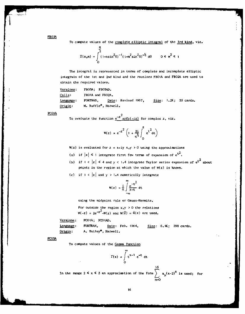
FBO3A

To compute values of the complete elliptic integral of the 3rd kind, viz.

tI(n,m) (l-nsin 2 0)-(I-m2 sin2 6)- dO 0 4 m2 4 1

0

The integral is represented in terms of complete and incomplete elliptic

integrals of the 1st and 2nd kind and the routines FBOIA and FBO2A are used to

obtain the required values.

Versions: FBO3A; FBO3AD.

Calls: FBOIA and FBO2A.

Language: FORTRAN, Date: Revised 1967, Size: 1.2K; 35 cards.

Origi: M. Ruffle*, Harwell.

A2

To evaluate the function e-z erfc(-iz) for complex z, viz.z

W(z) = e-z 2 + I e t2dt)0

W(z) is evaluated for z = x+iy x,y > 0 using the approximations

t2 2(a) if IzI -< I integrate first few terms of expansion of et2

(b) if I < jzi 4 4 and y < 1.4 integrate Taylor series expansion of et 2 about

points in the region at which the value of W(z) is known.

(c) if I < 1zI and y > 1.4 numerically integrate

o 2W(z) e i - dt

-t0

using the midpoint rule or Gauss-Hermite.

For outside the region x,y > 0 the relations

W(-z) = 2e-z 2-W(z) and W(i) = WV(z) are used.

Versions: FCO1A; FCOIAD.


Origin: A. Bailey*, Harwell.

FC03A

To compute values of the Ganm function

00

r(x) f t x - 1 e-t dt

0

15

In the range 2 4 x 4 3 an approximation of the form Z an(x - 2) n is used; for

n--O

16

x > 10 Stirling's approximation is used including up to 10 terms of the asymptotic

expansion.

For other values except x = 0 or a negative integer the relationship

r(x+i) = xr(x) is used to relate the required value with the range 2 4 x 4 3.

Accuracies: FCO3A < 10 Ir(x)l; FcoA < 1o- 14 jr(x)l.

Remark: the IBM functions GAMAV and DGAMMA are faster routines but the former

is inferior in accuracy to FCO3A for large x and neither allow x < 0.

Versions: FC03L; FCO3AD.

Language: FORTRAN, Date: March 1963, Size: 1K; 37 cards.


FCOA

To compute values of the Beta function

B(x,y) = (1-t) y -l dt

0

The relation B(x,y) = r(x)r(y)/r(x+y) is used. Approximations similar to those used

by FCOA are used but taking advantage of the combined form that is being evaluated.

-6 -14Accuracies: FCOSA < 10 ; FCOAD < 10

Versions: FCO5A; FCO5AD.


Origin: S. Marlowv, Harwell.

FC1cA

Computes the real and imaginary part of the Fresnel integral

x

f(x) = C(x) + iS(x) = ( t-eidt

The approximations usel are of the form

11

(a) 0 < x 4 4 f(x) e - i X (an + ib n ) )

Z n n 4n=O

-i e-i4

(b) x > 4 f(x) - + e (c + id) (2 Z n n xn=O

See J. Boersman, Maths. of Computation, Vol. 14, No. 72, 1960.

-6 -7Accuracies: PICQA < 10 , FCIcAD < 3 x 10 7

Versions: FCIOA; FC10.D.

Language: FORTRAN, Date: July 1963 Size: 1.6K; 36 cards.


17

I1To compute values of the exponential integral

E(x) = -' dt x > 0X

21

x

(a) forn<x 4 4

n--O

20

(b) for x > 4 b (,) exp(-x)

n=O

Accuracies: FICIIA < 10 -6; FC11AD < 107 12 .

Versions: FC1IA; FC1AD.



FC I2

Computes the real and imaginary parts of the Plasma Dispersion Function

00 2I e-

Z(z) =- r dt where z =x+iy,

for the case y > 0, and the analytic continuation of this for y < 0 as defined by

Fried and Conte, 'The Plasma Dispersion Function', Academic Press, 1961. The

derivative Z'(z) = -2(1+zZ(Z)) is also computed.

If y )? 2.75 or if y > 2 and x > 4 an asymptotic continued fraction due to

Fried and Conte is used, otherwise if x > 6.25 a rational approximation from

Abramowitz and Stegun is used, otherwise a Taylor series is used.

Accurac : approx. 10- 6 absolute.

Versions: Fc12A; FC12AD.


Origi: R. Fletcher, Harwell.

FC13A

To compute values of Dawson's Integral

xe X2 et 2

F(x) =e - x fetdt

0

for x real.

....... ... ..... ........ ... .. .... ...... . ... .. ... ... ....... . ... . .. .. I .. ... ... . . 1 ... .. . I ! ...

The following approximations are used,

(a) x2 < 6 a Taylor series expansion.

(b) 6 < x 2 < 36 a series expansion in (x2-x 2 where x is a lower limit

of one of eight subranges in [6,36].

(c) x2 > 36 an asymptotic series.

Accuracies: -3A<10 5 IF(x)I; FC13AD < 10713 IF(x)l.

Versions: FC13A; FC13AD.

Calls: PBOIAD.


Origi: A.R. Curtis, Harwell.

FDOIASGiven an integer n will compute 2.

Versions: FDOIAS; there is no double length version.

Language: 360/BAL, Date: November 1971, Size: .1K; 73 cards.

Origi: M.J. Hopper, Harwell.

FDOIBS

Given an integer n will compute 16n .

Versions: FDOIBS; there is no double length version.

Language: 360/BAL, Date: November 1971, Size: .IK; 66 cards.


FFOIA

Computes values of the Bessel functions Jo(x) and Y (x). A Chebyshev series

in x is used if 0 < x 4 8 and a similar series in - if x > 8, see,C.W. Clenshaw,x'Mathematical Tables', Vol. 5, NPL.

Accuracies: FFOIA 6 sig. figs.; FFOIAD 9 sig. figs.; except near x = 8 where

the accuracies may be inferior to those given.

Versions: FFOIA; FFOIAD.

Language: FORTRAN, Date: April 1963, Size: 1.9K; 102 cards.


FFO2A

To compute values of the Bessel functions J.(x) and Yixl. A Chebyshev series

in x is used if 0 4 x 4 8 and a similar series in - if x > 8, see,C.W. Clenshaw,x'Mathematical Tables', Vol. 5, NPL.

Accuracies: FFO2A 6 sig. figs.; FFO2AD 9 sig. figs.; except near x = 8 where

the accuracies will be inferior to those given.

Versions: FFO2A; FFO2AD.


Origi S. Marlow, Harwell.

19

FFO___

Computes values of the Bessel functions Io(x) and K0 W). A Chebyshev serie-

in x is used if 0 e x 4 8 and a similar series in - if x > 8, see,C.W. Clenaha%%.x

'Mathematical Tables', Vol. 5, NPL.

Accuracies: FFOSA 6 sig. figs.; FFO3AD 9 sig. figs.; except near \ = 8 where

the accuracies will be inferior to those givei.


Language: FORTRAN, Date: Dec. 1966, Size: 1.8K; 97 cardS.


FF04A

Computes values of the Bessel functions Ii(x) and K (0. A Chebyshev series

in x is used if 0 4 x 4 8 and a similar series in - if x > 8, see,C.W. Clenha%%,x

'Mathematical Tables', Vol. 5, NPL.

Accuracies: FF04A 6 sig. figs.; FFO4AD 9 sig. figs.; except near x = e %here

the accuracies will be inferior to those given.

Versions: FF04A; FFO4AD.

Language: FORTRAN, Date: Dec. 1966, Size: 1.7K; 94 cards.

Origin: S. Marlow, Harwell*

FF0O.4

Given x ) 0 computes the values of the Spherical Bessel functions

jn ( x ) ( 77k Jn+ (x)

for n = 0 up to N, N ( 29.

The method used is based upon the recurrence relation

jl(x) 2= jn(x) - in I(x)

given by F.J. Corbal6 and J.L. Uretsky, J.A.C.M., Vol. 6, No. 3.

Accuracies: FFOSA 6 sig. figs.; FF05AD 8 sig. figs.

Versions: FFO.; FFO5AD.


Origin: F.R. Hopgood*, Harwell.

FF06A

Given x > 0 computes values of all the Bessel functions ber(x). bel(x). ker(x),

kei(x), ber'(x), bei'(x), ker'l(x) and kei'(x).

A Chebyshev series in x is used if x C 10 and a similar series in - if x > 109Ax

See,F.D. Burgoyne, Maths. Comp., Vol. 17, No. 83, 1963.

20

Accuracies: FF06A sig. figs.; FF06AD 8 sig. figs, for x IC 10,6 sig. figs.

otherwise.


Language: FORTRAN, Date: Oct. 1964, Size: 3.1K; 83 cards.

Orgin: S. Marlow, Harwell.

FO1A

To compute the various vector coupling coefficients (3-j, 6-j, 9-j and their

kindred) of the theory of angular momentum in quantum mechanics, i.e. the Wigner 3-j,

6-j and 9-j symbols, the Clebsch-Gordan and Wigner coefficient, the Racah coeffi-

cient and Jahn's U-function.

Versions: FGOIA; FGOIAD.

Language: FORTRAN, Date: Aug. 1969, Size: 10.7K; 448 cards.

Origin: J. Soper, Harwell.

FTO1ACalculates discrete fourier transforms. Given equally spaced complex data

f(n) n = 0,1,2,...,N-1, of period N, it calculates the transform

N-I

f~)= f(n) exp rxml M = 0,1,2,...,N-1

n--O

or alternatively given f(m) m = 0,1,2,...,N-1 calculates the inverse transform

N-I

f(n) =(m) exp m = 0,1,2,...,N-1

m=O

where in both cases N must be a power of 2.

The 'Fast Fourier Transform' method is used, see, W.M. Gentleman and G. Sande,

'Fourier Transforms in Place', Proc. Fall Joint Computer Conference, 1966.

Versions: FTOIA; FTOIAD.



G. Geometrical Problems

GAOATo calculate the cartesian co-ordinates x,y,z of a point given in spherical

co-ordinates r,8,0; or vice versa.

Versions: GAOIA; GAOIAD.

Language: FORTRAN, Date: April 1964, Size: .8K; 30 cards.

Origi: A. Hearn*, Harwell.

21

GAO2A 4Calculates the area bounded by a contour f(x,y) = c and the side(s) of a

triangle. The triangle is assumed to have vertices (0,0), (2.0), (2.2) and the

user must provide values of the function f(x,y) at the vertices and mid-points

of the sides of the triangle. A point where the contour cuts the triangle must

also be given.

The function f(x,y) is approximated over the triangle by a quadratic form

defined using the six given function values.

Versions: GAO2A; GAO2AD.


Origin: D. Miller*, Harwell.

GA03Ao __ ___________________________

Constructs a system of plane contours f(x,y) = ck k=1,2,...,N over the

rectangular region x1 4 x < Xn, 'Y < y < yn and calculates the areas between

successive contours.

A mesh of isoceles triangles is constructed over the region and the contours

are generated using linear interpolation.

The user must provide code to evaluate f(x,y) at any point in the region.

Versions: GAO3A; GAOSAD.



GAO4.

To compute the solid angle subtended by a disc of unit radius from a general

point (r,h) in the plane perpendicular to the plane of the disc.

The integral expression for the solid angle is represented in terms of

J complete and incomplete elliptic integrals of the first kind, see M. Ruffle,

AERE - R.5419.

Versions: GAO4A; GAO4AD.

Calls: FBOIA and FBO2A.


Origin: M. Ruffle*, Harwell.

GAO5ATo efficiently determine whether a point (x~y) is interior or exterior to a

given closed region in the x,y plane. The boundary of the region may be specified

as a polygon or by a pair of parametric cubic splines, x(t) and y(t). Polar co-

ordinates may optionally be used.

The method is described in J.K. Reid, AERE - R.7298.

Versions: GAOSA; GAO5AD.

Calls: KBO1A and NBOIA.

Language: FORTRAN, Date: October 1972, Size: 7.9K; 400 cards.

Origin: J.K. Reid, Harwell.

22

I. Integer FUNCTIONS: including system facilities for FORTRAN programmers (see also

section Z).

IA01AS

Provides the FORTRAN user with facilities to allocate main storage during

execution, i.e. provides the user with the 360/OS GETMAIN and FRENIAIN facilities.

The routine can be used to get any number of areas of main core, to free areas

and to obtain the size of the largest currently available contiguous free area.

The areas obtained by IAOIAS are referenced using normal FORTRAN arrays but using

a displacement on the subscript which is supplied by IAOIAS.

Remark: The routine provides a limited form of dynamic allocation of arrays at

execution time but is highly system dependent and should be avoided In

programs intended to be computer independent.

Language: 360/BAL, Date: June 1970, Size: .5K; 192 cards.


ICO IAS

Given a character string and a search character locates the position of the

first occurrence of the character in the strin& or optionally locates the first

non-occurrence of the character.

In either case the search my be made in a forward direction from the beginning

or in a backward direction from the end.

Versions ICOIAS.

Language: 360/BAL, Date: October 1971, Size: .1K; 79 cards.


ICo2AS

To compare two character strings giving a less than, an equal to or a greater

than result.

Versions: ICO2A.S.

Language: 360/BAL, Date: October 1971, Size: .IK; 54 cards.


IDOAS

Computes the integer part of log gi, -n a real floating point number x.

Versions: IDOIAS; there is no double lenth version.

Language: 360/BAL, Date: Novembe- 1971, Size: .1K; 66 cards.

Origin: M.J. Hopper, Harwell.

IDiBSComputes the integer durt of Iog1 ( x given a real floating point number x.

Versions: IDOIBS; there is no double length version.

Languag: 360/BAL, Date: November 1971, Size: .iK; 55 cards.


23

ID02AL

Finds K the H.C.F. of two given integers I and J. It also finds integers M

and N such that

MI - NJ = K K >O

and M*I, N*J ) 0 and such that maxjlNf,Mjj is minimized.

Languag: FORTRAN, Date: July 1964, Size: .6K; 36 cards.

Origi: A. Gavan*, Harwell.

ID03A~Calculates the number of seconds elapsed between two given times given in

units of years, months, days and hours. The times must lie in the range 1st March,

1900 to 28th Feb. 2000.

Language: FORTRAN, Date: Aug. 1964, Size: iK; 44 cards.

Origin: A. Bailey*, Harwell.

K. Sorting and using sorted information

KA.IAS

To locate a specified entry in a given table. The fixed length entries in

the table are assumed to have been ordered on a key field within each entry into

either ascending or descending order, the ordering being specified in an index

array. The key field is assumed to contain non-numeric information and may be

any length up to 256 characters.

A simple binary search technique is used.

Remark: The subroutine has been designed to be used on tables sorted by KB1(YS

but may be used on Its own to generate and maintain ordered tables.


Origin: M.J. Hopper.

KBOIA

To sort an array of numbers into ascending order. The 'Quicksort' method is

used, see, C.A.R. Hoare, 'Quicksort', Computer Journal, April 1962.

Versions: KBOIA; KBOIAD; KBOIB integers; KBOIC halfWord integers.

Languaxe: FORTRAN, Date: May 1966, Size: 2.7K; 122 cards.

Origi: M. Reynolds*, Harwell.

KBO2A

To sort an array of numbers into descending order. The 'Quicksort' method is

used, see, C.A.R. Hoare, 'Quicksort', Computer Journal, April 1962.

Versions: KBO2A; KBO2AD; KBO2B integers; KB02C half~ord integers.

Language: FORTRAN, Dat'e: May 1966, Size: 2.6K; 115 cards.


24

KBOSA

To sort an array of numbers into ascending order maintaining an index array

to preserve a record of the original order.

The 'Quicksort' method is used, see, C.A.R. Hoare, 'Quicksort', Computer

Journal, April 1962.

Versions: KBO3A; KBOUAD; KBO3B integers; KBOC halfword integers.



KBO4A

To sort an array of numbers into descending order maintaining an index array

to preserve a record of the original order.

The 'Quicksort' method is used, see, C.A.R. Hoare, 'Quicksort', Computer

Journal, April 1962.

Versions: KBO4A; KBO4AD; KBO4B integers; KB04C halfword integers.

Languag FORTRAN, Date: May 1966, Size: 2.9K; 124 cards.

Origin: M. Reynolds*, Harwell.

KBI __S

To sort a table of fixed length entries into ascending or descending order,

sorting on a key field within each entry. The keyfield is assumed to contain non-

numeric information.

The entries in the table are not moved but rather an index array is returned

specifying the required ascending or descending order.

Subsorting on several fields may be performed.

Remark: Excellent for sorting text type information.

Language: 360/BAL, Date: May 1969, Size: .7K; 393 cards.

Origi: K. Moody, IBM.

KB1 IA

To sort n numbers from an array of m numbers, n < m. Options are provided

for sorting either the first n smallest or the first n largest numbers either in

terms of their algebraic values or their absolute values.

Versions: KBIIA; KB11AD; KB11AI.

Calls: MXOIA and MXO2A.



KCOA

Given a set of intervals on the real line, the routine finds the smallest set

of disjoint intervals whose union is the union of the original set, i.e. given

intervals which overlap one another it will reduce the number of intervals by

merging together overlapping intervals.

25

Versions: KCOIA; KCOIAD.

Language: FORTRAN, Date: Aug. 1964, Size: .5K; 19 cards.

Origi: D. Willis*, Harwell.

KCo20L

Given two sets of non-overlapping intervals, the routine merges the two sets

together and returns the smallest set of non-overlapping intervals which are common

to both the original sets.

Versions: KCO2A; KC92AD.

Lanxuage: FORTRAN, Date: Aug. 1964, Size: .7K; 32 cards.

Origin: D. Willis*, Harwell.

L. Linear progranming

IAOIA

Solves the general linear programming problem, i.e., find x which minimizes

the linear function + ... + C

f(x)=cx 1 + C 2X 2 n n

Subject to linear constraints

ailx1 + a1 2x 2 + ... + a.nxn 4< b. i=1,2,...,1

aj1x1 + a 2 x + .. " + ax = b. J=1+1,...,m

i1 2 2 n n j

where x i 0 i=I,2,...,n.

The Revised Simplex method is used where an inverse of the basis matrix is

maintained and updated at each iteration.

Versions: LAOIA; LAOIAD.

Calls: MCOMAS.

Language: FORTRAN, Date: Jan. 1966, Size: 50.8K; 359 cards.


LAo2

To find a feasible point to a set of linear constraints, i.e. find values

x I , ... ,x n which satisfy given constraints of the form

1j 0 x uj J=1,2,...,n

ailx I + al2 x2 + ... + anxn ;) d =2,...m

where additionally any of the inequalities may be strict equalities.

The method is described in R. Fletcher, 'The calculation of feasible points

for linearly constrained optimization problems', AERE - R.6354.

26

Versions: LAO2A; LAO2AD.

Calls: MBOI and !MCOAS.



LA03A

To factorize a sparse matrix A = LU, solve corresponding systems of equations,and update the factorization when a column of A is modified or replaced.

The method of factorization and treatment of sparsity is similar to that used

in MA18A, which is documented in the A.E.R.E. report R.6844.

The subroutine has been written primarily to handle the functions normally

performed on bases in linear programming problems, but its usefulness is not

necessarily restricted to that field.

Versions: LAOSA; LAO3AD.

Calls: KBIOAS.



M. Linear Algebra (see also section E)

MAO 1 B

To solve a system of n linear algebraic equations in n unknowns with one or

more right-hand sides

n

Z ax = i=1,2,...,n I=1,2,...,k

j=I

and optionally compute the inverse matrix A- I of the equation coefficient matrix

A = jaii.,

Gaussian elimination with partial pivoting is used, see 'Modem Computing

Methods', NPL, 1957, with double length accumulation of inner products.

Remark: Superseded by Mh21A.

Versions: MAOIB; MAOIBD.

Calls: WCOS.



MAO7A

To solve a system of n linear algebraic equations in n unknowns

n

a 13xi = b i i=1,2,...,n

when the equation coefficient matrix A = jaj is band structured.

27

The equations are solved by the method of Gaussian elimination without inter-

changes of rows so that stability is not guaranteed. The matrix A is presented to

the routine in a compact form.

When it is required to solve several systems which have identical left-hand

sides A, the routine can either be re-entered in a way that saves repeating the

elimination phase, or will except more than one right-hand side.

Remark: The pivoting strategy used makes the routine unreliable for systems

which are not positive definite or diagonally dominant, try M4O7B.

Versions: MAO7A; MAO7AD.


Origi: D. Russell, Atlas Laboratory, Chilton, Berks.

MAo7B

To solve a system of n linear algebraic equations in n unknowns,

n

T , a ..jx = i=1,2,...,n

j=1

where the equation coefficient matrix A = a ijI has a band structure.

The equations are solved by the method of Gaussian elimination with partial

pivoting. The matrix A is passed to the routine in a compact form.

When several systems with identical left-hand side matrices A are to be

solved the routine may be re-entered in a way that avoids repeating the elimination

phase.

Remark: For positive definite band systems see also MA15A.

Versions: MAO7B; MAO7BD.



MkOBA

Forms the normal equations of the linear least squares problem, i.e. given

an overdetermined system of linear algebraic equationsn

Z ajxJ b i=1,2" bim m> n,

j=1I

or more compactly Ax = b, the subroutine sets up the equations AT Ax = ATb. There

may be more than one right-hand size.

Remark: If the solution is required see MAO9A.

Versions: MAOA; MAOBAD.

Calls: SCO.S

Language: FORTRAN, Date: June 1964, Size: 1.3K ; 19 cards.


28

M&09A

Solves the linear least squares problem by the so-called normal equations

method, i.e. given an overdetermined system of linear algebraic equations

nZ a .x = bi i=1,2,...,m m > n; Ax = b

j=1

sets up and solves the system ATAx = ATb. The solution so obtained is such thatm n 2

the sum of squares of the equation residuals { a..x. - bi is a minimum.

i=1 j=1

Cholesky decomposition is used to solve the system. Equations with more than

one right-hand side can be solved and the user has options to obtain equation

residuals, sum of squares value and the inverse (ATA] - 1 which is usually required

for the variance-covariance matrix.

Remark: For a large number of unknowns the method is likely to give poor

results particularly when applied to fitting polynomials; try MA14A

or for polynomials VCOIA.

Versions: I'M09A; MAO9AD.

Calls: MAOSA, MAIOA and MCO3S.

Language: FORTRAN, Date: June 1964; Size: I.5K; 19 cards.


MA1Q0.


n

L a = b. i=1,2,...,n

j=1

where the coefficient matrix A =aij is symmetric positive definite. The inverse

matrix A is optionally computed.

Symmetric Cholesky decomposition is used with inner products accumulated

double length.

Remark: Superseded by MA22A.

Versions: MAIOA; MA10A.D.

Calls: MCOMS.



To solve an overdetermined system of m linear algebraic equations in n unknowns

in the minimax sense, i.e. given equations

n

Y a x = b i i=1,2,...,m m > n

J=I

find the solution x. j=.1,2,...,n such that

n

max a a.jx. - bi

j=1

is minimized.

The problem is posed as an n by m dual linear programming problem which is

solved using a special adaptation of the Simplex algorithm.

The routine returns residual values and may be requested to print solution

details.

The routine may be applied to the problem of approximation by linear combina-

tions of general functions over a discrete point set.

Versions: MAIIB; MAIIBD.



MA12A


n

a.x. = b. i=1,2,...,n_ J I

j=1

when the coefficient matrix A = laij I is upper Hessenberg or upper Hessenberg

squared.

The routine may be re-entered to provide additional right-hand sides for the

economic solution of systems with the same coefficient matrix A.

Gaussian elimination with partial pivoting is used accumulating inner products

double length.

Versions: MA12A; MA12AD.Calls: MCO3AS.



MA14A

To calculate a least squares solution to an over-determined system of m linear

equations in n unknowns, i.e. given equations

n,jx b, ==1,2,.. ,m m ;? n

J=Ij= 1

calculate the solution vector x = jxj such that the sum of squares of residuals

m n

F(x) Z aijxj - bi

i=1 J=l

30

is minimised. The user may specify that the first k equations, n > k > 0, are

satisfied exactly in which case the least squares solution to the constrained

problem is calculated.

There is a re-entry facility which allows further systems having the same

left-hand sides to be solved econoically. Another entry may be called io obtain

solution standard deviations and the variance-covariance matrix for the previous

calculation. The automatic printing of results and the talculation of equation

residuals are additional options.

The routine can be used to solve the general linear least squares data fitting

problem with, or without, equality side conditions.

Sl____.____s_ : OAO__ and __O__S

Versions: MAMA; MA14AD.

Calls: OA02A and MCOSAS.




nZ ax.= b. i=1 ,2,...,na iix

j=!

where the coefficient matrix A =a.jj is band structured. symmetric and positive

definite.

TSymmetric (LDL ) decomposition is used and full advantage is taken of any

variation in band width. For very large systems it uses scratch space on backing

store, otherwise it uses fast core storage.

There is a re-entry facility which allows further systems with the same

coefficient matrix to be solved economically. The user must supply a subroutine

to pass to MA15C the row elements of A.

The method is described in J.K. Reid, AERE Report - R.7119.

Remarks: This is an improved version of MA15A which has now been removed from

the Library.

Versions: MAl5C; MA15CD.

Calls: MCO2AS.



MA16A


n

axj= bi i=1,2,...,nJ=J

j= 1

31

* when the coefficient matrix A = aijJ is synmetric positive definite and is very

large and sparse. It uses the method of conjugate gradients, see, J.K. Reid,

AERE - R.6545.

The user is required to write code to multiply the matrix A into a vector

where full advantage of the sparsity of A may be taken into account in the code.

Versions: MA16A; MA16AD.

Language: FORTRAN, Date: Oct. 1970, Size: i.IK; 55 cards.


MA17A


n

=a x b. i=1,2,...,n; AA = b

j=1

where the coefficient matrix A = Jaij is large and sparse and symmetric positive

definite.

It provides facilities to (a) decompose the matrix A into factors LDL

T

where L is lower triangular and D diagonal, (b) to solve the system Ax = b or

compute the product Ab, (c) factorize economically a new matrix which has the

same sparsity structure as a previous one.

MA17A is a variant of MA1SA the subroutine for the general linear sparse case

and provides similar options, see MAlSA.

The method is described in J.K. Reid, AERE Report - R.7119.


Calls: KBICAS.

Language: FORTRAN, Date: April 1972, Size: 7K; 355 cards.



n

a x -b. i=l,2,...,n; Ax = b

j=1

where the coefficient matrix A = Ja1J is large and sparse, i.e. contains mostly

zero elements.

It provides facilities to (a) decompose the matrix A into triangular factors,

(b) to solve the system Ax = b or solve A Tx = b or carry out either of the opera-

tions Ab or ATb, (c) to factorize economically a new matrix which has the same

sparsity structure as a previous one, and, (d) load a new matrix into the list

processing form required by facility (c). For (d) the user must supply a sub-

routine to pass over the columns of the new matrix one at a time.

32

;.L .....

Optionally, automatic implicit scaling of equations and unknowns is performed.

Gaussian elimination is used combined with list processing methods to economise on

storage. The pivotal strategies used are designed to keep down the growth in the

number of non-zero elements. The degree to which the routine does this is under

the control of the user giving a choice of error growth against savings in storage.

A measure of the error growth is returned.

The method is described in A.R. Curtis and J.K. Reid, AERE - R.6844.


Calls: MC12A and KBIOAS.


Origi: A.R. Curtis and J.K. Reid, Harwell.

Mr2QkTo solve an overdetermined system of m linear equations in n unknowns in the

L sense, i.e. given equations

n

a a ijx j = b. i =,2,...,m m > n

j=1

find a solution x. j = 1,2,...,n such that

m n

i=1 j=l

is minimized. There is an option of constraining the solution so that x3 > 0

j = 1,2,...,n.

The problem is posed as a primal LP problem and solved using a variant of the

standard Simplex method which has the ability to pass through several Simplex

vertices at each iteration, see I. Barrowdale and F.D.K. Roberts; an improved

algorithm for discrete L linear approximation; Maths. Dept. preprint, Univ. of

Victoria, Canada.

The routine can be used for L linear data fitting problems.

Versions: MA2OA; MA2OAD. MA2OB; MA2OBD, B versions constrain x. > 0Jj = 1,2,..° ,n.


Origi: I. Barrowdale, Univ. of Victoria, Canada.

Given an n by n matrix A = Jaijj performs one or more of the following tasks.

(a) solves the system of linear algebraic equations

n

a aijx 1 = b1 i=1,2,...,n

j=1

33

given the right-hand sides b. i=1,2,...,n, and provides a re-entry facility

for the rapid solution of further systems of equations which have the same

elements a.ij

(b) computes the inverse matrix A- I of A.

(c) computes the value of the determinant of A.

The subroutine will optionally perform iterative refinement in order to both

improve the accuracy of the answer (solution or inverse) and provide error esti-

mates based either on the precision of the computer or on user supplied accuracy

information. An option for scaling the matrix is provided.

The method is basically Gaussian elimination with partial pivoting, implicit

scaling and iterative refinement and applying small random perturbations in order

to estimate errors, see S. Marlow and J.K. Reid, AERE - R.6899.


Calls: FAOIAS, MCOAS and MCI(.

Language: FORTRAN, Date: Aug. 1971, Size: 9K; 353 cards.

Origi: S. Marlow and J.K. Reid, Harwell.

MA22A

Given a symmetric positive definite n by n matrix A = faij this subroutine

performs one or more of the following tasks.

(a) Solves the system of linear algebraic equations

n

Z a..x. = b i=1,2,...,n

j=1

given the right-hand sides b i i=1,2,...,n, and provides a re-entry facility

for the rapid solution of further systems of equations which have the same

elements ai..-

(b) computes the inverse matrix A- of A.

(c) computes the value of the determinant of A.

This subroutine provides for the symmetric positive definite case all the

facilities provided by MA21A for the general real case. Symmetric decomposition

is used in the elimination phase otherwise the method details are the same as for

Mk21A.


Calls: FAO1AS and MCO3AS.

Language: FORTRAN, Date: Aug. 1971, Size: 8K; 285 cards.

Origin: S. Marlow and J.K. Reid, Harwell.

34

MA234

Given a complex n by n matrix A =a.j. and a complex right hand side b.

i=I,n this subroutine will solve the complex linear equations, compute the inverse

matrix or evaluate the determinant. It is a complex version of Mi21A and offers

identical facilities.

The FORTRAN COMPLEX facility is used.


Calls: FAOIAS, ME06AS and MEO7A.


Origin: S. Marlow and J.K. Reid, Harwell.

p MA24A

Given a complex Hermitian n by n matrix A = Jaij and a complex right hand

side bi i=1,n this subroutine will solve the complex linear equations, compute the

inverse matrix or evaluate the determinant. It is a Hermitian version of MA22A

and offers identical facilities.

The FORTRAN COMPLEX facility is used.


Calls: FAO1AS and MEO6AS.


Origi: S. Marlow and J.K. Reid, Harwell.

MBOIB

To compute the inverse matrix A- 1 of an n by n real matrix A = jaijl.

Gaussian elimination with partial pivoting is used with inner products

accumulated double length.


Versions: MBOIB, MBOIBD.

Calls: WCO3AS.


Origi: L. Morgan*, Harwell.

MBo2A

To evaluate the adjoint (or adjugate) matrix of an n by n real matrix

A = jaijj, n 4 20, and A may be singular.

The determinant is also evaluated and optionally the inverse of A (A non-

singular) instead of the adjoint. The relationship Adj(A) = det(A).A - I is used.

Gaussian elimination with partial pivoting is used.

Remark: There are more efficient routines in the library for evaluating

determinants and inverses.

Versions: MBO2A; MBO2AD.

Language: FORTRAN, Date: Dec. 1963, Size: 4K; 98 cards.

Origin: G. Packham*, Harwell.

35

MB04A

Given A the inverse matrix of a partitioned n by n real symmetric matrix

A, A

A + 1A A3

where A1 is (n-i) by (n-1), A2 a row vector and A3 a scalar; this subroutine

calculates the (n-1) by (n-1) inverse matrix A -1 of the submatrix A,.

Versions: MBO4A; MBO4AD.

Language: FORTRAN, Date: May 1964, Size: .6K; 14 cards.

Origin: M.J.D. Powell, Harwell.

MB05A

Given a partitioned n by n real symmetric matrix

MBOSA

A A

-1

where AI is (n-1) by (n-1), A2 is a row vector and A3 a scalar, and given A the

inverse of the submatrix A; the subroutine calculates A- I the inverse of A.

Versions: MBOSA; MBOSAD.

Language: FORTRAN, Date: May 1964, Size: 1K; 26 cards.

Orig: M.J.D. Powell, Harwell.

MB)I CA

To calculate A the generalized inverse of an m by n rectangular matrix A,

i.e. such that AA+A = A.

The user may either specify the rank of A or provide an estimate of the

accuracy of the elements in A in order that the rank may be estimated automatic-

ally.

Versions: MBICA; there is no double precision version.

Calls: MCO3AS.


Origi: M.J.D. Powell, Harwell.

MBI iA

To calculate A+ the generalized inverse of an m by n (m n) rectangular matrix

A in the special case that the rank of A is equal to m, i.e. such that AA+A = A

which with full rank can be defined as A = AT(AAT)- '.

Householder type orthogonal transformations with row and column interchanges

are used in a method described in M.J.D. Powell, AERE - R.6072.

Versions: MBIIA; MB11AD.

Lan ge: FORTRAN, Date: May 1969, Size: 3.3K; 153 cards.

Origzi: M.J.D. Powell, Harwell.

36

RCOIAS

To calculate the product of two matrices, i.e. given compatible matrices

A =aij ] and B = Jbl forms the product matrix C =cijj where

n!~~ ij a aiK bKj iI2..I ~ ,,.,

K=1

Inner products are accumulated double length.

Versions: MCOIAS; 1WO1AD.

Language: 560/BAL, Date: Sept. 1967, Size: .2K; 74 cards.


Mo__2AS

To evaluate the inner product aTb of two vectors a = Jail and b = Jbil of

length n, i.e. evaluate

n

s= a.b.

The products are accumulated double length, and use of WO2AS will in general result

in faster execution compared with any equivalent FORTRAN code.

Versions: MCO2AS; MCO2AD; MWO2BS; MCO2BD; in the B versions the elements of

the vectors can be stored in any regular fashion, i.e. the user gives

the first two elements of each vector and the subroutine locates the

rest by using the displacement of the second from the first and the

length of the vector.

Language: 360/BAL, Date: Aug. 1967, Size: .)K; 26 cards.


To evaluate the sum of a number c and an inner product a Tb of two vectors

a = Jail and b = Jbi j using double length accumulation of intermediate results

to minimize rounding errors, i.e. evaluate

n

s = t c t a b

i= 1

the signs being specified. The elements a and b may be stored in any regular

fashion. The first two elements of each vector are given and the displacement

of the second from the first and the length n are used to locate the remainder.

The use of MCOAS will in general result in faster execution than any equivalent

FORTRAN code.

Versions: NJO3AS; MCOSAD; the result s will on request be returned to full

double precision in the single precision version MCOAS.



37 MO"

Transforms an n by n real symmetric matrix A in to a tri-diagonal matrix having

the same eigenvalues as A.

Householder's method is used, see, J.H. Wilkinson, Numerische Mathematik,

Dec. 1962.

Versions: MCO4B; MCO4BD.

Language : FORTRAN, Date: 1966, Size: 2.1K; 61 cards.

Origi: Harwell.

MCOSAS

To evaluate the sum of triple products of elements of three given vectors

aail, b bi and c = Jcij of length n, i.e.evaluate

nS = b c

i= 1

the products are accumulated double length and the use of MC05AS will in general

result in faster execution time than any equivalen FORTRAN code.

Remark: Useful for weighted linear least squares problems where an inner product

of two vectors x and y modified by a vector of weights w is required.

Versions: MCOSAS; MCOMAD.

Language: 360/BAL, Date: December 1971, Size: .IK; 66 cards.


MCO6A

Applies the Gram-Schmidt orthogonalization process to n vectors in an m

dimensional space, n < m.

The vectors are passed as adjacent columns in a two dimensional array. Double

length accumulation of inner products is performed.

Versions: MNO6A; MCO6AD.

Calls: NUO2BS.


Origin: Osbourne*, Harwell.

MC07A

Given an n by n real symmetric matrix A calculates the coefficients of its

characteristic polynomial the roots of which will be the elgenvalues of A.

The matrix is reduced to tri-diagonal form by Householder's method and the

coefficients of the polynomial calculated using a recurrence relation.

Remark: This method should not be used to find eigenvalues but rather EAOC.

Versions: MCO7A; M[CO7AD.

Calls: ?.04B.



MCOBA

Transforms an n by n real matrix A to an upper Hessenberg matrix having the

same eigenvalues as A.

Householder's method is used, see, J.H. Wilkinson, Numerische Mathemtik, 1962.

Versions: MCOSA; MCOaAD.



NO9A

Given a sparse matrix A stored in a compact form and two vectors x and y,

evaluates either of the matrix-vector products a = + Ax or b = y + ATx.

Versions: MCO9A; MCO9AD.

Language: FORTRAN, Date: February 1972, Size: .8K; 21 cards.


Calculates scaling factors for the rows and columns of an n by n real matrix.

If the scaling is applied before Gaussian elimination with pivoting the choice

of pivots will more likely lead to low growth in round-off errors. The scaling

factors are returned as integral powers of 16.

The method is described in A.R. Curtis and J.K. Reid, AERE - TP.444, 1971.

Versions: NCI0; hU1OAD.


Origi: A.R. Curtis and J.K. Reid, Harwell.

NUt I 1A

To carry out a rank one update to a given positive definite or semi-definite

synmetric matrix which is stored in a factorized form A = LDL T , i.e. given a rankTTone matrix oww forms A = A + Oww T .

The routine was written to be used by optimization routines and will also

(i) accumulate a sum of rank one updates, (ii) carry out projection and allied

operations on A which reduce the rank, and (iii) update rank deficient matrices

where it is known from other considerations that the rank remains unchanged.

There are additional entry points which, factorize A = LDL T, recover A from

its factors, compute Ax or A-Ix, and obtain A in factored form.

The method is described in M.J.D. Powell and R. Fletcher, Harwell Theoretical

Physics report TP.519.

Versions: MCIlA; MCe1AD.

Languag: FORTRAN, Date: Jan. 1973, Size: 4.9K; 275 cards.


39

MC I 2A

Calculates scaling factors for the rows and columns of an n by n real sparse

matrix.


of pivots will more likely lead to low gr(vth of round-off errors. The factors

returned are integral powers of 16.

The method is described in A.R. Curtis and J.K. Reid, AERE - TP.444, 1971.

The matrix is stored in the condensed form used by MA]aA.

Versions: MC12A; MCI2AD.


Orixi: A.R. Curtis, Harwell.

Given the pattern of nonzeros of a sparse matrix A, finds a symmietric permuta-

tion that makes the matrix block upper triangular, i.e. finds P such that U = PAP I

is block upper triangular.

The method is that of R.W.H. Sargent and A.W. Westerberg, Trans. Inst. Chem.

Engineers (1964), 42, 190-197.

Versions: MC13A; MCI3AD; MC13C; MC13CD; the A versions use INTEGER*2s and

the C versions INTEGER*4s.Language: FORTRAN, Date: Feb. 1973, Size: 2.2K; 218 cards.

Origi: I. Duff, Oxford Univ., J.K. Reid, Harwell.

MC14ATransforms an n by n real matrix A to an upper Hessenberg matrix having the

same eigenvalues as A.

Transformations of the form I - .uuT are used, see J.H. Wilkinson and

C. Reinsch, 'Handbook for Automatic Computation - Linear Algebra', Springer-Verlag.

There is an option for specifying A as a submatrix of a larger matrix.

Versions: NC14A; MC14AD.

Calls: MC03AS.


Oriin: ORTHES from the above reference, modified for Harwell by S. Marlow.

Mc 154

To scale the rows and columns of a given real matrix A so that its elements

are suitably balanced for accurate computation of its eigenvalues and eigenvectors.

Diagonal similarity transformations are used based on powers of 16 so that on

a hexadecimal based computer only the exponent fields of the matrix elements are

modified. Searches along rows and columns for isolated eigenvalues are also made

and the matrix permuted so as to group such eigenvalues together. For the method

see J.H. Wilkinson and C. Reinsch, 'Handbook for Automatic Computation - Linear

Algebra', Springer-Verlag.

40

Versions: MCISA; MC15AD.


Origin: BALANCE from the above reference, modified for Harwell by S. Marlow.

MDO3h

To evaluate the determinant of an n by n real symmetric matrix.

Gaussian elimination is used with a diagonal pivotal strategy which preserves

symmetry (and can be unstable unless the matrix is positive definite).


Versions: MDOSA; MDOSAD.



MEOIB

Transforms an n by n Hermitian matrix into a tri-diagonal matrix having the

the same eigenvalues. Householder's method is used, see, J.H. Wilkinson, Numerische

Mathematik, Dec. 1962.

The FORTRAN COMPLEX facility is not used.

Versions: MEOIB; MEOIBD.

Language: FORTRAN, Date: 1966, Size: 3.4K; 78 cards.

Origin: Harwell.

MEo2A

Given an Hermitian matrix H and a complex vector z, computes the complex

product x = Hz.

The FORTRAN COMPLEX facility is not used.

Versions: MEO2A; MEO2AD.

Language: FORTRAN, Date: July 1963, Sizet IK; 20 cards.

Origi: E.J. York*, Harwell.

ME04A

To solve a system of n complex linear algebraic equations in n unknowns.

nax = bi i=I,2,... ,n

j=1

Gaussian elimination is used. The FORTRAN COMPLEX facility is not used.


Versions: MEO4A; MEO4AD; MEO4B; MEO4BD; B versions solve system which is

complex upper Hessenberg.

Calls: MC3O3AS.


Origi: Harwell.

41

ME06AS

To evaluate the sum of a complex constant c and an inner product of two complex

vectors a = Jail and b = Jbi1 accumulating intermediate results double length, i.e.

evaluaten

s = a- c i a b i

i= 1

the signs being specified.

The elements of the vectors a and b may be stored in any regular fashion. The

first two elements of each vector are given and the displacement of the second from

the first and the length n are used to locate the remainder. There is an option

which allows the user to specify the vector b to be the complex conjugate of the

actual vector passed to the routine. The constant and the elements of the vectors

must be FORTRAN COMPLEX variables.

Versions: ME06AS; MEO6AD; s may optionally be returned to full double precision

when using the single precision version ME06AS.

Language: 360/BAL, Date: June 1971, Size: .3K; 121 cards.


MEO7A

Calculates scaling factors for the rows and columns of an n by n comple

matrix.


of pivots will more likely lead to low growth in round-off errors. The scaling

factors are returned as integral powers of 16.

See, A.R. Curtis and J.K. Reid, AERE - TP.444, 1971.

Versions: MEO7A; MEO7AD.



Transforms an n by n complex Hermitian matrix A = laijI a1 j =aji , to a tri-

diagonal Hermitian matrix having the same eigenvalues as A.

Complex Householder orthogonal transformations of the form (I - Tuu) are

applied, see Wilkinson, J.H. Numerische Mathematik, December 1962.

Versions: MEOSA; MEOAD.

Calls: MEO6AS.

Language: FORTRAN, Date: September 1971; Size: 3.2K; 77 cards.

Oriin: S. Marlow, Harwell.

42

To extend the MAX and MIN facilities of FORTRAN. They find the position of

the algebraic minimum or maximum element in a vector of numbers.

The vector my be stored in any regular fashion, the user specifies the first

and second elements and the number of elements in the vector.

The most common application is to find the minimum or maximum element in a

simple FORTRAN array.

Versions: MXO1A; MXO1AD; MX01I integers.

Language: 360/BAL, Date: Dec. 1969, Size: . IK; 45 cards.


MXO2A

To extend the MAX and MIN facilities of FORTRAN. They find the position of

the minimum or maximum elements of absolute value in a vector of numbers.

The vector may be stored in any regular fashion, the user specifies the first

and second elements and the number of elements in the vector.

The most common application is to find the minimum or maximum element of

absolute value in a simple FORTRAN array.

Versions: MX02A; MXO2AD; MX021 integers.

Language: 360/BAL, Date: Dec. 1969, Size: .1K; 49 cards.

Ori : M.J. Hopper, Harwell.

N. Non-linear Equations

NBO1A

To find a real zero of a continuous function f(x) of one variable in a given

interval a 4 x 4 b, i.e. solve the non-linear equation in one variable

f(x) = 0 a 4 x < b

The user must supply code to evaluate f(x) at any point in the interval.

A binary search of the interval is made to find an interval [cL,f] such that

the signs of f(aL) and f(3) differ. The zero is then located by a combination of

linear interpolation and binary subdivision.

The user can limit the number of function evaluations and must specify an e

so that any point F such that jf(0) < e is considered a zero of f(x).

Versions: NBOIA; NBOIAD.


Origin: M.J.D. Powell and S. Marlow, Harwell.

43

NSOIA

To solve a systemi, of n non-linear equations in n unknowns, i.e. solve

fi (XI,x2,... ,Xn) i=1,2,...,n

The user must supply initial estimates of x1I,x2,...,x n and a subroutine to

compute values of the functions f. i=1,2,...,n.

The method uses the ideas of Newton-Raphson and Steepest descent coupled with

Broyden's method for improving Jacobi matrices, see, M.J.D. Powell, AERE - R.5947.

Derivatives are not required but the user must indicate a reasonable step size

to be used for approximating derivatives by finite differences. A solution to then

system is accepted when f 2 4 6, s specified by the user.

i=1

Versions: NSO1A; NSOIAD.

Calls: MBO1B and CALFUN (a user routine).



NSOA

To solve a system of m nonlinear equations in n unknowns, x =xj~x2,...,x n

of the form

n

ri(x) = fi(x) + a ixj = 0 i=1,2,...,m m > n

j=I

where the matrices JaijI and 13fI./axj are sparse.

The overdeternined case, m > n, is handled by taking the solution to be thatm

which minimizes the sum of squares s =_ ir(x)]2 . This makes the routine suit-i=I 1

able for the nonlinear data fitting problem and parameter variances and covariances

can be generated. Derivatives are optional and when not provided by the user are

estimated using a definite difference approximation.

The algorithm is based on Fletcher's version of the Marquardt method, see

R. Fletcher, AERE Report - R.6799, and is described in J.K. Reid, AERE Report

R.7295.

The user must supply Jaijj in a condensed form, an initial estimate of x, and

a subroutine to calculate fi(x) and optionally af/ axj.

Versions: NSO3A; NSO3AD.

Calls: KBIOAS, MA17A, MCO2AS, MCO9A and TDO2A.

Language: FORTRAN, Date: October 1972, Size: 12. X; 473 cards.


44

0. Input and Output

'To print out an m by n natrix in an easily read format. The FORTRAN format

used to print the elements is fixed. There is no limit to the size of matrix and

the output will extend ov,,r Several numbered pages if necessary.

Versions: OAO1A; OAO1AD.

Language: FORTRAN, Date: April 1963, Size: IK; 45 irds.

Origi: E.J. York*, Harwell.

oA.2A

To print out the contents of a single dimensioned array in tabular form.

The array is printed as a series of subtables, column length given by the

user, of numbers printed in an E FORMAT to a number of significant figures specified

by the user. Each member of the array will be identified by an integer printed

alongside its entry in the table.


Language: FORTRAN, Date: June 1968, Size: I.IK; 63 cards.


OAO3ATo print out in tabular form the contents of two single dimensioned arrays.

The FORMAT types (F, E or D) and the number of significant figures to be

printed must be separately specified for both arrays.

The arrays are tabulated as a series of subtables, column length specified

by the user, with corresponding elements from each array forming columns of pairs

of numbers. As many columns as possible are fitted across the page and as many

subtables are produced as are required to exhaust the arrays.

It is useful for tabulating a function y(x) and its argument.


Calls: MXO2A.



OB 1A

To draw on the graph plotter a smooth, tangentially continuous curve through a

given sequence of points xiy i i=1,2,...,n where optionally, the directions at each

point may be specified. Cusps and closed curves can be drawn if required.

The smooth curve is generated as a sequence of straight line segments. The

method is described in S. Marlow and M.J.D. Powell, AERE Report - R.7092 and is

based on a method due to D.J. McConalogue.

The user is expected to have initialized graph plotting through the GHOST

system and set the scaling before calling the subroutine.

45

Versions: OBIIA.

Calls: NBOIA and SHVECS (a GHOST routine).

Language: FORTRAN, Date: March 1972, Size: 5.IK; 408 cards.

Origi: S. Marlow and M.J.D. Powell, Harwell.

OB 1 2A

To draw on the graph plotter a cubic spline defined by its knots, function

values and first derivative values at the knots.

The spline is approximated by a sequence of straight line segments to within

an accuracy under the control of the user. The method is described in S. Marlow

and M.J.D. Powell, AERE Report R.7470.

The user is expected to have initialized graph plotting through the GHOST

system and set the scaling before calling the routine.

Remark: The routine is dependent on the local graph plotting system only through

one routine and that is one for drawing a sequence of line segments.

Versions: OB12A.

Calls: SHVECS (a GHOST routine).


Origin: S. Marlow and M.J.D. Powell, Harwell.

OIATo produce a graph of several dependent variables against an independent vari-

able on the line printer or teletype.

The dependent variables are identified on the graph by symbolic names chosen

by the user. The graph is orientated so that the independent variable axis runs

down the page thus allowing graphs of arbitrary length to be produced. A graph

may be put out in sections and different graphs can be put on different output

streams. The user must supply upper and lower bounds on the dependent variables

for scaling purposes.

Versions: OCOlA; no double precision version.



ODO IA

To allow the FORTRAN programier to read or write paper tape. This is a two

stage process; in stage one of reading a paper tape the tape is first read by one

of the 360's peripheral computers and the data is stored on disk; then stage two

the user calls ODOIA in a program run on the 360 to read the data from disk. To

write a paper tape the process is reversed. See, Chapter 13.5 in the Harwell

'Computer User's Manual'.


Origin: D. McVicar, Harwell.

46

0D02A

To allow the FORTRAN programmer to read or write Dectape. This is a two stage

process similar to that for reading and writing paper tape, see ODOA.


Origin: R. Garside*, Harwell.

OEO,_A

Provides simple editing facilities for the modification of source language

and data which may be stored on any sequentially organised backing store or

presented as a card deck.

The editing is performed according to commands given by the user on control

cards. There are facilities for replacing, inserting and deleting statements, and

changing specified fields in a statement. The new version of the source statements

can optionally be re-sequence numbered. The new version, along with changes made,

is listed.

The user controls the destination of the output from the routine by supplying

an appropriate DD card and by specifiing the stream number.

Calls: INTRAN and OUTRAN (two user routines).



ONOIB

To provide a 'free format' input facility for the FORTRAN user.

The subroutine is designed to read data items as opposed to records (i.e.

cards) although it does provide facilities for monitoring record type input.

It offers facilities to, read numeric data, identify keywords held in a

dictionary, build and add to the dictionary, recognize bad input data and allow

the user to take corrective action, recognise and identify special characters,

list each input record as it is read in, provide and allow the user to reset a

pointer within the record to the current item, read BCD information.


Origin: M. Ruffle*, Harwell.

ONo2A

Given a data card containing numeric data items constructs the FORTRAN format

required to read the numbers from the card.

The format is returned in an array for the user to use in a REMAD statement.

The subroutine was designed for use with the Harwell teletype system when it is

not always convenient to type in data in a fixed format.

Calls: ZAO3AS.



47

Ip. Pol.nomiLals and Rational Functions

PAOIA

To find all the real and complex roots of a polynomial with real coefficients,

i.e. calculate the zeros of

ao+aIx+a2x +...+anx 0

The method is that of D.E. Muller, MTAC, 1956.

Versions: PAOIA; PAOIAD.


Origin: SHARE program C2* MLF HPRS, translated for Harwell by D. McVicar.

PA02L

To find all the real roots of a polynomial with real coefficients that fall

within a given interval a < x < b, i.e. calculate the zeros of

2 naO+aIx+a 2 x +...+anx = 0 a < x % b n < 49

The subroutine will also return the number of real roots above, below and

within the interval and there is an option to request all the real roots.

Sturm's sequence polynomials are generated to bracket the roots then a

combination of Newton Raphson and bisection is used to refine each root.

Versions: PAO2A. PAO2AD; PAO2B; PAO2BD; the B versions provide an estinate

of error growth induced by using a recurrence relation to generate

the Sturm' s sequence.



PAOSA

To find all the roots of a cubic polynomial, i.e. calculate the zeros of

a0 +a Ix+a 2 x 2 +a 3 x 3 = 0

A non-iterative method is used.

Versions: PAO3A; PAO3AD.


Origin: H. Simmonds*, Harwell.

PAO4ATo find the number of real roots above, below and within a specified interval

a < x -< b.

Sturm's sequence polynomials are used. The degree of the polynomial must be

less than 21.

Versions: PAO4A; PAO4AD.


Origin: M. Lancefield*, Harwell.

48

PAToiaa Cn

To find all the roots of a quartic polynomial, i.e. the zeros of

2 3 4ao+a x+a x +a x +ax = 0

01 2 3 4

The method is non-iterative, see, Maths. of Computation, 279-281, July 1960.

Remark: An iterative method is likely to produce more accurate results,try PAO2B.

Versions: PAOSA; PAO5AD.

Calls: PAO3A.

Language: FORTRAN, Date: Jan. 1963, Size: I.8K; 96 cards.


PBOIAS

To compute the value of a polynomial

2 nP(x) = a0+aIx+a 2x +.. .+an x

The value is calculated using the nested form

P(x) = ( .... ((anx+an-I )x+...+a 1 )x+a0

accumulating intermediate results double length.

Versions: PBOIAS; PBOIAD.

Language: 360/BAL, Date: Aug. 1967, Size: .IK; 34 cards.


PBO2AS

To compute the complex value of the real polynomial

2 znP(z) = a0 +at z+a 2 z +...+a n

for complex argument z.

The method is synthetic division by a quadratic factor, see, R. Butler and

E. Kerr, 'Introduction to Numerical Methods', Pitman.

P(z) and z must be FORTRAN COMPLEX variables; the calculation is carried

out in real arithmetic accumulating intermediate results double length.

Versions: PBO2AS; PBO2AD.

Language: 360/BAL, Date: July 1967, Size: .3K; 124 cards.


o__A

To calculate the coefficients of a polynomial given all its roots, the roots

must be real, i.e. given real numbers r.,,...,% calculate aota ,...,a n with

a. = 1 such that

49

2 n KxF(_.) ..(_a+a I x+a 2 x +...+anx -)

Versions: PCOIA; PCOIAD.

Language: FORTRAN, Date: Aug. 1967, Size: .SK; 45 cards.

Origin: W.E. Hart*, Harwell.

PCo2A

Given n+I points xi y i--O,1,2,...,n calculates the coefficients of the

polynomial that passes through all n+l points, i.e. the interpolation polynomial

1 2 nP(x) a a+alxax+.+n

* such that P(xi) = Y1 i--O,1,2,...,n

The coefficients of the Lesbegue polynomials LK(x), i.e. such that LK(x i ) 0

i K and LK(xK) = 1, are calculated using PCOIAS and PBOIAS, the coefficients

aoa I ...,a n are then obtained from

n

P(x) '

P ) YKLII(x)

K=O

Versions,: PCO2A; PC02AD.

Calls: PBO1AS and PCOIA.


Origin: L. Morgan*, Harwell.

Given a real root of a polynomial divides out the root to obtain the

coefficients of the reduced polynomial, i.e. given a root . and polynomial

ao+aIx+...+anxn calculates b. j=O,1,...,n-i such that

aoa Ix+...+anX n (- _)(bj+blx+...+b n-I

where assumed to be zero.

Synthetic division of a polynomial by a linear factor is used accumulating

intermediate results double length. The root is divided out from the end least

likely to produce error growth in the b s. The user has an option to force the

division to be carried out from either end.

Versions: PDOIAS; PDOIAD.

Laa ae: 360/BAL, Date: May 1967, Size: .2K; 80 cards.

Orix: Harwell.

s0

PD02A

To find the first m terms of the Taylor series expansion of functions of a

given polynomial (or polynomials).

n KLet the polynomials be A(x) = ab±a1 x+..*.+a x and B(x) = bO+b x+...+b x and

nsuppose the Taylor series to be T(x) =to~~tlx+...+t m x+... the expansions are

obtained by considering identities between A(x), B(x) and TVx). The functions

covered and identities used are

PDO2A: T(x) =I/A(x) ; A(x)T(x) m1

PD02B: T(x) =log[e A(x)1; T'(x)AMx) A'(x), T(O)=log e(a 0)

PD02c: T(x) =expj(A(x)] ; T'(x) A'(x)T(x), T(0)=exp(a 0 )

PDO2D: (T,1x)=sin[A(x)] ; Ts:(x)mA'(x)T (x), T,(0)=ia)(Tc~x)=cosLA(x) J ; T C (x)mA (x)T (x)W T ()=c a0 )

PDO2E: T(x) =[A( x)]r ; A(x)T'(x)=rA'(x)T(x), T(O) = a 0r

POO2F: T(x) =-A(x)B(x) ; T(x)aA(x)B(x)

Versions: PDO2A; PD02AD; PDO2B; PD02BD; PDO2C; PDO2CD; PD02D; PDO2DD;

PDO2E; PD02ED; PDO2F; PDO2FD; PD02G; PD02GDo

Calls: Nt.02BS.

Language: FORTRAN, Date: Dec. 1970, Size: .7K; 43 cards.

Origin M.J. Popper, Harwell.

PDOSA

Given a polynomial in x, i.e.

PWx = a0+a x+...+an x n n! 50

calculates the coefficients b.i j=0,1,...,n of the polynomial under a change of

variable z=ux+v, i.e. such that

aO+a Ix+..*.+a nx n a b 0+b I(ux+v)+...+b n(ux+v) n

Versions: PDOSA; PDOWA.

Calls: PRO1AS.

Language: FORTRAN, Date: June 1966, Size: .8K; 29 cards.

Origin A.R. Curtis, Harwell.

PEOIA

Calculates the coefficients of a polynomial give the coefficients of its

expansion in terms of Chebyshev polynomials, i.e. given b.i j=O,1,...,n find

a. J=O,,..,,n such that

aO~~x..+anxn bTo(x)+bIT (x)+...+ n Tnx) n40

If the polynomial is known to be an odd or even function the calculation can be

simplified and the routine can take advantage of this.

51

Versions: PEOIA; PEOIAD.

Calls: MCO3AS.

Language: FORTRAN, Date: June 1963, Size: X; 65 cards.


PEO3A

Given the coefficients of a polynomial calculates the coefficients of its

expansion in terms of Chebyshev polynomials, i.e. given a. j--O,I,...,n find

b. j--O,I,...,n such that

boTo(x) +b I T I (x)+..•.+b n Tn(x)m e x..anx n1C4

Versions: PEO3A; PEO3AD.

Language: FORTRAN, Date: Sept. 1963, Size: .SK; 34 cards.

Origi: C. Brittian*, Harwell.

PEO4A

Given a function f(x) in the range u 4 x 4 v finds a rational approximation of

the form

0aoT 0 (z)+a IT I (z)+...+amTm(z)

m'n T0 (z )+b I T I (z)...+b nTn( z)

where TK(z) is the Chebyshev polynomial of order K and -1 A z = 2 1 andV-U

O m (10,0 n (10.

The approximation found is such that Rmn(ZK) = f[ (z.(v-u)+v+u)1 K--0,1,...,m+n

where the zK are the zeros of T,n+,(z).

The routine returns a guide to how close the approximation is to the 'best

approximation' in the minimax sense. Also returned are the coefficients of the

equivalent form

nR mn(x) x+=ooPx

m ( 0 + 3x+. * $nxn

The user nust provide a function subroutine to evaluate f(x).


Calls: MA21A and FUNCT (a user routine).

Lnguage: FORTRAN, Date: Aug. 1963, Size: 7.7K; 300 cards.

Origin: A.T. Sinden*, Harwell.

PEO5AD

Given a smooth function f(x) in the range u k x ( v finds a weighted rational

approximation of the form

ao+alx+..•.+am xm,n(x) = n

R mn bo+bex+...+bxn

52

which is 'best' in the sense that

f(x) - R (x)max I Iu4X4v w(x)

is minimized, W(x) is a positive weight function. The cases n=O or m=O are handled

but there is a restriction 0 4 m < 10, 0 4 n 4 10 and m+-n 4 15.

The method is iterative and uses the two stage Maehly algorithm, see,

H.J. Maehly, J. Ass. Comp. Mach., 1963, with third order inverse iteration to

solve the eigenvalue problem, see, A.R. Curtis and Osborne, Computer Journal,

Vol. 9, no. 3, 1966.

The user must supply code to evaluate f(x) and W(x).

Versions: PEO5AD; there is no single precision version.

Calls: MAOIBD, MCOIAD, MCO3AD, PBOIAD, PDOSAD and ZEOIAD.

Language: FORTRAN, Date: 1967, Size: 32.IK; 630 cards.


PE06A

Given a polynomial C(x) of degree K finds the coefficients a. j=O,1,...,m and

b j=1,2,...,n of the Pad6 approximationJ

mao+a Ix+...+a

xPm (x) = 0m m-~K mn2

mn 1+b x+...+b xn

such that the first m+n+i coefficients of the Taylor series expansion of P (x)mnnare the same as the first m+n+1 coefficients of c(x).

The m zeros, the n poles and residues of the approximation are also returned.


Calls: MA21A and PAOIA.

Language: FORTRAN, Date: Jan. 1964, Size: 3.5K. 86 cards.

Origi: L, Morgan*, Harwell.

PEO7A

To compute the value of a polynomial P(x) of degree n which is expressed as a

linear combination of orthogonal polynomials QK(x) K=O,1,...,n, i.e.

P(x) = CoQo(x)+cIQ(x)+...+c nQ n(x)

where the polynomials QK(x) are defined by the recurrence relation

Qo(X) = 1, Q1(x) = X-GO

Qk+,(x) = (x- a)(K(x) - PQK,(x) K=1,2....

See F.J. Smith, 'Maths. of Computation', Jan. 1965.

53

Remark: Can be used to compute values of polynomial fits obtained by VCOIA.

Versions: PEO7A ; PEO7AD.

Language: FORTRAN, Date: July 1964, Size: .5K; 20 cards.

Origi: S. Northcliffe*, Harwell.

PEOSA

To obtain the coefficients a. j.0,1,...,n of a polynomial P(x) of degree n

which is expressed as a linear combination of orthogonal polynomials QK(x)

K--O,1,...,n, i.e.

I n C 0 (x) +c 1 Q 2 (x)+.. +Cn%(x)

where the polynomials QK(x) are defined by the recurrence relation

Qo(x) = , QI(x) = x-<O

QK+I(X) = (x-'ak)QK()- QKI(x) K=1,2....

Remark: Can be used to obtain the coefficients of polynomial fits produced by

VCO IA.

Versions: PEOSA; PEO8AD.


Origi: S. Northcliffe*, Harwell.

PEiIA

Given m values of a function f(x) calculates the nth degree inimax polynomial

approximation P(x), m > n, 2 4 n 4 25, such that

max - P(x) I

is minimized.

See P.C. Curtiss and W.L. Frank, Journal, A.C.M., 1959.

Versions: PEtIA; PEIIAD.


Orig-i: S. Marlow, Harwell.

Q. Numerical Integration

QAOIAS b

To evaluate the integral [ f(x)dx using one of five Newton-Cotes formulae,li #a

i.e. Trapezoidal rule, Simpson's rule, the I rule and the five and six point

formulae.

The user must supply values of the integrand f(x) tabulated at equal intervals

in a 4 x 4 b, hence the interval size must be chosen by the user.

Double length accumulation of intermediate results is carried out to minimize

rounding errors.

54

Remark: One of the adaptive quadrature routines, QAO2A, QAO4A or QAO5A may give

better results than QAOiAS.

Versions: QAOIAS; QAOIAD.



QAO2A

To evaluate the integral ]a f(x)dx to a specified absolute accuracy.

The subroutine uses a variable step Simpson's rule using at each step an

integration step based on 4th differences which is chosen small enough to achieve

the required accuracy.

The user must specify a minimum integration step-size and provide a subroutine

to evaluate the integrand f(x).

Remark: Unless only limited accuracy is required, or core store is linited,

either QA04A or QAO5A may be better, especially on 'difficult integrands'.

Versions: QAO2A; QAO2AD. Both use double precision arithmetic.

Calls: CALCIN (a user routine).

Language: FORTRAN, Date: March 1963, Size: 3.3(; 175 cards.

Origin: M.J.D. Powell and A.R. Curtis, Harwell.

QAO3A

To tabulate an integral function of the form

xg(x) = g(a) + f f(t)dt

a

at points x=a, a+h, a+2h,...,a+mh to a specified accuracy.

The subroutine uses a variable step Simpson's rule using at each step an

integration step, based on 4th differences, which is chosen small enough to achieve

the required accuracy.

The user must specify a minimum integration step-size and provide a subroutine

to evaluate the integrand f(x).

Versions: QAO3A; QAO3AD.

Calls: CALCIN (a user routine).


Origi: M.J.D. Powell, Harwell,

To evaluate the integral f(x)dx to a specified relative or absolute

accuracy.

An adaptive scheme is used based on a three point Gaussian quadrature, see

I.G.A. Robinson, 'Adaptive Gaussian Integration', Australian Comp. Journal, Vol. 3,

no. 3. The user must provide a FUNCTION subprogram to calculate values of the

integrand f(x).

55-A

Remark: Shorter than QAO5A but less efficient.

Versions: QAO4A; QAO4AD. Both use double precision arithmetic.Language: FORTRAN, Date: May 1972, Size: 5.7K; 186 cards.

Origin: I.G.A. Robinson, Univ. of Melbourne, implement for Harwell by

A.B. Smith*.

QA05A lbTo evaluate the integral ]f(x)dx to a specified accuracy which may be relative

or absolute, a

The subroutine uses an adaptive scheme based on Romberg extrapolation and

Trapezoidal rule, and is described under the name CADRE in C. deBoor, 'CADRE:

an algorithm for numerical quadrature' in 'Mathematical Software' Ed. J.R. Rice,

Academic Press.

The user must supply a subroutine to evaluate f(x) a < x 4 b. The subroutine

returns error estimates and attempts to identify any singularities and discontinui-

ties in f(x).

Remark: Powerful and efficient, but rather large in core requirement.

Versions: QAOSA; QAO5AD. Both use double precision arithmetic.

Language: FORTRAN, Date: October 1972, Size: 26K; 353 cards.

Origin: Subroutine CADRE, C. de Boor, Purdue Univ.; modified for Harwell by

A.R. Curtis.

QBOIATo evaluate the multi-dimensioned integral

b b 2 bn

2. f(xx 2 ,...,xn)dX1 'dx 2 ... ,Idx n 1 4 n 4 6

a I a2 an

where the limits aK and bK can be functions of x1 ,x 2 ,...,XK_! and a and bI

constants. The user must specify for each dimension which type of quadrature

is to be used, Simpson's Rule, Gauss quadrature or a quadrature based on Chebyshev

polynomials.

A relative accuracy can be requested and a subroutine to compute the values

of the limits and integrand must be provided.

Versions: QBOIA; QBOIAD.

Calls: LIMITS (a user routine).


Origin: F.R. Hopgood*, Harwell.

QC2AD

To provide weights and zeros for Gaussian type quadratures of integrals of

the form

oe-x f(x) dx

0

56

The weights and zero are calculated to give exact results when f(x) is a polynomial

of' degree 2k- in z = where a is chosen by the user. A range of quadratures maya+ X

be requested. The calculations are relatively expensive and the routine should only

be used when the quadrature is to be applied to many integrals.

Remark: Use of this routine is likely to give better results than Gauss-Laguerre

for bounded f(x).

Versions: QCO2AD: there i1 no single precision version.

Calls: NBO1AD and QAOAD.



To evaluate integrals of the formb rb

f f(t) sin xt dt and j f(t) cos xt dt

a a

to a specified absolute accuracy.

Filon's method is used where a quadrature formula is derived by approximating

to f(x) by a piece-wise quadratic interpolant.

The user must provide a subroutine to evaluate the function f(x).

Remark: The method is to be preferred to Simpson's Rule if Ix(b-a)j 1 10.

Versions: QDOIA; QDOIAD.

Calls: F (a user routine).


Origi: W.E. Hart*, ihrwell.

QMOIA

Estimate the value of the n dimensional integral

b Ibl bn

... f(xlx 29,....Xn) dxdx2,...,dxn n < 20

a 1 a2 an

to a specified accuracy by a Monte Carlo method.

The method is that of 'Weighted Uniform Sampling' , see, M.J.D. Powell and

1. Swann, AERE - TP.207, 1966.

The sampling method requires an approximation to f(x) which has the properties

Jg(x)dx = 1 R region of integration

R

and f(x) 7 ag(x) 0 a constant.

The user must provide a subroutine to compute values of f(x) and g(x).

57

Versions: QMOIA; QMOIAD.

Calls: FAOIAS and EVAL (a user routine).


Origi: D. Green*, Harwell.

S. Statistics

SAOIA

To evaluate the cumulative chi-squared probability function, i.e. given a2

statistic x distributed as X with n degrees a freedom evaluate the probability

of x > X

nln t

Q(X,n) I jt e - 2 dt

22 r (.2) x2

to an absolute accuracy, where x > 0 and n an integer > 1.

The approximations used are; a convergent series based on the expansion for

the integral Q(xn); an asymptotic series for the complement probability

P(x,n) = b-Q(x,n); and for very large x and n an approximation based on a

Gaussian distribution. Empirical boundaries Q(x,n) < 10-0 and Q(x,n) > I - 10-

are used to define regions in which the probability, within the guaranteed

accuracy, can be set to 0 or I aid allow truncated forms of the series to be

used giving savings in computer time.

Accuracies: SAOIA < 5x10 ; SAOIAD < 5x10 0

Versions: SAOIA; SAOIAD.


Origi: M.J. Hopper and J. Hedger, Harwell.

SAO2A

To evaluate the one-sided cumulative distribution function of Student's t

distribution with n degrees of freedom, i.e. Lvaluate

t n-lf

P(nt) = II-- + - dO -o t < 0ooB(n0 n

-t

A series expansion is used, let 0L = tan - then if n is even

P(nt) - !+ sin L [Wj cos 2CL+...+ 1.3.56...(n-2 cosn-2a

and if n is odd

P(n,t) = C+ sin CL os o1A Cos3o*.. 2.4... n- Cos n 2

58

Versions: SAO2A; no double length version.

Language: FORTRAN, Date: Dec. 1970, Size: .8K; 29 cards.

Origi: D.G. Paplworth, MRC, Hanell.

SAO3A

To evaluate the complement of the cumulative distribution function of the

variance ratio distribution with (n,m) degrees of freedom.

n m n-2

2 2 2n2

m f 2 n+m

Pln,m,F) - nm ( --±- df 0 4 F o<B(,) F

Series expansions in sin 0. and cos 0Q are used for the integral, wheretan- nF

m

Versions: SAOA; no double length version.

Language : FORTRAN, Date: Dec. 1970, Size: 1.3K; 57 cards.

Origin: D.G. Papworth, vRC, Harvell.

SVOIA

To extract from a minimization of a sum of squares by VAO2A an approximation

to the variance-covarianc matrix at the minimum.

Given that th sum of squares of functions

m

K=1

has been minimized by VAO2A, calculates an approximation to the inverse matrix G I

where G = gij is given by

m f K(x) afK(x)

gij = xL .7 3 i=1,2,... ,n; j=1,2,...,n

K=I

Finite difference approximations are used for the derivatives.

Versions: SVOIA; SVOIAD.

Language: FORTRAN, Date: Dec. 196.1, Size: 1.6K; 57 cards.


T. Interpolation and Approximation

TAOIA

To compute and print out a table of differences of a function when the function

values are given at equal intervals.

The function values must be integer and passed to the routine in an array.

The user specifies the highest order difference required up to a maximum of 14.

Versions: TAOIA; TAOIAD.

Language: FORTRAN, Date: Feb. 1963, Size: 2.K; 81 cards.

Origin: M..J.D. Powell, larNvell.

59

ITAO2A

To evaluate the divided differences of a function f(x) tabulated at points

x < x < ... < x not necessarily equally spaced.

The values of the function and the points x. imust be passed to the routine inJan array. The user specifies the order differences required and may direct the

subroutine to return the difference table in various compact forms. The table is

not printed out by the subroutine.

Versions: TAO2A; TAO2AD.

Langiage: FORTRAN, Date: Feb. 1965, Size: 1.5K; 63 cards.

Origin: D. Russell, Atlas Laboratory, Chilton, Berks.

TAO3A

To evaluate the central differences of a function tabulated at equal intervals.

The function values must be passed to the subroutine in an array. The user

specifies the order of the highest order differences required and may direct the

routine to return the difference table in various compact forms. No printing is

done.

Versions: TAO3A; TAO3AD.


Origi: D. Russell, Atlas Laboratory, Chilton, Berks.

TBOIA

To interpolate the value of an even function f(x), i.e. such that

f(-x) = f(x), given n+1 function values f. at points x. i=1,2,...,n+ notI I

necessarily equally spaced.

A polynomial P(x) of degree 2n is constructed such that P(x.) = f, and

P(-x)= fi i=1,2,...,n+1 and based on the Lagrange interpolation formula. The

coefficients of P(x) are not computed.

Versions: TBOIA; TBOIAD.

Language: FORTRAN, Date: March 1963, Size: .7K; 29 cards.

Origin: A.G. Hearn*, Harwell.

TBO2A

To interpolate the value of a function given n+I function values fi at points

xi i.:1,2,...,n+l not necessarilN equally spaced.

The interpolation is based on the nth degree polynomial which passes through

the n+l points obtained by the Langrange interpolation formula. The coefficients

of the polynomial are not computed.

Versions: TBO2A; TBO2AD.


Origin: A.G. Hearn*, Harwell.

60

TBO3A

Calculates the coefficients of the piece-wise cubic function which interpolates

n+1 given function values fi at points x. i=1,2,...,n+1.3. 1

The interpolation function derived will have the following properties; it will

be continuous, have continuous first derivative and if the fis defined a quadratic

polynomial would represent it exactly. The routine returns the coefficients of the

n cubics C.(0) corresponding to the n intervals xi+ to x. in the transformed vari-

x - x.

able e- i.e.

OI 2 .5C i(0E) = ao,+a 0+a 2 e +a 3 ) 0 < e <

Versions: TBO3A; TBO3AD.


Origi: D. Miller*, Harwvell.

TBO4A

Given function values f, ,f2 ... Ifn at points xI < x2 < ... < Xn' not necessar-

ily equally spaced, finds a cubic spline S(x) that interpolates the n function values,

i.e. S(x.) = fi i=I,2,...,n where S(x) has knots at the points xi i=1,2,...,n.

The 3rd derivative at the points x2 and x n- is forced to be continuous.

The spline is defined on return by the knots xi, its values at the knots f.

and its first derivative values at the knots.

Versions: TBO4A; TBOAD.



TBOSAGiven function values fi i=1,2,...,n at points x < x2 < ... < Xn, not neces-

sarily equally spaced, finds a periodic cubic spline S(x) that interpolates the n

function values, i .e.

S(x.) = f. i=1,2,...,n f n=fI

where S(x) has knots x. i=1,2,...,n.

The splir, id.,efined on return by the knots xi, its values at the knots and

its first derivative values at the knots.

Versions: TBOSA; TBOSAD. i


Origin: J.K. Reid, Harweli.

61

TDOA

To estimate first or second derivatives given a table of function values and

finite uifferences. The two formulae

1 3 1 5hfo (6 - 6 + o 6 o "0 o 6 0a

h 2f (62 _ 1 4 + f6 .)o - 2 90o 0

are used and the user specifies the highest order of differences which can be used

anu the required accuracy. The routine will return a condition flag indicating

whether the number of differences supplied was sufficient to achieve the accuracy.

The routine does not use special formulae at the ends of the range and the user is

expected to extend the table so that there are a sufficient number of differences

for the end values.

Versions: TDOIA; TOOIAD.

Language: FORTRAN, Date: 1965, Size: 3K; 136 cards.

Origin: P. Hallowell, Atlas Laboratory, Chilton, Berks.

TDO2AGiven functions f i(x ,x2 ,...,Xnt) i=1,2,...,m evaluates an approximation to

the Jacobian matrix J = af./ax.I using finite differences. The routine is intended

for the case when J is sparse or band structured and has additional entries whichgiven the functions fI construct the sparsity pattern for J.

Method references: A.R. Curtis, M.J.D. Powell and JK. Reid, A.E.R.E. Report

TP.476 and A.R. Curtis and J.K. Reid, A.E.R.E. Report TP.477.

Derivatives are estimated by

f i axf i(x I..xl + ...,Xng t) - f i(xl ...,x j-h i ..... Xnt01

J

where the steplengths h. are automatically chosen by the routine within bounds

specified by the user.

Versions: TDO2A; TDO2AD.

Language: FORTRAN, Date: February 1972, Size: 4.2K; 172 cards.

Origin: J.K. Reid, HarNell.

TGOIA

To compute the value of a cubic spline when the spline is defined over a given

range a to b in the standard format.

The value outside the range is defined to be the value at the nearest limit

point a or b.

Versions: 7TOIA; TGOtAD.

Language: FORTRAN, Date: Nov. 1966, Size: IX; 43 cards.


62

TGOIB

To compute the value of a cubic spline given in terms of its knot points and

its values and first derivative values at the knots.

The spline value is defined to be zero outside the range. A facility is

provided for reducing the search time for the knot interval containing the point

at which the spline value is required; this makes tabulation of a spline economical.

Versions: TGOIB; TGOIBD.

Language: FORTRAN, Date: 1966, Size: 1K; 83 cards.


TSO1A

Finds a cubic spline approximation to a given smooth function f(x) within a

prescribed accuracy 6, i.e. finds a cubic spline S(x) such that

IS(x) - f(x)j < c a < x ! b

The method is given in M.J.D. Powell, AERE - R.7308.

The user must provide a subroutine to evaluate f(x). The spline is returned

in terms of the knots, the function values and first derivative values at the knots.

Remark: TGO1B may be used to obtain values of the spline.

Versions: TSOIA; TSOIAD.

Language: FORTRAN, Date: Dec. 1972, Size,: 4.8K; 278 cards.


V. Minimization and Nonlinear Data Fitting

VAO2A

To minimize a sum of squares of m functions of n variables, i.e. find

x = x1 , 2 .. . ,x n to minimise

mF~x If i(1)12 m >_ n

1=1

Derivative values are not required.

The method is described in M.J.D. Powell, Computer Journal, Vol. 7, No. 4,

1965.

A common application is that of fitting a general function G(t,x) of n vari-

ables x = xx 2 .°.,xn to discrete data t. y. i=1,2,...m, in the least squaressense.

An initial estimate of the solution and the accuracy required in the variables

must be provided. The length of step taken at each iteration can be restricted.

63

Remark: Superseded by VAO5A.

Calls: VOOIA and CALFUN (a user routine).

Versions: VAO2A; VAO2AD.



VAO3A

Reduces the problem of finding the minimun of a function of n variables to

that of finding a minimum of a function of one variable many times, i.e. find the

mitumum of F(x ,x 2 ,...,x ) given that the user can always supply the minimum of

F(X +Xd I x + Xd . x n +d1 2 n' n

for any values of x. and d. i=1,2,...,n the subroutine provides.I I

The method used is the same as that used by VAO4A, except that for VAO3A the

user has to calculate X. Thus better accuracy and faster computation times can be

obtained.

The user must give an initial estimate of the minimum position and specify the

accuracy required in the final solution. A subroutine is required to calculate the

minimum of g().


Calls: MINLIN (a user routine).



VAO4A

To find the minimum of a general function of n variables, i.e.

F(x ,2Y,...x ,n ). Values of the derivatives are not required.

A variation of the simple method of changing one variable at a time is used.

The method is such that when applied to a quadratic form, it causes conjugate

directions of search to be chosen, so when applied to a general function the ulti-

mate rate of convergence is fast, see, M.J.D. Powell, Computer Journal, Vol. 7,

No. 2, 1964.

The method is iterative and requires the user to give an initial estimate of

the minimum position. The required accuracies in the solution must be specified

and a sibroutine to calculate values of F(xi,x 2 ,...,x n ) provided.


Calls: CALCFX (a user routine).



64

VA05A

To minimise a sum of squares of m functions in n variables, i.e. find

x = x1 ,x 2 ,...,x n to minimise

m

F(x) f(xl 2 m > n

Values of derivatives are not required.

A hybrid method is used combining features from the Newton-Raphson, Steepest

descent and Marquardt methods and calculating and maintaining an approximation to

the first derivative matrix using the ideas of Broyden.

The subroutine can be applied to the problem of fitting a general function

G(t,x) of n variables x = X1 2 9,...,x n to data points ti Yi i=1,2,...,m where

mF() = T lyi - (ti 1) 12

i= 1

would be the function to be minimised.

It is important that the variables are scaled so that their magnitudes are

similar. An initial estimate of the solution is required and the user must specify

the accuracy with which the minimum value of F(x) is to be found. A subroutine to

compute values of the m functions fi(x) must be provided.


Calls: MBI1A and CALFUN (a user routine)



VAO6A

To calculate the minimum of a general function of n variables when values of

the derivatives with respect to the variables can be provided, i.e. find

ox = X,. to minimise the function F(x) given LF j=1,2,...,n.

The method is a hybrid one based on the steepest descent algorithm and on

the generalised Newton iteration, see M.J.D. Powell, AERE - R.6469, 1970.

The user must provide initial estimates of the solution and provide a sub-

routine to calculate values of the function and its derivatives.


Calls: CALCFG (a user routine).



65

\AO7A

To minimise a sum of squares of m functions of n variables when values of the

derivatives of the functions with respect to the variables are available, i.e., find

x =xx 2 ,...,x n to minimise

m

F(x) = . (x)i 2 m > n m < 203, n < 25

j=1

f. (x)given I j=1,2,...,n; i=I,2,...,m.

The subroutine uses a modified Marquardt method, see, R. Fletcher,

AERE - R.6799.

The method is iterative and the user must supply an initial estimate of the

final solution. It allows extra side conditions to be applied in a limited way.

A subroutine must be provided to evaluate the fi(x) and derivatives. There

are three options for implicit scaling of the variables. The user must specify

the accuracy required in the solution.

Typically the functions fi(x) might be residuals of a non-linear least squares

data fitting problem.


Calls: MA10A and MCO3AS.



V\XO8A

To find the ninimum of a general function f(x) of several variables

x= ox2 , . . . , xn given that values of the derivatives af/oxi can be calculated.xI

The subroutine should be used on large problems when storage space is at a premium.

The method of conjugate gradients is used, see R. Fletcher and C.M. Reeves,

Computer Journal, Vol. 7, p. 149.


Cal Ls: MC3OAS.

Language : FORTRAN, Date: January 1972, Size: 2.1K; 84 cards.

:rigi R. Fletcher, Harwell.

VAOYA


the derivatives with respect to the variables can be provided, i.e. findtF

21 x,x 2,...,x n to minimize the function F(x) given j=,2,...,n.

JThe method is a quasi-Newton method and is described in R. Fletcher, Computer

,Journal, Vol. 13, 1970.

The user must provide initial estimates of the solution and provide a subroutine

to calculate the function and its derivatives.

66

Remark: This routine supersedes VAO1A and complements VAO6A.


Calls: NI I IA.


Origin: R. Fletcher, Harwell.

VAIOA

To find a minimum of a general function F(x, X2 ,...,xn) of n variables. It is

assumed that the function is differentiable although values of the derivatives are

not required.

A quasi-Newton method ;s used where derivatives are estimated by differences

ani is described in R. Fletcher, 'FORTRAN subroutines for minimization by quasi-

Newton methods' , AERE Report - R.7125.

The user is required to provide an initial estimate of the minimum position

and a subroutine to evaluate the function. There are options for providing an

estimate of the Hessian matrix. Orf- of these, to use the Hessian from a previous

problem, allow problems that are similar to be solved economically.

Remark: VA104 is likely to be more efficient and less likely to be effected by

round off error than VAO4A.

Versions: VAIOA; VAIQD.

Calls: MNIIA.

Language: FORTRALN, Date: April 1972, Size: 3.9K; 193 cards.


VAI IA


both the first and second derivatives with respect to the variables can be provided,

i.e. find x = x,x 2 ,...,xn to minimize a function F(x) given- j=1,2,...,n and2F T

ax .ax.j L

The method is based on the Newton method and is described in M.D. Hebden,

AERE Report - R.7160.

The user can specify the absolute accuracies required in each variable and

must give an initial estimate of the solution and provide subroutines to evaluate

F(x) and its first and second derivatives.

Versions: VAIIA; VA1lAD.

Calls: MEO3AS.


Origin: M.D. Hebden, Harwell.

67

VBO IA

To calculate the best least squares fit to given data t. y. w. i=l,2,...,m by

f(t,x) a general function of t and n parameters x = x1 ,x2,...,x n . Values of

derivatives are required, i.e. find x such that

m

F(x) w i lyi - f(ti '.,x)12 m > n

1=1

is minimized given afi/ax. i=1,2,...,m; j=i,2,...,n.

The method used is a modified Marquardt method, see R. Fletcher, AERE - R.6799.

An initial estimate of the solution is required and also a subroutine to calculate

values of f(t,x) and its derivatives.

An estimate of the standard deviations of the final parameters and the variance-

covariance matrix for the fit are returned to the user.

Remark: Replaces the old version of VBOIA/AD which used a Newton method.

Versions: VBOIA; VBOIAD.

Calls: MA1OA, MCOAS, OAOIA, SAOIA and DERIV (a user routine).



VBO3A

To minimise a sum of squares of m functions of n variables when values of

derivatives with respect to the variables are available, i.e. find x=x,,x2,...x n

to minimise

m

F(x) Z f(x) 2 m > n

i=1

af.Igiven -- i=1,2,...,m; j={,?,...,n.

The method is an iterative descent rmetiod with quadratic convergence, see,

R. Fletcher and M.J.D. Powell, Computer Journal, Vol. 6, No. 2, July 1963.

An initial estimate of the solution and the accuracy required in the solution

must he specified. A subroutine must be provided for evaluating fi( i=1,2,...,m

and the derivatives.

The subroutine may be applied to least squares data fitting problems.

Versions: VBO3A; VBO3AD.

Calls: MBOIB, VDO2A and CALCFG (a user routine).



68

VB05B

To calculate the best weighted least squares fit to given data x y w

i=1,2,...,m by a cubic spline S(x) which has knots j=1,2,...,n specified by the

user, i.e. finds S(x) such that

m

F , w 1yi - S(xi)I2 2 4 n

i=l1

is minimised and Fi 4 x 1 4 for all i.

The spline is represented in terms of fundamental splines to obtain a sparse

overdetermined system of linear equations in parameters defining S(x). The equa-

tions are triangularised and solved using Householder type orthogonal transforma-

tions. Full advantage is taken of the sparsity structure resulting in a minimum

storage requirement.

The spline S(x) is represented on return to the user by the knots, and its

values and the values of its first derivatives at the knots.

Remark: Values of S(x) can be computed using TGOIB.

Versions: VBO5B; VBO5BD.



VBO6ATo calculate a least squares fit to given data xi Yi wi i=1,2,...,m by a cubic

spline (x) , which has knots FI i=1,2,...,n specified by the user, and subject to

smoothing conditions imposed under the control of the user, i.e. given n-2 smoothing

factors e. j=2,3,...,n-1 minimises

m n-I

F = Z w2 lyi-S(xi)12 + E, 2 d 2 m > 3

1=1 j=2

where dj j=2,3,...,n-1 are the discontinuities in third derivative of S(x) at the

knots Ej j=2,3,...,n-1.

The spline is represented in terms of fundamental splines to obtain a sparse

overdetermined system of linear equations which is triangularised and solved using

Householder type orthogonal transformations. Full advantage is taken of the

sparsity structure resulting in a minimal storage requirement. For discussion of

the smoothing term see, M.J.D. Powell, AERE - TP.308, 1967.

The spline is represented on return by the knots, its values at the knots and

its first derivative values at the knots.

Remark: Values of S(x) can be computed using TGOIB.

Versions: VBO6A; VBO6AD.



69

7vco77ATo calculate a 'best' weighted least squares fit to given data xi Yi wiw. i=1,2,...,m by a polynomial Pn(x) of specified degree n, i.e. find P (x) such

n nthat

F w. ly, Pn(Xi)1 2 m >n nF=Zwi= 1

is minimised.

The polynomial Pn(x) is represented as a linear combination of orthogonal

polynomials Q.(x) j=O,1,...,n orthogonal over the point set x. i=!,2,...,m, see,

G.E. Forsythe, Journal of S.I.A.M., Vol. 5, 1957.

In addition to the recurrence relation parameters defining the Q.(x)s the

subroutine returns and prints the parameter variances, number of residual sign

changes and residual variances.

Remark: PEO7A and PEO8A can be used to evaluate Pn (x) or obtain its coefficients.nJ

Versions: VCO1A; VCOIAD.



VC03A

To calculate a smooth weighted least squares fit to given data xi yi w

i=1,2,...,m by a cubic spline S(x). The subroutine automatically chooses the

'best' knots i i=1,2,...,n and smoothing factors e j=2,3,...,n-1 so as to

minimise

m n-I

F= w ly - S(x )j 2 + o2 d2

i=1 j=2

where d3 is the third derivative discontinuity at the jth knot. While maintaining a

degree of smoothness the routine also attempts to follow trends in the data, see

M.J.D. Powell, AERE - TP.307, 1967. The method is iterative; VBO6A is used to

solve the intermediate least squares problems.

The spline is represented by the knots, its values at the knots and its first

derivative values at the knots.

Reark: Values of S(x) can be obtained using TGOIB.

Versions: VCO3A; VCO3AD.

Calls: VBO6A.

Language: FORTRAN, Date: Oct. 1967, Size: 5.1K; 267 cards.


VC041A

To fit a straight line to data, i.e. given data points x I y i=1,2,...,m and

optionally weights w i=1,2,...,m computes the best straight line fit, y(x) = a + bx,

which minimizes the sum of squares

70

m

s = wi yiy - (a + bx) 2 m > 2

i= 1

There are options for obtaining the fit x(y) = p + qy and information is also

available for the general analysis of the correlation problem.


Calls: MCO2AS, MNO5AS, M02A and OAO3A.


Origin: J. Ledger*, Harwell.

VCo5A

To calculate the best weighted least squares fit to given data x., Yi, wj.

i=1,2,...,m by a sum of n decaying exponentials, i.e. find a. and b. j=1,2,...,n

to minimize

M ~ n2S w2 i - aje x m >- 2n, b. 4 0 j=l,2,...,n

i=1 j=1

A method is used (VAI IA) which utilizes both first and second derivatives.

Code for calculating values of the derivatives is not required of the user but is

included in VCO5A itself.

The user must specify the accuracy required in the b s (the a s are obtained

via MA14A). The routine returns the parameter variance-covariance matrix, the sumof squares and the residuals.


Calls: MA14A, MA22A and VA! IA.

Language: FORTRAN, Date: July 1973, Size: 7K; 181 cards.

Origi: M.D. Hebden, Harwell.

VDO1A

To find a minimum of a general function f(x) of one variable to within a

specified accuracy.

The method is iterative and an estimate of the minimum position at each stageis predicted by constructing a quadratic function defined by three previous esti-

mates of the position.

The user must supply the initial estimate and indicate a reasonable change

to be made in the variable to start off the search. Code must be provided to

evaluate f(x).

Versions: VDOIA; VDOIAD.



71

I!

VDO2A

To find a minimum of a general function f(x) of one variable to within a

specified accuracy when values of its first derivative can be provided.

The position of the minimum is predicted using a cubic defined by the function

and derivative values at two previous estimates of the minimum.

The initial estimate is supplied by the user and an indication must be given

as to a reasonable change to make to start off the search. Code must be provided

to evaluate f(x) and its first derivative.

Versions: VDO2A; VDO2AD.



VEO IA

To find the minimum of a general function f(xI ,x2 ,... ,x n ), of n variables,

subject to the variables satisfying m linear inequality constraints

m

i> i i=,2,...,M

j=1af

when values of the derivatives i-- j=1,2,...,n are available.J

The method is that of Davidon's, based on using an approximation H to the

inverse Hessian matrix of f(x), but enabling linear inequality constraints to be

dealt with by projection techniques.

An initial estimate of the solution which satisfies the constraints must be

given. The user must also specify the accuracy required and give a lower bound for

the value of f(x). Values of f(x) and-- must be provided through a subroutine.

VEOIA provides additional options which allow it to be used efficiently for

solving parametric programming problems, i.e. when it is required to vary the

definition of f(x) or vary the constraints in some way.

Remark: See also NIEO3A and VEOSA.

Versions: VEOIA; VEOIAD.

Calls: NCO3AS and FUINT (a user routine).

Language: FORTRAN, Date: Dec. 1969, Size: 13K; 359 cards.


VEO2A

To find a minimum of quadratic function of the form

f(x) = I' xTAx - bx

where A = a i is a symwtric matrix, b a vector and x the vector of n variables

Xx2 ... ,x n which are sought subject to the linear constraints

X <- 4 U u i=1,2,...,nI I 7

72!

n

and Z Cl X n > d. i=1,2,...,m

j=1

Any of the inequalities may be designated as strict qualities.

For the method see, R. Fletcher, AERE - TP.401 and R. Fletcher, AERE - R.6370.

The subroutine offers several modes of operation including the case when A is

positive definite and the case of parametric programming when f(x) and the con-

straints may be varied slightly.

Versions: VEO2A; VEO2AD.

Calls: LAO2A, MBOIB and MCO3S.



VEo3A

To find the minimum of a general function f(x) of n variables x = ....xn

subject to the variables satisfying m linear constraints

1. 5 x. S u.I Il I

n

andcij xj diand ~ ~ i =,,,,t

j=1

where any of the constraints may be made strict equalities. Derivatives

j=1,2,...,n are required.

The method is given in R. Fletcher, AERE - TP.431. There are several modes

of operation and certain modes require the user to supply an initial feasible

solution. Scaling can be specified and a subroutine must be provided to compute

values of the function f(x) and its derivatives.

Remark: See also VEOIA and VEOSA.

Versions: VEOSA; there is no double precision version.

Calls: LAO2A, MCO3AS and VEO2A.



VEo4A

To find x = XlX2,...9Xnl that minimizes a quadratic function of the form

Q('3) = XZAx - bTx

where A = Jaij] is symmetric matrix and b a vector and where x is subject to bounds

I xi Ui i=1,2,...,n.

The method is that of R. Fletcher and M.P. Jackson (1973), Harwell Report

rV. 528.

73

The routine can be used to solve linear least squares data fitting problems in

cases when the variables are subject to bounds. For this application there is an

extra entry point which provides the variance covariance matrix for the fit.




VEO5A

To find the minimum of a general function f(x ,x2,. ,xn ) of n variables,

subject to bounds and linear constraints of the form

I I b

n

andc x i >i d j=1,2,...,m

i=1

afValues of the derivatives af i=1,2,...,n are required. Variables can be specified

as unbounded and constraints as strict equalities, and advantage can be taken of

sparsity in the constraints.

The method is a variant of Goldfarb's algorithm and is described in the Harwell

report, A. Buckley, TP.544.

The user specifies the accuracy required and must provide a subroutine to

calculate values of f(x) and its first derivatives. An initial feasible point is

optional.

The routine has been designed so that the user can optionally change certain

parameters which are used to control the algorithm. These parameters and additional

output parameters are stored in COMMON blocks.



Origi: A. Buckley*, Harwell.

Z. Non-FORTRAN and System Facilities

ZAO1AS

Provides the FORTRAN programmer with the facility for measuring the real time

elapsed in executing a section of program.

The routine uses the 360/OS TIME facility to obtain a real time clock reading.

It uses clock reading to update its own internal clock. Note: It is necessary to

do it this way in order to allow timing across day changes. The ZAOIAS clock is

initialised to zero and does not give the time of day.

74

Remark: In a multi-programming environment elapsed time is not very useful for

measuring the efficiency of programs and ZAO2AS which times relative to

activity should be used.

Language: 360/BAL, Date: Aug. 1967, Size: .IK; 57 cards.


ZAt2AS

Provides the FORTRAN progranmr with the following task timing facilities.(1) ZAO2AS, to measure the c.p.u. activity in executing a section of progam, i~e,

using a clock which only ticks on when the program has control of the c.p.u.

(2) ZAO2BS request an interrupt to occur after a specified interval of time

(relative to activity) when either, an ABEND with a user provided completion

code is forced, or, control is given to a user provided subroutine;

(3) ZAO2CS return the amount of time still to run for the step; (4) ZAO2DS to

ABEND or pass control to a user subroutine, as for ZAO2BS, at a specified interval

before the step time chop is due.

The 370/OS STIMER and TTIMER facilities are used. The routine maintains an

internal clock which is updated at every call.

The interrupt request passed to ZAO2BS or ZAO2DS may be changed or cancelled.

All four facilities may be used in the same program.

Language: 360/BAL, Date: December 1970, Size: 1.2K; 606 cards.

Origi: R.C.F. McLatchie and M.J. Hopper, Harwell.

ZAO3AS

To cause the transfer of data performed by the next READ or WRITE statement to

be from storage to storage.

The user provides an array which is presented to the FORTRAN I/O support

routines as the buffer to be used on the next I/O operation. On a READ the infor-

mation put into the array by the user is transferred into the variables in the READ

statement list. If the operation is a formatted READ the information is converted

under FORMAT before being transferred. On a WRITE the process is reversed so that

after the write has been performed the buffer array will contain the output record

constructed from the list.

ZAO3AS allows the FORTRAN programmer to manipulate character information by

making use of the FORTRAN FORMAT facilities. It can also be used to re-read input

records.

_angu 360/BAL, Date: Aug. 1967, Size: .2K; 74 cards.

Origi: SHARE program CORE I adapted for Harwell by R.C.F. McLatchie.

ZA05AS

Converts a line of ASCII data to an EBCDIC card image. It provides in conjunc-

tion with ZAO3AS, a facility for reading lines of ASCII paper tape data and data

cards.

The user provides the routine with an array containing the line of ASCII data

and another array to receive the card image. The routine provides several checking

options.

75

Language: 360/BAL, Date: 1967, Size: 1.3K ; 257 cards.

Origi: Harwell.

ZAO6AS

Enables a FORTRAN program to gain access to PARM information given on the EXEC

card for the step.

The information must be given ir h! form Keyword = n, or Keyword = string or

just Keyword. The user specifies to the routine the Keyword to be searched for then

depending on the option selected either, the integer value n is returned, or, the

string of text 'string' is returned or an indication of whether the Keyword was

found is returned.

The routine locates the PAI field using the register 1 value found in the

first save area for the task.

Language: 360/BAL, Date: Jan. 1970, Size: .4K; 174 cards.


ZAO7AS

To set a return code for a job step, i.e. a code number between 0 and 4095 which

can be tested on subsequent steps with the EXEC card COND parameter. This allows

steps of a job to be executed conditionally on the success or failure of a previous

step.

A call to ZAO7AS is equivalent to a CALL EXIT but with an argument specifying

the return code.

Remark: The FORTRAN statement STOP n also returns a code but its value n must

be given as a constant.



ZAO8AS

To obtain the time of day in hours, minutes and seconds. The time is returned

as an 8 byte character string in the form hh.mm.ss which can be immediately printed

using an A8 format.

The 360/OS TIME facility is used.

Language: 360/BAL, Date: 1967, Size: .1K; 45 cards.

Oriin: W.E. Hart*, Harwell.

ZA09AS

To obtain the current date in days, months and years. The date is returned as

an 8 byte character string in the form dd/mm/yy which can be printed using an A8

format.



Origin: W.E. Hart*, Harwell.

76

ZA1 QkS

To obtain the current date in days, months and years. The date is returned inthree parts, the day (integer), the month abbreviated (characters) and the year

(integer).


Language: 370/BAL, Date: 1967, Size: .3K; 62 cards.

Origin: Harwell.

ZA12AS

To allow a FORTRAN program to send a message to the 360 operator's console.

The 360/OS WTO facility is used.


Origi: W.E. Hart*, Harwell.

ZAI 5AS

To give the FORTRAN user Lhe facility of translating from one internal

character code to another. Five options are available, (i) EBCDIC to BCD, i(ii) BCD to EBCDIC, (iii) a translation specified by a 256 byte translate table

supplied by the user, (iv) mixed EBCDIC/BCD to EBCDIC, and (v) EBCDIC to UNIVAC

field data code.

Remark: The routine is useful for translating card decks punched in BCD into

EBCDIC for use on the 360.

Language: 360/BAL, Date: March 1971, Size: 1.2K; 217 cards.

Origi: M.J. Hopper, Harwell.4

ZA16AS

To allow a FORTRAN program to swop the names of two disk data sets during

execution and/or return the number of tracks currently in use in a data set.

Its main purpose is to allow a disk data set to be maintained through updates

in a way which is safe and is completed in a single job step. This is done by

creating the new version as a temporary data set and swopping names if the update

is successfully completed and allowing the system to delete the unwanted version.

Langui: 360/BAL, Date: October 1972, Size: 1.5K; 206 cards.Origi: H.A. Kearsey, Harwell.

ZA1I7ASTo allow a FORTRAN program to extract information from the TIOT system control

block. Therc are options to, (a) obtain the jobname, (b) check for the presence of

a Dname, and (c) return a copy of the TIOr in an array provided by the user.

Language: 360/BAL, Date: November 1972, Size: .3K; 93 cards.

Origin: H.A. Kearsey, Harwell.

To allow a FORTRAN program to obtain the BLKSIZE. LRE)CL and RWXFM values from

the DCB fields of either a JFUB (DO statement), a DSCB (disk data set label) or

from an open DCB.

77

Language: 360/BAL, Date: Dec. 1972, Size: .SK; 202 cards.


ZEOIA

To estimate the rounding errors generated in floating point arithmetic. The

method is independent of computer.

A 100 pairs of positive numbers are generated chosen to be not exactly repre-

sentable either on a decimal computer or one working to base 2, 4, 8, 16, etc.

Floating point operations are carried out on the numbers in such a way as to give

estimates of the maximum and mean errors.

Versions: ZEOIA; ZEOIAD.

Language: FORTRAN, Date: June 1966, Size: .8K; 35 cards.

Origi: A.R. Curtis, Harwell.

ZROIAS

To set a return code for a job step, i.e. a code number between 0 and 4095

which can be tested on subsequent steps with the EXEC card COND parameter. The

routine must be link-edited into the user's program as the main entry to the

program.

Remark: See also ZAO7AS and FORTRAN STOP.

Language: 360/BAL, Date: Sept. 1968, Size: .2K; 24 cards.


ZRO2AS

To provide, (i) the entry point address of the module in which the subroutine

is incorporated, (ii) the length and contents of the PARM field.

The PARM field is returned in an array supplied by the user.

Remark: See also ZAO6AS for PARM field processing.


Origi: G. Hunter*, Harwell.

ZR03AS

To allow a FORTRAN program to obtain copies of certain system control blocks,

(CDE, channel prog., CVT, DCB, DEB, DSCB, IOB, JFCB, RB, TCB, TIOT, UCB). Only one

control block can be copied at a time and the user must specify how many bytes are

to be copied. There is an option to allow the user to specify the address of the

area to be copied thereby making it possible to chain through control blocks to

obtain areas of interest not directly covered by the routine.

Versions: ZROMAS.

Language: 360/BAL, Date: Jan. 1973, Size: 1.2K; 356 cards.


78

ZR WOAS

In the event of certain types of program interrupt, to print out information to

assist in determining the cause and precise location of the interrupt.

The interrupts intercepted by ZR1CAS are those with completion codes OCI to OCS.

The common ones occurring in FORTRAN programs are, OC5 Addressing (array

subscript error?), OCi Operation (overwriting code or address tables?), 0C4 Protec-

tion (subscript error?).

The information printed by ZR1OAS includes, interrupt address, old PSW,register contents, 96 byte core dump of area around interrupt address.

The 360/OS SPIE facility is used to intercept the interrupts; the addresses

etc. are retrieved using 360/OS control blocks and printed output produced using

normal FORTRAN I/O routines. Execution is terminated using a CALL EXIT.

Language: 360/BAL, Date: 1968, Size: 1.5K; 263 cards.

Origi: K. Moody, IBM, modified: G. Hunter*, M.J. Hopper, Harwell.

ZVO1AD

To allow a FORTRAN program to access information contained on a DO card.

The subroutine obtains the information by reading the Job File Control Block

(JFCB) associated with the DD card from the System Job Queue.

The DDname must be of the form FTnnFOO1 and options are provided for obtaining;

the volume serial no.; t he data set name, and the JFCB (which contains an internal

representation of the DD card information).

Language: 360/BAL, Date: Nov. 1967, Size: .4K; 57 cards.


7

AERE Reports

Some of the more recent library routines written by the Numerical Analysis Group at

Harwell have been published as A.E.R.E. reports. Each report gives details beyond those

norially found in the library write ups and also contains a listing of the routine. The

reports can be obtained from Harwell or from H.M. Stationery Office. The following list

gives the routines which have been published in this way. 'IGAO5A 'A FORTRAN subroutine for determining rapidly whether points are inside a plane

region', J.K. Reid, R.7298.

IA02A 'The calculation of feasible points for linearly constrained optimization

problems', R. Fletcher, R.6354.

MA1SC 'Two FORTRAN subroutines for direct solution of linear equations whose matrix

is sparse, symmetric and positive-definite', J.K. Reid, R.7119.

Mk16A 'A FORTRAN subroutine for the solution of large sparse sets of linear equations

by conjugate gradients', J.K. Reid, R.654S.

MAI7A See MAIC.

M418A 'FORTRAN subroutines for the solution of sparse sets of linear equations',

A.R. Curtis and J.K. Reid, R.6844.

MA21A 'FORTRAN subroutines for the solution of linear equations, inversion of matrices

and evaluation of determinants', S. Marlow and J.K. Reid, R.6899.

MA22A See MA21A.

MA25A See Mk21A.

MA24A See MA21A.

MBI IA 'A FORTRAN subroutine to invert a rectangular matrix of full rank', M.J.D. Powell,

R.6072.

MCOA See NSO3A.

Mc i Ok, See Mk21A.

MC12A See Mk 18A.

MEO7A See MA21A.

NBOIA See OBIIA.

NSOIA 'A FORTRAN subroutine for solving systems of non-linear algebraic equations',

M.J.D. Powell, R.5947.

NSO3A 'FORTRAN subroutines for the solution of sparse systems of non-linear equations',

J.K. Reid, R.7293.

OB1IA 'A FORTRAN subroutine for drawing a curve through a given sequence of data

points', S. Marlow and M.J.D. Powell, R.7092.

OB12A 'A FORTRAN subroutine for plotting a cubic spline function', S. Marlow and

M.J.D. Powell, R.7470.

TDO2A See rSO3A.

80

TSOIA 'A FORTRAN subroutine for calculating a cubic spline approximation to a given

function', M.J.D. Powell, R.7308.

VAO6A 'A FORTRAN subroutine for unconstrained minimization, requiring first derivatives

of the objective function', M.J.D. Powell, R.6469.

VAO7A 'A modified Marquardt subroutine for non-linear least squares', R. Fletcher,

R.6799.

VAO8A 'A FORTRAN subroutine for minimization by the method of conjugate gradients',

R. Fletcher, R.7073.

VAO9A 'FORTRAN subroutines for minimization by quasi-Newton methods', R. Fletcher,

R.7125.

VAIG See VAO9A.

VEO2A 'A FORTRAN subroutine for general quadratic programming', R. Fletcher, R.6370.

81

PART' II: Topics of General Interest to Users of the Hlarwell

Subroutine Library

A. Using the Harwell Subroutine Library

1. Naming conventions

Library subroutines fall into specific groups, each group being associated with a

different type of problem, i.e. Differential equations, matrix calculations, input/output

aids, etc. Each main group is further subdivided and the grouping is reflected in the

subroutine name.

The name is always of a standard form 'aannbc' where a, b and c are alphabetic and

n numeric. This form as well as providing scope for classification was chosen as a form

unlikely to conflict with the names of user subroutines.

The first two characters 'aa' identify the main classification group and sub-group

to which the subroutine belongs, e.g. in the matrix calculation group which has names

beginning with M

UA solutions of linear equations

MB inverses of matrices

MC matrix and vector operations

The third and fourth characters, the two digits 'nn', identify the subroutine within

the sub-group, e.g.

MAO7 solves a band structured system of linear equations

MA12 solves an upper Hessenberg system of linear equations

The fifth character 'V' is primarily to denote a close relationship. If a modified

version of a subroutine is introduced and for some reason the new version cannot

completely replace the old the fifth character is used to distinguish between the two

versions, e.g.

PAO2B is essentially the same subroutine as PAO2A except that the B version

generates an error estimate.

The fifth character is also used when

(a) the library subroutine as presented to the user is really a package of sub-

routines,

(b) the subroutine contains additional entry points, and

(c) the library subroutine contains named COMM N areas.

The library subroutine DCOIAD is a good example of this for it consists of 7 subroutines

DCOIAD, DCOICD, DCOIDD, DCOIED, DCOIFD, DCO1GD and DCOIZD, and has 2 secondary entry

points DCOIBD and DCOIXD, and 6 named COMM4N areas DCOIHD, DCOIID, DCOIJD, DCOIKD, DCOILD

and DCO1YD.

The sixth character 'c' can be one of the following

omitted - the subroutine expects its real arguments to be single length, i.e. REAL*4,

and usually works in single length arithmetic.

S - written in 360/assembler code and will expect its real arguments to be given

single length.

84

D -for both FORTRAN and assembler it expects real arguments to be double length,

i.e. REAL8, and usually workcs in double length arithmetic.

I - for both FORTRAN and assembler it expects its arguments to be integer, i.e.

INTEXJER*4.

A few of the subroutines do not conform to the above contentions.

2. Write ups (subroutine specifications)

2.1 What a write up should tell you

Each subroutine in the library has associated with it a set of specification

notes. Each set of notes, which we shall refer to as write ups, describes the

subroutine's requirements and the facilities it offers. A write up consists usually

of the following sections:

(i) Purpose: a brief description of what the subroutine does. The content of

this section should provide sufficient information for the potential user

to decide whether the subroutine is going to be of any use.

(2) Argument list: gives the details required to use the subroutine, i.e.

argument specifications, initial values, variable types, calling sequences

if any. In the description it is assumed that the user is familiar with

the idea of using a SUBROUTINE or FUNC~TION routine and is aware of thedifferences between FORTRAN types such as REAL*8, REAL*4, LOGICAL*1, etc.

(3) General information: covers such things as use of COMWIN, specification of

user supplied subroutines, other library routines called, details of printed

output, etc.

(4) Method: a brief description of the method used or a reference to a descrip-

tion of the method.

(5) Example: an example of the use of the subroutine.

2.2 Problems in interpreting write ups

The lack of rigid rules in respect to the layout and presentation of the informa-

tion contained in write ups does sometimes lead to misunderstandiing. Usually the

trouble arises from the conflict between the variation in precision, length and type

of the FORTRAN variables used on the Iffd/360 and trying to make one write up describe

the requirements of all versions of the routine. The following sections nay be found

useful in this respect.

2.3 Double precision and other versions

The use of double and single length versions of a library routine are often so

similar that it is a practice to produce only one write up which is used to serve

both versions. The write up will be written in terms of the single Length version

and it is assumed that the user can deduce what is required for the double length

version.

Recent write ups give at the top right hand corner of the first page the names

of the versions covered by the write up in an abbreviated form using the ''character

85

to combine the names, e.g. write up NIXOIA/AD/I describes the three routines

MXO1A with REAL* 4 arguments

MXOIAD with REAL*8 arguments

?MXO1I with INTBJER*4 arguments.

*: When a write up is fairly old and gives only the single length name it can be assumed

that a double length version exists and its name is obtained, in the case of a FORTRAN

routine, by adding a D to the end and, in the case of an assembler routine, replacing

the final S by a D. Only a few library routines have no double length version, apart

that is from those for which double precision is not appropriate.

2.4 Argument types

For write ups that say nothing about the type or length of arguments, usually

pre-360 write ups, the FORTRAN implicit convention for types should be used, i.e. real

variable names begin with letters A to H or 0 to Z and integers I to N. In more recent

write ups the type and sometimes the length are stated. Where t'.e length is omitted

real arguments are assumed to be 4 or 8 byte reals depending on whether the single or

double length version is being used. Integers unless otherwise stated are always 4

byte integers.

2.5 Obtaining write ups

Write ups for library routines are contained in five filing cabinets marked

'Harwell Subroutine Library Public Files' which stand in the computer reception area

in Building 8.12. Users are invited to take any copies required or if it is difficult

to get access to the computer building request computer reception to send them. For

requests from outside Harwell see section on external users.

2.6 Write up queries

If a user has difficulty in either obtaining or understanding a write up the

queries facility offered by the library should be used. The librarian would particu-

larly welcome any constructive criticisms or comments concerning write ups so that

they can be improved and mistakes corrected.

From time to time write ups are modified or corrected or sometimes completely

re-written and these changes are publicised through the subroutine library's informa-

tion service, see section 4.

For a user who does not keep back numbers of Harwell subroutine library bulletins

there is no easy way to find out whether a write up obtained some time ago is still

the current version. It is hoped sometime in the future to record the date when a

write up has been re-issued in a computer generated index. Meanwhile it would be

appreciated if before notifying us of any errors in a write up a check is made to

see if it is the most up-to-date version.

3. Using library subroutines in programs

3.1 How to get hold of the routines

To use a library routine in a program first obtain a write up, code the call tothe routine inLo your program setting the arguments as specified in the write up and

86

then run the program. Compiled versions of the subroutines being called will auto-

matically be included into your program by the Linkage Editor, or Fast Loader depending

on which Job Control Language procedure you are using.

The subroutines are fetched from a library (p.d.s. data set) called HAR.LIB which

contains compiled versions of all the routines in the Harwell Subroutine Library.

HAR.LIB is normally joined with the IBM FORTRAN library, i.e. the one which contains

routines such as EXP, SQRT, under the DD name SYSLIB. If the userts program is to be

stored permnently on disk for future use routines from these two libraries can be

optionally omitted from the stored program by specifying the Linkage Editor option

NCAL, see Harwell Users Manual for details.

3.2 What to do if trouble occurs

It may happen that during the course of developing a program which uses library

routines an interrupt occurs due to an abnormal condition and that at the time of the

interrupt one of the library routines had control. It is always tempting to suspect

the library routine because it is the unknown quantity.

On the whole library routines tend to be well tried and tested, by thu mere fact

that they are used a lot, and in our experience in over 90 per cent of the queries

concerning the malfunctioning of library routines it turns out to be the calling

program which was in error. If you have trouble come and see us but we do ask that

you make reasonably sure before coming to us that the error is associated with a

library routine and you bring along plenty of evidence, a print out of the argument

values before entry is always useful.

4. Library information facilities

4.1 General queries

General queries concerning library routines should be directed to Mr. S. Marlow,

Building 8.9, Ext. 2930.

4.2 Computer generated index

A list of names of all the routines in the library is kept on disk for access by

computer. Each entry in the list consists of a sentence or two describing the purpose

of the routine. It is kept fairly up to datp and users may for this reason still find

it useful.

There is usually a copy of the index on the general notice board in the computer

reception area which may be referred to but should not be taken away. You may obtain

your own copy by running a job on the computer using the procedure HARSLX. The

following

/1 user's JOB card

po d ASX

will produce a listing of the library index. 1he job can be run in 2CK.

4.3 Day to day information files

The most up to date information on library changes is kept in four HUW files in

the library's line file library, identifier HSL. The four files are

87

AO-A92 G33 TONIC ENERGY RESEARCH ESTABLISHMENT HARWELL (ENGLAND) F/6 12.,lHARWELL SUBROUTINE LIBRARY. A CATALOGUE OF SUBROUTINES (1973),(U)"UL 73 M .j HOPPER

UNCLASSIFIED ,EBE-R-747? NL

HSLS - lists new routines recently put in the library, giving purpose and date of

update into the library.

HSLM - lists the routines that have been modified or corrected and my include reports

of uncorrected errors, although this is not often as errors are usually put

right immediately. Each entry will give the reason for the modification and

date of update into the library.

HSLW - gives a list of new and modified write ups with the date when they were put

into the public filing cabinets for general use.

HSLP - a promised list of routines, that is routines currently being written and will

be going into the library in a short time. The name of the author and exten-

sion number is usually given to allow a potential user of the routine to

contact the author to discuss special problems.

The lists cover a period of about 3 months and are ordered so that the most

recent changes come first, just like the TODAY file run by the central computer group.

To examine the files just to see the latest changes you should copy the relevant file

into your own line file library, examine it pressing the attention key when you have

seen enough, and finally destroying it, eg. to see what new routines have been put in

the library

COPY HSLS HSLS HSL

EX HSLS

To make a more permanent copy a macro called MNEWS can be used. This is also

kept in HSL and must be copied over before it can be used. MNEWS when used with no

parameters specified will type out all four files in a paged form suitable for pinning

on a notice board. The pages are designed to be stapled together at the top and are

of different length so that each section projects below the other for easy reference.

Note that before using MNEWS all four files must be copied over into your file library.

MNEWS can be used to list just one of the files at a time by specifying the file name

of the file to be listed as a parameter, eg. to list the file HSIM

COPY MNEWS MNEWS HSL

COPY HSLU HSLM HSL

MNEWS LSIW

4.4 The library news sheet

The macro MNEWS is used by us to produce a news sheet which consists of the four

files HSLS, HSLM, HSLW and HSLP. Copies of the news sheet are put on the notice boards

sited at the collection points around the Harwell establishment. They are sent out

every two or three weeks or when sufficient changes have been mde to warrant the

effort.

4.5 The library status index

The library has a program, which it uses for maintenance purposes, which will scan

through the source and load module libraries and produce a list of certain status

information pertinent to each routine. Each entry in the list of routines will give

88

Date of update into source library.

Date of update into load module library (compiled versions).4

Number of cards in source deck.

Size of compiled routine in bytes.

Language and compiler.

Names of private routines and COMMO~KN areas integrated with routine.

Entry point names.

External references, names of routines called by the routine.

Names of all library routines required to be loaded with the routine.Names of all routines in the library which call this routine.

A copy of this status index can usually be found on the general notice board in

the computer reception area. It is not run off very often and the list on the notice

boardl may be several weeks out of date. The program is not generally available but

*any user sufficiently interested should ask us for the JCL details. It can be used

on any load module library.

4.6 The libr-ary bulletin

This is used to publicise subroutine libr-ary news. It is produced approximately

every three or four months and gives details of new routines introduced in the period

covered. It gives news of changes to routines and write ups, errors, proposed dele-

tions and promised routines. The bulletin is also used to publicise policy changes

and discusses the effect on the library of changes to the computer hardware or the

computer operating system. Contributions by nonlibrary staff are always welcome,

particularly if they are concerned with comparisons carried out between routines or

describe difficulties experienced with routines.

4.7 Sunmry of information sources

The following list summarizes the various sources of library information and

gives the approximate frequency with which they are updated or circulated.

(a) HIJW files, see 4.3, (within hours of the change being made).

Wb the subroutine library notice board in computer reception area, displays lists

of the four HIM files (within same as (a)).

(c) news sheet on notice boards at collection points, see 4.4 (1 -4 weeks).I

(d) computer generated index, see 4.2 (2 months).

(e) bulletin, see 4.6 (3 - 6 months).

(f) supplements to this library catalogue (4 - 6 months).

(g) this catalogue of subroutines (2 years).

(W status index, copy on notice board, see 4.5 (2 - 4 months).

S. Obtaining copies of library routines in source form

In exceptional circumstances a user nay require a copy of a library routine in source

form either as a listing produced on the line printer, a card deck or as a file in MIM the

Harwell teletype system. A complete copy of the library in source form is kept on a

89

magnetic tape which is always kept at hand in the computer room for the operators to mount

when requested.

5.1 Listings and card decks

To obtain copies of routines from the tape a user must run a job using the cata-

logued procedure HARSLS. This procedure allows the user to obtain listings and card

decks which may be punched in either EBCDIC or BCD code. Other options are available

for specifying sequence numbering, changing output stream number ,nd specifying the

line count for paging.

The statements required to run the basic form of the procuedure, i.e. with options

defaulted (details of defaults further on), are as follows

// user's job card... ,RBGION=9KSEXEC HARSLS

//SYSIN DD *control cards as described below

The control cards must be of the following form

*keyword,namel(nl) ,name2(n2),....etce.

The character '*' must be in column one of the control card and the rest following

with no embedded blanks, no continuation of cards is allowed. The keyword can be

any one of the following

LIST for listings on the line printer.

PUNCHE for EBCDIC card decks (and listings).

PUNCHB for BCD card decks (and listings).

namel,name2,... ,etc. are the names of the library routines required and the numbers

nl,n2,.. in parenthesis should specify the number of copies required. If the paren-

thesis and numbers are omitted only one copy is assumed.

Restriction: Not more than 50 names my be specified all told and the number of

copies given in parenthesis is restricted to a maximnum of 10.

Example: the following

// job card// EKBC HARSLS

//SYSIN DD *•LIST,FAOIAS ,KBOIA(3) ,VAO5AD*PUNCHE ,MA 14AA.

would produce one listing each of FAOIAS and VAO5AD with 3 listings of KBOIA and a

card deck punched in EBCDIC code with a listing of MA14A.

HARSLS is a magnetic tape job and must be run as such. The tape can be referred

to as the HARWELL SUBROUTINE LIBRARY SOURCE TAPE or just H.S.L. SOURCE TAPE and must

be READ only and file protected. Users are referred to the Harwell User's Manual for

job card and operator instructions relevant to running a job which uses magnetic tape,

produces card output and many lines of printer output.

90

The procedure offers some additional options which are requested through the PARM

field of the EXEC card. The following are currently available.

PRINT=n specifies the FORTRAN stream number which is to be used for listings,

default n=6.

PUNCH=n specifies the FORTRAN stream number which is to be used for punching

card output, default n=7.

LINECNT=n specifies the number of lines per page for listings, default n-42.

NOSEQL specifies that no line numbers are to be printed on the listings,

if NOSEQL is omitted line numbers are printed.

NOSEQP specifies that no sequence numbers are to be punched on card output,

if NOSEQP is omitted sequence numbers are punched in columns 73-80 of

each card.

INC=n specifies the increment to be used for sequence numbering punched card

output, default n1.

NOLET specifies that if any control card errors were detected the job is to

be terminated (all cards are scanned for errors first). If NOLET is

omitted the program will ignore all the requests on any control card

found to contain errors but will continue to retrieve routines

requested on control cards free from errors.

SPOOL=n controls whether the program spools the routines from tape to disk

before producing the required number of copies. If more than n copies

of the routine are requested it is spooled to disk first. Default n=1..

Example of specifying options : the following statements

// job card// EXEC HARSLS,PARM=' INC=10O,LINCNT=60,NOSEQLI

//SYSIN Do **PUNCHE, PDO2AI,

would produce a card deck of PDO2A with sequence numbers punched in columns 73-80

starting 100,200,300,... ,etc. and a list of the routine with no line numbers printed

and page throws every 60 lines.

5.2 IEM Scientific Subroutine Package: SSP

A copy of the IM SSP library is held on magnetic tape and the procedure HARSLS

can be used to obtain listings and card decks. To use HARSLS for this purpose you must

(I) punch LIB=SSP on the EXEC card, e.g.

// EX HARSLSLIB=SSPPAiM ..... '

(ii) refer to the tape in operator instructions as the SSP LIBRARY SOURCE TAPE.

To use the SSP routines In a program you must first obtain a source deck and

include it in your program. The SSP library is not available on the system in

compiled form (as a load module library). It is not possible for Harwell Subroutine

Library staff to deal with queries concerning the internals of SSP routines and we

91

take no responsibility for the proper working of the routines.

The current version of the library on tape is equivalent to version III mod 1

except for the sample program packages DASCR,REGRE,STEPR,WANO,FACTO,POLRG and KOM

which are still version III mod 0. A list of routines available is given in the IBM

document 'H20-0166-5 SYSTR/360 Scientific Subroutine Package Version III; Applica-

tion description'. A more detailed list including listings of the routines and write

ups is given in 'H20-0205-3 SYSTEI/360 Scientific Subroutine Package, Version III;

Programmer's Manual'. Copies of these can be seen in the information room Building

8.12 and the Mathemtics Library in Building 8.9, room G.16.

5.3 Obtaining library routines as HUW files

A library routine can be put into a user's line files by means of a HUL macro

called MHARSLS. The macro will construct and run a JCL file in the user's line file

to copy over the routine. The user supplies the name of the subroutine required, only

one name is allowed, and a copy of the routine is put into as many files needed to

contain it, up to a maximum of 4. The name of the first file created will be that of

the subroutine itself and subsequent files will have the same name but with the digits

1,2,3 added to the end. The files will have a file type of U and it is up to the user

to change the type using the FILETYPE command.

As the card output facility of HARSLS is used the first line of the first file

generated will be a HARSLS header card for punched output. This is copied as a

comment card and gives the date the routine was last put onto the tape, this may be

useful to you, delete if not required.

In addition to the line file output a normal HARSLS line printer listing is

produced which should be consulted in the event of failure, i.e. when the routine

requested is not found on the tape.

5.4 To run the macro MHARSLS

The macro is kept on the line file with identifier HtW and must be first copied

into the user's line file. The statement

COPY MHARSLS MHARSLS HUW

will do this. It takes up about 2 blocks and a further 2 blocks will be taken by

the JCL file called HLWSLS which it generates. To use the macro type in

MHARSLS name,SSP,NOCCIS

where SSP and NOCOMS can be omitted.

name is the name of the library routine required.

SSP is coded if the routine is in the IM SSP library. If omitted the Harwell

Subroutine Library is assumed.

NJCCMS is coded if comment cards in the routine are not to be copied across. The

option is useful when line file space is short and is particularly needed

for SSP routines which tend to contain rather a high proportion of comment

92

B. Data fitting and approximation

1. Introduction

We consider the problem of calculating a function f(t) to fit some data, or for use

in subsequent computer calculations.

In the data fitting problem we are given a number of measurements, (yi,t1 )

(i=1,2,...,m) say, where y. is the measured value of the function at the point t i , and

we wish to calculate a function f(t) such that the differences Jyi-f(ti)j are small forbt

all values of i. For example for physical reasons we may want f(t) to have the form ae

where a and b are parameters, and in this case we may calculate the values of a and b tominimize the expression

mbt2Z y.-aeY

In the approximation problem we are given a function y(t), specified perhaps by a

computer subroutine, and we wish to calculate another function, f(t), that is close to

y(t) and that is especially suitable for computer calculation. For example it may take

one minute to calculate a value of y(t), but we may be able to find a sufficiently

accurate approximation f(t), whose values take only a few milliseconds to compute, and

therefore it would save computer time to use f(t) in place of y(t) in any subsequent

calculations.

In a data fitting or approximation problem we must decide on the form of f(t), which

is discussed in Section 2. Also we must decide on how we will measure the goodness of

an approximation f(t) to y(t), and this matter is discussed in Section 3. Then in

Section 4 we summarise the numerical methods that are held in the Harwell subroutine

library for data fitting and for approximation.

2. The choice of f(t)

Frequently one lets f(t) be a polynomial

n

f(t) a ti. (2)

j=o

where the degree is prescribed, and where the values of the coefficients aj have to be

calculated. However it is often better to let f(t) be the ratio of two polynomialsn nt

f(t) = a a t j / b itJ, (5)

J=-) J=O

where now n and n' are given. This case is called "rational approximation", and it is

especially efficient when the function to be approximated, y(t), is analytic. However

if y(t) has many peaks, then it is usually worthwhile to divide the range of t into

pieces, and this can be achieved automatically by letting f(t) be a "cubic spline func-

tion", which is a function that is composed of cubic polynomial pieces, joined so that

97

the function is continuous and has continuous first and second derivatives. The use of

cubic splines is recommended, because we have a number of subroutines for calculating

them.

For all these forms of f(t) we have to calculate the values of parameters like

a.(j=O,1,...,n) in expression (2), and it is feasible to let f(t) have many forms that

depend on parameters. A quite general and very useful form is

nf(t) = Z aj j(t) (4)

j=o

where the functions b.(t) are prescribed. Sometimes these functions are suggested by

knowledge of the application, and sometimes they are guessed. For example if t denotes

a vector of two variables, (tx,t y) say, then it may be convenient to try the approxima-

tion

f(t) = ao+alt +a t +at +a4t 2+att (5)0 l x 2y 3 x 4y 5 xy

Note that in expression (4) the parameters aj occur linearly, and in this case we say we

have a "linear approximation problem". The solution of linear problems is usually

straightforward.

The general approximation problem occurs when

f(t) = f(t,a1,a2,...,an) , (6)

and this equation states that f(t) depends in a general way on the parameters

(a,,a 2,...,an). For example in equation (1) the approximating function is ae , so

it is the case

a tf(t,al,a2 )= aIe 2 (7)

We do have subroutines that calculate the required values of the parameters (a1 ,a2 ,...,an)

in the general case, but these calculations are less sure than in the linear case.

3. The error of the approximation

Having chosen a function f(t,aia 2,... I an), we must calculate values for the

parameters (aia 2 ,..., an), so we require a criterion to fix the best values of the

parameters. Frequently, especially in data fitting problems, we minimize the sum of

squares or the errors, in which case we require the values of (al,a 2 ,...,an) that

give the least value of the expression

mZ Y - f(t1 9a,'a2",,a n)12 , (8)

for example expression (1). However instead of minimising this expression one may prefer

to minimize

98

max lYi - f(tia1,a2 "(an)l9)=I 2,. .. f

orm

Z-lyi - f(t,ai,a2,...,an)] (10)

We prefer expression (9) when we require to make the largest difference

lyi - f(ti,al,a 2,...,an)I as small as possible, and it is often worthwhile to use

expression (10) if it is possible that just a few of the data errors are very large.

But usually expression (8) is preferred, perhaps with some prescribed positive weights

(wl w2 ,...,wm), in which case the expression that is minimized is

* mZ wi[y i - f(ti,a,a 2,...,an)1l 2 . (11)

1=1

In a similar way weights can be included with expressions (9) and (10).

Usually the different choices (8), (9) and (10) lead to different methods of calcula-

tion for obtaining the parameters (a1 ,a2,...,an), and as a general rule expression (8) is

the easiest to use. One exception is that if a rational approximation (3) is required,

then expression (9) is the easiest. In practice one should often minimize the expression

that gives the easiest calculation, because although the calculated approximation will

depend on the function that is minimized, the differences in these approximations are

frequently unimportant.

So far the remarks of this section concern data fitting, for the situation is a little

different when one wishes to approximate a given mathematical function. In this case the

function y(t) may be defined over an interval, say 0 ( t 4 1, and then the analogue of

expression (9), for instance, is the expression

max ly(t) - f(t,al,a 2,...,an)l . (12)0 t { 1

There are some subroutines for minimizing expressions like the one above, and then y(t)

must be specified by a computer subroutine.

Another common method of function approximation is interpolation. Here one calcu-

lates just enough values of y(t), say y(t1), y(t2 ),*...y(tm). to determine the parameters

of f(t) by satisfying the equations

Y(ti) = f(ti), i=1,2,...,m. (13)

Of course if f(t) has the form (6) then mn. This method is unsuitable for data fitting

because there is no smoothing of data errors.

Another disadvantage of interpolation is that the choice of points (tlt 2 ,...,tm)

can be critical. It is therefore mone satisfactory from the point of view of robustness

let m exceed the number of parameterss, and to minimize say the sum of squares (8).

99

4. The subroutines of the Harwell library

For the interpolation problem (13), the following subroutines are available. When

f (t) is a polynomial then either its coefficients can be calculated by subroutine PCO2,

or the value of f(t) for a single value of t can be calculated by subroutine TBO2. When

f(t) is a cubic spline function then use TBO4 or TBO5 depending on whether f(t) is to

be periodic. Both these routines place the knots of the spline at the interpolation

points. When f(t) is a more general function of the form (4), then the equations (13)

give a system of simultaneous linear equations for the required parameters al, which can

be solved by subroutine NIA21. When f(t) has the general form (6), then the equations (13)

may be non-linear, in which case subroutine NSOI is recommended. However if f(t) is a

rational function (3), then a direct method for calculating its coefficients from equation

(13) is known, but it is not held at present in the Harwell subroutine library.

The other subroutines that are useful for data fitting and approximation when f(t)

is a polynomial are as follows. To minimize expression (9) use PE1 I, and to minimize

expression (8) or (11) use VC01 , except that VC04 is available for least squares fitting

by a straight line. In fact to maintain numerical accuracy subroutine VCO1 defines f(t)

in terms of orthogonal polynomials, and to find the actual coefficients of f(t) one may

call PE08 after using VCO1. Instead it is usually more accur-ate to use PE07 after WOJ1,

but this subroutine only calculates the value of f(t) for any given value of t.

When fNO is a rational function (3), then subroutines PEO4 and PE05 are available.

PE04 minimizes expression (12), and PE05 minimizes expression (12) including a weight

function. Note that the range of t is now an interval, and therefore the user must

provide a subroutine to calculate y(t).

In addition to the routines for interpolating a cubic spline function, the following

routines are also available for the case when f(t) is a cubic spline. VB05 minimizes

cxpression (8), and VB06 minimizes expression (8) plus a smoothing term, the purpose of

this snoothing term being to damp the effect of data errors. Also there is a subroutine

called VC03 that is more sophisticated than any of the routines mentioned already, for

it automautically assigns the number and the joins of the cubic polynomial pieces of f(t).

Here the intention is to take account of all the trends of the data, without following

data errors. Finally there is a spline routine called TSOI that also assigns the poly-

nomial pieces automatically. This routine is intended for the case when y(t) is a

mathematical function, specified by a computer subroutine, and it aims to calculate

f(t) so that throughout the range of t the difference If(t) - y(t0I is less than aprescribed tolerance.

In addition to the special purpose routines mentioned above, some of the general

algorithms of the Harwell library can be used when the form of f(t) is more general. In

particular we have stated already that the linear form (4) is quite manageable. In this

case the function (8) can be minimized by Wd14, the function (9) by MAII, and the func-

tion (10) by MA20. Also subroutine MA09 is available for the least squares problem, butusually MA14 is more accurate.

Finally there is the case (6) when f(t) depends in a general way on the parameters(a,a 2 ... ,a n). Sometimes the form of this dependence can be exploitedand specially

100

efficient subroutines can be written, for example for fitting sums of exponentials the

subroutine W05 is available. However usually a special routine is not available, and

then it is necessary to calculate the function, like expression (8), (9) or (10), which

is to be minimized to define (a1 ,a2 ,o..,an), and to use a general routine for unconstrained

mini ization. Therefore the reader is referred to section C on methods for optimization.

In particular note that the minimization of a sum of squares is relatively easy, so, unless

there is an excellent reason for doing something different, one should prefer to calculate

(a1 ,a 2 ,...,an) by minimizing expression (8). The most reliable subroutines for minimizing

a sum of squares are VAO5, VAO7 and VB01. It is awkward to minimize expressions (9) and

(10) by general methods, because they have discontinuous derivatives. Therefore we hope

to provide some subroutines that are designed for these calculations.

1

101

C. Optimization

1. Introduction

In this section the use of subroutines which deal with problems related to optimiza-

tion will be described. These subroutines appear mostly in group V, but there are also

subroutines from groups L, M and N. The ultimate aim of this section is to give a

"flow diagram" whereby users can determine whether there is a suitable program in the

library for their particular problem, if so which it is, and if not, what action should

be taken. Some general points however will first be made.

A flow diagram of the type presented below is necessarily crude and does not take

into account any special knowledge which the user might have. When possible, this

special knowledge should be used to as large an extent as possible in formulating the

problem, and in choosing a subroutine. Users are also expected to pose their problems

with care, giving attention to such problems as scaling of variables and avoidance of

cancellation, which can be of crucial importance. It is also wise that any formula for

evaluating derivatives should first be checked by differences in function values. We

are always keen to ensure the best use of library subroutines, so that any Harwell user

who is in doubt on any of these points should seek advice from a member of the Numerical

Analysis Group.

The problem under consideration will in general terms be assum3d to be that of

minimizing a function F(x) of many variables x = (x ,x2...,x n In addition the values

of x which are allowed might be restricted in that they have to satisfy equations like

c.(x) = 0 or > 0. Such expressions are referred to as constraints, and a number of

constraint functions are referred to collectively as the vector c(x). It will be assumed

that F and c are differentiable, if not, seek advice. In what follows, the concept of

functions which are linear in x is important, and in particular f(x) is linear in x if

it can be expressed as f(x) = Za x. + b, where a. and b are independent of x. The problem

stated in these general terms is not conveniently solved by a single algorithm, so the

choice of algorithm is determined by the more detailed structure of the problem, and by

what information about the problem is available.

It is often possible to simplify a formulation, and three devices in connection with

this will be described. One is that linear equality constraints in the formulation can

sometimes be used to eliminate variables. This can also be done with sparse non-linear

equality constraints in some circumstances. Another device is that some constraints can

be removed by making a non-linear transformation of variables. Typically a variable x

subject to a constraint x > 0 can be removed by transforming to the variable y = log x.

When minimizing with respect to y, the constraint x > 0 will automatically be imposed.

Further possibilities are outlined in M.J. Box, D. Davies and W.H. Swann, "Non-linear

Optimization Techniques" ICI Monograph No. 5, Oliver and Boyd, London (1969). Finally

in certain sums of squares problems, where

m M ~ 2 T

i= 1

102

it often happens that the residuals f are linear in some of the variables, and this can

be taken into account when posing the problem. The variables supplied to the optimization

device should be the non-linear variables, because every time that f must be calculated,

the linear variables can first be found by a linear least squares calculation. Care should

be taken when evaluating derivatives in the modified formulation.

I%nen considering choosing an algorithm, users are advised to evaluate first deriva-

tives of their objective functions if at all possible. Subroutines using derivatives are

muach more efficient, and very reliable whereas subroutines not using derivatives fail more

often than is desirable, and are also affected much more seriously by bad scaling or undue

cancellation. The evaluation of second derivatives is ouch less desirable, and in fact

only one subroutine for minimization of a general function which use such information in

the most efficient way is available in the library. In this and a number of other cases,there are a number of well tried methods which do not appear in the library, but which

might be included if need arose. Such possibilities are indicated in the flow diagram.

When following the flow diagram, users will either be advised to use a particular sub-

routine, or will be recommended to seek further guidance under one of the headings ?, ??,

or ???. These mean roughly as follows

? There is no method in the libr-ary, but one could be added readily, if effort

were available. Users are advised to contact the subroutine librarian to see

what can be done.

?? No direct techniques are available, but by using a penalty function (see

R. Fletcher, "Methods for the solution of optimization problems", T.P.432,

(1970) for instance) a suitable reformulation of the problem might be

possible. It is hoped to introduce such a method into the library in the

near future and users should check whether this has been done.

??? No direct techniques are available in the library and there is no obvious way

of transfonnuing the problem.

In cases 7 and particularly ???, Harwell users are advised to seek advice from a member

of the Numerical Analysis Group.

2. The flow diagram

1. Does the problem have only one variable (If No, go to 2)

Use VD02A or VD01A depending upon whether or not derivatives of F are available.

2. Are both F and c linear (If No, go to 3)5

Use IAOIA, or consider using the IEM~ mathemratical programmning system MPS,

3. Is F a sum of squares, F = f Tf (If No, go to 10)

Questions 4-9 concern methods for minimizing-sums of-squares.

4. Are both f and c linear (If No, go to 5)

If the constraints are all equalities then use of MA14A is appropriate.

Otherwise there are special methods for the problems which do not appear in the

103

library; either go to 7, or neglect the fact that F is a sum of squares and use

either VEO2A or VEO4A as appropriate.

5. Are there any constraints (If No, go to 7)

6. Are both the derivatives af i Nxj_ available and the constraints linear

(If No, go to ??)

A method for solving this problem efficiently could be written. Hence go to ?,

or neglect the fact that F is a sum of squares and use VEOIA. Feasible points in

connection with this problem can be calculated using LAO2A.

7. Is the matrix of derivatives af /, sparse (If No, go to 8)1 J

Use of NSO3A is generally appropriate, whether or not the derivatives can be

calculated explicitly.

8. Can you evaluate the derivatives af./ax. (If No, go to 9)IiI

A general purpose routine for this problem is VAO7A. Alternatively if the

problem is one of data fitting, then VBOIA is the equivalent method but provides

specialized input, and outputs statistical information such as standard deviations.

If exceptionally the rate of convergence of these methods is poor, use VBO3A.

9. Is m = n (If Yes, use NSOIA; if No, use VAO5A)

10. Are first derivatives aF/ x. available (If Yes, go to 14)

Questions 11-13 concern methods without derivatives.

11. Are there any constraints (If Yes, go to 7?)

12. Is F subject to gross errors (If No, go to 13)

Methods may exist for solving this problem, but are not available in the library.

Hence go to 7.

13. Use routine VAIOA. If exceptionally this fails, try VAO4A. Alternatively, if

it is possible to use special information to program a line search in an efficient

way, use VAO3A.

14. Are second derivatives a2 F/(ax, ax1) available? (If Yes, go to 19)

Questions 15-18 concern methods which use first derivatives.

15. Is the problem large; for instance does the need to store one or two nxn

matrices cause embarrassment (If No, got to 17)

16. Are there any constraints (If Yes, go to ???)

Use VAO8A.

17. Are there any constraints (If Yes, go to 18)

Use VAO9A. If exceptionally this fails, try VA06A which is guaranteed to

converge, apart from the effects of round-off error, but may take more evaluations

of F(x) and be more susceptible to badly scaled variables.

104

18. Are the constraints non-linear (If Yes, go to ??)

* I Use either VEOIA, VEO3A or VEOSA. VEOMA is guaranteed to converge, and will

probably require fewer objective function evaluations. VEOIA uses less housekeeping

time per iteration however. VEOSA is particularly efficient when it is known that

many constraints will be active at the solution, and when the constraints are sparse.

Feasible points in connection with this problem can be calculated using LA02A.

19. Is F quadratic and c linear ? (If No, go to 20)

If the constraints are all either upper or lower bounds (like a 1 x-C b), then

use VEO4A. Otherwise use VEO2A.

Questions 19-21 concern methods using second derivatives.

20. Are there any constraints (If Yes, go to 21)

Use VA 11A.

21. Are the constraints non-linear 7 (If Yes, go to ?")

There are no methods in the library which use all the informtion to its full

extent. However such a method could readily be written:, hence go to ?, or

alternatively neglect the availability of second derivatives and go to 18. Feasible

points in connection with this problem can be calculated using LAO2A.

105

D. Linear Algebra

I. Introduction

In this section we consider

i) the solution of a system of n linear equations

n

= bi, i=1,2,...,n (1)

j=1

which may be written in matrix notation as the equation

Ax = b; (2)

2) the evaluation of the inverse of a matrix A;

3) the evaluation of the determinant of the matrix A;

4) the approximate solution of the overdetermined system of linear equations

n

L~ajj= b, i=1,2,...,m (3)a ijxj bit

J=1

with m > n, and associated problems;

5) the eigenvalue problem of finding x, X such that

Ax = Bx, (4)

where B is usually the identity matrix I, and

6) matrix and vector multiplication.

These problems are handled by sections M and E of the subroutine library.

We will distinguish between the cases where A is full (all or near all elements

non-zero) or sparse (where so many elements are zero that it is worthwhile to take special

account of them) and the cases where A does or does not have the property of being sym-

metric (or Hermitian in the complex case) and positive definite, that is a1 = a.. for

all i,j and

n n

j T iajxj > 0

i=I J=1

unless xi = 0 for i=1,2,...,n.

2. Full matrices: solution of linear equations, matrix inversion and determinantevaluation

For the case where A is full the subroutines MA2IA and MA22A perform any of the

three jobs in question for the general and the symmetric positive-definite cases,

respectively. Also there are versions for use when all the elements are complex, MA25A

handling the general case and Mk24A the case where A is Hermitian positive definite.

These subroutines are described in an AERE report (Marlow and Reid, 1971). This report

106

also contains a brief summary of the mathematical background to the method of Gaussian

elimination. These subroutines include facilities for the rapid solution of further

systems with the sae matrix and for providing error estimates based either on the

computer word-length or on user-supplied information. They supersede subroutines MAO1B,

MBOIB, 003A, MEO4A; it is intended that these be withdrawn gradually from the library

and so they will not be compared or described here.

3. Solution of sparse systems of linear equations of band form

A form of sparse matrix that arises quite frequently and can easily be exploitedduring Gaussian elimination is a band matrix (aii = 0 if li-JI > k). Very substantial

savings in storage and computing time result from this. MAO7B handles the general case

with real coefficients; MAO7A also handles this case and is more economical in storage

and computing time because it uses no interchanges but is dangerous to use except where

it is known that no inchanges are needed, e.g.

if la iil II la

for all i or

la,,I Iaj il

for all i. MA15C handles the symmetric and positive-definite band case and takes

advantage of any variability in band-width, see Jennings (1966); it can treat very large

systems since it uses backing store if necessary and so is very suitable, for example, for

solving equations arising from discritization of two-dimensional elliptic partial differen-

tial equations. It is described by Reid (1972).

4. Solution of very sparse systems of linear equations

For matrices that are very sparse (e.g. an average of 4 to 10 non-zeros per row) and

do not have a compact band structure, three subroutines, MA16A, MA17A or M18A are avail-

able. MAISA treats the general real case by Gaussian elimination, storing only the non-

zeros and choosing pivots in a way designed to limit any increase in the number of non-

zeros; it can treat very efficiently further systems with the same matrix or another

matrix with the same pattern of zeros and non-zeros. It has been documented by Curtis

and Reid (1971). MA16A and MA17A treat the case where the matrix is symmetric and

positive definite. MA17A is a version of MA1SA that has been designed to exploit the

symmetry but apart from this its method and facilities are very similar. It has been

described by Reid (1972). MA16A is quite different since it uses the method of conjugate

gradients; very large systems can be solved since the user is required only to provide a

subroutine which calculates Ax after being given x and the explicit storage of A is unneces-

sary. This has been documented by Reid (1970).

5. Approximate solution of over-determined systems of equations

Since in general we cannot solve an overdetenined system exactly we must be content

with minimizing some measure of the error b-Ax. The most frequently used measure is the

sum of squares

107

m n 2

S[b1 -Z ajix i] 5i=I j=1

this is minimized at the solution of the linear system

ATAx = ATb, (6)

known as the normal equations (see, for example, Fox, 1964, page 81). Subroutine MOSA.constructs this system and VAO9A both constructs and solves it, assuming that it is non-

singular. A disadvantage of this technique is that the system (6) tends to be ill-

conditioned, that is small errors in ATA or ATb have a comparatively large effect on x.

The problem can be overcome by transforming the system using elementary orthogonal trans-formations and so avoiding the formation of the system (6) (see Businger and Golub, 1965);

subroutine Mk14A proceeds in this way and allows the user to specify that some of his

equations be satisfied exactly. MNO9A is however faster than M414A. Both subroutinesprovide, if required, (ATA) - I which may be used to estimate the variances and covariances

of xi, i=1,2,...,n.

In the case where ATA is singular the least squares problem (5) does not have aunique solution. If we choose from all those vectors which minimize (5.1) the one with

least value for

n 2X.2

then we obtain a problem with a unique solution and the matrix A+ (generalised inverseof A) is defined by the condition that Ab is this unique vector for all possible

vectors b. Where ATA is non-singular A = (ATA) -AT and where A is square and non-singular A = A- ' . Subroutine MBIQ calculates this generalised inverse, if requested,will estimate the rank of A and MB11A finds A+ in the case where ATA is non-singular

(but note that it is written as if m and n were interchanged and A replaced by AT).

In addition routines MW11B and MA20A are available for solving the over-determinedproblem in the sense of minimizing the expressions

n

ax b1 -l aijxjJl; m t n (7)J=1

andm n

Z b, - Z a..ix i 1; m ; n ,(8)

1=1 j=1

respectively. In general it is more expensive to solve these problems than the leastsquares one since a sequence of subproblems have to be solved by the simplex algorithm

108

of linear programing or an equivalent procedure. Measure (7) is suitable in the approxi-

nation problem where it is important that each error be small. Measure (8) has an advant-

age in data-fitting in that isolated equations with gross errors tend to be ignored.

6. The eigenvalue problem

All the techniques used in the library are described by Wilkinson (1965).

The eigenvalue problem for a symmetric matrix is far mre straightforward than for

an unsymetric matrix for it is better conditioned and all eigenvectors always exist.

The simplest technique is that of Jacobi, which is an iterative method which may be

used to find all eigenvalues and eigenvectors. The convergence will be particularly rapid

for matrices all of whose off-diagonal elements are small. Subroutine EAO3A implements a

variant of this algorithm.

In general, however, Jacobi's method is slower than the use of Householder transforma-

tions to reduce the matrix to tridiagonal form (MCO4B) followed by the QR algorithm to find

the eigenvalues (EAQ9C) or the eigenvalues and eigenvectors (EA08C). Subroutines EA06C and

EA07C are available to provide a single call for all eigenvalues and eigenvectors or all

eigenvalues of a given symetric matrix.

Hermitian matrices may be handled in a very similar way, and MEOBA, EC06C, ECO7C,

ECOSC and BC09C correspond exactly to MCO4B. EAO6C, EA07C, EA09C and EAO9C.

If a single eigenvalue, nearest to a given number, and corresponding eigenvector is

required, then EAO2A is available. This uses inverse iteration.

For the unsymnetric eigenvalue problem EBO7A is available to find all the eigenvalues

and EB06A is available for all eigenvalues and eigenvectors. It should be noted that this

problem may be very ill-conditioned. The method used involves first choosing a scaling

similarity transformation DAD- I so that the matrix is better balanced (MISA), then an

orthogonal reduction to Hessenberg form (MC14A) and finally the QR algorithm applied to

the Hessenberg matrix (EBOA for elgenvalue and egenvectors and EBO9A for eigenvalues

only). These routines are Fortran versions of the Algol procedures of Wilkinson and

Reinsch (1971).

For the general eigenvalue problem Ax = %Bx where A is symmetric and B is symmetric

and positive definite the subroutine EA1 1A is available. This performs a Cholesky decompo-

sition of B in order to reduce the problem to a standard eigenvalue problem for a symmetric

matrix.

7. Matrix and vector multiplication

Subroutines M[COIAS, MCO2AS, MCO2BS and MCO3AS, written in IEM 360 assembler language

are available for matrix multiplication and vector inner products. They are faster than

any comparable FORTRAN loop and are accurate since all intermediate results are held in

double precision. MO9A is a Fortran subroutine for computing the product of a sparse

matrix and a full vector.

109

References

P. Businger and G.H. Colub (1965) Linear least squares solutions of Householder

transformations. Numer. Math. 7, 269.

A.R. Curtis and J.K. Reid (1971) Fortran subroutines for the solution of sparse sets of

linear equations. AERIE report R-6844.

L. Fox (1964) An introduction to numerical linear algebra. Clarendon Press, Oxford.

A. Jennings (1966) A compact storage scheme for the solution of symmetric linear

simultaneous equations. Comp. J. 9, 281.

S. Marlow and J.K. Reid (1971) Fortran subroutines for the solution of linear equations,

inversion of matrices and evaluation of determinants. AERE report R 6899.

J.K. Reid (1970) A Fortran subroutine for the solution of large sparse sets of linear

equations by conjugate gradients. AERE report R-6545.

J.K. Reid (1972) Two Fortran subroutines for direct solution of linear equations whose

matrix is sparse, symmetric and positive-definite. AERE report R-7119.

J.H. Wilkinson (1965) The algebraic eigenvalues problem. Clarendon Press, Oxford.

J.H. Wilkinson and C. Reinsch (1971) Handbook for automatic computation, Vol. II, linear

algebra. Springer-Verlag.

Ito

E. Quadrature

1. Introduction

In this section we consider the problem of evaluating the definite integralb

I(a,b; f) = f f(x) dxa

or various generalisations of it. The relevant routines fall into four categories, as

follows:

QA these are routines to solve the simple problem specified in equation (1), except that

QAO3A produces the answer for a series of values of b.

QB the one routine in this group evaluates a multi-dimensional integral, for up to six

dimensions.

QD the single routine in this group is used for evaluating Fourier integrals where the

trigonometric term is highly oscillatory.

QM there is again only one routine in this group, for multi-dimensional integrals up to

twenty dimensions, using a Monte Carlo method.

There is also a routine, QCO2AD, which does not evaluate any integral of the form (1)or similar, but instead calculates weights and evaluation points (see below) enabling

certain integrals to be evaluated by the user. This routine is described in Section 5.

The methods available for numerically evaluating equation (1) all choose a number of

values xi, i=I to n, of the argument x, and approximate to I by a suitable linear combina-

tion of the integrand values f(x i )

n

I Zjw. f(x i ) (2)

i=1

where the numbers wi (usually positive) are called weights. Methods for numerical integra-

tion are called adaptive if the choice of the number n of sampling points and their posi-

tions xI is influenced directly by the values of the integrand found at earlier sampling

points; in the opposite case, the number and position of the xi is determined only by the

limits a and b of integration and possibly by comparing some estimate of error with a

requested tolerance. Generally speaking, adaptive methods are more efficient with diffi-

cult integrands (e.g. those containing an integrable singularity, or which vary much more

rapidly in some parts of the interval of integration than in others), especially if fairly

high accuracy is required.

Integration is a numerical process capable inherently of quite high accuracy, because

of the smoothing effect which results from adding values of the integrand with positive

weights, thus giving rounding errors a chance to cancel. Clearly this basic stability can

be eroded if there is considerable arithmetic cancellation in evaluating the integral,

i.e. if f(x) is somewhere positive and elsewhere negative, and the value of I is small

compared with that of

, , I1

b

J(a,b; f) J If(x)I dx (3)a

For this reason therefore, if one requests a specified relative accuracy in I (e.g. that-6

the error should not exceed 10 I), it is likely that the subroutine will in fact attempt

to limit the error to the specified accuracy relative to the value of J.

Another instance where the basic numerical stability of quadrature may not be fully

reflected in a practical subroutine is where the subroutine tries to assess the local

accuracy by carrying out numerical operations on values of the integrand which amount to

finite differencing. For example, it would be reasonable for an adaptive routine to

take evaluation points x. at a certain spacing h, using finite differences of the inte-i

grand values f(x.) as estimates of the derivatives of f(x); it might then try to choose

h so as to achieve some accuracy requirement, reducing h if it seemed that the accuracy

requirement would not be met. However, if the computed values of f(x.) were subject to

considerable rounding error, the finite differences would be dominated by this rounding

error, and reducing h would not reduce them; the subroutine would therefore continue to

reduce h in a fruitless attempt to achieve the requested accuracy, until some lower bound

was reached. This would be very inefficient; instead, it would be desirable to recognise

that the accuracy was not attainable, and to give the best practicable answer.

2. Subroutines for one-dimensional quadrature (group QA)

This group tackles directly the problems stated in (1), using approximations of the

form (2). There are five routines in the group, one non-adaptive and the others adaptive.

The non-adaptive routine, QAOIAS, must be used if the integand f(x) is defined only by a

table of equally spaced values, and the information given in the write-up ay enable the

accuracy obtainable to be assessed. Although the write-up describes a possible iterative

technique for achieving a required accuracy in the case where f(x) can be computed for any

x by means of a subroutine, this method of use of the routine is not likely to be effi-

cient compared with the alternative of using one of the adaptive subroutines, especially

if the integrand varies more rapidly in some parts of the range than in others. Therefore,

use of this routine is recommended only when the adaptive routines cannot be used because

f(x) cannot readily be computed between tabulated values.

It is convenient to discuss the three routines QA02A, QAO4A and QAOSA, together. They

all have similar objectives, namely to achieve a given requested accuracy in evaluating

equation (1) All will fail if b < a. There are minor differences, especially in the way

the error request is interpreted by the routine. QAO2A interprets it as an absolute error

on the value of I, QAO4A interprets it as an error relative to J, while QAO5A can be given

two accuracy parameters, one to be interpreted as absolute and the other as relative, and

will attempt to meet whichever turns out to be less demanding.

There is also a considerable difference in the basic approach of the routines. QAO2A

starts at one end of the range, and works towards the other, trying t1 achieve an error

which is uniformly distributed over the range. It therefore needs little work space,

because it carries only a few function values at a time. The others first cover the range

fairly coarsely, obtaining first approximations to I and J, and also an estimate of the

112

error on I. If, as normally happens, this error estimate is too large, they then sub-divide

the range, stacking function values for part of it in temporary work space, and refining the

sub-division of the other part. This process can be nested quite deeply (e.g. to 30 levels

in QA04A) with the result that quite a lot of work space is needed, and the routines occupy

more memory than QA02A. As soon as they consider they have achieved adequate accuracy on

one sub-interval of the range, they then unstack another sub-interval and choose further

evaluation points x i within this one, again nesting down until sufficient accuracy has been

achieved. They also use higher order integration formulae on each sub-interval than QA02A

(which uses Simpson's rule), with the result that they are considerably more economical in

function evaluations except when only modest accuracy is required. Moreover, as it happens

QAO4A and QAO5A have been made considerably more robust than QAO2A in the face of singulari-

ties or discontinuities in the integrand function f(x).

All three of the routines have their own individual (one might almost say eccentric)

ways of indicating that they may not have been able to achieve the requested accuracy, and

of nevertheless returning the best approximation they can. So far as efficiency is

concerned (measured by the number of function evaluations taken to achieve the result), it

is convenient first to discuss the difference between QA02A and the others, and then to

distinguish between QAO4A and QAOSA separately. Many tests have been carried out, and

although it is difficult to generalise with absolute confidence, nevertheless a very rough

guiding principal for integrands which do not present a special difficulty one may expect

QAO2A to be competitive for error tolerances larger than about 10- 4 (relative accuracy),

and to be no longer competitive when the tolerance is 10- 6 or less. It has tended to

perform quite well on smooth oscillatory integrands with perhaps 10-100 cycles of oscilla-

tion in the range. However, it should be definitely avoided if the integrand has any kind-of discontinuity or singularity (e.g. like x-5 at one end of the range) or if it is subject

to rounding error. On smooth integrands it may be %orth using even for high accuracies (of

course, double precision versions should be used when relative errors below about 10-6 are

wanted), if it is important to save storage space. However, in such cases use of QAO4AD

should be considered if at all possible.

We turn now to the comparison between QA04A and QAOSA. First we note that QAOSA is

a very large subroutine, occupying over four times as much memory as QAO4A. As against

this, QA05A is noticeably more efficient at accuracies better than about 10-4 on most

problems, and the efficiency ratio may become large at really high accuracies. QAO5A is

also better on integrands with various types of singularity which it has been programmed

to recognise, but it may give disappointing results compared with QA04A on singularities

of other types. Both routines are quite rugged in the presence of rounding error, although

since this more commonly makes itself felt in situations where high accuracy has been

requested QAOSA is frequently more economical in such cases.

On the whole, the choice between QAO4A and QAOSA could well be based on the following

considerations: if memory requirements are likely to be a problem choose QAO4A; or else

if high accuracy is required choose QAOSA, but otherwise choose QAO4A. On further

consideration, not referred to previously, which might be of importance in some cases is

the minimum number of function evaluations which the subroutine can possibly use, even

on a very simple integrand. The point here is that if this number is too small the

113

subroutine might erroneously conclude that the integrand was very simple, while with a

larger minimum number of evaluation points the probability of this hiappenining must be

considerably reduced. The minimum possible numbers are 17 for QAO2A, 9 for QAO4A, and

5 for QAOSA; however, QO5A does have some additional protection built in for the cases

in which the values of the integrand at five equally spaced points lie on a straight line.

We turn now to QAO3A, which carries out a slightly different function from the others.

It tabulates the value of the integral at equally spaced values of the upper limit b. It

is closely similar to QAO2A in internal design, and ro on integands which offer no

particular difficulty its performance is likely to be comparable. However, some modifica-

tions which were recently made to QAO2A to make it more rugged in the face of rounding

errors or singularities have not been made to QAO3A, and while no instance is known of

difficulty being caused by this, it is clearly conceivable that on some problem it might

arise. If this happened, the remedy would be to use one of the other adaptive routines

over each sub-interval for which the interval was required, accumulating the sum of the

results to obtain the answers.

3. Multi-dimensional quadrature (groups QB and QM)

Subroutines QBOIA and QMOIA fulfil fairly closely related functions, but the methods

they use are very different. Thus it is easy to understand why they are in different

groups, but nevertheless it is useful to treat them in a single discussion. QBOIA treats

a multi-dimensional integral as a repeated integral, using as its integration method the

"product" of separate conventional one-dimensional methods in each of the dimensions. The

one-dimensional methods available are discussed below. An advantage of the repeated inte-

gral approach is that it is easy to allow the limits of an inner integral to depend on the

variables of integration of outer integrals, and this facility is provided. QMOIA, on the

other hand, treats the repeated integral as one over a volume of n-dimensional space,

generating points at random in this space for estimation of the integral by a Monte Carlo

sampling technique. The shape of the region must therefore be rectangular. An advantage

of this approach is fairly easily explained by means of a simple example. Suppose that a

six-dimensional integral has to be evaluated, and that to achieve the required accuracy

one would need approximately n points for each one dimensional quadrature involved. Then

the total number of evaluation points required will be N=n6 and this can rapidly become

large with n. With the Monte Carlo approach, one chooses in advance how many evaluation

points to use, and because there is no particular relationship between the individual co-

ordinates of one evaluation point and those of another, one hopes that N need not be so

large. In fact, this will depend very much on the accuracy required, but certainly for

moderate accuracy the Monte Carlo approach is likely to be more efficient when the number

of dimensions is high.

Let us consider now the two routines separately, starting with Q8OIA. The user is

provided with a facility by which he can choose one of three types of integration method

for each of the nested one-dimensional integrals. One choice available is an adaptive

Simpson's rule (this is of the nested type used in QAO4A and QAOSA, not the progressive

type used In QAO2A, so that storage is needed for stacking function values which will be

needed later). An alternative method is Chebyshev integration based on interpolating therintegrand with a polynomial of degree 2 , where r is varied up to 7 if necessary in an

114

attempt to achieve the required accuracy. Because the evaluation points are determined in

advance for each r, the spacing cannot be varied to be closer where the integrand varies

more rapiely, so this is not a truly adaptive method. However, it will often be the case ;that the outer integrations of a repeated integral will have fairly smooth integrands, and

in this case very good results may be obtained for quite modest values of r; for theinner integrals, one would expect Simpson's rule to give better results. It is also poss-

ible for the user to specify an n point Gauss quadrature formula for values of n up to 15;

no error estimate .s possible in this case, but nevertheless this may be a useful facility

where earlier experiments have shown what values of n to use for integrals of the type

concerned. There would then be two advantages: (i) the total number of evaluation

points to be used would be known in advance, so that the computational cost could be

controlled; (ii) because the integration points used are definitely fixed, the approxi-

mation to the integral which is computed will be a smooth function of any parameters on

which the integrand (but not the limits) depends in a smooth nanner, and this may be usefo}

if it is intended to think of t' integral as a function of these parameters.

Turning now to QMOIA, this provides the facility of using the "weighted uniform samp-

ling" method. If the integrand is a function f(x), where x is the vector of co-ordinate

values, and if a function g(x) is known having the property that the integral of g(x) is

unity, and g varies in a rather similar manner to f, then the variance of the error in

evaluating the integral is related to the variance of the ratio f/g, instead of merely

to the variance of f. As an example, suppose that integrand was a smooth function multi-

plied by I/r, where r was the distance from a point in the multi-dimensional region (we

can assume that the point where r would not be used as an evaluation point). It may be

that the integral of 1/r over the region could be evaluated exactly, so that we could take

g(x) = c/r, where c was a constant chosen to make the integral of g exactly equal to unity.

Then we would expect to get the integral of f quite accurately, since the ratio f/g would

not vary nearly so much as f itself. One might even go further, and use this technique in

the case where the region of integration was not rectangular in shape. One would define

both f and g to be zero (or to have some very small value) outside the true region of

integration, and would enclose the latter in a rectangular region over which the integral

was requested. There would be an inefficiency due to the fact that some evaluation points

would fall outside the true region of integration, and so would be wasted; however, the

method ought to work, and the inefficiency would be small if the volume of the enclosing

rectangular region was not much greater than that of the desired region of integration.

Because the relative efficiency of Monte Carlo methods tends to increase with increas-

ing number of dimensions, it is probably wise to prefer QBOIA for those problems of dimen-

sion up to six for which it can be used, restricting QMOIA to higher dimensional problems.

However, such advice can only be tentative, and if many similar integrals are likely to be

needed some experiment may well be worthwhile.

4. Fourier integrals (group QD)

There is only one subroutine in this group, namely QDO1A, and it uses a well known

method to evaluate Fourier type integrals in cases where the "frequency" is large, so that

the integrand as a whole is highly oscillatory. The method attains an accuracy comparable

115

to that which would be obtained apnlying Simpson's rule to the non-oscillatory factor only,

and this is usually highly satisfactory. Because the method needs equally spaced function

values, it cannot be truly adaptive, but instead operates in a manner rather similar to

that described for the Chebyshev option in QBOIA. The subroutine is definitely to be pre-

ferred to an ordinary adaptive method applied to the whole integrand in cases where the

trigometric factor oscillates through a considerable number of complete cycles in the range

of integration.

5. The subroutine QCO2AD

This subroutine can be used to calculate weights w. and evaluation points x. in order

to use (2) as an approximation to

ex f(x) dx (4)

0

The well known Gauss-Laguerre quadrature formulas are commonly used to evaluate integrals

of this type, but they are designed to be efficient in the case where f(x) is a polynomial

whose degree does not exceed 2K-1 for a K-point formula. Experience has shown that the

Gauss-Laguerre formulae are inefficient when used with functions f(x) which do not tend

to infini*; with x, as a polynomial must do, but instead tend to a finite limit. Subroutine

QCO2AD uw.i be used to obtain weights wi and evaluation points xi, for a range of values of

K; these can be used in exactly the same way as Gauss-Laguerre weights and evaluation

point6, but can often give much more rapid convergence to the true value of I as the order

K is increased.

Unfortunately, it is necessary for the user to supply some qualitative information

about the range of x in which most of the variation of f(x) takes place. This is supplied

in the form of a parameter a; while the choice of a is not too critical, nevertheless

better results will be obtained if it is chosen wisely, and the following considerations

may be helpful. If, for example, f(x) varies monotonically from its value at x=O to its

limit as x tends to infinity, then a good value of a to choose would be such that f(a) is

half way thromgh this range of variation of f. If f(x) oscillates several times before

tending to a limit, then the value of a should be chosen so that there are roughly as many

major oscillations of f to the left of x=a as to the right of it. If nearly all the vari-

ation of f is concentrated in an interval xI < x < x2, then one could choose a=(x,x 2 )

Generally speaking, the object is to choose a so that the graph of f(x) against the vari-

able z=x/(a+x) would be unduly cramped towards z=O or towards z=1.

For the sake of compatibility with an earlier version of QC02AD the arrays which the

user .must supply for the subroutine to return its results in have fixed dimensions. This

may be inconvenient to a user who wants only the results for fairly low values of K. The

user has also to supply an error tolerance which the subroutine will use in evaluating the

weights and values, and it is suggested that this tolerance should be made fairly small,

sincc the routine, which has recently been considerably modified, is not unduly expensive

in computer time, and in any case is not likely to be used very frequently. The routine

is capable of very high accuracy if required, up to the almost limit of the double

precision word.

116

It is perhaps worth repeating that this subroutine does not evaluate the integral (4);

it mer .ly returns numbers which the user may substitute in equation (2) in order to evaluate

the integral.

117

AERE - k 7477Supplement No. 1

HARWELLSUBROUTINELIBRARYA CATALOGUE OFSUBROUTINES (1973)

SUPPLEMENT NO. 1

Compiled by M. J. Hopper

This supplement gives a list of new subroutines introduced into the Library in the

period August 1973 to July 1974.

Computer Science and Systems Division,AERE, HARKELL.

August, 1974

HL74/31 59(CI 3)/KE

- I

~ I4

~i ItI

P i -I

* I

I

ISBN -0-- 70-5802 54-X

-2--

DD03AD

Solves systems of ordinary differential eqjations constituting tw-point

boundary-value or eigenvalue problems having the form

Yi = 1,2,..,n a < t < b

with boundary conditions of the form

hi (yi (a),. ..,y n(a),yI(b),..,yn(b),t ,..,4p) = 0 i = 1,2,..,n + p

The method is an extension of the multiple shooting method by M.R. Osborne

(J. Math. Anal. Appl. 27, 1969) and H.B. Keller (Numerical Methods for Two-point

Boundary Value Problems, Blaisdell, 1968) and using a 4th order Runge-Kutta method

by R. England (Computer Journal, 12, 1969) for the associated initial value

problems.

Th- provision of shooting and matching points is optional. The user must

specify a required accuracy ana can set a limit on the number of integrations over

a < x < b. Starting values for y i = 1,2,..,n must be given and subroutines

provided to evaluate gi and hi .

Versions: DD03AD; no single precision version.

Calls: MCO2AD, NSO3AD.

Laaguage: FORTRAN, Date: Oct. 1973, Size: 21.5K; 737 cards.


FPO A

Given an interval (a,3), a < 3, this subroutine automatically determines

axis limits, label points and label formats suitable for drawing a labelled axis

on the graph plotter.

A new interval (a,b) and a label interval h is calculated such that a and b

are multiples of h and round figure numbers which satisfy a < a < < b. No

graph plotting is performed.

Versions: FPO1A



AI 9A

Calculates the minimax solution of a system of m linear algebraic equations

in n unknowns, m > n, where the maximum element of the solution is subject to a

simple bound. Given equations

n

Id x.=b, i = 1,2,..,m m > n

j=1

find the solution x j = 1,2,..,n such thatJ

j =1

. . -3-

is minimized subject to the bounds Ixii g J = 1,2,..,n.

A variation of the 'exchange algorithm' i:s used that incorporates a technique

for reducing the number of iterations, and which will also provide a defined

solution even when the matrix Ja.,J is rank deficient.

Versions: MA19A; MAI9AD

Laaguage: FORTRAN, Date: March 1974, Size: 8.3K; 336 cards.

Origin: K. Madsen, Copenhagen.

OBOIA

Prints a string of EBCDIC characters on the graph plotter using the GHOST

graphics facilities. The association of symbol with EBCDIC code is compatible

with a line printer fitted with the Harwell special text chain. Thus, the

routine can be used to simulate line printer output.

Versions: OBOIA.

Calls: ICO1AS.



PAO6AD

To find all the real and complex roots of a polynomial with complex coeffi-

cients, i.e. calculate the zeros of

2 na + alx + a2x + ... + anx = 0

The user can supply error bounds on the coefficients of the polynomial and

the routine returns bounds on the moduli of the errors in the roots.

The roots are found by the method of Madsen (BIT, 13, 71-75, 1973) and error

bounds by the application of Rouche's theorem as recomended by Wilkinson (J. Inst.

Maths. Applics., 8, 16-35, 1971).

Versions: PAO6AD; there is no single precision version.

Language: FORTRAN, Date: November 1973, Size: 8.1K; 271 cards.

Origi: K. Madsen, Copenhagen, and J.K. Reid, HarNell.

PAO7AD

To find all the real and complex roots of a polynomial with real coefficients,

i.e. calculate the zeros of

2 na 0 + aIx + + ... + anx = 0

The user cai supply error bounds on the coefficients of the polynomial and the

routine returns bounds on the moduli of the errors in the roots.

The roots are found by the method of Madsen (BIT, 13, 71-75, 1973) and error

bounds by the application of Rouche's theorem as recommended by Wilkinson

(J. Inst. Maths. Applics., 8, 16-35, 1971).

Remark: This routine supersedes PAOIA/AD

Versions: PAO7AD; there is no single precision version.

-4-

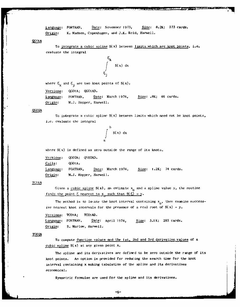
i77--Language: FORTRAN, Date: November 1973, Size: 8.2K; 373 cards.

Origi K. Madsen, Copenhagen, and J.K. Reid, Harwell.

To integrate a cubic spline S(x) between limits which are knot points, i.e.

evaluate the integral

Ek

J S(x) dx

where Ek and Ej are two knot points of S(x).

Versions: QGOIA; QGOIAD.

Languag: FORTRAN, Date: March 1974, Size: .8K; 46 cards.


To integrate a cubic spline S(x) between limits which need not be knot points,

i.e. evaluate the integral

b

a S(x) dx

a

where S(x) is defined as zero outside the range of its knots.

Versions: QGO2A; QGO2AD.

Calls: QGOIA.


Origgi: M.J. Hopper, Harwell.

TC'0_1A

Given a cubic spline S(x), an estimate x and a spline value y, the routine

finds the point E nearest to x such that S(E) =

The method is to lo,:ate the knot interval containing x0 , then examine success-

ive nearest knot intervals for the presence of a real root of S(x) - y.

Versions: TCOIA; TCOIAD.



TGO2A

To compute function values and the 1st. 2nd and 3rd derivative values of a

cubic spline S(x) at any given point x.

The spline and its derivatives are defined to be zero outside the range of its

knot points. An option is provided for reducing the search time for the knot

interval containing x making tabulation of the spline and its derivatives

economical.

Symmetric formulae are used for the spline and its derivatives.

-5-

Versions: TGO2A; TGO2AD.

Language: FCRTRAN, Date: March 1974, Size: 1.4K; 109 cards.


VE06A

To find x = Ix, x 2 ,.., X that minimizes a quadratic function of the form

= iT T

Q(x) =% +-T HX + x

where H is symmetiic positive definite and x is subject to linear constraints

Cx <b and/or simple bounds 1. < x < u j = 1,2,..,n. The matrix H and

constraint matrix C are assumed to be sparse and the nolIzero elements of these

two matrices must be provided in a compact form.

The routine could be used for linear least squares data fitting problems which

are subject to constraints and are sparse.

versions: VE06A; VEO6AD.

Calls: LAOSA.

Language: FRTRAN, Date: June 1974, Size: 20.1K; 1114 cards.

Origin: D. Divall, Southampton.

VFOIA

To minimize a general function f(x) of several variables x =xl9x 2 , . . x n l

subject to general nonlinear constraints ci(x) = 0 i = 1,2,..k and ci(x) > 0

i = k + 1,..,m, k - n. Derivatives of f(x) and all the functions ci(x),

i = 1,2,..,m, must be provided.

The method is described by Fletcher in the A.E.R.E. internal report CSS 2,

Dec., 1973. A penalty function of the form

m

X) + 2 )- )2

i=1 ii

is used.

Th2 user must provide subroutines to calculate derivatives and function values,

and must give an initial estimate of the solution (which need not be feasible) and

accuracy requirements.

Versions: VFOIA; VFO]AD.

Calls: ?MCI ]A, VAO9A, VEO4A.

L : FORTRAN, Date: September 1973, Size: 25.7K; 245 cards.

Origin: R. Fletcher*, Harwell.

VGOIA

To find the minimax solution to a system of nonlinear equations

f i (xI9x2,..n x = 0 i = 1,2,..,m. Derivatives of the fi with respect to the x.

are required.

* No longer at Harwell.

-6-

The method is described in a Harwell internal report TP.559 by K. Madsen.

The user must provide a subroutine to compute function values and derivatives

and provide an initial approximation to the solution. The number of iterations

can be limited and accuracy requirements specified.

The routine can be used for data fitting, m > n, Wien minimax is preferred

to least squares.

Versions: VGOIA, VGOJAD.

Calls: MA9A.

Language: FORTRAN, Date: Jun-- 1974, Size: 2.8K; 92 cards.


* VG;O2A

To find the minimax solution to a system of nonlinear equations

fi(x xx 2 ,..,Xn) = 0 i = 1,2,..,m. Derivatives are not required.

The nkthod is described in a Harwell internal report TP.559 by K. Madsen.

The user must provide a subroutine to evaluate f and provide an initial

approximation to the solution. The total number of iterations can be limited

and accuracy requirements specified.

The routine is applicable to the minimax data fitting problem.

Versions: VIJO2A, VGO2AD.

Calls: MA19A.



---

GENERAL INDEX

This is a revised index which covers both the original 1973 catalogueand this supplement, it supersedes all previous indexes. New referencesare indicated by the mark 111.

References to Harwell and Theorectical Physics Division reports takethe form R-nnnn or TP-nnn. The Computer User's Manual references, TP-389,are identified by the prefix CUM and refer to the chapter or appendixnumber.

A BCD ONOIB, ZAISASBCD source tape 95

ABEND ZAO2AS, ZRIOAS Bessel functionsaccounting parameters CUM-6 ber,bei,ker,kei,etc. FFO6Aadaptive quadrature QAO2A, QAO3A, 10 and KO FFO3A

QA04A, QAO5A Ii and KI FFO4AAitken extrapolation EAO2A JO and YO FFOIAangular momentum FGOIA JI and Yi FFO2Aapproximation problem 97-Ot spherical FFO5Abest Lp TP-397, TP-469 Beta function FCO5Acubic spline TP-252, TSOlA, 100 binary search KAOIAS, NBOIAerror in 99 binary subdivision NBOIA, PAO2Aexplanation of 97 bisection PAO2Alinear 98 bisection method ECO2Alinear minimax thro best Lp Bjorck.A. MA14ATP-470 BLKSIZE ZA18AS

minimax TP-179, TP-190 Boersman.J. FCIOAnonlinear 98 Booker.D.V. R-7129of plane regions TP-420 boundary values DDOIA, DDO2A,Pade' PEO6A DD03AD '), DPOIA, DPO2Apolynomial TP-229, tOO bounded variables NA19A~'l, VEO2A,polynomial-least squares VCOtA VEO4A, VEO6A 'l2polynomial-minimax PEltA Box.N.J. 102rational functions PEO4A, PEO5AD Brittian.C PEO3Arational minimax TP-442 Broyden.C.G. NSOtA, VAO5Asurface fitting for contour Buckley.A. VEO5Aplotting TP-531 buffer-I/O ZAO3AS

area bounded by contour GAO2A, Burgoyne.F.P. FFO6AGAO3A Businger.P. 108

arrays Butler.R. PBO2ASmax. or min. element MXOtA, byte 3MXO2Aprint out OAO2A, OAO3A

ASCII code ZAO5AS Casymptotic series SAOIAATLAS Laboratory DDOIA, DDO2A, c.p.u. time left in step ZAO2AS

DPOIA, DPO2A, MAO7A, TDOIA CADRE QAO5Aaxes FPO1A(12 CALL EXIT ZAO7AS, ZRIOAS

Calls 3cartesian co-ordinates GAOtA

B catalogue supplements 3catalogue-conventions used 2

backing store MAI5C, OEOtA CDE ZRO3ASBailey.A. FCOIA, IDO3A channel program ZRO3ASbalancing - see also character codes for 7 track source

equilibration, EBO6A, EBO7A, tape 95MCI5A character conversion ZAO5AS,

Barrowdale.l. MA2OA, TP-442 ZAI5AS

i -8-

character string manipulation integration QGO1A,,', QGO2A',1compare two strings IC02AS interpolation TB04A, TBO5Afind a given character in a inverse interpolation TCOIA'',string ICOAS least squares TP-264, TP-308,

find next non-blank ICOIAS VBO5B, VB06A, VCO3Acharacteristic polynomial - real parametric CAO5A

MCO7A periodic TBO5Acharacteristic values - see plot graph of OBI2A

ei-envalues Curtis.A.R. DCO1AD, DCO2AD, FCI3A,charging FTOIA, MAIBA, MCIOA, MCI2A,

copies of library routines 93 MEO7A, OC01A, OEOIA, PDO3A,for use of computer CUM-D PEO5AD, QAO5A, R-5600, R-6844,

Chebyshev integration 114 TDO2A, TP-179, TP-190, TP-252,Chebyshev polynomial PEOIA, PEO3A, TP-423, TP-444, TP-450, TP-476,

PEO4A, QBOIA TP-477, TSOIA, ZEOIA, 107Chebyshev series FF0A, FFO2A, Curtiss.P.C. PEllA

FF03A, FF04A, FF06A curve drawing OBItA, R-7092Chebyshev sets TP-203 curve fitting - see data fittingchi-squared probability function cusps OBIlA

SAOIA CVT ZRO3ASCholesky MA09A, MA1OAClebsch-Gordan FGOIAClenshaw.C.W. FFOtA, FFO2A, FFO3A, D

FFO4Aclock-computer ZAOIAS, ZA02AS data fitting MAO9A, MAItB, MAl4A,closed curves OBItA MAAI14, MA2OA, 97-101closed region GAO5A bounded variables VEO4A,COMMON areas-names of 84 VEO6A4 1

completion code ZAO2AS choices of fitting function 97computer clock ZAOIAS, ZAO2AS cubic spline VBO5B, VBO6A,conjugate directions TP-454, VAO4A VCO3A, 100conjugate gradients MAI6A, MCIOA, explanation of 97

MC12A, R-6545, TP-411, TP-445, general program for R-7129VAO8A, 107 linear 98

constraints LAOIA, LAO2A, MA14A, linear constraints VEO2A,MA2OA, TP-478, VAO7A, VEOIA, VEO6AI )VEO2A, VEO3A, VEO5A, VEO6A(l), minimax VGO1A-), VGO2A(l)VFO1A ,(), 102 nonlinear NSO3A, VAO2A, VAO5A,

Conte' FCI2A VAO7A, VBO1A, VBO3A, VQOtA(l ,contours GAO3A VGO2A(l,, 98, 10tconversion polynomial 100

ASCII to EBCDIC ZAO5AS rational functions no facilityBCD to EBCDIC ZAI5AS sparse VEO6A' 1EBCDIC to BCD ZA15AS sparse Jacobian NSO3AEBCDIC to UNIVAC field data straight line fit VCO4AZA15AS sums of exponentials 101

under FORMAT ZAO3AS types of error norm 98copy area of core ZRO3AS data setCorbalo' F.J. FFO5A DECtape ODO2Acore dump ZRtOAS paper tape ODOtAcorrelation VCO4A swop names of ZAI6ASCrank-Nicolson DPOIA track usage ZAI6AScrib sheets CUM-6 datecubic - zeros of PAO3A of write ups 86cubic splines todays date ZAO9AS, ZAIOAS

approximation problem TSOlA use in library catalogue 3curve fitting TP-307 Davidon.W.C. VE01Adefining a closed region CAO5A Davies.D. 102definition of 98 Dawson's integral FCI3Aderivative values TGO2A' DCB ZAIBAS, ZRO3ASevaluation of TGOIA, TGOtB, DD card information ZVOIAD

TGO2AI1 DDname

if -9.

check presence of ZA17AS general complex no facilityDEB ZRO3AS Hermitian EC06C, EC07C, MEOIB,deBoor.C. QAO5A MEO8Adebug information ZRIOAS Hermitian tri-diagonal ECO2A,debugging programs CUM-t2 ECO8C, EC09CDECtape CUM-13, ODO2A, ZAO5AS nearest to a given estimateDECtape JCL CUM-6 EAO2Adeficient rank MAl9A(1). MBtIA power method EAO2Adegrees of freedom SAOIA, SAO2A, real matrix EBO6A, EBO7A

SAO3A real symmetric EAO3A, EA06C,determinant MA21A, MA22A, MA23A, EA07C, MCO4B

MA24A, MBO2A, MDO3A, 106 real symmetric tri-diagonaldiagonally dominant EA03A EAO8C, EAO9Cdictionary ONOIB scaling a matrix MC15Adifferential correction algorithm upper Hessenberg EBOSA, EBO9A,

TP-442 MCOSA, MCI4Adifferential equations-ordinary eigenvectors 106

boundary value form Ax = eBx EAIIAeigenvalue problems DD03AD(11 general complex no facilitylinear 2nd order DDOIA Hermitian EC06Cnonlinear 2nd order DDO2A Hermitian tri-diagonal EC08C1st order systems DDO3AD(Il power method EAO2A

differential equations-ordinary real matrix EBO6Ainitial value real symmetric EAO3A, EA06C

Gear's method DCOIAD, DCO2AD real symmetric tri-diagonalHermite interpolation TP-423 EAO8CRunge-Kutta DAOIA, DAO2A scaling a matrix MCl5Asystems DAOIA, DA02A, DCOtAD, upper Hessenberg EBO5A, EBO8ADCO2AD elliptic integrals

differential equations-partial complete 1st and 2nd kind FBOtAelliptic no facility, 107 complete 3rd kind FBO3Afinite element method no incomplete 1st and 2nd kindfacility, TP-436 FBO2A

hyperbolic no facility England.R. DDO3AD- ,

Laplace's equation TP-422, entry point address ZRO2ASTP-436 entry points-names of 84

parabolic-linear DPOIA equations - see solution ofparabolic-nonlinear DPO2A equations

discontinuity-3rd derivative VCO3A equilibration MA17A, tIAIBA, MA2RA,disjoint intervals KCOIA, KCO2A MA22A, MA23A, MA24A, TP-444disk characteristics CUM-H equilibration factors MCIOA,disks - demountable CUM-8 MC12A, MEO7ADivall.D. VEO6A(1) Erisman.A.M. TP-525double precision names 85 error analysis-cubic spline R-5600double rank algorithms TP-471 error estimates KA21A, MA22A,DSCB ZA18AS, ZRO3AS MA23A, MA24A, PAO2A, PAO6AD '1,DSK M ZVOIAD PA07AD '), 107Duff.I. MCl3A, TP-526 Error functiondummy READ and WRITE ZAO3AS complex FCOIAdynamic allocation of storage erf(x) and erfc(x) see IBM ERF,

IAOIAS ERFC, DERF and DERFC functionserror norms 98, 108exchange algorithm MA19A,)

E Exponential integral FC11Aexternal users 93

EBCDIC OBOIAI''edit ooammnds OEOlAedit facilities OEOIA Feigenvalue problem togeigenvalues R-7168, 106 fast data link system TP-464

characteristic polynomial MCO7A fast Fourier transforms FTOIAform Ax = eBx EAIIA Fast loader 87

-10-

FATAL R-7129 Gavan.A. IDO2Afeasible solution LAO2A, R-6354 Gear.C.W. DCOIADFilon's method QD01A general registers-contents ZRIOASfinite differences generalized inverse MBlOA, MB11A,

approximation to derivatives 108NSOlA, NSO3A, SVOIA, TDOIA, generating pseudo errors FAO3ATDO2A, TP-476, TP-477 Gentleman.W.M. FTO1A

central TAO3A GETMAIN IAOIASdivided differences TAO2A GHOST OBOIA-', OBIIA, OBI2A,table of TAOiA TP-484

Fisher's F probability SAO3A Golub.C.H. MAI&A, 108fitting - see data fitting Gram-Schmidt orthogonalizationFletcher.R. FCl2A, LAO2A, MCIIA, MCO6A

R-6354, R-6370, R-6799, R-7073, Grant.J.A. TP-397, TP-469, TP-470R-7125, TP-368, TP-383, TP-397, graph plottingTP-401, rP-431, TP-432, TP-449, axis limits FP01A1'1TP-453, TP-454, TP-456, TP-469, contour plotting TP-531TP-470, TP-478, TP-529, VAO7A, cubic spline OB12AVAO8A, VAO9A, VA1OA, VBOlA, curve through points OBIlA,VEOIA, VE02A, VEO3A, VEO4A, R-7092VFOIA(I), 103 label formats FPOIA ,)

floating point arithmetic ZEOIA label points FPOIA-FORMAT-construction at execution line printer simulation OBOIA4 I

time ON02A on line printer OCOlAForsythe.G.E. VCO1A on teletype OCOlAFORTRAN compilers CUM-I print text OBOlA1'1FORTRAN I/O CUM-17 users' manual (GHOST) TP-484FORTRAN II 2 Green.D. QMOIAFORTRAN IV 2FORTRAN variable types CUM-5Fourier integrals 115 HFourier transforms-discrete FTOIAFox.L. DDOtA Hallovell.P. DDOIA, DDO2A, DPOIA,fractional part FAO2AS DPO2A, TDOIAFrank.W.L. PEIIA HAR.LIB 87free format input ONOiB, ONO2A HARSLSFREEMAIN IAO1AS control card format 90Fresnel integral FCOA PARM field options 91Fried FCI2A Hart.W.E. PCOtAS, QDOIA, ZAO8AS,fundamental cubic spline VBO5B, ZAOAS, ZAI2AS

VBO6A Harwell computer CUM-5, IHarwell Subroutine Library t

Bulletin 89C charges for library material 93

external users 93Gamma function FCO3A, see also IBM how to use the library 84-96

GAMMA, DOAMMA, ALGAMA and DLGAMA information files 87functions naming conventions 84

Garside.R. ODO2A news sheet 88Gauss quadrature 115 request form 96

QBOIA source tape 90Gauss-Laguerre QCO2AD, 116 status index 88Gaussian distribution FAO3A summary of information sourcesGaussian elimination MAOIB, MAO7A, 89

MAO7B, MAI2A, MAI8A, MA2tA, up to date changes 87MA22A, MA23A, MA24A, MBOlB, use outside Harwell 93HBO2A, MCIOA, MC12A, MDO3A, HASP CUM-BME04A, MEO7A, R-6899, TP-444, Hastings.C.R. FBOtA107 HCF IDO2A

Gaussian elimination, stability of Hearn.A.G. GAQtA, TBOtA, TBO2ATP-441 Hebden.M.D. TP-397, TP-469,

Caussian quadrature QC02AD TP-470, TP-515, TP-529, VAlIA

-11

Hedger.J. SAOIA interrupt-timer ZAO2ASHermite interpolation in ODEs inverse interpolation TCOIA1'

TP-423 inverse iteration EBO5A

Hermitian ECOA inverse matrix 106Hessenberg EBO5A, EBOSA, EBOgA, IOB ZRO3AS

MA12A isoceles triangle CAO3AHessian VEOIA iterative refinement of solutionhighest common factor ID02A MA21A, MA22A, MA23A, MA24A,Hoare.C.A.R. KBOIA, KBO2A, KBO3A, R-6899

KBO4AHop'lood.F.R. FFO5A, QBOIAQo',er.M.J. FDOIAS, FPOIA~11 J

IAOIAS, IC0IAS, IC02AS, IDOIAS,:rn BS, KAAAS, KBtlA, LAOIA, Jackson.M.P. VEO4AMA09A, MAO0A, MAIOA, MA11B, Jacobi's method EAO3A, 109MAIA, MCO5AS, MXOIA, MXO2A, Jacobian NS03AnVA2A, OAO3A, OB0A , PAO2A, Jahn's U function FGO1AP302AS, PDO2A, QAO1AS, QC01A1 , JCL procedures CUM-18Q,2A-, SAOIA, TGOIB, JFCB ZAI8AS, ZRO3AS, ZVOIADFCO2A , ZAO2AS, ZAO6AS, Job Control Language CUM-6,AW7AS, ZAISAS, ZRO3AS jobname ZA17AS

householder orthogonal Jones.R.L. TP-484transformations EA06C, EA07C,EMC6C, ECO7C, MA14A, MB11A,MCO'MB, MCO7A, MEOIB, NEOBA, KVB05B, VBO6A

HSLM 88 Kearsey.H.A. ZA16AS, ZA17ASSSLP %8 Keller.H.B. DDO3AD1 11

RSLS 68 Kerr.E. PBO2ASHSLW 98 keywords-identify ONOIBHunter.C. ZRO2AS, ZRIOAS knots OBI2A, QGOIA'11, TBO4A,HUW TBO5A, TCOIA, TCOIB, TGO2AII),

obtaining library routines 92 TSOIA, VBO5B, VPO6A, VCO3Asubmi:tiug a program CUM-6

L

Lagrange iSterpolation TBOIA,index--computer generated 87 TBO2Ainformation -- general computing Lancefield M. PA04A

CUM_-M Language 2information-up to date changes 87 Laplace's equation - finiteinitial value problems DAOIA, elements TP-436

DA02A, DCOIAD, DCO2AD latent roots - see eigenvaluesinteger part latent vectors - see eigeuvectorsdouble precision number DINT least squares-linear MA08A, MAO9A,WR to base 16 IDOIBS MAI4A, 100tog to base 2 IDOIAS bounded variables VEO2A, VEO4A,

integration - see quadrature VE06A1Iinterior point (closed region) linear constraints VEO2A,

OA05A, R-7298 VE06A'interpolation 99 linear equality constraints

cubic spline R-5600, TBO4A, MAW4ATP-?52, 100 polynomial VCOIA

cubic spline- periodic TBO5A singular normal equations 108evpn tunction TBOIA straight line fit VCO4AaneraI linear case 100 least squares-nonlinear NSO3A,HOr''mit,', in ODEs TP-423 R-6799, TP-439, VAO2A, VAO5A,Lagrange TBO1A, TBO2A VAO7A, VBOIA, VBO3Alinear NBOIA no derivatives NSO3A, VAO2A,piece-wise cubics TBO3A VAO5Apulytomial PCO2A, TBO2A, 100 Ledger.J. VCO4A

-12-

A WD' Jul11 Rol! I~ I ~

Lesbegue polynomial PCO2A eigenvalues of EAO2A, EAO3A,library routines EA06C, EA07C, EAO8C, EA09C,argument types 86 EAItA, EB06A, EBO7A, EBOSA,double precision names 85 EBO9A, ECO2A, EC06C, EC07C,names of 84 EC08C, EC09C, 109obtaining as HUW files 92 eigenvectors of EAO2A, EAO3A,omitting from stored programs EA06C, EAO8C, EAIIA, EBOSA,CUM-1O, 87 EB06A, EBO8A, EC06C, ECOSC, 109requirements 85 equilibration MCIOA, MCI2A,source decks and listings 89-92 MEO7Aspecifications 85 factorization of (sparse) MAI7A,using in programs 86 MASA, TP-500write ups 85 factorize LAO3A

line printer text chain OBOIA"') generalized inverse MBIOA,linear algebra 106-110 MBtIA, R-6072, 108linear interpolation CAO3A Hermitian EC06C, EC07C, ECO8C,linear programming MAIIB, MA2OA, EC09C, MA24A, MEOIB, MEO2A,

R-6354 ME08A, 106feasible solution LAO2A Hermitian tri-diagonal ECO2A,revised Simplex method LAOIA MEOSAupdate basis LAO3A Hessenberg form EB05A, EBOeA,

Linkage Editor CUM-tO, 87 EBO9A, MAI2A, MCOHA, MC14A,LIST 90 MEO4ALRECL ZA18AS Hessian VAIOA, VEOIA

inverse MAOIB, MAIOA, MA21A,MA22A, MA23A, MA24A, MBOIB,

M MBO2A, MB04A, MBO5A, R-6899, 106Jacobian NSOIA, TDO2A, TP-476,

Madsen.K. MA19A(1), PA06AD('I, TP-477PAO7AD( l ), VGOtA '' ), VGO2A(I) large and sparse MA16A, MAI7A,

SMaehly.H.J. PEO5AD HAl8A, TD02Amagnetic tapes CUM-16 LP basis LAO3AMarkov sets TP-203 matrix-vector product(sparse)Marlow.S. EAIIA, EBO6A, EBO7A, MCO9A

EBO8A, EBOPA, EC06C, EC07C, multiplication 106EC08C, EC09C, FBOIA, FC03A, optimization applications MClIAFCO5A, FCIOA, FCtIA, FFOIA, over determined MAO8A, MAO9A,FFO2A, FFO3A, FFO4A, FFO6A, MA1tB, MA14A, MA2OA, 106MA21A, MA22A, MA23A, MA24A, partitioned MBO4A, MBO5AMCt4A, MCI5A, MEO6AS, MEO7A, print out OA0iAMEO8A, OBIIA, OBI2A, PAO5A, product of MCOIAS, 109PEOIA, PEI1A, R-6899, R-7092, property A TP-445TCOIA 'I, 106 rank one update MCi1A

Marquardt method NSO3A, R-6799, real general EBO6A, EBO7AVAO5A, VAO7A, VBOIA real symmetric EAO2A, EAO3A,

mathematical programing TP-478 EA06C, EA07C, EA08C, EAtlA,mathematical programming - MBO4A, MBO5A, MCO4B, MCO7A,

nonlinear TP-368, TP-449 MDO3A, 106matrices real symmetric tri-diagonal

adjoint MBO2A EA09Cadjugate MBO2A rectangular MBIOA, MBIIAbalancing EBO6A, MCI5A scaling MCIOA, MCI2A, MCI5A,band structured MAO7A, MAO7B, MEO7A, TP-444MAl5C, TDO2A, 107 sparse LAO3A, MAl6A, MAi7A,

complex ECO2A, EC06C, EC07C, MAI8A, MCOQA, MCI2A, MCI3A,EC08C, ECOQC, MA23A, MA24A, R-6545, TP-500, 106) 107MEOIA, MEO7A sparse to block triangular MCl3A

complex matrix-vector product sparse, stability ofMEO2A factorization TP-525

deficient rank AIA) sparsity "rderings TP-526determinant MA21A, MA22A, MA23A, symmetric positive definiteMA24A, MBO2A, MDO3A, R-6899, 106 EAlIA, MAIQA, MAI5C, MAt6A,

MA17A, MA22A, MCI1A, VEO6A ' , nested form (polynomials) I'BOIAS106 Newton-Coates QAO1AS

tr -diagona EAOSC, EAOQC, Newton-Raphson NSOA, PAO2A,ECOC, EC09C, MC04B, MEOIB VAO5A, VAO6A, VAIIA

update factorization LAO3A nonlinear least squares VAO2A,variance-covariance matrix VA05A, VAO7A, VB01A, VBO3AmA14A, VEO4A, 1OB normal equations MAO8A, MAO9A, lO

vcConalogue.D.J. OBIA Northcliffe.S. PEO7A, PEOSAicstohie. R.C.F. DINT, FAOIAS, numerical advisory service TP-529

MCO1AS, MCO2AS, MCO2BS, MCO3AS,ON02A, PBOIAS, TP-435, TP-464,ZAOIAS, ZAO2AS, ZAO3AS 0

McVicar.D. DAOlA, ODOIA, ZROIAS,ZVOIAD OCI-0C5 interrupts ZPIOAS

merging intervals KCO1A, KCO2A old PSW ZRIOASMerson DA0 A, DAO2A optimization MCIIA, R-6469,message to operator ZA12AS TP-393, TP-430, TP-431, VAO4A,MEARSLS VAO6A, VAOSA, VAO9A, VAIOA,

how to use 92 VAIIA, VDO1A, VD02A, VEO1A,Miller.D. GA02A, TBO3A VEO2A, VEO3A, VE04A, VEOSA,minimax MAt1B, MAIgA', PE04A, VEO6AI1I, VF0A1'', 102-105

PEO5AD, PEtIA conjugate direction methodnin'mization of a function 102-105 TP-454, TP-483

bouds on variables VEO4A conjugate gradients R-7073eliminating variables 102 constraints TP-439, TP-478,flow diagram for choice of TP-49b, 102routine 103 eliminating variables 102

large problems VAO8A flow diagram for choice oflinear LAOIA routine 103!near constraints LAOIA, VEOIA, large problems VAO8A

VEO2A, VEO3A, VEO5A, VE06A 1) linear constraints TP-431,no ('erivatives VAO3A, VAO4A, TP-453, VEOIA, VEO2A, VE03A,VA1OA, VDO'A VEOSA

non-linear constraints VF01A111 non-linear constraints VFOlA ,one variable VDO1A, VDO2A penalty function TP-478quadratic function VEO2A, VEO4A, quadrati. programming R-6370,

VEO6A' I TP-401sparsity VEO5A quadratic termination propertiessum of squares R-6799, VAO7A, TP-471, TP-472VBO1A, VBO3A quasi-Newton method R-7125

sum of squares, no derivatives rank one methods TP-372VAO2A, VAO5A search directions TP-492

using 2nd derivatives TP-515 sum of squares R-6799, TP-161,1st and 2nd derivatives VAIIA VAO2A, VAO5A, VAO7A, VBO3A1st derivatives VA0A, VAO8A, survey of methods TP-340,VAO9A, VEOIA, VEO3A, VEO5A, TP-432, TP-456, TP-495VFO!A using 2nd derivatives TP-515

modify a program (stored on disk) variable metric algorithmCUM-9 TP-382, TP-383, TP-459

Monte Carlo QMOIA, 114 orderingMoody.K. KBIOAS, ZRIOAS numbers KBOIA, KBO2A, KBO3A,Morgan.L. FBO2A, MBO1B, PCO2A, KBO4A, KBIIA

PEO6A tables KAOIAS, KBIOASmultiple shooting method DDO3AD,,, with index array KAOIAS, KBO3A,multiplicative congruent method KBO4A, KBIOAS

FAOIAS Origin 3multiprogramming ZAOIAS orthogonal polynomial PE07A,

PEO8A, QCO2AD, VCOIA, 100orthogonal transformations EAO3A,

N EBO6A, 108Osborne.M. PEO5AD

NCAL 87 Osbourne MCO6A

- I -

Osbourne.M. DDO3AD (1) TP-430, TP-439, TP-442, TP-459,

over determined matrix MAO8A, TP-471, TP-472, TP-483, TP-492,MAO9A TP-495, TP-531, TSOIA, VAO2A,

overlay programs CUM-E VAO4A, VAO5A, VAO6A, VBO3A,VBO5B, VBO6A, VCO3A, VDOIA,VDO2A

p power method EAO2A

powers to base 16 FDOIASPackham.G. MBO2A powers to base 2 FDOIASPade' approximation problem PEO6A predictor-corrector method DCOIAD,paper tape CUM-13, ODOIA, ZAO5AS DCO2ADpaper tape JCL CUM-6 programs-store on disk CUM-8Papworth.D.G. SAO2A, SAO3A PSW ZRIOASparametric programming problems PUNCHB 9o

VEOIA, VEO2A PUNCHE 90Parlett.B. R-7168PARM field ZAO6AS, ZRO2ASpartial pivoting MAOIB, MAO7B, Q

MAl2A, MA21A, MA23A, MBOtB,MEO4A QR algorithm EAO6C, EA07C, EA08C,

penalty function VFOIA1 EA09C, EAIIA, EBO6A, EBO7A,permutation (matrix) MCI3A EBOBA, EBO9A, EC06C, EC07C,plasma dispersion function FCI2A EC08C, EC09C, 109plotting - see graph plotting quadratic form GAO2Apolar co-ordinates GAO5A quadratic programming R-6370,poles-Pade' approximation problem TP-401, VEO3A

PEO6A quadraturepolygon GAO5A adaptive QAO2A, QAO3A, QAO4A,polynomial - complex QAO5A, III

zeros, complex and real choice of routine 111-117PAO6AD4 ) cubic splines QGOIA1l), QGO2A(l)

polynomial - real 97 Gauss QAO4A, QCO2ADchange of variable PDO3A Monte Carlo QMOIA, TP-207, 114coefficients of PCOIAS, PEOBA multidimensional QBOIA, QMOIA,cubic, zeros of' PAO3A 114divide out root PDOIAS Newton-Coates QAOIASevaluation of PBOIAS, PBO2AS, optimal formulae TP-223, TP-224,PEO7A TP-225, TP-227functions of PDO2A relative error 112in terms of Chebyshev polynomial Simpsons rule QAO2APEOIA, PEO3A tabulation of an integral QAO3Ainterpolation PCO2A trigonometric QDOIAleast squares VCOIA weights IIIminimax approximation problem quantum mechanics FC12A, FGOIAPEtIA quartic PAO5Anumber of roots PAO4A quasi-Newton method VAOQA, VAIOAorthogonal PEO7A, PEOeA, VCOIA Quasi-random numbers no facilityquartic, zeros of PAO5A queriesreal zeros of PAO2A external users 93reduced polynomial PDOIAS general 87zeros, complex and real write ups 86PAO7AD'I' QUICKSORT KBOIA, KBO2A, KBO3A,

Powell.M.J.D. MAl4A, MBO4A, MBO5A, KBO4AMBIOA, MBIIA, MCO7A, MClIA,MDO3A, NSOIA, OBIIA, OB12A,QAO2A, QAO3A, QMOIA, R-5600, RR-5947, R-6072, R-6469, R-7092,SVOIA, TAOI4, TDO2A, TGOIA, Raoah FGOIATP-161, TP-179, TP-190, TP-203, random numbers FAOIAS, FAO3ATP-207, TP-229, TP-252, TP-264, rank MBIOA, MBIIA, 108TP-307, TP-308, TP-328, TP-340, rank one update MCIIATP-364, TP-372, TP-382, TP-393, rational approximation 97, tO0

-15-

in terms of Chebyshev polynomial Ruffle.M. FBO3A, GAO&A, ONOtBPE04A Runge-Kutta DAOIA, DAO2A

minimax PEO5AD running a program CUM-3Pade' PEO6A Russel.D. MAO7A, TAO2A, TAO3A

Rayleigh quotients EAOBCRB ZR03ASre-issues 3 Sre-read input ZAO3ASread special characters ONOIB Salmon.L. R-7129real time ZAQIAS Sande.G. FTO1ARECFM ZAI8AS Sard's hypothesis TP-225record format ZAIeAS scaling MA17A, MAl8A, MA2tA,recurrence relation PA02A, PEO7A, MA22A, MA23A. MA24A

PEO8A, VCO1A scaling factors MCIOA, MCI2A,reduction of matrices MC15A, MEO7A

to Hessenberg form MCOSA, MC14A Scientific Subroutine Package-IBMto tri-diagonal MCO4B, MEO1B 91to tri-diagonal Hermitian form sequence numbers OEOiA, 91MEOA sequences

Reeves.C.M VAO8A acceleration of convergence noREGION CUM-6 facilityregression VC04A SHARE ZAO3ASReid.J.K. EA06C, EA07C, EA08C, Simmonds.H. PAO3A

GAO5A, LA03Ao MAO7B, MAl4A, simplex method LAOIA, MAltB,MAI5C, MAI6A, HAI7A, HAl8A, MA2OA, 108MA2lA, MA22A, MA23A, MA24A, Simpson's rule QAOIAS, QAO2A,MCO9A, MC1OA, MCl2A, MCt3A, QAO3A. QBOIA, 114MEO7A, NSO3A, PA06AD('l, Sinden.A.T. PEO4APAO7AD l), R-6545, R-6844, singularities - integrand QAO5AR-6899, R-7119, R-7293, R-7298, Size 3TB04A, TBO5A, TDO2A, TP-411, Smith.A.B. DAO2A, FAO3A, QAO04TP-420, TP-422, TP-436, TP-441, Smith.F.J. PEO7ATP-444, TP-445, TP-450, TP-476, smooth curve OBlIA, VCO3ATP-477, TP-500, TP-525, TP-526, smoothing VBO5B, VBO6A, VCOIAo106, 107 VCO3A

Reinsch.C. EBO6A, EBO7A, EBO8A, smoothing factors VBO6A, VCO3AEBO9A, MC14A, MCt5A solid angle GAO4A

residual sign changes VCOIA solution of algebraicresidual variances MA14A equations-linear LAO3A, MAOIB,residues-pade' approximation MA21A, '06

problem PEO6A band structured KAO7A, MAO7B,return code ZAO7AS, ZROlAS MAt5C, R-7119revised simplex method LAOIA complex MA23A, MEOiAReynolds.M. EBO5A, KBOIA, KBO2A, error estimates R-689g

KBO3A, KBO4A, MA12A general discussion R-6899Rice.J.R. QAO5A Hermitian MA24ARoberts.F.D.K. TP-442 Hessenberg form MAI2A, MEO4ARobinson.I.C.A. QAO4A L'' solution MA20ARomberg extrapolation QAO5A large and sparse MA16A, MAI7A,roots MAISAcubic PAO3A least squares MAO9A, MA14Adivide out PDOIAS minimax (with simple bounds)general function NBOIA MAt PA I

number of PAO4A minimax solution MAIl8polynomial PAO2A, PAO7AD(II orthogonal transformations MA14Apolynomial (complex coefficients) over determined MAOQA, MAIIB.PAO6AD'II MAl4A, MAlPA''', KA2OA, 100,quartic PAO5A t06, 107

Rouche's theorem PAO6AD ' , sparse MA16A, MAI7A, MAI8A,PAO7AD'11 R-6844, R-7119, TP-411, TP-450,

rounding errors-estimation of t07ZEOIA symmetric positive definite

-16-

MAIOA, MAI5C, MA16A, MAI7A, KAOIASMA22A, R-7119 tabulate function values OAO3A

solution of equations-nonlinear task time ZAO2ASminimax VGOIA ( 11 , VGO2A(11 Taylor series expansion PDO2Aover determined systems NSO3A, TCB ZRO3ASVCOtA ( l ), VC02A'1) textsingle equation NBOIA compare two strings IC02ASsparse Jacobian NSO3A, R-7293 find given character ICOIASsystems NSOIA, NSO3A, R-5947, order table of' KAOIAS, KBIOASTP-364, VGOIA(1) , V02A(1) three-eighths rule QAOIAS

Soper.J. EAO3A, FGOIA TIME macro ZAOIAS, ZAOBAS, ZAO9AS,sort-key KAOIAS, KBIOAS ZAIOASsorting time of day ZAOSASascending order KAOIAS, KBOIA, time-difference between two timesKBO3A, KBIOAS IDO3Adescending order KAOIAS, KBO2A, timer interrupt relative to stepKB04A, KBIOAS time chop ZAO2ASnumbers KBOIA, KBO2A, KBO3A, timer interrupt-to request ZAO2ASKBO4A, KBIIA timing programs ZAOIAS, ZA02AStables KAOIAS, KBIOAS TIOT ZAl7AS, ZRO3AStext KAOIAS, KBIOAS transformationswith index array KAOIAS, KBO3A, Hermitian to tri-diagonal MEOIBKBO4A, KBIOAS Hermitian to tri-diagonalIst n from m KB11A Hermitian MEO8A

source decks-modification of OEOIA real gene.'al to Hessenbergsparsity pattern TDO2A MC08A, MCI4Aspherical co-ordinates GAOIA real symmetric to tri-diagonalSPIE ZRIOAS MCO4BSpringer-Handbook EBO6A, EBO7A, trapezoidal rule QAOIAS, QAO5A

EBO8A, EBOgA, HCI4A, CI5A tri-diagonal EAO9C, ECO2ASSP library 91 TSO TP-435SSP source tape 91 TTIMER ZAO2ASstandard deviations FA03A, MAl4A, Turner.A.B. TP-422

NSO3A, VBOIAstatistics SAOIA, SAO2A, SAO3A,

SVOIA Usteepest descent NSOIA, VAO5A,

VAO6A UCB ZRO3ASstep return code ZAO7AS, ZROiAS uniform distribution FAOIASstep time ZAO2AS union of intervals KCOiAStern.M.D. TP-223, TP-224, TP-225, unitary diagonal transformation

TP-227 ECO8C, EC09Cstiff systems DCOIAD unitary transformations MCO4B,

STIMER ZAO2AS MCO8A, MCI4AStirling's approximation FCO3A updates for catalogue 3straight line fit VCO4A Uretsky.J.L. FFO5AStudent's t probability SAO2ASturm sequences ECO2A, PAO2A,

PA04A Vsubmatrix-inversion of MBO4ASwann.J. QMOIA, TP-207 variable band width MA15C, 107Swann.W.H. 102 variable metric algorithm TP-382,symmetric positive definite TP-383, TP-459definition of 106 variance VCOIA

synthetic division PBO2AS, PDOIAS variance ratio probability SAO3ASYSLIB 87 variance-covariance matrix MAO9A,system control blocks ZRO3AS MAt4A, NSO3A, SVOIA, VBOIA,

VEO4A, 108vector coupling coefficients FCOIA

T vectorscomplex inner product MEO6AS

table-search for specified entry inner product of MCO2AS, MC02BS,

-17-

MCO3AS, tog Ymanipulationi of 109max. or min. element HXOIA, York.E.J. EA02A, EC02A. GA03A,

MX02A MAO1B, MCO8A, MEO2A. NBOIA,

multiplication 106 IJAOIA, VCOIA

orthogonal TP-328print out OA02A, OA03Atriple inner product of MC05AS Z

Versions 2 zrsovolume serial n~umber ZVOIAD zeroc of 03

Gaussian quadrature QC02AD

w general function NBOIAPade' approximation problem

weighted uniform sampling QNOlA. PE08A

TP-207, It5 polynomial PAO2A, PA07ADI''

weights OC02AD, VC04A, 99 polynomial (complex coefficients)

Wigner FGOIA PA06ADII

Wilkinbon.J.l. EB06A, EB07A, quartic PA05A

EBOBA, EB0OA, MCO'4B, MCO8A.MC14A. MC15A, MEOI, ME08A,PA06AD~l). PAO7ADI), 109 3

Willis.D. KCOIA, KC02A2write ups 85, 86 5/L2

WMO ZA12AS

Documents

ESTABLISHMENT HARWELL LA. 73 M ImEEEEEEEE,.,hEEE C … · U.K.(excluding VAT) £20 for the first two subroutines plus £2 for each subroutine in excess of two. ... into the column