Essential spectra of quasi-parabolic composition operators

JID:YJMAA AID:15472 /FLA [m3G; v 1.50; Prn:3/12/2010; 10:50] P.1 (1-21)

J. Math. Anal. Appl. ••• (••••) •••–•••

Contents lists available at ScienceDirect

Journal of Mathematical Analysis andApplications

www.elsevier.com/locate/jmaa

Essential spectra of quasi-parabolic composition operatorson Hardy spaces of analytic functions

Ugur Gül

Sabancı University, Faculty of Engineering and Natural Sciences, 34956 Tuzla, Istanbul, Turkey

a r t i c l e i n f o a b s t r a c t

Article history:Received 16 August 2010Available online xxxxSubmitted by J.H. Shapiro

Dedicated to the memory of Ali Yıldız(1976–2006)

Keywords:Composition operatorsHardy spacesEssential spectra

In this work we study the essential spectra of composition operators on Hardy spaces ofanalytic functions which might be termed as “quasi-parabolic.” This is the class of compo-sition operators on H2 with symbols whose conjugate with the Cayley transform on theupper half-plane are of the form ϕ(z) = z + ψ(z), where ψ ∈ H∞(H) and �(ψ(z)) > ε > 0.We especially examine the case where ψ is discontinuous at infinity. A new method isdevised to show that this type of composition operator fall in a C*-algebra of Toeplitzoperators and Fourier multipliers. This method enables us to provide new examples of es-sentially normal composition operators and to calculate their essential spectra.

© 2010 Elsevier Inc. All rights reserved.

1. Introduction

This work is motivated by the results of Cowen (see [5]) on the spectra of composition operators on H2(D) induced byparabolic linear fractional non-automorphisms that fix a point ξ on the boundary. These composition operators are preciselythe essentially normal linear fractional composition operators [3]. These linear fractional transformations for ξ = 1 take theform

ϕa(z) = 2iz + a(1 − z)

2i + a(1 − z)

with �(a) > 0. Their upper half-plane re-incarnations via the Cayley transform C (see p. 3) are the translations

C−1 ◦ ϕa ◦ C(w) = w + a

acting on the upper half-plane.Cowen [5] has proved that

σ(Cϕa ) = σe(Cϕa ) = {eiat : t ∈ [0,∞)

} ∪ {0}.Bourdon, Levi, Narayan, Shapiro [3] dealt with composition operators with symbols ϕ such that the upper half-plane

re-incarnation of ϕ satisfies

C−1 ◦ ϕ ◦ C(z) = pz + ψ(z),

where p > 0, �(ψ(z)) > ε > 0 for all z ∈ H and limz→∞ ψ(z) = ψ0 ∈ H exist. Their results imply that the essential spectrumof such a composition operator with p = 1 is{

eiψ0t : t ∈ [0,∞)} ∪ {0}.

E-mail address: [email protected].

0022-247X/$ – see front matter © 2010 Elsevier Inc. All rights reserved.doi:10.1016/j.jmaa.2010.11.055

http://dx.doi.org/10.1016/j.jmaa.2010.11.055

http://www.ScienceDirect.com/

http://www.elsevier.com/locate/jmaa

mailto:[email protected]

http://dx.doi.org/10.1016/j.jmaa.2010.11.055


2 U. Gül / J. Math. Anal. Appl. ••• (••••) •••–•••

In this work we are interested in composition operators whose symbols ϕ have upper half-plane re-incarnation

C−1 ◦ ϕ ◦ C(z) = z + ψ(z)

for a bounded analytic function ψ satisfying �(ψ(z)) > ε > 0 for all z ∈ H. This class will obviously include those studiedin [3] with p = 1. However we will be particularly interested in the case where ψ does not have a limit at infinity. We callsuch composition operators “quasi-parabolic.” Our most precise result is obtained when the boundary values of ψ lie in QC,the space of quasi-continuous functions on T, which is defined as

QC = [H∞ + C(T)

] ∩ [H∞ + C(T)

].

We recall that the set of cluster points Cξ (ψ) of ψ ∈ H∞ is defined to be the set of points z ∈ C for which there is asequence {zn} ⊂ D so that zn → ξ and ψ(zn) → z.

In particular we prove the following theorem.

Theorem B. Let ϕ : D → D be an analytic self-map of D such that

ϕ(z) = 2iz + η(z)(1 − z)

2i + η(z)(1 − z),

where η ∈ H∞(D) with �(η(z)) > ε > 0 for all z ∈ D. If η ∈ QC ∩ H∞ then we have

(1) Cϕ : H2(D) → H2(D) is essentially normal,(2) σe(Cϕ) = {eizt : t ∈ [0,∞], z ∈ C1(η)} ∪ {0},

where C1(η) is the set of cluster points of η at 1.

Moreover, for general η ∈ H∞ with �(η(z)) > ε > 0 (but no requirement that η ∈ QC), we have

σe(Cϕ) ⊇ {eizt : t ∈ [0,∞), z ∈ R1(η)

} ∪ {0},where the local essential range Rξ (η) of an η ∈ L∞(T) at ξ ∈ T is defined to be the set of points z ∈ C so that, for all ε > 0and δ > 0, the set

η−1(B(z, ε)) ∩ {

eit : |t − t0| � δ}

has positive Lebesgue measure, where eit0 = ξ . We note that ([25]) for functions η ∈ QC ∩ H∞ ,

Rξ (η) = Cξ (η).

The local essential range R∞(ψ) of ψ ∈ L∞(R) at ∞ is defined as the set of points z ∈ C so that, for all ε > 0 and n > 0,we have

λ(ψ−1(B(z, ε)

) ∩ (R − [−n,n])) > 0,

where λ is the Lebesgue measure on R.The Cayley transform induces a natural isometric isomorphism between H2(D) and H2(H). Under this identification

“quasi-parabolic" composition operators correspond to operators of the form

T ϕ(z)+iz+i

Cϕ = Cϕ + T ψ(z)z+i

Cϕ,

where ϕ(z) = z + ψ(z) with ψ ∈ H∞ on the upper half-plane, and Ta is the multiplication operator by a.We work on the upper half-plane and use Banach algebra techniques to compute the essential spectra of operators that

correspond to “quasi-parabolic" operators. Our treatment is motivated by [9] where the translation operators are consideredas Fourier multipliers on H2 (we refer the reader to [17] for the definition and properties of Fourier multipliers). Throughoutthe present work, H2(H) will be considered as a closed subspace of L2(R) via the boundary values. With the help of Cauchyintegral formula we prove an integral formula that gives composition operators as integral operators. Using this integralformula we show that operators that correspond to “quasi-parabolic" operators fall in a C*-algebra generated by Toeplitzoperators and Fourier multipliers.

The remainder of this paper is organized as follows. In Section 2 we give the basic definitions and preliminary materialthat we will use throughout. For the benefit of the reader we explicitly recall some facts from Banach algebras and Toeplitzoperators. In Section 3 we first prove an integral representation formula for composition operators on H2 of the upperhalf-plane. Then we use this integral formula to prove that a “quasi-parabolic” composition operator is written as a seriesof Toeplitz operators and Fourier multipliers which converges in operator norm. In Section 4 we analyze the C*-algebragenerated by Toeplitz operators with QC(R) symbols and Fourier multipliers modulo compact operators. We show that thisC*-algebra is commutative and we identify its maximal ideal space using a related theorem of Power (see [18]). In Section 5,using the machinery developed in Sections 3 and 4, we determine the essential spectra of “quasi-parabolic” composition


U. Gül / J. Math. Anal. Appl. ••• (••••) •••–••• 3

operators. We also give an example of a “quasi-parabolic” composition operator Cϕ for which ψ ∈ QC(R) but does not havea limit at infinity and compute its essential spectrum.

In the last section we examine the case of Cϕ with

ϕ(z) = z + ψ(z),

where ψ ∈ H∞(H), �(ψ(z)) > ε > 0 but ψ is not necessarily in QC(R). Using Power’s theorem on the C*-algebra generatedby Toeplitz operators with L∞(R) symbols and Fourier multipliers, we prove the result

σe(Cϕ) ⊇ {eizt : z ∈ R∞(ψ), t ∈ [0,∞)

} ∪ {0},where ϕ(z) = z + ψ(z), ψ ∈ H∞ with �(ψ(z)) > ε > 0.

2. Notation and preliminaries

In this section we fix the notation that we will use throughout and recall some preliminary facts that will be used inthe sequel.

Let S be a compact Hausdorff topological space. The space of all complex valued continuous functions on S will bedenoted by C(S). For any f ∈ C(S), ‖ f ‖∞ will denote the sup-norm of f , i.e.

‖ f ‖∞ = sup{∣∣ f (s)

∣∣: s ∈ S}.

For a Banach space X , K (X) will denote the space of all compact operators on X and B(X) will denote the space of allbounded linear operators on X . The open unit disc will be denoted by D, the open upper half-plane will be denoted by H,the real line will be denoted by R and the complex plane will be denoted by C. The one point compactification of R willbe denoted by R which is homeomorphic to T. For any z ∈ C, �(z) will denote the real part, and �(z) will denote theimaginary part of z, respectively. For any subset S ⊂ B(H), where H is a Hilbert space, the C*-algebra generated by S willbe denoted by C∗(S). The Cayley transform C will be defined by

C(z) = z − i

z + i.

For any a ∈ L∞(R) (or a ∈ L∞(T)), Ma will be the multiplication operator on L2(R) (or L2(T)) defined as

Ma( f )(x) = a(x) f (x).

For convenience, we remind the reader of the rudiments of Gelfand theory of commutative Banach algebras and Toeplitzoperators.

Let A be a commutative Banach algebra. Then its maximal ideal space M(A) is defined as

M(A) = {x ∈ A∗: x(ab) = x(a)x(b) ∀a,b ∈ A

}where A∗ is the dual space of A. If A has identity then M(A) is a compact Hausdorff topological space with the weak*topology. The Gelfand transform Γ : A → C(M(A)) is defined as

Γ (a)(x) = x(a).

If A is a commutative C*-algebra with identity, then Γ is an isometric *-isomorphism between A and C(M(A)). If A is aC*-algebra and I is a two-sided closed ideal of A, then the quotient algebra A/I is also a C*-algebra (see [1] and [7]). Fora ∈ A the spectrum σA(a) of a on A is defined as

σA(a) = {λ ∈ C: λe − a is not invertible in A},where e is the identity of A. We will use the spectral permanency property of C*-algebras (see [20, p. 283] and [7, p. 15]);i.e. if A is a C*-algebra with identity and B is a closed *-subalgebra of A, then for any b ∈ B we have

σB(b) = σA(b). (1)

To compute essential spectra we employ the following important fact (see [20, p. 268] and [7, pp. 6, 7]): If A is a commu-tative Banach algebra with identity then for any a ∈ A we have

σA(a) = {Γ (a)(x) = x(a): x ∈ M(A)

}. (2)

In general (for A not necessarily commutative), we have

σA(a) ⊇ {x(a): x ∈ M(A)

}. (3)

For a Banach algebra A, we denote by com(A) the closed ideal in A generated by the commutators {a1a2 − a2a1:a1,a2 ∈ A}. It is an algebraic fact that the quotient algebra A/com(A) is a commutative Banach algebra. The reader canfind detailed information about Banach and C*-algebras in [20] and [7] related to what we have reviewed so far.



The essential spectrum σe(T ) of an operator T acting on a Banach space X is the spectrum of the coset of T in theCalkin algebra B(X)/K (X), the algebra of bounded linear operators modulo compact operators. The well-known Atkinson’stheorem identifies the essential spectrum of T as the set of all λ ∈ C for which λI − T is not a Fredholm operator. Theessential norm of T will be denoted by ‖T ‖e which is defined as

‖T ‖e = inf{‖T + K‖: K ∈ K (X)

}.

The bracket [·] will denote the equivalence class modulo K (X). An operator T ∈ B(H) is called essentially normal if T ∗T −T T ∗ ∈ K (H) where H is a Hilbert space and T ∗ denotes the Hilbert space adjoint of T .

The Hardy space of the unit disc will be denoted by H2(D) and the Hardy space of the upper half-plane will be denotedby H2(H).

The two Hardy spaces H2(D) and H2(H) are isometrically isomorphic. An isometric isomorphism Φ : H2(D) → H2(H) isgiven by

Φ(g)(z) =(

1√π(z + i)

)g

(z − i

z + i

). (4)

The mapping Φ has an inverse Φ−1 : H2(H) → H2(D) given by

Φ−1( f )(z) = eiπ2 (4π)

12

(1 − z)f

(i(1 + z)

1 − z

).

For more details see [11, pp. 128–131] and [14].Using the isometric isomorphism Φ , one may transfer Fatou’s theorem in the unit disc case to upper half-plane and may

embed H2(H) in L2(R) via f → f ∗ where f ∗(x) = limy→0 f (x + iy). This embedding is an isometry.Throughout the paper, using Φ , we will go back and forth between H2(D) and H2(H). We use the property that Φ

preserves spectra, compactness and essential spectra i.e. if T ∈ B(H2(D)) then

σB(H2(D))(T ) = σB(H2(H))

(Φ ◦ T ◦ Φ−1),

K ∈ K (H2(D)) if and only if Φ ◦ K ◦ Φ−1 ∈ K (H2(H)) and hence we have

σe(T ) = σe(Φ ◦ T ◦ Φ−1). (5)

We also note that T ∈ B(H2(D)) is essentially normal if and only if Φ ◦ T ◦ Φ−1 ∈ B(H2(H)) is essentially normal.The Toeplitz operator with symbol a is defined as

Ta = P Ma|H2 ,

where P denotes the orthogonal projection of L2 onto H2. A good reference about Toeplitz operators on H2 is Douglas’treatise [8]. Although the Toeplitz operators treated in [8] act on the Hardy space of the unit disc, the results can betransfered to the upper half-plane case using the isometric isomorphism Φ introduced by Eq. (4). In the sequel the followingidentity will be used:

Φ−1 ◦ Ta ◦ Φ = Ta◦C−1 , (6)

where a ∈ L∞(R). We also employ the fact

‖Ta‖e = ‖Ta‖ = ‖a‖∞ (7)

for any a ∈ L∞(R), which is a consequence of Theorem 7.11 of [8, pp. 160–161] and Eq. (6). For any subalgebra A ⊆ L∞(R)

the Toeplitz C*-algebra generated by symbols in A is defined to be

T (A) = C∗({Ta: a ∈ A}).It is a well-known result of Sarason (see [21,23] and also [19]) that the set of functions

H∞ + C = {f1 + f2: f1 ∈ H∞(D), f2 ∈ C(T)

}is a closed subalgebra of L∞(T). The following theorem of Douglas [8] will be used in the sequel.

Theorem 1 (Douglas’ theorem). Let a,b ∈ H∞ + C then the semi-commutators

Tab − Ta Tb ∈ K(

H2(D)), Tab − Tb Ta ∈ K

(H2(D)

),

and hence the commutator

[Ta, Tb] = Ta Tb − Tb Ta ∈ K(

H2(D)).



Let QC be the C*-algebra of functions in H∞ + C whose complex conjugates also belong to H∞ + C . Let us also definethe upper half-plane version of QC as the following:

QC(R) = {a ∈ L∞(R): a ◦ C−1 ∈ QC

}.

Going back and forth with Cayley transform one can deduce that QC(R) is a closed subalgebra of L∞(R).By Douglas’ theorem and Eq. (6), if a, b ∈ QC(R), then

Ta Tb − Tab ∈ K(

H2(H)).

Let scom(QC(R)) be the closed ideal in T (QC(R)) generated by the semi-commutators {Ta Tb − Tab: a,b ∈ QC(R)}. Then wehave

com(

T(QC(R)

)) ⊆ scom(QC(R)

) ⊆ K(

H2(H)).

By Proposition 7.12 of [8] and Eq. (6) we have

com(

T(QC(R)

)) = scom(QC(R)

) = K(

H2(H)). (8)

Now consider the symbol map

Σ : QC(R) → T(QC(R)

)defined as Σ(a) = Ta . This map is linear but not necessarily multiplicative; however if we let q be the quotient map

q : T(QC(R)

) → T(QC(R)

)/scom

(QC(R)

),

then q ◦Σ is multiplicative; moreover by Eqs. (7) and (8), we conclude that q ◦Σ is an isometric *-isomorphism from QC(R)

onto T (QC(R))/K (H2(H)).

Definition 2. Let ϕ : D → D or ϕ : H → H be a holomorphic self-map of the unit disc or the upper half-plane. The composi-tion operator Cϕ on H p(D) or H p(H) with symbol ϕ is defined by

Cϕ(g)(z) = g(ϕ(z)

), z ∈ D or z ∈ H.

Composition operators of the unit disc are always bounded [6] whereas composition operators of the upper half-planeare not always bounded. For the boundedness problem of composition operators of the upper half-plane see [14].

The composition operator Cϕ on H2(D) is carried over to (ϕ(z)+i

z+i )Cϕ on H2(H) through Φ , where ϕ = C ◦ ϕ ◦ C−1, i.e.we have

ΦCϕΦ−1 = T(ϕ(z)+i

z+i )Cϕ . (9)

However this gives us the boundedness of Cϕ : H2(H) → H2(H) for

ϕ(z) = pz + ψ(z),

where p > 0, ψ ∈ H∞ and �(ψ(z)) > ε > 0 for all z ∈ H:Let ϕ : D → D be an analytic self-map of D such that ϕ = C−1 ◦ ϕ ◦ C, then we have

ΦCϕΦ−1 = Tτ Cϕ

where

τ (z) = ϕ(z) + i

z + i.

If

ϕ(z) = pz + ψ(z)

with p > 0, ψ ∈ H∞ and �(ψ(z)) > ε > 0, then T 1τ

is a bounded operator. Since ΦCϕΦ−1 is always bounded we conclude

that Cϕ is bounded on H2(H).We recall that any function in H2(H) can be recovered from its boundary values by means of the Cauchy integral. In fact

we have [12, pp. 112–116] if f ∈ H2(H) and if f ∗ is its non-tangential boundary value function on R, then

f (z) = 1

2π i

+∞∫f ∗(x)dx

x − z, z ∈ H. (10)

−∞



The Fourier transform F f of f ∈ S(R) (the Schwartz space, for a definition see [20, Section 7.3, pp. 168] and [27, p. 134])is defined by

(F f )(t) = 1√2π

+∞∫−∞

e−itx f (x)dx.

The Fourier transform extends to an invertible isometry from L2(R) onto itself with inverse

(F −1 f

)(t) = 1√

2π

+∞∫−∞

eitx f (x)dx.

The following is a consequence of a theorem due to Paley and Wiener [12, pp. 110–111]. Let 1 < p < ∞. For f ∈ L p(R), thefollowing assertions are equivalent:

(i) f ∈ H p ,(ii) supp( f ) ⊆ [0,∞).

A reformulation of the Paley–Wiener theorem says that the image of H2(H) under the Fourier transform is L2([0,∞)).By the Paley–Wiener theorem we observe that the operator

Dϑ = F −1Mϑ F

for ϑ ∈ C([0,∞]) maps H2(H) into itself, where C([0,∞]) denotes the set of continuous functions on [0,∞) which havelimits at infinity. Since F is unitary we also observe that

‖Dϑ‖ = ‖Mϑ‖ = ‖ϑ‖∞. (11)

Let F be defined as

F = {Dϑ ∈ B

(H2(H)

): ϑ ∈ C([0,∞])}. (12)

We observe that F is a commutative C*-algebra with identity and the map D : C([0,∞]) → F given by

D(ϑ) = Dϑ

is an isometric *-isomorphism by Eq. (11). Hence F is isometrically *-isomorphic to C([0,∞]). The operator Dϑ is usuallycalled a “Fourier Multiplier.”

An important example of a Fourier multiplier is the translation operator S w : H2(H) → H2(H) defined as

S w f (z) = f (z + w)

where w ∈ H. We recall that

S w = Dϑ

where ϑ(t) = eiwt (see [9] and [10]). Other examples of Fourier multipliers that we will need come from convolutionoperators defined in the following way:

Kn f (x) = 1

2π i

∞∫−∞

− f (w)dw

(x − w + iα)n+1, (13)

where α ∈ R+ . We observe that

F Kn f (x) =∞∫

−∞e−itx

( ∞∫−∞

− f (w)dw

(t − w + iα)n+1

)dt

=∞∫

−∞

∞∫−∞

e−i(t−w)e−iwx(− f (w))

(t − w + iα)n+1dw dt

=( ∞∫ −e−ivx dv

(v + iα)n+1

)( ∞∫e−iwx f (w)dw

).

−∞ −∞



Since∞∫

−∞

−e−ivx dv

(v + iα)n+1= (−ix)ne−αx

n! ,

this implies that

Kn = Dϑn (14)

where

ϑn(t) = (−it)ne−αt

n! .

For p > 0 the dilation operator V p ∈ B(H2(H)) is defined as

V p f (z) = f (pz). (15)

3. An approximation scheme for composition operators on Hardy spaces of the upper half-plane

In this section we devise an integral representation formula for composition operators and using this integral formulawe develop an approximation scheme for composition operators induced by maps of the form

ϕ(z) = pz + ψ(z),

where p > 0 and ψ ∈ H∞ such that �(ψ(z)) > ε > 0 for all z ∈ H. By the preceding section we know that these maps inducebounded composition operators on H2(H). We approximate these operators by linear combinations of Toeplitz operators andFourier multipliers. In establishing this approximation scheme our main tool is the integral representation formula that weprove below.

One can use Eq. (10) to represent composition operators with an integral kernel under some conditions on the analyticsymbol ϕ : H → H. One may apply the argument (using the Cayley transform) done after Eq. (4) to H∞(H) to show that

limt→0

ϕ(x + it) = ϕ∗(x)

exists for almost every x ∈ R. The most important condition that we will impose on ϕ is �(ϕ∗(x)) > 0 for almost everyx ∈ R. We have the following proposition.

Proposition 3. Let ϕ : H → H be an analytic function such that the non-tangential boundary value function ϕ∗ of ϕ satisfies�(ϕ∗(x)) > 0 for almost every x ∈ R. Then the composition operator Cϕ on H2(H) is given by

(Cϕ f )∗(x) = 1

2π i

∞∫−∞

f ∗(ξ)dξ

ξ − ϕ∗(x)for almost every x ∈ R.

Proof. By Eq. (10) above one has

Cϕ( f )(x + it) = 1

2π i

∞∫−∞

f ∗(ξ)dξ

ξ − ϕ(x + it).

Let x ∈ R be such that limt→0 ϕ(x + it) = ϕ∗(x) exists and �(ϕ∗(x)) > 0. We have∣∣∣∣∣Cϕ( f )(x + it) − 1

2π i

∞∫−∞

f ∗(ξ)dξ

ξ − ϕ∗(x)

∣∣∣∣∣=

∣∣∣∣∣ 1

2π i

∞∫−∞

f ∗(ξ)dξ

ξ − ϕ(x + it)− 1

2π i

∞∫−∞

f ∗(ξ)dξ

ξ − ϕ∗(x)

∣∣∣∣∣= 1

2π

∣∣ϕ(x + it) − ϕ∗(x)∣∣∣∣∣∣∣

∞∫−∞

f ∗(ξ)dξ

(ξ − ϕ(x + it))(ξ − ϕ∗(x))

∣∣∣∣∣� |ϕ(x + it) − ϕ∗(x)|

2π‖ f ‖2

( ∞∫dξ

(|(ξ − ϕ(x + it))(ξ − ϕ∗(x))|)2

) 12

, (16)

−∞



by Cauchy–Schwarz inequality. When |ϕ(x + it) − ϕ∗(x)| < ε, by triangle inequality, we have∣∣ξ − ϕ(x + it)∣∣ �

∣∣ξ − ϕ∗(x)∣∣ − ε. (17)

Fix ε0 > 0 such that

ε0 = inf{|ξ − ϕ∗(x)|: ξ ∈ R}2

.

This is possible since �(ϕ∗(x)) > 0.Choose ε > 0 such that ε0 > ε. Since limt→0 ϕ(x + it) = ϕ∗(x) exists, there exists δ > 0 such that for all 0 < t < δ we

have ∣∣ϕ(x + it) − ϕ∗(x)∣∣ < ε < ε0.

So by Eq. (17) one has∣∣ξ − ϕ(x + it)∣∣ �

∣∣ξ − ϕ∗(x)∣∣ − ε0 � ε0 (18)

for all t such that 0 < t < δ. By Eq. (18) we have

1

|ξ − ϕ(x + it)| � 1

|ξ − ϕ∗(x)| − ε0

which implies that

∞∫−∞

dξ

(|(ξ − ϕ(x + it))(ξ − ϕ∗(x))|)2�

∞∫−∞

dξ

|ξ − ϕ∗(x)|4 − ε0|ξ − ϕ∗(x)|2 . (19)

By the right-hand side inequality of Eq. (18), the integral on the right-hand side of Eq. (19) converges and its value onlydepends on x and ε0. Let Mε0,x be the value of that integral, then by Eqs. (16) and (19) we have∣∣∣∣∣Cϕ( f )(x + it) − 1

2π i

∞∫−∞

f ∗(ξ)dξ

ξ − ϕ∗(x)

∣∣∣∣∣� |ϕ(x + it) − ϕ∗(x)|

2π‖ f ‖2

( ∞∫−∞

dξ

|ξ − ϕ∗(x)|4 − ε0|ξ − ϕ∗(x)|2) 1

2

= |ϕ(x + it) − ϕ∗(x)|2π

‖ f ‖2(Mε0,x)12 � ε

2π‖ f ‖2(Mε0,x)

12 .

Hence we have

limt→0

Cϕ( f )(x + it) = Cϕ( f )∗(x) = 1

2π i

∞∫−∞

f ∗(ξ)dξ

ξ − ϕ∗(x)

for x ∈ R almost everywhere. �Throughout the rest of the paper we will identify a function f in H2 or H∞ with its boundary function f ∗ . We continue

with the following simple geometric lemma that will be helpful in our task.

Lemma 4. Let K ⊂ H be a compact subset of H. Then there is an α ∈ R+ such that sup{|αi−z

α |: z ∈ K } < δ < 1 for some δ ∈ (0,1).

Proof. Let ε = inf{�(z): z ∈ K }, R1 = sup{�(z): z ∈ K }, R2 = sup{�(z): z ∈ K }, R3 = inf{�(z): z ∈ K } and R = max{|R2|, |R3|}.Since K is compact ε �= 0, R1 < +∞ and also R < +∞. Let C be the center of the circle passing through the points ε

2 i,−R − R1 + iε and R + R1 + iε. Then C will be on the imaginary axis, hence C = αi for some α ∈ R

+ and this α satisfieswhat we want. �

We formulate and prove our approximation scheme as the following proposition.

Proposition 5. Let ϕ : H → H be an analytic self-map of H such that

ϕ(z) = pz + ψ(z),



p > 0 and ψ ∈ H∞ is such that �(ψ(z)) > ε > 0 for all z ∈ H. Then there is an α ∈ R+ such that for Cϕ : H2 → H2 we have

Cϕ = V p

∞∑n=0

Tτn Dϑn ,

where the convergence of the series is in operator norm, Tτn is the Toeplitz operator with symbol τn,

τ (x) = iα − ψ(x), ψ(x) = ψ

(x

p

),

V p is the dilation operator defined in Eq. (15) and Dϑn is the Fourier multiplier with ϑn(t) = (−it)ne−αt

n! .

Proof. Since for ϕ(z) = pz + ψ(z) where ψ ∈ H∞ with �(ψ(z)) > ε > 0 for all z ∈ H and p > 0, we have

�(ϕ∗(x)

)� ε > 0 for almost every x ∈ R.

We can use Proposition 3 for Cϕ : H2 → H2 to have

(Cϕ f )(x) = 1

2π i

∞∫−∞

f (w)dw

w − ϕ(x)= 1

2π i

∞∫−∞

f (w)dw

w − px − ψ(x).

Without loss of generality, we take p = 1, since if p �= 1 then we have

(V 1p

Cϕ)( f )(x) = 1

2π i

∞∫−∞

f (w)dw

w − x − ψ(x), (20)

where ψ(x) = ψ( xp ) and Vβ f (z) = f (βz) (β > 0) is the dilation operator. We observe that

−1

x − w + ψ(x)= −1

x − w + iα − (iα − ψ(x))= −1

(x − w + iα)(1 − (iα−ψ(x)x−w+iα ))

. (21)

Since �(ψ(z)) > ε > 0 for all z ∈ H and ψ ∈ H∞ , we have ψ(H) is compact in H, and then by Lemma 4 there is an α > 0such that∣∣∣∣ iα − ψ(x)

x − w + iα

∣∣∣∣ < δ < 1

for all x, w ∈ R, so we have

1

1 − (iα−ψ(x)x−w+iα )

=∞∑

n=0

(iα − ψ(x)

x − w + iα

)n

.

Inserting this into Eq. (21) and then into Eq. (20), we have

(Cϕ f )(x) =M−1∑n=0

Tτn Kn f (x) + RM f (x),

where Tτn f (x) = τn(x) f (x), τ (x) = iα − ψ(x), Kn is as in Eq. (13) and

RM f (x) = 1

2π iTτ M+1

∞∫−∞

f (w)dw

(x − w + iα)M(w − x − ψ(x)).

By Eq. (14) we have

Kn f (x) = Dϑn f (x) and ϑn(t) = (−it)ne−αt

n! .

Since Cϕ is bounded it is not difficult to see that

‖RM‖ � ‖Tτ ‖‖Cϕ‖δM

which implies that ‖RM‖ → 0 as M → ∞. Hence we have

Cϕ =∞∑

n=0

Tτn Dϑn ,

where the convergence is in operator norm. �



4. A Ψ –C*-algebra of operators on Hardy spaces of analytic functions

In the preceding section we have shown that “quasi-parabolic” composition operators on the upper half-plane lie in theC*-algebra generated by certain Toeplitz operators and Fourier multipliers. In this section we will identify the maximal idealspace of the C*-algebra generated by Toeplitz operators with a class of symbols and Fourier multipliers. The C*-algebrasgenerated by multiplication operators and Fourier multipliers on L2(R) are called “pseudo-differential C*-algebras” and theyhave been studied in a series of papers by Power (see [17,18]) and by Cordes and Herman (see [4]). Our C*-algebra is ananalogue of “pseudo-differential C*-algebras” introduced in [17] and [18]; however our C*-algebra acts on H2 instead of L2.Our “Ψ –C*-algebra” will be denoted by Ψ (A, C([0,∞])) and is defined as

Ψ(

A, C([0,∞])) = C∗(T (A) ∪ F

),

where A ⊆ L∞(R) is a closed subalgebra of L∞(R) and F is as defined by Eq. (12).We will now show that if a ∈ QC(R) and ϑ ∈ C([0,∞]), the commutator [Ta, Dϑ ] is compact on H2(H). But before that,

we state the following fact from [16, p. 215] which implies that

P Ma − Ma P ∈ K(L2)

for all a ∈ QC, where P denotes the orthogonal projection of L2 onto H2:

Lemma 6. Let a ∈ L∞(T) and P be the orthogonal projection of L2(T) onto H2(D) then the commutator [P , Ma] = P Ma − Ma P iscompact on L2(T) if and only if a ∈ QC.

The following lemma and its proof is a slight modification of Lemma 2.0.15 of [24].

Lemma 7. Let a ∈ QC(R) and ϑ ∈ C([0,∞]). Then we have

[Ta, Dϑ ] = Ta Dϑ − Dϑ Ta ∈ K(

H2(H)).

Proof. Let P : L2(R) → H2(H) be the orthogonal projection of L2 onto H2 and let a ∈ QC(R). Observe that

Dχ[0,∞)= P

where χ[0,∞) is the characteristic function of [0,∞). Let P : L2(T) → H2(D) be the orthogonal projection of L2 onto H2 onthe unit disc. By Lemma 6 and by the use of Φ defined as in Eq. (4) (observe that Φ extends to be an isometric isomorphismfrom L2(T) onto L2(R)) we have

[Ma, Dχ[0,∞)] = [Ma, P ] = Φ ◦ [Ma◦C−1 , P ] ◦ Φ−1 ∈ K

(L2(R)

).

Consider Dχ[t,∞)for t > 0 on L2:

Dχ[t,∞)= F −1Mχ[t,∞)

F = F −1 S−t Mχ[0,∞)St F

= F −1 S−t F F −1Mχ[0,∞)F F −1 St F = Me−it w Dχ[0,∞)

Meit w ,

where St : L2 → L2 is the translation operator

St f (x) = f (x + t).

Hence we have

[Ma, Dχ[t,∞)] = Me−it w [Ma, Dχ[0,∞)

]Meit w ∈ K(L2(R)

).

Since the algebra of compact operators is an ideal. So we have

[Ta, Dχ[t,∞)] = P [Ma, Dχ[t,∞)

]|H2 ∈ K(

H2(H)).

Consider the characteristic function χ[t,r) of some interval [t, r) where 0 < t < r. Since

χ[t,r) = χ[t,∞) − χ[r,∞)

we have

Dχ[t,r) = Dχ[t,∞)− Dχ[r,∞)

.

So

[Ta, Dχ ] = [Ta, Dχ ] − [Ta, Dχ ] ∈ K(

H2(H)).
[t,r) [t,∞) [r,∞)



, C([0,∞]))

Let ϑ ∈ C([0,∞]) then for all ε > 0 there are t0 = 0 < t1 < · · · < tn ∈ R+ and c1, c2, . . . , cn, cn+1 ∈ C such that∥∥∥∥∥ϑ −

(n∑

j=1

c jχ[t j−1,t j)

)− cn+1χ[tn,∞)

∥∥∥∥∥∞<

ε

2‖Ta‖ .

Hence we have∥∥∥∥∥[Ta, Dϑ ] −[

Ta,

n∑j=1

c j Dχ[t j−1,t j )+ cn+1 Dχ[tn+1,∞)

]∥∥∥∥∥= ∥∥[Ta, Dϑ−(

∑nj=1 c jχ[t j−1,t j ])−cn+1χ[tn ,∞)

]∥∥ � 2‖Ta‖ ε

2‖Ta‖ = ε.

Since [Ta,

n∑j=1

c j Dχ[t j−1,t j )+ cn+1 Dχ[tn+1,∞)

]∈ K

(H2(H)

),

letting ε → 0 we have [Ta, Dϑ ] ∈ K (H2(H)). �Now consider the C*-algebra Ψ (QC(R), C([0,∞])). By Douglas’ theorem and Lemma 7, the commutator ideal com(Ψ (QC(R)

falls inside the ideal of compact operators K (H2(H)). Since T (C(R)) ⊂ Ψ (QC(R), C([0,∞])) as in Eq. (9) we conclude that

com(Ψ

(QC(R), C

([0,∞]))) = K(

H2(H)).

Therefore we have

Ψ(QC(R), C

([0,∞]))/K(

H2(H)) = Ψ

(QC(R), C

([0,∞]))/com(Ψ(QC(R), C

([0,∞])) (22)

and Ψ (QC(R), C([0,∞]))/K (H2(H)) is a commutative C*-algebra with identity. So it is natural to ask for its maximal idealspace and its Gelfand transform. We will use the following theorem of Power (see [18]) to characterize its maximal idealspace:

Theorem 8 (Power’s theorem). Let C1 , C2 be two C*-subalgebras of B(H) with identity, where H is a separable Hilbert space, suchthat M(Ci) �= ∅, where M(Ci) is the space of multiplicative linear functionals of Ci , i = 1,2, and let C be the C*-algebra that theygenerate. Then for the commutative C*-algebra C = C/com(C) we have M(C) = P (C1, C2) ⊂ M(C1) × M(C2), where P (C1, C2) isdefined to be the set of points (x1, x2) ∈ M(C1) × M(C2) satisfying the condition:

Given 0 � a1 � 1, 0 � a2 � 1, a1 ∈ C1 , a2 ∈ C2

xi(ai) = 1 with i = 1,2 ⇒ ‖a1a2‖ = 1.

Proof of this theorem can be found in [18]. Using Power’s theorem we prove the following result.

Theorem 9. Let

Ψ(QC(R), C

([0,∞])) = C∗(T(QC(R)

) ∪ F).

Then the C*-algebra Ψ (QC(R), C([0,∞]))/K (H2(H)) is a commutative C*-algebra and its maximal ideal space is

M(Ψ

(QC(R), C

([0,∞]))) ∼= (M∞

(QC(R)

) × [0,∞]) ∪ (M

(QC(R)

) × {∞}),where

M∞(QC(R)

) ={

x ∈ M(QC(R)

): x|C(R) = δ∞ with δ∞( f ) = limt→∞ f (t)

}is the fiber of M(QC(R)) at ∞.

Proof. By Eq. (22) we already know that Ψ (QC(R), C([0,∞]))/K (H2(H)) is a commutative C*-algebra. Since any x ∈ M(A)

vanishes on com(A) we have

M(A) = M(

A/com(A)).

By Eq. (8)

T(QC(R)

)/com

(T

(QC(R)

)) = T(QC(R)

)/K

(H2(H)

)



is isometrically *-isomorphic to QC(R), hence we have

M(

T(QC(R)

)) = M(QC(R)

).

Now we are ready to use Power’s theorem. In our case,

H = H2, C1 = T(QC(R)

), C2 = F and C = Ψ

(QC(R), C

([0,∞]))/K(

H2(H)).

We have

M(C1) = M(QC(R)

)and M(C2) = [0,∞].

So we need to determine (x, y) ∈ M(QC(R)) ×[0,∞] so that for all a ∈ QC(R) and ϑ ∈ C([0,∞]) with 0 < a, ϑ � 1, we have

a(x) = ϑ(y) = 1 ⇒ ‖Ta Dϑ‖ = 1 or ‖Dϑ Ta‖ = 1.

For any x ∈ M(QC(R)) consider x = x|C(R) then x ∈ M(C(R)) = R. Hence M(QC(R)) is fibered over R, i.e.

M(QC(R)

) =⋃t∈R

Mt,

where

Mt = {x ∈ M

(QC(R)

): x = x|C(R) = δt}.

Let x ∈ M(QC(R)) such that x ∈ Mt with t �= ∞ and y ∈ [0,∞). Choose a ∈ C(R) and ϑ ∈ C([0,∞]) such that

a(x) = a(t) = ϑ(y) = 1, 0 � a � 1, 0 � ϑ � 1, a(z) < 1

for all z ∈ R\{t} and ϑ(w) < 1 for all w ∈ [0,∞]\{y}, where both a and ϑ have compact supports. Consider ‖Ta Dϑ‖H2 . Letϑ be

ϑ(w) ={

ϑ(w) if w � 0,

ϑ(−w) if w < 0,

then

P Ma D ϑ |H2 = Ta Dϑ ,

where P : L2 → H2 is the orthogonal projection of L2 onto H2. So we have

‖Ta Dϑ‖H2 � ‖Ma D ϑ‖L2 .

By a result of Power (see [17] and also [24]) under these conditions we have

‖Ma D ϑ‖L2 < 1 ⇒ ‖Ta Dϑ‖H2 < 1 ⇒ (x, y) /∈ M(C), (23)

so if (x, y) ∈ M(C), then either y = ∞ or x ∈ M∞(QC(R)).Let y = ∞ and x ∈ M(QC(R)). Let a ∈ QC(R) and ϑ ∈ C([0,∞]) such that

0 � a,ϑ � 1 and a(x) = ϑ(y) = 1.

Consider

‖Dϑ Ta‖H2 = ∥∥F Dϑ Ta F −1∥∥

L2([0,∞))= ∥∥Mϑ F Ta F −1

∥∥L2([0,∞))

= ∥∥Mϑ F(

F −1Mχ[0,∞)F

)Ma F −1

∥∥L2([0,∞))

= ∥∥Mϑ F Ma F −1∥∥

L2([0,∞)). (24)

Choose f ∈ L2([0,∞)) with ‖ f ‖L2([0,∞)) = 1 such that∥∥(F Ma F −1) f

∥∥ � 1 − ε

for given ε > 0. Since ϑ(∞) = 1 there exists w0 > 0 so that

1 − ε � ϑ(w) � 1 ∀w � w0.

Let t0 � w0. Since the support of (S−t0 F Ma F −1) f lies in [t0,∞) where St is the translation by t , we have∥∥Mϑ

(S−t0 F Ma F −1) f

∥∥2

� inf{ϑ(w): w ∈ (w0,∞)

}∥∥(F Ma F −1) f

∥∥2 � (1 − ε)2. (25)

Since

S−t0 F Ma F −1 = F Ma F −1 S−t0



and S−t0 is an isometry on L2([0,∞)) by Eqs. (24) and (25), we conclude that∥∥Mϑ F Ma F −1∥∥

L2([0,∞))= ‖Dϑ Ta‖H2 = 1 ⇒ (x,∞) ∈ M(C) ∀x ∈ M(C1).

Now let x ∈ M∞(QC(R)) and y ∈ [0,∞]. Let a ∈ QC(R) and ϑ ∈ C([0,∞]) such that

a(x) = ϑ(y) = 1 and 0 � φ,ϑ � 1.

By a result of Sarason (see [22, Lemmas 5 and 7]) for a given ε > 0 there is a δ > 0 so that∣∣∣∣∣a(x) − 1

2δ

δ∫−δ

a ◦ C−1(eiθ )dθ

∣∣∣∣∣ � ε. (26)

Since a(x) = 1 and 0 � a � 1, this implies that for all ε > 0 there exists w0 > 0 such that 1 − ε � a(w) � 1 for a.e. w with|w| > w0. Let ϑ be

ϑ(w) ={

ϑ(w) if w � 0,

0 if w < 0.

Then we have

Dϑ Ta = D ϑ Ma.

Let ε > 0 be given. Let g ∈ H2 so that ‖g‖2 = 1 and ‖Dϑ g‖2 � 1 − ε. Since 1 − ε � a(w) � 1 for a.e. w with |w| > w0, thereis a w1 > 2w0 so that

‖S w1 g − Ma S w1 g‖2 � 2ε.

We have ‖Dϑ‖ = 1 and this implies that

‖D ϑ S w1 g − D ϑ Ma S w1 g‖2 � 2ε. (27)

Since S w Dϑ = Dϑ S w and S w is unitary for all w ∈ R, we have

‖D ϑ Ma S w1 g‖2 � 1 − 3ε

and (x, y) ∈ M(C) for all x ∈ M∞(C1). �The Gelfand transform Γ of Ψ (QC(R), C([0,∞]))/K (H2(H)) looks like

Γ

([ ∞∑j=1

Ta j Dϑ j

])(x, t) =

{∑∞j=1 a j(x)ϑ j(t) if x ∈ M∞(QC(R)),∑∞j=1 a j(x)ϑ j(∞) if t = ∞.

(28)

5. Main results

In this section we characterize the essential spectra of quasi-parabolic composition operators with translation functionsin QC class which is the main aim of the paper. In doing this we will heavily use Banach algebraic methods. We start withthe following proposition from Hoffman’s book (see [11, p. 171]):

Proposition 10. Let f be a function in A ⊆ L∞(T) where A is a closed *-subalgebra of L∞(T) which contains C(T). The range of fon the fiber Mα(A) consists of all complex numbers ζ with this property: for each neighborhood N of α and each ε > 0, the set{| f − ζ | < ε

} ∩ N

has positive Lebesgue measure.

Hoffman states and proves Proposition 10 for A = L∞(T) but in fact his proof works for a general C*-subalgebra ofL∞(T) that contains C(T).

Using a result of Shapiro [25] we deduce the following lemma that might be regarded as the upper half-plane version ofthat result:

Lemma 11. If ψ ∈ QC(R) ∩ H∞(H) we have

R∞(ψ) = C∞(ψ)

where C∞(ψ) is the cluster set of ψ at infinity which is defined as the set of points z ∈ C for which there is a sequence {zn} ⊂ H sothat zn → ∞ and ψ(zn) → z.



Proof. Since the pullback measure λ0(E) = |C(E)| is absolutely continuous with respect to the Lebesgue measure λ on R

where | · | denotes the Lebesgue measure on T and E denotes a Borel subset of R, we have if ψ ∈ L∞(R) then

R∞(ψ) = R1(ψ ◦ C−1). (29)

By the result of Shapiro (see [25]) if ψ ∈ QC(R) ∩ H∞(H) then we have

R1(ψ ◦ C−1) = C1

(ψ ◦ C−1).

Since

C1(ψ ◦ C−1) = C∞(ψ)

we have

R∞(ψ) = C∞(ψ). �Firstly we have the following result on the upper half-plane:

Theorem A. Let ψ ∈ QC(R) ∩ H∞(H) such that �(ψ(z)) > ε > 0 for all z ∈ H then for ϕ(z) = z + ψ(z) we have

(1) Cϕ : H2(H) → H2(H) is essentially normal,(2) σe(Cϕ) = {eizt : t ∈ [0,∞], z ∈ C∞(ψ) = R∞(ψ)} ∪ {0}

where C∞(ψ) and R∞(ψ) are the set of cluster points and the local essential range of ψ at ∞ respectively.

Proof. By Proposition 5 we have the following series expansion for Cϕ :

Cϕ =∞∑j=0

1

j! (Tτ ) j D(−it) je−αt (30)

where τ (z) = iα − ψ(z). So we conclude that if ψ ∈ QC(R) ∩ H∞(H) with �(ψ(z)) > ε > 0 then

Cϕ ∈ Ψ(QC(R), C

([0,∞]))where ϕ(z) = z + ψ(z). Since Ψ (QC(R), C([0,∞]))/K (H2(H)) is commutative, for any T ∈ Ψ (QC(R), C([0,∞])) we haveT ∗ ∈ Ψ (QC(R), C([0,∞])) and[

T T ∗] = [T ][T ∗] = [T ∗][T ] = [

T ∗T]. (31)

This implies that (T T ∗ − T ∗T ) ∈ K (H2(H)). Since Cϕ ∈ Ψ (QC(R), C([0,∞])) we also have(C∗

ϕCϕ − CϕC∗ϕ

) ∈ K(

H2(H)).

This proves (1).For (2) we look at the values of Γ [Cϕ] at M(Ψ (QC(R), C([0,∞]))/K (H2(H))) where Γ is the Gelfand transform of

Ψ (QC(R), C([0,∞]))/K (H2(H)). By Theorem 9 we have

M(Ψ

(QC(R), C

([0,∞]))/K(

H2(H))) = (

M(QC(R)

) × {∞}) ∪ (M∞

(QC(R)

) × [0,∞]).By Eqs. (28) and (30) we have the Gelfand transform Γ [Cϕ ] of Cϕ at t = ∞ as

(Γ [Cϕ])(x,∞) =

∞∑j=0

1

j! τ (x)ϑ j(∞) = 0 ∀x ∈ M(QC(R)

)(32)

since ϑ j(∞) = 0 for all j ∈ N where ϑ j(t) = (−it) je−αt . We calculate Γ [Cϕ ] of Cϕ for x ∈ M∞(QC(R)) as

(Γ [Cϕ])(x, t) =

(Γ

[ ∞∑j=0

1

j! (Tτ ) j D(−it) je−αt

])(x, t)

=∞∑j=0

1

j! τ (x) j(−it) je−αt = eiψ(x)t (33)

for all x ∈ M∞(QC(R)) and t ∈ [0,∞]. So we have Γ [Cϕ] as the following:



Γ([Cϕ])(x, t) =

{eiψ(x)t if x ∈ M∞(QC(R)),

0 if t = ∞.(34)

Since Ψ = Ψ (QC(R), C([0,∞]))/K (H2(H)) is a commutative Banach algebra with identity, by Eqs. (2) and (34) we have

σΨ

([Cϕ]) = {Γ [Cϕ](x, t): (x, t) ∈ M

(Ψ

(QC(R), C

([0,∞]))/K(

H2))}= {

eix(ψ)t : x ∈ M∞(QC(R)

), t ∈ [0,∞)

} ∪ {0}. (35)

Since Ψ is a closed *-subalgebra of the Calkin algebra B(H2(H))/K (H2(H)) which is also a C*-algebra, by Eq. (1) we have

σΨ

([Cϕ]) = σB(H2)/K (H2)

([Cϕ]). (36)

But by definition σB(H2)/K (H2)([Cϕ ]) is the essential spectrum of Cϕ . Hence we have

σe(Cϕ) = {eiψ(x)t : x ∈ M∞

(QC(R)

), t ∈ [0,∞)

} ∪ {0}. (37)

Now it only remains for us to understand what the set {ψ(x) = x(ψ): x ∈ M∞(QC(R))} looks like, where M∞(QC(R)) isas defined in Theorem 9. By Proposition 10 and Eq. (29) we have{

ψ(x): x ∈ M∞(QC(R)

)} = { ˆψ ◦ C−1(x): x ∈ M1(QC)} = R1

(ψ ◦ C−1) = R∞(ψ).

By Lemma 11 we have

σe(Cϕ) = {(Γ [Cϕ])(x, t): (x, t) ∈ M

(Ψ

(QC(R), C

([0,∞]))/K(

H2(H)))}

= {eizt : t ∈ [0,∞), z ∈ C∞(ψ) = R∞(ψ)

} ∪ {0}. �Theorem B. Let ϕ : D → D be an analytic self-map of D such that

ϕ(z) = 2iz + η(z)(1 − z)

2i + η(z)(1 − z)

where η ∈ H∞(D) with �(η(z)) > ε > 0 for all z ∈ D. If η ∈ QC ∩ H∞ then we have

(1) Cϕ : H2(D) → H2(D) is essentially normal,(2) σe(Cϕ) = {eizt : t ∈ [0,∞], z ∈ C1(η) = R1(η)} ∪ {0}

where C1(η) and R1(η) are the set of cluster points and the local essential range of η at 1 respectively.

Proof. Using the isometric isomorphism Φ : H2(D) → H2(H) introduced in Section 2, if ϕ : D → D is of the form

ϕ(z) = 2iz + η(z)(1 − z)

2i + η(z)(1 − z)

where η ∈ H∞(D) satisfies �(η(z)) > δ > 0 then, by Eq. (9), for ϕ = C−1 ◦ ϕ ◦ C we have ϕ(z) = z + η ◦ C(z) and

Φ ◦ Cϕ ◦ Φ−1 = Cϕ + T η◦C(z)z+i

Cϕ . (38)

For η ∈ QC we have both

Cϕ ∈ Ψ(QC(R), C

([0,∞])) and T η◦C(z)z+i

∈ Ψ(QC(R), C

([0,∞]))and hence

Φ ◦ Cϕ ◦ Φ−1 ∈ Ψ(QC(R), C

([0,∞])).Since Ψ (QC(R), C([0,∞]))/K (H2) is commutative and Φ is an isometric isomorphism, (1) follows from the argument fol-lowing Eq. (5) (Cϕ is essentially normal if and only if Φ ◦ Cϕ ◦ Φ−1 is essentially normal) and by Eq. (31).

For (2) we look at the values of Γ [Φ ◦ Cϕ ◦ Φ−1] at M(Ψ (QC(R), C([0,∞]))/K (H2)) where Γ is the Gelfand transformof Ψ (QC(R), C([0,∞]))/K (H2). Again applying the Gelfand transform for

(x,∞) ∈ M(Ψ

(QC(R), C

([0,∞]))/K(

H2)) ⊂ M(QC(R)

) × [0,∞]we have(

Γ[Φ ◦ Cϕ ◦ Φ−1])(x,∞)

= (Γ [Cϕ])(x,∞) + ((

Γ [Tη◦C])(x,∞))((

Γ [T 1 ])(x,∞))((

Γ [Cϕ])(x,∞)).

i+z



Appealing to Eq. (32) we have (Γ [Cϕ ])(x,∞) = 0 for all x ∈ M(QC(R)) hence we have(Γ

[Φ ◦ Cϕ ◦ Φ−1])(x,∞) = 0

for all x ∈ M(QC(R)). Applying the Gelfand transform for

(x, t) ∈ M∞(QC) × [0,∞] ⊂ M(Ψ

(QC(R), C

([0,∞]))/K(

H2))we have(

Γ[Φ ◦ Cϕ ◦ Φ−1])(x, t) = (

Γ [Cϕ])(x, t) + ((Γ [Tη◦C])(x, t)

)((Γ [T 1

i+z])(x, t)

)((Γ [Cϕ])(x, t)

).

Since x ∈ M∞(QC(R)) we have

(Γ [T 1

i+z])(x, t) =

ˆ(1

i + z

)(x) = x

(1

i + z

)= 0.

Hence we have(Γ

[Φ ◦ Cϕ ◦ Φ−1])(x, t) = (

Γ [Cϕ])(x, t)

for all (x, t) ∈ M∞(QC(R)) × [0,∞]. Moreover we have(Γ

[Φ ◦ Cϕ ◦ Φ−1])(x, t) = (

Γ [Cϕ])(x, t)

for all (x, t) ∈ M(Ψ (QC(R), C([0,∞]))/K (H2)). Therefore by similar arguments in Theorem A (Eqs. (35) and (36)) we have

σe(Φ ◦ Cϕ ◦ Φ−1) = σe(Cϕ ).

By Theorem A (together with Eq. (37)) and Eq. (5) we have

σe(Cϕ) = σe(Cϕ ) = {eizt : z ∈ R∞(η ◦ C) = R1(η), t ∈ [0,∞]}. �

We add a few remarks on these theorems:1. In case ψ ∈ H∞(H) ∩ C(R) ⊂ QC(R) we recall that

σe(Cϕ) ={

eiz0t : t ∈ [0,∞), z0 = limx→∞ψ(x)

}∪ {0}

where ϕ(z) = z + ψ(z) with �(ψ(z)) > δ > 0 for all z ∈ H. Hence we recapture a result from the work of Kriete andMoorhouse [13] and also from the work of Bourdon, Levi, Narayan and Shapiro [3]. However Theorems A and B allow usto compute the essential spectra of operators not considered by [3] or [13]. To illustrate this point we give an example ofψ ∈ QC(R) ∩ H∞(H) so that ψ /∈ C(R). Recall that an analytic function f on the unit disc is in the Dirichlet space if andonly if

∫D

| f ′(z)|2 dA(z) < ∞. We will use the following proposition (see also [26]):

Proposition 12. 1 Every bounded analytic function of the unit disc that is in the Dirichlet space is in QC.

Proof. By the VMO version of Fefferman’s theorem on BMO (see Chapter 5 of [22]): f ∈ VMOA if and only if | f ′(z)|2(1 −|z|)dA(z) is a vanishing Carleson measure. And by a result of Sarason (see [20] and [22]) we have VMOA ∩ L∞ = ([H∞ +C(T)] ∩ [H∞ + C(T)]) ∩ H∞ . So we only need to show that if f is in the Dirichlet space then | f ′(z)|2(1 − |z|)dA(z) is avanishing Carleson measure: Let S(I) = {reiθ : eiθ ∈ I and 1 − |I|

2 < r < 1} be the Carleson window associated to the arc I ⊆ T

where |I| denotes the length of the arc I . Then for any z ∈ S(I) we have 1 − |z| < |I|. So we have∫S(I)

∣∣ f ′(z)∣∣2(

1 − |z|)dA(z) � |I|∫

S(I)

∣∣ f ′(z)∣∣2

dA(z).

Let In be a sequence of decreasing arcs so that |In| → 0 and let χS(In) be the characteristic function of S(In). Then χS(In)

is in the unit ball of L∞(D,dA) which is the dual of L1(D,dA). Hence by Banach–Alaoglu theorem, there is a subsequenceχS(Ink ) so that∫

D

χS(Ink )g dA =∫

S(Ink )

g dA →∫D

φg dA

1 The author is indebted to Professor Joe Cima for pointing out this proposition.



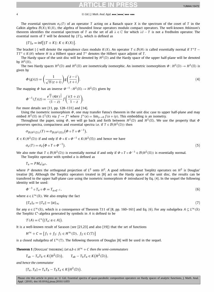
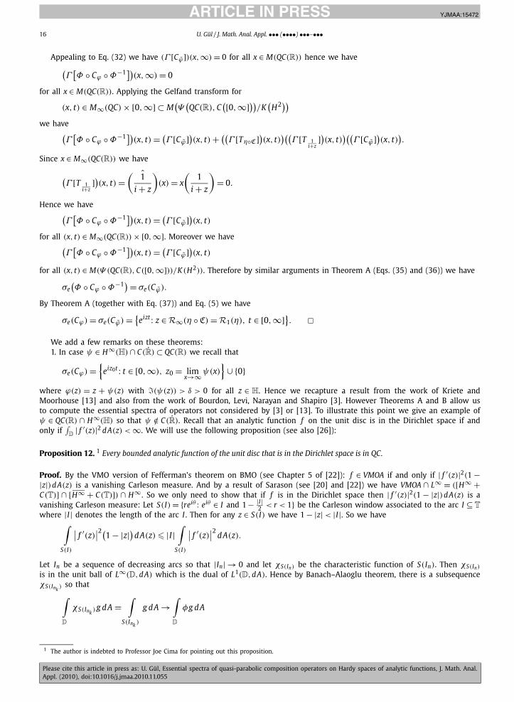
Fig. 1. Essential spectra of Cϕ for a = −5 and b = 5.

as k → ∞ for all g ∈ L1(D,dA) for some φ ∈ L∞(D,dA). In particular if we take g ∈ L∞(D,dA) ⊂ L1(D,dA) we observe that∣∣∣∣∫

S(Ink )

g dA

∣∣∣∣ � A(

S(Ink ))‖g‖∞

so we have | ∫S(Ink )g dA| → 0 as k → ∞ if g ∈ L∞(D,dA). Since L∞(D,dA) is dense in L1(D,dA) we have

∫D

φg dA = 0

for all g ∈ L1(D,dA) and hence φ ≡ 0. Since | f ′|2 ∈ L1(D,dA) we have∫

S(In)| f ′|2 dA → 0 as n → ∞. Since L1(D,dA) is

separable the weak* topology of the unit ball of L∞(D,dA) is metrizable. This implies that

lim|I|→0

∫S(I)

∣∣ f ′∣∣2dA = 0.

This proves the proposition. �We are ready to construct our example of a “quasi-parabolic" composition operator which has thick essential spectrum:

Let D be the simply connected region bounded by the curve α : [−π,π ] → C such that α is continuous on [−π,0)∪ (0,π ]with

α(t) ={

3i + i(t + i (b−a)2 sin( 3π2

4t )) + (a+b)2 if t ∈ (0, π

2 ],i(3 + t) + (a+b)

2 if t ∈ [−π2 ,0]

and α(π) = α(−π) = (1 + π2 ) + i(3 + π

2 ) + (a+b)2 , a < b. By the Riemann mapping theorem there is a conformal mapping

ψ : D → D that is bi-holomorphic. One can choose ψ to satisfy limθ→0− ψ(eiθ ) = 3i. Since D has finite area and ψ is one-to-one and onto, ψ is in the Dirichlet space and hence, by Proposition 12, ψ ∈ QC. Let ψ = ψ ◦ C. Then ψ ∈ QC(R) andψ �∈ H∞(H) ∩ C(R). We observe that

C∞(ψ) = {3i + x: x ∈ [a,b]}.

So for Cϕ : H2(H) → H2(H) and for Cϕ : H2(D) → H2(D), we have (see Figs. 1, 2)

σe(Cϕ) = σe(Cϕ ) = {ei(3i+x)t : t ∈ [0,∞), x ∈ [a,b]} ∪ {0}

where

ϕ(z) = z + ψ(z) and ϕ = C ◦ ϕ ◦ C−1.



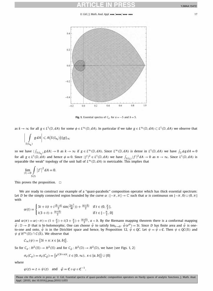
Fig. 2. Essential spectra of Cϕ for a = 5 and b = 25.

2. We recall that for any a, ϑ ∈ C(R) the operator Ma Dϑ is Hilbert Schmidt on L2(R) (see pp. 482–484 of [17]). Hencefor a ∈ C(R) and ϑ ∈ C([0,∞]) with a(∞) = ϑ(∞) = 0 the operator Ta Dϑ is compact on H2(H). Combining this fact withEqs. (30) and (38) we conclude that for ϕ : D → D with

ϕ(z) = C−1 ◦ ϕ ◦ C(z) = z + ψ(z),

ψ ∈ H∞ and �(ψ(z)) > ε > 0, the operator Φ ◦ Cϕ ◦ Φ−1 − Cϕ is compact on H2(H).

6. Further results

In this last part of the paper we will prove a more general result about Cϕ with ϕ(z) = z +ψ(z), ψ ∈ H∞: We will showthat if ϕ(z) = z + ψ(z) with ψ ∈ H∞ and �(ψ(z)) > ε > 0 for all z ∈ H then

σe(Cϕ) ⊇ {eizt : t ∈ [0,∞), z ∈ R∞(ψ)

} ∪ {0}where R∞(ψ) is the local essential range of ψ at infinity. We use the following Theorems 13 and 14 to prove the aboveresult. Theorem 13 is due to Axler [2] and we give a full proof of Theorem 14 using Power’s theorem and Axler’s theorem.

Theorem 13 (Axler’s theorem). Let f ∈ L∞ , then there is a Blaschke product B and b ∈ H∞ + C so that f = Bb.

Theorem 14. Let

Ψ(L∞(R), C

([0,∞])) = C∗(T(L∞(R)

) ∪ F)

be the C*-algebra generated by Toeplitz operators with L∞ symbols and Fourier multipliers on H2(H) and let M(Ψ ) be the space ofmultiplicative linear functionals on Ψ (L∞(R), C([0,∞]))/K (H2(H)). Then we have

M(Ψ ) ∼= (M∞

(L∞(R)

) × [0,∞]) ∪ (M

(L∞(R)

) × {∞})where

M∞(L∞(R)

) = {x ∈ M

(L∞(R)

): x|C(R) = δ∞}

is the fiber of M(L∞(R)) at infinity.

Proof. Consider the symbol map

Σ : L∞(R) → T(L∞(R)

)defined by Σ(ψ) = Tψ . Clearly Σ is injective. Let ψ1 = ϕ1ϕ2 and ψ2 = ϕ3ϕ4 with ϕ j ∈ H∞ , j ∈ {1,2,3,4}. Then Tϕ2ϕ4 =T ϕ2 T ϕ4 . This implies that

Tψ1ψ2 − Tψ1 Tψ2 = T ϕ [T ϕ , Tϕ1 ]Tϕ3 .
2 4



Since L∞(R) is spanned by such ψ1 and ψ2’s we have

Tψ1ψ2 − Tψ1 Tψ2 ∈ com(

T(L∞(R)

))for all ψ1, ψ2 ∈ L∞(R) (for more details see [15, p. 345]). Since Σ is injective, q ◦ Σ is a C*-algebra isomorphism fromL∞(R) onto T (L∞(R))/com(T (L∞(R))) where

q : T(L∞(R)

) → T(L∞(R)

)/com

(T

(L∞(R)

))is the quotient map. So M(T (L∞(R))) = M(L∞(R)). Since

K(

H2) ⊂ com(

T(L∞(R)

))we also have

M(

T(L∞(R)

)/K

(H2)) ∼= M

(L∞(R)

).

Hence using Power’s theorem we can identify

M(Ψ ) ∼= (M∞

(L∞(R)

) × [0,∞]) ∪ (M

(L∞(R)

) × {∞})where

M∞(L∞(R)

) = {x ∈ M

(L∞(R)

): x|C(R) = δ∞}

is the fiber of M(L∞(R)) at infinity:Let (x, y) ∈ M(L∞(R)) × [0,∞) so that x|C(R) = δt with t �= ∞. Choose a ∈ C(R) and ϑ ∈ C([0,∞]) having compact

supports such that

a(t) = ϑ(y) = 1, 0 � a � 1, 0 � ϑ � 1, a(z) < 1

for all z ∈ R\{t} and ϑ(w) < 1 for all w ∈ [0,∞]\{y}. Using the same arguments as in Eq. (23) we have

‖Ta Dϑ‖H2 < 1

which implies that

(x, y) /∈ M(Ψ

(T

(L∞(R)

), C

([0,∞]))/K(

H2(H)))

.

So if (x, y) ∈ M(Ψ (L∞(R), C([0,∞]))/K (H2(H))) then either y = ∞ or x ∈ M∞(L∞(R)).Let y = ∞ and x ∈ M(L∞(R)). Let a ∈ L∞(R) and ϑ ∈ C([0,∞]) such that

0 � ϑ � 1, 0 � a � 1 and a(x) = ϑ(y) = 1.

Using the same arguments as in Eqs. (24) and (25) together with the fact that

limw→∞‖K S w f ‖2 = 0 (39)

for any K ∈ K (H2(H)) and for all f ∈ H2(H), we have

‖Dϑ Ta‖e = ‖Dϑ Ta‖H2 = 1.

This implies that

(x,∞) ∈ M(Ψ

(L∞(R), C

([0,∞]))/K(

H2(H)))

for all x ∈ M(L∞(R)).Now let x ∈ M∞(L∞(R)) and y ∈ [0,∞]. Let a ∈ L∞(R) and ϑ ∈ C([0,∞]) such that

a(x) = ϑ(y) = 1 and 0 � ϑ � 1, 0 � a � 1.

Since a ∈ L∞ , by Axler’s theorem there is a Blaschke product B and b ∈ H∞ + C so that a = Bb. Since ˆ|B|(x) = |B(x)| = 1we have |b(x)| = 1. We have M(H∞ + C) ∼= M(H∞)/H (see Corollary 6.42 of [8]), the Poisson kernel is also asymptoticallymultiplicative on H∞ + C (see Lemma 6.44 of [8]) and by Carleson’s Corona theorem we observe that Eq. (26) is also validfor b for any ε > 0. Since 0 � |b| � 1 this implies that there is a w0 > 0 so that 1 − ε < |b(w)| < 1 for a.e. w with |w| > w0.After that we use the same arguments as in Eqs. (27) and (39) and since |B| = 1 a.e., we have

‖Dϑ T Bb‖e = ‖Dϑ MB Mb‖H2 = 1.

This implies that

(x, y) ∈ M(Ψ/K

(H2(H)

))for all x ∈ M∞(L∞(R)). �

Now we state and prove the main result of this section:



Theorem C. Let ϕ : H → H be an analytic self-map of H such that ϕ(z) = z + ψ(z) with ψ ∈ H∞(H) and �(ψ(z)) > ε > 0 for allz ∈ H. Then for Cϕ : H2(H) → H2(H) we have

σe(Cϕ) ⊇ {eizt : z ∈ R∞(ψ), t ∈ [0,∞)

} ∪ {0}where R∞(ψ) is the local essential range of ψ at infinity.

Proof. By Proposition 5 we have if ϕ(z) = z + ψ(z) with ψ ∈ H∞(H) and �(ψ(z)) > δ > 0 for all z ∈ H then

Cϕ ∈ Ψ(L∞(R), C

([0,∞])).By Theorem 14 we have

M(Ψ

(L∞(R), C

([0,∞])/K(

H2(H)))) ∼= (

M∞(L∞(R)

) × [0,∞]) ∪ (M

(L∞(R)

) × {∞}).If y = ∞ then for ϕ(z) = z + ψ(z) with ψ ∈ H∞ and �(ψ(z)) > δ > 0 we have

(x,∞)([Cϕ]) =

∞∑j=0

1

j!(τ (x)

) jϑ j(∞) = 0

since ϑ j(∞) = 0 for all j where τ and ϑ j are as in Eq. (32). If x ∈ M∞(L∞(R)) then as in Eq. (33), we have (x, y)([Cϕ ]) =eiψ(x)y . By Eqs. (34) and (3) we have

σe(Cϕ) ⊇ {x([Cϕ]): x ∈ M

(Ψ

(L∞(R), C

([0,∞]))/K(

H2(H)))}

and this implies that

σe(Cϕ) ⊇ {eiψ(x)t : x ∈ M∞

(L∞(R)

), t ∈ [0,∞)

} ∪ {0}.By Proposition 10 we have{

ψ(x): x ∈ M∞(L∞(R)

)} = R∞(ψ)

where R∞(ψ) is the local essential range of ψ at infinity. Hence we have

σe(Cϕ) ⊇ {eizt : z ∈ R∞(ψ), t ∈ [0,∞)

} ∪ {0}. �In the above theorem we do not have in general equality since Ψ (L∞(R), C([0,∞])) is not commutative. And we also

have the corresponding result for the unit disc:

Theorem D. Let ϕ : D → D be an analytic self-map of D such that

ϕ(z) = 2iz + η(z)(1 − z)

2i + η(z)(1 − z)

where η ∈ H∞(D) with �(η(z)) > ε > 0 for all z ∈ D. Then for Cϕ : H2(D) → H2(D) we have

σe(Cϕ) ⊇ {eizt : t ∈ [0,∞), z ∈ R1(η)

} ∪ {0}where R1(η) is the local essential range of η at 1.

Proof. Repeating the same arguments as in the proof of Theorem B, we have

Φ ◦ Cϕ ◦ Φ−1 ∈ Ψ(L∞(R), C

([0,∞]))/K(

H2(H)).

Take (x,∞) ∈ M(Ψ (L∞(R), C([0,∞]))/K (H2(H))), since (x,∞)([Cϕ ]) = 0 we have

(x,∞)([

Φ ◦ Cϕ ◦ Φ−1]) = 0.

For (x, y) ∈ M∞(L∞(R)) × [0,∞] we have (x, y)([T 1i+z

]) = 0 and hence we have

(x, y)([

Φ ◦ Cϕ ◦ Φ−1]) = (x, y)([Cϕ])

for all x ∈ M∞(L∞(R)). Therefore by Eq. (5) and Theorem C we have

σe(Cϕ) = σe(Φ ◦ Cϕ ◦ Φ−1) ⊇ {

eizt : t ∈ [0,∞), z ∈ R1(η) = R∞(η ◦ C)} ∪ {0}. �



Acknowledgments

The author would like to express his deep gratitude to his post-doc adviser Prof. Thomas L. Kriete for his help and support throughout his visit toUVA in 2009. The author wishes to express his gratitude to his Ph.D. adviser Prof. Aydın Aytuna for very useful and fruitful discussions on the subject, andto his co-adviser Prof. Theodore W. Gamelin for his support during his visits to UCLA in 2005 and 2006. The author wishes to express his thanks to thefollowing people: Operator Theory group of UVA, Prof. William T. Ross, Türker Özsarı, Mrs. Julie Riddleberger, Dr. Erdal Karapınar, Dr. Ayla Ayalp Ross andDale Ross. This work was supported by grants from TUBITAK (The Scientific and Technological Research Council of Turkey) both by a doctoral scholarshipand a post-doctoral scholarship.

References

[1] W. Arveson, An Invitation to C* Algebras, Grad. Texts in Math., vol. 39, Springer-Verlag, 1976.[2] S. Axler, Factorization of L∞ functions, Ann. of Math. 106 (1977) 567–572.[3] P.S. Bourdon, D. Levi, S.K. Narayan, J.H. Shapiro, Which linear fractional composition operators are essentially normal?, J. Math. Anal. Appl. 280 (2003)

30–53.[4] H.O. Cordes, E.A. Herman, Gelfand theory of pseudo differential operators, Amer. J. Math. 90 (1968) 681–717.[5] C.C. Cowen, Composition operators on H2, J. Operator Theory 9 (1983) 77–106.[6] C.C. Cowen, B.D. MacCluer, Composition Operators on Spaces of Analytic Functions, CRC Press, 1995.[7] K.R. Davidson, C*-Algebras by Example, Fields Inst. Monogr., vol. 6, AMS, 1996.[8] R.G. Douglas, Banach Algebra Techniques in Operator Theory, second edition, Grad. Texts in Math., vol. 179, Springer, 1998.[9] E.A. Gallardo-Gutierrez, A. Montes-Rodriguez, Adjoints of linear fractional composition operators on the Dirichlet space, Math. Ann. 327 (1) (2003)

117–134.[10] W.M. Higdon, The spectra of composition operators from linear fractional maps acting upon the Dirichlet space, J. Funct. Anal. 220 (1) (2005) 55–75.[11] K. Hoffman, Banach Spaces of Analytic Functions, Prentice Hall Inc., Englewood Cliffs, NJ, 1962.[12] P. Koosis, Introduction to H p Spaces, London Math. Soc. Lecture Note Ser., vol. 40, 1980.[13] T. Kriete, J. Moorhouse, Linear relations in the Calkin algebra for composition operators, Trans. Amer. Math. Soc. 359 (2007) 2915–2944.[14] V. Matache, Composition operators on Hardy spaces of a half-plane, Proc. Amer. Math. Soc. 127 (5) (1999) 1483–1491.[15] N.K. Nikols’kii, Treatise on the Shift Operator: Spectral Function Theory, Springer-Verlag, Berlin, 1986.[16] N.K. Nikols’kii, Operators, Functions and Systems: An Easy Reading. Vol. 1. Hardy, Hankel and Toeplitz, Mathematical Surveys and Monographs, vol. 92,

AMS, Providence, RI, 2002.[17] S.C. Power, Commutator ideals and pseudo-differential C*-Algebras, Quart. J. Math. Oxford (2) 31 (1980) 467–489.[18] S.C. Power, Characters on C*-algebras, the joint normal spectrum and a pseudo-differential C*-algebra, Proc. Edinb. Math. Soc. (2) 24 (1) (1981) 47–53.[19] S.C. Power, Hankel Operators on Hilbert Space, Pitman Advanced Publishing Program, London, 1982.[20] W. Rudin, Functional Analysis, McGraw–Hill Inc., 1973.[21] D. Sarason, Functions of vanishing mean oscillation, Trans. Amer. Math. Soc. 207 (1975) 391–405.[22] D. Sarason, Toeplitz operators with piecewise quasicontinuous symbols, Indiana Univ. Math. J. (2) 26 (1977) 817–838.[23] D. Sarason, Function Theory on the Unit Circle, Lecture Notes for a Conference at Virginia Polytechnic and State University, Blacksburg, Virginia, 1978.[24] R.J. Schmitz, Toeplitz-composition C*-algebras with piecewise continuous symbols, Ph.D. thesis, University of Virginia, Charlottesville, 2008.[25] J.H. Shapiro, Cluster set, essential range, and distance estimates in BMO, Michigan Math. J. 34 (1987) 323–336.[26] D.A. Stegenga, A geometric condition which implies BMOA, in: Harmonic Analysis in Euclidean Spaces (Proc. Sympos. Pure Math., Williams Coll.,

Williamstown, Mass., 1978), Part 1, Proc. Sympos. Pure Math., vol. XXXV, AMS, Providence, RI, 1979, pp. 427–430.[27] E. Stein, R. Shakarchi, Fourier Analysis, An Introduction, Princeton Lect. Anal., vol. I, Princeton University Press, 2003.

Documents

Essential spectra of quasi-parabolic composition operators