Embed Size (px)
Citation preview
Essential Mathematicsand
Statistics for ScienceSecond Edition
Graham CurrellAntony Dowman
The University of the West of England, UK
A John Wiley & Sons, Ltd., Publication


Essential Mathematicsand
Statistics for ScienceSecond Edition


Essential Mathematicsand
Statistics for ScienceSecond Edition
Graham CurrellAntony Dowman
The University of the West of England, UK
A John Wiley & Sons, Ltd., Publication

This edition first published 2009, c© 2009 by John Wiley & Sons.
Wiley-Blackwell is an imprint of John Wiley & Sons, formed by the merger of Wiley’s global Scientific, Technicaland Medical business with Blackwell Publishing.
Registered office: John Wiley & Sons Ltd, The Atrium, Southern Gate, Chichester, West Sussex, PO19 8SQ, UnitedKingdom
Other Editorial offices:9600 Garsington Road, Oxford, OX4 2DQ, UK
111 River Street, Hoboken, NJ 07030-5774, USA
For details of our global editorial offices, for customer services and for information about how to apply forpermission to reuse the copyright material in this book please see our website at www.wiley.com/wiley-blackwell.
The right of the author to be identified as the author of this work has been asserted in accordance with theCopyright, Designs and Patents Act 1988.
All rights reserved. No part of this publication may be reproduced, stored in a retrieval system, or transmitted, in anyform or by any means, electronic, mechanical, photocopying, recording or otherwise, except as permitted by the UKCopyright, Designs and Patents Act 1988, without the prior permission of the publisher.
Wiley also publishes its books in a variety of electronic formats. Some content that appears in print may not beavailable in electronic books.
Designations used by companies to distinguish their products are often claimed as trademarks. All brand names andproduct names used in this book are trade names, service marks, trademarks or registered trademarks of theirrespective owners. The publisher is not associated with any product or vendor mentioned in this book. Thispublication is designed to provide accurate and authoritative information in regard to the subject matter covered. It issold on the understanding that the publisher is not engaged in rendering professional services. If professional adviceor other expert assistance is required, the services of a competent professional should be sought.
Library of Congress Cataloging-in-Publication Data
Currell, Graham.Essential mathematics and statistics for science / Graham Currell, Antony Dowman. – 2nd ed.
p. cm.Includes index.ISBN 978-0-470-69449-7 – ISBN 978-0-470-69448-0
1. Science–Statistical methods. 2. Science–Mathematics. I. Dowman, Antony. II. Title.Q180.55.S7C87 2009507.2–dc22
2008052795
ISBN: 978-0-470-69449-7 (HB)978-0-470-69448-0 (PB)
A catalogue record for this book is available from the British Library.
Typeset in 10/12pt Times and Century Gothic by Laserwords Private Limited, Chennai, India.Printed and bound in Great Britain by Antony Rowe Ltd, Chippenham, Wiltshire.
First Impression 2009

To
Jenny and Felix
Jan, Ben and Jo.

Contents
Preface xi
On-line Learning Support xv
1 Mathematics and Statistics in Science 1
1.1 Data and Information 21.2 Experimental Variation and Uncertainty 21.3 Mathematical Models in Science 4
2 Scientific Data 7
2.1 Scientific Numbers 82.2 Scientific Quantities 152.3 Chemical Quantities 202.4 Angular Measurements 31
3 Equations in Science 41
3.1 Basic Techniques 413.2 Rearranging Simple Equations 533.3 Symbols 633.4 Further Equations 683.5 Quadratic and Simultaneous Equations 78
4 Linear Relationships 87
4.1 Straight Line Graph 894.2 Linear Regression 994.3 Linearization 107
5 Logarithmic and Exponential Functions 113
5.1 Mathematics of e, ln and log 1145.2 Exponential Growth and Decay 128
6 Rates of Change 145
6.1 Rate of Change 1456.2 Differentiation 152
viii CONTENTS
7 Statistics for Science 161
7.1 Analysing Replicate Data 1627.2 Describing and Estimating 1687.3 Frequency Statistics 1767.4 Probability 1907.5 Factorials, Permutations and Combinations 203
8 Distributions and Uncertainty 211
8.1 Normal Distribution 2128.2 Uncertainties in Measurement 2178.3 Presenting Uncertainty 2248.4 Binomial and Poisson Distributions 230
9 Scientific Investigation 243
9.1 Scientific Systems 2439.2 The ‘Scientific Method’ 2459.3 Decision Making with Statistics 2469.4 Hypothesis Testing 2509.5 Selecting Analyses and Tests 256
10 t-tests and F -tests 261
10.1 One-sample t-tests 26210.2 Two-sample t-tests 26710.3 Paired t-tests 27210.4 F -tests 274
11 ANOVA – Analysis of Variance 279
11.1 One-way ANOVA 27911.2 Two-way ANOVA 28611.3 Two-way ANOVA with Replication 29011.4 ANOVA Post Hoc Testing 296
12 Non-parametric Tests for Medians 299
12.1 One-sample Wilcoxon Test 30112.2 Two-sample Mann–Whitney U -test 30512.3 Paired Wilcoxon Test 30812.4 Kruskal–Wallis and Friedman Tests 311
13 Correlation and Regression 315
13.1 Linear Correlation 31613.2 Statistics of Correlation and Regression 32013.3 Uncertainty in Linear Calibration 324
14 Frequency and Proportion 331
14.1 Chi-squared Contingency Table 33214.2 Goodness of Fit 34014.3 Tests for Proportion 343

CONTENTS ix
15 Experimental Design 349
15.1 Principal Techniques 34915.2 Planning a Research Project 357
Appendix I: Microsoft Excel 359
Appendix II: Cumulative z -areas for Standard Normal Distribution 363
Appendix III: Critical Values: t -statistic and Chi-squared, χ2 365
Appendix IV: Critical F -values at 0.05 (95 %) Significance 367
Appendix V: Critical Values at 0.05 (95 %) Significance for: Pearson’s CorrelationCoefficient, r , Spearman’s Rank Correlation Coefficient, rS, and Wilcoxon LowerLimit, W L 369
Appendix VI: Mann–Whitney Lower Limit, UL, at 0.05 (95 %) Significance 371
Short Answers to ‘Q’ Questions 373
Index 379

Preface
The main changes in the second edition have been driven by the authors’ direct experience ofusing the book as a core text for teaching mathematics and statistics to students on a range ofundergraduate science courses.
Major developments include:
• Integration of ‘how to do it’ video clips via the Website to provide students with audio-visualworked answers to over 200 ‘Q’ questions in the book.
• Improvement in the educational development for certain topics, providing a greater clarityin the learning process for students, e.g. in the approach to handling equations in Chapter 3and the development of exponential growth in Chapter 5.
• Reorientation in the approach to hypothesis testing to give priority to an understanding ofthe interpretation of p-values , although still retaining the calculation of test statistics. Thestatistics content has been substantially reorganized.
• Movement of some content to the Website, e.g. Bayesian statistics and some of the statisticaltheory underpinning regression and analysis of variance.
• Revised computing tutorials on the Website to demonstrate the use of Excel and Minitab formany of the data analysis techniques. These include video demonstrations of the requiredkeystrokes for important techniques.
The book was designed principally as a study text for students on a range of undergraduatescience programmes: biological, environmental, chemical, forensic and sports sciences. It cov-ers the majority of mathematical and statistical topics introduced in the first two years of suchprogrammes, but also provides important aspects of experimental design and data analysis thatstudents require when carrying out extended project work in the later years of their degreeprogrammes.
The comprehensive Website actively supports the content of the book, now including exten-sive video support. The book can be used independently of the Website, but the close integrationbetween them provides a greater range and depth of study possibilities. The Website can beaccessed at:
www.wiley.com/go/currellmaths2
The introductory level of the book assumes that readers will have studied mathematics withmoderate success to Year 11 of normal schooling. Currently in the UK, this is equivalent to aGrade C in Mathematics in the General Certificate of Secondary Education (GCSE).
There are Revision Mathematics notes available on the associated Website for those readerswho need to refresh their memories on relevant topics of basic mathematics – BODMAS,number line, fractions, percentages, areas and volumes, etc. A self-assessment test on these
xii PREFACE
‘basic’ topics is also available on the Website to allow readers to assess their need to use thismaterial.
The first eight chapters in the book introduce the basic mathematics and statistics that arerequired for the modelling of many different scientific systems. The remaining chapters arethen primarily related to experimental investigation in science, and introduce the statisticaltechniques that underpin data analysis and hypothesis testing.
Over 200 worked Examples in the text are used to develop the various topics. Thecalculations for many of these Examples are also performed using Microsoft Excel(office.microsoft.com) and the statistical analysis program Minitab (www.minitab.com). Thefiles for these calculations are available via the Website.
Readers can test their understanding as each topic develops by working through over 200‘Q’ questions in the book. The numeric answers are given at the end of the book, but fullworked answers are also available through the Website in both video and printed (pdf) format.
Throughout the book, readers have the opportunity of learning how to use software toperform many of the calculations. This strong integration of paper-based and computer-basedcalculations both supports an understanding of the mathematics and statistics involved anddevelops experience with the use of appropriate software for data handling and analysis.
Scientific contextThe diverse uses of mathematics and statistics in the various disciplines of science place dif-ferent emphases on the various topics. However, there is a core of mathematical and statisticaltechniques that is essentially common to all branches of experimental science, and it is thismaterial that forms the basis of this book. We believe that we have developed a coherentapproach and consistent nomenclature, which will make the material appropriate across thevarious disciplines.
When developing questions and examples at an introductory level, it is important to achievea balance between treating each topic as pure mathematics or embedding it deeply in a scientific‘context’. Too little ‘context’ can reduce the scientific interest, but too much can confuse theunderstanding of the mathematics. The optimum balance varies with topic and level.
The ‘Q’ questions and Examples in the book concentrate on clarity in developing the topicsstep by step through each chapter. Where possible we have included a scientific context thatis understandable to readers from a range of different disciplines.
Experimental designThe process of good experimental planning and design is a topic that is often much neglectedin an undergraduate course. Although the topic pervades all aspects of science, it does not havea clear focus in any one particular branch of the science, and is rarely treated coherently in itsown right.
Good experimental design is dependent on the availability of suitable mathematical andstatistical techniques to analyse the resulting data. A wide range of such methods are introducedin this book:
• Regression analysis (Chapters 4 and 13) for relationships that are inherently linear or canbe linearized.
PREFACE xiii
• Logarithmic and/or exponential functions (Chapter 5) for systems involving natural growthand decay, or for systems with a logarithmic response.
• Modelling with Excel (Chapter 6) for rates of change.• Probabilities (Chapter 7), frequency and proportions (Chapter 14) and Bayesian statistics
(Website) to interpret categorical data, ratios and likelihood.• Statistical distributions (Chapter 8) for modelling random behaviour in complex systems.• Statistical analysis (Chapters 9 to 14) for hypothesis testing in a variety of systems.• Analysis of variance (Chapter 11) for hypothesis testing of complex experimental systems.• Experimental design overview (Chapter 15).
Computing softwareThere are various software packages available that can help scientists in implementing math-ematics and statistics. Some university departments have strong preferences for one or theother.
Microsoft Excel spreadsheets can be used effectively for a variety of purposes:
• basic data handling – sorting and manipulating data;• data presentation using graphs, charts, tables;• preparing data and graphs for export to other packages;• performing a range of mathematical calculations; and• performing a range of statistical calculations.
Minitab (Minitab Inc.) is designed specifically for statistical data analysis. The data is enteredin columns and a wide range of analyses can be performed using menu-driven instructionsand interactive dialogue boxes. The results are provided as printed text, graphs or new columndata.
Most students find that the statistical functions in Excel are a helpful introduction to usingstatistics, but for particular problems it is more useful to turn to the packages designed specif-ically for statistical analysis. Nevertheless, it is usually convenient to use Excel for organizingdata into an appropriate layout before exporting to the specialized package.
The book has used Excel 2003 and Minitab 15 to provide all of the software calculationsused, and the relevant files are available on the Website. However, there are several othersoftware packages that can perform similar tasks, and information on some of these is alsogiven on the Website.
Most of the graphs in the book have been prepared using Excel, except for those identifiedas having been produced using Minitab.

On-line Learning Support
The book’s Website (www.wiley.com/go/currellmaths2) provides extensive learning supportintegrated closely with the content of the book.
Important learning elements referenced within the book are:
• Examples (e.g. Example 7.12) with worked answers given directly within the text, and withsupporting files available on the Website where appropriate.
• ‘Q’ questions (e.g. Q7.13) with numerical answers at the end of the book, but with fullworked answers on video or pdf files via the Website.
• Equations – referred to using square brackets, e.g. [7.16].
The Website for the second edition provides the following structural support:
• ‘How to do it’ – answers to all ‘Q’ questions. Over 200 flash video clips provide workedanswers to all of the ‘Q’ questions in the book, and can be viewed directly over the Internet.The worked answers are also presented in pdf files.
• Further practice questions. Additional questions and answers are provided which enablestudents to further practise/test their understanding. Many students find these particularlyuseful in some skill areas, such as chemical calculations, rearranging equations, logs andexponentials, etc.
• Excel and Minitab tutorials. Keystroke tutorials provide a guide to using Excel 2007 andMinitab 15 for some of the important analyses developed in the book.
• Excel and Minitab files. These files provide the software calculations for the examples, ‘Q’questions, tables and figures presented in the book. In appropriate cases, these are linkedwith video explanations.
• Additional materials. Additional learning materials (pdf files), including revision mathe-matics (basic skills of the number line, BODMAS, fractions, powers, areas and volumes),Bayesian statistics, transformation of data, weighted and nonlinear regression, data variance.
• Reference materials. Statistical tables, Greek symbols.• Links. Access to ongoing development of teaching materials associated with the book,
including on-line self-assessment.
VideosThe Website hosts a large number of feedback and instructional videos that have been developedsince the first edition of the book was published. Most of these are very short (a few minutes)and provide students with the type of feedback they might expect to receive when asking

xvi ON-LINE LEARNING SUPPORT
a tutor ‘how to do’ a particular question or computer technique. The videos are targeted toproduce support just at the point when the student is really involved with trying to understanda particular detailed problem, and provide the focused help that is both required and verywelcome.
These videos are used by students of all abilities: advanced students use them just as a quickcheck on their own self-study, but weaker students can pause and rerun the videos to providea very effective self-managed ‘tutorial’.
The video formats include a ‘hand-written’ format for paper-based answers, and ‘keystroke’demonstrations for computer-based problems. These match directly the form and content of theknowledge and skills that the student is trying to acquire. The separate videos can be vieweddirectly and quickly over the Internet, using flash technology which is already loaded withmost Internet browsers.
1Mathematics and Statisticsin Science
OverviewScience students encounter mathematics and statistics in three main areas:
• Understanding and using theory.• Carrying out experiments and analysing results.• Presenting data in laboratory reports and essays.
Unfortunately, many students do not fully appreciate the need for understanding mathematicsand/or statistics until it suddenly confronts them in a lecture or in the write-up of an experiment.There is indeed a ‘chicken and egg’ aspect to the problem:
Some science students have little enthusiasm to study mathematics until it appears in a lecture ortutorial – by which time it is too late! Without the mathematics, they cannot fully understand thescience that is being presented, and they drift into a habit of accepting a ‘second-best’ sciencewithout mathematics. The end result could easily be a drop of at least one grade in their finaldegree qualification.
All science is based on a quantitative understanding of the world around us – an understandingdescribed ultimately by measurable values. Mathematics and statistics are merely the processesby which we handle these quantitative values in an effective and logical way.
Mathematics and statistics provide the network of links that tie together the details of ourunderstanding, and create a sound basis for a fundamental appreciation of science as a whole.Without these quantifiable links, the ability of science to predict and move forward into newareas of understanding would be totally undermined.
In recent years, the data handling capability of information technology has made mathe-matical and statistical calculations far easier to perform, and has transformed the day-to-daywork in many areas of science. In particular, a good spreadsheet program, like Excel, enablesboth scientists and students to carry out extensive calculations quickly, and present results andreports in a clear and accurate manner.
Essential Mathematics and Statistics for Science 2nd Edition Graham Currell and Antony DowmanCopyright c© 2009 John Wiley & Sons, Ltd
2 MATHEMATICS AND STATISTICS IN SCIENCE
1.1 Data and InformationReal-world information is expressed in the mathematical world through data.
In science, some data values are believed to be fixed in nature. We refer to values that arefixed as constants, e.g. the constant c is often used to represent the speed of light in a vacuum,c = 3.00 × 10⁸ m s−1.
However, most measured values are subject to change. We refer to these values as variables,e.g. T for temperature, pH for acidity.
The term parameter refers to a variable that can be used to describe a relevant characteristicof a scientific system, or a statistical population (see 7.2.2), e.g. the actual pH of a buffersolution, or the average (mean) age of the whole UK population. The term statistic refers to avariable that is used to describe a relevant characteristic of a sampled (see 7.2.2) set of data,e.g. five repeated measurements of the concentration of a solution, or the average (mean) ageof 1000 members of the UK population.
Within this book we use the convention of printing letters and symbols that represent quan-tities (constants and variables) in italics, e.g. c, T and p.
The letters that represent units are presented in normal form, e.g. m s−1 gives the units ofspeed in metres per second.
There is an important relationship between data and information, which appears whenanalysing more complex data sets. It is a basic rule that:
It is impossible to get more ‘bits’ of information from a calculation than the number of ‘bits’ ofdata that is put into the calculation.
For example, if a chemical mixture contains three separate compounds, then it is necessary tomake at least three separate measurements on that mixture before it is possible to calculate theconcentration of each separate compound.
In mathematics and statistics, the number of bits of information that are available in a dataset is called the degrees of freedom, df , of that data set. This value appears in many statisticalcalculations, and it is usually easy to calculate the number of degrees of freedom appropriateto any given situation.
1.2 Experimental Variation and UncertaintyThe uncertainty inherent in scientific information is an important theme that appears throughoutthe book.
The true value of a variable is the value that we would measure if our measurement processwere ‘perfect’. However, because no process is perfect, the ‘true value’ is not normally known.
The observed value is the value that we produce as our best estimate of the true value.The error in the measurement is the difference between the true value and the observed
value:
Error = Observed value − True value [1.1]
As we do not normally know the ‘true value’, we cannot therefore know the actual error inany particular measurement. However, it is important that we have some idea of how large theerror might be.
1.2 EXPERIMENTAL VARIATION AND UNCERTAINTY 3
The uncertainty in the measurement is our best estimate of the magnitude of possible errors.The magnitude of the uncertainty must be derived on the basis of a proper understanding of themeasurement process involved and the system being measured. The statistical interpretation ofuncertainty is derived in 8.2.
The uncertainty in experimental measurements can be divided into two main categories:
Measurement uncertainty. Variations in the actual process of measurement will give somedifferences when the same measurement is repeated under exactly the same conditions. Forexample, repeating a measurement of alcohol level in the same blood sample may giveresults that differ by a few milligrams in each 100 millilitres of blood.
Subject uncertainty. A subject is a representative example of the system (9.1) being measured,but many of the systems in the real world have inherent variability in their responses. Forexample, in testing the effectiveness of a new drug, every person (subject) will have aslightly different reaction to that drug, and it would be necessary to carry out the test on awide range of people before being confident about the ‘average’ response.
Whatever the source of uncertainty, it is important that any experiment must be designed bothto counteract the effects of uncertainty and to quantify the magnitude of that uncertainty.
Within each of the two types of uncertainty, measurement and subject , it is possible toidentify two further categories:
Random error. Each subsequent measurement has a random error, leading to imprecision inthe result. A measurement with a low random error is said to be a precise measurement.
Systematic error. Each subsequent measurement has the same recurring error. A systematicerror shows that the measurement is biased , e.g. when setting the liquid level in a burette,a particular student may always set the meniscus of the liquid a little too low.
The precision of a measurement is the best estimate for the purely random error in ameasurement.
The trueness of a measurement is the best estimate for the bias in a measurement.The accuracy of a measurement is the best estimate for the overall error in the final result,
and includes both the effects of a lack of precision (due to random errors) and bias (due tosystematic errors).
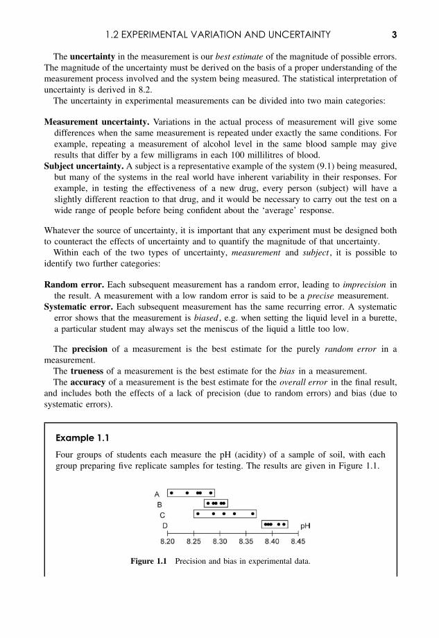
Example 1.1
Four groups of students each measure the pH (acidity) of a sample of soil, with eachgroup preparing five replicate samples for testing. The results are given in Figure 1.1.
Figure 1.1 Precision and bias in experimental data.
4 MATHEMATICS AND STATISTICS IN SCIENCE
What can be said about the accuracy of their results?
It is possible to say that the results from groups A and C show greater random uncertainty(less precision) than groups B and D. This could be due to such factors as a lack of carein preparing the five samples for testing, or some electronic instability in the pH meterbeing used.
Groups B and D show greater precision, but at least one of B or D must have somebias in their measurements, i.e. poor ‘trueness’. The bias could be due to an error insetting the pH meter with a buffer solution, which would then make every one of thefive measurements in the set wrong by the same amount.
With the information given, very little can be said about the overall accuracy of themeasurements; the ‘true’ value is not known, and there is no information about possiblebias in any of the results. For example if the true value were pH = 8.40, this wouldmean that groups A, B and C were all biased, with the most accurate measurementbeing group D.
The effect of random errors can be managed and quantified using suitable statistical methods(8.2, 8.3 and 15.1.2). The presentation of uncertainty as error bars on graphs is developed inan Excel tutorial on the Website.
Systematic errors are more difficult to manage in an experiment, but good experiment design(Chapter 15) aims to counteract their effect as much as possible.
1.3 Mathematical Models in ScienceA fundamental building block of both science and mathematics is the equation .
Science uses the equation as a mathematical model to define the relationship between one ormore factors in the real world (3.1.6). It may then be possible to use mathematics to investigatehow that equation may lead to new conclusions about the world.
Perhaps the most famous equation, arising from the general theory of relativity, is:
E = mc2
which relates the amount of energy, E (J), that would be released if a mass, m (kg), of matterwas converted into energy (e.g. in a nuclear reactor). E and m are both variables and theconstant c(= 3.00 × 10⁸ m s−1) is the speed of light.
Example 1.2
Calculate the amount of matter, m, that must be converted completely into energy, if theamount of energy, E, is equivalent to that produced by a medium-sized power station inone year: E = 1.8 × 10¹³ J.
1.3 MATHEMATICAL MODELS IN SCIENCE 5
Rearranging the equation E = mc2 gives:
m = E
c2
Substituting values into the equation:
m = 1.8 × 10¹³
(3.00 × 10⁸)2⇒ 0.000 20 kg ⇒ 0.20 g
This equation tells us that if only 0.20 g of matter is converted into energy, it willproduce an energy output equivalent to a power station operating for a year!
This is why the idea of nuclear power continues to be so very attractive.
Example 1.2 indicates some of the common mathematical processes used in handlingequations in science: rearranging the equation, using scientific notation, changing of units,and ‘solving’ the equation to derive the value of an unknown variable.
Equations are used to represent many different types of scientific processes, and often employa variety of mathematical functions to create suitable models.
In particular, many scientific systems behave in a manner that is best described using anexponential or logarithmic function, e.g. drug elimination in the human body, pH values.Example 1.3 shows how both the growth and decay of a bacteria population can be described,in part, by exponential functions.
Example 1.3
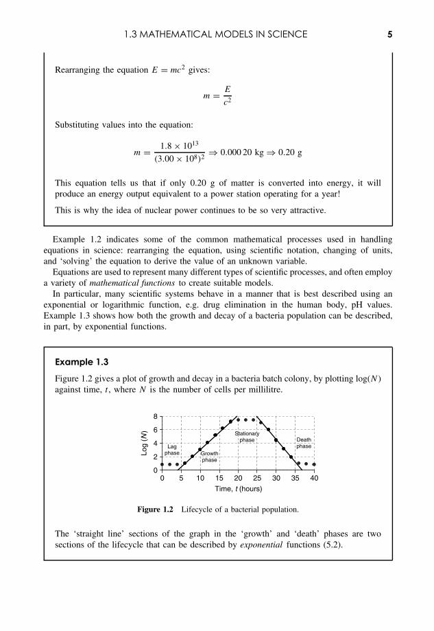
Figure 1.2 gives a plot of growth and decay in a bacteria batch colony, by plotting log(N )against time, t , where N is the number of cells per millilitre.
0
2
4
6
8
0 5 10 15 20 25 30 35 40
Time, t (hours)
Log
(N)
Lagphase Growth
phase
Stationaryphase Death
phase
Figure 1.2 Lifecycle of a bacterial population.
The ‘straight line’ sections of the graph in the ‘growth’ and ‘death’ phases are twosections of the lifecycle that can be described by exponential functions (5.2).
6 MATHEMATICS AND STATISTICS IN SCIENCE
Another aspect of real systems is that they often have significant inherent variability , e.g.similar members of a plant crop grow at different rates, or repeated measurements of therefractive index of glass may give different results. In these situations, we need to developstatistical models that we can use to describe the underlying behaviour of the system as awhole.
The particular statistical model that best fits the observed data is often a good guide to thescientific processes that govern the system being measured. Example 1.4 shows the Poissondistribution that could be expected if plants were distributed randomly with an average of 3.13plants per unit area.
Example 1.4
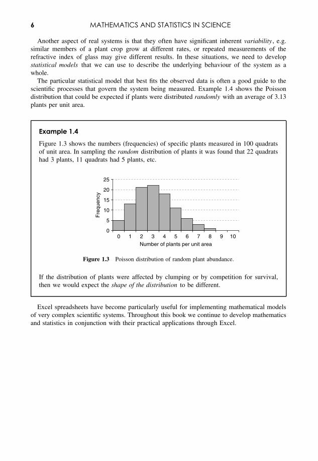
Figure 1.3 shows the numbers (frequencies) of specific plants measured in 100 quadratsof unit area. In sampling the random distribution of plants it was found that 22 quadratshad 3 plants, 11 quadrats had 5 plants, etc.
0
5
10
15
20
25
0 1 2 3 4 5 6 7 8 9 10
Number of plants per unit area
Fre
quen
cy
Figure 1.3 Poisson distribution of random plant abundance.
If the distribution of plants were affected by clumping or by competition for survival,then we would expect the shape of the distribution to be different.
Excel spreadsheets have become particularly useful for implementing mathematical modelsof very complex scientific systems. Throughout this book we continue to develop mathematicsand statistics in conjunction with their practical applications through Excel.
2Scientific Data
Overview
Website • ‘How to do it’ video answers for all ‘Q’ questions.• Revision mathematics notes for basic mathematics:
BODMAS, number line, fractions, powers, areas and volumes.• Excel tutorials: scientific calculations, use of formulae, functions, formatting
(scientific numbers, decimal places), etc.
Data in science appears in a variety of forms. However, there is a broad classification of datainto two main categories:
• Quantitative data. The numeric value of quantitative data is recorded as a measurable (orparametric) variable, e.g. time, pH, temperature, etc.
• Qualitative (or categorical) data. Qualitative data is grouped into different classes, and thenames of the classes serve only to distinguish, or rank, the different classes, and have noother quantitative value, e.g. grouping people according to their nationality, eye colour, etc.
Quantitative data can be further divided into:
Discrete data. Only specific values are used, e.g. counting the number of students in a classwill only give integer values.
Continuous data. Using values specified to any accuracy as required, e.g. defining time, usingseconds, to any number of decimal places as appropriate (e.g. 75.85206 s).
Quantitative data can be further subdivided into:
Ratio data. The ‘zero’ of a ratio scale has a true ‘zero’ value in science, and the ratios of datavalues also have scientific meaning. For example, the zero, 0 K, of the absolute temperaturescale in thermodynamics is a true ‘absolute zero’ (there is nothing colder!), and 100 K istwice the absolute ‘temperature’ of 50 K.
Interval data. The ‘zero’ of an interval scale does not have a true ‘zero’ value in science,and the ratios of data values do not have scientific meaning. Nevertheless the data intervals
Essential Mathematics and Statistics for Science 2nd Edition Graham Currell and Antony DowmanCopyright c© 2009 John Wiley & Sons, Ltd
8 SCIENTIFIC DATA
are still significant. For example, the zero, 0 ◦C, of the Celsius temperature scale, is justthe temperature of melting ice and not a true ‘zero’, and 100 ◦C is not ‘twice as hot’ as50 ◦C. However, the degree intervals are the same in both the absolute and Celsius scales.
Qualitative data can be further divided into:
Ordinal data. The classes have a sense of progression from one class to the next, e.g. degreeclassifications (first, upper second, lower second, third), opinion ratings in a questionnaire(excellent, good, satisfactory, poor, bad).
Nominal (named) data. There is no sense of progression between classes, e.g. animal species,nationality.
This chapter is concerned mainly with calculations involving continuous quantitative data,although examples of other types of data appear elsewhere within the book. The topics includedrelate to some of the most common calculations that are performed in science:
• Using scientific (or standard) notation.• Displaying data to an appropriate precision.• Handling units, and performing the conversions between them.• Performing routine calculations involving chemical quantities.• Working with angular measurements in both degrees and radians.
2.1 Scientific Numbers2.1.1 IntroductionThis unit describes some of the very common arithmetical calculations that any scientist needsto perform when working with numerical data. Students wishing to refresh their memory ofbasic mathematics can also refer to the revision resources available on the book’s dedicatedWebsite.
2.1.2 Scientific (standard) notationScientific notation is also called standard notation or exponential notation .
In scientific notation, the digits of the number are written with the most significant figurebefore the decimal point and all other digits after the decimal point. This ‘number’ is thenmultiplied by the correct ‘power of 10’ to make it equal to the desired value. For example:
230 = 2.30 × 10²
0.00230 = 2.30 × 10⁻³
2.30 = 2.30 × 100 ⇒ 2.30 × 1 ⇒ 2.30
In Excel, other software and some calculators, the ‘power of 10’ is preceded by the letter ‘E’,e.g. the number −3.56 × 10⁻¹¹ would appear as −3.56E-11.
2.1 SCIENTIFIC NUMBERS 9
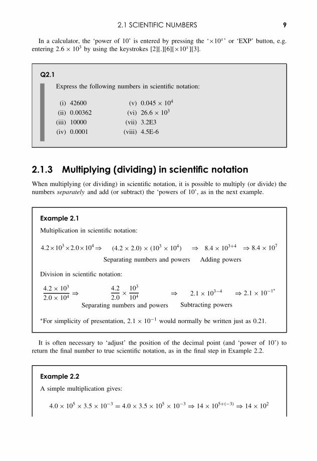
In a calculator, the ‘power of 10’ is entered by pressing the ‘×10x’ or ‘EXP’ button, e.g.entering 2.6 × 10³ by using the keystrokes [2][.][6][×10x ][3].
Q2.1Express the following numbers in scientific notation:
(i) 42600 (v) 0.045 × 10⁴
(ii) 0.00362 (vi) 26.6 × 10³
(iii) 10000 (vii) 3.2E3
(iv) 0.0001 (viii) 4.5E-6
2.1.3 Multiplying (dividing) in scientific notationWhen multiplying (or dividing) in scientific notation, it is possible to multiply (or divide) thenumbers separately and add (or subtract) the ‘powers of 10’, as in the next example.
Example 2.1
Multiplication in scientific notation:
4.2×103×2.0×104 ⇒ (4.2 × 2.0) × (103 × 104)
Separating numbers and powers
⇒ 8.4 × 10³+4
Adding powers
⇒ 8.4 × 10⁷
Division in scientific notation:
4.2 × 10³
2.0 × 10⁴⇒ 4.2
2.0× 10³
104
Separating numbers and powers
⇒ 2.1 × 10³−4
Subtracting powers
⇒ 2.1 × 10⁻¹∗
∗For simplicity of presentation, 2.1 × 10⁻¹ would normally be written just as 0.21.
It is often necessary to ‘adjust’ the position of the decimal point (and ‘power of 10’) toreturn the final number to true scientific notation, as in the final step in Example 2.2.
Example 2.2
A simple multiplication gives:
4.0 × 105 × 3.5 × 10−3 = 4.0 × 3.5 × 105 × 10−3 ⇒ 14 × 105+(−3) ⇒ 14 × 102
10 SCIENTIFIC DATA
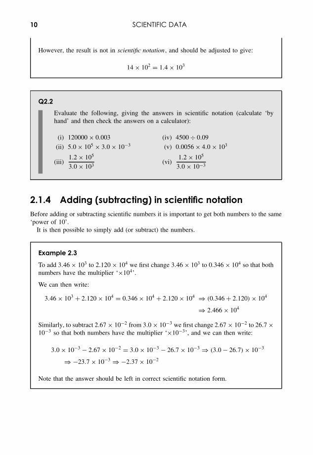
However, the result is not in scientific notation , and should be adjusted to give:
14 × 102 = 1.4 × 10³
Q2.2Evaluate the following, giving the answers in scientific notation (calculate ‘byhand’ and then check the answers on a calculator):
(i) 120000 × 0.003 (iv) 4500 ÷ 0.09
(ii) 5.0 × 105 × 3.0 × 10−3 (v) 0.0056 × 4.0 × 103
(iii)1.2 × 10⁵
3.0 × 10³(vi)
1.2 × 10⁵
3.0 × 10⁻³
2.1.4 Adding (subtracting) in scientific notationBefore adding or subtracting scientific numbers it is important to get both numbers to the same‘power of 10’.
It is then possible to simply add (or subtract) the numbers.
Example 2.3
To add 3.46 × 10³ to 2.120 × 10⁴ we first change 3.46 × 10³ to 0.346 × 10⁴ so that bothnumbers have the multiplier ‘×104’.
We can then write:
3.46 × 10³ + 2.120 × 104 = 0.346 × 10⁴ + 2.120 × 10⁴ ⇒ (0.346 + 2.120) × 104
⇒ 2.466 × 10⁴
Similarly, to subtract 2.67 × 10⁻² from 3.0 × 10⁻³ we first change 2.67 × 10⁻² to 26.7 ×10⁻³ so that both numbers have the multiplier ‘×10−3’, and we can then write:
3.0 × 10⁻³ − 2.67 × 10−2 = 3.0 × 10⁻³ − 26.7 × 10⁻³ ⇒ (3.0 − 26.7) × 10−3
⇒ −23.7 × 10⁻³ ⇒ −2.37 × 10⁻²
Note that the answer should be left in correct scientific notation form.
2.1 SCIENTIFIC NUMBERS 11
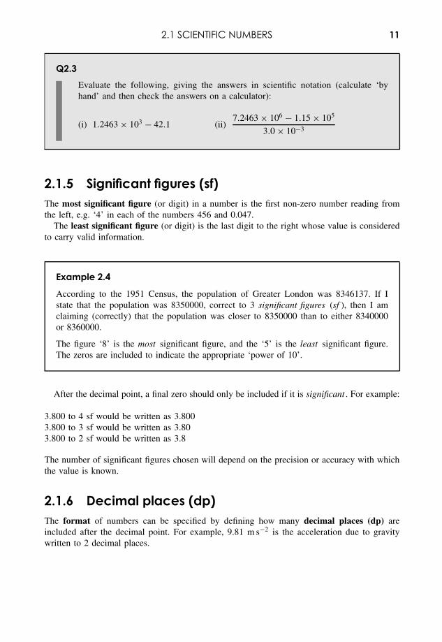
Q2.3Evaluate the following, giving the answers in scientific notation (calculate ‘byhand’ and then check the answers on a calculator):
(i) 1.2463 × 10³ − 42.1 (ii)7.2463 × 10⁶ − 1.15 × 10⁵
3.0 × 10⁻³
2.1.5 Significant figures (sf)The most significant figure (or digit) in a number is the first non-zero number reading fromthe left, e.g. ‘4’ in each of the numbers 456 and 0.047.
The least significant figure (or digit) is the last digit to the right whose value is consideredto carry valid information.
Example 2.4
According to the 1951 Census, the population of Greater London was 8346137. If Istate that the population was 8350000, correct to 3 significant figures (sf ), then I amclaiming (correctly) that the population was closer to 8350000 than to either 8340000or 8360000.
The figure ‘8’ is the most significant figure, and the ‘5’ is the least significant figure.The zeros are included to indicate the appropriate ‘power of 10’.
After the decimal point, a final zero should only be included if it is significant . For example:
3.800 to 4 sf would be written as 3.8003.800 to 3 sf would be written as 3.803.800 to 2 sf would be written as 3.8
The number of significant figures chosen will depend on the precision or accuracy with whichthe value is known.
2.1.6 Decimal places (dp)The format of numbers can be specified by defining how many decimal places (dp) areincluded after the decimal point. For example, 9.81 m s−2 is the acceleration due to gravitywritten to 2 decimal places.
12 SCIENTIFIC DATA
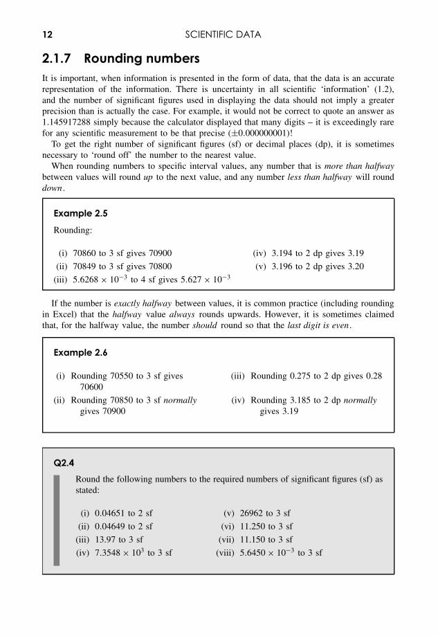
2.1.7 Rounding numbersIt is important, when information is presented in the form of data, that the data is an accuraterepresentation of the information. There is uncertainty in all scientific ‘information’ (1.2),and the number of significant figures used in displaying the data should not imply a greaterprecision than is actually the case. For example, it would not be correct to quote an answer as1.145917288 simply because the calculator displayed that many digits – it is exceedingly rarefor any scientific measurement to be that precise (±0.000000001)!
To get the right number of significant figures (sf) or decimal places (dp), it is sometimesnecessary to ‘round off’ the number to the nearest value.
When rounding numbers to specific interval values, any number that is more than halfwaybetween values will round up to the next value, and any number less than halfway will rounddown .
Example 2.5
Rounding:
(i) 70860 to 3 sf gives 70900 (iv) 3.194 to 2 dp gives 3.19
(ii) 70849 to 3 sf gives 70800 (v) 3.196 to 2 dp gives 3.20
(iii) 5.6268 × 10⁻³ to 4 sf gives 5.627 × 10⁻³
If the number is exactly halfway between values, it is common practice (including roundingin Excel) that the halfway value always rounds upwards. However, it is sometimes claimedthat, for the halfway value, the number should round so that the last digit is even .
Example 2.6
(i) Rounding 70550 to 3 sf gives70600
(iii) Rounding 0.275 to 2 dp gives 0.28
(ii) Rounding 70850 to 3 sf normallygives 70900
(iv) Rounding 3.185 to 2 dp normallygives 3.19
Q2.4Round the following numbers to the required numbers of significant figures (sf) asstated:
(i) 0.04651 to 2 sf (v) 26962 to 3 sf
(ii) 0.04649 to 2 sf (vi) 11.250 to 3 sf
(iii) 13.97 to 3 sf (vii) 11.150 to 3 sf
(iv) 7.3548 × 10³ to 3 sf (viii) 5.6450 × 10⁻³ to 3 sf
2.1 SCIENTIFIC NUMBERS 13
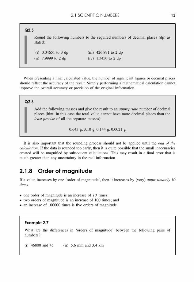
Q2.5Round the following numbers to the required numbers of decimal places (dp) asstated:
(i) 0.04651 to 3 dp (iii) 426.891 to 2 dp
(ii) 7.9999 to 2 dp (iv) 1.3450 to 2 dp
When presenting a final calculated value, the number of significant figures or decimal placesshould reflect the accuracy of the result. Simply performing a mathematical calculation cannotimprove the overall accuracy or precision of the original information.
Q2.6Add the following masses and give the result to an appropriate number of decimalplaces (hint: in this case the total value cannot have more decimal places than theleast precise of all the separate masses):
0.643 g, 3.10 g, 0.144 g, 0.0021 g
It is also important that the rounding process should not be applied until the end of thecalculation . If the data is rounded too early, then it is quite possible that the small inaccuraciescreated will be magnified by subsequent calculations. This may result in a final error that ismuch greater than any uncertainty in the real information.
2.1.8 Order of magnitudeIf a value increases by one ‘order of magnitude’, then it increases by (very) approximately 10times :
• one order of magnitude is an increase of 10 times;• two orders of magnitude is an increase of 100 times; and• an increase of 100000 times is five orders of magnitude.
Example 2.7
What are the differences in ‘orders of magnitude’ between the following pairs ofnumbers?
(i) 46800 and 45 (ii) 5.6 mm and 3.4 km
14 SCIENTIFIC DATA
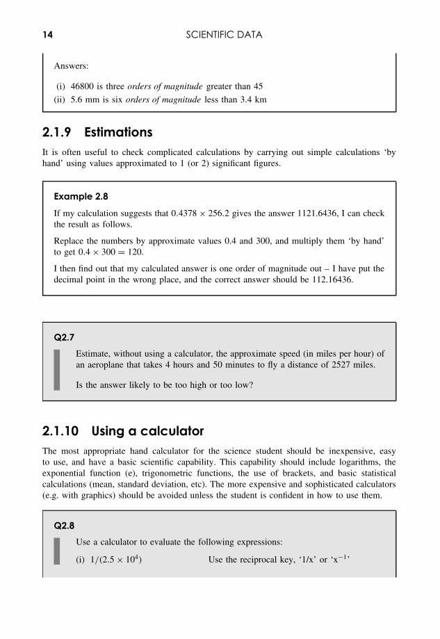
Answers:
(i) 46800 is three orders of magnitude greater than 45
(ii) 5.6 mm is six orders of magnitude less than 3.4 km
2.1.9 EstimationsIt is often useful to check complicated calculations by carrying out simple calculations ‘byhand’ using values approximated to 1 (or 2) significant figures.
Example 2.8
If my calculation suggests that 0.4378 × 256.2 gives the answer 1121.6436, I can checkthe result as follows.
Replace the numbers by approximate values 0.4 and 300, and multiply them ‘by hand’to get 0.4 × 300 = 120.
I then find out that my calculated answer is one order of magnitude out – I have put thedecimal point in the wrong place, and the correct answer should be 112.16436.
Q2.7Estimate, without using a calculator, the approximate speed (in miles per hour) ofan aeroplane that takes 4 hours and 50 minutes to fly a distance of 2527 miles.
Is the answer likely to be too high or too low?
2.1.10 Using a calculatorThe most appropriate hand calculator for the science student should be inexpensive, easyto use, and have a basic scientific capability. This capability should include logarithms, theexponential function (e), trigonometric functions, the use of brackets, and basic statisticalcalculations (mean, standard deviation, etc). The more expensive and sophisticated calculators(e.g. with graphics) should be avoided unless the student is confident in how to use them.
Q2.8Use a calculator to evaluate the following expressions:
(i) 1/(2.5 × 104) Use the reciprocal key, ‘1/x’ or ‘x−1’
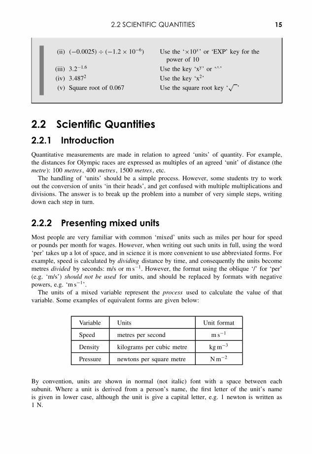
2.2 SCIENTIFIC QUANTITIES 15
(ii) (−0.0025) ÷ (−1.2 × 10⁻⁶) Use the ‘×10x’ or ‘EXP’ key for thepower of 10
(iii) 3.2−1.6 Use the key ‘xy’ or ‘∧’
(iv) 3.4872 Use the key ‘x2’
(v) Square root of 0.067 Use the square root key ‘√
’
2.2 Scientific Quantities2.2.1 IntroductionQuantitative measurements are made in relation to agreed ‘units’ of quantity. For example,the distances for Olympic races are expressed as multiples of an agreed ‘unit’ of distance (themetre): 100 metres , 400 metres , 1500 metres , etc.
The handling of ‘units’ should be a simple process. However, some students try to workout the conversion of units ‘in their heads’, and get confused with multiple multiplications anddivisions. The answer is to break up the problem into a number of very simple steps, writingdown each step in turn.
2.2.2 Presenting mixed unitsMost people are very familiar with common ‘mixed’ units such as miles per hour for speedor pounds per month for wages. However, when writing out such units in full, using the word‘per’ takes up a lot of space, and in science it is more convenient to use abbreviated forms. Forexample, speed is calculated by dividing distance by time, and consequently the units becomemetres divided by seconds: m/s or m s−1. However, the format using the oblique ‘/’ for ‘per’(e.g. ‘m/s’) should not be used for units, and should be replaced by formats with negativepowers, e.g. ‘m s−1’.
The units of a mixed variable represent the process used to calculate the value of thatvariable. Some examples of equivalent forms are given below:
Variable Units Unit format
Speed metres per second m s−1
Density kilograms per cubic metre kg m−3
Pressure newtons per square metre N m−2
By convention, units are shown in normal (not italic) font with a space between eachsubunit. Where a unit is derived from a person’s name, the first letter of the unit’s nameis given in lower case, although the unit is give a capital letter, e.g. 1 newton is written as1 N.
16 SCIENTIFIC DATA
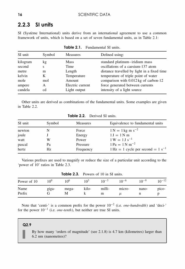
2.2.3 SI unitsSI (Systeme International) units derive from an international agreement to use a commonframework of units, which is based on a set of seven fundamental units, as in Table 2.1:
Table 2.1. Fundamental SI units.
SI unit Symbol Measures Defined using:
kilogram kg Mass standard platinum–iridium masssecond s Time oscillations of a caesium-137 atommetre m Length distance travelled by light in a fixed timekelvin K Temperature temperature of triple point of watermole mol Amount comparison with 0.012 kg of carbon-12ampere A Electric current force generated between currentscandela cd Light output intensity of a light source
Other units are derived as combinations of the fundamental units. Some examples are givenin Table 2.2.
Table 2.2. Derived SI units.
SI unit Symbol Measures Equivalence to fundamental units
newton N Force 1 N = 1 kg m s−2
joule J Energy 1 J = 1 N mwatt W Power 1 W = 1 J s−1
pascal Pa Pressure 1 Pa = 1 N m−2
hertz Hz Frequency 1 Hz = 1 cycle per second = 1 s−1
Various prefixes are used to magnify or reduce the size of a particular unit according to the‘power of 10’ ratios in Table 2.3.
Table 2.3. Powers of 10 in SI units.
Power of 10 109 106 103 10−3 10−6 10−9 10−12
Name giga- mega- kilo- milli- micro- nano- pico-Prefix G M k m µ n p
Note that ‘centi-’ is a common prefix for the power 10−2 (i.e. one-hundredth) and ‘deci-’for the power 10−1 (i.e. one-tenth), but neither are true SI units.
Q2.9By how many ‘orders of magnitude’ (see 2.1.8) is 4.7 km (kilometres) larger than6.2 nm (nanometres)?
2.2 SCIENTIFIC QUANTITIES 17
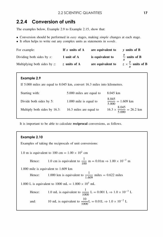
2.2.4 Conversion of unitsThe examples below, Example 2.9 to Example 2.15, show that:
• Conversion should be performed in easy stages, making simple changes at each stage.• It often helps to write out any complex units as statements in words .
For example: If x units of A are equivalent to y units of B
Dividing both sides by x: 1 unit of A is equivalent toyx
units of B
Multiplying both sides by z: z units of A are equivalent to z × yx
units of B
Example 2.9
If 5.000 miles are equal to 8.045 km, convert 16.3 miles into kilometres.
Starting with: 5.000 miles are equal to 8.045 km
Divide both sides by 5: 1.000 mile is equal to8.045
5.000= 1.609 km
Multiply both sides by 16.3: 16.3 miles are equal to 16.3 × 8.045
5.000= 26.2 km
It is important to be able to calculate reciprocal conversions, as follows.
Example 2.10
Examples of taking the reciprocals of unit conversions:
1.0 m is equivalent to 100 cm = 1.00 × 102 cm
Hence: 1.0 cm is equivalent to1
100m = 0.01m ⇒ 1.00 × 10⁻² m
1.000 mile is equivalent to 1.609 km
Hence: 1.000 km is equivalent to1
1.609miles = 0.622 miles
1.000 L is equivalent to 1000 mL = 1.000 × 10³ mL
Hence: 1.0 mL is equivalent to1
1000L = 0.001 L ⇒ 1.0 × 10⁻³ L
and: 10 mL is equivalent to10
1000L = 0.01L ⇒ 1.0 × 10⁻² L
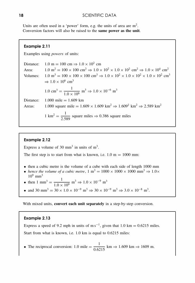
18 SCIENTIFIC DATA
Units are often used in a ‘power’ form, e.g. the units of area are m2.Conversion factors will also be raised to the same power as the unit.
Example 2.11
Examples using powers of units:
Distance: 1.0 m = 100 cm ⇒ 1.0 × 102 cm
Area: 1.0 m2 = 100 × 100 cm2 ⇒ 1.0 × 102 × 1.0 × 102 cm2 ⇒ 1.0 × 104 cm2
Volumes: 1.0 m3 = 100 × 100 × 100 cm3 ⇒ 1.0 × 102 × 1.0 × 102 × 1.0 × 102 cm3
⇒ 1.0 × 106 cm3
1.0 cm3 = 1
1.0 × 10⁶m3 ⇒ 1.0 × 10⁻⁶ m3
Distance: 1.000 mile = 1.609 km
Areas: 1.000 square mile = 1.609 × 1.609 km2 ⇒ 1.6092 km2 ⇒ 2.589 km2
1 km2 = 1
2.589square miles ⇒ 0.386 square miles
Example 2.12
Express a volume of 30 mm3 in units of m3.
The first step is to start from what is known, i.e. 1.0 m = 1000 mm:
• then a cubic metre is the volume of a cube with each side of length 1000 mm• hence the volume of a cubic metre, 1 m3 = 1000 × 1000 × 1000 mm3 ⇒ 1.0×
109 mm3
• then 1 mm3 = 1
1.0 × 10⁹m3 ⇒ 1.0 × 10⁻⁹ m3
• and 30 mm3 = 30 × 1.0 × 10−9 m3 ⇒ 30 × 10−9 m3 ⇒ 3.0 × 10⁻⁸ m3.
With mixed units, convert each unit separately in a step-by-step conversion.
Example 2.13
Express a speed of 9.2 mph in units of m s−1, given that 1.0 km = 0.6215 miles.
Start from what is known, i.e. 1.0 km is equal to 0.6215 miles:
• The reciprocal conversion: 1.0 mile = 1
0.6215km ⇒ 1.609 km ⇒ 1609 m.
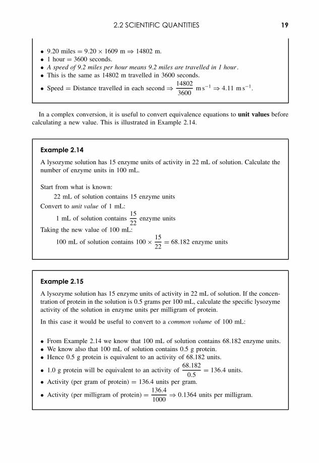
2.2 SCIENTIFIC QUANTITIES 19
• 9.20 miles = 9.20 × 1609 m ⇒ 14802 m.• 1 hour = 3600 seconds.• A speed of 9.2 miles per hour means 9.2 miles are travelled in 1 hour .• This is the same as 14802 m travelled in 3600 seconds.
• Speed = Distance travelled in each second ⇒ 14802
3600m s−1 ⇒ 4.11 m s−1.
In a complex conversion, it is useful to convert equivalence equations to unit values beforecalculating a new value. This is illustrated in Example 2.14.
Example 2.14
A lysozyme solution has 15 enzyme units of activity in 22 mL of solution. Calculate thenumber of enzyme units in 100 mL.
Start from what is known:
22 mL of solution contains 15 enzyme units
Convert to unit value of 1 mL:
1 mL of solution contains15
22enzyme units
Taking the new value of 100 mL:
100 mL of solution contains 100 × 15
22= 68.182 enzyme units
Example 2.15
A lysozyme solution has 15 enzyme units of activity in 22 mL of solution. If the concen-tration of protein in the solution is 0.5 grams per 100 mL, calculate the specific lysozymeactivity of the solution in enzyme units per milligram of protein.
In this case it would be useful to convert to a common volume of 100 mL:
• From Example 2.14 we know that 100 mL of solution contains 68.182 enzyme units.• We know also that 100 mL of solution contains 0.5 g protein.• Hence 0.5 g protein is equivalent to an activity of 68.182 units.
• 1.0 g protein will be equivalent to an activity of68.182
0.5= 136.4 units.
• Activity (per gram of protein) = 136.4 units per gram.
• Activity (per milligram of protein) = 136.4
1000⇒ 0.1364 units per milligram.
20 SCIENTIFIC DATA
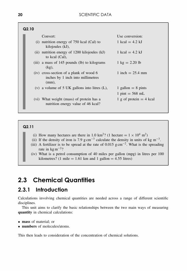
Q2.10
Convert: Use conversion:
(i) nutrition energy of 750 kcal (Cal) tokilojoules (kJ),
1 kcal = 4.2 kJ
(ii) nutrition energy of 1200 kilojoules (kJ)to kcal (Cal),
1 kcal = 4.2 kJ
(iii) a mass of 145 pounds (lb) to kilograms(kg),
1 kg = 2.20 lb
(iv) cross-section of a plank of wood 6inches by 1 inch into millimetres(mm),
1 inch = 25.4 mm
(v) a volume of 5 UK gallons into litres (L), 1 gallon = 8 pints
1 pint = 568 mL
(vi) What weight (mass) of protein has anutrition energy value of 46 kcal?
1 g of protein = 4 kcal
Q2.11
(i) How many hectares are there in 1.0 km2? (1 hectare = 1 × 10⁴ m2)
(ii) If the density of iron is 7.9 g cm−3 calculate the density in units of kg m−3.(iii) A fertilizer is to be spread at the rate of 0.015 g cm−2. What is the spreading
rate in kg m−2?(iv) What is a petrol consumption of 40 miles per gallon (mpg) in litres per 100
kilometres? (1 mile = 1.61 km and 1 gallon = 4.55 litres)
2.3 Chemical Quantities2.3.1 IntroductionCalculations involving chemical quantities are needed across a range of different scientificdisciplines.
This unit aims to clarify the basic relationships between the two main ways of measuringquantity in chemical calculations:
• mass of material; or• numbers of molecules/atoms.
This then leads to consideration of the concentration of chemical solutions.
2.3 CHEMICAL QUANTITIES 21
2.3.2 Quantity (grams and moles)The standard unit of mass is the kilogram (kg), and we also use grams (g), milligrams (mg),micrograms (µg). For example, we may buy 1 kg of salt from a shop, or weigh out 10 g ofsodium chloride in a laboratory.
However, it is also common to measure quantity by number. We often need a measure ofnumber to buy integer (whole) numbers of items such as eggs, oranges or buns.
When shopping, a common unit of number is the ‘dozen’, where:
• One dozen of any item = 12 items.
For example, buying half a dozen eggs = 0.5 dozen ⇒ 0.5 × 12 ⇒ 6 eggsWe also need a measure of number in chemistry because when atoms and molecules react,
they do so in simple whole (integer) numbers.We know that one water molecule, H2O, contains two hydrogen atoms, H, plus one oxygen
atom, O:
H2O ⇔ 2H + O
However, when dealing with atoms and molecules in chemistry, a ‘dozen’ is far too small aquantity, and instead we count atoms and molecules using the much larger ‘mole’:
• 1 mole of any item ⇒ 6.02 × 10²³ items (to 3 significant figures).
For example, weighing out 0.5 moles of sodium chloride (NaCl) gives 0.5 × 6.02 × 1023 ⇒3.01 × 10²³ molecules of sodium chloride:
1 mole of any substance will contain the same number(= 6.02 × 10²³) of items[2.1]
The Avogadro constant is the number of items in 1 mole of any substance:
NA = 6.02 × 10²³ mol−1 (to 3 sf)
Counting molecules and atoms, we can describe the formation of water:
1 mole of H2O molecules ⇔ 2 moles of H atoms + 1 mole of O atoms
22 SCIENTIFIC DATA
The above statement using ‘moles’ gives a clearer understanding of the chemical formation,H2O, of water than the equivalent statement using ‘mass’:
18 g of water ⇔ 2 g of hydrogen + 16 g of oxygen
Example 2.16
Calculate the mass of 1 mole of hydrogen molecules, H2, given that the mass of 1 moleof hydrogen atoms, H, is 1.0 g (to 2 sf).
1 mole of H2 molecules consists of 2 moles of H atoms .
Hence, the mass of 1 mole of hydrogen molecules, H2, is 2 × 1.0 g = 2.0 g.
2.3.3 Relative atomic and molecular masses, Ar and MrA key calculation in chemistry involves working out the mass required of a substance toobtain a given number of moles of that substance. As illustrated in Example 2.16, this con-version depends on the ratio of the mass of a single molecule of the compound to a mass(approximately) equal to that of a single hydrogen atom:
• Relative atomic mass, Ar (also written RAM ), is used for the relative mass of an element,and is equal to the ratio of the average mass of 1 atom of that element to a mass equal(almost) to 1 hydrogen atom. On this basis:
Ar for hydrogen, H = 1.0 (to 1dp)
Ar for oxygen, O = 16.0 (to 1 dp)
Ar for carbon, C = 12.0 (to 1 dp)
• Relative molecular mass, Mr (also called molecular weight or written RMM ), of a sub-stance is equal to the ratio of the average mass of 1 molecule of that substance to a massequal (almost) to 1 hydrogen atom. On this basis:
Mr for hydrogen, H2 = 2 × 1.0 = 2.0 (to 1 dp)
Mr for water, H2O = 2 × 1.0 + 16.0 = 18.0 (to 1 dp)
Mr for methane, CH4 = 12.0 + 4 × 1.0 = 16.0 (to 1 dp)
2.3 CHEMICAL QUANTITIES 23
The exact values for Ar and Mr are actually based on the ratio of the atomic and molecularmasses to one-twelfth of the mass of the carbon-12 isotope (written 12C). Using this scale themass of 1 mole of H atoms equals 1.01 g (and not 1.00 g). However, in all but the most exactcalculations, it is still useful to think of the scale of masses starting with H = 1.0, at least to1 decimal place.
The term average mass is used to allow for the mixture of isotopes of different masses thatoccurs for all elements, as given in Example 2.17.
Example 2.17
In a naturally occurring sample of chlorine atoms, 76 % of them will be the 35Cl isotope(with Ar = 35.0) and approximately 24 % will be the 37Cl isotope (with Ar = 37.0).
Calculate the average Ar for the mixture.
Taking 100 atoms of naturally occurring chlorine, 76 will have a ‘mass’ = 35.0 and theremainder a ‘mass’ = 37.0.
Total ‘mass’ for 100 atoms = 76 × 35.0 + 24 × 37.0 ⇒ 3548.
Average ‘mass’ in a natural sample of chlorine, Ar = 3548/100 ⇒ 35.5 (to 1 dp)
Q2.12
In a naturally occurring sample of boron atoms about 80 % will be the 11B iso-tope (with Ar = 11.0) and approximately 20 % the 10B isotope (with Ar = 10.0).Estimate the average Ar for the mixture.
It is also useful to define the mass (in grams) of 1 mole of the substance:
• Molar mass, Mm, of a substance is the mass, in grams , of 1 mole of that substance. Unitsare g mol−1.
This now gives us the key statement that links the measurement by mass (in grams) with thenumber of moles of any substance:
1 mole of a substance has a mass in grams (molar mass) numerically
equal to the value of its relative molecular mass, Mr [2.2]
In practice, the relative molecular mass, Mr, for a molecule is calculated by adding the relativeatomic masses, Ar, of its various atoms.
24 SCIENTIFIC DATA
Example 2.18
Calculate the relative molecular mass, molar mass and mass of 1 mole of calcium car-bonate, CaCO3, given relative atomic masses Ca = 40.1, C = 12.0, O = 16.0 (all valuesto 1 dp).
Mr = 40.1 + 12.0 + 3 × 16.0 ⇒ 100.1(a pure number)
Molar mass = 100.1 g mol−1 (equals the relative molecular mass, Mr, in grams permole).
Mass of 1 mole = 100.1 g (numerically equals the molar mass in grams).
Q2.13Using relative atomic masses C = 12.0, H = 1.0, O = 16.0, calculate the followingvalues for aspirin, C9H8O4, giving the relevant units:
(i) relative molecular mass, Mr
(ii) molar mass, Mm
(iii) mass of 1 mole
2.3.4 Conversion between moles and gramsConsider a substance, X, with a relative molecular mass, Mr (for an element, we use relativeatomic mass, Ar, instead of Mr).
From equation [2.2]:
• 1 mole of X has a mass of Mr g.
Hence, for n moles of the substance:
• n moles of X has a mass of n × Mr g.
If n moles of the substance has a mass m g, we can write:
m = n × Mr (m in grams) [2.3]
We can rearrange the equation by dividing m by Mr on the left-hand side (LHS), leaving n onthe right-hand side (RHS), and then swapping sides to give:
2.3 CHEMICAL QUANTITIES 25
n = m
Mr(m in grams) [2.4]
These two equations allow us to perform simple conversions between the quantity of a substancemeasured in grams, m, and the same quantity measured in numbers of moles, n.
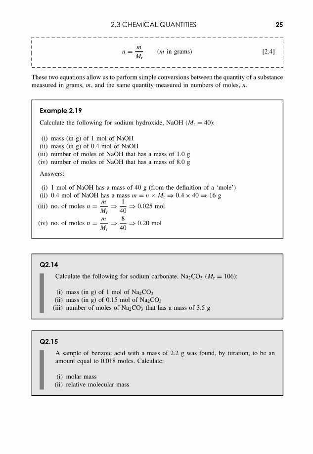
Example 2.19
Calculate the following for sodium hydroxide, NaOH (Mr = 40):
(i) mass (in g) of 1 mol of NaOH(ii) mass (in g) of 0.4 mol of NaOH
(iii) number of moles of NaOH that has a mass of 1.0 g(iv) number of moles of NaOH that has a mass of 8.0 g
Answers:
(i) 1 mol of NaOH has a mass of 40 g (from the definition of a ‘mole’)(ii) 0.4 mol of NaOH has a mass m = n × Mr ⇒ 0.4 × 40 ⇒ 16 g
(iii) no. of moles n = m
Mr⇒ 1
40⇒ 0.025 mol
(iv) no. of moles n = m
Mr⇒ 8
40⇒ 0.20 mol
Q2.14Calculate the following for sodium carbonate, Na2CO3 (Mr = 106):
(i) mass (in g) of 1 mol of Na2CO3
(ii) mass (in g) of 0.15 mol of Na2CO3
(iii) number of moles of Na2CO3 that has a mass of 3.5 g
Q2.15A sample of benzoic acid with a mass of 2.2 g was found, by titration, to be anamount equal to 0.018 moles. Calculate:
(i) molar mass(ii) relative molecular mass
26 SCIENTIFIC DATA
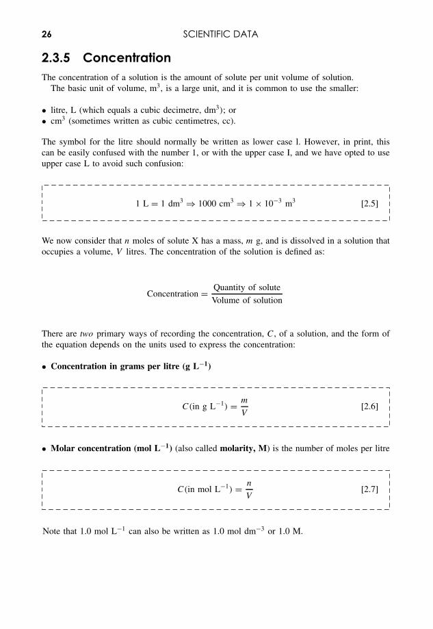
2.3.5 ConcentrationThe concentration of a solution is the amount of solute per unit volume of solution.
The basic unit of volume, m3, is a large unit, and it is common to use the smaller:
• litre, L (which equals a cubic decimetre, dm3); or• cm3 (sometimes written as cubic centimetres, cc).
The symbol for the litre should normally be written as lower case l. However, in print, thiscan be easily confused with the number 1, or with the upper case I, and we have opted to useupper case L to avoid such confusion:
1 L = 1 dm3 ⇒ 1000 cm3 ⇒ 1 × 10⁻³ m3 [2.5]
We now consider that n moles of solute X has a mass, m g, and is dissolved in a solution thatoccupies a volume, V litres. The concentration of the solution is defined as:
Concentration = Quantity of solute
Volume of solution
There are two primary ways of recording the concentration, C, of a solution, and the form ofthe equation depends on the units used to express the concentration:
• Concentration in grams per litre (g L−1)
C(in g L−1) = m
V[2.6]
• Molar concentration (mol L−1) (also called molarity, M) is the number of moles per litre
C(in mol L−1) = n
V[2.7]
Note that 1.0 mol L−1 can also be written as 1.0 mol dm−3 or 1.0 M.
2.3 CHEMICAL QUANTITIES 27
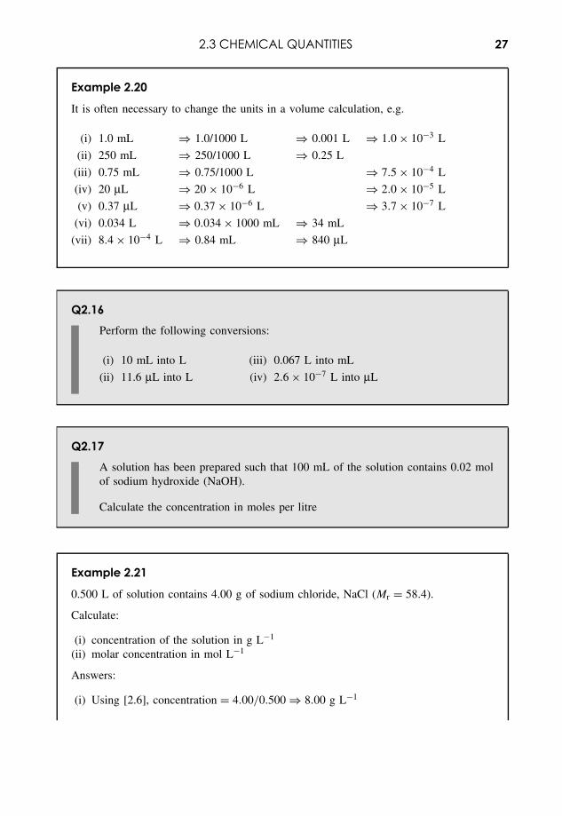
Example 2.20
It is often necessary to change the units in a volume calculation, e.g.
(i) 1.0 mL ⇒ 1.0/1000 L ⇒ 0.001 L ⇒ 1.0 × 10⁻³ L
(ii) 250 mL ⇒ 250/1000 L ⇒ 0.25 L
(iii) 0.75 mL ⇒ 0.75/1000 L ⇒ 7.5 × 10⁻⁴ L
(iv) 20 µL ⇒ 20 × 10−6 L ⇒ 2.0 × 10⁻⁵ L
(v) 0.37 µL ⇒ 0.37 × 10⁻⁶ L ⇒ 3.7 × 10⁻⁷ L
(vi) 0.034 L ⇒ 0.034 × 1000 mL ⇒ 34 mL
(vii) 8.4 × 10⁻⁴ L ⇒ 0.84 mL ⇒ 840 µL
Q2.16Perform the following conversions:
(i) 10 mL into L (iii) 0.067 L into mL
(ii) 11.6 µL into L (iv) 2.6 × 10⁻⁷ L into µL
Q2.17A solution has been prepared such that 100 mL of the solution contains 0.02 molof sodium hydroxide (NaOH).
Calculate the concentration in moles per litre
Example 2.21
0.500 L of solution contains 4.00 g of sodium chloride, NaCl (Mr = 58.4).
Calculate:
(i) concentration of the solution in g L−1
(ii) molar concentration in mol L−1
Answers:
(i) Using [2.6], concentration = 4.00/0.500 ⇒ 8.00 g L−1
28 SCIENTIFIC DATA
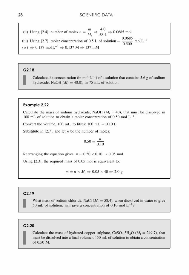
(ii) Using [2.4], number of moles n = m
Mr⇒ 4.0
58.4⇒ 0.0685 mol
(iii) Using [2.7], molar concentration of 0.5 L of solution = 0.0685
0.500mol L−1
(iv) ⇒ 0.137 mol L−1 ⇒ 0.137 M ⇒ 137 mM
Q2.18
Calculate the concentration (in mol L−1) of a solution that contains 5.6 g of sodiumhydroxide, NaOH (Mr = 40.0), in 75 mL of solution.
Example 2.22
Calculate the mass of sodium hydroxide, NaOH (Mr = 40), that must be dissolved in100 mL of solution to obtain a molar concentration of 0.50 mol L−1.
Convert the volume, 100 mL, to litres: 100 mL = 0.10 L
Substitute in [2.7], and let n be the number of moles:
0.50 = n
0.10
Rearranging the equation gives: n = 0.50 × 0.10 ⇒ 0.05 mol
Using [2.3], the required mass of 0.05 mol is equivalent to:
m = n × Mr ⇒ 0.05 × 40 ⇒ 2.0 g
Q2.19What mass of sodium chloride, NaCl (Mr = 58.4), when dissolved in water to give50 mL of solution, will give a concentration of 0.10 mol L−1?
Q2.20Calculate the mass of hydrated copper sulphate, CuSO4.5H2O (Mr = 249.7), thatmust be dissolved into a final volume of 50 mL of solution to obtain a concentrationof 0.50 M.
2.3 CHEMICAL QUANTITIES 29
Other common terminologies relating to concentration include:
• millimoles, mmol: 1 mmol is equivalent to 1.0 × 10⁻³ mol
• millimolar, mM: 1 mM is equivalent to 1.0 × 10⁻³ M
= 1.0 × 10⁻³ mol L−1
• parts per million, ppm: 1 ppm is equivalent to 1 mg L−1
• parts per billion, ppb: 1 ppb is equivalent to 1 µg L−1.
Percentage concentrations are often expressed as ratios (multiplied by 100) between themasses or volumes of the solute and solvent, giving the options:
Weight of solute per volume of solution: %w/v
Volume of solute per volume of solution: %v/v
Weight of solute per weight of solution: %w/w
where the ‘weights’ are usually given in grams and ‘volumes’ in millilitres.Note that 1.0 mL of water has a mass (‘weight’) of 1.0 g.
Example 2.23
Examples of typical calculations of equivalence:
• 10 mL = 0.01 L, 2 mL = 0.002 L, etc.
• 0.025 mmol in 10 mL is equivalent to0.025
0.01mmol L−1 = 2.5 mM
• 0.023 mg in 10 mL is equivalent to0.023
0.01= 2.3 mg L−1 ⇒ 2.3 ppm
• 6.70 × 10⁻⁷ g in 2 mL is equivalent to6.70 × 10−7
0.002= 0.000335 g L−1 ⇒
335 µg L−1
• 335 µg L−1 is equivalent to 335 ppb
• 1.2 g of solute in 50 mL of solution has a concentration of1.2
50× 100 = 2.4 %w/v
• 10 mL of solute diluted to 200 mL has a concentration of10
200× 100 = 5 %v/v
• 0.88 g of solute in a total of 40 g has a concentration of0.88
40× 100 = 2.2 %w/w.
2.3.6 DilutionsIn most dilutions, the amount of the solute stays the same. In this case it is useful to use thedilution equation:
30 SCIENTIFIC DATA
Vi × Ci = Vf × Cf [2.8]
where Vi and Ci are the initial volumes and concentrations and Vf and Cf are the final values.The concentrations can be measured as molarities or mass/volume, but the same units must
be used on each side of the equation:
Dilution factor or ratio ⇒ Vf
Vi
= Ci
Cf
[2.9]
Example 2.24
20 mL of a solution of concentration 0.3 M is transferred to a 100 mL graduated flask,and solvent is added up to the 100 mL mark. Calculate the concentration, Cf, of the finalsolution.
The amount of the solute is the same in the initial 20 mL as in the final 100 mL, so wecan use the dilution equation [2.8]:
20 × 0.3 = 100 × Cf
Cf = 20 × 0.3
100⇒ 0.06 M
Example 2.25
It is necessary to produce 200 mL of 30 mM saline solution (sodium chloride, NaCl,in solution). Calculate the volume of a 35 g L−1 stock solution of saline that would berequired to be made up to a final volume of 200 mL (Mr of NaCl is 58.4).
In this question, the concentrations of the two solutions are initially in differentforms – moles and grams. We choose to convert 35 g L−1 to a molar concentration.
We know that 58.4 g (= 1 mol) of NaCl in 1.00 L gives a concentration of 1.00 M:
• 1.00 g of NaCl in 1.00 L gives a concentration of1.00
58.4M
• 35.0 g of NaCl in 1.00 L gives a concentration of 35.0 × 1.00
58.4⇒ 0.599 M ⇒
599 mM.
2.4 ANGULAR MEASUREMENTS 31
We can now use [2.8] to find the initial volume, Vi, of 0.599 M (= 599 mM) saline thatmust be diluted to give 200 mL of 30 mM saline:
Vi × 599 = 200 × 30
Vi = 200 × 30
599⇒ 10.02 mL
Q2.21
5.0 mL of a solution of concentration 2.0 mol L−1 is put into a 100 mL graduatedflask and pure water is added, bringing the total volume in the flask to exactly100 mL.
Calculate the concentration of the new solution.
Q2.22
A volume, V , of a solution of concentration 0.8 mol L−1 is put into a 100 mLgraduated flask, and pure solvent is added to bring the volume up to 100 mL.If the concentration of the final solution is 40 mM, what was the initial volume,V ?
Q2.23Calculate the volume of a 0.15 M solution of the amino acid alanine that wouldbe needed to make up to a final volume of 100 mL in order to produce 100 mLof 30 mM alanine?
2.4 Angular Measurements2.4.1 IntroductionIn many aspects of undergraduate science, students rarely encounter the need to measure anglesor solve problems involving rotations. However, angular measurements do occur routinely ina variety of practical situations. The mathematics is not difficult, and, in most cases, it is onlynecessary to refresh the ideas of simple trigonometry or to revisit Pythagoras!
32 SCIENTIFIC DATA
2.4.2 Degrees and radiansThere are 360◦ (degrees) in a full circle.
Example 2.26
Why are there ‘360’ degrees in a circle?
The choice of ‘360’ was made when ‘fractions’ were used in calculations far morefrequently than they are now. The number ‘360’ was particularly good because it can bedivided by many different factors: 2, 3, 4, 5, 6, 8, 9, 10, 12, 15, 18, 20, 24, 30, 36, 40,45, 60, 72, 90, 120, 180!
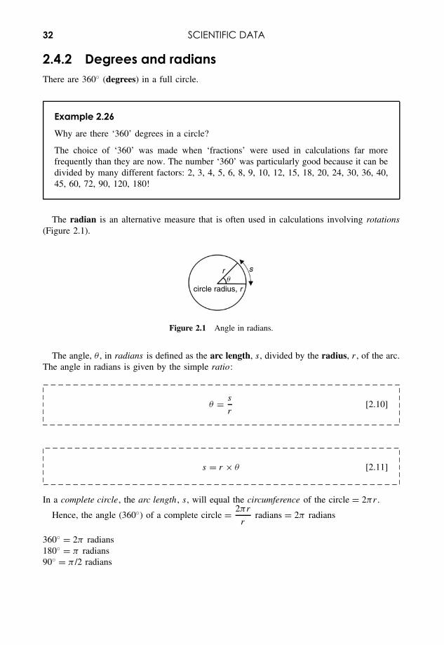
The radian is an alternative measure that is often used in calculations involving rotations(Figure 2.1).
circle radius, r
r sq
Figure 2.1 Angle in radians.
The angle, θ , in radians is defined as the arc length, s, divided by the radius, r , of the arc.The angle in radians is given by the simple ratio:
θ = s
r[2.10]
s = r × θ [2.11]
In a complete circle, the arc length , s, will equal the circumference of the circle = 2πr .
Hence, the angle (360◦) of a complete circle = 2πr
rradians = 2π radians
360◦ = 2π radians180◦ = π radians90◦ = π /2 radians
2.4 ANGULAR MEASUREMENTS 33
1 radian = 180
πdegrees = 57.3 . . . degrees [2.12]
2.4.3 Conversion between degrees and radians
x in radians becomes x × 180/π in degrees [2.13]
θ in degrees becomes θ × π/180 in radians [2.14]
In Excel, to convert an angle:
• from radians to degrees, use the function DEGREES; and• from degrees to radians, use the function RADIANS.
Q2.24Convert the following angles from degrees to radians or vice versa:
(i) 360◦ into radians (iv) 1.0 radian into degrees
(ii) 90◦ into radians (v) 2.1 radians into degrees
(iii) 170◦ into radians (vi) 3.5π radians into degrees
Example 2.27
The towns of Nairobi and Singapore both lie approximately on the equator of the Earthat longitudes 36.9 ◦E and 103.8 ◦E respectively. The radius of the Earth at the equator is6.40 × 103 km.
Calculate the distance between Nairobi and Singapore along the surface of the Earth.
The equator of the Earth is the circumference of a circle with radius r = 6.40 × 10³ km.Nairobi and Singapore are points on the circumference of this circle separated by anangle:
θ = 103.8◦ − 36.9◦ = 66.9◦.
34 SCIENTIFIC DATA
Converting this angle to radians:
θ = 66.9 × π/180 radians = 1.168 radians
The distance on the ground between Nairobi and Singapore will be given by the arclength, s, between them. Using [2.11]:
s = r × θ = 6.40 × 103 × 1.168 km = 7.47 × 10³ km
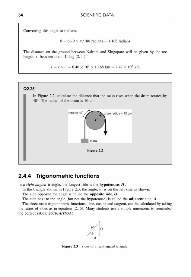
Q2.25In Figure 2.2, calculate the distance that the mass rises when the drum rotates by40◦. The radius of the drum is 10 cm.
Figure 2.2
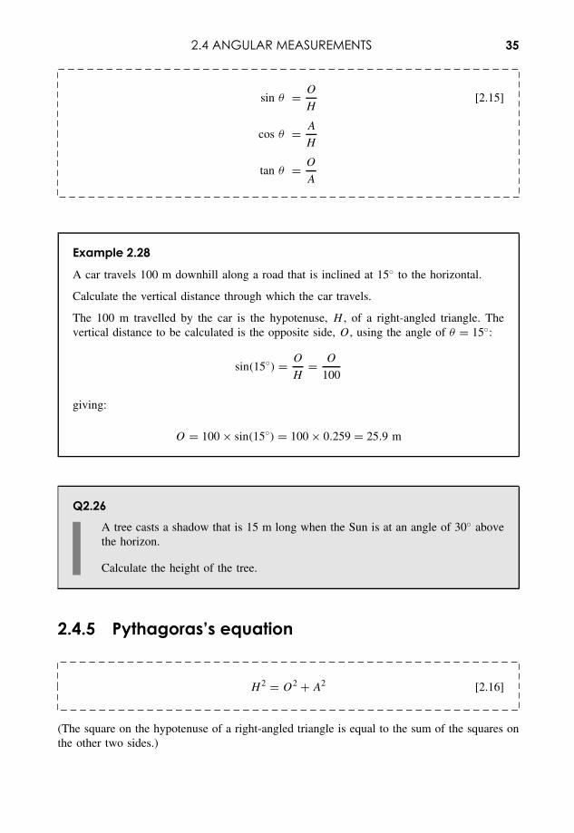
2.4.4 Trigonometric functionsIn a right-angled triangle, the longest side is the hypotenuse, H .
In the triangle shown in Figure 2.3, the angle, θ , is on the left side as shown.The side opposite the angle is called the opposite side, O .The side next to the angle (but not the hypotenuse) is called the adjacent side, A.The three main trigonometric functions, sine, cosine and tangent, can be calculated by taking
the ratios of sides as in equation [2.15]. Many students use a simple mnemonic to rememberthe correct ratios: SOHCAHTOA!
Figure 2.3 Sides of a right-angled triangle.
2.4 ANGULAR MEASUREMENTS 35
sin θ = O
H[2.15]
cos θ = A
H
tan θ = O
A
Example 2.28
A car travels 100 m downhill along a road that is inclined at 15◦ to the horizontal.
Calculate the vertical distance through which the car travels.
The 100 m travelled by the car is the hypotenuse, H , of a right-angled triangle. Thevertical distance to be calculated is the opposite side, O , using the angle of θ = 15◦:
sin(15◦) = O
H= O
100
giving:
O = 100 × sin(15◦) = 100 × 0.259 = 25.9 m
Q2.26A tree casts a shadow that is 15 m long when the Sun is at an angle of 30◦ abovethe horizon.
Calculate the height of the tree.
2.4.5 Pythagoras’s equation
H 2 = O2 + A2 [2.16]
(The square on the hypotenuse of a right-angled triangle is equal to the sum of the squares onthe other two sides.)
36 SCIENTIFIC DATA
Q2.27One side of a rectangular field is 100 m long, and the diagonal distance from onecorner to the opposite corner is 180 m. Calculate the length of the other side ofthe field.
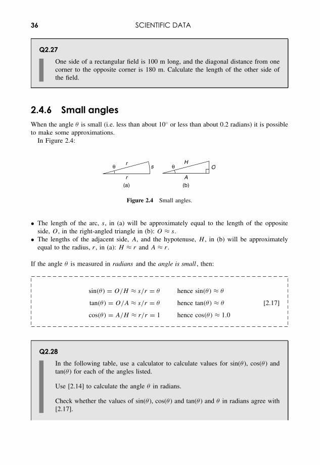
2.4.6 Small anglesWhen the angle θ is small (i.e. less than about 10◦ or less than about 0.2 radians) it is possibleto make some approximations.
In Figure 2.4:
(a)
r A
HO
rsθ θ
(b)
Figure 2.4 Small angles.
• The length of the arc, s, in (a) will be approximately equal to the length of the oppositeside, O , in the right-angled triangle in (b): O ≈ s.
• The lengths of the adjacent side, A, and the hypotenuse, H , in (b) will be approximatelyequal to the radius, r , in (a): H ≈ r and A ≈ r .
If the angle θ is measured in radians and the angle is small , then:
sin(θ) = O/H ≈ s/r = θ hence sin(θ) ≈ θ
tan(θ) = O/A ≈ s/r = θ hence tan(θ) ≈ θ [2.17]
cos(θ) = A/H ≈ r/r = 1 hence cos(θ) ≈ 1.0
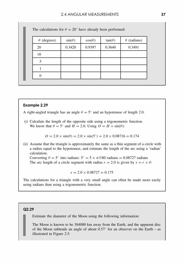
Q2.28In the following table, use a calculator to calculate values for sin(θ ), cos(θ ) andtan(θ ) for each of the angles listed.
Use [2.14] to calculate the angle θ in radians.
Check whether the values of sin(θ ), cos(θ ) and tan(θ ) and θ in radians agree with[2.17].
2.4 ANGULAR MEASUREMENTS 37
The calculations for θ = 20◦ have already been performed:
θ (degrees) sin(θ ) cos(θ ) tan(θ ) θ (radians)
20 0.3420 0.9397 0.3640 0.3491
10
5
1
0
Example 2.29
A right-angled triangle has an angle θ = 5◦ and an hypotenuse of length 2.0.
(i) Calculate the length of the opposite side using a trigonometric function.We know that θ = 5◦ and H = 2.0. Using O = H × sin(θ):
O = 2.0 × sin(θ) = 2.0 × sin(5◦) = 2.0 × 0.08716 = 0.174
(ii) Assume that the triangle is approximately the same as a thin segment of a circle witha radius equal to the hypotenuse, and estimate the length of the arc using a ‘radian’calculation.Converting θ = 5◦ into radians: 5◦ = 5 × π /180 radians = 0.08727 radiansThe arc length of a circle segment with radius r = 2.0 is given by s = r × θ :
s = 2.0 × 0.08727 = 0.175
The calculations for a triangle with a very small angle can often be made more easilyusing radians than using a trigonometric function.
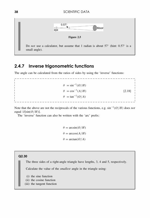
Q2.29Estimate the diameter of the Moon using the following information:
The Moon is known to be 384000 km away from the Earth, and the apparent discof the Moon subtends an angle of about 0.57◦ for an observer on the Earth – asillustrated in Figure 2.5.
38 SCIENTIFIC DATA
Figure 2.5
Do not use a calculator, but assume that 1 radian is about 57◦ (hint: 0.57◦ is asmall angle).
2.4.7 Inverse trigonometric functionsThe angle can be calculated from the ratios of sides by using the ‘inverse’ functions:
θ = sin−1(O/H)
θ = cos−1(A/H) [2.18]
θ = tan−1(O/A)
Note that the above are not the reciprocals of the various functions, e.g. sin−1(O/H) does notequal 1/[sin(O/H)].
The ‘inverse’ function can also be written with the ‘arc’ prefix:
θ = arcsin(O/H)
θ = arccos(A/H)
θ = arctan(O/A)
Q2.30The three sides of a right-angle triangle have lengths, 3, 4 and 5, respectively.
Calculate the value of the smallest angle in the triangle using:
(i) the sine function(ii) the cosine function
(iii) the tangent function
2.4 ANGULAR MEASUREMENTS 39
2.4.8 Calculating angular measurementsThe calculation of basic angular measurements can be carried out on a calculator. Note that itis necessary to set up the ‘mode’ of the calculator to define whether it is using degrees (DEG)or radians (RAD).
Example 2.30 gives some examples of angle calculations on a calculator.
Example 2.30
Converting 36◦
to radians using 36 × π /180:
36◦ = 0.6283 . . . radians
Converting 1.3 radians to degrees using 1.3 × 180/π :
1.3 radians = 74.48 . . .◦
Setting the calculator to DEG mode:
sin(1.4) = 0.024 . . . cos−1(0.21) = 77.88 . . .◦
Setting the calculator to RAD mode:
sin(1.4) = 0.986 . . . cos−1(0.21) = 1.359 . . . radians
2.4.9 Using Excel for angular measurementsWhen using Excel for angle calculations (see Appendix I), it is important to note that Exceluses radians as its unit of angle, not degrees . To convert an angle, θ , in radians to degrees, usethe function DEGREES, and to convert from degrees to radians, use the function RADIANS.Alternatively it is possible to use formulae derived from [2.13] and [2.14].
Excel uses the functions SIN, COS and TAN to calculate the basic trigonometric ratios. Theinverse trigonometric functions are ASIN, ACOS and ATAN.
The value of π in Excel is obtained by entering the expression ‘= PI()’.
Example 2.31
For the following functions and formulae in Excel:
‘= DEGREES(B4)’ converts the angle held in cell B4 from a value given in radians toa value given in degrees.
‘= B4*180/PI()’ also converts the angle held in cell B4 from a value given in radiansto a value given in degrees.
‘= SIN(RADIANS(B4))’ gives the sine of the angle (in degrees) held in cell B4.‘= DEGREES(ACOS(C3/D3))’ gives the angle (in degrees) for a triangle where the
length of the adjacent side is held in C3 and the length of the hypotenuse is held inD3.

40 SCIENTIFIC DATA
Q2.31Refer to Q2.26, where a tree casts a shadow that is 15 m long when the Sun is atan angle of 30
◦above the horizon.
Write out the formula that would be used in Excel to calculate the height of thetree, assuming that the length of the shadow was entered into cell D1 and the angleof the Sun in degrees was entered into cell D3.

3Equations in Science
Overview
Website • ‘How to do it’ video answers for all ‘Q’ questions.• Revision mathematics notes for basic mathematics:
BODMAS, number line, fractions, powers, areas and volumes.• Greek symbols.• Excel tutorial: use of ‘Solver’.
An equation in mathematics is a model for a relationship in science, and within the modelit may be necessary to use letters, or other symbols, to represent the different variables of ascientific system. If we then manipulate the equation using the rules of algebra, we can generatenew equations and relationships that might tell us something new about the science itself!
We start (3.1) by reviewing the basic rules and techniques of algebra, and then apply themspecifically to the task of rearranging simple equations (3.2).
We then introduce (3.3) some of the more common symbols, subscripts, superscripts andother annotations that mathematics and science use to convey additional detail in equations.This then leads to further techniques (3.4) in rearranging and solving equations.
We complete the chapter by developing simple procedures for the solution of both quadraticand simultaneous equations (3.5).
3.1 Basic Techniques3.1.1 IntroductionEquations in science frequently use letters to show how factors combine to produce a specificoutcome.
As a simple example, we know that the area of a right-angled triangle is equal to half thebase times the height. The formula giving the area can be written as an equation:
Area = 1/2 × Base × Height
Essential Mathematics and Statistics for Science 2nd Edition Graham Currell and Antony DowmanCopyright c© 2009 John Wiley & Sons, Ltd
42 EQUATIONS IN SCIENCE
In algebra we often use single letters or abbreviations to ‘stand for’ the various factors in anequation, and hence we could write:
A = 0.5 × b × h
where A = area, b = length of the base and h = height of the triangle.In this section we introduce some basic algebraic techniques in the context of their use in
handling simple equations.Some students may find it useful to refresh their understanding of the basic mathematics
associated with handling numbers, powers, fractions, etc., by visiting the Revision Mathematicssection of the Website.
3.1.2 BODMAS (or BIDMAS)The order for working out an algebraic expression follows the acronym BODMAS (or BID-MAS): Brackets first, then power Of (or Indices), followed by Divide or Multiply, and finallyAdd or Subtract.
Q3.1Check that you understand the BODMAS rules, by replacing x with the num-ber 2 and y with the number 3 in the following expressions, and calculate thevalues:
(i) 3x2 (v) 4(y − x2)
(ii) (3x)2 (vi) 2xy2
(iii) 4(y − x) (vii) xy − yx
(iv)x
y2(viii)
x + y
x
3.1.3 Algebraic equationsWe can illustrate the versatility of equations by considering the changing speed of a cartravelling along a road. We can use just the one equation for several situations:
v = u + at [3.1]
where v = final velocity, u = initial velocity, a = acceleration and t = time passed. (Equation[3.1] assumes that the acceleration involved is constant.)
3.1 BASIC TECHNIQUES 43
Example 3.1
In the first situation, the car is initially travelling at u = 10 m s−1 (approx. 20 mph),and then the driver accelerates at a rate of a = 2 m s−2 (increasing by 2 m s−1 for eachsecond) for a period of t = 10 seconds. The final velocity is given by:
Final velocity, v = 10 + 2 × 10 = 10 + 20 = 30 m s−1 (approx. 67 mph)
Example 3.2
In another situation, a high-performance car starts from rest (with an initial velocityu = 0 m s−1) and then accelerates at a = 6 m s−2 for t = 4.5 seconds, giving
Final velocity = 0 + 6 × 4.5 = 27 m s−1 (0 to 60 mph in 4.5 seconds!)
We have used different values of v, u, a and t to describe the different situations.In this context, v, u, a and t are called the variables in the equation.
Q3.2Use equation 3.1 to calculate the final velocity of a car which is initially going at5 m s−1 and then accelerates at a rate of a = 3 m s−2 for a period of 4 seconds.
Q3.3Use equation [3.1] to calculate the final velocity of a car which is initially going at30 m s−1 and then accelerates at a rate of a = −5 m s−2 (the negative sign showsthat this is actually a deceleration) for a period of 6 seconds.
In some types of problems, one of the factors may have the same constant value for a rangeof different situations. For example, in Einstein’s well-known equation:
E = mc2 [3.2]
E is the amount of energy (in joules) released when a mass, m (in kg), of matter is completelyannihilated. E and m are both variables related by the constant c, which has a value of3.0 × 108 m s−1.
44 EQUATIONS IN SCIENCE
Example 3.3
Use equation [3.2] to calculate the total energy produced when 1.0 mg (1 milligram =one-thousandth of a gram) is totally annihilated in a nuclear reactor.
Now 1.0 mg = 1.0 × 10⁻³ g = 1.0 × 10⁻⁶ kg, so
E = 1.0 × 10−6 × (3.0 × 108)2 = 9.0 × 1010 = 90 000 MJ
(enough energy to power a 1 kW heater continuously for almost 3 years).
The separate parts of an algebraic expression are often called ‘terms’.There are certain conventions which define how ‘terms’ in algebra should be written:
• A term with a number times a letter, e.g. 5 × a, would usually be written just as 5a (thenumber in a product goes before the letter, and it must not be written after the letter as a5).
• A term with ‘1×’ such as 1 × t would just be written as t without the ‘1’.• A product of letters, e.g. k × a, could be written as ka or ak .• Sometimes a raised full stop is used to represent the multiplication sign between letters:
k × a (= ka) could also be written as k · a (but 3a would not be written as 3 · a).
Q3.4Given that v = u + at , decide whether each of the following statements is eithertrue, T, or false, F:
If t = 5, the equation could be written as v = u + a5 T/F
If t = 5, the equation could be written as v = u + a × 5 T/F
If t = 5, the equation could be written as v = u + 5a T/F
If a = 1, the equation could be written as v = u + t T/F
Very often in science, we use letters from the Greek alphabet (see Website) in addition tothose from the English alphabet. For example:
v = f × λ
where v is the velocity of a wave with a frequency, f , and a wavelength, λ (lambda), and:
ω = θ/t
3.1 BASIC TECHNIQUES 45
where ω (omega) is the angular velocity of a wheel when it rotates through an angle, θ (theta),in a time, t .
3.1.4 Negative valuesThe ‘sign’ of a term adds a ‘sense of direction’ to the value that follows it.
If, in a particular problem, we consider upwards to be the positive direction, then an objectgoing upwards with a speed of 5 m s−1 would have a velocity of +5 m s−1, whereas an objectfalling downwards with the same speed would have a velocity of −5 m s−1.
For a stone thrown vertically into the air, we can still use equation [3.1] with u = initialupward velocity and v = final upward velocity. In this case, the acceleration will be a = −9.8m s−2, which is the constant acceleration due to gravity. It is written as negative here becausewe have chosen upwards as being the positive direction in this problem, but gravity actsdownwards .
The equation describing the upward velocities becomes:
v = u − 9.8t [3.3]
Example 3.4
If a stone is thrown upwards at 10 m s−1, how fast will it be travelling upwards after
(i) t = 0.5 seconds?
(ii) t = 1 second?
(iii) t = 2 seconds?
Using equation [3.3]:
(i) v = 10 − 9.8 × 0.5 = 5.1 m s−1 the stone is slowing down
(ii) v = 10 − 9.8 × 1 = 0.2 m s−1 it has almost stopped
(iii) v = 10 − 9.8 × 2 = −9.6 m s−1 it is now falling downwards with
increasing speed
There are three main rules when using signs with algebraic terms:
• The sign ‘goes with’ the term that follows it.• If there is no sign, then it is assumed that the sign is positive.• The order of the terms is not important as long as the ‘sign’ stays with its associated
term.
Hence the equation v = u − 9.8t can be rearranged to give v = −9.8t + u.
46 EQUATIONS IN SCIENCE
Multiplying with negative terms follows the familiar rules:
• a minus times a minus gives a plus;• a plus times a minus gives a minus.
For example, in calculating the terms a × t and −a × t :
If a = −3 and t = −2 then a × t = (−3) × (−2) = +6
If a = −3 and t = −2 then −a × t = −(−3) × (−2) = −6
If a = 3 and t = −2 then a × t = 3 × (−2) = −6
If a = −3 and t = 2 then −a × t = −(−3) × 2 = +6
3.1.5 BracketsBrackets (also called parentheses) are used to group together the terms that are multiplied bythe same factor (in the example below the factor is a). For example:
2a + 3a ⇒ (2 + 3)a ⇒ 5a
Similarly, counting ‘a’s in the expression xa + ya gives us the equation:
xa + ya ⇒ (x + y)a
i.e. x lots of ‘a’ plus y lots of ‘a’ give a total of (x + y) lots of ‘a’.We can also change the order of multiplication:
(x + y)a ⇒ a(x + y)
When multiplying out brackets the factor outside the bracket multiplies every term inside thebracket:
a(x + y) ⇒ ax + ay ⇒ xa + ya
(which equals the original expression above).If the multiplying factor is a minus sign, then every term inside the bracket is multiplied by
‘−1’, and changes sign:
−(3a − 2b) ⇒ −3a − (−2b) ⇒ −3a + 2b
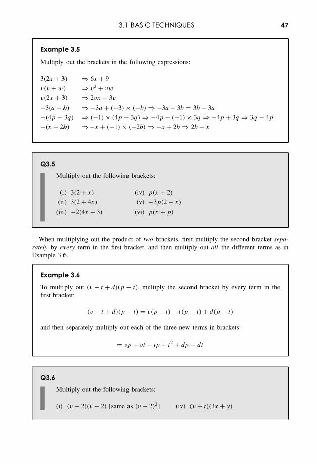
3.1 BASIC TECHNIQUES 47
Example 3.5
Multiply out the brackets in the following expressions:
3(2x + 3) ⇒ 6x + 9
v(v + w) ⇒ v2 + vw
v(2x + 3) ⇒ 2vx + 3v
−3(a − b) ⇒ −3a + (−3) × (−b) ⇒ −3a + 3b = 3b − 3a
−(4p − 3q) ⇒ (−1) × (4p − 3q) ⇒ −4p − (−1) × 3q ⇒ −4p + 3q ⇒ 3q − 4p
−(x − 2b) ⇒ −x + (−1) × (−2b) ⇒ −x + 2b ⇒ 2b − x
Q3.5Multiply out the following brackets:
(i) 3(2 + x) (iv) p(x + 2)
(ii) 3(2 + 4x) (v) −3p(2 − x)
(iii) −2(4x − 3) (vi) p(x + p)
When multiplying out the product of two brackets, first multiply the second bracket sepa-rately by every term in the first bracket, and then multiply out all the different terms as inExample 3.6.
Example 3.6
To multiply out (v − t + d)(p − t), multiply the second bracket by every term in thefirst bracket:
(v − t + d)(p − t) = v(p − t) − t (p − t) + d(p − t)
and then separately multiply out each of the three new terms in brackets:
= vp − vt − tp + t2 + dp − dt
Q3.6Multiply out the following brackets:
(i) (v − 2)(v − 2) [same as (v − 2)2] (iv) (v + t)(3x + y)
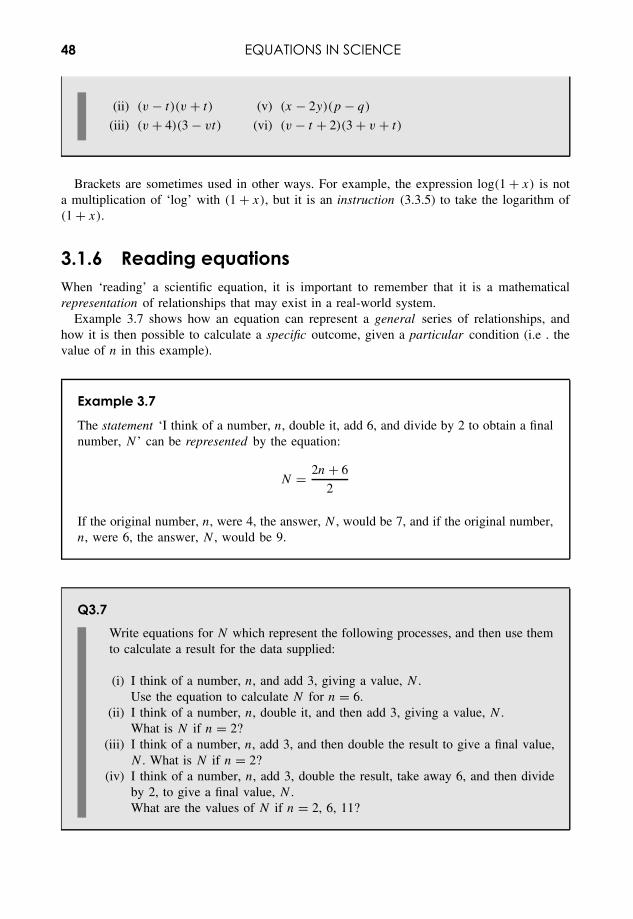
48 EQUATIONS IN SCIENCE
(ii) (v − t)(v + t) (v) (x − 2y)(p − q)
(iii) (v + 4)(3 − vt) (vi) (v − t + 2)(3 + v + t)
Brackets are sometimes used in other ways. For example, the expression log(1 + x) is nota multiplication of ‘log’ with (1 + x), but it is an instruction (3.3.5) to take the logarithm of(1 + x).
3.1.6 Reading equationsWhen ‘reading’ a scientific equation, it is important to remember that it is a mathematicalrepresentation of relationships that may exist in a real-world system.
Example 3.7 shows how an equation can represent a general series of relationships, andhow it is then possible to calculate a specific outcome, given a particular condition (i.e . thevalue of n in this example).
Example 3.7
The statement ‘I think of a number, n, double it, add 6, and divide by 2 to obtain a finalnumber, N ’ can be represented by the equation:
N = 2n + 6
2
If the original number, n, were 4, the answer, N , would be 7, and if the original number,n, were 6, the answer, N , would be 9.
Q3.7Write equations for N which represent the following processes, and then use themto calculate a result for the data supplied:
(i) I think of a number, n, and add 3, giving a value, N .Use the equation to calculate N for n = 6.
(ii) I think of a number, n, double it, and then add 3, giving a value, N .What is N if n = 2?
(iii) I think of a number, n, add 3, and then double the result to give a final value,N . What is N if n = 2?
(iv) I think of a number, n, add 3, double the result, take away 6, and then divideby 2, to give a final value, N .What are the values of N if n = 2, 6, 11?
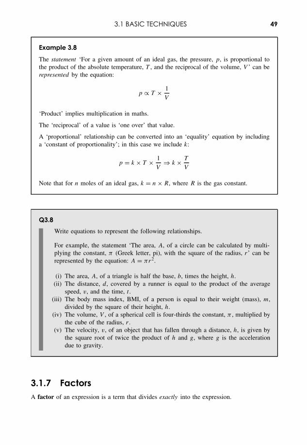
3.1 BASIC TECHNIQUES 49
Example 3.8
The statement ‘For a given amount of an ideal gas, the pressure, p, is proportional tothe product of the absolute temperature, T , and the reciprocal of the volume, V ’ can berepresented by the equation:
p ∝ T × 1
V
‘Product’ implies multiplication in maths.
The ‘reciprocal’ of a value is ‘one over’ that value.
A ‘proportional’ relationship can be converted into an ‘equality’ equation by includinga ‘constant of proportionality’; in this case we include k:
p = k × T × 1
V⇒ k × T
V
Note that for n moles of an ideal gas, k = n × R, where R is the gas constant.
Q3.8Write equations to represent the following relationships.
For example, the statement ‘The area, A, of a circle can be calculated by multi-plying the constant, π (Greek letter, pi), with the square of the radius, r’ can berepresented by the equation: A = πr2.
(i) The area, A, of a triangle is half the base, b, times the height, h.(ii) The distance, d, covered by a runner is equal to the product of the average
speed, v, and the time, t .(iii) The body mass index, BMI, of a person is equal to their weight (mass), m,
divided by the square of their height, h.(iv) The volume, V , of a spherical cell is four-thirds the constant, π , multiplied by
the cube of the radius, r .(v) The velocity, v, of an object that has fallen through a distance, h, is given by
the square root of twice the product of h and g, where g is the accelerationdue to gravity.
3.1.7 FactorsA factor of an expression is a term that divides exactly into the expression.
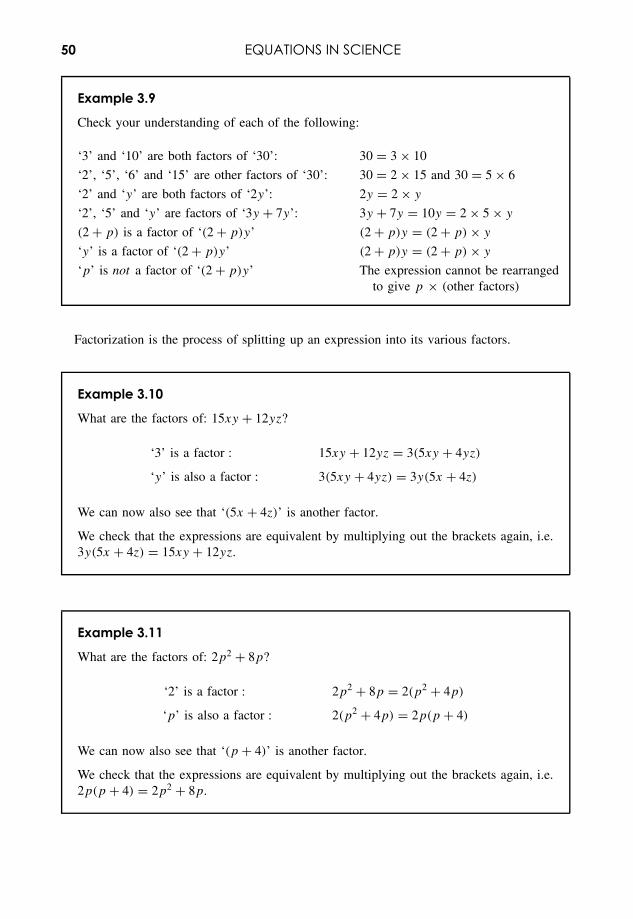
50 EQUATIONS IN SCIENCE
Example 3.9
Check your understanding of each of the following:
‘3’ and ‘10’ are both factors of ‘30’: 30 = 3 × 10
‘2’, ‘5’, ‘6’ and ‘15’ are other factors of ‘30’: 30 = 2 × 15 and 30 = 5 × 6
‘2’ and ‘y’ are both factors of ‘2y’: 2y = 2 × y
‘2’, ‘5’ and ‘y’ are factors of ‘3y + 7y’: 3y + 7y = 10y = 2 × 5 × y
(2 + p) is a factor of ‘(2 + p)y’ (2 + p)y = (2 + p) × y
‘y’ is a factor of ‘(2 + p)y’ (2 + p)y = (2 + p) × y
‘p’ is not a factor of ‘(2 + p)y’ The expression cannot be rearrangedto give p × (other factors)
Factorization is the process of splitting up an expression into its various factors.
Example 3.10
What are the factors of: 15xy + 12yz?
‘3’ is a factor : 15xy + 12yz = 3(5xy + 4yz)
‘y’ is also a factor : 3(5xy + 4yz) = 3y(5x + 4z)
We can now also see that ‘(5x + 4z)’ is another factor.
We check that the expressions are equivalent by multiplying out the brackets again, i.e.3y(5x + 4z) = 15xy + 12yz.
Example 3.11
What are the factors of: 2p2 + 8p?
‘2’ is a factor : 2p2 + 8p = 2(p2 + 4p)
‘p’ is also a factor : 2(p2 + 4p) = 2p(p + 4)
We can now also see that ‘(p + 4)’ is another factor.
We check that the expressions are equivalent by multiplying out the brackets again, i.e.2p(p + 4) = 2p2 + 8p.
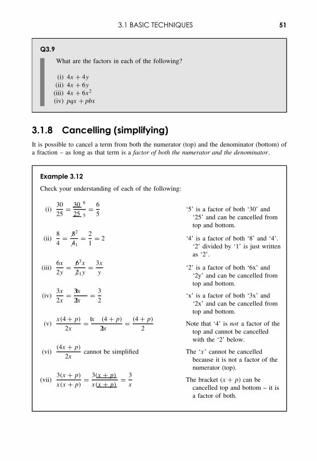
3.1 BASIC TECHNIQUES 51
Q3.9What are the factors in each of the following?
(i) 4x + 4y
(ii) 4x + 6y
(iii) 4x + 6x2
(iv) pqx + pbx
3.1.8 Cancelling (simplifying)It is possible to cancel a term from both the numerator (top) and the denominator (bottom) ofa fraction – as long as that term is a factor of both the numerator and the denominator .
Example 3.12
Check your understanding of each of the following:
(i)30
25= 30 6
25 5= 6
5‘5’ is a factor of both ‘30’ and
‘25’ and can be cancelled fromtop and bottom.
(ii)8
4= 82
41= 2
1= 2 ‘4’ is a factor of both ‘8’ and ‘4’.
‘2’ divided by ‘1’ is just writtenas ‘2’.
(iii)6x
2y= 63x
21y= 3x
y‘2’ is a factor of both ‘6x’ and
‘2y’ and can be cancelled fromtop and bottom.
(iv)3x
2x= 3x
2x= 3
2‘x’ is a factor of both ‘3x’ and
‘2x’ and can be cancelled fromtop and bottom.
(v)x(4 + p)
2x= x (4 + p)
2x= (4 + p)
2Note that ‘4’ is not a factor of the
top and cannot be cancelledwith the ‘2’ below.
(vi)(4x + p)
2xcannot be simplified The ‘x’ cannot be cancelled
because it is not a factor of thenumerator (top).
(vii)3(x + p)
x(x + p)= 3(x + p)
x(x + p)= 3
xThe bracket (x + p) can be
cancelled top and bottom – it isa factor of both.
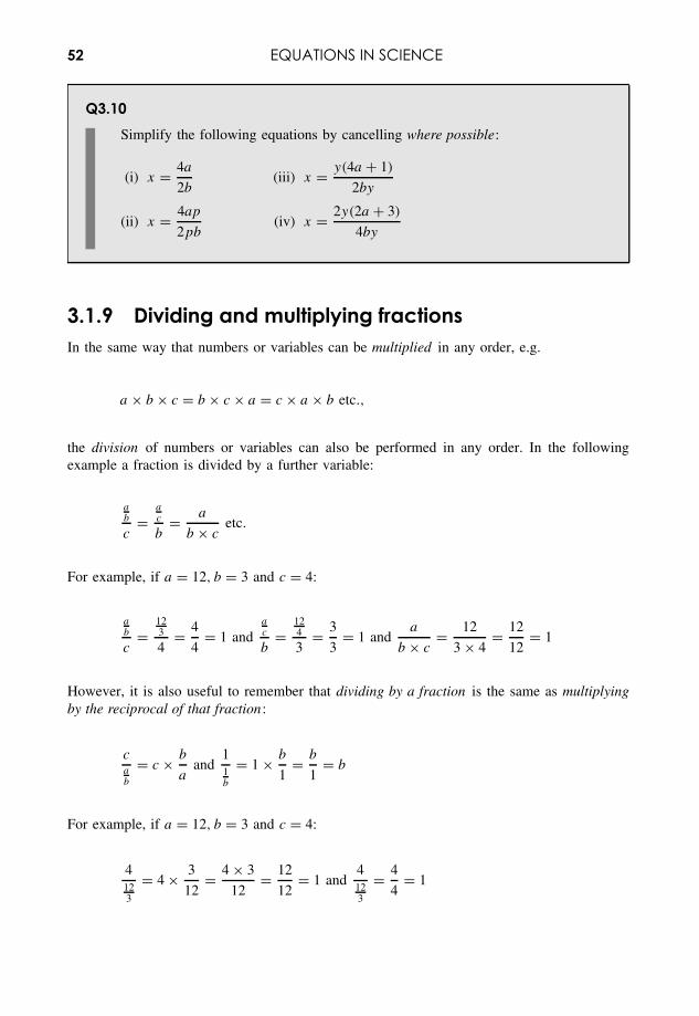
52 EQUATIONS IN SCIENCE
Q3.10Simplify the following equations by cancelling where possible:
(i) x = 4a
2b(iii) x = y(4a + 1)
2by
(ii) x = 4ap
2pb(iv) x = 2y(2a + 3)
4by
3.1.9 Dividing and multiplying fractionsIn the same way that numbers or variables can be multiplied in any order, e.g.
a × b × c = b × c × a = c × a × b etc.,
the division of numbers or variables can also be performed in any order. In the followingexample a fraction is divided by a further variable:
ab
c=
ac
b= a
b × cetc.
For example, if a = 12, b = 3 and c = 4:
ab
c=
123
4= 4
4= 1 and
ac
b=
124
3= 3
3= 1 and
a
b × c= 12
3 × 4= 12
12= 1
However, it is also useful to remember that dividing by a fraction is the same as multiplyingby the reciprocal of that fraction:
cab
= c × b
aand
11b
= 1 × b
1= b
1= b
For example, if a = 12, b = 3 and c = 4:
4123
= 4 × 3
12= 4 × 3
12= 12
12= 1 and
4123
= 4
4= 1
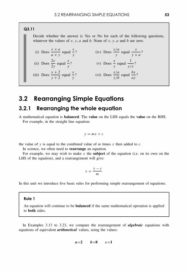
3.2 REARRANGING SIMPLE EQUATIONS 53
Q3.11Decide whether the answer is Yes or No for each of the following questions,whatever the values of x, y, a and b. None of x, y, a and b are zero.
(i) Doesx × a
a × yequal
x
y? (iv) Does
x/a
yequal
x
y × a?
(ii) Does2x
2yequal
x
y? (v) Does
x
yequal
1
y/x?
(iii) Doesx + 2
y + 2equal
x
y? (vi) Does
x/a
y/bequal
bx
ay?
3.2 Rearranging Simple Equations3.2.1 Rearranging the whole equationA mathematical equation is balanced. The value on the LHS equals the value on the RHS.
For example, in the straight line equation:
y = mx + c
the value of y is equal to the combined value of m times x then added to c.In science, we often need to rearrange an equation.For example, we may wish to make x the subject of the equation (i.e. on its own on the
LHS of the equation), and a rearrangement will give:
x = y − c
m
In this unit we introduce five basic rules for performing simple rearrangement of equations.
Rule 1
An equation will continue to be balanced if the same mathematical operation is appliedto both sides.
In Examples 3.13 to 3.23, we compare the rearrangement of algebraic equations withequations of equivalent arithmetical values, using the values:
a=2 b=8 c=1
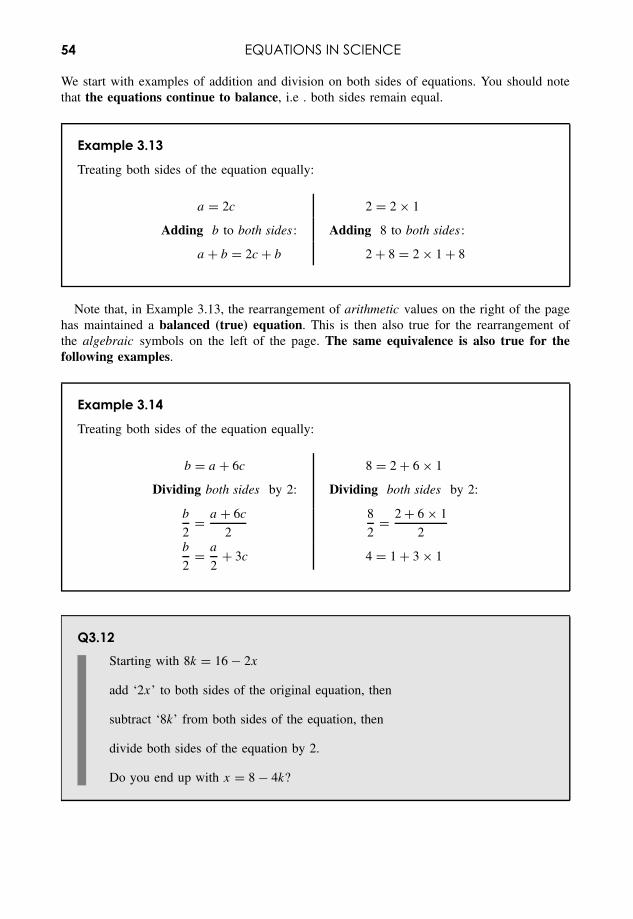
54 EQUATIONS IN SCIENCE
We start with examples of addition and division on both sides of equations. You should notethat the equations continue to balance, i.e . both sides remain equal.
Example 3.13
Treating both sides of the equation equally:
a = 2c 2 = 2 × 1
Adding b to both sides : Adding 8 to both sides :
a + b = 2c + b 2 + 8 = 2 × 1 + 8
Note that, in Example 3.13, the rearrangement of arithmetic values on the right of the pagehas maintained a balanced (true) equation. This is then also true for the rearrangement ofthe algebraic symbols on the left of the page. The same equivalence is also true for thefollowing examples.
Example 3.14
Treating both sides of the equation equally:
b = a + 6c 8 = 2 + 6 × 1
Dividing both sides by 2: Dividing both sides by 2:
b
2= a + 6c
2
8
2= 2 + 6 × 1
2b
2= a
2+ 3c 4 = 1 + 3 × 1
Q3.12Starting with 8k = 16 − 2x
add ‘2x’ to both sides of the original equation, then
subtract ‘8k’ from both sides of the equation, then
divide both sides of the equation by 2.
Do you end up with x = 8 − 4k?
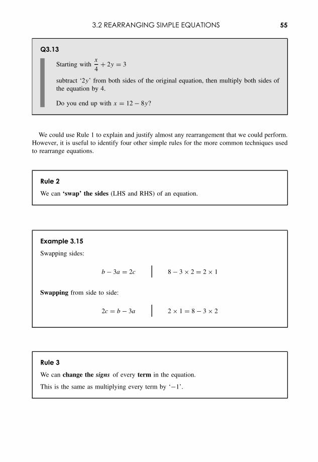
3.2 REARRANGING SIMPLE EQUATIONS 55
Q3.13
Starting withx
4+ 2y = 3
subtract ‘2y’ from both sides of the original equation, then multiply both sides ofthe equation by 4.
Do you end up with x = 12 − 8y?
We could use Rule 1 to explain and justify almost any rearrangement that we could perform.However, it is useful to identify four other simple rules for the more common techniques usedto rearrange equations.
Rule 2
We can ‘swap’ the sides (LHS and RHS) of an equation.
Example 3.15
Swapping sides:
b − 3a = 2c 8 − 3 × 2 = 2 × 1
Swapping from side to side:
2c = b − 3a 2 × 1 = 8 − 3 × 2
Rule 3
We can change the signs of every term in the equation.
This is the same as multiplying every term by ‘−1’.
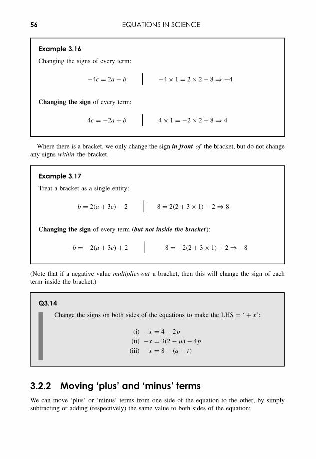
56 EQUATIONS IN SCIENCE
Example 3.16
Changing the signs of every term:
−4c = 2a − b −4 × 1 = 2 × 2 − 8 ⇒ −4
Changing the sign of every term:
4c = −2a + b 4 × 1 = −2 × 2 + 8 ⇒ 4
Where there is a bracket, we only change the sign in front of the bracket, but do not changeany signs within the bracket.
Example 3.17
Treat a bracket as a single entity:
b = 2(a + 3c) − 2 8 = 2(2 + 3 × 1) − 2 ⇒ 8
Changing the sign of every term (but not inside the bracket):
−b = −2(a + 3c) + 2 −8 = −2(2 + 3 × 1) + 2 ⇒ −8
(Note that if a negative value multiplies out a bracket, then this will change the sign of eachterm inside the bracket.)
Q3.14Change the signs on both sides of the equations to make the LHS = ‘ + x’:
(i) −x = 4 − 2p
(ii) −x = 3(2 − µ) − 4p
(iii) −x = 8 − (q − t)
3.2.2 Moving ‘plus’ and ‘minus’ termsWe can move ‘plus’ or ‘minus’ terms from one side of the equation to the other, by simplysubtracting or adding (respectively) the same value to both sides of the equation:
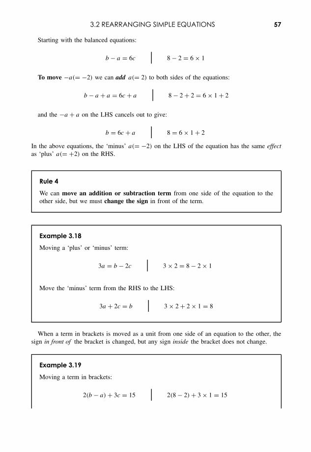
3.2 REARRANGING SIMPLE EQUATIONS 57
Starting with the balanced equations:
b − a = 6c 8 − 2 = 6 × 1
To move −a(= −2) we can add a(= 2) to both sides of the equations:
b − a + a = 6c + a 8 − 2 + 2 = 6 × 1 + 2
and the −a + a on the LHS cancels out to give:
b = 6c + a 8 = 6 × 1 + 2
In the above equations, the ‘minus’ a(= −2) on the LHS of the equation has the same effectas ‘plus’ a(= +2) on the RHS.
Rule 4
We can move an addition or subtraction term from one side of the equation to theother side, but we must change the sign in front of the term.
Example 3.18
Moving a ‘plus’ or ‘minus’ term:
3a = b − 2c 3 × 2 = 8 − 2 × 1
Move the ‘minus’ term from the RHS to the LHS:
3a + 2c = b 3 × 2 + 2 × 1 = 8
When a term in brackets is moved as a unit from one side of an equation to the other, thesign in front of the bracket is changed, but any sign inside the bracket does not change.
Example 3.19
Moving a term in brackets:
2(b − a) + 3c = 15 2(8 − 2) + 3 × 1 = 15
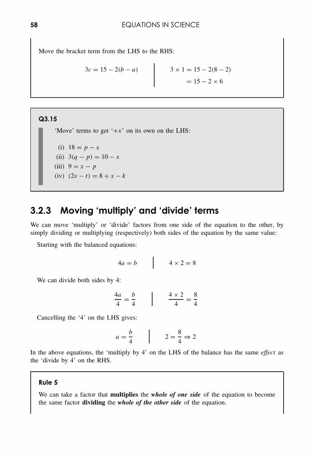
58 EQUATIONS IN SCIENCE
Move the bracket term from the LHS to the RHS:
3c = 15 − 2(b − a) 3 × 1 = 15 − 2(8 − 2)
= 15 − 2 × 6
Q3.15‘Move’ terms to get ‘+x’ on its own on the LHS:
(i) 18 = p − x
(ii) 3(q − p) = 10 − x
(iii) 9 = x − p
(iv) (2v − t) = 8 + x − k
3.2.3 Moving ‘multiply’ and ‘divide’ termsWe can move ‘multiply’ or ‘divide’ factors from one side of the equation to the other, bysimply dividing or multiplying (respectively) both sides of the equation by the same value:
Starting with the balanced equations:
4a = b 4 × 2 = 8
We can divide both sides by 4:
4a
4= b
4
4 × 2
4= 8
4
Cancelling the ‘4’ on the LHS gives:
a = b
42 = 8
4⇒ 2
In the above equations, the ‘multiply by 4’ on the LHS of the balance has the same effect asthe ‘divide by 4’ on the RHS.
Rule 5
We can take a factor that multiplies the whole of one side of the equation to becomethe same factor dividing the whole of the other side of the equation.
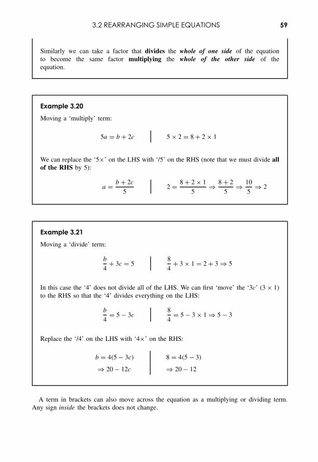
3.2 REARRANGING SIMPLE EQUATIONS 59
Similarly we can take a factor that divides the whole of one side of the equationto become the same factor multiplying the whole of the other side of theequation.
Example 3.20
Moving a ‘multiply’ term:
5a = b + 2c 5 × 2 = 8 + 2 × 1
We can replace the ‘5×’ on the LHS with ‘/5’ on the RHS (note that we must divide allof the RHS by 5):
a = b + 2c
52 = 8 + 2 × 1
5⇒ 8 + 2
5⇒ 10
5⇒ 2
Example 3.21
Moving a ‘divide’ term:
b
4+ 3c = 5
8
4+ 3 × 1 = 2 + 3 ⇒ 5
In this case the ‘4’ does not divide all of the LHS. We can first ‘move’ the ‘3c’ (3 × 1)to the RHS so that the ‘4’ divides everything on the LHS:
b
4= 5 − 3c
8
4= 5 − 3 × 1 ⇒ 5 − 3
Replace the ‘/4’ on the LHS with ‘4×’ on the RHS:
b = 4(5 − 3c) 8 = 4(5 − 3)
⇒ 20 − 12c ⇒ 20 − 12
A term in brackets can also move across the equation as a multiplying or dividing term.Any sign inside the brackets does not change.

60 EQUATIONS IN SCIENCE
Example 3.22
Moving a divisor in brackets:
b
(6c − a)= 2
8
(6 × 1 − 2)= 2
Replace the ‘/()’ on the LHS with ‘×()’ on the RHS:
b = 2(6c − a) 8 = 2(6 × 1 − 2)
⇒ 12c − 2a ⇒ 12 − 4
Q3.16Multiply or divide by factors to get ‘x’ on its own on the LHS:
(i) 2x = 60 + 20p
(ii)x
4= 5 − 2q
(iii) x(s − m) = k
(iv)x
(2p − q)= 8
3.2.4 Solving an equation for an unknown valueWe often need to rearrange an equation to find the value of an unknown term.
The unknown value is often denoted by ‘x’.For example, we may need to find the value, ‘x’, which satisfies the following equation:
x + 50 = 60
Simple inspection of the equation will tell us that the value of ‘x’ must be 10.However, we can also use a formal rearrangement of the equation, by moving the +50 from
the LHS to become −50 on the RHS:
x = 60 − 50 = 10
The final equation giving x = 10 is the solution to the problem.
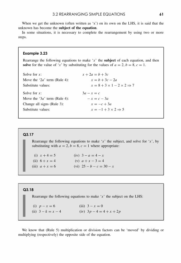
3.2 REARRANGING SIMPLE EQUATIONS 61
When we get the unknown (often written as ‘x’) on its own on the LHS, it is said that theunknown has become the subject of the equation.
In some situations, it is necessary to complete the rearrangement by using two or moresteps.
Example 3.23
Rearrange the following equations to make ‘x’ the subject of each equation, and thensolve for the value of ‘x’ by substituting for the values of a = 2, b = 8, c = 1.
Solve for x: x + 2a = b + 3c
Move the ‘2a’ term (Rule 4): x = b + 3c − 2a
Substitute values: x = 8 + 3 × 1 − 2 × 2 ⇒ 7
Solve for x: 3a − x = c
Move the ‘3a’ term (Rule 4): − x = c − 3a
Change all signs (Rule 3): x = −c + 3a
Substitute values: x = −1 + 3 × 2 ⇒ 5
Q3.17Rearrange the following equations to make ‘x’ the subject, and solve for ‘x’, bysubstituting with a = 2, b = 8, c = 1 where appropriate:
(i) x + 4 = 5 (iv) 3 − a = 4 − x
(ii) 6 + x = 4 (v) a + x − 3 = 4
(iii) a + x = 6 (vi) 25 − b − c = 30 − x
Q3.18Rearrange the following equations to make ‘x’ the subject on the LHS:
(i) p − x = 6 (iii) 3 − x = 0
(ii) 3 − k = x − 4 (iv) 3p − 4 = 4 + x + 2p
We know that (Rule 5) multiplication or division factors can be ‘moved’ by dividing ormultiplying (respectively) the opposite side of the equation.
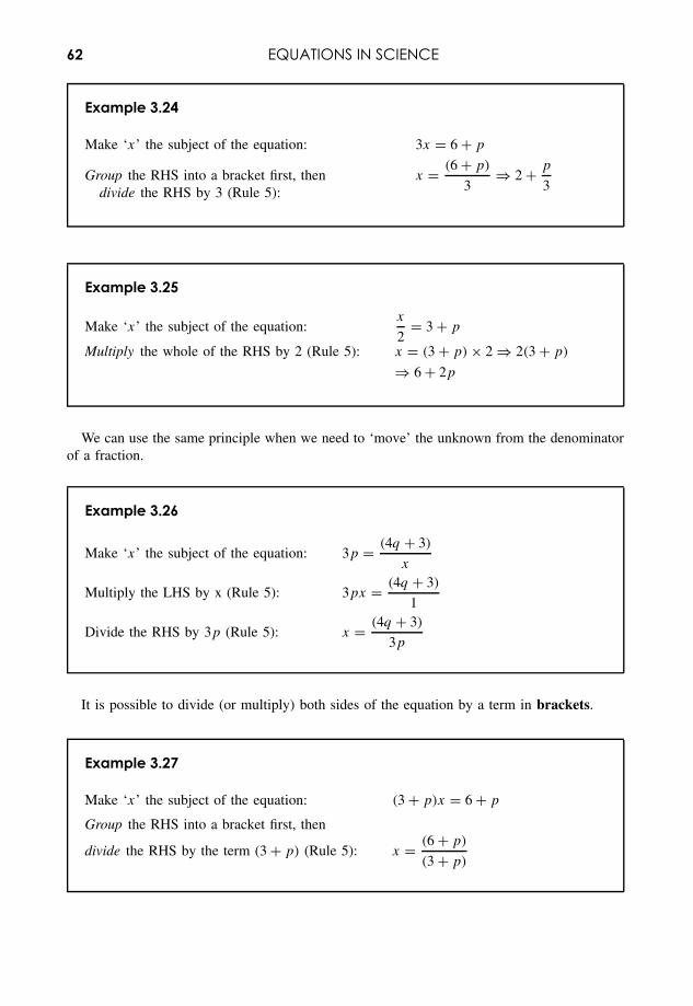
62 EQUATIONS IN SCIENCE
Example 3.24
Make ‘x’ the subject of the equation: 3x = 6 + p
Group the RHS into a bracket first, thendivide the RHS by 3 (Rule 5):
x = (6 + p)
3⇒ 2 + p
3
Example 3.25
Make ‘x’ the subject of the equation:x
2= 3 + p
Multiply the whole of the RHS by 2 (Rule 5): x = (3 + p) × 2 ⇒ 2(3 + p)
⇒ 6 + 2p
We can use the same principle when we need to ‘move’ the unknown from the denominatorof a fraction.
Example 3.26
Make ‘x’ the subject of the equation: 3p = (4q + 3)
x
Multiply the LHS by x (Rule 5): 3px = (4q + 3)
1
Divide the RHS by 3p (Rule 5): x = (4q + 3)
3p
It is possible to divide (or multiply) both sides of the equation by a term in brackets.
Example 3.27
Make ‘x’ the subject of the equation: (3 + p)x = 6 + p
Group the RHS into a bracket first, then
divide the RHS by the term (3 + p) (Rule 5): x = (6 + p)
(3 + p)
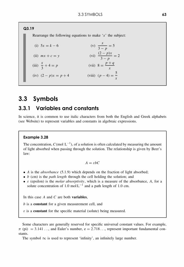
3.3 SYMBOLS 63
Q3.19Rearrange the following equations to make ‘x’ the subject:
(i) 5x = k − 6 (v)x
3 − p= 5
(ii) mx + c = y (vi)(2 − p)x
3 − p= 2
(iii)x
3+ 4 = p (vii) 8 = p + q
x
(iv) (2 − p)x = p + 4 (viii) (p − 4) = 5
x
3.3 Symbols3.3.1 Variables and constantsIn science, it is common to use italic characters from both the English and Greek alphabets(see Website) to represent variables and constants in algebraic expressions.
Example 3.28
The concentration, C(mol L−1), of a solution is often calculated by measuring the amountof light absorbed when passing through the solution. The relationship is given by Beer’slaw:
A = εbC
• A is the absorbance (5.1.9) which depends on the fraction of light absorbed;• b (cm) is the path length through the cell holding the solution; and• ε (epsilon) is the molar absorptivity , which is a measure of the absorbance, A, for a
solute concentration of 1.0 mol L−1 and a path length of 1.0 cm.
In this case A and C are both variables,
b is a constant for a given measurement cell, and
ε is a constant for the specific material (solute) being measured.
Some characters are generally reserved for specific universal constant values. For example,π (pi) = 3.141 . . ., and Euler’s number, e = 2.718 . . ., represent important fundamental con-stants.
The symbol ∞ is used to represent ‘infinity’, an infinitely large number.
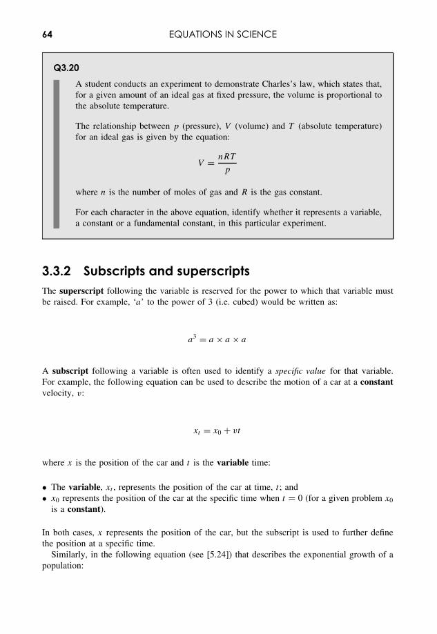
64 EQUATIONS IN SCIENCE
Q3.20A student conducts an experiment to demonstrate Charles’s law, which states that,for a given amount of an ideal gas at fixed pressure, the volume is proportional tothe absolute temperature.
The relationship between p (pressure), V (volume) and T (absolute temperature)for an ideal gas is given by the equation:
V = nRT
p
where n is the number of moles of gas and R is the gas constant.
For each character in the above equation, identify whether it represents a variable,a constant or a fundamental constant, in this particular experiment.
3.3.2 Subscripts and superscriptsThe superscript following the variable is reserved for the power to which that variable mustbe raised. For example, ‘a’ to the power of 3 (i.e. cubed) would be written as:
a3 = a × a × a
A subscript following a variable is often used to identify a specific value for that variable.For example, the following equation can be used to describe the motion of a car at a constantvelocity, v:
xt = x0 + vt
where x is the position of the car and t is the variable time:
• The variable, xt , represents the position of the car at time, t ; and• x0 represents the position of the car at the specific time when t = 0 (for a given problem x0
is a constant).
In both cases, x represents the position of the car, but the subscript is used to further definethe position at a specific time.
Similarly, in the following equation (see [5.24]) that describes the exponential growth of apopulation:
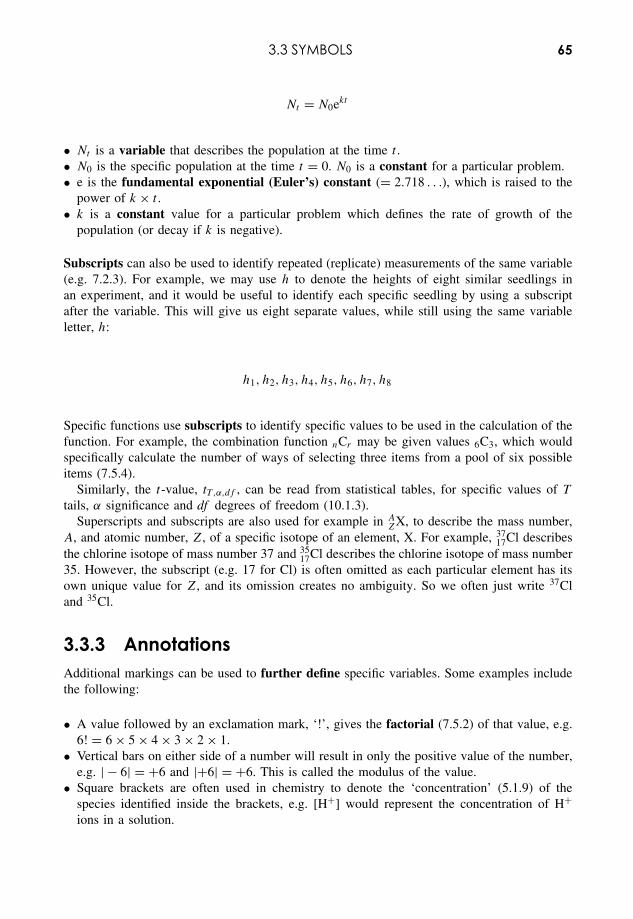
3.3 SYMBOLS 65
Nt = N0ekt
• Nt is a variable that describes the population at the time t .• N0 is the specific population at the time t = 0. N0 is a constant for a particular problem.• e is the fundamental exponential (Euler’s) constant (= 2.718 . . .), which is raised to the
power of k × t .• k is a constant value for a particular problem which defines the rate of growth of the
population (or decay if k is negative).
Subscripts can also be used to identify repeated (replicate) measurements of the same variable(e.g. 7.2.3). For example, we may use h to denote the heights of eight similar seedlings inan experiment, and it would be useful to identify each specific seedling by using a subscriptafter the variable. This will give us eight separate values, while still using the same variableletter, h:
h1, h2, h3, h4, h5, h6, h7, h8
Specific functions use subscripts to identify specific values to be used in the calculation of thefunction. For example, the combination function nCr may be given values 6C3, which wouldspecifically calculate the number of ways of selecting three items from a pool of six possibleitems (7.5.4).
Similarly, the t-value, tT ,α,df , can be read from statistical tables, for specific values of T
tails, α significance and df degrees of freedom (10.1.3).Superscripts and subscripts are also used for example in A
ZX, to describe the mass number,A, and atomic number, Z, of a specific isotope of an element, X. For example, 37
17Cl describesthe chlorine isotope of mass number 37 and 35
17Cl describes the chlorine isotope of mass number35. However, the subscript (e.g. 17 for Cl) is often omitted as each particular element has itsown unique value for Z, and its omission creates no ambiguity. So we often just write 37Cland 35Cl.
3.3.3 AnnotationsAdditional markings can be used to further define specific variables. Some examples includethe following:
• A value followed by an exclamation mark, ‘!’, gives the factorial (7.5.2) of that value, e.g.6! = 6 × 5 × 4 × 3 × 2 × 1.
• Vertical bars on either side of a number will result in only the positive value of the number,e.g. | − 6| = +6 and |+6| = +6. This is called the modulus of the value.
• Square brackets are often used in chemistry to denote the ‘concentration’ (5.1.9) of thespecies identified inside the brackets, e.g. [H+] would represent the concentration of H+ions in a solution.
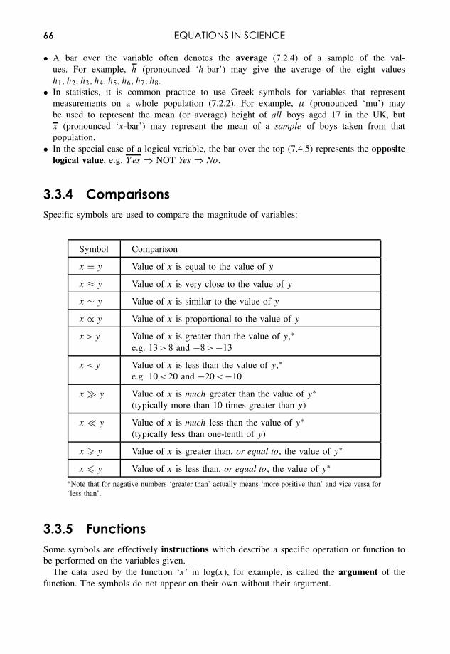
66 EQUATIONS IN SCIENCE
• A bar over the variable often denotes the average (7.2.4) of a sample of the val-ues. For example, h (pronounced ‘h-bar’) may give the average of the eight valuesh1, h2, h3, h4, h5, h6, h7, h8.
• In statistics, it is common practice to use Greek symbols for variables that representmeasurements on a whole population (7.2.2). For example, µ (pronounced ‘mu’) maybe used to represent the mean (or average) height of all boys aged 17 in the UK, butx (pronounced ‘x-bar’) may represent the mean of a sample of boys taken from thatpopulation.
• In the special case of a logical variable, the bar over the top (7.4.5) represents the oppositelogical value, e.g. Yes ⇒ NOT Yes ⇒ No.
3.3.4 ComparisonsSpecific symbols are used to compare the magnitude of variables:
Symbol Comparison
x = y Value of x is equal to the value of y
x ≈ y Value of x is very close to the value of y
x ∼ y Value of x is similar to the value of y
x ∝ y Value of x is proportional to the value of y
x >y Value of x is greater than the value of y,∗e.g. 13 > 8 and −8 >−13
x <y Value of x is less than the value of y,∗e.g. 10 < 20 and −20 <−10
x y Value of x is much greater than the value of y∗(typically more than 10 times greater than y)
x � y Value of x is much less than the value of y∗(typically less than one-tenth of y)
x � y Value of x is greater than, or equal to, the value of y∗
x � y Value of x is less than, or equal to, the value of y∗
∗Note that for negative numbers ‘greater than’ actually means ‘more positive than’ and vice versa for‘less than’.
3.3.5 FunctionsSome symbols are effectively instructions which describe a specific operation or function tobe performed on the variables given.
The data used by the function ‘x’ in log(x), for example, is called the argument of thefunction. The symbols do not appear on their own without their argument.
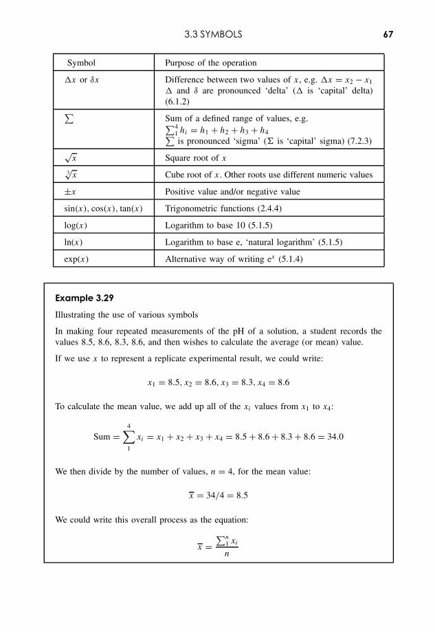
3.3 SYMBOLS 67
Symbol Purpose of the operation
�x or δx Difference between two values of x, e.g. �x = x2 − x1
� and δ are pronounced ‘delta’ (� is ‘capital’ delta)(6.1.2)∑Sum of a defined range of values, e.g.∑4
1 hi = h1 + h2 + h3 + h4∑is pronounced ‘sigma’ ( is ‘capital’ sigma) (7.2.3)
√x Square root of x
3√
x Cube root of x. Other roots use different numeric values
±x Positive value and/or negative value
sin(x), cos(x), tan(x) Trigonometric functions (2.4.4)
log(x) Logarithm to base 10 (5.1.5)
ln(x) Logarithm to base e, ‘natural logarithm’ (5.1.5)
exp(x) Alternative way of writing ex (5.1.4)
Example 3.29
Illustrating the use of various symbols
In making four repeated measurements of the pH of a solution, a student records thevalues 8.5, 8.6, 8.3, 8.6, and then wishes to calculate the average (or mean) value.
If we use x to represent a replicate experimental result, we could write:
x1 = 8.5, x2 = 8.6, x3 = 8.3, x4 = 8.6
To calculate the mean value, we add up all of the xi values from x1 to x4:
Sum =4∑1
xi = x1 + x2 + x3 + x4 = 8.5 + 8.6 + 8.3 + 8.6 = 34.0
We then divide by the number of values, n = 4, for the mean value:
x = 34/4 = 8.5
We could write this overall process as the equation:
x =∑n
1 xi
n
68 EQUATIONS IN SCIENCE
Q3.21Explain carefully what is meant by all the symbols, annotations, etc., in the fol-lowing equations:
(i) pH = − log([H+]) (see 5.1.9)
(ii) At = A0 exp(−0.693t/T1/2) (see 5.2.4)
(iii) χ2 =∑
i
(Oi − Ei)2
Ei
(see 14.1.2)
3.4 Further Equations3.4.1 IntroductionWe introduced the basic rules for rearranging simple equations in 3.2:
Rule 1: Both sides of an equation must be treated equally .Rule 2: The two sides of an equation can be swapped.Rule 3: The signs for every term in an equation can be reversed (+/−).Rule 4: A term can be moved from one side to the other, provided that its sign is reversed.Rule 5: A multiplier/divisor factor of one side can become a divisor/multiplier factor of the
other .
We now derive Rule 6 for inverse operations, together with some additional techniques andstrategies.
3.4.2 Inverse operationsSometimes we want to ‘undo’ an operation and take a step backwards by using an inverseprocess. Some simple examples will illustrate the process.
If we are required to ‘solve’ the equation:
x = 52
we know that the ‘square’ of 5 is 25 (5 raised to the power of 2), hence we can write thesolution directly:
x = 25
3.4 FURTHER EQUATIONS 69
The inverse process to the ‘square’ is the ‘square root’. Taking the square root of a squarednumber takes the value back to the original number! Thus:
√x2 = x
The following example illustrates the ‘inverse’ problem.
Example 3.30
Solve the following equation for ‘x’:
x2 = 9
We must ‘undo’ the squaring process, and work ‘backwards’ to find a number which,when squared, gives 9.
Using Rule 1 of rearranging equations, we take the square root of both sides to get:
√x2 =
√9
We know that√
x2 = x, and finding√
9 from a calculator (= 3), we would rewrite theabove equation to give:
x = 3
In fact, the square root of 9 could be either +3 or −3, and we should write the solution:
x = ±3
We cannot tell from the mathematics which solution (+ or −) is correct, but looking backat the science of the problem will tell us whether both solutions are possible, or whether justone is correct (see Examples 3.43 and 3.44).
In the above example, the square operation on the LHS can be ‘undone’, and the same effectachieved, by the inverse operation of taking the square root of the RHS.
Example 3.31
If x2 = 22, calculate the value of ‘x’.
As the ‘square root’ is the inverse process for ‘square’, we take the square root of bothsides of the equation:
√x2 =
√22
70 EQUATIONS IN SCIENCE
Using a calculator to evaluate√
22 = 4.69, we can then write the solution:
x = ±4.69
We can also use the inverse operation approach to ‘undo’ an equation involving the reciprocalof (‘one over’) the unknown value.
To ‘undo’ a reciprocal, 1/x, the inverse operation is to take the reciprocal again ‘to getback’ to ‘x’ (see 3.1.9):
11x
= x
Example 3.32
Solve the following equation for x:
1
x= 4
We take the reciprocal of both sides:
11x
= 1
4
The LHS just equals x, which then gives:
x = 1
4
In the above example, the reciprocal operation on the LHS can be ‘undone’, and the sameeffect achieved, by the inverse operation of taking the reciprocal of the RHS.
Rule 6
The effect of an operation on (the whole of) one side of the equation can be ‘undone’,and its effect replaced, by applying the inverse operation to (the whole of) the other sideof the equation.
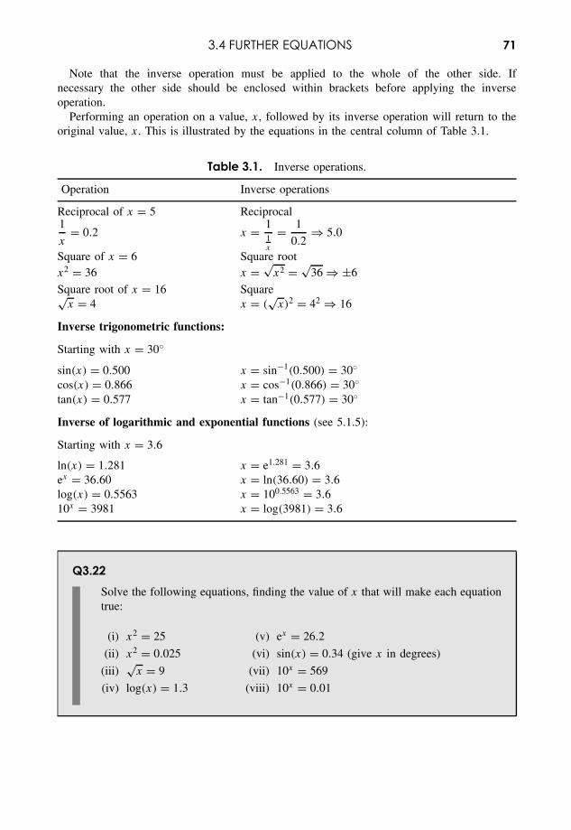
3.4 FURTHER EQUATIONS 71
Note that the inverse operation must be applied to the whole of the other side. Ifnecessary the other side should be enclosed within brackets before applying the inverseoperation.
Performing an operation on a value, x, followed by its inverse operation will return to theoriginal value, x. This is illustrated by the equations in the central column of Table 3.1.
Table 3.1. Inverse operations.
Operation Inverse operations
Reciprocal of x = 5 Reciprocal1
x= 0.2 x = 1
1x
= 1
0.2⇒ 5.0
Square of x = 6 Square rootx2 = 36 x =
√x2 = √
36 ⇒ ±6
Square root of x = 16 Square√x = 4 x = (
√x)2 = 42 ⇒ 16
Inverse trigonometric functions:
Starting with x = 30◦
sin(x) = 0.500 x = sin−1(0.500) = 30◦cos(x) = 0.866 x = cos−1(0.866) = 30◦tan(x) = 0.577 x = tan−1(0.577) = 30◦
Inverse of logarithmic and exponential functions (see 5.1.5):
Starting with x = 3.6
ln(x) = 1.281 x = e1.281 = 3.6ex = 36.60 x = ln(36.60) = 3.6log(x) = 0.5563 x = 100.5563 = 3.610x = 3981 x = log(3981) = 3.6
Q3.22Solve the following equations, finding the value of x that will make each equationtrue:
(i) x2 = 25 (v) ex = 26.2
(ii) x2 = 0.025 (vi) sin(x) = 0.34 (give x in degrees)
(iii)√
x = 9 (vii) 10x = 569
(iv) log(x) = 1.3 (viii) 10x = 0.01
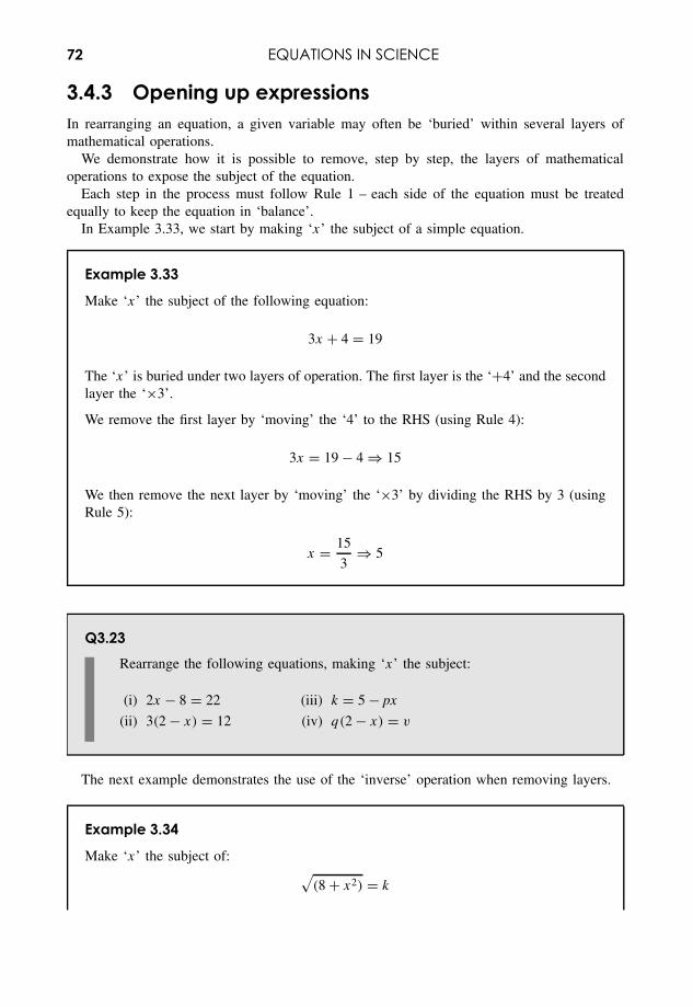
72 EQUATIONS IN SCIENCE
3.4.3 Opening up expressionsIn rearranging an equation, a given variable may often be ‘buried’ within several layers ofmathematical operations.
We demonstrate how it is possible to remove, step by step, the layers of mathematicaloperations to expose the subject of the equation.
Each step in the process must follow Rule 1 – each side of the equation must be treatedequally to keep the equation in ‘balance’.
In Example 3.33, we start by making ‘x’ the subject of a simple equation.
Example 3.33
Make ‘x’ the subject of the following equation:
3x + 4 = 19
The ‘x’ is buried under two layers of operation. The first layer is the ‘+4’ and the secondlayer the ‘×3’.
We remove the first layer by ‘moving’ the ‘4’ to the RHS (using Rule 4):
3x = 19 − 4 ⇒ 15
We then remove the next layer by ‘moving’ the ‘×3’ by dividing the RHS by 3 (usingRule 5):
x = 15
3⇒ 5
Q3.23Rearrange the following equations, making ‘x’ the subject:
(i) 2x − 8 = 22 (iii) k = 5 − px
(ii) 3(2 − x) = 12 (iv) q(2 − x) = v
The next example demonstrates the use of the ‘inverse’ operation when removing layers.
Example 3.34
Make ‘x’ the subject of: √(8 + x2) = k
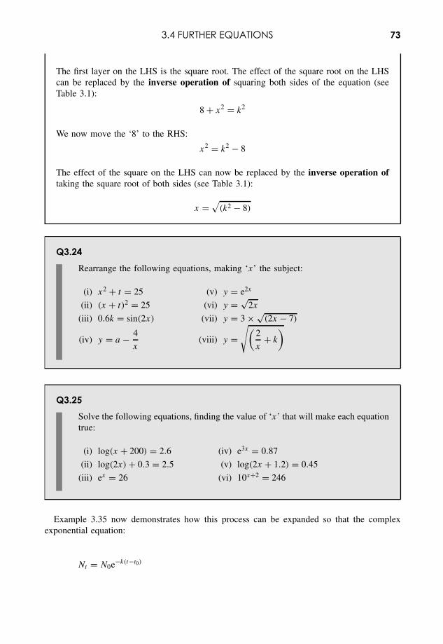
3.4 FURTHER EQUATIONS 73
The first layer on the LHS is the square root. The effect of the square root on the LHScan be replaced by the inverse operation of squaring both sides of the equation (seeTable 3.1):
8 + x2 = k2
We now move the ‘8’ to the RHS:
x2 = k2 − 8
The effect of the square on the LHS can now be replaced by the inverse operation oftaking the square root of both sides (see Table 3.1):
x =√
(k2 − 8)
Q3.24Rearrange the following equations, making ‘x’ the subject:
(i) x2 + t = 25 (v) y = e2x
(ii) (x + t)2 = 25 (vi) y = √2x
(iii) 0.6k = sin(2x) (vii) y = 3 × √(2x − 7)
(iv) y = a − 4
x(viii) y =
√(2
x+ k
)
Q3.25Solve the following equations, finding the value of ‘x’ that will make each equationtrue:
(i) log(x + 200) = 2.6 (iv) e3x = 0.87
(ii) log(2x) + 0.3 = 2.5 (v) log(2x + 1.2) = 0.45
(iii) ex = 26 (vi) 10x+2 = 246
Example 3.35 now demonstrates how this process can be expanded so that the complexexponential equation:
Nt = N0e−k(t−t0)
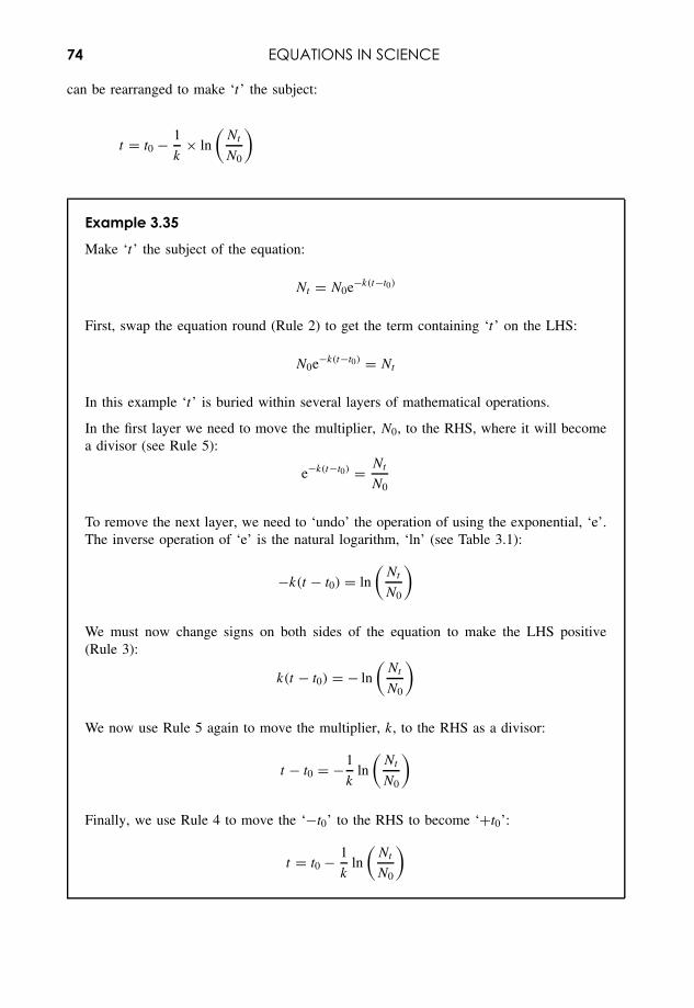
74 EQUATIONS IN SCIENCE
can be rearranged to make ‘t’ the subject:
t = t0 − 1
k× ln
(Nt
N0
)
Example 3.35
Make ‘t’ the subject of the equation:
Nt = N0e−k(t−t0)
First, swap the equation round (Rule 2) to get the term containing ‘t’ on the LHS:
N0e−k(t−t0) = Nt
In this example ‘t’ is buried within several layers of mathematical operations.
In the first layer we need to move the multiplier, N0, to the RHS, where it will becomea divisor (see Rule 5):
e−k(t−t0) = Nt
N0
To remove the next layer, we need to ‘undo’ the operation of using the exponential, ‘e’.The inverse operation of ‘e’ is the natural logarithm, ‘ln’ (see Table 3.1):
−k(t − t0) = ln
(Nt
N0
)
We must now change signs on both sides of the equation to make the LHS positive(Rule 3):
k(t − t0) = − ln
(Nt
N0
)
We now use Rule 5 again to move the multiplier, k, to the RHS as a divisor:
t − t0 = −1
kln
(Nt
N0
)
Finally, we use Rule 4 to move the ‘−t0’ to the RHS to become ‘+t0’:
t = t0 − 1
kln
(Nt
N0
)
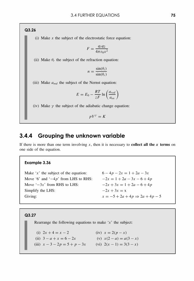
3.4 FURTHER EQUATIONS 75
Q3.26
(i) Make x the subject of the electrostatic force equation:
F = q1q2
4πε0x2
(ii) Make θr the subject of the refraction equation:
n = sin(θi)
sin(θr )
(iii) Make ared the subject of the Nernst equation:
E = E0 − RT
zFln
(ared
aox
)
(iv) Make γ the subject of the adiabatic change equation:
pV γ = K
3.4.4 Grouping the unknown variableIf there is more than one term involving x, then it is necessary to collect all the x terms onone side of the equation.
Example 3.36
Make ‘x’ the subject of the equation: 6 − 4p − 2x = 1 + 2a − 3x
Move ‘6’ and ‘−4p’ from LHS to RHS: −2x = 1 + 2a − 3x − 6 + 4p
Move ‘−3x’ from RHS to LHS: −2x + 3x = 1 + 2a − 6 + 4p
Simplify the LHS: −2x + 3x = x
Giving: x = −5 + 2a + 4p ⇒ 2a + 4p − 5
Q3.27Rearrange the following equations to make ‘x’ the subject:
(i) 2x + 4 = x − 2 (iv) x = 2(p − x)
(ii) 3 − a + x = 6 − 2x (v) x(2 − a) = a(3 − x)
(iii) x − 3 − 2p = 5 + p − 3x (vi) 2(x − 1) = 3(3 − x)
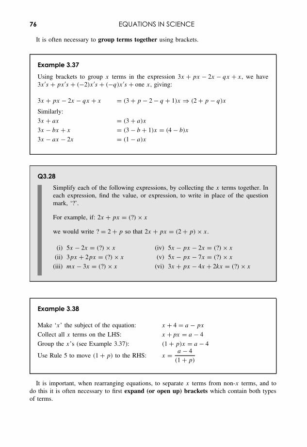
76 EQUATIONS IN SCIENCE
It is often necessary to group terms together using brackets.
Example 3.37
Using brackets to group x terms in the expression 3x + px − 2x − qx + x, we have3x ′s + px ′s + (−2)x ′s + (−q)x ′s + one x, giving:
3x + px − 2x − qx + x = (3 + p − 2 − q + 1)x ⇒ (2 + p − q)x
Similarly:
3x + ax = (3 + a)x
3x − bx + x = (3 − b + 1)x = (4 − b)x
3x − ax − 2x = (1 − a)x
Q3.28Simplify each of the following expressions, by collecting the x terms together. Ineach expression, find the value, or expression, to write in place of the questionmark, ‘?’.
For example, if: 2x + px = (?) × x
we would write ? = 2 + p so that 2x + px = (2 + p) × x.
(i) 5x − 2x = (?) × x (iv) 5x − px − 2x = (?) × x
(ii) 3px + 2px = (?) × x (v) 5x − px − 7x = (?) × x
(iii) mx − 3x = (?) × x (vi) 3x + px − 4x + 2kx = (?) × x
Example 3.38
Make ‘x’ the subject of the equation: x + 4 = a − px
Collect all x terms on the LHS: x + px = a − 4
Group the x’s (see Example 3.37): (1 + p)x = a − 4
Use Rule 5 to move (1 + p) to the RHS: x = a − 4
(1 + p)
It is important, when rearranging equations, to separate x terms from non-x terms, and todo this it is often necessary to first expand (or open up) brackets which contain both typesof terms.
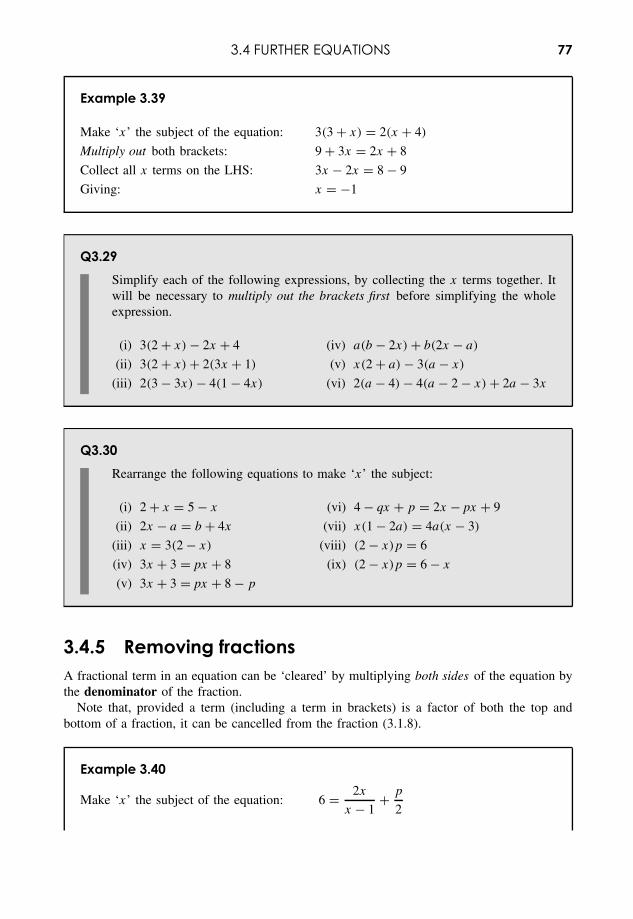
3.4 FURTHER EQUATIONS 77
Example 3.39
Make ‘x’ the subject of the equation: 3(3 + x) = 2(x + 4)
Multiply out both brackets: 9 + 3x = 2x + 8
Collect all x terms on the LHS: 3x − 2x = 8 − 9
Giving: x = −1
Q3.29Simplify each of the following expressions, by collecting the x terms together. Itwill be necessary to multiply out the brackets first before simplifying the wholeexpression.
(i) 3(2 + x) − 2x + 4 (iv) a(b − 2x) + b(2x − a)
(ii) 3(2 + x) + 2(3x + 1) (v) x(2 + a) − 3(a − x)
(iii) 2(3 − 3x) − 4(1 − 4x) (vi) 2(a − 4) − 4(a − 2 − x) + 2a − 3x
Q3.30Rearrange the following equations to make ‘x’ the subject:
(i) 2 + x = 5 − x (vi) 4 − qx + p = 2x − px + 9
(ii) 2x − a = b + 4x (vii) x(1 − 2a) = 4a(x − 3)
(iii) x = 3(2 − x) (viii) (2 − x)p = 6
(iv) 3x + 3 = px + 8 (ix) (2 − x)p = 6 − x
(v) 3x + 3 = px + 8 − p
3.4.5 Removing fractionsA fractional term in an equation can be ‘cleared’ by multiplying both sides of the equation bythe denominator of the fraction.
Note that, provided a term (including a term in brackets) is a factor of both the top andbottom of a fraction, it can be cancelled from the fraction (3.1.8).
Example 3.40
Make ‘x’ the subject of the equation: 6 = 2x
x − 1+ p
2
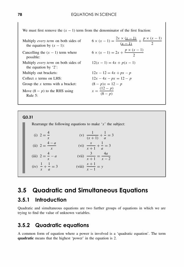
78 EQUATIONS IN SCIENCE
We must first remove the (x − 1) term from the denominator of the first fraction:
Multiply every term on both sides ofthe equation by (x − 1):
6 × (x − 1) = 2x × (x − 1)
(x − 1)+ p × (x − 1)
2
Cancelling the (x − 1) term wherepossible:
6 × (x − 1) = 2x + p × (x − 1)
2
Multiply every term on both sides ofthe equation by ‘2’:
12(x − 1) = 4x + p(x − 1)
Multiply out brackets: 12x − 12 = 4x + px − p
Collect x terms on LHS: 12x − 4x − px = 12 − p
Group the x terms with a bracket: (8 − p)x = 12 − p
Move (8 − p) to the RHS usingRule 5:
x = (12 − p)
(8 − p)
Q3.31Rearrange the following equations to make ‘x’ the subject:
(i) 2 = 4
x(v)
1
(x + 1)+ 1
a= 3
(ii) 2 = 4 − a
x(vi)
x
x + 1+ 1
a= 3
(iii) 2 = 4
x− a (vii)
3
x + 1= 4a
x − 2
(iv)1
x+ 1
a= 3 (viii)
x + 1
x − 1= y
3.5 Quadratic and Simultaneous Equations3.5.1 IntroductionQuadratic and simultaneous equations are two further groups of equations in which we aretrying to find the value of unknown variables.
3.5.2 Quadratic equationsA common form of equation where a power is involved is a ‘quadratic equation’. The termquadratic means that the highest ‘power’ in the equation is 2.
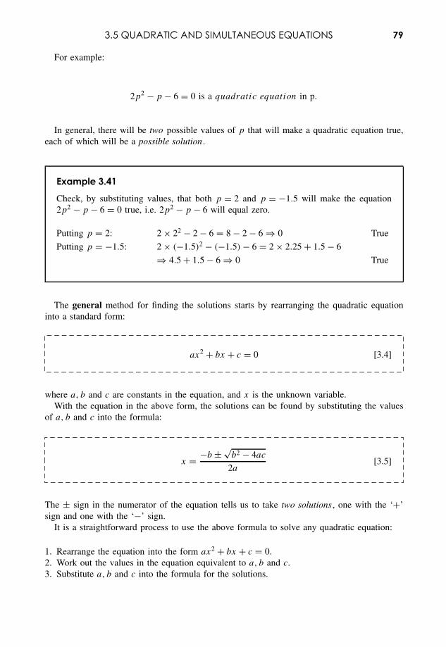
3.5 QUADRATIC AND SIMULTANEOUS EQUATIONS 79
For example:
2p2 − p − 6 = 0 is a quadratic equation in p.
In general, there will be two possible values of p that will make a quadratic equation true,each of which will be a possible solution .
Example 3.41
Check, by substituting values, that both p = 2 and p = −1.5 will make the equation2p2 − p − 6 = 0 true, i.e. 2p2 − p − 6 will equal zero.
Putting p = 2: 2 × 22 − 2 − 6 = 8 − 2 − 6 ⇒ 0 True
Putting p = −1.5: 2 × (−1.5)2 − (−1.5) − 6 = 2 × 2.25 + 1.5 − 6
⇒ 4.5 + 1.5 − 6 ⇒ 0 True
The general method for finding the solutions starts by rearranging the quadratic equationinto a standard form:
ax2 + bx + c = 0 [3.4]
where a, b and c are constants in the equation, and x is the unknown variable.With the equation in the above form, the solutions can be found by substituting the values
of a, b and c into the formula:
x = −b ± √b2 − 4ac
2a[3.5]
The ± sign in the numerator of the equation tells us to take two solutions , one with the ‘+’sign and one with the ‘−’ sign.
It is a straightforward process to use the above formula to solve any quadratic equation:
1. Rearrange the equation into the form ax2 + bx + c = 0.2. Work out the values in the equation equivalent to a, b and c.3. Substitute a, b and c into the formula for the solutions.
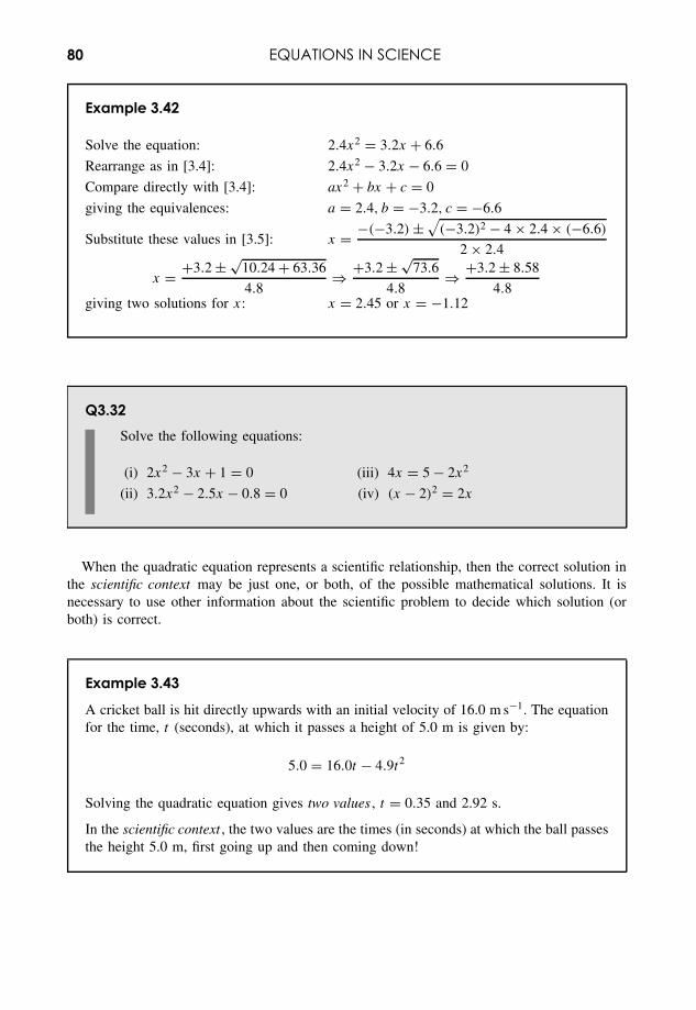
80 EQUATIONS IN SCIENCE
Example 3.42
Solve the equation: 2.4x2 = 3.2x + 6.6
Rearrange as in [3.4]: 2.4x2 − 3.2x − 6.6 = 0
Compare directly with [3.4]: ax2 + bx + c = 0
giving the equivalences: a = 2.4, b = −3.2, c = −6.6
Substitute these values in [3.5]: x = −(−3.2) ±√
(−3.2)2 − 4 × 2.4 × (−6.6)
2 × 2.4
x = +3.2 ± √10.24 + 63.36
4.8⇒ +3.2 ± √
73.6
4.8⇒ +3.2 ± 8.58
4.8giving two solutions for x: x = 2.45 or x = −1.12
Q3.32Solve the following equations:
(i) 2x2 − 3x + 1 = 0 (iii) 4x = 5 − 2x2
(ii) 3.2x2 − 2.5x − 0.8 = 0 (iv) (x − 2)2 = 2x
When the quadratic equation represents a scientific relationship, then the correct solution inthe scientific context may be just one, or both, of the possible mathematical solutions. It isnecessary to use other information about the scientific problem to decide which solution (orboth) is correct.
Example 3.43
A cricket ball is hit directly upwards with an initial velocity of 16.0 m s−1. The equationfor the time, t (seconds), at which it passes a height of 5.0 m is given by:
5.0 = 16.0t − 4.9t2
Solving the quadratic equation gives two values , t = 0.35 and 2.92 s.
In the scientific context , the two values are the times (in seconds) at which the ball passesthe height 5.0 m, first going up and then coming down!
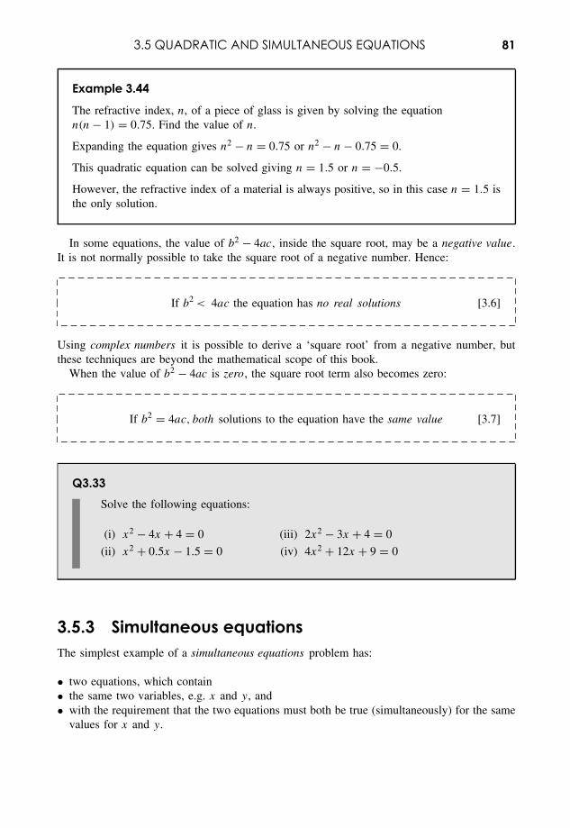
3.5 QUADRATIC AND SIMULTANEOUS EQUATIONS 81
Example 3.44
The refractive index, n, of a piece of glass is given by solving the equationn(n − 1) = 0.75. Find the value of n.
Expanding the equation gives n2 − n = 0.75 or n2 − n − 0.75 = 0.
This quadratic equation can be solved giving n = 1.5 or n = −0.5.
However, the refractive index of a material is always positive, so in this case n = 1.5 isthe only solution.
In some equations, the value of b2 − 4ac, inside the square root, may be a negative value.It is not normally possible to take the square root of a negative number. Hence:
If b2 < 4ac the equation has no real solutions [3.6]
Using complex numbers it is possible to derive a ‘square root’ from a negative number, butthese techniques are beyond the mathematical scope of this book.
When the value of b2 − 4ac is zero, the square root term also becomes zero:
If b2 = 4ac, both solutions to the equation have the same value [3.7]
Q3.33Solve the following equations:
(i) x2 − 4x + 4 = 0 (iii) 2x2 − 3x + 4 = 0
(ii) x2 + 0.5x − 1.5 = 0 (iv) 4x2 + 12x + 9 = 0
3.5.3 Simultaneous equationsThe simplest example of a simultaneous equations problem has:
• two equations, which contain• the same two variables, e.g. x and y, and• with the requirement that the two equations must both be true (simultaneously) for the same
values for x and y.
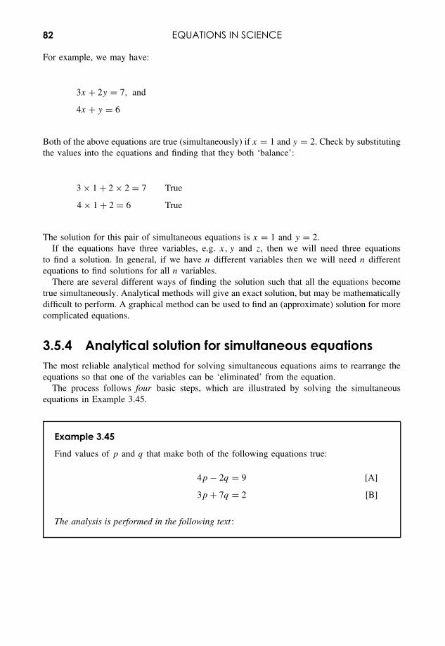
82 EQUATIONS IN SCIENCE
For example, we may have:
3x + 2y = 7, and
4x + y = 6
Both of the above equations are true (simultaneously) if x = 1 and y = 2. Check by substitutingthe values into the equations and finding that they both ‘balance’:
3 × 1 + 2 × 2 = 7 True
4 × 1 + 2 = 6 True
The solution for this pair of simultaneous equations is x = 1 and y = 2.If the equations have three variables, e.g. x, y and z, then we will need three equations
to find a solution. In general, if we have n different variables then we will need n differentequations to find solutions for all n variables.
There are several different ways of finding the solution such that all the equations becometrue simultaneously. Analytical methods will give an exact solution, but may be mathematicallydifficult to perform. A graphical method can be used to find an (approximate) solution for morecomplicated equations.
3.5.4 Analytical solution for simultaneous equationsThe most reliable analytical method for solving simultaneous equations aims to rearrange theequations so that one of the variables can be ‘eliminated’ from the equation.
The process follows four basic steps, which are illustrated by solving the simultaneousequations in Example 3.45.
Example 3.45
Find values of p and q that make both of the following equations true:
4p − 2q = 9 [A]
3p + 7q = 2 [B]
The analysis is performed in the following text :
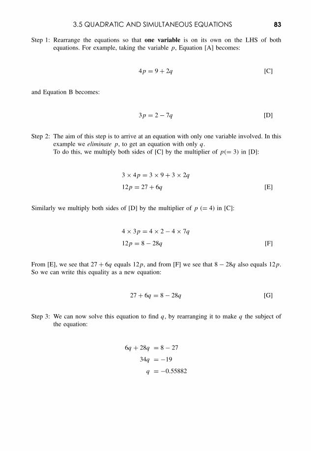
3.5 QUADRATIC AND SIMULTANEOUS EQUATIONS 83
Step 1: Rearrange the equations so that one variable is on its own on the LHS of bothequations. For example, taking the variable p, Equation [A] becomes:
4p = 9 + 2q [C]
and Equation B becomes:
3p = 2 − 7q [D]
Step 2: The aim of this step is to arrive at an equation with only one variable involved. In thisexample we eliminate p, to get an equation with only q.To do this, we multiply both sides of [C] by the multiplier of p(= 3) in [D]:
3 × 4p = 3 × 9 + 3 × 2q
12p = 27 + 6q [E]
Similarly we multiply both sides of [D] by the multiplier of p (= 4) in [C]:
4 × 3p = 4 × 2 − 4 × 7q
12p = 8 − 28q [F]
From [E], we see that 27 + 6q equals 12p, and from [F] we see that 8 − 28q also equals 12p.So we can write this equality as a new equation:
27 + 6q = 8 − 28q [G]
Step 3: We can now solve this equation to find q, by rearranging it to make q the subject ofthe equation:
6q + 28q = 8 − 27
34q = −19
q = −0.55882
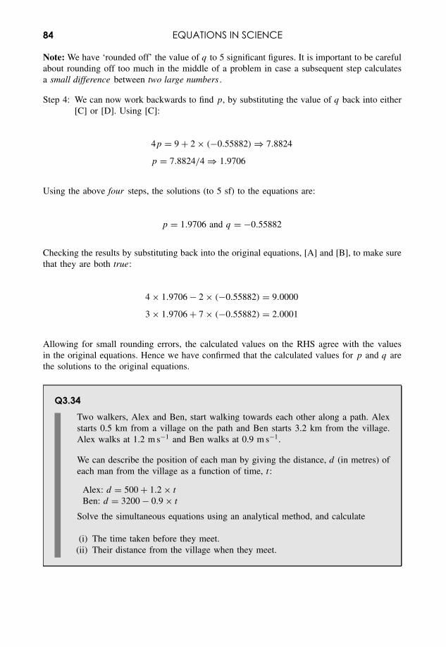
84 EQUATIONS IN SCIENCE
Note: We have ‘rounded off’ the value of q to 5 significant figures. It is important to be carefulabout rounding off too much in the middle of a problem in case a subsequent step calculatesa small difference between two large numbers .
Step 4: We can now work backwards to find p, by substituting the value of q back into either[C] or [D]. Using [C]:
4p = 9 + 2 × (−0.55882) ⇒ 7.8824
p = 7.8824/4 ⇒ 1.9706
Using the above four steps, the solutions (to 5 sf) to the equations are:
p = 1.9706 and q = −0.55882
Checking the results by substituting back into the original equations, [A] and [B], to make surethat they are both true:
4 × 1.9706 − 2 × (−0.55882) = 9.0000
3 × 1.9706 + 7 × (−0.55882) = 2.0001
Allowing for small rounding errors, the calculated values on the RHS agree with the valuesin the original equations. Hence we have confirmed that the calculated values for p and q arethe solutions to the original equations.
Q3.34Two walkers, Alex and Ben, start walking towards each other along a path. Alexstarts 0.5 km from a village on the path and Ben starts 3.2 km from the village.Alex walks at 1.2 m s−1 and Ben walks at 0.9 m s−1.
We can describe the position of each man by giving the distance, d (in metres) ofeach man from the village as a function of time, t :
Alex: d = 500 + 1.2 × t
Ben: d = 3200 − 0.9 × t
Solve the simultaneous equations using an analytical method, and calculate
(i) The time taken before they meet.(ii) Their distance from the village when they meet.
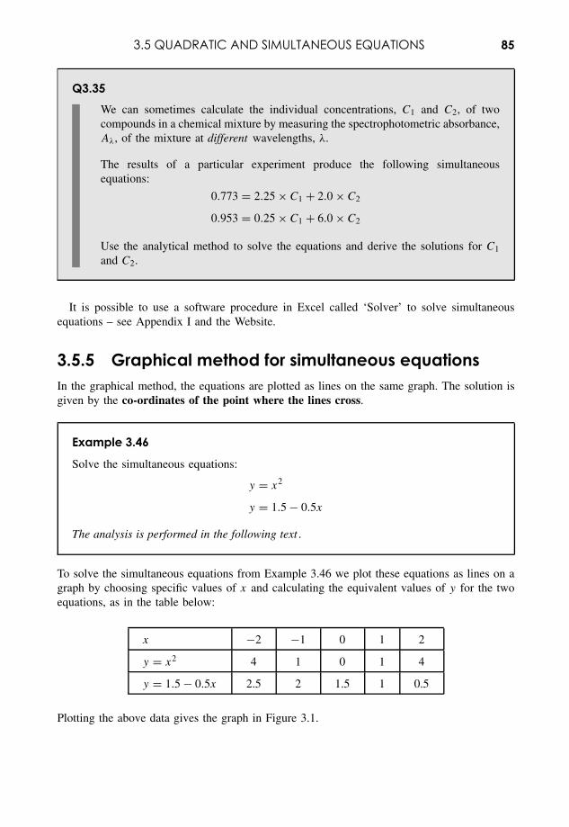
3.5 QUADRATIC AND SIMULTANEOUS EQUATIONS 85
Q3.35We can sometimes calculate the individual concentrations, C1 and C2, of twocompounds in a chemical mixture by measuring the spectrophotometric absorbance,Aλ, of the mixture at different wavelengths, λ.
The results of a particular experiment produce the following simultaneousequations:
0.773 = 2.25 × C1 + 2.0 × C2
0.953 = 0.25 × C1 + 6.0 × C2
Use the analytical method to solve the equations and derive the solutions for C1
and C2.
It is possible to use a software procedure in Excel called ‘Solver’ to solve simultaneousequations – see Appendix I and the Website.
3.5.5 Graphical method for simultaneous equationsIn the graphical method, the equations are plotted as lines on the same graph. The solution isgiven by the co-ordinates of the point where the lines cross.
Example 3.46
Solve the simultaneous equations:
y = x2
y = 1.5 − 0.5x
The analysis is performed in the following text .
To solve the simultaneous equations from Example 3.46 we plot these equations as lines on agraph by choosing specific values of x and calculating the equivalent values of y for the twoequations, as in the table below:
x −2 −1 0 1 2
y = x2 4 1 0 1 4
y = 1.5 − 0.5x 2.5 2 1.5 1 0.5
Plotting the above data gives the graph in Figure 3.1.
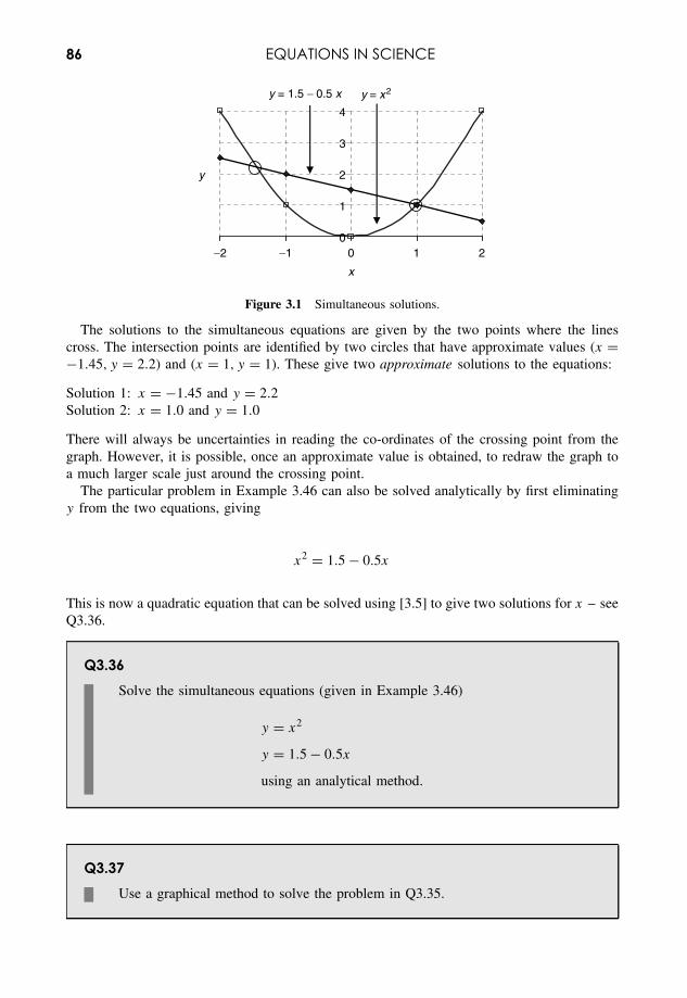
86 EQUATIONS IN SCIENCE
0
1
2
3
4
−2 −1 0 1 2
x
y
y = x2y = 1.5 − 0.5 x
Figure 3.1 Simultaneous solutions.
The solutions to the simultaneous equations are given by the two points where the linescross. The intersection points are identified by two circles that have approximate values (x =−1.45, y = 2.2) and (x = 1, y = 1). These give two approximate solutions to the equations:
Solution 1: x = −1.45 and y = 2.2Solution 2: x = 1.0 and y = 1.0
There will always be uncertainties in reading the co-ordinates of the crossing point from thegraph. However, it is possible, once an approximate value is obtained, to redraw the graph toa much larger scale just around the crossing point.
The particular problem in Example 3.46 can also be solved analytically by first eliminatingy from the two equations, giving
x2 = 1.5 − 0.5x
This is now a quadratic equation that can be solved using [3.5] to give two solutions for x – seeQ3.36.
Q3.36Solve the simultaneous equations (given in Example 3.46)
y = x2
y = 1.5 − 0.5x
using an analytical method.
Q3.37Use a graphical method to solve the problem in Q3.35.
4Linear Relationships
Overview
Website • ‘How to do it’ video answers for all ‘Q’ questions.• Excel tutorials: drawing x –y graphs, performing linear regression, use of
best-fit trendlines and calibration lines, linearization of scientific data.• Excel files appropriate to selected ‘Q’ questions and Examples.
The linear relationship is one of the most common mathematical relationships used in science,and is often described on an x –y graph by the equation:
y = mx + c
where m is the slope of the line, and c is the intercept of the line where it crosses they-axis.
Note that, in various contexts, the equation of the straight line is also often written asy = a + bx , where a is the intercept and b is the slope. However, for consistency in this book,we will always use the form y = mx + c.
As a simple example of a straight line relationship, the values for temperature in the Celsius,C, and Fahrenheit, F , scales are related by the linear equation:
F = 1.8 × C + 32 [4.1]
When plotted on an x –y graph, with F on the y-axis and C on the x-axis, the above relationshipappears as a straight line, as in Figure 4.1.
The slope, m, and intercept, c, of the straight line in Figure 4.1 are given by m = 1.8 andc = 32. The plotted data points show the temperatures for:
Melting ice, (0,32): C = 0 ◦C and F = 32 ◦F
Essential Mathematics and Statistics for Science 2nd Edition Graham Currell and Antony DowmanCopyright c© 2009 John Wiley & Sons, Ltd
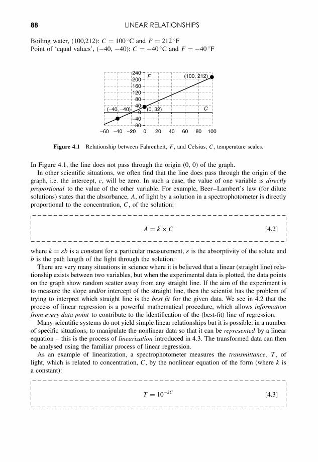
88 LINEAR RELATIONSHIPS
Boiling water, (100,212): C = 100 ◦C and F = 212 ◦FPoint of ‘equal values’, (−40, −40): C = −40 ◦C and F = −40 ◦F
−80−40
04080
120160200240
−60 −40 −20 0 20 40 60 80 100
F
C
(100, 212)
(−40, −40) (0, 32)
Figure 4.1 Relationship between Fahrenheit, F , and Celsius, C, temperature scales.
In Figure 4.1, the line does not pass through the origin (0, 0) of the graph.In other scientific situations, we often find that the line does pass through the origin of the
graph, i.e. the intercept, c, will be zero. In such a case, the value of one variable is directlyproportional to the value of the other variable. For example, Beer–Lambert’s law (for dilutesolutions) states that the absorbance, A, of light by a solution in a spectrophotometer is directlyproportional to the concentration, C, of the solution:
A = k × C [4.2]
where k = εb is a constant for a particular measurement, ε is the absorptivity of the solute andb is the path length of the light through the solution.
There are very many situations in science where it is believed that a linear (straight line) rela-tionship exists between two variables, but when the experimental data is plotted, the data pointson the graph show random scatter away from any straight line. If the aim of the experiment isto measure the slope and/or intercept of the straight line, then the scientist has the problem oftrying to interpret which straight line is the best fit for the given data. We see in 4.2 that theprocess of linear regression is a powerful mathematical procedure, which allows informationfrom every data point to contribute to the identification of the (best-fit) line of regression.
Many scientific systems do not yield simple linear relationships but it is possible, in a numberof specific situations, to manipulate the nonlinear data so that it can be represented by a linearequation – this is the process of linearization introduced in 4.3. The transformed data can thenbe analysed using the familiar process of linear regression.
As an example of linearization, a spectrophotometer measures the transmittance, T , oflight, which is related to concentration, C, by the nonlinear equation of the form (where k isa constant):
T = 10−kC [4.3]
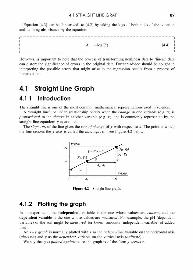
4.1 STRAIGHT LINE GRAPH 89
Equation [4.3] can be ‘linearized’ to [4.2] by taking the logs of both sides of the equationand defining absorbance by the equation:
A = −log(T ) [4.4]
However, is important to note that the process of transforming nonlinear data to ‘linear’ datacan distort the significance of errors in the original data. Further advice should be sought ininterpreting the possible errors that might arise in the regression results from a process oflinearization.
4.1 Straight Line Graph4.1.1 IntroductionThe straight line is one of the most common mathematical representations used in science.
A ‘straight line’, or linear, relationship occurs when the change in one variable (e.g. y) isproportional to the change in another variable (e.g. x), and is commonly represented by thestraight line equation: y = mx + c.
The slope, m, of the line gives the rate of change of y with respect to x. The point at whichthe line crosses the y-axis is called the intercept , c – see Figure 4.2 below.
y-axis
x-axis
y1
y2
y2−y1
x2x1
x2−x1
(x2, y2)
(x1, y1)
y = mx + c
c
q
0
Figure 4.2 Straight line graph.
4.1.2 Plotting the graphIn an experiment, the independent variable is the one whose values are chosen , and thedependent variable is the one whose values are measured . For example, the pH (dependentvariable) of the soil might be measured for known amounts (independent variable) of addedlime.
An x –y graph is normally plotted with x as the independent variable on the horizontal axis(abscissa) and y as the dependent variable on the vertical axis (ordinate).
We say that y is plotted against x, or the graph is of the form y versus x .
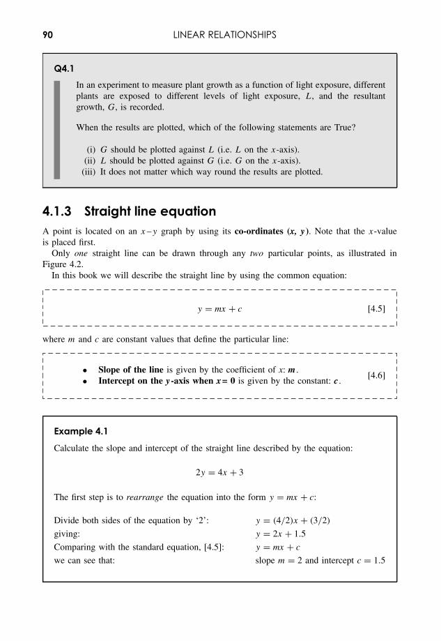
90 LINEAR RELATIONSHIPS
Q4.1In an experiment to measure plant growth as a function of light exposure, differentplants are exposed to different levels of light exposure, L, and the resultantgrowth, G, is recorded.
When the results are plotted, which of the following statements are True?
(i) G should be plotted against L (i.e. L on the x-axis).(ii) L should be plotted against G (i.e. G on the x-axis).
(iii) It does not matter which way round the results are plotted.
4.1.3 Straight line equationA point is located on an x –y graph by using its co-ordinates (x, y). Note that the x-valueis placed first.
Only one straight line can be drawn through any two particular points, as illustrated inFigure 4.2.
In this book we will describe the straight line by using the common equation:
y = mx + c [4.5]
where m and c are constant values that define the particular line:
• Slope of the line is given by the coefficient of x: m.
• Intercept on the y-axis when x= 0 is given by the constant: c.[4.6]
Example 4.1
Calculate the slope and intercept of the straight line described by the equation:
2y = 4x + 3
The first step is to rearrange the equation into the form y = mx + c:
Divide both sides of the equation by ‘2’: y = (4/2)x + (3/2)
giving: y = 2x + 1.5
Comparing with the standard equation, [4.5]: y = mx + c
we can see that: slope m = 2 and intercept c = 1.5
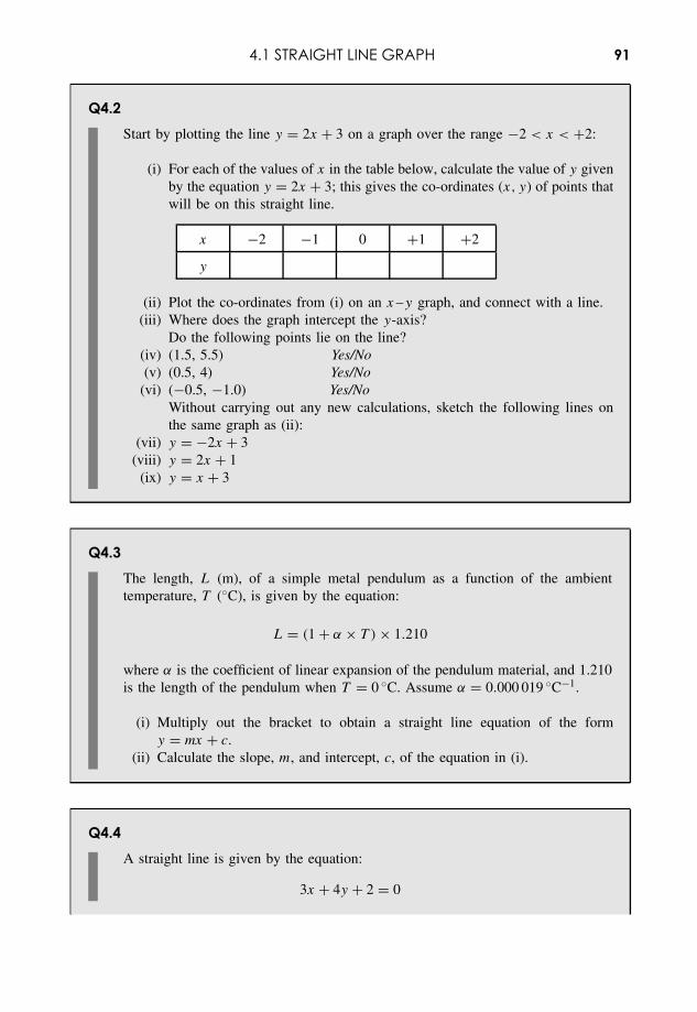
4.1 STRAIGHT LINE GRAPH 91
Q4.2Start by plotting the line y = 2x + 3 on a graph over the range −2 < x < +2:
(i) For each of the values of x in the table below, calculate the value of y givenby the equation y = 2x + 3; this gives the co-ordinates (x, y) of points thatwill be on this straight line.
x −2 −1 0 +1 +2
y
(ii) Plot the co-ordinates from (i) on an x –y graph, and connect with a line.(iii) Where does the graph intercept the y-axis?
Do the following points lie on the line?(iv) (1.5, 5.5) Yes/No(v) (0.5, 4) Yes/No
(vi) (−0.5, −1.0) Yes/NoWithout carrying out any new calculations, sketch the following lines onthe same graph as (ii):
(vii) y = −2x + 3(viii) y = 2x + 1
(ix) y = x + 3
Q4.3The length, L (m), of a simple metal pendulum as a function of the ambienttemperature, T (◦C), is given by the equation:
L = (1 + α × T ) × 1.210
where α is the coefficient of linear expansion of the pendulum material, and 1.210is the length of the pendulum when T = 0 ◦C. Assume α = 0.000 019 ◦C−1.
(i) Multiply out the bracket to obtain a straight line equation of the formy = mx + c.
(ii) Calculate the slope, m, and intercept, c, of the equation in (i).
Q4.4A straight line is given by the equation:
3x + 4y + 2 = 0
92 LINEAR RELATIONSHIPS
Rearrange the equation to make y the subject of the equation. Hence, calculate theslope and intercept of the line.
If a particular point with co-ordinates (x, y) lies on the line, then the values of x and y willmake the equation balance, i.e. the value of y will equal the value of mx + c and the equationwill be TRUE.
If the point (x, y) does not lie on the line, then the equation will not balance, and the valueof y will not equal the value of mx + c.
Example 4.2
The point (3,10) lies on the straight line y = 2x + 4:
Check by replacing x with ‘3’: 2x + 4 ⇒ 2 × 3 + 4 ⇒ 6 + 4 ⇒ 10
which balances with y = 10 – the equation is TRUE.
The point (4,14) does not lie on the straight line y = 2x + 4:
Check by replacing x with ‘4’: 2x + 4 ⇒ 2 × 4 + 4 ⇒ 8 + 4 ⇒ 12
which does not balance with y = 14.
It is often necessary to calculate a value for x, given a value of y on a known straight line.We need then to rearrange equation [4.5] to make x the subject of the equation:
x = (y − c)
m[4.7]
Q4.5A straight line (y = mx + c) has a slope of +4 and an intercept of −3. Calculatethe value of x when y = 4
Q4.6The cooking time for a joint of meat is written as 40 minutes per kilogram plus20 minutes.
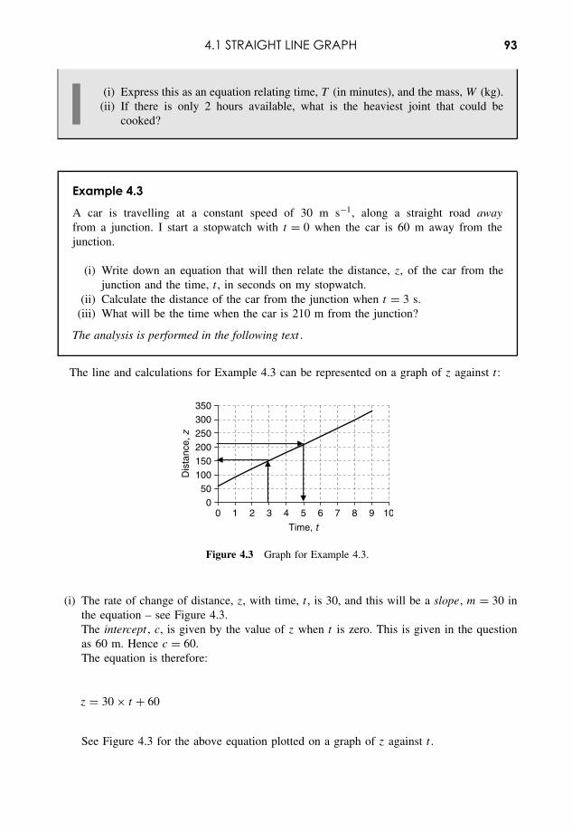
4.1 STRAIGHT LINE GRAPH 93
(i) Express this as an equation relating time, T (in minutes), and the mass, W (kg).(ii) If there is only 2 hours available, what is the heaviest joint that could be
cooked?
Example 4.3
A car is travelling at a constant speed of 30 m s−1, along a straight road awayfrom a junction. I start a stopwatch with t = 0 when the car is 60 m away from thejunction.
(i) Write down an equation that will then relate the distance, z, of the car from thejunction and the time, t , in seconds on my stopwatch.
(ii) Calculate the distance of the car from the junction when t = 3 s.(iii) What will be the time when the car is 210 m from the junction?
The analysis is performed in the following text .
The line and calculations for Example 4.3 can be represented on a graph of z against t :
050
100150200250300350
0 1 2 3 4 5 6 7 8 9 10
Time, t
Dis
tanc
e, z
Figure 4.3 Graph for Example 4.3.
(i) The rate of change of distance, z, with time, t , is 30, and this will be a slope, m = 30 inthe equation – see Figure 4.3.The intercept , c, is given by the value of z when t is zero. This is given in the questionas 60 m. Hence c = 60.The equation is therefore:
z = 30 × t + 60
See Figure 4.3 for the above equation plotted on a graph of z against t .
94 LINEAR RELATIONSHIPS
(ii) When t = 3, we can use the above equation to calculate:
z = 30 × 3 + 60 ⇒ 90 + 60 ⇒ 150 m
(iii) To find a value for t it is necessary to rearrange the above equation into the form givenby [4.7]:
t = (z − 60)
30
Substituting values gives: t = (210 − 60)/30 ⇒ 150/30 ⇒ 5 s.
Q4.7
A car is travelling at a constant speed of 20 m s−1 along a straight road towardsa junction. It is at a distance z = 140 m away from the junction when I start mystopwatch at time t = 0 s.
(i) Which of the following equations will now describe the motion of the car?(a) z = 20t + 140(b) z = 20t − 140(c) z = −20t + 140(d) z = −20t − 140
(ii) What will be the time when the car passes the junction?(iii) What will be the position of the car when t = 20 s?
4.1.4 Calculating slope and interceptThe slope, m , of the straight line (Figure 4.2) that passes through points (x1, y1) and (x2, y2)is given by the equation:
m = (y2 − y1)
(x2 − x1)or m = (y1 − y2)
(x1 − x2)[4.8]
The intercept, c, of the straight line is the value of y at the point where the line passes throughthe y-axis (Figure 4.2), i.e. the value of y when x = 0.
To calculate the equation of a straight line that passes through the two points (x1, y1) and(x2, y2):
1. Calculate the slope, m, using [4.8].
4.1 STRAIGHT LINE GRAPH 95
2. Substitute the value of m and the co-ordinates of one point (x1, y1) or (x2, y2) into[4.5] – this gives an equation where the intercept, c, is the only unknown value. Rearrangethe equation to make c the subject:
c = y1 − m × x1 or c = y2 − m × x2
and calculate the value of the intercept, c.
Example 4.4
Calculate the equation of the line that passes through the points (−2, 3) and (2, 1).
Calculating the slope:
m = (y2 − y1)
(x2 − x1)⇒ (1 − 3)
(2 − (−2))⇒ −2
(2 + 2)⇒ −2
4⇒ −0.5
Substitute m into the equation y2 = mx2 + c, with the co-ordinates x2 = 2 and y2 = 1:
1 = (−0.5) × 2 + c ⇒ −1 + c
Rearranging gives the intercept:
c = 1 + 1 = 2
The equation of the straight line is therefore:
y = −0.5x + 2
Q4.8Calculate the slopes of the straight lines which pass through each of the followingpairs of points:
(i) (1, 1) and (2, 3) (iv) (2.0, 3.0) and (1.0, 3.5)
(ii) (−1, 1) and (2, 3) (v) (0, 1) and (1, 0)
(iii) (1, 1) and (2, −3) (vi) (2.0, 3.0) and (1.0, −3.5)
In some cases where it is necessary to calculate the coefficients of a straight line, the slope,m, may already be known. It is then possible to go directly to step 2 in the calculation processoutlined above.
96 LINEAR RELATIONSHIPS
Q4.9Derive the equations of the straight line that has:
(i) a slope of 2.0 and passes through the point (0, 3)(ii) a slope of 0.5 and passes through the point (2, 3)
(iii) a slope of −0.5 and passes through the point (2, 3)
Q4.10If C represents the temperature in degrees Celsius and F represents the temperaturein degrees Fahrenheit, water boils at a temperature given by C = 100 and F = 212and water freezes at a temperature given by C = 0 and F = 32. Derive a straightline equation which will give F as a function of C.
Hence calculate the value of C when F = 0(hint: F and C become the y- and x-axes of a graph).
4.1.5 Intersecting linesIf two straight lines y = mAx + cA and y = mBx + cB meet at a point (x0, y0), then the valuesof x0 and y0 will make both equations true simultaneously :
y0 = mAx0 + cA
y0 = mBx0 + cB
Any unknown variables can (usually) be found by the methods of simultaneous equations.
Example 4.5
Calculate the co-ordinates of the crossing point for the two straight lines:
y = −0.5x + 2
y = x − 1
Using simultaneous equations (3.5.3) to ‘solve’ the above equations, we find that thevalues x = 2 and y = 1 will make both equations true simultaneously.
4.1 STRAIGHT LINE GRAPH 97
Substituting these values back into the above equations makes both equations TRUE.
The point (2, 1) therefore lies on both lines. This is the point where the lines cross .
4.1.6 Parallel and perpendicular linesParallel lines have the same slope:
mA = mB [4.9]
(but different intercepts, cA = cB).Perpendicular lines have slopes mA and mB given by the relationships:
mA = − 1
mBand mB = − 1
mA[4.10]
Example 4.6
Calculate the equation of the line which is perpendicular to the line y = −0.5x + 2 andpasses through the point (−2, 3).
The slope of the first line, mA = −0.5
Thus the slope of the perpendicular line, mB = −(
1
mA
)⇒ −
(1
−0.5
)⇒ 2
Substitute this value of m into the equation y = mBx + cB, with the co-ordinates (−2, 3),and calculate the value of the intercept, cB:
3 = 2 × (−2) + cB ⇒ −4 + cB
Hence cB = 7, and the equation of the line becomes: y = 2x + 7
Q4.11A second line is parallel to the line y = 3x + 2, and passes through the point(1,1). What is the equation of this second line?
98 LINEAR RELATIONSHIPS
Q4.12A second line is perpendicular to the line y = 3x + 2, and passes through thepoint (1,1). What is the equation of this second line?
Example 4.7
Write down the equation of the line that is parallel to the x-axis (horizontal) and passesthrough the y-axis at y = 2.5.
A line that is parallel to the x-axis has slope m = 0.
If the line passes through the y-axis at y = 2.5, then c = 2.5.
Hence the equation of line is:
y = 2.5
Whatever the value of x, the horizontal line gives the same value, y = 2.5.
Q4.13Write down the equation of the line that is parallel to the y-axis (vertical) andpasses through the x-axis at x = −1.5.
4.1.7 Interpolation and extrapolationThese are defined as follows:
Interpolation – finding the co-ordinates of a point on the line between existing points.Extrapolation – finding the co-ordinates of a point on the line outside existing points.
In both interpolation and extrapolation, it is necessary to calculate first the equation of the linethat passes through the two points, and then find the value of x (or y) equivalent to a newvalue of y (or x).
Q4.14A straight line passes through the points (2, 3) and (4, 4). Calculate the values of:
(i) y when x = 3.8 (iii) y where the line crosses the y-axis
(ii) x when y = 5.6 (iv) x where the line crosses the x-axis
4.2 LINEAR REGRESSION 99
Q4.15Initially, at time t = 0, the height, h, of a plant is 15 cm, and it then grows linearlyover a 20-day period, reaching a height of 20 cm. Derive a straight line equationwhich will give the height, h, as a function of the time, t , in days.
(i) What is the height when t = 5 days?(ii) Estimate the height of the tree 8 days after the end of the 20-day period,
assuming that it continues to grow at the same rate.
4.1.8 Angle of slopeThe angle, θ , between the line and the x-axis (Figure 4.2) is given by the equation:
tan(θ) = (y2 − y1)
(x2 − x1)= m [4.11]
The angle, θ , can then be calculated using the inverse tangent function (2.4.7):
θ = tan−1(m) or arctan(m) [4.12]
Q4.16A map shows the height contours on the side of a hill of fairly uniform slope. Apoint on the 250 m contour line is seen to be 400 m horizontally from a point onthe 200 m contour line.
(i) Calculate the average slope, m, between the two points.(ii) Calculate the average slope angle of the ground with respect to the horizontal.
4.2 Linear Regression4.2.1 IntroductionThere are very many situations in science where it is believed that a linear (straight line)relationship exists between two variables. However, when experimental data is plotted, thedata points on the graph show some random scatter away from any straight line. If the aim of
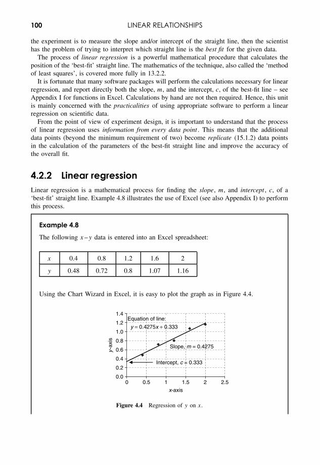
100 LINEAR RELATIONSHIPS
the experiment is to measure the slope and/or intercept of the straight line, then the scientisthas the problem of trying to interpret which straight line is the best fit for the given data.
The process of linear regression is a powerful mathematical procedure that calculates theposition of the ‘best-fit’ straight line. The mathematics of the technique, also called the ‘methodof least squares’, is covered more fully in 13.2.2.
It is fortunate that many software packages will perform the calculations necessary for linearregression, and report directly both the slope, m, and the intercept, c, of the best-fit line – seeAppendix I for functions in Excel. Calculations by hand are not then required. Hence, this unitis mainly concerned with the practicalities of using appropriate software to perform a linearregression on scientific data.
From the point of view of experiment design, it is important to understand that the processof linear regression uses information from every data point . This means that the additionaldata points (beyond the minimum requirement of two) become replicate (15.1.2) data pointsin the calculation of the parameters of the best-fit straight line and improve the accuracy ofthe overall fit.
4.2.2 Linear regressionLinear regression is a mathematical process for finding the slope, m, and intercept , c, of a‘best-fit’ straight line. Example 4.8 illustrates the use of Excel (see also Appendix I) to performthis process.
Example 4.8
The following x –y data is entered into an Excel spreadsheet:
x 0.4 0.8 1.2 1.6 2
y 0.48 0.72 0.8 1.07 1.16
Using the Chart Wizard in Excel, it is easy to plot the graph as in Figure 4.4.
y = 0.4275x + 0.333
0.0
0.2
0.4
0.6
0.8
1.0
1.2
1.4
0 0.5 1 1.5 2 2.5
x-axis
y-a
xis
Slope, m = 0.4275
Equation of line:
Intercept, c = 0.333
Figure 4.4 Regression of y on x.
4.2 LINEAR REGRESSION 101
The best-fit straight line is drawn using the Linear Trendline option in Excel, which canalso print the equation of the line on the graph.
The best-fit straight line in Figure 4.4 is called the line of regression of y on x .The process of linear regression assumes that the only significant uncertainties are in the
y-direction . The x-values for each data point are assumed to be accurate.The line of regression of x on y (note reversal of x and y) will usually give a slightly
different line.
Q4.17The heart rates of athletes were measured 3 minutes after completing a series of‘step-ups’ at different rates. If a process of linear regression is to be used to analysethe relationship between step-up rate and heart rate, decide which variable shouldbe plotted on the y-axis and which variable on the x-axis.
4.2.3 Regression and correlationIt is important to know the difference (see also Chapter 13) between regression andcorrelation:
Linear correlation is a specific measure of the extent to which the values of two variablesare known to change in a way that could be described by a straight line equation . The useof linear correlation as a statistical test is introduced in 13.1.3.
Linear regression is a process that can be used to calculate the slope and intercept of a best-fitlinear equation after it has been shown that two variables are indeed linearly correlated.
Q4.18In each of the following situations, one variable is plotted against another, but it isnecessary to decide whether to test for correlation between the variables or carryout a regression analysis . (The process of carrying out a test for correlation isgiven in 13.1.3.)
(i) Aluminium levels are recorded against sizes of fishpopulations to investigate whether the level of alu-minium in river water affects the size of the fishpopulation.
Correlation/Regression
(ii) The increase in oxygen consumption of a species ofsmall mammal is measured as a function of bodyweight, in order to derive an equation that relates thetwo factors.
Correlation/Regression
102 LINEAR RELATIONSHIPS
(iii) A researcher records the abundance of heather plantsas a function of soil pH in different areas to see if thepH has an effect on the survival of the plant.
Correlation/Regression
(iv) Student marks are recorded for both coursework andexamination to see if good students generally performwell in both and weaker students perform badly inboth.
Correlation/Regression
4.2.4 Software calculationsExcel and other statistical software can be used to calculate both the slope and intercept of thebest-fit line of regression through a set of data points – see Appendix I:
Excel Functions, fx :
• SLOPE – calculates the best-fit slope (with no restriction on the intercept)• INTERCEPT – calculates the best-fit intercept• LINEST – calculates the best-fit slope (can be used to force zero intercept).
(Functions in Excel give dynamic results, which change if the input values change.)
Excel Data Analysis Tools:
• Regression options calculate slope and intercept (plus other data), and can force theintercept to be zero (c = 0).
(Data Analysis Tools in Excel are non-dynamic, giving a ‘one-off’ calculation.)
Excel Trendline:
• Calculates slope and intercept, and can force the intercept to be any chosen value.
The slope and intercept can be displayed on the chart but cannot be used directly in furthercalculations. It may be necessary to format Trendline in order to show an appropriate numberof significant figures for these values.
Other statistics software packages will produce similar results. For example, Minitab pro-duces results for slope, m, and intercept, c, in the ‘equation’ form:
C2 = c + m C1
where C1 and C2 are the columns in Minitab that hold the x- and y-data respectively.
4.2 LINEAR REGRESSION 103
Example 4.9
In an experiment to measure the relationship between the variables P and Q, the valuesof P were measured for specific values of Q, and the data entered into rows 1 and 2 ofan Excel spreadsheet as below:
A B C D E F
1 Q 1 3 5 7 9
2 P 3.9 7.2 7.9 12.5 13.6
3 Slope = 1.235 Intercept = 2.845
The entry ‘= SLOPE(B2:F2,B1:F1)’ into cell B3 of the Excel spreadsheet gives the slopeof the best-fit line, m = 1.235.
And the entry ‘= INTERCEPT(B2:F2,B1:F1)’ into cell E3 of the Excel spreadsheet givesthe intercept of the best-fit line, c = 2.845.
The two expressions for SLOPE and INTERCEPT assume that cells B2 to F2 hold the‘y-data’ and cells B1 to F1 hold the ‘x-data’.
Q4.19Using the data from Example 4.9:
(i) Write down the equation of the line of regression, P on Q.(ii) Plot the original data, plus the line of regression, on a graph.
(iii) Using the results from (i), calculate the value of P on the line of regressionequivalent to a value of Q = 3.4.
Q4.20The data in the table below gives the result of a spectrophotometric measurement,where the y variable is the absorbance, A, and the x variable is the concentration,C (mmol L−1).
C (x) 10 15 20 25
A (y) 0.37 0.48 0.7 0.81
104 LINEAR RELATIONSHIPS
Use Excel and/or other statistics software to perform a linear regression to obtainvalues for:
(i) Slope of the best-fit straight line.(ii) Intercept of the best-fit straight line.
4.2.5 Forcing zero interceptSometimes it is known that the best-fit straight line should pass through the origin of the graph,i.e. have zero intercept, c = 0.
Excel can be used to perform a linear regression while forcing a zero intercept using any ofthe following methods – see Appendix I:
• Function LINEST• Data Analysis Tools > Regression• Graph Trendline (can force the intercept to be any chosen value).
In Minitab it is possible to force a zero intercept by clicking ‘Options. . .’ in the Regressiondialogue box and checking the Fit Intercept option.
Q4.21Using the same data as in Q4.20, make the assumption that the best-fit straight lineshould pass through the origin of the A versus C graph.
Calculate the slope of the line of regression with zero intercept using:
(i) Excel function LINEST(ii) Excel Data Analysis Tools
(iii) Excel Trendline(iv) Other statistics software
4.2.6 Calibration lineThe process of linear regression is frequently used to produce a best-fit calibration line. Forexample, spectrophotometric measurements often measure the absorbances, A, of solutionsof known concentrations, C, and plot the best-fit straight line of A against C. The linearrelationship can then be used to calculate the concentration, CO, of the unknown solution froma measured value of its absorbance, AO.
A line of linear regression is drawn (Figure 4.5) using n data points of known values of y,corresponding to known values of x (calibration data). The coefficients of the line of regression
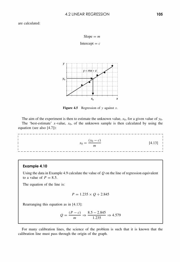
4.2 LINEAR REGRESSION 105
are calculated:
Slope = m
Intercept = c
y
yo
xo x
y = mx + c
Figure 4.5 Regression of y against x.
The aim of the experiment is then to estimate the unknown value, x0, for a given value of y0.The ‘best-estimate’ x-value, x0, of the unknown sample is then calculated by using the
equation (see also [4.7]):
x0 = (y0 − c)
m[4.13]
Example 4.10
Using the data in Example 4.9 calculate the value of Q on the line of regression equivalentto a value of P = 8.5.
The equation of the line is:
P = 1.235 × Q + 2.845
Rearranging this equation as in [4.13]:
Q = (P − c)
m⇒ 8.5 − 2.845
1.235⇒ 4.579
For many calibration lines, the science of the problem is such that it is known that thecalibration line must pass through the origin of the graph.
106 LINEAR RELATIONSHIPS
For example, in a spectrophotometric measurement it may be known that:
• the absorbance of the solution obeys Beer’s Law (A = k × C); and• the spectrophotometer was accurately set up so that a solution of zero concentration records
an absorbance of zero.
Then we can assume that the calibration line must pass through the origin of the graph of A
against C.In this case, we can force the line of regression to pass through the origin and ensure that
the intercept c = 0.
Q4.22Different masses w (in grams) of a sugar were dissolved in 100 mL of water andthe angle of rotation θ (in degrees) of polarized light in the solution was measuredin a polarimeter. The following results were obtained.
w(g) 1.5 3 4.5 6 7.5
θ (degrees) 1.3 2.7 4 5.2 6.6
(i) Assuming that pure water gives no rotation, find the best-fit equation for θ interms of w.
(ii) Calculate the best estimate of w for a sugar solution that gives a rotation of 4.9◦.
4.2.7 Interpolation and extrapolation errorsThe processes of interpolation and extrapolation were introduced in 4.1.7.
There is inherent uncertainty in the values for the slope, m, and intercept, c, calculatedusing linear regression. Hence there will also be uncertainty in the calculation of the value,xO, when using [4.13].
The calculation for the experimental uncertainty in the final value for xO is given in 13.3.3.From this calculation it is possible to draw some general conclusions.
The calibration data should be chosen such that the unknown test value falls within thecentral half of the calibration range. For example, if the calibration data covers absorbancesfrom 0.2 to 0.6 (not forcing through the origin), then, ideally, the absorbance of the test solutionshould fall within the range from 0.3 to 0.5.
Provided that the test data falls within this central calibration range, then equation [13.9] isa good estimation of the overall uncertainty in the final value of xO.
As the interpolated test values move towards the ends of the calibration range, then theuncertainties will increase – see Figure 13.7.
If the test values fall outside the range of calibration data (extrapolation) then theuncertainties will begin to increase very rapidly, and great care must be taken in usingextrapolated values.
Good experimental design should take the above considerations into account when planningthe choice of calibration values.
4.3 LINEARIZATION 107
4.3 Linearization4.3.1 IntroductionWe have seen (4.2) how the mathematics of linear regression is a simple, yet powerful, pro-cedure that can be used to identify a best-fit straight line in a set of data that is expectedto follow a linear relationship. However, many scientific systems do not yield simple linearrelationships.
There are statistical methods for fitting data to specific types of curves using nonlinearregression but these methods are beyond the scope of this book. As an alternative to theuse of nonlinear regression, it is possible, in a number of specific situations, to manipulatethe nonlinear data so that it can be represented by a linear equation – this is the processof linearization . The transformed data can then be analysed using the familiar process oflinear regression. However, it is important to note (4.3.4) that the process of transforming thenonlinear data can distort the significance of errors in the original data.
4.3.2 General principlesLinearization is a mathematical process whereby a nonlinear equation (e.g. involving variablesP and Q) can be represented as a straight line on a suitable graph.
The original equation must be manipulated in such a way that it appears in the form:
f(P ) = m × f(Q) + c [4.14]
where f(P ) and f(Q) are functions of the original variables, P and Q, respectively.The above equation is in the same form as the straight line equation:
y = m × x + c
and we can see that plotting f(P ) against f(Q) (in place of y and x) will give a straight linewith a slope m and an intercept c.
There are three common ways of linearizing a nonlinear function:
• Change of variable.• Using logarithms (log or ln) to bring powers down onto the equation line.• Using natural logarithms for an exponential equation.
In this chapter we only consider the ‘change of variable’ method.Section 5.1.8 outlines the method for using logarithms to linearize equations with power
terms of the form T = k × Ln, where T and L are variables but n is an unknown constant.Section 5.2.6 outlines the procedure for linearizing exponential equations of the form
Nt = N0ekt , where Nt and t are the variables.
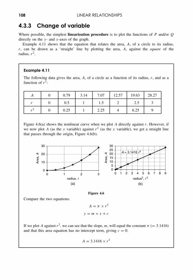
108 LINEAR RELATIONSHIPS
4.3.3 Change of variableWhere possible, the simplest linearization procedure is to plot the functions of P and/or Q
directly on the y- and x-axes of the graph.Example 4.11 shows that the equation that relates the area, A, of a circle to its radius,
r , can be drawn as a ‘straight’ line by plotting the area, A, against the square of theradius, r2.
Example 4.11
The following data gives the area, A, of a circle as a function of its radius, r , and as afunction of r2:
A 0 0.79 3.14 7.07 12.57 19.63 28.27
r 0 0.5 1 1.5 2 2.5 3
r2 0 0.25 1 2.25 4 6.25 9
Figure 4.6(a) shows the nonlinear curve when we plot A directly against r . However, ifwe now plot A (as the y variable) against r2 (as the x variable), we get a straight linethat passes through the origin, Figure 4.6(b).
(a) (b)
0
10
20
30
0 1 2 3radius, r
Are
a, A
05
1015202530
0 1 2 3 4 5 6 7 8 9
radius2, r 2
Are
a, A
A = 3.1416 r2
Figure 4.6
Compare the two equations:
A = π × r2
y = m × x + c
If we plot A against r2, we can see that the slope, m, will equal the constant π (= 3.1416)and that this area equation has no intercept term, giving c = 0:
A = 3.1416 × r2
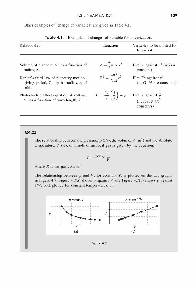
4.3 LINEARIZATION 109
Other examples of ‘change of variables’ are given in Table 4.1.
Table 4.1. Examples of changes of variable for linearization.
Relationship Equation Variables to be plotted forlinearization
Volume of a sphere, V , as a function ofradius, r
V = 4
3π × r3 Plot V against r3 (π is a
constant)
Kepler’s third law of planetary motiongiving period, T , against radius, r , oforbit
T 2 = 4π2
GMr3 Plot T 2 against r3
(π, G, M are constants)
Photoelectric effect equation of voltage,V , as a function of wavelength, λ
V = hc
e
(1
λ
)− φ Plot V against
1
λ(h, c, e, φ areconstants)
Q4.23
The relationship between the pressure, p (Pa), the volume, V (m3) and the absolutetemperature, T (K), of 1 mole of an ideal gas is given by the equation:
p = RT × 1
V
where R is the gas constant.
The relationship between p and V , for constant T , is plotted on the two graphsin Figure 4.7. Figure 4.7(a) shows p against V and Figure 4.7(b) shows p against1/V , both plotted for constant temperatures, T .
p versus V
V
p
p versus 1/V
1/V
(a) (b)
p
Figure 4.7
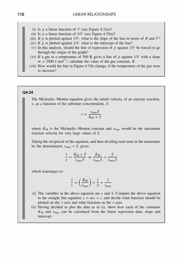
110 LINEAR RELATIONSHIPS
(i) Is p a linear function of V (see Figure 4.7(a))?(ii) Is p a linear function of 1/V (see Figure 4.7(b))?
(iii) If p is plotted against 1/V , what is the slope of the line in terms of R and T ?(iv) If p is plotted against 1/V , what is the intercept of the line?(v) In this analysis, should the line of regression of p against 1/V be forced to go
through the origin of the graph?(vi) If a gas at a temperature of 300 K gives a line of p against 1/V with a slope
m = 2500 J mol−1, calculate the value of the gas constant, R.(vii) How would the line in Figure 4.7(b) change, if the temperature of the gas were
to increase?
Q4.24The Michaelis–Menten equation gives the initial velocity of an enzyme reaction,v, as a function of the substrate concentration, S:
ν = vmaxS
KM + S
where KM is the Michaelis–Menten constant and vmax would be the maximumreaction velocity for very large values of S.
Taking the reciprocal of the equation, and then dividing each term in the numeratorby the denominator, vmax × S, gives:
1
ν= KM + S
vmaxS⇒ KM
vmaxS+ S
vmaxS
which rearranges to:
1
ν=
(KM
vmax
)× 1
S+ 1
vmax
(i) The variables in the above equation are v and S. Compare the above equationto the straight line equation y = mx + c, and decide what function should beplotted on the y-axis and what function on the x-axis.
(ii) Having decided to plot the data as in (i), show how each of the constantsKM and vmax can be calculated from the linear regression data: slope andintercept.

4.3 LINEARIZATION 111
4.3.4 Error warningWhen using a linearization technique for nonlinear data, the transformation process will alsoact on the errors in the data points, and this can have the effect of distorting the importanceof some of the points in the final regression process.
It is always important to be careful about interpreting the accuracy of results obtained bya linearization process, and possibly seek further guidance, particularly when relying on theaccuracy of an extrapolated value.

5Logarithmic and ExponentialFunctions
Overview
Website • ‘How to do it’ video answers for all ‘Q’ questions.• Excel tutorials: use of powers, logarithms, exponentials, linearization of expo-
nential functions.
Logarithmic and exponential functions in mathematics are particularly useful (and common)in science because they can be used as accurate models for many real-world processes.
The mathematics of these functions can be handled very easily, provided that a few basicrules are learnt. The first unit here (5.1) concentrates on developing an understanding that willdirectly underpin the use of the functions in a scientific context.
The exponential function is particularly important in modelling growth or decay systems inall branches of science, e.g. elimination of a drug from the bloodstream, radioactive decay,bacterial growth, etc. Although these processes are all based on the same mathematics, thescientists in different areas have developed different ways of quantifying the processes. Forexample:
• ‘1 log’ decay (or ‘2 log’, ‘3 log’, etc.) in drug elimination;• ‘generation time’ in bacterial growth;• ‘time constant’ in electronic circuits.
The second unit (5.2) demonstrates that it is easy to compare numerical calculations based onthese different historical methods.
We see in 5.1.5 that a logarithm is essentially the inverse function of an exponential function.However, logarithms also have an important modelling role in their own right, particularly insystems where a multiplication of an input to a system produces an additive effect on theoutput, e.g. in decibel and pH scales.
The student will also often meet the use of logarithmic scales on graphs. These may be usedto linearize an exponential function (5.2.6) or may simply be used to condense data whichcovers a wide data range.
Essential Mathematics and Statistics for Science 2nd Edition Graham Currell and Antony DowmanCopyright c© 2009 John Wiley & Sons, Ltd
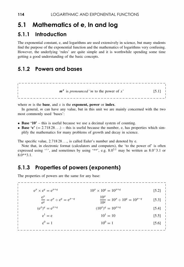
114 LOGARITHMIC AND EXPONENTIAL FUNCTIONS
5.1 Mathematics of e, ln and log5.1.1 IntroductionThe exponential constant, e, and logarithms are used extensively in science, but many studentsfind the purpose of the exponential function and the mathematics of logarithms very confusing.However, the underlying ‘rules’ are quite simple and it is worthwhile spending some timegetting a good understanding of the basic concepts.
5.1.2 Powers and bases
mx is pronounced ‘m to the power of x’ [5.1]
where m is the base, and x is the exponent, power or index.In general, m can have any value, but in this unit we are mainly concerned with the two
most commonly used ‘bases’:
• Base ‘10’ – this is useful because we use a decimal system of counting.• Base ‘e’ (= 2.718 28 . . .) – this is useful because the number, e, has properties which sim-
plify the mathematics for many problems of growth and decay in science.
The specific value, 2.718 28 . . ., is called Euler’s number and denoted by e.Note that, in electronic format (calculators and computers), the ‘to the power of’ is often
expressed using ‘∧’, and sometimes by using ‘**’, e.g. 8.03.1 may be written as 8.0∧3.1 or8.0**3.1.
5.1.3 Properties of powers (exponents)The properties of powers are the same for any base:
ep × eq = ep+q 10p × 10q = 10p+q [5.2]
ep
eq= ep ÷ eq = ep−q 10p
10q= 10p ÷ 10q = 10p−q [5.3]
(ep)q = ep×q (10p)q = 10p×q [5.4]
e1 = e 101 = 10 [5.5]
e0 = 1 100 = 1 [5.6]
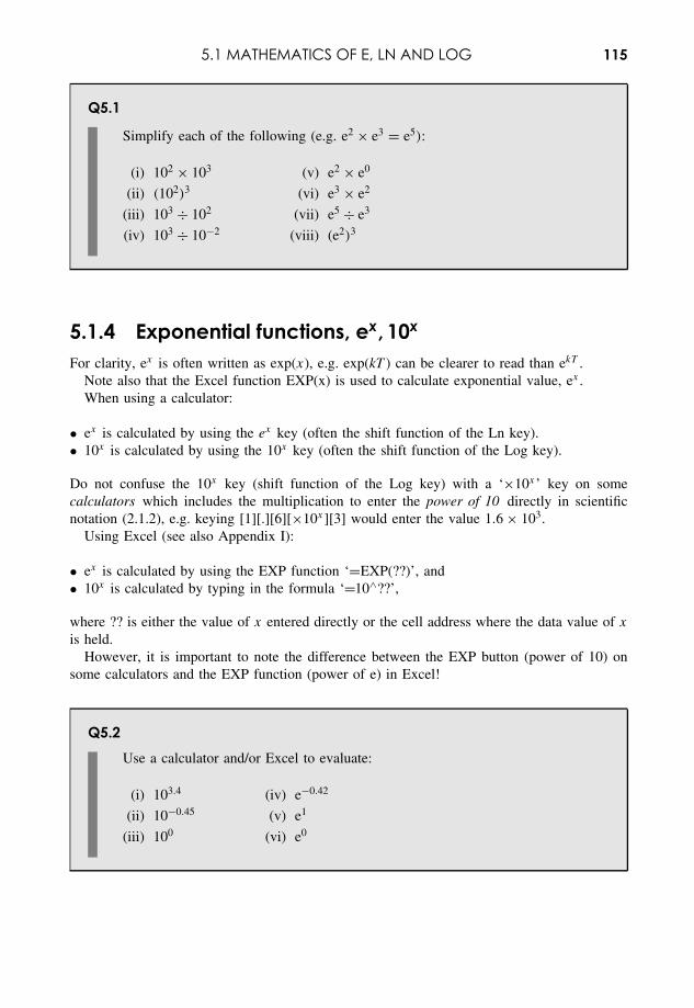
5.1 MATHEMATICS OF E, LN AND LOG 115
Q5.1
Simplify each of the following (e.g. e2 × e3 = e5):
(i) 102 × 103 (v) e2 × e0
(ii) (102)3 (vi) e3 × e2
(iii) 103 ÷ 102 (vii) e5 ÷ e3
(iv) 103 ÷ 10−2 (viii) (e2)3
5.1.4 Exponential functions, ex, 10x
For clarity, ex is often written as exp(x), e.g. exp(kT ) can be clearer to read than ekT .Note also that the Excel function EXP(x) is used to calculate exponential value, ex .When using a calculator:
• ex is calculated by using the ex key (often the shift function of the Ln key).• 10x is calculated by using the 10x key (often the shift function of the Log key).
Do not confuse the 10x key (shift function of the Log key) with a ‘×10x’ key on somecalculators which includes the multiplication to enter the power of 10 directly in scientificnotation (2.1.2), e.g. keying [1][.][6][×10x ][3] would enter the value 1.6 × 10³.
Using Excel (see also Appendix I):
• ex is calculated by using the EXP function ‘=EXP(??)’, and• 10x is calculated by typing in the formula ‘=10∧??’,
where ?? is either the value of x entered directly or the cell address where the data value of x
is held.However, it is important to note the difference between the EXP button (power of 10) on
some calculators and the EXP function (power of e) in Excel!
Q5.2Use a calculator and/or Excel to evaluate:
(i) 103.4 (iv) e−0.42
(ii) 10−0.45 (v) e1
(iii) 100 (vi) e0
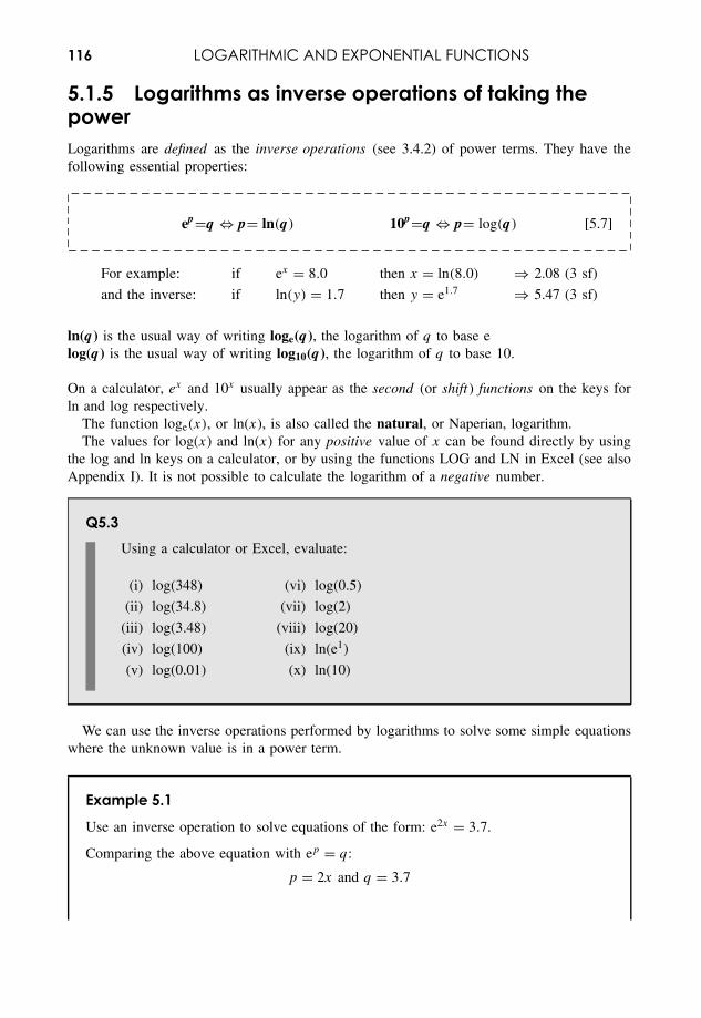
116 LOGARITHMIC AND EXPONENTIAL FUNCTIONS
5.1.5 Logarithms as inverse operations of taking thepowerLogarithms are defined as the inverse operations (see 3.4.2) of power terms. They have thefollowing essential properties:
ep=q ⇔ p= ln(q) 10p=q ⇔ p= log(q) [5.7]
For example: if ex = 8.0 then x = ln(8.0) ⇒ 2.08 (3 sf)
and the inverse: if ln(y) = 1.7 then y = e1.7 ⇒ 5.47 (3 sf)
ln(q) is the usual way of writing loge(q), the logarithm of q to base elog(q) is the usual way of writing log10(q), the logarithm of q to base 10.
On a calculator, ex and 10x usually appear as the second (or shift) functions on the keys forln and log respectively.
The function loge(x), or ln(x), is also called the natural, or Naperian, logarithm.The values for log(x) and ln(x) for any positive value of x can be found directly by using
the log and ln keys on a calculator, or by using the functions LOG and LN in Excel (see alsoAppendix I). It is not possible to calculate the logarithm of a negative number.
Q5.3Using a calculator or Excel, evaluate:
(i) log(348) (vi) log(0.5)
(ii) log(34.8) (vii) log(2)
(iii) log(3.48) (viii) log(20)
(iv) log(100) (ix) ln(e1)
(v) log(0.01) (x) ln(10)
We can use the inverse operations performed by logarithms to solve some simple equationswhere the unknown value is in a power term.
Example 5.1
Use an inverse operation to solve equations of the form: e2x = 3.7.
Comparing the above equation with ep = q:
p = 2x and q = 3.7
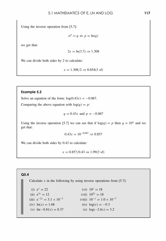
5.1 MATHEMATICS OF E, LN AND LOG 117
Using the inverse operation from [5.7]:
ep = q ⇔ p = ln(q)
we get that:
2x = ln(3.7) ⇒ 1.308
We can divide both sides by 2 to calculate:
x = 1.308/2 ⇒ 0.654(3 sf)
Example 5.2
Solve an equation of the form: log(0.43x) = −0.067.
Comparing the above equation with log(q) = p:
q = 0.43x and p = −0.067
Using the inverse operation [5.7] we can see that if log(q) = p then q = 10p and weget that:
0.43x = 10−0.067 ⇒ 0.857
We can divide both sides by 0.43 to calculate:
x = 0.857/0.43 ⇒ 1.99(3 sf)
Q5.4Calculate x in the following by using inverse operations from [5.7]:
(i) ex = 22 (vi) 10x = 18
(ii) e3x = 12 (vii) 102x = 18
(iii) e−2x = 3.1 × 10⁻³ (viii) 10−x = 1.0 × 10⁻⁷
(iv) ln(x) = 1.68 (ix) log(x) = −9.3
(v) ln(−0.81x) = 0.37 (x) log(−2.6x) = 3.2
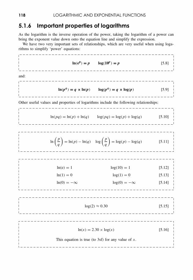
118 LOGARITHMIC AND EXPONENTIAL FUNCTIONS
5.1.6 Important properties of logarithmsAs the logarithm is the inverse operation of the power, taking the logarithm of a power canbring the exponent value down onto the equation line and simplify the expression.
We have two very important sets of relationships, which are very useful when using loga-rithms to simplify ‘power’ equations:
ln(ep) = p log(10p) = p [5.8]
and:
ln(pq ) = q × ln(p) log(pq ) = q × log(p) [5.9]
Other useful values and properties of logarithms include the following relationships:
ln(pq) = ln(p) + ln(q) log(pq) = log(p) + log(q) [5.10]
ln
(p
q
)= ln(p) − ln(q) log
(p
q
)= log(p) − log(q) [5.11]
ln(e) = 1 log(10) = 1 [5.12]
ln(1) = 0 log(1) = 0 [5.13]
ln(0) = −∞ log(0) = −∞ [5.14]
log(2) ≈ 0.30 [5.15]
ln(x) = 2.30 × log(x) [5.16]
This equation is true (to 3sf) for any value of x.
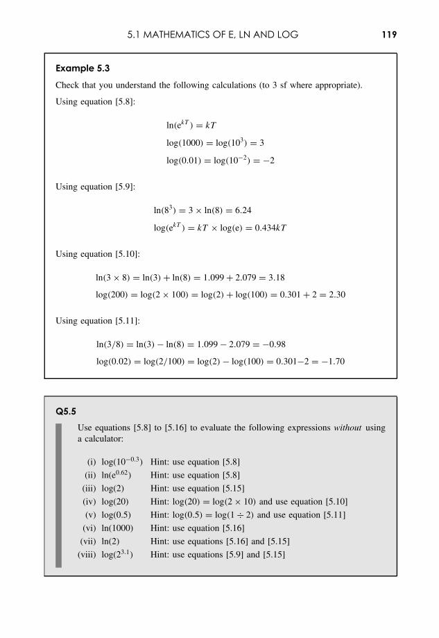
5.1 MATHEMATICS OF E, LN AND LOG 119
Example 5.3
Check that you understand the following calculations (to 3 sf where appropriate).
Using equation [5.8]:
ln(ekT ) = kT
log(1000) = log(103) = 3
log(0.01) = log(10−2) = −2
Using equation [5.9]:
ln(83) = 3 × ln(8) = 6.24
log(ekT ) = kT × log(e) = 0.434kT
Using equation [5.10]:
ln(3 × 8) = ln(3) + ln(8) = 1.099 + 2.079 = 3.18
log(200) = log(2 × 100) = log(2) + log(100) = 0.301 + 2 = 2.30
Using equation [5.11]:
ln(3/8) = ln(3) − ln(8) = 1.099 − 2.079 = −0.98
log(0.02) = log(2/100) = log(2) − log(100) = 0.301−2 = −1.70
Q5.5Use equations [5.8] to [5.16] to evaluate the following expressions without usinga calculator:
(i) log(10−0.3) Hint: use equation [5.8]
(ii) ln(e0.62) Hint: use equation [5.8]
(iii) log(2) Hint: use equation [5.15]
(iv) log(20) Hint: log(20) = log(2 × 10) and use equation [5.10]
(v) log(0.5) Hint: log(0.5) = log(1 ÷ 2) and use equation [5.11]
(vi) ln(1000) Hint: use equation [5.16]
(vii) ln(2) Hint: use equations [5.16] and [5.15]
(viii) log(23.1) Hint: use equations [5.9] and [5.15]
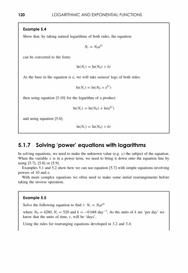
120 LOGARITHMIC AND EXPONENTIAL FUNCTIONS
Example 5.4
Show that, by taking natural logarithms of both sides, the equation:
Nt = N0ekt
can be converted to the form:
ln(Nt) = ln(N0) + kt
As the base in the equation is e, we will take natural logs of both sides:
ln(Nt ) = ln(N0 × ekt )
then using equation [5.10] for the logarithm of a product:
ln(Nt ) = ln(N0) + ln(ekt )
and using equation [5.8]:
ln(Nt) = ln(N0) + kt
5.1.7 Solving ‘power’ equations with logarithmsIn solving equations, we need to make the unknown value (e.g. x) the subject of the equation.When the variable x is in a power term, we need to bring it down onto the equation line byusing [5.7], [5.8] or [5.9].
Examples 5.1 and 5.2 show how we can use equation [5.7] with simple equations involvingpowers of 10 and e.
With more complex equations we often need to make some initial rearrangements beforetaking the inverse operation.
Example 5.5
Solve the following equation to find t : Nt = N0ekt
where N0 = 4260, Nt = 520 and k = −0.048 day−1. As the units of k are ‘per day’ weknow that the units of time, t , will be ‘days’.
Using the rules for rearranging equations developed in 3.2 and 3.4:
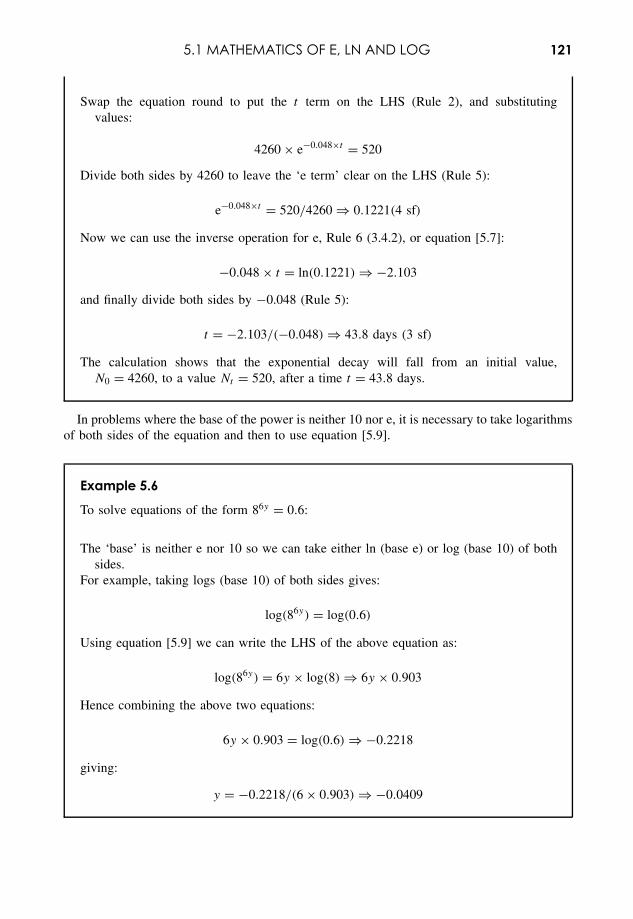
5.1 MATHEMATICS OF E, LN AND LOG 121
Swap the equation round to put the t term on the LHS (Rule 2), and substitutingvalues:
4260 × e−0.048×t = 520
Divide both sides by 4260 to leave the ‘e term’ clear on the LHS (Rule 5):
e−0.048×t = 520/4260 ⇒ 0.1221(4 sf)
Now we can use the inverse operation for e, Rule 6 (3.4.2), or equation [5.7]:
−0.048 × t = ln(0.1221) ⇒ −2.103
and finally divide both sides by −0.048 (Rule 5):
t = −2.103/(−0.048) ⇒ 43.8 days (3 sf)
The calculation shows that the exponential decay will fall from an initial value,N0 = 4260, to a value Nt = 520, after a time t = 43.8 days.
In problems where the base of the power is neither 10 nor e, it is necessary to take logarithmsof both sides of the equation and then to use equation [5.9].
Example 5.6
To solve equations of the form 86y = 0.6:
The ‘base’ is neither e nor 10 so we can take either ln (base e) or log (base 10) of bothsides.
For example, taking logs (base 10) of both sides gives:
log(86y) = log(0.6)
Using equation [5.9] we can write the LHS of the above equation as:
log(86y) = 6y × log(8) ⇒ 6y × 0.903
Hence combining the above two equations:
6y × 0.903 = log(0.6) ⇒ −0.2218
giving:
y = −0.2218/(6 × 0.903) ⇒ −0.0409
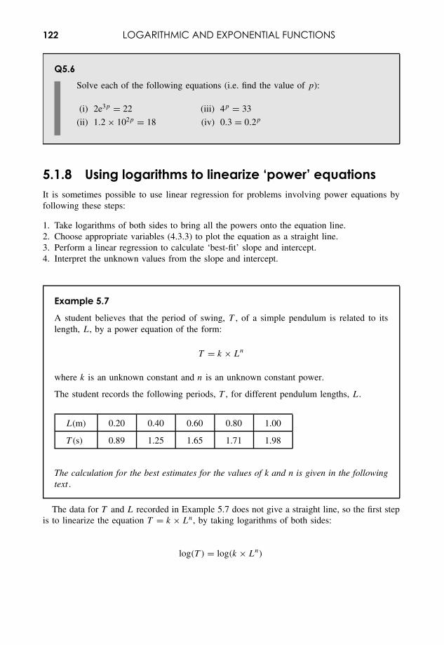
122 LOGARITHMIC AND EXPONENTIAL FUNCTIONS
Q5.6Solve each of the following equations (i.e. find the value of p):
(i) 2e3p = 22 (iii) 4p = 33
(ii) 1.2 × 10²p = 18 (iv) 0.3 = 0.2p
5.1.8 Using logarithms to linearize ‘power’ equationsIt is sometimes possible to use linear regression for problems involving power equations byfollowing these steps:
1. Take logarithms of both sides to bring all the powers onto the equation line.2. Choose appropriate variables (4.3.3) to plot the equation as a straight line.3. Perform a linear regression to calculate ‘best-fit’ slope and intercept.4. Interpret the unknown values from the slope and intercept.
Example 5.7
A student believes that the period of swing, T , of a simple pendulum is related to itslength, L, by a power equation of the form:
T = k × Ln
where k is an unknown constant and n is an unknown constant power.
The student records the following periods, T , for different pendulum lengths, L.
L(m) 0.20 0.40 0.60 0.80 1.00
T (s) 0.89 1.25 1.65 1.71 1.98
The calculation for the best estimates for the values of k and n is given in the followingtext .
The data for T and L recorded in Example 5.7 does not give a straight line, so the first stepis to linearize the equation T = k × Ln, by taking logarithms of both sides:
log(T ) = log(k × Ln)
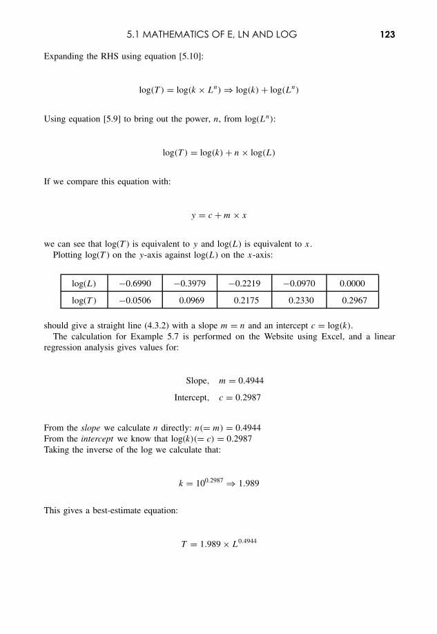
5.1 MATHEMATICS OF E, LN AND LOG 123
Expanding the RHS using equation [5.10]:
log(T ) = log(k × Ln) ⇒ log(k) + log(Ln)
Using equation [5.9] to bring out the power, n, from log(Ln):
log(T ) = log(k) + n × log(L)
If we compare this equation with:
y = c + m × x
we can see that log(T ) is equivalent to y and log(L) is equivalent to x.Plotting log(T ) on the y-axis against log(L) on the x-axis:
log(L) −0.6990 −0.3979 −0.2219 −0.0970 0.0000
log(T ) −0.0506 0.0969 0.2175 0.2330 0.2967
should give a straight line (4.3.2) with a slope m = n and an intercept c = log(k).The calculation for Example 5.7 is performed on the Website using Excel, and a linear
regression analysis gives values for:
Slope, m = 0.4944
Intercept, c = 0.2987
From the slope we calculate n directly: n(= m) = 0.4944From the intercept we know that log(k)(= c) = 0.2987Taking the inverse of the log we calculate that:
k = 100.2987 ⇒ 1.989
This gives a best-estimate equation:
T = 1.989 × L0.4944
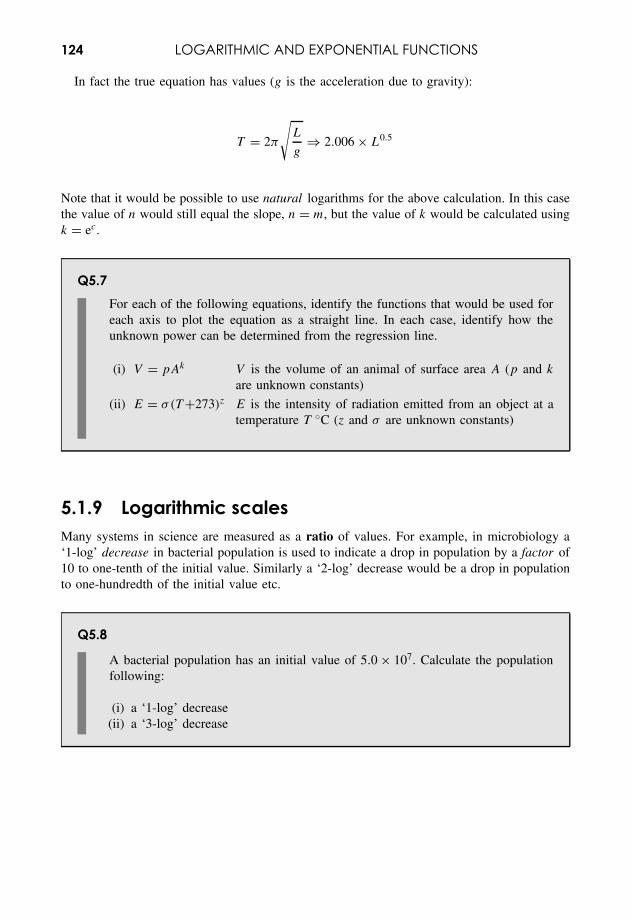
124 LOGARITHMIC AND EXPONENTIAL FUNCTIONS
In fact the true equation has values (g is the acceleration due to gravity):
T = 2π
√L
g⇒ 2.006 × L0.5
Note that it would be possible to use natural logarithms for the above calculation. In this casethe value of n would still equal the slope, n = m, but the value of k would be calculated usingk = ec.
Q5.7For each of the following equations, identify the functions that would be used foreach axis to plot the equation as a straight line. In each case, identify how theunknown power can be determined from the regression line.
(i) V = pAk V is the volume of an animal of surface area A (p and k
are unknown constants)
(ii) E = σ(T +273)z E is the intensity of radiation emitted from an object at atemperature T ◦C (z and σ are unknown constants)
5.1.9 Logarithmic scalesMany systems in science are measured as a ratio of values. For example, in microbiology a‘1-log’ decrease in bacterial population is used to indicate a drop in population by a factor of10 to one-tenth of the initial value. Similarly a ‘2-log’ decrease would be a drop in populationto one-hundredth of the initial value etc.
Q5.8
A bacterial population has an initial value of 5.0 × 10⁷. Calculate the populationfollowing:
(i) a ‘1-log’ decrease(ii) a ‘3-log’ decrease
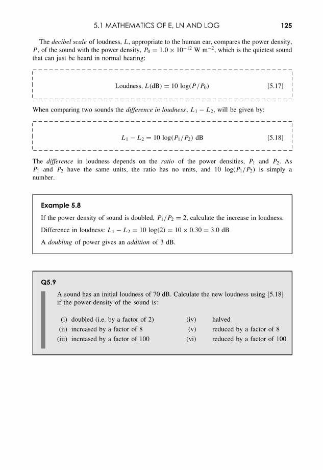
5.1 MATHEMATICS OF E, LN AND LOG 125
The decibel scale of loudness, L, appropriate to the human ear, compares the power density,P , of the sound with the power density, P0 = 1.0 × 10⁻¹² W m−2, which is the quietest soundthat can just be heard in normal hearing:
Loudness, L(dB) = 10 log(P/P0) [5.17]
When comparing two sounds the difference in loudness , L1 − L2, will be given by:
L1 − L2 = 10 log(P1/P2) dB [5.18]
The difference in loudness depends on the ratio of the power densities, P1 and P2. AsP1 and P2 have the same units, the ratio has no units, and 10 log(P1/P2) is simply anumber.
Example 5.8
If the power density of sound is doubled, P1/P2 = 2, calculate the increase in loudness.
Difference in loudness: L1 − L2 = 10 log(2) = 10 × 0.30 = 3.0 dB
A doubling of power gives an addition of 3 dB.
Q5.9A sound has an initial loudness of 70 dB. Calculate the new loudness using [5.18]if the power density of the sound is:
(i) doubled (i.e. by a factor of 2) (iv) halved
(ii) increased by a factor of 8 (v) reduced by a factor of 8
(iii) increased by a factor of 100 (vi) reduced by a factor of 100
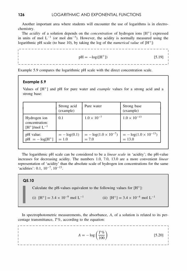
126 LOGARITHMIC AND EXPONENTIAL FUNCTIONS
Another important area where students will encounter the use of logarithms is in electro-chemistry.
The acidity of a solution depends on the concentration of hydrogen ions [H+] expressedin units of mol L−1 (or mol dm−3). However, the acidity is normally measured using thelogarithmic pH scale (to base 10), by taking the log of the numerical value of [H+]:
pH = −log([H+]) [5.19]
Example 5.9 compares the logarithmic pH scale with the direct concentration scale.
Example 5.9
Values of [H+] and pH for pure water and example values for a strong acid and astrong base:
Strong acid Pure water Strong base(example) (example)
Hydrogen ionconcentration:[H+]/mol L−1
0.1 1.0 × 10⁻⁷ 1.0 × 10⁻¹³
pH value:pH = − log[H+]
= − log(0.1)
= 1.0= − log(1.0 × 10⁻⁷)
= 7.0= − log(1.0 × 10⁻¹³)
= 13.0
The logarithmic pH scale can be considered to be a linear scale in ‘acidity’; the pH-valueincreases for decreasing acidity. The numbers 1.0, 7.0, 13.0 are a more convenient linearrepresentation of ‘acidity’ than the absolute scale of hydrogen ion concentrations for the same‘acidities’: 0.1, 10−7, 10−13.
Q5.10
Calculate the pH-values equivalent to the following values for [H+]:
(i) [H+] = 3.4 × 10⁻⁹ mol L−1 (ii) [H+] = 3.4 × 10⁻⁴ mol L−1
In spectrophotometric measurements, the absorbance, A, of a solution is related to its per-centage transmittance, T %, according to the equation:
A = − log
(T %
100
)[5.20]
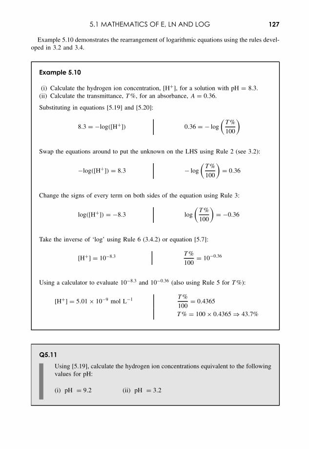
5.1 MATHEMATICS OF E, LN AND LOG 127
Example 5.10 demonstrates the rearrangement of logarithmic equations using the rules devel-oped in 3.2 and 3.4.
Example 5.10
(i) Calculate the hydrogen ion concentration, [H+], for a solution with pH = 8.3.(ii) Calculate the transmittance, T %, for an absorbance, A = 0.36.
Substituting in equations [5.19] and [5.20]:
8.3 = −log([H+]) 0.36 = − log
(T %
100
)
Swap the equations around to put the unknown on the LHS using Rule 2 (see 3.2):
−log([H+]) = 8.3 − log
(T %
100
)= 0.36
Change the signs of every term on both sides of the equation using Rule 3:
log([H+]) = −8.3 log
(T %
100
)= −0.36
Take the inverse of ‘log’ using Rule 6 (3.4.2) or equation [5.7]:
[H+] = 10−8.3 T %
100= 10−0.36
Using a calculator to evaluate 10−8.3 and 10−0.36 (also using Rule 5 for T %):
[H+] = 5.01 × 10⁻⁹ mol L−1 T %
100= 0.4365
T % = 100 × 0.4365 ⇒ 43.7%
Q5.11Using [5.19], calculate the hydrogen ion concentrations equivalent to the followingvalues for pH:
(i) pH = 9.2 (ii) pH = 3.2
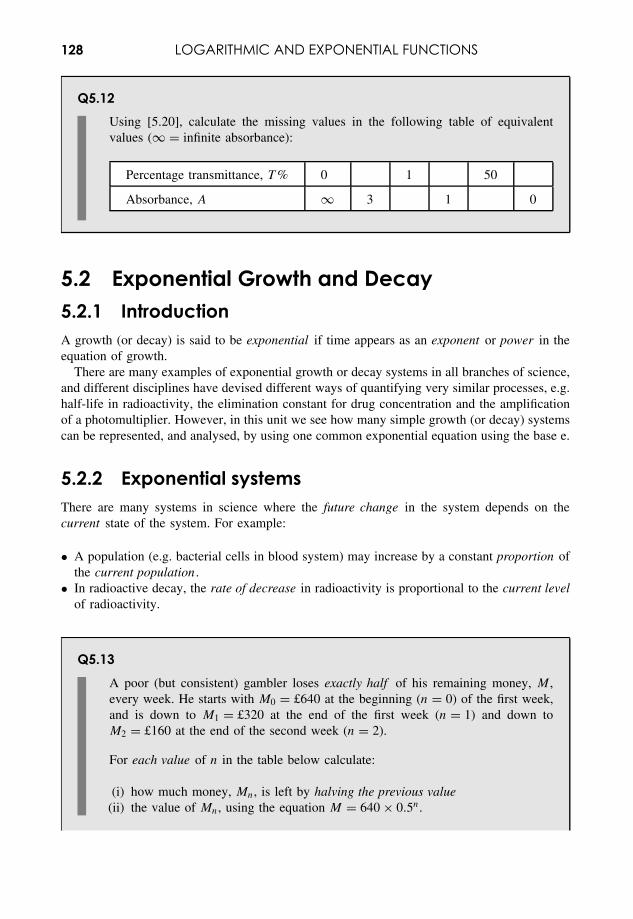
128 LOGARITHMIC AND EXPONENTIAL FUNCTIONS
Q5.12Using [5.20], calculate the missing values in the following table of equivalentvalues (∞ = infinite absorbance):
Percentage transmittance, T % 0 1 50
Absorbance, A ∞ 3 1 0
5.2 Exponential Growth and Decay5.2.1 IntroductionA growth (or decay) is said to be exponential if time appears as an exponent or power in theequation of growth.
There are many examples of exponential growth or decay systems in all branches of science,and different disciplines have devised different ways of quantifying very similar processes, e.g.half-life in radioactivity, the elimination constant for drug concentration and the amplificationof a photomultiplier. However, in this unit we see how many simple growth (or decay) systemscan be represented, and analysed, by using one common exponential equation using the base e.
5.2.2 Exponential systemsThere are many systems in science where the future change in the system depends on thecurrent state of the system. For example:
• A population (e.g. bacterial cells in blood system) may increase by a constant proportion ofthe current population .
• In radioactive decay, the rate of decrease in radioactivity is proportional to the current levelof radioactivity.
Q5.13A poor (but consistent) gambler loses exactly half of his remaining money, M ,every week. He starts with M0 = £640 at the beginning (n = 0) of the first week,and is down to M1 = £320 at the end of the first week (n = 1) and down toM2 = £160 at the end of the second week (n = 2).
For each value of n in the table below calculate:
(i) how much money, Mn, is left by halving the previous value(ii) the value of Mn, using the equation M = 640 × 0.5n.
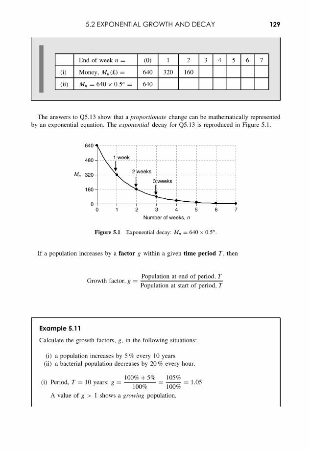
5.2 EXPONENTIAL GROWTH AND DECAY 129
End of week n = (0) 1 2 3 4 5 6 7
(i) Money, Mn(£) = 640 320 160
(ii) Mn = 640 × 0.5n = 640
The answers to Q5.13 show that a proportionate change can be mathematically representedby an exponential equation. The exponential decay for Q5.13 is reproduced in Figure 5.1.
0
160
320
480
640
0 1 2 3 4 5 6 7
Number of weeks, n
1 week
Mn2 weeks
3 weeks
Figure 5.1 Exponential decay: Mn = 640 × 0.5n.
If a population increases by a factor g within a given time period T , then
Growth factor, g = Population at end of period, T
Population at start of period, T
Example 5.11
Calculate the growth factors, g, in the following situations:
(i) a population increases by 5 % every 10 years(ii) a bacterial population decreases by 20 % every hour.
(i) Period, T = 10 years: g = 100% + 5%
100%= 105%
100%= 1.05
A value of g > 1 shows a growing population.
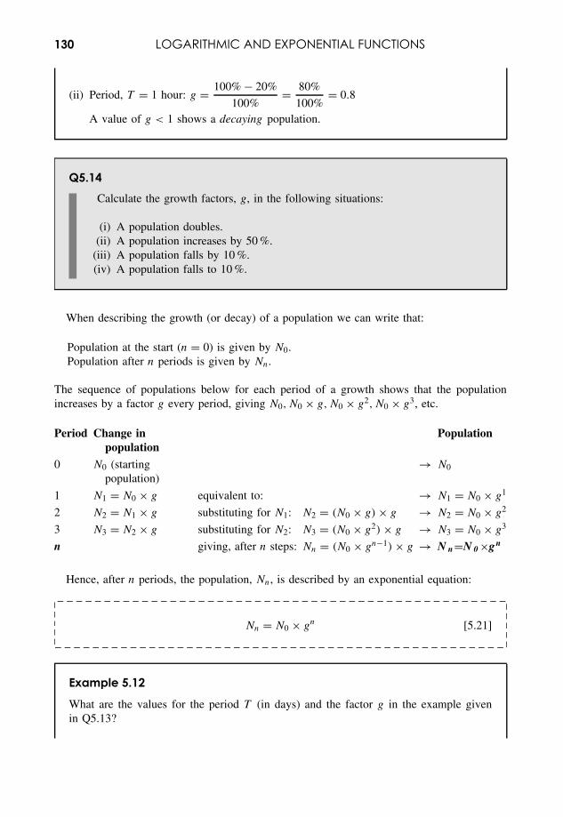
130 LOGARITHMIC AND EXPONENTIAL FUNCTIONS
(ii) Period, T = 1 hour: g = 100% − 20%
100%= 80%
100%= 0.8
A value of g < 1 shows a decaying population.
Q5.14Calculate the growth factors, g, in the following situations:
(i) A population doubles.(ii) A population increases by 50 %.
(iii) A population falls by 10 %.(iv) A population falls to 10 %.
When describing the growth (or decay) of a population we can write that:
Population at the start (n = 0) is given by N0.Population after n periods is given by Nn.
The sequence of populations below for each period of a growth shows that the populationincreases by a factor g every period, giving N0, N0 × g, N0 × g2, N0 × g3, etc.
Period Change inpopulation
Population
0 N0 (startingpopulation)
→ N0
1 N1 = N0 × g equivalent to: → N1 = N0 × g1
2 N2 = N1 × g substituting for N1: N2 = (N0 × g) × g → N2 = N0 × g2
3 N3 = N2 × g substituting for N2: N3 = (N0 × g2) × g → N3 = N0 × g3
n giving, after n steps: Nn = (N0 × gn−1) × g → N n=N 0 ×gn
Hence, after n periods, the population, Nn, is described by an exponential equation:
Nn = N0 × gn [5.21]
Example 5.12
What are the values for the period T (in days) and the factor g in the example givenin Q5.13?
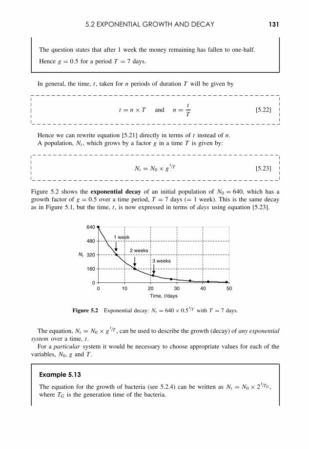
5.2 EXPONENTIAL GROWTH AND DECAY 131
The question states that after 1 week the money remaining has fallen to one-half.
Hence g = 0.5 for a period T = 7 days.
In general, the time, t , taken for n periods of duration T will be given by
t = n × T and n = t
T[5.22]
Hence we can rewrite equation [5.21] directly in terms of t instead of n.A population, Nt , which grows by a factor g in a time T is given by:
Nt = N0 × gt/T [5.23]
Figure 5.2 shows the exponential decay of an initial population of N0 = 640, which has agrowth factor of g = 0.5 over a time period, T = 7 days (= 1 week). This is the same decayas in Figure 5.1, but the time, t , is now expressed in terms of days using equation [5.23].
0
160
320
480
640
0 10 20 30 40 50
Time, t /days
1 week
Nt2 weeks
3 weeks
Figure 5.2 Exponential decay: Nt = 640 × 0.5t/T with T = 7 days.
The equation, Nt = N0 × gt/T , can be used to describe the growth (decay) of any exponential
system over a time, t .For a particular system it would be necessary to choose appropriate values for each of the
variables, N0, g and T .
Example 5.13
The equation for the growth of bacteria (see 5.2.4) can be written as Nt = N0 × 2t/TG ,
where TG is the generation time of the bacteria.
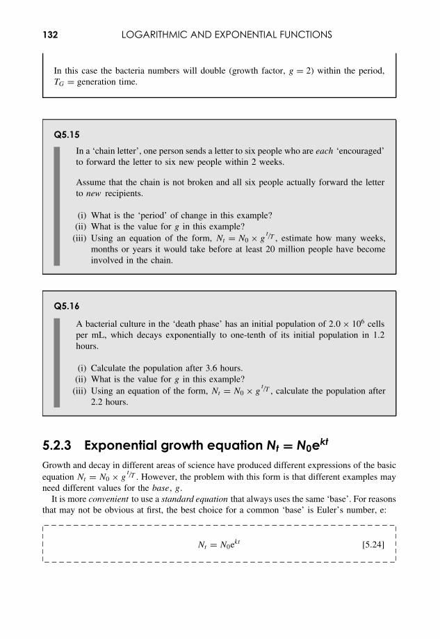
132 LOGARITHMIC AND EXPONENTIAL FUNCTIONS
In this case the bacteria numbers will double (growth factor, g = 2) within the period,TG = generation time.
Q5.15In a ‘chain letter’, one person sends a letter to six people who are each ‘encouraged’to forward the letter to six new people within 2 weeks.
Assume that the chain is not broken and all six people actually forward the letterto new recipients.
(i) What is the ‘period’ of change in this example?(ii) What is the value for g in this example?
(iii) Using an equation of the form, Nt = N0 × gt/T , estimate how many weeks,
months or years it would take before at least 20 million people have becomeinvolved in the chain.
Q5.16
A bacterial culture in the ‘death phase’ has an initial population of 2.0 × 10⁶ cellsper mL, which decays exponentially to one-tenth of its initial population in 1.2hours.
(i) Calculate the population after 3.6 hours.(ii) What is the value for g in this example?
(iii) Using an equation of the form, Nt = N0 × gt/T , calculate the population after
2.2 hours.
5.2.3 Exponential growth equation Nt = N0ekt
Growth and decay in different areas of science have produced different expressions of the basicequation Nt = N0 × g
t/T . However, the problem with this form is that different examples mayneed different values for the base, g.
It is more convenient to use a standard equation that always uses the same ‘base’. For reasonsthat may not be obvious at first, the best choice for a common ‘base’ is Euler’s number, e:
Nt = N0ekt [5.24]
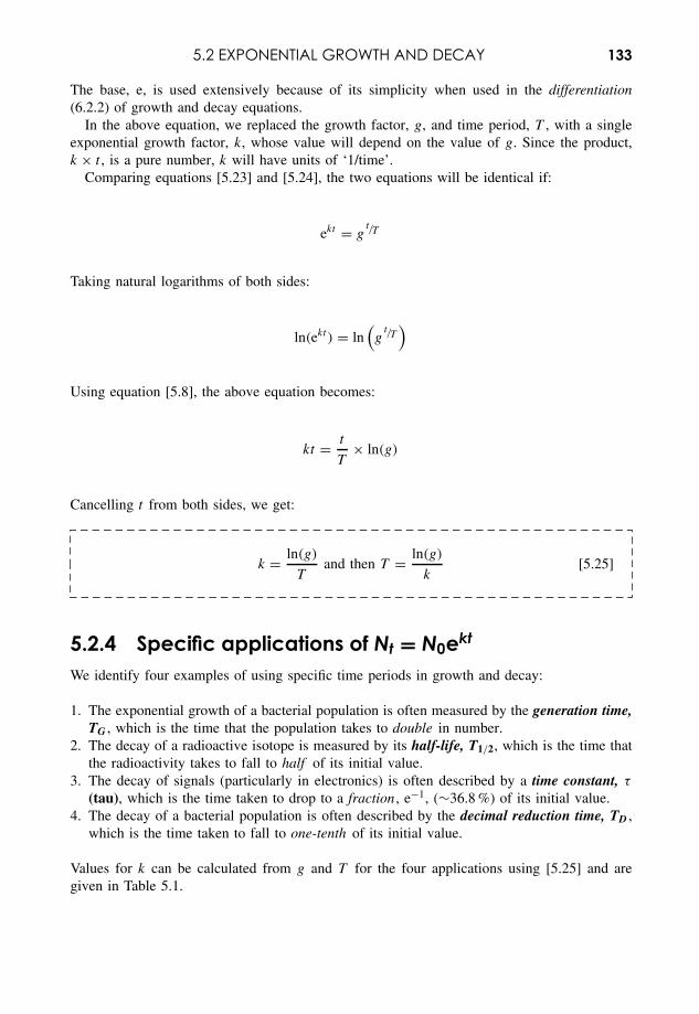
5.2 EXPONENTIAL GROWTH AND DECAY 133
The base, e, is used extensively because of its simplicity when used in the differentiation(6.2.2) of growth and decay equations.
In the above equation, we replaced the growth factor, g, and time period, T , with a singleexponential growth factor, k, whose value will depend on the value of g. Since the product,k × t , is a pure number, k will have units of ‘1/time’.
Comparing equations [5.23] and [5.24], the two equations will be identical if:
ekt = gt/T
Taking natural logarithms of both sides:
ln(ekt ) = ln(g
t/T)
Using equation [5.8], the above equation becomes:
kt = t
T× ln(g)
Cancelling t from both sides, we get:
k = ln(g)
Tand then T = ln(g)
k[5.25]
5.2.4 Specific applications of Nt = N0ekt
We identify four examples of using specific time periods in growth and decay:
1. The exponential growth of a bacterial population is often measured by the generation time,TG , which is the time that the population takes to double in number.
2. The decay of a radioactive isotope is measured by its half-life, T1/2, which is the time thatthe radioactivity takes to fall to half of its initial value.
3. The decay of signals (particularly in electronics) is often described by a time constant, τ
(tau), which is the time taken to drop to a fraction , e−1, (∼36.8 %) of its initial value.4. The decay of a bacterial population is often described by the decimal reduction time, TD ,
which is the time taken to fall to one-tenth of its initial value.
Values for k can be calculated from g and T for the four applications using [5.25] and aregiven in Table 5.1.
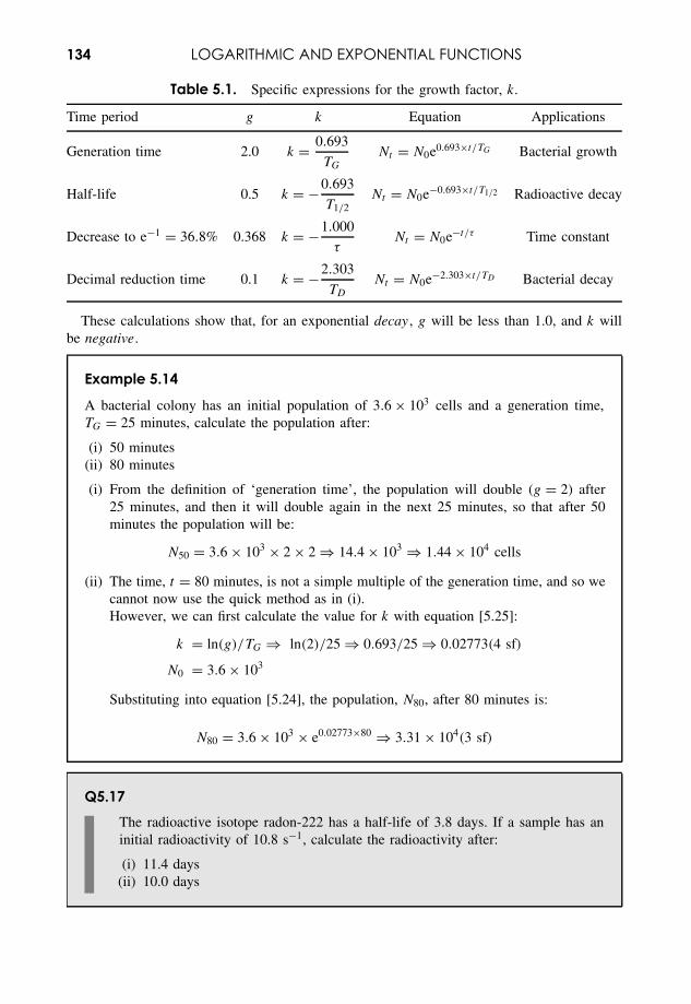
134 LOGARITHMIC AND EXPONENTIAL FUNCTIONS
Table 5.1. Specific expressions for the growth factor, k.
Time period g k Equation Applications
Generation time 2.0 k = 0.693
TG
Nt = N0e0.693×t/TG Bacterial growth
Half-life 0.5 k = −0.693
T1/2Nt = N0e−0.693×t/T1/2 Radioactive decay
Decrease to e−1 = 36.8% 0.368 k = −1.000
τNt = N0e−t/τ Time constant
Decimal reduction time 0.1 k = −2.303
TD
Nt = N0e−2.303×t/TD Bacterial decay
These calculations show that, for an exponential decay , g will be less than 1.0, and k willbe negative.
Example 5.14
A bacterial colony has an initial population of 3.6 × 10³ cells and a generation time,TG = 25 minutes, calculate the population after:
(i) 50 minutes(ii) 80 minutes
(i) From the definition of ‘generation time’, the population will double (g = 2) after25 minutes, and then it will double again in the next 25 minutes, so that after 50minutes the population will be:
N50 = 3.6 × 103 × 2 × 2 ⇒ 14.4 × 10³ ⇒ 1.44 × 10⁴ cells
(ii) The time, t = 80 minutes, is not a simple multiple of the generation time, and so wecannot now use the quick method as in (i).However, we can first calculate the value for k with equation [5.25]:
k = ln(g)/TG ⇒ ln(2)/25 ⇒ 0.693/25 ⇒ 0.02773(4 sf)
N0 = 3.6 × 10³
Substituting into equation [5.24], the population, N80, after 80 minutes is:
N80 = 3.6 × 10³ × e0.02773×80 ⇒ 3.31 × 10⁴(3 sf)
Q5.17The radioactive isotope radon-222 has a half-life of 3.8 days. If a sample has aninitial radioactivity of 10.8 s−1, calculate the radioactivity after:
(i) 11.4 days(ii) 10.0 days
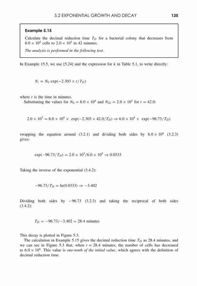
5.2 EXPONENTIAL GROWTH AND DECAY 135
Example 5.15
Calculate the decimal reduction time TD for a bacterial colony that decreases from6.0 × 104 cells to 2.0 × 10³ in 42 minutes.
The analysis is performed in the following text .
In Example 15.5, we use [5.24] and the expression for k in Table 5.1, to write directly:
Nt = N0 exp(−2.303 × t/TD)
where t is the time in minutes.Substituting the values for N0 = 6.0 × 10⁴ and N42 = 2.0 × 10³ for t = 42.0:
2.0 × 103 = 6.0 × 10⁴ × exp(−2.303 × 42.0/TD) ⇒ 6.0 × 10⁴ × exp(−96.73/TD)
swapping the equation around (3.2.1) and dividing both sides by 6.0 × 10⁴ (3.2.3)gives:
exp(−96.73/TD) = 2.0 × 10³/6.0 × 104 ⇒ 0.0333
Taking the inverse of the exponential (3.4.2):
−96.73/TD = ln(0.0333) ⇒ −3.402
Dividing both sides by −96.73 (3.2.3) and taking the reciprocal of both sides(3.4.2):
TD = −96.73/−3.402 = 28.4 minutes
This decay is plotted in Figure 5.3.The calculation in Example 5.15 gives the decimal reduction time TD as 28.4 minutes, and
we can see in Figure 5.3 that, when t = 28.4 minutes, the number of cells has decreasedto 6.0 × 10⁴. This value is one-tenth of the initial value, which agrees with the definition ofdecimal reduction time.
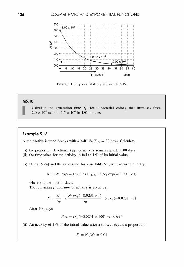
136 LOGARITHMIC AND EXPONENTIAL FUNCTIONS
0.0
1.0
2.0
3.0
4.0
5.0
6.0
7.0
0 5 10 15 20 25 30 35 40 45 50 55 60
t /min
N/1
04
6.00 x 10⁴
2.00 x 10³
0.60 x 10⁴
TD = 28.4
Figure 5.3 Exponential decay in Example 5.15.
Q5.18Calculate the generation time TG for a bacterial colony that increases from2.0 × 104 cells to 1.7 × 10⁶ in 180 minutes.
Example 5.16
A radioactive isotope decays with a half-life T1/2 = 30 days. Calculate:
(i) the proportion (fraction), F100, of activity remaining after 100 days(ii) the time taken for the activity to fall to 1 % of its initial value.
(i) Using [5.24] and the expression for k in Table 5.1, we can write directly:
Nt = N0 exp(−0.693 × t/T1/2) ⇒ N0 exp(−0.0231 × t)
where t is the time in days.The remaining proportion of activity is given by:
Ft = Nt
N0⇒ N0 exp(−0.0231 × t)
N0⇒ exp(−0.0231 × t)
After 100 days:
F100 = exp(−0.0231 × 100) ⇒ 0.0993
(ii) An activity of 1 % of the initial value after a time, t , equals a proportion:
Ft = Nt/N0 = 0.01
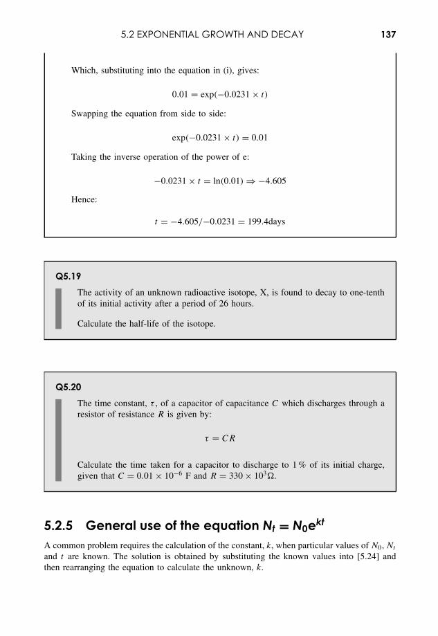
5.2 EXPONENTIAL GROWTH AND DECAY 137
Which, substituting into the equation in (i), gives:
0.01 = exp(−0.0231 × t)
Swapping the equation from side to side:
exp(−0.0231 × t) = 0.01
Taking the inverse operation of the power of e:
−0.0231 × t = ln(0.01) ⇒ −4.605
Hence:
t = −4.605/−0.0231 = 199.4days
Q5.19The activity of an unknown radioactive isotope, X, is found to decay to one-tenthof its initial activity after a period of 26 hours.
Calculate the half-life of the isotope.
Q5.20The time constant, τ , of a capacitor of capacitance C which discharges through aresistor of resistance R is given by:
τ = CR
Calculate the time taken for a capacitor to discharge to 1 % of its initial charge,given that C = 0.01 × 10⁻⁶ F and R = 330 × 103�.
5.2.5 General use of the equation Nt = N0ekt
A common problem requires the calculation of the constant, k, when particular values of N0, Nt
and t are known. The solution is obtained by substituting the known values into [5.24] andthen rearranging the equation to calculate the unknown, k.
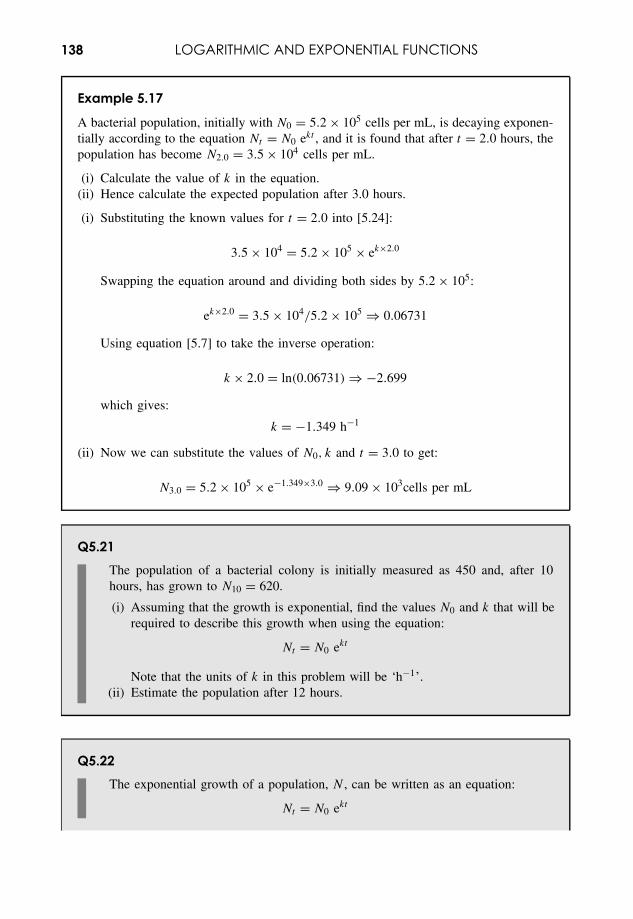
138 LOGARITHMIC AND EXPONENTIAL FUNCTIONS
Example 5.17
A bacterial population, initially with N0 = 5.2 × 10⁵ cells per mL, is decaying exponen-tially according to the equation Nt = N0 ekt , and it is found that after t = 2.0 hours, thepopulation has become N2.0 = 3.5 × 10⁴ cells per mL.
(i) Calculate the value of k in the equation.(ii) Hence calculate the expected population after 3.0 hours.
(i) Substituting the known values for t = 2.0 into [5.24]:
3.5 × 104 = 5.2 × 10⁵ × ek×2.0
Swapping the equation around and dividing both sides by 5.2 × 10⁵:
ek×2.0 = 3.5 × 10⁴/5.2 × 105 ⇒ 0.06731
Using equation [5.7] to take the inverse operation:
k × 2.0 = ln(0.06731) ⇒ −2.699
which gives:
k = −1.349 h−1
(ii) Now we can substitute the values of N0, k and t = 3.0 to get:
N3.0 = 5.2 × 10⁵ × e−1.349×3.0 ⇒ 9.09 × 10³cells per mL
Q5.21The population of a bacterial colony is initially measured as 450 and, after 10hours, has grown to N10 = 620.
(i) Assuming that the growth is exponential, find the values N0 and k that will berequired to describe this growth when using the equation:
Nt = N0 ekt
Note that the units of k in this problem will be ‘h−1’.(ii) Estimate the population after 12 hours.
Q5.22The exponential growth of a population, N , can be written as an equation:
Nt = N0 ekt
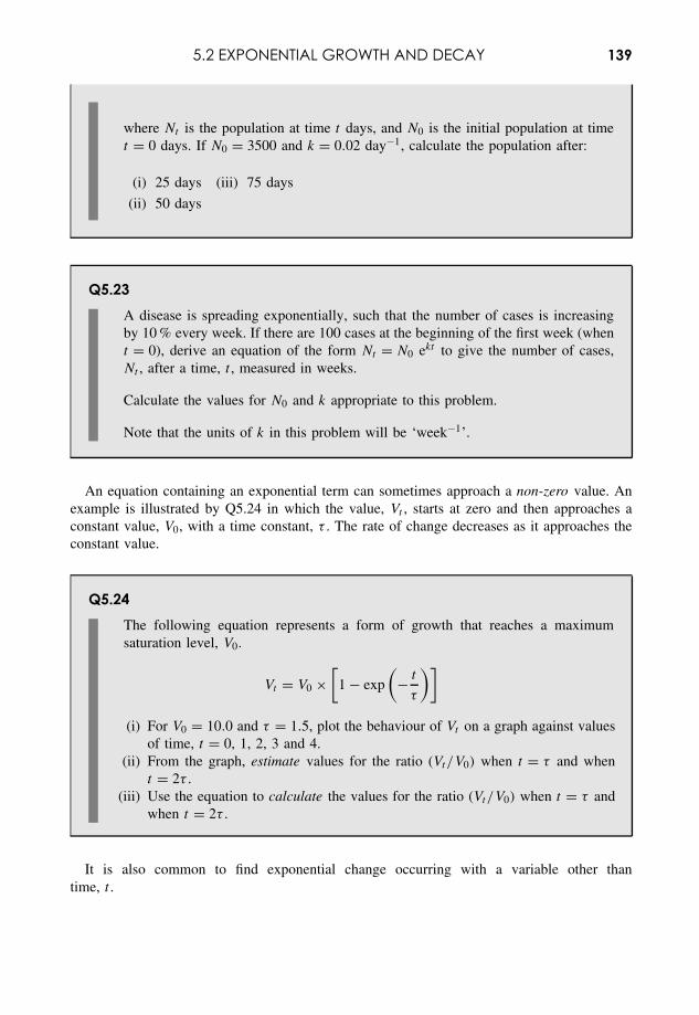
5.2 EXPONENTIAL GROWTH AND DECAY 139
where Nt is the population at time t days, and N0 is the initial population at timet = 0 days. If N0 = 3500 and k = 0.02 day−1, calculate the population after:
(i) 25 days (iii) 75 days
(ii) 50 days
Q5.23A disease is spreading exponentially, such that the number of cases is increasingby 10 % every week. If there are 100 cases at the beginning of the first week (whent = 0), derive an equation of the form Nt = N0 ekt to give the number of cases,Nt , after a time, t , measured in weeks.
Calculate the values for N0 and k appropriate to this problem.
Note that the units of k in this problem will be ‘week−1’.
An equation containing an exponential term can sometimes approach a non-zero value. Anexample is illustrated by Q5.24 in which the value, Vt , starts at zero and then approaches aconstant value, V0, with a time constant, τ . The rate of change decreases as it approaches theconstant value.
Q5.24The following equation represents a form of growth that reaches a maximumsaturation level, V0.
Vt = V0 ×[
1 − exp
(− t
τ
)]
(i) For V0 = 10.0 and τ = 1.5, plot the behaviour of Vt on a graph against valuesof time, t = 0, 1, 2, 3 and 4.
(ii) From the graph, estimate values for the ratio (Vt/V0) when t = τ and whent = 2τ .
(iii) Use the equation to calculate the values for the ratio (Vt/V0) when t = τ andwhen t = 2τ .
It is also common to find exponential change occurring with a variable other thantime, t .
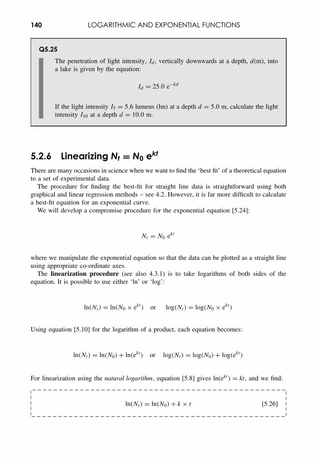
140 LOGARITHMIC AND EXPONENTIAL FUNCTIONS
Q5.25The penetration of light intensity, Id , vertically downwards at a depth, d(m), intoa lake is given by the equation:
Id = 25.0 e−kd
If the light intensity I5 = 5.6 lumens (lm) at a depth d = 5.0 m, calculate the lightintensity I10 at a depth d = 10.0 m.
5.2.6 Linearizing Nt = N0 ekt
There are many occasions in science when we want to find the ‘best fit’ of a theoretical equationto a set of experimental data.
The procedure for finding the best-fit for straight line data is straightforward using bothgraphical and linear regression methods – see 4.2. However, it is far more difficult to calculatea best-fit equation for an exponential curve.
We will develop a compromise procedure for the exponential equation [5.24]:
Nt = N0 ekt
where we manipulate the exponential equation so that the data can be plotted as a straight lineusing appropriate co-ordinate axes.
The linearization procedure (see also 4.3.1) is to take logarithms of both sides of theequation. It is possible to use either ‘ln’ or ‘log’:
ln(Nt) = ln(N0 × ekt ) or log(Nt) = log(N0 × ekt )
Using equation [5.10] for the logarithm of a product, each equation becomes:
ln(Nt) = ln(N0) + ln(ekt ) or log(Nt ) = log(N0) + log(ekt )
For linearization using the natural logarithm , equation [5.8] gives ln(ekt ) = kt , and we find:
ln(Nt) = ln(N0) + k × t [5.26]
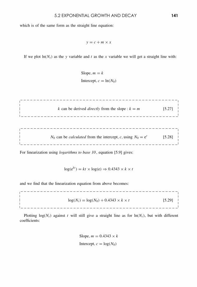
5.2 EXPONENTIAL GROWTH AND DECAY 141
which is of the same form as the straight line equation:
y = c + m × x
If we plot ln(Nt) as the y variable and t as the x variable we will get a straight line with:
Slope, m = k
Intercept, c = ln(N0)
k can be derived directly from the slope : k = m [5.27]
N0 can be calculated from the intercept, c, using N0 = ec [5.28]
For linearization using logarithms to base 10 , equation [5.9] gives:
log(ekt ) = kt × log(e) ⇒ 0.4343 × k × t
and we find that the linearization equation from above becomes:
log(Nt) = log(N0) + 0.4343 × k × t [5.29]
Plotting log(Nt) against t will still give a straight line as for ln(Nt), but with differentcoefficients:
Slope, m = 0.4343 × k
Intercept, c = log(N0)
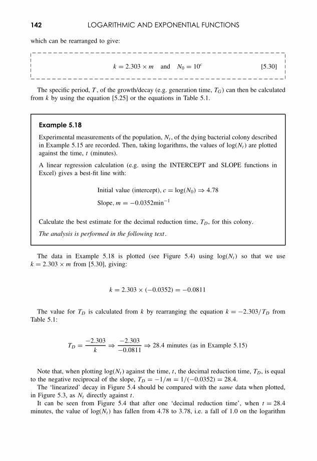
142 LOGARITHMIC AND EXPONENTIAL FUNCTIONS
which can be rearranged to give:
k = 2.303 × m and N0 = 10c [5.30]
The specific period, T , of the growth/decay (e.g. generation time, TG) can then be calculatedfrom k by using the equation [5.25] or the equations in Table 5.1.
Example 5.18
Experimental measurements of the population, Nt , of the dying bacterial colony describedin Example 5.15 are recorded. Then, taking logarithms, the values of log(Nt ) are plottedagainst the time, t (minutes).
A linear regression calculation (e.g. using the INTERCEPT and SLOPE functions inExcel) gives a best-fit line with:
Initial value (intercept), c = log(N0) ⇒ 4.78
Slope, m = −0.0352min−1
Calculate the best estimate for the decimal reduction time, TD , for this colony.
The analysis is performed in the following text .
The data in Example 5.18 is plotted (see Figure 5.4) using log(Nt) so that we usek = 2.303 × m from [5.30], giving:
k = 2.303 × (−0.0352) = −0.0811
The value for TD is calculated from k by rearranging the equation k = −2.303/TD fromTable 5.1:
TD = −2.303
k⇒ −2.303
−0.0811⇒ 28.4 minutes (as in Example 5.15)
Note that, when plotting log(Nt ) against the time, t , the decimal reduction time, TD , is equalto the negative reciprocal of the slope, TD = −1/m = 1/(−0.0352) = 28.4.
The ‘linearized’ decay in Figure 5.4 should be compared with the same data when plotted,in Figure 5.3, as Nt directly against t .
It can be seen from Figure 5.4 that after one ‘decimal reduction time’, when t = 28.4minutes, the value of log(Nt) has fallen from 4.78 to 3.78, i.e. a fall of 1.0 on the logarithm
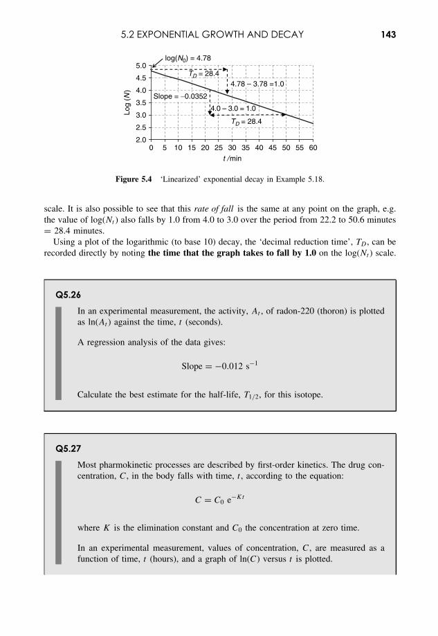
5.2 EXPONENTIAL GROWTH AND DECAY 143
2.0
2.5
3.0
3.5
4.0
4.5
5.0
0 5 10 15 20 25 30 35 40 45 50 55 60
t /min
Log
(N)
TD = 28.4
log(N0) = 4.78
Slope = −0.0352
4.0 – 3.0 = 1.0
TD = 28.44.78 – 3.78 =1.0
Figure 5.4 ‘Linearized’ exponential decay in Example 5.18.
scale. It is also possible to see that this rate of fall is the same at any point on the graph, e.g.the value of log(Nt ) also falls by 1.0 from 4.0 to 3.0 over the period from 22.2 to 50.6 minutes= 28.4 minutes.
Using a plot of the logarithmic (to base 10) decay, the ‘decimal reduction time’, TD , can berecorded directly by noting the time that the graph takes to fall by 1.0 on the log(Nt ) scale.
Q5.26In an experimental measurement, the activity, At , of radon-220 (thoron) is plottedas ln(At ) against the time, t (seconds).
A regression analysis of the data gives:
Slope = −0.012 s−1
Calculate the best estimate for the half-life, T1/2, for this isotope.
Q5.27Most pharmokinetic processes are described by first-order kinetics. The drug con-centration, C, in the body falls with time, t , according to the equation:
C = C0 e−Kt
where K is the elimination constant and C0 the concentration at zero time.
In an experimental measurement, values of concentration, C, are measured as afunction of time, t (hours), and a graph of ln(C) versus t is plotted.
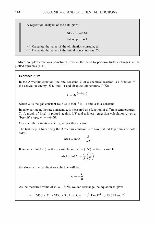
144 LOGARITHMIC AND EXPONENTIAL FUNCTIONS
A regression analysis of the data gives:
Slope = −0.61
Intercept = 4.1
(i) Calculate the value of the elimination constant, K .(ii) Calculate the value of the initial concentration, C0.
More complex equations sometimes involve the need to perform further changes to theplotted variables (4.3.3).
Example 5.19
In the Arrhenius equation, the rate constant, k, of a chemical reaction is a function ofthe activation energy, E (J mol−1) and absolute temperature, T (K):
k = Ae(−E/RT
)
where R is the gas constant (= 8.31 J mol−1 K−1) and A is a constant.
In an experiment, the rate constant, k, is measured as a function of different temperatures,T . A graph of ln(k) is plotted against 1/T and a linear regression calculation gives a‘best-fit’ slope, m = −6450.
Calculate the activation energy, E, for this reaction.
The first step in linearizing the Arrhenius equation is to take natural logarithms of bothsides:
ln(k) = ln(A) − E
RT
If we now plot ln(k) as the y variable and write (1/T ) as the x variable:
ln(k) = ln(A) − E
R
(1
T
)
the slope of the resultant straight line will be:
m = −E
R
As the measured value of m = −6450, we can rearrange the equation to give:
E = 6450 × R ⇒ 6450 × 8.31 ⇒ 53.6 × 10³ J mol−1 ⇒ 53.6 kJ mol−1
6Rates of Change
Overview
Website • ‘How to do it’ video answers for all ‘Q’ questions.• Excel files appropriate to selected ‘Q’ questions and Examples.
Nature is not static, and much interesting science is concerned with how systemschange.
We start the first unit with familiar calculations of average speed, by recording change ofposition within a finite time interval. The calculation of speed is related to the slope of a lineon a distance against time graph. We then develop the more general case for calculating speedat an instant, when the speed is represented by a continuously varying curve on a graph. This‘rate of change’ mathematics is also applied to other systems.
Simple examples in Excel are used to demonstrate how continuously varying data can bemodelled in a suitable spreadsheet format. The calculations for approximate models are rela-tively simple, but it is often possible to develop solutions to the required degree of accuracy.
The analytical mathematics (calculus) of differentiation is beyond the scope of this book.However, the second unit introduces the concept of ‘differentiation’ and gives a brief intro-duction to some ideas of calculus.
6.1 Rate of Change6.1.1 IntroductionThe most familiar ‘rate of change’ is probably speed . We express speed, v, as a rate ofchange of distance, z, with time, t , e.g. ‘miles per hour’ or ‘metres per second’. How-ever, ‘rates of change’ are found in all areas of science involving a variety of differentvariables.
We start with simple examples of average speeds within finite periods of time, and thenprogress to the more general case of a continuously varying x –y relationship.
Essential Mathematics and Statistics for Science 2nd Edition Graham Currell and Antony DowmanCopyright c© 2009 John Wiley & Sons, Ltd
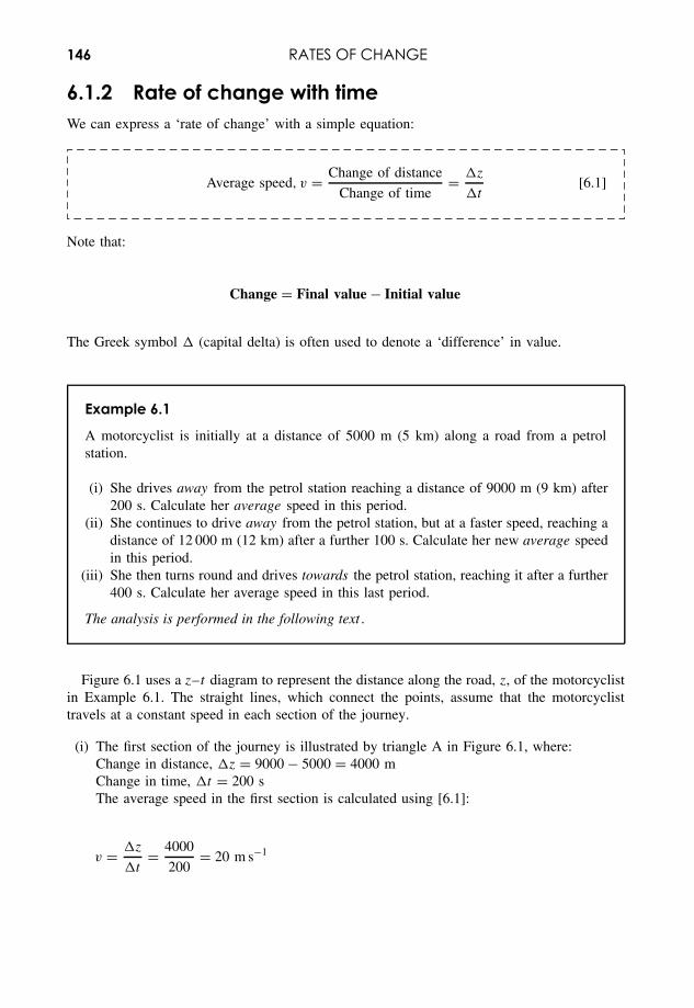
146 RATES OF CHANGE
6.1.2 Rate of change with timeWe can express a ‘rate of change’ with a simple equation:
Average speed, v = Change of distance
Change of time= �z
�t[6.1]
Note that:
Change = Final value − Initial value
The Greek symbol � (capital delta) is often used to denote a ‘difference’ in value.
Example 6.1
A motorcyclist is initially at a distance of 5000 m (5 km) along a road from a petrolstation.
(i) She drives away from the petrol station reaching a distance of 9000 m (9 km) after200 s. Calculate her average speed in this period.
(ii) She continues to drive away from the petrol station, but at a faster speed, reaching adistance of 12 000 m (12 km) after a further 100 s. Calculate her new average speedin this period.
(iii) She then turns round and drives towards the petrol station, reaching it after a further400 s. Calculate her average speed in this last period.
The analysis is performed in the following text .
Figure 6.1 uses a z–t diagram to represent the distance along the road, z, of the motorcyclistin Example 6.1. The straight lines, which connect the points, assume that the motorcyclisttravels at a constant speed in each section of the journey.
(i) The first section of the journey is illustrated by triangle A in Figure 6.1, where:Change in distance, �z = 9000 − 5000 = 4000 mChange in time, �t = 200 sThe average speed in the first section is calculated using [6.1]:
v = �z
�t= 4000
200= 20 m s−1
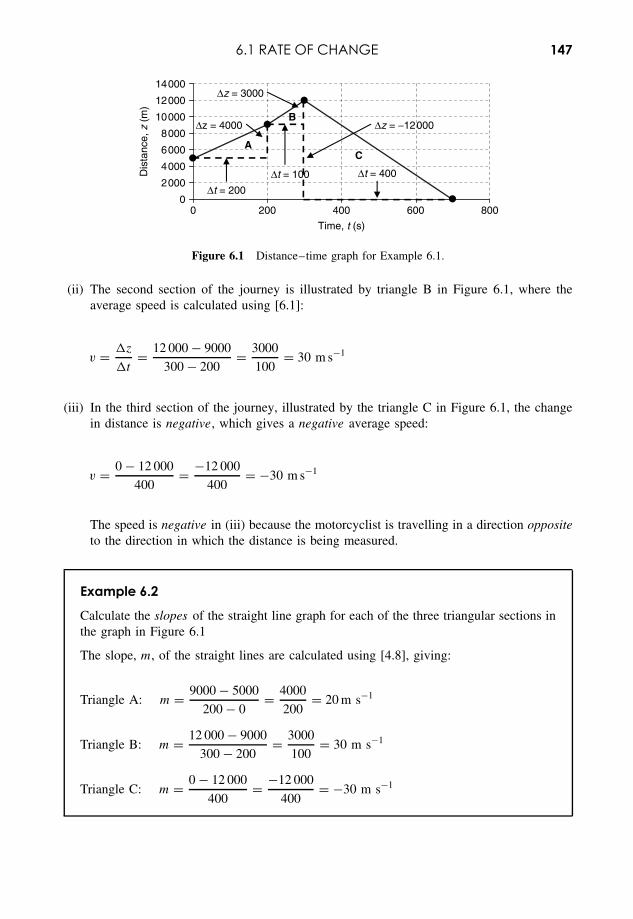
6.1 RATE OF CHANGE 147
0
2000
4000
6000
8000
10000
12000
14000
0 200 400 600 800
Time, t (s)
Dis
tanc
e, z
(m
)
∆z = 4000
∆t = 100
∆t = 200
∆z = 3000
∆z = −12000
A
B
C
∆t = 400
Figure 6.1 Distance–time graph for Example 6.1.
(ii) The second section of the journey is illustrated by triangle B in Figure 6.1, where theaverage speed is calculated using [6.1]:
v = �z
�t= 12 000 − 9000
300 − 200= 3000
100= 30 m s−1
(iii) In the third section of the journey, illustrated by the triangle C in Figure 6.1, the changein distance is negative, which gives a negative average speed:
v = 0 − 12 000
400= −12 000
400= −30 m s−1
The speed is negative in (iii) because the motorcyclist is travelling in a direction oppositeto the direction in which the distance is being measured.
Example 6.2
Calculate the slopes of the straight line graph for each of the three triangular sections inthe graph in Figure 6.1
The slope, m, of the straight lines are calculated using [4.8], giving:
Triangle A: m = 9000 − 5000
200 − 0= 4000
200= 20 m s−1
Triangle B: m = 12 000 − 9000
300 − 200= 3000
100= 30 m s−1
Triangle C: m = 0 − 12 000
400= −12 000
400= −30 m s−1
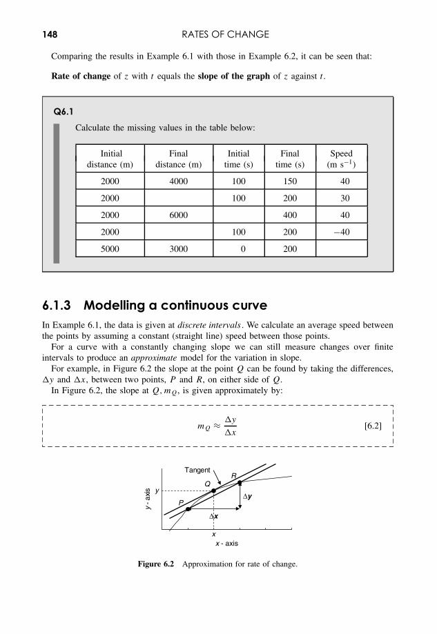
148 RATES OF CHANGE
Comparing the results in Example 6.1 with those in Example 6.2, it can be seen that:
Rate of change of z with t equals the slope of the graph of z against t .
Q6.1Calculate the missing values in the table below:
Initial Final Initial Final Speeddistance (m) distance (m) time (s) time (s) (m s−1)
2000 4000 100 150 40
2000 100 200 30
2000 6000 400 40
2000 100 200 −40
5000 3000 0 200
6.1.3 Modelling a continuous curveIn Example 6.1, the data is given at discrete intervals . We calculate an average speed betweenthe points by assuming a constant (straight line) speed between those points.
For a curve with a constantly changing slope we can still measure changes over finiteintervals to produce an approximate model for the variation in slope.
For example, in Figure 6.2 the slope at the point Q can be found by taking the differences,�y and �x, between two points, P and R, on either side of Q.
In Figure 6.2, the slope at Q, mQ, is given approximately by:
mQ ≈ �y
�x[6.2]
x - axis
y - a
xis
∆x
∆yy
x
Tangent
P
QR
Figure 6.2 Approximation for rate of change.
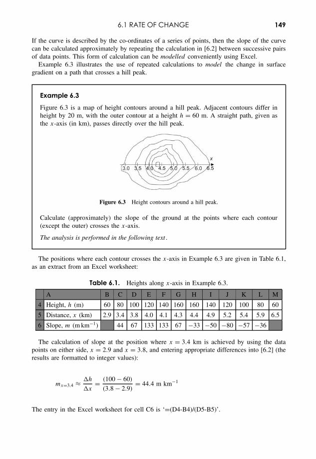
6.1 RATE OF CHANGE 149
If the curve is described by the co-ordinates of a series of points, then the slope of the curvecan be calculated approximately by repeating the calculation in [6.2] between successive pairsof data points. This form of calculation can be modelled conveniently using Excel.
Example 6.3 illustrates the use of repeated calculations to model the change in surfacegradient on a path that crosses a hill peak.
Example 6.3
Figure 6.3 is a map of height contours around a hill peak. Adjacent contours differ inheight by 20 m, with the outer contour at a height h = 60 m. A straight path, given asthe x-axis (in km), passes directly over the hill peak.
Figure 6.3 Height contours around a hill peak.
Calculate (approximately) the slope of the ground at the points where each contour(except the outer) crosses the x-axis.
The analysis is performed in the following text .
The positions where each contour crosses the x-axis in Example 6.3 are given in Table 6.1,as an extract from an Excel worksheet:
Table 6.1. Heights along x-axis in Example 6.3.
A B C D E F G H I J K L M
4 Height, h (m) 60 80 100 120 140 160 160 140 120 100 80 60
5 Distance, x (km) 2.9 3.4 3.8 4.0 4.1 4.3 4.4 4.9 5.2 5.4 5.9 6.5
6 Slope, m (m km−1) 44 67 133 133 67 −33 −50 −80 −57 −36
The calculation of slope at the position where x = 3.4 km is achieved by using the datapoints on either side, x = 2.9 and x = 3.8, and entering appropriate differences into [6.2] (theresults are formatted to integer values):
mx=3.4 ≈ �h
�x= (100 − 60)
(3.8 − 2.9)= 44.4 m km−1
The entry in the Excel worksheet for cell C6 is ‘=(D4-B4)/(D5-B5)’.
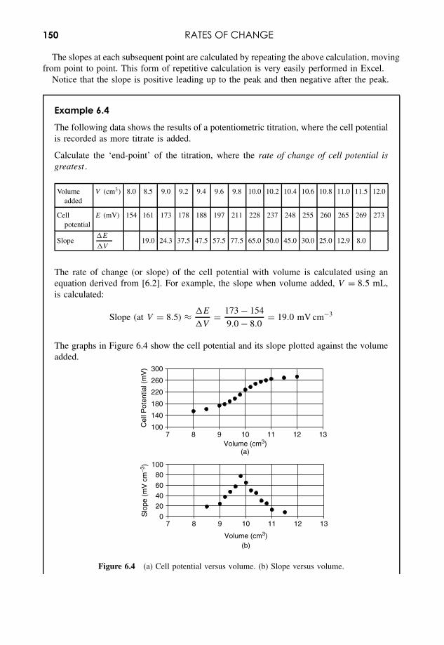
150 RATES OF CHANGE
The slopes at each subsequent point are calculated by repeating the above calculation, movingfrom point to point. This form of repetitive calculation is very easily performed in Excel.
Notice that the slope is positive leading up to the peak and then negative after the peak.
Example 6.4
The following data shows the results of a potentiometric titration, where the cell potentialis recorded as more titrate is added.
Calculate the ‘end-point’ of the titration, where the rate of change of cell potential isgreatest .
Volumeadded
V (cm3) 8.0 8.5 9.0 9.2 9.4 9.6 9.8 10.0 10.2 10.4 10.6 10.8 11.0 11.5 12.0
Cellpotential
E (mV) 154 161 173 178 188 197 211 228 237 248 255 260 265 269 273
Slope�E
�V19.0 24.3 37.5 47.5 57.5 77.5 65.0 50.0 45.0 30.0 25.0 12.9 8.0
The rate of change (or slope) of the cell potential with volume is calculated using anequation derived from [6.2]. For example, the slope when volume added, V = 8.5 mL,is calculated:
Slope (at V = 8.5) ≈ �E
�V= 173 − 154
9.0 − 8.0= 19.0 mV cm−3
The graphs in Figure 6.4 show the cell potential and its slope plotted against the volumeadded.
(a)
(b)
100
140
180
220
260
300
7 8 9 10 11 12 13Volume (cm3)
Cel
l Pot
entia
l (m
V)
0
20
40
60
80
100
7 8 9 10 11 12 13
Volume (cm3)
Slo
pe (
mV
cm
−3)
Figure 6.4 (a) Cell potential versus volume. (b) Slope versus volume.
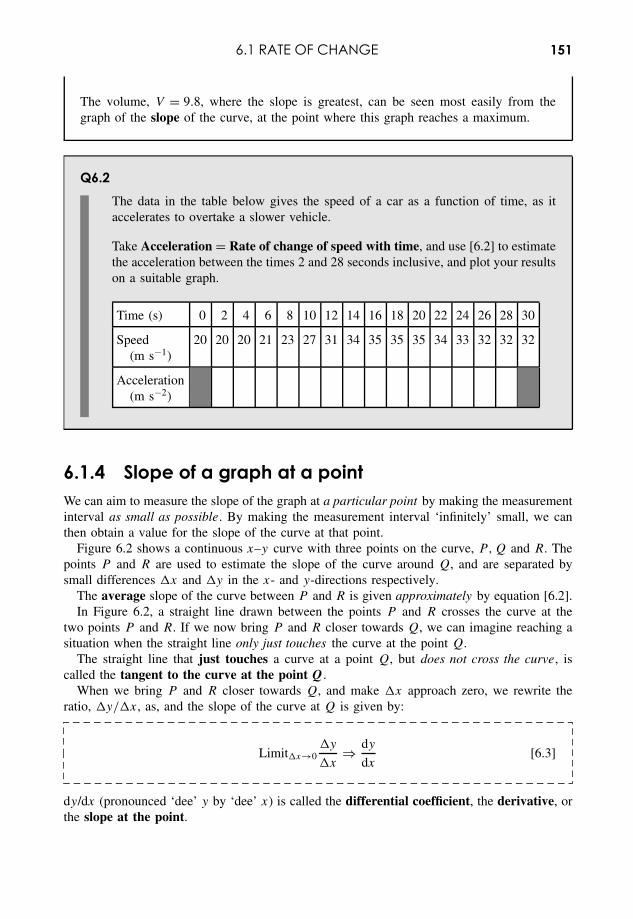
6.1 RATE OF CHANGE 151
The volume, V = 9.8, where the slope is greatest, can be seen most easily from thegraph of the slope of the curve, at the point where this graph reaches a maximum.
Q6.2The data in the table below gives the speed of a car as a function of time, as itaccelerates to overtake a slower vehicle.
Take Acceleration = Rate of change of speed with time, and use [6.2] to estimatethe acceleration between the times 2 and 28 seconds inclusive, and plot your resultson a suitable graph.
Time (s) 0 2 4 6 8 10 12 14 16 18 20 22 24 26 28 30
Speed(m s−1)
20 20 20 21 23 27 31 34 35 35 35 34 33 32 32 32
Acceleration(m s−2)
6.1.4 Slope of a graph at a pointWe can aim to measure the slope of the graph at a particular point by making the measurementinterval as small as possible. By making the measurement interval ‘infinitely’ small, we canthen obtain a value for the slope of the curve at that point.
Figure 6.2 shows a continuous x–y curve with three points on the curve, P, Q and R. Thepoints P and R are used to estimate the slope of the curve around Q, and are separated bysmall differences �x and �y in the x- and y-directions respectively.
The average slope of the curve between P and R is given approximately by equation [6.2].In Figure 6.2, a straight line drawn between the points P and R crosses the curve at the
two points P and R. If we now bring P and R closer towards Q, we can imagine reaching asituation when the straight line only just touches the curve at the point Q.
The straight line that just touches a curve at a point Q, but does not cross the curve, iscalled the tangent to the curve at the point Q .
When we bring P and R closer towards Q, and make �x approach zero, we rewrite theratio, �y/�x, as, and the slope of the curve at Q is given by:
Limit�x→0�y
�x⇒ dy
dx[6.3]
dy/dx (pronounced ‘dee’ y by ‘dee’ x) is called the differential coefficient, the derivative, orthe slope at the point.
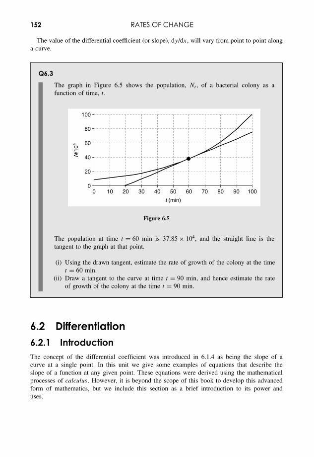
152 RATES OF CHANGE
The value of the differential coefficient (or slope), dy/dx, will vary from point to point alonga curve.
Q6.3The graph in Figure 6.5 shows the population, Nt , of a bacterial colony as afunction of time, t .
0
20
40
60
80
100
0 10 20 30 40 50 60 70 80 90 100
t (min)
N/1
04
Figure 6.5
The population at time t = 60 min is 37.85 × 10⁴, and the straight line is thetangent to the graph at that point.
(i) Using the drawn tangent, estimate the rate of growth of the colony at the timet = 60 min.
(ii) Draw a tangent to the curve at time t = 90 min, and hence estimate the rateof growth of the colony at the time t = 90 min.
6.2 Differentiation6.2.1 IntroductionThe concept of the differential coefficient was introduced in 6.1.4 as being the slope of acurve at a single point. In this unit we give some examples of equations that describe theslope of a function at any given point. These equations were derived using the mathematicalprocesses of calculus . However, it is beyond the scope of this book to develop this advancedform of mathematics, but we include this section as a brief introduction to its power anduses.
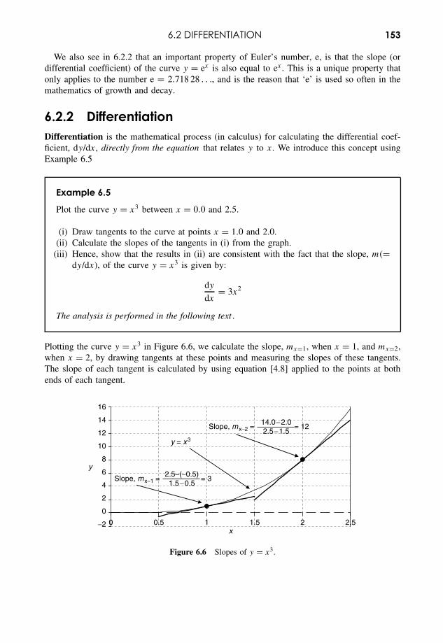
6.2 DIFFERENTIATION 153
We also see in 6.2.2 that an important property of Euler’s number, e, is that the slope (ordifferential coefficient) of the curve y = ex is also equal to ex . This is a unique property thatonly applies to the number e = 2.718 28 . . ., and is the reason that ‘e’ is used so often in themathematics of growth and decay.
6.2.2 DifferentiationDifferentiation is the mathematical process (in calculus) for calculating the differential coef-ficient, dy/dx, directly from the equation that relates y to x. We introduce this concept usingExample 6.5
Example 6.5
Plot the curve y = x3 between x = 0.0 and 2.5.
(i) Draw tangents to the curve at points x = 1.0 and 2.0.(ii) Calculate the slopes of the tangents in (i) from the graph.
(iii) Hence, show that the results in (ii) are consistent with the fact that the slope, m(=dy/dx), of the curve y = x3 is given by:
dy
dx= 3x2
The analysis is performed in the following text .
Plotting the curve y = x3 in Figure 6.6, we calculate the slope, mx=1, when x = 1, and mx=2,when x = 2, by drawing tangents at these points and measuring the slopes of these tangents.The slope of each tangent is calculated by using equation [4.8] applied to the points at bothends of each tangent.
−2
0
2
4
6
8
10
12
14
16
0 0.5 1 1.5 2 2.5x
y
y = x3
Slope, mx−1 =2.5–(−0.5)1.5−0.5
= 3
Slope, mx−2 =14.0−2.02.5−1.5
= 12
Figure 6.6 Slopes of y = x3.
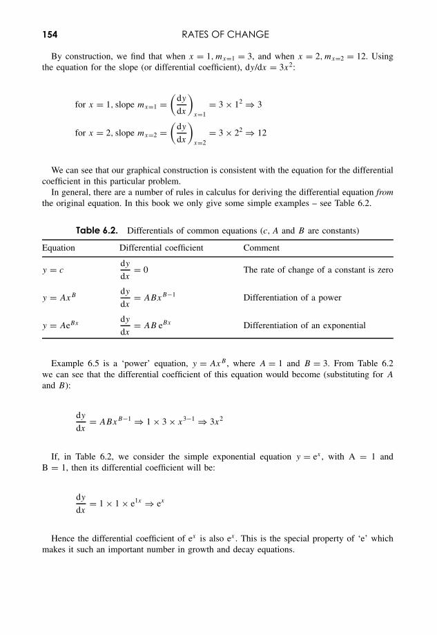
154 RATES OF CHANGE
By construction, we find that when x = 1, mx=1 = 3, and when x = 2, mx=2 = 12. Usingthe equation for the slope (or differential coefficient), dy/dx = 3x2:
for x = 1, slope mx=1 =(
dy
dx
)x=1
= 3 × 12 ⇒ 3
for x = 2, slope mx=2 =(
dy
dx
)x=2
= 3 × 22 ⇒ 12
We can see that our graphical construction is consistent with the equation for the differentialcoefficient in this particular problem.
In general, there are a number of rules in calculus for deriving the differential equation fromthe original equation. In this book we only give some simple examples – see Table 6.2.
Table 6.2. Differentials of common equations (c, A and B are constants)
Equation Differential coefficient Comment
y = cdy
dx= 0 The rate of change of a constant is zero
y = AxBdy
dx= ABxB−1 Differentiation of a power
y = AeBxdy
dx= AB eBx Differentiation of an exponential
Example 6.5 is a ‘power’ equation, y = AxB , where A = 1 and B = 3. From Table 6.2we can see that the differential coefficient of this equation would become (substituting for A
and B):
dy
dx= ABxB−1 ⇒ 1 × 3 × x3−1 ⇒ 3x2
If, in Table 6.2, we consider the simple exponential equation y = ex , with A = 1 andB = 1, then its differential coefficient will be:
dy
dx= 1 × 1 × e1x ⇒ ex
Hence the differential coefficient of ex is also ex . This is the special property of ‘e’ whichmakes it such an important number in growth and decay equations.
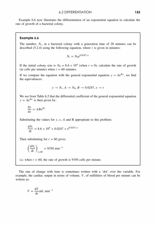
6.2 DIFFERENTIATION 155
Example 6.6 now illustrates the differentiation of an exponential equation to calculate therate of growth of a bacterial colony.
Example 6.6
The number, Nt , in a bacterial colony with a generation time of 28 minutes can bedescribed (5.2.4) using the following equation, where t is given in minutes:
Nt = N0e0.0247×t
If the initial colony size is N0 = 8.6 × 10⁴ (when t = 0), calculate the rate of growth(in cells per minute) when t = 60 minutes.
If we compare the equation with the general exponential equation y = AeBx , we findthe equivalences:
y → Nt, A → N0, B → 0.0247, x → t
We see from Table 6.2 that the differential coefficient of the general exponential equationy = AeBx is then given by:
dy
dx= ABeBx
Substituting the values for y, x, A and B appropriate to this problem:
dNt
dt= 8.6 × 104 × 0.0247 × e0.0247×t
Then substituting for t = 60 gives:(dNt
dt
)t=60
= 9350 min−1
i.e. when t = 60, the rate of growth is 9350 cells per minute.
The rate of change with time is sometimes written with a ‘dot’ over the variable. Forexample, the cardiac output in terms of volume, V , of millilitres of blood per minute can bewritten as:
V = dV
dtmL min−1
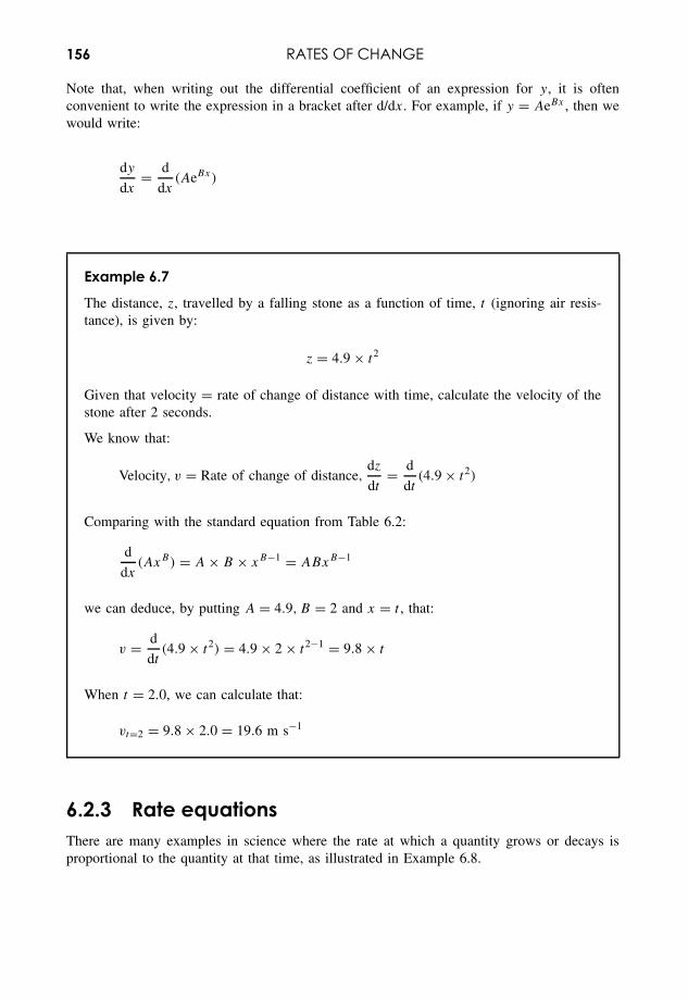
156 RATES OF CHANGE
Note that, when writing out the differential coefficient of an expression for y, it is oftenconvenient to write the expression in a bracket after d/dx. For example, if y = AeBx , then wewould write:
dy
dx= d
dx(AeBx)
Example 6.7
The distance, z, travelled by a falling stone as a function of time, t (ignoring air resis-tance), is given by:
z = 4.9 × t2
Given that velocity = rate of change of distance with time, calculate the velocity of thestone after 2 seconds.
We know that:
Velocity, v = Rate of change of distance,dz
dt= d
dt(4.9 × t2)
Comparing with the standard equation from Table 6.2:
d
dx(AxB) = A × B × xB−1 = ABxB−1
we can deduce, by putting A = 4.9, B = 2 and x = t , that:
v = d
dt(4.9 × t2) = 4.9 × 2 × t2−1 = 9.8 × t
When t = 2.0, we can calculate that:
vt=2 = 9.8 × 2.0 = 19.6 m s−1
6.2.3 Rate equationsThere are many examples in science where the rate at which a quantity grows or decays isproportional to the quantity at that time, as illustrated in Example 6.8.
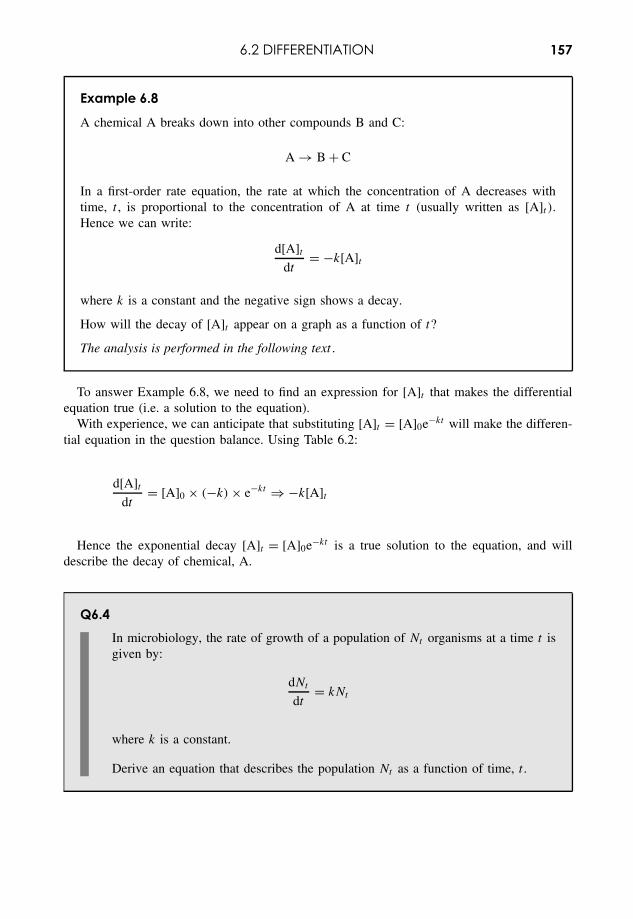
6.2 DIFFERENTIATION 157
Example 6.8
A chemical A breaks down into other compounds B and C:
A → B + C
In a first-order rate equation, the rate at which the concentration of A decreases withtime, t , is proportional to the concentration of A at time t (usually written as [A]t ).Hence we can write:
d[A]tdt
= −k[A]t
where k is a constant and the negative sign shows a decay.
How will the decay of [A]t appear on a graph as a function of t?
The analysis is performed in the following text .
To answer Example 6.8, we need to find an expression for [A]t that makes the differentialequation true (i.e. a solution to the equation).
With experience, we can anticipate that substituting [A]t = [A]0e−kt will make the differen-tial equation in the question balance. Using Table 6.2:
d[A]tdt
= [A]0 × (−k) × e−kt ⇒ −k[A]t
Hence the exponential decay [A]t = [A]0e−kt is a true solution to the equation, and willdescribe the decay of chemical, A.
Q6.4In microbiology, the rate of growth of a population of Nt organisms at a time t isgiven by:
dNt
dt= kNt
where k is a constant.
Derive an equation that describes the population Nt as a function of time, t .
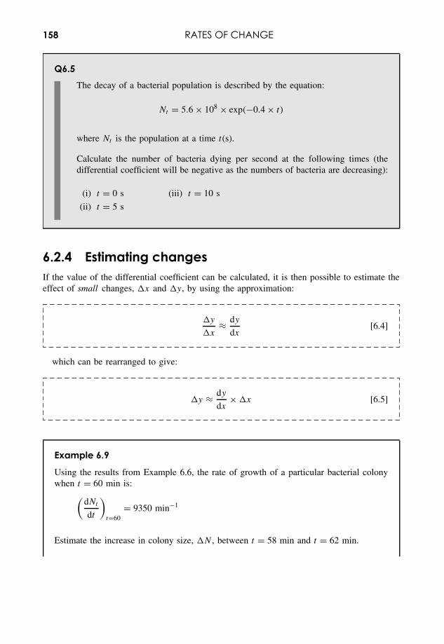
158 RATES OF CHANGE
Q6.5The decay of a bacterial population is described by the equation:
Nt = 5.6 × 10⁸ × exp(−0.4 × t)
where Nt is the population at a time t(s).
Calculate the number of bacteria dying per second at the following times (thedifferential coefficient will be negative as the numbers of bacteria are decreasing):
(i) t = 0 s (iii) t = 10 s
(ii) t = 5 s
6.2.4 Estimating changesIf the value of the differential coefficient can be calculated, it is then possible to estimate theeffect of small changes, �x and �y, by using the approximation:
�y
�x≈ dy
dx[6.4]
which can be rearranged to give:
�y ≈ dy
dx× �x [6.5]
Example 6.9
Using the results from Example 6.6, the rate of growth of a particular bacterial colonywhen t = 60 min is:(
dNt
dt
)t=60
= 9350 min−1
Estimate the increase in colony size, �N , between t = 58 min and t = 62 min.
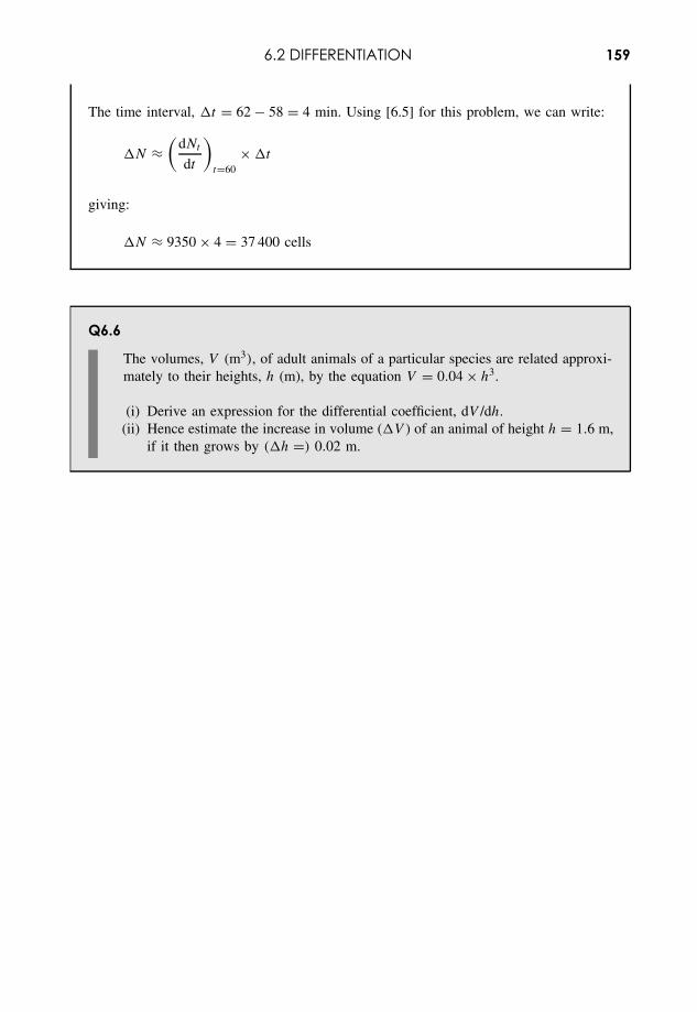
6.2 DIFFERENTIATION 159
The time interval, �t = 62 − 58 = 4 min. Using [6.5] for this problem, we can write:
�N ≈(
dNt
dt
)t=60
× �t
giving:
�N ≈ 9350 × 4 = 37 400 cells
Q6.6
The volumes, V (m3), of adult animals of a particular species are related approxi-mately to their heights, h (m), by the equation V = 0.04 × h3.
(i) Derive an expression for the differential coefficient, dV /dh.(ii) Hence estimate the increase in volume (�V ) of an animal of height h = 1.6 m,
if it then grows by (�h =) 0.02 m.

7Statistics for Science
Overview
Website • ‘How to do it’ video answers for all ‘Q’ questions.• Excel tutorial: statistical calculations.• Excel and Minitab files appropriate to selected ‘Q’ questions and Examples.
All scientific experiments suffer from experimental uncertainty due to either subject variabilityand/or measurement variability (1.2). This variability can occur with the actual subjects beingmeasured, e.g. different colonies of bacteria will grow at different rates even though the condi-tions appear to be the same. The variability can also appear in the actual measurement processitself, e.g. repeated measurements on the same fragment of glass may yield slightly differentvalues for its refractive index, because of the limited accuracy of the measurement process.
There are three main ways in which statistical analysis is particularly useful in science:
• Presenting data in visual formats which aid understanding of the underlying patterns.• Calculating ‘best estimates’ for the ‘true’ values of the parameters being measured.• ‘Testing’ for the ‘truth’ of possible scientific hypotheses through an evaluation of the prob-
abilities of error.
This chapter starts with a common situation in data analysis, i.e. repeated (replicate) measure-ments made to obtain a best estimate of an unknown value. The first step is to be able todisplay the data using a box and whisker plot . The next is to be able to calculate a quantitativeresult, the confidence interval , which incorporates an expression of the underlying uncertaintyin the data.
The following units then develop the elements of statistics that are particularly useful for dataanalysis in science, introducing methods that are used to describe and quantify the variabilitythat occurs in a simple set of experimental data. The section highlights the fact that a set ofexperimental results only represents a sample of all the possible values that could be obtainedif the experiment could be repeated over and over again. We then use statistics to infer , froma data sample, best estimates for the characteristics of the actual system being measured.
With more extensive data sets it is often more convenient to record the number (or frequency)of data values falling within given data ranges . The characteristics of the data are then describedby the characteristics of the overall frequency distribution or probability distribution.
Essential Mathematics and Statistics for Science 2nd Edition Graham Currell and Antony DowmanCopyright c© 2009 John Wiley & Sons, Ltd
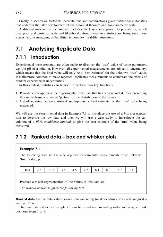
162 STATISTICS FOR SCIENCE
Finally, a section on factorials, permutations and combinations gives further basic statisticsthat underpin the later development of the binomial theorem and non-parametric tests.
Additional material on the Website includes the Bayesian approach to probability, whichuses prior and posterior odds and likelihood ratios. Bayesian statistics are being used moreextensively in managing probabilities in complex ‘real-life’ situations.
7.1 Analysing Replicate Data7.1.1 IntroductionExperimental measurements are often made to discover the ‘true’ value of some parameter,e.g. the pH of a solution. However, all experimental measurements are subject to uncertainty,which means that the final value will only be a ‘best estimate’ for the unknown ‘true’ value.It is therefore common to make repeated (replicate) measurements to counteract the effects ofrandom experimental uncertainties.
In this context, statistics can be used to perform two key functions:
1. Provide a description of the experimental ‘raw’ data that has been recorded, often presentingthis in the form of a visual ‘picture’ of the distribution of the values.
2. Calculate, using certain statistical assumptions, a ‘best estimate’ of the ‘true’ value beingmeasured.
We will use the experimental data in Example 7.1 to introduce the use of a box and whiskerplot to describe the raw data and then we will use a case study to investigate the cal-culation of a 95 % confidence interval to give the best estimate of the ‘true’ value beingmeasured.
7.1.2 Ranked data – box and whisker plots
Example 7.1
The following data set has nine replicate experimental measurements of an unknown‘true’ value, µ.
Data 2.3 11.3 3.8 4.5 4.2 8.1 6.3 3.7 3.3
Produce a visual representation of the values in this data set.
The worked answer is given the following text .
Ranked data has the data values sorted into ascending (or descending) order and assigned arank position .
The nine data values in Example 7.1 can be sorted into ascending order and assigned rankpositions from 1 to 9.
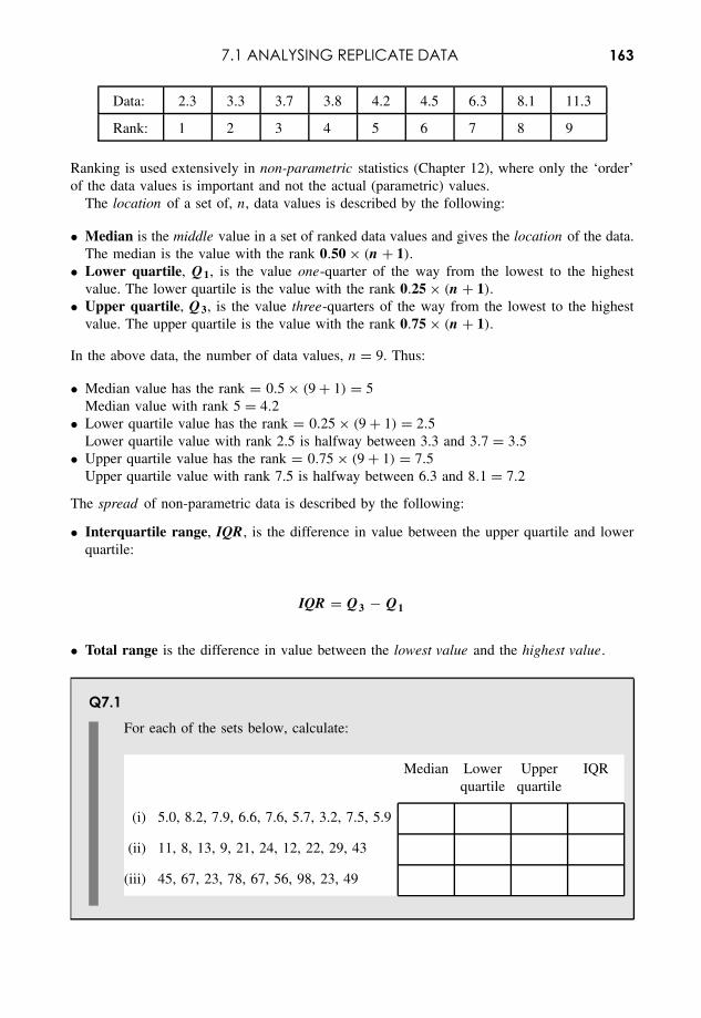
7.1 ANALYSING REPLICATE DATA 163
Data: 2.3 3.3 3.7 3.8 4.2 4.5 6.3 8.1 11.3
Rank: 1 2 3 4 5 6 7 8 9
Ranking is used extensively in non-parametric statistics (Chapter 12), where only the ‘order’of the data values is important and not the actual (parametric) values.
The location of a set of, n, data values is described by the following:
• Median is the middle value in a set of ranked data values and gives the location of the data.The median is the value with the rank 0.50 × (n + 1).
• Lower quartile, Q1, is the value one-quarter of the way from the lowest to the highestvalue. The lower quartile is the value with the rank 0.25 × (n + 1).
• Upper quartile, Q3, is the value three-quarters of the way from the lowest to the highestvalue. The upper quartile is the value with the rank 0.75 × (n + 1).
In the above data, the number of data values, n = 9. Thus:
• Median value has the rank = 0.5 × (9 + 1) = 5Median value with rank 5 = 4.2
• Lower quartile value has the rank = 0.25 × (9 + 1) = 2.5Lower quartile value with rank 2.5 is halfway between 3.3 and 3.7 = 3.5
• Upper quartile value has the rank = 0.75 × (9 + 1) = 7.5Upper quartile value with rank 7.5 is halfway between 6.3 and 8.1 = 7.2
The spread of non-parametric data is described by the following:
• Interquartile range, IQR, is the difference in value between the upper quartile and lowerquartile:
IQR = Q3 − Q1
• Total range is the difference in value between the lowest value and the highest value.
Q7.1For each of the sets below, calculate:
Median Lower Upper IQRquartile quartile
(i) 5.0, 8.2, 7.9, 6.6, 7.6, 5.7, 3.2, 7.5, 5.9
(ii) 11, 8, 13, 9, 21, 24, 12, 22, 29, 43
(iii) 45, 67, 23, 78, 67, 56, 98, 23, 49
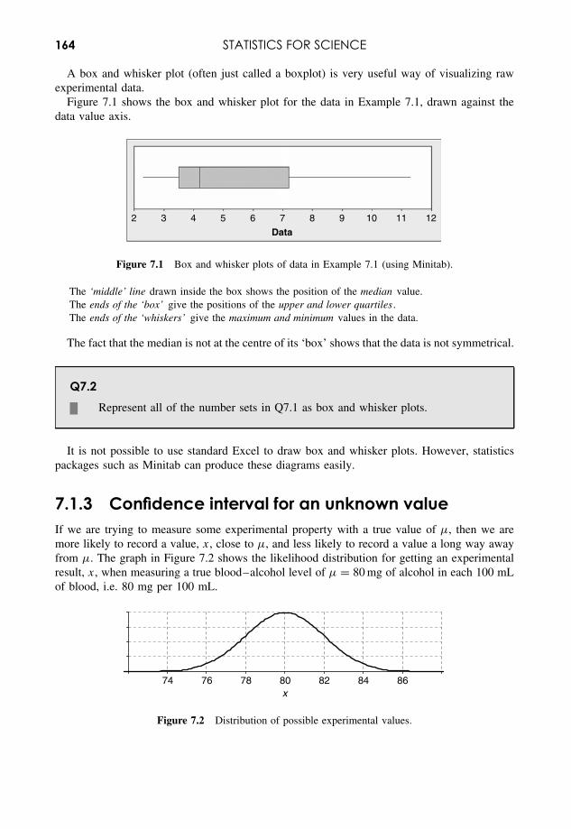
164 STATISTICS FOR SCIENCE
A box and whisker plot (often just called a boxplot) is very useful way of visualizing rawexperimental data.
Figure 7.1 shows the box and whisker plot for the data in Example 7.1, drawn against thedata value axis.
9 10 11 122 3 4 5 6 7 8
Data
Figure 7.1 Box and whisker plots of data in Example 7.1 (using Minitab).
The ‘middle’ line drawn inside the box shows the position of the median value.The ends of the ‘box’ give the positions of the upper and lower quartiles .The ends of the ‘whiskers’ give the maximum and minimum values in the data.
The fact that the median is not at the centre of its ‘box’ shows that the data is not symmetrical.
Q7.2Represent all of the number sets in Q7.1 as box and whisker plots.
It is not possible to use standard Excel to draw box and whisker plots. However, statisticspackages such as Minitab can produce these diagrams easily.
7.1.3 Confidence interval for an unknown valueIf we are trying to measure some experimental property with a true value of µ, then we aremore likely to record a value, x, close to µ, and less likely to record a value a long way awayfrom µ. The graph in Figure 7.2 shows the likelihood distribution for getting an experimentalresult, x, when measuring a true blood–alcohol level of µ = 80 mg of alcohol in each 100 mLof blood, i.e. 80 mg per 100 mL.
x807876 82 84 8674
Figure 7.2 Distribution of possible experimental values.
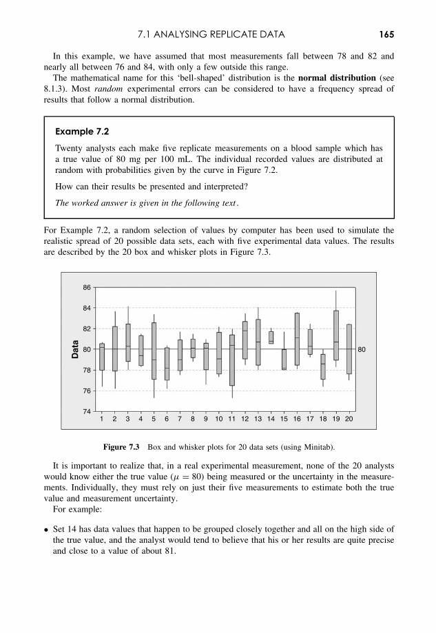
7.1 ANALYSING REPLICATE DATA 165
In this example, we have assumed that most measurements fall between 78 and 82 andnearly all between 76 and 84, with only a few outside this range.
The mathematical name for this ‘bell-shaped’ distribution is the normal distribution (see8.1.3). Most random experimental errors can be considered to have a frequency spread ofresults that follow a normal distribution.
Example 7.2
Twenty analysts each make five replicate measurements on a blood sample which hasa true value of 80 mg per 100 mL. The individual recorded values are distributed atrandom with probabilities given by the curve in Figure 7.2.
How can their results be presented and interpreted?
The worked answer is given in the following text .
For Example 7.2, a random selection of values by computer has been used to simulate therealistic spread of 20 possible data sets, each with five experimental data values. The resultsare described by the 20 box and whisker plots in Figure 7.3.
86
84
82
80 80
78
76
741 2 3 4 5 6 7 8 9 10 11 12 13 14 15 16 17 18 19 20
Dat
a
Figure 7.3 Box and whisker plots for 20 data sets (using Minitab).
It is important to realize that, in a real experimental measurement, none of the 20 analystswould know either the true value (µ = 80) being measured or the uncertainty in the measure-ments. Individually, they must rely on just their five measurements to estimate both the truevalue and measurement uncertainty.
For example:
• Set 14 has data values that happen to be grouped closely together and all on the high side ofthe true value, and the analyst would tend to believe that his or her results are quite preciseand close to a value of about 81.
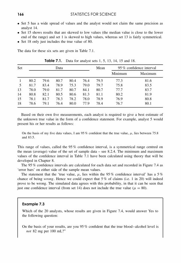
166 STATISTICS FOR SCIENCE
• Set 5 has a wide spread of values and the analyst would not claim the same precision asanalyst 14.
• Set 15 shows results that are skewed to low values (the median value is close to the lowerend of the range) and set 1 is skewed to high values, whereas set 13 is fairly symmetrical.
• Set 18 only just includes the true value of 80.
The data for these six sets are given in Table 7.1.
Table 7.1. Data for analyst sets 1, 5, 13, 14, 15 and 18.
Set Data Mean 95 % confidence interval
Minimum Maximum
1 80.2 79.6 80.7 80.4 76.4 79.5 77.3 81.65 81.7 83.4 78.9 75.3 79.0 79.7 75.8 83.5
13 78.0 79.0 81.7 80.7 84.1 80.7 77.7 83.714 80.8 82.1 80.5 80.6 81.3 81.1 80.2 81.915 78.1 81.7 78.3 78.2 78.0 78.9 76.9 80.818 78.6 79.1 76.4 80.0 77.9 78.4 76.7 80.1
Based on their own five measurements, each analyst is required to give a best estimate ofthe unknown true value in the form of a confidence statement. For example, analyst 5 wouldpresent his or her results as follows:
On the basis of my five data values, I am 95 % confident that the true value, µ, lies between 75.8and 83.5.
This range of values, called the 95 % confidence interval, is a symmetrical range centred onthe mean (average) value of the set of sample data – see 8.2.4. The minimum and maximumvalues of the confidence interval in Table 7.1 have been calculated using theory that will bedeveloped in Chapter 8.
The 95 % confidence intervals are calculated for each data set and recorded in Figure 7.4 as‘error bars’ on either side of the sample mean values.
The statement that the ‘true value, µ, lies within the 95 % confidence interval’ has a 5 %chance of being wrong . Hence we could expect that 5 % of claims (i.e. 1 in 20) will indeedprove to be wrong. The simulated data agrees with this probability, in that it can be seen thatjust one confidence interval (from set 14) does not include the true value (µ = 80).
Example 7.3
Which of the 20 analysts, whose results are given in Figure 7.4, would answer Yes tothe following question:
On the basis of your results, are you 95 % confident that the true blood–alcohol level isnot 82 mg per 100 mL?”
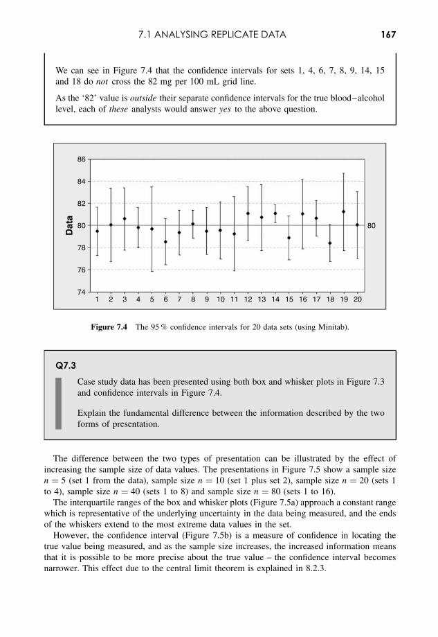
7.1 ANALYSING REPLICATE DATA 167
We can see in Figure 7.4 that the confidence intervals for sets 1, 4, 6, 7, 8, 9, 14, 15and 18 do not cross the 82 mg per 100 mL grid line.
As the ‘82’ value is outside their separate confidence intervals for the true blood–alcohollevel, each of these analysts would answer yes to the above question.
86
84
82
80 80
78
76
741 2 3 4 5 6 7 8 9 10 11 12 13 14 15 16 17 18 19 20
Dat
a
Figure 7.4 The 95 % confidence intervals for 20 data sets (using Minitab).
Q7.3Case study data has been presented using both box and whisker plots in Figure 7.3and confidence intervals in Figure 7.4.
Explain the fundamental difference between the information described by the twoforms of presentation.
The difference between the two types of presentation can be illustrated by the effect ofincreasing the sample size of data values. The presentations in Figure 7.5 show a sample sizen = 5 (set 1 from the data), sample size n = 10 (set 1 plus set 2), sample size n = 20 (sets 1to 4), sample size n = 40 (sets 1 to 8) and sample size n = 80 (sets 1 to 16).
The interquartile ranges of the box and whisker plots (Figure 7.5a) approach a constant rangewhich is representative of the underlying uncertainty in the data being measured, and the endsof the whiskers extend to the most extreme data values in the set.
However, the confidence interval (Figure 7.5b) is a measure of confidence in locating thetrue value being measured, and as the sample size increases, the increased information meansthat it is possible to be more precise about the true value – the confidence interval becomesnarrower. This effect due to the central limit theorem is explained in 8.2.3.
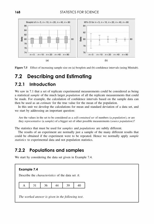
168 STATISTICS FOR SCIENCE
(a) (b)
Boxplot of n = 5, n = 10, n = 20, n = 40, n = 80 95% CI for n = 5, n = 10, n = 20, n = 40, n = 80
n = 5 n = 10 n = 20 n = 40 n = 80 n = 5 n = 10 n = 20 n = 40 n = 80
86
84
82
80 80 80
78
76
84
82
80
78
7674
Dat
a
Dat
a
Figure 7.5 Effect of increasing sample size on (a) boxplots and (b) confidence intervals (using Minitab).
7.2 Describing and Estimating7.2.1 IntroductionWe saw in 7.1 that a set of replicate experimental measurements could be considered as beinga statistical sample of the much larger population of all the replicate measurements that couldbe made. For example, the calculation of confidence intervals based on the sample data canthen be used as an estimate for the true value for the mean of the population.
In this unit we develop the calculations for mean and standard deviation of a data set, andwe start by addressing an important question:
Are the values in the set to be considered as a self-contained set of numbers (a population), or arethey representative (a sample) of a bigger set of other possible measurements (source population)?
The statistics that must be used for samples and populations are subtly different.The results of an experiment are normally just a sample of the many different results that
could be obtained if the experiment were to be repeated. Hence we normally apply samplestatistics to experimental data and not population statistics.
7.2.2 Populations and samplesWe start by considering the data set given in Example 7.4.
Example 7.4
Describe the characteristics of the data set A:
A 31 36 44 39 40
The worked answer is given in the following text .
7.2 DESCRIBING AND ESTIMATING 169
The way in which we treat the five numbers in Example 7.4 will depend on whether the dataset A is:
• a population consisting of just the numbers 31, 36, 44, 39, 40, with no other numbersinvolved; or
• a sample of five replicate experimental measurements, which form part of a much largersource population of measurements that could be created if the experiment were repeatedmany times.
We can test whether a data set is a sample or a population by considering the effect of repeatingthe process by which the data values were identified .
If repeating the process of identification still gives the same values, then the data set is apopulation , but if different values can be produced then the set is a sample.
A student collects all 200 frogs (a population) from a specific pond and, finding that 120are female and 80 male, he concludes that the proportion of females in that pond is 0.60. Asecond student collects all the frogs again (the same population) and will record exactly thesame proportion of females to males. By comparison, a student who randomly picks just 50frogs only collects a sample, and may get a different proportion of females and males in everydifferent sample of 50 frogs that he may select – see Example 14.7.
A sample of values only gives us best estimates of the population values that we are tryingto measure. However it is possible, through good experiment design (15.1), to obtain resultsthat are sufficiently accurate for the purpose, without the need to make an excessive numberof measurements.
Q7.4Identify, for each of the following data sets, whether the data set is a sample or apopulation:
(i) The four numbers {5.1, 5.2, 5.1, 5.3}. Sample/Population
(ii) Four repeated measurements of the pH of asolution.
Sample/Population
(iii) The numbers recorded in 37 spins of a roulettewheel.
Sample/Population
(iv) The 37 numbers (including ‘0’) on a roulettewheel.
Sample/Population
(v) The scores achieved by England in all theirfootball matches during the 2002 World Cup.
Sample/Population
(vi) The amount of pocket money received by arandom selection of children as part of a‘lifestyle’ survey.
Sample/Population
If data set A (Example 7.4) is a self-contained population , then we can use statistics simplyto describe the characteristics of the data set.
170 STATISTICS FOR SCIENCE
If, however, the data set A is a sample of experimental values, then we will use statistics toestimate the characteristics of the source population of experimental measurements from whichthe sample was derived. For example, we will use the average (mean) value of the sample datato estimate what would be the average (mean) value if the experiment were repeated manymore times.
A parameter is a variable that is used to describe some characteristic of a population . Aparameter is usually given a Greek letter as a symbol, e.g. µ for population mean and σ forpopulation standard deviation.
A statistic is a variable that is used to describe some characteristic of a sample, e.g. x forsample mean and s for sample standard deviation.
The value of the statistic of a sample (e.g. mean of the sample) is used to estimate the valueof the equivalent parameter of the population (i.e. mean of the population) from which thesample was drawn. Different samples from the same population will typically give differentvalues for the same statistic (i.e. different sample means).
7.2.3 Statistics notationTypically, a calculation in statistics may be dealing with very many data values, and it wouldbe time consuming to write out every single number. Instead, statistics often use a form ofshorthand to show what is happening in the calculations.
Subscripts are used to identify particular values in a set of data. For example, the valuesfrom data set A in Example 7.4 could be written as a1, a2, a3, a4, a5, where a1 = 31, a2 = 36,etc.
The Greek symbol∑
(capital sigma) is often used to indicate the summation (addition) of arange of numbers:
∑51 (ai) is shorthand in statistics for saying ‘add together a1, a2, a3, a4, a5’.
Example 7.5
Using the values of data set A from Example 7.4, the summation is written as:
∑5
1(ai) = a1 + a2 + a3 + a4 + a5 = 31 + 36 + 44 + 39 + 40 = 190
In general, for n values of x to be added together, we would write:
∑n
1(xi) = x1 + x2 + x3 + · · · + xn−1 + xn [7.1]
The above equation says ‘sum all values of xi for i ranging from 1 to n’.
7.2 DESCRIBING AND ESTIMATING 171
Note that when the values of all the possible variables in a set are to be added together, thesummation is often written in simplified forms:
∑n
1(xi) =
∑i
(xi) =∑
(xi)
It is well worth taking a few minutes to understand each new symbol when it appears. The abil-ity to ‘read’ statistics more fluently will be an enormous help in developing a good understandof statistics as a whole.
Q7.5
Calculate∑5
1 (xi) for the following set of x-values:
x1 = 4.9, x2 = 4.7, x3 = 5.1, x4 = 4.9, x5 = 4.4
7.2.4 Means and averagesThe mean (or average value) for a population is usually written as µ(mu).
The mean (or average value) for a sample is usually written as x.The mean value, x, of a sample of data is the best estimate for the unknown mean, µ, of
the source population from which the sample was derived. Note that x is a statistic, which isused to estimate the value of the parameter, µ.
For example, opinion pollsters take samples of about 1000 people to get best estimatesfor the way in which the population may choose to vote in a political election. The votingintentions of the population are estimated from the sample results.
The mean values for the sample, x, and the population, µ, are both calculated as the simpleaverages of the data values:
Sample mean, x = Sum of all data values
Number of data values=
∑n1 (xi)
n=
∑(xi)
n[7.2]
Population mean, µ = Sum of all data values
Number of data values=
∑n1 (xi)
n=
∑(xi)
n[7.3]
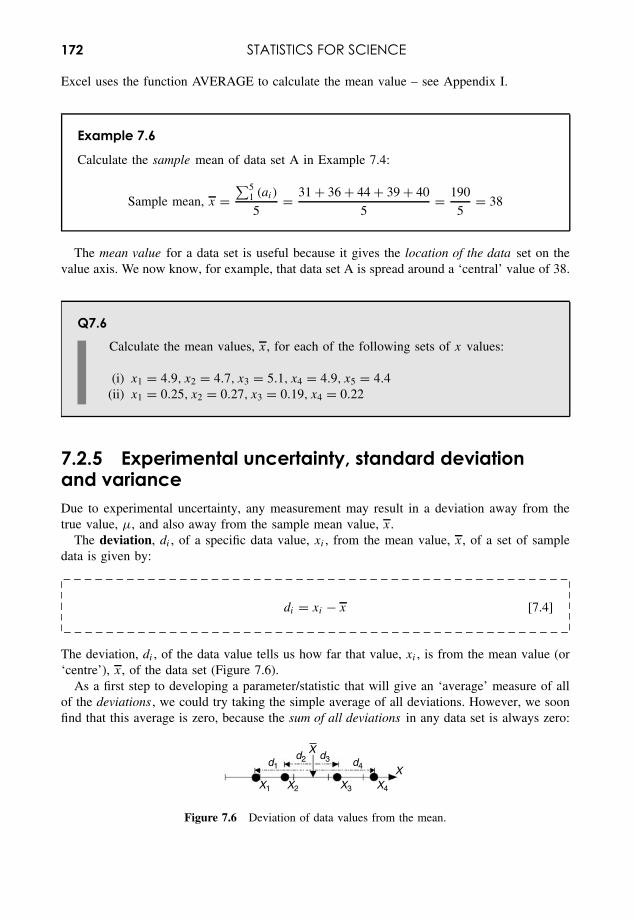
172 STATISTICS FOR SCIENCE
Excel uses the function AVERAGE to calculate the mean value – see Appendix I.
Example 7.6
Calculate the sample mean of data set A in Example 7.4:
Sample mean, x =∑5
1 (ai)
5= 31 + 36 + 44 + 39 + 40
5= 190
5= 38
The mean value for a data set is useful because it gives the location of the data set on thevalue axis. We now know, for example, that data set A is spread around a ‘central’ value of 38.
Q7.6Calculate the mean values, x, for each of the following sets of x values:
(i) x1 = 4.9, x2 = 4.7, x3 = 5.1, x4 = 4.9, x5 = 4.4(ii) x1 = 0.25, x2 = 0.27, x3 = 0.19, x4 = 0.22
7.2.5 Experimental uncertainty, standard deviationand varianceDue to experimental uncertainty, any measurement may result in a deviation away from thetrue value, µ, and also away from the sample mean value, x.
The deviation, di , of a specific data value, xi , from the mean value, x, of a set of sampledata is given by:
di = xi − x [7.4]
The deviation, di , of the data value tells us how far that value, xi , is from the mean value (or‘centre’), x, of the data set (Figure 7.6).
As a first step to developing a parameter/statistic that will give an ‘average’ measure of allof the deviations , we could try taking the simple average of all deviations. However, we soonfind that this average is zero, because the sum of all deviations in any data set is always zero:
d2 d3d1
X1 X2 X3 X4
X d4
X
Figure 7.6 Deviation of data values from the mean.
7.2 DESCRIBING AND ESTIMATING 173
∑n
1(di) =
∑n
1(xi − x) = 0
Instead of the simple average of deviations, we can try the average of (deviations)2, becausethe sum of all (deviations)2 is not zero:
∑n
1(d2
i ) =∑n
1(xi − x)2 = 0
The next step is to provide an ‘average’ value for (deviations)2 by dividing the sum by n − 1to produce a statistic called the sample variance of the data:
Sample variance, s2 =∑n
1 d2i
n − 1⇒
∑n1 (xi − x)2
n − 1[7.5]
However, variance cannot be used as a direct measure of spread , because it has units whichare the square of the units for the data value, e.g. the variance of a measurement of time inseconds would have units of (seconds)2.
Finally, by taking the square root of the sample variance, we produce the sample standarddeviation (equation [7.6]), which does have the same units as the data values, and has becomethe most commonly used indicator to describe the spread of experimental data values:
Sample standard deviation, s =√∑n
1 (xi − x)2
n − 1[7.6]
If we were trying to describe the spread of a population , where the mean value is given byµ, then we would use the statistic:
Population standard deviation, σ =√∑n
1 (xi − µ)2
n[7.7]
In most experimental situations we only have a sample set of data. In this case our bestestimate of the unknown population standard deviation, σ , is given by the sample standarddeviation , s.
The difference between the divisors in equations [7.6] and [7.7] results from the fact thatσ is describing the spread of the actual data values, whereas s is estimating the spread of
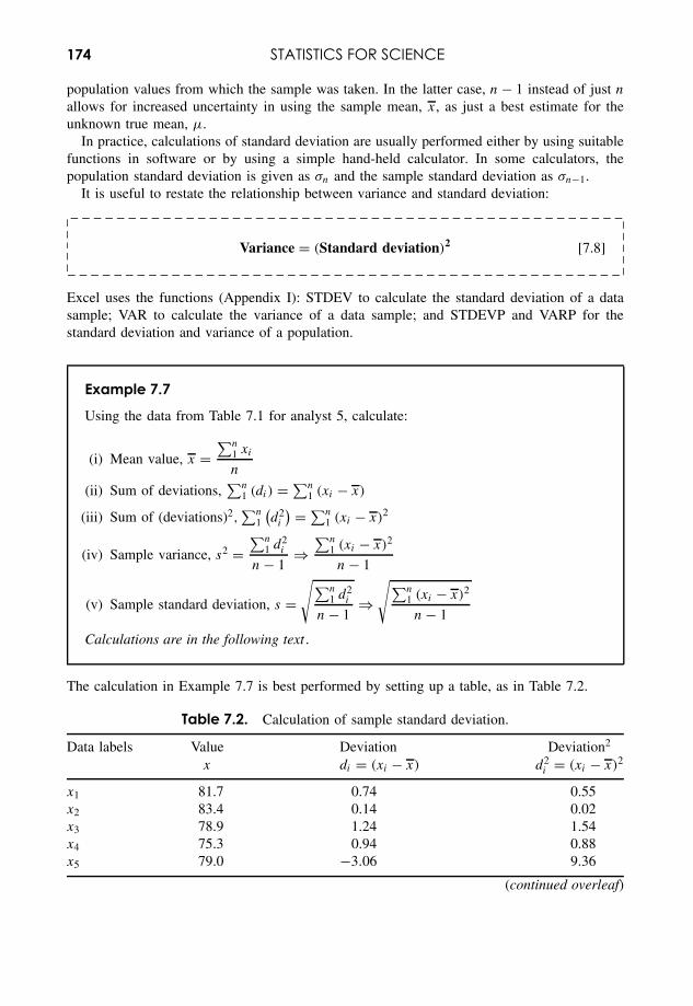
174 STATISTICS FOR SCIENCE
population values from which the sample was taken. In the latter case, n − 1 instead of just n
allows for increased uncertainty in using the sample mean, x, as just a best estimate for theunknown true mean, µ.
In practice, calculations of standard deviation are usually performed either by using suitablefunctions in software or by using a simple hand-held calculator. In some calculators, thepopulation standard deviation is given as σn and the sample standard deviation as σn−1.
It is useful to restate the relationship between variance and standard deviation:
Variance = (Standard deviation)2 [7.8]
Excel uses the functions (Appendix I): STDEV to calculate the standard deviation of a datasample; VAR to calculate the variance of a data sample; and STDEVP and VARP for thestandard deviation and variance of a population.
Example 7.7
Using the data from Table 7.1 for analyst 5, calculate:
(i) Mean value, x =∑n
1 xi
n
(ii) Sum of deviations,∑n
1 (di) = ∑n1 (xi − x)
(iii) Sum of (deviations)2,∑n
1
(d2
i
) = ∑n1 (xi − x)2
(iv) Sample variance, s2 =∑n
1 d2i
n − 1⇒
∑n1 (xi − x)2
n − 1
(v) Sample standard deviation, s =√∑n
1 d2i
n − 1⇒
√∑n1 (xi − x)2
n − 1
Calculations are in the following text .
The calculation in Example 7.7 is best performed by setting up a table, as in Table 7.2.
Table 7.2. Calculation of sample standard deviation.
Data labels Value Deviation Deviation2
x di = (xi − x) d2i = (xi − x)2
x1 81.7 0.74 0.55x2 83.4 0.14 0.02x3 78.9 1.24 1.54x4 75.3 0.94 0.88x5 79.0 −3.06 9.36
(continued overleaf)
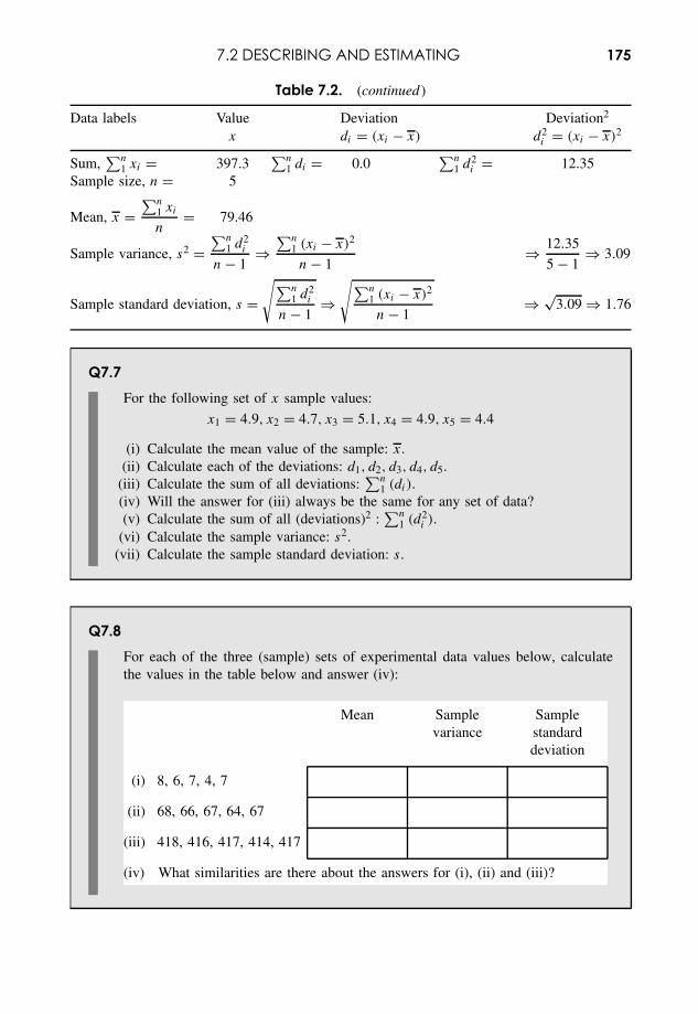
7.2 DESCRIBING AND ESTIMATING 175
Table 7.2. (continued )
Data labels Value Deviation Deviation2
x di = (xi − x) d2i = (xi − x)2
Sum,∑n
1 xi = 397.3∑n
1 di = 0.0∑n
1 d2i = 12.35
Sample size, n = 5
Mean, x =∑n
1 xi
n= 79.46
Sample variance, s2 =∑n
1 d2i
n − 1⇒
∑n1 (xi − x)2
n − 1⇒ 12.35
5 − 1⇒ 3.09
Sample standard deviation, s =√∑n
1 d2i
n − 1⇒
√∑n1 (xi − x)2
n − 1⇒ √
3.09 ⇒ 1.76
Q7.7For the following set of x sample values:
x1 = 4.9, x2 = 4.7, x3 = 5.1, x4 = 4.9, x5 = 4.4
(i) Calculate the mean value of the sample: x.(ii) Calculate each of the deviations: d1, d2, d3, d4, d5.
(iii) Calculate the sum of all deviations:∑n
1 (di).(iv) Will the answer for (iii) always be the same for any set of data?(v) Calculate the sum of all (deviations)2 :
∑n1 (d2
i ).(vi) Calculate the sample variance: s2.
(vii) Calculate the sample standard deviation: s.
Q7.8For each of the three (sample) sets of experimental data values below, calculatethe values in the table below and answer (iv):
Mean Sample Samplevariance standard
deviation
(i) 8, 6, 7, 4, 7
(ii) 68, 66, 67, 64, 67
(iii) 418, 416, 417, 414, 417
(iv) What similarities are there about the answers for (i), (ii) and (iii)?
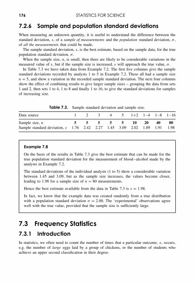
176 STATISTICS FOR SCIENCE
7.2.6 Sample and population standard deviationsWhen measuring an unknown quantity, it is useful to understand the difference between thestandard deviation, s, of a sample of measurements and the population standard deviation, σ ,of all the measurements that could be made.
The sample standard deviation, s, is the best estimate, based on the sample data, for the truepopulation standard deviation, σ .
When the sample size, n, is small, then there are likely to be considerable variations in themeasured value of s, but if the sample size is increased, s will approach the true value, σ .
In Table 7.3 we have taken data from Example 7.2. The first five columns give the samplestandard deviations recorded by analysts 1 to 5 in Example 7.2. These all had a sample sizen = 5, and show a variation in the recorded sample standard deviation. The next four columnsshow the effect of combining results to give larger sample sizes – grouping the data from sets1 and 2, then sets 1 to 4, 1 to 8 and finally 1 to 16, to give the standard deviations for samplesof increasing size.
Table 7.3. Sample standard deviation and sample size.
Data source 1 2 3 4 5 1+2 1–4 1–8 1–16
Sample size, n 5 5 5 5 5 10 20 40 80Sample standard deviation, s 1.76 2.42 2.27 1.45 3.09 2.02 1.89 1.91 1.98
Example 7.8
On the basis of the results in Table 7.3 give the best estimate that can be made for thetrue population standard deviation for the measurement of blood–alcohol made by theanalysts in Example 7.2.
The standard deviations of the individual analysts (1 to 5) show a considerable variationbetween 1.45 and 3.09, but as the sample size increases, the values become closer,leading to 1.98 for a sample size of n = 80 measurements.
Hence the best estimate available from the data in Table 7.3 is s = 1.98.
In fact, we know that the example data was created randomly from a true distributionwith a population standard deviation σ = 2.00. The ‘experimental’ observations agreewell with the true value, provided that the sample size is sufficiently large.
7.3 Frequency Statistics7.3.1 IntroductionIn statistics, we often need to count the number of times that a particular outcome, x, occurs,e.g. the number of large eggs laid by a group of chickens, or the number of students whoachieve an upper second classification in their degree.
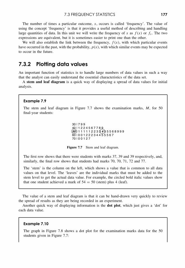
7.3 FREQUENCY STATISTICS 177
The number of times a particular outcome, x, occurs is called ‘frequency’. The value ofusing the concept ‘frequency’ is that it provides a useful method of describing and handlinglarge quantities of data. In this unit we will write the frequency of x as f (x) or fx . The twoexpressions are equivalent, but it is sometimes easier to print one than the other.
We will also establish the link between the frequency, f (x), with which particular eventshave occurred in the past, with the probability, p(x), with which similar events may be expectedto occur in the future.
7.3.2 Plotting data valuesAn important function of statistics is to handle large numbers of data values in such a waythat the analyst can easily understand the essential characteristics of the data set.
A stem and leaf diagram is a quick way of displaying a spread of data values for initialanalysis.
Example 7.9
The stem and leaf diagram in Figure 7.7 shows the examination marks, M , for 50final-year students:
30 | 7 9 940 | 1 2 2 4 5 6 7 7 8 950 | 1 1 1 1 1 2 2 3 3 4 5 5 5 6 8 9 9 960 | 0 0 1 2 2 2 3 4 4 5 5 5 6 770 | 0 0 1 2 7
Figure 7.7 Stem and leaf diagram.
The first row shows that there were students with marks 37, 39 and 39 respectively, and,similarly, the final row shows that students had marks 70, 70, 71, 72 and 77.
The ‘stem’ is the column on the left, which shows a value that is common to all datavalues on that level. The ‘leaves’ are the individual marks that must be added to thestem level to get the actual data value. For example, the circled bold italic values showthat one student achieved a mark of 54 = 50 (stem) plus 4 (leaf).
The value of a stem and leaf diagram is that it can be hand-drawn very quickly to reviewthe spread of results as they are being recorded in an experiment.
Another quick way of displaying information is the dot plot, which just gives a ‘dot’ foreach data value.
Example 7.10
The graph in Figure 7.8 shows a dot plot for the examination marks data for the 50students given in Figure 7.7:
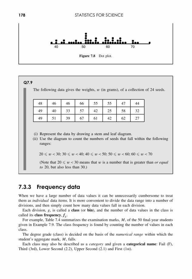
178 STATISTICS FOR SCIENCE
40 50 60 70
Figure 7.8 Dot plot.
Q7.9The following data gives the weights, w (in grams), of a collection of 24 seeds.
48 46 46 66 55 55 47 44
49 40 33 57 42 25 58 32
49 51 39 67 61 42 62 27
(i) Represent the data by drawing a stem and leaf diagram.(ii) Use the diagram to count the numbers of seeds that fall within the following
ranges:
20 � w < 30; 30 � w < 40; 40 � w < 50; 50 � w < 60; 60 � w < 70
(Note that 20 � w < 30 means that w is a number that is greater than or equalto 20, but also less than 30.)
7.3.3 Frequency dataWhen we have a large number of data values it can be unnecessarily cumbersome to treatthem as individual data items. It is more convenient to divide the data range into a number ofdivisions, and then simply count how many data values fall in each division.
Each division, g, is called a class (or bin), and the number of data values in the class iscalled its class frequency, fg.
For example, Table 7.4 summarizes the examination marks, M , of the 50 final-year studentsgiven in Example 7.9. The class frequency is found by counting the number of values in eachclass.
The degree grade (class) is decided on the basis of the numerical range within which thestudent’s aggregate mark, M , falls.
Each class may also be described as a category and given a categorical name: Fail (F),Third (3rd), Lower Second (2.2), Upper Second (2.1) and First (1st).
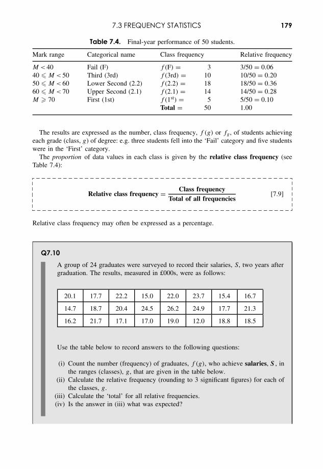
7.3 FREQUENCY STATISTICS 179
Table 7.4. Final-year performance of 50 students.
Mark range Categorical name Class frequency Relative frequency
M < 40 Fail (F) f (F) = 3 3/50 = 0.0640 � M < 50 Third (3rd) f (3rd) = 10 10/50 = 0.2050 � M < 60 Lower Second (2.2) f (2.2) = 18 18/50 = 0.3660 � M < 70 Upper Second (2.1) f (2.1) = 14 14/50 = 0.28M � 70 First (1st) f (1st) = 5 5/50 = 0.10
Total = 50 1.00
The results are expressed as the number, class frequency, f (g) or fg , of students achievingeach grade (class, g) of degree: e.g. three students fell into the ‘Fail’ category and five studentswere in the ‘First’ category.
The proportion of data values in each class is given by the relative class frequency (seeTable 7.4):
Relative class frequency = Class frequencyTotal of all frequencies
[7.9]
Relative class frequency may often be expressed as a percentage.
Q7.10A group of 24 graduates were surveyed to record their salaries, S, two years aftergraduation. The results, measured in £000s, were as follows:
20.1 17.7 22.2 15.0 22.0 23.7 15.4 16.7
14.7 18.7 20.4 24.5 26.2 24.9 17.7 21.3
16.2 21.7 17.1 17.0 19.0 12.0 18.8 18.5
Use the table below to record answers to the following questions:
(i) Count the number (frequency) of graduates, f (g), who achieve salaries, S , inthe ranges (classes), g, that are given in the table below.
(ii) Calculate the relative frequency (rounding to 3 significant figures) for each ofthe classes, g.
(iii) Calculate the ‘total’ for all relative frequencies.(iv) Is the answer in (iii) what was expected?
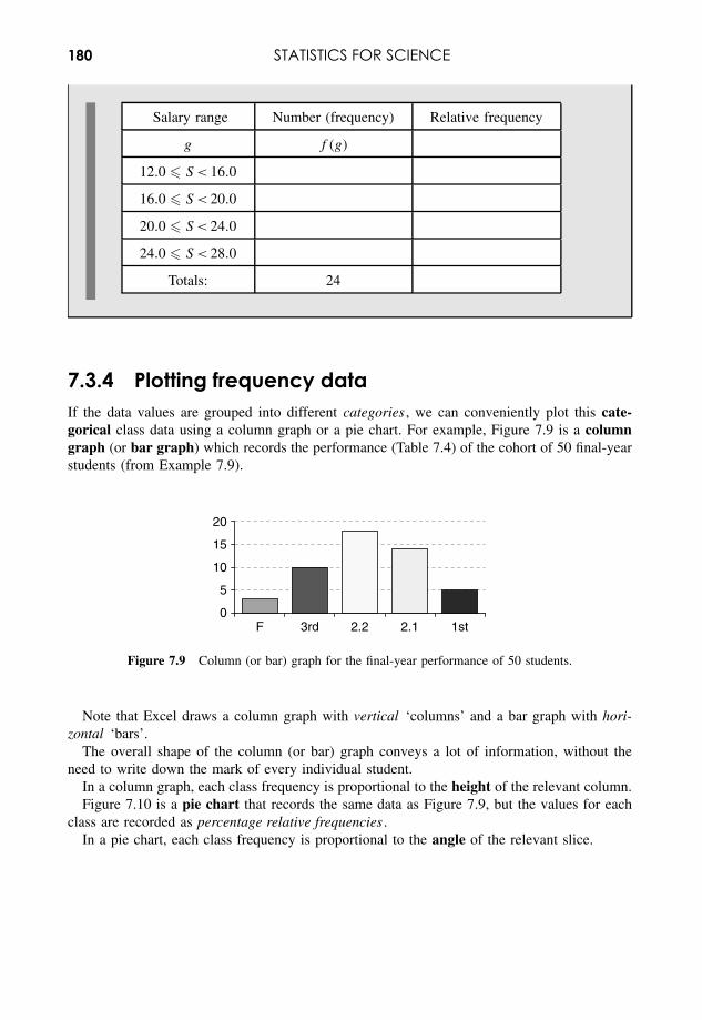
180 STATISTICS FOR SCIENCE
Salary range Number (frequency) Relative frequency
g f (g)
12.0 � S < 16.0
16.0 � S < 20.0
20.0 � S < 24.0
24.0 � S < 28.0
Totals: 24
7.3.4 Plotting frequency dataIf the data values are grouped into different categories , we can conveniently plot this cate-gorical class data using a column graph or a pie chart. For example, Figure 7.9 is a columngraph (or bar graph) which records the performance (Table 7.4) of the cohort of 50 final-yearstudents (from Example 7.9).
0
5
10
15
20
F 3rd 2.2 2.1 1st
Figure 7.9 Column (or bar) graph for the final-year performance of 50 students.
Note that Excel draws a column graph with vertical ‘columns’ and a bar graph with hori-zontal ‘bars’.
The overall shape of the column (or bar) graph conveys a lot of information, without theneed to write down the mark of every individual student.
In a column graph, each class frequency is proportional to the height of the relevant column.Figure 7.10 is a pie chart that records the same data as Figure 7.9, but the values for each
class are recorded as percentage relative frequencies .In a pie chart, each class frequency is proportional to the angle of the relevant slice.
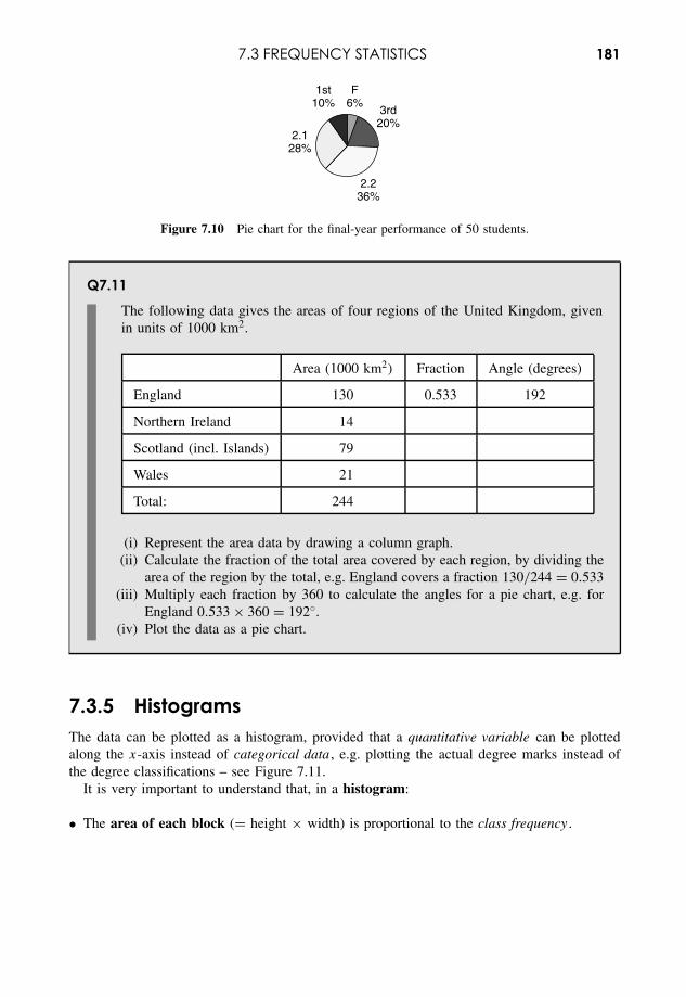
7.3 FREQUENCY STATISTICS 181
F6%
3rd20%
2.236%
2.128%
1st10%
Figure 7.10 Pie chart for the final-year performance of 50 students.
Q7.11The following data gives the areas of four regions of the United Kingdom, givenin units of 1000 km2.
Area (1000 km2) Fraction Angle (degrees)
England 130 0.533 192
Northern Ireland 14
Scotland (incl. Islands) 79
Wales 21
Total: 244
(i) Represent the area data by drawing a column graph.(ii) Calculate the fraction of the total area covered by each region, by dividing the
area of the region by the total, e.g. England covers a fraction 130/244 = 0.533(iii) Multiply each fraction by 360 to calculate the angles for a pie chart, e.g. for
England 0.533 × 360 = 192◦.(iv) Plot the data as a pie chart.
7.3.5 HistogramsThe data can be plotted as a histogram, provided that a quantitative variable can be plottedalong the x-axis instead of categorical data , e.g. plotting the actual degree marks instead ofthe degree classifications – see Figure 7.11.
It is very important to understand that, in a histogram:
• The area of each block (= height × width) is proportional to the class frequency .
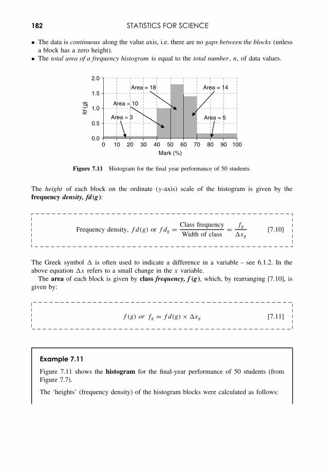
182 STATISTICS FOR SCIENCE
• The data is continuous along the value axis, i.e. there are no gaps between the blocks (unlessa block has a zero height).
• The total area of a frequency histogram is equal to the total number , n, of data values.
0.0
0.5
1.0
1.5
2.0
40 50 60 70 90 1003020100
Area = 10
fd (
g)
80
Area = 18 Area = 14
Area = 5Area = 3
Mark (%)
Figure 7.11 Histogram for the final year performance of 50 students.
The height of each block on the ordinate (y-axis) scale of the histogram is given by thefrequency density, fd (g):
Frequency density, f d(g) or f dg = Class frequency
Width of class= fg
�xg
[7.10]
The Greek symbol � is often used to indicate a difference in a variable – see 6.1.2. In theabove equation �x refers to a small change in the x variable.
The area of each block is given by class frequency, f (g), which, by rearranging [7.10], isgiven by:
f (g) or fg = f d(g) × �xg [7.11]
Example 7.11
Figure 7.11 shows the histogram for the final-year performance of 50 students (fromFigure 7.7).
The ‘heights’ (frequency density) of the histogram blocks were calculated as follows:
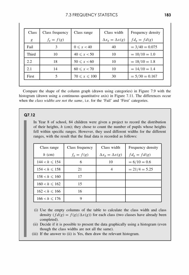
7.3 FREQUENCY STATISTICS 183
Class Class frequency Class range Class width Frequency density
g fg = f (g) �xg = �x(g) f dg = f d(g)
Fail 3 0 � x < 40 40 = 3/40 = 0.075
Third 10 40 � x < 50 10 = 10/10 = 1.0
2.2 18 50 � x < 60 10 = 18/10 = 1.8
2.1 14 60 � x < 70 10 = 14/10 = 1.4
First 5 70 � x � 100 30 = 5/30 = 0.167
Compare the shape of the column graph (drawn using categories) in Figure 7.9 with thehistogram (drawn using a continuous quantitative axis) in Figure 7.11. The differences occurwhen the class widths are not the same, i.e. for the ‘Fail’ and ‘First’ categories.
Q7.12In Year 8 of school, 84 children were given a project to record the distributionof their heights, h (cm); they chose to count the number of pupils whose heightsfell within specific ranges. However, they used different widths for the differentranges, with the result that the final data is recorded as follows:
Class range Class frequency Class width Frequency density
h (cm) fg = f (g) �xg = �x(g) f dg = f d(g)
144 <h � 154 6 10 = 6/10 = 0.6
154 <h � 158 21 4 = 21/4 = 5.25
158 <h � 160 17
160 <h � 162 15
162 <h � 166 16
166 <h � 176 9
(i) Use the empty columns of the table to calculate the class width and classdensity (f d(g) = f (g)/�x(g)) for each class (two classes have already beencompleted).
(ii) Decide if it is possible to present the data graphically using a histogram (eventhough the class widths are not all the same).
(iii) If the answer to (ii) is Yes, then draw the relevant histogram.
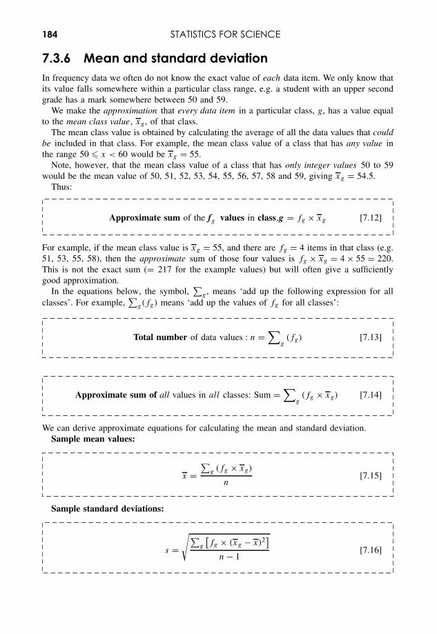
184 STATISTICS FOR SCIENCE
7.3.6 Mean and standard deviationIn frequency data we often do not know the exact value of each data item. We only know thatits value falls somewhere within a particular class range, e.g. a student with an upper secondgrade has a mark somewhere between 50 and 59.
We make the approximation that every data item in a particular class, g, has a value equalto the mean class value, xg, of that class.
The mean class value is obtained by calculating the average of all the data values that couldbe included in that class. For example, the mean class value of a class that has any value inthe range 50 � x < 60 would be xg = 55.
Note, however, that the mean class value of a class that has only integer values 50 to 59would be the mean value of 50, 51, 52, 53, 54, 55, 56, 57, 58 and 59, giving xg = 54.5.
Thus:
Approximate sum of the fg values in class,g = fg × xg [7.12]
For example, if the mean class value is xg = 55, and there are fg = 4 items in that class (e.g.51, 53, 55, 58), then the approximate sum of those four values is fg × xg = 4 × 55 = 220.This is not the exact sum (= 217 for the example values) but will often give a sufficientlygood approximation.
In the equations below, the symbol,∑
g , means ‘add up the following expression for allclasses’. For example,
∑g(fg) means ‘add up the values of fg for all classes’:
Total number of data values : n =∑
g(fg) [7.13]
Approximate sum of all values in all classes: Sum =∑
g(fg × xg) [7.14]
We can derive approximate equations for calculating the mean and standard deviation.Sample mean values:
x =∑
g (fg × xg)
n[7.15]
Sample standard deviations:
s =√∑
g
[fg × (xg − x)2
]n − 1
[7.16]
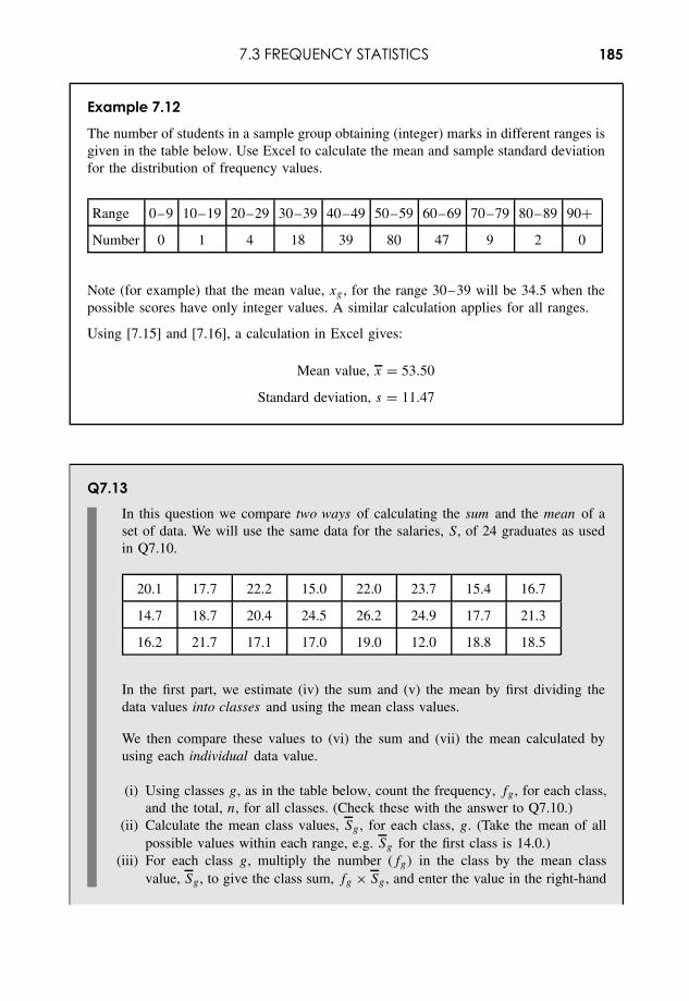
7.3 FREQUENCY STATISTICS 185
Example 7.12
The number of students in a sample group obtaining (integer) marks in different ranges isgiven in the table below. Use Excel to calculate the mean and sample standard deviationfor the distribution of frequency values.
Range 0–9 10–19 20–29 30–39 40–49 50–59 60–69 70–79 80–89 90+Number 0 1 4 18 39 80 47 9 2 0
Note (for example) that the mean value, xg , for the range 30–39 will be 34.5 when thepossible scores have only integer values. A similar calculation applies for all ranges.
Using [7.15] and [7.16], a calculation in Excel gives:
Mean value, x = 53.50
Standard deviation, s = 11.47
Q7.13In this question we compare two ways of calculating the sum and the mean of aset of data. We will use the same data for the salaries, S, of 24 graduates as usedin Q7.10.
20.1 17.7 22.2 15.0 22.0 23.7 15.4 16.7
14.7 18.7 20.4 24.5 26.2 24.9 17.7 21.3
16.2 21.7 17.1 17.0 19.0 12.0 18.8 18.5
In the first part, we estimate (iv) the sum and (v) the mean by first dividing thedata values into classes and using the mean class values.
We then compare these values to (vi) the sum and (vii) the mean calculated byusing each individual data value.
(i) Using classes g, as in the table below, count the frequency, fg , for each class,and the total, n, for all classes. (Check these with the answer to Q7.10.)
(ii) Calculate the mean class values, Sg , for each class, g. (Take the mean of allpossible values within each range, e.g. Sg for the first class is 14.0.)
(iii) For each class g, multiply the number (fg) in the class by the mean classvalue, Sg, to give the class sum, fg × Sg , and enter the value in the right-hand
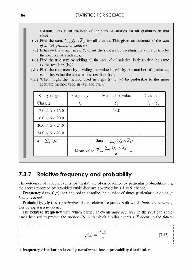
186 STATISTICS FOR SCIENCE
column. This is an estimate of the sum of salaries for all graduates in thatclass.
(iv) Find the sum,∑
g fg × Sg , for all classes. This gives an estimate of the sumof all 24 graduates’ salaries .
(v) Estimate the mean value, S, of all the salaries by dividing the value in (iv) bythe number of graduates, n.
(vi) Find the true sum by adding all the individual salaries. Is this value the sameas the result in (iv)?
(vii) Find the true mean by dividing the value in (vi) by the number of graduates,n. Is this value the same as the result in (iv)?
(viii) When might the method used in steps (i) to (v) be preferable to the moreaccurate method used in (vi) and (vii)?
Salary range Frequency Mean class value Class sum
Class, g fg Sg fg × Sg
12.0 � S < 16.0 14.0
16.0 � S < 20.0
20.0 � S < 24.0
24.0 � S < 28.0
n = ∑g (fg) = Sum = ∑
g (fg × Sg) =
Mean value, S =∑
g (fg × Sg)
n=
7.3.7 Relative frequency and probabilityThe outcomes of random events (or ‘trials’) are often governed by particular probabilities, e.g.the scores recorded by six-sided cubic dice are governed by a 1 in 6 chance.
Frequency data, f (g), can be used to describe the number of times particular outcomes , g,have occurred .
Probability, p(g), is a prediction of the relative frequency with which future outcomes , g,can be expected to occur .
The relative frequency with which particular events have occurred in the past can some-times be used to predict the probability with which similar events will occur in the future:
p(g) = f (g)
n[7.17]
A frequency distribution is easily transformed into a probability distribution.
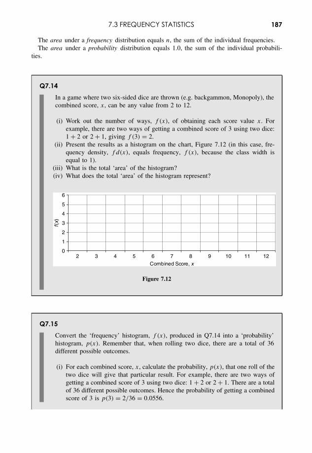
7.3 FREQUENCY STATISTICS 187
The area under a frequency distribution equals n, the sum of the individual frequencies.The area under a probability distribution equals 1.0, the sum of the individual probabili-
ties.
Q7.14In a game where two six-sided dice are thrown (e.g. backgammon, Monopoly), thecombined score, x, can be any value from 2 to 12.
(i) Work out the number of ways, f (x), of obtaining each score value x. Forexample, there are two ways of getting a combined score of 3 using two dice:1 + 2 or 2 + 1, giving f (3) = 2.
(ii) Present the results as a histogram on the chart, Figure 7.12 (in this case, fre-quency density, f d(x), equals frequency, f (x), because the class width isequal to 1).
(iii) What is the total ‘area’ of the histogram?(iv) What does the total ‘area’ of the histogram represent?
0
1
2
3
4
5
6
Combined Score, x
f(x)
2 3 4 5 6 7 8 9 10 11 12
Figure 7.12
Q7.15Convert the ‘frequency’ histogram, f (x), produced in Q7.14 into a ‘probability’histogram, p(x). Remember that, when rolling two dice, there are a total of 36different possible outcomes.
(i) For each combined score, x, calculate the probability, p(x), that one roll of thetwo dice will give that particular result. For example, there are two ways ofgetting a combined score of 3 using two dice: 1 + 2 or 2 + 1. There are a totalof 36 different possible outcomes. Hence the probability of getting a combinedscore of 3 is p(3) = 2/36 = 0.0556.
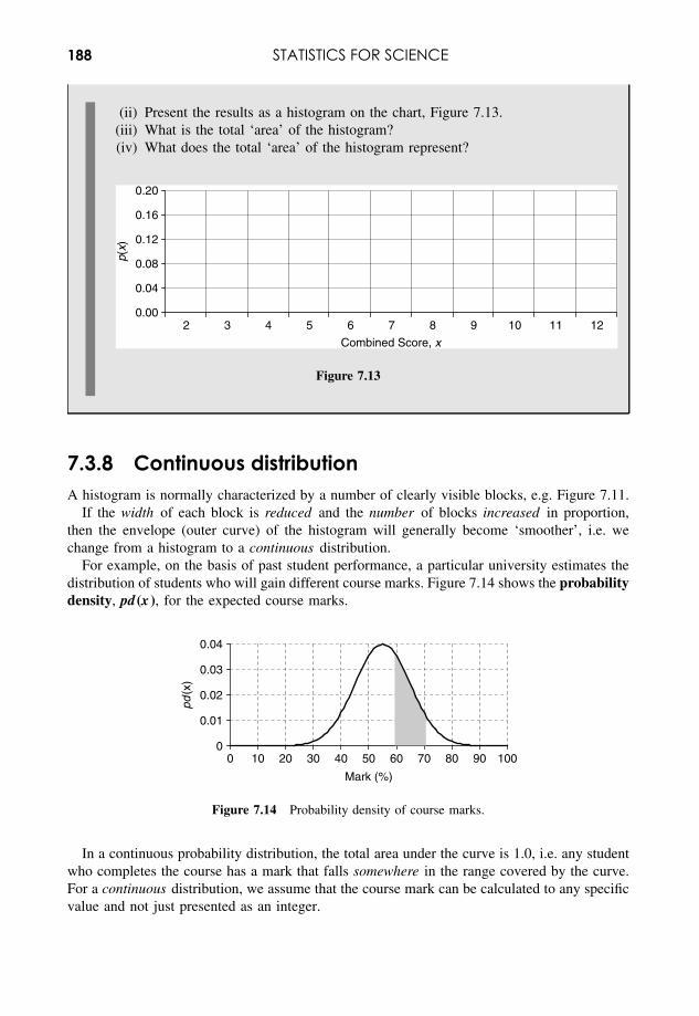
188 STATISTICS FOR SCIENCE
(ii) Present the results as a histogram on the chart, Figure 7.13.(iii) What is the total ‘area’ of the histogram?(iv) What does the total ‘area’ of the histogram represent?
0.00
0.04
0.08
0.12
0.16
0.20
Combined Score, x
p(x)
2 3 4 5 6 7 8 9 10 11 12
Figure 7.13
7.3.8 Continuous distributionA histogram is normally characterized by a number of clearly visible blocks, e.g. Figure 7.11.
If the width of each block is reduced and the number of blocks increased in proportion,then the envelope (outer curve) of the histogram will generally become ‘smoother’, i.e. wechange from a histogram to a continuous distribution.
For example, on the basis of past student performance, a particular university estimates thedistribution of students who will gain different course marks. Figure 7.14 shows the probabilitydensity, pd (x ), for the expected course marks.
pd(x
)
Mark (%)
0
0.01
0.02
0.03
0.04
0 10 20 30 40 50 60 70 80 90 100
Figure 7.14 Probability density of course marks.
In a continuous probability distribution, the total area under the curve is 1.0, i.e. any studentwho completes the course has a mark that falls somewhere in the range covered by the curve.For a continuous distribution, we assume that the course mark can be calculated to any specificvalue and not just presented as an integer.
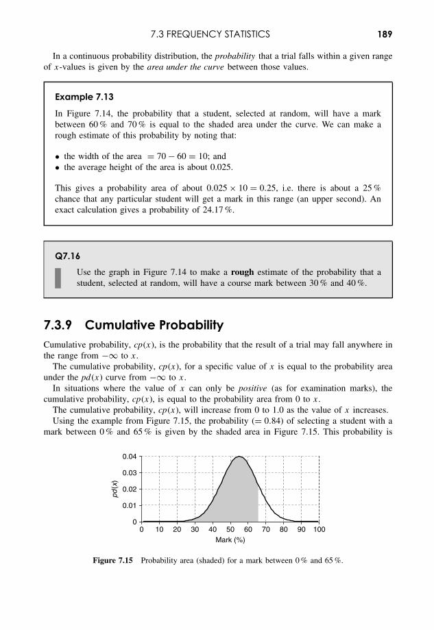
7.3 FREQUENCY STATISTICS 189
In a continuous probability distribution, the probability that a trial falls within a given rangeof x-values is given by the area under the curve between those values.
Example 7.13
In Figure 7.14, the probability that a student, selected at random, will have a markbetween 60 % and 70 % is equal to the shaded area under the curve. We can make arough estimate of this probability by noting that:
• the width of the area = 70 − 60 = 10; and• the average height of the area is about 0.025.
This gives a probability area of about 0.025 × 10 = 0.25, i.e. there is about a 25 %chance that any particular student will get a mark in this range (an upper second). Anexact calculation gives a probability of 24.17 %.
Q7.16Use the graph in Figure 7.14 to make a rough estimate of the probability that astudent, selected at random, will have a course mark between 30 % and 40 %.
7.3.9 Cumulative ProbabilityCumulative probability, cp(x), is the probability that the result of a trial may fall anywhere inthe range from −∞ to x.
The cumulative probability, cp(x), for a specific value of x is equal to the probability areaunder the pd (x) curve from −∞ to x.
In situations where the value of x can only be positive (as for examination marks), thecumulative probability, cp(x), is equal to the probability area from 0 to x.
The cumulative probability, cp(x), will increase from 0 to 1.0 as the value of x increases.Using the example from Figure 7.15, the probability (= 0.84) of selecting a student with a
mark between 0 % and 65 % is given by the shaded area in Figure 7.15. This probability is
pd(x
)
Mark (%)
0
0.01
0.02
0.03
0.04
0 10 20 30 40 50 60 70 80 90 100
Figure 7.15 Probability area (shaded) for a mark between 0 % and 65 %.
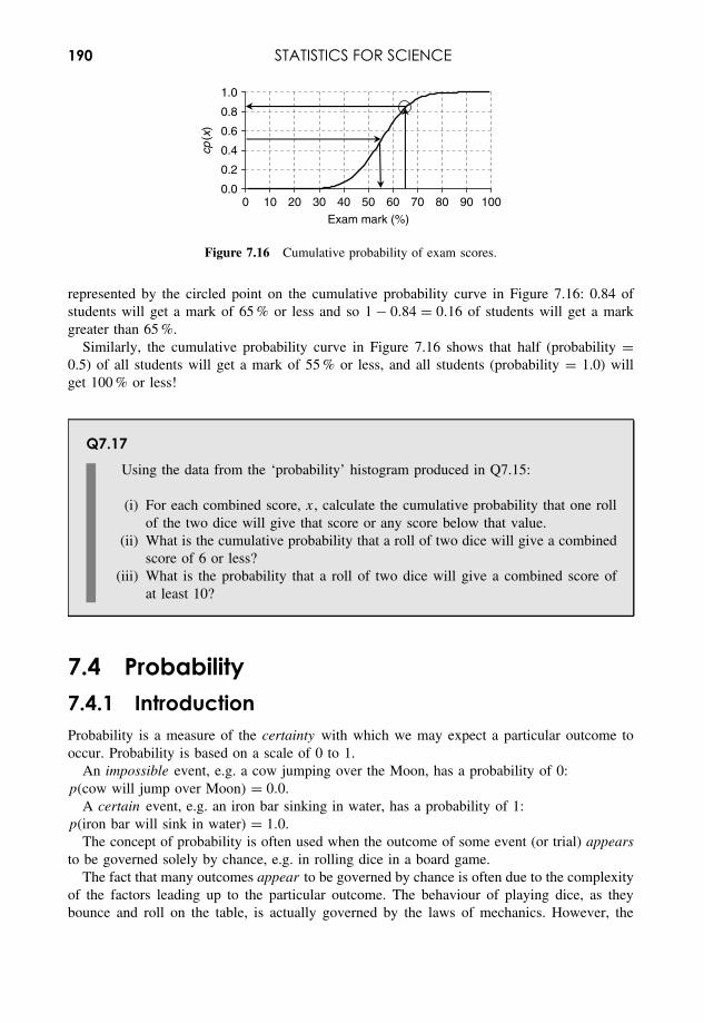
190 STATISTICS FOR SCIENCE
0.0
0.2
0.4
0.6
0.8
1.0
0 10 20 30 40 50 60 70 80 90 100cp
(x)
Exam mark (%)
Figure 7.16 Cumulative probability of exam scores.
represented by the circled point on the cumulative probability curve in Figure 7.16: 0.84 ofstudents will get a mark of 65 % or less and so 1 − 0.84 = 0.16 of students will get a markgreater than 65 %.
Similarly, the cumulative probability curve in Figure 7.16 shows that half (probability =0.5) of all students will get a mark of 55 % or less, and all students (probability = 1.0) willget 100 % or less!
Q7.17Using the data from the ‘probability’ histogram produced in Q7.15:
(i) For each combined score, x, calculate the cumulative probability that one rollof the two dice will give that score or any score below that value.
(ii) What is the cumulative probability that a roll of two dice will give a combinedscore of 6 or less?
(iii) What is the probability that a roll of two dice will give a combined score ofat least 10?
7.4 Probability7.4.1 IntroductionProbability is a measure of the certainty with which we may expect a particular outcome tooccur. Probability is based on a scale of 0 to 1.
An impossible event, e.g. a cow jumping over the Moon, has a probability of 0:p(cow will jump over Moon) = 0.0.
A certain event, e.g. an iron bar sinking in water, has a probability of 1:p(iron bar will sink in water) = 1.0.
The concept of probability is often used when the outcome of some event (or trial) appearsto be governed solely by chance, e.g. in rolling dice in a board game.
The fact that many outcomes appear to be governed by chance is often due to the complexityof the factors leading up to the particular outcome. The behaviour of playing dice, as theybounce and roll on the table, is actually governed by the laws of mechanics. However, the
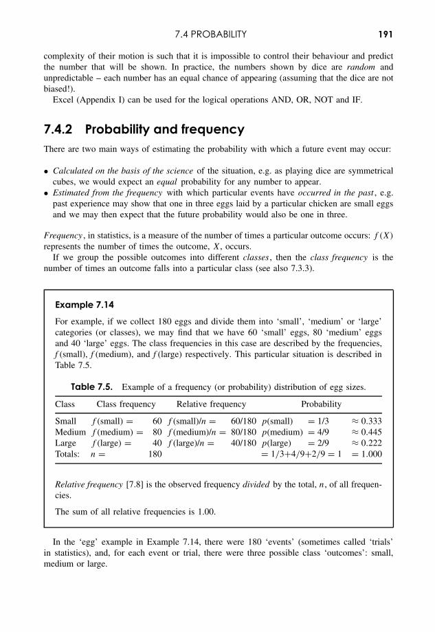
7.4 PROBABILITY 191
complexity of their motion is such that it is impossible to control their behaviour and predictthe number that will be shown. In practice, the numbers shown by dice are random andunpredictable – each number has an equal chance of appearing (assuming that the dice are notbiased!).
Excel (Appendix I) can be used for the logical operations AND, OR, NOT and IF.
7.4.2 Probability and frequencyThere are two main ways of estimating the probability with which a future event may occur:
• Calculated on the basis of the science of the situation, e.g. as playing dice are symmetricalcubes, we would expect an equal probability for any number to appear.
• Estimated from the frequency with which particular events have occurred in the past , e.g.past experience may show that one in three eggs laid by a particular chicken are small eggsand we may then expect that the future probability would also be one in three.
Frequency , in statistics, is a measure of the number of times a particular outcome occurs: f (X)
represents the number of times the outcome, X, occurs.If we group the possible outcomes into different classes , then the class frequency is the
number of times an outcome falls into a particular class (see also 7.3.3).
Example 7.14
For example, if we collect 180 eggs and divide them into ‘small’, ‘medium’ or ‘large’categories (or classes), we may find that we have 60 ‘small’ eggs, 80 ‘medium’ eggsand 40 ‘large’ eggs. The class frequencies in this case are described by the frequencies,f (small), f (medium), and f (large) respectively. This particular situation is described inTable 7.5.
Table 7.5. Example of a frequency (or probability) distribution of egg sizes.
Class Class frequency Relative frequency Probability
Small f (small) = 60 f (small)/n = 60/180 p(small) = 1/3 ≈ 0.333Medium f (medium) = 80 f (medium)/n = 80/180 p(medium) = 4/9 ≈ 0.445Large f (large) = 40 f (large)/n = 40/180 p(large) = 2/9 ≈ 0.222Totals: n = 180 = 1/3+4/9+2/9 = 1 = 1.000
Relative frequency [7.8] is the observed frequency divided by the total, n , of all frequen-cies.
The sum of all relative frequencies is 1.00.
In the ‘egg’ example in Example 7.14, there were 180 ‘events’ (sometimes called ‘trials’in statistics), and, for each event or trial, there were three possible class ‘outcomes’: small,medium or large.
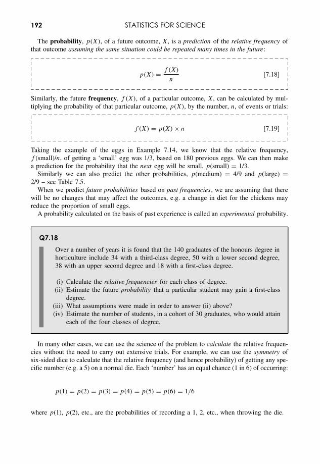
192 STATISTICS FOR SCIENCE
The probability, p(X), of a future outcome, X, is a prediction of the relative frequency ofthat outcome assuming the same situation could be repeated many times in the future:
p(X) = f (X)
n[7.18]
Similarly, the future frequency, f (X), of a particular outcome, X, can be calculated by mul-tiplying the probability of that particular outcome, p(X), by the number, n, of events or trials:
f (X) = p(X) × n [7.19]
Taking the example of the eggs in Example 7.14, we know that the relative frequency,f (small)/n, of getting a ‘small’ egg was 1/3, based on 180 previous eggs. We can then makea prediction for the probability that the next egg will be small, p(small) = 1/3.
Similarly we can also predict the other probabilities, p(medium) = 4/9 and p(large) =2/9 – see Table 7.5.
When we predict future probabilities based on past frequencies , we are assuming that therewill be no changes that may affect the outcomes, e.g. a change in diet for the chickens mayreduce the proportion of small eggs.
A probability calculated on the basis of past experience is called an experimental probability.
Q7.18Over a number of years it is found that the 140 graduates of the honours degree inhorticulture include 34 with a third-class degree, 50 with a lower second degree,38 with an upper second degree and 18 with a first-class degree.
(i) Calculate the relative frequencies for each class of degree.(ii) Estimate the future probability that a particular student may gain a first-class
degree.(iii) What assumptions were made in order to answer (ii) above?(iv) Estimate the number of students, in a cohort of 30 graduates, who would attain
each of the four classes of degree.
In many other cases, we can use the science of the problem to calculate the relative frequen-cies without the need to carry out extensive trials. For example, we can use the symmetry ofsix-sided dice to calculate that the relative frequency (and hence probability) of getting any spe-cific number (e.g. a 5) on a normal die. Each ‘number’ has an equal chance (1 in 6) of occurring:
p(1) = p(2) = p(3) = p(4) = p(5) = p(6) = 1/6
where p(1), p(2), etc., are the probabilities of recording a 1, 2, etc., when throwing the die.
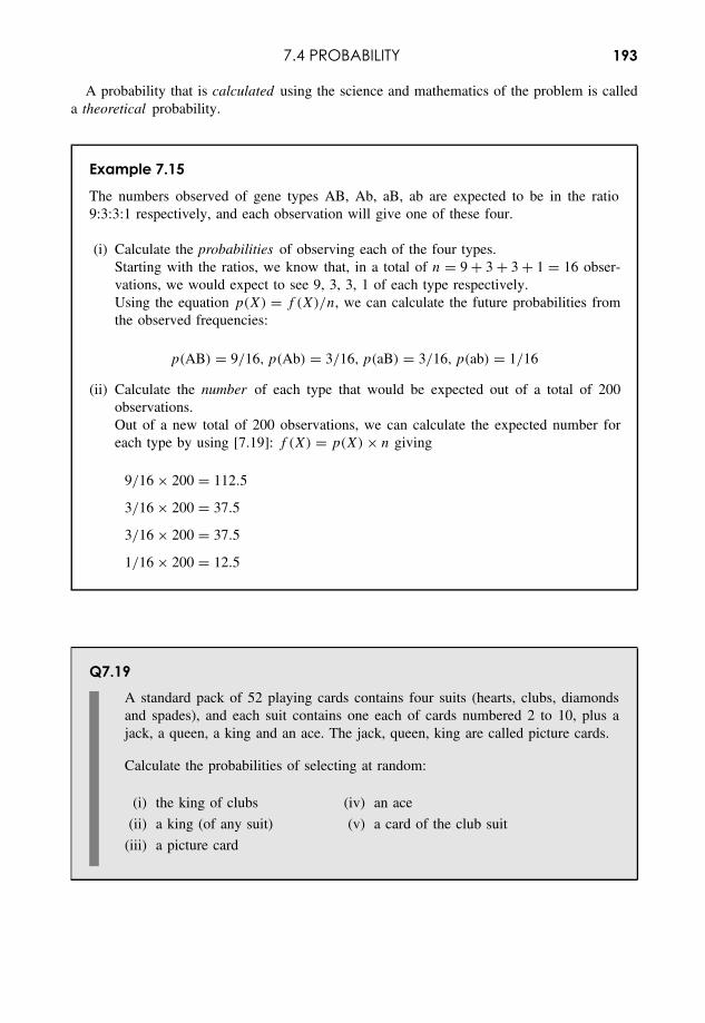
7.4 PROBABILITY 193
A probability that is calculated using the science and mathematics of the problem is calleda theoretical probability.
Example 7.15
The numbers observed of gene types AB, Ab, aB, ab are expected to be in the ratio9:3:3:1 respectively, and each observation will give one of these four.
(i) Calculate the probabilities of observing each of the four types.Starting with the ratios, we know that, in a total of n = 9 + 3 + 3 + 1 = 16 obser-vations, we would expect to see 9, 3, 3, 1 of each type respectively.Using the equation p(X) = f (X)/n, we can calculate the future probabilities fromthe observed frequencies:
p(AB) = 9/16, p(Ab) = 3/16, p(aB) = 3/16, p(ab) = 1/16
(ii) Calculate the number of each type that would be expected out of a total of 200observations.Out of a new total of 200 observations, we can calculate the expected number foreach type by using [7.19]: f (X) = p(X) × n giving
9/16 × 200 = 112.5
3/16 × 200 = 37.5
3/16 × 200 = 37.5
1/16 × 200 = 12.5
Q7.19A standard pack of 52 playing cards contains four suits (hearts, clubs, diamondsand spades), and each suit contains one each of cards numbered 2 to 10, plus ajack, a queen, a king and an ace. The jack, queen, king are called picture cards.
Calculate the probabilities of selecting at random:
(i) the king of clubs (iv) an ace
(ii) a king (of any suit) (v) a card of the club suit
(iii) a picture card
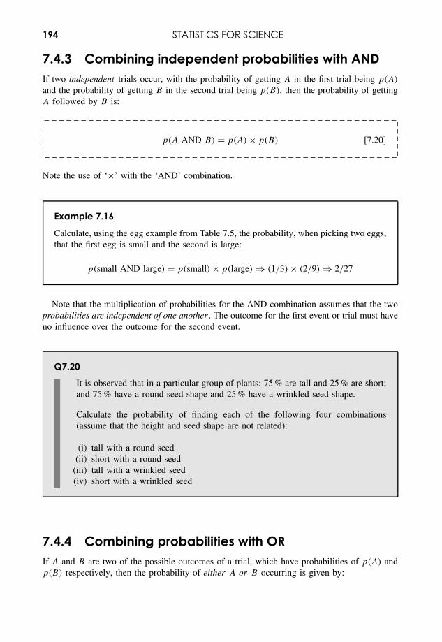
194 STATISTICS FOR SCIENCE
7.4.3 Combining independent probabilities with ANDIf two independent trials occur, with the probability of getting A in the first trial being p(A)
and the probability of getting B in the second trial being p(B), then the probability of gettingA followed by B is:
p(A AND B) = p(A) × p(B) [7.20]
Note the use of ‘×’ with the ‘AND’ combination.
Example 7.16
Calculate, using the egg example from Table 7.5, the probability, when picking two eggs,that the first egg is small and the second is large:
p(small AND large) = p(small) × p(large) ⇒ (1/3) × (2/9) ⇒ 2/27
Note that the multiplication of probabilities for the AND combination assumes that the twoprobabilities are independent of one another . The outcome for the first event or trial must haveno influence over the outcome for the second event.
Q7.20It is observed that in a particular group of plants: 75 % are tall and 25 % are short;and 75 % have a round seed shape and 25 % have a wrinkled seed shape.
Calculate the probability of finding each of the following four combinations(assume that the height and seed shape are not related):
(i) tall with a round seed(ii) short with a round seed
(iii) tall with a wrinkled seed(iv) short with a wrinkled seed
7.4.4 Combining probabilities with ORIf A and B are two of the possible outcomes of a trial, which have probabilities of p(A) andp(B) respectively, then the probability of either A or B occurring is given by:
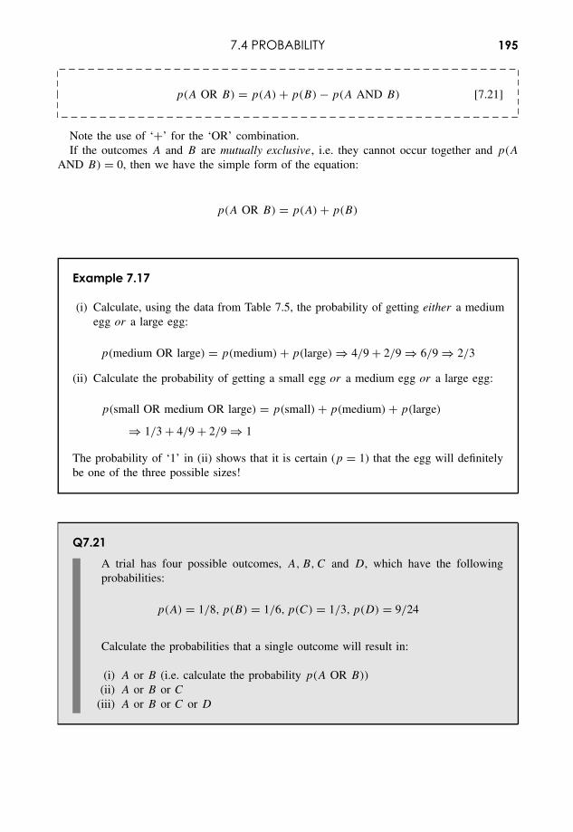
7.4 PROBABILITY 195
p(A OR B) = p(A) + p(B) − p(A AND B) [7.21]
Note the use of ‘+’ for the ‘OR’ combination.If the outcomes A and B are mutually exclusive, i.e. they cannot occur together and p(A
AND B) = 0, then we have the simple form of the equation:
p(A OR B) = p(A) + p(B)
Example 7.17
(i) Calculate, using the data from Table 7.5, the probability of getting either a mediumegg or a large egg:
p(medium OR large) = p(medium) + p(large) ⇒ 4/9 + 2/9 ⇒ 6/9 ⇒ 2/3
(ii) Calculate the probability of getting a small egg or a medium egg or a large egg:
p(small OR medium OR large) = p(small) + p(medium) + p(large)
⇒ 1/3 + 4/9 + 2/9 ⇒ 1
The probability of ‘1’ in (ii) shows that it is certain (p = 1) that the egg will definitelybe one of the three possible sizes!
Q7.21A trial has four possible outcomes, A, B, C and D, which have the followingprobabilities:
p(A) = 1/8, p(B) = 1/6, p(C) = 1/3, p(D) = 9/24
Calculate the probabilities that a single outcome will result in:
(i) A or B (i.e. calculate the probability p(A OR B))
(ii) A or B or C
(iii) A or B or C or D
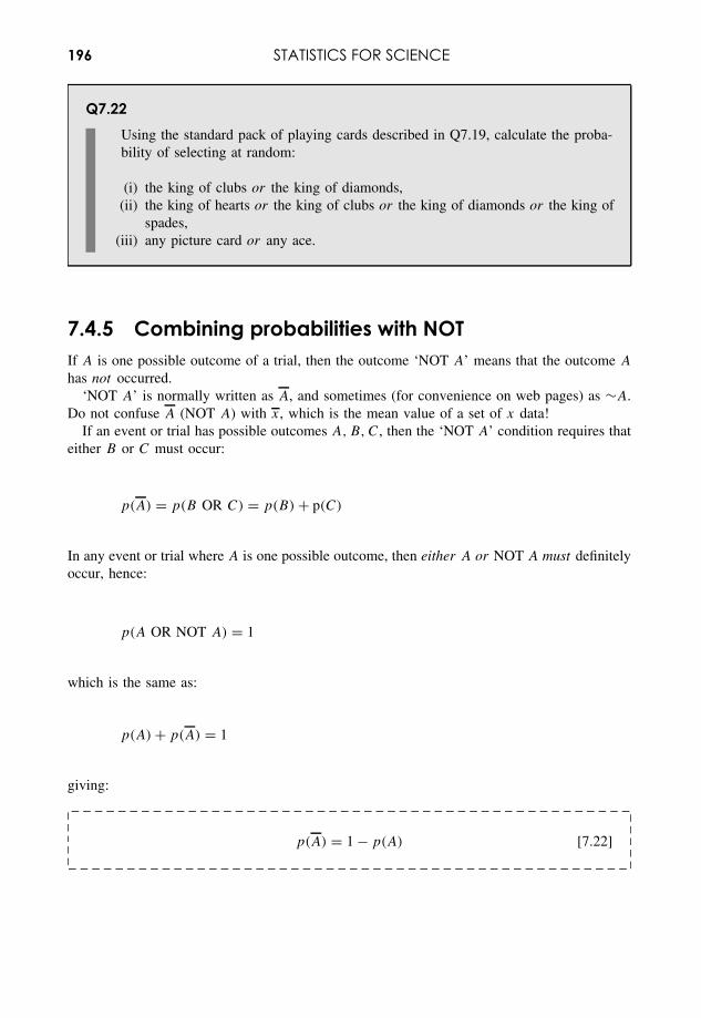
196 STATISTICS FOR SCIENCE
Q7.22Using the standard pack of playing cards described in Q7.19, calculate the proba-bility of selecting at random:
(i) the king of clubs or the king of diamonds,(ii) the king of hearts or the king of clubs or the king of diamonds or the king of
spades,(iii) any picture card or any ace.
7.4.5 Combining probabilities with NOTIf A is one possible outcome of a trial, then the outcome ‘NOT A’ means that the outcome A
has not occurred.‘NOT A’ is normally written as A, and sometimes (for convenience on web pages) as ∼A.
Do not confuse A (NOT A) with x, which is the mean value of a set of x data!If an event or trial has possible outcomes A, B, C, then the ‘NOT A’ condition requires that
either B or C must occur:
p(A) = p(B OR C) = p(B) + p(C)
In any event or trial where A is one possible outcome, then either A or NOT A must definitelyoccur, hence:
p(A OR NOT A) = 1
which is the same as:
p(A) + p(A) = 1
giving:
p(A) = 1 − p(A) [7.22]
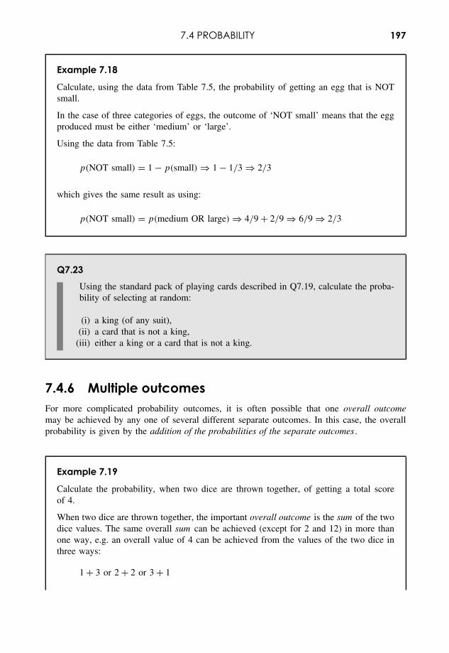
7.4 PROBABILITY 197
Example 7.18
Calculate, using the data from Table 7.5, the probability of getting an egg that is NOTsmall.
In the case of three categories of eggs, the outcome of ‘NOT small’ means that the eggproduced must be either ‘medium’ or ‘large’.
Using the data from Table 7.5:
p(NOT small) = 1 − p(small) ⇒ 1 − 1/3 ⇒ 2/3
which gives the same result as using:
p(NOT small) = p(medium OR large) ⇒ 4/9 + 2/9 ⇒ 6/9 ⇒ 2/3
Q7.23Using the standard pack of playing cards described in Q7.19, calculate the proba-bility of selecting at random:
(i) a king (of any suit),(ii) a card that is not a king,
(iii) either a king or a card that is not a king.
7.4.6 Multiple outcomesFor more complicated probability outcomes, it is often possible that one overall outcomemay be achieved by any one of several different separate outcomes. In this case, the overallprobability is given by the addition of the probabilities of the separate outcomes .
Example 7.19
Calculate the probability, when two dice are thrown together, of getting a total scoreof 4.
When two dice are thrown together, the important overall outcome is the sum of the twodice values. The same overall sum can be achieved (except for 2 and 12) in more thanone way, e.g. an overall value of 4 can be achieved from the values of the two dice inthree ways:
1 + 3 or 2 + 2 or 3 + 1
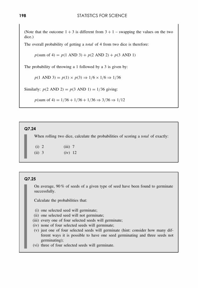
198 STATISTICS FOR SCIENCE
(Note that the outcome 1 + 3 is different from 3 + 1 – swapping the values on the twodice.)
The overall probability of getting a total of 4 from two dice is therefore:
p(sum of 4) = p(1 AND 3) + p(2 AND 2) + p(3 AND 1)
The probability of throwing a 1 followed by a 3 is given by:
p(1 AND 3) = p(1) × p(3) ⇒ 1/6 × 1/6 ⇒ 1/36
Similarly: p(2 AND 2) = p(3 AND 1) = 1/36 giving:
p(sum of 4) = 1/36 + 1/36 + 1/36 ⇒ 3/36 ⇒ 1/12
Q7.24When rolling two dice, calculate the probabilities of scoring a total of exactly:
(i) 2 (iii) 7
(ii) 3 (iv) 12
Q7.25On average, 90 % of seeds of a given type of seed have been found to germinatesuccessfully.
Calculate the probabilities that:
(i) one selected seed will germinate;(ii) one selected seed will not germinate;
(iii) every one of four selected seeds will germinate;(iv) none of four selected seeds will germinate;(v) just one of four selected seeds will germinate (hint: consider how many dif-
ferent ways it is possible to have one seed germinating and three seeds notgerminating);
(vi) three of four selected seeds will germinate.
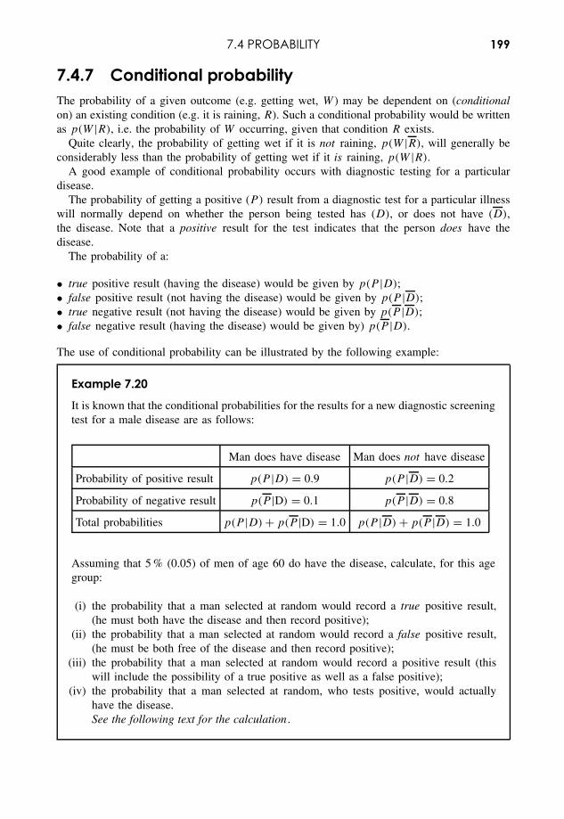
7.4 PROBABILITY 199
7.4.7 Conditional probabilityThe probability of a given outcome (e.g. getting wet, W ) may be dependent on (conditionalon) an existing condition (e.g. it is raining, R). Such a conditional probability would be writtenas p(W |R), i.e. the probability of W occurring, given that condition R exists.
Quite clearly, the probability of getting wet if it is not raining, p(W |R), will generally beconsiderably less than the probability of getting wet if it is raining, p(W |R).
A good example of conditional probability occurs with diagnostic testing for a particulardisease.
The probability of getting a positive (P ) result from a diagnostic test for a particular illnesswill normally depend on whether the person being tested has (D), or does not have (D),the disease. Note that a positive result for the test indicates that the person does have thedisease.
The probability of a:
• true positive result (having the disease) would be given by p(P |D);• false positive result (not having the disease) would be given by p(P |D);• true negative result (not having the disease) would be given by p(P |D);• false negative result (having the disease) would be given by) p(P |D).
The use of conditional probability can be illustrated by the following example:
Example 7.20
It is known that the conditional probabilities for the results for a new diagnostic screeningtest for a male disease are as follows:
Man does have disease Man does not have disease
Probability of positive result p(P |D) = 0.9 p(P |D) = 0.2
Probability of negative result p(P |D) = 0.1 p(P |D) = 0.8
Total probabilities p(P |D) + p(P |D) = 1.0 p(P |D) + p(P |D) = 1.0
Assuming that 5 % (0.05) of men of age 60 do have the disease, calculate, for this agegroup:
(i) the probability that a man selected at random would record a true positive result,(he must both have the disease and then record positive);
(ii) the probability that a man selected at random would record a false positive result,(he must be both free of the disease and then record positive);
(iii) the probability that a man selected at random would record a positive result (thiswill include the possibility of a true positive as well as a false positive);
(iv) the probability that a man selected at random, who tests positive, would actuallyhave the disease.See the following text for the calculation .
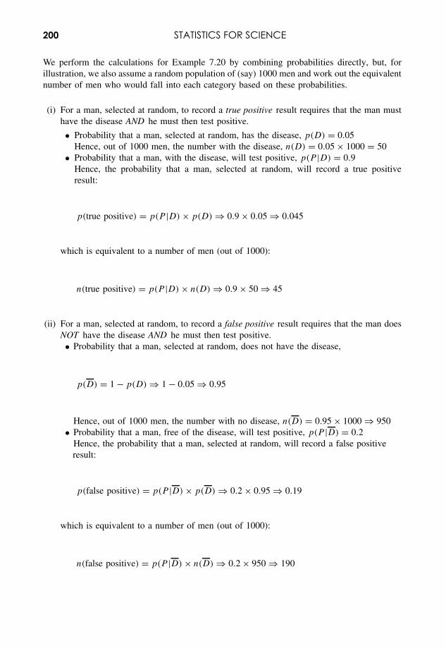
200 STATISTICS FOR SCIENCE
We perform the calculations for Example 7.20 by combining probabilities directly, but, forillustration, we also assume a random population of (say) 1000 men and work out the equivalentnumber of men who would fall into each category based on these probabilities.
(i) For a man, selected at random, to record a true positive result requires that the man musthave the disease AND he must then test positive.
• Probability that a man, selected at random, has the disease, p(D) = 0.05Hence, out of 1000 men, the number with the disease, n(D) = 0.05 × 1000 = 50
• Probability that a man, with the disease, will test positive, p(P |D) = 0.9Hence, the probability that a man, selected at random, will record a true positiveresult:
p(true positive) = p(P |D) × p(D) ⇒ 0.9 × 0.05 ⇒ 0.045
which is equivalent to a number of men (out of 1000):
n(true positive) = p(P |D) × n(D) ⇒ 0.9 × 50 ⇒ 45
(ii) For a man, selected at random, to record a false positive result requires that the man doesNOT have the disease AND he must then test positive.• Probability that a man, selected at random, does not have the disease,
p(D) = 1 − p(D) ⇒ 1 − 0.05 ⇒ 0.95
Hence, out of 1000 men, the number with no disease, n(D) = 0.95 × 1000 ⇒ 950• Probability that a man, free of the disease, will test positive, p(P |D) = 0.2
Hence, the probability that a man, selected at random, will record a false positiveresult:
p(false positive) = p(P |D) × p(D) ⇒ 0.2 × 0.95 ⇒ 0.19
which is equivalent to a number of men (out of 1000):
n(false positive) = p(P |D) × n(D) ⇒ 0.2 × 950 ⇒ 190
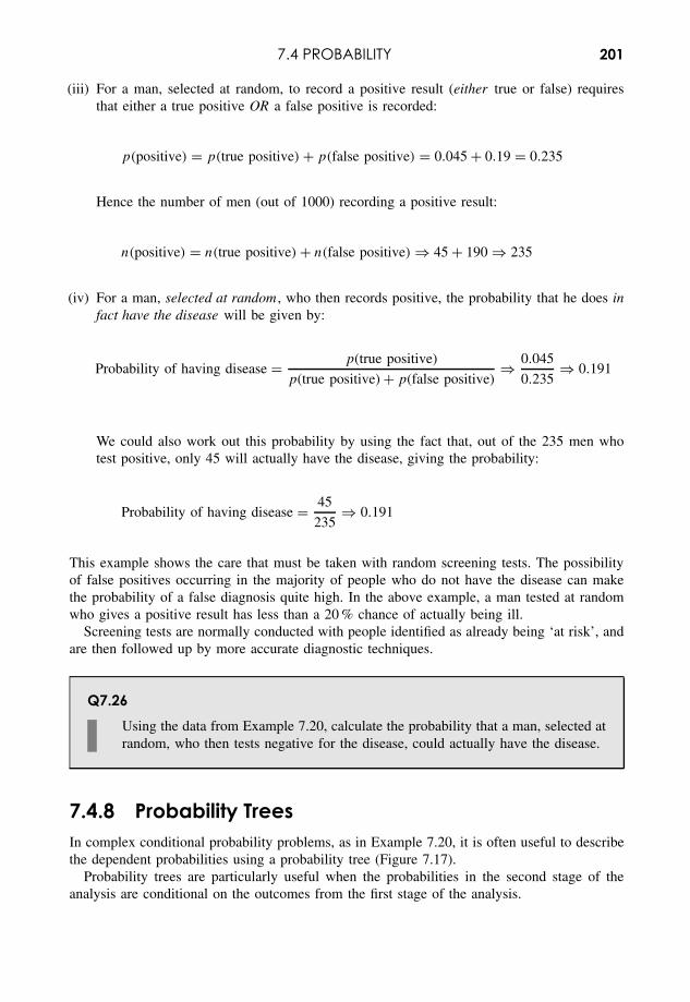
7.4 PROBABILITY 201
(iii) For a man, selected at random, to record a positive result (either true or false) requiresthat either a true positive OR a false positive is recorded:
p(positive) = p(true positive) + p(false positive) = 0.045 + 0.19 = 0.235
Hence the number of men (out of 1000) recording a positive result:
n(positive) = n(true positive) + n(false positive) ⇒ 45 + 190 ⇒ 235
(iv) For a man, selected at random , who then records positive, the probability that he does infact have the disease will be given by:
Probability of having disease = p(true positive)
p(true positive) + p(false positive)⇒ 0.045
0.235⇒ 0.191
We could also work out this probability by using the fact that, out of the 235 men whotest positive, only 45 will actually have the disease, giving the probability:
Probability of having disease = 45
235⇒ 0.191
This example shows the care that must be taken with random screening tests. The possibilityof false positives occurring in the majority of people who do not have the disease can makethe probability of a false diagnosis quite high. In the above example, a man tested at randomwho gives a positive result has less than a 20 % chance of actually being ill.
Screening tests are normally conducted with people identified as already being ‘at risk’, andare then followed up by more accurate diagnostic techniques.
Q7.26Using the data from Example 7.20, calculate the probability that a man, selected atrandom, who then tests negative for the disease, could actually have the disease.
7.4.8 Probability TreesIn complex conditional probability problems, as in Example 7.20, it is often useful to describethe dependent probabilities using a probability tree (Figure 7.17).
Probability trees are particularly useful when the probabilities in the second stage of theanalysis are conditional on the outcomes from the first stage of the analysis.
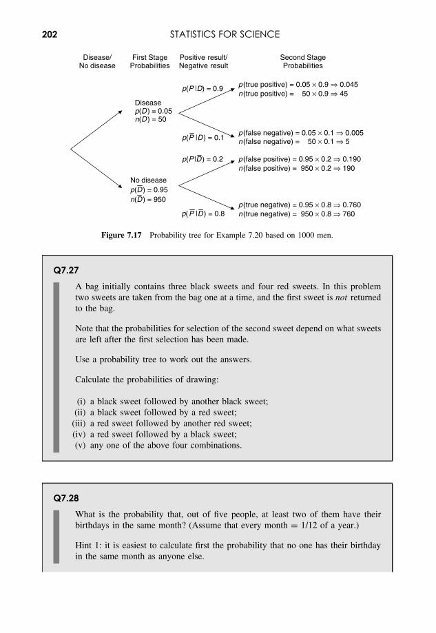
202 STATISTICS FOR SCIENCE
Disease/No disease
First StageProbabilities
p(P |D) = 0.9 p (true positive) = 0.05 × 0.9 ⇒ 0.045n (true positive) = 50 × 0.9 ⇒ 45
Diseasep(D) = 0.05n(D) = 50
p(P |D) = 0.1p (false negative) = 0.05 × 0.1 ⇒ 0.005n (false negative) = 50 × 0.1 ⇒ 5
p(P |D) = 0.2 p (false positive) = 0.95 × 0.2 ⇒ 0.190n (false positive) = 950 × 0.2 ⇒ 190
No diseasep(D ) = 0.95n(D) = 950
p(P |D) = 0.8p (true negative) = 0.95 × 0.8 ⇒ 0.760n (true negative) = 950 × 0.8 ⇒ 760
Positive result/Negative result
Second StageProbabilities
Figure 7.17 Probability tree for Example 7.20 based on 1000 men.
Q7.27A bag initially contains three black sweets and four red sweets. In this problemtwo sweets are taken from the bag one at a time, and the first sweet is not returnedto the bag.
Note that the probabilities for selection of the second sweet depend on what sweetsare left after the first selection has been made.
Use a probability tree to work out the answers.
Calculate the probabilities of drawing:
(i) a black sweet followed by another black sweet;(ii) a black sweet followed by a red sweet;
(iii) a red sweet followed by another red sweet;(iv) a red sweet followed by a black sweet;(v) any one of the above four combinations.
Q7.28What is the probability that, out of five people, at least two of them have theirbirthdays in the same month? (Assume that every month = 1/12 of a year.)
Hint 1: it is easiest to calculate first the probability that no one has their birthdayin the same month as anyone else.
7.5 FACTORIALS, PERMUTATIONS AND COMBINATIONS 203
Hint 2: pick one person and then calculate the probability that the next person to bepicked will have a birthday in a different month, and then the probability that thenext person will also have a birthday in a different month to the previous two, etc.
7.5 Factorials, Permutations and Combinations7.5.1 IntroductionThis unit develops the statistics for calculating the number of ways of obtaining particulararrangements of objects and events. These calculations have particular relevance in a range ofprobability calculations, from the likelihood of winning the National Lottery to the distributionof plants across a field.
7.5.2 FactorialThe factorial, n!, of a number, n, is the number multiplied by every integer between itselfand one:
n! = n × (n − 1) × (n − 2) × · · · × 3 × 2 × 1 [7.23]
Scientific calculators can calculate the factorial of a number directly – look for the x ! function.The factorial can be calculated in Excel (Appendix I) using the function FACT(x).It is useful to note some particular values:
1! = 1 [7.24]
n! = n × (n − 1)! [7.25]
0! = 1(This is not obvious, but should be remembered!) [7.26]
Example 7.21
1! = 1 0! = 1
2! = 2 × 1! = 2 × 1 = 2 0!/3! = 1/6
3! = 3 × 2! = 3 × 2 = 6 20! = 20 × 19!
4! = 4 × 3! = 4 × 3 × 2 = 24
etc.
204 STATISTICS FOR SCIENCE
Division using factorials Using a simple numerical example first:
Example 7.22
8!
5!= 8 × 7 × 6× 5× 4× 3× 2 × 1
5× 4× 3× 2 × 1= 8 × 7 × 6
1= 336
In Example 7.22, the 5! in the denominator cancels with all the terms from 5 to 1 in thenumerator, leaving only 8 × 7 × 6.
Hence, we can write a general formula for the division of factorials, where n> m:
n!
m!= n × (n − 1) × · · · × (m + 2) × (m + 1) [7.27]
Example 7.23
Using equation [7.27]:
(i) 6!/4! = 6 × 5 = 30(ii) 46!/41! = 46 × (46 − 1) × · · · × (41 + 2) × (41 + 1) = 46 × 45 × 44 × 43 × 42
Q7.29Work out the values of each of the following without using a calculator (check theresults afterwards using a calculator):
(i) 5! (iv) 3! − 3!
(ii) (4 − 3)! (v)7!
5!
(iii) (3 − 3)! (vi)101!
99!
7.5.3 PermutationsA mathematical permutation is the number of ways of arranging r items in order when selectedfrom n items.
7.5 FACTORIALS, PERMUTATIONS AND COMBINATIONS 205
Arranging n items in order The simplest problem is to find out how many ways it ispossible to arrange n items into different sequences (or order).
Example 7.24
If we have three items, X, Y and Z, we can produce six possible arrangements whichdiffer in the ordering of the items:
XYZ, XZY, YXZ, YZX, ZXY, ZYX
We can calculate the number of ways mathematically by considering how many ‘choices’we have when filling the first, second and third places in order. Initially we have threechoices for which letter to put in first place (e.g. Y), but we will then only have a choiceof two letters left (e.g. X and Z) for the second place, and then only one letter for thethird place:
We have a choiceof three itemsfor the firstplace (X, Y orZ)
We now havetwo choicesleft for thesecond place
We only haveone ‘choice’left for thefinal place
Total number ofdifferent ways
3 ×2 ×1 = 3! = 6
Thus the total number of possible arrangements was 3 × 2 × 1 = 3!.
In general:
Number of ways of arranging n items in order = n! [7.28]
Q7.30In how many ways can the four nitrogen bases, A, T, G and C, be arranged indifferent orders?
Arranging r items in order when selected from n possible items We can illustrate theproblem using the following example.
206 STATISTICS FOR SCIENCE
Example 7.25
As a specific example, consider selecting 3 (= r) items, in a specific order , from7 (= n) items (e.g. TUVWXYZ). The number of ways can be calculated asfollows:
We have a choiceof n = 7 itemsfor the firstplace
We now have(7 − 1)
choices left forthe secondplace
We now have(7 − 2)
choices left forthe third place
Total number ofdifferent ways
7 ×6 ×5 = 7 × 6 × 5
In this example the total number of ways of ordering 3 (= r) from 7 (= n) items is7 × 6 × 5 = 210.
We can rewrite the number as follows:
7 × 6 × 5 = 7 × 6 × 5× 4× 3× 2 × 1
4× 3× 2 × 1= 7!
4!= 7!
(7 − 3)!= n!
(n − r)!
The general formula for arranging r items in order when selected from n possible items isgiven by the permutation function:
nPr = n!
(n − r)![7.29]
This function can also be calculated directly in most scientific calculators. Enter the ‘n’ valuefirst, press the nPr button, enter the ‘r’ value, and press ‘=’.
The nPr function can be calculated in Excel (Appendix I) using the function PERMUT(n, r).
Example 7.26
Calculate the number of ways of selecting the first, second and third horses (orderimportant) in a race with 10 horses:
10P3 = 10!/(10 − 3)! = 10 × 9 × 8 = 720
7.5 FACTORIALS, PERMUTATIONS AND COMBINATIONS 207
Q7.31An athlete has eight different trophies, but only has room for four trophies in adisplay cabinet.
How many different ways is it possible to display just four trophies out of eight,assuming that the display order is important?
7.5.4 CombinationsA mathematical combination is the number of different ways of selecting ‘r’ items from ‘n’items when the order is not important.
Example 7.27
Calculate the number of ways of selecting 2 items from 4 possible items.
There are 12(= 4P2) different ways of ordering 2 letters from the 4 letters W, X, Yand Z:
WX, WY, WZ, XW, XY, XZ, YW, YX, YZ, ZW, ZX, ZY
However, if the order of selection is not important, then there are no differences betweeneach of the following 6 pairs of selections:
WX and XW, WY and YW, WZ and ZW, XY and YX, XZ and ZX, YZ and ZY
In this case there will then be only 6 different ways of selecting 2 items from 4 itemswith the order not important:
WX, WY, WZ, XY, XZ, ZY
The number of ways of selecting r items from n items when the order is not important isgiven by the function nCr .
We know that the number of ways that each selection of the r items can be ordered amongstthemselves is r!. Hence, from the previous two statements, we see that the number of ways offirst selecting and then ordering r items from n items, nPr , is given by the equation:
nPr = nCr × r! [7.30]
208 STATISTICS FOR SCIENCE
The number of combinations can therefore be calculated using:
nCr = nPr
r![7.31]
which is the same as:
nCr = n!
r! × (n − r)![7.32]
This function can also be calculated directly in most scientific calculators. Enter the ‘n’value first, press the nCr button, enter the ‘r’ value, and press ‘=’.
The nCr function can be calculated in Excel (Appendix I) using the function COMBIN(n, r).Example 7.27 can be solved using [7.32], to give the number of ways of selecting (r =) 2
items from (n =) 4 items (W, X, Y and Z) where the order is not important:
4C2 = 4!
2! × (4 − 2)!= 24
2 × 2= 6
Example 7.28
Calculate the number of ways of selecting the first, second and third horses in a racewith 10 horses, where order is not important (see Example 7.26):
10C3 = 10P3/3! = 720/6 = 120
Example 7.29
UK National Lottery (Lotto)
Calculate the probability of getting the jackpot in the UK National Lottery (Lotto), where6 different numbers must be selected from 49 numbers.
The number of arrangements of 6 numbers selected from 49 numbers is:
49P6 = 1.0068 × 10¹⁰

7.5 FACTORIALS, PERMUTATIONS AND COMBINATIONS 209
However, many of the above arrangements will have selected the same numbers but ina different order . For each set of 6 numbers, there are 6! ways of rearranging them intoa different order.
To win the lottery, the order of the six numbers is not important. The number of waysof selecting 6 numbers in any order from 49 numbers is:
49C6 = 49P6/6! = 1.0068 × 10¹⁰/6! = 139 838 16 ≈ 14million
The aim, when buying a lottery ticket, is to guess which one of the 14 million possibleselections of the 6 numbers will occur.
Thus the probability of selecting the correct six numbers is 1 in 14 million!
Q7.32A football manager has a squad of 20 players.
How many different teams of 11 players could be selected from the squad?

8Distributions and Uncertainty
Overview
Website • ‘How to do it’ video answers for all ‘Q’ questions.• Excel tutorials: statistical calculations, calculation of uncertainties.• Excel files appropriate to selected ‘Q’ questions and Examples.
The concept of a continuous ‘distribution’ in statistics was introduced in 7.3.8, and is a methodof describing how the values of a data variable may be spread over a given range. Thedistribution may record the variability of data that has been recorded in the past (frequencydistribution) or predict the variability with which data values might be expected to be recordedin the future (probability distribution).
This chapter describes three distributions important in science – the normal, binomial andPoisson distributions. These have importance in modelling different systems in science:
• The normal distribution can be used to model a very wide range of systems where thedistribution follows the familiar ‘bell-shaped’ curve. A particularly common application inscience occurs in relation to experimental uncertainty.
• The binomial distribution applies to systems where, at the fundamental level, the systemcan be in one of two possible states – hence the prefix ‘bi’. A classic example of binomialstatistics might calculate the probability of getting eight heads when a coin is tossed 10times.
• The Poisson distribution is a special case of the binomial distribution, which occurs whenthe individual probability of a given event is low. This distribution can be used to estimatethe probabilities for the occurrences of such events, e.g. the probability that a particularnumber of cases of a randomly occurring disease may appear in a specific locality.
The most important parameters used to describe a distribution – mean, standard deviation,variance – have already been introduced in 7.2.4 and 7.2.6, and are used to describe the locationand spread of the distribution.
Other parameters that are used to describe the characteristic shape of distributions are givenon the Website.
Essential Mathematics and Statistics for Science 2nd Edition Graham Currell and Antony DowmanCopyright c© 2009 John Wiley & Sons, Ltd
212 DISTRIBUTIONS AND UNCERTAINTY
Different types of scientific mechanisms may produce experimental data with different dis-tributions. If it is possible to confirm that the data falls into one or other type of distribution,then it is possible to deduce that one mechanism is more likely to be operating than a possiblealternative. In this respect, ‘goodness of fit’ (14.2) is a useful hypothesis test that can be usedto assess whether an experimental distribution might be different from a particular theoreticalmodel.
The impact of experimental uncertainty on scientific measurements has been introduced in1.2. The normal distribution has particular value in dealing with experimental uncertainty, asit closely models the variability in the results of many types of experimental measurement. Inparticular, the random uncertainty can be quantified by defining a confidence interval at X%,which has an X% probability of including the true value being measured.
For example, if an experimental result is presented as:
4.67 ± 0.05 (95 % CI)
then it can be stated with 95 % probability that the true value of the variable being measuredlies between 4.62 (= 4.67 − 0.05) and 4.72 (= 4.67 + 0.05).
The ways in which the uncertainties in separate variables combine in a calculation of overalluncertainty is discussed in 8.3.3.
8.1 Normal Distribution8.1.1 IntroductionThe bell-shaped normal distribution is the most widely used distribution in science. Of particularimportance is the fact that many experimental variations can be described effectively by usingthe normal distribution.
8.1.2 Experimental uncertaintyThere is always some uncertainty when making any experimental measurement. If we aretrying to measure some experimental property whose true value is µ, then we are morelikely to record a value close to µ, and less likely to record a value a long way awayfrom µ.
The probability density, pd (x) (7.3.8), of recording a particular value, x, is largest whenx is close to µ, but then the probability falls off as a ‘bell-shaped’ curve on either sideof µ.
Example 8.1
Figure 8.1 shows the probabilities of getting an experimental result, x, in specific ranges,when measuring a true blood–alcohol level of 80 mg per 100 mL, i.e. 80 mg of alcohol
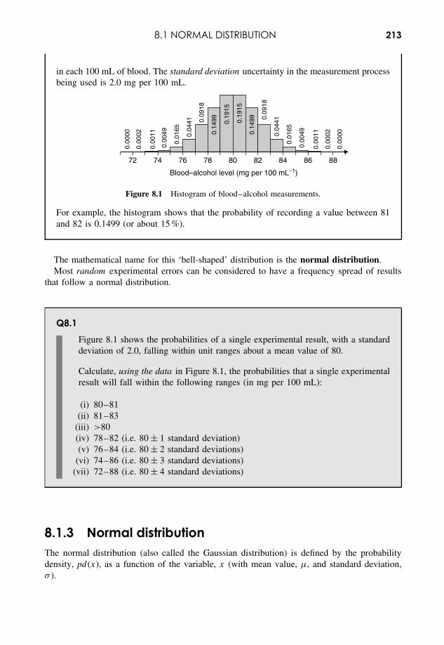
8.1 NORMAL DISTRIBUTION 213
in each 100 mL of blood. The standard deviation uncertainty in the measurement processbeing used is 2.0 mg per 100 mL.
0.19
15
0.19
15
0.09
18
0.14
99
0.04
41
0.00
49
0.00
02
0.01
65
0.00
00
0.00
11
80 82 847876 86 887472
Blood–alcohol level (mg per 100 mL−1)
0.14
990.09
18
0.04
41
0.01
65
0.00
49
0.00
11
0.00
02
0.00
00
Figure 8.1 Histogram of blood–alcohol measurements.
For example, the histogram shows that the probability of recording a value between 81and 82 is 0.1499 (or about 15 %).
The mathematical name for this ‘bell-shaped’ distribution is the normal distribution.Most random experimental errors can be considered to have a frequency spread of results
that follow a normal distribution.
Q8.1Figure 8.1 shows the probabilities of a single experimental result, with a standarddeviation of 2.0, falling within unit ranges about a mean value of 80.
Calculate, using the data in Figure 8.1, the probabilities that a single experimentalresult will fall within the following ranges (in mg per 100 mL):
(i) 80–81(ii) 81–83
(iii) >80(iv) 78–82 (i.e. 80 ± 1 standard deviation)(v) 76–84 (i.e. 80 ± 2 standard deviations)
(vi) 74–86 (i.e. 80 ± 3 standard deviations)(vii) 72–88 (i.e. 80 ± 4 standard deviations)
8.1.3 Normal distributionThe normal distribution (also called the Gaussian distribution) is defined by the probabilitydensity, pd (x), as a function of the variable, x (with mean value, µ, and standard deviation,σ ).
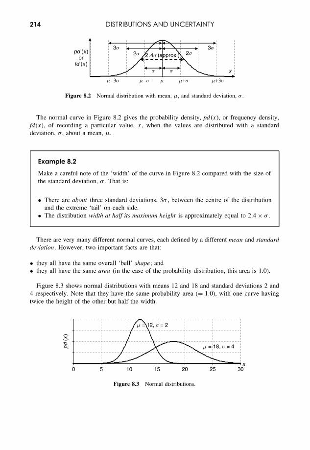
214 DISTRIBUTIONS AND UNCERTAINTY
m
pd (x )or
fd (x )x
m+sm−s
ss
2s3s
m+3sm−3s
3s
2.4s (approx.) 2s
Figure 8.2 Normal distribution with mean, µ, and standard deviation, σ .
The normal curve in Figure 8.2 gives the probability density, pd (x), or frequency density,fd (x), of recording a particular value, x, when the values are distributed with a standarddeviation, σ , about a mean, µ.
Example 8.2
Make a careful note of the ‘width’ of the curve in Figure 8.2 compared with the size ofthe standard deviation, σ . That is:
• There are about three standard deviations, 3σ , between the centre of the distributionand the extreme ‘tail’ on each side.
• The distribution width at half its maximum height is approximately equal to 2.4 × σ .
There are very many different normal curves, each defined by a different mean and standarddeviation . However, two important facts are that:
• they all have the same overall ‘bell’ shape; and• they all have the same area (in the case of the probability distribution, this area is 1.0).
Figure 8.3 shows normal distributions with means 12 and 18 and standard deviations 2 and4 respectively. Note that they have the same probability area (= 1.0), with one curve havingtwice the height of the other but half the width.
0 5 10 15 20 25 30
pd (
x)
x
m = 12, s = 2
m = 18, s = 4
Figure 8.3 Normal distributions.
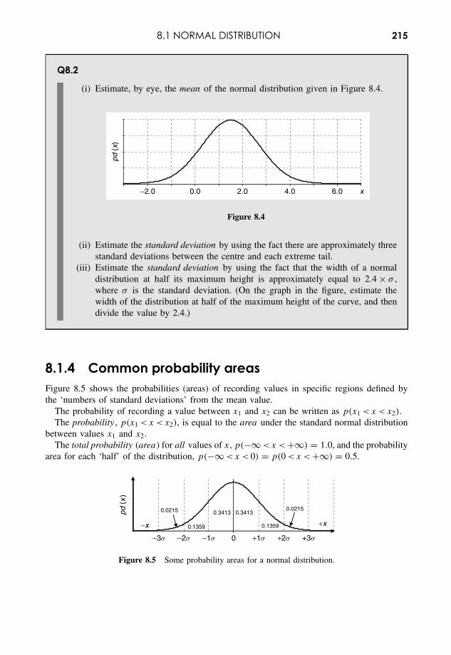
8.1 NORMAL DISTRIBUTION 215
Q8.2
(i) Estimate, by eye, the mean of the normal distribution given in Figure 8.4.
pd (
x)
x2.00.0 4.0 6.0−2.0
Figure 8.4
(ii) Estimate the standard deviation by using the fact there are approximately threestandard deviations between the centre and each extreme tail.
(iii) Estimate the standard deviation by using the fact that the width of a normaldistribution at half its maximum height is approximately equal to 2.4 × σ ,where σ is the standard deviation. (On the graph in the figure, estimate thewidth of the distribution at half of the maximum height of the curve, and thendivide the value by 2.4.)
8.1.4 Common probability areasFigure 8.5 shows the probabilities (areas) of recording values in specific regions defined bythe ‘numbers of standard deviations’ from the mean value.
The probability of recording a value between x1 and x2 can be written as p(x1 <x <x2).The probability , p(x1 <x <x2), is equal to the area under the standard normal distribution
between values x1 and x2.The total probability (area) for all values of x, p(−∞ <x <+∞) = 1.0, and the probability
area for each ‘half’ of the distribution, p(−∞ <x < 0) = p(0 <x < +∞) = 0.5.
0
pd (
x)
+x−x
0.34130.3413
0.1359
0.0215
0.1359
0.0215
−3s −2s −1s +1s +2s +3s
Figure 8.5 Some probability areas for a normal distribution.
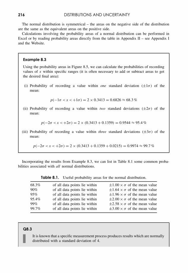
216 DISTRIBUTIONS AND UNCERTAINTY
The normal distribution is symmetrical – the areas on the negative side of the distributionare the same as the equivalent areas on the positive side.
Calculations involving the probability areas of a normal distribution can be performed inExcel or by reading probability areas directly from the table in Appendix II – see Appendix Iand the Website.
Example 8.3
Using the probability areas in Figure 8.5, we can calculate the probabilities of recordingvalues of x within specific ranges (it is often necessary to add or subtract areas to getthe desired final area):
(i) Probability of recording a value within one standard deviation (±1σ ) of themean:
p(−1σ <x < +1σ) = 2 × 0.3413 = 0.6826 ≈ 68.3 %
(ii) Probability of recording a value within two standard deviations (±2σ ) of themean:
p(−2σ <x <+2σ) = 2 × (0.3413 + 0.1359) = 0.9544 ≈ 95.4 %
(iii) Probability of recording a value within three standard deviations (±3σ ) of themean:
p(−2σ <x < +2σ) = 2 × (0.3413 + 0.1359 + 0.0215) = 0.9974 ≈ 99.7 %
Incorporating the results from Example 8.3, we can list in Table 8.1 some common proba-bilities associated with all normal distributions.
Table 8.1. Useful probability areas for the normal distribution.
68.3% of all data points lie within ±1.00 × σ of the mean value90% of all data points lie within ±1.64 × σ of the mean value95% of all data points lie within ±1.96 × σ of the mean value95.4% of all data points lie within ±2.00 × σ of the mean value99% of all data points lie within ±2.58 × σ of the mean value99.7% of all data points lie within ±3.00 × σ of the mean value
Q8.3It is known that a specific measurement process produces results which are normallydistributed with a standard deviation of 4.
8.2 UNCERTAINTIES IN MEASUREMENT 217
If 100 000 replicate measurements could be made of a true value equal to 50, usethe information in Table 8.1 to estimate the number of results that would record avalue:
(i) between 46 and 54(ii) between 42.16 and 57.84
(iii) outside the range 38 to 62(iv) greater than 54 (hint: use your result from (i))
8.2 Uncertainties in Measurement8.2.1 IntroductionWe have seen in 1.2 that a typical experimental measurement will have a random uncertainty,which may be due to either:
• a variation in the measurement procedure itself (e.g. uncertainty in the response of a pHelectrode); or
• a natural variation in the subjects being measured (e.g. different plants of the same cropgrow at different rates).
The problems of experimental uncertainty are fundamental to all experimental science, anda more extensive discussion of experimental variation is given in 11.1.2.
8.2.2 Experimental variation and true valueIn a typical experimental measurement, we aim to try to identify the unknown value, µ, ofsome scientific parameter (e.g. pH of a particular solution, or the average growth rate of cropplants).
The true value (1.2) means something slightly different in each of the two types of experi-mental uncertainty:
• Where the uncertainty is due entirely to the measurement process itself, the true value isthe single actual value, µ, of the subject that is being measured (e.g. the true pH of thesolution).
• Where the major uncertainty lies in the subjects that are being measured, the true value isthe mean value, µ, of all the possible measurements (population) that could be made (e.g.the mean growth rate of all the plants of a given crop).
Fortunately, we can apply the same statistics to both of the above situations. We see that themean value, x, of a sample of n experimental measurements is used as a ‘best estimate’ fortrue mean value, µ, that would be obtained if a full population (see 7.2.2) of measurementscould be made.
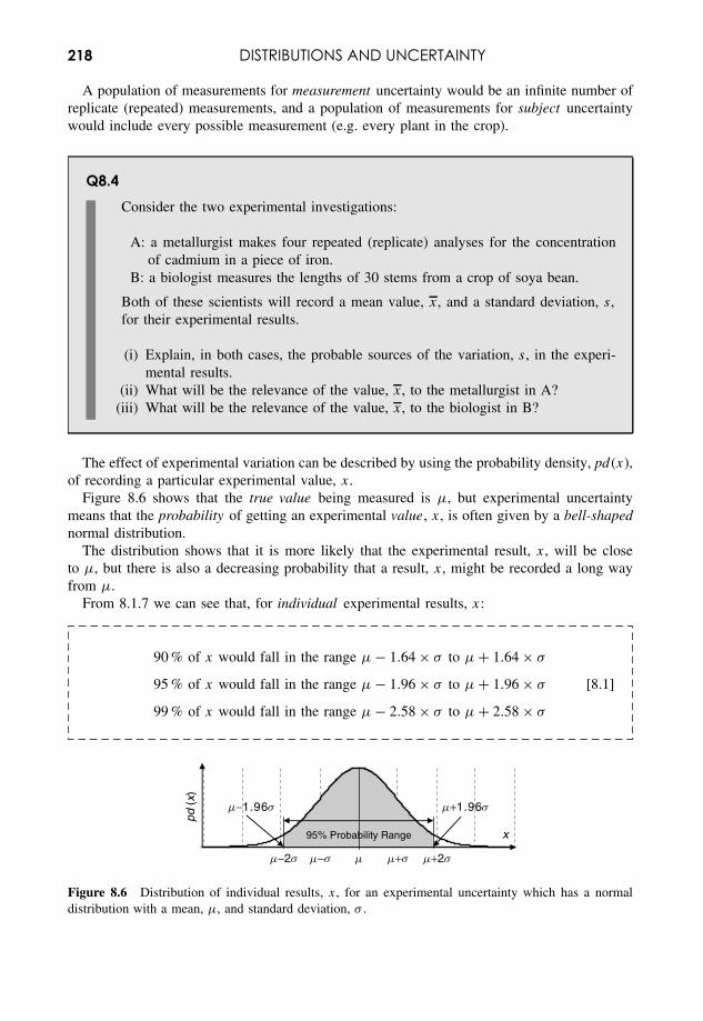
218 DISTRIBUTIONS AND UNCERTAINTY
A population of measurements for measurement uncertainty would be an infinite number ofreplicate (repeated) measurements, and a population of measurements for subject uncertaintywould include every possible measurement (e.g. every plant in the crop).
Q8.4Consider the two experimental investigations:
A: a metallurgist makes four repeated (replicate) analyses for the concentrationof cadmium in a piece of iron.
B: a biologist measures the lengths of 30 stems from a crop of soya bean.
Both of these scientists will record a mean value, x, and a standard deviation, s,for their experimental results.
(i) Explain, in both cases, the probable sources of the variation, s, in the experi-mental results.
(ii) What will be the relevance of the value, x, to the metallurgist in A?(iii) What will be the relevance of the value, x, to the biologist in B?
The effect of experimental variation can be described by using the probability density, pd (x),of recording a particular experimental value, x.
Figure 8.6 shows that the true value being measured is µ, but experimental uncertaintymeans that the probability of getting an experimental value, x, is often given by a bell-shapednormal distribution.
The distribution shows that it is more likely that the experimental result, x, will be closeto µ, but there is also a decreasing probability that a result, x, might be recorded a long wayfrom µ.
From 8.1.7 we can see that, for individual experimental results, x:
90 % of x would fall in the range µ − 1.64 × σ to µ + 1.64 × σ
95 % of x would fall in the range µ − 1.96 × σ to µ + 1.96 × σ [8.1]
99 % of x would fall in the range µ − 2.58 × σ to µ + 2.58 × σ
m
pd (
x)
x
m+sm−s m+2sm−2s
m+1.96sm−1.96s
95% Probability Range
Figure 8.6 Distribution of individual results, x, for an experimental uncertainty which has a normaldistribution with a mean, µ, and standard deviation, σ .
8.2 UNCERTAINTIES IN MEASUREMENT 219
It is worth remembering the numbers 1.64, 1.96 and 2.58 – they occur frequently.
Q8.5In a particular experiment to measure the concentration of lead in drinking water,the experimental procedure has a standard deviation uncertainty of 2.0 ppb. Anumber of analysts each make a single experimental measurement.
If the true value of the concentration is 23 ppb, estimate the range of values withinwhich 95 % of the analysts’ results are likely to fall.
8.2.3 Replicate measurements, sample means andstandard errorThe uncertainty in a single experimental measurement is given directly by the standard devi-ation, σ , of the experimental variation – see 8.2.2. However, it is good scientific practice totake several repeat (or replicate) measurements, n, and then take the average (mean) of thatsample of n measurements.
When we take an increasing number of replicate measurements, the mean, x, of our replicateswill tend to become closer to the ‘true’ value, µ. This is a consequence of a statistical theorycalled the ‘central limit theorem’.
Another important consequence of the central limit theorem is that the distribution of sam-ple mean values will tend towards a normal distribution, even if the distribution of theindividual measurements is not normal (e.g. a Poisson distribution). By taking the meanvalues of data samples, we are more likely to ensure that our experimental uncertaintiesdo follow normal distributions – this is important for the validity of much of the statisticsused to analyse such data. In practice, a sample size of at least 30 data values is usuallysufficient.
The reduced uncertainty (or improved precision) when taking the mean of n replicate mea-surements is given by:
Standard error of the mean, SE = σ√n
[8.2]
Note that the equivalent statistic when using the sample standard deviation, s, is called thestandard uncertainty – see [8.4].
According to the central limit theorem, the distribution of the possible mean values, x, ofn experimental measurements follows a normal distribution, as in Figure 8.7, with a mean (ofmean values) = µ and a standard deviation of SE = σ/
√n.
Figure 8.7 gives the probability density, pd (x), for recording mean values, x, ofdifferent sample sizes, n. The sample size n = 1 represents a single measurement as inFigure 8.6.
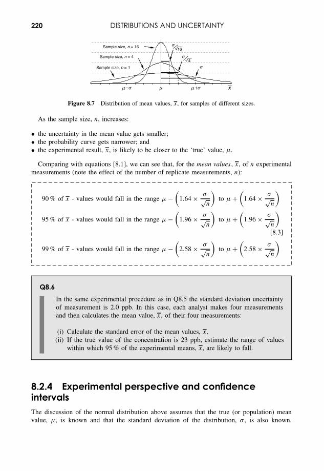
220 DISTRIBUTIONS AND UNCERTAINTY
m
Sample size, n = 16
Sample size, n = 4
Sample size, n = 1
m+s x
s
s4
16
s
m−s
Figure 8.7 Distribution of mean values, x, for samples of different sizes.
As the sample size, n, increases:
• the uncertainty in the mean value gets smaller;• the probability curve gets narrower; and• the experimental result, x, is likely to be closer to the ‘true’ value, µ.
Comparing with equations [8.1], we can see that, for the mean values , x, of n experimentalmeasurements (note the effect of the number of replicate measurements, n):
90 % of x - values would fall in the range µ −(
1.64 × σ√n
)to µ +
(1.64 × σ√
n
)
95 % of x - values would fall in the range µ −(
1.96 × σ√n
)to µ +
(1.96 × σ√
n
)[8.3]
99 % of x - values would fall in the range µ −(
2.58 × σ√n
)to µ +
(2.58 × σ√
n
)
Q8.6In the same experimental procedure as in Q8.5 the standard deviation uncertaintyof measurement is 2.0 ppb. In this case, each analyst makes four measurementsand then calculates the mean value, x, of their four measurements:
(i) Calculate the standard error of the mean values, x.(ii) If the true value of the concentration is 23 ppb, estimate the range of values
within which 95 % of the experimental means, x, are likely to fall.
8.2.4 Experimental perspective and confidenceintervalsThe discussion of the normal distribution above assumes that the true (or population) meanvalue, µ, is known and that the standard deviation of the distribution, σ , is also known.
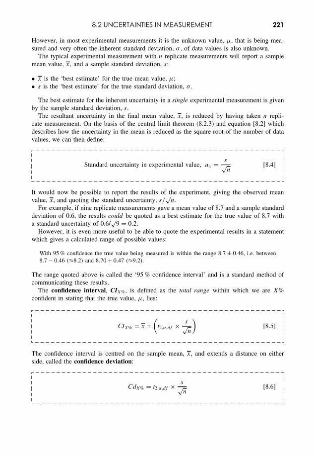
8.2 UNCERTAINTIES IN MEASUREMENT 221
However, in most experimental measurements it is the unknown value, µ, that is being mea-sured and very often the inherent standard deviation, σ , of data values is also unknown.
The typical experimental measurement with n replicate measurements will report a samplemean value, x, and a sample standard deviation, s:
• x is the ‘best estimate’ for the true mean value, µ;• s is the ‘best estimate’ for the true standard deviation, σ .
The best estimate for the inherent uncertainty in a single experimental measurement is givenby the sample standard deviation, s.
The resultant uncertainty in the final mean value, x, is reduced by having taken n repli-cate measurement. On the basis of the central limit theorem (8.2.3) and equation [8.2] whichdescribes how the uncertainty in the mean is reduced as the square root of the number of datavalues, we can then define:
Standard uncertainty in experimental value, ux = s√n
[8.4]
It would now be possible to report the results of the experiment, giving the observed meanvalue, x, and quoting the standard uncertainty, s/
√n.
For example, if nine replicate measurements gave a mean value of 8.7 and a sample standarddeviation of 0.6, the results could be quoted as a best estimate for the true value of 8.7 witha standard uncertainty of 0.6/
√9 = 0.2.
However, it is even more useful to be able to quote the experimental results in a statementwhich gives a calculated range of possible values:
With 95 % confidence the true value being measured is within the range 8.7 ± 0.46, i.e. between8.7 − 0.46 (≈8.2) and 8.70 + 0.47 (≈9.2).
The range quoted above is called the ‘95 % confidence interval’ and is a standard method ofcommunicating these results.
The confidence interval, CIX %, is defined as the total range within which we are X%confident in stating that the true value, µ, lies:
CIX% = x ±(
t2,α,df × s√n
)[8.5]
The confidence interval is centred on the sample mean, x, and extends a distance on eitherside, called the confidence deviation:
CdX% = t2,α,df × s√n
[8.6]
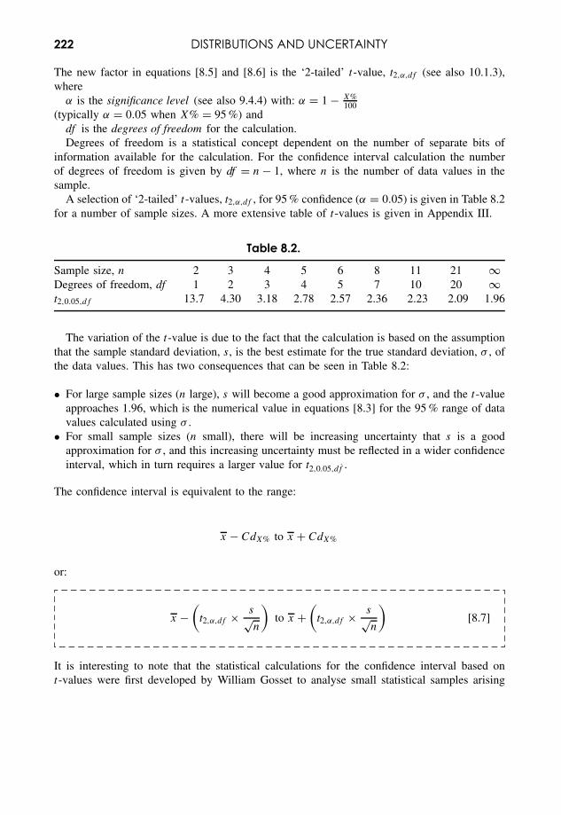
222 DISTRIBUTIONS AND UNCERTAINTY
The new factor in equations [8.5] and [8.6] is the ‘2-tailed’ t-value, t2,α,df (see also 10.1.3),where
α is the significance level (see also 9.4.4) with: α = 1 − X%100
(typically α = 0.05 when X% = 95 %) anddf is the degrees of freedom for the calculation.Degrees of freedom is a statistical concept dependent on the number of separate bits of
information available for the calculation. For the confidence interval calculation the numberof degrees of freedom is given by df = n − 1, where n is the number of data values in thesample.
A selection of ‘2-tailed’ t-values, t2,α,df , for 95 % confidence (α = 0.05) is given in Table 8.2for a number of sample sizes. A more extensive table of t-values is given in Appendix III.
Table 8.2.
Sample size, n 2 3 4 5 6 8 11 21 ∞Degrees of freedom, df 1 2 3 4 5 7 10 20 ∞t2,0.05,df 13.7 4.30 3.18 2.78 2.57 2.36 2.23 2.09 1.96
The variation of the t-value is due to the fact that the calculation is based on the assumptionthat the sample standard deviation, s, is the best estimate for the true standard deviation, σ , ofthe data values. This has two consequences that can be seen in Table 8.2:
• For large sample sizes (n large), s will become a good approximation for σ , and the t-valueapproaches 1.96, which is the numerical value in equations [8.3] for the 95 % range of datavalues calculated using σ .
• For small sample sizes (n small), there will be increasing uncertainty that s is a goodapproximation for σ , and this increasing uncertainty must be reflected in a wider confidenceinterval, which in turn requires a larger value for t2,0.05,df .
The confidence interval is equivalent to the range:
x − CdX% to x + CdX%
or:
x −(
t2,α,df × s√n
)to x +
(t2,α,df × s√
n
)[8.7]
It is interesting to note that the statistical calculations for the confidence interval based ont-values were first developed by William Gosset to analyse small statistical samples arising
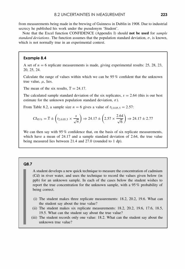
8.2 UNCERTAINTIES IN MEASUREMENT 223
from measurements being made in the brewing of Guinness in Dublin in 1908. Due to industrialsecrecy he published his work under the pseudonym ‘Student’.
Note that the Excel function CONFIDENCE (Appendix I) should not be used for samplestandard deviations . The function assumes that the population standard deviation, σ , is known,which is not normally true in an experimental context.
Example 8.4
A set of n = 6 replicate measurements is made, giving experimental results: 25, 28, 23,20, 25, 24.
Calculate the range of values within which we can be 95 % confident that the unknowntrue value, µ, lies.
The mean of the six results, x = 24.17.
The calculated sample standard deviation of the six replicates, s = 2.64 (this is our bestestimate for the unknown population standard deviation, σ ).
From Table 8.2, a sample size n = 6 gives a value of t2,0.05,5 = 2.57:
CI95 % = x ±(
t2,0.05,5 × s√n
)⇒ 24.17 ±
(2.57 × 2.64√
6
)⇒ 24.17 ± 2.77
We can then say with 95 % confidence that, on the basis of six replicate measurements,which have a mean of 24.17 and a sample standard deviation of 2.64, the true valuebeing measured lies between 21.4 and 27.0 (rounded to 1 dp).
Q8.7A student develops a new quick technique to measure the concentration of cadmium(Cd) in river water, and uses the technique to record the values given below (inppb) for an unknown sample. In each of the cases below the student wishes toreport the true concentration for the unknown sample, with a 95 % probability ofbeing correct.
(i) The student makes three replicate measurements: 18.2, 20.2, 19.6. What canthe student say about the true value?
(ii) The student makes six replicate measurements: 18.2, 20.2, 19.6, 17.6, 18.5,19.5. What can the student say about the true value?
(iii) The student records only one value: 18.2. What can the student say about theunknown true value?
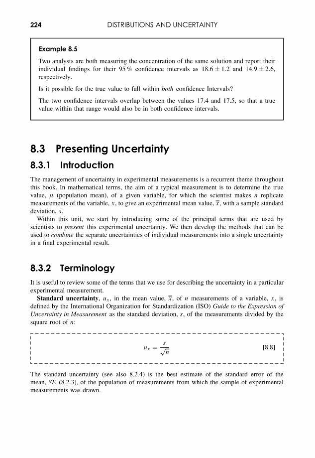
224 DISTRIBUTIONS AND UNCERTAINTY
Example 8.5
Two analysts are both measuring the concentration of the same solution and report theirindividual findings for their 95 % confidence intervals as 18.6 ± 1.2 and 14.9 ± 2.6,respectively.
Is it possible for the true value to fall within both confidence Intervals?
The two confidence intervals overlap between the values 17.4 and 17.5, so that a truevalue within that range would also be in both confidence intervals.
8.3 Presenting Uncertainty8.3.1 IntroductionThe management of uncertainty in experimental measurements is a recurrent theme throughoutthis book. In mathematical terms, the aim of a typical measurement is to determine the truevalue, µ (population mean), of a given variable, for which the scientist makes n replicatemeasurements of the variable, x, to give an experimental mean value, x, with a sample standarddeviation, s.
Within this unit, we start by introducing some of the principal terms that are used byscientists to present this experimental uncertainty. We then develop the methods that can beused to combine the separate uncertainties of individual measurements into a single uncertaintyin a final experimental result.
8.3.2 TerminologyIt is useful to review some of the terms that we use for describing the uncertainty in a particularexperimental measurement.
Standard uncertainty, ux , in the mean value, x, of n measurements of a variable, x, isdefined by the International Organization for Standardization (ISO) Guide to the Expression ofUncertainty in Measurement as the standard deviation, s, of the measurements divided by thesquare root of n:
ux = s√n
[8.8]
The standard uncertainty (see also 8.2.4) is the best estimate of the standard error of themean, SE (8.2.3), of the population of measurements from which the sample of experimentalmeasurements was drawn.
8.3 PRESENTING UNCERTAINTY 225
We define a new term, relative uncertainty, Rux , in the mean value, x, as the percentageratio of the standard uncertainty to the mean value. Relative uncertainty is the percentageuncertainty in a particular experimental result :
Rux = 100 × ux
xand ux = x × Rux
100[8.9]
We have defined, in 8.2.4, a new term, confidence deviation (Cd ), which is the range in eitherdirection from the mean value, x, within which the true value, µ, can be expected to lie, witha confidence of X%:
CdX% = t2,α,df × s√n
[8.10]
Confidence interval (CI ) is the range of values (8.2.4) within which the true value, µ, canbe expected to lie, with a confidence of X%:
CIX% = x ± CdX%
CIX% = x ±(
t2,α,df × s√n
)[8.11]
It is also useful to note two terms that are used to describe the precision of an experimentalprocess rather than the uncertainty in a particular measurement: relative standard deviation(RSD) and coefficient of variation (CV ) both give the ratio of the population standard devi-ation, σ , to the mean value, i.e. the fractional standard deviation. The coefficient of variationis the ‘percentage’ equivalent of relative standard deviation:
RSD = σ
x
CV = 100 × σ
x% [8.12]
When presenting results, the experimental method used should be made explicit, and sufficientinformation (e.g. sample size, n) should be given to enable the readers to interpret the uncer-tainty in any of the formats given. The final result should be given with an appropriate numberof significant figures (2.1.7).
226 DISTRIBUTIONS AND UNCERTAINTY
Example 8.6
Nine experimental measurements give a mean value of 56.26 with a sample standarddeviation of 5.7.
(i) Calculate values for the standard uncertainty, ux , and relative uncertainty, Rux .(ii) Express the final result using a 95 % confidence interval.
Here:
(i) ux = 5.7√9
⇒ 1.9
Rux = 100 × 1.9
56.26⇒ 3.38 %
(ii) Degrees of freedom, df = n − 1 ⇒ 9 − 1 ⇒ 8t-value for two-tailed, 95 %, 8 degrees of freedom = 2.31:
CI95 % = 56.26 ± 2.31 × 1.9 ⇒ 56.26 ± 4.389
which would give a final result, with rounding, expressed as:
µ = 56.3 ± 4.4 (95 %CI)
Q8.8A particular measurement procedure is quoted as having a coefficient of variation[8.12] of 5 %. Calculate the standard error of the mean [8.2] that would be expectedfor the mean of eight replicate measurements of a true value of 4.5 ppm.
8.3.3 Combining uncertaintiesThere are many occasions in science when a final result, x, will be given by the combinationof two or more values, e.g. a, b. The initial uncertainties in a, b can be expressed as:
• standard uncertainties, ua and ub; and/or• relative uncertainties:
Rua = 100 × ua
aand Rub = 100 × ub
b
8.3 PRESENTING UNCERTAINTY 227
The ways in which we combine the uncertainties depend on the way in which the values a
and b are combined.For addition and subtraction equations we combine the squares of standard uncertainties,
but for multiplication and division we combine the squares of relative uncertainties:
If x = k × a (k is a constant) then use: ux = k × ua or Rux = Rua [8.13]
If x = a + b or x = a − b, then use: ux =√
u2a + u2
b [8.14]
If x = a × b or x = a
b, then use: Rux =
√Ru2
a + Ru2b [8.15]
If x = an (n is a constant) then use: Rux = n × Rua [8.16]
In performing calculations, it is often necessary to change between standard uncertainty andrelative uncertainty using equations [8.9].
Example 8.7
The measurements of the two sides of a rectangle record the values:
a = 8.4 mm with a standard deviation uncertainty, ua = 0.5 mm
b = 6.7 mm with a standard deviation uncertainty, ub = 0.5 mm
Calculate the following values, together with both the standard and relative uncertaintiesin each value:
(i) Sum of the two lengths: t = a + b
(ii) Difference in the lengths: d = a − b
(iii) Perimeter of the rectangle: p = 2(a + b)
(iv) Ratio of the lengths of the sides: r = a/b
(v) Area of the rectangle: A = a × b
Answers are given in the following text .
We can answer Example 8.7 by using equations [8.13] to [8.16]:
(i) The addition of the two lengths gives t = 8.4 + 6.7 = 15.1 mm.As this is an ‘addition’, we must calculate the uncertainty, ut , by using [8.14]:
ut =√
0.52 + 0.52 = 0.707 mm
228 DISTRIBUTIONS AND UNCERTAINTY
The relative uncertainty is: Rut = 100 × ut
t⇒ 100 × 0.707
15.1 ⇒ 4.68 %(ii) The difference between the two lengths gives d = 8.4 − 6.7 = 1.7 mm.
As this is a ‘subtraction’, we still calculate the uncertainty, ut , by using [8.14]:
ut =√
0.52 + 0.52 = 0.707 mm
The relative uncertainty is: Rut = 100 × ut
t⇒ 100 × 0.707
1.7 ⇒ 41.6 %In (i) and (ii), notice that, although the absolute error, u, is the same, the relative error,Ru t , becomes much larger in (ii) because the actual value is much less (1.7 instead of15.1).
(iii) To calculate the perimeter, p = 2(a + b), we can use t = a + b from (i), where t =15.1 mm and ut = 0.707, and calculate p = 2t ⇒ 30.2 mm.As we are multiplying by a constant, we use [8.13]:
up = 2 × ut = 2 × 0.707 = 1.414 mm
The relative uncertainty is: Rup = 100 × up
p⇒ 100 × 1.414
30.2 ⇒ 4.68 %Note that the relative uncertainty has stayed the same (4.7 %) when simply multiplying t
by the constant.(iv) The ratio of the sides gives: r = a
b⇒ 8.4
6.7 ⇒ 1.254 (pure number with no units)As this is a ‘division’, we must use [8.9] to calculate the relative uncertainties of a and b:
Rua = 100 × ua
a⇒ 100 × 0.5
8.4⇒ 5.952 %
Rub = 100 × ub
b⇒ 100 × 0.5
6.7⇒ 7.463 %
Using [8.15], the relative uncertainty is:
Rur =√
Ru2a + Ru2
b ⇒√
5.9422 + 7.4632 ⇒ 9.55 %
Using [8.9] to calculate the absolute uncertainties:
ur = r × Rur
100⇒ 1.254 × 9.55
100⇒ 0.120 mm
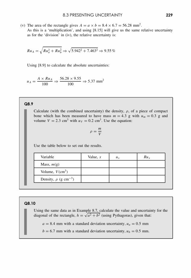
8.3 PRESENTING UNCERTAINTY 229
(v) The area of the rectangle gives A = a × b = 8.4 × 6.7 = 56.28 mm2.As this is a ‘multiplication’, and using [8.15] will give us the same relative uncertaintyas for the ‘division’ in (iv), the relative uncertainty is:
RuA =√
Ru2a + Ru2
b ⇒√
5.9422 + 7.4632 ⇒ 9.55 %
Using [8.9] to calculate the absolute uncertainties:
uA = A × RuA
100⇒ 56.28 × 9.55
100⇒ 5.37 mm2
Q8.9Calculate (with the combined uncertainty) the density, ρ, of a piece of compactbone which has been measured to have mass m = 4.3 g with um = 0.3 g andvolume V = 2.3 cm3 with uV = 0.2 cm3. Use the equation:
ρ = m
V
Use the table below to set out the results.
Variable Value, x ux Rux
Mass, m(g)
Volume, V (cm3)
Density, ρ (g cm−3)
Q8.10Using the same data as in Example 8.7, calculate the value and uncertainty for thediagonal of the rectangle, h = √
a2 + b2 (using Pythagoras), given that:
a = 8.4 mm with a standard deviation uncertainty, ua = 0.5 mm
b = 6.7 mm with a standard deviation uncertainty, ub = 0.5 mm.
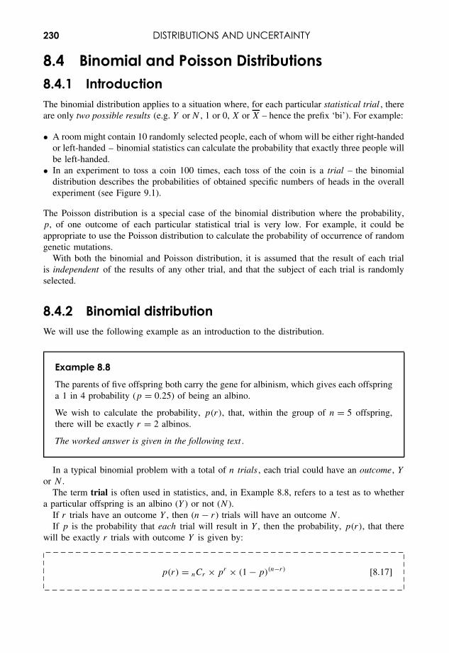
230 DISTRIBUTIONS AND UNCERTAINTY
8.4 Binomial and Poisson Distributions8.4.1 IntroductionThe binomial distribution applies to a situation where, for each particular statistical trial , thereare only two possible results (e.g. Y or N , 1 or 0, X or X – hence the prefix ‘bi’). For example:
• A room might contain 10 randomly selected people, each of whom will be either right-handedor left-handed – binomial statistics can calculate the probability that exactly three people willbe left-handed.
• In an experiment to toss a coin 100 times, each toss of the coin is a trial – the binomialdistribution describes the probabilities of obtained specific numbers of heads in the overallexperiment (see Figure 9.1).
The Poisson distribution is a special case of the binomial distribution where the probability,p, of one outcome of each particular statistical trial is very low. For example, it could beappropriate to use the Poisson distribution to calculate the probability of occurrence of randomgenetic mutations.
With both the binomial and Poisson distribution, it is assumed that the result of each trialis independent of the results of any other trial, and that the subject of each trial is randomlyselected.
8.4.2 Binomial distributionWe will use the following example as an introduction to the distribution.
Example 8.8
The parents of five offspring both carry the gene for albinism, which gives each offspringa 1 in 4 probability (p = 0.25) of being an albino.
We wish to calculate the probability, p(r), that, within the group of n = 5 offspring,there will be exactly r = 2 albinos.
The worked answer is given in the following text .
In a typical binomial problem with a total of n trials , each trial could have an outcome, Y
or N .The term trial is often used in statistics, and, in Example 8.8, refers to a test as to whether
a particular offspring is an albino (Y ) or not (N ).If r trials have an outcome Y , then (n − r) trials will have an outcome N .If p is the probability that each trial will result in Y , then the probability, p(r), that there
will be exactly r trials with outcome Y is given by:
p(r) = nCr × pr × (1 − p)(n−r) [8.17]
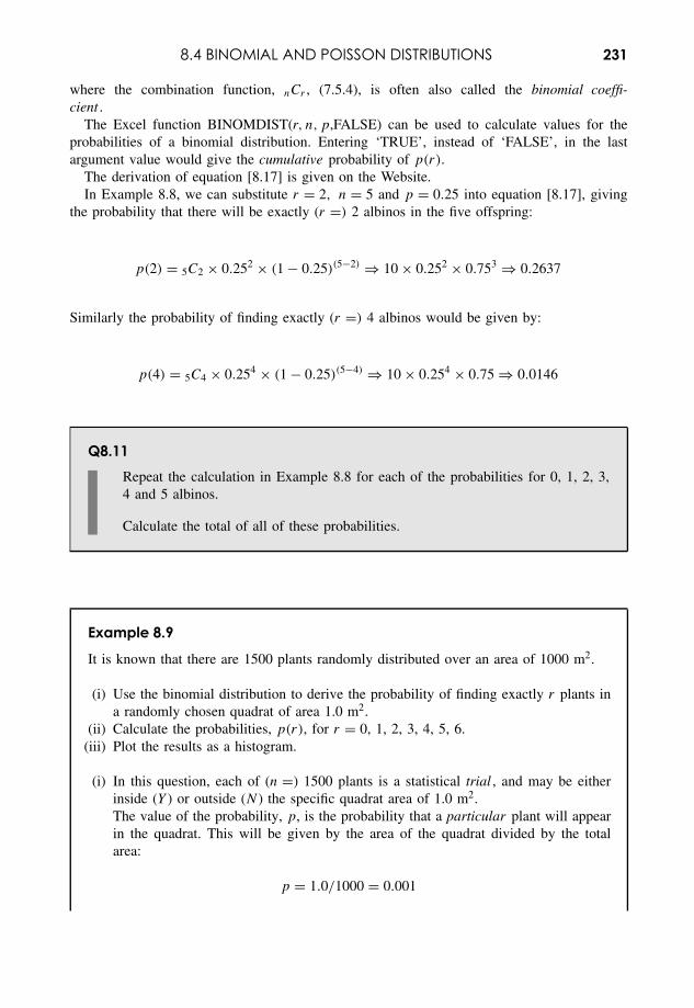
8.4 BINOMIAL AND POISSON DISTRIBUTIONS 231
where the combination function, nCr , (7.5.4), is often also called the binomial coeffi-cient .
The Excel function BINOMDIST(r, n, p,FALSE) can be used to calculate values for theprobabilities of a binomial distribution. Entering ‘TRUE’, instead of ‘FALSE’, in the lastargument value would give the cumulative probability of p(r).
The derivation of equation [8.17] is given on the Website.In Example 8.8, we can substitute r = 2, n = 5 and p = 0.25 into equation [8.17], giving
the probability that there will be exactly (r =) 2 albinos in the five offspring:
p(2) = 5C2 × 0.252 × (1 − 0.25)(5−2) ⇒ 10 × 0.252 × 0.753 ⇒ 0.2637
Similarly the probability of finding exactly (r =) 4 albinos would be given by:
p(4) = 5C4 × 0.254 × (1 − 0.25)(5−4) ⇒ 10 × 0.254 × 0.75 ⇒ 0.0146
Q8.11Repeat the calculation in Example 8.8 for each of the probabilities for 0, 1, 2, 3,4 and 5 albinos.
Calculate the total of all of these probabilities.
Example 8.9
It is known that there are 1500 plants randomly distributed over an area of 1000 m2.
(i) Use the binomial distribution to derive the probability of finding exactly r plants ina randomly chosen quadrat of area 1.0 m2.
(ii) Calculate the probabilities, p(r), for r = 0, 1, 2, 3, 4, 5, 6.(iii) Plot the results as a histogram.
(i) In this question, each of (n =) 1500 plants is a statistical trial , and may be eitherinside (Y ) or outside (N ) the specific quadrat area of 1.0 m2.The value of the probability, p, is the probability that a particular plant will appearin the quadrat. This will be given by the area of the quadrat divided by the totalarea:
p = 1.0/1000 = 0.001
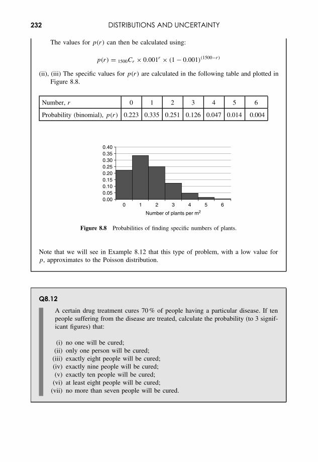
232 DISTRIBUTIONS AND UNCERTAINTY
The values for p(r) can then be calculated using:
p(r) = 1500Cr × 0.001r × (1 − 0.001)(1500−r)
(ii), (iii) The specific values for p(r) are calculated in the following table and plotted inFigure 8.8.
Number, r 0 1 2 3 4 5 6
Probability (binomial), p(r) 0.223 0.335 0.251 0.126 0.047 0.014 0.004
0.000.050.100.150.200.250.300.350.40
0 1 2 3 4 5 6
Number of plants per m2
Figure 8.8 Probabilities of finding specific numbers of plants.
Note that we will see in Example 8.12 that this type of problem, with a low value forp, approximates to the Poisson distribution.
Q8.12A certain drug treatment cures 70 % of people having a particular disease. If tenpeople suffering from the disease are treated, calculate the probability (to 3 signif-icant figures) that:
(i) no one will be cured;(ii) only one person will be cured;
(iii) exactly eight people will be cured;(iv) exactly nine people will be cured;(v) exactly ten people will be cured;
(vi) at least eight people will be cured;(vii) no more than seven people will be cured.
8.4 BINOMIAL AND POISSON DISTRIBUTIONS 233
8.4.3 Parameters of the binomial distributionThe mean value, µ, of the binomial distribution is given by:
µ = n × p [8.18]
When making experimental measurements of a binomial distribution, the experimental meanvalue, r , would be a best estimate of the true mean, µ. The best estimate of the individualprobability, p, would then be given by:
p ≈ r
n[8.19]
The standard deviation, σ , of the binomial distribution is given by:
σ =√
n × p × (1 − p) [8.20]
Example 8.10
Calculate the probabilities, p(r), of recording r heads when a balanced coin is tossed100 times.
(i) Plot the results on a probability distribution as a function of r .(ii) Calculate the mean and standard deviation of this distribution.
The worked answer is given in the following text .
In Example 8.10, the probability that a single toss of the coin will give a ‘head’ is p = 0.5.Using equation [8.17], the probability distribution will then be defined by:
p(r) = 100Cr × 0.5r × 0.5(100−r) ⇒ 100Cr × 0.5100
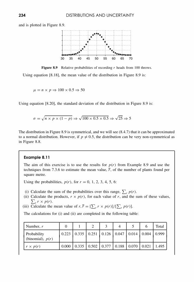
234 DISTRIBUTIONS AND UNCERTAINTY
and is plotted in Figure 8.9.
30 35 40 45 50 55 60 65 70
Figure 8.9 Relative probabilities of recording r heads from 100 throws.
Using equation [8.18], the mean value of the distribution in Figure 8.9 is:
µ = n × p ⇒ 100 × 0.5 ⇒ 50
Using equation [8.20], the standard deviation of the distribution in Figure 8.9 is:
σ =√
n × p × (1 − p) ⇒ √100 × 0.5 × 0.5 ⇒
√25 ⇒ 5
The distribution in Figure 8.9 is symmetrical, and we will see (8.4.7) that it can be approximatedto a normal distribution. However, if p = 0.5, the distribution can be very non-symmetrical asin Figure 8.8.
Example 8.11
The aim of this exercise is to use the results for p(r) from Example 8.9 and use thetechniques from 7.3.6 to estimate the mean value, r , of the number of plants found persquare metre.
Using the probabilities, p(r), for r = 0, 1, 2, 3, 4, 5, 6:
(i) Calculate the sum of the probabilities over this range,∑
r p(r).(ii) Calculate the products, r × p(r), for each value of r , and the sum of these values,∑
r r × p(r).(iii) Calculate the mean value of r, r = [
∑r r × p(r)]/[
∑r p(r)].
The calculations for (i) and (ii) are completed in the following table:
Number, r 0 1 2 3 4 5 6 Total
Probability 0.223 0.335 0.251 0.126 0.047 0.014 0.004 0.999(binomial), p(r)
r × p(r) 0.000 0.335 0.502 0.377 0.188 0.070 0.021 1.495

8.4 BINOMIAL AND POISSON DISTRIBUTIONS 235
Note that, in the table above, the sum of probabilities,∑
r p(r), is not exactly equal to1.000. This is because there is still a very small probability that seven or more plantsmay be recorded, and we have not included this in our total.
The experimental mean value can be calculated:
r =[∑
r
r × p(r)
] /[∑r
p(r)
]= 1.495/0.999 ≈ 1.50
The true mean of the distribution is given by equation [8.18]:
µ = n × p ⇒ 1500 × 0.001 ⇒ 1.5
which agrees with the result calculated from the values of p(r).
8.4.4 Poisson distributionAs with the binomial distribution, the Poisson distribution calculates the probabilities of observ-ing a certain number, r , of outcomes, each of which has a probability, p, of occurring. However,the Poisson distribution assumes that the probability that an individual trial will produce aspecific outcome is very small, i.e. p � 0.1.
Typical examples of Poisson distributions include situations where relatively few events arebeing counted in a small section of a much larger environment, such as:
• numbers of plants in a small area of a large field;• radioactive decay events occurring in a small time interval out of an overall decay period;• occurrences of a rare illness in a town.
In each of the above examples, the probability, p, that a particular event (plant, decay event,ill person) will be found in the particular situation (area, time interval, town) will be small.
The Poisson probability, p(r), of finding r occurrences of a particular outcome is definedby:
p(r) = e−µ × µr
r![8.21]
where µ is the mean number of such outcomes that would normally be expected to occur.Note that the Poisson probability does not depend on a value of n (total number of possible
trials).
236 DISTRIBUTIONS AND UNCERTAINTY
The Excel function POISSON(r , µ, False) can be used to calculate values for the probabilitiesof a binomial distribution. Entering ‘True’, instead of ‘False’, in the last argument value wouldgive the cumulative probability of p(r).
We now use Example 8.12, in comparison with Example 8.9, to investigate the use of thePoisson equation when p is very small.
Example 8.12
It is known that, on average, a random spread of particular rare plants in a field givesan average of 1.5 plants per square metre. Use the Poisson distribution to derive theprobability of finding exactly r plants in a quadrat of area 1.0 m2.
Calculate the probabilities, p(r), for r = 0, 1, 2, 3, 4, 5, 6. (Note the similarity with thequestion in Example 8.9.)
The worked answer is given in the following text .
In Example 8.12, we are given the mean value, µ = 1.5, of the number of plants that will fallwithin an area of 1.0 m2.
As we are testing an area of 1.0 m2 out of a whole field, then the probability, p, that anyparticular plant will randomly fall within the quadrat will be very small. For example, the valueof p in Example 8.10 was calculated to be 0.001. Hence we can use the Poisson probabilityfrom equation [8.21]:
p(r) = e−1.5 × 1.5r
r!
The results of the calculation for r = 0, 1, 2, 3, 4, 5, 6 are given in Table 8.3, together withthe results from the binomial calculation from Example 8.9.
Table 8.3.
Number, r 0 1 2 3 4 5 6
Probability (Poisson), p(r) 0.223 0.335 0.251 0.126 0.047 0.014 0.004Probability (binomial), p(r) 0.223 0.335 0.251 0.126 0.047 0.014 0.004
It can be seen from Table 8.3 that, to 3 decimal places, the results from the Poisson andbinomial distributions are the same for this problem with p = 0.001.
Q8.13The number of deaths due to a specific disease per year per 100 000 people ison average 50. Assuming that the occurrence of each incidence of the disease is
8.4 BINOMIAL AND POISSON DISTRIBUTIONS 237
random, calculate the probability that in a particular group of 1000 people theremay be:
(i) no deaths (iii) two deaths
(ii) one death (iv) more than two deaths
8.4.5 Using binomial and/or Poisson distributionsWhen the individual probability, p, is very small, then it is possible to use either the binomialor the Poisson distribution. However:
• for the binomial distribution it is necessary to know values for n and p; but• for the Poisson distribution it is only necessary to know the value of µ.
It is useful to note that, for the binomial distribution, the maximum value for r would be equalto n, but that for the Poisson distribution there is no theoretical maximum value for r .
The use of the above ideas is illustrated in Example 8.13.
Example 8.13
A service engineer is responsible for responding to emergency breakdowns from 2500customers. He normally receives four calls per day.
Calculate the probability that he would receive eight calls in a particular day.
(assume no customer has more than one breakdown per day)
Use both the binomial and Poisson distributions to answer the question.
This is a binomial-type problem because any one customer will only have a breakdown(Y ) or no breakdown (N ).
Calculation assuming a binomial distribution
We need to calculate values for n and p to use in [8.17].
The value of n equals the maximum possible value for r , which is the maximum numberof calls per day, n = 2500.
The mean number of calls is known to be µ = 4.
From [8.18], the probability, p, that any one customer will have a breakdown, is:
p = µ/n = 4/2500 = 0.0016
238 DISTRIBUTIONS AND UNCERTAINTY
We need to calculate p(r), where r = 8:
p(8) = 2500C8 × 0.00168 × (1 − 0.0016)2492 = 0.02972
Calculation assuming a Poisson distribution
For the Poisson distribution we already have the mean value, µ = 4. Hence:
p(8) = e−4 × 48
8!= 0.02977
The two results are virtually identical.
8.4.6 Cumulative distributionsThe expression for p(r) calculates the probability that exactly r occurrences of a particular con-dition (Y ) will occur. In practice, many problems are concerned with the combined probabilityof several possible values of r occurring.
The cumulative probability (see 7.3.9) for all values of r from 0 to r ′ is given by:
cp(r � r ′) = p(0) + p(1) + · · · + p(r ′ − 1) + p(r ′)
Example 8.14
Using the data from Table 8.3, we can calculate the probabilities of finding:
(i) two or less plants per quadrat(ii) three or more plants per quadrat.
Here:
(i) cp(r � 2) = p(0) + p(1) + p(2) = 0.223 + 0.335 + 0.251 = 0.809(ii) cp(r � 3) = 1 − cp(r � 2) = 1 − 0.809 = 0.191
8.4.7 Approximations for the binomial distributionThere are two important approximations for the binomial distribution, which occur when:
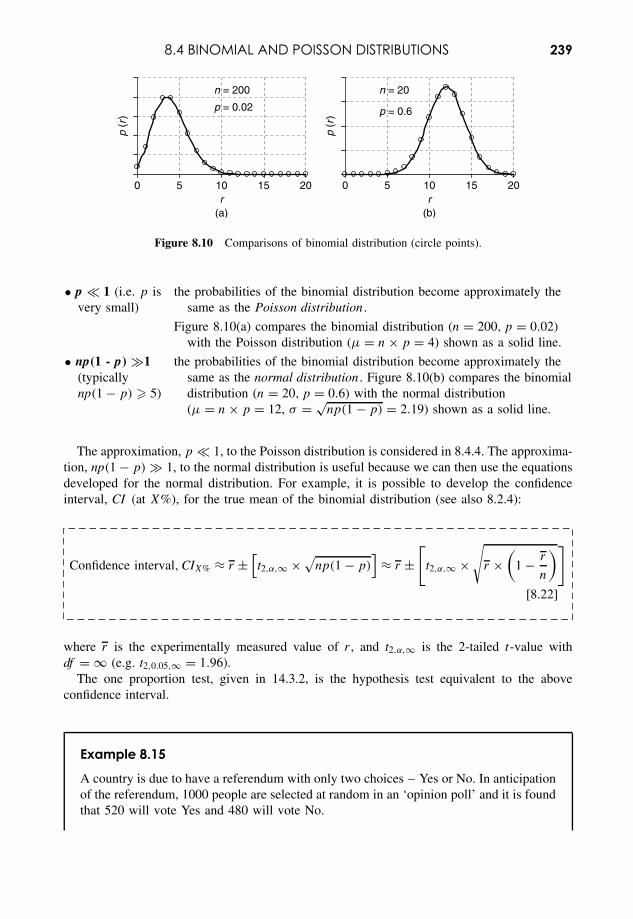
8.4 BINOMIAL AND POISSON DISTRIBUTIONS 239
0 5 10 15 20
p (r
)
r
n = 200
p = 0.02
0 5 10 15 20
p (r
)
r(a) (b)
n = 20
p = 0.6
Figure 8.10 Comparisons of binomial distribution (circle points).
• p � 1 (i.e. p isvery small)
the probabilities of the binomial distribution become approximately thesame as the Poisson distribution .
Figure 8.10(a) compares the binomial distribution (n = 200, p = 0.02)with the Poisson distribution (µ = n × p = 4) shown as a solid line.
• np(1 - p) 1(typicallynp(1 − p) � 5)
the probabilities of the binomial distribution become approximately thesame as the normal distribution . Figure 8.10(b) compares the binomialdistribution (n = 20, p = 0.6) with the normal distribution(µ = n × p = 12, σ = √
np(1 − p) = 2.19) shown as a solid line.
The approximation, p � 1, to the Poisson distribution is considered in 8.4.4. The approxima-tion, np(1 − p) 1, to the normal distribution is useful because we can then use the equationsdeveloped for the normal distribution. For example, it is possible to develop the confidenceinterval, CI (at X%), for the true mean of the binomial distribution (see also 8.2.4):
Confidence interval, CIX% ≈ r ±[t2,α,∞ ×
√np(1 − p)
]≈ r ±
[t2,α,∞ ×
√r ×
(1 − r
n
)]
[8.22]
where r is the experimentally measured value of r , and t2,α,∞ is the 2-tailed t-value withdf = ∞ (e.g. t2,0.05,∞ = 1.96).
The one proportion test, given in 14.3.2, is the hypothesis test equivalent to the aboveconfidence interval.
Example 8.15
A country is due to have a referendum with only two choices – Yes or No. In anticipationof the referendum, 1000 people are selected at random in an ‘opinion poll’ and it is foundthat 520 will vote Yes and 480 will vote No.
240 DISTRIBUTIONS AND UNCERTAINTY
Calculate the 95 % confidence interval for the true proportion of people who will voteYes.
From the sample, n = 1000 and r = 520.
The two-tailed confidence interval (see [8.22]) for the true number of Yes votes out ofeach group of 1000 people will be:
CI95 % ≈ 520 ±[
1.96 ×√
520 ×(
1 − 520
1000
)]⇒ 520 ± 31
Thus, for each group of 1000 voters, the number predicted (at 95 % confidence) to voteYes lies between 489 and 551.
This converts to a proportion of between 0.489 and 0.551.
Q8.14A random sample of 50 frogs is taken from a lake, and it is found that 37 are femaleand 13 are male. Estimate, with a 95 % confidence interval, the true proportion offemale frogs in the lake’s frog population.
(See also Example 14.6)
8.4.8 Shape of a distributionThe mean and standard deviation of a distribution are, respectively, measures of location (orposition) and spread (or width).
As we have seen (compare Figures 8.8 and 8.9) distributions can also have differentshapes . Other statistical parameters have been introduced to describe different shapecharacteristics:
Skewness. is a measure of the extent to which the distribution is skewed to one side or theother.
Kurtosis. is a measure of the extent to which the top of the distribution may be either flatteror more peaked than the normal distribution.
A more in-depth discussion of these is given on the Website.One further measure of interest is the ratio of the variance of the distribution to the mean
value. The coefficient of dispersion, CD , is given by:
8.4 BINOMIAL AND POISSON DISTRIBUTIONS 241
CD = Variance
Mean= σ 2
µ
which, using equations [8.18] and [8.20], for the binomial distribution becomes:
CD = n × p × q
n × p= q [8.23]
A good example in the use of the coefficient of dispersion, CD , is in the distribution of random‘events’, e.g. plants in a field:
• If the events (plants) are individually distributed at random, then the number of plants ina small area will be given by the Poisson distribution (see Example 8.12). For the Poissondistribution, CD ≈ 1.
• If there is a supportive ‘interaction’ between the events (plants), then the events may grouptogether (plant clumping). Another example would be the development of ‘clusters’ of anotherwise random disease, e.g. possible increase in the incidence of disease cases due tolocal pollution. In this case, the increased probability of ‘high-count’ groups would giveCD > 1.
• If the events compete for resources, then they will tend to spread out and give a more evendistribution. This will give a smaller dispersion of values around the mean value, resultingin CD < 1.
Q8.15In assessing the distribution of a species of plant, the two data sets, A and B, inthe table below record the frequencies with which specific numbers were recordedin 100 quadrats. The means and standard deviations of the two distributions aregiven.
Number ofplants
0 1 2 3 4 5 6 7 8 9 10 Mean Standarddeviation
Frequency, A 5 13 21 22 18 11 6 3 1 0 0 3.13 1.76
Frequency, B 10 14 17 18 16 12 7 4 1 1 0 3.13 2.04
The frequency distributions are also recorded in the line graph shown inFigure 8.11.
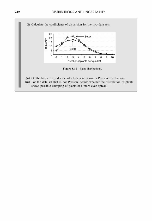
242 DISTRIBUTIONS AND UNCERTAINTY
(i) Calculate the coefficients of dispersion for the two data sets.
0
5
10
15
20
25
0 1 2 3 4 5 6 7 8 9 10
Number of plants per quadrat
Fre
quen
cy
Set A
Set B
Figure 8.11 Plant distributions.
(ii) On the basis of (i), decide which data set shows a Poisson distribution.(iii) For the data set that is not Poisson, decide whether the distribution of plants
shows possible clumping of plants or a more even spread.
9Scientific Investigation
Overview
Website • Excel files appropriate to selected Examples.• Example hypothesis tests in Excel and Minitab.
Science is concerned with understanding the way in which the natural world works. Thisincludes the biology of the living world, the chemistry of atomic and molecular structures,the physics of forces and systems, but it also includes the more applied sciences, e.g. sportsscience, forensic science, the environmental sciences, etc.
In this chapter we see that science is used to investigate a wide range of different systems,and that there are many different types of ‘scientific investigation’.
We also see that the power and effectiveness of science, as a way of accurately describingnature, grew out of the Renaissance in the sixteenth century with the development of the‘scientific method’.
As an essential feature of the ‘scientific method’, we concentrate on the issues involved withthe setting and testing of hypotheses. The statistical implementation of hypothesis tests for arange of different system parameters is developed using both parametric and non-parametrictests.
The final chapter in the book takes hypothesis testing into more complex scientific investi-gations, and highlights the interdependence between the experiment design and the statisticsinvolved in assessing the validity of the proposed hypotheses.
9.1 Scientific SystemsAny system that is being investigated can normally be characterized by:
• Outcomes – observable changes in the system.• Factors – ‘inputs’ to the system that may affect the outcomes.• Mechanisms – the actual processes (often hidden) within the system that link the ‘input’
factors to the ‘observed’ outcomes.• Subjects – representative examples of the ‘scientific system’ that are used for the particular
experiment.
Essential Mathematics and Statistics for Science 2nd Edition Graham Currell and Antony DowmanCopyright c© 2009 John Wiley & Sons, Ltd
244 SCIENTIFIC INVESTIGATION
Each ‘factor’ will have two, or more, ‘levels’, and a change of ‘level’ may cause a particular‘outcome’ from the system. ‘Outcomes’ and ‘levels’ will be measured by suitable experimentalvariables.
Example 9.1
It is claimed that omega 3 oils, found in many fish, reduce ‘clogging’ of the arteries. Inthis case the ‘system’ is the human body, the ‘outcome’ is reduced deposits in the arteries,the ‘factor’ relates to different ‘levels’ of intake of omega 3 oils, and the ‘mechanism’ isthe way in which the body metabolizes these oils. In an experiment, suitable ‘variables’must be used to measure the amount of arterial deposit and the intake (‘levels’) of omega3 oils.
There are three main levels in which science can normally understand such a system, suchas that described in Example 9.1. It may be possible to:
1. Confirm a correlation (or association) between the input factor(s) and the system out-come(s), e.g. an outcome may change following a change in a factor. However, a correlationbetween factor and outcome does not necessarily mean that the change in the factor is thereason for the change in the outcome.
2. Confirm a causal relationship between the input factor(s) and the system outcome(s). Inthis case, a change in a factor (cause) can be demonstrated to be the reason for the changein outcome (effect).
3. Explain the mechanism by which the factor causes the outcome to change. The under-standing of this mechanism must give more than a description of past observations; itmust be sufficiently good to be able to predict how the system will work under modifiedconditions.
In the case of the omega 3 example (Example 9.1):
• At level 1, the variable that records arterial deposits and the variable that measures oil intakemay show close correlation, but the oil intake might not be the ‘cause’ of the reduction indeposits. For example, the reduction in arterial deposits may be due to the fish diet forreasons not related to the omega 3 oils. The fish diet may be the ‘cause’ that both reducesarterial deposits (an effect) and, coincidentally, increases the intake of omega 3 oils (nowan effect and not a cause).
• Alternatively at level 2, a ‘cause and effect’ relationship could be shown to exist between‘factor’ and ‘outcome’ (i.e. the omega 3 oils actually reduce arterial deposits), but themechanism by which this works might not be fully understood.
• Ideally, at level 3, science should be able to demonstrate, within the constraints of the‘scientific method’ (9.2), a robust understanding of the mechanism involved in the process.This understanding must continue to be essentially correct as further discoveries are madeabout the system.
Scientific ‘systems’ can be recognized in all branches of science – from an understanding ofthe properties of subatomic particles to the behaviour of the Universe itself. In all cases,the development of understanding identifies the same three levels: correlation, causation,mechanism .
9.2 THE ‘SCIENTIFIC METHOD’ 245
9.2 The ‘Scientific Method’At a minimum level, any work in science must be characterized by an accuracy and objectivityin the collection of data, and a commitment to base conclusions solely on experimental results.
An important distinction should now be made between the processes used to reach conclu-sions:
Induction: comparative conclusions about one system are made on the basis of what is knownto happen in a different system.
Deduction: new conclusions are drawn as direct logical consequences of known facts.
Inductive reasoning may be considered to be equivalent to an intelligent guess that might proveto be wrong. Inductive reasoning is often a good starting point to consider how a new systemmight work and suggest possible hypotheses, but we will see that deduction, and not induction,is the fabric of true science.
Example 9.2
In trying to understand the mechanism of elasticity in the common elastic band, we maycompare the effect with elasticity in other materials. For example, we know that whenwe pull on a metal wire it will stretch and when we pull on an elastic band it will alsostretch. We may make an induction that the mechanisms are basically similar in the twocases, although different in magnitude.
If our induction is correct, we might expect that, when we heat up an elastic band, itwill stretch in the same way that a metal wire will stretch on heating. However, whenwe perform the experiment, we find that a stretched elastic band will tend to contracton heating. Our induction about similar mechanisms must be wrong in this case!
Deductive reasoning starts from known facts, and then proceeds to work out the inevitableconsequences of those facts. The process of deduction is faultless, but the accuracy of theconclusions still depends on the accuracy of the original facts on which the deduction wasbased.
The ‘scientific method’ itself is based on a cycle of hypothesis, experiment, deduction andprediction:
• Observations or inductive reasoning are often the starting point where observations beginto suggest a possible mechanism that might explain the behaviour of a system. (In Example9.2 it is thought that the mechanism for elasticity in the elastic band could be similar to thatin the metal wire.)
• A hypothesis is developed which describes an aspect of the proposed mechanism in thescientific system. The choice between the truth or otherwise of this hypothesis is oftenwritten as two alternatives:H1: Proposed hypothesis – the proposed mechanism is correct.H0: Null hypothesis – the proposed mechanism is not correct.(In Example 9.2 the proposed hypothesis is that the mechanism in the elastic band is similarto that in the metal wire.)
246 SCIENTIFIC INVESTIGATION
• An experiment is devised, whose outcome should give evidence to support, or not support,the proposed hypothesis, H1. (In Example 9.2 the proposed hypothesis predicts that an elasticband should expand on heating.)
• The experiment is performed and a decision is made as to whether the new understandingof the system is likely to be true. The conclusion is a deduction based on the observedfacts. (In Example 9.2, the observed facts do not support the proposed hypothesis. A newmechanism must be found to explain the behaviour of the elastic band.)
• If the proposed hypothesis is supported, then the proposed mechanism should be used topredict other observable behaviour patterns for the system. If these predictions are testedusing the ‘hypothesis-testing’ approach, and continue to confirm the new explanations, thenthis understanding begins to be accepted as a good description of the system.
The process of the ‘scientific method’ is also referred to as the ‘hypothetico-deductive’ method,emphasizing the two key elements of the concept.
When a hypothesis continues to satisfy more and more experimental tests, then it willgradually be accepted as a scientific fact. However, it must be remembered that the processof the ‘scientific method’ does not end with the discovery of ‘fact’, just because it satisfiesall current experimental data. Any scientific ‘fact’ may be modified in the future if furtherexperimental results fail to conform to the accepted theory.
Example 9.3
An excellent example of the ‘scientific method’ occurred in the development of the theoryof relativity by Albert Einstein. The new theory, for which there were many doubters,predicted that light from a star would be deflected as it passed close to our Sun.
This prediction would test the theory of relativity, and in 1919 during an eclipse of theSun the apparent positions of stars close to the Sun were found to shift according toEinstein’s prediction. Since that time, the theory of relativity has continued to predictevents accurately, and is now an accepted ‘fact’ of science.
However, as part of the ‘cycle’ of the scientific method, it is always probable that the cur-rent theory of relativity will be superceded by new ‘facts’ as more precise measurementsdemand a revised or alternative explanation.
9.3 Decision Making with Statistics9.3.1 IntroductionMany investigations in science seek to answer a simple ‘Yes or No’ question. For example:
• Is a new vaccine effective in preventing an infection?• Do glass fragments at the scene of a crime come from different sources?• Does a particular training regime improve athletic performance?
The statement of the initial ‘Yes or No’ question is a hypothesis statement, which we canpresent in two parts:
9.3 DECISION MAKING WITH STATISTICS 247
• ‘Yes’ is the Proposed hypothesis; and• ‘No’ is the Null hypothesis.
However, any scientific investigation is subject to errors and uncertainties, and the results donot give an absolute answer to the ‘Yes or No’ question – this is where the statistics come in!
The statistical analysis in a hypothesis test is based on the experimental data recorded,and normally calculates the probability (p-value) that it would be wrong to choose the ‘Yes’(proposed hypothesis) answer to the question. There is never an absolute certainty in the finalanswer, but at least it is possible to assess the probability of making at least one type of error.
We will introduce hypothesis testing by working through an extended example in 9.3.2. Thefollowing sections then highlight the separate elements of the hypothesis-testing procedure.
9.3.2 Calculation of p-valuesWe will introduce the concept of the p-value in hypothesis testing by using the investigationoutlined in Example 9.4.
Example 9.4
A sports club follows a long-standing tradition in which it always tosses the same specialcoin at the start of a game. However, some club members believe that the coin might bebiased so that it produces more heads than tails. They ask you to toss the coin 100 timesand then, using your knowledge of statistics, decide whether the coin is indeed biasedin favour of heads.
The analysis is performed in the following text .
You accept the task outlined in Example 9.4. You realize that the true situation must be oneof two alternatives, which you express in terms of a proposed hypothesis (labelled as H1) andits ‘null’ option (labelled as H0):
Proposed hypothesis, H1: The coin gives more heads than tails.
Null hypothesis, H0: The coin does not give more heads than tails.
You will toss the coin n = 100 times, and on the basis of the number of heads, r , recorded,you will decide whether you will ‘accept’ or ‘not accept’ that the proposed hypothesis, H1, iscorrect.
Clearly there could be two possible correct outcomes. You might be correct by ‘AcceptingH1’ for a biased coin, or you might be correct by ‘Not accepting H1’ where there is no bias.
However, there could be two different types of error that you could make, each with differentconsequences:
• Type I error. You accept H1 believing that the coin is biased, when in fact it is perfectlyfair. The consequence is that you have unnecessarily ended the long-standing tradition.
• Type II error. With limited experimental data, you choose not to accept H1, but the coinis actually biased. Your poor experimental skills have failed to identify a real problem.
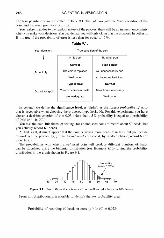
248 SCIENTIFIC INVESTIGATION
The four possibilities are illustrated in Table 9.1. The columns give the ‘true’ condition of thecoin, and the rows give your decision.
You realize that, due to the random nature of the process, there will be an inherent uncertaintywhen you make your decision. You decide that you will only claim that the proposed hypothesis,H1, is true if the probability of error is less than (or equal to) 5 %.
Table 9.1.
Your decision: True condition of the coin
H1 is true H1 is not true
Accept H1
Correct
The coin is replaced
Well done!
Type I error
You unnecessarily end
an important tradition.
Do not accept H1
Type II error
Your experimental skills
are inadequate
Correct
No action is necessary
Well done!
In general, we define the significance level, α (alpha), as the largest probability of errorthat is acceptable when choosing the proposed hypothesis, H1. For this experiment, you havechosen a decision criterion of α = 0.05. (Note that a 5 % probability is equal to a probabilityof 0.05 or ‘1 in 20’.)
You toss the coin 100 times, expecting (for an unbiased coin) to record about 50 heads, butyou actually record 60 heads.
At first sight, it might appear that the coin is giving more heads than tails, but you decideto work out the probability, p, that an unbiased coin could, by random chance, record 60 ormore heads.
The probabilities with which a balanced coin will produce different numbers of headscan be calculated using the binomial distribution (see Example 8.10), giving the probabilitydistribution in the graph shown in Figure 9.1.
Probabilitysum = 0.0284
30 35 40 45 50 55 60 65 70
Figure 9.1 Probabilities that a balanced coin will record r heads in 100 throws.
From this distribution, it is possible to identify the key probability area:
Probability of recording 60 heads or more, p(r � 60) = 0.0284
9.3 DECISION MAKING WITH STATISTICS 249
You now realize that the p-value, p = 0.0284, is:
• the probability that a perfectly balanced coin might, by random chance, record 60 or moreheads;
• the probability that the null hypothesis, H0, might be true;• the probability of a Type I error if you accept H1 (reject H0).
On the basis of the information in the text, you must now make the critical decision, comparingthe observed probability p-value, p = 0.0284, with your initial significance level criterion,α = 0.05:
Do you ‘Accept H1’ and declare the coin to be biased, or do you ‘Not accept H1’ and say thatyou cannot be sure that it is biased?
As the probability that you will be wrong (p = 0.0284) is less than your upper limit of(α =) 0.05, you actually choose to accept H1 and claim that coin is biased.
The old coin is discarded and the club committee choose a new coin.
Example 9.5
Having discarded the original coin (Example 9.4), the committee now ask you to checkwhether the new coin might be biased, giving either more heads or more tails.
The worked answer is given in the following text .
The question posed in Example 9.5 requires a new experiment, so you establish the newhypotheses which take into account that the coin might be biased in either direction:
Proposed hypothesis, H1: The number of heads is different from thenumber of tails.
Null hypothesis, H0: The number of heads is the same as thenumber of tails.
In this case you would accept that the coin is biased (H1) if it gives either a significantly highor a low number of heads.
You toss the new coin 100 times and again you record 60 heads. However, you now expressthis result as:
Difference between the recorded result of 60 and the ‘expected’ result of 50 = 10.
You now need to work out the probability, p, that an unbiased coin could, by random chance,record a difference of 10 or more heads, i.e. either 40 or less, or 60 or more.
The probabilities with which a balanced coin will produce different numbers of heads canbe calculated again using the binomial distribution (Figure 9.2).
From this distribution, it is possible to identify the total probability area of recording adifference or 10 or more heads:
p(difference � 10) = p(r � 40) + p(r � 60) = 0.0284 + 0.0284 = 0.0568
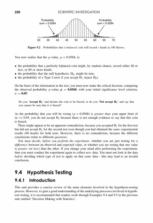
250 SCIENTIFIC INVESTIGATION
Probabilitysum = 0.0284
Probabilitysum = 0.0284
30 35 40 45 50 55 60 65 70
Figure 9.2 Probabilities that a balanced coin will record r heads in 100 throws.
You now realize that the p-value, p = 0.0568, is:
• the probability that a perfectly balanced coin might, by random chance, record either 40 orless, or 60 or more heads;
• the probability that the null hypothesis, H0, might be true;• the probability of a Type I error if you accept H1 (reject H0).
On the basis of the information in the text, you must now make the critical decision, comparingthe observed probability p-value, p = 0.0568, with your initial significance level criterion,α = 0.05:
Do you ‘Accept H1’ and declare the coin to be biased, or do you ‘Not accept H1’ and say thatyou cannot be sure that it is biased?
As the probability that you will be wrong (p = 0.0568) is greater than your upper limit of(α =) 0.05, you do not accept H1 because there is not enough evidence to say that this coinis biased.
There might appear to be an apparent contradiction, because you accepted H1 for the first testbut did not accept H1 for the second test even though you had obtained the same experimentalresults (60 heads) for both tests. However, there is no contradiction, because the differentconclusions relate to different questions .
You must decide, before you perform the experiment , whether you are just testing for adifference between an observed and expected value, or whether you are testing that one valueis greater (or less) than the other. If you change your mind after performing the experiment,then you must conduct the experiment again to collect new data. You must not look at the databefore deciding which type of test to apply on that same data – this may lead to an invalidconclusion.
9.4 Hypothesis Testing9.4.1 IntroductionThis unit provides a concise review of the main elements involved in the hypothesis-testingprocess. However, to gain a good understanding of the underlying processes involved in hypoth-esis testing, it is recommended that readers work through Examples 9.4 and 9.5 in the previousunit entitled ‘Decision Making with Statistics’.
9.4 HYPOTHESIS TESTING 251
9.4.2 Hypothesis statementIt is essential, before performing any experimental measurements, to state the proposed hypoth-esis being tested, usually written as H1, and the null hypothesis , usually written as H0:
Proposed hypothesis, H1: Smoking increases the probability of lung cancer.
Null hypothesis, H0: Smoking does not affect the probability of lung cancer.
The proposed hypothesis usually demonstrates that a factor (9.1) does indeed cause some‘effect’ or ‘change of value’. The null hypothesis usually demonstrates ‘no factor effect’ or the‘status quo’.
A scientific experiment must be precise about what is actually being measured, and willnormally measure some physical, chemical or biological variable, which will then be used asan indicator in choosing which hypothesis is believed to be correct.
It is also important that any ‘vague’ terminology should be accurately defined – for example,‘smoking’ in the above example may be defined as five cigarettes per day.
Example 9.6
As part of a monitoring procedure, an analyst wishes to test whether the lead content ofa water supply exceeds 50 ppb. State the relevant hypotheses.
If the true lead content is µ, the appropriate hypotheses for this test would be:
Proposed hypothesis, H1: Lead content is greater than 50 ppb, µ > 50 ppb.
Null hypothesis, H0: Lead content equals 50 ppb, µ = 50 ppb.
9.4.3 TailsIn defining a hypothesis statement in respect of a possible factor ‘effect’, there are two possi-bilities:
• 2-tailed: the factor effect may operate in either direction; or• 1-tailed: the factor is only being tested for an effect in one particular direction .
The hypothesis statement in Example 9.6 is ‘1-tailed’, because the proposed hypothesis onlyproposes an increase in lead concentration. Example 9.7 gives an example of a ‘2-tailed’hypothesis in a similar context. In this case the proposed hypothesis proposes either an increaseor a decrease.
Example 9.7
As part of a monitoring procedure, an analyst wishes to test whether the lead content ofa water supply is not equal to 50 ppb. State the relevant hypotheses.
252 SCIENTIFIC INVESTIGATION
If the true lead content is µ, the appropriate hypotheses for this test would be:
Proposed hypothesis, H1: Lead content does not equal 50 ppb, µ = 50 ppb.
Null hypothesis, H0: Lead content equals 50 ppb, µ = 50 ppb.
It is useful to remember that, for the same data set (for a symmetrical distribution) :
p-value for a 2-tailed test = 2 × p-value for a 1-tailed test [9.1]
Q9.1Decide, for each of the following statements for proposed hypotheses, whichimplies a 1-tailed test and which implies a 2-tailed test.
Number of tails
(i) An athlete’s performance is enhanced when using aparticular dietary supplement.
1/2
(ii) Low-level background music affects people’scapacity to memorize a list of names.
1/2
(iii) The mean content of breakfast cereal packets filledby a certain filling machine is less than 580 g.
1/2
(iv) An increase in a car driver’s blood–alcohol level to40 mg per 100 mL will change the probability ofhaving an accident.
1/2
9.4.4 Decisions based on the p-valueThe decision process starts with the assumption that the null hypothesis might be true.
Statistics software is used to calculate the probability (p-value) that the null hypothesiscould produce the observed experimental results. If this probability is sufficiently small (i.e. itis unlikely that the null hypothesis is true), then the proposed hypothesis would be acceptedas being true instead.
With this type of question, there are two ways of being wrong :
• deciding ‘proposed’ when ‘null’ is correct (Type I error); and• deciding ‘null’ when ‘proposed’ is correct (Type II error).
In terms of the hypotheses, the Type I and Type II errors could occur as in Table 9.2.
9.4 HYPOTHESIS TESTING 253
Table 9.2. Errors in a hypothesis test.
Conclusion: True situationH1 true H1 not true
Accept H1 Correct result Type I errorDo not accept H1 Type II error Correct result
In making the decision that the proposed hypothesis is true, it is necessary to decide howsmall the p-value must be so that we can confidently reject the null hypothesis and avoid aType I Error.
Before starting the experiment, we must choose the value of the significance level, α (see9.3.2). The significance level, α (alpha), is the largest probability of error that is acceptablewhen choosing the proposed hypothesis, H1.
If a conclusion is claimed to be significant , then the results normally indicate that H1 iscorrect with less than a 0.05 (5 %) chance of being wrong. If a conclusion is claimed to behighly significant , then the probability of H1 being wrong is normally less than 0.01 (or 1 %).
Note that the term confidence level is often used to express the percentage probabilityof being right , e.g. confidence levels of 95 % and 99 % for being right are equivalent tosignificance levels of 0.05 and 0.01, respectively, for being wrong!
The choice of a value for the significance level, α, depends on the context of the problem,and the consequences that would arise if H1 were chosen in error. The default level for mostscientific research is taken as α = 0.05.
The probability of a Type I error for a given experiment is given by the p-value, which canbe calculated from the experimental results – see 9.3.2. The probability of a Type II error isdenoted by β (beta), which is usually much more difficult to calculate.
The significance level, α, is the maximum probability of a Type I error that would beacceptable. Its value must be decided as part of the initial experiment design process.
On the basis of the relative values of α and p, it is then possible to make the decision:
If p � α Accept proposed hypothesis, H1, at a significance level of α
[9.2]If p >α Insufficient evidence to accept proposed hypothesis
Most software programs (e.g. Excel, Minitab) will calculate a p-value for the given statisticaltest. This makes performing a statistical test very easy, as the decision is based only on therelative sizes of p and α.
9.4.5 Power of the experimentThe power of an experiment is a measure of how successful the experiment will be in con-firming the existence of a ‘factor’ effect, if such an effect actually exists. It is the ‘opposite’of the probability of a Type II error:
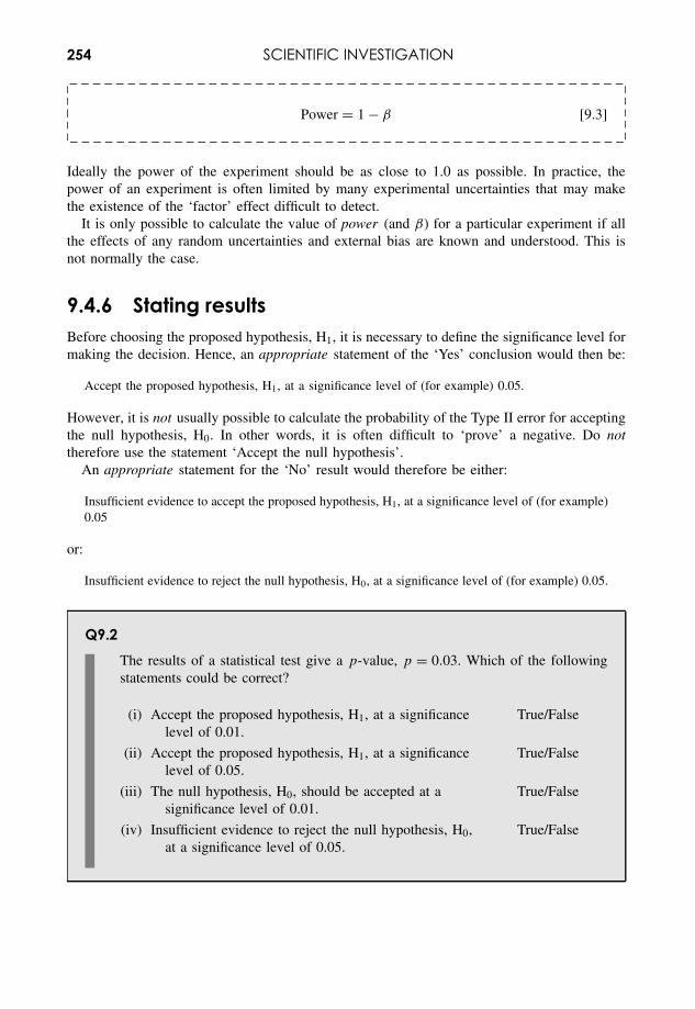
254 SCIENTIFIC INVESTIGATION
Power = 1 − β [9.3]
Ideally the power of the experiment should be as close to 1.0 as possible. In practice, thepower of an experiment is often limited by many experimental uncertainties that may makethe existence of the ‘factor’ effect difficult to detect.
It is only possible to calculate the value of power (and β) for a particular experiment if allthe effects of any random uncertainties and external bias are known and understood. This isnot normally the case.
9.4.6 Stating resultsBefore choosing the proposed hypothesis, H1, it is necessary to define the significance level formaking the decision. Hence, an appropriate statement of the ‘Yes’ conclusion would then be:
Accept the proposed hypothesis, H1, at a significance level of (for example) 0.05.
However, it is not usually possible to calculate the probability of the Type II error for acceptingthe null hypothesis, H0. In other words, it is often difficult to ‘prove’ a negative. Do nottherefore use the statement ‘Accept the null hypothesis’.
An appropriate statement for the ‘No’ result would therefore be either:
Insufficient evidence to accept the proposed hypothesis, H1, at a significance level of (for example)0.05
or:
Insufficient evidence to reject the null hypothesis, H0, at a significance level of (for example) 0.05.
Q9.2The results of a statistical test give a p-value, p = 0.03. Which of the followingstatements could be correct?
(i) Accept the proposed hypothesis, H1, at a significancelevel of 0.01.
True/False
(ii) Accept the proposed hypothesis, H1, at a significancelevel of 0.05.
True/False
(iii) The null hypothesis, H0, should be accepted at asignificance level of 0.01.
True/False
(iv) Insufficient evidence to reject the null hypothesis, H0,at a significance level of 0.05.
True/False
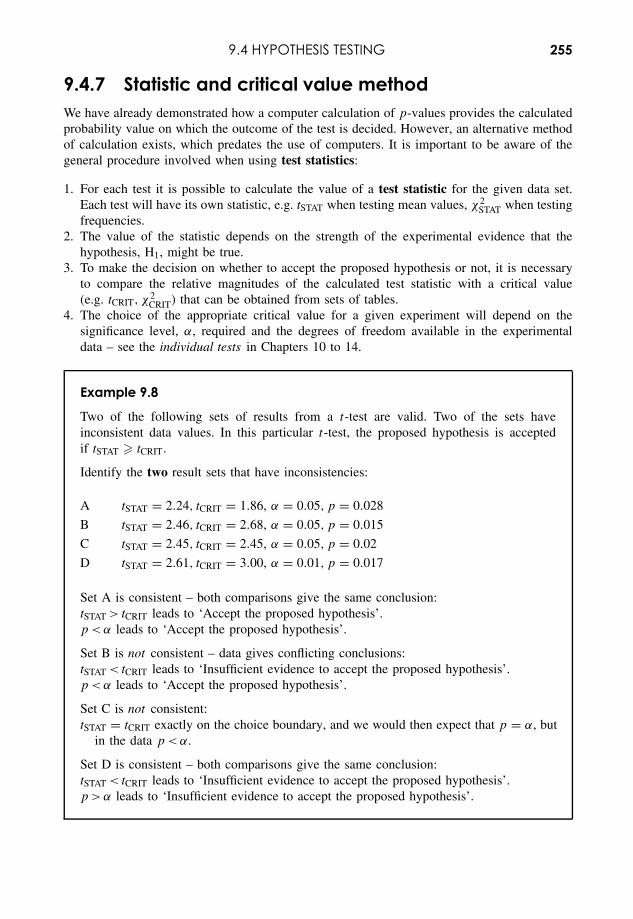
9.4 HYPOTHESIS TESTING 255
9.4.7 Statistic and critical value methodWe have already demonstrated how a computer calculation of p-values provides the calculatedprobability value on which the outcome of the test is decided. However, an alternative methodof calculation exists, which predates the use of computers. It is important to be aware of thegeneral procedure involved when using test statistics:
1. For each test it is possible to calculate the value of a test statistic for the given data set.Each test will have its own statistic, e.g. tSTAT when testing mean values, χ2
STAT when testingfrequencies.
2. The value of the statistic depends on the strength of the experimental evidence that thehypothesis, H1, might be true.
3. To make the decision on whether to accept the proposed hypothesis or not, it is necessaryto compare the relative magnitudes of the calculated test statistic with a critical value(e.g. tCRIT, χ2
CRIT) that can be obtained from sets of tables.4. The choice of the appropriate critical value for a given experiment will depend on the
significance level, α, required and the degrees of freedom available in the experimentaldata – see the individual tests in Chapters 10 to 14.
Example 9.8
Two of the following sets of results from a t-test are valid. Two of the sets haveinconsistent data values. In this particular t-test, the proposed hypothesis is acceptedif tSTAT � tCRIT.
Identify the two result sets that have inconsistencies:
A tSTAT = 2.24, tCRIT = 1.86, α = 0.05, p = 0.028
B tSTAT = 2.46, tCRIT = 2.68, α = 0.05, p = 0.015
C tSTAT = 2.45, tCRIT = 2.45, α = 0.05, p = 0.02
D tSTAT = 2.61, tCRIT = 3.00, α = 0.01, p = 0.017
Set A is consistent – both comparisons give the same conclusion:tSTAT > tCRIT leads to ‘Accept the proposed hypothesis’.p <α leads to ‘Accept the proposed hypothesis’.
Set B is not consistent – data gives conflicting conclusions:tSTAT < tCRIT leads to ‘Insufficient evidence to accept the proposed hypothesis’.p <α leads to ‘Accept the proposed hypothesis’.
Set C is not consistent:tSTAT = tCRIT exactly on the choice boundary, and we would then expect that p = α, but
in the data p <α.
Set D is consistent – both comparisons give the same conclusion:tSTAT < tCRIT leads to ‘Insufficient evidence to accept the proposed hypothesis’.p >α leads to ‘Insufficient evidence to accept the proposed hypothesis’.
256 SCIENTIFIC INVESTIGATION
9.5 Selecting Analyses and Tests9.5.1 IntroductionThis unit provides an introduction to some of the most commonly used statistical tests. For thedetailed workings and examples of each test, readers are referred elsewhere in the book or onthe Website.
An investigation in science often involves making one or more sets of replicate experimentalmeasurements (7.1.2) which are statistical samples (7.2.2) of the population of all the mea-surements (possibly infinite) that could be made. A typical statistical test then calculates theprobability (p-value) that the null hypothesis might explain the observed experimental data.
It is important to remember that the statistical test calculates the probability that the proposedhypothesis is not true. It does not directly calculate the probability that the proposed hypothesisis true.
The choice of an appropriate test is an integral part of the overall process of designing theexperimental procedure – see Chapter 15. The detailed choice depends on a range of factors,but, in particular, it is essential to be clear about:
• what statistic is being tested, e.g. mean values, distribution of frequencies, proportions, etc.;• whether the distribution of values being tested follows a specific distribution, e.g. a normal
distribution;• whether the test is 1-tailed or 2-tailed; and• what is the significance level being used for the test?
9.5.2 Assumptions in using statistical testsStatistical tests make certain assumptions about how the test was performed and possibly theunderlying variation of the data being measured.
Each measurement must be randomly selected and independent of any other measurement.For example, ‘random selection’ would require that seedlings being selected for different
growth conditions must be chosen by an objectively random procedure (15.1.3).The requirement for ‘independence’ between measurements aims to counteract any ‘hidden’
association between replicate measurements. This is particularly important in relation to possi-ble errors in the measurement process itself. For example, if one instrument is used to measureone sample set of replicates and another instrument is used to measure a second sample set,then any bias between the instruments will be translated into an apparent difference betweenthe experimental results.
There is a wide range of tests, called parametric tests, which make the assumption that thedata values are being sampled from a known distribution , and for these tests the exact datavalues are used directly in the calculations.
An alternative range of tests, called non-parametric tests, do not make any assumption aboutan underlying distribution, and use data values only to rank the data in order.
The parametric t-tests, F -tests, ANOVAs, Pearson’s correlation and regression all assumethat the data is drawn from a normal distribution. This is often a valid assumption for mostexperimental data, particularly where mean values are calculated from large sample sizes. Ithas also been shown that these most commonly used tests are quite robust when dealing withdata that is not normally distributed in that they still provide correct conclusions.
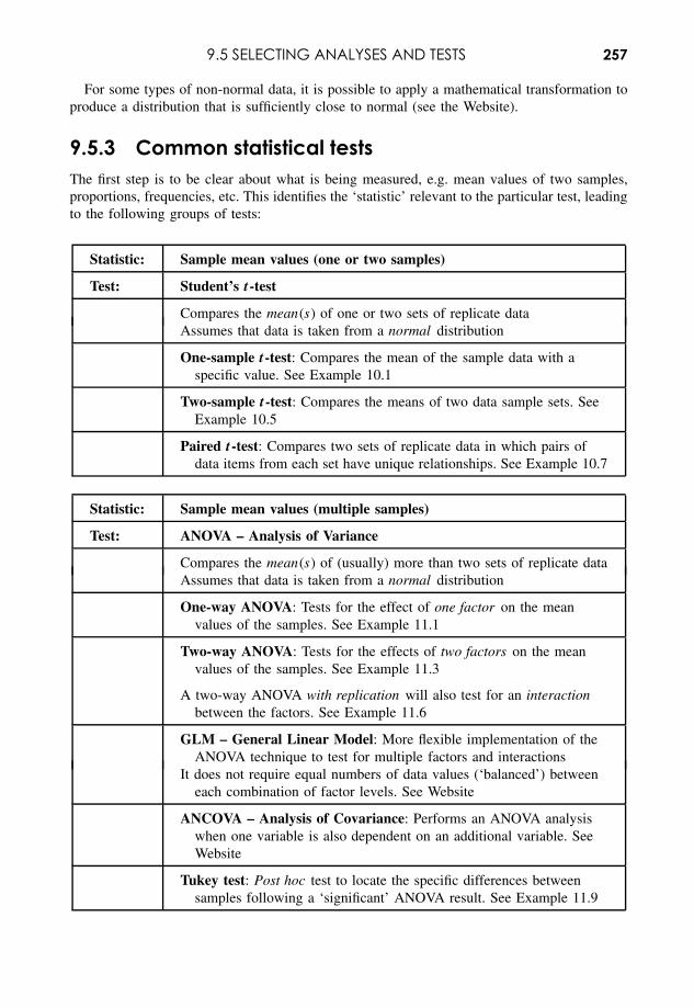
9.5 SELECTING ANALYSES AND TESTS 257
For some types of non-normal data, it is possible to apply a mathematical transformation toproduce a distribution that is sufficiently close to normal (see the Website).
9.5.3 Common statistical testsThe first step is to be clear about what is being measured, e.g. mean values of two samples,proportions, frequencies, etc. This identifies the ‘statistic’ relevant to the particular test, leadingto the following groups of tests:
Statistic: Sample mean values (one or two samples)
Test: Student’s t-test
Compares the mean(s) of one or two sets of replicate dataAssumes that data is taken from a normal distribution
One-sample t-test: Compares the mean of the sample data with aspecific value. See Example 10.1
Two-sample t-test: Compares the means of two data sample sets. SeeExample 10.5
Paired t-test: Compares two sets of replicate data in which pairs ofdata items from each set have unique relationships. See Example 10.7
Statistic: Sample mean values (multiple samples)
Test: ANOVA – Analysis of Variance
Compares the mean(s) of (usually) more than two sets of replicate dataAssumes that data is taken from a normal distribution
One-way ANOVA: Tests for the effect of one factor on the meanvalues of the samples. See Example 11.1
Two-way ANOVA: Tests for the effects of two factors on the meanvalues of the samples. See Example 11.3
A two-way ANOVA with replication will also test for an interactionbetween the factors. See Example 11.6
GLM – General Linear Model: More flexible implementation of theANOVA technique to test for multiple factors and interactions
It does not require equal numbers of data values (‘balanced’) betweeneach combination of factor levels. See Website
ANCOVA – Analysis of Covariance: Performs an ANOVA analysiswhen one variable is also dependent on an additional variable. SeeWebsite
Tukey test: Post hoc test to locate the specific differences betweensamples following a ‘significant’ ANOVA result. See Example 11.9
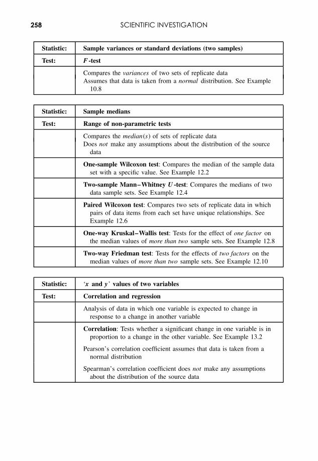
258 SCIENTIFIC INVESTIGATION
Statistic: Sample variances or standard deviations (two samples)
Test: F -test
Compares the variances of two sets of replicate dataAssumes that data is taken from a normal distribution. See Example
10.8
Statistic: Sample medians
Test: Range of non-parametric tests
Compares the median(s) of sets of replicate dataDoes not make any assumptions about the distribution of the source
data
One-sample Wilcoxon test: Compares the median of the sample dataset with a specific value. See Example 12.2
Two-sample Mann–Whitney U -test: Compares the medians of twodata sample sets. See Example 12.4
Paired Wilcoxon test: Compares two sets of replicate data in whichpairs of data items from each set have unique relationships. SeeExample 12.6
One-way Kruskal–Wallis test: Tests for the effect of one factor onthe median values of more than two sample sets. See Example 12.8
Two-way Friedman test: Tests for the effects of two factors on themedian values of more than two sample sets. See Example 12.10
Statistic: ‘x and y’ values of two variables
Test: Correlation and regression
Analysis of data in which one variable is expected to change inresponse to a change in another variable
Correlation: Tests whether a significant change in one variable is inproportion to a change in the other variable. See Example 13.2
Pearson’s correlation coefficient assumes that data is taken from anormal distribution
Spearman’s correlation coefficient does not make any assumptionsabout the distribution of the source data
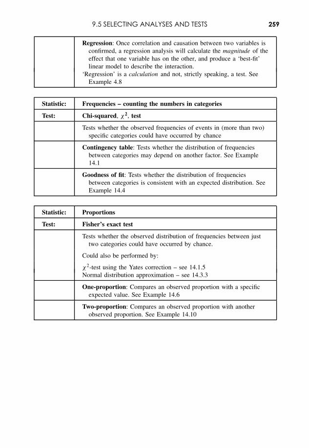
9.5 SELECTING ANALYSES AND TESTS 259
Regression: Once correlation and causation between two variables isconfirmed, a regression analysis will calculate the magnitude of theeffect that one variable has on the other, and produce a ‘best-fit’linear model to describe the interaction.
‘Regression’ is a calculation and not, strictly speaking, a test. SeeExample 4.8
Statistic: Frequencies – counting the numbers in categories
Test: Chi-squared, χ2, test
Tests whether the observed frequencies of events in (more than two)specific categories could have occurred by chance
Contingency table: Tests whether the distribution of frequenciesbetween categories may depend on another factor. See Example14.1
Goodness of fit: Tests whether the distribution of frequenciesbetween categories is consistent with an expected distribution. SeeExample 14.4
Statistic: Proportions
Test: Fisher’s exact test
Tests whether the observed distribution of frequencies between justtwo categories could have occurred by chance.
Could also be performed by:
χ2-test using the Yates correction – see 14.1.5Normal distribution approximation – see 14.3.3
One-proportion: Compares an observed proportion with a specificexpected value. See Example 14.6
Two-proportion: Compares an observed proportion with anotherobserved proportion. See Example 14.10

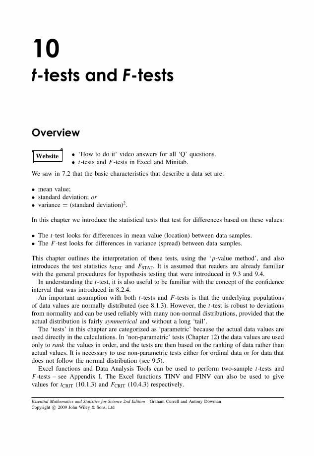
10t-tests and F-tests
Overview
Website • ‘How to do it’ video answers for all ‘Q’ questions.• t-tests and F -tests in Excel and Minitab.
We saw in 7.2 that the basic characteristics that describe a data set are:
• mean value;• standard deviation; or• variance = (standard deviation)2.
In this chapter we introduce the statistical tests that test for differences based on these values:
• The t-test looks for differences in mean value (location) between data samples.• The F -test looks for differences in variance (spread) between data samples.
This chapter outlines the interpretation of these tests, using the ‘p-value method’, and alsointroduces the test statistics tSTAT and FSTAT. It is assumed that readers are already familiarwith the general procedures for hypothesis testing that were introduced in 9.3 and 9.4.
In understanding the t-test, it is also useful to be familiar with the concept of the confidenceinterval that was introduced in 8.2.4.
An important assumption with both t-tests and F -tests is that the underlying populationsof data values are normally distributed (see 8.1.3). However, the t-test is robust to deviationsfrom normality and can be used reliably with many non-normal distributions, provided that theactual distribution is fairly symmetrical and without a long ‘tail’.
The ‘tests’ in this chapter are categorized as ‘parametric’ because the actual data values areused directly in the calculations. In ‘non-parametric’ tests (Chapter 12) the data values are usedonly to rank the values in order, and the tests are then based on the ranking of data rather thanactual values. It is necessary to use non-parametric tests either for ordinal data or for data thatdoes not follow the normal distribution (see 9.5).
Excel functions and Data Analysis Tools can be used to perform two-sample t-tests andF -tests – see Appendix I. The Excel functions TINV and FINV can also be used to givevalues for tCRIT (10.1.3) and FCRIT (10.4.3) respectively.
Essential Mathematics and Statistics for Science 2nd Edition Graham Currell and Antony DowmanCopyright c© 2009 John Wiley & Sons, Ltd
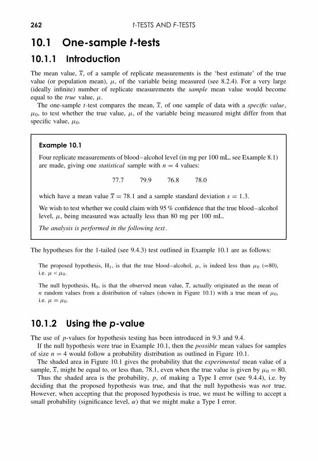
262 t-TESTS AND F-TESTS
10.1 One-sample t-tests10.1.1 IntroductionThe mean value, x, of a sample of replicate measurements is the ‘best estimate’ of the truevalue (or population mean), µ, of the variable being measured (see 8.2.4). For a very large(ideally infinite) number of replicate measurements the sample mean value would becomeequal to the true value, µ.
The one-sample t-test compares the mean, x, of one sample of data with a specific value,µ0, to test whether the true value, µ, of the variable being measured might differ from thatspecific value, µ0.
Example 10.1
Four replicate measurements of blood–alcohol level (in mg per 100 mL, see Example 8.1)are made, giving one statistical sample with n = 4 values:
77.7 79.9 76.8 78.0
which have a mean value x = 78.1 and a sample standard deviation s = 1.3.
We wish to test whether we could claim with 95 % confidence that the true blood–alcohollevel, µ, being measured was actually less than 80 mg per 100 mL.
The analysis is performed in the following text .
The hypotheses for the 1-tailed (see 9.4.3) test outlined in Example 10.1 are as follows:
The proposed hypothesis, H1, is that the true blood–alcohol, µ, is indeed less than µ0 (=80),i.e. µ<µ0.
The null hypothesis, H0, is that the observed mean value, x, actually originated as the mean ofn random values from a distribution of values (shown in Figure 10.1) with a true mean of µ0,i.e. µ = µ0.
10.1.2 Using the p-valueThe use of p-values for hypothesis testing has been introduced in 9.3 and 9.4.
If the null hypothesis were true in Example 10.1, then the possible mean values for samplesof size n = 4 would follow a probability distribution as outlined in Figure 10.1.
The shaded area in Figure 10.1 gives the probability that the experimental mean value of asample, x, might be equal to, or less than, 78.1, even when the true value is given by µ0 = 80.
Thus the shaded area is the probability, p, of making a Type I error (see 9.4.4), i.e. bydeciding that the proposed hypothesis was true, and that the null hypothesis was not true.However, when accepting that the proposed hypothesis is true, we must be willing to accept asmall probability (significance level, α) that we might make a Type I error.
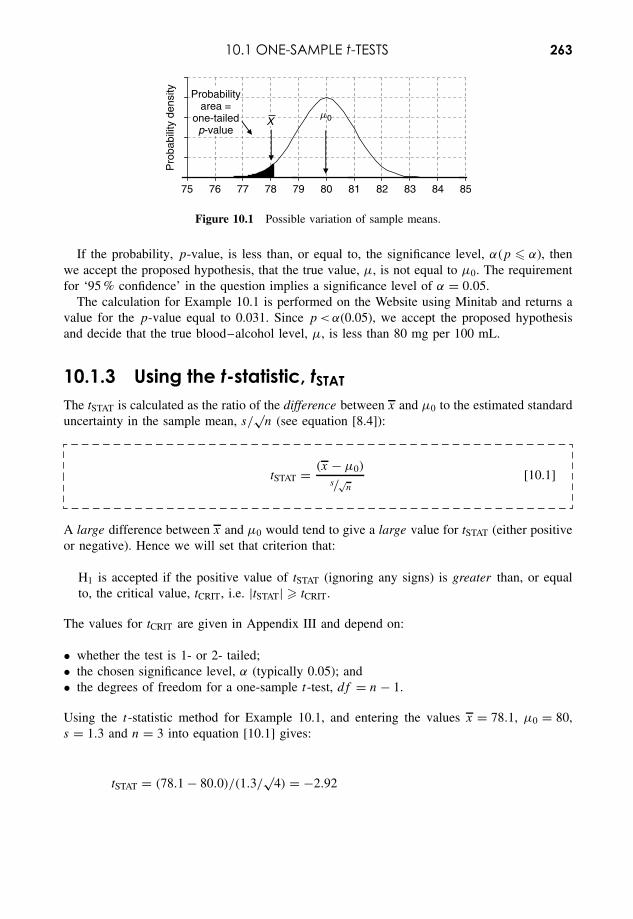
10.1 ONE-SAMPLE t-TESTS 263
75 76 77 78 79 80 81 82 83 84 85
Pro
babi
lity
dens
ity
m0
Probabilityarea =
one-tailedp-value
X
Figure 10.1 Possible variation of sample means.
If the probability, p-value, is less than, or equal to, the significance level, α(p � α), thenwe accept the proposed hypothesis, that the true value, µ, is not equal to µ0. The requirementfor ‘95 % confidence’ in the question implies a significance level of α = 0.05.
The calculation for Example 10.1 is performed on the Website using Minitab and returns avalue for the p-value equal to 0.031. Since p <α(0.05), we accept the proposed hypothesisand decide that the true blood–alcohol level, µ, is less than 80 mg per 100 mL.
10.1.3 Using the t-statistic, tSTATThe tSTAT is calculated as the ratio of the difference between x and µ0 to the estimated standarduncertainty in the sample mean, s/
√n (see equation [8.4]):
tSTAT = (x − µ0)
s/√n
[10.1]
A large difference between x and µ0 would tend to give a large value for tSTAT (either positiveor negative). Hence we will set that criterion that:
H1 is accepted if the positive value of tSTAT (ignoring any signs) is greater than, or equalto, the critical value, tCRIT, i.e. |tSTAT| � tCRIT.
The values for tCRIT are given in Appendix III and depend on:
• whether the test is 1- or 2- tailed;• the chosen significance level, α (typically 0.05); and• the degrees of freedom for a one-sample t-test, df = n − 1.
Using the t-statistic method for Example 10.1, and entering the values x = 78.1, µ0 = 80,s = 1.3 and n = 3 into equation [10.1] gives:
tSTAT = (78.1 − 80.0)/(1.3/√
4) = −2.92
264 t-TESTS AND F-TESTS
From Appendix III, for a 1-tailed t-test with df = 4 − 1 = 3 and α = 0.05 we find that:
tCRIT = 2.35
Since |tSTAT| � tCRIT we accept the proposed hypothesis, H1: µ < 80.0.
Q10.1The mean level of pollutant in the wastewater of an industrial company should notexceed 3.50 × 10⁻⁸ g L−1.
An experiment is conducted to decide whether the wastewater has a mean level ofpollutant greater than 3.50 × 10⁻⁸ g L−1. If it is concluded that it does, then theprobability of error in the conclusion should not be greater than 1 in 20.
Replicate analysis of six samples of the water reveal levels of3.45, 3.65, 3.58, 3.56, 3.68 and 3.59 × 10⁻⁸ g L−1.
(i) State the hypotheses appropriate to this problem.(ii) What is the appropriate level of confidence for this test?
(iii) Calculate the mean and standard deviation of the sample.(iv) Calculate the t-statistic, tSTAT, appropriate to this problem.(v) Decide if this is a 1-tailed or 2-tailed t-test.
(vi) Calculate the number of degrees of freedom for tCRIT.(vii) Look up the value for t−critical, tCRIT.
(viii) Comment on whether the level of pollutant is greater than 3.50 × 10⁻⁸ g L−1.
10.1.4 Applying one-sample t-testsWe will illustrate the use of the one-sample t-test by using the replicate data of the samplesets 13, 14 and 18 from Example 7.2, which are given in Table 7.1 and reproduced here inTable 10.1.
Table 10.1.
Set Data Mean, x Std dev., s
13 78.0 79.0 81.7 80.7 84.1 80.7 2.38414 80.8 82.1 80.5 80.6 81.3 81.1 0.65818 78.6 79.1 76.4 80.0 77.9 78.4 1.355
10.1 ONE-SAMPLE t-TESTS 265
Example 10.2
Test whether the analysts who record data sets 13, 14 and 18 would conclude (separately)that the true blood–alcohol level, µ, was not equal to (i.e. different from) the specificvalue, µ0 = 80.0 mg per 100 mL.
The analysis is performed in the following text .
The relevant 2-tailed hypotheses for the question in Example 10.2 would be
H1: µ = 80.0H0: µ = 80.0
We can calculate values for tSTAT using equation [10.1], look up values for tCRIT and usesoftware to calculate p-values, leading to the following conclusions:
Analyst tSTAT tCRIT p-value Decision Conclusion(α = 0.05)
13 0.66 2.78 0.547 Do not accept H1 µ could be 80.0
14 3.60 2.78 0.023 Accept H1 µ is not 80.0
18 −2.64 2.78 0.058 Do not accept H1 µ could be 80.0
We know that the ‘true’ value from which the data samples were drawn was indeed 80.0 (seeExample 7.2). Hence we can see that:
• Analysts 13 and 18 have arrived at the correct conclusion.• However, the data for analyst 14 has, by chance, led to an incorrect Type I error (compare
the results of confidence intervals given in Table 7.1 and displayed in Figure 7.4).
Example 10.3
We have seen (in Table 7.1 and displayed in Figure 7.4) that, for data set 18, theconfidence interval (with 95 % confidence) is from 76.7 to 80.1. Is this consistent withthe conclusion reached by analyst 18 using the 2-tailed t-test that the true value couldbe 80.0?
The value of 80.0 falls within the limits of the calculated confidence interval. Hence itmust be accepted that the true value could be 80.0, and this is indeed consistent with theconclusion reached by using the 2-tailed t-test in Example 10.2.
266 t-TESTS AND F-TESTS
Example 10.4
Analyst 18 then notices that most of the data values in set 18 fall below 80.0 and decidesto redo the t-test, but this time using a 1-tailed test (α = 0.05) to ask whether the truevalue of the blood–alcohol is less than 80.0.
The new, 1-tailed, hypotheses are:
H1: µ < 80.0H0: µ = 80.0
The calculation gives the results:
Analyst tSTAT tCRIT p-value Decision Conclusion
18 −2.64 2.13 0.029 Accept H1 µ is less than 80.0
Note that the value of tCRIT has changed with the number of ‘tails’ implied in the question.
As the p-value is now less than 0.05, analyst 18 decides to accept H1 and concludes thatthe true blood–alcohol level µ is less than 80.0.
Which of the following is the correct conclusion (they cannot both be right)? Either:
The evidence is sufficient to claim that µ is less than 80.0 (from the 1-tailed test).
or:
There is not enough evidence to claim a difference between µ and 80.0 (from the2-tailed test in Example 10.2)
The answer is given in the following text .
The ‘conclusion’ reached in Example 10.4 using the 1-tailed test was invalid, because theanalyst used the same data twice – once to decide on the direction to test for the 1-tailed test,and then again to actually carry out the test. The choice and direction of any test must bedecided independently of the data that is being analysed.
Q10.2Two new sets of measurements, X and Y, of the same blood–alcohollevel as in Example 7.2 give the following values for tSTAT, tCRIT and the
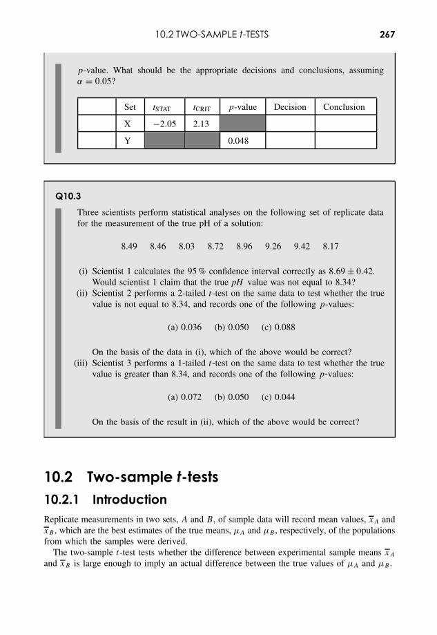
10.2 TWO-SAMPLE t-TESTS 267
p-value. What should be the appropriate decisions and conclusions, assumingα = 0.05?
Set tSTAT tCRIT p-value Decision Conclusion
X −2.05 2.13
Y 0.048
Q10.3Three scientists perform statistical analyses on the following set of replicate datafor the measurement of the true pH of a solution:
8.49 8.46 8.03 8.72 8.96 9.26 9.42 8.17
(i) Scientist 1 calculates the 95 % confidence interval correctly as 8.69 ± 0.42.Would scientist 1 claim that the true pH value was not equal to 8.34?
(ii) Scientist 2 performs a 2-tailed t-test on the same data to test whether the truevalue is not equal to 8.34, and records one of the following p-values:
(a) 0.036 (b) 0.050 (c) 0.088
On the basis of the data in (i), which of the above would be correct?(iii) Scientist 3 performs a 1-tailed t-test on the same data to test whether the true
value is greater than 8.34, and records one of the following p-values:
(a) 0.072 (b) 0.050 (c) 0.044
On the basis of the result in (ii), which of the above would be correct?
10.2 Two-sample t-tests10.2.1 IntroductionReplicate measurements in two sets, A and B, of sample data will record mean values, xA andxB , which are the best estimates of the true means, µA and µB , respectively, of the populationsfrom which the samples were derived.
The two-sample t-test tests whether the difference between experimental sample means xA
and xB is large enough to imply an actual difference between the true values of µA and µB .
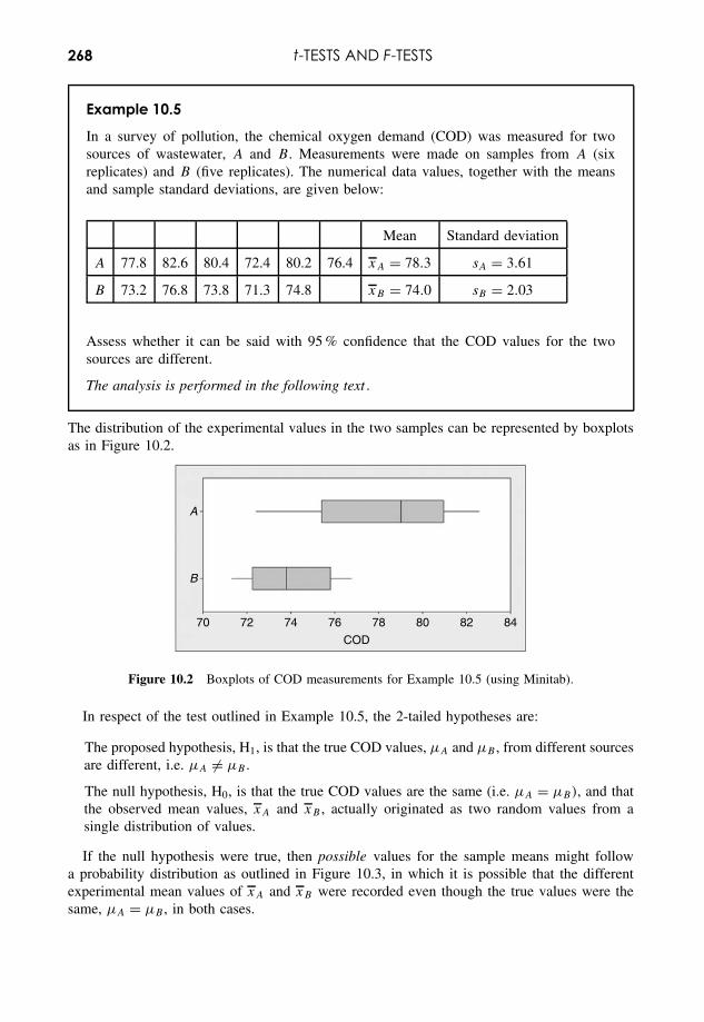
268 t-TESTS AND F-TESTS
Example 10.5
In a survey of pollution, the chemical oxygen demand (COD) was measured for twosources of wastewater, A and B. Measurements were made on samples from A (sixreplicates) and B (five replicates). The numerical data values, together with the meansand sample standard deviations, are given below:
Mean Standard deviation
A 77.8 82.6 80.4 72.4 80.2 76.4 xA = 78.3 sA = 3.61
B 73.2 76.8 73.8 71.3 74.8 xB = 74.0 sB = 2.03
Assess whether it can be said with 95 % confidence that the COD values for the twosources are different.
The analysis is performed in the following text .
The distribution of the experimental values in the two samples can be represented by boxplotsas in Figure 10.2.
74 76 78 80 82 8470
B
A
72
COD
Figure 10.2 Boxplots of COD measurements for Example 10.5 (using Minitab).
In respect of the test outlined in Example 10.5, the 2-tailed hypotheses are:
The proposed hypothesis, H1, is that the true COD values, µA and µB , from different sourcesare different, i.e. µA = µB .
The null hypothesis, H0, is that the true COD values are the same (i.e. µA = µB), and thatthe observed mean values, xA and xB , actually originated as two random values from asingle distribution of values.
If the null hypothesis were true, then possible values for the sample means might followa probability distribution as outlined in Figure 10.3, in which it is possible that the differentexperimental mean values of xA and xB were recorded even though the true values were thesame, µA = µB , in both cases.
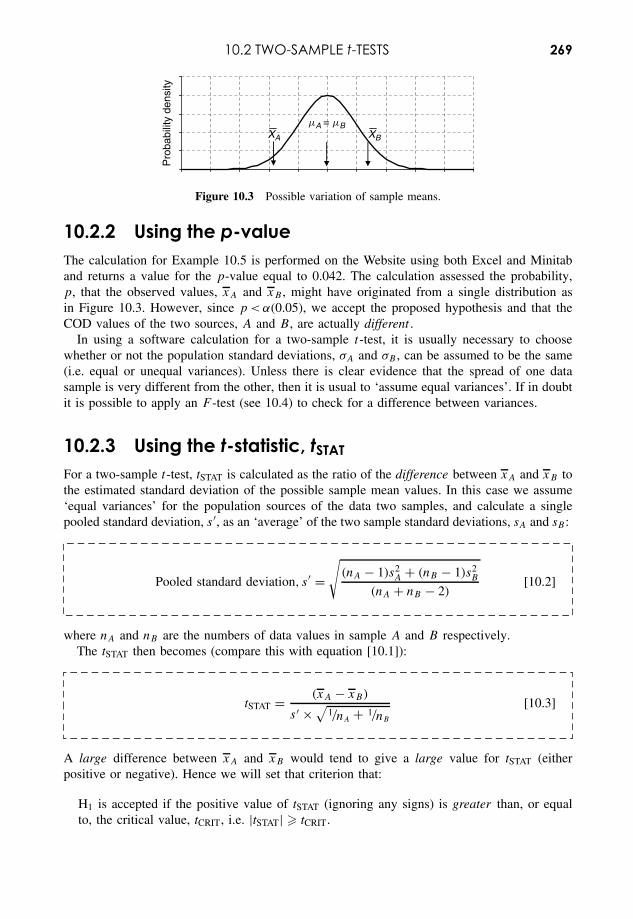
10.2 TWO-SAMPLE t-TESTS 269
Pro
babi
lity
dens
ity
mA = mBXBXA
Figure 10.3 Possible variation of sample means.
10.2.2 Using the p-valueThe calculation for Example 10.5 is performed on the Website using both Excel and Minitaband returns a value for the p-value equal to 0.042. The calculation assessed the probability,p, that the observed values, xA and xB , might have originated from a single distribution asin Figure 10.3. However, since p < α(0.05), we accept the proposed hypothesis and that theCOD values of the two sources, A and B, are actually different .
In using a software calculation for a two-sample t-test, it is usually necessary to choosewhether or not the population standard deviations, σA and σB , can be assumed to be the same(i.e. equal or unequal variances). Unless there is clear evidence that the spread of one datasample is very different from the other, then it is usual to ‘assume equal variances’. If in doubtit is possible to apply an F -test (see 10.4) to check for a difference between variances.
10.2.3 Using the t-statistic, tSTATFor a two-sample t-test, tSTAT is calculated as the ratio of the difference between xA and xB tothe estimated standard deviation of the possible sample mean values. In this case we assume‘equal variances’ for the population sources of the data two samples, and calculate a singlepooled standard deviation, s ′, as an ‘average’ of the two sample standard deviations, sA and sB :
Pooled standard deviation, s ′ =√
(nA − 1)s2A + (nB − 1)s2
B
(nA + nB − 2)[10.2]
where nA and nB are the numbers of data values in sample A and B respectively.The tSTAT then becomes (compare this with equation [10.1]):
tSTAT = (xA − xB)
s ′ × √1/nA + 1/nB
[10.3]
A large difference between xA and xB would tend to give a large value for tSTAT (eitherpositive or negative). Hence we will set that criterion that:
H1 is accepted if the positive value of tSTAT (ignoring any signs) is greater than, or equalto, the critical value, tCRIT, i.e. |tSTAT| � tCRIT.
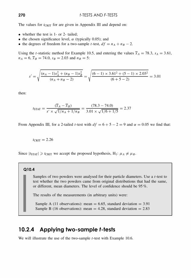
270 t-TESTS AND F-TESTS
The values for tCRIT for are given in Appendix III and depend on:
• whether the test is 1- or 2- tailed;• the chosen significance level, α (typically 0.05); and• the degrees of freedom for a two-sample t-test, df = nA + nB − 2.
Using the t-statistic method for Example 10.5, and entering the values xA = 78.3, sA = 3.61,nA = 6, xB = 74.0, sB = 2.03 and nB = 5:
s ′ =√
(nA − 1)s2A + (nB − 1)s2
B
(nA + nB − 2)=
√(6 − 1) × 3.612 + (5 − 1) × 2.032
(6 + 5 − 2)= 3.01
then:
tSTAT = (xA − xB)
s ′ × √1/nA + 1/nB
= (78.3 − 74.0)
3.01 × √1/6 + 1/5
= 2.37
From Appendix III, for a 2-tailed t-test with df = 6 + 5 − 2 = 9 and α = 0.05 we find that:
tCRIT = 2.26
Since |tSTAT| � tCRIT we accept the proposed hypothesis, H1: µA = µB .
Q10.4Samples of two powders were analysed for their particle diameters. Use a t-test totest whether the two powders came from original distributions that had the same,or different, mean diameters. The level of confidence should be 95 %.
The results of the measurements (in arbitrary units) were:
Sample A (11 observations): mean = 6.65, standard deviation = 3.91Sample B (16 observations): mean = 4.28, standard deviation = 2.83
10.2.4 Applying two-sample t-testsWe will illustrate the use of the two-sample t-test with Example 10.6.
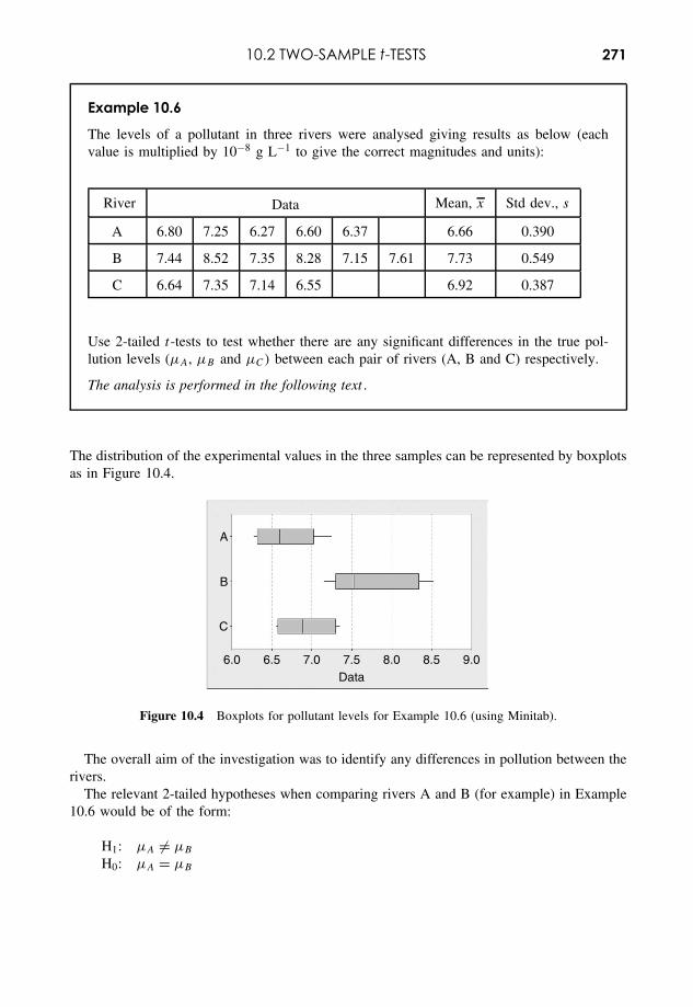
10.2 TWO-SAMPLE t-TESTS 271
Example 10.6
The levels of a pollutant in three rivers were analysed giving results as below (eachvalue is multiplied by 10−8 g L−1 to give the correct magnitudes and units):
River Data Mean, x Std dev., s
A 6.80 7.25 6.27 6.60 6.37 6.66 0.390
B 7.44 8.52 7.35 8.28 7.15 7.61 7.73 0.549
C 6.64 7.35 7.14 6.55 6.92 0.387
Use 2-tailed t-tests to test whether there are any significant differences in the true pol-lution levels (µA, µB and µC) between each pair of rivers (A, B and C) respectively.
The analysis is performed in the following text .
The distribution of the experimental values in the three samples can be represented by boxplotsas in Figure 10.4.
A
B
C
6.0 6.5 7.0 7.5 8.0 8.5 9.0Data
Figure 10.4 Boxplots for pollutant levels for Example 10.6 (using Minitab).
The overall aim of the investigation was to identify any differences in pollution between therivers.
The relevant 2-tailed hypotheses when comparing rivers A and B (for example) in Example10.6 would be of the form:
H1: µA = µB
H0: µA = µB
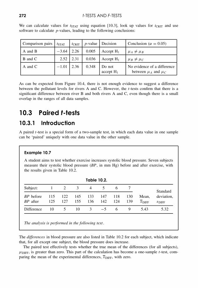
272 t-TESTS AND F-TESTS
We can calculate values for tSTAT using equation [10.3], look up values for tCRIT and usesoftware to calculate p-values, leading to the following conclusions:
Comparison pairs tSTAT tCRIT p-value Decision Conclusion (α = 0.05)
A and B −3.64 2.26 0.005 Accept H1 µA = µB
B and C 2.52 2.31 0.036 Accept H1 µB = µC
A and C −1.01 2.36 0.348 Do notaccept H1
No evidence of a differencebetween µA and µC
As can be expected from Figure 10.4, there is not enough evidence to suggest a differencebetween the pollutant levels for rivers A and C. However, the t-tests confirm that there is asignificant difference between river B and both rivers A and C, even though there is a smalloverlap in the ranges of all data samples.
10.3 Paired t-tests10.3.1 IntroductionA paired t-test is a special form of a two-sample test, in which each data value in one samplecan be ‘paired’ uniquely with one data value in the other sample.
Example 10.7
A student aims to test whether exercise increases systolic blood pressure. Seven subjectsmeasure their systolic blood pressure (BP , in mm Hg) before and after exercise, withthe results given in Table 10.2.
Table 10.2.
Subject: 1 2 3 4 5 6 7Standard
BP before 115 122 145 133 147 118 130 Mean, deviation,BP after 125 127 155 136 142 124 139 xDIFF sDIFF
Difference 10 5 10 3 −5 6 9 5.43 5.32
The analysis is performed in the following text .
The differences in blood pressure are also listed in Table 10.2 for each subject, which indicatethat, for all except one subject, the blood pressure does increase.
The paired test effectively tests whether the true mean of the differences (for all subjects),µDIFF, is greater than zero. This part of the calculation has become a one-sample t-test, com-paring the mean of the experimental differences, xDIFF, with zero.
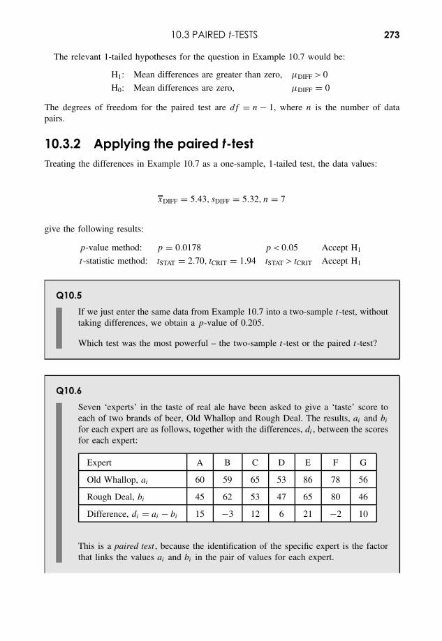
10.3 PAIRED t-TESTS 273
The relevant 1-tailed hypotheses for the question in Example 10.7 would be:
H1: Mean differences are greater than zero, µDIFF > 0
H0: Mean differences are zero, µDIFF = 0
The degrees of freedom for the paired test are df = n − 1, where n is the number of datapairs.
10.3.2 Applying the paired t-testTreating the differences in Example 10.7 as a one-sample, 1-tailed test, the data values:
xDIFF = 5.43, sDIFF = 5.32, n = 7
give the following results:
p-value method: p = 0.0178 p < 0.05 Accept H1
t-statistic method: tSTAT = 2.70, tCRIT = 1.94 tSTAT > tCRIT Accept H1
Q10.5If we just enter the same data from Example 10.7 into a two-sample t-test, withouttaking differences, we obtain a p-value of 0.205.
Which test was the most powerful – the two-sample t-test or the paired t-test?
Q10.6Seven ‘experts’ in the taste of real ale have been asked to give a ‘taste’ score toeach of two brands of beer, Old Whallop and Rough Deal. The results, ai and bi
for each expert are as follows, together with the differences, di , between the scoresfor each expert:
Expert A B C D E F G
Old Whallop, ai 60 59 65 53 86 78 56
Rough Deal, bi 45 62 53 47 65 80 46
Difference, di = ai − bi 15 −3 12 6 21 −2 10
This is a paired test , because the identification of the specific expert is the factorthat links the values ai and bi in the pair of values for each expert.
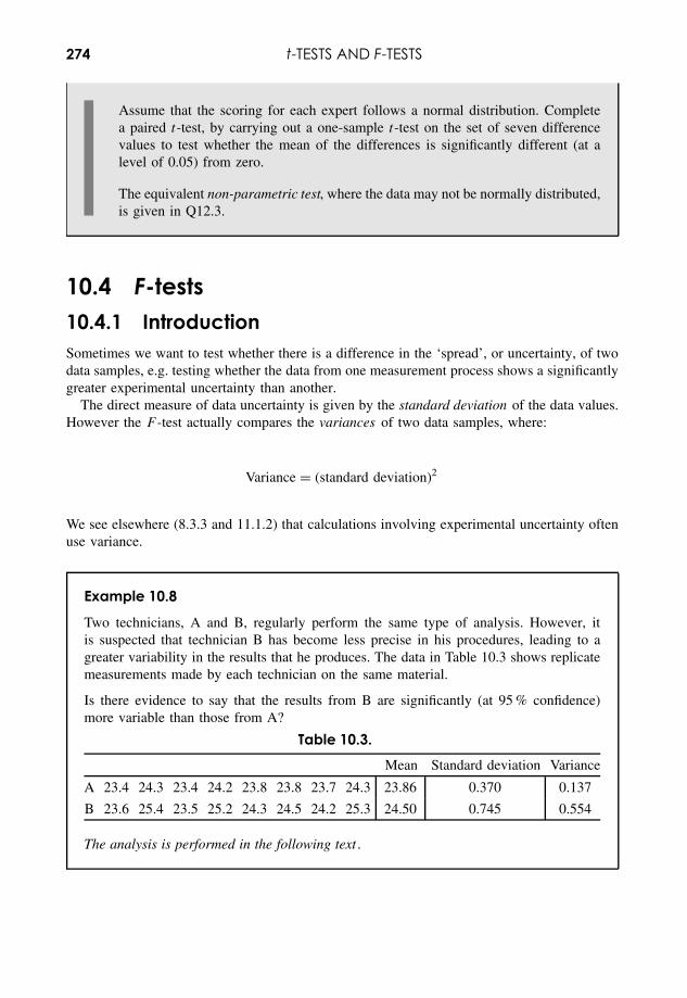
274 t-TESTS AND F-TESTS
Assume that the scoring for each expert follows a normal distribution. Completea paired t-test, by carrying out a one-sample t-test on the set of seven differencevalues to test whether the mean of the differences is significantly different (at alevel of 0.05) from zero.
The equivalent non-parametric test, where the data may not be normally distributed,is given in Q12.3.
10.4 F-tests10.4.1 IntroductionSometimes we want to test whether there is a difference in the ‘spread’, or uncertainty, of twodata samples, e.g. testing whether the data from one measurement process shows a significantlygreater experimental uncertainty than another.
The direct measure of data uncertainty is given by the standard deviation of the data values.However the F -test actually compares the variances of two data samples, where:
Variance = (standard deviation)2
We see elsewhere (8.3.3 and 11.1.2) that calculations involving experimental uncertainty oftenuse variance.
Example 10.8
Two technicians, A and B, regularly perform the same type of analysis. However, itis suspected that technician B has become less precise in his procedures, leading to agreater variability in the results that he produces. The data in Table 10.3 shows replicatemeasurements made by each technician on the same material.
Is there evidence to say that the results from B are significantly (at 95 % confidence)more variable than those from A?
Table 10.3.Mean Standard deviation Variance
A 23.4 24.3 23.4 24.2 23.8 23.8 23.7 24.3 23.86 0.370 0.137
B 23.6 25.4 23.5 25.2 24.3 24.5 24.2 25.3 24.50 0.745 0.554
The analysis is performed in the following text .
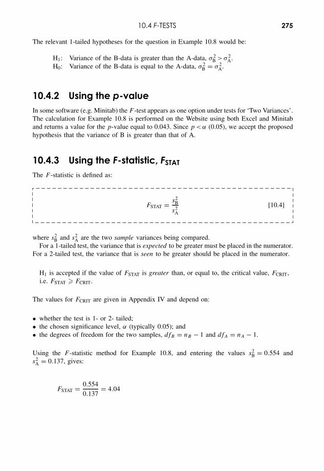
10.4 F-TESTS 275
The relevant 1-tailed hypotheses for the question in Example 10.8 would be:
H1: Variance of the B-data is greater than the A-data, σ 2B >σ 2
A.H0: Variance of the B-data is equal to the A-data, σ 2
B = σ 2A.
10.4.2 Using the p-valueIn some software (e.g. Minitab) the F -test appears as one option under tests for ‘Two Variances’.The calculation for Example 10.8 is performed on the Website using both Excel and Minitaband returns a value for the p-value equal to 0.043. Since p <α (0.05), we accept the proposedhypothesis that the variance of B is greater than that of A.
10.4.3 Using the F-statistic, FSTATThe F -statistic is defined as:
FSTAT = s2B
s2A
[10.4]
where s2B and s2
A are the two sample variances being compared.For a 1-tailed test, the variance that is expected to be greater must be placed in the numerator.
For a 2-tailed test, the variance that is seen to be greater should be placed in the numerator.
H1 is accepted if the value of FSTAT is greater than, or equal to, the critical value, FCRIT,i.e. FSTAT � FCRIT.
The values for FCRIT are given in Appendix IV and depend on:
• whether the test is 1- or 2- tailed;• the chosen significance level, α (typically 0.05); and• the degrees of freedom for the two samples, dfB = nB − 1 and dfA = nA − 1.
Using the F -statistic method for Example 10.8, and entering the values s2B = 0.554 and
s2A = 0.137, gives:
FSTAT = 0.554
0.137= 4.04
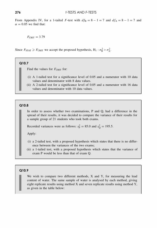
276 t-TESTS AND F-TESTS
From Appendix IV, for a 1-tailed F -test with dfB = 8 − 1 = 7 and dfA = 8 − 1 = 7 andα = 0.05 we find that:
FCRIT = 3.79
Since FSTAT � FCRIT we accept the proposed hypothesis, H1 : σ 2B >σ 2
A.
Q10.7Find the values for FCRIT for:
(i) A 1-tailed test for a significance level of 0.05 and a numerator with 10 datavalues and denominator with 8 data values.
(ii) A 2-tailed test for a significance level of 0.05 and a numerator with 16 datavalues and denominator with 10 data values.
Q10.8In order to assess whether two examinations, P and Q, had a difference in thespread of their results, it was decided to compare the variance of their results fora sample group of 21 students who took both exams.
Recorded variances were as follows: s2P = 85.0 and s2
Q = 195.5.
Apply:
(i) a 2-tailed test, with a proposed hypothesis which states that there is no differ-ence between the variances of the two exams;
(ii) a 1-tailed test, with a proposed hypothesis which states that the variance ofexam P would be less than that of exam Q.
Q10.9We wish to compare two different methods, X and Y, for measuring the leadcontent of water. The same sample of water is analysed by each method, givingeight replicate results using method X and seven replicate results using method Y,as given in the table below:

10.4 F-TESTS 277
Mean Standard Variancedeviation
X 83.3 81.4 81.0 79.8 82.5 84.7 83.2 83.3 82.40 1.57 2.47
Y 81.5 77.9 76.9 74.7 79.9 84.3 81.3 79.50 3.24 10.47
(i) As we can see from the data that s2Y > s2
X, would it be acceptable to use a1-tailed test when testing for a difference in variance?
(ii) Test for a difference in the experimental uncertainty between the two methods.(iii) Test for a difference in the mean values reported by the two methods.

11ANOVA – Analysis of Variance
Overview
Website • ‘How to do it’ video answers for all ‘Q’ questions.• Implementation of ANOVAs in Excel and Minitab.• Additional material: ANCOVAs.
We saw in Chapter 10 how the two-sample t-test tests for a difference between the mean valuesof two data samples.
ANOVAs form a set of analytical tests which can be used to identify possible differences inthe mean values of more than two data samples.
As its name suggests, an ANOVA uses the analysis of variances in the overall data to identifywhether there are factors involved which cause variations beyond the inherent experimentalvariation in the data values. At its simplest level, the ANOVA performs an F -test to testwhether the overall variance in the data values from all samples is significantly greater thanthe inherent experimental variance within each sample. If the F -test gives a significant result,then it can be concluded that there is a significant difference between the mean values of thesamples.
In this chapter we look at some increasing sophistication in the ANOVA, identifying theeffects of multiple factors and any interaction between them. The introduction of even morepowerful ANOVAs is continued on the Website.
We also discuss what can be done after an ANOVA has detected an effect, by introducingthe use of post hoc tests.
11.1 One-way ANOVA11.1.1 IntroductionWe can illustrate the use of the ANOVA analytical approach by considering the followingexample.
Essential Mathematics and Statistics for Science 2nd Edition Graham Currell and Antony DowmanCopyright c© 2009 John Wiley & Sons, Ltd
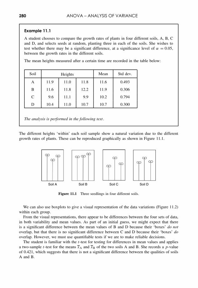
280 ANOVA – ANALYSIS OF VARIANCE
Example 11.1
A student chooses to compare the growth rates of plants in four different soils, A, B, Cand D, and selects seeds at random, planting three in each of the soils. She wishes totest whether there may be a significant difference, at a significance level of α = 0.05,between the growth rates in the different soils.
The mean heights measured after a certain time are recorded in the table below:
Soil Heights Mean Std dev.
A 11.9 11.0 11.8 11.6 0.493
B 11.6 11.8 12.2 11.9 0.306
C 9.6 11.1 9.9 10.2 0.794
D 10.4 11.0 10.7 10.7 0.300
The analysis is performed in the following text .
The different heights ‘within’ each soil sample show a natural variation due to the differentgrowth rates of plants. These can be reproduced graphically as shown in Figure 11.1.
Soil A Soil B Soil C Soil D
Figure 11.1 Three seedlings in four different soils.
We can also use boxplots to give a visual representation of the data variations (Figure 11.2)within each group.
From the visual representations, there appear to be differences between the four sets of data,in both variability and mean values. As part of an initial guess, we might expect that thereis a significant difference between the mean values of B and D because their ‘boxes’ do notoverlap, but that there is no significant difference between C and D because their ‘boxes’ dooverlap. However, we must use quantifiable tests if we are to make reliable decisions.
The student is familiar with the t-test for testing for differences in mean values and appliesa two-sample t-test for the means xA and xB of the two soils A and B. She records a p-valueof 0.421, which suggests that there is not a significant difference between the qualities of soilsA and B.
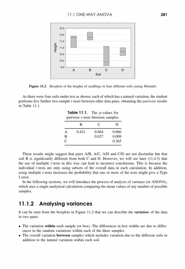
11.1 ONE-WAY ANOVA 281
12.5
12.0
11.5
11.0
10.5
10.0
9.5
Hei
ght
A BSoil
C D
Figure 11.2 Boxplots of the heights of seedlings in four different soils (using Minitab).
As there were four soils under test as shown, each of which has a natural variation, the studentperforms five further two-sample t-tests between other data pairs, obtaining the pairwise resultsin Table 11.1.
Table 11.1. The p-values forpairwise t-tests between samples.
B C D
A 0.421 0.064 0.060B 0.027 0.009C 0.365
These results might suggest that pairs A/B, A/C, A/D and C/D are not dissimilar but thatsoil B is significantly different from both C and D. However, we will see later (11.4.3) thatthe use of multiple t-tests in this way can lead to incorrect conclusions. This is because theindividual t-tests are only using subsets of the overall data in each calculation. In addition,using multiple t-tests increases the probability that one or more of the tests might give a TypeI error.
In the following sections, we will introduce the process of analysis of variance (or ANOVA),which uses a single analytical calculation comparing the mean values of any number of possiblesamples.
11.1.2 Analysing variancesIt can be seen from the boxplots in Figure 11.2 that we can describe the variation of the datain two parts:
• The variation within each sample (or box). The differences in box widths are due to differ-ences in the random variations within each of the three samples.
• The overall variation between samples which includes variation due to the different soils inaddition to the natural variation within each soil.
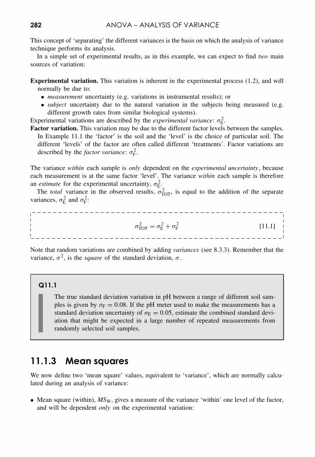
282 ANOVA – ANALYSIS OF VARIANCE
This concept of ‘separating’ the different variances is the basis on which the analysis of variancetechnique performs its analysis.
In a simple set of experimental results, as in this example, we can expect to find two mainsources of variation:
Experimental variation. This variation is inherent in the experimental process (1.2), and willnormally be due to:• measurement uncertainty (e.g. variations in instrumental results); or• subject uncertainty due to the natural variation in the subjects being measured (e.g.
different growth rates from similar biological systems).Experimental variations are described by the experimental variance: σ 2
E .Factor variation. This variation may be due to the different factor levels between the samples.
In Example 11.1 the ‘factor’ is the soil and the ‘level’ is the choice of particular soil. Thedifferent ‘levels’ of the factor are often called different ‘treatments’. Factor variations aredescribed by the factor variance: σ 2
F .
The variance within each sample is only dependent on the experimental uncertainty , becauseeach measurement is at the same factor ‘level’. The variance within each sample is thereforean estimate for the experimental uncertainty, σ 2
E .The total variance in the observed results, σ 2
TOT, is equal to the addition of the separatevariances, σ 2
E and σ 2F :
σ 2TOT = σ 2
E + σ 2F [11.1]
Note that random variations are combined by adding variances (see 8.3.3). Remember that thevariance, σ 2, is the square of the standard deviation, σ .
Q11.1The true standard deviation variation in pH between a range of different soil sam-ples is given by σF = 0.08. If the pH meter used to make the measurements has astandard deviation uncertainty of σE = 0.05, estimate the combined standard devi-ation that might be expected in a large number of repeated measurements fromrandomly selected soil samples.
11.1.3 Mean squaresWe now define two ‘mean square’ values, equivalent to ‘variance’, which are normally calcu-lated during an analysis of variance:
• Mean square (within), MSW, gives a measure of the variance ‘within’ one level of the factor,and will be dependent only on the experimental variation:
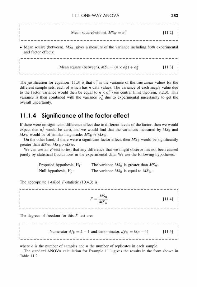
11.1 ONE-WAY ANOVA 283
Mean square(within), MSW = σ 2E [11.2]
• Mean square (between), MSB, gives a measure of the variance including both experimentaland factor effects:
Mean square (between), MSB = (n × σ 2F ) + σ 2
E [11.3]
The justification for equation [11.3] is that σ 2F is the variance of the true mean values for the
different sample sets, each of which has n data values. The variance of each single value dueto the factor variance would then be equal to n × σ 2
F (see central limit theorem, 8.2.3). Thisvariance is then combined with the variance σ 2
E due to experimental uncertainty to get theoverall uncertainty.
11.1.4 Significance of the factor effectIf there were no significant difference effect due to different levels of the factor, then we wouldexpect that σ 2
F would be zero, and we would find that the variances measured by MSB andMSW would be of similar magnitude: MSB ≈ MSW.
On the other hand, if there were a significant factor effect, then MS B would be significantlygreater than MS W: MS B >MS W.
We can use an F -test to test that any difference that we might observe has not been causedpurely by statistical fluctuations in the experimental data. We use the following hypotheses:
Proposed hypothesis, H1: The variance MSB is greater than MSW.
Null hypothesis, H0: The variance MSB is equal to MSW.
The appropriate 1-tailed F -statistic (10.4.3) is:
F = MSB
MSW[11.4]
The degrees of freedom for this F -test are:
Numerator dfB = k − 1 and denominator, dfW = k(n − 1) [11.5]
where k is the number of samples and n the number of replicates in each sample.The standard ANOVA calculation for Example 11.1 gives the results in the form shown in
Table 11.2.
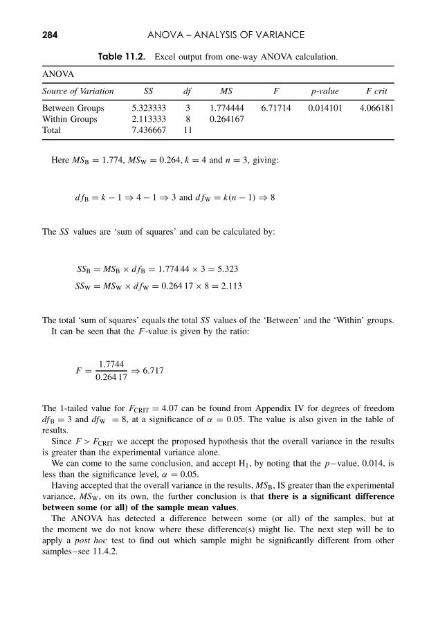
284 ANOVA – ANALYSIS OF VARIANCE
Table 11.2. Excel output from one-way ANOVA calculation.
ANOVA
Source of Variation SS df MS F p-value F crit
Between Groups 5.323333 3 1.774444 6.71714 0.014101 4.066181Within Groups 2.113333 8 0.264167Total 7.436667 11
Here MSB = 1.774, MSW = 0.264, k = 4 and n = 3, giving:
dfB = k − 1 ⇒ 4 − 1 ⇒ 3 and dfW = k(n − 1) ⇒ 8
The SS values are ‘sum of squares’ and can be calculated by:
SSB = MSB × dfB = 1.774 44 × 3 = 5.323
SSW = MSW × dfW = 0.264 17 × 8 = 2.113
The total ‘sum of squares’ equals the total SS values of the ‘Between’ and the ‘Within’ groups.It can be seen that the F -value is given by the ratio:
F = 1.7744
0.264 17⇒ 6.717
The 1-tailed value for FCRIT = 4.07 can be found from Appendix IV for degrees of freedomdfB = 3 and dfW = 8, at a significance of α = 0.05. The value is also given in the table ofresults.
Since F >FCRIT we accept the proposed hypothesis that the overall variance in the resultsis greater than the experimental variance alone.
We can come to the same conclusion, and accept H1, by noting that the p−value, 0.014, isless than the significance level, α = 0.05.
Having accepted that the overall variance in the results, MSB, IS greater than the experimentalvariance, MSW, on its own, the further conclusion is that there is a significant differencebetween some (or all) of the sample mean values.
The ANOVA has detected a difference between some (or all) of the samples, but atthe moment we do not know where these difference(s) might lie. The next step will be toapply a post hoc test to find out which sample might be significantly different from othersamples–see 11.4.2.
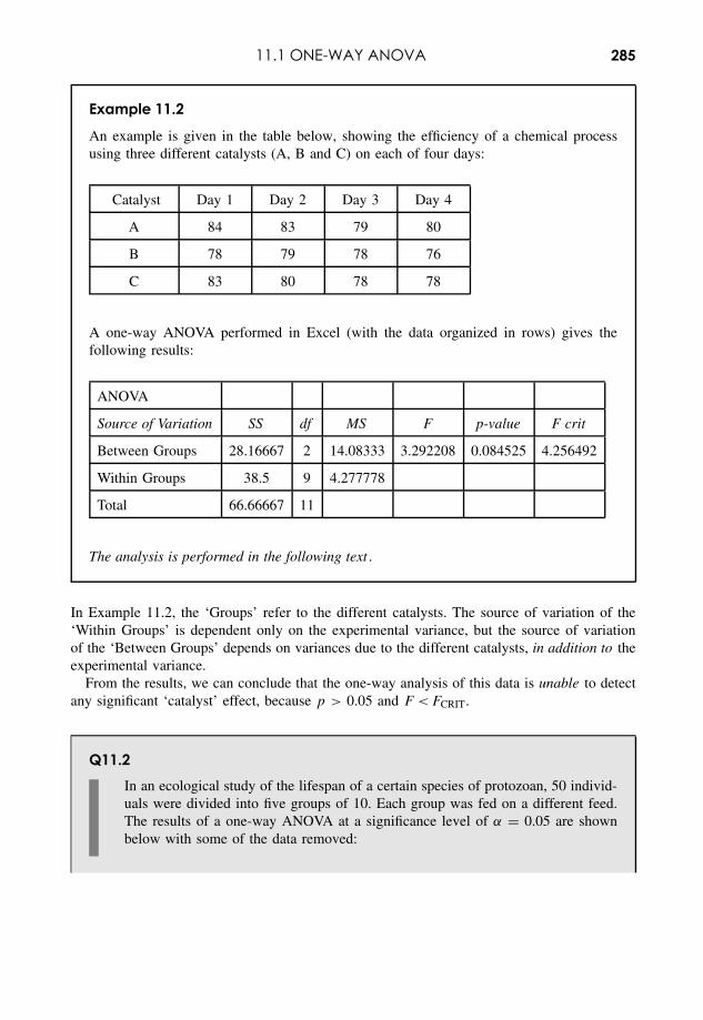
11.1 ONE-WAY ANOVA 285
Example 11.2
An example is given in the table below, showing the efficiency of a chemical processusing three different catalysts (A, B and C) on each of four days:
Catalyst Day 1 Day 2 Day 3 Day 4
A 84 83 79 80
B 78 79 78 76
C 83 80 78 78
A one-way ANOVA performed in Excel (with the data organized in rows) gives thefollowing results:
ANOVA
Source of Variation SS df MS F p-value F crit
Between Groups 28.16667 2 14.08333 3.292208 0.084525 4.256492
Within Groups 38.5 9 4.277778
Total 66.66667 11
The analysis is performed in the following text .
In Example 11.2, the ‘Groups’ refer to the different catalysts. The source of variation of the‘Within Groups’ is dependent only on the experimental variance, but the source of variationof the ‘Between Groups’ depends on variances due to the different catalysts, in addition to theexperimental variance.
From the results, we can conclude that the one-way analysis of this data is unable to detectany significant ‘catalyst’ effect, because p > 0.05 and F <FCRIT.
Q11.2In an ecological study of the lifespan of a certain species of protozoan, 50 individ-uals were divided into five groups of 10. Each group was fed on a different feed.The results of a one-way ANOVA at a significance level of α = 0.05 are shownbelow with some of the data removed:
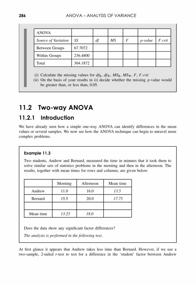
286 ANOVA – ANALYSIS OF VARIANCE
ANOVA
Source of Variation SS df MS F p-value F crit
Between Groups 67.7072
Within Groups 236.4800
Total 304.1872
(i) Calculate the missing values for dfB, dfW, MSB, MSW, F , F crit(ii) On the basis of your results in (i) decide whether the missing p-value would
be greater than, or less than, 0.05.
11.2 Two-way ANOVA11.2.1 IntroductionWe have already seen how a simple one-way ANOVA can identify differences in the meanvalues or several samples. We now see how the ANOVA technique can begin to unravel morecomplex problems.
Example 11.3
Two students, Andrew and Bernard, measured the time in minutes that it took them tosolve similar sets of statistics problems in the morning and then in the afternoon. Theresults, together with mean times for rows and columns, are given below:
Morning Afternoon Mean time
Andrew 11.0 16.0 13.5
Bernard 15.5 20.0 17.75
Mean time 13.25 18.0
Does the data show any significant factor differences?
The analysis is performed in the following text .
At first glance it appears that Andrew takes less time than Bernard. However, if we use atwo-sample, 2-tailed t-test to test for a difference in the ‘student’ factor between Andrew
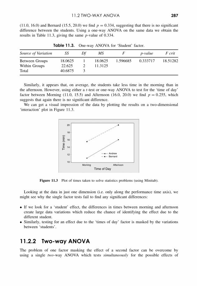
11.2 TWO-WAY ANOVA 287
(11.0, 16.0) and Bernard (15.5, 20.0) we find p = 0.334, suggesting that there is no significantdifference between the students. Using a one-way ANOVA on the same data we obtain theresults in Table 11.3, giving the same p-value of 0.334.
Table 11.3. One-way ANOVA for ‘Student’ factor.
Source of Variation SS Df MS F p-value F crit
Between Groups 18.0625 1 18.0625 1.596685 0.333717 18.51282Within Groups 22.625 2 11.3125Total 40.6875 3
Similarly, it appears that, on average, the students take less time in the morning than inthe afternoon. However, using either a t-test or one-way ANOVA to test for the ‘time of day’factor between Morning (11.0, 15.5) and Afternoon (16.0, 20.0) we find p = 0.255, whichsuggests that again there is no significant difference.
We can get a visual impression of the data by plotting the results on a two-dimensional‘interaction’ plot in Figure 11.3.
Morning Afternoon
AndrewBernard
10
12
14
16
18
20
Time of Day
Tim
e (m
in)
Figure 11.3 Plot of times taken to solve statistics problems (using Minitab).
Looking at the data in just one dimension (i.e. only along the performance time axis), wemight see why the single factor tests fail to find any significant differences:
• If we look for a ‘student’ effect, the differences in times between morning and afternooncreate large data variations which reduce the chance of identifying the effect due to thedifferent student.
• Similarly, testing for an effect due to the ‘times of day’ factor is masked by the variationsbetween ‘students’.
11.2.2 Two-way ANOVAThe problem of one factor masking the effect of a second factor can be overcome byusing a single two-way ANOVA which tests simultaneously for the possible effects of
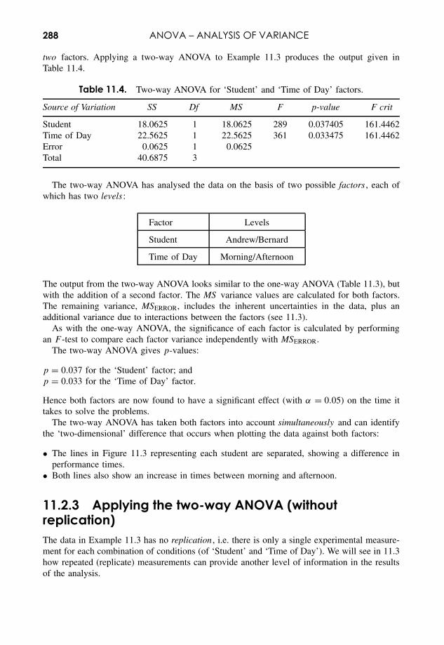
288 ANOVA – ANALYSIS OF VARIANCE
two factors. Applying a two-way ANOVA to Example 11.3 produces the output given inTable 11.4.
Table 11.4. Two-way ANOVA for ‘Student’ and ‘Time of Day’ factors.
Source of Variation SS Df MS F p-value F crit
Student 18.0625 1 18.0625 289 0.037405 161.4462Time of Day 22.5625 1 22.5625 361 0.033475 161.4462Error 0.0625 1 0.0625Total 40.6875 3
The two-way ANOVA has analysed the data on the basis of two possible factors , each ofwhich has two levels :
Factor Levels
Student Andrew/Bernard
Time of Day Morning/Afternoon
The output from the two-way ANOVA looks similar to the one-way ANOVA (Table 11.3), butwith the addition of a second factor. The MS variance values are calculated for both factors.The remaining variance, MSERROR, includes the inherent uncertainties in the data, plus anadditional variance due to interactions between the factors (see 11.3).
As with the one-way ANOVA, the significance of each factor is calculated by performingan F -test to compare each factor variance independently with MSERROR.
The two-way ANOVA gives p-values:
p = 0.037 for the ‘Student’ factor; andp = 0.033 for the ‘Time of Day’ factor.
Hence both factors are now found to have a significant effect (with α = 0.05) on the time ittakes to solve the problems.
The two-way ANOVA has taken both factors into account simultaneously and can identifythe ‘two-dimensional’ difference that occurs when plotting the data against both factors:
• The lines in Figure 11.3 representing each student are separated, showing a difference inperformance times.
• Both lines also show an increase in times between morning and afternoon.
11.2.3 Applying the two-way ANOVA (withoutreplication)The data in Example 11.3 has no replication , i.e. there is only a single experimental measure-ment for each combination of conditions (of ‘Student’ and ‘Time of Day’). We will see in 11.3how repeated (replicate) measurements can provide another level of information in the resultsof the analysis.
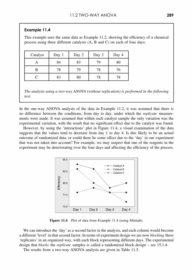
11.2 TWO-WAY ANOVA 289
Example 11.4
This example uses the same data as Example 11.2, showing the efficiency of a chemicalprocess using three different catalysts (A, B and C) on each of four days:
Catalyst Day 1 Day 2 Day 3 Day 4
A 84 83 79 80
B 78 79 78 76
C 83 80 78 78
The analysis using a two-way ANOVA (without replication) is performed in the followingtext .
In the one-way ANOVA analysis of the data in Example 11.2, it was assumed that there isno difference between the conditions, from day to day, under which the replicate measure-ments were made. It was assumed that within each catalyst sample the only variation was theexperimental variation, with the result that no significant effect due to the catalyst was found.
However, by using the ‘interactions’ plot in Figure 11.4, a visual examination of the datasuggests that the values tend to decrease from day 1 to day 4. Is this likely to be an actualoutcome of randomized data, or could there be some effect due to the ‘day’ in our experimentthat was not taken into account? For example, we may suspect that one of the reagents in theexperiment may be deteriorating over the four days and affecting the efficiency of the process.
82.5
80.0
77.5
75.0
85.0
Catalyst CCatalyst B
Catalyst A
Day 1 Day 2 Day 3 Day 4
Effi
cien
cy
Figure 11.4 Plot of data from Example 11.4 (using Minitab).
We can introduce the ‘day’ as a second factor in the analysis, and each column would becomea different ‘level’ in that second factor. In terms of experiment design we are now blocking these‘replicates’ in an organized way, with each block representing different days. The experimentaldesign that blocks the replicate samples is called a randomized block design – see 15.1.4.
The results from a two-way ANOVA analysis are given in Table 11.5.
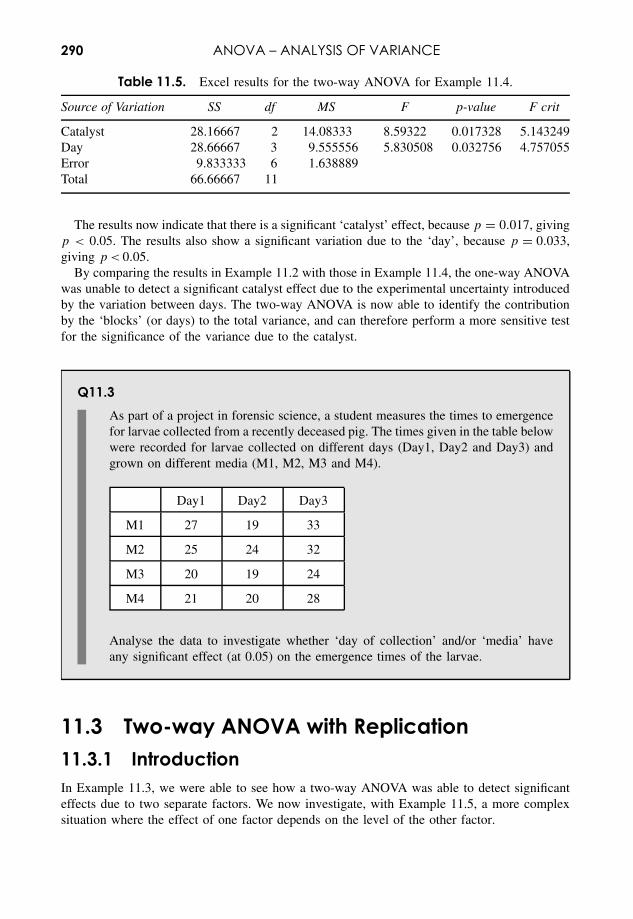
290 ANOVA – ANALYSIS OF VARIANCE
Table 11.5. Excel results for the two-way ANOVA for Example 11.4.
Source of Variation SS df MS F p-value F crit
Catalyst 28.16667 2 14.08333 8.59322 0.017328 5.143249Day 28.66667 3 9.555556 5.830508 0.032756 4.757055Error 9.833333 6 1.638889Total 66.66667 11
The results now indicate that there is a significant ‘catalyst’ effect, because p = 0.017, givingp < 0.05. The results also show a significant variation due to the ‘day’, because p = 0.033,giving p < 0.05.
By comparing the results in Example 11.2 with those in Example 11.4, the one-way ANOVAwas unable to detect a significant catalyst effect due to the experimental uncertainty introducedby the variation between days. The two-way ANOVA is now able to identify the contributionby the ‘blocks’ (or days) to the total variance, and can therefore perform a more sensitive testfor the significance of the variance due to the catalyst.
Q11.3As part of a project in forensic science, a student measures the times to emergencefor larvae collected from a recently deceased pig. The times given in the table belowwere recorded for larvae collected on different days (Day1, Day2 and Day3) andgrown on different media (M1, M2, M3 and M4).
Day1 Day2 Day3
M1 27 19 33
M2 25 24 32
M3 20 19 24
M4 21 20 28
Analyse the data to investigate whether ‘day of collection’ and/or ‘media’ haveany significant effect (at 0.05) on the emergence times of the larvae.
11.3 Two-way ANOVA with Replication11.3.1 IntroductionIn Example 11.3, we were able to see how a two-way ANOVA was able to detect significanteffects due to two separate factors. We now investigate, with Example 11.5, a more complexsituation where the effect of one factor depends on the level of the other factor.
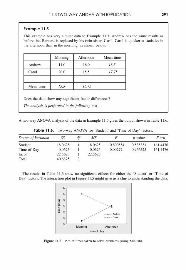
11.3 TWO-WAY ANOVA WITH REPLICATION 291
Example 11.5
This example has very similar data to Example 11.3. Andrew has the same results asbefore, but Bernard is replaced by his twin sister, Carol. Carol is quicker at statistics inthe afternoon than in the morning, as shown below:
Morning Afternoon Mean time
Andrew 11.0 16.0 13.5
Carol 20.0 15.5 17.75
Mean time 15.5 15.75
Does the data show any significant factor differences?
The analysis is performed in the following text .
A two-way ANOVA analysis of the data in Example 11.5 gives the output shown in Table 11.6.
Table 11.6. Two-way ANOVA for ‘Student’ and ‘Time of Day’ factors.
Source of Variation SS df MS F p-value F crit
Student 18.0625 1 18.0625 0.800554 0.535331 161.4476Time of Day 0.0625 1 0.0625 0.00277 0.966525 161.4476Error 22.5625 1 22.5625Total 40.6875 3
The results in Table 11.6 show no significant effects for either the ‘Student’ or ‘Time ofDay’ factors. The interaction plot in Figure 11.5 might give us a clue to understanding the data:
Morning Afternoon
Andrew
Carol
10
12
14
16
18
20
22
Time of Day
Tim
e (m
in)
Figure 11.5 Plot of times taken to solve problems (using Minitab).
292 ANOVA – ANALYSIS OF VARIANCE
The plot in Figure 11.5 appears to show that, ‘on average’, Andrew takes less time than Carol,but, while Andrew takes more time in the afternoon than in the morning, Carol’s performanceis reversed.
We can see that the effect of the ‘Time of Day’ factor depends on the ‘Student’ factor.There appears to be an interaction between the two factors. However, with the data as given,the two-way ANOVA calculation is unable to separate the data variation due to the possibleinteraction from the variations due to random experimental uncertainty – both are included inMSERROR.
We will see in the next section that the analytical process can be made more powerfulby collecting additional data. It is possible to separate the effect of the interaction from theexperimental uncertainty by estimating the magnitude of experimental uncertainty throughrepeated data values , or replicates , for measurement.
11.3.2 Two-way ANOVA with replicationIn the context of an ANOVA, a replicate measurement requires repeating a measurement underexactly the same combinations of conditions. For example, in Example 11.5 this would requireat least two measurements for each combination of student and time of day.
Example 11.6
The data in the table below has the same mean values as Example 11.5, but now includestwo replicate measurements for each factor combination:
Morning Afternoon Mean time
Andrew 11.3, 10,7 15.8, 16.2 13.5
Carol 21.2, 18.8 15.2, 15.8 17.75
Mean time 15.5 15.75
Does the data show any significant effects?
The analysis is performed in the following text :
We can perform a two-way ANOVA with replication , to obtain the output inTable 11.7.
The replicate data has enabled the ANOVA to estimate the average variance within eachfactor combination, giving an estimate of the inherent experimental uncertainty in each mea-surement. With this information the ANOVA is able to separate the variance due to theinteraction, MSINTERACTION, from that due to the experimental uncertainty, which is givenby the mean square (within) value, MSW. Without replication data, these two variances hadbeen combined in Table 11.6 in the MSERROR value.
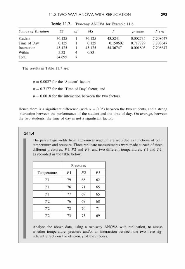
11.3 TWO-WAY ANOVA WITH REPLICATION 293
Table 11.7. Two-way ANOVA for Example 11.6.
Source of Variation SS df MS F p-value F crit
Student 36.125 1 36.125 43.5241 0.002735 7.708647Time of Day 0.125 1 0.125 0.150602 0.717729 7.708647Interaction 45.125 1 45.125 54.36747 0.001803 7.708647Within 3.32 4 0.83Total 84.695 7
The results in Table 11.7 are:
p = 0.0027 for the ‘Student’ factor;p = 0.7177 for the ‘Time of Day’ factor; and
p = 0.0018 for the interaction between the two factors.
Hence there is a significant difference (with α = 0.05) between the two students, and a stronginteraction between the performance of the student and the time of day. On average, betweenthe two students, the time of day is not a significant factor.
Q11.4The percentage yields from a chemical reaction are recorded as functions of bothtemperature and pressure. Three replicate measurements were made at each of threedifferent pressures, P 1, P 2 and P 3, and two different temperatures, T 1 and T 2,as recorded in the table below:
Pressures
Temperature P 1 P 2 P 3
T 1 79 68 62
T 1 76 71 65
T 1 77 69 65
T 2 76 69 68
T 2 72 70 71
T 2 73 73 69
Analyse the above data, using a two-way ANOVA with replication, to assesswhether temperature, pressure and/or an interaction between the two have sig-nificant effects on the efficiency of the process.
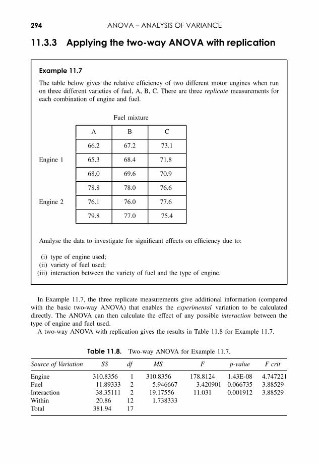
294 ANOVA – ANALYSIS OF VARIANCE
11.3.3 Applying the two-way ANOVA with replication
Example 11.7
The table below gives the relative efficiency of two different motor engines when runon three different varieties of fuel, A, B, C. There are three replicate measurements foreach combination of engine and fuel.
Fuel mixture
A B C
66.2 67.2 73.1
Engine 1 65.3 68.4 71.8
68.0 69.6 70.9
78.8 78.0 76.6
Engine 2 76.1 76.0 77.6
79.8 77.0 75.4
Analyse the data to investigate for significant effects on efficiency due to:
(i) type of engine used;(ii) variety of fuel used;
(iii) interaction between the variety of fuel and the type of engine.
In Example 11.7, the three replicate measurements give additional information (comparedwith the basic two-way ANOVA) that enables the experimental variation to be calculateddirectly. The ANOVA can then calculate the effect of any possible interaction between thetype of engine and fuel used.
A two-way ANOVA with replication gives the results in Table 11.8 for Example 11.7.
Table 11.8. Two-way ANOVA for Example 11.7.
Source of Variation SS df MS F p-value F crit
Engine 310.8356 1 310.8356 178.8124 1.43E-08 4.747221Fuel 11.89333 2 5.946667 3.420901 0.066735 3.88529Interaction 38.35111 2 19.17556 11.031 0.001912 3.88529Within 20.86 12 1.738333Total 381.94 17
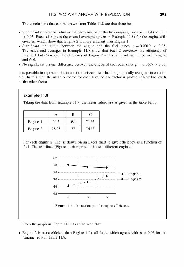
11.3 TWO-WAY ANOVA WITH REPLICATION 295
The conclusions that can be drawn from Table 11.8 are that there is:
• Significant difference between the performance of the two engines, since p = 1.43 × 10⁻⁸
< 0.05. Excel also gives the overall averages (given in Example 11.8) for the engine effi-ciencies, which show that Engine 2 is more efficient than Engine 1.
• Significant interaction between the engine and the fuel, since p = 0.0019 < 0.05.The calculated averages in Example 11.8 show that Fuel C increases the efficiency ofEngine 1 but decreases the efficiency of Engine 2 – this is an interaction between engineand fuel.
• No significant overall difference between the effects of the fuels, since p = 0.0667 > 0.05.
It is possible to represent the interaction between two factors graphically using an interactionplot. In this plot, the mean outcome for each level of one factor is plotted against the levelsof the other factor.
Example 11.8
Taking the data from Example 11.7, the mean values are as given in the table below:
A B C
Engine 1 66.5 68.4 71.93
Engine 2 78.23 77 76.53
For each engine a ‘line’ is drawn on an Excel chart to give efficiency as a function offuel. The two lines (Figure 11.6) represent the two different engines.
62
66
70
74
78
82
A B C
Engine 1
Engine 2
Figure 11.6 Interaction plot for engine efficiences.
From the graph in Figure 11.6 it can be seen that:
• Engine 2 is more efficient than Engine 1 for all fuels, which agrees with p < 0.05 for the‘Engine’ row in Table 11.8.
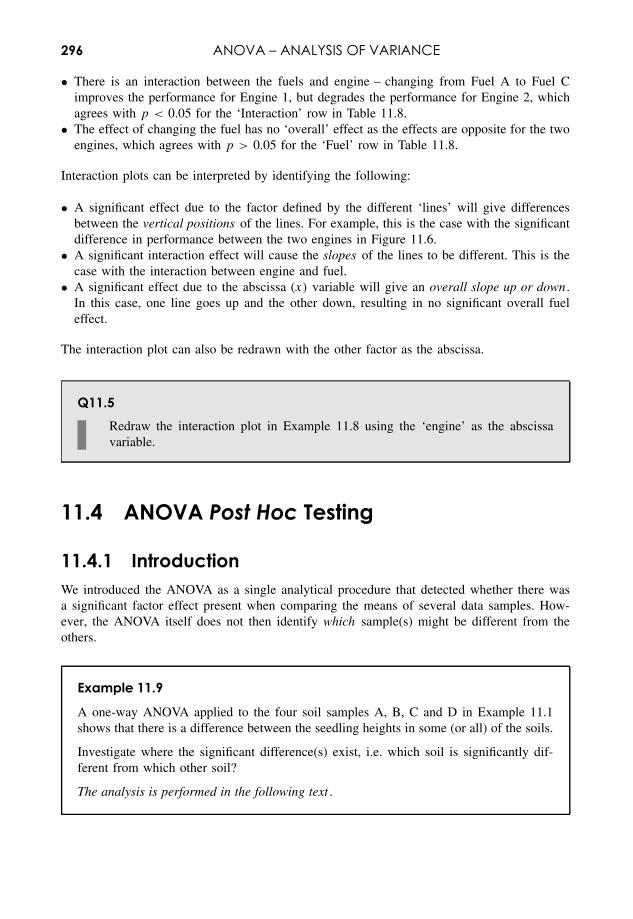
296 ANOVA – ANALYSIS OF VARIANCE
• There is an interaction between the fuels and engine – changing from Fuel A to Fuel Cimproves the performance for Engine 1, but degrades the performance for Engine 2, whichagrees with p < 0.05 for the ‘Interaction’ row in Table 11.8.
• The effect of changing the fuel has no ‘overall’ effect as the effects are opposite for the twoengines, which agrees with p > 0.05 for the ‘Fuel’ row in Table 11.8.
Interaction plots can be interpreted by identifying the following:
• A significant effect due to the factor defined by the different ‘lines’ will give differencesbetween the vertical positions of the lines. For example, this is the case with the significantdifference in performance between the two engines in Figure 11.6.
• A significant interaction effect will cause the slopes of the lines to be different. This is thecase with the interaction between engine and fuel.
• A significant effect due to the abscissa (x) variable will give an overall slope up or down .In this case, one line goes up and the other down, resulting in no significant overall fueleffect.
The interaction plot can also be redrawn with the other factor as the abscissa.
Q11.5Redraw the interaction plot in Example 11.8 using the ‘engine’ as the abscissavariable.
11.4 ANOVA Post Hoc Testing
11.4.1 IntroductionWe introduced the ANOVA as a single analytical procedure that detected whether there wasa significant factor effect present when comparing the means of several data samples. How-ever, the ANOVA itself does not then identify which sample(s) might be different from theothers.
Example 11.9
A one-way ANOVA applied to the four soil samples A, B, C and D in Example 11.1shows that there is a difference between the seedling heights in some (or all) of the soils.
Investigate where the significant difference(s) exist, i.e. which soil is significantly dif-ferent from which other soil?
The analysis is performed in the following text .
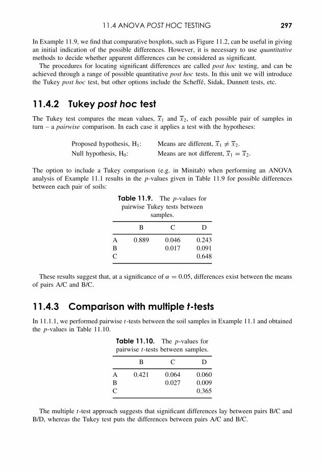
11.4 ANOVA POST HOC TESTING 297
In Example 11.9, we find that comparative boxplots, such as Figure 11.2, can be useful in givingan initial indication of the possible differences. However, it is necessary to use quantitativemethods to decide whether apparent differences can be considered as significant.
The procedures for locating significant differences are called post hoc testing, and can beachieved through a range of possible quantitative post hoc tests. In this unit we will introducethe Tukey post hoc test, but other options include the Scheffe, Sidak, Dunnett tests, etc.
11.4.2 Tukey post hoc testThe Tukey test compares the mean values, x1 and x2, of each possible pair of samples inturn – a pairwise comparison. In each case it applies a test with the hypotheses:
Proposed hypothesis, H1: Means are different, x1 = x2.
Null hypothesis, H0: Means are not different, x1 = x2.
The option to include a Tukey comparison (e.g. in Minitab) when performing an ANOVAanalysis of Example 11.1 results in the p-values given in Table 11.9 for possible differencesbetween each pair of soils:
Table 11.9. The p-values forpairwise Tukey tests between
samples.
B C D
A 0.889 0.046 0.243B 0.017 0.091C 0.648
These results suggest that, at a significance of α = 0.05, differences exist between the meansof pairs A/C and B/C.
11.4.3 Comparison with multiple t-testsIn 11.1.1, we performed pairwise t-tests between the soil samples in Example 11.1 and obtainedthe p-values in Table 11.10.
Table 11.10. The p-values forpairwise t-tests between samples.
B C D
A 0.421 0.064 0.060B 0.027 0.009C 0.365
The multiple t-test approach suggests that significant differences lay between pairs B/C andB/D, whereas the Tukey test puts the differences between pairs A/C and B/C.
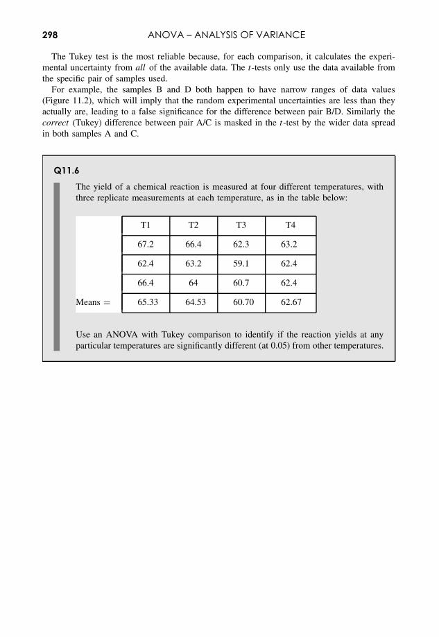
298 ANOVA – ANALYSIS OF VARIANCE
The Tukey test is the most reliable because, for each comparison, it calculates the experi-mental uncertainty from all of the available data. The t-tests only use the data available fromthe specific pair of samples used.
For example, the samples B and D both happen to have narrow ranges of data values(Figure 11.2), which will imply that the random experimental uncertainties are less than theyactually are, leading to a false significance for the difference between pair B/D. Similarly thecorrect (Tukey) difference between pair A/C is masked in the t-test by the wider data spreadin both samples A and C.
Q11.6The yield of a chemical reaction is measured at four different temperatures, withthree replicate measurements at each temperature, as in the table below:
T1 T2 T3 T4
67.2 66.4 62.3 63.2
62.4 63.2 59.1 62.4
66.4 64 60.7 62.4
Means = 65.33 64.53 60.70 62.67
Use an ANOVA with Tukey comparison to identify if the reaction yields at anyparticular temperatures are significantly different (at 0.05) from other temperatures.
12Non-parametric Testsfor Medians
Overview
Website • ‘How to do it’ video answers for all ‘Q’ questions.• Wilcoxon, Mann–Whitney, Kruskal–Wallis and Friedman tests in Minitab.
Chapter 9 introduced the concept of a ‘hypothesis test’, and Chapters 10 and 11 developedthe parametric t-tests and ANOVAs for performing hypothesis tests for differences in meanvalues. The term parametric refers to the fact that the data values are used directly in thecalculations for the various test statistics. This can be contrasted with non-parametric testswhere the numerical values are only significant in establishing the ‘ranking’, or order, of thedata values.
In this chapter, we introduce a range of non-parametric tests for differences in median values:the Wilcoxon, Mann–Witney, Kruskal–Wallis and Friedman tests. The Wilcoxon tests are thenon-parametric equivalents of one-sample t-tests and paired t-tests, and the Mann–Whitneytest is equivalent to a two-sample t-test. The Kruskal–Wallis and Friedman tests analyseexperimental data with more than two samples and are the non-parametric equivalents of theone-way and two-way ANOVAs (Chapter 11).
Non-parametric statistics must be used for ordinal data (Chapter 2 Overview), which doesnot have an inherent numerical value, but does have a sense of progression. For example,‘opinion’ scores in a questionnaire may be ranked 1 = excellent, 2 = good, 3 = satisfactory,4 = poor, 5 = bad, but these values cannot be used directly in calculations of parametricvariables such as mean and standard deviation . Non-parametric statistics use the median valueand interquartile range (7.1.2) as the equivalent measures of location and spread.
Non-parametric tests can sometimes be used in place of their parametric equivalents forquantitative data. For example, the parametric data values, 21.2 m, 23.7 m and 22.3 m can beranked in order as 1, 3 and 2 respectively, and the data could be used in either parametric ornon-parametric tests. However, due to the loss of information in transforming parametric datato non-parametric data, the non-parametric tests are usually less powerful (9.4.5) then theirparametric equivalents.
Essential Mathematics and Statistics for Science 2nd Edition Graham Currell and Antony DowmanCopyright c© 2009 John Wiley & Sons, Ltd
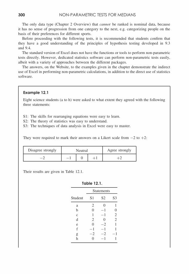
300 NON-PARAMETRIC TESTS FOR MEDIANS
The only data type (Chapter 2 Overview) that cannot be ranked is nominal data, becauseit has no sense of progression from one category to the next, e.g. categorizing people on thebasis of their preferences for different sports.
Before proceeding with the following tests, it is recommended that students confirm thatthey have a good understanding of the principles of hypothesis testing developed in 9.3and 9.4.
The standard version of Excel does not have the functions or tools to perform non-parametrictests directly. However, dedicated statistics software can perform non-parametric tests easily,albeit with a variety of approaches between the different packages.
The answers, on the Website, to the examples given in the chapter demonstrate the indirectuse of Excel in performing non-parametric calculations, in addition to the direct use of statisticssoftware.
Example 12.1
Eight science students (a to h) were asked to what extent they agreed with the followingthree statements:
S1: The skills for rearranging equations were easy to learn.S2: The theory of statistics was easy to understand.S3: The techniques of data analysis in Excel were easy to master.
They were required to mark their answers on a Likert scale from −2 to +2:
Disagree strongly Neutral Agree strongly
−2 −1 0 +1 +2
Their results are given in Table 12.1.
Table 12.1.
Statements
Student S1 S2 S3
a 2 0 1b 0 −1 0c 1 −1 2d 2 0 2e 0 −2 1f −1 −1 1g −2 −2 −1h 0 −1 1
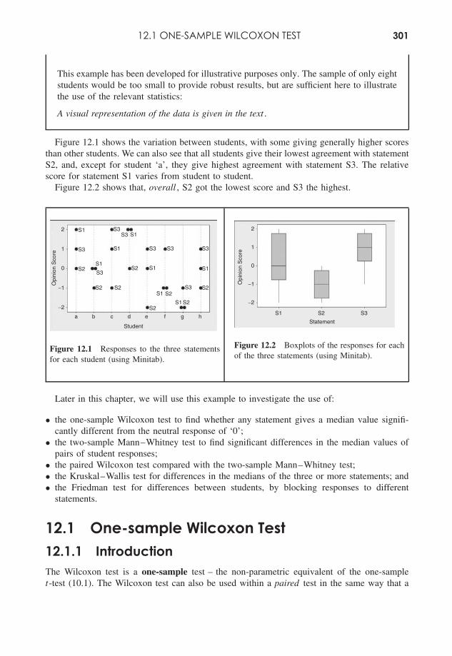
12.1 ONE-SAMPLE WILCOXON TEST 301
This example has been developed for illustrative purposes only. The sample of only eightstudents would be too small to provide robust results, but are sufficient here to illustratethe use of the relevant statistics:
A visual representation of the data is given in the text .
Figure 12.1 shows the variation between students, with some giving generally higher scoresthan other students. We can also see that all students give their lowest agreement with statementS2, and, except for student ‘a’, they give highest agreement with statement S3. The relativescore for statement S1 varies from student to student.
Figure 12.2 shows that, overall , S2 got the lowest score and S3 the highest.
S1
S1
S1
S1
S1
S1
S1
S1
S3
S3
S2
a b c d
Student
2
1
0
Opi
nion
Sco
re
−1
−2
e f g h
S2
S2
S2
S2S2
S2
S3S3
S3 S3 S3
S3
S2
Figure 12.1 Responses to the three statementsfor each student (using Minitab).
2
1
0
S1 S2
Statement
Opi
nion
Sco
re
S3
−1
−2
Figure 12.2 Boxplots of the responses for eachof the three statements (using Minitab).
Later in this chapter, we will use this example to investigate the use of:
• the one-sample Wilcoxon test to find whether any statement gives a median value signifi-cantly different from the neutral response of ‘0’;
• the two-sample Mann–Whitney test to find significant differences in the median values ofpairs of student responses;
• the paired Wilcoxon test compared with the two-sample Mann–Whitney test;• the Kruskal–Wallis test for differences in the medians of the three or more statements; and• the Friedman test for differences between students, by blocking responses to different
statements.
12.1 One-sample Wilcoxon Test12.1.1 IntroductionThe Wilcoxon test is a one-sample test – the non-parametric equivalent of the one-samplet-test (10.1). The Wilcoxon test can also be used within a paired test in the same way that a
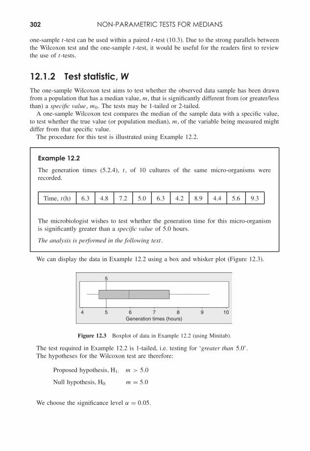
302 NON-PARAMETRIC TESTS FOR MEDIANS
one-sample t-test can be used within a paired t-test (10.3). Due to the strong parallels betweenthe Wilcoxon test and the one-sample t-test, it would be useful for the readers first to reviewthe use of t-tests.
12.1.2 Test statistic, WThe one-sample Wilcoxon test aims to test whether the observed data sample has been drawnfrom a population that has a median value, m, that is significantly different from (or greater/lessthan) a specific value, m0. The tests may be 1-tailed or 2-tailed.
A one-sample Wilcoxon test compares the median of the sample data with a specific value,to test whether the true value (or population median), m, of the variable being measured mightdiffer from that specific value.
The procedure for this test is illustrated using Example 12.2.
Example 12.2
The generation times (5.2.4), t , of 10 cultures of the same micro-organisms wererecorded.
Time, t(h) 6.3 4.8 7.2 5.0 6.3 4.2 8.9 4.4 5.6 9.3
The microbiologist wishes to test whether the generation time for this micro-organismis significantly greater than a specific value of 5.0 hours.
The analysis is performed in the following text .
We can display the data in Example 12.2 using a box and whisker plot (Figure 12.3).
5
54 6 7 8 9 10Generation times (hours)
Figure 12.3 Boxplot of data in Example 12.2 (using Minitab).
The test required in Example 12.2 is 1-tailed, i.e. testing for ‘greater than 5.0’.The hypotheses for the Wilcoxon test are therefore:
Proposed hypothesis, H1: m > 5.0
Null hypothesis, H0: m = 5.0
We choose the significance level α = 0.05.
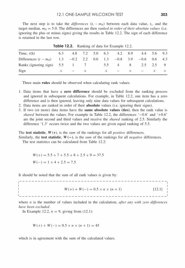
12.1 ONE-SAMPLE WILCOXON TEST 303
The next step is to take the differences (ti − m0) between each data value, ti , and thetarget median, m0 = 5.0. The differences are then ranked in order of their absolute values (i.e.ignoring the plus or minus signs) giving the results in Table 12.2. The sign of each differenceis retained in the last row.
Table 12.2. Ranking of data for Example 12.2.
Time, t(h) 6.3 4.8 7.2 5.0 6.3 4.2 8.9 4.4 5.6 9.3
Differences (t − m0) 1.3 −0.2 2.2 0.0 1.3 −0.8 3.9 −0.6 0.6 4.3
Ranks (ignoring sign) 5.5 1 7 5.5 4 8 2.5 2.5 9
Sign + − + + − + − + +
Three main rules should be observed when calculating rank values:
1. Data items that have a zero difference should be excluded from the ranking processand ignored in subsequent calculations. For example, in Table 12.2, one item has a zerodifference and is then ignored, leaving only nine data values for subsequent calculations.
2. Data items are ranked in order of their absolute values (i.e. ignoring their signs).3. If two (or more) data items have the same absolute values (ties), then the rank value is
shared between the values. For example in Table 12.2, the differences ‘−0.6’ and ‘+0.6’are the joint second and third values and receive the shared ranking of 2.5. Similarly thedifference ‘1.3’ occurs twice and the two values are given equal ranking of 5.5.
The test statistic, W (+), is the sum of the rankings for all positive differences.Similarly, the test statistic, W (−), is the sum of the rankings for all negative differences.
The test statistics can be calculated from Table 12.2:
W(+) = 5.5 + 7 + 5.5 + 8 + 2.5 + 9 = 37.5
W(−) = 1 + 4 + 2.5 = 7.5
It should be noted that the sum of all rank values is given by:
W(+) + W(−) = 0.5 × n × (n + 1) [12.1]
where n is the number of values included in the calculation, after any with zero differenceshave been excluded .
In Example 12.2, n = 9, giving from (12.1):
W(+) + W(−) = 0.5 × n × (n + 1) = 45
which is in agreement with the sum of the calculated values.
304 NON-PARAMETRIC TESTS FOR MEDIANS
If the sample median, m, is close to the specific value, m0 (null hypothesis), we would expectthe values of W(+) and W(−) to be very similar.
However, for the proposed hypothesis to be true, we would expect there to be a significantdifference between W(+) and W(−), with one of them having a significantly low value.
The critical values normally given for the Wilcoxon test are the lower critical values, WL.Appendix V gives critical values at α = 0.5 for sample sizes, n.
The conditions for accepting the proposed hypothesis, H1, are:
Accept H1 if either W(+) � WL or W(−) � WL.
In Example 12.2, the lower critical value, WL, for a 1-tailed test with n = 9 and α = 0.5 isWL = 8. Since W(−) < WL we accept the proposed hypothesis, H1.
A 1-tailed Wilcoxon test for the problem in Example 12.2 is performed on the Websiteusing Minitab and returns a p-value of 0.043. Since p < 0.05, we again accept the proposedhypothesis, H1.
12.1.3 Applying the one-sample Wilcoxon testFor problems involving ordinal data, the data is already ranked.
Example 12.3
Referring to the data in Example 12.1 presented in Chapter 12 Overview, we now wishto test separately whether the medians, m, for the student responses for each statement,S1, S2 and S3, in Table 12.1 are significantly different from the specific value, m0 = 0.
The analysis is performed in the following text .
The relevant 2-tailed hypotheses for the question in Example 12.3 would be:
H1: m = 0
H0: m = 0
Using Minitab on the Website to perform a 2-tailed Wilcoxon test we obtain the values inTable 12.3 for W(+), W(−), WL and p-value.
When the p-value results in Table 12.3 are compared with the boxplots in Figure 12.2:
• The conclusions for statements S1 (m could be 0) and S2 (m = 0) agree with the visualboxplot display.
• It would be difficult to make a decision from the boxplot data for S3 as the values overlapthe value m0 = 0. The p-value is close to 0.05, but there is just not enough evidence toaccept H1.
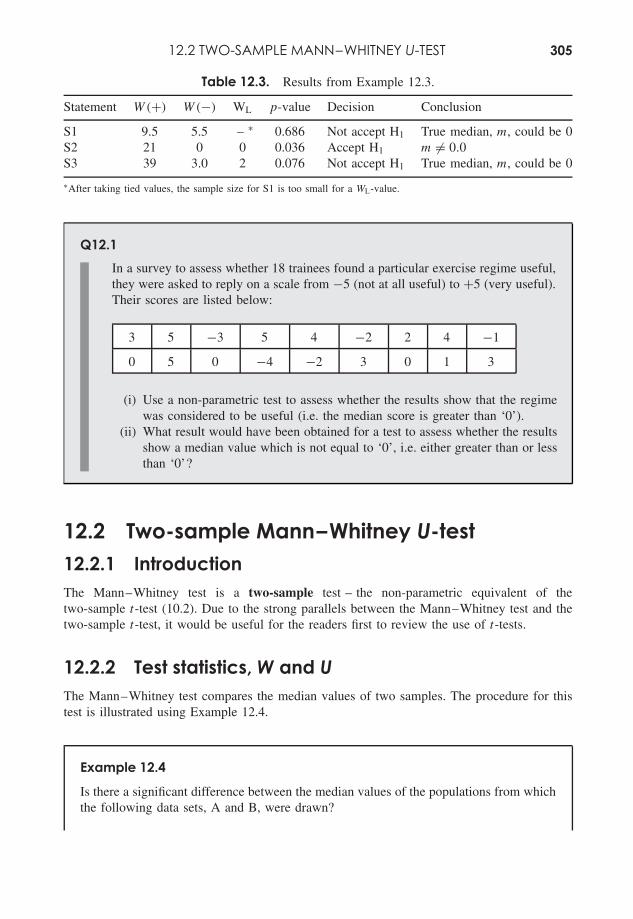
12.2 TWO-SAMPLE MANN–WHITNEY U-TEST 305
Table 12.3. Results from Example 12.3.
Statement W(+) W(−) WL p-value Decision Conclusion
S1 9.5 5.5 – ∗ 0.686 Not accept H1 True median, m, could be 0S2 21 0 0 0.036 Accept H1 m = 0.0S3 39 3.0 2 0.076 Not accept H1 True median, m, could be 0
∗After taking tied values, the sample size for S1 is too small for a WL-value.
Q12.1In a survey to assess whether 18 trainees found a particular exercise regime useful,they were asked to reply on a scale from −5 (not at all useful) to +5 (very useful).Their scores are listed below:
3 5 −3 5 4 −2 2 4 −1
0 5 0 −4 −2 3 0 1 3
(i) Use a non-parametric test to assess whether the results show that the regimewas considered to be useful (i.e. the median score is greater than ‘0’).
(ii) What result would have been obtained for a test to assess whether the resultsshow a median value which is not equal to ‘0’, i.e. either greater than or lessthan ‘0’?
12.2 Two-sample Mann–Whitney U-test12.2.1 IntroductionThe Mann–Whitney test is a two-sample test – the non-parametric equivalent of thetwo-sample t-test (10.2). Due to the strong parallels between the Mann–Whitney test and thetwo-sample t-test, it would be useful for the readers first to review the use of t-tests.
12.2.2 Test statistics, W and UThe Mann–Whitney test compares the median values of two samples. The procedure for thistest is illustrated using Example 12.4.
Example 12.4
Is there a significant difference between the median values of the populations from whichthe following data sets, A and B, were drawn?
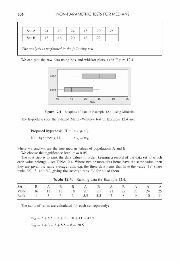
306 NON-PARAMETRIC TESTS FOR MEDIANS
Set A 21 23 24 18 20 25
Set B 18 16 20 18 22
The analysis is performed in the following text .
We can plot the raw data using box and whisker plots, as in Figure 12.4.
Set A
Set B
16 18 20 22 24 26Data
Figure 12.4 Boxplots of data in Example 12.4 (using Minitab).
The hypotheses for the 2-tailed Mann–Whitney test in Example 12.4 are:
Proposed hypothesis, H1: mA = mB
Null hypothesis, H0: mA = mB
where mA and mB are the true median values of populations A and B.We choose the significance level α = 0.05.The first step is to rank the data values in order, keeping a record of the data set to which
each value belongs – see Table 12.4. Where two or more data items have the same value, thenthey are given the same average rank, e.g. the three data items that have the value ‘18’ shareranks ‘2’, ‘3’ and ‘4’, giving the average rank ‘3’ for all of them.
Table 12.4. Ranking data for Example 12.4.
Set B A B B A B A B A A AValue 16 18 18 18 20 20 21 22 23 24 25Rank 1 3 3 3 5.5 5.5 7 8 9 10 11
The sums of ranks are calculated for each set separately:
WA = 3 + 5.5 + 7 + 9 + 10 + 11 = 45.5
WB = 1 + 3 + 3 + 5.5 + 8 = 20.5
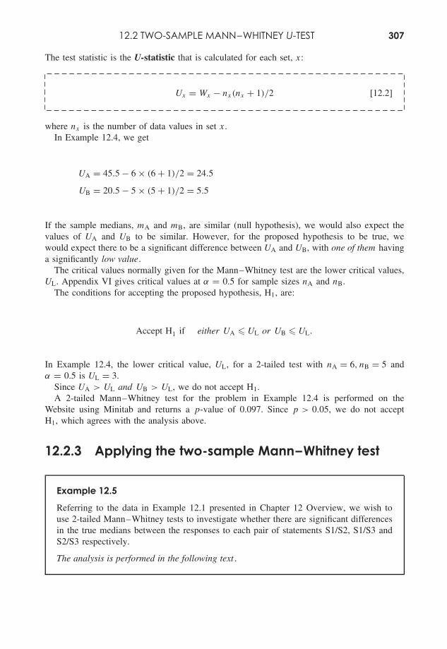
12.2 TWO-SAMPLE MANN–WHITNEY U-TEST 307
The test statistic is the U-statistic that is calculated for each set, x:
Ux = Wx − nx(nx + 1)/2 [12.2]
where nx is the number of data values in set x.In Example 12.4, we get
UA = 45.5 − 6 × (6 + 1)/2 = 24.5
UB = 20.5 − 5 × (5 + 1)/2 = 5.5
If the sample medians, mA and mB, are similar (null hypothesis), we would also expect thevalues of UA and UB to be similar. However, for the proposed hypothesis to be true, wewould expect there to be a significant difference between UA and UB, with one of them havinga significantly low value.
The critical values normally given for the Mann–Whitney test are the lower critical values,UL. Appendix VI gives critical values at α = 0.5 for sample sizes nA and nB.
The conditions for accepting the proposed hypothesis, H1, are:
Accept H1 if either UA � UL or UB � UL.
In Example 12.4, the lower critical value, UL, for a 2-tailed test with nA = 6, nB = 5 andα = 0.5 is UL = 3.
Since UA > UL and UB > UL, we do not accept H1.A 2-tailed Mann–Whitney test for the problem in Example 12.4 is performed on the
Website using Minitab and returns a p-value of 0.097. Since p > 0.05, we do not acceptH1, which agrees with the analysis above.
12.2.3 Applying the two-sample Mann–Whitney test
Example 12.5
Referring to the data in Example 12.1 presented in Chapter 12 Overview, we wish touse 2-tailed Mann–Whitney tests to investigate whether there are significant differencesin the true medians between the responses to each pair of statements S1/S2, S1/S3 andS2/S3 respectively.
The analysis is performed in the following text .
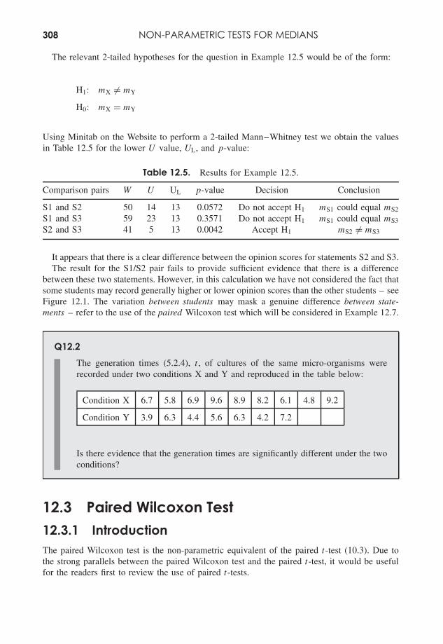
308 NON-PARAMETRIC TESTS FOR MEDIANS
The relevant 2-tailed hypotheses for the question in Example 12.5 would be of the form:
H1: mX = mY
H0: mX = mY
Using Minitab on the Website to perform a 2-tailed Mann–Whitney test we obtain the valuesin Table 12.5 for the lower U value, UL, and p-value:
Table 12.5. Results for Example 12.5.
Comparison pairs W U UL p-value Decision Conclusion
S1 and S2 50 14 13 0.0572 Do not accept H1 mS1 could equal mS2
S1 and S3 59 23 13 0.3571 Do not accept H1 mS1 could equal mS3
S2 and S3 41 5 13 0.0042 Accept H1 mS2 = mS3
It appears that there is a clear difference between the opinion scores for statements S2 and S3.The result for the S1/S2 pair fails to provide sufficient evidence that there is a difference
between these two statements. However, in this calculation we have not considered the fact thatsome students may record generally higher or lower opinion scores than the other students – seeFigure 12.1. The variation between students may mask a genuine difference between state-ments – refer to the use of the paired Wilcoxon test which will be considered in Example 12.7.
Q12.2The generation times (5.2.4), t , of cultures of the same micro-organisms wererecorded under two conditions X and Y and reproduced in the table below:
Condition X 6.7 5.8 6.9 9.6 8.9 8.2 6.1 4.8 9.2
Condition Y 3.9 6.3 4.4 5.6 6.3 4.2 7.2
Is there evidence that the generation times are significantly different under the twoconditions?
12.3 Paired Wilcoxon Test12.3.1 IntroductionThe paired Wilcoxon test is the non-parametric equivalent of the paired t-test (10.3). Due tothe strong parallels between the paired Wilcoxon test and the paired t-test, it would be usefulfor the readers first to review the use of paired t-tests.
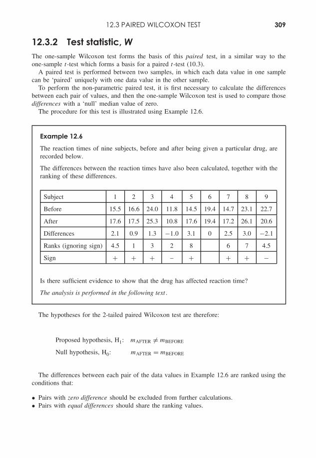
12.3 PAIRED WILCOXON TEST 309
12.3.2 Test statistic, WThe one-sample Wilcoxon test forms the basis of this paired test, in a similar way to theone-sample t-test which forms a basis for a paired t-test (10.3).
A paired test is performed between two samples, in which each data value in one samplecan be ‘paired’ uniquely with one data value in the other sample.
To perform the non-parametric paired test, it is first necessary to calculate the differencesbetween each pair of values, and then the one-sample Wilcoxon test is used to compare thosedifferences with a ‘null’ median value of zero.
The procedure for this test is illustrated using Example 12.6.
Example 12.6
The reaction times of nine subjects, before and after being given a particular drug, arerecorded below.
The differences between the reaction times have also been calculated, together with theranking of these differences.
Subject 1 2 3 4 5 6 7 8 9
Before 15.5 16.6 24.0 11.8 14.5 19.4 14.7 23.1 22.7
After 17.6 17.5 25.3 10.8 17.6 19.4 17.2 26.1 20.6
Differences 2.1 0.9 1.3 −1.0 3.1 0 2.5 3.0 −2.1
Ranks (ignoring sign) 4.5 1 3 2 8 6 7 4.5
Sign + + + – + + + −
Is there sufficient evidence to show that the drug has affected reaction time?
The analysis is performed in the following text .
The hypotheses for the 2-tailed paired Wilcoxon test are therefore:
Proposed hypothesis, H1: mAFTER = mBEFORE
Null hypothesis, H0: mAFTER = mBEFORE
The differences between each pair of the data values in Example 12.6 are ranked using theconditions that:
• Pairs with zero difference should be excluded from further calculations.• Pairs with equal differences should share the ranking values.
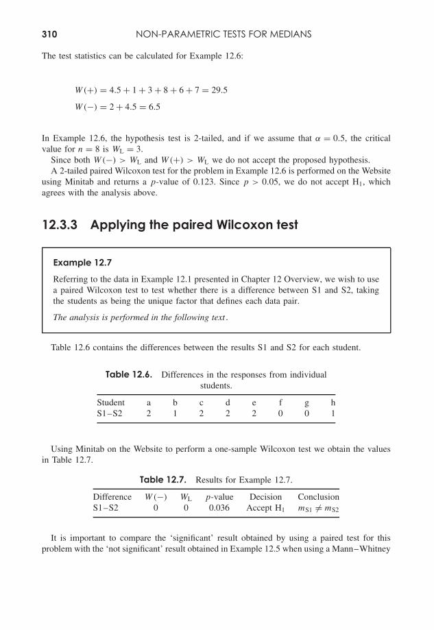
310 NON-PARAMETRIC TESTS FOR MEDIANS
The test statistics can be calculated for Example 12.6:
W(+) = 4.5 + 1 + 3 + 8 + 6 + 7 = 29.5
W(−) = 2 + 4.5 = 6.5
In Example 12.6, the hypothesis test is 2-tailed, and if we assume that α = 0.5, the criticalvalue for n = 8 is WL = 3.
Since both W(−) > WL and W(+) > WL we do not accept the proposed hypothesis.A 2-tailed paired Wilcoxon test for the problem in Example 12.6 is performed on the Website
using Minitab and returns a p-value of 0.123. Since p > 0.05, we do not accept H1, whichagrees with the analysis above.
12.3.3 Applying the paired Wilcoxon test
Example 12.7
Referring to the data in Example 12.1 presented in Chapter 12 Overview, we wish to usea paired Wilcoxon test to test whether there is a difference between S1 and S2, takingthe students as being the unique factor that defines each data pair.
The analysis is performed in the following text .
Table 12.6 contains the differences between the results S1 and S2 for each student.
Table 12.6. Differences in the responses from individualstudents.
Student a b c d e f g hS1–S2 2 1 2 2 2 0 0 1
Using Minitab on the Website to perform a one-sample Wilcoxon test we obtain the valuesin Table 12.7.
Table 12.7. Results for Example 12.7.
Difference W(−) WL p-value Decision ConclusionS1–S2 0 0 0.036 Accept H1 mS1 = mS2
It is important to compare the ‘significant’ result obtained by using a paired test for thisproblem with the ‘not significant’ result obtained in Example 12.5 when using a Mann–Whitney
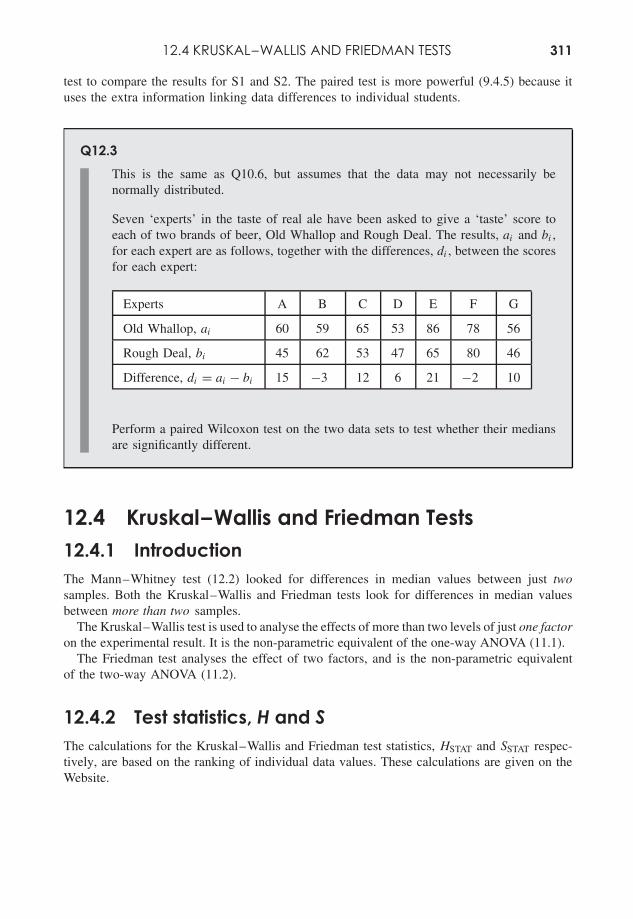
12.4 KRUSKAL–WALLIS AND FRIEDMAN TESTS 311
test to compare the results for S1 and S2. The paired test is more powerful (9.4.5) because ituses the extra information linking data differences to individual students.
Q12.3This is the same as Q10.6, but assumes that the data may not necessarily benormally distributed.
Seven ‘experts’ in the taste of real ale have been asked to give a ‘taste’ score toeach of two brands of beer, Old Whallop and Rough Deal. The results, ai and bi ,for each expert are as follows, together with the differences, di , between the scoresfor each expert:
Experts A B C D E F G
Old Whallop, ai 60 59 65 53 86 78 56
Rough Deal, bi 45 62 53 47 65 80 46
Difference, di = ai − bi 15 −3 12 6 21 −2 10
Perform a paired Wilcoxon test on the two data sets to test whether their mediansare significantly different.
12.4 Kruskal–Wallis and Friedman Tests12.4.1 IntroductionThe Mann–Whitney test (12.2) looked for differences in median values between just twosamples. Both the Kruskal–Wallis and Friedman tests look for differences in median valuesbetween more than two samples.
The Kruskal–Wallis test is used to analyse the effects of more than two levels of just one factoron the experimental result. It is the non-parametric equivalent of the one-way ANOVA (11.1).
The Friedman test analyses the effect of two factors, and is the non-parametric equivalentof the two-way ANOVA (11.2).
12.4.2 Test statistics, H and SThe calculations for the Kruskal–Wallis and Friedman test statistics, HSTAT and SSTAT respec-tively, are based on the ranking of individual data values. These calculations are given on theWebsite.
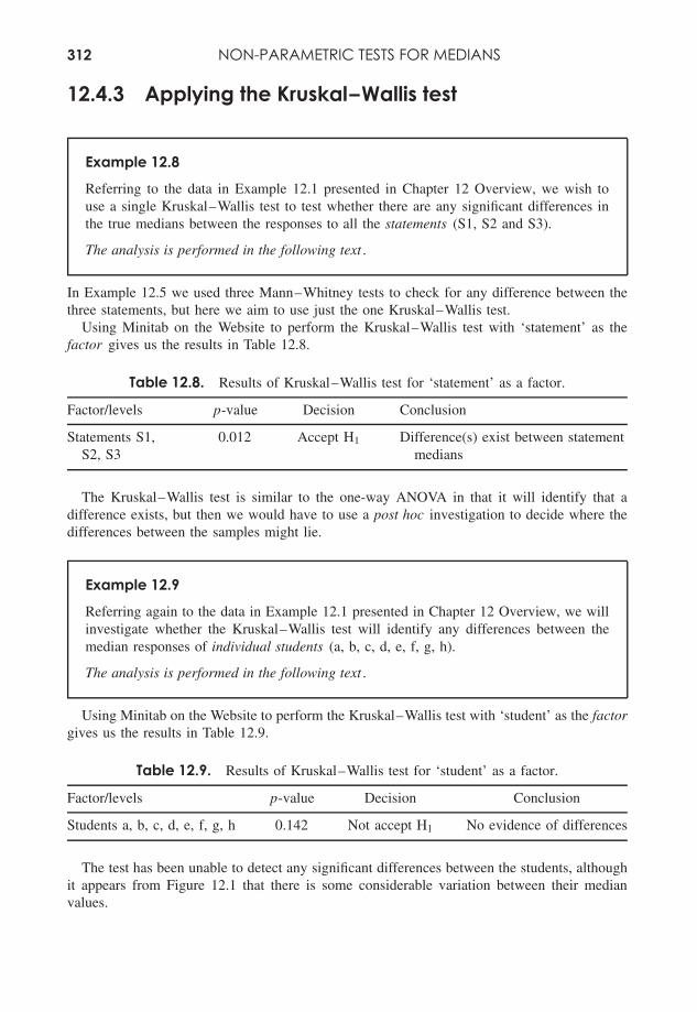
312 NON-PARAMETRIC TESTS FOR MEDIANS
12.4.3 Applying the Kruskal–Wallis test
Example 12.8
Referring to the data in Example 12.1 presented in Chapter 12 Overview, we wish touse a single Kruskal–Wallis test to test whether there are any significant differences inthe true medians between the responses to all the statements (S1, S2 and S3).
The analysis is performed in the following text .
In Example 12.5 we used three Mann–Whitney tests to check for any difference between thethree statements, but here we aim to use just the one Kruskal–Wallis test.
Using Minitab on the Website to perform the Kruskal–Wallis test with ‘statement’ as thefactor gives us the results in Table 12.8.
Table 12.8. Results of Kruskal–Wallis test for ‘statement’ as a factor.
Factor/levels p-value Decision Conclusion
Statements S1,S2, S3
0.012 Accept H1 Difference(s) exist between statementmedians
The Kruskal–Wallis test is similar to the one-way ANOVA in that it will identify that adifference exists, but then we would have to use a post hoc investigation to decide where thedifferences between the samples might lie.
Example 12.9
Referring again to the data in Example 12.1 presented in Chapter 12 Overview, we willinvestigate whether the Kruskal–Wallis test will identify any differences between themedian responses of individual students (a, b, c, d, e, f, g, h).
The analysis is performed in the following text .
Using Minitab on the Website to perform the Kruskal–Wallis test with ‘student’ as the factorgives us the results in Table 12.9.
Table 12.9. Results of Kruskal–Wallis test for ‘student’ as a factor.
Factor/levels p-value Decision Conclusion
Students a, b, c, d, e, f, g, h 0.142 Not accept H1 No evidence of differences
The test has been unable to detect any significant differences between the students, althoughit appears from Figure 12.1 that there is some considerable variation between their medianvalues.
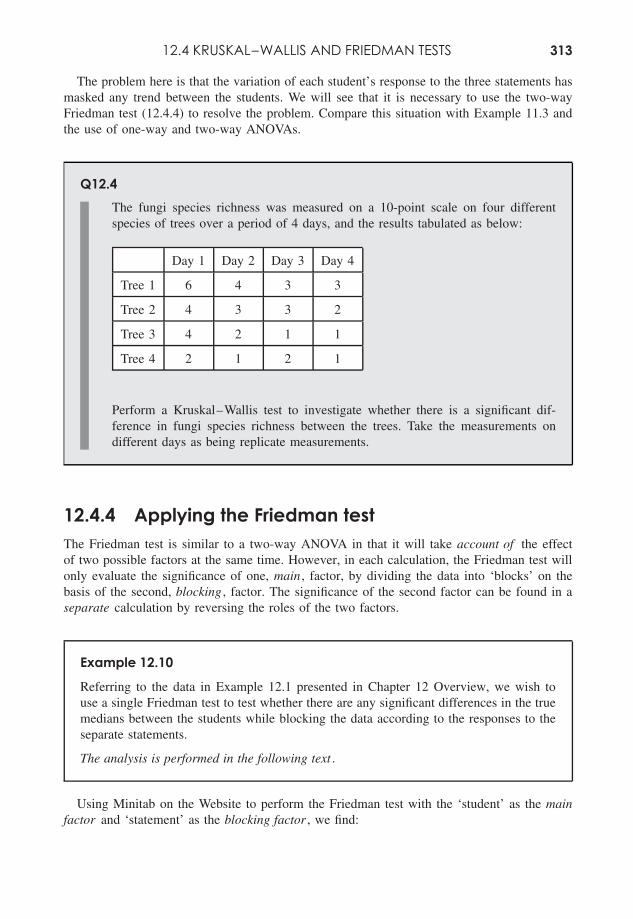
12.4 KRUSKAL–WALLIS AND FRIEDMAN TESTS 313
The problem here is that the variation of each student’s response to the three statements hasmasked any trend between the students. We will see that it is necessary to use the two-wayFriedman test (12.4.4) to resolve the problem. Compare this situation with Example 11.3 andthe use of one-way and two-way ANOVAs.
Q12.4The fungi species richness was measured on a 10-point scale on four differentspecies of trees over a period of 4 days, and the results tabulated as below:
Day 1 Day 2 Day 3 Day 4
Tree 1 6 4 3 3
Tree 2 4 3 3 2
Tree 3 4 2 1 1
Tree 4 2 1 2 1
Perform a Kruskal–Wallis test to investigate whether there is a significant dif-ference in fungi species richness between the trees. Take the measurements ondifferent days as being replicate measurements.
12.4.4 Applying the Friedman testThe Friedman test is similar to a two-way ANOVA in that it will take account of the effectof two possible factors at the same time. However, in each calculation, the Friedman test willonly evaluate the significance of one, main , factor, by dividing the data into ‘blocks’ on thebasis of the second, blocking , factor. The significance of the second factor can be found in aseparate calculation by reversing the roles of the two factors.
Example 12.10
Referring to the data in Example 12.1 presented in Chapter 12 Overview, we wish touse a single Friedman test to test whether there are any significant differences in the truemedians between the students while blocking the data according to the responses to theseparate statements.
The analysis is performed in the following text .
Using Minitab on the Website to perform the Friedman test with the ‘student’ as the mainfactor and ‘statement’ as the blocking factor , we find:
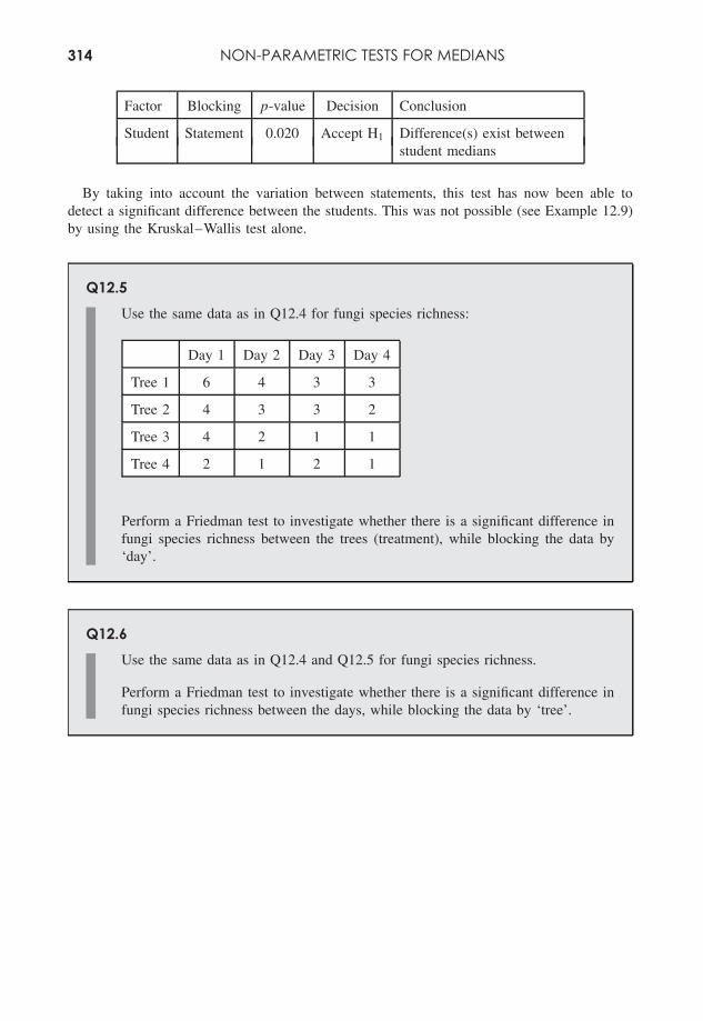
314 NON-PARAMETRIC TESTS FOR MEDIANS
Factor Blocking p-value Decision Conclusion
Student Statement 0.020 Accept H1 Difference(s) exist betweenstudent medians
By taking into account the variation between statements, this test has now been able todetect a significant difference between the students. This was not possible (see Example 12.9)by using the Kruskal–Wallis test alone.
Q12.5Use the same data as in Q12.4 for fungi species richness:
Day 1 Day 2 Day 3 Day 4
Tree 1 6 4 3 3
Tree 2 4 3 3 2
Tree 3 4 2 1 1
Tree 4 2 1 2 1
Perform a Friedman test to investigate whether there is a significant difference infungi species richness between the trees (treatment), while blocking the data by‘day’.
Q12.6Use the same data as in Q12.4 and Q12.5 for fungi species richness.
Perform a Friedman test to investigate whether there is a significant difference infungi species richness between the days, while blocking the data by ‘tree’.
13Correlation and Regression
OverviewWebsite • ‘How to do it’ video answers for all ‘Q’ questions.
• Correlation tests in Excel and Minitab.• Excel tutorial: uncertainty in linear calibration.
Correlation is a measure of the extent to which the values of two variables of a system arerelated (or correlated). For example, both the height and weight of a child normally increaseas the child gets older – there is a correlation between height and weight.
It must be noted, however, that the fact that two parameters are correlated does not nec-essarily mean that one is a cause and the other an effect . In the example of the height andweight of a child, both increases are the result of the growth of the child. The underlying‘cause’ (factor) is the maturity of the child, and the height and weight are both ‘effects’(outcomes).
If two variables are correlated, the relationship between them could follow very many dif-ferent mathematical functions, e.g. the numbers of bacteria in a dying population may followan exponential decay equation. However, linear correlation is a measure of the extent to whichthere is a linear relationship between two variables, i.e. the extent to which their relationshipcan be expressed in terms of a straight line.
A linear regression analysis is the process of deriving the slope and intercept of the straightline equation that can be used to describe the relationship between the two variables. Whenperforming a linear regression it is normally assumed that there is a causal relationship, i.e.the value of one variable is dependent on the value of the other. We saw in 4.1.2 that thedependent variable is placed on the y-axis of an x –y graph with the independent variable onthe x-axis.
In simple terms:
• ‘correlation’ asks if there is a relationship between two variables; and• ‘regression’ measures how one variable is dependent on the other through the slope and
intercept of a ‘best-fit’ straight line.
Essential Mathematics and Statistics for Science 2nd Edition Graham Currell and Antony DowmanCopyright c© 2009 John Wiley & Sons, Ltd
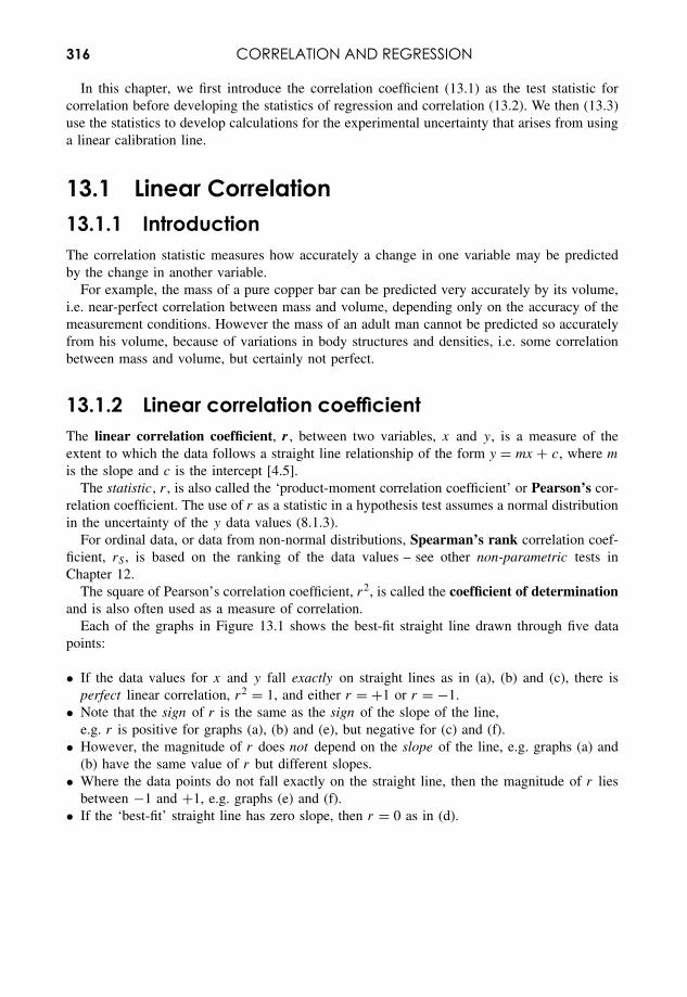
316 CORRELATION AND REGRESSION
In this chapter, we first introduce the correlation coefficient (13.1) as the test statistic forcorrelation before developing the statistics of regression and correlation (13.2). We then (13.3)use the statistics to develop calculations for the experimental uncertainty that arises from usinga linear calibration line.
13.1 Linear Correlation13.1.1 IntroductionThe correlation statistic measures how accurately a change in one variable may be predictedby the change in another variable.
For example, the mass of a pure copper bar can be predicted very accurately by its volume,i.e. near-perfect correlation between mass and volume, depending only on the accuracy of themeasurement conditions. However the mass of an adult man cannot be predicted so accuratelyfrom his volume, because of variations in body structures and densities, i.e. some correlationbetween mass and volume, but certainly not perfect.
13.1.2 Linear correlation coefficientThe linear correlation coefficient, r , between two variables, x and y, is a measure of theextent to which the data follows a straight line relationship of the form y = mx + c, where m
is the slope and c is the intercept [4.5].The statistic, r , is also called the ‘product-moment correlation coefficient’ or Pearson’s cor-
relation coefficient. The use of r as a statistic in a hypothesis test assumes a normal distributionin the uncertainty of the y data values (8.1.3).
For ordinal data, or data from non-normal distributions, Spearman’s rank correlation coef-ficient, rS , is based on the ranking of the data values – see other non-parametric tests inChapter 12.
The square of Pearson’s correlation coefficient, r2, is called the coefficient of determinationand is also often used as a measure of correlation.
Each of the graphs in Figure 13.1 shows the best-fit straight line drawn through five datapoints:
• If the data values for x and y fall exactly on straight lines as in (a), (b) and (c), there isperfect linear correlation, r2 = 1, and either r = +1 or r = −1.
• Note that the sign of r is the same as the sign of the slope of the line,e.g. r is positive for graphs (a), (b) and (e), but negative for (c) and (f).
• However, the magnitude of r does not depend on the slope of the line, e.g. graphs (a) and(b) have the same value of r but different slopes.
• Where the data points do not fall exactly on the straight line, then the magnitude of r liesbetween −1 and +1, e.g. graphs (e) and (f).
• If the ‘best-fit’ straight line has zero slope, then r = 0 as in (d).
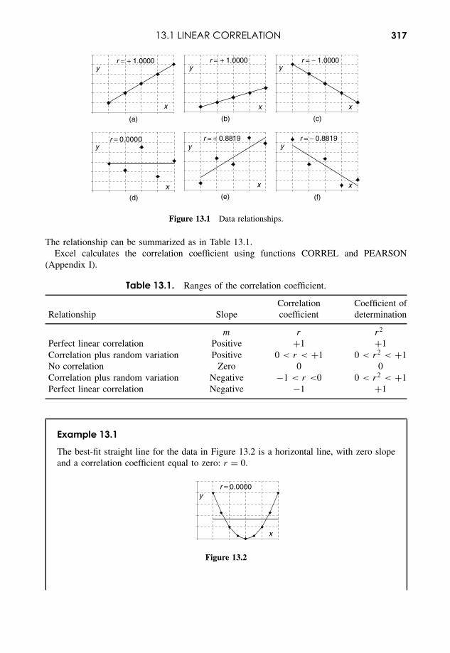
13.1 LINEAR CORRELATION 317
y
x
r = + 1.0000
(a)
y
x
r = 0.0000
(d)
y
x
r = + 1.0000
(b)
y
x
r = + 0.8819
(e)
y
x
r = − 1.0000
(c)
y
x
r = − 0.8819
(f)
Figure 13.1 Data relationships.
The relationship can be summarized as in Table 13.1.Excel calculates the correlation coefficient using functions CORREL and PEARSON
(Appendix I).
Table 13.1. Ranges of the correlation coefficient.
Correlation Coefficient ofRelationship Slope coefficient determination
m r r2
Perfect linear correlation Positive +1 +1Correlation plus random variation Positive 0 < r < +1 0 < r2 < +1No correlation Zero 0 0Correlation plus random variation Negative −1 < r <0 0 < r2 < +1Perfect linear correlation Negative −1 +1
Example 13.1
The best-fit straight line for the data in Figure 13.2 is a horizontal line, with zero slopeand a correlation coefficient equal to zero: r = 0.
y
x
r = 0.0000
Figure 13.2
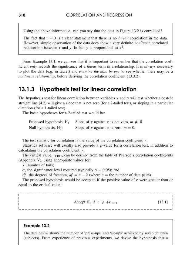
318 CORRELATION AND REGRESSION
Using the above information, can you say that the data in Figure 13.2 is correlated?
The fact that r = 0 is a clear statement that there is no linear correlation in the data.However, simple observation of the data does show a very definite nonlinear correlatedrelationship between x and y. In fact y is proportional to x2.
From Example 13.1, we can see that it is important to remember that the correlation coef-ficient only records the significance of a linear term in a relationship. It is always necessaryto plot the data (e.g. in Excel) and examine the data by eye to see whether there may be anonlinear relationship, before deriving the correlation coefficient (13.3.2).
13.1.3 Hypothesis test for linear correlationThe hypothesis test for linear correlation between variables x and y will test whether a best-fitstraight line (4.2) will give a slope that is not zero (for a 2-tailed test), or sloping in a particulardirection (for a 1-tailed test).
The basic hypotheses for a 2-tailed test would be:
Proposed hypothesis, H1: Slope of y against x is not zero, m = 0.
Null hypothesis, H0: Slope of y against x is zero, m = 0.
The test statistic for correlation is the value of the correlation coefficient, r .Statistics software will usually also provide a p-value for a correlation test, in addition to
calculating the correlation coefficient, r .The critical value, rCRIT, can be derived from the table of Pearson’s correlation coefficients
(Appendix V), using appropriate values for:T , number of tails;α, the significance level required (typically α = 0.05); anddf , the degrees of freedom, df = n − 2 (where n = the number of data pairs).The proposed hypothesis would be accepted if the positive value of r were greater than or
equal to the critical value:
Accept H1 if |r| � +rCRIT [13.1]
Example 13.2
The data below shows the number of ‘press-ups’ and ‘sit-ups’ achieved by seven children(subjects). From experience of previous experiments, we devise the hypothesis that a
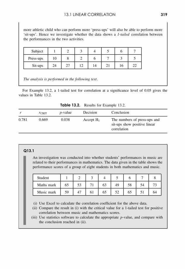
13.1 LINEAR CORRELATION 319
more athletic child who can perform more ‘press-ups’ will also be able to perform more‘sit-ups’. Hence we investigate whether the data shows a 1-tailed correlation betweenthe performances in the two activities.
Subject 1 2 3 4 5 6 7
Press-ups 10 8 2 6 7 3 5
Sit-ups 24 27 12 14 21 16 22
The analysis is performed in the following text .
For Example 13.2, a 1-tailed test for correlation at a significance level of 0.05 gives thevalues in Table 13.2.
Table 13.2. Results for Example 13.2.
r rCRIT p-value Decision Conclusion
0.781 0.669 0.038 Accept H1 The numbers of press-ups andsit-ups show positive linearcorrelation
Q13.1An investigation was conducted into whether students’ performances in music arerelated to their performances in mathematics. The data given in the table shows theperformance scores of a group of eight students in both mathematics and music.
Student 1 2 3 4 5 6 7 8
Maths mark 65 53 71 63 49 58 54 73
Music mark 59 47 61 65 52 65 51 64
(i) Use Excel to calculate the correlation coefficient for the above data.(ii) Compare the result in (i) with the critical value for a 1-tailed test for positive
correlation between music and mathematics scores.(iii) Use statistics software to calculate the appropriate p-value, and compare with
the conclusion reached in (ii).
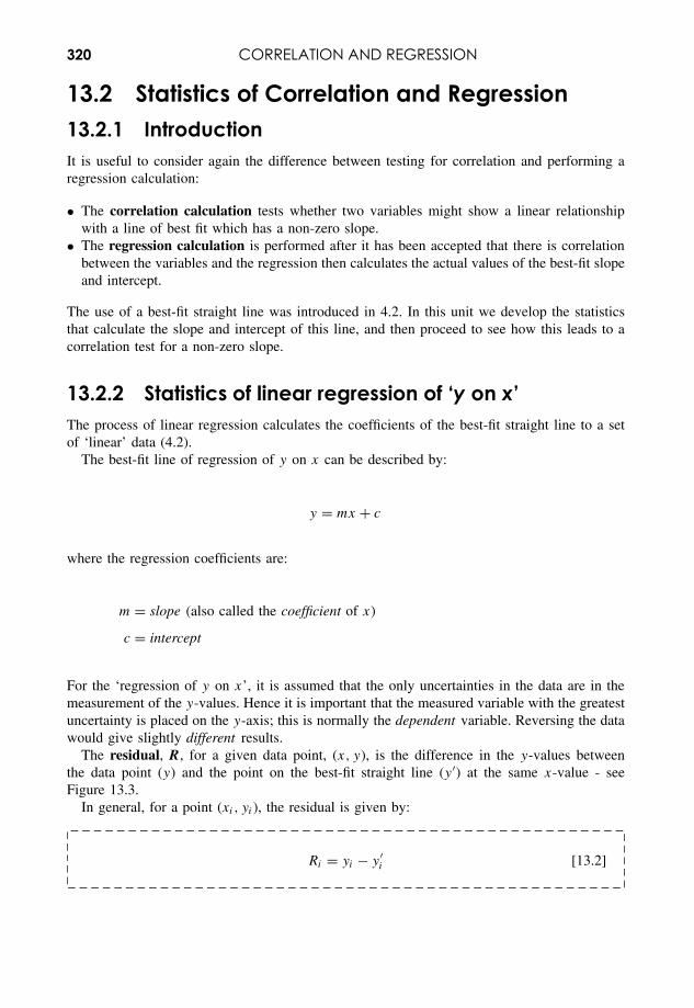
320 CORRELATION AND REGRESSION
13.2 Statistics of Correlation and Regression13.2.1 IntroductionIt is useful to consider again the difference between testing for correlation and performing aregression calculation:
• The correlation calculation tests whether two variables might show a linear relationshipwith a line of best fit which has a non-zero slope.
• The regression calculation is performed after it has been accepted that there is correlationbetween the variables and the regression then calculates the actual values of the best-fit slopeand intercept.
The use of a best-fit straight line was introduced in 4.2. In this unit we develop the statisticsthat calculate the slope and intercept of this line, and then proceed to see how this leads to acorrelation test for a non-zero slope.
13.2.2 Statistics of linear regression of ‘y on x’The process of linear regression calculates the coefficients of the best-fit straight line to a setof ‘linear’ data (4.2).
The best-fit line of regression of y on x can be described by:
y = mx + c
where the regression coefficients are:
m = slope (also called the coefficient of x)
c = intercept
For the ‘regression of y on x’, it is assumed that the only uncertainties in the data are in themeasurement of the y-values. Hence it is important that the measured variable with the greatestuncertainty is placed on the y-axis; this is normally the dependent variable. Reversing the datawould give slightly different results.
The residual, R, for a given data point, (x, y), is the difference in the y-values betweenthe data point (y) and the point on the best-fit straight line (y ′) at the same x-value - seeFigure 13.3.
In general, for a point (xi, yi), the residual is given by:
Ri = yi − y ′i [13.2]
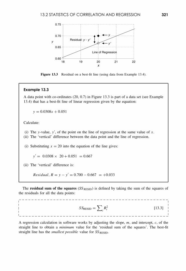
13.2 STATISTICS OF CORRELATION AND REGRESSION 321
0.60
0.65
0.70
0.75
18 19 20 21 22
Residual: y − y ′
y
y ′
Line of Regression
x
y
Figure 13.3 Residual on a best-fit line (using data from Example 13.4).
Example 13.3
A data point with co-ordinates (20, 0.7) in Figure 13.3 is part of a data set (see Example13.4) that has a best-fit line of linear regression given by the equation:
y = 0.0308x + 0.051
Calculate:
(i) The y-value, y ′, of the point on the line of regression at the same value of x.(ii) The ‘vertical’ difference between the data point and the line of regression.
(i) Substituting x = 20 into the equation of the line gives:
y ′ = 0.0308 × 20 + 0.051 = 0.667
(ii) The ‘vertical’ difference is:
Residual, R = y − y ′ = 0.700 − 0.667 = +0.033
The residual sum of the squares (SS RESID) is defined by taking the sum of the squares ofthe residuals for all the data points:
SSRESID =∑
iR2
i [13.3]
A regression calculation in software works by adjusting the slope, m, and intercept, c, of thestraight line to obtain a minimum value for the ‘residual sum of the squares’. The best-fitstraight line has the smallest possible value for SS RESID.
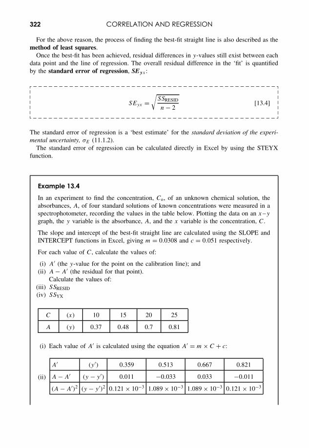
322 CORRELATION AND REGRESSION
For the above reason, the process of finding the best-fit straight line is also described as themethod of least squares.
Once the best-fit has been achieved, residual differences in y-values still exist between eachdata point and the line of regression. The overall residual difference in the ‘fit’ is quantifiedby the standard error of regression, SE yx :
SEyx =√
SSRESID
n − 2[13.4]
The standard error of regression is a ‘best estimate’ for the standard deviation of the experi-mental uncertainty, σE (11.1.2).
The standard error of regression can be calculated directly in Excel by using the STEYXfunction.
Example 13.4
In an experiment to find the concentration, Co, of an unknown chemical solution, theabsorbances, A, of four standard solutions of known concentrations were measured in aspectrophotometer, recording the values in the table below. Plotting the data on an x –y
graph, the y variable is the absorbance, A, and the x variable is the concentration, C.
The slope and intercept of the best-fit straight line are calculated using the SLOPE andINTERCEPT functions in Excel, giving m = 0.0308 and c = 0.051 respectively.
For each value of C, calculate the values of:
(i) A′ (the y-value for the point on the calibration line); and(ii) A − A′ (the residual for that point).
Calculate the values of:(iii) SSRESID
(iv) SSYX
C (x) 10 15 20 25
A (y) 0.37 0.48 0.7 0.81
(i) Each value of A′ is calculated using the equation A′ = m × C + c:
(ii)
A′ (y ′) 0.359 0.513 0.667 0.821
A − A′ (y − y ′) 0.011 −0.033 0.033 −0.011
(A − A′)2 (y − y ′)2 0.121 × 10⁻³ 1.089 × 10⁻³ 1.089 × 10⁻³ 0.121 × 10⁻³
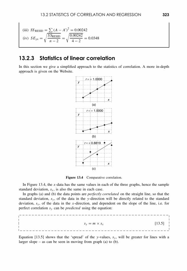
13.2 STATISTICS OF CORRELATION AND REGRESSION 323
(iii) SS RESID = ∑(A − A′)2 = 0.00242
(iv) SEyx =√
SSRESID
n − 2=
√0.00242
4 − 2= 0.0348
13.2.3 Statistics of linear correlationIn this section we give a simplified approach to the statistics of correlation. A more in-depthapproach is given on the Website.
y
x
r = + 1.0000
y
x
r = + 1.0000
y
x
r = + 0.8819
(a)
(b)
(c)
Figure 13.4 Comparative correlation.
In Figure 13.4, the x-data has the same values in each of the three graphs, hence the samplestandard deviation, sx , is also the same in each case.
In graphs (a) and (b) the data points are perfectly correlated on the straight line, so that thestandard deviation, sy , of the data in the y-direction will be directly related to the standarddeviation, sx , of the data in the x-direction, and dependent on the slope of the line, i.e. forperfect correlation sy can be predicted using the equation:
sy = m × sx [13.5]
Equation [13.5] shows that the ‘spread’ of the y-values, sy , will be greater for lines with alarger slope – as can be seen in moving from graph (a) to (b).
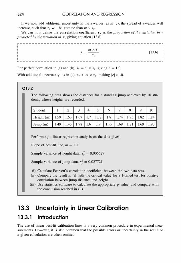
324 CORRELATION AND REGRESSION
If we now add additional uncertainty in the y-values, as in (c), the spread of y-values willincrease, such that sy will be greater than m × sx .
We can now define the correlation coefficient, r , as the proportion of the variation in ypredicted by the variation in x, giving equation [13.6]:
r = m × sx
sy
[13.6]
For perfect correlation in (a) and (b), sy = m × sx , giving r = 1.0.
With additional uncertainty, as in (c), sy > m × sx , making |r|<1.0.
Q13.2The following data shows the distances for a standing jump achieved by 10 stu-dents, whose heights are recorded:
Student 1 2 3 4 5 6 7 8 9 10
Height (m) 1.59 1.63 1.67 1.7 1.72 1.8 1.74 1.75 1.82 1.84
Jump (m) 1.49 1.45 1.78 1.6 1.9 1.55 1.69 1.81 1.69 1.93
Performing a linear regression analysis on the data gives:
Slope of best-fit line, m = 1.11
Sample variance of height data, s2x = 0.006627
Sample variance of jump data, s2y = 0.027721
(i) Calculate Pearson’s correlation coefficient between the two data sets.(ii) Compare the result in (i) with the critical value for a 1-tailed test for positive
correlation between jump distance and height.(iii) Use statistics software to calculate the appropriate p-value, and compare with
the conclusion reached in (ii).
13.3 Uncertainty in Linear Calibration13.3.1 IntroductionThe use of linear best-fit calibration lines is a very common procedure in experimental mea-surements. However, it is also common that the possible errors or uncertainty in the result ofa given calculation are often omitted.
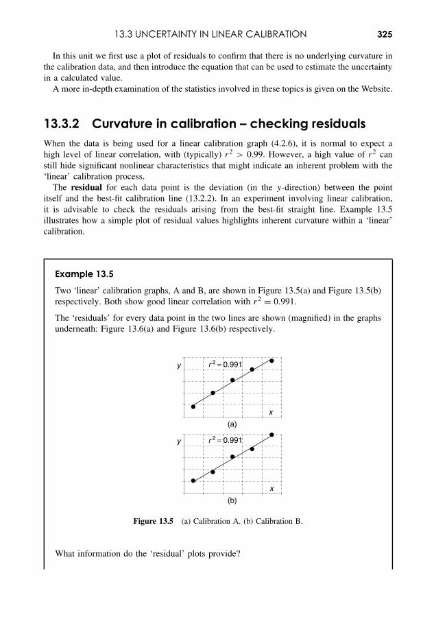
13.3 UNCERTAINTY IN LINEAR CALIBRATION 325
In this unit we first use a plot of residuals to confirm that there is no underlying curvature inthe calibration data, and then introduce the equation that can be used to estimate the uncertaintyin a calculated value.
A more in-depth examination of the statistics involved in these topics is given on the Website.
13.3.2 Curvature in calibration – checking residualsWhen the data is being used for a linear calibration graph (4.2.6), it is normal to expect ahigh level of linear correlation, with (typically) r2 > 0.99. However, a high value of r2 canstill hide significant nonlinear characteristics that might indicate an inherent problem with the‘linear’ calibration process.
The residual for each data point is the deviation (in the y-direction) between the pointitself and the best-fit calibration line (13.2.2). In an experiment involving linear calibration,it is advisable to check the residuals arising from the best-fit straight line. Example 13.5illustrates how a simple plot of residual values highlights inherent curvature within a ‘linear’calibration.
Example 13.5
Two ‘linear’ calibration graphs, A and B, are shown in Figure 13.5(a) and Figure 13.5(b)respectively. Both show good linear correlation with r2 = 0.991.
The ‘residuals’ for every data point in the two lines are shown (magnified) in the graphsunderneath: Figure 13.6(a) and Figure 13.6(b) respectively.
y
x
r 2 = 0.991
y
x
r 2 = 0.991
(a)
(b)
Figure 13.5 (a) Calibration A. (b) Calibration B.
What information do the ‘residual’ plots provide?
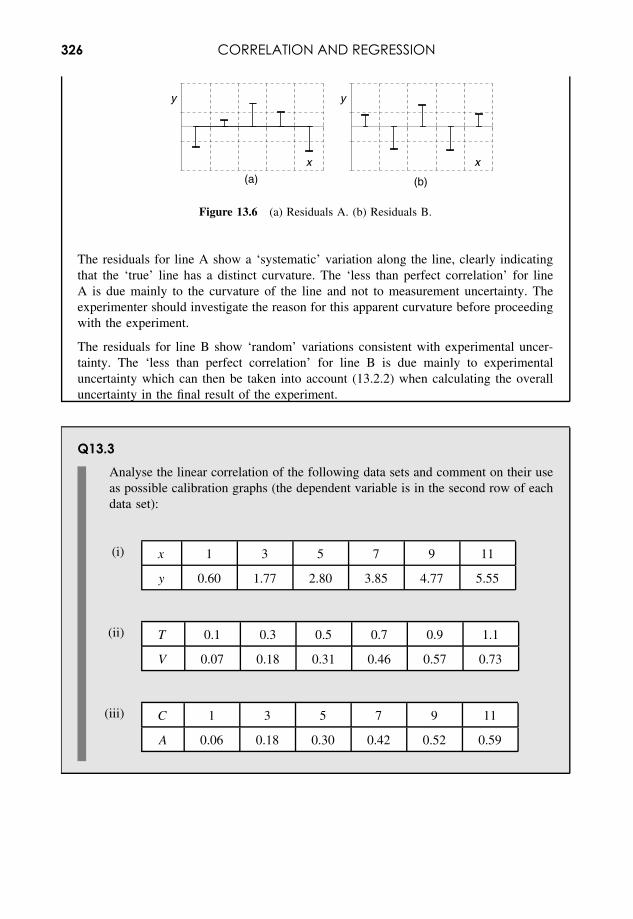
326 CORRELATION AND REGRESSION
y
x
(a)
y
x
(b)
Figure 13.6 (a) Residuals A. (b) Residuals B.
The residuals for line A show a ‘systematic’ variation along the line, clearly indicatingthat the ‘true’ line has a distinct curvature. The ‘less than perfect correlation’ for lineA is due mainly to the curvature of the line and not to measurement uncertainty. Theexperimenter should investigate the reason for this apparent curvature before proceedingwith the experiment.
The residuals for line B show ‘random’ variations consistent with experimental uncer-tainty. The ‘less than perfect correlation’ for line B is due mainly to experimentaluncertainty which can then be taken into account (13.2.2) when calculating the overalluncertainty in the final result of the experiment.
Q13.3Analyse the linear correlation of the following data sets and comment on their useas possible calibration graphs (the dependent variable is in the second row of eachdata set):
(i) x 1 3 5 7 9 11
y 0.60 1.77 2.80 3.85 4.77 5.55
(ii) T 0.1 0.3 0.5 0.7 0.9 1.1
V 0.07 0.18 0.31 0.46 0.57 0.73
(iii) C 1 3 5 7 9 11
A 0.06 0.18 0.30 0.42 0.52 0.59
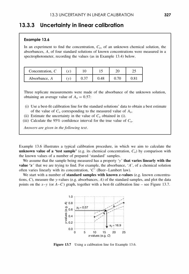
13.3 UNCERTAINTY IN LINEAR CALIBRATION 327
13.3.3 Uncertainty in linear calibration
Example 13.6
In an experiment to find the concentration, Co, of an unknown chemical solution, theabsorbances, A, of four standard solutions of known concentrations were measured in aspectrophotometer, recording the values (as in Example 13.4) below.
Concentration, C (x) 10 15 20 25
Absorbance, A (y) 0.37 0.48 0.70 0.81
Three replicate measurements were made of the absorbance of the unknown solution,obtaining an average value of Ao = 0.57:
(i) Use a best-fit calibration line for the standard solutions’ data to obtain a best estimateof the value of Co corresponding to the measured value of Ao.
(ii) Estimate the uncertainty in the value of Co obtained in (i).(iii) Calculate the 95% confidence interval for the true value of Co.
Answers are given in the following text .
Example 13.6 illustrates a typical calibration procedure, in which we aim to calculate theunknown value of a ‘test sample’ (e.g. its chemical concentration, Co) by comparison withthe known values of a number of prepared ‘standard’ samples.
We assume that the sample being measured has a property ‘y’ that varies linearly with thevalue ‘x ’ that we are trying to find. For example, the absorbance, ‘A’, of a chemical solutionoften varies linearly with its concentration, ‘C’ (Beer–Lambert law).
We start with a number of standard samples with known x-values (e.g. known concentra-tions, C), measure the y-values (e.g. absorbances, A) of the standard samples, and plot the datapoints on the x–y (or A–C ) graph, together with a best-fit calibration line – see Figure 13.7.
0.0
0.2
0.4
0.6
0.8
1.0
0 5 10 15 20 25x-values (e.g. C)
x0 = 16.9
y0 = 0.57
y-va
lues
(e.
g. A
)
Figure 13.7 Using a calibration line for Example 13.6.
328 CORRELATION AND REGRESSION
We then measure the y−value, yo (e.g. Ao) of the test sample, and use the calibration lineto find the equivalent x-value, xo(Co = 16.9), by reading the value of xo (= 16.9) equivalentto yo (Ao = 0.57) – see the arrows in Figure 13.7.
It is possible to use a graphical construction to obtain an estimate for xo (or Co), as above.However, we now find the value of xo by calculation:
• Typically the best-fit calibration line is drawn with n calibration data points .• The slope, m , and intercept, c, of the calibration line are calculated.• A ‘best-estimate’ y-value, yo, of the unknown sample is calculated by taking the mean value
of k replicate sample measurements .• The ‘best-estimate’ x-value, x o, of the unknown sample is then calculated by using the
equation:
xo = yo − c
m[13.7]
For Example 13.6:
xo = 0.57 − 0.051
0.0308= 16.85
Having calculated the best estimate of the unknown, xo, value, the next step is to calculatean estimate of the experimental uncertainty, uxo , in that value.
The uncertainty, uxo , arises from two sources:
• Uncertainty in the true position of the calibration line, based on n data points.• Uncertainty in the true value of yo, based on k replicate measurements.
In Figure 13.7 the dashed lines in the diagram show the ranges within which it is possibleto be 95% confident of drawing the position of a best-fit calibration line as a ‘free fit’ of bothslope and intercept.
For the ‘free fit’ calibration line in Figure 13.7, the uncertainty uxo is given by:
uxo = SEyx
m×
√1
k+ 1
n+ (yo − y)2
m2 × (n − 1) × s2x
[13.8]
where:
• SE yx is the standard uncertainty of regression – see 13.2.2;• m is the slope of the calibration line, e.g. a ‘flatter’ slope (small m) would increase the
range of uncertainty in the x-value for a given uncertainty in the y-value;• y is the mean value of the y-data calibration values;
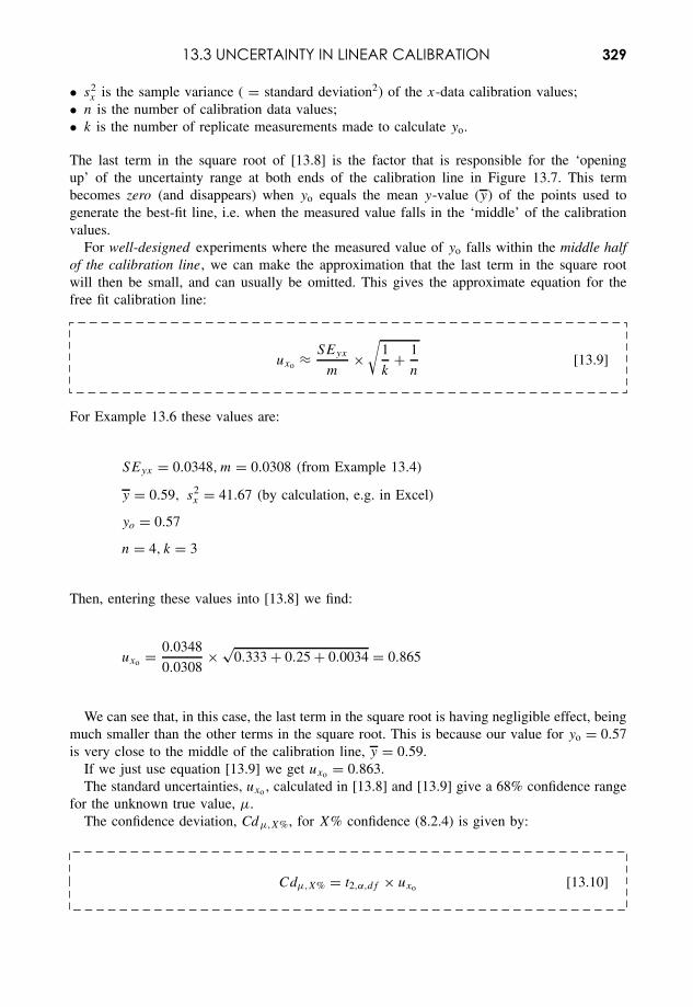
13.3 UNCERTAINTY IN LINEAR CALIBRATION 329
• s2x is the sample variance ( = standard deviation2) of the x-data calibration values;
• n is the number of calibration data values;• k is the number of replicate measurements made to calculate yo.
The last term in the square root of [13.8] is the factor that is responsible for the ‘openingup’ of the uncertainty range at both ends of the calibration line in Figure 13.7. This termbecomes zero (and disappears) when yo equals the mean y-value (y) of the points used togenerate the best-fit line, i.e. when the measured value falls in the ‘middle’ of the calibrationvalues.
For well-designed experiments where the measured value of yo falls within the middle halfof the calibration line, we can make the approximation that the last term in the square rootwill then be small, and can usually be omitted. This gives the approximate equation for thefree fit calibration line:
uxo ≈ SEyx
m×
√1
k+ 1
n[13.9]
For Example 13.6 these values are:
SEyx = 0.0348, m = 0.0308 (from Example 13.4)
y = 0.59, s2x = 41.67 (by calculation, e.g. in Excel)
yo = 0.57
n = 4, k = 3
Then, entering these values into [13.8] we find:
uxo = 0.0348
0.0308× √
0.333 + 0.25 + 0.0034 = 0.865
We can see that, in this case, the last term in the square root is having negligible effect, beingmuch smaller than the other terms in the square root. This is because our value for yo = 0.57is very close to the middle of the calibration line, y = 0.59.
If we just use equation [13.9] we get uxo = 0.863.The standard uncertainties, uxo , calculated in [13.8] and [13.9] give a 68% confidence range
for the unknown true value, µ.The confidence deviation, Cdµ,X%, for X% confidence (8.2.4) is given by:
Cdµ,X% = t2,α,df × uxo [13.10]
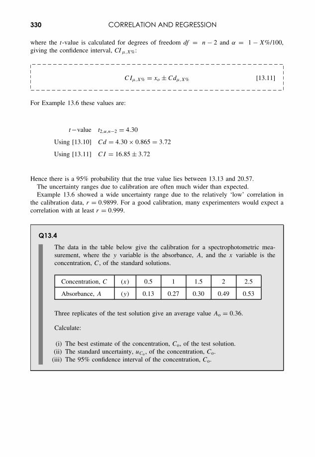
330 CORRELATION AND REGRESSION
where the t-value is calculated for degrees of freedom df = n − 2 and α = 1 − X%/100,giving the confidence interval, CI µ,X%:
CIµ,X% = xo ± Cdµ,X% [13.11]
For Example 13.6 these values are:
t−value t2,α,n−2 = 4.30
Using [13.10] Cd = 4.30 × 0.865 = 3.72
Using [13.11] CI = 16.85 ± 3.72
Hence there is a 95% probability that the true value lies between 13.13 and 20.57.The uncertainty ranges due to calibration are often much wider than expected.Example 13.6 showed a wide uncertainty range due to the relatively ‘low’ correlation in
the calibration data, r = 0.9899. For a good calibration, many experimenters would expect acorrelation with at least r = 0.999.
Q13.4The data in the table below give the calibration for a spectrophotometric mea-surement, where the y variable is the absorbance, A, and the x variable is theconcentration, C, of the standard solutions.
Concentration, C (x) 0.5 1 1.5 2 2.5
Absorbance, A (y) 0.13 0.27 0.30 0.49 0.53
Three replicates of the test solution give an average value Ao = 0.36.
Calculate:
(i) The best estimate of the concentration, Co, of the test solution.(ii) The standard uncertainty, uCo , of the concentration, Co.
(iii) The 95% confidence interval of the concentration, Co.
14Frequency and Proportion
Overview
Website • ‘How to do it’ video answers for all ‘Q’ questions.• Chi-squared tests in Excel and Minitab.• Proportion tests in Minitab.
There are many occasions when the experimental variable being measured is the frequency withwhich particular events occur, e.g. counting how many seeds have germinated under differentsets of conditions.
The chi-squared, χ2, hypothesis tests provide a family of tests often used to analyse setsof frequencies. The calculated χ2 statistic is used to test whether an observed distribution offrequencies might have occurred purely by chance or whether an underlying factor had causeda deviation from an expected distribution.
The first unit applies the χ2 test to a contingency table which assesses whether differencesbetween frequency distributions of observed events might be due to different external condi-tions. For example, we might investigate whether the number of seeds germinating is dependenton (contingent on) particular conditions of temperature and moisture.
The second unit tests whether a single set of frequencies represent a ‘good fit’ with anexpected set of frequencies. The ‘goodness of fit’ test is used to test whether the observeddistribution of events might be consistent with an underlying theory. This test can be used toassess whether observed distributions may, or may not, follow certain predicted distributions(e.g. Poisson).
When the possible observed events fall into one of just two possible categories , then wehave a simple proportion, e.g. the proportion of times that a tossed coin will give a ‘head’.We saw in 9.3.2 that the simple choice of two alternatives can be analysed using the binomialdistribution, and in 14.3.2 this is developed into Fisher’s exact test. We also investigate the useof both χ2 statistics and a normal distribution when comparing an observed proportion withan expected proportion.
Excel functions can be used to perform a χ2 test – see Appendix I. The Excel functionCHIINV can also be used to give values for χ2
CRIT (14.1.2 and 14.2.2).
Essential Mathematics and Statistics for Science 2nd Edition Graham Currell and Antony DowmanCopyright c© 2009 John Wiley & Sons, Ltd
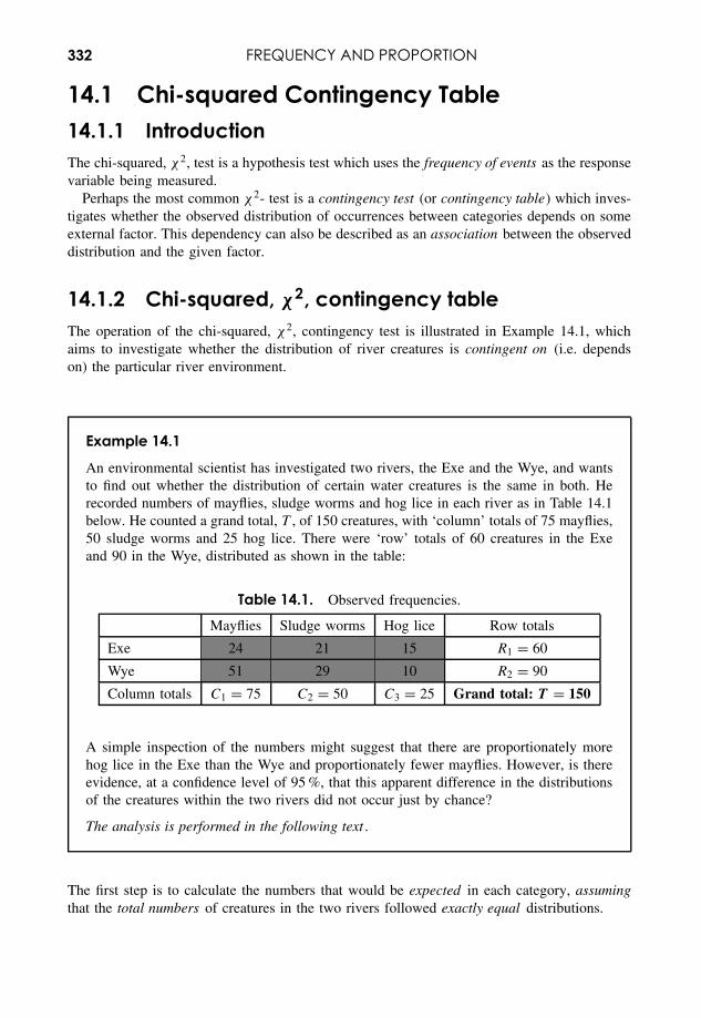
332 FREQUENCY AND PROPORTION
14.1 Chi-squared Contingency Table14.1.1 IntroductionThe chi-squared, χ2, test is a hypothesis test which uses the frequency of events as the responsevariable being measured.
Perhaps the most common χ2- test is a contingency test (or contingency table) which inves-tigates whether the observed distribution of occurrences between categories depends on someexternal factor. This dependency can also be described as an association between the observeddistribution and the given factor.
14.1.2 Chi-squared, χ2, contingency tableThe operation of the chi-squared, χ2, contingency test is illustrated in Example 14.1, whichaims to investigate whether the distribution of river creatures is contingent on (i.e. dependson) the particular river environment.
Example 14.1
An environmental scientist has investigated two rivers, the Exe and the Wye, and wantsto find out whether the distribution of certain water creatures is the same in both. Herecorded numbers of mayflies, sludge worms and hog lice in each river as in Table 14.1below. He counted a grand total, T , of 150 creatures, with ‘column’ totals of 75 mayflies,50 sludge worms and 25 hog lice. There were ‘row’ totals of 60 creatures in the Exeand 90 in the Wye, distributed as shown in the table:
Table 14.1. Observed frequencies.
Mayflies Sludge worms Hog lice Row totals
Exe 24 21 15 R1 = 60
Wye 51 29 10 R2 = 90
Column totals C1 = 75 C2 = 50 C3 = 25 Grand total: T = 150
A simple inspection of the numbers might suggest that there are proportionately morehog lice in the Exe than the Wye and proportionately fewer mayflies. However, is thereevidence, at a confidence level of 95 %, that this apparent difference in the distributionsof the creatures within the two rivers did not occur just by chance?
The analysis is performed in the following text .
The first step is to calculate the numbers that would be expected in each category, assumingthat the total numbers of creatures in the two rivers followed exactly equal distributions.
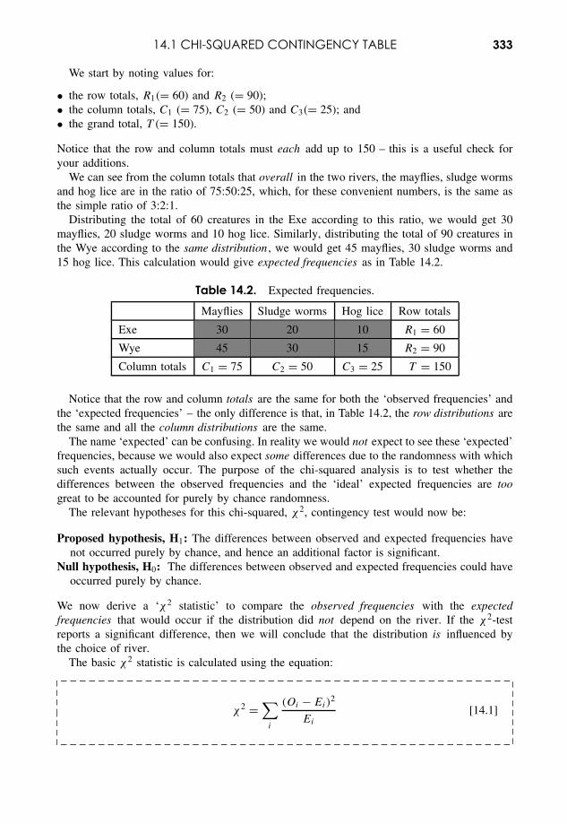
14.1 CHI-SQUARED CONTINGENCY TABLE 333
We start by noting values for:
• the row totals, R1(= 60) and R2 (= 90);• the column totals, C1 (= 75), C2 (= 50) and C3(= 25); and• the grand total, T (= 150).
Notice that the row and column totals must each add up to 150 – this is a useful check foryour additions.
We can see from the column totals that overall in the two rivers, the mayflies, sludge wormsand hog lice are in the ratio of 75:50:25, which, for these convenient numbers, is the same asthe simple ratio of 3:2:1.
Distributing the total of 60 creatures in the Exe according to this ratio, we would get 30mayflies, 20 sludge worms and 10 hog lice. Similarly, distributing the total of 90 creatures inthe Wye according to the same distribution , we would get 45 mayflies, 30 sludge worms and15 hog lice. This calculation would give expected frequencies as in Table 14.2.
Table 14.2. Expected frequencies.
Mayflies Sludge worms Hog lice Row totals
Exe 30 20 10 R1 = 60
Wye 45 30 15 R2 = 90
Column totals C1 = 75 C2 = 50 C3 = 25 T = 150
Notice that the row and column totals are the same for both the ‘observed frequencies’ andthe ‘expected frequencies’ – the only difference is that, in Table 14.2, the row distributions arethe same and all the column distributions are the same.
The name ‘expected’ can be confusing. In reality we would not expect to see these ‘expected’frequencies, because we would also expect some differences due to the randomness with whichsuch events actually occur. The purpose of the chi-squared analysis is to test whether thedifferences between the observed frequencies and the ‘ideal’ expected frequencies are toogreat to be accounted for purely by chance randomness.
The relevant hypotheses for this chi-squared, χ2, contingency test would now be:
Proposed hypothesis, H1: The differences between observed and expected frequencies havenot occurred purely by chance, and hence an additional factor is significant.
Null hypothesis, H0: The differences between observed and expected frequencies could haveoccurred purely by chance.
We now derive a ‘χ2 statistic’ to compare the observed frequencies with the expectedfrequencies that would occur if the distribution did not depend on the river. If the χ2-testreports a significant difference, then we will conclude that the distribution is influenced bythe choice of river.
The basic χ2 statistic is calculated using the equation:
χ2 =∑
i
(Oi − Ei)2
Ei
[14.1]
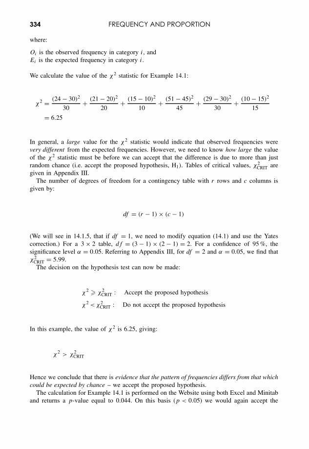
334 FREQUENCY AND PROPORTION
where:
Oi is the observed frequency in category i, andEi is the expected frequency in category i.
We calculate the value of the χ2 statistic for Example 14.1:
χ2 = (24 − 30)2
30+ (21 − 20)2
20+ (15 − 10)2
10+ (51 − 45)2
45+ (29 − 30)2
30+ (10 − 15)2
15
= 6.25
In general, a large value for the χ2 statistic would indicate that observed frequencies werevery different from the expected frequencies. However, we need to know how large the valueof the χ2 statistic must be before we can accept that the difference is due to more than justrandom chance (i.e. accept the proposed hypothesis, H1). Tables of critical values, χ2
CRIT aregiven in Appendix III.
The number of degrees of freedom for a contingency table with r rows and c columns isgiven by:
df = (r − 1) × (c − 1)
(We will see in 14.1.5, that if df = 1, we need to modify equation (14.1) and use the Yatescorrection.) For a 3 × 2 table, df = (3 − 1) × (2 − 1) = 2. For a confidence of 95 %, thesignificance level α = 0.05. Referring to Appendix III, for df = 2 and α = 0.05, we find thatχ2
CRIT = 5.99.The decision on the hypothesis test can now be made:
χ2 � χ2CRIT : Accept the proposed hypothesis
χ2 <χ2CRIT : Do not accept the proposed hypothesis
In this example, the value of χ2 is 6.25, giving:
χ2 > χ2CRIT
Hence we conclude that there is evidence that the pattern of frequencies differs from that whichcould be expected by chance – we accept the proposed hypothesis.
The calculation for Example 14.1 is performed on the Website using both Excel and Minitaband returns a p-value equal to 0.044. On this basis (p < 0.05) we would again accept the
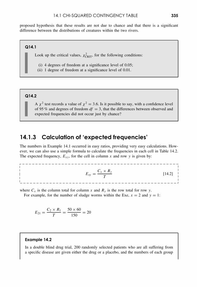
14.1 CHI-SQUARED CONTINGENCY TABLE 335
proposed hypothesis that these results are not due to chance and that there is a significantdifference between the distributions of creatures within the two rivers.
Q14.1
Look up the critical values, χ2CRIT, for the following conditions:
(i) 4 degrees of freedom at a significance level of 0.05;(ii) 1 degree of freedom at a significance level of 0.01.
Q14.2
A χ2 test records a value of χ2 = 3.6. Is it possible to say, with a confidence levelof 95 % and degrees of freedom df = 3, that the differences between observed andexpected frequencies did not occur just by chance?
14.1.3 Calculation of ‘expected frequencies’The numbers in Example 14.1 occurred in easy ratios, providing very easy calculations. How-ever, we can also use a simple formula to calculate the frequencies in each cell in Table 14.2.The expected frequency, Exy , for the cell in column x and row y is given by:
Exy = Cx × Ry
T[14.2]
where Cx is the column total for column x and Ry is the row total for row y.For example, for the number of sludge worms within the Exe, x = 2 and y = 1:
E21 = C2 × R1
T= 50 × 60
150= 20
Example 14.2
In a double blind drug trial, 200 randomly selected patients who are all suffering froma specific disease are given either the drug or a placebo, and the numbers of each group
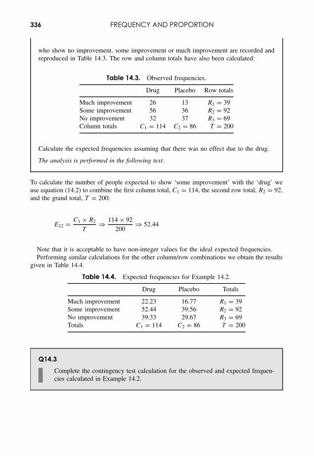
336 FREQUENCY AND PROPORTION
who show no improvement, some improvement or much improvement are recorded andreproduced in Table 14.3. The row and column totals have also been calculated:
Table 14.3. Observed frequencies.
Drug Placebo Row totals
Much improvement 26 13 R1 = 39Some improvement 56 36 R2 = 92No improvement 32 37 R3 = 69Column totals C1 = 114 C2 = 86 T = 200
Calculate the expected frequencies assuming that there was no effect due to the drug.
The analysis is performed in the following text .
To calculate the number of people expected to show ‘some improvement’ with the ‘drug’ weuse equation (14.2) to combine the first column total, C1 = 114, the second row total, R2 = 92,and the grand total, T = 200:
E12 = C1 × R2
T⇒ 114 × 92
200⇒ 52.44
Note that it is acceptable to have non-integer values for the ideal expected frequencies.Performing similar calculations for the other column/row combinations we obtain the results
given in Table 14.4.
Table 14.4. Expected frequencies for Example 14.2.
Drug Placebo Totals
Much improvement 22.23 16.77 R1 = 39Some improvement 52.44 39.56 R2 = 92No improvement 39.33 29.67 R3 = 69Totals C1 = 114 C2 = 86 T = 200
Q14.3Complete the contingency test calculation for the observed and expected frequen-cies calculated in Example 14.2.
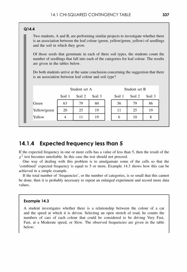
14.1 CHI-SQUARED CONTINGENCY TABLE 337
Q14.4Two students, A and B, are performing similar projects to investigate whether thereis an association between the leaf colour (green, yellow/green, yellow) of seedlingsand the soil in which they grow.
Of those seeds that germinate in each of three soil types, the students count thenumber of seedlings that fall into each of the categories for leaf colour. The resultsare given in the tables below.
Do both students arrive at the same conclusion concerning the suggestion that thereis an association between leaf colour and soil type?
Student set A Student set B
Soil 1 Soil 2 Soil 3 Soil 1 Soil 2 Soil 3
Green 63 79 60 56 79 86
Yellow/green 20 25 19 11 25 19
Yellow 4 11 19 6 10 8
14.1.4 Expected frequency less than 5If the expected frequency in one or more cells has a value of less than 5, then the result of theχ2 test becomes unreliable. In this case the test should not proceed.
One way of dealing with this problem is to amalgamate some of the cells so that the‘combined’ expected frequency is equal to 5 or more. Example 14.3 shows how this can beachieved in a simple example.
If the total number of ‘frequencies’, or the number of categories, is so small that this cannotbe done, then it is probably necessary to repeat an enlarged experiment and record more datavalues.
Example 14.3
A student investigates whether there is a relationship between the colour of a carand the speed at which it is driven. Selecting an open stretch of road, he counts thenumbers of cars of each colour that could be considered to be driving Very Fast,Fast, at a Moderate speed, or Slow. The observed frequencies are given in the tablebelow:
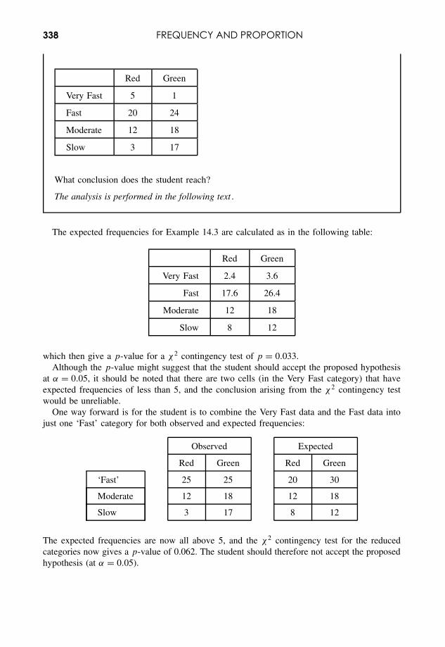
338 FREQUENCY AND PROPORTION
Red Green
Very Fast 5 1
Fast 20 24
Moderate 12 18
Slow 3 17
What conclusion does the student reach?
The analysis is performed in the following text .
The expected frequencies for Example 14.3 are calculated as in the following table:
Red Green
Very Fast 2.4 3.6
Fast 17.6 26.4
Moderate 12 18
Slow 8 12
which then give a p-value for a χ2 contingency test of p = 0.033.Although the p-value might suggest that the student should accept the proposed hypothesis
at α = 0.05, it should be noted that there are two cells (in the Very Fast category) that haveexpected frequencies of less than 5, and the conclusion arising from the χ2 contingency testwould be unreliable.
One way forward is for the student is to combine the Very Fast data and the Fast data intojust one ‘Fast’ category for both observed and expected frequencies:
Observed Expected
Red Green Red Green
‘Fast’ 25 25 20 30
Moderate 12 18 12 18
Slow 3 17 8 12
The expected frequencies are now all above 5, and the χ2 contingency test for the reducedcategories now gives a p-value of 0.062. The student should therefore not accept the proposedhypothesis (at α = 0.05).
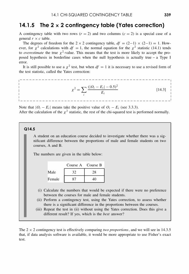
14.1 CHI-SQUARED CONTINGENCY TABLE 339
14.1.5 The 2 × 2 contingency table (Yates correction)A contingency table with two rows (r = 2) and two columns (c = 2) is a special case of ageneral r × c table.
The degrees of freedom for the 2 × 2 contingency table, df = (2−1) × (2−1) = 1. How-ever, for χ2 calculations with df = 1, the normal equation for the χ2 statistic (14.1) tendsto overestimate the true χ2-value. This means that the test is more likely to accept the pro-posed hypothesis in borderline cases when the null hypothesis is actually true – a Type Ierror.
It is still possible to use a χ2 test, but when df = 1 it is necessary to use a revised form ofthe test statistic, called the Yates correction:
χ2 =∑
i
(|Oi − Ei | − 0.5)2
Ei
[14.3]
Note that |Oi − Ei | means take the positive value of Oi − Ei (see 3.3.3).After the calculation of the χ2 statistic, the rest of the chi-squared test is performed normally.
Q14.5A student on an education course decided to investigate whether there was a sig-nificant difference between the proportions of male and female students on twocourses, A and B.
The numbers are given in the table below:
Course A Course B
Male 32 28
Female 87 40
(i) Calculate the numbers that would be expected if there were no preferencebetween the courses for male and female students.
(ii) Perform a contingency test, using the Yates correction, to assess whetherthere is a significant difference in the proportions between the courses.
(iii) Repeat the test in (ii) without using the Yates correction. Does this give adifferent result? If yes, which is the best answer?
The 2 × 2 contingency test is effectively comparing two proportions , and we will see in 14.3.5that, if data analysis software is available, it would be more appropriate to use Fisher’s exacttest.

340 FREQUENCY AND PROPORTION
14.2 Goodness of Fit14.2.1 IntroductionA goodness of fit test tests whether an observed distribution of occurrences in specific categoriesis significantly different from the distribution that would have been expected. For example, wecould test whether the numbers of students obtaining various grade categories is significantlydifferent between years.
We will see that the χ2 test can be used to compare the observed frequency , O , in eachcategory with the expected frequency , E. In some examples, it may be necessary to calculateexpected frequencies on the basis of an expected set of ratios .
The procedure can also be used to test whether the distribution of some experimentallyobserved frequencies might follow a known distribution pattern, e.g. a normal distribution ora Poisson distribution – see the Website.
It should be noted that there are also alternative methods available in statistics software fortesting for goodness of fit to a distribution, e.g. for testing whether a given set of sample datais likely to have been drawn from a normal distribution.
14.2.2 Comparison with defined ratiosExample 14.4 illustrates the use of the χ2 statistic when comparing observed frequencies witha set of ratios that is predicted, either by theory or by historical measurements.
Example 14.4
Measurement of genotypes is expected to show types AB, Ab, aB, ab occurring in theratio 9:3:3:1. A sample of T = 200 observations gave observed frequencies, Oi , of 131,28, 32 and 9 respectively in the four groups.
Test whether this distribution of values shows a significant difference from the expectedratios.
The analysis is performed in the following text .
The relevant hypotheses for the test in Example 14.4 would be:
Proposed hypothesis, H1: The differences between observed frequencies and the given ratioshave not occurred just by chance, and hence an additional factor is significant.
Null hypothesis, H0: The differences between observed frequencies and the given ratios mighthave occurred just by chance.
We set out the calculations in the form of a table (Table 14.5) in which we calculate thetotals, T and RT , for both the observed numbers and the ratio values respectively:
We can see that the fraction of observations falling into the category AB would be equal toRAB = 9 of a total of RT = 16. Thus the expected frequency for category AB would be found
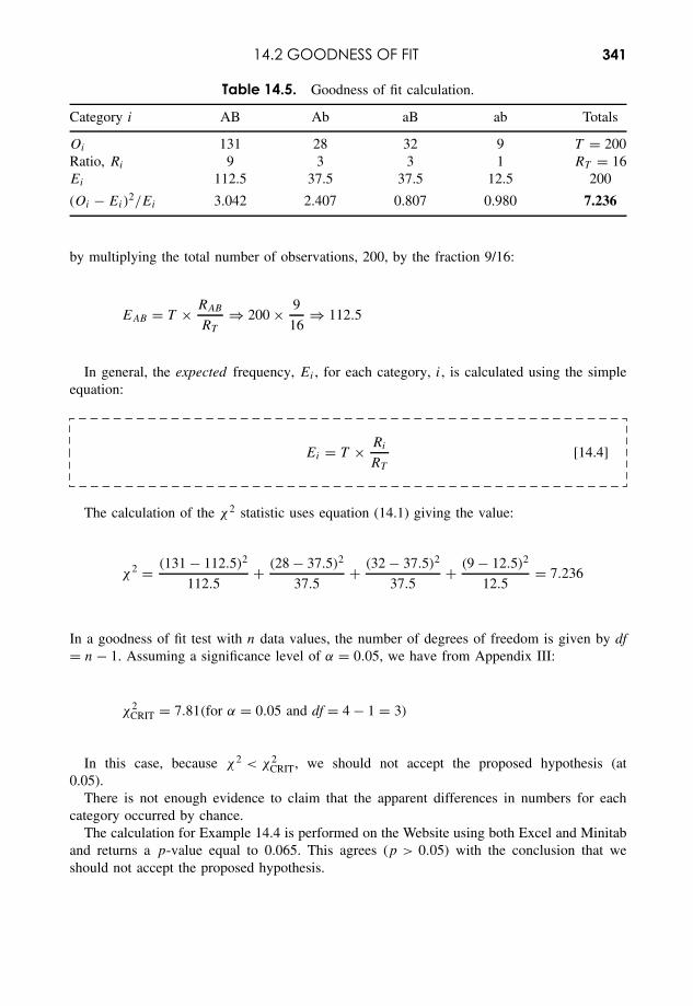
14.2 GOODNESS OF FIT 341
Table 14.5. Goodness of fit calculation.
Category i AB Ab aB ab Totals
Oi 131 28 32 9 T = 200Ratio, Ri 9 3 3 1 RT = 16Ei 112.5 37.5 37.5 12.5 200
(Oi − Ei)2/Ei 3.042 2.407 0.807 0.980 7.236
by multiplying the total number of observations, 200, by the fraction 9/16:
EAB = T × RAB
RT
⇒ 200 × 9
16⇒ 112.5
In general, the expected frequency, Ei , for each category, i, is calculated using the simpleequation:
Ei = T × Ri
RT
[14.4]
The calculation of the χ2 statistic uses equation (14.1) giving the value:
χ2 = (131 − 112.5)2
112.5+ (28 − 37.5)2
37.5+ (32 − 37.5)2
37.5+ (9 − 12.5)2
12.5= 7.236
In a goodness of fit test with n data values, the number of degrees of freedom is given by df= n − 1. Assuming a significance level of α = 0.05, we have from Appendix III:
χ2CRIT = 7.81(for α = 0.05 and df = 4 − 1 = 3)
In this case, because χ2 < χ2CRIT, we should not accept the proposed hypothesis (at
0.05).There is not enough evidence to claim that the apparent differences in numbers for each
category occurred by chance.The calculation for Example 14.4 is performed on the Website using both Excel and Minitab
and returns a p-value equal to 0.065. This agrees (p > 0.05) with the conclusion that weshould not accept the proposed hypothesis.
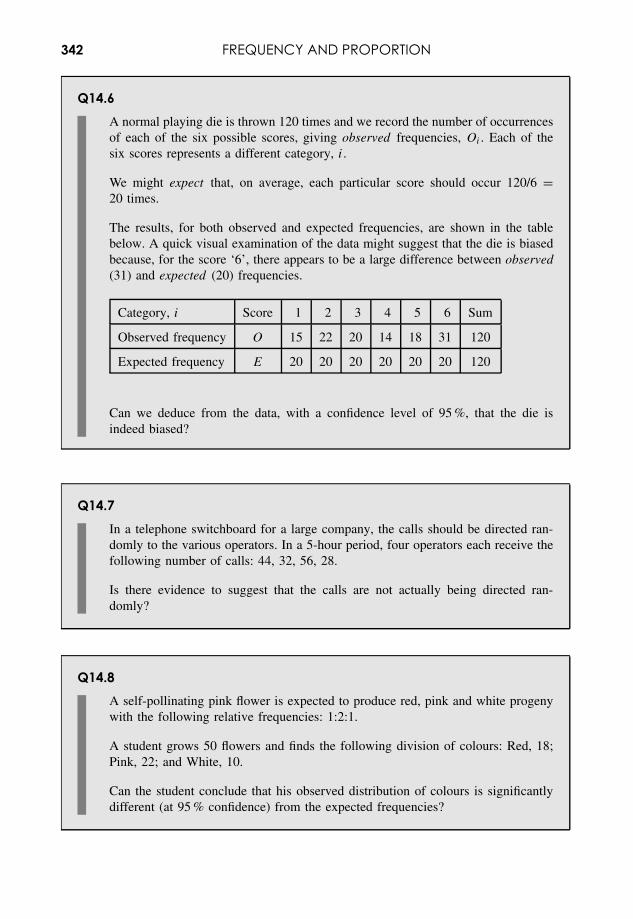
342 FREQUENCY AND PROPORTION
Q14.6A normal playing die is thrown 120 times and we record the number of occurrencesof each of the six possible scores, giving observed frequencies, Oi . Each of thesix scores represents a different category, i.
We might expect that, on average, each particular score should occur 120/6 =20 times.
The results, for both observed and expected frequencies, are shown in the tablebelow. A quick visual examination of the data might suggest that the die is biasedbecause, for the score ‘6’, there appears to be a large difference between observed(31) and expected (20) frequencies.
Category, i Score 1 2 3 4 5 6 Sum
Observed frequency O 15 22 20 14 18 31 120
Expected frequency E 20 20 20 20 20 20 120
Can we deduce from the data, with a confidence level of 95 %, that the die isindeed biased?
Q14.7In a telephone switchboard for a large company, the calls should be directed ran-domly to the various operators. In a 5-hour period, four operators each receive thefollowing number of calls: 44, 32, 56, 28.
Is there evidence to suggest that the calls are not actually being directed ran-domly?
Q14.8A self-pollinating pink flower is expected to produce red, pink and white progenywith the following relative frequencies: 1:2:1.
A student grows 50 flowers and finds the following division of colours: Red, 18;Pink, 22; and White, 10.
Can the student conclude that his observed distribution of colours is significantlydifferent (at 95 % confidence) from the expected frequencies?
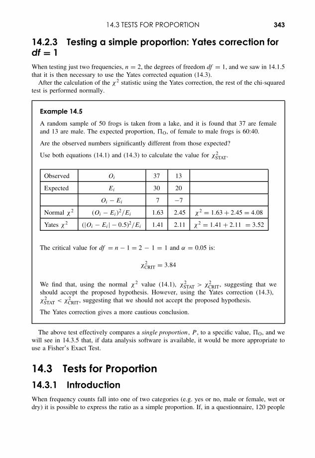
14.3 TESTS FOR PROPORTION 343
14.2.3 Testing a simple proportion: Yates correction fordf = 1When testing just two frequencies, n = 2, the degrees of freedom df = 1, and we saw in 14.1.5that it is then necessary to use the Yates corrected equation (14.3).
After the calculation of the χ2 statistic using the Yates correction, the rest of the chi-squaredtest is performed normally.
Example 14.5
A random sample of 50 frogs is taken from a lake, and it is found that 37 are femaleand 13 are male. The expected proportion, �O, of female to male frogs is 60:40.
Are the observed numbers significantly different from those expected?
Use both equations (14.1) and (14.3) to calculate the value for χ2STAT.
Observed Oi 37 13
Expected Ei 30 20
Oi − Ei 7 −7
Normal χ2 (Oi − Ei)2/Ei 1.63 2.45 χ2 = 1.63 + 2.45 = 4.08
Yates χ2 (|Oi − Ei | − 0.5)2/Ei 1.41 2.11 χ2 = 1.41 + 2.11 = 3.52
The critical value for df = n − 1 = 2 − 1 = 1 and α = 0.05 is:
χ2CRIT = 3.84
We find that, using the normal χ2 value (14.1), χ2STAT > χ2
CRIT, suggesting that weshould accept the proposed hypothesis. However, using the Yates correction (14.3),χ2
STAT < χ2CRIT, suggesting that we should not accept the proposed hypothesis.
The Yates correction gives a more cautious conclusion.
The above test effectively compares a single proportion , P , to a specific value, �O, and wewill see in 14.3.5 that, if data analysis software is available, it would be more appropriate touse a Fisher’s Exact Test.
14.3 Tests for Proportion14.3.1 IntroductionWhen frequency counts fall into one of two categories (e.g. yes or no, male or female, wet ordry) it is possible to express the ratio as a simple proportion. If, in a questionnaire, 120 people
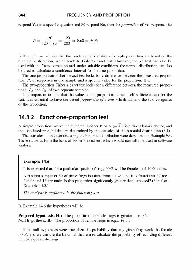
344 FREQUENCY AND PROPORTION
respond Yes to a specific question and 80 respond No, then the proportion of Yes responses is:
P = 120
120 + 80⇒ 120
200⇒ 0.60 ⇒ 60 %
In this unit we will see that the fundamental statistics of simple proportion are based on thebinomial distribution, which leads to Fisher’s exact test. However, the χ2 test can also beused with the Yates correction and, under suitable conditions, the normal distribution can alsobe used to calculate a confidence interval for the true proportion.
The one-proportion Fisher’s exact test looks for a difference between the measured propor-tion, P , of responses in one sample and a specific value for the proportion, �O.
The two-proportion Fisher’s exact test looks for a difference between the measured propor-tions, PA and PB, of two separate samples.
It is important to note that the value of the proportion is not itself sufficient data for thetest. It is essential to have the actual frequencies of events which fall into the two categoriesof the proportion.
14.3.2 Exact one-proportion testA simple proportion, where the outcome is either Y or N (= Y), is a direct binary choice, andthe associated probabilities are determined by the statistics of the binomial distribution (8.4).
The statistics of an exact test using the binomial distribution were developed in Example 9.4.These statistics form the basis of Fisher’s exact test which would normally be used in softwareanalysis.
Example 14.6
It is expected that, for a particular species of frog, 60 % will be females and 40 % males.
A random sample of 50 of these frogs is taken from a lake, and it is found that 37 arefemale and 13 are male. Is this proportion significantly greater than expected? (See alsoExample 14.5.)
The analysis is performed in the following text .
In Example 14.6 the hypotheses will be:
Proposed hypothesis, H1: The proportion of female frogs is greater than 0.6.Null hypothesis, H0: The proportion of female frogs is equal to 0.6.
If the null hypothesis were true, then the probability that any given frog would be femaleis 0.6, and we can use the binomial theorem to calculate the probability of recording differentnumbers of female frogs.
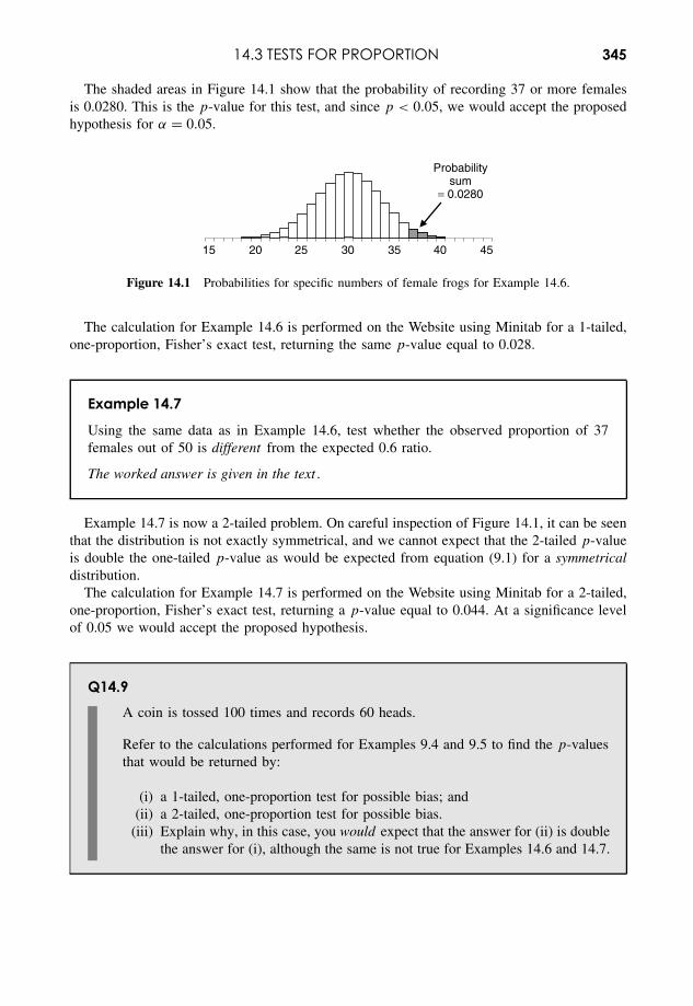
14.3 TESTS FOR PROPORTION 345
The shaded areas in Figure 14.1 show that the probability of recording 37 or more femalesis 0.0280. This is the p-value for this test, and since p < 0.05, we would accept the proposedhypothesis for α = 0.05.
15 20 25 30 35 40 45
Probabilitysum
= 0.0280
Figure 14.1 Probabilities for specific numbers of female frogs for Example 14.6.
The calculation for Example 14.6 is performed on the Website using Minitab for a 1-tailed,one-proportion, Fisher’s exact test, returning the same p-value equal to 0.028.
Example 14.7
Using the same data as in Example 14.6, test whether the observed proportion of 37females out of 50 is different from the expected 0.6 ratio.
The worked answer is given in the text .
Example 14.7 is now a 2-tailed problem. On careful inspection of Figure 14.1, it can be seenthat the distribution is not exactly symmetrical, and we cannot expect that the 2-tailed p-valueis double the one-tailed p-value as would be expected from equation (9.1) for a symmetricaldistribution.
The calculation for Example 14.7 is performed on the Website using Minitab for a 2-tailed,one-proportion, Fisher’s exact test, returning a p-value equal to 0.044. At a significance levelof 0.05 we would accept the proposed hypothesis.
Q14.9A coin is tossed 100 times and records 60 heads.
Refer to the calculations performed for Examples 9.4 and 9.5 to find the p-valuesthat would be returned by:
(i) a 1-tailed, one-proportion test for possible bias; and(ii) a 2-tailed, one-proportion test for possible bias.
(iii) Explain why, in this case, you would expect that the answer for (ii) is doublethe answer for (i), although the same is not true for Examples 14.6 and 14.7.
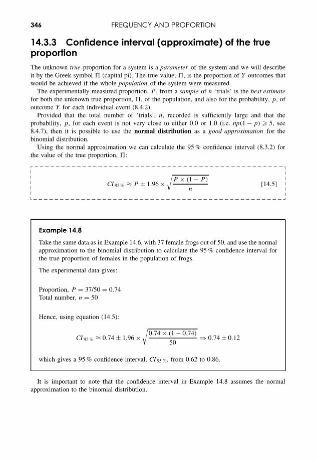
346 FREQUENCY AND PROPORTION
14.3.3 Confidence interval (approximate) of the trueproportionThe unknown true proportion for a system is a parameter of the system and we will describeit by the Greek symbol � (capital pi). The true value, �, is the proportion of Y outcomes thatwould be achieved if the whole population of the system were measured.
The experimentally measured proportion, P , from a sample of n ‘trials’ is the best estimatefor both the unknown true proportion, �, of the population, and also for the probability, p, ofoutcome Y for each individual event (8.4.2).
Provided that the total number of ‘trials’, n, recorded is sufficiently large and that theprobability, p, for each event is not very close to either 0.0 or 1.0 (i.e. np(1 − p) � 5, see8.4.7), then it is possible to use the normal distribution as a good approximation for thebinomial distribution.
Using the normal approximation we can calculate the 95 % confidence interval (8.3.2) forthe value of the true proportion, �:
CI 95 % ≈ P ± 1.96 ×√
P × (1 − P )
n[14.5]
Example 14.8
Take the same data as in Example 14.6, with 37 female frogs out of 50, and use the normalapproximation to the binomial distribution to calculate the 95 % confidence interval forthe true proportion of females in the population of frogs.
The experimental data gives:
Proportion, P = 37/50 = 0.74Total number, n = 50
Hence, using equation (14.5):
CI 95 % ≈ 0.74 ± 1.96 ×√
0.74 × (1 − 0.74)
50⇒ 0.74 ± 0.12
which gives a 95 % confidence interval, CI 95 %, from 0.62 to 0.86.
It is important to note that the confidence interval in Example 14.8 assumes the normalapproximation to the binomial distribution.
14.3 TESTS FOR PROPORTION 347
Q14.10A coin is tossed 100 times and records 60 heads.
(i) Use the normal distribution approximation to calculate the 95 % confidenceinterval for the true probability of recording a ‘head’ in a single toss.
(ii) Does your answer in (i) suggest that, at a significance level of 0.05, the coinis biased and does not have a true probability of 0.5?
14.3.4 Comparison of statistical testsExample 14.9 illustrates the fact that it is not uncommon to find that there is more than justone way of addressing a given analytical problem.
Example 14.9
Compare Examples 14.5, 14.7 and 14.8 to investigate three ways of addressing the sametwo-tailed, one-proportion test.
Do the conclusions differ on whether the proportion of 37 out of 50 is significantlydifferent from 0.6?
Chi-squared test
The standard calculation of the chi-squared test (Example 14.5) identifies a significantdifference, but the Yates correction is more cautious, suggesting that there is no significantdifference.
Confidence interval calculation
The confidence interval (Example 14.8) for the true proportion gives a range from 0.62to 0.86, and as 0.6 is just outside this range, this suggests a significant difference.
One-proportion exact test
The p-value of 0.044 from Fisher’s exact test (Example 14.7) is just in favour of asignificant difference.
Clearly from Example 14.9, the approximations using the chi-squared distribution or thenormal distribution can return slightly different values and conclusions. However, provided the
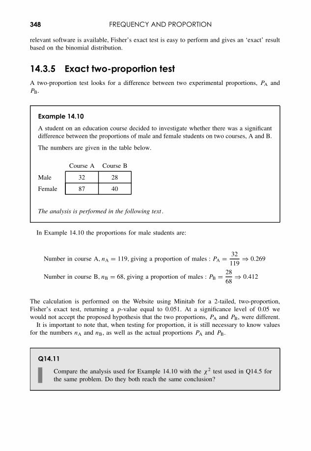
348 FREQUENCY AND PROPORTION
relevant software is available, Fisher’s exact test is easy to perform and gives an ‘exact’ resultbased on the binomial distribution.
14.3.5 Exact two-proportion testA two-proportion test looks for a difference between two experimental proportions, PA andPB.
Example 14.10
A student on an education course decided to investigate whether there was a significantdifference between the proportions of male and female students on two courses, A and B.
The numbers are given in the table below.
Course A Course B
Male 32 28
Female 87 40
The analysis is performed in the following text .
In Example 14.10 the proportions for male students are:
Number in course A, nA = 119, giving a proportion of males : PA = 32
119⇒ 0.269
Number in course B, nB = 68, giving a proportion of males : PB = 28
68⇒ 0.412
The calculation is performed on the Website using Minitab for a 2-tailed, two-proportion,Fisher’s exact test, returning a p-value equal to 0.051. At a significance level of 0.05 wewould not accept the proposed hypothesis that the two proportions, PA and PB, were different.
It is important to note that, when testing for proportion, it is still necessary to know valuesfor the numbers nA and nB, as well as the actual proportions PA and PB.
Q14.11
Compare the analysis used for Example 14.10 with the χ2 test used in Q14.5 forthe same problem. Do they both reach the same conclusion?

15Experimental Design
Overview
There is an enormous variety of possible ways to design experiments, and it is important thateach design is tailored to fit the particular investigation. Consequently, it is not possible to givea step-by-step guide to producing the correct design in any given situation. The only practicalapproach is to develop each new experiment on the basis of knowledge and experience of therange of fundamental design principles and data analysis techniques that may be appropriate.This chapter aims to provide an overview of key aspects of experimental design and their linkswith suitable statistical tests.
The objective of good experimental design is to reduce the errors in any measurementand improve the confidence in the final experimental result. In particular, a good experimen-tal design will counteract the effects of possible systematic errors, and take account of themagnitude of possible random errors.
The process of experimental design proceeds hand in hand with the availability of statisticaltechniques for analysing data. In particular, readers are recommended to read Chapters 9 to14 in conjunction with this chapter, and follow the development of statistical tests in parallelwith their use in supporting good experimental design.
15.1 Principal Techniques15.1.1 IntroductionIn general there are five main techniques used in experimental design:
Replication – counteracts the effect of random experimental uncertainties, and makes theireffect more explicit in the analysis.
Randomization – counteracts hidden systematic errors (bias) and makes the effects of randomsubject uncertainties more explicit in the analysis.
Repeated measures or pairing – counteracts for systematic differences between subjects bylinking subject responses in all factor levels.
Essential Mathematics and Statistics for Science 2nd Edition Graham Currell and Antony DowmanCopyright c© 2009 John Wiley & Sons, Ltd
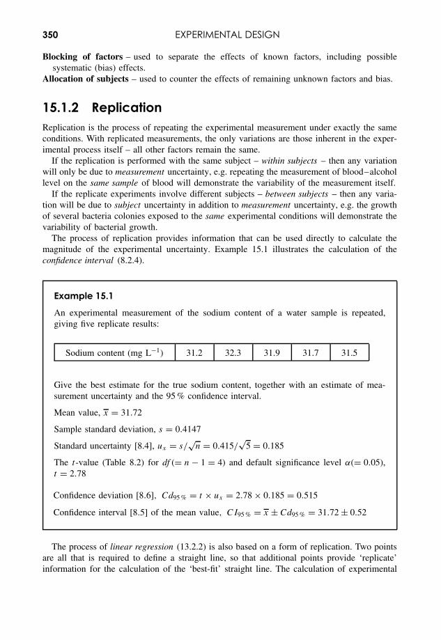
350 EXPERIMENTAL DESIGN
Blocking of factors – used to separate the effects of known factors, including possiblesystematic (bias) effects.
Allocation of subjects – used to counter the effects of remaining unknown factors and bias.
15.1.2 ReplicationReplication is the process of repeating the experimental measurement under exactly the sameconditions. With replicated measurements, the only variations are those inherent in the exper-imental process itself – all other factors remain the same.
If the replication is performed with the same subject – within subjects – then any variationwill only be due to measurement uncertainty, e.g. repeating the measurement of blood–alcohollevel on the same sample of blood will demonstrate the variability of the measurement itself.
If the replicate experiments involve different subjects – between subjects – then any varia-tion will be due to subject uncertainty in addition to measurement uncertainty, e.g. the growthof several bacteria colonies exposed to the same experimental conditions will demonstrate thevariability of bacterial growth.
The process of replication provides information that can be used directly to calculate themagnitude of the experimental uncertainty. Example 15.1 illustrates the calculation of theconfidence interval (8.2.4).
Example 15.1
An experimental measurement of the sodium content of a water sample is repeated,giving five replicate results:
Sodium content (mg L−1) 31.2 32.3 31.9 31.7 31.5
Give the best estimate for the true sodium content, together with an estimate of mea-surement uncertainty and the 95 % confidence interval.
Mean value, x = 31.72
Sample standard deviation, s = 0.4147
Standard uncertainty [8.4], ux = s/√
n = 0.415/√
5 = 0.185
The t-value (Table 8.2) for df (= n − 1 = 4) and default significance level α(= 0.05),t = 2.78
Confidence deviation [8.6], Cd95 % = t × ux = 2.78 × 0.185 = 0.515
Confidence interval [8.5] of the mean value, CI95 % = x ± Cd95 % = 31.72 ± 0.52
The process of linear regression (13.2.2) is also based on a form of replication. Two pointsare all that is required to define a straight line, so that additional points provide ‘replicate’information for the calculation of the ‘best-fit’ straight line. The calculation of experimental
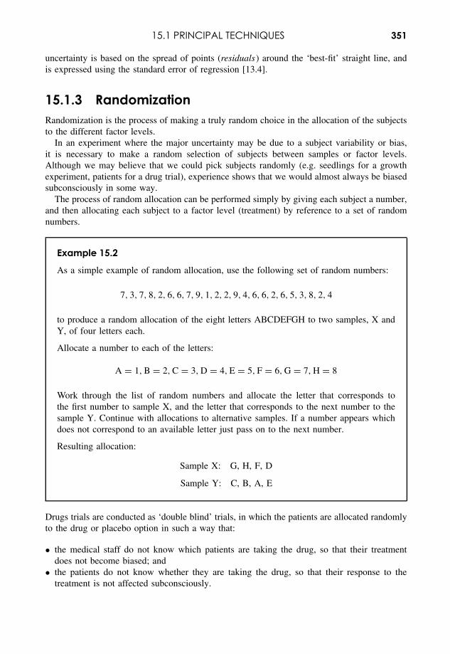
15.1 PRINCIPAL TECHNIQUES 351
uncertainty is based on the spread of points (residuals) around the ‘best-fit’ straight line, andis expressed using the standard error of regression [13.4].
15.1.3 RandomizationRandomization is the process of making a truly random choice in the allocation of the subjectsto the different factor levels.
In an experiment where the major uncertainty may be due to a subject variability or bias,it is necessary to make a random selection of subjects between samples or factor levels.Although we may believe that we could pick subjects randomly (e.g. seedlings for a growthexperiment, patients for a drug trial), experience shows that we would almost always be biasedsubconsciously in some way.
The process of random allocation can be performed simply by giving each subject a number,and then allocating each subject to a factor level (treatment) by reference to a set of randomnumbers.
Example 15.2
As a simple example of random allocation, use the following set of random numbers:
7, 3, 7, 8, 2, 6, 6, 7, 9, 1, 2, 2, 9, 4, 6, 6, 2, 6, 5, 3, 8, 2, 4
to produce a random allocation of the eight letters ABCDEFGH to two samples, X andY, of four letters each.
Allocate a number to each of the letters:
A = 1, B = 2, C = 3, D = 4, E = 5, F = 6, G = 7, H = 8
Work through the list of random numbers and allocate the letter that corresponds tothe first number to sample X, and the letter that corresponds to the next number to thesample Y. Continue with allocations to alternative samples. If a number appears whichdoes not correspond to an available letter just pass on to the next number.
Resulting allocation:
Sample X: G, H, F, D
Sample Y: C, B, A, E
Drugs trials are conducted as ‘double blind’ trials, in which the patients are allocated randomlyto the drug or placebo option in such a way that:
• the medical staff do not know which patients are taking the drug, so that their treatmentdoes not become biased; and
• the patients do not know whether they are taking the drug, so that their response to thetreatment is not affected subconsciously.
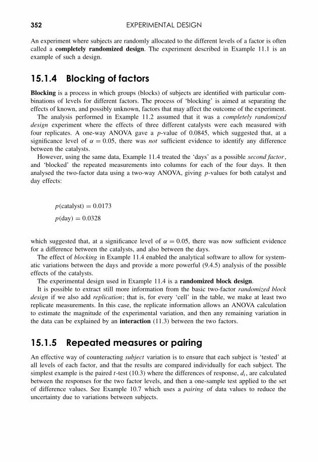
352 EXPERIMENTAL DESIGN
An experiment where subjects are randomly allocated to the different levels of a factor is oftencalled a completely randomized design. The experiment described in Example 11.1 is anexample of such a design.
15.1.4 Blocking of factorsBlocking is a process in which groups (blocks) of subjects are identified with particular com-binations of levels for different factors. The process of ‘blocking’ is aimed at separating theeffects of known, and possibly unknown, factors that may affect the outcome of the experiment.
The analysis performed in Example 11.2 assumed that it was a completely randomizeddesign experiment where the effects of three different catalysts were each measured withfour replicates. A one-way ANOVA gave a p-value of 0.0845, which suggested that, at asignificance level of α = 0.05, there was not sufficient evidence to identify any differencebetween the catalysts.
However, using the same data, Example 11.4 treated the ‘days’ as a possible second factor ,and ‘blocked’ the repeated measurements into columns for each of the four days. It thenanalysed the two-factor data using a two-way ANOVA, giving p-values for both catalyst andday effects:
p(catalyst) = 0.0173
p(day) = 0.0328
which suggested that, at a significance level of α = 0.05, there was now sufficient evidencefor a difference between the catalysts, and also between the days.
The effect of blocking in Example 11.4 enabled the analytical software to allow for system-atic variations between the days and provide a more powerful (9.4.5) analysis of the possibleeffects of the catalysts.
The experimental design used in Example 11.4 is a randomized block design.It is possible to extract still more information from the basic two-factor randomized block
design if we also add replication; that is, for every ‘cell’ in the table, we make at least tworeplicate measurements. In this case, the replicate information allows an ANOVA calculationto estimate the magnitude of the experimental variation, and then any remaining variation inthe data can be explained by an interaction (11.3) between the two factors.
15.1.5 Repeated measures or pairingAn effective way of counteracting subject variation is to ensure that each subject is ‘tested’ atall levels of each factor, and that the results are compared individually for each subject. Thesimplest example is the paired t-test (10.3) where the differences of response, di , are calculatedbetween the responses for the two factor levels, and then a one-sample test applied to the setof difference values. See Example 10.7 which uses a pairing of data values to reduce theuncertainty due to variations between subjects.
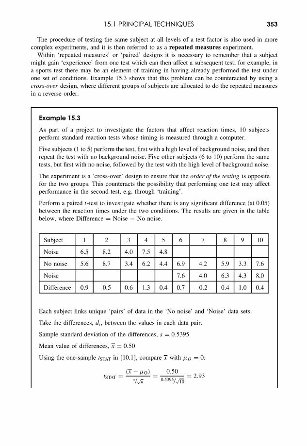
15.1 PRINCIPAL TECHNIQUES 353
The procedure of testing the same subject at all levels of a test factor is also used in morecomplex experiments, and it is then referred to as a repeated measures experiment.
Within ‘repeated measures’ or ‘paired’ designs it is necessary to remember that a subjectmight gain ‘experience’ from one test which can then affect a subsequent test; for example, ina sports test there may be an element of training in having already performed the test underone set of conditions. Example 15.3 shows that this problem can be counteracted by using across-over design, where different groups of subjects are allocated to do the repeated measuresin a reverse order.
Example 15.3
As part of a project to investigate the factors that affect reaction times, 10 subjectsperform standard reaction tests whose timing is measured through a computer.
Five subjects (1 to 5) perform the test, first with a high level of background noise, and thenrepeat the test with no background noise. Five other subjects (6 to 10) perform the sametests, but first with no noise, followed by the test with the high level of background noise.
The experiment is a ‘cross-over’ design to ensure that the order of the testing is oppositefor the two groups. This counteracts the possibility that performing one test may affectperformance in the second test, e.g. through ‘training’.
Perform a paired t-test to investigate whether there is any significant difference (at 0.05)between the reaction times under the two conditions. The results are given in the tablebelow, where Difference = Noise − No noise.
Subject 1 2 3 4 5 6 7 8 9 10
Noise 6.5 8.2 4.0 7.5 4.8
No noise 5.6 8.7 3.4 6.2 4.4 6.9 4.2 5.9 3.3 7.6
Noise 7.6 4.0 6.3 4.3 8.0
Difference 0.9 −0.5 0.6 1.3 0.4 0.7 −0.2 0.4 1.0 0.4
Each subject links unique ‘pairs’ of data in the ‘No noise’ and ‘Noise’ data sets.
Take the differences, di , between the values in each data pair.
Sample standard deviation of the differences, s = 0.5395
Mean value of differences, x = 0.50
Using the one-sample tSTAT in [10.1], compare x with µO = 0:
tSTAT = (x − µO)
s/√n
= 0.500.5395/
√10
= 2.93
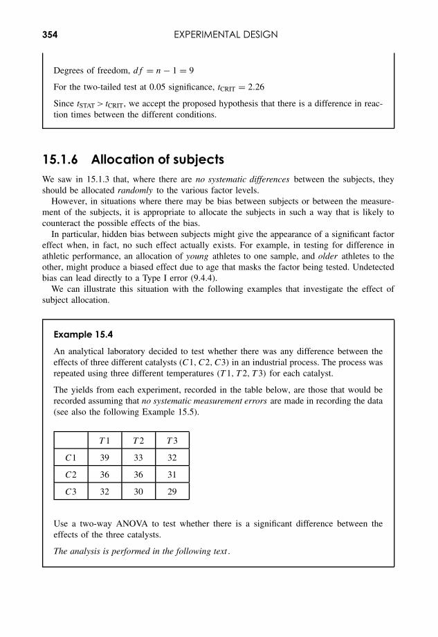
354 EXPERIMENTAL DESIGN
Degrees of freedom, df = n − 1 = 9
For the two-tailed test at 0.05 significance, tCRIT = 2.26
Since tSTAT > tCRIT, we accept the proposed hypothesis that there is a difference in reac-tion times between the different conditions.
15.1.6 Allocation of subjectsWe saw in 15.1.3 that, where there are no systematic differences between the subjects, theyshould be allocated randomly to the various factor levels.
However, in situations where there may be bias between subjects or between the measure-ment of the subjects, it is appropriate to allocate the subjects in such a way that is likely tocounteract the possible effects of the bias.
In particular, hidden bias between subjects might give the appearance of a significant factoreffect when, in fact, no such effect actually exists. For example, in testing for difference inathletic performance, an allocation of young athletes to one sample, and older athletes to theother, might produce a biased effect due to age that masks the factor being tested. Undetectedbias can lead directly to a Type I error (9.4.4).
We can illustrate this situation with the following examples that investigate the effect ofsubject allocation.
Example 15.4
An analytical laboratory decided to test whether there was any difference between theeffects of three different catalysts (C1, C2, C3) in an industrial process. The process wasrepeated using three different temperatures (T 1, T 2, T 3) for each catalyst.
The yields from each experiment, recorded in the table below, are those that would berecorded assuming that no systematic measurement errors are made in recording the data(see also the following Example 15.5).
T 1 T 2 T 3
C1 39 33 32
C2 36 36 31
C3 32 30 29
Use a two-way ANOVA to test whether there is a significant difference between theeffects of the three catalysts.
The analysis is performed in the following text .
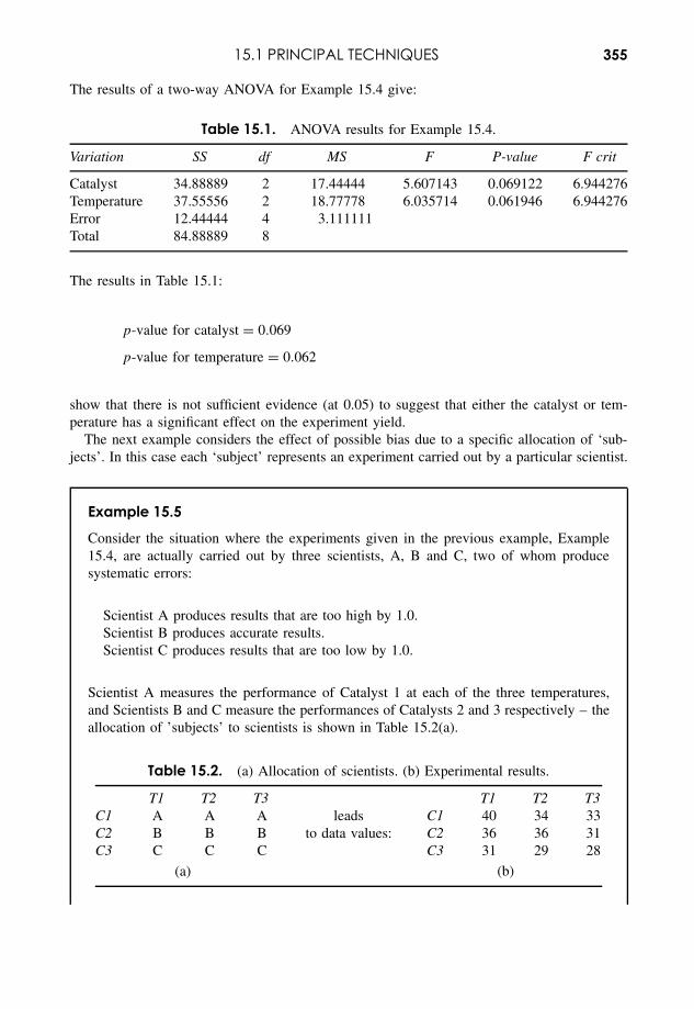
15.1 PRINCIPAL TECHNIQUES 355
The results of a two-way ANOVA for Example 15.4 give:
Table 15.1. ANOVA results for Example 15.4.
Variation SS df MS F P-value F crit
Catalyst 34.88889 2 17.44444 5.607143 0.069122 6.944276Temperature 37.55556 2 18.77778 6.035714 0.061946 6.944276Error 12.44444 4 3.111111Total 84.88889 8
The results in Table 15.1:
p-value for catalyst = 0.069
p-value for temperature = 0.062
show that there is not sufficient evidence (at 0.05) to suggest that either the catalyst or tem-perature has a significant effect on the experiment yield.
The next example considers the effect of possible bias due to a specific allocation of ‘sub-jects’. In this case each ‘subject’ represents an experiment carried out by a particular scientist.
Example 15.5
Consider the situation where the experiments given in the previous example, Example15.4, are actually carried out by three scientists, A, B and C, two of whom producesystematic errors:
Scientist A produces results that are too high by 1.0.Scientist B produces accurate results.Scientist C produces results that are too low by 1.0.
Scientist A measures the performance of Catalyst 1 at each of the three temperatures,and Scientists B and C measure the performances of Catalysts 2 and 3 respectively – theallocation of ’subjects’ to scientists is shown in Table 15.2(a).
Table 15.2. (a) Allocation of scientists. (b) Experimental results.
T1 T2 T3 T1 T2 T3C1 A A A leads C1 40 34 33C2 B B B to data values: C2 36 36 31C3 C C C C3 31 29 28
(a) (b)
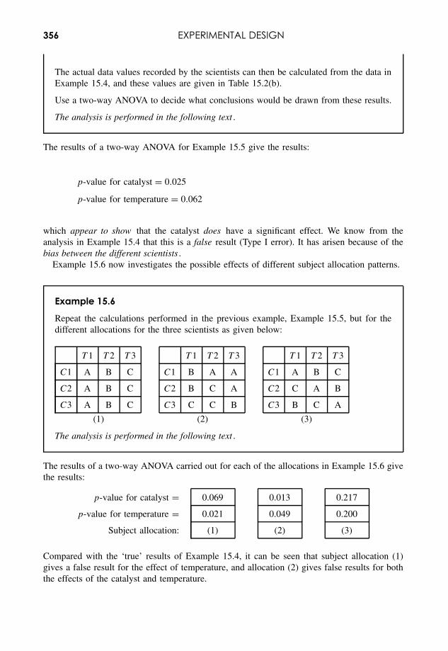
356 EXPERIMENTAL DESIGN
The actual data values recorded by the scientists can then be calculated from the data inExample 15.4, and these values are given in Table 15.2(b).
Use a two-way ANOVA to decide what conclusions would be drawn from these results.
The analysis is performed in the following text .
The results of a two-way ANOVA for Example 15.5 give the results:
p-value for catalyst = 0.025
p-value for temperature = 0.062
which appear to show that the catalyst does have a significant effect. We know from theanalysis in Example 15.4 that this is a false result (Type I error). It has arisen because of thebias between the different scientists .
Example 15.6 now investigates the possible effects of different subject allocation patterns.
Example 15.6
Repeat the calculations performed in the previous example, Example 15.5, but for thedifferent allocations for the three scientists as given below:
T 1 T 2 T 3 T 1 T 2 T 3 T 1 T 2 T 3
C1 A B C C1 B A A C1 A B C
C2 A B C C2 B C A C2 C A B
C3 A B C C3 C C B C3 B C A
(1) (2) (3)
The analysis is performed in the following text .
The results of a two-way ANOVA carried out for each of the allocations in Example 15.6 givethe results:
p-value for catalyst = 0.069 0.013 0.217
p-value for temperature = 0.021 0.049 0.200
Subject allocation: (1) (2) (3)
Compared with the ‘true’ results of Example 15.4, it can be seen that subject allocation (1)gives a false result for the effect of temperature, and allocation (2) gives false results for boththe effects of the catalyst and temperature.

15.2 PLANNING A RESEARCH PROJECT 357
In subject allocations (1) and (2) the systematic errors in measurement have created theappearance of significant effects in the results, leading to Type I errors. However, theresults for subject allocation (3) show increased p-values (compared with Example 15.4),which reduces the probability of making a Type I error. This is consistent with the fact thatgreater errors have been introduced into the measurement process because of the bias of twoscientists.
The important aspect of allocation (3) is that each of the values of A, B and C appears onceonly in each row and column . By ensuring that every level of every factor has at least oneoccurrence of each subject type (A, B or C), the differences between subject types are morelikely to be reduced.
Any arrangement of items where each item appears just once in every row and column iscalled a Latin square. A very popular example of a Latin square is the number arrangementfor the Japanese Sudoku puzzle. Tables of Latin squares are available for each size of square,and the particular one to be used should be selected at random.
In the above example, the allocation of scientists to the labels A, B and C should be madeat random.
As a final note, it is important to understand that any particular allocation of subjects maycoincidentally work with other variations in measurement to produce increased errors. How-ever, provided that the proper procedures are followed, then it is more likely that an appropriateallocation of subjects will reduce the probability of errors.
15.2 Planning a Research ProjectCarrying out a science project as an undergraduate is likely to be the first major piece oforiginal work carried out by a student.
Many student projects are marred by the fact that the student did not anticipate how thedata would be analysed and failed to collect data that was essential for the process of analysis.Too often, a student reports ‘no measurable effect was discovered’ because the design of theexperiment did not ensure that the data collected would match the methods used to analyse it.
If the process of data collection is not planned to match the requirements of the analyticalprocess, then information will be lost. A loss of information will then lead to:
• increased uncertainty in the experimental results; and• a reduction in the ‘power’ of a hypothesis test (9.4.5).
Before starting the project, the student should:
• be clear about the type of investigation – hypothesis testing or direct measurement;• focus clearly on the types of quantitative conclusions that could be drawn from the results
of the experiments;• identify the possible sources of uncertainty (random and systematic) in the measurements;• decide what mathematical or statistical process could be used for analysing the data;• create an experiment design;• plan the complete experimental process from measurement to analysis• carry out a short ‘pilot’ experiment to assess the methods to be used, and to obtain some
example data; and

358 EXPERIMENTAL DESIGN
• check all stages of the analytical process using ‘test’ data derived either from the pilotexperiment, or by taking an intelligent guess at the sort of values that might be produced inthe experiments.
A set of short ‘pilot’ measurements at the very beginning of the project can be extremelyuseful in picking up any unforeseen problems at an early stage, and can often suggest usefulmodifications to the main experimental plan. In addition, ‘pilot’ measurements will produce‘test’ data with appropriate precision and variance suitable for checking the data analysisprocedures.
This procedure of working through the whole process of data collection and analysis allowsthe student to check that nothing has been left out, and prevents the embarrassing scenario ofpreparing to write up the project only to realize that an essential element of data was neverrecorded!
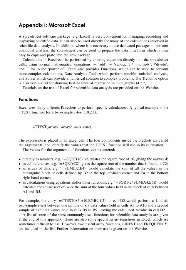
Appendix I: Microsoft Excel
A spreadsheet software package (e.g. Excel) is very convenient for managing, recording anddisplaying scientific data. It can also be used directly for many of the calculations involved inscientific data analysis. In addition, where it is necessary to use dedicated packages to performadditional analysis, the spreadsheet can be used to prepare the data in a form which is theneasy to copy and paste into the new package.
Calculations in Excel can be performed by entering equations directly into the spreadsheetcells, using normal mathematical operations: + ‘add’, − ‘subtract’, * ‘multiply’, /‘divide’,and ˆ for to the ‘power of’. Excel also provides Functions, which can be used to performmore complex calculations, Data Analysis Tools which perform specific statistical analyses,and Solver which can provide a numerical solution to complex problems. The Trendline optionis also very useful for drawing best-fit lines of regression in x –y graphs (4.2.2).
Tutorials on the use of Excel for scientific data analysis are provided on the Website.
Functions
Excel uses many different functions to perform specific calculations. A typical example is theTTEST function for a two-sample t-test (10.2.1):
=TTEST(array1 , array2 , tails, type)
The expression is placed in an Excel cell. The four components inside the brackets are calledthe arguments, and identify the values that the TTEST function will use in its calculation.
The values for the arguments of functions can be entered:
• directly as numbers, e.g. ‘=SQRT(16)’ calculates the square root of 16, giving the answer 4;• as cell references, e.g. ‘=SQRT(C8)’ gives the square root of the number that is found in C8;• as arrays of data, e.g. ‘=SUM(B2:E4)’ would calculate the sum of all the values in the
rectangular block of cells defined by B2 in the top left-hand corner and E4 in the bottomright-hand corner;
• as calculations using equations and/or other functions, e.g. ‘=SQRT(2*SUM(A4:B5))’ wouldcalculate the square root of twice the sum of the four values held in the block of cells betweenA4 and B5.
For example, the entry ‘=TTEST(A5:A10,B5:B9,1,2)’ in cell D2 would perform a 1-tailed,two-sample t-test between one sample of six data values held in cells A5 to A10 and a secondsample of five data values held in cells B5 to B9, leaving the calculated p-value in cell D2.
A list of some of the most commonly used functions for scientific data analysis are givenat the end of this appendix. There are also some special Array Functions in Excel, which aresometimes difficult to use. However, two useful array functions, LINEST and FREQUENCY,are included in the list. Further information on their use is given on the Website.
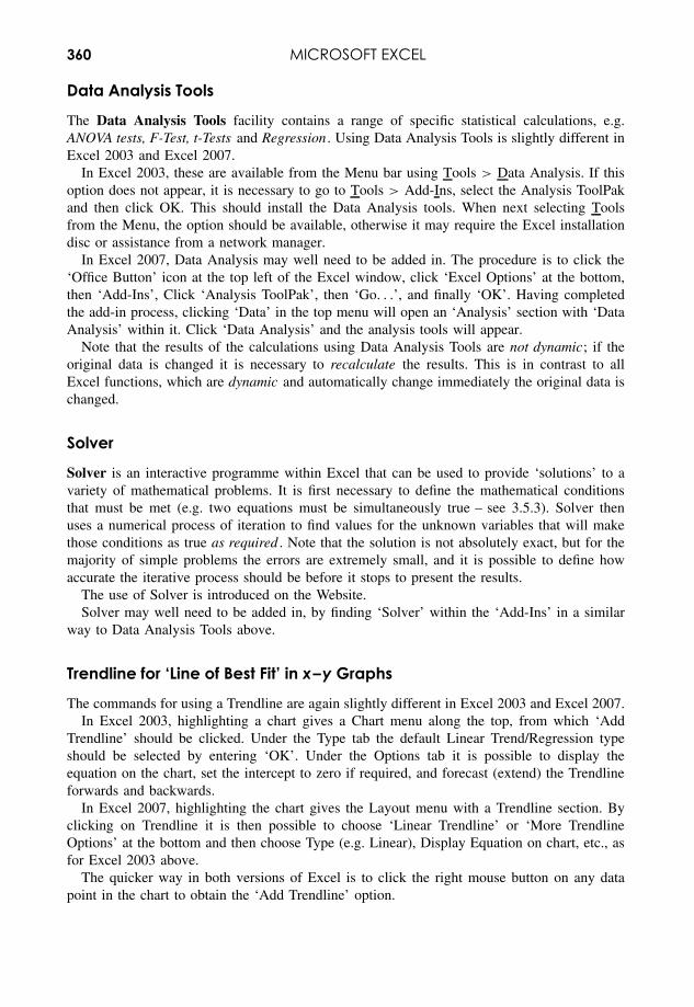
360 MICROSOFT EXCEL
Data Analysis Tools
The Data Analysis Tools facility contains a range of specific statistical calculations, e.g.ANOVA tests, F-Test, t-Tests and Regression . Using Data Analysis Tools is slightly different inExcel 2003 and Excel 2007.
In Excel 2003, these are available from the Menu bar using Tools > Data Analysis. If thisoption does not appear, it is necessary to go to Tools > Add-Ins, select the Analysis ToolPakand then click OK. This should install the Data Analysis tools. When next selecting Toolsfrom the Menu, the option should be available, otherwise it may require the Excel installationdisc or assistance from a network manager.
In Excel 2007, Data Analysis may well need to be added in. The procedure is to click the‘Office Button’ icon at the top left of the Excel window, click ‘Excel Options’ at the bottom,then ‘Add-Ins’, Click ‘Analysis ToolPak’, then ‘Go. . .’, and finally ‘OK’. Having completedthe add-in process, clicking ‘Data’ in the top menu will open an ‘Analysis’ section with ‘DataAnalysis’ within it. Click ‘Data Analysis’ and the analysis tools will appear.
Note that the results of the calculations using Data Analysis Tools are not dynamic; if theoriginal data is changed it is necessary to recalculate the results. This is in contrast to allExcel functions, which are dynamic and automatically change immediately the original data ischanged.
Solver
Solver is an interactive programme within Excel that can be used to provide ‘solutions’ to avariety of mathematical problems. It is first necessary to define the mathematical conditionsthat must be met (e.g. two equations must be simultaneously true – see 3.5.3). Solver thenuses a numerical process of iteration to find values for the unknown variables that will makethose conditions as true as required . Note that the solution is not absolutely exact, but for themajority of simple problems the errors are extremely small, and it is possible to define howaccurate the iterative process should be before it stops to present the results.
The use of Solver is introduced on the Website.Solver may well need to be added in, by finding ‘Solver’ within the ‘Add-Ins’ in a similar
way to Data Analysis Tools above.
Trendline for ‘Line of Best Fit’ in x–y Graphs
The commands for using a Trendline are again slightly different in Excel 2003 and Excel 2007.In Excel 2003, highlighting a chart gives a Chart menu along the top, from which ‘Add
Trendline’ should be clicked. Under the Type tab the default Linear Trend/Regression typeshould be selected by entering ‘OK’. Under the Options tab it is possible to display theequation on the chart, set the intercept to zero if required, and forecast (extend) the Trendlineforwards and backwards.
In Excel 2007, highlighting the chart gives the Layout menu with a Trendline section. Byclicking on Trendline it is then possible to choose ‘Linear Trendline’ or ‘More TrendlineOptions’ at the bottom and then choose Type (e.g. Linear), Display Equation on chart, etc., asfor Excel 2003 above.
The quicker way in both versions of Excel is to click the right mouse button on any datapoint in the chart to obtain the ‘Add Trendline’ option.
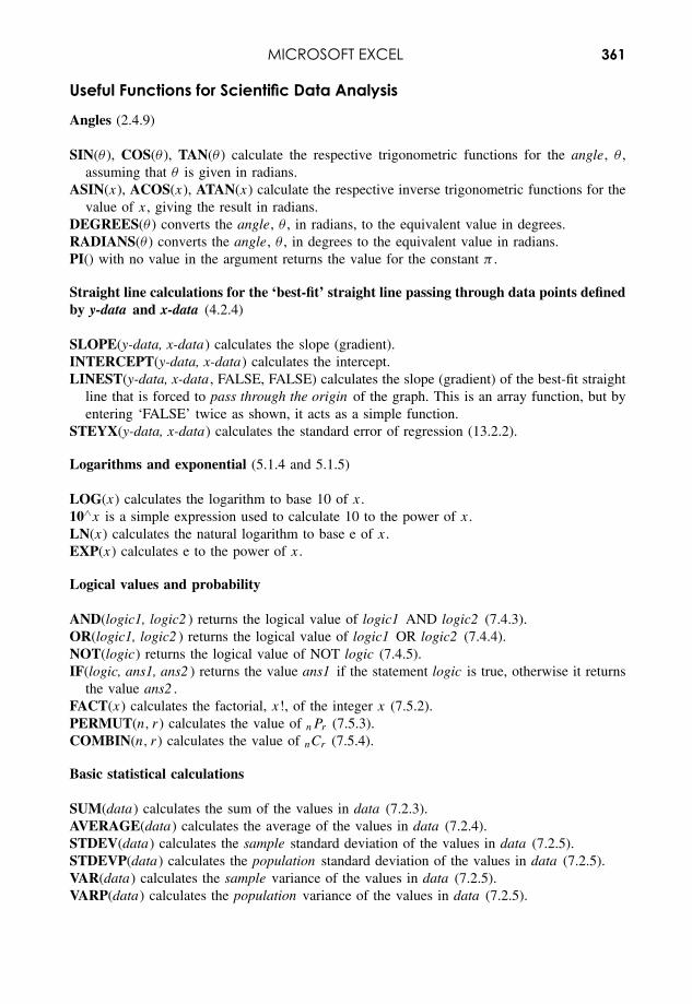
MICROSOFT EXCEL 361
Useful Functions for Scientific Data Analysis
Angles (2.4.9)
SIN(θ ), COS(θ ), TAN(θ ) calculate the respective trigonometric functions for the angle, θ ,assuming that θ is given in radians.
ASIN(x), ACOS(x), ATAN(x) calculate the respective inverse trigonometric functions for thevalue of x, giving the result in radians.
DEGREES(θ ) converts the angle, θ , in radians, to the equivalent value in degrees.RADIANS(θ ) converts the angle, θ , in degrees to the equivalent value in radians.PI() with no value in the argument returns the value for the constant π .
Straight line calculations for the ‘best-fit’ straight line passing through data points definedby y-data and x-data (4.2.4)
SLOPE(y-data, x-data) calculates the slope (gradient).INTERCEPT(y-data, x-data) calculates the intercept.LINEST(y-data, x-data , FALSE, FALSE) calculates the slope (gradient) of the best-fit straight
line that is forced to pass through the origin of the graph. This is an array function, but byentering ‘FALSE’ twice as shown, it acts as a simple function.
STEYX(y-data, x-data) calculates the standard error of regression (13.2.2).
Logarithms and exponential (5.1.4 and 5.1.5)
LOG(x) calculates the logarithm to base 10 of x.10∧x is a simple expression used to calculate 10 to the power of x.LN(x) calculates the natural logarithm to base e of x.EXP(x) calculates e to the power of x.
Logical values and probability
AND(logic1, logic2 ) returns the logical value of logic1 AND logic2 (7.4.3).OR(logic1, logic2 ) returns the logical value of logic1 OR logic2 (7.4.4).NOT(logic) returns the logical value of NOT logic (7.4.5).IF(logic, ans1, ans2 ) returns the value ans1 if the statement logic is true, otherwise it returns
the value ans2 .FACT(x) calculates the factorial, x!, of the integer x (7.5.2).PERMUT(n, r) calculates the value of nPr (7.5.3).COMBIN(n, r) calculates the value of nCr (7.5.4).
Basic statistical calculations
SUM(data) calculates the sum of the values in data (7.2.3).AVERAGE(data) calculates the average of the values in data (7.2.4).STDEV(data) calculates the sample standard deviation of the values in data (7.2.5).STDEVP(data) calculates the population standard deviation of the values in data (7.2.5).VAR(data) calculates the sample variance of the values in data (7.2.5).VARP(data) calculates the population variance of the values in data (7.2.5).
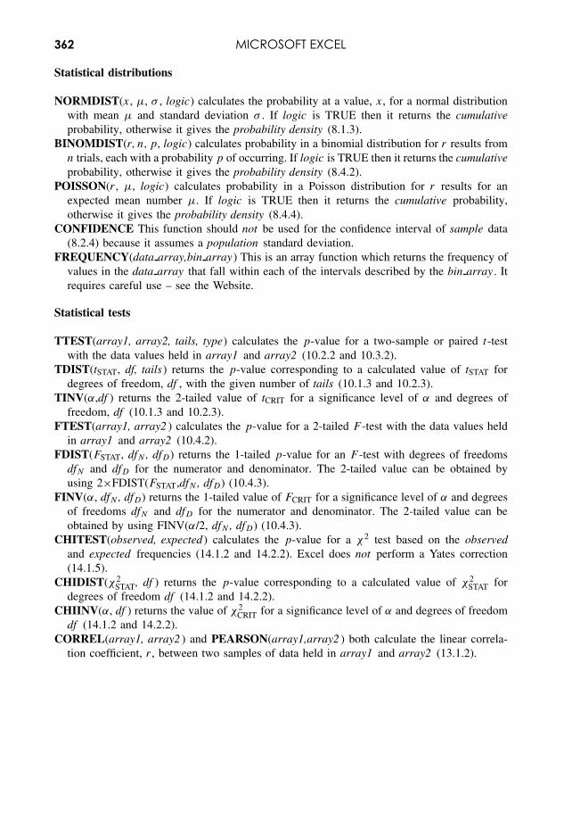
362 MICROSOFT EXCEL
Statistical distributions
NORMDIST(x, µ, σ , logic) calculates the probability at a value, x, for a normal distributionwith mean µ and standard deviation σ . If logic is TRUE then it returns the cumulativeprobability, otherwise it gives the probability density (8.1.3).
BINOMDIST(r, n, p, logic) calculates probability in a binomial distribution for r results fromn trials, each with a probability p of occurring. If logic is TRUE then it returns the cumulativeprobability, otherwise it gives the probability density (8.4.2).
POISSON(r , µ, logic) calculates probability in a Poisson distribution for r results for anexpected mean number µ. If logic is TRUE then it returns the cumulative probability,otherwise it gives the probability density (8.4.4).
CONFIDENCE This function should not be used for the confidence interval of sample data(8.2.4) because it assumes a population standard deviation.
FREQUENCY(data array,bin array) This is an array function which returns the frequency ofvalues in the data array that fall within each of the intervals described by the bin array . Itrequires careful use – see the Website.
Statistical tests
TTEST(array1, array2, tails, type) calculates the p-value for a two-sample or paired t-testwith the data values held in array1 and array2 (10.2.2 and 10.3.2).
TDIST(tSTAT, df, tails) returns the p-value corresponding to a calculated value of tSTAT fordegrees of freedom, df , with the given number of tails (10.1.3 and 10.2.3).
TINV(α,df ) returns the 2-tailed value of tCRIT for a significance level of α and degrees offreedom, df (10.1.3 and 10.2.3).
FTEST(array1, array2 ) calculates the p-value for a 2-tailed F -test with the data values heldin array1 and array2 (10.4.2).
FDIST(FSTAT, dfN , dfD) returns the 1-tailed p-value for an F -test with degrees of freedomsdfN and dfD for the numerator and denominator. The 2-tailed value can be obtained byusing 2×FDIST(FSTAT,dfN , dfD) (10.4.3).
FINV(α, dfN , dfD) returns the 1-tailed value of FCRIT for a significance level of α and degreesof freedoms dfN and dfD for the numerator and denominator. The 2-tailed value can beobtained by using FINV(α/2, dfN , dfD) (10.4.3).
CHITEST(observed, expected ) calculates the p-value for a χ2 test based on the observedand expected frequencies (14.1.2 and 14.2.2). Excel does not perform a Yates correction(14.1.5).
CHIDIST(χ2STAT, df ) returns the p-value corresponding to a calculated value of χ2
STAT fordegrees of freedom df (14.1.2 and 14.2.2).
CHIINV(α, df ) returns the value of χ2CRIT for a significance level of α and degrees of freedom
df (14.1.2 and 14.2.2).CORREL(array1, array2 ) and PEARSON(array1,array2 ) both calculate the linear correla-
tion coefficient, r , between two samples of data held in array1 and array2 (13.1.2).
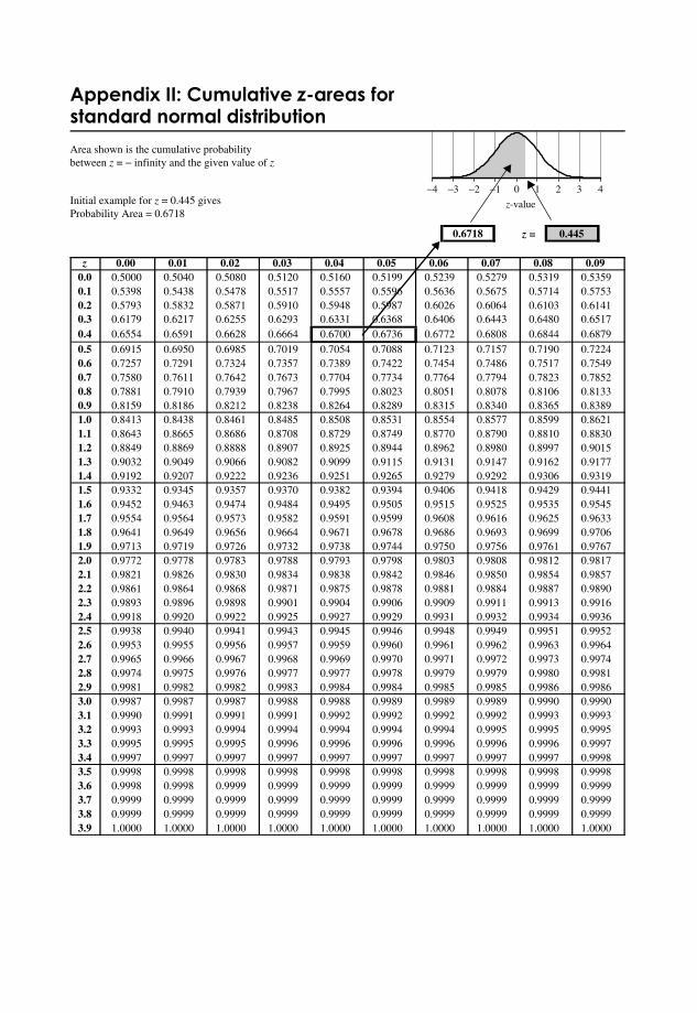
Appendix II: Cumulative z-areas forstandard normal distributionArea shown is the cumulative probabilitybetween z = − infinity and the given value of z
Initial example for z = 0.445 givesProbability Area = 0.6718
0.6718 z = 0.445
z 0.00 0.01 0.02 0.03 0.04 0.05 0.06 0.07 0.08 0.090.0 0.5000 0.5040 0.5080 0.5120 0.5160 0.5199 0.5239 0.5279 0.5319 0.53590.1 0.5398 0.5438 0.5478 0.5517 0.5557 0.5596 0.5636 0.5675 0.5714 0.57530.2 0.5793 0.5832 0.5871 0.5910 0.5948 0.5987 0.6026 0.6064 0.6103 0.61410.3 0.6179 0.6217 0.6255 0.6293 0.6331 0.6368 0.6406 0.6443 0.6480 0.65170.4 0.6554 0.6591 0.6628 0.6664 0.6700 0.6736 0.6772 0.6808 0.6844 0.68790.5 0.6915 0.6950 0.6985 0.7019 0.7054 0.7088 0.7123 0.7157 0.7190 0.72240.6 0.7257 0.7291 0.7324 0.7357 0.7389 0.7422 0.7454 0.7486 0.7517 0.75490.7 0.7580 0.7611 0.7642 0.7673 0.7704 0.7734 0.7764 0.7794 0.7823 0.78520.8 0.7881 0.7910 0.7939 0.7967 0.7995 0.8023 0.8051 0.8078 0.8106 0.81330.9 0.8159 0.8186 0.8212 0.8238 0.8264 0.8289 0.8315 0.8340 0.8365 0.83891.0 0.8413 0.8438 0.8461 0.8485 0.8508 0.8531 0.8554 0.8577 0.8599 0.86211.1 0.8643 0.8665 0.8686 0.8708 0.8729 0.8749 0.8770 0.8790 0.8810 0.88301.2 0.8849 0.8869 0.8888 0.8907 0.8925 0.8944 0.8962 0.8980 0.8997 0.90151.3 0.9032 0.9049 0.9066 0.9082 0.9099 0.9115 0.9131 0.9147 0.9162 0.91771.4 0.9192 0.9207 0.9222 0.9236 0.9251 0.9265 0.9279 0.9292 0.9306 0.93191.5 0.9332 0.9345 0.9357 0.9370 0.9382 0.9394 0.9406 0.9418 0.9429 0.94411.6 0.9452 0.9463 0.9474 0.9484 0.9495 0.9505 0.9515 0.9525 0.9535 0.95451.7 0.9554 0.9564 0.9573 0.9582 0.9591 0.9599 0.9608 0.9616 0.9625 0.96331.8 0.9641 0.9649 0.9656 0.9664 0.9671 0.9678 0.9686 0.9693 0.9699 0.97061.9 0.9713 0.9719 0.9726 0.9732 0.9738 0.9744 0.9750 0.9756 0.9761 0.97672.0 0.9772 0.9778 0.9783 0.9788 0.9793 0.9798 0.9803 0.9808 0.9812 0.98172.1 0.9821 0.9826 0.9830 0.9834 0.9838 0.9842 0.9846 0.9850 0.9854 0.98572.2 0.9861 0.9864 0.9868 0.9871 0.9875 0.9878 0.9881 0.9884 0.9887 0.98902.3 0.9893 0.9896 0.9898 0.9901 0.9904 0.9906 0.9909 0.9911 0.9913 0.99162.4 0.9918 0.9920 0.9922 0.9925 0.9927 0.9929 0.9931 0.9932 0.9934 0.99362.5 0.9938 0.9940 0.9941 0.9943 0.9945 0.9946 0.9948 0.9949 0.9951 0.99522.6 0.9953 0.9955 0.9956 0.9957 0.9959 0.9960 0.9961 0.9962 0.9963 0.99642.7 0.9965 0.9966 0.9967 0.9968 0.9969 0.9970 0.9971 0.9972 0.9973 0.99742.8 0.9974 0.9975 0.9976 0.9977 0.9977 0.9978 0.9979 0.9979 0.9980 0.99812.9 0.9981 0.9982 0.9982 0.9983 0.9984 0.9984 0.9985 0.9985 0.9986 0.99863.0 0.9987 0.9987 0.9987 0.9988 0.9988 0.9989 0.9989 0.9989 0.9990 0.99903.1 0.9990 0.9991 0.9991 0.9991 0.9992 0.9992 0.9992 0.9992 0.9993 0.99933.2 0.9993 0.9993 0.9994 0.9994 0.9994 0.9994 0.9994 0.9995 0.9995 0.99953.3 0.9995 0.9995 0.9995 0.9996 0.9996 0.9996 0.9996 0.9996 0.9996 0.99973.4 0.9997 0.9997 0.9997 0.9997 0.9997 0.9997 0.9997 0.9997 0.9997 0.99983.5 0.9998 0.9998 0.9998 0.9998 0.9998 0.9998 0.9998 0.9998 0.9998 0.99983.6 0.9998 0.9998 0.9999 0.9999 0.9999 0.9999 0.9999 0.9999 0.9999 0.99993.7 0.9999 0.9999 0.9999 0.9999 0.9999 0.9999 0.9999 0.9999 0.9999 0.99993.8 0.9999 0.9999 0.9999 0.9999 0.9999 0.9999 0.9999 0.9999 0.9999 0.99993.9 1.0000 1.0000 1.0000 1.0000 1.0000 1.0000 1.0000 1.0000 1.0000 1.0000
−4 −3 −2 −1 0 1 2 3 4
z-value


Appendix III: Critical values –t-statistic and chi-squared, χ2
t-statistic Chi-squaredTails Degrees Significance Significance
of freedom1 or 2
2
12
12121212121212121212121212121212121212121
95%0.05
3.84
5.99
7.81
9.49
11.07
12.59
14.07
15.51
16.92
18.31
19.68
21.03
22.36
23.68
25.00
26.30
27.59
28.87
30.14
31.41
37.65
67.50
99%0.01
6.63
9.21
11.34
13.28
15.09
16.81
18.48
20.09
21.67
23.21
24.72
26.22
27.69
29.14
30.58
32.00
33.41
34.81
36.19
37.57
44.31
76.152
df1
2
3
4
5
6
7
8
9
10
11
12
13
14
15
16
17
18
19
20
25
50
Infinity
1
95%0.05
12.71
6.314.30
2.923.182.352.782.132.572.022.451.942.361.892.311.862.261.832.231.812.201.802.181.782.161.772.141.762.131.752.121.752.111.742.101.732.091.732.091.722.061.712.011.681.96
1.64
99%0.01
63.66
31.829.92
6.965.844.544.603.754.033.363.713.143.503.003.362.903.252.823.172.763.112.723.052.683.012.652.982.622.952.602.922.582.902.572.882.552.862.542.852.532.792.492.682.402.58
2.33


Appendix IV: Critical F values at 0.05 (95 %) significance
dfN = Degrees of freedom for Numerator
dfD = Degrees of freedom for Denominator
Tails dfN = 1 2 3 4 5 6 7 8 9 10 15 20 30 50 100
1 or 2 dfD
2 1 648 799 864 900 922 937 948 957 963 969 985 993 1001 1008 1013
1 161 199 216 225 230 234 237 239 241 242 246 248 250 252 253
2 2 38.5 39.0 39.2 39.2 39.3 39.3 39.4 39.4 39.4 39.4 39.4 39.4 39.5 39.5 39.5
1 18.5 19.0 19.2 19.2 19.3 19.3 19.4 19.4 19.4 19.4 19.4 19.4 19.5 19.5 19.5
2 3 17.4 16.0 15.4 15.1 14.9 14.7 14.6 14.5 14.5 14.4 14.3 14.2 14.1 14.0 14.0
1 10 10 9.28 9.12 9.01 8.94 8.89 8.85 8.81 8.79 8.70 8.66 8.62 8.58 8.55
2 4 12.2 10.6 9.98 9.60 9.36 9.20 9.07 8.98 8.90 8.84 8.66 8.56 8.46 8.38 8.32
1 7.71 6.94 6.59 6.39 6.26 6.16 6.09 6.04 6.00 5.96 5.86 5.80 5.75 5.70 5.66
2 5 10.0 8.43 7.76 7.39 7.15 6.98 6.85 6.76 6.68 6.62 6.43 6.33 6.23 6.14 6.08
1 6.61 5.79 5.41 5.19 5.05 4.95 4.88 4.82 4.77 4.74 4.62 4.56 4.50 4.44 4.41
2 6 8.81 7.26 6.60 6.23 5.99 5.82 5.70 5.60 5.52 5.46 5.27 5.17 5.07 4.98 4.92
1 5.99 5.14 4.76 4.53 4.39 4.28 4.21 4.15 4.10 4.06 3.94 3.87 3.81 3.75 3.71
2 7 8.07 6.54 5.89 5.52 5.29 5.12 4.99 4.90 4.82 4.76 4.57 4.47 4.36 4.28 4.21
1 5.59 4.74 4.35 4.12 3.97 3.87 3.79 3.73 3.68 3.64 3.51 3.44 3.38 3.32 3.27
2 8 7.57 6.06 5.42 5.05 4.82 4.65 4.53 4.43 4.36 4.30 4.10 4.00 3.89 3.81 3.74
1 5.32 4.46 4.07 3.84 3.69 3.58 3.50 3.44 3.39 3.35 3.22 3.15 3.08 3.02 2.97
2 9 7.21 5.71 5.08 4.72 4.48 4.32 4.20 4.10 4.03 3.96 3.77 3.67 3.56 3.47 3.40
1 5.12 4.26 3.86 3.63 3.48 3.37 3.29 3.23 3.18 3.14 3.01 2.94 2.86 2.80 2.76
2 10 6.94 5.46 4.83 4.47 4.24 4.07 3.95 3.85 3.78 3.72 3.52 3.42 3.31 3.22 3.15
1 4.96 4.10 3.71 3.48 3.33 3.22 3.14 3.07 3.02 2.98 2.85 2.77 2.70 2.64 2.59
2 15 6.20 4.77 4.15 3.80 3.58 3.41 3.29 3.20 3.12 3.06 2.86 2.76 2.64 2.55 2.47
1 4.54 3.68 3.29 3.06 2.90 2.79 2.71 2.64 2.59 2.54 2.40 2.33 2.25 2.18 2.12
2 20 5.87 4.46 3.86 3.51 3.29 3.13 3.01 2.91 2.84 2.77 2.57 2.46 2.35 2.25 2.17
1 4.35 3.49 3.10 2.87 2.71 2.60 2.51 2.45 2.39 2.35 2.20 2.12 2.04 1.97 1.91
2 30 5.57 4.18 3.59 3.25 3.03 2.87 2.75 2.65 2.57 2.51 2.31 2.20 2.07 1.97 1.88
1 4.17 3.32 2.92 2.69 2.53 2.42 2.33 2.27 2.21 2.16 2.01 1.93 1.84 1.76 1.70
2 50 5.34 3.97 3.39 3.05 2.83 2.67 2.55 2.46 2.38 2.32 2.11 1.99 1.87 1.75 1.66
1 4.03 3.18 2.79 2.56 2.40 2.29 2.20 2.13 2.07 2.03 1.87 1.78 1.69 1.60 1.52
2 100 5.18 3.83 3.25 2.92 2.70 2.54 2.42 2.32 2.24 2.18 1.97 1.85 1.71 1.59 1.48
1 3.94 3.09 2.70 2.46 2.31 2.19 2.10 2.03 1.97 1.93 1.77 1.68 1.57 1.48 1.39
Example
Critical F -value for one-tailed test with dfN = 15 and dfD = 8 at 0.05 significance:
F1,0.05,15,8 = 3.22

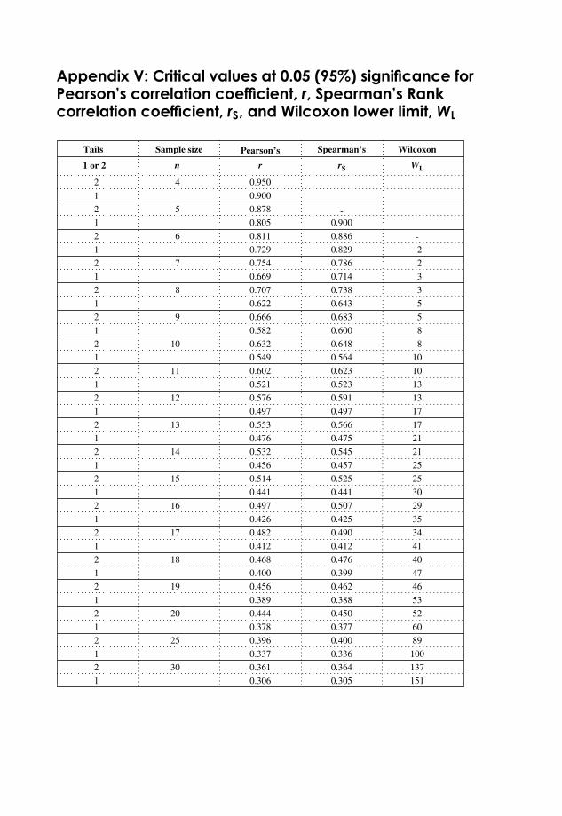
Appendix V: Critical values at 0.05 (95%) significance forPearson’s correlation coefficient, r, Spearman’s Rankcorrelation coefficient, rS, and Wilcoxon lower limit, WL
Tails Sample size Pearson’s Spearman’s Wilcoxon
1 or 2 n
-2
2
3
3
5
5
8
WL
10
13
13
17
17
21
21
25
25
30
29
35
34
41
40
47
46
53
52
60
89
100
137
151
4
5
6
7
8
9
11
12
13
14
15
16
17
18
19
20
25
30
10 8
2
1
2
1
2
1
2
1
2
1
2
1
2
1
2
1
2
1
2
1
2
1
2
1
2
1
2
1
2
1
2
1
2
1
2
1
2
1
r
0.950
0.900
0.878
0.805
0.811
0.729
0.754
0.669
0.707
0.622
0.666
0.582
0.602
0.521
0.576
0.497
0.553
0.476
0.532
0.456
0.514
0.441
0.497
0.426
0.482
0.412
0.468
0.400
0.456
0.389
0.444
0.378
0.396
0.337
0.361
0.306
0.632
0.549
-0.900
0.886
0.829
0.786
0.714
0.738
0.643
0.683
0.600
rS
0.623
0.523
0.591
0.497
0.566
0.475
0.545
0.457
0.525
0.441
0.507
0.425
0.490
0.412
0.476
0.399
0.462
0.388
0.450
0.377
0.400
0.336
0.364
0.305
0.648
0.564 10


Appendix VI: Mann–Whitney lower limit, UL,at 0.05 (95 %) significance
Tails Sample sizes
1 or 2 n2 n1 = 2 3 4 5 6 7 8 9 10 11 12 13 14 15 16 17 18 19 20
2 2 0 1 1 1 1 1 2 2 2 2
1 0 1 1 1 1 2 2 3 3 3 3 4 4 4
2 3 0 1 1 2 2 3 3 4 4 5 5 6 6 7 7 8
1 0 1 2 2 3 4 4 5 5 6 7 7 8 9 9 10 11
2 4 0 1 2 3 4 4 5 6 7 8 9 10 11 11 12 13 14
1 0 1 2 3 4 5 6 7 8 9 10 11 12 14 15 16 17 18
2 5 0 1 2 3 5 6 7 8 9 11 12 13 14 15 17 18 19 20
1 1 2 4 5 6 8 9 11 12 13 15 16 18 19 20 22 23 25
2 6 1 2 3 5 6 8 10 11 13 14 16 17 19 21 22 24 25 27
1 2 3 5 7 8 10 12 14 16 17 19 21 23 25 26 28 30 32
2 7 1 3 5 6 8 10 12 14 16 18 20 22 24 26 28 30 32 34
1 0 2 4 6 8 11 13 15 17 19 21 24 26 28 30 33 35 37 39
2 8 0 2 4 6 8 10 13 15 17 19 22 24 26 29 31 34 36 38 41
1 1 3 5 8 10 13 15 18 20 23 26 28 31 33 36 39 41 44 47
2 9 0 2 4 7 10 12 15 17 20 23 26 28 31 34 37 39 42 45 48
1 1 4 6 9 12 15 18 21 24 27 30 33 36 39 42 45 48 51 54
2 10 0 3 5 8 11 14 17 20 23 26 29 33 36 39 42 45 48 52 55
1 1 4 7 11 14 17 20 24 27 31 34 37 41 44 48 51 55 58 62
2 11 0 3 6 9 13 16 19 23 26 30 33 37 40 44 47 51 55 58 62
1 1 5 8 12 16 19 23 27 31 34 38 42 46 50 54 57 61 65 69
2 12 57 61 65 69
1 64 68 72 77
2 13 63 67 72 76
1 70 75 80 84
2 14 69 74 78 83
1 77 82 87 92
2 15 75 80 85 90
1 83 88 94 100
2 16 81 86 92 98
1 89 95 101 107
2 17 87 93 99 105
1 96 102 109 115
2 18 93 99 106 112
1 102 109 116 123
2 19 99 106 113 119
1 109 116 123 130
2 20 105 112 119 127
1
1 4 7 11 14 18 22 26 29 33 37 41 45 49 53
2 5 9 13 17 21 26 30 34 38 42 47 51 55 60
1 4 8 12 16 20 24 28 33 37 41 45 50 54 59
2 6 10 15 19 24 28 33 37 42 47 51 56 61 65
1 5 9 13 17 22 26 31 36 40 45 50 55 59 64
3 7 11 16 21 26 31 36 41 46 51 56 61 66 71
1 5 10 14 19 24 29 34 39 44 49 54 59 64 70
3 7 12 18 23 28 33 39 44 50 55 61 66 72 77
1 6 11 15 21 26 31 37 42 47 53 59 64 70 75
3 8 14 19 25 30 36 42 48 54 60 65 71 77 83
2 6 11 17 22 28 34 39 45 51 57 63 69 75 81
3 9 15 20 26 33 39 45 51 57 64 70 77 83 89
2 7 12 18 24 30 36 42 48 55 61 67 74 80 86
4 9 16 22 28 35 41 48 55 61 68 75 82 88 95
2 7 13 19 25 32 38 45 52 58 65 72 78 85 92
4 10 17 23 30 37 44 51 58 65 72 80 87 94 101
2 8 14 20 27 34 41 48 55 62 69 76 83 90 98
4 11 18 25 32 39 47 54 62 69 77 84 92 100 107 115 123 130 138

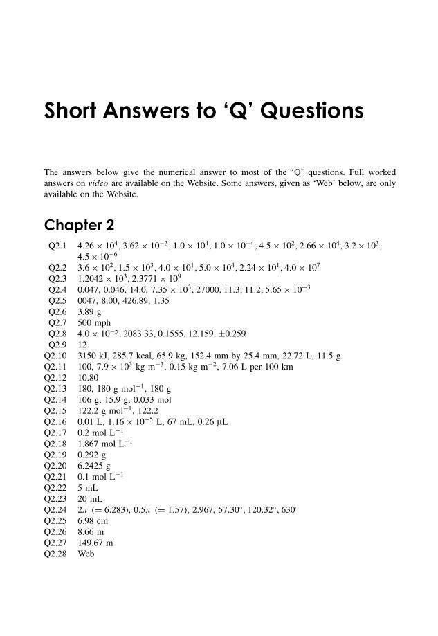
Short Answers to ‘Q’ Questions
The answers below give the numerical answer to most of the ‘Q’ questions. Full workedanswers on video are available on the Website. Some answers, given as ‘Web’ below, are onlyavailable on the Website.
Chapter 2Q2.1 4.26 × 10⁴, 3.62 × 10⁻³, 1.0 × 10⁴, 1.0 × 10⁻⁴, 4.5 × 10², 2.66 × 10⁴, 3.2 × 10³,
4.5 × 10⁻⁶
Q2.2 3.6 × 10², 1.5 × 10³, 4.0 × 101, 5.0 × 10⁴, 2.24 × 101, 4.0 × 10⁷
Q2.3 1.2042 × 10³, 2.3771 × 10⁹
Q2.4 0.047, 0.046, 14.0, 7.35 × 10³, 27000, 11.3, 11.2, 5.65 × 10⁻³
Q2.5 0047, 8.00, 426.89, 1.35Q2.6 3.89 gQ2.7 500 mphQ2.8 4.0 × 10⁻⁵, 2083.33, 0.1555, 12.159, ±0.259Q2.9 12
Q2.10 3150 kJ, 285.7 kcal, 65.9 kg, 152.4 mm by 25.4 mm, 22.72 L, 11.5 gQ2.11 100, 7.9 × 10³ kg m−3, 0.15 kg m−2, 7.06 L per 100 kmQ2.12 10.80Q2.13 180, 180 g mol−1, 180 gQ2.14 106 g, 15.9 g, 0.033 molQ2.15 122.2 g mol−1, 122.2Q2.16 0.01 L, 1.16 × 10⁻⁵ L, 67 mL, 0.26 µLQ2.17 0.2 mol L−1
Q2.18 1.867 mol L−1
Q2.19 0.292 gQ2.20 6.2425 gQ2.21 0.1 mol L−1
Q2.22 5 mLQ2.23 20 mLQ2.24 2π (= 6.283), 0.5π (= 1.57), 2.967, 57.30◦, 120.32◦, 630◦Q2.25 6.98 cmQ2.26 8.66 mQ2.27 149.67 mQ2.28 Web
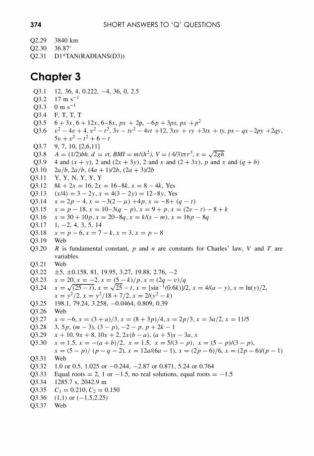
374 SHORT ANSWERS TO ‘Q’ QUESTIONS
Q2.29 3840 kmQ2.30 36.87◦Q2.31 D1*TAN(RADIANS(D3))
Chapter 3Q3.1 12, 36, 4, 0.222, −4, 36, 0, 2.5Q3.2 17 m s−1
Q3.3 0 m s−1
Q3.4 F, T, T, TQ3.5 6 + 3x, 6 + 12x, 6–8x, px + 2p, −6p + 3px, px +p2
Q3.6 v2 − 4v + 4, v2 − t2, 3v − tv 2 − 4vt +12, 3xv + vy +3tx + ty, px− qx−2py +2qy ,5v + v2 − t2 + 6 − t
Q3.7 9, 7, 10, [2,6,11]Q3.8 A = (1/2)bh, d = vt, BMI = m/(h2), V = ( 4/3)πr3, v = √
2gh
Q3.9 4 and (x + y), 2 and (2x + 3y), 2 and x and (2 + 3x), p and x and (q + b)
Q3.10 2a/b, 2a/b, (4a + 1)/2b, (2a + 3)/2b
Q3.11 Y, Y, N, Y, Y, YQ3.12 8k + 2x = 16, 2x = 16–8k, x = 8 − 4k, YesQ3.13 (x/4) = 3 − 2y, x = 4(3 − 2y) = 12–8y, YesQ3.14 x = 2p − 4, x = −3(2 − µ) +4p, x = −8+ (q − t)Q3.15 x = p − 18, x = 10–3(q – p), x = 9 + p, x = (2v − t) − 8 + k
Q3.16 x = 30 + 10p, x = 20–8q, x = k/(s − m), x = 16p − 8q
Q3.17 1, −2, 4, 3, 5, 14Q3.18 x = p − 6, x = 7 − k, x = 3, x = p − 8Q3.19 WebQ3.20 R is fundamental constant, p and n are constants for Charles’ law, V and T are
variablesQ3.21 WebQ3.22 ±5, ±0.158, 81, 19.95, 3.27, 19.88, 2.76, −2Q3.23 x = 20, x = −2, x = (5 − k)/p, x = (2q − v)/q
Q3.24 x = √(25 − t), x = √
25 − t, x = [sin−1(0.6k)]/2, x = 4/(a − y), x = ln(y)/2,x = y2/2, x = y2/18 + 7/2, x = 2/(y2 − k)
Q3.25 198.1, 79.24, 3.258, −0.0464, 0.809, 0.39Q3.26 WebQ3.27 x = −6, x = (3 + a)/3, x = (8 + 3p)/4, x = 2p/3, x = 3a/2, x = 11/5Q3.28 3, 5p, (m − 3), (3 − p), −2 − p, p + 2k − 1Q3.29 x + 10, 9x + 8, 10x + 2, 2x(b − a), (a + 5)x − 3a, x
Q3.30 x = 1.5, x = −(a + b)/2, x = 1.5, x = 5/(3 − p), x = (5 − p)/(3 − p),x = (5 − p)/ (p − q − 2), x = 12a/(6a − 1), x = (2p − 6)/6, x = (2p − 6)/(p − 1)
Q3.31 WebQ3.32 1.0 or 0.5, 1.025 or −0.244, −2.87 or 0.871, 5.24 or 0.764Q3.33 Equal roots = 2, 1 or −1.5, no real solutions, equal roots = −1.5Q3.34 1285.7 s, 2042.9 mQ3.35 C1 = 0.210, C2 = 0.150Q3.36 (1,1) or (−1.5,2.25)Q3.37 Web
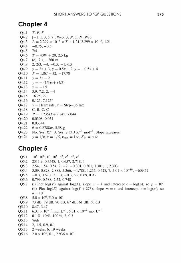
SHORT ANSWERS TO ‘Q’ QUESTIONS 375
Chapter 4Q4.1 T , F, F
Q4.2 [−1, 1, 3, 5, 7], Web, 3, N, Y, N , WebQ4.3 L = 2.299 × 10⁻⁵ × T + 1.21, 2.299 × 10⁻⁵, 1.21Q4.4 −0.75, −0.5Q4.5 7/4Q4.6 T = 40W + 20, 2.5 kgQ4.7 (c), 7 s, −260 mQ4.8 2, 2/3, −4, −0.5, −1, 6.5Q4.9 y = 2x + 3, y = 0.5x + 2, y = −0.5x + 4
Q4.10 F = 1.8C + 32, −17.78Q4.11 y = 3x − 2Q4.12 y = − (1/3)x+ (4/3)Q4.13 x = −1.5Q4.14 3.9, 7.2, 2, −4Q4.15 16.25, 22Q4.16 0.125, 7.125◦Q4.17 y = Heart rate, x = Step−up rateQ4.18 C, R, C, CQ4.19 P = 1.235Q + 2.845, 7.044Q4.20 0.0308, 0.051Q4.21 0.03344Q4.22 θ = 0.8788w, 5.58 gQ4.23 No, Yes, RT , 0, Yes, 8.33 J K−1 mol−1, Slope increasesQ4.24 y = 1/v, x = 1/S, vmax = 1/c, KM = m/c
Chapter 5Q5.1 105, 106, 10, 105, e2, e5, e2, e6
Q5.2 2511.9, 0.3548, 1, 0.657, 2.718, 1Q5.3 2.54, 1.54, 0.54, 2, −2, −0.301, 0.301, 1.301, 1, 2.303Q5.4 3.09, 0.828, 2.888, 5.366, −1.788, 1.255, 0.628, 7, 5.01 × 10⁻¹⁰, −609.57Q5.5 −0.3, 0.62, 0.3, 1.3, −0.3, 6.9, 0.69, 0.93Q5.6 0.799, 0.588, 2.52, 0.748Q5.7 (i) Plot log(V ) against log(A), slope m = k and intercept c = log(p), so p = 10c
(ii) Plot log(E) against log(T + 273), slope m = z and intercept c = log(σ ), soσ = 10c
Q5.8 5.0 × 10⁶, 5.0 × 10⁴
Q5.9 73 dB, 79 dB, 90 dB, 67 dB, 61 dB, 50 dBQ5.10 8.47, 3.47Q5.11 6.31 × 10⁻¹⁰ mol L−1, 6.31 × 10⁻⁴ mol L−1
Q5.12 0.1 %, 10 %, 100 %, 2, 0.3Q5.13 WebQ5.14 2, 1.5, 0.9, 0.1Q5.15 2 weeks, 6, 19 weeksQ5.16 2.0 × 10³, 0.1, 2.936 × 10⁴
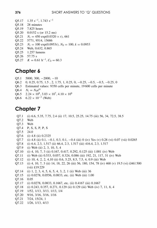
376 SHORT ANSWERS TO ‘Q’ QUESTIONS
Q5.17 1.35 s−1, 1.743 s−1
Q5.18 28 minutesQ5.19 7.825 hoursQ5.20 0.0152 s (or 15.2 ms)Q5.21 Nt = 450 exp(0.0320 × t), 661Q5.22 5771, 9514, 15686Q5.23 Nt = 100 exp(0.0953t), N0 = 100, k = 0.0953Q5.24 Web, 0.632, 0.865Q5.25 1.257 lumensQ5.26 57.75 sQ5.27 K = 0.61 h−1, C0 = 60.3
Chapter 6Q5.1 5000, 300, −2000, −10Q6.2 0, 0.25, 0.75, 1.5 , 2, 1.75, 1, 0.25, 0, −0.25, −0.5, −0.5, −0.25, 0Q6.3 Estimated values: 9350 cells per minute, 19 600 cells per minuteQ6.4 Nt = N0ekt
Q6.5 2.24 × 10⁸, 3.03 × 10⁷, 4.10 × 10⁶
Q6.6 6.22 × 10⁻³ (Web)
Chapter 7Q7.1 (i) 6.6, 5.35, 7.75, 2.4 (ii) 17, 10.5, 25.25, 14.75 (iii) 56, 34, 72.5, 38.5Q7.2 WebQ7.3 WebQ7.4 P, S, S, P, P, SQ7.5 24.0Q7.6 (i) 4.8 (ii) 0.2325Q7.7 (i) 4.8 (ii) 0.1, −0.1, 0.3, 0.1, −0.4 (iii) 0 (iv) Yes (v) 0.28 (vi) 0.07 (vii) 0.0265Q7.8 (i) 6.4, 2.3, 1.517 (ii) 66.4, 2.3, 1.517 (iii) 416.4, 2.3, 1.517Q7.9 (i) Web (ii) 2, 3, 10, 5, 4
Q7.10 (i) 4, 10, 7, 3 (ii) 0.167, 0.417, 0.292, 0.125 (iii) 1.001 (iv) WebQ7.11 (i) Web (ii) 0.533, 0.057, 0.324, 0.086 (iii) 192, 21, 117, 31 (iv) WebQ7.12 (i) 10, 4, 2, 2, 4,10 (ii) 0.6, 5.25, 8.5, 7.5, 4, 0.9 (iii) WebQ7.13 (i) 4, 10, 7, 3 (ii) 14, 18, 22, 26 (iii) 56, 180, 154, 78 (iv) 468 (v) 19.5 (vi) £461 500
(vii) £19 229Q7.14 (i) 1, 2, 3, 4, 5, 6, 5, 4, 3, 2, 1 (ii) Web (iii) 36Q7.15 (i) 0.0278, 0.0556, 0.0833, etc. (ii) Web (iii) 1.00Q7.16 0.05Q7.17 (i) 0.0278, 0.0833, 0.1667, etc. (ii) 0.4167 (iii) 0.1667Q7.18 (i) 0.243, 0.357, 0.271, 0.129 (ii) 0.129 (iii) Web (iv) 7, 11, 8, 4Q7.19 1/52, 1/13, 3/13, 1/13, 1/4Q7.20 9/16, 3/16, 3/16, 1/16Q7.21 7/24, 15/24, 1Q7.22 1/26, 1/13, 4/13
SHORT ANSWERS TO ‘Q’ QUESTIONS 377
Q7.23 1/13, 12/13, 1Q7.24 1/36, 1/18, 1/6, 1/36Q7.25 0.9, 0.1, 0.6561, 0.0001, 0.0036, 0.2916Q7.26 0.0065Q7.27 1/7, 2/7, 2/7, 2/7, 1Q7.28 0.618Q7.29 120, 1, 1, 0, 42, 10100Q7.30 24Q7.31 1680Q7.32 167 960
Chapter 8Q8.1 0.1915, 0.2417, 0.5000, 0.6828, 0.9546, 0.9974, 1.000Q8.2 1.5, 1.2, 1.2Q8.3 68 300, 95 000, 300, 15 850Q8.4 WebQ8.5 19.08 to 26.92Q8.6 1.0, 21.04 to 24.96Q8.7 16.8 to 21.9, 17.9 to 20.0, WebQ8.8 0.08 ppmQ8.9 1.87, 0.21
Q8.10 10.75, 0.5Q8.11 0.2373, 0.3955, 0.2637, 0.0879, 0.0146, 0.0010, 1.0000Q8.12 5.9 × 10⁻⁶, 1.4 × 10⁻⁴, 0.233, 0.121, 0.028, 0.383, 0.617Q8.13 0.606, 0.303, 0.076, 0.014Q8.14 0.74 ± 0.12Q8.15 (i) CDA = 0.99, CDB = 1.33 (ii) A (iii) Clumping
Chapter 9Q9.1 1, 2, 1, 2Q9.2 F, T, F, F
Chapter 10Q10.1 (ii) 0.05 (iii) 3.585 × 10⁻⁸, 0.080 × 10⁻⁸ (iv) 2.60 (v) 1 (vi) 5 (vii) 2.02Q10.2 WebQ10.3 (i) No (ii) c (iii) cQ10.4 WebQ10.5 Paired t-testQ10.6 tSTAT = 2.54, tCRIT = 2.45, Sig., p = 0.044 (Web)Q10.7 3.68, 3.77Q10.8 WebQ10.9 Web
378 SHORT ANSWERS TO ‘Q’ QUESTIONS
Chapter 11Q11.1 0.094Q11.2 WebQ11.3 WebQ11.4 WebQ13.5 WebQ13.6 Web
Chapter 12Q12.1 W+ = 92, W− = 28, WL = 30, Sig.Q12.2 UY = 12, UL = 12, Sig., p = 0.044Q12.3 W(−) = 3, WL = 2, Not sig.Q12.4 H = 7.43, χ2
CRIT = 7.81, Not sig.
Q12.5 S = 9.53, χ2CRIT = 7.81, Sig.
Q12.6 S = 7.73, χ2CRIT = 7.81, Not sig. (Web)
Chapter 13Q13.1 (i) r = 0.715 (ii) rcrit = 0.622, Sig. (iii) p = 0.023Q13.2 (i) r = 0.542, (ii) rcrit = 0.549, Not sig. (iii) p = 0.0526Q13.3 WebQ13.4 1.578, 0.1477, 1.11 to 2.05
Chapter 14Q14.1 9.49, 6.63Q14.2 χ2
CRIT = 7.81, χ2STAT = 3.6, No
Q14.3 χ2STAT = 5.23, χ2
CRIT = 5.99, No
Q14.4 A : χ2STAT = 10.61, B : χ2
STAT = 2.06, χ2CRIT = 9.49, Web
Q14.5 (ii) χ2STAT = 3.42 (iii) χ2
STAT = 4.05, χ2CRIT = 3.84
Q14.6 χ2STAT = 9.5, χ2
CRIT = 11.07, No
Q14.7 χ2STAT = 12, χ2
CRIT = 7.81, Yes
Q14.8 χ2STAT = 3.28, χ2
CRIT = 5.99, NoQ14.9 0.0284, 0.0568, symmetrical distribution
Q14.10 (i) 0.504 to 0.696 (ii) biasedQ14.11 Yes, if the Yates correction used

Index
Note: Figures and Tables are indicated by italic page numbers
abscissa 89absorbance 63, 88, 89, 104, 106, 126, 127, 322,
327, 331see also Beer–Lambert law; Beer’s law
acceleration 151accuracy of measurement 3adiabatic change equation 75algebraic equations 42–5
reading 48–9rearranging 53–62
analysis of covariance (ANCOVA) 258analysis of variance (ANOVA) 257, 279–98
assumption in using 257Excel calculations 283, 285, 290one-way 257, 279–85post hoc testing 296–8two-way 257, 286–90, 356–7, 358
AND [logical operator], combining withprobabilities 194
angle(s)conversion between degrees and radians 33–4,
39small (approximations) 36–7units 32
angular measurements 31–40calculating 39Excel calculations 39
annotations 65–6, 155arccos 38arcsin 38arctan 38arguments of functions 66
in Excel calculations 361Arrhenius equation 144association 244
test for 334see also contingency; correlation
atomic mass, relative 22, 23
Essential Mathematics and Statistics for Science 2nd Edition Graham Currell and Antony DowmanCopyright c© 2009 John Wiley & Sons, Ltd
average 171–2symbol for 66
average mass 23Avogadro constant/number 21
bar graph 180bases 114Bayesian statistics 162Beer–Lambert law 88, 327Beer’s law 63, 106‘bell-shaped’ curve 164–5, 211, 212–13, 218
see also normal distributionbias 4bin 178
see also classbinomial coefficient 231binomial distribution 211, 230–2
approximations 238–39, 348examples 230, 231, 233Excel calculations 231, 364parameters describing 233–5using 237–8
binomial probability 231blocking of factors (in experiment design) 352,
354blood-alcohol levels 164–7, 264–6BODMAS (or BIDMAS) rules 42box and whisker plot (boxplot) 161, 164, 165,
268, 271, 281, 301, 302, 306brackets 46–8
expanding/opening up 76–7
calculator 14angle calculations 39combination calculations 208EXP button 9, 115factorials 203
380 INDEX
calculator (continued )logarithms 116permutation calculations 206standard deviation calculations 174
calibration line 104–6, 324–31checking residuals 325–6uncertainty in 327–30
categorical data 7plotting 180
categorical name 178, 179category 178causal relationship 244Celsius/Fahrenheit temperature scales conversion
87–8central limit theorem 219certain event 190change
estimating 158–9rate of 145–51
chemical quantities 20–31chi-squared (χ2) statistic 333, 335–6
critical values 336, 369–71chi-squared (χ2) test 259, 333, 334–40
comparison with other tests 349Excel calculations 333, 364–5with Yates correction 260, 341
class 178class frequency 178, 179, 191, 192
in histogram 181, 182, 183clustering/clumping of events 241coefficient of determination 316
ranges 317coefficient of dispersion 241coefficient of variation 225coin tossing 211, 230, 233–4, 247–50,
333column graph 180combinations 207–8
Excel functions 208–9, 364comparisons, symbols for 66concentration, chemical symbol 65concentration of solutions 26–9
in grams per litre 26molarity 26
conditional probability 199–201confidence deviation 221, 225, 329confidence interval 161, 212
for binomial distribution 239in calibration 33095% confidence interval 166–7, 221of proportion 348, 349of sample mean 221, 225for unknown value 164–8
confidence level 253constants 2, 43
symbols 63contingency, test for 259, 333, 334–7
contingency table 334–72 x 2 (Yates correction) 341
continuous curve, rate of change 148–51continuous data 7continuous distribution 188–9, 211conversion of units 17–19co-ordinates (on graph) 90correlation 244, 315
calculation 320linear 315, 316–19statistics 323–4test for 259, 318–19see also Pearson’s correlation coefficient;
Spearman’s rank correlation coefficientcorrelation coefficient 316–18, 324
ranges 317cosine 34, 35critical value method 255critical values
chi-squared statistic 369–71F -statistic 275, 284, 373–4Mann–Whitney test statistic 377–8t-statistic 263, 270, 369–71Wilcoxon test statistic 304, 375–6
cumulative distributions 238cumulative probability 189–90, 238
data 2, 7–40continuous 7discrete 7frequency 178–9, 186interval 7nominal 8ordinal 8ratio 7
Data Analysis Tools (Excel) 362data values, plotting 177–8decay 130, 131, 134, 135–6, 138decibel scale 124–5decimal places (dp) 11decimal reduction time 133, 134, 135, 136,
142–3decision making, statistics used 246–50deduction 245, 246degrees 32
conversion to radians 33–4, 39degrees of freedom (df) 2
ANOVA 283, 284, 287, 288, 290, 291, 293,294, 357
chi-squared tests 336, 341confidence interval calculation 222contingency table 336, 341correlation test 318F -test 275, 283goodness-of-fit test 343, 345t-tests 263, 270
INDEX 381
denominator (in fraction) 51, 77density 15dependent variable 89derivative see differential coefficientdeviation 172differential coefficient 151–2
calculating 153–6differentiation 152–9dilution equation 29–30dilution factor or ratio 30dilutions 29–31discrete data 7dispersion of values 241distance–time graph 147distribution
binomial 211, 230–2continuous 188–9, 211frequency 161, 186–7, 191, 211normal 165, 211, 212–16parameters describing 171–2, 176, 211, 214Poisson 6, 211, 230, 235–7probability 161, 186–7, 191, 211shapes 240standard normal 215, 367
divisionfactorials 203–4fractions 52scientific notation 9
dot plot 177, 178double blind trials 353
Einstein’s theory of relativity 4, 246electrostatic force equation 75energy equivalence equation 4–5, 43equations 4–5, 41
algebraic equations 42–5basic techniques 41–53differential coefficients (listed) 154grouping the unknown variable 75–7moving ‘multiply’ and ‘divide’ terms 58–60moving ‘plus’ and ‘minus’ terms 56–8opening up expressions 72–4quadratic equations 78–81reading 48–9rearranging 53–62, 68removing fractions 77–8simplifying 51–2simultaneous equations 81–2solving for unknown value(s) 60–2subject of equation 53, 61, 72, 74, 75, 76, 77
error 2random 3, 4systematic 3, 4Type I 247, 252, 253, 262, 356, 358, 359Type II 247, 252, 253
error bars 4
estimations 14Euler’s number (e) 63, 65, 114, 132, 153exact one-proportion test 240, 260, 346–7
comparison with other tests 349exact two-proportion test 260, 350Excel calculations 361–5
angles 39, 363ANOVA 283, 285, 290best-fit straight line calculations 100, 322,
362–3, 363combinations 208, 364exponentials 115, 363factorials 203, 363graph drawing 180, 295linear regression 100–1, 102, 103, 142, 362–3logarithms 116, 363logical operations 363permutations 204, 364slope of curve 149solutions for simultaneous equations 85, 362statistical calculations 172, 174, 364statistical distributions 223, 231, 236, 364statistical tests 261, 316, 333, 364–5
Excel functions 361–2, 363–5expected frequency
calculation of 337–8, 342–3less than 5 (five) 339–40
expected proportion 345experiment 246
power of 253–4experiment design 351–60
blocking of factors 352, 354completely randomized 354objective of good design 351pairing in 351, 354–6randomization in 351, 353–4randomized block 354repeated measures in 351, 354–6replication in 351, 352–3subject allocation 352, 356–9techniques 351–9
experimental uncertainty/variation 2–4, 106,172–5, 212–13, 217–19, 282
presenting 224–9standard deviation 282, 322
exponent 114exponential constant (e) 63, 65, 114, 132, 153exponential equations 132–3
differential coefficients 154–5exponential functions 5, 113, 115
Excel calculations 115inverse of 71, 113, 116–17
exponential growth and decay 128–44exponential growth equation 132–3
general use 137–9linearizing 140–4specific applications 133–7

382 INDEX
exponential notation see scientific notationexponential systems 128–32extrapolation (on graph) 98
errors (linear regression) 106
F -statistic 275critical values 275, 284, 373–4
F -test 258, 274–6F -statistic used 275–6mean squares and 283p-value used 275
factor variance 282factor variation 282factorials 203–4
division using 203–4Excel functions 203, 363
factorization 50factors
experimental 243, 244, 282blocking of 289, 352, 354
mathematical 49–50Fahrenheit/Celsius temperature scales conversion
87–8false negatives 199false positives 199–201first-order rate equation 157Fisher’s exact test 260, 333, 346–7
comparison with other tests 349fractions
cancelling terms in 51dividing by 52division of 52multiplication of 52removing from equations 77–8simplifying 51
frequencycompared with probability 191–3relative 186tests for 259, 333, 334–41
frequency data 178–9, 186plotting 180–1
frequency density, in histogram 182, 183frequency distribution 161, 186–7, 191, 211frequency statistics 176–90, 177Friedman test 259, 299, 301, 311, 313–14functions 5
with subscripts 65symbols for 66–7
Gaussian distribution see normal distributiongeneral linear model (GLM) 258generation time 131–2, 133, 134, 142, 302‘goodness of fit’ test 212, 259, 333, 342–3gradient see slopegraph
co-ordinates 90
intercept 87, 88, 89, 90, 93slope 87, 88, 89, 90, 93straight line graph 89–98
graphical methods, solving simultaneousequations 85–6
Greek letters/symbols 44–5, 63, 66, 146, 170,182, 348
growth 128, 129–30, 131–2, 133, 134, 155
H -statistic 311half-life 133, 134, 136height contours 149histograms 181–3, 213, 232hypotenuse (of right-angled triangle) 34hypothesis 245hypothesis statement 246–7, 251hypothesis testing 250–5
chi-squared test 259, 333, 334–40correlation tests 259, 318–19F -test 257, 274–6Friedman test 259, 299, 301, 311, 313–14goodness of fit test 212, 259, 333, 342–3Kruskal–Wallis test 259, 299, 301, 311,
312–13Mann–Whitney U -test 258, 299, 301, 305–8p-value calculation 247–50stating results 254t-tests 257, 262–73Wilcoxon tests 258, 299, 301, 301–5, 308–11
impossible event 190independence between measurements 256independent variable 89index/indices 114induction 245infinity symbol 63instructions 48, 66interaction of factors 287, 289, 294, 295, 354interaction plot 287, 289, 295intercept of graph 87, 88, 89, 90, 93
calculating 94–5interpolation (on graph) 98
errors (linear regression) 106interquartile range (IQR) 163, 299intersecting lines (on graph) 96–7interval data 7inverse cosine function 38, 71inverse operations 68–71, 116inverse sine function 38, 71inverse tangent function 38, 71, 99inverse trigonometric functions 38, 71
Kepler’s third law of planetary motion 109Kruskal–Wallis test 259, 299, 301, 311–13kurtosis 241
INDEX 383
Latin square 359least significant figure/number 11least squares, method of 100, 321Likert scale 300linear correlation 315, 316–19
compared with linear regression 101, 315statistics 323–4
linear correlation coefficient 316–18linear regression 88, 99–106
best-fit straight line 100–1, 320–2calibration line 104–6, 324compared with linear correlation 101, 315Excel calculations 100–1, 102, 103, 142,
362–3extrapolation errors 106interpolation errors 106‘power’ equations solved using 122–4software calculations 102–3statistics 320–3zero intercept forced 104
linear relationships 87–111linearization 88–9, 107–11
change-of-variable method 108–9error warning 111general principles 107logarithmic approach 122–4, 140–4
logarithmic functions 113inverse of 71
logarithmic scales 124–7logarithms
Excel calculations 116as inverse operations 116–17linearization using 122–4, 140–4natural/Naperian 116properties 118–19, 120solving ‘power’ equations 120–1see also natural logarithms
logical operationscombining probabilities with 193–7Excel functions 363–4
Lotto (UK National Lottery) 208loudness 124–5lower quartile 163
Mann–Whitney U -test 258, 299, 301,305–8
applying 307–8test statistic 305–7see also U -statistic
mathematical models 4–6mean squares (MS) 282–3mean value(s) 171–2
binomial distribution 233–35calculations 174, 175effect of sample size 220normal distribution 214
standard error of 219symbol(s) for 66, 171tests for 257–8, 262, 267
measurement uncertainty 3, 217, 218, 282mechanisms 243, 244, 245median(s) 163, 299
tests for 258–9, 299–314method of least squares 100, 321Michaelis–Menten equation 110Minitab
box and whisker plots 164, 165, 268, 271, 281,301, 302, 306
graph plotting 287, 289, 291linear regression 102non-parametric tests 304, 307, 308, 310, 312,
313–14mixed units 15
conversion of 18–19modelling 4–6modulus 65molar concentration 26, 27molar mass 23molarity 26molecular mass, relative 22, 23molecular weight 22moles 21–2
conversion to mass in grams 24–5most significant figure/number 11motor engine–fuel combinations, ANOVA
calculations 294–6multiple t-tests 281
compared with Tukey test 297–8multiplication
fractions 52scientific notation 9–10
Naperian logarithms 116natural logarithms 116
linearization using 124, 140negative values 45–6Nernst equation 75nominal data 8, 300non-parametric tests 163, 256, 258–9,
299–314normal distribution 165, 211, 212–16
as approximation for binomial distribution 238,348
Excel calculations 364parameters describing 214probability areas for 215–16, 263, 367
NOT [logical operator], combining withprobabilities 196
notationscientific 8–9statistics 170–1
numerator (in fraction) 51
384 INDEX
observed value 2one-proportion exact test 240, 260, 346–7
comparison with other tests 349one-sample t-test 257, 262–6
applying 264–6non-parametric equivalent 299, 301p-value used 262–3significance of factor effect 283–5
one-sample Wilcoxon test 258, 299,301–5
applying 304–5test statistic used 302–4see also W -statistic
one-tailed test 251, 262, 264one-tailed Wilcoxon test 304one-way ANOVA 257, 279–85
analysing variances 281–2mean squares and 282–3non-parametric equivalent 299, 311significance of factor effect 283–5
OR [logical operator], combining withprobabilities 194–5
order of magnitude 13–14ordinal data 8, 299ordinate (on graph) 89outcomes 243, 244
p-valuein ANOVA 281, 284, 285, 287, 288, 290, 291,
293, 294, 295, 296, 357, 358calculation 247–50in correlation test 319decisions based on 252–3in F -test 275in non-parametric tests 304, 305, 308, 310,
312, 314in t-tests 262–3, 269, 297
paired t-test 257, 272–3applying 273, 281non-parametric equivalent 299, 308
paired Wilcoxon test 258, 299, 301, 308–11applying 310–11test statistic 309–10see also W -statistic
pairing (in experiment design) 351, 354–6parallel lines (on graph) 97, 98parameter 2, 170parametric tests 256, 261, 299parentheses see bracketsPearson’s correlation coefficient 259, 316
critical values 318, 375–6percentage concentrations 29permutations 204–6
Excel functions 206, 364perpendicular lines (on graph) 97pH scale 126, 127
pharmacokinetic processes 143photoelectric effect equation 109pi (π ) 63pie chart 180, 181pilot experiment/measurements 359, 360Poisson distribution 6, 211, 230, 235–7
as approximation for binomial distribution238
examples 235–36Excel calculations 236, 364using 237
Poisson probability 236pooled standard deviation 269population 168, 169
characteristics 170population growth and decay 128, 129–32,
134–6, 138, 155population mean 171population standard deviation 173, 176potentiometric titration 150–1power 114
inverse operations 116–17properties 114
‘power’ equationsdifferential coefficients 154linearizing using logarithms 122–4simplifying 118solving by logarithms 120–1
power of experiment 253–4non-parametric tests 299, 311
power of hypothesis test (β) 254precision of measurement 3predictions 246pressure 15probability 190–201
binomial 231combining with AND 194combining with NOT 196combining with OR 194–5compared with frequency 191–3conditional 199–201cumulative 189–90experimental 191multiple outcomes 197Poisson 236theoretical 192
probability areas (in distributions) 215–16, 250,263, 367
probability density 188probability distribution 161, 186–7, 191,
211probability trees 201product-moment correlation coefficient see
Pearson’s correlation coefficientproportion, tests for 260, 345–50proportionality 49Pythagoras’s equation 35
INDEX 385
quadratic equations 78–81qualitative data 7quantitative data 7quartiles 163
radians 32conversion to degrees 33–4, 39
radioactive decay 128, 133, 134, 136–7,143
random error 3, 4random selection 256randomization 351, 353–4randomized block design 289, 354ranking of data 162–3
in non-parametric tests 256, 261, 299, 303, 304rate of change 145–51
annotation 155continuous curve 148–51with time 146–8
rate equations 156–7ratio data 7ratio of values 124, 125reciprocal 70, 71reciprocal conversion of units 17refraction equation 75regression
calculation 259, 320compared with correlation 101, 315linear 99–106, 315, 320standard error of 322statistics 320–3
relative class frequency 179, 191, 191relative frequency 186relative molecular mass 22, 23relative standard deviation 225relative uncertainty 225
combining 226, 227, 228–9relativity theory 4, 246repeated measures experiment 351, 354–6replicate data 100, 352
analysing 162–8replicate measurements 219, 292, 352replication
in experiment design 351, 352–3two-way ANOVA with 290–6
research project, planning 359–60residual 320, 321
for linear calibration line 325–6residual sum of squares 321rounding 12–13
S-statistic 311sample 168, 169
characteristics 170sample mean 171, 219
calculations 171, 172, 184, 185
sample standard deviation 173, 176calculations 174, 175, 184, 185
sample variance 173calculations 174, 175relationship to standard deviation 174, 274test for 258, 274–6
scientific data 7–40scientific method 243, 245–6
example 246scientific notation 8–9
addition in 10–11division in 9multiplication in 9–10subtraction in 10–11
scientific numbers 8–14scientific quantities 15–20scientific systems 243–4screening tests 201SI units 16
derived 16fundamental 16
significant figures (sf) 11significant level (α) 248, 253
F -test 275t-tests 263, 270
simultaneous equations 81–2analytical solution 82–5Excel procedure for solving 85, 362graphical method for solving 85–6
sine 34, 35skewness 240slope of graph 87, 88, 89, 90, 93
angle 99at point on curve 151–2average 148, 151calculating 94–5
solutions, concentration 26–9solutions to equations 60–2Solver (Excel) 362Spearman’s rank correlation coefficient 259, 316
critical values 375–6spectrophotometric measurements 63, 88–9, 106,
126, 127, 331speed 15, 18–19, 145–8spread of population 173–4square 68–9, 71square root 69, 71standard deviation 172, 173
binomial distribution 233–235normal distribution 214pooled, in two-way t-test 269relationship to variance 174, 274, 282test for 258, 274–6see also population standard deviation; relative
standard deviation; sample standarddeviation
standard error of regression 322
386 INDEX
standard error of sample mean 219standard normal distribution, probability areas for
215, 367standard notation see scientific notationstandard uncertainty 219, 221, 224
combining 226, 227statistic 2, 170, 255statistical tests
assumptions in using 256–7overview 257–60
statistics 161–209notation 170–1
stem and leaf diagram 177straight line graph 89–99
best-fit line 100–6equation describing 87, 90–4extrapolation 98interpolation 98intersecting lines 96–7parallel lines 97, 98perpendicular lines 97plotting 89–90
Student’s t-test 223, 257subject of equation 53, 61, 72, 74, 75, 76, 77subject uncertainty 3, 217, 218, 282subjects 243
allocation in experiments 352, 356–9subscripts 64–5, 170sum of squares (SS) 284
residual 321superscripts 64–5symbols 63–7systematic error 3, 4
t-statisticcritical values 263, 270, 369–71use in one-sample t-test 263–4use in two-sample t-test 269–70
t-tests 257multiple 281, 297–8one-sample 257, 262–6paired 257, 272–3two-sample 257, 267–72
tails 251–2see also one-tailed . . .; two-tailed . . .
tangent to curve 148, 151tangent (trigonometric function) 34, 35terms (in algebra) 44test assumptions 256–7
ANOVA 257chi-squared test 334correlation 259F -test 258, 261non-parametric tests 258t-test 257, 261
test statistics 255
see also chi-squared statistic; F -statistic;H -statistic; S-statistic; t-statistic;U -statistic; W -statistic
test(s) forcontingency 259, 333, 334–7correlation 259, 318–19frequency 259, 333, 334–41goodness of fit 259, 342–4means 257–8, 262–73medians 258–9, 299–314proportion 260, 345–50standard deviations 258, 274–6variances 258, 274–6
time constant (τ ) 133transmittance 88, 126, 127treatments (factor levels) 282, 353Trendline (Excel) for line of best fit 362–3trial, meaning of term 186, 191, 230–232trigonometric functions 34–5
inverse 38, 71true negatives 199true positives 199–201true proportion, confidence interval 348true value 2, 217trueness of measurement 3Tukey test 258, 297
comparison with multiple t-tests 297–8two-proportion exact test 260, 346, 350two-sample Mann–Whitney U -test 258, 299,
301, 305–8applying 307–8test statistic(s) 305–7
two-sample t-test 257, 267–72applying 270–2, 280non-parametric equivalent 299, 305p-value used 262–3t-statistic used 263–4
two-tailed hypothesis 251, 304, 306, 307, 308,309
two-tailed Mann–Whitney test 306, 307, 308two-tailed paired Wilcoxon test 309–10two-tailed t-test 270two-tailed Wilcoxon test 304two-way ANOVA 257, 286–90
applying 288–90, 356–7, 358non-parametric equivalent 299, 311
two-way ANOVA with replication 290–6applying 294–6
Type I error 247, 252, 253, 262, 356, 358,359
Type II error 247, 252, 253
U -statistic 307lower limit, critical values 307, 377–8
uncertaintycalibration line 328–30

INDEX 387
combining uncertainties 226–9experimental 2–4, 106, 172–5, 212–13,
217–19relative 225standard 219, 221, 224terminology 224–6
unit values 19units
conversion of 17–19mixed 15, 18–19SI 16
upper quartile 163
variables 2, 43dependent 89independent 89symbols for 63
variance(s) 173
analysing 281–2relationship to standard deviations 174, 274,
282test for 258, 274–6
volume of sphere 109
W -statistic 302–4critical values 304, 375–6use in Mann–Whitney test 306
Wilcoxon testone-sample 258, 299, 301–5paired 258, 299, 301, 308–11
x –y graph 89best-fit lines 100–6, 318, 362–3, 363
Yates correction 260, 341, 345