Embed Size (px)
Citation preview
Essays on Transportation Infrastructure,Urbanisation and Economic Growth:
Evidence from China
Xiaobo He
Submitted in fulfilment of the requirements
of the degree of Doctor of Philosophy
at the University of Adelaide
June 18, 2013
School of Economics
The University of Adelaide

2
ABSTRACT
China’s spectacular economic growth during the reform era from 1978 to 2008
has captivated much attention both in academia and in the policy arena. This
thesis looks at this period of Chinese economic reforms and the consequences
for China’s economic growth, urbanisation, and income inequality, in which
transportation infrastructure plays a pivotal role.
Among many contributors to the economic growth in China, as measured
by GDP per capita growth, recent studies shed light on the importance of
transportation infrastructure. Therefore, a comprehensive understanding of
the function of transportation infrastructure in the context of China and
an accurate quantification of its contribution are desired. Accompanying
the GDP per capita growth, China also experienced a rapid process of
urbanisation during 1978–2008. However, whether the GDP per capita
growth causes urbanisation is not yet clear.
After the accession to the WTO in 2001, China became an important
player in world trade. For example, China’s exports increased from USD
0.27 trillion in 2001 to USD 1.43 trillion in 2008, which has resulted in
massive income growth nation-wide. However, the income has been unequally
distributed among wage earners. Since urban wage earners are more likely
to work in exporting sectors, it is important to analyse the impact of
accessibility to international markets, as measured by length of current
transport routes from origin city to its nearest major seaport, on income
inequality in urban China.
This thesis explores three major areas and improves upon existing
methodology. First, it delineates the effect of changes in the density
of transportation infrastructure, as measured by length of highways and
railroads per square kilometre, on short-run and long-run GDP per capita
Abstract ii
growth. Second, it explores the causal impact of annual GDP per capita
growth on urbanisation. Third, it quantifies the impact of market access
on urban income inequality. Methodologically, this thesis contributes to the
literature in terms of providing several identification strategies to pin down
endogeneity issues, for instance, reverse causality, measurement errors, and
omitted variable bias.
This thesis estimates the short-run (annual) causal effects of changes in
the density of transportation infrastructure on economic growth. Using
province-level data (1985–2008), this thesis finds that improvement of
transportation infrastructure has been statistically significant in raising
annual GDP growth per capita. During 1985–2008, on average, a one
standard deviation increase in the density of transportation infrastructure
accounted for a 6–8.3 percentage point increase in annual GDP per capita
growth. This short-run effect is highly robust to a battery of sensitivity tests
in magnitude and statistical significance, which confirms previous findings in
the literature.
This thesis further quantifies the causal impact of changes in the density
of transportation infrastructure on long-run GDP per capita growth, i.e. over
a 15-year period. Based on provincial data (1978–2008), the estimates show
that a one standard deviation increase in the initial level of transportation
infrastructure stock is associated with a 1.54 to 2.44 percentage point increase
in GDP per capita growth in the long run. This long-run effect is not
reduced by the inclusion of additional control variables. Quantifying this
causal impact is crucial, since little work has been done to date about how
the initial level of infrastructure drives long-run economic growth.
This thesis also studies whether China’s rapid GDP per capita growth
has affected urbanisation, since the causal link between these two variables
cannot be easily identified. Based on provincial data (1985–2008), this
thesis finds that the increase in annual growth in GDP per capita has had
a positive causal effect on the urbanisation rate. The effect is strongly
robust to a battery of sensitivity tests that bring into the regression different
sets of covariates potentially relevant to urbanisation. Thus, the thesis
contributes to the literature by confirming the causal impact of economic
Abstract iii
growth on urbanisation in China as it transforms from a centrally-planned
to a decentralised economy.
Finally, this thesis looks at the influence of accessibility to international
markets on urban wage earners. Using a cross-sectional individual income
dataset (2002), the estimates show that every 1 percent increase in length
of current transport routes from the origin city to the international markets
(i.e. the nearest seaport), ceteris paribus, has a negative impact on individual
wages of 0.086 percent. This causal effect remains robust to the inclusion of
various additional controls. The finding emphasises that the heterogeneous
accessibility to international markets has led to income disparities among
urban wage earners following China’s accession to the WTO in 2001.
CONTENTS
Statements of Contributions . . . . . . . . . . . . . . . . . . . . . . . . ix
1. General Introduction . . . . . . . . . . . . . . . . . . . . . . . . . . 1
1 Introduction . . . . . . . . . . . . . . . . . . . . . . . . . . . . 1
2 Research Questions . . . . . . . . . . . . . . . . . . . . . . . . 4
3 Summary of Core Chapters . . . . . . . . . . . . . . . . . . . 7
2. Background . . . . . . . . . . . . . . . . . . . . . . . . . . . . . . . 10
1 Introduction . . . . . . . . . . . . . . . . . . . . . . . . . . . . 10
2 Background of China’s Economic Development . . . . . . . . . 11
2.1 Fiscal Reforms . . . . . . . . . . . . . . . . . . . . . . 11
2.2 Economic Growth . . . . . . . . . . . . . . . . . . . . . 14
2.3 Transportation Infrastructure . . . . . . . . . . . . . . 19
2.4 Urbanisation Process, Hukou Reforms and Rural-Urban
Migration . . . . . . . . . . . . . . . . . . . . . . . . . 22
2.5 Income (Wage) Inequality in Urban China . . . . . . . 25
3 Econometric Issues . . . . . . . . . . . . . . . . . . . . . . . . 28
3.1 Infrastructure and Economic Growth . . . . . . . . . . 31
3.2 Urbanisation and Economic Growth . . . . . . . . . . . 32
3.3 Market Access and Income Inequality . . . . . . . . . . 33
4 Significance of Core Chapters . . . . . . . . . . . . . . . . . . 34
4.1 Chapters 3-4: Transportation Infrastructure and Eco-
nomic Growth . . . . . . . . . . . . . . . . . . . . . . . 34
4.2 Chapter 5: Economic Growth and Urbanisation . . . . 36
4.3 Chapter 6: Market Access and Income Inequality . . . 37
Contents v
3. The Effect of Transportation Infrastructure on Growth: The Case of
China . . . . . . . . . . . . . . . . . . . . . . . . . . . . . . . . . . 39
1 Introduction . . . . . . . . . . . . . . . . . . . . . . . . . . . . 39
2 Related Literature . . . . . . . . . . . . . . . . . . . . . . . . 44
3 Data and Variables . . . . . . . . . . . . . . . . . . . . . . . . 46
4 Methodology . . . . . . . . . . . . . . . . . . . . . . . . . . . 49
4.1 The Estimating Equation . . . . . . . . . . . . . . . . 49
4.2 Instrumental Variables . . . . . . . . . . . . . . . . . . 51
5 Empirical Results . . . . . . . . . . . . . . . . . . . . . . . . . 54
5.1 Baseline Results . . . . . . . . . . . . . . . . . . . . . . 54
5.2 Coastal versus Non-Coastal Regions . . . . . . . . . . . 58
5.3 Attributes of Provincial Leaders . . . . . . . . . . . . . 60
5.4 Alternative Constructions of Instrumental Variables . . 63
5.5 Further Discussion . . . . . . . . . . . . . . . . . . . . 70
6 Conclusion . . . . . . . . . . . . . . . . . . . . . . . . . . . . . 71
4. Long-Run Impact of Transportation Infrastructure on Growth: Evi-
dence from China . . . . . . . . . . . . . . . . . . . . . . . . . . . . 74
1 Introduction . . . . . . . . . . . . . . . . . . . . . . . . . . . . 74
2 Data and Methodology . . . . . . . . . . . . . . . . . . . . . . 78
3 Empirical Results . . . . . . . . . . . . . . . . . . . . . . . . . 83
3.1 OLS and IV Results . . . . . . . . . . . . . . . . . . . 83
3.2 Robustness Checks . . . . . . . . . . . . . . . . . . . . 87
3.3 Alternative Instruments . . . . . . . . . . . . . . . . . 91
4 Conclusion . . . . . . . . . . . . . . . . . . . . . . . . . . . . . 94
5. Does Economic Growth affect Urbanisation? New Evidence from
China and the Chinese National Congress . . . . . . . . . . . . . . 97
1 Introduction . . . . . . . . . . . . . . . . . . . . . . . . . . . . 97
2 Data and Methodology . . . . . . . . . . . . . . . . . . . . . . 103
2.1 Data . . . . . . . . . . . . . . . . . . . . . . . . . . . . 103
2.2 Methodology . . . . . . . . . . . . . . . . . . . . . . . 105
2.3 Instrumental Variables . . . . . . . . . . . . . . . . . . 108
Contents vi
2.4 Further Remarks . . . . . . . . . . . . . . . . . . . . . 109
3 Empirical Results . . . . . . . . . . . . . . . . . . . . . . . . . 111
3.1 OLS Estimates . . . . . . . . . . . . . . . . . . . . . . 111
3.2 2SLS Estimates . . . . . . . . . . . . . . . . . . . . . . 112
3.3 Robustness Checks . . . . . . . . . . . . . . . . . . . . 114
4 Conclusion . . . . . . . . . . . . . . . . . . . . . . . . . . . . . 126
6. Wages and Access to International Markets: Evidence from Urban
China . . . . . . . . . . . . . . . . . . . . . . . . . . . . . . . . . . 129
1 Introduction . . . . . . . . . . . . . . . . . . . . . . . . . . . . 129
2 Background . . . . . . . . . . . . . . . . . . . . . . . . . . . . 132
2.1 Related Literature . . . . . . . . . . . . . . . . . . . . 132
2.2 Historical Factor Endowments . . . . . . . . . . . . . . 135
3 Data and Methodology . . . . . . . . . . . . . . . . . . . . . . 139
3.1 Data . . . . . . . . . . . . . . . . . . . . . . . . . . . . 139
3.2 Methodology . . . . . . . . . . . . . . . . . . . . . . . 141
3.3 Instrumental Variables . . . . . . . . . . . . . . . . . . 144
4 Empirical Results . . . . . . . . . . . . . . . . . . . . . . . . . 146
4.1 OLS Estimates . . . . . . . . . . . . . . . . . . . . . . 146
4.2 2SLS Estimates . . . . . . . . . . . . . . . . . . . . . . 148
4.3 Robustness Checks . . . . . . . . . . . . . . . . . . . . 153
5 Conclusion . . . . . . . . . . . . . . . . . . . . . . . . . . . . . 157
7. Conclusion . . . . . . . . . . . . . . . . . . . . . . . . . . . . . . . . 161
1 Concluding Remarks . . . . . . . . . . . . . . . . . . . . . . . 161
2 Key Contributions . . . . . . . . . . . . . . . . . . . . . . . . 164
2.1 Identification Strategies . . . . . . . . . . . . . . . . . 164
2.2 Policy Implications . . . . . . . . . . . . . . . . . . . . 165
3 Further Research . . . . . . . . . . . . . . . . . . . . . . . . . 166
8. Appendix . . . . . . . . . . . . . . . . . . . . . . . . . . . . . . . . 168
LIST OF TABLES
2.1 Fiscal Decentralisation (Percent) and Institutional Changes
(1953–2005) . . . . . . . . . . . . . . . . . . . . . . . . . . . . 12
2.2 China’s GDP Per Capita Level and Annual Growth (1961–2010) 15
2.3 Contributors to GDP Growth and Average Annual Growth of
TFP (1952–2005) . . . . . . . . . . . . . . . . . . . . . . . . . 19
2.4 Five-Year Average Economic Growth Across Countries (1961–
2010) . . . . . . . . . . . . . . . . . . . . . . . . . . . . . . . . 19
2.5 Highway Investments in China (1990 and 2000) . . . . . . . . 21
2.6 Public and Private Highway Investments in China (1981–2000) 22
2.7 Related Econometric Methods . . . . . . . . . . . . . . . . . . 30
3.1 Correlation Between Transportation Infrastructure Growth
and Government Spending Growth, 1977–2006 . . . . . . . . . 43
3.2 Summary Statistics, 1985–2008 . . . . . . . . . . . . . . . . . 48
3.3 Baseline Regressions . . . . . . . . . . . . . . . . . . . . . . . 56
3.4 2SLS Regressions for Coastal and Non-Coastal Regions . . . . 59
3.5 Attributes of Provincial Leaders As Additional Controls . . . . 62
3.6 IV Regressions Using Alternative Instruments . . . . . . . . . 66
3.7 IV Regressions Using Alternative Instruments For Coastal and
Non-Coastal Regions . . . . . . . . . . . . . . . . . . . . . . . 68
3.8 List of Variables . . . . . . . . . . . . . . . . . . . . . . . . . . 73
4.1 Summary Statistics (1978–2008) . . . . . . . . . . . . . . . . . 79
4.2 OLS Regressions (1978–2008) . . . . . . . . . . . . . . . . . . 85
4.3 IV Regressions (1978–2008) . . . . . . . . . . . . . . . . . . . 86
4.4 Robustness Checks . . . . . . . . . . . . . . . . . . . . . . . . 88
4.5 The Use of Alternative Instrumental Variables . . . . . . . . . 93
List of Tables viii
4.6 List of Variables . . . . . . . . . . . . . . . . . . . . . . . . . . 96
5.1 Summary Statistics of Pooled Data, 1985–2008 . . . . . . . . . 105
5.2 OLS Regressions . . . . . . . . . . . . . . . . . . . . . . . . . 111
5.3 2SLS Regressions . . . . . . . . . . . . . . . . . . . . . . . . . 113
5.4 Robustness Check 1 – Attributes of Provincial Leaders . . . . 116
5.5 Robustness Check 2 – Government Expenditure . . . . . . . . 119
5.6 Robustness Check 3 – Labour Force Characteristics . . . . . . 121
5.7 Robustness Check 4 – Agricultural Output and Urban Wage
Growth . . . . . . . . . . . . . . . . . . . . . . . . . . . . . . 122
5.8 Robustness Check 5 – Population Density and Rainfall . . . . 123
5.9 Robustness Check 6 – Alternative Forms of Time Trend . . . . 124
5.10 List of Variables . . . . . . . . . . . . . . . . . . . . . . . . . . 128
6.1 Summary Statistics . . . . . . . . . . . . . . . . . . . . . . . . 142
6.2 OLS Regressions 1 . . . . . . . . . . . . . . . . . . . . . . . . 147
6.3 OLS Regressions 2 . . . . . . . . . . . . . . . . . . . . . . . . 149
6.4 2SLS Regressions (Second Stage) . . . . . . . . . . . . . . . . 151
6.5 2SLS Regressions (First Stage) . . . . . . . . . . . . . . . . . . 152
6.6 Robustness Checks . . . . . . . . . . . . . . . . . . . . . . . . 155
6.7 Sample Sensitivity Tests . . . . . . . . . . . . . . . . . . . . . 156
6.8 List of Variables . . . . . . . . . . . . . . . . . . . . . . . . . . 160
8.1 Supplementary Results for Table ?? . . . . . . . . . . . . . . . 168
8.2 Designations for Qing Dynasty Guilds (1655–1911) . . . . . . 171
8.3 Supplementary Results for Table 5.3 . . . . . . . . . . . . . . 176
8.4 Supplementary Results for Table 5.8 (Rainfall) . . . . . . . . . 178
8.5 Rainfall as Instruments of GDP Growth Per Capita . . . . . . 179
8.6 Category of Occupations . . . . . . . . . . . . . . . . . . . . . 180
8.7 Category of Sectors and Ownerships . . . . . . . . . . . . . . . 181
LIST OF FIGURES
1.1 Diagram of Core Concepts in the Thesis . . . . . . . . . . . . 5
2.1 China’s Development Issues Revisited . . . . . . . . . . . . . . 11
2.2 Structure of Government . . . . . . . . . . . . . . . . . . . . . 13
2.3 GDP Per Capita in China (1960–2011) . . . . . . . . . . . . . 16
2.4 Annual Growth Rate of GDP Per Capita in China (1961–2011) 17
2.5 Average Length of Railroads and Express Highways in China
(1962–2010) . . . . . . . . . . . . . . . . . . . . . . . . . . . . 20
2.6 Urbanisation Process in China (1949–2010) . . . . . . . . . . . 23
2.7 Wage Inequality in Urban China (1988, 1995, 2002 and 2007) . 27
3.1 Annual Growth Rate of Provincial Government Expenditure,
1976–2006 . . . . . . . . . . . . . . . . . . . . . . . . . . . . . 41
4.1 The Distribution of Guilds Density in 1911 . . . . . . . . . . . 83
5.1 Annual Growth Rate of Provincial GDP Per Capita and
Provincial Government Expenditure Share (1977–2008) . . . . 101
5.2 Regional Differences in the Urbanisation Rate (2008) . . . . . 104
6.1 Average Railway Density (1978–2008) . . . . . . . . . . . . . . 137
6.2 Railway Density (1911) . . . . . . . . . . . . . . . . . . . . . . 138
6.3 Map of Sampled Areas . . . . . . . . . . . . . . . . . . . . . . 140
ACKNOWLEDGMENTS
I gratefully acknowledge the constant supervision and support from my
supervisors, Prof. Christopher Findlay and Dr Nicholas Sim. I thank Prof.
Findlay for his generous advice on this thesis. I owe sincere thanks to
Nicholas, my co-author on three papers, for his invaluable guidance on not
only applied econometrics but also critical thinking and academic writing.
I will never forget those discussions with Nicholas via email overnight, for
which I am very grateful.
The thesis could not have been completed without the help from Prof.
Andrew Watson, Prof. Christine Wong, Associate Prof. Markus Bruckner,
Associate Prof. Ralph Bayer and Dr Tatyana Chesnokova. I acknowledge
Prof. Vernon Henderson, Prof. Daniel Berkowitz, Prof. Antoni Chawluk and
four anonymous referees for their insightful comments on Chapter 3. I thank
Prof. Bruce Blonigen, Prof. Yves Zenou and four anonymous referees for
their helpful comments on Chapter 5. I am grateful to Dr Nicola Chandler
for the professional editing. I also express sincere thanks to my friends:
Kai, Faqin, Hang, Jiang, Di, Chaohua, Han-Hsin, Dou, Sinard, Kofi, Oscar,
Sharmina, David, Anh, Jayanthi, Jaga, Lin, Wenshou and Xue. Particularly,
I acknowledge Faqin for his constructive comments on Chapter 6.
I thank the Graduate Centre (University of Adelaide) and the National
Institute of Labour Studies (NILS, Flinders University) for the scholarship
and financial support. My appreciation also goes to Prof. Kostas Mavro-
maras, the Director of NILS, who offered me the opportunity to work with
experienced economists which in turn enriched this thesis. I express thanks
to Rong and Tiger for their help during the toughest stage of my PhD.
Last, I am forever indebted to my dearest parents for their endless love
and unconditional support.
DECLARATION
I, XIAOBO HE certify that this work contains no material which has been
accepted for the award of any other degree or diploma at any university or
tertiary institution and, to the best of my knowledge and belief, contains
no material previously published or written by another person, except where
due reference has been made in the text.
The author acknowledges that copyright of co-authored works contained
within the thesis resides with the copyright holder of those works.
[1] Xiaobo He and Nicholas C.S. Sim (2012). The Effect of Transportation
Infrastructure on Growth: The Case of China.
[2] Xiaobo He and Nicholas C.S. Sim (2012). Long-Run Impact of
Transportation Infrastructure on Growth: Evidence from China.
[3] Xiaobo He and Nicholas C.S. Sim (2012). Does Economic Growth
affect Urbanization? New Evidence from China and the Chinese National
Congress.
I give consent to this copy of my thesis, when deposited in the University
Library, being made available for loan and photocopying, subject to the
provisions of the Copyright Act 1968.
I also give permission for the digital version of my thesis to be made available
on the web, via the University’s digital research repository, the Library
catalogue and also through web search engines, unless permission has been
granted by the University to restrict access for a period of time.
SIGNATURE: DATE: June 18, 2013

0. STATEMENTS OF CONTRIBUTIONS
0. STATEMENTS OF CONTRIBUTIONS xiii
Statement of AuthorshipThe Effect of Transportation Infrastructure on Growth: The Case of China
(submitted for publication)
Xiaobo He
Contributed to methodology and data collection, performed empirical
analysis, interpreted results and wrote manuscript (Contribution: 50%)
Certification that the statement of contribution is accurate:
SIGNATURE: DATE: June 18, 2013
Nicholas C.S. Sim
Contributed to conceptualization of article and methodology, interpreted
results, provided critical evaluation and editing of manuscript (Contribution:
50%)
Certification that the statement of contribution is accurate and permis-
sion is given for the inclusion of the paper in the thesis:
SIGNATURE: DATE: June 18, 2013
0. STATEMENTS OF CONTRIBUTIONS xiv
Statement of AuthorshipLong-Run Impact of Transportation Infrastructure on Growth: Evidence
from China
(text in manuscript)
Xiaobo He
Contributed to data collection, documented historical background, per-
formed empirical analysis, interpreted results and wrote manuscript (Contri-
bution: 70%)
Certification that the statement of contribution is accurate:
SIGNATURE: DATE: June 18, 2013
Nicholas C.S. Sim
Contributed to conceptualization of article and methodology, provided
critical evaluation and editing of manuscript (Contribution: 30%)
Certification that the statement of contribution is accurate and permis-
sion is given for the inclusion of the paper in the thesis:
SIGNATURE: DATE: June 18, 2013

0. STATEMENTS OF CONTRIBUTIONS xv
Statement of AuthorshipDoes Economic Growth affect Urbanization? New Evidence from China
and the Chinese National Congress
(submitted for publication)
Xiaobo He
Contributed to methodology and data collection, performed empirical
analysis, interpreted results and wrote manuscript (Contribution: 70%)
Certification that the statement of contribution is accurate:
SIGNATURE: DATE: June 18, 2013
Nicholas C.S. Sim
Contributed to conceptualization of article and methodology, provided
critical evaluation and editing of manuscript (Contribution: 30%)
Certification that the statement of contribution is accurate and permis-
sion is given for the inclusion of the paper in the thesis:
SIGNATURE: DATE: June 18, 2013
0. STATEMENTS OF CONTRIBUTIONS xvi
Statement of AuthorshipWages and Access to International Markets: Evidence from Urban China
(submitted for publication)
Xiaobo He
Contributed to conceptualization of article and methodology, collected
and cleaned data, performed empirical analysis, interpreted results and wrote
manuscript (Contribution: 100%)
Certification that the statement of contribution is accurate:
SIGNATURE: DATE: June 18, 2013
1. GENERAL INTRODUCTION
1. Introduction
Prior to 1978, China was a highly centralised economy run by the central
government and a closed economy isolated from the rest of the world.
In 1978, the government initiated a series of reforms among which fiscal
decentralisation and trade liberalisation were fundamental. Following the
reforms, the annual growth rate of total factor productivity (TFP) increased
from 0.5 percent to 3.8 percent over the period 1952–1978 to 1978–2005. This
prolonged strong economic growth has been referred to in the literature as
the ‘China miracle’, to which fiscal decentralisation and trade liberalisation
have been identified as contributors. Accompanying the economic growth,
as measured by GDP per capita growth, China also experienced a rapid
process of urbanisation and rising income inequality during 1978–2008. This
thesis looks at the period of Chinese economic reforms over 1978–2008 and
the consequences for China’s economic growth, urbanisation and income
inequality, in which transportation infrastructure plays a pivotal role.
Transportation infrastructure has had, and continues to have important
impacts on propelling China’s economic development. Improvements to
transportation infrastructure reduce trade costs (e.g. commuting and
shipping costs) between trading partners, which increases internal trade
and generates direct welfare benefits across Chinese cities. The decline of
transportation costs also translates into lower costs and higher productivity
in exporting sectors. In particular, it stimulates export-oriented industries in
coastal regions where physical capital and high-skilled workers agglomerate.
Beyond the direct effects, upgraded transportation infrastructure has indirect
effects on China’s economic development, since it lowers migration costs
1. GENERAL INTRODUCTION 2
between rural and urban China, which facilitates the acceleration of the
process of urbanisation. For urbanised regions, it is also noteworthy that
the differentials between cities in terms of the provision of transportation
infrastructure may lead to income inequality. The increasing income
inequality in urban China has recently become a major issue debated among
policy-makers and academics.
The rising provision of transportation infrastructure is largely benefited
from fiscal decentralisation. In general, fiscal decentralisation denotes the
transformation of fiscal controls from the central government to lower admin-
istrative levels. A rich body of research has looked at fiscal decentralization in
China and confirmed its positive influence on economic growth, which echoes
the conventional wisdom that decentralisation motivates local governments
to deliver region-specific public services.1 The fiscal reforms in the 1980s
and 1990s allowed provincial governments to retain a larger share of local
tax revenues and as a consequence, provincial governments became richer
and more powerful in terms of government expenditure. Meanwhile, the
competition in GDP growth per capita between provinces occurred from
the late 1980s, since a good performance in the sense of local economic
growth may determine provincial leaders’ promotion. Given the fiscal
decentralisation and the presence of promotional pressure among provincial
leaders, Chinese provinces became more aggressive in expanding government
expenditure and targeting a higher rate of annual GDP per capita growth.
This leads to an interesting stylised fact in China that the growth of GDP per
capita tends to spike in the year of the National Congress of the Communist
Party of China (hereafter, the National Congress of the CPC) or the year
before it. Since 1977, the Communist Party of China convenes every five years
at the National Congress in the capital city of Beijing to discuss internal
party matters in which appointments of provincial and central leaders are
the most important matters, and to ratify national development objectives
such as economic growth targets. This unique political environment and
its potential cyclical influence on economic growth provides us with a good
1 See Shen et al. (2012) for a detailed historical background of China’s fiscaldecentralisation.
1. GENERAL INTRODUCTION 3
opportunity to implement a quasi-natural experiment which analyses China’s
economic growth over the period 1978–2008.
Among many contributors to the GDP per capita growth, recent studies
have shed light on the importance of transportation infrastructure. In the
context of China, the impact of the increasing density of transportation
infrastructure, as measured by length of highways and railroads per square
kilometre, on annual economic growth has not yet been accurately quantified.
This thesis investigates this short-run effect which is closely related to fiscal
decentralisation and the cyclical pattern of government expenditure in China.
While this short-run effect is often emphasised in the literature, the effect of
the increasing density of transportation infrastructure on long-run economic
growth is never clear as the causal relationship between these two variables is
difficult to identify. This thesis provides a new perspective, by quantifying the
causal impact of changes in the initial level of transportation infrastructure
stock on long-run GDP per capita growth, i.e. over a 15-year period.
The unprecedented process of urbanisation and rapid economic growth
during 1978–2008 in China has raised the question as to whether economic
growth causes urbanisation. In the existing literature, scholars often
emphasise the causal effect of urbanisation on economic growth but not the
opposite relationship. This is because traditionally urbanisation is considered
as a contributor to economic growth. Recently, the economic growth–
urbanisation nexus has been paid attention to, for instance, Bruckner (2012)
has looked at the impact of economic growth on urbanisation in sub-Saharan
Africa. This thesis attempts to contribute to close the gap by confirming
the existence of the causal effect of economic growth on urbanisation using
China as a case study.
China began the process of opening up its borders in 1978 and became
a key player in global trade, particularly after its accession to the WTO in
2001. While rising trade may contribute to a higher level of national income,
it could also cause income disparities in an emerging economy like China,2
for example, its Gini coefficient reached 42.5 percent in 2005 relative to
2 See Richardson (1995) for initial thoughts and Harrison et al. (2010) for recentempirical findings.
1. GENERAL INTRODUCTION 4
29.1 percent in 1981 according to the World Development Indicators (World
Bank). One stream of studies has indicated the importance of location and
accessibility to markets in causing this income inequality.3 Theoretically,
the New Economic Geography (NEG) model provides an insight into income
disparities by showing a precise channel through which geographic location
has influence on individual wages. This thesis looks at the impact of the
access to international markets on income inequality in China. Since urban
wage earners are more likely to work in exporting sectors, this thesis focuses
on the impact of accessibility to international markets on income inequality
among urban wage earners. Linking to the latest literature that uses the
Mincer (1974) wage function embedded in a framework of NEG theory, this
thesis intends to quantify the effect of an increase in length of transport
routes connecting the origin city to the international market (i.e. the nearest
seaport) on individual wages in urban China.
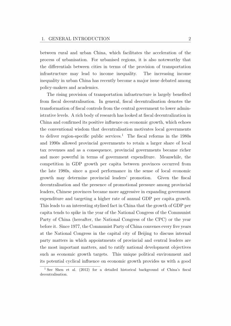
2. Research Questions
In order to visualise the research questions, this section first paints a
general picture of the key relationships of interest in the thesis. As can
be seen in Figure 1.1, four concepts covered in this thesis are (economic)
growth, urbanisation, (transportation) infrastructure, and income inequality.
Empirically, due to the presence of two-way causalities, it is not easy
to identify the relationships illustrated below. This thesis intends to
provide new identification strategies to disentangle the three main causal
relationships which are shown in Figure 1.1, numbered 1, 2 and 3.
Changes in the density of transportation infrastructure are essential in
the system. This contributes to economic growth, because it can reduce
internal trade costs and facilitate production. Furthermore, it may stimulate
economic growth through an indirect channel, i.e. urbanisation, because
upgrading transportation infrastructure can lower the cost of rural-to-urban
3 For instance, Benjamin et al. (2005) find some empirical evidence that geographiclocation perhaps drove spatial income inequality in rural China from 1987 to 2002.
1. GENERAL INTRODUCTION 5
Fig. 1.1: Diagram of Core Concepts in the Thesis
Growth
Infrastructure Urbanisation Income inequality
1
2
3
migration and ultimately increase the rate of urbanisation. Last, the
uneven distribution of transportation infrastructure may result in income
disparities among wage earners, which may potentially hinder further
economic growth. Rather than studying all relationships illustrated in Figure
1.1, this thesis concentrates on three major nexuses, i.e. (1) transportation
infrastructure to economic growth, (2) economic growth to urbanisation, and
(3) transportation infrastructure to income inequality.
This thesis uses a mixture of data. It uses provincial panel data to look at
the first and second nexus. The advantage of using provincial panel datasets
is that one can eliminate provincial time-invariant unobservable factors that
may confound the causal effects of endogenous variables of interest. However,
the cost is also obvious that this type of study relies on macro-level data
that cannot explicitly capture individual behaviour in economic activities.
To provide micro-level evidence, this thesis uses cross-sectional individual
income data to analyse the third nexus.
This thesis first explores the research question: “What is the short-run
effect of changes in the density of transportation infrastructure on economic
growth in China?” Although the contribution of changes in transportation
infrastructure to short-run GDP per capita growth has been often mentioned
(Esfahani and Ramirez, 2003; Calderon and Chong, 2004; Calderon and
Serven, 2005), the causal relationship to date is not yet clear-cut due to
the confounding effect that rapid economic growth in turn increases demand
for expanding transportation infrastructure. This motivates the exploration
in Chapter 3 that uses a national political event — the National Congress of
1. GENERAL INTRODUCTION 6
the Communist Party of China to construct instrumental variables to identify
the causal effect of changes in the density of transportation infrastructure on
economic growth.
Extending the first exploration, this thesis investigates the causal effect of
improvement of transportation infrastructure on long-run economic growth.
Hence, the second question of interest is: “What is the long-run impact of
changes in the density of transportation infrastructure on economic growth
in China?” Generally speaking, this is not an easy question to address
due to the presence of endogeneity issues. For instance, better initial
conditions of transportation infrastructure could be positively correlated
with natural resources, local income level, and other unobserved factors
that can promote long-run growth, for instance, the tightness of connection
between local governments and the central government. To this end,
omitted unobservables, such as geographical conditions, social norms, and
political environment, may confound the effects running from transportation
infrastructure to long-run growth. Since little has been done to date to
mitigate the endogeneity bias in this field, Chapter 4 contributes to the
literature by proposing a new strategy employing the density of Chinese
guilds, as measured by the number of guilds in the Qing dynasty per 10,000
people, to identify exogenous variation in the initial level of provision of the
transportation infrastructure.
During 1978–2008, we observed that massive flows of rural-urban migra-
tion in China, facilitated by upgraded transportation networks, raised the
rate of urbanisation, as measured by local urban population as a share of
total local population. Existing studies (Quigley, 1998; Henderson, 2003;
Duranton and Puga, 2004; Duranton, 2008) have arrived at a consensus that
urbanisation is positively associated with growth, while researchers until re-
cently have paid little attention to the opposite relationship, i.e. the economic
growth-urbanisation nexus. Due to the reverse causality, it is not easy to
quantify the causal impact of economic growth on urbanisation.4 Bruckner
4 The potential channels through which rapid economic growth may potentially increasethe degree of urbanisation are as follows. First, regions with relatively high rates of GDPper capita growth attract rural migrants, because they often offer higher wages. Second,rapid economic growth usually occurs (especially in developing countries) together with
1. GENERAL INTRODUCTION 7
(2012) finds that income growth did not significantly raise urbanisation in
sub-Saharan Africa. By contrast, Henderson (2002) shows economic growth
could lead to a higher level of urbanisation based on data from 85 countries
over the period 1960–1990. Given these conflicting results above, it is worth
identifying the causal effect of economic growth on urbanisation. Using China
as a case study, Chapter 5 addresses the question: “Does economic growth
affect urbanisation?”, and uses instrumental variables to mitigate the reverse
effect running from urbanisation to economic growth.
Through the lens of NEG theory (Krugman, 1991; Krugman and
Venables, 1995), empirical studies (Redding and Venables, 2004; Hanson,
2005; Head and Mayer, 2006) confirm the impact of increasing market
access on nominal wages. Following this stream of literature and recent
explorations using Chinese data (Hering and Poncet, 2010; Hou and Emran,
2012; Kamal et al., 2012), Chapter 6 addresses the question: “How does
access to international markets affect individual wages?” In the area of
income inequality, this is a new topic for China, because scholars usually
underscore the aggregated impact of trade openness on national income
(Dollar and Kraay, 2004; Wacziarg and Welch, 2008) or address the reason
why increased exporting activities promote regional income and GDP per
capita growth (Lemoine and Unal-Kesenci, 2004; Sun and Heshmati, 2010;
Jarreau and Poncet, 2012). However, these studies fail to address the fact
that there are losses resulting from situations where there is failure to access
international markets. Moreover, understanding the impact of access to
international markets on urban wage earners is important for Chinese policy-
makers, because transportation infrastructure was provided unevenly across
regions during 1978–2006 (Chen and Yao, 2011), which generates inter-
regional physical differentials of accessibility to international markets.
rising FDI and international trade, which resulted in increased demand for more labour,which in turn results in more people working and living in cities (urban areas).
1. GENERAL INTRODUCTION 8
3. Summary of Core Chapters
The thesis is organised as follows. This chapter states the research
questions, presents the motivation for the research, and summarises empirical
findings in this thesis. Chapter 2 provides an introductory background
of China’s economic development, summarises related econometric issues,
and highlights the significance of the thesis. Chapters 3 to 6 are core
chapters. Chapter 3 and Chapter 4 address the causal effect of changes
in the density of transportation infrastructure on both short-run and long-
run economic growth. Chapter 5 explores whether economic growth causally
affects urbanisation. Chapter 6 quantifies the impact of the provision of
transportation infrastructure on income inequality in urban China. Chapter
7 gives concluding remarks and discusses further studies.
Chapter 3 looks at the short-run causal effect of changes in the density
of transportation infrastructure on economic growth. It uses the timing of
an exogenous event – the National Congress of the Communist Party of
China – to construct two-stage least squares (2SLS) estimates of the within-
province effect of changes in the density of transportation infrastructure
on GDP growth per capita during 1985–2008. It looks at whether the
timing of the National Congress is associated with changes in the density
of transportation infrastructure. While the ordinary least squares (OLS)
estimate is nearly zero, the 2SLS estimate shows that an increase in the
density of transportation infrastructure has a statistically significant effect on
raising GDP growth per capita. This effect of improvement of transportation
infrastructure on growth is robust to the inclusion of additional control
variables in the regression, to running separate regressions for coastal and
non-coastal provinces, and to utilising four alternative constructions of
instrumental variables based on information about the National Congress.
Chapter 4 studies the long-run effect that changes in the provision
of transportation infrastructure had on growth using Chinese provincial
data during 1978–2008. Because of the endogeneity of transportation
infrastructure, Chapter 4 constructs an instrument based on the density of
the number of the Chinese guilds in the population, which are associations
1. GENERAL INTRODUCTION 9
serving numerous economic and social functions going back to the Qing
dynasty, and finds this instrument to be powerful. The instrumental variable
estimate shows that changes in the provision of transportation infrastructure
has a quantitatively important influence on long-run economic growth, which
is strongly robust to a battery of sensitivity tests that bring into the regression
different sets of potentially relevant covariates.
Chapter 5 explores the causal link between economic growth and
urbanisation. Using a panel dataset of Chinese provinces during 1985–2008,
it proposes a new identification strategy to construct instrumental variables
estimates of the within-province effect that GDP growth per capita has
on the urbanisation rate. This strategy uses the timing of the National
Congress of the CPC, which is a five-yearly meeting where national economic
policies are debated. Chapter 5 finds that GDP growth per capita is strongly
associated with the timing of the National Congress. Using instrumental
variables that convey this timing information, 2SLS estimates are used to
show whether economic growth has a statistically significant effect on raising
the urbanisation rate.
While previous chapters mainly rely on aggregated data, Chapter 6 offers
some micro evidence of how the provision of transportation infrastructure
affects income inequality in urban China. In Chapter 6, the provision
of transportation infrastructure is proxied by length of current transport
routes from origin city to its nearest major seaport. Using China Household
Income Project Survey (2002) data, Chapter 6 addresses the causal effect
of the improvement of transportation infrastructure on urban wage earners.
Using historical information, i.e. prefecture-level population density in 1820,
to construct instrumental variables for current transport routes, the 2SLS
regressions show a statistically significant effect of better transportation
infrastructure on individual wages in urban China. This causal effect remains
robust to various sensitivity tests which bring relevant covariates such as
current labour market structure, historical factor endowments, and initial
population development into the regression.
2. BACKGROUND
1. Introduction
This thesis analyses China’s economic growth, urbanisation and income
inequality in which transportation infrastructure played an important role
during 1978–2008. This chapter provides the background of China’s economic
development, reviews the related literature, and summarises the significance
of the core chapters (i.e. Chapters 3 to 6).
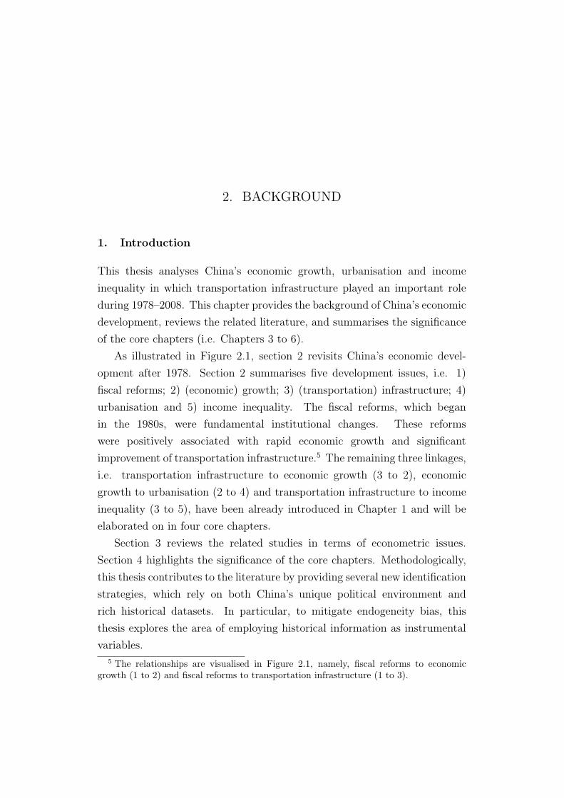
As illustrated in Figure 2.1, section 2 revisits China’s economic devel-
opment after 1978. Section 2 summarises five development issues, i.e. 1)
fiscal reforms; 2) (economic) growth; 3) (transportation) infrastructure; 4)
urbanisation and 5) income inequality. The fiscal reforms, which began
in the 1980s, were fundamental institutional changes. These reforms
were positively associated with rapid economic growth and significant
improvement of transportation infrastructure.5 The remaining three linkages,
i.e. transportation infrastructure to economic growth (3 to 2), economic
growth to urbanisation (2 to 4) and transportation infrastructure to income
inequality (3 to 5), have been already introduced in Chapter 1 and will be
elaborated on in four core chapters.
Section 3 reviews the related studies in terms of econometric issues.
Section 4 highlights the significance of the core chapters. Methodologically,
this thesis contributes to the literature by providing several new identification
strategies, which rely on both China’s unique political environment and
rich historical datasets. In particular, to mitigate endogeneity bias, this
thesis explores the area of employing historical information as instrumental
variables.
5 The relationships are visualised in Figure 2.1, namely, fiscal reforms to economicgrowth (1 to 2) and fiscal reforms to transportation infrastructure (1 to 3).
2. BACKGROUND 11
Fig. 2.1: China’s Development Issues Revisited
2. Growth 3. Infrastructure
4. Urbanisation 5. Income inequality
1. Fiscal reforms
2. Background of China’s Economic Development
The great expansion of the Chinese economy attracts much attention from
academics, however, no simple factor can explain the unprecedented China
miracle, whereby real GDP per capita rose from USD 145.5 to USD
2426.3 between 1975 and 2010. To understand why China could achieve
a consistently high rate of GDP per capita growth during 1978–2008, it is
necessary to look first at China’s development pattern after 1978.
This section introduces the fiscal reforms which propelled China’s eco-
nomic development and drove its rapid economic growth during 1978–2008.
The latest fiscal reform initiated in 1994 allowed the provincial governments
to raise the regional GDP per capita growth through expanding government
expenditure. This decentralisation reform contributed to increasing the
provision of transportation infrastructure — the central theme of this thesis.
In addition, this section delineates China’s economic growth, development
of transportation infrastructure, rapid process of urbanisation and urban
income inequality.
2.1 Fiscal Reforms
In order to demystify China’s economic growth and development by un-
derstanding the economic history and fundamental institutions, Table 2.1
outlines the evolution of fiscal decentralisation and institutional changes in
the major development phases. In addition, this chapter illustrates the

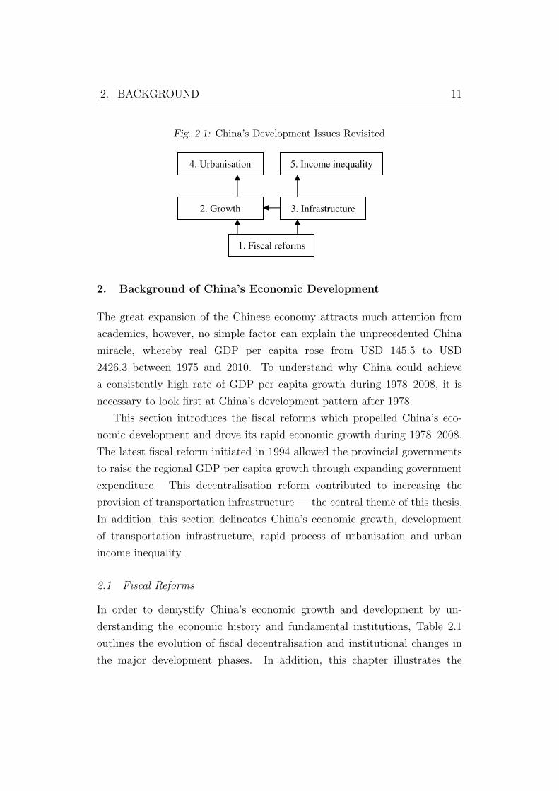
2. BACKGROUND 12
hierarchy of Chinese governments in Figure 2.2. The highest authority of
the nation is the central government, while the sub-national administrative
units constitute provinces, prefectures, counties (or cities) and townships (or
villages).
Tab. 2.1: Fiscal Decentralisation (Percent) and Institutional Changes (1953–2005)
Note: All information is obtained from Xu (2011). HRS denotes Household ResponsibilitySystem initiated in 1979 and completed in 1984. The HRS allocated the collectiveagricultural land to rural households, giving them relative autonomy over land use, andallocated them to contract land, machinery and other physical capital from collectiveorganizations.
The People’s Republic of China which was founded in 1949 started its
first Five-Year Plan in 1953 when a transplantation of the Soviet model had
been completed.6 Initially, the central authority tightly controlled taxation
and government spending so that only 17 percent of revenue went to local
government accounts and 26 percent of expenditure was used for sub-national
items. After two high-cost campaigns, the Great Leap Forward (1958–
6 The Five-Year Plan was borrowed from the Soviet model which emphasised thatthe process of economic development should be designed and monitored by the centralgovernment only. For instance, each Five-Year Plan would announce some key economictargets like the GDP level, the level of agricultural outputs and the rate of GDP per capitagrowth, among others.
A NOTE:
This figure/table/image has been removed to comply with copyright regulations. It is included in the print copy of the thesis held by the University of Adelaide Library.
2. BACKGROUND 13
Fig. 2.2: Structure of Government
Central Government
Provinces
Prefectures
Counties/Cities
Townships/Villages
1961) and the Cultural Revolution (1966–1976), which encouraged regional
competition in over-fulfilling centrally-planned targets, local governments
shared more than 80 percent of total tax revenue and more than a half
of total government expenditure by the late 1970s.7 In 1980,8 the central
authority started the first fiscal reform. During 1980–1993, the so-called
‘fiscal contract system’ was implemented. Under such a system, provincial
governments shared their revenues with the central government according to
those predetermined schemes.9 In other words, the provincial governments
remitted ‘contracted’ revenues to the central government.
Starting in 1994, the ‘fiscal contract system’ was replaced by the ‘fiscal
sharing rule’ which aimed to increase central tax revenue. The ‘fiscal sharing
rule’ introduced the tax assignment, which specified the way revenues were
shared between sub-national governments and the central government. As
illustrated in Table 2.1, the proportion of sub-national revenue to national
revenue shrank from 78.0 percent in 1993 to 44.3 percent in 1994.
7 See Xu (2011) which summarises the Chinese political institutions and revisits majoreconomic and political reforms after 1949.
8 This was two years after the official economic liberalisation announced by the centralgovernment in 1978.
9 Detailed phases of ‘fiscal contract system’ are discussed in Shen et al. (2012).
2. BACKGROUND 14
An interesting finding from Table 2.1 is that the ratio of sub-national
expenditure to total expenditure rose from 45.7 percent in 1980 to 74.1
percent in 2005, while the ratio of sub-national revenue to total revenue
declined from 75.5 percent to 47.7 percent during the same period. At first
glance, this seemed to be incredible. How could sub-national governments
achieve this? Jin et al. (2005) and Shen et al. (2012) suggest it was ‘extra-
budgetary’ funding that financed the expansion of government spending. The
‘extra-budgetary’ funding, as pointed out by Montinola et al. (1995), was a
special revenue component which was retained by sub-national governments
during 1980–1993.10 Although the central authority intended to restrict the
ability of sub-national governments to increase local coffers through ‘extra-
budgetary’ funds under the ‘fiscal sharing rule’, the actual proportion of sub-
national expenditure to national expenditure increased from 70 percent in
1994 to 74 percent in 2005. In order to find the source for the relatively higher
growth of the proportion of sub-national expenditure to total expenditure
after 1994, Wong and Bird (2008) investigate the Chinese fiscal system and
point out that sub-national governments could still maintain large, under-
reported extra-budgetary reserves after 1994 and use these ‘secrete’ reserves
for their own purposes.
The changes in the Chinese fiscal system, which funds to provincial
governments, reinforces political and economic powers of those provincial
governments, may in turn promote regional economic growth. For example,
provincial governments are able to increase the investment on transportation
infrastructure under the current ‘fiscal sharing rule’ without the substantial
financial support from the central government. The essential work of this
thesis is built on this unique fiscal pattern in China.
10 Due to loose reporting requirements, provincial governments were able to retain extra-budgetary reserves which in fact had continued to grow after the 1994 fiscal reform (Wongand Bird, 2008).
2. BACKGROUND 15
2.2 Economic Growth
In order to draw a general picture of China’s income level and its growth
pathway, this section starts with the evolution of China’s GDP per capita
during 1961–2010. Shown in Table 2.2, China’s GDP per capita rose from
USD 105.5 in 1961 to USD 2,426.3 in 2010, which was one of the most
impressive development stories following the Second World War.11
Tab. 2.2: China’s GDP Per Capita Level and Annual Growth (1961–2010)
Year Real GDP per capita (USD) Annual growth (Percent)
1961 105.5 -26.4
1965 100.1 13.6
1970 122.3 16.1
1975 145.5 6.8
1980 186.4 6.5
1985 289.7 12.0
1990 391.7 2.3
1995 658.0 9.7
2000 949.2 7.5
2005 1464.1 10.6
2010 2426.3 9.9
Note: Data are obtained from the World Development Indicators (World Bank). RealGDP per capita is deflated to constant 2000 US dollars. Annual growth denotes averageyearly growth rate of real GDP per capita.
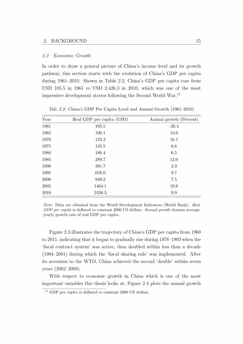
Figure 2.3 illustrates the trajectory of China’s GDP per capita from 1960
to 2011, indicating that it began to gradually rise during 1978–1993 when the
‘fiscal contract system’ was active, then doubled within less than a decade
(1994–2001) during which the ‘fiscal sharing rule’ was implemented. After
its accession to the WTO, China achieved the second ‘double’ within seven
years (2002–2008).
With respect to economic growth in China which is one of the most
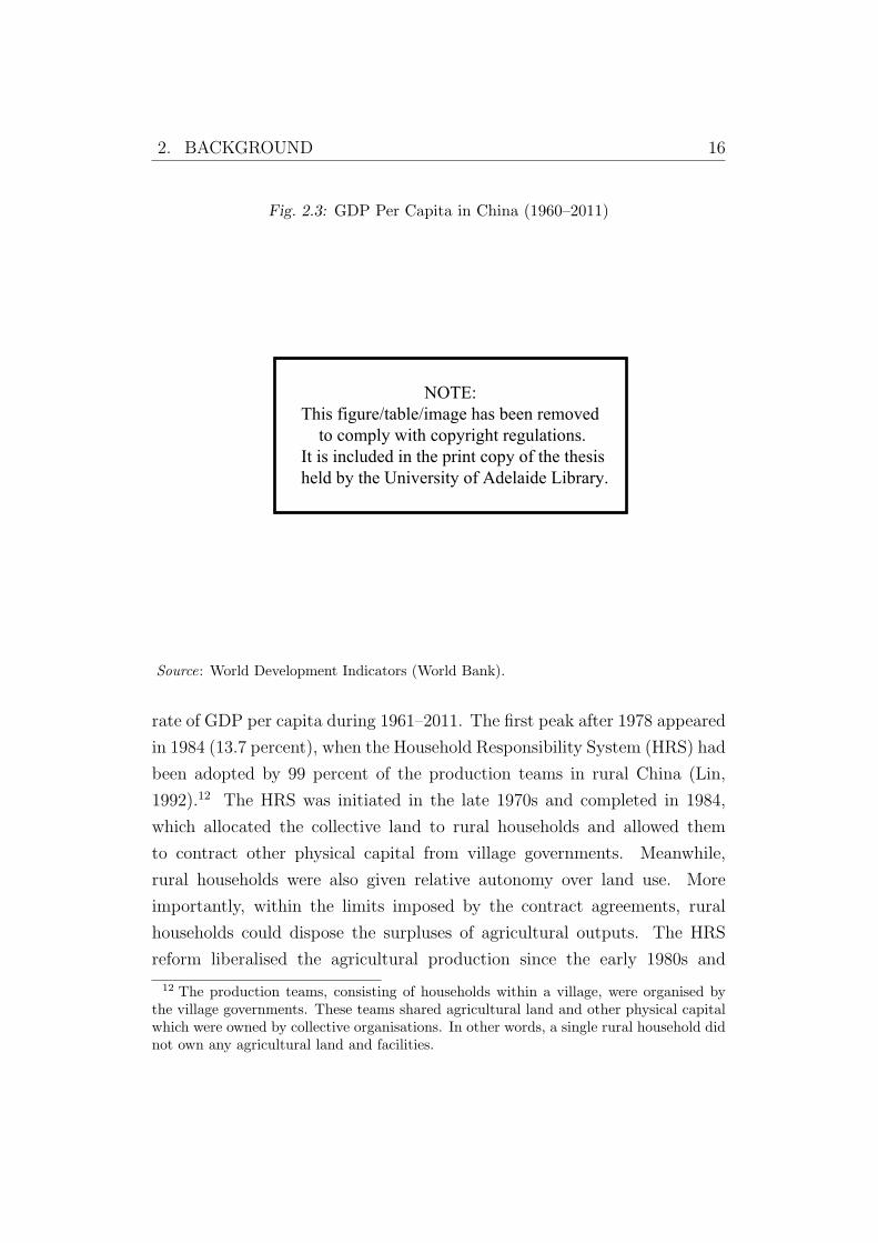
important variables this thesis looks at, Figure 2.4 plots the annual growth
11 GDP per capita is deflated to constant 2000 US dollars.
2. BACKGROUND 16
Fig. 2.3: GDP Per Capita in China (1960–2011)
Source: World Development Indicators (World Bank).
rate of GDP per capita during 1961–2011. The first peak after 1978 appeared
in 1984 (13.7 percent), when the Household Responsibility System (HRS) had
been adopted by 99 percent of the production teams in rural China (Lin,
1992).12 The HRS was initiated in the late 1970s and completed in 1984,
which allocated the collective land to rural households and allowed them
to contract other physical capital from village governments. Meanwhile,
rural households were also given relative autonomy over land use. More
importantly, within the limits imposed by the contract agreements, rural
households could dispose the surpluses of agricultural outputs. The HRS
reform liberalised the agricultural production since the early 1980s and
12 The production teams, consisting of households within a village, were organised bythe village governments. These teams shared agricultural land and other physical capitalwhich were owned by collective organisations. In other words, a single rural household didnot own any agricultural land and facilities.
A NOTE:
This figure/table/image has been removed to comply with copyright regulations. It is included in the print copy of the thesis held by the University of Adelaide Library.
2. BACKGROUND 17
resulted in a significant growth in agricultural outputs as shown in Lin (1992).
During 1989 to 1990 when radical political changes occurred in the
Eastern bloc countries, China’s rate of growth also fell to around 2 percent
which was the lowest pace since 1978. But the political instability only
resulted in a pause of GDP per capita growth, as China surprisingly returned
to a 12.8 percent rate of growth in 1992 (the second peak) when the central
government officially announced the transformation from a central-planned
to a market-based economy. Between the Asian financial crisis (1997–1998)
and the latest global financial crisis (2008–2009), China reached its third
peak of economic growth after 1978, i.e. 13.6 percent per annum in 2007.
Fig. 2.4: Annual Growth Rate of GDP Per Capita in China (1961–2011)
Source: World Development Indicators (World Bank).
As China has undergone economic development since the 1950s, it is
interesting to note that the relative contributions of the determinants of
economic growth (e.g. physical capital, human capital and TFP) varied
A NOTE:
This figure/table/image has been removed to comply with copyright regulations. It is included in the print copy of the thesis held by the University of Adelaide Library.
2. BACKGROUND 18
over time. In other words, sometimes one factor might contribute more to
economic growth relative to the other two factors. During period of the initial
economic prosperity recovering from the Korean War (1950–1953), as can be
seen in Table 2.3 (row 1), the TFP grew strongly (4.7 percent). During the
Great Leap Forward (1958–1961), the central government emphasised the
role of heavy industry by allocating more physical and human capital. This
resulted in a relative labour shortage in the other industries and caused a
steep decline in productivity. Letting the data speak, the average annual
growth of TFP reduced from 4.7 percent (1952–1957) to -1.0 percent (1957–
1965). During the Great Leap Forward, physical capital became almost the
only engine of economic growth, as physical capital accounted for 93.1 percent
of total contribution to GDP growth (see row 2 in Table 2.3).
After 1965, the Cultural Revolution began and led to a 10-year period of
chaos during which the peak of disruption to the national economy occurred
over the period 1967–1968 (Perkins and Rawski, 2008). Field (1986) reports
that the gross value of industrial output shrank from RMB 152.6 billion to
RMB 122.3 billion between 1966–1968.13 As described in Li et al. (2010),
“At the onset of the Cultural Revolution, all primary schools in urban China
were closed for 2–3 years, and secondary- and tertiary-level institutions were
closed for much of the period.”
During 1965–1978, two-thirds of economic growth was attributed to
physical capital (67.7 percent), which recalled the scenario during the
Great Leap Forward. It was the economic reform starting from 1978 that
reconfirmed the key position of TFP in China’s economic growth. In
particular, as summarised in Table 2.3, the TFP kept rising during 1978–
2005 and was the strongest contributor to GDP per capita growth relative to
physical and human capital for a decade (1985–1995). During the period
1995–2005, although the TFP still grew, China returned to the growth
pattern which relied heavily on physical capital accumulation.
Finally, it is worth providing a cross-country comparison displaying
China’s economic growth relative to other economies. Table 2.4 shows that
from the late 1970s, China’s economy followed the booming trajectory which
13 The gross value gross value of industrial output is deflated to 1957 constant prices.
2. BACKGROUND 19
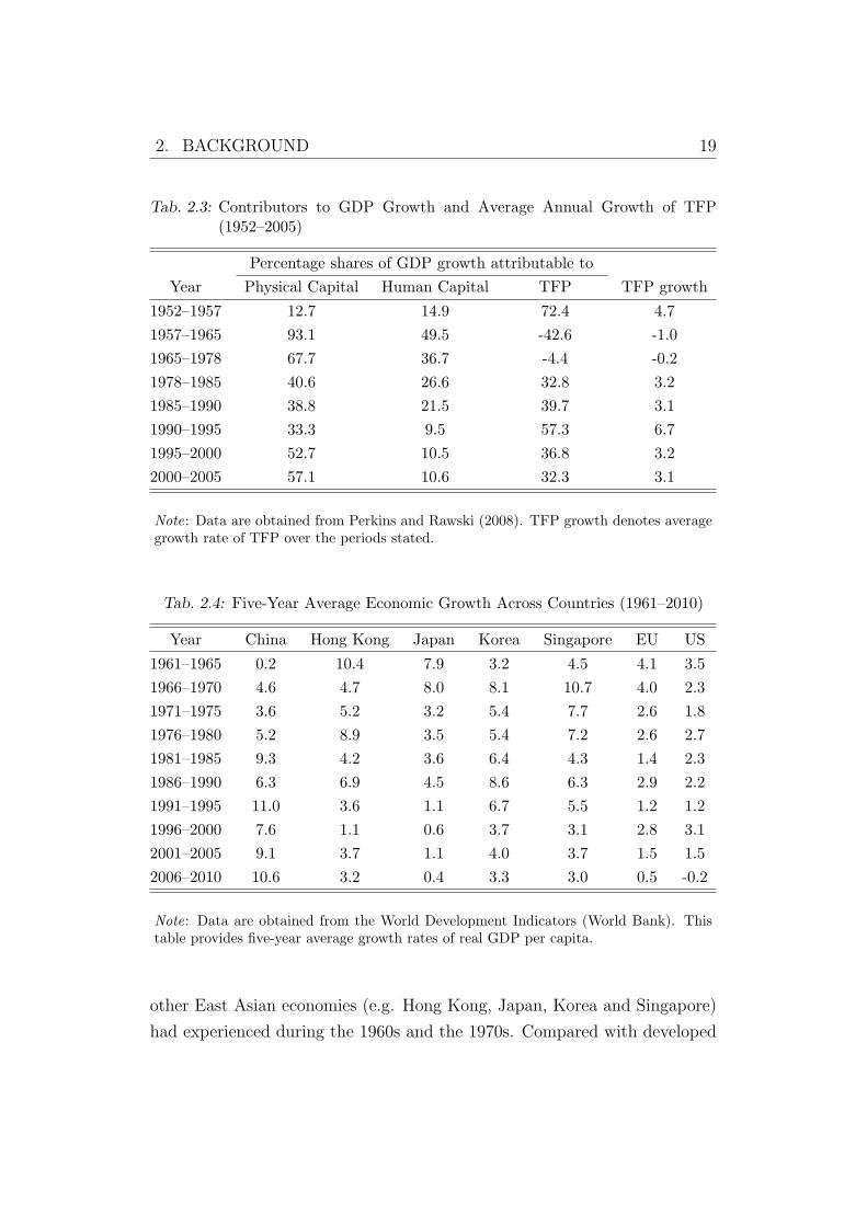
Tab. 2.3: Contributors to GDP Growth and Average Annual Growth of TFP(1952–2005)
Percentage shares of GDP growth attributable to
Year Physical Capital Human Capital TFP TFP growth
1952–1957 12.7 14.9 72.4 4.7
1957–1965 93.1 49.5 -42.6 -1.0
1965–1978 67.7 36.7 -4.4 -0.2
1978–1985 40.6 26.6 32.8 3.2
1985–1990 38.8 21.5 39.7 3.1
1990–1995 33.3 9.5 57.3 6.7
1995–2000 52.7 10.5 36.8 3.2
2000–2005 57.1 10.6 32.3 3.1
Note: Data are obtained from Perkins and Rawski (2008). TFP growth denotes averagegrowth rate of TFP over the periods stated.
Tab. 2.4: Five-Year Average Economic Growth Across Countries (1961–2010)
Year China Hong Kong Japan Korea Singapore EU US
1961–1965 0.2 10.4 7.9 3.2 4.5 4.1 3.5
1966–1970 4.6 4.7 8.0 8.1 10.7 4.0 2.3
1971–1975 3.6 5.2 3.2 5.4 7.7 2.6 1.8
1976–1980 5.2 8.9 3.5 5.4 7.2 2.6 2.7
1981–1985 9.3 4.2 3.6 6.4 4.3 1.4 2.3
1986–1990 6.3 6.9 4.5 8.6 6.3 2.9 2.2
1991–1995 11.0 3.6 1.1 6.7 5.5 1.2 1.2
1996–2000 7.6 1.1 0.6 3.7 3.1 2.8 3.1
2001–2005 9.1 3.7 1.1 4.0 3.7 1.5 1.5
2006–2010 10.6 3.2 0.4 3.3 3.0 0.5 -0.2
Note: Data are obtained from the World Development Indicators (World Bank). Thistable provides five-year average growth rates of real GDP per capita.
other East Asian economies (e.g. Hong Kong, Japan, Korea and Singapore)
had experienced during the 1960s and the 1970s. Compared with developed
2. BACKGROUND 20
economies, China’s growth since the late 1970s exceeded the highest growth
rate for the US and the EU during the period 1961–2010, as shown in Table
2.4.
2.3 Transportation Infrastructure
China has made huge investments in transportation infrastructure which
mainly consisted of highways and railroads in the 1990s and the 2000s,
which resulted in a significant increase in the provision of transportation
infrastructure. For instance, tracking the evolution of transportation
infrastructure in 210 Chinese prefectures during 1962–2010, Baum-Snow and
Turner (2012) show that between 1990 and 2010, the length of railroads in a
prefecture on average increased from 142.03 to 209.17 kilometres.
For more details, Figure 2.5 illustrates that an average prefecture saw
its length of railroads gradually grew from 93.39 to 132.96 kilometres during
the pre-reform era (i.e. prior to 1978), then jumped to 207.38 kilometres by
2005, and steadily rose to 209.17 kilometres by 2010. In addition, Figure 2.5
displays that before 1990 there were no express highways between Chinese
prefectures. However, the Chinese government earmarked a large-scale of
construction of express highways from the 1990s, which resulted in the
average length of express highways per prefecture rising to 47.39 kilometres
in 1999 and jumping to 222.09 kilometres by 2010.
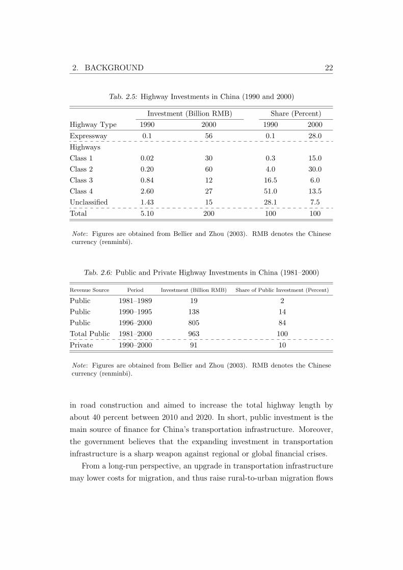
According to a comprehensive analysis of China’s road infrastructure
in Bellier and Zhou (2003), the investment focus shifted from low-grade
highways towards expressways between 1990 and 2000. Table 2.5 shows that
the share of expressway investment rose from 0.1 percent to 28.0 percent
between 1990 and 2000; meanwhile, low-grade (Class 4) highways declined
from 51.0 percent to 13.5 percent.
Furthermore, Bellier and Zhou (2003) point out that the construction of
roads heavily relied on public investment in China. As can been see in Table
2.6, private investment during 1990–2000 accounted for only 10 percent of
total public investment in transportation infrastructure over the period 1981–
2. BACKGROUND 21
Fig. 2.5: Average Length of Railroads and Express Highways in China (1962–2010)
Source: Baum-Snow and Turner (2012).
2000.14
A significant expansion of public investment (RMB 805 billion) in Chinese
highways during 1996–2000 is shown in Table 2.6, which in part relates
to the Asian financial crisis between 1997 and 1998. In the wake of this
crisis, the Chinese government encouraged public entities to take medium-
and long-term infrastructure loans. As Bellier and Zhou (2003) compute,
from 1998 to 2002, 30 percent of public bonds (around RMB 200 billion)
issued by the government went to infrastructure. Likewise, a similar
policy was implemented as a response to the 2008–2009 global financial
crisis. In 2008, the government announced a stimulus package of RMB
1.52 trillion for infrastructure projects. This package included investment
14 There was a very low level of private investment in highway investment until the early1990s, as the related laws and regulations for private investment, particularly foreigninvestment, were not fully established until 1995 (Bellier and Zhou, 2003).
A NOTE:
This figure/table/image has been removed to comply with copyright regulations. It is included in the print copy of the thesis held by the University of Adelaide Library.
2. BACKGROUND 22
Tab. 2.5: Highway Investments in China (1990 and 2000)
Investment (Billion RMB) Share (Percent)
Highway Type 1990 2000 1990 2000
Expressway 0.1 56 0.1 28.0
Highways
Class 1 0.02 30 0.3 15.0
Class 2 0.20 60 4.0 30.0
Class 3 0.84 12 16.5 6.0
Class 4 2.60 27 51.0 13.5
Unclassified 1.43 15 28.1 7.5
Total 5.10 200 100 100
Note: Figures are obtained from Bellier and Zhou (2003). RMB denotes the Chinesecurrency (renminbi).
Tab. 2.6: Public and Private Highway Investments in China (1981–2000)
Revenue Source Period Investment (Billion RMB) Share of Public Investment (Percent)
Public 1981–1989 19 2
Public 1990–1995 138 14
Public 1996–2000 805 84
Total Public 1981–2000 963 100
Private 1990–2000 91 10
Note: Figures are obtained from Bellier and Zhou (2003). RMB denotes the Chinesecurrency (renminbi).
in road construction and aimed to increase the total highway length by
about 40 percent between 2010 and 2020. In short, public investment is the
main source of finance for China’s transportation infrastructure. Moreover,
the government believes that the expanding investment in transportation
infrastructure is a sharp weapon against regional or global financial crises.
From a long-run perspective, an upgrade in transportation infrastructure
may lower costs for migration, and thus raise rural-to-urban migration flows
2. BACKGROUND 23
as mentioned in Combes et al. (2013). In addition, Baum-Snow and Turner
(2012) and Baum-Snow et al. (2012) reveal the potential link between the
development of transportation infrastructure (including roads and railroads)
and the evolution of urbanisation in China. In the next section, the issues
which relate to the urbanisation process and rural-to-urban migration are
carefully reviewed.
2.4 Urbanisation Process, Hukou Reforms and Rural-Urban Migration
According to Henderson (2005), urbanisation is the process by which
an economy undergoes the restructure from predominantly agricultural
production to manufacturing and services. In China, a series of agricultural
reforms (e.g. the HRS reform) significantly raised agricultural productivity
in the early 1980s and reduced the demand for rural labour in agricultural
production. The labour surplus in rural China, together with the booming
of exporting sectors in coastal regions, started the engine of China’s
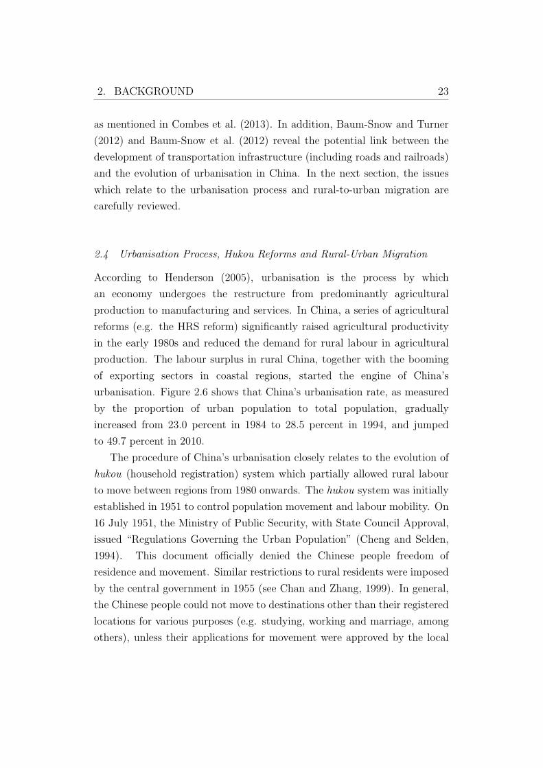
urbanisation. Figure 2.6 shows that China’s urbanisation rate, as measured
by the proportion of urban population to total population, gradually
increased from 23.0 percent in 1984 to 28.5 percent in 1994, and jumped
to 49.7 percent in 2010.
The procedure of China’s urbanisation closely relates to the evolution of
hukou (household registration) system which partially allowed rural labour
to move between regions from 1980 onwards. The hukou system was initially
established in 1951 to control population movement and labour mobility. On
16 July 1951, the Ministry of Public Security, with State Council Approval,
issued “Regulations Governing the Urban Population” (Cheng and Selden,
1994). This document officially denied the Chinese people freedom of
residence and movement. Similar restrictions to rural residents were imposed
by the central government in 1955 (see Chan and Zhang, 1999). In general,
the Chinese people could not move to destinations other than their registered
locations for various purposes (e.g. studying, working and marriage, among
others), unless their applications for movement were approved by the local
2. BACKGROUND 24
Fig. 2.6: Urbanisation Process in China (1949–2010)
Cultural Revolution
.1.2
.3.4
.5ur
bani
satio
n ra
te
1949 1954 1959 1964 1969 1974 1979 1984 1989 1994 1999 2004 2009
Source: National Bureau of Statistics China (2010) and World Development Indicators(World Bank).
governments. However, this process was difficult and many people could not
move as their applications were rejected.
From the early 1980s, the central government gradually implemented
various programmes to devolve fiscal and administrative powers to lower-
level governments (i.e. counties, townships and villages), so they took over
control of migration (Chan and Buckingham, 2008). The local governments
tended to have a more relaxed approach to allowing people to leave, which
eased the flow of migration from rural areas. Meanwhile, the attitudes of
city (destination) governments towards immigrants from rural areas also
became more relaxed. Prior to the early 1990s, if migrants from rural
areas were found not to have been granted residency (migrated without
permission), they would be expelled from that destination and sent back to
2. BACKGROUND 25
their origin locations. Rather than expelling migrant workers, the destination
governments enacted rules to regulate these new ‘immigrants’ from the early
1990s onwards. For example, in 1995, rural migrants were required to present
four documents (i.e. individual identification card, temporary residency,
and employment certificate issued by labour bureaus in both the origin
and destination locations) in order to ‘legally’ live and work in urban areas
(see Cai et al. (2008) for more detailed regulations). The relatively relaxed
migration policies during the 1990s had a significantly positive impact on
the rapid increase of the urbanisation rate after 1995, which is illustrated in
Figure 2.6.
According to Harris and Todaro (1970), migration decisions are usually
driven by income differentials between origin and destination locations. This
theory may also apply in China. Using Chinese data, a growing body of
literature explains the question about why rural labour migrates to urban
areas. Relying on household survey data from Sichuan province in 1995,
Zhao (1999) argues that the shortage of farmland and the abundance of
household labour significantly affected labour migration. This so-called
‘push’ effect implies that due to the reduction in relative marginal income
from farming, rural labour begins to leave the countryside. There also
exists a source of ‘pull’ effect, that is due to the relatively higher potential
income in urban areas. Using data from 29 provinces over two periods (i.e.
1985–1990 and 1990–1995), Poncet (2006) finds that the income difference
between destination and origin locations has a statistically significant and
quantitatively large effect on migration flows.
Migration per se is costly. The costs consist of, for example, transport,
temporary unemployment, social security and children’s living and education
costs in urban China. Among these costs, the most important one which has a
significant impact on migration decisions is transport cost. As transport costs
may not always be measured directly, empirical studies often use migration
distance to proxy for it. Poncet (2006) shows that migration flows decline
significantly with the increase in distance between origin and destination
locations. A study of rural migrants using survey data from the Rural Urban
Migration in China (RUMiC, 2007), i.e. Zhang and Zhao (2013), estimates
2. BACKGROUND 26
the income-distance elasticity, and reports that to induce a migrant to move
1 percent farther away from his origin location, the potential income in the
destination location has to increase by roughly 1.5 percent. In other words,
based on survey data on rural-to-urban migrants in 15 Chinese cities in 2007,
Zhang and Zhao (2013) find that the income-distance elasticity was around
1.5.
Although rural migrants may benefit from potentially higher earnings
in urban areas relative to staying in the countryside, their actual wages are
lower than they should be. This issue which relates to wage inequality among
urban wage earners is documented in the next section.
2.5 Income (Wage) Inequality in Urban China
China’s labour reforms began in 1983 when the HRS (agricultural) reform
was introduced in most rural areas and had the effect of liberalising
agricultural labour. After 1983, China started transforming it centrally-
planned labour allocation system into a liberalised labour market in urban
areas,15 which led to a mounting wage inequality within the urban labour
market as illustrated in this section.
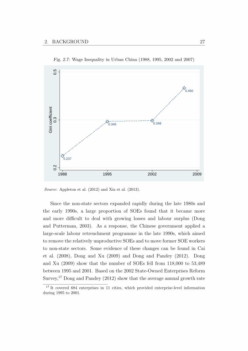
Recent studies such as Appleton et al. (2012) and Xia et al. (2013), use
the China Household Income Project Survey (CHIPS) data to delineate the
trend of wage inequality during 1988–2007 in urban China.16 As can be
seen in Figure 2.7, the wage inequality (Gini coefficient) rose from 0.237 in
1988 to 0.345 in 1995, remaining relatively stable during 1995 to 2002, and
sharply increased to 0.450 by 2007. It is noteworthy that over the period
1988–2007, the Chinese government applied two major programmes, i.e. the
retrenchment within SOEs (state-owned enterprises) and the relaxation of
controls on rural-urban migration. These measures aimed to restructure the
state-owned sectors and liberalise the national labour market, respectively.
15 See Appleton et al. (2005), which studies the evolution of wage structure during 1988–2002 when China began the liberalisation of its labour market.
16 CHIPS data contain four waves for 1988, 1995, 2002 and 2007. The surveys werenational representative, and samples were randomly drawn from the annual nationalhousehold income survey of the National Bureau of Statistics of China.
2. BACKGROUND 27
Fig. 2.7: Wage Inequality in Urban China (1988, 1995, 2002 and 2007)
0.237
0.345 0.348
0.450
0.2
0.3
0.5
Gin
i coe
ffici
ent
1988 1995 2002 2009
Source: Appleton et al. (2012) and Xia et al. (2013).
Since the non-state sectors expanded rapidly during the late 1980s and
the early 1990s, a large proportion of SOEs found that it became more
and more difficult to deal with growing losses and labour surplus (Dong
and Putterman, 2003). As a response, the Chinese government applied a
large-scale labour retrenchment programme in the late 1990s, which aimed
to remove the relatively unproductive SOEs and to move former SOE workers
to non-state sectors. Some evidence of these changes can be found in Cai
et al. (2008), Dong and Xu (2009) and Dong and Pandey (2012). Dong
and Xu (2009) show that the number of SOEs fell from 118,000 to 53,489
between 1995 and 2001. Based on the 2002 State-Owned Enterprises Reform
Survey,17 Dong and Pandey (2012) show that the average annual growth rate
17 It covered 684 enterprises in 11 cities, which provided enterprise-level informationduring 1995 to 2001.
2. BACKGROUND 28
of output among surveyed SOEs fell from -0.159 in 1996 to -0.201 in 1998.
In addition, based on the data from the Labour Statistical Year Book (1999–
2005), Cai et al. (2008) report that 27.04 million workers from SOEs were
laid off during 1998–2004. As most of laid-off (in Chinese, xiagang) workers
were more likely to be low-skilled and/or unemployed,18 they might face a
low-income trap in the long run.19 In summary, the retrenchment within
SOEs resulted in a huge number of laid-off workers whose wages were much
lower than the average level within the respective occupation. The presence
of these low-income workers during the late 1990s and early 2000s could be
one of the sources of wage inequality between urban wage earners.
The another factor which contributed to the liberalisation of the Chinese
labour market but potentially worsened the wage inequality in urban China
is the relaxation of controls on rural-to-urban migration. Various studies
find that rural migrants in the destination cities experience low wages (or
total income) relative to urban permanent residents. Using Shanghai as a
case study, Wang and Zuo (1999) report that in 1995, even though rural
migrants worked on average 25 percent longer per week (54 versus 43 hours)
than urban workers who were permanent residents, they earned 40 percent
less income.20 Also looking at Shanghai, Meng and Zhang (2001) find that
the wage differentials between migrants and non-migrants was 50 percent
in 1995.21 More importantly, Meng and Zhang (2001) indicate that wage
differentials between the two groups were largely attributed to discrimination
within the market, as they find that 83 percent of the hourly wage differential
resulted from unequal payment within a given occupation. For nation-
wide evidence, Demurger et al. (2009), based on China Household Income
18 Cai et al. (2008) indicate that the registered unemployment rate rose from 3.1 percentin 1998 to 4.2 percent in 2004 due to the sudden spike of millions of laid-off workers in theurban labour market.
19 Due to China’s underdeveloped social security system, these laid-off workers were lesslikely or unlikely to be compensated for unemployment. Also, it was relatively difficult forthem to find new jobs, since they were less competitive in the urban labour market.
20 The data were obtained from the Shanghai Floating Population Survey which wasconducted by the Institute of Population Studies at Shanghai Academy of Social Sciencesin late 1995.
21 Meng and Zhang (2001) use data from the Shanghai Floating Population Survey andthe Shanghai Residents and Floating Population Survey.
2. BACKGROUND 29
Project Survey (CHIPS, 2002) data, show that urban residents earned 1.3
times higher annual income than long-term rural migrants in 12 surveyed
provinces.22
To sum up, it is believed that the rising number of two types of workers,
namely low-skilled, laid-off workers from former SOEs and rural migrants
who are discriminated against in terms of wages, significantly widened the
wage gap among urban wage earners after the late 1990s. This seems to be an
unavoidable ‘cost’ of the reshaping of SOEs and the nation-wide liberalisation
of the labour force.
3. Econometric Issues
One of the central challenges in empirical studies is endogeneity that is
typically caused by omitted variables, measurement errors and simultaneity.
For instance, studies that seek to identify causal relationships between
infrastructure and economic growth have to solve for the reverse causality.
Moreover, in the case of China, measurement errors in national accounting
could be another source of endogeneity. This section revisits econometric
issues of endogeneity in the literature which closely relate to this thesis.
To mitigate endogeneity bias, existing literature offers several methods,
for example, fixed effects estimation, dynamic panel data estimation, the
simultaneous equations approach and instrumental variables estimation.
Table 2.7 lists major studies which relate to the topics of interest, where
the upper panel summarises those studies that primarily investigate the
relationship between infrastructure and economic growth,23 while the lower
panel outlines those studies that mainly look at the association between
urbanisation and economic growth.
22 Combes et al. (2013), using 2007 Urban Household Survey data, provide some evidencethat the larger the share of migrants in a destination city, the higher the local workers’wages. This could also in part explain the recent rising wage inequality in Chinese cities.
23 Some studies look at the relationship between infrastructure (stock or investment) andthe three measures, i.e. income, consumption and productivity.
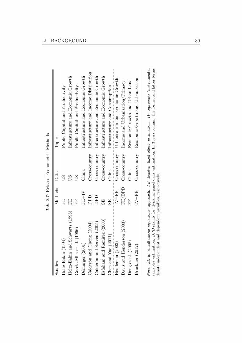
2. BACKGROUND 30
Tab.2.7:RelatedEconometricMethods
Studies
Methods
Data
Topics
Holtz-E
akin
(199
4)FE
US
PublicCapitalandProductivity
Holtz-E
akin
andSchwartz
(199
5)FE
US
Infrastructure
andEconomic
Growth
Garcia-Milaet
al.(199
6)FE
US
PublicCapitalandProductivity
Dem
urger
(200
1)FE+IV
China
Infrastructure
andEconomic
Growth
Calderon
andChon
g(200
4)DPD
Cross-country
Infrastructure
andIncomeDistribution
Calderon
andServen
(200
5)DPD
Cross-country
Infrastructure
andEconomic
Growth
Esfah
anian
dRam
irez
(200
3)SE
Cross-country
Infrastructure
andEconomic
Growth
Chen
andYao
(201
1)SE
China
Infrastructure
andConsumption
Henderson(200
3)IV
+FE
Cross-country
UrbanisationandEconomic
Growth
Dav
isan
dHenderson(200
3)FE/DPD
Cross-country
IncomeandUrbanisation/Primacy
Denget
al.(200
8)FE
China
Economic
Growth
andUrbanLand
Bruckner
(201
2)IV
+FE
Cross-country
Economic
Growth
andUrbanisation
Note:SE
is‘sim
ultan
eousequations’
approach.FE
den
otes
‘fixed
effect’
estimation.IV
represents
‘instrumental
variab
les’estimation.DPD
stan
dsfor‘dynam
icpan
eldata’
estimation.In
Topicscolumn,theform
eran
dlatter
term
sden
oteindep
endentan
ddep
endentvariab
les,
respectively.
2. BACKGROUND 31
3.1 Infrastructure and Economic Growth
The first method to ameliorate endogeneity is employing fixed effects
estimation embedded in a panel data framework. This method is used
in early studies based on state-level data in the US, for example, Holtz-
Eakin (1994), Holtz-Eakin and Schwartz (1995) and Garcia-Mila et al.
(1996). Fixed effect estimations in principle can partial out time-invariant
unobservable heterogeneity. By employing this approach, one actually deals
with omitted variables (e.g. geographical conditions and cultural norms)
which are constant over time. However, although fixed effect estimations
are able to purge time-invariant unobservables, they cannot deal with
omitted idiosyncratic variables. More importantly, fixed effects estimations
cannot avoid the reverse response of GDP per capita growth to changes in
infrastructure stock (or investment).
In order to solve the reverse causality which is the main problem in this
area, dynamic panel methods and the simultaneous equations approach are
often practised. Caselli et al. (1996) first show that a per capita growth
equation can be expressed as an autoregression in per capita output levels,
which thus can be conveniently estimated by the well-known dynamic panel
approach developed in Arellano and Bond (1991). Using cross-country data,
Calderon and Chong (2004) and Calderon and Serven (2005) apply this
dynamic panel method and find that the improvement of infrastructure stock
raises growth per capita and reduces income inequality. The alternative
way is to treat reverse causality in a system of simultaneous equations.
Esfahani and Ramirez (2003) employ this approach to identify the causal
effect of changes in infrastructure on economic growth and indicate that the
contribution of infrastructure services to GDP is substantial. A related study
using Chinese provincial data and adopting a similar method is Chen and
Yao (2011), which shows that the larger share of infrastructure investment in
government expenditure lowered household consumption during 1978–2006.
Methodologically, the simultaneous equations approach is a sharp weapon in
terms of dealing with reverse causality and delineating the mediators that
link infrastructure stock with GDP per capita growth. But in practice, it
2. BACKGROUND 32
is not easily implementable using Chinese data. This is because standard
simultaneous equations models assume that the endogenous and exogenous
variables are directly measured and have no measurement error. However,
Chinese data may contain significant measurement errors, which invalidates
this crucial assumption.
The problem of measurement errors in Chinese data is emphasised
by Rawski (2001), Rawski and Xiao (2001), Chow (2006), and Ravallion
and Chen (2007), in which researchers claim that the data obtained from
the National Bureau of Statistics of China may contain non-negligible
measurement errors. If these errors are classical, the OLS estimates will
be attenuated. This issue cannot be fully solved by employing fixed
effects estimation. Furthermore, the attenuation due to the presence of
measurement errors cannot be purged by a standard simultaneous equations
approach. Thus, recent empirical studies often adopt instrumental variables
to identify the causal relationship between infrastructure and China’s
regional economic growth, for example, Demurger (2001) and Banerjee et al.
(2012).
3.2 Urbanisation and Economic Growth
It is widely accepted that the causality of economic growth and urbanisation
runs in both directions. At one end of the discussion, there exists a large body
of literature, for instance, Quigley (1998), Henderson (2003), Duranton and
Puga (2004), and Duranton (2008), that almost unequivocally emphasises the
positive effect that urbanisation has on economic growth. At the other end,
the literature pays little attention to the opposite relationship, i.e. economic
growth to urbanisation. The reason may be that in urban economics, the
endogenous response of economic growth to urbanisation is a complicated
econometric issue that usually calls for proper instrumental variables which
in practice are often difficult to find. Bruckner (2012) is one of the very
few studies that successfully finds good instrumental variables in this area.
Based on data from sub-Saharan Africa, Bruckner (2012) uses rainfall shocks
2. BACKGROUND 33
as instruments for economic growth and finds that GDP growth per capita is
not a significant cause of urbanisation once the size of the agricultural sector
is taken into account in the regression. For China, the most directly related
study, i.e. Deng et al. (2008), examines the determinants of urbanisation
but does not carefully identify the causal effect of economic growth on
urbanisation.
3.3 Market Access and Income Inequality
In the recent studies (see Hering and Poncet, 2010; Hou and Emran, 2012;
and Kamal et al., 2012, among others), researchers are interested in the
question about how market access drives income inequality. However, given
the difficulty of obtaining longitudinal data of regional market accessibility
and individual income, one has to solve the major problem of using cross-
sectional data, i.e. the problem of omitted variables. In a cross-sectional
dataset, unobservables cannot be easily purged by employing fixed effects
estimations reviewed in the last section, because the explanatory variable —
market access is one of the regional fixed effects. If one intends to include
regional dummies in the estimation to eliminate time-invariant heterogeneity,
OLS estimates will be quantitatively small and statistically insignificant.
However, leaving those unobservable variables in error terms causes standard
endogeneity problems.
There exist at least three sources of omitted unobservable variables.
First of all, individuals (or households) choose the place to live based
on their own abilities which affects their earning potential. Second, the
distribution of infrastructure is rarely random. For example, Chen and
Yao (2011) address the uneven development of transportation infrastructure
across regions over the period 1978–2006. Intuitively, the distribution
of highways and railroads is likely to be positively associated with rich
natural endowments, higher income levels and future development potential
as discussed in Hou and Emran (2012). Last, endowments matter in a
broad sense. These endowments can be traditional links between Chinese
2. BACKGROUND 34
cities and western trade partners, which were initially built up in the late
19th century. Alternatively, the endowments can be spill-over effects from
surrounding domestic markets. For example, a city which is closer to local
business centres, e.g. provincial capitals, big cities and transportation hubs,
tends to own more endowments which may affect local income. None of
the above three factors, i.e. individual unobserved ability, determinants
of the provision of transportation infrastructure, and city-level unobserved
endowments, can be simply quantified or proxied for. In other words, they
are often treated as error terms in empirical studies. To mitigate endogeneity
bias like these omitted variables, proper instrumental variables that should
be only correlated with market access but independent from individual
(household) income are desired in this research area.
4. Significance of Core Chapters
This section compares the four cores chapters with the existing literature,
and highlights the primary significance of them in terms of identification
strategies.
4.1 Chapters 3-4: Transportation Infrastructure and Economic Growth
What do we already know about the role of transportation infrastructure
in economic development? At the heart of this literature, researchers have
paid attention to the impacts of changes in transportation infrastructure
on income levels and economic growth. An early study (Holtz-Eakin and
Schwartz, 1995) using US data for the 1970s and 1980s indicates that an
increase in the rate of infrastructure investment only had a negligible impact
on productivity growth. By contrast, a rich body of recent studies employing
cross-country data paints the opposite picture. For instance, Esfahani and
Ramirez (2003) find that infrastructure services substantially contribute to
GDP per capita growth. In additional, Calderon and Serven (2005) reveal
that changes in infrastructure stock had a positive impact on economic
growth and reduced income inequality based on data from more than 100
2. BACKGROUND 35
countries over the period 1960–2000. Using similar data from 1960 to
1997, Calderon and Chong (2004) confirm that better infrastructure lowered
income inequality. Calderon and Chong (2004) also show that in developing
countries, it was the quantity of infrastructure that played a more important
role in inequality reduction relative to the quality of infrastructure. In the
case of China, the world’s largest developing economy, Demurger (2001)
indicates that uneven distribution of transportation infrastructure caused
heterogeneous economic growth across Chinese provinces during 1985–1998.
This thesis provides empirical evidence for the causal effects of changes
in the density of transportation infrastructure on economic growth in
China, which enhances the understanding of the causal relationship between
transportation infrastructure and economic growth in developing countries.
Based on provincial panel data over the period 1985 to 2008, Chapter 3 uses
the timing of the National Congress of the CPC to construct instrument
variables to achieve the identification. Unlike Demurger (2001) who uses
internal instruments, e.g. lagged trade and FDI, to mitigate endogeneity
biases caused by reverse causality, Chapter 3 emphasises the importance of
using external instruments, i.e. the timing of the National Congress of the
CPC. This is because internal instruments could suffer from weak instrument
problems and could overestimate the effect of interest.24
Since the causal effect of the expansion of initial transportation infras-
tructure on long-run economic growth has not been investigated to date,
this thesis contributes to the literature by providing a new identification
strategy to quantify this effect. Chapter 4 employs the density of ownership
of Chinese guilds, as measured by the number of guilds in the Qing dynasty
per 10,000 people, to identify exogenous variation in the initial level of
provision of transportation infrastructure. Using Chinese provincial panel
data over the period 1978 to 2008, Chapter 4 shows that changes in the
provision of transportation infrastructure have a substantial influence on
long-run economic growth. Methodologically, Chapter 4 is one of the very
few studies (e.g. Banerjee et al., 2012, Fang and Zhao, 2009, among others)
24 The detailed comparison between Demurger (2001) and this research will be providedin Chapter 3.
2. BACKGROUND 36
that use Chinese historical events as instruments. The strong and robust
first-stage results shown in Chapter 4 demonstrate that historical events
can have quantitatively large impact on contemporary endogenous variables.
Intuitively, Chapter 4 indicates that current heterogeneity of the provision
of transportation infrastructure may substantially affect regional economic
growth in the long run. In short, Chapter 4 is the first exploration to quantify
the effect of the provision of initial transportation infrastructure on long-run
GDP per capita growth across Chinese provinces, suggesting that policy-
makers should pay attention to this province-specific long-run effect.
4.2 Chapter 5: Economic Growth and Urbanisation
To date, it is not yet clear-cut whether economic growth affects urbanisation.
Some studies like Fay and Opal (2000) and Poelhekke (2011) show that
urbanisation could take place in the absence of growth, citing sub-Saharan
Africa and some Latin American countries as notable cases. By contrast,
Henderson (2002) shows that economic growth could lead to a higher level of
urbanisation based on data from 85 countries over the period 1960–1990. As
the existing studies have not arrived at a consensus that economic growth
causally raises urbanisation, it is worth identifying this causal relationship
using China as a case study.
Chapter 5 proposes a simple empirical strategy which uses the timing
of the National Congress of the CPC to identify the exogenous variation in
economic growth cyclically during 1985–2008. As this five-yearly national
event has been exogenously scheduled, it is independent from the massive
rural-to-urban migration which resulted in the rapid process of urbanisation
during the period of interest. Using this identification strategy, Chapter 5
finds that economic growth has a statistically significant effect on raising the
urbanisation rate.
This is one of the very few studies that attempt to investigate the causal
relationship between economic growth and urbanisation. Also, it is the first
one that looks at this causal relationship in China. The results shown in
2. BACKGROUND 37
Chapter 5 not only contribute to the empirical literature by providing a
new identification scheme, but also have importation policy implications.
As increasing urbanisation has raised critical environmental issues in China,
from the sustainable development perspective, policy-makers should keep the
balance between urbanisation and economic growth. However, this is not easy
to manage, because the balancing calls for a recalibration of the GDP per
capita growth target which may be detrimental to the local economy from
the governments’ point of view.
4.3 Chapter 6: Market Access and Income Inequality
Recently, economists have began to look at the relationship between market
access and China’s labour market (both rural and urban) based on micro
data. For instance, Hering and Poncet (2010) estimate the wage equation
in a NEG framework, investigating the effect of access to both domestic and
international markets on individual wages. They find that the heterogeneous
geography of market access has a significant impact on individual differences
in economic returns to labour. In addition, Kamal et al. (2012) emphasise
that market access affects wages paid to both skilled and unskilled workers.
Departing from Hering and Poncet (2010) and Kamal et al. (2012), Hou
and Emran (2012) quantify the direct impact of rural households living
relatively far away from local business centres and international markets
on their consumption. Their findings, relying on CHIPS (1995), show that
the better the access to markets, measured as the length of transport routes
that connect households and domestic markets (local business centres) and
international markets (the nearest seaports), the greater the positive impact
on rural consumption, which supplements Hering and Poncet (2010) and
Kamal et al. (2012).
Following Hou and Emran (2012), Chapter 6 defines market access as
the length of current transport routes from the origin city to its nearest
major seaport. Chapter 6 proposes a new identification strategy that
uses heterogeneity of inter-prefecture population density in 1820 to identify
2. BACKGROUND 38
the effect of accessibility to international markets on individual wages in
urban China. Based on CHIPS (2002) data, Chapter 6 finds that the
lengths of contemporary transport routes connecting the origin city and its
nearest major seaport are significantly affected by differentials in historical
population density, which suggests that those instruments that this study
constructs successfully capture exogenous variation in access to international
markets. Using these instruments, Chapter 6 confirms that an increase
in distance from the origin city to international markets (i.e. the nearest
seaport) had a negative impact on individual wages in urban China in 2002.
In summary, this study explores the research area of using historical
information as instrumental variables to mitigate endogeneity problems of
contemporary variables. Moreover, the main finding indicates that an
upgrade in transportation infrastructure may have a ‘negative’ effect in that
it may widen the wage gap between urban wage earners. This reminds
policy-makers to think of complementary policies, when stimulus packages
which propel the development of regional transportation infrastructure are
implemented.
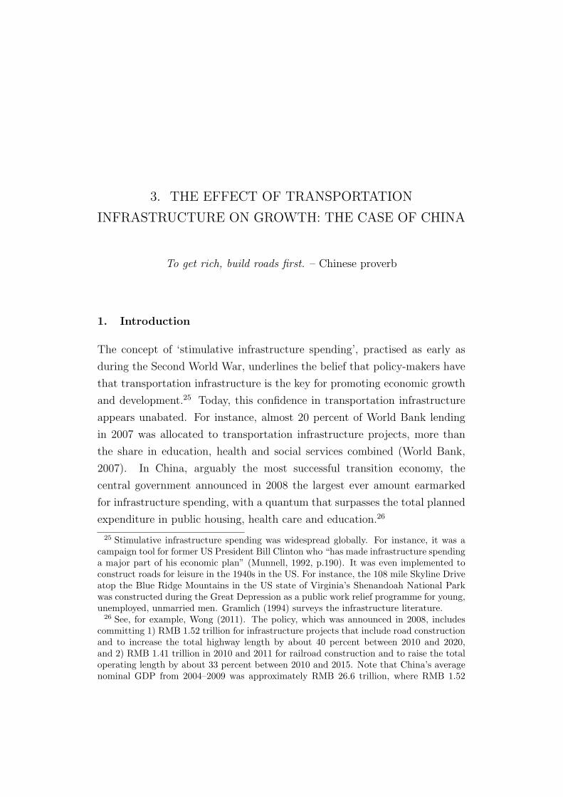
3. THE EFFECT OF TRANSPORTATION
INFRASTRUCTURE ON GROWTH: THE CASE OF CHINA
To get rich, build roads first. – Chinese proverb
1. Introduction
The concept of ‘stimulative infrastructure spending’, practised as early as
during the Second World War, underlines the belief that policy-makers have
that transportation infrastructure is the key for promoting economic growth
and development.25 Today, this confidence in transportation infrastructure
appears unabated. For instance, almost 20 percent of World Bank lending
in 2007 was allocated to transportation infrastructure projects, more than
the share in education, health and social services combined (World Bank,
2007). In China, arguably the most successful transition economy, the
central government announced in 2008 the largest ever amount earmarked
for infrastructure spending, with a quantum that surpasses the total planned
expenditure in public housing, health care and education.26
25 Stimulative infrastructure spending was widespread globally. For instance, it was acampaign tool for former US President Bill Clinton who “has made infrastructure spendinga major part of his economic plan” (Munnell, 1992, p.190). It was even implemented toconstruct roads for leisure in the 1940s in the US. For instance, the 108 mile Skyline Driveatop the Blue Ridge Mountains in the US state of Virginia’s Shenandoah National Parkwas constructed during the Great Depression as a public work relief programme for young,unemployed, unmarried men. Gramlich (1994) surveys the infrastructure literature.
26 See, for example, Wong (2011). The policy, which was announced in 2008, includescommitting 1) RMB 1.52 trillion for infrastructure projects that include road constructionand to increase the total highway length by about 40 percent between 2010 and 2020,and 2) RMB 1.41 trillion in 2010 and 2011 for railroad construction and to raise the totaloperating length by about 33 percent between 2010 and 2015. Note that China’s averagenominal GDP from 2004–2009 was approximately RMB 26.6 trillion, where RMB 1.52
3. THE EFFECT OF TRANSPORTATION INFRASTRUCTURE ONGROWTH: THE CASE OF CHINA 40
From the policy perspective, the positive correlation between changes in
density of transportation infrastructure (hereafter, changes in transportation
infrastructure), as measured by length of railway and highway per squared
kilometre area, and economic growth may be viewed as an encouraging
empirical regularity. Nevertheless, academics even to date are confronted
with the problem of identifying the extent to which this correlation reflects
the causal effect on economic growth that is due to changes in transportation
infrastructure. Obtaining a consistent estimate of this causal effect is
complicated by two issues. First, the data may contain measurement errors,
which if they are classical, will attenuate the least-squares estimate towards
zero and understate the true contribution of transportation infrastructure
towards economic growth.27 Second, provision of infrastructure can respond
endogenously to economic growth, as higher levels of economic growth
may in return encourage the expansion of infrastructure services. Ideally,
an experiment that randomly distributes infrastructure can avoid reverse
causality, however, it is empirically infeasible. Thus, careful analysis of the
causal link requires finding an external source of variation in changes in
transportation infrastructure as a means of identification, which itself is a
significant hurdle to overcome.
trillion and RMB 1.41 trillion were approximately USD 0.23 trillion and USD 0.22 trillionrespectively. Sources: The road to success, HSBC Emerging Market Report, March 10,2010; China infra construction sector, JP Morgan Asia Pacific Equity Research, 5 January,2011.
27 In the case of China which is the focus of this study, the data are obtained from theNational Bureau of Statistics of China (NBSC), which according to Rawski (2001), Rawskiand Xiao (2001), Chow (2006), and Ravallion and Chen (2007) may contain measurementerrors.
3. THE EFFECT OF TRANSPORTATION INFRASTRUCTURE ONGROWTH: THE CASE OF CHINA 41
Fig.3.1:
Annual
Growth
Rate
ofProvincialGovernmentExpenditure,1976–2006
−.50.51 −.50.51 −.50.51 −.50.51 −.50.51
19
77
19
82
19
87
19
92
19
97
20
02
20
07
19
77
19
82
19
87
19
92
19
97
20
02
20
07
19
77
19
82
19
87
19
92
19
97
20
02
20
07
19
77
19
82
19
87
19
92
19
97
20
02
20
07
19
77
19
82
19
87
19
92
19
97
20
02
20
07
19
77
19
82
19
87
19
92
19
97
20
02
20
07
An
hu
iB
eiji
ng
Fu
jian
Ga
nsu
Gu
an
gd
on
gG
ua
ng
xi
Gu
izh
ou
Ha
ina
nH
eb
ei
He
ilon
gjia
ng
He
na
nH
ub
ei
Hu
na
nIn
ne
r M
on
go
liaJia
ng
su
Jia
ng
xi
Jili
nL
iao
nin
g
Nin
gxia
Qin
gh
ai
Sh
aa
nxi
Sh
an
do
ng
Sh
an
gh
ai
Sh
an
xi
Sic
hu
an
Tia
njin
Xin
jian
gY
un
na
nZ
he
jian
g
An
nu
al g
row
th r
ate
of p
rovin
cia
l g
ove
rnm
en
t e
xp
en
ditu
re (
19
76
−2
00
6)
Note:Thefigu
replots
theaverag
eof
thean
nual
governmentexpen
diture
grow
thof
22provinces,threemunicipalities
andfourau
tonom
ousregion
s,less
Chon
gqingmunicipalityan
dTibet
autonom
ousregion
.Dataareob
tained
from
the
National
Bureau
ofStatisticsof
China(N
BSC).Theverticallines
representtheyears
oftheNational
Con
gress,which
are197
7,1982,
1987
,19
92,19
97,200
2an
d20
07.
3. THE EFFECT OF TRANSPORTATION INFRASTRUCTURE ONGROWTH: THE CASE OF CHINA 42
Focusing on the case of China, this chapter seeks to address these issues
and contribute to the literature on the causal effect that transportation
infrastructure has on economic growth. Employing a provincial panel dataset
during 1985–2008, it does so by proposing an identification strategy to
construct 2SLS estimates of the within-province causal effects that use the
timing of an exogenous event – National Congress of the Communist Party of
China (CPC) – as a source of external variation in changes in transportation
infrastructure. This strategy relies on the interplay of two institutional
features in the Chinese political and fiscal system. For a start, it appeals
to the unique Chinese political environment where government interventions
for promoting economic development and growth are frequent and influential,
and where some of these intervening policies originate from major political
events such as the National Congress of the CPC. Since 1977, the CPC
convenes every five years at the National Congress in the capital city of
Beijing to discuss internal party matters and ratify national development
objectives such as economic growth targets.28 Because the Chinese fiscal
system is highly decentralised, the vast majority of responsibilities of
accomplishing such national objectives, in particular the implementation
of fiscal spending and the provision of infrastructure, are assigned to local
governments (Wong, 2011).29 Therefore, while the congressional event per se
may not be directly associated with provincial economic growth, the recurring
National Congress may engender a cyclical pattern in the expenditure of
provincial governments, in particular the expenditure on transportation
infrastructure, which in turn may generate the variation in serviceable
transportation infrastructure that is useful for identifying its effect on growth.
Figure 3.1 offers some visual evidence that the spending of provincial
governments and the timing of the National Congress are linked. Plotting
the annual growth rate of provincial government expenditure from 1976
28 For instance, in the most recent (12th) five-year plan ratified bythe National Congress, the central government sets a target of 7percent of annual economic growth during 2011-2015 with significantimprovement in the quality and performance of economic development. Seehttp://www.chinadaily.com.cn/china/2011npc/2011-03/05/content 12120516.htm.
29 In recent times, the local governments have accounted for more than 80 percent of thenational budgetary expenditures. See Wong (2011).
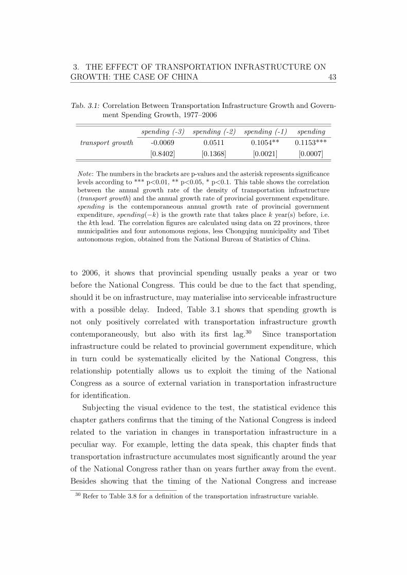
3. THE EFFECT OF TRANSPORTATION INFRASTRUCTURE ONGROWTH: THE CASE OF CHINA 43
Tab. 3.1: Correlation Between Transportation Infrastructure Growth and Govern-ment Spending Growth, 1977–2006
spending (-3) spending (-2) spending (-1) spending
transport growth -0.0069 0.0511 0.1054** 0.1153***
[0.8402] [0.1368] [0.0021] [0.0007]
Note: The numbers in the brackets are p-values and the asterisk represents significancelevels according to *** p<0.01, ** p<0.05, * p<0.1. This table shows the correlationbetween the annual growth rate of the density of transportation infrastructure(transport growth) and the annual growth rate of provincial government expenditure.spending is the contemporaneous annual growth rate of provincial governmentexpenditure, spending(−k) is the growth rate that takes place k year(s) before, i.e.the kth lead. The correlation figures are calculated using data on 22 provinces, threemunicipalities and four autonomous regions, less Chongqing municipality and Tibetautonomous region, obtained from the National Bureau of Statistics of China.
to 2006, it shows that provincial spending usually peaks a year or two
before the National Congress. This could be due to the fact that spending,
should it be on infrastructure, may materialise into serviceable infrastructure
with a possible delay. Indeed, Table 3.1 shows that spending growth is
not only positively correlated with transportation infrastructure growth
contemporaneously, but also with its first lag.30 Since transportation
infrastructure could be related to provincial government expenditure, which
in turn could be systematically elicited by the National Congress, this
relationship potentially allows us to exploit the timing of the National
Congress as a source of external variation in transportation infrastructure
for identification.
Subjecting the visual evidence to the test, the statistical evidence this
chapter gathers confirms that the timing of the National Congress is indeed
related to the variation in changes in transportation infrastructure in a
peculiar way. For example, letting the data speak, this chapter finds that
transportation infrastructure accumulates most significantly around the year
of the National Congress rather than on years further away from the event.
Besides showing that the timing of the National Congress and increase
30 Refer to Table 3.8 for a definition of the transportation infrastructure variable.
3. THE EFFECT OF TRANSPORTATION INFRASTRUCTURE ONGROWTH: THE CASE OF CHINA 44
in transportation infrastructure are potentially linked, this chapter also
contributes to the literature in the following aspects. Firstly, only a handful
of papers to date had looked at how timing of the National Congress could
have causal implications.31 This chapter uses this information about the
National Congress for identification, and thus proposes another avenue to
complement existing techniques for pinning down the causal effect of changes
in transportation infrastructure in the study of its effect on growth in China.
Secondly, this chapter also highlights the important role of transportation
infrastructure in channelling the forces from the timing of the National
Congress into cyclical variation in economic growth, as this chapter finds
that the timing of the National Congress has a positive influence on GDP
growth per capita through the accumulation of transportation infrastructure.
The rest of the discussion is organised as follows. Section 2 provides
some background on the literature and section 3 presents the data and the
summary statistics. The methodology and results are discussed in sections 4
and 5. Section 6 concludes.
2. Related Literature
This work is related to the research agenda, linking back to Aschauer (1989),
that looks at the impact of infrastructure on growth.32 In this literature,
identifying the causality of infrastructure is complicated by the endogenous
response of infrastructure to growth. One solution is to model this reverse
causality together with the main causal relationship using a simultaneous
31 Piotroski et al. (2010) examine how local and provincial government entities mightmanipulate the flow of negative financial information into the stock prices of state-controlled firms. They find that state-controlled firms are significantly less likely toexperience negative stock price crashes in the congress years and political promotionevents. Shen et al. (2008) show that activities in the Chinese initial public offering (IPO)market could be politically influenced, as IPO volumes typically declined after the congressyear, only to rise towards a peak in the quarter of the next National Congress.
32 Aschauer (1989), who brought this topic to the fore, as well as Holtz-Eakin (1988),Munnell (1990) and Rubin (1991), first find the return on public capital in production tobe far greater than that on private capital. But this result is hardly plausible, as it wouldmotivate the undertaking of public capital investment by the private sector, which onerarely observes.
3. THE EFFECT OF TRANSPORTATION INFRASTRUCTURE ONGROWTH: THE CASE OF CHINA 45
equations approach (Esfahani and Ramirez, 2003).33 Another solution is to
ascribe this endogeneity to the presence of fixed effects, hence employ fixed
effects estimation34 or dynamic panel methods (e.g. Calderon and Chong,
2004 and Calderon and Serven, 2005).35 Nevertheless, even if fixed effects
were dealt with, there could still be omitted idiosyncratic variables that are
correlated with infrastructure that call for the use of external information to
achieve identification.36
To ameliorate the issue of endogeneity, some studies have pointed out that
since the contribution of output growth towards infrastructure stock would
be very small, the endogeneity in infrastructure should not be too serious if
infrastructure stock and not flow were used as the regressor.37 In this study,
infrastructure stock is used as the regressor and a 2SLS approach is adopted
as a safeguard.
This work is related to Chen and Fleisher (1996), Fleisher and Chen
(1997), Demurger (2001), Fleisher et al. (2010), and Chen and Yao (2011).
Chen and Fleisher (1996) and Fleisher and Chen (1997) look at the
determinants of GDP growth and TFP among Chinese provinces but the
impact of transportation infrastructure is not included in their study. This
is undertaken in Fleisher et al. (2010), although the context is mainly on
the impact of infrastructure on TFP growth. Using Chinese provincial panel
data over the period 1978–2006, Chen and Yao (2011) analyse the implication
of increasing the proportion of government budgets for investments in
transportation, although unlike this chapter’s focus on economic growth,
33 A simultaneous equations approach is employed by Binswanger et al. (1993), whoexamine the effects on agricultural output from government’s physical infrastructureexpenditure.
34 In earlier studies based on US state-level panel data, Holtz-Eakin (1994), Holtz-Eakinand Schwartz (1995) and Garcia-Mila et al. (1996) find that introducing fixed effects mayeliminate the positive effect of infrastructure on growth.
35 Caselli et al. (1996) show that the per capita growth equation can be expressed asan autoregression in per capita output levels, which can then be estimated using theidentification scheme of Arellano and Bond (1991). Calderon and Chong (2004) andCalderon and Serven (2005) employ cross-country panel data and find that infrastructurestock reduces income inequality and increases growth positively.
36 This could be due to relevant omitted variables or measurement error in theexplanatory variable of interest. See Angrist and Pischke (2009) p.225.
37 See, for example, Estache et al. (2005) and Arnold et al. (2007).

3. THE EFFECT OF TRANSPORTATION INFRASTRUCTURE ONGROWTH: THE CASE OF CHINA 46
they are primarily concerned with the response of household consumption.
Also using Chinese provincial panel data, Demurger (2001) looks at how
transportation infrastructure could drive provincial income disparities in
China. While Demurger (2001) employs internal instruments, e.g. lagged
trade and FDI, this chapter intends to use external instruments which rely
on the timing of an exogenous event – the National Congress – as an empirical
strategy to estimate the causal effect of transportation infrastructure.
In this regard, this research is also related to a handful of papers
that consider the issue of identifying the exogenous variation in changes in
transportation infrastructure.38 Based on Chinese county-level data to study
how access to transportation infrastructure may affect growth, Banerjee
et al. (2012) use the distance of a county from transport networks that
connect historical treaty ports and business centres to construct an exogenous
proxy of accessibility to current transportation infrastructure. Li and Li
(2010) examine the causal effect on firms’ inventory levels by controlling
for omitted variables that might affect infrastructure and inventory jointly.
Li (2009) looks at the welfare implication of the provision of transport by
employing a quasi-natural experiment approach. This work complements
these identification schemes by introducing a simple, yet powerful, instrument
for transportation infrastructure that draws information from the timing of
the National Congress.
38 See also Fernald (1999), Michaels (2008), Keller and Shiue (2008) and Donaldson(2010). Based on industry-level data for the US, Fernald (1999) identifies the causal effectof roads on US industrial productivity from 1953 to 1989 by examining how the intensityof vehicle use by different industries is linked to their productivity levels. Causality ispinned down if changes in road growth are associated with larger changes in productivitygrowth in industries that are more vehicle intensive. A difference-in-difference approach todeal with the endogeneity issue is employed by Michaels (2008), who examines the effect ofhighway construction in the US in the 1950s, and Donaldson (2010), who studies the effectof railroad construction in 19th century India. Keller and Shiue (2008) look at the effectof steam train in 19th century Europe by employing an instrumental variable approachfor identification.
3. THE EFFECT OF TRANSPORTATION INFRASTRUCTURE ONGROWTH: THE CASE OF CHINA 47
3. Data and Variables
The study utilises panel data drawn from the China Compendium of
Statistics, which is compiled by the Department of Comprehensive Statistics
of the National Bureau of Statistics. The year 1985 is chosen to be the
starting period of the sample as there are many missing observations on
the covariates prior to 1985. The end of sample year in the dataset is
2008.39 Regional data are available for 31 sub-national administrative units
in mainland China,40 including 22 provinces, four municipalities (Beijing,
Shanghai, Tianjin, and Chongqing41) and five autonomous regions (Tibet,
Xinjiang, Ningxia, Inner Mongolia and Guangxi). The inclusion of the data
on municipalities is consistent with Fleisher and Chen (1997) as doing so will
help to maximise the use of available information. For exposition sake, this
chapter calls each sub-national unit ‘province’. The summary statistics are
presented in Table 3.2.42
The dependent variable is real GDP growth per capita. The control
variables include production factors consisting of physical and human capital,
and provincial attributes reflecting geographical constraints and economic
heterogeneity. As proxies for physical and human capital shares, this chapter
uses fixed investment to GDP ratio and secondary school enrolment rate
(e.g. Demurger, 2001).43 In relation to section 4, these variables are grouped
and represented collectively as the vector xit, where i is the province index
and t is the year index. The additional controls that are considered are,
39 This chapter sticks to 1985 as the starting year following Demurger (2001).40 According to official classification, all regions excluding Hong Kong, Macao and
Taiwan are categorised as East (12), Central (9) and West (10). East: Beijing, Tianjin,Shanghai, Shangdong, Hebei, Liaoning, Fujian, Jiangsu, Zhejiang, Guangdong, Guangxi,Hainan. Central: Heilongjiang, Henan, Hunan, Hubei, Inner Mongolia, Jilin, Anhui,Jiangxi, Shanxi. West: Chongqing, Gansu, Guizhou, Ningxia, Qinghai, Shaanxi, Sichuan,Tibet, Xinjiang, Yunnan.
41 Chongqing was designated a municipality in the year 1997. The other three cities wereinitially municipalities when the People’s Republic of China was established in 1949.
42 A detailed list of variables is available in Table 3.8.43 Because infrastructure is a stock variable and fixed capital formation contains
information about infrastructure, using fixed investment to GDP ratio instead amelioratesthe collinearity between capital and infrastructure given that the fixed investment ratio isa flow variable and the density of transportation infrastructure, the infrastructure variable,is a stock.
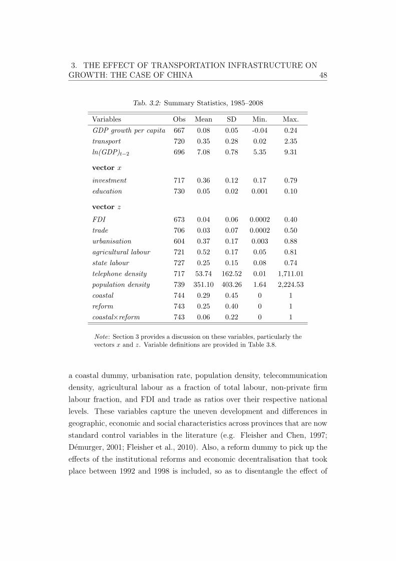
3. THE EFFECT OF TRANSPORTATION INFRASTRUCTURE ONGROWTH: THE CASE OF CHINA 48
Tab. 3.2: Summary Statistics, 1985–2008
Variables Obs Mean SD Min. Max.
GDP growth per capita 667 0.08 0.05 -0.04 0.24
transport 720 0.35 0.28 0.02 2.35
ln(GDP)t−2 696 7.08 0.78 5.35 9.31
vector x
investment 717 0.36 0.12 0.17 0.79
education 730 0.05 0.02 0.001 0.10
vector z
FDI 673 0.04 0.06 0.0002 0.40
trade 706 0.03 0.07 0.0002 0.50
urbanisation 604 0.37 0.17 0.003 0.88
agricultural labour 721 0.52 0.17 0.05 0.81
state labour 727 0.25 0.15 0.08 0.74
telephone density 717 53.74 162.52 0.01 1,711.01
population density 739 351.10 403.26 1.64 2,224.53
coastal 744 0.29 0.45 0 1
reform 743 0.25 0.40 0 1
coastal×reform 743 0.06 0.22 0 1
Note: Section 3 provides a discussion on these variables, particularly thevectors x and z. Variable definitions are provided in Table 3.8.
a coastal dummy, urbanisation rate, population density, telecommunication
density, agricultural labour as a fraction of total labour, non-private firm
labour fraction, and FDI and trade as ratios over their respective national
levels. These variables capture the uneven development and differences in
geographic, economic and social characteristics across provinces that are now
standard control variables in the literature (e.g. Fleisher and Chen, 1997;
Demurger, 2001; Fleisher et al., 2010). Also, a reform dummy to pick up the
effects of the institutional reforms and economic decentralisation that took
place between 1992 and 1998 is included, so as to disentangle the effect of
3. THE EFFECT OF TRANSPORTATION INFRASTRUCTURE ONGROWTH: THE CASE OF CHINA 49
this policy from the effect of the timing of the National Congress.44 These
additional control variables are grouped and represented as the vector zit.
The key explanatory variable in this chapter is the density of trans-
portation infrastructure, defined as the sum of the length of roads and
railroads in kilometres divided by the total land area in square kilometres.
This measure of transportation infrastructure is widely adopted by existing
studies for China (Demurger, 2001; Fan and Zhang, 2004; Ding and Knight,
2011) and for cross-country analysis (Esfahani and Ramirez, 2003; Calderon
and Chong, 2004; Calderon and Serven, 2005).45 As discussed, a measure
related to infrastructure stock, rather than its flow, is preferred on the
basis of ameliorating the possibility of endogeneity due to reverse causality
from growth. In addition, this study prefers to focus on the causality of
infrastructure stock than infrastructure spending for two reasons. Firstly,
by focusing on the causal effect of infrastructure spending, the question
at hand becomes fundamentally different. Secondly, as spending may be
inefficient and wasteful, the expenditure itself may not materialise into
intended levels of infrastructure output. In other words, the study of the
effects of transportation investment is not the same as the study of the effects
of materialised transportation infrastructure, which is the main focus of this
study.
44 This period corresponds to the third phase of China’s economic reform towards a moremarket-oriented and open economy.
45 It should be mentioned that together with infrastructure stock, Calderon and Chong(2004) also look at the causal effect of infrastructure quality. They find that the causaleffect of infrastructure stock is more quantitatively important.
3. THE EFFECT OF TRANSPORTATION INFRASTRUCTURE ONGROWTH: THE CASE OF CHINA 50
4. Methodology
4.1 The Estimating Equation
In the spirit of the celebrated Barro framework,46 considered by Chen and
Fleisher (1996), Fleisher and Chen (1997) and Demurger (2001) in their study
of economic growth in China, the main estimating equation is as follows,
git = c+ ϕ transportit + β ln(yit−2) + γ′xit + ρ′zit + αi + γrt + uit, (3.1)
where git represents the average annual growth rate of real GDP per capita for
province i at time t, yit represents the level of real GDP per capita, αi is the
province fixed effect that controls for time-invariant permanent differences
across provinces and uit is the error term.
The causal variable of interest is transportit, the density of transportation
infrastructure, where its impact is summarised by ϕ. In order to identify
ϕ, it is important to carefully consider the issue of omitted variables that
may be correlated with both transportit and git. To address this issue and
to ameliorate the problem of omitted variable bias, ln(yit−2) is included to
control for differences in the past condition across provinces. Also, the vector
xit is included to control for production factors such as physical and human
capital as these factors are inputs in the production process.
To control for the uneven development and differences in geographic,
economic and social characteristics across provinces, the inclusion of the
vector zit is considered. The vector zit, by soaking up the remaining effects
on growth that are not captured by xit, also plays the role of disentangling
the possible effects related to other policy changes from the effect of the
National Congress on transportation infrastructure. For example, being an
aggregate event, not only may the National Congress impact the formation
of transportation infrastructure, it may also influence trade policies that
might in turn have non-trivial effects on growth. Therefore, without taking
46 Using data obtained from 98 countries over the period 1965–1985, Barro (1991)investigates what determines GDP per capita growth. The main variables estimated inBarro (1991) are initial level of GDP per capita, human capital, physical capital andgovernment investment.
3. THE EFFECT OF TRANSPORTATION INFRASTRUCTURE ONGROWTH: THE CASE OF CHINA 51
into account the possible changes in trade policies that are related to the
National Congress, the 2SLS estimate may be confounded by the effect that
runs from the National Congress to these policy ‘shocks’, and ultimately to
economic growth. In order to identify the link between the timing of the
National Congress and transportation infrastructure so as to pin down the
effect of changes in transportation infrastructure on economic growth, it is
important to partial out these confounding effects. To the extent that these
effects are manifested through some measure of provincial trade, which this
chapter has included as a component in the vector zit, this may be achievable
by controlling for the vector zit in the regression analysis.
To smooth out short term fluctuations, this chapter follows a previous
protocol of using averages for continuous variables according to the averaging
scheme (x∗it−1+2x∗it+x∗it+1)/4 for some continuous variable x∗it (e.g. Demurger,
2001). For binary indicators, this study will use the start of the averaging
period so that the t − 1th observation is used for the regression indexed by
t. The use of an averaging scheme, as in Chen and Fleisher (1996), Fleisher
and Chen (1997) and Demurger (2001), would dampen any extant systemic
shock that is not already soaked up by the vectors xit and zit.47 Hence, this
averaging scheme serves as a additional precautionary measure to deal with
systemic shocks that affect all the regions identically, from Tibet and Xinjiang
autonomous regions in China’s deep west to Beijing, Shanghai or Guangdong
province in the coastal east, even though the occurrence of such shocks on a
regular basis seems unlikely given the immense diversity in culture, religion
and governance across these regions. Moreover, these shocks, if they exist,
are likely to be due to global effects that are not associated with the timing
of the National Congress in a systematic way, in which case any omitted
remnant of these shocks (after what xit and zit have absorbed) should not
infringe upon the empirical strategy.
To add another layer of safeguard, this chapter includes γrt that represents
a separate trend for each of three regions (r) — East, Central and
West regions — which is based on the official classification of grouping
47 This, perhaps, explains why the models of Chen and Fleisher (1996) and Fleisher andChen (1997) abstract from year fixed effects.
3. THE EFFECT OF TRANSPORTATION INFRASTRUCTURE ONGROWTH: THE CASE OF CHINA 52
administrative units. Including a trend is important for two related reasons.
Firstly, the measure of transportation infrastructure that is used in this paper
and elsewhere in the literature contains an increasing trend. This is because
its denominator (the area of the province) is fixed while the numerator
(transportation infrastructure stock) is rising over time. Secondly, the GDP
growth per capita of emerging countries may have an increasing trend. This is
the case for most Chinese provinces during the sample period.48 As a result,
the trends might give a misleading impression about how the covariates are
related, and therefore must be purged to safeguard against confounding the
main causal relationship.
4.2 Instrumental Variables
The identification strategy uses the timing of the National Congress and
constructs Congress, an indicator variable that is equal to one for the year
of the National Congress and zero for the other years, as an instrument for
transportation infrastructure. Besides Congress, there are reasons why using
indicators of the years before the National Congress as additional instruments
might be a good strategy from the identification standpoint. Firstly, it is
best to let the data speak and take an agnostic stance on how the timing of
the National Congress is related to the variation in changes in transportation
infrastructure. Secondly, infrastructure could accumulate before the National
Congress as construction might commence early. Thirdly, since the 1980s, the
five-year plans outlining the national economic goals are drawn in the year
before the National Congress.49 Therefore, Congress(−1), which indicates
the year before the National Congress, and Congress(−2), which indicates
the two years before it, might potentially help to pick up further variation in
transportation infrastructure.
48 As opposed to emerging countries, the GDP growth per capita of developed countriesmay fluctuate around some steady state level without exhibiting a trend.
49 The first Five-Year Plan was implemented for 1953 to 1957. A recent example is the11th plan (2006-2010), which proposed that GDP per capita, urbanisation rate, and ruralnet income per capita towards the end of 2010 should reach 19,270 yuan, 47 percent, and4,150 yuan, respectively. See Fan (2006).
3. THE EFFECT OF TRANSPORTATION INFRASTRUCTURE ONGROWTH: THE CASE OF CHINA 53
The identifying assumption in this chapter relies on the premise that
provincial economic growth is not directly associated with the National
Congress per se, but indirectly with the timing of the National Congress
as the policy objectives it ratifies are executed by local governments in
a decentralised way. That being said, some issues related to exclusion
restriction are worth further clarification. Firstly, to foster economic growth,
local officials may engage in other ‘growth enhancing’ activities besides
investment in transportation infrastructure.50 While data at a more micro-
level are not available, the issue will be taken care of insofar as the effects
of these activities are manifested through the determinants of economic
growth, such as fixed investment and education, that the estimating equation
has already included as control variables. Secondly, provincial leaders of
different backgrounds might adopt different development strategies, which
are influenced by attitudes and ambitions that are not observable. However,
this chapter holds on to the view that attitudes and ambitions per se
should not directly contribute to growth, but indirectly through the economic
activities that are influenced by these unobserved characteristics. Therefore,
this unobserved heterogeneity, if it is not already taken care of by fixed effects,
should not pose an issue as long as the effects of such concomitant economic
activities are captured by the control variables in the model.51 That said,
section 5.4 checks for the sensitivity of the estimation results to the inclusion
of certain attributes of local leaders as additional controls and finds that the
results remain robust. Finally, the identification strategy is based on the
timing of the National Congress, which is an aggregate event. Its effect may
therefore be confounded by other unobserved shocks such as policy changes
that are not related to the formation of transportation infrastructure but
nevertheless are non-trivial for economic growth. To address this issue, this
chapter includes not just the vector xit in the estimating equation, but also
50 For instance, local governments may provide easier loans to particular sectors ordirectly subsidise local state-owned monopolistic firms (Shen et al., 2012).
51 For instance, while there are different industrial development strategies adopted byprovincial leaders, these activities may be captured more conventionally by the othercontrol variables. As an example, the 2008 Olympic Games in Beijing involves theconstruction of stadiums and relevant facilities, which involves fixed capital formationthat is included as a control variable in the estimating equation.

3. THE EFFECT OF TRANSPORTATION INFRASTRUCTURE ONGROWTH: THE CASE OF CHINA 54
considers the inclusion of the large zit vector in an attempt to soak up these
unobserved shocks and to partial out any effects that may confound the
link that goes from the timing of the National Congress to transportation
infrastructure, and ultimately to growth.
As a model-based assessment of instrument validity, this study will
employ the overidentifying restrictions test. Rejecting the test implies that
one or more instruments are invalid, or the model is mis-specified, or both.
But it does not distinguish which condition or if both conditions are violated.
This study will also check for weak instruments as they would cause the true
standard errors to be understated.52 To do so, this study will report the first
stage F-statistic, motivated by the rule-of-thumb on adequate instrument
strength if it is greater than 10. This study will also report the Kleibergen
and Paap (KP) (2006) Wald statistic for further evidence on instrument
weakness. The KP statistic will be evaluated against a critical value, adopted
from Stock and Yogo (2005), that 15 percent is the maximal rejection rate
the researcher is willing to tolerate if the true rejection rate is 5 percent.53
Observing a KP statistic that exceeds this critical value implies that the
maximal rejection rate is smaller than 15 percent, hence the actual size of
the test is between the 5 percent and 15 percent levels. Last but not least,
standard errors are clustered for each province.
5. Empirical Results
In all regressions, the vector xit is included to control for physical and human
capital inputs into the production process. This study also takes into account
the time-invariant permanent differences by including province fixed effects
while controlling for region-specific time trends. To check for the sensitivity of
the estimation results to omitted variables, the baseline regressions juxtapose
52 For instance, the congress instruments resemble instruments of political cycles,reminiscent of Levitt (1997) who considers electoral cycles to identify the causal impactof the number of police officers on crime, although these instruments are later found to beweak (Murray, 2006).
53 This follows from the suggestion of Stock et al. (2002).
3. THE EFFECT OF TRANSPORTATION INFRASTRUCTURE ONGROWTH: THE CASE OF CHINA 55
the estimates that are based on omitting versus including the vector zit. Since
the main interest is to estimate the effect of transportation infrastructure,
the estimated effects of other control variables are suppressed for the sake of
presentation.
5.1 Baseline Results
Table 3.3 summarises the baseline results from the OLS and 2SLS regressions.
While the OLS regression is unidentified, it nonetheless provides a useful
starting point for investigating the direction of bias in the estimate of
how transportation infrastructure affects economic growth. Column (1)
shows that the OLS estimate of the response of growth to transportation
infrastructure is very close to zero. If the premise that transportation
infrastructure is growth enhancing, this weak association suggests at first
sight that the OLS estimate is downward biased. This bias, however, does not
appear to be due to omitted variables, given that the OLS estimate remains
stubbornly close to zero even when the vector zit, which encompasses both
macroeconomic and policy-related variables, is included in the regression
(see column (2)). Instead, it is symptomatic of measurement errors in the
data, which come from NBSC. According to Rawski (2001), Rawski and Xiao
(2001), Chow (2006) and Ravallion and Chen (2007), data from NBSC may
contain measurement errors. If these measurement errors are classical, the
least squares estimates will be attenuated, which may explain why the OLS
estimates are nearly zero.
To address the issues of measurement errors and reverse causality, column
(3) reports the 2SLS estimates of both first and second stage regressions.
The first stage regression in column (3) confirms that transportation
infrastructure is substantially influenced by the year of the National Congress
and the years before it. Moreover, the positive effect on transportation
infrastructure among the congress instruments is strongest for Congress
but weakest for Congress(−2), suggesting that transportation infrastructure
accumulates the most around the year of the National Congress. Concerning
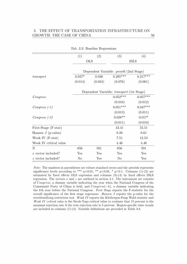
3. THE EFFECT OF TRANSPORTATION INFRASTRUCTURE ONGROWTH: THE CASE OF CHINA 56
Tab. 3.3: Baseline Regressions
(1) (2) (3) (4)
OLS 2SLS
Dependent Variable: growth (2nd Stage)
transport 0.027* 0.026 0.295*** 0.217***
(0.014) (0.024) (0.076) (0.061)
Dependent Variable: transport (1st Stage)
Congress 0.052*** 0.057***
(0.016) (0.012)
Congress (-1) 0.051*** 0.047***
(0.013) (0.011)
Congress (-2) 0.028** 0.017*
(0.011) (0.010)
First-Stage (F-stat) 43.41 55.51
Hansen J (p-value) 0.28 0.61
Weak IV (F-stat) 7.51 12.53
Weak IV critical value 4.46 4.46
N 656 501 656 501
x vector included? Yes Yes Yes Yes
z vector included? No Yes No Yes
Note: The numbers in parentheses are robust standard errors and the asterisk representssignificance levels according to *** p<0.01, ** p<0.05, * p<0.1. Columns (1)-(2) areestimated by fixed effects OLS regression and columns (3)-(4) by fixed effects 2SLSregression. The vectors x and z are outlined in section 4.1. The instrument set consistsof Congress, a dummy variable indicating the year when the National Congress of theCommunist Party of China is held, and Congress(−k), a dummy variable indicatingthe kth year before the National Congress. First Stage reports the F-statistic for theoverall significance of the first stage regressors. Hansen J reports the p-value for theoveridentifying restriction test. Weak IV reports the Kleibergen-Paap Wald statistic andWeak IV critical value is the Stock-Yogo critical value to evaluate that 15 percent is themaximal rejection rate if the true rejection rate is 5 percent. Region-specific time trendsare included in columns (1)-(4). Variable definitions are provided in Table 3.8.
3. THE EFFECT OF TRANSPORTATION INFRASTRUCTURE ONGROWTH: THE CASE OF CHINA 57
identification, the first stage F-statistic in column (3) is well above the Staiger
and Stock (1997) rule-of-thumb threshold of 10, suggesting that the congress
instruments are powerful.
Given that the instruments are strong, the second stage regression shows
that the effect of transportation infrastructure on growth is both quantita-
tively large and statistically significant. Unlike the tenuous infrastructure-
growth relationship reflected by the OLS estimates, column (3) shows
that a one standard deviation increase in the density of transportation
infrastructure accounts for an 8.3 percentage point increase in GDP growth
per capita on average.54 This strong effect is not an artefact of omitted
variables and policy changes that may interfere with the strategy of using
the timing of the National Congress for identification. For instance, as a
robustness check, column (4) shows that including the vector zit does not
eliminate the substantial effect that the timing of the National Congress
(especially the variable Congress) has on transportation infrastructure, nor
does it drive away the significant contribution of transportation infrastructure
towards growth, where a one standard deviation increase in transport density,
ceteris paribus, has the effect of raising GDP growth per capita by more than
6 percentage points on average.
The congress instruments are significant drivers of the variation in
transportation infrastructure with a total impact of 0.121 (column (4))
to 0.131 (column (3)) reported in the first stage regressions. Therefore,
through the transportation infrastructure channel, the indirect impact of
the total congress effect on growth is non-trivial, where the total effect
from the timing of the National Congress is associated with a 2.63 (column
(4)) to 3.86 (column (3)) percentage point increase in GDP growth per
capita on the year of the National Congress.55 This implies that through
the formation of transportation infrastructure, the timing of the National
54 One standard deviation in transportation infrastructure is 0.28. The coefficient ontransportation infrastructure in column (3) is 0.295. Therefore, the “8.3 percentage points”result that is reported in the text is derived from 100× 0.295× 0.28.
55 Focusing on column (4), the figure 2.63 is computed based on 100× 0.217× (0.057 +0.047 + 0.017) = 2.63, where (0.057 + 0.047 + 0.017) captures the total response oftransportation infrastructure to the three congress instruments.
3. THE EFFECT OF TRANSPORTATION INFRASTRUCTURE ONGROWTH: THE CASE OF CHINA 58
Congress may generate cyclical increases in provincial economic growth,
an empirical regularity of separate interest. Much of this increase in
growth can be attributed to the information arising from the year of the
National Congress and the year before it, as the effects of Congress and
Congress(−1) on transportation infrastructure are much larger than the
effect of Congress(−2).
Columns (3)-(4) report the p-value of the overidentifying restrictions
test. The Hansen J statistics with p-values of 0.28 and 0.61 imply that
the overidentifying restrictions test is not rejected, hence supporting both
the model specification and the validity of instruments. The fact that the
p-value of the Hansen J in column (4) is 0.61 and is much greater than the
p-value of 0.28 in column (3) suggests that a model that controls for the
vector zit would be preferred. As mentioned, the weakness of instruments
would cause the true standard errors to be understated and distort the size
of the hypothesis test. To evaluate weak instruments, columns (3)-(4) also
report the KP statistic and the critical value corresponding to a 15 percent
maximal size for a 5 percent hypothesis test. Against a critical value of
4.36, the KP statistics of 7.51 and 12.53 in columns (3) and (4), respectively,
suggest again that the congress instruments are strong and the size distortion
would be mild.
5.2 Coastal versus Non-Coastal Regions
The coastal and non-coastal regions in China differ not only in terms of
geographical characteristics, but also in terms of how their economies are
structured, and in the distribution of key production factors such as physical
and human capital, FDI and trade, all of which contribute to income and
productivity gaps between these regions (e.g. Chen and Fleisher, 1996;
Fleisher and Chen, 1997; Fleisher et al., 2010). Through separate regressions
for coastal and non-coastal regions, this study may investigate if the positive
influence of the congress instruments on transportation infrastructure, as
well as the positive effect of transportation infrastructure on growth, remain
3. THE EFFECT OF TRANSPORTATION INFRASTRUCTURE ONGROWTH: THE CASE OF CHINA 59
present when due considerations are made with respect to the heterogeneity
across coastal and non-coastal regions in China.56
Columns (1) and (2) of Table 3.4 report the 2SLS estimates based on
the sample of coastal provinces, and columns (3) and (4) report the same
for non-coastal provinces. In the first stage regression, this chapter finds
yet again that the timing of the National Congress has a large impact on
transportation infrastructure. For the coastal region, the total effect of
the congress instruments on transportation infrastructure ranges from 0.156
when zit is controlled (column (2)) to 0.174 when zit is omitted (column (1)).
For the non-coastal region, columns (3)-(4) show that the total congress
effect in the first stage regression, although smaller, remains non-trivial.
While the timing of the National Congress is an important determinant of
transportation infrastructure for both coastal and non-coastal regions, the
larger impact of the National Congress with respect to the coastal region is
perhaps reflective of the fact that governments in the coastal region have been
more responsive to the National Congress, or that their efforts to accumulate
infrastructure have been more successful than governments in the non-coastal
region.
From the second stage regressions pertaining to coastal and non-coastal
regions (see columns (1)-(4) of Table 3.4), it is evident that the contribution
of transportation infrastructure towards growth is robust. Nonetheless,
there are regional disparities in the response of growth to transportation
infrastructure. For instance, column (2) reports a coefficient of 0.192 on
transportation infrastructure for the coastal region whereas column (4)
reports a coefficient of 0.239 for the non-coastal region, where both estimates
are statistically significant at the 1 percent level. This implies that controlling
for zit, a one standard deviation increase in transport density, ceteris paribus,
has an effect of raising GDP growth per capita on average by 5.4 percentage
points in the coastal region and 6.7 percentage points in the non-coastal
region. Since transportation infrastructure is relatively less developed in the
56 To simplify matters, this study includes a common regional trend for each coastaland non-coastal region. For the non-coastal regions, this study could use separate trendsfor Central and West regions. As it turns out, the results are not sensitive to using twoseparate regional trends or a common trend.
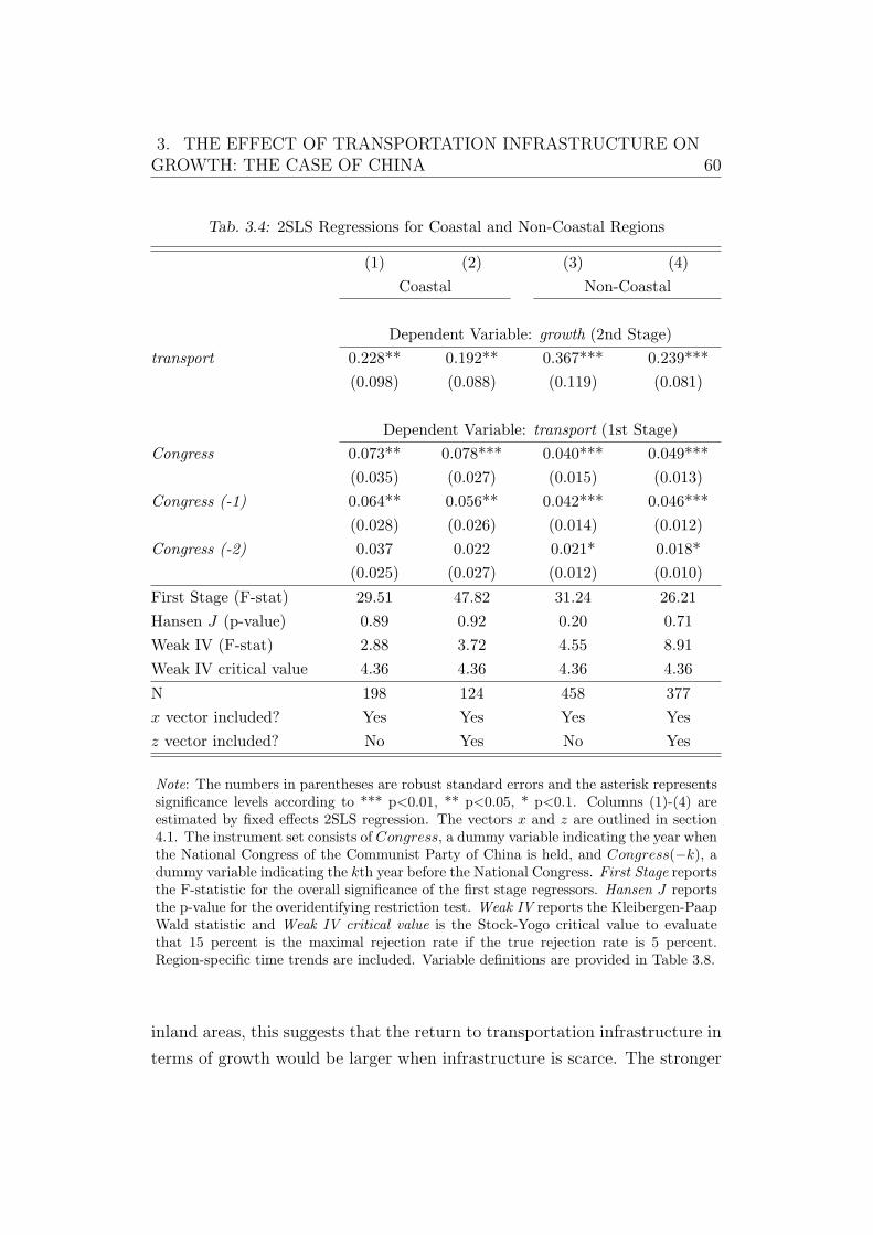
3. THE EFFECT OF TRANSPORTATION INFRASTRUCTURE ONGROWTH: THE CASE OF CHINA 60
Tab. 3.4: 2SLS Regressions for Coastal and Non-Coastal Regions
(1) (2) (3) (4)
Coastal Non-Coastal
Dependent Variable: growth (2nd Stage)
transport 0.228** 0.192** 0.367*** 0.239***
(0.098) (0.088) (0.119) (0.081)
Dependent Variable: transport (1st Stage)
Congress 0.073** 0.078*** 0.040*** 0.049***
(0.035) (0.027) (0.015) (0.013)
Congress (-1) 0.064** 0.056** 0.042*** 0.046***
(0.028) (0.026) (0.014) (0.012)
Congress (-2) 0.037 0.022 0.021* 0.018*
(0.025) (0.027) (0.012) (0.010)
First Stage (F-stat) 29.51 47.82 31.24 26.21
Hansen J (p-value) 0.89 0.92 0.20 0.71
Weak IV (F-stat) 2.88 3.72 4.55 8.91
Weak IV critical value 4.36 4.36 4.36 4.36
N 198 124 458 377
x vector included? Yes Yes Yes Yes
z vector included? No Yes No Yes
Note: The numbers in parentheses are robust standard errors and the asterisk representssignificance levels according to *** p<0.01, ** p<0.05, * p<0.1. Columns (1)-(4) areestimated by fixed effects 2SLS regression. The vectors x and z are outlined in section4.1. The instrument set consists of Congress, a dummy variable indicating the year whenthe National Congress of the Communist Party of China is held, and Congress(−k), adummy variable indicating the kth year before the National Congress. First Stage reportsthe F-statistic for the overall significance of the first stage regressors. Hansen J reportsthe p-value for the overidentifying restriction test. Weak IV reports the Kleibergen-PaapWald statistic and Weak IV critical value is the Stock-Yogo critical value to evaluatethat 15 percent is the maximal rejection rate if the true rejection rate is 5 percent.Region-specific time trends are included. Variable definitions are provided in Table 3.8.
inland areas, this suggests that the return to transportation infrastructure in
terms of growth would be larger when infrastructure is scarce. The stronger
3. THE EFFECT OF TRANSPORTATION INFRASTRUCTURE ONGROWTH: THE CASE OF CHINA 61
positive effect of transportation infrastructure observed for the non-coastal
region also suggests that transportation infrastructure can help to narrow
the income gap between the wealthier coastal provinces and their less affluent
non-coastal neighbours.
5.3 Attributes of Provincial Leaders
This section conducts a sensitivity test that is motivated by the consideration
that provincial leaders might adopt different development strategies based
on their own attributes. Chen et al. (2005) and Li and Zhou (2005) find
that provincial secretaries of the CPC and provincial governors are evaluated
based on certain criteria such as the annual growth rate and five-year average
provincial GDP per capita. If personal attributes of provincial leaders
can affect policy outcomes in their regions, these attributes may interact
with the timing of the National Congress to influence economic growth.
Consequently, this might violate the exclusion restriction required of the
congress instruments, an indication of which would be fragility of the baseline
estimates when the attributes of local leaders are introduced as additional
controls. Even though this is not an infallible procedure, the sensitivity check
reported below concurs that the baseline results are robust, which offers
some limited support that exploiting the timing of the National Congress is
a reasonable strategy from the estimation standpoint.
To control for the personal characteristics of local leaders, this study
forms vectors xSEC and xGOV that contain the attributes of two key sorts of
provincial leaders, the provincial CPC secretary (xSEC) and the provincial
governor (xGOV ). Drawing from the study of Chen et al. (2005) and Li
and Zhou (2005), this study constructs variables of personal characteristics
that are related to the tenure, age (including its square), education and
past working experience of the secretary or governor. The tenure is defined
as the kth year of one’s current assignment in either a CPC secretary or
a provincial governor position. The education variable is a binary variable
that is equal to one if a leader is an alumnus of a choice university in China,
3. THE EFFECT OF TRANSPORTATION INFRASTRUCTURE ONGROWTH: THE CASE OF CHINA 62
which is a way of extracting information about the ambition and personal
network of a local leader.57 Following Li and Zhou (2005), this study also
considers the implication of working experience by constructing a binary
variable that is equal to one if a leader has past experience or is currently
holding a joint appointment in the central government. Li and Zhou (2005)
find that having connections with the central government may increase the
promotional chances of local leaders, which may in turn influence the type
of development strategies they choose to pursue for their local regions.
Table 3.5 reports the estimation results based on the regression that
controls for xSEC (column (1)), xGOV (column (2)), or both (column (3)).
For the sake of conciseness, this study suppresses the estimated coefficients
on the extra controls, some of which are statistically significant, and focuses
on what is essential – whether the baseline estimates are robust.58 Table
3.5 shows that the estimated coefficient on transport density across columns
(1)–(3) ranges from 0.222 to 0.240. These estimates are clearly closer to
the baseline estimate of 0.217 (see column (4) of Table 3.3) than the OLS
estimate which is nearly zero. Therefore, these results show that the baseline
estimates are robust to the inclusion of the attributes of provincial leaders
as additional controls, despite the fact that these attributes may affect the
efficacy of managing and implementing policies including those ratified by
the National Congress.
5.4 Alternative Constructions of Instrumental Variables
As a further robustness check on the effect of transportation infrastructure on
growth, this study considers several alternative constructions of instrumental
variables, which are motivated by one caveat with respect to using Congress,
57 The choice universities are Peking University, Tsinghua University, Fudan University,Jiaotong University and Renmin University. This study distinguishes between local leaderswho are graduates from choice versus non-choice universities instead of considering whetherthese leaders have or haven not acquired a university degree, since a significant majorityof local leaders are university graduates.
58 Adding characteristics of provincial leaders into the regression, this study finds thatthe tenure and connection of provincial CPC secretaries are statistically significant butthe characteristics of the provincial governors are not individually statistically significant.Details are available in Appendix A (Table 8.1).
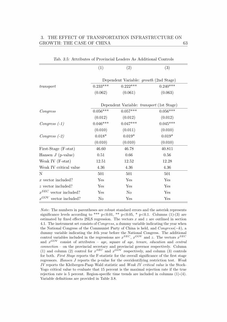
3. THE EFFECT OF TRANSPORTATION INFRASTRUCTURE ONGROWTH: THE CASE OF CHINA 63
Tab. 3.5: Attributes of Provincial Leaders As Additional Controls
(1) (2) (3)
Dependent Variable: growth (2nd Stage)
transport 0.233*** 0.222*** 0.240***
(0.062) (0.061) (0.063)
Dependent Variable: transport (1st Stage)
Congress 0.056*** 0.057*** 0.056***
(0.012) (0.012) (0.012)
Congress (-1) 0.046*** 0.047*** 0.045***
(0.010) (0.011) (0.010)
Congress (-2) 0.018* 0.019* 0.019*
(0.010) (0.010) (0.010)
First-Stage (F-stat) 46.60 46.78 40.811
Hansen J (p-value) 0.51 0.66 0.56
Weak IV (F-stat) 12.51 12.52 12.28
Weak IV critical value 4.36 4.36 4.36
N 501 501 501
x vector included? Yes Yes Yes
z vector included? Yes Yes Yes
xSEC vector included? Yes No Yes
xGOV vector included? No Yes Yes
Note: The numbers in parentheses are robust standard errors and the asterisk representssignificance levels according to *** p<0.01, ** p<0.05, * p<0.1. Columns (1)-(3) areestimated by fixed effects 2SLS regression. The vectors x and z are outlined in section4.1. The instrument set consists of Congress, a dummy variable indicating the year whenthe National Congress of the Communist Party of China is held, and Congress(−k), adummy variable indicating the kth year before the National Congress. The additionalcontrol variables included in the regressions are xSEC , xGOV and z. The vectors xSEC
and xGOV consist of attributes – age, square of age, tenure, education and centralconnection – on the provincial secretary and provincial governor respectively. Column(1) and column (2) control for xSEC and xGOV respectively, and column (3) controlsfor both. First Stage reports the F-statistic for the overall significance of the first stageregressors. Hansen J reports the p-value for the overidentifying restriction test. WeakIV reports the Kleibergen-Paap Wald statistic and Weak IV critical value is the Stock-Yogo critical value to evaluate that 15 percent is the maximal rejection rate if the truerejection rate is 5 percent. Region-specific time trends are included in columns (1)-(4).Variable definitions are provided in Table 3.8.
3. THE EFFECT OF TRANSPORTATION INFRASTRUCTURE ONGROWTH: THE CASE OF CHINA 64
Congress(−1) and Congress(−2) as instruments. Specifically, the economic
consequences of the National Congress, while it is an aggregate event, may
not be uniform across all provinces. Therefore, it is important to construct an
instrument that draws information from the timing of the National Congress
in a way that allows the effect of the National Congress to be province-
specific.
To construct such alternative instruments, this chapter first constructs a
so-called intensity function, related to the timing of the National Congress,
that is indexed by time only. The intensity function increases in magnitude,
and thus becomes more intense so to speak, the closer that the period t
is to the next National Congress. Taking an agnostic approach on how
the intensity function should look like, this chapter considers two possible
constructions. Letting kt denote the k number of years that period t is
before the next National Congress, where kt takes a value of either 4, 3, 2, 1,
or 0, the first function, which is called the linear intensity function, is defined
to be
f(kt) = 5− kt.
For instance, if t coincides with the year of the National congress, kt is
equal to zero and the intensity function has the maximum value of 5. This
chapter also considers a second construction, which this study calls the
convex intensity function, defined as
g(kt) = 1/(1 + kt).
This is a convex intensity function because as kt decreases, the function g
increases at an increasing rate. In order to obtain an instrument that contains
variation across both time and provinces, this study interacts the intensity
function, f or g, with a variable that exhibits provincial variation. This study
considers two such variables, which are linked to the National Congress as
well.
The first variable is seats share, defined as the number of congressional
seats of a province divided by the total number of seats in the National
Congress. This variable captures differences in political power across
3. THE EFFECT OF TRANSPORTATION INFRASTRUCTURE ONGROWTH: THE CASE OF CHINA 65
provinces. Thus, the effect of the National Congress may be more important
for provinces that are relatively more powerful in the sense that is described
by seats share. Since information about the number of congressional
seats is only available since 2007, this study constructs seats share using
2007 data provided by Xinhua Net, which would be reasonable if the
relative political power of each province did not vary too much over the
sample period. The second variable is lagged spending, which is the
lagged government expenditure. As discussed in section 1, the variation in
government expenditure appears to be related to the timing of the National
Congress. Since the variation in lagged government spending is also related to
the formation of transportation infrastructure (as serviceable infrastructure
materialises from investments with a delay), the impact of the National
Congress on transportation infrastructure might be more evident in provinces
with higher levels of lagged government spending.
Controlling for zit throughout, Table 3.6 revisits the 2SLS regressions
in Table 3.3 by employing four alternative sets of instruments. Each
instrument set is produced by interacting either the f or g intensity function
with seats share or lagged spending. Regardless of how the instruments
are constructed, Table 3.6 shows that the 2SLS estimates of the effect of
transportation infrastructure on growth are both quantitatively large and
statistically significant, with first stage F-statistics that are even larger than
the baseline case (compare Table 3.6 with column (4) of Table 3.3). These
second stage estimates are also very similar whether or not the linear or
convex intensity function is used in the computation, implying that the shape
of the intensity function is not crucial. Furthermore, the range of the new
estimates, from 0.195 (column (1)) to 0.266 (column (2)), also contains the
baseline estimate of 0.217 (see column (4) of Table 3.3). Therefore, despite
using four different instrumental variable definitions, this study finds that
the estimated effects of transportation infrastructure in Table 3.6 are very
similar to the baseline estimates in Table 3.3, hence offering some evidence
on the robustness of the results.
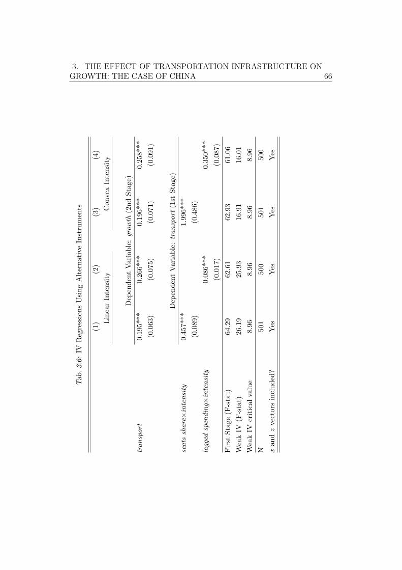
3. THE EFFECT OF TRANSPORTATION INFRASTRUCTURE ONGROWTH: THE CASE OF CHINA 66
Tab
.3.6:
IVRegressionsUsingAlternativeInstruments
(1)
(2)
(3)
(4)
LinearIntensity
Convex
Intensity
Dep
endentVariable:growth
(2ndStage)
transport
0.195***
0.266***
0.196***
0.258***
(0.063)
(0.075)
(0.071)
(0.091)
Dep
endentVariable:transport
(1st
Stage)
seats
share×intensity
0.457***
1.996***
(0.089)
(0.486)
lagged
spen
ding×
intensity
0.086***
0.350***
(0.017)
(0.087)
First
Stage
(F-stat)
64.29
62.61
62.93
61.06
WeakIV
(F-stat)
26.19
25.93
16.91
16.01
WeakIV
critical
value
8.96
8.96
8.96
8.96
N501
500
501
500
xan
dzvectors
included?
Yes
Yes
Yes
Yes
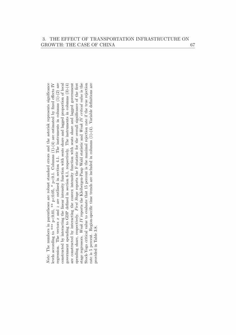
3. THE EFFECT OF TRANSPORTATION INFRASTRUCTURE ONGROWTH: THE CASE OF CHINA 67
Note:Thenumbersin
parentheses
arerobust
stan
darderrors
andtheasterisk
represents
sign
ificance
levelsaccordingto
***p<0.01
,**
p<0.05
,*p<0.1.
Columns(1)-(4)areestimated
byfixed
effects
IVregression.
Thevectors
xan
dzareou
tlined
insection4.1.
Theinstruments
incolumns(1)-(2)are
constructed
byinteractingthelinearintensity
functionwithseatssharean
dlagg
edproportion
oflocal
governmentspen
dingto
GDP
defi
ned
insection6.1,
respectively.
Theinstruments
incolumns(3)-(4)
areconstructed
byinteractingtheconvexintensity
function
with
seatssharean
dlagg
edgovernment
spen
dingshare,
respectively.
First
Stage
reports
theF-statistic
fortheoverallsign
ificance
ofthefirst
stag
eregressors.WeakIV
reports
theKleibergen-Paa
pWaldstatistican
dWeakIV
criticalvalueis
the
Stock-Yog
ocritical
valueto
evaluatethat
15percentis
themax
imal
rejectionrate
ifthetruerejection
rate
is5percent.
Region-specifictimetren
dsareincluded
incolumns(1)-(4).
Variable
defi
nitionsare
provided
inTab
le3.8.
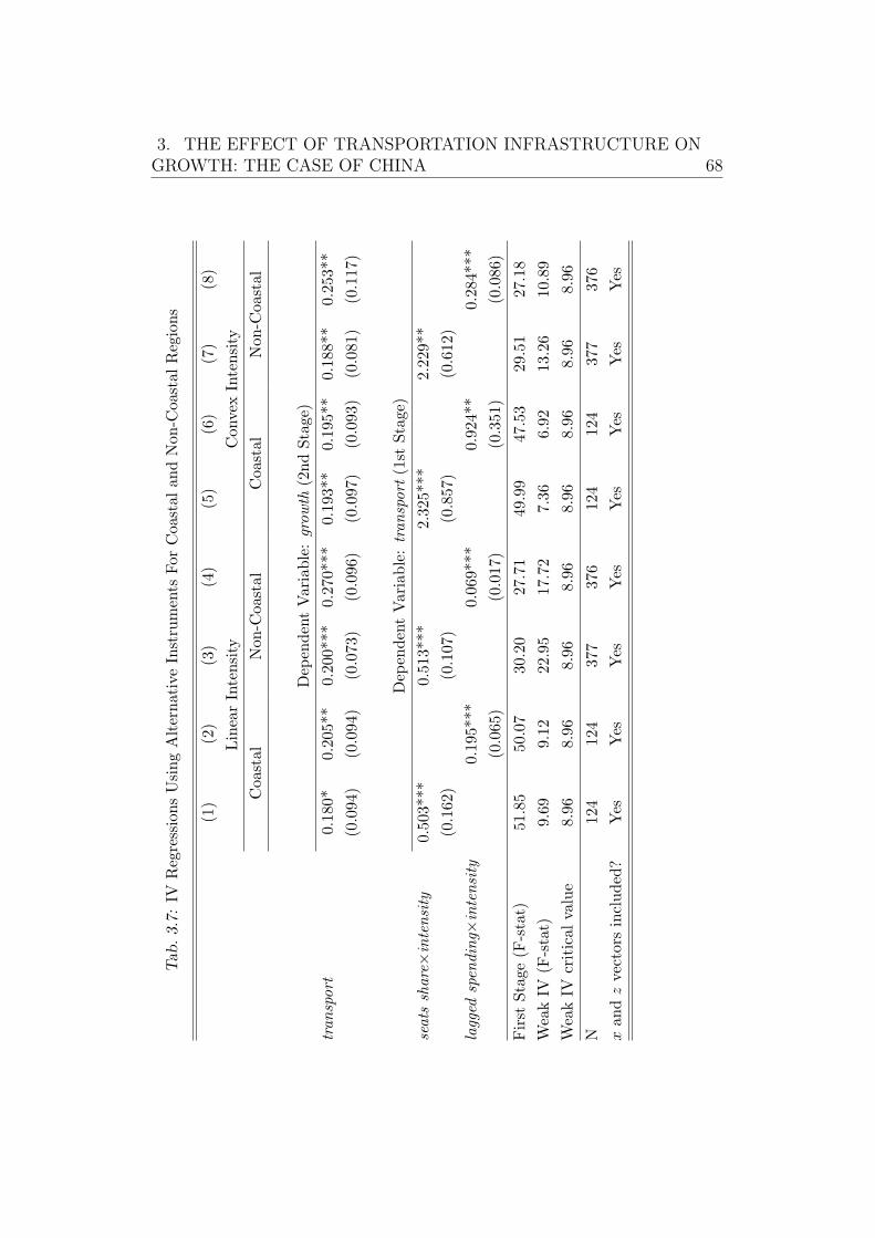
3. THE EFFECT OF TRANSPORTATION INFRASTRUCTURE ONGROWTH: THE CASE OF CHINA 68
Tab
.3.7:
IVRegressionsUsingAlternativeInstruments
ForCoastalandNon-C
oastalRegions
(1)
(2)
(3)
(4)
(5)
(6)
(7)
(8)
LinearIntensity
ConvexIntensity
Coa
stal
Non-C
oastal
Coastal
Non-C
oastal
Dep
endentVariable:growth
(2ndStage)
transport
0.18
0*0.205**
0.200***
0.270***
0.193**
0.195**
0.188**
0.253**
(0.094
)(0.094)
(0.073)
(0.096)
(0.097)
(0.093)
(0.081)
(0.117)
Dep
endentVariable:transport
(1st
Stage)
seats
share×intensity
0.50
3***
0.513***
2.325***
2.229**
(0.162
)(0.107)
(0.857)
(0.612)
lagged
spen
ding×
intensity
0.195***
0.069***
0.924**
0.284***
(0.065)
(0.017)
(0.351)
(0.086)
First
Stage
(F-stat)
51.85
50.07
30.20
27.71
49.99
47.53
29.51
27.18
WeakIV
(F-stat)
9.69
9.12
22.95
17.72
7.36
6.92
13.26
10.89
WeakIV
critical
value
8.96
8.96
8.96
8.96
8.96
8.96
8.96
8.96
N12
4124
377
376
124
124
377
376
xan
dzvectorsincluded?
Yes
Yes
Yes
Yes
Yes
Yes
Yes
Yes
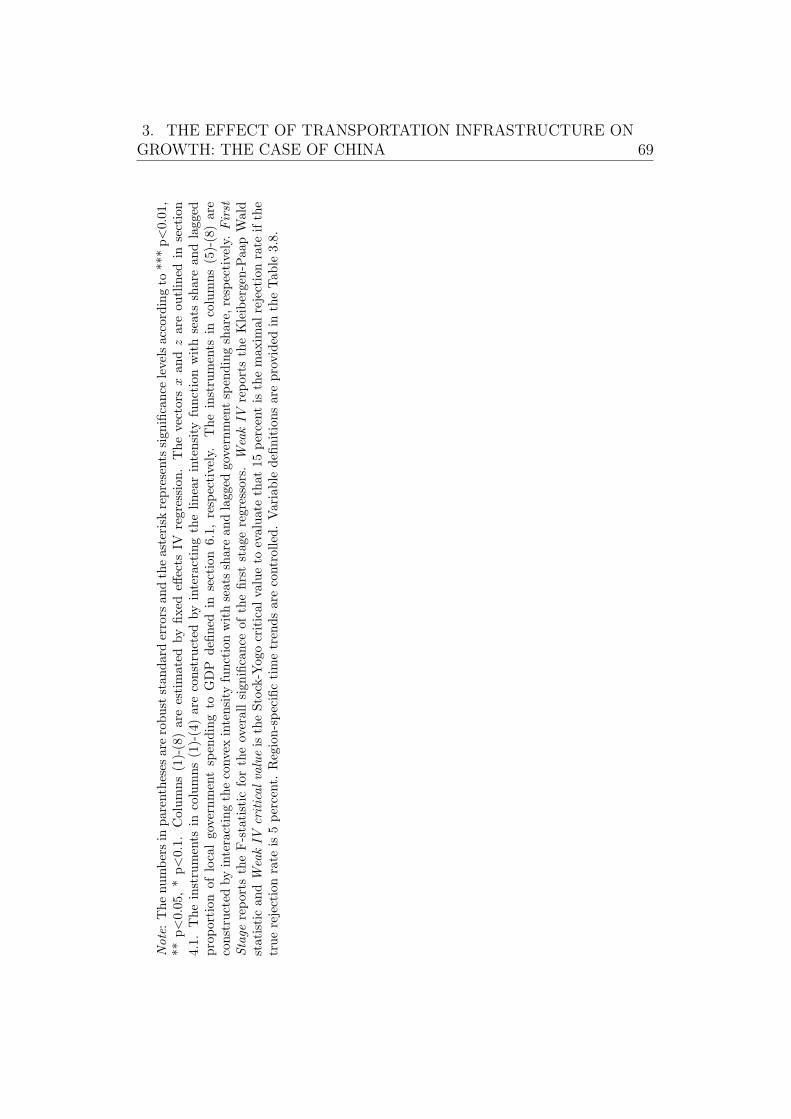
3. THE EFFECT OF TRANSPORTATION INFRASTRUCTURE ONGROWTH: THE CASE OF CHINA 69
Note:Thenumbersin
parentheses
arerobust
stan
darderrors
andtheasterisk
represents
sign
ificance
levelsaccordingto
***p<0.01
,**
p<0.05
,*p<0.1.
Columns(1)-(8)areestimated
byfixed
effects
IVregression
.Thevectors
xan
dzareou
tlined
insection
4.1.
Theinstruments
incolumns(1)-(4)areconstructed
byinteractingthelinearintensity
functionwithseatssharean
dlagg
edproportion
oflocalgovernmentspen
dingto
GDP
defi
ned
insection
6.1,
respectively.
Theinstruments
incolumns(5)-(8)are
constructed
byinteractingtheconvexintensity
functionwithseatssharean
dlagg
edgovernmentspen
dingshare,
respectively.
First
Stage
reports
theF-statistic
fortheoverallsign
ificance
ofthefirststag
eregressors.WeakIV
reports
theKleibergen-Paa
pWald
statistican
dWeakIV
criticalvalueistheStock-Y
ogocritical
valueto
evaluatethat
15percentisthemax
imal
rejectionrate
ifthe
truerejectionrate
is5percent.
Region-specifictimetren
dsarecontrolled.Variable
defi
nitionsareprovided
intheTab
le3.8.
3. THE EFFECT OF TRANSPORTATION INFRASTRUCTURE ONGROWTH: THE CASE OF CHINA 70
The robustness of the effect of transportation infrastructure is further
supported by its quantitative and statistical significance in the regressions
for both coastal and non-coastal regions, reported in Table 3.7, where the four
alternative instruments are considered. Again, the new estimates in Table
3.7 turn out to be similar in magnitude to the baseline estimates pertaining
to the coastal and inland provinces in Table 3.4. Take the coastal regression
as an example. The baseline estimate of 0.192 in the second stage regression
(see column (2) of Table 3.4) is very similar to the estimates of 0.193 and
0.195 that are based on the convex intensity function (see columns (5)-(6) of
Table 3.7). The similarity between the baseline and new estimates reiterates
the resilience of the results to different constructions of instrumental variables
that utilise information from the National Congress.
5.5 Further Discussion
The study of whether the transportation infrastructure and growth relation-
ship is causal is of first order importance. One of the most influential papers
looking at this relationship for China is Demurger (2001), whose fixed effects
2SLS estimates provide some early indication that this causal effect may be
non-trivial. In her paper, she finds that the increase in GDP growth per
capita following a 0.1 increase in transport density ranges from 339 to 456
basis points.59 Compared to these findings, the conclusions in this chapter
are more modest. For instance, column (4) of Table 3.3 suggests that a 0.1
increase in transport density would only raise GDP growth per capita by
217 basis points on average. Therefore, this implies that the causal effect of
transportation infrastructure, while is important for economic growth, may
not be as large as previously found in the literature. On the other hand, this
chapter’s findings are tempered by the county-level study of Banerjee et al.
59 In Model (2) in Table 2 of Demurger (2001), the coefficient on transport andtransport2 is 0.754 and −1.121 respectively. Using the average transport density of 0.2655during 1985–1998 and omitting the coefficient on transport × pop.density, the marginaleffect of transport density on growth for the ‘average’ province is 0.754−1.121transport =0.754 − (1.121 × 0.2655) = 0.4564. Therefore, if transport density increases by 0.1, theyearly GDP growth per capita would increase by approximately 456 basis points onaverage. Similarly, based on Model (4) in Table 2 of her paper, a similar computationleads to a marginal effect of 0.3389.
3. THE EFFECT OF TRANSPORTATION INFRASTRUCTURE ONGROWTH: THE CASE OF CHINA 71
(2012), who find that a county’s proximity to transportation networks does
not have a statistically significant effect on its economic growth. Overall,
even though Banerjee et al. (2012) do not consider transport density as
the main causal variable, their finding of a weak effect of accessibility to
transportation networks on growth in contrast with the strong results of
Demurger (2001) shows that there is some way to go in reaching a consensus
on what the causal relationship between transportation infrastructure and
economic growth might be with respect to China.
6. Conclusion
Focusing on China, this chapter proposes a new identification strategy that
exploits the timing of the National Congress to identify the within-province
effect that transportation infrastructure has on growth. Letting the data
speak, it finds that transportation infrastructure is most strongly influenced
around the year of the National Congress and the set of congress instruments
constructed, which are associated with the timing of the National Congress,
generates significant response in transportation infrastructure.
The main empirical results are presented as follows. The OLS estimate
of the within-province effect of transportation infrastructure on growth
is tenuous at best, a possible reflection of the overpowering influence of
attenuation bias due to measurement errors in the data. By contrast, the
2SLS estimate paints an opposite picture. With the density of transportation
infrastructure as the main causal variable, the 2SLS estimate shows that
an increase in the density of transportation infrastructure, ceteris paribus,
has an effect of raising GDP growth per capita by more than 6 percentage
points on average. This effect is robust to the inclusion of a large number of
additional control variables in the regression, as these variables are included
to eliminate any bias that may arise from omitting potentially relevant
variables, and to soak up the effects of other unobserved shocks such as
policy changes that may coincide with the National Congress but are not
related to the formation of transportation infrastructure. It is also robust
3. THE EFFECT OF TRANSPORTATION INFRASTRUCTURE ONGROWTH: THE CASE OF CHINA 72
to running separate regressions for coastal and non-coastal provinces as
these regions differ not only in geographical characteristics, but also in
how their economies are structured; as well as to utilising four alternative
constructions of instrumental variables that allow for an aggregate event such
as the National Congress to have province-specific effects on transportation
infrastructure. Therefore, taking a broader perspective, the resilience of the
main causal estimate that emerges from these robustness checks underscores
the positive contribution that transportation infrastructure has made to the
economic development of China.
Echoing the Chinese adage ‘To get rich, build roads first’, this study
provides some evidence that the positive association between transporta-
tion infrastructure and economic growth is causal, therefore affirming the
positive role that transportation infrastructure has played in the economic
development and transition of China. With respect to the magnitude of
this causal effect, this study shows a more moderate result than that which
has been reported in the seminal work in this area, i.e. Demurger (2001),
implying that the economic returns to the improvement of transportation
infrastructure may be diminishing over a longer period of time.
Although the short-run causal effect of the changes in transportation
infrastructure on economic growth is carefully analysed in this chapter, one
may still wonder what is the role of transportation infrastructure in China’s
long-run GDP per capita growth. Thus, Chapter 4 will explore this problem
by proposing a new identification strategy to mitigate endogeneity issues, and
quantify the casual effect of the improvement of transportation infrastructure
on long-run economic growth.
3. THE EFFECT OF TRANSPORTATION INFRASTRUCTURE ONGROWTH: THE CASE OF CHINA 73
Tab.3.8:ListofVariables
GDP
growth
percapita
theannualgrowth
rate
ofrealGDP
per
capita
transport
length
ofrailway
andhighway
(km)÷
regionalarea(km
2)
ln(G
DP)
logarithm
ofrealGDP
per
capita
vecto
rx
investmen
ttotalfixed
investment(flow
)÷
totalnominalGDP
education
secondary
schoolenrolm
ent÷
population
vecto
rz
FDI
localnominalFDI(U
SD)÷
nationalnominalFDI(U
SD)
trade
localnominaltotaltrade(U
SD)÷
nationalnominaltotaltrade(U
SD)
urbanisation
urbanpopulation÷
totalpopulation
agriculturallabour
agriculturallabour÷
localem
ployed
labour
state
labour
labourem
ployedin
state
andcollectivefirm
s÷
localem
ployedlabour
populationden
sity
regionaltotalpopulation÷
regionalarea(km
2)
telephoneden
sity
telephonesubscribers÷
regionalarea(km
2)
coastal
dummy=1ifprovincesare
locatedin
coastalregions*
reform
dummy=1ifyearis
between1992and1998
coastal×
reform
coastaldummymultiplied
byreform
dummy
Note:*T
hecoastalregion
sareLiaon
ing,
Heb
ei,Tianjin,Shan
don
g,Jiangsu,Shan
ghai,Zhejiang,
Fujian
andGuan
gdon
g.
4. LONG-RUN IMPACT OF TRANSPORTATION
INFRASTRUCTURE ON GROWTH: EVIDENCE FROM
CHINA
1. Introduction
In development economics, the contribution of transportation infrastructure
to economic growth is a key topic that captivates much attention among
academics and policy-makers alike.60 This issue is especially relevant to
China where behind its impressive growth trajectory in recent years is
the rapid expansion of modern transportation infrastructure. Even as
recently as 2008, the Chinese central government earmarked the largest ever
infrastructure spending surpassing the total planned expenditure in public
housing, health care and education, which underscored the confidence in
infrastructure that the government had as a way of securing the country’s
economic future. From the policy perspective, transportation infrastructure
is a key focal point because of its potential benefits for economic development.
For instance, access to transportation helps to facilitate the flow of human
capital and draw workers to places where economic opportunities are more
abundant. It also helps to connect different regions through trade, enabling
them to specialise in their core economic strengths that are important
for fostering local economic development.61 Even though transportation
60 For instance, almost 20 percent of World Bank lending in 2007 was allocated totransportation infrastructure projects, more than the share in education, health and socialservices combined (World Bank, 2007).
61 Donaldson (2010) documents a strong positive link between economic developmentand the transition from autarky to trade among regions in colonial India, where thistransition was facilitated by the construction of railroads that reduced inter-regional tradecosts during the 19th century. As he explains, before the advent of railroads, bullocksthat travel no more than 30 kilometres a day were the main source of transport for India’s

4. LONG-RUN IMPACT OF TRANSPORTATION INFRASTRUCTUREON GROWTH: EVIDENCE FROM CHINA 75
infrastructure appears to be important for the economy in the early stage
of economic development, a study of its causal effect is by no means
straightforward, primarily because of the problem of reverse causality where
higher levels of economic growth may in turn encourage the expansion of
infrastructure services. In the related literature that spans more than two
decades, this is arguably the most challenging problem to deal with and one
that is a subject of intense interest even to this day.
Based on provincial level data (1978–2008), this chapter seeks to answer
that question: “What is the long-run impact of changes in the density
of transportation infrastructure on economic growth in China?” Because
transportation infrastructure is an endogenous determinant of economic
growth, OLS regressions are fundamentally unidentified and better estima-
tion strategies are therefore vital to address this research question. While
instrumental variable estimation has been used to cut through the problem of
endogeneity (e.g. Banerjee et al., 2012), the focus on long-run growth raises
a formidable challenge in finding a suitable instrument for transportation
infrastructure. Specifically, most of the variation in the data that the
regression draws upon comes from cross-section datasets, since long-run
economic growth is constructed by averaging the annual growth rate of
GDP per capita over a significant period of time and this reduces one’s
ability to utilise much of the time variation in the data. In order to
obtain a reasonably exogenous instrument for transportation infrastructure,
a venture into history for the instrument search appears necessary. This
chapter proposes an instrument that is related to the presence of Chinese
guilds, which were forms of corporate collective action that first came
about during the Ming dynasty (1368–1644) and flourished towards the
end of the Qing dynasty (1644–1911). Literally translated in Chinese as
‘trade-line association’ (Quan, 1934) and known by the populace throughout
China by a generic designation, ‘mutual help association’, the guild was an
association that was involved in any form of craft, merchant and trade (Moll-
commodity trade. In contrast, trains during that time could travel 20 times faster andat much lower freight rates per unit distance travelled. Therefore, the construction ofrailroads in colonial India had led to a dramatic reduction in trade costs, encouraginginter-regional trade that helps to foster economic development.
4. LONG-RUN IMPACT OF TRANSPORTATION INFRASTRUCTUREON GROWTH: EVIDENCE FROM CHINA 76
Murata, 2008). The Chinese guilds served numerous important economic
and social functions such as the provision of hospitality and entertainment
services, training of skilled crafts and tradesmen, and the development of
educational and municipal services. The presence of Chinese guilds is an
important indicator of past infrastructure provision, as these guilds represent
the integration of economic and social activities.62 Therefore, information
about the Chinese guilds could be used to construct a candidate instrument
insofar as modern infrastructure (1978–2008) is linked with past (1911)
infrastructure.
In the literature, the endogenous response of infrastructure to economic
growth is a significant obstacle to overcome in any empirical analysis,
especially since it is infeasible to ‘randomly distribute’ infrastructure as
one would in an ideal experiment. Hence, the identification of the
effect of changes in transportation infrastructure on economic growth and
development has been a topic of intense interest among academics where
various solutions have been proposed to partially address the confounding
influence due to its endogenous nature. This chapter relates to this stream
of work that considers the issue of identifying the exogenous variation in
transportation infrastructure in the context of China.63 For instance, based
on Chinese provincial panel data over the period 1985–1998, Demurger (2001)
looks at how changes in transportation infrastructure could drive provincial
income disparities in China, employing internal instruments, e.g. lagged
trade and FDI. Using Chinese county-level data, Banerjee et al. (2012) study
the causal effect of changes in transportation infrastructure by constructing
an instrument that is based on information about a county’s distance from
62 See Appendix B for more details.63 There are related studies on other countries as well. For instance, based on industry-
level data for the US, Fernald (1999) identifies the causal effect of the provision of roadson US industrial productivity from 1953 to 1989 by examining how the intensity of vehicleuse by different industries is linked to their productivity levels. Causality is pinned downif changes the increase in the provision of roads is associated with larger changes inproductivity growth in industries that are more vehicle intensive. A difference-in-differenceapproach to deal with the endogeneity issue is employed by Michaels (2008), who examinesthe effect of highway construction in the US in the 1950s. Keller and Shiue (2008) look atthe effect of steam trains in 19th century Europe by employing an instrumental variableapproach for identification.

4. LONG-RUN IMPACT OF TRANSPORTATION INFRASTRUCTUREON GROWTH: EVIDENCE FROM CHINA 77
main transportation networks that link up cities in the past. While the
existing studies of China’s transportation infrastructure mainly investigate
its short-run effect on economic growth, this chapter complements the
literature and Chapter 3 by proposing a new instrument for transportation
infrastructure and by focusing on its long-run economic implication.
Using data from 1978–2008, this chapter splits this sample into two
halves of similar size and constructs long-run growth for each time period,
based on the average annual growth during 1978–1993 and 1994–2008. By
splitting the sample so as to obtain a two-period panel, one can eliminate
province fixed effects that represent all time-invariant permanent differences
while still focusing on the impact that transportation infrastructure has on
long-run GDP growth per capita. Controlling for province fixed effects is
paramount because of the immense diversity in culture, religion, geographic
characteristics and governance that one observes, for example, from Tibet
and Xinjiang in China’s deep west to the more developed areas in the
coastal east, and this diversity could confound the relationship between
infrastructure and economic growth. Nevertheless, OLS regression may
still be unidentified, because unlike instrumental variable (IV) regression,
it cannot be used to address the issue of reverse causality that confounds the
causal effect of transportation infrastructure.
The first stage regression reveals that the density of guilds, defined
as the number of guilds per 10,000 people, is a powerful instrument for
transportation infrastructure. The IV estimate offers evidence that the
expansion of transportation infrastructure is beneficial for long-run GDP
growth per capita. This is in stark contrast to the OLS estimates that suggest
that the effect of transportation infrastructure on growth is not (statistically)
significantly different from zero. The strong benefits of transportation
infrastructure are robust to a battery of sensitivity tests. These tests
bring into four covariates the regression that are potentially relevant to
economic growth,64 and the robustness that emerges from the sensitivity
tests underscores the significant role that transportation infrastructure has
64 These covariates consist of the urbanisation rate, openness, public employment shareand agricultural labour share.
4. LONG-RUN IMPACT OF TRANSPORTATION INFRASTRUCTUREON GROWTH: EVIDENCE FROM CHINA 78
played in propelling the long-term economic development of China.
The remainder of this chapter is organised as follows. Section 2 describes
the data, variables and the methodology. Section 3 presents the empirical
results as well as the results from the robustness checks. Section 4 concludes.
2. Data and Methodology
The main dataset is obtained from the China Compendium of Statistics,
which is compiled by the Department of Comprehensive Statistics at the
National Bureau of Statistics of China. There are 31 sub-national adminis-
trative units in mainland China,65 including 22 provinces, four municipalities
(Beijing, Shanghai, Tianjin and Chongqing) and five autonomous regions
(Tibet, Xinjiang, Ningxia, Inner Mongolia and Guangxi).66 But due to
missing data, this chapter excludes information about Hainan and Tibet and
uses data for the remaining 29 administrative units. For ease of discussion,
each administrative unit is henceforth referred to as a ‘province’. The
summary statistics are reported in Table 4.1.67
The dataset spans from 1978 to 2008. This study splits the sample
into two approximately equal halves corresponding to the periods 1978–
1993 and 1994–2008 as this helps to construct long-run economic growth
and employ panel data estimation at the same time. By splitting this way
and constructing a set of two-period panel data, one may eliminate province
fixed effects that represent all time-invariant permanent differences across
provinces. Controlling for province fixed effects is crucial because the differ-
ences in culture, religion, geographic characteristics and governance across
regions in China could confound the relationship between transportation
infrastructure and economic growth. Therefore, by using a two-period panel,
65 They are Anhui, Beijing, Chongqing, Fujian, Gansu, Guangdong, Guangxi, Guizhou,Hainan, Hebei, Heilongjiang, Henan, Hunan, Hubei, Inner Mongolia, Jiangsu, Jiangxi,Jilin, Liaoning, Ningxia, Qinghai, Shanghai, Shandong, Shanxi, Shaanxi, Sichuan, Tianjin,Tibet, Xinjiang, Yunnan and Zhejiang, excluding Hong Kong, Macao and Taiwan.
66 Chongqing was designated a municipality in the year 1997. The other three cities wereinitially municipalities when the People’s Republic of China was established in 1949.
67 Table 4.6 provides the definitions of the variables used in this chapter.
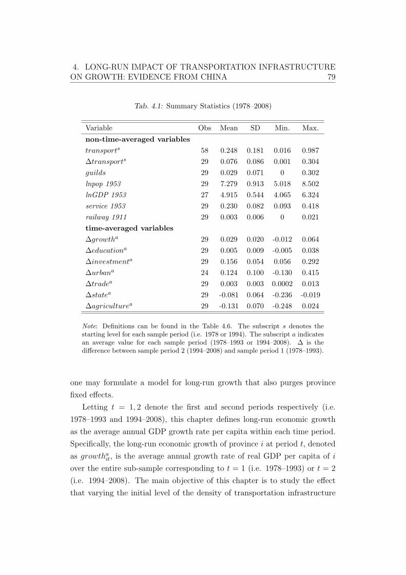
4. LONG-RUN IMPACT OF TRANSPORTATION INFRASTRUCTUREON GROWTH: EVIDENCE FROM CHINA 79
Tab. 4.1: Summary Statistics (1978–2008)
Variable Obs Mean SD Min. Max.
non-time-averaged variables
transports 58 0.248 0.181 0.016 0.987
∆transports 29 0.076 0.086 0.001 0.304
guilds 29 0.029 0.071 0 0.302
lnpop 1953 29 7.279 0.913 5.018 8.502
lnGDP 1953 27 4.915 0.544 4.065 6.324
service 1953 29 0.230 0.082 0.093 0.418
railway 1911 29 0.003 0.006 0 0.021
time-averaged variables
∆growtha 29 0.029 0.020 -0.012 0.064
∆educationa 29 0.005 0.009 -0.005 0.038
∆investmenta 29 0.156 0.054 0.056 0.292
∆urbana 24 0.124 0.100 -0.130 0.415
∆tradea 29 0.003 0.003 0.0002 0.013
∆statea 29 -0.081 0.064 -0.236 -0.019
∆agriculturea 29 -0.131 0.070 -0.248 0.024
Note: Definitions can be found in the Table 4.6. The subscript s denotes thestarting level for each sample period (i.e. 1978 or 1994). The subscript a indicatesan average value for each sample period (1978–1993 or 1994–2008). ∆ is thedifference between sample period 2 (1994–2008) and sample period 1 (1978–1993).
one may formulate a model for long-run growth that also purges province
fixed effects.
Letting t = 1, 2 denote the first and second periods respectively (i.e.
1978–1993 and 1994–2008), this chapter defines long-run economic growth
as the average annual GDP growth rate per capita within each time period.
Specifically, the long-run economic growth of province i at period t, denoted
as growthait, is the average annual growth rate of real GDP per capita of i
over the entire sub-sample corresponding to t = 1 (i.e. 1978–1993) or t = 2
(i.e. 1994–2008). The main objective of this chapter is to study the effect
that varying the initial level of the density of transportation infrastructure
4. LONG-RUN IMPACT OF TRANSPORTATION INFRASTRUCTUREON GROWTH: EVIDENCE FROM CHINA 80
has on long-run average GDP growth per capita. In term of estimation,
the main causal variable is transportsit, the start of the period measure of
transportation density, defined as the total length of railways and highways in
kilometres over the total provincial area in squared kilometres. For instance,
for t = 1, transportsit is the density of transportation infrastructure in 1978.
The focus on transportation infrastructure at the beginning of each period as
the main causal variable allows the study of its impact on long-run economic
growth from that point (i.e 1978 or 1994) onwards. Therefore, the main
estimating equation of this chapter relates growthait to transportsit as,
growthait = c+ α transportsit + β′Xait + µi + ϵit, (4.1)
where c is a general intercept term and µi represents province i’s fixed effect.
The variable ϵit represents any province i’s unconditioned variable that may
affect its long-run growth rate, e.g. for t = 1, it represents any unconditioned
factor that may affect the average annual growth rate during 1978–1993.
The estimation of α might be complicated by omitted variables that are
possibly related to both transportation infrastructure and economic growth.
To this end, this study also considers the inclusion of a vector Xait that
represents other potentially relevant control variables. These variables are
introduced into equation (4.1) to also serve another purpose: to evaluate the
robustness of the estimate of the effect of the initial level of the density
of transportation infrastructure as summarised by the parameter α. In
the baseline regressions, the vector Xait contains two variables, namely, the
average annual fixed investment formation to GDP ratio and a measure of
human capital proxied by the teacher to student ratio at secondary schools,
both of which are standard determinants of economic growth.68 In the
68 This study uses secondary school teacher-student ratio as a proxy for human capital.Other studies have considered proxies such as the number of secondary school studentsand the ratio of secondary school students to total population (e.g. Barro, 1991, Li andHuang, 2009). Given data limitations, researchers have pointed out that the average classsize of secondary schools is the best possible measure of human capital as it reflects theaverage quality of education across provinces. For instance, Glass and Smith (1979), Glasset al. (1982), and Angrist and Lavy (1999) show that reducing the class size could lead tobetter student performance in standardised tests.
4. LONG-RUN IMPACT OF TRANSPORTATION INFRASTRUCTUREON GROWTH: EVIDENCE FROM CHINA 81
robustness checks, the vector Xait is expanded to include information related
to the urbanisation rate, trade openness, the size of the public sector, and
the size of the agricultural sector, all of which are potentially related to
transportation infrastructure and growth as discussed further in section 3.2.
To eliminate the fixed effects, this study estimates equation (4.1) in first
difference taken across the two periods indexed by t = 2 and t = 1. In first
difference, the estimating equation is given by,69
∆growthait = α∆transportsit + β′∆Xait +∆ϵit, (4.2)
where the causal effect of transportation infrastructure on long-run growth,
i.e. α, can be estimated by examining the effect that ∆transportsit has
on ∆growthait. While equation (4.2) purges the province fixed effects,
OLS regression may still be unidentified as it does not take into account
the endogenous response of transportation infrastructure to (potential)
economic growth. For instance, transportation infrastructure can respond
endogenously to GDP per capita growth as higher levels of economic
growth may in turn cause the expansion of infrastructure services. Indeed,
the inadequacy of eliminating fixed effects as a way of dealing with the
endogeneity of transportation infrastructure can be inferred from earlier
studies based on the US state-level panel data where Holtz-Eakin (1994),
Holtz-Eakin and Schwartz (1995) and Garcia-Mila et al. (1996) find that
introducing fixed effects may eliminate the positive effect of infrastructure
on growth. As can be seen in section 3.1, this is echoed in this study as the
OLS estimate after purging fixed effects is nearly zero. In order to obtain
consistent estimates of α, this calls for the use of IV estimation, which in the
context of equation (4.2), requires an instrument for ∆transportsit.
The instrument proposed in this chapter uses historical information
related to the Chinese guilds. There is a large body of literature in geography
and anthropology that discusses how the Chinese guilds were associated
with the early urban structure in China prior to 1911 (e.g. Rowe, 1984).
69 In a two-period panel dataset, the first difference estimator is the same as the within-province estimator.
4. LONG-RUN IMPACT OF TRANSPORTATION INFRASTRUCTUREON GROWTH: EVIDENCE FROM CHINA 82
The Chinese guilds (explained in Appendix B) were forms of corporate
collective action that flourished towards the end of Qing dynasty (1644-
1991). During its heyday, the guilds provided a wide range of economic
and social services that were intertwined with day-to-day living, such as the
matching of skilled workers with employers, providing a meeting place for
merchants and their buyers, as well as offering hospitality services in the
form of hotels, restaurants and entertainment centres. The guilds were also
involved in the training of skilled crafts and tradesmen (Golas, 1977; Moll-
Murata, 2008) and in the provision of educational and municipal services
such as elementary schooling to guild members, firefighting, policing and the
maintenance of streets and bridges for local residents (Rowe, 1992).
The presence of Chinese guilds thus offers some insight into the impor-
tance of business and social networks, as well as an indirect indication of
the extent of infrastructure development that existed in the past. This is
reminiscent of the concept of ‘central place’ from ‘central place theory’ in
the anthropology literature, which is a theory of location for retail trade that
is discussed in Skinner (1977). It is believed that the industrialisation and
trade agglomerations were more likely to occur in the places that guilds were
flourished, as central place models point out that major centres (or cities)
primarily serve and support their surroundings, including smaller centres
and rural hinterlands Wang (1999). According to the central place theory,
it is not surprising that guilds agglomerated to the regions that were more
likely to develop towards large centres (modern cities) and demand for more
transportation infrastructure.
Using this historical information, one can construct a measure of the
density of guilds, defined by the number of guilds in 1911 per 10,000 local
inhabitants,70 as an instrument for ∆transportsit. The number of guilds that
existed in the year 1911 is obtained from Moll-Murata (2008). Figure 4.1
plots the distribution of guilds density across China defined by current (2008)
provincial boundaries. It shows that the guilds are more concentrated in the
70 Historical population in 1911 is not available to construct the guilds density variable,so instead this chapter uses historical population data in 1933 that is documented byZhongguo tu di ren kou, zu dian zhi du zhi tong ji fen xi (National Bureau of Statistics ofRepublic of China, 1978).
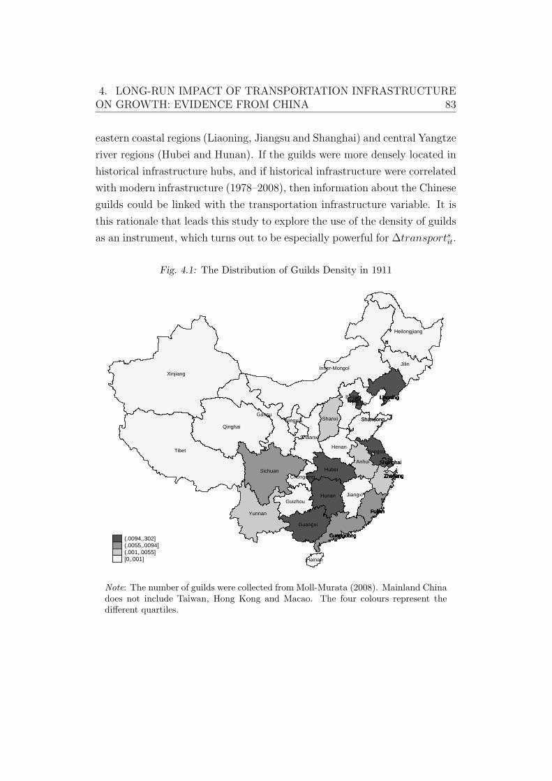
4. LONG-RUN IMPACT OF TRANSPORTATION INFRASTRUCTUREON GROWTH: EVIDENCE FROM CHINA 83
eastern coastal regions (Liaoning, Jiangsu and Shanghai) and central Yangtze
river regions (Hubei and Hunan). If the guilds were more densely located in
historical infrastructure hubs, and if historical infrastructure were correlated
with modern infrastructure (1978–2008), then information about the Chinese
guilds could be linked with the transportation infrastructure variable. It is
this rationale that leads this study to explore the use of the density of guilds
as an instrument, which turns out to be especially powerful for ∆transportsit.
Fig. 4.1: The Distribution of Guilds Density in 1911
Heilongjiang
Inner-MongolXinjiang
Jilin
Liaoning
Gansu
HebeiBeijing
Shanxi
Tianjin
Qinghai
HebeiLiaoningLiaoningLiaoningLiaoning
Shaanxi
Ningxia
Tibet
ShandongShandong
HenanJiangsu
Anhui
Sichuan HubeiShanghai
Chongqing
ShanghaiShanghai
ZhejiangZhejiangZhejiangZhejiangZhejiangZhejiangZhejiangZhejiang
JiangxiHunan
Zhejiang
Yunnan
Guizhou
Zhejiang
Fujian
Zhejiang
Fujian
Guangxi
FujianFujianFujianFujian
GuangdongGuangdongGuangdongGuangdongGuangdongGuangdongGuangdong
Hainan
Guangdong
Fujian
(.0094,.302](.0055,.0094](.001,.0055][0,.001]
Note: The number of guilds were collected from Moll-Murata (2008). Mainland Chinadoes not include Taiwan, Hong Kong and Macao. The four colours represent thedifferent quartiles.
4. LONG-RUN IMPACT OF TRANSPORTATION INFRASTRUCTUREON GROWTH: EVIDENCE FROM CHINA 84
3. Empirical Results
3.1 OLS and IV Results
Table 4.2 summarises the baseline results from OLS regressions. While the
OLS regression is unidentified, it nonetheless provides a useful starting point
for investigating the direction of bias in the estimate of how transportation
infrastructure affects economic growth. Controlling for province fixed effects,
column (1) of Table 4.3 shows that the OLS estimate of the response
of economic growth to transportation infrastructure is not statistically
significantly different from zero. This weakness in the OLS estimate is
perhaps symptomatic of a deeper problem that goes beyond the issue of
omitted variables as it cannot be resolved by the introduction of possibly
relevant covariates into the regression. For instance, columns (2)-(4) control
for education and physical investment, which could be linked to both
transportation infrastructure and economic growth, and show that the OLS
estimates of the impact of the initial level of the density of transportation
infrastructure on long-run economic growth remain stubbornly close to zero.
If the premise that transportation infrastructure enhances economic growth
holds, the weakness of the OLS estimate suggests the possibility that it is
downward biased. This problem may be due to measurement error in the
data of the National Bureau of Statistics of China, which has already been
highlighted by Rawski (2001), Rawski and Xiao (2001), Chow (2006), and
Ravallion and Chen (2007). If this measurement error were classical, the
least squares estimates would be attenuated. Together with the problem of
reverse causality, the presence of measurement errors will confound the causal
relationship and this requires the use of an instrument for transportation
infrastructure in order to obtain consistent estimates of its effect on growth.
To this end, Table 4.3 reports the IV estimates using the density of
guilds as an instrument for transportation infrastructure. In the simplest
regression specification with province fixed effects purged, the first stage
result in column (1) shows that the density of guilds is a statistically
significant explanatory variable for transportation infrastructure. It is also
an especially powerful instrument, as column (1) shows that the first stage
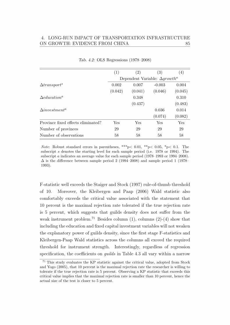
4. LONG-RUN IMPACT OF TRANSPORTATION INFRASTRUCTUREON GROWTH: EVIDENCE FROM CHINA 85
Tab. 4.2: OLS Regressions (1978–2008)
(1) (2) (3) (4)
Dependent Variable: ∆growtha
∆transports 0.002 0.007 -0.003 0.004
(0.042) (0.041) (0.046) (0.045)
∆educationa 0.348 0.310
(0.437) (0.483)
∆investmenta 0.036 0.014
(0.074) (0.082)
Province fixed effects eliminated? Yes Yes Yes Yes
Number of provinces 29 29 29 29
Number of observations 58 58 58 58
Note: Robust standard errors in parentheses, ***p< 0.01, **p< 0.05, *p< 0.1. Thesubscript s denotes the starting level for each sample period (i.e. 1978 or 1994). Thesubscript a indicates an average value for each sample period (1978–1993 or 1994–2008).∆ is the difference between sample period 2 (1994–2008) and sample period 1 (1978–1993).
F-statistic well exceeds the Staiger and Stock (1997) rule-of-thumb threshold
of 10. Moreover, the Kleibergen and Paap (2006) Wald statistic also
comfortably exceeds the critical value associated with the statement that
10 percent is the maximal rejection rate tolerated if the true rejection rate
is 5 percent, which suggests that guilds density does not suffer from the
weak instrument problem.71 Besides column (1), columns (2)-(4) show that
including the education and fixed capital investment variables will not weaken
the explanatory power of guilds density, since the first stage F-statistics and
Kleibergen-Paap Wald statistics across the columns all exceed the required
threshold for instrument strength. Interestingly, regardless of regression
specification, the coefficients on guilds in Table 4.3 all vary within a narrow
71 This study evaluates the KP statistic against the critical value, adopted from Stockand Yogo (2005), that 10 percent is the maximal rejection rate the researcher is willing totolerate if the true rejection rate is 5 percent. Observing a KP statistic that exceeds thiscritical value implies that the maximal rejection rate is smaller than 10 percent, hence theactual size of the test is closer to 5 percent.
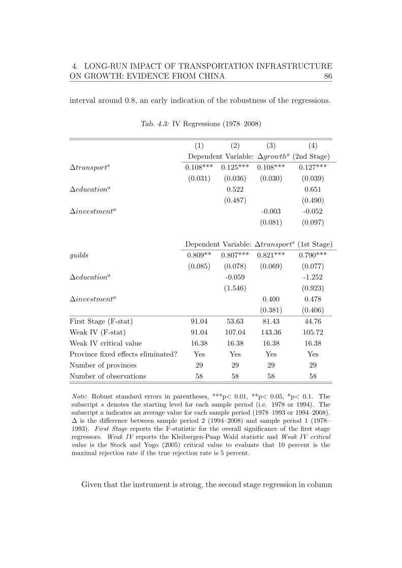
4. LONG-RUN IMPACT OF TRANSPORTATION INFRASTRUCTUREON GROWTH: EVIDENCE FROM CHINA 86
interval around 0.8, an early indication of the robustness of the regressions.
Tab. 4.3: IV Regressions (1978–2008)
(1) (2) (3) (4)
Dependent Variable: ∆growtha (2nd Stage)
∆transports 0.108*** 0.125*** 0.108*** 0.127***
(0.031) (0.036) (0.030) (0.039)
∆educationa 0.522 0.651
(0.487) (0.490)
∆investmenta -0.003 -0.052
(0.081) (0.097)
Dependent Variable: ∆transports (1st Stage)
guilds 0.809** 0.807*** 0.821*** 0.790***
(0.085) (0.078) (0.069) (0.077)
∆educationa -0.059 -1.252
(1.546) (0.923)
∆investmenta 0.400 0.478
(0.381) (0.406)
First Stage (F-stat) 91.04 53.63 81.43 44.76
Weak IV (F-stat) 91.04 107.04 143.36 105.72
Weak IV critical value 16.38 16.38 16.38 16.38
Province fixed effects eliminated? Yes Yes Yes Yes
Number of provinces 29 29 29 29
Number of observations 58 58 58 58
Note: Robust standard errors in parentheses, ***p< 0.01, **p< 0.05, *p< 0.1. Thesubscript s denotes the starting level for each sample period (i.e. 1978 or 1994). Thesubscript a indicates an average value for each sample period (1978–1993 or 1994–2008).∆ is the difference between sample period 2 (1994–2008) and sample period 1 (1978–1993). First Stage reports the F-statistic for the overall significance of the first stageregressors. Weak IV reports the Kleibergen-Paap Wald statistic and Weak IV criticalvalue is the Stock and Yogo (2005) critical value to evaluate that 10 percent is themaximal rejection rate if the true rejection rate is 5 percent.
Given that the instrument is strong, the second stage regression in column
4. LONG-RUN IMPACT OF TRANSPORTATION INFRASTRUCTUREON GROWTH: EVIDENCE FROM CHINA 87
(1) of Table 4.3 shows that the impact of transportation infrastructure
on long-run economic growth, i.e. the estimate of α, is both statistically
significant and quantitatively large. Unlike the OLS estimates that are not
significantly different from zero, column (1) reports that a one standard
deviation improvement in the initial level of the density of transportation
infrastructure raises the long-run average growth of GDP per capita by
about 1.95 percentage points.72 This estimated effect of transportation
infrastructure on long-run growth is not confounded by permanent differences
across provinces such as the heterogeneity in the local culture, religion,
institutions and geography, as province fixed effects have already been
eliminated. At first pass, it does not appear to be confounded by omitted
variables, since the effect of transportation infrastructure remains strong even
after the introduction of the education and fixed investment variables into
the regression.
3.2 Robustness Checks
Table 4.4 reports a battery of robustness checks to evaluate the sensitivity
of the baseline IV estimates to the inclusion of potentially relevant omitted
variables in the long-run growth regression.73 The first robustness check
includes the average provincial urbanisation rate in the baseline model, as the
urban economics literature has found that urbanisation may be an important
determinant of economic growth.74 When controlling for information about
the urbanisation rate, column (1) of Table 4.4 shows that the effect of
transportation infrastructure on long-run growth remains robust. The new,
72 One standard deviation of transports is 0.181. Therefore, the 1.95 percentage pointincrease reported here is derived based on 0.181×0.108×100=1.95.
73 As the growth regression of (4.2) considers the time-averaged of economic growth asthe dependent variable, the robustness checks introduces additional covariates into theregression that are expressed as time-averages as well. The intuition is that the errorterm in (4.2) is the time-averaged of the unobservables during each time block (i.e. 1978–1993 or 1994–2008), hence the information drawn out from the error term should have atime-averaged expression.
74 See Quigley (1998), Henderson (2003), Duranton and Puga (2004), Duranton (2008),among others.
4. LONG-RUN IMPACT OF TRANSPORTATION INFRASTRUCTUREON GROWTH: EVIDENCE FROM CHINA 88
statistically significant coefficient of 0.085 on transportation infrastructure,
unlike the OLS estimates, shows that transportation infrastructure is an
important determinant of long-run growth. The first stage regression in this
robustness check also re-emphasises the sharpness of guilds density as an
instrument, where its effect on transportation infrastructure is similar to the
baseline estimates and the first stage F-statistic is much greater than the
rule-of-thumb threshold of 10.
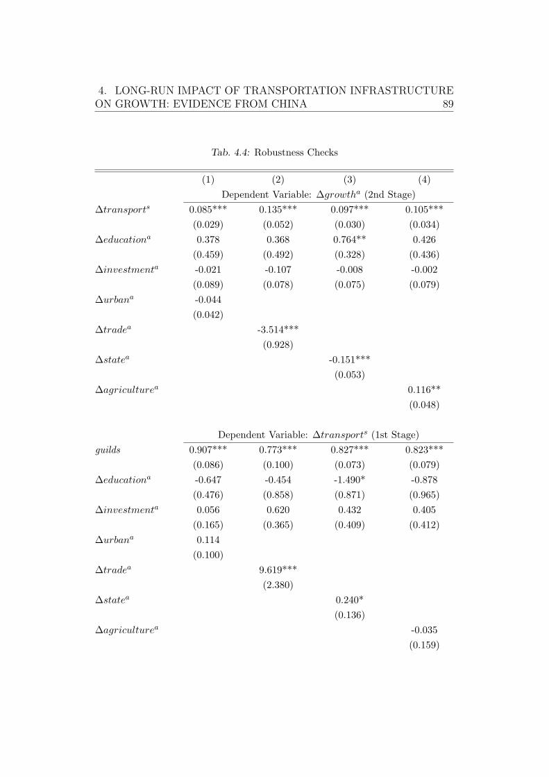
4. LONG-RUN IMPACT OF TRANSPORTATION INFRASTRUCTUREON GROWTH: EVIDENCE FROM CHINA 89
Tab. 4.4: Robustness Checks
(1) (2) (3) (4)
Dependent Variable: ∆growtha (2nd Stage)
∆transports 0.085*** 0.135*** 0.097*** 0.105***
(0.029) (0.052) (0.030) (0.034)
∆educationa 0.378 0.368 0.764** 0.426
(0.459) (0.492) (0.328) (0.436)
∆investmenta -0.021 -0.107 -0.008 -0.002
(0.089) (0.078) (0.075) (0.079)
∆urbana -0.044
(0.042)
∆tradea -3.514***
(0.928)
∆statea -0.151***
(0.053)
∆agriculturea 0.116**
(0.048)
Dependent Variable: ∆transports (1st Stage)
guilds 0.907*** 0.773*** 0.827*** 0.823***
(0.086) (0.100) (0.073) (0.079)
∆educationa -0.647 -0.454 -1.490* -0.878
(0.476) (0.858) (0.871) (0.965)
∆investmenta 0.056 0.620 0.432 0.405
(0.165) (0.365) (0.409) (0.412)
∆urbana 0.114
(0.100)
∆tradea 9.619***
(2.380)
∆statea 0.240*
(0.136)
∆agriculturea -0.035
(0.159)
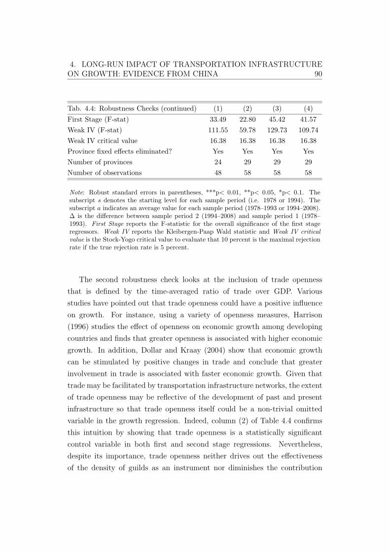
4. LONG-RUN IMPACT OF TRANSPORTATION INFRASTRUCTUREON GROWTH: EVIDENCE FROM CHINA 90
Tab. 4.4: Robustness Checks (continued) (1) (2) (3) (4)
First Stage (F-stat) 33.49 22.80 45.42 41.57
Weak IV (F-stat) 111.55 59.78 129.73 109.74
Weak IV critical value 16.38 16.38 16.38 16.38
Province fixed effects eliminated? Yes Yes Yes Yes
Number of provinces 24 29 29 29
Number of observations 48 58 58 58
Note: Robust standard errors in parentheses, ***p< 0.01, **p< 0.05, *p< 0.1. Thesubscript s denotes the starting level for each sample period (i.e. 1978 or 1994). Thesubscript a indicates an average value for each sample period (1978–1993 or 1994–2008).∆ is the difference between sample period 2 (1994–2008) and sample period 1 (1978–1993). First Stage reports the F-statistic for the overall significance of the first stageregressors. Weak IV reports the Kleibergen-Paap Wald statistic and Weak IV criticalvalue is the Stock-Yogo critical value to evaluate that 10 percent is the maximal rejectionrate if the true rejection rate is 5 percent.
The second robustness check looks at the inclusion of trade openness
that is defined by the time-averaged ratio of trade over GDP. Various
studies have pointed out that trade openness could have a positive influence
on growth. For instance, using a variety of openness measures, Harrison
(1996) studies the effect of openness on economic growth among developing
countries and finds that greater openness is associated with higher economic
growth. In addition, Dollar and Kraay (2004) show that economic growth
can be stimulated by positive changes in trade and conclude that greater
involvement in trade is associated with faster economic growth. Given that
trade may be facilitated by transportation infrastructure networks, the extent
of trade openness may be reflective of the development of past and present
infrastructure so that trade openness itself could be a non-trivial omitted
variable in the growth regression. Indeed, column (2) of Table 4.4 confirms
this intuition by showing that trade openness is a statistically significant
control variable in both first and second stage regressions. Nevertheless,
despite its importance, trade openness neither drives out the effectiveness
of the density of guilds as an instrument nor diminishes the contribution
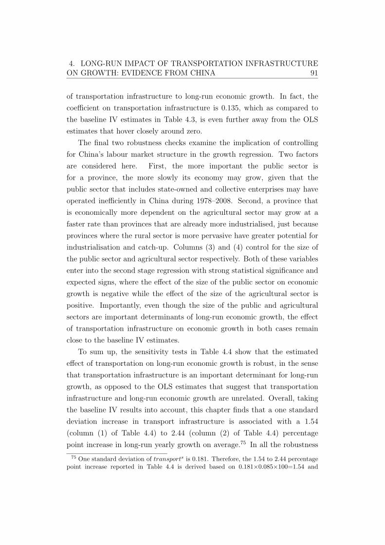
4. LONG-RUN IMPACT OF TRANSPORTATION INFRASTRUCTUREON GROWTH: EVIDENCE FROM CHINA 91
of transportation infrastructure to long-run economic growth. In fact, the
coefficient on transportation infrastructure is 0.135, which as compared to
the baseline IV estimates in Table 4.3, is even further away from the OLS
estimates that hover closely around zero.
The final two robustness checks examine the implication of controlling
for China’s labour market structure in the growth regression. Two factors
are considered here. First, the more important the public sector is
for a province, the more slowly its economy may grow, given that the
public sector that includes state-owned and collective enterprises may have
operated inefficiently in China during 1978–2008. Second, a province that
is economically more dependent on the agricultural sector may grow at a
faster rate than provinces that are already more industrialised, just because
provinces where the rural sector is more pervasive have greater potential for
industrialisation and catch-up. Columns (3) and (4) control for the size of
the public sector and agricultural sector respectively. Both of these variables
enter into the second stage regression with strong statistical significance and
expected signs, where the effect of the size of the public sector on economic
growth is negative while the effect of the size of the agricultural sector is
positive. Importantly, even though the size of the public and agricultural
sectors are important determinants of long-run economic growth, the effect
of transportation infrastructure on economic growth in both cases remain
close to the baseline IV estimates.
To sum up, the sensitivity tests in Table 4.4 show that the estimated
effect of transportation on long-run economic growth is robust, in the sense
that transportation infrastructure is an important determinant for long-run
growth, as opposed to the OLS estimates that suggest that transportation
infrastructure and long-run economic growth are unrelated. Overall, taking
the baseline IV results into account, this chapter finds that a one standard
deviation increase in transport infrastructure is associated with a 1.54
(column (1) of Table 4.4) to 2.44 (column (2) of Table 4.4) percentage
point increase in long-run yearly growth on average.75 In all the robustness
75 One standard deviation of transports is 0.181. Therefore, the 1.54 to 2.44 percentagepoint increase reported in Table 4.4 is derived based on 0.181×0.085×100=1.54 and
4. LONG-RUN IMPACT OF TRANSPORTATION INFRASTRUCTUREON GROWTH: EVIDENCE FROM CHINA 92
checks, the effect of the density of guilds on the initial level of transportation
infrastructure also remains similar to the baseline IV estimates and this
provides some ratification of the use of the density of guilds as an estimation
strategy in this study.
3.3 Alternative Instruments
Can other candidate instruments be used in this study? At first glance, it
appears that other historical information, for instance, about past population
size, GDP, and the extant transportation infrastructure during historical
times, could be used to construct an instrument for the transportation
infrastructure variable. Therefore, one might wonder if there is a need
to zero in on the use of the density of guilds as an estimation strategy.
The following discussion briefly shows that while modern transportation
infrastructure might be linked to history in many ways, the density of
guilds is unique in its explanatory power for transportation infrastructure as
compared to other plausible instruments based on historical information. In
other words, among plausible instruments for transportation infrastructure
based on different historical information, the density of guilds turns out to
be the best, although this does not imply that the density of guilds is the
only available instrument for the study of transportation infrastructure on
long-run economic growth. That being said, this finding highlights the fact
that locating a suitable historical information for the construction of the
instrument for transportation infrastructure turns out to be more challenging
than it might be expected.
To provide some evidence in support of the density of guilds as an
instrument for transportation infrastructure, Table 4.5 shows the estimation
results that are obtained using four alternative (historical) instruments.76
The first alternative instrument is the log of provincial population in 1953.
0.181×0.135×100=2.44.76 This study gathers the data of historical population, GDP, and size of service sector
from the China Compendium of Statistics. Railway density in 1911 is calculated based onMa (1983).
4. LONG-RUN IMPACT OF TRANSPORTATION INFRASTRUCTUREON GROWTH: EVIDENCE FROM CHINA 93
This is the year when the first population census was conducted since the
founding of the People’s Republic of China. The rationale of using past
population as an instrument is based on the idea that past population is likely
to be related to past levels of transportation infrastructure, and in turn the
level of modern transportation infrastructure that needs to be instrumented
here.77 The second alternative instrument is the log of real GDP per
capita in 1953, which reflects an initial economic condition. If wealthier
provinces also have better infrastructure, then past information about the
wealth of a province would be related to its past levels of infrastructure,
hence using a measure of past wealth such as the log of real GDP per
capita as an instrument might work. The third alternative instrument is
the ratio of service sector GDP to total GDP in 1953. In a way, this variable
might have a similar effect on transportation infrastructure as the density of
guilds, considering that the Chinese guilds were historically service providers.
Finally, the fourth alternative instrument is the density of railroads in
1911.78 Since the transportation infrastructure variable captures the density
of roads and railways combined, the density of historical railroads might
be informative about transportation infrastructure given that some of these
historical railway lines have been upgraded into the railway lines that are in
operation today.
Table 4.5 shows that the log of real GDP per capital in 1953 and
the density of railroads in 1911 are statistically significant determinants of
transportation infrastructure. However, in the first stage regression, the log
of population in 1953 and the size of the service sector in 1953 turn out
to be statistically insignificant. As compared to guilds density, all the four
77 Furthermore, alluding to the 19th century US as an example, the initial populationmay be positively associated with the expanding demand for the construction of railroadsas Fogel (1962) has argued.
78 Based on information such as railway track lengths, the years when constructionstarted, the years when tracks opened, and the locations of origin and terminal stations ofboth main and spur lines provided by Ma (1983), it is possible to obtain the total lengthsof railroads that existed in 1911, which this study then assigns to each province accordingto contemporary provincial boundaries provided by Google Maps for the calculation of thedensity historical railway. In the calculation, this study eliminates the spur lines that werereported as dismantled, where the various reasons for the dismantling are discussed in Ma(1983).
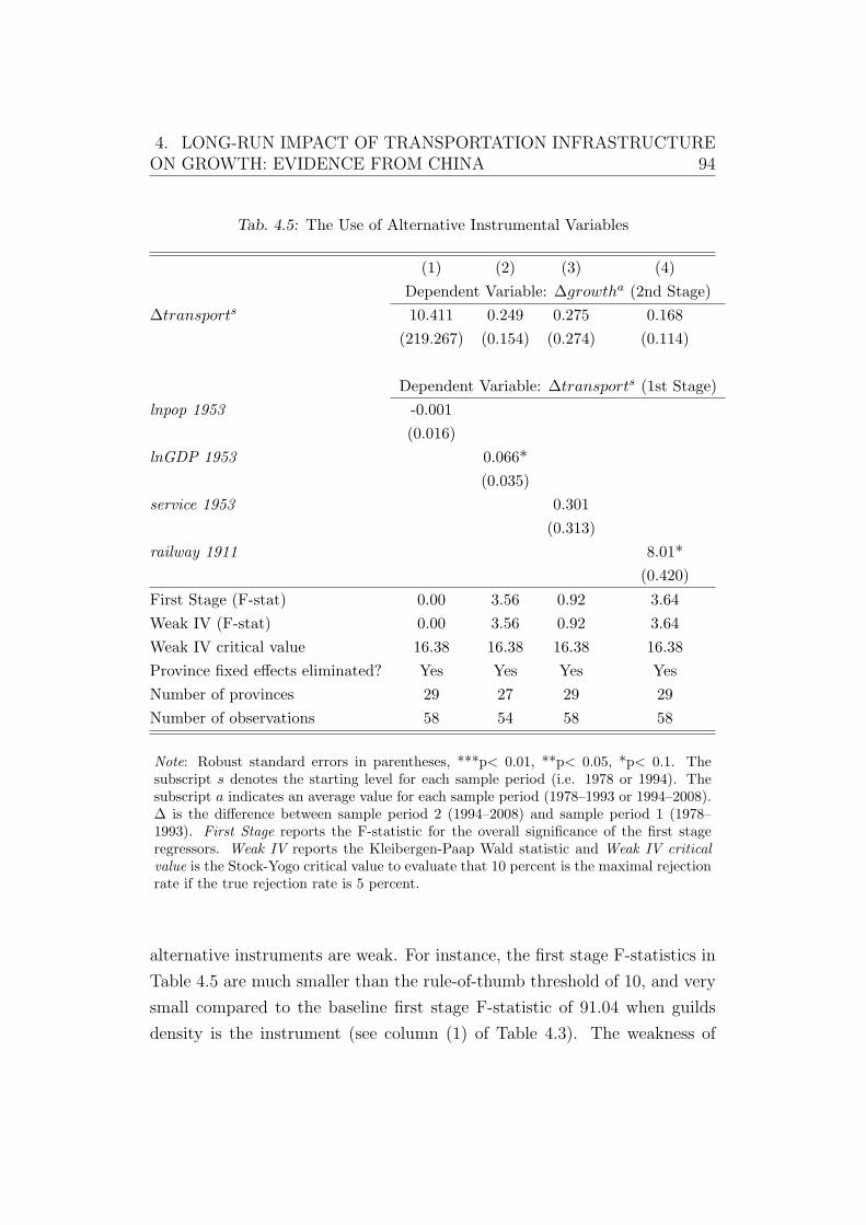
4. LONG-RUN IMPACT OF TRANSPORTATION INFRASTRUCTUREON GROWTH: EVIDENCE FROM CHINA 94
Tab. 4.5: The Use of Alternative Instrumental Variables
(1) (2) (3) (4)
Dependent Variable: ∆growtha (2nd Stage)
∆transports 10.411 0.249 0.275 0.168
(219.267) (0.154) (0.274) (0.114)
Dependent Variable: ∆transports (1st Stage)
lnpop 1953 -0.001
(0.016)
lnGDP 1953 0.066*
(0.035)
service 1953 0.301
(0.313)
railway 1911 8.01*
(0.420)
First Stage (F-stat) 0.00 3.56 0.92 3.64
Weak IV (F-stat) 0.00 3.56 0.92 3.64
Weak IV critical value 16.38 16.38 16.38 16.38
Province fixed effects eliminated? Yes Yes Yes Yes
Number of provinces 29 27 29 29
Number of observations 58 54 58 58
Note: Robust standard errors in parentheses, ***p< 0.01, **p< 0.05, *p< 0.1. Thesubscript s denotes the starting level for each sample period (i.e. 1978 or 1994). Thesubscript a indicates an average value for each sample period (1978–1993 or 1994–2008).∆ is the difference between sample period 2 (1994–2008) and sample period 1 (1978–1993). First Stage reports the F-statistic for the overall significance of the first stageregressors. Weak IV reports the Kleibergen-Paap Wald statistic and Weak IV criticalvalue is the Stock-Yogo critical value to evaluate that 10 percent is the maximal rejectionrate if the true rejection rate is 5 percent.
alternative instruments are weak. For instance, the first stage F-statistics in
Table 4.5 are much smaller than the rule-of-thumb threshold of 10, and very
small compared to the baseline first stage F-statistic of 91.04 when guilds
density is the instrument (see column (1) of Table 4.3). The weakness of
4. LONG-RUN IMPACT OF TRANSPORTATION INFRASTRUCTUREON GROWTH: EVIDENCE FROM CHINA 95
the alternative instruments is also highlighted by the weak Kleibergen-Paap
Wald statistics in Table 4.5, all of which are far from exceeding the required
critical value of 16.38. Therefore, not all historical information is alike. In
the case of identifying the effect of transportation infrastructure on long-
run economic growth, the density of guilds turns out to be an especially
powerful instrument while the other instruments that appear to be related
to transportation infrastructure at the early stage of economic development
turn out to be weak or even irrelevant.
4. Conclusion
This chapter studies the effect that transportation infrastructure has on
long-run growth. By splitting the available dataset into two periods, one
can eliminate any time-invariant determinants of economic growth that may
confound the main causal relationship of interest. Nevertheless, as there is no
guarantee that purging the province fixed effects will adequately address the
issue that transportation infrastructure is endogenous, a main contribution
of this chapter is to propose an instrument that draws information from the
presence of Chinese guilds, using the insight that the guilds were central
places of economic and social activities as far back as the Qing dynasty.
Letting the data speak, this chapter finds that the density of guilds
is an especially powerful instrument for the initial level of the density
of transportation infrastructure, much more so than instruments that are
constructed using other historical information related to past population,
income, and transportation infrastructure. While the OLS estimates of the
effect of transportation infrastructure on long-run economic growth are very
close to zero, the IV estimates show that transportation infrastructure is an
important determinant of long-run growth, where a one standard deviation
increase in the initial level of the density of transport infrastructure is
associated with a 1.54 to 2.44 percentage point increase in the long-run
growth (approximately a 15-year period) on average. More importantly, the
strong causal effect of transportation infrastructure is highly robust in a
battery of sensitivity tests where four potentially relevant determinants of
4. LONG-RUN IMPACT OF TRANSPORTATION INFRASTRUCTUREON GROWTH: EVIDENCE FROM CHINA 96
growth – urbanisation, openness, share of agricultural labour, and share of
public sectoral labour – are included in the regression.
The finding of the causal link between the initial level of transportation
infrastructure and long-run growth in China complements the literature
that mainly focuses on the short-run effect of transportation infrastructure.
For instance, Demurger (2001) studies the effect of the improvement of
transportation infrastructure on three-year averages of GDP per capita
growth using Chinese provincial panel data (1985–1998). This chapter
extends the exploration in Chapter 3 which has investigated the short-run
causal effect of transportation infrastructure on yearly GDP growth per
capita among Chinese provinces over the period 1985–2008. It is worth
noting that the size of the long-run effect reported in this chapter is not
directly comparable with the magnitude of the short-run effect estimated in
Chapter 3. This is because it captures an average effect of the improvement
of initial level of transportation infrastructure on a 15-year average of
economic growth rather than an effect of annual changes in transportation
infrastructure on yearly economic growth. Overall, this thesis confirms that
the increasing provision of transportation infrastructure significantly causes
both short-run (a one-year period) and long-run (a 15-year period) GDP per
capita growth, highlighting the importance of transportation infrastructure
in China’s regional economic development.
For the study of the long-run implications of transportation infrastruc-
ture, the use of the density of guilds as its instrument is not restricted to
the context of economic growth. It would also be interesting, for instance, to
examine the effect of transportation infrastructure on the long-run evolution
of income inequality (e.g. Calderon and Chong, 2004 and Calderon and
Serven, 2005).79 Because transportation infrastructure reduces trade costs
as shown in Donaldson (2010), it can help provinces that are lagging behind
to catch up with their wealthier counterparts.80
79 Calderon and Chong (2004) and Calderon and Serven (2005) study the impact ofinfrastructure on inequality using cross-country data and find that infrastructure stockaffects income inequality negatively.
80 Although this thesis will not elaborate on the theme of the long-run evolution of incomeinequality, Chapter 6 provides some micro-evidence which is related to the question about
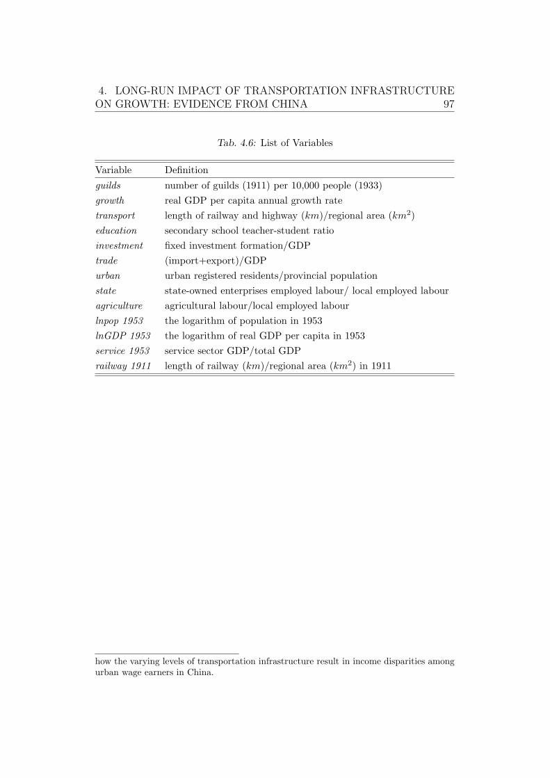
4. LONG-RUN IMPACT OF TRANSPORTATION INFRASTRUCTUREON GROWTH: EVIDENCE FROM CHINA 97
Tab. 4.6: List of Variables
Variable Definition
guilds number of guilds (1911) per 10,000 people (1933)
growth real GDP per capita annual growth rate
transport length of railway and highway (km)/regional area (km2)
education secondary school teacher-student ratio
investment fixed investment formation/GDP
trade (import+export)/GDP
urban urban registered residents/provincial population
state state-owned enterprises employed labour/ local employed labour
agriculture agricultural labour/local employed labour
lnpop 1953 the logarithm of population in 1953
lnGDP 1953 the logarithm of real GDP per capita in 1953
service 1953 service sector GDP/total GDP
railway 1911 length of railway (km)/regional area (km2) in 1911
how the varying levels of transportation infrastructure result in income disparities amongurban wage earners in China.
5. DOES ECONOMIC GROWTH AFFECT
URBANISATION? NEW EVIDENCE FROM CHINA AND
THE CHINESE NATIONAL CONGRESS
1. Introduction
At the heart of economic development and urban economics, the relationship
between economic growth and the rate of urbanisation is a topic that has
captivated much attention in both academic and policy arenas.81 This
discussion is especially germane to China given that one of the most striking
facts about its recent development experience is the massive expansion of its
urban population. For example, Figure 2.6 (Chapter 2) shows that China’s
urbanisation rate, measured as the percentage of population living in urban
areas as defined by the NBSC, rose slowly starting from its founding year
of 1949, fluctuated during the Great Famine (1959–1961) and the Great
Cultural Revolution (1966–1976), and embarked upon an impressive upward
trajectory from 1978 onwards. In conjunction with this spectacular rise
in the rate of urbanisation, China has also seen an unprecedented rate of
economic growth that has averaged roughly 9 percent over the period 1978–
2008, touching 14 percent at various times (Holz, 2008). While existing
research has largely focused on the extent to which urbanisation contributes
to growth, where the case of China has been scrutinised (e.g. Zheng et al.,
2009; Tian et al., 2010; Wei and Hao, 2010), the literature has recently paid
81 It is widely accepted that the causality of economic growth and urbanisation runs inboth directions. At one end of the discussion, there exists a large body of literature thatalmost unequivocally emphasises the positive effect that urbanisation has on economicgrowth (e.g. Quigley, 1998; Henderson, 2003; Duranton and Puga, 2004; Duranton,2008). At the other end, the literature offers some evidence that economic growth attractsmigration from rural to urban regions, which contributes to further development of urbanareas (e.g. Zhang and Song, 2003).

5. DOES ECONOMIC GROWTH AFFECT URBANISATION? NEWEVIDENCE FROM CHINA AND THE CHINESE NATIONALCONGRESS 99
more attention to the opposite relationship — the causal effect of economic
growth on urbanisation.82
Unquestionably, many factors could contribute to how urbanisation
evolves, and economic growth is not alone in this function. Nonetheless,
while it has been acknowledged that economic growth may affect urbanisation
in non-trivial ways (Davis and Henderson, 2003; Bruckner, 2012), the
fundamental question of whether this effect exists, let alone how strong it
is, is difficult to answer objectively based on the somewhat limited empirical
evidence from academic research.
The confirmation of the presence of a causal link between economic
growth and urbanisation in China can enhance the understanding of China’s
economic growth as explored in previous chapters. Unlike Chapter 3 and
Chapter 4 which focus on the determinants of economic growth, this chapter
analyses the causal effect of economic growth on a key macro variable, i.e.
urbanisation. In other words, this chapter investigates economic growth in
terms of its contribution to China’s broad economic development.
There are two methodological issues to be dealt with in this study. The
first issue is the problem of reverse causality that runs from urbanisation
to economic growth. In the literature, instrumental variable estimation has
been utilised to cut through this complication (e.g. Bruckner, 2012), but
in the context of China, existing research has offered little guidance on how
to obtain such an instrument to achieve identification. The second issue is
the possibility of measurement errors in the data. Given that the data come
from the National Bureau of Statistics of China (NBSC), measurement errors
could be present as Rawski (2001), Rawski and Xiao (2001), and Chow (2006)
have forewarned. These measurement errors may attenuate the least-squares
estimate towards zero and cause the OLS regression to understate the true
effect of economic growth.
Inspecting the data, Figure 5.1 shows that provincial economic growth
and provincial government spending contain a cyclical feature that appears
82 The literature has not arrived at a consensus on the extent to which growthaffects urbanisation. For example, Bruckner (2012) finds that income growth does notsignificantly raise urbanisation in sub-Saharan Africa conditional on changes in the shareof agricultural value added, while Henderson (2002) comes to the opposite conclusion.
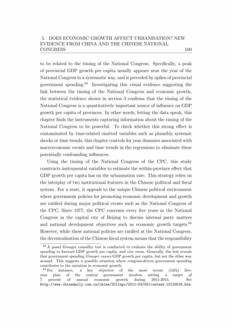
5. DOES ECONOMIC GROWTH AFFECT URBANISATION? NEWEVIDENCE FROM CHINA AND THE CHINESE NATIONALCONGRESS 100
to be related to the timing of the National Congress. Specifically, a peak
of provincial GDP growth per capita usually appears near the year of the
National Congress in a systematic way, and is preceded by spikes of provincial
government spending.83 Investigating this visual evidence suggesting the
link between the timing of the National Congress and economic growth,
the statistical evidence shown in section 3 confirms that the timing of the
National Congress is a quantitatively important source of influence on GDP
growth per capita of provinces. In other words, letting the data speak, this
chapter finds the instruments capturing information about the timing of the
National Congress to be powerful. To check whether this strong effect is
contaminated by time-related omitted variables such as plausibly systemic
shocks or time trends, this chapter controls for year dummies associated with
macroeconomic events and time trends in the regressions to eliminate these
potentially confounding influences.
Using the timing of the National Congress of the CPC, this study
constructs instrumental variables to estimate the within-province effect that
GDP growth per capita has on the urbanisation rate. This strategy relies on
the interplay of two institutional features in the Chinese political and fiscal
system. For a start, it appeals to the unique Chinese political environment
where government policies for promoting economic development and growth
are ratified during major political events such as the National Congress of
the CPC. Since 1977, the CPC convenes every five years at the National
Congress in the capital city of Beijing to discuss internal party matters
and national development objectives such as economic growth targets.84
However, while these national policies are ratified at the National Congress,
the decentralisation of the Chinese fiscal system means that the responsibility
83 A panel Granger causality test is conducted to evaluate the ability of governmentspending to forecast GDP growth per capita, and vice versa. Generally, the test revealsthat government spending Granger causes GDP growth per capita, but not the other wayaround. This suggests a possible situation where congress-driven government spendingcontributes to the variation in economic growth.
84 For instance, a key objective of the most recent (12th) five-year plan of the central government involves setting a target of7 percent of annual economic growth during 2011-2015. Seehttp://www.chinadaily.com.cn/china/2011npc/2011-03/05/content 12120516.htm.
5. DOES ECONOMIC GROWTH AFFECT URBANISATION? NEWEVIDENCE FROM CHINA AND THE CHINESE NATIONALCONGRESS 101
of implementing them rest, not on the central government, but on local
governments (Wong, 2011).85 Therefore, the recurring National Congress
may engender a cyclical pattern in policy-related expenditure by provincial
governments, and in turn produce cyclical peaks in provincial economic
growth that is useful for estimating its effect on urbanisation.
The main result of this work underscores the importance of addressing the
confounding issues related to the work. For example, this chapter finds that
the OLS estimate of the impact of growth on urbanisation is stubbornly close
to zero, despite the introduction of additional covariates and province fixed
effects in the hope of capturing the ‘deep determinants’ of urbanisation and
ameliorating the extent of omitted variable bias. While the OLS estimates
are tenuous at best, a possible reflection of the overpowering influence of
attenuation bias due to measurement errors in the data, the 2SLS estimate
suggests that growth is an important factor of urbanisation. The magnitude
of this effect is strongly robust in a battery of sensitivity tests and not once in
these robustness checks was its statistical significance driven out. Therefore,
it is safe to conclude that economic growth does affect urbanisation in China.
85 In recent times, the local governments have accounted for more than 80 percent of thenational budgetary expenditures. See Wong (2011).
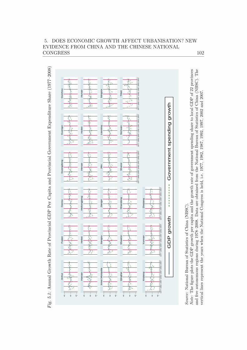
5. DOES ECONOMIC GROWTH AFFECT URBANISATION? NEWEVIDENCE FROM CHINA AND THE CHINESE NATIONALCONGRESS 102Fig.5.1:
Annual
Growth
Rateof
Provincial
GDP
Per
CapitaandProvincialGovernmentExpenditure
Share
(1977–2008)
-.50.5 -.50.5 -.50.5 -.50.5 -.50.5
1977
1982
1987
1992
1997
2002
2007
1977
1982
1987
1992
1997
2002
2007
1977
1982
1987
1992
1997
2002
2007
1977
1982
1987
1992
1997
2002
2007
1977
1982
1987
1992
1997
2002
2007
1977
1982
1987
1992
1997
2002
2007
Anhui
Fujian
Gansu
Guangdong
Guangxi
Guiz
hou
Hain
an
Hebei
Heilongjiang
Henan
Hubei
Hunan
Inner
Mongolia
Jia
ngsu
Jia
ngxi
Jilin
Lia
onin
gN
ingxia
Qin
ghai
Shaanxi
Shandong
Shanxi
Sic
huan
Tib
et
Xin
jiang
Yunnan
Zhejiang
GD
P g
row
thG
ove
rnm
en
t sp
en
din
g g
row
th
Source:NationalBureau
ofStatisticsof
China(N
BSC).
Note:Thefigu
replots
theGDPgrow
thper
capitaan
dthegrow
thrate
ofgovernmentspen
dingshareto
localGDPof
22provinces
andfiveau
tonom
ousregion
sduring19
78–2
008.
Dataareob
tained
from
theNational
Bureau
ofStatisticsof
China(N
BSC).
The
verticallines
representtheyears
when
theNational
Con
gressis
held,i.e.
1977
,19
82,19
87,19
92,19
97,20
02an
d20
07.
5. DOES ECONOMIC GROWTH AFFECT URBANISATION? NEWEVIDENCE FROM CHINA AND THE CHINESE NATIONALCONGRESS 103
This chapter is related to the literature that focuses on identifying
the causal effect of income levels and growth on urbanisation.86 In a
cross-country study, Davis and Henderson (2003) use lagged covariates as
instruments in a first-difference framework to show that higher income levels
contribute to the acceleration of urbanisation. For countries in sub-Saharan
Africa, Bruckner (2012) uses rainfall-driven variation in economic growth
to study its impact on urbanisation,87 but his identification strategy is
not applicable in this study as precipitation does not have a statistically
significant effect on the GDP growth per capita of Chinese provinces.88 Using
a county-level fixed effects model for China, Deng et al. (2008) examine the
causes of urbanisation but abstract from an in-depth focus on the issue of
identification. This is critical as the fixed effects estimator cannot handle the
identification issues of this chapter in an adequate way.
While there is some evidence that economic growth affects urbanisation,
the literature remains divided on the existence of such a causal link. For
instance, Zhang and Song (2003) provide some indirect evidence by way
of Granger causality tests to show that economic growth Granger causes
(positively) rural-to-urban migration but not vice versa,89 while in a study
of Brazilian cities, da Mata et al. (2007) find the existence of an incremental
effect of a city’s income per capita on its population level. However, Fay
86 The literature goes back to Harris and Todaro (1970) who suggest that the processof urbanisation could implicitly be driven by economic growth. This is because economicgrowth often transpires into an expanding rural-urban income gap, which encourages rural-urban migration and increases the incidence of urbanisation. See also Henderson (1986)and Becker and Morrison (1999). Davis and Henderson (2003) and Henderson and Wang(2007) consider how institutions, such as the extent of democratisation and the fiscaldecentralisation, may redistribute the concentration of urbanisation away from primarycities and help smaller cities to compete more freely for firms and human capital.
87 Bruckner (2012) finds that GDP growth per capita is not a significant cause ofurbanisation once the size of the agricultural sector, which captures the consequence ofsectoral shifts driven by economic development, is taken into account in the regression.
88 The evidence is provided in section 3.3 (the fifth robustness check). This, perhaps,underscores the fact that the key driver of growth in China from the mid-1980s onwardscomes primarily from the rainfall-insensitive manufacturing sector rather than rainfall-sensitive agricultural sector.
89 Even though Granger causality is not true causality, the fact that economic growthGranger causes rural-urban migration may, though not necessarily, imply that a causaleffect exists.
5. DOES ECONOMIC GROWTH AFFECT URBANISATION? NEWEVIDENCE FROM CHINA AND THE CHINESE NATIONALCONGRESS 104
and Opal (2000) and Poelhekke (2011) present some intriguing evidence
that urbanisation could take place in the absence of growth, citing sub-
Saharan African and some Latin American countries as notable cases.90 This
contrasting evidence suggests that addressing the basic question of whether
economic growth affects urbanisation may not be as straightforward as it
seems.
The rest of the chapter is organised as follows. Section 2 outlines the data
and the methodology. Section 3 presents the main empirical results and the
sensitivity checks. Section 4 concludes.
2. Data and Methodology
2.1 Data
This study utilises panel data from 1985 to 2008 that are drawn from the
China Compendium of Statistics, which is compiled by the Department of
Comprehensive Statistics of the National Bureau of Statistics of China. This
dataset is available for 31 sub-national administrative units in mainland
China,91 which consist of 22 provinces, four municipalities (Beijing, Shanghai,
Tianjin and Chongqing92) and five autonomous regions (Tibet, Xinjiang,
Ningxia, Inner Mongolia and Guangxi). This study excludes municipalities
in the dataset as they are highly urbanised, and includes information on
the 22 provinces and five autonomous regions only. The heterogeneity in
the extent of urbanisation across these regions is shown in Figure 5.2. The
variables in this study are listed in Table 5.10 and their summary statistics
90 For instance, Bolivia’s urban dwellers grew more than twice as fast as national totalpopulation during 1980–1985, however, its manufacturing sector declined around 5 percentper annum (Poelhekke, 2011).
91 According to official classification, all regions excluding Hong Kong, Macao andTaiwan are categorised as East (12 administrative units), Central (9) and West (10).East: Beijing, Tianjin, Shanghai, Shangdong, Hebei, Liaoning, Fujian, Jiangsu, Zhejiang,Guangdong, Guangxi, Hainan. Central: Heilongjiang, Henan, Hunan, Hubei, InnerMongolia, Jilin, Anhui, Jiangxi, Shanxi. West: Chongqing, Gansu, Guizhou, Ningxia,Qinghai, Shaanxi, Sichuan, Tibet, Xinjiang, Yunnan.
92 Chongqing was designated a municipality in 1997. The other three cities weredesignated municipalities when the People’s Republic of China was established in 1949.
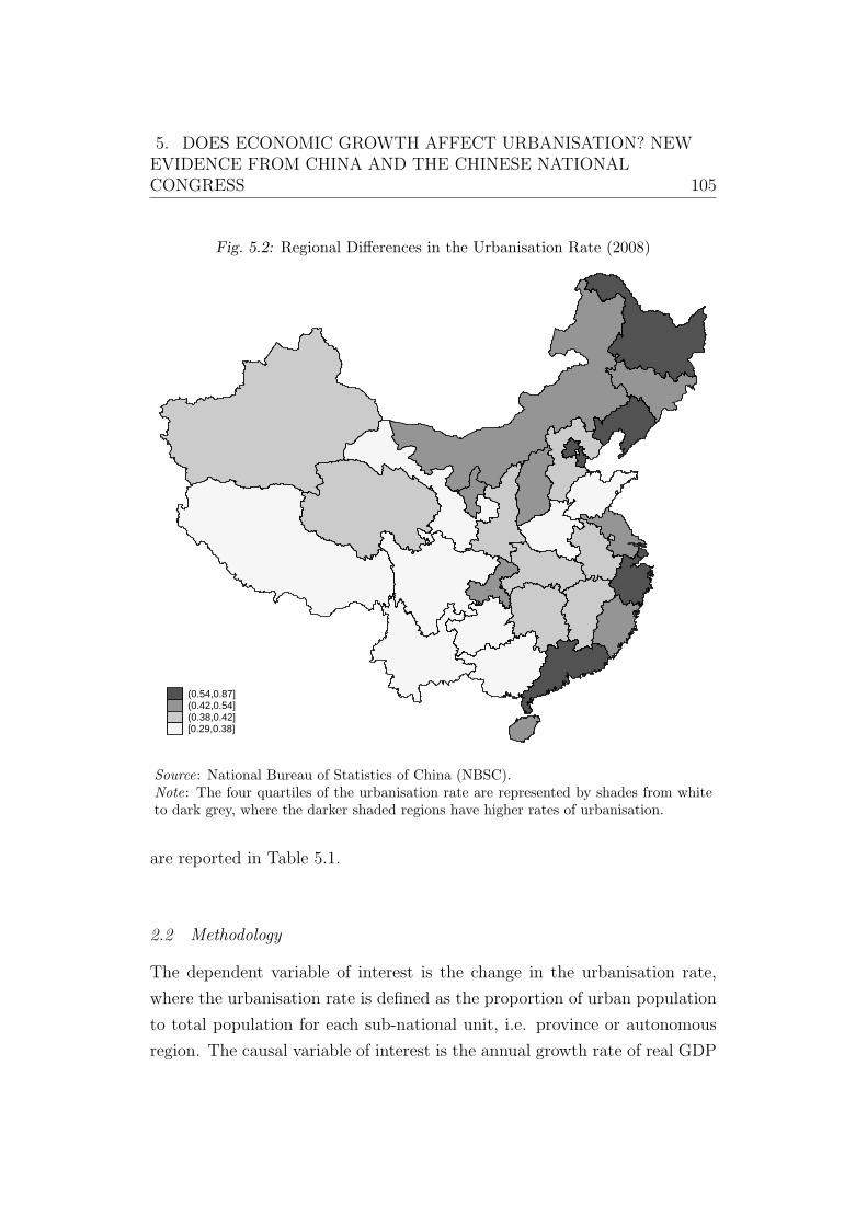
5. DOES ECONOMIC GROWTH AFFECT URBANISATION? NEWEVIDENCE FROM CHINA AND THE CHINESE NATIONALCONGRESS 105
Fig. 5.2: Regional Differences in the Urbanisation Rate (2008)
(0.54,0.87](0.42,0.54](0.38,0.42][0.29,0.38]
Source: National Bureau of Statistics of China (NBSC).Note: The four quartiles of the urbanisation rate are represented by shades from whiteto dark grey, where the darker shaded regions have higher rates of urbanisation.
are reported in Table 5.1.
2.2 Methodology
The dependent variable of interest is the change in the urbanisation rate,
where the urbanisation rate is defined as the proportion of urban population
to total population for each sub-national unit, i.e. province or autonomous
region. The causal variable of interest is the annual growth rate of real GDP
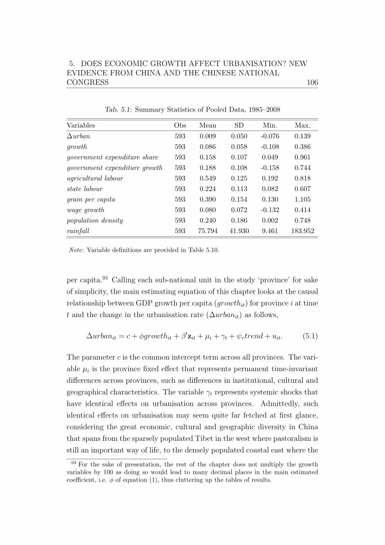
5. DOES ECONOMIC GROWTH AFFECT URBANISATION? NEWEVIDENCE FROM CHINA AND THE CHINESE NATIONALCONGRESS 106
Tab. 5.1: Summary Statistics of Pooled Data, 1985–2008
Variables Obs Mean SD Min. Max.
∆urban 593 0.009 0.050 -0.076 0.139
growth 593 0.086 0.058 -0.108 0.386
government expenditure share 593 0.158 0.107 0.049 0.961
government expenditure growth 593 0.188 0.108 -0.158 0.744
agricultural labour 593 0.549 0.125 0.192 0.818
state labour 593 0.224 0.113 0.082 0.607
grain per capita 593 0.390 0.154 0.130 1.105
wage growth 593 0.080 0.072 -0.132 0.414
population density 593 0.240 0.186 0.002 0.748
rainfall 593 75.794 41.930 9.461 183.952
Note: Variable definitions are provided in Table 5.10.
per capita.93 Calling each sub-national unit in the study ‘province’ for sake
of simplicity, the main estimating equation of this chapter looks at the causal
relationship between GDP growth per capita (growthit) for province i at time
t and the change in the urbanisation rate (∆urbanit) as follows,
∆urbanit = c+ ϕgrowthit + β′zit + µi + γt + ψrtrend+ uit. (5.1)
The parameter c is the common intercept term across all provinces. The vari-
able µi is the province fixed effect that represents permanent time-invariant
differences across provinces, such as differences in institutional, cultural and
geographical characteristics. The variable γt represents systemic shocks that
have identical effects on urbanisation across provinces. Admittedly, such
identical effects on urbanisation may seem quite far fetched at first glance,
considering the great economic, cultural and geographic diversity in China
that spans from the sparsely populated Tibet in the west where pastoralism is
still an important way of life, to the densely populated coastal east where the
93 For the sake of presentation, the rest of the chapter does not multiply the growthvariables by 100 as doing so would lead to many decimal places in the main estimatedcoefficient, i.e. ϕ of equation (1), thus cluttering up the tables of results.
5. DOES ECONOMIC GROWTH AFFECT URBANISATION? NEWEVIDENCE FROM CHINA AND THE CHINESE NATIONALCONGRESS 107
country’s most important economic centres are found. Nevertheless, to be
conservative, this study uses a focused approach to include year dummies that
capture what might plausibly be shocks to urbanisation that have identical
effects across provinces. These year dummies capture four nation-wide events
that are contained in the sample period. The first event is the revolution in
the Eastern bloc countries that some argue contributed to a brief moment
of political instability and economic slowdown in China during 1989–1990.94
The next three events are the Asian financial crisis of 1997–1998, the dot-com
bubble of 2000 and the global financial crisis that started in 2007. While these
global events may bear on urbanisation across China, their effects are unlikely
to be identical across provinces (e.g. western regions such as Xinjiang and
Tibet are less exposed to international economic fluctuations relative to the
coastal provinces). However, because the main estimation will be utilising the
timing of an aggregate event, namely the National Congress, as an estimation
strategy, it is advisable to err on the side of caution by partialling out these
potentially systemic effects on urbanisation even if they are indeed absent.
As an additional layer of safeguard, this study introduces a region-specific
trend ψr for region r based on the official grouping of administrative units
into East, Central and West regions.95 This study uses region-specific trends
instead of a single national trend because the national trend is nested in the
model if the effect ψr is the same for each region r. That aside, the time
trend is used to capture the trending effect of urbanisation that may either
be due to omitted trending variables or policies that cause the trend to occur.
For instance, over the last two decades, the hukou — a household registration
system aimed at controlling the movement of people from rural to urban areas
– was gradually relaxed. Therefore, over time, the relaxation of the hukou
system will cause urbanisation rate to rise even controlling for the effect of
economic growth. Because the flow of rural workers into urban regions might
94 For instance, Naughton (2008) addresses the political economy of China’s economictransition, and outlines the major political events during the last 30 years that include thestudent protests that took place in 1989. Perkins and Rawski (2008) show that the 1989event is associated with a major drop in TFP. They also point out that during 1989–1990,the expansion of private enterprises paused.
95 Please refer to section 3 for further details.
5. DOES ECONOMIC GROWTH AFFECT URBANISATION? NEWEVIDENCE FROM CHINA AND THE CHINESE NATIONALCONGRESS 108
occur at a different pace across different regions in China, partialling out the
time trend at the regional level provides an extra safeguard to address this
issue as well as helping eliminate any correlation between GDP growth per
capita and the urbanisation rate that may be driven by trends, possibly
caused by other external factors.
To identify the effect of growthit, i.e. ϕ, it is also important to consider
the pitfall of leaving out variables that are possibly correlated with growthit
and ∆urbanit. To address its consequence transpiring as omitted variable
bias, this chapter includes two additional sets of covariates in the regression
framework.
The set of covariates is represented by the vector zit, which consists
of an economic reform dummy that is equal to one for the years 1992 to
1998. This reform dummy reflects the institutional transition and economic
decentralisation that took place during the third phase of China’s economic
reform from 1992 to 1998. Since the reform is potentially correlated with
both economic growth and the rate of urbanisation, it would be prudent to
partial out its effect as has been done elsewhere in the literature.96 The
vector zit also consists of the interaction between the reform dummy and a
coastal indicator variable. Through this interaction term, one may capture
the heterogeneous effect of the economic reform on urbanisation from coastal
to inland regions, since the rates of urbanisation are vastly different across
China as Figure 5.2 suggests.97
2.3 Instrumental Variables
Even if the issue of omitted variables is taken care of, OLS regression would
still be inconsistent as it does not handle the problem of reverse causality that
runs from urbanisation to growth as well as the issue of measurement errors
96 This economic reform dummy is considered as a control variable in the study of China’seconomic growth. See, for example, Demurger (2001).
97 For example, the coastal position of provinces may be linked to better climates thancomparable inland regions and to factors that are supportive of a wider range of economicactivities such as trade and FDI, all of which are amenable to the process of urbanisationand help foster the development of urban areas in the coastal provinces. See also Li (2011).
5. DOES ECONOMIC GROWTH AFFECT URBANISATION? NEWEVIDENCE FROM CHINA AND THE CHINESE NATIONALCONGRESS 109
that will attenuate the estimates towards zero. To this end, this chapter uses
the timing of the National Congress as an attempt to achieve identification.
The National Congress of the CPC is the country’s most important
public political event led by the General Secretary, senior party leaders
and grassroots members. While the National Congress was held even
before the establishment of China as the People’s Republic,98 it was not
until 1977 that the meeting took place at five-yearly intervals. During
the National Congress, both internal party matters, such as promoting,
demoting and turning over senior party and provincial leaders, and national
economic objectives are discussed. The key economic objectives ratified by
the National Congress often include specific growth targets for the country,
where it is incumbent upon local governments to ensure that these targets are
met.99 Incentive-wise, the ranking of provincial GDP growth has become an
important measure for assessing the performance of local leaders, who could
be promoted for exceeding growth expectations or even dismissed for poor
performance.100 Therefore, even though the decentralisation of the Chinese
fiscal system meant that the responsibility of implementing these policies
rests, not on the central government, but on local governments, a system of
incentives is in place to encourage the local leaders to work towards fulfilling
the country’s economic ambitions.
Because of the decentralised fiscal system, an aggregate event as the
National Congress could have implications for provincial economic growth.
To capture the effect of the National Congress, this study constructs an
instrument, Congress, which is a binary indicator that is equal to one
in the year of the National Congress and zero in other years. Besides
Congress, there are reasons why using indicators of the years before the
National Congress as additional instruments might be preferable from the
98 The first National Congress was held in 1921, and the People’s Republic of China wasfounded in 1949.
99 For example, in the 11th Five-Year Plan (2005-2010) the national gross GDP wastargeted to achieve RMB 26.1 trillion with an average 7.5 percent growth over a five-yearperiod (Fan, 2006).100 For instance, Chen et al. (2005), Li and Zhou (2005) and Wu (2010) showed thata higher economic growth rate during the five-year tenure of officials and larger growthdifferentials between current and previous leaders would raise promotional chances.
5. DOES ECONOMIC GROWTH AFFECT URBANISATION? NEWEVIDENCE FROM CHINA AND THE CHINESE NATIONALCONGRESS 110
identification standpoint. Firstly, it is best to let the data speak and take
an agnostic stance on how the timing of the National Congress is linked
to growth. Secondly, it may take time for growth-enhancing policies to
achieve their intended outcomes, so that the effect of the National Congress
on growth might be more apparent towards the latter part of the five-year
meetings cycle, that is, just before the next meeting takes place.101 Therefore,
this study also utilises Congress(−1), which indicates the year before the
National Congress, and Congress(−2), which indicates two years before it,
as additional instruments for growth together with Congress.
2.4 Further Remarks
Before concluding this section, some remarks are in order. Firstly, for the
congress instruments to be valid, they must be correlated with economic
growth but uncorrelated with the omitted determinants of the urbanisation
rate, captured collectively by uit in (5.1). While the first assumption can
be verified, the second assumption — the exclusionary restriction — cannot
be tested without overidentification. Therefore, utilising additional infor-
mation about the timing of the National Congress through Congress(−1)
and Congress(−2) will be helpful for the purpose of implementing the
overidentifying restrictions test.
Secondly, exclusion restriction requires that the congress dummies affect
urbanisation only through economic growth. In other words, it precludes the
existence of a direct effect that the timing of the National Congress might
have on the urbanisation rate. Since the congress dummies capture “cycles”,
the exclusion restriction is tantamount to asserting that people do not flow
into urban areas in a cyclical manner, and not for the particular reason that
101 In addition, the recent fiscal decentralisation has provided local leaders with furtherdegrees of flexibility to increase public expenditure for the stimulation of GDP growth(Zhang and Zou, 1998; Jin et al., 2005). Therefore, given that GDP growth is a keyperformance metric when assessing local leaders, who may use the National Congress toseek promotion to the central government (e.g. Blanchard and Shleifer, 2001; Li and Zhou,2005), the evaluation of local leaders using a GDP-based benchmark may encourage themto stimulate GDP growth prior to the event.
5. DOES ECONOMIC GROWTH AFFECT URBANISATION? NEWEVIDENCE FROM CHINA AND THE CHINESE NATIONALCONGRESS 111
the National Congress is held that year. No doubt, the National Congress
may ratify policies to encourage urbanisation by relaxing the hukou system,
but the implication of relaxing the restriction on human flow into urban areas
is likely to produce a trending, not cyclical, effect on urbanisation that the
time trend in the regression will capture.
Thirdly, the first stage equation where growth is regressed on the excluded
congress instruments (among other controls) does not have to be causal. That
is, the instruments do not have to be uncorrelated with the error term in the
first stage (economic growth) equation. Instead, they have to be orthogonal
to the error term in the second stage (urbanisation) equation for the purpose
of identification. Because the timing of the National Congress is exogenous,
one can rule out such correlation that is due to the reverse causal effect
of urbanisation on the instruments. Nonetheless, this does not guarantee
that the instruments used in this study are uncorrelated with all omitted
determinants of urbanisation, which are consolidated by the second stage
error term. While not an infallible response to this issue, one could examine
whether the causal estimates are sensitive to the inclusion of potential factors
of urbanisation that are initially omitted from the urbanisation equation.
Guided by the literature, this study gathers a set of additional regression
covariates to perform a battery of robustness checks in section 3.3. If the
estimation strategy is not robust, the baseline result would be fragile when
these covariates are added to the regression, but this is not the case as section
3.3 demonstrates.
3. Empirical Results
3.1 OLS Estimates
Table 5.2 summarises the estimation results from OLS regression. Even
though the OLS regression is unidentified, it provides a useful starting point
for investigating the extent of the estimation issues that could confound
the causal effect of growth on urbanisation. For instance, the positive
reverse causation that runs from urbanisation could lead to overestimating

5. DOES ECONOMIC GROWTH AFFECT URBANISATION? NEWEVIDENCE FROM CHINA AND THE CHINESE NATIONALCONGRESS 112
the causal effect of growth, which is the focus of this chapter. On the other
hand, measurement errors in the data could have an attenuation effect that
counteracts this upward bias arising from reverse causality. If the effect of
measurement error is powerful enough, OLS regression may understate the
true contribution of growth to urbanisation, producing results that would
bound the instrumental variable estimates from below.
Tab. 5.2: OLS Regressions
(1) (2) (3) (4) (5)
Dependent Variable: ∆urban
growth 0.046** 0.045* 0.045** 0.074** 0.095**
(0.021) (0.024) (0.021) (0.035) (0.046)
zit included? No Yes Yes Yes Yes
µi included? No No Yes Yes Yes
γt included? No No No Yes Yes
Regional time trend included? No No No No Yes
N 593 593 593 593 593
Note: The numbers in parentheses are robust standard errors. The vector zit consists ofthe indicator variable reform and interaction between reform and coastal. Definitions ofthe variables are provided in Table 5.10.
In the simplest pooled regression model, column (1) shows that the OLS
estimate of the slope coefficient is nearly zero. This weakness of the OLS
estimate reflects a deeper issue that goes beyond the problem of omitted
variable bias, since it cannot be overcome by the introduction of additional
covariates. For instance, column (2) includes the vector zit consisting of
the economic reform dummy and its interaction with a coastal indicator
variable. Despite including these additional covariates, the OLS estimates of
the effect of growth on urbanisation remain very close to the simple pooled
regression estimate in column (1). Moreover, as columns (3)-(5) show, the
OLS estimates remain stubbornly close to zero even after controlling for
province fixed effects, year dummies that capture possible systemic shocks to
urbanisation, and region-specific time trends. This implies that identification
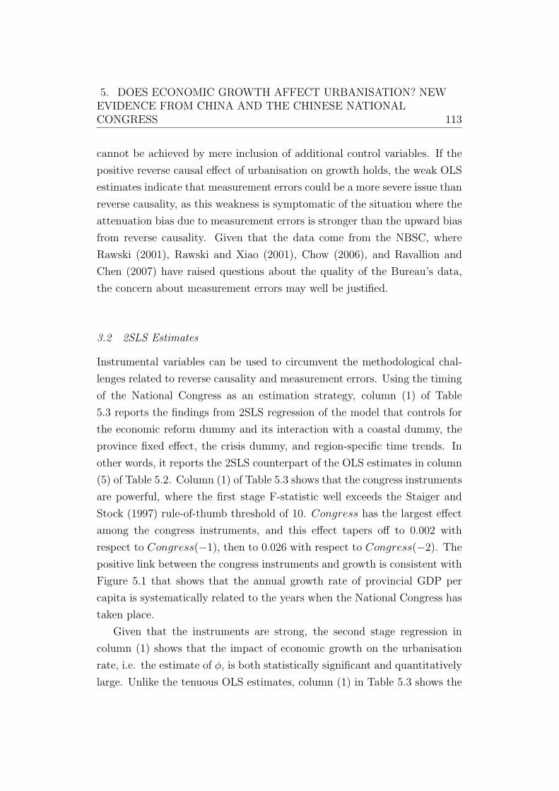
5. DOES ECONOMIC GROWTH AFFECT URBANISATION? NEWEVIDENCE FROM CHINA AND THE CHINESE NATIONALCONGRESS 113
cannot be achieved by mere inclusion of additional control variables. If the
positive reverse causal effect of urbanisation on growth holds, the weak OLS
estimates indicate that measurement errors could be a more severe issue than
reverse causality, as this weakness is symptomatic of the situation where the
attenuation bias due to measurement errors is stronger than the upward bias
from reverse causality. Given that the data come from the NBSC, where
Rawski (2001), Rawski and Xiao (2001), Chow (2006), and Ravallion and
Chen (2007) have raised questions about the quality of the Bureau’s data,
the concern about measurement errors may well be justified.
3.2 2SLS Estimates
Instrumental variables can be used to circumvent the methodological chal-
lenges related to reverse causality and measurement errors. Using the timing
of the National Congress as an estimation strategy, column (1) of Table
5.3 reports the findings from 2SLS regression of the model that controls for
the economic reform dummy and its interaction with a coastal dummy, the
province fixed effect, the crisis dummy, and region-specific time trends. In
other words, it reports the 2SLS counterpart of the OLS estimates in column
(5) of Table 5.2. Column (1) of Table 5.3 shows that the congress instruments
are powerful, where the first stage F-statistic well exceeds the Staiger and
Stock (1997) rule-of-thumb threshold of 10. Congress has the largest effect
among the congress instruments, and this effect tapers off to 0.002 with
respect to Congress(−1), then to 0.026 with respect to Congress(−2). The
positive link between the congress instruments and growth is consistent with
Figure 5.1 that shows that the annual growth rate of provincial GDP per
capita is systematically related to the years when the National Congress has
taken place.
Given that the instruments are strong, the second stage regression in
column (1) shows that the impact of economic growth on the urbanisation
rate, i.e. the estimate of ϕ, is both statistically significant and quantitatively
large. Unlike the tenuous OLS estimates, column (1) in Table 5.3 shows the
5. DOES ECONOMIC GROWTH AFFECT URBANISATION? NEWEVIDENCE FROM CHINA AND THE CHINESE NATIONALCONGRESS 114
Tab. 5.3: 2SLS Regressions
(1) (2) (3)
Panel A. Dependent Variable:
∆urban ∆urban (t+ 1) ∆urban (t+ 2)
growth 0.452** -0.235 0.286
(0.191) (0.290) (0.182)
Panel B. Dependent Variable: growth
Congress 0.025*** 0.021*** 0.023***
(0.008) (0.008) (0.008)
Congress (-1) 0.002 -0.004 -0.004
(0.005) (0.005) (0.005)
Congress (-2) 0.019*** 0.015** 0.015**
(0.007) (0.007) (0.007)
zit included? Yes Yes Yes
µi and γt included? Yes Yes Yes
Regional time trend included? Yes Yes Yes
First-Stage (F-stat) 50.77 44.37 40.15
Hansen J (p-value) 0.26 0.86 0.57
N 593 571 549
Note: The numbers in parentheses are robust standard errors. Column (1) estimatesthe baseline estimating equation of (5.1). Columns (2)-(3) re-estimate the model byregressing ∆urban at period t+1 and t+2 on the period t control variables of (5.1). Thevariable µi represents province fixed effect, and γt captures possible systemic shocks tothe urbanisation rate that come from four key events discussed in section 2. The vectorzit consists of the indicator variable reform and interaction between reform and coastal.The instrument set consists of Congress, a dummy variable indicating the year whenthe National Congress of the Communist Party of China is held, and Congress(−k),a dummy variable indicating the kth year before the National Congress. Definitionsof the variables are provided in Table 5.10. First Stage reports the F-statistic for theoverall significance of the first stage regressors. Hansen J reports the p-value for theoveridentifying restriction test.
2SLS regression yields a much larger estimate of the within-province effect of
growth on urbanisation, where a 1 percentage point increase in GDP growth
per capita raises the change in the urbanisation rate by 0.452 percentage
5. DOES ECONOMIC GROWTH AFFECT URBANISATION? NEWEVIDENCE FROM CHINA AND THE CHINESE NATIONALCONGRESS 115
points on average. The larger 2SLS estimate of the effect of growth is
indicative of the overpowering influence of measurement errors, since if the
effect of reverse causality were dominant, it would cause an upward bias
in the OLS estimate instead of a downward bias that is observed here.
There is no evidence that the quantitative significance of the 2SLS estimate
is an unintended consequence of model misspecification and questionable
instruments validity, as the overidentifying restriction test in column (1)
is not rejected at standard significance levels. While there is a positive
link in the contemporaneous sense between GDP growth per capita and
the change in the urbanisation rate, one does not observe a statistically
significant lagged effect of growth on urbanisation. For instance, columns
(2)-(3) consider the impact of the period t GDP growth per capita on the
change in the urbanisation rate in periods t + 1 and t + 2 and show that
the coefficient of GDP growth per capita is statistically insignificant in both
cases. This implies that growth has no lagged effect on urbanisation, and
that the relationship between growth and urbanisation is more transient than
persistent in nature.102
3.3 Robustness Checks
This section conducts robustness checks to evaluate the sensitivity of the
baseline estimate in column (1) of Table 5.3. They are carried out by
including in the baseline regression five sets of covariates that are potentially
relevant to urbanisation in various aspects.
The first robustness check is motivated by the concern that provincial
leaders might adopt different development and urbanisation strategies based
on their personal background.103 To address this issue, this study controls
102 To save space, this chapter has omitted the events dummies from the tables. The fullresults are available in Table 8.3 of Appendix C. As it turns out, except for the 1989–1990 revolution following the collapse of communism in the Eastern bloc countries, themacroeconomic events related to the Asian financial crisis, dot-com bubble and the globalfinancial crisis do not have a statistically significant effect on urbanisation, although theyare statistically significant negative determinants of growth.103 Chen et al. (2005) and Li and Zhou (2005) argue that provincial secretaries of theCPC and provincial governors are evaluated based on certain criteria such as the annual
5. DOES ECONOMIC GROWTH AFFECT URBANISATION? NEWEVIDENCE FROM CHINA AND THE CHINESE NATIONALCONGRESS 116
for the personal characteristics and attributes of two key provincial leaders
– the provincial CPC secretary and the provincial governor. Drawing
from the study of Chen et al. (2005) and Li and Zhou (2005), this study
constructs variables of personal characteristics that are related to the tenure,
age (including its square), education and professional connections of the
provincial secretary or governor. The tenure is defined as the kth year of
one’s current assignment in either a CPC secretary or a provincial governor
position. The education variable is a binary variable that is equal to one
if a leader is an alumnus of a choice university in China, which is a way
of extracting information about the ambition and personal network of a
local leader.104 The professional connection variable is a binary variable
that is equal to one if a leader has past experience or is currently holding
a joint-appointment in the central government.105 Table 5.4 shows that the
baseline estimate of the coefficient on growth, which is 0.452 (see column (1)
of Table 5.3), remains identical up to two decimal places after controlling for
the attributes of the provincial governor or secretary. This implies that the
attributes of provincial leaders are not particularly important in influencing
the economic growth-urbanisation relationship, despite the fact that the
implementation of national policies rest largely on provincial governments
and its efficacy may depend on the leaders’ characteristics.
The second robustness check considers the implication of including the
provincial expenditure growth and the expenditure share of provincial GDP
into the baseline model. This is an important exercise as policies originating
from the National Congress may be related to the expenditure of provincial
governments, which may in turn affect the rate of urbanisation.106 As it turns
growth rate and five-year average provincial GDP per capita.104 The choice universities are Peking University, Tsinghua University, Fudan University,Jiaotong University and Renmin University. This study distinguishes local leaders whoare graduates from choice versus non-choice universities instead of considering whetherthese leaders do or do not have a university degree, since a significant majority of localleaders are university graduates.105 For instance, Li and Zhou (2005) find that having connections with the centralgovernment may increase the promotional opportunities of local leaders, which may inturn influence the type of development strategies they choose to pursue for their localregions.106 For instance, Becker and Morrison (1988) find that government expenditure and urban
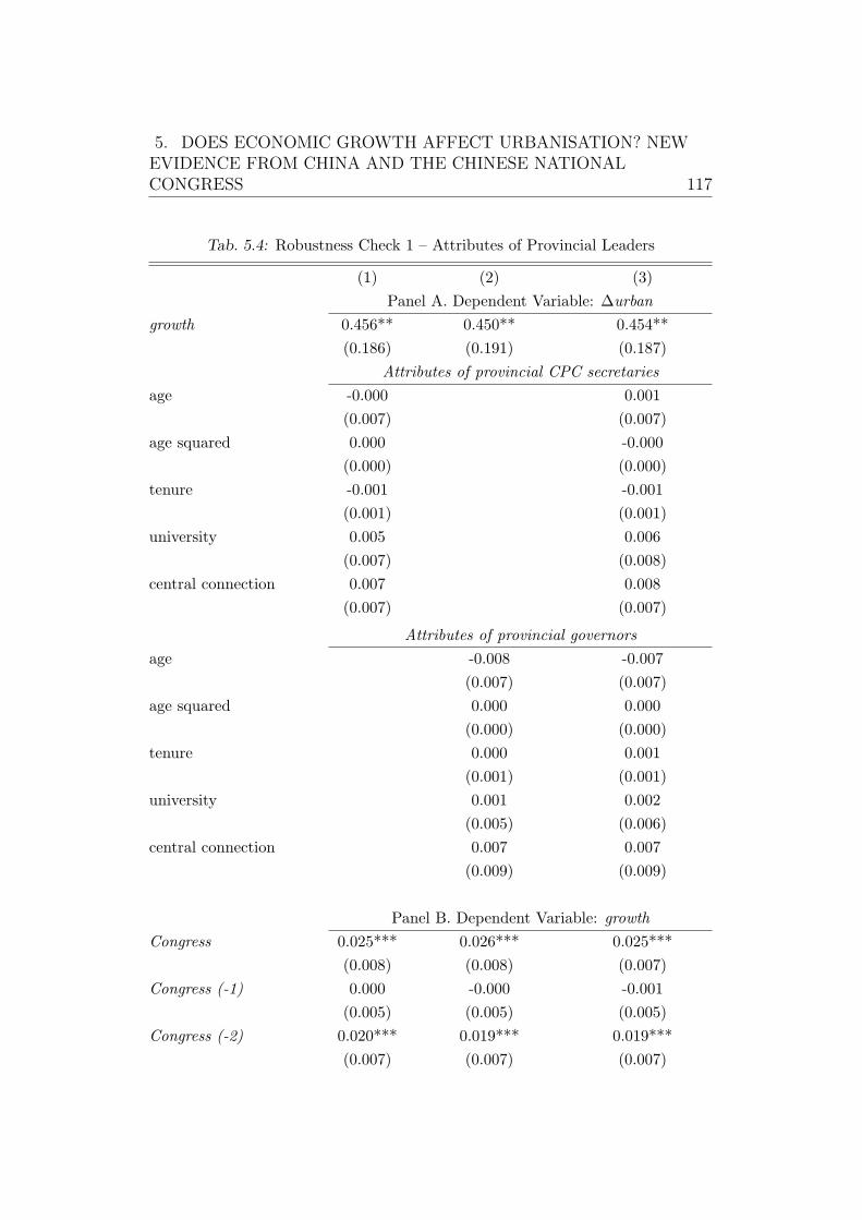
5. DOES ECONOMIC GROWTH AFFECT URBANISATION? NEWEVIDENCE FROM CHINA AND THE CHINESE NATIONALCONGRESS 117
Tab. 5.4: Robustness Check 1 – Attributes of Provincial Leaders
(1) (2) (3)
Panel A. Dependent Variable: ∆urban
growth 0.456** 0.450** 0.454**
(0.186) (0.191) (0.187)
Attributes of provincial CPC secretaries
age -0.000 0.001
(0.007) (0.007)
age squared 0.000 -0.000
(0.000) (0.000)
tenure -0.001 -0.001
(0.001) (0.001)
university 0.005 0.006
(0.007) (0.008)
central connection 0.007 0.008
(0.007) (0.007)
Attributes of provincial governors
age -0.008 -0.007
(0.007) (0.007)
age squared 0.000 0.000
(0.000) (0.000)
tenure 0.000 0.001
(0.001) (0.001)
university 0.001 0.002
(0.005) (0.006)
central connection 0.007 0.007
(0.009) (0.009)
Panel B. Dependent Variable: growth
Congress 0.025*** 0.026*** 0.025***
(0.008) (0.008) (0.007)
Congress (-1) 0.000 -0.000 -0.001
(0.005) (0.005) (0.005)
Congress (-2) 0.020*** 0.019*** 0.019***
(0.007) (0.007) (0.007)
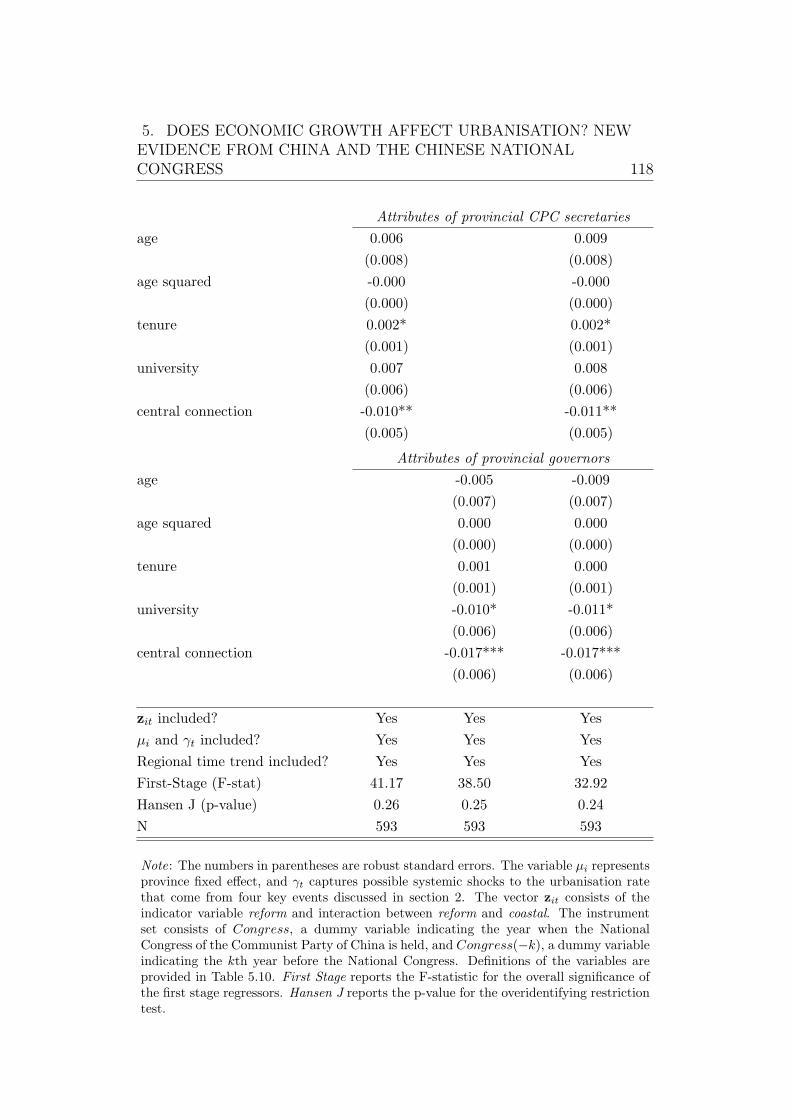
5. DOES ECONOMIC GROWTH AFFECT URBANISATION? NEWEVIDENCE FROM CHINA AND THE CHINESE NATIONALCONGRESS 118
Attributes of provincial CPC secretaries
age 0.006 0.009
(0.008) (0.008)
age squared -0.000 -0.000
(0.000) (0.000)
tenure 0.002* 0.002*
(0.001) (0.001)
university 0.007 0.008
(0.006) (0.006)
central connection -0.010** -0.011**
(0.005) (0.005)
Attributes of provincial governors
age -0.005 -0.009
(0.007) (0.007)
age squared 0.000 0.000
(0.000) (0.000)
tenure 0.001 0.000
(0.001) (0.001)
university -0.010* -0.011*
(0.006) (0.006)
central connection -0.017*** -0.017***
(0.006) (0.006)
zit included? Yes Yes Yes
µi and γt included? Yes Yes Yes
Regional time trend included? Yes Yes Yes
First-Stage (F-stat) 41.17 38.50 32.92
Hansen J (p-value) 0.26 0.25 0.24
N 593 593 593
Note: The numbers in parentheses are robust standard errors. The variable µi representsprovince fixed effect, and γt captures possible systemic shocks to the urbanisation ratethat come from four key events discussed in section 2. The vector zit consists of theindicator variable reform and interaction between reform and coastal. The instrumentset consists of Congress, a dummy variable indicating the year when the NationalCongress of the Communist Party of China is held, and Congress(−k), a dummy variableindicating the kth year before the National Congress. Definitions of the variables areprovided in Table 5.10. First Stage reports the F-statistic for the overall significance ofthe first stage regressors. Hansen J reports the p-value for the overidentifying restrictiontest.
5. DOES ECONOMIC GROWTH AFFECT URBANISATION? NEWEVIDENCE FROM CHINA AND THE CHINESE NATIONALCONGRESS 119
out, Table 5.5 shows that the effect of growth on urbanisation remains highly
robust. Even upon including the expenditure growth (column (1)), or the
expenditure share of GDP (column (2)), or both (column (3)), the estimate
of ϕ ranges tightly from 0.456 to 0.482, which is close to the baseline estimate
of 0.452. Also interesting is the observation that the first stage regression
is robust. In Panel B, the coefficients on the congress instruments in Table
5.5 are very similar to the baseline estimates with first stage F-statistics that
are much greater than 10, suggesting that using the expenditure variables as
controls has not weakened the power of the congress instruments.
The third robustness check considers whether the transition of China’s
labour market may confound the growth-urbanisation relationship. As
Henderson (2005) argues, the process of urbanisation is usually accompanied
by shifts in importance away from the agricultural sector and towards the
manufacturing and services sectors. In the case of China, structural changes
in the labour market following the liberalisation of the Chinese economy
may affect not only the rural labour force but also reduce the share of
labour employed in state-owned and collective enterprises. Thus, the third
robustness check controls for the share of the labour force in the agricultural
sector and the share of the labour force in public and state-owned enterprises
in this exercise. Column (3) of Table 5.6 shows that urbanisation is negatively
related to the size of the agricultural and public sector, confirming that
provinces with larger agricultural and public sectors would also urbanise at a
much slower pace.107 Importantly, Table 5.6 shows that the effect of growth
on urbanisation remains highly resilient when the labour share variables are
included as controls. The same is true for the first stage regression in Table
5.6, where the estimated coefficients on the congress instruments are largely
unaffected.
Related to the third robustness check, the fourth robustness check
addresses the question of whether the share of the agricultural labour force
is a suitable variable for capturing the size of the agricultural sector. After
population are positively correlated. Bruckner (2012) also considered the inclusion ofgovernment expenditure as a further robustness check.107 A similar result is also found in Bruckner (2012) for the case of sub-Saharan Africa.
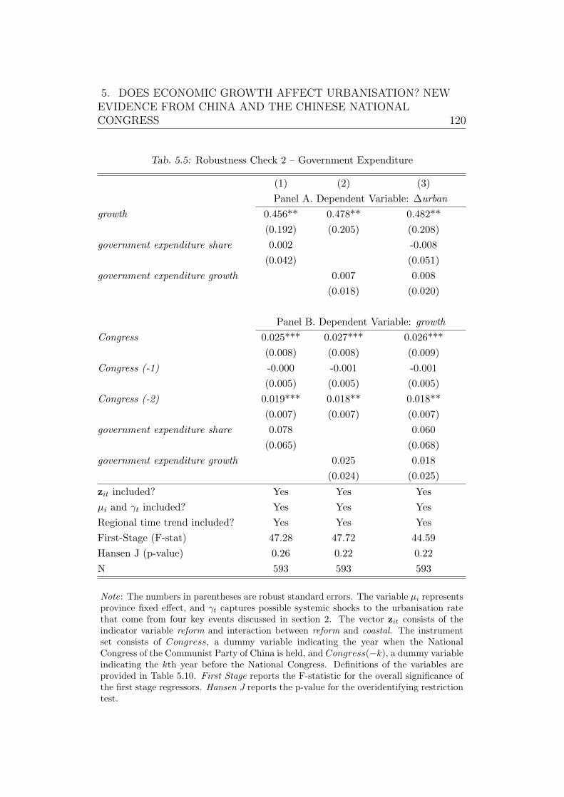
5. DOES ECONOMIC GROWTH AFFECT URBANISATION? NEWEVIDENCE FROM CHINA AND THE CHINESE NATIONALCONGRESS 120
Tab. 5.5: Robustness Check 2 – Government Expenditure
(1) (2) (3)
Panel A. Dependent Variable: ∆urban
growth 0.456** 0.478** 0.482**
(0.192) (0.205) (0.208)
government expenditure share 0.002 -0.008
(0.042) (0.051)
government expenditure growth 0.007 0.008
(0.018) (0.020)
Panel B. Dependent Variable: growth
Congress 0.025*** 0.027*** 0.026***
(0.008) (0.008) (0.009)
Congress (-1) -0.000 -0.001 -0.001
(0.005) (0.005) (0.005)
Congress (-2) 0.019*** 0.018** 0.018**
(0.007) (0.007) (0.007)
government expenditure share 0.078 0.060
(0.065) (0.068)
government expenditure growth 0.025 0.018
(0.024) (0.025)
zit included? Yes Yes Yes
µi and γt included? Yes Yes Yes
Regional time trend included? Yes Yes Yes
First-Stage (F-stat) 47.28 47.72 44.59
Hansen J (p-value) 0.26 0.22 0.22
N 593 593 593
Note: The numbers in parentheses are robust standard errors. The variable µi representsprovince fixed effect, and γt captures possible systemic shocks to the urbanisation ratethat come from four key events discussed in section 2. The vector zit consists of theindicator variable reform and interaction between reform and coastal. The instrumentset consists of Congress, a dummy variable indicating the year when the NationalCongress of the Communist Party of China is held, and Congress(−k), a dummy variableindicating the kth year before the National Congress. Definitions of the variables areprovided in Table 5.10. First Stage reports the F-statistic for the overall significance ofthe first stage regressors. Hansen J reports the p-value for the overidentifying restrictiontest.
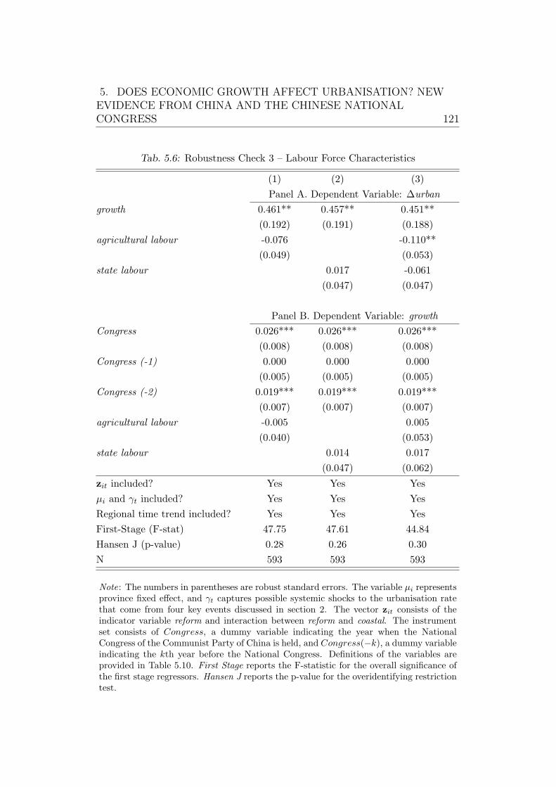
5. DOES ECONOMIC GROWTH AFFECT URBANISATION? NEWEVIDENCE FROM CHINA AND THE CHINESE NATIONALCONGRESS 121
Tab. 5.6: Robustness Check 3 – Labour Force Characteristics
(1) (2) (3)
Panel A. Dependent Variable: ∆urban
growth 0.461** 0.457** 0.451**
(0.192) (0.191) (0.188)
agricultural labour -0.076 -0.110**
(0.049) (0.053)
state labour 0.017 -0.061
(0.047) (0.047)
Panel B. Dependent Variable: growth
Congress 0.026*** 0.026*** 0.026***
(0.008) (0.008) (0.008)
Congress (-1) 0.000 0.000 0.000
(0.005) (0.005) (0.005)
Congress (-2) 0.019*** 0.019*** 0.019***
(0.007) (0.007) (0.007)
agricultural labour -0.005 0.005
(0.040) (0.053)
state labour 0.014 0.017
(0.047) (0.062)
zit included? Yes Yes Yes
µi and γt included? Yes Yes Yes
Regional time trend included? Yes Yes Yes
First-Stage (F-stat) 47.75 47.61 44.84
Hansen J (p-value) 0.28 0.26 0.30
N 593 593 593
Note: The numbers in parentheses are robust standard errors. The variable µi representsprovince fixed effect, and γt captures possible systemic shocks to the urbanisation ratethat come from four key events discussed in section 2. The vector zit consists of theindicator variable reform and interaction between reform and coastal. The instrumentset consists of Congress, a dummy variable indicating the year when the NationalCongress of the Communist Party of China is held, and Congress(−k), a dummy variableindicating the kth year before the National Congress. Definitions of the variables areprovided in Table 5.10. First Stage reports the F-statistic for the overall significance ofthe first stage regressors. Hansen J reports the p-value for the overidentifying restrictiontest.
5. DOES ECONOMIC GROWTH AFFECT URBANISATION? NEWEVIDENCE FROM CHINA AND THE CHINESE NATIONALCONGRESS 122
all, the size of the agricultural labour force may be more closely related
to rural population than the size of the agricultural sector per se. To this
end, the fourth robustness check employs a measure of agricultural output,
grain per capita, as a proxy for the size of the agricultural sector. Besides
controlling for grain per capita, it also considers the growth rate of real
urban wage as a possible confounder. The reason is that urban wage growth
may encourage rural-to-urban migration, and at the same time, could be
correlated with economic growth. When controlling for grain per capita,
column (1) of Table 5.7 shows that the estimated causal effect of growth is
identical to the baseline estimate of 0.452. The robustness of this effect is not
compromised when controlling for urban wage growth, or grain per capita
and urban wage growth simultaneously.
The fifth robustness check introduces population density and provincial
rainfall variation into the estimating equation, both of which could be related
to urbanisation.108 For example, Deng et al. (2008) find that the level of
population is associated with the size of the urban core area, and Barrios
et al. (2006) show that climatic change, as proxied by rainfall, is an important
determinant of rural-urban migration in sub-Saharan Africa.109 Concerning
rainfall, although it has been used as an instrument for output, income and
growth, the estimation strategy of constructing instruments using rainfall
data are not implementable in this study as the effect of rainfall on growth
across provinces in China is statistically insignificant.110 That said, while
108 This study uses rainfall data from the Terrestrial Air Temperatureand Precipitation: Monthly and Annual Time Series (1900 - 2008).http://climate.geog.udel.edu/∼climate/html pages/download.html. Table5.8 only focuses on the effect of contemporary precipitation on urbanisation. Thepotential impacts of quadratic rainfall and lagged rainfall on urbanisation are carefullyinvestigated in Table 8.4 of Appendix C.109 Deng et al. (2008) find that a 1 percent increase in population would raise the urbancore area (hectares) by 0.186 percent. See also Bruckner (2012) who uses the level ofpopulation as an additional control variable in his sensitivity checks.110 The omitted results are available in Table 8.5 of Appendix C. Furthermore, it isimportant to note that rainfall may be correlated with unobserved determinants ofurbanisation. For instance, there is a large body of literature in climatology that showsthat urbanisation can affect rainfall patterns. Since urbanisation may cause variations inrainfall in return, this may raise questions on the validity of using rainfall to constructinstrumental variables for growth for the study of its impact on urbanisation.
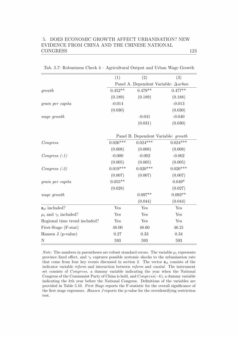
5. DOES ECONOMIC GROWTH AFFECT URBANISATION? NEWEVIDENCE FROM CHINA AND THE CHINESE NATIONALCONGRESS 123
Tab. 5.7: Robustness Check 4 – Agricultural Output and Urban Wage Growth
(1) (2) (3)
Panel A. Dependent Variable: ∆urban
growth 0.452** 0.479** 0.477**
(0.189) (0.189) (0.188)
grain per capita -0.014 -0.013
(0.030) (0.030)
wage growth -0.041 -0.040
(0.031) (0.030)
Panel B. Dependent Variable: growth
Congress 0.026*** 0.024*** 0.024***
(0.008) (0.008) (0.008)
Congress (-1) -0.000 -0.002 -0.002
(0.005) (0.005) (0.005)
Congress (-2) 0.019*** 0.020*** 0.020***
(0.007) (0.007) (0.007)
grain per capita 0.055** 0.049*
(0.028) (0.027)
wage growth 0.097** 0.093**
(0.044) (0.044)
zit included? Yes Yes Yes
µi and γt included? Yes Yes Yes
Regional time trend included? Yes Yes Yes
First-Stage (F-stat) 48.00 48.60 46.21
Hansen J (p-value) 0.27 0.33 0.34
N 593 593 593
Note: The numbers in parentheses are robust standard errors. The variable µi representsprovince fixed effect, and γt captures possible systemic shocks to the urbanisation ratethat come from four key events discussed in section 2. The vector zit consists of theindicator variable reform and interaction between reform and coastal. The instrumentset consists of Congress, a dummy variable indicating the year when the NationalCongress of the Communist Party of China is held, and Congress(−k), a dummy variableindicating the kth year before the National Congress. Definitions of the variables areprovided in Table 5.10. First Stage reports the F-statistic for the overall significance ofthe first stage regressors. Hansen J reports the p-value for the overidentifying restrictiontest.
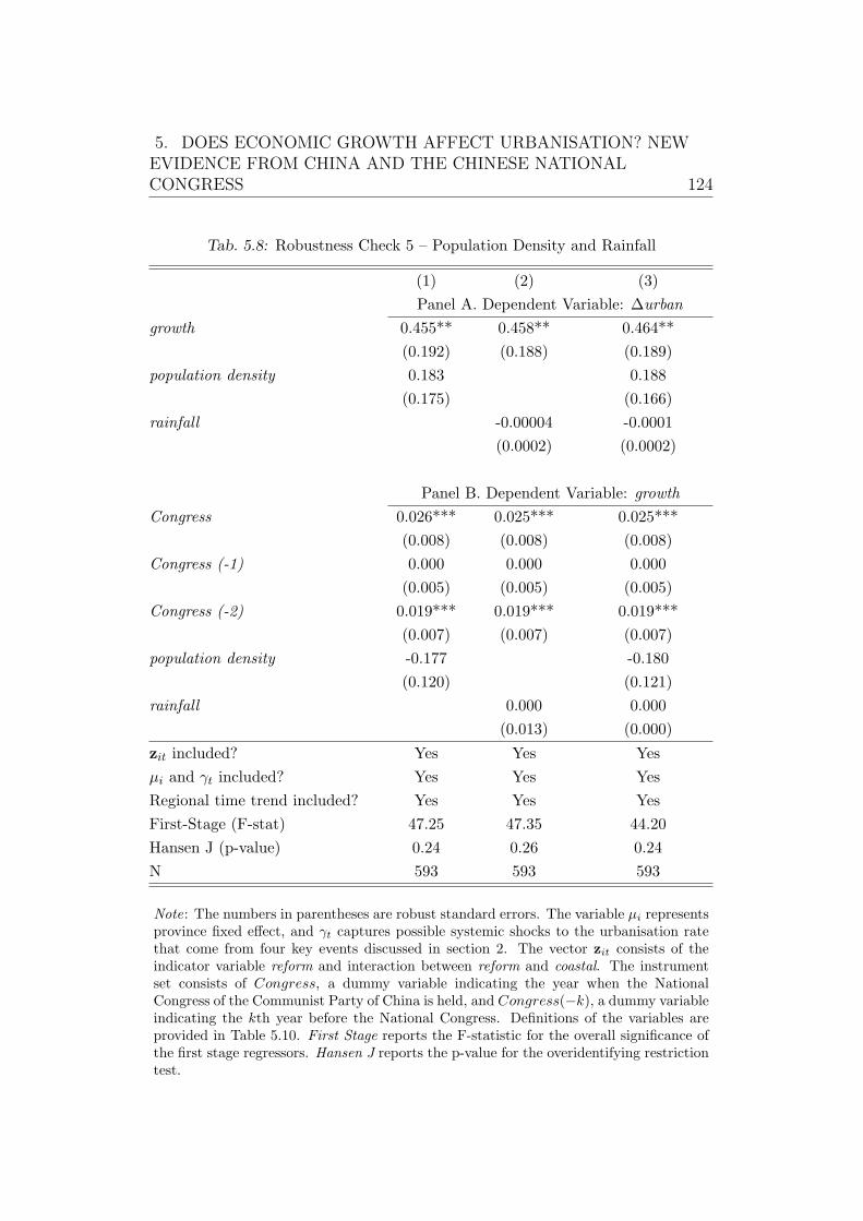
5. DOES ECONOMIC GROWTH AFFECT URBANISATION? NEWEVIDENCE FROM CHINA AND THE CHINESE NATIONALCONGRESS 124
Tab. 5.8: Robustness Check 5 – Population Density and Rainfall
(1) (2) (3)
Panel A. Dependent Variable: ∆urban
growth 0.455** 0.458** 0.464**
(0.192) (0.188) (0.189)
population density 0.183 0.188
(0.175) (0.166)
rainfall -0.00004 -0.0001
(0.0002) (0.0002)
Panel B. Dependent Variable: growth
Congress 0.026*** 0.025*** 0.025***
(0.008) (0.008) (0.008)
Congress (-1) 0.000 0.000 0.000
(0.005) (0.005) (0.005)
Congress (-2) 0.019*** 0.019*** 0.019***
(0.007) (0.007) (0.007)
population density -0.177 -0.180
(0.120) (0.121)
rainfall 0.000 0.000
(0.013) (0.000)
zit included? Yes Yes Yes
µi and γt included? Yes Yes Yes
Regional time trend included? Yes Yes Yes
First-Stage (F-stat) 47.25 47.35 44.20
Hansen J (p-value) 0.24 0.26 0.24
N 593 593 593
Note: The numbers in parentheses are robust standard errors. The variable µi representsprovince fixed effect, and γt captures possible systemic shocks to the urbanisation ratethat come from four key events discussed in section 2. The vector zit consists of theindicator variable reform and interaction between reform and coastal. The instrumentset consists of Congress, a dummy variable indicating the year when the NationalCongress of the Communist Party of China is held, and Congress(−k), a dummy variableindicating the kth year before the National Congress. Definitions of the variables areprovided in Table 5.10. First Stage reports the F-statistic for the overall significance ofthe first stage regressors. Hansen J reports the p-value for the overidentifying restrictiontest.
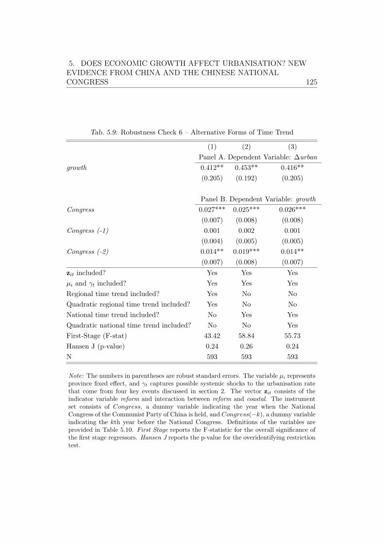
5. DOES ECONOMIC GROWTH AFFECT URBANISATION? NEWEVIDENCE FROM CHINA AND THE CHINESE NATIONALCONGRESS 125
Tab. 5.9: Robustness Check 6 – Alternative Forms of Time Trend
(1) (2) (3)
Panel A. Dependent Variable: ∆urban
growth 0.412** 0.453** 0.416**
(0.205) (0.192) (0.205)
Panel B. Dependent Variable: growth
Congress 0.027*** 0.025*** 0.026***
(0.007) (0.008) (0.008)
Congress (-1) 0.001 0.002 0.001
(0.004) (0.005) (0.005)
Congress (-2) 0.014** 0.019*** 0.014**
(0.007) (0.008) (0.007)
zit included? Yes Yes Yes
µi and γt included? Yes Yes Yes
Regional time trend included? Yes No No
Quadratic regional time trend included? Yes No No
National time trend included? No Yes Yes
Quadratic national time trend included? No No Yes
First-Stage (F-stat) 43.42 58.84 55.73
Hansen J (p-value) 0.24 0.26 0.24
N 593 593 593
Note: The numbers in parentheses are robust standard errors. The variable µi representsprovince fixed effect, and γt captures possible systemic shocks to the urbanisation ratethat come from four key events discussed in section 2. The vector zit consists of theindicator variable reform and interaction between reform and coastal. The instrumentset consists of Congress, a dummy variable indicating the year when the NationalCongress of the Communist Party of China is held, and Congress(−k), a dummy variableindicating the kth year before the National Congress. Definitions of the variables areprovided in Table 5.10. First Stage reports the F-statistic for the overall significance ofthe first stage regressors. Hansen J reports the p-value for the overidentifying restrictiontest.
5. DOES ECONOMIC GROWTH AFFECT URBANISATION? NEWEVIDENCE FROM CHINA AND THE CHINESE NATIONALCONGRESS 126
the effect of rainfall on growth in China may be weak at best, rainfall could
affect urbanisation in China through rural-urban migration.111 As with the
previous robustness checks, Table 5.8 shows that the estimated effect of
growth on urbanisation is nearly identical to the baseline estimate, and the
same can be said about the estimated effect of the congress instruments. For
instance, adding rainfall into the regression, defined by the average annual
precipitation (mm), column (2) shows that the estimated incremental impact
of growth on urbanisation is nearly identical to the baseline estimate. With
respect to the congress instruments, Table 5.8 shows that these variables are
not only statistically significant for growth, the magnitude of their effects are
also highly robust.
The sixth robustness check, reported in Table 5.9, explores how sensitive
the baseline results are to various specifications of the time trend. First, it
includes the square of the region-specific time trend to capture any non-linear
trending effect (column (1)). Second, it replaces the region-specific time
trends used in (5.1) with a single national time trend (column (2)). Finally,
it controls for the national time trend and its square (column (3)). As Table
5.9 shows, the estimation outcomes are not sensitive to the choice of region-
specific versus national time trend. Furthermore, adding the squared trend
only reduces the effect of growth on urbanisation slightly without driving out
its statistical significance.
Overall, the sensitivity tests provide compelling evidence that the
estimate of the effect of growth is robust, which offers some support for the
‘congress cycles’ estimation strategy used here. Furthermore, the estimated
effect of the timing of the National Congress is highly resilient. For instance,
while the baseline estimate of the coefficient on Congress is 0.025, the
estimates of this coefficient range from 0.024 to 0.027 across the sensitivity
tests. Likewise, the estimates of the effect of Congress(-2) in the robustness
checks vary in a narrow vicinity around the baseline estimate.
111 Barrios et al. (2006) show that climatic change, as proxied by rainfall, is an importantdeterminant of rural-urban migration in sub-Saharan Africa.
5. DOES ECONOMIC GROWTH AFFECT URBANISATION? NEWEVIDENCE FROM CHINA AND THE CHINESE NATIONALCONGRESS 127
4. Conclusion
The combination of rapid urbanisation and an impressive record of economic
growth is a striking feature in the development experience of China. However,
concrete empirical evidence on whether economic growth affects urbanisation
in China, let alone how strong this causal effect could be, is limited. The
weak OLS estimates of the effect of economic growth, which remain tenuous
despite eliminating a host of confounders that include province fixed effects,
remind us that addressing a question as fundamental as whether economic
growth affects urbanisation may not be straightforward.
Due to the complexity of endogeneity issues, current empirical studies
have not arrived at a consensus as to whether economic growth causally
raises urbanisation. For example, Bruckner (2012) finds that economic
growth did not significantly raise urbanisation in sub-Saharan Africa. By
contrast, Henderson (2002) shows economic growth could lead to a higher
level of urbanisation based on data from 85 countries. While the objective
of this chapter is a more modest one than to bring this debate to a close, the
robustness of the findings based on 2SLS estimates offers relatively concrete
evidence that economic growth matters for urbanisation, particularly for
the case of China where there are policy implications. For instance, four
potential crises – diminishing land resources, water and energy shortages,
overpopulation and weakening environmental sustainability – are on the cusp
of reaching the tipping point following the rapid rate of urbanisation in
China.112 But these problems are not straightforward to address, as the
observation that urbanisation in China is so strongly driven by economic
growth beyond the effects of rainfall, government expenditure, labour force
composition, and population growth – factors of urbanisation emphasised
previously in the literature113 – suggests that slowing down the rate of
urbanisation would be difficult without relaxing some growth targets, and
112 See, for example, the article “Too Big, Too Fast” by Jianhua Feng in the BeijingReview, http://www.bjreview.cn/EN/En-2005/05-43-e/china-4.htm.113 See, for example, Mohan (1984), Becker and Morrison (1988), Zhang and Song (2003),Henderson (2005), Barrios et al. (2006) and Bruckner (2012). This finding has been verifiedin the robustness checks in section 3.3.
5. DOES ECONOMIC GROWTH AFFECT URBANISATION? NEWEVIDENCE FROM CHINA AND THE CHINESE NATIONALCONGRESS 128
that maintaining an environmentally sustainable rate of urbanisation while
achieving high economic growth may be a difficult balancing act from the
policy perspective.114
This chapter makes two contributions relating to both identification
strategy and policy implications. First, because the study of the impact of
economic growth on urbanisation must insulate itself from reverse causality
and because of measurement errors, this chapter proposes a new but simple
estimation strategy that uses the timing of the National Congress to estimate
the within-province causal effect that growth has on urbanisation. The robust
first-stage results in sections 3.2 and 3.3 have shown a close relationship
between economic growth and the timing of the National Congress that is not
confounded by systemic macroeconomic events and time trends. Therefore,
this work offers a new way to think about identifying the independent
variation in economic growth in the context of China, which is useful for
the study of its causal implication.
Second, this study sheds light on whether economic growth, a key
policy target, could have contributed to the rampant rate of urbanisation
which brought along a set of economic, social and environmental challenges.
These potential problems though have not been studied in this chapter are
addressed in the literature. Based on 2SLS estimates, this chapter has
confirmed that economic growth caused urbanisation in China during 1985–
2009 when the rapid pace of urbanisation threatened sustainable development
(see Chen, 2002; Chang and Brada, 2006; Feng et al., 2009; Du et al., 2012).
From the policy perspective, this means that managing a sustainable rate
of urbanisation while maintaining high rates of economic growth could be
difficult to balance, and perhaps the panacea for ameliorating the problems
of urbanisation might involve recalibrating the GDP growth targets that are
central to the economic plans of Chinese local governments.
114 Henderson (2009) offers a comprehensive overview of urbanisation and its relatedpolicy issues in China.
5. DOES ECONOMIC GROWTH AFFECT URBANISATION? NEWEVIDENCE FROM CHINA AND THE CHINESE NATIONALCONGRESS 129
Tab.5.10:ListofVariables
∆urban
annual
chan
gein
theurbanisationrate
growth
annual
grow
thrate
ofrealGDP
per
capita
coastal
dummy=1ifprovincesare
locatedin
coastalregions
reform
dummy=1ifyearis
between1992and1998
coastal×
reform
coastaldummymultiplied
byreform
dummy
age
ageof
lead
ers,
provincialsecretary
orgovernor
tenure
Thekth
yearofone’scurrentassignmentasaprovincialsecretary
orgovernor
education
dummy=1ifaleader
holdsuniversity
degreefrom
choiceuniversities
centralconnection
dummy=1ifaleader
haspast
orcurrentworkingexperience
inthecentralgovernment
governmen
texpenditure
share
localgovernmentexpenditure
÷localtotalGDP
governmen
texpenditure
growth
annual
grow
thrate
oflocalgovernmentexpenditure
populationden
sity
region
altotalpopulation(unit:thousand)÷
regionalarea(km
2)
populationgrowth
annual
grow
thrate
ofregionaltotalpopulation
agriculturallabour
size
ofag
riculturallabourforce÷
size
oflocallabourforce
state
labour
size
oflabou
rforcein
state
andcollectivefirm
s÷
size
oflocallabourforce
grain
percapita
annual
grainou
tputper
capita(ton)
wage
growth
annual
grow
thrate
ofrealurbanwage
rainfall
averag
ean
nual
precipitation(m
m)
crisis
year
dummyfornegativemacroeconomic
shocks
Note:Thecoastalregion
sareLiaon
ing,
Heb
ei,Shan
don
g,Jiangsu,Zhejiang,
Fujian
andGuan
gdon
g.Thechoice
universities
are
PekingUniversity,Tsingh
uaUniversity,Fudan
University,Jiaoton
gUniversity,an
dRen
min
University.Realurban
wag
eisdefi
ned
astheaverag
eof
annual
real
wag
ein
urban
publicsector
consistingof
state-ow
ned
enterprisesan
dcollectiveenterprises.
6. WAGES AND ACCESS TO INTERNATIONAL
MARKETS: EVIDENCE FROM URBAN CHINA
1. Introduction
In development economics literature, cross-country studies emphasise the
contribution of transportation infrastructure to economic growth (e.g. Es-
fahani and Ramirez, 2003; Calderon and Chong, 2004; and Calderon and
Serven, 2005), in which the positive link appears undebatable. However,
China is a special case which makes the relationship between transportation
infrastructure and economic growth more complicated. In China where
economic growth was rapid and infrastructure investment was substantial
during 1978 to 2008,115 the increasing inter-regional disparity of trans-
portation infrastructure drove heterogeneous income growth and economic
development.116 While the empirical studies on China (e.g. Demurger
(2001); Chen and Yao (2011)) using highly aggregated data have arrived at a
consensus that transportation infrastructure has a strong impact on economic
growth, recent work by Banerjee et al. (2012), using Chinese county-level
data, shows that proximity to transportation network does not necessarily
cause GDP per capita growth. These contrasting findings raise a new
question about how transportation infrastructure influences income (wages
only) from a micro perspective. This is important, as highly aggregated
data like provincial and national data may not explicitly capture individual
115 For example, in 2008, the Chinese government announced a package that includedcommitting 1) RMB 1.52 trillion for infrastructure projects that included road constructionand to increase the total highway length by about 40 percent between 2010 and 2020, and2) RMB 1.41 trillion in 2010 and 2011 for railroad construction and to raise the totaloperating length by about 33 percent between 2010 and 2015.116 See Demurger (2001) and Chen and Yao (2011) for the periods 1985–1998 and 1978–2006, respectively.
6. WAGES AND ACCESS TO INTERNATIONAL MARKETS:EVIDENCE FROM URBAN CHINA 131
attributes that affect individual wages. Focusing on urban wage inequality,
this chapter supplements Chapters 3 and 4, by providing some micro-level
evidence for urban China.
In the growing literature which uses aggregated endowments to explain
micro-level income differentials, researchers indicate that the differences in
accessibility to transportation infrastructure, as a proxy for market access,
may lead to income disparities (Banerjee et al., 2012; Hou and Emran,
2012). The market access reflects the trading activities between the origin
location and its domestic and international trade partners. The seminal work
in this area is Hering and Poncet (2010) which follows a New Economics
Geography (NEG) framework. Using urban data from the China Household
Income Project Survey (CHIPS, 1995), Hering and Poncet (2010) show that
geographical heterogeneity of market access has significant impacts on the
disparities of individual wages. Building on Hering and Poncet (2010), Kamal
et al. (2012) employ a similar theoretical framework but extend the empirical
analysis by including urban samples from both CHIPS (1995) and CHIPS
(2002). They find that the impact of access to markets on individual wages
is heterogeneous among different types of workers. Using CHIPS (2002) data,
Hou and Emran (2012) show that the accessibility to market, as measured
by the distance from the origin place to its local business centres and major
seaports, significantly affects rural household consumption levels.
The major challenge of using cross-sectional income data is that omitted
unobservables cannot be easily purged, as cross-sectional data do not contain
time-series information thus fixed effects estimations like in Chapters 3
and 4 cannot be used to eliminate time-invariant unobservable factors.117
Methodologically, one may eliminate city-level fixed effects by introducing
city dummies in this case. However, it is not appropriate either, because the
variable of interest is itself a part of fixed effects which will be removed by
117 Recall that there are three types of endogeneity problems, i.e. omitted variables,measurement errors and reverse causality. In Chapters 3 and 4, the major resources ofendogeneity are measurement errors and reverse causality, since time-invariant omittedvariables which are problematic in empirical studies are eliminated in fixed-effectsestimations. In this chapter, the serious issue of endogeneity is mainly due to omittedvariables.
6. WAGES AND ACCESS TO INTERNATIONAL MARKETS:EVIDENCE FROM URBAN CHINA 132
dummy variables. Therefore, following the studies that use instrumental
variables to ameliorate omitted biases caused by endogenous problems
(see Hering and Poncet, 2010; Hou and Emran, 2012; and Kamal et al.,
2012, among others), this chapter proposes a new instrumental variable
employing historical information to identify the exogenous variation in length
of transport routes connecting the origin city and its nearest major seaport.
The instrumental variable relies on historical information, i.e. China’s
inter-prefecture population in 1820. It is worth noting that an instrument
including historical population does not violate the exclusion restriction only
if the population is predetermined prior to the construction of the first
railroad. The instrument proposed in this chapter satisfies this condition,
as the first Chinese railroad was completed in 1881, so it could not affect
the distribution of population in 1820. In other words, the instrument is
not correlated with unobservable error terms that may affect the endogenous
variable (transport routes) and the dependent variable (individual wages).
Using urban samples of CHIPS (2002), this chapter finds that instru-
ments that use information from the historical population are significantly
correlated with the length of transport routes. The strong effect is
not confounded by omitting city characteristics (e.g. geographical and
topographical conditions, contemporary population and political ranking)
that might contaminate the impact of historical population on the present
transportation infrastructure, since additional covariates, such as elevation,
slope, latitude, longitude, current population density, administrative level
and autonomous status are carefully taken into account in the regressions.
Following a Mincer (1974) wage equation, this study shows that while
the OLS estimates provide statistically insignificant and quantitatively zero
effects of accessibility to international markets, proxied by length of transport
routes, on individual hourly wages in urban China, the 2SLS estimates
indicate a clear causal relationship that an increase in length of transport
routes from the origin city to the international market (i.e. the nearest
seaport), ceteris paribus, has a negative impact on individual wages in that
origin city. Furthermore, the causal result remains strongly resilient in a
battery of sensitivity tests.
6. WAGES AND ACCESS TO INTERNATIONAL MARKETS:EVIDENCE FROM URBAN CHINA 133
The rest of the chapter is organised as follows. Section 2 addresses the
related literature and the Chinese economic history. Section 3 outlines the
data and the methodology. Section 4 presents the main empirical findings and
the results of robustness checks. Section 5 provides the concluding remarks.
2. Background
2.1 Related Literature
In this chapter, the market access refers to importing and exporting activities
between locations which are affected by heterogeneous transport routes
linking the origin city with the trade partners. This study benefits from
the conceptual framework initiated by the seminal studies on the NEG
(Krugman, 1991; Krugman and Venables, 1995; Fujita et al., 1999). In
Fujita et al. (1999), the market access of a location is defined as the sum
of the market capacity (total trade potential) of surrounding locations that
open up their borders. It is worth nothing that the computation of market
access requires a weighting scheme based on bilateral distance of the origin
location and its trade partners. Given the definition of market access, the
NEG theory models nominal wages in a location as a function of the market
access, and predicts that wages are relatively high at business centres.118 The
prediction is important for this chapter for two reasons. First, it indicates
a possible direction of the impact of accessibility to markets on wages from
theoretical perspectives. Second, it implies the necessity of eliminating effects
from accessibility to domestic markets, if one aims to identify the specific
contribution of accessibility to international markets to wage levels.
Recent empirical studies also shed light on the world’s largest developing
economy, China, emphasising its rapid market liberalisation. During the
second phase of economic reform (1992–1997),119 Poncet (2005) finds that
118 A business centre is the hub where trade quantity is the highest in the region. Forexample, a provincial capital can be the business centre within the province.119 The economic reform of China consists of three main phases, i.e. 1978–1991, 1992–1997 and 1998 onwards.
6. WAGES AND ACCESS TO INTERNATIONAL MARKETS:EVIDENCE FROM URBAN CHINA 134
the domestic market fragmentation became severe,120 indicating that the
domestic market integration in a developing country like China may not
be consistently improving. Poncet (2003) confirms that China’s ‘Open Door’
policy succeeded in opening up its borders to international markets but failed
to reduce inter-provincial trade barriers. Built on these preliminary explo-
rations, Hering and Poncet (2010) estimate the wage equation embedded
in an NEG framework, addressing the effect of access to both domestic and
international markets on individual wages.121 Using CHIPS (1995) data, they
claim that the heterogeneous geography of market access has a significant
impact on individual differences in economic returns to labour. In addition,
they find greater wage sensitivity to market access for highly-skilled workers
relative to low-skilled workers; and for workers in non-public firms compared
with workers in public firms. Using both CHIPS (1995) and CHIPS (2002)
data, Kamal et al. (2012) underscore that market access affects wages paid to
both skilled and unskilled workers, and argue that this influence was stronger
for workers in state-owned firms relative to workers in other types of firms
(e.g. private firms) during 1995–2002.
Departing from Hering and Poncet (2010) and Kamal et al. (2012)
who investigate urban wage earners, Hou and Emran (2012) look at rural
households, and quantify the direct impact of being relatively far away
from both domestic and international markets. Their findings, relying on
CHIPS (1995), show that the better the access to markets, measured as the
length of transport routes that connect households and domestic markets
(local business centres) and international markets (the nearest seaports), the
greater the positive impact on rural consumption, which supplements Hering
and Poncet (2010) and Kamal et al. (2012). This chapter accepts the measure
of market access from Hou and Emran (2012), but emphasises the effect of
access to international markets rather than general access to markets (e.g.
Hering and Poncet, 2010; Kamal et al., 2012) on urban wage earners.
120 Local authorities govern most economic activities in one region across differenteconomic sectors. Thus, the Chinese market structure is characterised as a ‘cellular’structure, which is also known as market fragmentation in China.121 This is the first attempt to estimate the Mincer (1974) wage equation in an NEGframework using micro data from China.
6. WAGES AND ACCESS TO INTERNATIONAL MARKETS:EVIDENCE FROM URBAN CHINA 135
This study also extends those explorations in economic history that
emphasise the importance of transportation infrastructure in the early
stages of market integration and economic development across countries, for
instance, Keller and Shiue (2008), Michaels (2008), Donaldson (2010) and
Banerjee et al. (2012). Importantly, these studies have raised the issue of
endogeneity of the initial construction of transportation infrastructure. A
typically endogeneity problem could be, for example, the construction of
highways. The initial design of highway routes is likely to correlated with
local attributes such as population and income level which may affect the
economic outcomes that researchers are investigating. Looking at the US in
the 1950s, Michaels (2008) uses the original plan of routes proposed in 1944
as an instrument for highway locations to deal with this endogeneity issue.
Relying on Chinese county-level data, Banerjee et al. (2012) use the distance
of a county from the transport networks that connect historical treaty ports
and business centres to construct an exogenous proxy of accessibility to
current transportation infrastructure.122 Donaldson (2010) studies the effects
of railroad construction in 19th century India, underlining the contribution of
railroads to initial spatial agglomeration which reduced inter-regional trade
costs. Keller and Shiue (2008) show that the effects of steam trains in
19th century Europe were substantially larger than customs liberalisation
and currency agreements in terms of increasing market size. This chapter’s
venture into Chinese history aiming to find an appropriate instrument is
informed by studies noted above.
Finally, the current studies that look at infrastructure development in
China usually use aggregated data, for example, provincial data. Using
122 The treaty ports are Chinese territories which were conquered by the westernersafter the First Opium War (1840). These ports were forced to open up to foreign tradeduring the second half of the 19th century to the early 20th century by unequal treaties.The Chinese government considered these treaties as unequal “because they were notnegotiated by nations treating each other as equals but were imposed on China after awar, and because they encroached upon China’s sovereign rights ... which reduced her tosemicolonial status”(Hsu, 1970). For example, the treaties were imposed the British (e.g.Treaty of Nanjing, Treaty of the Bogue, Convention of Peking and Boxer Protocol), theFrench (e.g. Treaty of Whampoa, Treaty of Tientsin, Convention of Peking and BoxerProtocol), the American (e.g. Treaty of Wanghia, Treaty of Tientsin and Boxer Protocol),and the German (Treaty of Tientsin and Boxer Protocol), among others.

6. WAGES AND ACCESS TO INTERNATIONAL MARKETS:EVIDENCE FROM URBAN CHINA 136
provincial panel data (1985–1998), Demurger (2001) investigates how het-
erogeneous provision of transportation infrastructure could drive provincial
income disparities in China. Relying on Chinese provincial panel data over
the period 1978–2006, Chen and Yao (2011) find that the increasing pro-
portion of the government budget allocated to investments in transportation
reduced household consumption. Using Chinese provincial panel datasets,
Chapters 3 and 4 of this thesis confirm the contributions of the improvement
of transportation infrastructure to short-run and long-run economic growth.
Although the existing literature has found aggregated effects of transporta-
tion infrastructure on income and consumption, it is still possible to improve
the understanding of the role of transportation infrastructure by introducing
microeconometric analysis. In general, increased provision of transportation
infrastructure may raise regional income growth, but it is not clear-cut
whether this may have heterogeneous effects on the wage distribution. Thus,
the empirical section of the chapter intends to quantify the causal impact
of the provision of transportation infrastructure, as measured by length of
current transport routes that connect the origin city and its nearest seaport,
on income inequality in urban China. This chapter contributes to the
literature by offering micro-level evidence built on individual income data
from urban China in 2002.
2.2 Historical Factor Endowments
The central concern of this chapter is to find exogenous variations in
transport routes connecting a location and its nearest seaport in 2002 in
China. Thus, this section discusses historical population at prefecture level
in 1820 which serves as the instrument variable. Moreover, the effects
on individual wages imposed by other potential historical endowments are
documented as well.
Cao (2000) provides a rich dataset including prefecture-level population
density in the Qing Dynasty (1776, 1820, 1851, 1880 and 1910). This
study gathers the information from the 1820 ‘census’ to construct the
6. WAGES AND ACCESS TO INTERNATIONAL MARKETS:EVIDENCE FROM URBAN CHINA 137
instruments.123 Three main reasons for choosing this dataset are presented.
First, the earliest railroad in China had been completed in 1881, implying
that data from 1880 and 1910 ‘censuses’ are not usable, as they could be
affected by the determinants of initial railroads and thus this would invalidate
exclusion restrictions in a 2SLS approach. Second, this study does not employ
data in 1851 not only because the timing is close to the First Opium War
(1840) but also because it is influenced by the Taiping Rebellion (1850–
1864) both of which caused a severe decline of population across Chinese
prefectures. Last, this study prefers the 1820 ‘census’ to the 1776 ‘census’,
as the former is relatively more accurate.
The intuitions of using prefecture-level historical population density as
instruments for current transport routes are presented as follows. First, the
example in the 19th century US reveals a positive link between population
and expanding demand for railroads (Fogel, 1962), which in part explains
why current routes which are built on initial railway networks are designed
according to the pattern of population distribution. Recall that prefecture
population in 1820 was not affected by the existence of the modern railway
system, which does not violate exclusion restrictions.124 Second, the history
of Chinese railroads which is reviewed by Ma (1983) offers some evidence
that rail routes are associated with surrounding population. For example,
the Beijing-Shenyang railroad (construction: 1881–1930) connects Beijing,
Tianjin, Hebei province and Liaoning province which were all areas of high
population density in the late 1800s. Figures 6.1 and 6.2, which illustrate the
railway density by the end of the Qing Dynasty (1911)125 and the average
123 In the Qing dynasty (1644–1911), there were no formal population censuses accordingto the modern-time statistical and demographical criterion. However, the Qing governmenthad relatively complete records of registered prefecture-level population in some years, e.g.1776, 1820, 1851, 1880 and 1910.124 The inclusion of other factors such as geographical and topographical conditions inthe analysis will ensure that the estimation does not omit key determinants of currenttransport routes.125 Since provincial boundaries do not remain constant from 1911 onwards, this studyuses the current Chinese map for provincial boundaries and the length of railways in 1911to compute the railway density in Figures 6.1 and 6.2. Based on information such asrailway track lengths, the years when construction started, the years when tracks opened,and the locations of origin and terminal stations of both main and spur lines provided by
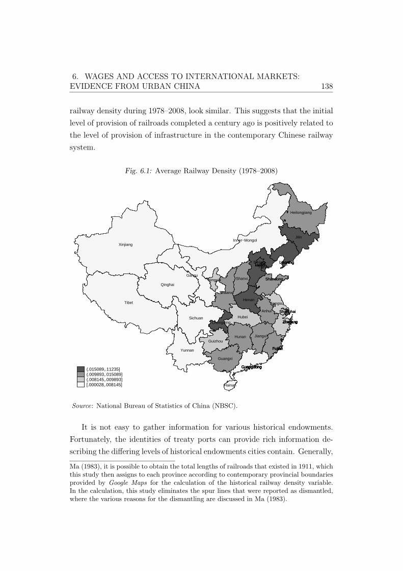
6. WAGES AND ACCESS TO INTERNATIONAL MARKETS:EVIDENCE FROM URBAN CHINA 138
railway density during 1978–2008, look similar. This suggests that the initial
level of provision of railroads completed a century ago is positively related to
the level of provision of infrastructure in the contemporary Chinese railway
system.
Fig. 6.1: Average Railway Density (1978–2008)
Heilongjiang
Inner−MongolXinjiang
Jilin
Liaoning
Gansu
HebeiBeijing
Shanxi
Tianjin
Qinghai
HebeiLiaoningLiaoningLiaoningLiaoning
Shaanxi
Ningxia
Tibet
ShandongShandong
HenanJiangsu
Anhui
Sichuan HubeiShanghai
Chongqing
ShanghaiShanghai
ZhejiangZhejiangZhejiangZhejiangZhejiangZhejiangZhejiangZhejiang
JiangxiHunan
Zhejiang
Yunnan
Guizhou
Zhejiang
Fujian
Zhejiang
Fujian
Guangxi
FujianFujianFujianFujian
GuangdongGuangdongGuangdongGuangdongGuangdongGuangdongGuangdong
Hainan
Guangdong
Fujian
(.015089,.11235](.009893,.015089](.008145,.009893][.000028,.008145]
Source: National Bureau of Statistics of China (NBSC).
It is not easy to gather information for various historical endowments.
Fortunately, the identities of treaty ports can provide rich information de-
scribing the differing levels of historical endowments cities contain. Generally,
Ma (1983), it is possible to obtain the total lengths of railroads that existed in 1911, whichthis study then assigns to each province according to contemporary provincial boundariesprovided by Google Maps for the calculation of the historical railway density variable.In the calculation, this study eliminates the spur lines that were reported as dismantled,where the various reasons for the dismantling are discussed in Ma (1983).
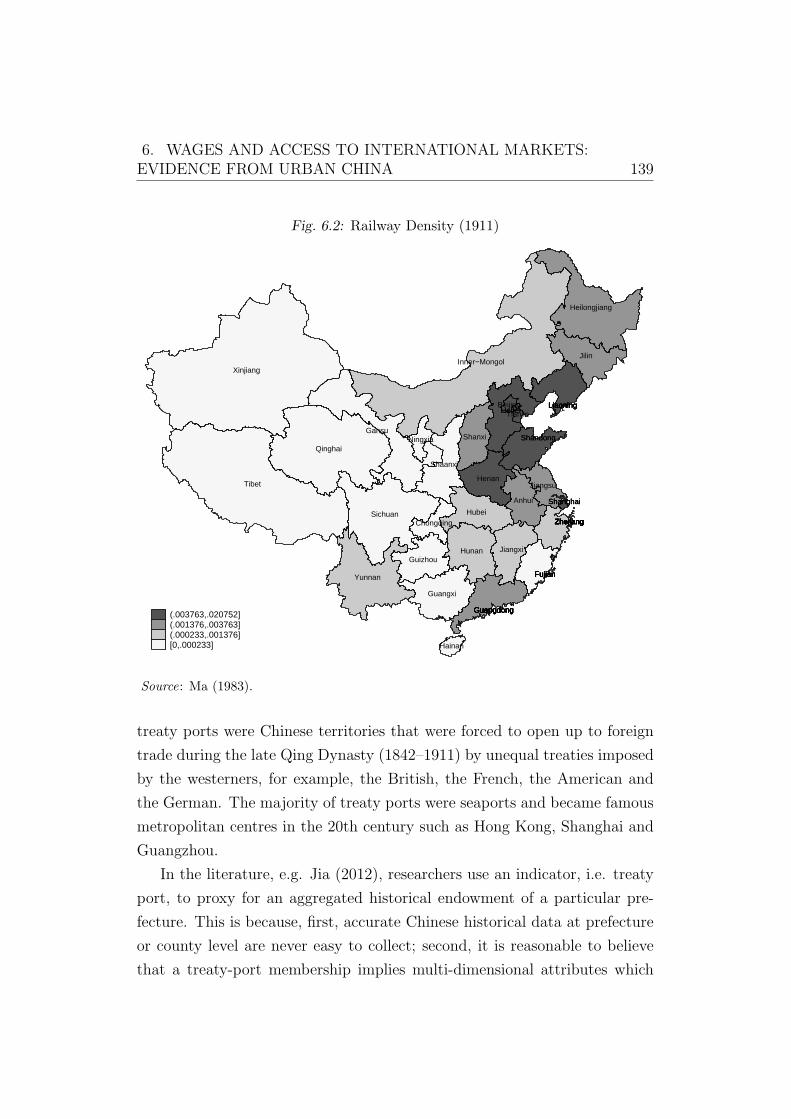
6. WAGES AND ACCESS TO INTERNATIONAL MARKETS:EVIDENCE FROM URBAN CHINA 139
Fig. 6.2: Railway Density (1911)
Heilongjiang
Inner−MongolXinjiang
Jilin
Liaoning
Gansu
HebeiBeijing
Shanxi
Tianjin
Qinghai
HebeiLiaoningLiaoningLiaoningLiaoning
Shaanxi
Ningxia
Tibet
ShandongShandong
HenanJiangsu
Anhui
Sichuan HubeiShanghai
Chongqing
ShanghaiShanghai
ZhejiangZhejiangZhejiangZhejiangZhejiangZhejiangZhejiangZhejiang
JiangxiHunan
Zhejiang
Yunnan
Guizhou
Zhejiang
Fujian
Zhejiang
Fujian
Guangxi
FujianFujianFujianFujian
GuangdongGuangdongGuangdongGuangdongGuangdongGuangdongGuangdong
Hainan
Guangdong
Fujian
(.003763,.020752](.001376,.003763](.000233,.001376][0,.000233]
Source: Ma (1983).
treaty ports were Chinese territories that were forced to open up to foreign
trade during the late Qing Dynasty (1842–1911) by unequal treaties imposed
by the westerners, for example, the British, the French, the American and
the German. The majority of treaty ports were seaports and became famous
metropolitan centres in the 20th century such as Hong Kong, Shanghai and
Guangzhou.
In the literature, e.g. Jia (2012), researchers use an indicator, i.e. treaty
port, to proxy for an aggregated historical endowment of a particular pre-
fecture. This is because, first, accurate Chinese historical data at prefecture
or county level are never easy to collect; second, it is reasonable to believe
that a treaty-port membership implies multi-dimensional attributes which
6. WAGES AND ACCESS TO INTERNATIONAL MARKETS:EVIDENCE FROM URBAN CHINA 140
determine a region’s modern-time economic development, and ultimately the
average individual income level.
Using the difference-in-difference approach, Jia (2012) points out that
population as a key measure of economic development grew around 30 percent
faster in treaty ports which were opened up to international markets after
the First Opium War (1840) than the rest of regions that were not opened
up during the second half of the 19th century. Furthermore, the effect
from historical endowments, though often unobservable, plays a pivotal role
in long-run economic growth. Findings from Jia (2012) show that treaty
ports were among the first to integrate with international markets and took
advantage of globalisation opportunities post to China’s ‘Open Door’ policy
implemented from 1978. On average, the growth rate of GDP per capita in
treaty ports was 35 percent higher than in surrounding regions that were not
forced to opened up to foreign trade after the First Opium War (1840), over
the period 1988–2007 (Jia, 2012).
This chapter emphasises the importance of the inclusion of historical
endowments in the estimation of wage differentials between treaty ports
and other cities. This is because they not only contribute information to
contemporary size of population and GDP per capita growth by prefecture
(city), but also because they have implications for the quality of institutions
among Chinese cities, which in turn could drive economic divergence (Fang
and Zhao, 2009). Fang and Zhao (2009) find that treaty ports are normally
better in the sense of both economic growth and institutions. These
institutions, i.e. social rules that protect property rights, can be interpreted
as municipal authorities, police, and judiciaries established by westerners
during the 1850s to the 1910s in treaty ports. Although one may argue
about how tight the links between the ‘western’ institutions and today’s
Chinese socialism are, empirical findings from Fang and Zhao (2009) reveal
that the large influence of the western institutions on China’s transition
from antiquity (prior to 1911) to modernity (1911 onwards) well explains
contemporary institutional differentials among Chinese cities. This study
therefore carefully controls for these historical endowments, proxied by an
indicator for treaty ports, in the sensitivity tests to partial out unobservable
6. WAGES AND ACCESS TO INTERNATIONAL MARKETS:EVIDENCE FROM URBAN CHINA 141
confounding effects.
3. Data and Methodology
3.1 Data
This chapter utilises individual information from the urban samples in the
China Household Income Project Survey (CHIPS, 2002), covering 20,632
individuals and 6,835 households from 77 cities in 12 provinces.126 Excluding
those areas that do not have complete city-level information, the empirical
analysis focuses on 63 cities and 7,979 urban wage earners aged from 18 to
60 whose personal characteristics of interest are not missing.127 In order to
visualise the geographical distribution of locations analysed in this chapter,
Figure 6.3 plots all sampled areas.
The dependent variable is the logarithm of individual hourly wage (lnW ).
In CHIPS (2002), individuals report their nominal annual income which
consists of regular salaries, bonuses and subsidies (including housing, medical,
child care and various regional subsidies). Following Hering and Poncet
(2010), this study defines the hourly wage as total income per working
hour. The actual working hours are obtained based on the number of
claimed work days per month along with the number of working hours per
day by individuals.128 The causal variable of interest is the accessibility to
international markets proxied by the logarithm of length of transport routes
from a sampled location to its nearest major seaport (lnD). The three major
seaports are Tianjin, Shanghai and Guangzhou located in the north-east, east
and south-east, respectively. This study measures the transport routes as the
shortest length of transport routes including railroads and highways which
126 These provinces (includes municipalities) are: Beijing, Shanxi, Liaoning, Jiangsu,Anhui, Henan, Hubei, Hunan, Guangdong, Chongqing, Sichuan, Yunnan and Gansu. Notethat this chapter employs a broader definition of city which includes counties from theurban samples in CHIPS (2002) following Hering and Poncet (2010) and Kamal et al.(2012).127 This chapter only looks at urban samples. For the sake of simplicity, the remainingsections refer to individual wages of urban wage earners as ‘individual wages’.128 Note that this study has excluded the number of days that workers are unemployed.
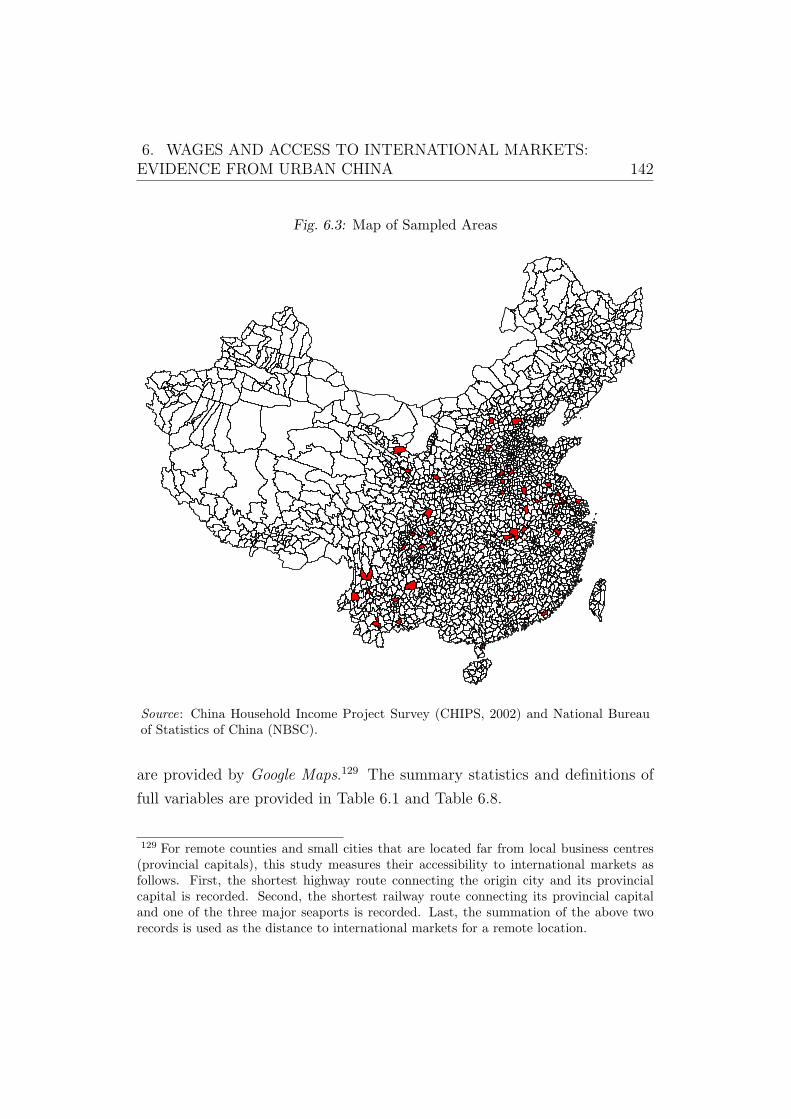
6. WAGES AND ACCESS TO INTERNATIONAL MARKETS:EVIDENCE FROM URBAN CHINA 142
Fig. 6.3: Map of Sampled Areas
Source: China Household Income Project Survey (CHIPS, 2002) and National Bureauof Statistics of China (NBSC).
are provided by Google Maps.129 The summary statistics and definitions of
full variables are provided in Table 6.1 and Table 6.8.
129 For remote counties and small cities that are located far from local business centres(provincial capitals), this study measures their accessibility to international markets asfollows. First, the shortest highway route connecting the origin city and its provincialcapital is recorded. Second, the shortest railway route connecting its provincial capitaland one of the three major seaports is recorded. Last, the summation of the above tworecords is used as the distance to international markets for a remote location.
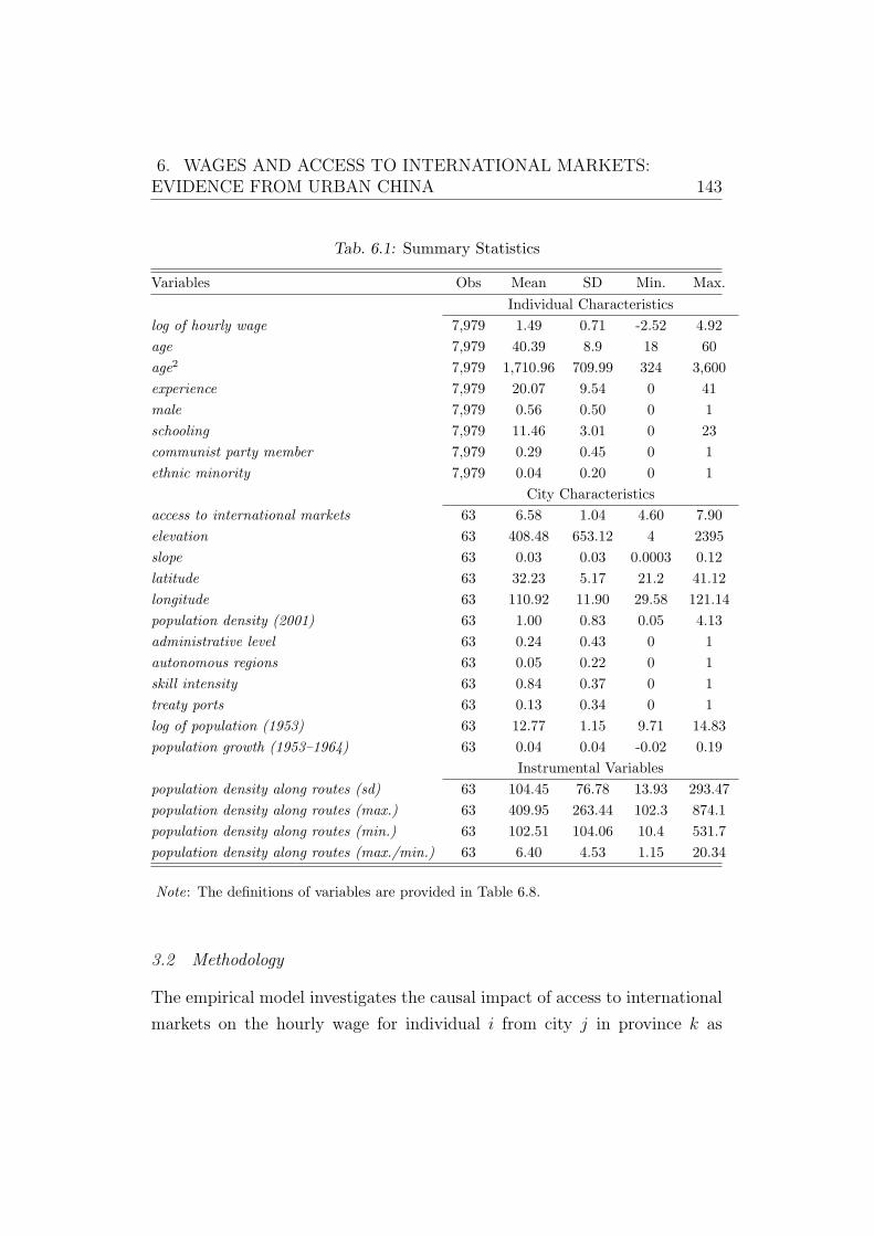
6. WAGES AND ACCESS TO INTERNATIONAL MARKETS:EVIDENCE FROM URBAN CHINA 143
Tab. 6.1: Summary Statistics
Variables Obs Mean SD Min. Max.
Individual Characteristics
log of hourly wage 7,979 1.49 0.71 -2.52 4.92
age 7,979 40.39 8.9 18 60
age2 7,979 1,710.96 709.99 324 3,600
experience 7,979 20.07 9.54 0 41
male 7,979 0.56 0.50 0 1
schooling 7,979 11.46 3.01 0 23
communist party member 7,979 0.29 0.45 0 1
ethnic minority 7,979 0.04 0.20 0 1
City Characteristics
access to international markets 63 6.58 1.04 4.60 7.90
elevation 63 408.48 653.12 4 2395
slope 63 0.03 0.03 0.0003 0.12
latitude 63 32.23 5.17 21.2 41.12
longitude 63 110.92 11.90 29.58 121.14
population density (2001) 63 1.00 0.83 0.05 4.13
administrative level 63 0.24 0.43 0 1
autonomous regions 63 0.05 0.22 0 1
skill intensity 63 0.84 0.37 0 1
treaty ports 63 0.13 0.34 0 1
log of population (1953) 63 12.77 1.15 9.71 14.83
population growth (1953–1964) 63 0.04 0.04 -0.02 0.19
Instrumental Variables
population density along routes (sd) 63 104.45 76.78 13.93 293.47
population density along routes (max.) 63 409.95 263.44 102.3 874.1
population density along routes (min.) 63 102.51 104.06 10.4 531.7
population density along routes (max./min.) 63 6.40 4.53 1.15 20.34
Note: The definitions of variables are provided in Table 6.8.
3.2 Methodology
The empirical model investigates the causal impact of access to international
markets on the hourly wage for individual i from city j in province k as
6. WAGES AND ACCESS TO INTERNATIONAL MARKETS:EVIDENCE FROM URBAN CHINA 144
follows,
lnWijk = c+ ϕlnDijk + γ′xijk + β′zjk + uijk (6.1)
The parameter c denotes the common intercept term across all individuals.
lnWijk and lnDijk are the dependent and independent variables respectively.
uijk is the disturbance. The causal effect of lnDijk on lnWijk, i.e. ϕ, explains
to what extent the accessibility to international markets, as measured by
length of current transport routes from the origin city to its nearest major
seaport, could affect individual wages. Considering omitted variables that
are correlated with individual wages, this study thus controls for two sets of
covariates.
The first set of covariates (xijk) aims to pin down the unobserved
individual heterogeneity. Following the Mincer (1974) wage equation, this
study includes the information of individual age (including its square),
working experience, gender and years of schooling in the empirical model.
Additionally, as Li et al. (2007) among others point out, the identity of
the Communist Party member could have an impact on income,130 and this
chapter considers a binary indicator which is equal to unity if an individual is
a member of the Chinese Communist Party. Given the fact that cultural and
linguistic background could potentially affect income (see Gustafsson and Li,
2003; Gustafsson and Ding, 2009; Li and Ding, 2009), it is worth identifying
whether an individual belongs to a minor ethnic group according to the
official classification.131 Following the literature (Zhao, 2002; Chen et al.,
2005; Hering and Poncet, 2010), this chapter employs various indicators to
partial out multi-dimensional fixed effects, for instance, sectoral categories,
firms’ ownerships, individual occupations and provincial unobservables.132
130 The positive selection effect of the Party membership exists at least for the oldergeneration. Thus, the membership of the Communist Party is employed in the covariatesas a safeguard.131 The latest population census (2010) reports that the proportion of Han, the onlymajor ethnic group, is 91.51 percent (National Bureau of Statistics China, 2011). Theremaining 55 groups are officially defined as minor ethnic groups in China.132 All fixed effects are captured by dummy variables. See Table 8.6 and Table 8.7 inAppendix D for detailed classifications.
6. WAGES AND ACCESS TO INTERNATIONAL MARKETS:EVIDENCE FROM URBAN CHINA 145
The second set of covariates is denoted by the vector zjk, which consists
of cities’ attributes. The heterogeneous geographical and topographical
conditions of locations are possibly associated with household income and
consumption (Hering and Poncet, 2010; Hou and Emran, 2012), therefore,
this chapter controls for these confounding factors such as elevation, slope,
latitude and longitude of each sampled city.133 Moreover, the vector zjk
includes other characteristics of cities, for instance, current population den-
sity, administrative level and autonomous status, as they may be correlated
with both individual wages and instrumental variables.134 Omitting current
population density is dangerous, because it is closely linked with historical
population that is used to construct the instrumental variables used in
the analysis. In other words, the failure to partial out this confounding
effect invalidates the exclusion restriction that requires instruments to be
uncorrelated with omitted variables. In addition, administrative level is
important. It in part denotes the political ranking of a city within a province,
which may determine the priority of development in the Chinese political
hierarchy hence local income level. Meanwhile, it to some extent implies
the historical development of a location, which may be influenced by the
population density in the 1820s. Last, autonomous status135 is included as it
captures fundamental features of ethnically minor counties that are culturally
and linguistically distinct from major Chinese Han regions.
Furthermore, the inclusion of cities’ characteristics purges the potential
impact of access to domestic markets on individual wages.136 In practice, it
is not easy to measure the influences from domestic markets. Some studies
like Hering and Poncet (2010) and Kamal et al. (2012) have defined access
to domestic markets. They first compute market capacity for a province
133 These data are collected from http://www.heavens-above.com. See Table 6.8 fordetailed definitions.134 This study also takes current labour market structure, historical endowments, andinitial population into account in the robustness checks.135 Counties where minor ethnic groups are major residents may be officially designatedas autonomous counties.136 For instance, this study controls for a city’s population density in 2001 which iscorrelated with its consumption potential. Moreover, this study includes a city’s latitudeand longitude to pin down its relative location. The consumption potential and locationinformation can help to reduce the potential spill-over effects from domestic markets.
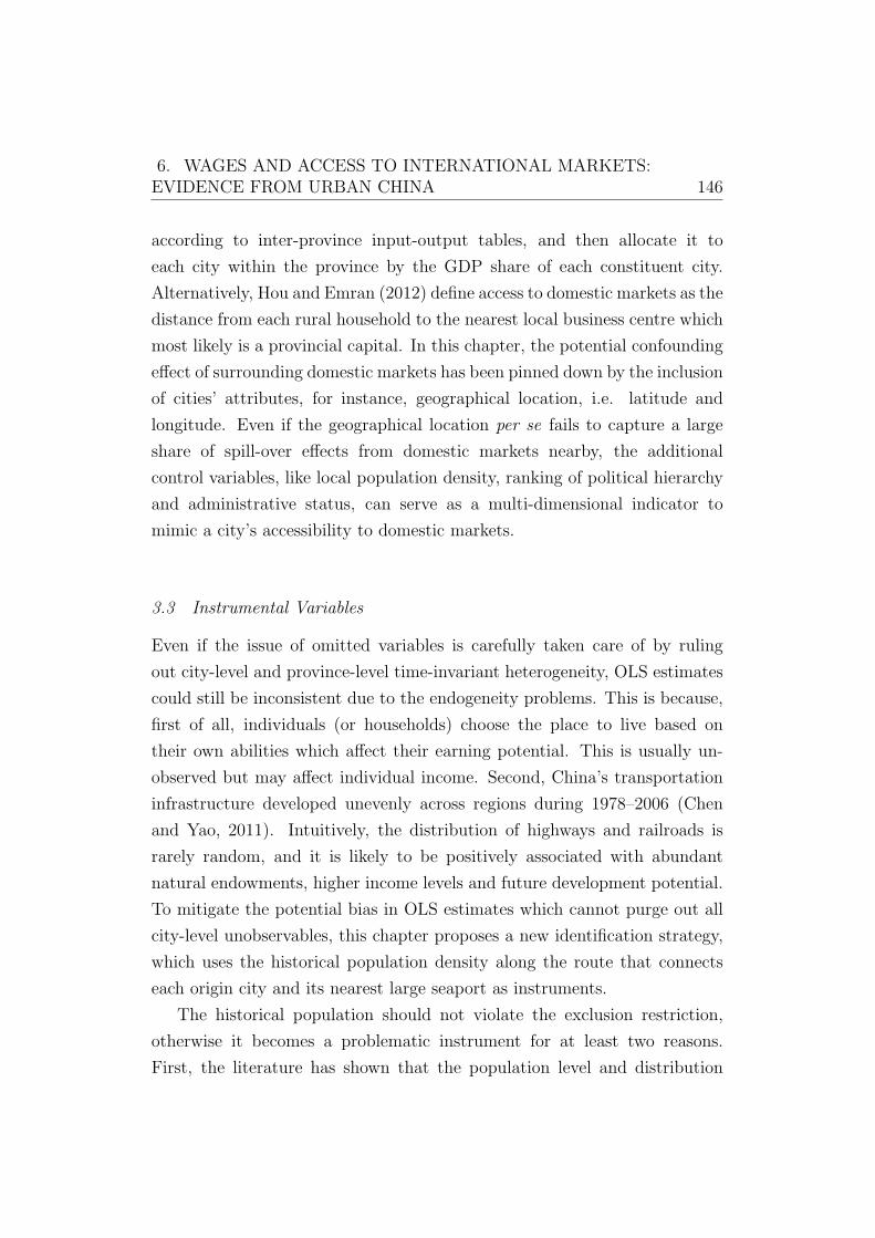
6. WAGES AND ACCESS TO INTERNATIONAL MARKETS:EVIDENCE FROM URBAN CHINA 146
according to inter-province input-output tables, and then allocate it to
each city within the province by the GDP share of each constituent city.
Alternatively, Hou and Emran (2012) define access to domestic markets as the
distance from each rural household to the nearest local business centre which
most likely is a provincial capital. In this chapter, the potential confounding
effect of surrounding domestic markets has been pinned down by the inclusion
of cities’ attributes, for instance, geographical location, i.e. latitude and
longitude. Even if the geographical location per se fails to capture a large
share of spill-over effects from domestic markets nearby, the additional
control variables, like local population density, ranking of political hierarchy
and administrative status, can serve as a multi-dimensional indicator to
mimic a city’s accessibility to domestic markets.
3.3 Instrumental Variables
Even if the issue of omitted variables is carefully taken care of by ruling
out city-level and province-level time-invariant heterogeneity, OLS estimates
could still be inconsistent due to the endogeneity problems. This is because,
first of all, individuals (or households) choose the place to live based on
their own abilities which affect their earning potential. This is usually un-
observed but may affect individual income. Second, China’s transportation
infrastructure developed unevenly across regions during 1978–2006 (Chen
and Yao, 2011). Intuitively, the distribution of highways and railroads is
rarely random, and it is likely to be positively associated with abundant
natural endowments, higher income levels and future development potential.
To mitigate the potential bias in OLS estimates which cannot purge out all
city-level unobservables, this chapter proposes a new identification strategy,
which uses the historical population density along the route that connects
each origin city and its nearest large seaport as instruments.
The historical population should not violate the exclusion restriction,
otherwise it becomes a problematic instrument for at least two reasons.
First, the literature has shown that the population level and distribution
6. WAGES AND ACCESS TO INTERNATIONAL MARKETS:EVIDENCE FROM URBAN CHINA 147
are affected by the presence of railroads in the past (Atack et al., 2009;
Donaldson, 2010). Second, for the case of China, Kung and Li (2011) find
that railways facilitated migration from the North China Plain (north) to
Manchuria (north-east) in the early 1900s, which confirms that the historical
distribution of population could have been influenced by the development
of initial railway system. In this regard, using historical population as an
instrument in the context of China is possible in principle but formidably
challenging in practice, as this requires the information from the early 1800s,
a period for which accurate prefecture-level population data are extremely
rare. After a venture into history, the author chooses to use data from
Cao (2000) which offers detailed population information for each prefecture
in 1820. The novel dataset allows the construction of a set of instrumental
variables consisting of four components — the standard deviation, maximum,
minimum, and ratio of the maximum over the minimum of prefecture-level
population density along the transport routes that link the origin cities with
their nearest major seaports.137
There may remain a concern about the exogeneity of the instruments,
and one may question why this study does not use historical county-level
population information which seems to be more accurate in this case.
The responses to the above two concerns are as follows. First, it is
better to let the data speak. The first-stage results reported in section
4.3 show that the instruments are sharp and robust. Second, countless
changes of administrative boundaries during the last two centuries make
it almost impossible to use historical county-level population information as
instruments. In contrast, most boundaries of prefectures remain constant in
their administrative areas (Cao, 2000), facilitating the attempt to construct
historical instruments in this study.
To sum up, having carefully considered other possible channels relating
historical population to contemporary economic activities, this chapter seeks
to use the heterogeneity of inter-prefecture population to generate the
exogenous variation in accessibility to international markets which is proxied
by length of transport routes connecting a city to its nearest major seaport.
137 Summary statistics are available in Table 6.1.
6. WAGES AND ACCESS TO INTERNATIONAL MARKETS:EVIDENCE FROM URBAN CHINA 148
4. Empirical Results
4.1 OLS Estimates
Table 6.2 summarises the compressed results from the OLS regressions. At
first glance, the OLS estimates reveal that being far from international
markets could significantly lower individual wages as column (1) shows.
However, ignoring individual characteristics and city-level fixed effects, the
OLS estimate tends to overemphasise the effect of access to international
markets on individual wages. This effect attenuates to less than half when
province fixed effects are included in column (2), suggesting that regional
heterogeneity is crucial in explaining China’s inter-regional wage differentials.
Alternatively, one may interpret the importance of the inclusion of province
fixed effects by looking at the R2 in column (2) that solely explains around
6 percent of variations in urban wages.138 In column (3), the estimation
examines how individual heterogeneity affects wages. Surprisingly, the
effect of accessibility to international markets on wages tapers off to almost
zero and becomes statistically insignificant, which confirms that neglecting
individual attributes may cause serious omitted variable bias. Moreover, the
R2 reported in column (3) shows that individual characteristics explain two
more percentage points of total variations in wages than province dummies
do.139 Last, column (4) shows zero and insignificant impacts of access to
international markets on individual wages when city characteristics and
province dummies are considered only.
As the effect of access to international markets on urban wages becomes
statistically insignificant and quantitatively small in the baseline OLS
estimation (column (4) of Table 6.2), further investigation intends to control
for more covariates to eliminate biases due to omitted variables. Table 6.3
looks at the suitability of the OLS estimations with the inclusion of both
138 It is derived from the exclusion of the 5 percent of variation which is explained byaccess to international markets in column (1).139 The explained fraction of wages variation by individual attributes is 13 percent. Thisis derived from 0.29− 0.11− 0.05 = 0.13.
6. WAGES AND ACCESS TO INTERNATIONAL MARKETS:EVIDENCE FROM URBAN CHINA 149
Tab. 6.2: OLS Regressions 1
(1) (2) (3) (4)
Dependent Variable: log of hourly wage
access to international markets -0.158*** -0.062** -0.029 0.009
(0.008) (0.030) (0.027) (0.034)
Individual characteristics included? No No Yes No
City characteristics included? No No No Yes
Province dummies included? No Yes Yes Yes
Observations 7,979 7,979 7,979 7,979
R-squared 0.05 0.11 0.29 0.13
Note: The numbers in parentheses are robust standard errors. The definitions of variablesare provided in Table 6.8.
individual characteristics and regional heterogeneity. As shown in columns
(1) to (5), all coefficients of individual attributes show reasonable signs. For
instance, the impact of age on wages is concave. Male urban wage earners
tend to have an advantage compared to female urban wage earners in the
Chinese labour market. Schooling, not surprisingly, plays an important role
in determining individual wages. The results in Table 6.3 are consistent with
the finding in Li et al. (2007) that being a Chinese Communist Party member
is positively correlated with higher wages. But no significant evidence is
found to support the argument that ethnic minorities suffer from lower wages.
However, for the variable of interest, access to international markets, the
OLS regressions show unexpected signs and insignificant coefficients, even
after multi-dimensional fixed effects are soaked up by ownership, occupation
and sector dummies in column (5). In other words, the inclusion of more
covariates cannot easily ameliorate the omitted variables bias. Therefore,
given the confidence that OLS estimates are troublesome, this study employs
2SLS regressions in the following discussions.
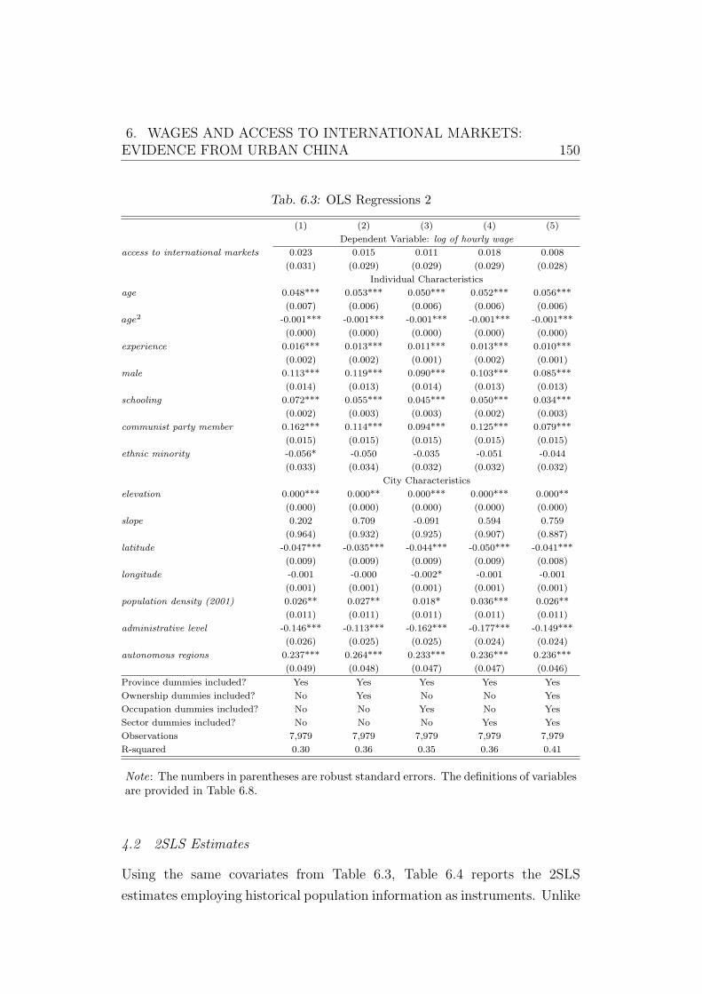
6. WAGES AND ACCESS TO INTERNATIONAL MARKETS:EVIDENCE FROM URBAN CHINA 150
Tab. 6.3: OLS Regressions 2
(1) (2) (3) (4) (5)
Dependent Variable: log of hourly wage
access to international markets 0.023 0.015 0.011 0.018 0.008
(0.031) (0.029) (0.029) (0.029) (0.028)
Individual Characteristics
age 0.048*** 0.053*** 0.050*** 0.052*** 0.056***
(0.007) (0.006) (0.006) (0.006) (0.006)
age2 -0.001*** -0.001*** -0.001*** -0.001*** -0.001***
(0.000) (0.000) (0.000) (0.000) (0.000)
experience 0.016*** 0.013*** 0.011*** 0.013*** 0.010***
(0.002) (0.002) (0.001) (0.002) (0.001)
male 0.113*** 0.119*** 0.090*** 0.103*** 0.085***
(0.014) (0.013) (0.014) (0.013) (0.013)
schooling 0.072*** 0.055*** 0.045*** 0.050*** 0.034***
(0.002) (0.003) (0.003) (0.002) (0.003)
communist party member 0.162*** 0.114*** 0.094*** 0.125*** 0.079***
(0.015) (0.015) (0.015) (0.015) (0.015)
ethnic minority -0.056* -0.050 -0.035 -0.051 -0.044
(0.033) (0.034) (0.032) (0.032) (0.032)
City Characteristics
elevation 0.000*** 0.000** 0.000*** 0.000*** 0.000**
(0.000) (0.000) (0.000) (0.000) (0.000)
slope 0.202 0.709 -0.091 0.594 0.759
(0.964) (0.932) (0.925) (0.907) (0.887)
latitude -0.047*** -0.035*** -0.044*** -0.050*** -0.041***
(0.009) (0.009) (0.009) (0.009) (0.008)
longitude -0.001 -0.000 -0.002* -0.001 -0.001
(0.001) (0.001) (0.001) (0.001) (0.001)
population density (2001) 0.026** 0.027** 0.018* 0.036*** 0.026**
(0.011) (0.011) (0.011) (0.011) (0.011)
administrative level -0.146*** -0.113*** -0.162*** -0.177*** -0.149***
(0.026) (0.025) (0.025) (0.024) (0.024)
autonomous regions 0.237*** 0.264*** 0.233*** 0.236*** 0.236***
(0.049) (0.048) (0.047) (0.047) (0.046)
Province dummies included? Yes Yes Yes Yes Yes
Ownership dummies included? No Yes No No Yes
Occupation dummies included? No No Yes No Yes
Sector dummies included? No No No Yes Yes
Observations 7,979 7,979 7,979 7,979 7,979
R-squared 0.30 0.36 0.35 0.36 0.41
Note: The numbers in parentheses are robust standard errors. The definitions of variablesare provided in Table 6.8.
4.2 2SLS Estimates
Using the same covariates from Table 6.3, Table 6.4 reports the 2SLS
estimates employing historical population information as instruments. Unlike
6. WAGES AND ACCESS TO INTERNATIONAL MARKETS:EVIDENCE FROM URBAN CHINA 151
the OLS estimates which are statistically insignificant and quantitatively
close to zero, the 2SLS estimates paint a different picture, indicating a
significantly negative causal impact of access to international markets on
individual wages.
Generally, the causal effects become stronger with the increase in the
number of multi-dimensional fixed effects considered in columns (1) to (5),
implying the presence of heterogeneity among urban wage earners in China.
This result is consistent with the findings in Hering and Poncet (2010)
who underline the within-province heterogeneous effects on individual wages.
Interestingly, Table 6.4 reports similar coefficients of all regressors but the
independent variable compared with that which have been found in Table
6.3, suggesting the endogeneity of access to international markets.
Using the estimate in column (5) as a benchmark, one can interpret that
every 1 percent increase in distance from the origin city to the international
market (i.e. the nearest seaport), ceteris paribus, has a negative impact on
individual wages of 0.086 percent. The effect is smaller than that found
by Hering and Poncet (2010) who report 0.136 as the elasticity of market
access derived from a similar wage equation controlling for the same fixed
effects.140 This may be because this study uses transport routes as a proxy
only for access to international markets,141 while Hering and Poncet (2010)
derive the indicator for both access to domestic and international markets
from an NEG model.142 Although the findings in this chapter and in Hering
140 See column (5) in Table 1 in Hering and Poncet (2010).141 The effects of domestic markets are probably ruled out by controlling for detailed cityattributes including population density and administrative level, among others.142 Since this study does not estimate the same causal effect as Hering and Poncet (2010),it is hard to say that this study underestimates the impact of accessibility to internationalmarkets on individual wages in urban China. Moreover, even though this chapter estimatesa broader concept of market access, the estimates could still be smaller than those inHering and Poncet for two reasons. First, this chapter has carefully controlled for cities’characteristics in the wage equation but Hering and Poncet have not. Comparing R2s inTable 6.4 with those in Table 1 in Hering and Poncet (2010), one can see that the variationin individual wages explained in this chapter on average is twice as much as that whichhas been explained in Hering and Poncet. Second, as Hering and Poncet have used CHIPS(1995) data, the smaller estimates this chapter reports could perhaps be the consequenceof a convergence of economic returns to market access, which indicates that a catch-upeffect occurred in inland China during 1995–2002.
6. WAGES AND ACCESS TO INTERNATIONAL MARKETS:EVIDENCE FROM URBAN CHINA 152
and Poncet (2010) are not directly comparable, their results considered as a
benchmark imply that at first pass the results of this study do not fall within
an unreasonable range.
As a model-based assessment of instrument validity, this study employs
the overidentifying restrictions test.143 The Hansen J tests in Table 6.4
all well exceed 0.1 thus one cannot reject the null hypothesis, indicating
that there is no evidence that the quantitatively significant estimates this
study finds above are an unintended consequence of model misspecification
and questionable instruments validity. Besides, this chapter also reports the
Kleibergen and Paap (KP) (2006) Wald statistic for evidence on instrument
weakness.144 As clearly shown in Table 6.4, all KP Wald statistics are
sufficiently large so that it is not necessary to worry about the issue of weak
instruments. To provide further evidence, Table 6.5 offers the first stage
results where the overall F-statistics are also large enough to avoid standard
weak instruments.
4.3 Robustness Checks
Using historical instruments in empirical studies is challenging, as they are
likely to be correlated with omitted determinants of individual wages. For the
sake of robustness, this section offers two sets of sensitivity tests, responding
to those concerns that first, instrumental variables may be associated with
macro-level unobservables and second, the causal effect found in section 4.2
may be driven by extreme values.
Table 6.6 reports the first set of robustness checks aiming to partial out
other channels through which historical population density could potentially
affect individual wages. Following Hering and Poncet (2010), the first robust-
143 Rejecting the test implies that one or more instruments are invalid, or the model ismisspecified, or both. But it does not distinguish which condition or if both conditionsare violated.144 The KP statistic is evaluated against a critical value, adopted from Stock and Yogo(2005), that 10 percent is the maximum rejection rate the researcher is willing to tolerateif the true rejection rate is 5 percent. This follows from the suggestion of Stock et al.(2002).
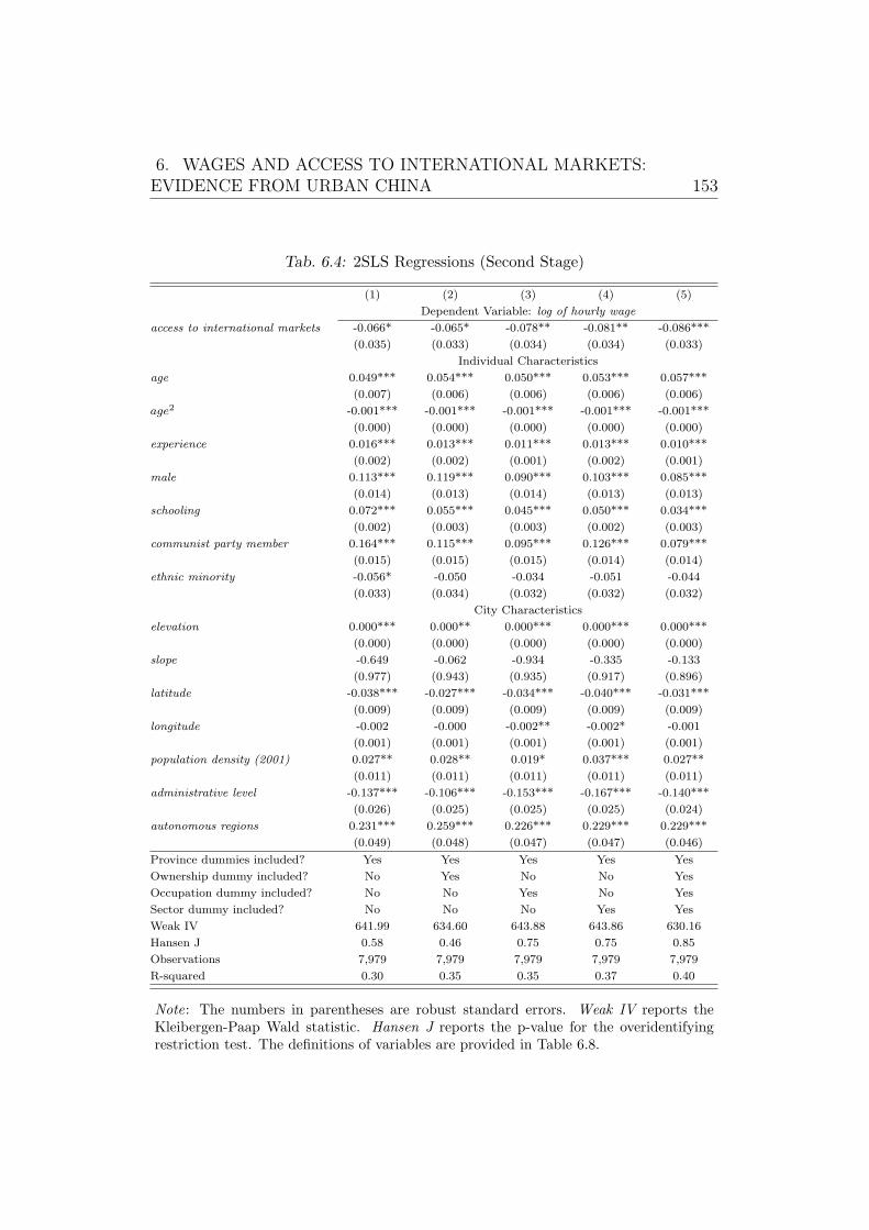
6. WAGES AND ACCESS TO INTERNATIONAL MARKETS:EVIDENCE FROM URBAN CHINA 153
Tab. 6.4: 2SLS Regressions (Second Stage)
(1) (2) (3) (4) (5)
Dependent Variable: log of hourly wage
access to international markets -0.066* -0.065* -0.078** -0.081** -0.086***
(0.035) (0.033) (0.034) (0.034) (0.033)
Individual Characteristics
age 0.049*** 0.054*** 0.050*** 0.053*** 0.057***
(0.007) (0.006) (0.006) (0.006) (0.006)
age2 -0.001*** -0.001*** -0.001*** -0.001*** -0.001***
(0.000) (0.000) (0.000) (0.000) (0.000)
experience 0.016*** 0.013*** 0.011*** 0.013*** 0.010***
(0.002) (0.002) (0.001) (0.002) (0.001)
male 0.113*** 0.119*** 0.090*** 0.103*** 0.085***
(0.014) (0.013) (0.014) (0.013) (0.013)
schooling 0.072*** 0.055*** 0.045*** 0.050*** 0.034***
(0.002) (0.003) (0.003) (0.002) (0.003)
communist party member 0.164*** 0.115*** 0.095*** 0.126*** 0.079***
(0.015) (0.015) (0.015) (0.014) (0.014)
ethnic minority -0.056* -0.050 -0.034 -0.051 -0.044
(0.033) (0.034) (0.032) (0.032) (0.032)
City Characteristics
elevation 0.000*** 0.000** 0.000*** 0.000*** 0.000***
(0.000) (0.000) (0.000) (0.000) (0.000)
slope -0.649 -0.062 -0.934 -0.335 -0.133
(0.977) (0.943) (0.935) (0.917) (0.896)
latitude -0.038*** -0.027*** -0.034*** -0.040*** -0.031***
(0.009) (0.009) (0.009) (0.009) (0.009)
longitude -0.002 -0.000 -0.002** -0.002* -0.001
(0.001) (0.001) (0.001) (0.001) (0.001)
population density (2001) 0.027** 0.028** 0.019* 0.037*** 0.027**
(0.011) (0.011) (0.011) (0.011) (0.011)
administrative level -0.137*** -0.106*** -0.153*** -0.167*** -0.140***
(0.026) (0.025) (0.025) (0.025) (0.024)
autonomous regions 0.231*** 0.259*** 0.226*** 0.229*** 0.229***
(0.049) (0.048) (0.047) (0.047) (0.046)
Province dummies included? Yes Yes Yes Yes Yes
Ownership dummy included? No Yes No No Yes
Occupation dummy included? No No Yes No Yes
Sector dummy included? No No No Yes Yes
Weak IV 641.99 634.60 643.88 643.86 630.16
Hansen J 0.58 0.46 0.75 0.75 0.85
Observations 7,979 7,979 7,979 7,979 7,979
R-squared 0.30 0.35 0.35 0.37 0.40
Note: The numbers in parentheses are robust standard errors. Weak IV reports theKleibergen-Paap Wald statistic. Hansen J reports the p-value for the overidentifyingrestriction test. The definitions of variables are provided in Table 6.8.
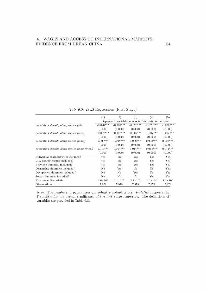
6. WAGES AND ACCESS TO INTERNATIONAL MARKETS:EVIDENCE FROM URBAN CHINA 154
Tab. 6.5: 2SLS Regressions (First Stage)
(1) (2) (3) (4) (5)
Dependent Variable: access to international markets
population density along routes (sd) -0.020*** -0.020*** -0.020*** -0.020*** -0.020***
(0.000) (0.000) (0.000) (0.000) (0.000)
population density along routes (min.) -0.007*** -0.007*** -0.007*** -0.007*** -0.007***
(0.000) (0.000) (0.000) (0.000) (0.000)
population density along routes (max.) 0.008*** 0.008*** 0.008*** 0.008*** 0.008***
(0.000) (0.000) (0.000) (0.000) (0.000)
population density along routes (max./min.) 0.014*** 0.014*** 0.014*** 0.014*** 0.014***
(0.000) (0.000) (0.000) (0.000) (0.000)
Individual characteristics included? Yes Yes Yes Yes Yes
City characteristics included? Yes Yes Yes Yes Yes
Province dummies included? Yes Yes Yes Yes Yes
Ownership dummies included? No Yes No No Yes
Occupation dummies included? No No Yes No Yes
Sector dummies included? No No No Yes Yes
First-stage F-statistic 3.6×10⁵ 2.1×10⁵ 2.4×10⁵ 1.9×10⁵ 1.1×10⁵
Observations 7,979 7,979 7,979 7,979 7,979
Note: The numbers in parentheses are robust standard errors. F-statistic reports theF-statistic for the overall significance of the first stage regressors. The definitions ofvariables are provided in Table 6.8.
6. WAGES AND ACCESS TO INTERNATIONAL MARKETS:EVIDENCE FROM URBAN CHINA 155
ness check includes city-level skill intensity which implies the accumulation
of local human capital. The indicator, skill intensity, is defined as the
proportion of the adult total labour force in the CHIPS (2002) that had
completed at least nine years of schooling.145 Accounting for skill intensity,
this chapter finds that the coefficient of access to international markets
remains statistically significant but quantitatively smaller than in column
(5) of Table 6.4. The shrink in the magnitude of the effect is possibly due to
external returns to schooling146 in Chinese cities as indicated in Liu (2007).147
The second robustness check looks at the inclusion of historical endow-
ments proxied by a binary indicator which is equal to unity if a city was
assigned to be a treaty port during the late 1800s.148 Treaty ports generally
developed better, because the westerners established municipal authorities,
police, judiciaries, manufacturing, and infrastructure in these cities (Banerjee
et al., 2012; Jia, 2012). Along with the ‘better’ institutions and earlier
industrialisation, the accessibility to railroads may facilitate the economic
prosperity in the majority of treaty ports, which could confound the effect
of access to international markets on wages.149 However, column (2) shows
that being a treaty port does not significantly raise individual wages given
that all other factors are carefully controlled for.150 More importantly, the
effect of access to international markets on wages is the same as column (5)
of Table 6.4, suggesting that the 2SLS estimates are tight and robust.
The final two robustness checks focus on the impact of the size of city-level
145 Nine years of schooling is equivalent to the completion of junior high school in China.146 External returns to schooling are the economic gains from the sharing of knowledgeamong workers. The key assumption is that a worker will gain a wage premium with theincrease in the average level of schooling of his group (e.g. firm level, sectoral level andcity level, among others).147 Using CHIPS (1988 and 1995), Liu (2007) finds a one-year increase in city averageeducation could increase individual earnings by between 11 and 13 percent, which indicatesthe presence of external returns to schooling among Chinese cities.148 Relevant information is obtained from Jia (2012).149 Note that even though prefecture population in 1820 used in this chapter is notdetermined by the status of treaty port after the First Opium War (1840), historicalpopulation still could be correlated with unobservables that raise the likelihood of beinga treaty port.150 Jia (2012) analyses 57 treaty ports and finds a positive relationship between being atreaty port and contemporary income over the period 1987–2007. In this study, only eightsampled cities were treaty ports in the late 1800s.
6. WAGES AND ACCESS TO INTERNATIONAL MARKETS:EVIDENCE FROM URBAN CHINA 156
population in 1953 and the early average rate of population growth during
1953–1964.151 It is possible that historical population is correlated with
initial population and its growth, although the population density in 2001
has been considered in equation (6.1). Therefore, one may argue that the
instrumental variables violate the exclusion restriction in a 2SLS estimation.
But, as columns (3) and (4) of Table 6.6 have shown, the coefficients of access
to international markets neither attenuate to zero nor become statistically
insignificant, which indicates that the historical instruments are not invalid.
The coefficients herein are similar to the baseline result in column (5) of Table
6.4, implying that the inclusion of early status and growth of population does
not confound the explanatory power of the instruments.152 Furthermore, only
the initial size of population in 1953 raises wages in 2002 but not the early
growth rate of population.
Although the omitted variables problem has been carefully examined
in Table 6.6, one may still be worried about the possibility that extreme
values can bias estimates. To this end, Table 6.7 provides a further test
to evaluate the sensitivity of the baseline 2SLS estimates to the exclusion
of extreme values in both dependent and independent variables. Columns
(1) and (2) show that the coefficients of access to international markets
remain unchanged compared with the result reported in column (5) of Table
6.4, excluding the top and bottom 10 percent urban wage earners in the
baseline model. This finding is crucial as it indicates that the causal effect
revealed in the 2SLS estimation is neither driven by the highest income
nor the lowest income group. Furthermore, Table 6.7 examines how the
exclusion of the nearest and farthest urban wage earners in terms of routes
distance from one’s location to the nearest major seaport affects the 2SLS
estimates, which is motivated by Banerjee et al. (2012). As one can see in
columns (3) and (4), the coefficients of interest are still significant, although
their magnitude departs from the baseline result in column (5) of Table
151 This is because 1953 and 1964 are the two population censuses after 1949 when thePeople’s Republic of China was founded. County-level population information is providedby National Bureau of Statistics China (1988) in which the first and second populationcensus (1953 and 1964 respectively) data are available.152 This is further confirmed by the first stage results listed in columns (3) and (4).
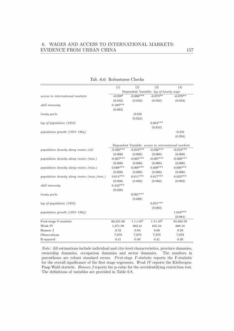
6. WAGES AND ACCESS TO INTERNATIONAL MARKETS:EVIDENCE FROM URBAN CHINA 157
Tab. 6.6: Robustness Checks
(1) (2) (3) (4)
Dependent Variable: log of hourly wage
access to international markets -0.059* -0.086*** -0.073** -0.079**
(0.032) (0.033) (0.032) (0.033)
skill intensity 0.180***
(0.063)
treaty ports -0.016
(0.024)
log of population (1953) 0.064***
(0.010)
population growth (1953–1964) -0.331
(0.294)
Dependent Variable: access to international markets
population density along routes (sd) -0.020*** -0.019*** -0.020*** -0.019***
(0.000) (0.000) (0.000) (0.000)
population density along routes (min.) -0.007*** -0.007*** -0.007*** -0.006***
(0.000) (0.000) (0.000) (0.000)
population density along routes (max.) 0.008*** 0.008*** 0.008*** 0.008***
(0.000) (0.000) (0.000) (0.000)
population density along routes (max./min.) 0.014*** 0.011*** 0.017*** 0.023***
(0.000) (0.002) (0.002) (0.002)
skill intensity 0.442***
(0.028)
treaty ports 0.091***
(0.008)
log of population (1953) 0.051***
(0.003)
population growth (1953–1964) 1.018***
(0.084)
First-stage F-statistic 60,221.69 1.1×10⁵ 1.5×10⁵ 94,462.59
Weak IV 1,271.99 662.41 635.24 668.18
Hansen J 0.52 0.84 0.68 0.93
Observations 7,979 7,979 7,979 7,979
R-squared 0.41 0.40 0.41 0.40
Note: All estimations include individual and city-level characteristics, province dummies,ownership dummies, occupation dummies and sector dummies. The numbers inparentheses are robust standard errors. First-stage F-statistic reports the F-statisticfor the overall significance of the first stage regressors. Weak IV reports the Kleibergen-Paap Wald statistic. Hansen J reports the p-value for the overidentifying restriction test.The definitions of variables are provided in Table 6.8.
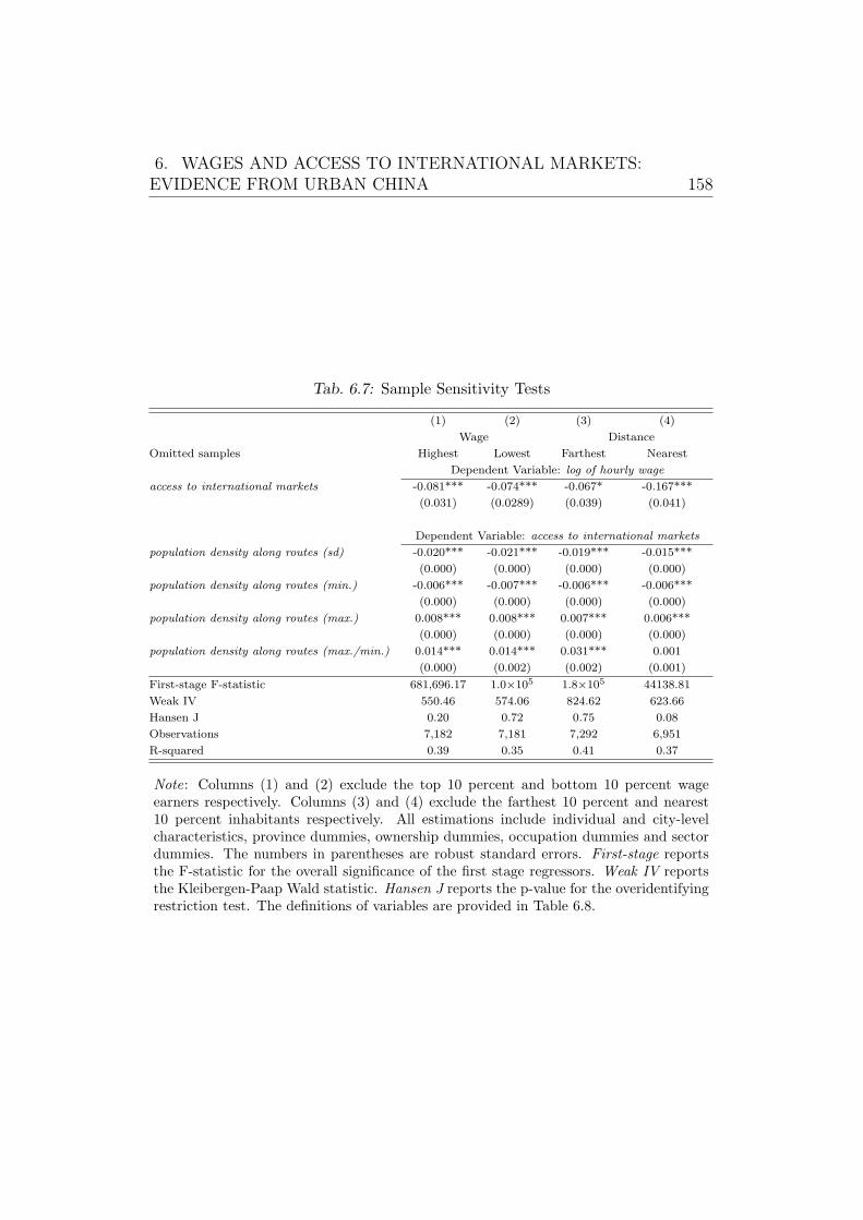
6. WAGES AND ACCESS TO INTERNATIONAL MARKETS:EVIDENCE FROM URBAN CHINA 158
Tab. 6.7: Sample Sensitivity Tests
(1) (2) (3) (4)
Wage Distance
Omitted samples Highest Lowest Farthest Nearest
Dependent Variable: log of hourly wage
access to international markets -0.081*** -0.074*** -0.067* -0.167***
(0.031) (0.0289) (0.039) (0.041)
Dependent Variable: access to international markets
population density along routes (sd) -0.020*** -0.021*** -0.019*** -0.015***
(0.000) (0.000) (0.000) (0.000)
population density along routes (min.) -0.006*** -0.007*** -0.006*** -0.006***
(0.000) (0.000) (0.000) (0.000)
population density along routes (max.) 0.008*** 0.008*** 0.007*** 0.006***
(0.000) (0.000) (0.000) (0.000)
population density along routes (max./min.) 0.014*** 0.014*** 0.031*** 0.001
(0.000) (0.002) (0.002) (0.001)
First-stage F-statistic 681,696.17 1.0×10⁵ 1.8×10⁵ 44138.81
Weak IV 550.46 574.06 824.62 623.66
Hansen J 0.20 0.72 0.75 0.08
Observations 7,182 7,181 7,292 6,951
R-squared 0.39 0.35 0.41 0.37
Note: Columns (1) and (2) exclude the top 10 percent and bottom 10 percent wageearners respectively. Columns (3) and (4) exclude the farthest 10 percent and nearest10 percent inhabitants respectively. All estimations include individual and city-levelcharacteristics, province dummies, ownership dummies, occupation dummies and sectordummies. The numbers in parentheses are robust standard errors. First-stage reportsthe F-statistic for the overall significance of the first stage regressors. Weak IV reportsthe Kleibergen-Paap Wald statistic. Hansen J reports the p-value for the overidentifyingrestriction test. The definitions of variables are provided in Table 6.8.

6. WAGES AND ACCESS TO INTERNATIONAL MARKETS:EVIDENCE FROM URBAN CHINA 159
6.4. The interpretation is two-fold. Firstly, the significant results again
suggest the 2SLS estimates are robust and reliable. Secondly, on the one
hand, not accounting for the farthest urban wage earners tends to weaken
the effect of access to international markets on wages, on the other hand,
excluding the nearest urban wage earners strengthens this effect. Overall,
the differential magnitude of these impacts complements the basic average
estimates in Table 6.4, which contributes to a comprehensive understanding
of the heterogeneous effect of being located far from international markets. In
sum, the results presented in Table 6.7 confirm the robustness of the baseline
2SLS estimates.
5. Conclusion
Focusing on urban China, this chapter proposes a new identification strategy
that uses heterogeneity of inter-prefecture population density in 1820 to
identify the effect of accessibility to international markets on individual wages
in urban China. It finds that the length of contemporary transport routes
connecting the origin city and its nearest major seaport is strongly influenced
by differentials in historical population density, which suggests that the set of
instruments this study constructs successfully captures independent variation
in access to international markets. Using these instruments, this chapter
finds that every 1 percent increase in length of current transport routes from
the origin city to international markets (i.e. the nearest seaport), ceteris
paribus, has a negative impact on individual wages of 0.086 percent. An
alternative interpretation could be that every 1 percent reduction of length of
transport routes from the origin city to its nearest seaport can raise individual
wages by 0.086 percent. This causal effect is robust to the inclusion of a
large number of additional control variables such as current labour market
structure, historical factor endowments, and initial population development,
to running separate regressions that exclude the 10 percent highest-income
and lowest-income urban wage earners respectively, and to running separate
regressions that get rid of the 10 percent nearest and farthest urban wage
6. WAGES AND ACCESS TO INTERNATIONAL MARKETS:EVIDENCE FROM URBAN CHINA 160
earners in terms of routes distance from one’s location to the nearest major
seaport respectively.
This chapter makes two contributions. First, it explores the research
area of using historical information as instrumental variables to mitigate
endogeneity problems of contemporary variables. The effort of providing
new historical instruments is related to the work in Banerjee et al. (2012)
and Chapter 4. Although this is not the first attempt to employ historical
information as instrumental variables, it is one of the pioneering studies that
use this approach to identify causal effects in the area of China’s economic
development.
Second, the main finding confirms that the accessibility to international
markets has significant and heterogeneous effects on individual wages among
Chinese cities. Relating to Chapters 3 and 4 that confirm the contributions of
the improvement of transportation infrastructure to short-run and long-run
economic growth using provincial data, this chapter provides some micro-
level evidence that the heterogeneity of transportation infrastructure, i.e. the
varying length of transport routes connecting the origin city and its nearest
major seaport, may result in income disparities in urban areas.
This chapter also has important policy implications. While Chapters
3 and 4 have pointed out the ‘positive’ effect of improving transportation
infrastructure which can raise regional economic growth, this chapter reveals
the ‘negative’ effect that it may widen the wage gap between urban wage
earners. The presence of the negative effect indicates the drawback of a
policy that focuses on raising investment in transportation infrastructure.
Therefore, policy-makers should realise that reducing wage inequality in
urban China while maintaining high rates of regional economic growth could
be difficult to manage. A possible solution may require complementary
policies that can efficiently deal with the increasing wage inequality among
urban wage earners.
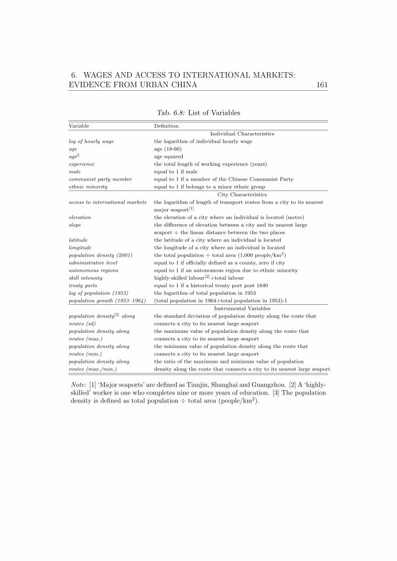
6. WAGES AND ACCESS TO INTERNATIONAL MARKETS:EVIDENCE FROM URBAN CHINA 161
Tab. 6.8: List of Variables
Variable Definition
Individual Characteristics
log of hourly wage the logarithm of individual hourly wage
age age (18-60)
age2 age squared
experience the total length of working experience (years)
male equal to 1 if male
communist party member equal to 1 if a member of the Chinese Communist Party
ethnic minority equal to 1 if belongs to a minor ethnic group
City Characteristics
access to international markets the logarithm of length of transport routes from a city to its nearest
major seaport[1]
elevation the elevation of a city where an individual is located (metre)
slope the difference of elevation between a city and its nearest large
seaport ÷ the linear distance between the two places
latitude the latitude of a city where an individual is located
longitude the longitude of a city where an individual is located
population density (2001) the total population ÷ total area (1,000 people/km2)
administrative level equal to 1 if officially defined as a county, zero if city
autonomous regions equal to 1 if an autonomous region due to ethnic minority
skill intensity highly-skilled labour[2]÷total labour
treaty ports equal to 1 if a historical treaty port post 1840
log of population (1953) the logarithm of total population in 1953
population growth (1953–1964) (total population in 1964÷total population in 1953)-1
Instrumental Variables
population density[3] along the standard deviation of population density along the route that
routes (sd) connects a city to its nearest large seaport
population density along the maximum value of population density along the route that
routes (max.) connects a city to its nearest large seaport
population density along the minimum value of population density along the route that
routes (min.) connects a city to its nearest large seaport
population density along the ratio of the maximum and minimum value of population
routes (max./min.) density along the route that connects a city to its nearest large seaport
Note: [1] ‘Major seaports’ are defined as Tianjin, Shanghai and Guangzhou. [2] A ‘highly-skilled’ worker is one who completes nine or more years of education. [3] The populationdensity is defined as total population ÷ total area (people/km2).
7. CONCLUSION
This research has investigated three causal relationships in China’s eco-
nomic development during 1978–2008, i.e. transportation infrastructure
to economic growth, economic growth to urbanisation, and transportation
infrastructure to income inequality. This chapter summarises empirical
findings from Chapters 3 to 6, outlines key contributions of this thesis, and
addresses potential further research.
1. Concluding Remarks
The first question of interest is: “What is the short-run effect of changes in
the density of transportation infrastructure on economic growth in China?”
Based on provincial panel data over the period 1985 to 2008, Chapter 3 uses
the timing of the National Congress of the Communist Party of China to
construct 2SLS estimates of within-province effect of changes in the density
of transportation infrastructure on GDP growth per capita. Chapter 3
finds that while the OLS estimate is nearly zero, the 2SLS estimate shows
that a one standard deviation increase in the density of transportation
infrastructure, ceteris paribus, has an effect of raising GDP growth per capita
by more than 6 percentage points on average. This short-run effect is robust
to the inclusion of a large number of additional control variables, to running
separate regressions for the coastal and non-coastal regions, and to the use
of instruments that still draw information from the National Congress but
are constructed in four different ways.
The second question this thesis has looked at is: “What is the long-run
impact of changes in the density of transportation infrastructure on economic
7. CONCLUSION 163
growth in China?” The quantification of this long-run impact contributes to
a better understanding of the role of transportation infrastructure in China’s
economic growth, which extends the analysis in Chapter 3. In order to
mitigate endogenous issues in the analysis, Chapter 4 employs the density
of ownership of Chinese guilds, as measured by the number of guilds in
the Qing dynasty per 10,000 people, to identify exogenous variation in the
initial level of provision of the transportation infrastructure. Using Chinese
provincial panel data over the period 1978 to 2008, Chapter 4 shows that
the OLS estimates of the effect of changes in the density of transportation
infrastructure on economic growth in the long run, i.e.over a 15-year period,
are very close to zero. However, the instrumental variable estimates suggest
that transportation infrastructure is an important determinant of long-run
economic growth, where a one standard deviation increase in the density
of the initial level of transport infrastructure is associated with a 1.54 to
2.44 percentage point increase in the long-run economic growth on average.
This result is not directly comparable with the magnitude of the short-
run effect estimated in Chapter 3, because it captures an average effect of
the improvement of initial level of transportation infrastructure on a 15-
year average of economic growth rather than an effect of annual changes in
transportation infrastructure on yearly economic growth. Furthermore, this
strong long-run causal effect of transportation infrastructure is highly robust
in a battery of sensitivity tests where four potentially relevant determinants
of growth – urbanisation, openness, share of agricultural labour, and share
of public sectoral labour – are added into the regression.
The third question that has been addressed in the thesis is: “Does
economic growth affect urbanisation?” Using a panel dataset for Chinese
provinces during 1985–2008, Chapter 5 proposes a new identification strategy
to construct instrumental variable estimates of the within-province effect that
GDP growth per capita has on the urbanisation rate. This strategy uses
the timing of the National Congress of the Communist Party. Chapter 5
finds that GDP growth per capita is strongly associated with the timing of
the National Congress. Using instrumental variables that convey this timing
information, 2SLS estimates suggest that economic growth has a statistically
7. CONCLUSION 164
significant effect on raising the urbanisation rate. This result is robust not
only to the inclusion of a battery of additional controls, i.e. attributes
of provincial leaders, government expenditure, labour force composition,
agricultural output, urban wage growth, population density and rainfall, but
also to the employment of alternative forms of time trend, i.e. national time
trend, its quadratic form and quadratic region-specific time trend.
The fourth question that has been investigated in the thesis is: “How
does access to international markets affect individual wages?” Chapter
6 proposes a new identification strategy that uses heterogeneity of inter-
prefecture population density in 1820 to identify the effect of accessibility to
international markets, as proxied by length of transport routes connecting
the origin city to its nearest major seaport, on individual wages in urban
China. Using China Household Income Project Survey (2002) data, Chapter
6 finds that the length of contemporary transport routes is strongly influenced
by differentials in historical population density. Based on 2SLS estimates,
Chapter 6 also shows every 1 percent increase in length of transport routes
from the origin city to international markets (i.e. accessibility to international
markets), ceteris paribus, has a negative impact on individual wages of
0.086 percent. An alternative interpretation could be that every 1 percent
reduction of length of transport routes from the origin city to its nearest
seaport can raise individual wages by 0.086 percent. This indicates the
importance of the provision of transportation infrastructure based on micro-
level evidence. The causal effect is robust to the inclusion of a host
of additional control variables such as current labour market structure,
historical factor endowments, and initial population development. The causal
effect remains unchanged, when the estimation excludes the 10 percent
highest-income and lowest-income urban wage earners respectively, or gets
rid of the 10 percent nearest and farthest urban wage earners in terms of
distance from one’s location to the nearest major seaport respectively.
7. CONCLUSION 165
2. Key Contributions
2.1 Identification Strategies
Methodologically, this thesis contributes to the empirical literature by
proposing new identification strategies, using China as a case study. A
common problem that occurs in the empirical analysis is endogeneity
caused by omitted variables, measurement errors, and reverse causality.
The instrumental variables approach, based on China’s political cycle and
historical information, helps to ameliorate endogeneity biases and achieve
identifications in the analysis.
In Chapter 3 and Chapter 5, two major casual relationships, i.e. trans-
portation infrastructure-economic growth and economic growth-urbanisation,
which suffer from the reserve causality problem, are analysed. The
endogeneity issues become more severe, as this thesis uses data obtained
from the National Bureau of Statistics of China (NBSC) which may contain
measurement errors (Rawski, 2001; Rawski and Xiao, 2001; Chow, 2006;
Ravallion and Chen, 2007). Chapters 3 and 5 employ standard fixed-effect
estimation in a panel data framework to purge provincial time-invariant
unobservables. For the time-variant unobservables, they use instrumental
variables, i.e. the timing of the National Congress of the Communist Party
of China (CPC), to mitigate the biases result from omitted variables. This is
the first study embedded in a economic growth framework that uses China’s
political cycle to construct instrumental variables. Technically, it helps to
generate exogenous variations in endogenous variables in order to ameliorate
biases caused by reverse causality and measurement errors. Intuitively,
the first-stage results in Chapters 3 and 5 paint a picture, illustrating
that China’s improvement of transportation infrastructure and GDP per
capita growth are statistically positively associated with the time of National
Congress of the CPC. Realising such a unique pattern of China’s economic
growth, development economists may follow the instrumental variables
proposed in this thesis to study other causal relationships of interest.
In addition, this thesis is one of the pioneering studies that uses China’s
7. CONCLUSION 166
historical information to construct instrumental variables.153 Chapters 4 and
6 employ information about ownership of Chinese guilds in the Qing dynasty
and prefecture-level population density in 1820 to instrument for the initial
level of transportation infrastructure and accessibility to transportation
infrastructure, respectively. The strong and robust first-stage results shown
in Chapters 4 and 6 indicate that historical events, even if this happened more
than 100 years ago, can still be important determinants of contemporary
macro variables. The close links between historical instrumental variables
and modern-time endogenous variables of interest are consistent with what
has been demonstrated in those influential studies in the literature exploring
the area of using historical instruments, e.g. Acemoglu et al. (2001), West
and Woessmann (2010), and Pascali (2012), among others.
In sum, this thesis provides powerful weapons to deal with complicated
endogeneity issues in the context of China. Importantly, those instrumental
variables involved in this research work well in both panel data framework and
cross-sectional data framework, which may benefit other empirical studies
that suffer from endogeneity problems.
2.2 Policy Implications
Combining macro and micro evidence, this research provides the first policy
implication that although the improvement of transportation infrastructure
can raise GDP per capita growth as presented in Chapter 3, policy-makers
should pay attention to the current uneven distribution of transportation
infrastructure across regions. Firstly, contemporary disparity of the provision
of transportation infrastructure may substantially affect regional economic
growth in the long run as shown in Chapter 4. Secondly, the divergence
of accessibility of transportation infrastructure may result in increasing
income inequality in urban areas as analysed in Chapter 6. This research
provides a reminder that although the overall quantity of transportation
153 To date, there is just a handful of working papers, e.g. Banerjee et al. (2012) andFang and Zhao (2009) among others, have used historical information to look at China’seconomic development.
7. CONCLUSION 167
infrastructure is crucial for China’s economic growth, the even distribution
of transportation infrastructure should not be neglected in the long run.
Furthermore, as Chinese policy-makers often emphasise the construction
of transportation infrastructure without a clear understanding of how to
distribute it, researchers should provide more evidence-based policy advice,
for instance, quantifying the actual influence of (un)even distribution of
transportation infrastructure on regional economic development relying on
both macro and micro data.
The second policy implication is related to the balancing of economic
growth and urbanisation. As shown in Chapter 5, China’s economic
growth causally raises its urbanisation rate. At first glance, policy-makers
might choose to focus on the positive contribution of economic growth to
urbanisation, if they intend to encourage rural-to-urban migration when
the overall urbanisation rate is relatively low during a certain stage of
development. However, the rapid pace at which urbanisation is occurring
in China raises critical issues that are not examined in this thesis but
in existing studies, such as rising CO2 emissions (Feng et al., 2009; Du
et al., 2012) and the proliferation of substandard living habitats known as
urban villages.154 From the sustainable development perspective, policy-
makers have to keep the balance between increasing urbanisation and rates
of economic growth. However, this requires recalibrating the GDP growth
targets, which is detrimental to economic growth. This research advises that
Chinese policy-makers should consider lowering economic growth targets at
least for those highly-urbanised regions.
154 Song and Zenou (2012) describe urban villages as habitats where “buildings areovercrowded; public stairways and pathways inside buildings are extremely narrow; publicfacilities are inadequate and poorly maintained; public roadways cannot meet the basicrequirements of transportation and fire control standards; distances between buildings arewell below standard and cannot meet fire control standards; and garbage is scattered andunhygienic”.
7. CONCLUSION 168
3. Further Research
This research has at least two directions of extension. The first one is closely
related to the topics that have been addressed in this thesis, while the second
one is a concern about technical issues.
Two causal relationships studied in this thesis are transportation infras-
tructure to economic growth and economic growth to urbanisation, but this
thesis has not yet investigated whether the improvement of transportation
infrastructure causally raises urbanisation in China. If this causal link
exists, researchers may be interested in quantifying the contribution of
the provision of transportation infrastructure to urbanisation. Several
recent studies, for instance, Baum-Snow and Turner (2012) and Baum-
Snow et al. (2012),155 use historical infrastructure networks (railroads) to
capture exogenous variations in contemporary transportation, and identify
the causal effects of the improvement of transportation infrastructure on
China’s urbanisation process. As they do not find statistically significant
evidence that the expansion of transportation infrastructure results in higher
urbanisation rates, more empirical studies in this area are desired to check
the robustness of their findings.
The second direction could be a further exploration in the area of
using historical information as instrumental variables. For example, guilds
density employed in Chapter 4 could instrument for current trade or FDI.
Alternatively, there are many potential candidates of historical instruments,
and they can be used in the areas other than the focus of this thesis. For
instance, Shiue (2002) provides a novel dataset of rice prices over the period
1743–1795 which can be used as instruments for the long-run condition of
agricultural production or stability of agricultural markets. Another example
could be to use temperature and rainfall information from Terrestrial Air
Temperature and Precipitation: Monthly and Annual Time Series (1900
- 2008) during 1900–1957 to construct a set of instrumental variables for
agricultural outputs during the Great Chinese Famine (1958–1961).
All ideas listed above may result in a host of studies that contribute to
155 These are all unpublished manuscripts.

7. CONCLUSION 169
a more comprehensive understanding of China’s economic development and
Chinese economic history.
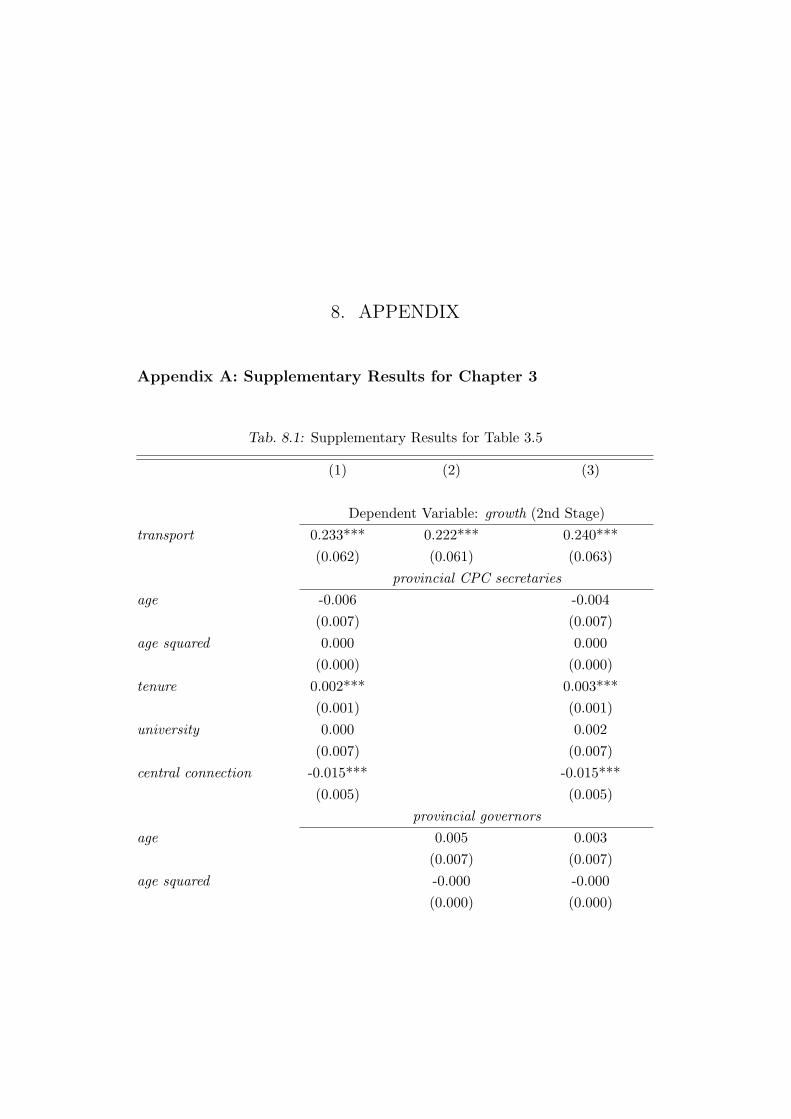
8. APPENDIX
Appendix A: Supplementary Results for Chapter 3
Tab. 8.1: Supplementary Results for Table 3.5
(1) (2) (3)
Dependent Variable: growth (2nd Stage)
transport 0.233*** 0.222*** 0.240***
(0.062) (0.061) (0.063)
provincial CPC secretaries
age -0.006 -0.004
(0.007) (0.007)
age squared 0.000 0.000
(0.000) (0.000)
tenure 0.002*** 0.003***
(0.001) (0.001)
university 0.000 0.002
(0.007) (0.007)
central connection -0.015*** -0.015***
(0.005) (0.005)
provincial governors
age 0.005 0.003
(0.007) (0.007)
age squared -0.000 -0.000
(0.000) (0.000)
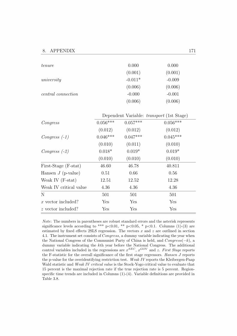
8. APPENDIX 171
tenure 0.000 0.000
(0.001) (0.001)
university -0.011* -0.009
(0.006) (0.006)
central connection -0.000 -0.001
(0.006) (0.006)
Dependent Variable: transport (1st Stage)
Congress 0.056*** 0.057*** 0.056***
(0.012) (0.012) (0.012)
Congress (-1) 0.046*** 0.047*** 0.045***
(0.010) (0.011) (0.010)
Congress (-2) 0.018* 0.019* 0.019*
(0.010) (0.010) (0.010)
First-Stage (F-stat) 46.60 46.78 40.811
Hansen J (p-value) 0.51 0.66 0.56
Weak IV (F-stat) 12.51 12.52 12.28
Weak IV critical value 4.36 4.36 4.36
N 501 501 501
x vector included? Yes Yes Yes
z vector included? Yes Yes Yes
Note: The numbers in parentheses are robust standard errors and the asterisk representssignificance levels according to *** p<0.01, ** p<0.05, * p<0.1. Columns (1)-(3) areestimated by fixed effects 2SLS regression. The vectors x and z are outlined in section4.1. The instrument set consists of Congress, a dummy variable indicating the year whenthe National Congress of the Communist Party of China is held, and Congress(−k), adummy variable indicating the kth year before the National Congress. The additionalcontrol variables included in the regressions are xSEC , xGOV and z. First Stage reportsthe F-statistic for the overall significance of the first stage regressors. Hansen J reportsthe p-value for the overidentifying restriction test. Weak IV reports the Kleibergen-PaapWald statistic and Weak IV critical value is the Stock-Yogo critical value to evaluate that15 percent is the maximal rejection rate if the true rejection rate is 5 percent. Region-specific time trends are included in Columns (1)-(4). Variable definitions are provided inTable 3.8.
8. APPENDIX 172
Appendix B: Background of Chinese Guilds (Chapter 4)
Origins and Characteristics
The Chinese guilds were forms of corporate collective action that first came
about during the Ming dynasty (1368–1644) and flourished towards the end of
the Qing dynasty (1644–1911). In Chinese, the most appropriate translation
of ‘guild’ is Hanghui which means “trade-line associations” (Quan, 1934).
The Chinese guilds provided a wide range of economic and social services,
for examples, the matching of skilled workers with employers, providing a
meeting place for merchants and their buyers, and offering hospitality services
in the form of hotels, restaurants and entertainment centres.
Generally, guilds were established by merchants who aimed to protect
themselves from being exploited and discriminated against by the Chinese
bureaucrats (Peng, 1995), since merchants were treated as the last-tier
citizens according to a transitional ranking of social strata before 1911. The
ranking was scholars (shi), peasants (nong), artisans (gong) and merchants
(shang). In this regard, merchants had to struggle for their own rights by
setting up associations like guilds.
There were many types of guilds such as Gongsuo, Huiguan and Tang,
among others. The majority of guilds (e.g. Gongsuo, Huiguan, Tang, Dian,
Bang, Hui, Gonghui, Ge, Zhuang, Gongguan, Hang and Hanghui) were
related to merchant and trade activities. A few of the guilds were named
as religious (or sacrificial) shrines and traditional Confucian academies (i.e.
Miao, She, Shuyuan, Ci and Si) but still served as merchant and trade
associations (Moll-Murata, 2008; Peng, 1995).
In general, all forms of “Chinese craft, merchant and trade associations”
could be regarded as guilds (Moll-Murata, 2008), although they might have
different functions. Table 8.2 shows the most common types of Chinese guilds
(1655-1911), of which Gongsuo and Huiguan were by far the largest groups.
Gongsuo and Huiguan mean ‘public hall’ and ‘(common-origin) assembly
house’, respectively. However, along with other forms of guilds, they were
also well known as “mutual help associations” among numerous sectors (Moll-
Murata, 2008), for instance, private banks (qianzhuang) in the Yangtze Delta
8. APPENDIX 173
Tab. 8.2: Designations for Qing Dynasty Guilds (1655–1911)
Source: Moll-Murata (2008).
(finance),156 the Wuzhou157 opium guild and the Ningbo158 fishermen’s guild
(fishery) (Peng, 1995).
Guilds had various functions, for example, Gongsuo and Huiguan played
different roles in commercial activities. The major members of Gongsuo,
which could be recognised as pre-modern (prior to 1911) Chinese unions,
156 The Yangtze Delta consists of southern Jiangsu province, northern Zhejiang provinceand Shanghai municipality.157 Wuzhou is a city which is close to the border between Guangxi and Guangdongprovinces.158 Ningbo is a coastal city and important seaport in Zhejiang province.
A NOTE:
This figure/table/image has been removed to comply with copyright regulations. It is included in the print copy of the thesis held by the University of Adelaide Library.
8. APPENDIX 174
were retailers and artisans. Gongsuo distinguished itself from other guilds,
because they engaged in wage bargaining between employees and employers,
whereas other guilds did not (Peng, 1995).
Huiguan did not serve as unions. Instead, they played a crucial role in
commercial activities that channel merchants, workers and artisans from the
same original communities. Most Huiguan functioned as hotels, restaurants,
entertainment centres and even job markets, since their members usually
came from the same provinces or prefectures. A good example would be
Sichuan Huiguan,159 i.e. those Huiguan located in Sichuan province and
financed by early immigrants. They were famous for their great contribution
to hosting new immigrants by providing accommodation and job information.
The new immigrants were peasants from neighbouring provinces who moved
to Sichuan province for jobs and better earnings. The presence of Huiguan
lowered their living and job-search costs. By contrast, those Huiguan located
in Peking160 mainly served as liaison offices, where the representatives of
the guilds would meet with the representatives of the central government
to discuss business and regulation issues (Moll-Murata, 2008). From an
economic perspective, the density of ownership of guilds in one province
could indicate the nature of local business networks, financial development
and commercial prosperity.
With regard to the question of whether Chinese guilds were legal entities,
Peng (1995) indicates that most guilds did not register their activities in
government departments. This was an issue because governments did not
recognise guilds as legal business entities. Meanwhile, guilds themselves
did not intend to be regulated by governments. They preferred to manage
business activities within sectors themselves. While there were no formal
arrangements, guilds were sometimes allowed informally by the governments
to regulate their markets given the condition that their members would pay
commodity taxes imposed by governments.
Having significant market power, guilds promised to protect their mem-
159 Sichuan is a south-western Chinese province.160 Also known as Beijing, the capital city of the Ming dynasty, the Qing dynasty andthe People’s Republic of China.
8. APPENDIX 175
bers against various uncertainties. For example, when diplomatic conflicts
between local merchants and foreigners occurred, the representatives of guilds
might negotiate with government officials to resolve issues on behalf of guild
members. The protection could also be achieved for some internal affairs
without the involvement of the governments, since the highest commissions
of guilds had jurisdictions which ensured that they could deal with internal
issues according to their ‘laws’ (Moll-Murata, 2008; Peng, 1995). But this did
not mean that the Chinese governments never attempted to regulate guilds.
In 1867, the government of Guangdong province banned a secretly-founded
tobacco guild which intended to monopolise the local market (Moll-Murata,
2008). This case implied that although sophisticated laws that could regulate
guilds were few, guilds still faced the risk from local government interventions.
In short, the answer to the question about whether Chinese guilds were legal
would be Hosea Morse’s161 famous dictum: “The guilds were never within
the law: they grew up outside the law; and as associations they neither
recognised the law nor claimed its protection.” (Morse, 1909)
To sum up, Chinese guilds essentially were not purely commercial
communities like European guilds (Moll-Murata, 2008; Peng, 1995). They
were not ‘normal’ associations either, in the sense that they were able
to perform as a form of independent socio-economically integrated entity
which implemented private rules, standards and even jurisdictions, and
central government rarely intervened if local governments acknowledged the
activities of particular guilds.
Economic Functions
The first economic function of guilds in the Qing dynasty was serving in
part as modern-time labour unions and pricing committees. As introduced
in Peng (1995), guild members including both employers (e.g. craftsmen and
merchants) and employees (e.g. apprentices) had to obey the regulations
in their guilds. These regulations mainly constituted of minimum wages for
apprenticeships and regulated prices of commodities or services. For example,
161 Hosea Morse (1855-1934) was the Statistical Secretary of the Inspectorate General ofCustoms in China.
8. APPENDIX 176
the management boards, the highest committees of all types of guilds whose
directors were recruited from registered members, imposed minimum wages
to protect the second-tier members, i.e. apprentices (xuetu), from being
exploited by the first-tier members — masters (shifu). The protection of
apprentices led to a relatively stable number of potential masters in the
future, because most masters (e.g. craftsmen or merchants) were previously
apprentices who had completed three-year formal apprenticeship contracts
and could afford registration fees of guilds (Moll-Murata, 2008; Peng, 1995).
Although some of the rules like the regulation of pricing might lead to
monopolies in a particular market, the other policies like the minimum wages
during the late Qing dynasty (1840–1911) ensured that people on low incomes
could afford food, clothes and accommodation.162 Overall, those regulations
imposed by Chinese guilds resulted in a stable provision of skilled labour and
contributed to the reduction of income inequality among members.
The second economic function of guilds was imposing some controls on
trade. For instance, a saggar maker in Jingdezhen163 could only purchase raw
materials from one supplier and sell their saggars to the nominated buyers
(Moll-Murata, 2008). Another example was the textile industry in Suzhou.164
Merchants (duanzhuang jihu) provided materials (e.g. cottons and silks) to
skilled workers (jigong). These workers were weavers who were involved in
the household production with their own spinning machines, and paid by
piece-rate wages (Peng, 1995). Although this might potentially restrict free
capital flows from a modern economics point of view, the control had been
a great revolution of resource allocation in an agrarian economy like the
Qing dynasty before 1840. Thus, an increase in the number of guilds was
seen as a positive signal of China’s commercialisation, industrialisation and
modernisation.
Last but not least, guilds donated to education and municipal services
162 From a modern perspective, guilds distorted wages and market prices. However, inpre-modern China (prior to 1911), guilds served as a successful stabiliser for the society.163 A saggar is a ceramic, boxlike container used in the firing of pottery to enclose orprotect ware in kilns. Jingdezhen is a town in Jiangxi province which is famous for theproduction of high-quality china.164 Suzhou is a city in Jiangsu province.

8. APPENDIX 177
(Moll-Murata, 2008). They provided elementary schools to members, as
well as firefighting, policing and maintenance of streets and bridges for local
residents (Rowe, 1992).
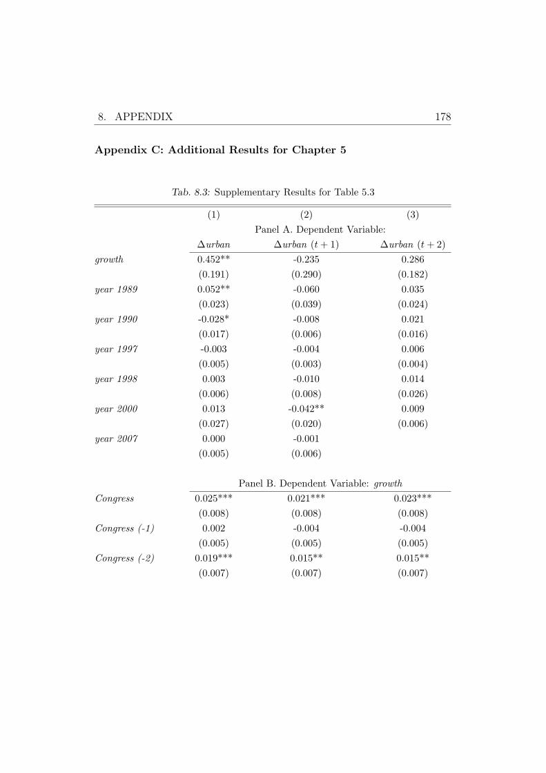
8. APPENDIX 178
Appendix C: Additional Results for Chapter 5
Tab. 8.3: Supplementary Results for Table 5.3
(1) (2) (3)
Panel A. Dependent Variable:
∆urban ∆urban (t+ 1) ∆urban (t+ 2)
growth 0.452** -0.235 0.286
(0.191) (0.290) (0.182)
year 1989 0.052** -0.060 0.035
(0.023) (0.039) (0.024)
year 1990 -0.028* -0.008 0.021
(0.017) (0.006) (0.016)
year 1997 -0.003 -0.004 0.006
(0.005) (0.003) (0.004)
year 1998 0.003 -0.010 0.014
(0.006) (0.008) (0.026)
year 2000 0.013 -0.042** 0.009
(0.027) (0.020) (0.006)
year 2007 0.000 -0.001
(0.005) (0.006)
Panel B. Dependent Variable: growth
Congress 0.025*** 0.021*** 0.023***
(0.008) (0.008) (0.008)
Congress (-1) 0.002 -0.004 -0.004
(0.005) (0.005) (0.005)
Congress (-2) 0.019*** 0.015** 0.015**
(0.007) (0.007) (0.007)
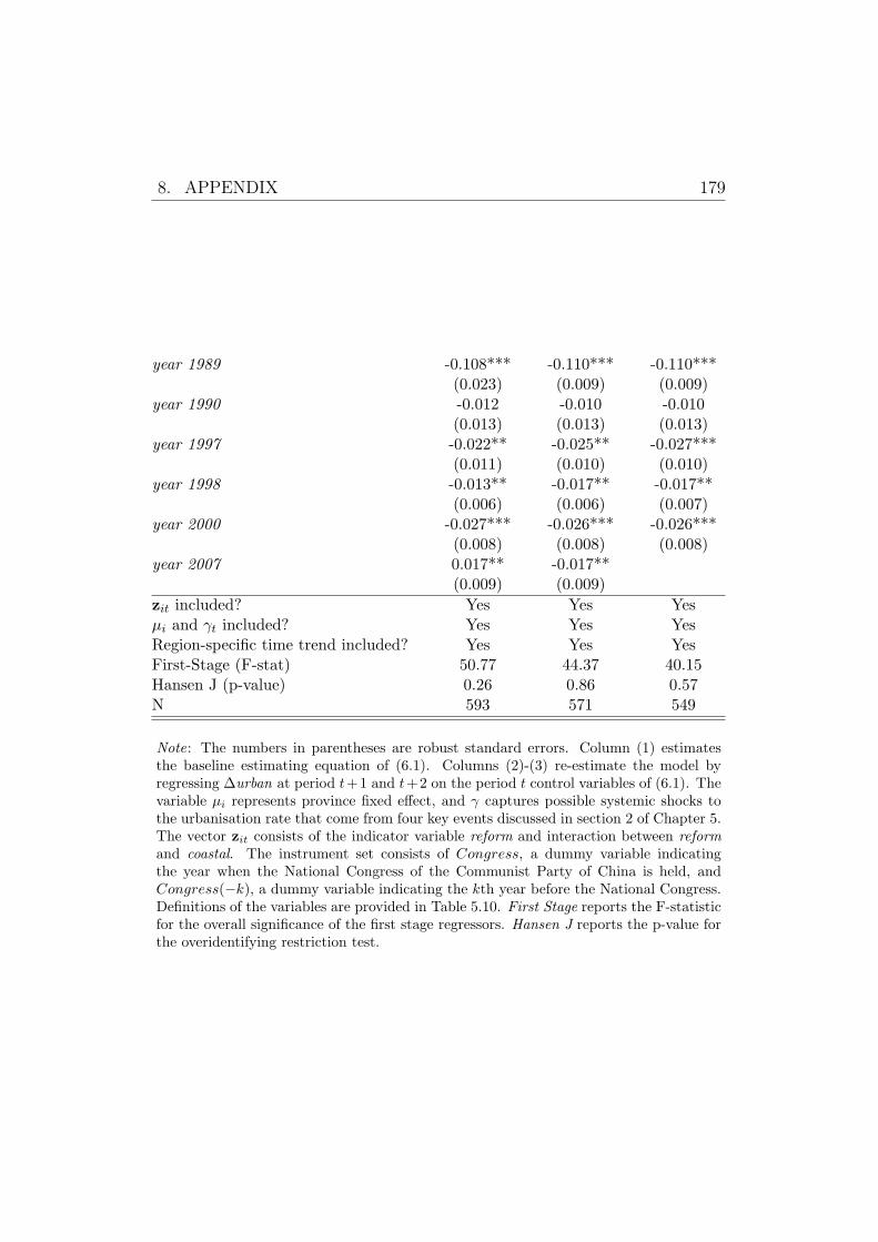
8. APPENDIX 179
year 1989 -0.108*** -0.110*** -0.110***(0.023) (0.009) (0.009)
year 1990 -0.012 -0.010 -0.010(0.013) (0.013) (0.013)
year 1997 -0.022** -0.025** -0.027***(0.011) (0.010) (0.010)
year 1998 -0.013** -0.017** -0.017**(0.006) (0.006) (0.007)
year 2000 -0.027*** -0.026*** -0.026***(0.008) (0.008) (0.008)
year 2007 0.017** -0.017**(0.009) (0.009)
zit included? Yes Yes Yesµi and γt included? Yes Yes YesRegion-specific time trend included? Yes Yes YesFirst-Stage (F-stat) 50.77 44.37 40.15Hansen J (p-value) 0.26 0.86 0.57N 593 571 549
Note: The numbers in parentheses are robust standard errors. Column (1) estimatesthe baseline estimating equation of (6.1). Columns (2)-(3) re-estimate the model byregressing ∆urban at period t+1 and t+2 on the period t control variables of (6.1). Thevariable µi represents province fixed effect, and γ captures possible systemic shocks tothe urbanisation rate that come from four key events discussed in section 2 of Chapter 5.The vector zit consists of the indicator variable reform and interaction between reformand coastal. The instrument set consists of Congress, a dummy variable indicatingthe year when the National Congress of the Communist Party of China is held, andCongress(−k), a dummy variable indicating the kth year before the National Congress.Definitions of the variables are provided in Table 5.10. First Stage reports the F-statisticfor the overall significance of the first stage regressors. Hansen J reports the p-value forthe overidentifying restriction test.
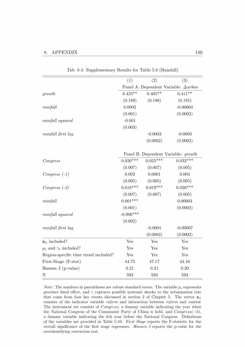
8. APPENDIX 180
Tab. 8.4: Supplementary Results for Table 5.8 (Rainfall)
(1) (2) (3)
Panel A. Dependent Variable: ∆urban
growth 0.425** 0.405** 0.411**
(0.189) (0.186) (0.185)
rainfall 0.0002 -0.00004
(0.001) (0.0002)
rainfall squared -0.001
(0.003)
rainfall first lag -0.0003 -0.0003
(0.0002) (0.0002)
Panel B. Dependent Variable: growth
Congress 0.026*** 0.025*** 0.032***
(0.007) (0.007) (0.005)
Congress (-1) 0.002 0.0001 0.004
(0.005) (0.005) (0.005)
Congress (-2) 0.018*** 0.019*** 0.026***
(0.007) (0.007) (0.005)
rainfall 0.001*** 0.00003
(0.001) (0.0002)
rainfall squared -0.006***
(0.002)
rainfall first lag -0.0001 -0.00007
(0.0002) (0.0002)
zit included? Yes Yes Yes
µi and γt included? Yes Yes Yes
Region-specific time trend included? Yes Yes Yes
First-Stage (F-stat) 44.75 47.17 44.16
Hansen J (p-value) 0.21 0.21 0.20
N 593 593 593
Note: The numbers in parentheses are robust standard errors. The variable µi representsprovince fixed effect, and γ captures possible systemic shocks to the urbanisation ratethat come from four key events discussed in section 2 of Chapter 5. The vector zitconsists of the indicator variable reform and interaction between reform and coastal.The instrument set consists of Congress, a dummy variable indicating the year whenthe National Congress of the Communist Party of China is held, and Congress(−k),a dummy variable indicating the kth year before the National Congress. Definitionsof the variables are provided in Table 5.10. First Stage reports the F-statistic for theoverall significance of the first stage regressors. Hansen J reports the p-value for theoveridentifying restriction test.
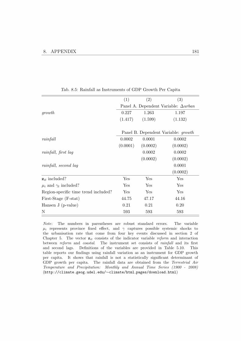
8. APPENDIX 181
Tab. 8.5: Rainfall as Instruments of GDP Growth Per Capita
(1) (2) (3)
Panel A. Dependent Variable: ∆urban
growth 0.227 1.263 1.197
(1.417) (1.599) (1.132)
Panel B. Dependent Variable: growth
rainfall 0.0002 0.0001 0.0002
(0.0001) (0.0002) (0.0002)
rainfall, first lag 0.0002 0.0002
(0.0002) (0.0002)
rainfall, second lag 0.0001
(0.0002)
zit included? Yes Yes Yes
µi and γt included? Yes Yes Yes
Region-specific time trend included? Yes Yes Yes
First-Stage (F-stat) 44.75 47.17 44.16
Hansen J (p-value) 0.21 0.21 0.20
N 593 593 593
Note: The numbers in parentheses are robust standard errors. The variableµi represents province fixed effect, and γ captures possible systemic shocks tothe urbanisation rate that come from four key events discussed in section 2 ofChapter 5. The vector zit consists of the indicator variable reform and interactionbetween reform and coastal. The instrument set consists of rainfall and its firstand second lags. Definitions of the variables are provided in Table 5.10. Thistable reports our findings using rainfall variation as an instrument for GDP growthper capita. It shows that rainfall is not a statistically significant determinant ofGDP growth per capita. The rainfall data are obtained from the Terrestrial AirTemperature and Precipitation: Monthly and Annual Time Series (1900 - 2008)(http://climate.geog.udel.edu/∼climate/html pages/download.html)
8. APPENDIX 182
Appendix D: Additional Information for Chapter 6
Tab. 8.6: Category of Occupations
Source: CHIPS (2002).
A NOTE:
This figure/table/image has been removed to comply with copyright regulations. It is included in the print copy of the thesis held by the University of Adelaide Library.
8. APPENDIX 183Tab
.8.7:
Categoryof
Sectors
andOwnerships
Sector
Ownership
Source:CHIP
S(200
2).
N
OTE
: Th
is fi
gure
/tabl
e/im
age
has b
een
rem
oved
to
com
ply
with
cop
yrig
ht re
gula
tions
. It
is in
clud
ed in
the
prin
t cop
y of
the
thes
is
hel
d by
the
Uni
vers
ity o
f Ade
laid
e Li
brar
y.
BIBLIOGRAPHY
Acemoglu, D., S. Johnson, and J. A. Robinson (2001). The colonial
origins of comparative development: An empirical investigation. American
Economic Review 91 (5), 1369–1401.
Angrist, J. D. and V. Lavy (1999). Using Maimonides’ rule to estimate
the effect of class size on scholastic achievement. Quarterly Journal of
Economics 114 (2), 533–575.
Angrist, J. D. and J.-S. Pischke (2009). Mostly Harmless Econometrics.
Princeton: Princeton University Press.
Appleton, S., L. Song, and Q. Xia (2005). Has China crossed the river?
The evolution of wage structure in urban China during reform and
retrenchment. Journal of Comparative Economics 33 (4), 644–663.
Appleton, S., L. Song, and Q. Xia (2012). Understanding urban wage
inequality in China 1988-2008: Evidence from quantile analysis. IZA
Discussion Papers 7101, Institute for the Study of Labor (IZA).
Arellano, M. and S. Bond (1991). Some tests of specification for panel data:
Monte Carlo evidence and an application to employment equations. Review
of Economic Studies 58 (2), 277–297.
Arnold, J., A. Bassanini, and S. Scarpetta (2007). Solow or Lucas?: Testing
growth models using panel data from oecd countries. OECD Economics
Department Working Papers 592, OECD Publishing.
Aschauer, D. A. (1989). Is public expenditure productive? Journal of
Monetary Economics 23 (2), 177–200.
BIBLIOGRAPHY 185
Atack, J., F. Bateman, M. Haines, and R. A. Margo (2009). Did railroads
induce or follow economic growth? Urbanization and population growth in
the American Midwest, 1850-60. Working Paper 14640, National Bureau
of Economic Research.
Banerjee, A., E. Duflo, and N. Qian (2012). On the road: Access to
transportation infrastructure and economic growth in China. Working
Paper 17897, National Bureau of Economic Research, Inc.
Barrios, S., L. Bertinelli, and E. Strobl (2006). Climatic change and rural-
urban migration: The case of sub-Saharan Africa. Journal of Urban
Economics 60 (3), 357 – 371.
Barro, R. J. (1991). Economic growth in a cross section of countries.
Quarterly Journal of Economics 106 (2), 407–443.
Baum-Snow, N., L. Brandt, J. V. Henderson, M. A. Turner, and Q. Zhang
(2012). Roads, railroads and decentralization of Chinese cities. mimeo.
Baum-Snow, N. and M. A. Turner (2012). Transportation and the
decentralization of Chinese cities. mimeo.
Becker, C. M. and A. R. Morrison (1988). The determinants of urban
population growth in sub-Saharan Africa. Economic Development and
Cultural Change 36 (2), 259–278.
Becker, C. M. and A. R. Morrison (1999). Urbanization in transforming
economies. In P. C. Cheshire and E. S. Mills (Eds.), Handbook of Regional
and Urban Economics, Volume 3 of Handbook of Regional and Urban
Economics, Chapter 43, pp. 1673–1790. Elsevier.
Bellier, M. and Y. M. Zhou (2003). Private participation in infrastructure
in China: Issues and recommendations for the road, water, and power
sectors. Working Paper No. 2, World Bank.
Benjamin, D., L. Brandt, and J. Giles (2005). The evolution of
income inequality in rural China. Economic Development and Cultural
Change 53 (4), 769–824.
BIBLIOGRAPHY 186
Binswanger, H. P., S. R. Khandker, and M. R. Rosenzweig (1993). How
infrastructure and financial institutions affect agricultural output and
investment in india. Journal of Development Economics 41 (2), 337–366.
Blanchard, O. and A. Shleifer (2001). Federalism with and without political
centralization: China versus Russia. IMF Staff Papers 48, 8.
Bruckner, M. (2012). Economic growth, size of the agricultural sector, and
urbanization in Africa. Journal of Urban Economics 71 (1), 26–36.
Cai, F., A. Park, and Y. Zhao (2008). The Chinese labor market in
the reform era. In L. Brandt and T. G. Rawski (Eds.), China’s Great
Economic Transformation, Chapter 6, pp. 167–214. Cambridge and New
York: Cambridge University Press.
Calderon, C. and A. Chong (2004). Volume and quality of infrastructure and
the distribution of income: An empirical investigation. Review of Income
and Wealth 50 (1), 87–106.
Calderon, C. and L. Serven (2005). The effects of infrastructure development
on growth and income distribution. World Bank Policy Research Working
Paper 3643, World Bank, Washington, D.C.
Cao, S. (2000). Zhongguo Renkou Shi Qing Shiqi (Population History of
China, Qing Period), Volume 5. Shanghai: Fudan University Press.
Caselli, F., G. Esquivel, and F. Lefort (1996). Reopening the convergence
debate: A new look at cross-country growth empirics. Journal of Economic
Growth 1 (3), 363–89.
Chan, K. and W. Buckingham (2008). Is China abolishing the hukou system?
The China Quarterly 195, 582–606.
Chan, K. and L. Zhang (1999). The hukou system and rural-urban migration
in China: Processes and changes. The China Quarterly 160, 818–855.
Chang, G. H. and J. C. Brada (2006). The paradox of China’s growing
under-urbanization. Economic Systems 30 (1), 24–40.
BIBLIOGRAPHY 187
Chen, A. (2002). Urbanization and disparities in China: Challenges of growth
and development. China Economic Review 13 (4), 407–411.
Chen, B. and Y. Yao (2011). The cursed virtue: Government infrastructural
investment and household consumption in Chinese provinces. Oxford
Bulletin of Economics and Statistics 73 (6), 856–877.
Chen, J. and B. M. Fleisher (1996). Regional income inequality and economic
growth in China. Journal of Comparative Economics 22 (2), 141–164.
Chen, Y., S. Demurger, and M. Fournier (2005). Earnings differentials and
ownership structure in Chinese enterprises. Economic Development and
Cultural Change 53 (4), 933–958.
Chen, Y., H. Li, and L.-A. Zhou (2005). Relative performance evaluation
and the turnover of provincial leaders in China. Economics Letters 88 (3),
421–425.
Cheng, T. and M. Selden (1994). The origins and social consequences of
China’s hukou system. The China Quarterly 139, 644–668.
Chow, G. (2006). Are Chinese official statistics reliable. CESifo Economic
Studies 52 (2), 396–414.
Combes, P.-P., S. Demurger, and S. Li (2013). Urbanisation and migration
externalities in China. Working Papers 1303, GATE Groupe d’ Analyse et
de Theorie Economique Lyon-St Etienne.
da Mata, D., U. Deichmann, J. Henderson, S. Lall, and H. Wang (2007).
Determinants of city growth in Brazil. Journal of Urban Economics 62 (2),
252–272.
Davis, J. C. and J. V. Henderson (2003). Evidence on the political economy
of the urbanization process. Journal of Urban Economics 53 (1), 98–125.
Demurger, S. (2001). Infrastructure development and economic growth: An
explanation for regional disparities in China? Journal of Comparative
Economics 29 (1), 95–117.
BIBLIOGRAPHY 188
Demurger, S., M. Gurgand, S. Li, and X. Yue (2009). Migrants as second-
class workers in urban China? A decomposition analysis. Journal of
Comparative Economics 37 (4), 610 – 628.
Deng, X., J. Huang, S. Rozelle, and E. Uchida (2008). Growth, population
and industrialization, and urban land expansion of China. Journal of
Urban Economics 63 (1), 96–115.
Ding, S. and J. Knight (2011). Why has China grown so fast? The role of
physical and human capital formation. Oxford Bulletin of Economics and
Statistics 73 (2), 141–174.
Dollar, D. and A. Kraay (2004). Trade, growth, and poverty. Economic
Journal 114 (493), F22–F49.
Donaldson, D. (2010). Railroads of the Raj: Estimating the impact of
transportation infrastructure. NBER Working Papers 16487, National
Bureau of Economic Research, Inc.
Dong, X.-Y. and M. Pandey (2012). Gender and labor retrenchment in
Chinese state owned enterprises: Investigation using firm-level panel data.
China Economic Review 23 (2), 385 – 395.
Dong, X.-Y. and L. Putterman (2003). Soft budget constraints, social
burdens, and labor redundancy in China’s state industry. Journal of
Comparative Economics 31 (1), 110–133.
Dong, X.-Y. and L. C. Xu (2009). Labor restructuring in china: Toward a
functioning labor market. Journal of Comparative Economics 37 (2), 287
– 305.
Du, L., C. Wei, and S. Cai (2012). Economic development and carbon dioxide
emissions in China: Provincial panel data analysis. China Economic
Review 23 (2), 371–384.
Duranton, G. (2008). Viewpoint: From cities to productivity and growth in
developing countries. Canadian Journal of Economics 41 (3), 689–736.
BIBLIOGRAPHY 189
Duranton, G. and D. Puga (2004). Micro-foundations of urban agglomeration
economies. In J. V. Henderson and J. F. Thisse (Eds.), Handbook of
Regional and Urban Economics, Volume 4, Chapter 48, pp. 2063–2117.
Elsevier.
Esfahani, H. S. and M. T. Ramirez (2003). Institutions, infrastructure, and
economic growth. Journal of Development Economics 70 (2), 443–477.
Estache, A., B. Speciale, and D. Veredas (2005). How much does
infrastructure matter to growth in Sub-Saharan Africa. mimeo.
Fan, C. C. (2006). China’s eleventh Five-Year Plan (2006-2010): From
‘getting rich first’ to ‘common prosperity’. Eurasian Geography and
Economics 47 (6), 708–723.
Fan, S. and X. Zhang (2004). Infrastructure and regional economic
development in rural China. China Economic Review 15 (2), 203–214.
Fang, Y. and Y. Zhao (2009). Do institutions matter? Estimating the effect of
institutions on economic performance in China. BOFIT Discussion Papers
9/2009, Bank of Finland, Institute for Economies in Transition.
Fay, M. and C. Opal (2000, August). Urbanization without growth : a not-
so-uncommon phenomenon. Policy Research Working Paper Series 2412,
The World Bank.
Feng, K., K. Hubacek, and D. Guan (2009). Lifestyles, technology and
CO2 emissions in China: A regional comparative analysis. Ecological
Economics 69 (1), 145–154.
Fernald, J. G. (1999). Roads to prosperity? Assessing the link between public
capital and productivity. American Economic Review 89 (3), 619–638.
Field, R. M. (1986). The performance of industry during the Cultural
Revolution: Second thoughts. The China Quarterly (108), 625–642.
BIBLIOGRAPHY 190
Fleisher, B., H. Li, and M. Zhao (2010). Human capital, economic
growth, and regional inequality in China. Journal of Development
Economics 92 (2), 215–231.
Fleisher, B. M. and J. Chen (1997). The coast-noncoast income gap,
productivity, and regional economic policy in China. Journal of
Comparative Economics 25 (2), 220–236.
Fogel, R. W. (1962). A quantitative approach to the study of railroads in
American economic growth: A report of some preliminary findings. Journal
of Economic History 22 (2), 163–197.
Fujita, M., P. Krugman, and A. J. Venables (1999). The Spatial Economy:
Cities, Regions and International Trade. Cambridge, MA: MIT Press.
Garcia-Mila, T., T. J. McGuire, and R. H. Porter (1996). The effect of
public capital in state-level production functions reconsidered. Review of
Economics and Statistics 78 (1), 177–80.
Glass, G., S. Cahen, M. Smith, and N. Filby (1982). School class size:
Research and policy. Beverly Hills, CA: Sage.
Glass, G. and M. Smith (1979). Meta-analysis of research on class size and
achievement. Educational Evaluation and Policy Analysis 1 (1), 2–16.
Golas, J. P. (1977). Early Ch’ing guilds. In G. Skinner (Ed.), The city in
late Imperial China. Stanford, CA: Stanford University Press.
Gramlich, E. M. (1994). Infrastructure investment: A review essay. Journal
of Economic Literature 32 (3), 1176–1196.
Gustafsson, B. and S. Ding (2009). Villages where China’s ethnic minorities
live. China Economic Review 20 (2), 193–207.
Gustafsson, B. and S. Li (2003). The ethnic minority-majority income gap
in rural China during transition. Economic Development and Cultural
Change 51 (4), 805–822.
BIBLIOGRAPHY 191
Hanson, G. (2005). Market potential, increasing returns and geographic
concentration. Journal of International Economics 67 (1), 1–24.
Harris, J. R. and M. P. Todaro (1970). Migration, unemployment &
development: A two-sector analysis. American Economic Review 60 (1),
126–142.
Harrison, A. (1996). Openness and growth: A time-series, cross-
country analysis for developing countries. Journal of Development
Economics 48 (2), 419–447.
Harrison, A., J. McLaren, and M. S. McMillan (2010). Recent findings on
trade and inequality. NBER Working Papers 16425, National Bureau of
Economic Research, Inc.
Head, K. and T. Mayer (2006). Regional wage and employment responses to
market potential in the EU. Regional Science and Urban Economics 36 (5),
573–594.
Henderson, J. V. (1986). Urbanization in a developing country : City size
and population composition. Journal of Development Economics 22 (2),
269–293.
Henderson, J. V. (2005). Urbanization and growth. In P. Aghion and
S. Durlauf (Eds.), Handbook of Economic Growth, Volume 1 of Handbook
of Economic Growth, Chapter 24, pp. 1543–1591. Elsevier.
Henderson, J. V. and H. G. Wang (2007). Urbanization and city growth:
The role of institutions. Regional Science and Urban Economics 37 (3),
283–313.
Henderson, V. (2002). Urbanization in developing countries. World Bank
Research Observer 17 (1), 89–112.
Henderson, V. (2003). The urbanization process and economic growth: The
so-what question. Journal of Economic Growth 8 (1), 47–71.
BIBLIOGRAPHY 192
Henderson, V. (2009). Urbanization in China: Policy issues and options.
China Economic Research and Advisory Programme Report.
Hering, L. and S. Poncet (2010). Market access and individual wages:
Evidence from China. Review of Economics and Statistics 92 (1), 145–
159.
Holtz-Eakin, D. (1988). The line item veto and public sector budgets :
Evidence from the states. Journal of Public Economics 36 (3), 269–292.
Holtz-Eakin, D. (1994). Public-sector capital and the productivity puzzle.
Review of Economics and Statistics 76 (1), 12–21.
Holtz-Eakin, D. and A. E. Schwartz (1995). Infrastructure in a structural
model of economic growth. Regional Science and Urban Economics 25 (2),
131–151.
Holz, C. A. (2008). China’s economic growth 1978-2025: What
we know today about China’s economic growth tomorrow. World
Development 36 (10), 1665–1691.
Hou, Z. and M. S. Emran (2012). Access to markets and rural poverty:
Evidence from household consumption in China. Review of Economics
and Statistics . forthcoming.
Hsu, I. C.-Y. (1970). The Rise of Modern China. New York: Oxford
University Press.
Jarreau, J. and S. Poncet (2012). Export sophistication and economic growth:
Evidence from China. Journal of Development Economics 97 (2), 281–292.
Jia, R. (2012). The legacies of forced freedom: China’s treaty ports. Review
of Economics and Statistics . conditional acceptance.
Jin, H., Y. Qian, and B. R. Weingast (2005). Regional decentralization
and fiscal incentives: Federalism, Chinese style. Journal of Public
Economics 89 (9–10), 1719–1742.
BIBLIOGRAPHY 193
Kamal, F., M. E. Lovely, and P. Ouyang (2012). Does deeper integration
enhance spatial advantages? Market access and wage growth in China.
International Review of Economics Finance 23 (C), 59–74.
Keller, W. and C. H. Shiue (2008). Institutions, technology, and trade. NBER
Working Paper 13913, National Bureau of Economic Research, Inc.
Kleibergen, F. and R. Paap (2006). Generalized reduced rank tests using the
singular value decomposition. Journal of Econometrics 133 (1), 97–126.
Krugman, P. (1991). Increasing returns and economic geography. Journal of
Political Economy 99 (3), 483–499.
Krugman, P. R. and A. J. Venables (1995). Globalization and the inequality
of nations. Quarterly Journal of Economics 110 (4), 857–880.
Kung, J. K. S. and N. Li (2011). Commercialization as exogenous shocks:
The effect of the soybean trade and migration in Manchurian villages,
1895-1934. Explorations in Economic History 48 (4), 568–589.
Lemoine, F. and D. Unal-Kesenci (2004). Assembly trade and technology
transfer: The case of China. World Development 32 (5), 829–850.
Levitt, S. D. (1997). Using electoral cycles in police hiring to estimate the
effect of police on crime. American Economic Review 87 (3), 270–290.
Li, H. and L. Huang (2009). Health, education, and economic growth
in China: Empirical findings and implications. China Economic
Review 20 (3), 374–387.
Li, H. and Z. Li (2010). Road investment and inventory reduction: Firm
level evidence from China. mimeo.
Li, H., P. Liu, J. Zhang, and N. Ma (2007). Economic returns to communist
party membership: Evidence from urban Chinese twins. Economic
Journal 117 (523), 1504–1520.
BIBLIOGRAPHY 194
Li, H., M. Rosenzweig, and J. Zhang (2010, 02). Altruism, favoritism, and
guilt in the allocation of family resources: Sophie’s choice in Mao’s mass
send-down movement. Journal of Political Economy 118 (1), 1–38.
Li, H. and L.-A. Zhou (2005). Political turnover and economic performance:
The incentive role of personnel control in China. Journal of Public
Economics 89 (9–10), 1743–1762.
Li, L. (2011). The incentive role of creating “cities” in China. China
Economic Review 22 (1), 172–181.
Li, S. and S. Ding (2009). An empirical analysis of income inequality between
a minority and the majority in urban China: The case of Ningxia Hui
autonomous region. Global COE Hi-Stat Discussion Paper Series GD08-
022, Institute of Economic Research, Hitotsubashi University.
Li, Z. (2009). Estimating the social return to transportation infrastructure
investment: A natural experiment. mimeo.
Lin, J. Y. (1992). Rural reforms and agricultural growth in China. American
Economic Review 82 (1), 34–51.
Liu, Z. (2007). The external returns to education: Evidence from Chinese
cities. Journal of Urban Economics 61 (3), 542–564.
Ma, L. (1983). Zhongguo tielu jianzhu biannian jianshi 1881-1981 (The
chronological history of Chinese railroad construction 1881-1981). Beijing:
Zhongguo Tiedao (China Railways) Press.
Meng, X. and J. Zhang (2001). The two-tier labor market in urban China:
Occupational segregation and wage differentials between urban residents
and rural migrants in Shanghai. Journal of Comparative Economics 29 (3),
485–504.
Michaels, G. (2008). The effect of trade on the demand for skill:
Evidence from the interstate highway system. Review of Economics and
Statistics 90 (4), 683–701.
BIBLIOGRAPHY 195
Mincer, J. A. (1974). Schooling, Experience and Earnings. New York:
Columbia University Press.
Mohan, R. (1984). The effect of population growth, the pattern of demand
and of technology on the process of urbanization. Journal of Urban
Economics 15 (2), 125–156.
Moll-Murata, C. (2008). Chinese guilds from the Seventeenth to the
Twentieth Centuries: An overview. International Review of Social
History 53 (Supplement S16), 213–247.
Montinola, G., Y. Qian, and B. R. Weingast (1995). Federalism, Chinese
style: The political basis for economic success in China. World
Politics 48 (1), 50–81.
Morse, H. B. (1909). Guilds in China.
Munnell, A. H. (1990). Why has productivity growth declined? Productivity
and public investment. New England Economic Review (Jan), 3–22.
Munnell, A. H. (1992). Infrastructure investment and economic growth.
Journal of Economic Perspectives 6 (4), 189–198.
Murray, M. P. (2006). Avoiding invalid instruments and coping with weak
instruments. Journal of Economic Perspectives 20 (4), 111–132.
National Bureau of Statistics China (1988). China Population Statistics
Yearbook (1988). Beijing: China Zhanwang Press.
National Bureau of Statistics China (2010). China Compendium of Statistics
(1949–2008). Beijing: China Statistics Press.
National Bureau of Statistics China (2011). The Sixth National Population
Census Gazette (No.1).
Naughton, B. (2008). A political economy of China’s economic transition.
In L. Brandt and T. G. Rawski (Eds.), China’s Great Economic
Transformation, Chapter 4, pp. 91–135. Cambridge and New York:
Cambridge University Press.
BIBLIOGRAPHY 196
Pascali, L. (2012, March). Banks and development: Jewish communities
in the Italian Renaissance and current economic performance. Working
Papers 562, Barcelona Graduate School of Economics.
Peng, Z. (1995). Zhongguo Gongshang Hanghui Shiliao Ji (Collection of
Historical Materials on Chinese Craft and Commercial Guilds). Beijing:
Zhonghua Book Company.
Perkins, D. H. and T. G. Rawski (2008). Forecasting China’s economic
growth to 2025. In L. Brandt and T. G. Rawski (Eds.), China’s Great
Economic Transformation, Chapter 20, pp. 829–886. Cambridge and New
York: Cambridge University Press.
Piotroski, J., T. Wong, and T. Zhang (2010). Political incentives to suppress
negative financial information: Evidence from state-controlled Chinese
firms.
Poelhekke, S. (2011). Urban growth and uninsured rural risk: Booming towns
in bust times. Journal of Development Economics 96 (2), 461–475.
Poncet, S. (2003). Measuring Chinese domestic and international integration.
China Economic Review 14 (1), 1–21.
Poncet, S. (2005). A fragmented China: Measure and determinants of China’s
domestic market disintegration. Review of International Economics 13 (3),
409–430.
Poncet, S. (2006, May). Provincial migration dynamics in China:
Borders, costs and economic motivations. Regional Science and Urban
Economics 36 (3), 385–398.
Quan, H. (1934). Zhongguo Hanghui Zhidu Shi (The History of the Chinese
Guild System). Xinshengming Book Company.
Quigley, J. M. (1998). Urban diversity and economic growth. Journal of
Economic Perspectives 12 (2), 127–138.
BIBLIOGRAPHY 197
Ravallion, M. and S. Chen (2007). China’s (uneven) progress against poverty.
Journal of Development Economics 82 (1), 1–42.
Rawski, T. G. (2001). What is happening to China’s gdp statistics? China
Economic Review 12 (4), 347–354.
Rawski, T. G. and W. Xiao (2001). Roundtable on Chinese economic
statistics introduction. China Economic Review 12 (4), 298–302.
Redding, S. and A. J. Venables (2004). Economic geography and
international inequality. Journal of International Economics 62 (1), 53–
82.
Richardson, J. D. (1995). Income inequality and trade: How to think, what
to conclude. Journal of Economic Perspectives 9 (3), 33–55.
Rowe, W. T. (1984). Hankow: Commerce and society in a Chinese city,
1796–1889. Berkeley, CA: Stanford University Press.
Rowe, W. T. (1992). Ming-Qing guilds. Ming Qing Yanjiu 1, 47–60.
Rubin, L. S. (1991). Productivity and the public capital stock: Another
look. Working Paper Series / Economic Activity Section 118, Board of
Governors of the Federal Reserve System (U.S.).
Shen, C., J. Jin, and H.-F. Zou (2012). Fiscal decentralization in China:
History, impact, challenges and next steps. Annals of Economics and
Finance 13 (1), 1–51.
Shen, Y., P. Li, and C.-T. Huang (2008). Hot issue or political issue: A
politically induced cycle in Chinese IPO market. mimeo.
Shiue, C. H. (2002). Transport costs and the geography of arbitrage in
eighteenth-century China. American Economic Review 92 (5), 1406–1419.
Skinner, G. W. (1977). Introduction: Urban social structure in Ch’ing
China. In G. Skinner (Ed.), The city in late Imperial China. Stanford,
CA: Stanford University Press.
BIBLIOGRAPHY 198
Song, Y. and Y. Zenou (2012). Urban villages and housing values in China.
Regional Science and Urban Economics 42 (3), 495–505.
Staiger, D. and J. H. Stock (1997). Instrumental variables regression with
weak instruments. Econometrica 65 (3), 557–586.
Stock, J. H., J. H. Wrigh, and M. Yogo (2002). A survey of weak instruments
and weak identification in generalized method of moments. Journal of
Business and Economic Statistics 20 (4), 518–529.
Stock, J. H. and M. Yogo (2005). Testing for weak instruments in linear
IV regression. In D. W. Andrews and J. H. Stock (Eds.), Identification
and Inference for Econometric Models: Essays in Honor of Thomas
Rothenberg, Chapter 5, pp. 80–108. Cambridge: Cambridge University
Press.
Sun, P. and A. Heshmati (2010). International trade and its effects on
economic growth in China. IZA Discussion Papers 5151, Institute for the
Study of Labor (IZA).
Tian, L., H. H. Wang, and Y. Chen (2010). Spatial externalities in China
regional economic growth. China Economic Review 21 (Supplement 1),
S20–S31.
Wacziarg, R. and K. H. Welch (2008). Trade liberalization and growth: New
evidence. World Bank Economic Review 22 (2), 187–231.
Wang, F. (1999). Modeling a central place system with interurban
transport costs and complex rural hinterlands. Regional Science and Urban
Economics 29 (3), 381–409.
Wang, F. and X. Zuo (1999). Inside China’s cities: Institutional barriers
and opportunities for urban migrants. American Economic Review 89 (2),
276–280.
Wei, Z. and R. Hao (2010). Demographic structure and economic growth:
Evidence from China. Journal of Comparative Economics 38 (4), 472–491.
BIBLIOGRAPHY 199
West, M. R. and L. Woessmann (2010). ‘Every catholic child in a
catholic school’: Historical resistance to state schooling, contemporary
private competition and student achievement across countries. Economic
Journal 120 (546), F229–F255.
Wong, C. (2011). The fiscal stimulus program and problems of
macroeconomic management in China. OECD Journal on Budgeting 3.
Wong, C. and R. Bird (2008). China’s fiscal system: A work in
progress. In L. Brandt and T. G. Rawski (Eds.), China’s Great Economic
Transformation, Chapter 12, pp. 429–466. Cambridge and New York:
Cambridge University Press.
World Bank (2007). Evaluation of World Bank support to transportation
infrastructure. World Bank Publications.
Wu, M. (2010). How does central authority govern the provincial leaders?
Evidence from China. mimeo.
Xia, Q., L. Song, S. Li, and S. Appleton (2013). The effects of the state
sector on wage inequality in urban China: 1988–2007. IZA Discussion
Papers 7142, Institute for the Study of Labor (IZA).
Xu, C. (2011). The fundamental institutions of China’s reforms and
development. Journal of Economic Literature 49 (4), 1076–1151.
Zhang, J. and Z. Zhao (2013). Measuring the income-distance tradeoff for
rural-urban migrants in China. IZA Discussion Papers 7160, Institute for
the Study of Labor (IZA).
Zhang, K. H. and S. Song (2003). Rural-urban migration and urbanization
in China: Evidence from time-series and cross-section analyses. China
Economic Review 14 (4), 386–400.
Zhang, T. and H.-F. Zou (1998). Fiscal decentralization, public spending,
and economic growth in China. Journal of Public Economics 67 (2), 221–
240.
BIBLIOGRAPHY 200
Zhao, Y. (1999). Leaving the countryside: Rural-to-urban migration
decisions in China. American Economic Review 89 (2), 281–286.
Zhao, Y. (2002). Earnings differentials between state and non-state
enterprises in urban China. Pacific Economic Review 7 (1), 181–197.
Zheng, J., A. Bigsten, and A. Hu (2009). Can China’s growth be sustained?
A productivity perspective. World Development 37 (4), 874–888.