Embed Size (px)
Citation preview
University of California
Los Angeles
Essays on Political Economy
A dissertation submitted in partial satisfaction
of the requirements for the degree
Doctor of Philosophy in Economics
by
Paulo Guilherme Melo Filho
2007

c© Copyright by
Paulo Guilherme Melo Filho
2007


To Rosa
iii
Table of Contents
1 Shopping for Support: Controlling Congress in Multiparty Pres-
idential Systems . . . . . . . . . . . . . . . . . . . . . . . . . . . . . . . 1
1.1 Introduction . . . . . . . . . . . . . . . . . . . . . . . . . . . . . . 1
1.2 Literature Review . . . . . . . . . . . . . . . . . . . . . . . . . . . 3
1.3 The Model . . . . . . . . . . . . . . . . . . . . . . . . . . . . . . . 7
1.3.1 Environment . . . . . . . . . . . . . . . . . . . . . . . . . 7
1.3.2 The Decision Problem . . . . . . . . . . . . . . . . . . . . 10
1.3.3 Optimal Decision . . . . . . . . . . . . . . . . . . . . . . . 11
1.3.4 Implications and Intuitions . . . . . . . . . . . . . . . . . . 15
1.4 Model Meets Data . . . . . . . . . . . . . . . . . . . . . . . . . . 16
1.4.1 Numeric Assumptions . . . . . . . . . . . . . . . . . . . . 16
1.4.2 Making Predictions . . . . . . . . . . . . . . . . . . . . . . 17
1.5 Conclusion . . . . . . . . . . . . . . . . . . . . . . . . . . . . . . . 22
Appendix . . . . . . . . . . . . . . . . . . . . . . . . . . . . . . . . . . 24
Figures . . . . . . . . . . . . . . . . . . . . . . . . . . . . . . . . . . . . 31
Bibliography . . . . . . . . . . . . . . . . . . . . . . . . . . . . . . . . 31
2 The Back-up Investment Incentives in the Brazilian Electrical
Sector Regulatory Model . . . . . . . . . . . . . . . . . . . . . . . . . 39
2.1 Introduction . . . . . . . . . . . . . . . . . . . . . . . . . . . . . . 39
2.2 The Brazilian Electrical Sector . . . . . . . . . . . . . . . . . . . . 40
iv
2.2.1 Origins and Development of the Sector . . . . . . . . . . . 40
2.2.2 The Change of Regimes . . . . . . . . . . . . . . . . . . . 42
2.2.3 The Crisis . . . . . . . . . . . . . . . . . . . . . . . . . . . 45
2.3 The Model . . . . . . . . . . . . . . . . . . . . . . . . . . . . . . . 47
2.4 Future Improvements and Conclusion . . . . . . . . . . . . . . . . 51
Figures . . . . . . . . . . . . . . . . . . . . . . . . . . . . . . . . . . . . 53
Bibliography . . . . . . . . . . . . . . . . . . . . . . . . . . . . . . . . 53
3 Multiple Equilibria on Determination of Corruption and Impli-
cations to Economic Growth: A Review . . . . . . . . . . . . . . . . 56
3.1 Introduction . . . . . . . . . . . . . . . . . . . . . . . . . . . . . . 56
3.2 Literature Review . . . . . . . . . . . . . . . . . . . . . . . . . . . 57
3.3 Future Work . . . . . . . . . . . . . . . . . . . . . . . . . . . . . . 60
Bibliography . . . . . . . . . . . . . . . . . . . . . . . . . . . . . . . . 60
v
List of Figures
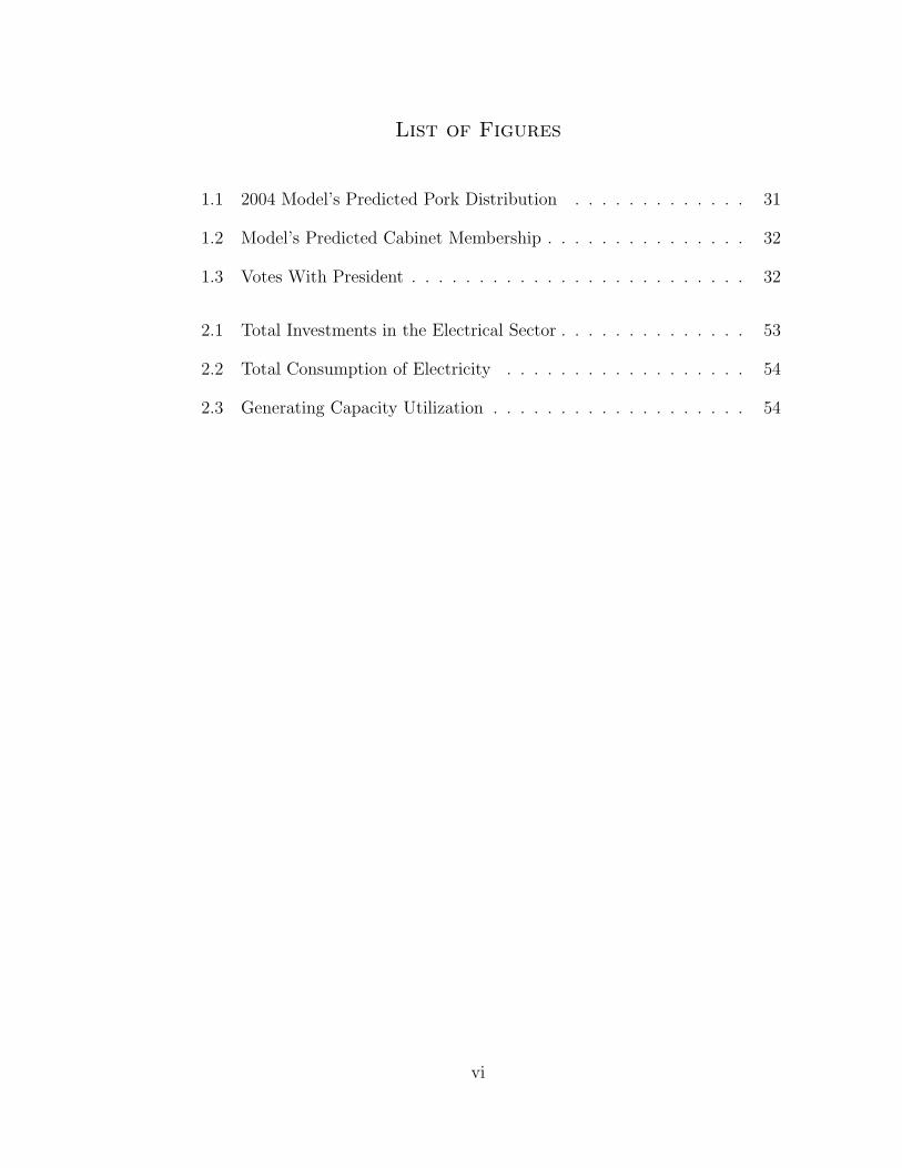
1.1 2004 Model’s Predicted Pork Distribution . . . . . . . . . . . . . 31
1.2 Model’s Predicted Cabinet Membership . . . . . . . . . . . . . . . 32
1.3 Votes With President . . . . . . . . . . . . . . . . . . . . . . . . . 32
2.1 Total Investments in the Electrical Sector . . . . . . . . . . . . . . 53
2.2 Total Consumption of Electricity . . . . . . . . . . . . . . . . . . 54
2.3 Generating Capacity Utilization . . . . . . . . . . . . . . . . . . . 54
vi

Acknowledgments
I gratefully thank David Levine, my main advisor, for his guidance and ded-
ication through all these years, always being available to discuss my work and
help me in my academic life. He is a great inspiration and I am very honored of
working with him.
I am very tankful to Jean-Laurent Rosenthal, co-chair of my dissertation
committee, for all his great comments and incentives to my work.
I am thankful to all the members of my dissertation committee —Hugo Hopen-
hayn, Matthias Doepke and Michael Chwe—, as well as Hongbin Cai, a former
member of this committee, for their support and valuable suggestions.
I was pleasured with the company of many colleges from the program, that
along these years become big friends. Gonzalo, Nelson, Flavinha, Rolf, Ili, Facu,
Juan, Hector, Miguel, Sebastian, Burcu. Without these guys this whole journey
would have been much harder.
Chapter 1 is a version of “Shopping for Support: Controlling Congress in Mul-
tiparty Presidential Systems”, a working paper co-authored with Cesar Zucco Jr.
That work counted with valuable comments from Barbara Geddes, Kathy Bawn,
Jeff Lewis, David Samuels, Patricio Navia, as well as participants in seminars at
the Economics and Political Science Departments at UCLA.
I am very grateful for the support from all my family. Even from a long
distance, they always helped and motivated me to get here.
I gratefully acknowledge the financial support from the Brazilian Ministry of
Science and Technology through the CNPq, and from the 2006-2007 Department
of Economics Dissertation Year Fellowship.
vii
Vita
October 7, 1973 Born in Recife, State of Pernambuco, Brazil
1995 Bachelor of Arts, Economics
Universidade Federal de Pernambuco (UFPE), Brazil
1996–1997 Teaching Assistant, Department of Economics
Pontifıcia Universidade Catolica do Rio de Janeiro (PUC-Rio),
Brazil
1997–1998 Research Assistant, Department of Economics
Pontifıcia Universidade Catolica do Rio de Janeiro (PUC-Rio),
Brazil
1998–1999 Lecturer, Department of Economics
Pontifıcia Universidade Catolica do Rio de Janeiro (PUC-Rio),
Brazil
1999 Master of Arts, Economics
Pontifıcia Universidade Catolica do Rio de Janeiro (PUC-Rio),
Brazil
1999–2002 Assessor of the Secretary of Economic Policy
Ministry of Finance, Brazil
2002–2006 International Doctorate Scholarship
Brazilian Ministry of Science and Technology - CNPq, Brazil
2003–2006 Teaching Assistant, Department of Economics
University of California, Los Angeles
viii
2005 Master of Arts, Economics
University of California, Los Angeles
2006–2007 Dissertation Year Fellowship, Department of Economics
University of California, Los Angeles
Publications and Presentations
Amadeo, Edward and Paulo Melo Filho (1999): “Apertura, Productivi-
dad y Empleo en el Brasil” in Productividad y Empleo en la Apertura Economica,
OIT. (in Spanish).
Melo Filho, Paulo and Cesar Zucco (2006): “Shopping for Support: Con-
trolling Congress in Multiparty Presidential Systems” paper presented at the
Latin American Meetings of The Econometric Society (LAMES), Mexico City.
ix
Abstract of the Dissertation
Essays on Political Economy
by
Paulo Guilherme Melo Filho
Doctor of Philosophy in Economics
University of California, Los Angeles, 2007
Professor David Levine, Co-chair
Professor Jean-Laurent Rosenthal, Co-chair
My dissertation, “Essays in Political Economy”, is composed by three different
essays were I analyze the functioning of different political institutions.
In Chapter 1, I propose a cost minimization approach to the problem of ob-
taining legislative support in a presidential multiparty setting. Presidents control
different types of politically useful resources, part of which, in such settings, has
to be spent to obtain support in the legislature. I present a formal model of
the president’s resource allocation decision problem. The most general result is
that even if there are economies of scale for dealing with parties rather than with
individual legislators, presidents will always do some of both. In the empirical
section, I use data from Brazil to simulate the model, and show that for some set
of parameters, the model’s predictions fit very closely the observed data.
In Chapter 2, I give a look at the Brazilian electrical sector. Until the middle
of the 1990s, all the Brazilian electric utilities were public companies. In 1995,
with the beginning of the privatization of those utilities, the government started
to implement a regulatory model for the sector. After almost one decade, the
regulatory model has failed in many ways. In particular, the investments in
x
thermal generation capacity to back-up the hydroelectric system did not happen,
resulting in a huge electrical crisis. I want to formulate a model that allows us to
understand the cause of the inefficacy of the regulation and helps to answer how
to improve the efficiency in this regulatory model.
Finally, in Chapter 3, I present a brief literature review on multiple equilibria
in the determination of the incidence of corruption, trying to emphasizes the
implications of corruption on economic growth.
xi
CHAPTER 1
Shopping for Support: Controlling Congress in
Multiparty Presidential Systems
1.1 Introduction
Presidents in multiparty presidential systems are frequently confronted with the
arduous task of post-electoral coalition building. An important part of this task
consists on deciding how to allocate various kinds of resources, such as cabinet
appointments, pork and jobs (henceforth spoils) to distribute to those who sup-
port the government in Congress. In this paper, we propose a cost minimization
approach to this problem, where the president controls different types of polit-
ically useful resources, part of which, he has to be spent to obtain support in
the legislature. We assume the president seeks to obtain the necessary support
to govern (pass legislation) using up the least possible amount of his political
resources. We present a formal model of the president’s resource allocation de-
cision problem. Our stylized president faces a legislature composed of parties,
which are depicted as distributions of individuals with some exogenously defined
level of affinity towards the government. Given the distribution of affinities, the
president decides how his political resources should be invested.
Although our model can be applied to any situation where an elected president
may negotiate with different political groups to build his coalition, this reality
1
is particularly common among Latin America countries. And there are many
evidences in the literature that in those countries, the allocation of spoils is
often more important than consensus building on issues. We observe president’s
coalition partners not demanding policy concessions even when the president’s
policies differ radically from their expressed ideology, apparently because they
value spoils more than concessions. It is also very common parties that should be
aligned with the president’s policies attempting to extract a high toll in exchange
for legislative support.
In our model, legislators have preferences on voting with or against the pres-
ident, which depend on their affinities, and are willing to trade their votes in
exchange for political favors. The parties are composed by legislators with dif-
ferent preferences, and the president choose to allocate political benefits for the
parties, or directly to individual legislators. The benefits allocated to parties are
common goods, that favors all the members from the party. Those are typically
cabinet positions.
But the president allocates also individual pork to legislators, to complement
the support obtained in exchange for the benefits given to parties. Dealing with
parties, the president generates more benefits than he does using only individual
pork, because the legislators from the same party share the “consumption” of the
common good. However, the heterogeneity of preferences across legislators from
the same party implies they have different “prices”. Therefore, the president will
always use also targeted expenditures to buy legislators at the margin, instead of
raising the allocation to the party wasting resources with “free-riders”.
In the empirical section of the paper, we use data on legislative votes, cabinet
composition and federal budget execution from Brazil for 2003 and 2004 to sim-
ulate the model. We use the distribution of cabinet posts among parties and the
2
allocation of resources to projects included in the budget law by individual leg-
islator’s amendments as proxies for the common and private goods respectively.
Then, we parameterize the model, to compare the allocations predicted by the
model with the ones observed in our data set. Our results show that for some
set of parameters, the model’s predictions fit very well the observed membership
of parties in the cabinet and the proportions of individual pork allocated for
legislators from each party.
The next section brings a literature review, mostly focused on executive-
legislative relations in Latin America, and try to situate our paper in that lit-
erature. In Section 1.3, we present our model, with the formalization of the
president’s decision problem, its general solution, and a brief discussion of some
of the model’s predictions. Section 1.4 has the empirical exercise with data from
Brazil, and Section 1.5 concludes.
1.2 Literature Review
The study of political institutions in Latin America has advanced markedly over
the past twenty years, and within this general area of interest, the study of
executive-legislative relations has enjoyed considerable attention. Since many
Latin American countries combine presidential regimes with multiparty systems,
Latin Americanists have drawn not only from the American Politics tradition
of legislative studies (Weingast and Marshall, 1988; Kiewiet and McCubbins,
1991; Cox and McCubbins, 1993; Krehbiel, 1991, 1998) and its interest in the
effects of legislative rules, the power of the party vis-a-vis its members, and
incentives faced by legislators, but also from the European literature of coalition
formation in multiparty systems (Laver and Shepsle, 1990; Laver and Schofield,
1990; Tsebelis, 2002).
3
What is now considered the canonical body of work in the discipline focused
initially on the capacity of the president to shape policy through the use of consti-
tutional and partisan powers (Shugart and Carey, 1992; Mainwaring and Shugart,
1997). Special attention was given to prerogatives such as exclusive introduction
of legislation, veto and decree power, on one hand, and to conditions such as
legislative fragmentation and indiscipline, on the other. While agreeing that for-
mally assigned powers matter in determining the holders of agenda and veto
power, Aleman and Tsebelis (2002) argued that positional dimensions such as
centrality of the agenda setter and dispersion of the veto players are fundamental
in predicting policy outcomes. Along the line that “policy position matters”, a
parallel literature has developed and to further understand the ideological struc-
ture of parties in Latin America (Alcantara, 1994-2000; Rosas, 2005; Zechmeister
and Luna, 2005).
Subsequently, scholars turned to yet another presidential prerogative – ap-
pointment power – and to the coalitional dynamics entailed by it. Perhaps the
first to call attention to the coalitional dynamics of multiparty presidential sys-
tems was Abranches (1988), and since Geddes (1994) noted the different political
uses of bureaucracies, several works have addressed the determinants of nomi-
nations to cabinet positions (Deheza, 1997; Amorim Neto, 1998, 2006; Altman,
2000) and have also directly or indirectly began tackling the issue of whether pro-
viding cabinet position does in fact affect the levels of support presidents obtain
in the legislature (Morgentstern, 2004; Desposato, 2004).
More recently a variant of this literature has emerged, mostly focused on
Brazil, that calls attention to the coalition management techniques adopted by
different presidents. These authors, have noted the role of pork in the electoral
prospects of legislators (Ames, 2001; Samuels, 2003) and from there turned to
4
the study of the president’s provision of pork to legislators as a mechanism to
obtain legislative support (Pereira and Mueller, 2004; Alston and Mueller, 2005).
What makes this topic especially interesting is that in Brazil, the executive
has a very high discretionary power to define budget appropriations.1 That pres-
idents use the decision power and their control over state resources in their bar-
gaining with legislatures has been noted and documented by scholars and casual
observers alike, but there is controversy as to the form by which this bargaining
takes place. In what is probably the majority position among Brazilian scholars,
Figueiredo and Limongi (2002) claim that parties play much greater role than
commonly assumed. Based on a positive research agenda that spans more than
15 years,2 they confidently claim that the concentration of power in the execu-
tive and the centralization of power inside the legislature “make any individual
action by legislators innocuous”. In this context, “the rational course of action
for legislators is to act through parties” (Figueiredo and Limongi, 2002, p.306),
and not bargain directly with the executive. They also add that to reduce trans-
action costs it is in the president’s best interest to negotiate with party rather
than individuals.
Though this is a relatively well developed literature, there are two main weak-
nesses. First though this body of work has identified an analyzed many different
tools the president has at his disposal to govern and build coalitions, most works
have focused on only one of these at a time, with the noteworthy exception of
recent work by Pereira et al. (2006).3 Second, this literature is almost exclusively
1As in other Latin American countries, the budget law merely “authorizes” expenditures.The executive has the power to cap or cancel expenditures and to determine the schedule ofdisbursements. Even in US the president has some power over the execution of the budget, butin most of the Latin American countries this is more clearly one of the president’s attributions.
2A considerable portion of their earlier research can be found in Figueiredo and Limongi(1999).
3In this paper, the authors call attention to the existence of a presidential “tool box,” aswell as to different styles of coalition management.
5
empirical, and very little formal theorization has been carried out though theo-
retic approaches exist in closely related topics, that could be adapted and applied
to this issue.
Our paper addresses both of these weaknesses, as we present a formal the-
oretical model in which presidents control different types of resources that are
allocated simultaneously to both parties and individual legislators. In this sense,
we attempt to go beyond a purely empirical treatment of the issue and take an
important step to unify the two variants of the literature in executive-legislative
relations in Brazil.
Our model builds on wide body of previous work. As the incipient but promis-
ing literature (Schady, 2000; Dias-Cayeros et al., 2003; Dias-Cayeros and Maga-
loni, 2003; Calvo and Murillo, 2004) that has analyzed the strategy behind Latin
American presidents spending decisions, we also focus on trying to explain when,
where and on whom the president will spend his resources. This literature follows
works such as Cox and McCubbins (1986) and Dixit and Londgregan (1996),
from whom we borrow part of the technical setup of the problem.4 However,
while these works address electorally guided spending, we adapt and apply it to
a legislative setup.
Within the specific context of legislatures, Groseclose and Snyder Jr (1996)
represent perhaps the culmination of a research tradition in legislative coalition
formation in an American setup. They claim that cost-effectiveness rather than
than ideology (Axelrod, 1970) or universalism (Weingast, 1979) explains why
supermajorities form so often, even when the canon of the discipline predicts
minimal winning coalitions should be prevalent (Riker, 1962; Shepsle, 1974; Baron
and Ferejohn, 1989). Like in Groseclose and Snyder Jr, we assume votes can be
4A very comprehensive literature review of this tradition can be found in Dias-Cayeros andMagaloni (2003).
6
bought and we share the interest on the costs of coalition building. However, the
disproportional amount of resources presidents control in Latin American polities
renders their setup with two competing vote-buyers inadequate. Hence, in our
model the president is the sole vote buyer.
More directly related to our specific case, Alston and Mueller (2005) and
Pereira and Mueller (2004) are, to the best of our knowledge, the only attempts in
the comparative politics literature to address this issue theoretically. Their model
treats legislators as points on an ideological continuum and patronage functions
as a second dimension. Their main result is that legislators on the ideological
fringe of the president’s coalition should receive more transfers than those closer
to the president. Though intuitive, their result implies that opposition legislators
and those too close to the president receive nothing. Additionally, their model
ignores the fact that parties do play a role in the bargaining between executive and
legislative patronage and that the president had other tools beside patronage at
his disposal. Our model, in comparison, treats legislators as constituent elements
of parties, but assumes that what parties receive is in some sense a public good
for the parties’ members. So, parties may generate economies of scale to the
president.
1.3 The Model
1.3.1 Environment
Legislators: Legislators have preferences based on political favors they can
receive from the president, and on whether they vote with or against the president.
Each legislator has an exogenous affinity toward the president, which determines
7
the difference on legislator’s utility depending on the way he votes.5 Let C be
the level of political benefits received by a legislator and X be the negative of his
affinity (i.e., how distant he is from the president), and the legislator’s utility is
defined as
U =
v(C) +X if voting against the president
v(C) if voting with the president,
(1.1)
with v(0) = 0, v′(C) > 0 and v′′(C) < 0.
For any given level of political benefits received by a legislator, if X > 0, he
would always prefer to vote against the president. However, a legislator with
X > 0 who receives no political benefits (C = 0) would be willing to vote with
the president in exchange for receiving some C > 0, as long as v(C)−X ≥ 0.6
Parties: Legislators are divided into J identifiable parties, with each legisla-
tor belonging to only one party.7 Each party j is composed by a continuum
of legislators with mass Nj > 1, heterogeneous in their preferences toward the
president. Legislators from party j have their parameter X distributed according
to the density function φj(X), with cdf Φj(X). The composition of the parties
5Note that the legislator’s affinity may aggregate his personal and ideological preferenceswith respect to the president and his political program. Although the legislator’s preferences aredetermined exclusively by the benefits received and how he votes, not being directly affectedby policy, the affinities may reflect the whole set of policies the president wants to pass inthe Congress. The main assumption we are making is that legislators do not care about theoutcome of the vote. This assumption contemplates the parsimony in our model, which helpsfor the empirical exercise. Moreover, legislators are generally evaluated by their constituencies,and are usually held accountable for the way they vote, no matter if their positions prevail orfail.
6For simplicity, we assume that whenever a legislator is indifferent, he votes with the pres-ident. It just helps us to have an uniform exposition of the problem, and our results do notdepend on that.
7Though we will refer to parties, these could be thought of as any kind of political groups,such as parties, regional groups or factions.
8
and, therefore, the diferent distributions φj are exogenous. And for simplicity,
we assume that the support of φj(X) is an interval [Xj, Xj].8
Political Favors: The president controls the allocations of two types of “goods”
he can use to obtain political support in the Congress: a common good M (“Min-
istries”), that he allocates to parties and benefits all party members; and a pri-
vate good P (“Pork”), allocated individually to legislators. Neither of these are
straight out cash transfers, but both have monetary equivalents. The common
goods are typically cabinet positions that are given to parties and that politically
benefit all of its members in proportion to the amount of resources controlled by
each Ministry. The private goods can be thought of as any kind of Pork, that
benefit legislators individually. The provision of both types of political favors
depends on discretionary decisions by the president. In the case of Brazil, which
we deal with in the empirical section, one very important source of legislator
specific pork are budget amendments presented by individual legislators.
Transfer Technology: For the legislators, political benefits are additive. The
total amount that enters their utility function is simply C = m + p, where m
and p denote the monetary equivalent of the benefit received from each type of
benefit provided by the president. From the president’s perspective, the main
difference between those goods is their respective “transfer technology”. For the
private goods P , the amount received by the legislator is exactly equal to the
amount transferred by the president. For the common goods M , we assume that
when the president provides Mj to party j, each legislator in that party receives
an equal amount mj = µj(Mj), where µj(0) = 0 and 1Nj< µ′j(Mj) < 1.
The first inequality, 1Nj
< µ′j(Mj), means that each individual legislator in
8It can be the case that Xj = −∞ and/or Xj =∞.
9
party j gets a marginal benefit from the common good M allocated to the party
greater than when the same amount of resource is divided and allocated individ-
ually. If the president wants to benefit all the members from a party with some
amount, it is cheaper to use M instead of P . The second inequality, µ′j(Mj) < 1,
just guarantees that there is some degree of rivalry in the consumption of the
common goods. The marginal benefit that a legislator gets from the resources
that goes to the party still lower than the marginal benefit from having the same
resources allocated directly to him. Thus, if the president wants to target a
specific legislator, it is cheaper to use P instead of M .
1.3.2 The Decision Problem
For any given distributions φj(X), the president can induce more legislators
to vote with him by providing political favors either to parties, or directly to
legislators. The president allocates an amount Mj of the common good to
party j and distributes individual pork among its legislators according to the
a function pj(X)9 in exchange for the votes of all legislators in that party with
v(mj + pj(X)) ≥ X. In this way, every legislator whose utility when voting
with the president and receiving the transfers is at least as high as when voting
against him without transfers, will choose to take part in the deal and vote with
the president. Legislators’ choice is effectively between getting X and not vot-
ing with the president, or voting with the president and receiving v(mj + pj(X)).
Hence, an increase in transfers causes some votes to switch over to the president’s
side. Exactly how the votes change depends on party’s and legislator’s specific
parameters, and this will drive the president’s decision on how to best spend his
9Actually, legislators in the same party j and with the same X could, in principle, receivedifferent amounts of P . However, because we assume a continuum of legislators, the president’soptimal allocation will always give the same amount pj(X) for those legislators, as we showlater.
10
resources.
The president does not seek to maximize the number of votes in congress,
but rather to minimize the costs of passing legislation provided he obtains a
necessary level of support Q >∑J
j=1NjΦj(0). If Q ≤∑J
j=1NjΦj(0), the problem
becomes trivial. Since legislators with X ≤ 0 are always better off voting with
the president, he does not need to expend any resources in order to have the
votes he needs. Thus, for the non-trivial case we are interested in, the president
needs to choose an allocation of resources that satisfies the “quorum constrain”
given by
J∑j=1
[Nj
∫ ∞−∞
1{v(mj + pj(X)) ≥ X}dΦj
]≥ Q (1.2)
where 1{·} denotes the indicator function, which is equal to 1 if the argument is
true, and 0 otherwise.
1.3.3 Optimal Decision
Proposition 1.1 The president’s optimal decision will be such that for each
party j there will be a cutpoint X∗j such that a legislators from that party with
“anti-affinity” X will vote with the president if and only if X ≤ X∗j . There will be
also another cutpoint Xj ≤ X∗j such that only the legislators with Xj < X ≤ X∗j
will receive pj(X) > 0.
Proof 1.1 Suppose that in the president’s optimal decision, party j receives
M∗j ≥ 0 of the common good. Then, each legislator in the party gets m∗j = µj(M
∗j ).
Define Xj = v(m∗j) and all legislators with X ≤ Xj will vote with the president
without receiving any P .
11
To use individual pork in order to get the vote from a legislator with X >
Xj, the president needs to give him pj(X) > 0 such that v(m∗j + pj(X)) = X.
Therefore, the marginal cost of those extra votes is increasing in X, and the
president either does not “buy” any extra vote (Xj = X∗j and pj(X) = 0 ∀X)
or buys extra legislators up to a cutpoint X∗j , and pj(X) > 0 if and only if
Xj < X ≤ X∗j .
Proposition 1.2 Let M∗j be the optimal provision of M to party j (with m∗j =
µj(M∗j )), and p∗j(X) the optimal provision of P . Then,
• Xj = v(m∗j), and
• v(m∗j + p∗j(X)) = X ∀X ∈ [Xj, X∗j ].
Proof 1.2 These follow directly from the proof of Proposition 1.1.
By Proposition 1.1, equation 1.2 becomes
J∑j=1
NjΦj(X∗j ) ≥ Q, (1.3)
and from the Proposition 1.2, we can write
p∗j(X) =
v−1(X)− v−1(Xj), if X ∈ [Xj, X∗j ];
0, otherwise.
Let Pj denote the president’s total expenditure in private goods (i.e. Pj =∫∞−∞Njpj(X)dΦj), and the president’s decision problem can be stated as:
12
minXj ,X∗
j
J∑j=1
(Mj + Pj)
s.t
J∑j=1
NjΦj(X∗j ) ≥ Q
Xj = v(µj(Mj))
Pj =
∫ X∗j
Xj
Nj
[v−1(X)− v−1(Xj)
]dΦj.
Proposition 1.3 allows us to derive the remaining two optimality conditions
for the allocation of resources. Equation 1.4 represents the Marginal Rate of
Substitution between Pj and Mj, keeping the votes from party j constant, and
thus refers to the optimal provision of favors within the same party. Equation
1.5 deals with the optimal allocation of resources across parties, and reflects the
notion that the Marginal Cost of support from each party should be the same.
Proposition 1.3 If the president’s decision problem has an interior solution, it
is such that within parties, we have
Nj
[Φj(X
∗j )− Φj(Xj)
]µ′j(M
∗j ) = 1, (1.4)
where Xj = v(µj(M∗j )). And across parties, the optimality condition is
v−1(X∗j )− v−1(Xj) = v−1(X∗k)− v−1(Xk) j, k = 1, ..., J. (1.5)
Proof 1.3 Direct from the first order conditions of president’s problem (see Ap-
13
pendix A).
Within Parties: Given the number of votes the president will need from some
party j, X∗j is defined. The question becomes which balance between Mj and Pj
the president will provide to obtain the necessary votes. The left hand side (LHS)
of equation 1.4 shows how the president’s expenditure with individual pork Pj
changes in response to a change in Mj, keeping the number of votes constant. The
legislators between Xj and X∗j are the ones who receive pj(X) > 0. Therefore,
when the president increases Mj, the individual benefit mj increases by µ′j(Mj),
and that is how much he can reduce the amount of pork given to each of those
legislators. Equation 1.4 tell us that the total reduction in Pj must be equal to
the increase in Mj. For example, if the LHS of equation 1.4 is less than one, the
president should decrease Mj, because the cost with pork to keep the same votes
would be lower than the economy with the common goods M . It implies that
whenever Mj > 0, we cannot have Xj = X∗j , which means Pj > 0. Or, in other
words, if party j has legislators been bought, some of them must be receiving
individual pork.
Across Parties: To determine how to allocate resources among parties in or-
der to meet the minimum support threshold, the president must compare the
marginal cost of buying votes from different parties. Equation 1.5 states that the
marginal cost of a vote must be equal across parties. The marginal cost associ-
ated with party j is measured as how much of P the president needs to give to
the marginal legislator he buys from that party: p∗j(X∗j ) = v−1(X∗j ) − v−1(Xj).
Although Mj changes when X∗j increases, the within parties optimality condition
guarantees that the marginal effect of the change in Mj is compensated by the
14
change in Pj.10
The Appendix B analyzes in details the cases when corner solution occur.
1.3.4 Implications and Intuitions
Here, we discuss some implications from our model. One of the main results from
the optimality conditions presented in the previous section is that, in any party
that receive benefits from the president, there are legislators that are “bought”
with individual pork. Although the president can delivery more benefits for the
legislators allocating the common good to the party, since the parties are het-
erogeneous, he can always buy legislators at the margin, using very few targeted
resources.
Another implication is that if the proportion of legislators receiving pork in
some party in not large, it will be better for the president to reduce the allocation
of the common goods (if the party is getting some) and increase the use of pork.
That happens because when he allocates the common good, there are many
legislators that get more than they need to vote with the president (the ones
with X < Xj). Therefore, it is better for the president to reduce the amount
of common good, and use individual pork to buy the legislators he would lose,
allocating the exactly amount to bring those legislators to his side. Only when
the president is buying a number sufficiently large of legislators from the party,
the widespread expenditure of the common good will compensate the economy
in terms of individual pork. As a consequence, parties with ministries will tend
to have a larger proportion of legislators getting individual pork than the parties
out of the cabinet.
10This result comes directly from the Envelope Theorem, and is discussed in details in theAppendix A.
15
We can see also that parties in average not so close to the president, but with
very heterogeneous affinities, may have legislators supporting the president in
exchange for pork. But those parties will hardly have a ministry. On the other
hand, more homogeneous parties that give support to the president are be very
likely to take part in the cabinet.
1.4 Model Meets Data
As a first attempt to gauge how well the model performs against real world data,
we present a exercise using data from Brazil for 2003 and 2004. We simulate the
president’s decision environment by feeding the model empirical stylized parties
that approximate real world conditions, and then compare the outputs of the
model with the observed patterns of votes and distributions of pork and cabinet
positions. Note that the essence of this exercise is an attempt to establish if the
model can match qualitatively the data on cabinet composition and distribution
of individual pork among the members of different parties for some parameteri-
zation.
Before showing the results of the actual simulations, which we do in Subsection
1.4.2, we spend Subsection 1.4.1 discussing the numeric assumptions that were
necessary to run the simulations and explaining the algorithm that was used.
Appendix C has a more detailed description of the data.
1.4.1 Numeric Assumptions
The algorithm used to obtain the predictions is mostly a straightforward imple-
mentation of the optimality conditions described in the previous section, adapted
to deal the possible corner solutions that arise whenever a party receives no M .
16
Details are given in the Appendix D. We now describe some basic assumptions
we do, in order to proceed with the simulations that follow.
The distribution of X: We assume φj ∼ logistic (λj, σj). The assumption of
a bell shaped distribution seems reasonable empirically, and the use of a logistic
distribution brings the advantage of a convenient analytical form.
The technology function: For the transfer technology of the common good,
we use the function µ(Mj, Nj) =kMj
Nj. In this form, k is a parameter that captures
the degree of non-rivalry of the common good. Greater is k, more the members of
the same party can share the political benefits of what is allocated to the party.
If k were 1, each member of the party would get 1Nj
of the total amount allocated
to the party, meaning that the good would be completely rival. In that case,
there would be no advantage on using M instead of P . On the other hand, if
we had k = Nj, the common good would be perfectly non-rival, and there would
be no reason for the president to deal with individuals. According to our general
assumptions for the transfer technology, we must have 1 < k < min(Nj) (see
Subsection 1.3.1).
The utility function: For the utility function, we assume the general form
U(C) = Cα, with 0 < α < 1, that meets all the theoretical assumptions made in
Section 1.3.
1.4.2 Making Predictions
Given the numeric assumptions explained above, from the point of view of the
model, parties are distributions of X defined by their sizes, means and standard
deviations. In order to obtain real world approximations of these values, it is
17
necessary to locate legislators in the continuum we call “affinity”.11 For the
current version of the model, we employed an “of the shelf” method of retrieving
ideal points as the basis of our procedure.
Ideal point estimation within legislatures has been a prolific literature in po-
litical science, as many theories require measures of legislators’ preferences in
order to be tested. The most popular approach to this problem has been NOMI-
NATE and its variants, developed by Poole and Rosenthal (Poole and Rosenthal,
1985, 1991; Lewis and Poole, 2004; Poole, 2005). Nonetheless, the Bayesian ap-
proach (Jackman, 2000; Clinton et al., 2000; Jackman, 2001), which includes a
specific software called IDEAL (Jackman, 2003), have been gaining popularity
with recent computation advances.12
Both of these approaches use roll calls as the data from which to retrieve un-
derlying ideal points through the use of a quadratic-normal random utility model.
While NOMINATE relies on maximum likelihood techniques, the Bayesian ap-
proach is a direct implementation of item response models. The latter has the
advantage of not needing a priori constrains on the estimates, and allows for easy
incorporation of covariates, which for the purposes of this paper, however, are
irrelevant. Therefore, we chose NOMINATE as our estimation technique.
We approximated affinities simply by estimating each legislator’s one dimen-
sional ideal point in the previous year, and computing the absolute distance
between their and the president’s ideal points.13 The spread and position of each
11Remember, X is the negative of the legislator’s affinity, which can also be interpreted asthe distance between the legislator and the president.
12Another variant in ideal point estimation not directly generalizable to non US scenarios isthe use of ADA scores, rather than roll calls, to estimate ideal points (Groseclose et al., 1999).Krehbiel and Rivers (1988) and Londregan (2000) are examples of yet another approach tothe subject, where small data sets are compensated for by the inclusion of information on thenature of the proposal being voted on.
13Though ideal points can be estimated in multiple dimensions, work on American politics(Poole and Rosenthal, 1997) and on Latin American politics (Rosas, 2005) suggests that usually
18
party was computed from the position of its members on this transformed scale.
These estimates, along with the size of the party in the actual year, were used as
inputs to the model.
Obviously, this is not a truly “exogenous” measure of affinity. After all, the
previous’ year roll call votes are a product of the previous year’s provision of
political favors. The upside is that, at least, this is not as redundant as using
the current year’s roll call patterns, especially if we consider that between 2002
and 2003 (one of the year’s used in our model) there was a presidential change.14
Between 2003 and 2004 changes were less acute, but there was still some variation
on the composition of government’s coalition.
We concur with many objections to this procedure, as an estimation of the
affinities. However, for our objective of having a set of parameters to simulate
our model, it allow us to calculate means and standard deviations to input for
the distributions φj, and see how the model performs with that parameters.
Inputting the model with these distributions, we try a wide range of values
for the parameters for the transfer technology and the utility function (k and
α respectively). Here, we present the results for the simulations with k = 3.2
and α = 2/3, the values that give the model’s best fit with the observed cabinet
composition and pork allocation for both years.
With those inputs, the model generate predictions about what the optimal
allocation of pork and cabinet positions should be, as well as what the expected
number of votes each party contributes to the president given this allocation
of resources. In this section, we discuss how well these aggregate party level
one dimension, and never more than two dimensions provide an accurate depiction of real worldpreferences.
14As a test of the robustness of our exercise, we tried also the simulations using same year’sroll call patterns. The results were very similar to the one we report here.
19
predictions fare against real world data. In is important to note that the model
also yields individual level predictions as to how much pork each legislator should
receive and how he should vote, but for lack of time and space we leave the task
of analyzing these predictions for future work.
We start by looking at the model’s pork allocation predictions, which are
the the percentage of the total pork predicted to be given to each party. Using
data from the Brazil, we compare these predictions with the actual execution
of legislator amendments to the budget. In Brazil, the executive sends a draft
budget to congress, and legislators are allowed to present amendments.15 The
amendments usually benefit legislator’s constituencies, but as is true with the
rest of the bill, the budget only “authorizes” expenditures. The executive has
the final say on appropriations, and given that revenues are usually overestimated
and there is a perennial need to shore up primary surpluses to meet debt servicing
need, most amendments are not executed or executed only partially. As has been
said in the literature, bargaining over the actual execution of these amendments
is a central part of executive–legislative relations in Brazil.16
Unfortunately, 2002 was an election year, which compromise our data on pork
distribution for 2003. Retention, measured as the share of legislators present in
the first vote in 2002 who were also present in the first vote in 2003, was only
around 52%, meaning that about half of the legislators in Congress in 2003 did
not present amendments to the budget for that year.17 Therefore, the president
had to use some other kind of pork to negotiate with those congressmen, and we
cannot account for that with the data at hand.
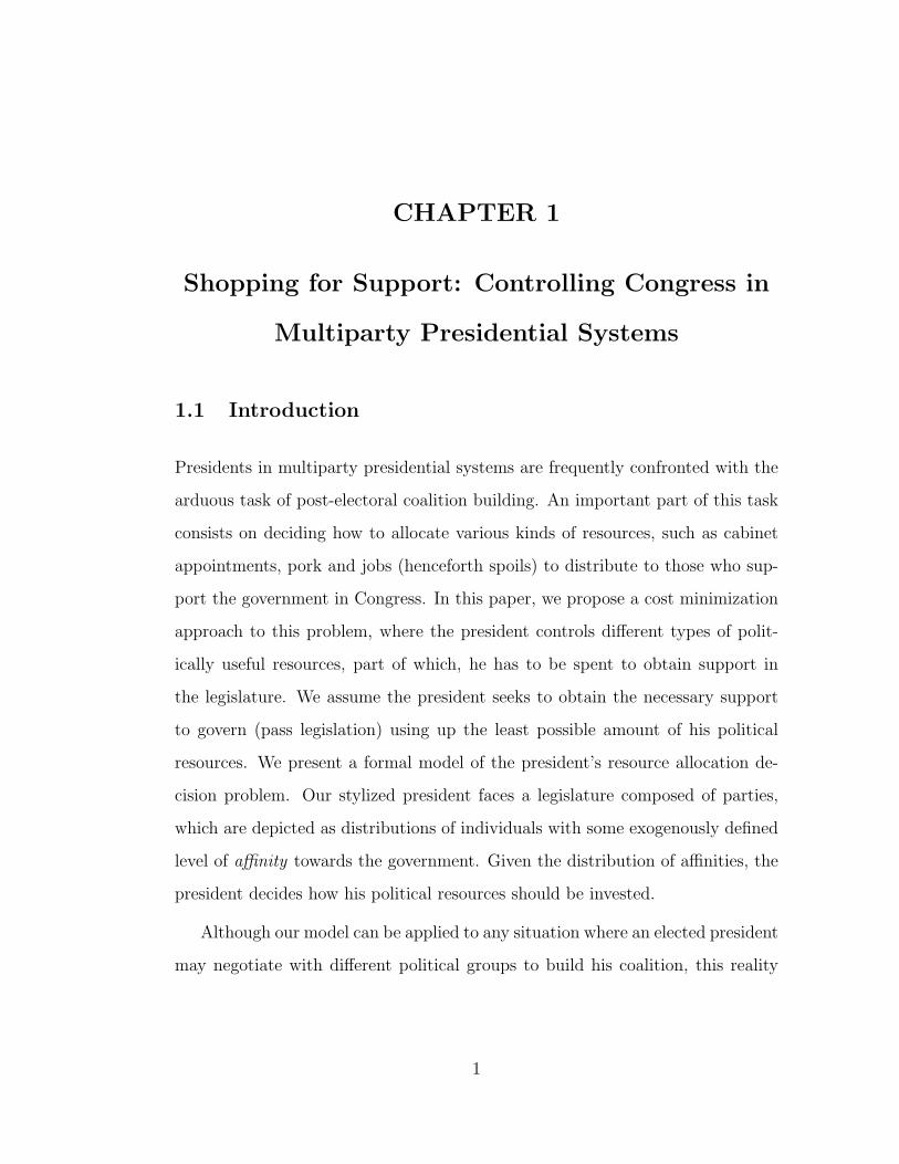
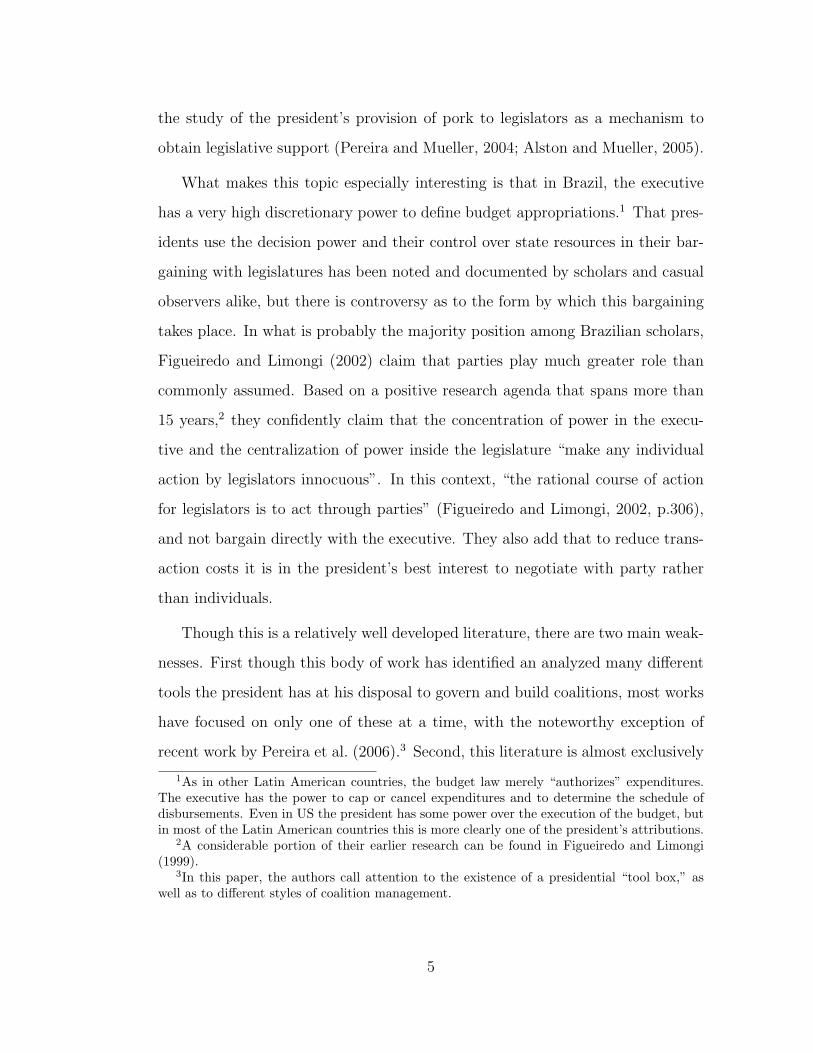
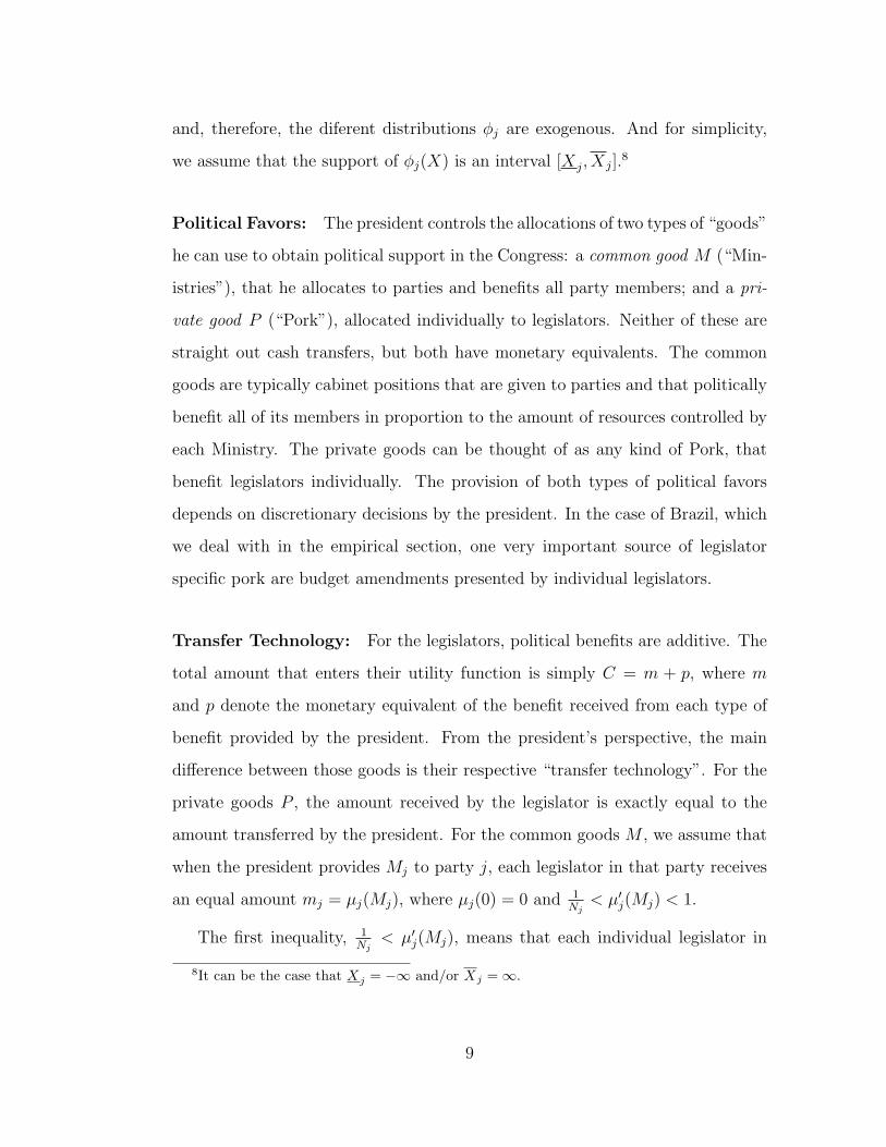
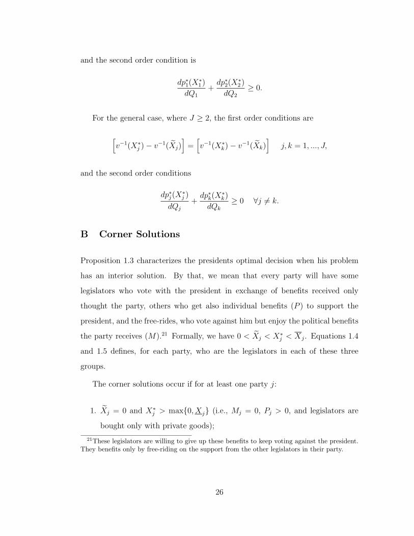
For 2004, we do not have that problem, and Figure 1.1 compares the model’s
15For the years used, legislators had a quota of 20 amendments for a total of up to 2 millionreais.
16Note that Figueiredo and Limongi (2002) question the importance of these amendments.17Between 2003 and 2004 retention was around 95%.
20
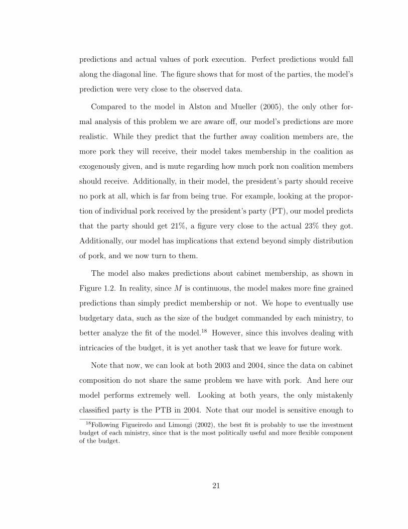
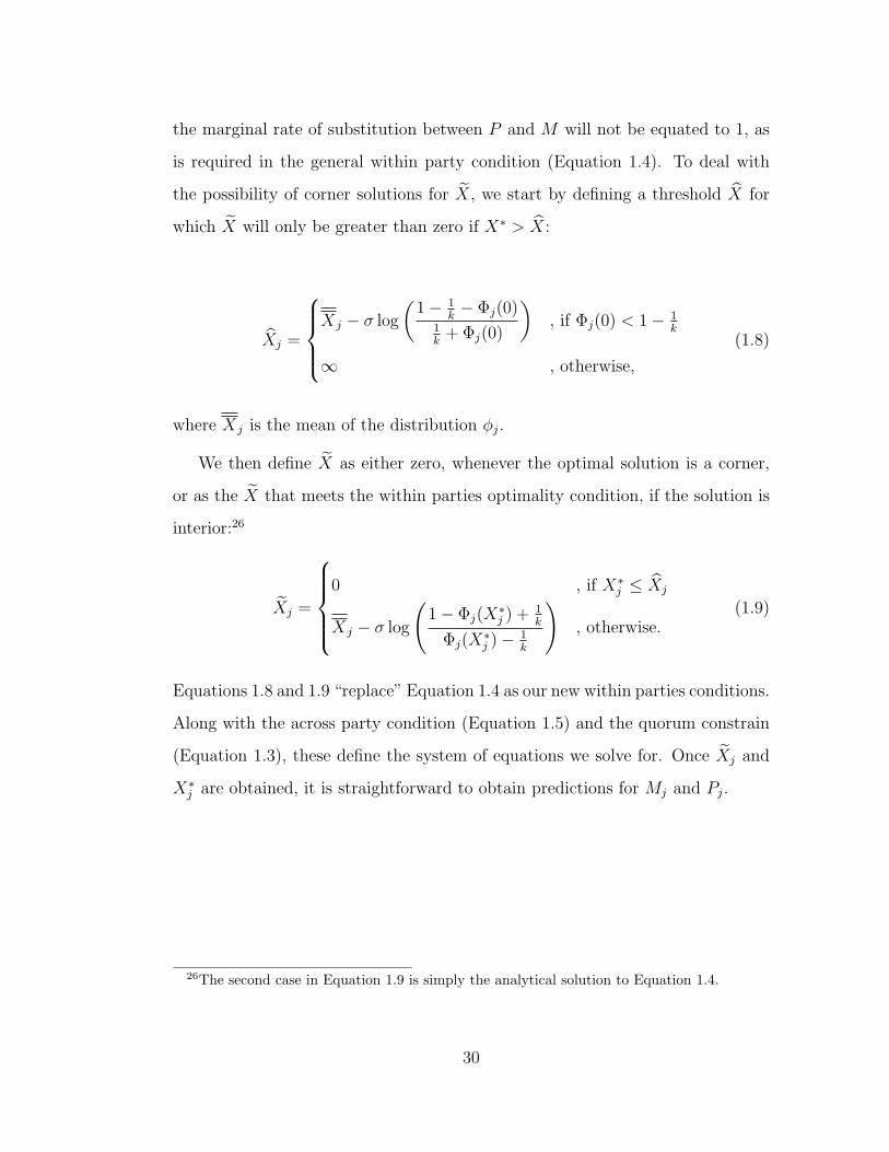
predictions and actual values of pork execution. Perfect predictions would fall
along the diagonal line. The figure shows that for most of the parties, the model’s
prediction were very close to the observed data.
Compared to the model in Alston and Mueller (2005), the only other for-
mal analysis of this problem we are aware off, our model’s predictions are more
realistic. While they predict that the further away coalition members are, the
more pork they will receive, their model takes membership in the coalition as
exogenously given, and is mute regarding how much pork non coalition members
should receive. Additionally, in their model, the president’s party should receive
no pork at all, which is far from being true. For example, looking at the propor-
tion of individual pork received by the president’s party (PT), our model predicts
that the party should get 21%, a figure very close to the actual 23% they got.
Additionally, our model has implications that extend beyond simply distribution
of pork, and we now turn to them.
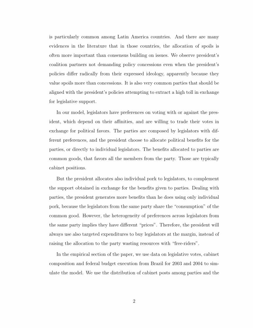
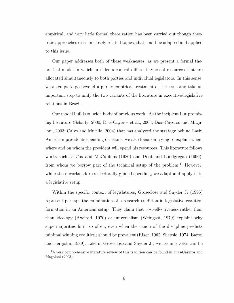
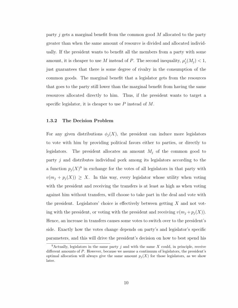
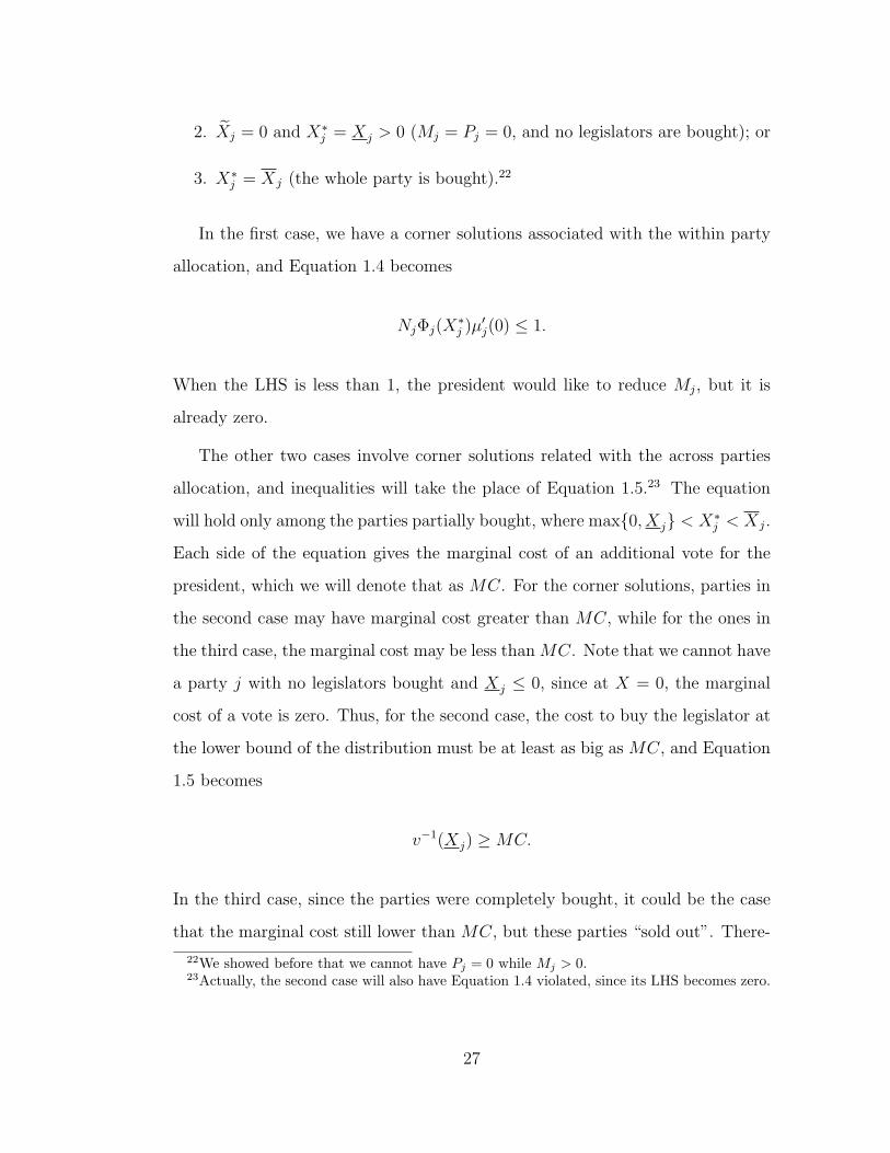
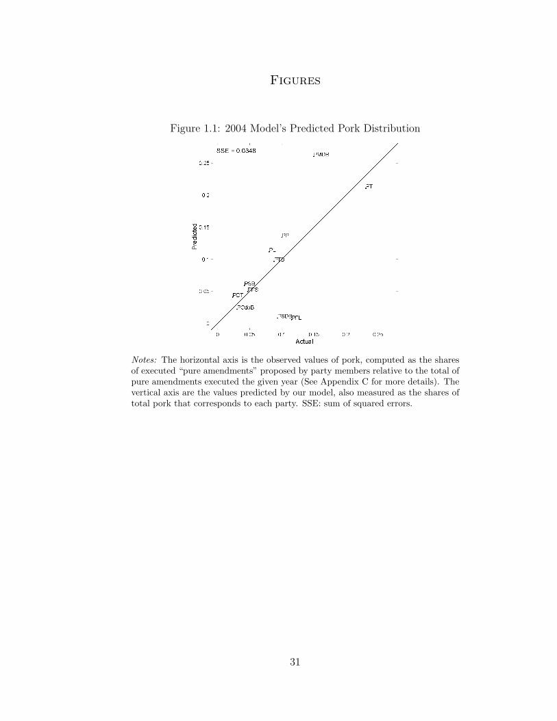
The model also makes predictions about cabinet membership, as shown in
Figure 1.2. In reality, since M is continuous, the model makes more fine grained
predictions than simply predict membership or not. We hope to eventually use
budgetary data, such as the size of the budget commanded by each ministry, to
better analyze the fit of the model.18 However, since this involves dealing with
intricacies of the budget, it is yet another task that we leave for future work.
Note that now, we can look at both 2003 and 2004, since the data on cabinet
composition do not share the same problem we have with pork. And here our
model performs extremely well. Looking at both years, the only mistakenly
classified party is the PTB in 2004. Note that our model is sensitive enough to
18Following Figueiredo and Limongi (2002), the best fit is probably to use the investmentbudget of each ministry, since that is the most politically useful and more flexible componentof the budget.
21
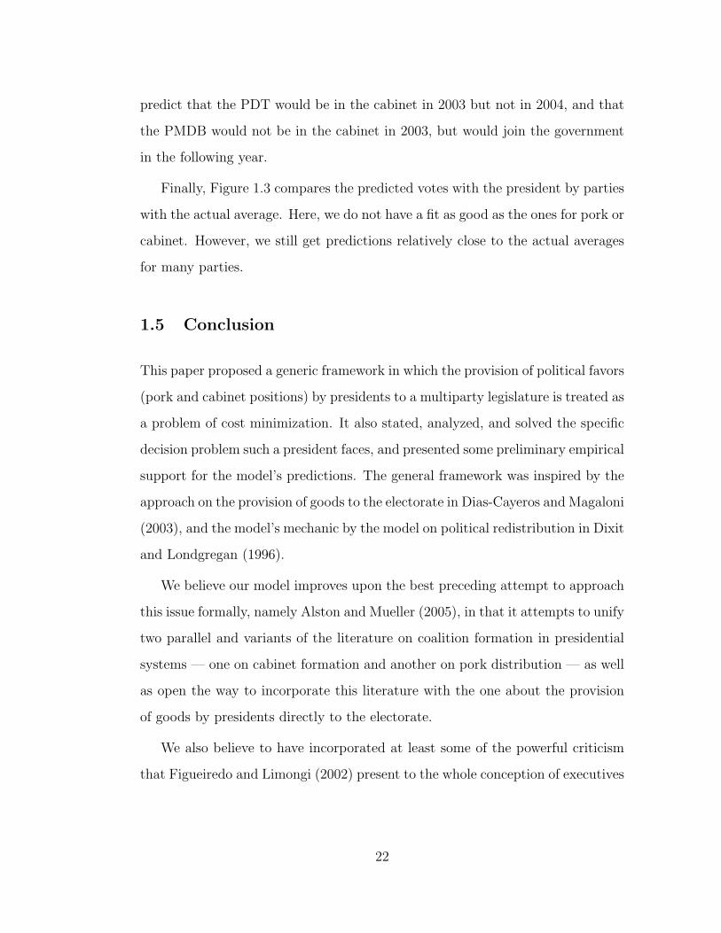
predict that the PDT would be in the cabinet in 2003 but not in 2004, and that
the PMDB would not be in the cabinet in 2003, but would join the government
in the following year.
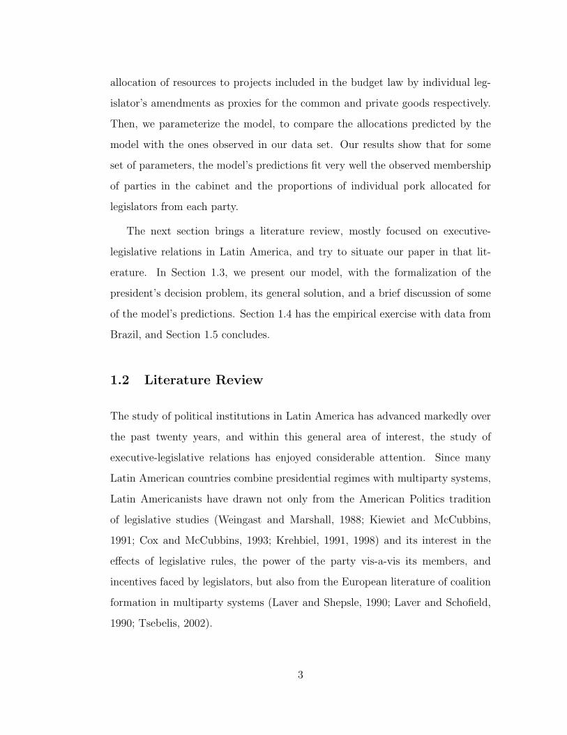
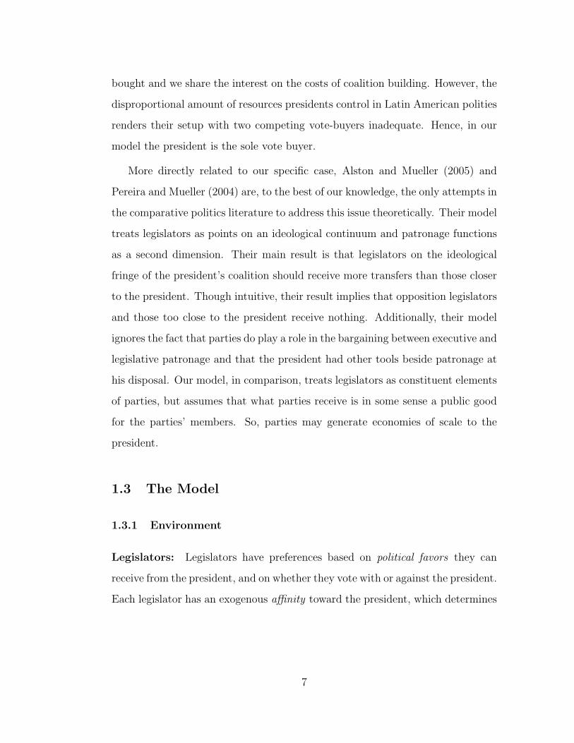
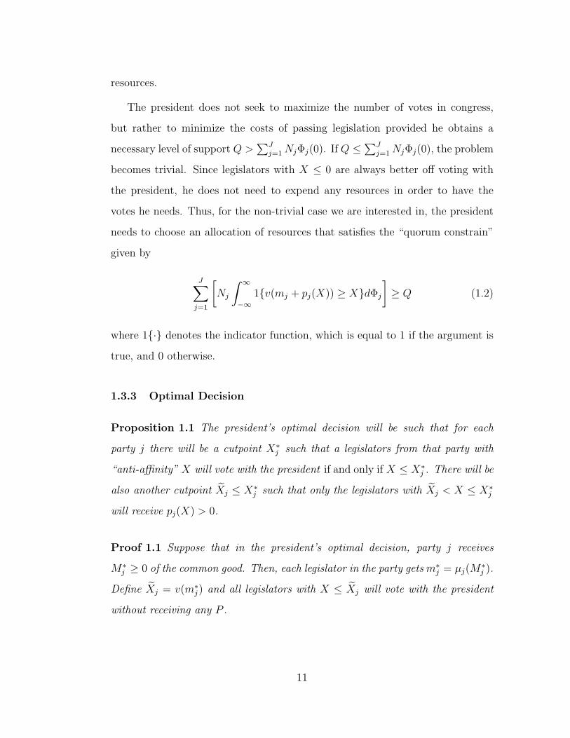
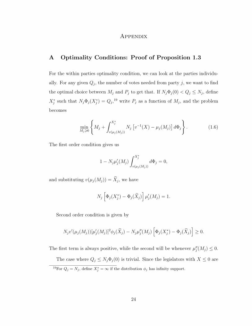
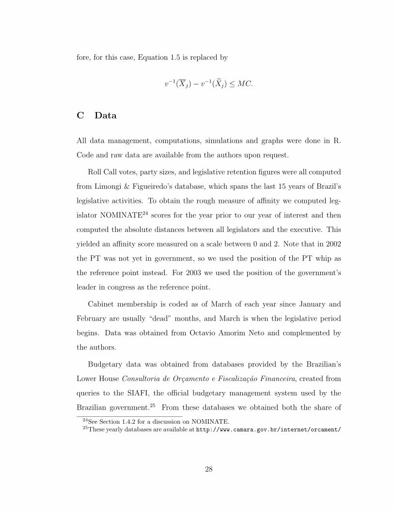
Finally, Figure 1.3 compares the predicted votes with the president by parties
with the actual average. Here, we do not have a fit as good as the ones for pork or
cabinet. However, we still get predictions relatively close to the actual averages
for many parties.
1.5 Conclusion
This paper proposed a generic framework in which the provision of political favors
(pork and cabinet positions) by presidents to a multiparty legislature is treated as
a problem of cost minimization. It also stated, analyzed, and solved the specific
decision problem such a president faces, and presented some preliminary empirical
support for the model’s predictions. The general framework was inspired by the
approach on the provision of goods to the electorate in Dias-Cayeros and Magaloni
(2003), and the model’s mechanic by the model on political redistribution in Dixit
and Londgregan (1996).
We believe our model improves upon the best preceding attempt to approach
this issue formally, namely Alston and Mueller (2005), in that it attempts to unify
two parallel and variants of the literature on coalition formation in presidential
systems — one on cabinet formation and another on pork distribution — as well
as open the way to incorporate this literature with the one about the provision
of goods by presidents directly to the electorate.
We also believe to have incorporated at least some of the powerful criticism
that Figueiredo and Limongi (2002) present to the whole conception of executives
22

buying support from locally minded individual legislators. In our model, parties
play an important role, bargaining with legislators is done on the margin and
the executive is the main actor. In principle, this is compatible both with a
story where legislator’s amendments are crucial and one where this dynamic is
marginal.
In the empirical part of the paper, we are still working to improve the analysis
in many ways, as we describe in Section 1.4. However, for the exercise we pro-
posed, of trying to establish if, for some set of parameters, the model can match
qualitatively the data on cabinet composition and distribution of individual pork,
the results were very satisfying. These results give us a great incentive to keep
working on that agenda, pursuing to advance on the estimations of the model,
and exploring the many possible extensions and applications of our model.
23
Appendix
A Optimality Conditions: Proof of Proposition 1.3
For the within parties optimality condition, we can look at the parties individu-
ally. For any given Qj, the number of votes needed from party j, we want to find
the optimal choice between Mj and Pj to get that. If NjΦj(0) < Qj ≤ Nj, define
X∗j such that NjΦj(X∗j ) = Qj,
19 write Pj as a function of Mj, and the problem
becomes
minMj>0
{Mj +
∫ X∗j
v(µj(Mj))
Nj
[v−1(X)− µj(Mj)
]dΦj
}. (1.6)
The first order condition gives us
1−Njµ′j(Mj)
∫ X∗j
v(µj(Mj))
dΦj = 0,
and substituting v(µj(Mj)) = Xj, we have
Nj
[Φj(X
∗j )− Φj(Xj)
]µ′j(Mj) = 1.
Second order condition is given by
Njv′(µj(Mj))[µ
′j(Mj)]
2φj(Xj)−Njµ′′j (Mj)
[Φj(X
∗j )− Φj(Xj)
]≥ 0.
The first term is always positive, while the second will be whenever µ′′j (Mj) ≤ 0.
The case where Qj ≤ NjΦj(0) is trivial. Since the legislators with X ≤ 0 are
19For Qj = Nj , define X∗j =∞ if the distribution φj has infinity support.
24
willing to vote with the president without receiving any political favors, we will
have Mj = Pj = 0. And finally, note that we cannot have Qj > Nj.
For the across parties, we will use the case with only two parties, for sim-
plicity, but the results can be extended for the general case with J ≥ 2. Define
TCj(Qj) as the minimum cost to “buy” Qj votes from party j.20 From the quo-
rum constraint we can write Q2 = Q − Q1, and the president’s problem can be
stated as
minQ1∈[0,N1]
{TC1(Q1) + TC2(Q−Q1)}. (1.7)
Now, note thatdTCj
dQj=
dTCj
dX∗j× dX∗
j
dQj. Applying the Envelope Theorem on (1.6),
and using NjΦj(X∗j ) = Qj, we get
dTCjdQj
= Njφj(X∗j )[v−1(X∗j )− µj(Mj)
]( 1
Njφj(X∗j )
)=[v−1(X∗j )− µj(Mj)
]= p∗j(X
∗j ).
Thus, the first order condition for (1.7) is
[v−1(X∗1 )− µ1(M1)
]−[v−1(X∗2 )− µj(M2)
]= 0,
or just
p∗1(X∗1 ) = p∗2(X
∗2 ),
20Let TCj(Qj) =∞ if Qj > Nj .
25
and the second order condition is
dp∗1(X∗1 )
dQ1
+dp∗2(X
∗2 )
dQ2
≥ 0.
For the general case, where J ≥ 2, the first order conditions are
[v−1(X∗j )− v−1(Xj)
]=[v−1(X∗k)− v−1(Xk)
]j, k = 1, ..., J,
and the second order conditions
dp∗j(X∗j )
dQj
+dp∗k(X
∗k)
dQk
≥ 0 ∀j 6= k.
B Corner Solutions
Proposition 1.3 characterizes the presidents optimal decision when his problem
has an interior solution. By that, we mean that every party will have some
legislators who vote with the president in exchange of benefits received only
thought the party, others who get also individual benefits (P ) to support the
president, and the free-rides, who vote against him but enjoy the political benefits
the party receives (M).21 Formally, we have 0 < Xj < X∗j < Xj. Equations 1.4
and 1.5 defines, for each party, who are the legislators in each of these three
groups.
The corner solutions occur if for at least one party j:
1. Xj = 0 and X∗j > max{0, Xj} (i.e., Mj = 0, Pj > 0, and legislators are
bought only with private goods);
21These legislators are willing to give up these benefits to keep voting against the president.They benefits only by free-riding on the support from the other legislators in their party.
26
2. Xj = 0 and X∗j = Xj > 0 (Mj = Pj = 0, and no legislators are bought); or
3. X∗j = Xj (the whole party is bought).22
In the first case, we have a corner solutions associated with the within party
allocation, and Equation 1.4 becomes
NjΦj(X∗j )µ′j(0) ≤ 1.
When the LHS is less than 1, the president would like to reduce Mj, but it is
already zero.
The other two cases involve corner solutions related with the across parties
allocation, and inequalities will take the place of Equation 1.5.23 The equation
will hold only among the parties partially bought, where max{0, Xj} < X∗j < Xj.
Each side of the equation gives the marginal cost of an additional vote for the
president, which we will denote that as MC. For the corner solutions, parties in
the second case may have marginal cost greater than MC, while for the ones in
the third case, the marginal cost may be less than MC. Note that we cannot have
a party j with no legislators bought and Xj ≤ 0, since at X = 0, the marginal
cost of a vote is zero. Thus, for the second case, the cost to buy the legislator at
the lower bound of the distribution must be at least as big as MC, and Equation
1.5 becomes
v−1(Xj) ≥MC.
In the third case, since the parties were completely bought, it could be the case
that the marginal cost still lower than MC, but these parties “sold out”. There-
22We showed before that we cannot have Pj = 0 while Mj > 0.23Actually, the second case will also have Equation 1.4 violated, since its LHS becomes zero.
27
fore, for this case, Equation 1.5 is replaced by
v−1(Xj)− v−1(Xj) ≤MC.
C Data
All data management, computations, simulations and graphs were done in R.
Code and raw data are available from the authors upon request.
Roll Call votes, party sizes, and legislative retention figures were all computed
from Limongi & Figueiredo’s database, which spans the last 15 years of Brazil’s
legislative activities. To obtain the rough measure of affinity we computed leg-
islator NOMINATE24 scores for the year prior to our year of interest and then
computed the absolute distances between all legislators and the executive. This
yielded an affinity score measured on a scale between 0 and 2. Note that in 2002
the PT was not yet in government, so we used the position of the PT whip as
the reference point instead. For 2003 we used the position of the government’s
leader in congress as the reference point.
Cabinet membership is coded as of March of each year since January and
February are usually “dead” months, and March is when the legislative period
begins. Data was obtained from Octavio Amorim Neto and complemented by
the authors.
Budgetary data was obtained from databases provided by the Brazilian’s
Lower House Consultoria de Orcamento e Fiscalizacao Financeira, created from
queries to the SIAFI, the official budgetary management system used by the
Brazilian government.25 From these databases we obtained both the share of
24See Section 1.4.2 for a discussion on NOMINATE.25These yearly databases are available at http://www.camara.gov.br/internet/orcament/
28
the budget controlled by each ministry as well as the amendments presented by
legislators. Legislators can present amendments to pre-existing projects (projects
included in the budget draft by the executive) or create new projects for which
no amount was reserved. In the former case, it is impossible to distinguish if
the amount executed was from the legislator’s amendment or not. Therefore, all
pork figures used in this paper take into consideration only “pure amendments,”
or the execution of amendments that created new projects. The computation of
“pure amendments” are only implemented for 2003 onwards, but we have made
arrangements to have them extended backwards until 1995, and will probably be
included in future versions of this paper.
D Algorithm
The only caveat is that instead of choosing the Xj and X∗j that minimize the pres-
ident’s costs we opted to solve analytically for Xj, and to optimize the resulting
system of J equations only for X∗j . This decision was made to allow for faster
computation, and also to facilitate dealing with the issue of corner solutions for
X.
Since previous to the allocation of any political favors, all the legislators with
X ≤ 0 vote with the president, all Xjs and X∗j s have to be non-negative numbers.
This is not much of a problem with X∗j s, since the use of a distribution such as
the logistic, with infinite support, ensures an interior solution for the across party
optimization problem. All parties have positive mass along the entire real line so
Equation 1.5 holds without alterations and all parties will have a positive X∗.
However, in some cases we might have a corner solution for X, in which case
principal/exibe.asp?idePai=2&cadeia=0@.
29
the marginal rate of substitution between P and M will not be equated to 1, as
is required in the general within party condition (Equation 1.4). To deal with
the possibility of corner solutions for X, we start by defining a threshold X for
which X will only be greater than zero if X∗ > X:
Xj =
Xj − σ log
(1− 1
k− Φj(0)
1k
+ Φj(0)
), if Φj(0) < 1− 1
k
∞ , otherwise,
(1.8)
where Xj is the mean of the distribution φj.
We then define X as either zero, whenever the optimal solution is a corner,
or as the X that meets the within parties optimality condition, if the solution is
interior:26
Xj =
0 , if X∗j ≤ Xj
Xj − σ log
(1− Φj(X
∗j ) + 1
k
Φj(X∗j )− 1k
), otherwise.
(1.9)
Equations 1.8 and 1.9 “replace” Equation 1.4 as our new within parties conditions.
Along with the across party condition (Equation 1.5) and the quorum constrain
(Equation 1.3), these define the system of equations we solve for. Once Xj and
X∗j are obtained, it is straightforward to obtain predictions for Mj and Pj.
26The second case in Equation 1.9 is simply the analytical solution to Equation 1.4.
30
Figures
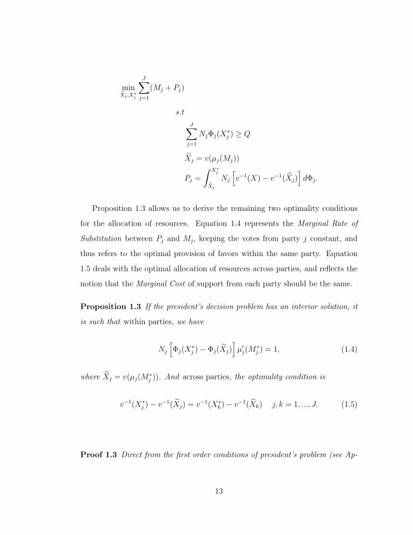
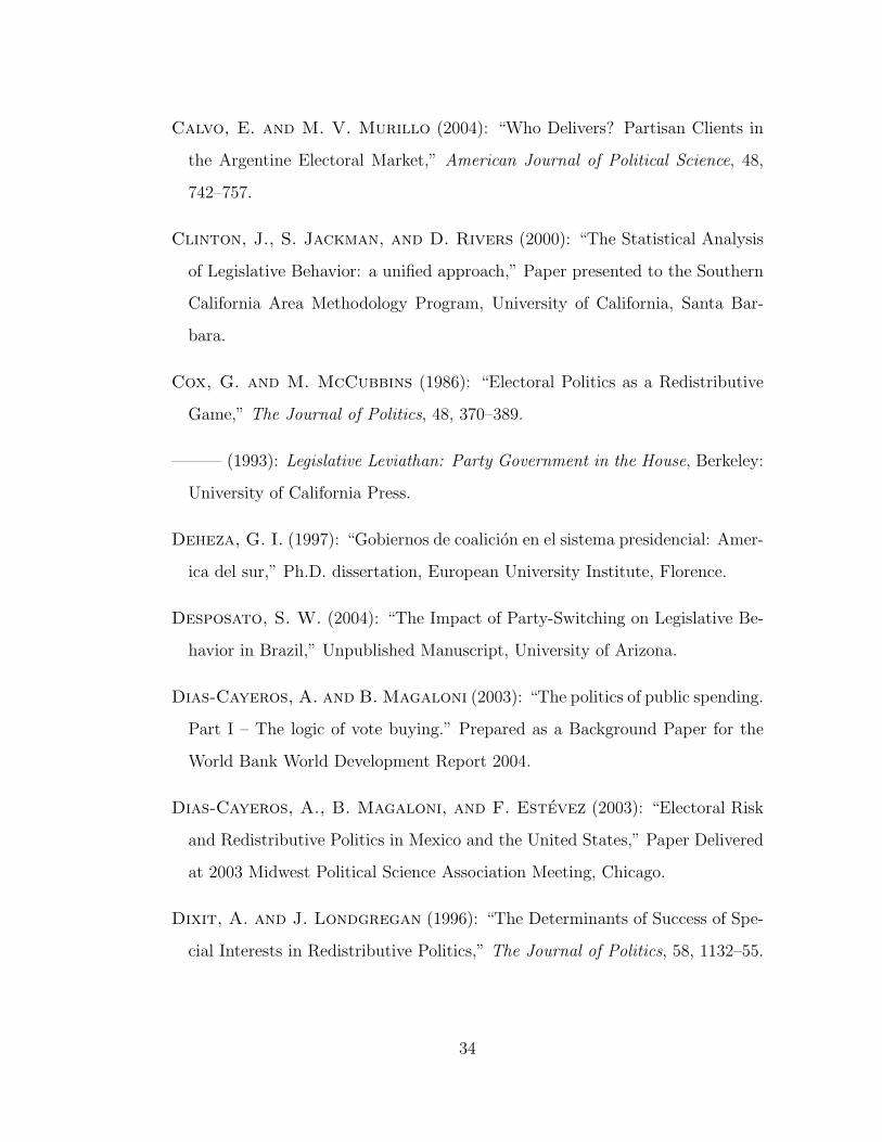
Figure 1.1: 2004 Model’s Predicted Pork Distribution
Notes: The horizontal axis is the observed values of pork, computed as the sharesof executed “pure amendments” proposed by party members relative to the total ofpure amendments executed the given year (See Appendix C for more details). Thevertical axis are the values predicted by our model, also measured as the shares oftotal pork that corresponds to each party. SSE: sum of squared errors.
31
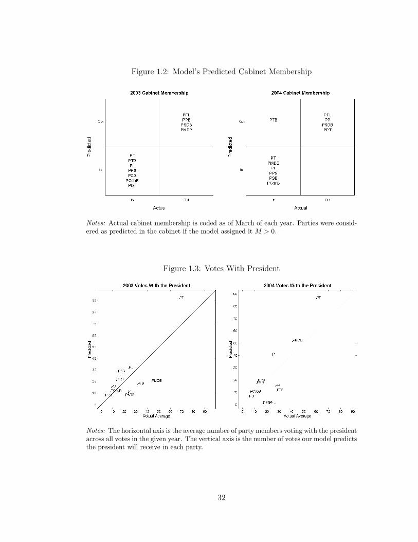
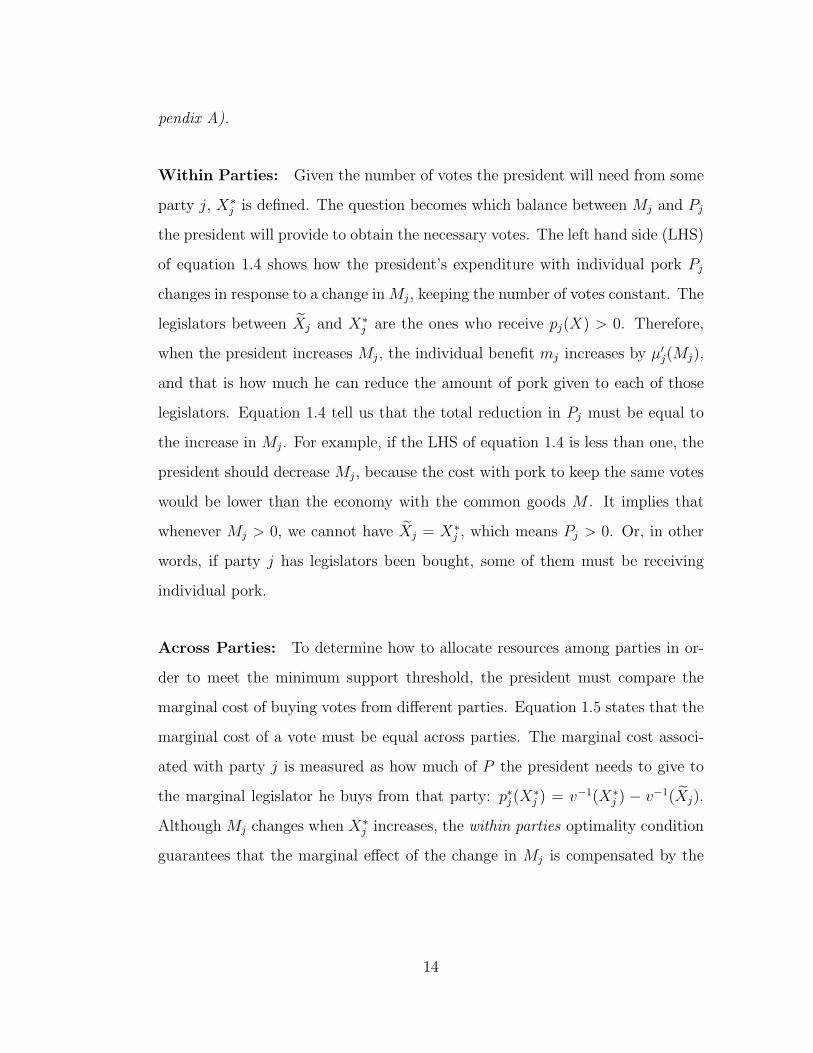
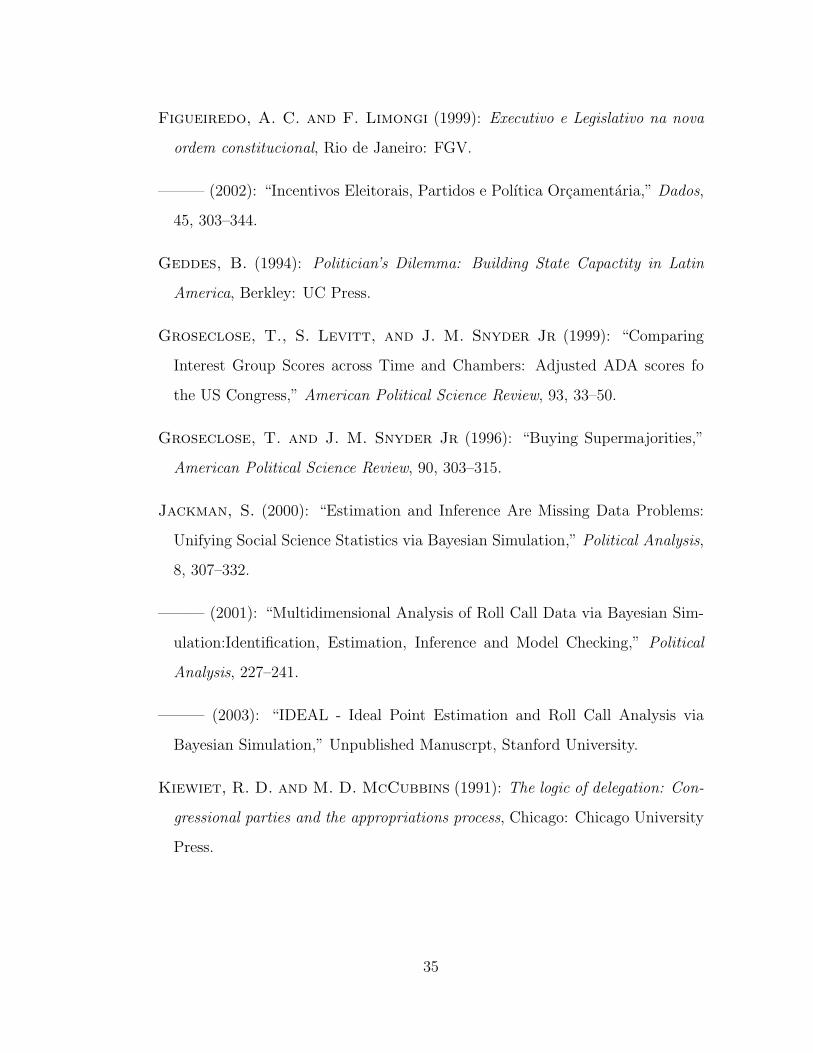
Figure 1.2: Model’s Predicted Cabinet Membership
Notes: Actual cabinet membership is coded as of March of each year. Parties were consid-ered as predicted in the cabinet if the model assigned it M > 0.
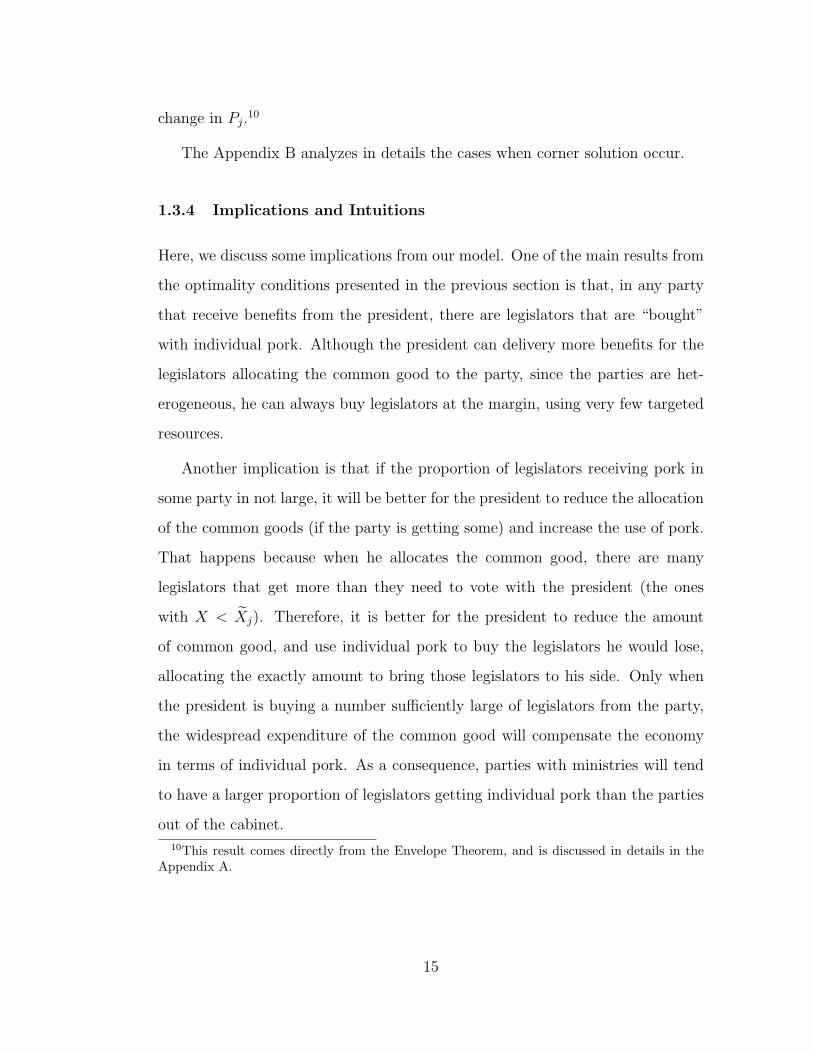
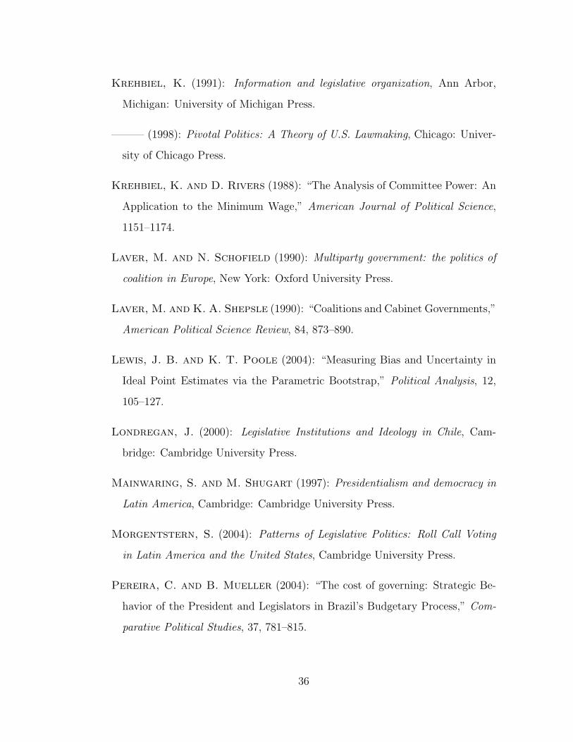
Figure 1.3: Votes With President
Notes: The horizontal axis is the average number of party members voting with the presidentacross all votes in the given year. The vertical axis is the number of votes our model predictsthe president will receive in each party.
32
Bibliography
Abranches, S. (1988): “Presidencialismo de coalizao,” Dados, 31, 5–34.
Alcantara, M. (1994-2000): “Proyecto de Elites Latinoaericanas (PELA),”
Technical Report, Universidad de Salamanca, Salamanca.
Aleman, E. and G. Tsebelis (2002): “Agenda Control in Latin American
Presidential Democracies,” Paper Delivered at the American Political Science
Association meeting.
Alston, L. J. and B. Mueller (2005): “Pork for Policy: Executive and
Legislative Exchange in Brazil,” NBER Working Paper 11273.
Altman, D. (2000): “The Politics of Coalition Formation and Survival in Mul-
tiparty Presidential Democracies: The Case of Uruguay 1989–1999,” Party
Politics, 6, 259–283.
Ames, B. (2001): The Deadlock of Democracy in Brazil, Ann Arbor: University
of Michigan Press.
Amorim Neto, O. (1998): “Of presidents, parties, and ministers: cabinet for-
mation and legislative decision-making under separation of powers,” Ph.D.
thesis, UCSD, San Diego.
——— (2006): “The Presidential Calculus: Executive Policy-Making and Cabi-
net Formation in the Americas,” Comparative Political Studies, 39, 415–440.
Axelrod, R. (1970): Conflict of interest, Chicago: Markham.
Baron, D. P. and J. A. Ferejohn (1989): “Bargaining in Legislatures,”
American Political Science Review, 83, 1181–1206.
33
Calvo, E. and M. V. Murillo (2004): “Who Delivers? Partisan Clients in
the Argentine Electoral Market,” American Journal of Political Science, 48,
742–757.
Clinton, J., S. Jackman, and D. Rivers (2000): “The Statistical Analysis
of Legislative Behavior: a unified approach,” Paper presented to the Southern
California Area Methodology Program, University of California, Santa Bar-
bara.
Cox, G. and M. McCubbins (1986): “Electoral Politics as a Redistributive
Game,” The Journal of Politics, 48, 370–389.
——— (1993): Legislative Leviathan: Party Government in the House, Berkeley:
University of California Press.
Deheza, G. I. (1997): “Gobiernos de coalicion en el sistema presidencial: Amer-
ica del sur,” Ph.D. dissertation, European University Institute, Florence.
Desposato, S. W. (2004): “The Impact of Party-Switching on Legislative Be-
havior in Brazil,” Unpublished Manuscript, University of Arizona.
Dias-Cayeros, A. and B. Magaloni (2003): “The politics of public spending.
Part I – The logic of vote buying.” Prepared as a Background Paper for the
World Bank World Development Report 2004.
Dias-Cayeros, A., B. Magaloni, and F. Estevez (2003): “Electoral Risk
and Redistributive Politics in Mexico and the United States,” Paper Delivered
at 2003 Midwest Political Science Association Meeting, Chicago.
Dixit, A. and J. Londgregan (1996): “The Determinants of Success of Spe-
cial Interests in Redistributive Politics,” The Journal of Politics, 58, 1132–55.
34
Figueiredo, A. C. and F. Limongi (1999): Executivo e Legislativo na nova
ordem constitucional, Rio de Janeiro: FGV.
——— (2002): “Incentivos Eleitorais, Partidos e Polıtica Orcamentaria,” Dados,
45, 303–344.
Geddes, B. (1994): Politician’s Dilemma: Building State Capactity in Latin
America, Berkley: UC Press.
Groseclose, T., S. Levitt, and J. M. Snyder Jr (1999): “Comparing
Interest Group Scores across Time and Chambers: Adjusted ADA scores fo
the US Congress,” American Political Science Review, 93, 33–50.
Groseclose, T. and J. M. Snyder Jr (1996): “Buying Supermajorities,”
American Political Science Review, 90, 303–315.
Jackman, S. (2000): “Estimation and Inference Are Missing Data Problems:
Unifying Social Science Statistics via Bayesian Simulation,” Political Analysis,
8, 307–332.
——— (2001): “Multidimensional Analysis of Roll Call Data via Bayesian Sim-
ulation:Identification, Estimation, Inference and Model Checking,” Political
Analysis, 227–241.
——— (2003): “IDEAL - Ideal Point Estimation and Roll Call Analysis via
Bayesian Simulation,” Unpublished Manuscrpt, Stanford University.
Kiewiet, R. D. and M. D. McCubbins (1991): The logic of delegation: Con-
gressional parties and the appropriations process, Chicago: Chicago University
Press.
35
Krehbiel, K. (1991): Information and legislative organization, Ann Arbor,
Michigan: University of Michigan Press.
——— (1998): Pivotal Politics: A Theory of U.S. Lawmaking, Chicago: Univer-
sity of Chicago Press.
Krehbiel, K. and D. Rivers (1988): “The Analysis of Committee Power: An
Application to the Minimum Wage,” American Journal of Political Science,
1151–1174.
Laver, M. and N. Schofield (1990): Multiparty government: the politics of
coalition in Europe, New York: Oxford University Press.
Laver, M. and K. A. Shepsle (1990): “Coalitions and Cabinet Governments,”
American Political Science Review, 84, 873–890.
Lewis, J. B. and K. T. Poole (2004): “Measuring Bias and Uncertainty in
Ideal Point Estimates via the Parametric Bootstrap,” Political Analysis, 12,
105–127.
Londregan, J. (2000): Legislative Institutions and Ideology in Chile, Cam-
bridge: Cambridge University Press.
Mainwaring, S. and M. Shugart (1997): Presidentialism and democracy in
Latin America, Cambridge: Cambridge University Press.
Morgentstern, S. (2004): Patterns of Legislative Politics: Roll Call Voting
in Latin America and the United States, Cambridge University Press.
Pereira, C. and B. Mueller (2004): “The cost of governing: Strategic Be-
havior of the President and Legislators in Brazil’s Budgetary Process,” Com-
parative Political Studies, 37, 781–815.
36
Pereira, C., T. J. Power, and E. D. Raile (2006): “The Presidential
Toolbox: Generating Support in a Multiparty Presidential Regime,” Paper
Delivered at the American Political Science Association Meeting, Philadelphia.
Poole, K. T. (2005): Spacial Models of Parliamentary Voting, Cambridge:
Cambridge University Press.
Poole, K. T. and H. Rosenthal (1985): “A Spacial Model of Legislative
Roll Call Analysis,” American Journal of Political Science, 29, 357–384.
——— (1991): “Patterns of Legislative Voting,” American Journal of Political
Science, 35, 228–278.
——— (1997): A Political-Economic History of Roll Call Voting, New York:
Oxford University Press.
Riker, W. (1962): The Theory of Political Coalitions, New Haven: Yale Uni-
versity Press.
Rosas, G. (2005): “The ideological organization of Latin American Legisla-
tive Parties: An Empirical Analysis of Elite Policy Preferences,” Comparative
Political Studies, 38, 824–849.
Samuels, D. (2003): Ambition, Federalism and Legislative Politics in Brazil,
Cambridge: Cambridge University Press.
Schady, N. R. (2000): “The Political Economy of Expenditures by the Peruvian
Social Fund (FONCODES), 91-95,” American Political Science Review, 94,
289–304.
Shepsle, K. (1974): “On the Size of Winning Coalitions,” American Political
Science Reveiw, 68, 505–518.
37
Shugart, M. S. and J. M. Carey (1992): Parties and Assemblies: Con-
stitutional Design and Electoral Dynamics, Cambridge: Cambridge University
Press.
Tsebelis, G. (2002): Veto Players: How Political Institutions Work, New York:
Princeton University Press and Russell Sage Foundation.
Weingast, B. (1979): “A Rational Choice Perspective on Congressional
Norms,” American Journal of Political Science, 245–262.
Weingast, B. R. and W. J. Marshall (1988): “The industrial organization
of congress; or, why legislatures, like firms, are not organized as markets,”
Journal of Political Economy, 96, 132–163.
Zechmeister, E. J. and J. P. Luna (2005): “Political Representation in Latin
America: A Study of Elite-Mass Conguence in Nine Countries,” Comparative
Political Studies, 38, 388–416.
38
CHAPTER 2
The Back-up Investment Incentives in the
Brazilian Electrical Sector Regulatory Model
2.1 Introduction
Until the middle of the 1990s, all the Brazilian electric utilities were public com-
panies, and the federal government centralized the planning and execution of all
the investments in generation. In 1995, with the beginning of the privatization
of those utilities, the government started to implement a regulatory model for
the sector. One of the most important targets of that regulation was how to
guarantee the necessary investments in generation. After almost one decade, the
regulatory model has failed in many fronts. In particular, the investments in
thermal generation capacity to back-up the hydroelectric system did not happen,
resulting in a huge electrical crisis.
In this paper, I analyze some aspects of the regulatory model implemented
after the start of the privatization, and present a model that helps to understand
how that regulation should work and why it did not. That model must helps to
understand how different features of the regulatory model affect the behavior of
the firms.
In the next Section, I present a big picture of the Brazilian electrical sector.
There I go from since its origin until the crisis in 2001, describing some important
39
characteristics about its regulatory model, especially about the generation, that
needs to be considered for in my analysis. In the Section 2.3, I present a model
that try, in a simplified way, to represent the environment described in the Section
2.2. This model is a starting point for the analysis, and need to be improved
to approach the many faces of the problem. Finally, in Section 2.4, I presented
futures improvements for the analysis presented here, and discuss some conclusion
that can be taken already.
2.2 The Brazilian Electrical Sector
2.2.1 Origins and Development of the Sector
The Brazilian electrical sector had its origin in the end of the nineteenth century.
In 1883, it was constructed the first hydroelectric plant of the country. From
that time until 1930, the sector developed basically by the private initiative,
with a massive participation of foreign companies. After the Revolution of 1930,
the growth of the nationalist ideas resulted in resistances against the control of
the electrical sector by foreign companies. In 1934, the Brazilian government
implemented the Codigo de Aguas that established the concession regime for
the utilization of hydric resources. Before, the rights over the waterfalls were
associated with the property of the ground, and with the Codigo, the Federal
government became the conceding power. The Codigo also established that the
prices should be based on the service costs and on the capital value, which should
be calculated from the historical costs of good and installations used. The Codigo
de Aguas represented a big reverse for the private companies in the sector, and
probably was directly related with the occurrence of crises that demanded saving
plans in 1939.
40
Although the Codigo de Aguas gave to the Federal government the control
over the concessions, until the beginning of the 1950’s the direct participation of
the state as investor still discrete. The strong increase in the demand, propelled
by the increasing urbanization and industrialization resulted in constants crises
of electricity supply. After that, along the 1950’s and the first half of the 1960’s,
we can observe the intense participation of the state in the electrical generation
sector. Data from Lima (1995) show that between 1952 and 1965 the installed
capacity increased more than 10% per year, going from 1,985 MW to 7,411 MW.
Most of the increase was due the public investment, as the participation of the
public generators in the total capacity went from 6.8% to 54.6% in the same
period.
In 1965, the government created the DNAEE (National Department of Water
and Energy), with the normative and regulatory functions, while the ELETROBRAS
was the Federal company that deal with planning and execution of the electrical
federal policy. According to Lima, that reform allowed the sector to auto-finance
the needed investments from 1967 and 1973. After that, the Federal government
opted to finance the electrical sector with foreign resources. However, the gov-
ernment may have taken that strategy more because of its necessity to finance
the balance account than because of the sector’s needs.
With the second oil shock in 1979, and the international financial crisis that
follows, that centralized model started to face difficulties to keep the investments.
As we can see in Figure 2.1, the total investments in the electrical sector fell from
US$ 15 billions in 1982 to US$ 5 billions in 1997. We should note that at this
point, almost all the utilities companies were public.
41
2.2.2 The Change of Regimes
In that context, the government decided to initiate the process of privatization
of the electrical sector. In 1995, the first distribution utility was privatized, and
in 1997 the privatization arrived in the generation sector, with the selling of the
first hydroelectric plant.
Just before the implementation of the new regulatory model, most of the reg-
ulatory tasks were performed by the DNAEE. It included the planning, coordina-
tion and development of the hydrological studies. The DNAEE was responsible
also for the evaluation of the price of the electricity and the supervision of the
concession in the electrical sector.
The planning of the system (generation and transmission) was responsibility
of the GCPS (Group of System Planning Coordination). The GCPS is coor-
dinated by the ELETROBRAS, the holding company of all Federal generation
subsidiaries, and was composed by these subsidiaries and the main distribution
companies (in general, state’s public companies). The GCPS used to prepare the
system expansion plan for 10, 15 and 25 years. However, it is important to note
that, in the centralized regime, the investments proposed by the GCPS depended
on the government’s final decision, and the data presented in the previous section
suggest that in the last years of that regime, most of them were not realized.
Finally, the GCOI (Interlinked Operation Coordinator Group) was responsible
for the coordination of the physical operation of the system, establishing the
criteria of the determination of who should generate, according to the hydrological
risks, transmission possibilities, and the costs of thermal generation available.
The GCOI had a composition similar to that of the GCPS, and counted also
with the DNAEE, as observer.
42
With the beginning of the privatization in the electrical sector, it was adopted
a new regulatory model, designed to regulate a sector based on private agents.
In that model, a new institution controlled by the generators took the task of
the coordination of the physical operation system. The planning of expansion of
generation became only indicative, and the new regulatory agency - the ANEEL
- took the responsibility over the process of concession for the new investments
in the expansion plan. It is important to note that there are no guarantees that
the proposed investments will be realized, and the potential investor may ask for
the ANEEL to open the concession process of some investment not included in
the indicative planning.
In this new environment, it was fundamental that to create the right incentives
for the private sector to take its part in the execution of what were planned,
specially taking in account the absence of investments in the last years of the old
regime.
As we saw in the Figure 2.1, the amount of investments in the electrical sector
fell continuously in the last years of the centralized system. From 1987 to 1997,
the investments decreased in almost two thirds, going from US$ 15.4 billions to
US$ 5.3 billions. This fall in the investments, together with the consistent increase
in the consumption until the crises after 2000 (see Figure 2.2), suggests that the
planning had became just indicative years before the new model. Those different
trends of investments and consumption resulted in a increasing utilization of
capacity. In Figure 2.3 we see that the capacity utilization in the generation
sector fluctuated around 45% in the 1970s, grew to almost 50% in the 1980s, and
increased eight percent points along the 1990s.
It is also important to notice that in a mainly hydroelectrical system like the
Brazilian one —in 2000 about 95% of a total of 356 GWh was produced from
43

hydroelectric plants, while the conventional thermal generation and the nuclear
generation produced the complement—, large reservoirs play and important role,
storing water from the rainy season to the dry season, and eventually from an
year to another. Therefore, the system needs to operate with a lower capacity
utilization than a system where the generation in mainly thermal/nuclear. In that
system, the non-hydroelectrical generation works as a backup, securing the system
against long periods of dryness, preventing the level of water in the reservoirs of
getting too low, which may drive the system in collapse. The need of backup will
be greater, higher is the average capacity utilization of the hydroelectrical plants.
As part of the incentives for the new investments in generation, distributors
were obliged to buy through long-run contracts at least 85% of their captive de-
mand. In that way, generators could have a guaranteed future demand for the
new investments. And to induce the investment in thermal plants that would
work as back-up in case of a long drought, the generators were exposed to a
“spot price” if their own generation were not enough to cover their contracts. It
was created a wholesale market (MAE), where the differences between contracts,
productions and demands would be compensated among generators and distrib-
utors. However, the MAE wholesale price did not come from the match between
supply and demand. Instead, it was set by the optimization model that deter-
mines the dispatch of the generation. The model calculates the cost of the water
in the reservoirs, chooses the best to way to generate energy to meet the demand,
and sets the MAE price at the marginal cost of the generation.1 In that way,
if the thermal plants are dispatched because of a shortage in the hydroelectric
generation due the low level of water in the reservoirs, the hydroelectric generator
without back-up plants would buy energy in the MAE to honor its contracts. In
1It is important to note that the Brazilian hydroelectric system is highly interlinked withmany generation plants and reservoirs in the same drainage basin. Because of that, the dispatchcontrol must be centralized, in order to optimize the use of the water.
44
the extreme case, if the thermal plants in the system are not enough to cover
a contracted demand, the MAE price would be extremely high,2 penalizing the
hydroelectric generator for not doing the back-up investment.
2.2.3 The Crisis
In 2001, a hard shortage in rainfalls, combined with the absence of investments
in generation, drove the Brazilian electrical sector to a big crisis, with a large
reduction in the hydroelectric generating capacity due the critically low level of
the reservoirs. The risk of blackouts resulted in the implementation of an energy
saving plan, with the establishment of quotas of consumption, in order to reduce
the whole demand for electricity in 20%, with a huge impact in the economic
activity. Of course, the crisis was even worse for the firms of the electrical sector.
Not only they were facing a mandatory reduction of 20% in their markets, but
also, according to the rules, the generators should be paying large amounts in the
MAE. The shortage drove the MAE price to a very high level, and the generators
should pay that to the distributor for the amount of contracted energy they
were not delivering. That situation resulted in a big pressure, from the agents
in the electrical sector and from the whole society, asking for a governmental
intervention, in order to mitigate the crisis.
The government answered the society creating a committee to due with the
crisis. This committee, composed with members of the government and the
regulatory agency, had the purpose of make feasible a short term expansion of the
electricity supply, and rearrange the regulatory model. As part of the regulatory
remodeling, they should find a solution for the current crisis in the sector.
2In that case, the cost of the water, that reflects in the marginal cost of generating more fromthe hydroelectrical plants, would take in account the social cost the deficit in power generation.
45
In order to help the electrical sector firms to overcome the crisis, many rules
were changed and, among them, the exposure of generators to the MAE price
during the saving plan period was drastically reduced, avoiding the insolvency
problem of the firms. At the end, the large penalty the generators should pay,
that was supposed to induce them to invest in back-up plants, was not paid.
For the short term expansion of the supply, the committee contracted many
emergency thermal plants, to increase the generation capacity, with the cost of
this expansion being passed through to the consumers. In general, these plants
were oil-fueled, which means their operational cost was extremely high, if com-
pared with the natural gas plants. We must note also that, since it was contracted
when the reservoirs were below the critical level, the amount of emergency gen-
eration capacity was higher than the regular back-up needed by the system.
Therefore, for the period that these emergency plants will be connected in the
system (about three years) the society will be paying for a “insurance” much
more expensive than that one the hydroelectric generators where expected to do.
It is true that the regulatory model had many problems on its implementation,
for example, the agents never completely agreed with the rules for the MAE.
However, the size of the help given to the agents suggests the presence of a moral
hazard problem. The agents were supposed to make investments in thermal plants
for back-up, to guarantee the generation capacity in the bad state (absence of
rain); otherwise, they should be punished in the bad state. But if they do not
invest and the bad state occurs, the effects of the electrical sector crisis spillover
all the economy. It results in a pressure from the society on the government to
fix the problems in the electrical sector. As part of the government actions to
help the sector, the regulator waives the agents from the punishment, avoiding
the crisis to be aggravated. The result is that the agents take the risk of not
46
investing in back-up because they know that in the bad state they will be helped,
and the risk of crisis in the electrical sector become bigger than should be.
2.3 The Model
To start with a model relatively simple, I will not include the distributor in the
model. Instead of that, I will assume a unique consumer with demand function
D (p) (and inverse demand P (·)) and no bargaining power. This consumer will
buy directly from the generator, through a noncontingent contract that specifies
price and quantity.
The model is a modification from the Bertrand competition with capacity
constraint in Kreps and Scheinkman (1983). In a first stage, two firms that al-
ready own identical hydroelectric plants, with stochastic generation capacity hi
(identically distributed and positively correlated across the firms), decide simul-
taneously to build additional thermal generation capacity. The cost for the firm
i of installing a thermal with generation capacity of ti is b (ti), and the marginal
cost of producing through the hydroelectric or the thermal plant, up to each
capacity constraint, is ch and ct respectively, where ch < ct.
In the second stage, before knowing hi’s, but knowing their distribution and
the thermal capacity of its opponent, each firms simultaneously set a price pi,
from the interval [0, P (0)], and the maximum quantity xi that it is willing to
contract. Then, like in Kreps and Scheinkman (1983), if p1 < p2, the consumer
will contract
q1 = min {x1, D (p1)}
47
from the firm 1, at the price p1, and
q1 = min {x2,max {0, D (p2)− x1}}
from the firm 2, at the price p2. The case where p1 > p2 is symmetric, and if
p1 = p2 = p, the consumer will contract
qi = min
{xi,max
{D(p)
2, D(p)− xj
}}
from the each firm i.
After the second stage, with prices and quantities {p1, p2, q1, q2} set, the hy-
droelectric generation capacity will be determined by the nature. Let gi = hi+ ti,
the total generating capacity of the firm i, and let the system total generating
capacities G = g1 + g2, H = h1 + h2 and T = t1 + t2 (total generating capacity,
hydro and thermal totals respectively). Then, the total quantity Q = q1 + q2
will be generated through the most efficient way, i.e., by the source with the
lower marginal cost. The marginal cost of the most expensive source used will
determine the wholesale price pMAE by which the firms can buy energy from the
other. Thus, if the hydroelectric generation is enough to cover the demand (i.e.,
if Q ≤ H), we have pMAE = ch. If instead of that, the thermal generation needs
to be used (H < Q ≤ G), we have pMAE = ct. In the extreme case, where the
total contracted quantity is higher than the total generating capacity (Q > G),
the wholesale price must be set on some arbitrary level. An alternative is put
this price as a function of the size of the deficit Q − G. By now, I will keep it
constant, but higher than the thermal marginal cost (pMAE = d > ct).
When the deficit occurs, if some firms have excess to sell for the others in
the wholesale market, they will do at that price d. After the wholesale trades,
48
the firms that still with deficit with respect to their contracts will pay for the
consumers this price, over the amount contracted but not delivered. It is straight-
forward that higher is this value d, greater is the incentive for the generator to
invest in back-up plants, to prevent against the bad state.
So, according to the realization of the hydroelectric generating capacity we
can have different situations:
Case 1: H ≥ Q
If the total hydro generating capacity is greater than the total contracted quan-
tity, only the hydro plants will be used. Even if for one of the firms, hi < qi, the
other will generate the additional and that will be traded between the firms by
the marginal cost of production (pMAE = ch). Then each firm will get
πi = qi (pi − ch)− b (ti) .
Case 2: H < Q ≤ G
In that case, the system will need to use the back-up plants, and if the firms
need to trade energy, they will at the price pMAE = ct. Therefore, if the hydro
capacity is less than the contracted quantity for both firms (hi < qi for i = 1, 2),
each firm gets
πi = hi (pi − ch) + (qi − hi) (pi − ct)− b (ti) . (2.1)
If one of the firms, say firm 1, does not need all the hydro capacity to cover
its contract (i.e., h1 > q1), the firm will sell its excess (h1 − q1) for the other at
49
pMAE = ct.3 Then, firm 1 would get
π1 = q1 (p1 − ch) + (h1 − q1) (ct − ch)− b (t1) ,
while the payoff for firm 2 still given by Equation 2.1.
Case 3: Q > G
That is the case where the system is in deficit, without generating capacity to
meet the demand. If it occurs with both firms in deficit (qi > gi for i = 1, 2),
each one will produce using all the capacity and they will need to pay for the
consumers the difference between the MAE price and the contracted price (d−pi)
times the deficit in its contract (the energy contracted but not delivered). Thus,
each one will get
πi = hi (pi − ch) + ti (pi − ct)− (qi − gi) (d− pi)− b (ti)
= piqi − hich − tict − (qi − gi) d− b (ti) . (2.2)
If for one of the firms (say firm 1) has total capacity greater than its contracted
quantity, the firm will sell this excess to the other, and its profit will be
π1 = p1q1 + (g1 − q1) d− h1ch − t1ct − b (t1) ,
while the other firm’s profit still the same given by Equation 2.2.
3Eventually, this firm will also generate from its thermal plant, to sell for the other. However,as long as we still have Q ≤ G, the price for the trade between the firms will be pMAE = ct,and it will not affect the profit of that firm.
50
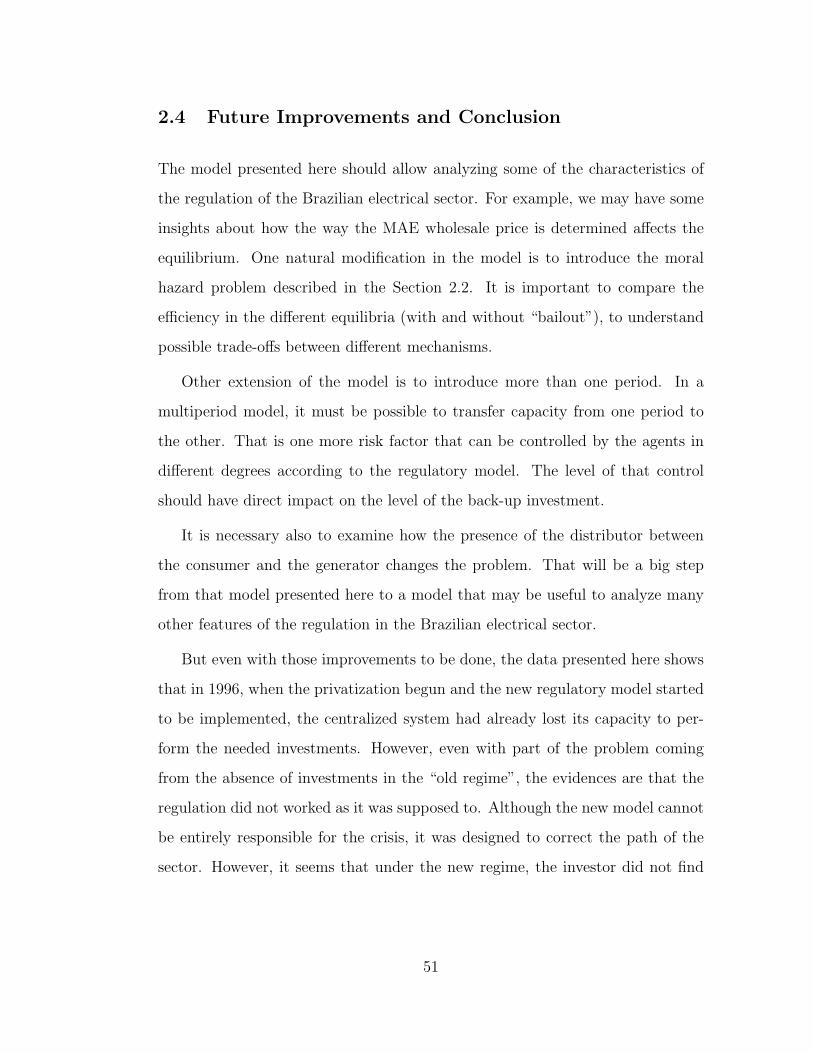
2.4 Future Improvements and Conclusion
The model presented here should allow analyzing some of the characteristics of
the regulation of the Brazilian electrical sector. For example, we may have some
insights about how the way the MAE wholesale price is determined affects the
equilibrium. One natural modification in the model is to introduce the moral
hazard problem described in the Section 2.2. It is important to compare the
efficiency in the different equilibria (with and without “bailout”), to understand
possible trade-offs between different mechanisms.
Other extension of the model is to introduce more than one period. In a
multiperiod model, it must be possible to transfer capacity from one period to
the other. That is one more risk factor that can be controlled by the agents in
different degrees according to the regulatory model. The level of that control
should have direct impact on the level of the back-up investment.
It is necessary also to examine how the presence of the distributor between
the consumer and the generator changes the problem. That will be a big step
from that model presented here to a model that may be useful to analyze many
other features of the regulation in the Brazilian electrical sector.
But even with those improvements to be done, the data presented here shows
that in 1996, when the privatization begun and the new regulatory model started
to be implemented, the centralized system had already lost its capacity to per-
form the needed investments. However, even with part of the problem coming
from the absence of investments in the “old regime”, the evidences are that the
regulation did not worked as it was supposed to. Although the new model cannot
be entirely responsible for the crisis, it was designed to correct the path of the
sector. However, it seems that under the new regime, the investor did not find
51

the incentives to resume the investments in the sector. It still necessary to look
deeply in the data and go further with the theoretical model to understand in
which extension inefficiencies of the regulatory model contributed for the crisis,
and how to improve that regulation.
52
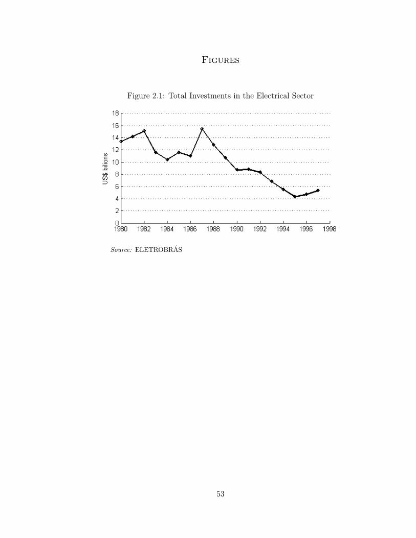
Figures
Figure 2.1: Total Investments in the Electrical Sector
Source: ELETROBRAS
53
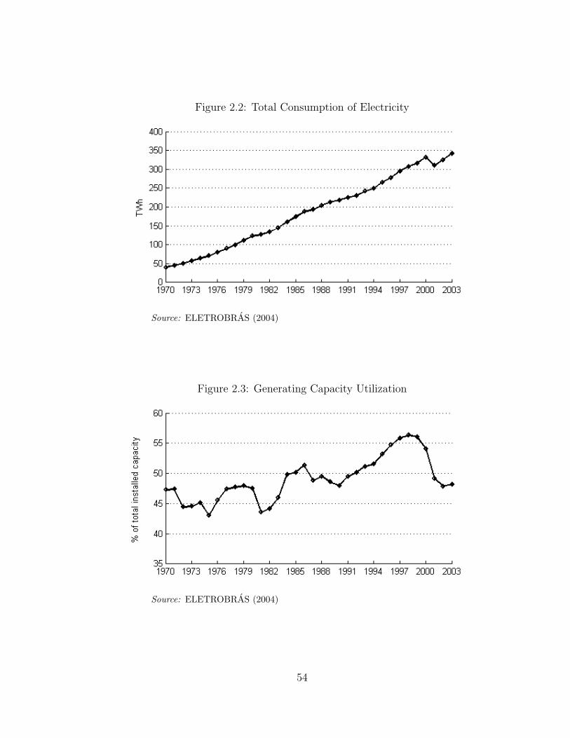
Figure 2.2: Total Consumption of Electricity
Source: ELETROBRAS (2004)
Figure 2.3: Generating Capacity Utilization
Source: ELETROBRAS (2004)
54
Bibliography
ELETROBRAS (2004): Balanco Energetico Nacional, Brasılia.
Kreps, D. M. and J. A. Scheinkman (1983): “Quantity Precommitment and
Bertrand Competition Yield Cournot Outcomes,” Bell Journal of Economics,
14, 326–337.
Lima, J. L. (1995): Polıticas de Governo e Desenvolvimento do Setor de Energia
Eletrica: do Codigo de Aguas a Crise dos Anos 80 (1934-1984), Rio de Janeiro:
Memoria da Eletricidade.
55
CHAPTER 3
Multiple Equilibria on Determination of
Corruption and Implications to Economic
Growth: A Review
3.1 Introduction
The level of corruption varies widely across countries in the world. Although
most people agree that corruption is something bad, and that societies should
create mechanisms to avoid or reduce the incidence of corruption, many countries
presents consistently very high level of corruption, despite the harm it cause to
their societies. On the other hand, many countries succeeds on keeping corruption
at a low level of incidence.
This work is the first step of a project where I plan to have a deep look on
determinants and implications of corruption, trying to understand the different
profiles of corruption across countries. Here, as a starting point, I present a
brief literature review on multiple equilibria on determination of the incidence
of corruption, trying to emphasizes the implications of corruption on economic
growth.
56
3.2 Literature Review
One of the most widespread ideas on why corruption is bad is related with its
implications to economic growth. Mauro (1995) presents an empirical analysis
on the effects of bureaucratic honesty and efficiency on economic growth. With
cross-section data, he finds that corruption reduces growth by lowering private
investments. Even looking at subsamples of countries where bureaucracies are
very cumbersome, his main result still holds, which challenges the idea that in
some extreme situations, corruption could be beneficial, by helping investors to
go through bureaucracies faster than usual.
Because of the effects of corruption on economic growth, we should expected
societies to make a huge effort in the attempt to reduce corruption. One of
the seminal papers on the economics of corruption, Rose-Ackerman (1975) an-
alyzes the relationship between the structure of the market and the incidence
of corruption in the process of governmental contracts, and points out that the
establishment of precise rules to direct the actions of government officials is one
way to reduce corruption. A clear definition of the government preferences helps
to reduce the occurrence of corruption on the contracting processes. So why do
some countries succeed on keeping the the incidence of corruption at a low level,
while others fail?
The general answer to that question in the theoretical literature is related with
the occurrence of multiple equilibria. Cadot (1987) models a situation where a
corrupt government official asks for a bribe, in order to let a candidate pass in
a test. The model is applied for three different assumptions on the information
available for each player —perfect, asymmetric and imperfect information—, with
the official asking for a bribe in the amount that maximizes his expected payoff,
given the information he has. When it is open the possibility of the superiors
57
of the corrupt official also being corrupt, the multiplicity of equilibria occurs.
With superiors being able to ask for a bribe to cover up when the subordinated
is denounced, it happens that higher is the corruption in one level, greater is the
incentive for corruption in the other. Typically, we have an equilibrium with low
corruption at the low level administration but no corruption from high-ranked
officials, and another with higher corruption from the low-ranked and corruption
occurring also at the high level administration.
In Andvig and Moene (1990), we have a model where the profitability of
the corruption depends on the established frequency of it. There, the incidence
of corruption is analyzed in a context of demand and supply, with bribers and
bribees behaving as “price takers”. On the supply side, higher is the proportion of
corrupt bureaucrats, lower is the expected cost of being caught, and then, higher
is the profitability of corruption. For the demand, when the overall corruption
is greater, the search for a corrupt bureaucrat to bribe becomes shorter, and
then more people engage in that search. This model also delivers many possible
situations where multiple equilibria occur.
Exploring the implications of corruption to economic growth, Murphy et al.
(1991) points out the importance of talented people working as entrepreneurs.
They argue that talented people will self-allocate to sectors that exhibits the
highest returns. With the development of the rent-seeking sector, some talented
people would be attracted to that sector, reducing the talents in the entrepreneur-
ship sector. There would be yet a second effect, where more talent in the rent-
seeking sector will increase the expropriation of the gains from the productive
and entrepreneurship sectors, reducing even more the returns in these sector,
and driving more talents to rent-seeking. In Murphy et al. (1993), the authors go
deep in their arguments, asserting that rent-seeking activities exhibit increasing
58
returns. That would occur due the existence of fixed costs to establish the rules
that favors the rent-seeking, the character of self-generating of those activities,
and finally, the lower probability of being caught stealing when more people steal.
They also emphasizes that the public rent-seeking by government officials is spe-
cially harmful to the entrepreneurship sector, in opposition to the productive
sector, since entrepreneurs are in greater need of the government services, such
as permits, licences and import quotas. Therefore, that kind of rent-seeking is
more adverse for the economic growth.
Back to the question of persistence of corruption, Dawid and Feichtinger
(1996) presents a dynamic model that focus on economically motivated corrup-
tion, between a bureaucrat and an agent outside. The bureaucrats like bribes, but
also care about their reputation. Higher is the expected level of corruption, lower
is the cost in reputation for being corrupt. In that model, there are two stable
equilibrium: one where all the bureaucrats are corrupt, and everybody accepts
corruption; and another where no one is corrupt and corruption is condemned by
all individuals.
Addressing the issue of persistence, together with the implications of corrup-
tion on economic growth, Mauro (2004) develops two distinct models for different
kind of corruption. The first model focus on corruption where individuals steal
from the government. In an environment similar to the one in Murphy et al.
(1993), the individuals allocate time between productive work and stealing from
the government expenditures. If many steals, probability of being caught is low.
We have strategic complementarity that results in multiple equilibria. In the bad
equilibrium, corruption is high, and growth is low due to the labor wasted in un-
productive activities and the low marginal product of capital, since a low share
of the government resources is allocated in production processes, where it was
59
supposed to be an input. In the second model, the corruption occurs with the
government that steals from the public. That model relates corruption with po-
litical instability and low economics growth, and also delivers multiple equilibria
through strategic complementarity. High corruption, with large brides, reduces
growth. The low growth rate brings the pressure from the society to change the
government. Thus, with a shorter horizon of the permanence in the power, the
members of the government want to charge larger bribes. Alternatively, with
small bribes, growth is bigger, we have a greater stability, and with a long hori-
zon, meaning a longer flow of bribes, the members of government charge lower
bribes.
3.3 Future Work
The next step in this project will be to extend the literature review presented
here, putting more emphasis on the empirical literature, to identify stylized facts
that the theoretical models do not explain satisfactorily. I have a particular
interest on the possible explanations for the developments of different types of
corruption in different societies.
60
Bibliography
Andvig, J. C. and K. O. Moene (1990): “How Corruption May Corrupt,”
Journal of Economic Behavior and Organization, 13, 63–76.
Cadot, O. (1987): “Corruption as a Gamble,” Journal of Public Economics,
33, 223–244.
Dawid, H. and G. Feichtinger (1996): “On the Persistence of Corruption,”
Journal of Economics, 64, 177–193.
Mauro, P. (1995): “Corruption and Growth,” The Quarterly Journal of Eco-
nomics, 110, 681–712.
——— (2004): “The Persistence of Corruption and Slow Economic Growth,”
IMF Staff Papers, 51, 1–18.
Murphy, K. M., A. Shleifer, and R. W. Vishny (1991): “The Allocation
of Talent: Implications for Growth,” The Quarterly Journal of Economics, 106,
503–530.
——— (1993): “Why Is Rent-Seeking So Costly to Growth?” The American
Economic Review, Papers and Proceedings, 83, 409–414.
Rose-Ackerman, S. (1975): “The Economics of Corruption,” Journal of Public
Economics, 4, 187–203.
61