Embed Size (px)
Citation preview
Essays on Naive Diversification
Bowei Li
(orcid.org/0000-0003-2487-4821)
A thesis submitted for the degree of Doctor of Philosophy
June 2018
Department of Finance
The University of Melbourne
The thesis is being submitted in partial fulfillment of the degree which is
not being completed under a jointly awarded degree.

Abstract
The mean-variance model pioneered by Nobel laureate Harry Markowitz is the
foundation of modern portfolio theory, and is widely applied in asset allocation and
active portfolio management. However, the naive 1/N diversification rule (the equal-
weight portfolio rule) has received much academic attention because of its superior
performance relative to mean-variance portfolio rules. This thesis consists of two
essays with respect to the naive 1/N diversification rule.
The first essay examines the sample selection bias in portfolio horse races with
the 1/N rule. Numerous studies have developed mean-variance portfolio rules to out-
perform the naive 1/N rule. However, the outperformance is often justified with a
small number of pre-selected datasets. Using a novel performance test based on a
large number of datasets, I compare various “1/N outperformers” with the naive rule.
The results show that although some “1/N outperformers” outperform the 1/N rule on
an average basis, a sample selection problem generally exists in claiming significant
outperformance over the naive benchmark. To further understand portfolio perfor-
mance, I explore the theoretical relations between assets’ return moments and the
performance of optimal versus naive diversification. These relations not only imply
strong performance predictability, but also can be exploited to deliver out-of-sample
portfolio benefits.
The second essay studies how January seasonality affects the relative performance
of the mean-variance and 1/N rules. I find that the good performance of the 1/N rule
does not depend on the January seasonality when value-weighted indexes are used for
i

portfolio construction. However, when individual stocks are formed into portfolios,
a large proportion of the empirical success of the 1/N rule is attributed to enormous
January returns. Mean-variance portfolio rules fail to outperform the naive rule on a
risk-adjusted basis; however, the relative performance reverses when January returns
are excluded. The results are robust with and without transaction costs, for various
mean-variance rules, and across different industries and characteristics.
ii

Declaration
This declaration is to certify that:
1. the thesis comprises only my original work towards the Doctor of Philosophy except
where indicated in the preface;
2. due acknowledgment has been made in the text to all other material used;
3. the thesis is fewer than the maximum word limit in length, exclusive of tables, maps,
bibliographies and appendices.
Signature:
iii

Preface
The thesis was edited by Elite Editing, and editorial intervention was restricted to
Standards D and E of the Australian Standards for Editing Practice as follows:
1. Standard D: Language and Illustrations; and
2. Standard E: Completeness and Consistency.
iv

Acknowledgement
Doctoral research is a long and fruitful journey. I would never have been able to
finish my doctoral thesis without the guidance of my committee members, help from
friends, and support from my family.
First and foremost, I am deeply indebted to my advisors Joachim Inkmann, Federico
Nardari, and Juan Sotes-Paladino for their greatest guidance and encouragement. I
have benefited tremendously from their supervision, and the completion of my doc-
toral studies would not be possible without their mentoring and support.
I would also like to extend my sincere thanks to the Department of Finance and all
the faculty members who have provided me with helpful feedback over the years, in
particular to Spencer Martin, Garry Twite, Antonio Gargano, Ravi Sastry, Gil Aharoni,
Thijs van der Heijden, Andrea Lu, Lyndon Moore, Zhen Shi, Jordan Neyland, and
Joshua Shemesh.
My fellow Ph.D. classmates have also provided useful feedback and comments for
my research over the years. Specifically, I would like to thank George Wang, Chelsea
Yao, Michael Liu, Michelle Zhou, Bill Zu, Emma Li, Yichao Zhu, Nguyet Nguyen,
Roc Lv, Yolanda Wang, Rob Manolache, and Steve Liu.
I also thank several conference discussants, Sean Anthonisz, Oleg Chuprinin,
Ilnara Gafiatullina, Xiaolu Wang, and Fang Zhen, and seminar participants at the
Financial Research Network (FIRN) Annual Conference, 29th Australasian Finance
and Banking Conference, 2016 Auckland Finance Meeting (AFM), AFM Doctoral
Symposium, SIRCA’s Young Researchers Workshop, and University of Melbourne
v

Finance Brown Bag Seminar.
Last but not least, I would like to thank my parents Jialong Li and Min Yu, for
giving birth to me in the first place and supporting me unconditionally throughout my
life. I dedicate this thesis to them.
vi

Contents
List of Figures 1
List of Tables 2
1 Introduction 4
1.1 Background . . . . . . . . . . . . . . . . . . . . . . . . . . . . . . . 4
1.2 Motivation and Contribution . . . . . . . . . . . . . . . . . . . . . . 5
1.3 Outline of the Thesis . . . . . . . . . . . . . . . . . . . . . . . . . . 7
2 Literature review 12
2.1 Mean-variance Diversification . . . . . . . . . . . . . . . . . . . . . 12
2.1.1 Bayesian Approaches . . . . . . . . . . . . . . . . . . . . . . 13
2.1.2 Shrinkage Techniques . . . . . . . . . . . . . . . . . . . . . 15
2.1.3 Portfolio Constraints . . . . . . . . . . . . . . . . . . . . . . 18
2.1.4 Conditional Mean-variance Strategies . . . . . . . . . . . . . 20
2.2 Naive Diversification . . . . . . . . . . . . . . . . . . . . . . . . . . 21
2.2.1 The Naive 1/N Portfolio Rule . . . . . . . . . . . . . . . . . 21
vii
Contents
2.2.2 “1/N Outperformers” . . . . . . . . . . . . . . . . . . . . . . 23
2.2.3 Portfolio Horse Races with the 1/N Rule . . . . . . . . . . . . 25
2.3 January Seasonality of Stock Returns . . . . . . . . . . . . . . . . . . 26
2.3.1 Some Stylized Facts . . . . . . . . . . . . . . . . . . . . . . 27
2.3.2 Reasons for the January Seasonality . . . . . . . . . . . . . . 29
2.4 Summary . . . . . . . . . . . . . . . . . . . . . . . . . . . . . . . . 32
3 Essay 1: Sample selection, return moments, and the performance of opti-
mal versus naive diversification 34
3.1 Introduction . . . . . . . . . . . . . . . . . . . . . . . . . . . . . . . 34
3.2 An Aggregate Performance Test . . . . . . . . . . . . . . . . . . . . 40
3.2.1 Test Statistic . . . . . . . . . . . . . . . . . . . . . . . . . . 40
3.2.2 Estimating Vm . . . . . . . . . . . . . . . . . . . . . . . . . . 42
3.2.3 Estimating ρp,q . . . . . . . . . . . . . . . . . . . . . . . . . 43
3.2.4 Statistical Inference in Each Dataset . . . . . . . . . . . . . . 44
3.3 Data, Strategies and Performance Measures . . . . . . . . . . . . . . 45
3.3.1 Data . . . . . . . . . . . . . . . . . . . . . . . . . . . . . . . 45
3.3.2 Portfolio Strategies . . . . . . . . . . . . . . . . . . . . . . . 46
3.3.3 Performance Measures . . . . . . . . . . . . . . . . . . . . . 50
3.4 Empirical Results . . . . . . . . . . . . . . . . . . . . . . . . . . . . 52
3.4.1 Results from Commonly Used Datasets . . . . . . . . . . . . 53
3.4.2 Results from a Large Number of Datasets . . . . . . . . . . . 55
viii

Contents
3.4.3 Robustness Checks . . . . . . . . . . . . . . . . . . . . . . . 59
3.5 The Mean-variance Properties of Optimal versus Naive Diversification 62
3.5.1 A Theoretical Framework . . . . . . . . . . . . . . . . . . . 63
3.5.2 A Numerical Example . . . . . . . . . . . . . . . . . . . . . 67
3.5.3 Estimation Errors . . . . . . . . . . . . . . . . . . . . . . . . 70
3.6 Return Moments and Performance Predictability . . . . . . . . . . . . 75
3.6.1 Predictive Regression . . . . . . . . . . . . . . . . . . . . . . 76
3.6.2 Hypotheses . . . . . . . . . . . . . . . . . . . . . . . . . . . 78
3.6.3 Predictive Results . . . . . . . . . . . . . . . . . . . . . . . . 78
3.6.4 A Portfolio Switching Strategy . . . . . . . . . . . . . . . . . 81
3.7 Conclusions . . . . . . . . . . . . . . . . . . . . . . . . . . . . . . . 85
4 Essay 2: Naive diversification and the January seasonality 104
4.1 Introduction . . . . . . . . . . . . . . . . . . . . . . . . . . . . . . . 104
4.2 Data . . . . . . . . . . . . . . . . . . . . . . . . . . . . . . . . . . . 108
4.3 Portfolio Strategies and Performance Measures . . . . . . . . . . . . 110
4.4 Performance Evaluation . . . . . . . . . . . . . . . . . . . . . . . . . 113
4.4.1 Performance Evaluation - FF Datasets . . . . . . . . . . . . . 113
4.4.2 Performance Evaluation - Stock Datasets . . . . . . . . . . . 114
4.5 Transaction Cost . . . . . . . . . . . . . . . . . . . . . . . . . . . . 118
4.6 Factor exposure of the 1/N Rule . . . . . . . . . . . . . . . . . . . . 122
4.7 Diminishing January Effect of the 1/N Rule . . . . . . . . . . . . . . 125
ix

Contents
4.8 Conclusion . . . . . . . . . . . . . . . . . . . . . . . . . . . . . . . 128
5 Concluding remarks 153
5.1 Summary of the Thesis . . . . . . . . . . . . . . . . . . . . . . . . . 154
5.2 Limitations and Potential Future Research . . . . . . . . . . . . . . . 158
Bibliography 160
Appendix 172
x

List of Figures
3.1 Relation between loss of the 1/N rule and expected return . . . . . 87
3.2 Relation between loss of the 1/N rule and volatility . . . . . . . . . 88
3.3 Relation between loss of the 1/N rule and correlation . . . . . . . . 89
1

List of Tables
3.1 Portfolio strategies considered . . . . . . . . . . . . . . . . . . . . 90
3.2 Out-of-sample performance in commonly used datasets . . . . . . 91
3.3 Sharpe ratios . . . . . . . . . . . . . . . . . . . . . . . . . . . . . . 93
3.4 Certainty-equivalent returns . . . . . . . . . . . . . . . . . . . . . 94
3.5 Portfolio turnover . . . . . . . . . . . . . . . . . . . . . . . . . . . 95
3.6 Robustness checks: risk aversion . . . . . . . . . . . . . . . . . . . 96
3.7 Robustness checks: expanding window . . . . . . . . . . . . . . . 97
3.8 Robustness checks: shortsale constraints . . . . . . . . . . . . . . 98
3.9 Relative performance versus return moments . . . . . . . . . . . . 99
3.10 Predictability of portfolio performance based on return moments 100
3.11 Performance of the switching strategy . . . . . . . . . . . . . . . . 101
3.12 Percentage of time each strategy is used for the switching strategy 103
4.1 Summary statistics for the number of stocks . . . . . . . . . . . . 131
4.2 Annualized returns - FF datasets . . . . . . . . . . . . . . . . . . . 132
4.3 Annualized Sharpe ratios - FF datasets . . . . . . . . . . . . . . . 133
2
List of Tables
4.4 Difference in average returns . . . . . . . . . . . . . . . . . . . . . 134
4.5 Difference in January returns . . . . . . . . . . . . . . . . . . . . . 135
4.6 Difference in non-January returns . . . . . . . . . . . . . . . . . . 136
4.7 Difference in Sharpe ratios . . . . . . . . . . . . . . . . . . . . . . 137
4.8 Difference in Sharpe ratios without Januaries . . . . . . . . . . . . 138
4.9 Annualized returns with transaction costs - FF datasets . . . . . . 139
4.10 Annualized Sharpe ratios with transaction costs - FF datasets . . . 140
4.11 Difference in average returns (with transaction cost) . . . . . . . . 141
4.12 Difference in January returns (with transaction cost) . . . . . . . 142
4.13 Difference in Non-January returns (with transaction cost) . . . . . 143
4.14 Difference in Sharpe ratios (with transaction cost) . . . . . . . . . 144
4.15 Difference in Sharpe ratios w/o Januaries (with transaction cost) . 145
4.16 Number of datasets outperforming the 1/N rule . . . . . . . . . . . 146
4.17 Factor January effects . . . . . . . . . . . . . . . . . . . . . . . . . 147
4.18 Average factor exposure for portfolio strategies . . . . . . . . . . . 148
4.19 Factor exposure of the 1/N portfolio rule - stock datasets . . . . . 149
4.20 Diminishing January effect on return of the 1/N rule . . . . . . . . 150
4.21 Diminishing January effect on Sharpe ratio of the 1/N rule . . . . 151
4.22 Time varying factor exposure of the 1/N portfolio rule . . . . . . . 152
3

Chapter 1
Introduction
1.1 Background
The mean-variance portfolio theory pioneered by Nobel laureate Harry Markowitz
is widely applied in asset allocation and portfolio management. A mean-variance
portfolio is constructed by maximizing the mean-variance utility given the investor’s
risk aversion. It relies on estimates of the expected returns and the covariance structure
of assets of interests. The naive 1/N diversification rule, in contrast, allocates portfolio
weights equally across assets, and is considered a heuristic decision bias (Benartzi and
Thaler, 2001).
From a performance perspective, mean-variance portfolios that rely on histori-
cal return moment estimates often produce unsatisfactory out-of-sample results be-
cause of estimation errors (Barry, 1974; Klein and Bawa, 1976; Michaud, 1989).
Although the literature on portfolio choice has not ceased to tackle the estimation
4
Chapter 1. Introduction
errors for mean-variance portfolios (e.g., Jorion, 1986; Kan and Zhou, 2007; Pastor
and Stambaugh, 2000), the 1/N rule, with no estimation errors, still reveals its su-
perior performance compared with mean-variance strategies. In an influential study,
DeMiguel, Garlappi, and Uppal (2009b) test 14 mean-variance strategies against the
naive 1/N portfolio rule. They find that none of the sophisticated mean-variance
strategies outperforms the naive benchmark consistently in terms of Sharpe ratio or
certainty-equivalent return. The finding of DeMiguel et al. (2009b) casts doubt on
mean-variance portfolio rules relative to the 1/N rule.
1.2 Motivation and Contribution
To reaffirm the usefulness of the mean-variance portfolio theory, a series of studies
attempt to propose new mean-variance strategies to challenge the 1/N rule. Many of
the newly proposed mean-variance strategies appear to successfully outperform the
1/N rule. However, to demonstrate outperformance over the naive benchmark, studies
that propose new mean-variance rules (e.g., Kirby and Ostdiek, 2012; Tu and Zhou,
2011), investigate a small number of pre-selected empirical datasets of stock port-
folios, primarily characteristic-based portfolios. If the outperformance is associated
with the datasets chosen, there is potentially sample selection bias in these portfolio
horse races.
The first essay of this thesis documents a selection bias in claiming outperformance
over the 1/N rule by proposing and applying a novel performance test. Existing studies
5
Chapter 1. Introduction
on sample selection bias are centered on three aspects, namely sample/database bias
(Chan et al., 1995; Kim, 1997; Kothari et al., 1995), delisting bias (Shumway, 1997;
Shumway and Warther, 1999) and survivorship bias (Carhart et al., 2002). Although
selection bias is discussed heavily in many areas of finance, it has not been examined
in the context of a portfolio horse race. This paper fills this gap in the literature on
sample selection issues by showing a unique selection bias in the horse races between
mean-variance and the 1/N rules.
The essay also adds to the recent debate regarding optimal mean-variance diversi-
fication versus naive 1/N diversification. The 1/N rule has been documented to have
good performance relative to mean-variance portfolios (see, for instance, DeMiguel
et al., 2009b; Pflug et al., 2012; Brown et al., 2013; while a number of studies at-
tempted to develop better mean-variance rules to challenge the naive strategy (for
example, Tu and Zhou, 2011; Kirby and Ostdiek, 2012; Kan, Wang, and Zhou, 2016).
Theoretically and empirically, I show that the performance of mean-variance versus
1/N rules is related to the return moments of assets used to construct portfolios.
The second essay is motivated by earlier literature on the January seasonality of
stock returns. The January seasonality is a phenomenon that January returns of com-
mon stocks are systematically higher than returns in the rest of the year. The litera-
ture on stock January seasonality has revealed a large January return for an equally-
weighted index and a less severe January effect for a value-weighted index (e.g., Gul-
tekin and Gultekin, 1983; Keim, 1983; Rozeff and Kinney, 1976). The superior perfor-
mance of the 1/N rule in constructing stock portfolios could be related to this January
6

Chapter 1. Introduction
effect. This study attempts to understand the relation between the January seasonality
and the performance of optimal versus naive diversification.
I find that a great proportion of the empirical success of the 1/N rule is attributed to
large January returns, when individual stocks rather than value-weighted indexes are
used to construct portfolios. This study is the first to link the performance of optimal
versus naive diversification with the classic January seasonality.
1.3 Outline of the Thesis
In this section, I outline the chapters of this thesis and provide an overview of each
chapter. The thesis is organized into five chapters. Chapter 2 reviews the literature on
mean-variance and naive diversification, as well as the literature on the January sea-
sonality of stocks returns. Chapter 3 presents the first essay on the sample selection
issue in the portfolio horse races between mean-variance and 1/N rules. Chapter 4
presents the second essay on the link between the January seasonality and the perfor-
mance of mean-variance versus 1/N rules. Chapter 5 concludes by summarizing the
main results, discussing the limitations of the thesis, and providing suggestions for
future research.
Chapter 2: Literature Review
In Chapter 2, I review the related literature on naive diversification and outline the
potential research questions that remain unanswered in the literature. Three aspects of
7

Chapter 1. Introduction
the literature are discussed, namely, the mean-variance portfolio theory and its devel-
opment, the naive 1/N portfolio rule, and the January seasonality of stock returns.
The literature on mean-variance portfolios and the 1/N rule reveals that tradi-
tional mean-variance rule and its extensions (for instance, the mean-variance rules
by Markowitz, 1952; Jorion, 1986; Kan and Zhou, 2007) performs badly relative to
the 1/N rule, since the naive rule involves no estimation errors. Newly developed
mean-variance strategies (for instance, the strategies by Kan, Wang, and Zhou; 2016;
Kirby and Ostdiek, 2012; Tu and Zhou, 2011) are shown to outperform the 1/N rule
based on a small number of selected datasets. Nonetheless, it is uncertain whether
these “1/N outperformers” truly outperform the 1/N rule on a large-sample basis.
The literature on the January seasonality of stock returns shows that the 1/N rule
exhibits very strong January returns (see, for instance, Gultekin and Gultekin, 1983;
Keim, 1983 Rozeff and Kinney, 1976). The good performance of the 1/N rule relative
to mean-variance portfolios could be driven by January returns of the 1/N rule. How-
ever, it is unclear how the January seasonality affects the portfolio horse races
between mean-variance and 1/N rules.
Chapter 3: Essay 1
Chapter 3 presents Essay 1, “Sample selection bias, return moments, and the perfor-
mance of optimal versus naive diversification.” This essay provides an answer to the
first question listed above.
I propose a novel performance test for the average performance across datasets.
8
Chapter 1. Introduction
This new test conducts statistical inference on the average portfolio performance while
considering performance uncertainty in each dataset. Based on the new test, I compare
the relative performance between the 1/N rule and 16 mean-variance strategies1 (in-
cluding 14 “1/N outperformers”), across 122 datasets of value-weighted stock portfo-
lios.2 These datasets are obtained from the French data library, and represent econom-
ically relevant assets that involve factor portfolios, industries, characteristics, and in-
ternational stock indexes. The empirical comparison based on the 122 datasets shows
that some strategies deliver larger certainty-equivalent (CEQ) returns and Sharpe ra-
tios compared with the 1/N rule, on an average basis. However, most of them cannot
significantly outperform the naive benchmark in terms of the average Sharpe ratio
across datasets at 5% level. The sample selection bias exist for these “1/N outper-
formers” in claiming outperformance over the 1/N rule.
To further understand the relative performance between optimal versus naive di-
versification, I examine the theoretical relations between the performance of mean-
variance versus 1/N rules against the assets’ return moments. Empirically, I find strong
predictability of the out-of-sample portfolio performance based on the in-sample re-
turn moments of assets. Further, I show that this predictability can lead to out-of-
sample portfolio benefits by using a switching strategy.
1See Table 3.1 for details.2See Appendix 1 for details.
9

Chapter 1. Introduction
Chapter 4: Essay 2
Chapter 4 presents Essay 2, “Naive diversification and the January seasonality.” This
essay provides an answer to the second question listed above.
I test performance of the 16 mean-variance rules (in Essay 1) against the 1/N rule
under different empirical settings. First, portfolio horse races are conducted based on
the 122 datasets (in Essay 1). Result shows that the relative performance between
mean-variance and 1/N rules is not affected by the January seasonality. However,
constructing portfolios using individual stocks produces completely different results.
I construct monthly mean-variance and 1/N portfolios based on 26 stock datasets.3
These stocks involve market-wide stocks, stocks from a certain industry, as well as
stocks with characteristics, such as size, value and momentum. By comparing various
mean-variance rules with the 1/N rule based on these test datasets, I find that the
1/N rule generates considerably larger January returns compared with mean-variance
portfolios. When January months are ruled out, the Sharpe ratio of the 1/N rule can
decrease up to 30%. In this case, mean-variance strategies are able to outperform the
1/N benchmark on a risk-adjusted basis. This result is consistent with and without
transaction costs, across different industries and various characteristics.
The reason behind the contrary results for individual stocks versus value-weighted
indexes is related to the size factor exposure of the 1/N rule. The 1/N rule has sig-
nificantly larger size factor exposures compared with mean-variance rules in the stock
datasets, while it exhibit similar or even smaller size factor exposures relative to mean-
3See Section 4.2 and Table 4.1 for details.
10

Chapter 1. Introduction
variance rules in the value-weighted index datasets. As the January seasonality is pri-
marily a size effect (Keim, 1983), this explains the discrepancy in the results obtained
under the two empirical settings. Essay 2 suggests that when portfolio horse races
is based on individual stocks, the January effect of the 1/N rule should be carefully
considered.
Chapter 5: Concluding Remarks
Chapter 5 provides a summary of the main findings and contributions of the thesis. I
also discuss some limitations of this thesis and recommendations for potential future
research.
11

Chapter 2
Literature review
In this chapter, I review the literature on mean-variance and naive 1/N diversification
rules. I also review the literature on the January seasonality of stock returns. I further
discuss potential unsolved research questions in the literature on naive diversification.
2.1 Mean-variance Diversification
The mean-variance model by Markowitz (1952, 1959) is the foundation of the modern
portfolio theory. In the mean-variance setup, an investor forms a myopic portfolio
based on the expected returns, the covariance matrix of returns, and his or her risk
aversion, as presented below:
x =1γ
Σ−1
µ (2.1)
where µ is the mean vector of asset excess returns, Σ is the variance-covariance matrix
12
Chapter 2. Literature review
of asset returns, and γ is the coefficient of relative risk aversion.
A mean-variance portfolio is often formed with its sample analog, where popula-
tion return moments are replaced by sample return moments. However, since return
moments are estimated with estimation errors, sample-based mean-variance rules of-
ten produce poor out-of-sample performance. Various methods have been designed
to address the estimation errors in mean-variance portfolios, including Bayesian ap-
proaches, shrinkage techniques, portfolio constraints, and mean-variance strategies
based on state variables.
2.1.1 Bayesian Approaches
A Bayesian approach is attractive for mean-variance portfolio construction. It not
only applies useful prior information about return moments, but also considers esti-
mation errors and model ambiguity. Barry (1974), Klein and Bawa (1976), and Brown
(1979) are early examples of Bayesian analysis on portfolio choice. Early Bayesian
portfolio studies mainly focus on the Bayesian portfolio with diffuse priors. However,
a Bayesian portfolio with diffuse priors inflates the variance-covariance matrix by a
factor that is greater than but close to one, which does not make a great difference to
the sample mean-variance rule.
The conjugate prior is a natural and common informative prior in Bayesian portfo-
lio analysis. The conjugate prior preserves the same class of distributions for the mean
vector and covariance matrix. Frost and Savarino (1986) find that a prior in which all
assets possess identical means, variances, and structured covariance improves the out-
13

Chapter 2. Literature review
of-sample performance of a Bayesian portfolio.
Jorion (1985) and Jorion (1986) apply the shrinkage estimation idea by James and
Stein (1961). Jorion addresses the estimation error and forms the expected return by
shrinking the sample mean toward the return on the global minimum-variance port-
folio, and accounts for the estimation error in the covariance matrix from a Bayesian
perspective. He shows that this portfolio provides significant out-of-sample perfor-
mance improvement over the sample mean-variance rule.
Black and Litterman (1992) provide a novel Bayesian solution to the mean-variance
problem. They assume that an investor starts with initial views consistent with the
CAPM equilibrium and then updates the initial views with his or her own views via
the Bayesian approach. The Black-Litterman model retains the main ideas of mean-
variance theory while addressing the issues regarding estimation errors for expected
returns.
Pastor (2000) and Pastor and Stambaugh (2000) introduce Bayesian portfolio pri-
ors that reflect an investor’s belief in an asset pricing model. The Bayesian portfolio
is formed with the shrinkage target based on the investor’s prior on the asset pricing
model and the shrinkage factor determined by the data. MacKinlay and Pastor (2000),
on the other hand, use information that is not captured by a particular asset pricing
model to construct mean-variance portfolios. Their portfolio is formed by estimat-
ing an expected return that takes into account missing factors, and it performs well
empirically compared with the sample mean-variance approach.
Another type of Bayesian portfolio analysis is based on economic objectives. Tu
14

Chapter 2. Literature review
and Zhou (2010) propose a method to construct priors on parameters that are backed
out from the solution of an economic objective. They find that Bayesian strategies
based on objective-based priors significantly outperform strategies under diffuse and
asset pricing priors, as well as some of the best Bayesian strategies in the literature.
More recently, Anderson and Cheng (2016) develop a Bayesian-averaging port-
folio strategy that produces excellent out-of-sample performance. The portfolio rule
assumes that the number of models increases with the sample size. Each period, when
new information becomes available, they estimate parameters for each model and
compute the probability that each model is correct. The portfolio strategy accounts
for parameter and model uncertainty, and is updated each period under the Bayesian-
averaging framework. This new portfolio rule outperforms leading strategies in the
literature on a majority of 24 datasets.
2.1.2 Shrinkage Techniques
Shrinkage methods are useful ways to address the estimation error in mean-variance
portfolios. There are, in general, three types of shrinkage approaches. First, investors
can shrink the sample mean vector to a mean vector target with less estimation errors.
Second, the shrinkage idea is applied to the covariance matrix or the inverse of the
covariance matrix. The third approach is to shrink the mean-variance portfolio directly
to a portfolio with less estimation errors.
A well-known example of the mean-variance portfolio with shrinkage mean vec-
tors is the Bayes-Stein portfolio by Jorion (1986). The Bayes-Stein shrinkage esti-
15

Chapter 2. Literature review
mator of expected return is a weighted average of the sample mean vector and the
mean of the global minimum-variance portfolio. In other words, the shrinkage target
of the sample mean vector is the mean return of the global minimum-variance port-
folio, which involves less estimation errors. The Bayes-Stein portfolio rule improves
the sample mean-variance rule substantially in terms of out-of-sample performance.
Shrinkage methods that are applied only to the covariance matrix focus on con-
structing the global minimum-variance portfolio. The minimum-variance portfolio
aims at minimizing the variance of portfolio returns. The implementation of the
minimum-variance portfolio only involves estimation of the covariance matrix. Es-
timating expected returns is more difficult than estimating the covariance matrix be-
tween assets, as Black and Litterman (1992) point out. However, when the number of
observations is not very large relative to the number of assets, the covariance matrix, as
the only input for the minimum-variance portfolio, is nearly singular and the estima-
tion error explodes when inverting it. Therefore, various approaches are proposed to
shrink the sample covariance matrix toward a target in order to reduce the estimation
error. Ledoit and Wolf (2003) propose a convex combination of the sample covariance
matrix and the single index covariance matrix for stock returns. Their approach selects
portfolios with significantly lower out-of-sample variance than those used in existing
approaches. Ledoit and Wolf (2004b) attempt to minimize the quadratic loss function
of the shrinkage covariance matrix by shrinking the sample covariance matrix toward
a scaled identity matrix, and the shrinkage estimator works well in Monte Carlo ex-
periments. Applying a similar rationale, Ledoit and Wolf (2004a) shrink the sample
16

Chapter 2. Literature review
covariance matrix toward a constant correlation model; their approach forms port-
folios with higher returns and lower variance than in existing shrinkage approaches
when the number of assets is small.
Instead of shrinking return moments, another way to reduce losses due to the es-
timation error is to shrink a portfolio directly to another portfolio – in other words,
to form a portfolio combination of two existing portfolios. While the mean-variance
theory suggests a two-fund portfolio, a riskless asset and the tangency portfolio, Kan
and Zhou (2007) seem to be the first to suggest holding other portfolios in addition to
the two funds in presence of estimation risk. In particular, they show that a portfolio
that combines the riskless asset, the sample tangency portfolio and the sample global
minimum-variance portfolio dominates the two-fund portfolio. To compare with the
1/N rule, DeMiguel, Garlappi, and Uppal (2009b) propose a portfolio that is a combi-
nation of the global minimum-variance portfolio and the 1/N portfolio. Results show
that the mixture of the minimum-variance portfolio and the 1/N portfolio has less
turnover than the minimum-variance portfolio, but it still cannot outperform the 1/N
rule consistently. Tu and Zhou (2011) propose a theory-based strategy to combine
the naive 1/N rule with non-naive rules. In particular, they propose four combination
strategies that combine the 1/N rule with four sophisticated strategies, including the
mean-variance strategies of Markowitz (1952), Jorion (1986), MacKinlay and Pastor
(2000), and Kan and Zhou (2007), respectively. They find that combination rules are
substantially better than their uncombined counterparts.
DeMiguel et al. (2013) conduct a good review and extension on the shrinkage
17

Chapter 2. Literature review
approaches proposed in the literature. They find that shrinkage intensity plays a sig-
nificant role in the performance of the shrinkage portfolio. For the mean-variance ap-
proach, they propose a different calibration criterion from Frost and Savarino (1986)
and Jorion (1986), which calibrates the shrinkage target to have the minimum bias
from the true expected return. The shrinkage intensity is calculated by minimizing
the quadratic loss of the shrinkage estimator. Their shrinkage mean-variance portfolio
outperforms the Bayes-Stein portfolio of Jorion (1986). DeMiguel et al. (2013) also
propose a calibration criterion to shrink the sample covariance matrix, which considers
the condition number optimally. Their approach forms minimum-variance portfolios
with higher Sharpe ratios than the strategies of Ledoit and Wolf (2003) and Ledoit and
Wolf (2004b).
2.1.3 Portfolio Constraints
Estimating the mean-variance portfolios using sample moments often involves ex-
treme weights on particular assets. Cohen and Pogue (1967) first argue that employ-
ing upper-bound restrictions hedges against the risk of estimation biases. Moreover,
Frost and Savarino (1988) empirically find that imposing upper bounds on portfolio
weights both reduces estimation bias and improves mean-variance portfolio perfor-
mance. Further, Jagannathan and Ma (2003) show that the short-sale constraint on the
minimum-variance portfolio is equivalent to shrinking the sample covariance matrix,
and hence reduces estimation errors.
18

Chapter 2. Literature review
DeMiguel, Garlappi, and Uppal (2009b) compare the 1/N rule with two types of
minimum-variance portfolios with constraints, namely the short-sale constraint and
the generalized constraint. The latter constraint restricts the portfolio weight invested
in a particular asset to not fall below 1/(2N). The portfolio can be regarded as a
combination of the 1/N policy and the minimum-variance portfolio with the short-
sale constraint. Results show that constrained portfolios achieve better performance
than their unconstrained counterparts, and the minimum-variance portfolio with the
generalized constraint performs better than portfolios with pure short-sale constraints.
However, none of the constrained portfolios outperforms the 1/N rule consistently.
Behr et al. (2013) propose a constrained minimum-variance portfolio based on
shrinkage theory. They impose both upper and lower weight constraints on minimum-
variance portfolios. Following Ledoit and Wolf (2003, 2004a,b), they apply a quadratic
measure of distance between the modified covariance matrix and the true but unknown
covariance matrix. The upper and lower bounds are estimated by minimizing the
quadratic distance. DeMiguel, Garlappi, Nogales, and Uppal (2009a) provide a gen-
eral framework that solves the traditional minimum-variance problem subject to the
constraint that the norm of portfolio weight vector does not exceed a given threshold.
Under this framework, they propose several norm-constrained strategies that aim to re-
duce estimation errors and improve performance. These newly developed constrained
strategies in both studies perform well relative to the 1/N rule and various existing
mean-variance rules in several selected datasets.
19

Chapter 2. Literature review
2.1.4 Conditional Mean-variance Strategies
The mean-variance strategies discussed above are strategies based on sample return
moments. However, there are portfolio rules that capture the time variation of state
variables to improve performance. A natural way of using predictability is to plug in
predicted return moments in the mean-variance analytical solution. The mean vector
is often estimated based on a predictive regression of excess returns (for instance, the
forecast combination approach of Rapach et al., 2010), and the sample estimator is
used for the covariance matrix.
Among other closed form plugged-in approaches, Campbell and Viceira (2005)
propose a buy-and-hold portfolio solution for long-term investors that includes a hedg-
ing demand for risky assets. Campbell et al. (2003) derive an analytical portfolio and
consumption solution from the Epstein-Zin utility. Further, Hoevenaars et al. (2008)
develop a portfolio rule involving risky liabilities, which is particularly useful for in-
stitutional investors.
In contrast to analytical portfolio solutions with plugged-in estimates, mean-variance
portfolio weight can be directly characterized as a function of state variables without
explicitly assuming the return-generating process. Brandt (1999) proposes a non-
parametric method that allows the optimal portfolio and consumption to vary with
time-varying investment opportunities. At-Sahalia and Brandt (2001) combine pre-
dictors in a single index that best captures time variations in state variables. This ap-
proach solves the “curse of dimensionality” in the non-parametric approach by Brandt
20
Chapter 2. Literature review
(1999). Brandt et al. (2009) present a conditional portfolio policy for a large num-
ber of stocks, since it involves no matrix inversion. This portfolio allows the weight
of each stock to depend directly on its characteristics, namely, size, book-to-market,
and momentum. This approach can effectively exploit common anomalies, but may
not be suitable for all asset classes (DeMiguel, Garlappi, and Uppal, 2009b). Unlike
Brandt et al. (2009), Brandt and Santa-Clara (2006) propose a portfolio rule for broad
asset classes, in which the weight for each asset class is a parameterized function of a
common set of macroeconomic variables.
2.2 Naive Diversification
2.2.1 The Naive 1/N Portfolio Rule
Since the development of the mean-variance portfolio theory over half a century ago,
advocates of mean-variance portfolios have never stopped tackling estimation errors
to improve portfolio performance. However, the naive 1/N diversification rule, or the
equally-weighted portfolio, has caught plenty of attention from both academics and
practitioners. The portfolio weight vector of the 1/N rule is presented below:
x1/N =1N
1N (2.2)
where 1N is an N-by-1 column vector of ones.
On the one hand, the naive 1/N rule is regarded as a portfolio allocation bias. Be-
21
Chapter 2. Literature review
nartzi and Thaler (2001) conduct survey experiments and find that investors tend to
use the 1/N rule to divide contributions evenly among the N options offered in his
or her retirement savings plan. Based on laboratory experiment, Baltussen and Post
(2011) find that investors follow a conditional 1/N diversification heuristic. The sub-
jects exclude “unattractive assets,” and allocate the available funds equally among the
remaining “attractive assets.” Reliance on the 1/N heuristic could be costly, for in-
stance, the allocation to stocks primary depends on the number of stock funds offered
in the saving plan.
On the other hand, the 1/N heuristic rule produces good out-of-sample perfor-
mance relative to mean-variance portfolios. Jobson and Korkie (1980) are the first to
find that the equally-weighted portfolio rule can outperform the mean-variance port-
folio because of estimation errors. Duchin and Levy (2009) test the efficiency of the
1/N rule relative to the mean-variance portfolio with varying numbers of assets. They
find that the mean-variance strategy outperforms the naive rule when the number of
assets is large, which implies that mean-variance diversification is more suitable for
institutional investors relative to individual investors. DeMiguel, Garlappi, and Uppal
(2009b) comprehensively compare the out-of-sample performance of the 1/N rule with
the mean-variance portfolio and its extensions. They test 14 mean-variance tangency
strategies in the literature against the naive benchmark. Results show that none of the
sophisticated mean-variance rules can outperform the 1/N rule consistently across all
eight datasets in the study. They theoretically justify that, to outperform the 1/N rule,
any sample-based mean-variance portfolio requires a very long sample to estimate
22
Chapter 2. Literature review
the expected returns and the covariance matrix if the number of assets is large. The
advantage of the 1/N rule is the absence of exposures to estimation bias.
The benefits of the 1/N rule are not merely the absence from estimation errors.
Pflug et al. (2012) find that the naive rule is rational in cases where an investor is
faced with a sufficiently high degree of model uncertainty in the form of ambiguous
loss distributions. They further show that when the degree of model uncertainty is
high enough, the optimal portfolio converges to the 1/N portfolio. Brown et al. (2013)
show that naive diversification increases tail risk measured by skewness and kurto-
sis, and exhibits a concave payoff. The outperformance of the 1/N rule relative to
mean-variance strategies partly derives from a compensation for the tail risk and the
reduced upside potential associated with the concave payoff. More recently, Fischer
and Gallmeyer (2016) find that the naive 1/N rule possesses the advantage of saving
taxes and transaction costs. They study the performance of mean-variance and 1/N
rules in a context where an investor faces both capital gain taxes and proportional
transaction costs. They find that none of the sophisticated trading strategies outper-
form a 1/N strategy augmented with a tax heuristic.
2.2.2 “1/N Outperformers”
Since the surprising results published by DeMiguel, Garlappi, and Uppal (2009b),
there has been a trend in portfolio choice studies to propose advanced mean-variance
strategies to challenge the 1/N rule. Examples of these studies are numerous, including
for instance, DeMiguel, Garlappi, Nogales, and Uppal (2009a), Tu and Zhou (2011),
23
Chapter 2. Literature review
Kirby and Ostdiek (2012, 2013), Behr et al. (2013), Anderson and Cheng (2016), and
Kan, Wang, and Zhou (2016).
One typical study is by Tu and Zhou (2011), who propose a theory-based mean-
variance portfolio. The mean-variance portfolio tackles the problem of estimation
errors by forming a combination between an existing mean-variance portfolio and the
1/N rule. The combined rule is estimated by minimizing the expected mean-variance
utility loss of the portfolio. The authors develop four combination rules under this
framework, namely the combinations of the 1/N rule with four sophisticated strategies
– the sample mean-variance rule, the Bayes-Stein rule of Jorion (1986), the “missing
factor” rule of MacKinlay and Pastor (2000), and the “three-fund” rule of Kan and
Zhou (2007). These newly proposed strategies outperform not only their sophisticated
uncombined strategies, but also the 1/N rule in most of the datasets in the study.
Kan, Wang, and Zhou (2016) argue that the success of the 1/N rule in DeMiguel,
Garlappi, and Uppal (2009b) is partly due to the exclusion of the riskless asset. To
challenge the 1/N rule, they propose a mean-variance portfolio without the risk-free
asset. The portfolio is a combination between the minimum-variance portfolio and a
zero-investment portfolio in which the total portfolio weight is zero. Like the combi-
nation rules of Tu and Zhou (2011), this optimal portfolio without the risk-free asset
is estimated by minimizing the expected mean-variance utility loss, and it performs
well relative to the 1/N rule in several selected datasets in the study.
Another “1/N outperformer” is developed by Kirby and Ostdiek (2012), who ar-
gue that the mean-variance strategies in DeMiguel, Garlappi, and Uppal (2009b) fail
24
Chapter 2. Literature review
because they target unreasonable expected returns. They compare the 1/N rule to a
constrained mean-variance portfolio with a reasonable return target and find that the
mean-variance rule outperforms (underperforms) the 1/N rule without (with) transac-
tion costs. Kirby and Ostdiek (2012) then propose nine mean-variance timing strate-
gies that reduce transaction costs and portfolio turnover substantially relative to tra-
ditional mean-variance rules. These timing strategies rely on an aggressive shrinkage
estimator of covariance matrix, the diagonal covariance matrix, and capture of the
difference of asset return moments based on a tuning parameter called the timing ag-
gressiveness. The nine strategies outperform the 1/N rule on a risk-adjusted basis in
several real datasets.
2.2.3 Portfolio Horse Races with the 1/N Rule
Newly proposed mean-variance strategies seem to successfully outperform the 1/N
rule. The datasets used to demonstrate the outperformance are mainly characteristic
portfolio datasets, for instance, the dataset of 25 size/book-to-market portfolios by
Fama and French (1993). In addition, the number of datasets investigated is relatively
small (from four to seven). Does the outperformance still hold on a large-sample
basis? In other words, it remains unclear whether there is a sample selection issue for
existing “1/N outperformers.”
Another gap in this strand of literature is the lack of a performance test that can ag-
gregate portfolio performance across datasets. Studies involving portfolio horse races
with the 1/N rule apply one of three statistical tests. The first test is developed by Job-
25

Chapter 2. Literature review
son and Korkie (1981) with a correction by Memmel (2003). Jobson and Korkie’s test
assumes that asset returns follow an independently and identically distributed (IID)
normal distribution asymptoticly over time. This test is applied by DeMiguel, Gar-
lappi, and Uppal (2009b); however, the assumption underlying the test is typically
violated in the data. Proposed by Ledoit and Wolf (2008), the second statistical test
relaxes the normal distribution assumption of Jobson and Korkie (1981). The test re-
samples from the observed data to form empirical distribution of the test statistic based
on the stationary bootstrap of Politis and Romano (1994). It is applied in several stud-
ies with portfolio horse races, for example, DeMiguel et al. (2013), and Behr et al.
(2013). Similar to Ledoit and Wolf’s test, the third test also relaxes the assumption of
Jobson and Korkie (1981), and is developed and applied by Kirby and Ostdiek (2012,
2013). The test statistic is calculated via the generalized method of moments (GMM),
and the distribution of the test statistic is obtained by resampling from the dataset with
the stationary bootstrap of Politis and Romano (1994).
All three tests above conduct statistical inference on portfolio performance against
a benchmark portfolio. However, each test only investigates performance in one single
dataset. All fail to aggregate portfolio performance across multiple datasets.
2.3 January Seasonality of Stock Returns
The January seasonality of stock returns is a well-recognized market anomaly that
January returns on stocks, especially small stocks, are substantially larger than returns
26
Chapter 2. Literature review
in non-January months. In this section, I discuss the causes of the January season-
ality. I also present some important stylized facts from the literature regarding the
seasonality.
2.3.1 Some Stylized Facts
In this section, I discuss some stylized facts from the literature with respect to the
January seasonality. The January seasonality seems to be first documented by Rozeff
and Kinney (1976) in their study of monthly equally-weighted returns on the NYSE
for the period January 1904 through December 1974. They find that, except for the
1929-1940 period, there are significant differences in average returns between January
and other months of the year. The return in January is on average 3.5%, while other
months deliver an average return of 0.5%. Over one-third of the annual returns occurs
in January.
Keim (1983) confirms the results of Rozeff and Kinney (1976) by investigating
common stocks on the NYSE and AMEX. He forms decile portfolios with respect to
market capitalization and finds that the January seasonality is concentrated in stocks
with the smallest capitalization. For these small stocks, almost 50% of their annual
returns occurs in January alone. In his study on daily stock returns in January, Keim
further demonstrates that the large January abnormal return is attributed to the first
week of trading in the month, particularly on the first trading day.
Gultekin and Gultekin (1983) provide international evidence of the January sea-
sonality in their examination of market returns in major developed countries. Among
27

Chapter 2. Literature review
the 16 markets studied, January returns are exceptionally large in 15 of these markets.
Empirical results also reveal that the January effect for the equally-weighted index
is more pronounced relative to the value-weighted index. This is consistent with the
argument of Keim (1983) that the January seasonality is primarily a small firm effect.
The January seasonality is related to other stock characteristics, such as momen-
tum and contrarian. Jegadeesh and Titman (1993, 2001) find that the momentum factor
of Carhart (1997) exhibits significantly negative January returns. Grundy and Martin
(2001) attribute the negative January return of the momentum factor to the short leg
of losers that tend to be extremely small firms in January. De Bondt and Thaler (1985,
1987) investigate contrarian stocks that experienced large losses during the prior five
years. The excess returns on these contrarian stocks are concentrated in Januaries.
The literature on January seasonality has documented a declining January season-
ality in recent years. Mehdian and Perry (2002) examine the January effect from 1964
to 1998 for three US stock indexes: the Dow Jones Composite, the NYSE Compos-
ite, and the S&P500. They find significant average January returns in the 1964-1987
sample. However, the US equity markets exhibit an insignificant January effect after
the 1987 market crash. Gu (2003) confirms the declining trend by investigating the
Russell indexes: the declining January effect has been pronounced for both large and
small stocks since 1988. Moller and Zilca (2008) take another perspective and investi-
gate the daily pattern of the January seasonality using all stocks on the NYSE, AMEX
and NASDAQ. They find a mean-reverting pattern in the second half of January and
a shorter duration of the seasonality. Because of higher abnormal returns in the first
28
Chapter 2. Literature review
half of January, the magnitude of the January seasonality is unchanged since 1994.
2.3.2 Reasons for the January Seasonality
The most popular explanation for the January seasonality is the tax-loss selling hy-
pothesis that investors wish to realize their capital losses before the new tax year. This
produces selling pressure on stocks near the end of the tax year and a price rebound at
the start of the new tax year. Since the tax year begins in January for many developed
markets, such as the US market, stocks in Januaries tend to deliver large and positive
average returns. Empirical results with respect to the tax-loss selling hypothesis are
mixed. Reinganum (1983) finds that January returns are larger for stocks that expe-
rienced higher capital losses in the preceding 12 months. He argues that this result
is consistent with the tax-loss hypothesis. Other studies that support the hypothe-
sis include Branch (1977), Dyl (1977), Givoly and Ovadia (1983), and Ritter (1988),
among others. Moreover, Gultekin and Gultekin (1983) study the January seasonality
around the world and find mixed support for the tax-loss hypothesis. Schultz (1985)
and Jones, Pearce, and Wilson (1987) investigate the January effect prior to the 1917
Tax Act, and find contrary evidence for the tax explanation. Further, Brown et al.
(1983) argue that the association between the January seasonality and the end of the
tax year in the US is not a causal relation.
There are many other explanations for the January seasonality. For example,
Chang and Pinegar (1989, 1990), and Kramer (1994) attribute the January effect to
seasonality in risk premiums. Kramer (1994) finds that an APT model with seasonal
29
Chapter 2. Literature review
risk premiums accounts for the January seasonality. Meanwhile, Chang and Pinegar
(1989, 1990) show that seasonality in the factors of Chen et al. (1986) explains the
January effect, at least partially.
Some studies (e.g., Lakonishok et al. (1991)) suggest that the January seasonality
may be caused by the prevalence of end-of-year “window dressing” by institutional
investors. According to this hypothesis, professional investors tend to eliminate loser
stocks from their portfolios prior to the end of important reporting periods to main-
tain the consistency of their investment philosophy. However, the link between the
window dressing behavior and the January effect, if present, would be concentrated
in large-cap stocks. Therefore, this hypothesis may have limited power to explain the
January effect that is pronounced for small-cap firms. Sias and Starks (1997) compare
the stock holdings by individual and institutional investors in January and the previ-
ous December, and find support for the tax-loss selling hypothesis in contrast to the
window dressing hypothesis.
A series of studies link the January effect to stock transaction costs. For instance,
Stoll and Whaley (1983) argue that investors demand higher returns on small-cap firms
because of the higher proportional bid-ask spreads for these firms. Keim (1983) no-
tices that the returns on small stocks are concentrated in Januaries, so only a seasonal
bid-ask spread can explain the seasonal small firm returns if the argument by Stoll and
Whaley (1983) is true. Schultz (1983) compares the bid-ask spreads in December with
those in June for 40 small-cap stocks on the NYSE. He finds no significant difference
in bid-ask spreads between the two months and concludes that the transaction cost
30

Chapter 2. Literature review
is not a cause of the small firm January effect. Clark, McConnell, and Singh (1992)
find mixed evidence for the transaction cost explanation. The average transaction cost
is lower at the end of January compared with December of the previous year. How-
ever, there is no cross-sectional correlation between January returns and the changes
in bid-ask spreads.
Other studies demonstrate that the January effect is associated with other factors,
such as turn-of-month liquidity and insider trading. Ogden (1990) finds support for the
turn-of-month liquidity hypothesis that the standardization of payments in the US at
the turn of each month induces a surge in stock returns in that month. Because of this
standardization, investors receive substantial amounts of cash at the turn of the year;
therefore, the cash reinvestment in the stock market leads to large January returns.
Moreover, Seyhun (1988) finds that corporate insiders in small firms increase their
stock holdings in December to capture the price run-up in January. However, the price
surge in January for small firms is not associated with an increase in the aggregate
insider purchase. Therefore, the January effect is not caused by a compensation for
the higher trading risk against informed traders.
Although the literature on the January seasonality focuses heavily on the causes
and the empirical evidence of the effect, little attention is paid to the implications of
the seasonality in portfolio horse races between the mean-variance and the 1/N rules.
The 1/N portfolio rule, which rebalances its portfolio weight continuously to the equal
weight, captures the January small firm effect by construction. Some studies, for
instance Rozeff and Kinney (1976), Gultekin and Gultekin (1983), and Keim (1983),
31

Chapter 2. Literature review
shed light on the possibility that the superior performance of the 1/N rule could be
related to the January effect. However, no research has investigated the link between
the January seasonality with the performance of mean-variance versus 1/N rules.
2.4 Summary
In this chapter, I review the literature on the naive 1/N diversification rule. I fo-
cus on three strands of related literature. First, the mean-variance portfolio theory
of Markowitz (1952) and its development are discussed. The main issue for imple-
menting the mean-variance portfolio in practice is the problem of estimation errors.
I examine four different techniques used to address estimation errors and improve
portfolio performance, including the Bayesian approaches, the shrinkage methods,
portfolio constraints, and exploiting state variables.
The second aspect of the literature concerns an influential paper by DeMiguel,
Garlappi, and Uppal (2009b) who find that no sophisticated mean-variance strategies
consistently outperform the naive 1/N rule. Since this study, there has been a trend in
the portfolio choice literature to propose new mean-variance rules to challenge the 1/N
rule. I discuss a potential problem in the studies involving portfolio horse races, the
sample selection bias. These studies tend to use a small number of portfolio datasets
to demonstrate outperformance over the 1/N rule for newly proposed mean-variance
strategies. It is unclear whether the outperformance is robust against a large number
of datasets.
32

Chapter 2. Literature review
The third strand of the literature focuses on the January seasonality that January
stock returns are substantially larger than returns in other months. Researchers have
attempted to provide empirical facts and explore the underlying reasons for this sea-
sonal anomaly. However, few studies relate this seasonality to the debate between the
mean-variance and the 1/N rules. Although a series of studies (Gultekin and Gultekin,
1983; Keim, 1983; Rozeff and Kinney, 1976) have provided some indirect evidence
that the success of the 1/N rule could be attributed to the January effect, the role of
the January effect in horse races between the mean-variance and the 1/N rules is still
uncertain.
33

Chapter 3
Essay 1: Sample selection, return
moments, and the performance of
optimal versus naive diversification
3.1 Introduction
The mean-variance portfolio theory pioneered by Markowitz (1952, 1959) is widely
applied in asset allocation and active portfolio management. Because the implemen-
tation of the mean-variance portfolio requires estimating return moments with uncer-
tainties, the portfolio often produces extreme weights that fluctuate substantially over
time, and performs poorly out of sample. In contrast, the naive 1/N diversification
rule, attributed to Talmud by Duchin and Levy (2009), invests equally across N assets
of interest and is subject to no estimation error. In an influential study, DeMiguel,
34

Chapter 3. Essay 1: Sample selection, return moments, and the performance ofoptimal versus naive diversification
Garlappi, and Uppal (2009b) question the value of the Markowitz theory relative to
the 1/N rule. They compare various mean-variance portfolio strategies with the naive
rule, and find that none of the sophisticated mean-variance strategies can outperform
the 1/N rule consistently, because the diversification benefit is more than offset by es-
timation errors. This surprising finding has led to a pattern of studies attempting to
develop better mean-variance strategies to challenge the naive rule.1
Many of the newly proposed mean-variance strategies appear to successfully out-
perform the 1/N rule—an observation that is comforting yet disconcerting. It is com-
forting because it reaffirms the usefulness of the Markowitz theory, but disconcerting
because it may result from the datasets chosen. To justify the outperformance over
the 1/N rule, existing studies that propose new mean-variance rules (for instance, Tu
and Zhou, 2011; Kirby and Ostdiek, 2012), invariably investigate a small number of
pre-selected empirical datasets of stock portfolios, primarily characteristic-based port-
folios. Although the empirical results suggest that these proposed strategies are able to
outperform the 1/N rule, the outperformance could be related to the selected datasets,
which potentially creates a sample selection bias in these portfolio horse races. The
objective of this paper is to examine whether the outperformance of various mean-
variance rules involves such a selection bias.
Existing testing methods in portfolio horse races evaluate portfolio performance in
a single dataset (such as the methods proposed by Jobson and Korkie, 1981; Ledoit and
Wolf, 2008; Kirby and Ostdiek, 2012). To avoid the selection bias of a small number
1Such as DeMiguel, Garlappi, Nogales, and Uppal (2009a), Tu and Zhou (2011), Kirby and Ostdiek(2012, 2013), Behr et al. (2013), Anderson and Cheng (2016), and Kan, Wang, and Zhou (2016).
35

Chapter 3. Essay 1: Sample selection, return moments, and the performance ofoptimal versus naive diversification
of datasets, this paper proposes a novel performance test based on a large number of
datasets. I record portfolio performance in each of many datasets, and summarize the
aggregate performance for each portfolio strategy. This new test conducts statistical
inference on the aggregate portfolio performance while taking into account perfor-
mance uncertainty in each dataset. The testing procedure also allows assessment of
the frequency of a mean-variance rule outperforming the naive benchmark.
Under different empirical settings, I compare the performance of the 1/N rule
with various mean-variance rules that are claimed to outperform the naive bench-
mark. First, these “1/N outperformers” are tested against the naive strategy by using
four commonly used portfolio datasets, namely, the 10 industry portfolios dataset, the
Fama-French three-factor portfolios dataset, the 25 size/book-to-market-sorted port-
folios dataset, and 10 momentum-sorted portfolios dataset. Results show that mean-
variance strategies outperform the 1/N rule in the two datasets of characteristic-sorted
portfolios. However, they are unable to outperform the 1/N rule on a risk adjusted
basis in the industry or factor portfolios datasets. This implies that the performance of
the mean-variance versus 1/N portfolio depends of the dataset selected.
To examine portfolio performance across a large number of datasets, I consider
122 datasets of monthly value-weighted portfolios from the French data library. The
empirical comparison based on the 122 datasets shows that although some strategies
significantly outperform the 1/N rule in terms of average CEQ return, “1/N outper-
formers” in general cannot deliver significantly larger average Sharpe ratios compared
with the naive benchmark. Most “1/N outperformers” fail to significantly outperform
36

Chapter 3. Essay 1: Sample selection, return moments, and the performance ofoptimal versus naive diversification
the 1/N rule in more than 60% of the datasets.
Portfolio choice studies have intensively investigated how parameter uncertainty
affects portfolio performance (for instance, Jorion, 1986; Garlappi et al., 2007; Kan
and Zhou, 2007), but no studies have related portfolio performance to the risk-return
features of the assets used to construct portfolios. To understand the driving force
behind the performance of optimal versus naive diversification, I examine the theo-
retical relations between the performance of the Markowitz versus the 1/N rule and
the assets’ return moments. Three effects (the expected return effect, volatility ef-
fect, and diversification/heterogeneity effect) are derived to explain these relations.
First, the expected return effect suggests that the mean-variance loss of the 1/N rule,
with respect to the optimal mean-variance portfolio, is an increasing function of the
average expected return and expected return dispersion. Second, the volatility effect
suggests that the loss of the 1/N rule is a decreasing function of the average volatil-
ity and volatility dispersion. Last, the diversification effect (the heterogeneity effect)
predicts that the 1/N utility loss tends to be large when the average and dispersion of
correlations are small (large). in the presence of estimation error, the mean-variance
portfolio and return moments are estimated with uncertainty. In this case, simulation
results suggest that relations between the relative performance and return moments
are consistent with the theoretical framework, when the estimation error of the mean-
variance portfolio is effectively reduced by the shortsale constraint. The analysis of
the mean-variance properties of portfolio performance not only adds to the current
body of knowledge, but also provides useful guidance in choosing between optimal
37

Chapter 3. Essay 1: Sample selection, return moments, and the performance ofoptimal versus naive diversification
versus naive diversification.
To study the practical value of these mean-variance properties, I investigate the
predictability of out-of-sample portfolio performance based on the in-sample return
moments of assets. A cross-sectional predictive regression is estimated for each of the
“1/N outperformers” across the 122 empirical datasets. The results show that assets’
return moments have a strong predictive ability for the performance of mean-variance
rules relative to the 1/N rule. More importantly, this predictability can be exploited to
deliver out-of-sample portfolio benefits. I use a switching strategy to demonstrate the
portfolio benefits. The switching strategy selects between a mean-variance rule and
the 1/N rule based on the forecast from the predictive regression. The results show
that, for each of the 16 mean-variance rules examined in this paper, the switching
strategy is able to significantly outperform both its raw mean-variance counterpart
and the 1/N rule on a risk-adjusted basis.
This paper contributes to the literature on sample selection problems in finance
studies by documenting a potential selection bias in a novel context—portfolio horse
races. Existing studies on sample selection bias are centered on three aspects, namely
sample/database bias (Kothari et al., 1995; Chan et al., 1995; Kim, 1997), delisting
bias (Shumway, 1997; Shumway and Warther, 1999) and survivorship bias (Carhart
et al., 2002). Although selection bias is discussed heavily in many areas of finance, it
has not been examined in the context of a portfolio horse race, at least to my knowl-
edge. This paper fills this gap in the literature on sample selection issues by showing
a unique selection bias in the datasets used in portfolio horse races.
38
Chapter 3. Essay 1: Sample selection, return moments, and the performance ofoptimal versus naive diversification
This study also adds to the recent debate regarding optimal Markowitz diversifi-
cation versus naive diversification. On one hand, theoretical and empirical studies in
favor of naive diversification suggest that the naive rule has several advantages and
attributes, including the absence of estimation error DeMiguel, Garlappi, and Uppal,
2009b) and model ambiguity (Pflug et al., 2012), and good empirical performance as
a compensation for higher tail risk (Brown et al., 2013). On the other hand, advo-
cates of mean-variance portfolio theory attempt to improve mean-variance strategies
to challenge the naive rule via different channels, such as portfolio combination (Tu
and Zhou, 2011), reducing portfolio turnover (Kirby and Ostdiek, 2012), and miti-
gating estimation risk (Kan, Wang, and Zhou, 2016). Even with newly developed
“1/N outperformers,” I find that mean-variance rules fail to consistently outperform
the naive 1/N rule across a large number of datasets. However, the Markowitz theory
is still useful in appropriate investment scenarios. Overall, the choice between optimal
versus naive diversification depends on the return moments of assets used for portfolio
constructions.
The rest of this paper is structured as follows. Section 3.2 proposes the new perfor-
mance test and discusses the statistical inference. Section 3.3 summarizes the data, the
portfolio strategies and the performance measures used in the empirical study. Sec-
tion 3.4 presents the empirical results. Section 3.5 demonstrates how return moments
affect the performance of optimal versus naive diversification. Section 3.6 studies
the predictability of portfolio performance based on assets’ return moments, and Sec-
tion 3.7 concludes.
39

Chapter 3. Essay 1: Sample selection, return moments, and the performance ofoptimal versus naive diversification
3.2 An Aggregate Performance Test
Sample selection bias in portfolio horse races with the 1/N rule involves performance
comparisons based on a small number of datasets. The performance tests—such as
the tests of Jobson and Korkie (1981), Ledoit and Wolf (2008) and Kirby and Ost-
diek (2012, 2013)—are based on performance from a single dataset. Existing port-
folio horse races often use six to seven empirical datasets, for instance, datasets of
characteristic-based stock portfolios, to justify the outperformance of the proposed
mean-variance rules over the 1/N rule. Despite empirical results suggesting that these
mean-variance rules outperform the naive 1/N rule, the outperformance is likely due
to the datasets selected. To avoid the selection bias of a small number of datasets, I
propose a performance test based on a large number of datasets.
This new test is the first performance test to investigate portfolio performance
across multiple datasets. The test statistic aggregates overall portfolio performance
and test performance built on statistics in each dataset. Therefore, the result of the
performance comparison is not biased by a single dataset with a particular structure.
This new test not only provides statistical inference on unbiased aggregate perfor-
mance but also considers performance uncertainty in each dataset.
3.2.1 Test Statistic
To illustrate, let λi = 1/M ∑Mm=1 λim and λ j = 1/M ∑
Mm=1 λ jm denote the average Sharpe
ratios for strategy i and j across M datasets, where λim and λ jm are the estimated
40

Chapter 3. Essay 1: Sample selection, return moments, and the performance ofoptimal versus naive diversification
Sharpe ratios for strategies i and j in dataset m.
Under the null hypothesis H0 : λ j− λi = 0, we have the following large-sample
approximation when M, the number of datasets, goes to infinity:
λ j− λi
V 1/2a∼ N(0,1) (3.1)
where V denotes the variance of λ j− λi. Therefore:
V = var(λ j− λi
)= var
[1M
M
∑m=1
(λ jm− λim)
]
=1
M2 var
[M
∑m=1
(λ jm− λim)
]
=1
M2
{M
∑m=1
var(
λ jm− λim
)+ ∑
p6=qρp,q
[var(
λ jp− λip
)] 12[var(
λ jq− λiq
)] 12
}
=1
M2
(MV + ∑
p6=qρp,qV
12
p V12
q
)
=1M
V +1
M2 ∑p6=q
ρp,qV12
p V12
q
where V is the average of Vm across M datasets, with Vm (m = 1,2, ...,M) being the
estimated variance of λ jm− λim discussed in Section 3.2.2 (the following section).
ρp,q is the estimated correlation between λ jp− λip (relative performance in dataset p)
and λ jq− λiq (relative performance in dataset q). The estimating procedure for ρp,q is
discussed in detail in Section 3.2.3.
41

Chapter 3. Essay 1: Sample selection, return moments, and the performance ofoptimal versus naive diversification
There is no evidence on the quality of the approximation; thus, the p-value for
H0 : λ j−λi = 0 is computed using a bootstrap approach. Each bootstrap trial consists
of two steps. Let Λ = (Λ1,Λ2, ...,ΛM), where Λm = (λim, λ jm), denotes the set of out-
of-sample Sharpe ratios for strategies i and j in dataset m. First, I construct a resample
Λ∗= (Λ∗1,Λ∗2, ...,Λ
∗M) of the original sample Λ with replacements (the size of resample
is M). Second, I calculate:
θ∗ =
(λ ∗j − λ ∗i )− (λ j− λi)
V ∗1/2, (3.2)
where λ ∗i , λ ∗j and V ∗ denote estimates for the resample. After undertaking B (B =
10,000) bootstrap trials in total, I compute the p-values for the t-statistic in Equa-
tion 3.1 using the observed percentiles of θ ∗. For other performance measures, I use
a similar approach to assess the statistical significance of average performance across
datasets.
3.2.2 Estimating Vm
I follow the approach by Kirby and Ostdiek (2012) to estimate Vm, the uncertainty
about the relative performance between two strategies in dataset m. Let λim and λ jm
denote the estimated Sharpe ratios for strategies i and j in dataset m, respectively.
If the two strategies have the same population Sharpe ratio, then we have the large-
42
Chapter 3. Essay 1: Sample selection, return moments, and the performance ofoptimal versus naive diversification
sample approximation as below:
λ jm− λim
V 1/2m
a∼ N(0,1) (3.3)
where Vm denotes a consistent estimator of the asymptotic variance of λ jm− λim.
The generalized method of moments is used to construct this estimator. Let et(θm)=
(rimt− σimλim, r jmt− σ jmλ jm, (rimt− σimλim)2− σ2
im, (r jmt− σ jmλ jm)2− σ2
jm)T , where
θm =(λim, λ jm, σ2im, σ
2jm)
T . θma∼N(θm, D−1
m SmD−1′m /T ), where Dm = 1/T ∑
t=Tt=1
∂et(θm)
∂ θ ′m
and Sm = Γ0m+∑sl=1(1−l/(s+1))(Γlm+Γ′lm) with Γlm = 1/T ∑
t=Tt=l+1 et(θm)et−l(θm)
′.
Sm is an estimator of Newey and West (1986) that accounts for the serial correlations
in asset returns. For the empirical analysis, s is set to be 5 and Vm = U22−2U21+U11,
where U = D−1m SmD−1′
m /T.
3.2.3 Estimating ρp,q
The correlation of relative performance in dataset p and q, ρp,q, is estimated by using
a block bootstrap approach.
Let {yp,t} = {(ri,p,t ,r j,p,t)} denote the set of out-of-sample excess returns for
strategies i and j in dataset p, where t = tp, ...,Tp; yq,t = (ri,q,t ,r j,q,t) denote the set
of out-of-sample excess returns for strategies i and j in dataset q, where t = tq, ...,Tq.
Note that yp,t and yq,t may not have the same size due to difference in the sample
periods.
For each resample, I first construct a matched sample for datasets p and q, {zp,q,t}=
43
Chapter 3. Essay 1: Sample selection, return moments, and the performance ofoptimal versus naive diversification
{(yp,t ,yq,t)}, where t = min(tp, tq), ...,max(Tp,Tq). When t is beyond the range for ei-
ther dataset p or q, the data is filled with a random draw from the original dataset.
Next, I construct a resample {z∗p,q,t} of {zp,q,t} using the stationary bootstrap of
Politis and Romano (1994). The resample is such that, in general, if z∗p,q,s = zp,q,t ,
then z∗p,q,s+1 = zp,q,t+1 with probability π and z∗p,q,s+1 is drawn randomly from {zp,q,t}
with probability 1−π . This delivers an expected block length of 1/(1−π).
After constructing a resample of the dataset p and q, I calculate the relative per-
formance λ ∗jp− λ ∗ip and λ ∗jq− λ ∗iq, for the resample of dataset p and q, respectively.
ρp,q is then computed as the correlation between λ ∗jp− λ ∗ip and λ ∗jq− λ ∗iq based on B
bootstrap trials. Following Kirby and Ostdiek (2012), I set B = 10,000 and π= 0.9 for
an expected block length of 10.
3.2.4 Statistical Inference in Each Dataset
Equation 3.3 can be used for statistical inference on relative performance in each
dataset. The p-value for H0 : λ jm−λim = 0 is computed using the method by Kirby
and Ostdiek (2012) based on a bootstrap method. Each bootstrap trial consists of two
steps. Let ym = (ym1,ym2, ...,ymT ), where ymt = (rimt ,r jmt), denote the set of out-of-
sample excess returns for strategies i and j in dataset m. First, I construct a resample
y∗m = (y∗m1,y∗m2, ...,y
∗mT ) using the stationary bootstrap of Politis and Romano (1994).
The resample is such that, in general, if y∗st = ymt , then y∗s,t+1 = ym,t+1 with probabil-
ity π and y∗s,t+1 is drawn randomly from ym with probability 1−π . This delivers an
expected block length of 1/(1−π).
44

Chapter 3. Essay 1: Sample selection, return moments, and the performance ofoptimal versus naive diversification
Second, I calculate
θ∗m =
(λ ∗jm− λ ∗im)− (λ jm− λim)
V ∗1/2m
(3.4)
where λ ∗im, λ ∗jm and V ∗m denote the estimates for the resample. After undertaking B
bootstrap trials in total, we compute the p-values for the t-statistic in Equation 3.3
using the observed percentiles of θ ∗m. Following Kirby and Ostdiek (2012), I set B
= 10,000 and π= 0.9 for an expected block length of 10. I use a similar approach to
assess the statistical significance of the certainty-equivalent (CEQ) return (The CEQ
return is also called mean-variance utility. It is defined in Section 3.3.3).
3.3 Data, Strategies and Performance Measures
3.3.1 Data
A sample selection problem is generally not resolvable within the sample that is sub-
ject to the problem. Studies that investigate sample selection bias in the literature
usually introduce other samples or data to argue against the original findings. For in-
stance, Kothari et al. (1995) examine the book-to-market anomaly in S&P data, and
conjecture the selection bias of COMPUSTAT data in the book-to-market results by
Fama and French (1992).
In this paper, I study the sample selection problem for a number of mean-variance
portfolio rules by considering a much larger universe of datasets. Specifically, in
45

Chapter 3. Essay 1: Sample selection, return moments, and the performance ofoptimal versus naive diversification
contrast to previous studies that use a small number (six to seven datasets) of selected
datasets of stock portfolios, this paper aims to eliminate sample selection bias by
testing 122 datasets from the French data library.2 Each dataset consists of monthly
value-weighted portfolio excess return series. The list of datasets are summarized
in Appendix 1. Most US datasets start from July 1963, and international datasets
generally start from 1990. All 122 datasets have a ending period of October 2017.
Consistent with DeMiguel et al. (2009b), the risk-free rate is the 90-day T-bill return.
3.3.2 Portfolio Strategies
A number of portfolio strategies have been proposed to challenge the result that op-
timal diversification cannot consistently outperform the 1/N diversification rule. In
this paper, I consider 13 “1/N outperformers” proposed in the literature—namely the
optimal risky portfolio by Kan, Wang, and Zhou (2016), four combination strate-
gies by Tu and Zhou (2011), and nine timing strategies by Kirby and Ostdiek (2012).
These studies are chosen not only because they are direct challenges to the findings
of DeMiguel, Garlappi, and Uppal (2009b, but also because they represent a variety
of both constrained and unconstrained advanced strategies under the modern portfolio
theory of Markowitz (1952, 1959).
The combination strategies by Tu and Zhou (2011) aim to reduce estimation error
in a mean-variance portfolio by combining the portfolio with the 1/N rule. These port-
2See the data library Web page (http://mba.tuck.dartmouth.edu/pages/faculty/ken.french/data library.html)for details.
46
Chapter 3. Essay 1: Sample selection, return moments, and the performance ofoptimal versus naive diversification
folios are variants of the standard mean-variance model that allows levered positions.
The combined portfolios are theoretically better than their uncombined counterparts,
and are empirically shown to outperform the 1/N rule. Mathematically, the portfolio
weight at time t is:
wCt = δtwS
t +(1− δt)w1/N (3.5)
where δt is the estimated combination coefficient,3
Four combination strategies are tested against the 1/N rule. They are the combina-
tion of 1/N with the sample mean-variance portfolio (denoted by “CML”), the combi-
nation of 1/N with the Bayes-Stein mean-variance portfolio of Jorion (1986) (denoted
by “CPJ”), the combination of 1/N with the “missing factor” model of MacKinlay and
Pastor (2000) (denoted by “CMP”), and the combination of 1/N with the “three-fund”
model of Kan and Zhou (2007) (denoted by “CKZ”).
Kan, Wang, and Zhou (2016) point out that the failure of sophisticated strategies
tested in DeMiguel, Garlappi, and Uppal (2009b is partly due to the exclusion of
the risk-free asset. In order to have a direct comparison with the 1/N rule of risky
asset only, they propose an optimal risky portfolio (denoted by “QL”) that performs
3Tu and Zhou (2011) estimate the combination coefficient by minimizing the expected utility lossof the combination portfolio, L(w∗,wC
t ) = U(w∗)− E[U(wCt )]. The utility loss can be written as
L(w∗,wCt ) =
γ
2 E[[(1− δ )a + δb]′Σ[(1− δ )a + δb]] = γ
2 E[(1− δ )2a′Σa + 2δ (1− δ )a′Σb + δ 2b′Σb],where a = w1/N − w∗ is the difference between the 1/N rule and the true optimal portfolio, andb = wS−w∗ is the difference between the estimated mean-variance portfolio and the true optimal one.Taking the first derivative of the utility loss with respect to the combination coefficient, δ , we obtainδ = π1−π13
π1−2π13+π3, where π1 = a′Σa, π13 = a′ΣE[b], and π3 = E[b′Σb]. Then the sample analogs are used
to estimate π1, π13 and π3, in order to obtain δt at each point in time. See Tu and Zhou (2011) fordetails.
47
Chapter 3. Essay 1: Sample selection, return moments, and the performance ofoptimal versus naive diversification
well relative to the 1/N rule in both calibrations and real datasets. The optimal risky
portfolio is calculated as:
wQLt = wg,t +
ct
γwz,t (3.6)
where wg,t is the estimated sample global minimum-variance portfolio; wz,t = Σ−1t (µt−
1N)µg,t is a zero position long-short portfolio; ct is an estimated scalar;4 and γ is the
coefficient of relative risk aversion.
Kirby and Ostdiek (2012) propose nine timing strategies based on aggressive shrink-
age estimators of the covariance matrix to reduce portfolio turnovers. They represent
a range of constrained strategies that rely on different sets of information, such as the
mean vector, covariance matrix, and conditioning variables capturing cross-sectional
returns. The timing strategies are shown to outperform the 1/N portfolio empirically in
the presence of high transaction costs. Specifically, they develop two broad classes of
timing strategies: the volatility timing strategy and reward-to-risk timing strategy. The
volatility timing strategy (denoted by “VT”) uses an aggressive shrinkage estimator—
the diagonal matrix of the sample covariance matrix—for the covariance matrix of the
global minimum-variance portfolio. An exogenously determined tuning parameter is
also introduced to measure the timing aggressiveness of volatility changes. Let Σd,t
4Kan et al. (2016) pick ct that maximizes the expected out-of-sample utility, E[U(wQLt (ct))].
ct=k3Ψ2
a,t
Ψ2a,t+
N−1T
, where k3 =(T−N−1)(T−N−4)
T (T−2) with T being the number of time series observations for the
estimation window; and Ψ2a,t is the estimated squared slope of the asymptote to the ex ante minimum-
variance frontier (a measure of the cross-sectional difference of expected returns across the N assets)given by Kan and Zhou (2007).
48

Chapter 3. Essay 1: Sample selection, return moments, and the performance ofoptimal versus naive diversification
denote the diagonal matrix of the sample covariance matrix at time t, and 1N is an N-
by-one column vector of ones. The portfolio weight for the volatility timing strategy
with a given timing aggressiveness, η , is shown below:
wV Tt =
(Σ−1d,t 1N)
η
1′N(Σ−1d,t 1N)η
. (3.7)
The second category of the timing strategy is the reward-to-risk timing strategy
which uses the diagonal of the sample covariance matrix as the covariance matrix for
the tangency portfolio with shortsale constraint. Similar to the volatility timing strat-
egy, the timing aggressiveness parameter is also introduced. Let µ+t denote the excess
return vector at time t where each element return is no less than zero. The portfolio
weight for the reward-to-risk timing strategy with a given timing aggressiveness, η , is
shown below:
wRRTt =
(Σ−1d,t µ
+t )η
1′N(Σ−1d,t µ
+t )η
. (3.8)
To further improve the performance of the reward-to-risk timing strategy, Kirby
and Ostdiek (2012) replace the mean vector with β+t = max(βt ,0), where βt is the
average beta estimated from the Carhart (1997) four-factor extension of the Fama and
French (1993) three-factor model. To distinguish between these two types of reward-
to-risk timing strategies, I call the former the “reward-to-risk” timing strategy (denoted
by “RRT”) and the latter the “conditional reward-to-risk” timing strategy (denoted by
49

Chapter 3. Essay 1: Sample selection, return moments, and the performance ofoptimal versus naive diversification
“CRRT”). The conditional reward-to-risk timing strategy is listed below:
wCRRTt =
(Σ−1d,t β
+t )η
1′N(Σ−1d,t β
+t )η
. (3.9)
For each category of the timing strategy, Kirby and Ostdiek (2012) consider timing
aggressiveness of one, two and four. Thus, there are nine timing strategies to be tested
in the study.
[Insert Table 3.1 here]
To compare with the 1/N portfolio benchmark, I also consider two traditional
approaches, the classical mean-variance portfolio (denoted by “MV”), and global-
minimum-variance portfolio (denoted by “MIN”). All the portfolio strategies and their
abbreviations are summarized in Table 3.1. Consistent with the literature, each port-
folio is estimated every month based on a rolling estimation window of 120 months.
3.3.3 Performance Measures
For performance evaluations in the empirical test, I consider the Sharpe ratio, certainty-
equivalent (CEQ) return, portfolio turnover, and outperformance frequency over the
naive 1/N rule. The first three measures are considered in DeMiguel, Garlappi, and
Uppal (2009b), while the last measure examines the frequency of an “1/N outper-
former” outperforming the naive benchmark.
50
Chapter 3. Essay 1: Sample selection, return moments, and the performance ofoptimal versus naive diversification
The out-of-sample Sharpe ratio of strategy k is defined as:
SRk =µk
σk(3.10)
where µk and σk denote the out-of-sample mean and volatility of excess return of
strategy k, respectively.
The CEQ return of strategy k is calculated as:
ˆCEQk = µk−γ
2σ
2k (3.11)
where γ is the coefficient of risk aversion. For the empirical comparison, I set γ equal
to three;5 however, the robustness of results will be checked for different γ values.
The third portfolio performance measure is the portfolio turnover, which is an
important measure in the presence of transaction costs. The turnover of strategy k is
defined as:
Turnoverk =1T
T
∑t=1
N
∑j=1
(|wk, j,t+1− wk, j,t+|) (3.12)
where wk, j,t+ is the portfolio weight on asset i for strategy k before rebalancing at
t +1, and wk, j,t+1 is the portfolio weight on asset i for strategy k after rebalancing at
t +1.
DeMiguel, Garlappi, and Uppal (2009b) pose the 1/N puzzle that sophisticated
5The choice of γ in studies involving portfolio horse race varies. For instance, DeMiguel, Garlappi,and Uppal (2009b) set γ = 1; Tu and Zhou (2011) and Kan, Wang, and Zhou (2016) consider one andthree; and Kirby and Ostdiek (2012) consider one and five.
51
Chapter 3. Essay 1: Sample selection, return moments, and the performance ofoptimal versus naive diversification
mean-variance strategies can hardly outperform the 1/N portfolio in a consistent man-
ner. To investigate the consistency of outperformance over the 1/N benchmark for a
number of “1/N outperformers,” I also consider the outperformance frequency as the
last portfolio performance measure. This new performance metric is recently applied
by Plyakha et al. (2014), who compare the performance of equally- versus value-
weighted portfolios. The outperformance frequency for strategy k relative to the 1/N
benchmark is defined as:
fk =mk
M(3.13)
where mk stands for the number of datasets in which the strategy k outperforms the
benchmark, and M is the total number of datasets. I consider the frequency of per-
formance in the Sharpe ratio and CEQ return, in terms of both point estimate and
significant outperformance.
3.4 Empirical Results
This section presents empirical evidence of the sample selection issues for the 14
advanced portfolio strategies in claiming their outperformance over the 1/N rule. It
begins by presenting the empirical results from four typical datasets, including the
10 industry portfolios dataset, the Fama-French three-factor portfolios dataset, the 25
size/book-to-market-sorted portfolios dataset, and the 10 momentum-sorted portfolio
dataset. The 10 industry portfolios and the three-factor portfolios datasets are used
in DeMiguel et al. (2009b), Tu and Zhou (2011) and Kan et al. (2016); the 25 Fama-
52

Chapter 3. Essay 1: Sample selection, return moments, and the performance ofoptimal versus naive diversification
French size/book-to-market portfolios dataset is tested in numerous portfolio studies
(See Pastor and Stambaugh (2000), Wang (2005), DeMiguel, Garlappi, and Uppal
(2009b), Tu and Zhou (2011), Kirby and Ostdiek (2012), and Kan, Wang, and Zhou
(2016)); and the 10 momentum portfolios dataset is applied in more recent studies,
such as Kirby and Ostdiek (2012, 2013).
However, testing portfolio strategies based on a small number of datasets could
potential bias the results. This is because certain dataset may have a particular struc-
ture that favors either mean-variance rules or the 1/N rule. Therefore, portfolio horse
races with a larger universe of datasets would create less biased results. Hence, in ad-
dition to the four typical datasets, 122 portfolio datasets from the French data library
are used to test each “1/N outperformer” against the 1/N benchmark.
3.4.1 Results from Commonly Used Datasets
Table 3.2 summarizes the annualized performance of each portfolio strategy based on
four commonly used portfolios dataset. Sharpe ratios and CEQ returns of non-naive
strategies are tested against those of the 1/N benchmark. ***,**,* indicate that the
strategy outperforms the 1/N rule at 1%, 5% and 10% level, respectively.
[Insert Table 3.2 here]
The sample mean-variance portfolio (MV) delivers negative CEQ returns in three
out of the four datasets, generates large portfolio turnover, underperforming the 1/N
rule. Although the global minimum-variance portfolio requires larger turnover than
53

Chapter 3. Essay 1: Sample selection, return moments, and the performance ofoptimal versus naive diversification
the 1/N rule, it outperforms the naive benchmark in terms of Sharpe ratio and CEQ
return in the 25 size/book-to-market portfolios and 10 momentum portfolios datasets.
Four combination strategies of Tu and Zhou (2011) outperform the sample mean-
variance (MV) rule. CKZ strategy performs the best, while CMP strategy performs the
worst. The result is consistent with Tu and Zhou (2011). Although the combination
strategies improves upon the MV strategy substantially, they do not outperform the
1/N rule consistently across the four datasets.
The optimal risky portfolio (QL) of Kan et al. (2016) requires smaller turnover
than the MV strategy, and delivers larger CEQ returns than the MV strategy in all
four datasets. However, it outperforms the 1/N benchmark in terms of Sharpe ration
and CEQ return in only two datasets, the 25 size/book-to-market portfolios and 10
momentum portfolios datasets.
The nine timing strategies of Kirby and Ostdiek (2012) deliver much smaller
turnover than other mean-variance rules. The volatility timing strategies and the con-
ditional reward-to-risk timing strategies outperform the 1/N rule on a risk-adjusted
basis in three out of the four datasets. However, none of the nine timing strategies is
able to consistently outperform the naive benchmark across the four datasets.
The CKZ strategy is the only mean-variance rule that delivers larger Sharpe ratio
and CEQ return compared with the 1/N rule. Other mean-variance strategies tend to
perform badly in terms of Sharpe ratio with respect to the 1/N benchmark in the Fama-
French three factor portfolios dataset. This is because the naive rule has a Sharpe ra-
tio of 0.614 that is not substantially different from the Sharpe ratio for the in-sample
54
Chapter 3. Essay 1: Sample selection, return moments, and the performance ofoptimal versus naive diversification
mean-variance portfolio (0.679). Mean-variance strategies generally significantly out-
perform the naive 1/N benchmark on a risk-adjusted basis in the size/book-to-market
and momentum portfolios datasets, while perform worse relatively to the 1/N bench-
mark in the industry and three-factor portfolios datasets. The results suggest that it is
hard to consistently outperform the 1/N rule in every dataset, and that there are certain
underlying factors that drive the performance of mean-variance versus 1/N diversifi-
cation.
3.4.2 Results from a Large Number of Datasets
Table 3.3 shows the results for out-of-sample Sharpe ratio of each portfolio strategy
based on the 122 Fama-French datasets. On average, the 1/N benchmark delivers an
annualized Sharpe ratio of 0.504 (0.494) before (after) a transaction cost of 50 basis
points. The naive rule performs substantially worse than the in-sample mean-variance
portfolio with perfect information on the true return moments of assets.
[Insert Table 3.3 here]
Before transaction costs, the traditional MV and MIN strategies are able to de-
liver significantly larger average Sharpe ratios compared with the 1/N rule. The CMP,
VT1, VT2, and VT2 strategies underperform the 1/N benchmark in terms of the av-
erage Sharpe ratio. The outperformance frequencies lie between 60% to 80%, except
for the CMP rule with an outperformance frequency of 20%. The frequencies of sig-
nificant outperformance (at 10% level) over the naive rule are much smaller. The
55
Chapter 3. Essay 1: Sample selection, return moments, and the performance ofoptimal versus naive diversification
MV and CMP rules generate significantly larger Sharpe ratios compared with the 1/N
rule in only 1% to 2% of the datasets. Being the best strategies, three conditional
reward-to-risk timing strategies (CRRT1, CRRT2 and CRRT4) outperform the 1/N
rule significantly in about 60% of the datasets.
When the transaction cost is introduced, the Sharpe ratio decreases for each strat-
egy. The MV strategy is the only one that has a negative average Sharpe ratio. For
mean-variance strategies with short positions, the outperformance frequencies reduce
sharply when transaction cost is considered. There are even mean-variance rules (MV,
CML, CPJ and CKZ) that significantly outperform the 1/N benchmark in none of the
122 datasets. Three conditional reward-to-risk timing strategies remain the best. They
outperform the 1/N rule in over 75% of the datasets, with significant outperformance
frequencies around 60%. Nonetheless, none of the 14 “1/N outperformers” is able to
significantly outperform the 1/N rule at 5% level on an average basis.
The results for CEQ returns are presented in Table 3.4. The 1/N benchmark de-
livers an annualized average CEQ return of 3.95% (3.54%) before (after) transaction
costs. The average CEQ return for the in-sample mean-variance portfolio is 42.14%
with no transaction cost, and decreases to 5.37% when transaction cost is considered.
Five unconstrained strategies underperform the 1/N rule, while other 11 constrained
strategies outperform the naive rule on an average basis before transaction costs. When
transaction cost is imposed, eight timing strategies of Kirby and Ostdiek (2012) out-
perform the naive benchmark significantly in terms of the average CEQ return.
56
Chapter 3. Essay 1: Sample selection, return moments, and the performance ofoptimal versus naive diversification
[Insert Table 3.4 here]
Although better than the MV strategy, three combination strategies (CML, CPJ and
CKZ) deliver large negative average CEQ returns. This is because for these strategies,
their CEQ returns can be as extreme as -1000% in certain datasets, for instance, the
38 and 48 industry portfolio datasets. In these cases, the uncombined counterparts
(the sample-based mean-variance rule, the Bayes-Stein rule and the three-fund model)
produce CEQ returns as extreme as -20000%. Therefore, even combined with the 1/N
rule, these combination strategies still deliver very poor performance especially when
they are unconstrained. These extreme numbers are likely to arise if a portfolio has
huge unconstrained shortsale positions that bet in the wrong direction for most of the
times. Excluding these “outliers” does not make these rules outperforming the 1/N
benchmark.
In terms of CEQ return outperformance frequencies with respect to the 1/N rule,
timing strategies are better than other mean-variance strategies in the horse races with
the 1/N rule. They have more than 60% outperformance frequencies. In particular,
three conditional reward-to-risk timing strategies outperform the 1/N rule in more than
75% of the datasets, with significant outperformance in about 60% of the datasets,
before and after transaction costs.
[Insert Table 3.5 here]
Table 3.5 summarizes the results for portfolio turnover based on the 122 FF datasets.
The 1/N rule requires, on average, 22% annualized turnover across the datasets. All 16
57
Chapter 3. Essay 1: Sample selection, return moments, and the performance ofoptimal versus naive diversification
sophisticated mean-variance strategies have larger turnover than the 1/N benchmark.
The nine timing strategies deliver comparable average turnover as the 1/N rule, but
the outperformance frequencies are very small. The MV strategy requires the largest
turnover, and other mean-variance strategies requires much less turnover compared
with MV, but still have large magnitudes in turnover relative to the 1/N rule. This
explains why their Sharpe ratios and CEQ returns substantially decreases when trans-
action cost is imposed.
In summary, the results from a large number of Fama-French datasets can be sum-
marized as follows. First, “1/N outperformers” improve upon the traditional sample
mean-variance rule in the horse races with the 1/N rule. Second, when transaction cost
is introduced, none of the 14 “1/N outperformers” significantly outperform the 1/N
rule, on average, in terms of Sharpe ratio; however, mean-variance timing strategies
generally deliver significantly better average CEQ returns than the 1/N benchmark.
Third, when outperformance frequency is considered, the best sophisticated rule is
able to outperform the naive rule in less than 80% of the datasets, with 60% signifi-
cant outperformance. Finally, all sophisticated strategies underperform the naive 1/N
rule with regard to portfolio turnover.
By comparing the results from the four typical datasets with those from the 122
Fama-French datasets, we find a clear distinction between the performances of the
“1/N outperformers.” When the four commonly used datasets are considered, the four
combination strategies of Tu and Zhou (2011) perform well with respect to CEQ re-
turns compared with the 1/N rule. However, they underperform the naive benchmark
58

Chapter 3. Essay 1: Sample selection, return moments, and the performance ofoptimal versus naive diversification
even before transaction costs across a large number of datasets. This is a potential
sample selection problem in claiming outperformance. The optimal risky portfolio
of Kan et al. (2016) performs well before transaction costs across a large number of
datasets, but it underperforms the naive benchmark when cost of portfolio rebalanc-
ing is introduced. The nine-timing strategies of Kirby and Ostdiek (2012) perform
consistently well with and without transaction costs. However, even the best strategy
that aims to mitigate estimation error and turnover is unable to beat the naive 1/N rule
in every dataset. The results imply that it is a extremely hard task to outperform the
1/N rule in every scenario, and that certain factors, other than estimation errors, can
potentially drive the performance of optimal mean-variance versus naive 1/N diversi-
fication.
3.4.3 Robustness Checks
This section discusses the robustness of the results in the previous section. The robust-
ness check is conducted in several aspects, including different risk aversions, portfolio
constraints, and expanding versus rolling estimation windows.
Different Risk Aversions
Table 3.6 shows the results for CEQ returns with risk aversions of one and five. With
no transaction costs, unconstrained mean-variance strategies (MV, CML, CPJ, CMP
and CKZ) underperform the 1/N rule, while other constrained sophisticated strategies
outperform the naive rule on an average basis. With transaction costs, only six reward-
59

Chapter 3. Essay 1: Sample selection, return moments, and the performance ofoptimal versus naive diversification
to-risk timing strategies deliver significantly larger average CEQ returns than the naive
benchmark for both γ = 1 and γ = 5. Three volatility timing strategies (VT1, VT2 and
VT4) significantly outperform the 1/N rule for risk aversion of five, but their relative
performance reverse when risk aversion is changed to one.
[Insert Table 3.6 here]
As for outperformance frequencies with respect to the 1/N benchmark, the results
are similar to the baseline results (Table 3.4) with risk aversion of three. The best
sophisticated rule, CRRT4, outperforms the 1/N rule in 70% (78%) of the datasets for
risk aversion of one (five). When it comes to significant outperformance, the frequen-
cies are less than 60%. Note that outperformance frequencies generally increase when
risk aversion is changed from one to five. This suggests that the naive 1/N diversifica-
tion favors low risk aversions, while mean-variance diversification is relatively more
suitable for investors with high risk aversions.
Expanding versus Rolling Estimation Windows
DeMiguel, Garlappi, and Uppal (2009b) find that a larger sample size stabilizes port-
folio weights and improves portfolio performance. Therefore, an expanding (rather
than rolling) estimation window is applied to each portfolio strategy when compet-
ing with the 1/N rule. The performance with transaction costs of 50 basis points for
various strategies based on an expanding window is presented in Table 3.7.
[Insert Table 3.7 here]
60
Chapter 3. Essay 1: Sample selection, return moments, and the performance ofoptimal versus naive diversification
When portfolio strategies are estimated with an expanding rather than rolling win-
dow, the performance of mean-variance strategies generally improves. In particular,
the global minimum-variance portfolio (MIN) significantly outperforms the 1/N rule
in terms of both Sharpe ratio and CEQ return, on average. However, the classical
sample mean-variance rule, the combinations rules, and the optimal risky rule still fail
to outperform the naive benchmark. For timing strategies, six reward-to-risk timing
strategies are able to outperform the 1/N rule on a risk-adjusted basis, and some of
them even require smaller turnover compared with the naive rule.
Portfolio Constraints
According to Jagannathan and Ma (2003), shortsale constraints have a shrinkage ef-
fect on portfolio weights, and subsequently may improve portfolio performance by
reducing estimation errors. For timing strategies, they involve non-negative portfolio
weights by construction, so only the MV, MIN, QL and four combination strategies
are imposed with shortsale constraints and tested against the naive rule.
[Insert Table 3.8 here]
The results in Table 3.8 show that shortsale constraints indeed improve portfo-
lio performance. For instance, with the constraint, strategies including MV, MIN, QL
and three combination rule deliver larger average Sharpe ratio and CEQ return than the
1/N rule even with transaction costs. However, they fail to do so in the baseline case
with no constraints. When short-sale is restricted, 14 out of the 16 non-naive strate-
61
Chapter 3. Essay 1: Sample selection, return moments, and the performance ofoptimal versus naive diversification
gies significantly outperform the 1/N rule in terms of average CEQ return; however,
the CRRT4 strategy remains the only one that generates significantly larger Sharpe
ratio at 10% level than the naive benchmark. As for portfolio turnover, none of the
sophisticated rules require less turnover than the 1/N rule.
To summarize, the baseline result is robust to changing risk aversions; and using
expanding estimation windows or imposing portfolio constraints effectively improve
performance for sophisticated mean-variance strategies. However, an expanding win-
dow fails to assist the combination and the optimal risk portfolio strategies to beat
the 1/N rule. Furthermore, although imposing the short-sale constraint is successful
in helping create significantly better CEQ returns than the naive rule; however, there
is lack of significance in the outperformance over the 1/N rule with regards to the
average Sharpe ratio.
3.5 The Mean-variance Properties of Optimal versus
Naive Diversification
The literature on portfolio choice often focuses on how parameter uncertainty affects
portfolio performance (see, for example, Jorion, 1986; Garlappi et al., 2007; Kan
and Zhou, 2007); however, no studies have related portfolio performance to the risk-
return features of the assets used to construct portfolios. This section examines the
relations between the performance of optimal versus naive diversification and assets’
return moments. It theoretically shows that the mean-variance utility loss of the 1/N
62
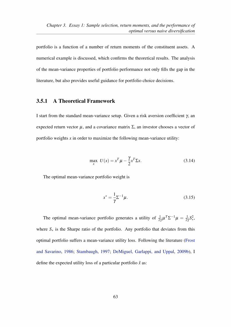
Chapter 3. Essay 1: Sample selection, return moments, and the performance ofoptimal versus naive diversification
portfolio is a function of a number of return moments of the constituent assets. A
numerical example is discussed, which confirms the theoretical results. The analysis
of the mean-variance properties of portfolio performance not only fills the gap in the
literature, but also provides useful guidance for portfolio choice decisions.
3.5.1 A Theoretical Framework
I start from the standard mean-variance setup. Given a risk aversion coefficient γ , an
expected return vector µ , and a covariance matrix Σ, an investor chooses a vector of
portfolio weights x in order to maximize the following mean-variance utility:
maxx
U(x) = xTµ− γ
2xT
Σx. (3.14)
The optimal mean-variance portfolio weight is
x∗ =1γ
Σ−1
µ. (3.15)
The optimal mean-variance portfolio generates a utility of 12γ
µT Σ−1µ = 12γ
S2∗,
where S∗ is the Sharpe ratio of the portfolio. Any portfolio that deviates from this
optimal portfolio suffers a mean-variance utility loss. Following the literature (Frost
and Savarino, 1986; Stambaugh, 1997; DeMiguel, Garlappi, and Uppal, 2009b), I
define the expected utility loss of a particular portfolio x as:
63

Chapter 3. Essay 1: Sample selection, return moments, and the performance ofoptimal versus naive diversification
L(x∗, x) =U(x∗)−E[U(x)] =12γ
µT
Σ−1
µ−E[U(x)]. (3.16)
According to DeMiguel, Garlappi, and Uppal (2009b), the 1/N rule is xew = cN 1N ,
where 1N is a N× 1 vector of ones and c is the fraction of wealth invested in risky
assets. The fraction invested in the risk-free asset is 1− c. The loss function of using
such a 1/N rule is:
L(x∗,xew) =U(x∗)− cN
1TN µ +
γ
2c2
N2 1TNΣ1N . (3.17)
The lowest bound of the loss is obtained by choosing c∗ = N1TN µ
γ1TNΣ1N
, so the 1/N rule
weight vector is:
xew =1T
N µ1N
γ1TNΣ1N
. (3.18)
Therefore, the lowest bound for the loss function of the 1/N rule is:
L(x∗,xew) =12γ
(µ
TΣ−1
µ− (1TN µ)2
1TNΣ1N
)=
12γ
(S2∗−S2
ew)
(3.19)
where S∗ is the Sharpe ratio of the optimal mean-variance portfolio and Sew is the
Sharpe ratio of the 1/N portfolio.
Based on this loss function of the 1/N rule, the following three propositions sum-
marize the performance of the 1/N according to changes in mean returns, volatilities,
correlations and risk aversion, respectively. The proof of each proposition is derived
64

Chapter 3. Essay 1: Sample selection, return moments, and the performance ofoptimal versus naive diversification
in detail in Appendix 2.
Proposition 1. Denote the mean vector for asset returns as µ = φ µ (φ > 0), where µ
is a fixed benchmark mean vector. For the loss function of the 1/N rule L(x∗,xew), we
have:
(1) ∂L(x∗,xew)∂φ
> 0;
(2) ∂ 2L(x∗,xew)∂φ 2 > 0.
Proposition 2. Denote the variance-covariance matrix of asset returns as Σ = λ 2Σ
(λ > 0), where Σ is a fixed benchmark variance-covariance matrix. For the loss func-
tion of the 1/N rule L(x∗,xew), we have:
(1) ∂L(x∗,xew)∂λ
< 0;
(2) ∂ 2L(x∗,xew)∂λ 2 > 0.
Proposition 3. Denote the variance-covariance matrix of the asset returns as Σ =
δ Σ+(1− δ )Σd , where 0 < δ ≤ 1. Σ is a benchmark variance-covariance matrix of
the asset returns, and Σd is an N by N diagonal matrix of Σ. For the loss function of
the 1/N rule L(x∗,xew), we have:
(1) ∂L(x∗,xew)∂δ
∝
(∑i6= j σi jxew
i xewj −∑i 6= j σi jx∗i x∗j
);
(2) ∂ 2L(x∗,xew)∂δ 2 ≥ 0.
Here σi j is the covariance between asset i and asset j; the portfolio weight in asset i
for the mean-variance portfolio is denoted as x∗i , and that for the 1/N rule is denoted
as xewi .
Proposition 1 shows that the mean-variance utility loss of the 1/N rule is an in-
65

Chapter 3. Essay 1: Sample selection, return moments, and the performance ofoptimal versus naive diversification
creasing function of the proportional change in asset expected returns. In other words,
the naive rule tends to have a higher utility loss when the average and dispersion of ex-
pected return are larger. In addition, ∂ 2L(x∗,xew)∂φ 2 > 0 indicates that this expected return
effect strengthens when the proportional return grows larger.
Proposition 2 demonstrates a volatility effect that the loss of the 1/N rule is a de-
creasing function of the proportional change in asset volatilities. As the proportional
volatility change affects both the average and dispersion of volatility, the naive rule
tends to have a higher mean-variance utility loss when the average and dispersion of
volatility are small. Moreover, ∂ 2L(x∗,xew)∂λ 2 > 0 shows that this volatility effect strength-
ens when proportional volatility becomes smaller.
Proposition 3 discusses the relation between the portfolio performance and the
proportional change in correlation which affects both the average and dispersion of
correlations. The proposition shows that the performance of the 1/N rule (relative to
the mean-variance portfolio) depends on ∑i6= j σi jxewi xew
j and ∑i6= j σi jx∗i x∗j . The former
is the variance of the 1/N portfolio attributed to covariances between asset returns,
and the latter is the variance of the optimal mean-variance portfolio attributed to co-
variances between asset returns. ∂ 2L(x∗,xew)∂δ 2 ≥ 0 suggests that the loss of the 1/N rule
is a strictly convex function in δ . This implies that a large loss of the 1/N portfolio
occurs at either low or high correlation regimes. On one hand, when correlations are
low, there are greater diversification benefits of using the mean-variance portfolio in
contrast to the 1/N rule (the diversification effect). On the other hand, when corre-
lations are high, lower diversification benefits call for the mean-variance portfolio to
66
Chapter 3. Essay 1: Sample selection, return moments, and the performance ofoptimal versus naive diversification
rely more on the mean and variance difference between assets to improve utility (the
heterogeneity effect). In both cases, the naive rule tends to have higher mean-variance
utility loss.
Overall, the three propositions theoretically show that the relative performance
of the 1/N rule with respect to the optimal mean-variance portfolio is a function of
the return moments of assets used to form portfolios. In general, the naive 1/N rule
tends to have higher mean-variance utility loss when: (1) the average and dispersion
of expected return are larger, (2) the average and dispersion of asset volatilities are
smaller, and (3) the average correlation and correlation dispersion are either very large
or very small. These mean-variance properties are useful in portfolio choice decisions,
which will be discussed in detail in Section 3.6.
3.5.2 A Numerical Example
To depict the mean-variance properties of optimal versus naive diversification in a
clearer manner, I use a numerical example to demonstrate the three propositions dis-
cussed above. The setup of the numerical example is similar to the simulation setup
in DeMiguel, Garlappi, and Uppal (2009b) and MacKinlay and Pastor (2000). In the
setup, N risky assets (including a single-factor portfolio) are considered. The excess
returns of the N−1 risky assets are generated by the factor model Rit =αi+βiRmt +εit .
Rit is the excess return on asset i, αi is the abnormal return for asset i, βi is the fac-
tor loading for asset i, Rmt is the excess returns on the factor portfolio, and εit is the
noise for asset i, which is independent with respect to the factor portfolio. The factor
67

Chapter 3. Essay 1: Sample selection, return moments, and the performance ofoptimal versus naive diversification
portfolio has an expected annual excess return of 8% and standard deviation of 16%.
The mispricing of all the assets is assumed to be zero, and the factor loadings, βi, are
evenly spread between 0.5 and 1.5. This allows the expected excess returns to vary
from 4 to 12% per year. The noises are cross-sectionally independent normal random
variables with zero means, and their volatilities are drawn from a uniform distribution
with a range of [0.10, 0.30]. The coefficient of relative risk aversion is assumed to be
three, and the annual risk-free rate follows a normal distribution with a mean of 2%
and standard deviation of 2%.
I regard the above setup as a baseline case and set the number of assets to be 25. I
denote the mean vector and covariance matrix of asset return in the baseline base as µ
and Σ, respectively, and define the new mean vector as µ = φ µ and the new covariance
matrix of asset return as Σ = λ 2(δ Σ+(1−δ )Σd) (where Σd is the diagonal matrix of
the baseline covariance matrix, Σ). This design allows me to use unique parameters
to adjust one single return moment of assets at a time, while holding other factors
constant. I change φ and λ from zero to two, while δ varies from zero to one to
ensure positive semi-definite for the covariance matrix. The mean-variance utility loss
of the 1/N rule with respect to the optimal mean-variance portfolio is calculated and
plotted against each return moment.
[Insert Figure 3.1 here]
Figure 3.1 plots the annual mean-variance utility loss of the 1/N rule against the
average expected return and return dispersion of assets used to construct portfolios. As
68

Chapter 3. Essay 1: Sample selection, return moments, and the performance ofoptimal versus naive diversification
both the average expected return and the expected return dispersion increase, the loss
of the 1/N portfolio increases exponentially. This is because the naive rule tends to
deviate more (less) from the mean-variance portfolio that is more (less) likely to have
extreme portfolio weights when the average expected return and return dispersion are
larger (smaller). This expected return effect magnifies with the proportional increase
in expected returns. The relation between the loss of the 1/N rule and expected returns
is consistent with the prediction of Proposition 1.
[Insert Figure 3.2 here]
Figure 3.2 shows the relation between the annualized mean-variance utility loss
of the 1/N rule and the average volatility and volatility dispersion of constituent as-
sets. The loss of the naive rule monotonically decreases at a diminishing rate with the
average and dispersion of volatilities. This is because when the volatilities are larger
(smaller), the mean-variance portfolio tends to rely less (more) on the return difference
between assets; thus, the 1/N rule tends to deviate less (more) from the mean-variance
portfolio. The volatility effect is consistent with the prediction of Proposition 2.
[Insert Figure 3.3 here]
To show the correlation effect, Figure 3.3 displays the loss of the 1/N portfolio for
different averages and dispersions of correlations of asset returns. In general, the loss
of the 1/N rule is a non-constant convex function in δ which affects both the aver-
age and dispersion of correlations. As the average correlation increases from 0.3 to
about 0.43 (correlation dispersion increases from 0.4 to 0.6), the loss of the 1/N rule
69

Chapter 3. Essay 1: Sample selection, return moments, and the performance ofoptimal versus naive diversification
increases. This is because when correlations increase, lower diversification benefits
call for the mean-variance portfolio to rely more on asset heterogeneity to improve
utility (the heterogeneity effect). If we further reduce the average correlation from 0.3
towards zero (correlation dispersion decreases from 0.4 towards zero), the loss of the
1/N rule increases. When correlations decrease, there are more diversification benefits
of using the optimal mean-variance portfolio in contrast to the 1/N rule (the diversifi-
cation effect). In accordance with Proposition 3, both correlation effects suggest that
the naive portfolio tends to have higher mean-variance utility loss when the averages
and dispersions of correlations are either very large or very small.
To summarize, the mean-variance properties of the 1/N rule shown in the numer-
ical example are consistent with the 1/N loss profiles discussed in Propositions 1 to
3. Generally, the mean-variance utility loss of the 1/N rule increases with the average
and dispersion of expected returns (the expected return effect). In addition, a small
average and dispersion of asset volatility are less in favor of the 1/N rule (the volatility
effect). In terms of the heterogeneity effect and diversification effect, a very large or
very small average correlation and correlation dispersion tend to associate with more
1/N loss. The application of these theoretical results is discussed in the next section.
3.5.3 Estimation Errors
The mean-variance properties of mean-variance versus naive diversification discussed
in previous sections involve no estimation errors. In fact, when a mean-variance port-
folio is constructed based on estimated return moments, the expected utility is smaller
70
Chapter 3. Essay 1: Sample selection, return moments, and the performance ofoptimal versus naive diversification
compared with the case based on true return moments. In addition, since true re-
turn moments are unknown, each return moment is estimated with biases. In this
section, I discuss how estimation errors may affect the theoretical results obtained in
Section 3.5.1.
When estimation error in both mean-variance portfolio and return moments are
introduced, it is difficult to obtain analytical results as in Section 3.5.1. Therefore, I
use simulations to demonstrate how relative performance between the mean-variance
and 1/N rules varies with each return moment.
Following the previous section, the simulation setup of DeMiguel et al. (2009b)
is used as a baseline case. I construct 1000 datasets of 1000-month excess return
series. For each dataset, the factor portfolio is simulated with an expected annual
excess return of 8% and standard deviation of 16%, while the risk-free rate is a normal
distributed random variable with a mean of 2% and standard deviation of 2% on an
annual basis. Key parameters, φ , λ , and δ are randomly selected from ranges (0,2],
(0,2], and (0,1], respectively. The number of assets, N, is also randomly picked from
3 to 100. Asset excess returns are then calculated from the factor model with alphas,
betas, and residual volatilities controlled by the three key parameters. Note that φ , λ ,
δ and N are fixed within each dataset, but vary across datasets.
For each dataset, I calculate the out-of-sample utility difference (for γ = 3) be-
tween the mean-variance portfolio and the 1/N rule, and study how the relative perfor-
mance changes with the three key return moment parameters. Because, in the presence
of estimation errors, φ , λ and δ are unobservable, I estimate these parameters for each
71

Chapter 3. Essay 1: Sample selection, return moments, and the performance ofoptimal versus naive diversification
dataset as below rather than using the true values.
φ =1T
T
∑t=1
1′N(µt ./µ)
N
λ =1T
T
∑t=1
1′N(vec(Σt)./vec(Σ)
N
δ =1T
T
∑t=1
1′N(vec(Σt− Σd,t)./vec(Σ− Σd))
N2−N
(3.20)
where µ , Σ and Σd are the mean vector, covariance matrix and diagonal covariance
matrix, respectively, for the baseline case; µt , Σt and Σd,t are the estimated moments
at time t; operator ./ stands for element-wise division; vec() refers to vectorizing a
matrix; 1′N is a row vector of ones of size N; and T is the number of out-of-sample
periods. With rolling estimation window of 120 months, T is 880 for each dataset.
Recall that φ , λ , and δ control for the proportional changes in return, volatility
and correlation with respect to a baseline case. Therefore, the idea underlying the
estimation methods for φ , λ , δ is to approximate the proportional changes by using
the element-wise division (./), and average the estimated changes across assets and
time. The following cross-sectional regression of relative performance is estimated to
study the performance of optimal versus naive diversification with estimation errors.
∆Um = a+b1φm +b2λm +b3δm +b4I{δm>0}+b5Nm + εm,(m = 1, ...,1000) (3.21)
where, for each dataset m, ∆Um denotes the annualized utility (for γ = 3) difference
between mean-variance portfolios and the 1/N rule; φm, λm, δm are the estimated pro-
72
Chapter 3. Essay 1: Sample selection, return moments, and the performance ofoptimal versus naive diversification
portional changes in return moments standardized across 1000 datasets; I{δm>0} is a
dummy variable with value of one if δm > 0 (zero otherwise); and Nm is the number
of assets in that dataset.
[Insert Table 3.9 here]
Table 3.8 shows the regression estimates for Equation 3.21 based on 1000 simu-
lated datasets. For the true optimal mean-variance portfolio, the results are consistent
with analytical framework. The utility difference between mean-variance and 1/N rule
increases with φm, and decreases with λm and δm. When δm is relatively large (δm > 0),
the dummy variable suggests that the relative performance tends to improve. This is
consistent with the result in Figure 3.3. Note that the slope associated with N is signifi-
cantly positive (0.0056), indicating diversification benefit improves for mean-variance
portfolio relative to the 1/N rule as the number of assets increases. The adjusted R-
square suggests that return moments can explain around 25% of variations in relative
performance between MV and 1/N.
The second set of results explain the relative performance between unconstrained
mean-variance portfolio and the 1/N rule in the presence of estimation errors. In gen-
eral, for unconstrained mean-variance rules, return moments do not have explanatory
power for relative performance. This is because, unconstrained MV rules tend to have
large estimation error, and deliver low and unstable CEQ returns (see Table 3.4). The
mean-variance features of the relative performance are jeopardized with large estima-
tion biases. However, N is significant with a large negative number (-0.0756), which
73

Chapter 3. Essay 1: Sample selection, return moments, and the performance ofoptimal versus naive diversification
suggests that the performance of the unconstrained portfolio relative to the 1/N bench-
mark becomes worse as the number of assets increases. This phenomenon is consis-
tent with DeMiguel et al. (2009b) who argue that the sample-based mean-variance
portfolio requires longer estimation window to beat the 1/N rule as N grows larger.
When the short-sale constraint is imposed, the return moments become useful in
explaining the cross-sectional variation in relative performance between the estimated
MV rule and the 1/N rule. In addition, the slopes associated with φm, λm, δm, and
I{δm>0} are significant, and consistent with the theoretical results. Note that the mag-
nitudes of slope estimates in this case are substantially smaller than those in the case
for the true optimal MV portfolio. This is because, with no estimation errors, there
is large CEQ return difference between the true optimal MV portfolio and the 1/N
rule. In other words, the dependent variables are much larger for the the true optimal
MV case, while the dependent variables for the constrained MV case have a much
smaller magnitude (constrained MV and 1/N rules have CEQ returns in similar mag-
nitudes). Interestingly, with the shortsale constraint, N is no longer significant. This
suggests that when estimation error is effectively reduced, as in the constrained case,
the number of assets no long explains the performance difference between MV and
1/N. Instead, return moments collectively capture around 28% of variation in the rela-
tive performance. The number is similar to the corresponding one in the case with no
estimation errors.
Overall, the simulation exercise confirms the theoretical results for the true opti-
mal mean-variance portfolio when no estimation error is involved. Due to large es-
74

Chapter 3. Essay 1: Sample selection, return moments, and the performance ofoptimal versus naive diversification
timation errors, the CEQ return difference between the estimated unconstrained MV
rule and the 1/N rule is not significantly associated with return moments. However,
when estimation errors are effectively reduced by portfolio constraints, the relative
performance between mean-variance rule and the 1/N rule is significantly driven by
return moments, and the result is consistent with the theoretical framework.
3.6 Return Moments and Performance Predictability
Motivated by the mean-variance properties of the 1/N rule, this section examines
whether investors can exploit the information on assets’ return moments when se-
lecting between optimal and naive diversification. The empirical results presented
earlier suggest that the naive 1/N rule is still difficult to defeat on an average basis
even for some “1/N outperformers.” However, sophisticated strategies are able to out-
perform the naive rule in some datasets. If investors can identify these scenarios ex
ante, it is likely to improve their returns on a risk-adjusted basis. Based on the theo-
retical properties of optimal and naive diversification, I develop four hypotheses that
are used to predict the performance of a mean-variance strategy relative to the naive
rule. Following this, the predictive results are presented based on the estimates from
the 122 Fama-French datasets used in the empirical analysis. Finally, I undertake a
portfolio switching exercise to demonstrate how investors could use this predictability
to improve portfolio performance.
75
Chapter 3. Essay 1: Sample selection, return moments, and the performance ofoptimal versus naive diversification
3.6.1 Predictive Regression
I consider all non-naive strategies examined in this study, and try to predict the out-
of-sample CEQ return difference between a sophisticated strategy and the naive 1/N
benchmark. For the predictors, I select a number of in-sample assets’ return mo-
ments. These return moments include the average asset return (µ), return dispersion
(∆µ), average volatility (σ ), volatility dispersion (∆σ ), average pair-wise correlation
(ρ), and correlation dispersion (∆ρ). The theoretical results suggest that the perfor-
mance between mean-variance and 1/N rules is related to proportional changes in
return, volatility and correlations, and the proportional change controls not only the
average magnitude but also range or dispersion of these return moments simultane-
ously. Therefore, the interaction terms for each return moment (µ×∆µ , σ ×∆σ and
ρ ×∆ρ) are of particular importance. DeMiguel, Garlappi, and Uppal (2009b) find
that estimation error in mean-variance portfolios increases with the number of assets.
Therefore, the number of assets (N) is also considered as one of the predictors for
portfolio performance. Brown, Hwang, and In (2013) find that the performance of
naive diversification relative to optimal diversification represents a compensation for
the increase in tail risk and the reduced upside potential associated with the concave
payoff. For this reason, I also examine a number of tail risk measures as control vari-
ables, including the average skewness (S), skewness dispersion (∆S), average kurtosis
(K), and kurtosis dispersion (∆K).
I define ∆Ui as the out-of-sample annualized CEQ return (for γ = 3) difference in
76

Chapter 3. Essay 1: Sample selection, return moments, and the performance ofoptimal versus naive diversification
dataset i between a sophisticated and the 1/N portfolio. The following cross-sectional
regression is estimated across M (M = 122 in this case) datasets:
∆Ui =α +β1Ni +β2µi +β3∆µi +β4∆σi +β5σi +β6∆ρi +β7ρi
+ γ1µi×∆µi + γ2σi×∆σi + γ3ρi×∆ρi
+Controls+ ei(i = 1, ......,M)
(3.22)
where ∆µi, ∆σi and ∆ρi are the dispersions in mean return, volatility and correlation,
respectively, for the annualized excess returns in dataset i; µi, σi and ρi are the average
levels of expected return, volatility and correlation, respectively; and Ni refers the
number of assets in dataset i. The control variables are tail risk measures including Si
(average skewness), Ki (average kurtosis), ∆Si (skewness dispersion) and ∆Ki (kurtosis
dispersion).
The simulation analysis in the previous section shows that the relative performance
between the mean-variance and 1/N rules is significantly related to return moments
when estimation error is effectively reduced with portfolio constraints. Therefore,
each sophisticated strategy is imposed with the shortsale constraint. All the return
moments are computed based on only the in-sample information (data for the first 120
months) in each dataset, while the CEQ returns are calculated using rest of the data.
77

Chapter 3. Essay 1: Sample selection, return moments, and the performance ofoptimal versus naive diversification
3.6.2 Hypotheses
Based on the predictive regression and the properties of optimal versus naive diversi-
fication derived earlier in this paper, I propose several hypotheses regarding the pre-
dictive directions for a number of variables.
H1—Expected return effect: Consistent with Proposition 1, a larger average ex-
pected return and wider expected return dispersion collectively predict better perfor-
mance of a mean-variance strategy relative to the naive 1/N rule (γ1 > 0).
H2—Volatility effect: Consistent with Proposition 2, a smaller average volatility
and narrower volatility dispersion collectively predict better performance of a mean-
variance strategy relative to the naive 1/N rule (γ2 < 0).
H3—Diversification effect: Consistent with Proposition 3, a smaller average cor-
relation and narrower correlation dispersion collectively predict better performance of
a mean-variance strategy relative to the naive 1/N rule (γ3 < 0).
H4—Heterogeneity effect: Consistent with Proposition 3, a larger average cor-
relation and wider correlation dispersion collectively predict better performance of a
mean-variance strategy relative to the naive 1/N rule (γ3 > 0).
3.6.3 Predictive Results
Equation 3.22 is estimated based on the 122 Fama-French datasets used in this pa-
per, and Table 3.10 reports the predictive results. In general, the in-sample return
moments have a strong predictive power for the out-of-sample portfolio performance.
78
Chapter 3. Essay 1: Sample selection, return moments, and the performance ofoptimal versus naive diversification
The predictive regression explains more than 20% of the out-of-sample performance
for all 16 strategies reflected by the adjusted R-square. However, the sophisticated
strategies show a large variation in predictability. For instance, on average, the re-
gression explains more than 50% of the performance for the six reward-to-risk tim-
ing strategies (RRT1, RRT2, RRT4, CRRT1, CRRT2 and CRRT4) relative to the 1/N
benchmark, while the adjusted R-square is about 27% for the traditional sample-based
mean-variance strategy. Different strategies have various sensitivities to the return mo-
ments of assets used for portfolio construction.
[Insert Table 3.10 here]
Individual predictors deliver predictive directions consistent with the hypotheses
above. For the expected return effect, 14 of the 16 sophisticated strategies are asso-
ciated with better performance when the average expected return and expected return
dispersion are simultaneously larger. Although the remaining two strategies (MV and
CKZ) have negative slopes on µ ×∆µ , they are statistically insignificant. For eco-
nomic significance, consider the QL strategy for example. If the average expected re-
turn and expected return dispersion both increase by 10%, the VT1 strategy improves
its CEQ return by 61 basis points relative to the naive 1/N rule.
The volatility effect has stronger statistical significance than the return effect. The
slope coefficients on σ ×∆σ are negative for all 16 strategies, with 10 of them hav-
ing statistical significance at 10% level. Coefficients on σ ×∆σ seem to have small
economic significance. For instance, if the average volatility and volatility dispersion
79

Chapter 3. Essay 1: Sample selection, return moments, and the performance ofoptimal versus naive diversification
both increase by 10%, several conditional reward-to-risk timing strategies improve
their CEQ returns by about six to eight basis points relative to the naive 1/N rule.
In terms of the influence of correlations, the heterogeneity effect dominates the
diversification effect. The diversification effect suggests that a mean-variance strategy
provides more diversification benefit relative to the 1/N rule when average correlation
and correlation dispersion are simultaneously small. In contrast, the heterogeneity
effect suggests that when the average correlation is large and diversification is difficult,
a mean-variance strategy improves its performance relative to the naive rule by taking
advantage of the heterogeneity of assets reflected by a large dispersion in correlations.
The result is consistent with the heterogeneity effect in contrast to the diversification
effect. It shows that the slope on ρ×∆ρ are positive for all 16 strategies, and half of
them possess statistical significance at 10% level.
In summary, the predictability of performance based on return moments is strong
for various mean-variance strategies. The regression results are consistent with the
expected return and the volatility effects; and the heterogeneity effect dominates the
diversification effect in all 16 cases. Although volatility and correlation effects seem to
have small economic significance, combining various return moment effects together
can deliver large magnitudes of economic significance. After all, these return mo-
ments collectively captures a large proportion of variation in the relative performance
between the mean-variance and 1/N rule, which is reflected by large R-squares.
80

Chapter 3. Essay 1: Sample selection, return moments, and the performance ofoptimal versus naive diversification
3.6.4 A Portfolio Switching Strategy
To examine whether the predictability of portfolio performance based on return mo-
ments can be translated into better out-of-sample portfolio benefits, I propose a dy-
namic switching strategy that can be applied in real time. The switching strategy is
a binary choice between a sophisticated mean-variance portfolio and the 1/N portfo-
lio, depending on the predictive values of the performance difference between the two
portfolios. If the predicted performance difference is positive (negative), the switch-
ing strategy applies the sophisticated portfolio (1/N rule) for the entire out-of-sample
period. Mathematically, the switching strategy takes the following portfolio weight:
wSt = I{∆U>0}w
Rt +(1− I{∆U>0})w1/N (3.23)
where wRt is the weight vector of a raw mean-variance strategy estimated at time t,
and w1/N is the equal weight. I{∆U>0} is an indicator function that takes the value
of one (zero) if the predicted CEQ return difference between the two rules is positive
(negative).
When the mean-variance rule and the 1/N rule have a large difference in portfolio
weights, switching from one to another can incur large transaction costs. Therefore,
to reduce excessive and meaningless switching, I also incorporate the portfolio weight
before rebalancing in this switching process. The idea is to evaluate the predicted
utility, adjusted for transaction costs, for the three constituent rules (the raw mean-
variance rule, the 1/N rule, and the switching rule before rebalancing at time t), and
81

Chapter 3. Essay 1: Sample selection, return moments, and the performance ofoptimal versus naive diversification
choose the one that delivers the largest net utility. The switching strategy is shown
mathematically as below:
wSt =arg max (U(x)−Turn(x)× cost)
x ∈ {wRt , w1/N , wS
t }(3.24)
where U(x) and Turn(x) are the predicted CEQ return and turnover for portfolio x,
respectively; cost is constant, equals 0.005 (transaction cost of 50 basis points); and
wSt is the weight vector for the switching strategy before rebalancing at time t.
I regard the 16 mean-variance rules in Table 3.1 as 16 raw strategies, implement the
switching strategy for each of the raw rules, and evaluate the performance of switching
strategies using the 122 Fama-French datasets. Following the literature, I use a rolling
window of 120 months to estimate portfolio weights. Since performance predictability
exist for the constrained mean-variance portfolio (Section 3.5.3), the 16 raw strategies
are imposed with shortsale constraints.
To predict CEQ returns, a regression similar to Equation 3.22 is used with cross-
validation. For asset returns with 120 observations (120-month rolling window), a se-
ries of portfolio returns can be calculated for a given strategy. The portfolio variance
is treated as constant, and estimated based on the whole sample. Each CEQ return is
then calculated based on each portfolio return observation and the constant variance.
Next, a series of CEQ return difference between a sophisticated rule and the 1/N rule
is created. For each CEQ return difference, I match it with the return moments cal-
82

Chapter 3. Essay 1: Sample selection, return moments, and the performance ofoptimal versus naive diversification
culated from the rest 119 observations of asset returns. The cross-sectional predictive
regression of CEQ return differences against return moments (Equation 3.22) is then
estimated. After that, return moments are computed based on the whole sample of
120 months, and are applied to the estimated regression. The predicted value from
the regression is actually the CEQ return difference. Adding it to the calculated CEQ
return of the 1/N rule, I back out the predicted CEQ return for a given sophisticated
strategy.
[Insert Table 3.11 here]
Table 3.11 summarizes the performance of the switching strategy for each of the
16 raw mean-variance rules, and compares the strategy with its raw rule and the 1/N
rule. Despite significant outperformance over 1/N in terms of CEQ return, the 16 raw
mean-variance rules do not deliver significantly larger Sharpe ratio compared with the
naive benchmark. When the switching strategy is applied, the performance of all 16
mean-variance rules improves significantly under all three performance measures. 16
switching strategies significantly outperform not only their mean-variance counter-
parts but also the 1/N benchmark on a risk adjusted basis. They all require much less
portfolio turnover, and some of the switching strategies even generate much smaller
turnover than the 1/N rule.
The outperformance frequency with respect to the 1/N rule is larger for each
switching strategy compared with its raw rule. All 16 switching rules outperform the
1/N rule in terms of Sharpe ratio and CEQ return in more than 60% of the datasets,
83

Chapter 3. Essay 1: Sample selection, return moments, and the performance ofoptimal versus naive diversification
and many of them deliver outperformance frequencies greater than 80%. They also
have large outperformance frequency with respect to the raw rules. In particular, the
switched CMP strategy outperforms the raw CMP strategy in 90% of the datasets.
Furthermore, all switching strategies require smaller turnover compared with their
raw rules in 100% of the 122 datasets.
[Insert Table 3.12 here]
Table 3.12 reports the percentage of all months each constituent rule is used for
the switching strategy, averaged across the 122 Fama-French datasets. The constituent
rules for the switching strategy consist of wRt , w1/N and wS
t . wRt stands for the raw
mean-variance strategy, and w1/N is the 1/N rule. wSt is the switching strategy before
rebalancing at time t. When wSt is applied, the portfolio does not rebalance at time t.
Results show that the switching strategy has a good balance in its constituent rules. It
applies the raw mean-variance rule more frequently compared with the 1/N rule, and
it rebalances the portfolio for 40% to 50% of the times in most cases.
Overall, the study on predictability of portfolio performance based on assets’ re-
turn moments reveals several interesting findings. First, return moments show strong
power in predicting the performance of mean-variance rules relative to the naive 1/N
rule. Second, motivated by the theoretical performance of optimal versus naive diver-
sification, three predictive effects are identified—namely, the expected return effect,
volatility effect, and the heterogeneity effect. Third, the predictability can be used
to improve portfolio performance. A switching strategy that exploits this predictabil-
84
Chapter 3. Essay 1: Sample selection, return moments, and the performance ofoptimal versus naive diversification
ity is able to outperforms both its raw mean-variance counterpart and the 1/N rule
significantly.
3.7 Conclusions
In this paper, a novel performance test is proposed to evaluate portfolio performance
based on a large universe of datasets. While existing performance tests provide statis-
tical inference based on a single dataset, the new test aggregates portfolio performance
across datasets, conduct inference on average performance while taking into account
performance uncertainty in each dataset.
Based on the test, I evaluate the naive 1/N rule against 14 mean-variance rules that
are claimed to outperform the naive benchmark. Although there are strategies that
outperform the 1/N rule on an average basis, a sample selection problem generally
exists in claiming outperformance over the benchmark. It remains a hard task for
mean-variance strategies to consistently outperform the 1/N rule in terms of Sharpe
ratio, CEQ return and portfolio turnover.
To further understand portfolio performance, this paper analyzes how the perfor-
mance of optimal versus naive diversification is related to the return moments of as-
sets used to construct portfolios. Theoretically and empirically, I demonstrate a strong
predictability of performance of mean-variance rules relative to the 1/N rule based on
the assets’ return moments. More importantly, this predictability can be translated to
out-of-sample portfolio benefits. A portfolio switching strategy that selects between a
85

Chapter 3. Essay 1: Sample selection, return moments, and the performance ofoptimal versus naive diversification
mean-variance rule and the 1/N rule based on performance forecasts is able to signifi-
cantly outperform both its raw mean-variance counterparts and the 1/N benchmark.
Recent literature has experienced a large trend in developing mean-variance port-
folio rules to challenge the naive 1/N rule. This paper suggests that these portfo-
lio successes are biased to some extent because they only exist in limited scenarios.
Newly developed mean-variance strategies that seek to outperform the 1/N portfolio
should not only demonstrate their outperformance in a small number of pre-selected
datasets; rather, to mitigate the sample selection problem, portfolio horse races should
be conducted across a large number of datasets.
86
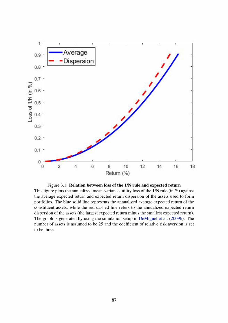
Figure 3.1: Relation between loss of the 1/N rule and expected returnThis figure plots the annualized mean-variance utility loss of the 1/N rule (in %) againstthe average expected return and expected return dispersion of the assets used to formportfolios. The blue solid line represents the annualized average expected return of theconstituent assets, while the red dashed line refers to the annualized expected returndispersion of the assets (the largest expected return minus the smallest expected return).The graph is generated by using the simulation setup in DeMiguel et al. (2009b). Thenumber of assets is assumed to be 25 and the coefficient of relative risk aversion is setto be three.
87
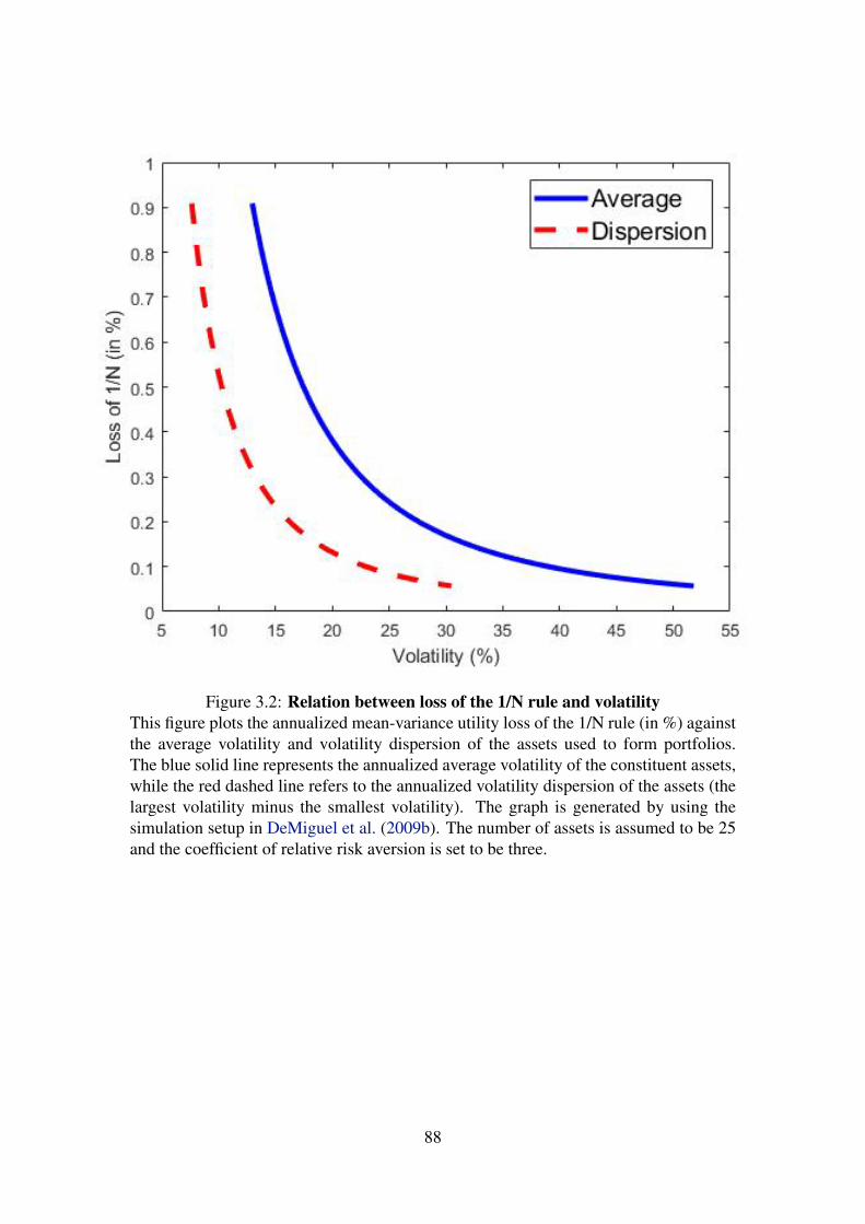
Figure 3.2: Relation between loss of the 1/N rule and volatilityThis figure plots the annualized mean-variance utility loss of the 1/N rule (in %) againstthe average volatility and volatility dispersion of the assets used to form portfolios.The blue solid line represents the annualized average volatility of the constituent assets,while the red dashed line refers to the annualized volatility dispersion of the assets (thelargest volatility minus the smallest volatility). The graph is generated by using thesimulation setup in DeMiguel et al. (2009b). The number of assets is assumed to be 25and the coefficient of relative risk aversion is set to be three.
88
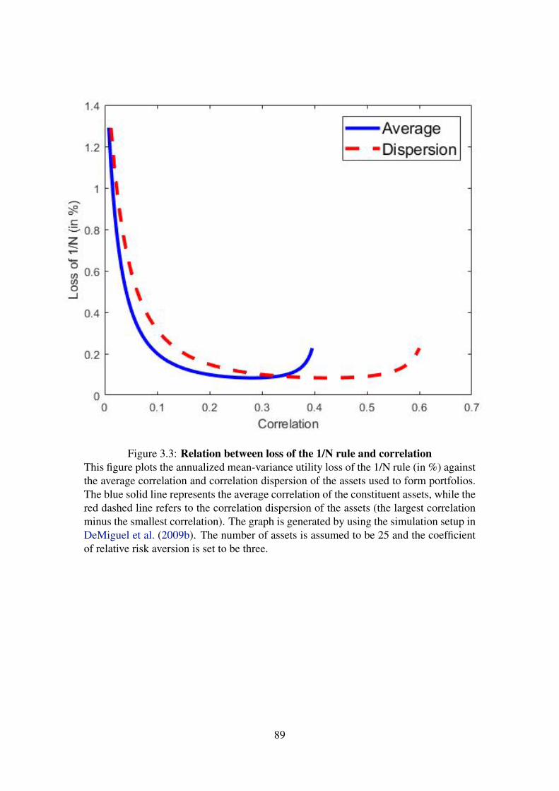
Figure 3.3: Relation between loss of the 1/N rule and correlationThis figure plots the annualized mean-variance utility loss of the 1/N rule (in %) againstthe average correlation and correlation dispersion of the assets used to form portfolios.The blue solid line represents the average correlation of the constituent assets, while thered dashed line refers to the correlation dispersion of the assets (the largest correlationminus the smallest correlation). The graph is generated by using the simulation setup inDeMiguel et al. (2009b). The number of assets is assumed to be 25 and the coefficientof relative risk aversion is set to be three.
89
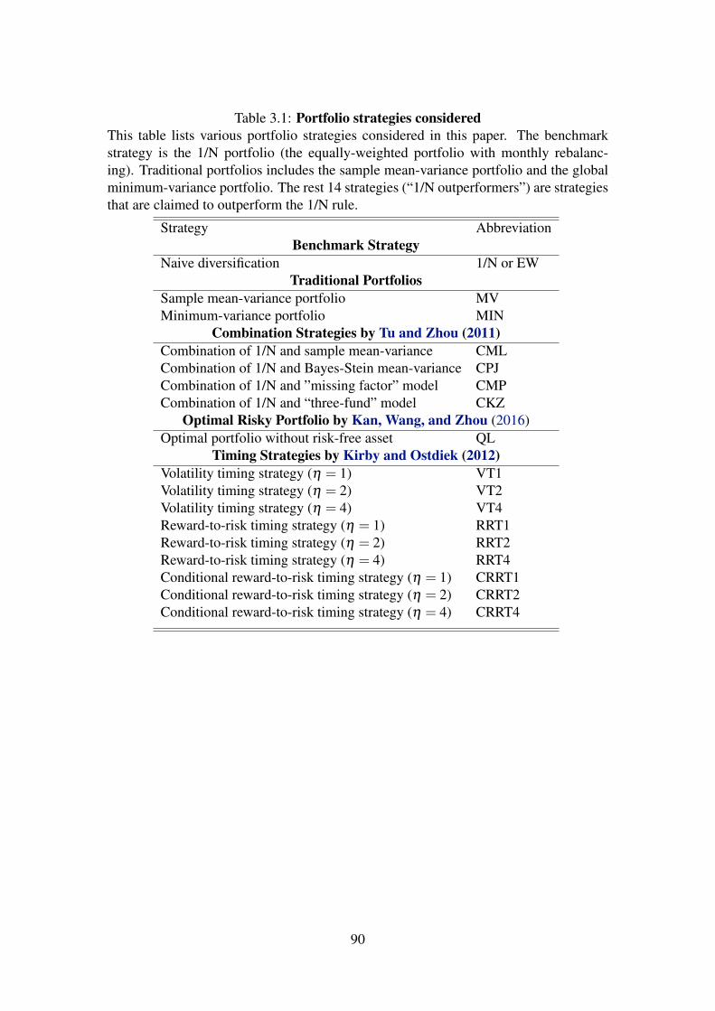
Table 3.1: Portfolio strategies consideredThis table lists various portfolio strategies considered in this paper. The benchmarkstrategy is the 1/N portfolio (the equally-weighted portfolio with monthly rebalanc-ing). Traditional portfolios includes the sample mean-variance portfolio and the globalminimum-variance portfolio. The rest 14 strategies (“1/N outperformers”) are strategiesthat are claimed to outperform the 1/N rule.
Strategy AbbreviationBenchmark Strategy
Naive diversification 1/N or EWTraditional Portfolios
Sample mean-variance portfolio MVMinimum-variance portfolio MIN
Combination Strategies by Tu and Zhou (2011)Combination of 1/N and sample mean-variance CMLCombination of 1/N and Bayes-Stein mean-variance CPJCombination of 1/N and ”missing factor” model CMPCombination of 1/N and “three-fund” model CKZ
Optimal Risky Portfolio by Kan, Wang, and Zhou (2016)Optimal portfolio without risk-free asset QL
Timing Strategies by Kirby and Ostdiek (2012)Volatility timing strategy (η = 1) VT1Volatility timing strategy (η = 2) VT2Volatility timing strategy (η = 4) VT4Reward-to-risk timing strategy (η = 1) RRT1Reward-to-risk timing strategy (η = 2) RRT2Reward-to-risk timing strategy (η = 4) RRT4Conditional reward-to-risk timing strategy (η = 1) CRRT1Conditional reward-to-risk timing strategy (η = 2) CRRT2Conditional reward-to-risk timing strategy (η = 4) CRRT4
90
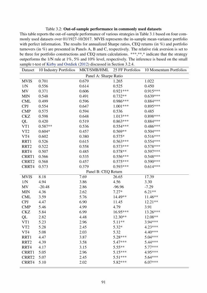
Table 3.2: Out-of-sample performance in commonly used datasetsThis table reports the out-of-sample performance of various strategies in Table 3.1 based on four com-monly used datasets over 01/1927-10/2017. MVIS represents the in-sample mean-variance portfoliowith perfect information. The results for annualized Sharpe ratios, CEQ returns (in %) and portfolioturnovers (in %) are presented in Panels A, B and C, respectively. The relative risk aversion is set tobe three for portfolio constructions and CEQ return calculations. ***,**,* indicate that the strategyoutperforms the 1/N rule at 1%, 5% and 10% level, respectively. The inference is based on the smallsample t-test of Kirby and Ostdiek (2012) discussed in Section 3.2.4.
Dataset 10 Industry Portfolios MKT/SMB/HML 25 FF Portfolios 10 Momentum PortfoliosPanel A: Sharpe Ratio
MVIS 0.701 0.679 1.265 1.0221/N 0.556 0.614 0.525 0.450MV 0.371 0.606 0.921*** 0.915***MIN 0.548 0.491 0.732** 0.639***CML 0.499 0.596 0.986*** 0.884***CPJ 0.554 0.647 1.001*** 0.895***CMP 0.575 0.594 0.536 0.485CKZ 0.598 0.648 1.013*** 0.898***QL 0.420 0.519 0.863*** 0.884***VT1 0.587** 0.536 0.554*** 0.486***VT2 0.604* 0.457 0.569** 0.504***VT4 0.602 0.380 0.575* 0.516***RRT1 0.526 0.615 0.563*** 0.554***RRT2 0.522 0.558 0.573*** 0.578***RRT4 0.507 0.485 0.578** 0.597***CRRT1 0.566 0.535 0.556*** 0.548***CRRT2 0.568 0.457 0.575*** 0.590***CRRT4 0.573 0.379 0.593*** 0.614***
Panel B: CEQ ReturnMVIS 8.18 7.69 26.65 17.391/N 4.94 3.86 4.56 3.30MV -20.48 2.86 -96.96 -7.29MIN 4.36 2.62 7.27* 6.21**CML 3.59 5.76 14.49** 11.46**CPJ 4.47 6.90 11.45 12.21**CMP 5.46 4.99 4.79 3.91CKZ 5.84 6.99 16.95*** 13.26***QL 2.82 4.48 12.30** 12.08**VT1 5.23 2.96 5.11** 3.94***VT2 5.28 2.45 5.32* 4.23***VT4 5.08 2.03 5.32 4.40***RRT1 4.47 3.87 5.28*** 5.04***RRT2 4.39 3.58 5.47*** 5.44***RRT4 4.17 3.15 5.55** 5.77***CRRT1 5.05 2.96 5.15*** 4.95***CRRT2 5.07 2.45 5.51*** 5.64***CRRT4 5.10 2.02 5.82*** 6.07***
91

Continued from previous page.Dataset 10 Industry Portfolios MKT/SMB/HML 25 FF Portfolios 10 Momentum Portfolios
Panel C: Portfolio Turnover1/N 25.61 24.05 21.28 20.53MV 3658 1314 53567 6976MIN 195.6 28.9 914.3 329.5CML 902.8 761.5 5637 2684CPJ 858.7 801.8 7464 2502CMP 129.4 130.6 94.54 102.0CKZ 647.4 722.3 4090 1950QL 700.6 291.7 4262 2431VT1 27.75 24.26 22.21 20.26VT2 32.57 26.51 25.79 23.17VT4 39.50 31.53 36.44 33.02RRT1 64.33 58.82 37.81 59.69RRT2 84.74 81.83 55.39 69.49RRT4 121.3 99.86 91.61 88.70CRRT1 34.99 24.24 22.65 23.61CRRT2 47.94 26.48 26.71 29.15CRRT4 72.41 31.53 37.70 40.70
92
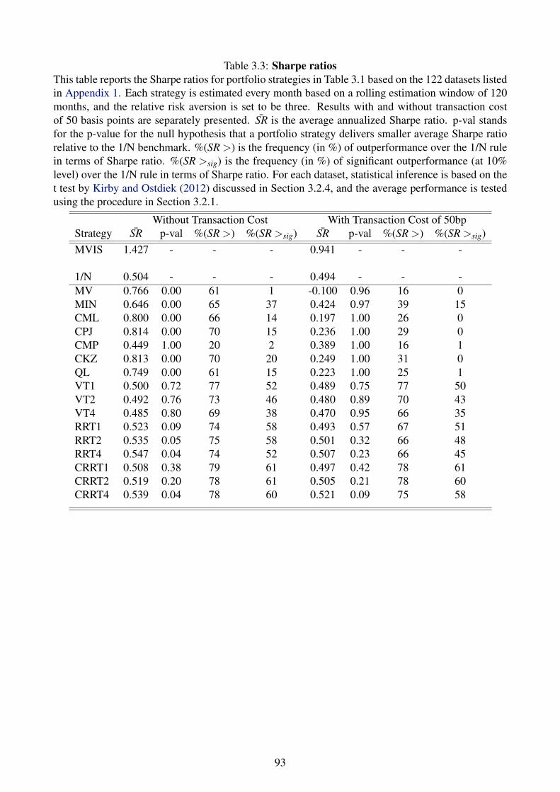
Table 3.3: Sharpe ratiosThis table reports the Sharpe ratios for portfolio strategies in Table 3.1 based on the 122 datasets listedin Appendix 1. Each strategy is estimated every month based on a rolling estimation window of 120months, and the relative risk aversion is set to be three. Results with and without transaction costof 50 basis points are separately presented. SR is the average annualized Sharpe ratio. p-val standsfor the p-value for the null hypothesis that a portfolio strategy delivers smaller average Sharpe ratiorelative to the 1/N benchmark. %(SR >) is the frequency (in %) of outperformance over the 1/N rulein terms of Sharpe ratio. %(SR >sig) is the frequency (in %) of significant outperformance (at 10%level) over the 1/N rule in terms of Sharpe ratio. For each dataset, statistical inference is based on thet test by Kirby and Ostdiek (2012) discussed in Section 3.2.4, and the average performance is testedusing the procedure in Section 3.2.1.
Without Transaction Cost With Transaction Cost of 50bpStrategy SR p-val %(SR >) %(SR >sig) SR p-val %(SR >) %(SR >sig)MVIS 1.427 - - - 0.941 - - -
1/N 0.504 - - - 0.494 - - -MV 0.766 0.00 61 1 -0.100 0.96 16 0MIN 0.646 0.00 65 37 0.424 0.97 39 15CML 0.800 0.00 66 14 0.197 1.00 26 0CPJ 0.814 0.00 70 15 0.236 1.00 29 0CMP 0.449 1.00 20 2 0.389 1.00 16 1CKZ 0.813 0.00 70 20 0.249 1.00 31 0QL 0.749 0.00 61 15 0.223 1.00 25 1VT1 0.500 0.72 77 52 0.489 0.75 77 50VT2 0.492 0.76 73 46 0.480 0.89 70 43VT4 0.485 0.80 69 38 0.470 0.95 66 35RRT1 0.523 0.09 74 58 0.493 0.57 67 51RRT2 0.535 0.05 75 58 0.501 0.32 66 48RRT4 0.547 0.04 74 52 0.507 0.23 66 45CRRT1 0.508 0.38 79 61 0.497 0.42 78 61CRRT2 0.519 0.20 78 61 0.505 0.21 78 60CRRT4 0.539 0.04 78 60 0.521 0.09 75 58
93
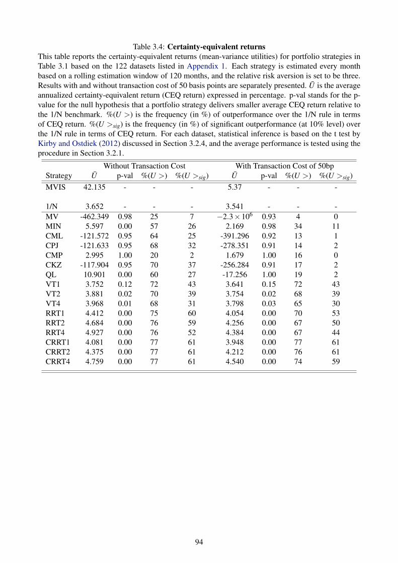
Table 3.4: Certainty-equivalent returnsThis table reports the certainty-equivalent returns (mean-variance utilities) for portfolio strategies inTable 3.1 based on the 122 datasets listed in Appendix 1. Each strategy is estimated every monthbased on a rolling estimation window of 120 months, and the relative risk aversion is set to be three.Results with and without transaction cost of 50 basis points are separately presented. U is the averageannualized certainty-equivalent return (CEQ return) expressed in percentage. p-val stands for the p-value for the null hypothesis that a portfolio strategy delivers smaller average CEQ return relative tothe 1/N benchmark. %(U >) is the frequency (in %) of outperformance over the 1/N rule in termsof CEQ return. %(U >sig) is the frequency (in %) of significant outperformance (at 10% level) overthe 1/N rule in terms of CEQ return. For each dataset, statistical inference is based on the t test byKirby and Ostdiek (2012) discussed in Section 3.2.4, and the average performance is tested using theprocedure in Section 3.2.1.
Without Transaction Cost With Transaction Cost of 50bpStrategy U p-val %(U >) %(U >sig) U p-val %(U >) %(U >sig)MVIS 42.135 - - - 5.37 - - -
1/N 3.652 - - - 3.541 - - -MV -462.349 0.98 25 7 −2.3×10⁶ 0.93 4 0MIN 5.597 0.00 57 26 2.169 0.98 34 11CML -121.572 0.95 64 25 -391.296 0.92 13 1CPJ -121.633 0.95 68 32 -278.351 0.91 14 2CMP 2.995 1.00 20 2 1.679 1.00 16 0CKZ -117.904 0.95 70 37 -256.284 0.91 17 2QL 10.901 0.00 60 27 -17.256 1.00 19 2VT1 3.752 0.12 72 43 3.641 0.15 72 43VT2 3.881 0.02 70 39 3.754 0.02 68 39VT4 3.968 0.01 68 31 3.798 0.03 65 30RRT1 4.412 0.00 75 60 4.054 0.00 70 53RRT2 4.684 0.00 76 59 4.256 0.00 67 50RRT4 4.927 0.00 76 52 4.384 0.00 67 44CRRT1 4.081 0.00 77 61 3.948 0.00 77 61CRRT2 4.375 0.00 77 61 4.212 0.00 76 61CRRT4 4.759 0.00 77 61 4.540 0.00 74 59
94
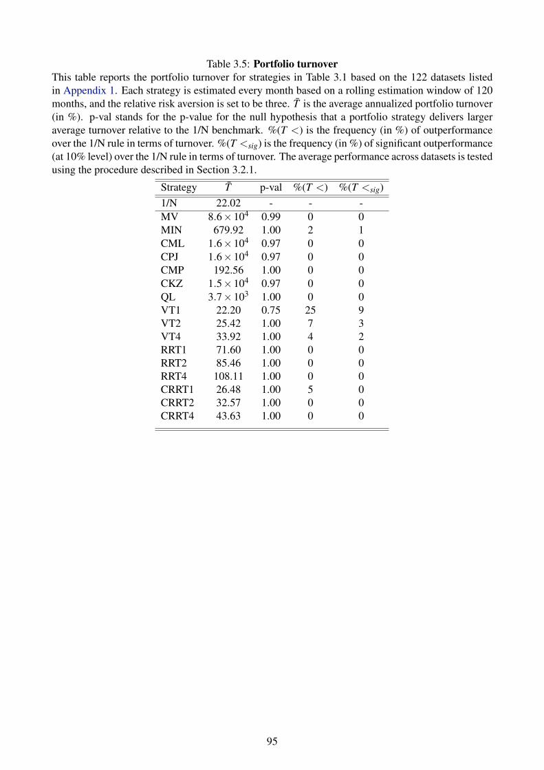
Table 3.5: Portfolio turnoverThis table reports the portfolio turnover for strategies in Table 3.1 based on the 122 datasets listedin Appendix 1. Each strategy is estimated every month based on a rolling estimation window of 120months, and the relative risk aversion is set to be three. T is the average annualized portfolio turnover(in %). p-val stands for the p-value for the null hypothesis that a portfolio strategy delivers largeraverage turnover relative to the 1/N benchmark. %(T <) is the frequency (in %) of outperformanceover the 1/N rule in terms of turnover. %(T <sig) is the frequency (in %) of significant outperformance(at 10% level) over the 1/N rule in terms of turnover. The average performance across datasets is testedusing the procedure described in Section 3.2.1.
Strategy T p-val %(T <) %(T <sig)1/N 22.02 - - -MV 8.6×10⁴ 0.99 0 0MIN 679.92 1.00 2 1CML 1.6×10⁴ 0.97 0 0CPJ 1.6×10⁴ 0.97 0 0CMP 192.56 1.00 0 0CKZ 1.5×10⁴ 0.97 0 0QL 3.7×10³ 1.00 0 0VT1 22.20 0.75 25 9VT2 25.42 1.00 7 3VT4 33.92 1.00 4 2RRT1 71.60 1.00 0 0RRT2 85.46 1.00 0 0RRT4 108.11 1.00 0 0CRRT1 26.48 1.00 5 0CRRT2 32.57 1.00 0 0CRRT4 43.63 1.00 0 0
95
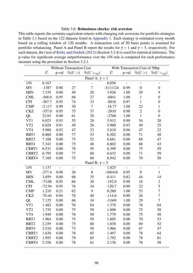
Table 3.6: Robustness checks: risk aversionThis table reports the certainty-equivalent returns with changing risk aversions for portfolio strategiesin Table 3.1 based on the 122 datasets listed in Appendix 1. Each strategy is estimated every monthbased on a rolling window of 120 months. A transaction cost of 50 basis points is assumed forportfolio rebalancing. Panel A and Panel B report the results for γ = 1 and γ = 5, respectively. Foreach dataset, the t test of Kirby and Ostdiek (2012) (Section 3.2.4) is used for statistical inference. Thep-value for significant average outperformance over the 1/N rule is computed for each performancemeasure using the procedure in Section 3.2.1.
Without Transaction Cost With Transaction Cost of 50bpU p-val %(U >) %(U >sig) U p-val %(U >) %(U >sig)
Panel A: γ = 11/N 6.167 - - - 6.056 - - -MV -1387 0.98 27 7 -3111124 0.99 0 0MIN 7.335 0.00 49 20 3.926 1.00 29 9CML -368.0 0.95 68 27 -6841 1.00 1 0CPJ -367.7 0.95 74 33 -8816 0.97 1 0CMP -2.117 0.99 30 7 -18.77 1.00 22 1CKZ -357.0 0.95 75 37 -2810 0.98 2 0QL 22.83 0.00 61 20 -2760 1.00 1 0VT1 6.023 0.93 55 28 5.912 0.90 54 28VT2 6.028 0.91 49 26 5.900 0.93 49 25VT4 5.988 0.92 47 23 5.818 0.96 47 22RRT1 6.860 0.00 77 53 6.502 0.00 71 48RRT2 7.108 0.00 75 52 6.681 0.00 69 47RRT4 7.343 0.00 75 48 6.802 0.00 68 43CRRT1 6.531 0.00 78 59 6.399 0.00 75 59CRRT2 6.795 0.00 77 60 6.632 0.00 71 59CRRT4 7.160 0.00 75 60 6.942 0.00 70 58
Panel B: γ = 51/N 1.137 - - - 1.025 - - -MV -277.4 0.98 26 8 -166416 0.95 9 1MIN 3.859 0.00 68 35 0.411 0.82 44 14CML -73.08 0.95 66 30 -192.0 0.98 18 2CPJ -72.94 0.95 76 34 -120.7 0.90 22 5CMP 1.210 0.21 62 9 0.260 1.00 53 7CKZ -70.44 0.94 78 40 -114.6 0.90 26 7QL 7.125 0.00 66 34 -3.049 1.00 29 7VT1 1.482 0.00 76 64 1.370 0.00 76 64VT2 1.735 0.00 75 59 1.608 0.00 75 58VT4 1.949 0.00 76 50 1.779 0.00 75 48RRT1 1.964 0.00 75 59 1.605 0.00 70 53RRT2 2.259 0.00 75 60 1.830 0.00 69 52RRT4 2.510 0.00 73 58 1.966 0.00 67 47CRRT1 1.630 0.00 78 65 1.497 0.00 78 64CRRT2 1.955 0.00 79 65 1.792 0.00 78 61CRRT4 2.358 0.00 78 61 2.138 0.00 78 58
96
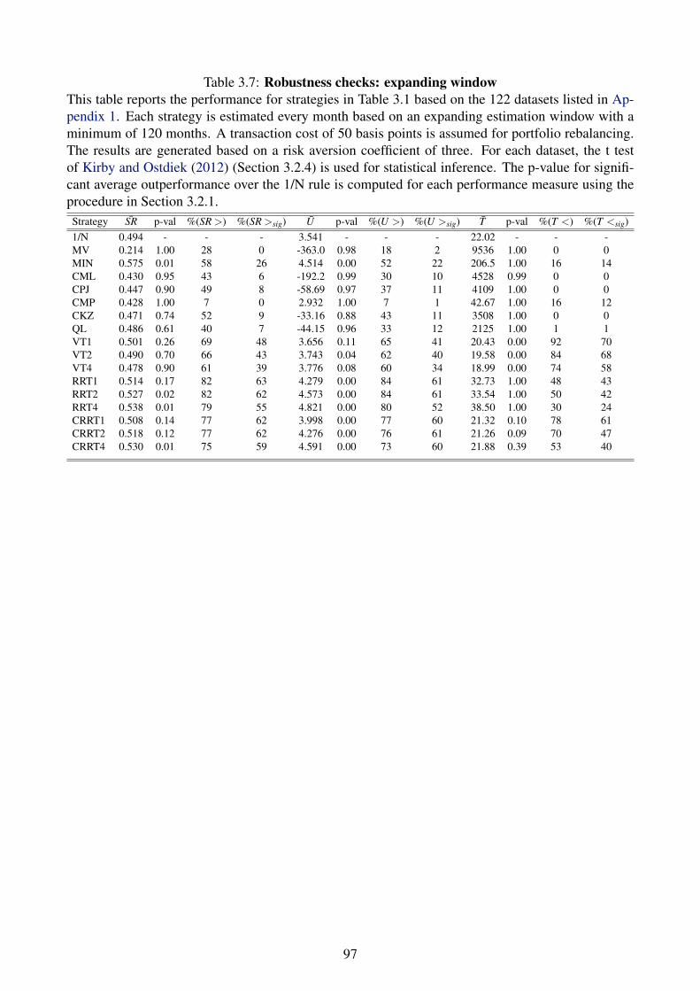
Table 3.7: Robustness checks: expanding windowThis table reports the performance for strategies in Table 3.1 based on the 122 datasets listed in Ap-pendix 1. Each strategy is estimated every month based on an expanding estimation window with aminimum of 120 months. A transaction cost of 50 basis points is assumed for portfolio rebalancing.The results are generated based on a risk aversion coefficient of three. For each dataset, the t testof Kirby and Ostdiek (2012) (Section 3.2.4) is used for statistical inference. The p-value for signifi-cant average outperformance over the 1/N rule is computed for each performance measure using theprocedure in Section 3.2.1.
Strategy SR p-val %(SR >) %(SR >sig) U p-val %(U >) %(U >sig) T p-val %(T <) %(T <sig)1/N 0.494 - - - 3.541 - - - 22.02 - - -MV 0.214 1.00 28 0 -363.0 0.98 18 2 9536 1.00 0 0MIN 0.575 0.01 58 26 4.514 0.00 52 22 206.5 1.00 16 14CML 0.430 0.95 43 6 -192.2 0.99 30 10 4528 0.99 0 0CPJ 0.447 0.90 49 8 -58.69 0.97 37 11 4109 1.00 0 0CMP 0.428 1.00 7 0 2.932 1.00 7 1 42.67 1.00 16 12CKZ 0.471 0.74 52 9 -33.16 0.88 43 11 3508 1.00 0 0QL 0.486 0.61 40 7 -44.15 0.96 33 12 2125 1.00 1 1VT1 0.501 0.26 69 48 3.656 0.11 65 41 20.43 0.00 92 70VT2 0.490 0.70 66 43 3.743 0.04 62 40 19.58 0.00 84 68VT4 0.478 0.90 61 39 3.776 0.08 60 34 18.99 0.00 74 58RRT1 0.514 0.17 82 63 4.279 0.00 84 61 32.73 1.00 48 43RRT2 0.527 0.02 82 62 4.573 0.00 84 61 33.54 1.00 50 42RRT4 0.538 0.01 79 55 4.821 0.00 80 52 38.50 1.00 30 24CRRT1 0.508 0.14 77 62 3.998 0.00 77 60 21.32 0.10 78 61CRRT2 0.518 0.12 77 62 4.276 0.00 76 61 21.26 0.09 70 47CRRT4 0.530 0.01 75 59 4.591 0.00 73 60 21.88 0.39 53 40
97
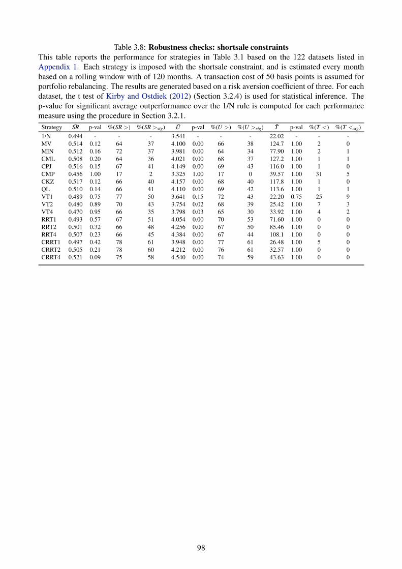
Table 3.8: Robustness checks: shortsale constraintsThis table reports the performance for strategies in Table 3.1 based on the 122 datasets listed inAppendix 1. Each strategy is imposed with the shortsale constraint, and is estimated every monthbased on a rolling window with of 120 months. A transaction cost of 50 basis points is assumed forportfolio rebalancing. The results are generated based on a risk aversion coefficient of three. For eachdataset, the t test of Kirby and Ostdiek (2012) (Section 3.2.4) is used for statistical inference. Thep-value for significant average outperformance over the 1/N rule is computed for each performancemeasure using the procedure in Section 3.2.1.Strategy SR p-val %(SR >) %(SR >sig) U p-val %(U >) %(U >sig) T p-val %(T <) %(T <sig)1/N 0.494 - - - 3.541 - - - 22.02 - - -MV 0.514 0.12 64 37 4.100 0.00 66 38 124.7 1.00 2 0MIN 0.512 0.16 72 37 3.981 0.00 64 34 77.90 1.00 2 1CML 0.508 0.20 64 36 4.021 0.00 68 37 127.2 1.00 1 1CPJ 0.516 0.15 67 41 4.149 0.00 69 43 116.0 1.00 1 0CMP 0.456 1.00 17 2 3.325 1.00 17 0 39.57 1.00 31 5CKZ 0.517 0.12 66 40 4.157 0.00 68 40 117.8 1.00 1 0QL 0.510 0.14 66 41 4.110 0.00 69 42 113.6 1.00 1 1VT1 0.489 0.75 77 50 3.641 0.15 72 43 22.20 0.75 25 9VT2 0.480 0.89 70 43 3.754 0.02 68 39 25.42 1.00 7 3VT4 0.470 0.95 66 35 3.798 0.03 65 30 33.92 1.00 4 2RRT1 0.493 0.57 67 51 4.054 0.00 70 53 71.60 1.00 0 0RRT2 0.501 0.32 66 48 4.256 0.00 67 50 85.46 1.00 0 0RRT4 0.507 0.23 66 45 4.384 0.00 67 44 108.1 1.00 0 0CRRT1 0.497 0.42 78 61 3.948 0.00 77 61 26.48 1.00 5 0CRRT2 0.505 0.21 78 60 4.212 0.00 76 61 32.57 1.00 0 0CRRT4 0.521 0.09 75 58 4.540 0.00 74 59 43.63 1.00 0 0
98
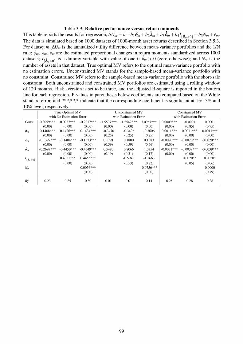
Table 3.9: Relative performance versus return momentsThis table reports the results for regression, ∆Um = a+b1φm+b2λm+b3δm+b4I{δm>0}+b5Nm+εm.The data is simulated based on 1000 datasets of 1000-month asset returns described in Section 3.5.3.For dataset m, ∆Um is the annualized utility difference between mean-variance portfolios and the 1/Nrule; φm, λm, δm are the estimated proportional changes in return moments standardized across 1000datasets; I{δm>0} is a dummy variable with value of one if δm > 0 (zero otherwise); and Nm is thenumber of assets in that dataset. True optimal MV refers to the optimal mean-variance portfolio withno estimation errors. Unconstrained MV stands for the sample-based mean-variance portfolio withno constraint. Constrained MV refers to the sample-based mean-variance portfolio with the short-saleconstraint. Both unconstrained and constrained MV portfolios are estimated using a rolling windowof 120 months. Risk aversion is set to be three, and the adjusted R-square is reported in the bottomline for each regression. P-values in parenthesis below coefficients are computed based on the Whitestandard error, and ***,**,* indicate that the corresponding coefficient is significant at 1%, 5% and10% level, respectively.
True Optimal MV Unconstrained MV Constrained MVwith No Estimation Error with Estimation Error with Estimation Error
Const 0.3059*** 0.0987*** -0.2237*** -1.5597*** -1.2542*** 3.0967*** 0.0009*** -0.0001 0.0001(0.00) (0.00) (0.00) (0.00) (0.00) (0.00) (0.00) (0.85) (0.95)
φm 0.1408*** 0.1426*** 0.1434*** -0.3470 -0.3496 -0.3606 0.0011*** 0.0011*** 0.0011***(0.00) (0.00) (0.00) (0.25) (0.25) (0.25) (0.00) (0.00) (0.00)
λm -0.1397*** -0.1404*** -0.1373*** 0.1791 0.1800 0.1383 -0.0020*** -0.0020*** -0.0020***(0.00) (0.00) (0.00) (0.59) (0.59) (0.66) (0.00) (0.00) (0.00)
δm -0.2697*** -0.4450*** -0.4649*** 0.5480 0.8066 1.0754 -0.0031*** -0.0039*** -0.0039***(0.00) (0.00) (0.00) (0.19) (0.31) (0.17) (0.00) (0.00) (0.00)
I{δm>0} 0.4031*** 0.4455*** -0.5943 -1.1663 0.0020** 0.0020*(0.00) (0.00) (0.53) (0.22) (0.05) (0.06)
Nm 0.0056*** -0.0756*** 0.0000(0.00) (0.00) (0.79)
R2a 0.23 0.25 0.30 0.01 0.01 0.14 0.28 0.28 0.28
99
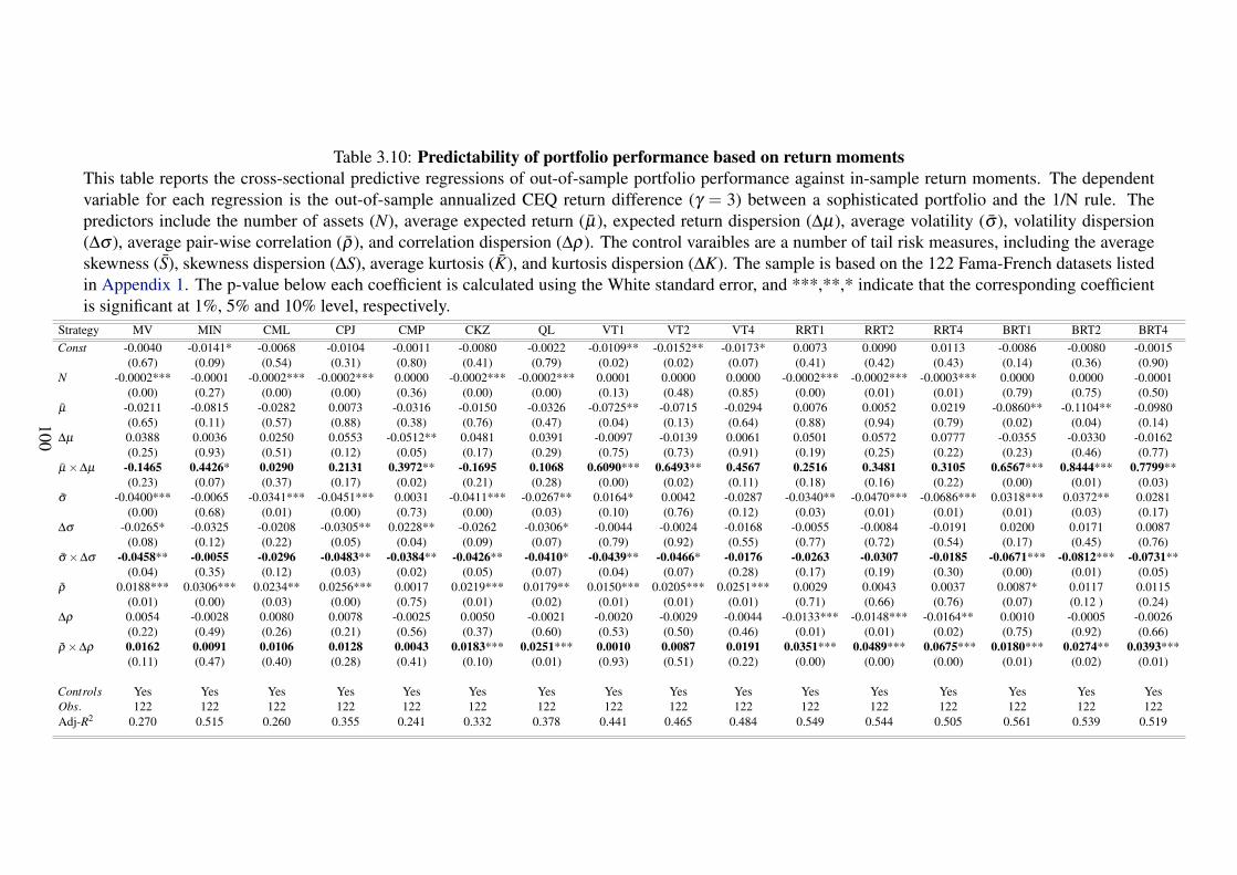
Table 3.10: Predictability of portfolio performance based on return momentsThis table reports the cross-sectional predictive regressions of out-of-sample portfolio performance against in-sample return moments. The dependentvariable for each regression is the out-of-sample annualized CEQ return difference (γ = 3) between a sophisticated portfolio and the 1/N rule. Thepredictors include the number of assets (N), average expected return (µ), expected return dispersion (∆µ), average volatility (σ ), volatility dispersion(∆σ ), average pair-wise correlation (ρ), and correlation dispersion (∆ρ). The control varaibles are a number of tail risk measures, including the averageskewness (S), skewness dispersion (∆S), average kurtosis (K), and kurtosis dispersion (∆K). The sample is based on the 122 Fama-French datasets listedin Appendix 1. The p-value below each coefficient is calculated using the White standard error, and ***,**,* indicate that the corresponding coefficientis significant at 1%, 5% and 10% level, respectively.
Strategy MV MIN CML CPJ CMP CKZ QL VT1 VT2 VT4 RRT1 RRT2 RRT4 BRT1 BRT2 BRT4Const -0.0040 -0.0141* -0.0068 -0.0104 -0.0011 -0.0080 -0.0022 -0.0109** -0.0152** -0.0173* 0.0073 0.0090 0.0113 -0.0086 -0.0080 -0.0015
(0.67) (0.09) (0.54) (0.31) (0.80) (0.41) (0.79) (0.02) (0.02) (0.07) (0.41) (0.42) (0.43) (0.14) (0.36) (0.90)N -0.0002*** -0.0001 -0.0002*** -0.0002*** 0.0000 -0.0002*** -0.0002*** 0.0001 0.0000 0.0000 -0.0002*** -0.0002*** -0.0003*** 0.0000 0.0000 -0.0001
(0.00) (0.27) (0.00) (0.00) (0.36) (0.00) (0.00) (0.13) (0.48) (0.85) (0.00) (0.01) (0.01) (0.79) (0.75) (0.50)µ -0.0211 -0.0815 -0.0282 0.0073 -0.0316 -0.0150 -0.0326 -0.0725** -0.0715 -0.0294 0.0076 0.0052 0.0219 -0.0860** -0.1104** -0.0980
(0.65) (0.11) (0.57) (0.88) (0.38) (0.76) (0.47) (0.04) (0.13) (0.64) (0.88) (0.94) (0.79) (0.02) (0.04) (0.14)∆µ 0.0388 0.0036 0.0250 0.0553 -0.0512** 0.0481 0.0391 -0.0097 -0.0139 0.0061 0.0501 0.0572 0.0777 -0.0355 -0.0330 -0.0162
(0.25) (0.93) (0.51) (0.12) (0.05) (0.17) (0.29) (0.75) (0.73) (0.91) (0.19) (0.25) (0.22) (0.23) (0.46) (0.77)µ×∆µ -0.1465 0.4426* 0.0290 0.2131 0.3972** -0.1695 0.1068 0.6090*** 0.6493** 0.4567 0.2516 0.3481 0.3105 0.6567*** 0.8444*** 0.7799**
(0.23) (0.07) (0.37) (0.17) (0.02) (0.21) (0.28) (0.00) (0.02) (0.11) (0.18) (0.16) (0.22) (0.00) (0.01) (0.03)σ -0.0400*** -0.0065 -0.0341*** -0.0451*** 0.0031 -0.0411*** -0.0267** 0.0164* 0.0042 -0.0287 -0.0340** -0.0470*** -0.0686*** 0.0318*** 0.0372** 0.0281
(0.00) (0.68) (0.01) (0.00) (0.73) (0.00) (0.03) (0.10) (0.76) (0.12) (0.03) (0.01) (0.01) (0.01) (0.03) (0.17)∆σ -0.0265* -0.0325 -0.0208 -0.0305** 0.0228** -0.0262 -0.0306* -0.0044 -0.0024 -0.0168 -0.0055 -0.0084 -0.0191 0.0200 0.0171 0.0087
(0.08) (0.12) (0.22) (0.05) (0.04) (0.09) (0.07) (0.79) (0.92) (0.55) (0.77) (0.72) (0.54) (0.17) (0.45) (0.76)σ ×∆σ -0.0458** -0.0055 -0.0296 -0.0483** -0.0384** -0.0426** -0.0410* -0.0439** -0.0466* -0.0176 -0.0263 -0.0307 -0.0185 -0.0671*** -0.0812*** -0.0731**
(0.04) (0.35) (0.12) (0.03) (0.02) (0.05) (0.07) (0.04) (0.07) (0.28) (0.17) (0.19) (0.30) (0.00) (0.01) (0.05)ρ 0.0188*** 0.0306*** 0.0234** 0.0256*** 0.0017 0.0219*** 0.0179** 0.0150*** 0.0205*** 0.0251*** 0.0029 0.0043 0.0037 0.0087* 0.0117 0.0115
(0.01) (0.00) (0.03) (0.00) (0.75) (0.01) (0.02) (0.01) (0.01) (0.01) (0.71) (0.66) (0.76) (0.07) (0.12 ) (0.24)∆ρ 0.0054 -0.0028 0.0080 0.0078 -0.0025 0.0050 -0.0021 -0.0020 -0.0029 -0.0044 -0.0133*** -0.0148*** -0.0164** 0.0010 -0.0005 -0.0026
(0.22) (0.49) (0.26) (0.21) (0.56) (0.37) (0.60) (0.53) (0.50) (0.46) (0.01) (0.01) (0.02) (0.75) (0.92) (0.66)ρ×∆ρ 0.0162 0.0091 0.0106 0.0128 0.0043 0.0183*** 0.0251*** 0.0010 0.0087 0.0191 0.0351*** 0.0489*** 0.0675*** 0.0180*** 0.0274** 0.0393***
(0.11) (0.47) (0.40) (0.28) (0.41) (0.10) (0.01) (0.93) (0.51) (0.22) (0.00) (0.00) (0.00) (0.01) (0.02) (0.01)
Controls Yes Yes Yes Yes Yes Yes Yes Yes Yes Yes Yes Yes Yes Yes Yes YesObs. 122 122 122 122 122 122 122 122 122 122 122 122 122 122 122 122Adj-R2 0.270 0.515 0.260 0.355 0.241 0.332 0.378 0.441 0.465 0.484 0.549 0.544 0.505 0.561 0.539 0.519
100
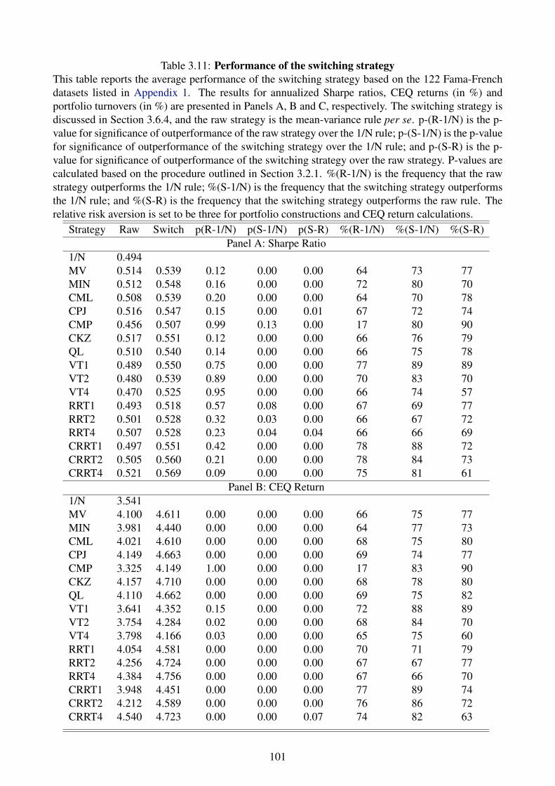
Table 3.11: Performance of the switching strategyThis table reports the average performance of the switching strategy based on the 122 Fama-Frenchdatasets listed in Appendix 1. The results for annualized Sharpe ratios, CEQ returns (in %) andportfolio turnovers (in %) are presented in Panels A, B and C, respectively. The switching strategy isdiscussed in Section 3.6.4, and the raw strategy is the mean-variance rule per se. p-(R-1/N) is the p-value for significance of outperformance of the raw strategy over the 1/N rule; p-(S-1/N) is the p-valuefor significance of outperformance of the switching strategy over the 1/N rule; and p-(S-R) is the p-value for significance of outperformance of the switching strategy over the raw strategy. P-values arecalculated based on the procedure outlined in Section 3.2.1. %(R-1/N) is the frequency that the rawstrategy outperforms the 1/N rule; %(S-1/N) is the frequency that the switching strategy outperformsthe 1/N rule; and %(S-R) is the frequency that the switching strategy outperforms the raw rule. Therelative risk aversion is set to be three for portfolio constructions and CEQ return calculations.
Strategy Raw Switch p(R-1/N) p(S-1/N) p(S-R) %(R-1/N) %(S-1/N) %(S-R)Panel A: Sharpe Ratio
1/N 0.494MV 0.514 0.539 0.12 0.00 0.00 64 73 77MIN 0.512 0.548 0.16 0.00 0.00 72 80 70CML 0.508 0.539 0.20 0.00 0.00 64 70 78CPJ 0.516 0.547 0.15 0.00 0.01 67 72 74CMP 0.456 0.507 0.99 0.13 0.00 17 80 90CKZ 0.517 0.551 0.12 0.00 0.00 66 76 79QL 0.510 0.540 0.14 0.00 0.00 66 75 78VT1 0.489 0.550 0.75 0.00 0.00 77 89 89VT2 0.480 0.539 0.89 0.00 0.00 70 83 70VT4 0.470 0.525 0.95 0.00 0.00 66 74 57RRT1 0.493 0.518 0.57 0.08 0.00 67 69 77RRT2 0.501 0.528 0.32 0.03 0.00 66 67 72RRT4 0.507 0.528 0.23 0.04 0.04 66 66 69CRRT1 0.497 0.551 0.42 0.00 0.00 78 88 72CRRT2 0.505 0.560 0.21 0.00 0.00 78 84 73CRRT4 0.521 0.569 0.09 0.00 0.00 75 81 61
Panel B: CEQ Return1/N 3.541MV 4.100 4.611 0.00 0.00 0.00 66 75 77MIN 3.981 4.440 0.00 0.00 0.00 64 77 73CML 4.021 4.610 0.00 0.00 0.00 68 75 80CPJ 4.149 4.663 0.00 0.00 0.00 69 74 77CMP 3.325 4.149 1.00 0.00 0.00 17 83 90CKZ 4.157 4.710 0.00 0.00 0.00 68 78 80QL 4.110 4.662 0.00 0.00 0.00 69 75 82VT1 3.641 4.352 0.15 0.00 0.00 72 88 89VT2 3.754 4.284 0.02 0.00 0.00 68 84 70VT4 3.798 4.166 0.03 0.00 0.00 65 75 60RRT1 4.054 4.581 0.00 0.00 0.00 70 71 79RRT2 4.256 4.724 0.00 0.00 0.00 67 67 77RRT4 4.384 4.756 0.00 0.00 0.00 67 66 70CRRT1 3.948 4.451 0.00 0.00 0.00 77 89 74CRRT2 4.212 4.589 0.00 0.00 0.00 76 86 72CRRT4 4.540 4.723 0.00 0.00 0.07 74 82 63
101
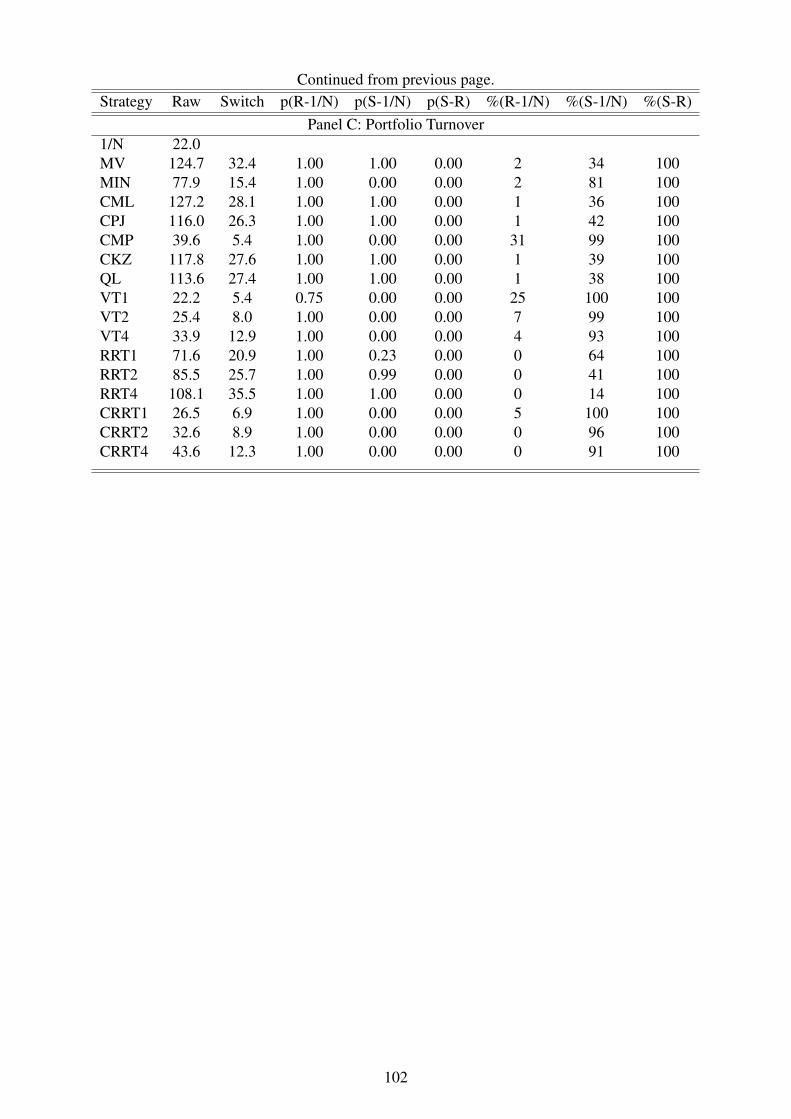
Continued from previous page.Strategy Raw Switch p(R-1/N) p(S-1/N) p(S-R) %(R-1/N) %(S-1/N) %(S-R)
Panel C: Portfolio Turnover1/N 22.0MV 124.7 32.4 1.00 1.00 0.00 2 34 100MIN 77.9 15.4 1.00 0.00 0.00 2 81 100CML 127.2 28.1 1.00 1.00 0.00 1 36 100CPJ 116.0 26.3 1.00 1.00 0.00 1 42 100CMP 39.6 5.4 1.00 0.00 0.00 31 99 100CKZ 117.8 27.6 1.00 1.00 0.00 1 39 100QL 113.6 27.4 1.00 1.00 0.00 1 38 100VT1 22.2 5.4 0.75 0.00 0.00 25 100 100VT2 25.4 8.0 1.00 0.00 0.00 7 99 100VT4 33.9 12.9 1.00 0.00 0.00 4 93 100RRT1 71.6 20.9 1.00 0.23 0.00 0 64 100RRT2 85.5 25.7 1.00 0.99 0.00 0 41 100RRT4 108.1 35.5 1.00 1.00 0.00 0 14 100CRRT1 26.5 6.9 1.00 0.00 0.00 5 100 100CRRT2 32.6 8.9 1.00 0.00 0.00 0 96 100CRRT4 43.6 12.3 1.00 0.00 0.00 0 91 100
102
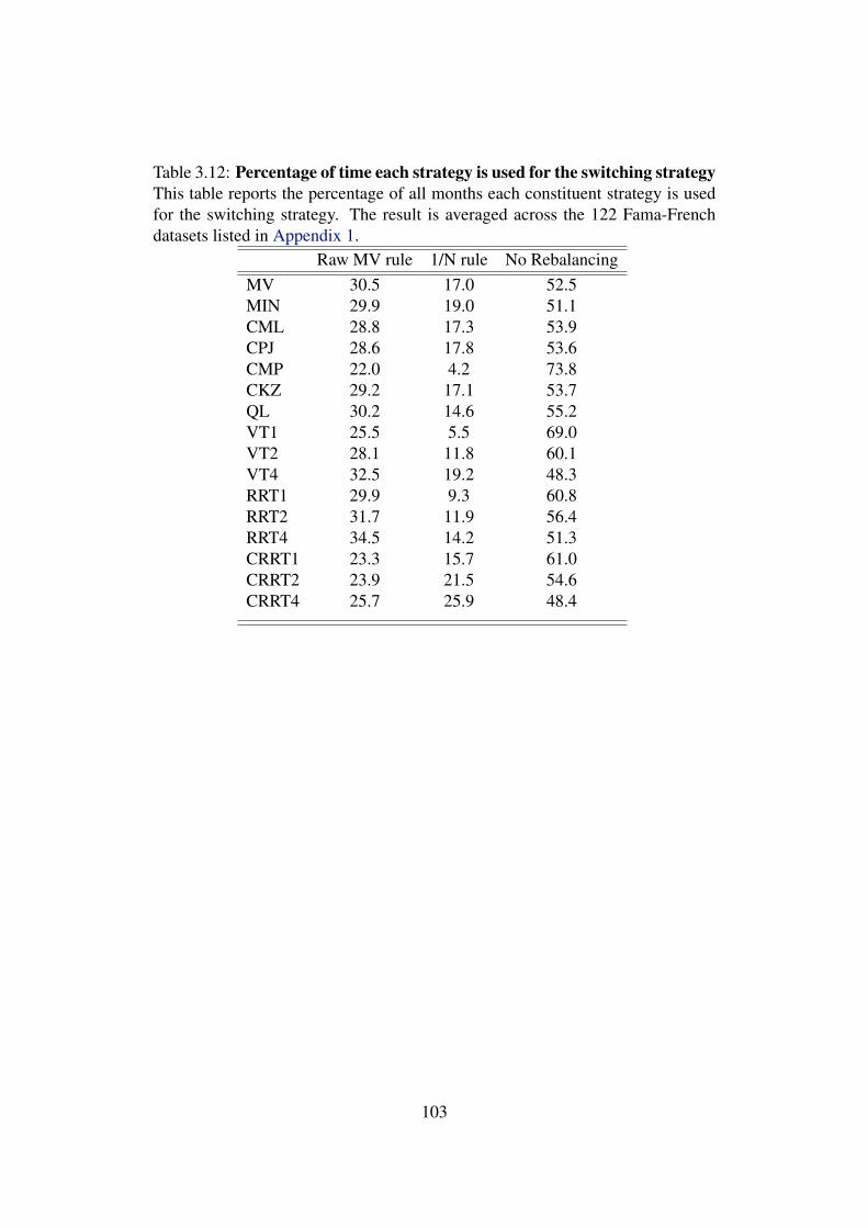
Table 3.12: Percentage of time each strategy is used for the switching strategyThis table reports the percentage of all months each constituent strategy is usedfor the switching strategy. The result is averaged across the 122 Fama-Frenchdatasets listed in Appendix 1.
Raw MV rule 1/N rule No RebalancingMV 30.5 17.0 52.5MIN 29.9 19.0 51.1CML 28.8 17.3 53.9CPJ 28.6 17.8 53.6CMP 22.0 4.2 73.8CKZ 29.2 17.1 53.7QL 30.2 14.6 55.2VT1 25.5 5.5 69.0VT2 28.1 11.8 60.1VT4 32.5 19.2 48.3RRT1 29.9 9.3 60.8RRT2 31.7 11.9 56.4RRT4 34.5 14.2 51.3CRRT1 23.3 15.7 61.0CRRT2 23.9 21.5 54.6CRRT4 25.7 25.9 48.4
103

Chapter 4
Essay 2: Naive diversification and
the January seasonality
4.1 Introduction
The January seasonality, the observation that the month of January appears to
have systematically higher returns than other months of the year, is one of the
most widely recognized stock anomalies. The anomaly has gained much attention
in the finance literature. For example, Gultekin and Gultekin (1983) show that the
January seasonality is more pronounced for equally-weighted portfolios than for
value-weighted portfolios. Further, Rozeff and Kinney (1976) find that from 1904
to 1974, an equal-weighted index of the New York Stock Exchange delivered an
average January return of 3.5%, while other months averaged about 0.5%. Over
one-third of the annual returns occurred in January alone. Moreover, Keim (1983)
104

finds that the anomaly is primarily concentrated in small stocks, and half of the
annualized excess returns occur in January.
Motivated by these empirical findings, this paper studies how the January sea-
sonality affects the performance of the naive 1/N diversification rule. DeMiguel
et al. (2009b) find that the naive rule performs as good as and sometimes even
better than sophisticated mean-variance portfolios. This paper attempts to under-
stand the link between the January seasonality and the performance of optimal
versus naive diversification.
I test the performance of 16 mean-variance rules against the 1/N rule under
different empirical settings. First, portfolio horse races are conducted based on a
large number of datasets of value-weighted index returns. The results reveal that
the relative performance between mean-variance and 1/N rules is not affected by
the January seasonality. Both mean-variance rules and the 1/N rule are able to
deliver larger January returns than non-January returns. When compared with the
1/N rule, a number of mean-variance strategies exhibits larger average returns in
and outside of Januaries. Although mean-variance strategies outperform the 1/N
rule more frequently in non-January months, excluding January returns does not
qualitatively affect the relative performance between mean-variance versus 1/N
rules.
However, constructing portfolios using individual stocks produces completely
different results. I construct monthly mean-variance and 1/N portfolios based on
26 datasets of individual stocks. These stocks involve market-wide stocks, stocks
105

from certain industry, as well as stocks with characteristics, such as size, value
and momentum. By comparing various mean-variance rules with the 1/N rule
based on these test datasets, I find that the 1/N rule generates considerably larger
January returns compared with mean-variance portfolios. When January months
are ruled out, the Sharpe ratio of the 1/N rule can decrease up to 30%. In this
case, mean-variance strategies are able to outperform the 1/N benchmark on a
risk-adjusted basis. This result is consistent with and without transaction costs,
across different industries and various characteristics.
The driving force behind these contrary results is linked to the size factor of
Fama and French (1993). The January seasonality is largely the small firm effect
according to Keim (1983). Results show that the 1/N rule exhibits comparable
size factor sensitivity relative to mean-variance rules when value-weighted in-
dexes are used for portfolio construction. Therefore, excluding January returns
does not alter the relative performance between mean-variance and the 1/N rule.
On the other hand, when individual stocks are used as constituent assets, the 1/N
portfolio has considerably larger exposure to the size factor compared with mean-
variance portfolios. Hence the performance of the naive rule relies heavily on the
January seasonality.
With individual stocks, the rebalancing feature of the naive 1/N diversification
rule produces large exposure to the size and value factors, and a negative exposure
to the momentum factor. Studies have documented strong and positive January
returns for small and value stocks (Jaffe et al., 1989; Jegadeesh and Titman, 2001;
106

Keim, 1983; Reinganum, 1983), and a reversed January pattern for momentum
stocks (Grundy and Martin, 2001; Jegadeesh and Titman, 1993). Hence, the 1/N
rule bets on all the correct directions of factors, and locks in large returns in
Januaries. However, I also find that this January effect of the 1/N rule has been
sharply diminishing in recent years, especially from 2007 to 2016. This diminish-
ing phenomenon is reflected by smaller January returns than non-January returns,
and by increased Sharpe ratios when January returns are excluded.
This paper is the first to link the performance of optimal versus naive diver-
sification with the classic January seasonality. The results in this paper show a
clear distinction in the January behaviors of the 1/N rule under different empiri-
cal settings. The findings add to the recent debate between optimal versus naive
diversification and provide implications for mean-variance portfolios.
The remainder of the paper is structured as follows. In Section 4.2, I discuss
the datasets used for the empirical test. Section 4.3 describes the portfolio strate-
gies and performance measures considered. Section 4.4 provides performance
evaluations, and Section 4.5 investigate whether transaction costs may affect the
results. Section 4.6 reports the factor exposure of the 1/N rule, and compares to
those for mean-variance portfolios. Section 4.7 analyzes the diminishing January
effect, and Section 4.8 concludes.
107

4.2 Data
Two sets of data are used in this study. The first set consists of the 122 datasets of
value-weighted stock portfolio returns (see Appendix 1 for details). DeMiguel,
Garlappi, and Uppal (2009b) use datasets of value-weighted stock portfolios to
challenge mean-variance strategies relative to the 1/N rule. Therefore, it is in
line with DeMiguel, Garlappi, and Uppal (2009b) by considering value-weighted
stock portfolios.
Constructing portfolios with individual stocks rather than value-weighted in-
dexes can produce quite different performance patterns. Hence, the second set of
data used in this study involves datasets of individual stocks. I consider monthly
return series of stocks from NYSE/AMEX/ NASDAQ on CRSP data files span-
ning from January 1926 to December 2016. Since mean-variance portfolios are
tested against the 1/N rule, only stocks with complete past 10-year returns are
selected, so that the means, variances, and covariances can be estimated with a
rolling estimation window of 120 months.1
I investigate portfolio contests not only with market-wide stocks, but also in
terms of constructing different industry and characteristic portfolios. I follow the
Kenneth French data library closely to select stocks for both industry and char-
acteristic portfolios. In terms of industry portfolios, I consider the Fama-French
17 industry definitions.2 Each stock that has past 10-year returns is assigned to
1The rolling window of 120 months for portfolio estimation is the standard practice in a num-ber of studies, for instance, Behr et al. (2013), DeMiguel et al. (2009b), DeMiguel et al. (2013),Kirby and Ostdiek (2012), and Tu and Zhou (2011).
2A narrower industry definition (for instance, 30, 38, 48, and 49 Fama-French industry defi-
108

an industry at the end of June of year t based on its four-digit SIC code at that
time. I use Compustat SIC codes for the fiscal year ending in calendar year t-1.
Whenever Compustat SIC codes are not available, I use CRSP SIC codes for June
of year t.
I consider popular stock characteristics, including high and low beta, small,
large, value, growth, momentum, and contrarian. Like the market and industry
portfolios, characteristic portfolios are constructed with stocks that possess past
10-year returns. The low (high) beta portfolio is formed with stocks that fall in
the bottom (top) decile of the market beta. The beta is estimated using the pre-
ceding five years of past monthly returns. The small (large) stock portfolio is
formed using stocks that are in the bottom (top) decile of market equity. The
value (growth) portfolio is constructed with stocks in the top (bottom) decile of
the book-to-market ratio. The momentum (contrarian) portfolio is constructed
using the stocks that are in the top (bottom) decile of the prior 212 (1360) months
returns. For beta, size, and book-to-market, stocks are assigned to each character-
istic decile once a year at the end of each June using the NYSE breakpoints. For
the momentum and contrarian portfolios, stocks are assigned every month based
on the NYSE breakpoints.
[Insert Table 4.1 here]
Table 4.1 provides the summary statistics for the number of stocks in each
nitions) generally provides more convincing results, but it is associated with a small number ofstocks (less than five) for some industries in almost all months.
109

portfolio category (dataset). Because each mean-variance strategy needs to be
estimated using 10 years of historical returns, the start of the out-of-sample period
is January 1937. Note that the value and growth portfolios are evaluated starting
from July 1962. This is because the earliest possible data in Compustat is from
July 1952.
4.3 Portfolio Strategies and Performance Measures
In the empirical analysis, I investigate the 1/N rule (the equally-weighted port-
folio), and study how the January seasonality affects horse races with mean-
variance strategies. To be consistent with Chapter 3, I consider 16 mean-variance
portfolio rules listed in Table 3.1. These mean-variance strategies include the
sample-based mean-variance rule, the global minimum-variance rule, four com-
bination strategies by Tu and Zhou (2011), one optimal risky portfolio rule by
Kan et al. (2016), as well as nine timing strategies by Kirby and Ostdiek (2012).
More detailed explanations for these strategies are shown in Section 3.3.2 of
Chapter 3.
DeMiguel et al. (2009b) compare a variety of mean-variance tangency portfo-
lios with the 1/N portfolio rule and reveal the superior performance of the naive
rule. To benchmark against their study, I investigate the tangency version of
mean-variance portfolios in this paper. It is shown in Chapter 3 that a number of
portfolio strategies produce very poor performance results with no portfolio con-
110

straints. According to Jagannathan and Ma (2003), the short-sale constraint has
a shrinkage effect, and generally improves the performance of a mean-variance
portfolio. Furthermore, with shortsale constraints, the long-only portfolio can be
easily implementable. Because of this, I impose the short-sale constraint for each
of the 16 mean-variance rules. Therefore, the portfolios investigated in this paper
are all full-investment long-only portfolios.
Table 4.1 shows that in many datasets, the number of assets exceeds the num-
ber of monthly observations (120 months). In these cases, the covariance matrix
could not be inverted in a normal way. To solve the issue of high dimensional
matrix inversion, I apply the covariance decomposition based on asset pricing
models. The covariance matrix at time t can be written as:
Σt = βtΣF,tβ′t +Σε,t (4.1)
where ΣF,t is the k-by-k covariance matrix for a k-factor model, Σε,t is an N-by-N
residual diagonal matrix, and βt (an N-by-k matrix) stores factor exposure for the
N stocks. I estimate the betas for each stock with a 120-month rolling regression
of the stock returns on the k-factor series. The inverse of Σt is then:
Σ−1t = Σ
−1ε,t −Σ
−1ε,t βt
(ΣF,t +β
′t Σ−1ε,t βt
)−1β′t Σ−1ε,t (4.2)
For the choice of factor models, I consider the single-factor CAPM, for sim-
plicity. However, inverting the covariance matrix with the assistance of other
111

factors models, such as the five-factor model of Fama and French (2015) or the
q-factor model by Hou et al. (2015), does not qualitatively affect the results.
In addition to the 16 mean-variance strategies, I also include the value-weighted
portfolio rule to compare with the naive benchmark. This is because a number of
studies finds that the January effect is pronounced for equally-weighted portfo-
lios rather than value-weighted portfolios (Gultekin and Gultekin, 1983; Rozeff
and Kinney, 1976; Keim, 1983). In addition, studies have shown that the 1/N
rule outperforms the value-weighted portfolio on a risk adjusted basis (see, for
instance, DeMiguel et al., 2009b; Plyakha et al., 2014). Therefore, it is worth in-
vestigating whether the outperformance of the 1/N rule over the value-weighted
rule is due to January returns.
Two performance measures, the average return and Sharpe ratio, are used to
compare performance. For return measures, I investigate the overall return, Jan-
uary return, and non-January return. For the Sharpe ratio, the overall Sharpe ratio,
and the Sharpe ratio without Januaries are examined. I employ the performance
test of Kirby and Ostdiek (2012) to test the relative performance difference in
datasets of individual stocks. A detailed explanation of the test is described in
Section 3.2.4 of Chapter 3. As for a large number of Fama-French datasets, I
use the aggregate method in Section 3.2.1 to conduct inference on average per-
formance across datasets.
112

4.4 Performance Evaluation
In this section, I conduct a formal performance evaluation for each of the portfo-
lios described in Section 4.3. The results for Fama-French datasets and individual
stock datasets are separately reported in the following two subsections.
4.4.1 Performance Evaluation - FF Datasets
Table 4.2 summarizes the average returns for the 1/N portfolio, the value-weighted
portfolio, and various mean-variance portfolios, based on the 122 Fama-French
datasets. The p-values indicate whether an alternative strategy delivers a signifi-
cantly larger return, on average, compared with the 1/N benchmark.
[Insert Table 4.2 here]
The 1/N rule has an annualized average return of 7.42%, an average January
return of 8.59% (annualized), and an average non-January return of 7.32% (an-
nualized). The January return is indeed larger than the non-January return for the
1/N rule, but the magnitude of difference is small. The value-weighted portfolio
delivers a close-to-zero January return on average, exhibiting no January effect.
Mean-variance portfolios, excluding those that do not depend on the mean vec-
tor (MIN, VT1, VT2 and VT4), exhibit larger returns relative to the 1/N rule,
for both January and non-January months. Similar to the 1/N rule, these mean-
variance rules all produce larger returns in Januaries compared with non-January
months. Interestingly, mean-variance strategies tend to have substantially smaller
113

outperformance frequencies with respect to the 1/N rule in Januaries compared
with non-January months. This suggests that the 1/N rule is able to exploit the
January seasonality, and is harder to beat in that month.
[Insert Table 4.3 here]
Table 4.3 reports the average annualized Sharpe ratios for the 1/N portfolio,
the value-weighted portfolio, and various mean-variance portfolios, based on the
122 Fama-French datasets. Only the value-weighted portfolio has a substantial
improvement in the Sharpe ratio by excluding January months. The 1/N rule de-
livers similar Sharpe ratios with and without Januaries. Mean-variance rules also
tend to produce very similar results before and after Januaries are excluded. Al-
though the outperformance frequency (over the 1/N benchmark) for each mean-
variance rule increases slightly when January returns are ruled out, the relative
risk-adjusted performance between mean-variance and 1/N rules is not signifi-
cantly affected by the January seasonality.
4.4.2 Performance Evaluation - Stock Datasets
Portfolio construction based on individual stocks rather than value-weighted in-
dexes could potentially produce very different results. Table 4.4 below reports the
average return difference for each strategy relative to the 1/N rule based on the
26 stock datasets described in 4.2. For the 1/N rule, the average monthly return
is shown; for other strategies, the average monthly return difference between the
114

strategy and the 1/N benchmark is reported. In Tables 4.4, 4.5 and 4.6, returns
are reported on a monthly basis in percentage, and ***,**,* indicate that the 1/N
rule outperforms a certain strategy at 1%, 5% and 10% level, respectively.
[Insert Table 4.4 here]
Table 4.4 shows that the 1/N portfolio delivers larger average monthly returns
compared with the value-weighted portfolio in all 26 datasets, with 17 cases being
significant. A number of mean-variance strategies also exhibit smaller average
return compared with the 1/N benchmark. In particular, the traditional sample-
based mean-variance portfolio produces worse return than the 1/N rule in 25 of 26
cases (except for the growth stocks dataset). The three conditional reward-to-risk
strategies tend to have comparable average return as the 1/N rule in most cases.
[Insert Table 4.5 here]
Table 4.5 reports the average difference in January returns for strategies com-
pared with the 1/N rule. The 1/N portfolio delivers significantly larger January
returns compared with other portfolios in almost every situation. In the dataset
involving large stocks, the January seasonality is less of an issue, since the Jan-
uary effect is primarily a small firm effect. In this case, a number of strategies
(MIN, QL, VT1, VT2, VT4, CRRT1, CRRT2 and CRRT4) actually outperform
the 1/N rule in terms of January returns.
[Insert Table 4.6 here]
115

Table 4.6 shows the average difference in non-January returns for strategies
compared with the 1/N rule. In contrast to January returns, non-January returns
favor the mean-variance portfolios rather than the 1/N portfolio. In particular,
the CRRT1 strategy only delivers smaller non-January returns compared with the
1/N benchmark in two industry stocks datasets among the 26 datasets.
Table 4.7 and Table 4.8 report the Sharpe ratio differences between sophisti-
cated portfolios and the 1/N rule. Table 4.7 shows the results for the entire sam-
ple, while Table 4.7 reports the results without January months. In these tables,
Sharpe ratios are annualized, and ***,**,* indicate that a strategy outperforms
the 1/N benchmark at 1%, 5% and 10% level, respectively. For the 1/N rule, the
Sharpe ratio is reported; for other strategies, the Sharpe ratio difference between
the strategy and the 1/N benchmark is presented.
[Insert Table 4.7 here]
Table 4.7 suggests that the value-weighted portfolio generally underperforms
the 1/N rule in terms of Sharpe ratio. The traditional sample-based mean-variance
rule fails to outperform the naive benchmark. It only produces larger Sharpe
ratios in 10 out of the 26 datasets, but none of them is significantly larger than
that of the 1/N rule. The volatility timing strategies and the conditional reward-
to-risk timing strategies appear to have much more significant outperformance
over the naive rule compared with other mean-variance rules. Being the worst
mean-variance rules, RRT4 and CML only exhibit larger Sharpe ratios relative to
116

the 1/N rule in eight and nine datasets, respectively, out of the 26 datasets.
[Insert Table 4.8 here]
To examine how the January seasonality affects the results, I exclude January
returns for each portfolio and re-calculate the Sharpe ratios. Table 4.8 summa-
rizes the results. All the mean-variance rules improve their relative performance
with respect to the 1/N benchmark. Even the value-weighted portfolio delivers
larger Sharpe ratios than the 1/N rule in 18 out of the 26 datasets. When Jan-
uaries are excluded, the two worst mean-variance strategies in Table 4.7, RRT4
and CML, increase their outperformance frequencies (relative to the 1/N rule)
from 8/26 to 19/26 and from 9/26 to 23/26, respectively. With no significant
outperformance over the 1/N rule in Table 4.7, the sample-based MV rule now
generates larger non-January Sharpe ratios relative to the naive rule in 23 out of
the 26 datasets (with 12 of them being significant at 10% level). It is clear that
excluding January returns reverses the outcome of portfolio horse races between
mean-variance versus 1/N portfolios.
To summarize, when value-weighted indexes are used for portfolio construc-
tion, mean-variance rules produce comparable or even larger January returns
compared with the naive 1/N rule. Although the 1/N rules in harder to beat in
Januaries versus non-January months, ruling out January returns does not quali-
tatively affect the result of portfolio horse races. However, when individual stocks
are used, the naive 1/N strategy exhibits considerably larger January returns com-
117

pared with the value-weighted portfolio and various mean-variance portfolios.
Excluding January returns in this case enables mean-variance strategies to out-
perform the 1/N benchmark on a risk-adjusted basis.
4.5 Transaction Cost
In this section, I investigate how transaction costs affect the results. For a given
portfolio, the turnover of each period is the sum of all the absolute changes in
portfolio weights from one period to the next. Then, the return to the portfolio
net of trading costs is:
rnett = rt−
N
∑i=1
ci,t |wi,t− wi,t | (4.3)
where ci,t reflects the proportional transaction cost for stock i at time t.
For the 122 datasets of value-weighted indexes in Appendix 1, I follow DeMiguel,
Garlappi, and Uppal (2009b), and set the proportional transaction cost to be con-
stant and equal to 50 basis points.
For individual datasets, transaction costs generally vary considerably across
stocks, being larger for small cap stocks than for large cap stocks. Also, transac-
tion costs have been gradually decreasing over time. To accommodate for these
empirical facts, I follow the transaction cost calculation approach by Brandt et al.
(2009), which allows for cross-sectional variation and captures the declining costs
over time.
118
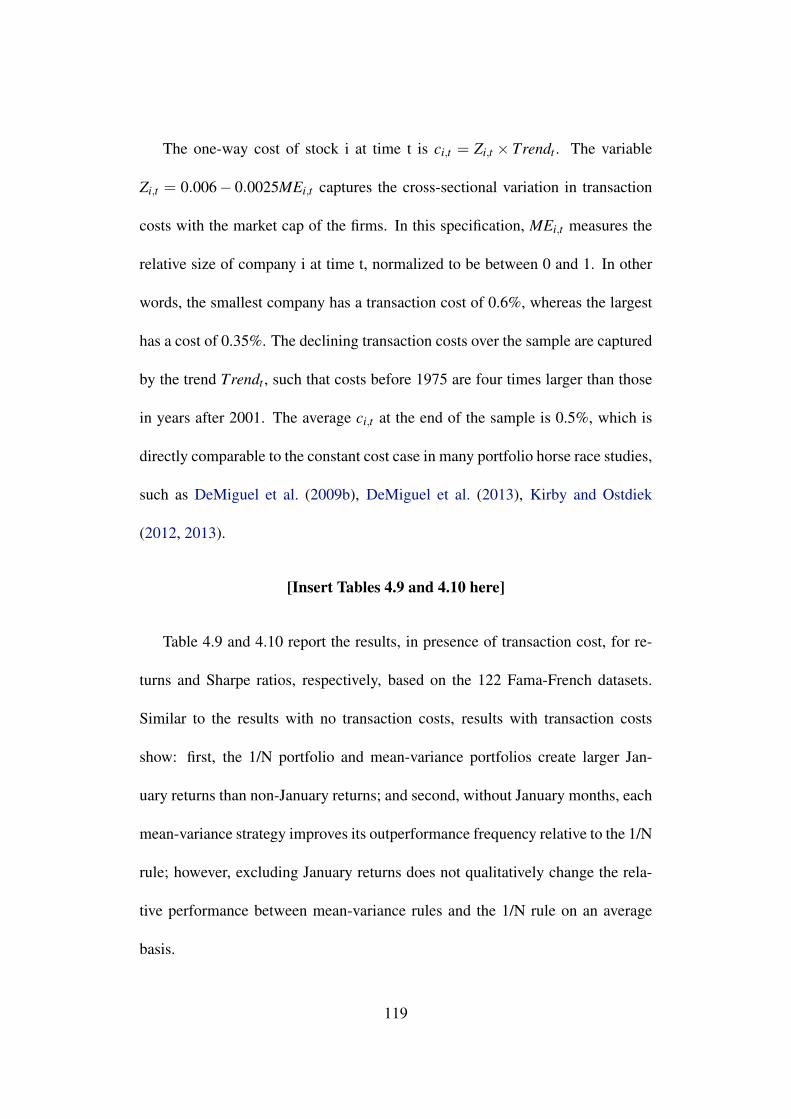
The one-way cost of stock i at time t is ci,t = Zi,t × Trendt . The variable
Zi,t = 0.006− 0.0025MEi,t captures the cross-sectional variation in transaction
costs with the market cap of the firms. In this specification, MEi,t measures the
relative size of company i at time t, normalized to be between 0 and 1. In other
words, the smallest company has a transaction cost of 0.6%, whereas the largest
has a cost of 0.35%. The declining transaction costs over the sample are captured
by the trend Trendt , such that costs before 1975 are four times larger than those
in years after 2001. The average ci,t at the end of the sample is 0.5%, which is
directly comparable to the constant cost case in many portfolio horse race studies,
such as DeMiguel et al. (2009b), DeMiguel et al. (2013), Kirby and Ostdiek
(2012, 2013).
[Insert Tables 4.9 and 4.10 here]
Table 4.9 and 4.10 report the results, in presence of transaction cost, for re-
turns and Sharpe ratios, respectively, based on the 122 Fama-French datasets.
Similar to the results with no transaction costs, results with transaction costs
show: first, the 1/N portfolio and mean-variance portfolios create larger Jan-
uary returns than non-January returns; and second, without January months, each
mean-variance strategy improves its outperformance frequency relative to the 1/N
rule; however, excluding January returns does not qualitatively change the rela-
tive performance between mean-variance rules and the 1/N rule on an average
basis.
119

[Insert Tables 4.11, 4.12, and 4.13 here]
Table 4.11, Table 4.12 and 4.13 show the results for average returns, January
returns and non-January returns for various strategies, based on the 26 individ-
ual stocks datasets, in presence of transaction costs. Returns are reported on a
monthly basis in percentage, and ***,**,* indicate that the 1/N rule outperforms
a certain strategy at 1%, 5% and 10% level, respectively.
With the effect of transaction costs, the results in the 26 datasets of indi-
vidual stocks are not qualitatively affected. Various mean-variance rules deliver
significantly smaller returns in Januaries compared with the 1/N rule. When Jan-
uary returns are ruled out, their underperformance disappear. In particular, three
conditional reward-to-risk timing strategies (CRRT1, CRRT2 and CRRT4) only
show smaller non-January returns than the 1/N rule in less than five out of the
26 datasets. Without January months, the sample-based mean-variance rule is
inferior to the 1/N rule in nine datasets, in contrast to inferior returns in all 26
datasets when all months are considered.
[Insert Tables 4.14 and 4.15 here]
The results for difference in Sharpe ratios (under transaction costs) with and
without Januaries are reported in Table 4.14 and 4.15, respectively, for the 26
individual datasets. Sharpe ratios are annualized, and ***,**,* indicate that a
certain strategy outperforms the 1/N rule at 1%, 5% and 10% level, respectively.
The result shows: when all months are considered, mean-variance portfolios
120

have small chances to outperform the 1/N rule in terms of Sharpe ratio; however,
they tend to create larger Sharpe ratios relative to the naive rule in most of the
datasets when January months are excluded. This is consistent with the results
for no transaction costs.
[Insert Table 4.16 here]
Table 4.16 provides a clearer picture of the relative performance by summa-
rizing the number of datasets in which each strategy outperforms the 1/N rule
in terms of overall return, January return, non-January return, Sharpe Ratio, as
well as Sharpe ratio without Januaries. It shows that mean-variance rules have
very scarce change to deliver larger January returns compared with the 1/N rule.
However, outside of January months, most mean-variance strategies outperform
the naive benchmark in terms of both return and Sharpe ratio. When January
returns are not considered, the relative performance between mean-variance and
1/N rule entirely reverses regardless of whether transaction cost exists.
In summary, the portfolio horse races under transaction cost confirms previ-
ous findings. The relative performance between mean-variance and 1/N portfo-
lios is not affected by the January seasonality when value-weighted indexes are
used for portfolio construction. However, when portfolios of individual stocks
are considered, the good performance of the naive 1/N rule is mainly attributed
to its massive January returns.
121

4.6 Factor exposure of the 1/N Rule
To study why the 1/N diversification rule exhibits completely different January
patterns using value-weighted indexes versus individual stocks, this section ex-
amines the exposure of the equally-weighted portfolio with respect to common
risk factors.
Table 4.17 summarizes the average returns for the four factors of Fama and
French (1993) and Carhart (1997), partitioning on Januaries and non-January
months. The data is obtained from the French data library. For US data, the mar-
ket, size, and value factors deliver significantly positive January returns, while
the momentum factor shows a contrary January effect. This evidence is consis-
tent with a number of studies, including Reinganum (1983), Keim (1983), and
Jegadeesh and Titman (1993, 2001). The negative January return for the momen-
tum factor is due to the short leg of losers that tend to be extremely small firms
in January (Grundy and Martin, 2001). Note that the market factor exhibits an
insignificant return difference between January and non-January months, and the
size factor generates an insignificant average non-January return.
[Insert Table 4.17 here]
Since the 122 datasets involve international data, I also investigate the Jan-
uary patterns for the four factors of other regional groups. The market factor does
not possess significant difference between January return and non-January return
across all seven regional groups. The size factor, on the other hand, delivers larger
122

January returns than non-January returns in all seven cases. The value factor has
relatively smaller January effect in Europe, Japan and Asia Pacific, compared to
US, and a reversed January pattern for the Global and North America. The mo-
mentum factor shows significantly positive but small difference between January
return and non-January return for only Europe and Asia Pacific. It seems that
across the globe, the size factor is the only factor that exhibits consistent Jan-
uary seasonality. This is consistent with the stylized fact that the January effect
is primarily a small firm effect.
I estimate the Fama-French-Carhart model for each strategy considered in this
chapter, and average each factor exposure across the two sets of datasets. The
Fama-French-Carhart model is a regression of returns against the four factors of
Fama and French (1993) and Carhart (1997), as shown below:
rt− r ft = α +β1MKT RFt +β2SMBt +β3HMLt +β4UMDt + εt , (4.4)
where MKT RFt , SMBt HMLt , and UMDt stand for the portfolio returns of the
market factor, size factor, value factor and momentum factor at time t, respec-
tively.
[Insert Table 4.18 here]
Table 4.18 reports the factor exposure for each strategy, averaged across the
122 Fama-French datasets and the 26 stock datasets, respectively. In the 122
123
datasets of value-weighted indexes, the 1/N rule tends to have comparable SMB
exposure relative to a number of mean-variance strategies, including MV, four
combination rules, and the optimal risky rule (QL). The three conditional reward-
to-risk timing strategies (CRRT1,CRRT2 and CRRT4) have larger average size
factor exposure compared to the 1/N rule. This explains why excluding January
returns does not alter the relative performance between mean-variance rules and
the 1/N rule in the 122 FF datasets. However, in the 26 stock datasets, the naive
1/N rule has the largest sensitivity to the size factor, on average, among all the
strategies. The size exposure of the 1/N rule is considerably larger than most of
the strategies. This is why its performance is largely driven by the January size
effect across the 26 stock datasets.
[Insert Table 4.19 here]
Table 4.19 provides a clear picture for the factor sensitivities of the 1/N rule
in each of the 26 individual datasets. For most of the cases, the 1/N portfolio has
positive exposure to the market, size, and value factors, and negative exposure to
the momentum factor. The 26 datasets are based on firms in the US where the
size and value factors deliver significantly positive difference between January
returns and non-January returns, while the momentum factor shows a contrary
January effect. Therefore, the naive 1/N rule always bets on the correct directions
of factor exposure to lock in enormous January returns.
The factor exposure can be linked to the rebalancing feature of the 1/N port-
124

folio. Compared with portfolios, the naive portfolio overweights small stocks; it
also overweights value stocks since high book-to-market stocks generally have
low market capitalizations. In addition, the 1/N rule always reverts back to the
equal weights from month to month and, hence, increases its size exposure from
one month to the next. The reversed momentum effect of the naive portfolio is
due to its constant equal-weight rebalancing scheme, which increases (decreases)
weights on stocks that perform badly (well) in the recent past.
4.7 Diminishing January Effect of the 1/N Rule
Despite strong empirical support for the existence of the January effect, recent re-
search has argued that the magnitude of the anomaly has declined. Riepe (1998)
notes that in more recent years, investors have had the knowledge and the instru-
ments to take advantage of the January effect. Mehdian and Perry (2002) and Gu
(2003) find that the January effect disappeared in terms of statistical significance
for the major US market indices in the 1990s, indicating that investors may have
begun taking advantage of the anomaly.
To investigate whether the January effect of the 1/N rule is diminishing in
the stock datasets, I separate the sample of the 26 stock datasets into eight 10-
year sub-periods. I evaluate two measures, the average return difference between
January and non-January months, and the percentage Sharpe ratio decrease with-
out Januaries. The average return difference between January and non-January
125
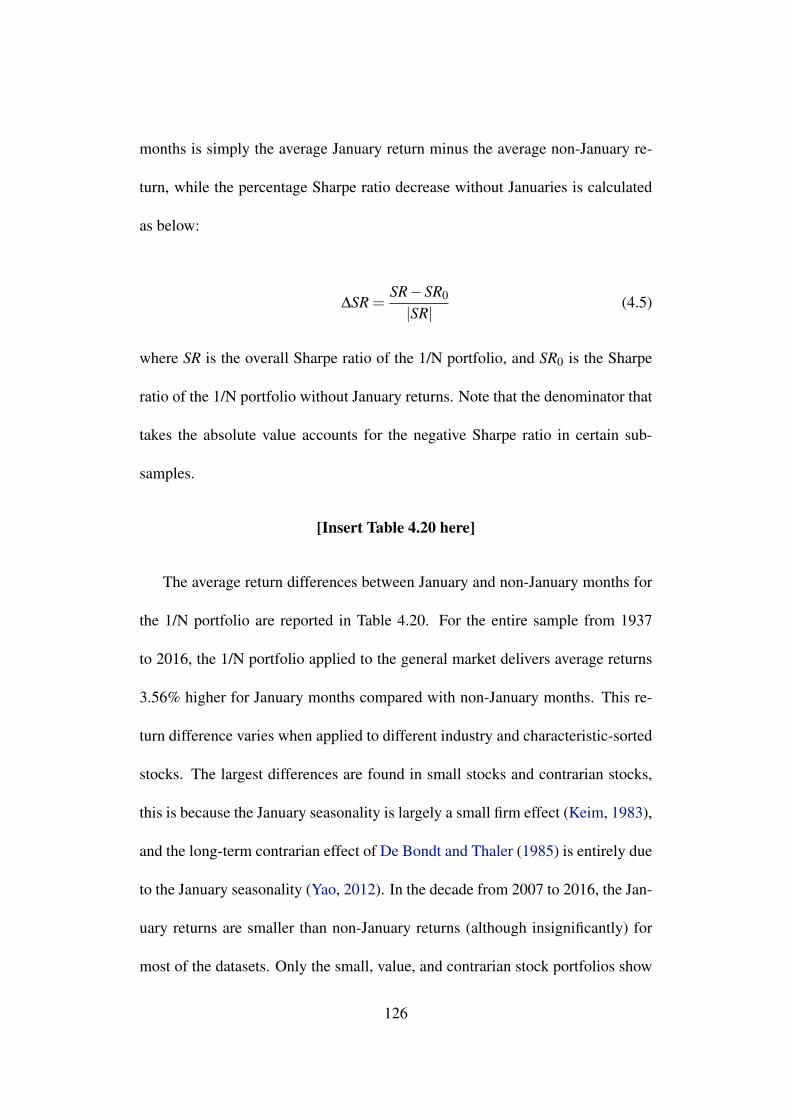
months is simply the average January return minus the average non-January re-
turn, while the percentage Sharpe ratio decrease without Januaries is calculated
as below:
∆SR =SR−SR0
|SR|(4.5)
where SR is the overall Sharpe ratio of the 1/N portfolio, and SR0 is the Sharpe
ratio of the 1/N portfolio without January returns. Note that the denominator that
takes the absolute value accounts for the negative Sharpe ratio in certain sub-
samples.
[Insert Table 4.20 here]
The average return differences between January and non-January months for
the 1/N portfolio are reported in Table 4.20. For the entire sample from 1937
to 2016, the 1/N portfolio applied to the general market delivers average returns
3.56% higher for January months compared with non-January months. This re-
turn difference varies when applied to different industry and characteristic-sorted
stocks. The largest differences are found in small stocks and contrarian stocks,
this is because the January seasonality is largely a small firm effect (Keim, 1983),
and the long-term contrarian effect of De Bondt and Thaler (1985) is entirely due
to the January seasonality (Yao, 2012). In the decade from 2007 to 2016, the Jan-
uary returns are smaller than non-January returns (although insignificantly) for
most of the datasets. Only the small, value, and contrarian stock portfolios show
126
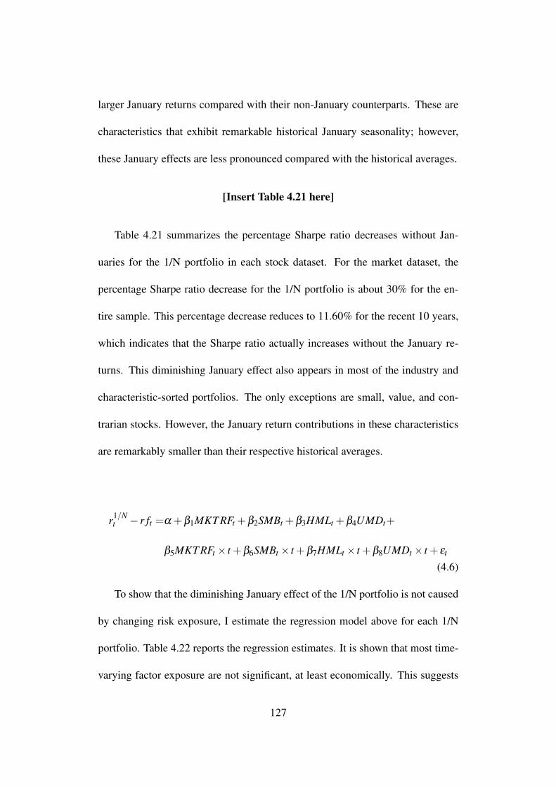
larger January returns compared with their non-January counterparts. These are
characteristics that exhibit remarkable historical January seasonality; however,
these January effects are less pronounced compared with the historical averages.
[Insert Table 4.21 here]
Table 4.21 summarizes the percentage Sharpe ratio decreases without Jan-
uaries for the 1/N portfolio in each stock dataset. For the market dataset, the
percentage Sharpe ratio decrease for the 1/N portfolio is about 30% for the en-
tire sample. This percentage decrease reduces to 11.60% for the recent 10 years,
which indicates that the Sharpe ratio actually increases without the January re-
turns. This diminishing January effect also appears in most of the industry and
characteristic-sorted portfolios. The only exceptions are small, value, and con-
trarian stocks. However, the January return contributions in these characteristics
are remarkably smaller than their respective historical averages.
r1/Nt − r ft =α +β1MKT RFt +β2SMBt +β3HMLt +β4UMDt+
β5MKT RFt× t +β6SMBt× t +β7HMLt× t +β8UMDt× t + εt
(4.6)
To show that the diminishing January effect of the 1/N portfolio is not caused
by changing risk exposure, I estimate the regression model above for each 1/N
portfolio. Table 4.22 reports the regression estimates. It is shown that most time-
varying factor exposure are not significant, at least economically. This suggests
127
that the diminishing January effect of the 1/N portfolio is not caused by increased
or decreased exposure with respect to the size, value, or momentum factors.
[Insert Table 4.22 here]
This section has illustrated that the January seasonality of the 1/N portfolio
has been disappearing in recent years. The diminishing January effect is asso-
ciated with a pattern of non-January returns outperforming January returns (al-
though insignificantly) in recent years. Since a substantial proportion of perfor-
mance of the 1/N portfolio is attributed to the January effect, this phenomenon
has meaningful implications for mean-variance and naive diversifications.
4.8 Conclusion
In this paper, I study how January seasonality affect the empirical success of the
1/N portfolio rule. I find: when constructing portfolios using value-weighted
stock indexes, the relative performance between mean-variance rules and the 1/N
rule is not affected by the January seasonality of stock returns.
However, when individual stocks are used for portfolio construction, result re-
verses. I find that a sizable proportion of Sharpe ratio of the 1/N rule is attributed
to large January returns. Generally, the naive rule delivers an average January re-
turn of 4.5%, which contributes to about 30% of its Sharpe ratio. Mean-variance
portfolios fail to outperform the naive benchmark in terms of the return or Sharpe
ratio. However, when January returns are excluded, mean-variance rules gen-
128

erally outperform the naive benchmark on a risk-adjusted basis. This result is
robust with and without transaction costs, for various mean-variance strategies,
and across different industries and characteristics.
The reason behind these contrary findings based on individual stocks versus
value-weighted indexes is related to the size factor exposure of the 1/N rule. Us-
ing value-weighted indexes, the 1/N rule exhibits similar or smaller size factor
exposure compared with mean-variance rules. However, it possess considerably
larger sensitivity to the size factor when individual stocks are used to form port-
folios. Since the January seasonality is primarily a small firm effect, excluding
January returns alters completely the relative performance between the mean-
variance and 1/N rules.
The January effect of the 1/N rule is related to its equal-weight rebalancing
feature, which leads to positive exposure to the size and value factors, and a
negative exposure to the momentum factor. The size and value factors deliver
large January returns, while the momentum factor has a reverse January pattern.
Because of this, the 1/N rule bets on all the correct directions of factors, and locks
in large returns in Januaries. However, I also find that the January effect of the
1/N rule has been disappearing at monthly frequencies in recent years. This is
reflected by smaller January returns than non-January returns, and by increased
Sharpe ratios when January returns are excluded.
In summary, this paper suggests that the great success of naive diversification
in constructing portfolios with individual stocks is largely due to the January
129

seasonality. The study contributes to the literature on horse races between optimal
and naive diversification, and provides implications for mean-variance portfolios.
130
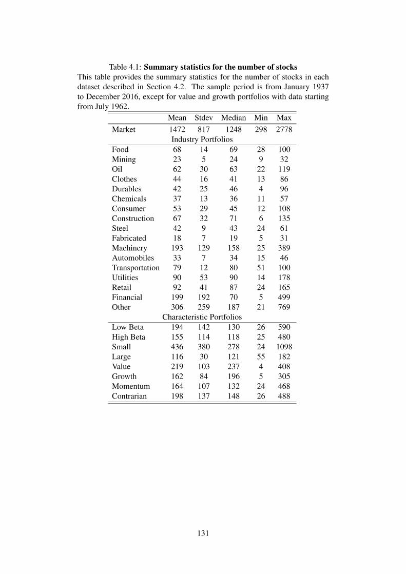
Table 4.1: Summary statistics for the number of stocksThis table provides the summary statistics for the number of stocks in eachdataset described in Section 4.2. The sample period is from January 1937to December 2016, except for value and growth portfolios with data startingfrom July 1962.
Mean Stdev Median Min MaxMarket 1472 817 1248 298 2778
Industry PortfoliosFood 68 14 69 28 100Mining 23 5 24 9 32Oil 62 30 63 22 119Clothes 44 16 41 13 86Durables 42 25 46 4 96Chemicals 37 13 36 11 57Consumer 53 29 45 12 108Construction 67 32 71 6 135Steel 42 9 43 24 61Fabricated 18 7 19 5 31Machinery 193 129 158 25 389Automobiles 33 7 34 15 46Transportation 79 12 80 51 100Utilities 90 53 90 14 178Retail 92 41 87 24 165Financial 199 192 70 5 499Other 306 259 187 21 769
Characteristic PortfoliosLow Beta 194 142 130 26 590High Beta 155 114 118 25 480Small 436 380 278 24 1098Large 116 30 121 55 182Value 219 103 237 4 408Growth 162 84 196 5 305Momentum 164 107 132 24 468Contrarian 198 137 148 26 488
131
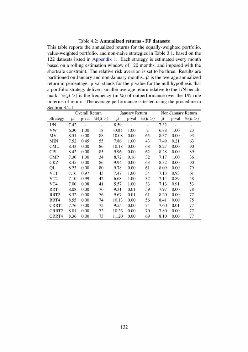
Table 4.2: Annualized returns - FF datasetsThis table reports the annualized returns for the equally-weighted portfolio,value-weighted portfolio, and non-naive strategies in Table 3.1, based on the122 datasets listed in Appendix 1. Each strategy is estimated every monthbased on a rolling estimation window of 120 months, and imposed with theshortsale constraint. The relative risk aversion is set to be three. Results arepartitioned on January and non-January months. µ is the average annualizedreturn in percentage. p-val stands for the p-value for the null hypothesis thata portfolio strategy delivers smaller average return relative to the 1/N bench-mark. %(µ >) is the frequency (in %) of outperformance over the 1/N rulein terms of return. The average performance is tested using the procedure inSection 3.2.1.
Overall Return January Return Non-January ReturnStrategy µ p-val %(µ >) µ p-val %(µ >) µ p-val %(µ >)1/N 7.42 - - 8.59 - - 7.32 - -VW 6.30 1.00 18 -0.01 1.00 2 6.88 1.00 23MV 8.51 0.00 88 10.08 0.00 65 8.37 0.00 93MIN 7.52 0.45 55 7.86 1.00 43 7.49 0.21 63CML 8.43 0.00 86 10.18 0.00 68 8.27 0.00 90CPJ 8.42 0.00 85 9.96 0.00 62 8.28 0.00 89CMP 7.30 1.00 34 8.72 0.16 32 7.17 1.00 36CKZ 8.45 0.00 86 9.94 0.00 63 8.32 0.00 90QL 8.23 0.00 80 9.78 0.00 61 8.09 0.00 79VT1 7.16 0.97 43 7.47 1.00 34 7.13 0.93 61VT2 7.10 0.99 42 6.68 1.00 32 7.14 0.89 58VT4 7.00 0.98 41 5.57 1.00 33 7.13 0.91 53RRT1 8.08 0.00 76 9.31 0.01 59 7.97 0.00 78RRT2 8.32 0.00 76 9.67 0.01 61 8.20 0.00 77RRT4 8.55 0.00 74 10.13 0.00 56 8.41 0.00 75CRRT1 7.76 0.00 75 9.55 0.00 74 7.60 0.01 77CRRT2 8.01 0.00 72 10.26 0.00 70 7.80 0.00 77CRRT4 8.36 0.00 73 11.20 0.00 69 8.10 0.00 77
132
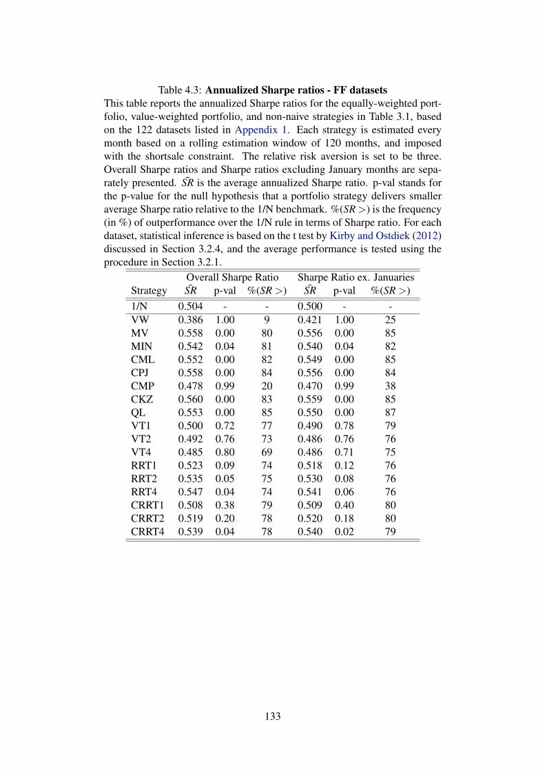
Table 4.3: Annualized Sharpe ratios - FF datasetsThis table reports the annualized Sharpe ratios for the equally-weighted port-folio, value-weighted portfolio, and non-naive strategies in Table 3.1, basedon the 122 datasets listed in Appendix 1. Each strategy is estimated everymonth based on a rolling estimation window of 120 months, and imposedwith the shortsale constraint. The relative risk aversion is set to be three.Overall Sharpe ratios and Sharpe ratios excluding January months are sepa-rately presented. SR is the average annualized Sharpe ratio. p-val stands forthe p-value for the null hypothesis that a portfolio strategy delivers smalleraverage Sharpe ratio relative to the 1/N benchmark. %(SR >) is the frequency(in %) of outperformance over the 1/N rule in terms of Sharpe ratio. For eachdataset, statistical inference is based on the t test by Kirby and Ostdiek (2012)discussed in Section 3.2.4, and the average performance is tested using theprocedure in Section 3.2.1.
Overall Sharpe Ratio Sharpe Ratio ex. JanuariesStrategy SR p-val %(SR >) SR p-val %(SR >)1/N 0.504 - - 0.500 - -VW 0.386 1.00 9 0.421 1.00 25MV 0.558 0.00 80 0.556 0.00 85MIN 0.542 0.04 81 0.540 0.04 82CML 0.552 0.00 82 0.549 0.00 85CPJ 0.558 0.00 84 0.556 0.00 84CMP 0.478 0.99 20 0.470 0.99 38CKZ 0.560 0.00 83 0.559 0.00 85QL 0.553 0.00 85 0.550 0.00 87VT1 0.500 0.72 77 0.490 0.78 79VT2 0.492 0.76 73 0.486 0.76 76VT4 0.485 0.80 69 0.486 0.71 75RRT1 0.523 0.09 74 0.518 0.12 76RRT2 0.535 0.05 75 0.530 0.08 76RRT4 0.547 0.04 74 0.541 0.06 76CRRT1 0.508 0.38 79 0.509 0.40 80CRRT2 0.519 0.20 78 0.520 0.18 80CRRT4 0.539 0.04 78 0.540 0.02 79
133
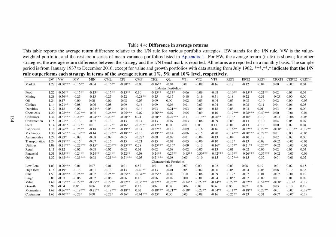
Table 4.4: Difference in average returnsThis table reports the average return difference relative to the 1/N rule for various portfolio strategies. EW stands for the 1/N rule, VW is the value-weighted portfolio, and the rest are a series of mean-variance portfolios listed in Appendix 1. For EW, the average return (in %) is shown; for otherstrategies, the average return difference between the strategy and the 1/N benchmark is reported. All returns are reported on a monthly basis. The sampleperiod is from January 1937 to December 2016, except for value and growth portfolios with data starting from July 1962. ***,**,* indicate that the 1/Nrule outperforms each strategy in terms of the average return at 1%, 5% and 10% level, respectively.
EW VW MV MIN CML CPJ CMP CKZ QL VT1 VT2 VT4 RRT1 RRT2 RRT4 CRRT1 CRRT2 CRRT4Market 1.22 -0.30*** -0.16** -0.04 -0.16** -0.20** -0.03 -0.16** -0.04 0.01 -0.08 -0.16 -0.12 -0.12 -0.04 0.00 -0.03 0.04
Industry PortfoliosFood 1.22 -0.20** -0.15** -0.13* -0.15** -0.15** 0.10 -0.15** -0.13* -0.06 -0.09 -0.08 -0.10** -0.15** -0.21** 0.02 0.03 0.04Mining 1.28 -0.36** -0.25 -0.13 -0.25 -0.22 -0.28** -0.25 -0.17 -0.10 -0.19 -0.31 -0.18 -0.22 -0.31 -0.03 0.00 0.00Oil 1.24 -0.17 -0.09 0.00 -0.09 -0.08 -0.05 -0.09 0.00 -0.02 -0.03 -0.04 -0.05 -0.08 -0.10 0.02 0.00 -0.05Clothes 1.14 -0.21** -0.08 -0.06 -0.08 -0.09 -0.16 -0.09 -0.06 -0.01 -0.03 -0.04 -0.04 -0.08 -0.11 0.04 0.06 0.05Durables 1.12 -0.18 -0.02 -0.24** -0.03 -0.04 -0.14 -0.03 -0.21** -0.03 -0.09 -0.18 -0.03 -0.03 0.01 0.03 0.04 0.00Chemicals 1.20 -0.28*** -0.27*** -0.05 -0.26*** -0.25*** -0.07 -0.26*** -0.07 -0.05 -0.09 -0.10 -0.17*** -0.28*** -0.43*** 0.00 -0.01 -0.04Consumer 1.34 -0.31*** -0.20** -0.24*** -0.20** -0.20** 0.21 -0.20** -0.24*** -0.11 -0.19** -0.26** -0.13* -0.16* -0.19 -0.03 -0.06 -0.08Construction 1.15 -0.21** -0.13 -0.07 -0.13 -0.13 -0.14 -0.13 -0.07 -0.03 -0.06 -0.09 -0.09 -0.13 -0.10 0.04 0.05 0.07Steel 1.14 -0.20** -0.17** 0.01 -0.17** -0.16* -0.28** -0.17** 0.01 -0.01 0.03 0.13 -0.08 -0.13 -0.19 0.00 0.02 0.04Fabricated 1.18 -0.26** -0.25** -0.18 -0.23** -0.19** -0.14 -0.22** -0.18 -0.09 -0.16 -0.16 -0.16** -0.22** -0.29** -0.08* -0.13** -0.19**Machinery 1.30 -0.36*** -0.19*** -0.14 -0.19*** -0.18*** -0.13 -0.19*** -0.14 -0.06 -0.15 -0.20 -0.14*** -0.20*** -0.27** 0.01 0.00 -0.05Automobiles 1.24 -0.23* -0.08 -0.08 -0.09 -0.05 -0.22* -0.08 -0.09 -0.01 -0.04 -0.13 -0.04 -0.10 -0.18 0.02 0.02 0.00Transportation 1.24 -0.28*** -0.15 -0.07 -0.15 -0.15 -0.21 -0.15 -0.07 -0.05 -0.06 -0.10 -0.13* -0.13 -0.08 -0.02 -0.02 -0.02Utilities 1.08 -0.21*** -0.22*** -0.15* -0.20*** -0.23*** 0.28 -0.23*** -0.15* -0.09 -0.13 -0.16* -0.15** -0.21** -0.25** -0.02 -0.03 -0.02Retail 1.11 -0.12 -0.02 -0.08 -0.02 -0.02 0.01 -0.02 -0.08 -0.02 -0.05 -0.13 -0.01 -0.02 -0.06 0.02 0.03 0.03Financial 1.31 -0.35*** -0.24** -0.24** -0.24** -0.22** -0.08 -0.24** -0.25** -0.15** -0.30*** -0.42*** -0.16** -0.26*** -0.35*** -0.02 -0.05 -0.09Other 1.32 -0.42*** -0.21*** -0.08 -0.21*** -0.21*** -0.03 -0.21*** -0.08 0.05 -0.10 -0.15 -0.17*** -0.15 -0.32 -0.01 -0.01 0.02
Characteristic PortfoliosLow Beta 1.03 -0.20*** -0.01 0.07 -0.01 -0.01 0.52 -0.01 0.08 0.07 0.00 -0.02 -0.03 0.08 0.19 -0.01 0.02 0.15High Beta 1.18 -0.19* -0.13 -0.01 -0.13 -0.13 -0.40** -0.13 -0.01 0.05 -0.02 -0.06 -0.05 -0.04 -0.08 0.08 0.19 0.35Small 1.53 -0.20*** -0.25** -0.02 -0.25** -0.25** -0.34** -0.25** -0.02 0.10 -0.06 -0.09 -0.17* -0.07 -0.01 -0.02 -0.01 0.10Large 0.89 -0.03 -0.06 -0.02 -0.06 -0.06 0.16 -0.06 -0.02 0.00 -0.01 -0.04 -0.05* -0.07 -0.09 0.01 0.01 0.02Value 1.60 -0.35*** -0.22** -0.25** -0.22** -0.22** -0.35*** -0.22** -0.25** -0.14** -0.27** -0.44** -0.22** -0.32** -0.54*** -0.08* -0.14* -0.19Growth 0.92 -0.04 0.05 0.06 0.05 0.07 0.15 0.06 0.08 0.06 0.07 0.06 0.03 0.07 0.09 0.03 0.10 0.19Momentum 1.68 -0.26*** -0.18*** -0.21** -0.18*** -0.18** 0.02 -0.18*** -0.21** -0.10* -0.22** -0.34** -0.11** -0.18** -0.27** -0.01 -0.07 -0.19**Contrarian 1.63 -0.40*** -0.23* 0.00 -0.23* -0.26* -0.61*** -0.23* 0.00 0.03 -0.08 -0.16 -0.25** -0.23 -0.31 -0.07 -0.07 -0.19
134
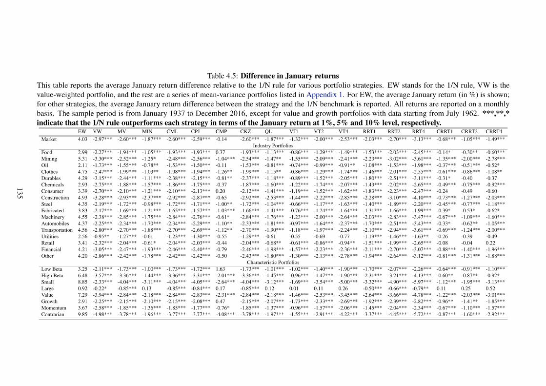
Table 4.5: Difference in January returnsThis table reports the average January return difference relative to the 1/N rule for various portfolio strategies. EW stands for the 1/N rule, VW is thevalue-weighted portfolio, and the rest are a series of mean-variance portfolios listed in Appendix 1. For EW, the average January return (in %) is shown;for other strategies, the average January return difference between the strategy and the 1/N benchmark is reported. All returns are reported on a monthlybasis. The sample period is from January 1937 to December 2016, except for value and growth portfolios with data starting from July 1962. ***,**,*indicate that the 1/N rule outperforms each strategy in terms of the January return at 1%, 5% and 10% level, respectively.
EW VW MV MIN CML CPJ CMP CKZ QL VT1 VT2 VT4 RRT1 RRT2 RRT4 CRRT1 CRRT2 CRRT4Market 4.03 -2.97*** -2.60*** -1.87*** -2.60*** -2.59*** -0.14 -2.60*** -1.87*** -1.32*** -2.00*** -2.53*** -2.03*** -2.70*** -3.13*** -0.68*** -1.05*** -1.49***
Industry PortfoliosFood 2.99 -2.27*** -1.94*** -1.05*** -1.93*** -1.93*** 0.37 -1.93*** -1.13*** -0.86*** -1.29*** -1.49*** -1.53*** -2.03*** -2.45*** -0.14* -0.30** -0.60***Mining 5.31 -3.30*** -2.52*** -1.25* -2.48*** -2.56*** -1.04*** -2.54*** -1.47** -1.55*** -2.09*** -2.41*** -2.23*** -3.02*** -3.61*** -1.35*** -2.00*** -2.78***Oil 2.11 -1.73*** -1.55*** -0.78** -1.53*** -1.50*** -0.11 -1.53*** -0.81*** -0.74*** -0.99*** -0.91** -1.08*** -1.53*** -1.98*** -0.37*** -0.51*** -0.52*Clothes 4.75 -2.47*** -1.99*** -1.03** -1.98*** -1.94*** -1.26** -1.99*** -1.15** -0.86*** -1.29*** -1.74*** -1.46*** -2.01*** -2.55*** -0.61*** -0.86*** -1.08**Durables 4.29 -3.15*** -2.44*** -1.11*** -2.38*** -2.15*** -0.81** -2.37*** -1.18*** -0.89*** -1.52*** -2.05*** -1.80*** -2.51*** -3.11*** -0.31* -0.40 -0.37Chemicals 2.93 -2.75*** -1.88*** -1.57*** -1.86*** -1.75*** -0.37 -1.87*** -1.60*** -1.22*** -1.74*** -2.07*** -1.43*** -2.02*** -2.65*** -0.49*** -0.75*** -0.92***Consumer 3.39 -2.70*** -2.10*** -1.21*** -2.10*** -2.13*** 0.20 -2.12*** -1.41*** -1.19*** -1.52*** -1.62*** -1.83*** -2.23*** -2.47*** -0.24 -0.49 -0.60Construction 4.93 -3.28*** -2.93*** -2.37*** -2.92*** -2.87*** -0.65 -2.92*** -2.53*** -1.44*** -2.22*** -2.85*** -2.28*** -3.10*** -4.10*** -0.73*** -1.27*** -2.03***Steel 4.35 -2.19*** -1.72*** -0.98*** -1.72*** -1.71*** -1.00** -1.72*** -1.04*** -0.66*** -1.17*** -1.63*** -1.40*** -1.89*** -2.20*** -0.45*** -0.77*** -1.18***Fabricated 3.83 -2.17*** -1.69*** -1.21*** -1.65*** -1.57*** -1.03*** -1.66*** -1.41*** -0.76*** -1.24*** -1.64*** -1.31*** -1.66*** -1.99*** -0.39* -0.53* -0.62*Machinery 4.55 -2.38*** -2.85*** -1.75*** -2.84*** -2.76*** -0.61* -2.84*** -1.76*** -1.23*** -2.00*** -2.64*** -2.03*** -2.83*** -3.47*** -0.67*** -1.09*** -1.60***Automobiles 4.37 -2.25*** -2.34*** -1.70*** -2.34*** -2.29*** -1.10** -2.33*** -1.81*** -0.97*** -1.64*** -2.37*** -1.70*** -2.51*** -3.43*** -0.33* -0.62** -1.05***Transportation 4.56 -2.80*** -2.70*** -1.88*** -2.70*** -2.69*** -1.12** -2.70*** -1.90*** -1.18*** -1.97*** -2.24*** -2.10*** -2.94*** -3.61*** -0.69*** -1.24*** -2.00***Utilities 2.56 -0.95** -1.27*** -0.61 -1.23*** -1.30*** -0.55 -1.29*** -0.61 -0.55 -0.69 -0.77 -1.19*** -1.46*** -1.63** -0.26 -0.39 -0.49Retail 3.41 -2.32*** -2.04*** -0.61* -2.04*** -2.03*** -0.44 -2.04*** -0.68** -0.61*** -0.86*** -0.94** -1.51*** -1.99*** -2.65*** -0.08 -0.04 0.22Financial 4.21 -3.05*** -2.47*** -1.93*** -2.46*** -2.40*** -0.79 -2.46*** -1.98*** -1.57*** -2.23*** -2.36*** -2.11*** -2.70*** -3.07*** -0.88*** -1.40*** -1.96***Other 4.20 -2.86*** -2.42*** -1.78*** -2.42*** -2.42*** -0.50 -2.43*** -1.80*** -1.30*** -2.13*** -2.78*** -1.94*** -2.64*** -3.12*** -0.81*** -1.31*** -1.88***
Characteristic PortfoliosLow Beta 3.25 -2.11*** -1.73*** -1.00*** -1.73*** -1.72*** 1.63 -1.73*** -1.01*** -1.02*** -1.40*** -1.90*** -1.70*** -2.07*** -2.26*** -0.64*** -0.91*** -1.10***High Beta 6.48 -3.57*** -3.36*** -1.44*** -3.36*** -3.31*** -2.01*** -3.36*** -1.45*** -0.96*** -1.47*** -1.90*** -2.31*** -3.21*** -4.13*** -0.60** -0.87** -0.92*Small 8.85 -2.33*** -4.04*** -3.11*** -4.04*** -4.05*** -2.64*** -4.04*** -3.12*** -1.69*** -3.54*** -5.00*** -3.32*** -4.90*** -5.97*** -1.12*** -1.95*** -3.13***Large 0.92 -0.22* -0.85*** 0.13 -0.85*** -0.84*** 0.17 -0.85*** 0.12 0.01 0.11 0.26 -0.50*** -0.66*** -0.79** 0.11 0.25 0.52Value 7.29 -3.94*** -2.84*** -2.18*** -2.84*** -2.83*** -2.31*** -2.84*** -2.18*** -1.46*** -2.53*** -3.45*** -2.64*** -3.66*** -4.78*** -1.22*** -2.03*** -3.01***Growth 2.91 -2.25*** -2.15*** -2.10*** -2.15*** -2.08*** 0.47 -2.15*** -2.07*** -1.73*** -2.33*** -2.69*** -1.92*** -2.39*** -2.82*** -0.96** -1.41** -1.85***Momentum 3.67 -2.58*** -1.85*** -1.36*** -1.85*** -1.77*** -0.76* -1.85*** -1.37*** -0.96*** -1.57*** -2.06*** -1.45*** -2.04*** -2.34*** -0.67*** -1.10*** -1.57***Contrarian 9.85 -4.98*** -3.78*** -1.96*** -3.77*** -3.77*** -4.08*** -3.78*** -1.97*** -1.55*** -2.91*** -4.22*** -3.37*** -4.45*** -5.72*** -0.87*** -1.60*** -2.92***
135
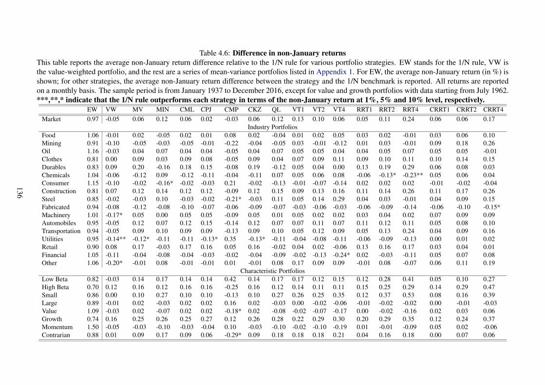
Table 4.6: Difference in non-January returnsThis table reports the average non-January return difference relative to the 1/N rule for various portfolio strategies. EW stands for the 1/N rule, VW isthe value-weighted portfolio, and the rest are a series of mean-variance portfolios listed in Appendix 1. For EW, the average non-January return (in %) isshown; for other strategies, the average non-January return difference between the strategy and the 1/N benchmark is reported. All returns are reportedon a monthly basis. The sample period is from January 1937 to December 2016, except for value and growth portfolios with data starting from July 1962.***,**,* indicate that the 1/N rule outperforms each strategy in terms of the non-January return at 1%, 5% and 10% level, respectively.
EW VW MV MIN CML CPJ CMP CKZ QL VT1 VT2 VT4 RRT1 RRT2 RRT4 CRRT1 CRRT2 CRRT4Market 0.97 -0.05 0.06 0.12 0.06 0.02 -0.03 0.06 0.12 0.13 0.10 0.06 0.05 0.11 0.24 0.06 0.06 0.17
Industry PortfoliosFood 1.06 -0.01 0.02 -0.05 0.02 0.01 0.08 0.02 -0.04 0.01 0.02 0.05 0.03 0.02 -0.01 0.03 0.06 0.10Mining 0.91 -0.10 -0.05 -0.03 -0.05 -0.01 -0.22 -0.04 -0.05 0.03 -0.01 -0.12 0.01 0.03 -0.01 0.09 0.18 0.26Oil 1.16 -0.03 0.04 0.07 0.04 0.04 -0.05 0.04 0.07 0.05 0.05 0.04 0.04 0.05 0.07 0.05 0.05 -0.01Clothes 0.81 0.00 0.09 0.03 0.09 0.08 -0.05 0.09 0.04 0.07 0.09 0.11 0.09 0.10 0.11 0.10 0.14 0.15Durables 0.83 0.09 0.20 -0.16 0.18 0.15 -0.08 0.19 -0.12 0.05 0.04 0.00 0.13 0.19 0.29 0.06 0.08 0.03Chemicals 1.04 -0.06 -0.12 0.09 -0.12 -0.11 -0.04 -0.11 0.07 0.05 0.06 0.08 -0.06 -0.13* -0.23** 0.05 0.06 0.04Consumer 1.15 -0.10 -0.02 -0.16* -0.02 -0.03 0.21 -0.02 -0.13 -0.01 -0.07 -0.14 0.02 0.02 0.02 -0.01 -0.02 -0.04Construction 0.81 0.07 0.12 0.14 0.12 0.12 -0.09 0.12 0.15 0.09 0.13 0.16 0.11 0.14 0.26 0.11 0.17 0.26Steel 0.85 -0.02 -0.03 0.10 -0.03 -0.02 -0.21* -0.03 0.11 0.05 0.14 0.29 0.04 0.03 -0.01 0.04 0.09 0.15Fabricated 0.94 -0.08 -0.12 -0.08 -0.10 -0.07 -0.06 -0.09 -0.07 -0.03 -0.06 -0.03 -0.06 -0.09 -0.14 -0.06 -0.10 -0.15*Machinery 1.01 -0.17* 0.05 0.00 0.05 0.05 -0.09 0.05 0.01 0.05 0.02 0.02 0.03 0.04 0.02 0.07 0.09 0.09Automobiles 0.95 -0.05 0.12 0.07 0.12 0.15 -0.14 0.12 0.07 0.07 0.11 0.07 0.11 0.12 0.11 0.05 0.08 0.10Transportation 0.94 -0.05 0.09 0.10 0.09 0.09 -0.13 0.09 0.10 0.05 0.12 0.09 0.05 0.13 0.24 0.04 0.09 0.16Utilities 0.95 -0.14** -0.12* -0.11 -0.11 -0.13* 0.35 -0.13* -0.11 -0.04 -0.08 -0.11 -0.06 -0.09 -0.13 0.00 0.01 0.02Retail 0.90 0.08 0.17 -0.03 0.17 0.16 0.05 0.16 -0.02 0.04 0.02 -0.06 0.13 0.16 0.17 0.03 0.04 0.01Financial 1.05 -0.11 -0.04 -0.08 -0.04 -0.03 -0.02 -0.04 -0.09 -0.02 -0.13 -0.24* 0.02 -0.03 -0.11 0.05 0.07 0.08Other 1.06 -0.20* -0.01 0.08 -0.01 -0.01 0.01 -0.01 0.08 0.17 0.09 0.09 -0.01 0.08 -0.07 0.06 0.11 0.19
Characteristic PortfoliosLow Beta 0.82 -0.03 0.14 0.17 0.14 0.14 0.42 0.14 0.17 0.17 0.12 0.15 0.12 0.28 0.41 0.05 0.10 0.27High Beta 0.70 0.12 0.16 0.12 0.16 0.16 -0.25 0.16 0.12 0.14 0.11 0.11 0.15 0.25 0.29 0.14 0.29 0.47Small 0.86 0.00 0.10 0.27 0.10 0.10 -0.13 0.10 0.27 0.26 0.25 0.35 0.12 0.37 0.53 0.08 0.16 0.39Large 0.89 -0.01 0.02 -0.03 0.02 0.02 0.16 0.02 -0.03 0.00 -0.02 -0.06 -0.01 -0.02 -0.02 0.00 -0.01 -0.03Value 1.09 -0.03 0.02 -0.07 0.02 0.02 -0.18* 0.02 -0.08 -0.02 -0.07 -0.17 0.00 -0.02 -0.16 0.02 0.03 0.06Growth 0.74 0.16 0.25 0.26 0.25 0.27 0.12 0.26 0.28 0.22 0.29 0.30 0.20 0.29 0.35 0.12 0.24 0.37Momentum 1.50 -0.05 -0.03 -0.10 -0.03 -0.04 0.10 -0.03 -0.10 -0.02 -0.10 -0.19 0.01 -0.01 -0.09 0.05 0.02 -0.06Contrarian 0.88 0.01 0.09 0.17 0.09 0.06 -0.29* 0.09 0.18 0.18 0.18 0.21 0.04 0.16 0.18 0.00 0.07 0.06
136
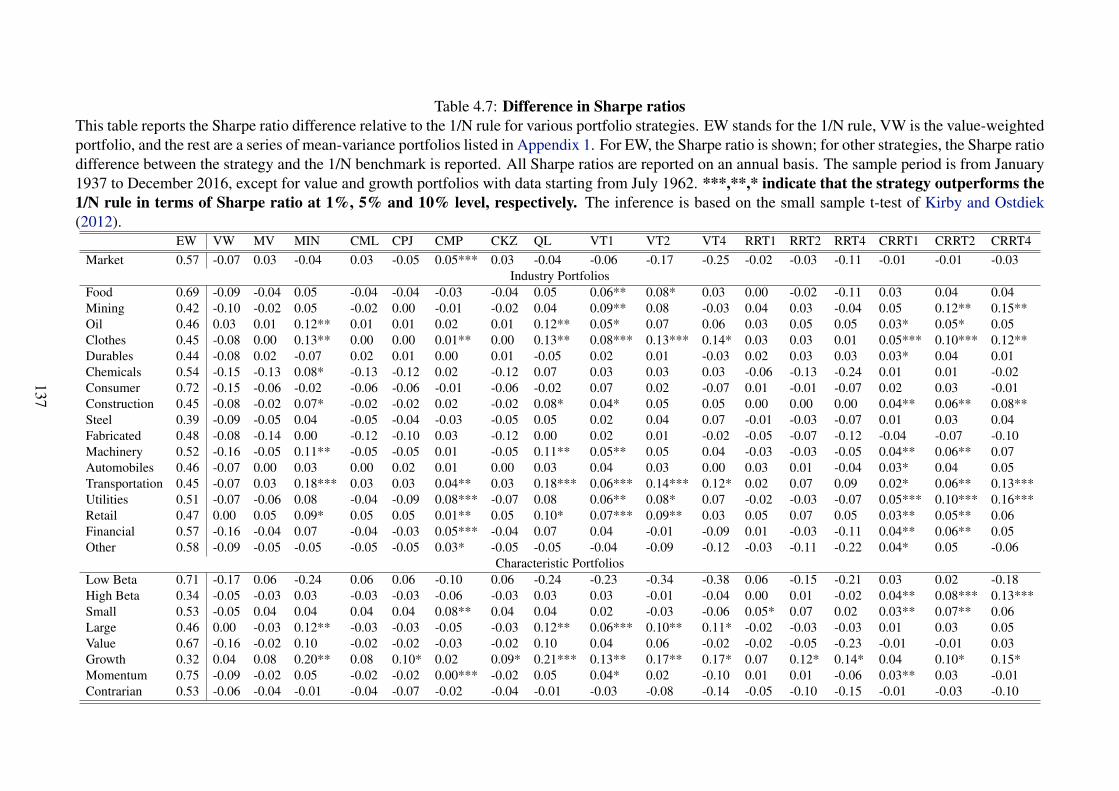
Table 4.7: Difference in Sharpe ratiosThis table reports the Sharpe ratio difference relative to the 1/N rule for various portfolio strategies. EW stands for the 1/N rule, VW is the value-weightedportfolio, and the rest are a series of mean-variance portfolios listed in Appendix 1. For EW, the Sharpe ratio is shown; for other strategies, the Sharpe ratiodifference between the strategy and the 1/N benchmark is reported. All Sharpe ratios are reported on an annual basis. The sample period is from January1937 to December 2016, except for value and growth portfolios with data starting from July 1962. ***,**,* indicate that the strategy outperforms the1/N rule in terms of Sharpe ratio at 1%, 5% and 10% level, respectively. The inference is based on the small sample t-test of Kirby and Ostdiek(2012).
EW VW MV MIN CML CPJ CMP CKZ QL VT1 VT2 VT4 RRT1 RRT2 RRT4 CRRT1 CRRT2 CRRT4Market 0.57 -0.07 0.03 -0.04 0.03 -0.05 0.05*** 0.03 -0.04 -0.06 -0.17 -0.25 -0.02 -0.03 -0.11 -0.01 -0.01 -0.03
Industry PortfoliosFood 0.69 -0.09 -0.04 0.05 -0.04 -0.04 -0.03 -0.04 0.05 0.06** 0.08* 0.03 0.00 -0.02 -0.11 0.03 0.04 0.04Mining 0.42 -0.10 -0.02 0.05 -0.02 0.00 -0.01 -0.02 0.04 0.09** 0.08 -0.03 0.04 0.03 -0.04 0.05 0.12** 0.15**Oil 0.46 0.03 0.01 0.12** 0.01 0.01 0.02 0.01 0.12** 0.05* 0.07 0.06 0.03 0.05 0.05 0.03* 0.05* 0.05Clothes 0.45 -0.08 0.00 0.13** 0.00 0.00 0.01** 0.00 0.13** 0.08*** 0.13*** 0.14* 0.03 0.03 0.01 0.05*** 0.10*** 0.12**Durables 0.44 -0.08 0.02 -0.07 0.02 0.01 0.00 0.01 -0.05 0.02 0.01 -0.03 0.02 0.03 0.03 0.03* 0.04 0.01Chemicals 0.54 -0.15 -0.13 0.08* -0.13 -0.12 0.02 -0.12 0.07 0.03 0.03 0.03 -0.06 -0.13 -0.24 0.01 0.01 -0.02Consumer 0.72 -0.15 -0.06 -0.02 -0.06 -0.06 -0.01 -0.06 -0.02 0.07 0.02 -0.07 0.01 -0.01 -0.07 0.02 0.03 -0.01Construction 0.45 -0.08 -0.02 0.07* -0.02 -0.02 0.02 -0.02 0.08* 0.04* 0.05 0.05 0.00 0.00 0.00 0.04** 0.06** 0.08**Steel 0.39 -0.09 -0.05 0.04 -0.05 -0.04 -0.03 -0.05 0.05 0.02 0.04 0.07 -0.01 -0.03 -0.07 0.01 0.03 0.04Fabricated 0.48 -0.08 -0.14 0.00 -0.12 -0.10 0.03 -0.12 0.00 0.02 0.01 -0.02 -0.05 -0.07 -0.12 -0.04 -0.07 -0.10Machinery 0.52 -0.16 -0.05 0.11** -0.05 -0.05 0.01 -0.05 0.11** 0.05** 0.05 0.04 -0.03 -0.03 -0.05 0.04** 0.06** 0.07Automobiles 0.46 -0.07 0.00 0.03 0.00 0.02 0.01 0.00 0.03 0.04 0.03 0.00 0.03 0.01 -0.04 0.03* 0.04 0.05Transportation 0.45 -0.07 0.03 0.18*** 0.03 0.03 0.04** 0.03 0.18*** 0.06*** 0.14*** 0.12* 0.02 0.07 0.09 0.02* 0.06** 0.13***Utilities 0.51 -0.07 -0.06 0.08 -0.04 -0.09 0.08*** -0.07 0.08 0.06** 0.08* 0.07 -0.02 -0.03 -0.07 0.05*** 0.10*** 0.16***Retail 0.47 0.00 0.05 0.09* 0.05 0.05 0.01** 0.05 0.10* 0.07*** 0.09** 0.03 0.05 0.07 0.05 0.03** 0.05** 0.06Financial 0.57 -0.16 -0.04 0.07 -0.04 -0.03 0.05*** -0.04 0.07 0.04 -0.01 -0.09 0.01 -0.03 -0.11 0.04** 0.06** 0.05Other 0.58 -0.09 -0.05 -0.05 -0.05 -0.05 0.03* -0.05 -0.05 -0.04 -0.09 -0.12 -0.03 -0.11 -0.22 0.04* 0.05 -0.06
Characteristic PortfoliosLow Beta 0.71 -0.17 0.06 -0.24 0.06 0.06 -0.10 0.06 -0.24 -0.23 -0.34 -0.38 0.06 -0.15 -0.21 0.03 0.02 -0.18High Beta 0.34 -0.05 -0.03 0.03 -0.03 -0.03 -0.06 -0.03 0.03 0.03 -0.01 -0.04 0.00 0.01 -0.02 0.04** 0.08*** 0.13***Small 0.53 -0.05 0.04 0.04 0.04 0.04 0.08** 0.04 0.04 0.02 -0.03 -0.06 0.05* 0.07 0.02 0.03** 0.07** 0.06Large 0.46 0.00 -0.03 0.12** -0.03 -0.03 -0.05 -0.03 0.12** 0.06*** 0.10** 0.11* -0.02 -0.03 -0.03 0.01 0.03 0.05Value 0.67 -0.16 -0.02 0.10 -0.02 -0.02 -0.03 -0.02 0.10 0.04 0.06 -0.02 -0.02 -0.05 -0.23 -0.01 -0.01 0.03Growth 0.32 0.04 0.08 0.20** 0.08 0.10* 0.02 0.09* 0.21*** 0.13** 0.17** 0.17* 0.07 0.12* 0.14* 0.04 0.10* 0.15*Momentum 0.75 -0.09 -0.02 0.05 -0.02 -0.02 0.00*** -0.02 0.05 0.04* 0.02 -0.10 0.01 0.01 -0.06 0.03** 0.03 -0.01Contrarian 0.53 -0.06 -0.04 -0.01 -0.04 -0.07 -0.02 -0.04 -0.01 -0.03 -0.08 -0.14 -0.05 -0.10 -0.15 -0.01 -0.03 -0.10
137
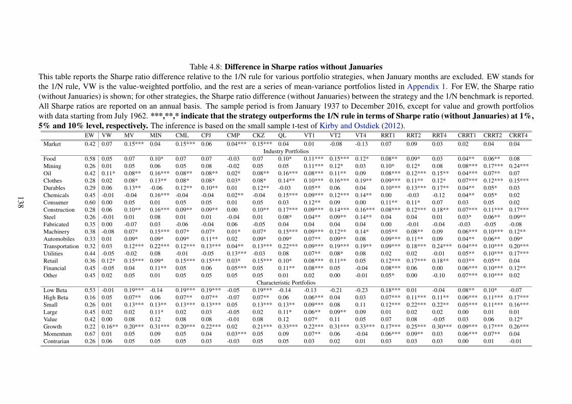
Table 4.8: Difference in Sharpe ratios without JanuariesThis table reports the Sharpe ratio difference relative to the 1/N rule for various portfolio strategies, when January months are excluded. EW stands forthe 1/N rule, VW is the value-weighted portfolio, and the rest are a series of mean-variance portfolios listed in Appendix 1. For EW, the Sharpe ratio(without Januaries) is shown; for other strategies, the Sharpe ratio difference (without Januaries) between the strategy and the 1/N benchmark is reported.All Sharpe ratios are reported on an annual basis. The sample period is from January 1937 to December 2016, except for value and growth portfolioswith data starting from July 1962. ***,**,* indicate that the strategy outperforms the 1/N rule in terms of Sharpe ratio (without Januaries) at 1%,5% and 10% level, respectively. The inference is based on the small sample t-test of Kirby and Ostdiek (2012).
EW VW MV MIN CML CPJ CMP CKZ QL VT1 VT2 VT4 RRT1 RRT2 RRT4 CRRT1 CRRT2 CRRT4Market 0.42 0.07 0.15*** 0.04 0.15*** 0.06 0.04*** 0.15*** 0.04 0.01 -0.08 -0.13 0.07 0.09 0.03 0.02 0.04 0.04
Industry PortfoliosFood 0.58 0.05 0.07 0.10* 0.07 0.07 -0.03 0.07 0.10* 0.11*** 0.15*** 0.12* 0.08** 0.09* 0.03 0.04** 0.06** 0.08Mining 0.26 0.01 0.05 0.06 0.05 0.08 -0.02 0.05 0.05 0.11*** 0.12* 0.03 0.10* 0.12* 0.08 0.08*** 0.17*** 0.24***Oil 0.42 0.11* 0.08** 0.16*** 0.08** 0.08** 0.02* 0.08** 0.16*** 0.08*** 0.11** 0.09 0.08*** 0.12*** 0.15** 0.04*** 0.07** 0.07Clothes 0.28 0.02 0.08* 0.13** 0.08* 0.08* 0.03* 0.08* 0.14** 0.10*** 0.16*** 0.19** 0.09*** 0.11** 0.12* 0.07*** 0.12*** 0.15***Durables 0.29 0.06 0.13** -0.06 0.12** 0.10** 0.01 0.12** -0.03 0.05** 0.06 0.04 0.10*** 0.13*** 0.17** 0.04** 0.05* 0.03Chemicals 0.45 -0.01 -0.04 0.16*** -0.04 -0.04 0.02** -0.04 0.15*** 0.09*** 0.12*** 0.14** 0.00 -0.03 -0.12 0.04** 0.05* 0.02Consumer 0.60 0.00 0.05 0.01 0.05 0.05 0.01 0.05 0.03 0.12** 0.09 0.00 0.11** 0.11* 0.07 0.03 0.05 0.02Construction 0.28 0.06 0.10** 0.16*** 0.09** 0.09** 0.00 0.10** 0.17*** 0.09*** 0.14*** 0.16*** 0.08*** 0.12*** 0.18** 0.07*** 0.11*** 0.17***Steel 0.26 -0.01 0.01 0.08 0.01 0.01 -0.04 0.01 0.08* 0.04** 0.09** 0.14** 0.04 0.04 0.01 0.03* 0.06** 0.09**Fabricated 0.35 0.00 -0.07 0.03 -0.06 -0.04 0.06 -0.05 0.04 0.04 0.04 0.04 0.00 -0.01 -0.04 -0.03 -0.05 -0.08Machinery 0.38 -0.08 0.07* 0.15*** 0.07* 0.07* 0.01* 0.07* 0.15*** 0.09*** 0.12** 0.14* 0.05** 0.08** 0.09 0.06*** 0.10*** 0.12**Automobiles 0.33 0.01 0.09* 0.09* 0.09* 0.11** 0.02 0.09* 0.09* 0.07** 0.09** 0.08 0.09*** 0.11** 0.09 0.04** 0.06** 0.09*Transportation 0.32 0.03 0.12*** 0.22*** 0.12*** 0.13*** 0.04** 0.13*** 0.22*** 0.09*** 0.19*** 0.19** 0.09*** 0.18*** 0.24*** 0.04*** 0.10*** 0.20***Utilities 0.44 -0.05 -0.02 0.08 -0.01 -0.05 0.13*** -0.03 0.08 0.07** 0.08* 0.08 0.02 0.02 -0.01 0.05** 0.10*** 0.17***Retail 0.36 0.12* 0.15*** 0.09* 0.15*** 0.15*** 0.03* 0.15*** 0.10* 0.08*** 0.11** 0.05 0.12*** 0.17*** 0.18** 0.03** 0.05** 0.04Financial 0.45 -0.05 0.04 0.11** 0.05 0.06 0.05*** 0.05 0.11** 0.08*** 0.05 -0.04 0.08*** 0.06 0.00 0.06*** 0.10*** 0.12**Other 0.45 0.02 0.05 0.01 0.05 0.05 0.05 0.05 0.01 0.02 0.00 -0.01 0.05* 0.00 -0.10 0.07*** 0.10*** 0.02
Characteristic PortfoliosLow Beta 0.53 -0.01 0.19*** -0.14 0.19*** 0.19*** -0.05 0.19*** -0.14 -0.13 -0.21 -0.23 0.18*** 0.01 -0.04 0.08** 0.10* -0.07High Beta 0.16 0.05 0.07** 0.06 0.07** 0.07** -0.07 0.07** 0.06 0.06*** 0.04 0.03 0.07*** 0.11*** 0.11** 0.06*** 0.11*** 0.17***Small 0.26 0.01 0.13*** 0.13** 0.13*** 0.13*** 0.05 0.13*** 0.13** 0.09*** 0.08 0.11 0.12*** 0.22*** 0.22** 0.05*** 0.11*** 0.16***Large 0.45 0.02 0.02 0.11* 0.02 0.03 -0.05 0.02 0.11* 0.06** 0.09** 0.09 0.01 0.02 0.02 0.00 0.01 0.01Value 0.42 0.00 0.08 0.12 0.08 0.08 -0.01 0.08 0.12 0.07* 0.11 0.05 0.07 0.08 -0.05 0.03 0.06 0.12*Growth 0.22 0.16** 0.20*** 0.31*** 0.20*** 0.22*** 0.02 0.21*** 0.33*** 0.22*** 0.31*** 0.33*** 0.17*** 0.25*** 0.30*** 0.09*** 0.17*** 0.26***Momentum 0.67 0.01 0.05 0.09 0.05 0.04 0.03*** 0.05 0.09 0.07** 0.06 -0.04 0.06*** 0.09** 0.03 0.06*** 0.07** 0.04Contrarian 0.26 0.06 0.05 0.05 0.05 0.03 -0.03 0.05 0.05 0.03 0.02 0.01 0.03 0.03 0.03 0.00 0.01 -0.01
138
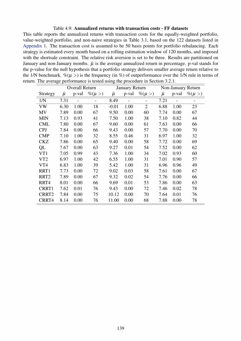
Table 4.9: Annualized returns with transaction costs - FF datasetsThis table reports the annualized returns with transaction costs for the equally-weighted portfolio,value-weighted portfolio, and non-naive strategies in Table 3.1, based on the 122 datasets listed inAppendix 1. The transaction cost is assumed to be 50 basis points for portfolio rebalancing. Eachstrategy is estimated every month based on a rolling estimation window of 120 months, and imposedwith the shortsale constraint. The relative risk aversion is set to be three. Results are partitioned onJanuary and non-January months. µ is the average annualized return in percentage. p-val stands forthe p-value for the null hypothesis that a portfolio strategy delivers smaller average return relative tothe 1/N benchmark. %(µ >) is the frequency (in %) of outperformance over the 1/N rule in terms ofreturn. The average performance is tested using the procedure in Section 3.2.1.
Overall Return January Return Non-January ReturnStrategy µ p-val %(µ >) µ p-val %(µ >) µ p-val %(µ >)1/N 7.31 - - 8.49 - - 7.21 - -VW 6.30 1.00 18 -0.01 1.00 2 6.88 1.00 23MV 7.89 0.00 67 9.50 0.00 60 7.74 0.00 67MIN 7.13 0.93 41 7.50 1.00 38 7.10 0.82 44CML 7.80 0.00 67 9.60 0.00 61 7.63 0.00 66CPJ 7.84 0.00 66 9.43 0.00 57 7.70 0.00 70CMP 7.10 1.00 32 8.55 0.46 31 6.97 1.00 32CKZ 7.86 0.00 65 9.40 0.00 58 7.72 0.00 69QL 7.67 0.00 63 9.27 0.01 54 7.52 0.00 62VT1 7.05 0.99 43 7.36 1.00 34 7.02 0.93 60VT2 6.97 1.00 42 6.55 1.00 31 7.01 0.90 57VT4 6.83 1.00 39 5.42 1.00 31 6.96 0.96 49RRT1 7.73 0.00 72 9.02 0.03 58 7.61 0.00 67RRT2 7.89 0.00 67 9.32 0.02 54 7.76 0.00 66RRT4 8.01 0.00 66 9.69 0.01 53 7.86 0.00 63CRRT1 7.62 0.01 76 9.43 0.00 72 7.46 0.02 78CRRT2 7.84 0.00 75 10.12 0.00 70 7.64 0.01 76CRRT4 8.14 0.00 76 11.00 0.00 68 7.88 0.00 78
139
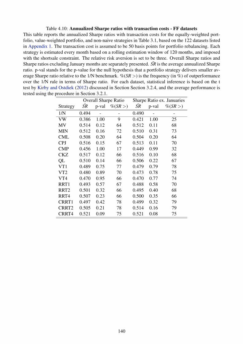
Table 4.10: Annualized Sharpe ratios with transaction costs - FF datasetsThis table reports the annualized Sharpe ratios with transaction costs for the equally-weighted port-folio, value-weighted portfolio, and non-naive strategies in Table 3.1, based on the 122 datasets listedin Appendix 1. The transaction cost is assumed to be 50 basis points for portfolio rebalancing. Eachstrategy is estimated every month based on a rolling estimation window of 120 months, and imposedwith the shortsale constraint. The relative risk aversion is set to be three. Overall Sharpe ratios andSharpe ratios excluding January months are separately presented. SR is the average annualized Sharperatio. p-val stands for the p-value for the null hypothesis that a portfolio strategy delivers smaller av-erage Sharpe ratio relative to the 1/N benchmark. %(SR >) is the frequency (in %) of outperformanceover the 1/N rule in terms of Sharpe ratio. For each dataset, statistical inference is based on the ttest by Kirby and Ostdiek (2012) discussed in Section Section 3.2.4, and the average performance istested using the procedure in Section 3.2.1.
Overall Sharpe Ratio Sharpe Ratio ex. JanuariesStrategy SR p-val %(SR >) SR p-val %(SR >)1/N 0.494 - - 0.490 - -VW 0.386 1.00 9 0.421 1.00 25MV 0.514 0.12 64 0.512 0.11 68MIN 0.512 0.16 72 0.510 0.31 73CML 0.508 0.20 64 0.504 0.20 64CPJ 0.516 0.15 67 0.513 0.11 70CMP 0.456 1.00 17 0.449 0.99 32CKZ 0.517 0.12 66 0.516 0.10 68QL 0.510 0.14 66 0.506 0.22 67VT1 0.489 0.75 77 0.479 0.79 78VT2 0.480 0.89 70 0.473 0.78 75VT4 0.470 0.95 66 0.470 0.77 74RRT1 0.493 0.57 67 0.488 0.58 70RRT2 0.501 0.32 66 0.495 0.40 68RRT4 0.507 0.23 66 0.500 0.35 66CRRT1 0.497 0.42 78 0.499 0.32 79CRRT2 0.505 0.21 78 0.514 0.16 79CRRT4 0.521 0.09 75 0.521 0.08 75
140
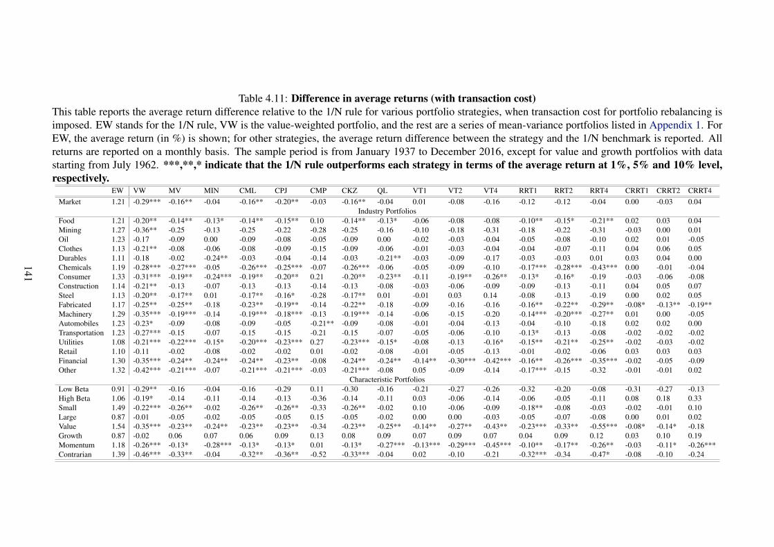
Table 4.11: Difference in average returns (with transaction cost)This table reports the average return difference relative to the 1/N rule for various portfolio strategies, when transaction cost for portfolio rebalancing isimposed. EW stands for the 1/N rule, VW is the value-weighted portfolio, and the rest are a series of mean-variance portfolios listed in Appendix 1. ForEW, the average return (in %) is shown; for other strategies, the average return difference between the strategy and the 1/N benchmark is reported. Allreturns are reported on a monthly basis. The sample period is from January 1937 to December 2016, except for value and growth portfolios with datastarting from July 1962. ***,**,* indicate that the 1/N rule outperforms each strategy in terms of the average return at 1%, 5% and 10% level,respectively.
EW VW MV MIN CML CPJ CMP CKZ QL VT1 VT2 VT4 RRT1 RRT2 RRT4 CRRT1 CRRT2 CRRT4Market 1.21 -0.29*** -0.16** -0.04 -0.16** -0.20** -0.03 -0.16** -0.04 0.01 -0.08 -0.16 -0.12 -0.12 -0.04 0.00 -0.03 0.04
Industry PortfoliosFood 1.21 -0.20** -0.14** -0.13* -0.14** -0.15** 0.10 -0.14** -0.13* -0.06 -0.08 -0.08 -0.10** -0.15* -0.21** 0.02 0.03 0.04Mining 1.27 -0.36** -0.25 -0.13 -0.25 -0.22 -0.28 -0.25 -0.16 -0.10 -0.18 -0.31 -0.18 -0.22 -0.31 -0.03 0.00 0.01Oil 1.23 -0.17 -0.09 0.00 -0.09 -0.08 -0.05 -0.09 0.00 -0.02 -0.03 -0.04 -0.05 -0.08 -0.10 0.02 0.01 -0.05Clothes 1.13 -0.21** -0.08 -0.06 -0.08 -0.09 -0.15 -0.09 -0.06 -0.01 -0.03 -0.04 -0.04 -0.07 -0.11 0.04 0.06 0.05Durables 1.11 -0.18 -0.02 -0.24** -0.03 -0.04 -0.14 -0.03 -0.21** -0.03 -0.09 -0.17 -0.03 -0.03 0.01 0.03 0.04 0.00Chemicals 1.19 -0.28*** -0.27*** -0.05 -0.26*** -0.25*** -0.07 -0.26*** -0.06 -0.05 -0.09 -0.10 -0.17*** -0.28*** -0.43*** 0.00 -0.01 -0.04Consumer 1.33 -0.31*** -0.19** -0.24*** -0.19** -0.20** 0.21 -0.20** -0.23** -0.11 -0.19** -0.26** -0.13* -0.16* -0.19 -0.03 -0.06 -0.08Construction 1.14 -0.21** -0.13 -0.07 -0.13 -0.13 -0.14 -0.13 -0.08 -0.03 -0.06 -0.09 -0.09 -0.13 -0.11 0.04 0.05 0.07Steel 1.13 -0.20** -0.17** 0.01 -0.17** -0.16* -0.28 -0.17** 0.01 -0.01 0.03 0.14 -0.08 -0.13 -0.19 0.00 0.02 0.05Fabricated 1.17 -0.25** -0.25** -0.18 -0.23** -0.19** -0.14 -0.22** -0.18 -0.09 -0.16 -0.16 -0.16** -0.22** -0.29** -0.08* -0.13** -0.19**Machinery 1.29 -0.35*** -0.19*** -0.14 -0.19*** -0.18*** -0.13 -0.19*** -0.14 -0.06 -0.15 -0.20 -0.14*** -0.20*** -0.27** 0.01 0.00 -0.05Automobiles 1.23 -0.23* -0.09 -0.08 -0.09 -0.05 -0.21** -0.09 -0.08 -0.01 -0.04 -0.13 -0.04 -0.10 -0.18 0.02 0.02 0.00Transportation 1.23 -0.27*** -0.15 -0.07 -0.15 -0.15 -0.21 -0.15 -0.07 -0.05 -0.06 -0.10 -0.13* -0.13 -0.08 -0.02 -0.02 -0.02Utilities 1.08 -0.21*** -0.22*** -0.15* -0.20*** -0.23*** 0.27 -0.23*** -0.15* -0.08 -0.13 -0.16* -0.15** -0.21** -0.25** -0.02 -0.03 -0.02Retail 1.10 -0.11 -0.02 -0.08 -0.02 -0.02 0.01 -0.02 -0.08 -0.01 -0.05 -0.13 -0.01 -0.02 -0.06 0.03 0.03 0.03Financial 1.30 -0.35*** -0.24** -0.24** -0.24** -0.23** -0.08 -0.24** -0.24** -0.14** -0.30*** -0.42*** -0.16** -0.26*** -0.35*** -0.02 -0.05 -0.09Other 1.32 -0.42*** -0.21*** -0.07 -0.21*** -0.21*** -0.03 -0.21*** -0.08 0.05 -0.09 -0.14 -0.17*** -0.15 -0.32 -0.01 -0.01 0.02
Characteristic PortfoliosLow Beta 0.91 -0.29** -0.16 -0.04 -0.16 -0.29 0.11 -0.30 -0.16 -0.21 -0.27 -0.26 -0.32 -0.20 -0.08 -0.31 -0.27 -0.13High Beta 1.06 -0.19* -0.14 -0.11 -0.14 -0.13 -0.36 -0.14 -0.11 0.03 -0.06 -0.14 -0.06 -0.05 -0.11 0.08 0.18 0.33Small 1.49 -0.22*** -0.26** -0.02 -0.26** -0.26** -0.33 -0.26** -0.02 0.10 -0.06 -0.09 -0.18** -0.08 -0.03 -0.02 -0.01 0.10Large 0.87 -0.01 -0.05 -0.02 -0.05 -0.05 0.15 -0.05 -0.02 0.00 0.00 -0.03 -0.05 -0.07 -0.08 0.00 0.01 0.02Value 1.54 -0.35*** -0.23** -0.24** -0.23** -0.23** -0.34 -0.23** -0.25** -0.14** -0.27** -0.43** -0.23*** -0.33** -0.55*** -0.08* -0.14* -0.18Growth 0.87 -0.02 0.06 0.07 0.06 0.09 0.13 0.08 0.09 0.07 0.09 0.07 0.04 0.09 0.12 0.03 0.10 0.19Momentum 1.18 -0.26*** -0.13* -0.28*** -0.13* -0.13* 0.01 -0.13* -0.27*** -0.13*** -0.29*** -0.45*** -0.10** -0.17** -0.26** -0.03 -0.11* -0.26***Contrarian 1.39 -0.46*** -0.33** -0.04 -0.32** -0.36** -0.52 -0.33*** -0.04 0.02 -0.10 -0.21 -0.32*** -0.34 -0.47* -0.08 -0.10 -0.24
141
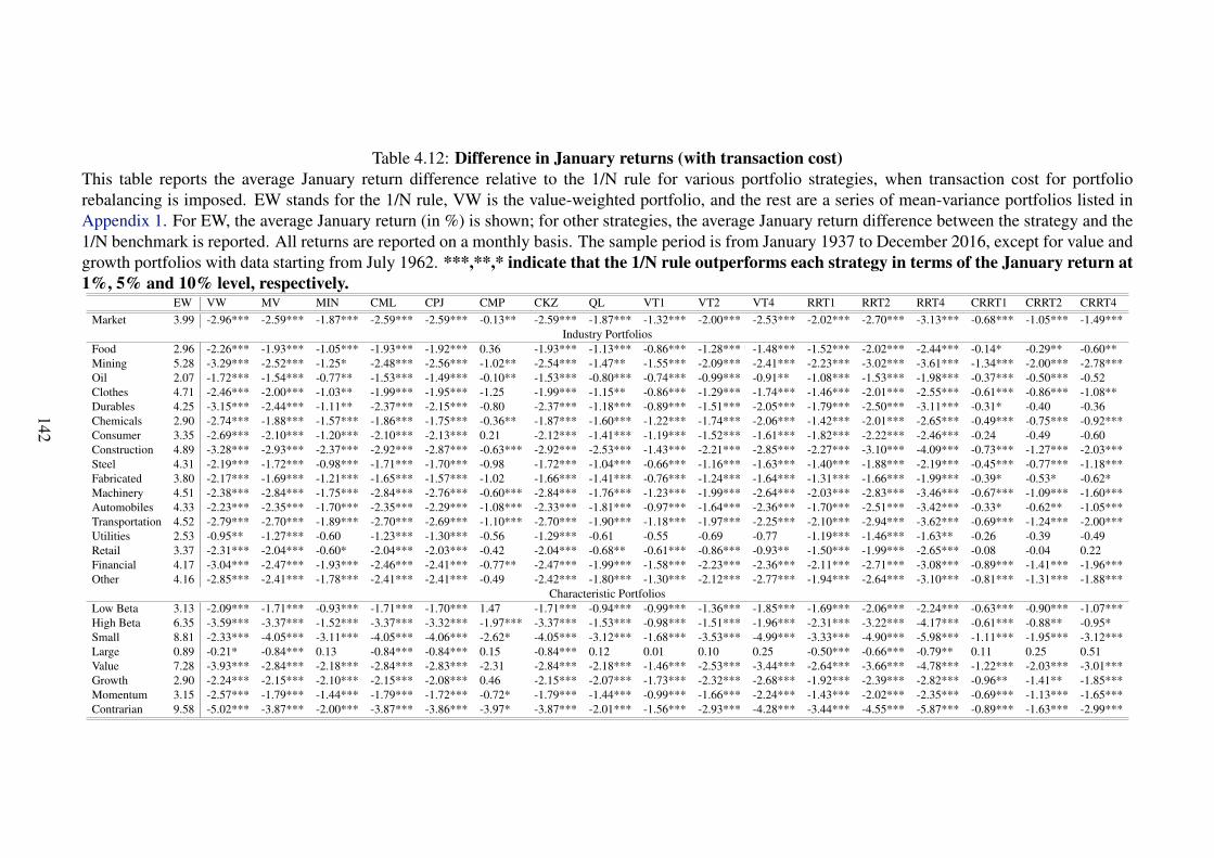
Table 4.12: Difference in January returns (with transaction cost)This table reports the average January return difference relative to the 1/N rule for various portfolio strategies, when transaction cost for portfoliorebalancing is imposed. EW stands for the 1/N rule, VW is the value-weighted portfolio, and the rest are a series of mean-variance portfolios listed inAppendix 1. For EW, the average January return (in %) is shown; for other strategies, the average January return difference between the strategy and the1/N benchmark is reported. All returns are reported on a monthly basis. The sample period is from January 1937 to December 2016, except for value andgrowth portfolios with data starting from July 1962. ***,**,* indicate that the 1/N rule outperforms each strategy in terms of the January return at1%, 5% and 10% level, respectively.
EW VW MV MIN CML CPJ CMP CKZ QL VT1 VT2 VT4 RRT1 RRT2 RRT4 CRRT1 CRRT2 CRRT4Market 3.99 -2.96*** -2.59*** -1.87*** -2.59*** -2.59*** -0.13** -2.59*** -1.87*** -1.32*** -2.00*** -2.53*** -2.02*** -2.70*** -3.13*** -0.68*** -1.05*** -1.49***
Industry PortfoliosFood 2.96 -2.26*** -1.93*** -1.05*** -1.93*** -1.92*** 0.36 -1.93*** -1.13*** -0.86*** -1.28*** -1.48*** -1.52*** -2.02*** -2.44*** -0.14* -0.29** -0.60**Mining 5.28 -3.29*** -2.52*** -1.25* -2.48*** -2.56*** -1.02** -2.54*** -1.47** -1.55*** -2.09*** -2.41*** -2.23*** -3.02*** -3.61*** -1.34*** -2.00*** -2.78***Oil 2.07 -1.72*** -1.54*** -0.77** -1.53*** -1.49*** -0.10** -1.53*** -0.80*** -0.74*** -0.99*** -0.91** -1.08*** -1.53*** -1.98*** -0.37*** -0.50*** -0.52Clothes 4.71 -2.46*** -2.00*** -1.03** -1.99*** -1.95*** -1.25 -1.99*** -1.15** -0.86*** -1.29*** -1.74*** -1.46*** -2.01*** -2.55*** -0.61*** -0.86*** -1.08**Durables 4.25 -3.15*** -2.44*** -1.11** -2.37*** -2.15*** -0.80 -2.37*** -1.18*** -0.89*** -1.51*** -2.05*** -1.79*** -2.50*** -3.11*** -0.31* -0.40 -0.36Chemicals 2.90 -2.74*** -1.88*** -1.57*** -1.86*** -1.75*** -0.36** -1.87*** -1.60*** -1.22*** -1.74*** -2.06*** -1.42*** -2.01*** -2.65*** -0.49*** -0.75*** -0.92***Consumer 3.35 -2.69*** -2.10*** -1.20*** -2.10*** -2.13*** 0.21 -2.12*** -1.41*** -1.19*** -1.52*** -1.61*** -1.82*** -2.22*** -2.46*** -0.24 -0.49 -0.60Construction 4.89 -3.28*** -2.93*** -2.37*** -2.92*** -2.87*** -0.63*** -2.92*** -2.53*** -1.43*** -2.21*** -2.85*** -2.27*** -3.10*** -4.09*** -0.73*** -1.27*** -2.03***Steel 4.31 -2.19*** -1.72*** -0.98*** -1.71*** -1.70*** -0.98 -1.72*** -1.04*** -0.66*** -1.16*** -1.63*** -1.40*** -1.88*** -2.19*** -0.45*** -0.77*** -1.18***Fabricated 3.80 -2.17*** -1.69*** -1.21*** -1.65*** -1.57*** -1.02 -1.66*** -1.41*** -0.76*** -1.24*** -1.64*** -1.31*** -1.66*** -1.99*** -0.39* -0.53* -0.62*Machinery 4.51 -2.38*** -2.84*** -1.75*** -2.84*** -2.76*** -0.60*** -2.84*** -1.76*** -1.23*** -1.99*** -2.64*** -2.03*** -2.83*** -3.46*** -0.67*** -1.09*** -1.60***Automobiles 4.33 -2.23*** -2.35*** -1.70*** -2.35*** -2.29*** -1.08*** -2.33*** -1.81*** -0.97*** -1.64*** -2.36*** -1.70*** -2.51*** -3.42*** -0.33* -0.62** -1.05***Transportation 4.52 -2.79*** -2.70*** -1.89*** -2.70*** -2.69*** -1.10*** -2.70*** -1.90*** -1.18*** -1.97*** -2.25*** -2.10*** -2.94*** -3.62*** -0.69*** -1.24*** -2.00***Utilities 2.53 -0.95** -1.27*** -0.60 -1.23*** -1.30*** -0.56 -1.29*** -0.61 -0.55 -0.69 -0.77 -1.19*** -1.46*** -1.63** -0.26 -0.39 -0.49Retail 3.37 -2.31*** -2.04*** -0.60* -2.04*** -2.03*** -0.42 -2.04*** -0.68** -0.61*** -0.86*** -0.93** -1.50*** -1.99*** -2.65*** -0.08 -0.04 0.22Financial 4.17 -3.04*** -2.47*** -1.93*** -2.46*** -2.41*** -0.77** -2.47*** -1.99*** -1.58*** -2.23*** -2.36*** -2.11*** -2.71*** -3.08*** -0.89*** -1.41*** -1.96***Other 4.16 -2.85*** -2.41*** -1.78*** -2.41*** -2.41*** -0.49 -2.42*** -1.80*** -1.30*** -2.12*** -2.77*** -1.94*** -2.64*** -3.10*** -0.81*** -1.31*** -1.88***
Characteristic PortfoliosLow Beta 3.13 -2.09*** -1.71*** -0.93*** -1.71*** -1.70*** 1.47 -1.71*** -0.94*** -0.99*** -1.36*** -1.85*** -1.69*** -2.06*** -2.24*** -0.63*** -0.90*** -1.07***High Beta 6.35 -3.59*** -3.37*** -1.52*** -3.37*** -3.32*** -1.97*** -3.37*** -1.53*** -0.98*** -1.51*** -1.96*** -2.31*** -3.22*** -4.17*** -0.61*** -0.88** -0.95*Small 8.81 -2.33*** -4.05*** -3.11*** -4.05*** -4.06*** -2.62* -4.05*** -3.12*** -1.68*** -3.53*** -4.99*** -3.33*** -4.90*** -5.98*** -1.11*** -1.95*** -3.12***Large 0.89 -0.21* -0.84*** 0.13 -0.84*** -0.84*** 0.15 -0.84*** 0.12 0.01 0.10 0.25 -0.50*** -0.66*** -0.79** 0.11 0.25 0.51Value 7.28 -3.93*** -2.84*** -2.18*** -2.84*** -2.83*** -2.31 -2.84*** -2.18*** -1.46*** -2.53*** -3.44*** -2.64*** -3.66*** -4.78*** -1.22*** -2.03*** -3.01***Growth 2.90 -2.24*** -2.15*** -2.10*** -2.15*** -2.08*** 0.46 -2.15*** -2.07*** -1.73*** -2.32*** -2.68*** -1.92*** -2.39*** -2.82*** -0.96** -1.41** -1.85***Momentum 3.15 -2.57*** -1.79*** -1.44*** -1.79*** -1.72*** -0.72* -1.79*** -1.44*** -0.99*** -1.66*** -2.24*** -1.43*** -2.02*** -2.35*** -0.69*** -1.13*** -1.65***Contrarian 9.58 -5.02*** -3.87*** -2.00*** -3.87*** -3.86*** -3.97* -3.87*** -2.01*** -1.56*** -2.93*** -4.28*** -3.44*** -4.55*** -5.87*** -0.89*** -1.63*** -2.99***
142
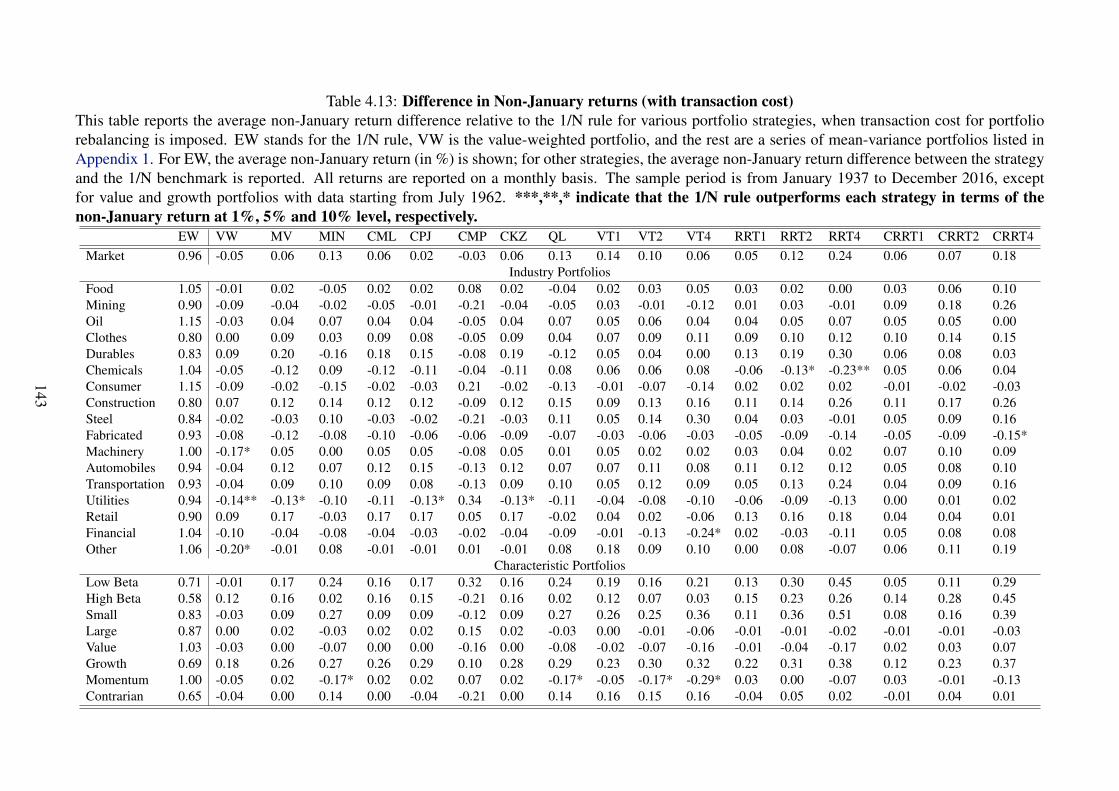
Table 4.13: Difference in Non-January returns (with transaction cost)This table reports the average non-January return difference relative to the 1/N rule for various portfolio strategies, when transaction cost for portfoliorebalancing is imposed. EW stands for the 1/N rule, VW is the value-weighted portfolio, and the rest are a series of mean-variance portfolios listed inAppendix 1. For EW, the average non-January return (in %) is shown; for other strategies, the average non-January return difference between the strategyand the 1/N benchmark is reported. All returns are reported on a monthly basis. The sample period is from January 1937 to December 2016, exceptfor value and growth portfolios with data starting from July 1962. ***,**,* indicate that the 1/N rule outperforms each strategy in terms of thenon-January return at 1%, 5% and 10% level, respectively.
EW VW MV MIN CML CPJ CMP CKZ QL VT1 VT2 VT4 RRT1 RRT2 RRT4 CRRT1 CRRT2 CRRT4Market 0.96 -0.05 0.06 0.13 0.06 0.02 -0.03 0.06 0.13 0.14 0.10 0.06 0.05 0.12 0.24 0.06 0.07 0.18
Industry PortfoliosFood 1.05 -0.01 0.02 -0.05 0.02 0.02 0.08 0.02 -0.04 0.02 0.03 0.05 0.03 0.02 0.00 0.03 0.06 0.10Mining 0.90 -0.09 -0.04 -0.02 -0.05 -0.01 -0.21 -0.04 -0.05 0.03 -0.01 -0.12 0.01 0.03 -0.01 0.09 0.18 0.26Oil 1.15 -0.03 0.04 0.07 0.04 0.04 -0.05 0.04 0.07 0.05 0.06 0.04 0.04 0.05 0.07 0.05 0.05 0.00Clothes 0.80 0.00 0.09 0.03 0.09 0.08 -0.05 0.09 0.04 0.07 0.09 0.11 0.09 0.10 0.12 0.10 0.14 0.15Durables 0.83 0.09 0.20 -0.16 0.18 0.15 -0.08 0.19 -0.12 0.05 0.04 0.00 0.13 0.19 0.30 0.06 0.08 0.03Chemicals 1.04 -0.05 -0.12 0.09 -0.12 -0.11 -0.04 -0.11 0.08 0.06 0.06 0.08 -0.06 -0.13* -0.23** 0.05 0.06 0.04Consumer 1.15 -0.09 -0.02 -0.15 -0.02 -0.03 0.21 -0.02 -0.13 -0.01 -0.07 -0.14 0.02 0.02 0.02 -0.01 -0.02 -0.03Construction 0.80 0.07 0.12 0.14 0.12 0.12 -0.09 0.12 0.15 0.09 0.13 0.16 0.11 0.14 0.26 0.11 0.17 0.26Steel 0.84 -0.02 -0.03 0.10 -0.03 -0.02 -0.21 -0.03 0.11 0.05 0.14 0.30 0.04 0.03 -0.01 0.05 0.09 0.16Fabricated 0.93 -0.08 -0.12 -0.08 -0.10 -0.06 -0.06 -0.09 -0.07 -0.03 -0.06 -0.03 -0.05 -0.09 -0.14 -0.05 -0.09 -0.15*Machinery 1.00 -0.17* 0.05 0.00 0.05 0.05 -0.08 0.05 0.01 0.05 0.02 0.02 0.03 0.04 0.02 0.07 0.10 0.09Automobiles 0.94 -0.04 0.12 0.07 0.12 0.15 -0.13 0.12 0.07 0.07 0.11 0.08 0.11 0.12 0.12 0.05 0.08 0.10Transportation 0.93 -0.04 0.09 0.10 0.09 0.08 -0.13 0.09 0.10 0.05 0.12 0.09 0.05 0.13 0.24 0.04 0.09 0.16Utilities 0.94 -0.14** -0.13* -0.10 -0.11 -0.13* 0.34 -0.13* -0.11 -0.04 -0.08 -0.10 -0.06 -0.09 -0.13 0.00 0.01 0.02Retail 0.90 0.09 0.17 -0.03 0.17 0.17 0.05 0.17 -0.02 0.04 0.02 -0.06 0.13 0.16 0.18 0.04 0.04 0.01Financial 1.04 -0.10 -0.04 -0.08 -0.04 -0.03 -0.02 -0.04 -0.09 -0.01 -0.13 -0.24* 0.02 -0.03 -0.11 0.05 0.08 0.08Other 1.06 -0.20* -0.01 0.08 -0.01 -0.01 0.01 -0.01 0.08 0.18 0.09 0.10 0.00 0.08 -0.07 0.06 0.11 0.19
Characteristic PortfoliosLow Beta 0.71 -0.01 0.17 0.24 0.16 0.17 0.32 0.16 0.24 0.19 0.16 0.21 0.13 0.30 0.45 0.05 0.11 0.29High Beta 0.58 0.12 0.16 0.02 0.16 0.15 -0.21 0.16 0.02 0.12 0.07 0.03 0.15 0.23 0.26 0.14 0.28 0.45Small 0.83 -0.03 0.09 0.27 0.09 0.09 -0.12 0.09 0.27 0.26 0.25 0.36 0.11 0.36 0.51 0.08 0.16 0.39Large 0.87 0.00 0.02 -0.03 0.02 0.02 0.15 0.02 -0.03 0.00 -0.01 -0.06 -0.01 -0.01 -0.02 -0.01 -0.01 -0.03Value 1.03 -0.03 0.00 -0.07 0.00 0.00 -0.16 0.00 -0.08 -0.02 -0.07 -0.16 -0.01 -0.04 -0.17 0.02 0.03 0.07Growth 0.69 0.18 0.26 0.27 0.26 0.29 0.10 0.28 0.29 0.23 0.30 0.32 0.22 0.31 0.38 0.12 0.23 0.37Momentum 1.00 -0.05 0.02 -0.17* 0.02 0.02 0.07 0.02 -0.17* -0.05 -0.17* -0.29* 0.03 0.00 -0.07 0.03 -0.01 -0.13Contrarian 0.65 -0.04 0.00 0.14 0.00 -0.04 -0.21 0.00 0.14 0.16 0.15 0.16 -0.04 0.05 0.02 -0.01 0.04 0.01
143
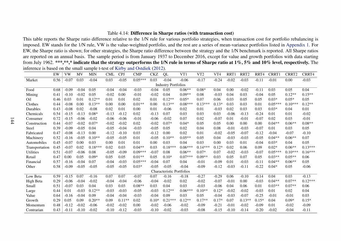
Table 4.14: Difference in Sharpe ratios (with transaction cost)This table reports the Sharpe ratio difference relative to the 1/N rule for various portfolio strategies, when transaction cost for portfolio rebalancing isimposed. EW stands for the 1/N rule, VW is the value-weighted portfolio, and the rest are a series of mean-variance portfolios listed in Appendix 1. ForEW, the Sharpe ratio is shown; for other strategies, the Sharpe ratio difference between the strategy and the 1/N benchmark is reported. All Sharpe ratiosare reported on an annual basis. The sample period is from January 1937 to December 2016, except for value and growth portfolios with data startingfrom July 1962. ***,**,* indicate that the strategy outperforms the 1/N rule in terms of Sharpe ratio at 1%, 5% and 10% level, respectively. Theinference is based on the small sample t-test of Kirby and Ostdiek (2012).
EW VW MV MIN CML CPJ CMP CKZ QL VT1 VT2 VT4 RRT1 RRT2 RRT4 CRRT1 CRRT2 CRRT4Market 0.56 -0.07 0.03 -0.04 0.03 -0.05 0.05*** 0.03 -0.04 -0.06 -0.17 -0.24 -0.02 -0.03 -0.11 -0.01 0.00 -0.03
Industry PortfoliosFood 0.68 -0.09 -0.04 0.05 -0.04 -0.04 -0.03 -0.04 0.05 0.06** 0.08* 0.04 0.00 -0.02 -0.11 0.03 0.05 0.04Mining 0.41 -0.10 -0.02 0.05 -0.02 0.00 -0.01 -0.02 0.04 0.09** 0.08 -0.03 0.04 0.03 -0.04 0.05 0.12** 0.15**Oil 0.46 0.03 0.01 0.12** 0.01 0.01 0.02 0.01 0.12** 0.05* 0.07 0.06 0.03 0.05 0.05 0.03* 0.05* 0.05Clothes 0.44 -0.08 0.00 0.13** 0.00 0.00 0.01** 0.00 0.13** 0.08*** 0.13*** 0.13* 0.03 0.03 0.01 0.05*** 0.10*** 0.12**Durables 0.43 -0.08 0.02 -0.08 0.02 0.01 0.00 0.01 -0.06 0.02 0.01 -0.03 0.02 0.03 0.03 0.03* 0.04 0.01Chemicals 0.54 -0.15 -0.13 0.08* -0.13 -0.12 0.02 -0.13 0.07 0.03 0.03 0.03 -0.06 -0.13 -0.24 0.01 0.01 -0.02Consumer 0.72 -0.15 -0.06 -0.02 -0.06 -0.06 -0.01 -0.06 -0.02 0.07 0.02 -0.07 0.01 -0.01 -0.07 0.02 0.03 -0.01Construction 0.44 -0.07 -0.02 0.07* -0.02 -0.02 0.02 -0.02 0.07* 0.04* 0.05 0.05 0.00 0.00 0.00 0.04** 0.06** 0.08**Steel 0.39 -0.09 -0.05 0.04 -0.05 -0.04 -0.03 -0.05 0.05 0.02 0.04 0.08 -0.01 -0.03 -0.07 0.01 0.03 0.05Fabricated 0.47 -0.08 -0.13 0.00 -0.12 -0.10 0.03 -0.12 0.00 0.02 0.01 -0.02 -0.05 -0.07 -0.12 -0.04 -0.07 -0.10Machinery 0.52 -0.16 -0.05 0.10** -0.05 -0.05 0.01 -0.05 0.10** 0.05** 0.05 0.04 -0.03 -0.03 -0.05 0.04** 0.06** 0.07Automobiles 0.45 -0.07 0.00 0.03 0.00 0.01 0.01 0.00 0.03 0.04 0.03 0.00 0.03 0.01 -0.04 0.03* 0.04 0.05Transportation 0.45 -0.07 0.02 0.18*** 0.02 0.03 0.04** 0.03 0.18*** 0.06*** 0.14*** 0.12* 0.02 0.06 0.09 0.02* 0.06** 0.13***Utilities 0.51 -0.07 -0.06 0.08 -0.05 -0.09 0.09*** -0.07 0.08 0.06** 0.07* 0.07 -0.02 -0.03 -0.07 0.05*** 0.10*** 0.16***Retail 0.47 0.00 0.05 0.09* 0.05 0.05 0.01** 0.05 0.10* 0.07*** 0.09** 0.03 0.05 0.07 0.05 0.03** 0.05** 0.06Financial 0.57 -0.16 -0.04 0.07 -0.04 -0.03 0.05*** -0.04 0.07 0.04 -0.01 -0.09 0.01 -0.03 -0.11 0.04** 0.06** 0.05Other 0.58 -0.09 -0.05 -0.05 -0.05 -0.05 0.03* -0.05 -0.05 -0.04 -0.09 -0.12 -0.03 -0.11 -0.22 0.04* 0.05 -0.06
Characteristic PortfoliosLow Beta 0.59 -0.15 0.07 -0.16 0.07 0.07 -0.07 0.07 -0.16 -0.18 -0.27 -0.29 0.06 -0.10 -0.14 0.04 0.03 -0.13High Beta 0.29 -0.06 -0.04 -0.02 -0.04 -0.04 -0.06 -0.04 -0.02 0.02 -0.02 -0.07 -0.01 0.00 -0.03 0.04** 0.07** 0.12***Small 0.51 -0.07 0.03 0.04 0.03 0.03 0.08** 0.03 0.04 0.03 -0.03 -0.06 0.04 0.06 0.01 0.03** 0.07** 0.06Large 0.44 0.01 -0.03 0.12** -0.03 -0.03 -0.05 -0.03 0.12** 0.06*** 0.10** 0.12* -0.02 -0.02 -0.03 0.01 0.02 0.04Value 0.64 -0.16 -0.04 0.09 -0.04 -0.04 -0.03 -0.04 0.09 0.03 0.05 -0.04 -0.03 -0.07 -0.25 -0.01 -0.01 0.03Growth 0.29 0.05 0.09 0.20** 0.09 0.11** 0.02 0.10* 0.21*** 0.12** 0.17** 0.17* 0.07 0.13** 0.15* 0.04 0.09* 0.15*Momentum 0.48 -0.12 -0.02 -0.06 -0.02 -0.02 0.00 -0.02 -0.06 -0.02 -0.09 -0.21 -0.01 -0.02 -0.09 0.01 -0.02 -0.09Contrarian 0.43 -0.11 -0.10 -0.02 -0.10 -0.12 -0.03 -0.10 -0.02 -0.03 -0.08 -0.15 -0.10 -0.14 -0.20 -0.02 -0.04 -0.11
144
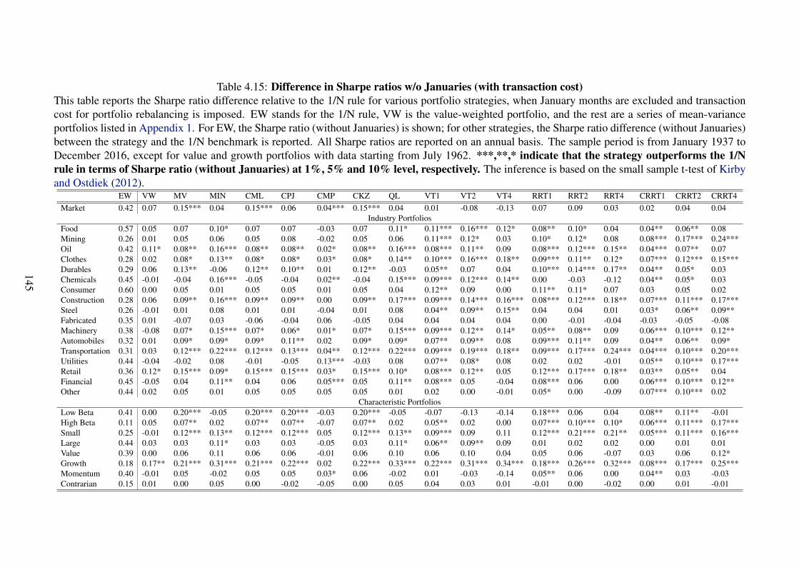
Table 4.15: Difference in Sharpe ratios w/o Januaries (with transaction cost)This table reports the Sharpe ratio difference relative to the 1/N rule for various portfolio strategies, when January months are excluded and transactioncost for portfolio rebalancing is imposed. EW stands for the 1/N rule, VW is the value-weighted portfolio, and the rest are a series of mean-varianceportfolios listed in Appendix 1. For EW, the Sharpe ratio (without Januaries) is shown; for other strategies, the Sharpe ratio difference (without Januaries)between the strategy and the 1/N benchmark is reported. All Sharpe ratios are reported on an annual basis. The sample period is from January 1937 toDecember 2016, except for value and growth portfolios with data starting from July 1962. ***,**,* indicate that the strategy outperforms the 1/Nrule in terms of Sharpe ratio (without Januaries) at 1%, 5% and 10% level, respectively. The inference is based on the small sample t-test of Kirbyand Ostdiek (2012).
EW VW MV MIN CML CPJ CMP CKZ QL VT1 VT2 VT4 RRT1 RRT2 RRT4 CRRT1 CRRT2 CRRT4Market 0.42 0.07 0.15*** 0.04 0.15*** 0.06 0.04*** 0.15*** 0.04 0.01 -0.08 -0.13 0.07 0.09 0.03 0.02 0.04 0.04
Industry PortfoliosFood 0.57 0.05 0.07 0.10* 0.07 0.07 -0.03 0.07 0.11* 0.11*** 0.16*** 0.12* 0.08** 0.10* 0.04 0.04** 0.06** 0.08Mining 0.26 0.01 0.05 0.06 0.05 0.08 -0.02 0.05 0.06 0.11*** 0.12* 0.03 0.10* 0.12* 0.08 0.08*** 0.17*** 0.24***Oil 0.42 0.11* 0.08** 0.16*** 0.08** 0.08** 0.02* 0.08** 0.16*** 0.08*** 0.11** 0.09 0.08*** 0.12*** 0.15** 0.04*** 0.07** 0.07Clothes 0.28 0.02 0.08* 0.13** 0.08* 0.08* 0.03* 0.08* 0.14** 0.10*** 0.16*** 0.18** 0.09*** 0.11** 0.12* 0.07*** 0.12*** 0.15***Durables 0.29 0.06 0.13** -0.06 0.12** 0.10** 0.01 0.12** -0.03 0.05** 0.07 0.04 0.10*** 0.14*** 0.17** 0.04** 0.05* 0.03Chemicals 0.45 -0.01 -0.04 0.16*** -0.05 -0.04 0.02** -0.04 0.15*** 0.09*** 0.12*** 0.14** 0.00 -0.03 -0.12 0.04** 0.05* 0.03Consumer 0.60 0.00 0.05 0.01 0.05 0.05 0.01 0.05 0.04 0.12** 0.09 0.00 0.11** 0.11* 0.07 0.03 0.05 0.02Construction 0.28 0.06 0.09** 0.16*** 0.09** 0.09** 0.00 0.09** 0.17*** 0.09*** 0.14*** 0.16*** 0.08*** 0.12*** 0.18** 0.07*** 0.11*** 0.17***Steel 0.26 -0.01 0.01 0.08 0.01 0.01 -0.04 0.01 0.08 0.04** 0.09** 0.15** 0.04 0.04 0.01 0.03* 0.06** 0.09**Fabricated 0.35 0.01 -0.07 0.03 -0.06 -0.04 0.06 -0.05 0.04 0.04 0.04 0.04 0.00 -0.01 -0.04 -0.03 -0.05 -0.08Machinery 0.38 -0.08 0.07* 0.15*** 0.07* 0.06* 0.01* 0.07* 0.15*** 0.09*** 0.12** 0.14* 0.05** 0.08** 0.09 0.06*** 0.10*** 0.12**Automobiles 0.32 0.01 0.09* 0.09* 0.09* 0.11** 0.02 0.09* 0.09* 0.07** 0.09** 0.08 0.09*** 0.11** 0.09 0.04** 0.06** 0.09*Transportation 0.31 0.03 0.12*** 0.22*** 0.12*** 0.13*** 0.04** 0.12*** 0.22*** 0.09*** 0.19*** 0.18** 0.09*** 0.17*** 0.24*** 0.04*** 0.10*** 0.20***Utilities 0.44 -0.04 -0.02 0.08 -0.01 -0.05 0.13*** -0.03 0.08 0.07** 0.08* 0.08 0.02 0.02 -0.01 0.05** 0.10*** 0.17***Retail 0.36 0.12* 0.15*** 0.09* 0.15*** 0.15*** 0.03* 0.15*** 0.10* 0.08*** 0.12** 0.05 0.12*** 0.17*** 0.18** 0.03** 0.05** 0.04Financial 0.45 -0.05 0.04 0.11** 0.04 0.06 0.05*** 0.05 0.11** 0.08*** 0.05 -0.04 0.08*** 0.06 0.00 0.06*** 0.10*** 0.12**Other 0.44 0.02 0.05 0.01 0.05 0.05 0.05 0.05 0.01 0.02 0.00 -0.01 0.05* 0.00 -0.09 0.07*** 0.10*** 0.02
Characteristic PortfoliosLow Beta 0.41 0.00 0.20*** -0.05 0.20*** 0.20*** -0.03 0.20*** -0.05 -0.07 -0.13 -0.14 0.18*** 0.06 0.04 0.08** 0.11** -0.01High Beta 0.11 0.05 0.07** 0.02 0.07** 0.07** -0.07 0.07** 0.02 0.05** 0.02 0.00 0.07*** 0.10*** 0.10* 0.06*** 0.11*** 0.17***Small 0.25 -0.01 0.12*** 0.13** 0.12*** 0.12*** 0.05 0.12*** 0.13** 0.09*** 0.09 0.11 0.12*** 0.21*** 0.21** 0.05*** 0.11*** 0.16***Large 0.44 0.03 0.03 0.11* 0.03 0.03 -0.05 0.03 0.11* 0.06** 0.09** 0.09 0.01 0.02 0.02 0.00 0.01 0.01Value 0.39 0.00 0.06 0.11 0.06 0.06 -0.01 0.06 0.10 0.06 0.10 0.04 0.05 0.06 -0.07 0.03 0.06 0.12*Growth 0.18 0.17** 0.21*** 0.31*** 0.21*** 0.22*** 0.02 0.22*** 0.33*** 0.22*** 0.31*** 0.34*** 0.18*** 0.26*** 0.32*** 0.08*** 0.17*** 0.25***Momentum 0.40 -0.01 0.05 -0.02 0.05 0.05 0.03* 0.06 -0.02 0.01 -0.03 -0.14 0.05** 0.06 0.00 0.04** 0.03 -0.03Contrarian 0.15 0.01 0.00 0.05 0.00 -0.02 -0.05 0.00 0.05 0.04 0.03 0.01 -0.01 0.00 -0.02 0.00 0.01 -0.01
145
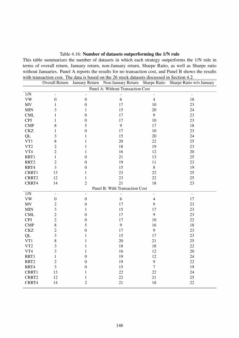
Table 4.16: Number of datasets outperforming the 1/N ruleThis table summarizes the number of datasets in which each strategy outperforms the 1/N rule interms of overall return, January return, non-January return, Sharpe Ratio, as well as Sharpe ratiowithout Januaries. Panel A reports the results for no transaction cost, and Panel B shows the resultswith transaction cost. The data is based on the 26 stock datasets discussed in Section 4.2.
Overall Return January Return Non-January Return Sharpe Ratio Sharpe Ratio w/o JanuaryPanel A: Without Transaction Cost
1/N - - - - -VW 0 0 6 4 18MV 1 0 17 10 23MIN 3 1 15 20 24CML 1 0 17 9 23CPJ 1 0 17 10 23CMP 8 5 9 17 18CKZ 1 0 17 10 23QL 3 1 15 20 24VT1 8 1 20 22 25VT2 2 1 18 19 23VT4 2 1 16 12 20RRT1 1 0 21 13 25RRT2 2 0 19 11 23RRT4 3 0 15 8 19CRRT1 13 1 23 22 25CRRT2 12 1 23 22 25CRRT4 14 2 21 18 23
Panel B: With Transaction Cost1/N - - - - -VW 0 0 6 4 17MV 2 0 17 9 23MIN 3 1 15 17 23CML 2 0 17 9 23CPJ 2 0 17 10 22CMP 8 5 9 16 18CKZ 2 0 17 9 23QL 3 1 15 17 23VT1 8 1 20 21 25VT2 3 1 18 18 22VT4 3 1 16 12 20RRT1 1 0 19 12 24RRT2 2 0 19 9 22RRT4 3 0 15 7 19CRRT1 13 1 22 22 24CRRT2 12 1 22 21 25CRRT4 14 2 21 18 22
146
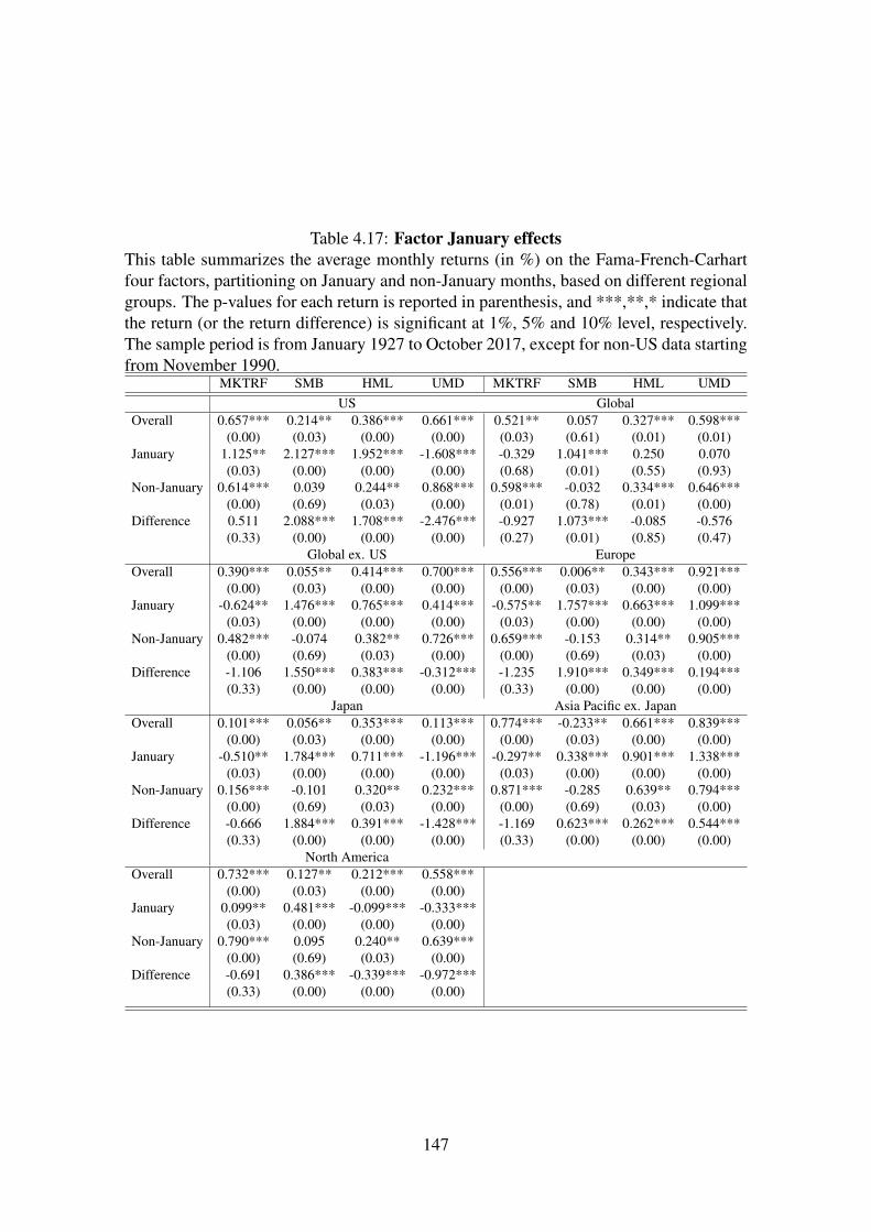
Table 4.17: Factor January effectsThis table summarizes the average monthly returns (in %) on the Fama-French-Carhartfour factors, partitioning on January and non-January months, based on different regionalgroups. The p-values for each return is reported in parenthesis, and ***,**,* indicate thatthe return (or the return difference) is significant at 1%, 5% and 10% level, respectively.The sample period is from January 1927 to October 2017, except for non-US data startingfrom November 1990.
MKTRF SMB HML UMD MKTRF SMB HML UMDUS Global
Overall 0.657*** 0.214** 0.386*** 0.661*** 0.521** 0.057 0.327*** 0.598***(0.00) (0.03) (0.00) (0.00) (0.03) (0.61) (0.01) (0.01)
January 1.125** 2.127*** 1.952*** -1.608*** -0.329 1.041*** 0.250 0.070(0.03) (0.00) (0.00) (0.00) (0.68) (0.01) (0.55) (0.93)
Non-January 0.614*** 0.039 0.244** 0.868*** 0.598*** -0.032 0.334*** 0.646***(0.00) (0.69) (0.03) (0.00) (0.01) (0.78) (0.01) (0.00)
Difference 0.511 2.088*** 1.708*** -2.476*** -0.927 1.073*** -0.085 -0.576(0.33) (0.00) (0.00) (0.00) (0.27) (0.01) (0.85) (0.47)
Global ex. US EuropeOverall 0.390*** 0.055** 0.414*** 0.700*** 0.556*** 0.006** 0.343*** 0.921***
(0.00) (0.03) (0.00) (0.00) (0.00) (0.03) (0.00) (0.00)January -0.624** 1.476*** 0.765*** 0.414*** -0.575** 1.757*** 0.663*** 1.099***
(0.03) (0.00) (0.00) (0.00) (0.03) (0.00) (0.00) (0.00)Non-January 0.482*** -0.074 0.382** 0.726*** 0.659*** -0.153 0.314** 0.905***
(0.00) (0.69) (0.03) (0.00) (0.00) (0.69) (0.03) (0.00)Difference -1.106 1.550*** 0.383*** -0.312*** -1.235 1.910*** 0.349*** 0.194***
(0.33) (0.00) (0.00) (0.00) (0.33) (0.00) (0.00) (0.00)Japan Asia Pacific ex. Japan
Overall 0.101*** 0.056** 0.353*** 0.113*** 0.774*** -0.233** 0.661*** 0.839***(0.00) (0.03) (0.00) (0.00) (0.00) (0.03) (0.00) (0.00)
January -0.510** 1.784*** 0.711*** -1.196*** -0.297** 0.338*** 0.901*** 1.338***(0.03) (0.00) (0.00) (0.00) (0.03) (0.00) (0.00) (0.00)
Non-January 0.156*** -0.101 0.320** 0.232*** 0.871*** -0.285 0.639** 0.794***(0.00) (0.69) (0.03) (0.00) (0.00) (0.69) (0.03) (0.00)
Difference -0.666 1.884*** 0.391*** -1.428*** -1.169 0.623*** 0.262*** 0.544***(0.33) (0.00) (0.00) (0.00) (0.33) (0.00) (0.00) (0.00)
North AmericaOverall 0.732*** 0.127** 0.212*** 0.558***
(0.00) (0.03) (0.00) (0.00)January 0.099** 0.481*** -0.099*** -0.333***
(0.03) (0.00) (0.00) (0.00)Non-January 0.790*** 0.095 0.240** 0.639***
(0.00) (0.69) (0.03) (0.00)Difference -0.691 0.386*** -0.339*** -0.972***
(0.33) (0.00) (0.00) (0.00)
147
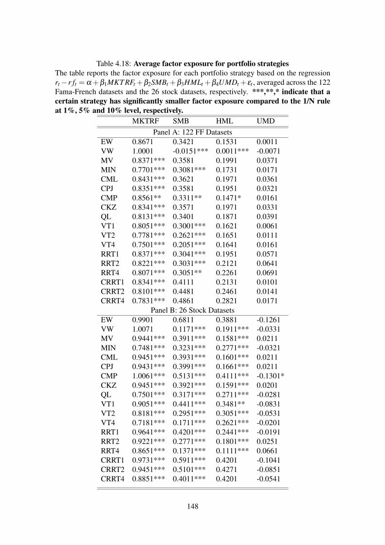
Table 4.18: Average factor exposure for portfolio strategiesThe table reports the factor exposure for each portfolio strategy based on the regressionrt− r ft = α +β1MKT RFt +β2SMBt +β3HMLt +β4UMDt +εt , averaged across the 122Fama-French datasets and the 26 stock datasets, respectively. ***,**,* indicate that acertain strategy has significantly smaller factor exposure compared to the 1/N ruleat 1%, 5% and 10% level, respectively.
MKTRF SMB HML UMDPanel A: 122 FF Datasets
EW 0.8671 0.3421 0.1531 0.0011VW 1.0001 -0.0151*** 0.0011*** -0.0071MV 0.8371*** 0.3581 0.1991 0.0371MIN 0.7701*** 0.3081*** 0.1731 0.0171CML 0.8431*** 0.3621 0.1971 0.0361CPJ 0.8351*** 0.3581 0.1951 0.0321CMP 0.8561** 0.3311** 0.1471* 0.0161CKZ 0.8341*** 0.3571 0.1971 0.0331QL 0.8131*** 0.3401 0.1871 0.0391VT1 0.8051*** 0.3001*** 0.1621 0.0061VT2 0.7781*** 0.2621*** 0.1651 0.0111VT4 0.7501*** 0.2051*** 0.1641 0.0161RRT1 0.8371*** 0.3041*** 0.1951 0.0571RRT2 0.8221*** 0.3031*** 0.2121 0.0641RRT4 0.8071*** 0.3051** 0.2261 0.0691CRRT1 0.8341*** 0.4111 0.2131 0.0101CRRT2 0.8101*** 0.4481 0.2461 0.0141CRRT4 0.7831*** 0.4861 0.2821 0.0171
Panel B: 26 Stock DatasetsEW 0.9901 0.6811 0.3881 -0.1261VW 1.0071 0.1171*** 0.1911*** -0.0331MV 0.9441*** 0.3911*** 0.1581*** 0.0211MIN 0.7481*** 0.3231*** 0.2771*** -0.0321CML 0.9451*** 0.3931*** 0.1601*** 0.0211CPJ 0.9431*** 0.3991*** 0.1661*** 0.0211CMP 1.0061*** 0.5131*** 0.4111*** -0.1301*CKZ 0.9451*** 0.3921*** 0.1591*** 0.0201QL 0.7501*** 0.3171*** 0.2711*** -0.0281VT1 0.9051*** 0.4411*** 0.3481** -0.0831VT2 0.8181*** 0.2951*** 0.3051*** -0.0531VT4 0.7181*** 0.1711*** 0.2621*** -0.0201RRT1 0.9641*** 0.4201*** 0.2441*** -0.0191RRT2 0.9221*** 0.2771*** 0.1801*** 0.0251RRT4 0.8651*** 0.1371*** 0.1111*** 0.0661CRRT1 0.9731*** 0.5911*** 0.4201 -0.1041CRRT2 0.9451*** 0.5101*** 0.4271 -0.0851CRRT4 0.8851*** 0.4011*** 0.4201 -0.0541
148
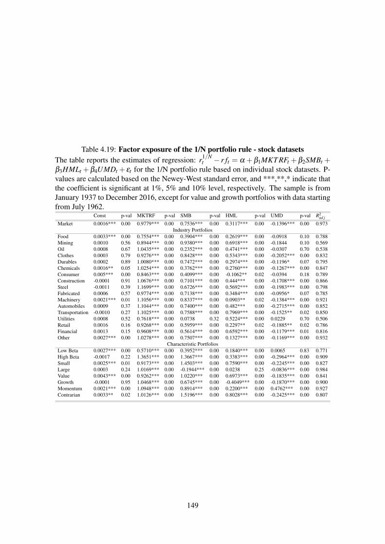
Table 4.19: Factor exposure of the 1/N portfolio rule - stock datasetsThe table reports the estimates of regression: r1/N
t − r ft = α +β1MKT RFt +β2SMBt +β3HMLt +β4UMDt + εt for the 1/N portfolio rule based on individual stock datasets. P-values are calculated based on the Newey-West standard error, and ***,**,* indicate thatthe coefficient is significant at 1%, 5% and 10% level, respectively. The sample is fromJanuary 1937 to December 2016, except for value and growth portfolios with data startingfrom July 1962.
Const p-val MKTRF p-val SMB p-val HML p-val UMD p-val R2ad j
Market 0.0016*** 0.00 0.9779*** 0.00 0.7536*** 0.00 0.3117*** 0.00 -0.1396*** 0.00 0.973Industry Portfolios
Food 0.0033*** 0.00 0.7554*** 0.00 0.3904*** 0.00 0.2619*** 0.00 -0.0918 0.10 0.788Mining 0.0010 0.56 0.8944*** 0.00 0.9380*** 0.00 0.6918*** 0.00 -0.1844 0.10 0.569Oil 0.0008 0.67 1.0435*** 0.00 0.2352*** 0.00 0.4741*** 0.00 -0.0307 0.70 0.538Clothes 0.0003 0.79 0.9276*** 0.00 0.8428*** 0.00 0.5343*** 0.00 -0.2052*** 0.00 0.832Durables 0.0002 0.89 1.0080*** 0.00 0.7472*** 0.00 0.2974*** 0.00 -0.1196* 0.07 0.795Chemicals 0.0016** 0.05 1.0254*** 0.00 0.3762*** 0.00 0.2760*** 0.00 -0.1267*** 0.00 0.847Consumer 0.005*** 0.00 0.8463*** 0.00 0.4099*** 0.00 -0.1062** 0.02 -0.0394 0.18 0.789Construction -0.0001 0.91 1.0676*** 0.00 0.7101*** 0.00 0.444*** 0.00 -0.1708*** 0.00 0.866Steel -0.0011 0.39 1.1699*** 0.00 0.6726*** 0.00 0.5692*** 0.00 -0.1983*** 0.00 0.798Fabricated 0.0006 0.57 0.9774*** 0.00 0.7138*** 0.00 0.3484*** 0.00 -0.0956* 0.07 0.785Machinery 0.0021*** 0.01 1.1056*** 0.00 0.8337*** 0.00 0.0903** 0.02 -0.1384*** 0.00 0.921Automobiles 0.0009 0.37 1.1044*** 0.00 0.7400*** 0.00 0.482*** 0.00 -0.2715*** 0.00 0.852Transportation -0.0010 0.27 1.1025*** 0.00 0.7588*** 0.00 0.7969*** 0.00 -0.1525** 0.02 0.850Utilities 0.0008 0.52 0.7618*** 0.00 0.0738 0.32 0.5224*** 0.00 0.0229 0.70 0.506Retail 0.0016 0.16 0.9268*** 0.00 0.5959*** 0.00 0.2297** 0.02 -0.1885** 0.02 0.786Financial 0.0013 0.15 0.9608*** 0.00 0.5614*** 0.00 0.6592*** 0.00 -0.1179*** 0.01 0.816Other 0.0027*** 0.00 1.0278*** 0.00 0.7507*** 0.00 0.1327*** 0.00 -0.1169*** 0.00 0.932
Characteristic PortfoliosLow Beta 0.0027*** 0.00 0.5710*** 0.00 0.3952*** 0.00 0.1840*** 0.00 0.0065 0.83 0.771High Beta -0.0017 0.22 1.3651*** 0.00 1.3667*** 0.00 0.3383*** 0.00 -0.2964*** 0.00 0.909Small 0.0025*** 0.01 0.9173*** 0.00 1.4503*** 0.00 0.7590*** 0.00 -0.2245*** 0.00 0.827Large 0.0003 0.24 1.0169*** 0.00 -0.1944*** 0.00 0.0238 0.25 -0.0836*** 0.00 0.984Value 0.0043*** 0.00 0.9262*** 0.00 1.0220*** 0.00 0.6973*** 0.00 -0.1835*** 0.00 0.841Growth -0.0001 0.95 1.0468*** 0.00 0.6745*** 0.00 -0.4049*** 0.00 -0.1870*** 0.00 0.900Momentum 0.0021*** 0.00 1.0948*** 0.00 0.8914*** 0.00 0.2200*** 0.00 0.4762*** 0.00 0.927Contrarian 0.0033** 0.02 1.0126*** 0.00 1.5196*** 0.00 0.8028*** 0.00 -0.2425*** 0.00 0.807
149
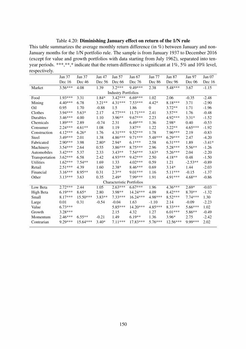
Table 4.20: Diminishing January effect on return of the 1/N ruleThis table summarizes the average monthly return difference (in %) between January and non-January months for the 1/N portfolio rule. The sample is from January 1937 to December 2016(except for value and growth portfolios with data starting from July 1962), separated into ten-year periods. ***,**,* indicate that the return difference is significant at 1%, 5% and 10% level,respectively.
Jan 37 Jan 37 Jan 47 Jan 57 Jan 67 Jan 77 Jan 87 Jan 97 Jan 07Dec 16 Dec 46 Dec 56 Dec 66 Dec 76 Dec 86 Dec 96 Dec 06 Dec 16
Market 3.56*** 4.08 1.39 3.2*** 9.49*** 2.38 5.48*** 3.67 -1.15Industry Portfolios
Food 1.93*** 3.31 1.84* 3.42*** 6.69*** 1.02 2.06 -0.35 -2.48Mining 4.40*** 6.78 3.21** 4.31*** 7.53*** 4.42* 8.18*** 3.71 -2.90Oil 0.95 1.70 -0.88 1.5 1.86 0 3.72** 1.71 -1.96Clothes 3.94*** 5.63* 2.17 4.77*** 11.71*** 2.41 3.57** 1.76 -0.48Durables 3.46*** 4.00 1.10 3.96** 9.67*** 2.23 4.92*** 3.31* -1.52Chemicals 1.89*** 2.89 -0.74 2.31 6.49*** 1.36 2.98* 0.40 -0.53Consumer 2.24*** 4.61** 1.08 1.19 3.87** 1.22 3.22** 4.65*** -1.92Construction 4.12*** 6.26* 1.76 4.31*** 9.52*** 1.78 7.96*** 2.19 -0.83Steel 3.49*** 2.01 1.38 4.86*** 9.71*** 5.48*** 6.29*** 2.47 -4.20Fabricated 2.90*** 3.98 2.80* 2.94* 6.1*** 2.58 6.31*** 1.89 -3.41*Machinery 3.54*** 2.64 0.55 3.86*** 8.75*** 2.96 5.28*** 5.56** -1.26Automobiles 3.42*** 5.37 2.33 3.43** 7.54*** 3.63* 5.26*** 2.04 -2.20Transportation 3.62*** 6.58 2.42 4.93*** 9.42*** 2.50 4.18** 0.48 -1.50Utilities 1.62*** 7.54** 1.69 1.33 4.02*** 0.59 1.21 -2.53** -0.89Retail 2.51*** 4.39 1.60 2.38* 8.46*** 0.69 3.14* 1.44 -2.03Financial 3.16*** 8.95** 0.31 2.3** 9.01*** 1.16 5.11*** -0.15 -1.37Other 3.13*** 3.63 0.35 2.49* 7.99*** 1.91 4.91*** 4.68** -0.86
Characteristic PortfoliosLow Beta 2.72*** 2.44 1.05 2.63*** 6.67*** 1.96 4.36*** 2.69* -0.03High Beta 6.19*** 8.65* 2.80 3.98** 14.24*** 4.09 8.42*** 8.70** -1.32Small 8.17*** 15.50*** 3.83** 7.33*** 16.24*** 4.98*** 8.52*** 7.74*** 1.30Large 0.01 0.31 -0.54 -0.04 1.63 -1.10 2.14 -0.09 -2.23Value 6.73*** 5.85*** 14.20*** 4.85*** 8.33*** 5.66*** 1.02Growth 3.28*** 2.15 4.32 1.27 6.01*** 5.86** -0.49Momentum 2.46*** 6.55** -0.21 1.49 6.19** 1.36 3.96* 2.75 -2.42Contrarian 9.29*** 15.64*** 3.40* 7.11*** 17.83*** 5.76*** 12.56*** 9.99*** 2.02
150
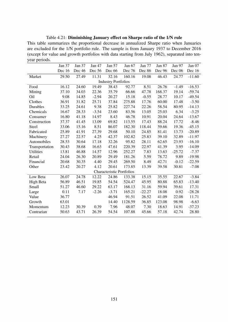
Table 4.21: Diminishing January effect on Sharpe ratio of the 1/N ruleThis table summarizes the proportional decrease in annualized Sharpe ratio when Januariesare excluded for the 1/N portfolio rule. The sample is from January 1937 to December 2016(except for value and growth portfolios with data starting from July 1962), separated into ten-year periods.
Jan 37 Jan 37 Jan 47 Jan 57 Jan 67 Jan 77 Jan 87 Jan 97 Jan 07Dec 16 Dec 46 Dec 56 Dec 66 Dec 76 Dec 86 Dec 96 Dec 06 Dec 16
Market 29.50 27.49 11.31 32.16 160.16 19.08 46.43 24.77 -11.60Industry Portfolios
Food 16.12 24.60 19.49 38.43 92.77 8.51 26.76 -1.49 -16.53Mining 37.10 34.03 22.36 35.79 66.66 47.78 168.37 19.14 -59.74Oil 9.08 14.85 -2.94 20.27 15.18 -0.55 28.77 10.17 -49.54Clothes 36.91 31.82 25.71 37.84 275.88 17.76 60.00 17.48 -3.50Durables 33.25 24.61 9.38 25.82 227.74 22.26 58.54 80.95 -14.13Chemicals 16.67 28.33 -3.54 23.60 83.56 13.05 25.03 6.34 -3.25Consumer 16.80 41.18 14.97 8.43 46.78 10.91 20.04 24.64 -13.67Construction 37.37 41.45 13.09 69.82 113.55 17.43 88.24 17.72 -8.46Steel 33.06 15.16 8.51 86.07 182.30 118.44 59.66 19.36 -45.15Fabricated 25.89 41.91 27.39 29.68 50.10 24.85 81.41 13.73 -20.89Machinery 27.27 22.57 4.25 42.37 102.82 25.83 39.10 32.89 -11.97Automobiles 28.53 30.64 17.18 32.26 95.82 28.11 62.65 23.93 -16.10Transportation 30.43 38.68 16.63 47.61 220.39 22.97 41.39 3.95 -14.09Utilities 13.81 46.88 14.57 12.96 252.27 7.83 13.63 -25.72 -7.37Retail 24.04 26.30 20.89 29.49 181.26 5.59 78.72 9.89 -19.98Financial 20.68 30.35 4.40 29.45 269.50 8.49 42.71 -0.12 -22.59Other 23.42 20.27 4.12 20.61 173.85 13.39 39.58 30.81 -7.08
Characteristic PortfoliosLow Beta 26.07 24.78 12.22 24.86 133.38 15.15 35.55 22.67 -3.84High Beta 56.89 46.51 19.85 54.54 524.47 45.95 80.88 65.83 -13.40Small 51.27 46.60 29.22 63.17 168.13 31.16 59.94 39.61 17.31Large 0.11 7.17 -2.26 -3.71 165.21 -22.27 18.08 0.92 -28.28Value 36.77 46.94 91.51 26.52 41.09 22.08 11.71Growth 63.01 14.40 1128.59 36.85 123.08 98.98 -6.63Momentum 12.23 30.39 0.39 7.96 48.07 7.30 18.63 14.91 -37.23Contrarian 50.63 43.71 26.39 54.54 107.88 45.66 57.18 42.74 28.80
151
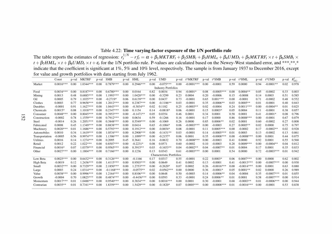
Table 4.22: Time varying factor exposure of the 1/N portfolio ruleThe table reports the estimates of regression: r1/N
t − r ft = α +β1MKT RFt +β2SMBt +β3HMLt +β4UMDt +β5MKT RFt × t +β6SMBt ×t +β7HMLt × t +β8UMDt × t + εt for the 1/N portfolio rule. P-values are calculated based on the Newey-West standard error, and ***,**,*indicate that the coefficient is significant at 1%, 5% and 10% level, respectively. The sample is from January 1937 to December 2016, exceptfor value and growth portfolios with data starting from July 1962.
Const p-val MKTRF p-val SMB p-val HML p-val UMD p-val t*MKTRF p-val t*SMB p-val t*HML p-val t*UMD p-val R2ad j
Market 0.0016*** 0.00 1.0344*** 0.00 0.7879*** 0.00 0.2946*** 0.00 -0.075*** 0.00 -0.0001*** 0.00 -0.0001 0.59 0.0000 0.94 -0.0001** 0.02 0.978Industry Portfolios
Food 0.0034*** 0.00 0.8187*** 0.00 0.6780*** 0.00 0.0164 0.82 0.0034 0.94 -0.0001* 0.08 -0.0005*** 0.00 0.0004** 0.05 -0.0002 0.33 0.803Mining 0.0013 0.48 0.6885*** 0.00 1.1993*** 0.00 1.0420*** 0.00 -0.3299 0.23 0.0004 0.20 -0.0006 0.15 -0.0008 0.14 0.0003 0.51 0.585Oil 0.0005 0.79 1.1035*** 0.00 -0.2719* 0.06 0.6139*** 0.00 0.0437 0.73 -0.0001 0.65 0.001*** 0.00 -0.0001 0.71 -0.0002 0.48 0.552Clothes 0.0003 0.77 0.9658*** 0.00 1.2012*** 0.00 0.2387*** 0.00 -0.1186** 0.03 -0.0001 0.35 -0.0006** 0.03 0.0005** 0.01 -0.0001 0.40 0.843Durables -0.0001 0.91 1.1627*** 0.00 1.0443*** 0.00 -0.3034** 0.02 0.1182 0.25 -0.0003** 0.02 -0.0004 0.24 0.0011*** 0.00 -0.0004** 0.01 0.825Chemicals 0.0015* 0.08 1.1018*** 0.00 0.2347*** 0.00 0.1154 0.14 -0.0818* 0.06 -0.0001 0.15 0.0003* 0.05 0.0004 0.11 -0.0001 0.38 0.857Consumer 0.0048*** 0.00 0.8045*** 0.00 0.3953*** 0.00 -0.1471** 0.05 0.0354 0.46 0.0001 0.34 0.0001 0.58 0.0001 0.41 -0.0001* 0.08 0.796Construction -0.0002 0.78 1.1559*** 0.00 0.7912*** 0.00 0.0634 0.59 -0.1266 0.16 -0.0001 0.17 0.0000 0.86 0.0008*** 0.00 -0.0001 0.67 0.879Steel -0.0014 0.26 1.2051*** 0.00 0.3848*** 0.00 0.5549*** 0.00 -0.1069 0.26 0.0000 0.85 0.0006** 0.02 0.0001 0.60 -0.0002 0.27 0.808Fabricated 0.0008 0.45 1.1349*** 0.00 0.8838*** 0.00 0.0414 0.65 -0.1084* 0.06 -0.0003*** 0.00 -0.0003 0.27 0.0005** 0.02 0.0000 0.75 0.797Machinery 0.0020*** 0.01 1.1686*** 0.00 0.5793*** 0.00 0.1912*** 0.00 -0.0654* 0.08 -0.0001 0.11 0.0005*** 0.00 -0.0002 0.17 -0.0002** 0.02 0.928Automobiles 0.0010 0.34 1.1619*** 0.00 1.0534*** 0.00 0.2908*** 0.00 -0.1431** 0.03 -0.0001 0.14 -0.0005*** 0.01 0.0003 0.13 -0.0002 0.13 0.861Transportation -0.0005 0.56 0.9974*** 0.00 1.1306*** 0.00 1.1099*** 0.00 -0.2157* 0.06 0.0001 0.35 -0.0008*** 0.00 -0.0008*** 0.00 0.0001 0.44 0.875Utilities 0.0016 0.14 1.1274*** 0.00 0.2095 0.45 0.3641 0.16 -0.0632 0.70 -0.0008*** 0.00 -0.0003 0.41 0.0000 0.92 0.0001 0.55 0.568Retail 0.0012 0.22 1.022*** 0.00 0.8507*** 0.00 -0.2231* 0.08 0.0571 0.60 -0.0002 0.10 -0.0003 0.28 0.0009*** 0.00 -0.0004** 0.04 0.812Financial 0.0016* 0.07 1.0379*** 0.00 0.9565*** 0.00 0.3915** 0.03 -0.1653** 0.04 -0.0002** 0.04 -0.0007** 0.01 0.0004 0.17 0.0001 0.35 0.833Other 0.0027*** 0.00 1.1804*** 0.00 0.7166*** 0.00 0.1236 0.13 0.0343 0.61 -0.0003*** 0.00 0.0001 0.54 0.0000 0.72 -0.0003*** 0.01 0.942
Characteristic PortfoliosLow Beta 0.0025*** 0.00 0.6432*** 0.00 0.3126*** 0.00 -0.1166 0.17 0.0317 0.55 -0.0001 0.22 0.0003* 0.06 0.0007*** 0.00 0.0000 0.62 0.802High Beta -0.0019 0.12 1.2436*** 0.00 1.4115*** 0.00 0.9503*** 0.00 0.0649 0.41 0.0002 0.13 -0.0001 0.41 -0.0013*** 0.00 -0.0007*** 0.00 0.930Small 0.0032*** 0.00 0.7329*** 0.00 2.1850*** 0.00 1.2753*** 0.00 -0.2620* 0.07 0.0002 0.26 -0.0016*** 0.00 -0.0014*** 0.00 0.0001 0.63 0.880Large 0.0003 0.24 1.0314*** 0.00 -0.1168*** 0.00 -0.0575** 0.02 -0.0562*** 0.00 0.0000 0.36 -0.0001* 0.05 0.0001** 0.02 0.0000 0.26 0.989Value 0.0038*** 0.00 0.9996*** 0.00 1.2164*** 0.00 0.8106*** 0.00 0.0648 0.50 -0.0003 0.14 -0.0006** 0.04 -0.0004 0.35 -0.0007*** 0.01 0.855Growth -0.0004 0.70 1.0825*** 0.00 0.4874*** 0.00 -0.4436*** 0.00 0.0593 0.33 -0.0001 0.24 0.0006** 0.01 0.0001 0.58 -0.0007*** 0.00 0.914Momentum 0.0017*** 0.01 1.0488*** 0.00 0.9540*** 0.00 0.3834*** 0.00 0.8016*** 0.00 0.0001 0.30 -0.0001 0.68 -0.0003** 0.01 -0.0006*** 0.00 0.944Contrarian 0.0035** 0.01 0.7341*** 0.00 1.8359*** 0.00 1.5429*** 0.00 -0.1820* 0.07 0.0005*** 0.00 -0.0008*** 0.01 -0.0016*** 0.00 -0.0001 0.53 0.838
152

Chapter 5
Concluding remarks
The recent literature on portfolio choice proposes various mean-variance portfolio
strategies to challenge the naive 1/N rule. However, little attention has been paid to
whether these newly developed strategies truly outperform the naive benchmark on a
large sample basis. In addition, it is unclear whether the good performance of the 1/N
rule in constructing stock portfolios is due to the January seasonality of stock returns.
In this thesis, I shed some light on these questions.
The first essay of the thesis investigates the performance of mean-variance versus
1/N rules across a large number of datasets based on a newly proposed performance
test. The second essay reveals that when individual stocks are used for portfolio con-
struction, the superior performance of the 1/N rule relative to mean-variance strategies
is largely attributed to the well-known January seasonality. This chapter first summa-
rizes the main results and contributions of the thesis. It then discusses limitations of
the thesis and provides some possible directions for future research.
153

5.1 Summary of the Thesis
In Chapter 2, I review the extensive literature on naive diversification. I identify two
potential unsolved questions in the literature on the naive 1/N rule. The first question
concerns whether newly proposed “1/N outperformers” in the recent literature truly
outperform the 1/N rule on a large sample basis. Although the mean-variance portfo-
lio theory of Markowitz (1952, 1959) is widely applied in practice, the naive 1/N rule
has shown superior performance relative to mean-variance portfolios (DeMiguel, Gar-
lappi, and Uppal, 2009b). Advocates of the mean-variance theory have not ceased in
their efforts to develop mean-variance strategies via different channels to outperform
the naive benchmark. However, the outperformance is often demonstrated based on a
small number of pre-selected empirical datasets. It is unclear whether this outperfor-
mance is associated with the datasets chosen. In other words, is the outperformance
robust on a large sample basis?
The second question that remains unclear concerns how the January seasonality of
stock returns affects the portfolio horse races between mean-variance and 1/N rules in
forming stock portfolios. The early literature on the January seasonality has shed light
on the fact that the returns on equally-weighted portfolios are systematically larger
in Januaries relative to other months (e.g., Gultekin and Gultekin, 1983; Keim, 1983;
Rozeff and Kinney, 1976). However, no prior study has explored the link between the
January seasonality and the performance of mean-variance versus 1/N diversification
rules.
154

In Chapter 3 (Essay 1), I study the sample selection issue in prior studies that
propose mean-variance strategies (“1/N outperformers”) to outperform the 1/N rule.
I design a novel performance test that conducts statistical inference on the average
performance across a large number of datasets, while existing performance tests, for
instance the tests of Jobson and Korkie (1981), Ledoit and Wolf (2008), and Kirby
and Ostdiek (2012), only investigate performance in a single dataset.
Based on the new test, portfolio horse races are performed with 122 datasets of
value-weighted portfolios, obtained from the French data library. These portfolios are
economically relevant assets, and involves factor portfolios, industries, characteristics,
and international stock indexes. Various “1/N outperformers” are tested against the
1/N rule based on the 122 datasets. Results show that although some of the “1/N
outperformers” are able to outperform the naive benchmark on average, they generally
do not deliver significant outperformance in terms of Sharpe ratio. The result is robust
to changing risk aversions, imposing shortsale constraints, as well as using expanding
rather than rolling estimation windows.
To understand the driving force behind the relative performance between the mean-
variance and 1/N rules, I examine how the utility difference between the mean-variance
portfolio and the 1/N portfolio is related to the assets’ return moments. Theoretically,
I find proportional changes in the mean, volatility and correlation affect the utility
difference. When estimation errors exist, a simulation exercise shows that the theoret-
ical results still hold when the mean-variance portfolio is imposed with the shortsale
constraints. Empirically, I find strong predictability of the out-of-sample performance
155

difference based on the in-sample return moments of assets. Furthermore, I design a
switching strategy that switches between a mean-variance rule and the 1/N rule based
on the predicted performance difference between the two rules. The switching strat-
egy significantly outperforms not only its raw mean-variance rule but also the 1/N rule
in terms of Sharpe ratio, certainty-equivalent (CEQ) return, and portfolio turnover, on
an average basis, in the 122 datasets.
This essay contributes to the literature on the debate between mean-variance ver-
sus naive diversification. It reveals a sample selection problem in claiming outperfor-
mance over the naive 1/N rule. The essay suggests to use a large number of datasets
for performance evaluations, and consider the average performance across datasets.
Theoretically and empirically, the performance of mean-variance strategies relative to
the 1/N rule is related to the return moments of underlying assets. It is recommended
to apply mean-variance or naive diversification in different investment scenarios de-
pending on the assets’ return moments.
In Chapter 4 (Essay 2), I investigate how January seasonality may affect the rel-
ative performance of mean-variance and 1/N rules. I find that the effect of January
seasonality on the relative performance depends on the assets used for portfolio con-
struction. When value-weighted indexes are used, as in DeMiguel, Garlappi, and
Uppal (2009b), the difference in Sharpe ratios between mean-variance rules and the
1/N rule is not substantially changed by excluding January returns. However, when
individual stocks are used for portfolio construction, the January returns of the 1/N
rule largely contribute to the Sharpe ratio of the naive rule. Mean-variance portfolios
156

fail to outperform the naive benchmark when all months are considered, but they gen-
erally deliver larger Sharpe ratios relative to the 1/N rule when Januaries are ruled out.
This result is consistent with and without transaction costs, across different industry
groups and various stock characteristics.
I find that the size factor exposure of the 1/N rule is the driving force behind the
contrary results. Compared with mean-variance rules, the 1/N rule has significantly
larger betas on the size factor in the stock datasets, but it shows comparable or even
smaller size factor exposures relative to mean-variance rules in the value-weighted
index datasets. The January seasonality is primarily a size effect (Keim, 1983). This
explains the different results obtained under the two empirical settings.
The equal weight rebalancing feature is actually related to the large January returns
for the 1/N rule, when individual stocks are used to form portfolios. The rebalancing
process of the 1/N rule leads to positive exposures to the size and value factors, and
a negative exposure to the momentum factor. Since small and value stocks have a
remarkable January returns, and momentum stocks exhibit a reversed January pattern,
the 1/N rule bets on all the correct directions of factors and locks in massive returns
in Januaries. However, I also find that the January seasonality of the 1/N rule is dis-
appearing in the data of recent years in which the naive rule tends to produce smaller
January returns than non-January returns, and its Sharpe ratio even increases when
January returns are excluded.
This essay is the first to link the relative performance of the mean-variance versus
1/N rules with the classic January seasonality. The results suggest that when individ-
157

ual stocks are used for portfolio construction, portfolio horse races between mean-
variance and 1/N rules should take the January effect into consideration.
5.2 Limitations and Potential Future Research
No research is without limitations. In this section, I discuss some of the limitations of
this thesis and offer some directions for potential future research.
First, the mean-variance properties of optimal versus naive diversification (Sec-
tion 3.5) involves no estimation errors. This is because it is hard to attain the analytical
relations between the relative performance and the return moments when estimation
error is introduced. However, the simulation exercise in 3.5.3 produces results con-
sistent with the theoretical relations for the constrained mean-variance portfolio, in
the presence of estimation errors. In addition, Section 3.6.3 finds that the predictive
directions based on returns, volatilities and correlations are generally consistent with
the theoretical relations. Second, the switching strategy in Section 3.6.4 is applied
to only the 1/N rule and a mean-variance rule. A natural extension would be a strat-
egy that switches across multiple mean-variance rules as well as the 1/N rule. Given
more candidate mean-variance rules to be considered, the performance could poten-
tially improves. Moreover, the 22 individual datasets in Essay 2 are based on US data.
Since the January seasonality is a global phenomenon, the investigation on the link
between the January seasonality and the relative performance of mean-variance ver-
sus 1/N rules can be conducted based on data from other countries. This could be left
158

for future work.
The findings presented in this thesis have additional implications for future re-
search. First, aside from the strategies tested in this study, plenty of other mean-
variance strategies have been developed to outperform the 1/N rule (e.g., Anderson
and Cheng, 2016; Behr et al., 2013; DeMiguel, Garlappi, Nogales, and Uppal, 2009a;
Kirby and Ostdiek, 2013). The large-sample performance test could be applied to
all these “1/N outperformers” to examine the sample selection issue. Second, the
performance evaluations on mean-variance and 1/N rules presented in this thesis are
conducted at monthly frequencies, and stocks are used as constituent assets. Although
this is standard practice in the literature, portfolio horse races could be conducted at
daily, weekly, and quarterly frequencies, and could be applied to other asset classes.
Third, the second essay in this thesis reveals the link between the January season-
ality and the performance of mean-variance versus 1/N rules. On the one hand, the
literature has shown that the January seasonality could be related to the tax-loss sell-
ing hypothesis (Reinganum, 1983, among others). On the other hand, Fischer and
Gallmeyer (2016) find that no trading strategy can outperform a 1/N trading strategy
augmented with a tax heuristic. A natural extension is to study the interactions among
the January seasonality, the tax benefit, and the performance of mean-variance versus
1/N diversification.
159
Bibliography
Anderson, E. W., and A.-R. Cheng. 2016. Robust Bayesian Portfolio Choices.
Review of Financial Studies 29:1330–1375.
At-Sahalia, Y., and M. W. Brandt. 2001. Variable Selection for Portfolio Choice.
Journal of Finance 56:1297–1351.
Baltussen, G., and G. T. Post. 2011. Irrational Diversification: An Examination
of Individual Portfolio Choice. Journal of Financial and Quantitative Analysis
46:1463–1491.
Barry, C. B. 1974. Portfolio analysis under uncertain means, variances, and co-
variances. Journal of Finance 29:515–522.
Behr, P., A. Guettler, and F. Miebs. 2013. On portfolio optimization: Imposing
the right constraints. Journal of Banking & Finance 37:1232–1242.
Benartzi, S., and R. H. Thaler. 2001. Naive diversification strategies in defined
contribution saving plans. American Economic Eeview pp. 79–98.
Black, F., and R. Litterman. 1992. Global Portfolio Optimization. Financial
Analysts Journal 48:28–43.
160
Branch, B. 1977. A tax loss trading rule. Journal of Business 50:198–207.
Brandt, M. W. 1999. Estimating Portfolio and Consumption Choice: A Condi-
tional Euler Equations Approach. Journal of Finance 54:1609–1645.
Brandt, M. W., and P. Santa-Clara. 2006. Dynamic Portfolio Selection by Aug-
menting the Asset Space. Journal of Finance 61:2187–2217.
Brandt, M. W., P. Santa-Clara, and R. Valkanov. 2009. Parametric Portfolio Poli-
cies: Exploiting Characteristics in the Cross-Section of Equity Returns. Review
of Financial Studies 22:3411–3447.
Brown, P., D. B. Keim, A. W. Kleidon, and T. A. Marsh. 1983. Stock return
seasonalities and the tax-loss selling hypothesis: Analysis of the arguments
and Australian evidence. Journal of Financial Economics 12:105–127.
Brown, S. 1979. The effect of estimation risk on capital market equilibrium.
Journal of Financial and Quantitative Analysis 14:215–220.
Brown, S. J., I. Hwang, and F. In. 2013. Why optimal diversification cannot out-
perform naive diversification: Evidence from tail risk exposure. SSRN Working
Paper .
Campbell, J. Y., Y. L. Chan, and L. M. Viceira. 2003. A multivariate model of
strategic asset allocation. Journal of Financial Economics 67:41–80.
Campbell, J. Y., and L. M. Viceira. 2005. The Term Structure of the Risk: Return
Trade-Off. Financial Analysts Journal 61:34–44.
161

Carhart, M. M. 1997. On persistence in mutual fund performance. Journal of
Finance 52:57–82.
Carhart, M. M., J. N. Carpenter, A. W. Lynch, and D. K. Musto. 2002. Mutual
fund survivorship. Review of Financial Studies 15:1439–1463.
Chan, L. K., N. Jegadeesh, and J. Lakonishok. 1995. Evaluating the performance
of value versus glamour stocks The impact of selection bias. Journal of Finan-
cial Economics 38:269–296.
Chang, E. C., and J. M. Pinegar. 1989. Seasonal fluctuations in industrial pro-
duction and stock market seasonals. Journal of Financial and Quantitative
Analysis 24:59–74.
Chang, E. C., and J. M. Pinegar. 1990. Stock market seasonals and prespecified
multifactor pricing relations. Journal of Financial and Quantitative Analysis
25:517–533.
Chen, N.-F., R. Roll, and S. A. Ross. 1986. Economic forces and the stock market.
Journal of Business pp. 383–403.
Clark, R. A., J. McConnell, and M. Singh. 1992. Seasonalities in NYSE bid-ask
spreads and stock returns in January. The Journal of Finance 47:1999–2014.
Cohen, K. J., and J. A. Pogue. 1967. An empirical evaluation of alternative
portfolio-selection models. Journal of Business pp. 166–193.
162
De Bondt, W. F., and R. Thaler. 1985. Does the stock market overreact? Journal
of Finance 40:793–805.
De Bondt, W. F., and R. H. Thaler. 1987. Further evidence on investor overreac-
tion and stock market seasonality. Journal of Finance 42:557–581.
DeMiguel, V., L. Garlappi, F. J. Nogales, and R. Uppal. 2009a. A Generalized
Approach to Portfolio Optimization: Improving Performance by Constraining
Portfolio Norms. Management Science 55:798–812.
DeMiguel, V., L. Garlappi, and R. Uppal. 2009b. Optimal versus naive diversi-
fication: How inefficient is the 1/N portfolio strategy? Review of Financial
Studies 22:1915–1953.
DeMiguel, V., A. Martin-Utrera, and F. J. Nogales. 2013. Size matters: Optimal
calibration of shrinkage estimators for portfolio selection. Journal of Banking
& Finance 37:3018–3034.
Duchin, R., and H. Levy. 2009. Markowitz versus the Talmudic portfolio diver-
sification strategies. Journal of Portfolio Management 35:71–74.
Dyl, E. A. 1977. Capital gains taxation and year-end stock market behavior.
Journal of Finance 32:165–175.
Fama, E. F., and K. R. French. 1992. The cross-section of expected stock returns.
Journal of Finance 47:427–465.
163
Fama, E. F., and K. R. French. 1993. Common risk factors in the returns on stocks
and bonds. Journal of Financial Economics 33:3–56.
Fama, E. F., and K. R. French. 2015. A five-factor asset pricing model. Journal
of Financial Economics 116:1 – 22.
Fischer, M., and M. F. Gallmeyer. 2016. Heuristic portfolio trading rules with
capital gain taxes. Journal of Financial Economics 119:611–625.
Frost, P. A., and J. E. Savarino. 1986. An empirical Bayes approach to efficient
portfolio selection. Journal of Financial and Quantitative Analysis 21:293–
305.
Frost, P. A., and J. E. Savarino. 1988. For better performance: Constrain portfolio
weights. Journal of Portfolio Management 15:29–34.
Garlappi, L., R. Uppal, and T. Wang. 2007. Portfolio selection with parameter
and model uncertainty: A multi-prior approach. Review of Financial Studies
20:41–81.
Givoly, D., and A. Ovadia. 1983. Year-End Tax-Induced Sales and Stock Market
Seasonality. Journal of Finance 38:171–185.
Grundy, B. D., and J. S. Martin. 2001. Understanding the nature of the risks and
the source of the rewards to momentum investing. Review of Financial Studies
14:29–78.
164

Gu, A. Y. 2003. The declining January effect: evidences from the US equity
markets. Quarterly Review of Economics and Finance 43:395–404.
Gultekin, M. N., and N. B. Gultekin. 1983. Stock market seasonality: Interna-
tional evidence. Journal of Financial Economics 12:469–481.
Hoevenaars, R. P., R. D. Molenaar, P. C. Schotman, and T. Steenkamp. 2008.
Strategic asset allocation with liabilities: Beyond stocks and bonds. Journal of
Economic Dynamics and Control 32:2939–2970.
Hou, K., C. Xue, and L. Zhang. 2015. Digesting Anomalies: An Investment
Approach. Review of Financial Studies 28:650.
Jaffe, J., D. B. Keim, and R. Westerfield. 1989. Earnings yields, market values,
and stock returns. Journal of Finance pp. 135–148.
Jagannathan, R., and T. Ma. 2003. Risk reduction in large portfolios: Why im-
posing the wrong constraints helps. Journal of Finance 58:1651–1684.
James, W., and C. Stein. 1961. Estimation with quadratic loss. Proceedings
of the fourth Berkeley symposium on mathematical statistics and probability
1:361–379.
Jegadeesh, N., and S. Titman. 1993. Returns to buying winners and selling losers:
Implications for stock market efficiency. Journal of Finance 48:65–91.
Jegadeesh, N., and S. Titman. 2001. Profitability of momentum strategies: An
evaluation of alternative explanations. Journal of Finance 56:699–720.
165
Jobson, J. D., and B. Korkie. 1980. Estimation for Markowitz efficient portfolios.
Journal of the American Statistical Association 75:544–554.
Jobson, J. D., and B. M. Korkie. 1981. Performance hypothesis testing with the
Sharpe and Treynor measures. Journal of Finance 36:889–908.
Jones, C. P., D. K. Pearce, and J. W. Wilson. 1987. Can tax-loss selling explain
the January effect? A note. Journal of Finance 42:453–461.
Jorion, P. 1985. International portfolio diversification with estimation risk. The
Journal of Business 58:259–78.
Jorion, P. 1986. Bayes-Stein estimation for portfolio analysis. Journal of Finan-
cial and Quantitative Analysis 21:279–292.
Kan, R., X. Wang, and G. Zhou. 2016. Optimal Portfolio Selection with and
Without Risk-Free Asset. SSRN Working Paper .
Kan, R., and G. Zhou. 2007. Optimal Portfolio Choice with Parameter Uncer-
tainty. Journal of Financial and Quantitative Analysis 42:621–656.
Keim, D. B. 1983. Size-related anomalies and stock return seasonality: Further
empirical evidence. Journal of Financial Economics 12:13–32.
Kim, D. 1997. A reexamination of firm size, book-to-market, and earnings price
in the cross-section of expected stock returns. Journal of Financial and Quan-
titative Analysis 32:463–489.
166
Kirby, C., and B. Ostdiek. 2012. Its all in the timing: simple active portfo-
lio strategies that outperform naive diversification. Journal of Financial and
Quantitative Analysis 47:437–467.
Kirby, C., and B. Ostdiek. 2013. Optimizing the performance of sample mean-
variance efficient portfolios. In AFA 2013 San Diego Meetings Paper.
Klein, R. W., and V. S. Bawa. 1976. The effect of estimation risk on optimal
portfolio choice. Journal of Financial Economics 3:215–231.
Kothari, S. P., J. Shanken, and R. G. Sloan. 1995. Another look at the crosssection
of expected stock returns. Journal of Finance 50:185–224.
Kramer, C. 1994. Macroeconomic seasonality and the January effect. Journal of
Finance 49:1883–1891.
Lakonishok, J., A. Shleifer, R. Thaler, and R. Vishny. 1991. Window dressing by
pension fund managers. American Economic Review 81:227–231.
Ledoit, O., and M. Wolf. 2003. Improved estimation of the covariance matrix of
stock returns with an application to portfolio selection. Journal of Empirical
Finance 10:603–621.
Ledoit, O., and M. Wolf. 2004a. Honey, I shrunk the sample covariance matrix.
Journal of Portfolio Management 30:110–119.
Ledoit, O., and M. Wolf. 2004b. A well-conditioned estimator for large-
167
dimensional covariance matrices. Journal of Multivariate Analysis 88:365–
411.
Ledoit, O., and M. Wolf. 2008. Robust performance hypothesis testing with the
Sharpe ratio. Journal of Empirical Finance 15:850–859.
MacKinlay, A. C., and L. Pastor. 2000. Asset pricing models: implications for
expected returns and portfolio selection. Review of Financial studies 13:883–
916.
Markowitz, H. 1952. Portfolio Selection. Journal of Finance 7:77–91.
Markowitz, H. 1959. Portfolio Selection: Efficient Diversification of Investments,
New York, John Wiely & Sons.
Mehdian, S., and M. J. Perry. 2002. Anomalies in US equity markets: A re-
examination of the January effect. Applied Financial Economics 12:141–145.
Memmel, C. 2003. Performance Hypothesis Testing with the Sharpe Ratio. Fi-
nance Letters 1:21–23.
Michaud, R. O. 1989. The Markowitz optimization enigma: is’ opti-
mized’optimal? Financial Analysts Journal pp. 31–42.
Moller, N., and S. Zilca. 2008. The evolution of the January effect. Journal of
Banking & Finance 32:447–457.
168
Newey, W. K., and K. D. West. 1986. A simple, positive semi-definite, het-
eroskedasticity and autocorrelationconsistent covariance matrix.
Ogden, J. P. 1990. Turn-of-Month Evaluations of Liquid Profits and Stock Re-
turns: A Common Explanation for the Monthly and January Effects. Journal
of Finance 45:1259–1272.
Pastor, L. 2000. Portfolio selection and asset pricing models. Journal of Finance
55:179–223.
Pastor, L., and R. F. Stambaugh. 2000. Comparing asset pricing models: an
investment perspective. Journal of Financial Economics 56:335–381.
Pflug, G. C., A. Pichler, and D. Wozabal. 2012. The 1/N investment strategy is
optimal under high model ambiguity. Journal of Banking & Finance 36:410–
417.
Plyakha, Y., R. Uppal, and G. Vilkov. 2014. Equal or value weighting? Implica-
tions for asset-pricing tests. SSRN Working Paper .
Politis, D. N., and J. P. Romano. 1994. The stationary bootstrap. Journal of the
American Statistical Association 89:1303–1313.
Rapach, D. E., J. K. Strauss, and G. Zhou. 2010. Out-of-Sample Equity Premium
Prediction: Combination Forecasts and Links to the Real Economy. Review of
Financial Studies 23:821–862.
169

Reinganum, M. R. 1983. The anomalous stock market behavior of small firms
in January: Empirical tests for tax-loss selling effects. Journal of Financial
Economics 12:89–104.
Riepe, M. W. 1998. Is publicity killing the January effect? Journal of Financial
Planning 11:64–70.
Ritter, J. R. 1988. The buying and selling behavior of individual investors at the
turn of the year. Journal of Finance 43:701–717.
Rozeff, M. S., and W. R. Kinney. 1976. Capital market seasonality: The case of
stock returns. Journal of Financial Economics 3:379–402.
Schultz, P. 1983. Transaction costs and the small firm effect: A comment. Journal
of Financial Economics 12:81–88.
Schultz, P. 1985. Personal income taxes and the January effect: Small firm stock
returns before the War Revenue Act of 1917: A note. Journal of Finance
40:333–343.
Seyhun, H. N. 1988. The January effect and aggregate insider trading. Journal
of Finance 43:129–141.
Shumway, T. 1997. The Delisting Bias in CRSP Data. Journal of Finance
52:327–340.
Shumway, T., and V. A. Warther. 1999. The delisting bias in CRSP’s Nasdaq data
and its implications for the size effect. Journal of Finance 54:2361–2379.
170
Sias, R. W., and L. T. Starks. 1997. Institutions and individuals at the turn-of-the-
year. Journal of Finance 52:1543–1562.
Stambaugh, R. F. 1997. Analyzing investments whose histories differ in length.
Journal of Financial Economics 45:285–331.
Stoll, H. R., and R. E. Whaley. 1983. Transaction costs and the small firm effect.
Journal of Financial Economics 12:57–79.
Tu, J., and G. Zhou. 2010. Incorporating economic objectives into Bayesian
priors: Portfolio choice under parameter uncertainty. Journal of Financial and
Quantitative Analysis 45:959–986.
Tu, J., and G. Zhou. 2011. Markowitz meets Talmud: A combination of sophis-
ticated and naive diversification strategies. Journal of Financial Economics
99:204–215.
Wang, Z. 2005. A shrinkage approach to model uncertainty and asset allocation.
Review of Financial Studies 18:673–705.
Yao, Y. 2012. Momentum, contrarian, and the January seasonality. Journal of
Banking & Finance 36:2757–2769.
171

Appendix
Appendix 1: List of Datasets
Dataset Time Period N Description1 7/1926-10/2017 3 Fama/French 3 Factors2 7/1963-10/2017 5 Fama/French 5 Factors3 7/1926-10/2017 10 10 Portfolios Formed on Size4 7/1926-10/2017 10 10 Portfolios Formed on Book-to-Market5 7/1963-10/2017 10 10 Portfolios Formed on Operating Profitability6 7/1963-10/2017 10 10 Portfolios Formed on Investment7 7/1926-10/2017 6 6 Portfolios Formed on Size and Book-to-Market8 7/1926-10/2017 25 25 Portfolios Formed on Size and Book-to-Market9 7/1926-10/2017 100 100 Portfolios Formed on Size and Book-to-Market
10 7/1963-10/2017 6 6 Portfolios Formed on Size and Operating Profitability11 7/1963-10/2017 25 25 Portfolios Formed on Size and Operating Profitability12 7/1963-10/2017 100 100 Portfolios Formed on Size and Operating Profitability13 7/1963-10/2017 6 6 Portfolios Formed on Size and Investment14 7/1963-10/2017 25 25 Portfolios Formed on Size and Investment15 7/1963-10/2017 100 100 Portfolios Formed on Size and Investment16 7/1963-10/2017 25 25 Portfolios Formed on Book-to-Market and Operating Profitability17 7/1963-10/2017 25 25 Portfolios Formed on Book-to-Market and Investment18 7/1963-10/2017 25 25 Portfolios Formed on Operating Profitability and Investment19 7/1963-10/2017 32 32 Portfolios Formed on Size, Book-to-Market, and Operating Profitability20 7/1963-10/2017 32 32 Portfolios Formed on Size, Book-to-Market, and Investment21 7/1963-10/2017 32 32 Portfolios Formed on Size, Operating Profitability, and Investment22 7/1951-10/2017 10 10 Portfolios Formed on Earnings/Price23 7/1951-10/2017 10 10 Portfolios Formed on Cashflow/Price24 7/1927-10/2017 10 10 Portfolios Formed on Dividend Yield25 1/1927-10/2017 4 FF3 + Momentum Factor (Mom)26 1/1927-10/2017 6 6 Portfolios Formed on Size and Momentum27 1/1927-10/2017 25 25 Portfolios Formed on Size and Momentum28 1/1927-10/2017 10 10 Portfolios Formed on Momentum29 1/1927-10/2017 5 FFC + Short-Term Reversal Factor (ST Rev)30 2/1926-10/2017 6 6 Portfolios Formed on Size and Short-Term Reversal31 2/1926-10/2017 25 25 Portfolios Formed on Size and Short-Term Reversal32 2/1926-10/2017 10 10 Portfolios Formed on Short-Term Reversal33 1/1931-10/2017 6 FFC + ST Rev + Long-Term Reversal Factor34 1/1931-10/2017 6 6 Portfolios Formed on Size and Long-Term Reversal35 1/1931-10/2017 25 25 Portfolios Formed on Size and Long-Term Reversal36 1/1931-10/2017 10 10 Portfolios Formed on Long-Term Reversal
Continued on next page
172

Table 1 – Continued from previous pageDataset Time Period N Description
37 7/1963-10/2017 10 10 Portfolios Formed on Accruals38 7/1963-10/2017 25 25 Portfolios Formed on Size and Accruals39 7/1963-10/2017 10 10 Portfolios Formed on Market Beta40 7/1963-10/2017 25 25 Portfolios Formed on Size and Market Beta41 7/1963-10/2017 10 10 Portfolios Formed on Net Share Issues42 7/1963-10/2017 25 25 Portfolios Formed on Size and Net Share Issues43 7/1963-10/2017 10 10 Portfolios Formed on Variance44 7/1963-10/2017 25 25 Portfolios Formed on Size and Variance45 7/1963-10/2017 10 10 Portfolios Formed on Residual Variance46 7/1963-10/2017 25 25 Portfolios Formed on Size and Residual Variance47 7/1926-10/2017 5 5 Industry Portfolios48 7/1926-10/2017 10 10 Industry Portfolios49 7/1926-10/2017 12 12 Industry Portfolios50 7/1926-10/2017 17 17 Industry Portfolios51 7/1926-10/2017 30 30 Industry Portfolios52 7/1926-10/2017 38 38 Industry Portfolios53 7/1926-10/2017 48 48 Industry Portfolios54 7/1926-10/2017 49 49 Industry Portfolios55 1/1975-12/2016 22 22 Country Portfolios56 1/1975-12/2016 5 5 Index Portfolios57 11/1990-10/2017 3 Fama/French Global 3 Factors58 7/1990-10/2017 3 Fama/French Global ex US 3 Factors59 7/1990-10/2017 3 Fama/French European 3 Factors60 7/1990-10/2017 3 Fama/French Japanese 3 Factors61 7/1990-10/2017 3 Fama/French Asia Pacific ex Japan 3 Factors62 7/1990-10/2017 3 Fama/French North American 3 Factors63 7/1990-10/2017 5 Fama/French Global 5 Factors64 7/1990-10/2017 5 Fama/French Global ex US 5 Factors65 7/1990-10/2017 5 Fama/French European 5 Factors66 7/1990-10/2017 5 Fama/French Japanese 5 Factors67 7/1990-10/2017 5 Fama/French Asia Pacific ex Japan 5 Factors68 7/1990-10/2017 5 Fama/French North American 5 Factors69 11/1990-10/2017 4 FF3 + Global Momentum Factor (Mom)70 11/1990-10/2017 4 FF3 + Global ex US Momentum Factor (Mom)71 11/1990-10/2017 4 FF3 + European Momentum Factor (Mom)72 11/1990-10/2017 4 FF3 + Japanese Momentum Factor (Mom)73 11/1990-10/2017 4 FF3 + Asia Pacific ex Japan Momentum Factor (Mom)74 11/1990-10/2017 4 FF3 + North American Momentum Factor (Mom)75 7/1990-10/2017 6 6 Global Portfolios Formed on Size and Book-to-Market76 7/1990-10/2017 6 6 Global ex US Portfolios Formed on Size and Book-to-Market77 7/1990-10/2017 6 6 European Portfolios Formed on Size and Book-to-Market78 7/1990-10/2017 6 6 Japanese Portfolios Formed on Size and Book-to-Market79 7/1990-10/2017 6 6 Asia Pacific ex Japan Portfolios Formed on Size and Book-to-Market80 7/1990-10/2017 6 6 North American Portfolios Formed on Size and Book-to-Market81 7/1990-10/2017 25 25 Global Portfolios Formed on Size and Book-to-Market82 7/1990-10/2017 25 25 Global ex US Portfolios Formed on Size and Book-to-Market83 7/1990-10/2017 25 25 European Portfolios Formed on Size and Book-to-Market84 7/1990-10/2017 25 25 Japanese Portfolios Formed on Size and Book-to-Market85 7/1990-10/2017 25 25 Asia Pacific ex Japan Portfolios Formed on Size and Book-to-Market
Continued on next page
173

Table 1 – Continued from previous pageDataset Time Period N Description
86 7/1990-10/2017 25 25 North American Portfolios Formed on Size and Book-to-Market87 7/1990-10/2017 6 6 Global Portfolios Formed on Size and Operating Profitability88 7/1990-10/2017 6 6 Global ex US Portfolios Formed on Size and Operating Profitability89 7/1990-10/2017 6 6 European Portfolios Formed on Size and Operating Profitability90 7/1990-10/2017 6 6 Japanese Portfolios Formed on Size and Operating Profitability91 7/1990-10/2017 6 6 Asia Pacific ex Japan Portfolios Formed on Size and Operating Profitability92 7/1990-10/2017 6 6 North American Portfolios Formed on Size and Operating Profitability93 7/1990-10/2017 25 25 Global Portfolios Formed on Size and Operating Profitability94 7/1990-10/2017 25 25 Global ex US Portfolios Formed on Size and Operating Profitability95 7/1990-10/2017 25 25 European Portfolios Formed on Size and Operating Profitability96 7/1990-10/2017 25 25 Japanese Portfolios Formed on Size and Operating Profitability97 7/1990-10/2017 25 25 Asia Pacific ex Japan Portfolios Formed on Size and Operating Profitability98 7/1990-10/2017 25 25 North American Portfolios Formed on Size and Operating Profitability99 7/1990-10/2017 6 6 Global Portfolios Formed on Size and Investment100 7/1990-10/2017 6 6 Global ex US Portfolios Formed on Size and Investment101 7/1990-10/2017 6 6 European Portfolios Formed on Size and Investment102 7/1990-10/2017 6 6 Japanese Portfolios Formed on Size and Investment103 7/1990-10/2017 6 6 Asia Pacific ex Japan Portfolios Formed on Size and Investment104 7/1990-10/2017 6 6 North American Portfolios Formed on Size and Investment105 7/1990-10/2017 25 25 Global Portfolios Formed on Size and Investment106 7/1990-10/2017 25 25 Global ex US Portfolios Formed on Size and Investment107 7/1990-10/2017 25 25 European Portfolios Formed on Size and Investment108 7/1990-10/2017 25 25 Japanese Portfolios Formed on Size and Investment109 7/1990-10/2017 25 25 Asia Pacific ex Japan Portfolios Formed on Size and Investment110 7/1990-10/2017 25 25 North American Portfolios Formed on Size and Investment111 11/1990-10/2017 6 6 Global Portfolios Formed on Size and Momentum112 11/1990-10/2017 6 6 Global ex US Portfolios Formed on Size and Momentum113 11/1990-10/2017 6 6 European Portfolios Formed on Size and Momentum114 11/1990-10/2017 6 6 Japanese Portfolios Formed on Size and Momentum115 11/1990-10/2017 6 6 Asia Pacific ex Japan Portfolios Formed on Size and Momentum116 11/1990-10/2017 6 6 North American Portfolios Formed on Size and Momentum117 11/1990-10/2017 25 25 Global Portfolios Formed on Size and Momentum118 11/1990-10/2017 25 25 Global ex US Portfolios Formed on Size and Momentum119 11/1990-10/2017 25 25 European Portfolios Formed on Size and Momentum120 11/1990-10/2017 25 25 Japanese Portfolios Formed on Size and Momentum121 11/1990-10/2017 25 25 Asia Pacific ex Japan Portfolios Formed on Size and Momentum122 11/1990-10/2017 25 25 North American Portfolios Formed on Size and Momentum
174

Appendix 2: Proof of Propositions
Proof of Proposition 1:
Denote the expected return vector of the assets as µ = φ µ (φ > 0), where µ (µ 6=
0×1N) is an N-by-1 benchmark mean vector for asset returns. The first derivative of
the loss function of the 1/N rule with respect to φ is derived below:
∂L(x∗,xew)
∂φ=
∂L∂ µ
∂ µ
∂φ
=∂
∂ µ
[12γ
(µ
TΣ−1
µ− (1TN µ)2
1TNΣ1N
)]∂ µ
∂φ
=∂
∂ µ
[12γ
(µ
TΣ−1
µ− (Nµ)2
1TNΣ1N
)]∂ µ
∂φ
=µT Σ−1
γµ
=φ
γµ
TΣ−1
µ.
When the mean vector is µ , µT Σ−1µ is the square of the Sharpe ratio for the
optimal mean-variance portfolio, so µT Σ−1µ > 0. For a risk averse investor, γ > 0.
Therefore, ∂L(x∗,xew)∂φ
= φ
γµT Σ−1µ > 0. Since µT Σ−1µ is independent of φ , ∂
φ
(∂L∂φ
)=
∂
φ
(φ
γµT Σ−1µ
)= 1
γµT Σ−1µ > 0.
175

Proof of Proposition 2:
Denote the variance-covariance matrix of the asset returns as Σ = λ 2Σ, where λ >
0 controls for the average of the volatilities and Σ is a benchmark variance-covariance
matrix of the asset returns. The first derivative of the loss function of the 1/N rule with
respect to λ is derived below:
∂L(x∗,xew)
∂λ=
∂
∂λ
[12γ
(µ
TΣ−1
µ− (Nµ)2
1TNΣ1N
)]
=12γ
[µ
T dΣ−1
dλµ +
(1TN µ)2
(1TNΣ1N)2
1TN
dΣ
dλ1N
]=
12γ
[−µ
TΣ−1 dΣ
dλΣ−1
µ +
(1T
N µ
1TNΣ1N
)2
1TN
dΣ
dλ1N
]
=12γ
[−µ
T (λ−2Σ−1)(2λ Σ)(λ−2
Σ−1)µ +
(1T
N µ
1TNλ 2Σ1N
)2
1TN(2λ Σ)1N
]
=1
γλ 3
[(1T
N µ)2
1TNΣ1N
−µT
Σ−1
µ
]=
1γλ
[(1T
N µ)2
1TNΣ1N
−µT
Σ−1
µ
]=
1γλ
(S2
ew−S2∗)
=− 2L(x∗,xew)
λ.
Unless the 1/N portfolio coincides with the optimal mean-variance portfolio, the
loss function of the 1/N rule L(x∗,xew) is positive. Therefore, ∂L(x∗,xew)∂λ
< 0.
The second derivative of the loss function of the 1/N rule with respect to λ is:
176

∂ 2L(x∗,xew)
∂λ 2 =∂
∂λ
(∂L∂λ
)=
1γλ 3
((1T
N µ)2
1TNΣ1N
−µT
Σ−1
µ
)=
∂
∂λ
[1
γλ 3
((1T
N µ)2
1TNΣ1N
−µT
Σ−1
µ
)]=− 3
γλ 4
((1T
N µ)2
1TNΣ1N
−µT
Σ−1
µ
)=
6λ 4 ×
12γ
(µ
TΣ−1
µ− (1TN µ)2
1TNΣ1N
).
When the variance-covariance matrix of assets returns is Σ, 12γ
(µT Σ−1µ− (1T
N µ)2
1TN Σ1N
)can be regarded the loss function of the 1/N portfolio. Unless the 1/N portfolio
coincides with the optimal mean-variance portfolio with a covariance matrix of Σ,
12γ
(µT Σ−1µ− (1T
N µ)2
1TN Σ1N
)is positive. Therefore, ∂ 2L(x∗,xew)
∂λ 2 = 6λ 4× 1
2γ
(µT Σ−1µ− (1T
N µ)2
1TN Σ1N
)>
0.
Proof of Proposition 3:
Denote the variance-covariance matrix of the asset returns as Σ = δ Σ+(1−δ )Σd ,
where 0 < δ ≤ 1 controls for the level of the correlations, Σ is a benchmark variance-
covariance matrix of the assets, and Σd is an N-by-N diagonal matrix whose elements
come from Σ. This specification allows δ to adjust the correlation level, while keeping
the volatility level of asset return unchanged. This setup can help us study the corre-
lation effect on the performance of 1/N per se. The larger δ is, the higher the average
correlation between asset return. To determine how the mean-variance utility loss of
the 1/N rule changes according to the change in correlations, we can study the sign of
177

∂L(x∗,xew)∂δ
.
∂L(x∗,xew)
∂δ=
∂
∂δ
[12γ
(µ
TΣ−1
µ− (Nµ)2
1TNΣ1N
)]
=12γ
[µ
T dΣ−1
dδµ +
(1TN µ)2
(1TNΣ1N)2
1TN
dΣ
dδ1N
]=
12γ
[−µ
TΣ−1 dΣ
dδΣ−1
µ +
(1T
N µ
1TNΣ1N
)2
1TN
dΣ
dδ1N
]
=12γ
[−µ
TΣ−1(Σ− Σd)Σ
−1µ +
(1T
N µ
1TNΣ1N
)2
1TN(Σ− Σd)1N
]
=γ
2
[−(
1γ
Σ−1
µ
)T
(Σ− Σd)
(1γ
Σ−1
µ
)+
(1T
N µ1N
γ1TNΣ1N
)T
(Σ− Σd)
(1T
N µ1N
γ1TNΣ1N
)]=
γ
2[−(x∗)T (Σ− Σd)x∗+(xew)T (Σ− Σd)xew]
=γ
2δ
[−(x∗)T (δ Σ−δ Σd)x∗+(xew)T (δ Σ−δ Σd)xew]
=γ
2δ
[−(x∗)T (Σ− Σd)x∗+(xew)T (Σ− Σd)xew]
=γ
2δ
[−(x∗)T
Σx∗+(x∗)TΣdx∗+(xew)T
Σxew− (xew)TΣdxew]
=γ
2δ
[−
(σ
2∗ −
N
∑i=1
σ2i x∗i
2
)+
(σ
2ew−
N
∑i=1
σ2i xew
i2
)]
=γ
2δ
[−∑
i 6= jσi jx∗i x∗j +∑
i6= jσi jxew
i xewj
].
Here σ2∗ and σ2
ew are variances of the mean-variance portfolio and the 1/N rule, re-
spectively. σ2i is the variance of the asset i, and σi j is the covariance between asset i
and asset j. The portfolio weight in asset i for the mean-variance portfolio is denoted
as x∗i , and that for the 1/N rule is denoted as xewi .
The mean-variance portfolio variance attributed to the covariance between as-
set returns is ∑i6= j σi jx∗i x∗j , and the 1/N rule variance attributed to the covariances is
178

∑i 6= j σi jxewi xew
j . If the variance attributed to the covariances between asset returns for
the mean-variance portfolio is larger (not larger) than that for the 1/N rule, then the
change in mean-variance utility loss of the 1/N rule is a decreasing (non-decreasing)
function in the proportional change in correlations.
We can further derive the second order derivative of the 1/N loss with respect to
δ . Applying the 1/N rule in practice involves no consideration of expected return or
covariance, so xewi = 1
N which is independent of δ . Therefore, we have:
∂ 2L(x∗,xew)
∂δ 2 =∂
∂δ
[∂L(x∗,xew)
∂δ
]=
∂
∂x∗
(∂L∂δ
)∂x∗
∂δ
=γ
2[−2(x∗)T (Σ− Σd)
] ∂x∗
∂δ
=γ[−(x∗)T (Σ− Σd)
][−1
γΣ−1(Σ− Σd)Σ
−1µ
]=γ
[−1
γµ
TΣ−1(Σ− Σd)
][−1
γΣ−1(Σ− Σd)Σ
−1µ
]=
1γ
[µ
TΣ−1(Σ− Σd)Σ
−1(Σ− Σd)Σ−1
µ].
As Σ−1 is a positive semidefinite matrix, for any 1-by-N vector z, z(Σ− Σd)zT is
non-negative. Let z = µT Σ−1(Σ− Σd), so ∂ 2L(x∗,xew)∂δ 2 = z(Σ− Σd)zT ≥ 0. Therefore,
for a small δ , ∂L(x∗,xew)∂δ
is likely to be negative.
179

Minerva Access is the Institutional Repository of The University of Melbourne
Author/s:
Li, Bowei
Title:
Essays on naive diversification
Date:
2018
Persistent Link:
http://hdl.handle.net/11343/214484
File Description:
Essays on Naive Diversification
Terms and Conditions:
Terms and Conditions: Copyright in works deposited in Minerva Access is retained by the
copyright owner. The work may not be altered without permission from the copyright owner.
Readers may only download, print and save electronic copies of whole works for their own
personal non-commercial use. Any use that exceeds these limits requires permission from
the copyright owner. Attribution is essential when quoting or paraphrasing from these works.