Embed Size (px)
Citation preview
ESSAYS ON HIGH-FREQUENCY MACROECONOMIC MONITORING
by
XIANG LI
A DISSERTATION
Presented to the Department of Economics and the Division of Graduate Studies of the University of Oregon
in partial fulfillment of the requirements for the degree of
Doctor of Philosophy
June 2021
DISSERTATION APPROVAL PAGE
Student: Xiang Li
Title: Essays on High-frequency Macroeconomic Monitoring
This dissertation has been accepted and approved in partial fulfillment of the requirements for the Doctor of Philosophy degree in the Department of Economics by:
Jeremy Piger Chairperson George Evans Core Member David Evans Core Member Thien Nguyen Institutional Representative
and
Andy Karduna Interim Vice Provost for Graduate Studies
Original approval signatures are on file with the University of Oregon Division of Graduate Studies.
Degree awarded June 2021
!ii

© 2021 Xiang Li
!iii
DISSERTATION ABSTRACT
Xiang Li
Doctor of Philosophy
Department of Economics
June 2021
Title: Essays on High-frequency Macroeconomic Monitoring
Real-time tracking of the present state of macroeconomic activity is of great
interest to firms, workers, financial market participants, and policymakers. This is
particularly true for tracking recessions in real time, as these episodes have very
significant costs on individuals and firms. Despite significant research focus on
forecasting and nowcasting macroeconomic activity, there are still substantial delays in
identifying key macroeconomic fluctuations. For example, the December 2007 peak of
the Great Recession was not identified until mid-to-late 2008 by statistical tracking
models in real time.
In this dissertation, the dominant theme is evaluating techniques and developing
novel datasets for an improved high-frequency monitoring of the macroeconomy. The
second chapter stands apart from the other chapters in its focus; however, they have some
connection in methods, particularly in the use of dynamic factor models. In the second
chapter, I monitor macroeconomic activity in China with a dynamic factor model and
investigate asymmetries in the effects of monetary policy in the Chinese overall economy
during the “high-growth” and “low-growth” phases. In the third and fourth chapters, I
!iv

shift my focus directly to the high-frequency monitoring of macroeconomic activity in
the United States. In the third chapter, I develop techniques to provide an improved
nowcast of U.S. business cycle phases in real time with the use of high-frequency data
and leading data. In the fourth chapter, I create a novel high-frequency news-based
sentiment indicator of aggregate economic conditions and investigate whether
information from news articles can improve the nowcast of low-frequency
macroeconomic variables.
!v

CURRICULUM VITAE
NAME OF AUTHOR: Xiang Li
GRADUATE AND UNDERGRADUATE SCHOOLS ATTENDED:
University of Oregon, Eugene, OR, United States of America University of Illinois at Urbana Champaign, IL, United States of America University of International Business and Economics, Beijing, China
DEGREES AWARDED:
Doctor of Philosophy, Economics, 2021, University of Oregon Master of Science, Policy Economics, 2015, University of Illinois at Urbana
Champaign Bachelor, Economics, 2013, University of International Business and Economics
AREAS OF SPECIAL INTEREST:
Macroeconomics Applied Econometrics
GRANTS, AWARDS, AND HONORS:
Graduate Teaching Fellowship, University of Oregon, 2016-2021
Kleinsorge Summer Research Fellowship, University of Oregon, 2020
Summer Teaching Fellowship, University of Oregon, 2018-2019
!vi

ACKNOWLEDGMENTS
I thank Professors George Evans, David Evans, and Thien Nguyen for their
feedback throughout the preparation of this manuscript. Special thanks are due to
Professor Jeremy Piger for his invaluable advice, continuous support, and tremendous
understanding during my Ph.D. study. He has always made himself available when I
needed guidance. His knowledge, experience, and mentorship sets an example that I
strive to emulate. Thanks to professors, the administrative staff, and fellow graduate
students of the Department of Economics for all their help.
I would like to also thank my friends, Mel Wilson, Hoa Duong, and Dan Li for their
kind help and unconditional support that have made my study and life in the past few
years a wonderful time. I thank Jon and Luna for their love. I love you both very much.
Finally, I would like to express my gratitude to my parents, Liguo Tang and Xiulan
Huang. I have great parents. They have always supported me and their continued support
has helped me through the hard times in my life. Without their tremendous love and
selfless devotion, it would be impossible for me to complete my study and reach my goal.
Mon and Dad, I love you so very much.
!vii
TABLE OF CONTENTS
Chapter Page
I. INTRODUCTION 1 ....................................................................................................
II. ARE EFFECTS OF MONETARY POLICY ASYMMETRIC IN CHINA? 4 ..........
II.1 Introduction 4 .....................................................................................................
II.2 Literature Review 6 ............................................................................................
II.3 Data 9 .................................................................................................................
II.4 Methodology 12 ...................................................................................................
II.4.1 Extracting Factors 12 ..................................................................................
II.4.2 Measuring Monetary Policy Shocks 14 ......................................................
II.4.3 Identifying High and Low Growth Phases 15 ............................................
II.4.4 Estimating Impulse Response Functions using Local Projections 17 ........
II.4.5 Inference 18 .................................................................................................
II.5 Results 19 .............................................................................................................
II.5.1 Baseline Results 19 .....................................................................................
II.5.2 Inference 21 ................................................................................................
II.5.3 Robustness Checks 22 ................................................................................
II.6 Conclusions 26 .....................................................................................................
III. NOWCASTING BUSINESS CYCLE PHASES WITH HIGH-FREQUENCY
DATA 28 .....................................................................................................................
III.1 Introduction 28 ....................................................................................................
!viii
Chapter Page
III.2 Methodology 31 ............................................................................................
III.2.1 Dynamic Factor Model at Daily Frequency 31 .........................................
III.2.2 Supervised Markov Regime - Switching Classifications 37 .....................
III.2.3 Business Cycle Phases Dating Procedure 40 ............................................
III.3 Vintage Dataset 41 ..............................................................................................
III.4 Results Using a Vintage Dataset 46 ....................................................................
III.4.1 Baseline Results 46 ....................................................................................
III.4.2 Robustness Checks 52 ................................................................................
III.5 Conclusions 58 ....................................................................................................
IV. A NEW HIGH-FREQUENCY, NEWS-BASED, INDICATOR OF
MACROECONOMIC ACTIVITY… 60 ....................................................................
IV.1 Introduction 60 ....................................................................................................
IV.2 Literature Review 61 ...........................................................................................
IV.3 Methodology to Construct NBSI 63 ...................................................................
IV.4 The News Based Sentiment Index 66 .................................................................
IV.5 Empirical Applications 70 ...................................................................................
IV.5.1 Nowcasting Business Cycle Phases 70 ......................................................
IV.5.2 Nowcasting Macroeconomic Variables 75 .................................................
IV.6 Conclusions 79 ....................................................................................................
IV. DISSERTATION CONCLUSION 80 .........................................................................
REFERENCES CITED 82 ...............................................................................................
!ix
LIST OF FIGURES
Figure Page II.1. The Economic Activity Factor and the Inflation Factor 14 ..................................II.2. Monetary Policy Shocks 15 ..................................................................................II.3. Probability of High-growth State 16 .....................................................................II.4. Impulse Response Functions 20 ............................................................................II.5. Aggregate Supply - Aggregate Demand Analysis 22 ...........................................II.6. Impulse Response Functions with 90 Percent Confidence Interval 23 .................II.7. Bootstrapped p-value 23 .......................................................................................II.8. Impulse Response Functions with c=-0.2 24 ........................................................II.9. Impulse Response Functions with theta=1 25 ......................................................II.10. Impulse Response Functions with theta=5 25 .......................................................III.1. Latent Real Economic Activity Factor at Daily Frequency on January 6, 1979 and March 7, 2020 36 .................................................................................III.2. Latent Real Economic Activity Factor at Daily Frequency on January 6, 1979 and March 27, 2021 37 ...............................................................................III.3. Training and Testing Set for the First Nowcasting 40 .........................................III.4. Analysis Dates 41 .................................................................................................III.5. Values of ICSA on May 23, 2009 44 ....................................................................IV.1. The Weekly News-Based Sentiment Index, April 1991 - March 2021 66 ............IV.2. The Weekly News-Based Sentiment Index, January 2020 - March 2021 67 .......IV.3. The Weekly News-Based Sentiment Index and the Initial Claims to Unemployment Insurance 68 ...............................................................................IV.4. The Monthly News-Based Sentiment Index and Macroeconomic Variables 69 ..
!x
LIST OF TABLES
Table Page II.1. Data Summary 11 .............................................................................................III.1. Reported Values of ICSA on May 23, 2009 42 ................................................III.2. Recessions Identified in Real-time 48 .............................................................III.3. Expansions Identified in Real-time 49 .............................................................III.4. False Recessions and False Expansions Identified in Real-time 51 ................III.5. False Recessions and False Expansions Identified in Real-time (threshold = 0.9)…………..…………..………………..……………….. 53 III.6. Recessions Identified in Real-time (threshold = 0.9) 54 .................................III.7. Expansions Identified in Real-time (threshold = 0.9) 55 ................................III.8. Recessions Identified in Real-time, with Industrial Production Included… 56 III.9. Expansions Identified in Real-time, with Industrial Production Included…. 57 III.10. False Recessions and False Expansions Identified in Real-time, with Industrial Production Included 58 ....................................................................IV.1. Text Example 64 ..............................................................................................IV.2. Contemporaneous Correlations between the Weekly NBSI and the Weekly Macroeconomic Variables 67 ..............................................................IV.3. Contemporaneous Correlations between the Monthly NBSI and the Monthly Macroeconomic Variables 69 ............................................................IV.4. False Recessions and False Expansions Identified in Real-time, with NBSI Excluded 73 ...................................................................................IV.5. False Recessions and False Expansions Identified in Real-time, with NBSI Included 73 ....................................................................................IV.6. Recessions and Expansions Identified in Real-time, with NBSI Excluded …74 IV.7. Recessions and Expansions Identified in Real-time, with NBSI Included …74 .IV.8. List of Variables …75 ..........................................................................................IV.9. Summary Statistics …77 .......................................................................................IV.10. Regression Results (full-sample) …77 .................................................................IV.11. Percentage Change in RMSE, with NBSI Included …78 .....................................
!xi
CHAPTER I
INTRODUCTION
Real-time tracking of the present state of macroeconomic activity is of great in-
terest to firms, workers, financial market participants, and policymakers. This is
particularly true for tracking recessions in real time, as these episodes have very
significant costs on individuals and firms. Despite significant research focus on fore-
casting and nowcasting macroeconomic activity, there are still substantial delays in
identifying key macroeconomic fluctuations. For example, the December 2007 peak
of the Great Recession was not identified until mid-to-late 2008 by statistical tracking
models in real time.
In this dissertation, the dominant theme is evaluating techniques and developing
novel datasets for an improved high-frequency monitoring of the macroeconomy. The
second chapter stands apart from the other chapters in its focus; however, they have
some connection in methods, particularly in the use of dynamic factor models. In the
second chapter, I focus on asymmetries in the effects of monetary policy in China.
In the third and fourth chapters, I shift my focus directly to the high-frequency
monitoring of macroeconomic activity in the United States.
I begin in the second chapter by studying the asymmetry in the response of the
Chinese economy to monetary policy. Asymmetry is defined in terms of the effects
of monetary policy in high-growth periods vs. low-growth periods. Chinese economic
activity and inflation are measured using dynamic factors extracted from a large
number of underlying indicators. Monetary policy shocks are identified from a factor-
augmented vector autoregression as in Fernald et al. (2014). High-growth and low-
growth phases are measured using a smooth transition logistic function. Finally, the
1
response of economic activity and inflation to monetary policy shocks in high-growth
periods vs. low-growth periods are estimated via the local projection method as in
Tenreyro and Thwaites (2016).
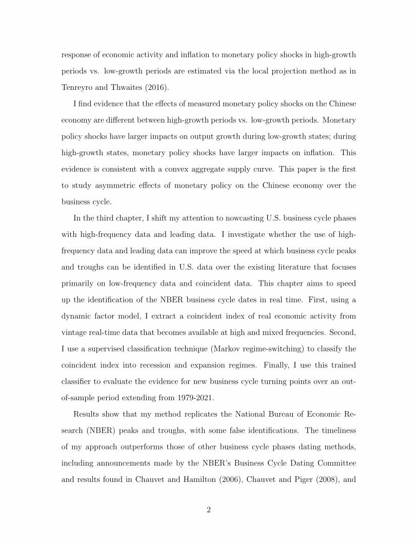
I find evidence that the effects of measured monetary policy shocks on the Chinese
economy are different between high-growth periods vs. low-growth periods. Monetary
policy shocks have larger impacts on output growth during low-growth states; during
high-growth states, monetary policy shocks have larger impacts on inflation. This
evidence is consistent with a convex aggregate supply curve. This paper is the first
to study asymmetric effects of monetary policy on the Chinese economy over the
business cycle.
In the third chapter, I shift my attention to nowcasting U.S. business cycle phases
with high-frequency data and leading data. I investigate whether the use of high-
frequency data and leading data can improve the speed at which business cycle peaks
and troughs can be identified in U.S. data over the existing literature that focuses
primarily on low-frequency data and coincident data. This chapter aims to speed
up the identification of the NBER business cycle dates in real time. First, using a
dynamic factor model, I extract a coincident index of real economic activity from
vintage real-time data that becomes available at high and mixed frequencies. Second,
I use a supervised classification technique (Markov regime-switching) to classify the
coincident index into recession and expansion regimes. Finally, I use this trained
classifier to evaluate the evidence for new business cycle turning points over an out-
of-sample period extending from 1979-2021.
Results show that my method replicates the National Bureau of Economic Re-
search (NBER) peaks and troughs, with some false identifications. The timeliness
of my approach outperforms those of other business cycle phases dating methods,
including announcements made by the NBER’s Business Cycle Dating Committee
and results found in Chauvet and Hamilton (2006), Chauvet and Piger (2008), and
2

Giusto and Piger (2017). In several cases, business cycle turning points are called
prior to their occurring, which demonstrates the value-added of incorporating leading
data into the analysis.
Finally, the fourth chapter of my dissertation is motivated by creating a new high-
frequency data that contains information about macroeconomic activity in the United
States. Using dictionary methods, I establish a news-based daily index of sentiment
regarding economic conditions from the Wall Street Journal daily articles. I also
incorporate the index in empirical studies as a complement to the more structured
macroeconomic data traditionally used.
Results suggest the high-frequency news-based sentiment index has information
useful for nowcasting low-frequency macroeconomic variables, including business cy-
cle turning points and monthly variables such as initial claims, unemployment rates,
the University of Michigan consumer sentiment index, and the nonfarm payroll em-
ployment. This improvement is primarily visible during recessions.
3
CHAPTER II
ARE THE EFFECTS OF MONETARY
POLICY ASYMMETRIC IN CHINA?
II.1 Introduction
Since 2000, China’s economic growth has been very strong. The reported GDP
growth rate surpassed 8 percent for a decade after 2000, reaching a local peak of 14
percent in 2007. This growth has led to China becoming an increasingly important
part of the world economy. It is now the second largest economic engine in the world
measured by nominal GDP, and the world’s largest economy by purchasing power
parity, contributing 27 percent of global GDP in 2018.
Despite this importance, there has been relatively little work done on understand-
ing the effects of Chinese monetary policy. One reason for the small amount of
research is the poor quality of Chinese macroeconomic data (Wallace, 2014; Rawski,
2001; Maier, 2011; Holz, 2014). Researchers like Mehrotra and Paakkonen (2011),
Fernald et al. (2015), and Clark et al. (2017) find that officially reported data has
become more informative in recent decades. Meanwhile, China has experienced rapid
institutional and structural changes, which may lead to changes in the Chinese mon-
etary policy mechanism post 2000 (He et al., 2013; Fernald et al., 2014; Chen et al.,
2016). In other countries, especially Western market economies, substantial attention
has been paid to state-dependence, or asymmetry, in the effects of policy over the
business cycle. Most papers find that monetary policy is more powerful in affecting
output during recessions than during expansions (Thoma, 1994; Garcia and Schaller,
4
2002; Lo and Piger, 2005; Weise, 1999; Kaufmann, 2002; Peersman and Smets, 2001).
However, in a recent influential paper, Tenreyro and Thwaites (2016) find an opposite
result.
I investigate how monetary policy instruments affect output growth and inflation,
and whether this effect is asymmetric across different states of output growth. Follow-
ing Fernald et al. (2014), I measure economic activity and inflation as dynamic factors
from a large number of Chinese economic indicators. To measure monetary policy,
I estimate a factor-augmented vector autoregression (FAVAR) and extract monetary
policy shocks using a Cholesky causal ordering with the policy variable ordered last.
As in Tenreyro and Thwaites (2016), I use a smooth transition logistic function to
measure high- and low-growth states in Chinese economic activity. Finally, to es-
timate the response of economic activity and inflation to monetary policy shocks in
different growth states, I use the method of local projections first introduced by Jorda
(2005).
I find evidence that the effects of measured monetary policy shocks on the Chinese
economy are different between high-growth periods vs. low-growth periods. Mone-
tary policy shocks have larger impacts on output growth in low-growth states. This is
consistent with the majority of the literature studying the asymmetric effects of mon-
etary policy shocks in Western economies. Additionally, I find that monetary policy
shocks have larger effects on inflation in high-growth states. Overall, this evidence is
consistent with a convex aggregate supply curve.
The remainder of this paper is structured as follows: Section 2.2 reviews the liter-
ature. Section 2.3 describes the dataset. Section 2.4 explains the empirical methods.
Section 2.5 sets out the main results. Section 2.6 concludes with some thoughts for
future research.
5

II.2 Literature Review
According to Lo and Piger (2005), the literature has focused on three types of
asymmetry: (1) asymmetry related to the direction of the monetary policy action,
(2) asymmetry related to the existing business cycle phase, and (3) asymmetry related
to the size of the policy action. I focus on the second type of asymmetry.
As one of the earliest papers in this area, Thoma (1994) defines the business
cycle, or the state of the economy, as deviations of the growth rate of output from
trend. Another method to identify the unobserved state of the economy is to use
a Markov regime switching model, as in Peersman and Smets (2001), Garcia and
Schaller (2002), Kaufmann (2002) and Lo and Piger (2005). These papers define
transition probabilities from the state of expansion to the state of recession as time-
varying functions of the changes of the observed monetary policy actions. In this
paper, I use a smooth transition logistic function to exploit variation in the degree of
the economic activity factor of being in a regime. This Smooth transition method has
been used in a number of papers to study the asymmetric effect of fiscal or monetary
policy on output across expansions and recessions, such as Weise (1999), Auerbach
and Gorodnichenko (2012), and Tenreyro and Thwaites (2016). 1
Early papers measure monetary policy shocks using the first difference of a mon-
etary policy instrument (Thoma, 1994; Peersman and Smets, 2001). Tenreyro and
Thwaites (2016) estimate monetary policy shocks as residuals from a nonlinear ana-
logue of the Romer and Romer (2004) regression. The majority of the literature has
measured the monetary shock using Choleski innovations identified from the contem-
poraneous relationships of the variables in a standard structural VAR model, with the
monetary policy tool ordered last (Weise, 1999; Peersman and Smets, 2001; Garcia
1I have used multiple two-state Markov regime switching models to capture the latent states. How-ever, this family of models only fit two periods where growth rate is very fast and the single periodwhere growth rate is very slow.
6
and Schaller, 2002; Lo and Piger, 2005; He et al., 2013; Fernald et al., 2014). This is
the method I adopt.
Much of the recent literature has measured the effects of macroeconomic shocks,
and possible asymmetry in these effects, using the Jorda (2005) method of local pro-
jections. For example, Auerbach and Gorodnichenko (2012) and Ramey and Zubairy
(2014) measure the asymmetric effects of fiscal policy over the business cycle, and
Tenreyro and Thwaites (2016) measure the asymmetric effects of monetary policy
over the business cycle. In this paper I will also use the method of local projections
to measure asymmetric effects of monetary policy in China.
Most papers that study asymmetric effects of monetary policy on output in West-
ern market economies find that monetary policy is more powerful in affecting output
during recessions than during expansions (Thoma, 1994; Garcia and Schaller, 2002; Lo
and Piger, 2005; Weise, 1999; Kaufmann, 2002; Peersman and Smets, 2001). However,
Tenreyro and Thwaites (2016) find an opposite result. I find evidence that Chinese
monetary policy shocks have larger impacts on output growth in low-growth states,
which is consistent with the majority of the literature in other countries.
For the literature that focus on Western market economies, output is measured
by industrial production and GDP volume, or the logarithm and the growth rate of
these indicators (Thoma, 1994; Weise, 1999; Peersman and Smets, 2001; Garcia and
Schaller, 2002; Kaufmann, 2002; Tenreyro and Thwaites, 2016). I focus on asymmetric
effects of monetary policy on output in China, where output cannot be measured
directly with industrial production or GDP, due to the poor quality of the officially
published Chinese economic data (Rawski, 2001; Maier, 2011; Wallace, 2014; Holz,
2014).
In the empirical literature that studies macroeconomics in China, there are mainly
two methods to deal with the quality issue of Chinese data. The first method is to
choose data that is not subject to government manipulation. Nakamura et al. (2014)
7
take a microeconomic perspective and use Chinese urban household survey data,
which is subject to less intervention from government compared with the headline
macroeconomic data. Based on the survey, the authors estimate Engle curves, and
”back out” the estimate of Chinese growth and inflation. Fernald et al. (2015) use
quarterly trading-partner export to China data, which is an independent measure-
ment. They find that economic activity factors extracted from electricity consump-
tion, rail freight, retail sales, an index of raw material supply are more informative
than the officially reported GDP alone. They also find that the information content
of Chinese GDP improves after 2008. Clark et al. (2017) use annual satellite night-
time lights data as an independent benchmark of Chinese economy growth. They find
that the growth rate of electricity production, railroad freight, and bank loans with
modified weights computed by nighttime lights data does a good job at predicting the
true unobserved Chinese economy growth. Their predictor of Chinese growth shows
that the rate of Chinese growth is higher than is reported in the official statistics.
The second method to evaluate Chinese economy when data is suspected to be
inaccurate is to extract latent factors from a large panel of underlying time series.
Mehrotra and Paakkonen (2011) use principal component analysis to evaluate China’s
growth from 1997 to 2009. Their estimated factor matches closely the reported GDP
dynamics, especially since 2002. He et al. (2013) treat output and inflation as observed
variables, measured by industrial production and consumer price index respectively.
The authors extract the monetary policy factor from 15 policy variables and apply
a factor-augmented vector autoregression model to study the monetary transmission
mechanism in China over the period from January 1998 to February 2010. Fernald
et al. (2014) also use a factor-augmented vector autoregression to estimate the ef-
fects of monetary policies on Chinese economy, over the period from January 2000 to
September 2013. They treat Chinese output and inflation as unobserved latent vari-
ables, and extract an economic activity factor and an inflation factor. Their factors
8
capture well the slowdown in China during the U.S. Great Recession and the follow-
ing recovery. Dynamic factors extracted from a large number of underlying variables
convey more information regarding Chinese economic activity than the reported GDP
data alone. Another advantage of this method is that no prior knowledge is needed
when determining which variables to include in the model, and data will speak in
terms of the goodness of fit. Therefore, this is the method I use.
To my knowledge, Chen et al. (2016) is the only paper that studies asymmetric
effects of monetary policy on Chinese economy. According to Chen et al. (2016),
the main function of Chinese monetary policy is to control the growth rate of money
supply M2 and provide support to achieve the GDP growth rate target set by the State
Council, the chief administrative authority of China. In contrast to my paper, which
focuses on asymmetric effects of monetary policy across high-growth and low-growth
states, Chen et al. (2016) focus on the normal state when actual GDP growth meets
the GDP growth rate target, and the shortfall state when actual GDP fails to meet
the GDP growth rate target. Chen et al. (2016) measure monetary policy shocks
as the difference between actual M2 growth and the systematic component of M2
growth, and adopts the official GDP and CPI data in their analysis. The structural
VAR approach suggests that when actual GDP growth fails to meet the GDP growth
target set by the government, monetary policy is more powerful in influencing the
economy. Their paper presents significant evidence of the existence of asymmetric
effects of Chinese monetary policy on the economy during above the target periods
and below the target periods of the economy.
II.3 Data
Table II.1 lists all the variables included in this paper. All data are downloaded
from the CEIC China Premium Database. As in Fernald et al. (2014), data series are
9
divided into three groups. The first group includes fundamental series that correlate
with output, from which the economic activity factor is extracted. The second group
includes four price indexes, from which the inflation factor is extracted. The third
group comprises the measure of monetary policy. This group has just one variable,
interest rates on loans to financial institutions for less than 20 days, which is the
central bank benchmark interest rate.
The release of monthly data series is affected by the two-week lunar calendar New
Year holiday, of which the first day begins between late January and late February.
For some indicators, the sum of January and February data is reported. 2 To get
monthly values of these indicators, I redistribute values for January and February so
that the growth rate from December to January equals the growth rate from January
to February. Then I obtain monthly values from March to December by taking first
differences.
After removing effects of the Chinese New Year, I use the Census X-12 ARIMA
package to adjust for seasonality. Then I take monthly growth rates of each series,
except for benchmark interest rates and price indexes. 3 Outliers of each series are
identified as those data points that lie outside 10 times the interquartile range from
the median. Outliers are treated as missing values and imputed as described below.
In addition to outliers, other sources of missing data include: (1) missing January
and February data, which systematically stem from the lunar calendar New Year
holiday; 4 (2) missing data exists at the beginning of the sample for indicators col-
lected later than January 2000; (3) in-sample missing data; (4) missing data exists
at the end of the sample for data that are no longer being released or not released in
synchronicity. I adopt an iterative expectation-maximization (EM) algorithm devel-
2These indicators include electricity consumption, fixed assets investment, fixed assets investmentin equipment purchase, fixed assets investment in new construction, real estate investment forresidential buildings, and floor space started for commodity buildings.
3Price indexes are measured in units where the previous month’s price level is fixed at 100.4These indicators include retail sales of consumer goods, crude steel production, real estate climateindex, electricity consumption, electricity production, natural gas production.
10
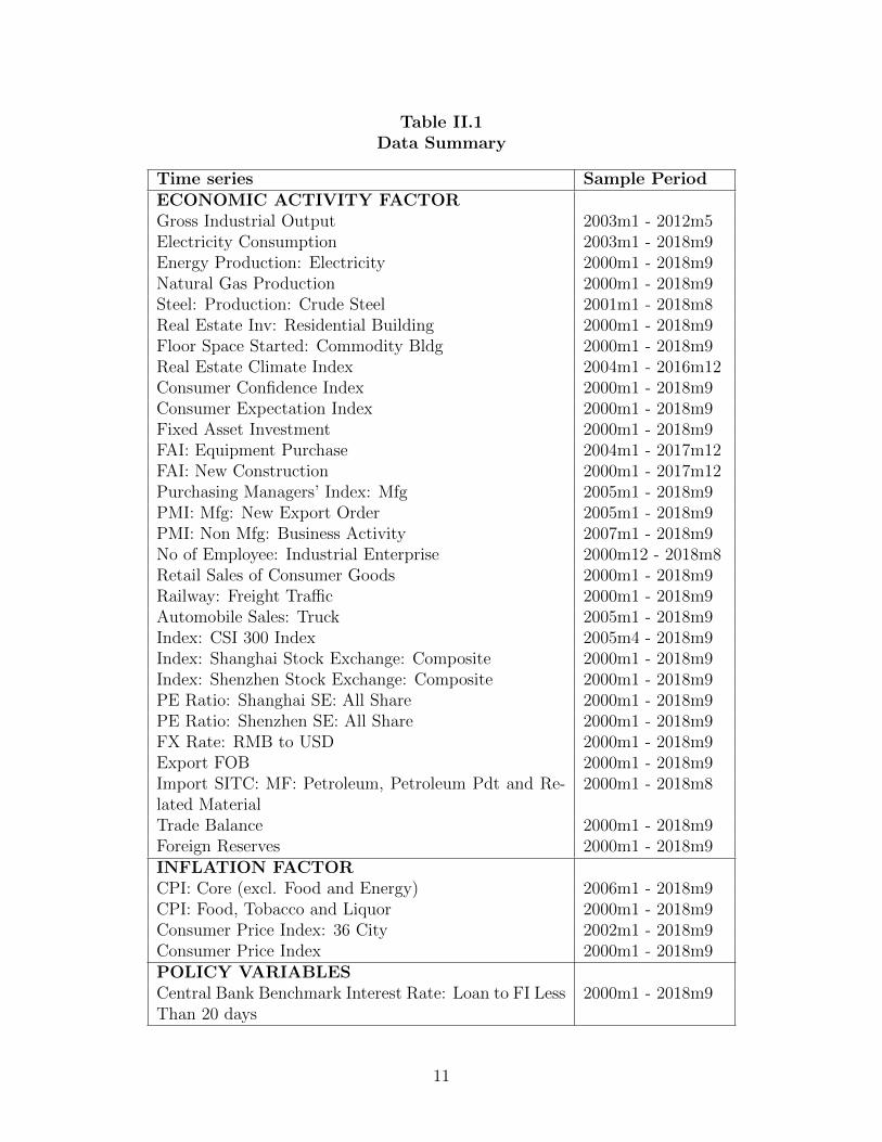
Table II.1Data Summary
Time series Sample PeriodECONOMIC ACTIVITY FACTORGross Industrial Output 2003m1 - 2012m5Electricity Consumption 2003m1 - 2018m9Energy Production: Electricity 2000m1 - 2018m9Natural Gas Production 2000m1 - 2018m9Steel: Production: Crude Steel 2001m1 - 2018m8Real Estate Inv: Residential Building 2000m1 - 2018m9Floor Space Started: Commodity Bldg 2000m1 - 2018m9Real Estate Climate Index 2004m1 - 2016m12Consumer Confidence Index 2000m1 - 2018m9Consumer Expectation Index 2000m1 - 2018m9Fixed Asset Investment 2000m1 - 2018m9FAI: Equipment Purchase 2004m1 - 2017m12FAI: New Construction 2000m1 - 2017m12Purchasing Managers’ Index: Mfg 2005m1 - 2018m9PMI: Mfg: New Export Order 2005m1 - 2018m9PMI: Non Mfg: Business Activity 2007m1 - 2018m9No of Employee: Industrial Enterprise 2000m12 - 2018m8Retail Sales of Consumer Goods 2000m1 - 2018m9Railway: Freight Traffic 2000m1 - 2018m9Automobile Sales: Truck 2005m1 - 2018m9Index: CSI 300 Index 2005m4 - 2018m9Index: Shanghai Stock Exchange: Composite 2000m1 - 2018m9Index: Shenzhen Stock Exchange: Composite 2000m1 - 2018m9PE Ratio: Shanghai SE: All Share 2000m1 - 2018m9PE Ratio: Shenzhen SE: All Share 2000m1 - 2018m9FX Rate: RMB to USD 2000m1 - 2018m9Export FOB 2000m1 - 2018m9Import SITC: MF: Petroleum, Petroleum Pdt and Re-lated Material
2000m1 - 2018m8
Trade Balance 2000m1 - 2018m9Foreign Reserves 2000m1 - 2018m9INFLATION FACTORCPI: Core (excl. Food and Energy) 2006m1 - 2018m9CPI: Food, Tobacco and Liquor 2000m1 - 2018m9Consumer Price Index: 36 City 2002m1 - 2018m9Consumer Price Index 2000m1 - 2018m9POLICY VARIABLESCentral Bank Benchmark Interest Rate: Loan to FI LessThan 20 days
2000m1 - 2018m9
11
oped by McCracken and Ng (2015) to handle missing values. This EM algorithm is
initialized by filling in missing data for each series with unconditional mean; then I
extract factors from the demeaned and standardized dataset; then I update missing
values using factors, and repeat this iterative procedure until factors converge.
After all missing values are imputed, the monthly dataset contains 224 months.
I standardize the dataset to have zero mean and unit variance. Following Stock and
Watson (2012), I remove a local mean from each series using a biweight kernel with
a bandwidth of 100 months. The biweight kernel smoothes the series.
II.4 Methodology
II.4.1 Extracting Factors
Estimates of economic activity and inflation are measured with the first principal
component of the series that measure output and price respectively. I follow Stock
and Watson (2016) to set up the dynamic factor model. The dynamic factor is shown
in Equations II.1 and II.2.
Xt = λ(L)ft + et (II.1)
ft = Ψ(L)ft−1 + ηt (II.2)
An n×1 vector of Xt contains observable underlying variables. ft is a k×1 vector
of latent common factors. The number of the observables n is assumed to be much
larger than the number of factors k. I let k = 1 to extract one factor from series that
correlate with output, and one factor from price indexes. ft is allowed to follow an
AR process. λ(L) and Ψ(L) are polynomials in the lag operator. λ is a n× k matrix
and Ψ(L) is a k × k matrix. λi(L) is the loading of Xit on ft, and λi(L)ft is the
12
common component of the ith variable Xi. ηt is assumed to be a mean-zero k × 1
vector of serially uncorrelated error term to the factors. The idiosyncratic term et is
a n× 1 vector and assumed to be uncorrelated with ηt at all leads and lags.
The principal component method is computationally simple. In addition, as long
as the correlation is not too big, et can be assumed to be correlated across series and
across observations. The standard strict factor model assumes et to be serially uncor-
related, while the approximate factor model relaxes this assumption. The principal
component method is appropriate to find an approximate factor structure, according
to Chamberlain and Rothschild (1983) and Stock and Watson (2002).
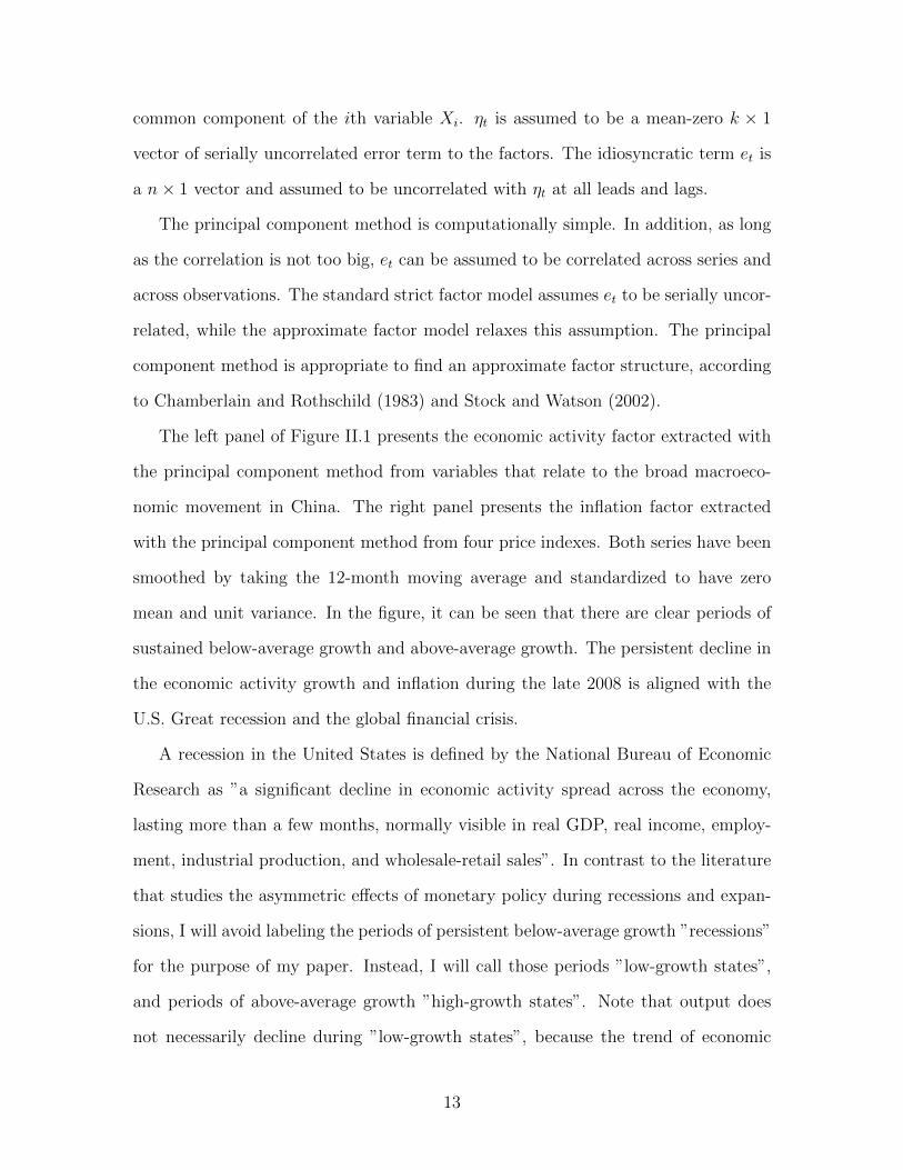
The left panel of Figure II.1 presents the economic activity factor extracted with
the principal component method from variables that relate to the broad macroeco-
nomic movement in China. The right panel presents the inflation factor extracted
with the principal component method from four price indexes. Both series have been
smoothed by taking the 12-month moving average and standardized to have zero
mean and unit variance. In the figure, it can be seen that there are clear periods of
sustained below-average growth and above-average growth. The persistent decline in
the economic activity growth and inflation during the late 2008 is aligned with the
U.S. Great recession and the global financial crisis.
A recession in the United States is defined by the National Bureau of Economic
Research as ”a significant decline in economic activity spread across the economy,
lasting more than a few months, normally visible in real GDP, real income, employ-
ment, industrial production, and wholesale-retail sales”. In contrast to the literature
that studies the asymmetric effects of monetary policy during recessions and expan-
sions, I will avoid labeling the periods of persistent below-average growth ”recessions”
for the purpose of my paper. Instead, I will call those periods ”low-growth states”,
and periods of above-average growth ”high-growth states”. Note that output does
not necessarily decline during ”low-growth states”, because the trend of economic
13
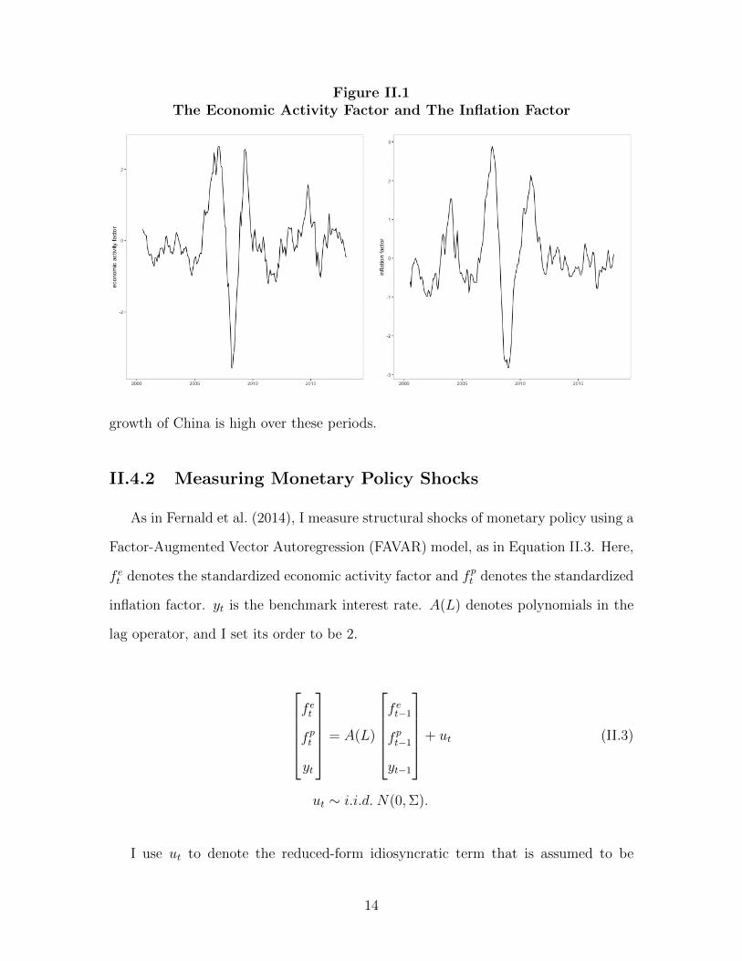
Figure II.1The Economic Activity Factor and The Inflation Factor
growth of China is high over these periods.
II.4.2 Measuring Monetary Policy Shocks
As in Fernald et al. (2014), I measure structural shocks of monetary policy using a
Factor-Augmented Vector Autoregression (FAVAR) model, as in Equation II.3. Here,
f et denotes the standardized economic activity factor and fpt denotes the standardized
inflation factor. yt is the benchmark interest rate. A(L) denotes polynomials in the
lag operator, and I set its order to be 2.
f et
fpt
yt
= A(L)
f et−1
fpt−1
yt−1
+ ut (II.3)
ut ∼ i.i.d. N(0,Σ).
I use ut to denote the reduced-form idiosyncratic term that is assumed to be
14
independent and identically distributed with zero mean. I identify the structural
shock through a Cholesky decomposition of Σ. This identification strategy assumes
that the monetary policy variable can respond to changes in the economic activity
factor and inflation factor contemporaneously, but the economic activity factor and
inflation factor respond to changes in monetary policy with a lag of one month or
more. This is implemented by recursively ordering the economic activity factor f et
and inflation factor fpt first, and the policy variable yt last. Monetary policy shocks
measured with the central bank benchmark interest rate are shown in Figure II.2.
Figure II.2Monetary Policy Shocks
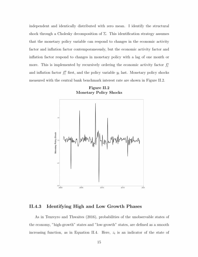
II.4.3 Identifying High and Low Growth Phases
As in Tenreyro and Thwaites (2016), probabilities of the unobservable states of
the economy, ”high-growth” states and ”low-growth” states, are defined as a smooth
increasing function, as in Equation II.4. Here, zt is an indicator of the state of
15
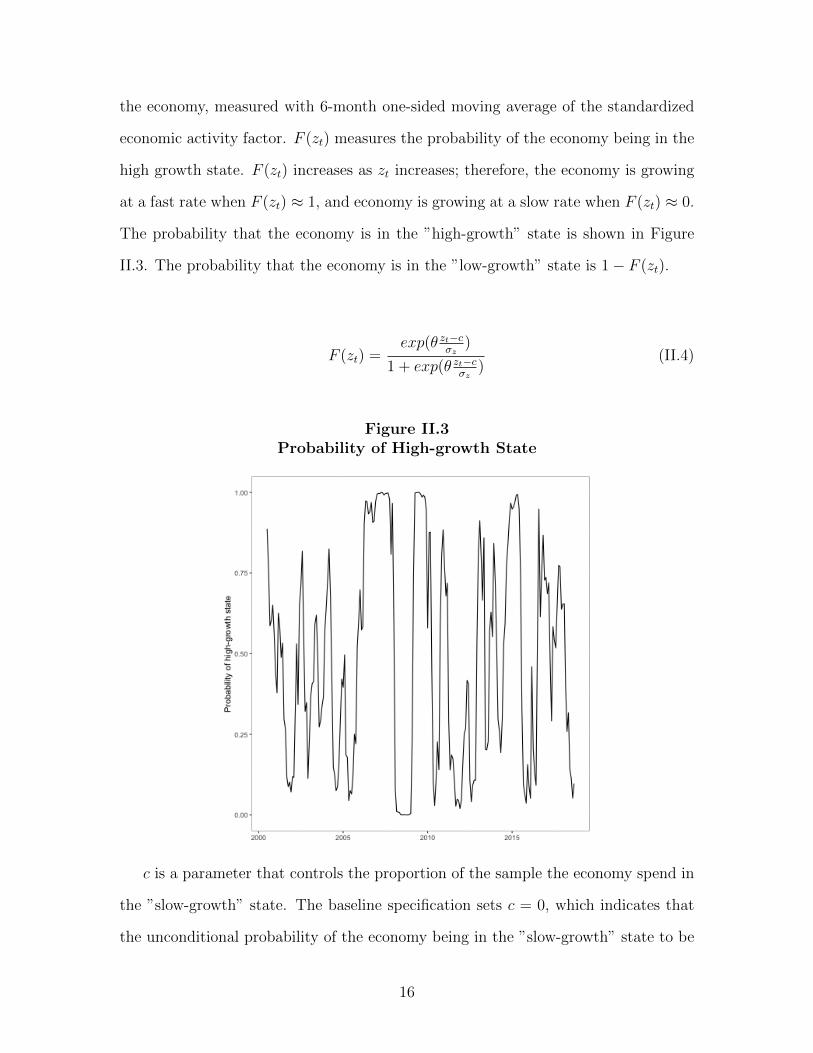
the economy, measured with 6-month one-sided moving average of the standardized
economic activity factor. F (zt) measures the probability of the economy being in the
high growth state. F (zt) increases as zt increases; therefore, the economy is growing
at a fast rate when F (zt) ≈ 1, and economy is growing at a slow rate when F (zt) ≈ 0.
The probability that the economy is in the ”high-growth” state is shown in Figure
II.3. The probability that the economy is in the ”low-growth” state is 1− F (zt).
F (zt) =exp(θ zt−c
σz)
1 + exp(θ zt−cσz
)(II.4)
Figure II.3Probability of High-growth State
c is a parameter that controls the proportion of the sample the economy spend in
the ”slow-growth” state. The baseline specification sets c = 0, which indicates that
the unconditional probability of the economy being in the ”slow-growth” state to be
16
equal to that in the ”high-growth” state, when zt = 0. σz is the standard deviation of
zt. θ is the parameter that controls how sharply the economy switches from the ”high-
growth” state to the ”low-growth” state as zt changes. As in Tenreyro and Thwaites
(2016), this parameter is calibrated to 3 in the baseline specification, indicating an
intermediate degree of intensity to the regime switching. The robustness of results to
each of these choices is investigated below.
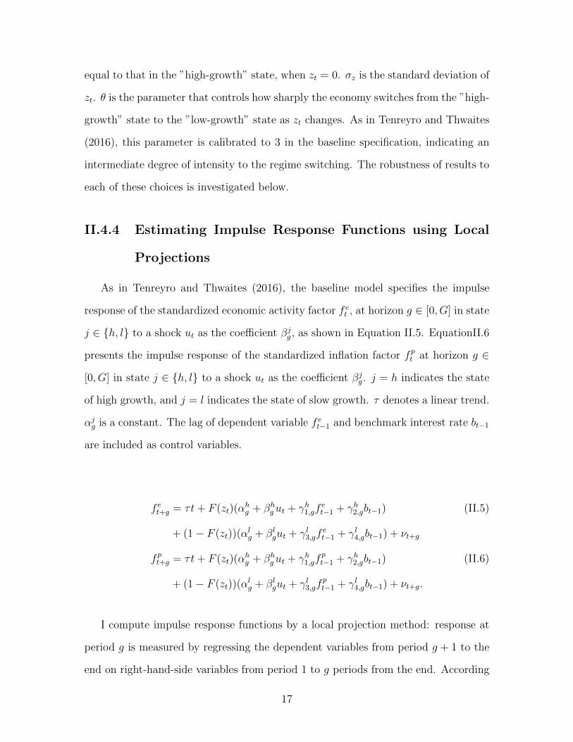
II.4.4 Estimating Impulse Response Functions using Local
Projections
As in Tenreyro and Thwaites (2016), the baseline model specifies the impulse
response of the standardized economic activity factor f et , at horizon g ∈ [0, G] in state
j ∈ h, l to a shock ut as the coefficient βjg , as shown in Equation II.5. EquationII.6
presents the impulse response of the standardized inflation factor fpt at horizon g ∈
[0, G] in state j ∈ h, l to a shock ut as the coefficient βjg . j = h indicates the state
of high growth, and j = l indicates the state of slow growth. τ denotes a linear trend.
αjg is a constant. The lag of dependent variable f et−1 and benchmark interest rate bt−1
are included as control variables.
f et+g = τt+ F (zt)(αhg + βhg ut + γh1,gf
et−1 + γh2,gbt−1) (II.5)
+ (1− F (zt))(αlg + βlgut + γl3,gf
et−1 + γl4,gbt−1) + νt+g
fpt+g = τt+ F (zt)(αhg + βhg ut + γh1,gf
pt−1 + γh2,gbt−1) (II.6)
+ (1− F (zt))(αlg + βlgut + γl3,gf
pt−1 + γl4,gbt−1) + νt+g.
I compute impulse response functions by a local projection method: response at
period g is measured by regressing the dependent variables from period g + 1 to the
end on right-hand-side variables from period 1 to g periods from the end. According
17

to Jorda (2005), computing impulse responses by local projections does not assume
specific structure on specification and the unknown true multivariate dynamic system
as required by a VAR model. With a VAR model, the impulse response function
is measured by extrapolating the one-period ahead forecast, while local projections
measure the impulse response function with direct multi-step forecasting.
An advantage of local projections is that it is easy to identify state-dependent
asymmetry by allowing the coefficients on ut to differ across two states, associated
with the probability of being in a particular state. Hence, the impact of policy shocks
on the economy in one state is separated from that in another state.
II.4.5 Inference
In order to construct confidence intervals for the impulse response functions es-
timated via local projections, I follow the suggestion of Jorda (2005) and construct
standard errors for each local projection regression using Newey-West standard errors.
The Newey-West correction is necessary as the vt+g disturbance term in the local pro-
jection regression has a moving average structure. In constructing the Newey-West
standard errors I follow Jorda (2005) and set the maximum lag equal to g + 1.
The null and alternative hypothesis of no asymmetry are given by the parametric
restrictions in Equations II.7 and II.8:
H0 : βhg − βlg = 0 (II.7)
H1 : βhg − βlg 6= 0 (II.8)
In order to test the null hypothesis of no asymmetry, I follow Tenreyro and
Thwaites (2016) to bootstrap the sign of βhg −βlg using a block bootstrap approach. 5
5Under the null hypothesis, coefficients of monetary policy shocks for high-growth periods and low-growth periods are the same, but coefficients of constant and control variables are different.
18
I construct 10,000 bootstrap datasets by drawing with replacement from the dataset.
The block length used in generating the replicate time series is fixed at G = 20.
Specifically, I first generate a random date and then select from that date the
next 20 observations from the original dataset, which is called the first block. I then
randomly draw a new time point, select the next 20 observations as a new block, and
add it to the first block. The process is repeated until the time series is equal to the
length of the original time series. This is called one bootstrap dataset. In total, I
have constructed 10,000 bootstrap datasets.
For each bootstrap dataset, I first randomly assign values of F (zt) with replace-
ment such that the null hypothesis of no asymmetry is satisfied in population. By
doing this, the actual F (zt) is randomly distributed across the data points so that
there shouldn’t be any relationship between F (zt) and the response of the economy
at t + h to shocks at time t. Then I calculate the the impulse response βhg and βlg
using the local projection method. The p-value of the test is then calculated as the
fraction of 10,000 cases in which the bootstrapped βhg − βlg is larger than the value of
βhg − βlg estimated in the baseline model.
II.5 Results
II.5.1 Baseline Results
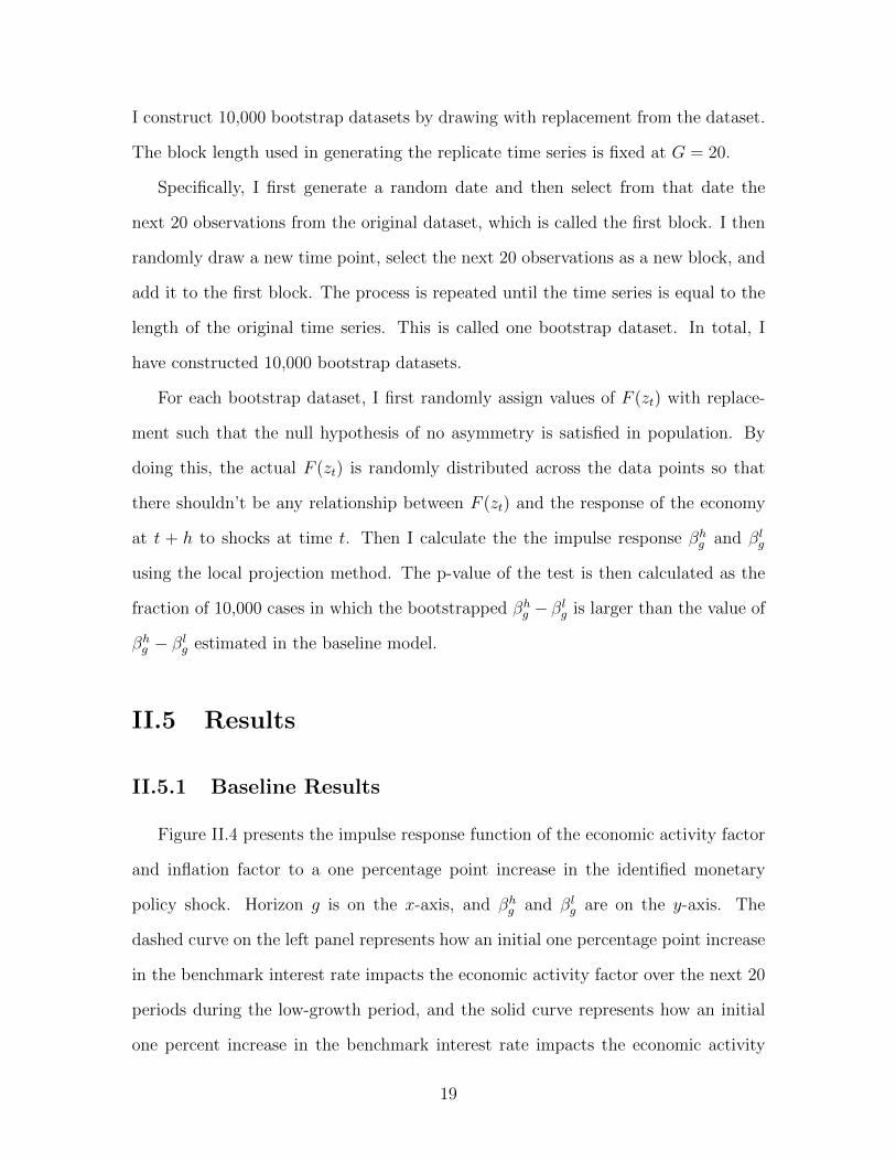
Figure II.4 presents the impulse response function of the economic activity factor
and inflation factor to a one percentage point increase in the identified monetary
policy shock. Horizon g is on the x-axis, and βhg and βlg are on the y-axis. The
dashed curve on the left panel represents how an initial one percentage point increase
in the benchmark interest rate impacts the economic activity factor over the next 20
periods during the low-growth period, and the solid curve represents how an initial
one percent increase in the benchmark interest rate impacts the economic activity
19
factor during the high-growth period. The counterpart curves on the right panel
show the response of the inflation factor to an initial one percent increase in the
benchmark interest rate during high-growth and low-growth periods respectively.
Figure II.4Impulse Response Functions
The economic activity factor is extracted from a large number of growth rates
of the underlying series. The negative economic activity factor during the first two
months represents a decline in the level of economic activity following the monetary
policy shock. Responses of economic activity during high-growth states and low-
growth states are negative for the initial two months. The results are consistent with
the standard theory that a tightening monetary policy leads to economic slowdown.
Starting from the third month, responses of economic activity during high-growth
states become positive and fluctuate around zero for the rest of the horizon, while
responses of economic activity during low-growth states are negative for seven con-
secutive months, and then dies out over time for the rest of the periods. The evidence
shows that monetary policy is more powerful in impacting economic activity during
low-growth states.
The inflation factor is extracted from growth rates of price indexes. Initial re-
20
sponses of the inflation factor to the monetary policy shock are positive for both
states. This is similar to the price puzzle found in the effects of a policy tightening
on inflation in studies of the effects of U.S. monetary policy on prices. Starting from
the third month, responses of the inflation factor during high-growth states becomes
negative and remains so for 13 months. This is the effect standard theory would
predict - a monetary policy tightening leads to an overall reduction in the price level.
Responses of the inflation factor during low-growth states fluctuate around zero for
the rest of the horizon. This evidence shows that monetary policy is more powerful
in impacting inflation during high-growth states.
The evidence that monetary policy shocks have larger impacts on output growth
during low-growth states and larger impacts on inflation during high-growth states
is consistent with a convex aggregate supply curve. As Figure II.5 shows, in such
a model, during high-growth periods when the economy is more likely to be on the
steep part of the aggregate supply curve, aggregate demand shifts should primarily
affect prices. In contrast, during low-growth periods, when the economy is on the flat
part of the aggregate supply curve, aggregate demand shifts should primarily affect
output.
II.5.2 Inference
Figure II.6 shows impulse response functions with 90 percent confidence intervals.
The confidence intervals are calculated with the Newey-West standard errors. There
is substantial uncertainty in the impulse response function estimates. This is not
surprising, as impulse response function estimates are often imprecise, and this is
compounded by the short time series and noisy nature of the Chinese data. How-
ever, despite this uncertainty, there are a number of horizons for which these impulse
response function estimates are significantly different from zero, suggesting that mon-
etary policy has statistically significant effects on the Chinese economy. Note that
21
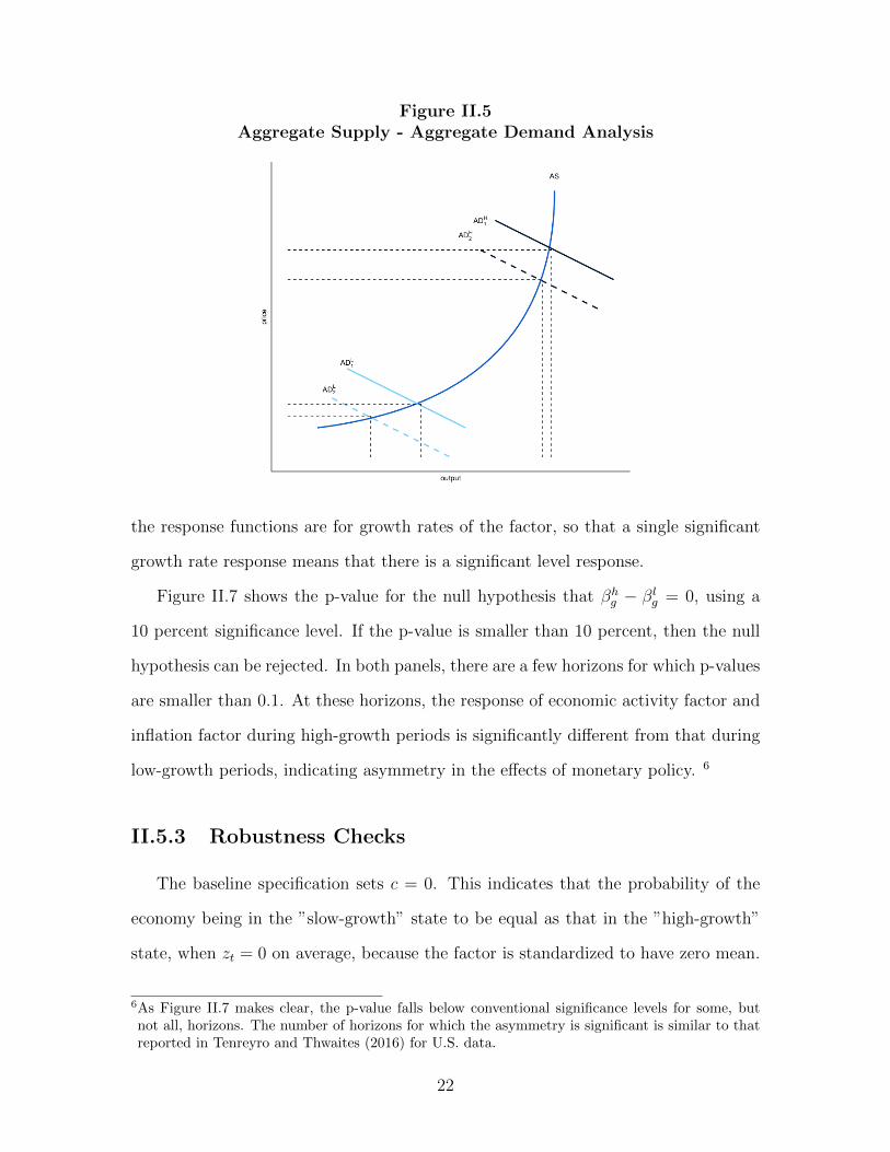
Figure II.5Aggregate Supply - Aggregate Demand Analysis
the response functions are for growth rates of the factor, so that a single significant
growth rate response means that there is a significant level response.
Figure II.7 shows the p-value for the null hypothesis that βhg − βlg = 0, using a
10 percent significance level. If the p-value is smaller than 10 percent, then the null
hypothesis can be rejected. In both panels, there are a few horizons for which p-values
are smaller than 0.1. At these horizons, the response of economic activity factor and
inflation factor during high-growth periods is significantly different from that during
low-growth periods, indicating asymmetry in the effects of monetary policy. 6
II.5.3 Robustness Checks
The baseline specification sets c = 0. This indicates that the probability of the
economy being in the ”slow-growth” state to be equal as that in the ”high-growth”
state, when zt = 0 on average, because the factor is standardized to have zero mean.
6As Figure II.7 makes clear, the p-value falls below conventional significance levels for some, butnot all, horizons. The number of horizons for which the asymmetry is significant is similar to thatreported in Tenreyro and Thwaites (2016) for U.S. data.
22
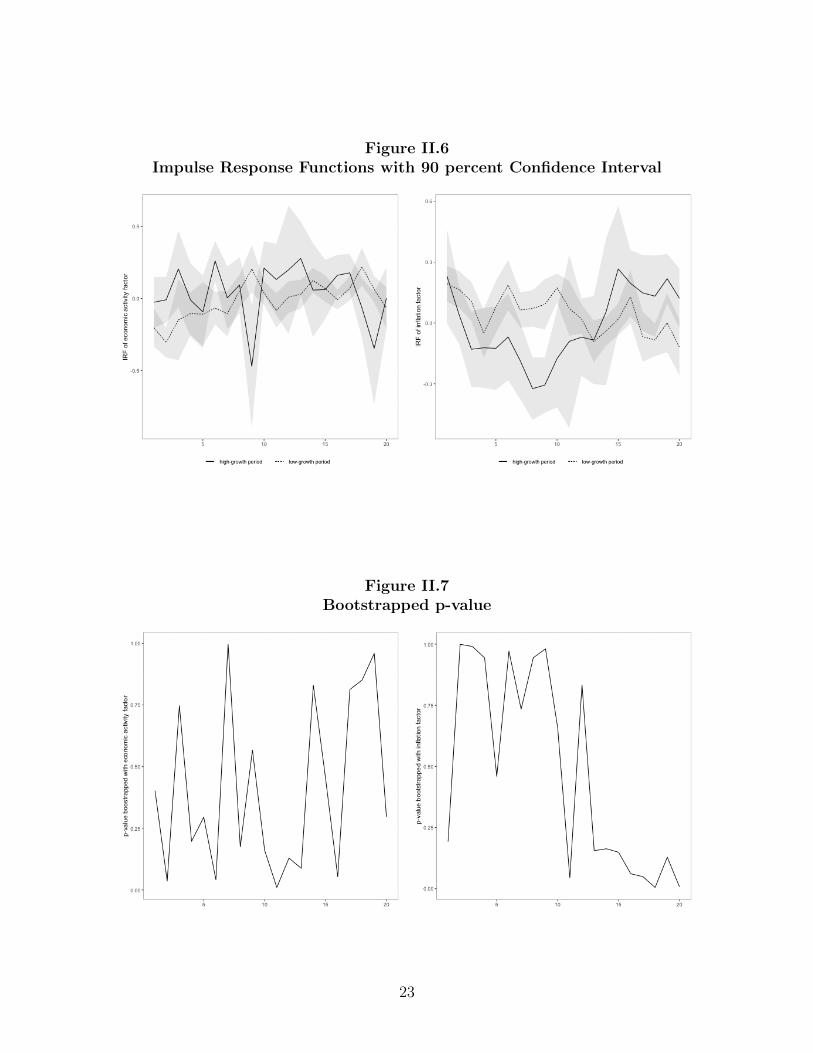
Figure II.6Impulse Response Functions with 90 percent Confidence Interval
Figure II.7Bootstrapped p-value
23
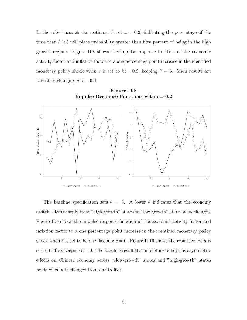
In the robustness checks section, c is set as −0.2, indicating the percentage of the
time that F (zt) will place probability greater than fifty percent of being in the high
growth regime. Figure II.8 shows the impulse response function of the economic
activity factor and inflation factor to a one percentage point increase in the identified
monetary policy shock when c is set to be −0.2, keeping θ = 3. Main results are
robust to changing c to −0.2.
Figure II.8Impulse Response Functions with c=-0.2
The baseline specification sets θ = 3. A lower θ indicates that the economy
switches less sharply from ”high-growth” states to ”low-growth” states as zt changes.
Figure II.9 shows the impulse response function of the economic activity factor and
inflation factor to a one percentage point increase in the identified monetary policy
shock when θ is set to be one, keeping c = 0. Figure II.10 shows the results when θ is
set to be five, keeping c = 0. The baseline result that monetary policy has asymmetric
effects on Chinese economy across ”slow-growth” states and ”high-growth” states
holds when θ is changed from one to five.
24
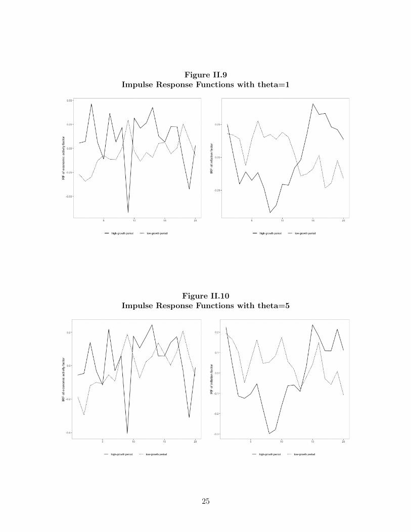
Figure II.9Impulse Response Functions with theta=1
Figure II.10Impulse Response Functions with theta=5
25
II.6 Conclusions
The literature that investigates asymmetries in the effects of China’s monetary
policy on economic activity and inflation is very limited. In this paper, I have inves-
tigated the asymmetric response of output growth and inflation to monetary policy
actions during ”high-growth” states and ”low-growth” states. The economic activity
factor and inflation factor are extracted from a large panel of underlying macroe-
conomic series using the principal component method. Monetary policy shocks are
identified with Choleski decomposition of residuals from a factor-augmented vector
autoregression. Probabilities of high-growth and low-growth phases are measured
using a smooth transition logistic function. Finally, I have used a local projection
method to measure the response of real economy to the identified monetary policy
shocks during ”high-growth” states and ”low-growth” states. The evidence is con-
sistent with monetary policy shocks having larger impacts on output growth during
low-growth states and monetary policy shocks have larger impacts on inflation during
high-growth states. This result is consistent with a convex aggregate supply curve.
There are periods during which the response of economic activity growth and
inflation are positive following an increase in the benchmark interest rate. This in-
dicates that economic activity and prices increase in response to a monetary policy
tightening. This is counter-intuitive and may suggest potential issues with standard
approaches to measure Chinese monetary policy shocks that have been used in the
existing literature. According to Romer and Romer (2004), the likelihood of endoge-
nous movements and anticipation movements can obscure the true effects of monetary
policy. Romer and Romer (2004) address this problem and derive the indicator of
monetary policy shocks by regressing the change in the intended policy interest rate
around the Federal Reserve’s internal forecast dates on these forecasts. The intended
monetary policy shocks are derived using the narrative record, and the forecasts are
26
publicly available in the ”Greenbook” before each meeting of the Federal Open Market
Committee.
To my knowledge, the People’s Bank of China (PBC) does not publish its internal
forecasts of inflation and real economic activity. Since 2009, the monetary policy
committee of the PBC has been publishing reports of each of its quarterly meeting.
Narrative analysis might be applicable to alleviate the endogeneity problem, which
can be the focus of potential future research of this topic. Future research of this
topic can also include the other two types of asymmetries: asymmetry related to the
direction of the monetary policy action, and asymmetry related to the size of the
policy action. This paper uses growth rates of factors to define phases of business
cycle. Instead, future research can focus on the level of the factors relative to trend,
and study the asymmetry of monetary policy over the cyclical component of the
factors.
27

CHAPTER III
NOWCASTING BUSINESS CYCLE
PHASES WITH HIGH-FREQUENCY
DATA
III.1 Introduction
A common definition of the business cycle is alternating phases of expansion and
recession, where an expansion is a period of widespread, persistent, economic growth,
and a recession is a period of widespread, persistent, economic contraction. The
existence of new turning points between these phases, commonly called peaks and
troughs, are of substantial interest to real-time economic decision makers, including
firms, policymakers, and individual consumers. Given this, a large literature has
developed attempts to forecast business cycle turning points, and business cycle peaks
in particular, with some limited success. 1 However, it is widely recognized that there
are many examples of recessions that were not predicted with any substantial lead
time, which leaves us trying to identify new recessions and expansions in a window
of time just prior to or, often, after the turning point occurs. Such an endeavor,
which is commonly called ”nowcasting” of business cycle turning points, has received
significant recent attention in the literature. 2
For the United States, one source of nowcasts is provided by the NBER, which pro-
1For recent contributions to this literature, see Berge (2015), Chauvet and Potter (2005), Kauppiand Saikkonen (2008), Ng (2014), and Rudebusch and Williams (2009).
2See for example, Chauvet and Piger (2008), Chauvet and Hamilton (2006), Fossati (2016), andGiusto and Piger (2017).
28
duces dates of new business cycle turning points in real time. However, the NBER’s
goal is to provide an accurate historical record of turning points, not speed of detec-
tion, and as a result their calls of new turning points often occur long after the fact.
For example, the December 2007 peak of the Great Recession was not announced by
the NBER until December 1, 2008. More recently, the NBER announced on June 8,
2020 that a new recession associated with the Covid-19 pandemic started in March
2020. As shown by Chauvet and Piger (2008) and Chauvet and Hamilton (2006),
statistical models are able to improve significantly on the speed of detection of new
turning points over the NBER. However, these models still produce new turning
points with a substantial lag time. For example, Hamilton (2011) surveys a range
of statistical models in use during 2008 and finds they would not have identified the
December 2007 peak in economic activity until late 2008.
Nearly all of the literature studying nowcasting of U.S. business cycle phases
uses coincident data at relatively low frequencies to nowcast business cycle phases,
namely monthly or quarterly data that moves contemporaneously with changes in
the overall economic activity. In other words, during periods of economic expansion,
the coincident data increases; when the economy contracts, the data falls. It seems
reasonable to expect that significant gains in the speed with which turning points
dates can be identified might be achieved by also incorporating data at the daily
or weekly frequency. There are several reasons for this expectation. First, high-
frequency data would allow additional variables to be incorporated than what has
typically been used in previous business cycle nowcasting literature, such as financial
market variables or initial claims of unemployment insurance. Second, the use of
high-frequency data would allow for more frequent updating of the model, since most
monthly or quarterly variables relevant for tracking the business cycle are released in
a cluster around the end of the month. Third, high-frequency variables generally have
much shorter reporting lags. For example, initial claims on unemployment insurance
29

for a given week are available only a few days after the week ends, whereas many
monthly series, such as personal income, are released after a full month delay.
In my paper I contribute in two primary ways to the literature studying nowcasting
of U.S. business cycle turning points. First, I study whether the use of high-frequency
data, namely weekly and daily data, can improve the speed at which business cycle
peaks and troughs post 1980 can be identified in U.S. data over the existing literature
that focuses primarily on monthly and quarterly data. To identify turning points
with data at high and mixed frequencies, I propose a three-step approach. First, I
use the mixed-frequency dynamic factor model as in Aruoba et al. (2009) (ADS). My
model allows me to extract a coincident index of real economic activity using daily,
weekly, monthly and quarterly data. Second, I train a supervised Markov regime-
switching classification technique to classify the coincident index into a daily measure
of recession and expansion regimes. The use of this Markov regime-switching model,
which contains a mechanism for capturing the very high persistence of the daily
business cycle phase indicator, performs significantly better than other commonly
used supervised machine learning classification approaches that assume independent
and identically distributed classes. Finally, I use the trained classifier to evaluate the
evidence for new business cycle turning points in end-of-sample data that has not
yet been classified by the NBER. I evaluate the out-of-sample performance of my
procedure for identifying new business cycle turning points in real time from January
1, 1979 to March 31, 2021 using a vintage dataset that contains the data that would
have been available at each date over this period.
The second contribution is to incorporate a mix of both leading variables and
coincident variables for the purpose of nowcasting business cycle turning points. The
existing literature focused on forecasting turning points has used only leading vari-
ables, while the literature focused on nowcasting turning points has used only coin-
cident variables. Here I use a dataset containing a significant number of standard
30

coincident variables used in the literature and by the NBER, which ensures that the
model will be able to eventually capture new business cycle turning points. However,
I also use a leading variable in the analysis, namely a yield curve premium, which has
been shown to have significant forecasting power for recessions. This leading variable
can help reinforce signals coming from coincident variables in the time periods prior
to and after recessions begin, and thus potentially speed up the identification of new
business cycle turning points.
I find that implementing these two additions - high-frequency data and leading
data - significantly and consistently improves the speed at which expansions and reces-
sions can be identified in the United States since 1979. As an example, incorporating
high-frequency data and leading data, namely the yield curve term premium and ini-
tial claims, produces a call of the December 2007 business cycle peak on March 30,
2008. This is 246 days ahead of the NBER announcement, and many months ahead
of the statistical procedures in the literature. In several cases, business cycle turn-
ing points are called prior to their occurring, which demonstrates the value-added of
incorporating leading data into the analysis.
The remainder of this paper is organized as follows. In section 3.2, I describe
the specification and estimation of my dynamic factor model at daily frequency. In
section 3.3, I describe the construction of the vintage, real-time dataset. Section
3.4 presents out-of-sampler exercise results to identify turning point dates using the
Markov regime switching classifier in real time. Section 3.5 concludes the paper.
III.2 Methodology
III.2.1 Dynamic Factor Model at Daily Frequency
In this section I lay out the model proposed in ADS and describe estimation and
filtering of the daily coincident index. I follow ADS to build a dynamic factor model
31
at daily frequency to extract a coincident index of real economic activity using weekly,
monthly and quarterly data. Let xt denote the underlying real economic activity at
day t, which is assumed to evolve daily with AR(1) dynamics. xt is described in
Equation III.1, where et is a white noise innovation with variance 1− ρ2.
xt = ρxt−1 + et (III.1)
I use the yield curve term premium for the daily variable y1t , defined as the differ-
ence between 10-year and 3-month U.S. Treasury yields. Because the term premium
is a stock variable, there are no aggregation issues. y1t depends linearly on xt and con-
temporaneously and serially uncorrelated innovations ut. Because the term premium
is reported every weekday, its persistence is modeled at the daily frequency with a
u1t term that follows AR(1) dynamics. y1t is modeled in Equation III.2, where ζt is a
white noise innovation with variance σ21.
y1t =
β1xt + u1t
NA
(III.2)
=
β1xt + γ1u
1t−1 + ζt y1t is observed
NA y1t is not observed
I use initial claims for unemployment insurance for the weekly variable y2t . Because
it is a flow variable reported on every Saturday covering the seven-day period from
Sunday to Saturday, y2t on Saturday is set to the sum of the previous seven daily
values, constructed with a weekly cumulator variable CWt . To model persistence at
the daily frequency, y2t is set to depend on its previous observed value with one-week
32
lag. Theoretically the persistence can be modeled with multiple lags of the u2t term;
however, the number of parameters need to be estimated will be unnecessarily large.
y2t is modeled in Equation III.3, where u2t is a white noise innovation with cumulated
variance 7× σ21.
y2t =
β2C
Wt + γ2y2,t−7 + u2t y2t is observed
NA y2t is not observed
(III.3)
CWt = ξWt C
Wt−1 + xt = ξWt C
Wt−1 + ρxt−1 + et
ξWt =
0 if t is the first day of a week
1 otherwise
I use nonfarm payroll employment for the monthly variable y3t . Because it is a
monthly stock variable, the end-of-month value is set to the end-of-month daily value.
Persistence is modeled with its observed value with one-month lag. The number of
days in each month is assumed to be 30 for simplicity. y3t is modeled in Equation
III.4, where u3t is a white noise innovation with variance σ31.
y3t =
β3xt + γ3y3,t−30 + u3t y3t is observed
NA y3t is not observed
(III.4)
I use real GDP for the quarterly variable y4t . Because it is a flow variable, the end-
of-quarter value is set to the sum of daily values within the quarter with a quarterly
cumulator variable CQt . Persistence is modeled with its observed value with one-
quarter lag. The number of days in each quarter is assumed to be 90 for simplicity.
y4t is modeled in Equation III.5, where u4t is a white noise innovation with cumulated
33

variance 90× σ41.
y4t =
β4C
Qt + γ4y4,t−90 + u4t y4t is observed
NA y4t is not observed
(III.5)
CQt = ξQt C
Qt−1 + xt = ξQt C
Qt−1 + ρxt−1 + et
ξQt =
0 if t is the first day of a quarter
1 otherwise
The initial claims for unemployment insurance, nonfarm payroll employment and
real GDP are coincident data that move with business cycle phases at the same time,
whereas the yield curve term premium is a leading data that moves before business
cycle phases. All yit are demeaned and detrended. This completes the specification of
the dynamic factor model at daily frequency. The measurement equation is cast as
in Equation III.6, and the transition equation is cast as in III.7.
y1t
y2t
y3t
y4t
︸ ︷︷ ︸
Υt
=
γ1 β1 0 0 0
0 0 β2 0 γ2 × y2,t−7
0 β3 0 0 γ3 × y3,t−30
0 0 0 β4 γ4 × y4,t−90
︸ ︷︷ ︸
FFt
×
u1t−1
xt
CWt
CQt
1
︸ ︷︷ ︸
θt
+
ζt
u2t
u3t
u4t
︸ ︷︷ ︸νt
(III.6)
34

u1t−1
xt
CWt
CQt
1
︸ ︷︷ ︸
θt
=
γ1 0 0 0 0
0 ρ 0 0 0
0 ρ ξWt 0 0
0 ρ 0 ξQt 0
0 0 0 0 1
︸ ︷︷ ︸
GGt
×
u1t−2
xt−1
CWt−1
CQt−1
1
︸ ︷︷ ︸θt−1
+
ζt−1
et
et
et
0
︸ ︷︷ ︸ωt
(III.7)
ζt
u2t
u3t
u4t
︸ ︷︷ ︸νt
∼ N
(
0
0
0
0
,
σ12 0 0 0
0 7× σ22 0 0
0 0 σ32 0
0 0 0 90× σ42
)
︸ ︷︷ ︸Vt
ζt−1
et
et
et
0
︸ ︷︷ ︸ωt
∼ N
(
0
0
0
0
0
,
σ12 0 0 0 0
0 1− ρ2 0 0 0
0 0 1− ρ2 0 0
0 0 0 1− ρ2 0
0 0 0 0 0
)
︸ ︷︷ ︸Wt
The model can also be represented in time-varying state-space form as in Equa-
tions III.8 and III.9. Υt is a vector of variables that are subject to missing values. θt
is a vector of state variables. νt and ωt are vectors of measurement and transition
shocks.
35
Υt = FFt × θt + νt (III.8)
θt = GGt × θt−1 + ωt (III.9)
Following ADS, I use the Kalman filter and smoother to obtain optimal extractions
of the latent state of real economic activity. At each analysis date, parameters are
re-estimated. As is standard for classical estimation, I initialize the Kalman filter
using the unconditional mean and covariance matrix of the state vector. Parameters
are estimated with maximum likelihood methods.
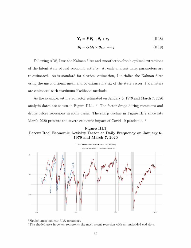
As the example, estimated factor estimated on January 6, 1979 and March 7, 2020
analysis dates are shown in Figure III.1. 3 The factor drops during recessions and
drops before recessions in some cases. The sharp decline in Figure III.2 since late
March 2020 presents the severe economic impact of Covid-19 pandemic. 4
Figure III.1Latent Real Economic Activity Factor at Daily Frequency on January 6,
1979 and March 7, 2020
3Shaded areas indicate U.S. recessions.4The shaded area in yellow represents the most recent recession with an undecided end date.
36
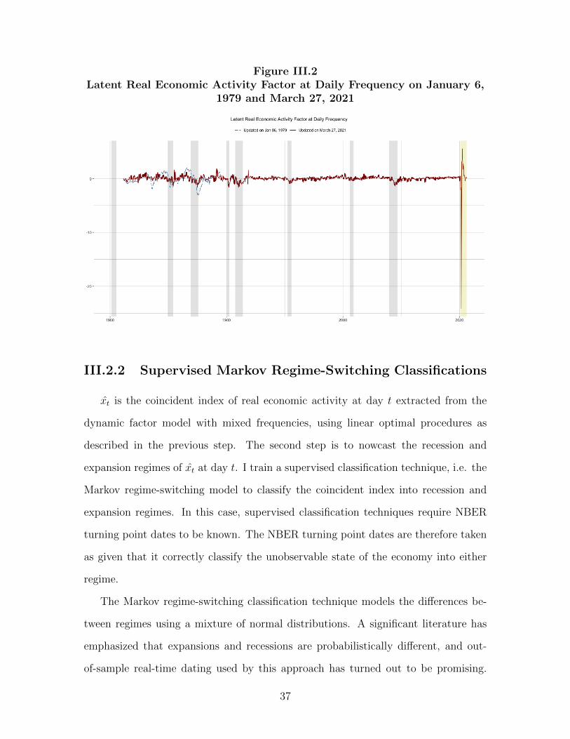
Figure III.2Latent Real Economic Activity Factor at Daily Frequency on January 6,
1979 and March 27, 2021
III.2.2 Supervised Markov Regime-Switching Classifications
xt is the coincident index of real economic activity at day t extracted from the
dynamic factor model with mixed frequencies, using linear optimal procedures as
described in the previous step. The second step is to nowcast the recession and
expansion regimes of xt at day t. I train a supervised classification technique, i.e. the
Markov regime-switching model to classify the coincident index into recession and
expansion regimes. In this case, supervised classification techniques require NBER
turning point dates to be known. The NBER turning point dates are therefore taken
as given that it correctly classify the unobservable state of the economy into either
regime.
The Markov regime-switching classification technique models the differences be-
tween regimes using a mixture of normal distributions. A significant literature has
emphasized that expansions and recessions are probabilistically different, and out-
of-sample real-time dating used by this approach has turned out to be promising.
37
Chauvet and Piger (2008) use a monthly real-time dataset and show that the dy-
namic factor Markov regime-switching model identifies NBER dates more accurately
and identifies troughs with a larger lead than a nonparametric algorithm. Camacho
et al. (2018) use a mixed-frequency dataset at monthly and quarterly frequencies,
and extend the Markov regime-switching dynamic factor model to monitor economic
activity on a monthly basis. Compared with a balanced panel of indicators, Camacho
et al. (2018) obtain substantial improvements in producing real-time business cycle
probabilities.
The transition between regimes is driven by a Markov process with pji, as specified
in Equation III.10. pji is the transition probability of St switching from regime i to
regime j. Camacho et al. (2015) and Owyang et al. (2005) found that the Markov
regime-switching AR(0) model provided accurate and robust identification of NBER
business cycle dates. As presented in Equations III.11 and III.12, I fit the first
difference of the coincident index, which is denoted ∆xt, to a univariate Markov
regime-switching AR(0) process with a switching mean.
pji = Pr(St = j|St−1 = i) (III.10)
∆xt = βSt + εt (III.11)
βSt = β0 + β1 × St (III.12)
εt ∼ N(0, σ2)
β1 < 0
The growth rate ∆xt has mean βSt , and deviations from this mean growth rate
38
are captured by the stochastic disturbance εt. The parameters of the model are
Ω = (β0, β1, p11, p22, σ)′. Let St ∈ 0, 1, where St = 0 indicates that day t is a expansion
regime, and St = 1 indicates that day t is a recession regime. When St switches from
0 to 1, the mean growth rate of economic activity switches from β0 to β0 + β1. This
implies that when the growth rate of economic activity switches from an expansion
regime which has higher growth to a recession regime which has lower growth, β1 < 0
ensures that the mean growth rate of economic activity declines. The model estimates
probabilities of a recession regime on day t conditional on data available on day T ,
denoted P (St = 1|ΨT ).
I estimate the Markov regime switching model using a non-parametric technique.
It directly ties the estimates to the NBER regimes, which is what I am trying to
nowcast. I estimate β0 and β1 as the mean of ∆xt in each NBER regime. I estimate
transition probabilities as the mean of the transitions using the NBER regimes. The
variance of the disturbance terms are estimated from the residuals of this regression.
Because NBER recession and expansion dates are known only with a substantial
lag, I do not use the NBER indicator that classifies the regime through the end of
the relevant sample to estimate parameters at each analysis date. Instead I adopt a
conservative approach and estimate model parameters on data ending one year prior
to the analysis date. Then, given the estimates, the filter developed in Hamilton
(1989) is run through to the end of the data available at the analysis date in order to
get the recession probabilities.
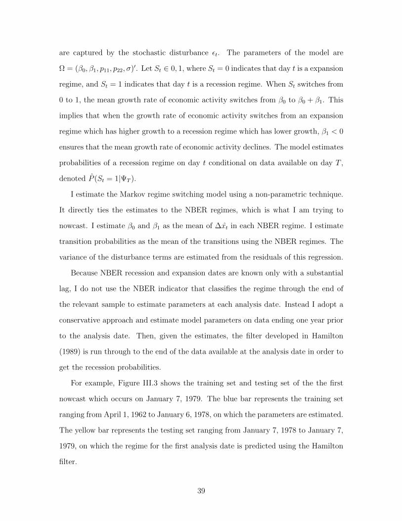
For example, Figure III.3 shows the training set and testing set of the the first
nowcast which occurs on January 7, 1979. The blue bar represents the training set
ranging from April 1, 1962 to January 6, 1978, on which the parameters are estimated.
The yellow bar represents the testing set ranging from January 7, 1978 to January 7,
1979, on which the regime for the first analysis date is predicted using the Hamilton
filter.
39
Figure III.3Training and Testing Set for the First Nowcasting
In a recent paper, Piger (2020) compares the timely performance of a wide range
of classifiers to nowcasting the U.S. expansion and recession phases at monthly fre-
quency, and finds that the k-nearest neighbor classifier and the random forest classifier
are quick to identify turning points while producing no false positives for a narrow
data set. I have trained a variety of supervised classification techniques to classify
the coincident index into recession and expansion regimes, including the k-nearest
neighbor classifier, the random forest classifier, and the Naive Bayes classifier. How-
ever, these classifiers failed to identify a large number of recessions, and overall their
performance was dominated by the Markov regime-switching classifier.
One explanation for the poor performance of these classifiers is that they do not
have a mechanism to capture the very high level of persistence of the daily regime
variable, the NBER indicator St. In other words, they assume St is independent and
identically distributed. At a daily frequency, the estimated values of P00 = Pr(St =
0|St−1 = 0) and P11 = Pr(St = 1|St−1 = 1) are very high. Over the full sample, P00
is 0.99962 and P11 is 0.99723. The Markov regime-switching based classifier captures
this persistence by modeling St as following a Markov process.
III.2.3 Business Cycle Phases Dating Procedures
Finally, I use the classifier to evaluate the evidence for new business cycle turnings
points in end-of-sample data that has not yet been classified by the NBER. In order
to convert recession probabilities P (St = 1|ΨT ) into a binary variable that defines
whether the economy is in an expansion or a recession regime on day t, and whether
40
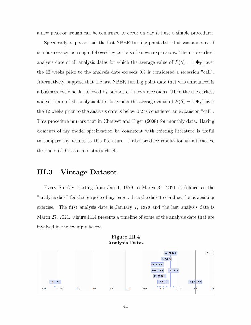
a new peak or trough can be confirmed to occur on day t, I use a simple procedure.
Specifically, suppose that the last NBER turning point date that was announced
is a business cycle trough, followed by periods of known expansions. Then the earliest
analysis date of all analysis dates for which the average value of P (St = 1|ΨT ) over
the 12 weeks prior to the analysis date exceeds 0.8 is considered a recession ”call”.
Alternatively, suppose that the last NBER turning point date that was announced is
a business cycle peak, followed by periods of known recessions. Then the the earliest
analysis date of all analysis dates for which the average value of P (St = 1|ΨT ) over
the 12 weeks prior to the analysis date is below 0.2 is considered an expansion ”call”.
This procedure mirrors that in Chauvet and Piger (2008) for monthly data. Having
elements of my model specification be consistent with existing literature is useful
to compare my results to this literature. I also produce results for an alternative
threshold of 0.9 as a robustness check.
III.3 Vintage Dataset
Every Sunday starting from Jan 1, 1979 to March 31, 2021 is defined as the
”analysis date” for the purpose of my paper. It is the date to conduct the nowcasting
exercise. The first analysis date is January 7, 1979 and the last analysis date is
March 27, 2021. Figure III.4 presents a timeline of some of the analysis date that are
involved in the example below.
Figure III.4Analysis Dates
41
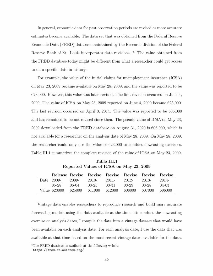
In general, economic data for past observation periods are revised as more accurate
estimates become available. The data set that was obtained from the Federal Reserve
Economic Data (FRED) database maintained by the Research division of the Federal
Reserve Bank of St. Louis incorporates data revisions. 5 The value obtained from
the FRED database today might be different from what a researcher could get access
to on a specific date in history.
For example, the value of the initial claims for unemployment insurance (ICSA)
on May 23, 2009 became available on May 28, 2009, and the value was reported to be
623,000. However, this value was later revised. The first revision occurred on June 4,
2009. The value of ICSA on May 23, 2009 reported on June 4, 2009 became 625,000.
The last revision occurred on April 3, 2014. The value was reported to be 606,000
and has remained to be not revised since then. The pseudo value of ICSA on May 23,
2009 downloaded from the FRED database on August 31, 2020 is 606,000, which is
not available for a researcher on the analysis date of May 28, 2009. On May 28, 2009,
the researcher could only use the value of 623,000 to conduct nowcasting exercises.
Table III.1 summarizes the complete revision of the value of ICSA on May 23, 2009.
Table III.1Reported Values of ICSA on May 23, 2009
Release Revise Revise Revise Revise Revise ReviseDate 2009-
05-282009-06-04
2010-03-25
2011-03-31
2012-03-29
2013-03-28
2014-04-03
Value 623000 625000 611000 612000 608000 607000 606000
Vintage data enables researchers to reproduce research and build more accurate
forecasting models using the data available at the time. To conduct the nowcasting
exercise on analysis dates, I compile the data into a vintage dataset that would have
been available on each analysis date. For each analysis date, I use the data that was
available at that time based on the most recent vintage dates available for the data.
5The FRED database is available at the following websitehttps://fred.stlouisfed.org/
42
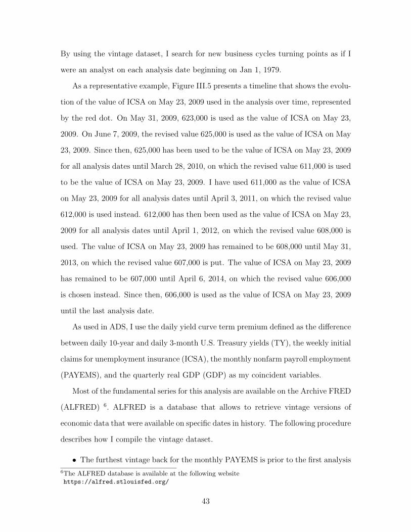
By using the vintage dataset, I search for new business cycles turning points as if I
were an analyst on each analysis date beginning on Jan 1, 1979.
As a representative example, Figure III.5 presents a timeline that shows the evolu-
tion of the value of ICSA on May 23, 2009 used in the analysis over time, represented
by the red dot. On May 31, 2009, 623,000 is used as the value of ICSA on May 23,
2009. On June 7, 2009, the revised value 625,000 is used as the value of ICSA on May
23, 2009. Since then, 625,000 has been used to be the value of ICSA on May 23, 2009
for all analysis dates until March 28, 2010, on which the revised value 611,000 is used
to be the value of ICSA on May 23, 2009. I have used 611,000 as the value of ICSA
on May 23, 2009 for all analysis dates until April 3, 2011, on which the revised value
612,000 is used instead. 612,000 has then been used as the value of ICSA on May 23,
2009 for all analysis dates until April 1, 2012, on which the revised value 608,000 is
used. The value of ICSA on May 23, 2009 has remained to be 608,000 until May 31,
2013, on which the revised value 607,000 is put. The value of ICSA on May 23, 2009
has remained to be 607,000 until April 6, 2014, on which the revised value 606,000
is chosen instead. Since then, 606,000 is used as the value of ICSA on May 23, 2009
until the last analysis date.
As used in ADS, I use the daily yield curve term premium defined as the difference
between daily 10-year and daily 3-month U.S. Treasury yields (TY), the weekly initial
claims for unemployment insurance (ICSA), the monthly nonfarm payroll employment
(PAYEMS), and the quarterly real GDP (GDP) as my coincident variables.
Most of the fundamental series for this analysis are available on the Archive FRED
(ALFRED) 6. ALFRED is a database that allows to retrieve vintage versions of
economic data that were available on specific dates in history. The following procedure
describes how I compile the vintage dataset.
• The furthest vintage back for the monthly PAYEMS is prior to the first analysis
6The ALFRED database is available at the following websitehttps://alfred.stlouisfed.org/
43
Figure III.5Values of ICSA on May 23, 2009
date, January 7, 1979. Hence I downloaded all vintages of ”All Employees, Total
Nonfarm (PAYEMS)” from the first available vintage post the first analysis date
to the first vintage post the last analysis date to construct the real-time series
of PAYEMS from April 1, 1962 to March 31, 2021.
• The furthest vintage back for the quarterly real GDP is December 4, 1991,
post the first analysis date, January 7, 1979. The Gross National Product
was the preferred measure of quarterly gross output produced by the Bureau
of Economic Analysis for the United States prior to 1991. On ALFRED, the
furthest vintage back for the Gross National Product is prior to the first analysis
date, January 7, 1979. Therefore, for analysis dates before December 4, 1991, I
use the vintage of the ”Real Gross National Product (GNPC96)” from April 1,
1962 to March 31, 2021. For analysis dates before December 4, 1991, I use the
vintage of the ”Real Gross Domestic Product (GDPC1)” from April 1, 1962 to
March 31, 2021 from ALFRED.
• The furthest vintage back for ICSA is May 28, 2009. For analysis dates prior
44
to May 28, 2009, I use the May 28, 2009 vintage of ”Initial Claims (ICSA)”
downloaded from ALFRED database to construct a pseudo real-time series.
This vintage reported on May 28, 2009 contains the value of ICSA from January
7, 1967, the start of the observation of ICSA, up to May 23, 2009. For analysis
dates after May 28, 2009, I use vintages of ICSA downloaded from ALFRED
database to construct the ”real” real-time vintage series from January 7, 1967
to March 31, 2021.
• The daily yield curve term premium isn’t revised, so I use the difference between
daily 10-year and daily 3-month U.S. Treasury yields from April 1, 1962 to
March 31, 2021. Both series are downloaded from FRED database as of March
31, 2021.
• I take the logarithm of ICSA, PAYEMS, and GDP. For each analysis date, I strip
TY, ICSA, and PAYEMS of a linear and a quadratic trend, and standardized
the residuals. I then strip GDP data of a linear, a quadratic and a cubic trend,
and standardized the residuals.
• I also include data lagged one period of ICSA, PAYEMS, and GDP into the
vintage dataset. 7
Following ADS, I use simple first-order dynamics throughout the framework to
reduce the number of parameters to be estimated. As shown below, the simple AR(1)
dynamics produces promising results.
7There are data entry mistakes to the vintage date downloaded from ALFRED. For example, forreal GDP release, the GDPC1 19991028 vintage and the GDPC1 20031210 vintage do not containany new information, and should be deleted. For ICSA release, the ICSA 20181121 vintage shouldbe deleted because it looks like this is an earlier than usual release and is replaced two days laterby another release. For the ICSA 20190703 vintage, there is a data entry error to the ICSA valuefor June 8, 2019. I filled in this value from the value from the previous release, 222000, because itlooks almost certainly like this is what the value should have been.
45
III.4 Results Using a Vintage Dataset
III.4.1 Baseline Results
Using the vintage dataset, I evaluate the ability of my approach to identify new
business cycle peaks and troughs in the United States since 1980. Table III.2 com-
pares the real-time performance of the Dynamic Factor Markov Switching Model at
Daily Frequency (DFMSDF) for detecting business cycle peaks in real time. The
table presents the result from Chauvet and Hamilton (2006) and Chauvet and Piger
(2008). While dynamic factor Markov-switching models are also the method adopted
in Chauvet and Hamilton (2006) and Chauvet and Piger (2008), Chauvet and Hamil-
ton (2006) include coincident variables at monthly and quarterly frequencies, and
Chauvet and Piger (2008) focuses mainly on multiple coincident variables at the
monthly frequencies. The table also compares these results to those from Giusto and
Piger (2017), which proposes a learning vector quantization approach to nowcast U.S.
recessions in real time using only monthly data and was shown to improve on other
leading approaches in the literature. Table III.3 presents the analogous results for
troughs.
The first column of the table shows the NBER turning points. 8 Taking the
NBER turning points as given, the second column shows the first day of the business
cycles phases, which is defined as the first day of the month following the month of
the NBER turning point. The third column shows analysis dates when turning points
are called using the DFMSDF method. The fourth column shows the number of days
the DFMSDF method takes to identify the turning point, which is the number of
days between values in the second column and the third column. The fifth column
shows the number of days the Business Cycle Dating Committee of the NBER takes
8The NBER turning points are available at the following websitehttps://www.nber.org/research/data/us-business-cycle-expansions-and-contractions
46

to identify the turning point and to make an announcement. The remaining column
shows the number of days it takes to identify the turning point in Chauvet and
Hamilton (2006), Chauvet and Piger (2008), and Giusto and Piger (2017).
For example, on June 3, 1980, the Business Cycle Dating Committee of the NBER
announced that a new recession started on February 1, 1980. This announcement was
made 123 days after the recession occurred. The DFMSDF method made a call on
April 27, 1980 and identified the recession 86 days after it started. Giusto and Piger
(2017) identifies this recession 92 days after the fact, Chauvet and Hamilton (2006)
identifies this recession 151 days after the fact, and Chauvet and Piger (2008) identifies
this recession 181 days after the fact. 9
The tables shows that the DFMSDF method identifies all NBER peaks and
troughs over the out of sample period. All of the NBER turning points dates in
the first column are identified by the DFMSDF method in the third column. The
tables also suggest that the DFMSDF method is very fast in identifying NBER turn-
ing points dates. The Business Cycle Dating Committee of the NBER, Chauvet and
Hamilton (2006), Chauvet and Piger (2008), and Giusto and Piger (2017) produce
NBER turning points dates with a significant delay. The fourth columns shows that
the peak and trough calls made by the DFMSDF approach are quicker than other
benchmarks.
9Chauvet and Hamilton (2006) and Chauvet and Piger (2008) does not provide the performance oftheir models in the identification of the Great Recession. However, Hamilton (2011) updates theresult of these methods in his survey paper.
47
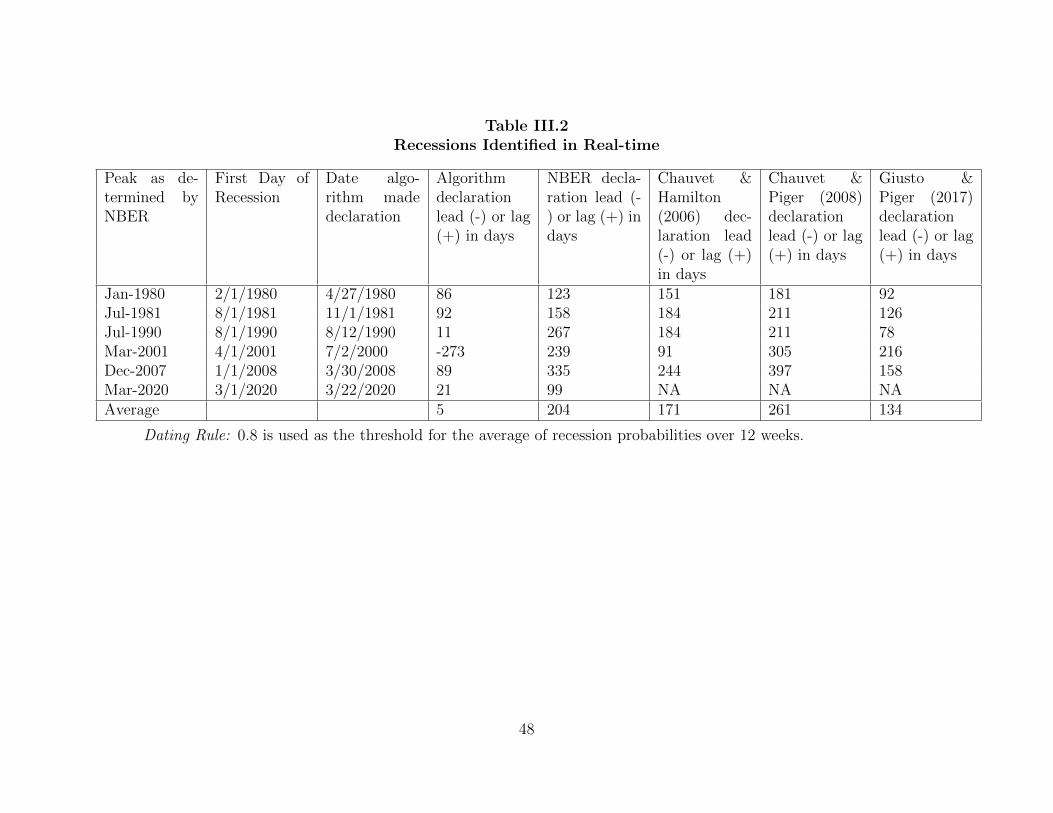
Table III.2Recessions Identified in Real-time
Peak as de-termined byNBER
First Day ofRecession
Date algo-rithm madedeclaration
Algorithmdeclarationlead (-) or lag(+) in days
NBER decla-ration lead (-) or lag (+) indays
Chauvet &Hamilton(2006) dec-laration lead(-) or lag (+)in days
Chauvet &Piger (2008)declarationlead (-) or lag(+) in days
Giusto &Piger (2017)declarationlead (-) or lag(+) in days
Jan-1980 2/1/1980 4/27/1980 86 123 151 181 92Jul-1981 8/1/1981 11/1/1981 92 158 184 211 126Jul-1990 8/1/1990 8/12/1990 11 267 184 211 78Mar-2001 4/1/2001 7/2/2000 -273 239 91 305 216Dec-2007 1/1/2008 3/30/2008 89 335 244 397 158Mar-2020 3/1/2020 3/22/2020 21 99 NA NA NAAverage 5 204 171 261 134
Dating Rule: 0.8 is used as the threshold for the average of recession probabilities over 12 weeks.
48

Table III.3Expansions Identified in Real-time
Trough asdeterminedby NBER
First Day ofExpansion
Date algo-rithm madedeclaration
Algorithmdeclarationlead (-) or lag(+) in days
NBER decla-ration lead (-) or lag (+) indays
Chauvet &Hamilton(2006) dec-laration lead(-) or lag (+)in days
Chauvet &Piger (2008)declarationlead (-) or lag(+) in days
Giusto &Piger (2017)declarationlead (-) or lag(+) in days
Jul-1980 8/1/1980 8/10/1980 9 341 122 152 127Nov-1982 12/1/1982 11/28/1982 -3 219 151 181 136Mar-1991 4/1/1991 6/2/1991 62 631 122 182 443Nov-2001 12/1/2001 8/19/2001 -104 593 182 219 308Jun-2009 9/1/2009 5/24/2009 -38 446 122 214 157Average -15 446 140 190 235
Dating Rule: 0.8 is used as the threshold for the average of recession probabilities over 12 weeks.
49
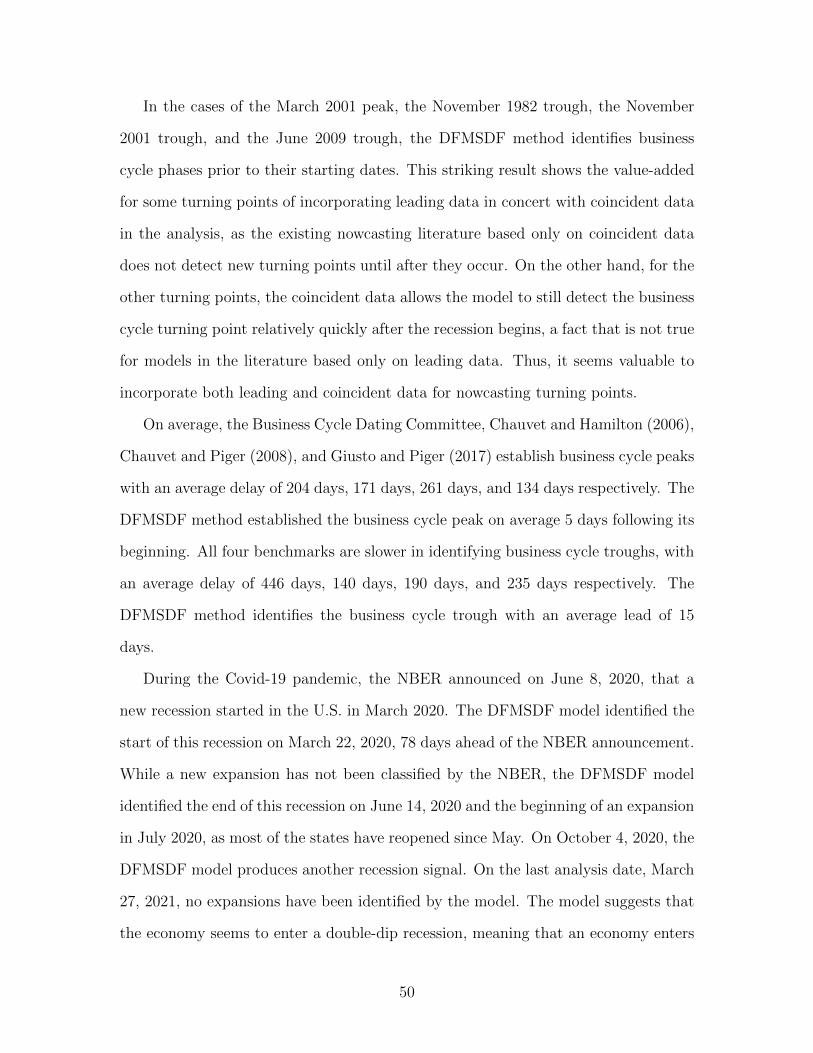
In the cases of the March 2001 peak, the November 1982 trough, the November
2001 trough, and the June 2009 trough, the DFMSDF method identifies business
cycle phases prior to their starting dates. This striking result shows the value-added
for some turning points of incorporating leading data in concert with coincident data
in the analysis, as the existing nowcasting literature based only on coincident data
does not detect new turning points until after they occur. On the other hand, for the
other turning points, the coincident data allows the model to still detect the business
cycle turning point relatively quickly after the recession begins, a fact that is not true
for models in the literature based only on leading data. Thus, it seems valuable to
incorporate both leading and coincident data for nowcasting turning points.
On average, the Business Cycle Dating Committee, Chauvet and Hamilton (2006),
Chauvet and Piger (2008), and Giusto and Piger (2017) establish business cycle peaks
with an average delay of 204 days, 171 days, 261 days, and 134 days respectively. The
DFMSDF method established the business cycle peak on average 5 days following its
beginning. All four benchmarks are slower in identifying business cycle troughs, with
an average delay of 446 days, 140 days, 190 days, and 235 days respectively. The
DFMSDF method identifies the business cycle trough with an average lead of 15
days.
During the Covid-19 pandemic, the NBER announced on June 8, 2020, that a
new recession started in the U.S. in March 2020. The DFMSDF model identified the
start of this recession on March 22, 2020, 78 days ahead of the NBER announcement.
While a new expansion has not been classified by the NBER, the DFMSDF model
identified the end of this recession on June 14, 2020 and the beginning of an expansion
in July 2020, as most of the states have reopened since May. On October 4, 2020, the
DFMSDF model produces another recession signal. On the last analysis date, March
27, 2021, no expansions have been identified by the model. The model suggests that
the economy seems to enter a double-dip recession, meaning that an economy enters
50
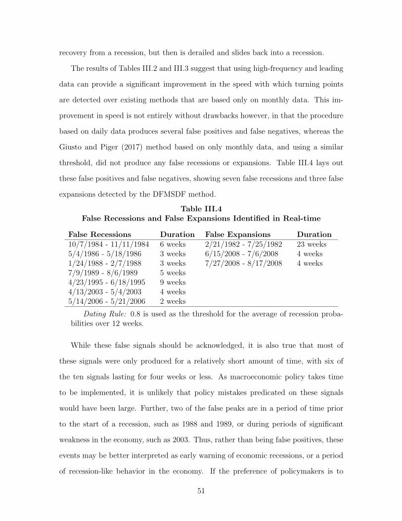
recovery from a recession, but then is derailed and slides back into a recession.
The results of Tables III.2 and III.3 suggest that using high-frequency and leading
data can provide a significant improvement in the speed with which turning points
are detected over existing methods that are based only on monthly data. This im-
provement in speed is not entirely without drawbacks however, in that the procedure
based on daily data produces several false positives and false negatives, whereas the
Giusto and Piger (2017) method based on only monthly data, and using a similar
threshold, did not produce any false recessions or expansions. Table III.4 lays out
these false positives and false negatives, showing seven false recessions and three false
expansions detected by the DFMSDF method.
Table III.4False Recessions and False Expansions Identified in Real-time
False Recessions Duration False Expansions Duration10/7/1984 - 11/11/1984 6 weeks 2/21/1982 - 7/25/1982 23 weeks5/4/1986 - 5/18/1986 3 weeks 6/15/2008 - 7/6/2008 4 weeks1/24/1988 - 2/7/1988 3 weeks 7/27/2008 - 8/17/2008 4 weeks7/9/1989 - 8/6/1989 5 weeks4/23/1995 - 6/18/1995 9 weeks4/13/2003 - 5/4/2003 4 weeks5/14/2006 - 5/21/2006 2 weeks
Dating Rule: 0.8 is used as the threshold for the average of recession proba-bilities over 12 weeks.
While these false signals should be acknowledged, it is also true that most of
these signals were only produced for a relatively short amount of time, with six of
the ten signals lasting for four weeks or less. As macroeconomic policy takes time
to be implemented, it is unlikely that policy mistakes predicated on these signals
would have been large. Further, two of the false peaks are in a period of time prior
to the start of a recession, such as 1988 and 1989, or during periods of significant
weakness in the economy, such as 2003. Thus, rather than being false positives, these
events may be better interpreted as early warning of economic recessions, or a period
of recession-like behavior in the economy. If the preference of policymakers is to
51
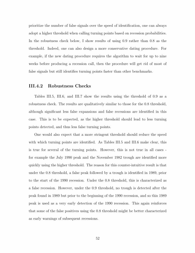
prioritize the number of false signals over the speed of identification, one can always
adopt a higher threshold when calling turning points based on recession probabilities.
In the robustness check below, I show results of using 0.9 rather than 0.8 as the
threshold. Indeed, one can also design a more conservative dating procedure. For
example, if the new dating procedure requires the algorithm to wait for up to nine
weeks before producing a recession call, then the procedure will get rid of most of
false signals but still identifies turning points faster than other benchmarks.
III.4.2 Robustness Checks
Tables III.5, III.6, and III.7 show the results using the threshold of 0.9 as a
robustness check. The results are qualitatively similar to those for the 0.8 threshold,
although significant less false expansions and false recessions are identified in this
case. This is to be expected, as the higher threshold should lead to less turning
points detected, and thus less false turning points.
One would also expect that a more stringent threshold should reduce the speed
with which turning points are identified. As Tables III.5 and III.6 make clear, this
is true for several of the turning points. However, this is not true in all cases -
for example the July 1990 peak and the November 1982 trough are identified more
quickly using the higher threshold. The reason for this counter-intuitive result is that
under the 0.8 threshold, a false peak followed by a trough is identified in 1989, prior
to the start of the 1990 recession. Under the 0.8 threshold, this is characterized as
a false recession. However, under the 0.9 threshold, no trough is detected after the
peak found in 1989 but prior to the beginning of the 1990 recession, and so this 1989
peak is used as a very early detection of the 1990 recession. This again reinforces
that some of the false positives using the 0.8 threshold might be better characterized
as early warnings of subsequent recessions.
52
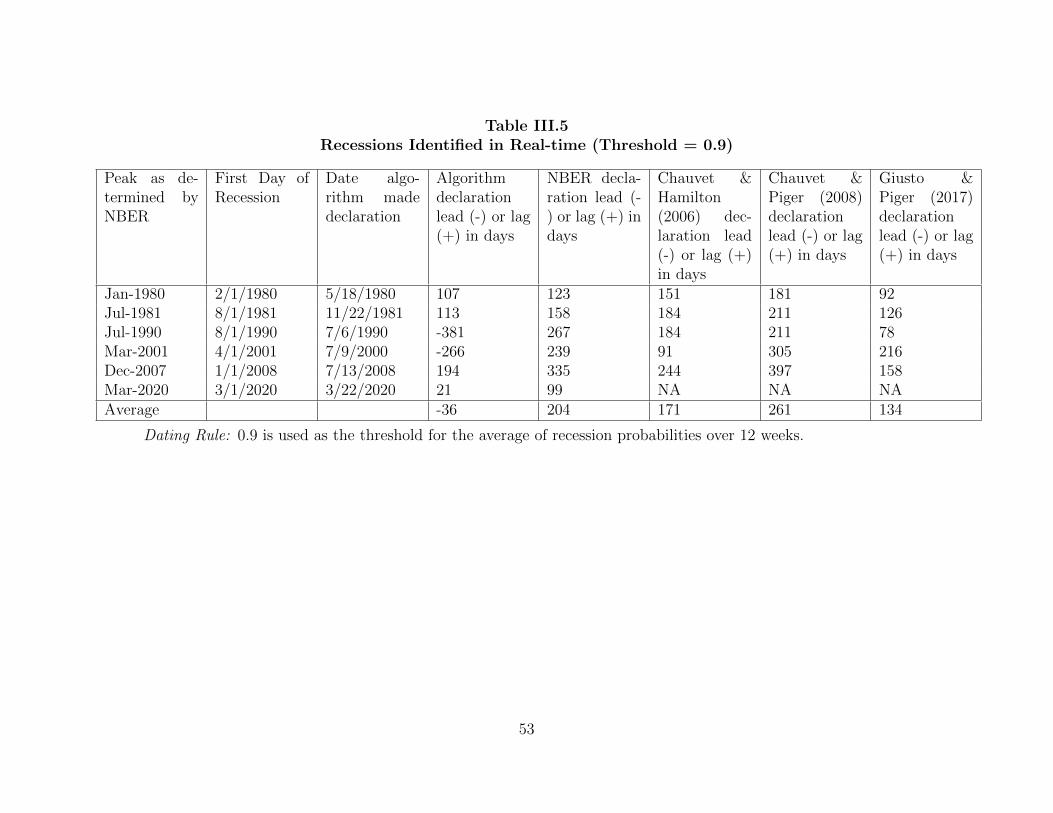
Table III.5Recessions Identified in Real-time (Threshold = 0.9)
Peak as de-termined byNBER
First Day ofRecession
Date algo-rithm madedeclaration
Algorithmdeclarationlead (-) or lag(+) in days
NBER decla-ration lead (-) or lag (+) indays
Chauvet &Hamilton(2006) dec-laration lead(-) or lag (+)in days
Chauvet &Piger (2008)declarationlead (-) or lag(+) in days
Giusto &Piger (2017)declarationlead (-) or lag(+) in days
Jan-1980 2/1/1980 5/18/1980 107 123 151 181 92Jul-1981 8/1/1981 11/22/1981 113 158 184 211 126Jul-1990 8/1/1990 7/6/1990 -381 267 184 211 78Mar-2001 4/1/2001 7/9/2000 -266 239 91 305 216Dec-2007 1/1/2008 7/13/2008 194 335 244 397 158Mar-2020 3/1/2020 3/22/2020 21 99 NA NA NAAverage -36 204 171 261 134
Dating Rule: 0.9 is used as the threshold for the average of recession probabilities over 12 weeks.
53
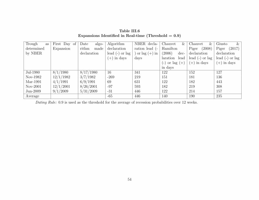
Table III.6Expansions Identified in Real-time (Threshold = 0.9)
Trough asdeterminedby NBER
First Day ofExpansion
Date algo-rithm madedeclaration
Algorithmdeclarationlead (-) or lag(+) in days
NBER decla-ration lead (-) or lag (+) indays
Chauvet &Hamilton(2006) dec-laration lead(-) or lag (+)in days
Chauvet &Piger (2008)declarationlead (-) or lag(+) in days
Giusto &Piger (2017)declarationlead (-) or lag(+) in days
Jul-1980 8/1/1980 8/17/1980 16 341 122 152 127Nov-1982 12/1/1982 3/7/1982 -269 219 151 181 136Mar-1991 4/1/1991 6/9/1991 69 631 122 182 443Nov-2001 12/1/2001 8/26/2001 -97 593 182 219 308Jun-2009 9/1/2009 5/31/2009 -31 446 122 214 157Average -65 446 140 190 235
Dating Rule: 0.9 is used as the threshold for the average of recession probabilities over 12 weeks.
54
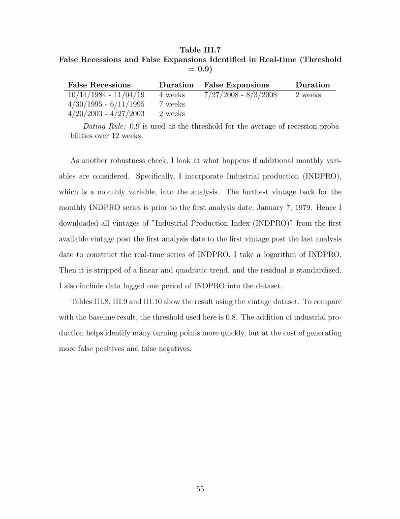
Table III.7False Recessions and False Expansions Identified in Real-time (Threshold
= 0.9)
False Recessions Duration False Expansions Duration10/14/1984 - 11/04/19 4 weeks 7/27/2008 - 8/3/2008 2 weeks4/30/1995 - 6/11/1995 7 weeks4/20/2003 - 4/27/2003 2 weeks
Dating Rule: 0.9 is used as the threshold for the average of recession proba-bilities over 12 weeks.
As another robustness check, I look at what happens if additional monthly vari-
ables are considered. Specifically, I incorporate Industrial production (INDPRO),
which is a monthly variable, into the analysis. The furthest vintage back for the
monthly INDPRO series is prior to the first analysis date, January 7, 1979. Hence I
downloaded all vintages of ”Industrial Production Index (INDPRO)” from the first
available vintage post the first analysis date to the first vintage post the last analysis
date to construct the real-time series of INDPRO. I take a logarithm of INDPRO.
Then it is stripped of a linear and quadratic trend, and the residual is standardized.
I also include data lagged one period of INDPRO into the dataset.
Tables III.8, III.9 and III.10 show the result using the vintage dataset. To compare
with the baseline result, the threshold used here is 0.8. The addition of industrial pro-
duction helps identify many turning points more quickly, but at the cost of generating
more false positives and false negatives.
55
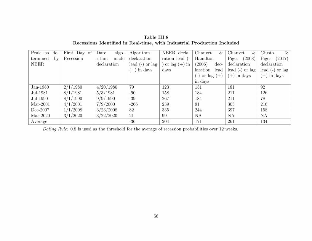
Table III.8Recessions Identified in Real-time, with Industrial Production Included
Peak as de-termined byNBER
First Day ofRecession
Date algo-rithm madedeclaration
Algorithmdeclarationlead (-) or lag(+) in days
NBER decla-ration lead (-) or lag (+) indays
Chauvet &Hamilton(2006) dec-laration lead(-) or lag (+)in days
Chauvet &Piger (2008)declarationlead (-) or lag(+) in days
Giusto &Piger (2017)declarationlead (-) or lag(+) in days
Jan-1980 2/1/1980 4/20/1980 79 123 151 181 92Jul-1981 8/1/1981 5/3/1981 -90 158 184 211 126Jul-1990 8/1/1990 9/9/1990 -39 267 184 211 78Mar-2001 4/1/2001 7/9/2000 -266 239 91 305 216Dec-2007 1/1/2008 3/23/2008 82 335 244 397 158Mar-2020 3/1/2020 3/22/2020 21 99 NA NA NAAverage -36 204 171 261 134
Dating Rule: 0.8 is used as the threshold for the average of recession probabilities over 12 weeks.
56
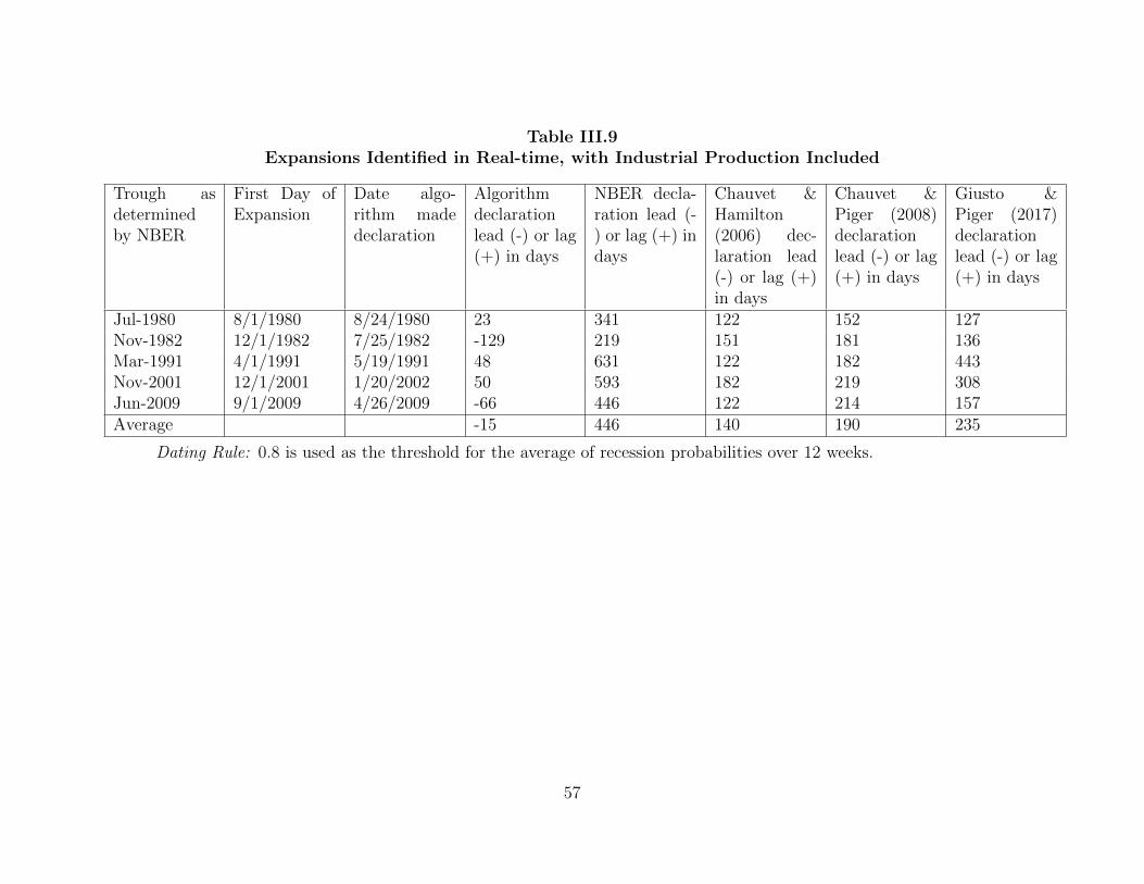
Table III.9Expansions Identified in Real-time, with Industrial Production Included
Trough asdeterminedby NBER
First Day ofExpansion
Date algo-rithm madedeclaration
Algorithmdeclarationlead (-) or lag(+) in days
NBER decla-ration lead (-) or lag (+) indays
Chauvet &Hamilton(2006) dec-laration lead(-) or lag (+)in days
Chauvet &Piger (2008)declarationlead (-) or lag(+) in days
Giusto &Piger (2017)declarationlead (-) or lag(+) in days
Jul-1980 8/1/1980 8/24/1980 23 341 122 152 127Nov-1982 12/1/1982 7/25/1982 -129 219 151 181 136Mar-1991 4/1/1991 5/19/1991 48 631 122 182 443Nov-2001 12/1/2001 1/20/2002 50 593 182 219 308Jun-2009 9/1/2009 4/26/2009 -66 446 122 214 157Average -15 446 140 190 235
Dating Rule: 0.8 is used as the threshold for the average of recession probabilities over 12 weeks.
57
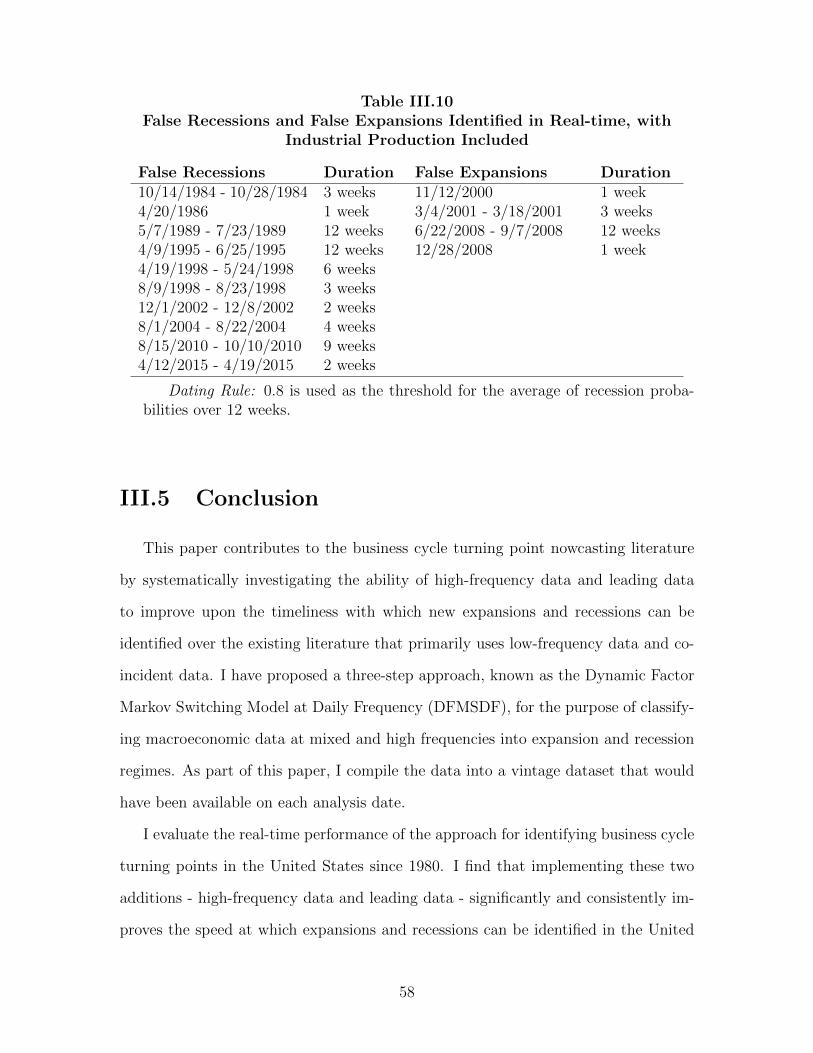
Table III.10False Recessions and False Expansions Identified in Real-time, with
Industrial Production Included
False Recessions Duration False Expansions Duration10/14/1984 - 10/28/1984 3 weeks 11/12/2000 1 week4/20/1986 1 week 3/4/2001 - 3/18/2001 3 weeks5/7/1989 - 7/23/1989 12 weeks 6/22/2008 - 9/7/2008 12 weeks4/9/1995 - 6/25/1995 12 weeks 12/28/2008 1 week4/19/1998 - 5/24/1998 6 weeks8/9/1998 - 8/23/1998 3 weeks12/1/2002 - 12/8/2002 2 weeks8/1/2004 - 8/22/2004 4 weeks8/15/2010 - 10/10/2010 9 weeks4/12/2015 - 4/19/2015 2 weeks
Dating Rule: 0.8 is used as the threshold for the average of recession proba-bilities over 12 weeks.
III.5 Conclusion
This paper contributes to the business cycle turning point nowcasting literature
by systematically investigating the ability of high-frequency data and leading data
to improve upon the timeliness with which new expansions and recessions can be
identified over the existing literature that primarily uses low-frequency data and co-
incident data. I have proposed a three-step approach, known as the Dynamic Factor
Markov Switching Model at Daily Frequency (DFMSDF), for the purpose of classify-
ing macroeconomic data at mixed and high frequencies into expansion and recession
regimes. As part of this paper, I compile the data into a vintage dataset that would
have been available on each analysis date.
I evaluate the real-time performance of the approach for identifying business cycle
turning points in the United States since 1980. I find that implementing these two
additions - high-frequency data and leading data - significantly and consistently im-
proves the speed at which expansions and recessions can be identified in the United
58
States since 1980. For example, with high-frequency and leading data included into
the analysis, the model identifies the start of the Great Recession on March 30, 2008,
246 days ahead of the NBER announcement and many months ahead of the statisti-
cal procedures surveyed in Hamilton (2011). In several cases, business cycle turning
points are called prior to their occurring, which demonstrates the value-added of
incorporating leading data into the analysis.
My approach is especially important during the Covid-19 pandemic. The NBER
announced on June 8, 2020 that a new recession associated with the pandemic has
started since March 2020. My approach identifies the start of this recession on March
22, 2020, 78 days ahead of the announcement from the NBER. With a more timely
identification of this recession, federal and state government can make informed deci-
sions to promote employment at a much faster pace. My approach can also be applied
to timely identify new recessions and expansions in other countries that provide in-
dicators of business cycle phases.
59
CHAPTER IV
A NEW HIGH-FREQUENCY,
NEWS-BASED, INDICATOR OF
MACROECONOMIC ACTIVITY
IV.1 Introduction
The information encoded in text has been recently used in empirical economics
research as a complement to the more structured macroeconomic and financial data
traditionally used (Gentzkow et al., 2019). Text selected from news, social media,
reports and speeches contains ”soft” information missing in more quantifiable vari-
ables. Unlike most of the headline macroeconomic data published at a relatively
low frequency and for which past observation periods are revised after the fact, text
such as news articles arrives daily and is not revised. These advantages make data
extracted from text an appealing candidate to build more accurate and timely now-
casting models about aggregate economic activity in real time.
In this paper I propose a text-based approach to create a high-frequency News-
Based Sentiment Index (NBSI) regarding aggregate economic conditions. Following
dictionary methods in the Natural Language Processing literature, NBSI is established
from lead paragraphs of news articles that are related to economic activity. The corpus
consists of economic and financial news articles published at a daily frequency in the
Wall Street Journal from April 1991 to March 2021.
In contrast to the text source and the computational approach used in the litera-
ture, my paper focuses on measuring the positive or negative feeling that traditional
60
news media conveys to the reader using dictionary-based sentiment analysis. The
news-based sentiment index picks up a wider range of information regarding economic
activity compared with the survey-based consumer sentiment index. The NBSI that
arrives at a daily frequency is a supplement to macroeconomic indicators available
at lower frequencies. Compared with the literature, this paper demonstrates that
textual data extracted from nontraditional data sources contains useful information
in economics research by exploring predictive capability of news sentiment in a wider
range of macroeconomic indicators, including business cycle turning points.
The remainder of this paper is organized as follows. In section 4.2 I review related
literature. In section 4.3 I present a text-based approach to create the NBSI regarding
aggregate economic conditions. Section 4.4 presents the NBSI and evaluates summary
correlations with other variables. Section 4.5 lays out two applications that investigate
the contribution of NBSI to nowcast business cycle turning points and lower-frequency
data. Section 4.6 concludes.
IV.2 Literature Review
There is a growing literature that uses constructed indices from internet queries,
social media, and traditional media for the purposes of forecasting and nowcasting
economic activity. Google Trends search engine data is a real-time daily and weekly
index of the volume of queries that users enter into Google. Choi and Varian (2012)
use Google Trend data from January 2004 to July 2011 to nowcast economic indicators
including initial claims for unemployment insurance and consumer confidence, and
find that simple seasonal auto-regression models that include relevant Google Trends
variables tend to outperform models that exclude these predictors. The authors
concludes that Google Trends may help in predicting the present.
61
Balke et al. (2017) explore the written description of economic activity contained
in the Beige Book to obtain a quantitative measure of current economic conditions.
Using a dynamic factor model that consists of the Beige Book measure and traditional
economic series, the authors find that the Beige Book picks up information about
current economic activity that is not contained in other quantitative data. This
informational advantage is relatively short-lived, lasting for three weeks.
The forecasting capability of social media data has also been explored in Lehrer
et al. (2019). The authors develop a deep learning algorithm to measure sentiment
within Twitter messages on an hourly basis and conduct an out of sample forecast-
ing exercise for the consumer confidence index. Their results show that including
consumer sentiment measures from Twitter improves forecast accuracy.
Kelly et al. (2019) model the inclusion and repetition of words of certain at-
tributes at a monthly frequency in the Wall Street Journal front page news articles.
The authors find out that the text from January 1990 to December 2010 documents
contains additional information that is useful for forecasting monthly macroeconomic
indicators beyond that of the benchmark dynamic factor model model.
Shapiro et al. (2020) derive a daily and monthly time-series sentiment from eco-
nomic and financial newspaper articles from January 1980 to April 2015 with dic-
tionary methods. The authors demonstrate that news sentiment is predictive of
consumer sentiment measured using surveys. The authors also find that positive
sentiment shocks increase consumption, output, and interest rates and dampen infla-
tion.
Bybee et al. (2020) apply topic models to estimate a daily time-series of news
attention to each theme. The authors use full text content of Wall Street Jour-
nal articles published from January 1984 to June 2017. The authors show that the
topic-based estimates accurately track a broad range of of economic variables such as
aggregate output (industrial production) and employment (non-farm payrolls). The
62
authors also find that the estimate have incremental forecasting power above and
beyond standard numerical predictors.
In contrast to Choi and Varian (2012), Balke et al. (2017), and Lehrer et al.
(2019), my paper focuses on text in the traditional news media. In contrast to the
computational approach used in Kelly et al. (2019) and Bybee et al. (2020), my
paper focuses on measuring the positive or negative feeling that a text conveys to the
reader using dictionary-based sentiment analysis. Shapiro et al. (2020) adopts the
similar method to construct a high-frequency time-series sentiment from economic
and financial newspaper; however, my paper explores predictive capability of news
sentiment in a wider range of macroeconomic indicators, including business cycle
turning points.
IV.3 Methodology to Construct NBSI
From the Factiva Database, I collect a large sample of lead paragraphs of arti-
cles published in The Wall Street Journal and The Wall Street Journal Online in
the United States from April 2, 1991 to March 31, 2021 that have the following sub-
jects: (1) News about commodity, debt, bond, equity, money and currency markets;
(2) Analysts’ comments or recommendations about corporations and industries; (3)
Economic performance or indicators, government finance, monetary policy, trade or
external payments.
The document downloaded from the database is a Rich Text Format file, which
contains indexes for custom search fields, such as indexes for column name, section
name, headline, author’s name, word count, publication date and time, source name,
lead paragraph, language code, subject code, region code, publisher name, and ac-
cession number. For the purpose of this topic, I only extract lead paragraphs and
publication dates by detecting the presence of the pattern of the index in each piece
63
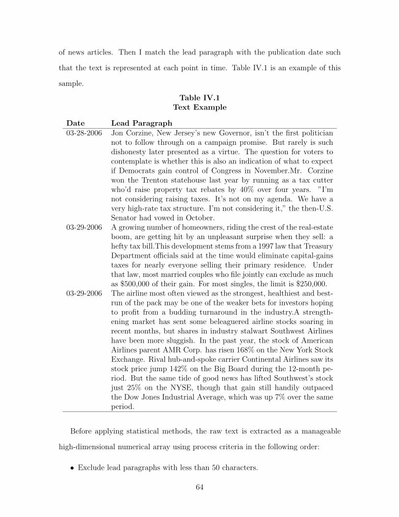
of news articles. Then I match the lead paragraph with the publication date such
that the text is represented at each point in time. Table IV.1 is an example of this
sample.
Table IV.1Text Example
Date Lead Paragraph03-28-2006 Jon Corzine, New Jersey’s new Governor, isn’t the first politician
not to follow through on a campaign promise. But rarely is suchdishonesty later presented as a virtue. The question for voters tocontemplate is whether this is also an indication of what to expectif Democrats gain control of Congress in November.Mr. Corzinewon the Trenton statehouse last year by running as a tax cutterwho’d raise property tax rebates by 40% over four years. ”I’mnot considering raising taxes. It’s not on my agenda. We have avery high-rate tax structure. I’m not considering it,” the then-U.S.Senator had vowed in October.
03-29-2006 A growing number of homeowners, riding the crest of the real-estateboom, are getting hit by an unpleasant surprise when they sell: ahefty tax bill.This development stems from a 1997 law that TreasuryDepartment officials said at the time would eliminate capital-gainstaxes for nearly everyone selling their primary residence. Underthat law, most married couples who file jointly can exclude as muchas $500,000 of their gain. For most singles, the limit is $250,000.
03-29-2006 The airline most often viewed as the strongest, healthiest and best-run of the pack may be one of the weaker bets for investors hopingto profit from a budding turnaround in the industry.A strength-ening market has sent some beleaguered airline stocks soaring inrecent months, but shares in industry stalwart Southwest Airlineshave been more sluggish. In the past year, the stock of AmericanAirlines parent AMR Corp. has risen 168% on the New York StockExchange. Rival hub-and-spoke carrier Continental Airlines saw itsstock price jump 142% on the Big Board during the 12-month pe-riod. But the same tide of good news has lifted Southwest’s stockjust 25% on the NYSE, though that gain still handily outpacedthe Dow Jones Industrial Average, which was up 7% over the sameperiod.
Before applying statistical methods, the raw text is extracted as a manageable
high-dimensional numerical array using process criteria in the following order:
• Exclude lead paragraphs with less than 50 characters.
64

• Tokenize the text into individual words and transform it to a tidy data structure.
• Strip stopwords such as ’a’, ’the’, ’to’, ’for’ out of token lists.
• Replace words with their root such that ”economic”, ”economics”, and ”eco-
nomically” are all replaced by the stem ”economic”.
• Assign ”positive” or ”negative” sentiment to words based on a general-purpose
”Bing” lexicon from Bing Liu and collaborators, which categorizes words in a
binary fashion. 1.
• Reverse sentiment of words preceded by negation words such as no, not, never,
without.
• Measure sentiment scores for each lead paragraph with npos−nneg
nwords, where npos,
nneg, and nwords represent separately the number of positive, negative, and total
words in each lead paragraph.
• Average over articles published on the same day to obtain the daily sentiment
index.
• Average over the daily sentiment for the same week to obtain the weekly NBSI,
denoted as NBSIw.
• Average over the daily sentiment for the same month to obtain the monthly
NBSI, denoted as NBSIm.
1More details about the ”Bing” lexicon are available at the following website https://www.cs.uic.
edu/~liub/FBS/sentiment-analysis.html
65
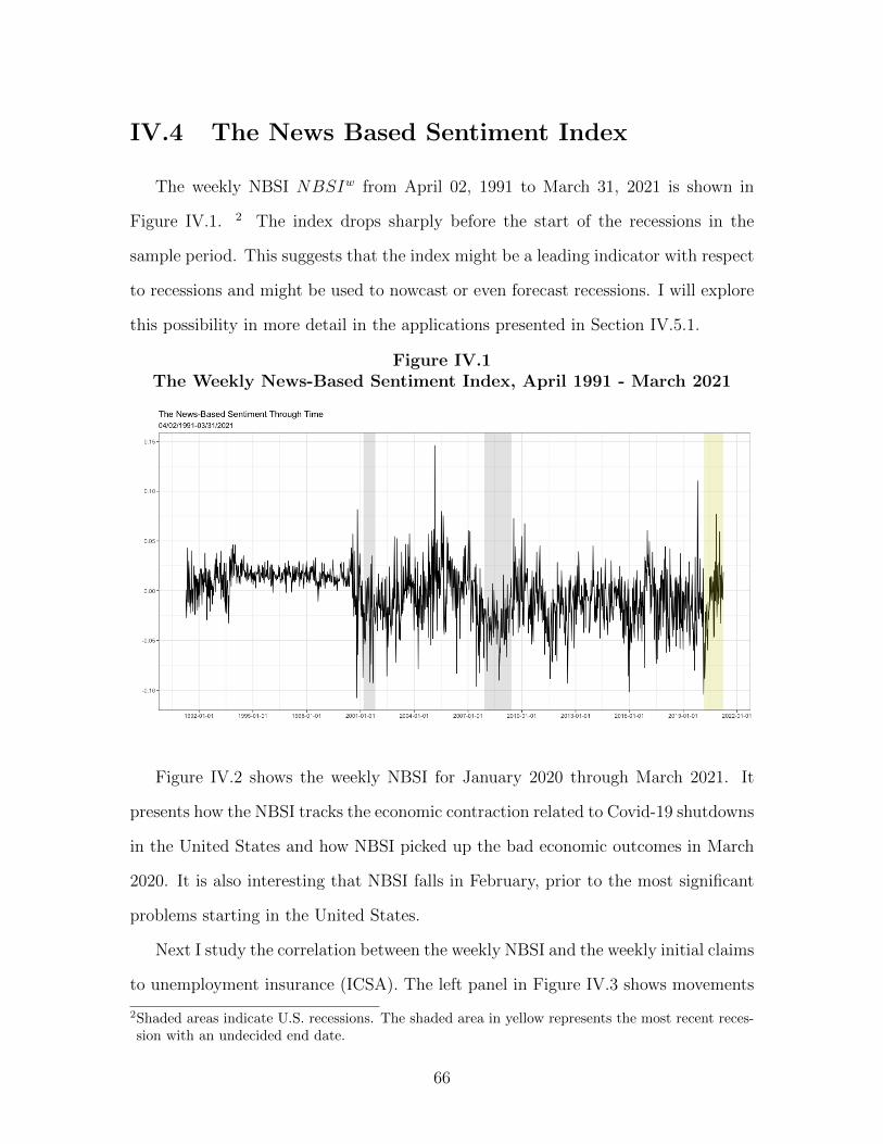
IV.4 The News Based Sentiment Index
The weekly NBSI NBSIw from April 02, 1991 to March 31, 2021 is shown in
Figure IV.1. 2 The index drops sharply before the start of the recessions in the
sample period. This suggests that the index might be a leading indicator with respect
to recessions and might be used to nowcast or even forecast recessions. I will explore
this possibility in more detail in the applications presented in Section IV.5.1.
Figure IV.1The Weekly News-Based Sentiment Index, April 1991 - March 2021
Figure IV.2 shows the weekly NBSI for January 2020 through March 2021. It
presents how the NBSI tracks the economic contraction related to Covid-19 shutdowns
in the United States and how NBSI picked up the bad economic outcomes in March
2020. It is also interesting that NBSI falls in February, prior to the most significant
problems starting in the United States.
Next I study the correlation between the weekly NBSI and the weekly initial claims
to unemployment insurance (ICSA). The left panel in Figure IV.3 shows movements
2Shaded areas indicate U.S. recessions. The shaded area in yellow represents the most recent reces-sion with an undecided end date.
66
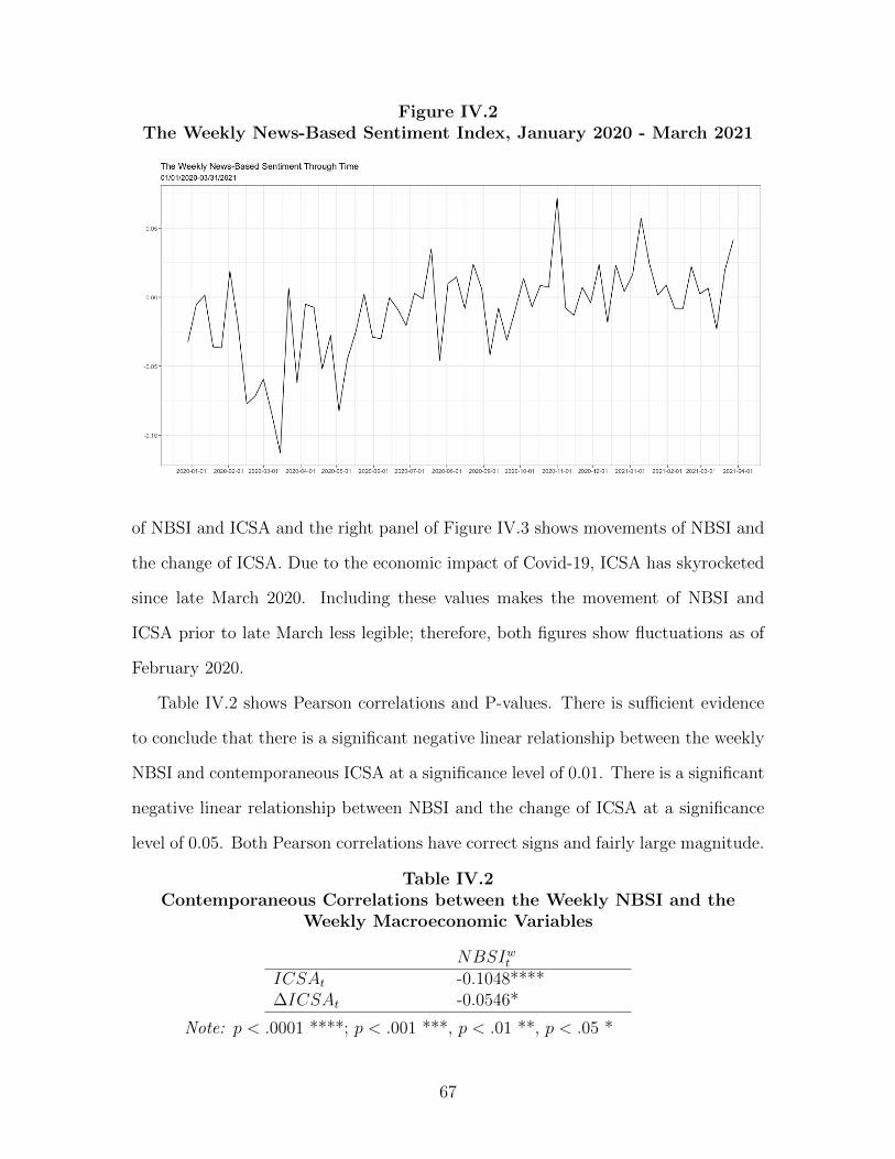
Figure IV.2The Weekly News-Based Sentiment Index, January 2020 - March 2021
of NBSI and ICSA and the right panel of Figure IV.3 shows movements of NBSI and
the change of ICSA. Due to the economic impact of Covid-19, ICSA has skyrocketed
since late March 2020. Including these values makes the movement of NBSI and
ICSA prior to late March less legible; therefore, both figures show fluctuations as of
February 2020.
Table IV.2 shows Pearson correlations and P-values. There is sufficient evidence
to conclude that there is a significant negative linear relationship between the weekly
NBSI and contemporaneous ICSA at a significance level of 0.01. There is a significant
negative linear relationship between NBSI and the change of ICSA at a significance
level of 0.05. Both Pearson correlations have correct signs and fairly large magnitude.
Table IV.2Contemporaneous Correlations between the Weekly NBSI and the
Weekly Macroeconomic Variables
NBSIwtICSAt -0.1048****∆ICSAt -0.0546*
Note: p < .0001 ****; p < .001 ***, p < .01 **, p < .05 *
67
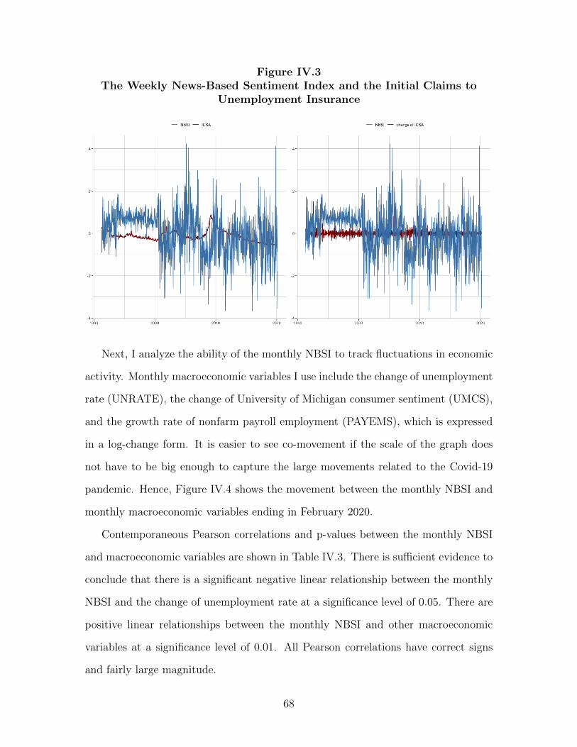
Figure IV.3The Weekly News-Based Sentiment Index and the Initial Claims to
Unemployment Insurance
Next, I analyze the ability of the monthly NBSI to track fluctuations in economic
activity. Monthly macroeconomic variables I use include the change of unemployment
rate (UNRATE), the change of University of Michigan consumer sentiment (UMCS),
and the growth rate of nonfarm payroll employment (PAYEMS), which is expressed
in a log-change form. It is easier to see co-movement if the scale of the graph does
not have to be big enough to capture the large movements related to the Covid-19
pandemic. Hence, Figure IV.4 shows the movement between the monthly NBSI and
monthly macroeconomic variables ending in February 2020.
Contemporaneous Pearson correlations and p-values between the monthly NBSI
and macroeconomic variables are shown in Table IV.3. There is sufficient evidence to
conclude that there is a significant negative linear relationship between the monthly
NBSI and the change of unemployment rate at a significance level of 0.05. There are
positive linear relationships between the monthly NBSI and other macroeconomic
variables at a significance level of 0.01. All Pearson correlations have correct signs
and fairly large magnitude.
68
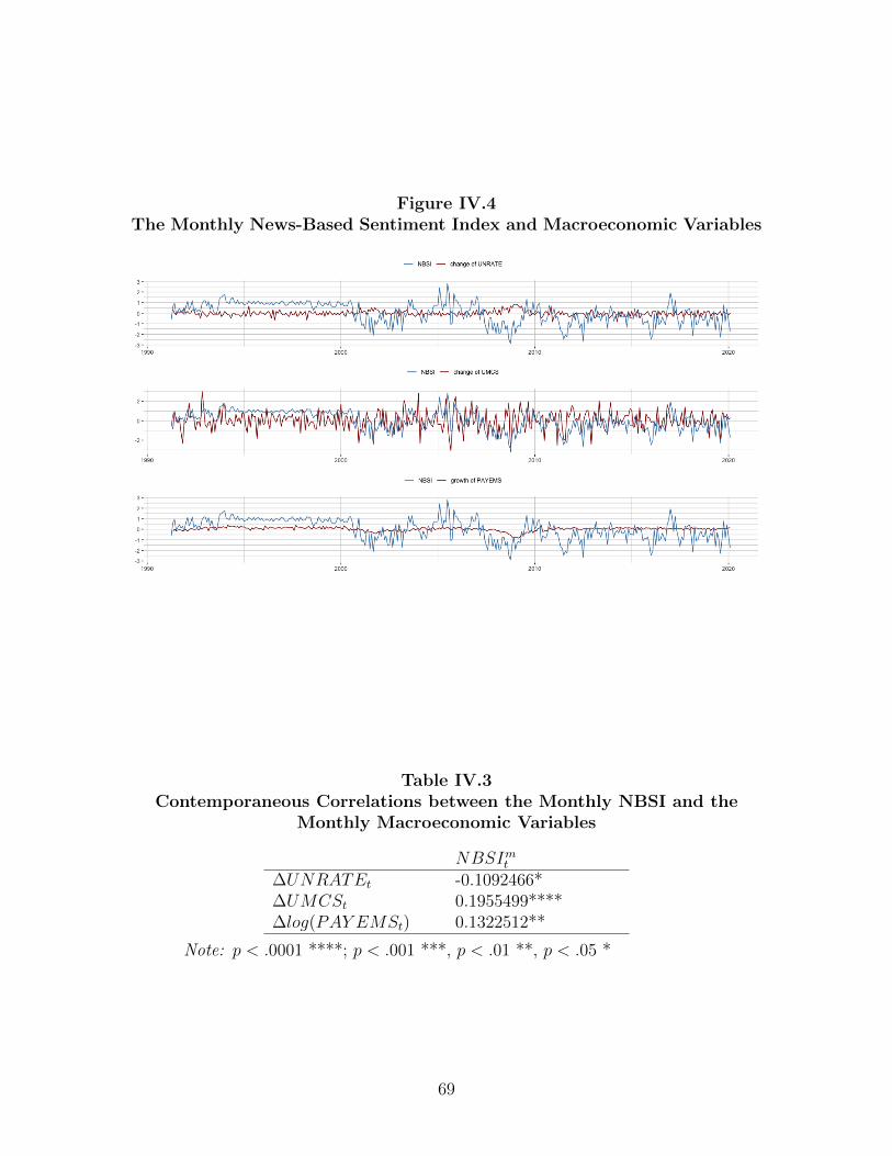
Figure IV.4The Monthly News-Based Sentiment Index and Macroeconomic Variables
Table IV.3Contemporaneous Correlations between the Monthly NBSI and the
Monthly Macroeconomic Variables
NBSImt∆UNRATEt -0.1092466*∆UMCSt 0.1955499****∆log(PAY EMSt) 0.1322512**
Note: p < .0001 ****; p < .001 ***, p < .01 **, p < .05 *
69
I have found that NBSI is correlated with various economic indicators and may
be helpful for short-term economic prediction. To evaluate the ability of NBSI in
predicting the present, this paper provides two applications. In the first application,
I incorporate NBSI in the business cycle phases nowcasting framework developed in
the third chapter, and estimate the contribution of NBSI to identify U.S. recessions in
real time. In the second application, I explore the power of NBSI to nowcast monthly
macroeconomic variables.
IV.5 Empirical Applications
IV.5.1 Nowcasting Business Cycle Phases
In this section I evaluate the ability of NBSI to improve turning point identification
in real time over the use of the index xt studied in the third chapter. To evaluate the
nowcasting ability of the NBSI on the U.S. recessions, in the baseline model, I exclude
the NBSI from the dataset and use the same estimation method and dating procedure
as described in the previous chapter to declare the date of turning points. To be
specific, I use the dataset that excludes NBSI from April 2, 1991 to March 31, 2021
to estimate the index xt from the dynamic factor model as specified in Equations IV.1
and IV.2. Then, I fit the estimated ∆xt to a Markov regime - switching AR(0) model
as specified in Equations IV.3 and IV.4. Data from April 2, 1991 to December 31,
2005 are used as the training set and remaining data from January 1, 2006 to March
31, 2021 are used as the testing set, in which recession probabilities P (St = 1|ΨT )
are estimated using the Hamilton filter. Lastly, following the business cycle dating
procedure proposed in the third chapter, I define day t as a recession phase if the
average value of P (St = 1|ΨT ) in the last 12 weeks exceeds 0.8, and define day t as an
expansion phase if the average value of P (St = 1|ΨT ) in the last 12 weeks is smaller
than 0.2.
70
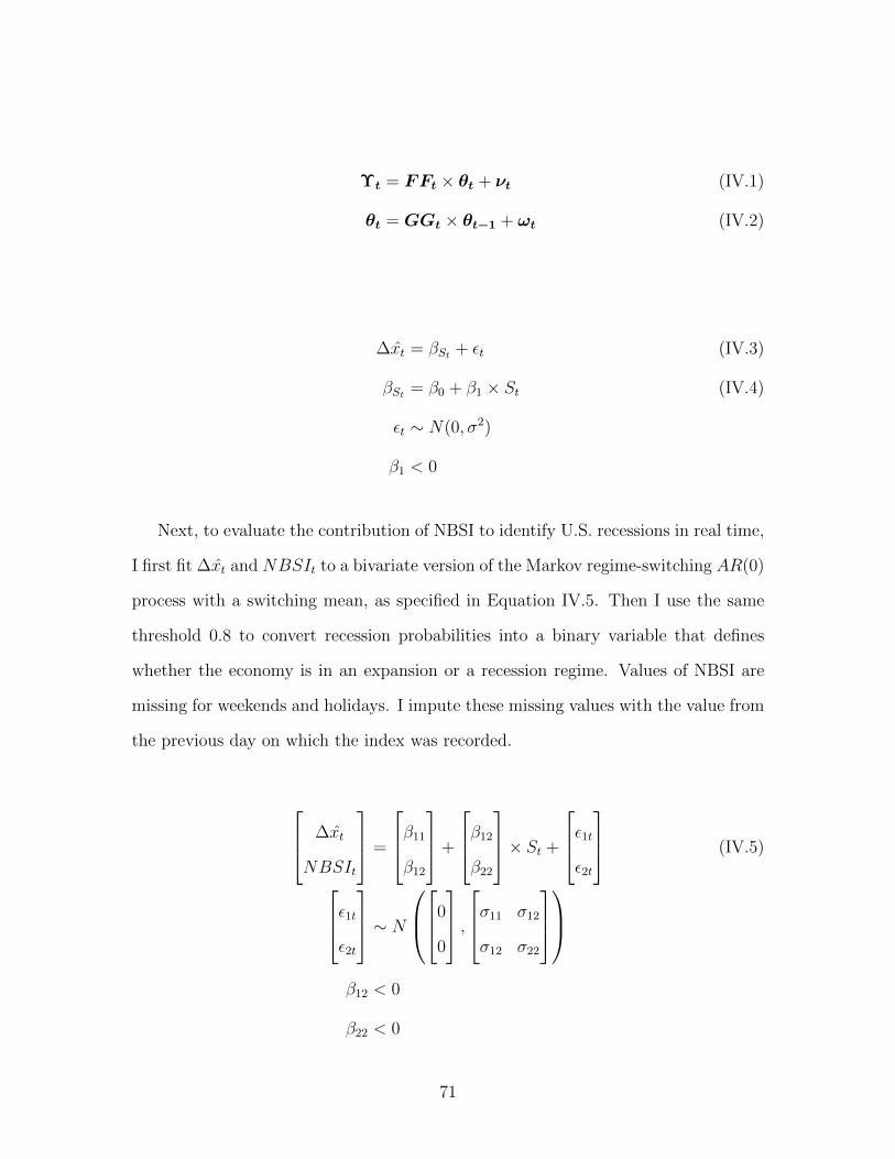
Υt = FFt × θt + νt (IV.1)
θt = GGt × θt−1 + ωt (IV.2)
∆xt = βSt + εt (IV.3)
βSt = β0 + β1 × St (IV.4)
εt ∼ N(0, σ2)
β1 < 0
Next, to evaluate the contribution of NBSI to identify U.S. recessions in real time,
I first fit ∆xt and NBSIt to a bivariate version of the Markov regime-switching AR(0)
process with a switching mean, as specified in Equation IV.5. Then I use the same
threshold 0.8 to convert recession probabilities into a binary variable that defines
whether the economy is in an expansion or a recession regime. Values of NBSI are
missing for weekends and holidays. I impute these missing values with the value from
the previous day on which the index was recorded.
∆xt
NBSIt
=
β11β12
+
β12β22
× St +
ε1tε2t
(IV.5)
ε1tε2t
∼ N
0
0
,σ11 σ12
σ12 σ22
β12 < 0
β22 < 0
71
Tables IV.4 and IV.5 show the identification of expansions and recessions with-
out NBSI incorporated. To assess the contribution of NBSI, I use only ∆xt on the
same shortened estimation window. Tables IV.6 and IV.7 show the identification of
expansions and recessions with NBSI incorporated. Similar to the baseline result,
the DFMSDF method predicts the occurrence of turning points faster than all other
sources. Compared with the result where NBSI is not incorporated in the analysis, in-
cluding NBSI accelerates the identification of the December 2007 Peak, and produces
less false positives and false negatives.
Incorporating high-frequency data and leading data, namely the yield curve term
premium and initial claims, produces a call of the December 2007 business cycle peak
on April 6, 2008. When information from the news-based sentiment index is further
incorporated, the December 2007 business cycle peak is identified even earlier, on
December 2, 2007. The contribution of the news-based sentiment index is promising
but more data is needed before concluding that the index helps to identify recessions
in real time over the use of the coincident index ∆xt alone.
72
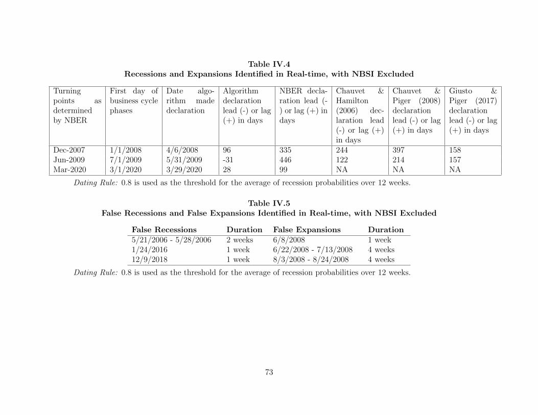
Table IV.4Recessions and Expansions Identified in Real-time, with NBSI Excluded
Turningpoints asdeterminedby NBER
First day ofbusiness cyclephases
Date algo-rithm madedeclaration
Algorithmdeclarationlead (-) or lag(+) in days
NBER decla-ration lead (-) or lag (+) indays
Chauvet &Hamilton(2006) dec-laration lead(-) or lag (+)in days
Chauvet &Piger (2008)declarationlead (-) or lag(+) in days
Giusto &Piger (2017)declarationlead (-) or lag(+) in days
Dec-2007 1/1/2008 4/6/2008 96 335 244 397 158Jun-2009 7/1/2009 5/31/2009 -31 446 122 214 157Mar-2020 3/1/2020 3/29/2020 28 99 NA NA NA
Dating Rule: 0.8 is used as the threshold for the average of recession probabilities over 12 weeks.
Table IV.5False Recessions and False Expansions Identified in Real-time, with NBSI Excluded
False Recessions Duration False Expansions Duration5/21/2006 - 5/28/2006 2 weeks 6/8/2008 1 week1/24/2016 1 week 6/22/2008 - 7/13/2008 4 weeks12/9/2018 1 week 8/3/2008 - 8/24/2008 4 weeks
Dating Rule: 0.8 is used as the threshold for the average of recession probabilities over 12 weeks.
73
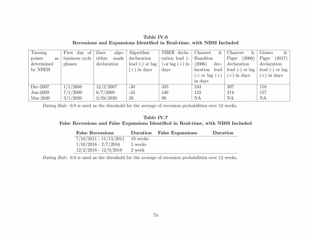
Table IV.6Recessions and Expansions Identified in Real-time, with NBSI Included
Turningpoints asdeterminedby NBER
First day ofbusiness cyclephases
Date algo-rithm madedeclaration
Algorithmdeclarationlead (-) or lag(+) in days
NBER decla-ration lead (-) or lag (+) indays
Chauvet &Hamilton(2006) dec-laration lead(-) or lag (+)in days
Chauvet &Piger (2008)declarationlead (-) or lag(+) in days
Giusto &Piger (2017)declarationlead (-) or lag(+) in days
Dec-2007 1/1/2008 12/2/2007 -30 335 244 397 158Jun-2009 7/1/2009 6/7/2009 -24 446 122 214 157Mar-2020 3/1/2020 3/29/2020 28 99 NA NA NA
Dating Rule: 0.8 is used as the threshold for the average of recession probabilities over 12 weeks.
Table IV.7False Recessions and False Expansions Identified in Real-time, with NBSI Included
False Recessions Duration False Expansions Duration7/10/2011 - 11/13/2011 19 weeks1/10/2016 - 2/7/2016 5 weeks12/2/2018 - 12/9/2018 2 week
Dating Rule: 0.8 is used as the threshold for the average of recession probabilities over 12 weeks.
74
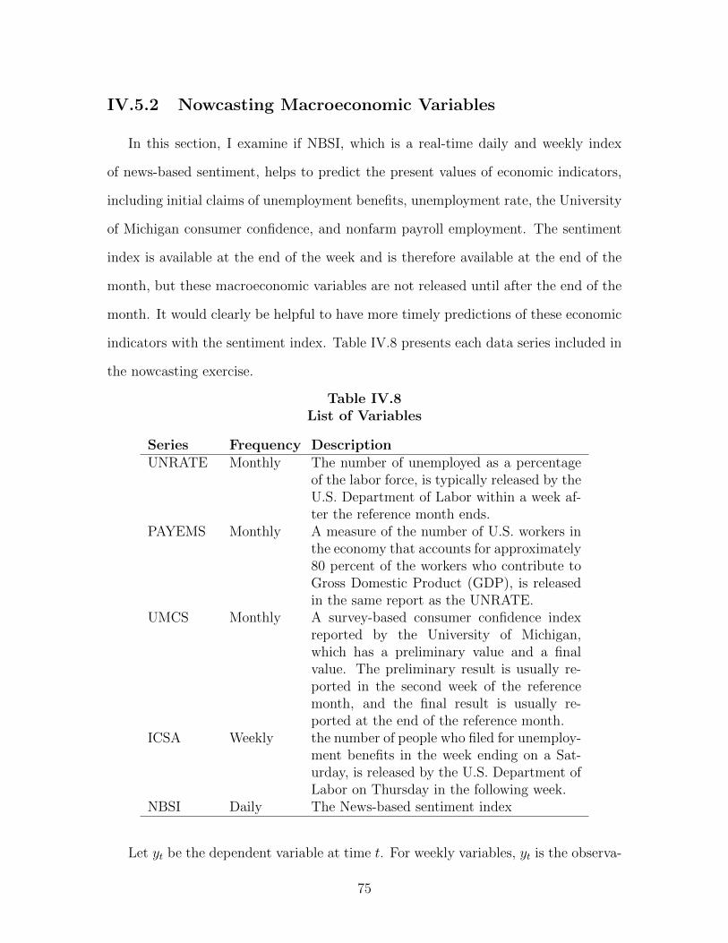
IV.5.2 Nowcasting Macroeconomic Variables
In this section, I examine if NBSI, which is a real-time daily and weekly index
of news-based sentiment, helps to predict the present values of economic indicators,
including initial claims of unemployment benefits, unemployment rate, the University
of Michigan consumer confidence, and nonfarm payroll employment. The sentiment
index is available at the end of the week and is therefore available at the end of the
month, but these macroeconomic variables are not released until after the end of the
month. It would clearly be helpful to have more timely predictions of these economic
indicators with the sentiment index. Table IV.8 presents each data series included in
the nowcasting exercise.
Table IV.8List of Variables
Series Frequency DescriptionUNRATE Monthly The number of unemployed as a percentage
of the labor force, is typically released by theU.S. Department of Labor within a week af-ter the reference month ends.
PAYEMS Monthly A measure of the number of U.S. workers inthe economy that accounts for approximately80 percent of the workers who contribute toGross Domestic Product (GDP), is releasedin the same report as the UNRATE.
UMCS Monthly A survey-based consumer confidence indexreported by the University of Michigan,which has a preliminary value and a finalvalue. The preliminary result is usually re-ported in the second week of the referencemonth, and the final result is usually re-ported at the end of the reference month.
ICSA Weekly the number of people who filed for unemploy-ment benefits in the week ending on a Sat-urday, is released by the U.S. Department ofLabor on Thursday in the following week.
NBSI Daily The News-based sentiment index
Let yt be the dependent variable at time t. For weekly variables, yt is the observa-
75
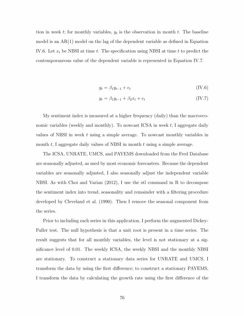
tion in week t; for monthly variables, yt is the observation in month t. The baseline
model is an AR(1) model on the lag of the dependent variable as defined in Equation
IV.6. Let xt be NBSI at time t. The specification using NBSI at time t to predict the
contemporaneous value of the dependent variable is represented in Equation IV.7.
yt = β1yt−1 + et (IV.6)
yt = β1yt−1 + β2xt + et (IV.7)
My sentiment index is measured at a higher frequency (daily) than the macroeco-
nomic variables (weekly and monthly). To nowcast ICSA in week t, I aggregate daily
values of NBSI in week t using a simple average. To nowcast monthly variables in
month t, I aggregate daily values of NBSI in month t using a simple average.
The ICSA, UNRATE, UMCS, and PAYEMS downloaded from the Fred Database
are seasonally adjusted, as used by most economic forecasters. Because the dependent
variables are seasonally adjusted, I also seasonally adjust the independent variable
NBSI. As with Choi and Varian (2012), I use the stl command in R to decompose
the sentiment index into trend, seasonality and remainder with a filtering procedure
developed by Cleveland et al. (1990). Then I remove the seasonal component from
the series.
Prior to including each series in this application, I perform the augmented Dickey-
Fuller test. The null hypothesis is that a unit root is present in a time series. The
result suggests that for all monthly variables, the level is not stationary at a sig-
nificance level of 0.01. The weekly ICSA, the weekly NBSI and the monthly NBSI
are stationary. To construct a stationary data series for UNRATE and UMCS, I
transform the data by using the first difference; to construct a stationary PAYEMS,
I transform the data by calculating the growth rate using the first difference of the
76
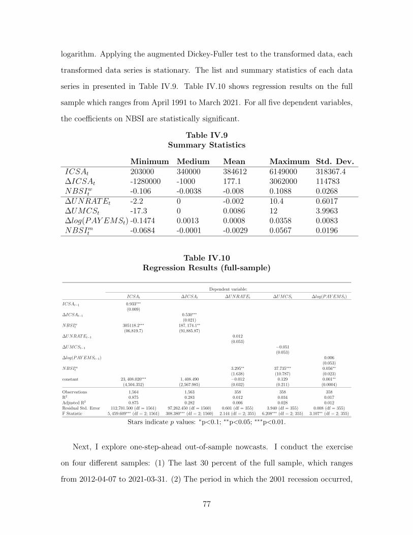
logarithm. Applying the augmented Dickey-Fuller test to the transformed data, each
transformed data series is stationary. The list and summary statistics of each data
series in presented in Table IV.9. Table IV.10 shows regression results on the full
sample which ranges from April 1991 to March 2021. For all five dependent variables,
the coefficients on NBSI are statistically significant.
Table IV.9Summary Statistics
Minimum Medium Mean Maximum Std. Dev.ICSAt 203000 340000 384612 6149000 318367.4∆ICSAt -1280000 -1000 177.1 3062000 114783NBSIwt -0.106 -0.0038 -0.008 0.1088 0.0268∆UNRATEt -2.2 0 -0.002 10.4 0.6017∆UMCSt -17.3 0 0.0086 12 3.9963∆log(PAY EMSt) -0.1474 0.0013 0.0008 0.0358 0.0083NBSImt -0.0684 -0.0001 -0.0029 0.0567 0.0196
Table IV.10Regression Results (full-sample)
Dependent variable:
ICSAt ∆ICSAt ∆UNRATEt ∆UMCSt ∆log(PAY EMSt)
ICSAt−1 0.933∗∗∗
(0.009)∆ICSAt−1 0.530∗∗∗
(0.021)NBSIwt 305118.2∗∗∗ 187, 174.1∗∗
(06,819.7) (91,885.87)∆UNRATEt−1 0.012
(0.053)∆UMCSt−1 −0.051
(0.053)∆log(PAY EMSt−1) 0.006
(0.053)NBSImt 3.295∗∗ 37.735∗∗∗ 0.056∗∗
(1.638) (10.787) (0.023)constant 23, 408.020∗∗∗ 1, 408.490 −0.012 0.129 0.001∗∗
(4,504.352) (2,567.985) (0.032) (0.211) (0.0004)
Observations 1,564 1,563 358 358 358R2 0.875 0.283 0.012 0.034 0.017Adjusted R2 0.875 0.282 0.006 0.028 0.012Residual Std. Error 112,701.500 (df = 1561) 97,262.450 (df = 1560) 0.601 (df = 355) 3.940 (df = 355) 0.008 (df = 355)F Statistic 5, 459.609∗∗∗ (df = 2; 1561) 308.380∗∗∗ (df = 2; 1560) 2.144 (df = 2; 355) 6.208∗∗∗ (df = 2; 355) 3.107∗∗ (df = 2; 355)
Stars indicate p values: ∗p<0.1; ∗∗p<0.05; ∗∗∗p<0.01.
Next, I explore one-step-ahead out-of-sample nowcasts. I conduct the exercise
on four different samples: (1) The last 30 percent of the full sample, which ranges
from 2012-04-07 to 2021-03-31. (2) The period in which the 2001 recession occurred,
77
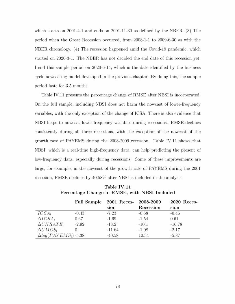
which starts on 2001-4-1 and ends on 2001-11-30 as defined by the NBER. (3) The
period when the Great Recession occurred, from 2008-1-1 to 2009-6-30 as with the
NBER chronology. (4) The recession happened amid the Covid-19 pandemic, which
started on 2020-3-1. The NBER has not decided the end date of this recession yet.
I end this sample period on 2020-6-14, which is the date identified by the business
cycle nowcasting model developed in the previous chapter. By doing this, the sample
period lasts for 3.5 months.
Table IV.11 presents the percentage change of RMSE after NBSI is incorporated.
On the full sample, including NBSI does not harm the nowcast of lower-frequency
variables, with the only exception of the change of ICSA. There is also evidence that
NBSI helps to nowcast lower-frequency variables during recessions. RMSE declines
consistently during all three recessions, with the exception of the nowcast of the
growth rate of PAYEMS during the 2008-2009 recession. Table IV.11 shows that
NBSI, which is a real-time high-frequency data, can help predicting the present of
low-frequency data, especially during recessions. Some of these improvements are
large, for example, in the nowcast of the growth rate of PAYEMS during the 2001
recession, RMSE declines by 40.58% after NBSI is included in the analysis.
Table IV.11Percentage Change in RMSE, with NBSI Included
Full Sample 2001 Reces-sion
2008-2009Recession
2020 Reces-sion
ICSAt -0.43 -7.23 -0.58 -0.46∆ICSAt 0.67 -1.69 -1.54 0.61∆UNRATEt -2.92 -18.2 -10.1 -16.78∆UMCSt 0 -11.64 -1.08 -2.17∆log(PAY EMSt) -5.38 -40.58 10.34 -5.87
78
IV.6 Conclusion
Applying dictionary methods, I have proposed a novel sentiment index based on
economic and financial news articles published at a daily frequency by the Wall Street
Journal. I have found that high-frequency news-based sentiment index can improve
the nowcast of low-frequency macroeconomic variables.
In the first application, I nowcast business cycle turning points with the news-
based sentiment index. Results show that incorporating the index helps to identify
the 2008-2009 recession 126 days earlier than the identification without using the
index. In the second application, I nowcast near-term values of economic indicators,
including initial claims, unemployment rate, the University of Michigan consumer
sentiment index, and nonfarm payroll employment. I have found that the simple
seasonal AR models that incorporating the index tend to outperform models that
exclude the index. This improvement is especially significant during recessions. 3
3I have also measured sentiment scores for each lead paragraph using npos−nneg, and have evaluatedthe predictive ability of the sentiment index established in this way using the two applications.For the first application, compared with Tables IV.6 and IV.7 in Section IV.5.1, including thesentiment index that does not scale over the size of the news article helps the model to identifythree turning points on the same days, i.e., 12/2/2007, 6/7/2009, and 3/29/2020; however, morefalse signals are produced. For the second application, compared with Table IV.11 in Section IV.5.2,the improvement generated by the model that includes the new sentiment index is smaller.
79
CHAPTER V
DISSERTATION CONCLUSION
In this dissertation, I investigate techniques to improve high-frequency monitor-
ing of macroeconomy. In contrast with the United States where there are alternating
phases of expansion and recession, China’s economic growth has been very strong and
presented a sustained expansion since 2000. Instead of classifying the Chinese eco-
nomic activity into phases of ”expansions” and ”recessions” as in the United States,
in the second chapter of my dissertation, I center on the ”high-growth” and ”low-
growth” phase in the Chinese overall economy. To monitor macroeconomic activity
in China, I adopt the dynamic factor model and extract a monthly economic activity
factor and a monthly inflation factor from a large panel of underlying economic in-
dicators. I find evidence that the effects of measured monetary policy shocks on the
Chinese economy are different between high-growth periods vs. low-growth periods.
Monetary policy shocks have larger impacts on output growth in low-growth states;
during high-growth states, monetary policy shocks have larger impacts on inflation.
In the third and the fourth chapters, I shift my focus to the high-frequency moni-
toring of macroeconomic activity in the United States. In the third chapter, I develop
techniques to provide an improved nowcast of U.S. business cycle phases in real time.
In contrast with the literature that primarily uses low-frequency data and coincident
data to nowcast business cycle phases, I focus on whether the use of high-frequency
data and leading data can improve the speed at which business cycle phases can be
identified. Using a combination of the mixed-frequency dynamic factor model and a
supervised Markov regime-switching model, I find that the addition of high-frequency
data and leading data significantly and consistently improves the speed at which ex-
80
pansions and recessions can be identified in the United States since 1980.
In the fourth chapter, I investigate whether information from news articles can
improve the nowcast of low-frequency macroeconomic variables. I create a novel high-
frequency news-based sentiment indicator of aggregate economic conditions from news
articles that are related to aggregate economic activity. I find that incorporating the
index accelerates the nowcast of the 2008-2009 recession. I also find that incorporating
the index improves the nowcast of economic indicators at lower-frequencies, and the
improvement is especially significant during recessions.
81
REFERENCES CITEDAruoba, B., Diebold, F., and Scotti, C. (2009). Real-time measurement of business
conditions. Journal of Business Economic Statistics, 27(4):417–427.
Auerbach, A. J. and Gorodnichenko, Y. (2012). Measuring the output responses tofiscal policy. American Economic Journal: Economy Policy, 4(2):1–27.
Balke, N. S., Fulmer, M., and Zhang, R. (2017). Incorporating the beige book into aquantitative index of economic activity. Journal of Forecasting, pages 497–514.
Berge, T. (2015). Predicting recessions with leading indicators: Model averaging andselection over the business cycle. Journal of Forecasting, pages 455–471.
Bybee, L., Kelly, B. T., Manela, A., and Xiu, D. (2020). The structure of economicnews. NBER Working Paper Series, (26648).
Camacho, M., Perez, G., and Poncela, P. (2015). Extracting nonlinear signals fromseveral economic indicators. Journal of Applied Econometrics, 30(7).
Camacho, M., Perez, G., and Poncela, P. (2018). Markov-switching dynamic factormodels in real time. International Journal of Forecasting, 34(4).
Chamberlain, G. and Rothschild, M. (1983). Arbitrage, factor structure, and mean-variance analysis on large asset markets. Econometrica, 51(5):1281–1304.
Chauvet, M. and Hamilton, J. (2006). Dating business cycle turning points. In P.R. Costas Milas and D. van Dijk (Eds.), Nonlinear time series analysis of businesscycles. Elsevier, North Holland, (132(1)).
Chauvet, M. and Piger, J. (2008). A comparison of the real-time performance ofbusiness cycle dating methods. Journal of Business and Economic Statistics.
Chauvet, M. and Potter, S. (2005). Forecasting recessions using the yield curve.Journal of Forecasting, (24).
Chen, K., Higgins, P., Waggoner, D. F., and Zha, T. (2016). China pro-growthmonetary policy and its asymmetric transmission. Federal Reserve Bank of AtlantaWorking Paper Series 2016-9.
Choi, H. and Varian, H. (2012). Predicting the present with google trends. TheEconomic Record, 88:2–9.
Clark, H., Pinkovskiy, M., and i Martin, X. S. (2017). China’s gdp growth may beunderstated. NBER Working Paper Series, 23323.
Cleveland, R., Clevel, W., McRae, J., and Tarpenning, I. (1990). Stl: A seasonal-trend decomposition procedure based on loess. Journal of Official Statistics, 6(1).
82
Fernald, J. G., Hsu, E., and Spiegel, M. M. (2015). Is china fudging its figures? evi-dence from trading partner data. Federal Reserve Bank of San Francisco WorkingPaper, 12.
Fernald, J. G., Spiegel, M. M., and Swason, E. T. (2014). Monetary policy effective-ness in china: Evidence from a favar model. Journal of international Money andFinance, 49(Part A):83–103.
Fossati, S. (2016). Dating u.s. business cycles with macro factors. Studies in NonlinearDynamics and Econometrics, 20.
Garcia, R. and Schaller, H. (2002). Are the effects of monetary policy asymmetric?Economic Inquiry, 40(1):102–119.
Gentzkow, M., Kelly, B., and Taddy, M. (2019). Text as data. Journal of EconomicLiterature, 57(3):535–574.
Giusto, A. and Piger, J. (2017). Identifying business cycle turning points in real timewith vector quantization. International Journal of Forecasting, 33(1).
Hamilton, J. (1989). A new approach to the economic analysis of nonstationary timeseries and the business cycle. Econometrica, (57).
Hamilton, J. D. (2011). Calling recessions in real time. International Journal ofForecasting, 27.
He, Q., Leung, P.-H., and Chong, R. T.-L. (2013). A factor-augmented var analysisof the monetary policy in china. China Economic Review, 25:88–104.
Holz, C. A. (2014). The quality of china’s gdp statistics. China Economic Review,30:309–338.
Jorda, O. (2005). Estimation and inference of impulse responses by local projections.American Economic Review, 95(1):161–182.
Kaufmann, S. (2002). Is there an asymmetric effect of monetary policy over time? abayesian analysis using austrian data. Empirical Economics, 27:277–297.
Kauppi, H. and Saikkonen, P. (2008). Predicting us recessions with dynamic binaryresponse models. The Review of Economics and Statistics, pages 777–791.
Kelly, B. T., Manela, A., and Moreira, A. (2019). Text selection. NBER WorkingPaper Series, (26517).
Lehrer, S., Xie, T., and Zeng, T. (2019). Does high-frequency social media dataimprove forecasts of low-frequency consumer confidence measures? Journal ofFinancial Econometrics, pages 1–24.
83
Lo, M. C. and Piger, J. (2005). Is the response of output to monetary policy asym-metric? evidence from a regime-switching coefficients model. Journal of Money,Credit, and Banking, 37(5):865–886.
Maier, P. (2011). Mixed frequency forecasts for chinese gdp. Bank of Canada workingpaper, 11.
McCracken, M. W. and Ng, S. (2015). Fred-md: A monthly database for macroeco-nomic research. NBER Working Paper Series, 2015-012B.
Mehrotra, A. and Paakkonen, J. (2011). Comparing china’s gdp statistics with coin-cident indicators. Journal of Comparative Economics, 39:406–411.
Nakamura, E., Steinsson, J., and Liu, M. (2014). Are chinese growth and inflationtoo smooth? evidence from engel curves. NBER Working Paper Series, 19893.
Ng, S. (2014). Boosting recessions. Canadian Journal of Economics, pages 1–34.
Owyang, M. T., Piger, J., and Wall, H. J. (2005). Business cycle phases in u.s. states.The Review of Economics and Statistics, 87(4).
Peersman, G. and Smets, F. (2001). Are the effects of monetary policy in the euroarea greater in recessions than in booms? European Central bank Working PaperNO. 52.
Piger, J. (2020). Turning points and classification. Macroeconomic Forecasting in theEra of Big Data, Peter Fuleky (ed.), Springer, pages 585–624.
Ramey, V. A. and Zubairy, S. (2014). Government spending multipliers in good timesand in bad: Evidence from u.s. historical data. NBER Working Paper Series, 20719.
Rawski, T. G. (2001). What is happening to china’s gdp statistics? China EconomicReview, 12(4):347–354.
Romer, C. D. and Romer, D. H. (2004). A new measure of monetary shocks: Deriva-tion and implications. American Economic Review, 94(4):1055–1084.
Rudebusch, G. D. and Williams, J. C. (2009). Forecasting recessions: The puzzle ofthe enduring power of the yield curve. Journal of Business and Economic Statistics,pages 492–503.
Shapiro, A. H., Sudhof, M., and Wilson, D. (2020). Measuring news sentiment.Federal Reserve Bank of San Francisco Working Paper, (2017-01).
Stock, J. H. and Watson, M. W. (2002). Macroeconomic forecasting using diffusionindexes. Journal of Business Economic Statistics, 20(2):147–162.
Stock, J. H. and Watson, M. W. (2012). Disentangling the channels of the 2007-09recession. Brookings Papers on Economic Activity, (1):81–135.
84
Stock, J. H. and Watson, M. W. (2016). Chapter 8-dynamic factor models, factor-augmented vector autoregressions, and structural vector autoregressions in macroe-conomics. Handbook of Macroeconomics, 2:415–525.
Tenreyro, S. and Thwaites, G. (2016). Pushing on a string: Us monetary policy is lesspowerful in recessions. American Economic Journal: Macroeconomics, 8(4):43–74.
Thoma, M. A. (1994). Subsample instability and asymmetries in money-incomecausality. Journal of Econometrics, 64(1):279–306.
Wallace, J. L. (2014). Juking the stats authoritarian information problems in china.Cambridge University Press, 46(1):11–29.
Weise, C. L. (1999). The asymmetric effects of monetary policy: A nonlinear vectorautoregression approach. Journal of Money, Credit and Banking, 31(1):85–108.
85