Embed Size (px)
Citation preview
The London School of Economics and Political Science
Essays on Financial Macroeconomics
Pedro Franco de Campos Pinto
A thesis submitted to the Department of Economics of the
London School of Economics for the degree of
Doctor of Philosophy.
London, July 2016
1

Declaration
I certify that the thesis I have presented for examination for the PhD degree of the LondonSchool of Economics and Political Science is solely my own work other than where I haveclearly indicated that it is the work of others (in which case the extent of any work carried outjointly by me and any other person is clearly identified in it).
The copyright of this thesis rests with the author. Quotation from it is permitted, providedthat full acknowledgment is made. This thesis may not be reproduced without my prior writ-ten consent.
I warrant that this authorization does not, to the best of my belief, infringe the rights of anythird party.
I declare that my thesis consists of 31, 976 words.
Statement of conjoint work
I confirm that the third and final chapter of the thesis was jointly co-authored with MichelAzulai and I contributed to 50% of this work.
2
Abstract
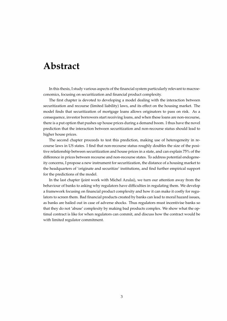
In this thesis, I study various aspects of the financial system particularly relevant to macroe-conomics, focusing on securitization and financial product complexity.
The first chapter is devoted to developing a model dealing with the interaction betweensecuritization and recourse (limited liability) laws, and its effect on the housing market. Themodel finds that securitization of mortgage loans allows originators to pass on risk. As aconsequence, investor borrowers start receiving loans, and when these loans are non-recourse,there is a put option that pushes up house prices during a demand boom. I thus have the novelprediction that the interaction between securitization and non-recourse status should lead tohigher house prices.
The second chapter proceeds to test this prediction, making use of heterogeneity in re-course laws in US states. I find that non-recourse status roughly doubles the size of the posi-tive relationship between securitization and house prices in a state, and can explain 75% of thedifference in prices between recourse and non-recourse states. To address potential endogene-ity concerns, I propose a new instrument for securitization, the distance of a housing market tothe headquarters of ‘originate and securitize’ institutions, and find further empirical supportfor the predictions of the model.
In the last chapter (joint work with Michel Azulai), we turn our attention away from thebehaviour of banks to asking why regulators have difficulties in regulating them. We developa framework focusing on financial product complexity and how it can make it costly for regu-lators to screen them. Bad financial products created by banks can lead to moral hazard issues,as banks are bailed out in case of adverse shocks. Thus regulators must incentivise banks sothat they do not ’abuse’ complexity by making bad products complex. We show what the op-timal contract is like for when regulators can commit, and discuss how the contract would bewith limited regulator commitment.
3

Dedication and Acknowledgments
Dedication
I dedicate this thesis firstly to my parents, who jointly inspired me to study Economicswhen I was a teenager, through countless discussions and debates, and who have alwayssupported me throughout my many years of study.
I also dedicate it to my loving wife, whose care and support these last three years havebeen a cornerstone of my life.
Acknowledgments and Thanks
I would be greatly remiss if I did not acknowledge and thanked the many people whohelped this thesis be possible.∗ I am indebted to Kevin Sheedy for his supervision, his helpand advice throughout my PhD has been priceless, and his willingness to dig deep into thedetails of my work has always been a remarkable, and enviable, aspect of his supervision.
For the first two chapters of this thesis, I received invaluable advice and counsel, and I ex-tend my thanks to Michael Peters, Rachel Ngai, Shengxing Zhang, Paolo Surico, Steve Pischke,Ethan Ilzetzki, Wouter den Haan, and Judith Shapiro.
In addition, a great many friends have made many suggestions and, to highlight only asome of them, I must thank Alex Clymo, Fabian Winkler, Markus Riegler, Svetlana Bryzgalova,Yan Liang, Thomas Drechsel, Joao Paulo Pessoa, Andreas Ek, Victor Westrupp, Michel Azulai,Thomas Carr, and Galina Shyndriayeva for theirs comments and suggestions.
In a similar vein, I extend my thanks to Oriol Anguera-Torrell and Stefanie Huber, and thethe seminar participants at the LSE, RES Easter School, York/Bank of England PhD Workshop,Spring 2015 Midwest Macro, TADC 2015 and EDP Jamboree for their helpful comments.
For the final chapter, both authors wish to extend their thanks to their supervisors, GerardPadro i Miguel and Kevin Sheedy, to Stephen Millard, David Baumslag, Ethan Ilzetzki andShengxing Zhang, and to the seminars participants at the LSE.
Finally, my time living in London could not have been as pleasant as it was without the thewarmth and friendship of many people, including all of the above, and my thanks must alsogo to David Solkin, Gilly Archer, Grace Armitage, Ben Solkin, Mateus Franco, Scarlett D’Avila,Mary Lally, to Jacqueline, Peter, Tim and Lucy Sawford, Marina Reis, Cesar Jimenez-Martinez,Sergio de Ferra, Jonathan Pinder, Oriol Carreras Baquer, Marcel Ribeiro, and to many others.
∗Financial support from the LSE and and the estate of Sho-Chieh Tsiang is gratefully acknowledged.
4
Contents
1 Introduction 9
2 Modelling Securitization and Non-Recourse Loans in the Housing Market 132.1 Introduction . . . . . . . . . . . . . . . . . . . . . . . . . . . . . . . . . . . . . . . . 132.2 Partial equilibrium with exogenous prices . . . . . . . . . . . . . . . . . . . . . . . 15
2.2.1 Borrowers . . . . . . . . . . . . . . . . . . . . . . . . . . . . . . . . . . . . . . 162.2.2 Originators . . . . . . . . . . . . . . . . . . . . . . . . . . . . . . . . . . . . . 172.2.3 Securitizers . . . . . . . . . . . . . . . . . . . . . . . . . . . . . . . . . . . . . 192.2.4 Timeline and definition of the equilibrium . . . . . . . . . . . . . . . . . . . 192.2.5 Securitizers’ optimal behaviour . . . . . . . . . . . . . . . . . . . . . . . . . 202.2.6 Screening equilibrium . . . . . . . . . . . . . . . . . . . . . . . . . . . . . . . 222.2.7 No screening equilibrium . . . . . . . . . . . . . . . . . . . . . . . . . . . . . 232.2.8 Summary and discussion . . . . . . . . . . . . . . . . . . . . . . . . . . . . . 23
2.3 General equilibrium . . . . . . . . . . . . . . . . . . . . . . . . . . . . . . . . . . . 232.3.1 Setup . . . . . . . . . . . . . . . . . . . . . . . . . . . . . . . . . . . . . . . . 232.3.2 Screening and non-screening equilibrium . . . . . . . . . . . . . . . . . . . 292.3.3 Summary and discussion . . . . . . . . . . . . . . . . . . . . . . . . . . . . . 32
2.4 Conclusion . . . . . . . . . . . . . . . . . . . . . . . . . . . . . . . . . . . . . . . . . 35
Appendices to the Chapter 372.A Appendix A - Model and empirics discussion . . . . . . . . . . . . . . . . . . . . . 37
2.A.1 Borrowers . . . . . . . . . . . . . . . . . . . . . . . . . . . . . . . . . . . . . . 372.A.2 Originators . . . . . . . . . . . . . . . . . . . . . . . . . . . . . . . . . . . . . 382.A.3 Securitization and Securitizers . . . . . . . . . . . . . . . . . . . . . . . . . . 382.A.4 General equilibrium . . . . . . . . . . . . . . . . . . . . . . . . . . . . . . . . 40
2.B Appendix B - Proofs . . . . . . . . . . . . . . . . . . . . . . . . . . . . . . . . . . . 432.B.1 Partial Equilibrium Proofs . . . . . . . . . . . . . . . . . . . . . . . . . . . . 432.B.2 General Equilibrium Proofs . . . . . . . . . . . . . . . . . . . . . . . . . . . . 452.B.3 Extensions Proofs . . . . . . . . . . . . . . . . . . . . . . . . . . . . . . . . . 49
3 House Prices, Securitization and Non-Recourse Loans in the US during the 2000s 513.1 Introduction . . . . . . . . . . . . . . . . . . . . . . . . . . . . . . . . . . . . . . . . 513.2 Model Predictions and Data . . . . . . . . . . . . . . . . . . . . . . . . . . . . . . . 53
3.2.1 Model Predictions . . . . . . . . . . . . . . . . . . . . . . . . . . . . . . . . . 543.2.2 Securitization . . . . . . . . . . . . . . . . . . . . . . . . . . . . . . . . . . . . 543.2.3 Recourse in the US . . . . . . . . . . . . . . . . . . . . . . . . . . . . . . . . . 55
5
CONTENTS 6
3.2.4 Other data . . . . . . . . . . . . . . . . . . . . . . . . . . . . . . . . . . . . . 563.2.5 Discussion of Data and Recourse . . . . . . . . . . . . . . . . . . . . . . . . 56
3.3 Empirical strategy and results . . . . . . . . . . . . . . . . . . . . . . . . . . . . . . 583.3.1 Boom period . . . . . . . . . . . . . . . . . . . . . . . . . . . . . . . . . . . . 583.3.2 Endogeneity and IV strategy . . . . . . . . . . . . . . . . . . . . . . . . . . . 633.3.3 Bust period . . . . . . . . . . . . . . . . . . . . . . . . . . . . . . . . . . . . . 66
3.4 Conclusion . . . . . . . . . . . . . . . . . . . . . . . . . . . . . . . . . . . . . . . . . 68
Appendices to the Chapter 703.A Appendix A - Empirics discussion . . . . . . . . . . . . . . . . . . . . . . . . . . . 70
3.A.1 Loan-to-value ratio . . . . . . . . . . . . . . . . . . . . . . . . . . . . . . . . 703.A.2 Subprime variable . . . . . . . . . . . . . . . . . . . . . . . . . . . . . . . . . 703.A.3 Robustness checks . . . . . . . . . . . . . . . . . . . . . . . . . . . . . . . . . 70
3.B Appendix B - Tables . . . . . . . . . . . . . . . . . . . . . . . . . . . . . . . . . . . . 723.B.1 Additional tables for boom period . . . . . . . . . . . . . . . . . . . . . . . . 723.B.2 Additional tables for instrumental variable regressions . . . . . . . . . . . . 743.B.3 Bust period regressions . . . . . . . . . . . . . . . . . . . . . . . . . . . . . . 753.B.4 Other tables . . . . . . . . . . . . . . . . . . . . . . . . . . . . . . . . . . . . . 76
3.C Appendix C - Other figures . . . . . . . . . . . . . . . . . . . . . . . . . . . . . . . 76
4 Dynamics of Regulation of Strategically Complex Financial Products 774.1 Introduction . . . . . . . . . . . . . . . . . . . . . . . . . . . . . . . . . . . . . . . . 774.2 Model . . . . . . . . . . . . . . . . . . . . . . . . . . . . . . . . . . . . . . . . . . . . 80
4.2.1 Basic set-up . . . . . . . . . . . . . . . . . . . . . . . . . . . . . . . . . . . . . 804.2.2 Timing . . . . . . . . . . . . . . . . . . . . . . . . . . . . . . . . . . . . . . . . 814.2.3 Equilibrium concept . . . . . . . . . . . . . . . . . . . . . . . . . . . . . . . . 834.2.4 Benchmark . . . . . . . . . . . . . . . . . . . . . . . . . . . . . . . . . . . . . 83
4.3 Optimal Regulation . . . . . . . . . . . . . . . . . . . . . . . . . . . . . . . . . . . . 844.3.1 Setting up the problem . . . . . . . . . . . . . . . . . . . . . . . . . . . . . . 844.3.2 Useful results . . . . . . . . . . . . . . . . . . . . . . . . . . . . . . . . . . . . 87
4.4 The Optimal Dynamic Contract . . . . . . . . . . . . . . . . . . . . . . . . . . . . . 924.4.1 Regulatory mechanisms with commitment . . . . . . . . . . . . . . . . . . . 924.4.2 Regulatory mechanisms without commitment and dynamic cycles . . . . . 103
4.5 Discussion . . . . . . . . . . . . . . . . . . . . . . . . . . . . . . . . . . . . . . . . . 1044.5.1 Transfers and Fines . . . . . . . . . . . . . . . . . . . . . . . . . . . . . . . . 1044.5.2 Different discount factors by banks and regulators . . . . . . . . . . . . . . 1064.5.3 More than one bank . . . . . . . . . . . . . . . . . . . . . . . . . . . . . . . . 106
4.6 Conclusion . . . . . . . . . . . . . . . . . . . . . . . . . . . . . . . . . . . . . . . . . 107
Appendices to the Chapter 1094.A Proofs . . . . . . . . . . . . . . . . . . . . . . . . . . . . . . . . . . . . . . . . . . . . 109
4.A.1 Lagrangian of the maximization problem . . . . . . . . . . . . . . . . . . . . 1254.A.2 Regulator’s ICR not binding . . . . . . . . . . . . . . . . . . . . . . . . . . . 126
References 130
List of Figures
2.1 Partial Equilibrium Timeline . . . . . . . . . . . . . . . . . . . . . . . . . . . . . . 202.2 General Equilibrium Timeline . . . . . . . . . . . . . . . . . . . . . . . . . . . . . 262.3 House prices in a sustained boom. . . . . . . . . . . . . . . . . . . . . . . . . . . 332.4 House prices in a boom and bust. . . . . . . . . . . . . . . . . . . . . . . . . . . . 34
3.1 House Prices in recourse and non-recourse states, from 1991 to 2013 . . . . . . . 523.2 House Prices in recourse and non-recourse states, from 1975 . . . . . . . . . . . 76
4.1 Optimal φ for δ = 0.995 . . . . . . . . . . . . . . . . . . . . . . . . . . . . . . . . . 954.2 Optimal α and γ for δ = 0.995 . . . . . . . . . . . . . . . . . . . . . . . . . . . . . 954.3 Optimal promised continuation values for δ = 0.995 . . . . . . . . . . . . . . . . 964.4 Optimal promised continuation values for δ = 0.995 in more detail . . . . . . . 974.5 Expected increase in v as a percentage of current v for δ = 0.995 . . . . . . . . . 984.6 Optimal φ for δ = 0.95 . . . . . . . . . . . . . . . . . . . . . . . . . . . . . . . . . 994.7 Optimal α and γ for δ = 0.95 . . . . . . . . . . . . . . . . . . . . . . . . . . . . . . 994.8 Optimal promised continuation values for δ = 0.95 . . . . . . . . . . . . . . . . 1004.9 Optimal promised continuation values for δ = 0.95 in more detail . . . . . . . . 1004.10 Expected increase in v as a percentage of current v for δ = 0.95 . . . . . . . . . . 1014.11 Optimal results for δ = 0.9 . . . . . . . . . . . . . . . . . . . . . . . . . . . . . . . 1024.12 Expected increase in v as a percentage of current v for δ = 0.9 . . . . . . . . . . 103
7

List of Tables
3.1 Data sources for controls and other variables . . . . . . . . . . . . . . . . . . . . 563.2 Descriptive statistics for Boom and full sample periods . . . . . . . . . . . . . . 573.3 Boom period, main regressions . . . . . . . . . . . . . . . . . . . . . . . . . . . . 593.4 Boom period, robustness checks . . . . . . . . . . . . . . . . . . . . . . . . . . . . 603.5 Share of covariates in explaining average, fitted house price growth . . . . . . . 623.6 First stage regressions for distance as an instrument . . . . . . . . . . . . . . . . 653.7 Instrumental variable regressions . . . . . . . . . . . . . . . . . . . . . . . . . . . 663.8 Boom period, main regression control results . . . . . . . . . . . . . . . . . . . . 723.9 Boom period, additional robustness checks - 1 . . . . . . . . . . . . . . . . . . . 723.10 Boom period, additional robustness checks - 2 . . . . . . . . . . . . . . . . . . . 733.11 Boom period, additional robustness checks - 3 . . . . . . . . . . . . . . . . . . . 733.12 Non-Western states, robustness checks . . . . . . . . . . . . . . . . . . . . . . . . 743.13 Reduced form regressions for instrument . . . . . . . . . . . . . . . . . . . . . . 743.14 Bust period, house price regressions . . . . . . . . . . . . . . . . . . . . . . . . . 753.15 Bust period, default regressions . . . . . . . . . . . . . . . . . . . . . . . . . . . . 753.16 ’Originate and securitize’ institutions . . . . . . . . . . . . . . . . . . . . . . . . . 76
4.1 Parameters used when delta is close to one . . . . . . . . . . . . . . . . . . . . . 94
8
Chapter 1
Introduction
Economics, like any area of research, requires a never ending effort to keep improvingitself, as what we do not know dwarfs, and seems to always dwarf, what we do. This istrue particularly in macroeconomics, I believe, where areas of research previously consideredof more secondary importance, are becoming ever more prominent, areas such as housing,finance and bounded rationality, and this thesis is written very much in the spirit of exploringthese new areas.
One of the most important reasons for this shift in academic importance lies with the GreatRecession. Research has turned towards the understanding and incorporation of financialtopics into macro models, as we, macroeconomists, severely underestimated the importanceof this topic previously, as is shown by the way that both the causes and the size of the GreatRecession are strongly linked with the financial crisis.
Similarly, the Great Recession also showed us how much more important housing, in par-ticular house prices, seems to be for the economy as whole, and how more research is neededin this area as well. Fortunately, housing, as an area of study, has greatly benefited fromthe ’empirical revolution’ economics as a whole is experiencing, with the advent of new datasources and techniques which has expanded the breadth and quality of empirical research.
This thesis seeks to explore topics that approach and combine both these areas of study,finance and housing, precisely because of their growing importance to macroeconomics. Ihope that by doing so, it might contribute to our better understanding of the causes behindthe Great Recession, and might help better prevent such events from happening again.
It does so by tackling two separate, but somewhat intermingled questions surrounding fi-nance. The first two chapters of the thesis focus on the housing boom and bust that took placein the US during the 2000s, and both offers and tests the hypothesis that securitization, wheninteracted with non-recourse (limited liability) mortgage loans, helped push house prices up-wards during the boom. The final chapter deals with the regulation of financial products, fo-cusing particularly on how complexity might be used to dodge regulatory screening of banks.The common thread between the two topics is securitization, being as it is, a complex financialproduct.
The first chapter presents the theoretical side of this investigation into housing. I modelthe housing market by dividing it into two separate markets, an origination/borrowing sec-tor, and a securitization/secondary market sector. I solve my model in a period of increaseddemand of uncertain duration, with two types of borrowers, safe ’owner-occupiers’, and risky
9
10
’investors’. We find two equilibrium results, in the first, loan originators, who are risk-averse,opt to screen out borrowers and only extend loans to the owner-occupiers. House prices thensimply reflect the fundamentals of the demand boom, whether loans are recourse or non-recourse.
In the second, loans are sold to the securitization market. The risk-shifting that happenswhen loans are sold combined with the lack of self selection by borrowers results in loan orig-inators stop screening, and speculators receive loans. And as the mortgages are non-recourse,these speculators will have an option value on defaulting that, given the chance for them tobecome marginal sellers, pushes up house prices.
I.e., my model predicts that the more securitization happens, the greater the likelihood thatspeculators will receive loans and have a chance of becoming marginal sellers, which can thenpush up house prices, this is the key prediction of the model. To a lesser extent, the modelalso predicts that the interaction between securitization and non-recourse loans leads to houseprices falling further in a bust (i.e., if the demand boom stops ‘early’) and that defaults willthen be higher.
This mechanism may seem like a purely theoretical one, but it has potentially importantimplications. The increase in house prices this mechanism creates will deviate from what someargue is the fundamental value of housing. This can, for example, then result in a misleadingsignal to the construction sector, or other potential home buyers. To the extent that this mightthen reinforce the trends that are driving the demand boom, something I do not formallyexplore in this thesis, this mechanism might lead to an overconstruction of housing for theformer or create a self-reinforcing mechanism for increase in house prices.
To test whether this mechanism is empirically relevant, the second chapter of the thesismakes uses of heterogeneity in recourse laws between US states. Virtually all US state lawsconcerning recourse have been stable since shortly after the Great Depression. I make use ofthis ’exogenous’ heterogeneity and regress house prices, on a state and city level, on a measureof securitization of new loans, the recourse status of a state/city and the interaction betweenthe two, for 2004 to 2006.
What I find is that this interaction is associated with a twice as large, positive effect fromsecuritization on house prices. More specifically, a 1% increase in securitization in recoursestates is associated with a 1% increase in house prices on average, whereas the same increaseleads to a approximately 2% increase in prices in non-recourse states. I also find that thismechanism can potentially explain around 75% or around 3.5 p.p. of the difference in increasein house prices between recourse and non-recourse states. Given that average house prices inthe US in 2004 had already increased around 40% in the previous 4 years, this further increaseof 3.5 p.p. comes from a high plateau and indicates how potent this mechanism can be.
As there is a potential issue of endogeneity between house prices and securitization, I use anovel instrument, the distance from a given housing market to the headquarters of ‘originateand securitize’ loan originators. Although the instrument currently has limitations, it providesfurther evidence for the model mechanism. Similarly, I find some favourable evidence thathouse prices did indeed fall further due to this mechanism, although there is no significantevidence of increased defaults during the bust.
As such, this chapter seems to validate concerns about how securitization and other finan-cial developments that might allow for shifting of risk from originators, and how recourselaws interact with each other. Given the evidence I find, jurisdictions that have non-recourse
11
laws, such as some US states and countries like Brazil, should be aware of these possibilitiesand may wish to mitigate these effects actively.
The final chapter follows straight into the last point, by trying to find the optimal regulationthat authorities should use when screening banks and dealing with complex financial prod-ucts. Moral hazard concerns surrounding bank bailouts have existed since the 19th century atleast, and the increased pace of development of financial innovation in the last 40 years raisesquestions of whether banks deliberately engineer products so as to make it harder for regula-tors to realize that they are de facto gambling, knowing that authorities will bailout them outshould the gamble fail.
To address this question, Michel Azulai and I formally model what is the optimal regula-tory regime that regulators should aim to use. In our framework, banks randomly receive newproducts, that are either good and complex, or bad and simple, and must essentially decidewhether to turn these bad products into complex (and still bad) ones; bad products, when theyfail, result in large costs to regulators. The incentive of banks to make bad products complexis that complex products are costly to screen by regulators, and this discourages them fromdoing so.
Furthermore, as we argue is the case in real life, we assume that there can be no directtransfers between regulators and banks. Thus the regulator’s problem lies mainly with findingthe optimal schedule of screening, conditional on public information available (summarizedinto the expected payoff for banks in each period), conditional on a promise keeping constraintand incentive compatibility constraints.
What we find is that, when regulators can make binding commitments, the optimal sched-ule is for regulators to begin by giving out low payoffs and do no screening. Despite the latter,banks will not choose to make their bad products complicated, as they are otherwise punished,and they are promised a reward phase should they keep to the schedule. This reward phase,which is eventually reached after a a number of periods, consists of banks then making full useof complexity, and regulators neither screening, nor punishing the banks, and is continuoushenceforth once reached.
We ague that this result, whilst intriguing, is unlikely to hold, however, if regulators can-not make such binding commitments and, as we discuss, there are likely several reasons whyregulators are unable to make binding commitments in practice. In the absence of bindingcommitments, we conjecture that the reward phase is then unsustainable, as regulators wouldhave incentives to deviate at that point and start screening banks instead, unraveling the equi-librium.
Our results thus make it clear how difficult it is for financial regulators to push bankstowards good behaviour, even with binding commitments, crises are not stopped, but post-poned; regulators face numerous constraints in what they can currently do. This suggeststhat, given the current institutional set-up, bailouts and financial crises may be to some extenta inevitable part of the financial system.
As such, to improve regulatory regimes and further minimize future crisis, changing theseconstraints would be a necessary step. Some possibilities may be along the lines of increasingthe scope for punishments of banks which are not just direct fines, such as making a portion ofremuneration be deferred and conditional on good future results for individual bankers1, orperhaps encouraging more whistleblowers even when clear evidence of criminal behaviour is
1Something which some regulators are currently exploring.
12
not available.This result ties together the themes of this thesis, which explores the institutional frame-
work that surrounds financial systems and the consequences this has on housing and financeitself, both areas of studies that macroeconomics cares about greatly. If the insights that thisthesis has found can help assist the economics profession in better understanding these areas,then my ambitions coming into the PhD have been fulfilled.
Chapter 2
Modelling Securitization andNon-Recourse Loans in the HousingMarket
Abstract
We study the effects of securitization and recourse (limited liability) laws on housing mar-kets. Securitization allows originators to pass on the risk of loans they originate. As a con-sequence, originators stop screening due to the absence of credible signalling to securitizers.This allows speculator borrowers, who are interested in buying for investment purposes, tostart receiving loans. When these loans are non-recourse, there is a put option that pushes uphouse prices during a demand boom. We thus predict that the interaction between securiti-zation and non-recourse status should lead to higher house prices. We also make predictionsconcerning the housing market in a bust period.
JEL Classification Numbers: E00, E44, G20, R31.Keywords: House prices, Securitization, Screening, Non-recourse loans.
2.1 Introduction
The national rise and fall of house prices experienced in the US during the 2000s was un-paralleled in the last 70 years, and the literature is still grappling with trying to explain thecause of this boom and bust. Given that many prominent economists, including Bernanke(2010) and Mian and Sufi (2014), have argued that the financial crisis and Great Recessionthat followed were a direct consequence of what happened in the US housing market in thatperiod, the importance of trying to understand this phenomenon cannot be understated.
Many explanations have been put forward to try to explain the pattern in house prices.Amongst others, it has been proposed that moral hazard in mortgage originations causedan increase in supply of loans (Mian and Sufi, 2009); that a decline in lending standards byoriginators led to an increase in demand for housing (Duca, Muellbauer and Murphy, 2011,and Dell’Ariccia, Igan and Laeven, 2012); that there was a large degree of misrepresentation ofthe quality of mortgages (Piskorski, Seru and Witkin, 2013); and that house buyers experienced
13
2.1. INTRODUCTION 14
overoptimism about the future trajectory of house prices (Case and Shiller, 2003, and Case,Shiller and Thompson, 2012).
All these papers, with the exception of Case, et al., emphasize the importance that privatesecuritization, such as CDOs and MBOs, had in affecting prices, which is not surprising, asprivate securitization also reached unprecedented levels in the 2000s. We seek to add to thisliterature by proposing a mechanism by which private securitization, when combined with‘recourse’ laws pertaining to foreclose, can affect house prices.
Our model follows the approach pioneered in Allen and Gorton (1993), where asymmetriesof information and agency problems result in a mechanism which affects asset prices1, result-ing in prices being higher than they would otherwise be2. Their results have been extendedto many different areas, such as between different sectors of the economy in Allen and Gale(2000) and Barlevy (2011), and there is experimental evidence that this mechanism can affectasset prices (Holmen, Kirchler and Kleinlercher, 2014). In particular, Barlevy and Fisher (2010),hereafter B&F, extend this mechanism to the housing sector; we use their framework to buildour model.
In B&F’s model, there exist two types of borrowers, those that value owning a house (hightypes) who can be interpreted as ‘traditional’ owner-occupiers, and those who do not (lowtypes) who can be thought as speculators3, with lenders unable to tell them apart. They findthat under certain conditions, house prices can be higher than their fundamental value4, aris-ing during a housing boom triggered by an increase in housing demand.
This appreciation in prices is mainly due to these loans being non-recourse, that is, of lim-ited liability, where in the case of a default, lenders can only recover the asset securing theloan5. This creates a put option value for speculators, as they can default cheaply/costlesslyshould prices fall. When speculators subsequently become marginal sellers, this pushes houseprices up. The model predicts that either demand keeps increasing for long enough such thata new, permanent high level of house prices becomes the equilibrium price, or, if housingdemand stops rising before that, that prices immediately drop and defaults happen.
We use B&F’s framework, but introduce two novel elements to this literature: a screeningtechnology that allows originators to costly screen borrowers, and a securitization market forloans. We choose to add these elements for several reasons, most saliently because there isempirical evidence that securitization interacted in important ways with screening by lendersduring the 2000s boom in the US; Mian and Sufi (2009), Keys, Mukherjee, Seru and Vig (2010)and Elul (2011) all find that more securitization of loans led to less screening by lenders. BothElul and Keys et al. find that this caused an increase in default rates in subprime mortgages,whilst the former also finds an increase in privately securitized prime loans, suggesting thatthis decrease in screening happened in all types of mortgages. Our addition of screening andsecuritization may also help explain why this mechanism may have not played a significant
1This literature denotes the effects of such mechanisms as rational bubbles.2This increase happens within the context of an agent-principal problem, where there are asymmetric payoffs for
a risky investment, such that the upside rewards the agent, but the downside is born mainly or completely by theprincipal; this incentivizes the agent to over-invest in the risky asset
3As we discuss in the Appendix, there is substantial evidence that speculators were a significant part of housebuyers during the 2000s housing boom in the US.
4As per Allen, Morris, and Postlewaite (1993): ’Value of an asset in normal use as opposed to (...) as speculativeinstrument.’
5Few countries outside of the US offer non-recourse mortgages, but Brazil became a important exception in 1997,when ’alienacao fiduciaria’ loans (article 27 of law 9.514) were established, which are not only non-recourse, but inthe case of defaults, if the market value of the repossessed asset is greater than the contractual value, borrowers areentitled to the value in excess of the contract, after costs; such loans may be sold via a ‘cessao de credito’ operation.
2.2. PARTIAL EQUILIBRIUM WITH EXOGENOUS PRICES 15
role prior to the 2000s, as we discuss in the next chapter.With these two new elements, we find that, under some parameter restriction, in housing
markets where loans are non-recourse there are two possible equilibria. In one, borrowersare screened and speculators are denied loans, however, counter-factually, no loans are se-curitized. In the other, no screening happens and loans are securitized. This is due to loanoriginators being unable to credibly signal to the securitization market whether a loan hasbeen made to a speculator type or not, combined with the non-recourse nature of loans.
As a consequence, in the absence of securitization, house prices follow fundamentals dur-ing a housing boom, but when securitization occurs, speculators’ access to loans pushes uphouse prices as in B&F. Furthermore, if the boom stops, house prices fall further and defaultscan take place when loans are being securitized. If loans are recourse, however, there is neveran option value for borrowers, and prices always follow the fundamentals, independently ofwhether there is securitization or not.
We thus predict that the combination of both factors, securitization and the presence ofnon-recourse laws, should have a positive effect on house prices in US states, compared tostates where either or both factors are missing. Depending on the size of originators andhow much they can affect house prices, this equilibrium can exist when we introduce down-payments.
This chapter and its results are related to the mainly empirical and growing literature onrecourse law in the United States, in particular how recourse laws affected the recent housingboom and bust, and whose inception happened largely due to the influential paper, Ghentand Kudlyak (2011). To the best of our knowledge, only one other paper, Nam and Oh (2014),explores a similar hypothesis to what we do in this chapter, that is, looking into the relationshipbetween non-recourse status on house prices on the basis of risk-shifting mechanism. Theirpaper only proposes the possibility of this mechanism, without an explicit housing model, andseeks only to investigate this question empirically.
This chapter is organized as follows. The next section presents a two period version ofthe model with static prices to illustrate our basic model mechanism of how securitization andscreening interact in our general equilibrium model. We then present in Section 2.3 our generalequilibrium model with endogenous prices, and discuss its implications in detail. Section 2.4concludes this chapter.
2.2 Partial equilibrium with exogenous prices
There are two periods in this version of the model. In the first period, transactions be-tween borrowers (B) and originators (O) happen. Borrowers consist of two types, owner-occupiers/high types (denoted by H) and speculators/low types (denoted by L). This is fol-lowed by a securitization period, where originators can sell mortgages to securitizers (S). Inthe second period, an exogenous house price increase/decrease happens and borrowers mustdecide whether to default or repay.
Houses initially cost 1 in period 1, and in period 2 will be 1 + Π. Π is a random variablethat equals π with probability q and −π with probability (1− q). All loans are of size 1 withtotal repayment in period 2 equal to 1 + r, and we restrict interest rates to be positive for allcases. As we only have one repayment period, any default is for 100% of the loan. If a loan
2.2. PARTIAL EQUILIBRIUM WITH EXOGENOUS PRICES 16
is in default, the house is immediately taken as collateral and sold for the prevailing marketprice.
We discuss the assumptions we make for each agent, including borrowers, and each marketof our model setup in Appendix A.
2.2.1 Borrowers
Borrowers derive a stock utility from owning a house. They are required to take on a loanto purchase a house and can only acquire one house. If they receive a loan in the first period,in period two they can either repay the loan from their income or from selling their house, orthe can default on the loan. Borrowers can choose which originator to approach for a loan inperiod one.
Borrowers consist of two types, ζ ∈ H, L, with γ low/speculators and (1 − γ) hightypes/owner-occupiers; we use these terms interchangeably. Both types have an income ofy, realized in period two, and where y is large enough to fully cover any level of mortgagerepayments.
Borrowers’ utility function is linear and separable between consumption goods and houseownership, such that for a borrower i:
UBi = ci + κiBi(1− Di)(1− Si)
where ci is the consumption in period 2; κi is the stock utility from owning a house at theend of period 2, with κi = 1 + κ for ζi = H and κi = 06 for ζi = L; and Bi, Di and Si areindicator functions, where a 1 indicates whether a borrower has bought a house, defaulted ona loan and sold a house, respectively.
The budget constraint of a borrower i is:
ci + Bi(1− Di)(1 + ri,j) = y + Bi(1− Di)Si(1 + Π)
where ri,j is the interest rate on a loan from originator j and y is the income of borrowers,high enough such that 1 + ri < y for any ri,j. Although borrowers are risk neutral, we canmake borrowers of both types be risk averse and find that our equilibrium results can hold,depending on the level of risk aversion; Appendix A provides a further discussion.
Borrowers have a set of 3 actions, Sζ,B. In the first period, they decide which originatorthey approach for a loan, choosing jB
i in J (where J is the set of originators). They do so takinginto account that each originator posts a set of information Λj. In the second period, borrowersdecide whether to default on a loan (Di), and whether to sell a house (Si).
The information set Λj = (SC(j), BO(j), r(.)) consists of the following. SC(j) is an indi-cator function which takes value 1 if j screens borrowers. BO(j) is an indicator function whichtakes value 1 if loans will be given to both types (as opposed to only high types). r(.) is theset of interest rates on the loans being offered, which we divide into different cases, dependingon SC(j) and BO(j). If SC(j) = 0, this is a non-screening Originator, so there will be a singleinterest rate rP,j (where P stands for pooled). If SC(j) = BO = 1, this is a screening Originatorwho gives loans to both types, so the set of rates will be rH,j and rL,j. If SC(j) = 1 and BO = 1,
6Although assuming that speculators derive zero utility from owning a house may seem extreme, we could re-normalize this to some positive number without loss of generality.
2.2. PARTIAL EQUILIBRIUM WITH EXOGENOUS PRICES 17
the set will consist of rH,j. Note that we use the notation r.,j to denote posted interest rates, asopposed to ri,j to denote interest rates in originated loans.
2.2.1.1 Borrowers’ optimal behaviour
We assume that π ≤ κ, as the equivalent condition always holds when we endogenizeprices, that is, house prices never exceed their value by owner-occupiers.
Borrowers’ optimal behaviour can be determined through a standard dominated actionanalysis. The resulting set of optimal strategies is very similar to the set that buyers havewhen playing a Bertrand competition, so we deem this as ’Bertrand-like’ competition.
As borrowers have the option to costlessly default in the second period, both types arealways at least weakly better off borrowing and buying a house; buying a house is a weakly-dominating strategy. Note that as low types have zero utility from owning a house, they onlybenefit from buying if they can sell the house at a profit.
To decide which jBi , high types will choose the Originator with lowest posted interest rate,
jHi = arg min
jr.,j, j ∈ J. Low types will first find the subset J′ ∈ J, such that ΛJ′ indicates
they will receive a loan, and then choose jLi = arg min
jr.,j, j ∈ J′. As Λj is common knowledge
for borrowers, in equilibrium we find that all borrowers of a given type must have the sameinterest rate on their mortgages. A proof for this is shown in the Appendix.
Owner-occupiers never wish to sell the house as π ≤ κ. As long as r. ≤ κ, they never wishto default in the second period and, as π ≤ κ < r., if r. > κ, they default on the loans in period2, irrespective of what happens to house prices.
For speculators, if house prices decrease, their best action is to default as house prices arenow worth less than loans π < 0. If house prices increase, then if π ≥ r., they can make aprofit by not defaulting and then selling the house; otherwise the cost of repaying is greaterand they then default.
As we show ahead, in equilibrium originators will set interest rates π ≥ ri,j, such that theset of optimal actions for borrowers, S∗i,B will consist of the following, which resembles the setof actions they will take in the general equilibrium model:
Conclusion 1 Owner-occupiers choose an originator jH. , which is offering the lowest interest rate from
set J of all originators. They never default or sell in the second period. Speculators choose originator jL. ,
with the lowest interest rate from set J′ of originators offering loans to speculators. In the second period,they default when prices fall, otherwise they do not default and sell the house.
2.2.2 Originators
Originators should be understood as the banks and other financial agents that create mort-gages. As such, they have two separate, but intertwined roles in our model. They decidewhether to extend loans to borrowers and at what interest rates, and they choose whether tosell loans to securitizers.
We assume that originators are risk averse, with the following utility function:
UOj = E(WO
j )− aV(WOj )− nj ∗ C
2.2. PARTIAL EQUILIBRIUM WITH EXOGENOUS PRICES 18
where WOj is the wealth they hold at the end of period two, E is the expectation operator,
a is a parameter determining risk aversion, V is the variance operator, nj is the number ofborrowers screened and C is the cost of screening per borrower screened.
The assumption that originators are risk averse and securitizers are risk neutral is an inte-gral part of our model; as we discuss in the next section, these two assumptions are requiredto model the securitization process7.
Although we use Bertrand-like competition and generic set J of originators for our modelresults, as an alternative, we can model our originators as having deep pockets and there beingfree-entry into the origination market and focus on a representative originator.
Originators will take 2 sets of actions in the model. They begin by posting the set of infor-mation Λj, that is, whether they screen borrowers or not; if they screen, whether they grantloans to both types or just owner-occupiers; and choosing the interest rates on loans. After aborrower approaches an originator, the originator acts according to their Λ.. The set of infor-mation Λ. is only visible to borrowers, not securitizers.
The second set of actions of originators is choosing whether to sell loans originated inthe securitization market. For each originator j′ there is a set I(j′) = ∀i|jB
i = j′ of loansthey originate, and we define I(j′, ζ) = i|jB
i = j′&ζi = ζ, of loans originates to ζ types.Furthermore, the number of screened borrowers is n′j(I(j′)) = |I(j′)| × SC(j′), that is, thenumber of loans originated times the decision to screen loans.
For all i ∈ I(j), originator j will choose qOi,j, whether they sell loan i or not, where qO
i,j = 1indicates they will sell. They do so by seeing what is the price paid for loans by the represen-tative securitizer, P∗(r). We define QO(j) to be the set of all qO
i,j for originator j.To simplify notation, we define the following variables. Xζ(r(.)) is a random variable that
indicates the rate of return from a loan with interest rate ri,j made to type ζ. For high types,XH(r(.)) = r(.). For low types, when prices are high, they repay, so XL(r(.)) = r(.) with proba-bility q; otherwise, XL(r(.)) = −π8, with probability (1− q), so E(XL(r(.))) = qr(.) − (1− q)π.
Now we define Y(QOj , SC, BO, I(j)) as the returns obtained for all 3 possible courses of
action that an originator can take concerning loan origination, that is, not screening, screeningand lending to both types, and screening and lending to owner-occupiers, in addition to theirchoices of selling/keeping a loan. We thus have that:
Y(QOj , 1, 0, I(j)) = ∑
i∈I(j)qO
i,j(P∗(ri)− 1) + (1− qOi,j)XH(ri)
Y(QOj , 1, 1, I(j)) = ∑
i∈I(j,H)
qOi,j(P∗(ri)− 1) + (1− qO
i,j)XH(ri)
+ ∑i∈I(j,L)
qOi,j(P∗(ri)− 1) + (1− qO
i,j)E(XL(ri))
Y(QOj , 0, ∅, I(j)) = ∑
i∈I(j,H)
qOi,j(P∗(ri)− 1) + (1− qO
i,j)XH(ri)
+ ∑i∈I(j,L)
qOi,j(P∗(ri)− 1) + (1− qO
i,j)E(XL(ri))
The wealth of an originator j at the end of period 2 will thus be:
WOj (I(j)) = SCj(1− BOj)Y(Q0, 1, 0, I(j)) + SCjBOjY(Q0, 1, 1, I(j))
+ (1− SCj)Y(Q0, 0, ∅, I(j))
7If originators are risk neutral, our results are very similar those of B&F and securitization plays no significantrole in determining house prices.
8A fall leads to speculators defaulting; the house is then repossessed and immediately sold at the market price.
2.2. PARTIAL EQUILIBRIUM WITH EXOGENOUS PRICES 19
Finally, note that the interest rates on loans can be used as signal of loan quality by orig-inators to securitizers. Although this is the only signal we allow between originators andsecuritizers, in practice other characteristics of a loan, such as differentiated loan-to-valueratios/down-payments, might also be used as such; a further discussion of the results of ourmodel with down-payments can be found in Appendix A. So the strategy set of an originatorj, Sj,O, consists of choosing the set of Λj and of choosing whether to sell each loan, Qj.
2.2.3 Securitizers
In this chapter and the next, the securitization market in our model refers to the privatesector securitization exclusively, and we opt not to include securitization done by governmentsponsored enterprises (GSEs); a further discussion of GSE securitization may be found in Ap-pendix A. Securitizers in our model consist of a single risk-neutral agent who buys loans fromoriginators and holds on to them, and only cares about their expected wealth at the end ofperiod 2, such that their utility function is:
US = E(WS)
where WS is the wealth they hold at the end of period two. Note that securitizers in ourmodel play both the role of the financial intermediates who securitize the loan and the financialagents who buy the loan. We opt to keep both roles in one agent to simplify our model. We userisk neutrality as a reduced form for the securitization process, in particular, as the reductionof uncertainty that stems from securitization. Appendix A provides a further discussion forboth issues.
We assume there is free-entry into the securitization market, so we can model our equi-librium results through a representative agent. Much like with originators, this would beequivalent to using a set of securitizers and ‘Bertrand-like’ competition. The securitizer’s onlyaction will be to post the price Pr for which they be will willing to buy a loan of interest rate r.Securitizers cannot condition their purchase of loans to specific originators.
As we discuss in the Appendix A, due to the complexities of the securitization process,securitizers cannot distinguish between high and low-type loans. Due to asymmetry of in-formation, the price securitizers are willing to pay depends on their beliefs, denoted by Ω(r)which is the probability that a loan of a given interest rate is of a low type.
The wealth of a securitizer at the end of period 2 will be:
WS(Qj) = ∑j∈J[ ∑
i∈I(j,H)
qOi,j(XH(ri)− P∗(ri))] + [ ∑
i∈I(j,L)qO
i,j(E(XL(ri))− P∗(ri))]
So the strategy set SS of securitizer consists of a set of Pr.
2.2.4 Timeline and definition of the equilibrium
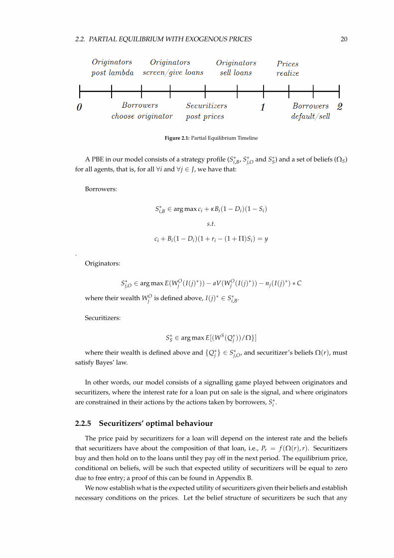
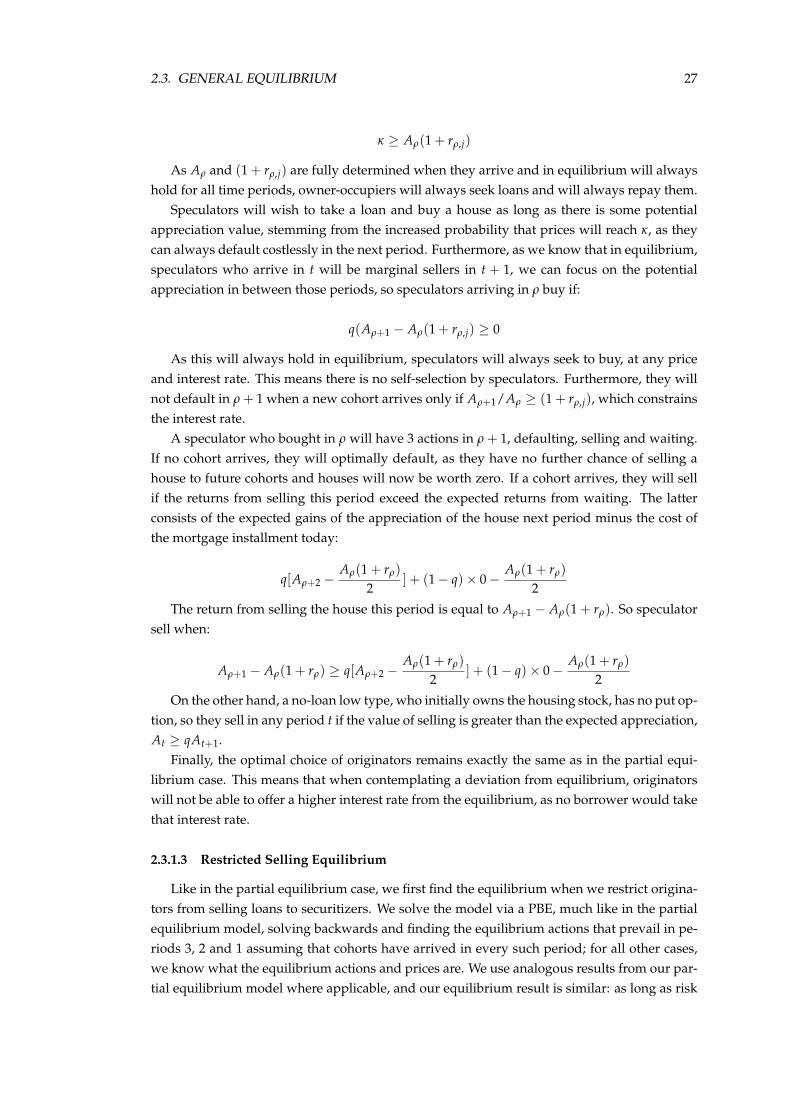
To summarize the possible actions taken in our model, we now present the timeline ofactions taken in Figure 2.1.
We now define the equilibrium of our model. As this is a signalling game, we focus ourattention on a Perfect Bayesian Equilibrium (PBE), under which beliefs are consistent withBayesian updating. This also means that we solve parts of the game via backwards induction.
2.2. PARTIAL EQUILIBRIUM WITH EXOGENOUS PRICES 20
Figure 2.1: Partial Equilibrium Timeline
A PBE in our model consists of a strategy profile (S∗i,B, S∗j,O and S∗S) and a set of beliefs (ΩS)for all agents, that is, for all ∀i and ∀j ∈ J, we have that:
Borrowers:
S∗i,B ∈ arg max ci + κBi(1− Di)(1− Si)
s.t.
ci + Bi(1− Di)(1 + ri − (1 + Π)Si) = y
.Originators:
S∗j,O ∈ arg max E(WOj (I(j)∗))− aV(WO
j (I(j)∗))− nj(I(j)∗) ∗ C
where their wealth WOj is defined above, I(j)∗ ∈ S∗i,B.
Securitizers:
S∗S ∈ arg max E[(WS(Q∗j ))/Ω]
where their wealth is defined above and Q∗j ∈ S∗j,O, and securitizer’s beliefs Ω(r), mustsatisfy Bayes’ law.
In other words, our model consists of a signalling game played between originators andsecuritizers, where the interest rate for a loan put on sale is the signal, and where originatorsare constrained in their actions by the actions taken by borrowers, S∗i .
2.2.5 Securitizers’ optimal behaviour
The price paid by securitizers for a loan will depend on the interest rate and the beliefsthat securitizers have about the composition of that loan, i.e., Pr = f (Ω(r), r). Securitizersbuy and then hold on to the loans until they pay off in the next period. The equilibrium price,conditional on beliefs, will be such that expected utility of securitizers will be equal to zerodue to free entry; a proof of this can be found in Appendix B.
We now establish what is the expected utility of securitizers given their beliefs and establishnecessary conditions on the prices. Let the belief structure of securitizers be such that any

2.2. PARTIAL EQUILIBRIUM WITH EXOGENOUS PRICES 21
given loan of interest rate rΩ has probability Ω of being of a low type, noting again that werestrict ourselves to r ≤ π:
EUSΩ(XH , XL, ) = (1−Ω)(1 + rΩ)−Ω[(1 + qrΩ − (1− q)(1− π)]− PΩ.
With free entry, EUSΩ = 0, so PΩ = (1−Ω)(1 + rΩ)−Ω[(1 + qrΩ)− (1− q)(1− π)]. In
particular, if Ω = 0, a belief that a loan is to a of high type, we have that with free entry:
P∗H = 1 + rH
where we abuse notation. If Ω = 1, a belief that loans consists only of low types, then withfree entry:
P∗L = 1 + qrL − (1− q)π
with similar abuse of notation. With this, we have established the full set of optimal actionsof securitizers with free entry, S∗S, conditional on their beliefs.
Note that, as expected, PH ≥ PL for two loans with the same interest rate but differentbeliefs about their types and that the price paid is monotonically decreasing in Ω, and that allP. are monotonically increasing in r.
2.2.5.1 Preview of results and strategy
To help the exposition that follows, we first show the equilibrium when originators arerestricted from selling loans. We then proceed to find the equilibrium under two different set ofactions for originators, whether they screen borrowers or not. Also note that we make severalassumptions about our model parameters to find our results, so we discuss what happensotherwise for each key assumption.
In a screening equilibrium with ‘low probabilities’, because the price paid for low typeloans is less than the cost of lending, if any selling of loans to securitizers were to happen,the only loans that could be sold to securitizers would be those consisting of owner-occupiers.However, originators are capable of masquerading speculators as owner-occupiers by offeringthem the same equilibrium interest rates, which would be a profitable deviation. Securitizersare thus unwilling to pay a high enough price for any loan put on sale, so none are sold.Originators will screen loans and only lend to owner-occupiers. With ‘high probabilities’, ascreening equilibrium where speculator loans are sold and owner-occupier loans are held byoriginators can be sustained.
In a no-screening equilibrium, which can only be sustained when costs are high enoughto stop originators from ’skimming the cream’, loans are sold to securitizers and both typesreceive loans. Thus, if loans are securitized, speculators will receive loans.
2.2.5.2 Restricted selling equilibrium
As high types never default there is no uncertainty from them, thus when originators arerestricted from selling, utility is additive.
As we show in Appendix B, if originators are sufficiently risk averse, satisfying a ≥ maxa, a,will always suffer negative utility by lending to speculators; thus, if possible, they will screen
2.2. PARTIAL EQUILIBRIUM WITH EXOGENOUS PRICES 22
and only give loans to owner-occupiers. This assumption is required for tractability, as ifa < maxa, a, originator’s set of optimal actions is very large and becomes conditional onour other parameters.
Furthermore, as originators are competing among each other via Bertrand-like pricing, wehave to have that EUO,H = 09. In equilibrium, interest rates must be such that their utility iszero and the equilibrium interest rate will be rH = C
(1−γ). Note that this requires that C
(1−γ)≤
π, which implies that a < 0, making a redundant. If C(1−γ)
> π, loans are too costly and nolending takes place.
Finally, borrowers will have utility EUH = κ + y− C(1−γ)
> y = EUL.
Conclusion 2 If originators are restricted from selling loans to securitizers and we have a ≥ a andC
(1−γ)≤ π, a unique screening equilibrium exists where only owner-occupiers receive loans, rH =
C(1−γ)
.
2.2.6 Screening equilibrium
We begin by setting q1−q < 1, as we are interested in cases with asymmetry in house price
movements analogous to the general equilibrium version of our model. From WOj , the profit
from selling a loan is Pi(ri)− 1, so originators will want to sell only if, for any given loan withinterest rate ri, Pi(ri) ≥ 1. As q
1−q < 1, PL(rL) < 110, speculator loans are not profitable andnot granting loans to speculators dominates.
A screening equilibrium where loans are extended only to owner-occupiers and are thensold to securitizers, and speculators are denied loans cannot be thus sustained. In such a case,first assume that the equilibrium posted interest rates (rL, rH) are different. A originator j′
could then profitably deviate by posting a Λj′ where they offer to grant loans to speculatorsand set rL,j′ = rH , masking speculators as owner-occupiers. Speculators would then choosej = j′ and this originator would have higher payoff, as PH ≥ 1.
Originators will not wish to hold on to loans made to speculators with a ≥ a as we dis-cussed in the previous subsection. So in a screening equilibrium, if q
1−q < 1, no equilibriumcan exist where screening takes place and low types receive loans. We can sustain this equi-librium by setting the off the equilibrium path beliefs of securitizers such that any loan put onsale is a low type loan (Ω = 1) for any interest rate, in which case no originator would wantto deviate and sell a loan, making these beliefs consistent. If, alternatively, rL = rH , then theequilibrium would not be sustained as not screening would strictly dominate screening fororiginators due to the cost of screening.
If q1−q > 1, then it is possible to sustain an equilibrium where speculator loans are sold and
owner-occupiers receive loans which are not sold, which we discuss further in the Appendix.
Conclusion 3 In a screening equilibrium, if speculators are sufficiently risk, only owner-occupiersreceive loans and originators do not sell loans to securitizers. If speculators are not too risky, then theirloans are sold and owner-occupiers loans are held on to by originators.
9If the equilibrium interest rate r′ was such that EU′ > 0 for a originator making loans, a different originatorcould offer 0 < r′′ < r′ attracting those borrowers and increase their profits.
10The highest possible interest rate such low types do not default is rL = π, and for that interest rate, PL =1 + π(2q− 1) < 1 for q
1−q < 1.
2.3. GENERAL EQUILIBRIUM 23
2.2.7 No screening equilibrium
From our results when originators are restricted from selling loans, if the cost of screeningis not incurred, then originators would never want to extend loans to simply hold-on to them.As such, if there is no screening taking place, a equilibrium can only exist if originators sellloans to securitizers.
Conclusion 4 In a no screening equilibrium, originators offer interest rates of rP = γ(1−q)π(1−γ)+qγ
, forany borrowers. Securitizers will set P∗P = 1 for any loans with an interest rate of rP (which impliesΩ(rP) = γ) and they have off-the-equilibrium path beliefs that Ω(r 6= rP) = 1).
We show that this is an equilibrium in Appendix B, under two additional parameter restric-tions, that γ ≤ 1
2(1−q) , so that interest rates are not too high, and that (1−γ)γ(1−q)(1−γ)+qγ
≤ C, whichguarantees that originators will not wish to ’skim the cream’. Otherwise, a no-screening equi-librium cannot be sustained.
2.2.8 Summary and discussion
Under the conditions that a > a (sufficient risk aversion), q1−q < 1 (low-types present a
bad risk), C(1−γ)
≤ π (sufficiently low screening costs), γ ≤ 12(1−q) (sufficiently low number
of low types) and (1−γ)γ(1−q)(1−γ)+qγ
≤ C (sufficiently high costs)11 we find there are two equilibria.The first is such originators screen and only lend to owner-occupiers and no loans are sold tosecuritizers. In the second, originators do not screen, thus allowing both types to have accessto loans, and originators sell both loans to the securitization market. Alternatively, if q
1−q > 1,then both types receive loans, both are screened and only speculator loans are sold.
This result illustrates the basic mechanism that will drive our results in the general equilib-rium set-up. The non-recourse nature of loans and their 100% LTV ratio means that borrowerswill not self-select, putting the onus on originators to screen out low and high types. In theabsence of a credible signalling, originators could mask speculators as owner-occupiers whenselling them to securitizers, which impedes any equilibrium wherein owner-occupiers loansare sold.
As we discuss further below, we believe that the equilibrium we find in our model whenthere is no securitization taking place may describe the state of the world before the securitiza-tion boom of the 2000s, whereas the equilibrium where it does may delineate how the marketstarted operating once securitization increased.
2.3 General equilibrium
2.3.1 Setup
The general equilibrium model differs from the partial equilibrium one as we now endog-enize the prices of houses, by including house sellers in addition to house buyers/borrowers.The model is of finite duration and finishes at period N12.
11Note that γ ≤ 12(1−q) guarantees that both our high cost and low cost conditions will hold simultaneously.
12The model generalizes to a infinite horizon model, as there is a simple mapping from flow utility of owninghouses and receiving a stock utility at the end of time in a finite period model
2.3. GENERAL EQUILIBRIUM 24
We assume the same settings for this model as in our partial equilibrium model, unlessnoted, and a discussion of our modeling choices may be found in Appendix A, so all variablesand agents are defined analogously to the partial equilibrium model.
House owners, prospective borrowers or otherwise, remain divided into two types, withanalogous utility functions to their partial equilibrium model, such that for borrower i of typeζ arriving at ρ utility is:
Uρi =
N
∑t=ρ+1
ct + κiBρNDρ+1NDρ+2
N
∏t=ρ+1
(1− St)
who faces a budget constraint such that aggregate expenditure is:
N
∑t=ρ
ct + BρNDρ+1(Aρ1 + rρ,j
2+ NDρ+2 Aρ
1 + rρ,j
2)
and aggregate income is:
N
∑t=ρ
y + Bi,ρNDi,ρ+1NDi,ρ+2(N
∏t=ρ+1
Si,t Ai,t)
where ct is consumption, y income, At house prices, rt,j interest rate from a loan by orig-inator j, Bt, NDt and St indicator functions for buying a house, not defaulting and selling ahouse. In addition, period by period budget constraints exist, as house buyers cannot save orborrow except via their (potential) single house purchase.
Originators will now seek to maximize
UOj =
N
∑t=1
E(WOj,t)− aV(WO
j,t)− nj,t ∗ C
where W is their wealth/profits in period t, a is the coefficient of risk aversion, nj,t totalborrowers screened and C is the cost of screening per borrower. We further define wealthanalogously to the partial equilibrium model, as
WOj,t(I(j, t)) = SCj,t(1− BOj,t)Y(Q0, 1, 0, I(j, t), t)
+ SCj,tBOj,tY(Q0, 1, 1, I(j, t), t)
+ (1− SCj,t)Y(Q0, 0, ∅, I(j, t), t)
where again SCj,t, BOj,t are indicator functions for screening and type lending,Y(Q0, SC, BO, I(j, t), t) is expected profit earned on conditional loans originated (I(j, t)) andon loans sold (Q0) at every period t. More precise definitions of Y(.) can be found in theAppendix A, and they are defined analogously to the partial equilibrium model.
Finally, the representative securitizer seeks to maximize
US =N
∑t=1
E(WSt (Qj))
i.e., the sum of their expected utility, where their wealth/profit per period is
2.3. GENERAL EQUILIBRIUM 25
WSt (Qj) = ∑
j∈J[ ∑
i∈I(j,H)
qOi,j(XH(ri)− P∗(ri))]
+ [ ∑i∈I(j,L)
qOi,j(E(XL(ri))− P∗(ri))]
We assume that there exists a fixed13 housing stock at t = 1 such that Ψ of houses areowned by low types and that all current high types own houses. To simplify our analysis, weassume there does not exist a renters market for this housing market14 and we exclude thepossibility of borrowers owning multiple houses.
At each time period, starting at 1, with probability q a cohort of size 1 of new borrowerswill enter this housing market and may buy houses, with (1 − γ) borrowers being owner-occupiers. This is conditional on a cohort having arrived in the last period, so if a cohort doesnot arrive in period M, no cohorts arrive in M + 1, M + 2... Arriving speculators, as in thepartial equilibrium model, will want to buy houses with the intent of reselling them, and willoptimally default if a cohort fails to arrive at any period.
We have two necessary conditions on the size of the housing stock, such that 2(1− γ) <
Ψ ≤ 2− γ15, and for analytical convenience, we assume that Ψ = 2− γ. We discuss how ourresults would change if we altered the size of our cohorts and/or housing stock in AppendixA.
The loan structure is such that loan repayments occur over two periods of time, so fora loan originated in t, half of the total loan payment of At(1 + rt) is paid in t + 1 and theother half at t + 2. Loans remain non-recourse and if defaults happen, whoever owns the loancontract at the moment of default proceeds to repossess the house and sell it in the market forthe prevailing price.
Originators can costlessly distinguish between new arrivals and buyers from previous pe-riods and will only extend loans to buyers of a new cohort. Buyers are required to acquire aloan to buy a house16. Borrowers’ income is such that they can always cover their loan pay-ments in every period and/or make early repayment of loans, for which there is no penalty.
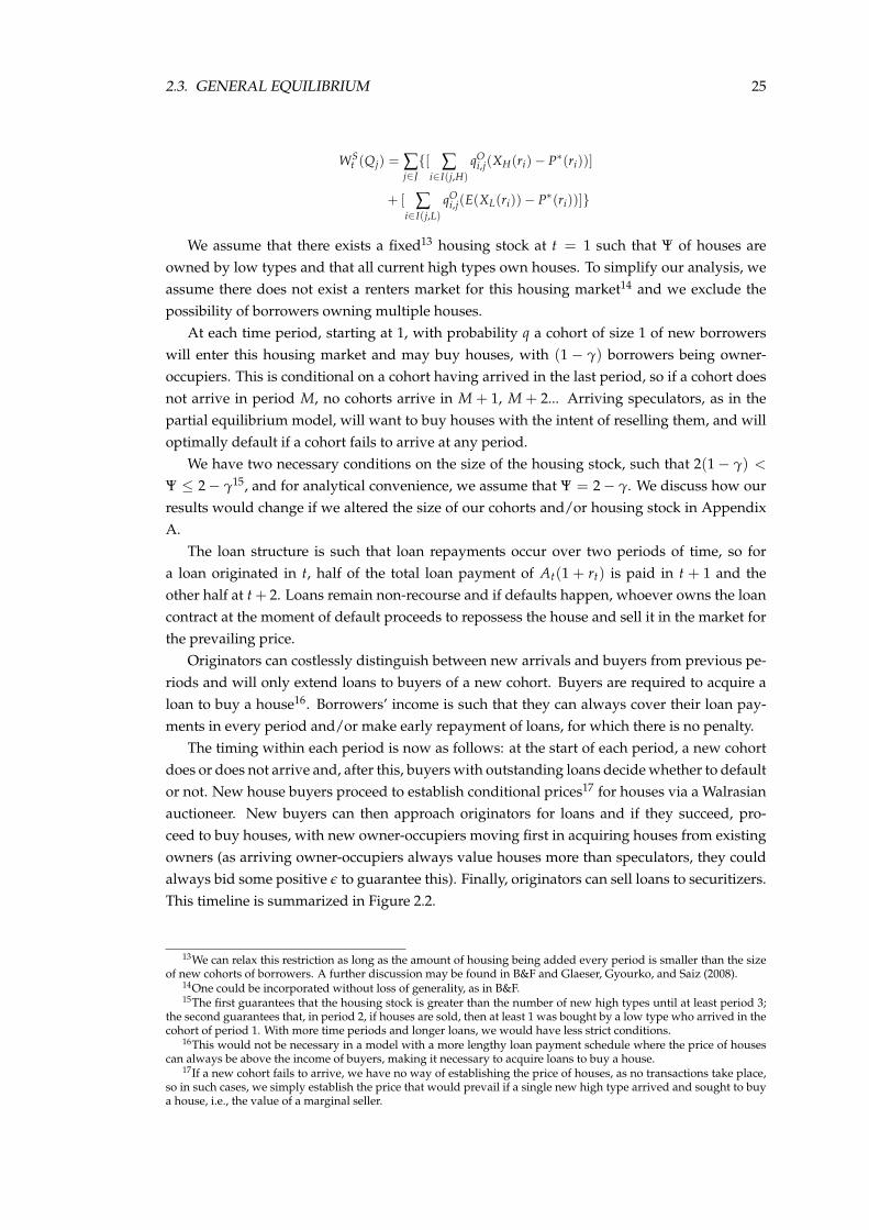
The timing within each period is now as follows: at the start of each period, a new cohortdoes or does not arrive and, after this, buyers with outstanding loans decide whether to defaultor not. New house buyers proceed to establish conditional prices17 for houses via a Walrasianauctioneer. New buyers can then approach originators for loans and if they succeed, pro-ceed to buy houses, with new owner-occupiers moving first in acquiring houses from existingowners (as arriving owner-occupiers always value houses more than speculators, they couldalways bid some positive ε to guarantee this). Finally, originators can sell loans to securitizers.This timeline is summarized in Figure 2.2.
13We can relax this restriction as long as the amount of housing being added every period is smaller than the sizeof new cohorts of borrowers. A further discussion may be found in B&F and Glaeser, Gyourko, and Saiz (2008).
14One could be incorporated without loss of generality, as in B&F.15The first guarantees that the housing stock is greater than the number of new high types until at least period 3;
the second guarantees that, in period 2, if houses are sold, then at least 1 was bought by a low type who arrived in thecohort of period 1. With more time periods and longer loans, we would have less strict conditions.
16This would not be necessary in a model with a more lengthy loan payment schedule where the price of housescan always be above the income of buyers, making it necessary to acquire loans to buy a house.
17If a new cohort fails to arrive, we have no way of establishing the price of houses, as no transactions take place,so in such cases, we simply establish the price that would prevail if a single new high type arrived and sought to buya house, i.e., the value of a marginal seller.
2.3. GENERAL EQUILIBRIUM 26
Figure 2.2: General Equilibrium Timeline
2.3.1.1 Prices and Fundamental Value
The key uncertainty in our model is whether at the end of time, the number of new hightypes exceeds the housing supply or not.
In periods 4 and beyond, if cohorts have arrived in all periods, the number of owner-occupiers exceeds the stock of houses immutably, so the equilibrium price must be equal tothe valuation of the marginal buyer, owner-occupiers borrowers, which is κ18.
If not, housing supply exceeds the number of owner-occupiers forever, so the equilibriumprice for houses will be equal to the value of the marginal seller, 019
So if a cohort fails to arrive prior to period 4, the price is equal to 0 from that period on-wards. If cohorts arrive in the first 3 periods, then the price will be equal to κ for all periodsonwards. In particular, as there is never any uncertainty for periods 4 and beyond, the pricemust either be κ or 0, as either enough cohorts have arrived or not.
To compare our house prices with some notion of fundamental value, we define funda-mental value of housing. Following Allen et al. (1993) and related literature, this is the ’Valueof an asset in normal use as opposed to (...) as speculative instrument’. That is, the fundamen-tal value is the value/price an asset would have if house buyers did not have loan contractsthat skewers their incentives by ‘safeguarding them from a negative shock’.
For periods 4 and beyond, as there is no ‘speculative’ element, the prices we have estab-lished are equal to the fundamental value. For periods 1 to 3, the fundamental value is bydefinition equal to the expected value for what the price will be in period 4, as this is the valueof a house if buyers could buy houses outright, without loans. Appendix B discusses andproves this claim. As such, the fundamental value after the arrival of new cohort in period 3is equal to κ, in 2 the value is qκ and in 1, it is q2κ. As we will demonstrate below, this will beequal to the price that prevails when no securitization takes place.
2.3.1.2 Borrower’s optimal actions
We briefly outline the optimal actions of borrowers, which is identical to the partial equi-librium case. Owner-occupiers arriving in ρ gain κ from owning a house, as long as the overallcost of a mortgage is lower than their utility value, they will always be willing to take on aloan and repay the loan fully, that is
18If the price was lower, then any owner-occupier who currently does not own a house would be willing to bidfor a house at a higher price A′ = A + ε ≤ κ. And as no high type is willing to sell for a price less than κ, the onlyequilibrium price is κ.
19As proof, first note that there is no chance of being able to re-sell the house in the future for a greater price, asno new cohorts can arrive, so all speculators/low types value the house at zero. If the equilibrium price was someA′ > 0, then any low type seller who is not selling could post a price A′ − ε ≥ 0 instead and make a profit, so onlyA = 0 can be an equilibrium price.
2.3. GENERAL EQUILIBRIUM 27
κ ≥ Aρ(1 + rρ,j)
As Aρ and (1 + rρ,j) are fully determined when they arrive and in equilibrium will alwayshold for all time periods, owner-occupiers will always seek loans and will always repay them.
Speculators will wish to take a loan and buy a house as long as there is some potentialappreciation value, stemming from the increased probability that prices will reach κ, as theycan always default costlessly in the next period. Furthermore, as we know that in equilibrium,speculators who arrive in t will be marginal sellers in t + 1, we can focus on the potentialappreciation in between those periods, so speculators arriving in ρ buy if:
q(Aρ+1 − Aρ(1 + rρ,j) ≥ 0
As this will always hold in equilibrium, speculators will always seek to buy, at any priceand interest rate. This means there is no self-selection by speculators. Furthermore, they willnot default in ρ + 1 when a new cohort arrives only if Aρ+1/Aρ ≥ (1 + rρ,j), which constrainsthe interest rate.
A speculator who bought in ρ will have 3 actions in ρ + 1, defaulting, selling and waiting.If no cohort arrives, they will optimally default, as they have no further chance of selling ahouse to future cohorts and houses will now be worth zero. If a cohort arrives, they will sellif the returns from selling this period exceed the expected returns from waiting. The latterconsists of the expected gains of the appreciation of the house next period minus the cost ofthe mortgage installment today:
q[Aρ+2 −Aρ(1 + rρ)
2] + (1− q)× 0−
Aρ(1 + rρ)
2
The return from selling the house this period is equal to Aρ+1 − Aρ(1 + rρ). So speculatorsell when:
Aρ+1 − Aρ(1 + rρ) ≥ q[Aρ+2 −Aρ(1 + rρ)
2] + (1− q)× 0−
Aρ(1 + rρ)
2
On the other hand, a no-loan low type, who initially owns the housing stock, has no put op-tion, so they sell in any period t if the value of selling is greater than the expected appreciation,At ≥ qAt+1.
Finally, the optimal choice of originators remains exactly the same as in the partial equi-librium case. This means that when contemplating a deviation from equilibrium, originatorswill not be able to offer a higher interest rate from the equilibrium, as no borrower would takethat interest rate.
2.3.1.3 Restricted Selling Equilibrium
Like in the partial equilibrium case, we first find the equilibrium when we restrict origina-tors from selling loans to securitizers. We solve the model via a PBE, much like in the partialequilibrium model, solving backwards and finding the equilibrium actions that prevail in pe-riods 3, 2 and 1 assuming that cohorts have arrived in every such period; for all other cases,we know what the equilibrium actions and prices are. We use analogous results from our par-tial equilibrium model where applicable, and our equilibrium result is similar: as long as risk
2.3. GENERAL EQUILIBRIUM 28
aversion is high enough and speculators are a minority, speculators will not receive loans.
Period 3 We begin by assuming that in periods 1 and 2, only arriving owner-occupiers, notspeculators, have bought houses, which we show will be an equilibrium action. If a new cohortfails to arrive, then owner-occupiers who bought houses in previous periods will not defaultas long as the total cost of their loan is less than their value of the house, which we will showwill hold if costs are not too high. So, equilibrium prices will be 0 and no defaults happen.
If a new cohort has arrived, as owner-occupiers move first when buying houses, all houseswill be purchased by owner-occupiers. This is because there will be 3(1 − γ) new owner-occupiers, and the housing stock, Ψ = 2− γ, is smaller for γ < 1
2 .The new owner-occupiers thus exhaust the supply of housing, meaning that even if a spec-
ulator were to receive a loan, they would never be able to purchase a house. As there is no risk,there is no need to screen borrowers by originators. As a consequence, originators will post asingle interest rate, will not screen borrowers and interest rates will be, due to the Bertrand-like competition, rP,3 = 0. This means that all high types receive loans, so the equilibriumprice of houses must be equal to the value of the marginal buyer:
A3 = κ
Period 2 We show in Appendix B that if originators have risk aversion such that
a ≥ a′′ =
√γ2 + (1−γ(1−q))2
q(1−q) − γ
2q2κ
then originator’s utility from not-screening and lending to both types is always less thanor equal to zero. This means that the unique equilibrium action will be for originators toscreen borrowers and only lend to owner-occupiers. We assume a ≥ a′′ mainly for tractability,as otherwise originators’ actions encompass a wide range of possibilities, depending on thevalues of our parameters and how risky speculators are, given q and γ.
Thus, in period 2, the number of buyers is smaller than the number of sellers, so price willbe equal to the value of the marginal seller. As in equilibrium no speculators receive loans, theequilibrium price is the value of no-loan low types, so the price is:
A2 = qκ
Under Bertrand competition/free entry, expected utility of originators remains zero, so theequilibrium interest rate will be rH,2 = C
(1−γ)qκ, for which we need that C ≤ qκ(1− q)(1− γ)
for high types to accept loans; otherwise the cost of screening is too high and originators donot lend. So under a ≥ a′′, originators screen and only lend to owner-occupiers.
Period 1 Under our assumptions a > a′′ and γ < 12 , as we show in Appendix B, speculators
would not receive loans in either a non-screening or a screening equilibrium. As the numberof owner-occupiers is smaller than the housing stock, equilibrium house prices are determinedby the expected value of the marginal sellers, the no-loan low type house owners. In this case,A1 = qA2 = q2κ and the equilibrium interest rate will be the same as in period 2, rH,1 =
C(1−γ)qκ
.

2.3. GENERAL EQUILIBRIUM 29
To summarize, we find our results by assuming that originators are sufficiently risk averse,a > a′′, that speculators are a minority, γ < 1
2 , and that costs are not too high, C < qκ(1−q)(1 − γ). Under such conditions, we find a unique equilibrium when originators are re-stricted from selling loans. As long as a new cohort of borrowers arrives every period, houseprices experience a boom, progressing from q2κ to qκ to κ, loans are only ever extended tohigh-types, with interest rates that eventually fall to zero at the end of the boom, and no de-faults ever happen. If a new cohort fails to arrive at any point, then house prices immediatelycollapse to 0 and remain there; no new loans are extended, but no defaults happen as onlyhigh types have received loans.
2.3.2 Screening and non-screening equilibrium
To distinguish our variables from the previous case, we denote the variables in this equi-librium with a tilde. We begin by providing some intuition and a discussion of the results wefind.
We have 4 possible equilibrium results, but focus our attention on just two equilibria, anal-ogous to the partial model results, with either screening or no-screening taking place in bothperiods 1 and 2. The other two possible equilibria outcomes consists of no-screening takingplace in period 1 and screening taking place in period 2 or vice-versa.
We can trim this set of 4 equilibria by assuming that securitizers will not switch beliefsabout the quality of loans between periods, a refinement that we believe seems reasonablein this context20. We prove in Appendix B that the other two equilibria produce outcomesin house prices identical to the screening equilibrium, i.e., there is no securitization, and alsodiscuss how relaxing this refinement of no belief switching would affect our results in a moregeneral model.
In the no-screening equilibrium, we have that both types receive loans in periods 1 and 2.This means that in period 2, the marginal seller of houses will be a speculator. This seller willhave a put option value, so house prices in period 2 are now higher. As a consequence, theprice in period 1 is also greater than the fundamental value, due to rational expectations. If acohort fails to arrive, this also implies that the fall in house prices will be much greater thanwould happen in the non-securitized market. We find that speculators who receive loans willdefault, as they lack further opportunities to sell.
We now proceed to prove and discuss, period-by-period, our two main equilibria. For bothcases, in periods 4 and beyond, prices are equal to the fundamental value, as we discuss above.
2.3.2.1 Period 3
To establish the price securitizers are willing to pay, we establish the beliefs of securitizersand then make sure that these beliefs are consistent, in a Bayesian sense, with what actuallyhappens in equilibrium.
In period 3, if a cohort arrives, as the housing supply is exhausted, only owner-occupiersbuy houses and take on loans. As a consequence, this is the belief that securitizers will haveof the composition of borrowers behind a loan, so that they can expect returns of:
20As is discussed in Lewis (2011), there is anecdotal evidence that the beliefs about loans of securitizers / buyersof securitized assets were largely unchanging throughout the 2000s up until the house prices themselves stoppedincreasing around 2007. As in our model the only big ’shock’ that can take place is a cohort falling to arrive, webelieve it is reasonable to assume that securitizers will maintain their belief structure as long as cohorts are arriving.
2.3. GENERAL EQUILIBRIUM 30
USH,3 = A3(1 + rH,3)− PH,3
With free entry, we have that PH,3 = A3(1 + rH,3). If originators choose to sell their loans,they will have a payoff of:
UOH,3 = PH,3 − A3 = A3rH,3
As housing supply is exhausted and only high-types receive loans / buy houses, pricesmust be, in equilibrium, A3 = κ. Due to Bertrand-like competition, in equilibrium rH,3 = 0.This means that PH,3 = A3, so originators are indifferent between selling and not selling loans,and either equilibria can be sustained.
If a cohort fails to arrive, prices collapse and are equal to 0.
2.3.2.2 Period 2
If a speculator receives a loan in period 2, they will default if a cohort does not arrive in 3.As we show in the Appendix, the equilibrium cost of the loan granted in period 2 is alwayssmaller than the price in 3, so if a new cohort arrives in 3, all speculators from period 2 selltheir houses to the new arrivals and repay the loan completely.
Thus, the prices that securitizers will be willing to pay will depend on their belief aboutthe loan composition. As we show in Appendix B, if securitizers believe a loan to consistexclusively of high types or low types, the price is respectively
PH,2 = A2(1 + rH,2) PL,2 = A2q(1 + rL,2)
If PL,2 ≤ A2, that is, if the cost of loan A2 is higher than the amount they receive for theloan, PL,2, then originators will not sell speculator loans. The price is lower than the cost ofthe loan if (1 + rL,2) ≤ 1
q ; in Appendix B, we show that this is true for all values of rL,2. If1 + rL,2 > 1
q , then speculator always default in period 3 and the price of the loan is zero. Assuch, we have an analogous situation to that of the exogenous price case, as loans believed toconsist only of low types will never be sold in equilibrium.
As we now show, this means only two possible equilibria can exist. Either originatorsscreen and do not sell their loans, or originators do not screen and sell loans to securitizers.
Screening equilibrium Similar to the partial equilibrium case, as the price that a loan be-lieved to consist of speculators is too low to compensate originators, we cannot have an equi-librium outcome where low type loans are sold to securitizers.
We can equally rule out a screening equilibrium where loans are extended only to owner-occupiers and are then sold to securitizers, with speculators denied loans, as originators woulddeviate by not screening and masking speculators as owner-occupiers by setting interest ratesto be the equilibrium rate. This would be a profitable deviation for both originators, as PH,2 ≥0, and for speculators, who would gain access to loans.
Consequently, if originators choose to screen, then the only possible equilibrium outcomeis for them to hold-on to loans. We can sustain this with off-the-equilibrium-path beliefs bysecuritizers that any loans sold are speculator loans. The equilibrium outcome is thus for
2.3. GENERAL EQUILIBRIUM 31
originators to screen, deny loans to speculators and set rH,2 = C(1−γ)qκ
as the interest rate.Owner-occupiers receive loans and no loans are put on sale on the securitization market.
As we are assuming there is no belief switching, we must have that this is the action thathappened in period 1. So the outcome of the housing market is identical to that which wefind with restricted selling. That is, only high types received loans in period 1 and only theyreceive loans in period 2. For this, we need the same set of assumptions, a > a′′ and C <
qκ(1− q)(1−γ). House prices will then be equal to ASC,2 = q2κ, where SC denotes a screeningequilibrium.
No-screening equilibrium The other equilibrium is where originators choose to not screenand sell the loans in the securitization market. Securitizers believe that any loan sold by theequilibrium interest rate rNSC,2 (where NSC denotes the no-screening equilibrium) has Ω = γ
low types and any loan sold off the equilibrium path has Ω = 1. From our assumption thatthere is no belief switching, in period 1 both types received loans. As Ψ = 2− γ, in period 2,at least one speculator who bought a house in period 1 will sell in period 2, and so becomesthe marginal seller.
The price of loans is then:
PNSC,2 = A2(1− γ(1− q))(1 + rNSC,2)
The expected utility of originators is EUONSC,2 = PNSC,2 − A2, such that due to Bertrand-
like competition, this will be equal to zero and the equilibrium interest rate is 1 + rNSC,2 =1
1−γ(1−q) .As we discuss in the partial equilibrium case, there is only one possible profitable deviation
for originators, which would be to ‘skim the cream’21, wherein originators screen, sell specu-lator loans and hold on to owner-occupier loans. In the Appendix, we show that originatorswill not deviate if C > A2(1−γ)γ(1−q)
1−γ(1−q) , which holds simultaneously with C < qκ(1− q)(1− γ).If costs are too low, then we will not be able to sustain this equilibrium and only a screening,no selling equilibrium remains.
The marginal sellers are now speculators who bought in period 1. As per the discussion oftheir optimal actions, speculators sell, in equilibrium, only if
A2 − A1(1 + rNSC,1) ≥ qκ − (1 + q)A1(1 + rNSC,1)
2
which implies that A2 ≥ qκ + 1−q2 A1(1 + rNSC,1), a deviation from the fundamental value
of houses.As in period 2 we have more sellers than buyers, the equilibrium price will be exactly equal
to that of the marginal seller, and A2 = qκ + 1−q2 A1(1 + rNSC,1). Combined with our results
below from period 1, this implies that equilibrium prices will be:
A2 = qκ2(1− γ(1− q))
2(1− γ(1− q))− q(1− q)> qκ22
21That is, any deviation with higher interest rates would not attract borrowers, and any deviation to a lower interestrate would, given securitizers’ beliefs and the lack of self-selection by speculators, result in lower prices for loans.
22Note that if A2(1 + rNSC,2) ≥ κ, the price would simply become that the value the high type borrower has ofthe house, as otherwise high types would default. As we show in the Appendix, this never holds in equilibrium andA2 < κ.

2.3. GENERAL EQUILIBRIUM 32
So in a no-screening equilibrium, originators set interest rates rNSC,2 = 11−γ(1−q) − 1, and
sell these loans to securitizers; securitizers believe that any loan with a different interest rateconsists of a low type. Both types of borrowers buy houses and, as the marginal seller will bea speculator who bought a house in period 1 and has the put option value, house prices arehigher than the screening equilibrium.
2.3.2.3 Period 1
Speculators who buy in period 1 will have identical actions to speculators who buy inperiod 2, that is to say, if no cohorts arrive, they default on their loans. If a cohort arrives,all arriving speculators are capable of selling their houses to the new buyers, and no defaultshappen. As consequence, the beliefs of securitizers map onto prices in the same way as before,so we have the same equilibrium price function as in period 1.
Screening equilibrium Analogously to our discussion of period 2, a screening equilibriumcan then be sustained if the off-the-equilibrium path beliefs are set such that any loan soldconsists of a low type. Thus, originators post a single interest rate rS,1 = C
(1−γ)qκ, and choose
to screen and deny loans to speculators. As such, only owner-occupiers receive loans and noloans are put on sale in the securitization market, so prices are equal to the fundamental value:
AS,1 = q2κ
No-screening equilibrium A no-screening equilibrium, can also be sustained by settingidentical conditions to the no-screening equilibrium of period 2, which, as we show in theAppendix, will stop originators from ’skimming the cream’. Thus originators extend loans toboth types, and then sell these loans to securitizers.
As the marginal seller, a no-loan low type, has no put option value, we have to have theresult that in equilibrium:
A1 = qA2
As the equilibrium interest rates are the same as that in period 2, we can combine this withour previous result that A2 = qκ + 1−q
2 A1(1 + rNSC,1), to find that
A1 = q2κ2(1− γ(1− q))
2(1− γ(1− q))− q(1− q)23
2.3.3 Summary and discussion
Our results are found under the assumptions that a > a′′ (sufficiently high risk aversion),A2(1−γ)γ(1−q)
1−γ(1−q) < C < qκ(1− q)(1− γ) (restricted costs)24 and γ < 12 (low types are a minority).
We find two mains results under no belief switching. In the screening equilibrium, orig-inators do not sell loans to securitizers, aka, our prediction when there is no securitization.Assuming cohorts arrive every period, as high types are the only borrowers to receive loans,
23As 2(1−γ(1−q))2(1−γ(1−q))−q(1−q) > 1, this shows that house prices deviate from fundamentals.
24If costs are too high, then no loans are granted in a screening equilibrium; if costs are too low, then we cannotsustain a no-screening equilibrium.
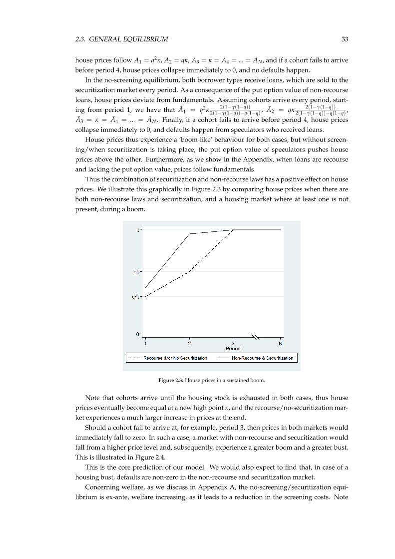
2.3. GENERAL EQUILIBRIUM 33
house prices follow A1 = q2κ, A2 = qκ, A3 = κ = A4 = ... = AN , and if a cohort fails to arrivebefore period 4, house prices collapse immediately to 0, and no defaults happen.
In the no-screening equilibrium, both borrower types receive loans, which are sold to thesecuritization market every period. As a consequence of the put option value of non-recourseloans, house prices deviate from fundamentals. Assuming cohorts arrive every period, start-ing from period 1, we have that A1 = q2κ
2(1−γ(1−q))2(1−γ(1−q))−q(1−q) , A2 = qκ
2(1−γ(1−q))2(1−γ(1−q))−q(1−q) ,
A3 = κ = A4 = ... = AN . Finally, if a cohort fails to arrive before period 4, house pricescollapse immediately to 0, and defaults happen from speculators who received loans.
House prices thus experience a ’boom-like’ behaviour for both cases, but without screen-ing/when securitization is taking place, the put option value of speculators pushes houseprices above the other. Furthermore, as we show in the Appendix, when loans are recourseand lacking the put option value, prices follow fundamentals.
Thus the combination of securitization and non-recourse laws has a positive effect on houseprices. We illustrate this graphically in Figure 2.3 by comparing house prices when there areboth non-recourse laws and securitization, and a housing market where at least one is notpresent, during a boom.
Figure 2.3: House prices in a sustained boom.
Note that cohorts arrive until the housing stock is exhausted in both cases, thus houseprices eventually become equal at a new high point κ, and the recourse/no-securitization mar-ket experiences a much larger increase in prices at the end.
Should a cohort fail to arrive at, for example, period 3, then prices in both markets wouldimmediately fall to zero. In such a case, a market with non-recourse and securitization wouldfall from a higher price level and, subsequently, experience a greater boom and a greater bust.This is illustrated in Figure 2.4.
This is the core prediction of our model. We would also expect to find that, in case of ahousing bust, defaults are non-zero in the non-recourse and securitization market.
Concerning welfare, as we discuss in Appendix A, the no-screening/securitization equi-librium is ex-ante, welfare increasing, as it leads to a reduction in the screening costs. Note
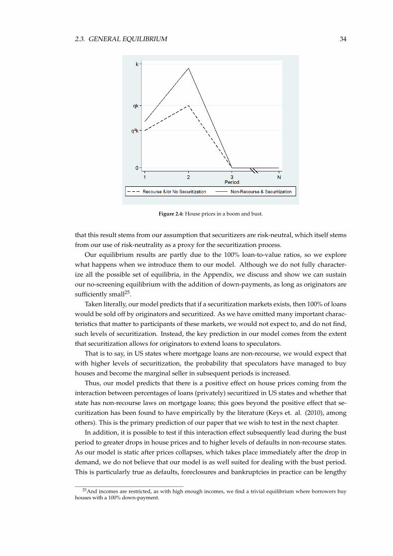
2.3. GENERAL EQUILIBRIUM 34
Figure 2.4: House prices in a boom and bust.
that this result stems from our assumption that securitizers are risk-neutral, which itself stemsfrom our use of risk-neutrality as a proxy for the securitization process.
Our equilibrium results are partly due to the 100% loan-to-value ratios, so we explorewhat happens when we introduce them to our model. Although we do not fully character-ize all the possible set of equilibria, in the Appendix, we discuss and show we can sustainour no-screening equilibrium with the addition of down-payments, as long as originators aresufficiently small25.
Taken literally, our model predicts that if a securitization markets exists, then 100% of loanswould be sold off by originators and securitized. As we have omitted many important charac-teristics that matter to participants of these markets, we would not expect to, and do not find,such levels of securitization. Instead, the key prediction in our model comes from the extentthat securitization allows for originators to extend loans to speculators.
That is to say, in US states where mortgage loans are non-recourse, we would expect thatwith higher levels of securitization, the probability that speculators have managed to buyhouses and become the marginal seller in subsequent periods is increased.
Thus, our model predicts that there is a positive effect on house prices coming from theinteraction between percentages of loans (privately) securitized in US states and whether thatstate has non-recourse laws on mortgage loans; this goes beyond the positive effect that se-curitization has been found to have empirically by the literature (Keys et. al. (2010), amongothers). This is the primary prediction of our paper that we wish to test in the next chapter.
In addition, it is possible to test if this interaction effect subsequently lead during the bustperiod to greater drops in house prices and to higher levels of defaults in non-recourse states.As our model is static after prices collapses, which takes place immediately after the drop indemand, we do not believe that our model is as well suited for dealing with the bust period.This is particularly true as defaults, foreclosures and bankruptcies in practice can be lengthy
25And incomes are restricted, as with high enough incomes, we find a trivial equilibrium where borrowers buyhouses with a 100% down-payment.
2.4. CONCLUSION 35
processes, and a richer model in those characteristics would be better suited to testing thismechanism in the bust period.
Finally, concerning other mechanisms that the literature has suggested as causes for theboom and bust, from moral hazard issues to overoptimism, from increase in loan supply tomispriced loans, we surmise that these most likely would interact with our own model insuch a way as to enhance each other.
For example, consider moral hazard issues such as outright fraud and, more generally,anything that makes it such that securitizers are not fully aware/misled about the composi-tion of mortgage loans and thus mispricing of loans. We expect that this would make ourconditions for an equilibrium less stringent (particularly the cost restriction for no ’skimmingthe cream’), whilst simultaneously providing an additional reason for why house prices mighthave increased, and also making it easier for an equilibrium such as ours to come about, evenwith large originators and down-payments
We believe that by setting up the model as we do, we are likely finding a lower bound forunder what conditions our mechanism might contribute to increased house prices.
2.4 Conclusion
The literature on the housing market has sought out many explanations for what led to theunprecedented boom and bust in the US during the 2000s. We seek to add to this literatureby proposing that the non-recourse status of mortgage loans in some states in the US, whencombined with the increase in private securitization experienced at that time, pushed up theprices of houses in those states beyond their fundamental value during the boom.
Our model generates an increase in house prices using the ‘risk shifting’ mechanism ofAllen and Gorton (1993), where the asymmetry of payoffs between loan originators and bor-rowers creates a put option value for the latter. We base our model on the work of Barlevyand Fisher (2010), but introduce two important, novel elements: screening of borrowers byoriginators and a securitization market.
We find that during a demand boom, when securitization takes place, originators shiftthe risks associated with the loans they extend by selling them to the securitization market.Furthermore, when these loans are non-recourse, originators cannot credibly signal whethera loan has been extended to a risky speculator or a owner-occupier. As result of this, a non-screening equilibrium is possible, where originators extend loans to both types and sell bothto securitizers. Due to the put option in non-recourse loans, speculator’s value of housingincreases, such that house prices increase when they can become marginal sellers.
We show that in the absence of securitization taking place and/or with recourse loans,house prices remain at the fundamental level. We thus predict that the interaction of privatesecuritization and non-recourse laws should lead to increased house price growth during aboom. Under some restrictions, we show that our results can exist even when borrowers arerisk-averse or there are down-payments on loans.
Our model also makes predictions for the bust period, although, due to the static natureof the bust period, is less suited for doing so. It predicts that the interaction effect betweensecuritization and non-recourse status from the boom period should lead to greater falls inhouse prices and more defaults during a subsequent bust.
2.4. CONCLUSION 36
We thus have established how, from a theoretical perspective, securitization and recourselaws might have significant effects on house prices. We now proceed, in the next chapter, totest these predictions for the case of the states in the US.
Appendices to the Chapter
2.A Appendix A - Model and empirics discussion
2.A.1 Borrowers
We can think of low type borrowers as being speculators as they only wish to buy a houseto take advantage of (potential) capital gains by selling it in a later period. There is substantialevidence that house buyers seeking to make capital gains were an important part of the hous-ing market in the US during the recent boom, as can be seen in Haughwout, Lee, Tracy andvan der Klaauw (2011), Bhutta (2015) and Bayer, Mangum and Roberts (2016). Haughwoutet al. (2011) for example, finds that around half of mortgage originations for house purchasesin states with greatest price appreciation at the top of the housing boom were done by suchborrowers.26 In our model, we need not assume such a large number of speculators: a smallnumber of low types is sufficient to generate increased house prices, as long as they have theopportunity to become the marginal sellers.
For the purposes of our model, we have that speculators and owner-occupiers are a sep-arate set of agents, but in practice there is likely a ‘spectrum’ of intentions from borrowersconcerning what they wish to do with houses. That is, borrowers utility from owning a houselikely span a wide range of values, which would turn owner-occupiers into speculators ifprices have risen sufficiently. We surmise that making such an addition to our model wouldgenerate analogous results, and opt for two separate sets of agents for tractability.
2.A.1.1 Risk Averse Borrowers
If we made borrowers risk averse with equivalent utility to that of the originators, thenthere is no change to the optimal behaviour of owner-occupiers, as their optimal decision isstill to never default, so there is no uncertainty/variance.
With non-recourse loans, speculators remain protected from a fall in house prices. How-ever, the uncertainty stemming from the change in house prices means that they only takea loan if the negative utility from this variance is smaller than the expected benefit, i.e., ifq(π − rP) ≥ aq(1− q)(π − rP)
2, where rP is the equilibrium, no-screening interest rate.This is true if a ≤ 1
(1−q)(π−rP), which we can show hold simultaneously with a ≥ a′ =
12(1−q)π , thus any a that satisfies both restrictions allows for both risk averse borrowers andoriginators and finds the same result in a no-screening equilibrium.
If, however, risk aversion is sufficiently high, then speculators never wish to take on loansin either equilibrium. In such a case, our model predicts that only owner-occupiers receiveloans.
We show in Appendix B, that the analogous result holds in general equilibrium for a largeenough probability, q > 0.25.
26Unlike our model, Haughwout et al. (2011) find evidence of speculator-like buyers by looking at second homepurchases, but as they conclude that this was done by speculators “apparently misreporting their intentions to occupythe property”, as “(...) many of the borrowers who claimed on the mortgage application that they planned to live inthe property they were purchasing had multiple first-lien mortgages when the transaction was complete”. This canbe thought as a part of the information that good screening discovers.
37
2.A. APPENDIX A - MODEL AND EMPIRICS DISCUSSION 38
2.A.2 Originators
The interaction within the group of originators and between originators and borrowers issimilar to that of a Bertrand competition, as borrowers can see the interest rate schedule andthe loan decision before deciding which originator to approach. Because of this Bertrand-likemarketplace, in the absence of scale effects, and with linear costs, we need not specify thenumber of originators that exist; the model would work equally well with just two originatorsas with a continuum of them.
Furthermore, this means that with deep pockets and free entry, we would find the sameresults, which allows us to use a representative originator to find some results.
Originators’ capacity to distinguish between the two types of borrowers comes at a costof C per each individual they screen. We can think of this being the cost needed to obtainextra information necessary to tell apart two borrowers whose observable characteristics areidentical (that is, any and all information used to price loans/mortgage securities). This could,for example, be thought of as information that only becomes available from when experiencedbank managers carefully investigate and vet potential borrowers.
A 2013 article by The Economist illustrates how this cost of screening can be significant:“Marquette’s [a bank] (...) approach was to have a lending officer accompanied by one of the bank’strustees (board members, in effect) visit every mortgage applicant on the Saturday after each applicationwas filed.” Originators may have problems in being able to signal the quality of loans, affectingthe incentives to screen if originators can sell: “Its overseers wanted it to sell its mortgages to protectitself from swings in property prices. (...) The subprime crisis revealed so much slapdash issuance thatbuyers of mortgages consider valuations provided by the originators worthless. So Marquette can nolonger conduct its own appraisals. Saturday visits have ended.27”
As Keys, et al argue, only contractual terms (such as LTV ratios and interest rates) andFICO scores were used by investors to evaluate the quality of a securitized pool. As such,although we have restricted the signal of loan quality between originators and securitizers tobe interest rates, other ‘hard’ characteristic of loans might have been used instead, in particular,the loan-to-value ratio, which we discuss below.
2.A.3 Securitization and Securitizers
We focus on the private securitization market in our modelling, as opposed to the GSEmarket. We do this for several reasons, firstly because the incentives of GSEs are difficult toascertain and model, given their dual role as for-profit companies which were also tasked withhelping finance low and middle income loans28.
Secondly, the literature has evidence that lending standards of loans associated with GSEschanged little during the 2000s. GSE securitization has a long history in the US, and theiroverall participation rate in creating loans changed little in the decade preceding the crisis.As Adelino, Schoar and Severino (2016) summarize “Loans that were sold to (and then guar-anteed by) the GSEs had to conform to higher origination standards than those sold to otherentities”. This can be seen in the default rates of GSE loans in 2008 and 2009 which, although
27Economist, Nov. 2013.28As per the Housing and Community Development Act of 1992, they ‘have an affirmative obligation to facilitate
the financing of affordable housing for low- and moderate-income families in a manner consistent with their overallpublic purposes, while maintaining a strong financial condition and a reasonable economic return”
2.A. APPENDIX A - MODEL AND EMPIRICS DISCUSSION 39
high by historical standards, were not even half as large as those at the lower end of the hous-ing market sold to the private sector (Angelides and Thomas, 2011).
Note as we do find evidence that house prices were affected by GSE loans in our regres-sions, albeit negatively, whether our mechanism may have had some effect in the 2000s re-mains an open question, and we cannot exclude such a possibility.
Private securitization expanded to unprecedented levels in the late 90s and the early 00s.This resulted in new financial agents buying these products and becoming exposed to the UShousing market for the first time, including agents outside of the US. Many of these agents,as discussed by Lewis (2011), had very little understanding of the US housing market, muchless of the constituent mortgage loans they held via the CDOs and MBS they owned. As wediscuss in the previous section, products were typically evaluated over aggregated/averagedinformation over the thousands of loans backing a single product, such as the average FICOscore. In addition, Elul (2011) finds evidence that originators of loans may have had accessto private information beyond that typically used by buyers of securitized products, resultingin adverse selection. For these reasons, we model securitizers as not being able to distinguishbetween the different types of borrowers behind a loan.
Buyers of securitized products would use such averaged information in part due to thecomplexity of the securitization process, which may have been deliberately made more com-plex due to moral hazard issues (Hofmann, 2008).
This makes securitization quite complex to model, as it involves numerous agents andsteps29. We can summarize it as consisting of aggregating loans from a number of differentmarkets, on the assumption that they exhibit some statistical independence from each other,and then slicing the returns from these loans into different tranches, so that the senior tranchesreceive priority in payments, and losses are absorbed by the lower tranches first. The wholeprocess involves a number of intermediaries and steps, most saliently a loan originator and asecuritization arranger, normally an investment bank.
The aggregation should result, if loans are statistically independent at least to some ex-tent, in both a reduction in uncertainty about the outcomes and a reduction in the variance.Combined with the creation of tranches, this would theoretically allow for high tranches to berelatively safe products; the arranger banks would normally hold on to the lowest tranches,the so called ‘residual’ or ‘junior’ tranches.
Given these complexities, we focus our attention on just one consequence of the securiti-zation process, the reduction in uncertainty. We do this by having securitizers be risk neutralas opposed to risk averse, allowing us to proxy this aspect of securitization in a tractable way.That is, as they do not have any loss of utility from risk aversion, securitizers will be willing topay a higher price for loans compared to originators, much like owners of securitized productsshould do if securitization reduces uncertainty (especially for owners of high tranches).
We can rationalize this approach as being directly equivalent to having a continuum ofidentical and independent housing markets, and allowing risk-adverse securitizers to pur-chase a diversified portfolio of each, and having all markets have the same equilibrium out-come of screening or no-screening. In such a case, there is no uncertainty about outcomes forsecuritizers, so no risk-aversion, and our ex-ante results become ex-post too.
This way of modeling securitization, although tractable, does have limitations. Although
29See Ashcraft and Schuermann (2008) for a discussion of the stages and the problems that might arise in each ofthese.
2.A. APPENDIX A - MODEL AND EMPIRICS DISCUSSION 40
we capture to some degree the benefits of securitization due to a reduction in risk and uncer-tainty, the absence of tranches is a significant omission. It may be possible, through havingmultiple housing markets, to create tranches in our model, albeit a previous version with justtwo markets had unreasonable had impracticably difficult dynamics. We surmise that includ-ing tranching would not rule out our equilibrium results, even if originators held on to juniortranches; we conjuncture this would result in higher interest rates/prices to compensate orig-inators, whilst still being low enough to be accepted by speculators.
Note finally that in our model we do not split up securitizers into the intermediaries that se-curitize the products and the ultimate holders of the securitized loans. This should be thoughtof as a reduced form of the process and simplifies the analysis by not adding an additionalagent.
2.A.4 General equilibrium
We define the profits for Originators conditional on what actions they take, Y(.), as follows.If they screen and only lend to owner-occupiers:
Y(QOj , 1, 0, I(j)) = ∑
i∈I(j)qO
i,j(P∗(ri)− 1) + (1− qOi,j)XH(ri)
If they screen and lend to both types:
Y(QOj , 1, 1, I(j)) = ∑
i∈I(j,H)
qOi,j(P∗(ri)− 1) + (1− qO
i,j)XH(ri)
+ ∑i∈I(j,L)
qOi,j(P∗(ri)− 1) + (1− qO
i,j)E(XL(ri))
Finally, if they don’t screen:
Y(QOj , 0, ∅, I(j)) = ∑
i∈I(j,H)
qOi,j(P∗(ri)− 1) + (1− qO
i,j)XH(ri)
+ ∑i∈I(j,L)
qOi,j(P∗(ri)− 1) + (1− qO
i,j)E(XL(ri))
The choice of N periods of time may seem arbitrary and it is, to some extent. Our set-upis isomorphic to having 3 periods of time by extending the set of actions taken in period 3and allowing borrowers to choose to fully repay or default on their loans. Consequently, forthe purposes of our model, our interest lies, in particular, with periods 1, 2 and 3, where asecuritized and non-securitized market might differ; periods 4 and beyond are necessary onlybecause we have loans that are paid out in 2 periods of time and that loans granted in period3 need the subsequent periods to be repaid30.
The entry of new borrowers, which increases the stock of high types, can be interpreted asan increase of demand for housing, and might be endogenized via the mechanisms of Duca,et al. (2011) or Case et al. (2012), among others, for the recent boom. Consequently, our modelcannot explain why fundamentals are changing, but may explain why our mechanism canhave potent effects on house prices during a boom.
The assumption that mortgage loans are repaid in two, equal sums is not innocuous, asthe higher the first repayment is in the first period, the less house prices will deviate from
30B&F have a similar modeling technique, as even though they have an infinite number of periods, their modelexperiences no further changes once a sufficient number of periods have passed and either cohorts stop arriving, orthe number of high types exceeds the housing stock.
2.A. APPENDIX A - MODEL AND EMPIRICS DISCUSSION 41
their fundamental value, as the option value of waiting is decreased in proportion to that.Similarly, having repayments happen over only two periods of time and a LTV ratio of 100%both increase how much prices deviate. A richer model would most likely have house pricedeviate from fundamentals over a longer period of time and by smaller amounts31.
2.A.4.1 Housing stock and cohort size
We make specific assumptions about our housing stock and cohort size, unlike B&F. Wedo so primarily so we can focus our attention on a model where the fundamental uncertainty,whether high types will exceed the housing supply, is resolved by period 3.
This is the smallest number of periods where it is possible to illustrate our model mecha-nism, as we require at least one period where low types can buy, and at least one period wherethey can become marginal sellers before high types exceed the housing supply.
As we discuss in Section 2.B.2 of Appendix B, we surmise that our model results wouldgeneralize to changes in housing supply and cohort size such that the fundamental uncertaintyis resolved for some period greater than 3. The only substantial difference would be that pricedeviation from fundamentals would not necessarily take place only if securitization happensevery period, but more generally, when there is ’sufficient securitization’ such that speculatorshave had access to loans.
2.A.4.2 Recourse loans
When loans are recourse, we can show that speculator’s marginal value of housing is al-ways equal to the fundamental value. A speculator obtaining a loan in period 1 can choose,in period 2, to either sell and repay today, A2 − A1(1 + r). The can also pay the install-ment −A(1 + r)/2 and wait, and with probability q a cohort arrives, so they sell and repayA3 − A1(1 + r)/2, but with probability (1 − q) a cohort fails to arrive, in which case theystill have to repay their loan installment, A1(1 + r)/2. Ergo, as speculators are the marginalsellers in period 2, we have that their value determines house prices, so A2 − A1(1 + r) =
−A(1+ r)/2+ q(A3−A1(1+ r)/2)+ (1− q)(−A1(1+ r)/2) = qA3−A1(1+ r), so A2 = qA3.As can be seen in the math, this holds more generally for any period t.
2.A.4.3 Loan-to-value ratio
Adding loan-to-value to our base model, as a choice variable for originators, results in atrivial equilibrium wherein down-payments are set to 100% and borrowers buy houses out-right. The reason for this is that with risk neutrality and no discounting, the payment of in-terest rates is always negative to utility of both types, so simply letting borrowers buy housesoutright would be the trivial equilibrium result.
Instead, if we wish to have a meaningful result with down-payments, we have to restrictincomes of borrowers to yρ, such that there is a maximum down-payment d, yρ = dAρ whenthey arrive.
As we show in the Appendix B, a no-screening equilibrium identical to our main result cannow be sustained, but only if loan originators are small and take the prices of houses as given;
31We also surmise that in a more general model, having teaser rates (smaller fixed rates that only last for thebeginning of the loan), would lead to greater deviations of prices, as both of which make it cheaper for a borrower towait.
2.A. APPENDIX A - MODEL AND EMPIRICS DISCUSSION 42
otherwise we will have a new equilibrium wherein down-payments are set to be as high aspossible, d, and interest rates are set high enough so as to discourage speculators, creatingself-selection without the need for screening.
The main reason for this result is the asymmetric effects of (restricted) down-payments forspeculators and owner-occupiers. Any positive d < 1 means that there is now a range of inter-est rates where speculators, but not owner-occupiers, do not wish to take-on loans, as defaultsare no longer costless. Owner-occupiers will be sufficiently compensated with a high enough dif house prices ‘switch’ to the fundamental price level when originators deviate, ergo, origina-tors are large enough; if house prices remain at the no-screening level when owner-occupierscontemplate the deviation, then no deviation exists, and we maintain our no-securitizationequilibrium with zero down-payments32.
As such, the extent to which our model results may be true depends on the LTV ratiosthat prevail. Concerning the housing boom and bust of the 2000s, the literature has foundthat these were very close to 100%. For example, Mayer, Pence, and Sherlund, (2009) findthat for securitized assets, “median combined loan-to-value ratio for subprime purchase loansrose from 90 percent in 2003 to 100 percent in 2005”, meaning that over 50% of these loanshad 100% LTV ratios, and they find a similar result for Alt-A mortgages, with LTV ratiosincreasing from 90% to 95%. Given in the no-speculator equilibrium we described above ourmodel predicts down-payments that are as high as possible, versus the zero down-paymentsin the no-screening result, this suggests that most likely we were in an equilibrium wherespeculators were receiving loans.
Finally, although our model predicts that speculators will not accept loans with positivedown-payments, if this were to happen then house price growth would depend on the down-payment, as the higher the down-payment, the smaller the put-option value, so the less houseprices deviate from fundamentals.
2.A.4.4 Welfare
Note that in all our equilibria, originators never hold speculator loans, thus their risk-aversion portion of utility is never a part of welfare considerations. This means that the dif-ference between the screening and a no-screening equilibria will consist of transfers of wealthbetween ‘de facto’ risk-neutral agents. This would suggest that welfare is the same for both sit-uations; however, in the screening equilibria, there are real costs of screening, which increasethe interest rates, lowering overall welfare.
Note that originators and securitizers, due to Bertrand-like competition/free entry alwayshave ex-ante zero utility in both cases, although if price collapses, whoever holds loans willhave losses in a no-screening equilibrium. Instead, ex-ante, welfare changes happen betweenborrowers and no-loan low types. In particular, we have that interest rates on loans are smallerwithout screening, C/(1− γ) > 1− /(1− γ(1− q)) due to our no-skimming condition. How-ever, as house prices are also higher, the overall effect is ambiguous for owner-occupiers. Onthe other hand, speculators, who proceed to gain access to loans and can potentially gain from
32In addition to these results, there are several ways we can maintain a no-screening equilibrium with large origi-nators by departing from our model assumptions. The simplest is if neither interest rates nor the LTV ratio are usedas signaling devices to securitizers. In that case, securitizers assume that loans are given out to both speculators andowner-occupiers, i.e., PNSC,. = PL,. = PH,.. This means that originators will wish to sell as many loans as possible, asthey do not benefit from signalling, so they optimize by setting d = 0. Thus, this result is equivalent to a mispricingof securitized assets by the securitization market, which Nam and Oh (2014) among others have found evidence for.
2.B. APPENDIX B - PROOFS 43
speculation, and no-loan low types, who receive higher prices for their houses, are unambigu-ously better off in a no-screening equilibrium.
2.B Appendix B - Proofs
2.B.1 Partial Equilibrium Proofs
In equilibrium, securitizers’ expected utility will be equal to zero due to free entry.Much like with Bertrand competition and the previous proof, if the equilibrium P′ were
such that E(U′/Ω, r) > 0 for a securitizer, a different securitizer could enter the market offer-ing P′′ > P′, buy the same loans and increase their payoff. In equilibrium, only a price suchthat E(U′/Ω, r) = 0 is sustainable.
If originators are restricted from selling their loans and are sufficiently risk averse, theyscreen and only lend to owner-occupiers.
In a screening equilibrium, if a loan is composed of high types the expected utility of hold-ing the loan is EUO,H = E(XH) = rH and for low types it is EUO,L = E(XL) − aV(XL) =
−aq× (rL)2(1− q) + q[1− 2a(1− q)π]× rL − π(1− q)[1 + aqπ].
A sufficient condition for loans never be extended to low types is UO,L ≤ 0 for all rL, and asufficient condition for this to hold is if q[1− 2a(1− q)π] < 0, which is true if:
a >1
2(1− q)π= a
So for a ≥ a, originators only lend to high types in a screening equilibrium (SC)and haveexpected utility of EUO,SC = (1− γ)rH − C.
If originators don’t screen (NSC), their utility is:
EUO,NSC = γEUO,H + (1− γ)EUO,L
This implies that their utility in a no-screening equilibrium will be smaller or equal to thatin a screening equilibrium, EUO,NSC ≤ EUO,SC, if and only if:
(1− γ)EUO,H + γEUO,L ≤ (1− γ)EUO,H − C ⇔ UOL ≤
−Cγ
This will hold if a > Cq(1−q)γπ2
33. So if a ≥ maxa, a, where, we have that EUO,NSC ≤EUO,SC.
If (1− q)/q > 1, then an equilibrium where both types receive loans and only speculatorloans are sold can be sustained.
With (1− q)/q > 1, then PL ≥ 1, so speculators will receive loans which are sold. In thatcase, owner-occupier loans cannot be sold, as either the equilibrium interest rates are the same,in which case not-screening dominates, or they are different, in which case not-screening andsetting interest rates equal to the lowest equilibrium interest rate dominates, in both cases dueto the real cost of screening.
33This guarantees that the term independent of r in UO,L is less than or equal to zero.
2.B. APPENDIX B - PROOFS 44
Thus, the only possible equilibrium is to hold on to originator loans and sell speculators’.This can be sustained if speculator loans are the lowest possible (i.e., if rL = (1− q)π/q), thereexists a rH such that EUO = (1− γ)rH + γ(qrL − (1− q)π)− C ≥ 0, which is rH = C/(1−γ) < π < κ, so owner-occupiers accept. Note that as rH = C/(1−γ) < (1− q)π/q = rL, thereis no way for a originator to deviate by not screening and setting rH = rL, as owner-occupierswould not accept a higher interest rate.
In partial equilibrium when there is no screening, the equilibrium is for loans to be soldby originators.
Recall our posited equilibrium actions: originators do not screen, and offer interest ratesof rP = γ(1−q)π
(1−γ)+qγto any borrower who approaches them, borrowers approach any originator
posting that information set, and securitizers pay P∗P = 1 for any loan with interest rate rP
and have beliefs that any loan with a different interest rate is composed of low types. Firstnote that our equilibrium price and interest rate make the expected utility of originators andsecuritizers equal to zero, as is required by the way we model our markets. Also note thatfrom our previous restriction on the value of rates, we must have that rP ≤ π, which is true ifγ ≤ 1
2(1−q) .What are the possible actions that an originator could contemplate that would deviate from
this equilibrium34? They can choose to not screen and offer an interest rate different from theequilibrium interest rate (and choose to hold or sell their loans)(PD1). They could choose toscreen and: not grant loans to high types (PD2); not grant loans to low types (PD3); grantloans to both and offer a different interest rate to high types (and choose to sell or keep theseloans)(PD4); grant loans to both and offer a different interest rate to low types (and choose tosell or keep these loans)(PD5); grant loans to both and offer a different interest rates to bothtypes (and choose to sell or keep these loans)(PD6); grant loans to both at the equilibriuminterest rate and choose to not sell either one or both of the loans(PD7).
If they choose to not screen and offer a different interest rate than the equilibrium interestrate, first note from our previous results, due to risk aversion, they would never wish to hold-on to loans. So if they wished to sell loans, the deviation interest rate they would contemplatecould only be lower than the equilibrium interest rate, as otherwise they will not attract anyborrowers35, who are better off at the equilibrium interest rate. As prices are monotonicallydecreasing in Ω and increasing in rζ , any deviation would result in a loan with a lower interestrate and a higher Ω on the part of securitizers, so the price would be smaller than the one theyreceive by staying in the equilibrium, ruling out PD1.
We now show that it is never optimal for originators to screen and not grant loans to hightypes. In all versions of our model, high types will never default36 and originators can alwayshold-on to any loan granted. As such, originators can always be made better, vis-a-vis choos-ing to screen and deny loans to high types, by granting a loan to a high type and holding on
34Note again that we have established the optimal actions of borrowers and securitizers, conditional on the actionsof originators and the beliefs of securitizers.
35Originators are thus constrained by the actions of the borrowers, as any successful deviation from a equilibriuminterest rate must be such that it not only increases the payoff of the originator, but must also increase (at least weakly)the payoff of the borrowers too. This is a somewhat surprising result that comes from the peculiarities of the Bertrand-like competition between originators, and we surmise that it would still hold even if other forms of competition wereused instead.
36This will be shown to be true in the general equilibrium model.

2.B. APPENDIX B - PROOFS 45
to these loans, as they will have a payoff of at least 0 for each high type37. So we need notcontemplate this deviation action further and rule out PD2. Similarly, their payoff would besmaller by screening and denying loans to low types, as they would have the cost of screeningand the same revenue38, so PD3 is ruled out.
For all our other possible deviations, note that from our discussion of PD1, the only possi-ble deviation interest rate that originators could offer would necessarily be lower, and as wehave demonstrated, that would result in a lower payoff by selling these loans, which meansthat we can rule out all other possible deviations except PD7. For PD7, originators might bebetter off by screening, offering loans to both types at the equilibrium interest rate, holdingon to loans made to high types and only selling loans composed of low types, ’skimming thecream’.
However, the resulting expected utility is lower or equal to the expected utility of takingthe equilibrium action if:
γ(P∗P − 1) + (1− γ)rP − C ≤ P∗P − 1, which will hold as long as (1−γ)γ(1−q)(1−γ)+qγ
≤ C.
So, as long as γ ≤ 12(1−q) and (1−γ)γ(1−q)
(1−γ)+qγ≤ C holds, we have a unique equilibrium.
2.B.2 General Equilibrium Proofs
The fundamental value of houses is the expected value of houses in period 4.From our definition of fundamental value, we note that if loans are needed to buy a house,
then there is no ‘speculative’ element, as the consequences of buying a house are fully born byany house buyer, both positive and negative.
In such a case, arriving new low types buyers will have an identical valuation to existinglow type house sellers, such that if the price that prevails is that of no-loans low type sellers,new low types will be indifferent between buying and selling a house, so, for simplicity, weassume they do not buy with the intention of selling.
As they both value the house at 0, this consists only the value that they might gain fromwaiting and selling the house in a future period, which is the expected value of house prices inperiod 4. Finally, for periods 1 and 2, housing supply will exceed the number of new high typebuyers arriving, the price that prevails will be that of the marginal seller; in period 3, either acohort arrives such that high types exceed the number of low sellers and the price is equal tothe marginal buyer’s value, κ, or it does not, so the price will be 0.
Under restricted selling, there exists a unique equilibrium such that originators screen andonly lend to high types in period 2.
Under Bertrand-like competition, we know that equilibrium interest rates will be such thatexpected utility of originators is equal to zero. As in the no-screening equilibria there is no costof screening and there is the additional revenue from high types, the utility that originatorshave from lending with the highest possible interest rate is always greater than or equal to the
37If a loan granted to a high type in a given period is A > 0, then high types will repay A(1 + rH) in total, sooriginators will have a payoff of ArH by holding on to the loan. As rH ≥ 0, ArH ≥ 0.
38Since the equilibrium price is 1, for every given loan, the revenue originators achieve by selling the loans issimply 0.
2.B. APPENDIX B - PROOFS 46
utility they receive if they were to screen and lend to both types. So any condition that satisfiesthe former, will guarantee the latter.
Noting again that defaults happen with probability q if lending happens to low types39 andutility is separable between types as there is no risk associated with high types, the expectedutility of lending in a no screening equilibrium for originators is
EUOP,2 = (1− γ)EUO
H,2 + γEUOL,2 = −aq(A2)
2r2P,2 + (1− γ(1− q))A2rP,2− (1− q)[γ + aA2]
This is a quadratic function of rP,2, with a positive coefficient only in the first order term,so the function only has non-negative values between its roots, if it has any, and it is mono-tonically decreasing in a. The weakest condition that guarantees that no lending will hap-pen is if a is large enough so that there are no real roots in this equation, the condition thatAa2 + aγ− (1−γ(1−q))2
4q(1−q)A ≥ 0, which itself is satisfied by setting a larger than the largest positive
root, a ≥
√γ2+
(1−γ(1−q))2q(1−q) −γ
2A = a′.Note here that a is inversely proportional to the value of house prices in this period, this
means that this risk aversion condition (that makes originators wish to screen and deny loansto low types) is decreasing in the price of houses. As giving loans to low types can only in-crease house prices, a sufficient condition comes from setting prices to be the smallest possiblevalue.
So setting A to be the smallest possible value, A = q2κ, we guarantee that originatorswill always be better off by screening and only lending to high types as long as they have
a ≥ a′′ =
√γ2+
(1−γ(1−q))2q(1−q) −γ
2q2κ.
Under restricted selling, originators will wish to screen and only lend to high types if a ≥ a′′
in period 1.From our previous proof, we need only show that in a no-screening equilibrium originators
have utility less than or equal to zero to guarantee a unique equilibrium where screening takesplace and only high types receive loans. Due to the assumption of Ψ = 2− γ, in period 2, iflow types received loans in period 1 and bought houses, in period 2 high types will end upbuying at least some houses from these new low types. That is, even if high types first buyhouses from old low types, they will, at least, have to buy a house from one new low type whobought a house in period 1.
If we assume that γ < 12 , and if high types arriving in period 2 buy first from new low types
who bought in period 1, they could buy all the houses these low types own, in which case newlow types would not default and would proceed to repay their loans. As this happens withprobability q, and if a cohort fails to arrive low types would default, this is identical to whathappens in period 2, so the condition a ≥ a′′ is a sufficient condition.
If high types do not first acquire their houses from low types who bought in period 1, thena portion of these low types would proceed to only partially repay their loans and may ormay not repay them in full in period 3. In such a case, this portion of low types are riskierthan the low types who repay in full in period 2, so the risk of lending to low types would beeven higher, so the utility that originators would have is necessarily less than or equal to theprevious case, such that a ≥ a′′ is a sufficient condition for originators to wish to screen andonly lend to low types.
39That is, they default if no new cohort arrives, and sell houses and repay their loans early if a cohort arrives.

2.B. APPENDIX B - PROOFS 47
The two equilibria when we relax our refinement of no belief switching by securitizers isidentical to the screening equilibrium.
Assume that securitizers’ beliefs changed between periods 1 and 2, such that now, it ispossible for a screening equilibrium to happen in period 1 (AE1), followed by a no-screeningequilibria in period 2, or vice-versa (AE2).
In AE1, as screening took place in period 1, no low types acquired loans in that period,which means there cannot be any low types with mortgages in period 2 selling houses, ergo,prices cannot deviate from fundamentals in period 2 and, by extension, in period 1. We couldmake this equilibrium hold by setting beliefs of securitizers analogously to their counterpartsin the screening equilibrium in period 1 and the no-screening equilibrium in period 2.
In AE2, under our assumption that Ψ = 2− γ, in the first period, the housing supply fallsby 1, as both high and low types buy houses, leaving the supply of houses equal to 1− γ. Inperiod 2, arriving high types are of size 1− γ, so they are exactly equal to the housing stockstill owned by old low types. As such, they buy only from old low types and prices cannotdeviate from fundamentals. We could sustain this equilibrium in an analogous manner to theway we discuss AE1.
Note that in both the above cases, as the risks of low types is lower than in the no-screeningequilibrium throughout, low types will not receive loans in all periods. This implies that ourconditions for the no-screening equilibrium will be sufficient for these to hold too.
In a more general model, where the initial housing stock is different from our assumptionthat Ψ = 2− γ, we would find different results. For example, if (1− γ) < Ψ′ ≤ 2− γ, thenAE1 would have an identical outcome, but in AE2, high types will buy from low types whobought in period 1 and we would have a deviation in house prices.
Similarly, if the size of the housing stock was larger and/or the size of cohorts smaller,such that the point at which high types exceed the housing supply is later than 3, we mightalso have equilibrium outcomes where securitization takes place in some, but not all periods.Nevertheless arriving low types become marginal sellers before high types exceed the housingstock, again resulting in a deviation from fundamentals.
However, in such scenarios, it would still be necessary for ’sufficient’ amounts of securiti-zation to take place for there to be deviations from fundamental price. The higher the numberof periods where securitization takes place, the more likely it is for prices to deviate and, po-tentially, the larger the deviations40.
The equilibrium cost of the loan in period 2 is always smaller than the price in 3.When prices deviate from fundamentals, we have that A2 = qκ + q(1 − q)(1 + r)/2, so
A2(2−q(1−q)(1+r)
2 ) = κ. So for a speculator to accept a loan in period 2, we must have that κ −A2(1+ rNSC) ≥ 0. Given the equilibrium no-screening interest rates rNSC,2 = 1/(1− γ(1− q),we can rewrite the above to be 2 ≥ 2q + q(1− q) + 2γ(1− q), so at most, when we have thatγ = 0.5, this will be equal to 1 > 2q− q2, which holds for all values of q < 1. If house pricesare lower, the cost of the loan is smaller, so this must also hold.
40If arriving low types become marginal sellers in more than one period, say two periods, than their put optionvalue will increase their value of waiting in both the last two periods before high types are equal or higher than thehousing supply, pushing prices higher in the penultimate period than the pure RE effect.

2.B. APPENDIX B - PROOFS 48
Securitizers pay PH,2 = A2(1 + rH,2) for loans they believe to consist of high types andPL,2 = A2q(1 + rL,2) for low types.
The expected utility of securitizers for a buying a loan with belief that it has Ω of low typeswill be US
Ω,2 = A2(1−Ω)(1+ rΩ,2) + A2Ω[q(1+ rΩ,2) + (1− q)A3,D]− PΩ,2, where A3,D is theprice that prevails if low types default, so that with free entry, PΩ,2 = A2(1−Ω)(1 + rΩ,2) +
A2Ω[q(1 + rΩ,2) + (1− q)A3]. As low types default in period 3 only if a cohort fails to arrive,we will have that A3 = 041, so PΩ,2 = A2(1−Ω(1− q))(1 + rΩ,2).
We must have that (1 + rL,2) ≤ 1q holds for all values of rL,2.
Note that there is a lower bound on the value of house prices whenever a cohort arrives,which is equal to the value houses take when there is no securitization market A2 = qκ. Houseprices cannot be valued by less if cohorts are arriving every period, this is the value old lowtypes have for houses, and they value houses in such a way that is always less than or equal tothe value of high types, κ, and new old types, which may be higher due to the default optionvalue. Low types won’t default in the next period, assuming a new cohort arrives, if andonly if A3 − A2(1 + rL,2) ≥ 0. We have that A3 = κ, so (1 + rL,2) ≤ κ
A2, which implies that
the largest possible interest rate that can be charged is when A2 is at its lower bound, qκ, so(1 + rL,2) ≤ 1
q42.
Originators will not wish to ’skim the cream’.The expected utility of skimming the cream is less than zero if and only if the cost of screen-
ing is higher than the benefits of ’skimming, which comes from selling low types and holdingon to high types, which is equal to C > (1− γ)A2rP,2 + γA2[(1− γ(1− q))(1 + rP,2)− 1]. Forthe equilibrium interest rate rP,2, this is equal to C > A2(1−γ)γ(1−q)
1−γ(1−q) . This will hold as long asthere exists values of C such that it satisfies this equation and that C < qκ(1− q)(1− γ) at thesame time, which now proceed to show.
Note that as A2 is increasing in γ and for γ < 12 , so is (1−γ)γ(1−q)
1−γ(1−q) , it is sufficient to prove
there can exist values of C for the limit value of γ = 12 . In such case, we must have that
qκ(1− q) 12 > A2
14 (1−q)
1− 12 (1−q)
which equal to 2qκ(1− 12 (1− q)) > A2. For γ = 1
2 , A2 = κq+q2
1+q2 , so
2qκ(1− 12 (1− q)) > κ
q+q2
1+q2 , which simplifies to 1 > 11+q2 , which holds for all real q. Note as
C > A2(1−γ)γ(1−q)1−γ(1−q) is increasing in A2, as long as A1 < A2 , this condition will hold in period 1
as well.
Prices in period 1 and 2 are less than κ.For our equilibrium values, AP,2 ≤ κ is equal to κ ≥ (qκ + q2κ
1−q2(1−γ(1−q))−q(1−q) )
11−γ(1−q) ,
which can be rewritten and simplified into 1− γ ≥ q2
2(1−γ(1−q))−q(1−q) and further simplified
into γ2(1− q)− γ(1 + (1− q)2) + 1− q(1− q)− q2
2 ≥ 0. First note that the zero order term,
1− q(1− q)− q2
2 is always greater than zero for q ∈ [0, 1]. Then note that γ2(1− q)− γ(1 +
41As we have discussed previously, this is a heavily stylized assumption, in so much that house prices neverdecline to 0 in real life. We could renormalize this value upwards as in B&F, but choose not to, as, essentially, whatwe must have is that the risk for buyers of loans to end up with houses post-defaults, which will happen when houseprices fall, is larger than the gains from lending to them if they don’t. Any changes would still have to satisfy this inour model.
42This holds strictly if we opt to have low types default when A3 − A2(1 + rL,2) = 0.
2.B. APPENDIX B - PROOFS 49
(1− q)2) has two roots, γ = 0 and γ = 11−q + 1− q > 1, such that for γ ∈ [0, 1], γ2(1− q)−
γ(1 + (1− q)2) ≤ 0, which means that our condition always holds.Note that as long as A1 ≤ A2, this condition holds for period 1 as well.
2.B.3 Extensions Proofs
We can have risk averse borrowers in general equilibrium.Like in partial equilibrium, we need to have that the benefits of screening outweigh the
costs stemming from risk aversion. This means that we have to have:
q(At+1 − At(1 + r)) ≥ aq(1− q)(At+1 − At(1 + r))2
We focus purely on speculators in period 1. If our results do not hold for speculators inperiod 2, we could change our housing stock size to be equal to 2, such that in the secondperiod the housing supply is 2(1− γ), which would guarantee that arriving owner-occupiersin period 2 will buy from at least 1 speculator, and at the same time, they will not exhaust thehousing supply, thus leading to the put option value changing house prices. Thus, the benefitsoutweigh the costs if
1(1−q)(A2−A1(1+r)) ≥ aThis holds with our restriction, for originators if
a′′ =
√γ2+
(1−γ(1−q))2q(1−q) −γ
2q2κ< 1
(1−q)(A2−A1(1+r))We test this numerically for our equilibrium values, using double decimal precision for q
and γ, and find that this holds for all q greater than qmin ∈ (0.27, 0.41), depending on the valueof gamma.
With restricted incomes and down-payments, a no-screening equilibrium can exist withsmall enough loan originators, otherwise only owner-occupiers receive loans.
As per our discussion in Appendix A, we have a trivial result when incomes are un-restricted, wherein the equilibrium is for borrowers to purchase homes with 100% down-payment. We thus focus on the case where there is a restricted income yρ = dAρ, and thusa maximum down-payment, d.
We begin by discussing what happens when originators wish to hold on to loans. Forany initial down-payment d, the addition of down-payments mean that there is now reduceduncertainty, so a pooling equilibrium is now:
EUOP,. = −aq((1− d)A.)
2r2P,. + (1− γ(1− q)(1− d))A.rP,. − (1− q)(1− d)[γ + aA.]
In the limit of d = 1, there is no uncertainty, so our previous results do not hold. Forany d, we have that they will hold if (1− d)Aa2 + aγ − (1−γ(1−q)(1−d))2
4q(1−q)(1−d)A ≥ 0, which itself issatisfied by setting a larger than the largest positive root of this equation, a′′′. We use this newrestriction, a > a′′′ for the results below.
We now show that speculators will now not take on loans if the interest rate is too high.Using the result from our previous extension proof, we need only show the conditions under
2.B. APPENDIX B - PROOFS 50
which a speculator from period 1 will not wish to take a loan. Given d, they now take on aloan if q(A2 − (1− d)A1(1 + r1))− dA1 ≥ 0.
Given that A1 = qA2, this will be strictly less than zero if and only if 1 + r > 1q(1−d) , thus
an originator may be able to deviate from equilibrium by selling loans with a positive d and1 + r = 1
q(1−d) , knowing that this is a credible deviation and that speculators will take on suchloans. In such a case, the price of these loans, where D stands for deviation, will be strictlypositive and originators will be able to make positive profits. Originators will compete toattract borrowers by setting the lowest possible interest rate and the highest possible down-payment, i.e., d and 1 + r = 1
q(1−d)From the above results, originators will not wish to hold on to speculators, and that if
1 + r < 1q(1−d) , speculators will not self-select. Thus, the only possible deviation is the afore-
mentioned one, with d and 1 + r = 1q(1−d) . The only question that remains is whether owner-
occupiers will wish to accept these new loans. They will not accept the new loans if the totalcost of the new loan is larger, that is, if at the equilibrium value for interest rates
(d + 1/q)AD > (d + (1− d)/(1− γ(1− q)))ANSC
If loan originators are small, such that the contemplated deviation from a no-screeningequilibrium remains with house prices at the no-screening equilibrium, we have that AD =
ANSC, such that they will not deviate if 1/q > (1 − d)/(1 − γ(1 − q)). Given that 1/q >
1/(1 − γ(1 − q)), there can be no d ∈ (0, 1) that makes this true. Thus, the no-screeningequilibrium is sustainable.
However, if loan originators are large enough to ‘influence’ house prices in equilibrium,then using our equilibrium results, they will deviate if
(d + 1/q)(1− (1− d)(1− q)q(1 + rNSC)
2) < (d + (1− d(1 + rNSC))
Which we can rewrite as
2 + (1− q)− 2/(q(1 + rNSC)) < d(2− q) + d2(1− q)q
We verify this numerically and find that it holds for all values of q and γ. Thus this resultis a possible deviation from the no-screening equilibrium, in which case there can be no equi-librium where speculators receive loans, and the equilibrium will have owner-occupier loanssold to securitizers, with the highest possible d and ‘high’ interest rates.
Chapter 3
House Prices, Securitization andNon-Recourse Loans in the USduring the 2000s
Abstract
We conduct an empirical study of the effects that private securitization and recourse (limitedliability) laws had on house prices. From our previous chapter, we have the prediction that theinteraction between private securitization and non-recourse status should lead to higher houseprices during a boom. We use heterogeneity across recourse laws in US states to test this. Aspredicted, non-recourse status roughly doubles the size of the positive relationship betweensecuritization and house prices and can explain around 75% of the difference in prices betweenrecourse and non-recourse states. To address potential endogeneity concerns, we propose anew instrument for securitization, the distance of a housing market to the headquarters of’originate and securitize’ institutions, and find further empirical support for our prediction.We conduct further tests concerning predictions for the interaction and the housing marketand find further, if more mixed, evidence for our model predictions.
JEL Classification Numbers: E00, E44, G20, R31.Keywords: House prices, Securitization, Screening, Non-recourse loans.
3.1 Introduction
The literature in macroeconomics is becoming ever more concerned with the importanceof the housing market. Iacoviello and Neri (2010) and Mian and Sufi (2014), among manyrecent papers, form part of the growing literature which finds evidence that the housing mar-ket, particularly how house prices change, forms an important part of both short and longterm dynamics in macroeconomics. As such, a better understanding of which factors lead tochanges in house prices, and a more general understanding of the housing market as a whole,now forms a significant part of the research agenda in macroeconomics.
This chapter seeks to add this literature, by testing the predictions from the previous chap-ter. There, we build a model which deals with the interaction between private securitization
51
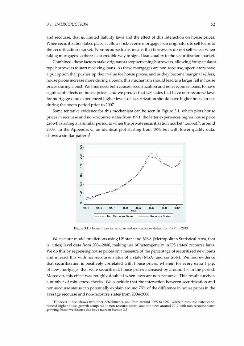
3.1. INTRODUCTION 52
and recourse, that is, limited liability laws and the effect of this interaction on house prices.When securitization takes place, it allows risk-averse mortgage loan originators to sell loans tothe securitization market. Non-recourse loans means that borrowers do not self-select whentaking mortgages so there is no credible way to signal loan quality to the securitization market.
Combined, these factors make originators stop screening borrowers, allowing for speculator-type borrowers to start receiving loans. As these mortgages are non-recourse, speculators havea put option that pushes up their value for house prices, and as they become marginal sellers,house prices increase more during a boom; this mechanism should lead to a larger fall in houseprices during a bust. We thus need both causes, securitization and non-recourse loans, to havesignificant effects on house prices, and we predict that US states that have non-recourse lawsfor mortgages and experienced higher levels of securitization should have higher house pricesduring the boom period prior to 2007.
Some tentative evidence for this mechanism can be seen in Figure 3.1, which plots houseprices in recourse and non-recourse states from 1991; the latter experiences higher house pricegrowth starting at a similar period to when the private securitization market ‘took-off’, around2003. In the Appendix C, an identical plot starting from 1975 but with lower quality data,shows a similar pattern1.
Figure 3.1: House Prices in recourse and non-recourse states, from 1991 to 2013
We test our model predictions using US state and MSA (Metropolitan Statistical Area, thatis, cities) level data from 2004-2006, making use of heterogeneity in US states’ recourse laws.We do this by regressing house prices on a measure of the percentage of securitized new loansand interact this with non-recourse status of a state/MSA (and controls). We find evidencethat securitization is positively correlated with house prices, wherein for every extra 1 p.p.of new mortgages that were securitized, house prices increased by around 1% in the period.Moreover, this effect was roughly doubled when laws are non-recourse. This result survivesa number of robustness checks. We conclude that the interaction between securitization andnon-recourse status can potentially explain around 75% of the difference in house prices in theaverage recourse and non-recourse states from 2004-2006.
1However it also shows two other detachments, one from around 1985 to 1992, wherein recourse states expe-rienced higher house growth compared to non-recourse states, and one since around 2012 with non-recourse statesgrowing faster; we discuss this issue more in Section 3.3
3.2. MODEL PREDICTIONS AND DATA 53
Due to possible endogeneity/reverse-causality issues between house prices and securitiza-tion, we use novel instrument for securitization, the weighted distance of a given MSA to thetwo closest headquarters of ’originate and securitize’ mortgage institutions. We find similarresults to our main regressions, but we note that there may be first stage problems with ourinstrument; in particular our first stage coefficients are inconsistent in recourse states. We takethis result as more evidence, but not conclusive evidence, that our mechanism played a role inthe US housing boom.
We also test our model predictions for the bust period, that house prices should fall moreand there should be more defaults due to the interaction effect stemming from the boom pe-riod. We use a similar empirical strategy to the boom period, but replace our contempora-nous measure of securitization with a measure for the average amount of securitization of theboom-period instead. We find weak evidence for our house price prediction, and no evidenceof increased defaults due to the interaction effect. We also find some evidence that securiti-zation as a whole played an role in determining house prices in both boom and bust, and fordefaults in the bust.
This chapter and its results are closely related to the growing literature on the effects ofrecourse laws in the United States, and in particular exploits the heterogeneity of states’ lawsgoing back to the Great Depression. Ghent and Kudlyak (2011)’s paper, by providing a bench-mark classification of recourse status and showing its effects on defaults, has proven veryinfluential, with Dobbie and Goldsmith-Pinkham (2014), Westrupp (2015) and Chan, Haugh-wout, Hayashi, and Van der Klaauw (2016) being recent papers that explore the effects ofrecourse status on defaults.
As we discuss in the previous chapter, our paper is closely related to Nam and Oh (2014),which proposes a similar hypothesis to the one our paper explores, that is, that non-recoursestatus may have affected prices in a risk-shifting mechanism. They investigate this possibil-ity empirically by looking at the effects of recourse on house prices during the boom periodby using state border discontinuities. They find that non-recourse states experienced greaterhouse price increases during the boom, and that borrowers were actively taking advantageof non-recourse status by taking on greater leverage and investing more in housing, and thatlenders were aware of the added risks; unlike our paper, they do not control for levels of secu-ritization. Our paper chooses to not follow their empirical strategy, however, following someof the concerns raised by Westrupp (2015).
This chapter is organized as follows. We briefly summarize the predictions of the lastchapter and discuss our data in Section 3.2. We present our empirical strategy and results inSection 3.3. Section 3.4 concludes this chapter.
3.2 Model Predictions and Data
We begin by first briefly summarizing the predictions obtained in the previous chapter ofthis thesis, and how they pertain to the empirical analysis. We then proceed to describe ourdataset and sources, and how we define what constitutes a non-recourse state. This is fol-lowed by a discussion of issues with our data and how we address them, and by a discussionconcerning the literature on the non-recourse status of mortgage laws in the US.
3.2. MODEL PREDICTIONS AND DATA 54
3.2.1 Model Predictions
Our model makes predictions about how house prices should evolve over time during aperiod of increased demand, depending on whether loans are recourse or not, and whetherprivate securitization is taking place. In all scenarios, house prices experience ‘boom-like’ be-haviour, reflecting the changes in fundamentals driving the increased demand. In marketswhere loans are non-recourse, the put option value of defaulting associated with limited li-ability can always potentially push up house prices, but in our model this will only happenwhen there is securitization, as otherwise loan originators screen out the risky speculators whomust receive loans for the option value to matter.
Our model has binary predictions for what happens to loans with the private securitiza-tion market, as either all loans are securitized, or none are. As 100% securitization does nothappen in practice, we need to interpret our model results in that light. We do so by seeing themodel as suggesting that the higher the levels of securitization, the greater the probability thatspeculators have managed to buy houses and, in subsequent periods, become the marginalseller2.
So, our primary prediction is that there is a positive effect on house prices due to the in-teraction between the percentage of loans securitized in a US state and whether that state hasnon-recourse law on mortgage loans. This prediction is distinct from the more establishedprediction that there is a positive effect on house prices coming from private securitization,which has been found previously by the literature.
We also have the prediction that this interaction effect, during a boom, subsequently leadsto greater drops in house prices during the bust period, and to higher levels of defaults, innon-recourse states. The former is due to house prices converging to the same level in allscenarios during a bust, thus falling more in non-recourse states that experienced higher levelsof securitization, and the latter from defaults of speculators who no longer profit from thedemand boom. As our model less well suited to dealing with the bust period, we treat thesepredictions as being of a secondary nature.
3.2.2 Securitization
To test the predictions of our model, we use the LAR datasets of the HMDA. The HMDAact was originally passed to collect data to check for discrimination in the US housing market.It requires most loan originators to report certain types of information on any loan request,successful or not. The act now covers around 80% of the mortgage loans according to Fishbeinand Essene (2010), and is available in the aggregated LAR datasets, on an annual basis.
Amongst other things, originators must report to whom they sell a loan if the loan is soldwithin the same calendar year of being originated. The possible categories to whom a loanis sold were changed in 2004, and have remained the same since. This change included theaddition of the category ‘Private Securitization’, which consists of any sale to a non-GSE entitywhere the originator believes the loan will be securitized in the private market3.
Our main measure of private securitization, ‘Sec’ is thus the percentage of loans which are
2This also corresponds to what we conclude in our discussion in the Appendix of the previous chapter concerning‘sufficient levels of securitization’ required for the interaction effect to take place.
3“If an institution selling a loan knows or reasonably believes that the loan will be securitized by the institutionpurchasing the loan, then the seller should use code ’5’ for “private securitization” regardless of the type or affiliationof the purchasing institution.”, according to http://www.ffiec.gov/hmda/faqreg.htm#purchaser.
3.2. MODEL PREDICTIONS AND DATA 55
believed by originators will be privately securitized, out of all successfully originated loansintended for houses purchases. Using the same category, we also find which loans were orig-inated and sold to/securitized by GSE entities4, and from that we obtain our variable ‘GSE’,the percentage of loans sold to GSEs of all successfully originated loans intended for housespurchases.
3.2.3 Recourse in the US
The question of whether mortgages are non-recourse in practice in the US5 is more com-plex than seems at first. State laws dictate the procedures taken after mortgage repaymentsstop, and there is a great deal of heterogeneity in how each state deals with this, as with thepossible ways borrowers and lenders can proceed once a default happens6. For the purposesof this paper, what matters is if the state permits deficiency judgments to be made on defaultedmortgages during a foreclosure procedure.
A deficiency judgment consists of a judicial ruling, during a foreclosure process, that theproceeds from the sale of an asset was insufficient to fully cover the loan that was secured bythat asset. As such, these permit lenders to recover the difference between the contracted valueof a house and the value obtained through selling the house, either by using the borrower’sincome, or other assets they possess.
A borrower can avoid this by declaring bankruptcy, but only if they file for chapter 7,which, according to Ghent and Kudlyak (2011), is not always possible in every American state;a chapter 13 filing does not eliminate the possibility of a deficiency judgment. Furthermore,the possibility of filling for chapter 7 bankruptcies was restricted in 2005, via the BAPCPA law,particularly for borrowers with higher income. From the perspective of our model, what mat-ters crucially is the relative ease/how cheaply a borrower can walk away from his mortgageobligations, and as we discuss in introduction, the most recent evidence seems to suggest thatnon-recourse status matters significantly in this respect.
Regarding how to classify the recourse status of a state, Ghent et al. (2011) and Mitman(2015), amongst others, use a very similar list that has a high degree of concurrence, withArizona, California, Iowa, Minnesota, Montana, North Dakota, Oregon and Washington beingconsidered non-recourse; they differ only in that Alaska, North Carolina and Wisconsin arealso considered non-recourse by Ghent et al.
This is a fairly typical result in the literature, as there is a degree of subjectivity in classifyingwhich states are recourse or not. However, most papers’ classifications have a large degree ofoverlap in states classified as non-recourse, particularly the West Coast and Northern states;they normally only differ in their classification on a small number of states. Consequently,and following most recent papers, we opt to use the Ghent et al. (2011) classification as thebenchmark for our regressions. We opt to use Mitman (2015) as a robustness check, and findthat our results are unaffected by this.
Finally, as Ghent et al. (2011) and Ghent (2012) document, recourse law for the vast majorityof states has largely stayed the same since the Great Depression until 2008, with, in some cases,
4Categories ‘Fannie Mae’, ‘Ginnie Mae’, ‘Freddie Mac’ and ‘Farmer Mac’.5As mentioned in the previous chapter, few other countries have non-recourse mortgage loans, with Brazil being
a notable exception.6According to Ghent and Kudlyak (2011), borrowers may give the house deed to the lender in exchange for no
further actions, they may find a purchaser for the house or they may enter a foreclosure procedure, which may or maynot be contested, during the former of which deficiency judgments may happen.
3.2. MODEL PREDICTIONS AND DATA 56
the laws remaining unchanged since the 19th century. Subsequently and in accordance withthe literature, I treat recourse status of states as exogenous for the purposes of the empirics.
3.2.4 Other data
We obtain house price levels from the FHFA’s HPI, which uses data from Freddie Mac andFannie Mae. For state-wide prices, this index uses the standard weighted repeat-sales method-ology7. For MSA-level data, we use the all-transactions index, due to greater coverage, despiteits methodological limitations. We believe that the limitations of using data stemming onlyfrom GSEs transactions is not a great one because there should be no significant segmentationbetween housing markets when it comes to the growth in house prices. Nevertheless, we doperform a robustness check using the Case-Shiller price index for 20 MSAs.
We define our controls and the other variables that we use, and the sources they come fromin Table 3.1. On an MSA-level, we have less data available and our data is of poorer quality,so we use our state-level regressions as a baseline whenever possible. As we use fixed-effectsand time dummies in most of our regressions, thus capturing nominal effects, we normalizehouse prices, population, income/ income growth, unemployment and interest rate measuresto be 100 in 2004, to facilitate the interpretation of the results.
Variable State-level MSA-levelPopulation ‘Resident Population’, US census ‘Resident Population’, US census
Income ‘Per Capita Personal Income’,U.S. Department of Commerce
Mean reported income of all loantransactions, HMDA*
Unemployment ‘Unemployment rate’,US. Bureau of Labor Statistics N/A
Subprime loans % of purchase, originated loanswith rates above 3%, HMDA**
% of purchase, originated loanswith rates above 3%, HMDA**
Unemployment ‘Unemployment rate’,US. Bureau of Labor Statistics N/A
LTI Loan Amount divided byIncome of the applicant, HMDA*** N/A
Interest rates Interest rate on ‘conventional loans’,FHFA N/A
Defaults % of mortgage debt 90+days delinquent, FRBNY N/A
*Including non-originated loans, around 10-15% of observations missing per annum.**In ’RateSpread’, following Mayer and Pence (2008), see also the Appendix A.***Only for originated loans, around 10-15% of observations missing per annum.
Table 3.1: Data sources for controls and other variables
A summary of the descriptive statistics of our main variables for the boom period (2004-2006) and the overall period of our analysis (2004-2012) can be found in Table 3.2. The averagevalues of our main variables are very similar for both types of states; non-recourse states doexperience slightly less defaults than recourse states, but this difference is not statistically sig-nificant.
3.2.5 Discussion of Data and Recourse
3.2.5.1 Securitization
There are two important limitations for our securitization data. Firstly, as the category ‘Pri-vate Securitization’ only began to be used from 2004 onwards, we have a limited amount of
7For data starting at 1991, we use the all-transactions index.

3.2. MODEL PREDICTIONS AND DATA 57
Average 2004-2006 Non-Recourse States Recourse StatesSecuritization (%) 3.66 (2.47) 3.94 (2.47)Income 34523 (3360) 35481 (6451)Income Growth (%) 4.91 (1.65) 5.29 (1.88)Population 6922 (9464) 5485 (5296)Unemployment (%) 4.98 (1.09) 4.83 (1.05)Mortgage Defaults (%) 0.85 (0.32) 1.21 (0.52)Subprime (%) 19.23 (7.97) 21.84 (7.13)
Average 2004-2012 Non-Recourse States Recourse StatesSecuritization (%) 1.86 (2.07) 1.75 (2.19)Income 38350 (4957) 39021 (7882)Income Growth (%) 3.77 (3.48) 3.47 (3.19)Population 7147 (9704) 5627 (5469)Unemployment (%) 6.37 (2.28) 6.34 (2.25)Mortgage Defaults (%) 2.93 (2.60) 3.47 (3.00)Subprime (%) 10.42 (8.37) 12.54 (8.86)Standard deviation in parenthesis.
Table 3.2: Descriptive statistics for Boom and full sample periods
data points available. Our main regressions will thus cover the period from 2004-2006, givingus only 3 years’ worth of data. The second concern is that the category ’Private Securitiza-tion’ only reports originators’ beliefs on how sold loans will be put to use, not on whethersecuritization actually took place, and only for loans sold within the same calendar year oforigination.
This means that there could be misreporting of the actual securitization levels of loanswithin states/MSAs due to at least 3 effects. Originators might report loans as having beensecuritized when they were not, it is possible that loans reported as sold to other types ofpurchasers were, subsequently, securitized and not reported as such8, and loans may havebeen sold to be securitized in a subsequent calendar year. We strongly suspect that the secondand/or third of these effect is dominant, as the LPS data used in Krainer and Laderman (2014),using somewhat different criteria for what loans to include, report that around 38% of loans inCalifornia were privately securitized in 2006, whereas we find it to be around 10%.
If our measure is under-reporting the amount of securitization in each state by the samefixed amount (for example, by 5 p.p. in each state), then this error would be captured by ourstate fixed-effects. However, if this error is proportional to the level of securitization takingplace in each state, then our estimates for the coefficient of securitization will be biased up-wards. Finally, there are likely to be the classic measurement error bias with our measure thatshould not affect our results significantly.
Fortunately for the purposes of this paper, we are mainly concerned with relative, cross-state measures of securitization, not absolute measures. Unless there are systematic differencesin the way originators in each state/MSA reported this category, then it should provide anaccurate measure of relative securitization.
As such, our estimates for the coefficient of securitization may be biased. However, therelative effects of securitization, when compared to other sources of variation on house prices,should be captured more accurately as we are using fixed-effects and time dummies.
8Of particular concern are the categories “Life insurance company, credit union, mortgage bank, or finance com-pany” and “Other type of purchaser”.
3.3. EMPIRICAL STRATEGY AND RESULTS 58
3.2.5.2 Non-recourse literature
The evidence concerning recourse and how it affects the housing market has changed overtime, and earlier evidence for the importance of recourse is more ambiguous: Pence (2003)summarizes the literature up to that point, noting that the effects of recourse/deficiency judg-ments on mortgages was ambiguous. They state that “lenders rarely pursue deficiency judg-ments” and they find weak empirical evidence for its importance. Despite this, they suggestthat recourse matters for people purchasing houses to speculate and when borrowers are in a‘non-hardship’ situation, both being cases where deficiency judgments are more likely to bepursued.
Other papers, particularly more recent papers, finds otherwise, however. The seminal pa-per, Ghent et al. (2011), finds that non-recourse states have higher default rates and that non-recourse alters the way borrowers default, which they take as evidence of strategic defaultson the part of borrowers. Pennington-Cross (2003) finds significant evidence that loans be-ing recourse increases the amounts recovered by lenders in case of a default. Dobbie andGoldsmith-Pinkham (2014) find evidence in the recent bust that home-owners in non-recoursestates experienced greater declines in debt, which they attribute to the protections afforded bythese laws, but also saw greater falls in house prices (due to increased foreclosures), leadingto a greater fall in consumption and income when compared to recourse states. Chan et al.(2016) find similarly that non-recourse status increases defaults on all types of housing debt.Westrupp (2015) also finds evidence of the importance of recourse status on the volume anddiscount levels of foreclosure sales.
Thus, the most recent evidence for whether a state’s recourse law affects how borrowersand lenders behave seems to indicate that it has significant effects. Given the results of Pence(2003), this suggests that recourse may have become more important during the boom andbust of the 2000s.
3.3 Empirical strategy and results
3.3.1 Boom period
We first test our model predictions for the boom period. To do this, we regress house priceson the interaction effect between securitization and the non-recourse status of a US state, atboth a state and a MSA level:
HPricei,t = β1Seci,t + β2NonReci + β3Sec× NonReci,t + γi,t + D20XXt + εi,t
HPricei,t are house prices in state/MSA i at time t, Seci,t is the percentage of mortgages thatare privately securitized of all house-purchase loans originated in i, t, NonReci is a dummy forwhether state i (or the state i in which a MSA is located) is non-recourse, γi,t are the controls9,consisting of income (Inc), population10 (Pop), income growth (IncG) and unemployment (Un-emp) for a state i, and income (Inc) and population (Pop) for a MSA i, and D20XXt are yeardummies.
9One potentially important control that we do not include is the loan-to-value ratio, due to data availability issuesfor those years, and this may result in a omitted variable bias in our results; see also Appendix A.
10As most regressions will have state or MSA fixed-effects and land can be supposed to be largely fixed for those3 years, this means that we are controlling for population density.
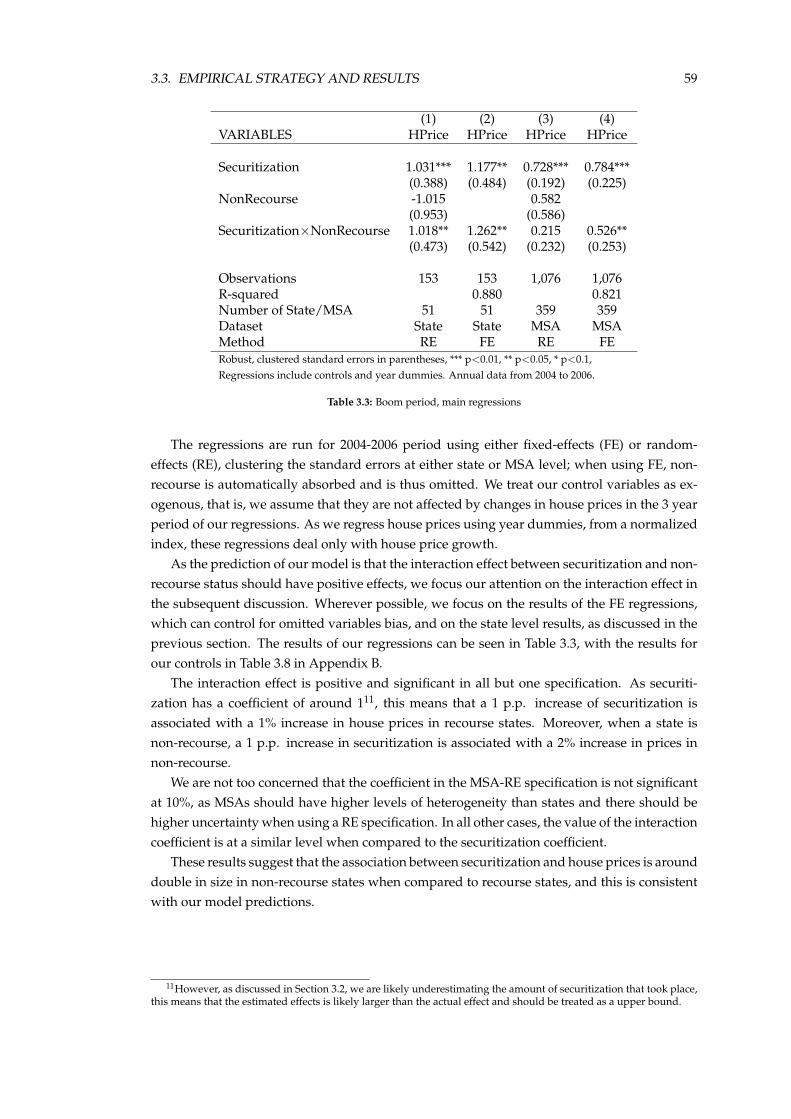
3.3. EMPIRICAL STRATEGY AND RESULTS 59
(1) (2) (3) (4)VARIABLES HPrice HPrice HPrice HPrice
Securitization 1.031*** 1.177** 0.728*** 0.784***(0.388) (0.484) (0.192) (0.225)
NonRecourse -1.015 0.582(0.953) (0.586)
Securitization×NonRecourse 1.018** 1.262** 0.215 0.526**(0.473) (0.542) (0.232) (0.253)
Observations 153 153 1,076 1,076R-squared 0.880 0.821Number of State/MSA 51 51 359 359Dataset State State MSA MSAMethod RE FE RE FERobust, clustered standard errors in parentheses, *** p<0.01, ** p<0.05, * p<0.1,Regressions include controls and year dummies. Annual data from 2004 to 2006.
Table 3.3: Boom period, main regressions
The regressions are run for 2004-2006 period using either fixed-effects (FE) or random-effects (RE), clustering the standard errors at either state or MSA level; when using FE, non-recourse is automatically absorbed and is thus omitted. We treat our control variables as ex-ogenous, that is, we assume that they are not affected by changes in house prices in the 3 yearperiod of our regressions. As we regress house prices using year dummies, from a normalizedindex, these regressions deal only with house price growth.
As the prediction of our model is that the interaction effect between securitization and non-recourse status should have positive effects, we focus our attention on the interaction effect inthe subsequent discussion. Wherever possible, we focus on the results of the FE regressions,which can control for omitted variables bias, and on the state level results, as discussed in theprevious section. The results of our regressions can be seen in Table 3.3, with the results forour controls in Table 3.8 in Appendix B.
The interaction effect is positive and significant in all but one specification. As securiti-zation has a coefficient of around 111, this means that a 1 p.p. increase of securitization isassociated with a 1% increase in house prices in recourse states. Moreover, when a state isnon-recourse, a 1 p.p. increase in securitization is associated with a 2% increase in prices innon-recourse.
We are not too concerned that the coefficient in the MSA-RE specification is not significantat 10%, as MSAs should have higher levels of heterogeneity than states and there should behigher uncertainty when using a RE specification. In all other cases, the value of the interactioncoefficient is at a similar level when compared to the securitization coefficient.
These results suggest that the association between securitization and house prices is arounddouble in size in non-recourse states when compared to recourse states, and this is consistentwith our model predictions.
11However, as discussed in Section 3.2, we are likely underestimating the amount of securitization that took place,this means that the estimated effects is likely larger than the actual effect and should be treated as a upper bound.

3.3. EMPIRICAL STRATEGY AND RESULTS 60
3.3.1.1 Robustness checks
We perform 22 baseline robustness checks (including variations on state/MSA), and eachtest is described and discussed in detail in Appendix A. We opt not to include certain controlsin our baseline regressions, such as our measure of subprime mortgages and our measure ofGSE securitized loans, due to concerns about endogeneity.
Among our robustness checks, we reinterpret our model predictions, by taking it moreliterally and assuming that there is a cut-off point at which the effects of high securitizationare felt and speculators start receiving loans. We propose and test this interpretation in twodifferent ways. We first restrict our sample to those MSAs with high level of securitizationand run the same regressions as the baseline. Alternatively, we create a dummy for MSAsabove the average value of securitization (‘Top Securitization MSA’) and use it instead ourmain measure of securitization, using the same specifications as our baseline regressions.
Some of these robustness checks are shown in Table 3.4, specifically, the results when weinclude a measure of subprime mortgages, when we exclude California, when restrict oursample to non-Western states/non-Coastal states, and when we use the ‘Top SecuritizationMSA’ dummy. Our other robustness test results are reported in Appendix B, in Tables 3.9 and3.1012.
(1) (2) (3) (4) (5)VARIABLES HPrice HPrice HPrice HPrice HPrice
Securitization 0.409 0.456 1.189 0.160(0.600) (0.598) (0.726) (0.335)
Securitization×NonRecourse 0.969* 1.264* -0.862** 1.487(0.518) (0.667) (0.403) (0.954)
Top Securitization MSA 1.655***(0.552)
Top Securitization MSA×NonRecourse 2.938**(1.172)
Observations 153 150 114 81 1,074R-squared 0.888 0.886 0.844 0.887Number of State/MSA 51 50 38 358Dataset State State State State MSAMethod FE FE FE FE REChange Subprime No Cali Non-Western Non-Coastal Top 50%Robust, clustered standard errors in parentheses, *** p<0.01, ** p<0.05, * p<0.1, Regressions include controlsand year dummies. Annual data from 2004 to 2006.
Table 3.4: Boom period, robustness checks
We interpret the results of our numerous robustness checks as showing that our baselineresults largely hold; the notable exception consists of when we regress only in non-Westernstates, which we discuss below. The interaction effect otherwise is positive and mostly signifi-cant, with a coefficient ranging from 0.36 to 3.7. This is a fairly high range, as is expected giventhat we change the range, measurement and add variables to our regressions in these tests. Thecoefficient is not significant when we extent our range to 2007, when we use the Case-Shillerindex, when we do Coastal and non-Coastal level regressions and when our measure of sub-prime loans (on a MSA, but not state level) is added. However, the coefficients we find in thesetests are compatible with our baseline regressions and it is only in these 5 of our 21 robustnesschecks (excluding the non-Western result) that the interaction term is non-significant.
The coefficient for securitization is significant in 9 of the 19 robustness checks that includeit, although always being positive and (excluding Subprime MSA-level and Non-Coastal re-gressions) with a coefficient ranging from 0.3 to 1.4, all of which suggest that this is a less
12Results for our controls are omitted for brevity’s sake.
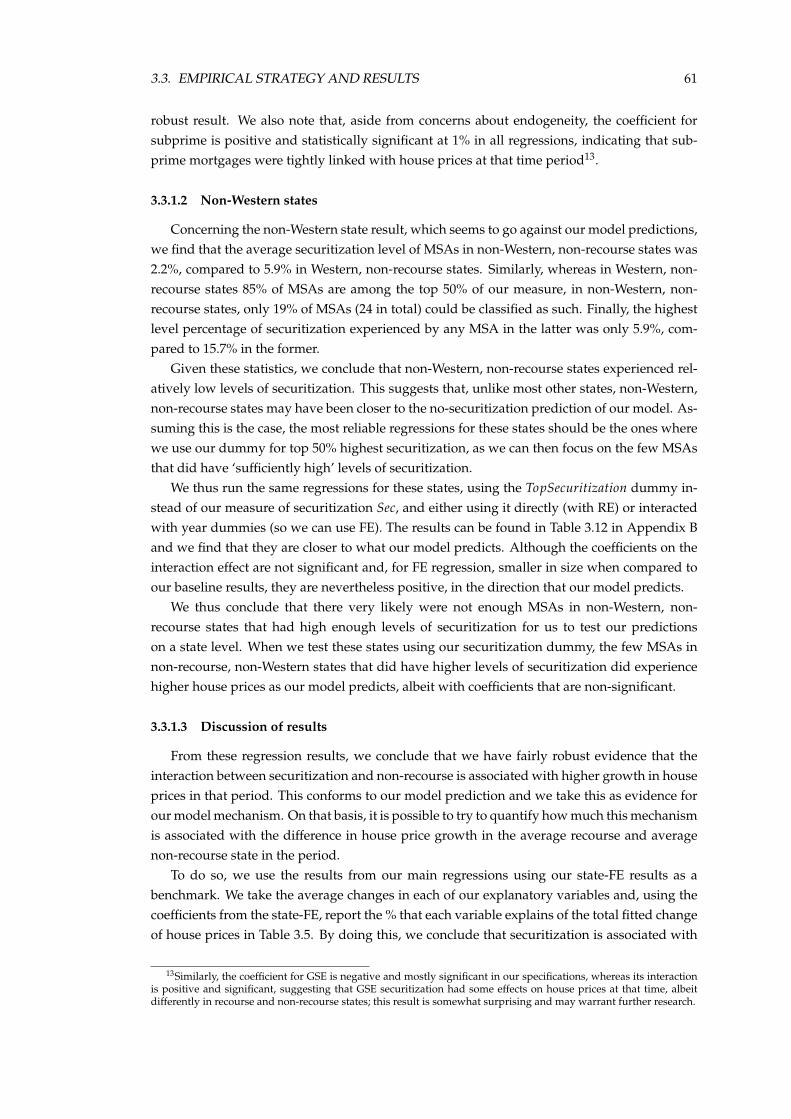
3.3. EMPIRICAL STRATEGY AND RESULTS 61
robust result. We also note that, aside from concerns about endogeneity, the coefficient forsubprime is positive and statistically significant at 1% in all regressions, indicating that sub-prime mortgages were tightly linked with house prices at that time period13.
3.3.1.2 Non-Western states
Concerning the non-Western state result, which seems to go against our model predictions,we find that the average securitization level of MSAs in non-Western, non-recourse states was2.2%, compared to 5.9% in Western, non-recourse states. Similarly, whereas in Western, non-recourse states 85% of MSAs are among the top 50% of our measure, in non-Western, non-recourse states, only 19% of MSAs (24 in total) could be classified as such. Finally, the highestlevel percentage of securitization experienced by any MSA in the latter was only 5.9%, com-pared to 15.7% in the former.
Given these statistics, we conclude that non-Western, non-recourse states experienced rel-atively low levels of securitization. This suggests that, unlike most other states, non-Western,non-recourse states may have been closer to the no-securitization prediction of our model. As-suming this is the case, the most reliable regressions for these states should be the ones wherewe use our dummy for top 50% highest securitization, as we can then focus on the few MSAsthat did have ‘sufficiently high’ levels of securitization.
We thus run the same regressions for these states, using the TopSecuritization dummy in-stead of our measure of securitization Sec, and either using it directly (with RE) or interactedwith year dummies (so we can use FE). The results can be found in Table 3.12 in Appendix Band we find that they are closer to what our model predicts. Although the coefficients on theinteraction effect are not significant and, for FE regression, smaller in size when compared toour baseline results, they are nevertheless positive, in the direction that our model predicts.
We thus conclude that there very likely were not enough MSAs in non-Western, non-recourse states that had high enough levels of securitization for us to test our predictionson a state level. When we test these states using our securitization dummy, the few MSAs innon-recourse, non-Western states that did have higher levels of securitization did experiencehigher house prices as our model predicts, albeit with coefficients that are non-significant.
3.3.1.3 Discussion of results
From these regression results, we conclude that we have fairly robust evidence that theinteraction between securitization and non-recourse is associated with higher growth in houseprices in that period. This conforms to our model prediction and we take this as evidence forour model mechanism. On that basis, it is possible to try to quantify how much this mechanismis associated with the difference in house price growth in the average recourse and averagenon-recourse state in the period.
To do so, we use the results from our main regressions using our state-FE results as abenchmark. We take the average changes in each of our explanatory variables and, using thecoefficients from the state-FE, report the % that each variable explains of the total fitted changeof house prices in Table 3.5. By doing this, we conclude that securitization is associated with
13Similarly, the coefficient for GSE is negative and mostly significant in our specifications, whereas its interactionis positive and significant, suggesting that GSE securitization had some effects on house prices at that time, albeitdifferently in recourse and non-recourse states; this result is somewhat surprising and may warrant further research.
3.3. EMPIRICAL STRATEGY AND RESULTS 62
around 31% of the increase of house prices in non-recourse states, compared to 18% in recoursestates.
Moreover, by the same method we can estimate how much the difference in growth ofhouse prices between states in that period was related to the interaction effect. Non-recoursestates experienced an increase in prices of around 21%, compared to around 16.5% for recoursestates in the period, of which around 75% is associated with our mechanism (around 3.4 p.p.increase from 2004). The rest is mainly associated with differences in the effects of popula-tion growth (25%), as securitization and income growth were largely similar for both types ofstates, and the effects of unemployment and income roughly cancel each other out.
Variable Non-Recourse RecourseSec 15% 18%SecNonRec 16% N/AInc 41% 55%Pop 18% 16%IncG -1% -1%Unemp 11% 11%At average values, shares each covariate explains fitted,
average house price growth in recourse and non-recourse
states from 2004-2006.
Table 3.5: Share of covariates in explaining average, fitted house price growth
3.3.1.4 House prices
One concern about our main empirical strategy is the possibility that non-recourse statesmay have systematically experienced bigger housing booms in the past, compared to recoursestates. Our data for house prices ranges from 1975 until 2016, and during that time, accordingto Agnello and Schuknecht (2011), the US experienced a single housing boom and a singlehousing bust, which makes it difficult to identify whether this is the case.
Observing the previously discussed Figure 3.1 finds no observable detachment prior to 00s.Figure 3.2, although consisting of lower quality data, show house price growth in recourseand non-recourse states tends to differ little except for around 3 periods, from around 1985to 1992, from around 2003 to 2011 and from around 2013 to 2016. We interpret that both thejoint-growth long-term trend and the first detachment, being the inverse of what a put-optionwould predict, as suggesting that risk-shifting mechanisms were likely not boosting houseprices prior to the 2000s, which is in accordance with our model predictions.
However, the subsequent detachment in house prices after 2012 is more concerning, andraises the question whether our interaction term is perhaps acting as a proxy for a more generaldetachment in house prices in non-recourse states starting in the 2000s. Given the observableconvergence during the bust period from 2008-2011, this is not a simple question to answer andwe believe that further investigation may be necessary for periods subsequent to the previousbust.
3.3. EMPIRICAL STRATEGY AND RESULTS 63
3.3.2 Endogeneity and IV strategy
3.3.2.1 Discussion of endogeneity
There is a critical issue of endogeneity/reverse causality for our interaction effect. Forexample, non-recourse states should be inherently more risky for lenders and owners of mort-gage loans (i.e., securitizers), when compared to recourse states, due to the lack of deficiencyjudgments. In addition, lenders and securitizers may believe that when house prices are grow-ing faster, loans are safer, as prices would have to fall more before the value of a house goesbelow the loan value. I.e., higher price growth may provide a buffer margin against defaults.If both these hypothesis hold, then higher levels of house prices would be required in non-recourse states to achieve similar levels of securitization, when compared to recourse states.
As this is what we find in the data and is an equivalent prediction when compared to ourmodel, we cannot rule out the possibility that house price growth is reverse-causing securiti-zation. If this is the case, then the standard problems with endogeneity apply and our baselineregression results may not be consistent.
In addition, the hypothesis that higher house price growth increases the buffer marginagainst defaults has other implications for endogeneity. In particular, this would lead to re-verse causality between securitization and house prices, which would also bias our results.
We opt for an instrumental variable approach to deal with these issues. As omitting anyconstituent component of an interaction term biases the estimates of the interaction itself, wechoose to focus our attention on finding an instrument for securitization. A valid instru-ment for securitization would also result in a valid instrument for our interaction term, byinteracting the instrument with non-recourse, as non-recourse can be considered exogenous.This would solve both issues with endogeneity simultaneously; having fixed-effects means weneed not worry about endogeneity from the non-recourse term directly.
3.3.2.2 Instrumental Variable strategy and results
To address the issue of endogeneity, we use what we believe is a new instrumental variablefor securitization. There is a long tradition of using geographic distance as an instrumentalvariable, one widely cited example being Hall and Jones (1999)14. Inspired by this and similarapproaches, we use distance from an MSA as a instrument, specifically the minimal distanceto the headquarters of the largest ’originate and securitize’ mortgage originators in the period.
A common element in the explanation for the housing boom and bust, such as seen inLewis (2011) among others, is that certain loan originators were ‘originate and sell’ institutions.These are institutions that specialized in creating mortgages and selling them to other entitiesso that these loans could be privately securitized, particularly subprime loans. We seek toidentify an analogous subset of such originators in our HMDA data. To do so, for 2004, 2005and 2006, we select the top 15 originators who originated the most loans destined for homepurchases and that were sold to be privately securitized. We then verify that at least 30% oftheir total loans originated were sold in such a fashion, and we select originators who satisfyboth criteria. This leaves us with a total of 18 institutions, covering 33%, 78% and 87% ofloans originated for private securitization in 2004, 2005 and 2006 respectively. We proceed toidentify 17 of these institutions via their ’RespondentID’ codes15 and investigate where their
14They use distance from the equator as an instrumental variable for social infrastructure of a country.15One, covering 1% of loans in 2005, was impossible to identify.
3.3. EMPIRICAL STRATEGY AND RESULTS 64
headquarters are located and the year they were founded.Our IV strategy assumes that if an MSA is closer to where the headquarters of these origi-
nators is located, than it is easier for the originators to participate in the housing market of thatMSA. We propose that closer MSAs make it easier for headquarters to monitor branches, thatheadquarters will more likely have greater knowledge, including legal knowledge, of closerhousing markets, headquarters will have incurred the fixed cost of complying with state reg-ulations, etc. At the same time, the validity of our instrument requires that these headquartersare not based in or near locations where house prices were expected to grow more in our pe-riod of 2004 to 2006. For this reason, we exclude 3 originators who were founded post-1996,leaving us with the originators found in Table 3.16 in Appendix B, all of which were foundedat least 8 years before our 2004, which we conjecture is enough time to satisfy the exclusionrestriction.
In addition, as some of these institutions are very large, and some are quite small, wewish to give appropriate weights reflecting their size. For this, we use the amount of loansoriginated16 in 2003 as weights. Finally, we opt to select the two closest originators, as a proxyfor the level of competition that a MSA encountered between originators. We give more weightto the distance of the larger one of the two and this results in our instrument, DistW.
We acknowledge the limitations of this instrument. Of particular concern is that our modelresults imply that no-screening takes place with securitization, which would suggest that adeeper knowledge of local markets would not matter in equilibrium, weakening our instru-ment’s power. In addition, it is possible that as loan originators have less knowledge of moredistant MSAs, this could lead to moral hazard problems and more loans being securitized thefurther away the MSA is from the headquarters, as opposed to being held. Thus, if the hetero-geneity of securitization from MSA to MSA has a larger effect than the effect of expansion ofbranches, then our instrument may have had the opposite effect on securitization. A furtherdiscussion of these issues may be found in Appendix A.
To implement our IV, we use both DistW and its interaction, DistW × NonRec, as instru-ments. The former is used to instrument Sec and the latter to instrument Sec× NonRec. Wethen proceed to estimate a similar same equation to our baseline results:
HPricei,t = β1Seci,t + β2NonReci + β3Sec× NonReci,t + D20XXt + γi,t + εi,t
We use fixed effects, using a clustered (at a MSA level), robust standard errors; as both ourinstruments are time invariant, to be able to use fixed effects on these regressions, we interactboth our instruments with year dummies17.
Before discussing our IV regression results, we first focus on the first stage results seen inTable 3.6, as they are not as expected. When instrumenting securitization, the coefficients fordistance (interacted with our year dummies) are positive, the opposite of what we would ex-pect; the F-statistic on excluded instruments is 8.28, which may be a sign of a weak instrument.When instrumenting for the interaction between securitization and non-recourse, however, thecoefficients on both distance and its interaction are negative as expected, with an F-statistic of15.71.
These results suggest that our instrument is not working as intended for all MSAs or, possi-
16Which resulted in excluding one more originator, LOAN CENTER OF CALIFORNIA, as there is no availabledata for loan origination prior to 2004; we believe it was previously exempt from reporting to the HMDA.
17Which assumes a time-differential effect of the instrument, another limitation of our approach.
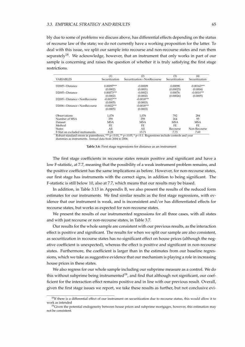
3.3. EMPIRICAL STRATEGY AND RESULTS 65
bly due to some of problems we discuss above, has differential effects depending on the statusof recourse law of the state; we do not currently have a working proposition for the latter. Todeal with this issue, we split our sample into recourse and non-recourse states and run themseparately18. We acknowledge, however, that an instrument that only works in part of oursample is concerning and raises the question of whether it is truly satisfying the first stagerestrictions.
(1) (2) (3) (4)VARIABLES Securitization Securitization×NonRecourse Securitization Securitization
D2005×Distance 0.00097*** -0.00009 0.00098 -0.00163***(0.0002) (0.0001) (0.00025) (0.0004)
D2005×Distance 0.00073*** -0.00021 0.00076 -0.0014***(0.0002) (0.0002) (0.00026) (0.0005)
D2005×Distance×NonRecourse -0.0027*** -0.0018***(0.0005) (0.0003)
D2006×Distance×NonRecourse -0.0022*** -0.0018***(0.0005) (0.0003)
Observations 1,076 1,076 792 284Number of MSA 359 359 264 95Dataset MSA MSA MSA MSAMethod FE FE FE FEStates All All Recourse Non-RecourseF-Stat on excluded instruments 8.28 15.71 7.73 7.69Robust standard errors in parentheses, *** p<0.01, ** p<0.05, * p<0.1. Regressions include controls and yeardummies as instruments. Annual data from 2004 to 2006.
Table 3.6: First stage regressions for distance as an instrument
The first stage coefficients in recourse states remain positive and significant and have alow F-statistic, at 7.7, meaning that the possibility of a weak instrument problem remains, andthe positive coefficient has the same implications as before. However, for non-recourse states,our first stage has instruments with the correct signs, in addition to being significant. TheF-statistic is still below 10, also at 7.7, which means that our results may be biased.
In addition, in Table 3.13 in Appendix B, we also present the results of the reduced formestimates for our instruments. We find similar results as the first stage regressions, with ev-idence that our instrument is weak, and is inconsistent and/or has differentiated effects forrecourse states, but works as expected for non-recourse states.
We present the results of our instrumented regressions for all three cases, with all statesand with just recourse or non-recourse states, in Table 3.7.
Our results for the whole sample are consistent with our previous results, as the interactioneffect is positive and significant. The results for when we split our sample are also consistent,as securitization in recourse states has no significant effect on house prices (although the neg-ative coefficient is unexpected), whereas the effect is positive and significant in non-recoursestates. Furthermore, the coefficient is larger than in the estimates from our baseline regres-sions, which we take as suggestive evidence that our mechanism is playing a role in increasinghouse prices in these states.
We also regress for our whole sample including our subprime measure as a control. We dothis without subprime being instrumented19, and find that although not significant, our coef-ficient for the interaction effect remains positive and in line with our previous result. Overall,given the first stage issues we report, we take these results as further, but not conclusive evi-
18If there is a differential effect of our instrument on securitization due to recourse status, this would allow it towork as intended
19Given the potential endogeneity between house prices and subprime mortgages, however, this estimation maynot be consistent.
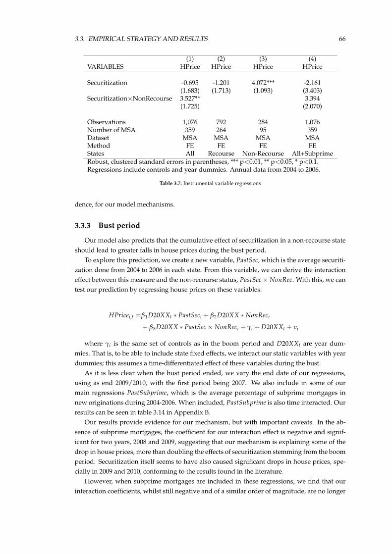
3.3. EMPIRICAL STRATEGY AND RESULTS 66
(1) (2) (3) (4)VARIABLES HPrice HPrice HPrice HPrice
Securitization -0.695 -1.201 4.072*** -2.161(1.683) (1.713) (1.093) (3.403)
Securitization×NonRecourse 3.527** 3.394(1.725) (2.070)
Observations 1,076 792 284 1,076Number of MSA 359 264 95 359Dataset MSA MSA MSA MSAMethod FE FE FE FEStates All Recourse Non-Recourse All+SubprimeRobust, clustered standard errors in parentheses, *** p<0.01, ** p<0.05, * p<0.1.Regressions include controls and year dummies. Annual data from 2004 to 2006.
Table 3.7: Instrumental variable regressions
dence, for our model mechanisms.
3.3.3 Bust period
Our model also predicts that the cumulative effect of securitization in a non-recourse stateshould lead to greater falls in house prices during the bust period.
To explore this prediction, we create a new variable, PastSec, which is the average securiti-zation done from 2004 to 2006 in each state. From this variable, we can derive the interactioneffect between this measure and the non-recourse status, PastSec× NonRec. With this, we cantest our prediction by regressing house prices on these variables:
HPricei,t =β1D20XXt ∗ PastSeci + β2D20XX ∗ NonReci
+ β3D20XX ∗ PastSec× NonReci + γi + D20XXt + υi
where γi is the same set of controls as in the boom period and D20XXt are year dum-mies. That is, to be able to include state fixed effects, we interact our static variables with yeardummies; this assumes a time-differentiated effect of these variables during the bust.
As it is less clear when the bust period ended, we vary the end date of our regressions,using as end 2009/2010, with the first period being 2007. We also include in some of ourmain regressions PastSubprime, which is the average percentage of subprime mortgages innew originations during 2004-2006. When included, PastSubprime is also time interacted. Ourresults can be seen in table 3.14 in Appendix B.
Our results provide evidence for our mechanism, but with important caveats. In the ab-sence of subprime mortgages, the coefficient for our interaction effect is negative and signif-icant for two years, 2008 and 2009, suggesting that our mechanism is explaining some of thedrop in house prices, more than doubling the effects of securitization stemming from the boomperiod. Securitization itself seems to have also caused significant drops in house prices, spe-cially in 2009 and 2010, conforming to the results found in the literature.
However, when subprime mortgages are included in these regressions, we find that ourinteraction coefficients, whilst still negative and of a similar order of magnitude, are no longer
3.3. EMPIRICAL STRATEGY AND RESULTS 67
statistically significant. Given the importance the literature has found for subprime mortgagesin explaining the housing market in the period, we feel that the results from the specificationthat includes our measure of subprime mortgages should receive significant weight.
Securitization still has significant and negative coefficients, as expected, and we find thatsubprime mortgages, although not reported here, also adversely affected house prices in theperiod, with negative and statistically significant coefficients 20.
Unlike our boom period regressions, as both PastSec and PastSubprime are measured priorto when we run our regressions, it less likely that there will be reverse causality with respectto house prices. Endogeneity issues may still exist if securitization was higher in states wherehouse prices were expected to grow the most during 2004-2006 and these states experiencedthe biggest falls in prices afterwards. As a simple test of this, we calculate the correlationbetween house price growth in states from 2004-2006 with 2007-2009. We find a correlation of-0.56 which we interpret as being sufficiently high for this to remain a concern, meaning thatour bust period results should be treated with a degree of caution.
As such, we find further, albeit weaker evidence for our mechanism’s effects on houseprices during the bust period, and evidence that securitization and subprime mortgages cre-ated in the boom period played an important role in determining house prices during thebust.
3.3.3.1 Defaults
Our model also predicts that defaults are increased in a bust when there are higher levelsof securitization in non-recourse states during a boom.
For defaults, we use MDe f ault, the percent of mortgage debt balance that is 90+ daysdelinquent in each state, for all mortgages. This may be a too broad measure of defaults,however, as our model focuses on defaults of home-purchase mortgages created during theboom. As before, we use the start date of 2007 and use as end dates of 2009/2010. We thenregress defaults on past securitization and its interaction effect:
MDe f aulti,t = β1D20XX ∗ PastSeci + β2D20XX ∗ Past× SecNonReci
+ γi + D20XXt + πi,t
As before, we interact our static variables with year dummies to allow for fixed effects. Ourresults are found in table 3.15 in Appendix B.
In none of our regressions are the coefficients of our interaction significant, nor are theyconsistently positive, from which we conclude that there is little evidence that our mechanismled to increased defaults during the bust, albeit given the limitation of using a broad measureof defaults. We do find evidence that securitization from the boom period increased defaultsin the bust period, a result that is robust, as the literature has previously found. Similarly,subprime mortgages from the boom period, the results of which we do not report here, alsoled to increased defaults during the subsequent bust.
20For every extra 1% of (average) mortgages that were subprime in a given state during the boom period, therewas a corresponding fall in house prices of around 0.5% for every year from 2008-2010, in 2004 prices.
3.4. CONCLUSION 68
3.4 Conclusion
This chapter seeks to add to the empirical literature exploring the causes behind the boomand bust in house prices observed in the US during the 2000s. In the previous chapter, webuild a model that explores the effects on the housing market, particularly on house prices,that securitization and non-recourse loans might have. Our model predicts that the interac-tion between these two factors should lead to increased house prices during a demand boom,compared to markets absent at least one of the two factors.
We find some empirical evidence for this prediction. We regress house prices, on an MSAand state level from 2004 to 2006, on securitization and its interaction with non-recourse statusof states. We find that the positive effect of securitization on house prices in the US was nearlydouble in non-recourse states, compared to recourse states. This effect is such that for every1 p.p. of securitized mortgage loans is associated with an increase in house prices by 1% inrecourse states, and 2% in non-recourse states. The mechanism can potentially explain around75% of the differences in growth of house prices between recourse and non-recourse statesfrom 2004-2006.
To control for potential endogeneity issues between house prices and securitization, we useas an IV the weighted distance between an MSA and the two closest headquarters of ‘originateand securitize’ mortgage institutions. Our results largely hold when doing so, particularly fornon-recourse states, but note that the first stage F-statistic low and our first stage coefficientsmay be inconsistent or possibly have differentiated effects for recourse states. As such, wetake this as more evidence, but not conclusive evidence, that this mechanism influenced houseprices at the time.
Our model also makes predictions for the bust period, although, due to the static natureof the bust period, is less suited for doing so. It predicts that the interaction effect betweensecuritization and non-recourse status from the boom period should lead to greater falls inhouse prices and more defaults during a subsequent bust. We find weak evidence for ourhouse price predictions during the bust period, and no evidence that our mechanism affecteddefaults during the bust.
Finally, we also find evidence that higher levels of securitization during the boom led toincreased house prices during the boom itself, and lead to greater falls in house prices andincreased defaults during the subsequent bust, as is consistent with what the literature haspreviously found.
We conclude by noting that there is currently an ongoing debate about whether mortgageoriginators should be forced to have a ’skin in the game’, that is, to hold on to at least somepercentage of any loan they originate. Given the results discussed above, we believe that itwould be wise to make these rules binding, particularly in jurisdictions where mortgage loansare non-recourse, or, as an alternative, proportional to the loan-to-value ratio of a mortgage.
Although securitization levels have currently fallen, it or similar financial innovationswhich allow mortgage originators to sell their loans could easily reappear in the near future.In that sense, the relatively recent changes21 by US regulators that relaxed the Dodd-Franklaws may have been counterproductive. The law originally required originators to have asubstantial ’skin in the game’ and these changes have instead exempted the vast majority ofmortgages in the US from such requirements.
21As reported in ”Banks Again Avoid Having Any Skin in the Game ”, New York Times, 23rd of October, 2014.
3.4. CONCLUSION 69
Taking note that our model results and, to a lesser extent, our empirical results are indepen-dent of the existence of subprime mortgages, these changes might be re-laying the foundationsfor future problems, even if subprime mortgages are more tightly controlled and regulated, oreven non-existent22.
22Similar concerns may also lie with Brazil, due to the relatively new innovation of similarly non-recourse ‘alien-acao fiduciaria’ mortgages.
Appendices to the Chapter
3.A Appendix A - Empirics discussion
3.A.1 Loan-to-value ratio
As we discuss in the Appendix to the previous chapter, house price growth may dependon the down payment set on mortgages; higher down-payments would lead to lower houseprices, assuming speculators take on loans, which our model would never predict happens.Thus, as a precaution, we would wish to include the LTV as an explanatory variable in our re-gressions as a robustness check, although there would also be concerns about reverse-causalityand endogeneity if we had such a measure (for much the same reasons as there are for securiti-zation and subprime loans). At this point, we do not have data that would allow us to includea measure of the average LTV for states or MSAs in the time period in which we do our re-gressions. As a consequence, we acknowledge that our regressions may suffer from omittedvariable bias.
3.A.2 Subprime variable
To obtain our measure of subprime mortgages, we follow the methodology of Mayer andPence (2008). They find that classifying loans with interest rate spread above 3% in the HMDAdataset provides a measure of subprime that is largely similar to alternative measures, suchas using the HUD classification. Our main measure of subprime thus consists of the percent-age of all loans destined for house purchases successfully originated which have that interestrate spread, to differentiate it from those originated from subprime specialists, which mayotherwise lead to issues with our IV strategy.
3.A.3 Robustness checks
All robustness checks use the same basic regression structure as our main regressions, butvary in the following ways: the start (2005) and end (2007) dates of our regressions are changed(state only); we use an alternate measure (Case-Shiller) of house prices (MSA only); we use analternate definition (NonRecKM) of recourse (state only); we include a measure of the per-centage of subprime loans (Subprime) originated for house purchases (both state and MSA);we include a measure of state (Int) interest rates on mortgage loans (state only); we omitCalifornia from our sample (both state and MSA); we run our regressions only in coastal ornon-coastal states (state only); we run our regressions only in Western or non-Western states(state only); we extend the range of our regressions to start from 1991 until 2004, for whichwe assume, incorrectly, that securitization is zero prior 2004 (state only); we restrict our sam-ple to the MSAs that were in the top 50% of MSAs with highest percentage of securitization(MSA only); instead of Sec and Sec × NonRec, we use a dummy for the MSAs with the top50% highest percentages of securitization, also including the related interaction effect withnon-recourse (TopSecand TopSec× NonRec), both interacted with year dummies (MSA only);we include our measure of securitization done by government sponsored agencies GSE andrun with and without its interaction with non-recourse GSENonRec (state only); we include
70
3.A. APPENDIX A - EMPIRICS DISCUSSION 71
a measure of the loan-to-income ratio LTI (state only); and we use all our additional controls,GSE and interaction, subprime, interest rates and loan-to-income All (state only).
We include these for a number of reasons. State interest rates are used as a proxy forfinancing conditions, but omitted in the main regressions due to concerns about endogeneity.Similarly, including subprime loans is due to concerns that our measure of securitization maybe just capturing the effects of subprime loans instead of securitization, with similar concernsabout endogeneity. As California is a non-recourse state that experienced particularly highincreases in house prices and high levels of securitization, omitting it serves to verify thatwe are not just capturing the effects of that state. Similarly, by using just coastal or Westernstates, we try to guarantee that we are not just capturing the effects of securitization in coastalvs inland or Western vs non-Western states. As GSE were responsible for a large amount ofsecuritization at the period, we aim to make sure that we are not capturing their effects withprivate securitization with and without the interaction with non-recourse status.
3.A.3.1 IV discussion
One way to test the validity of our instrument is to compare the percentage of securitizationdone in each city by each originator. If we have correctly identified our set of originators as‘originate and securitize’ types, then the variation of securitization done in each city shouldchange little. To test for this, for every year and for every originator, we calculate the averagesecuritization level done for each city. We then calculate the standard deviation of each subsetfor each originator in each year, finding that the average standard deviations for each year areas follows: in 2004, 15.8%; in 2005, 15.5% and in 2006, 21.3%, relatively high numbers.
Furthermore, the evidence for each originator is mixed, and it seems that some, but notall of our originators are satisfying our criteria. Both ‘LOAN CENTER OF CALIFORNIA’ and‘CHAPEL MORTGAGE’ originators have low standard deviation of these frequencies, at lessthan 1%, and ‘COUNTRYWIDE HOME LOANS’, ‘AEGIS MORTGAGE’ and ‘FREMONT IN-VESTMENT & LOAN’ have persistently low standard deviations, at less than 15%. On theother hand, ‘EAGLE HOME MORTGAGE’, ‘DELTA FUNDING’ and ‘FIRST RESIDENTIALMORTGAGE’ all have standard deviations of above 30% in at least one year, suggesting thatthey may not be satisfying our criteria. These results suggest that further refinement of origi-nators being used as instruments may be required, and it not yet clear whether the issues weraise in the main text are being dealt with appropriately.
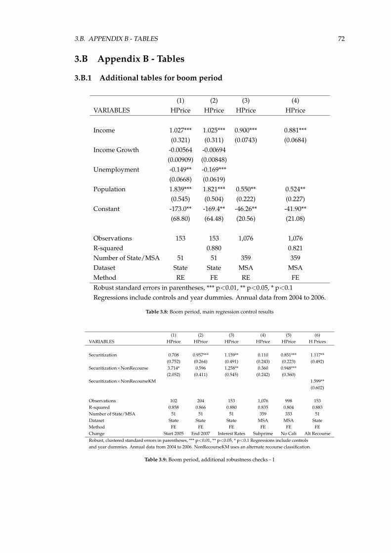
3.B. APPENDIX B - TABLES 72
3.B Appendix B - Tables
3.B.1 Additional tables for boom period
(1) (2) (3) (4)VARIABLES HPrice HPrice HPrice HPrice
Income 1.027*** 1.025*** 0.900*** 0.881***(0.321) (0.311) (0.0743) (0.0684)
Income Growth -0.00564 -0.00694(0.00909) (0.00848)
Unemployment -0.149** -0.169***(0.0668) (0.0619)
Population 1.839*** 1.821*** 0.550** 0.524**(0.545) (0.504) (0.222) (0.227)
Constant -173.0** -169.4** -46.26** -41.90**(68.80) (64.48) (20.56) (21.08)
Observations 153 153 1,076 1,076R-squared 0.880 0.821Number of State/MSA 51 51 359 359Dataset State State MSA MSAMethod RE FE RE FE
Robust standard errors in parentheses, *** p<0.01, ** p<0.05, * p<0.1Regressions include controls and year dummies. Annual data from 2004 to 2006.
Table 3.8: Boom period, main regression control results
(1) (2) (3) (4) (5) (6)VARIABLES HPrice HPrice HPrice HPrice HPrice H Prices
Securitization 0.708 0.957*** 1.159** 0.110 0.851*** 1.117**(0.752) (0.264) (0.491) (0.243) (0.223) (0.492)
Securitization×NonRecourse 3.714* 0.596 1.258** 0.360 0.948***(2.052) (0.411) (0.545) (0.242) (0.360)
Securitization×NonRecourseKM 1.599**(0.602)
Observations 102 204 153 1,076 998 153R-squared 0.858 0.866 0.880 0.835 0.804 0.883Number of State/MSA 51 51 51 359 333 51Dataset State State State MSA MSA StateMethod FE FE FE FE FE FEChange Start 2005 End 2007 Interest Rates Subprime No Cali Alt RecourseRobust, clustered standard errors in parentheses, *** p<0.01, ** p<0.05, * p<0.1 Regressions include controlsand year dummies. Annual data from 2004 to 2006. NonRecourseKM uses an alternate recourse classification.
Table 3.9: Boom period, additional robustness checks - 1
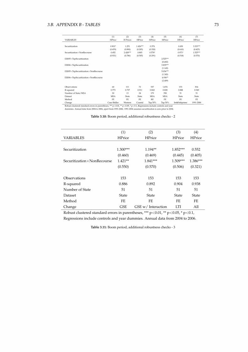
3.B. APPENDIX B - TABLES 73
(1) (2) (3) (4) (5) (6) (7)VARIABLES HPrice H Prices HPrice HPrice HPrice HPrice HPrice
Securitization 0.901* 1.251 1.426*** 0.374 0.430 3.333***(0.470) (0.890) (0.205) (0.320) (0.610) (0.425)
Securitization×NonRecourse 0.452 2.428*** 0.803 0.574* 0.971* 1.525***(0.921) (0.786) (0.505) (0.291) (0.518) (0.570)
D2005×TopSecuritization 2.525***(0.682)
D2006×TopSecuritization 3.835***(1.145)
D2005×TopSecuritization×NonRecourse 5.036***(1.345)
D2006×TopSecuritization×NonRecourse 4.936**(2.409)
Observations 60 111 72 537 1,074 153 816R-squared 0.773 0.737 0.911 0.843 0.828 0.888 0.949Number of State/MSA 20 13 24 179 358 51 51Dataset MSA State State MSA MSA State StateMethod FE FE FE RE FE FE FEChange Case-Shiller Western Coastal Top 50% Top 50% Int&Subprime 1991-2006
Robust clustered standard errors in parentheses, *** p<0.01, ** p<0.05, * p<0.1, Regressions include controls and yeardummies. Annual data from 2004 to 2006, apart from 1991-2006. 1991-2006 assumes securitization is zero prior to 2004.
Table 3.10: Boom period, additional robustness checks - 2
(1) (2) (3) (4)VARIABLES HPrice HPrice HPrice HPrice
Securitization 1.300*** 1.194** 1.852*** 0.552(0.460) (0.469) (0.445) (0.405)
Securitization×NonRecourse 1.421** 1.841*** 1.509*** 1.386***(0.550) (0.570) (0.506) (0.321)
Observations 153 153 153 153R-squared 0.886 0.892 0.904 0.938Number of State 51 51 51 51Dataset State State State StateMethod FE FE FE FEChange GSE GSE w/ Interaction LTI All
Robust clustered standard errors in parentheses, *** p<0.01, ** p<0.05, * p<0.1,Regressions include controls and year dummies. Annual data from 2004 to 2006.
Table 3.11: Boom period, additional robustness checks - 3

3.B. APPENDIX B - TABLES 74
(1) (2)VARIABLES HPrice HPrice
TopSecuritization 2.341***(0.569)
TopSecuritization×NonRecourse 0.870(3.123)
D2005×TopSecuritization 3.045***(0.713)
D2006×TopSecuritization 4.753***(1.192)
D2005×TopSecuritization×NonRecourse 0.694(3.560)
D2006×TopSecuritization×NonRecourse 0.791(5.707)
Observations 837 837R-squared 0.784Number of MSA 279 279Dataset MSA MSAMethod RE FERobust standard errors in parentheses, *** p<0.01, ** p<0.05, * p<0.1Regressions include controls and year dummies. Annual data from 2004-2006
Table 3.12: Non-Western states, robustness checks
3.B.2 Additional tables for instrumental variable regressions
(1) (2) (3)VARIABLES HPrice HPrice HPrice
D2005×Distance -0.0006 -0.0008 -0.0055**(0.0012) (0.0011) (0.0022)
D2005×Distance -0.0017 -0.00199 -0.0076**(0.0021) (0.0020) (0.0034)
D2005×Distance×NonRecourse -0.0042*(0.0024)
D2006×Distance×NonRecourse -0.0046( 0.0038)
Observations 1,077 792 285Number of MSA 359 264 95Dataset MSA MSA MSAMethod FE FE FEStates All Recourse Non-Recourse
Robust, clustered standard errors in parentheses, *** p<0.01, ** p<0.05,* p<0.1. Regressions include controls and year dummies as instruments.Annual data from 2004 to 2006.
Table 3.13: Reduced form regressions for instrument
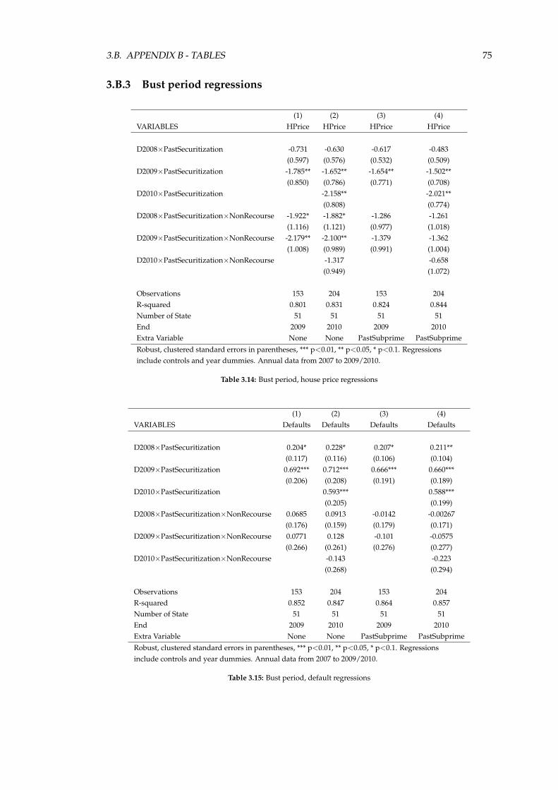
3.B. APPENDIX B - TABLES 75
3.B.3 Bust period regressions
(1) (2) (3) (4)VARIABLES HPrice HPrice HPrice HPrice
D2008×PastSecuritization -0.731 -0.630 -0.617 -0.483(0.597) (0.576) (0.532) (0.509)
D2009×PastSecuritization -1.785** -1.652** -1.654** -1.502**(0.850) (0.786) (0.771) (0.708)
D2010×PastSecuritization -2.158** -2.021**(0.808) (0.774)
D2008×PastSecuritization×NonRecourse -1.922* -1.882* -1.286 -1.261(1.116) (1.121) (0.977) (1.018)
D2009×PastSecuritization×NonRecourse -2.179** -2.100** -1.379 -1.362(1.008) (0.989) (0.991) (1.004)
D2010×PastSecuritization×NonRecourse -1.317 -0.658(0.949) (1.072)
Observations 153 204 153 204R-squared 0.801 0.831 0.824 0.844Number of State 51 51 51 51End 2009 2010 2009 2010Extra Variable None None PastSubprime PastSubprime
Robust, clustered standard errors in parentheses, *** p<0.01, ** p<0.05, * p<0.1. Regressionsinclude controls and year dummies. Annual data from 2007 to 2009/2010.
Table 3.14: Bust period, house price regressions
(1) (2) (3) (4)VARIABLES Defaults Defaults Defaults Defaults
D2008×PastSecuritization 0.204* 0.228* 0.207* 0.211**(0.117) (0.116) (0.106) (0.104)
D2009×PastSecuritization 0.692*** 0.712*** 0.666*** 0.660***(0.206) (0.208) (0.191) (0.189)
D2010×PastSecuritization 0.593*** 0.588***(0.205) (0.199)
D2008×PastSecuritization×NonRecourse 0.0685 0.0913 -0.0142 -0.00267(0.176) (0.159) (0.179) (0.171)
D2009×PastSecuritization×NonRecourse 0.0771 0.128 -0.101 -0.0575(0.266) (0.261) (0.276) (0.277)
D2010×PastSecuritization×NonRecourse -0.143 -0.223(0.268) (0.294)
Observations 153 204 153 204R-squared 0.852 0.847 0.864 0.857Number of State 51 51 51 51End 2009 2010 2009 2010Extra Variable None None PastSubprime PastSubprime
Robust, clustered standard errors in parentheses, *** p<0.01, ** p<0.05, * p<0.1. Regressionsinclude controls and year dummies. Annual data from 2007 to 2009/2010.
Table 3.15: Bust period, default regressions
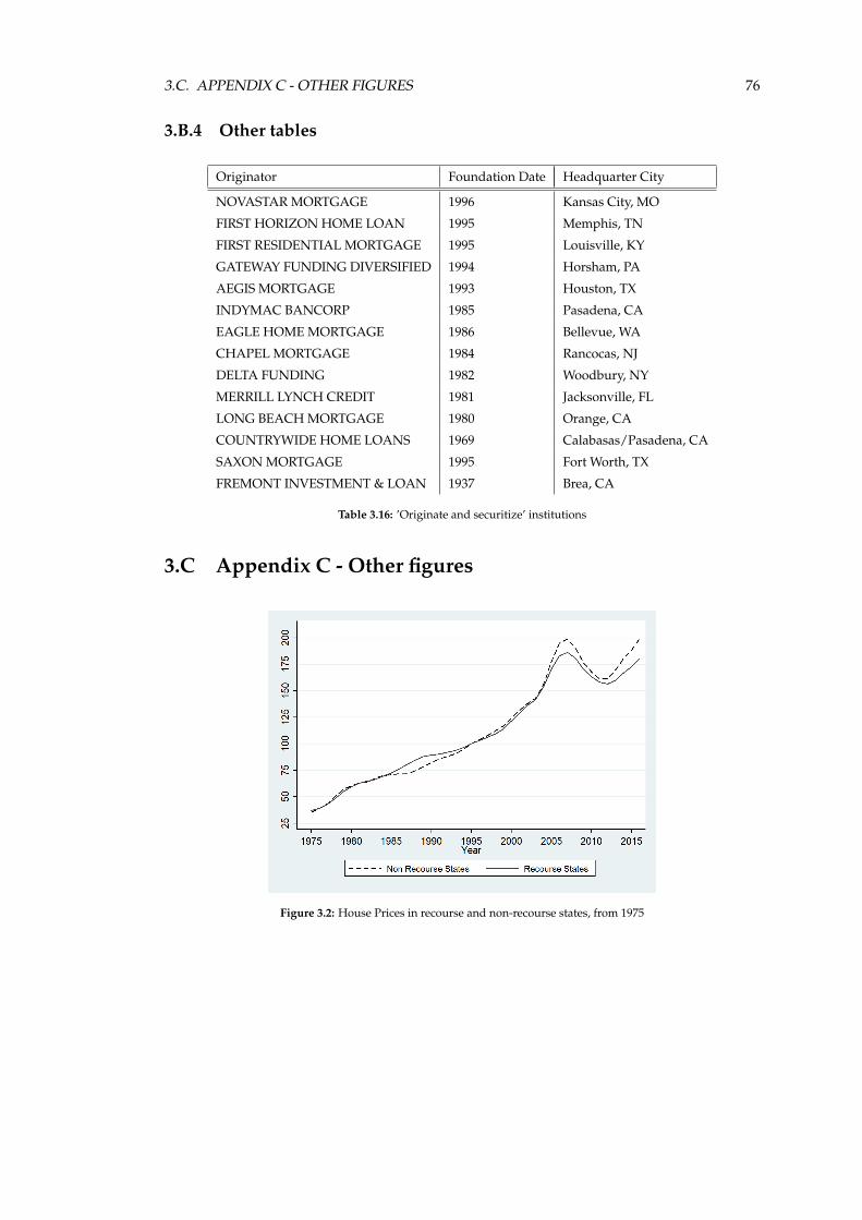
3.C. APPENDIX C - OTHER FIGURES 76
3.B.4 Other tables
Originator Foundation Date Headquarter City
NOVASTAR MORTGAGE 1996 Kansas City, MO
FIRST HORIZON HOME LOAN 1995 Memphis, TN
FIRST RESIDENTIAL MORTGAGE 1995 Louisville, KY
GATEWAY FUNDING DIVERSIFIED 1994 Horsham, PA
AEGIS MORTGAGE 1993 Houston, TX
INDYMAC BANCORP 1985 Pasadena, CA
EAGLE HOME MORTGAGE 1986 Bellevue, WA
CHAPEL MORTGAGE 1984 Rancocas, NJ
DELTA FUNDING 1982 Woodbury, NY
MERRILL LYNCH CREDIT 1981 Jacksonville, FL
LONG BEACH MORTGAGE 1980 Orange, CA
COUNTRYWIDE HOME LOANS 1969 Calabasas/Pasadena, CA
SAXON MORTGAGE 1995 Fort Worth, TX
FREMONT INVESTMENT & LOAN 1937 Brea, CA
Table 3.16: ’Originate and securitize’ institutions
3.C Appendix C - Other figures
Figure 3.2: House Prices in recourse and non-recourse states, from 1975
Chapter 4
Dynamics of Regulation ofStrategically Complex FinancialProducts ∗
Abstract
Banks can use complexity to make new financial products costly to screen by regulators.Bad financial products created by banks can lead to moral hazard issues, as banks are bailedout in case of negative shocks. Thus, regulators should incentivise banks so that they do not’abuse’ complexity by making new bad products complex. We find the optimal regulationregime in a framework without transfers and where regulators can make binding commit-ments, with low discount factors. Initially, regulators do not screen and banks do not makeuse of complexity. Once a bank has received enough positive shocks, in the form of good fi-nancial products, regulators then stop screening and allow banks to make use of bad, complexproducts as a reward for their previous actions. We discuss why this mechanism may not holdwhen regulators cannot commit, and discuss the implications of a lack of commitment.
JEL Classification Numbers: C73, D86, E44, E61, G20.Keywords: Financial Complexity, Financial Regulation, Optimal Contracts.
4.1 Introduction
As was seen in the recent financial crisis and in prior crises, banks and other financial insti-tutions are likely to be bailed out in situations where depositors could lose their savings, whenintra-banking capital flows are at risk of stopping or when ‘systemic’ institutions may collapse.This creates a moral hazard problem between bankers/banks and regulators/governments, asbanks and bankers have incentives to take risky bets that result in a large payoff to themselvesshould they work, but upon failure, impose large costs on regulators due to bailouts, with littlecost to the banks.
To avoid such costly consequences, financial regulators should want to prevent banks fromtaking such risks, in particular, from issuing, holding and/or buying risky financial products.
∗Joint work with Michel Azulai. Author Affiliation: London School of Economics. e-mail: [email protected]..
77
4.1. INTRODUCTION 78
As these regulations stop banks from enjoying the moral hazard rents arising from limitedliability and bailouts, banks might want to avoid the oversight of financial regulatory agencies.Given these incentives, how should regulatory agencies design their monitoring proceduresover time, taking into account that banks are trying to dodge oversight?
In this paper, we consider the problem of optimal dynamic regulation of a bank, largeenough to affect risk at a systemic level, which might try to avoid financial regulation by mak-ing its financial products complex to avoid regulatory oversight. In our model, each periodof time starts with banks devising an idea for a new financial product. This new idea couldbe thought of as a new form of aggregating and distributing risk, such as a new securitiza-tion method, or a new way of making payoffs contingent on certain outcomes, such as a newderivative. In the model and from the perspective of regulators, a new product idea will eitherbe a good idea involving no risk, or a bad idea, akin to a risky bet with the potential to result ina bailout and/or large social welfare losses. For simplicity, we assume that banks will hold onto new products they create, thus exposing themselves directly to the product risk; we discussthe implications of having more banks below.
Once banks have developed their new financial product, they know what quality and com-plexity the product has; for simplicity, we assume all good products are inherently complexand all bad products are inherently simple. In practice, this inherent complexity might be aconsequence of the number of states/outcomes on which a risky derivative’s outcome is condi-tional, or, as another example, as the consequence of having a securitization process be appliedmultiple times to a group of assets1, such as with a CDO squared. Crucially, added complexitybrings about costs to regulatory oversight, and can be manipulated by banks, which can turnsimple assets into complex assets - for instance, by securitizing a group of highly correlatedassets, increasing complexity without significantly reducing risk.
These assumptions seem to be realistic features of the problem that financial regulatorsface. Firstly, regulatory authorities make frequent mention in official documents of how re-sources must be used wisely and how costly it is to monitor banks. The Office of the Comptrollerof the Currency (OCC), concerning the frequency of on site examinations of banks2, states that’Before increasing the frequency of examinations, supervisory offices should consider howOCC resources can be used most efficiently(...)’3. Eisenbach, et al. (2015), a report by the NewYork Federal Reserve describing the regulatory activity of the Federal Reserve, stresses that,in the context of supervisory activities, ‘Resources are often constrained in the sense that thereis often more work that could be done than there is time or staff to do it.’ Finally, there is anempirical literature dealing the costs regulators face when regulating banks, such as Hirtle andLopez (1999) or Eisenbach, Lucca and Townsend (2016), which also takes the costs regulatorsface as substantial.
Secondly, banks seem to be able to manipulate the complexity of their financial productsand at least anecdotal evidence of such behaviour exists. For example, a former trader at Sa-lomon Brothers, when discussing the bank in the 80s, claimed that ‘Many “new products”
1It seem plausible that many good assets are inherently complex, both in principle and in practice. For example,securitizing a sufficiently large number of uncorrelated mortgages can create high quality tranches that are of very lowrisk, but understanding how uncorrelated these mortgages are requires a great deal of time and effort, particularlywhen the loans backing them may in the thousands.
2Bank Supervision Process - Comptrollers Handbook3Similarly, the Prudential Regulatory Authority (PRA), concerning the amount of information that banks should
send when requested, states that ‘It is essential, however, that supervisors are not overwhelmed by the amount ofinformation that they have to analyze.’, in Section 188, The Prudential Regulation Authority’s approach to bankingsupervision March 2016.
4.1. INTRODUCTION 79
invented by Salomon Brothers were outside the rules of the regulatory game (...). To attractnew investors and to dodge new regulations, the market became ever more arcane and com-plex.’4. There is also the evidence from the related literature which deals with complexity inretail financial markets, wherein complexity may be used to mislead or defraud consumers,by making it hard for them to fully comprehend the nature (i.e., risks and potential payoffs)of the product they might be purchasing, resulting in product mispricing; see for exampleAgnew and Szykman (2005), Carlin (2009) or Celerier and Vallee (2013). Thus, evidence thatbanks might deliberately structure products to be complex, with the intent of misleading otheragents and/or bending/breaking the rules, exists.
We study this set-up when the bank and the regulator interact over time repeatedly, andthe regulator can design dynamic regulatory procedures to provide incentives for banks tonot hide bad assets by making them complex. In doing so, however, the regulator faces lim-itations in designing its optimal regulation. The key assumption we make is that it cannotdesign mechanisms with fines and bonuses for banks as rewards for keeping their bad finan-cial products simple. The reason for this assumption is that such a mechanism would requirepunishments, such as a fine, to take place when banks have been caught out creating bad andcomplex financial products.
Banks are likely to be caught out, however, when there is a crisis happening, meaning that,instead of fines, regulators will be forced into bailouts. Given the need for these bailouts andtheir size, regulators would then need to provide large bonuses/transfers to banks duringgood times to create an effective incentive system, which would be politically dubious giventhe high payments that would be required5.
Our paper proceeds to firstly find the optimal mechanism for regulators when they canmake binding commitments. We find that in such cases, the resulting mechanism will be suchthat banks either choose full complexity or no complexity at any moment of time. Regulatorsbegin by promising and delivering relatively low payoff values to banks, these values beingthe sole state variable in our model, close to the Nash Equilibrium values. During this ini-tial period, banks will choose to not use complexity and regulators will not screen products,despite the latter creating incentives for banks to deviate.
This outcome is made possible by the fact that regulators promise to punish the banks ifthey opt to make use of complexity, and by not deviating, banks will receive positive shocks,mainly in the form of bad products, that lead to higher promised continuation values. Even-tually, both bad products and good products deliver the same, positive continuation values,and these higher continuation values are delivered to the banks via a ‘reward’ phase for banks,wherein regulators stop screening altogether and banks are free to use bad, complex productswith no punishment. As such, this results in a path for bank payoffs resembling a randomwalk with a positive drift, followed by a set increase every period until the ‘reward’ phase ismet and payoffs become completely static.
However, it is likely that regulators cannot make such binding commitments. In particular,we conjecture and discuss that the regulator cannot commit to not screening when it is in the‘reward’ phase of this mechanism, as once we relax the commitment constraint, we surmisethat a completely lax screening regime and absence of punishment for using bad, complexproducts would be infeasible, as regulators would want to deviate towards screening at this
4Lewis (1989)5A further discussion on the question of fines and punishment may be found in Section 4.5.
4.2. MODEL 80
point. So, in the absence of commitment, this would require regulators to have more a moder-ate ‘reward’ phase instead. Thus, we conjecture, but do not prove, that the optimal dynamicregulatory mechanism without commitment is similar to the above, but with more moderate‘punishment’ and ‘reward’ phases, with neither regulators, nor banks choosing extremum val-ues for screening and complexity6. We also argue that similar results happen when regulatorsare sufficiently more patient than banks. Our results thus highlight the constraints placed onfinancial regulators, and how difficult it is to eliminate financial crises.
Our paper is related to the literature on optimal banking regulation in the context of moralhazard, such as in Prescott (2004) and Blum (2008), although these and other papers mainlyfocus on questions related to bank capital, and also to the larger, mainly empirical literature onbanking regulations, such as Barth, Caprio and Levine (2004). It is also related to the literatureon optimal bank opacity, such as Dang, Gorton, Holmstrm, and Ordonez (2014), which positsthat banks use opacity in their balance sheet loans to avoid issues from information external-ities from investment projects and liquidity concerns. Our approach in finding the optimalregulatory mechanism stems from the literature on dynamic games with one-sided privateinformation, such as in Abreu, Pearce and Stacchetti (1990), and Li, Matouschek and Powell(2015). To the best of our knowledge, this is the first time this approach is taken in the bankregulation literature.
This paper is organized as follows. In Section 4.2 we state the model set-up and equilibriumconcepts, as well as finding a benchmark, static result. In Section 4.3 we set up the regulator’soptimal contract problem and discuss and delineate some useful results. In Section 4.4 weexecute the optimization program via a Lagrangian, find the optimal regulation contract forwhen the regulator can make binding commitments and then discuss the optimal solution weshould find when the regulator cannot make such commitments. In Section 4.5 we discusssome possible model extensions and in Section 4.6 we conclude.
4.2 Model
4.2.1 Basic set-up
In the beginning of each period t = 1, 2, ..., a bank creates a single, new financial product.This product can be either one of two types: good products (G) or bad products (B). Bankswill hold-on to the products they create, and good products will pay pt = M with probability1 to banks that create them, with a guaranteed payoff rt normalized to zero to regulators. Badfinancial products, on the other hand, suffer idiosyncratic shocks at the end of a period. Withprobability θ, they produce an identical positive outcome of pt = M and rt = 0 to banks andregulators. But with probability 1− θ, the product suffers a negative shock, and banks, dueto their systemic nature, are bailed out by regulators. Consequently, banks receive pt = 0 andregulators have a payoff of rt = −R. Regulators will thus wish to impede banks from using B.
How are financial products created? As with the literature in innovation and technologi-cal growth, here innovation is modeled in a reduced form and we abstract from using moredetailed mechanisms. In the beginning of a period, a bank will receive a financial productexogenously, that will be a good product with probability µ and be a bad one with probability
6We surmise that this form of provision of incentives is likely to create cycles of complex bad financial products,and analogous cycles of strong/weak regulatory oversight of these products.
4.2. MODEL 81
1− µ. For tractability, we assume the draw of quality of the financial product to be iid overtime and that all products can only be used once by banks7.
Once these financial products are created, banks may decide to make bad products ‘com-plex’ or ‘simple’. We assume that all new good products are complex8 for tractability, and thatall new bad products are initially simple, or can be made complex at a cost D. Simple prod-ucts are easily inspected and understood by regulators, and they can distinguish a simple badproduct from a good one costlessly. Complex products are costly for regulators to inspect andwe model this by assuming regulators must pay a cost C if they wish to tell whether a newcomplex product is bad or good.
In the context of mortgage backed securities, the process of securitization can used to bun-dle together a small set of mortgages with similar characteristics and clear diversification, thuscreating a simple product, or, by using various different methods9, bundle them together inways that the regulator might only understand after considerable effort analyzing the prod-uct (a complex product). In practice, the timing of when this analysis/screening happens willdepend on how large a product is, relative to a bank’s balance sheet, and how quickly it isgrowing. In our model and for simplicity, we assume that a new complex product can bescreened within the same period of time as it is created. We can justify this by assuming thatthe product at this point will have grown enough to be a worry, but is still small enough thatif prohibited, it will not result in significant payoffs to the bank or the regulator.
Note that we allow regulators to veto products from being used only if they have beenscreened. This can be rationalized as a requirement that regulators must clearly justify theirveto to a bank, otherwise such vetoes might be contested in the courts of law. It may alsoserve as a reduced form for the fact that good products can create positive externalities for thesociety as a whole, and regulators do not wish to impede good products from being createdindiscriminately10. That is, when complex good products are relatively frequent enough rel-ative to complex bad products, and the social benefits are high enough, regulators would notwish to indiscriminately veto complex products.
4.2.2 Timing
Each period t has the following timing:
1. A public random variable x ∈ [0, 1] is realized.
2. Nature determines whether a new product is good (with probability µ) or bad (withprobability 1− µ), and the bank receive this new product.
3. A bank with a good product (G) has no actions they can take. A bank with a bad product(B) chooses the probability α at which it will make B complex at a cost D, such that atprobability (1− α) the product is kept simple at no cost.
7An example of the latter could be a bank finding a pool of mortgages that is not diversified, and developing acomplex securitization product from that pool.
8This is a reduced form for having some new good products be inherently simple and some be inherently andirreducibly complex.
9Such as using very large and opaque sets of mortgages or applying the securitization process on top of alreadysecuritized products, such as ’CDO squared’.
10Although we do not explicitly incorporate the latter into the regulators’ payoffs and this may be a area for futureresearch.
4.2. MODEL 82
4. Any new complex product falls under the supervision of the regulator before payoffsare realized, and the regulator chooses whether to screen the product at cost C withprobability γ/to not screen it with probability 1− γ.
5. The regulator then forbids/prohibits the bank from using any simple bad product orany screened, complex bad product, and both the regulator and the bank receive payoff0, in addition to any costs they may have incurred. If the product is not screened oris screened and is determined to be good, then the bank is allowed to use it with theassociated payoffs described above.
Assuming the existence of the public randomization device x considerably simplifies theanalysis of such games, and is frequently used in the theoretical and applied literature ongames with imperfect public monitoring. In particular, it allows us to assume that the set ofpossible equilibrium payoffs is convex11.
We also assume that γ, the probability of screening, is directly publicly observable by thebank and the regulator. The main motivation for this is to maintain simplicity in our model andresults; in particular, it makes dealing with some of the constraints pertaining to the regulatorin the optimization problem easier, and it should be possible to relax this assumption. Wealso argue that this is likely not an unrealistic assumption to make: most big banks in the UShave existed for many decades, and thus have ample experience interacting with regulators,whose institutional setting are likely to change slowly. Thus banks can infer, based on theirexperience and public information, what level of scrutiny regulators currently have.
Per the literature, we assume that both the bank and the regulator discount payoffs at rateδ ∈ (0, 1). We normalize present discounted payoffs by multiplying them by 1− δ. With this,the present discounted value payoff of the regulator is
φ = (1− δ)E[∞
∑t=0
δt(rt − Cγt)]
while the present discounted value payoff of the bank is
v = (1− δ)E[∞
∑t=0
δt(pt − Dαt)]
Finally, we assume that the parameters of the model satisfy the following:
Assumption 1 (i) (1− µ)(1− θ)R > C(ii) θM > D
We use these two assumptions so that our analysis focuses on the more economically inter-esting cases. The first assumption requires that the costs of screening a complex product is nothigher than the expected loss to regulators, if banks always opted to make their products com-plicated. Otherwise, the regulator would simply choose to never screen a product. The secondassumption makes the expected profits in making a bad financial product complex higher thanthe cost of making it complex. Much like our previous assumption, we would otherwise havethat banks would never choose to make their products complex, and the regulatory problemin question would not exist.
11See also Abreu, Pearce and Stacchetti (1990) and p. 41 in Mailath and Samuelson (2006)
4.2. MODEL 83
4.2.3 Equilibrium concept
To solve this game, we consider a Perfect Public Bayesian Equilibrium, which is a sub-set of Perfect Bayesian Equilibria where strategies are conditional only on public informa-tion. We will refer to these as PPEs, or sometimes, when it is not ambiguous to do so, asequilibria. First let ct ∈ 0, 1 be a dummy indicating complexity choice of a bank in pe-riod t, and st ∈ 0, G, B be the outcome of the screening process by the regulator (wherest = 0 denotes no screening). A public history of this game can be summarized as ht =
(c1, γ1, s1, p1, ..., ct−1, γt−1, st−1, pt−1), where pt ∈ ∅ 0, M denotes the performance of theproduct, with returns of 0, M if the product is allowed, and pt = ∅ if the product is forbid-den by the regulator12. Let the set of such histories beHt.
Then, we consider as a Perfect Public Bayesian Equilibrium a set of strategies αt : Ht →∆0, 1 (that is, conditional on public history, a mixed decision of complexity) and γt : Ht ×0, 1 → ∆0, 1 (that is, conditional on public history and a realization of complexity, a mixeddecision of screening the product), such that all players best respond to each other. We thenlook at the best such equilibrium for the regulator. We need not consider private strategies aspart of the set of strategies as all sequential equilibrium outcomes will be a PPE outcome too13.
4.2.4 Benchmark
Before solving for the full dynamic game, it is useful to consider the benchmark case ofwhat happens in a Perfect Bayesian Equilibrium of the one-shot stage game. As per our set-up, all simple products are bad products and are identified as such costlessly. Thus, regulatorswill forbid the product as it is bad, and payoffs are equal to zero.
On the other hand, a regulator that has observed a complex product solves the followingmaximization problem:
maxγ−γC− (1− γ)(1− µ)(1− θ)R
where µ = µµ+α(1−µ)
is the expected probability that any complex product is a good one.Clearly, the regulator will choose to regulate with positive probability if and only if C ≤(1− µ)(1− θ)R (and in particular, he is willing to mix strategies if this expression holds withequality).
A bank with a good product has no actions and thus need not be considered in this analysis.A bank with a bad financial product, however, faces the following problem:
maxα
α[−D + (1− γ)θM]
As with the regulator, the bank decides to make its bad financial product complex as long as(1− γ)θM ≥ D (and in particular, he’s willing to mix strategies if this condition holds withequality).
With all this in mind, it can be easily seen that this stage game has one unique PerfectBayesian equilibrium under assumption 1. In particular, the bank chooses to make the badproduct complex so that µ = 1− C
(1−θ)R (which implies α = µ1−µ
C(1−θ)R−C ∈ (0, 1) by assump-
12Note that pt, the return to banks, is informationally equivalent to rt.13For more details, see p.330 in Mailath and Samuelson (2006)

4.3. OPTIMAL REGULATION 84
tion 1), and the regulator chooses to screen complex products with probability γ = 1− DθM ∈
(0, 1) by assumption 1.This means that the expected payoff from the regulator facing a complex financial product
is equal to −C, while his payoff observing a simple product is simply 0; given the rate ofgood and bad product creation µ/(1− µ) and α, this means that the expected payoff for theregulator at the beginning of time is (1− µ)α(−C) = − µC2
(1−θ)R−C . As for the bank, its expectedpayoff when it receives a bad product is equal to 0, while its payoff when it has a good productis M, so its expected payoff at the beginning of time is µM.
4.3 Optimal Regulation
4.3.1 Setting up the problem
We begin by characterizing the constraints that must be satisfied by the payoffs of the reg-ulator and banks such that they belong to the set of values that can be attained in equilibrium.To do so, we follow Abreu, Pearce and Stacchetti (1990), turning our problem of finding theoptimal equilibrium into a recursive problem. More precisely, instead of designing the optimalset of strategies to be followed by players subject to strategies being an equilibrium, we focuson the problem of choosing current actions and continuation values for both the bank and theregulator.
In doing so, we face the constraints that given their current actions and continuation val-ues, the bank and the regulator must want to follow the strategies we assign to them (ICconstraints), and secondly, that the continuation values we are assigning for the bank and theregulator must be values that they can in fact attain in equilibrium (which we designate as Econstraints).
We then proceed to find the optimal actions and new continuation values for the players,subject to the IC and E constraints and a further promise keeping constraint (PKC). The PKCis used to guarantee that, in recursive problem, the continuation value promised to the banksin the previous period is delivered in the current period. We then proceed analogously forevery stage of the game.
Note then that in any given period t, the IC constraints will only depend on the incentivesthe player has from t onwards, and that conditional on the continuation values the player isreceiving, the IC constraint is not affected by the history of play prior to t. The same appliesfor the E constraints as the repeated game from t+ 1 onwards is the same as the repeated gamefrom t onwards, so that the set of feasible continuation payoffs that can be given to players inequilibrium is the same over time, and independent of history.
Finally, the promise keeping constraint only depends on the continuation value promisedto players in period t − 1, and on the discounted present values from t onwards. As a con-sequence, this problem of designing actions and continuation payoffs in stage t only dependson the history up until stage t through the last promised continuation values, which we treatas a state variable. This is what allows this methodology to turn the problem of finding theoptimal equilibrium into a recursive problem. Similar approaches are taken in the literaturepioneered by Spear and Srivastava (1987) and Phelan and Townsend (1991).
With this in mind, the continuation values in a PPE in stage t will depend on the pastpromised value (which we omit, since for most of the analysis, this can be taken to be a generic
4.3. OPTIMAL REGULATION 85
v, φ), and on the set of public outcomes/information in t. In our problem, this will consistof the set c, γ, s, p; that is, respectively, the complexity choice c, the choice of intensity ofregulation γ, the outcome of the screening process s and the outcome (or no outcome, if theproduct is forbidden) of the product in said period p14. In particular, as we are focusing onsolving the optimal contract problem for the regulator, we will characterize the ’promised’continuation values that the regulator proposes to the banks and to itself, to induce both agentsto choose a specific set of actions.
Let v be the value or payoff that the bank receives in any given period and the value orpayoff the bank was promised last period. Moreover, let w(c, γ, s, p) be the promised contin-uation value the bank gets after public information is set in that period. I.e., w(c, γ, s, M) willbe the continuation value of the bank for a given (c, γ, s) and a positive return on the product,M, and w(c, γ, s, 0) will be the continuation value the bank gets after a failure 0 of the product.
Our first constraint will deal with the requirement that regulators are consistent with theirpromises over time. This requires that:
v = (1− δ)µM+(1− µ)α[−D + (1− γ)θM]
+ δµEα,γ,p[w(c, γ, s, p)|G] + (1− µ)Eα,γ,p[w(c, γ, s, p)|B]
That is, if the regulator promised the bank a continuation value w(c, γ, s, M) after output of Mand w(c, γ, s, 0) after output of 0, having promised in the last period a continuation value of v,then any optimal contract must have the equation above satisfied so that the regulator’s lastpromise is kept. Hence, as per the literature, we will also refer to this as the Promise KeepingConstraint (PKC).
Secondly, notice that the regulator will never want to set γ > 0 and to set (1− δ)[−D +
(1− γ)θM] + δ× cont. value < 0+ δ× cont. value as a way of inducing no complexity for badproducts, that is, inducing the bank to strictly prefer no complexity with γ > 0. To see why,consider the counterfactual: in such a case, the regulator could provide incentives for the samechoice of no complexity by reducing γ (and the associated cost of screening complex products)while still keeping the inequality weakly satisfied. This implies that in equilibrium, it must bethat if the regulator wants to provide incentives for the bank to choose α ∈ [0, 1), then it mustbe that:
(1− δ)[−D + (1− γ)θM] + δEγ,p[w(1, γ, s, p)|B] ≤ δEγ,p[w(0, γ, s, p)|B]
where the left hand side is the expected payoff of the bank with a bad product who chooses tomake it complex, and the right hand side is the payoff if it chooses to keep the product simple.The above holds with equality whenever γ > 0. Similarly, if the regulator wants to provideincentives for α = 1, it needs to be the case that:
(1− δ)[−D + (1− γ)θM]+δEγ,p[w(1, γ, s, p)|B] ≥ δEγ,p[w(0, γ, s, p)|B]
As per norm, we refer to these two constraints as forming the ICB set, that is, the IncentiveCompatibility constraint set for complexity choice by banks.
Thirdly, we need to guarantee that the regulator has incentives to comply with our de-
14We abuse notation somewhat, by using p instead of defining a new p.
4.3. OPTIMAL REGULATION 86
signed regulatory mechanism. That is, we have to design a regulation that provides incentivesfor the regulator to not deviate, by having some punishment in case of deviation, as is standardin the literature. Denote by φ(c, γ, s, p) the continuation value of the regulator after the set ofoutcomes c, γ, s, p. To make sure that the regulator has incentives to implement the amount ofscreening γ, it needs to be weakly better off doing so rather than pursuing an alternative levelof screening γ 6= γ. Since γ is observable by the bank and the regulator, we assume that afterγ 6= γ is chosen, the bank and the regulator move, in the next stage, to the worse equilibriumfor the regulator. Denote the payoff of this worse equilibrium for the regulator as φ. Then, theregulator prefers to choose γ rather than γ as long as:
(1− γ)(1− µ)(1− δ)(1− θ)(−R) + δ[θφ(1, γ, 0, M) + (1− θ)φ(1, γ, 0, 0)]
+ (1− γ)µδφ(1, γ, 0, M)+ γ −(1− δ)C + δµφ(1, γ, G, M) + δ(1− µ)φ(1, γ, B, ∅)
≥ (1− δ)max(1− µ)(−R),−C+ δφ
To elaborate, notice that the first line is the present value payoff the regulator gets if he doesnot screen and the product turns out to be bad. The second line contains, firstly, the payoffthe regulator gets if he does not screen and the product turns out to be good, and secondly,the payoff the regulator gets if he screens. This payoff in the first two lines needs to be higherthan the payoff from deviating towards γ, which is the payoff of either screening fully or ofnot screening at all, plus the continuation value upon γ, which is φ. We will refer to this set ofconstraints as the set of Incentive Compatibility constraints for the Regulator, ICR.
Finally, it must be that for any given feasible v promised in the last period by the regulator,the set of chosen promised continuation values, w(c, γ, s, M), w(c, γ, s, 0), and φ(c, γ, c, p) arealso feasible in equilibrium. That is, the regulator cannot promise continuation values that areunfeasible to attain in equilibrium. To satisfy this restriction, let the minimum and maximumattainable values in equilibrium be [w, w], we must then have that w(c, γ, s, M), w(c, γ, s, 0) ∈[w, w] for all c, s.
Denote the present value payoffs for the regulator and the bank in a given period to beφ, v, and let E be the set of (φ, v) that can happen in equilibrium. Consider now the problemφ(v) = supφ : (φ, v) ∈ E - that is, the problem of maximizing the regulator’s payoff subjectto delivering v to the bank, and subject to (φ, v) being attainable in equilibrium. The followinglemma is then useful in solving this problem:
Lemma 5 The set E is compact and convex. The function φ(v) is concave. Finally, any solution to theproblem φ(v) with α∗, γ∗ as the current period actions and with w(c, γ∗, s, p) as continuation valuesfor the bank, must have φ(c, γ∗, s, p) = φ(w(c, γ∗, s, p)) as the continuation value to the regulator onthe equilibrium path.
A proof of this lemma may be found in the Appendix. The lemma serves several differentpurposes: firstly, it shows that the problem φ(v) has a solution, since the set E is compact. Asmentioned before, it also implies that we can take w(c, γ, s, p) ∈ [w, w] as an appropriate de-scription of the set of continuation values the bank can obtain in equilibrium. Thirdly, it guar-antees that whenever the regulator promises a continuation value w for the bank, it promiseshimself a continuation value φ(w) that is efficient - that is, the regulator does not punish him-self by promising himself a continuation value φ(c, γ, s, p) < φ(w(c, γ, s, p)). The intuition forthis is clear: if the regulator was choosing φ(c, γ, s, p) < φ(w(c, γ, s, p)) on the equilibrium
4.3. OPTIMAL REGULATION 87
path, it could deviate towards offering the same w(c, γ, s, p) to the bank (hence, keeping PKCand ICB valid) but offering himself φ(w(c, γ, s, p)) on the equilibrium path (relaxing ICR andincreasing his own payoff).
We can now state the schedule to find the regulator’s optimal contract. Firstly, we maxi-mize the recursive problem of the regulator, by choosing γ and the set of promised continua-tion values to the banks, subject to the four previous sets of constraints:
φ(v) =
maxγ,α
w(c,γ,s,p)∀(c,s,p)
µ(1− δ)(−γC) + δEγ[φ(w(1, γ, s, M))|G]
+ (1− µ)(1− α)[(1− δ)0 + δφ(w(0, γ, 1, ∅))]
+ α[(1− δ)(−γC− (1− γ)(1− θ)R) + δEγ,p[φ(w(1, γ, s, p))|B]
s.t. ICB, ICR, PKC, w(c, γ, s, p) ∈ [w, w]
Once the we have solved this recursive problem, we need to further find the optimal v for thefirst stage. This will come from solving for v∗ = arg maxv∈[w,w] φ(v), which is equivalent tosolving to the first period problem.
Once we have the set of values for γ, w(c, γ, s, p) and v, we can then characterize theoptimal regulation contract. Start with the optimal v∗, which maximizes the problem of theregulator. Then select γ, α and continuation values to maximize the problem φ(v∗) of the reg-ulator conditional on assigning value v∗ to the bank. Once complexity, screening and perfor-mance is realized, then, the design problem determines a new value w(c, γ, s, p) to be assignedto the bank. This new value then determines next period choices of γ, α (which are made con-ditional on the history of the game, since w depends on the first period history of the game).By proceeding in this way progressively, we can characterize the optimal regulation15.
4.3.2 Useful results
Before we perform the aforementioned schedule, we further restrict the optimization prob-lem by proving some useful Lemmas. We begin with the following lemma on ICB:
Lemma 6 Without loss of generality, it is optimal to either set:
δw(0, γ, B, ∅) ≥ (1− δ)[−D + (1− γ)θM] + δEγ,p[w(1, γ, s, p)|B]
or to set w(0, γ, B, ∅) = w. That is, it is either weakly optimal to give weakly more incentives for c = 0or to set w(0, γ, B, ∅) = w.
This has a simple intuition: if we were giving strictly more incentives for c = 1, we couldincrease w(0, γ, B, ∅) up until ICB is binding without affecting payoffs - since payoffs for nocomplexity would be out-of-equilibrium payoffs when providing strict incentives for c = 1.This will be feasible as long as we can do so while still setting w(0, γ, B, ∅) ≤ w.
We can also provide some helpful bounds on w and w:
15As we explain above, finding the optimal contract is equivalent to finding the optimal equilibrium actions, andneed not be interpreted literally; the natural question of whether regulators make explicit promises to banks in practiceis an open question.
4.3. OPTIMAL REGULATION 88
Lemma 7 In equilibrium, w = µM. Moreover, φ ∈[−C,− µ(1−θ)RC
(1−θ)R−C
]. w ≤ µM + (1− µ)[−D +
θM], holding with equality if the regulator had commitment (or ICR never binds), and with strictinequality if the regulator has no commitment (ICR binds for some v).
This is a straight-forward lemma to prove: first, note that the bank might get payoff µM ifwe play the repeated static PBE, and that the bank could never get a payoff smaller thanµM because the bank could always deviate and choose c = 0 in all periods that his producthappens to be bad.
Similarly, the bank cannot get a payoff above M when his product is good, and above−D + θM when his product is bad, due to assumption 1. As a consequence, his discountedpresent value payoff cannot be above µM + (1− µ)[−D + θM]. In the Appendix, we showthat this limit can be attained with commitment, but cannot be attained without commitment.
Finally, note that the regulator could always be awarded his static PBE payoff in everyperiod, which guarantees that φ ≤ − µ(1−θ)RC
(1−θ)R−C . Also, the regulator cannot be awarded lessthan −C, since if he got less than that, he could always deviate towards monitoring wheneverthe product is complex and get a payoff of −C[µ + (1− µ)α], which is at least −C.16
With this shown, we can prove the next lemma, which turns out to be crucial for the anal-ysis.
Lemma 8 φ(v) is weakly decreasing in v for v ≥ v∗, with v∗ ∈ [w, µM + (1− δ)(1− µ)(−D +
θM)].
While the proof is somewhat long, the intuition for this result is fairly simple. Consider aproblem where we first fix γ and choose α and continuation values subject to all constraints,with value φ(v, γ). Clearly, if γ∗(v) is the optimal solution to φ(v), then φ(v) = φ(v, γ∗(v)).
Now, consider relaxing the PKC constraint in the problem φ(v, γ), by letting the bank re-ceive weakly more than v and by letting the bank receive continuation values consistent withthis relaxed problem (as opposed to continuation values in the original problem). Clearly, thevalue of this new problem would be decreasing in v.17 We then show that, in this problem,either PKC is binding, or γ 6= γ∗(v): more precisely, we show that for all γ values that can becandidate solutions for γ∗(v), if PKC was not binding, we could decrease w(c, γ, s, p) by ε forsome state c, γ, s, p) while satisfying all constraints,18 and improving continuation values inthe relaxed problem (after all, the continuation values in the relaxed problem are decreasingin v). In that case, if PKC is binding in this relaxed problem, this relaxed problem yields afeasible and optimal solution for φ(v, γ) whenever γ is a plausible candidate for the optimalγ∗(v).
Although we have that φ(v, γ) must be weakly decreasing in v, we have yet to show thatwe are able to satisfy all of our constraints. To tackle this issue, we first show that the regulatoris constrained to pick:
γ ≥ max
γPBE − v− µM(1− δ)(1− µ)θM
, 0
after all, the maximum punishment we can offer with continuation values is w = µM. Ifmonitoring is low enough, we will end up being forced to deliver more than v to the bank.
16Note also that −C is the regulator’s minmax payoff.17As for v < v′, any solution feasible for the problem v′ is also feasible for problem v.18More precisely, we show that whenever such a deviation does not satisfy one of the constraints, then γ cannot
be optimal, and is not a candidate for γ∗(v).
4.3. OPTIMAL REGULATION 89
Then, for v < µM + (1− δ)(1− µ)(−D + θM), the lower is v, the more this constraint limitsthe choice of γ, and this constraints the value φ(v) from increasing in v as we reduce v belowv∗ ≤ µM + (1− δ)(1− µ)(−D + θM).
This however shows implicitly that as δ → 1, φ(v) becomes decreasing for almost all v.This result will be important in the numerical computations of the model.
In the next lemma, we show that the choice of optimal α by the banks is restricted whenγ > γPBE. For this, let αMIN be the minimum value of α consistent with ICR for given levels ofγ and w(1, γ, ·) (note that continuation values w(0, γ, B, ∅) do not affect ICR, since incentivesfor monitoring are only an issue after the bank shows up with a complex asset). Similarly, letαMAX be the maximum value of α consistent with ICR for a given γ and w(1, γ, ·). Then, wehave the following lemma.
Lemma 9 If the optimal dynamic regulatory mechanism implies γ > γPBE in a given period, then theoptimal choice of α by the banks will be α = αMIN . αMIN is weakly increasing in γ.
A sketch of proof follows, with further details provided in the Appendix. Begin by assum-ing otherwise, such that α > αMIN . We show that there exists a possible deviation, whereina regulatory mechanism with equilibrium α = αMIN can be used instead, by changing thepromised continuation values. We then show that this deviation satisfies the constraints of theregulator’s problem, and that the bank is indifferent between the two mechanisms. We thenshow that this results in a weakly higher payoff for the regulator. Consequently, the deviationis feasible and has a weakly higher payoff for the regulator, so that there is a solution to theproblem where, whenever γ > γPBE, α = αMIN .
From this result, the following corollary immediately follows:
Corollary 10 It cannot be optimal to set γ > γPBE in the dynamic regulatory mechanism.
The proof follows the fact that the higher the γ, the higher the expected cost of screeningand the higher is αMIN . Moreover, given that we are requiring the bank to choose αMIN ≥ 0,we have to reward the bank with higher continuation values for choosing complexity whenγ > γPBE (since the bank’s static incentives with γ > γPBE are to choose α = 0). Thus, fromour Lemma 9, if we start at γ > γPBE, we could deviate and obtain a lower level of complexbad products (lower αMIN), with a lower cost of monitoring (lower γPBE and lower CγPBE),and with lower continuation value rewards for complexity, up until we reach γ = γPBE.
The next few lemmas further simplify the solution to the optimal dynamic regulation prob-lem.
Lemma 11 Whenever it is optimal to set γ > 0 and α = 0, then it is optimal for ICB to hold withequality.
If it is optimal to set γ = 0 and α = 0, then if v < µM + 1−δ1−θ [−D + θM], it is optimal to set ICB
to hold with equality.If it is optimal to set γ = 0 and α = 0, then if v ≥ µM + 1−δ
1−θ [−D + θM], it must be optimal to
set w(1, γ, 0, M) = w(0, γ, B, ∅) = v−(1−δ)µMδ , and ICB becomes weakly non-binding.
The intuition for this lemma is fairly simple: we could try to give strict incentives for α = 0 bysetting ICB not to be binding. However, if we are also setting γ > 0, this cannot be optimal,since we could reduce γ, keep providing weak incentives for α = 0, we would not change
4.3. OPTIMAL REGULATION 90
the bank’s payoffs (since he chooses α = 0 either way), and the fall in monitoring costs whenα = 0 would be profitable for the regulator.
If we want to provide incentives for α = 0 with γ = 0, on the other hand, we need to bemore careful. We can show that when α = γ = 0, ICR always holds. Moreover, if we startedproviding strict incentives for α = 0, we could try deviating in the direction of w(1, γ, 0, M) =
w(0, γ, B, ∅) while keeping the average of these two continuation values constant. If we doso, we will still satisfy PKC, we will still satisfy ICB for a small deviation, and we will stillhave continuation values in [w, w]. However, this will improve the regulator’s payoff, giventhat φ(w) is concave and the regulator dislikes risk in continuation values. This implies thathaving α = 0, γ = 0, w(1, γ, 0, M) 6= w(0, γ, B, ∅) and ICB non-binding cannot be optimal.
For v < µM + 1−δ1−θ [−D + θM], we will not be able to fully move towards w(1, γ, 0, M) =
w(0, γ, B, ∅) while still having ICB non-binding. The reason for that is that for v small enough,having w(1, γ, 0, M) = w(0, γ, B, ∅) would require a very strong punishment in the form ofw(1, γ, 0, 0) in order to keep ICB satisfied. However, if v is small enough, w(1, γ, 0, M) =
w(0, γ, B, ∅) would be also small (due to PKC), and this would in turn imply that the punish-ment w(1, γ, 0, 0) would be smaller than w. Hence, for v < µM + 1−δ
1−θ [−D + θM], we will havethat if α = γ = 0, ICB needs to be binding on the optimal regulatory mechanism, and thatw(1, γ, 0, M) 6= w(0, γ, B, ∅).
If, on the other hand, v ≥ µM + 1−δ1−θ [−D + θM], then we can show that if it is optimal to
set α = γ = 0, it is optimal to set w(1, γ, 0, M) = w(0, γ, B, ∅) = v−(1−δ)µMδ , and to have ICB
non-binding. The reason for that is, as discussed two paragraphs above, this will allow theregulator to have lower continuation value risk.
Note also that lemma 6 states that if we were to give more incentives for the bank to setc = 1, we could always increase w(0, γ, s, p) up until ICB is binding or up until it hits w. As aconsequence, the only circumstances in which we might not want to have ICB binding are ifeither α = 0 and γ = 0, or if α = 1 and w(0, γ, B, ∅) = w.
The next lemma further simplifies the problem by showing that whenever the regulatordetects that the product is bad and complex(either by engaging in costly monitoring or byobserving a failure), the regulator should give the same continuation value to the bank.
Lemma 12 It is optimal to set w(1, γ, B, ∅) = w(1, γ, 0, 0)
The proof for this is immediate: if this was not the case, the regulator could deviate towardsa mechanism that delivers w(1, γ, B, ∅) = w(1, γ, 0, 0) whilst maintaining the same expectedvalues for complex bad products, which reduces the risk in continuation values that the regu-lator faces (which is good for the regulator given that φ(v) is concave), and, furthermore, thiswould increase the value of the objective function and relax ICR. Moreover, by deviating in away that keeps constant the expected continuation value for the bank conditional on detectedcomplex bad products, we will be trivially satisfying ICB and keeping PKC.
The next step also considerably simplifies the analysis by reducing the optimal space of α
under consideration. We begin by defining some special values for α. Let αMIN ∈ [0, 1] be theminimum α consistent with ICR and let αMAX ∈ [0, 1] be the maximum α consistent with ICR
holding (for given levels of γ and continuation values). Then define αT to be:
αT ≡ µ
1− µ
(1− δ)C + δ[φ(w(1, γ, 0, M))− φ(w(1, γ, G, M))]
(1− δ)[(1− θ)R− C] + δθ[φ(w(1, γ, B, ∅))− φ(w(1, γ, 0, M))]
4.3. OPTIMAL REGULATION 91
As can be seen from the payoff function of the regulator, αT is the value of α that makes theregulator indifferent between increasing or decreasing γ. We then prove that:
Lemma 13 Whenever γ > 0, or γ = 0 and the ICB holds with equality, we have that:(i) If αT ≥ 1, the optimal solution for the regulator’s problem is to set α ∈ αMIN , 1, that is, either
αMIN or 1. Additionally, the regulator’s objective function is decreasing in γ.(ii) If αT < 1, then αT ∈ [αMIN , αMAX ]. Moreover, for every solution to the optimal regulation
problem, there is an alternative solution where α ∈ αMIN , αMAX. If α = αMIN , then the regulator’sobjective function is weakly decreasing in γ. If α = αMAX , then the regulator’s objective function isweakly increasing in γ (and strictly increasing if αMIN 6= αMAX).
The intuition for this lemma is also relatively simple: whenever we can actually choose anyvalue of α (that is, whenever ICB holds with equality, implying that the bank is indifferentbetween payoffs), then given that the payoff function from the regulator is linear in α, theregulator can either prefer to set the minimum feasible α, the maximum feasible α, or be indif-ferent. Hence, it is possible, without loss of generality, to restrict the set of optimal values tothe extreme α choices. Moreover, the lemma shows that given a level of γ and continuationvalues that make ICB hold with equality, we can see what are the maximum and minimumlevels of α simply by looking at ICR: after all, with γ and continuation values that make ICB
hold with equality, the bank will be indifferent between different levels of α, and thus changingthe values of α will not affect the PKC.
Another property of the optimal solution which also helps to simplify the analysis follows:
Lemma 14 If either (a) αT ≥ 1, (b) it is optimal to set α = αMIN or (c) it is optimal to set α =
αMAX = αT , then it is optimal to set φ′(w(1, γ, B, ∅)) = φ′(w(1, γ, 0, 0)) ≥ 0.Moreover, if either (i) given γ, w(1, γ, 0, M) and w(1, γ, G, M), we have αMIN = 0, or (ii) γ = 0,
then whenever it is optimal to set α = αMIN = 0, it is optimal to set w(1, γ, B, ∅) = w(1, γ, 0, 0) = w.
The intuition for this lemma is that, if we want to minimize the incentives the bank has inchoosing complexity and implement the minimum feasible α, then the choice of w(1, γ, B, ∅)
such that φ′(w(1, γ, B, ∅)) < 0 will either be irrelevant (if the minimum feasible α is 0) inwhich case the above setting is trivially possible; or will require us to compensate for choosinga lower punishment of w(1, γ, B, ∅) by increasing γ. In this case, we could reduce monitoring(which is desirable under αMIN ≤ αT or when αT ≥ 1) and reduce w(1, γ, B, ∅) in a way thatkeeps the payoff from complexity constant (and hence, keeps the overall payoffs from the bankconstant), while reducing the costs of monitoring and the costs of providing a higher contin-uation value for the bank in the future (which is costly under φ′(w(1, γ, B, ∅) < 0). Since,from lemma 12, w(1, γ, 0, 0) = w(1, γ, B, ∅) in the optimal solution, the same logic applies tow(1, γ, 0, 0).
On the other hand, whenever αMIN = 0, then if it is optimal to set α = αMIN = 0, then itis optimal to engage in maximum punishments w(1, γ, B, ∅) = w(1, γ, 0, 0) = w. The reasonfor that is that under α = 0, states (1, γ, B, ∅) and (1, γ, 0, 0) never happen on equilibrium, sothat increasing this punishment comes at no direct cost, and it is without loss of generality toassume so. Moreover, if γ > 0, deviating towards such maximum punishments further allowus to reduce γ, which is good for the regulator when α = 0.
Finally, note also from lemma 8 that this result suggests that if δ → 1, then w(1, γ, B, ∅) =
w(1, γ, 0, 0)→ w, even if αMIN > 0.
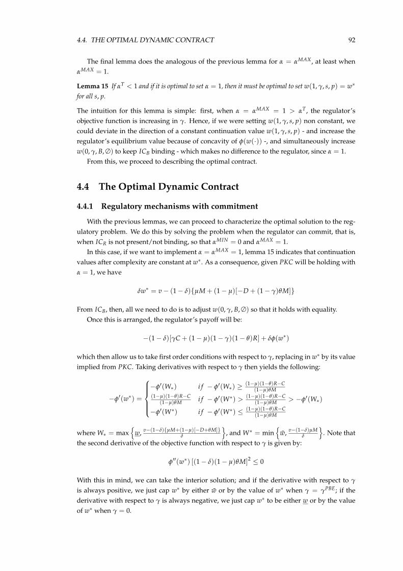
4.4. THE OPTIMAL DYNAMIC CONTRACT 92
The final lemma does the analogous of the previous lemma for α = αMAX , at least whenαMAX = 1.
Lemma 15 If αT < 1 and if it is optimal to set α = 1, then it must be optimal to set w(1, γ, s, p) = w∗
for all s, p.
The intuition for this lemma is simple: first, when α = αMAX = 1 > αT , the regulator’sobjective function is increasing in γ. Hence, if we were setting w(1, γ, s, p) non constant, wecould deviate in the direction of a constant continuation value w(1, γ, s, p) - and increase theregulator’s equilibrium value because of concavity of φ(w(·)) -, and simultaneously increasew(0, γ, B, ∅) to keep ICB binding - which makes no difference to the regulator, since α = 1.
From this, we proceed to describing the optimal contract.
4.4 The Optimal Dynamic Contract
4.4.1 Regulatory mechanisms with commitment
With the previous lemmas, we can proceed to characterize the optimal solution to the reg-ulatory problem. We do this by solving the problem when the regulator can commit, that is,when ICR is not present/not binding, so that αMIN = 0 and αMAX = 1.
In this case, if we want to implement α = αMAX = 1, lemma 15 indicates that continuationvalues after complexity are constant at w∗. As a consequence, given PKC will be holding withα = 1, we have
δw∗ = v− (1− δ)µM + (1− µ)[−D + (1− γ)θM]
From ICB, then, all we need to do is to adjust w(0, γ, B, ∅) so that it holds with equality.Once this is arranged, the regulator’s payoff will be:
−(1− δ)[γC + (1− µ)(1− γ)(1− θ)R] + δφ(w∗)
which then allow us to take first order conditions with respect to γ, replacing in w∗ by its valueimplied from PKC. Taking derivatives with respect to γ then yields the following:
−φ′(w∗) =
−φ′(W∗) i f − φ′(W∗) ≥ (1−µ)(1−θ)R−C
(1−µ)θM(1−µ)(1−θ)R−C
(1−µ)θM i f − φ′(W∗) > (1−µ)(1−θ)R−C(1−µ)θM > −φ′(W∗)
−φ′(W∗) i f − φ′(W∗) ≤ (1−µ)(1−θ)R−C(1−µ)θM
where W∗ = max
w, v−(1−δ)µM+(1−µ)[−D+θM]δ
, and W∗ = min
w, v−(1−δ)µM
δ
. Note that
the second derivative of the objective function with respect to γ is given by:
φ′′(w∗) [(1− δ)(1− µ)θM]2 ≤ 0
With this in mind, we can take the interior solution; and if the derivative with respect to γ
is always positive, we just cap w∗ by either w or by the value of w∗ when γ = γPBE; if thederivative with respect to γ is always negative, we just cap w∗ to be either w or by the valueof w∗ when γ = 0.
4.4. THE OPTIMAL DYNAMIC CONTRACT 93
Crucially, once we decide to set α = αMAX , if γ ∈ (0, γPBE) and w∗ ∈ (w, w), then wewill decide to award a continuation value w∗ to the bank that is independent of γ, α and v. Inparticular, this means that once we set α = αMAX = 1, we will set future actions and futurecontinuation values in a way that is independent from the level of v that led to α = αMAX = 1.In this sense, once we set α = αMAX = 1, we are doing the equivalent of erasing history forthe next period onwards. Moreover, γ changes in a way that allows the bank to get v.
If we set γ ∈ 0, γPBE, we will award a continuation value that depends on v, and hence,the future of play will depend on the history that led to a promise of v.
If, on the other hand, we want to implement α = αMIN = 0, then lemma 14 indicatesthat without loss of generality, we will have w(1, γ, B, ∅) = w(1, γ, 0, 0) = w. Moreover,Section 4.A.1 of the Appendix shows that, from the first order conditions to the Lagrangianof this problem, we get w(1, γ, G, M) = v. We need to further determine w(1, γ, 0, M) andw(0, γ, B, ∅).
However, we know that if γ > 0, then lemma 11 tells us that ICB is binding, so that thebank is indifferent between complexity and no complexity. Consequently, from PKC, we getthat:
v = (1− δ)µM + δµ[γv + (1− γ)w(1, γ, 0, M)] + (1− µ)w(0, γ, B, ∅)
(once again, using the fact that we can write the bank’s payoff as the payoff from no complexityafter a bad product). Also, at γ > 0, we know that due to ICB binding:
(1− δ)[−D + (1− γ)θM] + δ[(γ + (1− γ)(1− θ))w + (1− γ)θw(1, γ, 0, M)] = δw(0, γ, B, ∅)
These two equations give us, implicitly, for each value of γ, a value for w(0, γ, B, ∅) and forw(1, γ, 0, M). Conditionally on α = 0, then, we get that the regulator’s objective function isgiven by:
µδ[γφ(v) + (1− γ)φ(w(1, γ, 0, M))]− (1− δ)γC+ (1− µ)δφ(w(0, γ, B, ∅))
From these last three equations, we can easily verify that conditionally on α = αMIN = 0, it isoptimal to set γ to make the derivative of the objective function above with respect to γ equalto zero. This means that:
(1− µ)
µφ′(w(0, γ, B, ∅))
∂w(0, γ, B, ∅)
∂γ
=1− δ
δC + φ(w(1, γ, 0, M))− φ(v)− (1− γ)φ′(w(1, γ, 0, M))
∂w(1, γ, 0, M)
∂γ
This expression has the following intuition: on the first line, we have the marginal benefitsof monitoring, which allows for the regulator to reduce the prize (in terms of continuationvalues) given to banks that do not make their bad assets complex. Naturally, the higher themonitoring, the lower this prize needs to be.
The second line, on the other hand, shows the marginal costs of monitoring. First of all,we have the direct costs of monitoring 1−δ
δ C. Secondly, we have an indirect cost of moni-toring: when the bank increases γ, it increases the number of times it finds out the productis good, leading to more times giving continuation values v rather than continuation values
4.4. THE OPTIMAL DYNAMIC CONTRACT 94
w(1, γ, 0, M) (note that w(1, γ, 0, M) is set to be a punishment relative to v, since the state1, γ, 0, M might happen when the bank has a bad product). The final term is a second indirectcost of monitoring: increasing monitoring reduces the profits from bad products (by increas-ing the number of times these products are forbidden), so that to keep delivering the promiseof v to the bank (needed to satisfy PKC), this requires the regulator to increase w(1, γ, 0, M)
with γ.Once we get these two solutions - one with α = 1, the other with α = 0, all there is left to do
is to compare the value of these two solutions when they’re both feasible. In particular, notethat while the solution with α = 1 is always feasible (that is, we can always adjust γ and w∗ sothat we deliver value v to the bank and have α = 1), if v > (1− δ)µM + δ[µM + (1− µ)[−D +
θM] = µM + δ(1− µ)[−D + θM], then it is impossible to attain value v while having α = 0and some continuation value w(·) ≤ w.
4.4.1.1 Numerical results for the optimal regulatory schedule with commitment when deltais close to 1
We first present the numerical results for when delta is close to one, as a benchmark forour analysis. As can be seen in Step 3.1 of Lemma 8, as delta gets closer to 1, the portion ofthe domain of φ that is weakly decreasing increases and tends towards the whole span of thedomain. Thus, we set relatively high value of δ to guarantee that19 the resulting function willbe weakly decreasing through its span.
Concerning which parameter values to use, we currently have no clear way of calibratingthem to match moments from the data, or a way of micro-founding them, and this remains anarea for future research. As such, we choose our parameters to satisfy the constraints comingfrom assumptions (i) and (ii), and opt to have the bank reward and bailout cost be of similarsize (equal, in this case), the costs of screening and making financial products complicated beof similar size and significantly smaller than the aforementioned parameters, and choosingprobabilities for µ and θ such that even when no screening takes place and bad products arealways make complex, bailouts are relatively rare (around 10% of the time). The values usedcan be seen in Table 4.1:
µ θ M D C R δ0.7 0.7 1 0.05 0.05 1 0.995
Table 4.1: Parameters used when delta is close to one
We plot the resulting φ function, and optimized values of α and γ for the span of possiblevalues for v, that is to say, between w and w, in Figures 4.1 and 4.2.
19Aside from a small approximation error for the very first step.
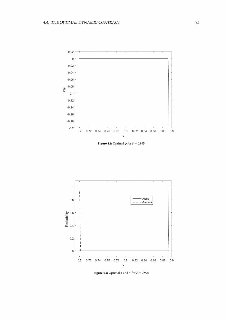
4.4. THE OPTIMAL DYNAMIC CONTRACT 95
Figure 4.1: Optimal φ for δ = 0.995
Figure 4.2: Optimal α and γ for δ = 0.995
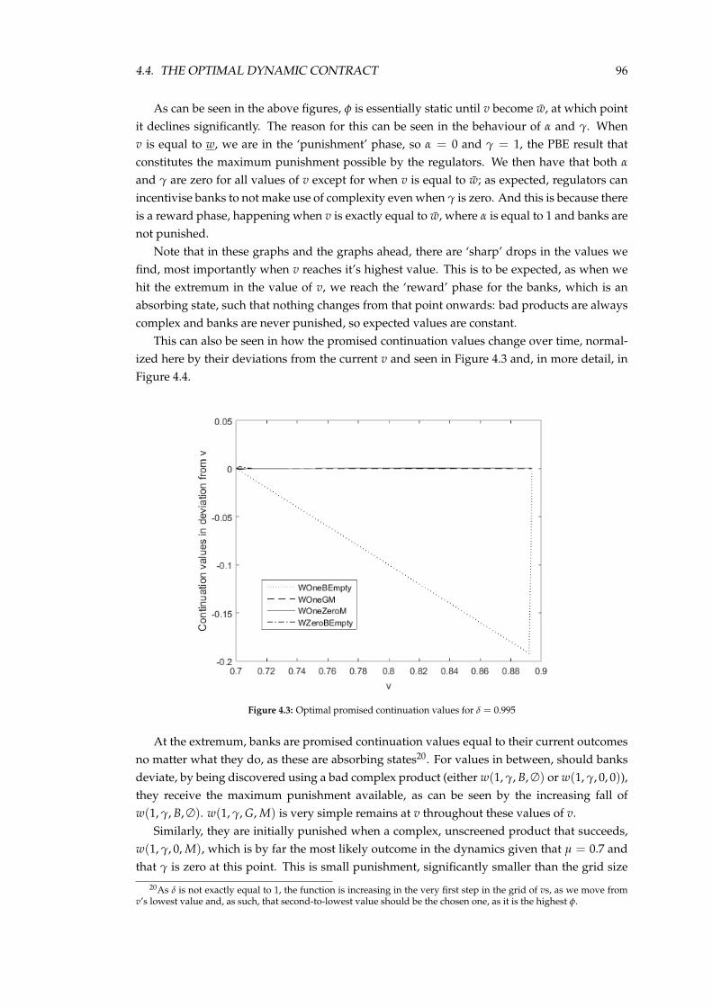
4.4. THE OPTIMAL DYNAMIC CONTRACT 96
As can be seen in the above figures, φ is essentially static until v become w, at which pointit declines significantly. The reason for this can be seen in the behaviour of α and γ. Whenv is equal to w, we are in the ‘punishment’ phase, so α = 0 and γ = 1, the PBE result thatconstitutes the maximum punishment possible by the regulators. We then have that both α
and γ are zero for all values of v except for when v is equal to w; as expected, regulators canincentivise banks to not make use of complexity even when γ is zero. And this is because thereis a reward phase, happening when v is exactly equal to w, where α is equal to 1 and banks arenot punished.
Note that in these graphs and the graphs ahead, there are ‘sharp’ drops in the values wefind, most importantly when v reaches it’s highest value. This is to be expected, as when wehit the extremum in the value of v, we reach the ‘reward’ phase for the banks, which is anabsorbing state, such that nothing changes from that point onwards: bad products are alwayscomplex and banks are never punished, so expected values are constant.
This can also be seen in how the promised continuation values change over time, normal-ized here by their deviations from the current v and seen in Figure 4.3 and, in more detail, inFigure 4.4.
Figure 4.3: Optimal promised continuation values for δ = 0.995
At the extremum, banks are promised continuation values equal to their current outcomesno matter what they do, as these are absorbing states20. For values in between, should banksdeviate, by being discovered using a bad complex product (either w(1, γ, B, ∅) or w(1, γ, 0, 0)),they receive the maximum punishment available, as can be seen by the increasing fall ofw(1, γ, B, ∅). w(1, γ, G, M) is very simple remains at v throughout these values of v.
Similarly, they are initially punished when a complex, unscreened product that succeeds,w(1, γ, 0, M), which is by far the most likely outcome in the dynamics given that µ = 0.7 andthat γ is zero at this point. This is small punishment, significantly smaller than the grid size
20As δ is not exactly equal to 1, the function is increasing in the very first step in the grid of vs, as we move fromv’s lowest value and, as such, that second-to-lowest value should be the chosen one, as it is the highest φ.
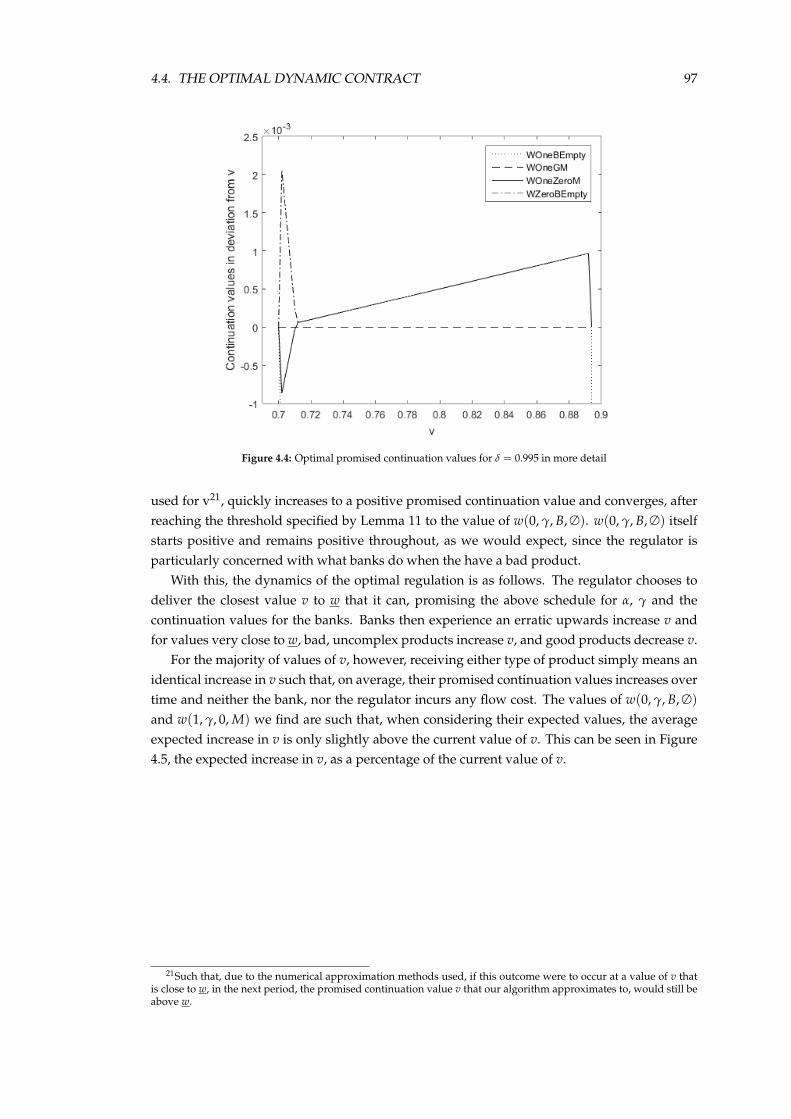
4.4. THE OPTIMAL DYNAMIC CONTRACT 97
Figure 4.4: Optimal promised continuation values for δ = 0.995 in more detail
used for v21, quickly increases to a positive promised continuation value and converges, afterreaching the threshold specified by Lemma 11 to the value of w(0, γ, B, ∅). w(0, γ, B, ∅) itselfstarts positive and remains positive throughout, as we would expect, since the regulator isparticularly concerned with what banks do when the have a bad product.
With this, the dynamics of the optimal regulation is as follows. The regulator chooses todeliver the closest value v to w that it can, promising the above schedule for α, γ and thecontinuation values for the banks. Banks then experience an erratic upwards increase v andfor values very close to w, bad, uncomplex products increase v, and good products decrease v.
For the majority of values of v, however, receiving either type of product simply means anidentical increase in v such that, on average, their promised continuation values increases overtime and neither the bank, nor the regulator incurs any flow cost. The values of w(0, γ, B, ∅)
and w(1, γ, 0, M) we find are such that, when considering their expected values, the averageexpected increase in v is only slightly above the current value of v. This can be seen in Figure4.5, the expected increase in v, as a percentage of the current value of v.
21Such that, due to the numerical approximation methods used, if this outcome were to occur at a value of v thatis close to w, in the next period, the promised continuation value v that our algorithm approximates to, would still beabove w.
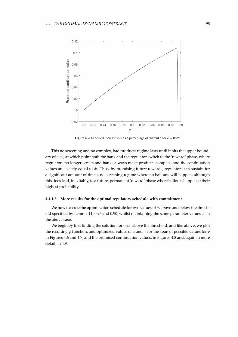
4.4. THE OPTIMAL DYNAMIC CONTRACT 98
Figure 4.5: Expected increase in v as a percentage of current v for δ = 0.995
This no screening and no complex, bad products regime lasts until it hits the upper bound-ary of v, w, at which point both the bank and the regulator switch to the ‘reward’ phase, whereregulators no longer screen and banks always make products complex, and the continuationvalues are exactly equal to w. Thus, by promising future rewards, regulators can sustain fora significant amount of time a no-screening regime where no bailouts will happen, althoughthis does lead, inevitably, to a future, permanent ‘reward’ phase where bailouts happen at theirhighest probability.
4.4.1.2 More results for the optimal regulatory schedule with commitment
We now execute the optimization schedule for two values of δ, above and below the thresh-old specified by Lemma 11, 0.95 and 0.90, whilst maintaining the same parameter values as inthe above case.
We begin by first finding the solution for 0.95, above the threshold, and like above, we plotthe resulting φ function, and optimized values of α and γ for the span of possible values for vin Figures 4.6 and 4.7, and the promised continuation values, in Figures 4.8 and, again in moredetail, in 4.9.
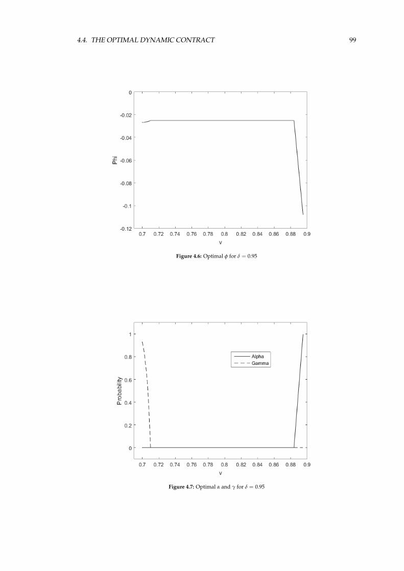
4.4. THE OPTIMAL DYNAMIC CONTRACT 99
Figure 4.6: Optimal φ for δ = 0.95
Figure 4.7: Optimal α and γ for δ = 0.95
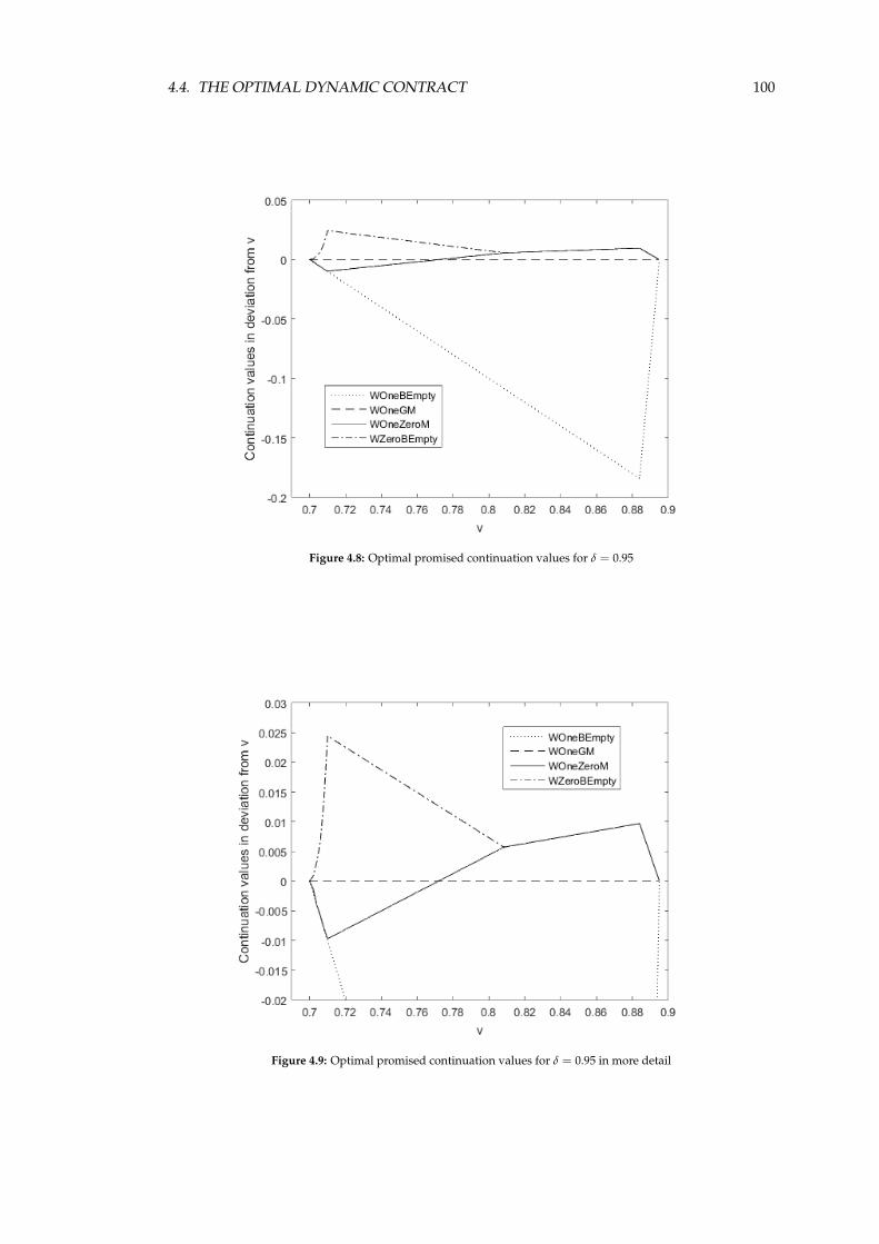
4.4. THE OPTIMAL DYNAMIC CONTRACT 100
Figure 4.8: Optimal promised continuation values for δ = 0.95
Figure 4.9: Optimal promised continuation values for δ = 0.95 in more detail
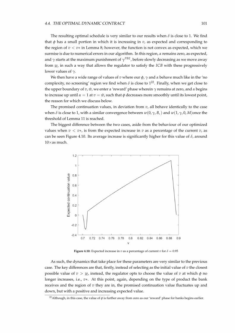
4.4. THE OPTIMAL DYNAMIC CONTRACT 101
The resulting optimal schedule is very similar to our results when δ is close to 1. We findthat φ has a small portion in which it is increasing in v, as expected and corresponding tothe region of v < v∗ in Lemma 8; however, the function is not convex as expected, which wesurmise is due to numerical errors in our algorithm. In this region, α remains zero, as expected,and γ starts at the maximum punishment of γPBE, before slowly decreasing as we move awayfrom w, in such a way that allows the regulator to satisfy the ICB with these progressivelylower values of γ.
We then have a wide range of values of v where our φ, γ and α behave much like in the ‘nocomplexity, no screening’ region we find when δ is close to 122. Finally, when we get close tothe upper boundary of v, w, we enter a ‘reward’ phase wherein γ remains at zero, and α beginsto increase up until α = 1 at v = w, such that φ decreases more smoothly until its lowest point,the reason for which we discuss below.
The promised continuation values, in deviation from v, all behave identically to the casewhen δ is close to 1, with a similar convergence between w(0, γ, B, ) and w(1, γ, 0, M)once thethreshold of Lemma 11 is reached.
The biggest difference between the two cases, aside from the behaviour of our optimizedvalues when v < v∗, is from the expected increase in v as a percentage of the current v, ascan be seen Figure 4.10. Its average increase is significantly higher for this value of δ, around10×as much.
Figure 4.10: Expected increase in v as a percentage of current v for δ = 0.95
As such, the dynamics that take place for these parameters are very similar to the previouscase. The key differences are that, firstly, instead of selecting as the initial value of v the closestpossible value of v > w, instead, the regulator opts to choose the value of v at which φ nolonger increases, i.e., v∗. At this point, again, depending on the type of product the bankreceives and the region of v they are in, the promised continuation value fluctuates up anddown, but with a positive and increasing expected value.
22Although, in this case, the value of φ is further away from zero as our ‘reward’ phase for banks begins earlier.
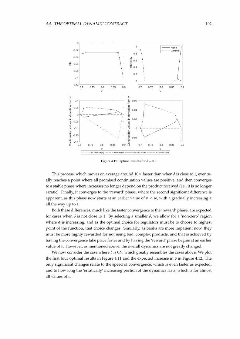
4.4. THE OPTIMAL DYNAMIC CONTRACT 102
Figure 4.11: Optimal results for δ = 0.9
This process, which moves on average around 10× faster than when δ is close to 1, eventu-ally reaches a point where all promised continuation values are positive, and then convergesto a stable phase where increases no longer depend on the product received (i.e., it is no longererratic). Finally, it converges to the ‘reward’ phase, where the second significant difference isapparent, as this phase now starts at an earlier value of v < w, with a gradually increasing α
all the way up to 1.Both these differences, much like the faster convergence to the ‘reward’ phase, are expected
for cases when δ is not close to 1. By selecting a smaller δ, we allow for a ‘non-zero’ regionwhere φ is increasing, and as the optimal choice for regulators must be to choose to highestpoint of the function, that choice changes. Similarly, as banks are more impatient now, theymust be more highly rewarded for not using bad, complex products, and that is achieved byhaving the convergence take place faster and by having the ‘reward’ phase begins at an earliervalue of v. However, as mentioned above, the overall dynamics are not greatly changed.
We now consider the case where δ is 0.9, which greatly resembles the cases above. We plotthe first four optimal results in Figure 4.11 and the expected increase in v in Figure 4.12. Theonly significant changes relate to the speed of convergence, which is even faster as expected,and to how long the ‘erratically’ increasing portion of the dynamics lasts, which is for almostall values of v.
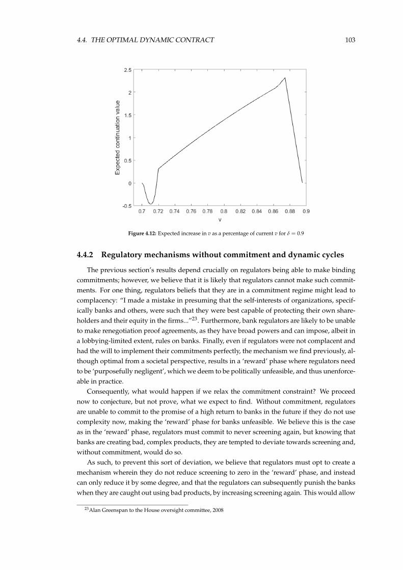
4.4. THE OPTIMAL DYNAMIC CONTRACT 103
Figure 4.12: Expected increase in v as a percentage of current v for δ = 0.9
4.4.2 Regulatory mechanisms without commitment and dynamic cycles
The previous section’s results depend crucially on regulators being able to make bindingcommitments; however, we believe that it is likely that regulators cannot make such commit-ments. For one thing, regulators beliefs that they are in a commitment regime might lead tocomplacency: “I made a mistake in presuming that the self-interests of organizations, specif-ically banks and others, were such that they were best capable of protecting their own share-holders and their equity in the firms...”23. Furthermore, bank regulators are likely to be unableto make renegotiation proof agreements, as they have broad powers and can impose, albeit ina lobbying-limited extent, rules on banks. Finally, even if regulators were not complacent andhad the will to implement their commitments perfectly, the mechanism we find previously, al-though optimal from a societal perspective, results in a ‘reward’ phase where regulators needto be ‘purposefully negligent’, which we deem to be politically unfeasible, and thus unenforce-able in practice.
Consequently, what would happen if we relax the commitment constraint? We proceednow to conjecture, but not prove, what we expect to find. Without commitment, regulatorsare unable to commit to the promise of a high return to banks in the future if they do not usecomplexity now, making the ‘reward’ phase for banks unfeasible. We believe this is the caseas in the ‘reward’ phase, regulators must commit to never screening again, but knowing thatbanks are creating bad, complex products, they are tempted to deviate towards screening and,without commitment, would do so.
As such, to prevent this sort of deviation, we believe that regulators must opt to create amechanism wherein they do not reduce screening to zero in the ‘reward’ phase, and insteadcan only reduce it by some degree, and that the regulators can subsequently punish the bankswhen they are caught out using bad products, by increasing screening again. This would allow
23Alan Greenspan to the House oversight committee, 2008
4.5. DISCUSSION 104
for a credible mechanism, as regulators do not wish to deviate as much, due to their low-but-not-zero levels of screening would lead to a lower use of complexity by banks, and will leadto a ‘reward’ phase for the regulators themselves when screening increases again.
We thus conjecture that this mechanism would consist of having the regulator start screen-ing financial products carefully, in a high γ phase, with the bank making low use of complex-ity with bad products. As more time passes without the detection of complex, bad financialproducts, the regulator slowly reduces the amount of screening it undertakes, while the bankslowly increases the rate at which it makes use of complexity, which corresponds to the ‘re-ward’ phase of the optimal mechanism with commitment. This laxer regime, however, will atsome point lead to a bad and complex product being detected, either through a direct screen-ing or through a product failure. Once either case happens, it subsequently triggers a ‘punish-ment’ phase, and regulators return to high levels of screening and banks reduce the amountof bad complex products they create.
These dynamics would be optimal as, much like in the commitment mechanism, they cre-ates incentives for banks to not make bad financial assets complex via its ‘punishment’ and‘reward’ phases. Banks will wish to create few complex bad products, as this allows themto enter a period of temporarily lax screening, and banks know that they will be punishedby more screening from regulators if they choose to deviate. If correct, this means that thedynamics in this sort of mechanism would be cyclical, with periods of strict screening andfew bad products that are unlikely to lead to bailouts, and periods of lax screening where badproducts are unlikely to be detected and, as a consequence, the probability of a bailout/crisisincreases. This seems to correspond to how financial regulation and financial crises happen inreality.
Note also that if this is the optimal mechanism, although it would have a smaller net-present value than the mechanism with commitment for regulators, it would still be an im-provement over just having the mixed-strategy Nash Equilibrium PBE. This would be becauseit would both reduce the total cost of screening of regulators, since they would need to screenless frequently24, and it would reduce the probability, and thus the total cost, of bailouts.
4.5 Discussion
As is the case with many theoretical papers, we have made many simplifying and stylizedassumptions that we might wish to explore further in the context of the model. In this sec-tion, we discuss these assumptions and how our results would change if we altered them: theassumption that regulators are unable to use fines/transfers to punish/reward banks, the as-sumption that regulators and banks have equal discount factors and the assumption that thereis a single bank for regulators to screen.
4.5.1 Transfers and Fines
As we discuss in the introduction, our model does not include the possibility of directpunishments or rewards to banks, such as via fines. In the context of dynamic games withone-sided private information, when it possible to make use of such transfers, the optimal
24Indeed, we surmise that the same restriction on γ, that it must be smaller or equal to γPBE, will hold in thismechanism.
4.5. DISCUSSION 105
mechanism normally becomes a static one, as can be seen in the more general setting of Levin(2003). This is a consequence of being able to make these transfers to and from the regula-tor and banks conditional on specific outcomes, and an optimal mechanism would then in-centivise banks to adopt no screening at any point by providing sufficient rewards for notdeviating and/or punishment for deviating.
However, as we discuss in the introduction, we do not believe that is a realistic assumptionin the case of our model. Begin with the issue of whether bankers face ex-post punishmentfor creating deliberately complex, bad products. In the aftermath of the financial crisis of2008, very few bankers were directly punished, via the criminal justice system. For example,the New York Times reported in 2014 (Eisinger, 2014), that only 1 Wall Street executive hadbeen convicted due to their actions prior to and during the financial crisis25, and a similarpattern seems holds in most major economies, such as the UK. Furthermore, in the immediateaftermath of a bank bailout, as was seen in the case of AIG, it can be necessary to maintainthe individuals directly responsible for creating the bad, complex products at the head of thebailed out firms. Indeed, it can even be necessary to give them high bonuses at such times,as their knowledge of these products can subsequently help minimize the costs of the bailoutitself (Sorkin, 2010).
Therefore, incentives for individual bankers to engage in moral hazard behaviour has beena problem and is likely to still exist. Aside from the criminal justice system, bankers havelimited liability in case things go wrong and the maximum punishment they then face is beingfired. Indeed, regulators, recognizing this problem, have started to try to change this; to takeone example, the PRA has created rules wherein senior bankers now face deferred variableremuneration, such that the deferred payments these bankers are due to receive may be less ifbanks suffer losses in subsequent periods, even if the banker has left his post. The effectivenessof these rules has yet to be tested, however.
So, if individual bankers are unlikely to face punishment post-fact, the question then iswhether this is true for banks themselves, where the answer is a bit more ambiguous. In a strictsense of timing, such punishments are not possible, as it is precisely during a bailout/crisisthat money has to be put into the banks, making punishments such as fines impossible. Oncepast the crisis, however, it might be possible to then levy fines, but the evidence that thishappens and has happened in the past is mixed at best.
Concerning the most recent crisis, banks have paid fines due to their misconduct in mort-gage products, such that total fines paid by US banks to financial regulators due to mortgagesand mortgage derivatives in the 8 years since the crisis has totaled around 80 billion dollars26.However, these fines are perhaps not as large as they seem, if compared to total profits of thebanking sector in the US of around 660 billion dollar earned in 4 and half years from 201027 orthe around 450 billion dollars used in the Troubled Asset Relief Program (TARP), which itselfwas used mainly to bailout banks.
Equally important, it should be noted that these (relatively) large fines are somewhat un-precedented if compared to the Savings and Loan Crisis, the most recent, previous ‘financial
25Although the same article does stress that in at least one previous financial crisis, the Savings and Loans crisis,more people working in the financial sector were jailed, although these were ’low ranking’ individuals and not highranking Wall Street bankers.
26Authors’ estimates using data from the Financial Times, http://blogs.ft.com/ftdata/2015/07/22/bank-fines-data/
27Wall Street Journal, http://www.wsj.com/articles/u-s-banking-industry-profits-racing-to-near-record-levels-1407773976
4.5. DISCUSSION 106
bailout’ crisis in the US. In that crisis, fines were little applied, even though the total cost tothe US government was over 120 billion dollars (Curry and Shibut, 2000). As such, the ev-idence that regulators can use fines as an effective punishment mechanism post-bailouts ismixed at best, as although fines have been imposed since 2008, these fines are a relatively newdevelopment, and their size may not be large enough to discourage future negative behaviour.
Finally, if bankers and banks cannot be punished directly post-fact, can they instead berewarded directly for good behaviour? We believe that this cannot be the case, as in modelsthat have optimal mechanisms using positive transfers, regulators have to reward agents theyregulate with positive transfers that are multiples of the size of the the payoff in case of annegative shock. As the TARP involved 450 billion dollars and the Savings and Loan Crisis cost120 billion dollars, this would involve sums of money that are, for both practical and politicalreasons, simply unfeasible28.
4.5.2 Different discount factors by banks and regulators
In our model, we assume that both regulators and banks have the same discount factor.However, in practice, given the incentives that banks face for short term results29, there is apossibility that governments and regulators might be more patient than the banks they regu-late, which although an unorthodox assumption, can produce interesting results. To explorethis possibility, we focus our attention on the FOC with respect to γ when α is equal to 1, inSection 4.4.
Note that the term of interest is (1−µ)(1−θ)R−C(1−µ)θM , and that the δ term has been canceled out
from the numerator and denominator. Yet this cancelling has only happened because regula-tors and banks are assumed to have the same discount factor, such that if the regulators andbanks have different δs, then the this FOC becomes δBoverδR
(1−µ)(1−θ)R−C(1−µ)θM , where δR and δB
are the regulator’s and bank’s discount factor respectively.Note that this means that this FOC term will be, if the regulator is more patient than the
bank, now smaller than previously, and also note that our results for when α = 0 remainunchanged. As a consequence, if this δBoverδR is small enough, then the value of −φ′(w∗)falls such that the promised continuation value upon α = 1 falls into the region of α = 0.Consequently, we create a cycle of complexity and no complexity by the part of the bankseven if the regulator has full commitment.
4.5.3 More than one bank
Finally, we assume that only one bank is being regulated in our model, and we do notdiscuss how a bailout to one individual bank can be analogous to a financial crisis. To ad-dress both issues, we must first discuss how exactly the way we model our financial productstranslates into how they work in practice, as we have, deliberately, kept this aspect abstract sofar.
Our model is kept simple by assuming that banks are creating and holding on to products.However, it is possible to interpret the model differently and assume that it means that banksare not just creating products and then holding on to them in their balance sheets, but that
28One possibility, however, which lies outside the framework in this paper, is for regulators to make better use ofwhistleblowers.
29See Terry (2015), for example.
4.6. CONCLUSION 107
these products can and do spread out into the more general financial system. For one thing,new products, if perceived to be successful, can rarely be kept a secret in financial markets forvery long30. So it can be possible to interpret our model in such a way that these productscan and are likely to be held on to the creating bank’s balance sheet, but that they are alsosold to clients, some of which are banks themselves, such that if a bank is holding on to aparticular asset, than other banks might choose to replicate this strategy. That is to say, oncethe ‘genie is out of the bottle’, and a bad product is left unscreened by regulators, that productwill subsequently spread out, and banks have incentives to maintain regulators ignorant of itstrue nature. In this set-up, with multiple banks, this translates into correlated product qualityshocks µ.
With this is mind, an immediate extension of this model to a set-up with multiple banksis to assume that both product quality shocks µ and payoff shocks θ are perfectly correlatedacross banks. In such a case, then our model results are unchanged and there is no differencebetween the one bank and multiple banks case31. Then the risk that individual banks face iseffectively an aggregate risk for the economy, and a bailout of a individual bank in our modelis akin to a more general bailout of the financial sector in a financial crisis. We believe thatthis a likely scenario for many new types of financial products, especially when institutionsthat did not create the product and have not fully screened it/understood its risks, choose tomake use of it nevertheless, due to the moral hazard incentives they face, which justifies a highproduct quality correlation. Additionally, as was largely the case of MBS and CDS products inthe subprime mortgage crisis, in many cases these products returns face aggregate risk whichexplains the correlations in payoffs.
It is less immediate, however, if µ is still very highly correlated but the correlation of thepayoff θ of new products is lower or even non-existent, which might be the case for manyother classes of financial products in practice. In this case, an individual failure of one bankwill indicate which other banks also have a bad complex product. This means that the prob-lem regulators face changes, as regulators now receive new information about the quality ofa product which multiple banks hold after bailing out only one bank. We conjecture that,as in Levin (2002), the optimal mechanism in this case would result in a collective punish-ment/heightened scrutiny towards all banks holding that failed product, and that regulatorycycles akin to the ones we have described previously might thus happen, even without anaggregate financial crisis.
Thus, our assumption of having a single bank, which helps keep the model tractable, canlikely be generalized into results that closely resemble our own.
4.6 Conclusion
Bank bailouts and limited liability create incentives for banks to evade oversight of regu-lators so as to use risky financial products which can payout substantially if the bet on themworks, but leaves regulators with large costs if the gamble fails. One way banks might evaderegulations is by deliberately making such risky products complex, making it difficult to fullygrasp the possible range of outcomes a product has, while knowing the costs that regulators
30Even if the expertise to fully understand these products might be.31In particular, the multi-bank public history of the game is the same as the individual banks’ histories.
4.6. CONCLUSION 108
face when trying to determine the nature of financial products and the limited resources theyhave.
Consequently, regulators are faced with the challenge of designing an optimal regulatoryregime that minimizes the possibility of bailouts without incurring substantial screening costs,especially as two possible methods to incentivise banks, the punishment of banks when thingsgo wrong, and positive transfers when things go right, are difficult to use in practice. Theformer would involve fines of banks at the same time as bailouts are happening, thus mak-ing them impossible, whereas the latter would involve transfers many times the size of bankbailouts and, thus, probably unfeasible in practice.
With these limitations in mind, we find that when regulators can make binding commit-ments, the optimal regulatory regime results in, initially, banks not making bad financial prod-ucts complex and regulators not having to screen, and this no screening and no bad, complexproducts regime lasts for a considerable amount of time. Banks choose not to deviate towardscomplexity because regulators can commit towards a ‘punishment’ phase and a ‘reward’ phaseshould banks choose to deviate or not deviate. The ‘reward’ phase, in particular, consists ofallowing banks to make bad products complex without regulators ever screening, which in-creases the payoff of banks, and once it is triggered, lasts until the end of time. However, this‘reward’ phase also results in the highest probability that banks will have to be bailed out,henceforth, and the ‘reward’ phase starts at the end of the no screening and no bad, complexproducts regime.
We discuss why such binding commitments are likely not possible for regulators in prac-tice, among other reasons because regulators would have incentives to deviate in the ‘reward’phase. Instead, we conjecture, but do not prove, that the optimal regulatory regime whenthere is no commitment by regulators should involve cycles of strong/weak regulatory over-sight and cycles of banks using and refraining from using complexity on bad products, which,if correct, would still be better than the PBE of Nash Equilibrium. We also argue that suchcycles may prevail if regulators are sufficiently more patient than banks.
Our results thus highlight how constrained financial regulators are with their current toolsto incentivise banks towards good behaviour, such that, given the current institutional set-up,bailouts and financial crises may be to some extent an inevitable part of the financial system.This suggests that regulators may have to make even more significant changes to the financialsystem, if they wish to minimize further the chances of crises. Along with some of the possi-bilities we discuss above, such as whistle-blowers and deferred remuneration, regulators maywish to increase the scope for punishments of banks which are not just direct fines.
Appendices to the Chapter
4.A Proofs
Proof of Lemma 5.Compactness of E is a direct consequence of theorem 4 in Abreu, Pearce and Stacchetti (1990).The convexity of E is a consequence of the existence of a public randomization device x, andthe fact that the set of payoffs feasible in equilibria under the presence of such public random-ization devices is convex (as is usual under correlated equilibria). From the compactness andconvexity of the equilibrium payoff set, we can assume that if (φ, v) ∈ E (that is, φ, v are equi-librium present value payoffs for the regulator and the bank, respectively), then v ∈ [w, w] forsome w, w.
To prove that φ(v) is concave, assume otherwise, that φ(v) is strictly convex in an interval[w∗, w∗] ∈ [w, w], with v ∈ (w∗, w∗). Let b ∈ (0, 1) be such that bw∗ + (1− b)w∗ = v. Giventhat φ(v) is not concave, deviate from equilibrium towards delivering the promised value ofv by delivering w∗ with probability b and w∗ with probability 1− b (which is feasible becauseof the existence of the public randomization device x). Given that w∗, w∗ ∈ [w, w], then it isclear that it is feasible to deliver these as equilibrium payoffs to the bank. Moreover, note thatφ(w∗), φ(w∗) are equilibrium payoffs for the regulator, since the definition of the function φ(v)requires that φ(v) ∈ E .
As a consequence, this deviation satisfies all equilibrium conditions. However, this deliversan expected payoff for the regulator of bφ(w∗) + (1− b)φ(w∗) > φ(bw∗ + (1− b)w∗) = φ(v),contradicting the definition of φ(v) as φ(v) = supφ : (φ, v) ∈ E, as there exists an alternative(φ, v) ∈ E with φ > φ(v). Thus φ(v) is (at least) weakly concave.
Finally, we now prove that given the equilibrium values α∗, γ∗ and w(c, γ∗, s, p), φ(c, γ∗, s, p) =φ(w(c, γ∗, s, p)). Assume otherwise, that the solution to the problem φ(v) specifies actionsα∗, γ∗ in the current period, continuation payoffs w(c, γ, s, p) for all γ to the bank, and de-livers continuation payoffs φ(c, γ, s, p) to the regulator, with φ(c, γ∗, s, p) < φ(w(c, γ∗, s, p)),that is, the continuation values for the regulator on the equilibrium path are not the maximumattainable continuation values for the regulator (in particular, for γ∗).
Then, deviate by keeping w(c, γ∗, s, p), γ∗, α∗ constant, but changing the continuation pay-offs for the regulator from φ towards φ∗(c, γ, s, p) = φ(c, γ, s, p) for γ 6= γ∗ and φ∗(c, γ∗, s, p) =φ(w(c, γ∗, s, p)). As the w have not changed, ICB, PKC and w ∈ [w, w] must still hold. More-over, since we increased continuation payoffs for the regulator after γ∗, without changingthe payoffs after γ 6= γ∗, it must be that the regulator has weakly more incentives to chooseγ∗ due to the weakly increased payoff, and hence ICR still holds. So in this deviation, allconstraints still hold. However, as the optimal choice of the regulator is still γ∗ (becauseICR still holds) and the optimal choice of the banks is still α∗, then the flow payoff to theregulator has not changed, but the continuation payoffs for the regulator has increased af-ter the proposed deviation. This then contradicts the optimality of φ(v), that was deliveredwith less than optimal continuation payoffs for the regulator on the equilibrium path, thusφ(c, γ∗, s, p) = φ(w(c, γ∗, s, p)).
Proof of Lemma 6.
109
4.A. PROOFS 110
Assume that it is instead optimal to set
(1− δ)[−D + (1− γ)θM] + δEγ,p[w(1, γ, s, p)|B] > δEγ,p[w(0, γ, s, p)|B]
that is, to provide strict incentives for α = 1. Consider then, firstly, the case where there ex-ists two states (c = 1, γ, s, p) and (c = 1, γ, s′, p′) 6= (c = 1, γ, s, p) such that w(1, γ, s, p) 6=w(1, γ, s′, p′). Let wAVG be the expected continuation value obtained by the bank, uncon-ditionally on the quality of the product but conditional on c = 1 (notice that with α = 1,implied by the assumption on ICB made in the proof, wAVG = µEγ[w(1, γ, s, M)|G] + (1−µ)Eγ,p[w(1, γ, s, p)|B]). Moreover, take a number κ ∈ (0, 1), for ε small. Then, deviate by im-plementing w(1, γ, s, p) with probability 1− κ, and by implementing w(1, γ, s, p) = wAVG withprobability κ. Keep w(0, γ, B, ∅) (the continuation payoff after no complexity) unchanged.
Given that we have assumed that the bank has strict incentives to set α = 1, then for κ
small enough, we will have that:
(1− δ)[−D + (1− γ)θM] + δ(1− κ)Eγ,p[w(1, γ, s, p)|B] + κwAVG ≥ δEγ,p[w(0, γ, s, p)|B]
which implies ICB still holds. Moreover, since we give the bank the same expected continua-tion value as before with probability 1− κ, and give him the average continuation value withprobability κ (notice that since α = 1, we never give the bank the continuation value after nocomplexity), this must mean that the average continuation value did not change, so that thebank must be receiving the same payoffs and PKC must still hold. Moreover, by concavityof φ(v), notice that with probability κ, we are giving the bank the same expected continua-tion value but with no variance, so with probability κ, the regulator’s continuation value aftercomplexity must weakly improve. Moreover, with probability 1− κ, the regulator’s contin-uation value after complexity does not change, since we keep giving the bank the same con-tinuation values as before in these events. As a consequence, the continuation value for theregulator weakly improves, relaxing ICR and increasing the value of the objective function,without changing α, γ. Finally, this deviation must obviously be feasible, since it must be thatif w(1, γ, s, p) ∈ [w, w], then wAVG ∈ [w, w]. As a consequence, it is clear that this deviation isfeasible, and weakly more profitable than the conjectured original regulatory mechanism, con-tradicting the optimality of the conjectured mechanism, and showing that either (i) the bankmust have weakly more incentives for c = 0 as opposed to c = 1 or (ii) given c = 1, we musthave w(1, γ, s, p) constant.
Assume then that it is optimal to set strict incentives for c = 1 and w(1, γ, s, p) = w∗ isconstant across states s, p (or, to set δw(0, γ, B, ∅) < (1− δ)[−D + (1− γ)θM] + δw∗). Deviatetowards setting δw(0, γ, B, ∅) = (1− δ)[−D + (1− γ)θM] + δw∗, while keeping α, γ, w∗ un-changed. Notice that w(0, γ, B, ∅) does not affect the regulator’s payoff nor the bank’s payoff(since state c, γ, s, p = 0, γ, B, ∅ happens with zero probability), so that changing w(0, γ, B, ∅)
leaves the regulator indifferent and so that PKC must still hold. Since ICR only matters aftercomplexity, w(0, γ, B, ∅) does not affect ICR. Moreover, w(0, γ, B, ∅) > w(0, γ, B, ∅) ≥ w, sothat the lower bound on continuation values is satisfied. As long as w(0, γ, B, ∅) ≤ w, thisdeviation is thus feasible and does not affect payoffs, so without loss of generality, we can takeICB to give weak incentives for α = 0, or to set w(0, γ, B, ∅) = w.
Proof of Lemma 7.
4.A. PROOFS 111
As mentioned in the text, w ≤ µM because playing the static PBE in all periods yields dis-counted present payoff to the bank of µM. Similarly, w ≥ µM because if the bank got a lowerpayoff than this, the bank could always deviate towards playing α = 0 whenever his prod-uct is bad, and this alternative strategy would yield a discounted present value payoff of µM.Hence, w = µM.
As for φ, notice that φ ≤ − µ(1−θ)RC(1−θ)R−C , since it is feasible to get −[µ + (1− µ)αPBE]γPBEC−
(1− µ)αPBE(1− γPBE)(1− θ)R = − µ(1−θ)RC(1−θ)R−C as a payoff to the regulator by playing the static
PBE in all periods. φ ≥ −C because if the regulator was getting something worse than this,he could always deviate towards always monitoring complex products (or γ = 1), whichyields discounted present value payoff−C[µ + (1− µ)α] (note that when the regulator alwaysmonitors, he never allows bad products to fail). The lowest value −C[µ + (1− µ)α] can attainis −C (also note that −C = minα maxγ−γC[µ + (1− µ)α]− (1− γ)(1− µ)α(1− θ)R, so that−C is the minmax payoff for the regulator).
On the other hand, w ≤ µM + (1 − µ)[−D + θM], after all, the bank will always get apayoff of M after good products, and cannot get a payoff higher than −D + θM after badproducts. If there is commitment, sustaining w = µM + (1− µ)[−D + θM] as a promise isfeasible: after all, prescribe α = 1, γ = 0, and w(c, γ, s, p) = w. Then, ICB is trivially satisfied,since (1− δ)[−D + (1− γ)θM] + δw = (1− δ)[−D + θM] + δw > δw. PKC is also triviallysatisfied after a promise of w, since w = v = (1 − δ)µM + (1 − µ)[−D + (1 − γ)θM] +
δw = (1− δ)µM + (1− µ)[−D + θM]+ δw, which implies w = µM + (1− µ)[−D + θM] asconjectured. All continuation values are trivially w(c, γ, s, p) = w ∈ [w, w]. With commitment,ICR is not present, so that this then satisfies all constraints.
Without commitment, on the other hand, it is not feasible to deliver w because ICR is vi-olated. After all, the only way to implement a discounted present value payoff to the bankof µM + (1− µ)[−D + θM] is to set, on the equilibrium path, α = 1 and γ = 0 for all peri-ods. However, under this scenario, the regulator is getting a discounted present value payoffof −(1− µ)(1− θ)R < −C from assumption 1. Hence, if the regulator unilaterally deviatestowards monitoring in all periods the product comes complex, he gets a discounted presentvalue payoff of −C, and this is a profitable deviation. This in turn shows that without com-mitment, it is not feasible to deliver payoff µM + (1− µ)[−D + θM] to the bank.
Proof of Lemma 8.Step 1: A relaxed problem - Consider the following two maximization problems: the first oneis simply:
φ(v, γ) =
maxα
w(c,γ,s,p)∀(c,γ,s,p)
µ(1− δ)(−γC) + δEγ[φ(w(1, γ, s, M), γ)|G]
+ (1− µ)(1− α)[(1− δ)0 + δφ(w(0, γ, 1, ∅), γ)]
+ α[(1− δ)(−γC− (1− γ)(1− θ)R) + δEγ,p[φ(w(1, γ, s, p), γ)|B]
s.t. PKC, ICB, ICR, w(c, γ, s, p) ∈ [w, w], φ(c, γ, s, p) = φ(w(c, γ, s, p), γ)
This problem is of interest because φ(v) = arg maxγφ(v, γ) : ∃ eq. with value v f or bank,level γ o f monitoring = arg maxγφ(v, γ) : solution to φ(v, γ) exists.32 With this in mind,
32Assume φ(v) < arg maxγφ(v, γ) : ∃ eq. with value v f or bank, level γ o f monitoring. Then, change α, w(·)
4.A. PROOFS 112
we are only interested in problem φ(v, γ) when there is an equilibrium with value v for thebank when the level of monitoring is γ. Throughout, we will typically denote the set of optimalγ in the problem φ(v) as γ∗(v).
The second problem we consider relaxes the promise keeping constraint in the problemabove:
φ(v, γ) =
maxα
w(c,γ,s,p)∀(c,γ,s,p)
µ(1− δ)(−γC) + δEγ[φ(w(1, γ, s, M), γ)|G]
+ (1− µ)(1− α)[(1− δ)0 + δφ(w(0, γ, 1, ∅), γ)]
+ α[(1− δ)(−γC− (1− γ)(1− θ)R) + δEγ,p[φ(w(1, γ, s, p), γ)|B]
s.t. v ≤ (1− δ)µM + (1− µ)α[−D + (1− γ)θM]
+ δµEα,γ,p[w(c, γ, s, p)|G] + (1− µ)Eα,γ,p[w(c, γ, s, p)|B]
ICB, ICR, w(c, γ, s, p) ∈ [w, w], φ(c, γ, s, p) = φ(w(c, γ, s, p), γ)
That is, we are taking problem φ(v, γ) and firstly, relaxing PKC, and secondly, letting theregulator have continuation payoffs φ(v, γ) as opposed to φ(v, γ).
Let a feasible solution to the relaxed problem above be given by a function φ(v, γ), strategyα and continuation values w(c, γ, s, p)c,γ,s,p such that all constraints hold. That is, a feasiblesolution is one where all constraints hold and the recursive equation for the regulator’s payoffis satisfied.
Step 2: Properties of the relaxed problem - First, notice that the solution to our originalproblem specified in the main text is a feasible solution to the relaxed problem shown in thisproof, and as a consequence, it must be that φ(v, γ) ≥ φ(v, γ). Secondly, notice that φ(v, γ)
must be weakly decreasing in v: after all, for v < v′, notice that any solution feasible for theproblem v′ is also feasible for problem v.
Thirdly, if we find that there exists a solution to problem φ(v, γ) with PKC binding, thenthis solution is feasible for problem φ(v, γ). Hence, if a given solution to φ(v, γ) has bindingPKC, then there exists a set of continuation values and a choice of α that yields value v to thebank (since PKC is binding) when the level of monitoring is γ, so that there is an equilibriumwith value v for the bank and γ monitoring.
In this case, if the solution to φ(v, γ) has binding PKC for all γ that allow for equilibria withvalue v for the bank, then the optimal solution to problem φ(v, γ∗(v)) specifies the optimalα, w(·) for problem φ(v).
Step 3.1: if, for a given v, we have weakly more incentives for c = 1, continuation valuesw(1, γ, s, p) = w and PKC is still non-binding, then there is no equilibrium with value v forthe bank and level γ of monitoring - To see this, note that if we have weakly more incentives
towards the solution to problem φ(v, γ∗(v)) which contradicts optimality of φ(v). Assume φ(v) > arg maxγφ(v, γ) :∃ eq. with value v f or bank, level γ o f monitoring. Then, change the solution of φ(v, γ∗(v)) to the solution for α, w(·)given in problem φ(v), which must satisfy all constraints in problem φ(v, γ∗(v)) (from the definition of φ(v) andφ(v, γ∗)). This then must mean this deviation improves the original solution of φ(v, γ∗(v)) and contradicts optimalityof such original solution. The last equality comes simply from the fact that as long as there exists a regulatory mecha-nism satisfying all constraints in problem φ(v, γ), then there exists an equilibrium with value v for the bank and levelγ of monitoring; given the constraint set is compact also, this guarantees also existence of the solution to problemφ(v, γ).

4.A. PROOFS 113
for c = 1 and w(1, γ, s, p) = w, we must have that:
(1− δ)[−D + (1− γ)θM] + δw ≥ δw(0, γ, B, ∅)
Moreover, due to this indifference, a non-binding PKC can be re-written as:
v < (1− δ)µM + (1− µ)[−D + (1− γ)θM]+ δw
Note, however, that any equilibrium where γ is played yields payoff to the bank:
(1− δ)µM + (1− µ)α[−D + (1− γ)θM]+ δE[w(c, γ, s, p)] ≥
(1− δ)µM + (1− µ)[−D + (1− γ)θM]+ δw
where the inequality comes from (i) ICB giving weakly more incentives for complexity and (ii)from w(·) ≥ w. But then, this implies that if we find that whenever w(1, γ, s, p) = w and ICB
binding, PKC is non-binding, then there is no equilibrium with level of monitoring γ yieldingvalue v to the bank.
Step 3.1’: For a given level of v, if there is an equilibrium with weakly more incentivesfor c = 1 and value v for the bank, then γ ≥ max
γPBE − v−µM
(1−δ)(1−µ)θM , 0
(or, if there are
weakly more incentives for c = 1, then γ ≥ max
γPBE − v−µM(1−δ)(1−µ)θM , 0
is a necessary
condition for there to exist an equilibrium with γ monitoring and value v for the bank) -Note that with weakly more incentives for c = 1, we have:
(1− δ)[−D + (1− γ)θM] + δE[w(1, γ, s, p)|B] ≥ δw(0, γ, B, ∅)
Moreover, in this case, we can write PKC as:
γ =µ
(1− µ)θ+ 1− D
θM+
δEγ,p[w(1, γ, s, p)]− v(1− δ)(1− µ)θM
≥ max
(1− δ)µM(1− δ)(1− µ)θM
+ 1− DθM
+δw− v
(1− δ)(1− µ)θM, 0
= max
γPBE − v− µM(1− δ)(1− µ)θM
, 0
For v = µM = w, this states that γ ≥ γPBE; while for v → µM + (1 − µ)[−D + θM] (anupper bound on w), this suggests γ ≥ − δ
(1−δ)γPBE. Finally, this lower limit on γ is 0 when
µM + γPBE(1− δ)(1− µ)θM = µM + (1− δ)(1− µ)[−D + θM] = vStep 4: For all γ ≤ γPBE and γ ≥ max
γPBE − v−µM
(1−δ)(1−µ)θM , 0
, if there are weak incen-tives for α = 0, then it is optimal in problem φ(v, γ) to set the promise keeping constraintto be binding - If there are weak incentives for α = 0, we must have
(1− δ)[−D + (1− γ)θM] + δEγ,p[w(1, γ, s, p)|B] ≤ δw(0, γ, B, ∅)
With γ ≤ γPBE, −D + (1− γ)θM ≥ 0, so that we must have Eγ,p[w(1, γ, s, p)] ≤ w(0, γ, B, ∅).Moreover, we have Eγ,p[w(1, γ, s, p)] < w(0, γ, B, ∅) if either γ < γPBE or ICB is non-binding.But then, it must be that at least w(0, γ, B, ∅) > w.
With this in mind, assume for a contradiction that it is optimal to set γ ≤ γPBE but to set
4.A. PROOFS 114
PKC not to be binding. Then, first note that if w(1, γ, G, M) > w, we can reduce w(1, γ, G, M)
by ε, which will still satisfy the relaxed PKC for ε small enough; this will not change ICB
(since (c, γ, s, p) = (1, γ, G, M) never happens when the product is bad, so it does not affect theincentives for banks with bad products); it will relax the modified ICR in the relaxed problemby weakly increasing φ(w(1, γ, G, M), γ) (and hence, it will increase the payoff the regulatorgets by choosing γ as opposed to γ 6= γ), and will still satisfy w(·) ∈ [w, w] for ε small enough.Yet, this will weakly increase the objective function by weakly increasing φ(w(1, γ, G, M), γ),while not changing anything else.
If w(1, γ, G, M) = w but there is some other state (c, γ, s, p) = (1, γ, s∗, p∗) such thatw(1, γ, s∗, p∗) > w, then we can deviate by reducing w(0, γ, s, p) by δ and reducing w(1, γ, s∗, p∗)by ε, in a way that keeps Eγ,p[w(1, γ, s, p)|B]−w(0, γ, B, ∅) constant. By construction, this willkeep ICB holding. For ε small enough, δ will also be small enough and relaxed PKC will stillbe satisfied; and we will also have w(·) ∈ [w, w]. Finally, this will relax ICR by weakly increas-ing φ(w(·), γ). Hence, this deviation is feasible, while weakly increasing the objective functionby increasing φ(·).
Finally, if w(1, γ, s, p) = w for all s, p, then if ICB is non-binding (that is, δw(0, γ, B, ∅) >
(1− δ)[−D + (1− γ)θM] + δw), we can deviate by reducing w(0, γ, B, ∅) by ε while still satis-fying ICB and relaxed PKC (as long as ε is small enough); we will still satisfy w(0, γ, B, ∅) ≥ wafter the deviation for ε small enough (since γ ≤ γPBE and non-binding ICB implies w(0, γ, B, ∅) >
w), this will not affect ICR since ICR only matters after complex products show up, and thiswill weakly increase the objective function for the regulator by weakly increasing φ(w(0, γ, B, ∅), γ)
and changing nothing else.If w(1, γ, s, p) = w for all s, p, ICB is binding, then γ ≥ max
γPBE − v−µM
(1−δ)(1−µ)θM , 0
guarantees either PKC is binding or relaxed PKC is violated, since
γ ≥ max
γPBE − v− µM(1− δ)(1− µ)θM
, 0≥ γPBE − v− µM
(1− δ)(1− µ)θM
which imply that (using the formula for γPBE):
v ≥ (1− δ)(1− µ)[−D + (1− γ)θM] + µM+ δµM
= (1− δ)µM + (1− µ)[−D + (1− γ)θM]+ δw
= (1− δ)µM + (1− µ)[−D + (1− γ)θM]+ δEγ,p[w(1, γ, s, p)]
which, given ICB is binding, is the payoff the bank obtains in case w(1, γ, s, p) = w. Thisconcludes step 4.
Step 5: If there exists γ ∈ γ∗(v) with γ > γPBE providing weak incentives for α = 0 andnon-binding PKC, then there exists γ′ ∈ [γPBE, γ] with γ′ ∈ γ∗(v) such that the solutionto φ(v, γ′) has binding PKC constraint - Whenever Eγ,p[w(1, γ, s, p)|B] ≤ w(0, γ, B, ∅) orwhenever w(1, γ, G, M) > w, the proof is exactly the same as that in step 4 (moreover, notethat γ > γPBE guarantees γ ≥
γPBE − v−µM
(1−δ)(1−µ)θM , 0
for v ≥ w = µM). Hence, we focusfrom now on on the case with Eγ,p[w(1, γ, s, p)|B] > w(0, γ, B, ∅) and with w(1, γ, G, M) = w.This immediately implies that there exists a state (c, γ, s, p) = (1, γ, s∗, p∗) 6= (1, γ, G, M) withw(1, γ, s∗, p∗) > w.
Hence, assume for a contradiction PKC is not binding. Then, if w(0, γ, B, ∅) > w, thenonce again, deviate by reducing w(1, γ, s∗, p∗) by ε and reducing w(0, γ, B, ∅) by δ in a way
4.A. PROOFS 115
that keeps Eγ,p[w(1, γ, s, p)|B] − w(0, γ, B, ∅) constant. This will keep satisfying ICB; for ε
small enough, δ will be small enough and PKC will still be satisfied; this will relax ICR byweakly increasing φ(w(1, ·), γ); and will still satisfy w(·) ≥ w for ε small enough. Moreover,this will also increase the regulator’s objective function by increasing φ(w(·), γ).
If, on the other hand, w(0, γ, B, ∅) = w, then deviate towards α = minαT , α, where αT isdefined to be:
αT ≡ µ
1− µ
(1− δ)C + δ[φ(w(1, γ, 0, M))− φ(w(1, γ, G, M))]
(1− δ)[(1− θ)R− C] + δθ[φ(w(1, γ, B, ∅))− φ(w(1, γ, 0, M))]
(that is, αT is the level of α below which the regulator finds it profitable to reduce γ, and abovewhich the regulator finds it profitable to increase γ). Moreover, reduce γ by δ, set w(1, γ −δ, s∗, p∗) = w(1, γ, s∗, p∗) − ε and, for c, s, p 6= 1, s∗, p∗, set w(c, γ − δ, s, p) = w(c, γ, s, p).Set δ and ε in a way that keeps (1 − δ)[−D + (1 − γ + δ)θM] + δEγ,p[w(1, γ − δ, s, p|B] =
(1− δ)[−D + (1− γ)θM] + δEγ,p[w(1, γ, s, p)|B] constant (note that reducing γ increases thispayoff, so that we need to reduce w(1, γ, s∗, p∗) to keep this constant).
Note that if the original solution was feasible for the problem φ(v, γ), then this postulatedsolution must be feasible for problem φ(v, γ− δ): after all, ICB must still hold since we havekept the payoff from complex bad products unchanged and because we have kept the pay-off from non-complex products unchanged. PKC must still hold for ε small enough, sinceoriginally it was not binding. If α ≤ αT , then ICR must have been weakly relaxed, sincethe only changes were (i) to weakly increase the regulators continuation value by reducingw(1, γ, s∗, p∗) and (ii) to reduce γ when the regulator finds it profitable to do so. If α > αT , onthe other hand, we have deviated towards αT , and at α = αT , ICR always holds (to see this,note that if −(1− µ)(1− θ)R ≥ −C, we have that
(1− γ)(1− µ)(1− δ)(1− θ)(−R) + δ[θφ(1, γ, 0, M) + (1− θ)φ(1, γ, 0, 0)]
+ (1− γ)µδφ(1, γ, 0, M)+ γ −(1− δ)C + δµφ(1, γ, G, M) + δ(1− µ)φ(1, γ, B, ∅)
=(1− µ)(1− δ)(1− θ)(−R) + δ[θφ(1, γ, 0, M) + (1− θ)φ(1, γ, 0, 0)]+ µδφ(1, γ, 0, M)
≥ −(1− δ)(1− µ)(1− θ)R + δφ = (1− δ)max−(1− µ)(1− θ)R,−C+ δφ
(where the first equality comes from indifference between some monitoring and no monitor-ing, and the second line is an implication of φ ≤ φ(1, γ, s, p)), which implies that when −(1−µ)(1− θ)R > −C, the ICR constraint holds. On the other hand, if −C > −(1− µ)(1− θ)R,note that:
(1− γ)(1− µ)(1− δ)(1− θ)(−R) + δ[θφ(1, γ, 0, M) + (1− θ)φ(1, γ, 0, 0)]
+ (1− γ)µδφ(1, γ, 0, M)+ γ −(1− δ)C + δµφ(1, γ, G, M) + δ(1− µ)φ(1, γ, B, ∅)
= −(1− δ)C + δµφ(1, γ, G, M) + δ(1− µ)φ(1, γ, B, ∅) ≥ −(1− δ)C + δφ
= (1− δ)max−(1− µ)(1− θ)R,−C+ δφ
(where the first equality comes from indifference between some monitoring and full monitor-ing, and the second line is also an implication of φ ≤ φ(1, γ, s, p)), once again, implying thatICR holds after the first deviation.)
Finally, this deviation is profitable for the regulator: if α ≤ αT , we are reducing γ when
4.A. PROOFS 116
it’s profitable to do so, and weakly increasing the regulator’s continuation value by reducingthe bank’s continuation value in state c, s, p = 1, s∗, p∗. If α > αT , the regulator first gains byreducing complexity towards αT when the product is bad, and then the move in γ does notchange his payoffs, while his continuation payoff increases from the reduction in the bank’scontinuation payoff in state c, s, p = 1, s∗, p∗.
This then says that if PKC is not binding, w(1, γ, G, M) = w(0, γ, B, ∅) = w, ∃s∗, p∗ withw(1, γ, s∗, p∗) > w and γ > γPBE, then there exists γ′ < γ such that φ(v, γ) ≤ φ(v, γ′),with w(1, γ′, s∗, p∗) < w(1, γ, s∗, p∗), w(1, γ, s, p) = w(1, γ′, s, p) for s, p 6= s∗, p∗ and weaklylower payoffs for the bank. Then, we will still have this deviation available up until either (i)w(1, γ, s, p) = w for all s, p, (ii) PKC becomes binding or (iii) γ becomes equal than γPBE. Inany of these cases, we have either found a solution with PKC binding or we have moved tothe cases covered by step 4, where we do not need to deviate with γ anymore, guaranteeingthe statement of the step 5.
Step 6: If there are strict incentives for α = 1 and γ ≥ max
γPBE − v−µM(1−δ)(1−µ)θM , 0
, then
PKC is binding - According to Lemma 6, this case is only relevant if w(0, γ, B, ∅) = w. So as-sume α = 1, PKC is not binding, ICB provides strict incentives for α = 1 and w(0, γ, B, ∅) = w.Then, if there exists some state (c, γ, s, p) = (1, γ, s, p) with w(1, γ, s, p) > w, we can triv-ially improve the payoff for the regulator by reducing w(1, γ, s, p) (and weakly increasing,as a consequence, φ(w(1, γ, s, p), γ)), while still satisfying PKC for a deviation small enough(since it was not binding), still satisfying ICB (because of strict incentives for α = 1), still sat-isfying w(1, γ, s, p) ∈ [w, w] for a small enough deviation, and relaxing ICR (by increasingφ(w(1, γ, s, p), γ)).
If, on the other hand, w(1, γ, s, p) = w for all s, p, while PKC is not binding, then the factthat we have strictly more incentives for c = 1 implies that γ < max
γPBE − v−µM
(1−δ)(1−µ)θM , 0
:after all, if there are strictly more incentives for c = 1, then we can write the bank’s payoff as:
(1− δ)µM + (1− µ)[−D + (1− γ)θM]+ δw > v
from the non-binding PKC constraint, which in turn implies:
γ < γPBE − v− µM(1− δ)(1− µ)θM
≤ max
γPBE − v− µM(1− δ)(1− µ)θM
, 0
Step 7: φ(v) = arg maxγ φ(v, γ) s.t. γ ≥ max
γPBE − v−µM(1−δ)(1−µ)θM , 0
- If there is γ ∈
γ∗(v) with γ > γPBE, then steps 5 and 6 can be used show that there exists γ′ ∈ [γPBE, γ] (sothat γ′ ≥ max
γPBE − v−µM
(1−δ)(1−µ)θM , 0
), such that φ(v, γ′) ≥ φ(v, γ) and such that φ(v, γ′)
has PKC binding. But then, it must mean that the solution to problem φ(v, γ′) is feasible toproblem φ(v, γ′), and that φ(v, γ′) ≥ φ(v, γ′). Superimposing this with φ(v, γ′) ≤ φ(v, γ′)
from step 2 then yields existence of a solution to problem φ(v, γ′) and that φ(v, γ′) = φ(v, γ′).Moreover, this logic suggests φ(v, γ′) = φ(v, γ′) ≥ φ(v, γ) ≥ φ(v, γ). However, γ ∈ γ∗(v)suggests φ(v, γ) ≥ φ(v, γ′), so that we must have φ(v, γ) = φ(v, γ) = φ(v, γ′) = φ(v, γ′)
whenever γ ∈ γ∗(v), with γ > γPBE. But then, this implies that if there is γ ∈ γ∗(v) withγ > γPBE, there exists a solution to the problem φ(v, γ) and that φ(v) = arg maxγφ(v, γ) :exists solution to φ(v, γ) = arg maxγφ(v, γ) : γ ≥ max
γPBE − v−µM
(1−δ)(1−µ)θM , 0.
If there exists γ ∈ γ∗(v) satisfying γ ≤ γPBE, then by step 3.1’, it must be that γ ≥
4.A. PROOFS 117
max
γPBE − v−µM(1−δ)(1−µ)θM , 0
. Moreover, whenever this was the case, steps 4 and 6 shown
that there exists a solution to problem φ(v, γ) with PKC is binding. But then, this solu-tion is feasible for problem φ(v, γ), so that φ(v, γ) ≤ φ(v, γ) whenever γ ≤ γPBE and γ ≥max
γPBE − v−µM
(1−δ)(1−µ)θM , 0
. This together with φ(v, γ) ≥ φ(v, γ) from step 2 guaranteesthen that φ(v, γ) = φ(v, γ) for γ in the range analyzed here. But then, this guarantees existenceof a solution to problem φ(v, γ) whenever γ ≤ γPBE and γ ≥ max
γPBE − v−µM
(1−δ)(1−µ)θM , 0
.Given that we know there exists no solution to problem φ(v, γ) whenγ < max
γPBE − v−µM
(1−δ)(1−µ)θM , 0
(from step 3.1’), this means that conditionally on the exis-
tence of γ ∈ γ∗(v) with γ ≤ γPBE, we can writeφ(v) = arg maxγφ(v, γ) : γ ≥ max
γPBE − v−µM
(1−δ)(1−µ)θM , 0 = arg maxγφ(v, γ) : γ ≥
max
γPBE − v−µM(1−δ)(1−µ)θM , 0
.
Putting the two paragraphs together, this logic guarantees the statement in step 7 is true.Step 8: There exists v∗ ∈ [w, µM+ (1− δ)(1− µ)(−D + θM)] such that φ(v) is decreasing
in v for v > v∗ - This is an immediate consequence of the envelope theorem applied to theproblem in step 7, of the fact that φ(v, γ) is decreasing in v from step 2, and of the fact thatfor v ≥ µM + (1 − δ)(1 − µ)[−D + θM], the constraint γ ≥ max
γPBE − v−µM
(1−δ)(1−µ)θM , 0
becomes simply γ ≥ 0.
Proof of Lemma 9.(Note: check step 7 from the proof of lemma 8). Assume otherwise, that we are in a contractwith equilibrium values of α > αMIN (the minimum α consistent with ICR) and γ > γPBE. Wenow propose the following deviation: first, change α towards α = αMIN . Additionally, changethe continuation payoff for the bank after a choice of no complexity to be:
Eα,γ,p[w(0, γ, B, ∅)] = w(0, γ, B, ∅)
= Eα,γ,p[w(1, γ, s, p)|B]− D(1− δ)
δ+ (1− γ)θM
(1− δ)
δ
Leave γ and all other continuation payoffs unchanged. Note that −D (1−δ)δ + (1− γ)θM (1−δ)
δ
must be less than zero, as γ > γPBE.With this deviation, the new payoff for banks is33:
v = µ(1− δ)M + δEγ,p[w(1, γ, s, p)|G]+ (1− µ)(1− δ)0 + δw(0, γ, B, ∅)
= µ(1− δ)M + δEγ,p[w(1, γ, s, p)|G]+ (1− µ)(1− δ)[−D + (1− γ)θM]
+ δEα,γ,p[w(1, γ, s, r)|B] = v
where the RHS denotes the payoff for the bank in the initial equilibrium, v, which was spec-ified in the promise keeping constraint. Note that when α ∈ (0, 1), banks must be indifferentbetween choosing α = 0 and α = 1 (otherwise, the bank would not be willing to choose c = 0and c = 1 both with positive probability), so we can substitute out the payoff from c = 0 bythe payoff from c = 1 and the resulting payoff from α ∈ (0, 1) must be the payoff from c = 1.Similarly, if the bank is choosing α = 1, then it must be that it’s getting the payoff from c = 1.Either way, since we had α > 0 originally, it must be that the bank is getting the payoff fromc = 1.
33We can omit α from the expectation term when the product is good, since no decision is available to banks.
4.A. PROOFS 118
As can be seen above, v = v, such that the PKC is still satisfied after the deviation (and re-laxed PKC is satisfied with no changes). Furthermore, as the continuation value after choosingcomplexity has not changed and the payoff of choosing no complexity is equal to the payoffof choosing complexity, it must be that the choice of α = αMIN is optimal and the ICB is stillsatisfied after the deviation.
Note that continuation values after complexity have not changed, and γ has not changed.As a consequence, it must be that the minimum α consistent with ICR has not changed, so thatαMIN remained unaltered. Then, by definition of αMIN , it must be that ICR is satisfied.
Thirdly, notice that for α > αMIN ≥ 0
δ[Eα,γ,p[w(1, γ, s, p)|B]− w(0, γ, B, ∅)] ≥ [D− (1− γ)θM](1− δ) > 0
(since the bank must be either indifferent or have weakly more incentives for α = 1 if it ischoosing α > 0, and since γ > γPBE implies −D + (1− γ)θM < 0) and that
δ[Eα,γ,p[w(1, γ, s, p)|B]− w(0, γ, B, ∅)] = [D− (1− γ)θM](1− δ) > 0
This implies that w(0, γ, B, ∅) ≥ w(0, γ, B, ∅). From the definition of w(0, γ, B, ∅), we havethat w(0, γ, B, ∅) < Eα,γ,p[w(1, γ, s, p)|B] (after all γ > γPBE implies −D + (1− γ)θM < 0).Since both w(1, γ, s, p) and w(0, γ, B, ∅) are promised values in the original optimal regulation,they must have been feasible, which imply Eγ,p[w(1, γ, s, p)|B], w(0, γ, B, ∅) ∈ [w, w]. But then,as a consequence, it must be that w(0, γ, B, ∅) ∈ [w, w].
Finally, we need now show that the deviation improves the payoff of the regulator. Now,in terms of the flow payoff in the current period, since α reduces, the regulator’s expectedcost of screening when the product is bad falls, keeping γ unchanged, and the number ofbad products approved reduces, so the cost of negative shocks to bad products is reduced.Consequently, the flow utility of the regulator is improved.
For the continuation values, first note that if we originally specified α = 1, the continua-tion value for the banks was originally specified to be w(1, γ, s, p), compared to the deviationvalue of w(0, γ, B, ∅) < E[w(1, γ, s, p)] with some probability and unchanged continuationvalues with the complementary probability. Now, we know that for fixed γ, φ(v, γ) is weaklydecreasing. But then E[φ(w(1, γ, s, p), γ)] ≤ φ(E[w(1, γ, s, p)], γ) ≤ φ(w(0, γ, B, ∅), γ), theformer inequality by Jensen’s inequality and concavity of φ(v, γ) (shown in the Appendix asanalogous to the proof in lemma 1), the latter by φ being decreasing in v; thus, the continuationvalues are higher in the deviation. Hence, if α = 1, it is clear that both flow payoffs and con-tinuation payoffs for the regulator increase after the deviation, contradicting the optimality ofthe original dynamic regulatory mechanism.
If we had in the original mechanism α ∈ (0, 1), then w(0, γ, B, ∅) = w(0, γ, B, ∅) <
Eγ,p[w(1, γ, s, p)|B], so that, analogously to the previous result,φ(w(0, γ, B, ∅), γ) = φ(w(0, γ, B, ∅), γ) ≥ E[φ(w(1, γ, s, p), γ)]; thus, by decreasing α, we’reincreasing the frequency of continuation values φ(w(0, γ, B, ∅), γ) and reducing the frequencyof continuation values φ(w(1, γ, s, p), γ) with Eγ,p[φ(w(1, γ, s, p), γ)|B] < φ(w(0, γ, B, ∅), γ).Hence, the continuation values are also higher in the deviation. Once again, for α ∈ (0, 1),it is clear that both flow payoffs and continuation payoffs for the regulator increase after thedeviation, contradicting the optimality of the original dynamic regulatory mechanism.
4.A. PROOFS 119
This concludes the proof that, whenever γ > γPBE, then if α > αMIN , we can find a devia-tion that reduces α towards αMIN , satisfies all constraints, and that makes the regulator betteroff in problem φ(v, γ).
Finally, it is easy to see that αMIN is weakly increasing in γ: to see this, take αT as definedin the proof of lemma 8 (which can be easily seen to be above zero under assumption 1). Wehave seen there that ICR holds at αT for all γ, w(1, γ, ·), so that it must be that αMIN ≤ αT .Moreover, below αT , the regulator loses from increasing monitoring. As a consequence, at anygiven level of α ≤ αT , the higher is γ, the lower is the regulator’s payoff after complexity.
Secondly, note that at αMIN , the regulator’s on-equilibrium path payoff from choosing γ
after complexity must be weakly increasing in α: if it was not, then we could decrease α by ε,increase the regulator’s payoff from γ after complexity and keep satisfying ICR, which wouldcontradict the assumption that the minimum α consistent with ICR is αMIN .
With these two arguments, it can then be easily seen that as γ increases, it must be thatαMIN increases by the implicit function theorem.
Proof of Lemma 11.Assume now γ > 0 but
(1− δ)[−D + (1− γ)θM] + δEγ,p[w(1, γ, s, p)|B] < δEγ,p[w(0, γ, s, p)|B]
If this is the case, then α = 0. Then, deviate by reducing γ. If the reduction in γ is smallenough, ICB will still hold. Given that α = 0, γ will not affect the bank’s payoffs, so that PKCstill holds. Also, given that α = 0, we can see that the regulator’s payoff after complexity isdecreasing in γ, so that reducing γ will flexibilize ICR. Finally, given α = 0, the regulator’spayoff is decreasing in γ, so that decreasing γ weakly increases the regulator’s payoff. Hence,the original mechanism can’t be optimal, suggesting that if it is optimal to set γ > 0, then itmust be that ICB is binding.
Assume now γ = 0 but it is optimal to set
(1− δ)[−D + (1− γ)θM] + δEγ,p[w(1, γ, s, p)|B] < δEγ,p[w(0, γ, s, p)|B]
so that α = 0 on the optimal mechanism. Assume initially that w(1, γ, 0, M) 6= w(0, γ, B, ∅)
(we will later analyze the case when they’re equal). Note first of all that for all continuationvalues, when α = γ = 0, ICR becomes:
δφ(1, γ, 0, M) ≥ δφ
which is trivially true given the assumption that φ is the worse continuation value for theregulator that is consistent with equilibrium. Hence, all continuation values we can possiblyset will still satisfy ICR. Also, note that when α = γ = 0, PKC is given by:
v = (1− δ)µM + δµw(1, γ, 0, M) + (1− µ)w(0, γ, B, ∅)
and that ICB is given by:
(1− δ)[−D + θM] + δ[θw(1, γ, 0, M) + (1− θ)w(1, γ, 0, 0)] < δw(0, γ, B, ∅)
4.A. PROOFS 120
With this in mind, then, let wAVG = µw(1, γ, 0, M) + (1− µ)w(0, γ, B, ∅). Deviate, withprobability 1− κ, towards setting w(1, γ, 0, M) = w(1, γ, 0, M) and w(0, γ, B, ∅) = w(0, γ, B, ∅),while with probability κ, set w(1, γ, 0, M) = wAVG and w(0, γ, B, ∅) = wAVG. Keep allother continuation values unchanged, and keep γ unchanged. Clearly, this deviation satisfiesw(c, γ, s, p) ∈ [w, w] because the deviation has kept continuation values either unchanged, ormoved them towards an average of continuation values wAVG. Moreover, this deviation must,by construction, keep PKC satisfied. Finally, for a small enough deviation, it must be that ICB
is satisfied. As shown previously, in this case, ICR is always satisfied. As a consequence, thisdeviation is feasible. Moreover, it improves the regulator’s payoff due to concavity of φ(v).Hence, we cannot have that it is optimal to have αMIN implemented with ICB non-binding,with γ = 0, and with w(1, γ, 0, M) 6= w(0, γ, B, ∅).
Next, assume w(1, γ, 0, M) = w(0, γ, B, ∅) = wAVG, that γ = 0, α = 0 and that ICB is notbinding. For this to be the case, then, we must have that, from PKC
v = (1− δ)µM + δwAVG → wAVG =v− (1− δ)µM
δ
while, from ICB, we must have:
(1− δ)[−D + θM] + δ(1− θ)w(1, γ, 0, 0) < δ(1− θ)v− (1− δ)µM
δ
Re-writing the expression above, we obtain that:
δ(1− θ)w(1, γ, 0, 0) < (1− θ)[v− µM]− (1− δ)[−D + θM] + δ(1− θ)µM
Now, this is feasible as long as the right hand side above is above δ(1− θ)w = δ(1− θ)µM(after all, in such a case, we are just requiring that δ(1− θ)w(1, γ, 0, 0) is lower than somethingabove δ(1− θ)w). This is the case as long as:
(1− θ)[v− µM] ≥ (1− δ)[−D + θM]
Noting that v ≤ µM + (1 − µ)[−D + θM] from lemma 7, we have that (1 − θ)[v − µM] ≤(1− θ)(1− µ)[−D + θM], so that a necessary condition for the above to hold for some v < w(with commitment) and for some v ≤ w (without commitment) is that 1− δ ≤ (1− θ)(1− µ).In this sense, if δ < θ(1− µ) + µ, it is impossible to have w(1, γ, 0, M) = w(0, γ, B, ∅) whilestill satisfying PKC and ICB providing strict incentives for α = 0. For δ ≥ θ(1− µ) + µ, on theother hand, we will need to have ICB holding with equality for all:
v < µM +1− δ
1− θ[−D + θM]
Finally, assume v ≥ µM + 1−δ1−θ [−D + θM], that it is optimal to set α = 0, γ = 0, and that
w(1, γ, 0, M) 6= w(0, γ, B, ∅). Note that in such a case where α = γ = 0, the regulator’s payoffis:
µδφ(w(1, γ, 0, M)) + (1− µ)δφ(w(0, γ, B, ∅))
4.A. PROOFS 121
Given that PKC must hold and α = 0, note that:
v = (1− δ)µM + δµw(1, γ, 0, M) + (1− µ)w(0, γ, B, ∅)
→ µw(1, γ, 0, M) + (1− µ)w(0, γ, B, ∅) =v− (1− δ)µM
δ
so that the expected continuation value is given as above. Finally, as before, when α = γ = 0,ICR always holds for all continuation values we might set.
Now, with these considerations in mind, deviate from the proposed mechanism abovetowards setting w(1, γ, 0, M) = w(0, γ, B, ∅) = v−(1−δ)µM
δ and w(1, γ, 0, 0) = w = µM. Keepα = γ = 0, and all other continuation values unchanged.
Clearly, this deviation must still satisfy PKC. Moreover, under the deviation, note that ICB
becomes:
(1− δ)[−D + θM] + δ
θ
v− (1− δ)µMδ
+ (1− θ)µM≤ δ
v− (1− δ)µMδ
(where the inequality holds because v ≥ µM + 1−δ1−θ [−D + θM]). This is clearly consistent with
α = γ = 0. ICR, as noted before, always holds. Finally, note that if the previous mechanismwas feasible, it delivered an expected continuation value of v−(1−δ)µM
δ , so that it must still befeasible to move towards these deviation values. As a consequence, if it was optimal to setγ = α = 0, it is still feasible to do so after our proposed deviation. However, this improves theregulator’s payoff because φ(v) is concave, and we’re keeping the same average continuationvalue while reducing risk.
Proof of Lemma 12.Assume w(1, γ, B, ∅) 6= w(1, γ, 0, 0). Deviate towards w(1, γ, B, ∅) = w(1, γ, 0, 0) = w∗ =γw(1,γ,B,∅)+(1−γ)(1−θ)w(1,γ,0,0)
γ+(1−γ)(1−θ). This deviation still satisfies ICB because it keeps the payoffs
from complex bad products constant. Given that it does not change the payoff from non-complex bad products, nor the payoffs from good products, it follows immediately that theoverall payoff from the banks does not change, so the PKC still holds. Thirdly, given thatw(1, γ, B, ∅), w(1, γ, 0, 0) ∈ [w, w], then w∗ ∈ [w, w] because it is a weighted average of w(1, γ, B, ∅)
and w(1, γ, 0, 0). Finally, the continuation payoffs from the regulator after detected complexbad products must have weakly increased, since we kept the average continuation value ofthe bank in this state constant, and since φ(v) is a concave function and we have reduced therisk the regulator faces. This implies ICR is relaxed and still holds, and that this is a weaklyprofitable deviation.
Proof of Lemma 13.As we discuss in the main text, αT delineates the point of indifference for the regulator be-tween screening and non-screening. This implies that when α > αT , the objective function ofthe regulator will be increasing in γ, when α < αT , the objective function of the regulator isdecreasing in γ, and with α = αT , the regulator is indifferent between different values of γ.
Secondly, note that at α = αT , the ICR holds. To see this, first note that at α = αT , theregulator is made indifferent between different levels of γ, so the regulator’s payoff after com-plexity is equal to the payoff of no monitoring and to the payoff from monitoring. This in turnimplies that ICR always holds under this deviation: after all, if −(1− µ)(1− θ)R ≥ −C, we
4.A. PROOFS 122
have that
(1− γ)(1− µ)(1− δ)(1− θ)(−R) + δ[θφ(1, γ, 0, M) + (1− θ)φ(1, γ, 0, 0)]
+ (1− γ)µδφ(1, γ, 0, M)+ γ −(1− δ)C + δµφ(1, γ, G, M) + δ(1− µ)φ(1, γ, B, ∅)
=(1− µ)(1− δ)(1− θ)(−R) + δ[θφ(1, γ, 0, M) + (1− θ)φ(1, γ, 0, 0)]+ µδφ(1, γ, 0, M)
≥ −(1− δ)(1− µ)(1− θ)R + δφ = (1− δ)max−(1− µ)(1− θ)R,−C+ δφ
(where the first equality comes from indifference between some monitoring and no monitor-ing, and the second line is an implication of φ ≤ φ(1, γ, s, p)), which implies that when −(1−µ)(1− θ)R > −C, the ICR constraint holds. On the other hand, if −C > −(1− µ)(1− θ)R,note that:
(1− γ)(1− µ)(1− δ)(1− θ)(−R) + δ[θφ(1, γ, 0, M) + (1− θ)φ(1, γ, 0, 0)]
+ (1− γ)µδφ(1, γ, 0, M)+ γ −(1− δ)C + δµφ(1, γ, G, M) + δ(1− µ)φ(1, γ, B, ∅)
= −(1− δ)C + δµφ(1, γ, G, M) + δ(1− µ)φ(1, γ, B, ∅) ≥ −(1− δ)C + δφ
= (1− δ)max−(1− µ)(1− θ)R,−C+ δφ
(where the first equality comes from indifference between some monitoring and full moni-toring, and the second line is also an implication of φ ≤ φ(1, γ, s, p)), once again, implyingthat ICR holds after the first deviation. Given that αT allows ICR to hold, then it is clear thatαT ∈ [αMIN , αMAX ]. Moreover, this implies that if we choose α = αMIN , the regulator’s payoffwill be weakly decreasing in γ and that at α = αMAX , the regulator’s payoff will be weaklyincreasing in γ.
Now, assume there is an optimal regulatory mechanism with α ∈ (αMIN , αMAX) (eitherα is in this interval or α ∈ αMIN , αMAX not to violate ICR). Consider either one of thefollowing two deviations: either deviate to α′ = αMIN , or towards α′′ = αMAX . Both deviationsstill satisfy ICB because we have assumed that ICB is binding (after all, we have assumedα ∈ (αMIN , αMAX) ∈ (0, 1)). They also satisfy PKC because the bank is indifferent betweendifferent levels of α due to ICB binding. By construction, both deviations satisfy ICR. Sincecontinuation values did not change, it is clear then that all constraints are satisfied with thisdeviation.
Yet, notice that by increasing α, the regulator’s objective function increases by:
−(1− δ)[γC + (1− γ)(1− θ)R]
+δ(γ + (1− γ)(1− θ))[φ(w(1, γ, B, ∅))− φ(w(0, γ, B, ∅))]
+(1− γ)θ[φ(w(1, γ, 0, M))− φ(w(0, γ, B, ∅))]
While the first line is clearly negative, the second and third lines are positive. Moreover, α doesnot show up in the expression above, so that the regulator’s objective function is linear in α.If the total effect is weakly negative, this shows that by increasing α, the regulator’s objectivefunction weakly decreases, so that decreasing α towards α′ = αMIN is a weakly profitableand feasible deviation. Alternatively, if the total effect is weakly positive, this shows that byincreasing α, the regulator’s objective function weakly increases, so that increasing α towardsαMAX is a weakly profitable and feasible deviation.
4.A. PROOFS 123
Proof of Lemma 14.Case 1: γ > 0 - Assume instead that it is optimal to set α = αMIN or that αT ≥ 1, γ > 0, butto have φ′(w(1, γ, B, ∅)) < 0. Deviate then by reducing γ by ε (which increases payoffs fromcomplex bad products by εθM(1 − δ)) and reducing w(1, γ, B, ∅) by ω = ε θM
γ−ε1−δ
δ (whichreduces payoffs from complex bad products by ωδ(γ− ε) = εθM(1− δ), after the reductionin γ). By construction, ICB will still hold after the deviation, and since there was no changein (i) the payoff from complex bad products, (ii) the payoff from simple bad products and(iii) the payoff from good products, this implies that PKC still holds. Given that w(1, γ, B, ∅)
fell marginally, φ(w(1, γ, B, ∅)) rises, so that ICR becomes more relaxed. Moreover, when γ
rises, the difference in on-equilibrium path payoffs for the regulator vs. off equilibrium pathdeviations changes by something proportional to:
(1− µ)αMIN(1− δ)[(1− θ)R− C] + δθ[φ(w(1, γ, 0, 0))− φ(w(1, γ, 0, M))]
−µ(1− δ)C + δµ[φ(w(1, γ, G, M))− φ(w(1, γ, 0, M))]
Note that the expression above is rising in αMIN and would be equal to zero if αMIN = αT .Given that αMIN ≤ αT , this implies the expression above is negative, and when γ rises withα = αMIN , ICR becomes “more binding”. Conversely, when γ falls, ICR is relaxed, and thissuggests that our proposed deviation relaxes ICR.
Finally, note that at α = αMIN ≤ αT , the fall in γ weakly increases the regulator’s pay-off, and the fall in w(1, γ, B, ∅) further increases the regulator’s payoff given the assumptionthat φ′(w(1, γ, B, ∅)) < 0. Hence, the proposed deviation is feasible and weakly profitable,suggesting that without loss of generality, when α = αMIN and γ > 0, it is optimal to setφ′(w(1, γ, B, ∅)) ≥ 0. The logic is analogous for w(1, γ, 0, 0), and finishes the proof.
Moreover, if for a given γ > 0, w(1, γ, 0, M) and w(1, γ, G, M), we still have αMIN =
0, start by assuming for a contradiction that w(1, γ, B, ∅) > w. Then, given αMIN = 0,the payoff of the regulator is not affected by w(1, γ, B, ∅), and it is weakly increasing inγ. Then, deviate by reducing w(1, γ, B, ∅) by ε, and reducing γ by ω, in a way that keeps(1− δ)[−D + (1− γ)θM] + Eγ,p[w(1, γ, s, p)|B] constant. Clearly, this deviation will still sat-isfy ICB. Given that we haven’t changed the payoff for the bank from good products, and thatthe payoff for the bank from bad products is δw(0, γ, B, ∅) when α = 0, we haven’t changedthe bank’s ex-ante payoffs, and PKC is still satisfied. Trivially, for ε small enough, we must stillsatisfy w(1, γ, B, ∅)− ε ∈ [w, w). Finally, since we have reduced γ while keeping α = 0, andw(1, γ, 0, M) and w(1, γ, G, M) constant, it must have been that we made ICR more flexibleand αMIN remained equal to zero. Hence, this deviation is feasible, and weakly profitable dueto the fall in γ when α = αMIN = 0 < αT .
Case 2: γ = 0 - Assume instead that it is optimal to set α = αMIN or that αT ≥ 1, γ = 0,but to have w(1, γ, B, ∅) > w. In this case, first note that when γ = 0, αMIN = 0, after all, atγ = α = 0, ICR reduces to:
δφ(w(1, γ, 0, M)) ≥ δφ
which is trivially true (so that the minimum α consistent with ICR given γ = 0 is αMIN = 0).Then, deviate by reducing w(1, γ, B, ∅). ICB will still hold, since the bank will find it strictlyoptimal to set α = 0 after the deviation. The PKC constraint will still hold because the bank
4.A. PROOFS 124
will keep receiving utility δw(0, γ, B, ∅) after bad products, and because the utility from goodproducts did not change. As shown above, ICR holds. Finally, given that α = 0, w(1, γ, B, ∅)
happened with zero probability, so that it does not affect the regulator’s payoff. Hence, with-out loss of generality, the optimal solution to the regulator’s problem has w(1, γ, B, ∅) = w.The same logic applies to w(1, γ, 0, 0).
Proof of Lemma 15.Assume that it is optimal to set α = αMAX and that αT < 1. In this case, lemma 13 guaranteesthat the regulator’s objective function is increasing in γ, and that the higher is γ, the higheris the regulator’s on-equilibrium payoff after complexity (so that ICR gets relaxed when γ
increases). Moreover, lemma 11 guarantees that under α = αMAX , either ICB is binding (afterall, αMAX ≥ αT > 0) or w(0, γ, B, ∅) = w. Finally, remember that corollary 1 suggests thatγ ≤ γPBE < 1 on the optimal solution, which guarantees that either ICB is binding andw(0, γ, B, ∅) ≥ E[w(1, γ, s, p)|B], or that w(0, γ, B, ∅) = w. Finally, let
w∗ =µ
µ + (1− µ)αMAX [γw(1, γ, G, M) + (1− γ)w(1, γ, 0, M)]
+(1− µ)αMAX
µ + (1− µ)αMAX [γ + (1− γ)(1− θ)]w(1, γ, B, ∅) + (1− γ)θw(1, γ, 0, M)
(that is, w∗ is the expected continuation payoff for the bank conditional on the productbeing complex but unconditional on the quality of the product).
Case 1: αMAX = 1 - In this case, deviate then towards w(1, γ, s, p) = w∗ for all s, p, andtowards w(0, γ, B, ∅) set so that ICB holds as below:
min(1− δ)[−D + (1− γ)θM] + δw∗, w = δw(0, γ, B, ∅)
Keep α and γ unchanged.By construction, it must be that ICB is either still binding and consistent with the choice of
α, or that w(0, γ, B, ∅) = w ≤ (1− δ)[−D + (1− γ)θM] + δw∗, once again, consistent with thechoice of α = 1. Also by construction, w∗ is a weighted average of the original continuationvalues, which guarantee that w∗ ∈ [w, w] as long as the original continuation values are in[w, w]. Moreover, given that we’re setting α = αMAX = 1, we can write the bank’s payoff afterdeviation as:
(1− δ)µM + (1− µ)[−D + (1− γ)θM]+ δw∗
= (1− δ)µM + (1− µ)[−D + (1− γ)θM]+ δµ[γw(1, γ, G, M) + (1− γ)w(1, γ, 0, M)]
+ δ(1− µ)[γ + (1− γ)(1− θ)]w(1, γ, B, ∅) + (1− γ)θw(1, γ, 0, M) = v
where the last equality comes from the original promise keeping constraint, and the first equal-ity is from the definition of w∗. This ensures the deviation still satisfies PKC.
It is clear that, by construction, the new expected continuation value did not change (usingthe assumption that α = αMAX = 1, this is solely due to the continuation values after complex-ity not depending on w(0, γ, B, ∅)). However, we have reduced risk in the bank’s continuationvalue, and due to concavity in φ, this increases the regulator’s continuation value (which doesnot depend on w(0, γ, B, ∅) because α = αMAX = 1). This same argument suggests that
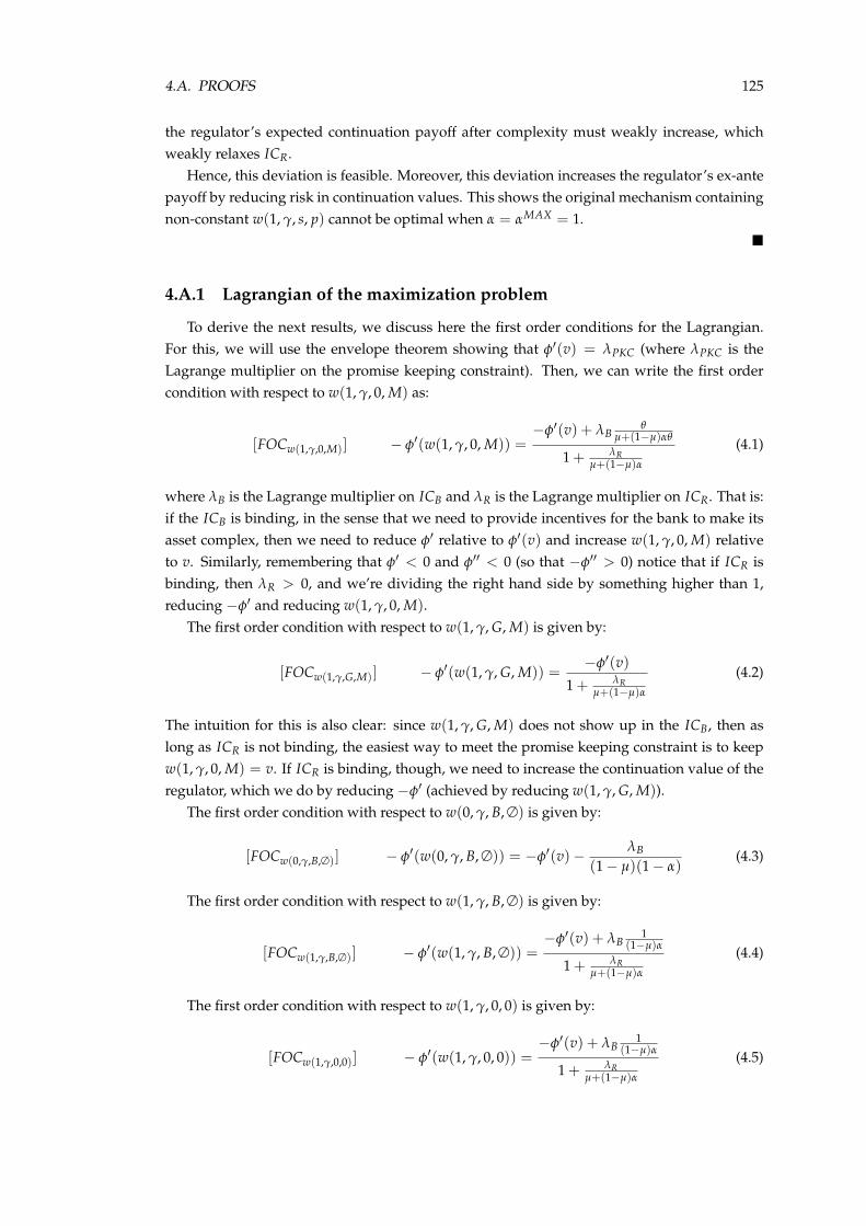
4.A. PROOFS 125
the regulator’s expected continuation payoff after complexity must weakly increase, whichweakly relaxes ICR.
Hence, this deviation is feasible. Moreover, this deviation increases the regulator’s ex-antepayoff by reducing risk in continuation values. This shows the original mechanism containingnon-constant w(1, γ, s, p) cannot be optimal when α = αMAX = 1.
4.A.1 Lagrangian of the maximization problem
To derive the next results, we discuss here the first order conditions for the Lagrangian.For this, we will use the envelope theorem showing that φ′(v) = λPKC (where λPKC is theLagrange multiplier on the promise keeping constraint). Then, we can write the first ordercondition with respect to w(1, γ, 0, M) as:
[FOCw(1,γ,0,M)] − φ′(w(1, γ, 0, M)) =−φ′(v) + λB
θµ+(1−µ)αθ
1 + λRµ+(1−µ)α
(4.1)
where λB is the Lagrange multiplier on ICB and λR is the Lagrange multiplier on ICR. That is:if the ICB is binding, in the sense that we need to provide incentives for the bank to make itsasset complex, then we need to reduce φ′ relative to φ′(v) and increase w(1, γ, 0, M) relativeto v. Similarly, remembering that φ′ < 0 and φ′′ < 0 (so that −φ′′ > 0) notice that if ICR isbinding, then λR > 0, and we’re dividing the right hand side by something higher than 1,reducing −φ′ and reducing w(1, γ, 0, M).
The first order condition with respect to w(1, γ, G, M) is given by:
[FOCw(1,γ,G,M)] − φ′(w(1, γ, G, M)) =−φ′(v)
1 + λRµ+(1−µ)α
(4.2)
The intuition for this is also clear: since w(1, γ, G, M) does not show up in the ICB, then aslong as ICR is not binding, the easiest way to meet the promise keeping constraint is to keepw(1, γ, 0, M) = v. If ICR is binding, though, we need to increase the continuation value of theregulator, which we do by reducing −φ′ (achieved by reducing w(1, γ, G, M)).
The first order condition with respect to w(0, γ, B, ∅) is given by:
[FOCw(0,γ,B,∅)] − φ′(w(0, γ, B, ∅)) = −φ′(v)− λB(1− µ)(1− α)
(4.3)
The first order condition with respect to w(1, γ, B, ∅) is given by:
[FOCw(1,γ,B,∅)] − φ′(w(1, γ, B, ∅)) =−φ′(v) + λB
1(1−µ)α
1 + λRµ+(1−µ)α
(4.4)
The first order condition with respect to w(1, γ, 0, 0) is given by:
[FOCw(1,γ,0,0)] − φ′(w(1, γ, 0, 0)) =−φ′(v) + λB
1(1−µ)α
1 + λRµ+(1−µ)α
(4.5)
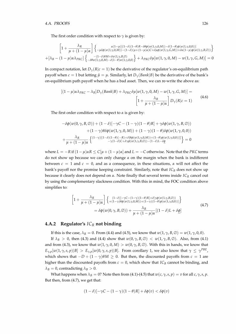
4.A. PROOFS 126
The first order condition with respect to γ is given by:[1 +
λRµ + (1− µ)α
] α(1−µ)[(1−δ)(1−θ)R−δθφ(w(1,γ,0,M))−δ(1−θ)φ(w(1,γ,0,0))]
−µδφ(w(1,γ,0,M))−(1−δ)(µ+(1−µ)α)C+δµφ(w(1,γ,G,M))+δα(1−µ)φ(w(1,γ,B,∅))
+[λB − (1− µ)αλPKC]
−(1−δ)θM+δw(1,γ,B,∅)
−δθw(1,γ,0,M)−δ(1−θ)w(1,γ,0,0)
+ λPKCδµ[w(1, γ, 0, M)− w(1, γ, G, M)] = 0
In compact notation, let Dγ(R|c = 1) be the derivative of the regulator’s on-equilibrium pathpayoff when c = 1 but letting µ = µ. Similarly, let Dγ(Bank|B) be the derivative of the bank’son-equilibrium path payoff when he has a bad asset. Then, we can re-write the above as:
[(1− µ)αλPKC − λB]Dγ(Bank|B) + λPKCδµ[w(1, γ, 0, M)− w(1, γ, G, M)] =[1 +
λRµ + (1− µ)α
]Dγ(R|c = 1)
(4.6)
The first order condition with respect to α is given by:
−δφ(w(0, γ, B, ∅)) + (1− δ)[−γC− (1− γ)(1− θ)R] + γδφ(w(1, γ, B, ∅))
+(1− γ)θδφ(w(1, γ, 0, M)) + (1− γ)(1− θ)δφ(w(1, γ, 0, 0))
+λR
µ + (1− µ)α
(1−γ)[(1−δ)(1−θ)(−R)+δ[θφ(w(1,γ,0,M))+(1−θ)φ(w(1,γ,0,0))]]
−γ(1−δ)C+δγφ(w(1,γ,B,∅))−(1−δ)L−δφ
= 0
where L = −R if (1−µ)αR ≤ C[µ+(1−µ)α] and L = −C otherwise. Note that the PKC termsdo not show up because we can only change α on the margin when the bank is indifferentbetween c = 1 and c = 0, and as a consequence, in these situations, α will not affect thebank’s payoff nor the promise keeping constraint. Similarly, note that ICB does not show upbecause it clearly does not depend on α. Note finally that several terms inside ICR cancel outby using the complementary slackness condition. With this in mind, the FOC condition abovesimplifies to: [
1 +λR
µ + (1− µ)α
] (1−δ)[−γC−(1−γ)(1−θ)R]+δ[γφ(w(1,γ,B,∅))
+(1−γ)θφ(w(1,γ,0,M))+(1−γ)(1−θ)φ(w(1,γ,0,0))]
= δφ(w(0, γ, B, ∅)) +
λRµ + (1− µ)α
[(1− δ)L + δφ]
(4.7)
4.A.2 Regulator’s ICR not binding
If this is the case, λR = 0. From (4.4) and (4.5), we know that w(1, γ, B, ∅) = w(1, γ, 0, 0).If λB > 0, then (4.3) and (4.4) show that w(0, γ, B, ∅) < w(1, γ, B, ∅). Also, from (4.1)
and from (4.3), we know that w(1, γ, 0, M) > w(0, γ, B, ∅). With this in hands, we know thatEγ,p[w(1, γ, s, p)|B] > Eγ,p[w(0, γ, s, p)|B]. From corollary 1, we also know that γ ≤ γPBE,which shows that −D + (1 − γ)θM ≥ 0. But then, the discounted payoffs from c = 1 arehigher than the discounted payoffs from c = 0, which show that ICB cannot be binding, andλB = 0, contradicting λB > 0.
What happens when λB = 0? Note then from (4.1)-(4.5) that w(c, γ, s, p) = v for all c, γ, s, p.But then, from (4.7), we get that:
(1− δ)[−γC− (1− γ)(1− θ)R] + δφ(v) < δφ(v)
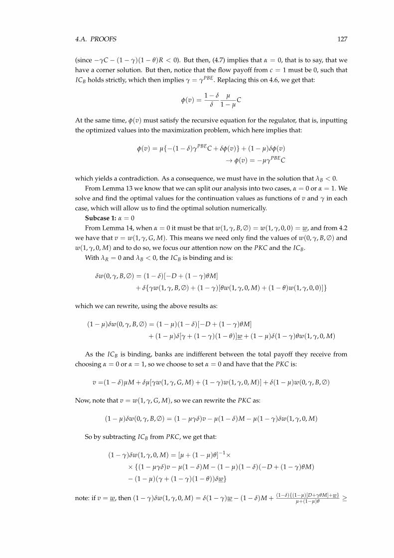
4.A. PROOFS 127
(since −γC − (1− γ)(1− θ)R < 0). But then, (4.7) implies that α = 0, that is to say, that wehave a corner solution. But then, notice that the flow payoff from c = 1 must be 0, such thatICB holds strictly, which then implies γ = γPBE. Replacing this on 4.6, we get that:
φ(v) =1− δ
δ
µ
1− µC
At the same time, φ(v) must satisfy the recursive equation for the regulator, that is, inputtingthe optimized values into the maximization problem, which here implies that:
φ(v) = µ−(1− δ)γPBEC + δφ(v)+ (1− µ)δφ(v)
→ φ(v) = −µγPBEC
which yields a contradiction. As a consequence, we must have in the solution that λB < 0.From Lemma 13 we know that we can split our analysis into two cases, α = 0 or α = 1. We
solve and find the optimal values for the continuation values as functions of v and γ in eachcase, which will allow us to find the optimal solution numerically.
Subcase 1: α = 0From Lemma 14, when α = 0 it must be that w(1, γ, B, ∅) = w(1, γ, 0, 0) = w, and from 4.2
we have that v = w(1, γ, G, M). This means we need only find the values of w(0, γ, B, ∅) andw(1, γ, 0, M) and to do so, we focus our attention now on the PKC and the ICB.
With λR = 0 and λB < 0, the ICB is binding and is:
δw(0, γ, B, ∅) = (1− δ)[−D + (1− γ)θM]
+ δγw(1, γ, B, ∅) + (1− γ)[θw(1, γ, 0, M) + (1− θ)w(1, γ, 0, 0)]
which we can rewrite, using the above results as:
(1− µ)δw(0, γ, B, ∅) = (1− µ)(1− δ)[−D + (1− γ)θM]
+ (1− µ)δ[γ + (1− γ)(1− θ)]w + (1− µ)δ(1− γ)θw(1, γ, 0, M)
As the ICB is binding, banks are indifferent between the total payoff they receive fromchoosing α = 0 or α = 1, so we choose to set α = 0 and have that the PKC is:
v =(1− δ)µM + δµ[γw(1, γ, G, M) + (1− γ)w(1, γ, 0, M)] + δ(1− µ)w(0, γ, B, ∅)
Now, note that v = w(1, γ, G, M), so we can rewrite the PKC as:
(1− µ)δw(0, γ, B, ∅) = (1− µγδ)v− µ(1− δ)M− µ(1− γ)δw(1, γ, 0, M)
So by subtracting ICB from PKC, we get that:
(1− γ)δw(1, γ, 0, M) = [µ + (1− µ)θ]−1×
× (1− µγδ)v− µ(1− δ)M− (1− µ)(1− δ)(−D + (1− γ)θM)
− (1− µ)(γ + (1− γ)(1− θ))δw
note: if v = w, then (1− γ)δw(1, γ, 0, M) = δ(1− γ)w− (1− δ)M + (1−δ)(1−µ)[D+γθM]+wµ+(1−µ)θ
≥
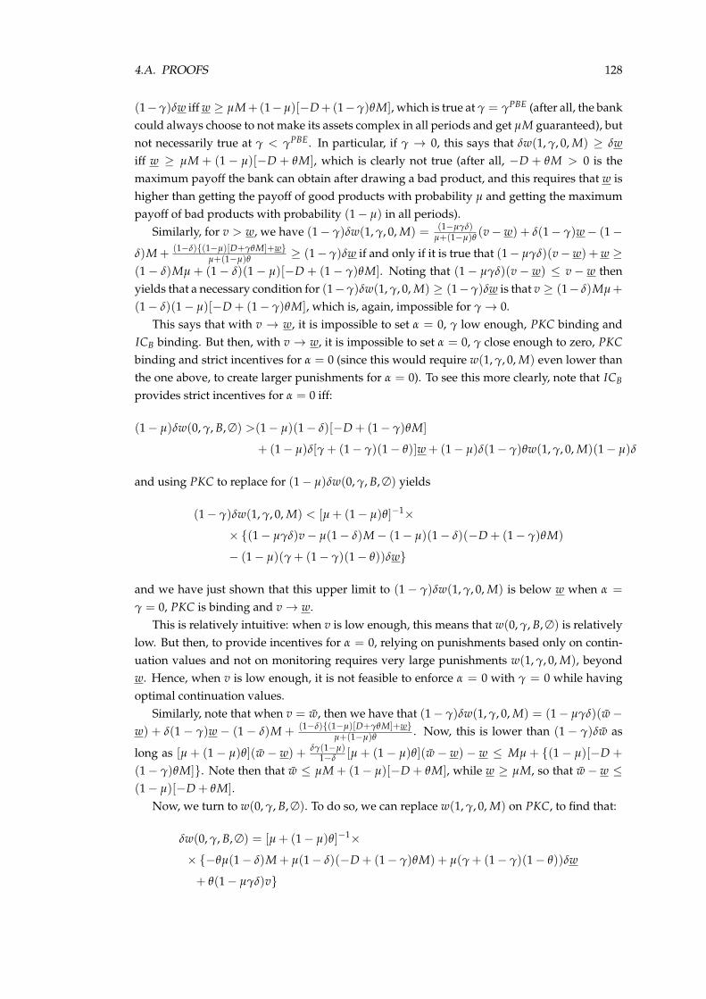
4.A. PROOFS 128
(1−γ)δw iff w ≥ µM+(1−µ)[−D+(1−γ)θM], which is true at γ = γPBE (after all, the bankcould always choose to not make its assets complex in all periods and get µM guaranteed), butnot necessarily true at γ < γPBE. In particular, if γ → 0, this says that δw(1, γ, 0, M) ≥ δwiff w ≥ µM + (1 − µ)[−D + θM], which is clearly not true (after all, −D + θM > 0 is themaximum payoff the bank can obtain after drawing a bad product, and this requires that w ishigher than getting the payoff of good products with probability µ and getting the maximumpayoff of bad products with probability (1− µ) in all periods).
Similarly, for v > w, we have (1− γ)δw(1, γ, 0, M) = (1−µγδ)µ+(1−µ)θ
(v− w) + δ(1− γ)w− (1−
δ)M + (1−δ)(1−µ)[D+γθM]+wµ+(1−µ)θ
≥ (1− γ)δw if and only if it is true that (1− µγδ)(v−w) + w ≥(1− δ)Mµ + (1− δ)(1− µ)[−D + (1− γ)θM]. Noting that (1− µγδ)(v − w) ≤ v − w thenyields that a necessary condition for (1−γ)δw(1, γ, 0, M) ≥ (1−γ)δw is that v ≥ (1− δ)Mµ+
(1− δ)(1− µ)[−D + (1− γ)θM], which is, again, impossible for γ→ 0.This says that with v → w, it is impossible to set α = 0, γ low enough, PKC binding and
ICB binding. But then, with v → w, it is impossible to set α = 0, γ close enough to zero, PKCbinding and strict incentives for α = 0 (since this would require w(1, γ, 0, M) even lower thanthe one above, to create larger punishments for α = 0). To see this more clearly, note that ICB
provides strict incentives for α = 0 iff:
(1− µ)δw(0, γ, B, ∅) >(1− µ)(1− δ)[−D + (1− γ)θM]
+ (1− µ)δ[γ + (1− γ)(1− θ)]w + (1− µ)δ(1− γ)θw(1, γ, 0, M)(1− µ)δ
and using PKC to replace for (1− µ)δw(0, γ, B, ∅) yields
(1− γ)δw(1, γ, 0, M) < [µ + (1− µ)θ]−1×
× (1− µγδ)v− µ(1− δ)M− (1− µ)(1− δ)(−D + (1− γ)θM)
− (1− µ)(γ + (1− γ)(1− θ))δw
and we have just shown that this upper limit to (1− γ)δw(1, γ, 0, M) is below w when α =
γ = 0, PKC is binding and v→ w.This is relatively intuitive: when v is low enough, this means that w(0, γ, B, ∅) is relatively
low. But then, to provide incentives for α = 0, relying on punishments based only on contin-uation values and not on monitoring requires very large punishments w(1, γ, 0, M), beyondw. Hence, when v is low enough, it is not feasible to enforce α = 0 with γ = 0 while havingoptimal continuation values.
Similarly, note that when v = w, then we have that (1− γ)δw(1, γ, 0, M) = (1− µγδ)(w−w) + δ(1 − γ)w − (1 − δ)M + (1−δ)(1−µ)[D+γθM]+w
µ+(1−µ)θ. Now, this is lower than (1 − γ)δw as
long as [µ + (1− µ)θ](w − w) + δγ(1−µ)1−δ [µ + (1− µ)θ](w − w) − w ≤ Mµ + (1− µ)[−D +
(1− γ)θM]. Note then that w ≤ µM + (1− µ)[−D + θM], while w ≥ µM, so that w− w ≤(1− µ)[−D + θM].
Now, we turn to w(0, γ, B, ∅). To do so, we can replace w(1, γ, 0, M) on PKC, to find that:
δw(0, γ, B, ∅) = [µ + (1− µ)θ]−1×
× −θµ(1− δ)M + µ(1− δ)(−D + (1− γ)θM) + µ(γ + (1− γ)(1− θ))δw
+ θ(1− µγδ)v

4.A. PROOFS 129
We thus have all the continuation values as functions of v and γ.Subcase 2: α = 1From Lemma 15 we know that when α = 1, w(1, γ, s, p) = w∗ for all values of s and p34.
This means that can trivially show by the PKC that δw(1, γ, s, p) = δw∗ = δv− (1− δ)µM +
(1− µ)[−D + (1− γ)θM]. With this result, we have all the continuation values as functionsof v and γ.
34Note that w(0, γ, s, p) need not be defined in this case, as it happens with zero probability
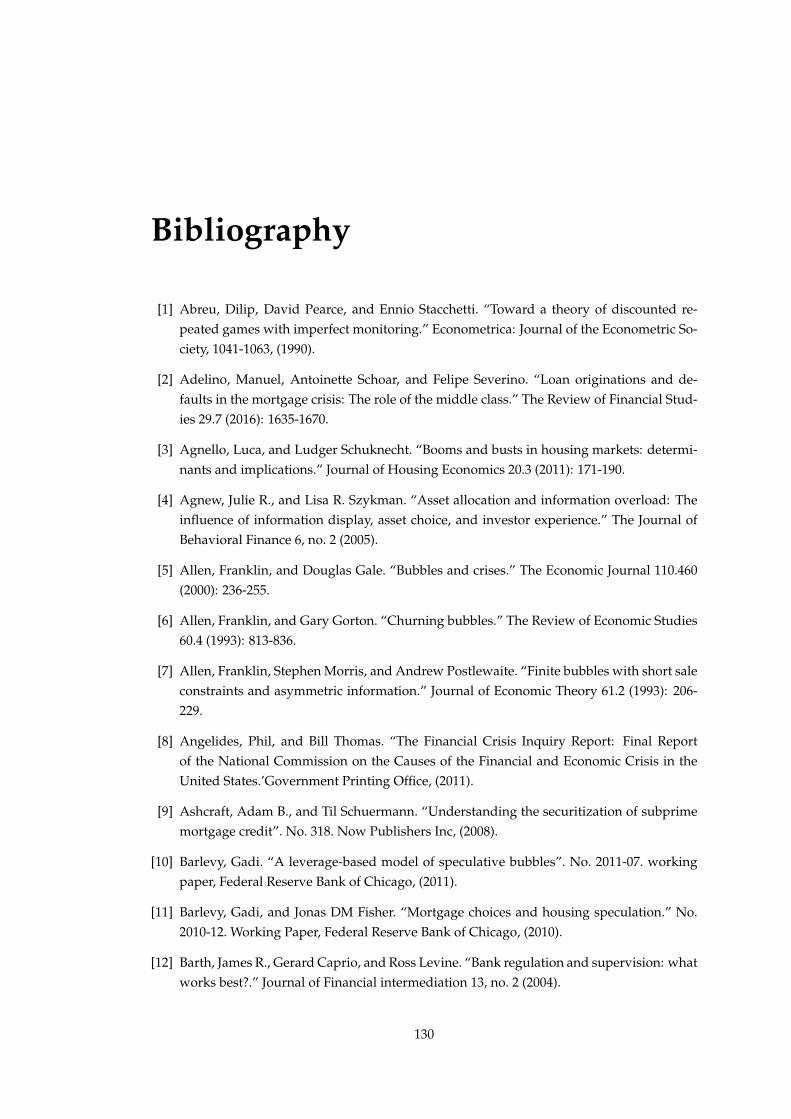
Bibliography
[1] Abreu, Dilip, David Pearce, and Ennio Stacchetti. “Toward a theory of discounted re-peated games with imperfect monitoring.” Econometrica: Journal of the Econometric So-ciety, 1041-1063, (1990).
[2] Adelino, Manuel, Antoinette Schoar, and Felipe Severino. “Loan originations and de-faults in the mortgage crisis: The role of the middle class.” The Review of Financial Stud-ies 29.7 (2016): 1635-1670.
[3] Agnello, Luca, and Ludger Schuknecht. “Booms and busts in housing markets: determi-nants and implications.” Journal of Housing Economics 20.3 (2011): 171-190.
[4] Agnew, Julie R., and Lisa R. Szykman. “Asset allocation and information overload: Theinfluence of information display, asset choice, and investor experience.” The Journal ofBehavioral Finance 6, no. 2 (2005).
[5] Allen, Franklin, and Douglas Gale. “Bubbles and crises.” The Economic Journal 110.460(2000): 236-255.
[6] Allen, Franklin, and Gary Gorton. “Churning bubbles.” The Review of Economic Studies60.4 (1993): 813-836.
[7] Allen, Franklin, Stephen Morris, and Andrew Postlewaite. “Finite bubbles with short saleconstraints and asymmetric information.” Journal of Economic Theory 61.2 (1993): 206-229.
[8] Angelides, Phil, and Bill Thomas. “The Financial Crisis Inquiry Report: Final Reportof the National Commission on the Causes of the Financial and Economic Crisis in theUnited States.’Government Printing Office, (2011).
[9] Ashcraft, Adam B., and Til Schuermann. “Understanding the securitization of subprimemortgage credit”. No. 318. Now Publishers Inc, (2008).
[10] Barlevy, Gadi. “A leverage-based model of speculative bubbles”. No. 2011-07. workingpaper, Federal Reserve Bank of Chicago, (2011).
[11] Barlevy, Gadi, and Jonas DM Fisher. “Mortgage choices and housing speculation.” No.2010-12. Working Paper, Federal Reserve Bank of Chicago, (2010).
[12] Barth, James R., Gerard Caprio, and Ross Levine. “Bank regulation and supervision: whatworks best?.” Journal of Financial intermediation 13, no. 2 (2004).
130
BIBLIOGRAPHY 131
[13] Bernanke, Ben S. “Monetary policy and the housing bubble.” speech at the annual meet-ing of the American Economic Association, Atlanta, Georgia. Vol. 3. (2010).
[14] Bhutta, Neil. “The ins and outs of mortgage debt during the housing boom and bust.”Journal of Monetary Economics (2015).
[15] Blum, Jurg M. “Why ‘Basel II’ may need a leverage ratio restriction.” Journal of Banking& Finance 32, no. 8 (2008).
[16] Case, Karl E., and Robert J. Shiller. “Is there a bubble in the housing market?.” BrookingsPapers on Economic Activity 2003.2 (2003): 299-362.
[17] Case, Karl E., Robert J. Shiller, and Anne Thompson. “What have they been thinking?Home buyer behavior in hot and cold markets.” No. w18400. National Bureau of Eco-nomic Research, (2012).
[18] Carlin, Bruce I. “Strategic price complexity in retail financial markets.” Journal of Finan-cial Economics 91, no. 3 (2009).
[19] Celerier, Claire, and Boris Vallee. “What drives financial complexity? A look into theretail market for structured products.” In A Look into the Retail Market for StructuredProducts (July 1, 2013), Paris December 2012 Finance Meeting EUROFIDAI-AFFI Paper.(2013).
[20] Chan, Sewin, Andrew Haughwout, Andrew T. Hayashi, and Wilbert Van der Klaauw.“Determinants of mortgage default and consumer credit use: the effects of foreclosurelaws and foreclosure delays.” Journal of Money, Credit and Banking 48.2-3 (2016): 393-413.
[21] Curry, Timothy, and Lynn Shibut. “The cost of the savings and loan crisis: truth andconsequences.” FDIC Banking Review 13.2 (2000): 26-35.
[22] Dang, Tri Vi, Gary Gorton, Bengt Holmstrm, and Guillermo Ordonez. “Banks as secretkeepers.” No. w20255. National Bureau of Economic Research, (2014).
[23] Dell’Ariccia, Giovanni, Deniz Igan, and Luc Laeven. “Credit booms and lending stan-dards: Evidence from the subprime mortgage market.” Journal of Money, Credit andBanking 44.2-3 (2012): 367-384.
[24] Dobbie, Will and Paul Goldsmith-Pinkham. “Debtor Protections and the Great Reces-sion”. Working Paper. (2014)
[25] Duca, John V., John Muellbauer, and Anthony Murphy. “House prices and credit con-straints: Making sense of the us experience*.” The Economic Journal 121.552 (2011): 533-551.
[26] Eisenbach, Thomas M., Andrew Haughwout, Beverly Hirtle, Anna Kovner, David O.Lucca, and Matthew C. Plosser. “Supervising large, complex financial institutions: Whatdo supervisors do?” FRB of New York Staff Report 729, (2015).
[27] Eisenbach, Thomas M., David O. Lucca and Robert M. Townsend. “The Economicsof Bank Supervision.” FRB of NY Staff Report No. 769, (2016). Retrieved fromhttp://ssrn.com/abstract=2750314
BIBLIOGRAPHY 132
[28] Eisinger, Jesse. “Why Only One Top Banker Went To Jail For The Fi-nancial Crisis”. New York Times, 30th of April, (2014). Retrieved fromhttp://www.nytimes.com/2014/05/04/magazine/only-one-top-banker-jail-financial-crisis.html
[29] Elul, Ronel. “Securitization and mortgage default”. No. 09-21. Federal Reserve Bank ofPhiladelphia (2011).
[30] FHFA Office of Inspector General. “FHFA’s Oversight of the Enterprises’ Efforts to Re-cover Losses from Foreclosure Sales”, AUD-2013-001 (2012).
[31] Fishbein, Allen and Ren Essene, “The Home Mortgage Disclosure Act at Thirty-Five: PastHistory, Current Issues” MF10-7, August (2010).
[32] Glaeser, Edward L., Joseph Gyourko, and Albert Saiz. “Housing supply and housingbubbles.” Journal of Urban Economics 64.2 (2008): 198-217.
[33] Glaeser, Edward L., Joshua D. Gottlieb, and Joseph Gyourko. “Can cheap credit ex-plain the housing boom?.” Housing and the Financial Crisis. University of Chicago Press(2013). 301-359.
[34] Ghent, Andra. “Americas mortgage laws in historical perspective.” Working paper, pages140, (2012).
[35] Ghent, Andra C., and Marianna Kudlyak. “Recourse and residential mortgage default:evidence from US states.” Review of Financial Studies 24.9 (2011): 3139-3186.
[36] Hall, Robert E., and Charles I. Jones. “Why Do Some Countries Produce So Much MoreOutput Per Worker Than Others?.” The Quarterly Journal of Economics 114.1 (1999): 83-116.
[37] Haughwout, Andrew, Donghoon Lee, Joseph S. Tracy, and Wilbert Van der Klaauw. “Realestate investors, the leverage cycle, and the housing market crisis.” FRB of New York StaffReport 514 (2011).
[38] Hirtle, Beverly, and Jose A. Lopez. “Supervisory information and the frequency of bankexaminations.” Economic Policy Review 5, no. 1, (1999).
[39] Hofmann, Anett. “Rien ne va plus-The 2007/2008 Credit Crunch and what gamblingBankers had to do with it.” The Warwick Economics Research Paper Series 892 (2008).
[40] Holmen, Martin, Michael Kirchler, and Daniel Kleinlercher. “Do option-like incentivesinduce overvaluation? Evidence from experimental asset markets.” Journal of EconomicDynamics and Control 40 (2014): 179-194.
[41] Iacoviello, Matteo, and Stefano Neri. “Housing market spillovers: evidence from an esti-mated DSGE model.” American Economic Journal: Macroeconomics 2.2 (2010).
[42] Krainer, John, and Elizabeth Laderman. “Mortgage loan securitization and relative loanperformance.” Journal of Financial Services Research 45.1 (2014): 39-66.
BIBLIOGRAPHY 133
[43] Keys, Benjamin J., Tanmoy K. Mukherjee, Amit Seru, and Vikrant Vig. “Did securitizationlead to lax screening? Evidence from subprime loans.” Journal of Monetary Economics56.5 (2009): 700-720.
[44] Levin, Jonathan. ”Multilateral contracting and the employment relationship.” QuarterlyJournal of economics (2002): 1075-1103.
[45] Levin, Jonathan. ”Relational incentive contracts.” The American Economic Review 93.3(2003): 835-857.
[46] Lewis, Michael. “Liar’s Poker.” WW Norton & Company, (1989).
[47] Lewis, Michael. “The big short: Inside the doomsday machine”. WW Norton & Company,(2011).
[48] Li, Jin, Niko Matouschek, and Michael Powell. “Power Dynamics in Organizations.”Mimeo, Northwestern University, (2015).
[49] Mailath, George J., and Larry Samuelson. “Repeated games and reputations.” Vol. 2. Ox-ford: Oxford university press, (2006).
[50] Mayer, Christopher J., and Karen Pence. “Subprime mortgages: what, where, and towhom?” No. w14083. National Bureau of Economic Research, 2008.
[51] Mayer, Christopher, Karen Pence, and Shane M. Sherlund. “The rise in mortgage de-faults.” The Journal of Economic Perspectives 23.1 (2009): 27-50.
[52] Mian, Atif, and Amir Sufi. “The consequences of mortgage credit expansion: Evidencefrom the US mortgage default crisis.” The Quarterly Journal of Economics 124.4 (2009):1449-1496.
[53] Mian, Atif, and Amir Sufi. “House of Debt: How They (and You) Caused the Great Re-cession, and How We Can Prevent It from Happening Again. University of Chicago Press(2014).
[54] Mitman, Kurt. “Macroeconomic Effects of Bankruptcy & Foreclosure Policies.”. PIERWorking Paper No. 11-015 (2015). Available at SSRN: http://ssrn.com/abstract=1857517
[55] Obstfeld, Maurice, and Kenneth S. Rogoff. “Global imbalances and the financial crisis:products of common causes”. London: Centre for Economic Policy Research (2009).
[56] The Office of the Comptroller of the Currency (OCC). “ComptrollersHandbook.” Bank Supervision Process, (2015). Retrieved fromhttp://www.occ.treas.gov/publications/publications-by-type/comptrollers-handbook/pub-ch-ep-bsp.pdf
[57] Nam, Tong Yob, and Seungjoon Oh. “Recourse Mortgage Law and the Housing Bubble”.Working Paper (2014).
[58] Pence, Karen M. “Foreclosing on opportunity: State laws and mortgage credit.” Reviewof Economics and Statistics 88.1 (2006): 177-182.
BIBLIOGRAPHY 134
[59] Pennington-Cross, Anthony. “Subprime and prime mortgages: Loss distributions.” Officeof Federal Housing Enterprise Oversight Working Paper 03-1 (2003).
[60] Phelan, Christopher, and Robert M. Townsend. “Computing multi-period, information-constrained optima.” The Review of Economic Studies 58.5, 853-881, (1991).
[61] Piskorski, Tomasz, Amit Seru, and James Witkin. “Asset quality misrepresentation byfinancial intermediaries: Evidence from RMBS market”. No. w18843. National Bureau ofEconomic Research, (2013).
[62] Prescott, Edward S. “Auditing and bank capital regulation.” FRB Richmond EconomicQuarterly 90, no. 4 (2004): 47-63.
[63] Prudential Regulation Authority (PRA). “The Prudential RegulationAuthoritys approach to banking supervision.” (2013) Retrieved fromhttp://www.bankofengland.co.uk/publications/Documents/praapproach/bankingappr1603.pdf
[64] Sorkin, Andrew Ross. “Too big to fail: the inside story of how Wall Street and Washingtonfought to save the financial system–and themselves”. Penguin, (2010).
[65] Spear, Stephen E., and Sanjay Srivastava. “On repeated moral hazard with discounting.”The Review of Economic Studies 54.4, 599-617, (1987).
[66] Terry, Stephen J. “The macro impact of short-termism.” Unpublished job market paper,(2015).
[67] Westrupp, Victor. “Foreclosure Sales and Recourse”. Working paper (2015).