Embed Size (px)
Citation preview
ESSAYS ON ENERGY AND MACROECONOMICS
A Dissertation
Presented to Cardi¤ Business School of
Cardi¤ University
in Partial Ful�llment of the Requirements for the Degree of
Doctor of Philosophy
by
Olayinka Oyekola
February 2016

c 2016 Olayinka Oyekola
ALL RIGHTS RESERVED

ESSAYS ON ENERGY AND MACROECONOMICS
Olayinka Oyekola, Ph.D.
Cardi¤ University 2016

... if we learn our limitations too soon, we never learn our power.
Hannibal Lecter
4
Abstract
This thesis represents largely the two sides to both theory and econometrics of dynamic
macroeconomics, namely stationary and non-stationary models and data. The stationary
part concludes with Chapter 3 and in Chapter 4, I look at the non-stationary side.
More speci�cally, I preview the thesis in Chapter 1 highlighting the modelling and
econometric approaches commonly found in the economics literature; also I report some
key results. In Chapter 2, I provide a comprehensive, but certainly far from being exhaus-
tive, review of the literature dating back to the publication of Stanley Jevon�s (1866) The
Coal Question, but with the main discussion beginning with Harold Hotelling�s (1931) The
Economics of Exhaustible Resources. I develop a two-sector open economy extension to
the Kydland and Prescott (1982), Long and Plosser (1983) and Kim and Loungani (1992)
models in Chapter 3 and estimate it on H-P �ltered annual U.S. data covering 64 years,
with the main purpose of discovering how energy price along with other supply-side and
demand-side shocks (imported and domestic) impacts on the U.S. economy. The model
presented only contains the current account and I restrict trade to balance in every pe-
riod. I �nd that model �ts the data for my benchmark variables of interest in the auxiliary
model: output, real exchange rate, energy use, and consumption. When more variables
and in particular sectoral variables are added, meanwhile, to the auxiliary model, I �nd
that the model�s performance especially as it relates to this estimated model parameters
did not �t. What I take from this is that the estimated structural parameters are not
globally applicable within this economic environment.
This model is then further extended by including the capital account in Chapter 4
before re-estimation, but now also on non-stationary data, which I suppose is more repre-
sentative of reality. I focus on the �t of the model to output and the economy�s measure
i
of competitiveness: the real exchange rate. I �nd that the energy price and technology
shocks have major e¤ects on the U.S. output and relative competitiveness. The mecha-
nisms by which these e¤ects are transmitted are two-fold. First is via the terms of trade
occurring as a resource drain on the economy as the U.S. would need to �nd extra resource
to commit to the import of crude oil. The second is via household�s reduced investment
activity. Both channels can be explained by the fact that the substitution away from oil
is happening at too slow a pace because of low estimated elasticities parameters. This
agrees with Hamilton who argued that oil shock works via demand contraction. I have in
this thesis veri�ed his conjecture via a well-motivated and detailed microfounded dynamic
stochastic general equilibrium (DSGE) model.
Finally, I review the thesis speculating on possible future extensions in Chapter 5.
iii

Biographical Sketch
I was born on the 30th December 1979 in Ibadan, the capital city of Oyo State, in
Nigeria where I sat my primary school leaving certi�cate exam at Ijokodo Community
Primary School in 1990 and attended Loyola College (1991-1996). I also obtained a
National Diploma in Accountancy from Abia State Polytechnic (2002-2004) graduating
with a Distinction. I moved to the United Kingdom in 2006 to further my studies and
have completed undergraduate (2007-2010) graduating with a First-Class, Masters (2011),
Masters in Research (2012), and PhD (2013-2015) in Economics all fromCardi¤University.
My areas of interest are macroeconomic modelling and applied energy macro econometrics.
Upon graduating, I will continue to work as a research economist in these areas.
iv
To my family.
My parents:
Olanrewaju Solomon Oyekola and Olakunle Janet Adelekan-Oyekola.
My siblings and their spouses:
Banji and Oluwafunmilola Kehinde, Olubayo and Oluwabayonle Omotoso, Akinwole and
Laitan Adelekan, Oluwatumininu Oyewole, Adewumi and Iyabo Oyekola, and Olawale
and Bukola Oyekola.
My nephews and nieces:
Adetola Kehinde, Obaloluwa Kehinde, Ikeoluwa Osunsami, Oluwabusola Omotoso,
Kikelomo Omotosho, Ebunlomo Omotoso, Omololu Omotoso, Akinkunmi Adelekan,
Akindeji Adelekan, Precious Adelekan, Praise Adelekan, Peter Adelekan, Pious
Adelekan, Sunbo Akinade, Taiwo Oyewole, Kehinde Oyewole, Fortune Oyekola,
Marvelous Oyekola, Paul Oyekola, Funmilayo Oyekola, David Oyekola, Timothy
Oyekola, Jonathan Oyekola, and Jason Oyekola.
My great nephews and nieces:
Divine Kehinde, Oluwasikemi Osunsami, and David Kehinde.
I am more because you are.
v

Acknowledgements
Mine is a life indebted to a lot of people most are real but a few are imaginary! Of
the real, I must say thank you to the rest of my family (yes, I come from a big one) and
friends: Fisayo Ishola, Kola Tayo, Kunle Tayo, Ademola and Tomilola Adedeji, Olumide
and Taiwo Ojo, Grandpa and Grandma Julius Fadimilehin, Soji Akintayo, Sola Akintayo,
Titi Adebiyi, Yemisi Onaolapo, Chidinma Emmanuel, Kunle Oyekola, and Niyi Oyekola.
Of this group are Oladipo, Yetunde, Praise, Ephraim, and Phillip Adedokun - they have
served as a massive guide and constant reminder of "where we came from!�I would also
like to thank Javaria Nawaz who has practically been there for the duration of my PhD -
what a reservoir of encouragement you have been.
I believe that everybody has someone destined to raise them up if they are ever fortu-
nate enough to meet them. I did not miss mine in Adelaja and Nnenna Ojobo, my role
models. Thank you for making yourself available to be used of God to ensure that I stayed
the course of my found path. Thanks to Oluwadamilola, Oluwatosin, and Oluwabusayo
for sharing their parents with me. You guys deserve your own paragraph.
I have partaken of the talents of many in my life and I would like to say thank you. So,
thank you to you all. I would like to mention a few. Thank you to Bishop Francis Wale
Oke for accepting the call of God. It is to your alter call that I responded those years
ago and the in�uence of the youth ministry of Christ Life Church, Ibadan, in forming the
dreams that I am now beginning to realise cannot be contested. Also, I would like to
thank all my friends from this period. Please let this su¢ ce as we all know that I would
need a few pages to list all your names. In addition, I would like to thank Pastor Esther
Olufunlayo for all her advice and prayers.
A few other organisations have been important to my growth over the years. In partic-
vi

ular, I would like to thank both the faculty and members of sta¤of Abia State Polytechnic
during the 2002-2004 academic sessions. I must mention of course the patron of The Book
Forum, Elder Onukaogu and the executive members. Those are days I really wish I could
replicate on a much larger scale, and it is because you chose to serve. Representative of
this group of sel�ess individuals are Bello Kolawole, Clinton Madukwe, Ogbonnaya Kanu,
Emmanuel Uduma, Gloria Ogiefo Kelani, Gloria Nwosu Adebayo, Amity Uche Kalu, and
Chima Okafor.
I want to say to the Economics Class of 2010 that you are about to have a Dr in
your ranks; thanks for all you do. For about 8 years, All Nations Church in Cardi¤ was
my home church and what a blessed, wonderful family of God. Thank you everybody.
I thank the following people especially for speci�c acts of kindness: Ayodeji and Tayo
Rotibi, Andrew and Deborah Guy, Rob and Annie Sherwin, David and Cheryl Walker,
Neil and Delyth Killen, and Kola and Tina Oduwaiye.
I am grateful to the faculty members (past and present) of Cardi¤ Business School
especially of the Economics Section for these past 8 years. Your combined wealth of knowl-
edge has been invaluable. In particular, I thank John Shorey, Caroline Joll, Max Gillman,
Laurence Copeland, Gerry Makepeace, Huw Dixon, Calvin Jones, Mai Le, Panayiotis
Poupourides, Akos Valentinyi, Kul Luintel, Michael Arghyrou, Helmuts Azacis, Kent
Matthews, Jack Li and Zhirong Ou. I also want to thank Elsie Phillips, Laine Clay-
ton, and Sara Bragg for all the support. In addition, I want to acknowledge Emmanuel
Ogbonna of the Business Management Section for being a quiet inspiration.
Now, a big fat thank you to two people without which there would be no thesis towrite an acknowledgement for. At some point, in the not so distant past, I had enough
questions in me to do six PhDs (I had a six chapter proposal, but as it turns out, any of it
was all I needed!) It was the tireless Patrick Minford who kept reminding me to set aside
all these important questions till I �nished my PhD. And, when I went o¤ course as I did
repeatedly, his carrot and stick approach was su¢ cient to lead me to writing a thesis I
am now proud to put my name on. So, thank you Patrick. He did not do it alone,my second advisor, David Meenagh was very encouraging and is undoubtedly one of the
most generous people I know professionally. Here is your big fat thank you.Finally, I acknowledge the �nancial support of Julian Hodge Foundation and the Pe-
vii

troleum Trust Development Fund.
viii
Table of Contents
Abstract . . . . . . . . . . . . . . . . . . . . . . . . . . . . . . . . . . . . . . . . iBiographical Sketch . . . . . . . . . . . . . . . . . . . . . . . . . . . . . . . . . . iiiDedication . . . . . . . . . . . . . . . . . . . . . . . . . . . . . . . . . . . . . . . vAcknowledgements . . . . . . . . . . . . . . . . . . . . . . . . . . . . . . . . . . viTable of Contents . . . . . . . . . . . . . . . . . . . . . . . . . . . . . . . . . . . ixList of Tables . . . . . . . . . . . . . . . . . . . . . . . . . . . . . . . . . . . . . xiList of Figures . . . . . . . . . . . . . . . . . . . . . . . . . . . . . . . . . . . . . xiiList of Abbreviations . . . . . . . . . . . . . . . . . . . . . . . . . . . . . . . . . xivList of Symbols . . . . . . . . . . . . . . . . . . . . . . . . . . . . . . . . . . . . xv
1 Preview 2
2 The Energy Question 5
3 Energy Business Cycles 153.1 Introduction . . . . . . . . . . . . . . . . . . . . . . . . . . . . . . . . . . . 153.2 The Model . . . . . . . . . . . . . . . . . . . . . . . . . . . . . . . . . . . . 183.3 Econometric Methodology . . . . . . . . . . . . . . . . . . . . . . . . . . . 323.4 Results . . . . . . . . . . . . . . . . . . . . . . . . . . . . . . . . . . . . . . 363.5 Conclusion . . . . . . . . . . . . . . . . . . . . . . . . . . . . . . . . . . . . 60
4 So, Do Energy Price Shocks Still Matter? 634.1 Introduction . . . . . . . . . . . . . . . . . . . . . . . . . . . . . . . . . . . 634.2 The Model . . . . . . . . . . . . . . . . . . . . . . . . . . . . . . . . . . . . 674.3 Econometric Methodology . . . . . . . . . . . . . . . . . . . . . . . . . . . 784.4 Results . . . . . . . . . . . . . . . . . . . . . . . . . . . . . . . . . . . . . . 854.5 Conclusion . . . . . . . . . . . . . . . . . . . . . . . . . . . . . . . . . . . . 115
5 Summary and Concluding Remarks 142
A Data Sources 146A.1 Chapter 2 . . . . . . . . . . . . . . . . . . . . . . . . . . . . . . . . . . . . 146A.2 Chapter 3 . . . . . . . . . . . . . . . . . . . . . . . . . . . . . . . . . . . . 149
B Supplementary Notes: Chapter 3 151B.1 Data Construction . . . . . . . . . . . . . . . . . . . . . . . . . . . . . . . 151B.2 Technical Appendix . . . . . . . . . . . . . . . . . . . . . . . . . . . . . . . 159
C Supplementary Notes: Chapter 4 178C.1 Data Construction . . . . . . . . . . . . . . . . . . . . . . . . . . . . . . . 178C.2 Technical Appendix . . . . . . . . . . . . . . . . . . . . . . . . . . . . . . . 179
ix

Bibliography 187
x
List of Tables
3.1 Calibration . . . . . . . . . . . . . . . . . . . . . . . . . . . . . . . . . . . 403.2 Driving Processes . . . . . . . . . . . . . . . . . . . . . . . . . . . . . . . 433.3 VAR Results for the Calibrated Model . . . . . . . . . . . . . . . . . . . . 463.4 Estimation . . . . . . . . . . . . . . . . . . . . . . . . . . . . . . . . . . . 483.5 VAR Results for Estimated Model . . . . . . . . . . . . . . . . . . . . . . 533.6 Business Cycle Statistics . . . . . . . . . . . . . . . . . . . . . . . . . . . . 603.7 Oil Price Increases and Causes, 1947-2008 . . . . . . . . . . . . . . . . . . 62
4.1 Calibration . . . . . . . . . . . . . . . . . . . . . . . . . . . . . . . . . . . 794.2 Structural parameters and Wald statistics . . . . . . . . . . . . . . . . . . 894.3 Estimated Parameters and Driving Processes . . . . . . . . . . . . . . . . 954.4 Variance Decomposition . . . . . . . . . . . . . . . . . . . . . . . . . . . . 1144.5 Steady State Parameters . . . . . . . . . . . . . . . . . . . . . . . . . . . . 1174.6 Test for Stationarity of Shocks . . . . . . . . . . . . . . . . . . . . . . . . 1184.7 Value of Coe¢ cients . . . . . . . . . . . . . . . . . . . . . . . . . . . . . . 1194.8 Variance Decomposition, 1949-2013 Shocks . . . . . . . . . . . . . . . . . 1204.9 Variance Decomposition, 1949-2013 Shocks (contd.) . . . . . . . . . . . . . 1214.10 Variance Decomposition, 2006-2012 Shocks . . . . . . . . . . . . . . . . . 1224.11 Variance Decomposition, 2006-2012 Shocks (contd.) . . . . . . . . . . . . . 1234.12 Oil Price Increases and Causes, 1947-2008 . . . . . . . . . . . . . . . . . . 1244.13 Model Predictions of Abnormal Growth and Recession . . . . . . . . . . . 125
xi
List of Figures
3.1 Crude oil price and the U.S. recessions . . . . . . . . . . . . . . . . . . . . 173.2 HP-�ltered data . . . . . . . . . . . . . . . . . . . . . . . . . . . . . . . . 373.3 Shocks of the estimated model. . . . . . . . . . . . . . . . . . . . . . . . . 503.4 Innovations of the estimated model. . . . . . . . . . . . . . . . . . . . . . 503.5 Cross-correlations: data vs. estimated model. . . . . . . . . . . . . . . . . 523.6 VAR IRFs of aet . . . . . . . . . . . . . . . . . . . . . . . . . . . . . . . . . 543.7 VAR IRFs of ant . . . . . . . . . . . . . . . . . . . . . . . . . . . . . . . . . 543.8 VAR IRFs of dwt . . . . . . . . . . . . . . . . . . . . . . . . . . . . . . . . . 553.9 VAR IRFs of gt. . . . . . . . . . . . . . . . . . . . . . . . . . . . . . . . . 553.10 VAR IRFs of �t. . . . . . . . . . . . . . . . . . . . . . . . . . . . . . . . . 553.11 VAR IRFs of oet . . . . . . . . . . . . . . . . . . . . . . . . . . . . . . . . . 563.12 VAR IRFs of ont . . . . . . . . . . . . . . . . . . . . . . . . . . . . . . . . . 563.13 VAR IRFs of pime;t . . . . . . . . . . . . . . . . . . . . . . . . . . . . . . . . 573.14 VAR IRFs of qt. . . . . . . . . . . . . . . . . . . . . . . . . . . . . . . . . 573.15 VAR IRFs of � t. . . . . . . . . . . . . . . . . . . . . . . . . . . . . . . . . 583.16 VAR IRFs of zet . . . . . . . . . . . . . . . . . . . . . . . . . . . . . . . . . 583.17 VAR IRFs of znt . . . . . . . . . . . . . . . . . . . . . . . . . . . . . . . . . 583.18 Prediction of recession by energy real business cycle model. . . . . . . . . 593.19 Business cycle ranking of data and model. . . . . . . . . . . . . . . . . . . 59
4.1 Output, oil price, and real exchange rate. U.S. Data 1929-2013 . . . . . . 654.2 Data used for estimation. . . . . . . . . . . . . . . . . . . . . . . . . . . . 864.3 Data used for estimation (contd.). . . . . . . . . . . . . . . . . . . . . . . 874.4 Shocks. . . . . . . . . . . . . . . . . . . . . . . . . . . . . . . . . . . . . . 914.5 Shocks (contd.). . . . . . . . . . . . . . . . . . . . . . . . . . . . . . . . . 924.6 Innovations. . . . . . . . . . . . . . . . . . . . . . . . . . . . . . . . . . . . 934.7 Innovations (contd.). . . . . . . . . . . . . . . . . . . . . . . . . . . . . . . 944.8 Propagation mechanism of oil price shock. . . . . . . . . . . . . . . . . . . 984.9 Sectoral propagation mechanism of oil price shock. . . . . . . . . . . . . . 1004.10 Shock decomposition for output. . . . . . . . . . . . . . . . . . . . . . . . 1024.11 Shock decomposition for real exchange rate. . . . . . . . . . . . . . . . . . 1034.12 Shock decomposition for output. . . . . . . . . . . . . . . . . . . . . . . . 1044.13 Shock decomposition for real exchange rate. . . . . . . . . . . . . . . . . . 1044.14 Impulse response functions. . . . . . . . . . . . . . . . . . . . . . . . . . . 1064.15 Impulse response functions (contd.). . . . . . . . . . . . . . . . . . . . . . 1094.16 Impulse response functions (contd.). . . . . . . . . . . . . . . . . . . . . . 1114.17 Accumulated shocks, 1967-1984. . . . . . . . . . . . . . . . . . . . . . . . 1264.18 Accumulated shocks, 1967-1984 (contd.). . . . . . . . . . . . . . . . . . . . 1274.19 Accumulated shocks, 1995-2012. . . . . . . . . . . . . . . . . . . . . . . . 1284.20 Accumulated shocks, 1995-2012 (contd.). . . . . . . . . . . . . . . . . . . . 1294.21 Year-on-Year Change in RGDP per capita and Crude Oil Price. . . . . . . 130
xii
4.22 IRFs to aet . . . . . . . . . . . . . . . . . . . . . . . . . . . . . . . . . . . . 1314.23 IRFs to ant . . . . . . . . . . . . . . . . . . . . . . . . . . . . . . . . . . . . 1314.24 IRFs to dwt . . . . . . . . . . . . . . . . . . . . . . . . . . . . . . . . . . . . 1324.25 IRFs to 't. . . . . . . . . . . . . . . . . . . . . . . . . . . . . . . . . . . . 1324.26 IRFs to 'wt . . . . . . . . . . . . . . . . . . . . . . . . . . . . . . . . . . . . 1334.27 IRFs to t. . . . . . . . . . . . . . . . . . . . . . . . . . . . . . . . . . . . 1334.28 IRFs to gt. . . . . . . . . . . . . . . . . . . . . . . . . . . . . . . . . . . . 1344.29 IRFs to �t. . . . . . . . . . . . . . . . . . . . . . . . . . . . . . . . . . . . 1344.30 IRFs to oet . . . . . . . . . . . . . . . . . . . . . . . . . . . . . . . . . . . . 1354.31 IRFs to ont . . . . . . . . . . . . . . . . . . . . . . . . . . . . . . . . . . . . 1354.32 IRFs to pime;t . . . . . . . . . . . . . . . . . . . . . . . . . . . . . . . . . . . 1364.33 IRFs to qt. . . . . . . . . . . . . . . . . . . . . . . . . . . . . . . . . . . . 1364.34 IRFs to rft . . . . . . . . . . . . . . . . . . . . . . . . . . . . . . . . . . . . 1374.35 IRFs to � t. . . . . . . . . . . . . . . . . . . . . . . . . . . . . . . . . . . . 1374.36 IRFs to #et . . . . . . . . . . . . . . . . . . . . . . . . . . . . . . . . . . . . 1384.37 IRFs to #nt . . . . . . . . . . . . . . . . . . . . . . . . . . . . . . . . . . . . 1384.38 IRFs to $t. . . . . . . . . . . . . . . . . . . . . . . . . . . . . . . . . . . . 1394.39 IRFs to $w
t . . . . . . . . . . . . . . . . . . . . . . . . . . . . . . . . . . . 1394.40 IRFs to �et . . . . . . . . . . . . . . . . . . . . . . . . . . . . . . . . . . . . 1404.41 IRFs to �nt . . . . . . . . . . . . . . . . . . . . . . . . . . . . . . . . . . . . 1404.42 IRFs to zet . . . . . . . . . . . . . . . . . . . . . . . . . . . . . . . . . . . . 1414.43 IRFs to znt . . . . . . . . . . . . . . . . . . . . . . . . . . . . . . . . . . . . 141
xiii
List of Abbreviations
ACP: Adjustment Cost ParameterADF: Augmented Dickey-FullerAR: AutoregressiveARIMA: Autoregressive Integrated Moving AverageBEA: Bureau of Economic AnalysisBLS: Bureau of Labour StatisticsBOP: Balance of PaymentsBTU: British Thermal UnitsCES: Constant Elasticity of SubstitutionCDSGE: Computable Dynamic Stochastic General EquilibriumCoCU: Cost of Capital UtilisationCPI: Consumer Price IndexDC: Domestic CountryDF: Depreciation FunctionDSGE: Dynamic Stochastic General EquilibriumEIA: Energy Information AgencyEoCU: Elasticity of Capital utilisationEoS: Elasticity of SubstitutionFC: Foreign CountryFD: First-di¤erenceFOC: First-order ConditionGDP: Gross Domestic ProductHP: Hodrick-PrescottIMF: International Monetary FundIFS: International Financial StatisticsII: Indirect InferenceIRF: Impulse Response FunctionKPLPKL: Kydland-Prescott-Long-Plosser-Kim-LounganiKPSS: Kwiatkowski�Phillips�Schmidt�ShinLIML: Limited Information Maximum LikelihoodNAICS: North American Industry Classi�cation SystemNBER: National Bureau of Economic AnalysisNGDP: Nominal Gross Domestic ProductNNFA: Nominal Net Foreign AssetsPOP: Population IndexPP: Phillips-PerronRBC: Real Business CyclesRGDP: Real Gross Domestic ProductRoW: Rest of the WorldSA: Simulated AnnealingSIC: Standard Industrial Classi�cation
xiv
SoCE: Share of Capital Services and EnergyTMD: Transformed Mahalanobis distanceUIP: Uncovered Interest ParityVAR: Vector AutoregressiveVECM: Vector Error Correction ModelWW II: World War II
xv
List of Symbols
The following notations are used.
Chapter 3
UPPER-CASE (�^�, lower-case) letters denote variables in their level (log-linear, steadystate) form; time, t, sub-scripts are generally omitted.Endogenous VariablesY�bY �: Aggregate output
Ye
�bYe�: Energy intensive sector outputYn
�bYn�: Non-energy intensive sector outputC� bC�: Consumption
I�bI�: Aggregate investment
Ie
�bIe�: Energy intensive investment goodsIe
�bIn�: Non-energy intensive investment goodsH� bH�: Aggregate labour hours
He
� bHe
�: Energy intensive sector labour hours
Hn
� bHn
�: Non-energy intensive sector labour hours
Ke
� bKe
�: Energy intensive sector capital
Kn
� bKn
�: Non-energy intensive sector capital
Ue
�bUe�: Energy intensive sector capital utilisation rateUn
�bUn�: Non-energy intensive sector capital utilisation rateE� bE�: Aggregate primary energy use
Ee
� bEe�: Energy intensive sector primary energy useEn
� bEn�: Non-energy intensive sector primary energy usePe
� bPe�: Relative price of energy intensive goodsPn
� bPn�: Relative price of non-energy intensive goodsW�cW�: Wages
R� bR�: Gross interest rate
Re
� bRe
�: Rental rate of energy intensive capital
xvi
Rn
� bRn
�: Rental rate of non-energy intensive capital
P� bP�: Real exchange rate
D� bD�: Domestic absorption
De
� bDe
�: Domestic absorption of energy intensive goods
Dn
� bDn
�: Domestic absorption of non-energy intensive goods
IM�dIM�: Aggregate import
IMe
�dIM e
�: Import of energy intensive goods
IMn
�dIMn
�: Import of non-energy intensive goods
EX�dEX�: Aggregate export
EXe
�dEXe
�: Export of energy intensive goods
EXn
�dEXn
�: Export of non-energy intensive goods
Dd� bDd
�: Total domestic demand of domestically produced goods
Df� bDf
�: Total foreign demand of foreign-produced goods
P d� bP d
�: Price index for the bundle of domestically produced goods
P f� bP f
�: Price index for the bundle of foreign-produced goods
�/ �C : Marginal utility of consumption�H : Marginal disutility of labour hoursExogenous VariablesAe
�bAe�: Energy intensive sector productivityAn
�bAn�: Non-energy intensive sector productivityDw
�bDw�: World demandG�bG�: Government spending
��b��: Labour supply
Oe
�bOe�: Energy intensive sector energy e¢ ciencyOn
�bOn�: Non-energy intensive sector energy e¢ ciencyPime
�bPime �: Price of imported energy intensive goodsPimn
�bPimn �: Price of imported non-energy intensive goodsQ�bQ�: Energy price
� (b�): Intertemporal preferenceZe
�bZe�: Energy intensive investment-speci�c technologyZn
�bZn�: Non-energy intensive investment-speci�c technologyPim
�bPim�: Price of composite import (the numeraire)Parameters�: Discount factor!: Inverse of Frisch elasticity of labour supply
xvii
": Consumption elasticity�: Habit formation parameter�e: Energy intensive sector share of capital services and energy�n: Non-energy intensive sector share of capital services and energy�e: Energy intensive sector elasticity of substitution between capital services and energy�n: Non-energy intensive sector elasticity of substitution between capital services andenergy�e1u
�e: Energy intensive sector marginal cost of capital utilisation�e: Energy intensive sector depreciation elasticity of capital utilisation�n1u
�n: Non-energy intensive sector marginal cost of capital utilisation�n: Non-energy intensive sector depreciation elasticity of capital utilisation e: Adjustment cost parameter for energy intensive goods n: Adjustment cost parameter for non-energy intensive goods�: Domestic country�s elasticity of substitution between domestic and imported �nalgoods�w: Foreign country�s elasticity of substitution between foreign and exported �nal goods�: Domestic country�s elasticity of substitution between imported energy and non-energygoods�w: Foreign country�s elasticity of substitution between exported energy and non-energygoods�: Share of energy intensive goods in the domestic country&: Domestic country�s elasticity of substitution between energy and non-energy intensivegoods�ue: Steady-state depreciation function of energy intensive investment goods�un: Steady-state depreciation function of non-energy intensive investment goods�e: Weight on capital services of the energy intensive sector�n: Weight on capital services of the non-energy intensive sectoreeke: Steady state energy intensive energy-capital ratio
enkn: Steady state non-energy intensive energy-capital ratio
ieke: Steady state energy intensive investment-capital ratio
inkn: Steady state non-energy intensive investment-capital ratio
keye: Steady state energy intensive capital-output ratio
knyn: Steady state non-energy intensive capital-output ratio
pep: Steady state ratio of the price of energy intensive goods to the general price level
pnp: Steady state ratio of the price of non-energy intensive goods to the general price level
iei: Steady state ratio of energy intensive investment to aggregate investment
ini: Steady state ratio of non-energy intensive investment to aggregate investment
yey: Steady state ratio of energy intensive output to aggregate output
yny: Steady state ratio of non-energy intensive output to aggregate output
heh: Steady state ratio of energy intensive hours to aggregate hours
hnh: Steady state ratio of non-energy intensive hours to aggregate hours
eee: Steady state ratio of energy intensive energy use to aggregate energy use
ene: Steady state ratio of non-energy intensive energy use to aggregate energy use
deye: Steady state ratio of domestic absorption of energy intensive goods to energy intensive
outputexeye: Steady state ratio of the export of energy intensive goods to energy intensive output
imeye: Steady state ratio of the import of energy intensive goods to energy intensive output
exe: Steady state ratio of aggregate export to aggregate energy use
ime: Steady state ratio of aggregate import to aggregate energy use
xviii
cy: Steady state share of consumption in outputiy: Steady state share of investment in outputgy: Steady state share of government expenditure in outputr: Steady state interest rate
Chapter 4
UPPER-CASE (lower-case) letters denote variables in their level (log-linear) form; notethat the Greek-lettered exogenous variables are used loosely as they appear for both theirlevel and log-linear forms.Endogenous VariablesYt (yt): Aggregate outputY et (y
et ): Energy intensive sector output
Y nt (y
nt ): Non-energy intensive sector output
Ct (ct): ConsumptionIt (it): Aggregate investmentIet (i
et ): Energy intensive investment goods
Int (int ): Non-energy intensive investment goods
Ht (ht): Aggregate labour hoursHet (h
et ): Energy intensive sector labour hours
Hnt (h
nt ): Non-energy intensive sector labour hours
Ket (k
et ): Energy intensive sector capital
Knt (k
nt ): Non-energy intensive sector capital
U et (u
et ): Energy intensive sector capital utilisation rate
Unt (u
nt ): Non-energy intensive sector capital utilisation rate
Et (et): Aggregate primary energy useEet (e
et): Energy intensive sector primary energy use
Ent (e
nt ): Non-energy intensive sector primary energy use
P et (p
et ): Relative price of energy intensive goods
P nt (p
nt ): Relative price of non-energy intensive goods
Wt (wt): WagesRt: Gross interest ratert: Net interest rateRet (r
et ): Rental rate of energy intensive capital
Rnt (r
nt ): Rental rate of non-energy intensive capital
Pt (pt): Real exchange rateDt (dt): Domestic absorptionDet (d
et ): Domestic absorption of energy intensive goods
Dnt (d
nt ): Domestic absorption of non-energy intensive goods
IMt (imt): Aggregate importIM e
t (imet ): Import of energy intensive goods
IMnt (im
nt ): Import of non-energy intensive goods
EXt (ext): Aggregate exportEXe
t (exet): Export of energy intensive goods
EXnt (ex
nt ): Export of non-energy intensive goods
Ddt
�ddt�: Total domestic demand of domestically produced goods
Dft
�dft
�: Total foreign demand of foreign-produced goods
P dt
�pdt�: Price index for the bundle of domestically produced goods
P ft
�pft
�: Price index for the bundle of foreign-produced goods
xix
�t/ �Ct : Marginal utility of consumption
�Ht : Marginal disutility of labour hoursExogenous VariablesAet (a
et ): Energy intensive sector productivity
Ant (ant ): Non-energy intensive sector productivity
Dwt (dwt ): World demand
't ('t): Preference for imported energy intensive goods'wt ('
wt ): Preference for exported energy intensive goods
t ( t): Preference for energy intensive goodsGt (gt): Government spending�t (�t): Labour supplyOet (o
et): Energy intensive sector energy e¢ ciency
Ont (ont ): Non-energy intensive sector energy e¢ ciency
Pime;t�pime;t�: Price of imported energy intensive goods
Pimn;t�pimn;t�: Price of imported non-energy intensive goods
Qt (qt): Energy price
Rft
�rft
�: Foreign interest rate
� t (� t): Intertemporal preference#et (#
et): Energy intensive sector capital cost shifter
#nt (#nt ): Non-energy intensive sector capital cost shifter
$t ($t): Preference for aggregate imported goods$wt ($
wt ): Preference for aggregate exported goods
�et (�et): Energy intensive sector wage bill shifter
�nt (�nt ): Non-energy intensive sector wage bill shifter
Zet (zet): Energy intensive investment-speci�c technology
Znt (znt ): Non-energy intensive investment-speci�c technology
Pimt (pimt ): Price of composite import (the numeraire)Parameters�: Discount factor!: Inverse of Frisch elasticity of labour supply": Consumption elasticity�: Habit formation parameter�e: Energy intensive sector share of capital services and energy�n: Non-energy intensive sector share of capital services and energy�e: Energy intensive sector elasticity of substitution between capital services and energy�n: Non-energy intensive sector elasticity of substitution between capital services andenergy�e1u
�e: Energy intensive sector marginal cost of capital utilisation�e: Energy intensive sector depreciation elasticity of capital utilisation�n1u
�n: Non-energy intensive sector marginal cost of capital utilisation�n: Non-energy intensive sector depreciation elasticity of capital utilisation e: Adjustment cost parameter for energy intensive goods n: Adjustment cost parameter for non-energy intensive goods f : Adjustment cost parameter for foreign bonds�: Domestic country�s elasticity of substitution between domestic and imported �nalgoods�w: Foreign country�s elasticity of substitution between foreign and exported �nal goods�: Domestic country�s elasticity of substitution between imported energy and non-energygoods
xx
�w: Foreign country�s elasticity of substitution between exported energy and non-energygoods�: Share of energy intensive goods in the domestic country&: Domestic country�s elasticity of substitution between energy and non-energy intensivegoods�ue: Steady-state depreciation function of energy intensive investment goods�un: Steady-state depreciation function of non-energy intensive investment goods�e: Weight on capital services of the energy intensive sector�n: Weight on capital services of the non-energy intensive sectoree
ke: Steady state energy intensive energy-capital ratio
en
kn: Steady state non-energy intensive energy-capital ratio
ie
ke: Steady state energy intensive investment-capital ratio
in
kn: Steady state non-energy intensive investment-capital ratio
ke
ye: Steady state energy intensive capital-output ratio
kn
yn: Steady state non-energy intensive capital-output ratio
pe
p: Steady state ratio of the price of energy intensive goods to the general price level
pn
p: Steady state ratio of the price of non-energy intensive goods to the general price level
ie
i: Steady state ratio of energy intensive investment to aggregate investment
in
i: Steady state ratio of non-energy intensive investment to aggregate investment
ye
y: Steady state ratio of energy intensive output to aggregate output
yn
y: Steady state ratio of non-energy intensive output to aggregate output
he
h: Steady state ratio of energy intensive hours to aggregate hours
hn
h: Steady state ratio of non-energy intensive hours to aggregate hours
ee
e: Steady state ratio of energy intensive energy use to aggregate energy use
en
e: Steady state ratio of non-energy intensive energy use to aggregate energy use
de
ye: Steady state ratio of domestic absorption of energy intensive goods to energy intensive
outputexe
ye: Steady state ratio of the export of energy intensive goods to energy intensive output
ime
ye: Steady state ratio of the import of energy intensive goods to energy intensive output
cy: Steady state share of consumption in outputiy: Steady state share of investment in outputgy: Steady state share of government expenditure in outputey: Steady state share of energy use in output
exy: Steady state share of export in output
imy: Steady state share of import in output
cd: Steady state share of consumption in domestic absorptionid: Steady state share of investment in domestic absorptiongd: Steady state share of government spending in domestic absorptionw: Steady state wage rater: Steady state interest ratef : Steady state foreign bonds
1

Chapter 1
Preview
Energy has di¤erent meanings to di¤erent people hence an engineer�s view of energy
and that of an economist is di¤erent. In fact, how we discuss energy may be as varied as
the number of di¤erent professionals at the table. This is why the study and interpretation
of energy related a¤airs would di¤er markedly across the many interconnected disciplines
of energy economics. The rami�cations of these views are observable in what interests the
researchers in such �elds of studies. There are two issues at least that are paramount and
to which virtually every one of us may agree: (1) that energy is progressive; and (2) that
the availability and the cost of energy is a security concern.
This thesis provides a macroeconomics take on the two points raised above whose com-
bined e¤ect is what I refer to as the energy question. It will evaluate the interrelationship
of energy and energy price with other prices (aggregate and sectoral, global and local) and
key macroeconomic variables like output, real exchange rate and consumption. Through-
out this thesis, the theme remains the same, which is to investigate how noticeable on
economic activities are changes in the energy market henceforth taken to be the crude oil
market.
The thesis is a collection of three essays beginning in Chapter 2, where I provide a
comprehensive, but not exhaustive, review of the economic literature on energy (price)
and aggregate economic �uctuations. It catalogues a number of in�uential contributions
2
and debates by many esteemed economists to this strand of economic research. In doing
this, a few econometric and theoretical models are discussed in more details than the rest,
but the message is clear: social scientists, just like the pure scientists, have been grappling
with the energy question.
Building on the literature, I study an open economy that is subjected to vagaries of
decisions by its trading partners especially the oil bloc. The question in mind then is
can a model be organised to approximate the behaviour of a multi-sector economy such
as the U.S. given a supply-side shock such as an energy (price) shock? Further, given
an array of supply- and demand-side shocks perturbing the economy per period, how
important is the e¤ect of energy (price) shock? How are these shocks transmitted through
the economy? Which is more disturbing between the impact and the transition e¤ects of
an energy (price) shock?
Developing functional model(s) to represent such a system could be a daunting exercise
because of the several numbers of contending variables and parameters. Thus beginning
with Chapter 3, I turn my attention to designing a two-sector computable dynamic sto-
chastic general equilibrium (CDSGE) open economy model of the U.S. that formally admit
energy into the production process in a way that can generate plausible parameter val-
ues with which an applied study can deal with a broad range of economic issues. The
model in this chapter falls in the lineage of Kydland-Prescott-Long-Plosser-Kim-Loungani
(KPLPKL, 1982, 1983, 1992) model in which I assume that (1) representative agents re-
side in a perfectly competitive economy making decisions regarding consumption, labour,
investment, and output; (2) representative agents in the domestic country trade with their
foreign counterparts; (3) imported crude oil is essential for production; and also (4) pro-
duction takes place in two sectors and four types of goods are available for consumption
and investment purposes.
Twelve shocks, domestic and imported, are allowed in the model and I require as a
benchmark that the model �ts the data for output, real exchange rate, energy use, and
consumption: output because it serves as a measure of a country�s total income; real
exchange rate because it serves as a determinant of a country�s relative competitiveness;
3
energy use because it serves as an indicator of special inputs into a country�s production
process; and consumption because it serves as a yardstick for evaluating a country�s wel-
fare. In Chapter 4, I examine the role of energy price shocks in e¤ecting changes both at
the aggregate and sectorial levels further by extending the model of the previous chapter
to include capital account and re-estimating the model on non-stationary sets of data. I
review the thesis, make concluding remarks, and speculate on possible future extensions
in Chapter 5.
4
Chapter 2
The Energy Question
It borders on intrigue that we are still faced by many energy related questions almost
a century on since Harold Hotelling�s (1931) Journal of Political Economy paper, "The
Economics of Exhaustible Resources." The problem of the day was �nancial as America
and the rest of the world were neck-deep in the Great Depression. This work, therefore,
was visionary. It was a general exposition on the problem of limits that is placed on a
society�s economic growth and development by its continued access to, or not, cheaply
sourced commodity inputs of which energy in the form of crude oil was and remains
principal.
He posed several questions many of which the profession is yet to satisfactorily provide
answers to. It, however, goes without saying that he laid a very solid foundation for the
study of resource economics theorising by exploiting his mathematical prowess on integrals
with �nite and in�nite constraints - calculus of variations. The work stood out - fresh and
robust, but still alone. A renowned outcome of this bold e¤ort is the Hotelling�s rule
p = p0e t (2.1)
which states that each unit of an exhaustible resource costs exactly same in every time
period, where the period t price is denoted by p, starting date t = 0 price is denoted by
5
p0, and denotes interest rate.1
Now, go back some 65 years and there was Stanley Jevons having a similar experience
as he wrote that �... coal is all powerful�referring to the �Iron Age�as the �Age of Coal�.
These show how commodities (replaceables and exhaustibles alike) have always been very
material to progress, but was never really given a prime seat in the congress of aggregate
macroeconomic determinants. It seems that mankind often focused on the marvel (Iron)
at the expense of the what derived it (Coal).
This is of course not intended to be an exhaustive review of the history of energy,
or the discovery of its usefulness for that matter. Thus, for the purpose of the present
review, let us fast forward to the 1970s when what happens in the energy sector began
to also pronouncedly a¤ect what happens in the non-energy sectors adversely.2 In the
current review, there is a tendency of bias towards pure consideration of the empirics and
theories of energy macroeconomics as relating to how these energy market changes impact
on output without much thoughts given to presumably demacating approaches that will
come to the fore when authors are grouped into schools or methodologies. When this
approach is taken, it must be for convenience of delivering the message.
In this period, the primary task of many of the authors was to improve the econometric
modelling of output-input relations. The problem was the assumption of negligible sub-
stitutability between energy and the other more traditional inputs (capital and labour),
which formed the main ingredients in the neoclassical considerations of production as
captured by authors such as Cobb and Douglas (1927) and Leontief (1953). Also, other
intermediate materials�inputs are treated mostly in isolation.3 A major limitation of the
empirical practices in these early periods is that energy (inputs) and prices are either
completely excluded from the procedure or treated as the only inputs.
1This result has been questioned on a few grounds. One is that it only holds under perfect competitionas already pointed out by Hotelling himself. Another one is that future cumulative production would runup the costs of extraction such that it gets costlier to postpone extraction in which case Hotelling�s rulebreaks down [see for example studies by Cummings (1969), Schulze (1974), Weinstern and Zeckhauser(1975), Peterson and Fisher (1977), and Arrow and Chang (1978) for early contributions in this area].
2See Devarajan and Fisher (1981) for comments on what transpired in the intervening years betweenHotelling�s paper and the oil crises of the 1970s.
3See Darmstadler et al. (1971), Dupree and West (1972), Schurr et al. (1960), Baxter and Rees(1968), and Mount et al. (1973) for such analysis.
6
Parks (1971) is one of the �rst authors to bring output and inputs together in a macro
econometric environment where cross-price elasticities of substitution and complementar-
ity can be studied. Building on this approach and in the aftermath of the 1973-74 oil
crisis, Berndt and Wood (1975) investigated how �rms choose their technology when pre-
sented with the prices of both their energy and non-energy input factors. So, they went
a step further than Parks (1971) by explicitly including energy inputs in their production
function. They argued that the �rms�decision depends on the substitution possibilities
available and considered the case where the required level of output comes from employing
capital, labour, energy, and materials (KLEM). They devised a translog (production) cost
function4 and using the iterative three-stage least squares (I3SLS) estimator on the U.S.
manufacturing time series data for the period 1947-1971, they �nd that energy demand is
price responsive with own price elasticity of roughly �0:5, that the Allen partial elasticity
of substitution between energy and labour is approximately 0:65 implying that the two
have low substitutability, that energy and capital are complements with Allen partial elas-
ticity of substitution of about �3:2, and also, their �nding lends support to the already
established high substitutability between capital and labour [see, for example, Berndt and
Wood (1975), Tables 4-5, pp. 264-265].5
To validate the results in the above studies Gri¢ n and Gregory (1976) applied the
same translog methodology to a panel of international manufacturing time series data,
which according to them is pertinent to the improvement they sought. Speci�cally, they
observed that there is too little variability in the price data from the previous studies, and
they stated three reservations of which I only mention the one they investigated, which is
that the results of both Berndt and Wood (1975) and Hudson and Jorgensen (1974) have
only general implications for the short-run cost functions. The following di¤erence must
be noted: unlike Berndt and Wood (1975) and Hudson and Jorgensen (1974), Gri¢ n and
Gregory assumed weak separability because of non-reliable intercountry price for interme-
diate materials such that they supposed that their translog cost function is homothetic in
capital, labour and energy (KLE) taking the form = [Y;1 (Pk; Pl; Pe) ; Pm; t] where
4This belongs to a class of cost functions that are twice di¤erentiable. For more on this type of costfunction, see Christensen et al. (1971, 1973).
5For corroborating results, see Berndt and Jorgensen (1973), Denny and Pinto (1976), Fuss (1977),among others.
7
Pi=k;l;e;m denote the input prices. Then, they collected data for manufacturing in nine
industrialised countries and estimated the model using iterative Zellner e¢ cient (IZEF)
procedure.
In presenting their results, they stated that if the assumption of weak separability is
not upheld, their results may be biased just as it could do from simultaneous equation bias
by not applying iterative three-stage least squares (I3SLS) estimator. Notwithstanding,
the main contribution of their work is that they point out the likelihood of sign reversals
in the estimates of capital-energy elasticities depending on time horizons: they obtained
positive numbers ranging from 1:02 for Belgium and 1:07 for the U.S. [see Gri¢ n and
Gregory (1976), Table 2, p. 851].6 The story would then be that long-run elasticities
are better captured by using panel data if the model one adopts involves a translog cost
function.
Beginning with the seminal contribution of Hamilton (1983), variations in the price of
oil has become an important correlate to study in relation to observed variations in many
indicators of aggregate and sectoral economic activities. In this work, Hamilton showed
with evidence that representing relative price of energy as an exogenous process is a good
practice. A large strand of theoretical and empirical literature has since been built around
this idea with results dividing macroeconomists on the relative importance of primary
energy or its price. It is not surprising today, with the bene�ts of more time series data
available and with characteristics that are indeed distinct to those that Hamilton studied,
to see all these opposing viewpoints. In fact, the economic e¤ects of energy price changes
on macroeconomic variables such as output, consumption, and investment appear to have
been reversed in studies that spanned beyond the Hamilton�s sample period to say late
1980s, or early 1990s [see, for example, Hooker (1997), Dhawan and Jeske (2008), and
6The intuition they provided for their result is supported by Berndt and Wood who argued that inresponse to (positively) large and persistent changes in the price of factor inputs, e.g. Organisation ofPetroleum Exporting Countries (OPEC) causing energy price rises of 1973, the engineering professionwould seek "the redesign and retro�tting potential of durable capital to facilitate interfuel substitution orimproved energy e¢ ciency..." [see Berndt and Wood (1977, p. 2)]. Given this, the economics professionwould solve its cost minimisation problem on the grounds that the engineer�s technological optimisationproblem has been solved. Thus, in the long-run, energy and capital are expected to be substitutesespecially when the reference for energy is fossil fuel. A word of caution is that Berndt and Wood(1977) submitted that this explanation is based on a two-input analysis and holds up the result ofcomplementarity between capital and energy citing their 1975 econometric account. Still, Pindyck (1977)also using KLE approach on international pooled cross-section and time-series data, �nds in support ofGri¢ n and Gregory (1976).
8

Blanchard and Gali (2007)].
Just as empirical studies between output and inputs su¤ered from not including energy
and non-energy inputs simultaneously prior to Berndt andWood (1975), theoretical model
did before the pioneering work of Kim and Loungani (1992) who studied the role of energy
in a real business cycle (RBC) model of the U.S. Their work can be viewed as a second wave
of extensions brought to the �rst generation re�tting of Solow�s (1956) neoclassical growth
model. Here, I consider Kydland and Prescott (1982) and Long and Plosser (1983) as the
�rst generation extension of Solow�s concept to technology shocks. Due to the success of
these papers, many extensions were carried out in the decade following to someimes lend
support to the �ndings while at some other times to point out their shortcomings. See
Kim and Loungani for references to some of the extensions, which I refer to as the �rst
wave extensions to Solow�s �rst generation extensions.
With many calls that the proponents of the RBC model should �nd a way other
than unobserved Solow residual technology to evaluate its explanatory powers. Kim and
Loungani picked up on the suggestions of, or perhaps, the challenge posed by two papers.
First, McCallum (1989) asks for the need to start incorporating more supply-side e¤ects
such as the energy price shocks into the RBC model, "Presumably, future RBC studies
will explicitly model these terms-of-trade e¤ects and thereby reduce their reliance on
unobserved technology shocks." The fact was that Kydland and Prescott and Long and
Plosser have no foreign sectors such that imported shocks were localised wrongly as part
of Solow residuals.7
Second, Christiano and Eichenbaum (1991) points out that RBC models were over-
predicting the correlation between real wage and hours proposing that a way to resolve this
issue would be to introduce measurable shocks, which they took to be government spending
shocks. Reconciling the two propositions, what was important in the contribution of Kim
and Loungani is that the very introduction of the energy price shocks was able to achieve
both goals of reducing reliance on unobserved Solow residuals and of moving the theory
closer to the data regarding its prediction of wage-productivity correlation.
7The �nding by Hall (1988) that Solow residual measurement is sensitive to changes in energy pricesalso supports this standpoint.
9
I now brie�y summarise their model and results. They worked with a modi�ed version
of Kydland and Prescott and Hansen�s (1985) indivisible labour model in which prices and
wages are perfectly �exible. Like Kydland and Prescott, they chose a constant-elasticity-
of-substitution (CES) production function with constant returns to scale property, but
unlike them, they included primary energy input in the production function instead of
inventory stock; while they admitted to have worked with both divisible and indivisible
labour economy, they presented results for only the latter. Further, while their model is
still a closed economy model of the U.S. it indeed is implicitly an open economy model
because the U.S. is a net importer of crude oil.8
Overall, they �nd that the model that simpli�es to the Cobb-Douglas production
function with three inputs achieves better results than the model with the CES form.
Speci�cally, a model with the energy price only was able to explain about 35% of output
volatility in the Cobb-Douglas case but just 16% in the CES case and when the Kydland-
Prescott-Hansen basic RBC model augment with energy price shock is considered, the
predicted correlation between real wage and productivity dropped by 17% in the Cobb-
Douglas case and by 11% in the CES case.9 Meanwhile, they obtained mixed results
in regards to the importance of energy shocks as mechanised by the exogenous relative
price of energy citing three possible channels of transmission via which their work could
be improved: (1) introduction of price and wage rigidity as in, for example, Gordon
(1975) and Phelps (1978), among others; (2) consideration of the e¤ects of uncertainty on
irreversible investment decisions as in Bernanke (1983); and (3) incorporating energy price
shocks into a multi-sector RBC model as pushed for by, for example, Loungani (1986) and
Hamilton (1988), among others.
Consequently, in an attempt to amplify the e¤ects of the changes in energy price
shocks on the variations in output volatility, Rotemberg and Woodford (1996) introduced
imperfect competition into the mix. They had two main intentions in the paper. The
�rst was to show that a model of imperfect competition can replicate the magnitude of
the quantitative e¤ects of energy price shocks on economic activity, especially output and
8Finn (1991) clari�es this interpretation of openness. Nevertheless, both theirs and Finn�s models arestill treated as closed economy because trade in other goods and services are not admitted.
9They noted that the drop in hours-wages correlation of 17% is comparable to the e¤ects of 20%brought about by government spending shock in Christiano and Eichenbaum (1991).
10
real wage, better than would a perfectly competitive model. The second was to observe
the innovations in the energy price shock that is exogenous part observable in the data
based on a previous study in which they investigated the role of innovations to military
purchases on output and real wages [Rotemberg and Woodford (1992)].
I �nd their approach to be quite interesting for two reasons. One, though the important
variable is the real price of crude oil, they followed Hamilton (1985) in identifying the
exogeneity of energy price shocks using the nominal price of oil. They referenced the fact
that Texas Railroad Commission (TRC) hugely controlled the nominal price of oil in the
U.S. In fact, Hamilton (pp. 99-100) wrote that
The standard operating procedure of the commission was to forecast each
month the demand for next month�s production and use this forecast to prorate
allowable production levels for each of the state�s producing wells. As a result,
gradual �uctuations in demand for petroleum were matched one-for-one by
regulatory adjustments in supply, so that discounts or premiums were rarely
allowed to continue long enough to lead to a change in posted prices. The
state commissions were largely successful in accomodating gradual adjustments
in demand associated with cyclical economic factors and the secular trends
of imports and new discoveries. However, I will argue ... that they were
generally unable to or unwilling to accomodate sudden shocks of an essentially
supply-based character, and ... that a "regulatory �lter" has been applied to
the obvious endogenous economic factors responsible for changes in petroleum
demand, so that only large exogenous shocks speci�c to petroleum sector show
up in the historical price series. For this reason, I argue that the nominal posted
price of crude oil in the United States ... uniquely tracked a series of exogenous
historical shocks to the petroleum sector during the regulatory regime.
Thus, to exclude the innovations in the real price of crude oil that may be due to
other domestic shocks, e.g. technology, taste, investment, or in�ation shocks, they opted
to recover the shocks to the real price of oil through the nominal price of oil. Two, they
set up a structural model that nests four types of market assumptions and simulate the
11
models to see which best matched their estimated responses of output and real wage to
the exogenous energy price shocks extracted from the above procedure. I next brie�y
review their model�s distinct features and summarise their �ndings.
More speci�cally on the model, they considered Kim and Loungani (1992) and Finn
(1991) type model under imperfect competition - this is implemented via the production
structure. To this end, they worked with a modi�ed production function of Gordon (1984)
and Bruno and Sachs (1985), where symmetric �rms combine an index of value-added
input, Vt,10 energy input, Et, and materials input, Mt, to produce gross output, Yt.11
Moreover, their speci�cation of the economy-wide resource constraint is also worth
mentioning. In a way, they stated that: Ct + It +Gt = Yt �Mt explaining that there are
no resource cost to be associated with energy production. Some collusive oligopolistic �rms
are just the �lucky�ones to be selling energy at the exogenous price, pEt, and redistributing
the resulting gains back to households who are the shareholders in the �rms. This is
clearly di¤erent from the interpretation of the economy-wide resource constraint in Kim-
Loungani-Finn speci�cation: Ct + It + Gt = Yt �Mt � pEtEt, which carries with it the
more realistic idea that it is what is left over after the costs of both materials and energy
inputs have been deducted from output that is available to the economy for use as either
consumption, investment, or government expenditure. Having said this, one must admit
that the results from both speci�cations are going to be congruent in that it really does
not matter whether the �rms or the households paid directly for the energy input.
Also important for mention is that four theories of mark-ups, denoted by �t, were
considered, viz: (1) perfect competition where �t = 1; (2) monopolistic competition
with homothetic tastes where �t = � > 1; (3) customer market model of Phelps and
Winter (1970) where �t = � (Xt=Yt) is decreasing in its arguments; and (4) implicit
collusion model of Rotemberg and Saloner (1986) where �t = � (Xt=Yt) is increasing in its
arguments.12 Finally, they stated an ad hoc equation to take into account the fact that
output of the economy contains domestic supply of energy but this was not modelled.
10Vt is composed of capital, Kt, and labour, Ht.11Formally, Yt = Q (Vt; G (Et;Mt)) with Vt = F (Kt; ztHt)� �t.12See Rotemberg and Woodford (1991, 1992, 1995) for details.
12
This they did by assuming that some constant fraction, sD 2 (0; 1), of energy, Et, used
for production in the economy is domestically-produced, Edt , and imposed this on the
economy-wide resource constraint to obtain: Yt�Mt� pEtEt+ pEtEdt . They set sD = 0:5
claiming that it approximates the share of U.S. oil usage that is produced domestically.
They �nd the following. The contraction in output generated by the competitive model
after a positive shock to the energy price is smaller than indicated by the data plus this
version failed to predict that output decline in the second year after the shock should be
greater than in the �rst year. On the static monopolistic competition model, they showed
that by just making the mark-up, �, equal to 1:2 instead of unity the contraction of
output 5� 8 quarters after the shock is double what it was under the perfect competition
model though the impact e¤ect is less. The customer market model was less successful
in predicting the second year level of output decline but got the most decline on impact.
The most successful of the models they presented is the implicit collusion model where
output contraction after 5 quarters is biggest and most persistent. More importantly,
given their parameterisation, only the implicit collusion model has a predicted path that
lies within the estimated con�dence interval. Finally, just as in the case of output, the
implicit collusion model achieves the best outcome of replicating the data statistics for
real wage.
Now, in a series of papers spanning over a decade and especially as a response to
Rotemberg and Woodford, Finn (2000)13 maintains that perfect competition can achieve
the same results so far capital utilisation rate is modelled to depend on energy usage -
this way, the main channel via which energy enters the production function is capital
utilisation, and not directly. A unique feature of this model is that capital utilisation
rate works endogenously to reduce output when energy prices go up while at the same
time posing a higher cost to the use of capital via increased depreciation costs. What
is important here is that Rotemberg and Woodford did not model endogenous capital
utilisation probably because Kim and Loungani�s perfect competition model on which
they base their version of perfect competition model did not.
13See also Finn (1991, 1995, 1996).
13
On the other hand, Finn describes a production function giving a standard neoclas-
sical appearance (output is produced using labour and services of capital as inputs)
albeit with a hidden trick - capital services is given as a function of capital utilisa-
tion.14 Formally, assuming a Cobb-Douglas form, Finn derived: yt = (ztlt)� (ktut)
(1��) =
(ztlt)�
�k
�1� 1
�1
�t
��1�0et
� 1�1
�(1��)because energy-capital complementarity is assumed to be
given by the technology relation: etkt= a (ut) where a (ut) =
�0u�1t
�1such that ut =
��1�0
etkt
� 1�1 .
The above is the direct channel as in Kim and Loungani and Rotemberg andWoodford,
which Finn claims needed the addition of the indirect channel under the perfect compe-
tition model to generate e¤ects of the magnitude obtained in models assuming imperfect
competition particularly the implicit collusion model.15 Finn presents results for the en-
dogenous capital utilisation and the constant capital depreciation models. She �nds that
the former model performs better than the latter and can match the estimated responses
of output and real wage to energy price increases just as did the imperfect competition
models of Rotemberg and Woodford.
My focus in this thesis is not to join the debate on which theory, perfect or imper-
fect competition, is right or wrong in explaining the question posed by the large negative
impact caused by energy price jump, especially when one considers its size in national
output. However, I �nd it odd though that limited research e¤ort has gone into consis-
tently building dynamic stochastic general equilibrium (DSGE) models around this clearly
important macroeconomic variable.
14This can be interpreted as a version of the idea of utilised capital put forth in Jorgensen and Griliches(1967). Instead of having a composite of energy and capital, Finn introduces a form of energy usage thatis an increasingly costly function of capital utilisation.
15See a few references in Finn (2000) of models with endogenous capital utilisation. Today, this is nowalmost common place to allow for this real rigidity in RBC modelling, where it is modelled to primarilytransmit via the capital accumulation equation, and is based on Keynes�idea of user cost of capital.
14
Chapter 3
Energy Business Cycles
... the interesting question raised by the ... model is surely not whether it can
be accepted as �true�... Of course the model is not �true�: this much is evident
from the axioms on which it is constructed. We know from the outset in an
enterprise like this (I would say, in any e¤ort in positive economics) that what
will emerge - at best - is a workable approximation that is useful in answering
a limited set of questions. Robert E. Lucas, Jr. (Models of Business Cycles,
1987, p. 45).
3.1 Introduction
Shocks come and they go often leading to and leaving behind unusual business cycle
realisations. Like the Hurricanes we like to name these events with examples including
the Great Depression in the 1930s, Stag�ation of the 1960s, Oil Crises in the 1970s,
the Great Moderation commencing in the 1980s, Japan�s lost decade for the 1990s, and
the Great Recession of the 2000s. Accompanying each of these experiences are usually
in�uxes of research e¤orts trying to explain what has happened, and sometimes o¤er
policy instruments for resolving the problem(s). The current chapter is related to such
studies seeking to explain causes, consequences, and paths to recovery following an adverse
15
shock. It is however di¤erent in one important dimension: it is a study not reacting per
se to a particular oil price shock but mainly adding to the ever growing body of work
on energy economics. Meanwhile, as in Blanchard and Gali (2007) exempting the policy
implications, this work is connected to the literature on both the impact e¤ect of energy
price movements on economic activities as put forth by Bruno and Sachs (1985) and the
surprisingly small changes to economic activities over time when energy prices move.
The above raised two further points of debate. First is that one of the important
questions that have been circulating in the economics profession since the Great Moder-
ation is, �Is the reduced in�uence of energy price shocks on output volatility observed in
the data since the mid-1980s the new norm? This is a legitimate concern if we consider
for instance that the positive percentage energy price change reached a high of 145% in
2008 having been climbing from 2002 and yet the Great Recession was attributed to the
demand shock of housing default and supply shock of �nancial credit constraint.
To answer this question, among others, a large strand of theoretical and empirical
literature has been built around a dividing line with many continuing to lend support to
the seminal contribution of Hamilton (1983), which showed that variations in the price of
oil is an important correlate to study in relation to observed variations in many indicators
of aggregate and sectoral economic activities. However, it is not surprising that with the
bene�ts of more time series data that is available and with economic characteristics that
are distinct to those that Hamilton studied, the economic e¤ects of energy price changes
on macroeconomic variables such as output, consumption, and investment appear to have
been reversed in studies that spanned beyond the Hamilton�s sample period to say late
1980s, or early 1990s [Hooker (1997)].
The second is like the �rst: there seems to be no agreement in outcome because of
the linear structure between oil (prices) and output assumed originally in Hamilton�s
empirical work, which technical interpretation and speci�cation has been carried over
into theoretical modelling [see, for example, Kim and Loungani (1992), Rotemberg and
Woodford (1996), and Finn (2000)]. This is a problem arising from treating energy price
shocks symmetrically. Indeed, researchers of oil-macroeconomic relationships in the late
16
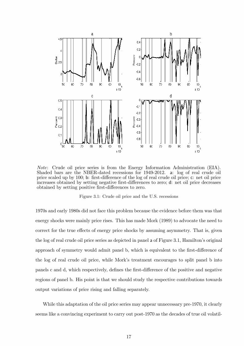
Note: Crude oil price series is from the Energy Information Administration (EIA).Shaded bars are the NBER-dated recessions for 1949-2012. a: log of real crude oilprice scaled up by 100; b: �rst-di¤erence of the log of real crude oil price; c: net oil priceincreases obtained by setting negative �rst-di¤erences to zero; d: net oil price decreasesobtained by setting positive �rst-di¤erences to zero.
Figure 3.1: Crude oil price and the U.S. recessions
1970s and early 1980s did not face this problem because the evidence before them was that
energy shocks were mainly price rises. This has made Mork (1989) to advocate the need to
correct for the true e¤ects of energy price shocks by assuming asymmetry. That is, given
the log of real crude oil price series as depicted in panel a of Figure 3.1, Hamilton�s original
approach of symmetry would admit panel b, which is equivalent to the �rst-di¤erence of
the log of real crude oil price, while Mork�s treatment encourages to split panel b into
panels c and d, which respectively, de�nes the �rst-di¤erence of the positive and negative
regions of panel b. His point is that we should study the respective contributions towards
output variations of price rising and falling separately.
While this adaptation of the oil price series may appear unnecessary pre-1970, it clearly
seems like a convincing experiment to carry out post-1970 as the decades of true oil volatil-
17
ities was ushered in. However, my benchmark approach is to treat energy price shocks
symmetrically. Hooker�s (1997) �nding that data does not support nonlinear and asym-
metric representation of the oil-macroeconomic variable interaction permits this launch
pad plus I am mainly interested in how energy price shocks impact aggregate macroeco-
nomic variables. Moreover, on theoretical grounds, this is the right place to start given
that my model does not capture asymmetric response of macroeconomic variables.
The remainder of this chapter proceeds as follows. In Section 3.2, I describe the main
features of the two-sector model in general form. In Section 3.3, I provide brief discussions
of the econometric method of indirect inference (II) used in estimating the model, the data
serving as the empirical counterparts to model variables, and the initial parameter values
used to initialise the starting points for the Simulated Annealing (SA) algorithm. I present
the main �ndings in Section 3.4 and conclude with Section 3.5.
3.2 The Model
The model is based on Long and Plosser (1983) as augmented by the model of Kim
and Loungani (1992). I set this up as a two-sector open economy model that is essential
to characterising the data properties of a two-sector U.S. open economy. I suppose that
the �nished goods of the two sectors are imperfect substitutes for similar products being
produced abroad; that is, trade is assumed necessary and made possible by representative
households in di¤erent countries who are willing to buy from other countries goods similar
to those being produced in their own countries mainly because they attribute di¤erent
qualities to products based on production origin. In what follows, I suppose that the econ-
omy is populated by a continuum of mass 1 of households, and a continuum of mass 1 of
�rms for each sector in each country. On the supply side, there are two production sectors
consisting of �rms producing two types of goods with di¤erent levels of energy intensities.
The �rms requiring greater amount of energy for production make up the energy intensive,
e, sector producing energy intensive goods, Ye, and the remaining �rms are the non-energy
intensive, n, sector producing non-energy intensive goods, Yn. The crude assumption is
18
that any product that is energy (non-energy) intensive in its production is likewise energy
(non-energy) intensive in its consumption. As is appropriate in this economy, the �rms
are supposed to engage three factors of production, namely: labour hours, capital services,
and primary energy. Labour hours and capital services are assumed to be internationally
immobile, but the domestic �rms import their primary energy requirement.1 Further, the
demand side consists of the households who demand composite consumption good, C,
make decisions on investment, I, pay taxes to or receive bene�ts from the government, T ,
and supply aggregate labour hours, H, which is costlessly shared to the two production
sectors of the domestic economy given the wage rate, W . Households can invest in two
types of physical capital, Ke and Kn, assumed to be subject to capital adjustment cost,
and have access to domestic bonds, B. Hence, they accumulate income from hiring their
labour hours and capital services out to the �rms and from pro�ts accruing due to their
ownership of the �rms and government debts. Lastly, I assume that households carry
out all trades in goods and services with the rest of the world while �rms trade in crude
oil. To simplify matters, the model economy has been described in terms of the domestic
country.2 Meanwhile, all prices have been expressed relative to the general price level
in the rest of the world, which has been chosen to be the numeraire, Pim = 1. I next
characterise the activities of domestic agents mostly in general forms.3
1The U.S. is a net oil importer.2Many open economy models, at least, whenever countries being modelled are allowed to produce
more than one good, are usually assumed to have such products as tradable and non-tradable, exportable(importable) and non-exportable (non-importable), etc. This is a valid assumption, however, given thatthis has been studied extensively, but also and very importantly due to the focus of my study, I haveshut down the non-tradable (/ non-exportable/ non-importable) of the model economies such that forthe purpose of my exercise, I have assumed that all produced goods and services are tradable betweenthe domestic country and the rest of the world. It is meant to be heuristic and I then use this to drawattention to a four-goods world. This is supported by Engel (1999) and Chari et al. (2002): they foundthat variations in the relative price of non-tradable are unimportant for accounting for the changes in realexchange rate. Hence, unlike in Stockman (1980), there is no complete specialisation in the productionof goods.
3I present the main functional forms in a later section, but for detailed and explicit set-up andcharacterisation of the agents�optimisation problems, the �rst-order conditions, and the log-linearisedversion, see the Supplementary Notes: Chapter 3. Foreign agents�problems and solutions can be inferredfrom those of the domestic agents. On the notation, I use the following: UPPER-CASE lettersX 0 � Xt+1,X � Xt, and X�1 � Xt�1 for dynamic variables for next, current, and last period, respectively; lower-caseletters, say x, to denote non-stochastic steady state of variables; hatted letters, �^�, to denote variablesin their log-linear form; and sans serif along with the Greek letters denote the exogenous state variables.
19
Households
The discussion begins with the households�decisions by considering �rst their links
with the domestic �rms and I leave till later their links with the rest of the world. The
lifetime utility function of the representative households is described by
EX1
0��U (C � �C�1; �H) (3.1)
where � denotes the �xed discount factor, � denotes the exogenous intertemporal pref-
erence shock, C denotes aggregate consumption, � denotes the exogenous labour supply
shock, H denotes the supply of labour hours, and � denotes the degree of habit formation.
The function U (�) is assumed to obey standard regularity conditions.
The sequential budget constraint of the household is given by
ER0B0 + C + I + T = B +WH +ReUeKe;�1 +RnUnKn;�1 + � (3.2)
which states that households�expenditure must be equated by their income. E is an ex-
pectation�s operator, ER0 = 1Rdenotes the stochastic discount factor with ER0B0 de�ning
period t�s price of period t+ 1�s random payment of B0, and R denoting interest rate, B
denotes domestic government�s bonds, T denotes lump-sum taxes or transfers, W denotes
consumer real wage rate, Re and Rn are sector-speci�c rental rates of capital services, Ue
and Un are sector-speci�c indexes of capital utilisation rates of the beginning-of-the-period
sector-speci�c capital stocks, Ke;�1 and Kn;�1, and � denotes the pro�t income from their
ownership of �rms.
Further, it is assumed that households choose the stocks of physical capital, Ke;�1 and
Kn;�1, which are, for j = e; n, the beginning-of-the-period t stock of capital in j sector.
Essentially, households determine these variables in period t�1, and are assumed to have
access to the following technologies for altering the quantities of e and n capital stocks
20
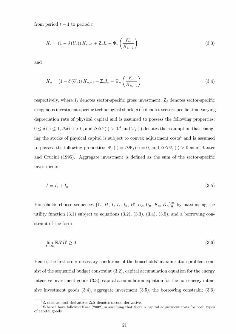
from period t� 1 to period t
Ke = (1� � (Ue))Ke;�1 + ZeIe �e�
Ke
Ke;�1
�(3.3)
and
Kn = (1� � (Un))Kn;�1 + ZnIn �n�
Kn
Kn;�1
�(3.4)
respectively, where Ij denotes sector-speci�c gross investment, Zj denotes sector-speci�c
exogenous investment-speci�c technological shock, � (�) denotes sector-speci�c time-varying
depreciation rate of physical capital and is assumed to possess the following properties:
0 � � (�) � 1, �� (�) > 0, and��� (�) > 0,4 and j (�) denotes the assumption that chang-
ing the stocks of physical capital is subject to convex adjustment costs5 and is assumed
to possess the following properties: j (�) = �j (�) = 0, and ��j (�) > 0 as in Baxter
and Crucini (1995). Aggregate investment is de�ned as the sum of the sector-speci�c
investments
I = Ie + In (3.5)
Households choose sequences fC, H, I, Ie, In, B0, Ue, Un, Ke, Kng10 by maximising the
utility function (3.1) subject to equations (3.2), (3.3), (3.4), (3.5), and a borrowing con-
straint of the form
limt!1
ER0B0 � 0 (3.6)
Hence, the �rst-order necessary conditions of the households�maximisation problem con-
sist of the sequential budget constraint (3.2), capital accumulation equation for the energy
intensive investment goods (3.3), capital accumulation equation for the non-energy inten-
sive investment goods (3.4), aggregate investment (3.5), the borrowing constraint (3.6)
4� denotes �rst derivative; �� denotes second derivative.5Where I have followed Kose (2002) in assuming that there is capital adjustment costs for both types
of capital goods.
21
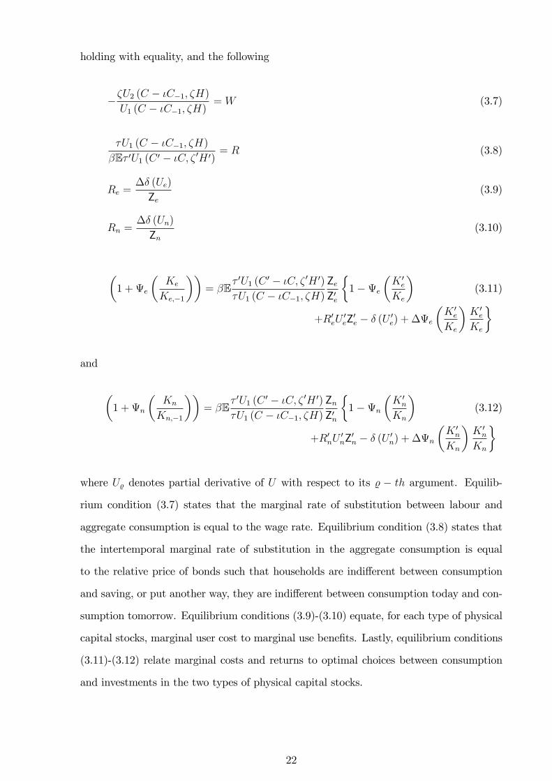
holding with equality, and the following
��U2 (C � �C�1; �H)
U1 (C � �C�1; �H)= W (3.7)
�U1 (C � �C�1; �H)
�E� 0U1 (C 0 � �C; � 0H 0)= R (3.8)
Re =�� (Ue)
Ze(3.9)
Rn =�� (Un)
Zn(3.10)
�1 + e
�Ke
Ke;�1
��= �E
� 0U1 (C0 � �C; � 0H 0)
�U1 (C � �C�1; �H)
ZeZ0e
�1�e
�K 0e
Ke
�(3.11)
+R0eU0eZ0e � � (U 0e) + �e
�K 0e
Ke
�K 0e
Ke
�
and
�1 + n
�Kn
Kn;�1
��= �E
� 0U1 (C0 � �C; � 0H 0)
�U1 (C � �C�1; �H)
ZnZ0n
�1�n
�K 0n
Kn
�(3.12)
+R0nU0nZ
0n � � (U 0n) + �n
�K 0n
Kn
�K 0n
Kn
�
where U% denotes partial derivative of U with respect to its % � th argument. Equilib-
rium condition (3.7) states that the marginal rate of substitution between labour and
aggregate consumption is equal to the wage rate. Equilibrium condition (3.8) states that
the intertemporal marginal rate of substitution in the aggregate consumption is equal
to the relative price of bonds such that households are indi¤erent between consumption
and saving, or put another way, they are indi¤erent between consumption today and con-
sumption tomorrow. Equilibrium conditions (3.9)-(3.10) equate, for each type of physical
capital stocks, marginal user cost to marginal use bene�ts. Lastly, equilibrium conditions
(3.11)-(3.12) relate marginal costs and returns to optimal choices between consumption
and investments in the two types of physical capital stocks.
22
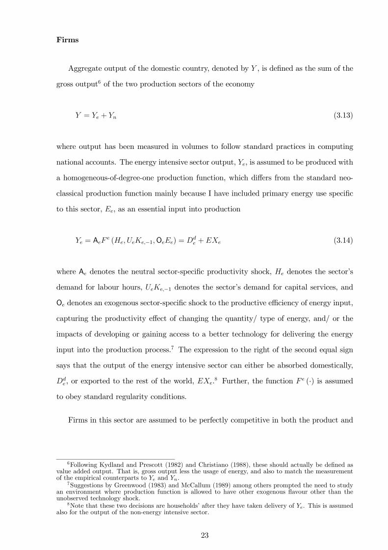
Firms
Aggregate output of the domestic country, denoted by Y , is de�ned as the sum of the
gross output6 of the two production sectors of the economy
Y = Ye + Yn (3.13)
where output has been measured in volumes to follow standard practices in computing
national accounts. The energy intensive sector output, Ye, is assumed to be produced with
a homogeneous-of-degree-one production function, which di¤ers from the standard neo-
classical production function mainly because I have included primary energy use speci�c
to this sector, Ee, as an essential input into production
Ye = AeFe (He; UeKe;�1;OeEe) = Dd
e + EXe (3.14)
where Ae denotes the neutral sector-speci�c productivity shock, He denotes the sector�s
demand for labour hours, UeKe;�1 denotes the sector�s demand for capital services, and
Oe denotes an exogenous sector-speci�c shock to the productive e¢ ciency of energy input,
capturing the productivity e¤ect of changing the quantity/ type of energy, and/ or the
impacts of developing or gaining access to a better technology for delivering the energy
input into the production process.7 The expression to the right of the second equal sign
says that the output of the energy intensive sector can either be absorbed domestically,
Dde , or exported to the rest of the world, EXe.8 Further, the function F e (�) is assumed
to obey standard regularity conditions.
Firms in this sector are assumed to be perfectly competitive in both the product and
6Following Kydland and Prescott (1982) and Christiano (1988), these should actually be de�ned asvalue added output. That is, gross output less the usage of energy, and also to match the measurementof the empirical counterparts to Ye and Yn.
7Suggestions by Greenwood (1983) and McCallum (1989) among others prompted the need to studyan environment where production function is allowed to have other exogenous �avour other than theunobserved technology shock.
8Note that these two decisions are households�after they have taken delivery of Ye. This is assumedalso for the output of the non-energy intensive sector.
23
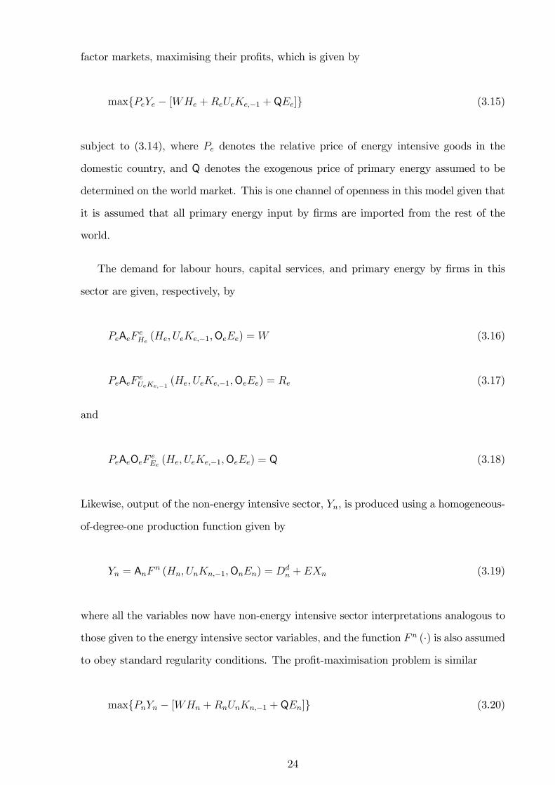
factor markets, maximising their pro�ts, which is given by
maxfPeYe � [WHe +ReUeKe;�1 + QEe]g (3.15)
subject to (3.14), where Pe denotes the relative price of energy intensive goods in the
domestic country, and Q denotes the exogenous price of primary energy assumed to be
determined on the world market. This is one channel of openness in this model given that
it is assumed that all primary energy input by �rms are imported from the rest of the
world.
The demand for labour hours, capital services, and primary energy by �rms in this
sector are given, respectively, by
PeAeFeHe (He; UeKe;�1;OeEe) =W (3.16)
PeAeFeUeKe;�1 (He; UeKe;�1;OeEe) = Re (3.17)
and
PeAeOeFeEe (He; UeKe;�1;OeEe) = Q (3.18)
Likewise, output of the non-energy intensive sector, Yn, is produced using a homogeneous-
of-degree-one production function given by
Yn = AnFn (Hn; UnKn;�1;OnEn) = Dd
n + EXn (3.19)
where all the variables now have non-energy intensive sector interpretations analogous to
those given to the energy intensive sector variables, and the function F n (�) is also assumed
to obey standard regularity conditions. The pro�t-maximisation problem is similar
maxfPnYn � [WHn +RnUnKn;�1 + QEn]g (3.20)
24
subject to (3.19), such that the demand for labour hours, capital services, and primary
energy by �rms in this sector are given, respectively, by
PnAnFnHn (Hn; RnUnKn;�1;OnEn) =W (3.21)
PnAnFnUnKn;�1 (Hn; RnUnKn;�1;OnEn) = Rn (3.22)
and
PnAnOnFnEn (Hn; RnUnKn;�1;OnEn) = Q (3.23)
Note that perfect competition implies that the �rms��rst-order conditions in both sectors
simply equate the marginal product of each input to its marginal cost.
Government
The government is also included in the current model and assumed to face the following
sequential budget constraint
G+B = T + ER0B0 (3.24)
where G denotes the exogenous government spending shock, and I follow An and Schorfheide
(2007) and Justiniano et al. (2009) in assuming that the �scal stance of the government
is fully Ricardian. Thus, the government through the Treasury can raise or reduce taxes
or transfers, and via the Federal Reserve increase or lower the short-term nominal interest
rate to achieve its policy stance.
25
Trade in Goods with the Rest of the World
So far I have discussed the model economy as if it was a closed one except for the
mention of the purchase of primary energy by �rms on the world market. This has
been done intentionally hoping that this structure helps in making the model interactions
more intelligible. I am now ready to open the model up more both between sectors
and between countries. My working assumption is that consumption, investment, and
government spending in the domestic country and rest of the world are composites of
domestic and the rest of the world�s energy and non-energy intensive goods. Clearly, I
have assumed away any extra costs that may arise due to import or export of a good or
service such as transport costs. Thus, I can de�ne the bundles of consumption, investment,
and government spending, respectively, as
C = �C�Cdpe ; C
dpn ; C
fpe ; C
fpn
�(3.25)
I = �I�Idpe ; I
dpn ; I
fpe ; I
fpn
�(3.26)
and
G = �G�Gdpe ;G
dpn ;G
fpe ;G
fpn
�(3.27)
where, for f = C; I;G, the aggregator function �f is supposed to be increasing and
homogeneous-of-degree-one in all its arguments, and for variable V = C; I;G, superscript
dp (fp) with subscript e (n) implies demand for domestically produced (foreign-produced)
energy (non-energy) intensive goods.
One way to proceed from here would be to choose a functional form for �f , and
given that households and the government have chosen their expenditures on C, I, and
G, then their respective problems reduce to that of maximising their utilities and pro�ts
by optimally allocating their aggregate expenditures among the components of each of C,
I, and G. This will yield the result I am looking for, but the number of variables and
expressions will, indeed, increase with this approach, and needlessly so, especially given
26
that my research goal does not require this much level of disaggregation. So, I do not
pursue this approach.
A second approach would be to continue to think in terms of aggregate variables as
much as is possible without compromising on the research goal. In fact, it so happens that
an easier way to deal with this is to remember that the sum of aggregate consumption,
aggregate investment, and aggregate government spending de�nes the aggregate spend-
ing of domestic households (or equivalently, is the domestic absorption), which can be
formalised as
D = C + I + G (3.28)
where, by implication, D is a composite of all the four types of goods
D = ��Dd; IM
�(3.29)
where the aggregator function � is supposed to be increasing and homogeneous-of-degree-
one in both its arguments, Dd denotes the quantity of domestically produced goods de-
manded by domestic residents, and IM denotes total spending of domestic residents on
imports. I �nd it more tractable, therefore, to pursue the analysis this way in terms of
aggregate demand rather than in terms of its components. As shown by Backus, et al.
(1995), the above aggregator function is su¢ cient for use if one is modelling two countries
with two goods as they did. However, I have a model of two countries and four goods
such that I need further disaggregation.
Again, at this junction, I could proceed in either of two ways. First, one could de�ne
the components of D as functions of energy and non-energy intensive goods; that is,
Dd = �d (De; Dn) and IM = �m (IMe; IMn). Second, one could just go back and deal
with D itself �rst de�ning it as a function of energy and non-energy intensive goods, and
given that, one could also split IM into a function of energy and non-energy intensive
27
goods. I favour this latter approach. Hence, both D and IM are de�ned, respectively, by
D = �(De; Dn) (3.30)
and
IM = � (IMe; IMn) (3.31)
where the aggregator functions� and � are supposed to be increasing and homogeneous-of-
degree-one in their arguments, De denotes total spending of domestic residents on energy
intensive goods, Dn denotes total spending of domestic residents on non-energy intensive
goods, IMe denotes total spending of domestic residents on imported energy intensive
goods, and IMn denotes total spending of domestic residents on imported non-energy
intensive goods.
Next, I cast the problems facing domestic residents in light of choices between domes-
tically produced and imported of each type of goods. First, they
minfP dDd + IM � PDg (3.32)
subject to equation (3.29), where P d is the price index for composite domestically produced
goods, P is the consumer price index in the domestic country, and the assumption is that
the consumer price index in the rest of the world, or equivalently the price of imported
composite goods, Pim, is the numeraire. Hence, P is also the real exchange rate.9
I can likewise state another problem for the agents, which consists in
minfPeDe + PnDn � PDg (3.33)
subject to equation (3.30). Then, relying on Walras�law, I shut down activities in the
9This is a crude appropriation of the purchasing power parity hypothesis by using the ratio of theexport and import prices to proxy the exchange rate between two economies.
28
market for the non-energy intensive goods since when the market for energy intensive
goods clear, the law implies that the market for the non-energy intensive goods clear.10
In addition, domestic residents choose the share of expenditure on imported goods
that must be allocated to the purchase of imported energy intensive goods by
minfPime IMe + Pimn IMn � IMg (3.34)
subject to equation (3.31), where Pime and Pimn are prices of imported energy and non-
energy intensive goods, respectively, and are treated as exogenous variables to the domestic
agents.11
Hence, domestic agents choose sequences fDe; IM; IMeg10 and the �rst-order condi-
tions associated with these choices are
�2�Dd; IM
�=1
P(3.35)
�1 (De; Dn) =PeP
(3.36)
and
�1 (IMe; IMn) = Pime (3.37)
where for function � = �;�;�, �% denotes partial derivative of � with respect to its %� th
argument.
In the same vein, I assume that the problems of agents in the rest of the world are a
mirror image to that of agents in the domestic country. Hence, I use the import functions of
foreign households to infer the export functions for the domestic country. More explicitly,
I want to know the quantities of aggregate exported goods and exported energy intensive
10Clearly,Dn = D�De. Thus, having obtained aggregate domestic absorption and domestic absorptionof energy intensive goods implies a solution for the non-energy intensive goods and its components.
11Only Pime appears in the model simulation because of the reason given in the previous footnote.
29
goods. To do this, I assume for the rest of the world that
Dw = �w�Df ; IM f
�(3.38)
where Dw = Cw + Iw + Gw denotes the aggregate world spending or demand, Df denotes
rest of the world�s demand for its own goods, and IM f denotes the aggregate import of
goods by the rest of the world from the domestic economy, which incidentally is equal
to the export of goods to the rest of the world by the domestic country denoted by
EX. So, I �nd it convenient to replace IM f (and its components) with EX (and its
components). Also, �w is supposed to be increasing and homogeneous-of-degree-one in
both its arguments. The required �rst-order condition is with respect to EX and is given
by
�w2�Df ; EX
�= P (3.39)
where �w% denotes partial derivative of �w with respect to its % � th argument. Noting
that EX is also a composite de�ned by
EX = �w�IM f
e ; IMfn
�= �w (EXe; EXn) (3.40)
where the aggregator function �w is supposed to be increasing and homogeneous-of-degree-
one in both its arguments. The required �rst-order condition is with respect to EXe and
is given by
�w1 (EXe; EXn) =PeP
(3.41)
where �w% denotes partial derivative of �w with respect to its %� th argument.
I conclude this sub-section by de�ning the real exchange rate, P , in the domestic
30
country as a function of the relative prices of energy and non-energy intensive goods
P = �(Pe; Pn) (3.42)
Market Clearing and Equilibrium Constraints
In order to close the model, I de�ne some aggregate variables and market-clearing
conditions. Aggregate demand for labour hours by the �rms is the sum of the two sectors�
demand for labour hours and is equal to the supply of labour hours by the households
H = He +Hn (3.43)
Aggregate demand for primary energy input by the �rms is the sum of the two sectors�
demand for primary energy imported from the rest of the world
E = Ee + En (3.44)
I assume for feasibility that the current account constraint is satis�ed in each period
PEX = QE + IM (3.45)
That is, the value of exports equals the value of imports: foreign demand for domestically
produced goods equals domestic demand for primary energy and foreign-produced goods.
A re-interpretation of the prices in the above is that P is the terms of trade in goods and
services, while P=Q is the oil terms of trade.
Given that the current account holds, total demand is, therefore, equal to total supply
D = Y (3.46)
31
Additionally, the sectoral market for energy intensive goods clear
Ye = De + EXe � IMe (3.47)
I am now able to round up this section by providing the de�nition of a competitive
equilibrium for the model.
De�nition 1 A competitive equilibrium is a set of 28 endogenous stochastic processes fC,
I, Ie, In, H, He, Hn, Ke, Kn, Ue, Un, E, Ee, En, Y , Ye, Yn, D, IM , IMe, De, EX, EXe,
P , Pe, Pn, W , Rg10 satisfying equations (3.3), (3.4), (3.5), (3.7), (3.8), (3.11), (3.12),
(3.13), (3.14), (3.16), (3.17), (3.18), (3.19), (3.21), (3.22), (3.23), (3.28), (3.35), (3.36),
(3.37), (3.39), (3.41), (3.42), (3.43), (3.44), (3.45), (3.46), and (3.47), given the set of
12 exogenous stochastic AR(1) processes fAe, An, Dw, G, �, Oe, On, Pime , Q, � , Ze, Zng10 ,
and the initial conditions C�1, Ke�1, K
n�1 and B0.
12
3.3 Econometric Methodology
In this section, I discuss the method of indirect inference used to evaluate and estimate
the model, and provide a documentation of the data used for estimation.
Indirect Inference
The econometric method of indirect inference (II) is adopted to evaluate the model�s
capacity to �t the data. This procedure is originally proposed in Minford et al. (2009)
and subsequently with a number of re�nements by Le et al. (2011) who evaluate the
method using Monte Carlo experiments. I only provide a brief overview here.13 The
approach employs an auxiliary model that is completely independent of the theoretical
12Note that in de�ning the competitive equilibrium and in the model simulation, I have combinedthe �rms��rst-order conditions with respect to capital services, (3.17) and (3.22) with the households��rst-order conditions with respect to capital utilisation rates, (3.9) and (3.10).
13Interested readers may consult Minford et al. (2009) and Le et al. (2011, 2012), and the referencestherein for details.
32
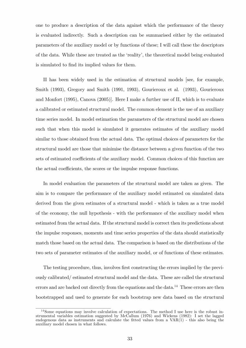
one to produce a description of the data against which the performance of the theory
is evaluated indirectly. Such a description can be summarised either by the estimated
parameters of the auxiliary model or by functions of these; I will call these the descriptors
of the data. While these are treated as the �reality�, the theoretical model being evaluated
is simulated to �nd its implied values for them.
II has been widely used in the estimation of structural models [see, for example,
Smith (1993), Gregory and Smith (1991, 1993), Gourieroux et al. (1993), Gourieroux
and Monfort (1995), Canova (2005)]. Here I make a further use of II, which is to evaluate
a calibrated or estimated structural model. The common element is the use of an auxiliary
time series model. In model estimation the parameters of the structural model are chosen
such that when this model is simulated it generates estimates of the auxiliary model
similar to those obtained from the actual data. The optimal choices of parameters for the
structural model are those that minimise the distance between a given function of the two
sets of estimated coe¢ cients of the auxiliary model. Common choices of this function are
the actual coe¢ cients, the scores or the impulse response functions.
In model evaluation the parameters of the structural model are taken as given. The
aim is to compare the performance of the auxiliary model estimated on simulated data
derived from the given estimates of a structural model - which is taken as a true model
of the economy, the null hypothesis - with the performance of the auxiliary model when
estimated from the actual data. If the structural model is correct then its predictions about
the impulse responses, moments and time series properties of the data should statistically
match those based on the actual data. The comparison is based on the distributions of the
two sets of parameter estimates of the auxiliary model, or of functions of these estimates.
The testing procedure, thus, involves �rst constructing the errors implied by the previ-
ously calibrated/ estimated structural model and the data. These are called the structural
errors and are backed out directly from the equations and the data.14 These errors are then
bootstrapped and used to generate for each bootstrap new data based on the structural
14Some equations may involve calculation of expectations. The method I use here is the robust in-strumental variables estimation suggested by McCallum (1976) and Wickens (1982): I set the laggedendogenous data as instruments and calculate the �tted values from a VAR(1) - this also being theauxiliary model chosen in what follows.
33
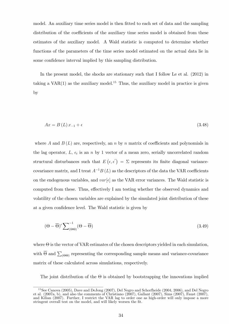
model. An auxiliary time series model is then �tted to each set of data and the sampling
distribution of the coe¢ cients of the auxiliary time series model is obtained from these
estimates of the auxiliary model. A Wald statistic is computed to determine whether
functions of the parameters of the time series model estimated on the actual data lie in
some con�dence interval implied by this sampling distribution.
In the present model, the shocks are stationary such that I follow Le et al. (2012) in
taking a VAR(1) as the auxiliary model.15 Thus, the auxiliary model in practice is given
by
Ax = B (L)x�1 + � (3.48)
where A and B (L) are, respectively, an n by n matrix of coe¢ cients and polynomials in
the lag operator, L, �t is an n by 1 vector of a mean zero, serially uncorrelated random
structural disturbances such that E��; �
0�= � represents its �nite diagonal variance-
covariance matrix, and I treat A�1B (L) as the descriptors of the data the VAR coe¢ cients
on the endogenous variables, and var[�] as the VAR error variances. The Wald statistic is
computed from these. Thus, e¤ectively I am testing whether the observed dynamics and
volatility of the chosen variables are explained by the simulated joint distribution of these
at a given con�dence level. The Wald statistic is given by
(���)0X�1
(��)(���) (3.49)
where� is the vector of VAR estimates of the chosen descriptors yielded in each simulation,
with � andP
(��) representing the corresponding sample means and variance-covariance
matrix of these calculated across simulations, respectively.
The joint distribution of the � is obtained by bootstrapping the innovations implied
15See Canova (2005), Dave and DeJong (2007), Del Negro and Schorfheide (2004, 2006), and Del Negroet al. (2007a, b), and also the comments of Christiano (2007), Gallant (2007), Sims (2007), Faust (2007),and Kilian (2007). Further, I restrict the VAR lag to order one as high-order will only impose a morestringent overall test on the model, and will likely worsen the �t.
34
by the data and the theoretical model; it is, therefore, an estimate of the small sample
distribution.16 Such a distribution is generally more accurate for small samples than the
asymptotic distribution; it is also shown to be consistent by Le et al. (2011) given that
the Wald statistic is �asymptotically pivotal�; they also showed it had quite good accuracy
in small sample Monte Carlo experiments.17
This testing procedure is then applied to a set of structural parameters, which have
been derived from calibration, estimation, or both, and put forward as the true ones; this
is the null hypothesis: H0. Regardless of how the parameters are obtained, the test then
asks, "Could these coe¢ cients within this model structure be the true numerical data
generating process?" Of course only one true model with one set of coe¢ cients is possible.
Nevertheless, one may have chosen coe¢ cients that are not exactly right numerically, so
that the same model with other coe¢ cient values could be correct. Only when one has
examined the model with all coe¢ cient values that are feasible within the model theory
will one have properly tested it. For this reason I later extend the procedure by a further
search algorithm, in which I seek other coe¢ cient sets that could do better in the test.
Thus, I calculate the minimum-value Wald statistic for each period using a powerful
algorithm based on Simulated Annealing (SA) in which search takes place over a wide
range around the initial values, with optimising search accompanied by random jumps
around the space.18 In e¤ect, this is estimation of the model by II; however, this estimation
is being done here to �nd whether the model can be rejected in itself and not for the sake
of �nding the most satisfactory estimates of the model parameters. Nevertheless of course
the method does this latter task as a by-product so that I can use the resulting unrejected
model as representing the best available estimated version. The merit of this extended
16The bootstraps in the tests are all drawn as time vectors so contemporaneous correlations betweenthe innovations are preserved.
17Speci�cally, they found on stationary data that the bias due to bootstrapping was just over 2% atthe 95% con�dence level and 0:6% at the 99% level. Meenagh et al. (2012) found even greater accuracyin Monte Carlo experiments on nonstationary data.
18I use a Simulated Annealing algorithm due to Ingber (1996). This mimics the behaviour of thesteel cooling process in which steel is cooled, with a degree of reheating at randomly chosen momentsin the cooling process - this ensures that the defects are minimised globally. Similarly, the algorithmsearches in the chosen range and as points that improve the objective are found it also accepts pointsthat do not improve the objective. This helps to stop the algorithm being caught in local minima. I�nd that this algorithm improves substantially here on a standard optimisation algorithm. My methodused a standard testing method: I take a set of model parameters (excluding error processes), extract theresulting residuals from the data using the LIML method, �nd their implied autoregressive coe¢ cients[AR(1) here] and then bootstrap the implied innovations with this full set of parameters to �nd theimplied Wald value. This is then minimised by the SA algorithm.
35
procedure is that one is able to compare the best possible versions of each model type
when �nally doing the comparison of model compatibility with the data.19
Data
Figure 3.3 displays the time paths for the data series that I make use of in the evaluation
and estimation of the model. These are U.S. annual data covering the period 1949-2013,
and are logarithmically transformed, real [using Bureau of Labour Statistics (BLS) series:
consumer price index (CPI, 2009=100)] per capita [using Bureau of Labour Statistics
(BLS) series: civilian non-institutionalised population over 16 years old] terms except for
wage rate, interest rate, real exchange rate, relative prices, and capital utilisation rates.
All series are �ltered following Hodrick and Prescott (1981, 1997) procedure setting the
smoothing parameter to 400. A detailed description of the data sources and construction
of the 28 observables (empirical counterparts to the endogenous variables) are presented
in the Supplementary Notes: Chapter 3.
3.4 Results
The presentation of results in this section is divided into two parts: the calibrated
version of the model is analysed in the �rst sub-section, and in the second sub-section, I
summarise the results from the estimated version of the model.
Empirical Analysis 1
In this part, I discuss the simulation of the model, the choice of speci�c functional
forms, the calibration of the model parameters, and quantitatively test the �t of the
model to data for a number of key macroeconomic variables.
19See Le et al. (2013) for a discussion of the advantages of using II method.
36
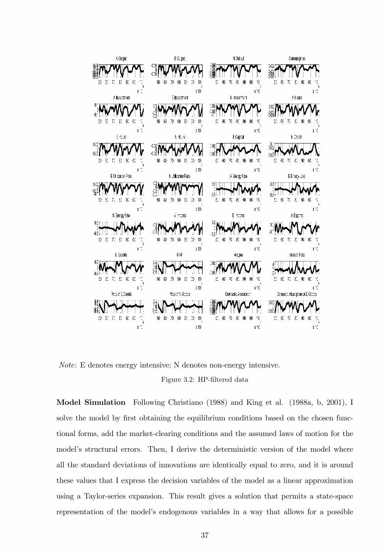
Note: E denotes energy intensive; N denotes non-energy intensive.
Figure 3.2: HP-�ltered data
Model Simulation Following Christiano (1988) and King et al. (1988a, b, 2001), I
solve the model by �rst obtaining the equilibrium conditions based on the chosen func-
tional forms, add the market-clearing conditions and the assumed laws of motion for the
model�s structural errors. Then, I derive the deterministic version of the model where
all the standard deviations of innovations are identically equal to zero, and it is around
these values that I express the decision variables of the model as a linear approximation
using a Taylor-series expansion. This result gives a solution that permits a state-space
representation of the model�s endogenous variables in a way that allows for a possible
37
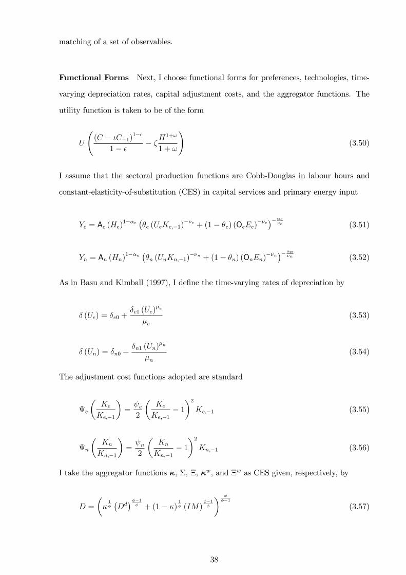
matching of a set of observables.
Functional Forms Next, I choose functional forms for preferences, technologies, time-
varying depreciation rates, capital adjustment costs, and the aggregator functions. The
utility function is taken to be of the form
U
(C � �C�1)
1��
1� �� �
H1+!
1 + !
!(3.50)
I assume that the sectoral production functions are Cobb-Douglas in labour hours and
constant-elasticity-of-substitution (CES) in capital services and primary energy input
Ye = Ae (He)1��e ��e (UeKe;�1)
��e + (1� �e) (OeEe)��e���e
�e (3.51)
Yn = An (Hn)1��n ��n (UnKn;�1)
��n + (1� �n) (OnEn)��n���n
�n (3.52)
As in Basu and Kimball (1997), I de�ne the time-varying rates of depreciation by
� (Ue) = �e0 +�e1 (Ue)
�e
�e(3.53)
� (Un) = �n0 +�n1 (Un)
�n
�n(3.54)
The adjustment cost functions adopted are standard
e
�Ke
Ke;�1
�= e2
�Ke
Ke;�1� 1�2
Ke;�1 (3.55)
n
�Kn
Kn;�1
�= n2
�Kn
Kn;�1� 1�2
Kn;�1 (3.56)
I take the aggregator functions �, �, �, �w, and �w as CES given, respectively, by
D =
��1��Dd���1
� + (1� �)1� (IM)
��1�
� ���1
(3.57)
38
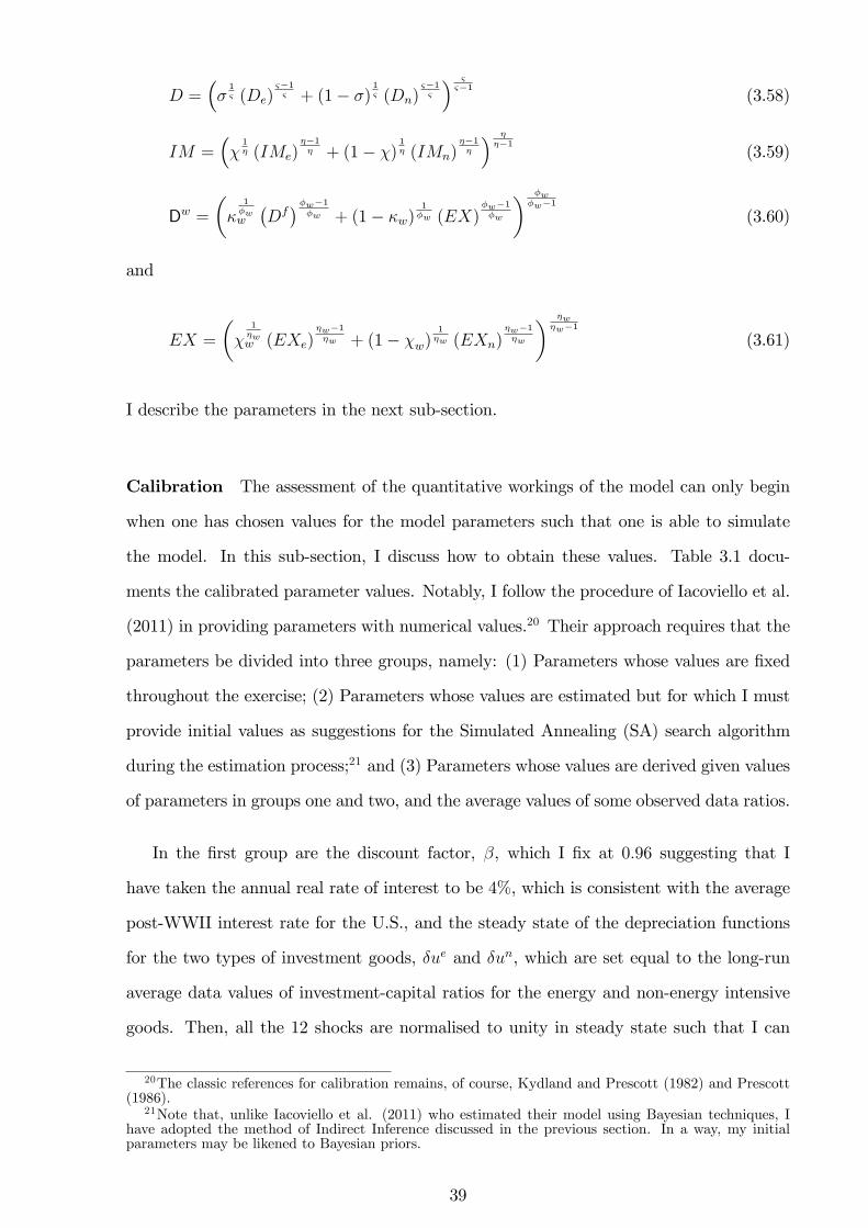
D =��1& (De)
&�1& + (1� �)
1& (Dn)
&�1&
� &&�1
(3.58)
IM =��1� (IMe)
��1� + (1� �)
1� (IMn)
��1�
� ���1
(3.59)
Dw =
��
1�ww
�Df��w�1
�w + (1� �w)1�w (EX)
�w�1�w
� �w�w�1
(3.60)
and
EX =
��
1�ww (EXe)
�w�1�w + (1� �w)
1�w (EXn)
�w�1�w
� �w�w�1
(3.61)
I describe the parameters in the next sub-section.
Calibration The assessment of the quantitative workings of the model can only begin
when one has chosen values for the model parameters such that one is able to simulate
the model. In this sub-section, I discuss how to obtain these values. Table 3.1 docu-
ments the calibrated parameter values. Notably, I follow the procedure of Iacoviello et al.
(2011) in providing parameters with numerical values.20 Their approach requires that the
parameters be divided into three groups, namely: (1) Parameters whose values are �xed
throughout the exercise; (2) Parameters whose values are estimated but for which I must
provide initial values as suggestions for the Simulated Annealing (SA) search algorithm
during the estimation process;21 and (3) Parameters whose values are derived given values
of parameters in groups one and two, and the average values of some observed data ratios.
In the �rst group are the discount factor, �, which I �x at 0:96 suggesting that I
have taken the annual real rate of interest to be 4%, which is consistent with the average
post-WWII interest rate for the U.S., and the steady state of the depreciation functions
for the two types of investment goods, �ue and �un, which are set equal to the long-run
average data values of investment-capital ratios for the energy and non-energy intensive
goods. Then, all the 12 shocks are normalised to unity in steady state such that I can
20The classic references for calibration remains, of course, Kydland and Prescott (1982) and Prescott(1986).
21Note that, unlike Iacoviello et al. (2011) who estimated their model using Bayesian techniques, Ihave adopted the method of Indirect Inference discussed in the previous section. In a way, my initialparameters may be likened to Bayesian priors.
39
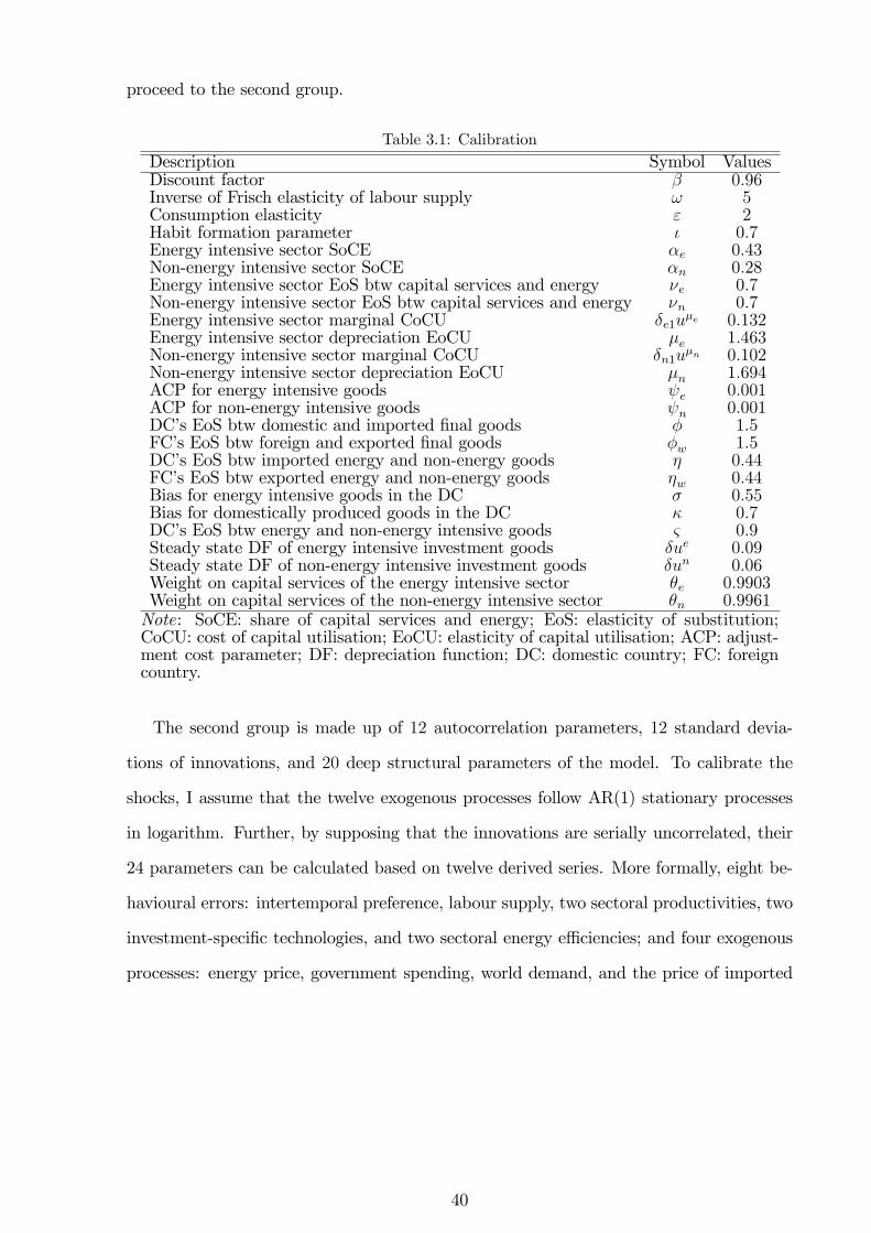
proceed to the second group.
Table 3.1: CalibrationDescription Symbol ValuesDiscount factor � 0:96Inverse of Frisch elasticity of labour supply ! 5Consumption elasticity " 2Habit formation parameter � 0:7Energy intensive sector SoCE �e 0:43Non-energy intensive sector SoCE �n 0:28Energy intensive sector EoS btw capital services and energy �e 0:7Non-energy intensive sector EoS btw capital services and energy �n 0:7Energy intensive sector marginal CoCU �e1u
�e 0:132Energy intensive sector depreciation EoCU �e 1:463Non-energy intensive sector marginal CoCU �n1u
�n 0:102Non-energy intensive sector depreciation EoCU �n 1:694ACP for energy intensive goods e 0:001ACP for non-energy intensive goods n 0:001DC�s EoS btw domestic and imported �nal goods � 1:5FC�s EoS btw foreign and exported �nal goods �w 1:5DC�s EoS btw imported energy and non-energy goods � 0:44FC�s EoS btw exported energy and non-energy goods �w 0:44Bias for energy intensive goods in the DC � 0:55Bias for domestically produced goods in the DC � 0:7DC�s EoS btw energy and non-energy intensive goods & 0:9Steady state DF of energy intensive investment goods �ue 0:09Steady state DF of non-energy intensive investment goods �un 0:06Weight on capital services of the energy intensive sector �e 0:9903Weight on capital services of the non-energy intensive sector �n 0:9961Note: SoCE: share of capital services and energy; EoS: elasticity of substitution;CoCU: cost of capital utilisation; EoCU: elasticity of capital utilisation; ACP: adjust-ment cost parameter; DF: depreciation function; DC: domestic country; FC: foreigncountry.
The second group is made up of 12 autocorrelation parameters, 12 standard devia-
tions of innovations, and 20 deep structural parameters of the model. To calibrate the
shocks, I assume that the twelve exogenous processes follow AR(1) stationary processes
in logarithm. Further, by supposing that the innovations are serially uncorrelated, their
24 parameters can be calculated based on twelve derived series. More formally, eight be-
havioural errors: intertemporal preference, labour supply, two sectoral productivities, two
investment-speci�c technologies, and two sectoral energy e¢ ciencies; and four exogenous
processes: energy price, government spending, world demand, and the price of imported
40
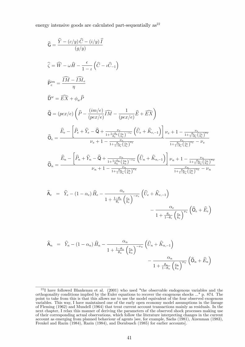
energy intensive goods are calculated part-sequentially as22
bG = bY � (c=y) bC � (i=y) bI(g=y)
b� = cW � ! bH � �
1� �
� bC � � bC�1�bPime =
dIM �dIM e
�
bDw = dEX + �w bPbQ = (pex=e)�bP � (im=e)
(pex=e)dIM � 1
(pex=e)bE +dEX�
bOe = bEe � � bPe + bYe � bQ+ �e
1+ 1��e�e( eeke )
��e
�bUe + bKe;�1
���e + 1� �e
1+ �e1��e (
eeke)�e
�e + 1� �e1+ �e
1��e (eeke)�e
�e1+ �e
1��e (eeke)�e � �e
bOn = bEn � � bPn + bYn � bQ+ �n
1+ 1��n�n( enkn )
��n
�bUn + bKn;�1
���n + 1� �n
1+ �n1��n (
enkn)�n
�n + 1� �n1+ �n
1��n (enkn)�n
�n1+ �n
1��n (enkn)�n � �n
bAe = bYe � (1� �e) bHe ��e
1 + 1��e�e
�eeke
���e �bUe + bKe;�1
�� �e
1 + �e1��e
�eeke
��e �bOe + bEe�
bAn = bYn � (1� �n) bHn ��n
1 + 1��n�n
�enkn
���n �bUn + bKn;�1
�� �n
1 + �n1��n
�enkn
��n �bOn + bEn�
22I have followed Blankenau et al. (2001) who used "the observable endogenous variables and theorthogonality conditions implied by the Euler equations to recover the exogenous shocks ..." p. 874. Thepoint to take from this is that this allows me to use the model equivalent of the four observed exogenousvariables. This way, I have maintained one of the early open economy model assumptions in the lineageof Fleming (1962) and Mundell (1964) that treat current account transactions mainly as residuals. In thenext chapter, I relax this manner of deriving the parameters of the observed shock processes making useof their corresponding actual observations, which follow the literature interpreting changes in the currentaccount as emerging from planned behaviour of agents [see, for example, Sachs (1981), Aizenman (1983),Frenkel and Razin (1984), Razin (1984), and Dornbusch (1985) for earlier accounts].
41
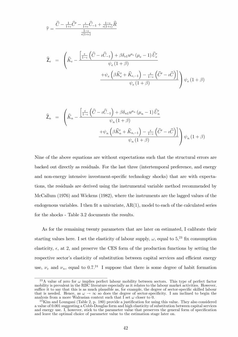
b� = bC � 11+�bC 0 � �
1+�bC�1 + 1��
�(1+�)bR
1���(1+�)
bZe =
0@ bKe �
h�1��
� bC � � bC�1�+ ��e1u�e (�e � 1) bU 0e
e (1 + �)
+ e
�� bK 0
e + bKe;�1
�� �
1��
� bC 0 � � bC�i e (1 + �)
1A e (1 + �)
bZn =
0@ bKn �
h�1��
� bC � � bC�1�+ ��n1u�n (�n � 1) bU 0n
n (1 + �)
+ n
�� bK 0
n +bKn;�1
�� �
1��
� bC 0 � � bC�i n (1 + �)
1A n (1 + �)
Nine of the above equations are without expectations such that the structural errors are
backed out directly as residuals. For the last three (intertemporal preference, and energy
and non-energy intensive investment-speci�c technology shocks) that are with expecta-
tions, the residuals are derived using the instrumental variable method recommended by
McCallum (1976) and Wickens (1982), where the instruments are the lagged values of the
endogenous variables. I then �t a univariate, AR(1), model to each of the calculated series
for the shocks - Table 3.2 documents the results.
As for the remaining twenty parameters that are later on estimated, I calibrate their
starting values here. I set the elasticity of labour supply, !, equal to 5,23 �x consumption
elasticity, �, at 2, and preserve the CES form of the production functions by setting the
respective sector�s elasticity of substitution between capital services and e¢ cient energy
use, �e and �n, equal to 0:7.24 I suppose that there is some degree of habit formation
23A value of zero for ! implies perfect labour mobility between sectors. This type of perfect factormobility is prevalent in the RBC literature especially as it relates to the labour market activities. However,su¢ ce it to say that this is as much plausible as, for example, the degree of sector-speci�c skilled labourthat is needed. Hence, as ! ! 1 so does the degree of sector-speci�city. I am inclined to begin theanalysis from a more Walrasian context such that I set ! closer to 0.
24Kim and Loungani (Table 2, p. 180) provide a justi�cation for using this value. They also considereda value of 0:001 suggesting a Cobb-Douglas form and high elasticity of substitution between capital servicesand energy use. I, however, stick to the parameter value that preserves the general form of speci�cationand leave the optimal choice of parameter value to the estimation stage later on.
42
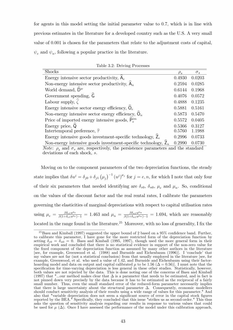
for agents in this model setting the initial parameter value to 0:7, which is in line with
previous estimates in the literature for a developed country such as the U.S. A very small
value of 0:001 is chosen for the parameters that relate to the adjustment costs of capital,
e and n, following a popular practice in the literature.
Table 3.2: Driving ProcessesShocks �s �sEnergy intensive sector productivity, bAe 0:4930 0:0203
Non-energy intensive sector productivity, bAn 0:2594 0:0285
World demand, bDw 0:6144 0:1968
Government spending, bG 0:4076 0:0572
Labour supply, b� 0:4888 0:1235
Energy intensive sector energy e¢ ciency, bOe 0:5881 0:5161
Non-energy intensive sector energy e¢ ciency, bOn 0:5873 0:5470
Price of imported energy intensive goods, bPime 0:5572 0:0405
Energy price, bQ 0:5366 0:3127Intertemporal preference, b� 0:5760 1:1988
Energy intensive goods investment-speci�c technology, bZe 0:2996 0:0733
Non-energy intensive goods investment-speci�c technology, bZn 0:2990 0:0730Note: �s and �s are, respectively, the persistence parameters and the standarddeviations of each shock, s.
Moving on to the component parameters of the two depreciation functions, the steady
state implies that �uj = �j0+ �j1��j��1
(uj)�j for j = e; n, for which I note that only four
of their six parameters that needed identifying are �e0, �n0, �e and �n. So, conditional
on the values of the discount factor and the real rental rates, I calibrate the parameters
governing the elasticities of marginal depreciations with respect to capital utilisation rates
using �e =��e1u�e
�(1+�e1u�e )�1 = 1:463 and �n =��n1u�n
�(1+�n1u�n )�1 = 1:694, which are reasonably
located in the range found in the literature.25 Moreover, with no loss of generality, I �x the
25Basu and Kimball (1997) suggested the upper bound of 2 based on a 95% con�dence band. Further,to calibrate this parameter, I have gone for the more restricted form of the depreciation function bysetting �e0 = �n0 = 0. Basu and Kimball (1995, 1997), though used the more general form in theirempirical work and concluded that there is no statistical evidence in support of the non-zero value forthe �xed component of the depreciation function as assumed by many other authors in the literature[see, for example, Greenwood et al. (1988) and Burnside and Eichenbaum (1996)]. I �conclude� thatmy values are not far (not a statistical conclusion) from that usually employed in the literature [see, forexample, Greenwood, et al. who used a value of 1:42, and Burnside and Eichenbaum using their factor-hoarding model and data on output and capital calibrated � to be 1:56 (� = 0:56)]. I must note that thespeci�cation for time-varying depreciation is less general in these other studies. Statistically, however,both values are not rejected by the data. This is done noting one of the concerns of Basu and Kimball(1997) that "...our method makes clear that � is a parameter that needs to be estimated, and in fact isnot pinned down very precisely by the data because it has to be estimated as the reciprocal of a fairlysmall number. Thus, even the small standard error of the reduced-form parameter necessarily impliesthat there is large uncertainty about the structural parameter �. Consequently, economic modellersshould conduct sensitivity analysis of their results using a wide range of values for this parameter." Andalso that "variable depreciation does not seem a signi�cant source of error in the capital stock �guresreported by the BEA." Speci�cally, they concluded that this issue "strikes us as second-order." This thusasks the question of sensitivity analysis regarding our results in response to various values that couldbe used for � (�). Once I have assessed the performance of the model under this calibration approach,
43
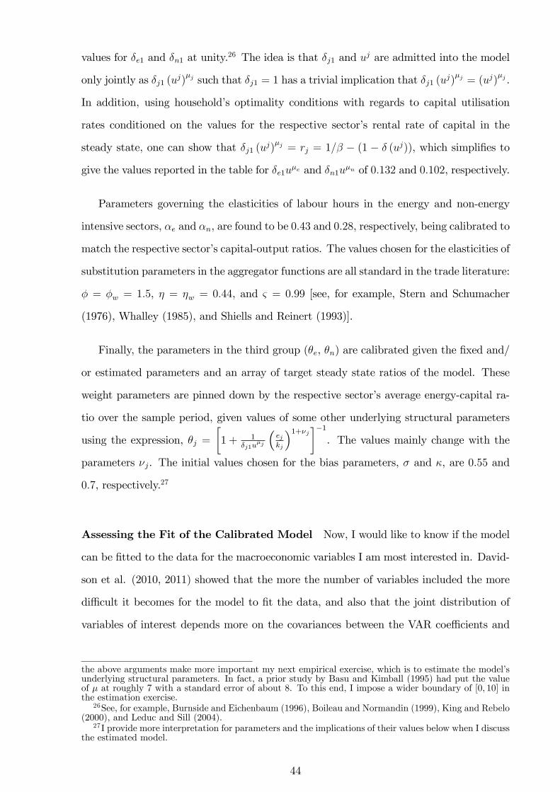
values for �e1 and �n1 at unity.26 The idea is that �j1 and uj are admitted into the model
only jointly as �j1 (uj)�j such that �j1 = 1 has a trivial implication that �j1 (uj)
�j = (uj)�j .
In addition, using household�s optimality conditions with regards to capital utilisation
rates conditioned on the values for the respective sector�s rental rate of capital in the
steady state, one can show that �j1 (uj)�j = rj = 1=� � (1 � � (uj)), which simpli�es to
give the values reported in the table for �e1u�e and �n1u�n of 0:132 and 0:102, respectively.
Parameters governing the elasticities of labour hours in the energy and non-energy
intensive sectors, �e and �n, are found to be 0:43 and 0:28, respectively, being calibrated to
match the respective sector�s capital-output ratios. The values chosen for the elasticities of
substitution parameters in the aggregator functions are all standard in the trade literature:
� = �w = 1:5, � = �w = 0:44, and & = 0:99 [see, for example, Stern and Schumacher
(1976), Whalley (1985), and Shiells and Reinert (1993)].
Finally, the parameters in the third group (�e, �n) are calibrated given the �xed and/
or estimated parameters and an array of target steady state ratios of the model. These
weight parameters are pinned down by the respective sector�s average energy-capital ra-
tio over the sample period, given values of some other underlying structural parameters
using the expression, �j =�1 + 1
�j1u�j
�ejkj
�1+�j��1. The values mainly change with the
parameters �j. The initial values chosen for the bias parameters, � and �, are 0:55 and
0:7, respectively.27
Assessing the Fit of the Calibrated Model Now, I would like to know if the model
can be �tted to the data for the macroeconomic variables I am most interested in. David-
son et al. (2010, 2011) showed that the more the number of variables included the more
di¢ cult it becomes for the model to �t the data, and also that the joint distribution of
variables of interest depends more on the covariances between the VAR coe¢ cients and
the above arguments make more important my next empirical exercise, which is to estimate the model�sunderlying structural parameters. In fact, a prior study by Basu and Kimball (1995) had put the valueof � at roughly 7 with a standard error of about 8. To this end, I impose a wider boundary of [0; 10] inthe estimation exercise.
26See, for example, Burnside and Eichenbaum (1996), Boileau and Normandin (1999), King and Rebelo(2000), and Leduc and Sill (2004).
27I provide more interpretation for parameters and the implications of their values below when I discussthe estimated model.
44
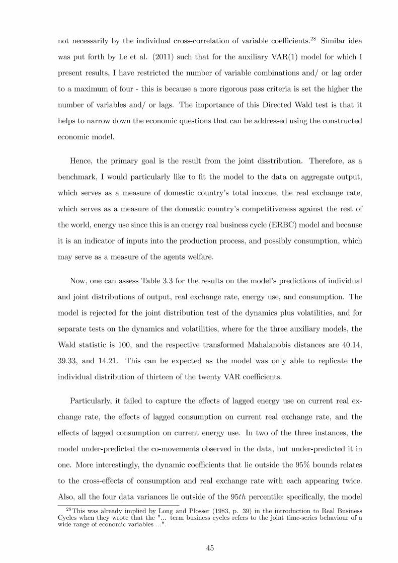
not necessarily by the individual cross-correlation of variable coe¢ cients.28 Similar idea
was put forth by Le et al. (2011) such that for the auxiliary VAR(1) model for which I
present results, I have restricted the number of variable combinations and/ or lag order
to a maximum of four - this is because a more rigorous pass criteria is set the higher the
number of variables and/ or lags. The importance of this Directed Wald test is that it
helps to narrow down the economic questions that can be addressed using the constructed
economic model.
Hence, the primary goal is the result from the joint disstribution. Therefore, as a
benchmark, I would particularly like to �t the model to the data on aggregate output,
which serves as a measure of domestic country�s total income, the real exchange rate,
which serves as a measure of the domestic country�s competitiveness against the rest of
the world, energy use since this is an energy real business cycle (ERBC) model and because
it is an indicator of inputs into the production process, and possibly consumption, which
may serve as a measure of the agents welfare.
Now, one can assess Table 3.3 for the results on the model�s predictions of individual
and joint distributions of output, real exchange rate, energy use, and consumption. The
model is rejected for the joint distribution test of the dynamics plus volatilities, and for
separate tests on the dynamics and volatilities, where for the three auxiliary models, the
Wald statistic is 100, and the respective transformed Mahalanobis distances are 40:14,
39:33, and 14:21. This can be expected as the model was only able to replicate the
individual distribution of thirteen of the twenty VAR coe¢ cients.
Particularly, it failed to capture the e¤ects of lagged energy use on current real ex-
change rate, the e¤ects of lagged consumption on current real exchange rate, and the
e¤ects of lagged consumption on current energy use. In two of the three instances, the
model under-predicted the co-movements observed in the data, but under-predicted it in
one. More interestingly, the dynamic coe¢ cients that lie outside the 95% bounds relates
to the cross-e¤ects of consumption and real exchange rate with each appearing twice.
Also, all the four data variances lie outside of the 95th percentile; speci�cally, the model28This was already implied by Long and Plosser (1983, p. 39) in the introduction to Real Business
Cycles when they wrote that the "... term business cycles refers to the joint time-series behaviour of awide range of economic variables ...".
45
Table 3.3: VAR Results for the Calibrated ModelCoe¢ cients Actual Lower Bound Upper Bound Mean
�bY ;bY 0:4913 �0:2048 1:2775 0:5753� bP ;bY �0:0076 �0:8295 0:9103 0:0572� bE;bY �0:0354 �0:1424 0:1600 0:0121� bC;bY 0:1080 �0:1121 0:1875 0:0255�bY ; bP 0:0047 �0:6448 0:3742 �0:1102� bP ; bP 0:6797 �0:1720 0:9948 0:4269
� bE; bP 0:1341{ �0:1331 0:0861 �0:0226� bC; bP 0:4435{ �0:1358 0:0862 �0:0207�bY ; bE 0:4621 �1:6359 1:7728 0:1506� bP ; bE �0:1641 �2:3913 1:9571 �0:0564� bE; bE 0:4959 0:1970 0:8475 0:5445
� bC; bE �1:2027{ �0:3194 0:4214 0:0378�bY ; bC 0:0697 �1:3391 0:7529 �0:2228� bP ; bC 0:0041 �1:3542 0:9729 �0:1666� bE; bC �0:0198 �0:1893 0:2235 0:0173� bC; bC 0:5978 0:5854 0:9816 0:8255
�2bY 0:0009\ 0:0139 0:0369 0:0241
�2bP 0:0314\ 0:0077 0:0199 0:0128
�2bE 0:0413\ 0:0778 0:2410 0:1514
�2bC 0:0004\ 0:0485 0:2361 0:1230Dynamics+Volatilities Dynamics Volatilities
Wald (%) 100 100 100TMD 40:14 39:33 14:21Note: �i;j denotes the VAR coe¢ cient of a lagged variable i on a variable j;�2j denotes the variance of variable j; bY denotes aggregate output; bP denotes
the real exchange rate; bE denotes aggregate energy use; bC denotes consumption;TMD denotes transformed Mahalanobis distance. {The VAR coe¢ cients that lieoutside of the 95% con�dence bounds; \the data variances of the variables thatlie outside of the 95% con�dence bounds.
over-projects the volatilities of output, consumption, and energy use, but under-projects
the variability in real exchange rate.
Empirical Analysis 2
Parameter Estimates I begin the discussion of the empirical results by considering the
estimated parameters in Table 3.4 where the calibrated values from Table 3.1 serve as the
initial values for the SA algorithm. Three of the parameters are kept �xed throughout the
exercise: �, �ue, and �un (the last two are indeed the steady state representations of the
depreciation functions), and two are derived from the calibrated/ estimated parameters:
�e and �n. Some of the estimates have values that are not too far from the suggested
46
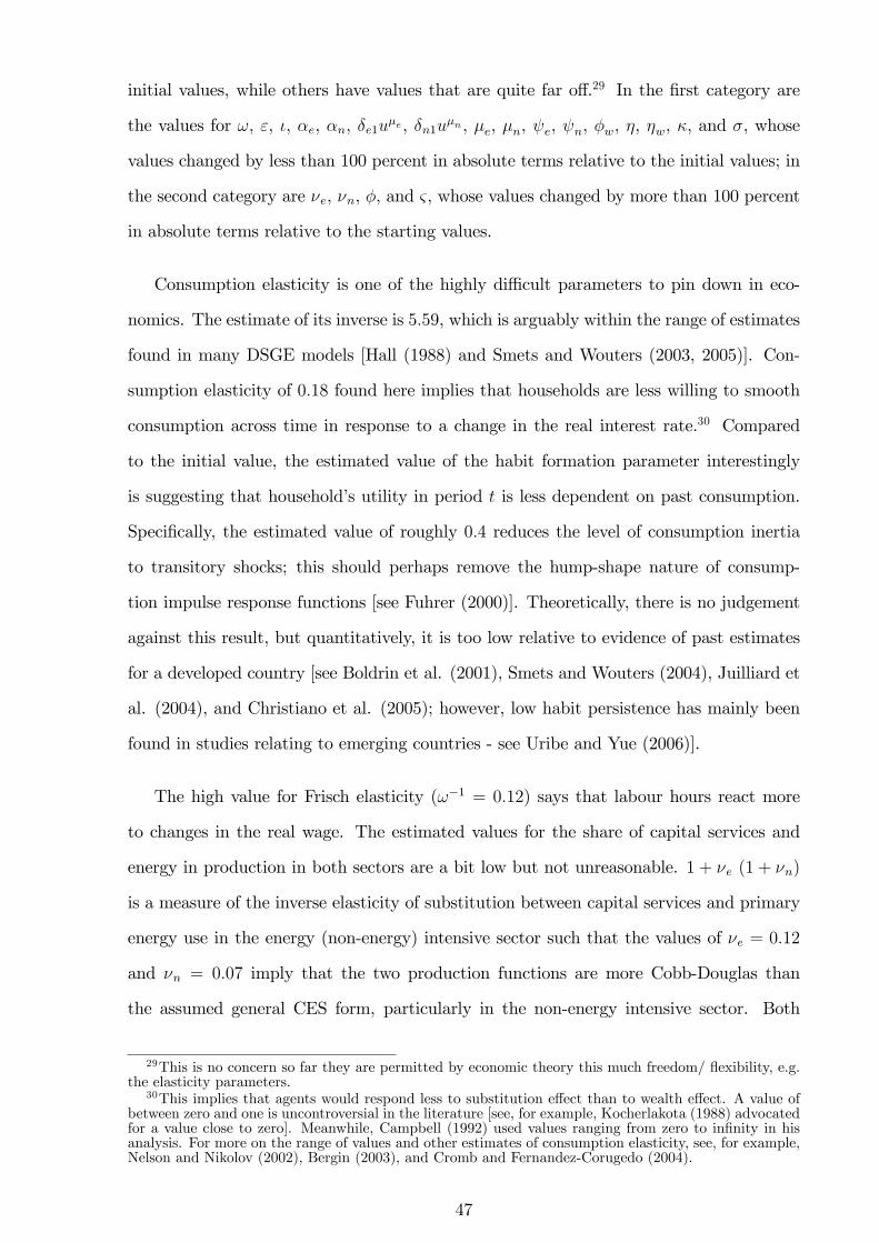
initial values, while others have values that are quite far o¤.29 In the �rst category are
the values for !, ", �, �e, �n, �e1u�e, �n1u�n, �e, �n, e, n, �w, �, �w, �, and �, whose
values changed by less than 100 percent in absolute terms relative to the initial values; in
the second category are �e, �n, �, and &, whose values changed by more than 100 percent
in absolute terms relative to the starting values.
Consumption elasticity is one of the highly di¢ cult parameters to pin down in eco-
nomics. The estimate of its inverse is 5:59, which is arguably within the range of estimates
found in many DSGE models [Hall (1988) and Smets and Wouters (2003, 2005)]. Con-
sumption elasticity of 0:18 found here implies that households are less willing to smooth
consumption across time in response to a change in the real interest rate.30 Compared
to the initial value, the estimated value of the habit formation parameter interestingly
is suggesting that household�s utility in period t is less dependent on past consumption.
Speci�cally, the estimated value of roughly 0:4 reduces the level of consumption inertia
to transitory shocks; this should perhaps remove the hump-shape nature of consump-
tion impulse response functions [see Fuhrer (2000)]. Theoretically, there is no judgement
against this result, but quantitatively, it is too low relative to evidence of past estimates
for a developed country [see Boldrin et al. (2001), Smets and Wouters (2004), Juilliard et
al. (2004), and Christiano et al. (2005); however, low habit persistence has mainly been
found in studies relating to emerging countries - see Uribe and Yue (2006)].
The high value for Frisch elasticity (!�1 = 0:12) says that labour hours react more
to changes in the real wage. The estimated values for the share of capital services and
energy in production in both sectors are a bit low but not unreasonable. 1 + �e (1 + �n)
is a measure of the inverse elasticity of substitution between capital services and primary
energy use in the energy (non-energy) intensive sector such that the values of �e = 0:12
and �n = 0:07 imply that the two production functions are more Cobb-Douglas than
the assumed general CES form, particularly in the non-energy intensive sector. Both
29This is no concern so far they are permitted by economic theory this much freedom/ �exibility, e.g.the elasticity parameters.
30This implies that agents would respond less to substitution e¤ect than to wealth e¤ect. A value ofbetween zero and one is uncontroversial in the literature [see, for example, Kocherlakota (1988) advocatedfor a value close to zero]. Meanwhile, Campbell (1992) used values ranging from zero to in�nity in hisanalysis. For more on the range of values and other estimates of consumption elasticity, see, for example,Nelson and Nikolov (2002), Bergin (2003), and Cromb and Fernandez-Corugedo (2004).
47
Table 3.4: Estimation
Description Symbol Initial Values] EstimationDiscount factorz � 0:96 0:96Inverse of Frisch elasticity of labour supply ! 5 8:64Consumption elasticity " 2 5:59Habit formation parameter � 0:7 0:38Energy intensive sector SoCE �e 0:43 0:43Non-energy intensive sector SoCE �n 0:28 0:39Energy intensive sector EoS btw capital services and energy �e 0:7 0:12Non-energy intensive sector EoS btw capital services and energy �n 0:7 0:07Energy intensive sector marginal CoCU �e1u
�e 0:132 0:32Energy intensive sector depreciation EoCU �e 1:463 5:51Non-energy intensive sector marginal CoCU �n1u
�n 0:102 0:44Non-energy intensive sector depreciation EoCU �n 1:694 4:32ACP for energy intensive goods e 0:001 0:003ACP for non-energy intensive goods n 0:001 0:002DC�s EoS btw domestic and imported �nal goods � 1:5 0:16FC�s EoS btw foreign and exported �nal goods �w 1:5 34:8DC�s EoS btw imported energy and non-energy goods � 0:44 0:51FC�s EoS btw exported energy and non-energy goods �w 0:44 2:12Bias for energy intensive goods in the DC � 0:55 0:48Bias for domestically produced goods in the DC � 0:7 0:68DC�s EoS btw energy and non-energy intensive goods & 0:9 0:27Steady state DF of energy intensive investment goodsz �ue 0:09 0:09Steady state DF of non-energy intensive investment goodsz �un 0:06 0:06Weight on capital services of the energy intensive sector{ �e 0:9902 0:9631Weight on capital services of the non-energy intensive sector{ �n 0:9961 0:9833Note: SoCE: share of capital services and energy; EoS: elasticity of substitution; CoCU: cost of capital util-isation; EoCU: elasticity of capital utilisation; ACP: adjustment cost parameter; DF: depreciation function;DC: domestic country; FC: foreign country. ]Calibrated values are used to initialise the simulated annealingsearch algorithm; zparameters that are �xed throughout the exercise; {parameters that are derived basedon �xed and estimated parameters.
estimates for the adjustment cost parameters are close to zero though they have di¤erent
quantitative impacts on the model. As it is, the value of 0:003 for the energy intensive
capital adjustment cost parameter compared to the 0:002 for the equivalent non-energy
intensive parameter means that the marginal user cost in the energy intensive sector
responds by 50% more to changes in interest rate than does the marginal user cost in the
accumulation of non-energy intensive capital goods.
Further, the estimate of the marginal costs of capital utilisation is 32% in the energy
intensive sector while it is 44% in the non-energy intensive sector. These di¤erent estimates
simply indicate that return to investment/ marginal product of capital services in the non-
energy intensive sector is higher. Greenwood et al. (1988) and related literature [see, for
example, Finn (1991, 1996), Burnside and Eichenbaum (1995), Baxter and Farr (2002),
and Leduc and Sill (2004)] suggest that there is yet to be an empirical guide on the choice
of a value (magnitude) for the elasticity of capital utilisation rate with Basu and Kimball
(1995) admitting that it is a problematic parameter to correctly value. My estimates
48
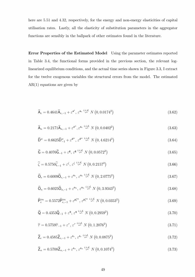
here are 5:51 and 4:32, respectively, for the energy and non-energy elasticities of capital
utilisation rates. Lastly, all the elasticity of substitution parameters in the aggregator
functions are sensibly in the ballpark of other estimates found in the literature.
Error Properties of the Estimated Model Using the parameter estimates reported
in Table 3.4, the functional forms provided in the previous section, the relevant log-
linearized equilibrium conditions, and the actual time series shown in Figure 3.3, I extract
for the twelve exogenous variables the structural errors from the model. The estimated
AR(1) equations are given by
bAe = 0:4641bAe;�1 + "ae
, "aei:i:d:v N
�0; 0:01742
�(3.62)
bAn = 0:2171bAn;�1 + "an
; "aei:i:d:v N
�0; 0:04022
�(3.63)
bDw = 0:6625bDw�1 + "dw
, "dw i:i:d:v N
�0; 4:62142
�(3.64)
bG = 0:4076bG�1 + "g, "gi:i:d:v N
�0; 0:05722
�(3.65)
b� = 0:5750b��1 + "� , "�i:i:d:v N
�0; 0:21572
�(3.66)
bOe = 0:6009bOe;�1 + "oe, "oei:i:d:v N
�0; 2:07752
�(3.67)
bOn = 0:6025bOn;�1 + "on, "oni:i:d:v N
�0; 3:93432
�(3.68)
bPime = 0:5572bPime;�1 + "pime , "p
ime
i:i:d:v N�0; 0:03532
�(3.69)
bQ = 0:4353bQ�1 + "q, "qi:i:d:v N
�0; 0:29592
�(3.70)
b� = 0:5759b��1 + "� , "�i:i:d:v N
�0; 1:20762
�(3.71)
bZe = 0:4585bZe;�1 + "ze, "zei:i:d:v N
�0; 0:08752
�(3.72)
bZn = 0:5708bZn;�1 + "zn, "zni:i:d:v N
�0; 0:10742
�(3.73)
49
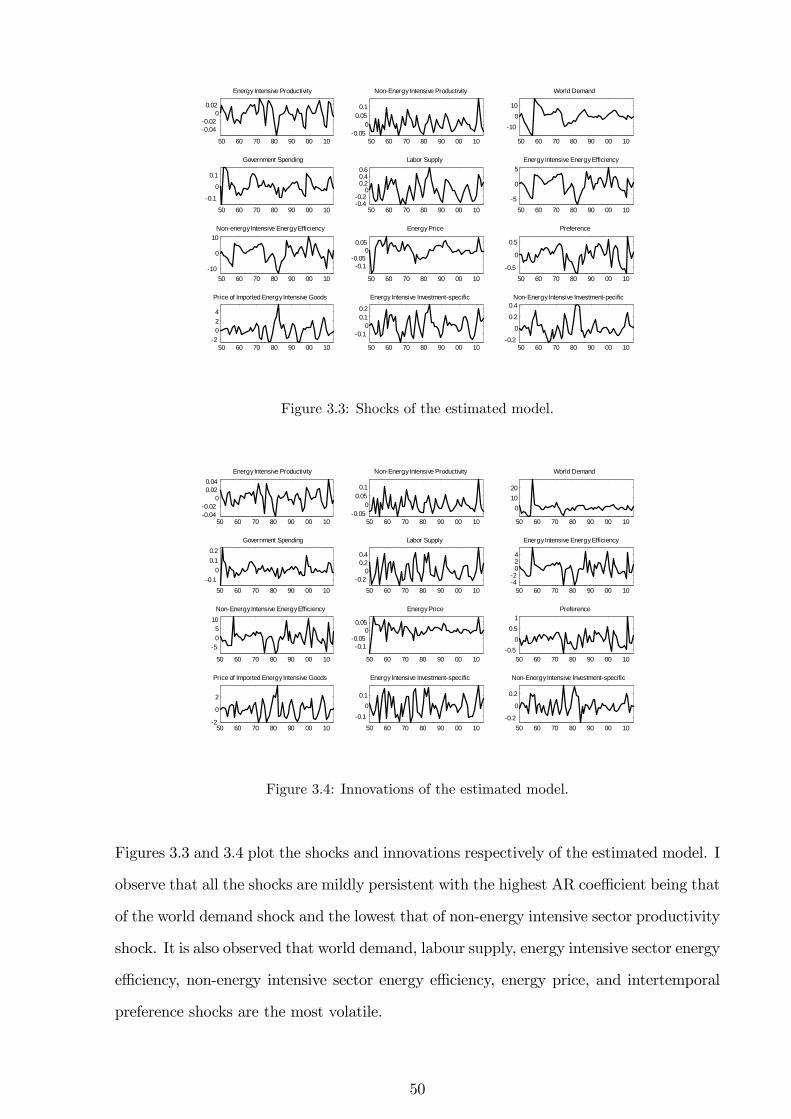
50 60 70 80 90 00 10
0.040.02
00.02
Energy Intensive Productivity
50 60 70 80 90 00 100.05
00.05
0.1
NonEnergy Intensive Productivity
50 60 70 80 90 00 10
100
10
World Demand
50 60 70 80 90 00 10
0.1
0
0.1
Government Spending
50 60 70 80 90 00 100.40.2
00.20.40.6
Labor Supply
50 60 70 80 90 00 105
0
5Energy Intensive Energy Efficiency
50 60 70 80 90 00 1010
0
10Nonenergy Intensive Energy Efficiency
50 60 70 80 90 00 10
0.10.05
00.05
Energy Price
50 60 70 80 90 00 100.5
0
0.5
Preference
50 60 70 80 90 00 102
024
Price of Imported Energy Intensive Goods
50 60 70 80 90 00 10
0.10
0.10.2
Energy Intensive Investmentspecific
50 60 70 80 90 00 100.2
0
0.2
0.4NonEnergy Intensive Investmentpecific
Figure 3.3: Shocks of the estimated model.
50 60 70 80 90 00 100.040.02
00.020.04
Energy Intensive Productivity
50 60 70 80 90 00 100.05
00.05
0.1
NonEnergy Intensive Productivity
50 60 70 80 90 00 10
01020
World Demand
50 60 70 80 90 00 100.1
00.10.2
Government Spending
50 60 70 80 90 00 100.2
00.20.4
Labor Supply
50 60 70 80 90 00 1042
024
Energy Intensive Energy Efficiency
50 60 70 80 90 00 10
505
10NonEnergy Intensive Energy Efficiency
50 60 70 80 90 00 10
0.10.05
00.05
Energy Price
50 60 70 80 90 00 100.5
00.5
1Preference
50 60 70 80 90 00 102
0
2
Price of Imported Energy Intensive Goods
50 60 70 80 90 00 10
0.10
0.1
Energy Intensive Investmentspecific
50 60 70 80 90 00 100.2
0
0.2
NonEnergy Intensive Investmentspecific
Figure 3.4: Innovations of the estimated model.
Figures 3.3 and 3.4 plot the shocks and innovations respectively of the estimated model. I
observe that all the shocks are mildly persistent with the highest AR coe¢ cient being that
of the world demand shock and the lowest that of non-energy intensive sector productivity
shock. It is also observed that world demand, labour supply, energy intensive sector energy
e¢ ciency, non-energy intensive sector energy e¢ ciency, energy price, and intertemporal
preference shocks are the most volatile.
50
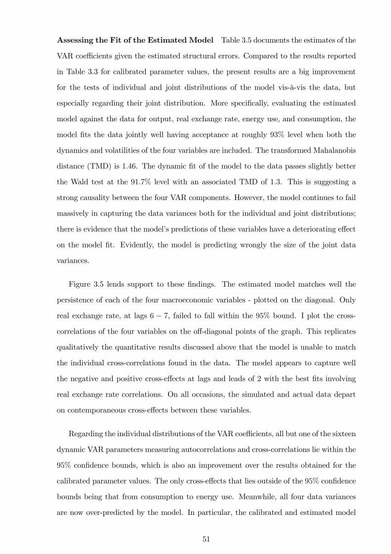
Assessing the Fit of the Estimated Model Table 3.5 documents the estimates of the
VAR coe¢ cients given the estimated structural errors. Compared to the results reported
in Table 3.3 for calibrated parameter values, the present results are a big improvement
for the tests of individual and joint distributions of the model vis-à-vis the data, but
especially regarding their joint distribution. More speci�cally, evaluating the estimated
model against the data for output, real exchange rate, energy use, and consumption, the
model �ts the data jointly well having acceptance at roughly 93% level when both the
dynamics and volatilities of the four variables are included. The transformed Mahalanobis
distance (TMD) is 1:46. The dynamic �t of the model to the data passes slightly better
the Wald test at the 91:7% level with an associated TMD of 1:3. This is suggesting a
strong causality between the four VAR components. However, the model continues to fail
massively in capturing the data variances both for the individual and joint distributions;
there is evidence that the model�s predictions of these variables have a deteriorating e¤ect
on the model �t. Evidently, the model is predicting wrongly the size of the joint data
variances.
Figure 3.5 lends support to these �ndings. The estimated model matches well the
persistence of each of the four macroeconomic variables - plotted on the diagonal. Only
real exchange rate, at lags 6 � 7, failed to fall within the 95% bound. I plot the cross-
correlations of the four variables on the o¤-diagonal points of the graph. This replicates
qualitatively the quantitative results discussed above that the model is unable to match
the individual cross-correlations found in the data. The model appears to capture well
the negative and positive cross-e¤ects at lags and leads of 2 with the best �ts involving
real exchange rate correlations. On all occasions, the simulated and actual data depart
on contemporaneous cross-e¤ects between these variables.
Regarding the individual distributions of the VAR coe¢ cients, all but one of the sixteen
dynamic VAR parameters measuring autocorrelations and cross-correlations lie within the
95% con�dence bounds, which is also an improvement over the results obtained for the
calibrated parameter values. The only cross-e¤ects that lies outside of the 95% con�dence
bounds being that from consumption to energy use. Meanwhile, all four data variances
are now over-predicted by the model. In particular, the calibrated and estimated model
51
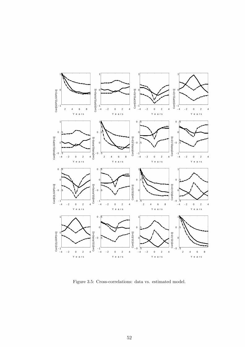
2 4 6 8 1
0
1
C
orr[G
DP(
t),G
DP(
ti)]
Y e a r s
4 2 0 2 4 1
0
1
Cor
r[GD
P(t),
RXR
(t+i)]
Y e a r s
4 2 0 2 4 1
0
1
C
orr[G
DP(
t),E(
t+i)]
Y e a r s
4 2 0 2 4 1
0
1
C
orr[G
DP(
t),C
(t+i)]
Y e a r s
4 2 0 2 4 0 . 5
0
0 . 5
1
C
orr[R
XR(t)
,GD
P(t+
i)]
Y e a r s
2 4 6 8 0 . 5
0
0 . 5
1
C
orr[R
XR(t)
,RXR
(ti)]
Y e a r s
4 2 0 2 4 1
0 . 5
0
0 . 5
C
orr[R
XR(t)
,E(t+
i)]
Y e a r s
4 2 0 2 4 1
0 . 5
0
0 . 5
C
orr[R
XR(t)
,C(t+
i)]
Y e a r s
4 2 0 2 4 1
0 . 5
0
0 . 5
Cor
r[E(t)
,GD
P(t+
i)]
Y e a r s
4 2 0 2 4 1
0 . 5
0
0 . 5
C
orr[E
(t),R
XR(t+
i)]
Y e a r s
2 4 6 8 0 . 5
0
0 . 5
1
C
orr[E
(t),E
(ti)]
Y e a r s
4 2 0 2 4 0 . 5
0
0 . 5
1 C
orr[E
(t),C
(t+i)]
Y e a r s
4 2 0 2 4 1
0
1
C
orr[C
(t),G
DP(
t+i)]
Y e a r s
4 2 0 2 4 1
0 . 5
0
0 . 5
Cor
r[C(t)
,RXR
(t+i)]
Y e a r s
4 2 0 2 4 0 . 5
0
0 . 5
1
Cor
r[C(t)
,E(t+
i)]
Y e a r s
2 4 6 8 0 . 5
0
0 . 5
1
Cor
r[C(t)
,C(t
i)]
Y e a r s
Figure 3.5: Cross-correlations: data vs. estimated model.
52
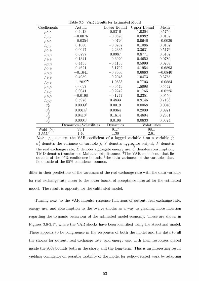
Table 3.5: VAR Results for Estimated ModelCoe¢ cients Actual Lower Bound Upper Bound Mean
�bY ;bY 0:4913 0:0316 1:0204 0:5756� bP ;bY �0:0076 �0:0628 0:0982 0:0132� bE;bY �0:0354 �0:0720 0:0646 �0:0039� bC;bY 0:1080 �0:0767 0:1086 0:0107�bY ; bP 0:0047 �2:2335 3:3631 0:5176� bP ; bP 0:6797 0:0987 0:8771 0:5107� bE; bP 0:1341 �0:3020 0:4652 0:0780� bC; bP 0:4435 �0:4135 0:5990 0:0769�bY ; bE 0:4621 �5:1792 4:1954 �0:6893� bP ; bE �0:1641 �0:8366 0:6663 �0:0840� bE; bE 0:4959 �0:2948 1:0473 0:3765
� bC; bE �1:2027{ �1:0638 0:7703 �0:0884�bY ; bC 0:0697 �0:6549 1:8098 0:5547� bP ; bC 0:0041 �0:2242 0:1765 �0:0225� bE; bC �0:0198 �0:1247 0:2351 0:0556� bC; bC 0:5978 0:4833 0:9146 0:7138
�2bY 0:0009\ 0:0019 0:0068 0:0040
�2bP 0:0314\ 0:0364 0:2030 0:0971
�2bE 0:0413\ 0:1614 0:4604 0:2851
�2bC 0:0004\ 0:0198 0:0633 0:0374Dynamics+Volatilities Dynamics Volatilities
Wald (%) 93:1 91:7 98:1TMD 1:46 1:30 2:61Note: �i;j denotes the VAR coe¢ cient of a lagged variable i on a variable j;�2j denotes the variance of variable j; bY denotes aggregate output; bP denotes
the real exchange rate; bE denotes aggregate energy use; bC denotes consumption;TMD denotes transformed Mahalanobis distance. {The VAR coe¢ cients that lieoutside of the 95% con�dence bounds; \the data variances of the variables thatlie outside of the 95% con�dence bounds.
di¤er in their predictions of the variances of the real exchange rate with the data variance
for real exchange rate closer to the lower bound of acceptance interval for the estimated
model. The result is opposite for the calibrated model.
Turning next to the VAR impulse response functions of output, real exchange rate,
energy use, and consumption to the twelve shocks as a way to gleaning more intuition
regarding the dynamic behaviour of the estimated model economy. These are shown in
Figures 3.6-3.17, where the VAR shocks have been identi�ed using the structural model.
There appears to be congruence in the responses of both the model and the data to all
the shocks for output, real exchange rate, and energy use, with their responses placed
inside the 95% bounds both in the short- and the long-term. This is an interesting result
yielding con�dence on possible usability of the model for policy-related work by adapting
53
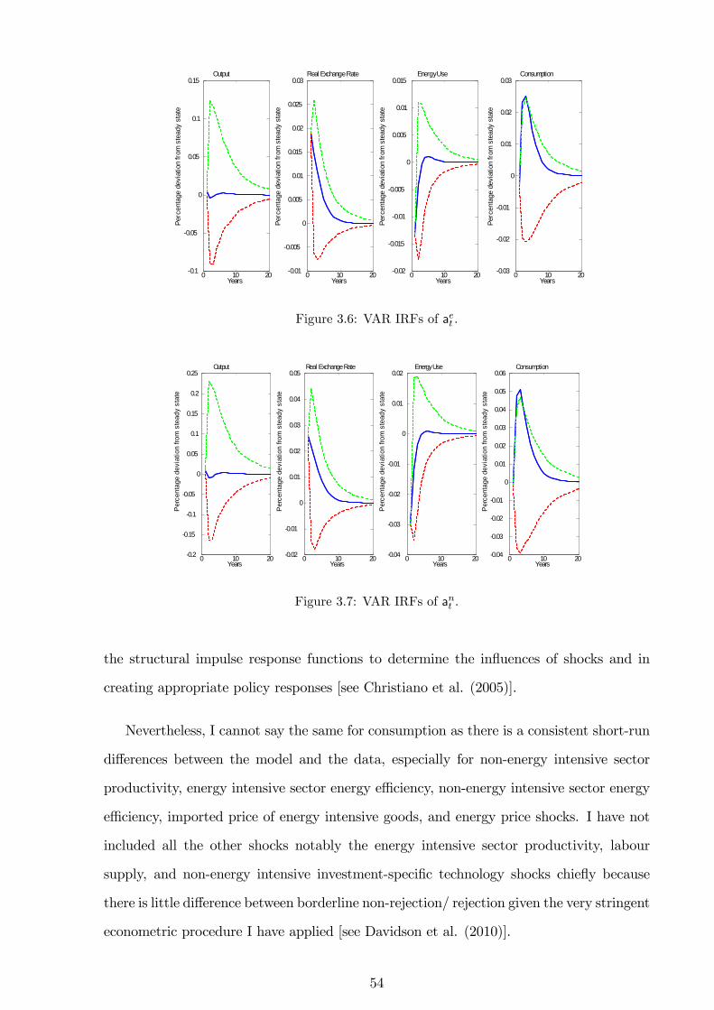
0 10 200.1
0.05
0
0.05
0.1
0.15
Perc
enta
ge d
evia
tion
from
ste
ady
stat
e
Years
Output
0 10 200.01
0.005
0
0.005
0.01
0.015
0.02
0.025
0.03
Perc
enta
ge d
evia
tion
from
ste
ady
stat
eYears
Real Exchange Rate
0 10 200.02
0.015
0.01
0.005
0
0.005
0.01
0.015
Perc
enta
ge d
evia
tion
from
ste
ady
stat
e
Years
Energy Use
0 10 200.03
0.02
0.01
0
0.01
0.02
0.03
Perc
enta
ge d
evia
tion
from
ste
ady
stat
e
Years
Consumption
Figure 3.6: VAR IRFs of aet .
0 10 200.2
0.15
0.1
0.05
0
0.05
0.1
0.15
0.2
0.25
Per
cent
age
devi
atio
n fro
m s
tead
y st
ate
Years
Output
0 10 200.02
0.01
0
0.01
0.02
0.03
0.04
0.05
Per
cent
age
devi
atio
n fro
m s
tead
y st
ate
Years
Real Exchange Rate
0 10 200.04
0.03
0.02
0.01
0
0.01
0.02P
erce
ntag
e de
viat
ion
from
ste
ady
stat
e
Years
Energy Use
0 10 200.04
0.03
0.02
0.01
0
0.01
0.02
0.03
0.04
0.05
0.06
Per
cent
age
devi
atio
n fro
m s
tead
y st
ate
Years
Consumption
Figure 3.7: VAR IRFs of ant .
the structural impulse response functions to determine the in�uences of shocks and in
creating appropriate policy responses [see Christiano et al. (2005)].
Nevertheless, I cannot say the same for consumption as there is a consistent short-run
di¤erences between the model and the data, especially for non-energy intensive sector
productivity, energy intensive sector energy e¢ ciency, non-energy intensive sector energy
e¢ ciency, imported price of energy intensive goods, and energy price shocks. I have not
included all the other shocks notably the energy intensive sector productivity, labour
supply, and non-energy intensive investment-speci�c technology shocks chie�y because
there is little di¤erence between borderline non-rejection/ rejection given the very stringent
econometric procedure I have applied [see Davidson et al. (2010)].
54
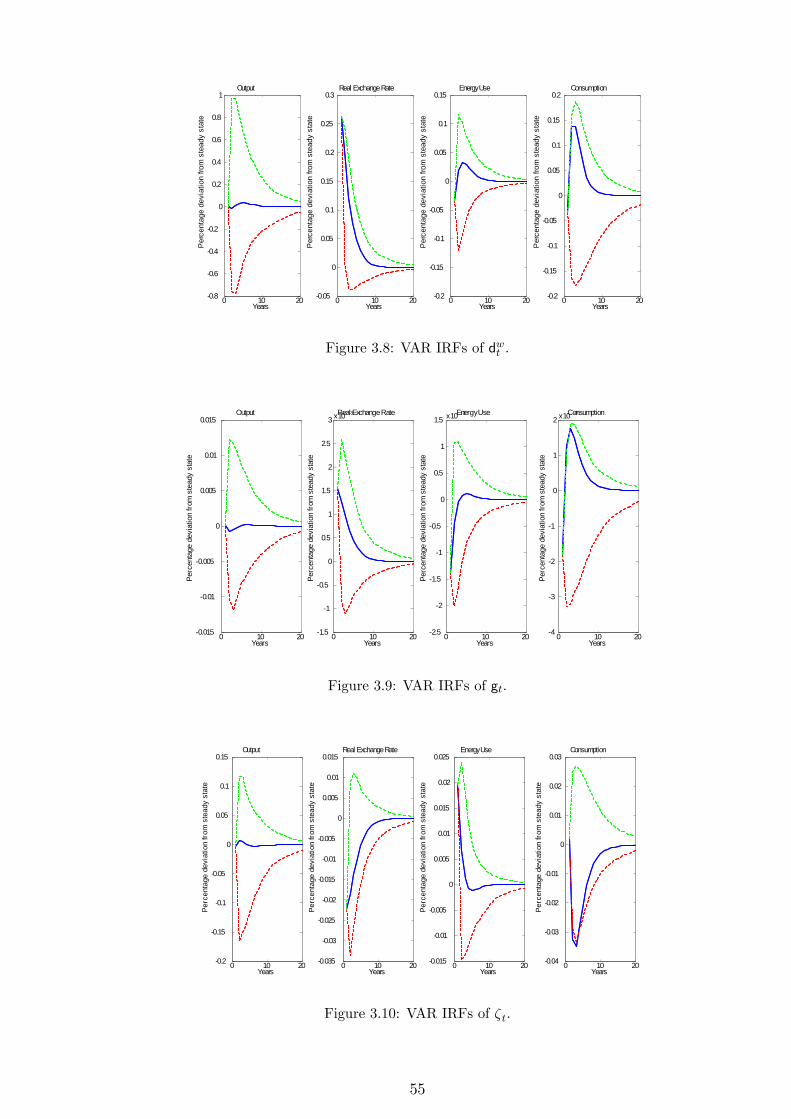
0 10 200.8
0.6
0.4
0.2
0
0.2
0.4
0.6
0.8
1
Per
cent
age
devi
atio
n fro
m s
tead
y st
ate
Years
Output
0 10 200.05
0
0.05
0.1
0.15
0.2
0.25
0.3
Per
cent
age
devi
atio
n fro
m s
tead
y st
ate
Years
Real Exchange Rate
0 10 200.2
0.15
0.1
0.05
0
0.05
0.1
0.15
Per
cent
age
devi
atio
n fro
m s
tead
y st
ate
Years
Energy Use
0 10 200.2
0.15
0.1
0.05
0
0.05
0.1
0.15
0.2
Per
cent
age
devi
atio
n fro
m s
tead
y st
ate
Years
Consumption
Figure 3.8: VAR IRFs of dwt .
0 10 200.015
0.01
0.005
0
0.005
0.01
0.015
Perc
enta
ge d
evia
tion
from
ste
ady
stat
e
Years
Output
0 10 201.5
1
0.5
0
0.5
1
1.5
2
2.5
3 x 10 3
Perc
enta
ge d
evia
tion
from
ste
ady
stat
e
Years
Real Exchange Rate
0 10 202.5
2
1.5
1
0.5
0
0.5
1
1.5 x 10 3
Perc
enta
ge d
evia
tion
from
ste
ady
stat
e
Years
Energy Use
0 10 204
3
2
1
0
1
2 x 10 3
Perc
enta
ge d
evia
tion
from
ste
ady
stat
e
Years
Consumption
Figure 3.9: VAR IRFs of gt.
0 10 200.2
0.15
0.1
0.05
0
0.05
0.1
0.15
Perc
enta
ge d
evia
tion
from
ste
ady
stat
e
Years
Output
0 10 200.035
0.03
0.025
0.02
0.015
0.01
0.005
0
0.005
0.01
0.015
Perc
enta
ge d
evia
tion
from
ste
ady
stat
e
Years
Real Exchange Rate
0 10 200.015
0.01
0.005
0
0.005
0.01
0.015
0.02
0.025
Perc
enta
ge d
evia
tion
from
ste
ady
stat
e
Years
Energy Use
0 10 200.04
0.03
0.02
0.01
0
0.01
0.02
0.03
Perc
enta
ge d
evia
tion
from
ste
ady
stat
e
Years
Consumption
Figure 3.10: VAR IRFs of �t.
55
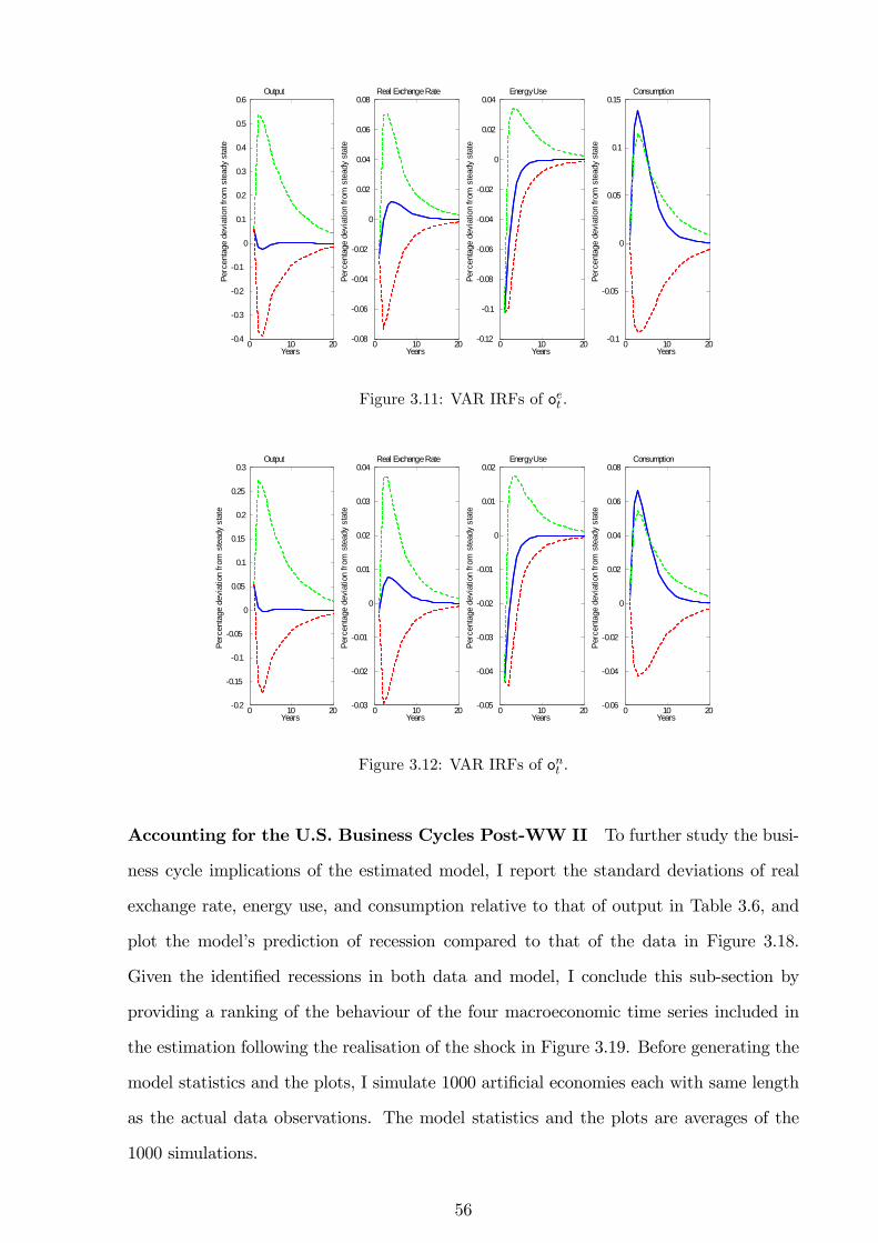
0 10 200.4
0.3
0.2
0.1
0
0.1
0.2
0.3
0.4
0.5
0.6
Perc
enta
ge d
evia
tion
from
ste
ady
stat
e
Years
Output
0 10 200.08
0.06
0.04
0.02
0
0.02
0.04
0.06
0.08
Perc
enta
ge d
evia
tion
from
ste
ady
stat
eYears
Real Exchange Rate
0 10 200.12
0.1
0.08
0.06
0.04
0.02
0
0.02
0.04
Perc
enta
ge d
evia
tion
from
ste
ady
stat
e
Years
Energy Use
0 10 200.1
0.05
0
0.05
0.1
0.15
Perc
enta
ge d
evia
tion
from
ste
ady
stat
e
Years
Consumption
Figure 3.11: VAR IRFs of oet .
0 10 200.2
0.15
0.1
0.05
0
0.05
0.1
0.15
0.2
0.25
0.3
Perc
enta
ge d
evia
tion
from
ste
ady
stat
e
Years
Output
0 10 200.03
0.02
0.01
0
0.01
0.02
0.03
0.04
Perc
enta
ge d
evia
tion
from
ste
ady
stat
e
Years
Real Exchange Rate
0 10 200.05
0.04
0.03
0.02
0.01
0
0.01
0.02Pe
rcen
tage
dev
iatio
n fro
m s
tead
y st
ate
Years
Energy Use
0 10 200.06
0.04
0.02
0
0.02
0.04
0.06
0.08
Perc
enta
ge d
evia
tion
from
ste
ady
stat
e
Years
Consumption
Figure 3.12: VAR IRFs of ont .
Accounting for the U.S. Business Cycles Post-WW II To further study the busi-
ness cycle implications of the estimated model, I report the standard deviations of real
exchange rate, energy use, and consumption relative to that of output in Table 3.6, and
plot the model�s prediction of recession compared to that of the data in Figure 3.18.
Given the identi�ed recessions in both data and model, I conclude this sub-section by
providing a ranking of the behaviour of the four macroeconomic time series included in
the estimation following the realisation of the shock in Figure 3.19. Before generating the
model statistics and the plots, I simulate 1000 arti�cial economies each with same length
as the actual data observations. The model statistics and the plots are averages of the
1000 simulations.
56
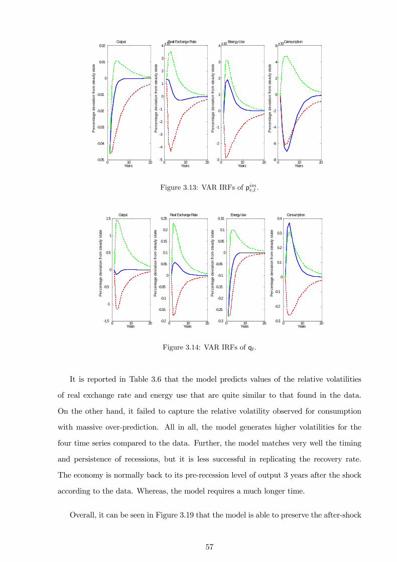
0 10 200.05
0.04
0.03
0.02
0.01
0
0.01
0.02
Per
cent
age
devi
atio
n fro
m s
tead
y st
ate
Years
Output
0 10 205
4
3
2
1
0
1
2
3
4 x 10 3
Per
cent
age
devi
atio
n fro
m s
tead
y st
ate
Years
Real Exchange Rate
0 10 203
2
1
0
1
2
3
4 x 10 3
Per
cent
age
devi
atio
n fro
m s
tead
y st
ate
Years
Energy Use
0 10 208
6
4
2
0
2
4
6 x 10 3
Per
cent
age
devi
atio
n fro
m s
tead
y st
ate
Years
Consumption
Figure 3.13: VAR IRFs of pime;t .
0 10 201.5
1
0.5
0
0.5
1
1.5
Perc
enta
ge d
evia
tion
from
ste
ady
stat
e
Years
Output
0 10 200.2
0.15
0.1
0.05
0
0.05
0.1
0.15
0.2
0.25
Perc
enta
ge d
evia
tion
from
ste
ady
stat
e
Years
Real Exchange Rate
0 10 200.3
0.25
0.2
0.15
0.1
0.05
0
0.05
0.1
0.15
Perc
enta
ge d
evia
tion
from
ste
ady
stat
e
Years
Energy Use
0 10 200.3
0.2
0.1
0
0.1
0.2
0.3
0.4
Perc
enta
ge d
evia
tion
from
ste
ady
stat
e
Years
Consumption
Figure 3.14: VAR IRFs of qt.
It is reported in Table 3.6 that the model predicts values of the relative volatilities
of real exchange rate and energy use that are quite similar to that found in the data.
On the other hand, it failed to capture the relative volatility observed for consumption
with massive over-prediction. All in all, the model generates higher volatilities for the
four time series compared to the data. Further, the model matches very well the timing
and persistence of recessions, but it is less successful in replicating the recovery rate.
The economy is normally back to its pre-recession level of output 3 years after the shock
according to the data. Whereas, the model requires a much longer time.
Overall, it can be seen in Figure 3.19 that the model is able to preserve the after-shock
57
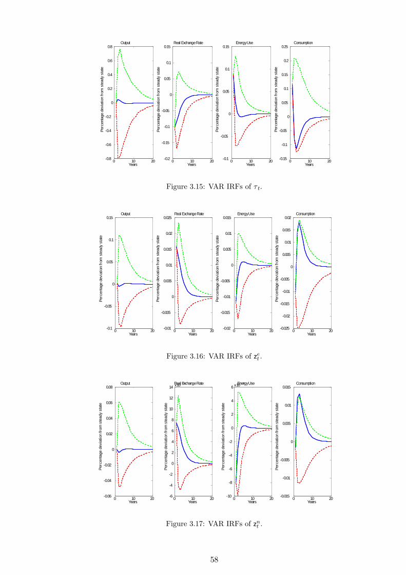
0 10 200.8
0.6
0.4
0.2
0
0.2
0.4
0.6
0.8
Perc
enta
ge d
evia
tion
from
ste
ady
stat
e
Years
Output
0 10 200.2
0.15
0.1
0.05
0
0.05
0.1
0.15
Perc
enta
ge d
evia
tion
from
ste
ady
stat
e
Years
Real Exchange Rate
0 10 200.1
0.05
0
0.05
0.1
0.15
Perc
enta
ge d
evia
tion
from
ste
ady
stat
e
Years
Energy Use
0 10 200.15
0.1
0.05
0
0.05
0.1
0.15
0.2
0.25
Perc
enta
ge d
evia
tion
from
ste
ady
stat
e
Years
Consumption
Figure 3.15: VAR IRFs of � t.
0 10 200.1
0.05
0
0.05
0.1
0.15
Perc
enta
ge d
evia
tion
from
ste
ady
stat
e
Years
Output
0 10 200.01
0.005
0
0.005
0.01
0.015
0.02
0.025
Perc
enta
ge d
evia
tion
from
ste
ady
stat
e
Years
Real Exchange Rate
0 10 200.02
0.015
0.01
0.005
0
0.005
0.01
0.015Pe
rcen
tage
dev
iatio
n fro
m s
tead
y st
ate
Years
Energy Use
0 10 200.025
0.02
0.015
0.01
0.005
0
0.005
0.01
0.015
0.02
Perc
enta
ge d
evia
tion
from
ste
ady
stat
e
Years
Consumption
Figure 3.16: VAR IRFs of zet .
0 10 200.06
0.04
0.02
0
0.02
0.04
0.06
0.08
Perc
enta
ge d
evia
tion
from
ste
ady
stat
e
Years
Output
0 10 206
4
2
0
2
4
6
8
10
12
14 x 10 3
Perc
enta
ge d
evia
tion
from
ste
ady
stat
e
Years
Real Exchange Rate
0 10 2010
8
6
4
2
0
2
4
6 x 10 3
Perc
enta
ge d
evia
tion
from
ste
ady
stat
e
Years
Energy Use
0 10 200.015
0.01
0.005
0
0.005
0.01
0.015
Perc
enta
ge d
evia
tion
from
ste
ady
stat
e
Years
Consumption
Figure 3.17: VAR IRFs of znt .
58
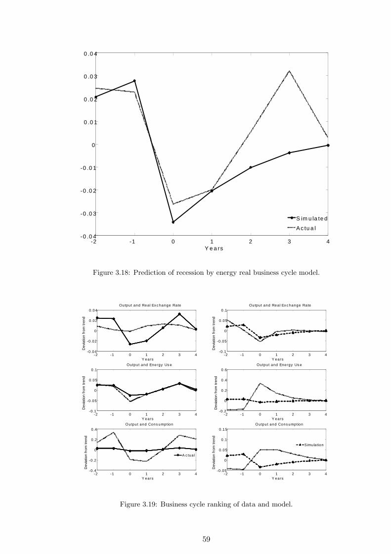
2 1 0 1 2 3 40 .0 4
0 .0 3
0 .0 2
0 .0 1
0
0 .0 1
0 .0 2
0 .0 3
0 .0 4
Y e a rs
S im u la te d
Ac tu a l
Figure 3.18: Prediction of recession by energy real business cycle model.
2 1 0 1 2 3 40.1
0.05
0
0.05
0.1Output and Real Ex c hange Rate
Dev
iatio
n fro
m tr
end
Y ears
2 1 0 1 2 3 40.2
0
0.2
0.4
0.6Output and Energy Us e
Dev
iatio
n fro
m tr
end
Y ears
2 1 0 1 2 3 40.05
0
0.05
0.1
0.15
Y ears
Dev
iatio
n fro
m tr
end
Output and Cons umption
2 1 0 1 2 3 40.04
0.02
0
0.02
0.04Output and Real Ex c hange Rate
Dev
iatio
n fro
m tr
end
Y ears
2 1 0 1 2 3 40.1
0.05
0
0.05
0.1Output and Energy Us e
Dev
iatio
n fro
m tr
end
Y ears
2 1 0 1 2 3 40.4
0.2
0
0.2
0.4
Y ears
Dev
iatio
n fro
m tr
end
Output and Cons umption
Simulation
A c tual
Figure 3.19: Business cycle ranking of data and model.
59
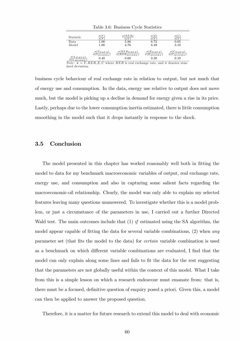
Table 3.6: Business Cycle Statistics
Statistic �(Y )�(Y )
�(RXR)�(Y )
�(E)�(Y )
�(C)�(Y )
Data 1:00 5:86 6:72 0:65Model 1:00 4:76 8:49 3:10
�(YDATA)�(YMODEL)
�(RXRDATA)�(RXRMODEL)
�(EDATA)�(EMODEL)
�(CDATA)�(CMODEL)
�(>DATA)�(>MODEL)
0:48 0:60 0:38 0:10
Note : > = Y;RXR;E;C where RXR is real exchange rate, and � denotes stan-dard deviation.
business cycle behaviour of real exchange rate in relation to output, but not much that
of energy use and consumption. In the data, energy use relative to output does not move
much, but the model is picking up a decline in demand for energy given a rise in its price.
Lastly, perhaps due to the lower consumption inertia estimated, there is little consumption
smoothing in the model such that it drops instantly in response to the shock.
3.5 Conclusion
The model presented in this chapter has worked reasonably well both in �tting the
model to data for my benchmark macroeconomic variables of output, real exchange rate,
energy use, and consumption and also in capturing some salient facts regarding the
macroeconomic-oil relationship. Clearly, the model was only able to explain my selected
features leaving many questions unanswered. To investigate whether this is a model prob-
lem, or just a circumstance of the parameters in use, I carried out a further Directed
Wald test. The main outcomes include that (1) if estimated using the SA algorithm, the
model appear capable of �tting the data for several variable combinations, (2) when any
parameter set (that �ts the model to the data) for certain variable combination is used
as a benchmark on which di¤erent variable combinations are evaluated, I �nd that the
model can only explain along some lines and fails to �t the data for the rest suggesting
that the parameters are not globally useful within the context of this model. What I take
from this is a simple lesson on which a research endeavour must emanate from: that is,
there must be a focused, de�nitive question of enquiry posed a priori. Given this, a model
can then be applied to answer the proposed question.
Therefore, it is a matter for future research to extend this model to deal with economic
60
issues along other dimensions and it is my hope that this model will be adjusted appro-
priately to answer many other macroeconomic questions particularly those that concern
energy issues and their policy implications. To kick-start such an agenda, I motivate two
particular possibilities in this concluding remark. First, the complete inter-country e¤ects
through (in)complete risk sharing and uncovered interest parity can be studied by allow-
ing both the domestic and foreign residents investment opportunities in both the domestic
and foreign bonds [see, for example, Gali and Monacelli (2005) and Corsetti et al. (2005)].
Having introduced capital accounts into the model, a second important and new e¤ort
could be to work with non-stationary data set. It is to these two exercises I now turn in
Chapter 4.
61

Table3.7:OilPriceIncreasesandCauses,1947-2008
OilPriceEpisode
PriceChanges(%)
PrincipalFactors
1947-1948
37Strongdemandvssupplyconstraints;shorterworkweek;Europeanreconstruction
1952-1953
10Iraniannationalisation;strike;abandonmentofcontrols
1956-1957
9SuezCrisis
1969
7SeculardeclineinU.S.reserves;strike
1970
8RuptureofTrans-Arabianpipeline;strike;strongdemandvssupplyconstraints(Libyanproductioncutbacks)
1973-1974
16,51
StagnatingU.S.production;strongdemandvssupplyconstraints(Arab-Israeliwar)
1978-1979
57Iranianrevolution
1980-1981
45Iran-IraqWar;pricecontrolremoval
1990
93GulfWarI
1999-2000
38Strongdemand
2002-2003
28Venezuelaunrest;GulfWarII
2007-2008
145
Strongdemandvssupplyconstraints
Source:Hamilton(1985,2011).
62
Chapter 4
So, Do Energy Price Shocks Still
Matter?
A parameter that is valid for a model in one economic environment cannot be
uncritically applied to a model embedded in a di¤erent economic environment.
Martin Browning, Lars Peter Hansen, and James J. Heckman (Handbook of
Macroeconomics, 1999, p. 546).
4.1 Introduction
Changes in oil prices are mostly unanticipated and are exogenous world events with
several macroeconomic implications for many countries, developed and developing. The
purpose of this study is to investigate how these occasional movements, in particular
positive percentage changes, in the price of oil go on to a¤ect the output and competitive-
ness (as measured by real exchange rate) of a typical oil-importing industrialised country
against the rest of the world. I take the U.S. as the example domestic country for this
exercise. To put this into perspective, I display in Figure 4.1 the historical data on U.S.
output (1929-2013) and its trend identi�ed by using the Hodrick-Prescott (HP, 1981, 1997)
�lter with the smoothing parameter set to 400 in row 1, oil price-output (1949-2013) re-
63
lationship in row 2, oil price-real exchange rate (1949-2013) relationship in row 3, and
output-real exchange rate (1949-2013) relationship in row 4.
Row 1 shows two of the measures by which economic downturns can be represented.
First is when outputs in consecutive periods are below the HP trend and the second is just
by observing the coincidence between output drops and the shaded bars, which are the
National Bureau of Economic Research (NBER) identi�ed recession dates. The time paths
of the oil price and output in row 2 shows that they often travel in opposite directions,
especially during periods of radical upswing in prices (i.e., oil price shocks). Clearly,
output is a lot less volatile than oil price. Oil price leads real exchange rate changes in
row 3, but the overall picture is that they move in the same direction. The reason for
this is that higher oil price gets transmitted into the consumer price index in the domestic
country such that using the ratio of export price to import price as a measure of the real
exchange rate implies that oil price and real exchange rate are positively correlated. The
last row shows that real exchange rate appears to also follow output with roughly 2-3 lags.
So, in the current chapter, I add to the signi�cantly growing body of literature that
is debating if energy price shocks still matter.1 This issue is addressed by building on
the seminal works of Kydland and Prescott (1982) and Long and Plosser (1983), which
have been extended in several ways with the closest in spirit to what I am studying here
being the pioneering works of Kim and Loungani (1992) and Finn (1991). In particular, I
combine the Kim and Loungani model with the multi-sector approach of Long and Plosser
in order to investigate the impacts of changes in the exogenous price of a factor input -
real price of oil - in in�uencing the U.S. business cycles and competitiveness vis-à-vis the
rest of the world. My model has the following important features: (1) production takes
place in two sectors with energy explicitly included as an input; (2) there is trade in goods
and services, and �nancial assets across countries; (3) the model is augmented with an
1The background to this work encompasses many strands of the macro econometric literature. Aninterested reader can consult Asafu-Adjaye (2000), Berndt and Wood (1975, 1979), Burbidge and Harrison(1984), Cavallo and Wu (2006), Darby (1982), De Gregorio et. al. (2007), Eldestein and Kilian (2007),Gri¢ n and Gregory (1976), Hamilton (1983, 1985, 1996, 2003, 2011), Hamilton and Herrara (2000),Herrera and Pesavento (2007), Hooker (1996, 1997, 2002), Hunt et. al. (2001), Kilian (2008), and Mork(1989), among others for empirical discussions; Blanchard and Gali (2010), Darby (1981), Dhawan andJeske (2006, 2008), Dhawan et. al. (2010), Finn (1991, 1995, 2000), Gillingham et. al. (2009), Harriset. al. (2009), Kim and Loungani (1992), Loungani (1986), Rotemberg and Woodford (1996), Schmidtand Zimmermann (2005), among others for theoretical underpinnings; and policy related papers, see, forexample, Barsky and Kilian (2002), Bernanke et. al. (1997), Blanchard and Simon (2001), Chakravorty(1997), Leduc and Sill (2004, 2006), and Stock and Watson (2003).
64
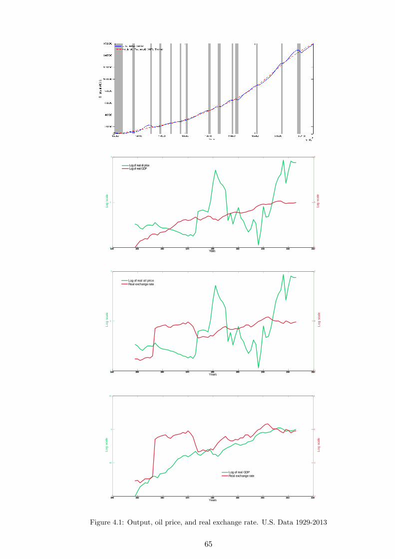
1940 1950 1960 1970 1980 1990 2000 2010 20202
1
0
Years
Log
scale
1940 1950 1960 1970 1980 1990 2000 2010 20204
5
6
Log
scale
Log of real oil priceLog of real GDP
1940 1950 1960 1970 1980 1990 2000 2010 20202
1
0
Years
Log
scal
e
1940 1950 1960 1970 1980 1990 2000 2010 20202
0
2
Log
scal
e
Log of real oil priceReal exchange rate
1940 1950 1960 1970 1980 1990 2000 2010 20204
4.5
5
5.5
Years
Log
scal
e
1940 1950 1960 1970 1980 1990 2000 2010 20202
1
0
1
Log
scal
e
Log of real GDPReal exchange rate
Figure 4.1: Output, oil price, and real exchange rate. U.S. Data 1929-2013
65
array of real rigidities and is driven by a number of exogenous shocks; and (4) the model
is estimated on un�ltered data of the U.S. covering the period 1949-2013 on an annual
frequency using the formal econometric method of indirect inference.
Thus, while it is a useful contribution that the model as it is spelt out in the next
section as a two-sector energy and non-energy model is to my best knowledge a new and,
as I will discuss later, an important set-up, I will like to draw attention to the fact that
the model has been estimated on non-stationary data. In reality, most macroeconomic
variables are non-stationary implying that we may be removing critical information when
we �lter them.2 Therefore, it is useful whenever technically permissible to develop a model
that can be used to describe un�ltered data. This is a major and novel contribution of
this chapter and in doing this, we have responded to the call by Kim and Loungani (1992)
that "... it may be fruitful, in future research, to develop versions of our model which can
accommodate nonstationarity in the price process."
The main �nding is that energy price shocks is not able to directly generate the
magnitude of economic downturn observed in the data. However, it possesses a strong
indirect transmission link that endogenously spread its e¤ect erroneously through the
system. This leads me to conclude that previous results that attribute minimal importance
to oil price shocks must be focusing on the energy cost share of gross domestic product.
I also �nd that external shocks have been responsible for explaining the volatility in U.S.
economic activities for a long time. This leads me to conclude that modelling the U.S. as
a closed economy assumes away a sizeable set of very relevant factors.
The remainder of this chapter proceeds as follows. In Section 4.2, I describe the main
features of the two-sector model in log-linearized form. In Section 4.3, I provide brief
discussions of the econometric method of indirect inference (II) used in estimating the
model, the non-stationary data serving as the empirical counterparts to model variables,
and the initial parameter values used to initialise the starting points for the Simulated
Annealling (SA) algorithm. I present the main �ndings in Section 4.4 and conclude with
Section 4.5.2See King and Rebelo (1993), Cochrane (1994), Cogley and Nason (1995), Canova (1998), Stock
and Watson (1999), and the references in them, for a review of �ltering methods and the strengths andweaknesses associated with each.
66
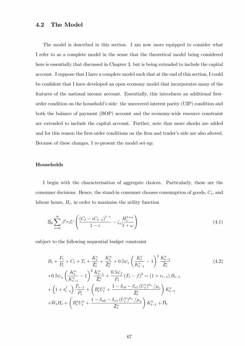
4.2 The Model
The model is described in this section. I am now more equipped to consider what
I refer to as a complete model in the sense that the theoretical model being considered
here is essentially that discussed in Chapter 3, but is being extended to include the capital
account. I suppose that I have a complete model such that at the end of this section, I could
be con�dent that I have developed an open economy model that incorporates many of the
features of the national income account. Essentially, this introduces an additional �rst-
order condition on the household�s side: the uncovered interest parity (UIP) condition and
both the balance of payment (BOP) account and the economy-wide resource constraint
are extended to include the capital account. Further, note that more shocks are added
and for this reason the �rst-order conditions on the �rm and trader�s side are also altered.
Because of these changes, I re-present the model set-up.
Households
I begin with the characterisation of aggregate choices. Particularly, these are the
consumer decisions. Hence, the stand-in consumer chooses consumption of goods, Ct, and
labour hours, Ht, in order to maximise the utility function
E01Xt=0
�t� tU
(Ct � �Ct�1)
1��
1� �� �t
H1+!t
1 + !
!(4.1)
subject to the following sequential budget constraint
Bt +FtPt+ Ct + Tt +
Ket
Zet+Knt
Znt+ 0:5 e
�Ket
Ket�1
� 1�2 Ke
t�1Zet
(4.2)
+0:5 n
�Knt
Knt�1
� 1�2 Kn
t�1Znt
+0:5 fPt
(Ft � f)2 = (1 + rt�1)Bt�1
+�1 + rft�1
� Ft�1Pt
+
�RetU
et +
1� �e0 � �e1 (Uet )�e =�e
Zet
�Ket�1
+WtHt +
�Rnt U
nt +
1� �n0 � �n1 (Unt )
�n =�nZnt
�Knt�1 + �t
67
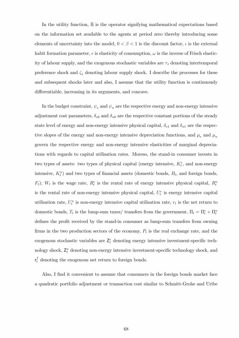
In the utility function, E is the operator signifying mathematical expectations based
on the information set available to the agents at period zero thereby introducing some
elements of uncertainty into the model, 0 < � < 1 is the discount factor, � is the external
habit formation parameter, � is elasticity of consumption, ! is the inverse of Frisch elastic-
ity of labour supply, and the exogenous stochastic variables are � t denoting intertemporal
preference shock and �t denoting labour supply shock. I describe the processes for these
and subsequent shocks later and also, I assume that the utility function is continuously
di¤erentiable, increasing in its arguments, and concave.
In the budget constraint, e and n are the respective energy and non-energy intensive
adjustment cost parameters, �e0 and �n0 are the respective constant portions of the steady
state level of energy and non-energy intensive physical capital, �e1 and �n1 are the respec-
tive slopes of the energy and non-energy intensive depreciation functions, and �e and �n
govern the respective energy and non-energy intensive elasticities of marginal deprecia-
tions with regards to capital utilisation rates. Moreso, the stand-in consumer invests in
two types of assets: two types of physical capital (energy intensive, Ket , and non-energy
intensive, Knt ) and two types of �nancial assets (domestic bonds, Bt, and foreign bonds,
Ft); Wt is the wage rate, Ret is the rental rate of energy intensive physical capital, R
nt
is the rental rate of non-energy intensive physical capital, U et is energy intensive capital
utilisation rate, Unt is non-energy intensive capital utilisation rate, rt is the net return to
domestic bonds, Tt is the lump-sum taxes/ transfers from the government, �t = �et +�nt
de�nes the pro�t received by the stand-in consumer as lump-sum transfers from owning
�rms in the two production sectors of the economy, Pt is the real exchange rate, and the
exogenous stochastic variables are Zet denoting energy intensive investment-speci�c tech-
nology shock, Znt denoting non-energy intensive investment-speci�c technology shock, and
rft denoting the exogenous net return to foreign bonds.
Also, I �nd it convenient to assume that consumers in the foreign bonds market face
a quadratic portfolio adjustment or transaction cost similar to Schmitt-Grohe and Uribe
68
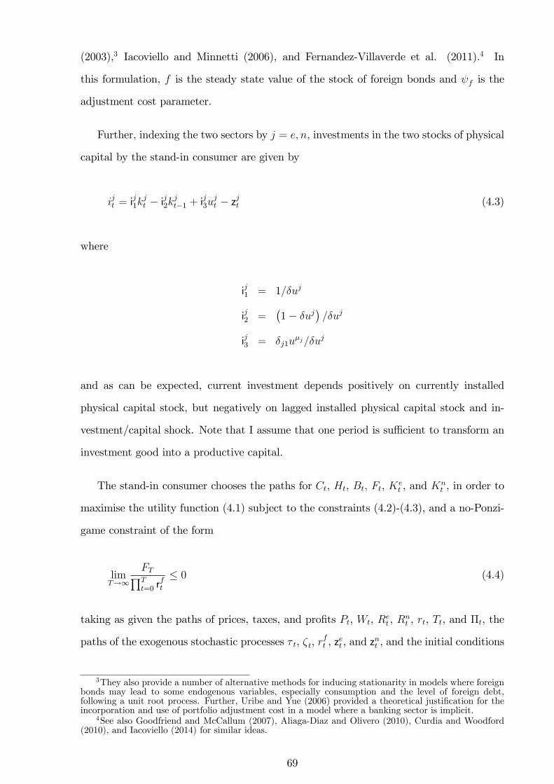
(2003),3 Iacoviello and Minnetti (2006), and Fernandez-Villaverde et al. (2011).4 In
this formulation, f is the steady state value of the stock of foreign bonds and f is the
adjustment cost parameter.
Further, indexing the two sectors by j = e; n, investments in the two stocks of physical
capital by the stand-in consumer are given by
ijt = ij1k
jt � ij2k
jt�1 + i
j3u
jt � zjt (4.3)
where
ij1 = 1=�uj
ij2 =�1� �uj
�=�uj
ij3 = �j1u�j=�uj
and as can be expected, current investment depends positively on currently installed
physical capital stock, but negatively on lagged installed physical capital stock and in-
vestment/capital shock. Note that I assume that one period is su¢ cient to transform an
investment good into a productive capital.
The stand-in consumer chooses the paths for Ct, Ht, Bt, Ft, Ket , and K
nt , in order to
maximise the utility function (4.1) subject to the constraints (4.2)-(4.3), and a no-Ponzi-
game constraint of the form
limT!1
FTQTt=0 r
ft
� 0 (4.4)
taking as given the paths of prices, taxes, and pro�ts Pt, Wt, Ret , R
nt , rt, Tt, and �t, the
paths of the exogenous stochastic processes � t, �t, rft , z
et , and z
nt , and the initial conditions
3They also provide a number of alternative methods for inducing stationarity in models where foreignbonds may lead to some endogenous variables, especially consumption and the level of foreign debt,following a unit root process. Further, Uribe and Yue (2006) provided a theoretical justi�cation for theincorporation and use of portfolio adjustment cost in a model where a banking sector is implicit.
4See also Goodfriend and McCallum (2007), Aliaga-Diaz and Olivero (2010), Curdia and Woodford(2010), and Iacoviello (2014) for similar ideas.
69
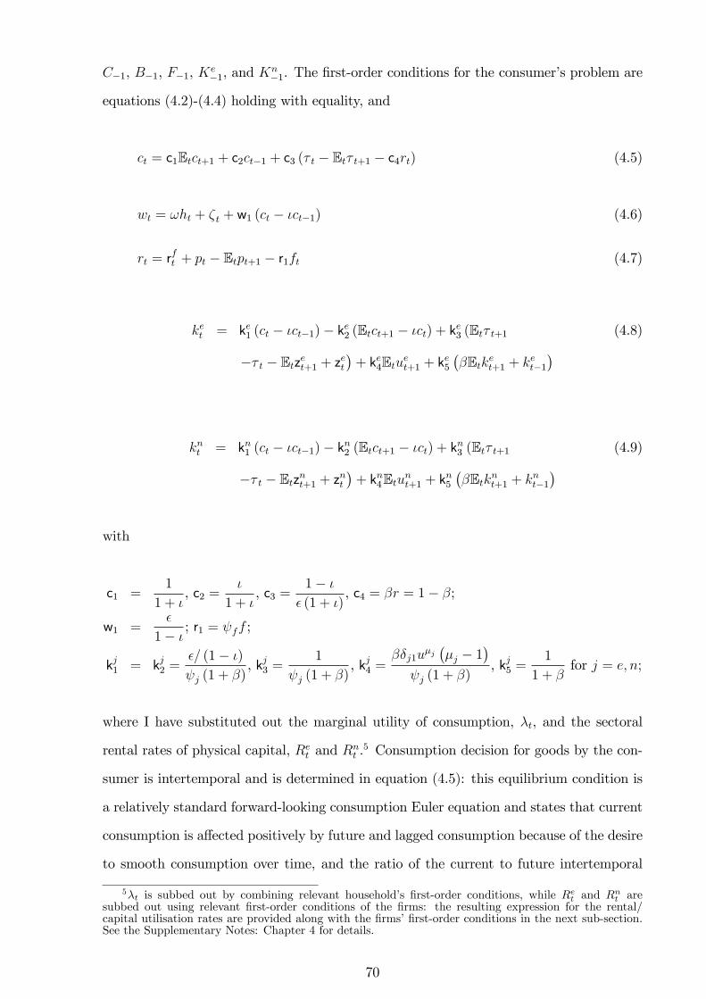
C�1, B�1, F�1, Ke�1, and K
n�1. The �rst-order conditions for the consumer�s problem are
equations (4.2)-(4.4) holding with equality, and
ct = c1Etct+1 + c2ct�1 + c3 (� t � Et� t+1 � c4rt) (4.5)
wt = !ht + �t + w1 (ct � �ct�1) (4.6)
rt = rft + pt � Etpt+1 � r1ft (4.7)
ket = ke1 (ct � �ct�1)� ke2 (Etct+1 � �ct) + ke3 (Et� t+1 (4.8)
�� t � Etzet+1 + zet�+ ke4Etuet+1 + ke5
��Etket+1 + ket�1
�
knt = kn1 (ct � �ct�1)� kn2 (Etct+1 � �ct) + kn3 (Et� t+1 (4.9)
�� t � Etznt+1 + znt�+ kn4Etunt+1 + kn5
��Etknt+1 + knt�1
�
with
c1 =1
1 + �, c2 =
�
1 + �, c3 =
1� �
� (1 + �), c4 = �r = 1� �;
w1 =�
1� �; r1 = ff ;
kj1 = kj2 =�= (1� �)
j (1 + �), kj3 =
1
j (1 + �), kj4 =
��j1u�j��j � 1
� j (1 + �)
, kj5 =1
1 + �for j = e; n;
where I have substituted out the marginal utility of consumption, �t, and the sectoral
rental rates of physical capital, Ret and R
nt .5 Consumption decision for goods by the con-
sumer is intertemporal and is determined in equation (4.5): this equilibrium condition is
a relatively standard forward-looking consumption Euler equation and states that current
consumption is a¤ected positively by future and lagged consumption because of the desire
to smooth consumption over time, and the ratio of the current to future intertemporal
5�t is subbed out by combining relevant household�s �rst-order conditions, while Ret and Rnt aresubbed out using relevant �rst-order conditions of the �rms: the resulting expression for the rental/capital utilisation rates are provided along with the �rms��rst-order conditions in the next sub-section.See the Supplementary Notes: Chapter 4 for details.
70
preference shock, but negatively by the current net return to domestic bonds. The im-
pact of the ratio � t=Et� t+1 being positive implies that a stand-in consumer weighs current
consumption more than investment, and hence, future consumption, among other things,
depends on the real return to domestic bonds. That is, a rise in the latter will lead to
a decrease in current consumption and causing investment to go up contemporaneously.
One can think of a similar impact on current consumption when there is a positive jump in
�nancial investment, which incidentally is an expected outcome whenever, say, the system
is hit by a positive interest rate shock.
Equilibrium condition (4.6), which determines how the stand-in consumer will supply
their labour hours to the production sectors, or equivalently the level of equilibrium wage,
says that equilibrium wage reacts positively to labour hours, current consumption, and
labour supply shock, but negatively to lagged consumption. Equilibrium condition (4.7)
summarises the uncovered interest parity condition stating that the net returns to domestic
and foreign bonds will be the same except for when current and expected real exchange
rates di¤er, and also domestic interest rate depends inversely on the volume of foreign
bonds. Capital Euler equations yield the equilibrium conditions (4.8) and (4.9), which
state that the respective physical capital is a positive function of current consumption,
lagged capital stock, both the expected physical capital and capital utilisation rate, the
ratio of future to current intertemporal preference shock, and the ratio of current to future
investment/ capital shock, but a negative function of expected consumption. Again, the
trade-o¤ between consumption and investment is highlighted in how the stocks of the two
physical capitals respond to the ratio of current-to-future intertemporal preference shocks.
Firms
I proceed with the characterisation of the disaggregate choices. Particularly, these
begin with the decisions of the producers. There are two sectors indexed by j in this
economy using a constant-elasticity-of-substitution (CES) production function, which is
de�ned to be Cobb-Douglas in labour hours and a CES aggregate in capital services and
71
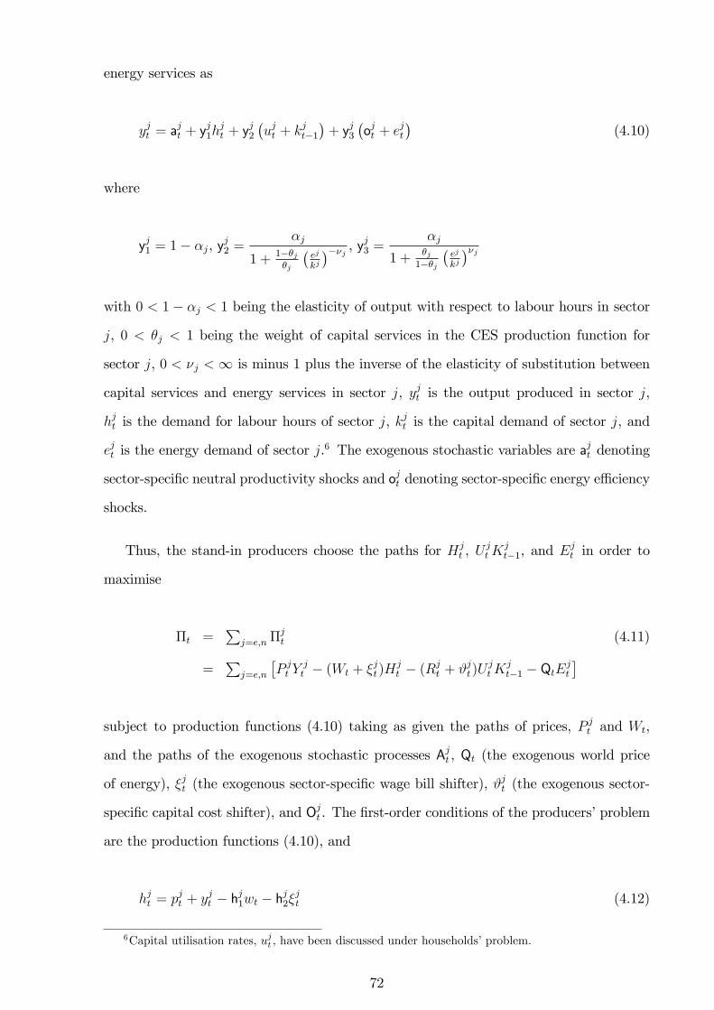
energy services as
yjt = ajt + y
j1h
jt + y
j2
�ujt + kjt�1
�+ yj3
�ojt + ejt
�(4.10)
where
yj1 = 1� �j, yj2 =
�j
1 +1��j�j
�ej
kj
���j , yj3 = �j
1 +�j1��j
�ej
kj
��jwith 0 < 1� �j < 1 being the elasticity of output with respect to labour hours in sector
j, 0 < �j < 1 being the weight of capital services in the CES production function for
sector j, 0 < �j <1 is minus 1 plus the inverse of the elasticity of substitution between
capital services and energy services in sector j, yjt is the output produced in sector j,
hjt is the demand for labour hours of sector j, kjt is the capital demand of sector j, and
ejt is the energy demand of sector j.6 The exogenous stochastic variables are ajt denoting
sector-speci�c neutral productivity shocks and ojt denoting sector-speci�c energy e¢ ciency
shocks.
Thus, the stand-in producers choose the paths for Hjt , U
jtK
jt�1, and E
jt in order to
maximise
�t =P
j=e;n�jt (4.11)
=P
j=e;n
�P jt Y
jt � (Wt + �jt)H
jt � (Rj
t + #jt)UjtK
jt�1 � QtE
jt
�
subject to production functions (4.10) taking as given the paths of prices, P jt and Wt,
and the paths of the exogenous stochastic processes Ajt , Qt (the exogenous world price
of energy), �jt (the exogenous sector-speci�c wage bill shifter), #jt (the exogenous sector-
speci�c capital cost shifter), and Ojt . The �rst-order conditions of the producers�problem
are the production functions (4.10), and
hjt = pjt + yjt � hj1wt � hj2�jt (4.12)
6Capital utilisation rates, ujt , have been discussed under households�problem.
72
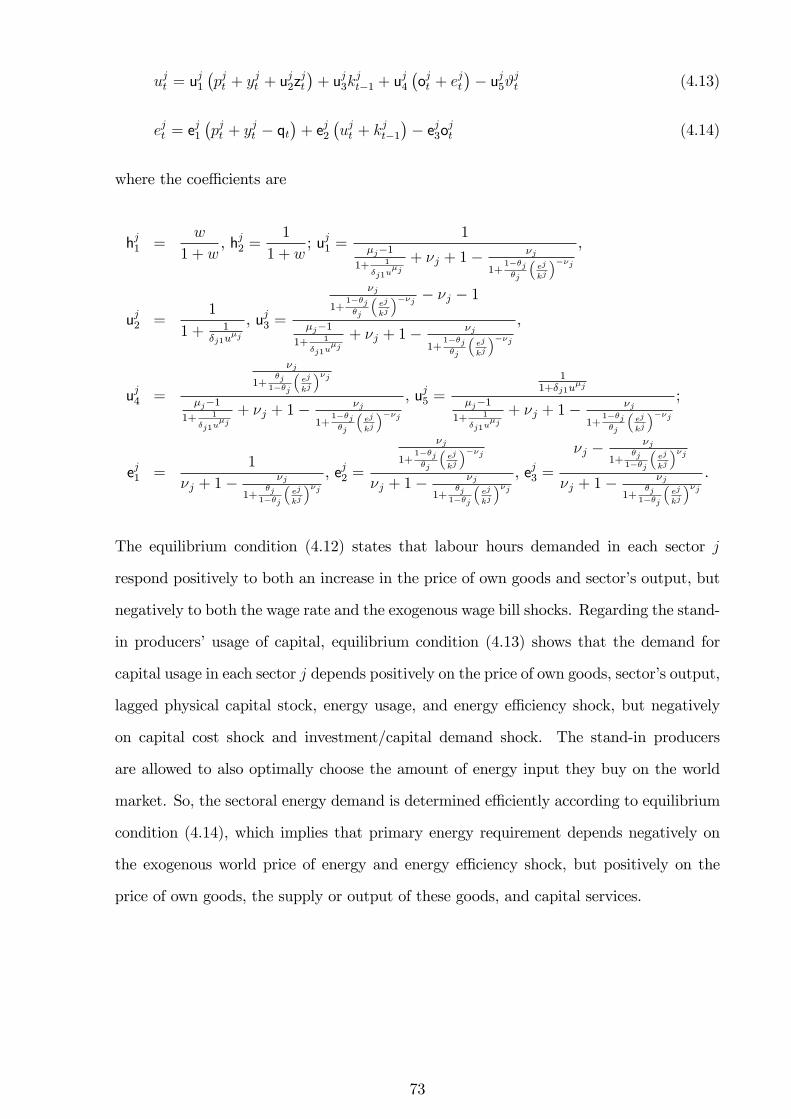
ujt = uj1
�pjt + yjt + u
j2zjt
�+ uj3k
jt�1 + u
j4
�ojt + ejt
�� uj5#
jt (4.13)
ejt = ej1
�pjt + yjt � qt
�+ ej2
�ujt + kjt�1
�� ej3o
jt (4.14)
where the coe¢ cients are
hj1 =w
1 + w, hj2 =
1
1 + w; uj1 =
1�j�1
1+ 1
�j1u�j
+ �j + 1� �j
1+1��j�j
�ej
kj
���j ,
uj2 =1
1 + 1�j1u
�j
, uj3 =
�j
1+1��j�j
�ej
kj
���j � �j � 1
�j�11+ 1
�j1u�j
+ �j + 1� �j
1+1��j�j
�ej
kj
���j ,
uj4 =
�j
1+�j
1��j
�ej
kj
��j�j�1
1+ 1
�j1u�j
+ �j + 1� �j
1+1��j�j
�ej
kj
���j , uj5 =
11+�j1u
�j
�j�11+ 1
�j1u�j
+ �j + 1� �j
1+1��j�j
�ej
kj
���j ;
ej1 =1
�j + 1� �j
1+�j
1��j
�ej
kj
��j , ej2 =
�j
1+1��j�j
�ej
kj
���j�j + 1� �j
1+�j
1��j
�ej
kj
��j , ej3 =
�j � �j
1+�j
1��j
�ej
kj
��j�j + 1� �j
1+�j
1��j
�ej
kj
��j .
The equilibrium condition (4.12) states that labour hours demanded in each sector j
respond positively to both an increase in the price of own goods and sector�s output, but
negatively to both the wage rate and the exogenous wage bill shocks. Regarding the stand-
in producers�usage of capital, equilibrium condition (4.13) shows that the demand for
capital usage in each sector j depends positively on the price of own goods, sector�s output,
lagged physical capital stock, energy usage, and energy e¢ ciency shock, but negatively
on capital cost shock and investment/capital demand shock. The stand-in producers
are allowed to also optimally choose the amount of energy input they buy on the world
market. So, the sectoral energy demand is determined e¢ ciently according to equilibrium
condition (4.14), which implies that primary energy requirement depends negatively on
the exogenous world price of energy and energy e¢ ciency shock, but positively on the
price of own goods, the supply or output of these goods, and capital services.
73
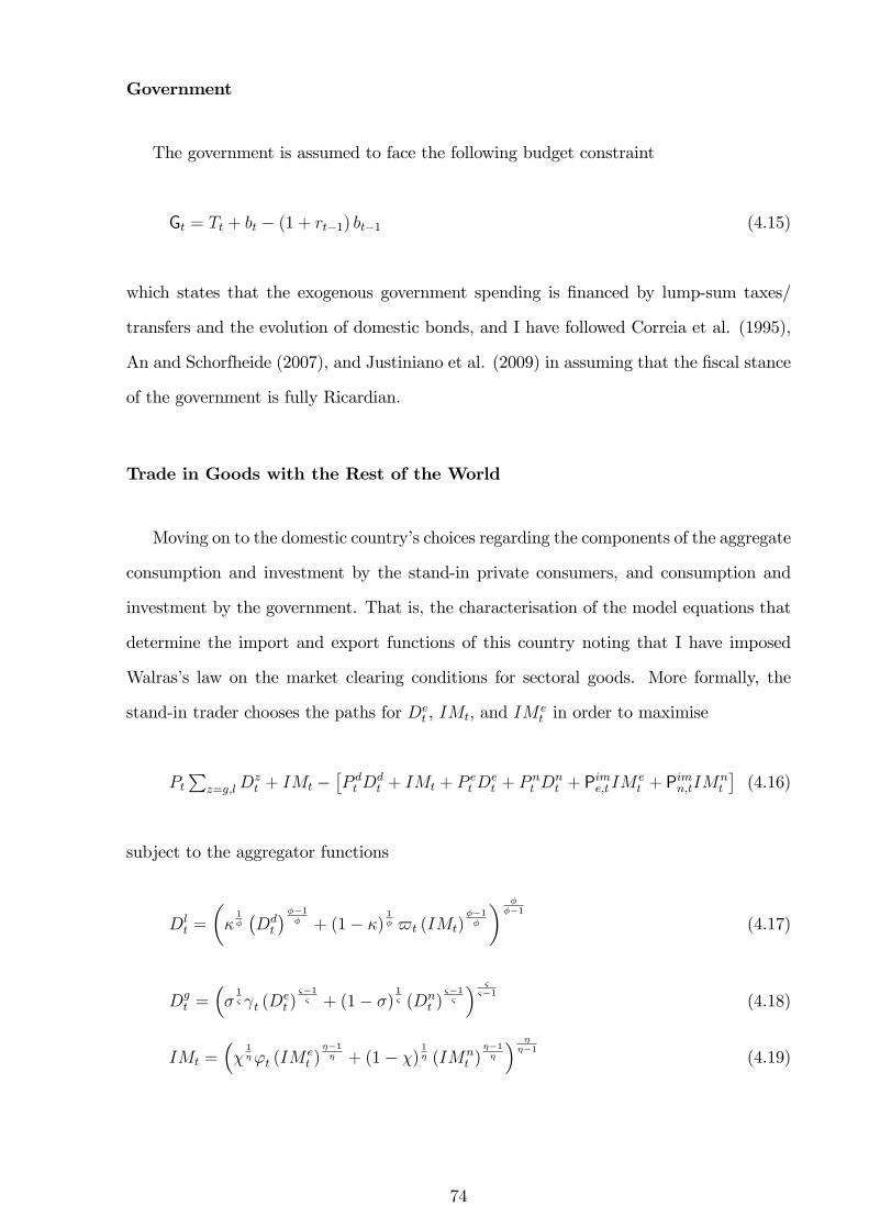
Government
The government is assumed to face the following budget constraint
Gt = Tt + bt � (1 + rt�1) bt�1 (4.15)
which states that the exogenous government spending is �nanced by lump-sum taxes/
transfers and the evolution of domestic bonds, and I have followed Correia et al. (1995),
An and Schorfheide (2007), and Justiniano et al. (2009) in assuming that the �scal stance
of the government is fully Ricardian.
Trade in Goods with the Rest of the World
Moving on to the domestic country�s choices regarding the components of the aggregate
consumption and investment by the stand-in private consumers, and consumption and
investment by the government. That is, the characterisation of the model equations that
determine the import and export functions of this country noting that I have imposed
Walras�s law on the market clearing conditions for sectoral goods. More formally, the
stand-in trader chooses the paths for Det , IMt, and IM e
t in order to maximise
PtP
z=g;lDzt + IMt �
�P dt D
dt + IMt + P e
t Det + P n
t Dnt + P
ime;tIM
et + P
imn;tIM
nt
�(4.16)
subject to the aggregator functions
Dlt =
��1��Ddt
���1� + (1� �)
1� $t (IMt)
��1�
� ���1
(4.17)
Dgt =
��1& t (D
et )
&�1& + (1� �)
1& (Dn
t )&�1&
� &&�1
(4.18)
IMt =��1�'t (IM
et )
��1� + (1� �)
1� (IMn
t )��1�
� ���1
(4.19)
74
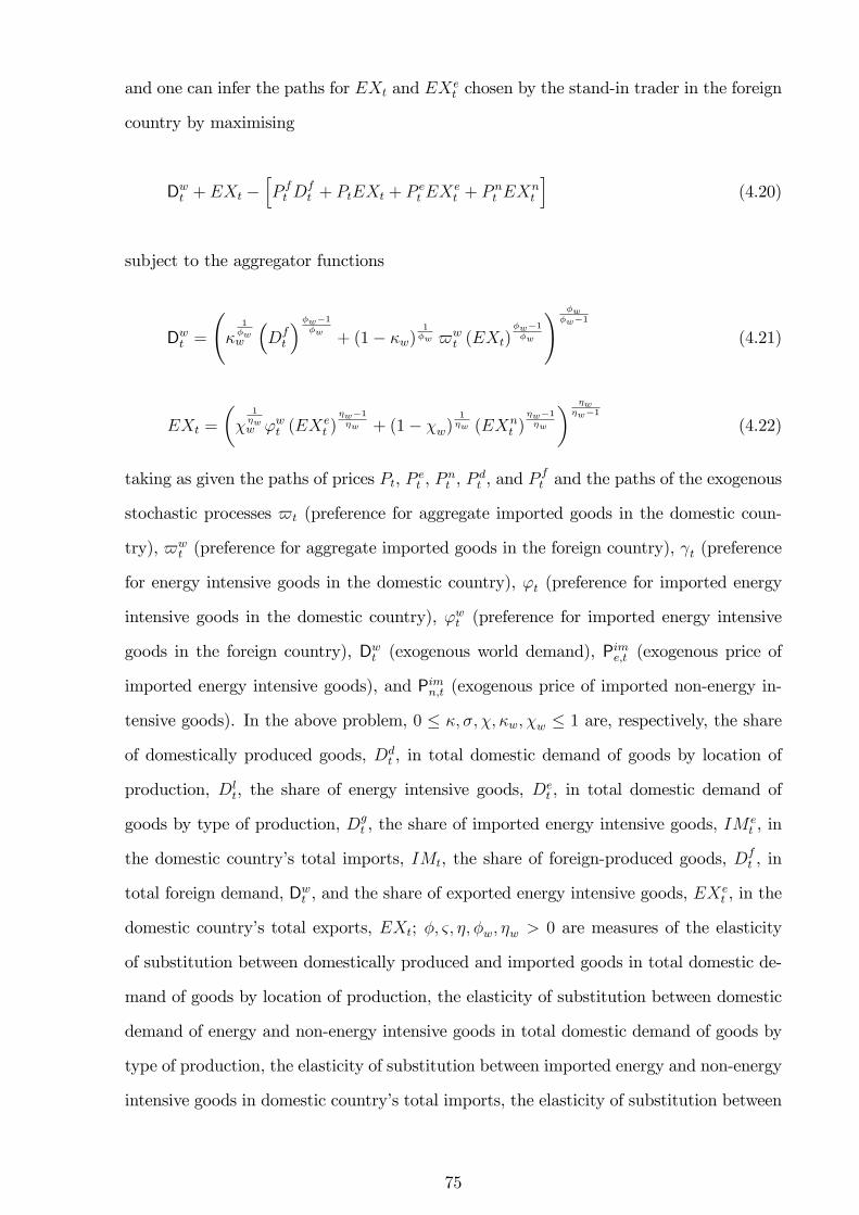
and one can infer the paths for EXt and EXet chosen by the stand-in trader in the foreign
country by maximising
Dwt + EXt �hP ft D
ft + PtEXt + P e
t EXet + P n
t EXnt
i(4.20)
subject to the aggregator functions
Dwt =
�
1�ww
�Dft
��w�1�w + (1� �w)
1�w $w
t (EXt)�w�1�w
! �w�w�1
(4.21)
EXt =
��
1�ww 'wt (EX
et )
�w�1�w + (1� �w)
1�w (EXn
t )�w�1�w
� �w�w�1
(4.22)
taking as given the paths of prices Pt, P et , P
nt , P
dt , and P
ft and the paths of the exogenous
stochastic processes $t (preference for aggregate imported goods in the domestic coun-
try), $wt (preference for aggregate imported goods in the foreign country), t (preference
for energy intensive goods in the domestic country), 't (preference for imported energy
intensive goods in the domestic country), 'wt (preference for imported energy intensive
goods in the foreign country), Dwt (exogenous world demand), Pime;t (exogenous price of
imported energy intensive goods), and Pimn;t (exogenous price of imported non-energy in-
tensive goods). In the above problem, 0 � �; �; �; �w; �w � 1 are, respectively, the share
of domestically produced goods, Ddt , in total domestic demand of goods by location of
production, Dlt, the share of energy intensive goods, D
et , in total domestic demand of
goods by type of production, Dgt , the share of imported energy intensive goods, IM
et , in
the domestic country�s total imports, IMt, the share of foreign-produced goods, Dft , in
total foreign demand, Dwt , and the share of exported energy intensive goods, EXet , in the
domestic country�s total exports, EXt; �; &; �; �w; �w > 0 are measures of the elasticity
of substitution between domestically produced and imported goods in total domestic de-
mand of goods by location of production, the elasticity of substitution between domestic
demand of energy and non-energy intensive goods in total domestic demand of goods by
type of production, the elasticity of substitution between imported energy and non-energy
intensive goods in domestic country�s total imports, the elasticity of substitution between
75
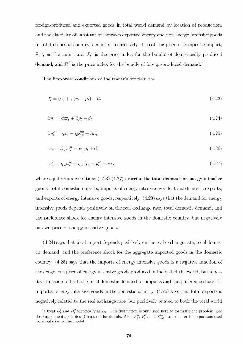
foreign-produced and exported goods in total world demand by location of production,
and the elasticity of substitution between exported energy and non-energy intensive goods
in total domestic country�s exports, respectively. I treat the price of composite import,
Pimt , as the numeraire, Pdt is the price index for the bundle of domestically produced
demand, and P ft is the price index for the bundle of foreign-produced demand.
7
The �rst-order conditions of the trader�s problem are
det = & t + & (pt � pet ) + dt (4.23)
imt = �$t + �pt + dt (4.24)
imet = �'t � �pime;t + imt (4.25)
ext = �w$wt � �wpt + d
wt (4.26)
exet = �w'wt + �w (pt � pet) + ext (4.27)
where equilibrium conditions (4.23)-(4.27) describe the total demand for energy intensive
goods, total domestic imports, imports of energy intensive goods, total domestic exports,
and exports of energy intensive goods, respectively. (4.23) says that the demand for energy
intensive goods depends positively on the real exchange rate, total domestic demand, and
the preference shock for energy intensive goods in the domestic country, but negatively
on own price of energy intensive goods.
(4.24) says that total import depends positively on the real exchange rate, total domes-
tic demand, and the preference shock for the aggregate imported goods in the domestic
country. (4.25) says that the imports of energy intensive goods is a negative function of
the exogenous price of energy intensive goods produced in the rest of the world, but a pos-
itive function of both the total domestic demand for imports and the preference shock for
imported energy intensive goods in the domestic country. (4.26) says that total exports is
negatively related to the real exchange rate, but positively related to both the total world
7I treat Dlt and D
gt identically as Dt. This distinction is only used here to formalise the problem. See
the Supplementary Notes: Chapter 4 for details. Also, P dt , Pft , and P
imn;t do not enter the equations used
for simulation of the model.
76
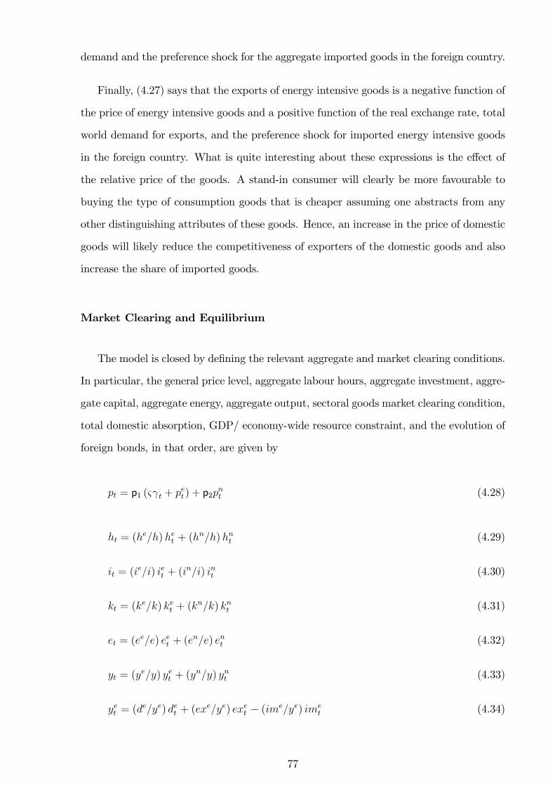
demand and the preference shock for the aggregate imported goods in the foreign country.
Finally, (4.27) says that the exports of energy intensive goods is a negative function of
the price of energy intensive goods and a positive function of the real exchange rate, total
world demand for exports, and the preference shock for imported energy intensive goods
in the foreign country. What is quite interesting about these expressions is the e¤ect of
the relative price of the goods. A stand-in consumer will clearly be more favourable to
buying the type of consumption goods that is cheaper assuming one abstracts from any
other distinguishing attributes of these goods. Hence, an increase in the price of domestic
goods will likely reduce the competitiveness of exporters of the domestic goods and also
increase the share of imported goods.
Market Clearing and Equilibrium
The model is closed by de�ning the relevant aggregate and market clearing conditions.
In particular, the general price level, aggregate labour hours, aggregate investment, aggre-
gate capital, aggregate energy, aggregate output, sectoral goods market clearing condition,
total domestic absorption, GDP/ economy-wide resource constraint, and the evolution of
foreign bonds, in that order, are given by
pt = p1 (& t + pet) + p2pnt (4.28)
ht = (he=h)het + (h
n=h)hnt (4.29)
it = (ie=i) iet + (i
n=i) int (4.30)
kt = (ke=k) ket + (k
n=k) knt (4.31)
et = (ee=e) eet + (e
n=e) ent (4.32)
yt = (ye=y) yet + (y
n=y) ynt (4.33)
yet = (de=ye) det + (ex
e=ye) exet � (ime=ye) imet (4.34)
77
dt = (c=d) ct + (i=d) it + (g=d) gt (4.35)
yt = (c=y) ct + (i=y) it + (g=y) gt + (ex=y) ext � (im=y) imt � (e=y) (qt + et) (4.36)
and
ft =�1 + rft�1
�ft�1 + (ex=y) (pt + ext)� (im=y) imt � (e=y) (qt + et) (4.37)
where p1 = � & (pe=p)1�& and p2 = (1� �) (pn=p)1�& .
I am now able to round up this section by providing the de�nition of a competitive
equilibrium for the model.
De�nition 2 Competitive equilibrium. Taking as given prices (pt, pet , pnt , wt, rt),
shocks (aet , ant , d
wt , 't, '
wt , t, gt, �t, o
et , o
nt , p
ime;t , qt, r
ft , � t, #
et , #
nt , $t, $w
t , �et , �
nt , z
et , z
nt ),
and the initial conditions for consumption, bonds, and capital (c�1, b�1, f�1, ke�1, kn�1),
a competitive equilibrium is characterised by a set of endogenous stochastic processes (ct,
ht, het , hnt , ft, it, i
et , i
nt , u
et , u
nt , k
et , k
nt , yt, y
et , y
nt , et, e
et , e
nt , dt, d
et , imt, ime
t , ext, exet , wt,
rt, pt, pet , pnt ) satis�ed by the solutions to the stand-in consumer, producer, and trader�s
problems, and the bond, labour, capital, energy, and good markets clear.
4.3 Econometric Methodology
In this section, I discuss the methodology used to choose parameter values - this con-
sists of the standard calibration approach and estimation using indirect inference approach.
I then provide a brief description of the data used for estimation.
Calibration
I know that the assessment of the quantitative workings of the model can only begin
when one has chosen values for the model parameters of preference and technology func-
tions, and hence, is able to simulate the model. This I have done by a combination of
78
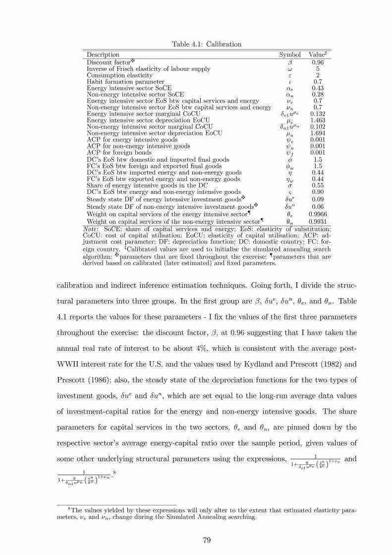
Table 4.1: CalibrationDescription Symbol Value]
Discount factorz � 0:96Inverse of Frisch elasticity of labour supply ! 5Consumption elasticity " 2Habit formation parameter � 0:7Energy intensive sector SoCE �e 0:43Non-energy intensive sector SoCE �n 0:28Energy intensive sector EoS btw capital services and energy �e 0:7Non-energy intensive sector EoS btw capital services and energy �n 0:7Energy intensive sector marginal CoCU �e1u
�e 0:132Energy intensive sector depreciation EoCU �e 1:463Non-energy intensive sector marginal CoCU �n1u
�n 0:102Non-energy intensive sector depreciation EoCU �n 1:694ACP for energy intensive goods e 0:001ACP for non-energy intensive goods n 0:001ACP for foreign bonds f 0:001DC�s EoS btw domestic and imported �nal goods � 1:5FC�s EoS btw foreign and exported �nal goods �w 1:5DC�s EoS btw imported energy and non-energy goods � 0:44FC�s EoS btw exported energy and non-energy goods �w 0:44Share of energy intensive goods in the DC � 0:55DC�s EoS btw energy and non-energy intensive goods & 0:90Steady state DF of energy intensive investment goodsz �ue 0:09Steady state DF of non-energy intensive investment goodsz �un 0:06Weight on capital services of the energy intensive sector{ �e 0:9966Weight on capital services of the non-energy intensive sector{ �n 0:9931Note: SoCE: share of capital services and energy; EoS: elasticity of substitution;CoCU: cost of capital utilisation; EoCU: elasticity of capital utilisation; ACP: ad-justment cost parameter; DF: depreciation function; DC: domestic country; FC: for-eign country. ]Calibrated values are used to initialise the simulated annealing searchalgorithm; zparameters that are �xed throughout the exercise; {parameters that arederived based on calibrated (later estimated) and �xed parameters.
calibration and indirect inference estimation techniques. Going forth, I divide the struc-
tural parameters into three groups. In the �rst group are �, �ue, �un, �e, and �n. Table
4.1 reports the values for these parameters - I �x the values of the �rst three parameters
throughout the exercise: the discount factor, �, at 0:96 suggesting that I have taken the
annual real rate of interest to be about 4%, which is consistent with the average post-
WWII interest rate for the U.S. and the values used by Kydland and Prescott (1982) and
Prescott (1986); also, the steady state of the depreciation functions for the two types of
investment goods, �ue and �un, which are set equal to the long-run average data values
of investment-capital ratios for the energy and non-energy intensive goods. The share
parameters for capital services in the two sectors, �e and �n, are pinned down by the
respective sector�s average energy-capital ratio over the sample period, given values of
some other underlying structural parameters using the expressions, 1
1+ q�e1u
�e (ee
ke )1+�e and
1
1+ q�n1u
�n (en
kn )1+�n .
8
8The values yielded by these expressions will only alter to the extent that estimated elasticity para-meters, �e and �n, change during the Simulated Annealing searching.
79
In the second group are the steady state parameters/ ratios which values are deter-
mined directly from the data except for the exogenous world price of energy and wage
rate, which are normalised to unity in steady state: see Table 4.5 for the calibrated val-
ues. There is not much to say about the parameters in the �rst two groups, but that their
values are kept �xed throughout the econometric exercise except for the sectoral capital
services share parameters.
In the third group are the model parameters I intend to estimate: !, ", �, �e, �n,
�e, �n, �e1u�e, �n1u�n, �e, �n, e, n, f , �, �w, �, �w, �, and &. Table 4.1 provides
the initial values serving as a guide to the Simulated Annealing (SA) algorithm (details
below) to �nd a more optimal values. Hence, as a starting point, I set the elasticity of
labour supply equal to 5, �x consumption elasticity at 2, and preserve the CES form of the
production functions by setting the respective sector�s elasticity of substitution between
capital services and e¢ cient energy use, �e and �n, equal to 0:7.9 Elasticities of labour
hours in the energy and non-energy intensive sectors, 1��e and 1��n, are calibrated to
be 0:57 and 0:72, respectively. I also suppose that there is some degree of habit formation
for agents in this model setting the initial parameter value to 0:7.
Next, I turn to calibrate the component parameters of the two depreciation functions.
In the steady state, these are given by �U e = �e0 + �e1 (�e)�1 (U e)�e and �Un = �n0 +
�n1 (�n)�1 (Un)�n for which I note that only four of the six parameters needed identifying
are �e0, �n0, �e and �n. Thus, with no loss of generality, I �x the values for �e1 and �n1
at unity.10 The idea is that, for j = e; n, �j1 and U j are admitted into the model only
jointly as �j1 (U j)�j such that �j1 = 1 has a trivial implication that �j1 (U j)
�j = (U j)�j .
Then, using household�s optimality conditions with regards to capital utilisation rates
conditioned on the values for the respective sector�s real rental rate of capital in the
steady state, I have that �j1 (U j)�j = Rj = 1=� � (1 � � (U j)), where I have already
calibrated � (U j). The previous expression then simpli�es to give the values reported in
the table for �e1u�e and �n1u�n of 0:132 and 0:102, respectively.
9Kim and Loungani (Table 2, p. 180) provide a justi�cation for using this value. They also considereda value of 0.001 suggesting a Cobb-Douglas form and high elasticity of substitution between capital servicesand energy use. I, however, stick to the parameter value that preserves the general form of speci�cationand leave the optimal choice of parameter value to the estimation stage later on.
10See, for example, Burnside and Eichenbaum (1996), Boileau and Normandin (1999), King and Rebelo(2000), and Leduc and Sill (2004).
80
Conditional on the values of the discount factor and the real rental rates, I calibrate
the parameters governing the elasticities of marginal depreciations with respect to capital
utilisation rates as �e =�e1(Ue)
�e
1+�e1(Ue)�e�1=� = 1:463 and �n =
�n1(Un)�n
1+�n1(Un)�n�1=� = 1:694, which
are reasonably located in the range found in the literature.11 For me, the point of adding
adjustment costs is mainly technical rather than for imposing a prori a very high friction
into the model. Thus, I have set the parameters that relate to the adjustment costs of
capital and foreign bonds, e, n, and f to a very small value of 0:001 to follow a
standard practice in the literature. This way I am permitting the model to inform me
when it has been estimated whether there is more or less real rigidity in the system. The
values chosen for the shares and elasticities of substitution parameters in the aggregator
functions are all standard in the literature.
Indirect Inference
The next task was to test how good my choices of parameters were by taking the
model to the data. If they �t each other, my job was done; otherwise, I would need to
proceed to estimating the twenty parameters in group three above. Now, I brie�y give an
overview of the method of indirect inference (II), which has increasingly been shown in
the literature to be statistically powerful in helping to evaluate models and in estimating
a model�s structural parameters to improve its performance. I am mainly concerned with
11Basu and Kimball (1997) suggested the upper bound of 2 based on a 95% con�dence band. Further,to calibrate this parameter, I have gone for the more restricted form of the depreciation function bysetting �e0 = �n0 = 0. Basu and Kimball (1995, 1997), though used the more general form in theirempirical work and concluded that there is no statistical evidence in support of the non-zero value forthe �xed component of the depreciation function as assumed by many other authors in the literature[see, for example, Greenwood et al. (1988) and Burnside and Eichenbaum (1996)]. I �conclude� thatmy values are not far (not a statistical conclusion) from that usually employed in the literature [see, forexample, Greenwood, et al. who used a value of 1:42, and Burnside and Eichenbaum using their factor-hoarding model and data on output and capital calibrated � to be 1:56 (� = 0:56)]. I must note that thespeci�cation for time-varying depreciation is less general in these other studies. Statistically, however,both values are not rejected by the data. This is done noting one of the concerns of Basu and Kimball(1997) that "...our method makes clear that � is a parameter that needs to be estimated, and in fact isnot pinned down very precisely by the data because it has to be estimated as the reciprocal of a fairlysmall number. Thus, even the small standard error of the reduced-form parameter necessarily impliesthat there is large uncertainty about the structural parameter �. Consequently, economic modellersshould conduct sensitivity analysis of their results using a wide range of values for this parameter." Andalso that "variable depreciation does not seem a signi�cant source of error in the capital stock �guresreported by the BEA." Speci�cally, they concluded that this issue "strikes us as second-order." This thusasks the question of sensitivity analysis regarding our results in response to various values that couldbe used for � (�). Once I have assessed the performance of the model under this calibration approach,the above arguments make more important my next empirical exercise, which is to estimate the model�sunderlying structural parameters. In fact, a prior study by Basu and Kimball (1995) had put the valueof � at roughly 7 with a standard error of about 8. To this end, I impose a wider boundary of [0; 10] inthe estimation exercise.
81
using the method for estimation in this chapter, but given how the procedure works I have
discussed both how it is used for evaluation and estimation purposes here.
Minford et al. (2009) originally proposed the use of II for evaluating a model�s capacity
in �tting the data, and subsequently with a number of re�nements by Le et al. (2011) who
evaluate the method using Monte Carlo experiments. The approach employs an auxiliary
model that is completely independent of the theoretical one to produce a description of
the data against which the performance of the theory is evaluated indirectly. Such a
description can be summarised either by the estimated parameters of the auxiliary model
or by functions of these; I will call these the descriptors of the data. While these are
treated as the �reality�, the theoretical model being evaluated is simulated to �nd its
implied values for them.
II has been widely used in the estimation of structural models [see, for example,
Smith (1993), Gregory and Smith (1991, 1993), Gourieroux et al. (1993), Gourieroux and
Monfort (1995), and Canova (2005)]. Here, my approach is two-fold - one is estimation and
the second is making a further use of II to evaluate structural model. The common element
is the use of an auxiliary time series model. In estimation the parameters of the structural
model are chosen such that when this model is simulated it generates estimates of the
auxiliary model similar to those obtained from the actual data. The optimal choices of
parameters for the structural model are those that minimise the distance between a given
functions of the two sets of estimated coe¢ cients of the auxiliary model. Common choices
of this function are the actual coe¢ cients, the scores or the impulse response functions. In
model evaluation the parameters of the structural model are taken as given. The aim is to
compare the performance of the auxiliary model estimated on simulated data derived from
the given estimates of a structural model - which is taken as a true model of the economy,
the null hypothesis - with the performance of the auxiliary model when estimated from
the actual data. If the structural model is correct then its predictions about the impulse
responses, moments and time series properties of the data should statistically match those
based on the actual data. The comparison is based on the distributions of the two sets of
parameter estimates of the auxiliary model, or of functions of these estimates.
82
The testing procedure thus involves �rst constructing the errors implied by the previ-
ously estimated/ calibrated structural model and the data. These are called the structural
errors and are backed out directly from the equations and the data.12 These errors are then
bootstrapped and used to generate for each bootstrap new data based on the structural
model. An auxiliary time series model is then �tted to each set of data and the sampling
distribution of the coe¢ cients of the auxiliary time series model is obtained from these
estimates of the auxiliary model. A Wald statistic is computed to determine whether
functions of the parameters of the time series model estimated on the actual data lie in
some con�dence interval implied by this sampling distribution.
Following Meenagh et al. (2012) I use as the auxiliary model a VECM which I re-
express as a VAR(1) for the macroeconomic variables of interest with a time trend and
with some residuals entered as exogenous non-stationary processes (these two elements
having the e¤ect of achieving cointegration).13 Thus, the auxiliary model, unlike in the
previous chapter where the model/ data is stationary, in practice is given by
yt = [I �K]yt�1 + xt�1 + gt+ vt (4.38)
where xt�1 is the stochastic trend in productivity, gt are the deterministic trends, and
vt are the VECM innovations. I treat as the descriptors of the data the VAR coe¢ cients
(on the endogenous variables only, I � K) and the VAR error variances (var[v]). The
Wald statistic is computed from these.14 Thus, e¤ectively I am testing whether the ob-
served dynamics and volatility of the chosen variables are explained by the simulated joint
12Some equations may involve calculation of expectations. The method I use here is the robust in-strumental variables estimation suggested by McCallum (1976) and Wickens (1982): I set the laggedendogenous data as instruments and calculate the �tted values from a VAR(1) - this also being the auxil-iary model chosen in what follows. Given that I am working with non-stationary data, the actual auxiliarymodel chosen is a VECM that got re-written as a VAR(1).
13See Le et al. (2013).14I do not attempt to match the time trends and the coe¢ cients on non-stationary trend productivity; I
assume that the model coe¢ cients yielding these balanced growth paths and e¤ects of trend non-stationaryshocks on the steady state are chosen accurately. However, I am not interested, for the exercise here, inany e¤ects on the balanced growth path, as this is �xed. As for the e¤ects of the non-stationary shockson the steady state I assume that any inaccuracy in this will not importantly a¤ect the business cycleanalysis I am carrying out - any inaccuracy would be important in assessing the e¤ect on the steady state,but this is not my focus. Thus, m assessment of the model is as if I was �ltering the data into stationaryform by regressing it on the time trends and trend productivity.
83
distribution of these at a given con�dence level. The Wald statistic is given by
(���)0X�1
(��)(���) (4.39)
where� is the vector of VAR estimates of the chosen descriptors yielded in each simulation,
with � andP
(��) representing the corresponding sample means and variance-covariance
matrix of these calculated across simulations, respectively. The joint distribution of the
� is obtained by bootstrapping the innovations implied by the data and the theoretical
model; it is therefore an estimate of the small sample distribution.15 Such a distribution is
generally more accurate for small samples than the asymptotic distribution; it is also shown
to be consistent by Le et al. (2011) given that theWald statistic is �asymptotically pivotal�;
they also showed it had quite good accuracy in small sample Monte Carlo experiments.16
This testing procedure is applied to a set of (structural) parameters put forward as
the true ones (H0, the null hypothesis); they can be derived from calibration, estimation,
or both. However derived, the test then asks: could these coe¢ cients within this model
structure be the true (numerical) model generating the data? Of course only one true
model with one set of coe¢ cients is possible. Nevertheless one may have chosen coe¢ cients
that are not exactly right numerically, so that the same model with other coe¢ cient values
could be correct. Only when one has examined the model with all coe¢ cient values that
are feasible within the model theory will one have properly tested it. For this reason I
later extend the procedure by a further search algorithm, in which I seek other parameter
sets that could do better in the test.
Thus, I calculate the minimum-value full Wald statistic for each period using a powerful
algorithm based on SA in which search takes place over a wide range around the initial
values, with optimising search accompanied by random jumps around the space.17 In
15The bootstraps in the tests are all drawn as time vectors so contemporaneous correlations betweenthe innovations are preserved.
16Speci�cally, they found on stationary data that the bias due to bootstrapping was just over 2% atthe 95% con�dence level and 0.6% at the 99% level. Meenagh et al. (2012) found even greater accuracyin Monte Carlo experiments on non-stationary data.
17I use a Simulated Annealing algorithm due to Ingber (1996). This mimics the behaviour of the steelcooling process in which steel is cooled, with a degree of reheating at randomly chosen moments in thecooling process� this ensuring that the defects are minimised globally. Similarly the algorithm searchesin the chosen range and as points that improve the objective are found it also accepts points that do notimprove the objective. This helps to stop the algorithm being caught in local minima. I �nd that thisalgorithm improves substantially here on a standard optimisation algorithm. The method used follows
84
e¤ect this is Indirect Inference estimation of the model; however here this estimation is
being done to �nd whether the model can be rejected in itself and not for the sake of
�nding the most satisfactory estimates of the model parameters. Nevertheless of course
the method does this latter task as a by-product so that I can use the resulting unrejected
model as representing the best available estimated version. The merit of this extended
procedure is that I can then compare the best possible versions of each model type when
�nally doing my comparison of model compatibility with the data.
Data
Figures 4.2-4.3 display the time paths for the data series that are used in the cali-
bration, estimation, and evaluation of the model. These are un�ltered U.S. annual data
covering the period 1949-2013, and are logarithmically transformed, real [using Bureau of
Labour Statistics (BLS) series: consumer price index (CPI, 2009=100)] per capita [using
Bureau of Labour Statistics (BLS) series: civilian non-institutionalised population over
16 years old] terms except for wage rate, interest rate, real exchange rate, and capital util-
isation rates.18 Meanwhile, just as the U.S. variables are de�ated by the U.S. CPI, world
CPI is used to de�ate world series, especially world demand and is also the numeraire.
4.4 Results
In this section, which I organise into two sub-sections, the main �ndings of the exercise
are discussed. Firstly, I examine the estimated parameter values. Secondly, I look at
the properties of the estimated model by considering some qualitative and quantitative
outcomes. While doing these, I emphasise at every opportunity the main focus of this
chapter, which is to determine how well this energy model of open economy can reproduce
the business cycle implications of output and real exchange rate of the U.S.
a standard testing method: I take a set of model parameters (excluding error processes), extract theresulting residuals from the data using the LIML method, �nd their implied autoregressive coe¢ cients(AR(1) here) and then bootstrap the implied innovations with this full set of parameters to �nd theimplied Wald value. This is then minimised by the SA algorithm.
18A detailed description of the data sources and construction of the observables are presented in theAppendix.
85
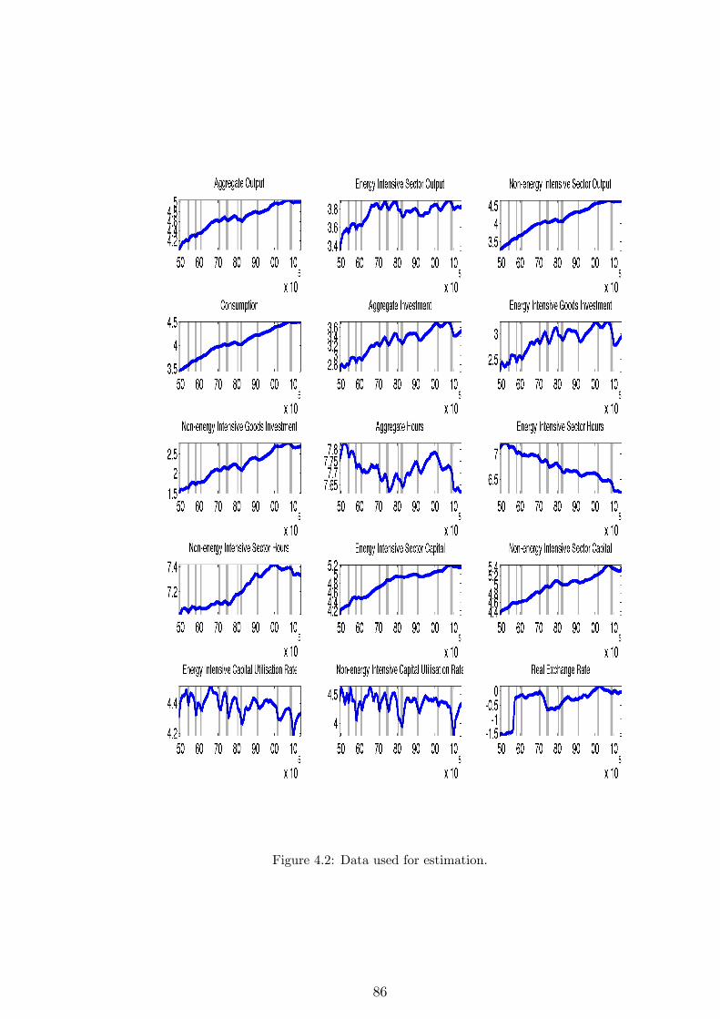
Figure 4.2: Data used for estimation.
86
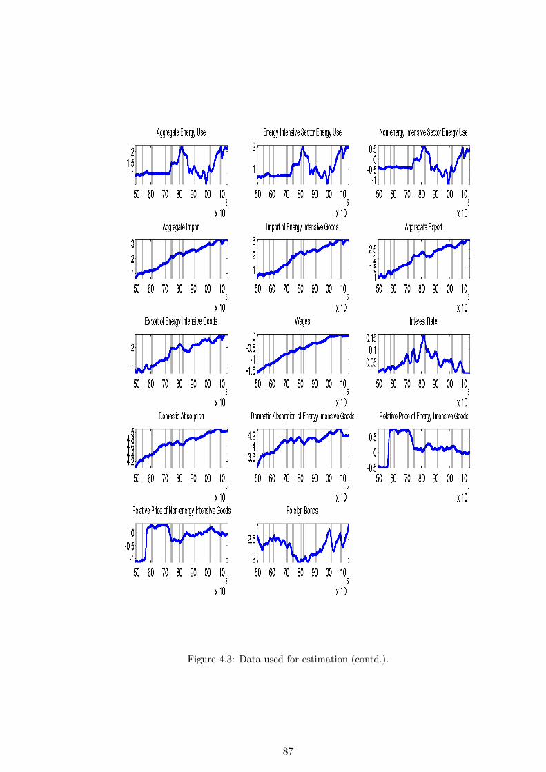
Figure 4.3: Data used for estimation (contd.).
87
Parameter Estimates
Structural Parameters Estimates of the model parameters are summarised in the up-
per panel of Table 4.2. Consumption elasticity, ", is one of the highly di¢ cult parameters
to pin down in economics. The estimate of its inverse is 1:24, which is arguably within
the range of estimates found in many DSGE models [Hall (1988) and Smets and Wouters
(2003, 2005)]. Consumption elasticity of 0:81 found here implies that households are more
willing to smooth consumption across time in response to a change in real interest rate.19
Compared to the initial value, the estimated value of the habit formation parameter in-
terestingly is suggesting that household�s utility in period t is less dependent on past
consumption. Speci�cally, the estimated value of 0:3 reduces any forms of consumption
inertia to transitory shocks; hence, the hump of consumption impulse response functions
becomes more sharpened - see Fuhrer (2000). Theoretically, there is no judgement against
this result as the focus of the research is not that of accounting for asset market relations,
but quantitatively, it is quite low for a developed country [see Boldrin et al. (2001) who
estimated a value of 0:7; Smets and Wouters (2004) who reported a value of 0:55; Chris-
tiano et al. (2005) who obtained a point estimate of 0:65]. In fact, low habit persistence is
usually associated with developing nations; for example, Uribe and Yue (2006) estimated
this to be 0:2 using a panel data for emerging countries.
Labour elasticities in the two sectors are 0:75 and 0:63 for the energy and non-energy
intensive sector, respectively. The high value for Frisch elasticity (!�1 = 0:17) says that
labour hours react more to changes in the real wage. 1 + �e (1 + �n) is a measure of
the inverse elasticity of substitution between capital services and primary energy use in
the energy (non-energy) intensive sector such that the values of �e = 0:29 and �n = 0:27
implies that there are high elasticities of substitution between the two factors in both
sectors. All estimates for the adjustment cost parameters are close to zero: the values of
0:0001, 0:0007, and 0:0001 for e, n, and f , respectively, which are all smaller than the
initial values by at least 30% justi�es my decision to assume that the cost of adjusting all
19This implies that agents would respond more to substitution e¤ect than to wealth e¤ect. A value ofbetween zero and one is uncontroversial in the literature [e.g., Kocherlakota (1988) advocated for a valueclose to zero]. Meanwhile, Campbell (1994) used values ranging from zero to in�nity in his analysis. Formore on the range of values and other estimates of consumption elasticity, see, for example, Nelson andNikolov (2002), Bergin (2003), and Cromb and Fernandez-Corugedo (2004).
88
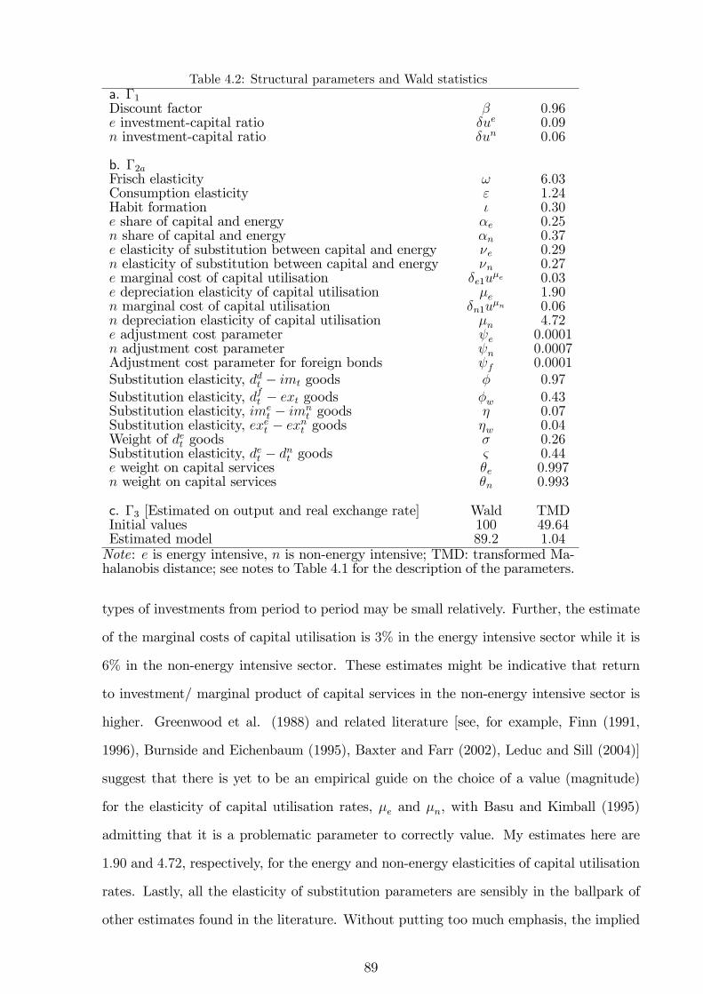
Table 4.2: Structural parameters and Wald statisticsa. �1Discount factor � 0:96e investment-capital ratio �ue 0:09n investment-capital ratio �un 0:06
b. �2aFrisch elasticity ! 6:03Consumption elasticity " 1:24Habit formation � 0:30e share of capital and energy �e 0:25n share of capital and energy �n 0:37e elasticity of substitution between capital and energy �e 0:29n elasticity of substitution between capital and energy �n 0:27e marginal cost of capital utilisation �e1u
�e 0:03e depreciation elasticity of capital utilisation �e 1:90n marginal cost of capital utilisation �n1u
�n 0:06n depreciation elasticity of capital utilisation �n 4:72e adjustment cost parameter e 0:0001n adjustment cost parameter n 0:0007Adjustment cost parameter for foreign bonds f 0:0001Substitution elasticity, ddt � imt goods � 0:97Substitution elasticity, dft � ext goods �w 0:43Substitution elasticity, ime
t � imnt goods � 0:07
Substitution elasticity, exet � exnt goods �w 0:04Weight of det goods � 0:26Substitution elasticity, det � dnt goods & 0:44e weight on capital services �e 0:997n weight on capital services �n 0:993
c. �3 [Estimated on output and real exchange rate] Wald TMDInitial values 100 49:64Estimated model 89:2 1:04Note: e is energy intensive, n is non-energy intensive; TMD: transformed Ma-halanobis distance; see notes to Table 4.1 for the description of the parameters.
types of investments from period to period may be small relatively. Further, the estimate
of the marginal costs of capital utilisation is 3% in the energy intensive sector while it is
6% in the non-energy intensive sector. These estimates might be indicative that return
to investment/ marginal product of capital services in the non-energy intensive sector is
higher. Greenwood et al. (1988) and related literature [see, for example, Finn (1991,
1996), Burnside and Eichenbaum (1995), Baxter and Farr (2002), Leduc and Sill (2004)]
suggest that there is yet to be an empirical guide on the choice of a value (magnitude)
for the elasticity of capital utilisation rates, �e and �n, with Basu and Kimball (1995)
admitting that it is a problematic parameter to correctly value. My estimates here are
1:90 and 4:72, respectively, for the energy and non-energy elasticities of capital utilisation
rates. Lastly, all the elasticity of substitution parameters are sensibly in the ballpark of
other estimates found in the literature. Without putting too much emphasis, the implied
89
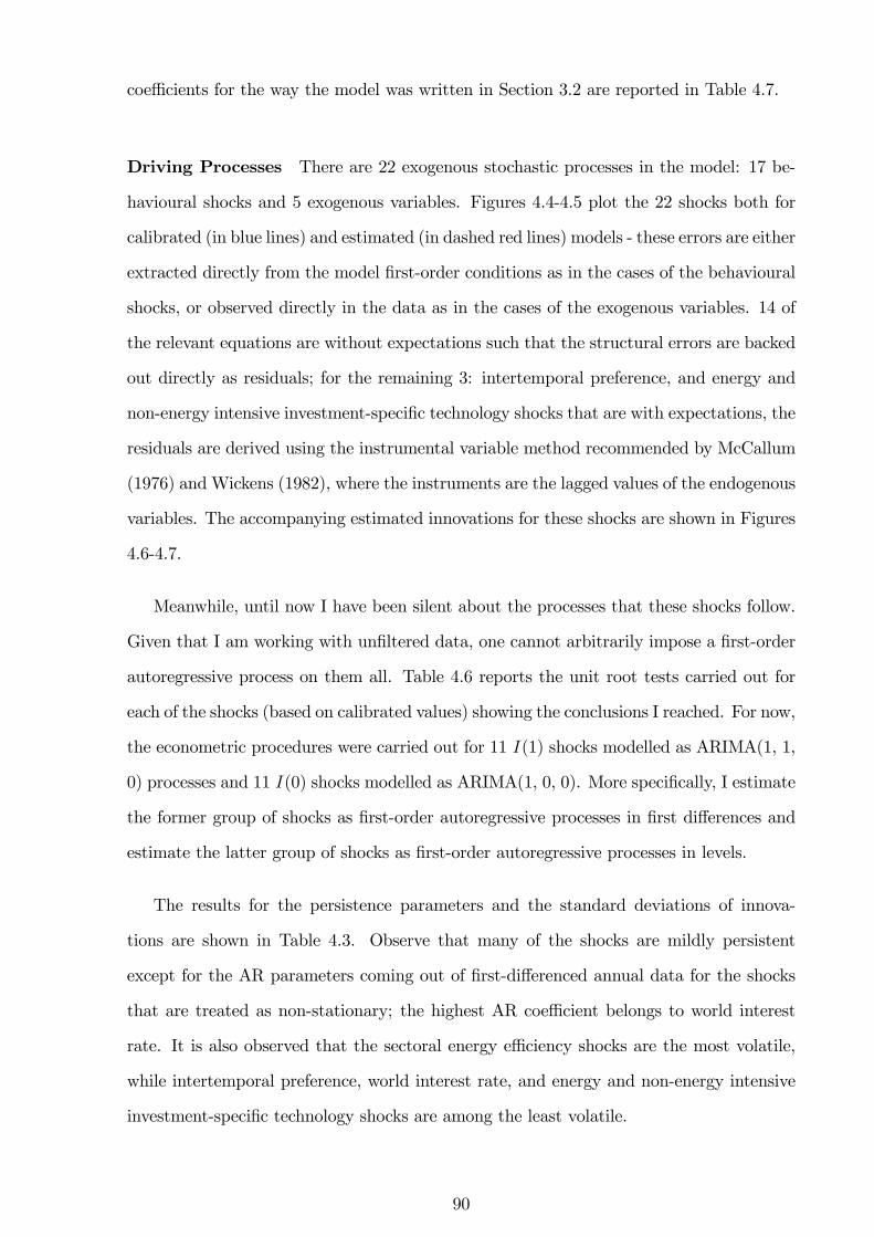
coe¢ cients for the way the model was written in Section 3.2 are reported in Table 4.7.
Driving Processes There are 22 exogenous stochastic processes in the model: 17 be-
havioural shocks and 5 exogenous variables. Figures 4.4-4.5 plot the 22 shocks both for
calibrated (in blue lines) and estimated (in dashed red lines) models - these errors are either
extracted directly from the model �rst-order conditions as in the cases of the behavioural
shocks, or observed directly in the data as in the cases of the exogenous variables. 14 of
the relevant equations are without expectations such that the structural errors are backed
out directly as residuals; for the remaining 3: intertemporal preference, and energy and
non-energy intensive investment-speci�c technology shocks that are with expectations, the
residuals are derived using the instrumental variable method recommended by McCallum
(1976) and Wickens (1982), where the instruments are the lagged values of the endogenous
variables. The accompanying estimated innovations for these shocks are shown in Figures
4.6-4.7.
Meanwhile, until now I have been silent about the processes that these shocks follow.
Given that I am working with un�ltered data, one cannot arbitrarily impose a �rst-order
autoregressive process on them all. Table 4.6 reports the unit root tests carried out for
each of the shocks (based on calibrated values) showing the conclusions I reached. For now,
the econometric procedures were carried out for 11 I (1) shocks modelled as ARIMA(1, 1,
0) processes and 11 I (0) shocks modelled as ARIMA(1, 0, 0). More speci�cally, I estimate
the former group of shocks as �rst-order autoregressive processes in �rst di¤erences and
estimate the latter group of shocks as �rst-order autoregressive processes in levels.
The results for the persistence parameters and the standard deviations of innova-
tions are shown in Table 4.3. Observe that many of the shocks are mildly persistent
except for the AR parameters coming out of �rst-di¤erenced annual data for the shocks
that are treated as non-stationary; the highest AR coe¢ cient belongs to world interest
rate. It is also observed that the sectoral energy e¢ ciency shocks are the most volatile,
while intertemporal preference, world interest rate, and energy and non-energy intensive
investment-speci�c technology shocks are among the least volatile.
90
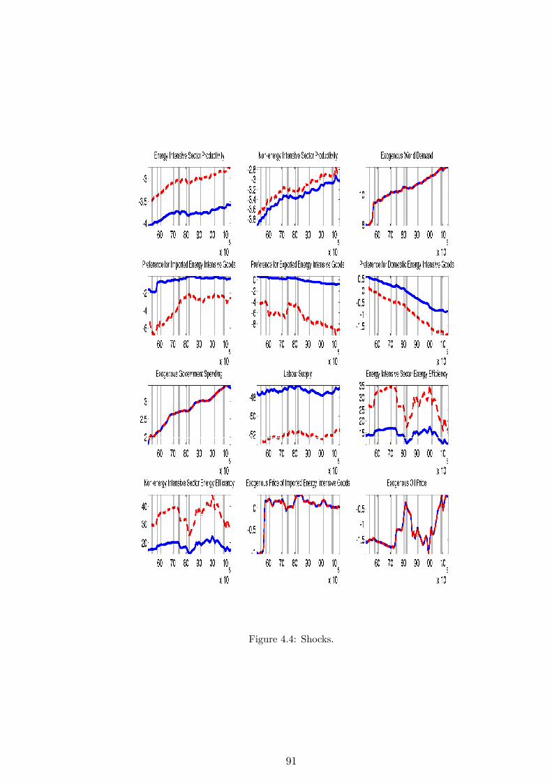
Figure 4.4: Shocks.
91
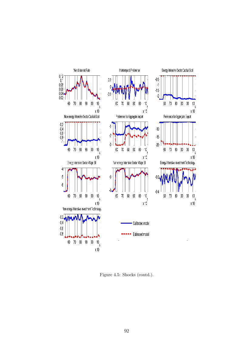
Figure 4.5: Shocks (contd.).
92
Figure 4.6: Innovations.
Properties of the Estimated Model
One of the main agenda in this section is to interrogate the estimated model about
the role of energy price shocks in causing the U.S. business cycles and especially in an
economic environment littered with a host of other shocks chief among which are the
productivity and other imported shocks. The main result is that the model can explain
the observed quantitative response of output to oil price increases, and I provide a the-
93
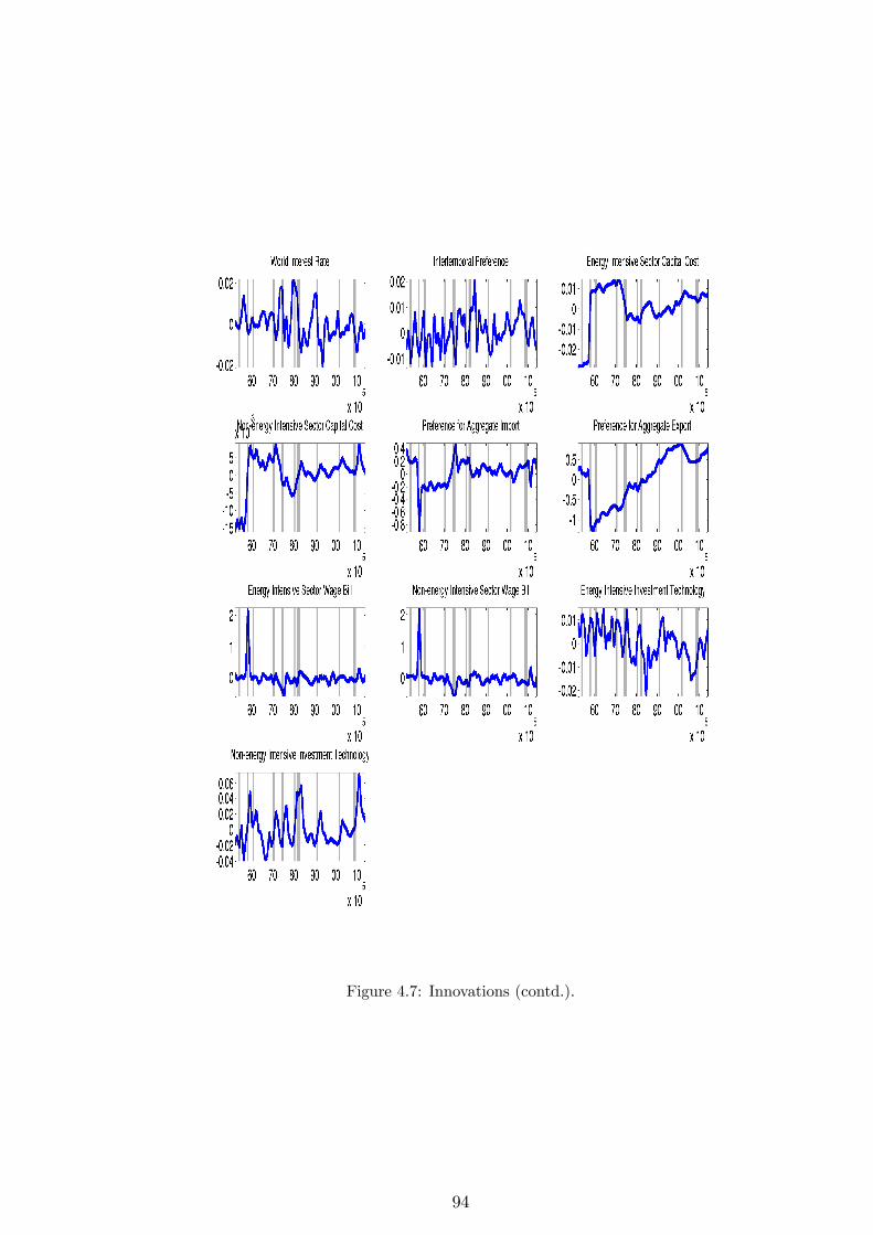
Figure 4.7: Innovations (contd.).
94
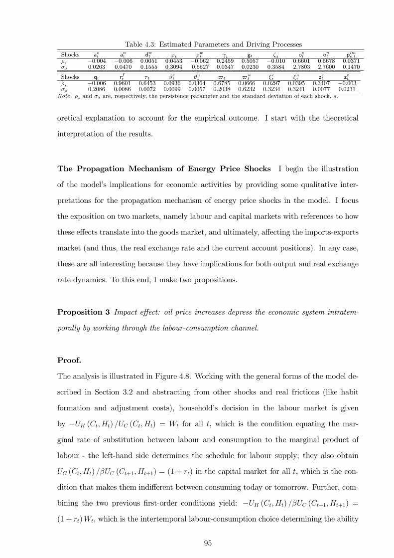
Table 4.3: Estimated Parameters and Driving ProcessesShocks aet ant dwt 't 'wt t gt �t oet ont pime;t�s �0:004 �0:006 0:0051 0:0453 �0:062 0:2459 0:5057 �0:010 0:6601 0:5678 0:0371�s 0:0263 0:0470 0:1555 0:3094 0:5527 0:0347 0:0230 0:3584 2:7803 2:7600 0:1470
Shocks qt rft � t #et #nt $t $wt �et �nt zet znt
�s �0:006 0:9601 0:6453 0:0936 0:0364 0:6785 0:0666 0:0297 0:0395 0:3407 �0:003�s 0:2086 0:0086 0:0072 0:0099 0:0057 0:2038 0:6232 0:3234 0:3241 0:0077 0:0231Note : �s and �s are, respectively, the persistence parameter and the standard deviation of each shock, s.
oretical explanation to account for the empirical outcome. I start with the theoretical
interpretation of the results.
The Propagation Mechanism of Energy Price Shocks I begin the illustration
of the model�s implications for economic activities by providing some qualitative inter-
pretations for the propagation mechanism of energy price shocks in the model. I focus
the exposition on two markets, namely labour and capital markets with references to how
these e¤ects translate into the goods market, and ultimately, a¤ecting the imports-exports
market (and thus, the real exchange rate and the current account positions). In any case,
these are all interesting because they have implications for both output and real exchange
rate dynamics. To this end, I make two propositions.
Proposition 3 Impact e¤ect: oil price increases depress the economic system intratem-
porally by working through the labour-consumption channel.
Proof.
The analysis is illustrated in Figure 4.8. Working with the general forms of the model de-
scribed in Section 3.2 and abstracting from other shocks and real frictions (like habit
formation and adjustment costs), household�s decision in the labour market is given
by �UH (Ct; Ht) =UC (Ct; Ht) = Wt for all t, which is the condition equating the mar-
ginal rate of substitution between labour and consumption to the marginal product of
labour - the left-hand side determines the schedule for labour supply; they also obtain
UC (Ct; Ht) =�UC (Ct+1; Ht+1) = (1 + rt) in the capital market for all t, which is the con-
dition that makes them indi¤erent between consuming today or tomorrow. Further, com-
bining the two previous �rst-order conditions yield: �UH (Ct; Ht) =�UC (Ct+1; Ht+1) =
(1 + rt)Wt, which is the intertemporal labour-consumption choice determining the ability
95
to smooth not just consumption, but also labour over time. This particular representation
makes explicit that household�s supply of labour depends on both the wage rate and the
stock of initial or current wealth (this is represented by the upward sloping curve in Figure
4.8). Meanwhile, on the production side and imposing symmetry between sectors (or work-
ing with the aggregate economy for the moment) to simplify the analysis, it is straightfor-
ward to derive the labour-energy ratio as FH (Ht; Kt; Et) =FE (Ht; Kt; Et) =Wt=Qt, where
the relative productivities on the left-hand determines the schedule for labour demand
(this is represented by the downward sloping curve in Figure 4.8). For a required level of
crude oil, a positive shock to its price, ceteris paribus, will lead to a fall in demand for
labour. Speci�cally, all things being equal, as Qt rises, Wt=Qt falls such that to maintain
the equal sign the ratio FH (Ht; Kt; Et) =FE (Ht; Kt; Et) must likewise go down, and sup-
pose that the required quantity of energy is �xed, the labour quantity demanded falls.20
Moreover, without assuming �xed energy necessary for production, labour demand can still
fall because of the fall inWt=Qt that signals to the �rms falling productivity of labour rel-
ative to energy use.21 Bringing the consumers and the producers together, equilibrium in
the labour market is given by: �UH (Ct; Ht) =�UC (Ct+1; Ht+1) = (1 + rt)Wt = Wt=Qt =
FH (Ht; Kt; Et) =FE (Ht; Kt; Et) which I �nd useful broken up into prices (1 + rt)Wt =
Wt=Qt implying that Qt = 1=� (1 + rt) and quantities �UH (Ct; Ht) =UC (Ct+1; Ht+1) =
FH (Ht; Kt; Et) =FE (Ht; Kt; Et), which equates intertemporal labour-consumption deci-
sion to the ratio of the two marginal products. The price relation gives a hint of the
connection to investment implying that when Qt goes up, rt must fall to maintain equi-
librium since the discount factor is constant.22 All things being equal, the resource drain
e¤ect can be shown to be given by: dYtdQt
��H;K
= (�) � 0 where always takes a negative
value for an oil-importing country like the U.S. and (�) include energy use and structural20As is standard in the literature when analysing short-run production function that labour is the
input that can be varied most quickly. An alternative way to see how this may happen is to writean expression for the marginal cost of energy input as Q = Wt
FH(Ht;Kt;Et)=FE(Ht;Kt;Et). Obviously, as Q
rises the numerator and/ or the denominator of the right-hand side must change appropriately to ensureequality.
21Formally, we assume that E 2�E;E
�indicating that there is a minimum level of energy required, E,
for �rms to be operational and a maximum level, E, that the �rms would import depending either on costor production possibility frontier. Further, note that the e¤ects of oil price shocks in this model are notdirect on the households because they are not modelled to use imported crude oil [see, for example, Dhawanand Jeske (2008) for an analysis that integrated imported crude oil into household utility function]. Butto the extent that the pro�ts of the �rms are a¤ected will the return to household�s investment be. Thisis one of the channels by which the negative spiral of this shock permeates the system.
22A re-arrangement of the intertemporal indi¤erence curve of the households that would lead to simi-lar conclusion is UC (Ct;Ht) =�UC (Ct+1;Ht+1) = (1 + rt) = �UH (Ct;Ht) =�UC (Ct+1;Ht+1)Wt, whichimplies that UC (Ct;Ht)Wt = �UH (Ct;Ht).
96
model parameters (e.g., share of energy use in production and elasticity of substitution
parameter).23 As drawn, the demand for labour is that which achieves point B in panel a
of Figure 4.8 with a corresponding lower output level YH1;K0;E0 in panel b.
The above result appears rooted in the notion that the model is able to generate
intertemporal labour-consumption substitution, which in itself is not a new idea, but to
my best knowledge this particular re-interpretation in relation to the impact e¤ect on
aggregate and sectoral macroeconomic variables is novel.24
Proposition 4 Transition e¤ect: oil price increases depress the economic system in-
tertemporally by working through the consumption-investment channel.
Proof.
The proof of the transition e¤ect follows from that of the impact e¤ect. Speci�cally, the
domestic �rms having absorbed the impact e¤ect transfers it to the households in the
form of job losses, possible lower wage rate, and lower return to last period�s investment
(end-of-period t pro�t declines). All told, this implies that the household�s stock of wealth
has declined, and since it is the households that make investment decisions in this model
what they have available to supply for capital formation against next period is reduced
creating the link to probable further output decreases in period t + 1. We illustrate this
outcome in Figure 4.8 shown by point C in panel a and output level YH2;K1;E1 in panel b.
I round this sub-section up by looking at the sectoral output �uctuations to which
the above results are tied and show how this impacts on aggregate output. Speci�cally,
when the price of imported energy goes up, this takes resources from the domestic country
transferring it to the RoW - this is easily seen by examining the economy-wide resource
constraint. The resulting e¤ect is that the total net imports must fall, unless the oil
23This value, (�), lost by the oil-importer is gained by the oil-exporter at least to the extent that thesupply of exports fails to match this amount [see for example Darby (1981)].
24See Lucas (1972a, 1972b, 1973) for the theoretical development of labour smoothing. Meanwhile, aclosely related interpretation brought to my attention after this analysis was put forth is that of factor-price frontier done for an aggregate economy by Blanchard and Gali (2010) in which oil is allowed toenter both consumption and production functions. While they discussed results that are similar to theimpact e¤ect for their aggregate economy, they did not discuss transition e¤ect. Arguments in Eastwood(1992) appear to follow this line of enquiry.
97
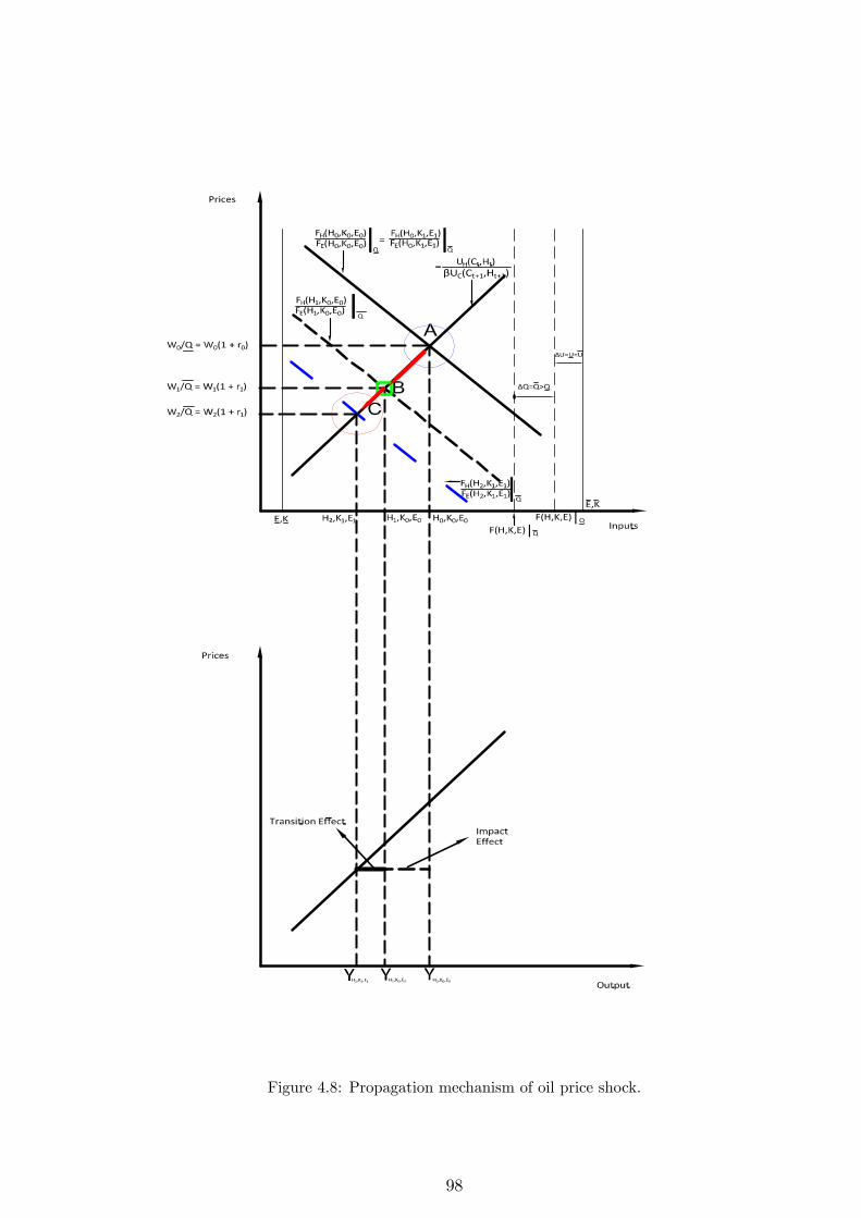
Figure 4.8: Propagation mechanism of oil price shock.
98
exporter buys at least an equivalent amount of goods from the domestic country. I abstract
from this possibility and explain the complementary outcome to the above propositions in
relation to international trade and competitiveness of the domestic country. Additionally,
an increase in the price of energy means that the price of goods that are more energy
intensive in their production also rises. These mechanisms of propagating the e¤ects of
energy price shocks via the sectors are explained next.
From the �rst-order conditions, both prices of energy and non-energy intensive goods
in the domestic country are derived endogenous, but of importance is that we can write
the solution to the price of non-energy intensive goods as a function of both the aggregate
price level and the price of energy intensive goods. My focus is on the latter and Figure
4.9 is used to illustrate this mechanism. Note that the vertical axes on both panels a and
b of the graph are labelled P et because of the reason just given. In particular, because the
energy intensive sector is assumed to be relatively both oil and capital more intensive, its
supply curve is drawn to be steeper such that the increase in the supply of energy intensive
goods due to P et rising is less than the drop in the supply of non-energy intensive goods
due to a fall in P nt . Thus, output falls and the demand for both types of goods fall to
reduce net exports as consumers are poorer. The e¤ect on real exchange rate is actually
ambiguous as it depends on a host of other factors.25
Accounting for Two Recessions Using the U.S. data over the sample period, I de�ne
an episode as involving abnormal growth if there is an annual growth of gross domestic
product (GDP) above 3.5%, which is the average growth rate of U.S. GDP over the sample
period. Also, I de�ne recession as any negative change in output. For both growth and
recession, I take as one episode every successive occurrence. I then seek to understand
these excessive U.S. business cycles. To undertake this study, I adopt the dating of the
U.S. recessions by the National Bureau of Economic Research (NBER) and the dating (and
causes) of oil crises and recession provided in Table 4.12, which is based on Hamilton�s
(1985, 2011) calculations.
25See Krugman (1983) and some of the references therein for factors that work to determine realexchange rate position after an oil price shock.
99
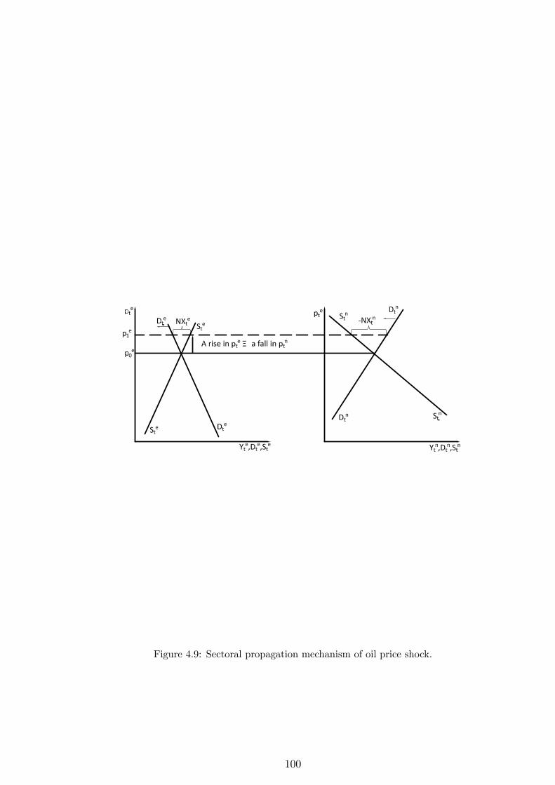
Figure 4.9: Sectoral propagation mechanism of oil price shock.
100
Then, I carry out the following experiments: (1) for output and real exchange rate
for which I have �tted the model to data and working with two selected sub-samples,26
I decompose each growth and recession/ depression according to the model based on the
twelve structural shocks - I depict the results in Figures 4.10-4.13; (2) I consider the role
played by each shock over these periods by examining the accumulated shocks for each
episode of abnormal growth and recession as shown in Figures 4.17-4.20; and (3) I generate
a pseudo data for 62,000 years using Monte Carlo techniques and use it to guess oil price-
macroeconomic relationship over my sample period - I then compare these predictions to
actual data as presented in Table 4.13 and Figure 4.21.
To investigate the e¤ects of energy related shocks on the historical macroeconomic
experiences of the U.S. in a model bu¤eted by numerous supply-side and demand-side
shocks, I construct the time paths for output and real exchange rate for the two sub-periods
opting for an orthogonalisation scheme that orders energy price shock �rst followed by the
remaining permanent shocks and then the transitory shocks. To this end, any contribution
due to the correlation between the shocks, say energy price shocks and the remaining
shocks (take the energy intensive sector productivity shock for example) is attributed to
the energy price shock. I extend this approach down the line till I reached the last shock,
which according to my ordering is the non-energy intensive investment-speci�c technology
shock.
Further, the shock decompositions for the variables are analysed in groups, viz: pro-
ductivity shocks, which include the energy and non-energy intensive sectors�neutral pro-
ductivities (aet and ant ), energy and non-energy intensive sectors� energy e¢ ciencies (o
et
and ont ), and energy and non-energy intensive goods�investment-speci�c technologies (zet
and znt ); preference shocks, which include the intertemporal preference (� t), labour supply
(�t), preference for imported energy intensive goods ('t), preference for exported energy
intensive goods ('wt ), preference for energy intensive goods ( t), preference for aggregate
imported goods ($t), and preference for aggregate exported goods ($wt ); cost-push shocks,
which include energy and non-energy intensive capital cost shifters (#et and #nt ), energy
26The two chosen sub-samples are 1967-1984 and 1995-2012 and are of equal lengths. The formerperiod is characterised by strike, reduction in Libyan supply, bursting of the Trans-Arabian pipeline,Iranian revolution, and the Iran-Iraq War; the latter period is characterised by the Second Gulf War,Venezuela unrest, and the overshooting of demand over supply.
101
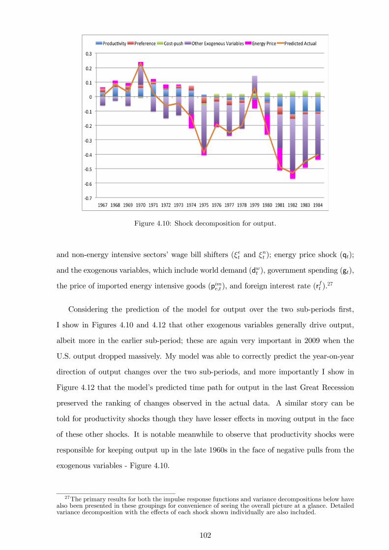
Figure 4.10: Shock decomposition for output.
and non-energy intensive sectors�wage bill shifters (�et and �nt ); energy price shock (qt);
and the exogenous variables, which include world demand (dwt ), government spending (gt),
the price of imported energy intensive goods (pime;t ), and foreign interest rate (rft ).
27
Considering the prediction of the model for output over the two sub-periods �rst,
I show in Figures 4.10 and 4.12 that other exogenous variables generally drive output,
albeit more in the earlier sub-period; these are again very important in 2009 when the
U.S. output dropped massively. My model was able to correctly predict the year-on-year
direction of output changes over the two sub-periods, and more importantly I show in
Figure 4.12 that the model�s predicted time path for output in the last Great Recession
preserved the ranking of changes observed in the actual data. A similar story can be
told for productivity shocks though they have lesser e¤ects in moving output in the face
of these other shocks. It is notable meanwhile to observe that productivity shocks were
responsible for keeping output up in the late 1960s in the face of negative pulls from the
exogenous variables - Figure 4.10.
27The primary results for both the impulse response functions and variance decompositions below havealso been presented in these groupings for convenience of seeing the overall picture at a glance. Detailedvariance decomposition with the e¤ects of each shock shown individually are also included.
102
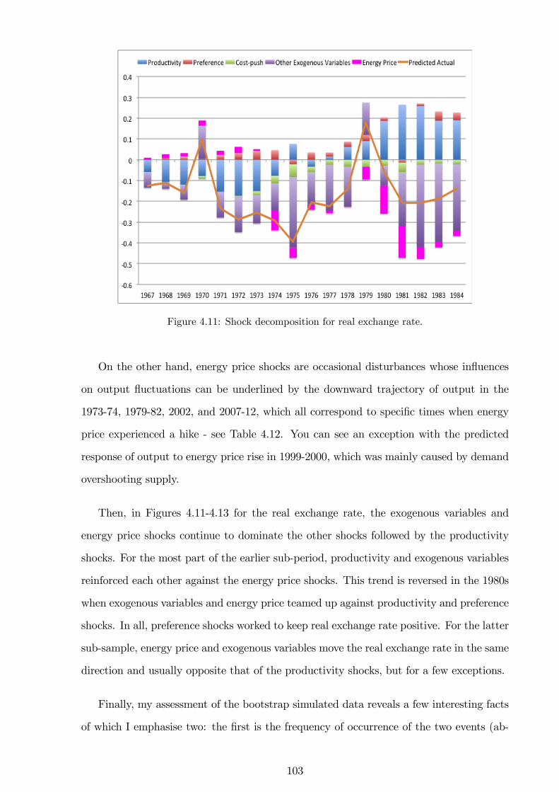
Figure 4.11: Shock decomposition for real exchange rate.
On the other hand, energy price shocks are occasional disturbances whose in�uences
on output �uctuations can be underlined by the downward trajectory of output in the
1973-74, 1979-82, 2002, and 2007-12, which all correspond to speci�c times when energy
price experienced a hike - see Table 4.12. You can see an exception with the predicted
response of output to energy price rise in 1999-2000, which was mainly caused by demand
overshooting supply.
Then, in Figures 4.11-4.13 for the real exchange rate, the exogenous variables and
energy price shocks continue to dominate the other shocks followed by the productivity
shocks. For the most part of the earlier sub-period, productivity and exogenous variables
reinforced each other against the energy price shocks. This trend is reversed in the 1980s
when exogenous variables and energy price teamed up against productivity and preference
shocks. In all, preference shocks worked to keep real exchange rate positive. For the latter
sub-sample, energy price and exogenous variables move the real exchange rate in the same
direction and usually opposite that of the productivity shocks, but for a few exceptions.
Finally, my assessment of the bootstrap simulated data reveals a few interesting facts
of which I emphasise two: the �rst is the frequency of occurrence of the two events (ab-
103
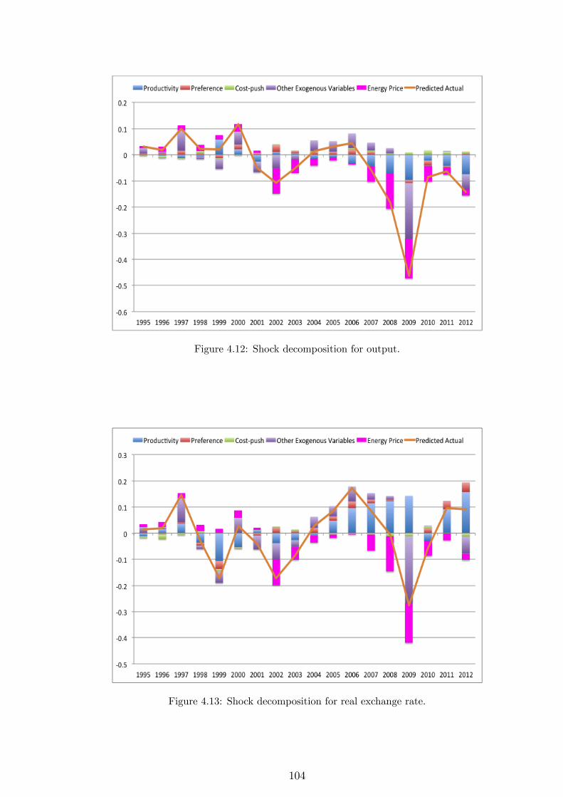
Figure 4.12: Shock decomposition for output.
Figure 4.13: Shock decomposition for real exchange rate.
104
normal growth and recession) in tango with oil price changes (down and up); the second is
the percentage of events involving oil price changes. I have shown by the results that the
adopted de�nitions of growth and recession are integral to the business cycle experiences
of the U.S. and that this would be the benchmark against which to judge every other
experience. More speci�cally, I �nd that of the times when there has been an abnormal
growth (a recession), about 17 (16) percent involve oil price decreases (increases). Unfor-
tunately, I am unable to quantify the magnitude of the e¤ects of these price changes on
output �uctuation, and thus are unable to say much on the asymmetric e¤ects attributes
of oil price changes. In addition, the experiment suggests that there will be no recession
(abnormal growth) and no oil price increases (decreases) in about every 2 years, and that,
on average, in about every 5 years, there is an oil price rise (fall) that does not impact on
output �uctuation. I split the sample period into two periods (pre-1980 and post-1980)
and �nd that the results remain similar across time.
Impulse Response Functions I now turn to a discussion of some of the impulse
response functions to grasp the dynamics implied by the model shocks. I mainly study the
e¤ects of a one-o¤standard deviation positive shock to some of the key exogenous variables
on selected variables focusing especially on output and real exchange rate (Figures 4.14-
4.16).28 Su¢ ce it to say that most of the variables have expected responses to each shock;
for when this is not so because of any feature(s) of my model, I underlined this in the
explanation that follows. Note that I have used the actual values of the shocks as either
extracted from the model or observed in the data, and have scaled the vertical axis of the
plots by 100 to make it easier for presentation.
I begin with the productivity shocks by �rst looking at the sectoral Solow residuals
- see rows 1 and 2 of Figure 4.14. Next, let us consider the productivity shocks starting
with the sectoral Solow residuals where it is obvious that the impact e¤ects generated
by sectoral productivity shocks in the energy intensive sector are di¤erent to that of
sectoral productivity shocks of the non-energy intensive sector. Given that there are
positive shocks to both sectoral productivities, Aet and Ant , respectively, (that is, �ae ; �an >
28See Figures 4.22-4.43 for the impulse responses of all the variables to all the exogenous variables.
105
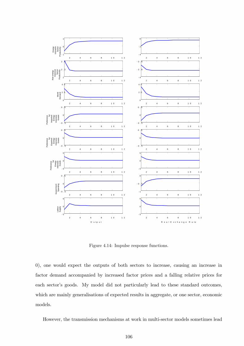
2 4 6 8 1 0 1 2 1
0
1
Ener
gyIn
tens
ive
Sect
orP
rodu
ctiv
ity2 4 6 8 1 0 1 2
4
2
0
2 4 6 8 1 0 1 22
2 . 2
2 . 4
Non
ene
rgy
Inte
nsiv
eSe
ctor
Pro
duct
ivity
2 4 6 8 1 0 1 2 4
3 . 8
3 . 6
2 4 6 8 1 0 1 20
2 0
4 0
Wor
ldD
eman
d
2 4 6 8 1 0 1 20
2 0
4 0
2 4 6 8 1 0 1 2 0 . 5
0
0 . 5
Pref
eren
ce for
Impo
rted
Ener
gyIn
tens
ive
Goo
ds
2 4 6 8 1 0 1 2 0 . 5
0
0 . 5
2 4 6 8 1 0 1 2 0 . 5
0
0 . 5
Pref
eren
ce for
Expo
rted
Ener
gyIn
tens
ive
Goo
ds
2 4 6 8 1 0 1 2 0 . 5
0
0 . 5
2 4 6 8 1 0 1 2 5
0
5
Pref
eren
ce for
Ener
gyIn
tens
ive
Goo
ds
2 4 6 8 1 0 1 2 5
0
5
2 4 6 8 1 0 1 2 0 . 5
0
0 . 5
Gov
ernm
ent
Spen
ding
2 4 6 8 1 0 1 2 1
0 . 5
0
2 4 6 8 1 0 1 2 5
0
5
Labo
urSu
pply
O u t p u t
2 4 6 8 1 0 1 2 5
0
5
R e a l E x c h a n g e R a t e
Figure 4.14: Impulse response functions.
0), one would expect the outputs of both sectors to increase, causing an increase in
factor demand accompanied by increased factor prices and a falling relative prices for
each sector�s goods. My model did not particularly lead to these standard outcomes,
which are mainly generalisations of expected results in aggregate, or one sector, economic
models.
However, the transmission mechanisms at work in multi-sector models sometimes lead
106
to contradicting dynamics as I see here. In fact, it is the case that permanent productivity
shocks in the energy and non-energy intensive sectors a¤ect some of the interesting model
variables di¤erently. For instance, productivity in the non-energy intensive sector lead to
standard results in output (aggregate and sectoral), consumption, wages, sectoral relative
prices, real exchange rate, and components of the BOP, but it is less so for productivity of
the energy intensive sector. I surmise that what is going on here is a form re-structuring
of resources. More speci�cally, contrary to standard results where one may expect that
a positive productivity shock would work by raising the productivity of factor inputs,
and hence, all of sectoral hours, capital utilisation rates, capital, and energy use should
increase, the model suggests that a positive productivity shock in the energy intensive
sector will raise productivity and hence, output of the energy intensive sector, but the
spill-over e¤ects to the non-energy intensive sector is negative.
Given that the magnitude of the increased output of the energy intensive sector is far
smaller than that of the fall in the non-energy intensive sector output, aggregate output
declines after energy intensive sector productivity shock hits the system. Consequently,
there is an accompanying fall in the demand for/ use of the factor inputs mainly because
aggregate demand (of output and investment) dropped signi�cantly more than the rise
of consumption aggregate demand. While it is puzzling that a positive technology can
end up depressing the economy, it is not for both the marginal costs of inputs and the
prices of the goods fell. The former is due to �rms reducing demand for inputs while the
latter serves as a devise to encourage more aggregate economic activities. This negative
response of hours to productivity shock has also been found in other studies [see, for
example, Christiano et al. (2003)].29 With regards to international trade, a fall in income
implies that there is an immediate drop in imports and rise in exports since foreigners are
relatively more well o¤. Real exchange rate depreciation occurs to aid in the re-balancing
of balance of payments accounts and thus, imports and exports begin to gradually travel
in opposite directions.
The remaining four productivity shocks in rows 1 and 2 of Figure 4.15 and rows 6 and
29However, the mechanism by which this contraction is e¤ected in their model is di¤erent to that inmine. I put forth a story of structural/ sectoral re-allocation of resources, while they explore the notionof nominal rigidity of prices.
107
7 of Figure 4.16 show that the remaining productivity shocks all produce standard results
for most of the key macroeconomic variables. I note the following exceptions. First, the
energy e¢ ciency shocks have the model implications of lowering the energy BTU input per
unit of the volume of output. Hence, all energy (aggregate and sectoral) usage dropped in
response to these shocks and because the amount of an input required has fallen, cost of
production also fell such that sectoral prices of goods followed suit. Second, I point out the
impact a¤ects of energy and non-energy intensive investment-speci�c technology shocks
on consumption - because these shocks move resources from consumption to investment,
it can be seen how the time paths for consumption and investment are almost a perfect
mirror image of each other.
Next, I investigate the impulse responses to the preference shocks beginning with the
labour supply shock. A positive shock has a negative correlation with output - see row 8 of
Figure 4.14. This result originates from the �rst-order condition (4.6), which implies that
@Ht=@�t < 0. This indeed has both the intratemporal and intertemporal e¤ects of drops
in both the aggregate consumption and investment though the latter in the non-energy
intensive sector still rose. Additionally, the substitution assumption between labour hours
and the CES of capital services and energy use implies that capital utilisation rate, capital,
and energy use all had to increase. This is what I observe except for capital demand in
the energy intensive sector, which also fell. An explanation for this can be o¤ered: the
model is, in this sense, indicating that labour hours and capital are complements in the
energy intensive sector. This contraction in labour supply and investment would lead to
a rise in wages and interest rate. It is now costlier to produce output in the two sectors;
hence, the jump in the sectoral prices.
The consequence is a rise in the country�s real exchange rate, signifying a drop in
competitiveness vis-à-vis the rest of the world so that imports and exports go up and
down, respectively. That is, as would be expected, the substitution e¤ects kicks into
full gear as the domestic economy runs down its foreign reserves. The dynamics of the
remaining preference shocks are quite interesting to look as depicted in rows 4 to 6 of
Figure 4.14, row 6 of Figure 4.15, and rows 2 and 3 of Figure 4.16. What is particularly
unique about these shocks, except the intertemporal preference shock, is that they act as
108
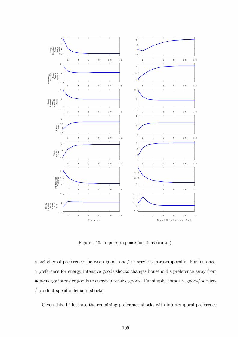
2 4 6 8 1 0 1 2
0
2
4
6
Ener
gyIn
tens
ive
Sect
orEn
ergy
Effic
ienc
y2 4 6 8 1 0 1 2
6
4
2
0
2 4 6 8 1 0 1 2 1 0
0
1 0
Non
ene
rgy
Inte
nsiv
eSe
ctor
Ener
gyEf
ficie
ncy
2 4 6 8 1 0 1 2
2 0
1 0
0
2 4 6 8 1 0 1 2 0 . 2
0
0 . 2
Pric
e of
Impo
rted
Ener
gyIn
tens
ive
Goo
ds
2 4 6 8 1 0 1 2 0 . 2
0
0 . 2
2 4 6 8 1 0 1 2
6
4
2
0
Ener
gyPr
ice
2 4 6 8 1 0 1 2
5
0
5
2 4 6 8 1 0 1 2
4
2
0
Wor
ldIn
tere
stR
ate
2 4 6 8 1 0 1 2
4
2
0
2 4 6 8 1 0 1 2
0
0 . 2
0 . 4
Inte
rtem
pora
lPr
efer
ence
2 4 6 8 1 0 1 2
0
0 . 2
0 . 4
2 4 6 8 1 0 1 2 0 . 2
0
0 . 2
Ener
gyIn
tens
ive
Sect
orC
apita
lC
ost
Shift
er
O u t p u t
2 4 6 8 1 0 1 2
0 . 0 1
0
0 . 0 1
0 . 0 2
0 . 0 3
R e a l E x c h a n g e R a t e
Figure 4.15: Impulse response functions (contd.).
a switcher of preferences between goods and/ or services intratemporally. For instance,
a preference for energy intensive goods shocks changes household�s preference away from
non-energy intensive goods to energy intensive goods. Put simply, these are good-/ service-
/ product-speci�c demand shocks.
Given this, I illustrate the remaining preference shocks with intertemporal preference
109
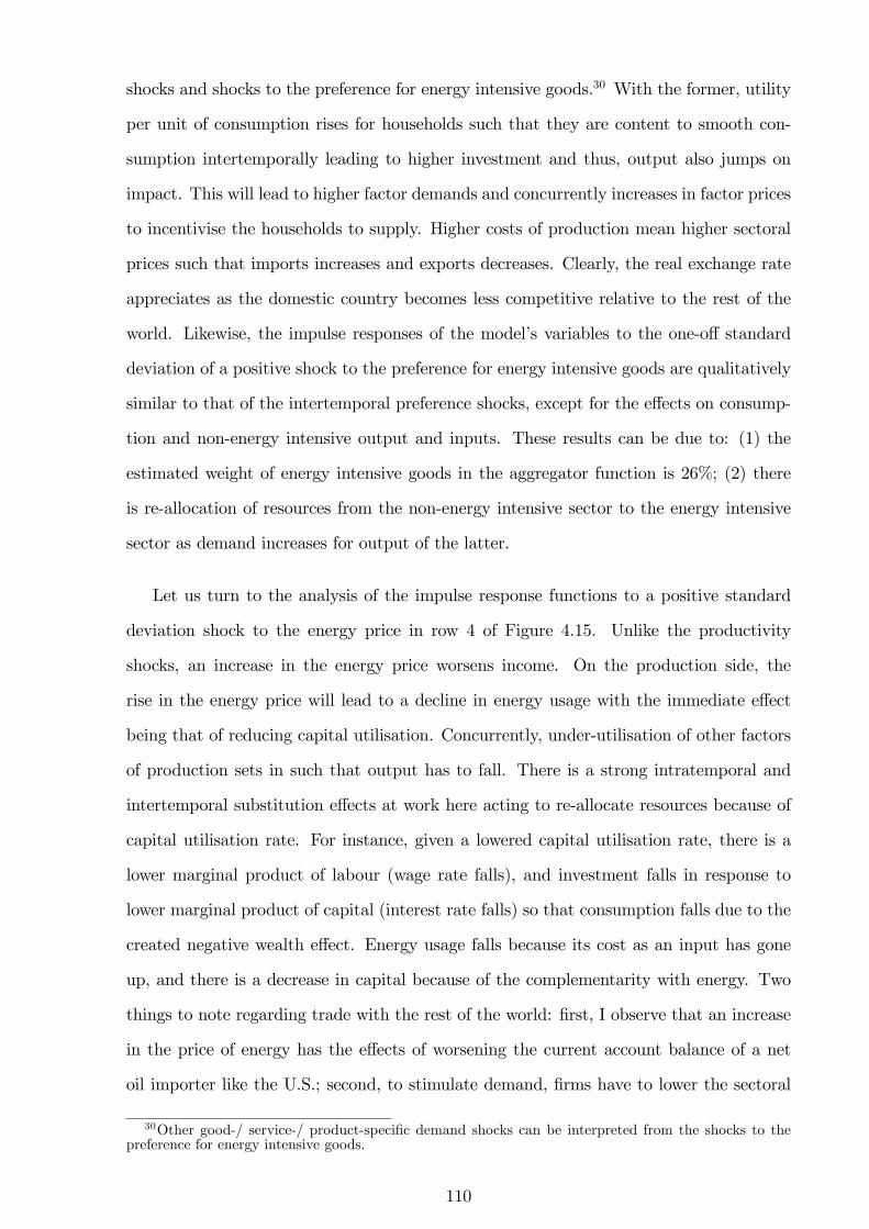
shocks and shocks to the preference for energy intensive goods.30 With the former, utility
per unit of consumption rises for households such that they are content to smooth con-
sumption intertemporally leading to higher investment and thus, output also jumps on
impact. This will lead to higher factor demands and concurrently increases in factor prices
to incentivise the households to supply. Higher costs of production mean higher sectoral
prices such that imports increases and exports decreases. Clearly, the real exchange rate
appreciates as the domestic country becomes less competitive relative to the rest of the
world. Likewise, the impulse responses of the model�s variables to the one-o¤ standard
deviation of a positive shock to the preference for energy intensive goods are qualitatively
similar to that of the intertemporal preference shocks, except for the e¤ects on consump-
tion and non-energy intensive output and inputs. These results can be due to: (1) the
estimated weight of energy intensive goods in the aggregator function is 26%; (2) there
is re-allocation of resources from the non-energy intensive sector to the energy intensive
sector as demand increases for output of the latter.
Let us turn to the analysis of the impulse response functions to a positive standard
deviation shock to the energy price in row 4 of Figure 4.15. Unlike the productivity
shocks, an increase in the energy price worsens income. On the production side, the
rise in the energy price will lead to a decline in energy usage with the immediate e¤ect
being that of reducing capital utilisation. Concurrently, under-utilisation of other factors
of production sets in such that output has to fall. There is a strong intratemporal and
intertemporal substitution e¤ects at work here acting to re-allocate resources because of
capital utilisation rate. For instance, given a lowered capital utilisation rate, there is a
lower marginal product of labour (wage rate falls), and investment falls in response to
lower marginal product of capital (interest rate falls) so that consumption falls due to the
created negative wealth e¤ect. Energy usage falls because its cost as an input has gone
up, and there is a decrease in capital because of the complementarity with energy. Two
things to note regarding trade with the rest of the world: �rst, I observe that an increase
in the price of energy has the e¤ects of worsening the current account balance of a net
oil importer like the U.S.; second, to stimulate demand, �rms have to lower the sectoral
30Other good-/ service-/ product-speci�c demand shocks can be interpreted from the shocks to thepreference for energy intensive goods.
110
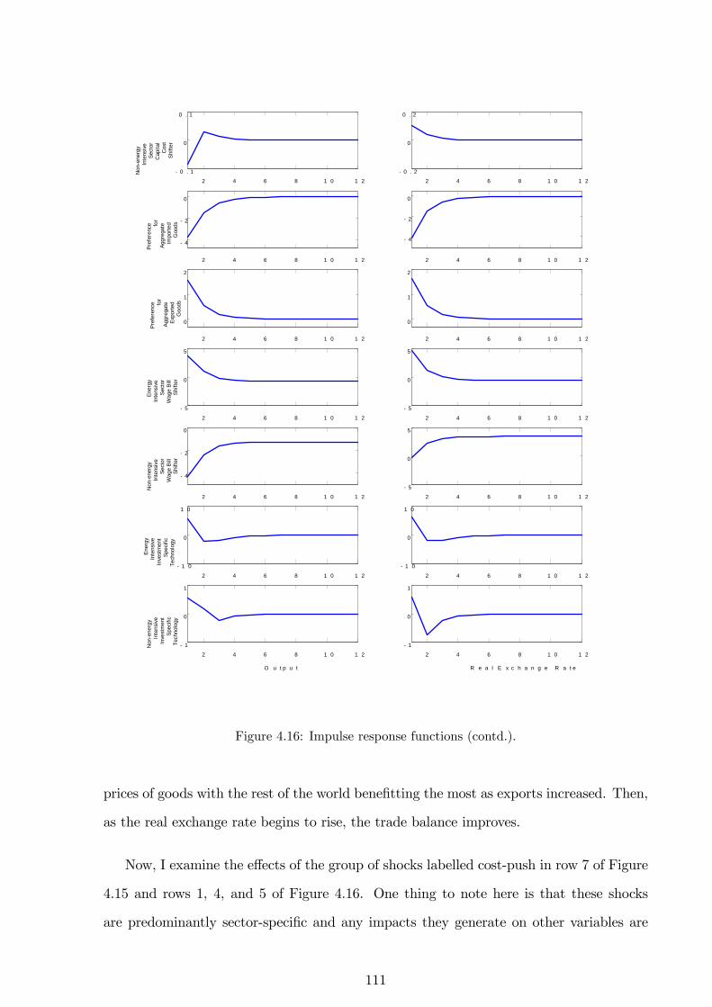
2 4 6 8 1 0 1 2 0 . 1
0
0 . 1
Non
ene
rgy
Inte
nsiv
eSe
ctor
Cap
ital
Cos
tSh
ifter
2 4 6 8 1 0 1 2 0 . 2
0
0 . 2
2 4 6 8 1 0 1 2
4
2
0
Pref
eren
ce for
Aggr
egat
eIm
porte
dG
oods
2 4 6 8 1 0 1 2
4
2
0
2 4 6 8 1 0 1 2
0
1
2
Pref
eren
ce for
Aggr
egat
eEx
porte
dG
oods
2 4 6 8 1 0 1 2
0
1
2
2 4 6 8 1 0 1 2
5
0
5
Ener
gyIn
tens
ive
Sect
orW
age
Bill
Shift
er
2 4 6 8 1 0 1 2
5
0
5
2 4 6 8 1 0 1 2
4
2
0
Non
ene
rgy
Inte
nsiv
eSe
ctor
Wag
e Bi
llSh
ifter
2 4 6 8 1 0 1 2
5
0
5
2 4 6 8 1 0 1 2
1 0
0
1 0
Ener
gyIn
tens
ive
Inve
stm
ent
Spec
ific
Tech
nolo
gy
2 4 6 8 1 0 1 2
1 0
0
1 0
2 4 6 8 1 0 1 2
1
0
1
Non
ene
rgy
Inte
nsiv
eIn
vest
men
tSp
ecifi
cTe
chno
logy
O u t p u t
2 4 6 8 1 0 1 2
1
0
1
R e a l E x c h a n g e R a t e
Figure 4.16: Impulse response functions (contd.).
prices of goods with the rest of the world bene�tting the most as exports increased. Then,
as the real exchange rate begins to rise, the trade balance improves.
Now, I examine the e¤ects of the group of shocks labelled cost-push in row 7 of Figure
4.15 and rows 1, 4, and 5 of Figure 4.16. One thing to note here is that these shocks
are predominantly sector-speci�c and any impacts they generate on other variables are
111
spill-over e¤ects. Moreover, only energy intensive sector wage bill shifter generated non-
standard results and so, I only discuss this shock under cost-push group and in relation
basically to output. I conjecture that the fall in labour hours demanded by �rms in the
energy intensive sector because of wage bill hike does not lead to a fall in output of the
energy intensive sector that is su¢ cient to lower aggregate output.
Finally, I consider the time paths of the endogenous variables to the observed exoge-
nous variables beginning with the impulse response functions to a positive world demand
shock - see row 3 of Figure 4.14. It is easy to interpret the distinct responses of the sectoral
variables to this shock. Considering each sector�s level of openness to international trade,
the share of energy intensive sector goods in cross-border trade is much larger such that
world demand shock a¤ects the sector�s output more. Further, the real exchange rate
appreciation occurred because the rest of the world increased their demand for domestic
exports. The impulse responses to world interest rate (see row 5 of Figure 4.15) are qual-
itatively alike to that of the energy price shock. This is because both are aggregate price
increases unlike a positive one-o¤ standard deviation shock to the imported price of energy
intensive goods in row 3 of Figure 4.15. Essentially, an increase in the imported price of
energy intensive goods will lead to fall in the import of such goods and consumption falls
for two reasons: �rst is that aggregate consumption is a composite involving imported
energy intensive goods and second is that domestic sectoral prices have been driven up
by positive imported price movement such that consumption goods are now more expen-
sive. Lastly, the crowding out e¤ects of government spending means that consumption
and investment fell on impact, and because government spending is non-productive in
the current model, it leads to a decrease in output, which particularly contradicts some
�ndings in the literature [for example, Finn (1998) and Ravn et al. (2012)]. I see that
the fall in consumption is trivial as households are able to smooth consumption overtime.
A further e¤ect is that both aggregate and sectoral labour hours increased on impact re-
�ecting household�s willingness to sacri�ce some leisure during hard times. Consequently,
wages fall as labour supply increases. This will cause output to start rising to lessen the
adverse wealth e¤ect accompanying the government spending shock.
112
Variance Decompositions To explain the percentage of variation in each variable that
is due to the di¤erent shocks, one can examine Table 4.4, which documents the variance
decomposition of the endogenous variables. It shows that every group is important to
some degree, in most cases, to explaining the variations in all variables. Looking at these
broad categorisations, exogenous variables are the most important to output followed by
the preference shocks and energy price is the least useful. In fact, for all variables, energy
price shocks make the least contribution to accounting for their movements. This is not
su¢ cient to shake my belief that energy price shock is (should be) a main covariate of
macroeconomic variables. For example, energy price shock is only approximately 4:55% of
the shocks in the model and accounts for 8:86% of movements in aggregate output, while
the productivity shocks make up approximately 27:27%, but are only able to account for
18:06% of movements in aggregate output. Proportionally and as would be expected,
energy price shock is more important to aggregate and sectoral energy usage being re-
sponsible for nearly a quarter, which will in turn lead to a drop or rise in output/ welfare
depending on whether it was a positive or a negative energy price shock. This latter com-
parison is even more pronounced when I observe that preference shocks, which make up
roughly 32% of the shocks can only determine 3:96% of aggregate energy use �uctuation,
2:85% of energy intensive sector energy use �uctuation, and 2:03% of non-energy intensive
sector energy use �uctuation. This is not surprising though given that energy use is not
modelled for the household and so there is a weak link between preference shocks and
energy usage.
Perhaps, a look at Tables 4.8-4.9 can provide a better insight into which shocks are
individually most (least) important. The key shocks are the permanent shocks accounting
for well over 90% of movements in all variables considered with the other shocks appearing
to be passengers in most contexts. For instance, the two sectoral Solow residuals are
the most important of the productivity shocks causing over 97% of the 18:06% share of
productivity shock in aggregate output volatility. This evidence can be seen in the share
of permanent shocks in the remaining categories reported in Table 4.4 as expanded in
Tables 4.8-4.9. It is interesting to see that variability in imports (aggregate and energy
intensive), exports (aggregate and energy intensive), and interest rate are dominated by
113
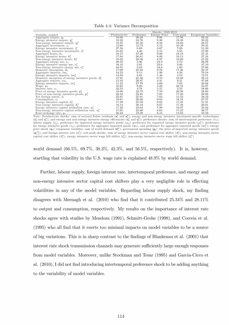
Table 4.4: Variance DecompositionShocks, 1949-2013
Variable, symbol Productivity Preference Energy Price Cost-push Exogenous VariablesAggregate output, yt 18:06 26:20 8:86 17:56 29:32Energy intensive output, yet 18:22 24:76 8:30 18:49 30:22Non-energy intensive output, ynt 18:37 25:56 8:58 18:93 28:57Aggregate investment, it 12:69 12:72 5:15 10:20 59:25Energy intensive investment, iet 27:56 9:89 3:67 7:69 51:20Non-energy intensive investment, int 31:64 4:40 2:15 3:83 57:98Aggregate hours, ht 18:15 27:20 9:06 18:19 27:41Energy intensive hours, het 17:84 26:81 8:89 19:13 27:34Non-energy intensive hours, hnt 18:03 26:98 8:97 19:00 27:02Aggregate energy use, et 29:32 3:96 24:9 3:74 38:09Energy intensive energy use, eet 34:10 2:85 23:0 3:00 37:10Non-energy intensive energy use, ent 44:55 2:03 24:8 1:60 27:06Domestic absorption, dt 17:69 25:83 8:76 17:36 30:37Aggregate imports, imt 14:23 9:11 1:98 4:50 70:18Energy intensive imports, ime
t 13:83 8:65 1:48 3:53 72:51Domestic aborption of energy intensive goods, det 17:91 25:30 8:55 18:09 30:14Aggregate exports, ext 12:43 26:87 4:41 9:21 47:08Energy intensive exports, exet 11:22 27:79 3:69 7:62 49:68Wage, wt 10:64 9:00 3:22 22:18 54:97Interest rate, rt 32:53 3:78 1:51 3:53 58:66Price of energy intensive goods, pet 19:96 22:75 7:59 20:90 28:80Price of non-energy intensive goods, pnt 22:32 22:85 7:65 17:20 29:98Net foreign assets, ft 22:81 25:91 7:63 15:32 28:33Consumption, ct 18:61 26:60 9:04 18:18 27:57Energy intensive capital, ket 17:20 25:59 8:65 17:35 31:21Non-energy intensive capital, knt 18:14 26:10 8:67 17:28 29:81Energy intensive capital utilisation rate, uet 17:29 23:62 7:99 16:07 35:02Non-energy intensive capital utilisation rate, unt 17:65 25:66 8:64 17:27 30:77Real exchange rate, pt 26:24 18:20 6:15 13:82 35:59
Note : Productivity shocks: sum of sectoral Solow residuals (aet and ant ), energy and non-energy intensive investment-speci�c technologies
(zet and znt ), and energy and non-energy intensive energy e¢ ciencies (o
et and o
nt ); preference shocks: sum of intertemporal preference (�t),
labour supply (�t), preference for imported energy intensive goods ('t), preference for exported energy intensive goods ('wt ), preference
for energy intensive goods ( t), preference for aggregate imported goods ($t), and preference for aggregate exported goods ($wt ); energy
price shock (qt); exogenous variables: sum of world demand (dwt ), government spending (gt), the price of imported energy intensive goods(pime;t), and foreign interest rate (r
ft ); cost-push shocks: sum of energy intensive sector capital cost shifter (#et ), non-energy intensive sector
capital cost shifter (#nt ), energy intensive sector wage bill shifter (�et ), non-energy intensive sector wage bill shifter (�
nt )
world demand (66:5%, 69:7%, 38:3%, 42:3%, and 56:5%, respectively). It is, however,
startling that volatility in the U.S. wage rate is explained 48:9% by world demand.
Further, labour supply, foreign interest rate, intertemporal preference, and energy and
non-energy intensive sector capital cost shifters play a very negligible role in e¤ecting
volatilities in any of the model variables. Regarding labour supply shock, my �nding
disagrees with Meenagh et al. (2010) who �nd that it contributed 25:34% and 28:11%
to output and consumption, respectively. My results on the importance of interest rate
shocks agree with studies by Mendoza (1991), Schmitt-Grohe (1998), and Correia et al.
(1995) who all �nd that it exerts too minimal impacts on model variables to be a source
of big variations. This is in sharp contrast to the �ndings of Blankenau et al. (2001) that
interest rate shock transmission channels may generate su¢ ciently large enough responses
from model variables. Moreover, unlike Stockman and Tesar (1995) and Garcia-Cicco et
al. (2010), I did not �nd introducing intertemporal preference shock to be adding anything
to the variability of model variables.
114
4.5 Conclusion
I have developed and estimated a two-sector dynamic stochastic equilibrium open
economy model of the United States in which imported oil is assumed to be crucial to
production in order to study the response of output and real exchange rate to the exoge-
nous positive movement in the price of oil. The main channels through which this shock
work are by raising the costs of production (when energy price shoots up) with the added
e¤ect of lowering the marginal productivity of the remaining inputs (i.e., labour and capi-
tal) on the production side and by acting as a resource drain in the economy-wide resource
constraint. I have shown qualitatively that output is a¤ected both intratemporally - the
impact e¤ect - and intertemporally - the transition e¤ect - and quantitatively assess these
results in the estimated model. I �nd that the macroeconomic e¤ects of oil price shock
are still sizeable and that real exchange rate moves to account for these changes after each
shock.
Meanwhile, it would be interesting to carry out the preceding exercises for a number of
countries and study how output and their competitiveness measured in real exchange rate
change with changes in the exogenous world price of crude oil. In doing this, it is perhaps
necessary and preferable to extend this model to include an energy-producing sector if
we were to fully grasp the e¤ects of oil price increases on the general price level and the
relative sectoral price. Further, it may be important to investigate more fully the cross-
country sectoral terms of trade. One may want to study if there are any cross-country
sectoral correlations of recessions. An advantage to this would include the opportunity
to study also the sectoral competitiveness along with the aggregate. In addition, it is
likely that there is a gap between theory and data regarding certain measurements that I
have used. Thus, it may be informative to have a version of this model augmented with
measurement error estimated in a future research. Finally, in the current paper I have
explained what happens to output and real exchange when there is an exogenous increase
in the real price of oil without any particular o¤er of a plausible policy recommendation
for accommodating such occurrences. Therefore, as a next step it will be interesting to
incorporate a monetary and/ or �scal channels by which there could be policy responses
115

as already been done in the literature. However, I think such an exercise within this
theoretical framework, when properly motivated, could lead to a more optimal plan of
actions.
116
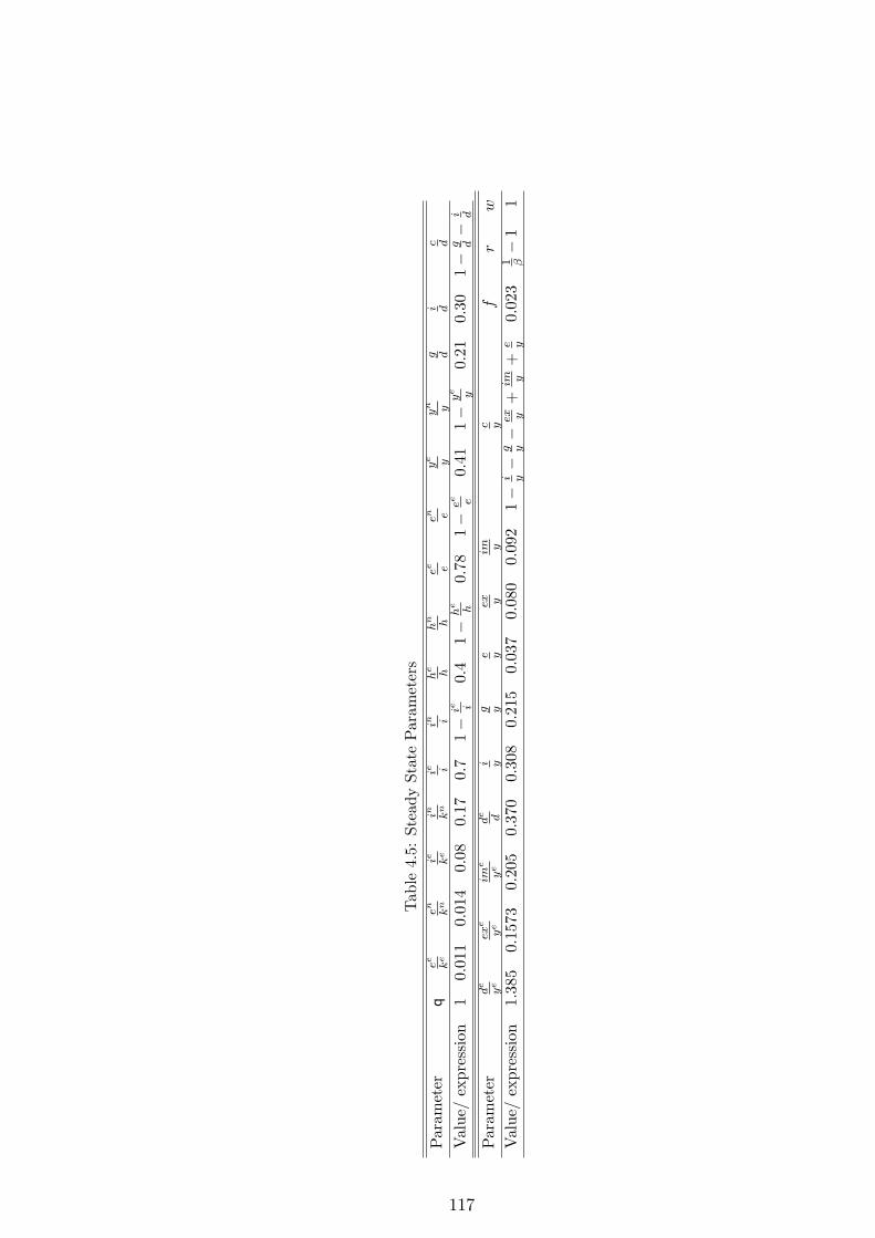
Table4.5:SteadyStateParameters
Parameter
qee ke
en kn
ie ke
in kn
ie iin i
he h
hn h
ee een e
ye y
yn y
g di d
c d
Value/expression
10:011
0:014
0:08
0:17
0:7
1�
ie i0:4
1�
he h
0:78
1�
ee e0:41
1�
ye y
0:21
0:30
1�
g d�
i d
Parameter
de
ye
exe
ye
ime
ye
de d
i yg y
e yex y
im yc y
fr
w
Value/expression
1:385
0:1573
0:205
0:370
0:308
0:215
0:037
0:080
0:092
1�
i y�
g y�
ex y+
im y+
e y0:023
1 ��1
1
117
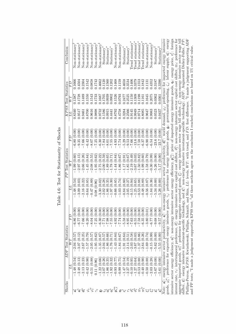
Table4.6:TestforStationarityofShocks
Shocks
ADFTestStatistics
PPTestStatistics
KPSSTestStatistics
Conclusion
LL
WT
FD
LL
WT
FD
LL
WT
FD
ae t�1:48(0:54)
�2:04(0:57)
�6:86(0:00)
�1:48(0:54)
�1:99(0:60)
�6:80(0:00)
0:8340
0:1387
0:1666
Non-stationaryy
an t�2:48(0:13)
�3:07(0:12)
�6:77(0:00)
�3:09(0:03)
�2:97(0:15)
�9:35(0:00)
0:9517
0:1728
0:4504
Non-stationaryz
dw t
�2:13(0:23)
�2:67(0:25)
�7:66(0:00)
�2:16(0:22)
�2:66(0:26)
�7:66(0:00)
0:9461
0:1489
0:2304
Non-stationaryz
't
�0:42(0:90)
�1:57(0:79)
�6:20(0:00)
�0:64(0:85)
�1:45(0:84)
�6:42(0:00)
0:8700
0:1550
0:1542
Non-stationaryz
'w t
�0:51(0:88)
�2:05(0:57)
�8:04(0:00)
�0:47(0:89)
�2:08(0:55)
�8:07(0:00)
0:9616
0:1543
0:0858
Non-stationaryz
t
0:11(0:96)
�1:95(0:62)
�7:25(0:00)
0:08(0:96)
�1:95(0:62)
�7:25(0:00)
0:9898
0:1733
0:1742
Non-stationaryz
gt
�1:22(0:66)
�1:35(0:87)
�6:30(0:00)
�3:30(0:02)
�2:75(0:22)
�6:30(0:00)
0:9732
0:1687
0:4662
Non-stationaryz
�t
�2:07(0:26)
�2:04(0:57)
�7:71(0:00)
�2:02(0:28)
�2:00(0:59)
�7:84(0:00)
0:1586
0:1705
0:1120
Stationary�
oe t
�1:86(0:35)
�1:86(0:66)
�7:98(0:00)
�1:86(0:35)
�1:89(0:65)
�8:01(0:00)
0:0915
0:0939
0:1560
Stationary�
on t
�1:92(0:32)
�1:76(0:71)
�7:55(0:00)
�1:97(0:30)
�1:78(0:71)
�7:55(0:00)
0:4441
0:0902
0:1202
Stationary�
pim e;t
�0:93(0:77)
�1:43(0:84)
�4:92(0:00)
�0:66(0:85)
�1:44(0:84)
�4:93(0:00)
0:8792
0:1526
0:1468
Non-stationaryz
qt
�0:99(0:75)
�1:84(0:67)
�7:74(0:00)
�1:03(0:74)
�1:86(0:67)
�7:74(0:00)
0:4758
0:0793
0:1159
Non-stationaryy
rf t�1:47(0:54)
�1:91(0:64)
�5:58(0:00)
�0:84(0:80)
�1:17(0:91)
�5:29(0:00)
0:3284
0:2477
0:4658
Stationary�
�t
�2:27(0:19)
�2:14(0:51)
�8:95(0:00)
�2:05(0:27)
�1:85(0:67)
�9:53(0:00)
0:2566
0:2525
0:3534
Stationary�
#e t
�0:10(0:95)
�2:03(0:58)
�7:63(0:00)
�0:15(0:94)
�2:19(0:49)
�7:66(0:00)
0:9145
0:1150
0:1406
Trendstationary�
#n t
�1:27(0:64)
�3:67(0:03)
�6:55(0:00)
�1:25(0:65)
�3:67(0:03)
�13:6(0:00)
0:9949
0:1309
0:3379
Trendstationary�
$t
�0:53(0:88)
�1:37(0:86)
�7:58(0:00)
�0:53(0:88)
�1:50(0:82)
�7:58(0:00)
0:9714
0:1198
0:1553
Trendstationary�
$w t
�0:40(0:90)
�2:64(0:26)
�6:35(0:00)
�0:48(0:89)
�1:99(0:60)
�6:37(0:00)
0:8085
0:1161
0:1842
Trendstationary�
�e t�0:50(0:88)
�1:69(0:74)
�3:80(0:01)
�0:56(0:87)
�1:58(0:79)
�6:90(0:00)
0:9647
0:1645
0:1131
Non-stationaryz
�n t�2:03(0:28)
�0:15(0:99)
�6:77(0:00)
�1:84(0:36)
�0:30(0:99)
�6:54(0:00)
0:9983
0:2075
0:4352
Non-stationaryz
ze t�5:67(0:00)
�5:62(0:00)
�9:68(0:00)
�5:34(0:00)
�5:26(0:00)
�23:6(0:00)
0:0523
0:0362
0:3187
Stationaryz
zn t�5:61(0:00)
�5:55(0:00)
�9:57(0:00)
�5:26(0:00)
�5:17(0:00)
�23:7(0:00)
0:0437
0:0361
0:3390
Stationaryz
Note:ae t:energyintensivesectorproductivity,an t:non-energyintensivesectorproductivity,dw t:worlddemand,'t:preferenceforimportedenergyintensive
goods,'w t:preferenceforexportedenergyintensivegoods, t:preferenceforenergyintensivegoods,gt:government-spending,�t:laboursupply,oe t:energy
intensivesectorenergye¢ciency,on t:non-energyintensivesectorenergye¢ciency,pim e;t:priceofimportedenergyintensivegoods,qt:energyprice,rf t:foreign
interestrate,�t:intertemporalpreference,#e t:energyintensivesectorcapitalcostshifter,#n t:non-energyintensivesectorcapitalcostshifter,$t:preferencefor
aggregateimportedgoods,$w t:preferenceforaggregateexportedgoods,�e t:energyintensivesectorwagebillshifter,�n t:non-energyintensivesectorwagebill
shifter,ze t:energyintensiveinvestment-speci�ctechnology,andzn t:non-energyintensiveinvestment-speci�ctechnology;ADF:AugmentedDickey-Fuller,PP:
Phillips-Perron,KPSS:Kwiatkowski,Phillips,Schmidt,andShin,LL:levels,WT:withtrend,andFD:�rstdi¤erence.y ImadeajudgementsupportingADF
andPPtests;
�ImadeajudgementsupportingKPSStest;z allthreemethodsagreeontheconclusionIreached;conclusionsarebasedon5%
criticalvalue.
118
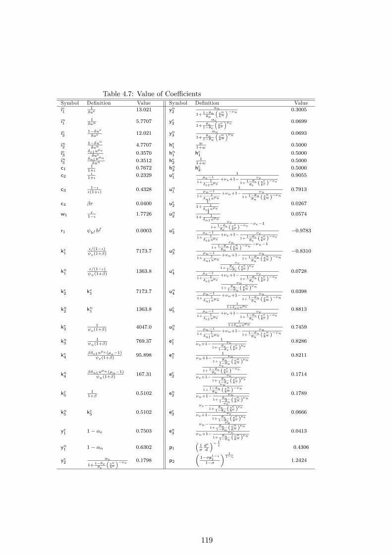
Table 4.7: Value of Coe¢ cientsSymbol De�nition Value Symbol De�nition Valueie1
1�ue
13:021 yn2�n
1+ 1��n�n
�en
kn
���n 0:3005
in11�un
5:7707 ye3�e
1+ �e1��e
�ee
ke
��e 0:0699
ie21��ue�ue
12:021 yn3�n
1+ �n1��n
�en
kn
��n 0:0693
in21��un�un
4:7707 he1w
1+w0:5000
ie3�e1u
�e
�ue0:3570 hn1 he1 0:5000
in3�n1u
�n
�un0:3512 he2
11+w
0:5000
c111+�
0:7672 hn2 he2 0:5000
c2�
1+�0:2329 ue1
1�e�1
1+ 1�e1u
�e
+�e+1� �e
1+1��e�e
( eeke )
��e0:9055
c31���(1+�)
0:4328 un11
�n�11+ 1
�n1u�n
+�n+1� �n
1+1��n�n
( enkn )
��n0:7913
c4 �r 0:0400 ue21
1+ 1�e1u
�e
0:0267
w1�
1�� 1:7726 un21
1+ 1�n1u
�n
0:0574
r1 bf bf 0:0003 ue3
�e
1+1��e�e
( eeke )
��e ��e�1
�e�11+ 1
�e1u�e
+�e+1� �e
1+1��e�e
( eeke )
��e�0:9783
ke1�=(1��) e(1+�)
7173:7 un3
�n
1+1��n�n
( enkn )
��n ��n�1
�n�11+ 1
�n1u�n
+�n+1� �n
1+1��n�n
( enkn )
��n�0:8310
kn1�=(1��) n(1+�)
1363:8 ue4
�e
1+�e
1��e (eeke )
�e
�e�11+ 1
�e1u�e
+�e+1� �e
1+1��e�e
( eeke )
��e0:0728
ke2 ke1 7173:7 un4
�n
1+�n
1��n (enkn )
�n
�n�11+ 1
�n1u�n
+�n+1� �n
1+1��n�n
( enkn )
��n0:0398
kn2 kn1 1363:8 ue5
11+�e1u
�e
�e�11+ 1
�e1u�e
+�e+1� �e
1+1��e�e
( eeke )
��e0:8813
ke31
e(1+�)4047:0 un5
11+�n1u
�n
�n�11+ 1
�n1u�n
+�n+1� �n
1+1��n�n
( enkn )
��n0:7459
kn31
n(1+�)769:37 ee1
1�e+1� �e
1+�e
1��e (eeke )
�e
0:8286
ke4��e1u
�e (�e�1) e(1+�)
95:898 en11
�n+1� �n
1+�n
1��n (enkn )
�n
0:8211
kn4��n1u
�n (�n�1) n(1+�)
167:31 ee2
�e
1+1��e�e
( eeke )
��e
�e+1� �e
1+�e
1��e (eeke )
�e
0:1714
ke51
1+�0:5102 en2
�n
1+1��n�n
( enkn )
��n
�n+1� �n
1+�n
1��n (enkn )
�n
0:1789
kn5 ke5 0:5102 ee3
�e� �e
1+�e
1��e (eeke )
�e
�e+1� �e
1+�e
1��e (eeke )
�e
0:0666
ye1 1� �e 0:7503 en3
�n� �n
1+�n
1��n (enkn )
�n
�n+1� �n
1+�n
1��n (enkn )
�n
0:0413
yn1 1� �n 0:6302 p1�1�de
d
�� 1&
0:4306
ye2�e
1+ 1��e�e
�ee
ke
���e 0:1798 p2
�1��p1�&11��
� 11�&
1:2424
119
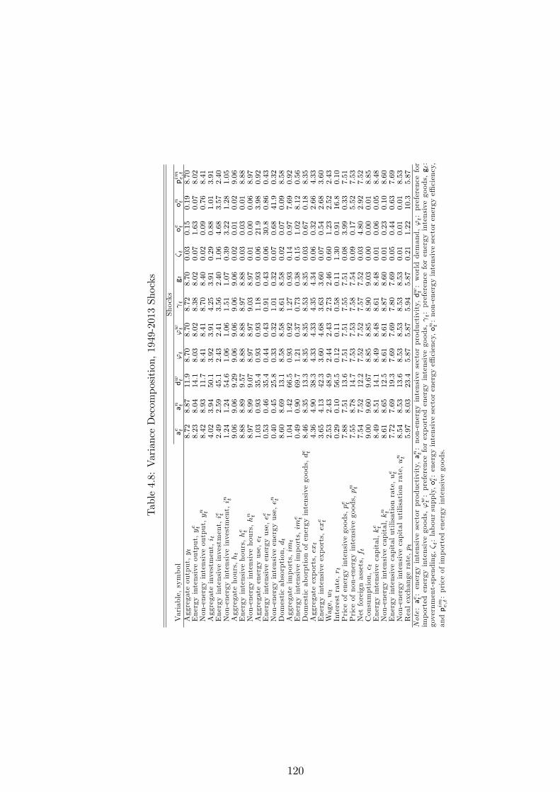
Table4.8:VarianceDecomposition,1949-2013Shocks
Shocks
Variable,symbol
ae t
an t
dw t
't
'w t
t
gt
�t
oe t
on t
pim e;t
Aggregateoutput,yt
8:72
8:87
11:9
8:70
8:70
8:72
8:70
0:03
0:15
0:19
8:70
Energyintensiveoutput,ye t
8:23
8:04
14:1
8:03
8:02
8:38
8:02
0:07
1:63
0:07
8:02
Non-energyintensiveoutput,yn t
8:42
8:93
11:7
8:41
8:41
8:70
8:40
0:02
0:09
0:76
8:41
Aggregateinvestment,i t
4:02
3:94
50:1
3:92
3:91
4:25
3:91
0:29
0:88
1:01
3:91
Energyintensiveinvestment,ie t
2:49
2:59
45:1
2:43
2:41
3:56
2:40
1:06
4:68
3:57
2:40
Non-energyintensiveinvestment,in t
1:24
1:24
54:6
1:06
1:06
1:51
1:07
0:39
3:22
1:28
1:05
Aggregatehours,ht
9:06
9:06
9:29
9:06
9:06
9:06
9:06
0:02
0:01
0:02
9:06
Energyintensivehours,he t
8:88
8:89
9:57
8:88
8:88
8:97
8:88
0:03
0:03
0:01
8:88
Non-energyintensivehours,hn t
8:97
8:99
9:07
8:97
8:97
9:03
8:97
0:01
0:00
0:06
8:97
Aggregateenergyuse,e t
1:03
0:93
35:4
0:93
0:93
1:18
0:93
0:06
21:9
3:98
0:92
Energyintensiveenergyuse,ee t
0:53
0:46
35:4
0:44
0:43
0:91
0:43
0:06
30:8
0:86
0:43
Non-energyintensiveenergyuse,en t
0:40
0:45
25:8
0:33
0:32
1:01
0:32
0:07
0:68
41:9
0:32
Domesticabsorption,dt
8:60
8:69
13:1
8:58
8:58
8:61
8:58
0:02
0:07
0:09
8:58
Aggregateimports,im
t1:04
1:42
66:5
0:93
0:92
1:27
0:93
0:14
0:97
7:69
0:92
Energyintensiveimports,im
e t0:49
0:90
69:7
1:21
0:37
0:73
0:38
0:15
1:02
8:12
0:56
Domesticaborptionofenergyintensivegoods,de t
8:46
8:35
13:3
8:35
8:35
8:53
8:35
0:03
0:67
0:18
8:35
Aggregateexports,ext
4:36
4:90
38:3
4:33
4:33
4:35
4:34
0:06
0:32
2:66
4:33
Energyintensiveexports,exe t
3:65
4:13
42:3
3:60
4:68
3:63
3:60
0:07
0:54
2:68
3:60
Wage,wt
2:53
2:43
48:9
2:44
2:43
2:73
2:46
0:60
1:23
2:52
2:43
Interestrate,r t
0:29
0:10
56:5
0:12
0:11
0:58
0:11
1:30
0:91
16:8
0:10
Priceofenergyintensivegoods,pe t
7:88
7:51
13:6
7:51
7:51
7:55
7:51
0:08
3:99
0:33
7:51
Priceofnon-energyintensivegoods,pn t
7:55
8:78
14:7
7:53
7:53
7:58
7:54
0:09
0:17
5:52
7:53
Netforeignassets,ft
7:54
7:52
12:2
7:52
7:52
7:57
7:52
0:03
4:80
2:92
7:52
Consumption,c t
9:00
9:60
9:67
8:85
8:85
8:90
9:03
0:00
0:00
0:01
8:85
Energyintensivecapital,ke t
8:49
8:51
14:1
8:49
8:48
8:61
8:48
0:01
0:06
0:05
8:48
Non-energyintensivecapital,kn t
8:61
8:65
12:5
8:61
8:61
8:87
8:60
0:01
0:23
0:10
8:60
Energyintensivecapitalutilisationrate,ue t
7:72
7:69
19:3
7:69
7:69
7:80
7:69
0:05
0:44
0:63
7:69
Non-energyintensivecapitalutilisationrate,un t
8:54
8:53
13:6
8:53
8:53
8:53
8:53
0:01
0:01
0:01
8:53
Realexchangerate,pt
5:97
8:03
23:4
5:87
5:87
5:94
5:87
0:21
1:22
10:3
5:87
Note:ae t:energy
intensivesectorproductivity,an t:non-energy
intensivesectorproductivity,dw t:worlddemand,'t:preferencefor
importedenergyintensivegoods,'w t:preferenceforexportedenergyintensivegoods, t:preferenceforenergyintensivegoods,gt:
government-spending,�t:laboursupply,oe t:energyintensivesectorenergye¢ciency,on t:non-energyintensivesectorenergye¢ciency,
andpim e;t:priceofimportedenergyintensivegoods.
120

Table4.9:VarianceDecomposition,1949-2013Shocks(contd.)
Shocks
Variable,symbol
qt
rf t�t
#e t
#n t
$t
$w t
�e t
�n t
ze tzn t
Aggregateoutput,yt
8:86
0:08
0:00
0:00
0:00
0:05
0:01
8:76
8:80
0:14
0:00
Energyintensiveoutput,ye t
8:30
0:13
0:00
0:00
0:00
0:21
0:05
9:82
8:67
0:25
0:00
Non-energyintensiveoutput,yn t
8:58
0:09
0:00
0:00
0:00
0:02
0:00
9:22
9:71
0:16
0:00
Aggregateinvestment,i t
5:15
1:33
0:00
0:00
0:00
0:34
0:02
5:43
4:76
2:83
0:02
Energyintensiveinvestment,ie t
3:67
1:35
0:00
0:00
0:00
0:35
0:08
4:01
3:68
8:88
5:35
Non-energyintensiveinvestment,in t
2:15
1:26
0:02
0:00
0:00
0:31
0:07
2:49
1:35
1:99
22:7
Aggregatehours,ht
9:06
0:00
0:00
0:00
0:00
0:00
0:00
9:07
9:12
0:01
0:00
Energyintensivehours,he t
8:89
0:02
0:00
0:00
0:00
0:03
0:01
9:86
9:27
0:03
0:00
Non-energyintensivehours,hn t
8:97
0:00
0:00
0:00
0:00
0:00
0:00
9:29
9:71
0:00
0:00
Aggregateenergyuse,e t
24:9
0:83
0:01
0:00
0:00
0:72
0:14
2:18
1:56
1:44
0:01
Energyintensiveenergyuse,ee t
23:0
0:83
0:01
0:00
0:00
0:83
0:17
1:77
1:23
1:44
0:01
Non-energyintensiveenergyuse,en t
24:8
0:67
0:01
0:00
0:00
0:26
0:03
1:03
0:56
1:14
0:01
Domesticabsorption,dt
8:76
0:13
0:00
0:00
0:00
0:03
0:00
8:69
8:68
0:23
0:00
Aggregateimports,im
t1:98
1:80
0:02
0:00
0:00
5:80
0:04
2:37
2:13
3:09
0:03
Energyintensiveimports,im
e t1:48
1:90
0:02
0:00
0:00
6:13
0:04
1:90
1:64
3:27
0:03
Domesticaborptionofenergyintensivegoods,de t
8:55
0:14
0:00
0:00
0:00
0:03
0:00
9:29
8:80
0:26
0:00
Aggregateexports,ext
4:41
0:12
0:00
0:00
0:00
0:07
13:7
4:43
4:78
0:19
0:00
Energyintensiveexports,exe t
3:69
0:14
0:00
0:00
0:00
0:08
15:7
3:72
3:89
0:22
0:00
Wage,wt
3:22
1:18
0:02
0:00
0:00
0:69
0:11
5:49
16:7
1:91
0:02
Interestrate,r t
1:51
1:98
0:02
0:00
0:00
1:42
0:24
2:31
1:22
14:1
0:38
Priceofenergyintensivegoods,pe t
7:59
0:15
0:00
0:00
0:00
0:09
0:01
11:6
9:32
0:25
0:00
Priceofnon-energyintensivegoods,pn t
7:65
0:19
0:00
0:00
0:00
0:11
0:02
7:95
9:25
0:30
0:01
Netforeignassets,ft
7:63
1:08
0:01
0:00
0:00
2:69
0:57
7:70
7:62
0:03
0:00
Consumption,c t
9:04
0:03
0:00
0:00
0:00
0:00
0:00
9:27
8:91
0:00
0:00
Energyintensivecapital,ke t
8:65
0:17
0:00
0:00
0:00
0:01
0:00
8:70
8:64
0:07
0:02
Non-energyintensivecapital,kn t
8:67
0:07
0:00
0:00
0:00
0:01
0:00
8:67
8:61
0:13
0:42
Energyintensivecapitalutilisationrate,ue t
7:99
0:33
0:00
0:00
0:00
0:32
0:07
8:14
7:92
0:80
0:02
Non-energyintensivecapitalutilisationrate,un t
8:64
0:14
0:00
0:00
0:00
0:07
0:01
8:69
8:58
0:26
0:03
Realexchangerate,pt
6:15
0:45
0:01
0:00
0:00
0:26
0:04
6:23
7:59
0:74
0:01
Note:qt:energyprice,rf t:foreigninterestrate,�t:intertemporalpreference,#e t:energyintensivesectorcapitalcostshifter,#n t:non-
energyintensivesectorcapitalcostshifter,$t:preferenceforaggregateimportedgoods,$w t:preferenceforaggregateexportedgoods,
�e t:energyintensivesectorwagebillshifter,�n t:non-energyintensivesectorwagebillshifter,ze t:energyintensiveinvestment-speci�c
technology,andzn t:non-energyintensiveinvestment-speci�ctechnology.
121
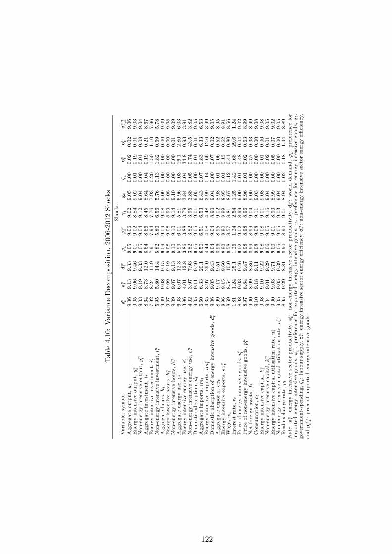
Table4.10:VarianceDecomposition,2006-2012Shocks
Shocks
Variable,symbol
ae t
an t
dw t
't
'w t
t
gt
�t
oe t
on t
pim e;t
Aggregateoutput,yt
9:06
9:13
9:33
9:05
9:06
9:02
9:05
0:00
0:02
0:02
9:06
Energyintensiveoutput,ye t
9:05
9:06
9:46
9:01
9:02
8:84
9:02
0:01
0:19
0:01
9:03
Non-energyintensiveoutput,yn t
9:03
9:19
9:33
9:05
9:04
9:12
9:04
0:00
0:01
0:08
9:04
Aggregateinvestment,i t
8:64
8:73
12:0
8:64
8:66
8:45
8:64
0:04
0:19
0:21
8:67
Energyintensiveinvestment,ie t
7:92
8:24
11:9
7:91
7:94
7:76
7:93
0:20
1:50
1:10
7:96
Non-energyintensiveinvestment,in t
5:95
5:80
14:4
5:82
5:80
6:56
5:76
0:13
1:82
0:69
5:78
Aggregatehours,ht
9:09
9:08
9:15
9:09
9:09
9:08
9:09
0:00
0:00
0:00
9:09
Energyintensivehours,he t
9:07
9:09
9:19
9:08
9:08
8:99
9:08
0:00
0:00
0:00
9:08
Non-energyintensivehours,hn t
9:09
9:07
9:13
9:10
9:10
9:14
9:10
0:00
0:00
0:01
9:09
Aggregateenergyuse,e t
6:03
6:07
12:3
5:99
6:01
5:81
5:96
0:03
16:1
2:80
6:03
Energyintensiveenergyuse,ee t
3:96
4:01
12:8
3:86
3:88
3:79
3:84
0:04
34:8
0:93
3:91
Non-energyintensiveenergyuse,en t
4:02
3:97
7:93
3:82
3:82
3:95
3:88
0:05
0:74
43:5
3:82
Domesticabsorption,dt
9:05
9:11
9:40
9:05
9:05
9:01
9:05
0:00
0:01
0:01
9:05
Aggregateimports,im
t6:60
6:33
20:1
6:50
6:51
6:53
6:43
0:07
0:83
6:33
6:53
Energyintensiveimports,im
e t4:35
3:97
29:0
4:44
4:08
4:48
3:99
0:14
1:66
12:6
3:99
Domesticaborptionofenergyintensivegoods,de t
9:06
9:05
9:43
9:04
9:04
8:90
9:04
0:00
0:07
0:02
9:05
Aggregateexports,ext
8:99
9:17
9:51
8:96
8:95
9:02
8:98
0:01
0:06
0:52
8:95
Energyintensiveexports,exe t
8:96
9:15
9:60
8:92
8:90
8:99
8:95
0:01
0:13
0:62
8:91
Wage,wt
8:69
8:54
10:0
8:58
8:57
8:81
8:67
0:12
0:41
0:80
8:56
Interestrate,r t
1:81
1:24
25:1
1:26
1:24
2:54
1:25
1:42
1:68
29:6
1:24
Priceofenergyintensivegoods,pe t
8:98
9:03
9:46
9:02
9:02
8:99
9:00
0:01
0:48
0:04
9:02
Priceofnon-energyintensivegoods,pn t
8:97
8:84
9:47
8:98
8:98
8:96
8:96
0:01
0:02
0:63
8:99
Netforeignassets,ft
9:00
8:99
8:86
8:99
8:99
9:04
9:00
0:00
0:57
0:33
8:99
Consumption,c t
9:10
9:18
9:11
9:08
9:08
9:11
9:03
0:00
0:00
0:00
9:08
Energyintensivecapital,ke t
9:08
9:10
9:22
9:08
9:08
9:01
9:08
0:00
0:01
0:00
9:08
Non-energyintensivecapital,kn t
9:04
9:01
9:29
9:06
9:05
9:16
9:04
0:00
0:02
0:01
9:05
Energyintensivecapitalutilisationrate,ue t
9:00
9:03
9:71
9:00
9:01
8:90
8:99
0:00
0:05
0:07
9:02
Non-energyintensivecapitalutilisationrate,un t
9:05
9:05
9:39
9:05
9:05
9:03
9:04
0:00
0:00
0:00
9:05
Realexchangerate,pt
8:95
9:29
8:81
8:90
8:90
9:01
8:94
0:02
0:18
1:44
8:89
Note:ae t:energy
intensivesectorproductivity,an t:non-energy
intensivesectorproductivity,dw t:worlddemand,'t:preferencefor
importedenergyintensivegoods,'w t:preferenceforexportedenergyintensivegoods, t:preferenceforenergyintensivegoods,gt:
government-spending,�t:laboursupply,oe t:energyintensivesectorenergye¢ciency,on t:non-energyintensivesectorenergye¢ciency,
andpim e;t:priceofimportedenergyintensivegoods.
122

Table4.11:VarianceDecomposition,2006-2012Shocks(contd.)
Shocks
Variable,symbol
qt
rf t�t
#e t
#n t
$t
$w t
�e t
�n t
ze tzn t
Aggregateoutput,yt
9:14
0:00
0:00
0:00
0:00
0:00
0:00
9:06
8:98
0:01
0:00
Energyintensiveoutput,ye t
9:15
0:01
0:00
0:00
0:00
0:01
0:00
9:00
9:10
0:02
0:00
Non-energyintensiveoutput,yn t
9:13
0:01
0:00
0:00
0:00
0:00
0:00
9:08
8:84
0:01
0:00
Aggregateinvestment,i t
9:27
0:20
0:00
0:00
0:00
0:04
0:00
8:78
8:39
0:44
0:01
Energyintensiveinvestment,ie t
8:72
0:30
0:00
0:00
0:00
0:07
0:00
8:09
7:58
2:03
2:87
Non-energyintensiveinvestment,in t
6:79
0:50
0:01
0:00
0:00
0:10
0:00
5:97
5:84
0:80
21:4
Aggregatehours,ht
9:10
0:00
0:00
0:00
0:00
0:00
0:00
9:09
9:04
0:00
0:00
Energyintensivehours,he t
9:10
0:00
0:00
0:00
0:00
0:00
0:00
9:06
9:16
0:00
0:00
Non-energyintensivehours,hn t
9:10
0:00
0:00
0:00
0:00
0:00
0:00
9:11
8:97
0:00
0:00
Aggregateenergyuse,e t
13:5
0:43
0:00
0:00
0:00
0:31
0:00
6:22
5:70
0:75
0:01
Energyintensiveenergyuse,ee t
14:1
0:65
0:01
0:00
0:00
0:55
0:01
4:16
3:60
1:16
0:02
Non-energyintensiveenergyuse,en t
11:0
0:51
0:01
0:00
0:00
0:17
0:00
3:85
4:11
0:88
0:02
Domesticabsorption,dt
9:15
0:01
0:00
0:00
0:00
0:00
0:00
9:06
8:98
0:02
0:00
Aggregateimports,im
t8:02
1:08
0:01
0:00
0:00
2:95
0:00
6:73
6:56
1:89
0:04
Energyintensiveimports,im
e t6:64
2:15
0:00
0:00
0:00
5:89
0:00
4:44
4:29
3:77
0:08
Domesticaborptionofenergyintensivegoods,de t
9:15
0:00
0:00
0:00
0:00
0:00
0:00
9:03
9:09
0:02
0:00
Aggregateexports,ext
8:93
0:02
0:00
0:00
0:00
0:01
0:09
8:94
8:88
0:03
0:00
Energyintensiveexports,exe t
8:89
0:02
0:00
0:00
0:00
0:01
0:12
8:90
8:87
0:04
0:00
Wage,wt
8:53
0:27
0:00
0:00
0:00
0:14
0:00
8:59
10:3
0:45
0:01
Interestrate,r t
4:21
2:54
0:03
0:00
0:00
1:55
0:01
1:80
1:87
18:5
1:16
Priceofenergyintensivegoods,pe t
9:05
0:01
0:00
0:00
0:00
0:01
0:00
9:10
8:78
0:02
0:00
Priceofnon-energyintensivegoods,pn t
9:02
0:02
0:00
0:00
0:00
0:01
0:00
8:98
9:14
0:03
0:00
Netforeignassets,ft
8:95
0:09
0:00
0:00
0:00
0:19
0:00
8:98
9:03
0:00
0:00
Consumption,c t
9:11
0:00
0:00
0:00
0:00
0:00
0:00
9:07
9:05
0:00
0:00
Energyintensivecapital,ke t
9:12
0:01
0:00
0:00
0:00
0:00
0:00
9:09
9:03
0:01
0:00
Non-energyintensivecapital,kn t
9:10
0:00
0:00
0:00
0:00
0:00
0:00
9:06
9:04
0:01
0:07
Energyintensivecapitalutilisationrate,ue t
9:16
0:03
0:00
0:00
0:00
0:02
0:00
9:05
8:90
0:07
0:00
Non-energyintensivecapitalutilisationrate,un t
9:12
0:01
0:00
0:00
0:00
0:00
0:00
9:07
9:01
0:02
0:05
Realexchangerate,pt
8:87
0:05
0:00
0:00
0:00
0:02
0:00
8:88
8:78
0:08
0:00
Note:qt:energyprice,rf t:foreigninterestrate,�t:intertemporalpreference,#e t:energyintensivesectorcapitalcostshifter,#n t:non-
energyintensivesectorcapitalcostshifter,$t:preferenceforaggregateimportedgoods,$w t:preferenceforaggregateexportedgoods,
�e t:energyintensivesectorwagebillshifter,�n t:non-energyintensivesectorwagebillshifter,ze t:energyintensiveinvestment-speci�c
technology,andzn t:non-energyintensiveinvestment-speci�ctechnology.
123
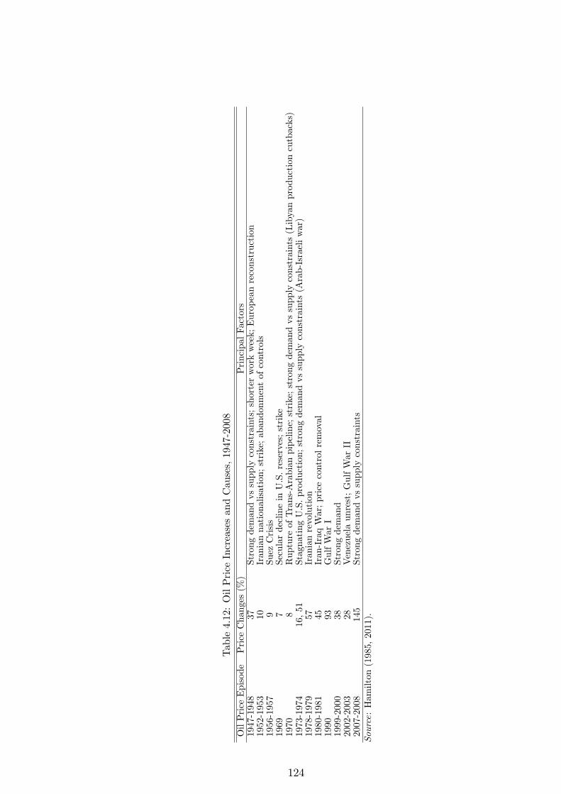
Table4.12:OilPriceIncreasesandCauses,1947-2008
OilPriceEpisode
PriceChanges(%)
PrincipalFactors
1947-1948
37Strongdemandvssupplyconstraints;shorterworkweek;Europeanreconstruction
1952-1953
10Iraniannationalisation;strike;abandonmentofcontrols
1956-1957
9SuezCrisis
1969
7SeculardeclineinU.S.reserves;strike
1970
8RuptureofTrans-Arabianpipeline;strike;strongdemandvssupplyconstraints(Libyanproductioncutbacks)
1973-1974
16,51
StagnatingU.S.production;strongdemandvssupplyconstraints(Arab-Israeliwar)
1978-1979
57Iranianrevolution
1980-1981
45Iran-IraqWar;pricecontrolremoval
1990
93GulfWarI
1999-2000
38Strongdemand
2002-2003
28Venezuelaunrest;GulfWarII
2007-2008
145
Strongdemandvssupplyconstraints
Source:Hamilton(1985,2011).
124
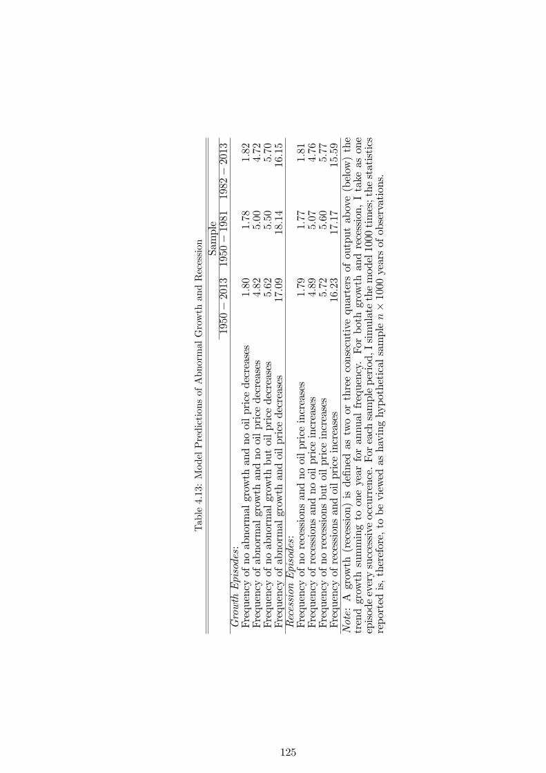
Table4.13:ModelPredictionsofAbnormalGrowthandRecession Sample
1950�2013
1950�1981
1982�2013
GrowthEpisodes:
Frequencyofnoabnormalgrowthandnooilpricedecreases
1:80
1:78
1:82
Frequencyofabnormalgrowthandnooilpricedecreases
4:82
5:00
4:72
Frequencyofnoabnormalgrowthbutoilpricedecreases
5:62
5:50
5:70
Frequencyofabnormalgrowthandoilpricedecreases
17:09
18:14
16:15
RecessionEpisodes:
Frequencyofnorecessionsandnooilpriceincreases
1:79
1:77
1:81
Frequencyofrecessionsandnooilpriceincreases
4:89
5:07
4:76
Frequencyofnorecessionsbutoilpriceincreases
5:72
5:60
5:77
Frequencyofrecessionsandoilpriceincreases
16:23
17:17
15:59
Note:Agrowth(recession)isde�nedastwoorthreeconsecutivequartersofoutputabove(below)the
trendgrowthsummingtooneyearforannualfrequency.Forbothgrowthandrecession,Itakeasone
episodeeverysuccessiveoccurrence.Foreachsampleperiod,Isimulatethemodel1000times;thestatistics
reportedis,therefore,tobeviewedashavinghypotheticalsamplen�1000yearsofobservations.
125
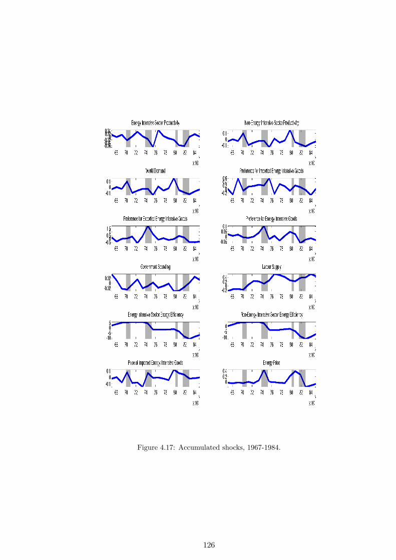
Figure 4.17: Accumulated shocks, 1967-1984.
126
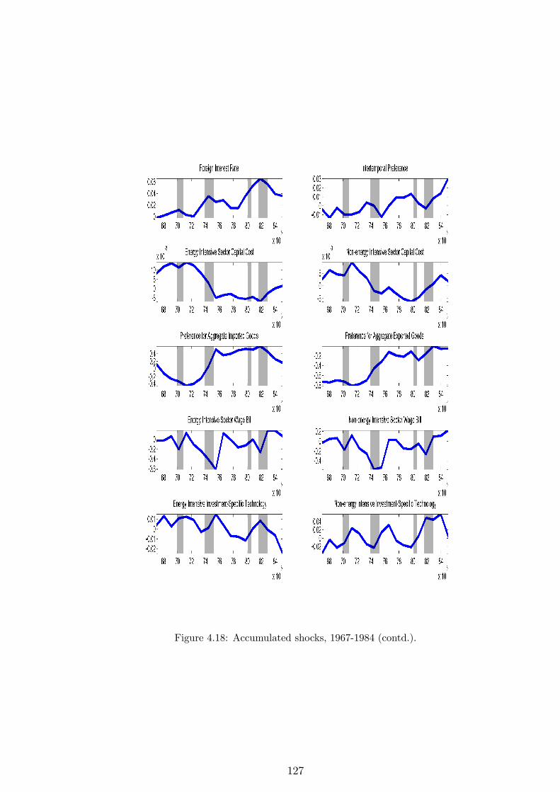
Figure 4.18: Accumulated shocks, 1967-1984 (contd.).
127
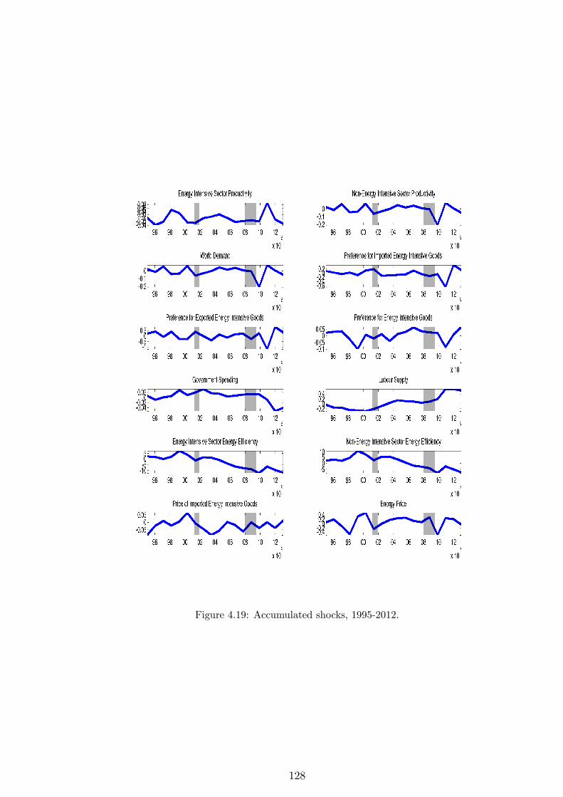
Figure 4.19: Accumulated shocks, 1995-2012.
128
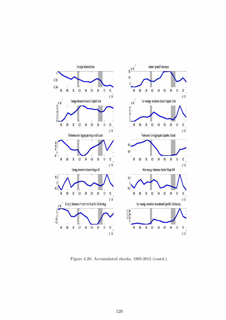
Figure 4.20: Accumulated shocks, 1995-2012 (contd.).
129
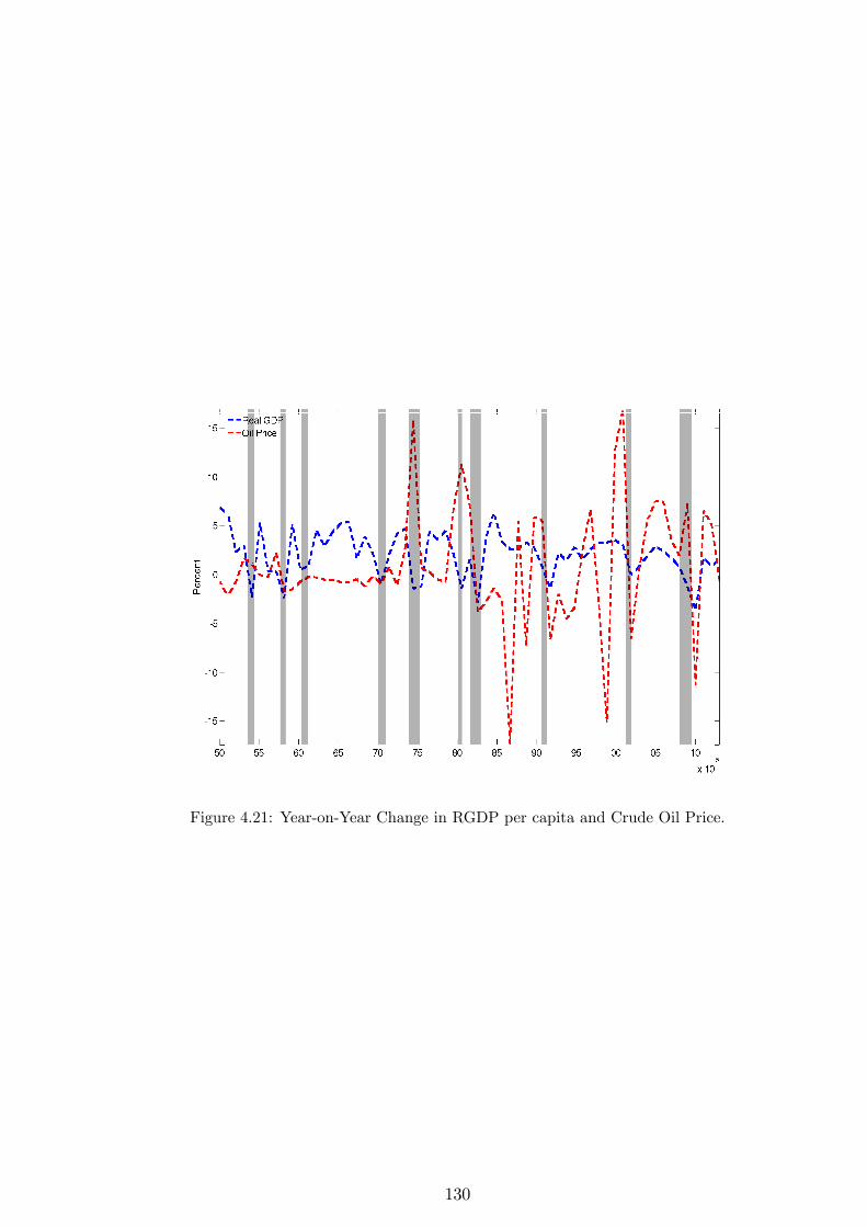
Figure 4.21: Year-on-Year Change in RGDP per capita and Crude Oil Price.
130
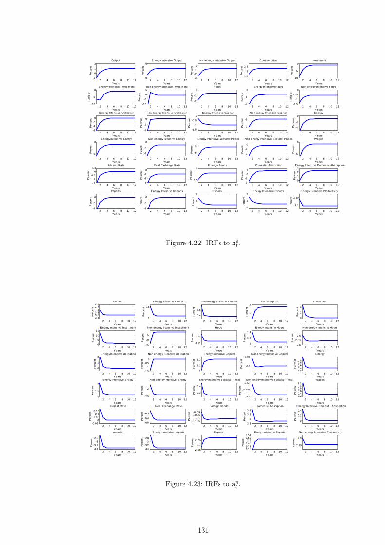
2 4 6 8 10 121
0
1
2Output
Per
cent
Years2 4 6 8 10 12
0
5Energy Intens ive Output
Per
cent
Years2 4 6 8 10 12
321
0
Nonenergy Intensive Output
Per
cent
Years2 4 6 8 10 12
1.5
2
2.5
Consumption
Per
cent
Years2 4 6 8 10 12
10
5
0Investment
Per
cent
Years
2 4 6 8 10 1210
5
0Energy Intens ive Investment
Per
cent
Years2 4 6 8 10 12
10
5
0
5Nonenergy Intensive Investment
Per
cent
Years2 4 6 8 10 12
2
1
0Hours
Per
cent
Years2 4 6 8 10 12
2
1
0Energy Intens ive Hours
Per
cent
Years2 4 6 8 10 12
1.5
1
0.5
0Nonenergy Intensive Hours
Per
cent
Years
2 4 6 8 10 12642
0
Energy Intensive Util isation
Per
cent
Years2 4 6 8 10 12
4
2
0
Nonenergy Intensive Utilisation
Per
cent
Years2 4 6 8 10 12
1.51
0.50
Energy Intensive Capital
Per
cent
Years2 4 6 8 10 12
2
1
Nonenergy Intensive Capital
Per
cent
Years2 4 6 8 10 12
4
2
0Energy
Per
cent
Years
2 4 6 8 10 12
5
0Energy Intens ive Energy
Per
cent
Years2 4 6 8 10 12
4
2
0Nonenergy Intensive Energy
Per
cent
Years2 4 6 8 10 12
6
4
Energy Intens ive Sec toral Prices
Per
cent
Years2 4 6 8 10 12
2
1
0
Nonenergy Intensive Sectoral Prices
Per
cent
Years2 4 6 8 10 12
5
0Wages
Per
cent
Years
2 4 6 8 10 121.5
10.5
00.5
Interes t Rate
Per
cent
Years2 4 6 8 10 12
321
0
Real Exchange Rate
Per
cent
Years2 4 6 8 10 12
0.5
1Foreign Bonds
Per
cent
Years2 4 6 8 10 12
21
01
Domestic Absorption
Per
cent
Years2 4 6 8 10 12
0123
Energy Intens ive Domestic Absorption
Per
cent
Years
2 4 6 8 10 124
2
0
Imports
Per
cent
Years2 4 6 8 10 12
4
2
0
Energy Intens ive Imports
Per
cent
Years2 4 6 8 10 12
0
1
2Exports
Per
cent
Years2 4 6 8 10 12
0
1
2Energy Intens ive Exports
Per
cent
Years2 4 6 8 10 12
4.1
4.12
Energy Intens ive Productivity
Per
cent
Years
Figure 4.22: IRFs to aet .
2 4 6 8 10 123.43.63.8
44.24.4
Output
Per
cent
Years2 4 6 8 10 12
1
1.5
Energy Intens ive Output
Per
cent
Years2 4 6 8 10 12
5.4
5.6
Nonenergy Intensive Output
Per
cent
Years2 4 6 8 10 12
5
6Consumption
Per
cent
Years2 4 6 8 10 12
0
2
4
Investment
Per
cent
Years
2 4 6 8 10 120
5
10
15Energy Intens ive Investment
Per
cent
Years2 4 6 8 10 12
15
10
5
Nonenergy Intensive Investment
Per
cent
Years2 4 6 8 10 12
1.2
1
Hours
Per
cent
Years2 4 6 8 10 12
1
1.2
1.4Energy Intens ive Hours
Per
cent
Years2 4 6 8 10 12
2.6
2.55
2.5
Nonenergy Intensive Hours
Per
cent
Years
2 4 6 8 10 12
0
1
2Energy Intensive Util isation
Per
cent
Years2 4 6 8 10 12
1.51
0.50
Nonenergy Intensive Utilisation
Per
cent
Years2 4 6 8 10 12
1
1.1
1.2
Energy Intensive Capital
Per
cent
Years2 4 6 8 10 12
2.4
2.35Nonenergy Intensive Capital
Per
cent
Years2 4 6 8 10 12
0.20.40.60.8
1
Energy
Per
cent
Years
2 4 6 8 10 121
1.5
2Energy Intens ive Energy
Per
cent
Years2 4 6 8 10 12
2.5
2
Nonenergy Intensive Energy
Per
cent
Years2 4 6 8 10 12
0.2
0.4
Energy Intens ive Sec toral Prices
Per
cent
Years2 4 6 8 10 12
7.8
7.675
7.55Nonenergy Intensive Sectoral Prices
Per
cent
Years2 4 6 8 10 12
0.20.40.60.8
11.2
Wages
Per
cent
Years
2 4 6 8 10 120.05
00.05
0.10.15
Interes t Rate
Per
cent
Years2 4 6 8 10 12
6.56.46.3
Real Exchange Rate
Per
cent
Years2 4 6 8 10 12
0.1050.1
0.0950.09
Foreign Bonds
Per
cent
Years2 4 6 8 10 12
2.83
3.23.4
Domestic Absorption
Per
cent
Years2 4 6 8 10 12
0
0.2
0.4Energy Intens ive Domestic Absorption
Per
cent
Years
2 4 6 8 10 123.43.2
32.8
Imports
Per
cent
Years2 4 6 8 10 12
3.43.2
32.8
Energy Intens ive Imports
Per
cent
Years2 4 6 8 10 12
2.65
2.7
2.75
Exports
Per
cent
Years2 4 6 8 10 12
2.442.462.48
2.52.522.54
Energy Intens ive Exports
Per
cent
Years2 4 6 8 10 12
7.85
7.9
Nonenergy Intensive Productivity
Per
cent
Years
Figure 4.23: IRFs to ant .
131
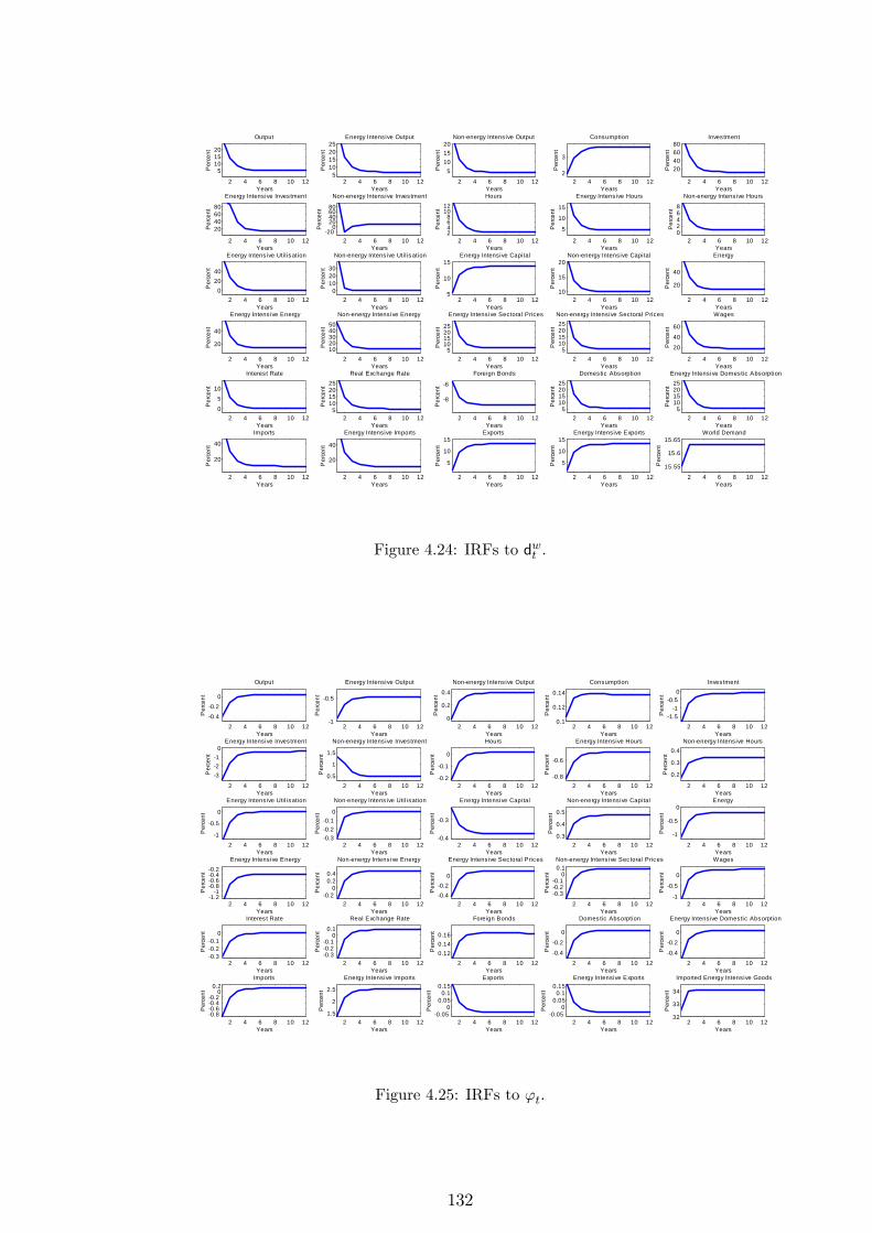
2 4 6 8 10 12
5101520
Output
Per
cent
Years2 4 6 8 10 12
510152025
Energy Intensive Output
Per
cent
Years2 4 6 8 10 12
5101520
Nonenergy Intensive Output
Per
cent
Years2 4 6 8 10 12
2
3
Consumption
Per
cent
Years2 4 6 8 10 12
20406080
Investment
Per
cent
Years
2 4 6 8 10 12
20406080
Energy Intensive InvestmentP
erce
nt
Years2 4 6 8 10 12
200
20406080
Nonenergy Intensive Investment
Per
cent
Years2 4 6 8 10 12
2468
1012
Hours
Per
cent
Years2 4 6 8 10 12
5
10
15
Energy Intensive Hours
Per
cent
Years2 4 6 8 10 12
02468
Nonenergy Intensive Hours
Per
cent
Years
2 4 6 8 10 120
2040
Energy Intensive Utilisation
Per
cent
Years2 4 6 8 10 12
0102030
Nonenergy Intensive Utilisation
Per
cent
Years2 4 6 8 10 12
5
10
15Energy Intensive Capital
Per
cent
Years2 4 6 8 10 12
10
15
20Nonenergy Intensive Capital
Per
cent
Years2 4 6 8 10 12
20
40
Energy
Per
cent
Years
2 4 6 8 10 12
20
40
Energy Intensive Energy
Per
cent
Years2 4 6 8 10 12
1020304050
Nonenergy Intensive EnergyP
erce
nt
Years2 4 6 8 10 12
510152025
Energy Intensive Sectoral Prices
Per
cent
Years2 4 6 8 10 12
510152025
Nonenergy Intensive Sectoral Prices
Per
cent
Years2 4 6 8 10 12
20
40
60
Wages
Per
cent
Years
2 4 6 8 10 1205
10
Interest Rate
Per
cent
Years2 4 6 8 10 12
510152025
Real Exchange Rate
Per
cent
Years2 4 6 8 10 12
8
6
Foreign Bonds
Per
cent
Years2 4 6 8 10 12
510152025
Domestic Absorption
Per
cent
Years2 4 6 8 10 12
510152025
Energy Intensive Domestic Absorption
Per
cent
Years
2 4 6 8 10 12
20
40
Imports
Per
cent
Years2 4 6 8 10 12
20
40
Energy Intensive Imports
Per
cent
Years2 4 6 8 10 12
5
10
15Exports
Per
cent
Years2 4 6 8 10 12
5
10
15Energy Intensive Exports
Per
cent
Years2 4 6 8 10 12
15.55
15.6
15.65World Demand
Per
cent
Years
Figure 4.24: IRFs to dwt .
2 4 6 8 10 120.40.2
0
Output
Per
cent
Years2 4 6 8 10 12
1
0.5
Energy Intensive Output
Per
cent
Years2 4 6 8 10 12
0
0.2
0.4
Nonenergy Intensive Output
Per
cent
Years2 4 6 8 10 12
0.1
0.12
0.14
Consumption
Per
cent
Years2 4 6 8 10 12
1.51
0.50
Investment
Per
cent
Years
2 4 6 8 10 12
321
0Energy Intensive Investment
Per
cent
Years2 4 6 8 10 12
0.5
1
1.5
Nonenergy Intens ive Investment
Per
cent
Years2 4 6 8 10 12
0.2
0.1
0
Hours
Per
cent
Years2 4 6 8 10 12
0.8
0.6
Energy Intensive Hours
Per
cent
Years2 4 6 8 10 12
0.2
0.3
0.4Nonenergy Intens ive Hours
Per
cent
Years
2 4 6 8 10 121
0.5
0
Energy Intensive Util isation
Per
cent
Years2 4 6 8 10 12
0.30.20.1
0
Nonenergy Intens ive Util isation
Per
cent
Years2 4 6 8 10 12
0.4
0.3
Energy Intensive Capital
Per
cent
Years2 4 6 8 10 12
0.3
0.4
0.5
Nonenergy Intensive Capital
Per
cent
Years2 4 6 8 10 12
1
0.5
0Energy
Per
cent
Years
2 4 6 8 10 121.2
10.80.60.40.2
Energy Intensive Energy
Per
cent
Years2 4 6 8 10 12
0.20
0.20.4
Nonenergy Intensive Energy
Per
cent
Years2 4 6 8 10 12
0.40.2
0
Energy Intensive Sectoral Prices
Per
cent
Years2 4 6 8 10 12
0.30.20.1
00.1Nonenergy Intens ive Sec toral Prices
Per
cent
Years2 4 6 8 10 12
1
0.5
0
Wages
Per
cent
Years
2 4 6 8 10 120.30.20.1
0
Interest Rate
Per
cent
Years2 4 6 8 10 12
0.30.20.1
00.1
Real Exchange Rate
Per
cent
Years2 4 6 8 10 12
0.120.140.16
Foreign Bonds
Per
cent
Years2 4 6 8 10 12
0.4
0.20
Domes tic Absorption
Per
cent
Years2 4 6 8 10 12
0.4
0.20
Energy Intensive Domestic Absorption
Per
cent
Years
2 4 6 8 10 120.80.60.40.2
00.2
Imports
Per
cent
Years2 4 6 8 10 12
1.5
2
2.5
Energy Intensive Imports
Per
cent
Years2 4 6 8 10 12
0.050
0.050.1
0.15Exports
Per
cent
Years2 4 6 8 10 12
0.050
0.050.1
0.15Energy Intensive Exports
Per
cent
Years2 4 6 8 10 12
32
33
34
Imported Energy Intensive Goods
Per
cent
Years
Figure 4.25: IRFs to 't.
132
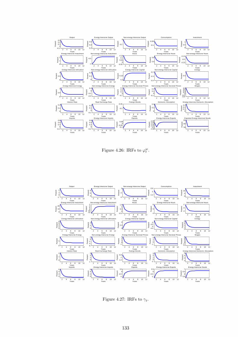
2 4 6 8 10 120.1
00.10.20.3
Output
Per
cent
Years2 4 6 8 10 12
0.2
0.4
0.6
Energy Intensive Output
Per
cent
Years2 4 6 8 10 12
0.2
0Nonenergy Intens ive Output
Per
cent
Years2 4 6 8 10 12
0.1
0.08
Consumption
Per
cent
Years2 4 6 8 10 12
0
0.5
1
Investment
Per
cent
Years
2 4 6 8 10 120
1
2
Energy Intensive Investment
Per
cent
Years2 4 6 8 10 12
1
0.5
Nonenergy Intensive Investment
Per
cent
Years2 4 6 8 10 12
0.050
0.050.1
0.15Hours
Per
cent
Years2 4 6 8 10 12
0.4
0.6
Energy Intensive Hours
Per
cent
Years2 4 6 8 10 12
0.25
0.2
0.15Nonenergy Intens ive Hours
Per
cent
Years
2 4 6 8 10 120
0.5
1Energy Intensive Util isation
Per
cent
Years2 4 6 8 10 12
0
0.1
0.2
Nonenergy Intens ive Util isation
Per
cent
Years2 4 6 8 10 12
0.2
0.25
Energy Intensive Capital
Per
cent
Years2 4 6 8 10 12
0.4
0.3
0.2Nonenergy Intens ive Capital
Per
cent
Years2 4 6 8 10 12
0
0.5
Energy
Per
cent
Years
2 4 6 8 10 120
0.5
1Energy Intensive Energy
Per
cent
Years2 4 6 8 10 12
0.40.2
00.2
Nonenergy Intens ive EnergyP
erce
nt
Years2 4 6 8 10 12
0.10
0.10.20.3
Energy Intensive Sectoral Prices
Per
cent
Years2 4 6 8 10 12
0.10
0.10.2
Nonenergy Intens ive Sectoral Prices
Per
cent
Years2 4 6 8 10 12
0.40.2
00.20.40.60.8
Wages
Per
cent
Years
2 4 6 8 10 12
0
0.1
0.2
Interest Rate
Per
cent
Years2 4 6 8 10 12
0.10
0.10.2
Real Exchange Rate
Per
cent
Years2 4 6 8 10 12
0.1
0.05Foreign Bonds
Per
cent
Years2 4 6 8 10 12
0
0.2
0.4Domestic Absorption
Per
cent
Years2 4 6 8 10 12
00.10.20.3
Energy Intensive Domestic Absorption
Per
cent
Years
2 4 6 8 10 120.2
00.20.40.6
Imports
Per
cent
Years2 4 6 8 10 12
0.20
0.20.40.6
Energy Intensive Imports
Per
cent
Years2 4 6 8 10 12
0.10.05
00.05
ExportsP
erce
nt
Years2 4 6 8 10 12
2.282.3
2.322.342.362.38
Energy Intensive Exports
Per
cent
Years2 4 6 8 10 12
58
60
62Exported Energy Intens ive Goods
Per
cent
Years
Figure 4.26: IRFs to 'wt .
2 4 6 8 10 121
012
Output
Per
cent
Years2 4 6 8 10 12
456
Energy Intensive Output
Per
cent
Years2 4 6 8 10 12
4
2
0Nonenergy Intens ive Output
Per
cent
Years2 4 6 8 10 12
1.2
1
0.8Consumption
Per
cent
Years2 4 6 8 10 12
05
10
Investment
Per
cent
Years
2 4 6 8 10 12
0
10
20
Energy Intensive Investment
Per
cent
Years2 4 6 8 10 12
1210
8642
Nonenergy Intensive Investment
Per
cent
Years2 4 6 8 10 12
0.50
0.51
1.5Hours
Per
cent
Years2 4 6 8 10 12
4
5
6Energy Intensive Hours
Per
cent
Years2 4 6 8 10 12
3
2
1Nonenergy Intens ive Hours
Per
cent
Years
2 4 6 8 10 1202468
Energy Intensive Util isation
Per
cent
Years2 4 6 8 10 12
012
Nonenergy Intens ive Util isation
Per
cent
Years2 4 6 8 10 12
2
2.5
3
Energy Intensive Capital
Per
cent
Years2 4 6 8 10 12
4.54
3.53
Nonenergy Intens ive Capital
Per
cent
Years2 4 6 8 10 12
02468
Energy
Per
cent
Years
2 4 6 8 10 120
5
Energy Intensive Energy
Per
cent
Years2 4 6 8 10 12
642
02
Nonenergy Intensive Energy
Per
cent
Years2 4 6 8 10 12
10123Energy Intensive Sectoral Prices
Per
cent
Years2 4 6 8 10 12
1012
Nonenergy Intensive Sectoral Prices
Per
cent
Years2 4 6 8 10 12
42
02468
Wages
Per
cent
Years
2 4 6 8 10 12
0
1
2Interest Rate
Per
cent
Years2 4 6 8 10 12
10123
Real Exchange Rate
Per
cent
Years2 4 6 8 10 12
1.21
0.8
Foreign Bonds
Per
cent
Years2 4 6 8 10 12
10123
Domestic Absorption
Per
cent
Years2 4 6 8 10 12
3456
Energy Intensive Domestic Absorption
Per
cent
Years
2 4 6 8 10 12
0246
Imports
Per
cent
Years2 4 6 8 10 12
0246
Energy Intensive Imports
Per
cent
Years2 4 6 8 10 12
10.5
00.5
Exports
Per
cent
Years2 4 6 8 10 12
10.5
00.5
Energy Intensive Exports
Per
cent
Years2 4 6 8 10 12
5.56
6.57
Energy Intensive Goods
Per
cent
Years
Figure 4.27: IRFs to t.
133
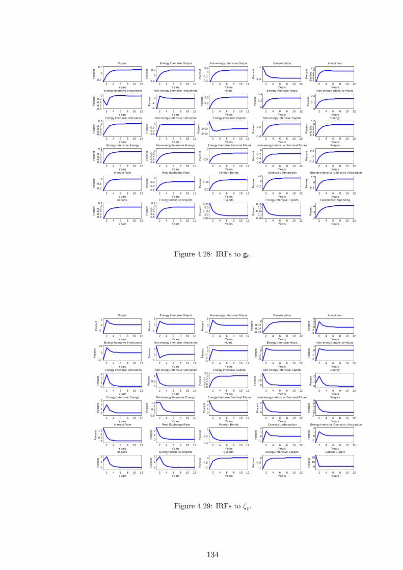
2 4 6 8 10 120.2
0
0.2Output
Per
cent
Years2 4 6 8 10 12
0.2
0
0.2
Energy Intens ive Output
Per
cent
Years2 4 6 8 10 12
0.20.1
00.1
Nonenergy Intensive Output
Per
cent
Years2 4 6 8 10 12
1.5
1Consumption
Per
cent
Years2 4 6 8 10 12
0.80.60.40.2
00.2
Investment
Per
cent
Years
2 4 6 8 10 120.80.60.40.2
0
Energy Intens ive InvestmentP
erce
nt
Years2 4 6 8 10 12
2
1
0
Nonenergy Intensive Investment
Per
cent
Years2 4 6 8 10 12
0
0.1
0.2
Hours
Per
cent
Years2 4 6 8 10 12
0
0.2
0.4Energy Intens ive Hours
Per
cent
Years2 4 6 8 10 12
0
0.1
0.2
Nonenergy Intensive Hours
Per
cent
Years
2 4 6 8 10 120.80.60.40.2
00.2
Energy Intens ive Util isation
Per
cent
Years2 4 6 8 10 12
0.60.40.2
0
Nonenergy Intensive Util isation
Per
cent
Years2 4 6 8 10 12
0.04
0.02
0
Energy Intens ive Capital
Per
cent
Years2 4 6 8 10 12
0.4
0.2
Nonenergy Intensive Capital
Per
cent
Years2 4 6 8 10 12
0.80.60.40.2
00.2
Energy
Per
cent
Years
2 4 6 8 10 120.80.60.40.2
00.2
Energy Intens ive Energy
Per
cent
Years2 4 6 8 10 12
0.80.60.40.2
0
Nonenergy Intensive EnergyP
erce
nt
Years2 4 6 8 10 12
0.5
0Energy Intens ive Sectoral Prices
Per
cent
Years2 4 6 8 10 12
0.60.40.2
0Nonenergy Intensive Sectoral Prices
Per
cent
Years2 4 6 8 10 12
1.5
1
0.5
Wages
Per
cent
Years
2 4 6 8 10 12
0.20.1
0
Interest Rate
Per
cent
Years2 4 6 8 10 12
0.60.40.2
0
Real Exchange Rate
Per
cent
Years2 4 6 8 10 12
0.1
0.15
Foreign Bonds
Per
cent
Years2 4 6 8 10 12
0.2
0
0.2Domestic Absorption
Per
cent
Years2 4 6 8 10 12
0.2
0
0.2Energy Intensive Domestic Absorption
Per
cent
Years
2 4 6 8 10 120.80.60.40.2
00.2
Imports
Per
cent
Years2 4 6 8 10 12
0.80.60.40.2
00.2
Energy Intensive Imports
Per
cent
Years2 4 6 8 10 12
0.050.1
0.150.2
0.25Exports
Per
cent
Years2 4 6 8 10 12
0.050.1
0.150.2
0.25Energy Intens ive Exports
Per
cent
Years2 4 6 8 10 12
2
3
4
Government Spending
Per
cent
Years
Figure 4.28: IRFs to gt.
2 4 6 8 10 12
1
0
1Output
Per
cent
Years2 4 6 8 10 12
2
0
2Energy Intens ive Output
Per
cent
Years2 4 6 8 10 12
1
0
1Nonenergy Intensive Output
Per
cent
Years2 4 6 8 10 12
0.060.040.02
0
Consumption
Per
cent
Years2 4 6 8 10 12
42
0246
Investment
Per
cent
Years
2 4 6 8 10 1210
0
10Energy Intens ive Investment
Per
cent
Years2 4 6 8 10 12
5
0
5
Nonenergy Intensive Investment
Per
cent
Years2 4 6 8 10 12
321
01
Hours
Per
cent
Years2 4 6 8 10 12
321
01
Energy Intens ive Hours
Per
cent
Years2 4 6 8 10 12
21
01
Nonenergy Intensive Hours
Per
cent
Years
2 4 6 8 10 120123
Energy Intens ive Util isation
Per
cent
Years2 4 6 8 10 12
0
0.5
1
Nonenergy Intensive Util isation
Per
cent
Years2 4 6 8 10 12
0.80.60.40.2
00.2
Energy Intens ive Capital
Per
cent
Years2 4 6 8 10 12
0
0.5
1
Nonenergy Intensive Capital
Per
cent
Years2 4 6 8 10 12
0
1
2
Energy
Per
cent
Years
2 4 6 8 10 12
0123
Energy Intens ive Energy
Per
cent
Years2 4 6 8 10 12
0.50
0.51
1.5
Nonenergy Intensive Energy
Per
cent
Years2 4 6 8 10 12
0123Energy Intens ive Sectoral Prices
Per
cent
Years2 4 6 8 10 12
012
Nonenergy Intensive Sectoral Prices
Per
cent
Years2 4 6 8 10 12
202468
Wages
Per
cent
Years
2 4 6 8 10 120
0.51
1.5
Interest Rate
Per
cent
Years2 4 6 8 10 12
012
Real Exchange Rate
Per
cent
Years2 4 6 8 10 12
0.4
0.2
0
Foreign Bonds
Per
cent
Years2 4 6 8 10 12
1012
Domestic Absorption
Per
cent
Years2 4 6 8 10 12
1012
Energy Intensive Domestic Absorption
Per
cent
Years
2 4 6 8 10 12
0
1
2Imports
Per
cent
Years2 4 6 8 10 12
0
1
2Energy Intensive Imports
Per
cent
Years2 4 6 8 10 12
10.5
0
Exports
Per
cent
Years2 4 6 8 10 12
10.5
0
Energy Intens ive Exports
Per
cent
Years2 4 6 8 10 12
01020
Labour Supply
Per
cent
Years
Figure 4.29: IRFs to �t.
134
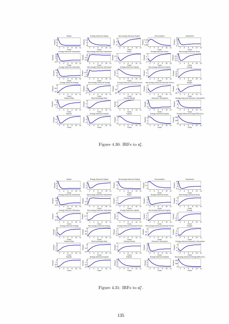
2 4 6 8 10 120
2
4
Output
Per
cent
Years2 4 6 8 10 12
05
10
Energy Intensive Output
Per
cent
Years2 4 6 8 10 12
2
1
0Nonenergy Intensive Output
Per
cent
Years2 4 6 8 10 12
0.050.1
0.15
Consumption
Per
cent
Years2 4 6 8 10 12
505
1015
Investment
Per
cent
Years
2 4 6 8 10 1210
0102030
Energy Intensive InvestmentP
erce
nt
Years2 4 6 8 10 12
2010
0
Nonenergy Intensive Investment
Per
cent
Years2 4 6 8 10 12
1.51
0.50
Hours
Per
cent
Years2 4 6 8 10 12
3
2
1
0Energy Intensive Hours
Per
cent
Years2 4 6 8 10 12
0.60.40.2
0Nonenergy Intensive Hours
Per
cent
Years
2 4 6 8 10 12
0
5
10
Energy Intensive Utilisation
Per
cent
Years2 4 6 8 10 12
1.51
0.50
Nonenergy Intensive Utilisation
Per
cent
Years2 4 6 8 10 12
0
1
2
Energy Intensive Capital
Per
cent
Years2 4 6 8 10 12
4
2
0Nonenergy Intensive Capital
Per
cent
Years2 4 6 8 10 12
302010
0Energy
Per
cent
Years
2 4 6 8 10 1240
20
0Energy Intensive Energy
Per
cent
Years2 4 6 8 10 12
642
0
Nonenergy Intensive EnergyP
erce
nt
Years2 4 6 8 10 12
20
10
0
Energy Intensive Sectoral Prices
Per
cent
Years2 4 6 8 10 12
321
0
Nonenergy Intensive Sectoral Prices
Per
cent
Years2 4 6 8 10 12
10
5
0Wages
Per
cent
Years
2 4 6 8 10 12
10.5
00.5
Interest Rate
Per
cent
Years2 4 6 8 10 12
4
2
0Real Exchange Rate
Per
cent
Years2 4 6 8 10 12
2
4
Foreign Bonds
Per
cent
Years2 4 6 8 10 12
0
2
4Domestic Absorption
Per
cent
Years2 4 6 8 10 12
0
5
10Energy Intensive Domestic Absorption
Per
cent
Years
2 4 6 8 10 12
4
2
0Imports
Per
cent
Years2 4 6 8 10 12
4
2
0Energy Intensive Imports
Per
cent
Years2 4 6 8 10 12
0
1
2Exports
Per
cent
Years2 4 6 8 10 12
0
1
2
Energy Intensive Exports
Per
cent
Years2 4 6 8 10 12
0
100
200
Energy Intensive Energy Effic iency
Per
cent
Years
Figure 4.30: IRFs to oet .
2 4 6 8 10 120246
Output
Per
cent
Years2 4 6 8 10 12
21
0
Energy Intensive Output
Per
cent
Years2 4 6 8 10 12
0
5
10Nonenergy Intensive Output
Per
cent
Years2 4 6 8 10 12
0
0.2
0.4
Consumption
Per
cent
Years2 4 6 8 10 12
505
10Investment
Per
cent
Years
2 4 6 8 10 1210
01020
Energy Intensive Investment
Per
cent
Years2 4 6 8 10 12
20
10
0
Nonenergy Intensive Investment
Per
cent
Years2 4 6 8 10 12
321
0
Hours
Per
cent
Years2 4 6 8 10 12
1
0
1
2Energy Intensive Hours
Per
cent
Years2 4 6 8 10 12
4
2
0
Nonenergy Intensive Hours
Per
cent
Years
2 4 6 8 10 1210
5
0
Energy Intensive Utilisation
Per
cent
Years2 4 6 8 10 12
1
0.5
0
Nonenergy Intensive Utilisation
Per
cent
Years2 4 6 8 10 12
0
1
2Energy Intensive Capital
Per
cent
Years2 4 6 8 10 12
321
0
Nonenergy Intensive Capital
Per
cent
Years2 4 6 8 10 12
15105
0
Energy
Per
cent
Years
2 4 6 8 10 128642
02
Energy Intensive Energy
Per
cent
Years2 4 6 8 10 12
40
20
0Nonenergy Intensive Energy
Per
cent
Years2 4 6 8 10 12
642
0
Energy Intensive Sectoral Prices
Per
cent
Years2 4 6 8 10 12
20
10
0
Nonenergy Intensive Sectoral Prices
Per
cent
Years2 4 6 8 10 12
15105
0
Wages
Per
cent
Years
2 4 6 8 10 12642
02
Interest Rate
Per
cent
Years2 4 6 8 10 12
20
10
0
Real Exchange Rate
Per
cent
Years2 4 6 8 10 12
2
4
6Foreign Bonds
Per
cent
Years2 4 6 8 10 12
10123
Domestic Absorption
Per
cent
Years2 4 6 8 10 12
4
2
0
Energy Intensive Domestic Absorption
Per
cent
Years
2 4 6 8 10 1215105
0
Imports
Per
cent
Years2 4 6 8 10 12
1510
50
Energy Intensive Imports
Per
cent
Years2 4 6 8 10 12
02468
Exports
Per
cent
Years2 4 6 8 10 12
0246
Energy Intensive Exports
Per
cent
Years2 4 6 8 10 12
0
100
200
Nonenergy Intensive Energy Effic iency
Per
cent
Years
Figure 4.31: IRFs to ont .
135
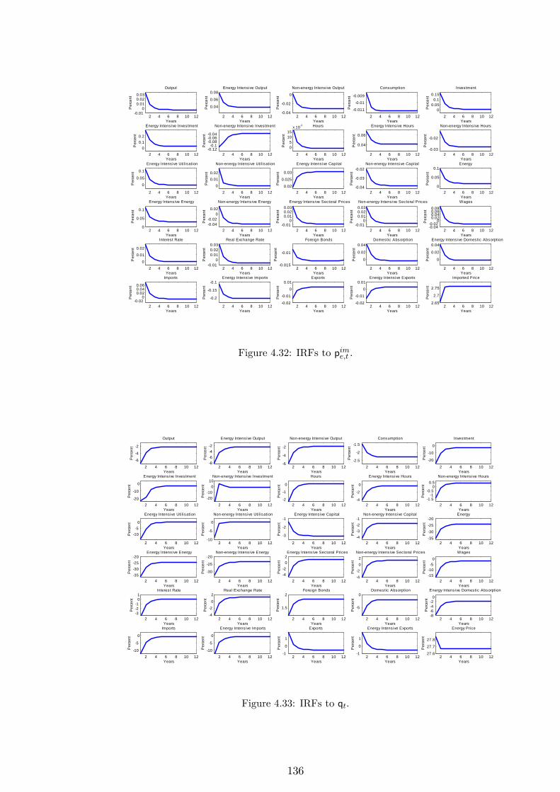
2 4 6 8 10 120.01
00.010.020.03
Output
Per
cent
Years2 4 6 8 10 12
0.04
0.06
0.08Energy Intensive Output
Per
cent
Years2 4 6 8 10 12
0.04
0.02
0
Nonenergy Intensive Output
Per
cent
Years2 4 6 8 10 12
0.011
0.01
0.009
Consumption
Per
cent
Years2 4 6 8 10 12
00.05
0.10.15
Investment
Per
cent
Years
2 4 6 8 10 120
0.10.2
Energy Intensive Investment
Per
cent
Years2 4 6 8 10 12
0.120.1
0.080.060.04
Nonenergy Intensive Investment
Per
cent
Years2 4 6 8 10 12
05
1015
x 103 Hours
Per
cent
Years2 4 6 8 10 12
0.04
0.06
Energy Intensive Hours
Per
cent
Years2 4 6 8 10 12
0.03
0.02
Nonenergy Intensive Hours
Per
cent
Years
2 4 6 8 10 12
0
0.05
0.1
Energy Intensive Utilisation
Per
cent
Years2 4 6 8 10 12
00.010.02
Nonenergy Intensive Utilisation
Per
cent
Years2 4 6 8 10 12
0.02
0.025
0.03
Energy Intensive Capital
Per
cent
Years2 4 6 8 10 12
0.04
0.03
0.02Nonenergy Intensive Capital
Per
cent
Years2 4 6 8 10 12
0
0.05
0.1Energy
Per
cent
Years
2 4 6 8 10 120
0.05
0.1
Energy Intensive Energy
Per
cent
Years2 4 6 8 10 12
0.040.02
00.02
Nonenergy Intensive EnergyP
erce
nt
Years2 4 6 8 10 12
0.010
0.010.020.03
Energy Intensive Sectoral Prices
Per
cent
Years2 4 6 8 10 12
0.010
0.010.020.03Nonenergy Intensive Sectoral Prices
Per
cent
Years2 4 6 8 10 12
0.040.02
00.020.040.060.08
Wages
Per
cent
Years
2 4 6 8 10 120
0.01
0.02
Interest Rate
Per
cent
Years2 4 6 8 10 12
0.010
0.010.020.03
Real Exchange Rate
Per
cent
Years2 4 6 8 10 12
0.015
0.01
Foreign Bonds
Per
cent
Years2 4 6 8 10 12
0
0.02
0.04Domestic Absorption
Per
cent
Years2 4 6 8 10 12
0
0.02
0.04Energy Intensive Domestic Absorption
Per
cent
Years
2 4 6 8 10 120.02
00.020.040.06
Imports
Per
cent
Years2 4 6 8 10 12
0.2
0.15
0.1Energy Intensive Imports
Per
cent
Years2 4 6 8 10 12
0.02
0.01
0
0.01Exports
Per
cent
Years2 4 6 8 10 12
0.02
0.01
0
0.01Energy Intensive Exports
Per
cent
Years2 4 6 8 10 12
2.65
2.7
2.75
Imported Price
Per
cent
Years
Figure 4.32: IRFs to pime;t .
2 4 6 8 10 12
6
4
2
Output
Per
cent
Years2 4 6 8 10 12
8642
Energy Intensive Output
Per
cent
Years2 4 6 8 10 12
6
4
2
Nonenergy Intensive Output
Per
cent
Years2 4 6 8 10 12
2.5
2
1.5Consumption
Per
cent
Years2 4 6 8 10 12
20
10
0
Investment
Per
cent
Years
2 4 6 8 10 1220
10
0
Energy Intensive Investment
Per
cent
Years2 4 6 8 10 12
2010
010
Nonenergy Intensive Investment
Per
cent
Years2 4 6 8 10 12
2
1
0
Hours
Per
cent
Years2 4 6 8 10 12
4
2
0
Energy Intensive Hours
Per
cent
Years2 4 6 8 10 12
1.51
0.50
0.5Nonenergy Intensive Hours
Per
cent
Years
2 4 6 8 10 12
105
0
Energy Intensive Utilisation
Per
cent
Years2 4 6 8 10 12
10
5
0
Nonenergy Intensive Utilisation
Per
cent
Years2 4 6 8 10 12
3
2
1Energy Intensive Capital
Per
cent
Years2 4 6 8 10 12
4321
Nonenergy Intensive Capital
Per
cent
Years2 4 6 8 10 12
35302520
Energy
Per
cent
Years
2 4 6 8 10 1235302520
Energy Intensive Energy
Per
cent
Years2 4 6 8 10 12
30
25
20Nonenergy Intensive Energy
Per
cent
Years2 4 6 8 10 12
42
02Energy Intensive Sectoral Prices
Per
cent
Years2 4 6 8 10 12
42
02
Nonenergy Intensive Sectoral Prices
Per
cent
Years2 4 6 8 10 12
15105
0
Wages
Per
cent
Years
2 4 6 8 10 12321
01
Interest Rate
Per
cent
Years2 4 6 8 10 12
4
2
0
2Real Exchange Rate
Per
cent
Years2 4 6 8 10 12
1.5
2Foreign Bonds
Per
cent
Years2 4 6 8 10 12
5
0Domestic Absorption
Per
cent
Years2 4 6 8 10 12
8642
0
Energy Intensive Domestic Absorption
Per
cent
Years
2 4 6 8 10 1210
5
0
Imports
Per
cent
Years2 4 6 8 10 12
10
5
0
Energy Intensive Imports
Per
cent
Years2 4 6 8 10 12
1
0
1
Exports
Per
cent
Years2 4 6 8 10 12
1
0
1
Energy Intensive Exports
Per
cent
Years2 4 6 8 10 12
27.6
27.7
27.8
Energy Price
Per
cent
Years
Figure 4.33: IRFs to qt.
136
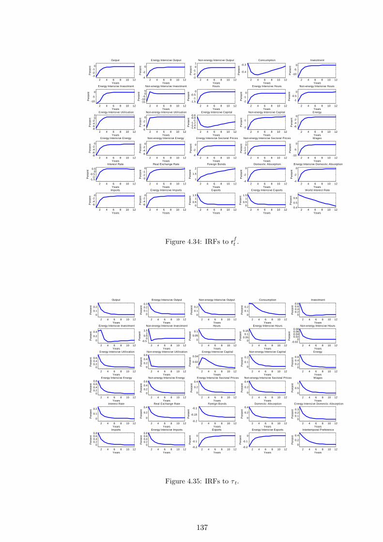
2 4 6 8 10 12321
0
Output
Per
cent
Years2 4 6 8 10 12
4
2
0
Energy Intensive Output
Per
cent
Years2 4 6 8 10 12
321
01
Nonenergy Intensive Output
Per
cent
Years2 4 6 8 10 12
0.4
0.3
Consumption
Per
cent
Years2 4 6 8 10 12
105
0
Investment
Per
cent
Years
2 4 6 8 10 1210
5
0
Energy Intensive InvestmentP
erce
nt
Years2 4 6 8 10 12
1510
505
Nonenergy Intensive Investment
Per
cent
Years2 4 6 8 10 12
1.51
0.50
Hours
Per
cent
Years2 4 6 8 10 12
21
0
Energy Intensive Hours
Per
cent
Years2 4 6 8 10 12
10.5
0
Nonenergy Intensive Hours
Per
cent
Years
2 4 6 8 10 128642
02
Energy Intensive Utilisation
Per
cent
Years2 4 6 8 10 12
642
0
Nonenergy Intensive Utilisation
Per
cent
Years2 4 6 8 10 12
1.61.41.2
10.80.6
Energy Intensive Capital
Per
cent
Years2 4 6 8 10 12
2
1
Nonenergy Intensive Capital
Per
cent
Years2 4 6 8 10 12
642
0Energy
Per
cent
Years
2 4 6 8 10 128642
0
Energy Intensive Energy
Per
cent
Years2 4 6 8 10 12
642
0
Nonenergy Intensive EnergyP
erce
nt
Years2 4 6 8 10 12
4
2
0
Energy Intensive Sectoral Prices
Per
cent
Years2 4 6 8 10 12
321
01
Nonenergy Intensive Sectoral Prices
Per
cent
Years2 4 6 8 10 12
10
5
0
Wages
Per
cent
Years
2 4 6 8 10 121.5
10.5
00.5
Interest Rate
Per
cent
Years2 4 6 8 10 12
321
0Real Exchange Rate
Per
cent
Years2 4 6 8 10 12
1
1.5
2Foreign Bonds
Per
cent
Years2 4 6 8 10 12
4
2
0Domestic Absorption
Per
cent
Years2 4 6 8 10 12
4
2
0Energy Intensive Domestic Absorption
Per
cent
Years
2 4 6 8 10 12
642
0
Imports
Per
cent
Years2 4 6 8 10 12
642
0
Energy Intensive Imports
Per
cent
Years2 4 6 8 10 12
00.5
11.5
ExportsP
erce
nt
Years2 4 6 8 10 12
00.5
11.5
Energy Intensive Exports
Per
cent
Years2 4 6 8 10 12
0.4
0.5
0.6
World Interest Rate
Per
cent
Years
Figure 4.34: IRFs to rft .
2 4 6 8 10 12
00.10.2
Output
Per
cent
Years2 4 6 8 10 12
00.10.20.3
Energy Intensive Output
Per
cent
Years2 4 6 8 10 12
00.10.2
Nonenergy Intensive Output
Per
cent
Years2 4 6 8 10 12
00.10.2
Consumption
Per
cent
Years2 4 6 8 10 12
00.20.40.60.8
Investment
Per
cent
Years
2 4 6 8 10 12
00.20.4
Energy Intensive Investment
Per
cent
Years2 4 6 8 10 12
0.50
0.51
1.5
Nonenergy Intensive Investment
Per
cent
Years2 4 6 8 10 12
00.05
0.1
Hours
Per
cent
Years2 4 6 8 10 12
00.05
0.10.15
Energy Intensive Hours
Per
cent
Years2 4 6 8 10 12
0.020
0.020.040.060.08
Nonenergy Intensive Hours
Per
cent
Years
2 4 6 8 10 120
0.20.40.6
Energy Intensive Utilisation
Per
cent
Years2 4 6 8 10 12
00.20.40.6
Nonenergy Intensive Utilisation
Per
cent
Years2 4 6 8 10 12
0
0.02
0.04Energy Intensive Capital
Per
cent
Years2 4 6 8 10 12
0
0.1
0.2
Nonenergy Intensive Capital
Per
cent
Years2 4 6 8 10 12
00.20.40.6
Energy
Per
cent
Years
2 4 6 8 10 120
0.20.40.60.8
Energy Intensive Energy
Per
cent
Years2 4 6 8 10 12
00.20.40.6
Nonenergy Intensive Energy
Per
cent
Years2 4 6 8 10 12
0
0.2
0.4Energy Intensive Sectoral Prices
Per
cent
Years2 4 6 8 10 12
0
0.2
0.4Nonenergy Intensive Sectoral Prices
Per
cent
Years2 4 6 8 10 12
0
0.5
1
Wages
Per
cent
Years
2 4 6 8 10 12
0
0.1
0.2
Interest Rate
Per
cent
Years2 4 6 8 10 12
0
0.2
0.4Real Exchange Rate
Per
cent
Years2 4 6 8 10 12
0.2
0.15
0.1Foreign Bonds
Per
cent
Years2 4 6 8 10 12
0
0.2
0.4Domestic Absorption
Per
cent
Years2 4 6 8 10 12
00.10.20.3
Energy Intensive Domestic Absorption
Per
cent
Years
2 4 6 8 10 120
0.20.40.60.8
Imports
Per
cent
Years2 4 6 8 10 12
00.20.40.60.8
Energy Intensive Imports
Per
cent
Years2 4 6 8 10 12
0.2
0.1
0
Exports
Per
cent
Years2 4 6 8 10 12
0.2
0.1
0
Energy Intensive Exports
Per
cent
Years2 4 6 8 10 12
0
0.2
0.4
Intertemporal Preference
Per
cent
Years
Figure 4.35: IRFs to � t.
137
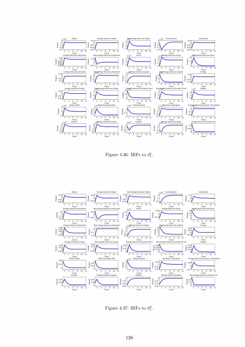
2 4 6 8 10 121510
505
x 103 Output
Per
cent
Years2 4 6 8 10 12
0.030.020.01
00.01
Energy Intensive Output
Per
cent
Years2 4 6 8 10 12
1012
x 103Nonenergy Intensive Output
Per
cent
Years2 4 6 8 10 12
642
02
x 105 Consumption
Per
cent
Years2 4 6 8 10 12
0.060.040.02
00.02
Investment
Per
cent
Years
2 4 6 8 10 120.080.060.040.02
00.02
Energy Intensive InvestmentP
erce
nt
Years2 4 6 8 10 12
0.02
0
0.02
Nonenergy Intensive Investment
Per
cent
Years2 4 6 8 10 12
1
0
1x 10³ Hours
Per
cent
Years2 4 6 8 10 12
4
2
0
2x 10³Energy Intensive Hours
Per
cent
Years2 4 6 8 10 12
0
5
10x 104Nonenergy Intensive Hours
Per
cent
Years
2 4 6 8 10 12
0.10.05
00.05
Energy Intensive Utilisation
Per
cent
Years2 4 6 8 10 12
321
01
x 103Nonenergy Intensive Utilisation
Per
cent
Years2 4 6 8 10 12
321
01
x 103Energy Intensive Capital
Per
cent
Years2 4 6 8 10 12
0
2
4
x 103Nonenergy Intensive Capital
Per
cent
Years2 4 6 8 10 12
0.020.01
00.01
Energy
Per
cent
Years
2 4 6 8 10 120.020.01
00.01
Energy Intensive Energy
Per
cent
Years2 4 6 8 10 12
5
0
5x 10³Nonenergy Intensive Energy
Per
cent
Years2 4 6 8 10 12
0
10
20x 103Energy Intensive Sectoral Prices
Per
cent
Years2 4 6 8 10 12
2
0
2x 10³Nonenergy Intensive Sectoral Prices
Per
cent
Years2 4 6 8 10 12
505
x 103 Wages
Per
cent
Years
2 4 6 8 10 122
0
2x 10³ Interest Rate
Per
cent
Years2 4 6 8 10 12
0123
x 103Real Exchange Rate
Per
cent
Years2 4 6 8 10 12
1
1.5
2
x 103 Foreign Bonds
Per
cent
Years2 4 6 8 10 12
1510
505
x 103Domestic Absorption
Per
cent
Years2 4 6 8 10 12
20
10
0
x 103Energy Intensive Domestic Absorption
Per
cent
Years
2 4 6 8 10 121510
505
x 103 Imports
Per
cent
Years2 4 6 8 10 12
1510
505
x 103Energy Intensive Imports
Per
cent
Years2 4 6 8 10 12
1510
50
x 104 ExportsP
erce
nt
Years2 4 6 8 10 12
1510
50
x 104Energy Intensive Exports
Per
cent
Years2 4 6 8 10 12
0
0.05
0.1
Energy Intensive Capital Cost
Per
cent
Years
Figure 4.36: IRFs to #et .
2 4 6 8 10 120.040.02
00.02
Output
Per
cent
Years2 4 6 8 10 12
0.020
0.02
Energy Intensive Output
Per
cent
Years2 4 6 8 10 12
0.040.02
00.02
Nonenergy Intensive Output
Per
cent
Years2 4 6 8 10 12
10
5
0x 104 Consumption
Per
cent
Years2 4 6 8 10 12
0.10
0.1
Investment
Per
cent
Years
2 4 6 8 10 120.20.1
00.1
Energy Intensive Investment
Per
cent
Years2 4 6 8 10 12
0.020
0.02
Nonenergy Intensive Investment
Per
cent
Years2 4 6 8 10 12
0
5
10x 103 Hours
Per
cent
Years2 4 6 8 10 12
0.02
0
0.02Energy Intensive Hours
Per
cent
Years2 4 6 8 10 12
05
1015
x 103Nonenergy Intensive Hours
Per
cent
Years
2 4 6 8 10 120.02
00.020.040.06
Energy Intensive Utilisation
Per
cent
Years2 4 6 8 10 12
0.2
0.1
0
Nonenergy Intensive Utilisation
Per
cent
Years2 4 6 8 10 12
1510
505
x 103Energy Intensive Capital
Per
cent
Years2 4 6 8 10 12
505
1015
x 103Nonenergy Intensive Capital
Per
cent
Years2 4 6 8 10 12
0.020
0.020.04
Energy
Per
cent
Years
2 4 6 8 10 12
0.020
0.020.04
Energy Intensive Energy
Per
cent
Years2 4 6 8 10 12
0.020
0.020.04
Nonenergy Intensive Energy
Per
cent
Years2 4 6 8 10 12
0
0.01
0.02
Energy Intensive Sectoral Prices
Per
cent
Years2 4 6 8 10 12
00.020.040.06
Nonenergy Intensive Sectoral Prices
Per
cent
Years2 4 6 8 10 12
00.020.040.06
Wages
Per
cent
Years
2 4 6 8 10 12
0
0.02
0.04Interest Rate
Per
cent
Years2 4 6 8 10 12
00.020.04
Real Exchange Rate
Per
cent
Years2 4 6 8 10 12
42
02
x 103 Foreign Bonds
Per
cent
Years2 4 6 8 10 12
0.040.02
00.02
Domestic Absorption
Per
cent
Years2 4 6 8 10 12
0.02
0
0.02
Energy Intensive Domestic Absorption
Per
cent
Years
2 4 6 8 10 120
0.020.04
Imports
Per
cent
Years2 4 6 8 10 12
00.020.04
Energy Intensive Imports
Per
cent
Years2 4 6 8 10 12
0.030.020.01
0
Exports
Per
cent
Years2 4 6 8 10 12
0.030.020.01
0
Energy Intensive Exports
Per
cent
Years2 4 6 8 10 12
00.10.2
Nonenergy Intensive Capital Cost
Per
cent
Years
Figure 4.37: IRFs to #nt .
138
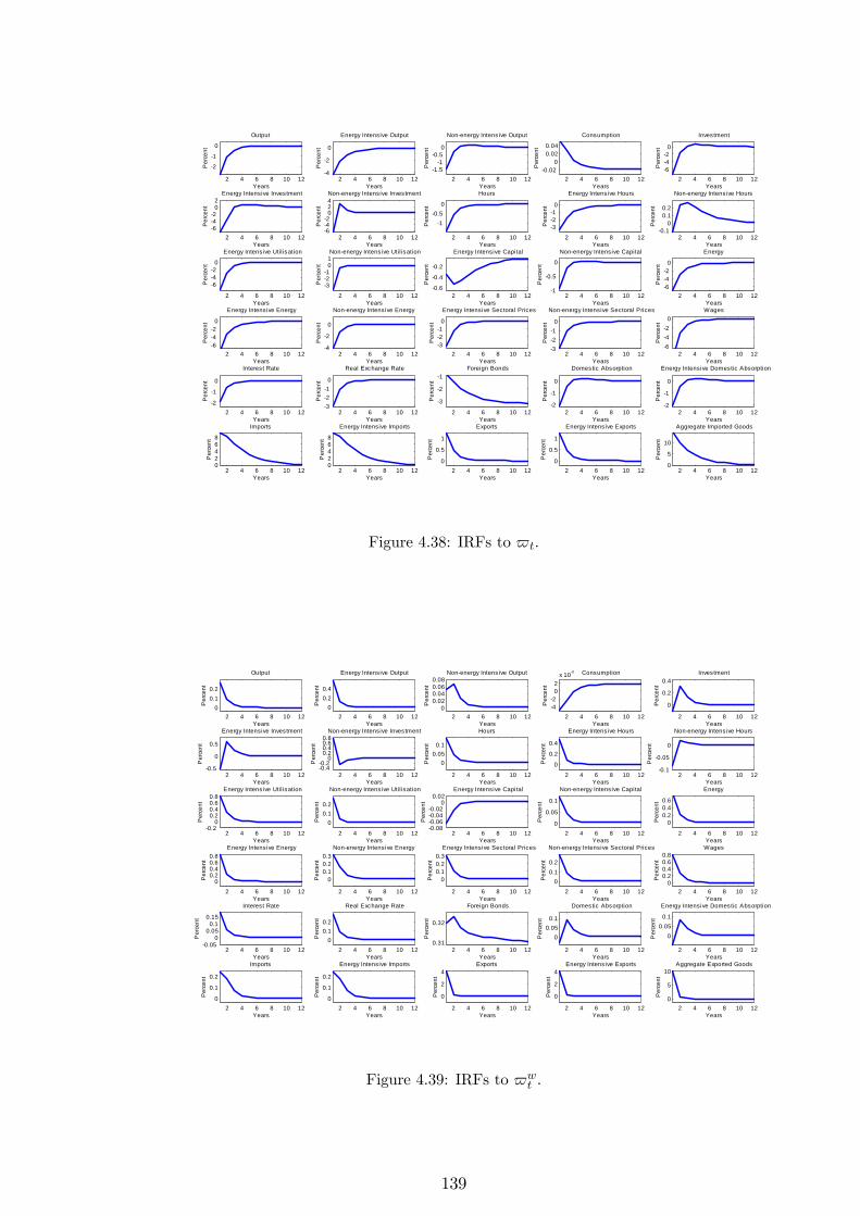
2 4 6 8 10 12
2
1
0
Output
Per
cent
Years2 4 6 8 10 12
4
2
0
Energy Intensive Output
Per
cent
Years2 4 6 8 10 12
1.51
0.50
Nonenergy Intensive Output
Per
cent
Years2 4 6 8 10 12
0.020
0.020.04
Consumption
Per
cent
Years2 4 6 8 10 12
642
0
Investment
Per
cent
Years
2 4 6 8 10 12642
02
Energy Intensive InvestmentP
erce
nt
Years2 4 6 8 10 12
642
024Nonenergy Intensive Investment
Per
cent
Years2 4 6 8 10 12
10.5
0
Hours
Per
cent
Years2 4 6 8 10 12
321
0
Energy Intensive Hours
Per
cent
Years2 4 6 8 10 12
0.10
0.10.2
Nonenergy Intensive Hours
Per
cent
Years
2 4 6 8 10 12
642
0
Energy Intensive Utilisation
Per
cent
Years2 4 6 8 10 12
321
01Nonenergy Intensive Utilisation
Per
cent
Years2 4 6 8 10 12
0.6
0.4
0.2
Energy Intensive Capital
Per
cent
Years2 4 6 8 10 12
1
0.5
0
Nonenergy Intensive Capital
Per
cent
Years2 4 6 8 10 12
642
0
Energy
Per
cent
Years
2 4 6 8 10 12642
0
Energy Intensive Energy
Per
cent
Years2 4 6 8 10 12
4
2
0
Nonenergy Intensive EnergyP
erce
nt
Years2 4 6 8 10 12
321
0
Energy Intensive Sectoral Prices
Per
cent
Years2 4 6 8 10 12
321
0
Nonenergy Intensive Sectoral Prices
Per
cent
Years2 4 6 8 10 12
642
0Wages
Per
cent
Years
2 4 6 8 10 122
1
0
Interest Rate
Per
cent
Years2 4 6 8 10 12
321
0
Real Exchange Rate
Per
cent
Years2 4 6 8 10 12
3
2
1Foreign Bonds
Per
cent
Years2 4 6 8 10 12
2
1
0
Domestic Absorption
Per
cent
Years2 4 6 8 10 12
2
1
0
Energy Intensive Domestic Absorption
Per
cent
Years
2 4 6 8 10 1202468
Imports
Per
cent
Years2 4 6 8 10 12
02468
Energy Intensive Imports
Per
cent
Years2 4 6 8 10 12
0
0.5
1
ExportsP
erce
nt
Years2 4 6 8 10 12
0
0.5
1
Energy Intensive Exports
Per
cent
Years2 4 6 8 10 12
0
5
10
Aggregate Imported Goods
Per
cent
Years
Figure 4.38: IRFs to $t.
2 4 6 8 10 120
0.10.2
Output
Per
cent
Years2 4 6 8 10 12
00.20.4
Energy Intensive Output
Per
cent
Years2 4 6 8 10 12
00.020.040.060.08
Nonenergy Intensive Output
Per
cent
Years2 4 6 8 10 12
42
02
x 103 Consumption
Per
cent
Years2 4 6 8 10 12
0
0.2
0.4Investment
Per
cent
Years
2 4 6 8 10 120.5
0
0.5
Energy Intensive Investment
Per
cent
Years2 4 6 8 10 12
0.40.2
00.20.40.60.8
Nonenergy Intensive Investment
Per
cent
Years2 4 6 8 10 12
00.05
0.1
Hours
Per
cent
Years2 4 6 8 10 12
0
0.2
0.4
Energy Intensive Hours
Per
cent
Years2 4 6 8 10 12
0.1
0.05
0
Nonenergy Intensive Hours
Per
cent
Years
2 4 6 8 10 120.2
00.20.40.60.8
Energy Intensive Utilisation
Per
cent
Years2 4 6 8 10 12
00.10.2
Nonenergy Intensive Utilisation
Per
cent
Years2 4 6 8 10 12
0.080.060.040.02
00.02
Energy Intensive Capital
Per
cent
Years2 4 6 8 10 12
0
0.05
0.1
Nonenergy Intensive Capital
Per
cent
Years2 4 6 8 10 12
00.20.40.6
Energy
Per
cent
Years
2 4 6 8 10 120
0.20.40.60.8
Energy Intensive Energy
Per
cent
Years2 4 6 8 10 12
00.10.20.3
Nonenergy Intensive Energy
Per
cent
Years2 4 6 8 10 12
00.10.20.3
Energy Intensive Sectoral Prices
Per
cent
Years2 4 6 8 10 12
00.10.2
Nonenergy Intensive Sectoral Prices
Per
cent
Years2 4 6 8 10 12
00.20.40.60.8
Wages
Per
cent
Years
2 4 6 8 10 120.05
00.05
0.10.15
Interest Rate
Per
cent
Years2 4 6 8 10 12
00.10.2
Real Exchange Rate
Per
cent
Years2 4 6 8 10 12
0.31
0.32
Foreign Bonds
Per
cent
Years2 4 6 8 10 12
00.05
0.1
Domestic Absorption
Per
cent
Years2 4 6 8 10 12
00.05
0.1
Energy Intensive Domestic Absorption
Per
cent
Years
2 4 6 8 10 120
0.1
0.2
Imports
Per
cent
Years2 4 6 8 10 12
0
0.1
0.2
Energy Intensive Imports
Per
cent
Years2 4 6 8 10 12
0
2
4Exports
Per
cent
Years2 4 6 8 10 12
0
2
4Energy Intensive Exports
Per
cent
Years2 4 6 8 10 12
0
5
10Aggregate Exported Goods
Per
cent
Years
Figure 4.39: IRFs to $wt .
139
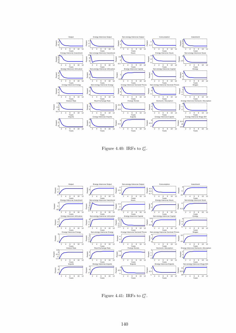
2 4 6 8 10 12
0
1
2Output
Per
cent
Years2 4 6 8 10 12
321
Energy Intensive Output
Per
cent
Years2 4 6 8 10 12
1
2
3
Nonenergy Intensive Output
Per
cent
Years2 4 6 8 10 12
1.2
1
Consumption
Per
cent
Years2 4 6 8 10 12
02468
Investment
Per
cent
Years
2 4 6 8 10 1202468
Energy Intensive InvestmentP
erce
nt
Years2 4 6 8 10 12
0
5
10Nonenergy Intensive Investment
Per
cent
Years2 4 6 8 10 12
0.5
0
0.5
Hours
Per
cent
Years2 4 6 8 10 12
5
4
3Energy Intensive Hours
Per
cent
Years2 4 6 8 10 12
2.5
3
Nonenergy Intensive Hours
Per
cent
Years
2 4 6 8 10 12024
Energy Intensive Utilisation
Per
cent
Years2 4 6 8 10 12
0
2
4Nonenergy Intensive Utilisation
Per
cent
Years2 4 6 8 10 12
0.5
1
Energy Intensive Capital
Per
cent
Years2 4 6 8 10 12
0
1
Nonenergy Intensive Capital
Per
cent
Years2 4 6 8 10 12
0
2
4
Energy
Per
cent
Years
2 4 6 8 10 120246
Energy Intensive Energy
Per
cent
Years2 4 6 8 10 12
0
2
4Nonenergy Intensive Energy
Per
cent
Years2 4 6 8 10 12
4
5
6
Energy Intensive Sectoral Prices
Per
cent
Years2 4 6 8 10 12
1
0
1Nonenergy Intensive Sectoral Prices
Per
cent
Years2 4 6 8 10 12
42
02
Wages
Per
cent
Years
2 4 6 8 10 120.5
00.5
11.5
Interest Rate
Per
cent
Years2 4 6 8 10 12
0
1
2Real Exchange Rate
Per
cent
Years2 4 6 8 10 12
0.8
0.6
Foreign Bonds
Per
cent
Years2 4 6 8 10 12
0
1
2Domestic Absorption
Per
cent
Years2 4 6 8 10 12
2
1
0Energy Intensive Domestic Absorption
Per
cent
Years
2 4 6 8 10 12
0
2
4Imports
Per
cent
Years2 4 6 8 10 12
0
2
4Energy Intensive Imports
Per
cent
Years2 4 6 8 10 12
1
0.5
0
ExportsP
erce
nt
Years2 4 6 8 10 12
1
0.5
0
Energy Intensive Exports
Per
cent
Years2 4 6 8 10 12
14.815
15.2
Energy Intensive Wage Bil l
Per
cent
Years
Figure 4.40: IRFs to �et .
2 4 6 8 10 123
2
1
0Output
Per
cent
Years2 4 6 8 10 12
0
2
Energy Intensive Output
Per
cent
Years2 4 6 8 10 12
4
3.5
3
Nonenergy Intensive Output
Per
cent
Years2 4 6 8 10 12
0.70.60.5
Consumption
Per
cent
Years2 4 6 8 10 12
10
5
0Investment
Per
cent
Years
2 4 6 8 10 1210
5
0Energy Intensive Investment
Per
cent
Years2 4 6 8 10 12
642
024Nonenergy Intensive Investment
Per
cent
Years2 4 6 8 10 12
2.5
2
1.5
Hours
Per
cent
Years2 4 6 8 10 12
2
3
4
Energy Intensive Hours
Per
cent
Years2 4 6 8 10 12
5.5
5
Nonenergy Intensive Hours
Per
cent
Years
2 4 6 8 10 12642
0
Energy Intensive Utilisation
Per
cent
Years2 4 6 8 10 12
321
0
Nonenergy Intensive Utilisation
Per
cent
Years2 4 6 8 10 12
1.61.41.2
10.80.6
Energy Intensive Capital
Per
cent
Years2 4 6 8 10 12
0.5
0
0.5Nonenergy Intensive Capital
Per
cent
Years2 4 6 8 10 12
642
0Energy
Per
cent
Years
2 4 6 8 10 12
5
0Energy Intensive Energy
Per
cent
Years2 4 6 8 10 12
321
01
Nonenergy Intensive Energy
Per
cent
Years2 4 6 8 10 12
6
5
4
Energy Intensive Sectoral Prices
Per
cent
Years2 4 6 8 10 12
0
2
4Nonenergy Intensive Sectoral Prices
Per
cent
Years2 4 6 8 10 12
15
10
Wages
Per
cent
Years
2 4 6 8 10 121.5
10.5
00.5
Interest Rate
Per
cent
Years2 4 6 8 10 12
0
1
2
Real Exchange Rate
Per
cent
Years2 4 6 8 10 12
0.6
0.8
Foreign Bonds
Per
cent
Years2 4 6 8 10 12
321
0Domestic Absorption
Per
cent
Years2 4 6 8 10 12
0
1
2
Energy Intensive Domestic Absorption
Per
cent
Years
2 4 6 8 10 12
2
0
2Imports
Per
cent
Years2 4 6 8 10 12
2
0
2Energy Intensive Imports
Per
cent
Years2 4 6 8 10 12
1
0.5
0
Exports
Per
cent
Years2 4 6 8 10 12
1
0.5
0
Energy Intensive Exports
Per
cent
Years2 4 6 8 10 12
20
20.5
21
Nonenergy Intensive Wage Bill
Per
cent
Years
Figure 4.41: IRFs to �nt .
140
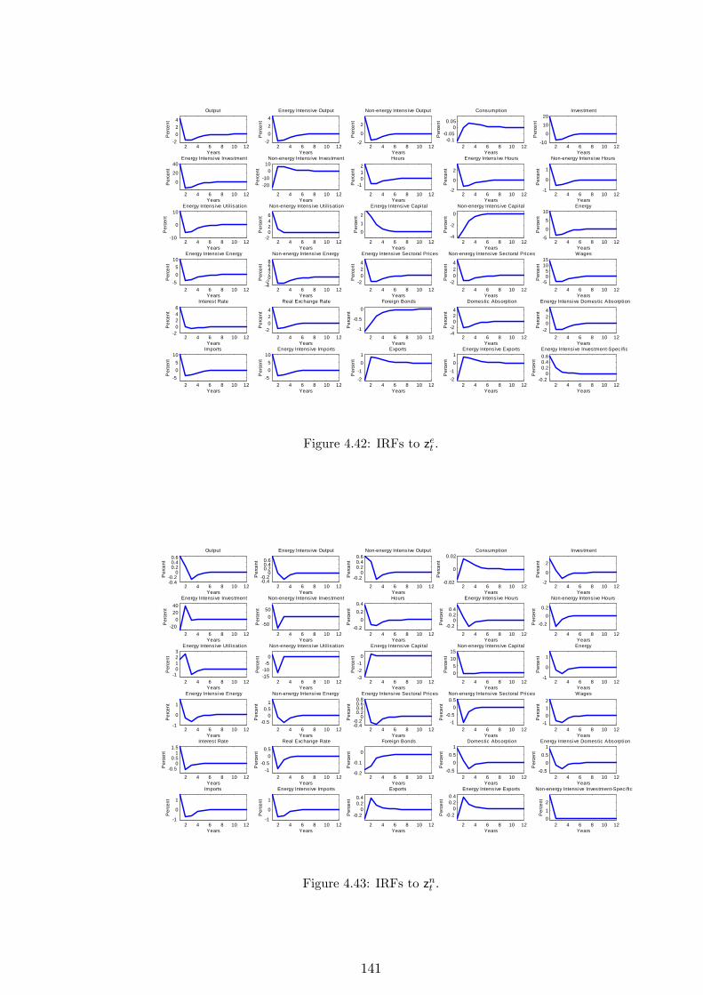
2 4 6 8 10 122
024
Output
Per
cent
Years2 4 6 8 10 12
2024
Energy Intensive Output
Per
cent
Years2 4 6 8 10 12
2
0
2
Nonenergy Intensive Output
Per
cent
Years2 4 6 8 10 12
0.10.05
00.05
Consumption
Per
cent
Years2 4 6 8 10 12
10
0
10
20Investment
Per
cent
Years
2 4 6 8 10 12
0
20
40Energy Intensive Investment
Per
cent
Years2 4 6 8 10 12
2010
010
Nonenergy Intensive Investment
Per
cent
Years2 4 6 8 10 12
1012
Hours
Per
cent
Years2 4 6 8 10 12
2
0
2
Energy Intensive Hours
Per
cent
Years2 4 6 8 10 12
1
0
1
Nonenergy Intensive Hours
Per
cent
Years
2 4 6 8 10 1210
0
10Energy Intensive Utilisation
Per
cent
Years2 4 6 8 10 12
20246
Nonenergy Intensive Utilisation
Per
cent
Years2 4 6 8 10 12
0
1
2
Energy Intensive Capital
Per
cent
Years2 4 6 8 10 12
4
2
0Nonenergy Intensive Capital
Per
cent
Years2 4 6 8 10 12
5
0
5
10Energy
Per
cent
Years
2 4 6 8 10 125
05
10Energy Intensive Energy
Per
cent
Years2 4 6 8 10 12
42
02468
Nonenergy Intensive EnergyP
erce
nt
Years2 4 6 8 10 12
2024
Energy Intensive Sectoral Prices
Per
cent
Years2 4 6 8 10 12
2024
Nonenergy Intensive Sectoral Prices
Per
cent
Years2 4 6 8 10 12
505
1015
Wages
Per
cent
Years
2 4 6 8 10 122
0246
Interest Rate
Per
cent
Years2 4 6 8 10 12
2024
Real Exchange Rate
Per
cent
Years2 4 6 8 10 12
1
0.5
0Foreign Bonds
Per
cent
Years2 4 6 8 10 12
42
024
Domestic Absorption
Per
cent
Years2 4 6 8 10 12
2024
Energy Intensive Domestic Absorption
Per
cent
Years
2 4 6 8 10 125
05
10Imports
Per
cent
Years2 4 6 8 10 12
505
10Energy Intensive Imports
Per
cent
Years2 4 6 8 10 12
21
01
ExportsP
erce
nt
Years2 4 6 8 10 12
21
01
Energy Intensive Exports
Per
cent
Years2 4 6 8 10 12
0.20
0.20.40.6Energy Intensive InvestmentSpecific
Per
cent
Years
Figure 4.42: IRFs to zet .
2 4 6 8 10 120.40.2
00.20.40.6
Output
Per
cent
Years2 4 6 8 10 12
0.40.2
00.20.40.6
Energy Intensive Output
Per
cent
Years2 4 6 8 10 12
0.20
0.20.40.6
Nonenergy Intensive Output
Per
cent
Years2 4 6 8 10 12
0.02
0
0.02Consumption
Per
cent
Years2 4 6 8 10 12
2
0
2
Investment
Per
cent
Years
2 4 6 8 10 1220
02040
Energy Intensive Investment
Per
cent
Years2 4 6 8 10 12
500
50
Nonenergy Intensive Investment
Per
cent
Years2 4 6 8 10 12
0.20
0.20.4
Hours
Per
cent
Years2 4 6 8 10 12
0.20
0.20.4
Energy Intensive Hours
Per
cent
Years2 4 6 8 10 12
0.20
0.2
Nonenergy Intensive Hours
Per
cent
Years
2 4 6 8 10 121
0123
Energy Intensive Utilisation
Per
cent
Years2 4 6 8 10 12
1510
50
Nonenergy Intensive Utilisation
Per
cent
Years2 4 6 8 10 12
321
0
Energy Intensive Capital
Per
cent
Years2 4 6 8 10 12
05
1015
Nonenergy Intensive Capital
Per
cent
Years2 4 6 8 10 12
1
0
1
Energy
Per
cent
Years
2 4 6 8 10 121
0
1
Energy Intensive Energy
Per
cent
Years2 4 6 8 10 12
0.50
0.51
Nonenergy Intensive Energy
Per
cent
Years2 4 6 8 10 12
0.40.2
00.20.40.60.8
Energy Intensive Sectoral Prices
Per
cent
Years2 4 6 8 10 12
10.5
00.5Nonenergy Intensive Sectoral Prices
Per
cent
Years2 4 6 8 10 12
1012
Wages
Per
cent
Years
2 4 6 8 10 12
0.50
0.51
1.5Interest Rate
Per
cent
Years2 4 6 8 10 12
10.5
00.5
Real Exchange Rate
Per
cent
Years2 4 6 8 10 12
0.2
0.1
0
Foreign Bonds
Per
cent
Years2 4 6 8 10 12
0.50
0.51
Domestic Absorption
Per
cent
Years2 4 6 8 10 12
0.50
0.51
Energy Intensive Domestic Absorption
Per
cent
Years
2 4 6 8 10 121
0
1
Imports
Per
cent
Years2 4 6 8 10 12
1
0
1
Energy Intensive Imports
Per
cent
Years2 4 6 8 10 12
0.20
0.20.4
Exports
Per
cent
Years2 4 6 8 10 12
0.20
0.20.4
Energy Intensive Exports
Per
cent
Years2 4 6 8 10 12
012
Nonenergy Intensive InvestmentSpecific
Per
cent
Years
Figure 4.43: IRFs to znt .
141
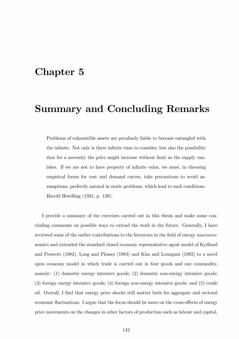
Chapter 5
Summary and Concluding Remarks
Problems of exhaustible assets are peculiarly liable to become entangled with
the in�nite. Not only is there in�nite time to consider, but also the possibility
that for a necessity the price might increase without limit as the supply van-
ishes. If we are not to have property of in�nite value, we must, in choosing
empirical forms for cost and demand curves, take precautions to avoid as-
sumptions, perfectly natural in static problems, which lead to such conditions.
Harold Hotelling (1931, p. 139).
I provide a summary of the exercises carried out in this thesis and make some con-
cluding comments on possible ways to extend the work in the future. Generally, I have
reviewed some of the earlier contributions to the literature in the �eld of energy macroeco-
nomics and extended the standard closed economy representative agent model of Kydland
and Prescott (1982), Long and Plosser (1983) and Kim and Loungani (1992) to a novel
open economy model in which trade is carried out in four goods and one commodity,
namely: (1) domestic energy intensive goods; (2) domestic non-energy intensive goods;
(3) foreign energy intensive goods; (4) foreign non-energy intensive goods; and (5) crude
oil. Overall, I �nd that energy price shocks still matter both for aggregate and sectoral
economic �uctuations. I argue that the focus should be more on the cross-e¤ects of energy
price movements on the changes in other factors of production such as labour and capital,
142
and less on the balance of payments�e¤ects once this shock hits the system.
Particularly, in Chapter 2, I comprehensively reviewed the extant literature on energy
(price) and aggregate economic �uctuations, citing a number of important contributions
and debates by many esteemed economists to this strand of economic research. In doing
this, a few econometric and theoretical models were discussed. Building on the literature,
I studied an open economy of the United States that is subjected to vagaries of decisions
by its trading partners especially the oil bloc. The questions in mind were, "Can a model
be organised to explain the behaviour of a multi-sector economy such as the U.S. given a
supply-side shock such as an energy (price) shock? Further, given an array of supply- and
demand-side shocks perturbing the economy per period, how important is the e¤ect of
energy (price) shock? How are these shocks transmitted through the economy? Which is
more disturbing between the impact and the transition e¤ects of an energy (price) shock?"
Thus beginning with Chapter 3, I turned my attention to designing a two-sector com-
putable dynamic stochastic general equilibrium (CDSGE) open economy model of the
U.S. that formally admit energy into the production process in a way that can generate
plausible parameter values with which an applied study can deal with a broad range of
economic issues. The model in this chapter falls in the lineage of Kydland and Prescott
(1982), Long and Plosser (1983), and Kim and Loungani (1992) models in which I assume
that (1) representative agents reside in a perfectly competitive economy making decisions
regarding consumption, labour, investment, and output; (2) representative agents in the
domestic country trade with their foreign counterparts; (3) imported crude oil is essential
for production; and also (4) production takes place in two sectors and four types of goods
are available for consumption and investment purposes. Twelve shocks, domestic and
imported, were added to the model and I required as a benchmark that the model �ts
the data for output, real exchange rate, energy use, and consumption: output because it
serves as a measure of a country�s total income; real exchange rate because it serves as
a determinant of a country�s relative competitiveness; energy use because it serves as an
indicator of special inputs into a country�s production process; and consumption because
it serves as a yardstick for evaluating a country�s welfare.
143
Furthermore, in Chapter 4, I examine the role of energy price shocks in e¤ecting
changes both at the aggregate and sectorial levels further by extending the model of
Chapter 3 to include capital account, added more domestic and imported shocks and
frictions before re-estimating the model on non-stationary data sets using the method of
indirect inference. The focus of the explanation in this chapter was output and the real
exchange rate. I showed that the main channels through which imported oil shock works
are by raising the costs of production (when energy price shoots up) with the added e¤ect
of lowering the marginal productivity of the remaining inputs (i.e., labour and capital)
on the production side and by acting as a resource drain in the economy-wide resource
constraint. I have shown qualitatively that output is a¤ected both intratemporally through
what I termed the impact e¤ect and intertemporally through what I labelled the transition
e¤ect. In addition, a quantitative assessment of the results in the estimated model model
was presented. A main contribution is that I was able to use a micro-founded multi-sector
DSGE model to �nd results that support some already established facts in relation to the
size of the e¤ects of oil price shock on macroeconomic variables like output and the real
exchange rate.
Next, I speculate on a few possible extensions to the model that could yet prove
fruitful in a future research endeavour. First, a useful extension for model implications
regarding energy policies and welfare evaluation would be to consider an economy with
money (M=P ) and energy use (Eh) by household,1 which can be achieved by increasing
the arguments in the utility function 4.1
EX1
0��U
�C � �C�1; �H; jE
h; vM
P
�(5.1)
where j and v are optional exogenous disturbances to energy use and real money balances,
respectively. Then, depending on if we are interested in considering the extent of price
�exibility in the economy, quadratic adjustment costs for nominal wage and price rigidities
can be speci�ed [see, for example, Hairault and Portier (1993) and Kim (2000)]. Moreover,
explicit modelling of the four goods may be important. I do think that the most rele-1As an example, see Dhawan and Jeske (2008) and Blanchard and Gali (2010) who modelled energy
use by household providing stylised facts on the share of household energy use in total GDP in the vicinityof that reported for the �rms.
144
vant contribution for this approach may be pursued by allowing traded goods to not only
be used for consumption/ investment purposes, but to be translated into the production
process as not all exchanged goods are completely �nished goods [see, for example, Gold-
berg and Campa (2010), Bergholt and Sveen (2014), and Eyquem and Kamber (2014)].2
This particular extension may have the following added advantages: (1) Beyond incorpo-
rating the level of energy intensity, this should help to admit the di¤erent levels of trade
intensities of the two sectors; and (2) We may also be able to examine the terms of trade
for goods of both sectors with the addition of extra cost channels via trade in intermediate
goods - this would be an extension to many open economy models that only analyse ag-
gregate terms of trade [see for example Backus et al. (1995), Mendoza (1995), and Backus
and Crucini (2000)]. Meanwhile, an extra dimension can be introduced if we are content
to assume that government spending is productive as in Finn (1998). Lastly, there are
two features of the model that have also been shut down to make the experiment less
complicated. The �rst is the non-inclusion of the non-traded sector, which Bruno (1976)
refers to as an "unimportant appendage" perhaps included for completeness. It has how-
ever been studied as an important sector of the economy since [see, for example, Tesar
(1989), Stockman (1990), Stockman and Tesar (1995)]. In fact, Stockman (1990) wrote
that "Both theory and evidence on open economies suggest the inclusion of non-traded
goods and multiple traded goods", which in that sense could further improve the model
presented in this thesis.
Finally, the story of this thesis is that we cannot continue to relegate interests in the
study of commodities in particular those that enter into the production process at one
stage or form to only when a shock occurs. There should indeed be a concerted and
maintained curiosity in the research of energy resources and this is not just in economics,
but a call to all disciplines that have been brought together by this matter. I belief that
this is the only way by which we will solve the energy question.
2A simplifying assumption in the model presented in Chapters 3 and 4 is that imported/ exportedgoods can directly be consumed or invested on arrival without any need for added value. This is rarelythe case.
145
Appendix A
Data Sources
Below is a detailed list and sources of the raw/ borrowed data that are made use
of in constructing the data series serving as the empirical counterparts to the model
macroeconomic variables in the main text.
A.1 Chapter 2
Bureau of Economic Analysis (www.bea.gov), 1949-2013
National Data, GDP and Personal Income
1. Table 1.1.5: Gross Domestic Product, billions of dollars, seasonally adjusted at
annual rate, extracted: 27 January, 2015.
2. Table 1.1.9: Implicit Price De�ators for Gross Domestic Product, 2009=100, sea-
sonally adjusted at annual rate, extracted: 27 January, 2015.
3. Table 2.4.5: Personal Consumption Expenditures by Type of Product, billions of
dollars, seasonally adjusted at annual rate, extracted: 30 January, 2015.
4. Table 3.9.5: Government Consumption Expenditures and Gross Investment, billions
of dollars, seasonally adjusted at annual rate, extracted: 30 January, 2015.
5. Tables 6.4B-6.4D: Full-Time and Part-Time Employees, extracted: 31 January, 2015.
146
6. Tables 6.5B-6.5D: Full-Time Equivalent Employees by Industry, extracted: 31 Jan-
uary, 2015.
7. Tables 6.7B-6.7D: Self-Employed Persons by Industry, extracted: 31 January, 2015.
8. Tables 6.8B-6.8D: Persons Engaged in Production by Industry, extracted: 31 Janu-
ary, 2015.
9. Tables 6.9B-6.9D: Hours Worked by Full-Time and Part-Time Employees by Indus-
try, extracted: 31 January, 2015.
National Data, Fixed Assets
1. Table 1.1: Current-Cost Net Stock of Fixed Assets and Consumer Durable Goods,
billions of dollars, seasonally adjusted at annual rate, extracted: 25 February, 2015.
2. Table 2.1: Current-Cost Net Stock of Private Fixed Assets, Equipment, Structures,
and Intellectual Property Products by Type, billions of dollars, seasonally adjusted
at annual rate, extracted: 30 January, 2015.
3. Table 2.7: Investment in Private Fixed Assets, Equipment, Structures, and Intellec-
tual Property Products by Type, billions of dollars, seasonally adjusted at annual
rate, extracted: 30 January, 2015.
4. Tables 7.1A-7.1B: Current-Cost Net Stock of Government Fixed Assets, billions of
dollars, seasonally adjusted at annual rate, extracted: 30 January, 2015.
5. Tables 7.5A-7.5B: Investment in Government Fixed Assets, billions of dollars, sea-
sonally adjusted at annual rate, extracted: 30 January, 2015.
6. Table 8.1: Current-Cost Net Stock of Consumer Durable Goods, billions of dollars,
seasonally adjusted at annual rate, extracted: 30 January, 2015.
Industry Data, GDP-by-Industry and Output-Input
1. Full-Time and Part-Time Employees by Industry.1
1The values for 1949 -1997 were downloaded from www.bea.gov/industry/gdpbyind_data.htm whilethe rest of the series (1998 - 2011) were obtained from the usual interactive section of the BEA�s GDP-by-Industry. To construct the values for 2012-2013, we calculate the growth rate of the series between1998 and 2011 using the expression g = exp[ 114 � ln(
obs1998obs2011
)]�1 and this is then used to project the valuesfor 2012 and 2013. All tables are extracted on 31 January, 2015 except the BEA�s GDP-by-Industryseries, which was downloaded in January, 2013. Currently, employment data are no longer available atthe BEA�s GDP-by-Industry section.
147
2. GDP by Industry, Value Added, millions of current dollars, extracted: 13 May, 2015.
Bureau of Labour Statistics (www.bls.gov), 1949-2013
1. Series ID: LNU00000000, Civilian Non-institutional Population between 16 and 64
Years Old, extracted: 27 January, 2015.2
2. Series ID: CUUR0000SA0, Consumer Price Index for All Urban Consumers: All
Items, Index 1982-84=100, seasonally adjusted, extracted: 29 January, 2015.3
Federal Reserve Bank of St. Louis (www.stlouisfed.org), 1949-2013
1. Series ID: PRS85006063, Nonfarm Business Sector: Compensation, Index 2009=100,
seasonally adjusted, extracted: 30 January, 2015.
2. Series ID: TFAABSHNO, Households and Non-pro�t Organizations; Total Financial
Assets, Level, Billions of Dollars, extracted: 13 May, 2015.
3. Series ID: TLBSHNO, Households and Non-pro�t Organizations; Total Liabilities,
Level, Billions of Dollars, extracted: 13 May, 2015.
Board of Governors of the Federal Reserve System (www.federalreserve.gov),
1949-2013
1. Series ID: G17/CAPUTL/CAPUTL.B00004.A, Manufacturing (SIC), n.s.a, per cent
of capacity in G17: Industrial Production and Capacity Utilization, G.17 Release,
extracted: 30 January, 2015.
2. Series ID: G17/CAPUTL/CAPUTL.G3361T3.A, Motor Vehicles and Parts (NAICS),
n.s.a, per cent of capacity in G17: Industrial Production and Capacity Utilization,
G.17 Release, extracted: 30 January, 2015.
3. Series ID: H15/H15/RIFSPFF_N.A, Federal Funds E¤ective Rate, 1955-2013, H15
Release, extracted: 30 January, 2015.
2We transformed the population data above into an index with 2009 value set to 100 following theapproach of Smets and Wouters (2007).
3Before use, the base year for the CPI index is transformed to 2009=100 from 1982-84=100.
148
Energy Information Administration (www.eia.gov), 1949-2013
1. Table 2.1: Energy Consumption by Sector, January, 2015 Monthly Energy Review,
extracted: 30 January, 2015.
2. Table 9.1: Crude Oil Price Summary, December 2014 Monthly Energy Review,
extracted: 30 January, 2015.
Smets and Wouters (2007)
1. 3-month treasury bill rates, 1949-1954.4
A.2 Chapter 3
As in Chapter 2 plus the following additional sources
United Nations
1. Total (world) population, both sexes combined, as of 1 July (thousands), 1950-2010.
World Bank
1. World population, World Development Indicators, World Bank Data, 1960-2013.5
International Monetary Fund
1. World Trade, Value in Millions of U.S. Dollars, International Financial Statistics,
1949-2013.
2. Prices of Major World Trade Commodities in U.S. Dollars, International Financial
Statistics, 1949-2013.
4I convert their quarterly data into annual data by averaging.5The population data for 1950-1959 are taken from the United Nations; we calculated the growth rate
for these 10 years and use it to obtain the data for 1949, while we use the population data from WorldDevelopment Indicators for 1960-2013. The series used to normalise the RoW variables is the above lessthe U.S. population.
149

3. Interest rates for Canada, France, Germany, Italy, Japan, and the U.K., Interna-
tional Financial Statistics, 1949-2013.
150
Appendix B
Supplementary Notes: Chapter 3
B.1 Data Construction
Output
Model variables: Y , Ye, Yn.
Data: Aggregate output, Y , is measured as the sum of the two sectoral outputs, Ye+Yn.
That is, the sum of gross outputs of the energy and non-energy intensive sectors. However,
due to a lack of data on gross output by industry dating back to 1949, which is the general
starting year of the variables, I instead construct the two sectoral gross domestic products
from the value added by industry data (Taken from GDP by Industry). More speci�cally,
aggregate output is de�ned as the total value added of all industries. Consequently,
energy intensive sector output, Yn, is de�ned as the sum of value added from agriculture
(including forestry, �shing, and hunting), mining, utilities, construction, manufacturing,
and transportation (and warehousing due to lack of further disaggregation) - sum of
excel worksheet lines 5, 8, 12, 13, 14, and 38; the non-energy intensive sector output,
Yn, is de�ned as the sum of value added from wholesale and retail trade, information,
�nance (including insurance, real estate, rental, and leasing), professional and business
services, educational services (including health care, and social assistance), arts (including
151
entertainment accommodation, and food services), and other services except government
- sum of excel worksheet lines 36, 37, 47, 52, 61, 70, 76, and 83. Lastly, due to lack of
su¢ cient disaggregation of government output, I split the output of the public sector into
two and added half each to Ye and Yn.
Consumption
Model variable: C.
Data: This is de�ned as personal consumption expenditures less durable goods (Taken
from Table 1.1.5. Gross Domestic Product).
Investment
Model variables: It, Ie, In.
Data: The measure of gross investment is taken to be the sum of personal consumption
expenditure on durable goods, and private nonresidential (structures and equipment) and
residential �xed investments. This was applied to the de�nition the two types of invest-
ment variables noting that aggregate investment is given as I = Ie + In. For investment
series, I combine Table 2.7: Investment in Private Fixed Assets, Equipment, Structures,
and Intellectual Property Products by Type and the series for consumer durables from
Table 2.4.5: Personal Consumption Expenditures by Type of Product, lines 3-24. Be-
ginning with the consumption of durable goods in Table 2.4.5, the following are assigned
investments that are non-energy intensive denoted by Idgn : furnishings and durable house-
hold equipment, recreational goods and vehicles, and other durable goods (sum of lines 8,
13, and 19) such that investment in the energy intensive type consumption durable goods
is given by Idge =Durable goods�Idgn (that is, line 3 minus the sum of lines 8, 13, and 19).
Further, assignment of Table 2.7 into investment by type is as follows. Investment in the
energy intensive goods are deemed to be given by the sum of equipment and structures
less residential equipment and improvements (sum of lines 2 and 35 minus the sum of
lines 34 and 74). Thus, investment in the non-energy intensive type goods is the sum of
residential equipment, improvements, and intellectual property products (sum of lines 34,
74, and 76).
152
Capital
Model variables: Ke, Kn.
Data: Following the constructions of energy and non-energy intensive investments
above, I build the series for capital using Table 8.1. Current-Cost Net Stock of Con-
sumer Durable Goods and Table 2.1. Current-Cost Net Stock of Private Fixed Assets,
Equipment, Structures, and Intellectual Property Products by Type. I have not mod-
elled aggregate capital in Chapter 3, and therefore have no need to construct an empirical
counterpart for it. I construct capital stock of the energy intensive goods as the sum of
nonresidential equipment and structures (that is, sum of lines 2 and 35 minus 34) and
capital stock of the non-energy intensive goods is calculated as the sum of residential
equipment and structures, and intellectual property products (that is, line 34). As in the
investment series above, non-energy intensive type capital stocks is taken as the sum of
furnishings and durable household equipment, recreational goods and vehicles, and other
durable goods (sum of lines 6, 11, and 17) such that capital stock in the energy intensive
type consumption durable goods is given by motor vehicles and parts (that is, line 2).
Labour hours
Model variables: H, He, Hn.
Data: Aggregate labour hours, H, is de�ned as hours of all persons engaged in pro-
duction and hours worked per sector, He and Hn, are calculated by following the proce-
dure of Herrendorf et al. (2013). Their procedure involves combining BEA�s GDP-by-
Industry data reported using NAICS classi�cation with BEA�s Income-and-Employment-
by-Industry data reported with three di¤erent classi�cations over the sample period (SIC72
for pre-1987, SIC87 between 1987-2000, and NAICS since 2001). This is necessary because
while the former data source follows the classi�cation I would prefer, they indicate that
the latter provides us with the kind of detailed industry level information I require for
assignment into the two sectors. Hence, for assignment into the two sectors, I follow in
similar veins as closely as feasibly permitted by the level of data disaggregation the de�ni-
tions of other sectoral variables as shown already above. Speci�cally, for each of the series,
153
employment and hours in agriculture, mining, utilities, construction, manufacturing and
transportation are classed as related to the energy intensive sector, while employment
and hours in wholesale, retail trade, information, �nance, professional services, education,
arts, and other services are non-energy intensive. Formally, the sectoral labour hours are
obtained using hj = NAICS hours of full-time equivalent employees + NAICS hours of
full-time equivalent employees � NAICS full-time employees � NAICS self-employed,
where NAICS self-employed = SIC self-employed � NAICS full-time and part-time em-
ployees � SIC full- and part-time employees, NAICS full-time equivalent employees =
SIC full-time equivalent employees � NAICS full-time and part-time employees � SIC
full-time and part-time employees, and NAICS hours of full-time equivalent employees
= SIC hours of full-time equivalent employees � NAICS full-time equivalent employees
� SIC full-time equivalent employees.
Capital utilisation rate
Model variables: Ue, Un.
Data: Following the assignment of industries into the two sectors, I deem it �t to
have two de�nitions of capital utilisation rate. Thus, capacity utilisation rate for total
manufacturing industry and capacity utilisation rate for motor vehicles and parts are
used as proxies for the measures of capital utilisation rates in the energy and non-energy
intensive sectors, respectively.
Energy use
Model variables: E, Ee, En.
Data: For total energy consumption in the economy, E, I take this to be the ag-
gregate consumption of primary energy or the consumption of fossil fuels comprising of
petroleum, coal, and natural gas measured in trillion British thermal units (BTUs) of the
private sector excluding the electric power sector.1 Energy consumption are provided for
1I do not include the consumption of renewables (geothermal, solar/ PV, and biomass) and electricityfor both theory and data reasons. On the data, if one chooses to use, for instance, total primary energyconsumption data, there is no data for biomass consumption until 1981. Also, I excluded the electricpower generating sector, which would have been classed as highly energy intensive sector given that closeto 70% of all primary energy is used, or lost, as this sector provides electricity to the �nal consumers. Ihave however not included it for one I have not modelled an energy producing sector, which would be the
154
four end-use sectors namely industrial, transportation, residential and commercial sectors.
Given a lack of further disaggregation, I use the primary energy consumption in both the
industrial and transportation sectors to proxy energy use in the energy intensive sector,
and primary energy consumption in both the residential and commercial sectors to proxy
energy use in the non-energy intensive sector. Hence, aggregate energy consumption in
this economy is formally given by E = Ee+En = dollar value of total primary energy use
= qt(Et�1 trillion={�1 million)
1 billion, where { = 5:78 is the conversion factor assumed for relating
BTUs to barrels of oil, which is similar to the �gure employed by the industry.
Domestic absorption
Model variable: D.
Data: By theoretical construction, D = Y , so that I use the same data for aggregate
output for domestic absorption.
Domestic demand of energy intensive goods
Model variable: De.
Data: This is constructed as De = private consumption of energy intensive goods
(Taken from Table 2.4.5: Personal Consumption Expenditures by Type of Product) +
private investment in energy intensive goods (Taken from Table 2.4.5: Personal Consump-
tion Expenditures by Type of Product and Table 2.7: Investment in Private Fixed Assets,
Equipment, Structures, and Intellectual Property Products by Type) + government con-
sumption of energy intensive goods (Taken from Table 3.9.5: Government Consumption
Expenditures and Gross Investment) + government investment in energy intensive goods
(Taken from Tables 7.5A-7.5B: Investment in Government Fixed Assets). Note that given
a lack of disaggregated data on government consumption expenditure, I therefore assume
that the share of government consumption in energy intensive goods is the same as for
government investment in energy intensive goods, and apply this share to the consumption
data.
case if I incorporate electricity into our total for energy consumption.
155
Aggregate import
Model variable: IM .
Data: This is taken to be the aggregate import (Taken from Table 1.1.5. Gross
Domestic Product).
Import of energy intensive goods
Model variable: IMe.
Data: This is taken to be the import of goods (Taken from Table 1.1.5. Gross Domestic
Product).
Aggregate export
Model variable: EX.
Data: This is taken to be the aggregate export (Taken from Table 1.1.5. Gross Do-
mestic Product).
Export of energy intensive goods
Model variable: EXe.
Data: This is taken to be the export of goods (Taken from Table 1.1.5. Gross Domestic
Product).
Wage rate
Model variable: W .
Data: This is a real index of hourly compensation (Series ID: PRS85006063, Nonfarm
Business Sector: Compensation).
Interest rate
Model variable: R.
156
Data: This is the three-month Treasury bill rate for 1949-1954 (Taken from Smets and
Wouters, 2007) where I have converted their quarterly data into annual data by averaging;
I use the federal funds rate for 1955-2013.
Real exchange rate
Model variable: P .
Data: General price level in the domestic country, which is taken to be the consumer
price index (CPI) for all urban consumers, relative to world CPI.
Price of energy intensive goods
Model variable: Pe.
Data: Calculated as the weighted average of the chain-type price indexes for value
added from agriculture, mining, utilities, construction, manufacturing, and transportation
(Taken from GDP by Industry).
Price of non-energy intensive goods
Model variable: Pn.
Data: Calculated as the weighted average of the chain-type price indexes for value
added from wholesale and retail trade, information, �nance, professional and business
services, educational services, arts, and other services (Taken from GDP by Industry).
157
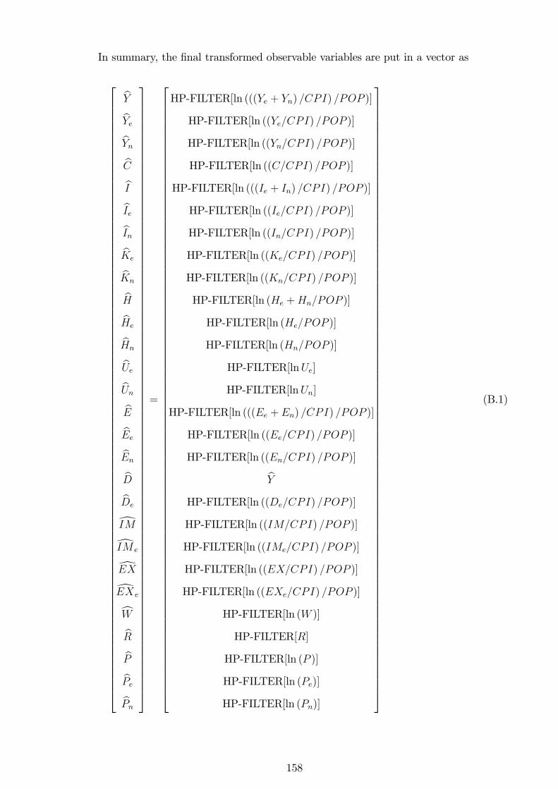
In summary, the �nal transformed observable variables are put in a vector as
26666666666666666666666666666666666666666666666666666666666666666666666666666666666666664
bYbYebYnbCbIbIebInbKebKnbHbHebHnbUebUnbEbEebEnbDbDedIMdIM edEXdEXecWbRbPbPebPn
37777777777777777777777777777777777777777777777777777777777777777777777777777777777777775
=
26666666666666666666666666666666666666666666666666666666666666666666666666666666666666664
HP-FILTER[ln (((Ye + Yn) =CPI) =POP )]
HP-FILTER[ln ((Ye=CPI) =POP )]
HP-FILTER[ln ((Yn=CPI) =POP )]
HP-FILTER[ln ((C=CPI) =POP )]
HP-FILTER[ln (((Ie + In) =CPI) =POP )]
HP-FILTER[ln ((Ie=CPI) =POP )]
HP-FILTER[ln ((In=CPI) =POP )]
HP-FILTER[ln ((Ke=CPI) =POP )]
HP-FILTER[ln ((Kn=CPI) =POP )]
HP-FILTER[ln (He +Hn=POP )]
HP-FILTER[ln (He=POP )]
HP-FILTER[ln (Hn=POP )]
HP-FILTER[lnUe]
HP-FILTER[lnUn]
HP-FILTER[ln (((Ee + En) =CPI) =POP )]
HP-FILTER[ln ((Ee=CPI) =POP )]
HP-FILTER[ln ((En=CPI) =POP )]bYHP-FILTER[ln ((De=CPI) =POP )]
HP-FILTER[ln ((IM=CPI) =POP )]
HP-FILTER[ln ((IMe=CPI) =POP )]
HP-FILTER[ln ((EX=CPI) =POP )]
HP-FILTER[ln ((EXe=CPI) =POP )]
HP-FILTER[ln (W )]
HP-FILTER[R]
HP-FILTER[ln (P )]
HP-FILTER[ln (Pe)]
HP-FILTER[ln (Pn)]
37777777777777777777777777777777777777777777777777777777777777777777777777777777777777775
(B.1)
158
where the Hodrick-Prescott smoothing parameter has been set to 400, CPI is consumer
price index, and POP is population index.
B.2 Technical Appendix
This section of the note provides details of the model set up and derivations of the
equilibrium conditions that appear in the main text. This is a two-sector two-region
open economy real business cycle (RBC) model where the sectors are the energy and
non-energy intensive sectors, and the regions are the domestic country and the rest of
the world (RoW). An essential feature of the model is that I recognise that all aspects
of the economy must be �powered�. I, however, only included energy in the production
sides. I assume that the consumer price index (CPI) in the RoW, Pim, is the numeraire
and I de�ned all domestic prices relative to this. Hence, domestic country�s CPI, P , is a
measure of the real exchange rate. Other important prices are the consumer real wage,
W , producer real wage in the energy intensive sector, W/Pe, and producer real wage in
the non-energy intensive sector, W/Pn, where Pe and Pn correspond, respectively, to the
relative prices of energy and non-energy intensive goods.
I use the following notations for convenience: UPPER-CASE letters X 0 � Xt+1,
X � Xt, and X�1 � Xt�1 for dynamic variables for next, current, and lagged periods,
respectively; lower-case letters, say x, to denote non-stochastic steady state variables; hat-
ted letters, �^�, to denote variables in their log-linear form; and �, � t, and sans serif letters
denote the exogenous state variables. I characterise the model in terms of the domestic
country.
Households Their dynamic problem can be formalised as that of
maxfC;H;I;Ie;In;B0;Ue;Un;Ke;Kng1t=0
" 1X0
��
(C � �C�1)
1��
1� �� �
H1+!
1 + !
!#| {z }
U
(B.2)
where the period utility, U, is assumed to obey the following standard regularity conditions:
159
U0> 0, U
00< 0, U1 > 0, U2 < 0, U11, U22 < 0, and U11U22�U212 > 0 (see Greenwood et al.,
1988); � and � are the exogenous stochastic intertemporal preference and labour supply
shocks, respectively, and are both assumed to be following AR(1) processes in logarithm,
which I write as
ln � = �� ln ��1 + "� (S29)
ln � = �� ln ��1 + "� (S30)
where for s1 = (� t; �t), the autoregressive parameters are conditioned by �s1 2 [0; 1) and
"s1 are i.i.d. normal distributions with zero means and innovation standard deviations,
�s1. I have included habit formation, �, to aid the model in replicating the data properties,
especially that of autocorrelation of consumption.
Denoting by �C the marginal utility of consumption and by �H the marginal disutility
of labour hours, I have that
�C = � (C � �C�1)�� (B.3)
�H = ��H! (B.4)
Further, households can accumulate two types of physical capital goods, which are as-
sumed to follow the laws of motion
Ke =
�1� �e0 �
�e1 (Ue)�e
�e
�Ke;�1 + ZeIe � 0:5 e
�Ke
Ke;�1� 1�2
Ke;�1 (B.5)
Kn =
�1� �n0 �
�n1 (Un)�n
�n
�Kn;�1 + ZnIn � 0:5 n
�Kn
Kn;�1� 1�2
Kn;�1 (B.6)
where for type t = e; n, I have allowed for both capital utilisation rates and adjustment
costs. In particular, capital utilisation rates are assumed to satisfy some standard regu-
larity conditions: 0 � �Ut � 1 and �Ut, ��Ut > 0 [see Greenwood et al. (1988), Baxter
and Farr (2002)]. Also, capital adjustment costs are assumed to satisfy some standard
160
regularity conditions: t (�) = � t (�) = 0 and �� t (�) > 0 [see Baxter and Crucini
(1995)]. The inclusion of capital utilisation rates and adjustment costs aid the model to
create some real rigidities. Variables Ze and Zn are the exogenous stochastic investment-
speci�c technology shocks for the two types of physical capital, and are both assumed to
be following AR(1) processes in logarithm, which I write as
lnZe = �ze lnZe;�1 + "ze (S31)
lnZn = �zn lnZn;�1 + "zn (S32)
where for s2 = (Ze;Zn), the autoregressive parameters are conditioned by �s2 2 [0; 1) and
"s2 are i.i.d. normal distributions with zero means and innovation standard deviations,
�s2.
Equipped with the knowledge that households consume and invest, are assumed to get
income from renting their labour hours and capital services to the �rms at the market
rates W , Re, and Rn, make pro�ts, �, from ownership of the �rms, and noting that they
pay (receive) taxes (transfers), T , to (from) the government, I write the sequential budget
constraint being faced by a representative agent as
ER0B0 + C + T +Ke
Ze+Kn
Zn+ 0:5 e
�Ke
Ke;�1� 1�2
Ke;�1
Ze(B.7)
+0:5 n
�Kn
Kn;�1� 1�2
Kn;�1
Zn= B +
ReUe +
1� �e0 � �e1(Ue)�e
�e
Ze
!Ke;�1
+WH +
RnUn +
1� �n0 � �n1(Un)�n
�n
Zn
!Kn;�1 + �
where E is the expectations operator, ER0 = 1Ris the stochastic discount factor, in which
case ER0B0 represents the current period�s price of a future period�s random payment of
B0.
In addition, I impose a borrowing constraint on the household to preclude them from
161
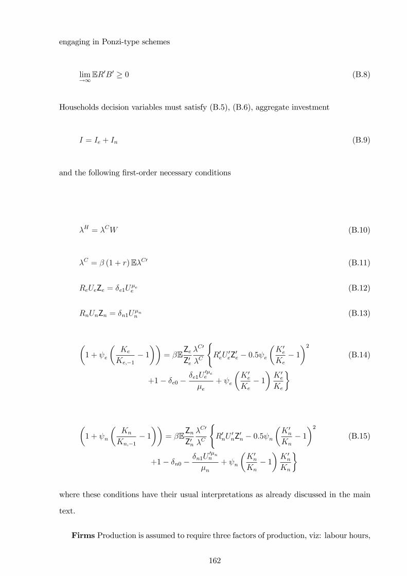
engaging in Ponzi-type schemes
lim!1
ER0B0 � 0 (B.8)
Households decision variables must satisfy (B.5), (B.6), aggregate investment
I = Ie + In (B.9)
and the following �rst-order necessary conditions
�H = �CW (B.10)
�C = � (1 + r)E�C0 (B.11)
ReUeZe = �e1U�ee (B.12)
RnUnZn = �n1U�nn (B.13)
�1 + e
�Ke
Ke;�1� 1��
= �EZeZ0e
�C0
�C
(R0eU
0eZ0e � 0:5 e
�K 0e
Ke
� 1�2
(B.14)
+1� �e0 ��e1U
0�ee
�e+ e
�K 0e
Ke
� 1�K 0e
Ke
�
�1 + n
�Kn
Kn;�1� 1��
= �EZnZ0n
�C0
�C
(R0nU
0nZ
0n � 0:5 n
�K 0n
Kn
� 1�2
(B.15)
+1� �n0 ��n1U
0�nn
�n+ n
�K 0n
Kn
� 1�K 0n
Kn
�
where these conditions have their usual interpretations as already discussed in the main
text.
Firms Production is assumed to require three factors of production, viz: labour hours,
162
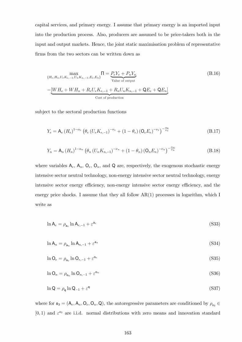
capital services, and primary energy. I assume that primary energy is an imported input
into the production process. Also, producers are assumed to be price-takers both in the
input and output markets. Hence, the joint static maximisation problem of representative
�rms from the two sectors can be written down as
maxfHe;Hn;UeKe;�1;UnKn;�1;Ee;Eng
� = PeYe + PnYn| {z }Value of output
(B.16)
�[WHe +WHn +ReUeKe;�1 +RnUnKn;�1 + QEe + QEn]| {z }Cost of production
subject to the sectoral production functions
Ye = Ae (He)1��e ��e (UeKe;�1)
��e + (1� �e) (OeEe)��e���e
�e (B.17)
Yn = An (Hn)1��n ��n (UnKn;�1)
��n + (1� �n) (OnEn)��n���n
�n (B.18)
where variables Ae, An, Oe, On, and Q are, respectively, the exogenous stochastic energy
intensive sector neutral technology, non-energy intensive sector neutral technology, energy
intensive sector energy e¢ ciency, non-energy intensive sector energy e¢ ciency, and the
energy price shocks. I assume that they all follow AR(1) processes in logarithm, which I
write as
lnAe = �ae lnAe;�1 + "ae (S33)
lnAn = �an lnAn;�1 + "an (S34)
lnOe = �oe lnOe;�1 + "oe (S35)
lnOn = �on lnOn;�1 + "on (S36)
lnQ = �q lnQ�1 + "q (S37)
where for s3 = (Ae;An;Oe;On;Q), the autoregressive parameters are conditioned by �s3 2
[0; 1) and "s3 are i.i.d. normal distributions with zero means and innovation standard
163
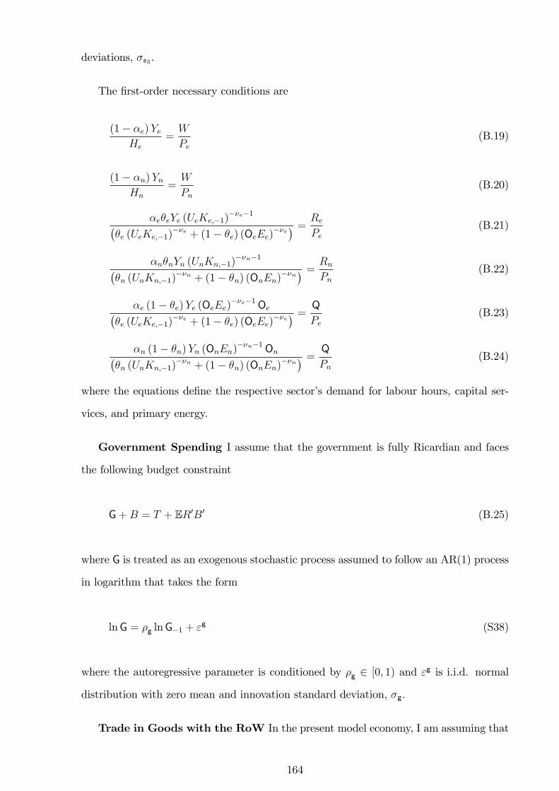
deviations, �s3.
The �rst-order necessary conditions are
(1� �e)YeHe
=W
Pe(B.19)
(1� �n)YnHn
=W
Pn(B.20)
�e�eYe (UeKe;�1)��e�1�
�e (UeKe;�1)��e + (1� �e) (OeEe)
��e� = Re
Pe(B.21)
�n�nYn (UnKn;�1)��n�1�
�n (UnKn;�1)��n + (1� �n) (OnEn)
��n� = Rn
Pn(B.22)
�e (1� �e)Ye (OeEe)��e�1Oe�
�e (UeKe;�1)��e + (1� �e) (OeEe)
��e� = Q
Pe(B.23)
�n (1� �n)Yn (OnEn)��n�1On�
�n (UnKn;�1)��n + (1� �n) (OnEn)
��n� = Q
Pn(B.24)
where the equations de�ne the respective sector�s demand for labour hours, capital ser-
vices, and primary energy.
Government Spending I assume that the government is fully Ricardian and faces
the following budget constraint
G+B = T + ER0B0 (B.25)
where G is treated as an exogenous stochastic process assumed to follow an AR(1) process
in logarithm that takes the form
lnG = �g lnG�1 + "g (S38)
where the autoregressive parameter is conditioned by �g 2 [0; 1) and "g is i.i.d. normal
distribution with zero mean and innovation standard deviation, �g.
Trade in Goods with the RoW In the present model economy, I am assuming that
164
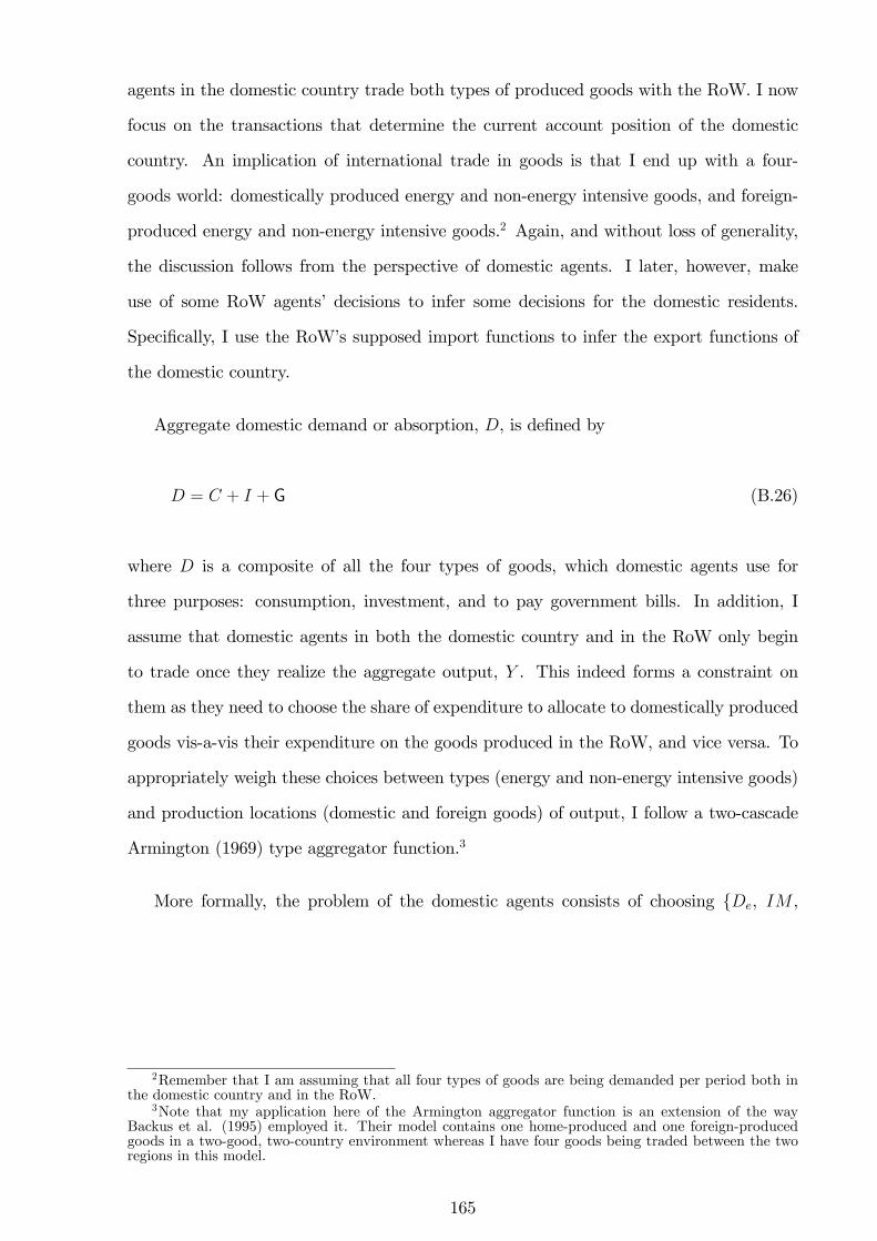
agents in the domestic country trade both types of produced goods with the RoW. I now
focus on the transactions that determine the current account position of the domestic
country. An implication of international trade in goods is that I end up with a four-
goods world: domestically produced energy and non-energy intensive goods, and foreign-
produced energy and non-energy intensive goods.2 Again, and without loss of generality,
the discussion follows from the perspective of domestic agents. I later, however, make
use of some RoW agents� decisions to infer some decisions for the domestic residents.
Speci�cally, I use the RoW�s supposed import functions to infer the export functions of
the domestic country.
Aggregate domestic demand or absorption, D, is de�ned by
D = C + I + G (B.26)
where D is a composite of all the four types of goods, which domestic agents use for
three purposes: consumption, investment, and to pay government bills. In addition, I
assume that domestic agents in both the domestic country and in the RoW only begin
to trade once they realize the aggregate output, Y . This indeed forms a constraint on
them as they need to choose the share of expenditure to allocate to domestically produced
goods vis-a-vis their expenditure on the goods produced in the RoW, and vice versa. To
appropriately weigh these choices between types (energy and non-energy intensive goods)
and production locations (domestic and foreign goods) of output, I follow a two-cascade
Armington (1969) type aggregator function.3
More formally, the problem of the domestic agents consists of choosing fDe, IM ,
2Remember that I am assuming that all four types of goods are being demanded per period both inthe domestic country and in the RoW.
3Note that my application here of the Armington aggregator function is an extension of the wayBackus et al. (1995) employed it. Their model contains one home-produced and one foreign-producedgoods in a two-good, two-country environment whereas I have four goods being traded between the tworegions in this model.
165
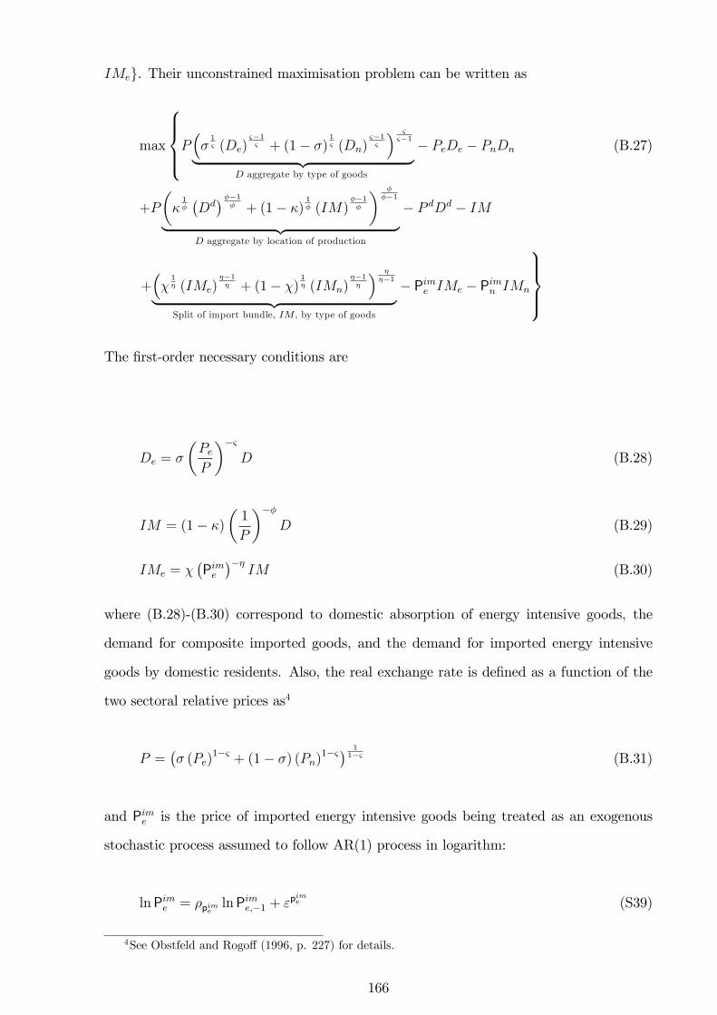
IMeg. Their unconstrained maximisation problem can be written as
max
8>><>>:P��1& (De)
&�1& + (1� �)
1& (Dn)
&�1&
� &&�1| {z }
D aggregate by type of goods
� PeDe � PnDn (B.27)
+P
��1��Dd���1
� + (1� �)1� (IM)
��1�
� ���1
| {z }D aggregate by location of production
� P dDd � IM
+��1� (IMe)
��1� + (1� �)
1� (IMn)
��1�
� ���1| {z }
Split of import bundle, IM , by type of goods
� Pime IMe � Pimn IMn
9>>=>>;The �rst-order necessary conditions are
De = �
�PeP
��&D (B.28)
IM = (1� �)
�1
P
���D (B.29)
IMe = ��Pime���
IM (B.30)
where (B.28)-(B.30) correspond to domestic absorption of energy intensive goods, the
demand for composite imported goods, and the demand for imported energy intensive
goods by domestic residents. Also, the real exchange rate is de�ned as a function of the
two sectoral relative prices as4
P =�� (Pe)
1�& + (1� �) (Pn)1�&� 1
1�& (B.31)
and Pime is the price of imported energy intensive goods being treated as an exogenous
stochastic process assumed to follow AR(1) process in logarithm:
lnPime = �pime lnPime;�1 + "p
ime (S39)
4See Obstfeld and Rogo¤ (1996, p. 227) for details.
166
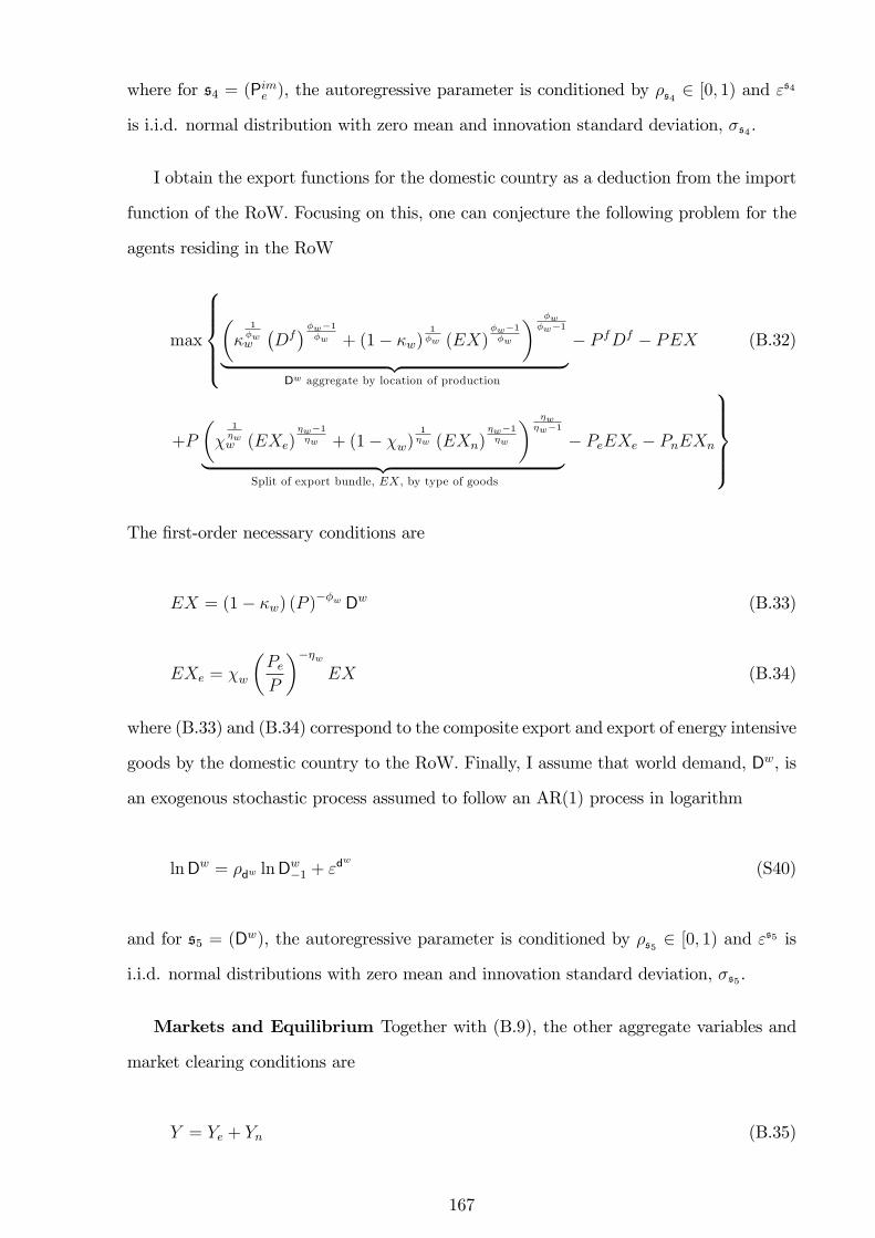
where for s4 = (Pime ), the autoregressive parameter is conditioned by �s4 2 [0; 1) and "s4
is i.i.d. normal distribution with zero mean and innovation standard deviation, �s4.
I obtain the export functions for the domestic country as a deduction from the import
function of the RoW. Focusing on this, one can conjecture the following problem for the
agents residing in the RoW
max
8>>><>>>:��
1�ww
�Df��w�1
�w + (1� �w)1�w (EX)
�w�1�w
� �w�w�1
| {z }Dw aggregate by location of production
� P fDf � PEX (B.32)
+P
��
1�ww (EXe)
�w�1�w + (1� �w)
1�w (EXn)
�w�1�w
� �w�w�1
| {z }Split of export bundle, EX, by type of goods
� PeEXe � PnEXn
9>>>=>>>;The �rst-order necessary conditions are
EX = (1� �w) (P )��w Dw (B.33)
EXe = �w
�PeP
���wEX (B.34)
where (B.33) and (B.34) correspond to the composite export and export of energy intensive
goods by the domestic country to the RoW. Finally, I assume that world demand, Dw, is
an exogenous stochastic process assumed to follow an AR(1) process in logarithm
lnDw = �dw lnDw�1 + "d
w
(S40)
and for s5 = (Dw), the autoregressive parameter is conditioned by �s5 2 [0; 1) and "s5 is
i.i.d. normal distributions with zero mean and innovation standard deviation, �s5.
Markets and Equilibrium Together with (B.9), the other aggregate variables and
market clearing conditions are
Y = Ye + Yn (B.35)
167
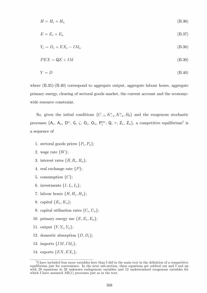
H = He +Hn (B.36)
E = Ee + En (B.37)
Ye = De + EXe � IMn (B.38)
PEX = QE + IM (B.39)
Y = D (B.40)
where (B.35)-(B.40) correspond to aggregate output, aggregate labour hours, aggregate
primary energy, clearing of sectoral goods market, the current account and the economy-
wide resource constraint.
So, given the initial conditions fC�1; Ke�1; K
n�1; B0g and the exogenous stochastic
processes fAe, An, Dw, G, �, Oe, On, Pime , Q, � , Ze, Zng, a competitive equilibrium5 is
a sequence of
1. sectoral goods prices fPe; Png;
2. wage rate fWg;
3. interest rates fR;Re; Rng;
4. real exchange rate fPg;
5. consumption fCg;
6. investments fI; Ie; Ing;
7. labour hours fH;He; Hng;
8. capital fKe; Kng;
9. capital utilisation rates fUe; Ung;
10. primary energy use fE;Ee; Eng;
11. output fY; Ye; Yng;
12. domestic absorption fD;Deg;
13. imports fIM; IMeg;
14. exports fEX;EXeg;
5I have included four more variables here than I did in the main text in the de�nition of a competitiveequilibrium just for convenience. In the next sub-section, these equations get subbed out and I end upwith 28 equations in 28 unknown endogenous variables and 12 undetermined exogenous variables forwhich I have assumed AR(1) processes just as in the text.
168

15. marginal utility of consumption f�Cg;
16. marginal disutility of labour hours f�Hg;
such that markets clear for:
1. labour hours;
2. capital;
3. primary energy use;
4. sectoral output; and
5. total output.
Log-linearising Equilibrium Conditions The last footnote suggests that I should
have 40 linearized equations in this sub-section solving for 28 endogenous and 12 exogenous
stochastic processes. I labelled these equations as S1, S2, ..., S28 for the endogenous
variables (S29-S40 for the exogenous variables are already de�ned in the preceding sub-
sections) implying that they are used in simulation and to distinguish them from other
model equations that �explain�them.
On the side of the households, combining (B.3), (B.4), and (B.10) yields the supply of
labour hours as
�H! =W
(C � �C�1)� (B.41)
which when log-linearized becomes
bH =1
!
�cW � b� � �
1� �
� bC � � bC�1�� (S1)
Consumption Euler equation is
�
(C � �C�1)� = �RE
� t+1(Ct+1 � �Ct)
� (B.42)
169
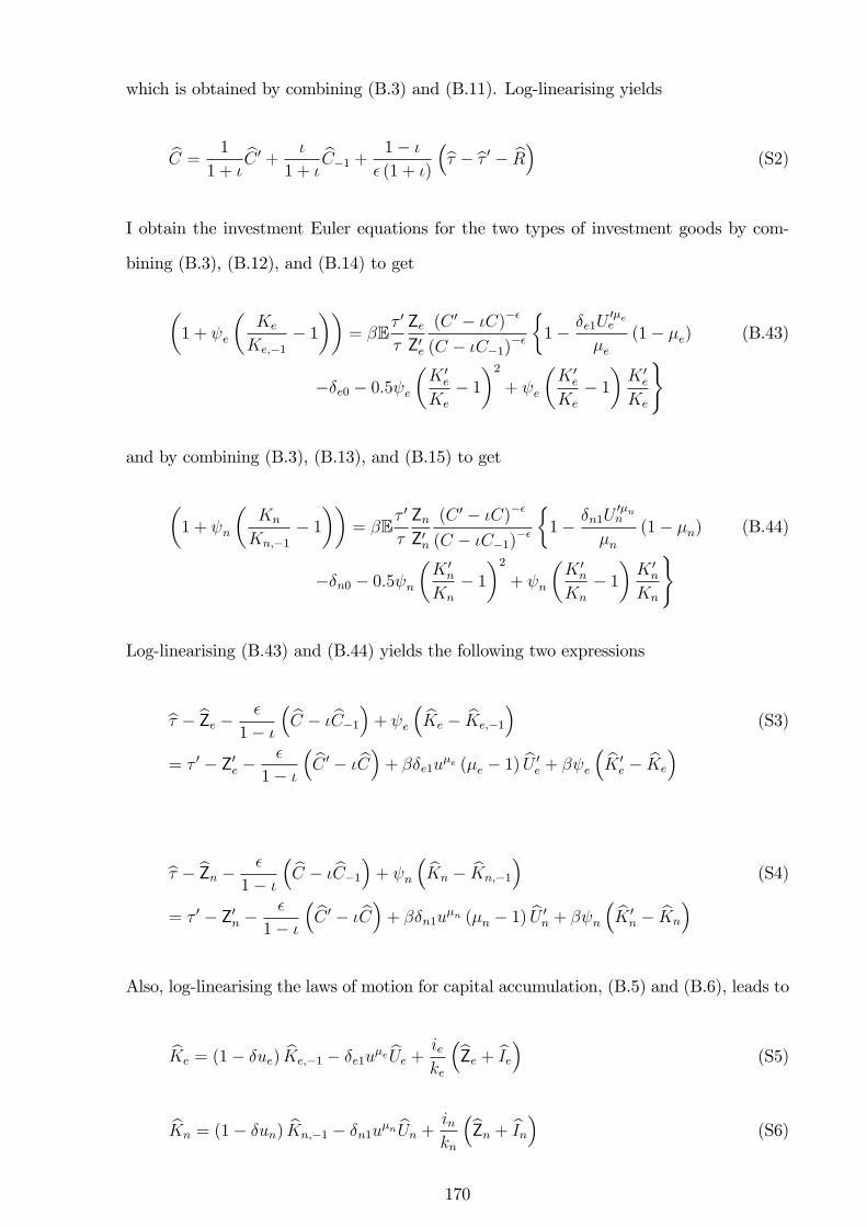
which is obtained by combining (B.3) and (B.11). Log-linearising yields
bC = 1
1 + �bC 0 + �
1 + �bC�1 + 1� �
� (1 + �)
�b� � b� 0 � bR� (S2)
I obtain the investment Euler equations for the two types of investment goods by com-
bining (B.3), (B.12), and (B.14) to get
�1 + e
�Ke
Ke;�1� 1��
= �E� 0
�
ZeZ0e
(C 0 � �C)��
(C � �C�1)��
�1� �e1U
0�ee
�e(1� �e) (B.43)
��e0 � 0:5 e�K 0e
Ke
� 1�2+ e
�K 0e
Ke
� 1�K 0e
Ke
)
and by combining (B.3), (B.13), and (B.15) to get
�1 + n
�Kn
Kn;�1� 1��
= �E� 0
�
ZnZ0n
(C 0 � �C)��
(C � �C�1)��
�1� �n1U
0�nn
�n(1� �n) (B.44)
��n0 � 0:5 n�K 0n
Kn
� 1�2+ n
�K 0n
Kn
� 1�K 0n
Kn
)
Log-linearising (B.43) and (B.44) yields the following two expressions
b� � bZe � �
1� �
� bC � � bC�1�+ e
� bKe � bKe;�1
�(S3)
= � 0 � Z0e ��
1� �
� bC 0 � � bC�+ ��e1u�e (�e � 1) bU 0e + � e
� bK 0e � bKe
�
b� � bZn � �
1� �
� bC � � bC�1�+ n
� bKn � bKn;�1
�(S4)
= � 0 � Z0n ��
1� �
� bC 0 � � bC�+ ��n1u�n (�n � 1) bU 0n + � n
� bK 0n � bKn
�
Also, log-linearising the laws of motion for capital accumulation, (B.5) and (B.6), leads to
bKe = (1� �ue) bKe;�1 � �e1u�e bUe + ie
ke
�bZe + bIe� (S5)
bKn = (1� �un) bKn;�1 � �n1u�n bUn + in
kn
�bZn + bIn� (S6)
170
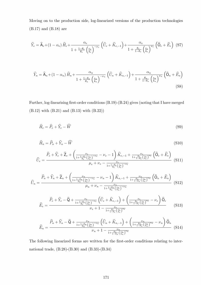
Moving on to the production side, log-linearized versions of the production technologies
(B.17) and (B.18) are
bYe = bAe+(1� �e) bHe+�e
1 + 1��e�e
�eeke
���e �bUe + bKe;�1
�+
�e
1 + �e1��e
�eeke
��e �bOe + bEe� (S7)
bYn = bAn+(1� �n) bHn+�n
1 + 1��n�n
�enkn
���n �bUn + bKn;�1
�+
�n
1 + �n1��n
�enkn
��n �bOn + bEn�(S8)
Further, log-linearising �rst-order conditions (B.19)-(B.24) gives (noting that I have merged
(B.12) with (B.21) and (B.13) with (B.22))
bHe = bPe + bYe �cW (S9)
bHn = bPn + bYn �cW (S10)
bUe = bPe + bYe + bZe + � �e
1+ 1��e�e( eeke )
��e � �e � 1� bKe;�1 +
�e1+ �e
1��e (eeke)�e
�bOe + bEe��e + �e � �e
1+ 1��e�e( eeke )
��e
(S11)
bUn = bPn + bYn + bZn + � �n
1+ 1��n�n( enkn )
��n � �n � 1� bKn;�1 +
�n1+ �n
1��n (enkn)�n
�bOn + bEn��n + �n � �n
1+ 1��n�n( enkn )
��n
(S12)
bEe = bPe + bYe � bQ+ �e
1+ 1��e�e( eeke )
��e
�bUe + bKe;�1
�+
��e
1+ �e1��e (
eeke)�e � �e
� bOe�e + 1� �e
1+ �e1��e (
eeke)�e
(S13)
bEn = bPn + bYn � bQ+ �n
1+ 1��n�n( enkn )
��n
�bUn + bKn;�1
�+
��n
1+ �n1��n (
enkn)�n � �n
� bOn�n + 1� �n
1+ �n1��n (
enkn)�n
(S14)
The following linearized forms are written for the �rst-order conditions relating to inter-
national trade, (B.28)-(B.30) and (B.33)-(B.34)
171
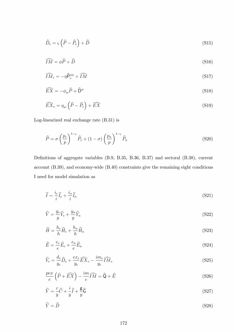
bDe = &� bP � bPe�+ bD (S15)
dIM = � bP + bD (S16)
dIM e = ��bPime +dIM (S17)
dEX = ��w bP + bDw (S18)
dEXe = �w
� bP � bPe�+dEX (S19)
Log-linearized real exchange rate (B.31) is
bP = �
�pep
�1�& bPe + (1� �)
�pnp
�1�& bPn (S20)
De�nitions of aggregate variables (B.9, B.35, B.36, B.37) and sectoral (B.38), current
account (B.39), and economy-wide (B.40) constraints give the remaining eight conditions
I need for model simulation as
bI = ieibIe + in
ibIn (S21)
bY = yeybYe + yn
ybYn (S22)
bH =hehbHe +
hnhbHn (S23)
bE = eeebEe + en
ebEn (S24)
bYe = deyebDe +
exeyedEXe �
ime
yedIM e (S25)
pex
e
� bP +dEX�� im
edIM = bQ+ bE (S26)
bY = c
ybC + i
ybI + g
ybG (S27)
bY = bD (S28)
172
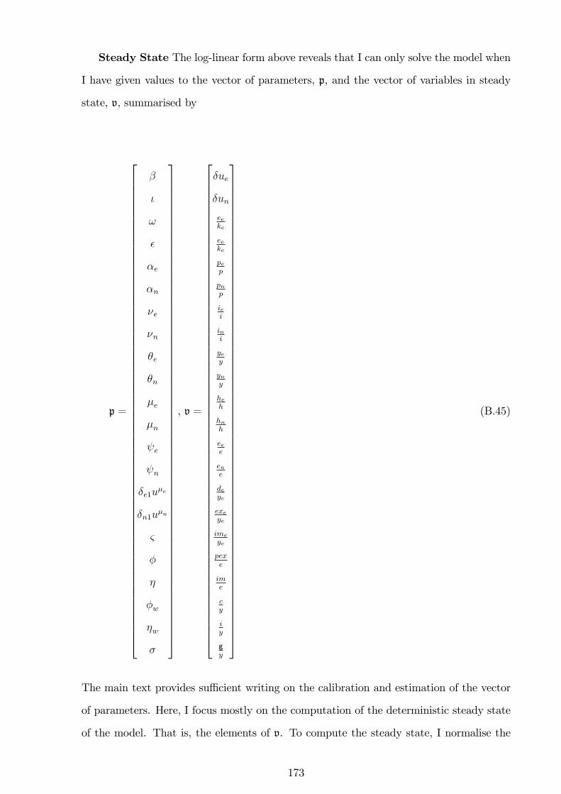
Steady State The log-linear form above reveals that I can only solve the model when
I have given values to the vector of parameters, p, and the vector of variables in steady
state, v, summarised by
p =
266666666666666666666666666666666666666666666666666666666666666666664
�
�
!
�
�e
�n
�e
�n
�e
�n
�e
�n
e
n
�e1u�e
�n1u�n
&
�
�
�w
�w
�
377777777777777777777777777777777777777777777777777777777777777777775
, v =
266666666666666666666666666666666666666666666666666666666666666666664
�ue
�un
eeke
eeke
pep
pnp
iei
ini
yey
yny
heh
hnh
eee
ene
deye
exeye
imeye
pexe
ime
cy
iy
gy
377777777777777777777777777777777777777777777777777777777777777777775
(B.45)
The main text provides su¢ cient writing on the calibration and estimation of the vector
of parameters. Here, I focus mostly on the computation of the deterministic steady state
of the model. That is, the elements of v. To compute the steady state, I normalise the
173
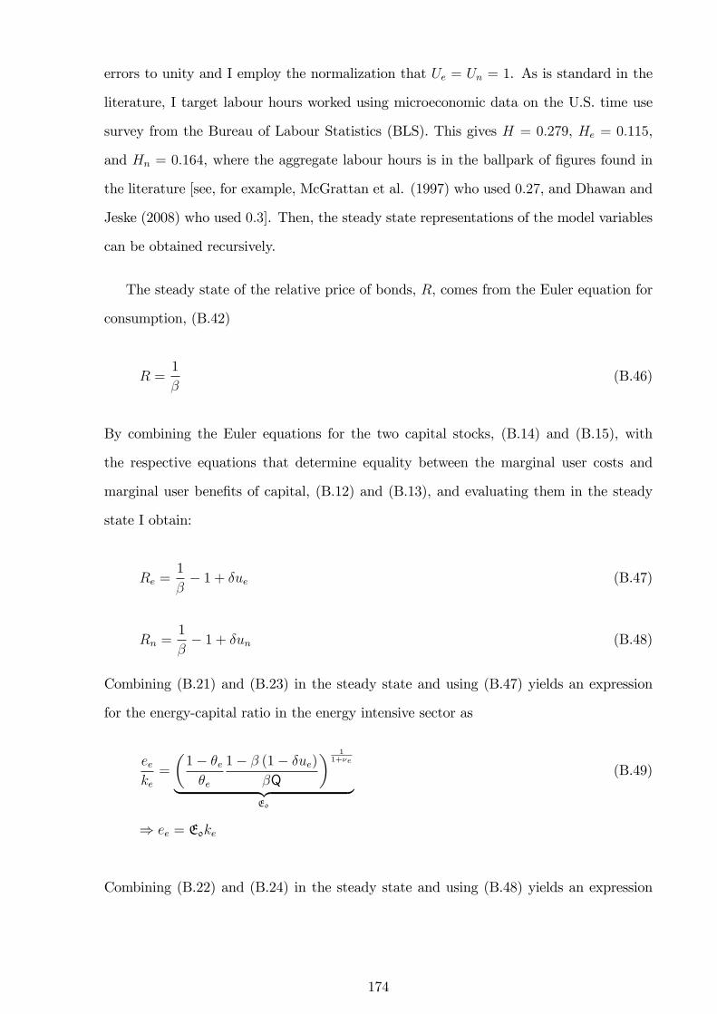
errors to unity and I employ the normalization that Ue = Un = 1. As is standard in the
literature, I target labour hours worked using microeconomic data on the U.S. time use
survey from the Bureau of Labour Statistics (BLS). This gives H = 0:279, He = 0:115,
and Hn = 0:164, where the aggregate labour hours is in the ballpark of �gures found in
the literature [see, for example, McGrattan et al. (1997) who used 0:27, and Dhawan and
Jeske (2008) who used 0:3]. Then, the steady state representations of the model variables
can be obtained recursively.
The steady state of the relative price of bonds, R, comes from the Euler equation for
consumption, (B.42)
R =1
�(B.46)
By combining the Euler equations for the two capital stocks, (B.14) and (B.15), with
the respective equations that determine equality between the marginal user costs and
marginal user bene�ts of capital, (B.12) and (B.13), and evaluating them in the steady
state I obtain:
Re =1
�� 1 + �ue (B.47)
Rn =1
�� 1 + �un (B.48)
Combining (B.21) and (B.23) in the steady state and using (B.47) yields an expression
for the energy-capital ratio in the energy intensive sector as
eeke=
�1� �e�e
1� � (1� �ue)
�Q
� 11+�e
| {z }E0
(B.49)
) ee = E0ke
Combining (B.22) and (B.24) in the steady state and using (B.48) yields an expression
174
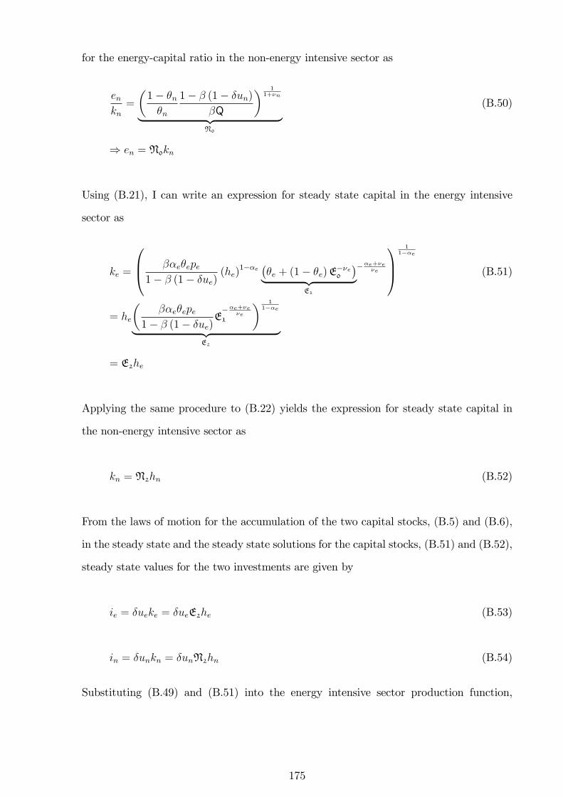
for the energy-capital ratio in the non-energy intensive sector as
enkn=
�1� �n�n
1� � (1� �un)
�Q
� 11+�n
| {z }N0
(B.50)
) en = N0kn
Using (B.21), I can write an expression for steady state capital in the energy intensive
sector as
ke =
0B@ ��e�epe1� � (1� �ue)
(he)1��e ��e + (1� �e)E
��e0
�| {z }E1
��e+�e�e
1CA1
1��e
(B.51)
= he
���e�epe
1� � (1� �ue)E��e+�e
�e1
� 11��e
| {z }E2
= E2he
Applying the same procedure to (B.22) yields the expression for steady state capital in
the non-energy intensive sector as
kn = N2hn (B.52)
From the laws of motion for the accumulation of the two capital stocks, (B.5) and (B.6),
in the steady state and the steady state solutions for the capital stocks, (B.51) and (B.52),
steady state values for the two investments are given by
ie = �ueke = �ueE2he (B.53)
in = �unkn = �unN2hn (B.54)
Substituting (B.49) and (B.51) into the energy intensive sector production function,
175
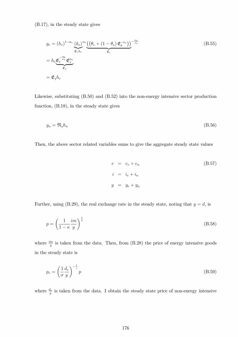
(B.17), in the steady state gives
ye = (he)1��e (ke)|{z}
E2he
�e���e + (1� �e)E
��e0
��| {z }E1
��e�e (B.55)
= heE��e�e
1 E�e2| {z }E3
= E3he
Likewise, substituting (B.50) and (B.52) into the non-energy intensive sector production
function, (B.18), in the steady state gives
yn = N3hn (B.56)
Then, the above sector related variables sums to give the aggregate steady state values
e = ee + en (B.57)
i = ie + in
y = ye + yn
Further, using (B.29), the real exchange rate in the steady state, noting that y = d, is
p =
�1
1� �
im
y
� 1�
(B.58)
where imyis taken from the data. Then, from (B.28) the price of energy intensive goods
in the steady state is
pe =
�1
�
dey
�� 1&
p (B.59)
where deyis taken from the data. I obtain the steady state price of non-energy intensive
176
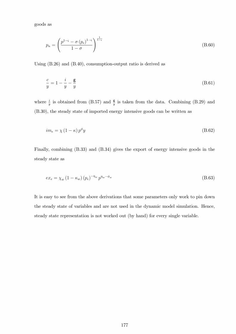
goods as
pn =
p1�& � � (pe)
1�&
1� �
! 11�&
(B.60)
Using (B.26) and (B.40), consumption-output ratio is derived as
c
y= 1� i
y� gy
(B.61)
where iyis obtained from (B.57) and g
yis taken from the data. Combining (B.29) and
(B.30), the steady state of imported energy intensive goods can be written as
ime = � (1� �) p�y (B.62)
Finally, combining (B.33) and (B.34) gives the export of energy intensive goods in the
steady state as
exe = �w (1� �w) (pe)��w p�w��w (B.63)
It is easy to see from the above derivations that some parameters only work to pin down
the steady state of variables and are not used in the dynamic model simulation. Hence,
steady state representation is not worked out (by hand) for every single variable.
177
Appendix C
Supplementary Notes: Chapter 4
C.1 Data Construction
All series are de�ned as in Chapter 2 except domestic absorption, Dt. Also, I have six
extra variables relating to the rest of the world to be de�ned.
Domestic absorption
Model variable: Dt.
Data: dt = Ct + It +Gt (Taken from Table 1.1.5. Gross Domestic Product).
Government spending
Model variable: Gt.
Data: This is government consumption expenditures and gross investment (Taken
from Table 1.1.5. Gross Domestic Product).
Real price of energy
Model variable: Qt.
Data: Qt is the nominal dollar price per barrel of crude oil proxied by the crude oil
178
domestic �rst purchase price (Taken from Table 9.1: Crude Oil Price Summary) divided
by the consumer price index (CPI).
Foreign bonds
Model variable: Ft.
Data: This is taken to be the ratio of nominal net foreign assets (NNFA) to nominal
GDP (NGDP), Ft = NNFANGDP
, where NNFA = Total Assets� Total Liabilities.
Foreign interest rate
Model variable: rft .
Data: Calculated as the weighted average of the interest rate for the G7 countries
taken from the International Financial Statistics (IFS).
World demand
Model variable: Dwt .
Data: This is measured as world trade less the U.S. imports taken from the Interna-
tional Financial Statistics (IFS).
Price of imported energy intensive goods
Model: Pime;t .
Data: This is the price of the U.S. imported manufactures from the rest of the world
taken from the International Financial Statistics (IFS).
C.2 Technical Appendix
In this section, I summarise the derivations of the equilibrium conditions in Chapter 3.
The model is the same as in the previous chapter, but with the addition of capital account.
Essentially, this introduces an additional �rst-order condition on the household�s side:
179
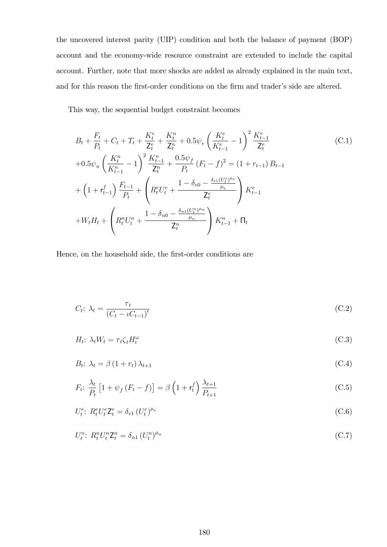
the uncovered interest parity (UIP) condition and both the balance of payment (BOP)
account and the economy-wide resource constraint are extended to include the capital
account. Further, note that more shocks are added as already explained in the main text,
and for this reason the �rst-order conditions on the �rm and trader�s side are altered.
This way, the sequential budget constraint becomes
Bt +FtPt+ Ct + Tt +
Ket
Zet+Knt
Znt+ 0:5 e
�Ket
Ket�1
� 1�2 Ke
t�1Zet
(C.1)
+0:5 n
�Knt
Knt�1
� 1�2 Kn
t�1Znt
+0:5 fPt
(Ft � f)2 = (1 + rt�1)Bt�1
+�1 + rft�1
� Ft�1Pt
+
0@RetU
et +
1� �e0 � �e1(Uet )�e
�e
Zet
1AKet�1
+WtHt +
0@Rnt U
nt +
1� �n0 � �n1(Unt )�n
�n
Znt
1AKnt�1 + �t
Hence, on the household side, the �rst-order conditions are
Ct: �t =� t
(Ct � �Ct�1)� (C.2)
Ht: �tWt = � t�tH!t (C.3)
Bt: �t = � (1 + rt)�t+1 (C.4)
Ft:�tPt
�1 + f (Ft � f)
�= �
�1 + rft
� �t+1Pt+1
(C.5)
U et : R
etU
et Z
et = �e1 (U
et )�e (C.6)
Unt : R
nt U
nt Z
nt = �n1 (U
nt )
�n (C.7)
180
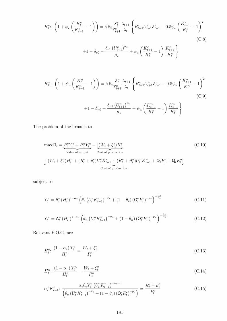
Ket :�1 + e
�Ket
Ket�1
� 1��
= �EtZetZet+1
�t+1�t
(Ret+1U
et+1Z
et+1 � 0:5 e
�Ket+1
Ket
� 1�2(C.8)
+1� �e0 ��e1�U et+1
��e�e
+ e
�Ket+1
Ket
� 1�Ket+1
Ket
)
Knt :�1 + n
�Knt
Knt�1
� 1��
= �EtZntZnt+1
�t+1�t
(Rnt+1U
nt+1Z
nt+1 � 0:5 n
�Knt+1
Knt
� 1�2(C.9)
+1� �n0 ��n1�Unt+1
��n�n
+ n
�Knt+1
Knt
� 1�Knt+1
Knt
)
The problem of the �rms is to
max�t = P et Y
et + P n
t Ynt| {z }
Value of output
� [(Wt + �et )Het| {z }
Cost of production
(C.10)
+(Wt + �nt )Hnt + (R
et + #et)U
etK
et�1 + (R
nt + #nt )U
nt K
nt�1 + QtE
et + QtE
nt ]| {z }
Cost of production
subject to
Y et = A
et (H
et )1��e
��e�U etK
et�1���e
+ (1� �e) (OetE
et )��e���e
�e (C.11)
Y nt = A
nt (H
nt )1��n
��n�Unt K
nt�1���n
+ (1� �n) (OntE
nt )��n���n
�n (C.12)
Relevant F.O.Cs are
Het :(1� �e)Y
et
Het
=Wt + �etP et
(C.13)
Hnt :(1� �n)Y
nt
Hnt
=Wt + �ntP nt
(C.14)
U etK
et�1:
�e�eYet
�U etK
et�1���e�1�
�e�U etK
et�1���e
+ (1� �e) (OetEet )��e� = Re
t + #etP et
(C.15)
181
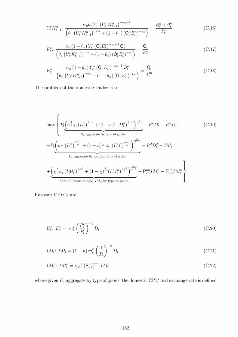
U etK
nt�1:
�n�nYnt
�Unt K
nt�1���n�1�
�n�Unt K
nt�1���n
+ (1� �n) (OntEnt )��n� = Rn
t + #ntP nt
(C.16)
Eet :
�e (1� �e)Yet (O
etE
et )��e�1Oet�
�e�U etK
et�1���e
+ (1� �e) (OetEet )��e� = Qt
P et
(C.17)
Ent :
�n (1� �n)Ynt (O
ntE
nt )��n�1Ont�
�n�Unt K
nt�1���n
+ (1� �n) (OntEnt )��n� = Qt
P nt
(C.18)
The problem of the domestic trader is to
max
8>><>>:Pt��1& t (D
et )
&�1& + (1� �)
1& (Dn
t )&�1&
� &&�1| {z }
Dt aggregate by type of goods
� P et D
et � P n
t Dnt (C.19)
+Pt
��1��Ddt
���1� + (1� �)
1� $t (IMt)
��1�
� ���1
| {z }Dt aggregate by location of production
� P dt D
dt � IMt
+��1�'t (IM
et )
��1� + (1� �)
1� (IMn
t )��1�
� ���1| {z }
Split of import bundle, IMt, by type of goods
� Pime;tIM et � Pimn;tIMn
t
9>>=>>;Relevant F.O.Cs are
Det : D
et = � &t
�P et
Pt
��&Dt (C.20)
IMt: IMt = (1� �)$�t
�1
Pt
���Dt (C.21)
IM et : IM
et = �'�t
�Pime;t���
IMt (C.22)
where givenDt aggregate by type of goods, the domestic CPI/ real exchange rate is de�ned
182
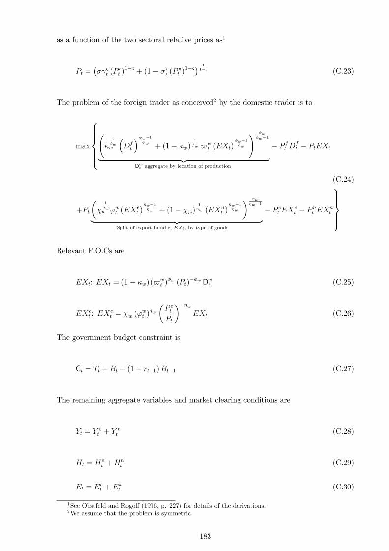
as a function of the two sectoral relative prices as1
Pt =�� &t (P
et )1�& + (1� �) (P n
t )1�&� 1
1�& (C.23)
The problem of the foreign trader as conceived2 by the domestic trader is to
max
8>>>><>>>>: �
1�ww
�Dft
��w�1�w + (1� �w)
1�w $w
t (EXt)�w�1�w
! �w�w�1
| {z }Dwt aggregate by location of production
� P ft D
ft � PtEXt
(C.24)
+Pt
��
1�ww 'wt (EX
et )
�w�1�w + (1� �w)
1�w (EXn
t )�w�1�w
� �w�w�1
| {z }Split of export bundle, EXt, by type of goods
� P et EX
et � P n
t EXnt
9>>>=>>>;Relevant F.O.Cs are
EXt: EXt = (1� �w) ($wt )
�w (Pt)��w Dwt (C.25)
EXet : EX
et = �w ('
wt )
�w
�P et
Pt
���wEXt (C.26)
The government budget constraint is
Gt = Tt +Bt � (1 + rt�1)Bt�1 (C.27)
The remaining aggregate variables and market clearing conditions are
Yt = Y et + Y n
t (C.28)
Ht = Het +Hn
t (C.29)
Et = Eet + En
t (C.30)
1See Obstfeld and Rogo¤ (1996, p. 227) for details of the derivations.2We assume that the problem is symmetric.
183
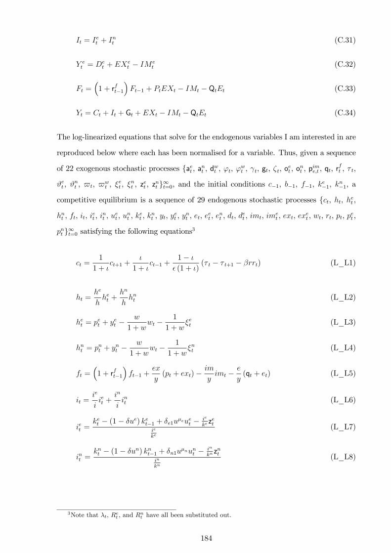
It = Iet + Int (C.31)
Y et = De
t + EXet � IM e
t (C.32)
Ft =�1 + rft�1
�Ft�1 + PtEXt � IMt � QtEt (C.33)
Yt = Ct + It + Gt + EXt � IMt � QtEt (C.34)
The log-linearized equations that solve for the endogenous variables I am interested in are
reproduced below where each has been normalised for a variable. Thus, given a sequence
of 22 exogenous stochastic processes faet , ant , dwt , 't, 'wt , t, gt, �t, oet , ont , pime;t , qt, rft , � t,
#et , #nt , $t, $w
t , �et , �
nt , z
et , z
nt g1t=0, and the initial conditions c�1, b�1, f�1, ke�1, kn�1, a
competitive equilibrium is a sequence of 29 endogenous stochastic processes fct, ht, het ,
hnt , ft, it, iet , i
nt , u
et , u
nt , k
et , k
nt , yt, y
et , y
nt , et, e
et , e
nt , dt, d
et , imt, ime
t , ext, exet , wt, rt, pt, p
et ,
pnt g1t=0 satisfying the following equations3
ct =1
1 + �ct+1 +
�
1 + �ct�1 +
1� �
� (1 + �)(� t � � t+1 � �rrt) (L_L1)
ht =he
hhet +
hn
hhnt (L_L2)
het = pet + yet �w
1 + wwt �
1
1 + w�et (L_L3)
hnt = pnt + ynt �w
1 + wwt �
1
1 + w�nt (L_L4)
ft =�1 + rft�1
�ft�1 +
ex
y(pt + ext)�
im
yimt �
e
y(qt + et) (L_L5)
it =ie
iiet +
in
iint (L_L6)
iet =ket � (1� �ue) ket�1 + �e1u
�euet � ie
kezet
ie
ke
(L_L7)
int =knt � (1� �un) knt�1 + �n1u
�nunt � in
knznt
in
kn
(L_L8)
3Note that �t, Ret , and Rnt have all been substituted out.
184
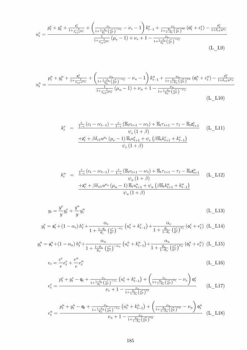
uet =
pet + yet +zet
1+ 1�e1u
�e
+
��e
1+ 1��e�e( eeke )
��e � �e � 1�ket�1 +
�e1+ �e
1��e (ee
ke )�e (oet + eet)�
#et1+�e1u�e
11+ 1
�e1u�e
(�e � 1) + �e + 1� �e
1+ 1��e�e( eeke )
��e
(L_L9)
unt =
pnt + ynt +znt
1+ 1�n1u
�n
+
��n
1+ 1��n�n( enkn )
��n � �n � 1�knt�1 +
�n1+ �n
1��n (en
kn )�n (ont + ent )�
#nt1+�n1u�n
11+ 1
�n1u�n
(�n � 1) + �n + 1� �n
1+ 1��n�n( enkn )
��n
(L_L10)
ket =�1�� (ct � �ct�1)� �
1�� (Etct+1 � �ct) + Et� t+1 � � t � Etzet+1 e (1 + �)
(L_L11)
+zet + ��e1u�e (�e � 1)Etuet+1 + e
��Etket+1 + ket�1
� e (1 + �)
knt =�1�� (ct � �ct�1)� �
1�� (Etct+1 � �ct) + Et� t+1 � � t � Etznt+1 n (1 + �)
(L_L12)
+znt + ��n1u�n (�n � 1)Etunt+1 + n
��Etknt+1 + knt�1
� n (1 + �)
yt =ye
yyet +
yn
yynt (L_L13)
yet = aet+(1� �e)h
et+
�e
1 + 1��e�e
�ee
ke
���e �uet + ket�1�+
�e
1 + �e1��e
�ee
ke
��e (oet + eet) (L_L14)
ynt = ant +(1� �n)h
nt +
�n
1 + 1��n�n
�en
kn
���n �unt + knt�1�+
�n
1 + �n1��n
�en
kn
��n (ont + ent ) (L_L15)
et =ee
eeet +
en
eent (L_L16)
eet =
pet + yet � qt + �e
1+ 1��e�e( eeke )
��e
�uet + ket�1
�+
��e
1+ �e1��e (
ee
ke )�e � �e
�oet
�e + 1� �e1+ �e
1��e (ee
ke )�e
(L_L17)
ent =
pnt + ynt � qt + �n
1+ 1��n�n( enkn )
��n
�unt + knt�1
�+
��n
1+ �n1��n (
en
kn )�n � �n
�ont
�n + 1� �n1+ �n
1��n (en
kn )�n
(L_L18)
185
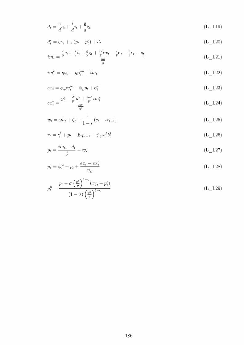
dt =c
dct +
i
dit +
g
dgt (L_L19)
det = & t + & (pt � pet ) + dt (L_L20)
imt =
cyct +
iyit +
gygt +
exyext � e
yqt � e
yet � yt
imy
(L_L21)
imet = �'t � �pime;t + imt (L_L22)
ext = �w$wt � �wpt + d
wt (L_L23)
exet =yet � de
yedet +
ime
yeime
t
exe
ye
(L_L24)
wt = !ht + �t +�
1� �(ct � �ct�1) (L_L25)
rt = rft + pt � Etpt+1 � bf b
fbft (L_L26)
pt =imt � dt
��$t (L_L27)
pet = 'wt + pt +ext � exet
�w(L_L28)
pnt =pt � �
�pe
p
�1�&(& t + pet)
(1� �)�pn
p
�1�& (L_L29)
186
Bibliography
[1] Aastveit, K. A., H. C. Bjornland, and L. A. Thorsrud (2011). The world is notenough! Small open economies and regional dependence. Working Paper 2011/16,Norges Bank.
[2] Adjemian, S., Bastani, H., Juillard, M., Mihoubi, F., Perendia, G., Ratto, M., andVillemot, S. (2011). Dynare: Reference manual, version 4. Dynare Working Papers1, CEPREMAP.
[3] Aliaga-Díaz, R., & Olivero, M. P. (2010). Macroeconomic implications of �deephabits�in banking. Journal of Money, Credit and Banking, 42(8), 1495-1521.
[4] An, S., & Schorfheide, F. (2007). Bayesian analysis of DSGE models. Econometricreviews, 26(2-4), 113-172.
[5] Armington, P. S. (1969). A Theory of Demand for Products Distinguished by Placeof Production (Une théorie de la demande de produits di¤érenciés d�après leur orig-ine)(Una teoría de la demanda de productos distinguiéndolos según el lugar de pro-ducción). Sta¤ Papers-International Monetary Fund, 16, 159-178.
[6] Arrow, K. J., & Chang, S. (1978). Optimal Pricing. Use and Explo) ration of Uncer-tain Natural Resource Stocks, Department of Economics Technical Report, HarvardUniversity.
[7] Asafu-Adjaye, J. (2000). The relationship between energy consumption, energyprices and economic growth: time series evidence from Asian developing countries.Energy economics, 22(6), 615-625.
[8] Aizenman, J. (1983). Modeling deviations from purchasing power parity (PPP) (No.w1066). National Bureau of Economic Research.
[9] Backus, D., Kehoe, P. J., & Kydland, F. E. (1993). International business cycles:theory and evidence (No. w4493). National Bureau of Economic Research.
[10] Barsky, R. B., & Kilian, L. (2002). Do we really know that oil caused the greatstag�ation? A monetary alternative. In NBER Macroeconomics Annual 2001, Vol-ume 16 (pp. 137-198). MIT Press.
187
[11] Basu, S., and Kimball, M. S. (1997). Cyclical productivity with unobserved inputvariation (No. w5915). National Bureau of Economic Research.
[12] Baxter, M., & Crucini, M. J. (1993). Explaining saving-investment correlations. TheAmerican Economic Review, 83(3), 416-436.
[13] Baxter, M. and Crucini, M. J. (1995). Business Cycles and the Asset Structure ofForeign Trade. International Economic Review, 36(4), 821-854.
[14] Baxter, M., & Farr, D. D. (2005). Variable capital utilization and internationalbusiness cycles. Journal of International Economics, 65(2), 335-347.
[15] Baxter, R. E., & Rees, R. (1968). Analysis of the industrial demand for electricity.The Economic Journal, 277-298.
[16] Bergin, P. R. (2003). Putting the �new open economy macroeconomics�to a test.Journal of International Economics, 60(1), 3-34.
[17] Bergholt, D., & Sveen, T. (2014). Sectoral interdependence and business cycle syn-chronization in small open economies.
[18] Bernanke S. Ben (1983); Irreversibility, uncertainty, and cyclical investment. Quar-terly Journal of Economics, 98, pp. 85�106.
[19] Bernanke, B. S., Gertler, M., Watson, M., Sims, C. A., & Friedman, B. M. (1997).Systematic monetary policy and the e¤ects of oil price shocks.Brookings papers oneconomic activity, 91-157.
[20] Berndt, E. R. and Jorgensen, D. W. (1973) "Production Structure," Chapter 3 inJorgensen, D. W., Berndt, E. R., Christensen, L. R., and E. A. Hudson, "U.S.Energy Resources and Economic Growth," Final Report to the Ford FoundationEnergy Policy Project, Washington, D. C., October.
[21] Berndt, E. R., & Christensen, L. R. (1973). The translog function and the substi-tution of equipment, structures, and labor in US manufacturing 1929-68. Journal ofeconometrics, 1(1), 81-113.
[22] Berndt, E. R., & Wood, D. O. (1975). Technology, prices, and the derived demandfor energy. The review of Economics and Statistics, 259-268.
[23] Berndt, E. R., & Wood, D. O. (1979). Engineering and econometric interpretationsof energy-capital complementarity. The American Economic Review, 342-354.
[24] Blanchard, Olivier J., and Jordi Gali. The Macroeconomic E¤ects of Oil Shocks:Why are the 2000s so di¤erent from the 1970s?. No. w13368. National Bureau ofEconomic Research, 2007.
[25] Blanchard, O., & Simon, J. (2001). The long and large decline in US output volatil-ity. Brookings papers on economic activity, 2001(1), 135-174.
188

[26] Blankenau, W., Kose, M. A., & Yi, K. M. (2001). Can world real interest ratesexplain business cycles in a small open economy?. Journal of Economic Dynamicsand Control, 25(6), 867-889.
[27] Boileau, M., & Normandin, M. (1999). Capacity utilization and the dynamics ofbusiness cycle �uctuations. Centre de recherche sur l�emploi et les �uctuationséconomiques, Université du Québec à Montréal (CREFÉ)= Center for Researchon Economic Fluctuations and Employment (CREFE).
[28] Boldrin, M., Christiano, L. J., & Fisher, J. D. (2001). Habit persistence, assetreturns, and the business cycle. American Economic Review, 149-166.
[29] Bouakez, H., Cardia, E., & Ruge-Murcia, F. J. (2009). The transmission of monetarypolicy in a multi-sector economy. International Economic Review, 50(4), 1243-1266.
[30] Bruno, M. (1976). The two-sector open economy and the real exchange rate.TheAmerican Economic Review, 566-577.
[31] Bruno, M., & Sachs, J. (1985). Economics of worldwide stag�ation. Cam-bridge MA:Harvard University Press.
[32] Burbidge, J., & Harrison, A. (1984). Testing for the e¤ects of oil-price rises usingvector autoregressions. International Economic Review, 459-484.
[33] Burnside, C. & Eichenbaum, M. (1996). Factor hoarding and the propagation ofbusiness cycle shocks. American Economic Review.
[34] Campbell, J. Y. (1994). Inspecting the mechanism: An analytical approach to thestochastic growth model. Journal of Monetary Economics, 33(3), 463-506.
[35] Canova, F. (1998). Detrending and business cycle facts. Journal of monetary eco-nomics, 41(3), 475-512.
[36] Canova, F. (2007). Methods for applied macroeconomic research (Vol. 13). PrincetonUniversity Press.
[37] Cavallo, M., & Wu, T. (2006). Measuring oil-price shocks using market-based infor-mation. Federal reserve bank of San Francisco working paper series, 28.
[38] Chakravorty, U., Roumasset, J., & Tse, K. (1997). Endogenous substitution amongenergy resources and global warming. Journal of Political Economy, 105(6), 1201-1234.
[39] Chari, V. V., Kehoe, P. J., & McGrattan, E. R. (2002). Can sticky price models gen-erate volatile and persistent real exchange rates?. The Review of Economic Studies,69(3), 533-563.
[40] Christensen, L. R., D. W. Jorgenson, & L. J. Lau. (1971). Conjugate Duality andthe Transcendental Logarithmic Production Function. Econometrica, 255-256.
189
[41] Christensen, L. R., Jorgenson, D. W., & Lau, L. J. (1973). Transcendental logarith-mic production frontiers. The review of economics and statistics, 28-45.
[42] Christiano, L. J. (1988). Why does inventory investment �uctuate so much?. Journalof Monetary Economics, 21(2), 247-280.
[43] Christiano, L. J., & Eichenbaum, M. (1991). Identi�cation and the liquidity e¤ectof a monetary policy shock (No. w3920). National Bureau of Economic Research.
[44] Christiano, L. J., Eichenbaum, M., & Vigfusson, R. (2003). What happens after atechnology shock? (No. w9819). National Bureau of Economic Research.
[45] Christiano, L. J., Eichenbaum, M., & Evans, C. L. (2005). Nominal rigidities andthe dynamic e¤ects of a shock to monetary policy. Journal of political Economy,113(1), 1-45.
[46] Cobb, C. W., & Douglas, P. H. (1928). A theory of production. The AmericanEconomic Review, 139-165.
[47] Cochrane, J. H. (1994, December). Shocks. In Carnegie-Rochester Conference serieson public policy (Vol. 41, pp. 295-364). North-Holland.
[48] Cogley, T., & Nason, J. M. (1995). E¤ects of the Hodrick-Prescott �lter on trendand di¤erence stationary time series Implications for business cycle research. Journalof Economic Dynamics and control, 19(1), 253-278.
[49] Collard, F., & Juillard, M. (2001a). Accuracy of stochastic perturbation methods:The case of asset pricing models. Journal of Economic Dynamics and Control, 25(6),979-999.
[50] Collard, F., & Juillard, M. (2001b). A higher-order Taylor expansion approach tosimulation of stochastic forward-looking models with an application to a nonlinearPhillips curve model. Computational Economics, 17(2-3), 125-139.
[51] Correia, I., Neves, J. C., & Rebelo, S. (1995). Business cycles in a small openeconomy. European Economic Review, 39(6), 1089-1113.
[52] Corsetti, G., Dedola, L., & Leduc, S. (2008). International risk sharing and thetransmission of productivity shocks. The Review of Economic Studies, 75(2), 443-473.
[53] Corsetti, G., & Pesenti, P. (2005). International dimensions of optimal monetarypolicy. Journal of Monetary economics, 52(2), 281-305.
[54] Cromb, R., & Corugedo, E. F. (2004). Long-term interest rates, wealth and con-sumption. Bank of England Working Paper No 243.
[55] Cummings, R. G. (1969). Some extensions of the economic theory of exhaustibleresources. Economic Inquiry, 7(3), 201-210.
190
[56] Curdia, V., &Woodford, M. (2011). The central-bank balance sheet as an instrumentof monetarypolicy. Journal of Monetary Economics, 58(1), 54-79.
[57] Darby, M. R. (1981). The real price of oil and the 1970s world in�ation (No. w629).National Bureau of Economic Research.
[58] Darby, M. R. (1982). The price of oil and world in�ation and recession. The AmericanEconomic Review, 738-751.
[59] Darmstadter, J., Schurr, S. H., Homan, P. T., Frank, H., Schanz Jr, J. J., Stau¤er,T. R., & Steele, H. (1971). Middle Eastern Oil and the Western World, prospectsand problems.
[60] Darmstadter, J., Dunkerley, J., & Alterman, J. (1978). How industrial societies useenergy. NASA STI/Recon Technical Report N, 78, 27572.
[61] DeJong, D. N., & Dave, C. (2011). Structural macroeconometrics. Princeton Uni-versity Press.
[62] De Gregorio, J., Landerretche, O., Neilson, C., Broda, C., & Rigobon, R. (2007).Another Pass-through Bites the Dust? Oil Prices and In�ation [with Comments].Economia, 155-208.
[63] Del Negro, M., Schorfheide, F., Smets, F., & Wouters, R. (2007). On the �t of newKeynesian models. Journal of Business & Economic Statistics, 25(2), 123-143.
[64] Del Negro, M, Schorfheide, F., Smets, F &Wouters, R. (2007b). Rejoinder to Com-ments on "On the Fit of New Keynesian Models," Journal of Business & EconomicStatistics, 159-162.
[65] Denny, M. G. S. and C. Pinto, (1976) The Energy Crisis and the Demand for Labour.Discussion Paper 36, Research Projects Group, Strategic Planning and ResearchDivision, Department of Manpower and Immigration, Ottawa, August.
[66] Devarajan, S., & Fisher, A. C. (1981). Hotelling�s" economics of exhaustible re-sources": Fifty years later. Journal of Economic Literature, 65-73.
[67] Dhawan, R., & Jeske, K. (2006). How resilient is the modern economy to energyprice shocks?. Economic Review-Federal Reserve Bank of Atlanta,91(3), 21.
[68] Dhawan, R., & Jeske, K. (2008). Energy price shocks and the macroeconomy: therole of consumer durables. Journal of Money, Credit and Banking, 40(7), 1357-1377.
[69] Dhawan, R., & Jeske, K. (2008). What determines the output drop after an energyprice increase: Household or �rm energy share?. Economics Letters, 101(3), 202-205.
[70] Dhawan, R., Jeske, K., & Silos, P. (2010). Productivity, energy prices and the greatmoderation: A new link. Review of Economic Dynamics, 13(3), 715-724.
191
[71] Dornbusch, R. (1985). Exchange rates and prices (No. w1769). National Bureau ofEconomic Research.
[72] Dupree, W. and J. West, "United States Energy Through the Year 2000," U.S.Department of the Interior (Washington: U.S. Government Printing O¢ ce,Dec.1972).
[73] Eastwood, R. K. (1992). Macroeconomic impacts of energy shocks. Oxford EconomicPapers, 403-425.
[74] Edelstein, P., & Kilian, L. (2007). The response of business �xed investment tochanges in energy prices: a test of some hypotheses about the transmission of energyprice shocks. The BE Journal of Macroeconomics, 7(1).
[75] Engel, C. (1999). Accounting for US Real Exchange Rates. The Journal of PoliticalEconomy, 107, 507-538.
[76] Eyquem, A., & Kamber, G. (2014). A note on the business cycle implications oftrade in intermediate goods. Macroeconomic Dynamics, 18(05), 1172-1186.
[77] Faust, J. (2007). Comment on "On the Fit of New Keynesian Models," Journal ofBusiness & Economic Statistics, 25, 154-156.
[78] Fernandez-Villaverde, J., Guerron-Quintana, P., Rubio-Ramirez, J., & Uribe, M.(2011). Risk Matters: The Real E¤ects of Volatility Shocks. American EconomicReview, 101(6), 2530-61.
[79] Finn, M. G. (1991). Energy price shocks, capacity utilization and business cycle�uctuations. Institute for Empirical Macroeconomics, Federal Reserve Bank of Min-neapolis.
[80] Finn, M. G. (1996). A theory of the capacity utilization/in�ation relationship. FRBRichmond Economic Quarterly, 82(3), 67-86.
[81] Finn, M. G. (1998). Cyclical e¤ects of government�s employment and goods pur-chases. International Economic Review, 39(3), 635-657.
[82] Finn, M. G. (2000). Perfect competition and the e¤ects of energy price increases oneconomic activity. Journal of Money, Credit and banking, 32(3), 400-416.
[83] Fleming, J. M. (1962). Domestic Financial Policies under Fixed and under FloatingExchange Rates (Politiques �nacierieures interieures avec un systeme de taux dechange �xe et avec un systeme de taux de change �uctuant)(Politica �nancierainterna bajo sistemas de tipos de cambio �jos o de tipos de cambio �uctuantes).Sta¤ Papers-International Monetary Fund, 369-380.
[84] Frenkel, J. A., & Razin, A. (1984). Fiscal policies, debt, and international economicinterdependence (No. w1266). National Bureau of Economic Research.
192
[85] Fuhrer, J. C. (2000). Habit formation in consumption and its implications formonetary-policy models. American Economic Review, 367-390.
[86] Fuss, M. A. (1977). The demand for energy in Canadian manufacturing: An exampleof the estimation of production structures with many inputs. Journal of Economet-rics, 5(1), 89-116.
[87] Gali, J. (1999). Technology, Employment, and the Business Cycle: Do TechnologyShocks Explain Aggregate Fluctuations? The American Economic Review, 89(1),249-271.
[88] Gali, J., & Monacelli, T. (2005). Monetary policy and exchange rate volatility in asmall open economy. The Review of Economic Studies, 72(3), 707-734.
[89] Gallant, A.R. Comments on "On the Fit of New Keynesian Models," Journal ofBusiness & Economic Statistics, 2007, 25, pp. 151-152.
[90] Gillingham, K., Newell, R. G., & Palmer, K. (2009). Energy e¢ ciency economicsand policy (No. w15031). National Bureau of Economic Research.
[91] Goldberg, L. S., & Campa, J. M. (2010). The sensitivity of the CPI to exchangerates: Distribution margins, imported inputs, and trade exposure. The Review ofEconomics and Statistics, 92(2), 392-407.
[92] Goodfriend, M., & McCallum, B. T. (2007). Banking and interest rates in monetarypolicy analysis: A quantitative exploration. Journal of Monetary Economics, 54(5),1480-1507.
[93] Gordon, R. J. (1975). The demand for and supply of in�ation. Journal of Law andEconomics, 807-836.
[94] Gourieroux, C., & Monfort, A. (1994). Simulation based econometric methods. CoreFoundation, Universite Catholique de Louvain.
[95] Gourieroux, C., Monfort, A., & Renault, E. (1993). Indirect inference. Journal ofapplied econometrics, 8, S85-S85.
[96] Greenwood, J. (1983). Expectations, the exchange rate, and the current account.Journal of Monetary Economics, 12(4), 543-569.
[97] Greenwood, J., Hercowitz, Z., & Hu¤man, G. W. (1988). Investment, capacity uti-lization, and the real business cycle. The American Economic Review, 402-417.
[98] Greenwood, J., Hercowitz, Z., & Krusell, P. (2000). The role of investment-speci�ctechnological change in the business cycle. European Economic Review, 44(1), 91-115.
[99] Gri¢ n, J. M., & Gregory, P. R. (1976). An intercountry translog model of energysubstitution responses. The American Economic Review, 845-857.
193
[100] Guerrieri, Lucas., Henderson, Dale., and Kim, Jinill. (2010). InterpretingInvestment-Speci�c Technology Shocks. International Finance Discussion Papers(Board of Governors of the Federal Reserve System), Number 1000.
[101] Hairault, J. O., & Portier, F. (1993). Money, New-Keynesian macroeconomics andthe business cycle. European Economic Review, 37(8), 1533-1568.
[102] Hall, R. E. (1988). Intertemporal Substitution in Consumption. The Journal ofPolitical Economy, 96, 339.
[103] Hall, R., & Diamond, P. (1990). Growth, Productivity, Unemployment: Essays tocelebrate Bob Solow�s Birthday. Growth, Productivity, Unemployment: Essays toCelebrate Bob Solow�s Birthday.
[104] Hamilton, J. D. (1983). Oil and the macroeconomy since World War II. The Journalof Political Economy, 228-248.
[105] Hamilton, J. D. (1985). Historical causes of postwar oil shocks and recessions. TheEnergy Journal, 97-116.
[106] Hamilton, J. D. (2003). What is an oil shock? Journal of econometrics, 113(2),363-398.
[107] Hamilton, J. D. (2011). Historical oil shocks (No. w16790). National Bureau ofEconomic Research.
[108] Hansen, G. D. (1985). Indivisible labor and the business cycle. Journal of monetaryEconomics, 16(3), 309-327.
[109] Herrera, A. M. & Hamilton, J. D. (2001). Oil shocks and aggregate macroeconomicbehavior: the role of monetary policy. Department of Economics, UCSD.
[110] Herrera, A. M., & Pesavento, E. (2007). Oil price shocks, systematic monetary policyand the great moderation, Michigan State Univeristy. Unpublished manuscript.
[111] Herrendorf, B., Herrington, C., & Valentinyi, A. (2013). Sectoral technology andstructural transformation. CEPR Discussion Papers 9386.
[112] Hodrick, R. J., & Prescott, E. C. (1997). Postwar US business cycles: an empiricalinvestigation. Journal of Money, credit, and Banking, 1-16.
[113] Hooker, M. A. (1996). What happened to the oil price-macroeconomy relationship?.Journal of monetary Economics, 38(2), 195-213.
[114] Hooker, M. A. (1997). Exploring the robustness of the oil price-macroeconomy rela-tionship. Division of Research and Statistics, Division of Monetary A¤airs, FederalReserve Board.
194
[115] Hooker, M. A. (2002). Are oil shocks in�ationary?: Asymmetric and nonlinear spec-i�cations versus changes in regime. Journal of Money, Credit, and Banking, 34(2),540-561.
[116] Hornstein, A. and J. Praschnik. (1997). Intermediate inputs and sectoral comove-ment in the business cycle. Journal of Monetary Economics 40(3), 573-595.
[117] Horvath, M. (2000). Sectoral shocks and aggregate �uctuations. Journal of MonetaryEconomics 45(1), 69-106.
[118] Hotelling, H. (1931). The economics of exhaustible resources. The journal of politicaleconomy, 137-175.
[119] Huang, K. X. and Z. Liu. (2007). Business cycles with staggered prices and in-ternational trade in intermediate inputs. Journal of Monetary Economics 54(4),1271-1289.
[120] Hudson, E. A., & Jorgenson, D. W. (1974). US energy policy and economic growth,1975-2000. The Bell Journal of Economics and Management Science, 461-514. OrHudson, E. A., & Jorgenson, D. W. (1978). The economic impact of policies toreduce US energy growth. Resources and Energy, 1(3), 205-229.
[121] Iacoviello, M. (2015). Financial Business Cycles. Review of Economic Dynamics,18(1), 140-163.
[122] Iacoviello, M. (2015). Financial business cycles. Review of Economic Dynamics,18(1), 140-163.
[123] Iacoviello, M., & Minetti, R. (2008). The credit channel of monetary policy: Evi-dence from the housing market. Journal of Macroeconomics, 30(1), 69-96.
[124] Iacoviello, M., Schiantarelli, F., & Schuh, S. (2011). Input and Output Inventoriesin General Equilibrium. International Economic Review, 52(4), 1179-1213.
[125] Ingber, L. (1996). Adaptive simulated annealing (ASA): Lessons learned. Controland cybernetics, 25, 33-54.
[126] Javier, G. C., Pancrazi, R., & Uribe, M. (2010). Real business cycles in emergingeconomies. Forthcoming American Economic Review.
[127] Jevons, W. S. (1906). The coal question. .
[128] Jorgenson, D. W., & Griliches, Z. (1967). The explanation of productivity change.The Review of Economic Studies, 249-283.
[129] Justiniano, A., Primiceri, G. E., & Tambalotti, A. (2010). Investment shocks andbusiness cycles. Journal of Monetary Economics, 57(2), 132-145.
[130] Kaldor, N. (1957). A model of economic growth. The economic journal, 591-624.
195
[131] Kilian, L. (2008a). Exogenous oil supply shocks: how big are they and how much dothey matter for the US economy?. The Review of Economics and Statistics,90(2),216-240.
[132] Kilian, L. (2008b). A comparison of the e¤ects of exogenous oil supply shocks onoutput and in�ation in the G7 countries. Journal of the European Economic Asso-ciation, 6(1), 78-121.
[133] Kilian, L. Comment on "On the Fit of New Keynesian Models," Journal of Business& Economic Statistics, 2007, 25, pp. 156-159.
[134] Kim, J. (2000). Constructing and estimating a realistic optimizing model of mone-tary policy. Journal of Monetary Economics, 45(2), 329-359.
[135] Kim, I. M., & Loungani, P. (1992). The role of energy in real business cycle models.Journal of Monetary Economics, 29(2), 173-189.
[136] King, R. G., Plosser, C. I., & Rebelo, S. T. (1988a). Production, growth and businesscycles: I. The basic neoclassical model. Journal of monetary Economics, 21(2), 195-232.
[137] King, R. G., Plosser, C. I., & Rebelo, S. T. (1988b). Production, growth and businesscycles: II. New directions. Journal of Monetary Economics, 21(2), 309-341.
[138] King, R. G., & Rebelo, S. T. (1993). Low frequency �ltering and real business cycles.Journal of Economic dynamics and Control, 17(1), 207-231.
[139] King, R. G., & Rebelo, S. T. (1999). Resuscitating real business cycles. Handbookof macroeconomics, 1, 927-1007.
[140] Kocherlakota, N. (1988). In defense of the time and state separable utility-basedasset pricing model. Manuscript (Northwestern University, Evanston, IL).
[141] Kose, M. A. (2002). Explaining business cycles in small open economies:�How muchdo world prices matter?�. Journal of International Economics, 56(2), 299-327.
[142] Kydland, F. E., & Prescott, E. C. (1982). Time to build and aggregate �uctuations.Econometrica: Journal of the Econometric Society, 1345-1370.
[143] Le, V. P. M., Meenagh, D., Minford, P., & Wickens, M. (2011). How much nominalrigidity is there in the US economy? Testing a New Keynesian DSGE Model usingindirect inference. Journal of Economic Dynamics and Control, 35(12), 2078-2104.
[144] Leduc, S., & Sill, K. (2004). A quantitative analysis of oil-price shocks, systematicmonetary policy, and economic downturns. Journal of Monetary Economics, 51(4),781-808.
[145] Leduc, S., & Sill, K. (2007). Monetary policy, oil shocks, and TFP: accounting forthe decline in US volatility. Review of Economic Dynamics, 10(4), 595-614.
196
[146] Leontief, W. (1953). Studies in the Structure of the American Economy (p. 224).New York: Oxford University Press.
[147] Long Jr, J. B., & Plosser, C. I. (1983). Real business cycles. The Journal of PoliticalEconomy, 39-69.
[148] Long, J. B., & Plosser, C. I. (1987). Sectoral vs. aggregate shocks in the businesscycle. The American Economic Review, 333-336.
[149] Loungani, P. (1986). Oil price shocks and the dispersion hypothesis. The Review ofEconomics and Statistics, 536-539.
[150] Lucas Jr, R. E. (1972a). Econometric testing of the natural rate hypothesis. Theeconometrics of price determination, 50, 59.
[151] Lucas, R. E. (1972b). Expectations and the Neutrality of Money. Journal of economictheory, 4(2), 103-124.
[152] Lucas, R. E., & Rapping, L. A. (1972). Unemployment in the Great Depression: Isthere a full explanation?. The Journal of Political Economy, 186-191.
[153] Lucas, R. E. (1973). Some international evidence on output-in�ation tradeo¤s. TheAmerican Economic Review, 326-334.
[154] McCallum, B.T., (1976). Rational expectations and the natural rate hypothesis:some consistent estimates. Econometrica 44, 4-52.
[155] McCallum, B. T. (1988). Real business cycle models (No. w2480). National Bureauof Economic Research.
[156] McCallum, B. T. (1989). Monetary economics: Theory and policy. Prentice Hall.
[157] McGrattan, E. R., Rogerson, R., & Wright, R. (1997). An equilibrium model of thebusiness cycle with household production and �scal policy. International EconomicReview, 267-290.
[158] Meenagh, D., Minford, P., & Wickens, M. R. (2012). Testing macroeconomic modelsby indirect inference on un�ltered data.
[159] Mendoza, E. G. (1991). Real business cycles in a small open economy. The AmericanEconomic Review, 797-818.
[160] Mendoza, E. G. (1995). The terms of trade, the real exchange rate, and economic�uctuations. International Economic Review, 101-137.
[161] Michielsen, T. O. (2013). The distribution of energy-intensive sectors in the USA.Journal of Economic Geography, lbs045.
197
[162] Minford, P., Theodoridis, K., & Meenagh, D. (2009). Testing a model of the UK bythe method of indirect inference. Open Economies Review, 20(2), 265-291.
[163] Mork, K. A. (1989). Oil and the macroeconomy when prices go up and down: anextension of Hamilton�s results. Journal of political Economy, 740-744.
[164] Mount, T. D., Chapman, L. D., & Tyrrell, T. J. (1973). Electricity demand in theUnited States: An econometric analysis (No. ORNL-NSF-EP�49; CONF-730205�5).
[165] Mundell, R. (1964). Tari¤ preferences and the terms of trade. The ManchesterSchool, 32(1), 1-13.
[166] Negro, M., & Schorfheide, F. (2005). Policy predictions if the model does not �t.Journal of the European Economic Association, 3(2-3), 434-443.
[167] Nelson, E., & Nikolov, K. (2004). Monetary Policy and Stag�ation in the UK. Jour-nal of Money, Credit, and Banking, 36(3), 293-318.
[168] Parks, R. W. (1971). Price responsiveness of factor utilization in Swedish manufac-turing, 1870-1950. The Review of Economics and Statistics, 129-139.
[169] Peterson, F. M., & Fisher, A. C. (1977). The Exploitation of Extractive ResourcesA Survey. The Economic Journal, 681-721.
[170] Phelps, E. S. (1978). Disin�ation without recession: Adaptive guideposts and mon-etary policy. Weltwirtschaftliches Archiv, 114(4), 783-809.
[171] Phelps, E. S., & Sidney, G. (1970). Winter, 1970, Optimal price policy under atom-istic competition. Microeconomic Foundations of Employment and In�ation Theory,Norton New York.
[172] Pindyck, R. S. (1977). Optimal economic stabilization policies under decentralizedcontrol and con�icting objectives. Automatic Control, IEEE Transactions on, 22(4),517-530.
[173] Pindyck, R. S. (1977). Cartel pricing and the structure of the world bauxite market.The Bell Journal of Economics, 343-360.
[174] Pindyck, R. S. (1979). Interfuel substitution and the industrial demand for energy:an international comparison. The Review of Economics and Statistics, 169-179.
[175] Pindyck, R. S. (1980). International comparisons of the residential demand for en-ergy. European Economic Review, 13(1), 1-24.
[176] Prescott, E. C. (1986, November). Theory ahead of business-cycle measurement. InCarnegie-Rochester Conference Series on Public Policy (Vol. 25, pp. 11-44). North-Holland.
198
[177] Ravn, M. O., Schmitt-Grohé, S., & Uribe, M. (2012). Consumption, governmentspending, and the real exchange rate. Journal of Monetary Economics, 59(3), 215-234.
[178] Razin, A. (1984). Capital movements, intersectoral resource shifts and the tradebalance. European Economic Review, 26(1), 135-152.
[179] Rotemberg, J. J., & Saloner, G. (1986). A supergame-theoretic model of price warsduring booms. The American Economic Review, 390-407.
[180] Rotemberg, J. J., &Woodford, M. (1991). Markups and the business cycle. In NBERMacroeconomics Annual 1991, Volume 6 (pp. 63-140). MIT Press.
[181] Rotemberg, J. J., & Woodford, M. (1992). Oligopolistic pricing and the e¤ects ofaggregate demand on economic activity. Journal of political Economy, 1153-1207.
[182] Rotemberg, J. and M. Woodford (1995): �Dynamic General Equilibrium Modelswith Imperfectly Competitive Product Markets,�in T. F. Cooley (ed.),Frontiers ofBusiness Cycle Research, Princeton: Princeton University Press.
[183] Rotemberg, J. J., & Woodford, M. (1996). Imperfect competition and the e¤ects ofenergy price increases on economic activity. Journal of Money, Credit and Banking,28(4), 549-577.
[184] Sachs, J. D. (1981). The Current Account in the Eacroeconomic Adjustment Process.
[185] Schmitt-Grohe, S. (1998). The international transmission of economic �uctuations::E¤ects of US business cycles on the Canadian economy. Journal of InternationalEconomics, 44(2), 257-287.
[186] Schmitt-Grohé, S., & Uribe, M. (2003). Closing small open economy models. Journalof international Economics, 61(1), 163-185.
[187] Schmitt-Grohé, S., & Uribe, M. (2004). Solving dynamic general equilibrium modelsusing a second-order approximation to the policy function. Journal of economicdynamics and control, 28(4), 755-775.
[188] Schulze, W. D. (1974). The optimal use of non-renewable resources: The theory ofextraction. Journal of Environmental Economics and Management, 1(1), 53-73.
[189] Schurr, S. H., Homan, P. T., Darmstadter, J., Frank, H., Schanz Jr, J. J., Stau¤er,T. R., & Steele, H. (1971). Middle Eastern Oil and the Western World, prospectsand problems.
[190] Schurr, S. H., & Netschert, B. C. (1960). Energy in the American economy, 1850-1975.
199
[191] Shiells, C. R., & Reinert, K. A. (1993). Armington models and terms-of-trade e¤ects:some econometric evidence for North America. Canadian Journal of Economics, 299-316.
[192] Sims, Christopher A. Comments on "On the Fit of New Keynesian Models," Journalof Business & Economic Statistics, 2007, 25, 152-154.
[193] Smets, F., & Wouters, R. (2003). An estimated dynamic stochastic general equilib-rium model of the euro area. Journal of the European economic association, 1(5),1123-1175.
[194] Smets, F., & Wouters, R. (2004). Forecasting with a Bayesian DSGE model: Anapplication to the Euro area. National Bank of Belgium Working Paper, (60).
[195] Smets, F., &Wouters, R. (2005). Bayesian new neoclassical synthesis (NNS) models:Modern tools for central banks. Journal of the European Economic Association, 3(2-3), 422-433.
[196] Smets, F., Wouters, R., (2007). Shocks and Frictions in US Business Cycles: ABayesian DSGE Approach. American Economic Review 97, 586-606.
[197] Smith, A., 1993. Estimating nonlinear time-series models using simulated vectorautoregressions. Journal of Applied Econometrics 8, S63-S84.
[198] Solow, R. M. (1956). A contribution to the theory of economic growth. The quarterlyjournal of economics, 65-94.
[199] Stern, R. M., Francis, J., & Schumacher, B. (1976). Price elasticities in internationaltrade: An annotated bibliography. London: Macmillan.
[200] Stock, J. H., & Watson, M. W. (1999). Business cycle �uctuations in US macroeco-nomic time series. Handbook of macroeconomics, 1, 3-64.
[201] Stock, J. H., & Watson, M. W. (2003). Has the business cycle changed and why?.In NBER Macroeconomics Annual 2002, Volume 17 (pp. 159-230). MIT press.
[202] Stockman, A. C. (1980). A theory of exchange rate determination. The Journal ofPolitical Economy, 673-698.
[203] Stockman, A. C., & Tesar, L. L. (1995). Tastes and technology in a two-countrymodel of the business cycle: Explaining international comovements. American Eco-nomic Review, 85(1), 168-185.
[204] The Pollution Prevention and Control (England and Wales) Regulations (2000).
[205] Uribe, M., & Yue, V. Z. (2006). Country spreads and emerging countries: Whodrives whom?. Journal of international Economics, 69(1), 6-36.
200
[206] Weinstein, M. C., & Zeckhauser, R. J. (1975). The optimal consumption of de-pletable natural resources. The Quarterly Journal of Economics, 371-392.
[207] Whalley, J. (1985). Trade liberalization among major world trading areas. MITPress.
[208] Wickens, M.R., 1982. The e¢ cient estimation of econometric models with rational
expectations. Review of Economic Studies 49, 55-67.
201