Essays on Debt Maturity

by

Wei Wei

Business AdministrationDuke University

Date:Approved:

Adriano Rampini, Co-Supervisor

S. Viswanathan, Co-Supervisor

Simon Gervais

Daniel Xu

Dissertation submitted in partial fulfillment of the requirements for the degree ofDoctor of Philosophy in Business Administration

in the Graduate School of Duke University2014

Abstract

Essays on Debt Maturity

by

Wei Wei

Business AdministrationDuke University

Date:Approved:

Adriano Rampini, Co-Supervisor

S. Viswanathan, Co-Supervisor

Simon Gervais

Daniel Xu

An abstract of a dissertation submitted in partial fulfillment of the requirements forthe degree of Doctor of Philosophy in Business Administration

in the Graduate School of Duke University2014

Copyright c© 2014 by Wei WeiAll rights reserved

Abstract

I study firms’ debt maturity decisions. I provide two models for optimal debt maturity

choices when facing stochastic productivity and rollover risk. The first model is based

on firms’ need to smooth their capital when facing uncertainties in external financing.

When the capital market freezes, new external financing is difficult. Firms with large

debt repayments due have to forego good investment opportunities and in severe

cases cut back on dividends. Long-term debt reduces immediate repayments and

allows firms to keep the borrowed capital for future production. Therefore, when

freezes are likely, firms respond by using more long-term financing and are better

prepared. However, when the probability of freezes is low, firms turn to short-term

financing. When a freeze suddenly occurs, the impact is significant and costly. The

model predicts that constrained firms use more short-term debt. Based on the model,

I propose investment-debt sensitivity as a new measure for financial constraints.

The second model depicts an economy in which entrepreneurs reallocate capital

resources through borrowing and lending in either short-term or long-term debt. In

expansions, productivity is more persistent and uncertainty in productivity is low,

so entrepreneurs can better predict their future prospects. Hence, they choose to

use more long-term debt to finance their productions. In recessions, future prospects

are less clear to the entrepreneurs; therefore, they choose to use more short-term

debt. The model explains the documented facts on pro-cyclical debt maturity in

the economy. It also highlights that the shortening debt maturity structure causes

capital resources to be less efficiently allocated in recessions further exacerbates the

iv

bad times. I argue that the change in the predictability of TFP drives pro-cyclical

debt maturity, and that the maturity structure further amplifies the fluctuations in

aggregate production.

v

To my parents, Bing Wei and Lanzhen Song.

vi

Contents

Abstract iv

List of Tables ix

List of Figures x

Acknowledgements xi

1 Rollover Risk and Debt Maturity 1

1.1 Introduction . . . . . . . . . . . . . . . . . . . . . . . . . . . . . . . . 1

1.2 Environment . . . . . . . . . . . . . . . . . . . . . . . . . . . . . . . . 5

1.2.1 Debt financing . . . . . . . . . . . . . . . . . . . . . . . . . . 6

1.2.2 Firm’s problem . . . . . . . . . . . . . . . . . . . . . . . . . . 7

1.3 Capital and Dividend Policy: . . . . . . . . . . . . . . . . . . . . . . . 13

1.4 Short-term v.s. Long-term debt . . . . . . . . . . . . . . . . . . . . . 16

1.4.1 Cash as negative short-term debt . . . . . . . . . . . . . . . . 16

1.4.2 Optimal long-term debt to capital ratio . . . . . . . . . . . . . 17

1.5 Fixed Cost of Long-term Debt Issuance . . . . . . . . . . . . . . . . . 19

1.6 Current v.s. Future Investments and Debt Maturity . . . . . . . . . . 21

1.7 Empirical Testing . . . . . . . . . . . . . . . . . . . . . . . . . . . . . 27

1.7.1 Financial constraints and debt maturity . . . . . . . . . . . . 27

1.7.2 Investment-debt sensitivity . . . . . . . . . . . . . . . . . . . . 29

1.7.3 Investment-debt sensitivity and the natural experiment . . . . 32

1.8 Related Literature . . . . . . . . . . . . . . . . . . . . . . . . . . . . 32

vii

1.9 Conclusion . . . . . . . . . . . . . . . . . . . . . . . . . . . . . . . . . 36

2 Resource Allocation and Debt Maturity 53

2.1 Introduction . . . . . . . . . . . . . . . . . . . . . . . . . . . . . . . . 53

2.2 Environment . . . . . . . . . . . . . . . . . . . . . . . . . . . . . . . . 57

2.3 Individual Problem . . . . . . . . . . . . . . . . . . . . . . . . . . . . 59

2.3.1 Capital, labor, and total debt . . . . . . . . . . . . . . . . . . 61

2.3.2 Consumption, net worth and long-term debt . . . . . . . . . . 62

2.4 Equilibrium and Dynamics . . . . . . . . . . . . . . . . . . . . . . . . 66

2.5 Debt Maturity and TFP losses . . . . . . . . . . . . . . . . . . . . . . 71

2.5.1 Importance of long-term debt . . . . . . . . . . . . . . . . . . 71

2.5.2 Pro-cyclical Debt Maturity . . . . . . . . . . . . . . . . . . . . 73

2.6 Conclusion . . . . . . . . . . . . . . . . . . . . . . . . . . . . . . . . . 74

A Proofs 84

Bibliography 109

Biography 113

viii

List of Tables

1.1 Summary Statistics. . . . . . . . . . . . . . . . . . . . . . . . . . . 45

1.2 Financial Constraints and Debt Maturity. . . . . . . . . . . . . 46

1.3 Investment Regression Full Panel. . . . . . . . . . . . . . . . . . 47

1.4 Investment Regression Whited Wu Groups. . . . . . . . . . . . 48

1.5 Investment Regression Size Groups. . . . . . . . . . . . . . . . . 49

1.6 Investment Regression Dividend Groups. . . . . . . . . . . . . 50

1.7 Investment Regression Reduction in Tariff. . . . . . . . . . . . 51

1.8 Definition of Variables. . . . . . . . . . . . . . . . . . . . . . . . . 52

2.1 Persistence of Idiosyncratic Productivity. . . . . . . . . . . . . 81

2.2 Effects of Long-term Debt. . . . . . . . . . . . . . . . . . . . . . . 82

2.3 Growth for In and Out of the Market. . . . . . . . . . . . . . . 83

ix

List of Figures

1.1 Capital Choices. . . . . . . . . . . . . . . . . . . . . . . . . . . . . 38

1.2 Dividends Payouts. . . . . . . . . . . . . . . . . . . . . . . . . . . 39

1.3 Dividends Payout Region. . . . . . . . . . . . . . . . . . . . . . . 40

1.4 Long-term v.s. Short-term Debt. . . . . . . . . . . . . . . . . . . 41

1.5 Debt Policies with Fixed Costs. . . . . . . . . . . . . . . . . . . 42

1.6 Contour of Debt Policies with Fixed Costs. . . . . . . . . . . . 43

1.7 Value Functions for Two Long-term Debt Levels. . . . . . . . 44

2.1 The Entrepreneur’s Problem (Timeline). . . . . . . . . . . . . . 76

2.2 Spectrum of Entrepreneurs in the Market. . . . . . . . . . . . . 77

2.3 Evolution of the Economy. . . . . . . . . . . . . . . . . . . . . . . 78

2.4 Wealth Shares and Long-term Debt Policy. . . . . . . . . . . . 79

2.5 Wealth Shares In and Out of Market. . . . . . . . . . . . . . . . 80

x

Acknowledgements

I am greatly indebted to Simon Gervais, Adriano Rampini, S. “Vish” Viswanathan,

and Daniel Xu for their encouragement, support, and guidance. I thank John Gra-

ham, Lukas Schmid, Barney Hartman-Glaser, and Ming Yang for helpful discussions

and comments. I am also grateful to Shiming Fu, Hyunseob Kim, Alex Young, Felix

Feng, Yan Liu, and Basil Williams for helpful discussions and conversations.

xi

1

Rollover Risk and Debt Maturity

1.1 Introduction

In the aftermath of the last recession, the government, the media, and the academia

all blamed short-term financing for causing and exacerbating the crisis. However, it

is important to understand why firms choose to take on so much short-term debt in

the first place. In this chapter, I provide a dynamic model of firm financing with

collateralized short and long-term debt in an environment with potential market

freezes. Firms may choose to borrow short-term debt which requires a lower interest

rate than long-term debt. However, they will be more exposed to rollover risk when

the debt repayment is due and the market for external financing freezes. Hence,

firms’ debt maturity decisions depend on the likelihood of a market freeze. The

model points out that when the probability of a financial market freeze is viewed

to be low, firms optimally switch to short-term financing. As a consequence they

become more vulnerable to adverse shocks to external financing. Consequently, when

the capital market suddenly freezes, the effects are devastating.

Prior literature on capital structure linked firms’ new investment and financing

decisions to their existing financial characteristics. However, when a firm tries to raise

1

capital through external financing, the (shadow) cost of borrowing usually depends

on both the firm’s characteristics and financial market conditions. For example, when

the firm has a weak balance sheet or dim future profitability, its cost of borrowing

will be high. Equally important, if the overall financing condition is severe, like

when the capital market collapses, the cost of borrowing will be high. Therefore,

the firm has to manage the accumulation of net worth while taking into account the

possible disruptions of financing shocks. In recent years, many papers have focused

on explaining how financial crises occur. In particular some focus on how short-

term debt structure leads to market freezes (see, for example, Acharya, Gales, and

Yorulmazer (2011)). In this chapter, I do not try to model how market freezes come

about, but rather treat it as an exogenous shock to the firm. This allows me to focus

on the firm’s response to the risk of not being able to borrow when a freeze occurs.

The main contribution of my model is to recognize that debt maturity structures

play an important role in balancing firm growth and hedging for rollover risk caused

by an adverse shock to external capital markets. Essentially, a long debt maturity

structure reduces the repayments due for each period. In the extreme case, with

perpetual long-term debt, firms never have to repay the principal of the debt, thus

they can keep the capital in production for all periods. On the other hand, short-

term debt demands a low interest rate but needs to be refinanced more often. Hence,

short-term debt facilitates the accumulation of net worth in the current period while

exposing the firm to higher future rollover risk when future financing is costly. This

trade off has important implications.

The model predicts that more constrained firms choose to use more short-term

debt in order to facilitate current investment and grow net worth faster. Using a quasi-

natural experiment from decreases in tariffs, I confirm that when firms become more

constrained due to exogenous increases to competition, they use more short-term debt.

On average, firms that experience abnormal increases in competition reduce their

2

fraction of long-term (maturing in more than 3 year) debt by 7.9%. Or equivalently,

the firms reduce their average debt maturity from 7.5 years to 7 years after the increase

in competition.1 Moreover, I propose a new measure for financial constraints based

on the fact that debt repayment should have a large impact on investment when firms

have difficulties raising new capital. In essence, more constrained firms have a bigger

sensitivity of investment to debt repayment. Hence, this investment-debt sensitivity

can be a good proxy for financial constraints. In the data, one standard deviation

increase in debt repayment leads to a more than 10% reduction in the investment

rate for the constrained firms.2 The same increase in debt repayment only leads

to a less than 3% reduction in the investment rate for the relatively unconstrained

firms. Moreover, the investment-debt sensitivity measure is unlikely to suffer from the

endogeneity problem that undermines the validity of investment-cash flow sensitivity.3

Finally, the investment-debt sensitivity performs well for all subperiods from 1967 to

2011. This means that the measure is reliable through time.

Unlike any of the existing models which use a constant maturity structure de-

cided at time 0, my model allows the firm to adjust its level of short and long-term

debt every period according to its new financial strength and new capital market

conditions. Despite its dynamic nature, the model is simple and tractable. Hence, it

allows for rich characterizations of the firm’s dividends, investments, short-term and

long-term financing decisions. The model highlights the effects of firms’ current net

worth and existing long-term debt on their dividend payout and new debt issuance

policies. It predicts that firms will use more long-term debt when facing better future

1If we assume that all debts maturing within 3 years have an average maturity of 2 years and alldebts maturing after 3 years have an average maturity of 15 years, then the average debt maturityis 7.5 years. Under the same assumption, firms shorten their debt maturity by half a year afterincreases in competition.

2The investment rate is the ratio of new investment to existing capital. It is calculated as newcapital expenditure divided by current net property, plant and equipment.

3When cash flows are persistent and when marginal Q fails to capture all information on invest-ment opportunities, current cash flows are naturally correlated with investments. Also, see Ericksonand Whited (2000, 2012) for measurement errors in marginal Q.

3

productivity. It also predicts that holding net worth constant, firms with proportion-

ally more long-term debt pay more dividends. I try to test those implications with

a quasi-natural experiment from exogenous drops in import tariffs. With fixed costs,

the model explains why firms sometimes choose to save cash instead of paying down

outstanding debt. A two period version of the model also allows me to explore how

the changes in future investment perspectives affect the current trade-off between

short and long-term debt.

The collateral constraints in my model are closely related to those derived from

limited contract enforcement. Unlike in Kehoe and Levine (1993, 2001, 2008), the

firm in my model can run away with a fraction of the capital without being excluded

from external capital markets. Rampini and Vishwanathan (2010, 2013) give detailed

derivations of collateral constraints from a dynamic model with limited enforcement.

With complete markets, the firm in their model can engage in risk managements by

contracting against a particular future state. However, the firm in my model can only

borrow non-state contingent debt. In this aspect, my collateral constraints are similar

to those in Kiyotaki and Moore (1997), except there are two types of debt and they

both have to be collateralized against the firms’ capital. This collateral constraint

fixes the maximum leverage that can be achieved by any mix of short and long-term

borrowing. It provides a clean and tractable way of modeling the advantage of short-

term debt over long-term debt in raising capital because short-term debt permits

higher leverage. My model offers a starting point for models that allow for dynamic

maturity choices.

The chapter is organized as follows. In Section 1.2, I first introduce the baseline

model and prove some standard results and properties. I also derive the optimality

conditions and give interpretations. In Section 1.3, I characterize the firm’s dividend

policy. In particular I show that under some financing conditions, firms’ dividend

policies depend on both their net worth and existing debt. In Section 1.4, I discuss

4

about the effect of the financing shock and describe the optimal long-term debt choices

for firms with different levels of net worth. In Section 1.5, I show some numerical

results and give some intuitions about firms’ optimal policy when there is fixed cost

for issuing long-term debt and how it differs from the baseline model. In Section 1.6,

I present a 2-period model and explain the effects of investment opportunity on firms’

debt maturity choices. In Section 1.7, I provide some empirical results that verify my

model predictions and propose a new measure for financial constraints. In Section

1.8, I relate my work to existing literature. Finally, in Section 1.9, I summarize the

main results. The proofs are presented in the appendix.

1.2 Environment

I consider an environment with two independent exogenous shocks that affect a firm’s

debt capacity and investment needs. First, with probability π, the capital market

freezes, hence the firm is unable to raise new capital. The assumption that the

firm loses access to external market with probability π, is merely a simplified way of

modeling financing shocks. In practice, the cost of external financing may fluctuate

exogenously (to the firm) when the lenders experience some supplier side shocks.

Hence, the transaction fee, the price, the interest rate, or the terms (such as maturity

or covenants) on a debt may vary from time to time even if the firm’s characteristics

stay the same. For simplicity, I lump all those adverse changes into the inability of

borrowing new debt. Of course, it is more or less the most extreme case of financing

shock.

Second, the firm’s productivity is stochastic. In each period, the productivity

realizes after the firm makes investment and financing decisions. When experiencing

low productivity realizations, the firm is short on internal resources because cash

flows are low. Consequently, it has to borrow more to maintain the same level of

production. When external financing is prevented by market freezes, the firm is force

5

to downsize and forgo good investment opportunities.

1.2.1 Debt financing

In this partial equilibrium model, the lenders have deep pockets in all times and

states. They are willing to lend in long-term at a return RL and in short-term at

a return RS   RL. Importantly, I assume that debt contracts cannot be written

contingent on the realizations of the two financing shocks.

Moreover, I assume that the firm can not save by lending in long term at rate

RL to prevent any firm from borrowing at RS and lending at RL simultaneously.

Equivalently, I can assume that the collateralizability of the long-term lending is very

low due to illiquidity in the secondary market for long-term debt. Hence, saving

through long-term lending significantly reduces the amount that the firm can borrow

with short-term debt. Since the firm’s production technology is average sufficiently

good, it will not try to save through long-term lending.

On the other hand, the firm can borrow long-term debt at a higher rate RL, and

save the unused resources at a low rate RS. Since long-term debt is valuable in terms

of helping the firm in endure times with refinancing difficulties, the firm might want

to keep the same level of long-term debt even when experiences bad productivity

shock currently. However, in order for the firm to satisfy the collateral constraint,

it has to now save in short-term and use that saving as collateral. Alternatively, we

can view it as that the firm needs to save cash instead of investing in capital in order

not to violate some covenants from long-term debt. For example, saving cash instead

of investing in fixed capital can help the firm maintaining a minimal current ratio,

especially when the firm experiences low recent cash flows.

In practice, suppose the firm invests in any type T-bill or money market funds,

then the amount will be deducted from short-term debt. Since those saving vehicles

are highly liquidity and bear low interest rates and since the firm can choose to sell

6

those investment at any time to invest in capital or pay down debt, those savings will

be considered negative short-term debt regardless their actual maturities.

Finally, if the firm does not have enough cash flow to pay for its debt obligation,

it can always choose to sell its capital. The capital depreciates at rate δ per period.

Also, the firm can always run away with all cash flows and a fraction θ of the remaining

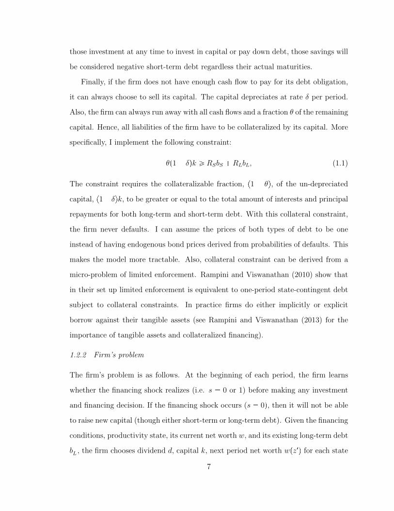
capital. Hence, all liabilities of the firm have to be collateralized by its capital. More

specifically, I implement the following constraint:

θp1� δqk ¥ RSbS �RLbL, (1.1)

The constraint requires the collateralizable fraction, p1 � θq, of the un-depreciated

capital, p1� δqk, to be greater or equal to the total amount of interests and principal

repayments for both long-term and short-term debt. With this collateral constraint,

the firm never defaults. I can assume the prices of both types of debt to be one

instead of having endogenous bond prices derived from probabilities of defaults. This

makes the model more tractable. Also, collateral constraint can be derived from a

micro-problem of limited enforcement. Rampini and Viswanathan (2010) show that

in their set up limited enforcement is equivalent to one-period state-contingent debt

subject to collateral constraints. In practice firms do either implicitly or explicit

borrow against their tangible assets (see Rampini and Viswanathan (2013) for the

importance of tangible assets and collateralized financing).

1.2.2 Firm’s problem

The firm’s problem is as follows. At the beginning of each period, the firm learns

whether the financing shock realizes (i.e. s � 0 or 1) before making any investment

and financing decision. If the financing shock occurs (s � 0q, then it will not be able

to raise new capital (though either short-term or long-term debt). Given the financing

conditions, productivity state, its current net worth w, and its existing long-term debt

b�L , the firm chooses dividend d, capital k, next period net worth wpz1q for each state

7

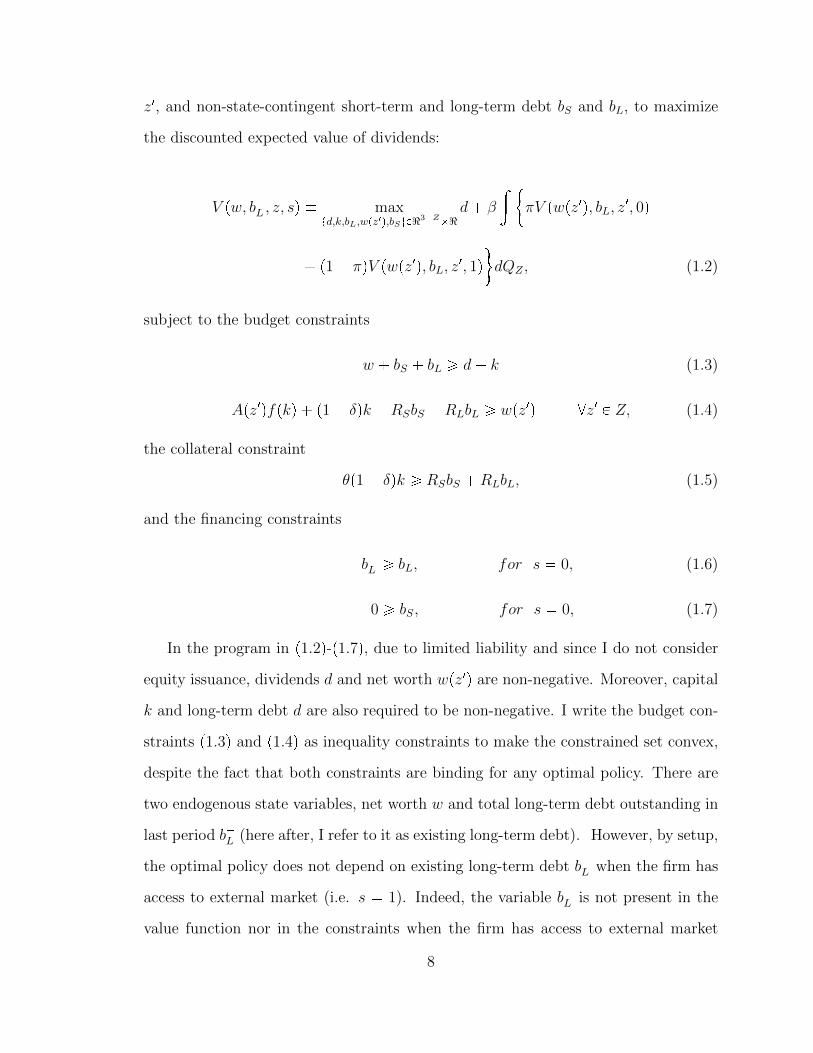
z1, and non-state-contingent short-term and long-term debt bS and bL, to maximize

the discounted expected value of dividends:

V pw, b�L , z, sq � maxtd,k,bL,wpz1q,bSuP<3�Z

� �<d� β

» "πV pwpz1q, bL, z

1, 0q

� p1� πqV pwpz1q, bL, z1, 1q

*dQZ , (1.2)

subject to the budget constraints

w � bS � bL ¥ d� k (1.3)

Apz1qfpkq � p1� δqk �RSbS �RLbL ¥ wpz1q @z1 P Z, (1.4)

the collateral constraint

θp1� δqk ¥ RSbS �RLbL, (1.5)

and the financing constraints

b�L ¥ bL, for s � 0, (1.6)

0 ¥ bS, for s � 0, (1.7)

In the program in p1.2q-p1.7q, due to limited liability and since I do not consider

equity issuance, dividends d and net worth wpz1q are non-negative. Moreover, capital

k and long-term debt d are also required to be non-negative. I write the budget con-

straints p1.3q and p1.4q as inequality constraints to make the constrained set convex,

despite the fact that both constraints are binding for any optimal policy. There are

two endogenous state variables, net worth w and total long-term debt outstanding in

last period b�L (here after, I refer to it as existing long-term debt). However, by setup,

the optimal policy does not depend on existing long-term debt b�L when the firm has

access to external market (i.e. s � 1). Indeed, the variable b�L is not present in the

value function nor in the constraints when the firm has access to external market

8

since the firm can freely adjust its capital and debt structure. Hence b�L is only a

state variable when financing shock occurs (i.e. s � 0).

I also require that production function and productivity shocks to satisfy the

following assumptions.

Assumption 1. f is strictly increasing, strictly concave, fp0q � 0, limkÑ0 fkpkq �

�8, and limk�8 fkpkq � 0.

Assumption 2. For all z, z P Z such that z ¡ z, (i) Apzq ¡ Apzq and (ii) Apzq ¡ 0.

To simplify notations, I use x to denote the choice variables, x � rd, k, bL, wpz1q, bSs,

and use Γpw, b�L , z, sq to denote the constraint set given state variables w, b�L , z, and

s. Thus, Γpw, b�L , z, sq is the set of x P <3�Z� � < such that p1.3q-p1.7q are satisfied.

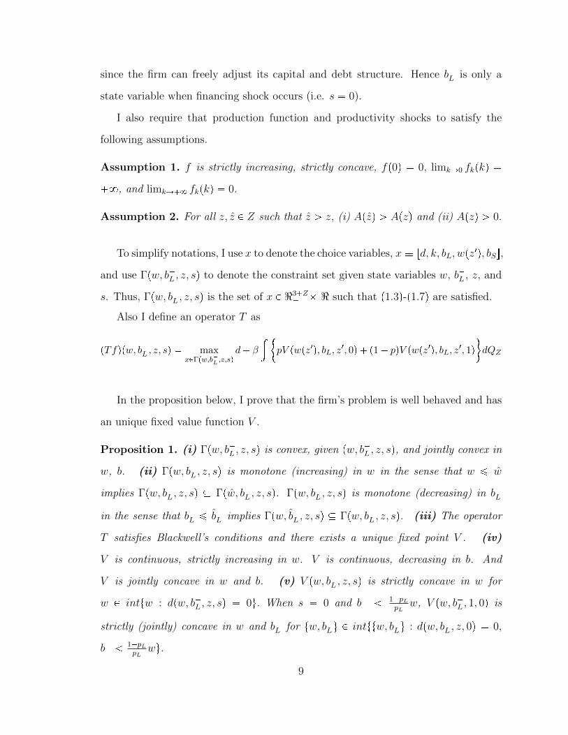
Also I define an operator T as

pTfqpw, b�L , z, sq � maxxPΓpw,b�L ,z,sq

d� β

» "pV pwpz1q, bL, z

1, 0q � p1� pqV pwpz1q, bL, z1, 1q

*dQZ

In the proposition below, I prove that the firm’s problem is well behaved and has

an unique fixed value function V .

Proposition 1. (i) Γpw, b�L , z, sq is convex, given pw, b�L , z, sq, and jointly convex in

w, b. (ii) Γpw, b�L , z, sq is monotone (increasing) in w in the sense that w ¤ w

implies Γpw, b�L , z, sq � Γpw, b�L , z, sq. Γpw, b�L , z, sq is monotone (decreasing) in b�L

in the sense that b�L ¤ b�L implies Γpw, b�L , z, sq � Γpw, b�L , z, sq. (iii) The operator

T satisfies Blackwell’s conditions and there exists a unique fixed point V . (iv)

V is continuous, strictly increasing in w. V is continuous, decreasing in b. And

V is jointly concave in w and b. (v) V pw, b�L , z, sq is strictly concave in w for

w P inttw : dpw, b�L , z, sq � 0u. When s � 0 and b�   1�pLpL

w, V pw, b�L , 1, 0q is

strictly (jointly) concave in w and b�L for tw, b�Lu P intttw, b�Lu : dpw, b�L , z, 0q � 0,

b�   1�pLpL

wu.

9

Let µ, βµpz1qπpz, z1q, βλ, γl, and γs be the multipliers on constraints p1.3q, p1.4q,

p1.5q, p1.6q, and p1.7q respectively. Also, let νd and νbL be the multipliers on the

constraints d ¥ 0 and bL ¥ 0. Finally, I will show in Lemma 6 that k ¡ 0 and

wpz1q ¡ 0 @z1 P Z.

From the envelop conditions and FOC with respect to d, I derive the following

equations:

V1pw, b�L , z, sq � µ � 1� νd. (1.8)

V2pw, b�L , z, 0q � γl

Hence, the marginal value of (current) net worth is equal to the value of dividend.

The marginal value of existing long-term debt is equal to the multiplier on the credit

constraint p1.6q when s � 0. In another word, the value of having additional long-

term debt is that it relaxes the credit constraint on long-term debt. However, when

s � 1, there is no value of having long-term debt, since the firm can borrow new

long-term debt anyway.

The capital k, short-term debt bS, and long-term debt bL decisions are governed

by the following FOCs respectively:

BV

Bk: µ � β

»rApz1qfkpkq � p1 � δqs

"πµpwpz1q, bL, z

1, 0q � p1 � πqµpwpz1q, bL, z1, 1q

*dQZ

� βθp1 � δqλ (1.9)

BV

BbS: µ � β

» "πµpwpz1q, bL, z

1, 0q � p1 � πqµpwpz1q, bL, z1, 1q

*dQZRS � βλRS � γs1s�0

(1.10)

BV

BbL: µ � β

» "πµpwpz1q, bL, z

1, 0q � p1 � πqµpwpz1q, bL, z1, 1q

*dQZRL � βλRL � γl1s�0

� βπ

»z1¥z

γlpwpz1q, bL, z

1, 0qdQZ � νbL

(1.11)

10

The first two FOCs are quite standard except that when s � 0, the firm may be

constrained because it can not raise new capital. The shadow cost of that constraint

is γs. The last equation states that when the firm chooses new long-term debt level,

it also takes into account the value the long-term debt might have in future when

the financing shock hits. More specifically, that value is βπ³z1¥z

γlpwpz1q, bl, z

1, 0qdQZ

which depends on both the probability of financing shock π and the realizations of

the productivity shock z1. Also, note that when net worth is too low, the collateral

constraint will bind. Hence, for z1 such that wpz1q  1�R�1

L θp1�δq

R�1L θp1�δq

bL, long-term debt

will not affect the firm’s choices. So, γlpwpz1q, bL, z

1, 0q � 0 for sure. The cut-off level,

z is defined by wpzq �1�R�1

L θp1�δq

R�1L θp1�δq

bL.

Now I start to characterize the firm’s optimal policy relation to its current state.

Proposition 2. There exists a state-contingent threshold lever of net worth, above

which the firm pays dividends. Firms with net worth above the threshold make the

same capital, debt, and end period net worth decision: (i) D wpb�L , z, sq s.t. @ w ¤ w,

d � 0 and @ w ¡ w, µ � 1, d ¡ 0. (ii) Also, @ w ¡ wpb�L , z, sq, rdo, ko, bL,o, bS,o

wopz1qs � rw � wpzq, ko, bL,o, bS,o wopz

1qs where rwpzq, ko, bL,o, bS,o wopz1qs attains

V pwpb�L , z, sq, b�L , z, sq. (iii) Finally, xo is unique for all w, b�L , z, s.

As typical in models with decreasing return to scale and collateral constraint, the

firm optimally chooses to invest all resource in capital when net worth is low. As

the firm accumulates more net worth, it becomes less constrained since the marginal

return on capital follows. Eventually, the firm starts to pay out dividend when it has

sufficiently high net worth and is operating with a high level of capital. From that

point on, any additional resource will have a marginal value of one. Hence, when net

worth is sufficiently high, the optimal choices for capital, debts, and end period net

worth are fixed and the firm pays out all additional resource as dividends.

11

Result 3. Under the stationary distribution, firms with sufficient net worth never

reduce their long-term debt level when refinancing is difficult. (i.e. when s � 0 and

R�1L θp1�δq

1�R�1L θp1�δq

w ¡ b�L , bL � b�L @pw, b�L , z, 0q)

The Result 3 states that the firm is always constrained by the amount of existing

long-term debt it has as long as it has sufficient net worth to support its current level

of long-term debt. The intuition is as follows.

The firm can increase long-term debt only when it has access to external market.

Since using more long-term debt hinders the accumulation of net worth for future and

the firm value is always increasing in net worth, the firm that currently has access to

external market will not choose to borrow with so much long-term debt such that the

firm will have excess long-term debt next period when it has no access to external

market (that is when s1 � 0). Therefore, under the stationary distribution, when

the firm has no access to external market, firm will always try to use as much long-

term debt as it can unless its net worth is insufficient to support its current level of

long-term debt (that is whenR�1L θp1�δq

1�R�1L θp1�δq

w   b�L).

When the firm does not have sufficient net worth compared to its old long-term

debt (that is whenR�1L θp1�δq

1�R�1L θp1�δq

w   b�L), it will still be collateral constrained when

without access to external market. In that case, the firm is forced to repay a fraction

of the existing long-term debt so that the new reduced level of long-term debt is fully

backed up by its new capital level. Hence, default never occurs as in the typical model

with collateral constrained.

Due to the complexity of the dynamic model, from this point on, I only discuss

model implications for i.i.d. productivity shock case. At the end, I will present results

on persistent productivity shocks in a simplified 2-period model.

12

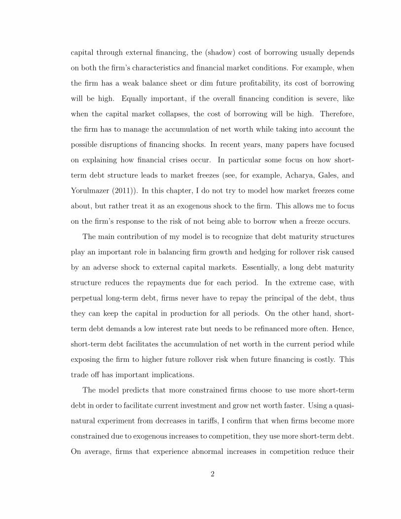
1.3 Capital and Dividend Policy:

The main focus of the chapter is centered around the idea that firms that finance

their capital more through long-term debt do not have to downsize as much when

refinancing is difficult because less debt repayment is due. Figure 1.1 illustrates this

point. The figure shows the optimal capital level as a function of net worth for each

of the following three cases: with external financing, without external financing but

with high long-term debt, and without external financing but with low long-term

debt. Following Proposition 2, for each case, the capital level is constant when net

worth is above a threshold wpb�L , sq. Below the threshold, capital level is increasing in

net worth and dividends are zero. First notice that even when the firm has sufficiently

large net worth and existing long-term debt, it will still choose a lower capital level

when has no access to external market (from the figure, the flat portion of dotted blue

line is higher than the flat portion of the solid red line). The reason is that, when

without access to external market, the firm can not raise short-term debt which has

a lower interest rate. Thus, the marginal cost of funding must be higher than that

when the firm has access to external market. That means that the marginal benefit

from production must also be lower. And due to strict concavity of the production

function, the firm must operate at lower capital level when without access to external

market no matter how much net worth and existing long-term debt it has. Second,

when the firm has less existing long-term debt, it is forced to operate at a lower

capital level (region where the red line is above the green line). Hence, when the firm

is previously with access to external market, suddenly the financing shock occurs and

the firm is now without access to external market, it will have to downsize to a greater

degree since it has used less long-term debt previously.

This fluctuation in capital level is costly to the firm because when the production

technology is strictly concave, the firm sometimes has to pass on high returns on cap-

13

ital. However, the firm may optimally choose not to smooth the fluctuation because

it is so constrained previously.

Finally, Figure 1.1 also shows that, when has no access to external market, the

firm postpones dividend when it has low level of existing long-term debt. Indeed, the

following proposition summarizes the observation.

Proposition 4. When financing constrained, firms with more long-term debt pay

dividends at a lower threshold. (i.e. wpb�L , 0q ¡ wpb�L , 0q, @b�L   b�L)

Firms with more existing long-term debt pay out earlier for two reasons. First,

when firms experience financing shocks, they can keep a higher capital level if they

have more long-term debt from previous period because those debt are not due. In

fact, as previously mentioned, those firms do operate with more capital and use more

long-term debt currently (see Result 3). Second and consequently, they need less

internal net worth to support the same level of capital next period when financing

shocks occur. Hence, they optimally pay out the current extra resource as dividend.

As seen from Figure 1.1, the firm starts paying dividend when it is able to sustain

a certain level of capital and its marginal return on capital is sufficiently low. Since

the firm’s current long-term debt choice can affect the fluctuation in capital level in

future and since the firm starts to pay out when capital level is sufficiently high, the

dividend dynamics will be affected by the firm’s debt maturity choices. In partic-

ular, let’s consider a firm which has sufficiently high net worth and pays dividends

currently. Next period, if the financing shock occurs, depending on the realization of

the production, either the firm has sufficient net worth so that it can keep operating

at a sufficiently high capital level and paying a dividend or it has to defer dividend

and put more net worth into financing capital investment. When the realization of

the productivity and hence net worth are very low, the firm will have to downsize by

selling its capital to repay debt and interests.

14

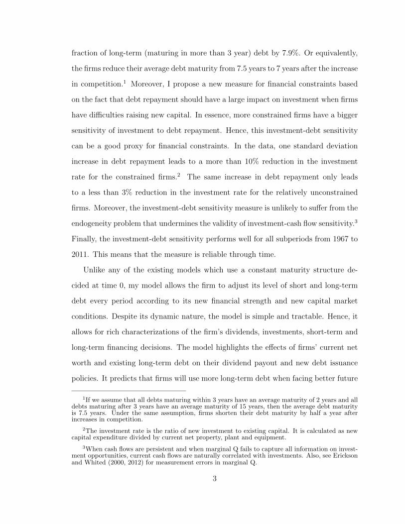
If the firm chose to raise more long-term debt previously, it will not have to

downsize as much when financing shock occurs next period. Also, the firm can still

pay out dividends in more states (productivity states) since in those states it can still

operate at a sufficiently higher capital level. On the other hand, if the firm raises little

long-term debt previously, it will have to downsize more and it has to omit dividends in

more states (productivity states). To illustrate this point, I keep all other parameters

the same and vary the probability of financing shock, p, as a comparative statics

exercise. The results are presented in Figures 1.2 and 1.3. In Figure 1.2, each line

shows the optimal next period net worth as a function of current next for a particular

existing long-term debt and financing state, pb�L , sq. The point at which the line turns

flat is the cut-off level of net worth at which the firm starts to pay dividends. The

interval rwLpb�Lq, wHpb

�Lqs represents the region in which a firm with existing long-

term debt, b�L , would pay dividend if it has access to external financing but would not

pay dividend otherwise. However, if the firm has existing long-term debt, b�L ¡ b�L ,

instead, the corresponding region shrinks to rwLpb�Lq, wHpb

�Lqs � rwLpb

�Lq, wHpb

�Lqs.

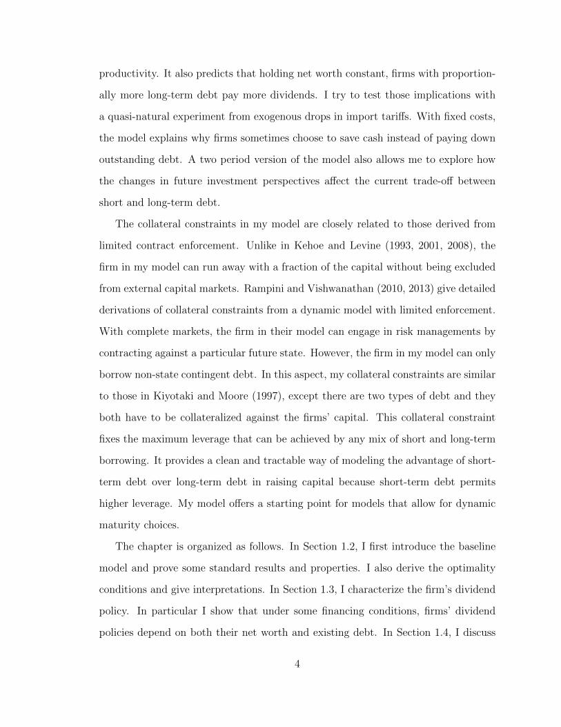
In Figure 1.3, I present the same result in the net worth and existing long-term

debt plane. The solid parts of the two blue lines are the locus of different levels of

possible next period net worth for two different levels of existing long-term debt. The

segments rwLpb�Lq, wHpb

�Lqs and rwLpb

�Lq, wHpb

�Lqs are the same as in Figure 1.2. The

shaded region is where firms with different levels of existing long-term debt would

pay dividends only if they have access to external market. Since the dividend paying

cutoff wpb�L , sq is constant when the firm has access to external market and decreasing

in b�L when financing shock occurs, the segment rwLpb�Lq, wHpb

�Lqs shortens as the firm

has more and more existing long-term debt. This means that the firm has to omit

dividends in fewer productivity states when financing shock occurs if it managed to

raise more long-term debt previously.

15

1.4 Short-term v.s. Long-term debt

In this Section, I describe the optimal short-term and long-term debt decisions. Due

to the complex nature of the dynamic model, I only give some intuitions and show

some numerical results.

1.4.1 Cash as negative short-term debt

Recently, many papers point out the fact that cooperations will save cash in case

they will have difficulty raising new capital in future. My model suggests that firms

can also use debt maturity management to help them endure times when financing

condition is severe. In particular, when are able to adjust their debt structure, firms

can control how much debt repayment due at the end of the period. When they expect

to experience financing difficulties, they reduce the amount due at period end. Hence,

firm’s cash and debt maturity decisions may be naturally linked. As illustrated in

my model, cash is equivalent to negative short-term debt. Therefore, only the net

short-term borrowing matters.

Of course there are other reasons for why firms use short-term debt and for why

firms hold cash reserves. Hence not all cash management activities can be viewed

as substitutes for short-term debt changes. However, based on the newly developed

theories on financing shock and cooperate cash savings, I believe that cash savings

are to a large extent driven by the firms’ concerns about future financing prospects.

Also, the rollover risk associated with short-term financing is well recognized. Hence,

firms’ cash management and debt maturity decisions should be interwind. Most

existing empirical papers on firms’ debt maturity choices never control for cash. It is

interesting to know whether their results could be overturned when properly taking

into account the connection between cash and short-term debt. Also, I think that to

what extent cash management affects the relation between firms’ debt maturity and

characteristics needs to be empirically investigated.

16

1.4.2 Optimal long-term debt to capital ratio

Long-term debt level is in general increasing in net worth. The rationale is the

following. Let’s fix a given level of optimal long-term debt choice. When current net

worth increases, capital level increases and next period net worth increases. Thus,

there will be less next period states in which the firm will be collateral constrained

given the long-term debt choice. And there will be more states in which additional

long-term debt is desirable. Therefore, the firm raises the optimal long-term level

when net worth increases. However, proportionally we observe the opposite pattern

which is summarized in the next result.

Result 5. Under the stationary distribution, firm with more net worth chooses a

lower long-term debt to capital ratio. (i.e. bLk

is decreasing in w for w P rwl, whs.)

Due to the strictly concavity of the production function (Assumption 1), when

net worth is low, the firm is more likely to have a next period net worth that is higher

than the current net worth. For example, when the firm’s net worth is lower than the

lowest net worth of ergodic distribution of net worth wl, its net worth is guaranteed

to be higher in all states next period. This means it can support a higher level of

debt next period. Therefore, initially in order to secure financing for the no access to

external market state, the firm has to raise large amount of long-term debt compared

to the relatively low level of net worth in current period. As current net worth

increases, on average, the ratio of next period net worth to current net worth drop

significantly. That is as the firm accumulates more net worth, its future net worth

will drop relative to its current net worth in more states next period. Especially in

some low productivity states next period, the firm will be forced to repay a fraction

of the long-term debt such that the new level of long-term debt is fully collateralized

by the firm’s capital. Thus, additional long-term debt does not provide any benefit

for those states. Hence, the firm finances less fraction of the capital using long-term

17

debt in the current period.

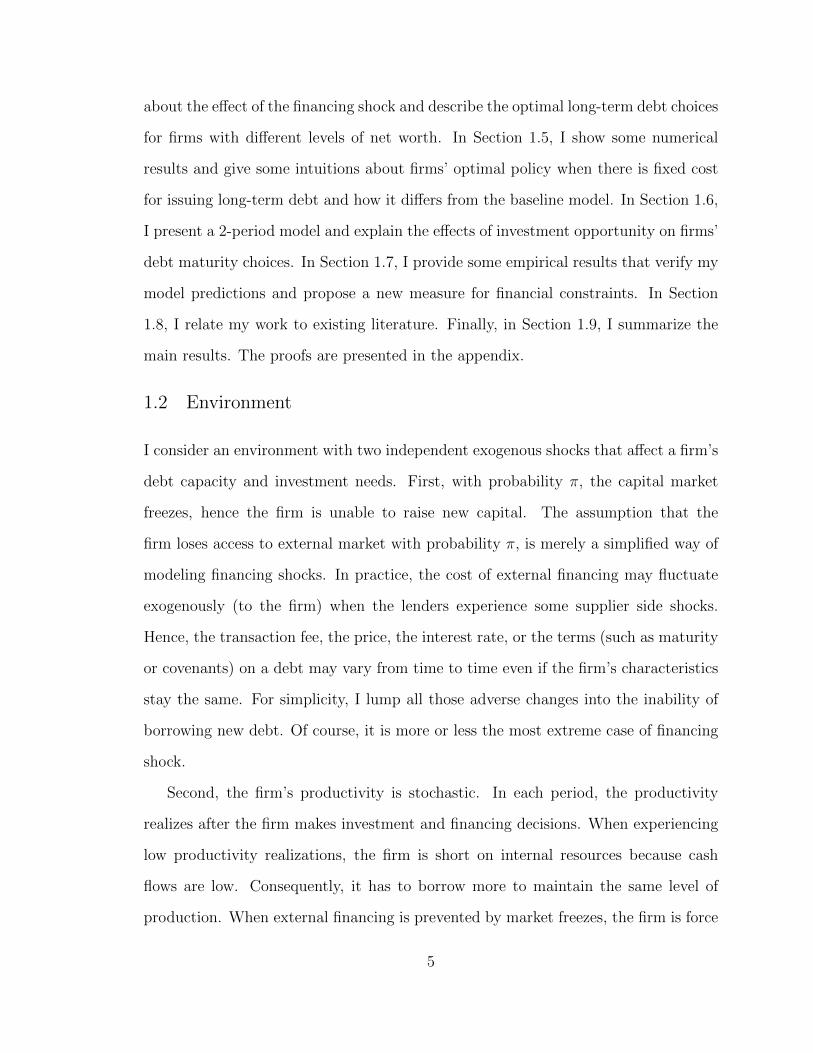
Therefore, even though in terms of level, the firm still borrows more long-term debt

when it has more net worth, in proportion to current capital, the firm is borrowing

less long-term debt. As illustrated in the left graph in Figure 1.4, the firm uses

proportionally less and less long-term debt as net worth increases. Some papers

documented that the long-term debt to total debt ratio increases with firm size.

Others have found that the ratio increases with firm size for most the cases but

decreases with size for very large firms. My model suggests that when the firm is able

to adjust its debt structure, the optimal long-term debt to capital ratio is decreasing

in net worth.

One undesirable pattern delivered from the model is the fact that firm with low

net worth saves by lending out in short-term. This is shown in the right graph of

Figure 1.4 and summarized as follows.

Result 6. When the probability of financing shock is high, firms with low net worth

choose to save through short-term debt. (i.e. for small w, bSpw, 1q   0)

Once again, when the firm has low net worth, its next period net worth is likely

to be higher than that of today. Hence, the collateral constraint for next period

is relaxed and the firm is allowed to borrow more in the absence of financing shock.

Therefore, not having access to external market is very costly for the firm next period.

Consequently, it will use a lot of long-term debt today in case it won’t be able to

borrow next period. In fact, when current net worth is low, the firm will save with

short-term debt as collateral in order to borrow more long-term debt in current period.

However, in the present of a fixed cost for long-term debt, firms with low net worth

will not use long-term debt to raise capital.

18

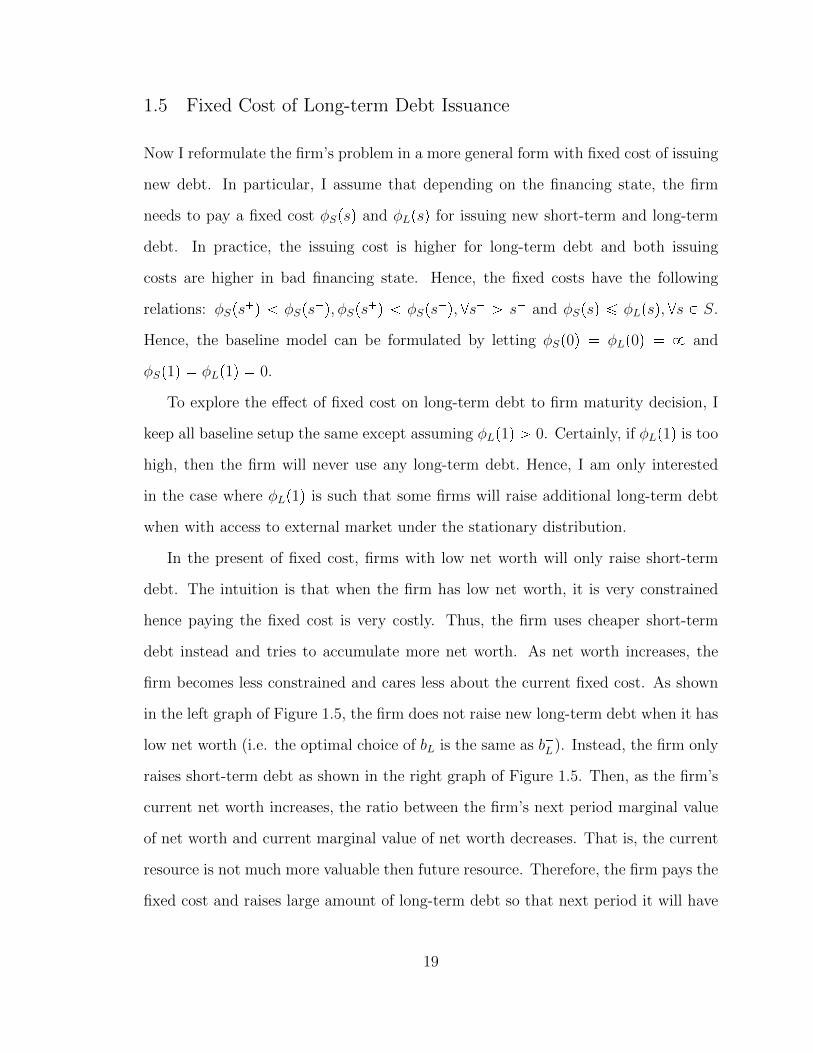
1.5 Fixed Cost of Long-term Debt Issuance

Now I reformulate the firm’s problem in a more general form with fixed cost of issuing

new debt. In particular, I assume that depending on the financing state, the firm

needs to pay a fixed cost φSpsq and φLpsq for issuing new short-term and long-term

debt. In practice, the issuing cost is higher for long-term debt and both issuing

costs are higher in bad financing state. Hence, the fixed costs have the following

relations: φSps�q   φSps

�q, φSps�q   φSps

�q, @s� ¡ s� and φSpsq ¤ φLpsq, @s P S.

Hence, the baseline model can be formulated by letting φSp0q � φLp0q � 8 and

φSp1q � φLp1q � 0.

To explore the effect of fixed cost on long-term debt to firm maturity decision, I

keep all baseline setup the same except assuming φLp1q ¡ 0. Certainly, if φLp1q is too

high, then the firm will never use any long-term debt. Hence, I am only interested

in the case where φLp1q is such that some firms will raise additional long-term debt

when with access to external market under the stationary distribution.

In the present of fixed cost, firms with low net worth will only raise short-term

debt. The intuition is that when the firm has low net worth, it is very constrained

hence paying the fixed cost is very costly. Thus, the firm uses cheaper short-term

debt instead and tries to accumulate more net worth. As net worth increases, the

firm becomes less constrained and cares less about the current fixed cost. As shown

in the left graph of Figure 1.5, the firm does not raise new long-term debt when it has

low net worth (i.e. the optimal choice of bL is the same as b�L). Instead, the firm only

raises short-term debt as shown in the right graph of Figure 1.5. Then, as the firm’s

current net worth increases, the ratio between the firm’s next period marginal value

of net worth and current marginal value of net worth decreases. That is, the current

resource is not much more valuable then future resource. Therefore, the firm pays the

fixed cost and raises large amount of long-term debt so that next period it will have

19

more resource from long-term when the financing shock hits. This corresponds to

Region A in Figure 1.6. Also, shown in Figure 1.5, this region is where the long-term

debt jumps up and the short-term debt jumps down. In fact, as shown in Region C

of Figure 1.6, there is a threshold level of net worth wpb�Lq below which the firm will

choose to not to raise new long-term even when it has access to external market. This

threshold depends on the firm’s existing long-term debt level. The higher the existing

long-term debt the higher the threshold. The rationale is related to the trade-off I

will discuss next.

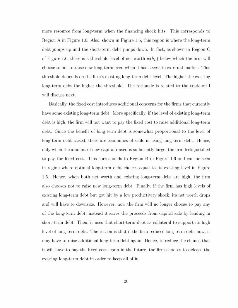
Basically, the fixed cost introduces additional concerns for the firms that currently

have some existing long-term debt. More specifically, if the level of existing long-term

debt is high, the firm will not want to pay the fixed cost to raise additional long-term

debt. Since the benefit of long-term debt is somewhat proportional to the level of

long-term debt raised, there are economies of scale in using long-term debt. Hence,

only when the amount of new capital raised is sufficiently large, the firm feels justified

to pay the fixed cost. This corresponds to Region B in Figure 1.6 and can be seen

in region where optimal long-term debt choices equal to its existing level in Figure

1.5. Hence, when both net worth and existing long-term debt are high, the firm

also chooses not to raise new long-term debt. Finally, if the firm has high levels of

existing long-term debt but got hit by a low productivity shock, its net worth drops

and will have to downsize. However, now the firm will no longer choose to pay any

of the long-term debt, instead it saves the proceeds from capital sale by lending in

short-term debt. Then, it uses that short-term debt as collateral to support its high

level of long-term debt. The reason is that if the firm reduces long-term debt now, it

may have to raise additional long-term debt again. Hence, to reduce the chance that

it will have to pay the fixed cost again in the future, the firm chooses to defease the

existing long-term debt in order to keep all of it.

20

1.6 Current v.s. Future Investments and Debt Maturity

For simplicity, I abstract from net worth effects for now and assume that the firm has

a linear production function. That is, ftpktq � kt and f 1tpktq � 1.

To facilitate the interpretation of the solution, I define the following terms. As in

Rampini and Vishwanathan (2010), I define down payment as the minimum amount

that the firm has to put down per unit of capital. In the case, it is one minus

the proportion borrowed with debt. Hence, the down payments with short-term

financing and with long-term financing are respectively, p � 1 � R�1θp1 � δq and

pL � 1 � R�1L θp1 � δq. Further, the reciprocals 1

pand 1

pLare the maximum leverages

through short-term and long-term financing. Notice that since long-term debt is more

expensive (i.e. RL ¡ R), short-term debt requires less down payment and offers higher

leverage. Later on, we will see that the firm trades off this benefit of short-term debt

with the cost of underinvestment. Now, I denote the net fully levered average return

on capital with RetpAtq � At � p1 � δqp1 � θq, the subscribe t denotes time. Hence,

if the firm only uses short-term debt, the net fully levered average return on internal

funds (net worth) is RetpAtqp

. If the firm only uses long-term debt, the net fully levered

average return on internal funds is RetpAtqpL

. Finally, I denote the ordinary gross return

on capital with RetpAtq � At � p1� δq.

Due to the linear objective at time 1, the firm either pays out all net worth as

dividends or invests as much as it can depending on the average productivity in time

2. If firm pays out all net worth at time 1, then at time 0 the firm is facing a one

period problem. It only needs to care about end of period net worth. Long-term debt

is never used at time 0 since it demands a higher return but provides no additional

benefit over short-term debt.

In order to focus on more interesting cases, I assume that the capital is sufficiently

productive at time 2, that is:

21

Assumption 3. E1A2 � p1� δq ¡ 1β, @A1.

With sufficiently high time 2 productivity, the firm invests all resources in capital

and pays out nothing at time 1. Moreover, if it has access to external financing ps � 1q,

it will retire all its current long-term debt and borrow only short-term debt until it

runs out of collateral. However, if the firm has no access to external financing, it will

be constrained either by its collateral or by its long-term debt holding depending on

the relation between its beginning long-term debt holding and net worth at time 1.

Hence, the firm’s time 1 decisions are straight forward.

Lemma 7. Under Assumption 3, the firm’s decisions at time 1 can be characterized

as follow:

• If the firm has access to external financing ps � 1q, then

d1 � 0, k2 �w1

p, b2 � p1

p� 1qw1, bL2 � 0, w2pA2q �

Ret2pw1.

• If it is without external financing ps � 0q and poorly capitalized (i.e. bL1 ¥

p 1pL� 1qw1), then

d1 � 0, k2 �w1

pL, b2 � 0, bL2 � p 1

pL� 1qw1, w2pA2q �

Ret2pLw1.

• If it is without external financing ps � 0q and well capitalized (i.e. bL1   p 1pL�

1qw1), then

d1 � 0, k2 � w1 � bL1 , bL2 � bL1 , b2 � 0, w2pA2q � ˆRet2pw1 � bL1 q �RLbL1 .

where w1 and bL1 are the time 1 beginning net worth and long-term debt holding.

And d1, k2, b2, bL2 are respectively the dividends payment, the capital level, short-term

debt holding, and long-term debt holding chosen at time 1. Finally, w2pA2q is the end

of period payout in each state of time 2 with productivity A2.

22

Lemma 7 classifies three type of states at time 1 and characterizes the optimal

choices and payoff for each type. For convenience, through out the chapter, I call

the states in which the firm’s time 1 decision is constrained by its net worth the

“collateral-constrained” states. I call the states in which the firm’s time 1 decision

is constrained by its long-term debt holding the “debt-constrained” states. Since the

beginning long-term debt holding bL1 is decided at time 0 and because the time 1 net

worth is one-to-one and increasing in time productivity 1, I can define and solve for

the cut-off value for determining the last two types of states.

Lemma 8. There exists a cut-off value of time 1 productivity,A, defined by:

A �

"A1 : w1pA1q �

bL1 pL1� pL

*. (1.12)

such that for all states above A, the firm is debt constrained and for all states below

A, the firm is collateral constrained.

At time 0 the firm chooses d0, k1, b1, bL1 , w1pA1q, to maximize the payout over the

two periods. The choices of bL1 and w1pA1q will determine which states are debt-

constrained and which are collateral-constrained. And at time 0, the firm knows

exactly what it will do in each state at time 1. Also, the return per capital only differs

between different types of states. Under parameterizations such that the collateral

constraint is binding at time 0, I can reformulate the firm’s time 0 problem in terms

of the ratio of optimal long-term debt to time 0 net worth, α �bL1w0

. And it can

be shown that the optimal long-term debt to net worth α, is pinned down by the

following FOC:

"p1 � πqE

RetpA2q

pRetpA1q � πPrrA1 ¤ AsEA1¤A

RetpA2q

pLRetpA1q

� πPrrA1 ¡ AsEA1¡ARetpA2qRetpA1q

*ppL � pq

pLp� πPrrA1 ¡ As

1 � pLpL

EA1¡ArRetpA2q �RLs

23

In essence, the firm chooses that optimal ratio such that the marginal cost is

equal to the marginal benefit of long-term debt. The left hand side of the equation

represents the marginal cost of long-term debt. It is the loss on the return on net

worth, which is the sum in the curly bracket, times the proportional reduction in

time 1 net worth. The right hand side of the equation represents the marginal benefit

of long-term debt. It is the gain from the difference between return on capital and

long-term debt interest rate times the proportional increase in long-term debt. So

the firm balances the loss from net worth reduction and the benefit from having more

long-term debt at time 1.

The following three propositions describe the effects of productivity prospects on

the firm’s maturity decisions:

Proposition 9. Firms with more persistent productivities proportionally use more

long-term debt (i.e. α increases with corrrA1, A2s.)

Proposition 10. When productivity shocks are independent, firms with better average

period 2 productivity proportionally use more long-term debt (i.e. When A1, A2 are

independent, α increases with EA2.)

Proposition 10 states that if the firm has better investment opportunities in the

distant future (at time 2), it will choose to use more long-term debt now. The

reason is that if the firm currently chooses a interior long-term debt level (α ¡ 0),

it must be that the proportional increase in long-term debt b�L is a lot bigger than

the proportional decrease in time 1 net worth w1pz1q caused by an increase in α.

Hence, if the return on capital for time 2 improves, the marginal benefit of long-term

debt raises more than the marginal benefit of time 1 net worth. Similarly, since

we consider a case in which the time 1 productivity is sufficiently high on average,

an increase in the correlation of the two shocks means better future productivities

24

(at time 2). Therefore, the firm also increases its use of long-term debt when the

correlation between time 1 and time 2 productivities increases.

The results have some similarities to the project and debt maturity matching

story. Basically, if most of the returns will come from future periods, the firm is more

afraid from being cutoff of fund supply and hence won’t have enough capital to take

advantage of those good returns. Hence, it starts to use more long-term debt now to

secure the access of fund. On the contrary, if the firm high current productivity, it

will do the opposite as summarized in Proposition 11.

Proposition 11. When probability of financing shock is low, firms with higher current

productivities proportionally use less long-term debt (i.e. for low π, α decreases when

A1 increases state by state.)

When the current productivity rises, there are two effects. First, the firm can gain

more from the higher leverage offered by the short-term financing. Second, because

the firm now will have more net worth next period on average, it can sustain higher

leverage next period. Hence, a market freeze will hurt the firm more. This second

effect makes the firm more willing to use long-term debt now, but it depends on the

probability of market freezes. When the probability, π, is low, the firm cares more

about capitalizing the current gains with more short-term financing. The proposition

suggests that firms that use relatively less long-term debt are the ones that have good

current investment opportunities. However, firms with less long-term debt will have to

downsize more when experiencing financing shocks in future. When the productivity

shocks are persistent, this means that at time 1 when financing condition is severe,

capital is inefficiently deployed across firms with different investment opportunities.

The ones with high return on capital have relatively less capital. Whereas the ones

with low return on capital have relatively more capital since they used more long-term

debt previously.

25

In practice, we do observe that firms with more growth options finance with more

short-term debt. Empirically, people have found that firms with higher marginal Q

and higher sales growth tend to have a larger fraction of short-term debt. Tradition-

ally this pattern is attributed to Myers’ debt overhand story. More specifically, the

firm with more future investment opportunities wants to have its debt mature before

the investment decision so that there will not be any incentive distortions between

the equity and debt holders. My model provides an alternative explanation. In the

present of both collateral and financing constraints, firms are trading off net worth

with long-term debt. When the probability of experiencing financing shocks is low,

firms with better current investment opportunities concern more about accumulat-

ing net worth and are willing to risk having to downsize more when financing shock

occurs.

Proposition 12. When financially constrained, firms use more short-term financing

as the cost of borrowing rises. (i.e. When θp1�δqR

is low, α decreases from a propor-

tional increase in both R and RL)

Last but not least, the model suggests that more constrained firms use more short-

term financing. This conclusion is profound but intuitive. The more constrained firms

borrow less from the financial markets. Hence, they rely more on their internal net

worth to finance most of their investments. As a result, they have less incentive to

hedge for future financing shocks. At the same time, since net worth is so important,

they want to build their net worth faster by investing more today. Therefore, they

use more short-term financing to increase leverage and production. This conclusion

is important because it improves our understanding of the relation between finan-

cial constraints and debt maturity. Prior research blamed firms for holding excessive

amounts of short-term debt under the belief that short-term financing made firms

more vulnerable to financial shocks, and frequent repayments due to a shorter-term

debt structure made firms more constrained. My model explains that firms borrow

26

short-term debt precisely because they are constrained. Thus, it is financial con-

straints that cause more short-term financing, not the other way around. In the next

section, I use a natural experiment to empirically test for this direction of causality.

1.7 Empirical Testing

In this section, I verify my model predictions and explore its potential in three steps.

First, I test whether more constrained firms use more short-term financing. Second,

I propose a measure for financial constraints based on my model and examine the

performs of my measure. Finally, I show that the proposed measure is consistent

with the natural experiment I use for some of the empirical tests.

1.7.1 Financial constraints and debt maturity

In the literature, measuring financial constraint is very difficult. Simply showing

correlation between debt maturity and some exiting measures of financial constraints

is not sufficient because the measures themselves may not reflect financial constraints

well. Plus, even if the measures for financial constraints are precise, simple correlation

still does not show causality due to potential endogeneity and simultaneity. Therefore,

I use a quasi-natural experiment to show that financial constraints cause firms to use

short-term debt.

Previous literature has shown that increase in competition leads to higher cost

of debt, lower profitability, and less research and development for the firms that

experience that increasing competition (Valta (2012), Hou and Robinson (2006), and

Fresard and Valta (2013)). Hence, I think that firms who experience more competition

are more constrained. Therefore, I use exogenous shocks to competition as exogenous

shocks to firm financial constraints.

My main data consist of Compustat and international trade data from Peter

Schott’s web site. The sample period is from 1989 to 2005. I exclude firms in the

27

financial (SIC 6000-7000) and utility (SIC 4400-5000) industries. Also, the sample

is restricted to those industries (mainly manufacturing) present in the international

trade data. I delete all observations with total assets less than five millon since the

very small firms tend to behave abnormally. I also require the observations to have

sufficient information for calculation control variables such as marginal Q, leverage,

asset maturity, etc. Main variables are defined in Table 1.8 in Appendix E. The

exogenous shocks to competition are define as follows.

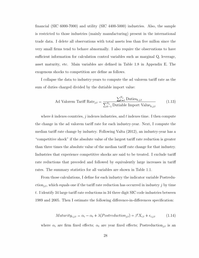
I collapse the data to industry-years to compute the ad valorem tariff rate as the

sum of duties charged divided by the dutiable import value:

Ad Valorem Tariff Ratej,t �

°Njk�1 Dutiesk,j,t°Nj

k�1 Dutiable Import Valuek,j,t(1.13)

where k indexes countries, j indexes industries, and t indexes time. I then compute

the change in the ad valorem tariff rate for each industry-year. Next, I compute the

median tariff rate change by industry. Following Valta (2012), an industry-year has a

“competitive shock” if the absolute value of the largest tariff rate reduction is greater

than three times the absolute value of the median tariff rate change for that industry.

Industries that experience competitive shocks are said to be treated. I exclude tariff

rate reductions that preceded and followed by equivalently large increases in tariff

rates. The summary statistics for all variables are shown in Table 1.1.

From those calculations, I define for each industry the indicator variable Postredu-

ctionj,t, which equals one if the tariff rate reduction has occurred in industry j by time

t. I identify 34 large tariff rate reductions in 34 three digit SIC code industries between

1989 and 2005. Then I estimate the following difference-in-differences specification:

Maturityi,j,t � αi � αt � λpPostreductionj,tq � β1Xi,t � εi,j,t (1.14)

where αi are firm fixed effects; αt are year fixed effects; Postreductionj,t is an

28

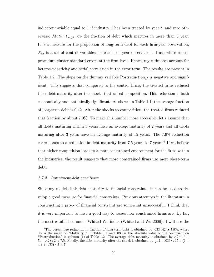
indicator variable equal to 1 if industry j has been treated by year t, and zero oth-

erwise; Maturityi,j,t are the fraction of debt which matures in more than 3 year.

It is a measure for the proportion of long-term debt for each firm-year observation;

Xi,t is a set of control variables for each firm-year observation. I use white robust

procedure cluster standard errors at the firm level. Hence, my estimates account for

heteroskedasticity and serial correlation in the error term. The results are present in

Table 1.2. The slope on the dummy variable Postreductionj,t is negative and signif-

icant. This suggests that compared to the control firms, the treated firms reduced

their debt maturity after the shocks that raised competition. This reduction is both

economically and statistically significant. As shown in Table 1.1, the average fraction

of long-term debt is 0.42. After the shocks to competition, the treated firms reduced

that fraction by about 7.9%. To make this number more accessible, let’s assume that

all debts maturing within 3 years have an average maturity of 2 years and all debts

maturing after 3 years have an average maturity of 15 years. The 7.9% reduction

corresponds to a reduction in debt maturity from 7.5 years to 7 years.4 If we believe

that higher competition leads to a more constrained environment for the firms within

the industries, the result suggests that more constrained firms use more short-term

debt.

1.7.2 Investment-debt sensitivity

Since my models link debt maturity to financial constraints, it can be used to de-

velop a good measure for financial constraints. Previous attempts in the literature in

constructing a proxy of financial constraint are somewhat unsuccessful. I think that

it is very important to have a good way to assess how constrained firms are. By far,

the most established one is Whited Wu index (Whited and Wu 2006). I will use the

4The percentage reduction in fraction of long-term debt is obtained by .033{.42 � 7.9%, where.42 is the mean of “Maturity3” in Table 1.1 and .033 is the absolute value of the coefficient on“Postreduction” in column (1) of Table 1.2. The average debt maturity is obtained by .42 � 15 �p1� .42q � 2 � 7.5. Finally, the debt maturity after the shock is obtained by p.42� .033q � 15� p1�.42 � .033q � 2 � 7.

29

index and some other classifications of financial constraint to show that measure does

proxy for financial constraints.

From the model, we see that when the firm takes on large amounts of debt pre-

viously and has to pay it back, it become very constrained so that it has to forego

good investment opportunities. Because of this negative impact of debt repayment

to investment, I think the sensitivity from investment to debt repayment is a good

measure for financial constraints. Suppose that a firm is totally unconstrained and

it can always borrow as much as it wants. Then no matter how much debt it has to

repay, its investment decision is not affected because it simply borrows more debt to

satisfy both the investment and repayment needs. On the other hand, suppose a firm

is very constrained and it can not borrow any new debt. Then when this firm has lots

of debt repayment, it has to decrease investment dramatically in order to make debt

repayments. Therefore, I suspect that the sensitivity of investment to debt repayment

is negative and significant. Furthermore, more constrained firms should have more

negative sensitivities of investment to debt repayment.

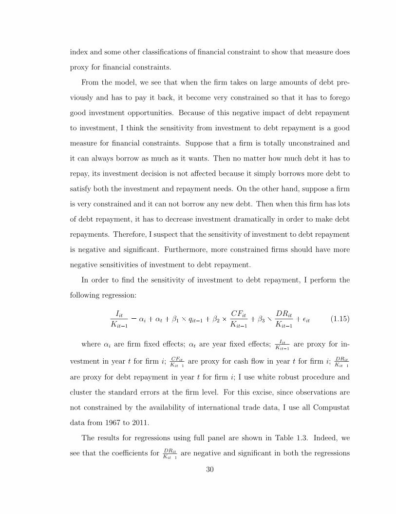
In order to find the sensitivity of investment to debt repayment, I perform the

following regression:

IitKit�1

� αi � αt � β1 � qit�1 � β2 �CFitKit�1

� β3 �DRit

Kit�1

� εit (1.15)

where αi are firm fixed effects; αt are year fixed effects; IitKit�1

are proxy for in-

vestment in year t for firm i; CFitKit�1

are proxy for cash flow in year t for firm i; DRitKit�1

are proxy for debt repayment in year t for firm i; I use white robust procedure and

cluster the standard errors at the firm level. For this excise, since observations are

not constrained by the availability of international trade data, I use all Compustat

data from 1967 to 2011.

The results for regressions using full panel are shown in Table 1.3. Indeed, we

see that the coefficients for DRitKit�1

are negative and significant in both the regressions

30

with and without additional control variables. The coefficient �.264 in Column (Ba-

sic) suggests that one standard deviation increase in debt repayment leads to about

7.8% decrease in investment rate, IitKit�1

. Hence, debt repayment indeed has a signif-

icant effect on investment. Next, I examine whether the coefficients for DRitKit�1

(the

investment-debt sensitivity) are more negative for more constrained firms. Since the

Whited Wu index, firm size, and dividend rates are so far the best proxy for finan-

cial constraints, I split the data into sub-samples based on those proxy for financial

constraints. Then I run the regression for each sub-sample and see if the coefficients

for DRitKit�1

(the investment-debt sensitivity) are more negative for the more constrained

sub-samples.

Table 1.4 shows the results for regressions on sub-samples based on Whited Wu

index. As we move from the least to most constrained sub-samples, the coefficients

for DRitKit�1

indeed become more negative and significant. For example, the sensitivity is

�.352 in Column (5) but is only �0.071 in Column (1). This means that for the most

constrained firms (Column (5)), one standard deviation increase in debt repayment

leads to a 10.9% reduction in investment rate. However, the same increase only leads

to a 2.1% reduction in investment rate for the least constrained firms. So the effect of

debt repayment on investment is substantially bigger for the more constrained firms.

The patterns are the same across sub-samples based on size and dividend rate (Table

1.5, Table 1.6). Therefore, I conclude that more constrained firms have more negative

investment-debt sensitivity.

In unreported robustness tests over subperiods, the investment-debt sensitivity

remains reliable for all time periods from 1967 to 2011. Moreover, although the

amount of debt repayment due next year may be related to previous financing and

investment decisions, it does not relate to future investment opportunities directly.

Therefore, I believe most of the effect of debt repayment on investment depends on

how constrained the firm is. Hence, investment-debt sensitivity is unlikely to suffer

31

endogeneity problems as investment-cash flow sensitivity does.3

1.7.3 Investment-debt sensitivity and the natural experiment

With the new measure for financial constraint, I now check whether the increase

in competition corresponds to increase in financial constraints. More specifically, I

examine whether the investment-debt sensitivity for the treated firms becomes more

negative after the increase in competition compared to the control firms. I conduct

the following regression:

Ii,j,tKi,j,t�1

�αi � αt � λ1DRi,j,t

Ki,j,t�1

� λ2Postj,t � λ3pDRi,j,t

Ki,j,t�1

� Postj,tq

� β1Xi,t � εi,j,t (1.16)

where αi are firm fixed effects; αt are year fixed effects; IitKit�1

are proxy for in-

vestment in year t for firm i; DRitKit�1

are proxy for debt repayment in year t for firm i;

Postreductionj,t is an indicator variable equal to 1 if industry j has been treated by

year t, and zero otherwise;DRi,j,tKi,j,t�1

� Postj,t is the interact between Postreductionj,t

and DRitKit�1

; This interaction term captures the change in investment-debt sensitivity for

the treated group before and after the shock compared to that of the control group.

Hence, I test to see whether coefficient for the termDRi,j,tKi,j,t�1

�Postj,t is significantly dif-

ferent from zero. In Table 1.7, we see that the coefficient for the termDRi,j,tKi,j,t�1

�Postj,t

is negative and significant with or without additional controls. Therefore, the data

suggest that the firms which experienced the increase in competition become more

constrained after the shock.

1.8 Related Literature

One of the important elements of my model is the rollover risk caused by the market

freezes. Throughout the literature on debt maturity, all papers have rollover risk

32

as the cost of short-term debt.5 Some try to explain how capital markets break

down. For example, Brunnermeier and Oehmke (2013) address financial institutions’

maturity mismatch problem in an equilibrium frame work. In the model, short-term

creditors may demand a higher face value on the new debt when their lending matures

and needs to be rolled over in states where default is more likely. Long-term creditors

bear the cost of increasing the face value. The bank (the borrower in their model)

is unable to commit to a single maturity structure. It optimally chooses to use more

short-term debt upon receiving interim signal regarding the probability of default.

Consequently, every creditor prefers to shorten its lending maturity and long-term

financing unravels. Focusing on the effects and implications of short-term financing,

Acharya, Gales, and Yorulmazer (2011) demonstrate that when the arrival of good

news is slower than the rate of rollover and when everyone is borrowing at short

term, liquidity dries up quickly and a market freeze may occur despite the fact that

the underlying asset quality is unchanged. This is due to the fact that, when a

debt is rolled over frequently, little information is revealed between rollover dates.

Thus, the difference in the debt capacities between high and low current states is big,

even though the fundamental values are almost the same. Both those papers provide

micro-foundation for the market freezes assumed in my model.

A variety of benefits of short-term financing have been introduced. For example,

short-term financing reduces the underinvestment problem caused by debt overhang

(Myers (1977); Childs, Mauer, and Ott (2005); Diamond and He (2012)). The idea

is that if debt matures and is settled before the firm decides whether to take a new

project, there will be no incentive distortion. In my model, short-term debt also

causes underinvestment because the firm has to use resource to repay the debt. Espe-

cially, when it experiences difficult obtaining new finance, the firm has to scale down.

5All theory papers mentioned in this section deal with rollover problem of short-term debt.Other important papers include Leland (1994), Leland and Toft (1996), Leland (1998), He andXiong (2012a 2012b), and He and Milbradt (2013)

33

However, short-term debt also helps to increase investment in current period since

it is borrowed at relatively low cost. So the firm’s main trade off is between current

investment and future investments.

Segura and Suarez (2013) have a model that is similar to mine. In their model,

short-term debt is relatively cheaper since it better accommodates preference shocks

that investors may experience. However, when preference shocks occur, the lending

supply shrinks dramatically. In deciding the optimal fraction of long-term and short-

term debt to use, banks trade off the lower cost of borrowing of short-term debt

with the higher cost when refinancing during systemic liquidity crisis. They conclude

that the banks’ optimal choice of long-term debt holding is inefficient. Government

regulations, such as debt maturity limits, Pigovian taxes, and liquidity insurances,

can make welfare improvements. Different from theirs, the main drive in the model is

the productivity shocks. The firm makes real investment decisions rather than having

a fix inflow every period.

In addition, short-term debt can be used as a disciplining device against agency

problems. In particular, many consider the problem of “risk-shifting” (Barnea, Hau-

gen, and Senbet (1980); Grossman and Hart (1982); Calomiris and Kahn (1991);

Leland (1998); Diamond and Rajan (2001); Eisenbach (2013); Cheng and Milbradt

(2012)). Others also build on the fact that short-term debt can help to prevent

managers from “empire-building”. With short-term debt, the creditors can decide

whether to continue the project if managers fail to pay. Since managers want to

continue negative NPV projects due to their private benefit, it is important for the

creditors to take control before things go awry (Grossman and Hart (1982); Benm-

elech (2006)). In my model, there is no incentive problem between the equity holders

and the managers. The benefit of short-term debt is simply the low interest rate. In

a dynamic environment, firms are more likely to take advantage of the low rate when

they need capital the most.

34

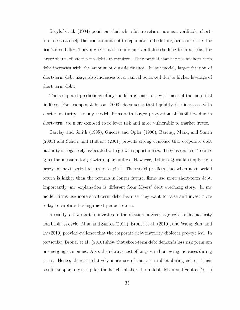
Berglof et al. (1994) point out that when future returns are non-verifiable, short-

term debt can help the firm commit not to repudiate in the future, hence increases the

firm’s credibility. They argue that the more non-verifiable the long-term returns, the

larger shares of short-term debt are required. They predict that the use of short-term

debt increases with the amount of outside finance. In my model, larger fraction of

short-term debt usage also increases total capital borrowed due to higher leverage of

short-term debt.

The setup and predictions of my model are consistent with most of the empirical

findings. For example, Johnson (2003) documents that liquidity risk increases with

shorter maturity. In my model, firms with larger proportion of liabilities due in

short-term are more exposed to rollover risk and more vulnerable to market freeze.

Barclay and Smith (1995), Guedes and Opler (1996), Barclay, Marx, and Smith

(2003) and Scherr and Hulburt (2001) provide strong evidence that corporate debt

maturity is negatively associated with growth opportunities. They use current Tobin’s

Q as the measure for growth opportunities. However, Tobin’s Q could simply be a

proxy for next period return on capital. The model predicts that when next period

return is higher than the returns in longer future, firms use more short-term debt.

Importantly, my explanation is different from Myers’ debt overhang story. In my

model, firms use more short-term debt because they want to raise and invest more

today to capture the high next period return.

Recently, a few start to investigate the relation between aggregate debt maturity

and business cycle. Mian and Santos (2011), Broner et al. (2010), and Wang, Sun, and

Lv (2010) provide evidence that the corporate debt maturity choice is pro-cyclical. In

particular, Broner et al. (2010) show that short-term debt demands less risk premium

in emerging economies. Also, the relative cost of long-term borrowing increases during

crises. Hence, there is relatively more use of short-term debt during crises. Their

results support my setup for the benefit of short-term debt. Mian and Santos (2011)

35

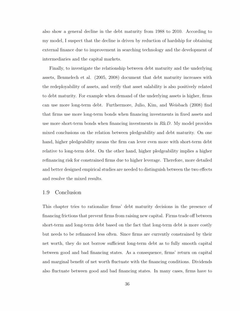
also show a general decline in the debt maturity from 1988 to 2010. According to

my model, I suspect that the decline is driven by reduction of hardship for obtaining

external finance due to improvement in searching technology and the development of

intermediaries and the capital markets.

Finally, to investigate the relationship between debt maturity and the underlying

assets, Benmelech et al. (2005, 2008) document that debt maturity increases with

the redeployability of assets, and verify that asset salability is also positively related

to debt maturity. For example when demand of the underlying assets is higher, firms

can use more long-term debt. Furthermore, Julio, Kim, and Weisbach (2008) find

that firms use more long-term bonds when financing investments in fixed assets and

use more short-term bonds when financing investments in R&D. My model provides

mixed conclusions on the relation between pledgeability and debt maturity. On one

hand, higher pledgeability means the firm can lever even more with short-term debt

relative to long-term debt. On the other hand, higher pledgeability implies a higher

refinancing risk for constrained firms due to higher leverage. Therefore, more detailed

and better designed empirical studies are needed to distinguish between the two effects

and resolve the mixed results.

1.9 Conclusion

This chapter tries to rationalize firms’ debt maturity decisions in the presence of

financing frictions that prevent firms from raising new capital. Firms trade off between

short-term and long-term debt based on the fact that long-term debt is more costly

but needs to be refinanced less often. Since firms are currently constrained by their

net worth, they do not borrow sufficient long-term debt as to fully smooth capital

between good and bad financing states. As a consequence, firms’ return on capital

and marginal benefit of net worth fluctuate with the financing conditions. Dividends

also fluctuate between good and bad financing states. In many cases, firms have to

36

omit dividends when they experience financing difficulties. Especially, when firms

think they have higher chance of obtaining new external financing in future, they

borrow more short-term debt and less long-term debt. In turn, they have to omit

dividends in more states when the financing shock hits.

Moreover, with fixed costs, the model is consistent with the fact that small firms

do not use long-term debt. It also explains why sometimes firms choose to save cash

instead of paying down outstanding debt. Especially, when financing condition is

severe, firms with large amount of existing long-term debt relative to their net worth

would use cash savings as collateral to support their outstanding debt. In doing so,

they pass on good investment opportunities and high returns on capital.

In a simplified two period version of the model, I explore the effects of current and

future investment opportunities on firm’s debt maturity choice. The model speaks to

the pattern that firms with good investment opportunity use more short-term debt. It

shows that those firms are willing to bear the risk of severely downsizing and passing

on investment opportunity in future because they are more concerned about taking

advantage of current investment opportunity and growing more net worth. Using a

quasi-natural experiment, I verify that more constrained firms use more short-term

debt. Finally, I propose investment-debt sensitivity as a new measure for financial

constraints. The data confirm that more constrained firms are associated with more

negative investment-debt sensitivities. Indeed, firm debt maturity choice is closed

related to financial constraints and firm investment needs.

37

0 0.1 0.2 0.3 0.4 0.5 0.6 0.7 0.8 0.90

0.1

0.2

0.3

0.4

0.5

w

k

Capital Choice

= 0.35 = 0.92 RL = 1.053 R

S = 1.045 P = 0.3 ah = 0.53 al = 0.05 = 0.1 = 0.8

k(1)

k(bLl )

k(bLh)

Figure 1.1: Capital Choices.

This figure shows the optimal capital choices as functions of net worth for threecases. The y-axis is capital level and x-axis is net worth level. The blue dotted lineis the optimal capital policy for a firm which currently has access to the externalmarket (s � 1). The red solid line is the optimal capital policy for a firm which hasno access to external market (s � 0) but with a high existing long-term debt levelbhL. Finally, the green solid line is the optimal capital policy for a firm which has noaccess to external market (s � 0) but with a low existing long-term debt level blL.The parameter values used in the numerical example are listed at the top of figure.I used fpkq � kα as the production function and Apzq is uniform distributed from0.05 to 0.53.

38

0 0.1 0.2 0.3 0.4 0.5 0.6 0.7 0.8 0.90

0.1

0.2

0.3

0.4

0.5

0.6

0.7

0.8

w

wp

Next period net worth

= 0.35 = 0.92 RL = 1.053 Rs = 1.045 h = 0.3 l = 0.1 a ~ Unif [0.05, 0.53] = 0.1 = 0.8

wp( h,1)

wp(bL( h),0)

wp(bL( l),0)

wp( l,1)

Figure 1.2: Dividends Payouts.

The figure shows two pairs of optimal next period net worth policies as functions ofcurrently net worth for the highest productivity realization. The y-axis is nextperiod net worth level and x-axis is current net worth level. The green and bluelines are policies for a firm in environment with low probability of experiencingfinancing shock (π � πl). In particular, the blue dotted line is the policy when thefirm has access to the external market (s � 1). The green solid line is the policywhen the firm has no access to external market (s � 0) but with existing long-termdebt level bLpπlq. bLpπlq is the optimal long-term debt chosen when the firm ispaying a dividend which having access to external market. The red and pink linesare policies for a firm in environment with low probability of experiencing financingshock (π � πh). In particular, the pink dotted line is the policy when the firm hasaccess to the external market (s � 1). The red solid line is the policy when the firmhas no access to external market (s � 0) but with existing long-term debt levelbLpπhq. Again bLpπhq is the optimal long-term debt chosen when the firm is paying a

dividend which having access to external market. The regions rwLpb�Lq, wHpb

�Lqs and

rwLpb�Lq, wHpb

�Lqs are where the firm will pay dividend if s � 1 and will not pay

dividend if s � 0 for the low πl and the high πh environments. The parameter valuesused in the numerical example are listed at the top of figure. I used fpkq � kα asthe production function and Apzq is uniform distributed from 0.05 to 0.53.

39

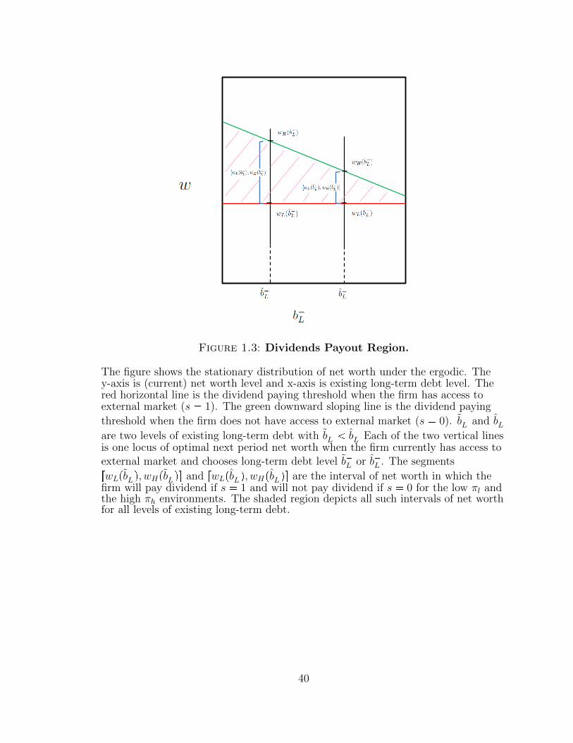
Figure 1.3: Dividends Payout Region.

The figure shows the stationary distribution of net worth under the ergodic. They-axis is (current) net worth level and x-axis is existing long-term debt level. Thered horizontal line is the dividend paying threshold when the firm has access toexternal market (s � 1). The green downward sloping line is the dividend paying

threshold when the firm does not have access to external market (s � 0). b�L and b�Lare two levels of existing long-term debt with b�L   b�L Each of the two vertical linesis one locus of optimal next period net worth when the firm currently has access toexternal market and chooses long-term debt level b�L or b�L . The segments

rwLpb�Lq, wHpb

�Lqs and rwLpb

�Lq, wHpb

�Lqs are the interval of net worth in which the

firm will pay dividend if s � 1 and will not pay dividend if s � 0 for the low πl andthe high πh environments. The shaded region depicts all such intervals of net worthfor all levels of existing long-term debt.

40

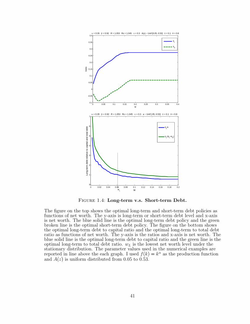
0 0.05 0.1 0.15 0.2 0.25 0.3 0.35 0.4-0.1

-0.05

0

0.05

0.1

0.15

0.2

0.25

0.3

0.35

0.4

w

Deb

ts

= 0.35 = 0.92 R = 1.053 Rs = 1.045 = 0.3 A(z) ~ Unif [0.05, 0.53] = 0.1 = 0.8

bL

bS

0 0.02 0.04 0.06 0.08 0.1 0.12 0.14 0.16 0.18 0.20

1

2

3

4

5

6

7

w

Long

-ter

m d

ebt

rela

tive

to c

apita

l and

tot

al d

ebt

= 0.35 = 0.92 R = 1.053 Rs = 1.045 = 0.3 a ~ Unif [.05, 0.53] = 0.1 = 0.8

bL/k

bL/(b

L+b

S)

wL

Figure 1.4: Long-term v.s. Short-term Debt.

The figure on the top shows the optimal long-term and short-term debt policies asfunctions of net worth. The y-axis is long-term or short-term debt level and x-axisis net worth. The blue solid line is the optimal long-term debt policy and the greenbroken line is the optimal short-term debt policy. The figure on the bottom showsthe optimal long-term debt to capital ratio and the optimal long-term to total debtratio as functions of net worth. The y-axis is the ratios and x-axis is net worth. Theblue solid line is the optimal long-term debt to capital ratio and the green line is theoptimal long-term to total debt ratio. wL is the lowest net worth level under thestationary distribution. The parameter values used in the numerical examples arereported in line above the each graph. I used fpkq � kα as the production functionand Apzq is uniform distributed from 0.05 to 0.53.

41

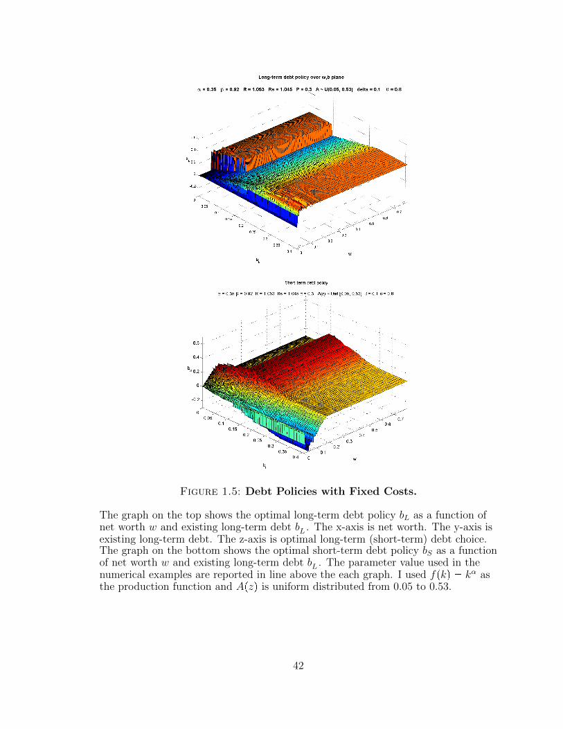
Figure 1.5: Debt Policies with Fixed Costs.

The graph on the top shows the optimal long-term debt policy bL as a function ofnet worth w and existing long-term debt b�L . The x-axis is net worth. The y-axis isexisting long-term debt. The z-axis is optimal long-term (short-term) debt choice.The graph on the bottom shows the optimal short-term debt policy bS as a functionof net worth w and existing long-term debt b�L . The parameter value used in thenumerical examples are reported in line above the each graph. I used fpkq � kα asthe production function and Apzq is uniform distributed from 0.05 to 0.53.

42

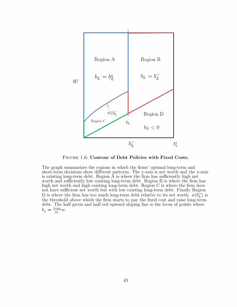
Figure 1.6: Contour of Debt Policies with Fixed Costs.

The graph summarizes the regions in which the firms’ optimal long-term andshort-term decisions show different patterns. The y-axis is net worth and the x-axisis existing long-term debt. Region A is where the firm has sufficiently high networth and sufficiently low existing long-term debt. Region B is where the firm hashigh net worth and high existing long-term debt. Region C is where the firm doesnot have sufficient net worth but with low existing long-term debt. Finally RegionD is where the firm has too much long-term debt relative to its net worth. wpb�Lq isthe threshold above which the firm starts to pay the fixed cost and raise long-termdebt. The half green and half red upward sloping line is the locus of points whereb�L �

1�pLpL

w.

43

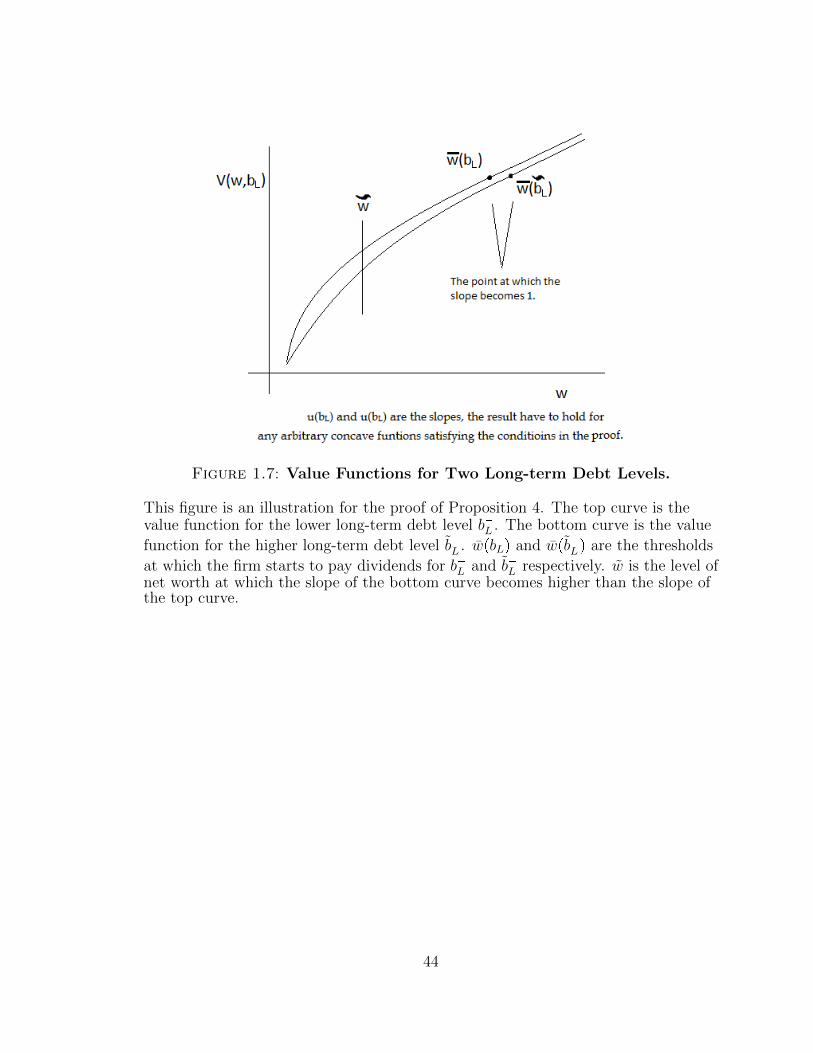
Figure 1.7: Value Functions for Two Long-term Debt Levels.

This figure is an illustration for the proof of Proposition 4. The top curve is thevalue function for the lower long-term debt level b�L . The bottom curve is the value

function for the higher long-term debt level b�L . wpbLq and wpb�Lq are the thresholds

at which the firm starts to pay dividends for b�L and b�L respectively. w is the level ofnet worth at which the slope of the bottom curve becomes higher than the slope ofthe top curve.

44

Table 1.1: Summary Statistics.This table presents the mean, standard deviation, minimum value, median,and maximum value for the variables used in the debt maturity regression(Equation 1.14). The total number of observations and the number of ob-servations identified as Post-reduction are also included at the bottom.

mean sd min p50 max

Maturity3 0.42 0.34 0.00 0.41 1.00

Log(AT) 5.33 2.07 1.61 5.10 12.42

Market NW 0.61 0.23 0.02 0.64 0.98

Marginal-Q 1.75 1.19 0.22 1.35 6.91

Oper. income 0.10 0.19 -1.11 0.13 0.56

Leverage 0.25 0.19 0.00 0.23 1.13

Asset maturity 8.23 6.18 0.30 6.53 28.22

CF Vol 0.03 0.05 0.00 0.02 0.32

Term spread 1.21 1.14 -0.36 0.83 3.06

Default prob 0.05 0.15 0.00 0.00 0.68

Whited Wu -0.27 0.11 -0.54 -0.26 -0.02

Observations 20282 Post. 8431

45

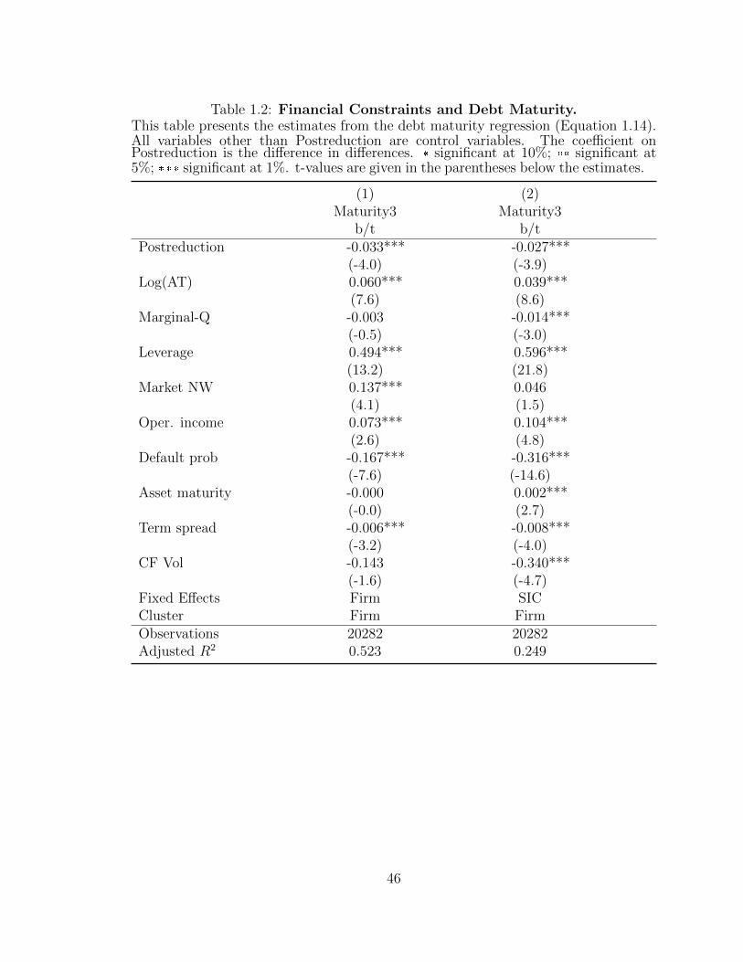
Table 1.2: Financial Constraints and Debt Maturity.This table presents the estimates from the debt maturity regression (Equation 1.14).All variables other than Postreduction are control variables. The coefficient onPostreduction is the difference in differences. � significant at 10%; �� significant at5%; ��� significant at 1%. t-values are given in the parentheses below the estimates.

(1) (2)Maturity3 Maturity3

b/t b/tPostreduction -0.033*** -0.027***

(-4.0) (-3.9)Log(AT) 0.060*** 0.039***

(7.6) (8.6)Marginal-Q -0.003 -0.014***

(-0.5) (-3.0)Leverage 0.494*** 0.596***

(13.2) (21.8)Market NW 0.137*** 0.046

(4.1) (1.5)Oper. income 0.073*** 0.104***

(2.6) (4.8)Default prob -0.167*** -0.316***

(-7.6) (-14.6)Asset maturity -0.000 0.002***

(-0.0) (2.7)Term spread -0.006*** -0.008***

(-3.2) (-4.0)CF Vol -0.143 -0.340***

(-1.6) (-4.7)Fixed Effects Firm SICCluster Firm FirmObservations 20282 20282Adjusted R2 0.523 0.249

46

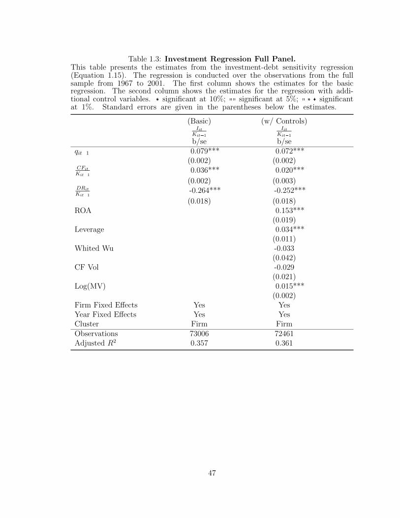
Table 1.3: Investment Regression Full Panel.This table presents the estimates from the investment-debt sensitivity regression(Equation 1.15). The regression is conducted over the observations from the fullsample from 1967 to 2001. The first column shows the estimates for the basicregression. The second column shows the estimates for the regression with addi-tional control variables. � significant at 10%; �� significant at 5%; � � � significantat 1%. Standard errors are given in the parentheses below the estimates.

(Basic) (w/ Controls)Iit

Kit�1

IitKit�1

b/se b/seqit�1 0.079*** 0.072***

(0.002) (0.002)CFitKit�1

0.036*** 0.020***

(0.002) (0.003)DRitKit�1

-0.264*** -0.252***

(0.018) (0.018)ROA 0.153***

(0.019)Leverage 0.034***

(0.011)Whited Wu -0.033

(0.042)CF Vol -0.029

(0.021)Log(MV) 0.015***

(0.002)Firm Fixed Effects Yes YesYear Fixed Effects Yes YesCluster Firm FirmObservations 73006 72461Adjusted R2 0.357 0.361

47

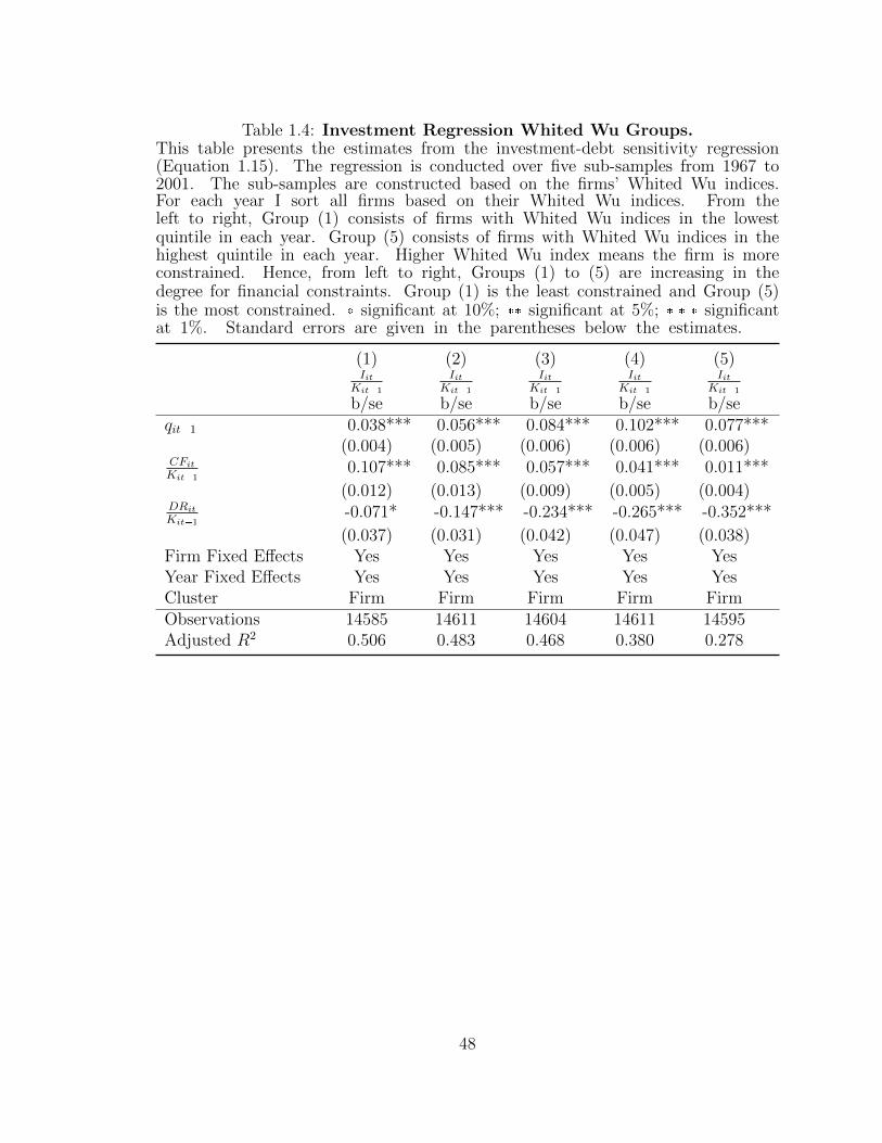
Table 1.4: Investment Regression Whited Wu Groups.This table presents the estimates from the investment-debt sensitivity regression(Equation 1.15). The regression is conducted over five sub-samples from 1967 to2001. The sub-samples are constructed based on the firms’ Whited Wu indices.For each year I sort all firms based on their Whited Wu indices. From theleft to right, Group (1) consists of firms with Whited Wu indices in the lowestquintile in each year. Group (5) consists of firms with Whited Wu indices in thehighest quintile in each year. Higher Whited Wu index means the firm is moreconstrained. Hence, from left to right, Groups (1) to (5) are increasing in thedegree for financial constraints. Group (1) is the least constrained and Group (5)is the most constrained. � significant at 10%; �� significant at 5%; � � � significantat 1%. Standard errors are given in the parentheses below the estimates.

(1) (2) (3) (4) (5)Iit

Kit�1

IitKit�1

IitKit�1

IitKit�1

IitKit�1

b/se b/se b/se b/se b/seqit�1 0.038*** 0.056*** 0.084*** 0.102*** 0.077***

(0.004) (0.005) (0.006) (0.006) (0.006)CFitKit�1

0.107*** 0.085*** 0.057*** 0.041*** 0.011***

(0.012) (0.013) (0.009) (0.005) (0.004)DRitKit�1

-0.071* -0.147*** -0.234*** -0.265*** -0.352***

(0.037) (0.031) (0.042) (0.047) (0.038)Firm Fixed Effects Yes Yes Yes Yes YesYear Fixed Effects Yes Yes Yes Yes YesCluster Firm Firm Firm Firm FirmObservations 14585 14611 14604 14611 14595Adjusted R2 0.506 0.483 0.468 0.380 0.278

48

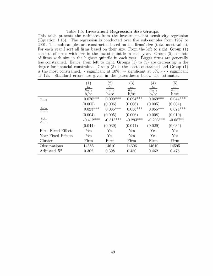
Table 1.5: Investment Regression Size Groups.This table presents the estimates from the investment-debt sensitivity regression(Equation 1.15). The regression is conducted over five sub-samples from 1967 to2001. The sub-samples are constructed based on the firms’ size (total asset value).For each year I sort all firms based on their size. From the left to right, Group (1)consists of firms with size in the lowest quintile in each year. Group (5) consistsof firms with size in the highest quintile in each year. Bigger firms are generallyless constrained. Hence, from left to right, Groups (1) to (5) are decreasing in thedegree for financial constraints. Group (5) is the least constrained and Group (1)is the most constrained. � significant at 10%; �� significant at 5%; � � � significantat 1%. Standard errors are given in the parentheses below the estimates.

(1) (2) (3) (4) (5)Iit

Kit�1

IitKit�1

IitKit�1

IitKit�1

IitKit�1

b/se b/se b/se b/se b/seqit�1 0.076*** 0.099*** 0.094*** 0.069*** 0.044***

(0.005) (0.006) (0.006) (0.005) (0.004)CFitKit�1

0.023*** 0.035*** 0.036*** 0.055*** 0.074***

(0.004) (0.005) (0.006) (0.008) (0.010)DRitKit�1

-0.412*** -0.313*** -0.293*** -0.203*** -0.087**

(0.044) (0.039) (0.041) (0.029) (0.034)Firm Fixed Effects Yes Yes Yes Yes YesYear Fixed Effects Yes Yes Yes Yes YesCluster Firm Firm Firm Firm FirmObservations 14585 14610 14606 14610 14595Adjusted R2 0.302 0.398 0.450 0.462 0.475

49

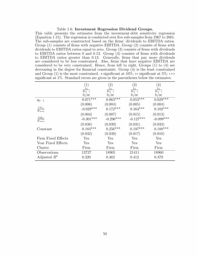
Table 1.6: Investment Regression Dividend Groups.This table presents the estimates from the investment-debt sensitivity regression(Equation 1.15). The regression is conducted over five sub-samples from 1967 to 2001.The sub-samples are constructed based on the firms’ dividends to EBITDA ratios.Group (1) consists of firms with negative EBITDA. Group (2) consists of firms withdividends to EBITDA ratios equal to zero. Group (3) consists of firms with dividendsto EBITDA ratios between 0 and 0.13. Group (4) consists of firms with dividendsto EBITDA ratios greater than 0.13. Generally, firms that pay more dividendsare considered to be less constrained. Also, firms that have negative EBITDA areconsidered to be very constrained. Hence, from left to right, Groups (1) to (4) aredecreasing in the degree for financial constraints. Group (4) is the least constrainedand Group (1) is the most constrained. � significant at 10%; �� significant at 5%; � � �significant at 1%. Standard errors are given in the parentheses below the estimates.

(1) (2) (3) (4)Iit

Kit�1

IitKit�1

IitKit�1

IitKit�1

b/se b/se b/se b/seqit�1 0.071*** 0.063*** 0.053*** 0.029***

(0.006) (0.004) (0.005) (0.004)CFitKit�1

-0.029*** 0.172*** 0.164*** 0.102***

(0.004) (0.007) (0.015) (0.013)DRitKit�1

-0.301*** -0.296*** -0.127*** -0.099***

(0.038) (0.039) (0.031) (0.033)Constant 0.183*** 0.256*** 0.197*** 0.188***

(0.032) (0.039) (0.017) (0.010)Firm Fixed Effects Yes Yes Yes YesYear Fixed Effects Yes Yes Yes YesCluster Firm Firm Firm FirmObservations 13727 18905 21411 18960Adjusted R2 0.320 0.462 0.412 0.379

50

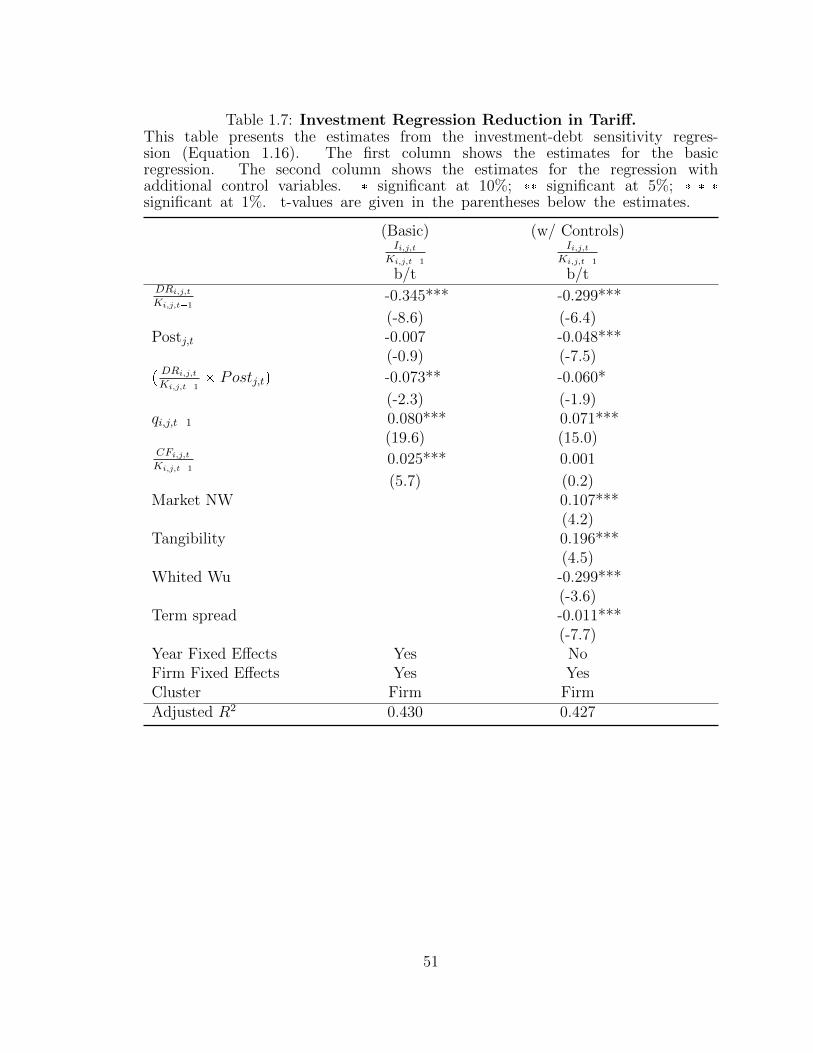
Table 1.7: Investment Regression Reduction in Tariff.This table presents the estimates from the investment-debt sensitivity regres-sion (Equation 1.16). The first column shows the estimates for the basicregression. The second column shows the estimates for the regression withadditional control variables. � significant at 10%; �� significant at 5%; � � �significant at 1%. t-values are given in the parentheses below the estimates.

(Basic) (w/ Controls)Ii,j,t

Ki,j,t�1

Ii,j,tKi,j,t�1

b/t b/tDRi,j,tKi,j,t�1

-0.345*** -0.299***

(-8.6) (-6.4)Postj,t -0.007 -0.048***

(-0.9) (-7.5)

pDRi,j,tKi,j,t�1

� Postj,tq -0.073** -0.060*

(-2.3) (-1.9)qi,j,t�1 0.080*** 0.071***

(19.6) (15.0)CFi,j,tKi,j,t�1

0.025*** 0.001

(5.7) (0.2)Market NW 0.107***

(4.2)Tangibility 0.196***

(4.5)Whited Wu -0.299***

(-3.6)Term spread -0.011***

(-7.7)Year Fixed Effects Yes NoFirm Fixed Effects Yes YesCluster Firm FirmAdjusted R2 0.430 0.427

51

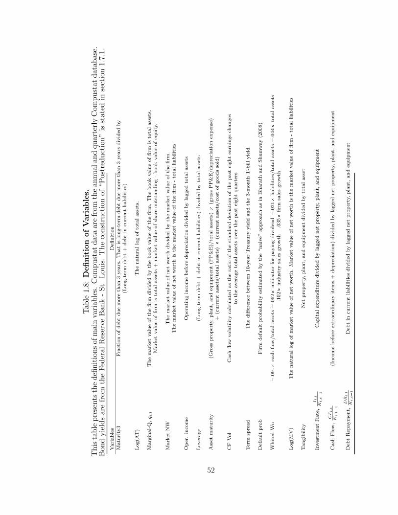
Tab

le1.

8:D

efinit

ion

of

Vari

able

s.T

his

table

pre

sents

the

defi

nit

ions

ofm

ain

vari

able

s.C

ompust

atdat

aar

efr

omth

ean

nual

and

quar

terl

yC

ompust

atdat

abas

e.B

ond

yie

lds

are

from

the

Fed

eral

Res

erve

Ban

k-

St.

Lou

is.

The

const

ruct

ion

of“P

ostr

educt

ion”

isst

ated

inse

ctio

n1.

7.1.

Vari

ab

les

Defi

nit

ion

Matu

rity

3F

ract

ion

of

deb

td

ue

more

than

3yea

rs.

Th

at

islo

ng-t

erm

deb

td

ue

more

than

3yea

rsd

ivid

edby

(Lon

g-t

erm

deb

t+

deb

tin

curr

ent

liab

ilit

ies)

Log(A

T)

Th

en

atu

ral

log

of

tota

lass

ets.

Marg

inal-

Q,q i,t

Th

em

ark

etvalu

eof

the

firm

div

ided

by

the

book

valu

eof

the

firm

.T

he

book

valu

eof

firm

isto

tal

ass

ets.

Mark

etvalu

eof

firm

isto

tal

ass

ets

+m

ark

etvalu

eof

share

ou

tsta

ndin

g-

book

valu

eof

equ

ity.

Mark

etN

WT

he

mark

etvalu

eof

net

wort

hd

ivid

edby

the

mark

etvalu

eof

the

firm

.T

he

mark

etvalu

eof

net

wort

his

the

mark

etvalu

eof

the

firm

-to

tal

liab

ilit

ies

Op

er.

inco

me

Op

erati

ng

inco

me

bef

ore

dep

reci

ati

on

div

ided

by

lagged

tota

lass

ets

Lev

erage

(Lon

g-t

erm

deb

t+

deb

tin

curr

ent

liab

ilit

ies)

div

ided

by

tota

lass

ets

Ass

etm

atu

rity

(Gro

ssp

rop

erty

,p

lant,

an

deq

uip

men

t(P

P&

E)/

tota

lass

ets)

�(g

ross

PP

&E

/d

epre

ciati

on

exp

ense

)+

(cu

rren

tass

ets/

tota

lass

ets)

�(c

urr

ent

ass

ets/

cost

of

good

sso

ld)

CF

Vol

Cash

flow

vola

tility

calc

ula

ted

as

the

rati

oof

the

stan

dard

dev

iati

on

of

the

past

eight

earn

ings

chan

ges

toth

eaver

age

tota

lass

ets

over

the

past

eight

qu

art

ers

Ter

msp

read

Th

ed

iffer

ence

bet

wee

n10-y

ear

Tre

asu

ryyie

ldan

dth

e3-m

onth

T-b

ill

yie

ld

Def

au

ltp

rob

Fir

md

efau

ltp

rob

ab

ilit

yes

tim

ate

dby

the

“n

aiv

e”ap

pro

ach

as

inB

hara

than

dS

hu

mw

ay

(2008)

Wh

ited

Wu

�.0

91�

cash

flow

/to

tal

ass

ets�.0

62�

ind

icato

rfo

rp

ayin

gd

ivid

end�.0

21�

liab

ilit

ies/

tota

lass

ets�.0

44�

tota

lass

ets

�.1

02�

ind

ust

rysa

les

gro

wth

�.0

35�

firm

sale

sgro

wth

Log(M

V)

Th

en

atu

ral

log

of

mark

etvalu

eof

net

wort

h.

Mark

etvalu

eof

net

wort

his

the

mark

etvalu

eof

firm

-to

tal

liab

ilit

ies

Tan

gib

ilit

yN

etp

rop

erty

,p

lant,

an

deq

uip

men

td

ivid

edby

tota

lass

et

Inves

tmen

tR

ate

,Ii,t

Ki,t�

1C

ap

ital

exp

end

itu

red

ivid

edby

lagged

net

pro

per

ty,

pla

nt,

an

deq

uip

men

t

Cash

Flo

w,CFi,t

Ki,t�

1(I

nco

me

bef

ore

extr

aord

inary

item

s+

dep

reci

ati

on

)d

ivid

edby

lagged

net

pro

per

ty,

pla

nt,

an

deq

uip

men

t

Deb

tR

epaym

ent,

DR

i,t

Ki,t�

1D

ebt

incu

rren

tliab

ilit

ies

div

ided

by

lagged

net

pro

per

ty,

pla

nt,

an

deq

uip

men

t

52

2

Resource Allocation and Debt Maturity

2.1 Introduction

In the previous chapter, I studied a single firm’s debt maturity decision when facing

future rollover risks. Now I investigate the aggregate implications. In recent years,

many study the effects of capital misallocation on aggregate productivity (Moll (2014),

Midrigan and Xu (2014), etc). When financial frictions prevent the most productive

agents in the economy to raise enough capital, some capital remains in the hands of

less productive agents. Hence, the aggregate productivity is lower than the first best

level. When more capital is misallocated, the aggregate productivity drops more. The

use of short-term financing leads to more rollover problems. When old debt is due and

new external financing is difficult, productive firms have to downsize and are unable to

deploy enough capital. Therefore, capital is misallocated and aggregate productivity

falls. Naturally, it seems that more use of long-term debt in the economy can reduce

the rollover risks and alleviate capital misallocation. However, in reality long-term

debt may also cause capital misallocation. For example, suppose a firm issues a long-

term debt to raise capital for the current production, but it becomes unproductive

in all future periods; unless the firm can reinvest in the market at the same interest

53

rate or unless the debt is callable, the firm will have to produce at a low rate and

keep paying the interest on the debt. On the other hand, suppose an entity lends

resources with a long-term contact, then it comes across a productive project; unless

the entity can ask for early total repayment on the loan or it can borrow from the

external market, the entity will not be able to deploy enough capital for the project.

Therefore, when there are frictions in both borrowing and lending, whether long-term

debt can help reduce misallocation depends on whether productivity is predictable. To

what degree long-term debt is helpful depends on how predictable future productivity

is. The use of long-term and short-term debt on the aggregate level should be related

to the predictability of future productivity. In this chapter, I explore the connections

between idiosyncratic productivity and aggregate debt maturity. I show why agents

in the economy sometimes choose to allocate resources more with long-term debt and

other times choose to allocate more with short-term debt. I explain how changes in

the predictability of total factor productivity (TFP) drive variations in aggregate debt

maturity. I also exam the effects of debt maturity on misallocation and aggregate

productivity.

Conventional wisdom would say that when cash flows become more volatile, firms

will want to reduce the amount of debt repayments in the short run by borrowing

with long-term debt instead of short-term debt. However, looking at the problem

only from the firm’s point of view is misleading. In equilibrium, the interest rate or

the price of long-term debt is determined taking in to account of each firm’s incentive

to borrow long-term debt in order to endure times with high uncertainty. Therefore,

on the aggregate level debt maturity may not increase with rising uncertainty. In

fact, empirical evidence suggests that on the aggregate level, corporate debt maturity

shortens during recessions or during financial crisis. Usually, both real and financial

bad times are associated with high uncertainty. Hence, it seems that aggregate debt

maturity drops as uncertainty rises. With a general equilibrium setup, my model

54

points out that the decrease in debt maturity is a direct response to the increase in

uncertainty in the idiosyncratic productivity. More specifically, the entrepreneurs will

use more short-term debt when productivity becomes less predictable.

The productivity process indeed changes from period to period. Some supports

are shown in the study of counter-cyclical uncertainty in production induced by de-

mand conditions (Bloom et al. (2007) and Bloom (2009)). Bloom and his co-authors

document that idiosyncratic productivity becomes more volatile following disasters

and in bad times. Also, Eisfeldt and Rampini (2006) point out that the dispersion

in productivity of firms is counter-cyclical. The increase in the volatility of TFP in

bad times could lead to a counter-cyclical dispersion. Moreover, as I will show in this

chapter, productivity is more persistent during expansions and less persistent during

recessions. Both facts suggest that future productivity is harder to predict during

economic downtown. Taking those facts as given, I build a dynamic general equi-

librium model in which entrepreneurs can at times allocate capital resources among

one another subject to collateral constraints. Other times entrepreneurs may fail

to find counter-parties, hence they may not be able to borrow or lend in the current

period. With persistent productivity and potential future exclusion from external cap-

ital market, entrepreneurs have incentives to arrange long-term transfer of resources

while they are able to borrow and lend. The degree to which the entrepreneurs

will conduct long-term transfer depends on how well they can predict their future

productivity. When productivity can be more precisely predicted, the entrepreneurs

will transfer more through long-term borrowing and lending. In the extreme case,

suppose the productivity is permanent and constant, the entrepreneurs will always

use long-term debt and never use any short-term debt. However, if the productivity

is serially uncorrelated, then the entrepreneurs may not use long-term debt at all

since the resource is likely to be stuck in the wrong hand in the future. Hence, it

is better for the entrepreneurs to reallocate every period with short-term debt. My

55

model provides guidelines on how the predictability of the idiosyncratic TFP relates

to aggregate debt maturity. In particular, my model explains that counter-cyclical

predictability of TFP leads to pro-cyclical aggregate debt maturity.

The pro-cyclical aggregate maturity of corporate debt has been well documented

recently. Main and Santos (2011) find that the value weighted average debt maturity

of all corporate debt in the economy is longer in good times and shorter in bad times.

Although their original paper considers financial good times and bad times, those

periods mostly coincide with expansions and recessions. They conjecture that firms

take more long-term debt as a precaution against difficult times in future. In indeed,

they discovered that the firms with strong balance sheets lengthen their current debt

and expand unused lines of credit during expansions. On the other hand, firms take

on more short-term debt and draw down their lines of credit during recessions. Chen,

Xu, and Yan (2013) also document the same pro-cyclical pattern. In their model,

long-term debt reduces the firm’s default risks. However, the long-term debt makes

the investors more exposed to liquidity shocks. During an expansion, firms issue

long-term debt so that they may have less debt maturing in the near future. When

recession comes, risk premium rises dramatically, so long-term debt is too expansive

to obtain. Hence firms switch to short-term debt. I take a look at the issue from a

aggregate point of view. Instead of relying on the premises of counter-cyclical risk

premium, I propose that the pro-cyclical pattern of aggregate debt maturity is driven

by the nature of the productivity process.

Existing literature commonly blames short-term financing for exacerbating the

problems in bad times. My model suggests that the more use of short-term debt

can also be a natural responds to the increasing uncertainty in productivity. Be-

cause the productivity is hard to predict in bad times, more reshuffle of resources is

needed each period. Hence, more short-term debt is used. Indeed, my model shows

that with low persistence in TFP, the benefit of long-term debt is small and the loss

56

in aggregate productivity is marginal. Nevertheless, the aggregate productivity of

entrepreneurs that are currently excluded from the external market is much lower

in the recessions than in the expansions. Hence there is a significant loss in aggre-

gate productivity from capital misalloction during recessions. Moreover, my model

quantifies the importance of long-term debt in alleviating capital misallocation and

preserving aggregate productivity when entrepreneurs are excluded from the external

capital market. Finally, my model illustrates that a financial crisis changes aggregate

productivity more dramatically in expansions than in recessions.

The rest of the Chapter proceeds as follows. Section 2.2 outlines the economic

environment. Section 2.3 presents the individual’s model and solutions. Section 2.4

describes the equilibrium and discusses the dynamics of the economic system. Section

2.5 investigates the relation of debt maturity and aggregate TFP. Finally, section 2.6

concludes the chapter.

2.2 Environment

In a frictionless economy, resources are always allocated to the most productivity

agents, therefore each realization of idiosyncratic TFP does not affect the overall pro-

duction on the aggregate level. Moreover, on the micro level, each agent does not have

to worry about future resource allocation, he only considers his borrowing or lending

decision on the spot for each period repetitively. However, When facing financial fric-

tions, entrepreneurs are sometimes unable to adjust their financial structure. Hence

they will tend to adjust more when they have the chance to do so. In particular, they

will use long-term debt to arrange long-term transfers in case they will not be able to

transfer in the future. When the volatility of the TFP shocks is high or when the TFP

process is less persistence, current TFP is less informative about future TFP. Hence

entrepreneurs would like to adjust through short-term contacts and adjust more each

period while taking more risk of stuck with suboptimal financial structure. To study

57

this intuition more rigorously, I build a general equilibrium model with the following

setup.

There is a continuum of entrepreneurs each identified by his or her own net worth

a, existing long-term debt b�, and TFP z. The entrepreneurs can borrow and lend

resources to one other, produce with capital and labor, and consume the output. The

entrepreneurs have log utility and discount future utility at rate β. Due to some

exogenous financial frictions, the entrepreneur may not be able to borrow or lend

with probability p. For future convenience, I say an entrepreneur is “in-the-market”

if he can borrow and lend and denote such a state with s � 1. I say an entrepreneur

is “out-of-market” if he cannot borrow or lend and denote the state with s � 0. The

exact micro-foundations for this frictions will be future works by itself. One could

think of it as a search friction where with probability p the entrepreneur does not find

a counter-party. The main results do not depend on this specific form of formulation.

In fact, I could use exogenous financing cost function that assign different costs of

borrowing and lending for a continuum of states.

In order to focus on the long-term debt’s role as a prearrangement vehicle, I stay

away from the entrepreneurs’ debt manipulating practice arise from the difference in

interest rates. To do so, I put restriction on the form of long-term debt payoff. I

require that the long-term debt pays the same as the short-term debt does when the

entrepreneur is in the market and pays a different rate if the entrepreneur is “out-of-

market”. So that the difference in interest rate occurs only in “out-of-market” state

where the entrepreneurs cannot adjust their capital structure.

The timeline is shown in Figure 2.1. Each day, the entrepreneur wakes up with his

net worth, a, and money borrowed last period, b�. Also, he observes his productivity

z and learns whether he is “in-the-market”. If he is “in-the-market”, in the morning,

before production he can borrow new short-term and long-term debt subject to a

collateral constraint. Then, he uses the money (own and borrowed) to buy capital

58

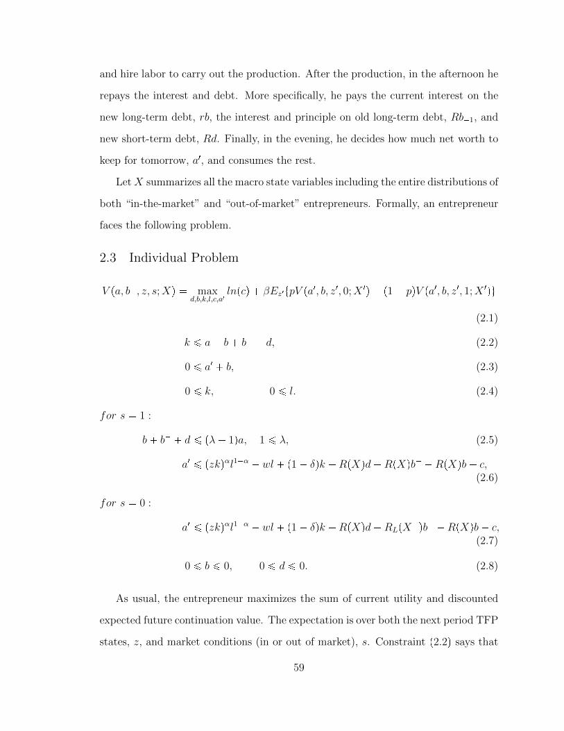
and hire labor to carry out the production. After the production, in the afternoon he

repays the interest and debt. More specifically, he pays the current interest on the

new long-term debt, rb, the interest and principle on old long-term debt, Rb�1, and

new short-term debt, Rd. Finally, in the evening, he decides how much net worth to

keep for tomorrow, a1, and consumes the rest.

LetX summarizes all the macro state variables including the entire distributions of

both “in-the-market” and “out-of-market” entrepreneurs. Formally, an entrepreneur

faces the following problem.

2.3 Individual Problem

V pa, b�, z, s;Xq � maxd,b,k,l,c,a1

lnpcq � βEz1tpV pa1, b, z1, 0;X 1q � p1� pqV pa1, b, z1, 1;X 1qu

(2.1)

k ¤ a� b� b� � d, (2.2)

0 ¤ a1 � b, (2.3)

0 ¤ k, 0 ¤ l. (2.4)

for s � 1 :

b� b� � d ¤ pλ� 1qa, 1 ¤ λ, (2.5)

a1 ¤ pzkqαl1�α � wl � p1� δqk �RpXqd�RpXqb� �RpXqb� c,(2.6)

for s � 0 :

a1 ¤ pzkqαl1�α � wl � p1� δqk �RpXqd�RLpX�qb� �RpXqb� c,

(2.7)

0 ¤ b ¤ 0, 0 ¤ d ¤ 0. (2.8)

As usual, the entrepreneur maximizes the sum of current utility and discounted

expected future continuation value. The expectation is over both the next period TFP

states, z, and market conditions (in or out of market), s. Constraint p2.2q says that

59

the total capital used in production must be financed out of the entrepreneur’s own

net worth and external borrowing. Constraint p2.3q makes sure that the entrepreneur

can only lend out as much as his own net worth at the end of the period. Collateral

constraint p2.5q states that the entrepreneur can only borrow up to a fraction pλ�1q of

its net worth. Hence, one can think of λ as the maximal leverage for the entrepreneur.

The budget constraints p2.6q and p2.7q govern the laws of motion for the entrepreneur’s

net worth. The entrepreneur’s end of period net worth is his profit from production

net of all liabilities and consumption. Although the principle of the long-term debt

is not due at the end of the current period, I still exclude it from the net worth

calculation. Since end period net worth determines the maximal leverage for next

period, this definition of net worth prevent levering on borrowed money. Also, the

difference between constraint p2.6q and p2.7q is that when the entrepreneur is “out-

of-market”, he pays a different rate RL on the long-term debt. This rate RL will be

pinned down in equilibrium and it will balance the demand and supply of long-term

debt. Finally, if the entrepreneur is “out-of-market”, then he is unable to borrow or

lend through either short or long term debt as stated by the set of constraints p2.8q.

Next, I characterize the solution of the model. By setup, the capital, labor, and

short-term debt decisions do not involve intertemporal trade-offs. Also, while in the

market, the entrepreneur can always adjust the total debt level with short term debt

subject to the linear collateral constraint and non-negativity constraint on capital.

Hence, I can separate the problems in the following way. First, the entrepreneur

chooses capital, labor, and total leverage to maximize his current wealth. Then he

decides on consumption, end period net worth, and long-term debt. The short-term

debt will be the difference between the total debt and the long-term debt (both old

and newly issued).

60

2.3.1 Capital, labor, and total debt

The solution to the entrepreneur’s within period profit maximization problem is sum-

marize by the following lemma:

Lemma 13.

kpa, b�, z, 1q �

"λa, if z ¥ z0, if z   z

where RpXq � zpXqπpXq � 1� δ,

π � αp1� α

W pXqqp1�αq{α.

kpa, b�, z, 0q � a� b�, lpa, b�, z, sq � p1� α

W pXqq

1α zk

First, the optimal labor decision is always linear in productivity and optimal cap-

ital level. When entrepreneurs are in the market, they lever up and produce at their

maximal scale allowed by the collateral constraint if they productivities are higher

than a cut-off level, z. Otherwise, they lend out all resources. When entrepreneurs

are out of market, they produce with all their resources regardless the productivity

level since they are living in autarky. Hence, the entrepreneur’s profits from produc-

tion, Πpa, b�, z, sq � pzkqαl1�α�Wl�p1� δqk, for state s � 0 and state s � 1 can be

reduced to Πpa, b�, z, 1q � maxtzπ � 1 � δ, 0uk and Πpa, b�, z, 0q � rzπ � 1 � δsk re-

spectively. Those are standard results due to the constant return to scale technology

as in Moll (2014).

Lemma 14. Existing long-term debt b� only affects short-term debt choice when

entrepreneurs are currently in the market.

When an entrepreneur is “in-the-market”, he can use both long-term and short-

term debt subject to a collateral constraint on the total amount of borrowing. The

maximum amount of resource he can borrow or lend is pinned down by his net worth.

61

Plus, the long-term and short-term interest rates are the same. Hence, the old long-

term debt outstanding will have no effects. In fact, any old long-term debt outstand

can be counted towards short-term debt.

Therefore, the problem can be reduced to the following consumption-saving and

portfolio choice problem.

2.3.2 Consumption, net worth and long-term debt

With optimal profit and leverage, I can rewrite the remaining problem as a simple

consumption, saving, and portfolio choice problem:

V pa, b�, z, sq � maxa1,b

lnpcq � βEz1tpV pa1, b, z1, 0q � p1� pqV pa1, b, z1, 1qu

a1 � rλmaxtzπ � r � δ, 0u �Rsa� c, 0 ¤ a1 � b, for s � 1

a1 � pzπ � 1� δqpa� b�q �RLb� � c b � 0, for s � 0

where π � αp1�αWqp1�αq{α.

Now let’s denote the returns on saving for states s � 1, 2 as Apz, 0q � zπ � 1 � δ

and Apz, 1q � λmaxtzπ � r � δ, 0u � RpXq respectively. Basically, A(z,s) is the

return on net worth (or internal funds) for state pz, sq. Let ηa1�b be the multiplier on

constraint p2.3q. I obtain the following optimality conditions.

Consumption Saving: (proportion to be consumed) for s � 0, 1

1

cpa, b�, z, sq� β

» 8

0

ppApz1, 0q

cpa1, b, z1, 0q�p1� pqApz1, 1q

cpa1, b, z1, 1qqψpz1|zqdz1 � ηa1�b,

Portfolio Choice: (proportion in long-term debt) for s � 1

» 8

0

Apz1, 0q �RL

cpa1, b, z1, 0qψpz1|zqdz1 � ηa1�b � 0,

Since the entrepreneur can always use short-term debt to make up the gap when

he is “in-the-market”, The long-term debt decision does not directly affect the en-

trepreneur’s saving decision through the budget constraint when s � 1. In general, if

62

he thinks that he will likely be very productive next period, he will borrow through

long-term debt to reduce its debt repayments at the end of the period. Hence, he

won’t have to downsize as much even if he is “out-of-market” next period. On the

other hand, if he thinks that he will likely be unproductive next period, he will lend

in long-term debt and receive the riskless return of RL tomorrow.

With log utility, the saving decision is separated from the long-term debt in the

sense that the consumption and saving decisions are not affected by long-term debt

choice. When constraint p2.3q is binding, the entrepreneur lends out all he has, hence

b � �a1.

Because of log utility and constant return to scale production, the decision rules

are linear in wealth. In our model, since total borrowing is constrained by net worth,

wealth is simply the product of net worth, a, and return on net worth, Apz, sq.

Furthermore, the proportional decisions on consumption, saving, and long-term debt

are only functions of current productivity level, z, and independent of the size or

wealth of the entrepreneur. Hence, I am able to characterize the affect of current

productivity on entrepreneurs’ decisions of what fraction of wealth they will consume,

save, and borrow/lend through long-term debt.

As long as zπ�1�δ ¡ 0, our result does not depend on the domain of productivity

shocks. For convenience I let z P r0,8q. Assuming RL ¥ Epz1|z � 0qπ� 1� δ, which

is always the case in equilibrium, I have the following solution.

Proposition 15. The policy function can be characterized as:

c � p1� βqApz, 1qa, b � φbpzqApz, 1qa, a1 � βApz, 1qa, for s � 1

c � p1�βqtApz, 0qpa�b�q�RLb�u, b � 0, a1 � βtApz, 0qpa�b�q�RLb

�u, for s � 0

φbpzq is defined by

# ³80

RLψpz1|zq

pβ�φbqpz1π�1�δq�RLφbdz1 � 1

β, if z ¡ z

φbpzq � �β, if z ¤ z

where z satisfies RL � Epz1|zqπ � 1� δ.

63

Since I have the closed form solutions, I can easily conduct the following compar-

ative statics.

Corollary 16. Proportionally long-term borrowing φb is decreasing in RL.

Naturally, when long-term debt becomes more expensive, entrepreneurs borrow

less of it.

Corollary 17. Entrepreneurs with higher initial net worth (a), consume more, ac-

cumulate more net worth, and use more debt. Entrepreneurs with higher current

productivity (z) consume more and accumulate more net worth.

As mentions before, all decisions are linear in net worth, a. Therefore, with the

same current productivity, bigger entrepreneurs make decisions on a large scale. The

effect of z on long-term debt, b, is subtle. Current productivity plays two roles.

First, it contributes to current wealth. Second, it provides information about future

productivity. To investigate this second effect, I put a commonly accepted structure

on the productivity process.

In particular, I assume that the productivity shocks are persistent, so the cur-

rent productivity level can predict future productivity levels. Hence, more and less

productive firms today will make different proportional long-term debt decisions.

Assumption 4. Suppose for any z�   z�, ψpz1�q first order stochastically dominates

ψpz1�q.

Under the assumption and from long-term debt policy given in proposition 15, I

have the following proposition.

Proposition 18. The optimal policy on long-term debt, φbpzq, is increasing in current

productivity, z. Moreover, φbpzq ¤ 0, for z ¤ zb, and φbpzq ¥ 0, for z ¥ zb, where zb

is defined by³80

ψpz1|zbq

z1π�1�δdz1 � 1

RL.

64

In corollary 17, we see that more productive entrepreneurs consume more and

keep more net worth. However, for long-term debt that is not always the case. En-

trepreneurs with current productivity greater than zb are borrowers. For them, an

increase in z indeed leads to more borrowing. However, for the lenders, increase in

z leads to a reduction in proportional lending, φb, but an increase in current wealth,

Apz, 1qa. Therefore, total lending in long-term debt may either rise or fall. Also,

Proposition 18 suggests that on an individual level, debt maturity is pro-cyclical.

That is the entrepreneurs will borrow more long-term debt when productivity is high

as in expansion and borrow less long-term debt when productivity is low as in re-

cession. However, under general equilibrium, the interest rate on the long-term debt

may also increase. Hence, it is unclear weather on the aggregate level, debt maturity

is pro-cyclical. In the next section, I will investigate what happens on the aggregate

level under general equilibrium. But first, let’s give a specific form to the TFP process

for easier exploration.

Suppose the productivity process is: logpz1q � ρ logpzq�σ2

2�σε, where ε � Np0, 1q.

I investigate how the persistence of productivity affects the long-term debt policy.

Proposition 19. φb is increasing in ρ for z ¡ 1 and decreasing in ρ for z   1.

The intuition is straight forward. For entrepreneurs with z ¡ 1, increase in ρ,

raises the condition mean of z1, hence the future investment opportunity becomes

better. Thus, the entrepreneurs borrow more long-term debt. The exact opposite

applies for entrepreneurs with z   1.

Proposition 20. φb is decreasing in σ.

When z1 becomes more volatile, the future investment is riskier, hence entrepreneurs

want to engage in more precautionary saving by reducing their long-term debt or lend

more through long-term debt.

65

2.4 Equilibrium and Dynamics

Let Gtpa, zq and gpa, zq be the cdf and pdf for the measure of entrepreneurs who are

currently in the market. Since, existing long-term debt does not matter when the

entrepreneurs are in the market. They can be measured simply with net worth a and

productivity z. Let Htpa, b�, zq and hpa, b�, zq be the measure of entrepreneurs who

are currently out of the market. The competitive equilibrium is defined by time paths

of prices Rt, Wt, t ¥ 0 and corresponding quantities, such that (i) taking equilibrium

prices as given, each entrepreneur maximizes p2.1q subject to p2.2q to p2.8q , and (ii)

the short-term debt, long-term debt, and labor markets clear at each point in time:

»z

»a

ktpa, zqdGtpa, zq �

»z

»a

adGtpa, zq,

»z

»a

btpa, zqdGtpa, zq � 0,

»z

»a

ltpa, zqdGtpa, zq �

»z

»a

»b�ltpa, zqdHtpa, b

�, zq � L.

The first equation is the market clearing condition for total resources. It states

that the total use of resources in production equals the total amount of resources

available at the beginning of the period. The second equation is the market clearing

condition for long-term debt. It states that overall there is net zero supply of long-

term debt since the entrepreneurs simply borrow and lend from one another. The

last equation is the market clearing condition for labor. It insures that at the current

wage level, all labor units are used by all the entrepreneurs.

The short term debt interest rate is determined by the marginal active (the ones

who produce) entrepreneurs in the market. Formally, I have the following relation:³80

³8zagpa, zqdzda � 1

λ

³80

³80agpa, zqdzda, where 1

λcan be viewed as the down pay-

ment per unit of investment the active entrepreneurs must provide with their own

money. The relation states that the total amount of resources in the hands of active

66

entrepreneurs is a fraction 1λ

of the total resources that are in the market. Later I will

discuss in more details about how the short-term interest rate is determined. Next,

I discuss how to keep track of the distributions of both in and out of the market

entrepreneurs.

Each period, there will be a fraction p of the entrepreneurs are “out-of-market”.

Their decisions are simple and do not affect the interest rates of the debt. Hence, I

focus mainly on the distribution and decisions of the entrepreneurs that are in the

market. Depending on the realizations of their idiosyncratic productivity shocks, A

spectrum of “in-the-market” entrepreneurs can be obtained as follows.

For all the entrepreneurs that are in the market, the entrepreneurs with pro-

ductivity higher than z will be active and produce. They borrow from the ones with

productivity lower than z. The entrepreneurs with productivity higher than zb borrow

long-term debt. Moreover, the higher the productivity, the more long-term debt is

borrowed. On the other hand, The entrepreneurs with productivity lower than zb

lend in long term. Furthermore, the ones with lower productivity lend more in long

term. Finally, there is a cut-off level of productivity z below which all entrepreneurs

lend all their net worth out through long-term debt. That is their optimal choice of

φb is �β. The cut-off z is determined by RL � Epz1|zqπ � 1� δ.

Now I derive the distributions of both “in-the-market” and “out-of-market” en-

trepreneurs. Let gtpa, φ�b , zq be the measure of entrepreneurs who are previously

“in-the-market” with net worth a, long-term debt proportion φ�b , and productivity

z. Let htpa, 0, zq be the measure of entrepreneurs who are previously “out-of-market”

with net worth a, zero long-term debt, and productivity z. The long-term debt is zero

because the entrepreneurs cannot raise long-term debt if they are “out-of-market” in

last period.

For entrepreneurs that are previously “in-the-market”, their existing long-term

debt is decided in last period based on their productivity in last period zt�1. I define

67

the wealth share of “in-the-market” entrepreneur with long-term debt to wealth ratio,

φ�b , and productivity, z, as:

u1t pφ

�b , zq �

1

Kint

» 8

0

a gtpa, φ�b , zq da,

where gtpa, φ�b , zq is the measure of “in-the-market” entrepreneurs with net worth a,

long-term debtφ�bβa, and productivity z and Kin

t �³80

³80

³8�βa gtpa, φ

�b , zqdφ

�b dzda

is the total resources that are in the market.

For entrepreneurs that are previously “out-of-market”, the existing long-term debt

is zero. Hence, I can track their wealth share with productivity alone. I define the

wealth share of “ out-of-market” entrepreneur with productivity, z, as:

u0t pzq �

1

Koutt

» 8

0

a htpa, 0, zq da, (2.9)

where htpa, 0, zq is the measure of “out-of-market” entrepreneur with net worth a,

zero long-term debt, and productivity z and Koutt �

³80

³80a htpa, 0, zqdzda is the total

resource that are out of the market. Similarly, the wealth share of the entrepreneurs

in the market with productivity z should be defined as:

ωtpzq �1

Kint

» 8

�β

» 8

0

a gtpa, φ�b , zq dadφ

�b �

1

Kint

» 8

0

» 8

0

a gtpa, φ�b pzt�1q, zq dadzt�1,

(2.10)

where Kint �

³80

³80

³8�βa gtpa, φ

�b , zqdφ

�b dzda is the total resource that are in the

market.

Taking in to account the measures of entrepreneurs both in and out of the market,

the economy as a whole evolve in the following way.

For entrepreneurs that are “in-the-market” in period t, I have the following laws

of motion for the wealth shares. First, the entrepreneurs that have productivity z1

68

next period have wealth shares:

ωt�1pz1q �

Kint

³80Apz, 1qωtpzqψpz

1|zq dz �Koutt

³80Apz, 1qu0

t pzqψpz1|zq dz

Kint

³80Apz, 1qωtpzq dz �Kout

t

³80Apz, 1qu0

t pzqdz(2.11)

For z ¡ z, φbpzq is an interior optimal choice depending on z, so the wealth share

of the type pφbpzq, z1q entrepreneurs is:

u1t�1pφbpzq, z

1q �Kint Apz, 1qωtpzq ψpz

1|zq �Koutt Apz, 1qu0

t pzqψpz1|zq

Kint

³80Apz, 1qωtpzq dz �Kout

t

³80Apz, 1qu0

t pzqdz(2.12)

For z ¤ z, φbpzq � �β and the wealth share of the type p�β, z1q entrepreneurs is:

u1t�1p�β, z

1q �

³z0Kint Apz, 1qωtpzq ψpz

1|zqdz �³z0Koutt Apz, 1qu0

t pzqψpz1|zqdz

Kint

³80Apz, 1qωtpzq dz �Kout

t

³80Apz, 1qu0

t pzqdz(2.13)

Finally, for entrepreneurs that have productivity z1 next period and are “out-of-

market” in period t, the wealth share is:

u0t�1pz

1q � (2.14)

Kint

³8�β

³80 tpβ � φ�b qpzπ � 1 � δq �RLφ

�b uu

1t pφ

�b , zqψpz

1|zqdzdφ�b �Koutt

³80 βpzπ � 1 � δqu0

t pzqψpz1|zqdz

Kint

³8�β

³80 tpβ � φ�b qpzπ � 1 � δq �RLφ

�b uu

1t pφ

�b , zqdzdφ

�b �Kout

t

³80 βpzπ � 1 � δqu0

t pzqdz

Given the current wealth shares ωtpzq, u1t pφ

�b , zq, u

0t pzq and transition density ψpz1|zq

for type z entrepreneurs, ωt�1pz1q, u1

t�1pφb, z1q, u0

t�1pz1q keep track of the wealth shares

of entrepreneurs at the beginning of period t�1. Eventually, these wealth shares will

stay unchanged as the system reach its stationary equilibrium.

From Lemma 1, the individual labor choice is lpa, b�, z, sq � p 1�αW pXq

q1α zk, hence the

labor market clearing condition for the economy is³80lpa, b�, z, sqωpzqdz �

³80p 1�αW pXq

q1α

zkωpzqdz � L. In equilibrium the wage is determined by the distributions of en-

trepreneurs both in and out of the market. More specifically, the wage is obtained

69

by:

Wt �rp1 � pq

³8z λzpKin

t ωtpzq �Koutt u0

t pzqqdz � p³80 zpKin

t

³80 p1 �

φ�bβqu1t pφ

�b , zqdz

� �Koutt u0

t pzqqdzsα

p1 � αq�1Lα(2.15)

The short-term interest rate is determined by the marginal borrower, which has

productivity z. Since some entrepreneurs that are currently in the market may be out

of the market in previous period, both the wealth shares of entrepreneurs in and out

of the market matter. The degree of financial friction and the distribution of wealth

shares of the entrepreneurs in the market will pin down z. More specifically, I have

1� 1�z0

Kint wtpzq � Kout

t u0t pzq

Kint �Kout

tdz.

The long-term interest rate is determined by the market clearing condition for

long-term debt. With wealth shares and long-term debt policy, the condition states³80φbpz,RLq

Kint wtpzq � Kout

t u0t pzq

Kint �Kout

tdz � 0. Finally, to find the total amount of resources in

and out of the market, I have the following relations. For total resources in the market,

Kint�1 � p1�pqtKin

t

³80Apz, 1qωtpzq dz�K

outt

³80Apz, 1qu0

t pzqdzu. For the resources out

of the market, Koutt�1 � ptKin

t

³8�β

³80tpβ � φ�b qpzπ � 1 � δq � RLφ

�b uu

1t pφ

�b , zqdzdφ

�b �

Koutt

³80βpzπ � 1� δqu0

t pzqdzu.

Now I investigate what affects the total use of long-term debt. From Proposition

19, I know that on the individual level, entrepreneurs with high (low) productivity

will borrow (lend) more long-term debt as the productivity process becomes more

persistent. Since both the demand and supply of long-term debt increase, the overall

use of long-term debt must increase. Figure 2.4 illustrates the increase use of long-

term debt for entrepreneurs with both low and high current productivities. The

green solid line presents the long-term debt policy when TFP is more persistent

(ρ � .9). The teal dotted broken line presents the long-term debt policy when TFP

is less persistent (ρ � .5). Comparing the two line, we see that entrepreneurs with

TFP below 1.36 choose to reduce long-term debt and entrepreneurs with TFP above

70

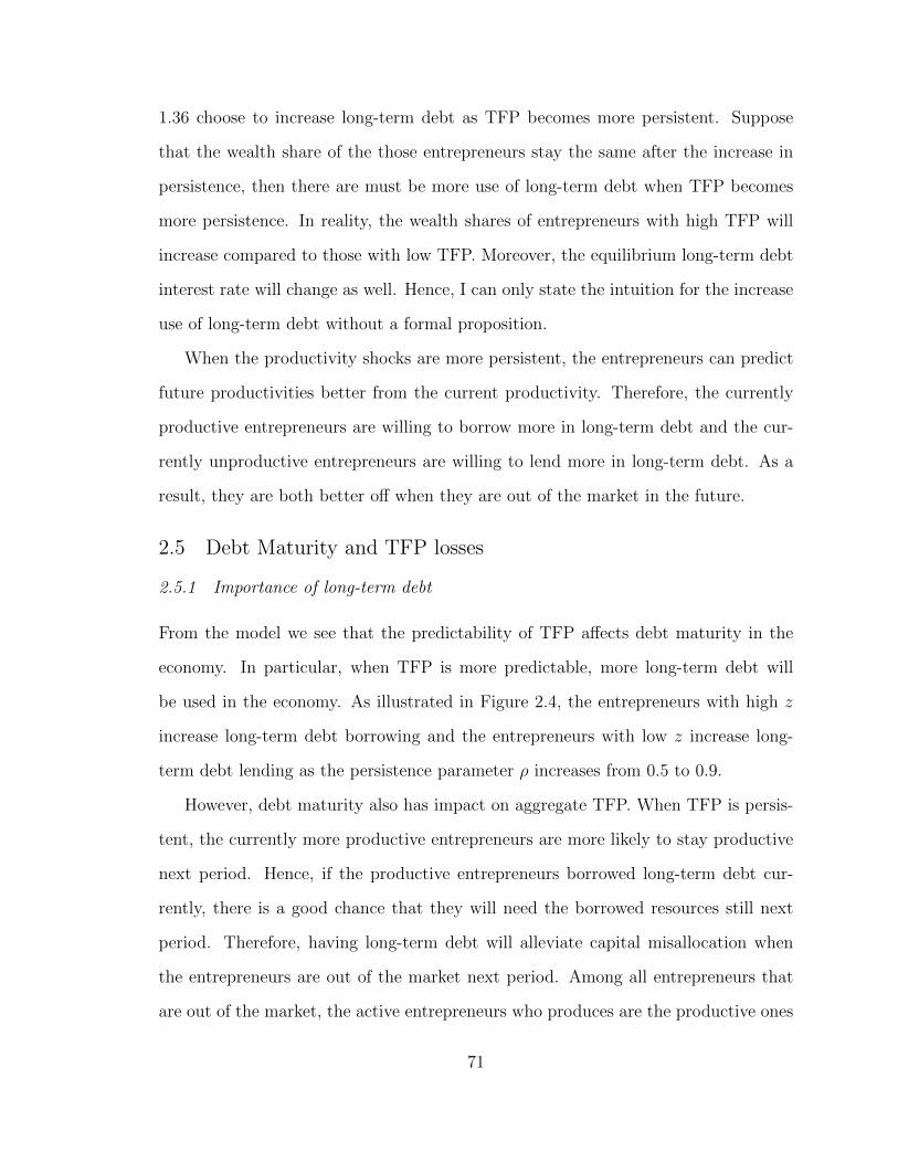
1.36 choose to increase long-term debt as TFP becomes more persistent. Suppose

that the wealth share of the those entrepreneurs stay the same after the increase in

persistence, then there are must be more use of long-term debt when TFP becomes

more persistence. In reality, the wealth shares of entrepreneurs with high TFP will

increase compared to those with low TFP. Moreover, the equilibrium long-term debt

interest rate will change as well. Hence, I can only state the intuition for the increase

use of long-term debt without a formal proposition.

When the productivity shocks are more persistent, the entrepreneurs can predict

future productivities better from the current productivity. Therefore, the currently

productive entrepreneurs are willing to borrow more in long-term debt and the cur-

rently unproductive entrepreneurs are willing to lend more in long-term debt. As a

result, they are both better off when they are out of the market in the future.

2.5 Debt Maturity and TFP losses

2.5.1 Importance of long-term debt

From the model we see that the predictability of TFP affects debt maturity in the

economy. In particular, when TFP is more predictable, more long-term debt will

be used in the economy. As illustrated in Figure 2.4, the entrepreneurs with high z

increase long-term debt borrowing and the entrepreneurs with low z increase long-

term debt lending as the persistence parameter ρ increases from 0.5 to 0.9.

However, debt maturity also has impact on aggregate TFP. When TFP is persis-

tent, the currently more productive entrepreneurs are more likely to stay productive

next period. Hence, if the productive entrepreneurs borrowed long-term debt cur-

rently, there is a good chance that they will need the borrowed resources still next

period. Therefore, having long-term debt will alleviate capital misallocation when

the entrepreneurs are out of the market next period. Among all entrepreneurs that

are out of the market, the active entrepreneurs who produces are the productive ones

71

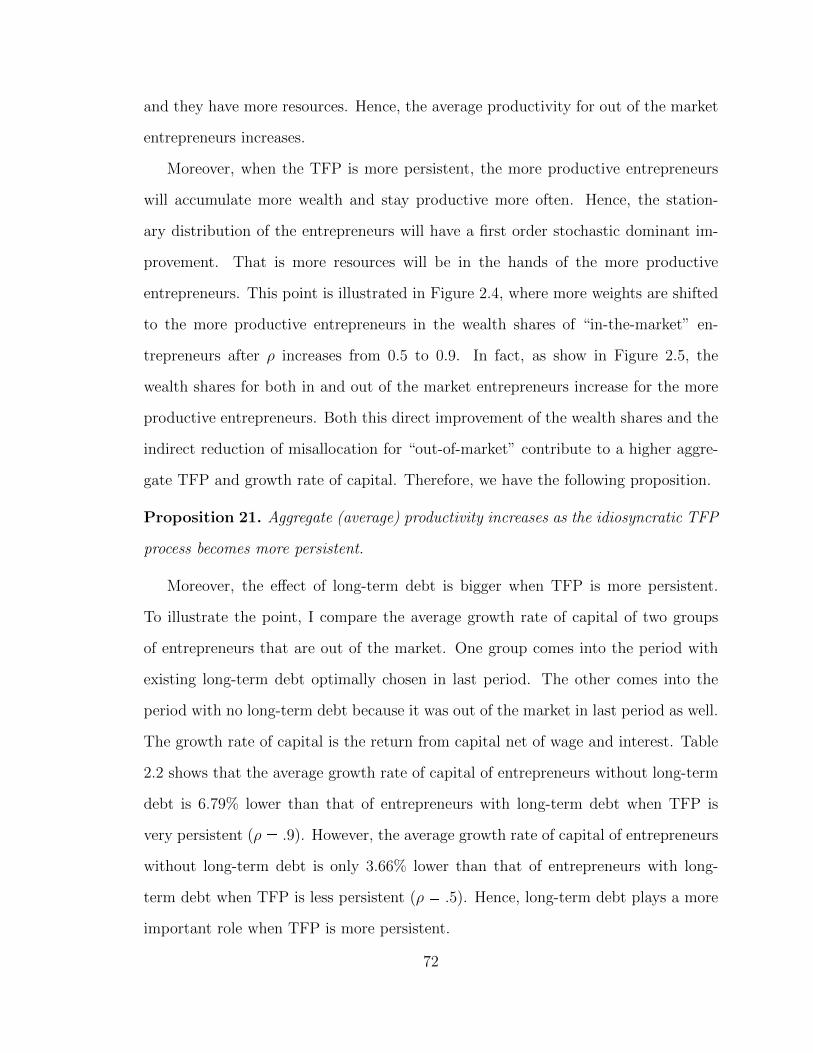
and they have more resources. Hence, the average productivity for out of the market

entrepreneurs increases.

Moreover, when the TFP is more persistent, the more productive entrepreneurs

will accumulate more wealth and stay productive more often. Hence, the station-

ary distribution of the entrepreneurs will have a first order stochastic dominant im-

provement. That is more resources will be in the hands of the more productive

entrepreneurs. This point is illustrated in Figure 2.4, where more weights are shifted

to the more productive entrepreneurs in the wealth shares of “in-the-market” en-

trepreneurs after ρ increases from 0.5 to 0.9. In fact, as show in Figure 2.5, the

wealth shares for both in and out of the market entrepreneurs increase for the more

productive entrepreneurs. Both this direct improvement of the wealth shares and the

indirect reduction of misallocation for “out-of-market” contribute to a higher aggre-

gate TFP and growth rate of capital. Therefore, we have the following proposition.

Proposition 21. Aggregate (average) productivity increases as the idiosyncratic TFP

process becomes more persistent.

Moreover, the effect of long-term debt is bigger when TFP is more persistent.

To illustrate the point, I compare the average growth rate of capital of two groups

of entrepreneurs that are out of the market. One group comes into the period with

existing long-term debt optimally chosen in last period. The other comes into the

period with no long-term debt because it was out of the market in last period as well.

The growth rate of capital is the return from capital net of wage and interest. Table

2.2 shows that the average growth rate of capital of entrepreneurs without long-term

debt is 6.79% lower than that of entrepreneurs with long-term debt when TFP is

very persistent (ρ � .9). However, the average growth rate of capital of entrepreneurs

without long-term debt is only 3.66% lower than that of entrepreneurs with long-

term debt when TFP is less persistent (ρ � .5). Hence, long-term debt plays a more

important role when TFP is more persistent.

72

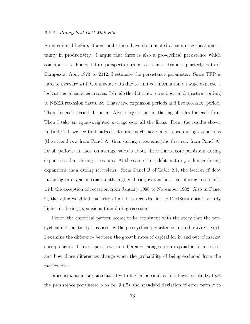
2.5.2 Pro-cyclical Debt Maturity

As mentioned before, Bloom and others have documented a counter-cyclical uncer-

tainty in productivity. I argue that there is also a pro-cyclical persistence which

contributes to blurry future prospects during recessions. From a quarterly data of

Compustat from 1973 to 2012, I estimate the persistence parameter. Since TFP is

hard to measure with Compustat data due to limited information on wage expense, I

look at the persistence in sales. I divide the data into ten subperiod datasets according

to NBER recession dates. So, I have five expansion periods and five recession period.

Then for each period, I run an AR(1) regression on the log of sales for each firm.

Then I take an equal-weighted average over all the firms. From the results shown

in Table 2.1, we see that indeed sales are much more persistence during expansions

(the second row from Panel A) than during recessions (the first row from Panel A)

for all periods. In fact, on average sales is about three times more persistent during

expansions than during recessions. At the same time, debt maturity is longer during

expansions than during recessions. From Panel B of Table 2.1, the faction of debt

maturing in a year is consistently higher during expansions than during recessions,

with the exception of recession from January 1980 to November 1982. Also in Panel

C, the value weighted maturity of all debt recorded in the DealScan data is clearly

higher in during expansions than during recessions.

Hence, the empirical pattern seems to be consistent with the story that the pro-

cyclical debt maturity is caused by the pro-cyclical persistence in productivity. Next,

I examine the difference between the growth rates of capital for in and out of market

entrepreneurs. I investigate how the difference changes from expansion to recession

and how those differences change when the probability of being excluded from the

market rises.

Since expansions are associated with higher persistence and lower volatility, I set

the persistence parameter ρ to be .9 (.5) and standard deviation of error term σ to

73

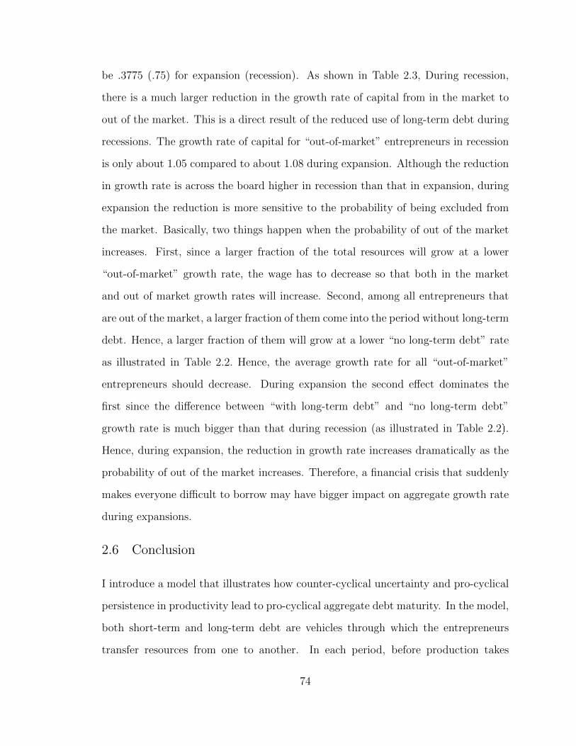
be .3775 (.75) for expansion (recession). As shown in Table 2.3, During recession,

there is a much larger reduction in the growth rate of capital from in the market to

out of the market. This is a direct result of the reduced use of long-term debt during

recessions. The growth rate of capital for “out-of-market” entrepreneurs in recession

is only about 1.05 compared to about 1.08 during expansion. Although the reduction

in growth rate is across the board higher in recession than that in expansion, during

expansion the reduction is more sensitive to the probability of being excluded from

the market. Basically, two things happen when the probability of out of the market

increases. First, since a larger fraction of the total resources will grow at a lower

“out-of-market” growth rate, the wage has to decrease so that both in the market

and out of market growth rates will increase. Second, among all entrepreneurs that

are out of the market, a larger fraction of them come into the period without long-term

debt. Hence, a larger fraction of them will grow at a lower “no long-term debt” rate

as illustrated in Table 2.2. Hence, the average growth rate for all “out-of-market”

entrepreneurs should decrease. During expansion the second effect dominates the

first since the difference between “with long-term debt” and “no long-term debt”

growth rate is much bigger than that during recession (as illustrated in Table 2.2q.

Hence, during expansion, the reduction in growth rate increases dramatically as the

probability of out of the market increases. Therefore, a financial crisis that suddenly

makes everyone difficult to borrow may have bigger impact on aggregate growth rate

during expansions.

2.6 Conclusion

I introduce a model that illustrates how counter-cyclical uncertainty and pro-cyclical

persistence in productivity lead to pro-cyclical aggregate debt maturity. In the model,

both short-term and long-term debt are vehicles through which the entrepreneurs

transfer resources from one to another. In each period, before production takes

74

place, the more productivity entrepreneurs will borrow from the less productivity

ones. Hence, the resources will be put into more efficient use. However, when the

entrepreneurs are sometimes unable to conduct such transfer in future periods, they

arrange for long-term transfer so that the productive ones may have more resources

when they can’t borrow in the future. Hence, the amount of long-term debt used is

directly linked to how predictable the productivity process is. When TFP is highly

persistent, more long-term debt is used. Long-term debt plays an important role in

alleviating capital misallocation and preserving aggregate productivity and growth

rate of capital. Finally, a sudden increase in the probability of not being able to

borrow may have a greater impact on aggregate growth rate during expansion than

during recession.

75

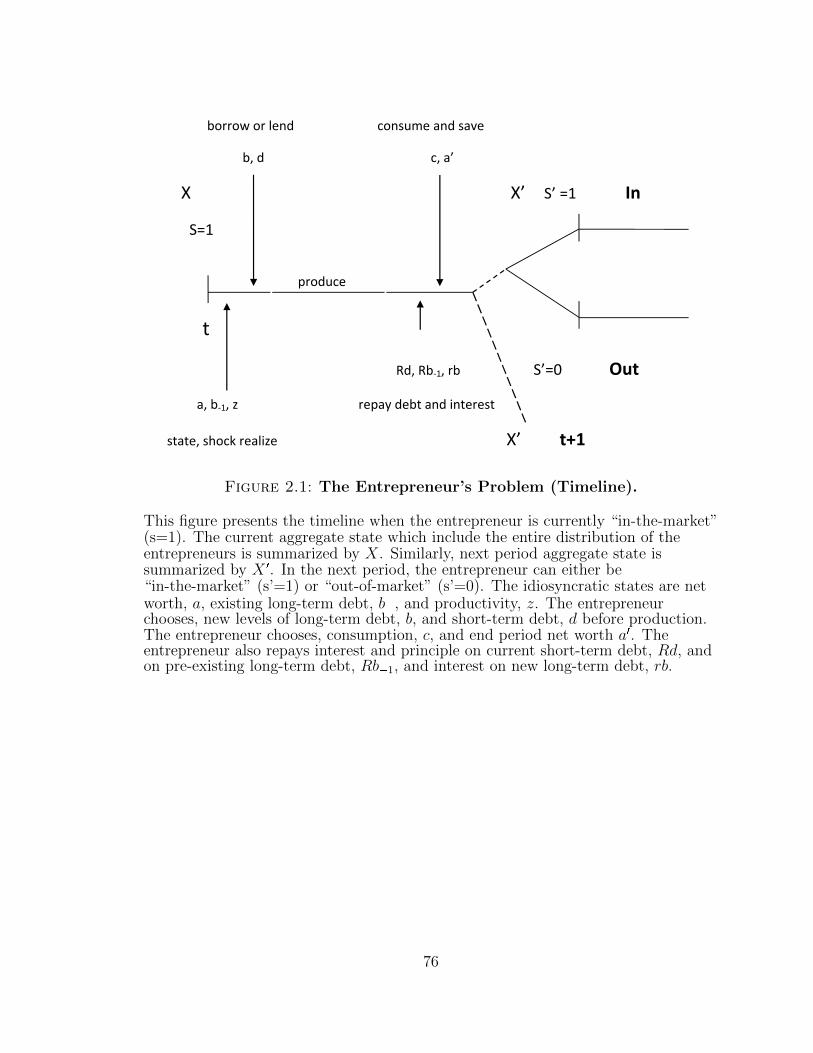
                   borrow or lend                          consume and save  

                               b, d                                                     c, a’           

        X                                                                                     X’     S’ =1             In 

             S=1                                                                                                                                                  

 

                  

            t                                                                      

                                                         Rd, Rb‐1, rb                 S’=0           Out                                    

           a, b‐1, z                                                        repay debt and interest 

     state, shock realize                                                                       X’            t+1 

 

                                                                                  

 

                                                  

produce  

 

Figure 2.1: The Entrepreneur’s Problem (Timeline).

This figure presents the timeline when the entrepreneur is currently “in-the-market”(s=1). The current aggregate state which include the entire distribution of theentrepreneurs is summarized by X. Similarly, next period aggregate state issummarized by X 1. In the next period, the entrepreneur can either be“in-the-market” (s’=1) or “out-of-market” (s’=0). The idiosyncratic states are networth, a, existing long-term debt, b�, and productivity, z. The entrepreneurchooses, new levels of long-term debt, b, and short-term debt, d before production.The entrepreneur chooses, consumption, c, and end period net worth a1. Theentrepreneur also repays interest and principle on current short-term debt, Rd, andon pre-existing long-term debt, Rb�1, and interest on new long-term debt, rb.

76

 

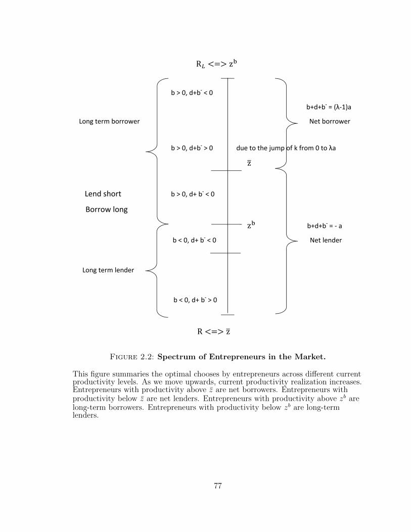
R z  

                                                                

                                                       b > 0, d+b‐ < 0 

                                                                                                                                                                             b+d+b‐ = (λ‐1)a                     

Long term borrower                                                                                                                                 Net borrower                   

 

                                                                      b > 0, d+b‐ > 0              due to the jump of k from 0 to λa 

                                                                                        z                                                                   

 

   Lend short                          b > 0, d+ b‐ < 0                                        

      Borrow long                                                               

                                                                                        z                            b+d+b‐ = ‐ a 

                                                 b < 0, d+ b‐ < 0                                                 Net lender 

                                                                                                                                                             

  Long term lender                          

 

                                                    b < 0, d+ b‐ > 0 

 

R z  

Figure 2.2: Spectrum of Entrepreneurs in the Market.

This figure summaries the optimal chooses by entrepreneurs across different currentproductivity levels. As we move upwards, current productivity realization increases.Entrepreneurs with productivity above z are net borrowers. Entrepreneurs withproductivity below z are net lenders. Entrepreneurs with productivity above zb arelong-term borrowers. Entrepreneurs with productivity below zb are long-termlenders.

77

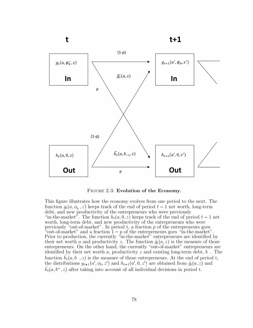
                                  t  t+1 

                                                            (1‐p) 

                                                                

                                                                                            

 

                                                                    P 

 

 

 

 

                                                              (1‐p)                                                  

 

 

  

                                                                                      P 

                            

 

       In 

       

         

      Out    

, ,  

               

 

      Out    

                            

 

       In 

, ,  

, 0,   , 0,  

,  

, ,

Figure 2.3: Evolution of the Economy.

This figure illustrates how the economy evolves from one period to the next. Thefunction gtpa, φ

�b , zq keeps track of the end of period t� 1 net worth, long-term

debt, and new productivity of the entrepreneurs who were previously“in-the-market”. The function htpa, 0, zq keeps track of the end of period t� 1 networth, long-term debt, and new productivity of the entrepreneurs who werepreviously “out-of-market”. In period t, a fraction p of the entrepreneurs goes“out-of-market” and a fraction 1� p of the entrepreneurs goes “in-the-market”.Prior to production, the currently “in-the-market” entrepreneurs are identified bytheir net worth a and productivity z. The function gtpa, zq is the measure of thoseentrepreneurs. On the other hand, the currently “out-of-market” entrepreneurs areidentified by their net worth a, productivity z and existing long-term debt, b�. Thefunction htpa, b

�, zq is the measure of those entrepreneurs. At the end of period t,the distributions gt�1pa

1, φb, z1q and ht�1pa

1, 0, z1q are obtained from gtpa, zq and

htpa, b�, zq after taking into account of all individual decisions in period t.

78

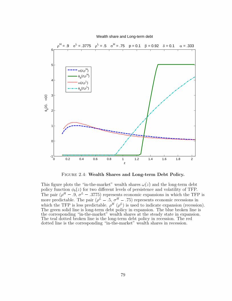
0 0.2 0.4 0.6 0.8 1 1.2 1.4 1.6 1.8 2-1

0

1

2

3

4

5

6

z

b(z),

(z)

Wealth share and Long-term debt

H = .9 L = .3775 L = .5 H = .75 p = 0.1 = 0.92 = 0.1 = .333

(z;H)

b(z;H)

(z;L)

b(z;L)

Figure 2.4: Wealth Shares and Long-term Debt Policy.

This figure plots the “in-the-market” wealth shares ωpzq and the long-term debtpolicy function φbpzq for two different levels of persistence and volatility of TFP.The pair (ρH � .9, σL � .3775) represents economic expansions in which the TFP ismore predictable. The pair (ρL � .5, σH � .75) represents economic recessions inwhich the TFP is less predictable. ρH (ρL) is used to indicate expansion (recession).The green solid line is long-term debt policy in expansion. The blue broken line isthe corresponding “in-the-market” wealth shares at the steady state in expansion.The teal dotted broken line is the long-term debt policy in recession. The reddotted line is the corresponding “in-the-market” wealth shares in recession.

79

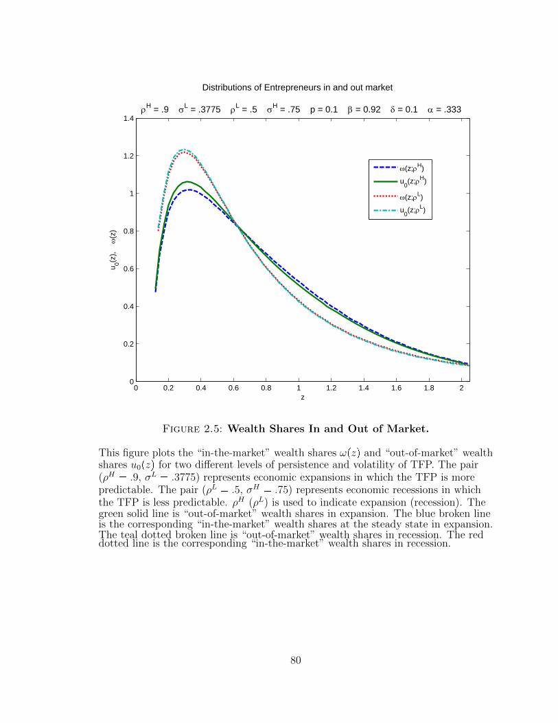
0 0.2 0.4 0.6 0.8 1 1.2 1.4 1.6 1.8 20

0.2

0.4

0.6

0.8

1

1.2

1.4

z

u 0(z),

(z)

Distributions of Entrepreneurs in and out market

H = .9 L = .3775 L = .5 H = .75 p = 0.1 = 0.92 = 0.1 = .333

(z;H)

u0(z;H)

(z;L)

u0(z;L)

Figure 2.5: Wealth Shares In and Out of Market.

This figure plots the “in-the-market” wealth shares ωpzq and “out-of-market” wealthshares u0pzq for two different levels of persistence and volatility of TFP. The pair(ρH � .9, σL � .3775) represents economic expansions in which the TFP is morepredictable. The pair (ρL � .5, σH � .75) represents economic recessions in whichthe TFP is less predictable. ρH (ρL) is used to indicate expansion (recession). Thegreen solid line is “out-of-market” wealth shares in expansion. The blue broken lineis the corresponding “in-the-market” wealth shares at the steady state in expansion.The teal dotted broken line is “out-of-market” wealth shares in recession. The reddotted line is the corresponding “in-the-market” wealth shares in recession.

80

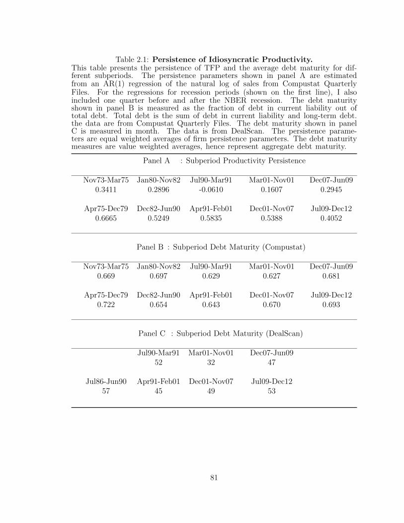
Table 2.1: Persistence of Idiosyncratic Productivity.This table presents the persistence of TFP and the average debt maturity for dif-ferent subperiods. The persistence parameters shown in panel A are estimatedfrom an AR(1) regression of the natural log of sales from Compustat QuarterlyFiles. For the regressions for recession periods (shown on the first line), I alsoincluded one quarter before and after the NBER recession. The debt maturityshown in panel B is measured as the fraction of debt in current liability out oftotal debt. Total debt is the sum of debt in current liability and long-term debt.the data are from Compustat Quarterly Files. The debt maturity shown in panelC is measured in month. The data is from DealScan. The persistence parame-ters are equal weighted averages of firm persistence parameters. The debt maturitymeasures are value weighted averages, hence represent aggregate debt maturity.

Panel A : Subperiod Productivity Persistence

Nov73-Mar75 Jan80-Nov82 Jul90-Mar91 Mar01-Nov01 Dec07-Jun090.3411 0.2896 -0.0610 0.1607 0.2945

Apr75-Dec79 Dec82-Jun90 Apr91-Feb01 Dec01-Nov07 Jul09-Dec120.6665 0.5249 0.5835 0.5388 0.4052

Panel B : Subperiod Debt Maturity (Compustat)

Nov73-Mar75 Jan80-Nov82 Jul90-Mar91 Mar01-Nov01 Dec07-Jun090.669 0.697 0.629 0.627 0.681

Apr75-Dec79 Dec82-Jun90 Apr91-Feb01 Dec01-Nov07 Jul09-Dec120.722 0.654 0.643 0.670 0.693

Panel C : Subperiod Debt Maturity (DealScan)

Jul90-Mar91 Mar01-Nov01 Dec07-Jun0952 32 47

Jul86-Jun90 Apr91-Feb01 Dec01-Nov07 Jul09-Dec1257 45 49 53

81

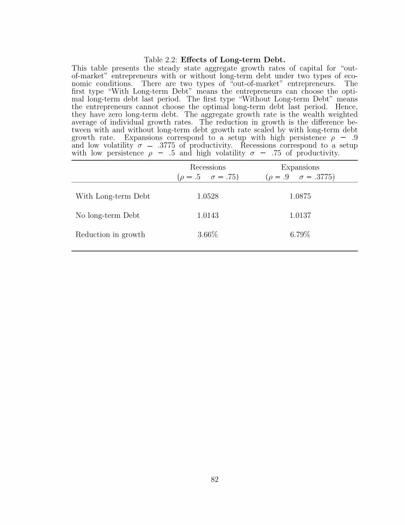
Table 2.2: Effects of Long-term Debt.This table presents the steady state aggregate growth rates of capital for “out-of-market” entrepreneurs with or without long-term debt under two types of eco-nomic conditions. There are two types of “out-of-market” entrepreneurs. Thefirst type “With Long-term Debt” means the entrepreneurs can choose the opti-mal long-term debt last period. The first type “Without Long-term Debt” meansthe entrepreneurs cannot choose the optimal long-term debt last period. Hence,they have zero long-term debt. The aggregate growth rate is the wealth weightedaverage of individual growth rates. The reduction in growth is the difference be-tween with and without long-term debt growth rate scaled by with long-term debtgrowth rate. Expansions correspond to a setup with high persistence ρ � .9and low volatility σ � .3775 of productivity. Recessions correspond to a setupwith low persistence ρ � .5 and high volatility σ � .75 of productivity.

Recessions Expansionspρ � .5 σ � .75q pρ � .9 σ � .3775q

With Long-term Debt 1.0528 1.0875

No long-term Debt 1.0143 1.0137

Reduction in growth 3.66% 6.79%

82

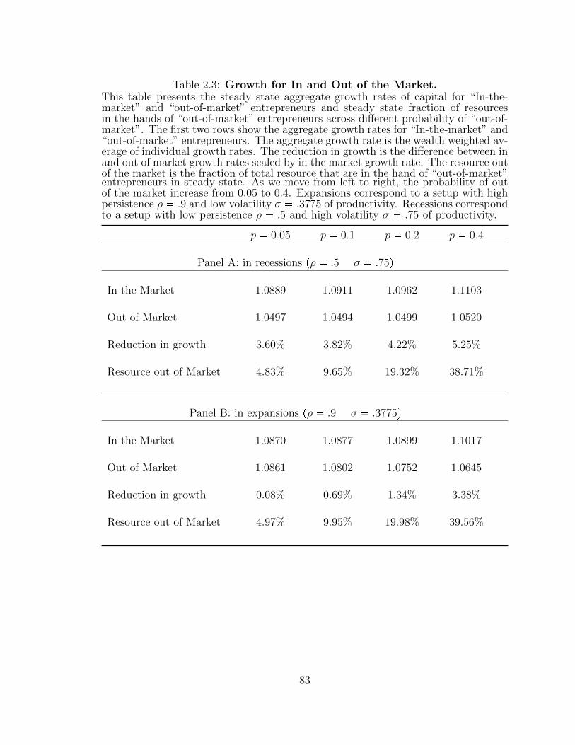
Table 2.3: Growth for In and Out of the Market.This table presents the steady state aggregate growth rates of capital for “In-the-market” and “out-of-market” entrepreneurs and steady state fraction of resourcesin the hands of “out-of-market” entrepreneurs across different probability of “out-of-market”. The first two rows show the aggregate growth rates for “In-the-market” and“out-of-market” entrepreneurs. The aggregate growth rate is the wealth weighted av-erage of individual growth rates. The reduction in growth is the difference between inand out of market growth rates scaled by in the market growth rate. The resource outof the market is the fraction of total resource that are in the hand of “out-of-market”entrepreneurs in steady state. As we move from left to right, the probability of outof the market increase from 0.05 to 0.4. Expansions correspond to a setup with highpersistence ρ � .9 and low volatility σ � .3775 of productivity. Recessions correspondto a setup with low persistence ρ � .5 and high volatility σ � .75 of productivity.

p � 0.05 p � 0.1 p � 0.2 p � 0.4

Panel A: in recessions pρ � .5 σ � .75q

In the Market 1.0889 1.0911 1.0962 1.1103

Out of Market 1.0497 1.0494 1.0499 1.0520

Reduction in growth 3.60% 3.82% 4.22% 5.25%

Resource out of Market 4.83% 9.65% 19.32% 38.71%

Panel B: in expansions pρ � .9 σ � .3775q

In the Market 1.0870 1.0877 1.0899 1.1017

Out of Market 1.0861 1.0802 1.0752 1.0645

Reduction in growth 0.08% 0.69% 1.34% 3.38%

Resource out of Market 4.97% 9.95% 19.98% 39.56%

83

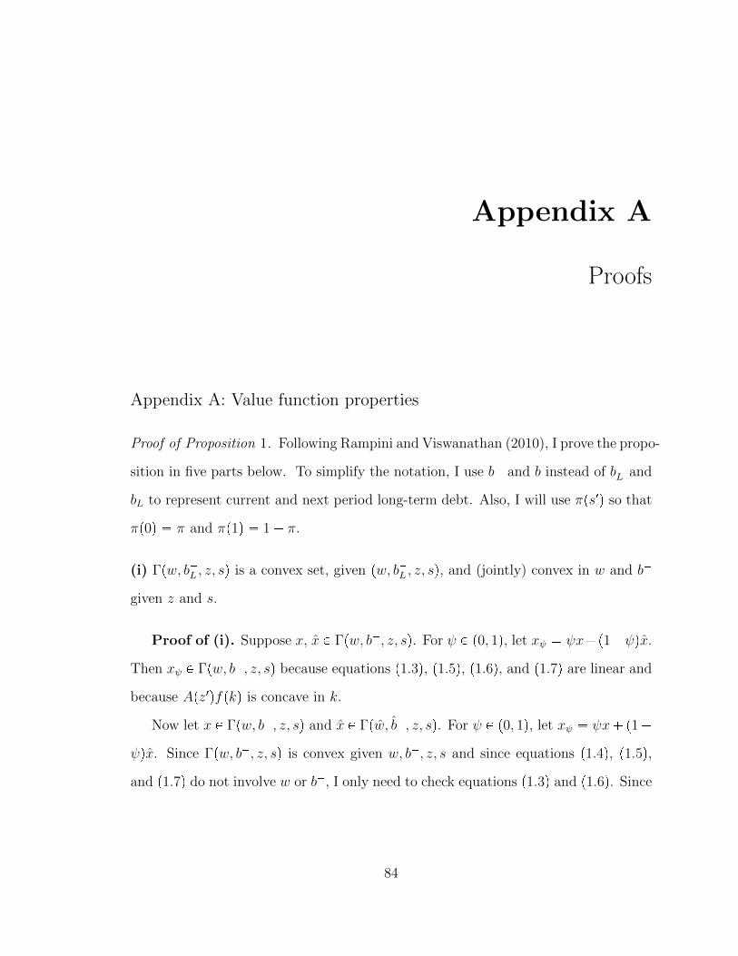
Appendix A

Proofs

Appendix A: Value function properties

Proof of Proposition 1. Following Rampini and Viswanathan (2010), I prove the propo-

sition in five parts below. To simplify the notation, I use b� and b instead of b�L and

bL to represent current and next period long-term debt. Also, I will use πps1q so that

πp0q � π and πp1q � 1� π.

(i) Γpw, b�L , z, sq is a convex set, given pw, b�L , z, sq, and (jointly) convex in w and b�

given z and s.

Proof of (i). Suppose x, x P Γpw, b�, z, sq. For ψ P p0, 1q, let xψ � ψx�p1�ψqx.

Then xψ P Γpw, b�, z, sq because equations p1.3q, p1.5q, p1.6q, and p1.7q are linear and

because Apz1qfpkq is concave in k.

Now let x P Γpw, b�, z, sq and x P Γpw, b�, z, sq. For ψ P p0, 1q, let xψ � ψx� p1�

ψqx. Since Γpw, b�, z, sq is convex given w, b�, z, s and since equations p1.4q, p1.5q,

and p1.7q do not involve w or b�, I only need to check equations p1.3q and p1.6q. Since

84

both constraints are linear in x, b�, and w , I have:

ψpw � bS � bq � p1� ψqpw � bS � bq ¥ ψpd� kq � p1� ψqpd� kq

ψb� � p1� ψqb� ¥ ψb� p1� ψqb, for s � 0

Thus, xψ P Γpψw � p1 � ψqw, ψb� � p1 � ψqb�, z, sq. Therefore, Γpw, b�, z, sq is

jointly convex in w and b.

Lemma 2 Γpw, b�, z, sq is monotone in w in the sense that w ¤ w implies Γpw, b�, z, sq

� Γpw, b�, z, sq and Γpw, b�, z, sq is monotone in b� in the sense that b� ¤ b� implies

Γpw, b�, z, sq � Γpw, b�, z, sq.

Proof of Lemma 2. Given b�, z, and s, increasing w only relaxes constraint

p1.3q. So, any feasible choice under Γpw, b�, z, sq is still feasible under Γpw, b�, z, sq.

Thus, if w ¤ w, then Γpw, b�, z, sq � Γpw, b�, z, sq.

Similarly, given w, z, and s, increasing b� only relaxes constraint p1.6q. So, if

b� ¤ b�, then Γpw, b�, z, sq � Γpw, b�, z, sq.

Lemma 3 The operator T satisfies Blackwell’s sufficient conditions for a contraction

and has a unique fixed point V.

Proof of Lemma 3. Suppose gpw, b�, z, sq ¥ fpw, b�, z, sq, @pw, b�, z, sq P <2� �

<� t0, 1u. Then, for any x P Γpw, b�, z, sq,

pTgqpw, b�, z, sq ¥ d� β¸s1

πps1q

»gpwpz1q, b, z1, s1qdQz

¥ d� β¸s1

πps1q

»fpwpz1q, b, z1, s1qdQz.

Thus,

pTgqpw, b�, z, sq � maxxPΓpa,b�,z,sq

d� β¸s1

πps1q

»gpwpz1q, b, z1, s1qdQz

85

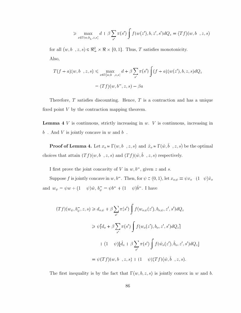
¥ maxxPΓpw,b�L ,z,sq

d� β¸s1

πps1q

»fpwpz1q, b, z1, s1qdQz � pTfqpw, b�, z, sq

for all pw, b�, z, sq P <2� � <� t0, 1u. Thus, T satisfies monotonicity.

Also,

T pf � aqpw, b�, z, sq ¤ maxxPΓpw,b�,z,sq

d� β¸s1

πps1q

»pf � aqpwpz1q, b, z, sqdQz

� pTfqpw, b�, z, sq � βa

Therefore, T satisfies discounting. Hence, T is a contraction and has a unique

fixed point V by the contraction mapping theorem.

Lemma 4 V is continuous, strictly increasing in w. V is continuous, increasing in

b�. And V is jointly concave in w and b�.

Proof of Lemma 4. Let xo P Γpw, b�, z, sq and xo P Γpw, b�, z, sq be the optimal

choices that attain pTfqpw, b�, z, sq and pTfqpw, b�, z, sq respectively.

I first prove the joint concavity of V in w, b�, given z and s.

Suppose f is jointly concave in w, b�. Then, for ψ P p0, 1q, let xo,ψ � ψxo�p1�ψqxo

and wψ � ψw � p1� ψqw, b�ψ � ψb� � p1� ψqb�. I have

pTfqpwψ, b�ψ , z, sq ¥ do,ψ � β

¸s1

πps1q

»fpwo,ψpz

1q, bo,ψ, z1, s1qdQz

¥ ψrdo � β¸s1

πps1q

»fpwopz

1q, bo, z1, s1qdQzs

� p1� ψqrdo � β¸s1

πps1q

»fpwopz

1q, bo, z1, s1qdQzs

� ψpTfqpw, b�, z, sq � p1� ψqpTfqpw, b�, z, sq.

The first inequality is by the fact that Γpw, b, z, sq is jointly convex in w and b.

86

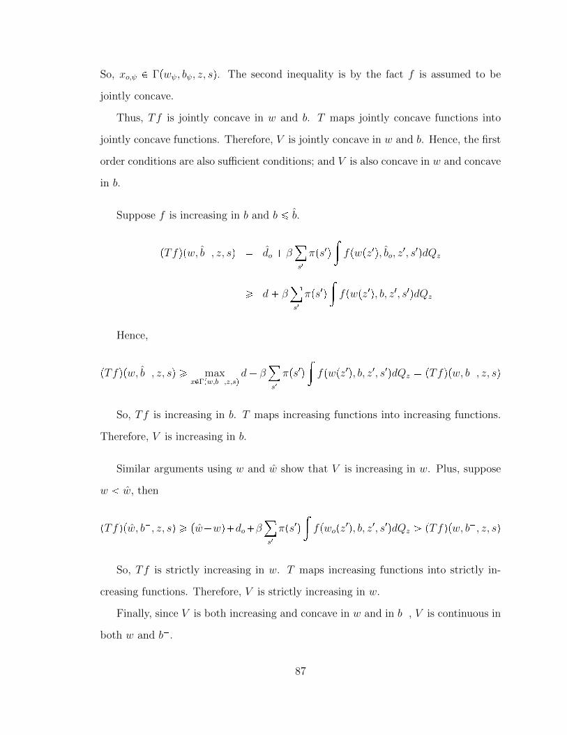
So, xo,ψ P Γpwψ, bψ, z, sq. The second inequality is by the fact f is assumed to be

jointly concave.

Thus, Tf is jointly concave in w and b. T maps jointly concave functions into

jointly concave functions. Therefore, V is jointly concave in w and b. Hence, the first

order conditions are also sufficient conditions; and V is also concave in w and concave

in b.

Suppose f is increasing in b and b ¤ b.

pTfqpw, b�, z, sq � do � β¸s1

πps1q

»fpwpz1q, bo, z

1, s1qdQz

¥ d� β¸s1

πps1q

»fpwpz1q, b, z1, s1qdQz

Hence,

pTfqpw, b�, z, sq ¥ maxxPΓpw,b�,z,sq

d� β¸s1

πps1q

»fpwpz1q, b, z1, s1qdQz � pTfqpw, b�, z, sq

So, Tf is increasing in b. T maps increasing functions into increasing functions.

Therefore, V is increasing in b.

Similar arguments using w and w show that V is increasing in w. Plus, suppose

w   w, then

pTfqpw, b�, z, sq ¥ pw�wq�do�β¸s1

πps1q

»fpwopz

1q, b, z1, s1qdQz ¡ pTfqpw, b�, z, sq

So, Tf is strictly increasing in w. T maps increasing functions into strictly in-

creasing functions. Therefore, V is strictly increasing in w.

Finally, since V is both increasing and concave in w and in b�, V is continuous in

both w and b�.

87

Lemma 5 V pw, b�, z, sq is strictly concave in w for w P inttw : dpw, b�, z, sq � 0u.

V pw, b�, 1, 0q is strictly concave in w and b� for tw, b�u P intttw, b�u : dpw, b�, z, 0q �

0, b�   1�pLpL

wu.

Proof of Lemma 5. First I show that suppose for @w, w P inttw : dpw, b�, z, sq �

0u and w ¥ w, if the optimal choices is such that ko � ko, then I have for ψ P p0, 1q and

xo,ψ � ψxo�p1�ψqxo, V pwψ, b�, z, sq ¡ do,ψ�β

°s1 πps

1q³V pwo,ψpz

1q, bo,ψ, z1, s1qdQz ¥

ψV pw, b�, z, sq�p1�ψqV pw, b�, z, sq. The strict inequality is due to the fact that con-

straint p1.4q is slack hence net worth levels wpz1q ¡ wo,ψpz1q are feasible for all z1. The

second inequality is due to the concavity of V. For simplicity, I let pL � 1�R�1L θp1�δq

represents the minimal down payment as discussed in Section 6.

From the FOCs, we have that when w Ñ 0, Apz1qfkpkq � p1 � δq ¡ RL, @z1 P Z.

Hence, there exists a level of net worth w s.t. @w   w, either the collateral constraint

is binding λ ¡ 0 or the financing constraint is bind γL ¡ 0. Then @w   w   w and

while λ ¡ 0, ko ¡ ko. Hence, V pw, b�, z, 0q with b� ¡ 1�pLpL

w and V pw, b�, z, 1q are

strictly concave in w for w   w. Also, for s � 0, given some b�, b� ¤ 1�pLpL

w, and

w, w   w, such that tw, b�u � tw, b�u, it must be that ko ¡ ko because bo � b�,

bo � b�, do � do � 0, bS,o � bS,o � 0, and budget constraints p1.3q and p1.4q are always

binding. Thus, V is strictly jointly concave in w and b�, @tw, b�u P p0, ws�r0, 1�pLpL

wq.

Now suppose w, w ¥ w, w ¡ w, and ko � ko. Then, b � bS   b � bS by equa-

tion p1.3q. Hence, either wpz1q ¡ wpz1q for all z1 or b ¡ b. Then for some low z1,

wpz1q, wpz1q   w, and for those z1 states, V pwo,ψpz1q, bo,ψ, z

1, 0q ¡ ψV pwopz1q, bo, z, 0q�

p1�ψqV pwopz1q, bo, z, 0q. Thus, V pwψ, b

�, z, sq ¡ ψV pw, b�, z, sq�p1�ψqV pw, b�, z, sq,

and V is also strictly concave for w   w   w. Next, let w be the new w, and applying

the same logic, I have that for all w P inttw : dpw, b�, z, sq � 0u, V is strictly concave

in w.

As asserted in Result 3, when s � 0, and w ¡ pL1�pL

b�, then bo � b�. Hence,

88

for tw, b�u, tw, b�u P p0, ws � r0, 1�pLpL

wq and tw, b�u � tw, b�u, then either ko � ko

or wopz1q � wopz

1q @z1 because equations p1.3q and p1.4q hold with equalities and

since bo � b�, bo � b�, do � do � 0, and RL ¡ RS. If the later is true, then

Dwopz1q � wopz

1q, and wopz1q, wopz

1q P inttw : dpw, b�, z, sq � 0u for some z1. Then a

convex combination can strictly increase V pwpz1q, b, z1, s1q for those z1. Therefore, V

is strictly (jointly) concave in w and b�, @ tw, b�u P p0, ws � r0, 1�pLpL

wq and where

do � 0.

Lemma 6 Since the debts are non-state contingent and collateralized, if k ¡ 0, then

wpz1q ¡ 0 @z1 P Z. More formally, from equation p1.4q and constraint p1.5q, we have:

wpz1q ¥ Apz1qfpkq � p1� δqp1� θqk ¡ 0 @z1 P Z.

Now to show that k ¡ 0, note that k Ñ 0, Apz1qfkpkq Ñ 8 @z1 by Assumptions 1

and 2. Thus, for k sufficiently small, Apz1qfkpkq � p1 � δq ¡ RL ¡ RS @z1 P Z. Then

from equations p1.9q and p1.11q, I obtain that when s � 1, λ ¡ 0. Similar for s � 0,

for any given bL if w is sufficiently low, constraint p1.6q will not bind and λ ¡ 0.

From constraint p1.3q, w � bS � bL ¥ k. Thus, for some w ¡ 0, constraint p1.3q will

bind only if k ¡ 0. Therefore starting will some w ¡ 0, all subsequent wptz, sutq and

kptz, sutq are positive.

Appendix B: Policy Functions

Proof of Proposition 2. Part (i): From equation 1.8, Vwpw, b�, z, sq � µpw, b�, z, sq ¥

1. Since V is concave in w (Lemma 4), µpw, b�, z, sq is decreasing in w. If dpw, b�, z, sq

¡ 0, then µpw, b�, z, sq � 1 and µpw, b�, z, sq � 1 for all w ¥ w. Let wpb�, z, sq �

inftw : dpw, b�, z, sq ¡ 0u.

Part (ii): Suppose w ¡ w ¥ wpb�, z, sq and let xo attain V pw, b�, z, sq.

89

V pw, b�, z, sq � V pw, b�, z, sq �³wwdV , since V1pw, b

�, z, sq � 1 for any w ¥

wpb�, z, sq. Hence xo � rw � w � do, ko, wopz1q, bos attains V pw, b�, z, sq.

Suppose xo, xo both attain V pw, b�, z, sq, and ko �� ko. Then by the fact that

Γpw, b�, z, sq is a convex set and the fact that fpkq is strictly concave,

Afpko,ψq � p1� δqko,ψ ¡ ψrAfpkoq � p1� δqkos � p1� ψqrAfpkoq � p1� δqkos

where ko,ψ � ψko � p1 � ψqko. Thus, there exists wo ¡ wo,ψ and its corresponding

xo P Γpw, b�, z, sq that give a higher V , a contradiction. So, kopw, b�, z, sq is unique

for all w, b�, z, s.

For w ¥ w ¥ wpb�, z, sq, let xo attain V pw, b�, z, sq and xo attain V pw, b�, z, sq.

Suppose ko �� ko. Then by concavity of Γpw, b�, z, sq in w [Lemma 1] and simi-

lar arguments as above, there exists a feasible choice such that V pwψ, b�, z, sq ¡

ψV pw, b�, z, sq� p1�ψqV pw, b�, z, sq, contradicting the fact that V is linear in w for

w ¥ wpb�, z, sq. Hence, kopw, b�, z, sq � kopb

�, z, sq for all w ¥ wpb�, z, sq.

From above argument, I know that for w ¥ w, the firm can always choose the

same optimal choices k, b, and w.

Part (iii): Now, I will prove the uniqueness of optimal new debt level, bo, bS,o, end

period worth net, wopz1q, and dividend, do.

For any optimal policy xo, if wopz1q ¥ wpb, z1, 0q for all z1, then by Proposition 4,

wopz1q ¥ wpbo, z

1, s1q and µpwpz1q, b, z1, s1q � 1 for all z1. In this case, from the optimal-

ity conditions, I know that either λ ¡ 0 or γs ¡ 0. If λ ¡ 0, then γlpwpz1q, bl, z

1, 0q ¡ 0

for some future state pz1, 0q. Since both conditions (1.4) and (1.5) hold as equality,

wopz1q are uniquely determined by ko. Since γlpwpz

1q, b, z1, 0q is strictly decreasing in

b, bo is also unique. Then, bS,o and do are unique by equations (1.5) and (1.3). On

the other hand, if γs ¡ 0, λ � 0 then γl ¡ 0 since µ ¥ 1 ¡ βRL and by optimality

90

condition (1.11). Thus, bS,o � 0 and bo � b�, so bS,o, bo are unique. Hence, wpz1q and

do are unique by equations (1.4) and (1.3).

Now Suppose x and x both obtain the optimal value and wpz1q   wpb, z1, 0q and

wpz1q   wpb, z1, 0q for some state pz1, 0q. I denote such state by z. Since equations

(1.4) hold for all z1, if wpz1q � wpz1q for some state z1, then wpz1q � wpz1q for all state

z1 and vice versa. Suppose either wpz1q � wpz1q for some z1 or b � b, then either

wpzq � wpzq or b � b. By Proposition 1, the region tpw1, bq : dpw1, bq � 0u is convex

and the value function V pw1, bq is strictly concave in that region. Hence, a convex

combination between twpzq , bu and twpzq, bu is feasible and attains a strictly higher

value, a contradiction. Therefore, it must be that b � b and wpz1q � wpz1q for all state

z1. Thus, bo and wopz1q are unique if wopz

1q   wpbo, z1, 0q for some pz1, 0q. Finally, do

and bS,o are also unique by equations (1.4) and (1.3).

Proof of Proposition 4. Figure 1.7 shows the value functions for two different levels

of long-term debt. I use the figure to illustrate the relations between the points

mentioned in the following proof.

By Proposition 1, for two levels of long-term debt, b�L ¡ b�L , both V pw, b�Lq and

V pw, b�Lq are increasing and concave in w. Also, V pw, b�Lq ¥ V pw, b�Lq at any point

w with strictly inequality when financing constraint is binding at w, b�L . Further,

by part (i) of Proposition 2, V pw, b�Lq and V pw, b�Lq eventually stay parallel since

µpw, b�Lq � µpw, b�Lq � 1 for w ¥ maxtwpb�L , z, 0q, wpb�L , z, 0qu. Finally, as w Ñ 0,

both V pw, b�Lq and V pw, b�Lq Ñ 0. Hence, µpw, b�Lq falls to 1 before µpw, b�Lq does.

That is, wpb�L , z, 0q ¡ wpb�L , z, 0q. Moreover, since V pw, b�Lq is strictly concave before

wpb�L , z, 0q, D wpb�L , b

�Lq s.t. µpw, b

�Lq ¡ µpw, b�Lq for all w P pwpb�L , b

�Lq, wpb

�L , z, 0qq.

Appendix C: 2-Period Model Formulation, FOC, and SOC

Proof of Lemma 7. Here I first solve the problem backward starting from time 1.

91

At time 1, when s � 1, the firm is solving the following problem:

maxd1,k2,bL2 ,b2,w2pA2q

d1 � βE1w2pA2q,

w1 � b2 � bL2 ¥ d1 � k2,

A2k2 � p1� δqk2 �Rb2 �RLbL2 ¥ w2pA2q

θp1� δqk2 ¥ Rb2 �RLbL2 ,

d1 ¥ 0, bL2 ¥ 0, b2 ¥ 0.

With linear production function under Assumption 3, the solution is: d1 � 0,

k2 �w1

q, b2 � p1

q� 1qw1, bL2 � 0, w2pA2q �

Ret2qw1.

At time 1, when s � 0, the firm is solving the following problem:

maxd1,k2,bL2 ,b2,w2pA2q

d1 � βE1w2pA2q,

w1 � b2 � bL2 ¥ d1 � k2,

A2k2 � p1� δqk2 �Rb2 �RLbL2 ¥ w2pA2q

θp1� δqk2 ¥ Rb2 �RLbL2 ,

bL1 ¥ bL2 ,

0 ¥ b2,

d1 ¥ 0, bL2 ¥ 0, b2 ¥ 0

As in the first case, the firm always wants to invest all in capital and payout

nothing at time 1.

If bL1 ¥ p 1qL� 1qw1, then the firm is constrained by w1, hence d1 � 0, k2 �

w1

qL,

b2 � 0, bL2 � p 1qL� 1qw1, w2pA2q �

Ret2qLw1.

92

If bL1   p 1qL� 1qw1, then the firm is constrained by bL1 , hence d1 � 0, k2 � w1� b

L1 ,

bL2 � bL1 , b2 � 0, w2pA2q � ˆRet2pw1 � bL1 q �RLbL1 .

Assuming a continuum of productivity states, and let gpA1q and gpA2|A1q be the

marginal density of A1 and the conditional density of A2 given A1, at time 0, the

problem becomes:

maxd0,k1,b1,bL1 ,w1pA1q

d0 � β2

"p1� πq

» AHAL

» AHAL

RetpA2q

pw1pA1qgpA2|A1qgpA1qdA2dA1

� π

» AAL

» AHAL

RetpA2q

pLw1pA1qgpA2|A1qgpA1qdA2dA1

� π

» AHA

» AHAL

RetpA2qw1pA1qgpA2|A1qgpA1qdA2dA1

� π

» AHA

» AHAL

rRetpA2q �RLsgpA2|A1qbL1 gpA1qdA2dA1

*(A.1)

Subject to the budget constraints

w0 � b1 � bL1 � k1 ¥ d0,

A1k1 � p1� δqk1 �RLbL1 �Rb1 ¥ w1pA1q,

the collateral constraint

θp1� δqk1 ¥ RLbL1 �Rb1,

the non-negativity constraints

b1 ¥ 0, bL1 ¥ 0, d0 ¥ 0, k1 ¥ 0, w1pA1q ¥ 0,

and where

A �

"A1 : w1pA1q �

bL1 pL1� pL

*.

93

Each line in the big curly bracket of equation A.1 represents a payoff for one of

the three sets of states the firm may end up in at time 1. The first line is the payoff

if the firm has external financing at time 1 (s � 1). The second line is the payoff if

the firm does not have external financing and does not have sufficient net worth to

keep all existing long-term debt at time 1 (s � 0, w1pA1q  bL1 pL1�pL

). The last line is

the payoff if the firm does not have external financing but has sufficient net worth at

time 1 (s � 0, w1pA1q ¥bL1 pL1�pL

).

I consider the case in which the productivity shocks are profitable enough such

that the firm will investment all in capital. Hence, the firm pays no dividends, d0 � 0.

Plus, the collateral constraint always binds.

Let α be the proportion of net worth that is used to lever through long-term debt.

More specifically, α � pLp1�pLq

bL1w0

. The interpretation is that if the firm uses αw0 as

the minimal downpayment to borrow with long-term debt, it will be able to raise

bL1 �p1�pLqpL

α w0.

Now the problem can be reformulated as follow: (since the whole problem is linear

in w0, I can divide it out and focus only on the proportional decision)

V pαq � maxα

p1� πq

» AHAL

» AHAL

RetpA2q

pw1pA1qgpA2|A1qgpA1qdA2dA1

� π

» AAL

» AHAL

RetpA2q

pLw1pA1, αqgpA2|A1qgpA1qdA2dA1

� π

» AHA

» AHAL

RetpA2qw1pA1, αqgpA2|A1qgpA1qdA2dA1

� π

» AHA

» AHAL

rRetpA2q �RLsgpA2|A1qbL1 pαqgpA1qdA2dA1

where

w1pA1, αq � Ret1pA1qLev w0 (A.2)

94

Ret1pA1q � A1 � p1� δqp1� θq (A.3)

Lev � rα

pL�

1� α

ps (A.4)

bL1 �p1� pLq

pLα w0 (A.5)

A �α

Lev� p1� δqp1� θq (A.6)

p � 1�R�1θp1� δq, pL � 1�R�1L θp1� δq. (A.7)

The first order condition is given by:

"p1� πq

» AHAL

» AHAL

"RetpA2q

pgpA2|A1qRet1pA1qgpA1q

*dA2dA1

� π

» AAL

» AHAL

"RetpA2q

pLgpA2|A1qRet1pA1qgpA1q

*dA2dA1

� π

» AHA

» AHAL

"RetpA2qgpA2|A1qRet1pA1qgpA1q

*dA2dA1

*ppL � pq

pLp

� π1� pLpL

» AHA

» AHAL

rRetpA2q �RLsgpA2|A1qgpA1qdA2dA1

Notice that the terms involving derivatives of A with respect to α cancel out

because at state A the firm is indifferent between being constrained by net worth or

being constrained by existing long-term debt. That is:

�bL1 pαq

» AHAL

rRetpA2q �RLsgpA2|AqgpAqdA2

�

"» AHAL

"RetpA2q

pLgpA2|AqRet1pAqgpAq

*dA2

�

» AHAL

"RetpA2qgpA2|AqRet1pAqgpAq

*dA2

*Levpαq � 0 @α

95

The second order derivative is:

B2V pαq

Bα2�� π

1� pLpL

» AHAL

rRetpA2q �RLsgpA2|AqgpAqdA2

�

"π

» AHAL

"RetpA2q

pLgpA2|AqRet1pAqgpAq

*dA2

� π

» AHAL

"RetpA2qgpA2|AqRet1pAqgpAq

*dA2

*ppL � pq

pLp

Which have the same sign as:

�1� pLpL

» AHAL

rRetpA2q �RLsgpA2|AqdA2 �

"» AHAL

"RetpA2q

pLgpA2|AqRet1pAq

*dA2

�

» AHAL

"RetpA2qgpA2|AqRet1pAq

*dA2

*ppL � pq

pLp

�

» AHAL

"ˆrRetpA2q �

RetpA2q

pLsRet1pAq

ppL � pq

pLp� rRetpA2q �RLs

1� pLpL

*gpA2|AqdA2

� �

» AHAL

"rRetpA2q

pL� RetpA2qsRet1pAq

1

pL

*gpA2|Aq dA2   0

Hence, B2V pαqBα2   0 @α. Therefore, there is a unique α for the problem.

Appendix D: 2-Period Model comparative statics

Proof of proposition 19. Now suppose that A2 � ρA1�ε. The density for A1 is gpA1q.

The density for ε is fpεq which is independent of A1. Hence, the FOC is:

96

"p1� πq

» AHAL

» "RetpρA1 � εq

pfpεqRetpA1qgpA1q

*dεdA1

� π

» AAL

» "RetpρA1 � εq

pLfpεqRetpA1qgpA1q

*dεdA1

� π

» AHA

» "RetpρA1 � εqfpεqRetpA1qgpA1q

*dεdA1

*ppL � pq

pLp

� π1� pLpL

» AHA

»rRetpρA1 � εq �RLsfpεqgpA1qdεdA1

or equivalently,

"p1� πq

» AHAL

RetpρA1q

pRetpA1qgpA1q dA1 � π

» AAL

RetpρA1q

pLRetpA1qgpA1qdA1

� π

» AHA

RetpρA1qRetpA1qgpA1qdA1

*ppL � pq

pLp

� π1� pLpL

» AHA

rRetpρA1q �RLsgpA1qdA1

And B2V pαqBαBρ

becomes:

�

"p1� πq

» AHAL

A1

pRetpA1qgpA1qdA1 � π

» AAL

A1

pLRetpA1qgpA1qdA1

� π

» AHA

A1RetpA1qgpA1q dA1

*ppL � pq

pLp� π

1� pLpL

» AHA

A1gpA1qdA1

97

From the FOC, we have that

B2V pαq

BαBρρ�

"p1� πq

» AHAL

p1� δqp1� θq

pRetpA1qgpA1qdA1

� π

» AAL

p1� δqp1� θq

pLRetpA1qgpA1qdA1

� π

» AHA

p1� δqRetpA1qgpA1q dA1

*ppL � pq

pLp

� π1� pLpL

rp1� δq �RLs

» AHA

gpA1qdA1 � 0

Since p1 � δq � RL   0 and the term in curly bracket is positive, B2V pαqBαBρ

¡ 0.

Therefore, by the SOC and implicit function theorem, BαBρ¡ 0.

Proof of proposition 10. Suppose for now the shocks are independent. Let ˆRet2 �

ErRetpA2qs, Ret2 � ErRetpA2qs, and Ret1 � ErRetpA1qs

The now FOC now becomes:

�

"p1� πq

Ret2q

Ret1 � πRet2qL

» AALRetpA1qgpA1qdA1

� π ˆRet2

» AHA

RetpA1qgpA1qdA1

*ppL � pq

pLp

� PrpA1 ¡ Aqπr ˆRet2 �RLs1� qLqL

� 0

And we have:

B2V pαq

BαBpEA2q� �

"p1� πq

Ret1q

�π

qL

» AALRetpA1qgpA1qdA1

� π

» AHA

RetpA1qgpA1qdA1

*ppL � pq

pLp� PrpA1 ¡ Aqπ

1� qLqL

98

By manipulating the term, we obtain the following equation:

�

"p1� πq

Ret1q

rRet2 � ˆRet2 �RLs �π

qLrRet2 � ˆRet2 �RLs

» AALRetpA1qgpA1qdA1

� πRL

» AHA

RetpA1qgpA1qdA1

*ppL � pq

pLp�

B2V pAq

BABpE1A2qr ˆRet2 �RLs �

BV pαq

Bα� 0

Since rRet2� ˆRet2�RLs ¡ 0, the term in the curly bracket is positive. Also, since

ˆRet2 �RL ¡ 0, we have B2V pαqBαBpEA2q

¡ 0. Finally, by the second order condition and the

implicit function theorem, we have: BαBpEA2q

¡ 0.

Proof of proposition 11. Now suppose instead that A1 � ε is the productivity at time

1, and still gpA1q is the marginal pdf for A1 and gpA2|A1q is the conditional pdf for

A2 given A1.

We have that A � αLev

� p1 � δqp1 � θq � ε, and the return for time 1 is now

RetpA1q � A1 � ε� p1� δqp1� θq. Hence, the now FOC is:

"p1� πq

» AHAL

» AHAL

"RetpA2q

pgpA2|A1qRet1pA1 � εqgpA1q

*dA2dA1

� π

» AAL

» AHAL

"RetpA2q

pLgpA2|A1qRet1pA1 � εqgpA1q

*dA2dA1

� π

» AHA

» AHAL

"RetpA2qgpA2|A1qRet1pA1 � εqgpA1q

*dA2dA1

*ppL � pq

pLp

� π1� pLpL

» AHA

» AHAL

rRetpA2q �RLsgpA2|A1qgpA1qdA2dA1

where A � αLev

� p1� δqp1� θq � ε. So B2V pαqBαBε

becomes:

99

π

"r

» AHAL

RetpA2q

pLgpA2|AqRet1pA� εqgpAqdA2

�

» AHAL

RetpA2qgpA2|AqRet1pA� εqgpAq dA2sppL � pq

pLp

�1� pLpL

» AHAL

rRetpA2q �RLsgpA2|AqgpAqdA2

*

�

"p1� πq

» AHAL

» AHAL

RetpA2q

pgpA2|A1qgpA1qdA2dA1

� π

» AAL

» AHAL

RetpA2q

pLgpA2|A1qgpA1q dA2dA1

� π

» AHA

» AHAL

RetpA2qgpA2|A1qgpA1q dA2dA1

*ppL � pq

pLp

The three terms together in the first curly bracket are the increase in marginal

benefit of long-term debt due to the increase in time 1 productivity. The three terms

together in the second curly bracket are the increase in marginal cost of long-term

debt due to the increase in time 1 productivity. As long as π is small, the sum in the

second bracket dominates that in the first bracket. Hence, for π small, B2V pαqBαBε

  0.

Thus by implicit function theorem and SOC, BαBε  0.

Proof of proposition 12. Now suppose that the interest rates for short-term and long-

term debt are λR and λRL where λ is a scalar which represents a proportional increase

or decrease in the interest rates. pL � 1�pλRLq�1θp1�δq and p � 1�pλRq�1θp1�δq.

Then the FOC is:

100

"p1� πq

» AHAL

» AHAL

"RetpA2q

pgpA2|A1qRet1pA1qgpA1q

*dA2dA1

� π

» AAL

» AHAL

"RetpA2q

pLgpA2|A1qRet1pA1qgpA1q

*dA2dA1

� π

» AHA

» AHAL

"RetpA2qgpA2|A1qRet1pA1qgpA1q

*dA2dA1

*ppL � pq

pLp

� π1� pLpL

» AHA

» AHAL

rRetpA2q � λRLsgpA2|A1qgpA1qdA2dA1

For convenience, let’s denote the sum of the three terms in the first curly brackets

by ErRet2 �Ret1;As. Also, let’s define:

ErRetpA2q;A1   As �³AAL

³AHAL

"RetpA2qgpA2|A1qRet1pA1qgpA1q

*dA2dA1,

ErRetpA2qs �³AAL

³AHAL

"RetpA2qgpA2|A1qRet1pA1qgpA1q

*dA2dA1,

and ErRetpA2q �RL;A1 ¡ As �³AHA

³AHALrRetpA2q � λRLsgpA2|A1qgpA1qdA2dA1.

Now take the derivative of V pαqBα

with respect to λ, we obtain:

B2V pαq

BαBλ� ErRet2 �Ret1;Asr

1

p2

θp1� δq

pλ2Rq�

1

p2L

θp1� δq

pλ2RLqs

�

"p1� πq

p2

θp1� δq

pλ2RqErRetpA2qs �

π

p2L

θp1� δq

pλ2RLqErRetpA2q;A1   As

*pp� pLq

pLp

� π1� pLpL

PrrA1 ¡ AsRL �π

p2L

θp1� δq

pλ2RLqErRetpA2q �RL;A1 ¡ As

Now evaluate the above derivative at λ � 1,

101

ErRet2 �Ret1;Asr1

p2

θp1� δq

R�

1

p2L

θp1� δq

RL

s

�

"p1� πq

p2

θp1� δq

RErRetpA2qs �

π

p2L

θp1� δq

RL

ErRetpA2q;A1   As

*pp� pLq

pLp

� π1� pLpL

PrrA1 ¡ AsRL �π

p2L

θp1� δq

RL

ErRetpA2q �RL;A1 ¡ As

  ErRet2 �Ret1;Asp1

p�

1

pLqp

1

p�

1

pLqθp1� δq

RL

� πp1

pL� 1qp

1

p�

1

pLqθp1� δq

RL

ErRetpA2q �RL;A1 ¡ As � π1� pLpL

PrrA1 ¡ AsRL

�

"p1� πq

p2

θp1� δq

RErRetpA2qs �

π

p2L

θp1� δq

RL

ErRetpA2q;A1   As

*pp� pLq

pLp

 

"p1� πq

pErRetpA2qs �

π

pLErRetpA2q;A1   As

*p1

p�

1

pLqθp1� δq

Rp

� π1� pLpL

PrrA1 ¡ AsRL

Hence, if θp1�δqRp

is small or if π is big, then B2V pαqBαBλ

  0. Therefore, by implicit

function theorem and SOC, BαBλ

  0. Here θp1�δqR

is the proportion per each unit of

capital that can be borrowed using short-term debt. 1p

is the leverage from short-term

financing. Hence, when the firm is constrained (i.e. when θp1�δqRp

is small), it uses even

more short-term debt when it becomes more constrained (i.e. when λ increases) .

Note: When θp1�δqR

is low, 1p

is also low. So, the first inequality is due to the fact that

p 1pL� 1qp1

p� 1

pLq � 1

p2L� r 1

pL

1p� p1

p� 1

pLqs which is well below 1

p2L

when 1p

and 1pL

are

low (i.g. when 1p  2). From the first order condition, ErRet2 � Ret1;Asp1

p� 1

pLq �

πp 1pL� 1qErRetpA2q � RL;A1 ¡ As � 0. Hence, the second inequality is due to the

first order condition and the fact that 1Rp

¡ 1RLpL

.

102

Appendix E: Resource Allocation and Debt Maturity

First I prove the following lemma that will be used in proofs later on.

Lemma 22. Suppose that³80fpxq � 0, fpxq ¤ 0 for x ¤ x0 and fpxq ¡ 0 for x ¡ x0.

Let gpxq ¥ 0 be a monotonic function defined on r0,8q. Then³80fpxqgpxq ¥ 0, if

gpxq is increasing, and³80fpxqgpxq ¤ 0, if gpxq is decreasing. The strict inequality

holds if gpxq is strictly increasing or decreasing.

Proof. I prove the case when gpxq is increasing. The same proof applies if gpxq

is decreasing.

» 8

0

fpxqgpxqdx �

» x0

0

fpxqgpxqdx�

» 8

x0

fpxqgpxqdx

¥

» x0

0

fpxqgpx0qdx�

» 8

x0

fpxqgpx0qdx

� gpx0q

» 8

0

fpxqdx � 0.

The inequality holds because fpxq ¤ 0 for x ¤ x0, fpxq ¡ 0 for x ¡ x0, and

because gpxq ¤ gpx0q for all x ¤ x0, gpx0q ¤ gpxq for all x0 ¤ x. The inequality

becomes strict if gpxq   gpx0q for all x   x0, gpx0q   gpxq for all x0   x.

Using the optimality conditions and plug in the expression for c and c1 for each

financial state s I have the following equations for the unconstraint problem (when

0 ¤ a1 � b is not binding)

103

1

Apz, 1qa� a1� β

» 8

0

�pApz1, 0q

Apz, 0qpa1 � bq �RLb� a2

�p1� pqApz1, 1q

Apz1, 1qa1 � a2

�ψpz1|zqdz1, s � 1,

1

Apz, 0qpa� b�q �RLb� � a1� β

» 8

0

�pApz1, 0q

Apz, 0qpa1 � bq �RLb� a2

�p1� pqApz1, 1q

Apz1, 1qa1 � a2

�ψpz1|z, σ1qdz1, s � 0,

» 8

0

Apz1, 0q �RL

Apz, 0qpa1 � bq �RLb� a2ψpz1|zqdz1 � 0, for s � 1.

where the returns on saving for states s � 1, 2 as Apz, 0q � zπ � 1 � δ and

Apz, 1q � λmaxtzπ � r � δ, 0u �R respectively.

Suppose that all optimal decisions are linear in wealth I write the choice variables

as:

c � p1� φ1aqApz, 1qa b � φbpzqApz, 1qa a1 � φ1

aApz, 1qa for s � 1

c � p1�φ0aqtApz, 0qpa�b

�q�RLb�u a1 � φ0

atApz, 0qpa�b�q�RLb

�u for s � 0

Now I prove that the current period maximization problem is concave in

φ1a, φ

0a, and φb.

Proof:

First note that V pa1, b, z1, sq is concave in a1 and b. Since φ1a, φ

0a, and φb are

linearly related to a1 and b,V pa1, b, z1, sq is also concave in φ1a, φ

0a, and φb. Moreover, the

current utility function logpwealth�a1q is concave in a1. Along with linear constraints,

I conclude that the objective function is concave in φ1a, φ

0a, and φb. Since I have proved

104

that the current objective function is concave in φ1a, φ

0a, and φb, I can find the solution

by the following procedure.

In first step, I guess and verify the solution for the unconstrained problem. Then

I prove monotonicity of the policy function φbpzq over RL and z. Finally, I derive

conditions under which constraint p2.3q is binding and characterize the solution for

the general case.

The solution for the unconstrained problem is determined by the following neces-

sary and sufficient optimality conditions:

1

1� φ0apzq

� β

» 8

0

pp

φ0apzqp1� φ0

apz1qq

�1� p

φ0apzqp1� φ1

apz1qqqψpz1|zqdz1 (A.8)

1

1� φ1apzq

� β

» 8

0

pppz1π � 1� δq

rpφ1apzq � φbpzqqpz1π � 1� δq �RLφbpzqsp1� φ0

apz1qq

(A.9)

�1� p

φ1apzqp1� φ1

apz1qqqψpz1|zqdz1 (A.10)

» 8

0

z1π � 1� δ �RL

rpφ1apzq � φbpzqqpz1π � 1� δq �RLφbpzqsp1� φ0

apz1qqψpz1|zqdz1 � 0. (A.11)

Suppose φ0apzq � φ1

apzq � β and φbpzq ¡ �β after simplification, equations pA.9q

and pA.11q become:

1

β�

1

β � φbpzq�

φbpzq

β � φbpzq

» 8

0

RLψpz1|zq

rpβ � φbpzqqpz1π � 1� δq �RLφbpzqsdz1.

1

β�

» 8

0

RLψpz1|zq

rpβ � φbpzqqpz1π � 1� δq �RLφbpzqsdz1.

105

which can both be satisfied if φbpzq is the solution to φbpzq ¡ �β and 1β�³8

0RLψpz

1|zqrpβ�φbpzqqpz1π�1�δq�RLφbpzqs

dz1.

Hence, a solution to the system of equations is φ0apzq � φ1

apzq � β, and φbpzq is

defined by:³80

RLψpz1|zq

pβ�φbqpz1π�1�δq�RLφbdz1 � 1

βand φbpzq ¡ �β.

Now I prove that φbpzq is decreasing in R for any z. That is for φb ¡ �β,

BφbBRL

  0. Proof:

By implicit function theorem, I have:

BφbBRL

�

³80

pβ�φbqpz1π�1�δqψpz1q

rpβ�φbqpz1π�1�δq�Rφbs2dz1³8

0Rrz1π�1�δ�Rsψpz1q

rpβ�φbqpz1π�1�δq�Rφbs2dz1

.

First, the numerator is always positive for φb ¥ �β.

Now notice that³80

ψpz1qrz1π�1�δ�RLsrpβ�φbqpz1π�1�δq�RLφbs

dz1 � 0 by equation pA.11q from the first

order conditions. Plus, 1rpβ�φbqpz1π�1�δq�RLφbs

is decreasing in z1 for φb ¡ �β. Thus,

by lemma 22 I have³80

ψpz1qrz1π�1�δ�RLsrpβ�φbqpz1π�1�δq�RLφbs2

dz1   0, for φb ¡ �β. Therefore, BφbBRL

  0

for φb ¡ �β.

Proof for 1rpβ�φbqpz1π�1�δq�RLφbs

is decreasing in z1 for φb ¡ �β.

B 1rpβ�φbqpz1π�1�δq�RLφbs

Bz1�

�pβ � φbqπ

rpβ � φbqpz1π � 1� δq �RLφbs2  0 for φb ¡ �β.

Now I prove that φbpzq is increasing in z if ψpz1|z � εq F.O.S.D. ψpz1|zq (or z

is positively autocorrelated).

Proof of BφbBz

  0 for φb ¡ �β:

Since φ1a is independent of z, I obtain the following by differentiating both sides

of equation pA.11q with respect to z:

106

» 80

pz1π � 1 � δ �RL

rpβ � φbpzqqpz1π � 1 � δq �RLφbpzqsqBψpz1|zq

Bzdz1

� φbpzq

» 80

ppz1π � 1 � δ �RLq

rpβ � φbpzqqpz1π � 1 � δq �RLφbpzqs

�pz1π � 1 � δ �RLq

rpβ � φbpzqqpz1π � 1 � δq �RLφbpzqsqψpz1|zqdz1

SinceB

z1π�1�δ�RLrpβ�φbpzqqpz

1π�1�δq�RLφbpzqs

Bz1� βRLπ

rpβ�φbpzqqpz1π�1�δq�RLφbpzqs2¡ 0, Hence, the right

hand side is positive because ψpz1|z � εq F.O.S.D. ψpz1|zq.

Also since³80

ψpz1qrz1π�1�δ�RLsrpβ�φbqpz1π�1�δq�RLφbs

dz1 � 0 by equation pA.11q and since

z1π�1�δ�RLrpβ�φbpzqqpz1π�1�δq�RLφbpzqs

is increasing in z1, by lemma 22, the integral on the left hand

side is positive. Therefore, φbpzq ¡ 0.

Therefore, the optimal proportional long-term debt decision, φb, is increasing in z

and decreasing in RL,

By equation pA.11q above, I obtain that when for the lowest level of productivity

zL, Epz1|zLqπ� 1� δ ¡ RL, then the constraint 0 ¤ a1� b is always slack for all z, so

the above solution holds.

Also, I know that for a given RL, φb monotonically decreases over z. Hence, for

z ¡ z, φb is defined by³80

RLψpz1|zq

pβ�φbqpz1π�1�δq�RLφbdz1 � 1

β, and for z   z, φb � �β, where

z satisfies RL � Epz1|zqπ � 1� δ.

Proof for Proposition 19

Suppose the productivity process is: logpz1q � ρ logpzq�σ2

2�σε, where ε � Np0, 1q.

Then z1 � zρeσε�σ2

2 and the FOCs in terms of z and ε are:

107

BφbBρ

�

�³8�8

zρeσε�σ2

2 RL logpzqπfpεq

rpβ�φbqpzρeσε�σ

22 π�1�δq�Rφbs2

dε

³8�8

RLrzρeσε�σ

22 π�1�δ�RLsfpεq

rpβ�φbqpzρeσε�σ

22 π�1�δq�Rφbs2

dε

.

Since³8�8

rzρeσε�σ2

2 π�1�δ�RLsfpεq

rpβ�φbqpzρeσε�σ

22 π�1�δq�RLφbs

dε � 0 by equation pA.11q and since

RLrpβ�φbpzqqpz1π�1�δq�RLφbpzqs

is decreasing in z1, by lemma 22, the denominator is always

negative. The numerator is positive if logpzq   1 and negative if logpzq ¡ 1. Therefore,

BφbBρ

  0, if logpzq   1, and BφbBρ

¡ 0, if logpzq ¡ 1.

108

Bibliography

Acharya, Viral, Douglas Gale, and Tanju Yorulmazer, 2011, Rollover Risk andMarket Freezes, Journal of Finance, 66, 1177-1209.

Barclay, Michael, and Clifford Smith Jr., 1995, The Maturity Structure of Cor-porate Debt, Journal of Finance, 50, 609-631.

Barclay, Michael, Leslie Marx, and Clifford Smith, 2003, The joint determinationof leverage and maturity, Journal of Corporate Finance, 9, 149-167.

Barnea, Amir, Robert Haugen, and Lemma Senbet, 1980, A Rational for DebtMaturity Structure and Call Provisions in the Agency Theoretic Framework,Journal of Finance, 35, 1223-1234.

Benmelech, Efraim, 2006, Managerial entrenchment and debt maturity: Theoryand evidence, working paper, Department of Economics, Harvard University.

Benmelech, Efraim, 2008, Asset salability and debt maturity: evidence fromnineteenth-century american railroads, Review of Financial Studies, 22, 1545-1583.

Benmelech, Efraim, Mark Garnaise, and Tobias Moskowitz, 2005, Do LiquidationValues Affect Financial Contracts? Evidence from Commercial Zoning Laws,Quarterly Journal of Economics, 120, 1121-1154.

Berglof, Eric, and Ernst-Ludwig von Thadden, 1994, Short-Term versus Long-Term Interests: Capital Structure with Multiple Investors, Quarterly Journalof Economics, 109, 1055-1084.

Bharath, Sreedhar, and Tyler Shumway, 2008, Forecasting default with the Mer-ton distance to default model, Review of Financial Studies, 21, 1339-1369.

Bloom, Nicholas, 2009, The Impact of Uncertainty Shocks, Econometrica, 77,623-685.

Bloom, Nicholas, Stephen Bond, and John Van Reenen, 2007, Uncertainty andInvestment Dynamics, Review of Economic Studies, 74, 391-415.

109

Broner, Fernando, Guido Lorenzoni, and Sergio Schmukler, 2013, Why do emerg-ing economies borrow short term?, Journal of the European Economic Associ-ation, 11, 67-100.

Brunnermeier, Markus and Martin Oehmke, 2013, The Maturity Rat Race, Jour-nal of Finance, 68, 483-521.

Calomiris, Charles, and Charles Kahn, 1991, The role of demandable debt instructuring optimal banking arrangements, American Economic Review, 81,497-513.

Cheng, Ing-Haw, and Konstantin Milbradt, 2012, The Hazards of Debt: RolloverFreezes Incentives, and Bailouts, Review of Financial Studies, 25, 1070-1110.

Childs, Paul, David Mauer, and Steven Ott, 2005, Interactions of corporatefinancing and investment decisions: The effects of agency conflicts, Journal ofFinancial Economics, 76, 667-690.

Datta, Sudip, Mai Iskandar-Datta, and Kartik Raman, 2005, Managerial StockOwnership and the Maturity Structure of Corporate Debt, Journal of Finance,60, 2333-2350.

Diamond, Douglas, 1991, Debt maturity structure and liquidity risk, QuarterlyJournal of Economics, 106, 709-737.

Diamond, Douglas, and Zhiguo He, 2014, A Theory of Debt Maturity: The Longand Short of Debt Overhang, Journal of Finance, 69, 719-762.

Diamond, Douglas, and Raghuram Rajan, 2001, Liquidity Risk, Liquidity Cre-ation, and Financial Fragility: A Theory of Banking, Journal of Political Econ-omy, 109, 287-327.

Duffie, Darrell, Nicolae Garleanu, and Lasse Heje Pedersen, 2005, Over-the-Counter Markets, Econometrica, 73, 1815-1847.

Eisenbach, Thomas, 2013, Rollover Risk as Market Discipline: A Two-SidedInefficiency, working paper, Federal Reserve Bank of New York.

Eisfeldt, Andrea, and Adriano Rampini, 2006, Capital reallocation and liquidity,Journal of Monetary Economics, 53, 369-399.

Erickson, Timothy, and Toni Whited, 2000, Measurement Error and the Rela-tionship between Investment and q, Journal of Political Economy, 108, 1027-1057.

Erickson, Timothy, and Toni Whited, 2012, Treating Measurement Error in To-bin’s q, Review of Financial Studies, 25, 1286-1329.

110

Fresard, Laurent, and Philip Valta, 2013, Competitive Pressure and CorporateInvestment: Evidence from Trade Liberalization, working paper, HEC Paris.

Grossman, Sanford, and Oliver Hart, 1982, Corporate financial structure andmanagerial incentives, in John J. McCall, ed.: The economics of informationand uncertainty (University of Chicago Press, Chicago).

Guedes, Jose, and Tim Opler, 1996, The Determinants of The Maturity of Cor-porate Debt Issues, Journal of Finance, 51, 1809-1833.

He, Zhiguo, and Konstantin Milbradt, 2013, Endogenous Liquidity and Default-able Bonds, forthcoming, Econometrica.

He, Zhiguo and Wei Xiong, 2012a, Rollover Risk and Credit Risk, Journal ofFinance, 67, 391-430.

He, Zhiguo and Wei Xiong, 2012b, Dynamic debt runs, Review of Financialstudies, 25, 1799-1843.

Hou, Kewei and David Robinson, 2006, Industry Concentration and AverageStock Returns, Journal of Finance, 61, 1927-1956.

Hui, Chen, Yu Xu, and Jun Yang, 2013, Systematic Risk, Debt Maturity, andthe Term Structure of Credit Spreads, MIT working paper, 2013.

Johnson, Shane, 2003, Debt Maturity and the Effects of Growth Opportunitiesand Liquidity Risk on Leverage, Review of Financial Studies, 16, 209-236.

Julio, Brandon, Woojin Kim, and Michael Weisbach, 2008, What Determinesthe Structure of Corporate Debt Issues?, NBER working paper.

Kehoe, Timothy, and David Levine, 1993, Debt-constrained asset markets, Re-view of Economic Studies, 60, 865-888.

Kehoe, Timothy, and David Levine, 2001, Liquidity constrained markets versusdebt constrained markets, Econometrica, 69, 575-598.

Kehoe, Timothy, and David Levine, 2008, Bankruptcy and collateral in debtconstrained markets, in Roger E. A. Farmer, ed.: Macroeconomics in the Smalland the Large: Essays on Microfoundations, Macroeconomic Applications, andEconomic History in Honor of Axel Leijonhufvud (Edward Elgar).

Kiyotaki, Nobuhiro, and John Moore, 1997, Credit cycles, Journal of PoliticalEconomy 105, 211-248.

Leland, Hayne, 1994, Corporate Debt Value, Bond Covenants, and OptimalCapital Structure, Journal of Finance, 49, 1213-1252.

111

Leland, Hayne, 1998, Agency Costs, Risk Management, and Capital Structure,Journal of Finance, 53, 1213-1243.

Leland, Hayne, and Klaus Bjerre Toft, 1996, Optimal Capital Structure, En-dogenous Bankruptcy, and the Term Structure of Credit Spreads, Journal ofFinance, 51, 987-1019.

Mian, A., and J. Santos, 2011, Liquidity Risk, and Maturity Management overthe Credit Cycle, working paper, Princeton.

Milbradt, Konstantin, and Martin Oehmke, 2013, Maturity Rationing and Col-lective Short-Termism, working paper MIT and Columbia University.

Midrigan, Virgiliu, and Daniel Xu, 2014, Finance and Misallocation: Evidencefrom Plant-level Data, American Economic Review, 104, 422-58.

Moll, Benjamin, 2014, Productivity Losses from Financial Frictions: Can Self-financing Undo Capital Misallocation?, forthcoming, American Economic Re-view.

Myers, Stewart C., 1977, Determinants of corporate borrowing, Journal of Fi-nancial Economics, 5, 147-175.

Puterman, Martin, 2005, Markov decision processes: discrete stochastic dynamicprogramming. New Jersey: John Wiley and Sons.

Rampini, Adriano, and S. Viswanathan, 2010, Collateral, risk management, andthe distribution of debt capacity, Journal of Finance, 65, 2293-2322.

Rampini, Adriano, and S. Viswanathan, 2013, Collateral and capital structure,Journal of Financial Economics, 109, 466-492.

Scherr, Frederick, and Heather Hulburt, 2001, The debt maturity structure ofsmall firms, Financial Management, 30, 85-111.

Sequra, Anatoli and Javier Suarez, 2013, Recursive Maturity Transformation,working paper, CEMFI.

Valta, Philip, 2012, Competition and the cost of debt, Journal of FinancialEconomics, 105, 661-682.

Whited, Toni and Guojun Wu, 2006, Financial Constraints Risk, Review of Fi-nancial Studies, 19, 531-559.

112

Biography

Wei Wei was born in Wuhan, the People’s Republic of China on November 9, 1985.

He graduated from the University of Mississippi with a Bachelor of Business Admin-

istration in Finance (summa cum laude) and a Bachelor of Sciences in Mathematics

(summa cum laude) in 2008. He will get a Doctor of Philosophy in Business Admin-

istration (Finance) from Duke University in 2014 and start as an Assistant Professor

of Finance at the University of Calgary in July 2014.

113