Embed Size (px)
Citation preview
Florida International UniversityFIU Digital Commons
FIU Electronic Theses and Dissertations University Graduate School
3-27-2015
Essays on Competition in the PharmaceuticalIndustryJiangyun [email protected]
DOI: 10.25148/etd.FI15032133Follow this and additional works at: https://digitalcommons.fiu.edu/etd
Part of the Econometrics Commons, Health Economics Commons, and the IndustrialOrganization Commons
This work is brought to you for free and open access by the University Graduate School at FIU Digital Commons. It has been accepted for inclusion inFIU Electronic Theses and Dissertations by an authorized administrator of FIU Digital Commons. For more information, please contact [email protected].
Recommended CitationWan, Jiangyun, "Essays on Competition in the Pharmaceutical Industry" (2015). FIU Electronic Theses and Dissertations. 1900.https://digitalcommons.fiu.edu/etd/1900
FLORIDA INTERNATIONAL UNIVERSITY
Miami, Florida
ESSAYS ON COMPETITION IN THE PHARMACEUTICAL INDUSTRY
A dissertation submitted in partial fulfillment of the
requirements for the degree of
DOCTOR OF PHILOSOPHY
in
ECONOMICS
by
Jiangyun Wan
2015
To: Dean Michael R. HeithausCollege of Art and Science
This dissertation, written by Jiangyun Wan, and entitled Essays on Competition inthe Pharmaceutical Industry, having been approved in respect to style and intellec-tual content, is referred to you for judgment.
We have read this dissertation and recommend that it be approved.
Cem Karayalcin
Timothy Page
Mira Wilkins
Kaz Miyagiwa, Major Professor
Date of Defense: March 27, 2015
The dissertation of Jiangyun Wan is approved.
Dean Michael R. HeithausCollege of Art and Science
Dean Lakshmi N. ReddiUniversity Graduate School
Florida International University, 2015
ii
c� Copyright 2015 by Jiangyun Wan
All rights reserved.
iii
DEDICATION
To my parents.
iv
ACKNOWLEDGMENTS
I wish to thank all the members of my dissertation committee, Professors
Karayalcin, Page and Wilkins, especially Professor Miyagiwa, my dissertation
supervisor, for their support and guidance while I was completing my dissertation.
v
ABSTRACT OF THE DISSERTATION
ESSAYS ON COMPETITION IN THE PHARMACEUTICAL INDUSTRY
by
Jiangyun Wan
Florida International University, 2015
Miami, Florida
Professor Kaz Miyagiwa, Major Professor
Chapter 1: Patents and Entry Competition in the Pharmaceutical Industry: The
Role of Marketing Exclusivity
E↵ective patent length for innovation drugs is severely curtailed because of extensive
e�cacy and safety tests required for FDA approval, raising concern over adequacy
of incentives for new drug development. The Hatch-Waxman Act extends patent
length for new drugs by five years, but also promotes generic entry by simplifying
approval procedures and granting 180-day marketing exclusivity to a first generic
entrant before the patent expires. In this paper we present a dynamic model to
examine the e↵ect of marketing exclusivity. We find that marketing exclusivity may
be redundant and its removal may increase generic firms’ profits and social welfare.
Chapter 2: Why Authorized Generics?: Theoretical and Empirical Investigations
Facing generic competition, the brand-name companies some-times launch generic
versions themselves called authorized generics. This practice is puzzling. If it is
cannibalization, it cannot be profitable. If it is divisionalization (Baye et al., 1996),
it should be practiced always instead of sometimes. I explain this phenomenon
in terms of switching costs in a model in which the incumbent first develops a
customer base to ready itself against generic competition later. I show that only
su�ciently low switching costs or large market size justifies launch of AGs. I then
use prescription drug data to test those results and find support.
vi
Chapter 3: The Merger Paradox and R&D
Oligopoly theory says that merger is unprofitable, unless a majority of firms in
industry merge. Here, we introduce R&D opportunities to resolve this so-called
merger paradox. We have three results. First, when there is one R&D firm, that
firm can profitably merge with any number of non-R&D firms. Second, with multiple
R&D firms and multiple non-R&D firms, all R&D firms can profitably merge. Third,
with two R&D firms and two non-R&D firms, each R&D firms prefer to merge with
a non-R&D firm. With three or more than non-R&D firms, however, the R&D firms
prefer to merge with each other.
vii
TABLE OF CONTENTS
CHAPTER PAGE
1. PATENTS AND ENTRY COMPETITION IN THE PHARMACEUTICALINDUSTRY: THE ROLE OF MARKETING EXCLUSIVITY . . . . . . . 1
1.1 Introduction . . . . . . . . . . . . . . . . . . . . . . . . . . . . . . . . . . 11.2 Hatch-Waxman and generic entry promotion . . . . . . . . . . . . . . . . 51.3 Model . . . . . . . . . . . . . . . . . . . . . . . . . . . . . . . . . . . . . 71.4 The Counterfactual: Hatch-Waxman without marketing exclusivity . . . 91.4.1 Two challengers in period 1 . . . . . . . . . . . . . . . . . . . . . . . . 101.4.2 One challenger in period 1 . . . . . . . . . . . . . . . . . . . . . . . . . 111.4.3 No challengers in period 1 . . . . . . . . . . . . . . . . . . . . . . . . . 121.4.4 Equilibrium in period 1 . . . . . . . . . . . . . . . . . . . . . . . . . . 131.5 Marketing exclusivity . . . . . . . . . . . . . . . . . . . . . . . . . . . . . 151.5.1 Two challengers in period 1 . . . . . . . . . . . . . . . . . . . . . . . . 161.5.2 One challenge in period 1 . . . . . . . . . . . . . . . . . . . . . . . . . 171.5.3 No challenges in period 1 . . . . . . . . . . . . . . . . . . . . . . . . . 191.5.4 Equilibrium in period 1 . . . . . . . . . . . . . . . . . . . . . . . . . . 191.6 The e↵ect of marketing exclusivity . . . . . . . . . . . . . . . . . . . . . 201.7 The welfare e↵ect of marketing exclusivity . . . . . . . . . . . . . . . . . 261.7.1 Marketing exclusivity . . . . . . . . . . . . . . . . . . . . . . . . . . . 271.7.2 No marketing exclusivity . . . . . . . . . . . . . . . . . . . . . . . . . . 271.7.3 The welfare impact of marketing exclusivity . . . . . . . . . . . . . . . 281.8 Concluding remarks . . . . . . . . . . . . . . . . . . . . . . . . . . . . . 29
2. WHY AUTHORIZED GENERICS?: THEORETICAL AND EMPIRICALINVESTIGATIONS . . . . . . . . . . . . . . . . . . . . . . . . . . . . . . 31
2.1 Introduction . . . . . . . . . . . . . . . . . . . . . . . . . . . . . . . . . . 312.2 Competitions Without AG . . . . . . . . . . . . . . . . . . . . . . . . . . 362.2.1 B 2 [0, B] . . . . . . . . . . . . . . . . . . . . . . . . . . . . . . . . . . 412.2.2 B 2 (B, (m+ 2s)/3) . . . . . . . . . . . . . . . . . . . . . . . . . . . . 422.2.3 B 2 [(m+ 2s)/3,1) . . . . . . . . . . . . . . . . . . . . . . . . . . . . 422.2.4 Global maxima without AG . . . . . . . . . . . . . . . . . . . . . . . . 432.3 With AG . . . . . . . . . . . . . . . . . . . . . . . . . . . . . . . . . . . 442.3.1 B 2 (0, B] . . . . . . . . . . . . . . . . . . . . . . . . . . . . . . . . . . 462.3.2 B 2 (B, (m+ 3s)/4) . . . . . . . . . . . . . . . . . . . . . . . . . . . . 472.3.3 B 2 [(m+ 3s)/4,1) . . . . . . . . . . . . . . . . . . . . . . . . . . . . 472.3.4 Global Maxima with AG . . . . . . . . . . . . . . . . . . . . . . . . . . 482.4 Comparisons . . . . . . . . . . . . . . . . . . . . . . . . . . . . . . . . . 492.5 Empirical investigations . . . . . . . . . . . . . . . . . . . . . . . . . . . 502.5.1 Data . . . . . . . . . . . . . . . . . . . . . . . . . . . . . . . . . . . . . 502.5.2 Methodology . . . . . . . . . . . . . . . . . . . . . . . . . . . . . . . . 54
viii
2.5.3 Results . . . . . . . . . . . . . . . . . . . . . . . . . . . . . . . . . . . 542.6 Conclusions . . . . . . . . . . . . . . . . . . . . . . . . . . . . . . . . . . 56
3. THE MERGER PARADOX AND R&D . . . . . . . . . . . . . . . . . . . 583.1 Introduction . . . . . . . . . . . . . . . . . . . . . . . . . . . . . . . . . . 583.2 A single R&D firm and merger . . . . . . . . . . . . . . . . . . . . . . . 603.3 Multiple R&D firms and merger . . . . . . . . . . . . . . . . . . . . . . . 643.4 Two R&D firms . . . . . . . . . . . . . . . . . . . . . . . . . . . . . . . . 683.5 Conclusions . . . . . . . . . . . . . . . . . . . . . . . . . . . . . . . . . . 71
BIBLIOGRAPHY . . . . . . . . . . . . . . . . . . . . . . . . . . . . . . . . . 72
Appendices . . . . . . . . . . . . . . . . . . . . . . . . . . . . . . . . . . . . . 74
VITA . . . . . . . . . . . . . . . . . . . . . . . . . . . . . . . . . . . . . . . . 87
ix
LIST OF FIGURES
FIGURE PAGE
1.1 Equilibrium Without Marketing Exclusivity . . . . . . . . . . . . . . . . 15
1.2 Equilibrium With Marketing Exclusivity . . . . . . . . . . . . . . . . . . 20
1.3 Equilibrium With/out Marketing Exclusivity: Comparisons . . . . . . . 21
2.1 g is relatively small so that B b(g) . . . . . . . . . . . . . . . . . . . . 38
2.2 g is intermediate so that b(g) < B < b(g) . . . . . . . . . . . . . . . . . 38
2.3 g is large so that b(g) B . . . . . . . . . . . . . . . . . . . . . . . . . . 39
2.4 The incumbent’s best-response function . . . . . . . . . . . . . . . . . . 40
A.1 � (⇧T � ⇧D/2)/(⇧D � ⇧T ) . . . . . . . . . . . . . . . . . . . . . . . . 78
A.2 � > (⇧T � ⇧D/2)/(⇧D � ⇧T ) . . . . . . . . . . . . . . . . . . . . . . . . 79
x
CHAPTER 1
PATENTS AND ENTRY COMPETITION IN THE
PHARMACEUTICAL INDUSTRY: THE ROLE OF MARKETING
EXCLUSIVITY
1.1 Introduction
The patent system strikes a delicate balance between the need to spur innovation
and the desire to disseminate it in society. To this end a patent gives an inventor
the exclusive rights to the innovation for a limited period - currently 20 years. For
new drugs, however, the e↵ective patent length is about half as long because of the
lengthy review process they must undergo prior to get approval from the FDA (U.S.
Food and Drug Administration). This review process requires preclinical (laboratory
and animal) and clinical (human) tests for e�cacy, safety, side e↵ects and reactions
from long-time use,1 and typically takes 12 to 13 years, severely curtailing the ef-
fective patent length for branded drugs and raising concern for the inadequacy of
incentives for the development of new drugs in the U.S. (Mossingho↵, 1999). Merely
extending patent length for innovation drugs, however, delays entry of generic drugs
and raises another concern; higher costs of medicines, which hurts consumers.2 Ef-
forts to walk a fine line between these conflicting problems resulted in the enactment
1The 1962 Kefauver-Harris Drug Amendments require both safety and e�cacy for anynew drugs to be approved for marketing by FDA. Especially, controlled pre-clinical andclinical tests must be set up to systematically demonstrate the safety and e�cacy (FDA100 years).
2Generic entry is likely to be a↵ected by non-profit factors. Recent work by Iizuka(2008) and Iizuka (2012), for example, use micro panel data from the Japanese pharma-ceutical markets to demonstrate the sensitivity of generic entry to the prescription pattern,especially, to physicians’ failure to internalize cost di↵erences o↵ered by generics.
1
of the 1984 Drug Price Competition and Patent Term Restoration Act, commonly
known as the Hatch-Waxman Act.
The Hatch-Waxman Act addresses both concerns noted above as follows. To
simulate innovation, it extends patent length for additional five years. To promote
generic entry, it takes a two-pronged approach. Firstly, it lowers entry costs for
generics by streamlining the review process for FDA approval; see section 2 below
for more on this. Secondly, it encourages generic drug producers to challenge the
patents of the branded drugs. To that e↵ect, Hatch-Waxman grants a first successful
generic entrant with marketing exclusivity for 180 days. In short, Hatch-Waxman
restores the incentives to develop new drugs with patent length extension but also di-
minishes such incentives by promoting generic penetration. Thus, its overall impact
on innovation incentives is opaque. In this paper we investigate this issue.
More specifically, in this paper we focus on the role of the marketing exclusivity
provision. This provision promotes early generic entry but also limits competition
among generics. Thus, it may have both pro-competitive and anti-competitive ef-
fects, just like Hatch-Waxman or the patent system itself.
Our analysis utilizes a multi-period model with three firms: one branded drug
company and two generic firms. We suppose that initially the branded drug company
markets its product under the patent, while generic drug companies are not yet in
the market. To enter, each generic firm must go through the review process for FDA
approval of their products. We assume that this process is not too costly to prevent
entry by both firms when the branded drug’s patent expires. This puts the focus
of our analysis on the generic firms’ entry strategies before the patent expires and
hence in the threat of infringement litigation by the branded drug company.
Our model features two key aspects of patent infringement litigation. A first
assumption is that litigation is stochastic. This assumption reflects the dominant
2
view among economists and legal scholars. For example Lemely and Shapiro (2005)
observe that a patent “does not confer upon its owner the right to exclude but a
right to try to exclude by asserting the patent in court” (p. 75) and continues thus:
“When the patent holder asserts the patent against an alleged infringer, the patent
holder is throwing the dice. If the patent has been found invalid, the property right
has been evaporated” (p. 75).
A second key assumption of our model is that litigation is time-consuming. Al-
though it is usually assumed away in the literature,3 lengthy litigation is a fact
of life, and it is especially important in the pharmaceutical industry. Because the
FDA in principle does not approve generic drugs before patent litigation disputes
are settled, the branded drug company can always delay generic entry by taking a
generic challenger to court.
We now outline our model. To present a simple tractable model while still
capturing the relevant features of the environment for our issue, we assume that the
incumbent’s patent expires at the beginning of the third period and focus on the
generic firms’ entry decisions in the first two periods. To model the time-consuming
litigation process, we assume that litigation takes one whole period. Thus, by filing
infringement, the incumbent is assured of the monopoly profit for at least one period.
If the patent is found invalid at the end of that period, FDA immediately approves
marketing of generics, whereas, if the patent is found valid, generic firms must wait
till the patent expires to enter.4
To evaluate the e↵ect of marketing exclusivity, we consider two scenarios. One
scenario is factual; Hatch-Waxman contains the marketing exclusivity provision so,
3See, e.g., Choi (1998) and Lemely and Shapiro (2005).
4We assume as in Choi (1998) that, when declared valid, the patent remains valid forthe remainder of its life.
3
although both generic firms may challenge the patent, at most one can successfully
enter. A second scenario is counterfactual; there is no market exclusivity, so both
generic firms are allowed to enter if the patent is found invalid. We then compare the
equilibrium outcomes of these two scenarios to determine the e↵ect of the marketing
exclusivity provision.
To get an intuitive understanding of the e↵ect of marketing exclusivity, consider
the counterfactual scenario. Suppose that one generic firm challenges the patent.
If the incumbent files suit for patent infringement, this generic firm must wait one
period and still faces the risk of entry denied since the patent may be valid. A non-
challenger, on the other hand, enters only if the patent was invalid, and hence faces
no risk confronting the challenger. Thus, in the counterfactual scenario, generic
firms may play a waiting game. In contrast, with marketing exclusivity, only one
generic firm can enter even the patent is invalid. Thus, with marketing exclusivity
generic firms may compete to be the first - and the only one - to compete with
the incumbent; that is, they may play a preemption game. In a word, marketing
exclusivity can be pro-competitive as regards generic entry but anti-competitive as
regards the incumbent.
Our main results can now be summarized as follows. Firstly, without marketing
exclusivity at most one generic firm challenges the patent. With marketing exclu-
sivity, there is the range of entry cost in which both generic firms challenge the
patent. However, since only one generic is allowed entry with marketing exclusivity,
either scenario has at most one entrant before the patent expires. However, with
marketing exclusivity generic firms are more willing to challenge the patent even if
entry costs are higher.
Secondly, marketing exclusivity produces contrasting e↵ects on the profits of
the incumbent and generic firms. When entry costs are low, marketing exclusivity
4
benefits the incumbent and hurts generics. When entry costs are high, marketing
exclusivity hurts the incumbent and benefits generic firms. Interestingly enough,
when entry costs are in the intermediate range, all firms can benefit from having
marketing exclusivity. Thus, marketing exclusivity may serve as a collusive device
between the incumbent and generic entrants.
Thirdly, the welfare e↵ect of marketing exclusivity may not be monotonic. While
it can lower social welfare at all entry cost, it is possible that when the entry cost is
in the intermediate range social welfare can be greater with marketing exclusivity
than without it.
The remainder of this paper is organized in 7 sections. Section 1.2 provides
additional information about entry promotion under the Hatch-Waxman Act. Sec-
tions 1.3 and 1.4 presents the multi-period model of generic entry without marketing
exclusivity and with marketing exclusivity, respectively. Section 1.5 compares the
results obtained in sections 1.3 and 1.4. Section 1.6 examines e↵ect of marketing ex-
clusivity on both the incumbent and generic firms. Section 1.7 examines the welfare
e↵ect of marketing exclusivity. The final section concludes.
1.2 Hatch-Waxman and generic entry promotion
In this section we provide additional background information about generic entry
promotion under Hatch-Waxman. As mentioned already, Hatch-Waxman takes a
two-pronged approach to generic entry promotion. One is by reducing entry costs
for generics. A previous e↵ort to do so, under the 1962 Kefauver-Harris Drug
Amendments, allowed generics (approved before 1962) to demonstrate the safety
solely through published research results versions of innovation drugs. Despite this
change, there was no generic entry for 150 drugs that went o↵ the patents after 1962
5
(Mossingho↵, 1999). This fact shows that even to run “paper-based” tests for safety
can be too costly for generic entry.
It is estimated that the cost of bringing a new drug to market ranges between
500 million and 1000 million dollars, and over 80% of R&D resources are allocated
to the preclinical (animal tests) and clinical (human tests) periods.5 Thus, it was
imperative to further streamline the testing process for generics. Now, a new process
called the Abbreviated New Drug Application (ANDA) process, exempts generics
from both pre-clinical and clinical tests, and requires only the bioequivalence tests
for FDA approval (Mossingho↵, 1999).
Furthermore, previously, innovation drug data were kept as trade secrets and
were made available fives years after innovation drugs were first marketed. Now,
brand-name drug data are available for generics firms to prove the safety and e�cacy
of their products, further reducing the entry costs for them.
We now turn to the second prong of generic entry promotion in Hatch-Waxman,
the 180-day marketing exclusivity provision. To be granted marketing exclusivity,
a generic company must challenge the branded drug’s patent. We first give a brief
description of the process of challenging the patents on innovation drugs and then
explain what exclusivity does to promote patent challenges. When challenging the
patent, a generic firm must file an ANDA to the FDA with a Paragraph IV cer-
tification, thereby claiming the invalidity of the patent, and also notify the patent
holder of this claim at the same time. Following such a notification, the patent
holder has 45 days to decide whether to file patent infringement suit. If the patent
holder sues the challenger, the FDA automatically stays approval of the generic drug
5Strategic Balancing of Patent and FDA Approval Process to Maximize Market Ex-clusivity (FDA poster)
6
for 30 months.6 If the patent holder wins the litigation suit, the patent is upheld
and generic entry is denied. If the patent is found invalid, FDA approval is granted
immediately for the generic. Given the risk of invalidation, the patent holder may
prefer to take no legal actions against the challenger within the 45-day period. In
this case, the generic producer is given FDA approval at the end of the 45-day
period. Even so, the patent holder reserves the right to sue the generic producer
later.7
1.3 Model
We consider a multi-period model of competition between an incumbent and two
potential entrants. Periods run from 1 to infinity. All actions take place at the
beginning of periods. All firms face the common discount factor denoted by �
(� < 1). At period 1 the incumbent is already a well-established manufacturer of
a branded drug. Two potential entrants are generic drug producers. To bring its
product to the market, each generic firm must incur the entry cost F (F > 0),
which covers the cost to obtain FDA approval. The incumbent’s patent is assumed
to expire at the end of the second period. Thus, generic firms can enter in period
3 or later without fear of patent infringement. In contrast, if they attempt entry
in periods 1 or 2, they must challenge the patent and face patent infringement
litigation.
Consumers regard the branded drug and its generic versions as homogenous in
quality. Moreover, all firms are assumed to use identical technologies to manufacture
6More specifically, FDA approval for marketing the generic drug is automatically stayedfor 30 months or until the court returns a verdict or until the patent expires, whichevercomes first.
7See Choi (1998) for more on this.
7
their products. Thus, when there is entry, each active firm receives an identical
profit, ⇧D or ⇧T , denoting the per-period duopoly and triopoly profit, respectively.
When there is no entry, we denote the incumbent’s per-period monopoly profit by
⇧M . These profits are assumed to satisfy the following standard conditions
Assumption 1:
(A) ⇧M > ⇧D > ⇧T ;
(B) 1/2⇧D < ⇧T < 3/4⇧D.
Assumption A says more competition lowers profit per firm. Assumption B is more
of technical nature and keeps probability of winning infringement suit between 0
and 1. Both assumptions are satisfied in Cournot oligopoly.
Let � denote the discounted sum of profit under triopoly; i.e., � = ⇧T/(1� �).
Assume that � � F > 0, meaning that entry is profitable for both generic firms
when the patent expires. This makes analysis tractable, allowing the analysis to be
focused on the central question of whether there is entry before the patent expires.
If generic firms challenge the patent in the first two periods, the incumbent can
either file patent infringement suit or accommodate entry. In case of the former
choice, we assume that the FDA stays approval until litigation disputes are settled.
As mentioned in the introduction, the two key features of litigation in our analysis
are that it is time-consuming and uncertain. To capture the first feature, we assume
that infringement litigation takes one period to be settled.8 This means that by
filing suit the incumbent can delay generic entry for one period. To represent the
second feature of litigation, we assume that the incumbent wins infringement suit
8If the incumbent takes two generic firms to a court at the same time, we assume thatthe probability that the incumbent wins the case is still ↵. This occurs if the result thatcomes out first determines the one that comes out second. More on this, see Choi (1998).
8
with positive probability ↵ 2 (0, 1), which is common knowledge.9 To keep the
analysis simple, we assume further that there are no court fees or litigation fees.
Even in the absence of legal costs, litigation imposes time costs on the challengers,
who must incur the entry cost F for FDA approval and then wait for one period for
a litigation outcome.
The incumbent may accommodate entry instead of filing infringement suit. In
such a case, the FDA immediately grants approval to bring the generic drug prod-
ucts to the market immediately. However, the incumbent reserves the right to file
infringement suit later so long as the patent is valid. In our model, it is possible
that the incumbent accommodates the entrants in period 1 and sues them in period
2. Then, if the patent is found infringed, infringers are ordered to make compen-
sations. In such case, we assume that infringers give the incumbent all the profits
they earned while they were infringing the patent.
1.4 The Counterfactual: Hatch-Waxman without market-
ing exclusivity
We begin with the counterfactual scenario: Hatch-Waxman without marketing ex-
clusivity. This case serves as the benchmark for isolating the e↵ect of marketing
exclusivity. The game begins with two generic producers simultaneously deciding,
in period 1, whether to challenge the patent of the incumbent’s patent. Let C de-
note the action challenge the patent and C the action do not challenge the patent.
Their decisions give rise to three types of subgames, depending on the number of
9In reality the value of ↵may be relatively small since the enactment of Hatch-Waxman.According to a 2002 FTC study entitled Generic Drug entry Prior to Patent Expiration,generic applicants prevailed 73 per cent of the cases in which a court has resolved thepatent dispute.
9
challengers. Let E00 denote a (symmetric) generic firm’s discounted sum of profits if
there are no challengers. If there is one challenger, the challenger’s profit is denoted
by E10 and that of the non-challenger by E01. If both firms challenge the patent,
each receives the profit E11. In the analysis to follow, we examine each subgame.
1.4.1 Two challengers in period 1
When both generic firms choose C in period 1, the incumbent sues them both
immediately despite the positive probability of patent invalidation. To see this,
observe that litigation yields the monopoly profit during period 1 because litigation
is time-consuming. In period 2, a court delivers a decision, leading to monopoly
(with probability ↵) or triopoly (with probability 1 � ↵). However, regardless of a
court decision, there is triopoly from period 3 on. Thus, the incumbent’s expected
profit equals
⇧M + �[↵⇧M + (1� ↵)⇧T ] + �2�. (1.1)
By contrast, accommodation yields ⇧T to the incumbent in period 1. In period 2,
the incumbent again earns ⇧T , whether it files suit or not, because the generic drugs
are already in the market and its sales cannot be blocked by litigation. However,
suing the entrants in period 2 dominates accommodating them once again because
of the possible compensations the incumbent receives. Since the compensations
amount to the sum of the profits earned by two generic firms in periods 1 and 2,
accommodating both firms in period 1 (and then suing them in period 2) yields
⇧T (1 + �) + �2�+ 2↵⇧T (1 + �) (1.2)
to the incumbent, where the third term represents the expected compensations.
Since ⇧M > 3⇧T , the profit is greater in (1.1) than in (1.2), and hence the conclusion:
10
the incumbent always files suit against both challengers in period 1. Therefore, the
each challenger’s equilibrium profit is
E11 = �F + �(1� ↵)⇧T + �2� (1.3)
The incumbent’s profit is given in (1.1).
1.4.2 One challenger in period 1
When only one firm chooses C in period 1, filing suit guarantees the profit ⇧M in
period 1 for the incumbent. In period 2, the incumbent earns ⇧M if the patent is
valid. If the patent is found invalid, both generic firms enter, resulting in triopoly.
Therefore, the incumbent’s expected profit from suing the challenger in period 1 is
the same as in (1.1)
⇧M + �[↵⇧M + (1� ↵)⇧T ] + �2�. (1.4)
We show that filing infringement suit again dominates accommodation. Accommo-
dation yields ⇧D to the incumbent in period 1. In period 2, if the other generic firm
challenges the patent, suing both entrants firms stays FDA approval for the second
challenger while allowing the marketing of the first generic. This yields the duopoly
⇧D again to the incumbent. In period 3, the patent has expired so there is triopoly,
regardless of a court decision. However, if the patent is valid, the incumbent re-
ceives compensations from the first entrant, which amounts to its duopoly profits in
periods 1 and 2. Thus, the incumbent’s profit is
(1 + �)⇧D + �2�+ ↵⇧D(1 + �), (1.5)
where the last term represents the compensations from the first generic firm. Since
not suing in period 2 yields only ⇧D + ��, filing an infringement suit in period
11
2 is the dominant strategy for the incumbent. Given this dominance, the second
generic firm chooses not to enter in period 2 to avoid prepaying the entry cost F .
Then, it is the dominant strategy for the incumbent to file suit against the firm it
accommodated in period 1. A quick check shows that the incumbent’s payo↵ is still
equal to the one in (1.5).
Since ⇧M > 2⇧D, the profit in (1.4) is greater than the one in (1.5), and hence the
conclusion follows: the incumbent sues the first challenger in period 1 in equilibrium.
The first challenger’s equilibrium profit equals
E10 = �F + �(1� ↵)⇧T + �2�. (1.6)
The non-challenger enters in period 2 only if the patent is found invalid; otherwise
it waits till period 3 to enter. Hence its profit is
E01 = �(1� ↵)(�� F ) + ↵�2(�� F ). (1.7)
The incumbent’s profit is given by (1.4).
1.4.3 No challengers in period 1
This case occurs if both firms choose C. Then, the incumbent earns the monopoly
profit in period 1. In period 2, generic firms again decide whether to challenge the
patent or not. We show that if both challenge the patent, filing infringement suit
again is the dominant strategy for the incumbent. Filing suit stays FDA approval
for one period and yields the monopoly profit to the incumbent. In period 3, the
patent expires, resulting in triopoly regardless of the court’s decision. Thus, the
incumbent’s profit from filing suit is
(1 + �)⇧M + �2�. (1.8)
12
In contrast, accommodating both firms in period 2 results in triopoly from then on,
so the incumbent’s profit is ⇧M + �⇧T + �2�. Clearly, the incumbent sues generic
firms in period 2, if both challenge the patent. The result is unchanged when there
is only one challenger in period 2. The conclusion follows: the incumbent always
files infringement suit in period 2, if it is challenged. Then, generic firms cannot
make sales before period 3, and hence it is better to postpone entry till period 3 to
avoid the entry cost prematurely. In a word, if there are no challengers in period
1, there are no challenges in period 2, either. Hence, each generic firm’s expected
profit (evaluated at period 1) equals
E00 = �2(�� F ) > 0. (1.9)
The incumbent’s profit is given in (1.8).
1.4.4 Equilibrium in period 1
Having solved all the subgames, we are ready to turn to the first-stage game, where
two generic firms simultaneously chooses an action from the set {C, C}. This game
is summarized in the table below, where the generic firms’ payo↵s Eij(i, j = 1, 0)
are already defined above.
c c
c E11, E11 E10, E01
c E01, E10 E00, E00
It is easy to show that E11 < E01 thereby ruling out the simultaneous challenges.
It is also verified that E00 < E10 if and only if
F > ⌘ (1� ↵)�⇧T/(1� �2).
13
Thus, if F > , the unique equilibrium has no challenging of the patent in periods
1 and 2. If F , there are two pure Nash equilibria, in which only one firm
challenges in period 1. There is also the equilibrium in mixed strategies.10 However,
this equilibrium is payo↵-dominated by (C, C) for � � (1�↵)/(2�↵). To keep the
analysis simple, therefore, we focus on the pure-strategy Nash equilibrium. Then,
we have:
Proposition 1.1 Suppose there is no marketing exclusivity in Hatch-Waxman.
(A) If F , one generic firm challenges the patent in period 1.
(B) If F > , there are no challenges before the patent expires,
where
⌘ (1� ↵)�⇧T/(1� �2).
A challenge to the patent occurs if the entry cost is low enough in the sense
that F . Since a second generic firm enters only if the patent is invalid, it
is concluded that two generic drugs are brought to the market in period 2 with
probability (1� ↵).
Corollary 1.1 If F , with probability (1 � ↵) two generics are brought to the
market in period 2. If F , two generic drugs are available only after the patent
expires.
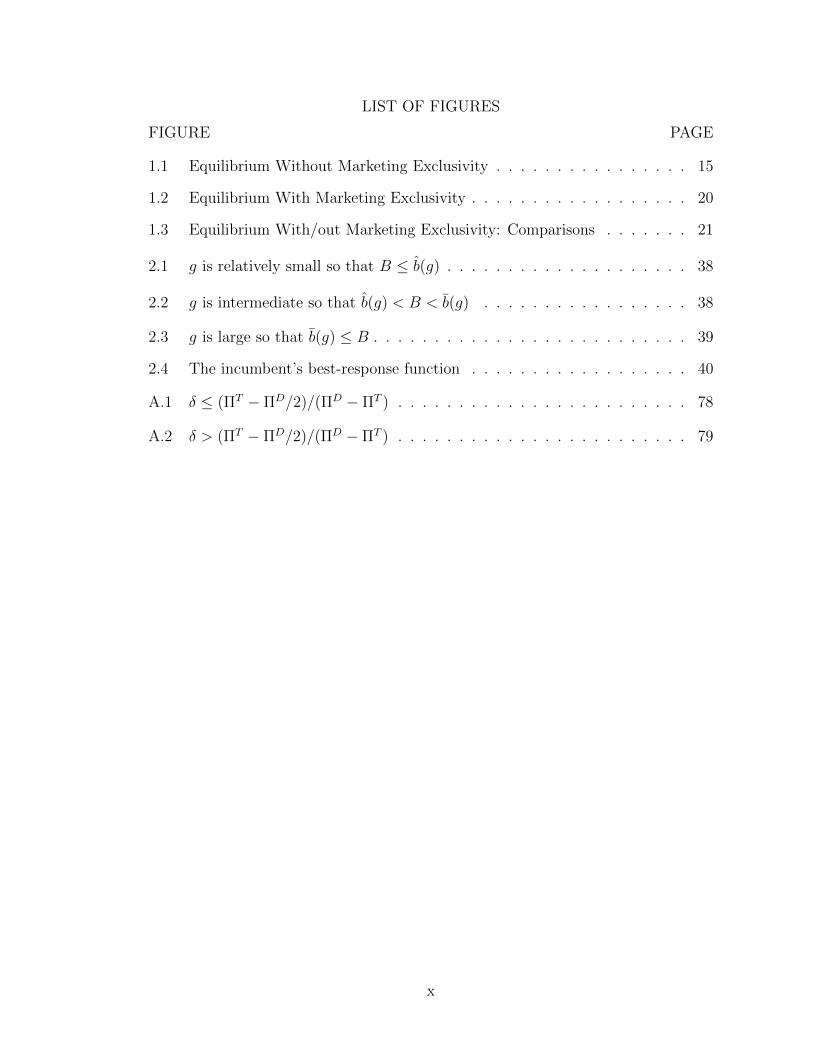
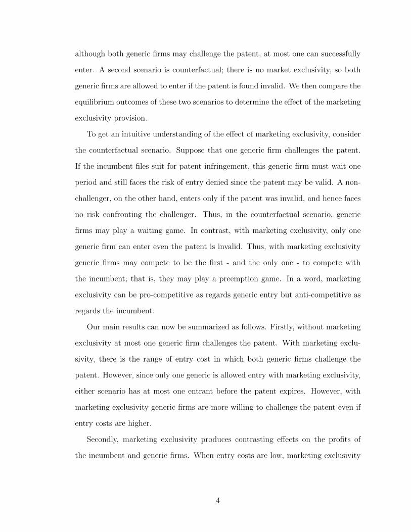
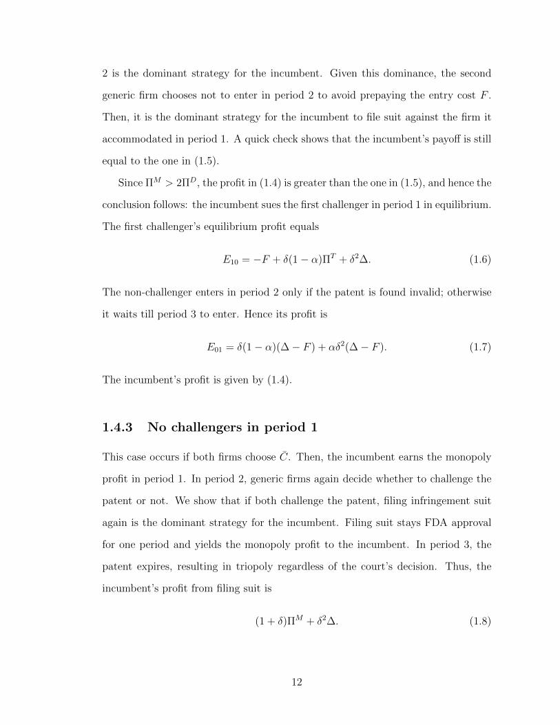
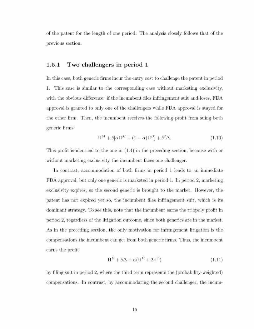
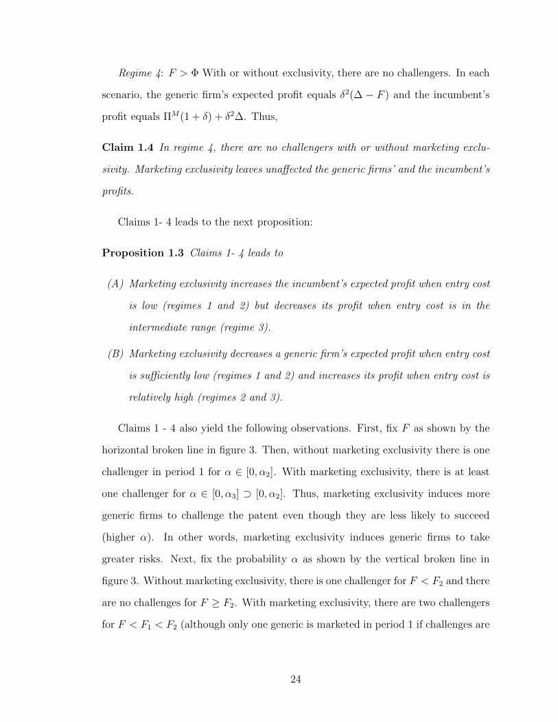
Figure 1 illustrates proposition 1. The line represents the relation F = . In
the area on and below this line there is one generic challenger in period 1; above
the line there are no challengers before the patent expires. Obviously, lower entry
cost and/or higher likelihood (low ↵) of patent invalidation entices a challenge to
the patent.
10Each firm challenges the patent with probability k = [�(1�↵)⇧T �F (1� �2)]/[�(1�↵)(1� �)(�� F )]. In this case, two firms enter with probability k2.
14
Figure 1.1: Equilibrium Without Marketing Exclusivity
We conclude this section with this remark. In the present model, only one firm
challenges in period 1 because of the time-consuming litigation process. If litigation
disputes are settled instantaneously as is usually assumed in the literature, there is
a range of parameter values in which there are two challengers in period 1. Thus,
the assumption of time-consuming litigation process is an important feature of our
analysis.
1.5 Marketing exclusivity
In this section we examine how marketing exclusivity a↵ects the generic firms’ entry
decisions. We assume that marketing exclusivity is granted to the first challenger
15
of the patent for the length of one period. The analysis closely follows that of the
previous section.
1.5.1 Two challengers in period 1
In this case, both generic firms incur the entry cost to challenge the patent in period
1. This case is similar to the corresponding case without marketing exclusivity,
with the obvious di↵erence: if the incumbent files infringement suit and loses, FDA
approval is granted to only one of the challengers while FDA approval is stayed for
the other firm. Then, the incumbent receives the following profit from suing both
generic firms:
⇧M + �[↵⇧M + (1� ↵)⇧D] + �2�. (1.10)
This profit is identical to the one in (1.4) in the preceding section, because with or
without marketing exclusivity the incumbent faces one challenger.
In contrast, accommodation of both firms in period 1 leads to an immediate
FDA approval, but only one generic is marketed in period 1. In period 2, marketing
exclusivity expires, so the second generic is brought to the market. However, the
patent has not expired yet so, the incumbent files infringement suit, which is its
dominant strategy. To see this, note that the incumbent earns the triopoly profit in
period 2, regardless of the litigation outcome, since both generics are in the market.
As in the preceding section, the only motivation for infringement litigation is the
compensations the incumbent can get from both generic firms. Thus, the incumbent
earns the profit
⇧D + ��+ ↵(⇧D + 2⇧T ) (1.11)
by filing suit in period 2, where the third term represents the (probability-weighted)
compensations. In contrast, by accommodating the second challenger, the incum-
16
bent forgoes the compensations, earning only ⇧D + ��, and hence the conclusion
follows. Under Assumption 1, the profit in (1.10) exceeds the profit in (1.11), so the
incumbent files infringement suit in period 1.
To calculate the generic firms’ profits, we use the assumption that both generic
firms believe each is granted marketing exclusivity with equal probabilities.11 Fur-
ther, note that the FDA grants marketing exclusivity to one challenger and stays
approval for the other. That means that when the marketing exclusivity expires
the FDA approves the second generic without another review process; that is, the
second generic firm can enter without incurring the entry cost F again. Under these
assumptions, each generic firm’s expected profit is
E11 = �F + �(1� ↵)(⇧D/2) + �2�. (1.12)
The incumbent’s equilibrium profit appears in (1.10).
1.5.2 One challenge in period 1
In this case by suing a single challenger in period 1, the incumbent has the profit
equal to the one in (1.10). The reason is that, as in the case of two challenges, the
second generic firm waits till period 3 to enter because (A) if the incumbent wins
the litigation, the second cannot challenge the patent in period 2; and (B) if the
first generic firm wins the suit, exclusivity prevents entry in period 2.
Accommodation of a single challenger is slightly more complicated than when
there are two challengers. In period 1, the challenger is accommodated and brings
its generic product to the market, resulting in duopoly. In period 2, the market
11In reality, there are cases in which two generic firms file applications on the same dayand end up sharing marketing exclusivity. This is a common strategy in the presence ofnumerous potential entrants. Given only two generic firms in our model, we disregardsuch a possibility.
17
exclusivity expires but the patent does not. If the second generic firm challenges the
patent in period 2, the incumbent chooses to file suit. The reason is that litigation
delays entry for one period, and with probability ↵ the patent is upheld, allowing
the incumbent to collect the compensations from the first generic firm. Therefore,
the incumbent’s expected profit equals
⇧D(1 + �) + �2�+ ↵⇧D(1 + �), (1.13)
where the last term represents the expected compensations. In constant, accom-
modating the second generic firm in period 2 yields ⇧T + ��, which is clearly less
than the profit in ((1.13). Thus, the incumbent sues the generic firms if the second
firm challenges the patent in period 2. Even if there is no challenge from the second
firm, the incumbent still sues the first entrant, because doing so yields the profit as
in ((1.13) while not suing yields ⇧D + ��, a smaller profit. Thus, the incumbent
sues the first entrant in period 2, regardless of what the second firm does in period
2. Hence, the second generic firm’s expected profit equals �F + �� from entry in
period 2 and �(�� F ) from non-entry. Clearly, the second firm waits till period 3.
We have shown that, if it accommodates the first entrant in period 1, the in-
cumbent sues that firm in period 2 and the second firm waits till period 3. The
incumbent’s profit is equal to the one given in (1.13). Since this profit is smaller
than the profit in ((1.10) obtained from suing the first challenger in period 1, the in-
cumbent always files infringement suit against the challenger in period 1. Therefore,
the challenge’s equilibrium expected profit is
E10 = �F + �(1� ↵)⇧D + �2�,
whereas the non-challenger’s profit is given by
E01 = �2(�� F ).
The incumbent’s profit is given in ((1.11).
18
1.5.3 No challenges in period 1
If there are no challengers in period 1, the incumbent is a monopoly in period 1.
In period 2, two generic firms again simultaneously decide whether to challenge
the patent or not. Since this case results in multiple subcases, requiring extensive
but less illuminating examination, we relegate the analysis of this case to the two
appendixes.
1.5.4 Equilibrium in period 1
Now we are ready to move back to period 1, where two generic firms play a
simultaneous-move game. This part of the analysis is tedious, so we present it in
Appendix B. The main conclusion from that appendix is the following proposition.
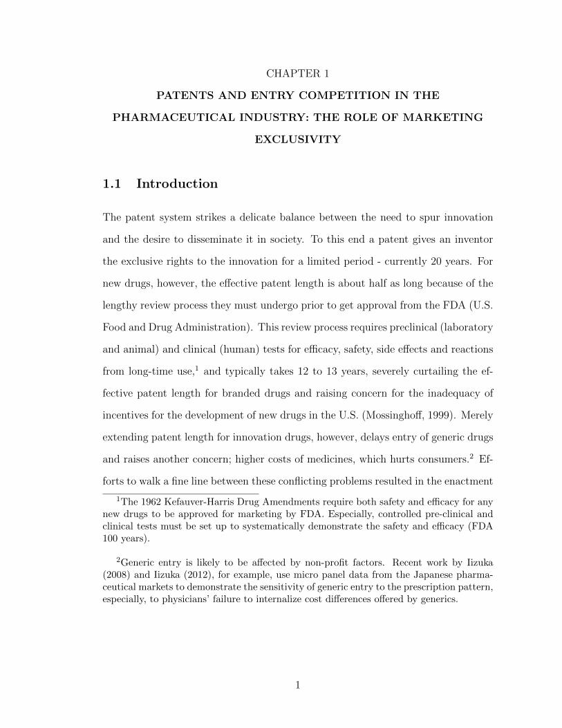
Proposition 1.2 Define � ⌘ �(1� ↵)⇧D/(1� �2).
(A) If F 2 (0,�/2), both generic firms challenge the patent in period 1.
(B) If F 2 (�/2,�), only one generic firm challenges the patent in period 1.
(C) If F 2 (�,1), neither firm challenges the patent in period 1.
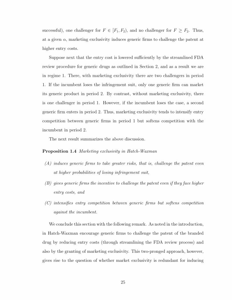
Figure 2 illustrates Proposition 2. Marketing exclusivity generates two critical
borderline equations: F = �/2 (represented by the yellow line) and F = � (repre-
sented by the blue line). The area below the line F = �/2 has both firms challenge
the patent in period 1 (although only one will be granted marketing exclusivity in
period 2). Between the two lines there is only one generic firm that challenges the
patent in period 1. Above the line F = �, thee are no challengers of the brand-name
drug’s patent in period 1.
The next result is an immediate consequence of Proposition 2.
19
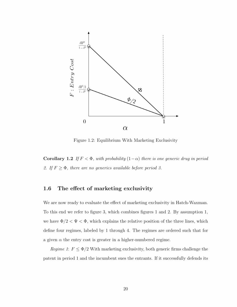
Figure 1.2: Equilibrium With Marketing Exclusivity
Corollary 1.2 If F < �, with probability (1�↵) there is one generic drug in period
2. If F � �, there are no generics available before period 3.
1.6 The e↵ect of marketing exclusivity
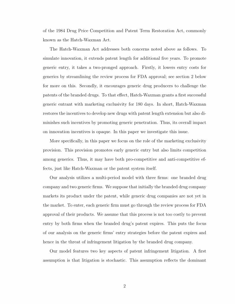
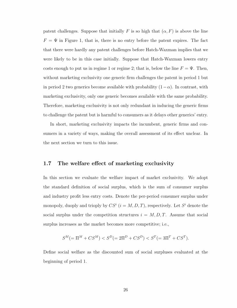
We are now ready to evaluate the e↵ect of marketing exclusivity in Hatch-Waxman.
To this end we refer to figure 3, which combines figures 1 and 2. By assumption 1,
we have �/2 < < �, which explains the relative position of the three lines, which
define four regimes, labeled by 1 through 4. The regimes are ordered such that for
a given ↵ the entry cost is greater in a higher-numbered regime.
Regime 1: F �/2 With marketing exclusivity, both generic firms challenge the
patent in period 1 and the incumbent sues the entrants. If it successfully defends its
20
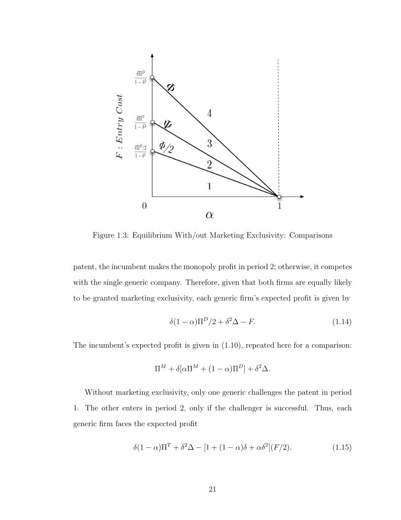
Figure 1.3: Equilibrium With/out Marketing Exclusivity: Comparisons
patent, the incumbent makes the monopoly profit in period 2; otherwise, it competes
with the single generic company. Therefore, given that both firms are equally likely
to be granted marketing exclusivity, each generic firm’s expected profit is given by
�(1� ↵)⇧D/2 + �2�� F. (1.14)
The incumbent’s expected profit is given in (1.10), repeated here for a comparison:
⇧M + �[↵⇧M + (1� ↵)⇧D] + �2�.
Without marketing exclusivity, only one generic challenges the patent in period
1. The other enters in period 2, only if the challenger is successful. Thus, each
generic firm faces the expected profit
�(1� ↵)⇧T + �2�� [1 + (1� ↵)� + ↵�2](F/2). (1.15)
21
If the patent is found invalid, the incumbent competes with both generic firms in
period 2; otherwise, it remains a monopoly. Therefore, the incumbent’s equilibrium
profit equals
⇧M + �↵⇧M + �(1� ↵)⇧T + �2�. (1.16)
The profit in (1.15) is greater than the profit in (1.14) while the profit in (1.16) is
less than the profit in (1.10).
Claim 1.1 In regime 1,
(A) there is one challenger without marketing exclusivity and two challengers with
marketing exclusivity;
(B) market exclusivity increases the incumbent’s expected profit and reduces the
generic firm’s expected profit.
Regime 2: F 2 (�/2, ] With marketing exclusivity, there is only one generic
challenge in period 1. Hence, the equilibrium profit to the incumbent is the same as
in regime 1 and is given in (1.16) above. As for the generic firm, we can show that a
challenger’s expected profit is �(1�↵)⇧D�F +�2� while that of the non-challenger
is �2(�� F ). Since both firms can be a challenger with equal likelihood, a generic
firm’s expected profit is given by
�(1� ↵)⇧D/2 + �2�� F (1� �2)/2. (1.17)
Without marketing exclusivity, there is also only one challenge in period 1. Each
generic firm’s expected profit equals the profit in (1.14). The incumbent’s equilib-
rium profit is given in (1.1), repeated below for a comparison
⇧M + �[↵⇧M + (1� ↵)⇧T ] + �2�.
Comparing the profits in (1.15) and (1.17) yields the first result of the next claim.
Comparing the profits in (1.10) and (1.1) yields the second.
22
Claim 1.2 In regime 2, where F 2 (�/2, ] the following results hold:
(A) There is only one challenger with or without marketing exclusivity.
(B) Marketing exclusivity increases the incumbent’s profit and
(C) Marketing exclusivity increases a generic firm’s profit if F > (2⇧T �⇧D)/(1�
�) and decreases a generic firm’s profit if the inequality is reversed.
For a given F , we are more likely to have F > (2⇧T � ⇧D)/(1 � �) when ↵
is higher (when the patent is found valid with higher probability). In such cases
marketing exclusivity increases all firms’ expected profits.
Regime 3: F 2 ( ,�] With marketing exclusivity, this regime leads to the same
equilibrium outcome as regime 2, with (1.10) and (1.17) showing the equilibrium
profits to the incumbent and each generic firm given, respectively. Regime 3 is
distinct from regime 2, however, because without marketing exclusivity there are
no challengers in regime 3. As both generic firms enter in period 3, their expected
profit is �2(� � F ) and the incumbent’s profit is ⇧M(1 + �) + �2�. Obviously,
the incumbent makes a greater profit without marketing exclusivity in this regime.
As for the generic firms, their profit in (1.17) exceeds �2(� � F ) if and only if
F � ⌘ (�(1� ↵)⇧D)/(1� �2). This inequality is satisfied in regime 3. Thus, we
have proved the following result.
Claim 1.3 In regime 3, the following results hold:
(A) There is one challenger without marketing exclusivity and one challenger with
marketing exclusivity.
(B) Marketing exclusivity reduces the incumbent’s profit and increases a generic
firm’s profit.
23
Regime 4: F > � With or without exclusivity, there are no challengers. In each
scenario, the generic firm’s expected profit equals �2(� � F ) and the incumbent’s
profit equals ⇧M(1 + �) + �2�. Thus,
Claim 1.4 In regime 4, there are no challengers with or without marketing exclu-
sivity. Marketing exclusivity leaves una↵ected the generic firms’ and the incumbent’s
profits.
Claims 1- 4 leads to the next proposition:
Proposition 1.3 Claims 1- 4 leads to
(A) Marketing exclusivity increases the incumbent’s expected profit when entry cost
is low (regimes 1 and 2) but decreases its profit when entry cost is in the
intermediate range (regime 3).
(B) Marketing exclusivity decreases a generic firm’s expected profit when entry cost
is su�ciently low (regimes 1 and 2) and increases its profit when entry cost is
relatively high (regimes 2 and 3).
Claims 1 - 4 also yield the following observations. First, fix F as shown by the
horizontal broken line in figure 3. Then, without marketing exclusivity there is one
challenger in period 1 for ↵ 2 [0,↵2]. With marketing exclusivity, there is at least
one challenger for ↵ 2 [0,↵3] � [0,↵2]. Thus, marketing exclusivity induces more
generic firms to challenge the patent even though they are less likely to succeed
(higher ↵). In other words, marketing exclusivity induces generic firms to take
greater risks. Next, fix the probability ↵ as shown by the vertical broken line in
figure 3. Without marketing exclusivity, there is one challenger for F < F2 and there
are no challenges for F � F2. With marketing exclusivity, there are two challengers
for F < F1 < F2 (although only one generic is marketed in period 1 if challenges are
24
successful), one challenger for F 2 [F1, F2), and no challenger for F � F2. Thus,
at a given ↵, marketing exclusivity induces generic firms to challenge the patent at
higher entry costs.
Suppose next that the entry cost is lowered su�ciently by the streamlined FDA
review procedure for generic drugs as outlined in Section 2, and as a result we are
in regime 1. There, with marketing exclusivity there are two challengers in period
1. If the incumbent loses the infringement suit, only one generic firm can market
its generic product in period 2. By contrast, without marketing exclusivity, there
is one challenger in period 1. However, if the incumbent loses the case, a second
generic firm enters in period 2. Thus, marketing exclusivity tends to intensify entry
competition between generic firms in period 1 but softens competition with the
incumbent in period 2.
The next result summarizes the above discussion.
Proposition 1.4 Marketing exclusivity in Hatch-Waxman
(A) induces generic firms to take greater risks, that is, challenge the patent even
at higher probabilities of losing infringement suit,
(B) gives generic firms the incentive to challenge the patent even if they face higher
entry costs, and
(C) intensifies entry competition between generic firms but softens competition
against the incumbent.
We conclude this section with the following remark. As noted in the introduction,
in Hatch-Waxman encourage generic firms to challenge the patent of the branded
drug by reducing entry costs (through streamlining the FDA review process) and
also by the granting of marketing exclusivity. This two-pronged approach, however,
gives rise to the question of whether market exclusivity is redundant for inducing
25
patent challenges. Suppose that initially F is so high that (↵, F ) is above the line
F = in Figure 1, that is, there is no entry before the patent expires. The fact
that there were hardly any patent challenges before Hatch-Waxman implies that we
were likely to be in this case initially. Suppose that Hatch-Waxman lowers entry
costs enough to put us in regime 1 or regime 2; that is, below the line F = . Then,
without marketing exclusivity one generic firm challenges the patent in period 1 but
in period 2 two generics become available with probability (1�↵). In contrast, with
marketing exclusivity, only one generic becomes available with the same probability.
Therefore, marketing exclusivity is not only redundant in inducing the generic firms
to challenge the patent but is harmful to consumers as it delays other generics’ entry.
In short, marketing exclusivity impacts the incumbent, generic firms and con-
sumers in a variety of ways, making the overall assessment of its e↵ect unclear. In
the next section we turn to this issue.
1.7 The welfare e↵ect of marketing exclusivity
In this section we evaluate the welfare impact of market exclusivity. We adopt
the standard definition of social surplus, which is the sum of consumer surplus
and industry profit less entry costs. Denote the per-period consumer surplus under
monopoly, duoply and trioply by CSi (i = M,D, T ), respectively. Let Si denote the
social surplus under the competition structures i = M,D, T . Assume that social
surplus increases as the market becomes more competitive; i.e.,
SM(= ⇧M + CSM) < SD(= 2⇧D + CSD) < ST (= 3⇧T + CST ).
Define social welfare as the discounted sum of social surpluses evaluated at the
beginning of period 1.
26
1.7.1 Marketing exclusivity
We first compute social welfare in the four regimes under marketing exclusivity.
Regime 1: In this regime there are two challengers in period 1 but the incumbent
remains a monopoly as it files infringement suit. In period 2 there is duopoly with
probability (1 � ↵) and monopoly otherwise. There is triopoly in period 3. Thus,
the social welfare is given by:
W (1) = SM � 2F + ↵�SM + (1� ↵)�SD + �2SD/(1� �) (1.18)
Regimes 2 and 3: In these regimes there is only one challenger in period 1. In
period 2, there is duopoly with probability (1 � ↵) and monopoly, otherwise. In
period 3 thee is triopoly. The social welfare is given by:
W (2, 3) = SM � F + ↵�SM + (1� ↵)�SD + �2[SD/(1� �)� F ]. (1.19)
Regime 4: There is no entry until period 3. Social welfare is given by
W (4) = (1 + �)SM + �2[SD/(1� �)� 2F ]. (1.20)
1.7.2 No marketing exclusivity
We next compute the social welfare without marketing exclusivity. In regimes 1
and 2, only one generic firm challenges in period 1. In period 2, if the patent is
invalidated, there is triopoly, as the first generic firm markets its product, and the
second also makes entry. Otherwise, there is monopoly until period 3, when the
second firm enters. Social welfare is:
W (1, 2) = SM �F +↵�SM +(1�↵)�ST +(�2SD)/(1��)��F [(1�↵)+↵�]. (1.21)
27
In regimes 3 and 4, there is no entry until period 3. The social welfare in these
regimes is identical to in (1.20) above
W (3, 4) = (1 + �)SM + �2[SD/(1� �)� 2F ] = W (4). (1.22)
1.7.3 The welfare impact of marketing exclusivity
With the above calculations we can now make welfare comparisons.
Regime 1:
W (1)� W (1, 2) = �F + (1� ↵)�(SD � ST )� �F [(1� ↵)� ↵�]
< F [(1� ↵)� + ↵�2 � 1]
= �(1� �)(1 + ↵�)F
< 0
Therefore, in this regime marketing exclusivity decreases social welfare.
Regime 2:
W (2, 3)� W (1, 2) = (1� ↵)�(SD � ST )� F [�2 � �(1� ↵)� ↵�2]
< ��(1� �)(1� ↵)F
< 0
Again, marketing exclusivity decreases social welfare.
Regime 3:
W (2, 3)� W (3, 4) = (1� ↵)�(SD � SM) + (�2 � 1)F.
The first term on the right is positive while the second is negative, so the impact of
marketing exclusivity is ambiguous. To sign the di↵erence, define F by
W (2, 3)� W (3, 4) = (1� ↵)�(SD � SM) + (�2 � 1)F = 0;
28
or
F = (1� ↵)�(SD � SM)/(1� �2).
Then, W (2, 3) � W (3, 4) > 0 if and only if F < F . Thus, marketing exclusivity
increases social welfare if and only if F < F . Since Fdepends on ↵, we can use
claim 3 above to derive
Claim 5: In regime 3:
(A) If SD � SM < ⇧T , then F > F for all ↵; i.e., marketing exclusivity decreases
social welfare.
(B) If SD � SM > ⇧D, then F < F for all ↵; i.e., marketing exclusivity increases
social welfare.
(C) If ⇧T SD � SM ⇧D, the e↵ect on welfare is indeterminate.
Regime 4: By (1.20), W (3, 4) = W (4) and hence marketing exclusivity has no
e↵ect on social welfare.
We summarize the main results of this section in
Proposition 1.5 Marketing exclusivity increases social welfare if and only if we
are in regime 3, i. e., F 2 ( ,�] and if F < F = (1� ↵)�(SD � SM)/(1� �2).
In general, both conditions on F are needed for the conclusion of proposition 6 to
hold. In the case of Cournot competition with linear demand and constant marginal
cost, regime 3 implies F < F and hence the second condition can be dispensed with.
1.8 Concluding remarks
Hatch-Waxman is intended to restore incentives for new drug development and
simultaneously promote generic entry. To accomplish the first objective, it has
29
extended patent length for new drugs; to accomplish the second, it has reduced
entry costs and granted marketing exclusivity to a first generic firm that successfully
challenges the patent. In this paper we find that marketing exclusivity suppresses
competition among generics and harms consumers. Thus, removing the marketing
exclusivity provision may improve social welfare, and benefit both consumers and
generic firms. One caveat to this conclusion is that marketing exclusivity is also
likely to raise the incumbent’s profits and hence the incentive to develop new drugs.
If this incentive-restoration e↵ect is su�ciently strong, new drugs may be brought
to the market sooner, thereby increasing social welfare in the long run. Exploring
this possibility is left for future research.
Finally, our analysis also points out a new direction for empirical research. Cur-
rently, there is overwhelming evidence showing dramatic increases, since Hatch-
Waxman, in the number of generics having been brought to markets before the
branded drugs’ patents expire. Our analysis raises the question as to what propor-
tion of such increases is solely due to the streamlining of testing and application
procedures and what proportion can be explained by marketing exclusivity alone.
It is hoped that future research also addresses this important question.
30
CHAPTER 2
WHY AUTHORIZED GENERICS?: THEORETICAL AND
EMPIRICAL INVESTIGATIONS
2.1 Introduction
When facing generic competition, the brand-name companies sometimes launch
generic versions of their own. Such generics, to be distinguished from ordinary
(unauthorized) generics, are called authorized generics (AGs). Authorized generics
contain exactly the same ingredients as the brand-name drugs and even come o↵
the same production line, but are sold by a third party in the generic category.
Authorized generics directly compete with both regular generics and brand-name
drugs. Since competition depresses the price of the brand-name drug, launching an
authorized generic is a form of cannibalization for the brand-name company. This
raises the question as to why the brand-name drug companies use such a strategy
in the first place.
On the other hand, launching authorized drugs may make business sense if the
brand-name drug company allows the authorized generic distributer to act as an
autonomous entity but receives a large part of the latter’s profit as side payments
through contracts. This e↵ect can be demonstrated with the standard model of
Cournot oligopoly, in which a firm can always increase total profit by splitting itself
into two autonomous entities. This idea is dubbed “divisionalization” by Baye et al.
(1996). But if this is profitable the brand-name companies should always launch the
AGs when facing generic competition. However, according to the AG list by the FDA
(U. S. Food and Drug Administration), only a small number of o↵-patent brand-
name drugs have had AGs. This fact gives rise to another puzzle: if divisionalization
31
is profitable, why don’t brand-name drug companies launch authorized generics for
all their o↵-the-patent drugs?
In this paper I attempt to address these puzzles. My investigation into the ra-
tionale for launch of authorized drugs begins by calling attention to yet another
puzzle. Since generics (including authorized generics or AGs) are functionally the
same as the brand-name drugs but priced lower, we would expect the prices of the
brand-name drugs to fall swiftly to be more competitive when the generics become
available in the market. However, we never see such precipitate price drops for
brand-name drugs. Nor do we see huge demand shifts from the brand-name drug to
the generics when the generics appear on the market. In this paper I explain these
twin puzzles in terms of the customer bases the brand-name drugs build prior to
generic entry. In economics jargon such customer bases can be analyzed using the
notion of switching costs, popularized by a series of papers by Klemperer (Klem-
perer, 1987). What are the switching costs a consumer incurs when she switches
from the brand-name drug to a generic? Drugs do not usually miraculously cure
fatal illnesses. Rather, they only reduce the risk of death without entirely eliminat-
ing it by relieving symptoms of the illness such as pain or anxiety or by altering
a clinical measurement - reduce cholesterol or blood pressure, for example. These
e↵ects are di�cult to detect and evaluate even for scientists. In a word, drugs are
essentially credence goods. As such, consumers tend to rely on personal experiences
to gain confidence in the e�cacy of the drug, and this confidence - and aversion
to an alternative drug - grows if they use the drug repeatedly. In this respect, the
brand-name drug has the first-mover advantage over generics simply because con-
sumers have been using the brand-name drug before generics appear on the market.
This acquired confidence in the brand-name drug serves as the switching cost - the
benefit a consumer must give up when switching to generics.
32
I now outline the present paper. I first present a two-period model of com-
petition between a brand-name drug company and a generic firm. In the first period
the brand-name company is a incumbent monopoly. In the second period a generic
firm enters and two compete in quantities. The customers who buy the brand-name
drug in the first period develop certain a�nities to it as explained above and form a
customer base for the incumbent in the second period. I assume that the brand-name
company can influence the size of its customer base but cannot a↵ect the switching
cost per se. In other words, I treat the switching cost as a key parameter of this
model. I then extend the analysis to allow the brand-name company to launch the
authorized generic in period 2. I assume that a third party markets the authorized
drug and all firms compete as Cournot oligopolists. I regard all three types of drugs
(brand-name, generic and authorized generic) as homogeneous. The only thing
that separates the brand-name drug from the other two in the second period is the
presence of the switching costs. Thus, consumers who bought the brand-name drugs
in the first period incur the same switching cost when they switch to either generic.
Finally, it is assumed that the profit from AG sales is received by the brand-name
company by contract (take-it-or-leave-it o↵er).
The analysis yields the following results. When the switching cost is relatively
small, the incumbent is more likely to launch an authorized generic. In that case, it
sells the brand-name drugs only to the customer base, and the authorized generic to
new customers to compete with the regular generic. This has an intuitive explana-
tion. In the standard Cournot game, launching of an AG only has the divisionaliza-
tion e↵ect, as shown by Baye et al. (1996). [6] In the presence of the customer base,
by contrast, launching an AG also has the cannibalization e↵ect, as it depresses
the prices of the generic drugs and tempts some consumers in the customer base
to switch. However, when the switching cost is su�ciently large, consumers do not
33
switch easily so the incumbents prefer to distort the first-period output to create
a larger customer base. Then the cannibalization is more damaging so it refrains
from launching an AG and content itself with serving only the customer base. By
contrast, when the switching cost is smaller, some consumer base erosion may oc-
cur, so creation of a large customer base is futile. But still it is preferable not to
launch an AG so as to prevent further customer base erosions due to the cannibal-
ization e↵ect it creates. When the switching cost is even smaller, however, there is
such substantial customer base erosion when the generic enters that the damage of
cannibalization is minimal relative to the benefit from divisionalization. Thus, it is
optimal for the incumbent to launch an AG when the switching cost is su�ciently
small. Thus, the formal model yields a testable hypothesis as to a possible rationale
for launching AGs. In the latter part of this paper, I test this hypothesis against
the data collected from the FDA website and find strong support.
I now relate my work to the literature. Some papers examine the e↵ects of
authorized generics on non-authorized generic entry. For example, the FTC’s 2009
report shows that the launch of AGs leads to low generic prices and revenues, and
speculates that this may even lead to a collusive agreement between the generic and
the brand-name firms and produce a double jeopardy for consumers: deferment of
generic entry and non-marketing of AGs.1 Chen (2007) examines the legal issues
arising from AGs, and calls for a legislative reform of the Hatch-Waxman Act.
Rei↵en and Ward (2005) shows that the launch of AGs reduces the number of
potential generic entrants in the future. However, Berndt et al. (2007) concludes
that, though AGs reduce the expected gains for generic patent challengers, su�cient
1Authorized Generics: An Interim Report of the Fed-eral Trade Commission, 2009. http://www.ftc.gov/reports/authorized-generics-interim-report-federal-trade-commission.
34
incentives remain for generic entry. Appelt (2010), examining the consequences of
AG in Germany, also finds that the introduction of AGs has no e↵ect on the number
of generic entrants, and therefore is not for entry deterrence.
While all these papers focus on the e↵ects of AGs on generic entry, little has been
done as to the e↵ects of AG launch on the brand-name companies. My paper is an
attempt to fill this lacuna in the literature. My findings are consistent with recent
empirical findings. For example, my first finding that brand-name companies launch
AGs when switching costs are low receives indirect support from Appelt (2010) who
identifies earning generic profits as the primary motive for introduction of AGs. My
result may also explain the empirical finding of Berndt et al. (2007) that drugs with
higher pre-generic revenues are more likely to have AGs. My analysis shows that
for a given switching cost, the incumbent is more likely to launch an AG if the
market is larger. The in- tuition is that an increase in demand (intercept) expands
the divisionalization e↵ect relative to the cannibalization e↵ect (more specifically,
it raises the sum of the combined profit from brand-name drug and AG sales by
a greater magnitude than the profit from brand-name drug sales alone). If the
pre-generic revenues are interpreted as a proxy of the market size, my finding is
consistent with that of these authors.
The remainder of this chapter is organized in 5 sections. In section 2 I present
a two-period model of Cournot oligopoly. In this version, the incumbent builds a
customer base in the first period but does not launch an AG when there is generic
entry in the second period. In section 3 I extend the model so as to allow the
incumbent to market an AG through a third party. In section 4 I compare the
incumbent’s profits between the two scenarios described above and show that the
launch of an AG is profitable to the incumbent only when the switching cost is
35
relatively small. In section 5 I present an empirical model to test the hypothesis
and discuss my empirical findings. Section 6 concludes the paper.
2.2 Competitions Without AG
This section presents a two-period model of entry and competition without AG. The
model has the following game structure. In period 1, a brand-name company, an
incumbent monopoly, chooses quantity B. I suppose that each consumer buys one
unit of a drug, so B represents the number of the customers who buy the branded
drug in period 1. Those customers develop a�nities towards the brand-name drug
and constitute its customer base. These a�nities they acquire define the switching
cost of this model, which we denote by s. In period 2, a generic firm enters and
two firms play a Cournot game. I assume that all drugs are produced at common
constant marginal cost, which I set equal zero to simplify the exposition. I assume
for tractability that the demand function is linear and is given by p = m � Q,
where m is demand intercept and Q is total supply. I then solve the model for the
subgame-perfect Nash equilibrium.
Let me begin with the second period, where the customer base B is given. Let
b and g, respectively, denote the quantity of output supplied by the incumbent and
the generic firm in period 2 so that Q = b + g. The entrant maximizes the profit
⇧g = (m� b� g)g, yielding the standard best-response function g(b) = (m� b)/2.
To derive the incumbent’s best-response function, note that the incumbent faces the
inverse demand function:
p2(b) =
8>><
>>:
m+ s� b� g if b B
m� b� g if b > B
36
which is discontinuous at output b = B. Therefore, the incumbent’s profit is dis-
continuous at b = B and given by
⇡b =
8>>>>>><
>>>>>>:
(m+ s� b� g)b if b < B
(m+ s� B � g)B if b = B
(m� b� g)b if b > B
In Figure 1, the curve to the left of B (solid line) displays the profit
⇡(b, s, g) = (m+ s� b� g)b,
while the one to the right of B (solid line) corresponds to the function
⇡(b, g) = (m� b� g)b.
Now, to obtain the incumbent’s best-response function, define these key quantities:
b(g) = argmax (m+ s� b� g)b and b(g) = argmax (m� b� g)b. Write the corre-
sponding maximum profits as ⇡(b, s, g) and ⇡(b, g). Define next the quantity b(g)
implicitly by ⇡(b, s, g) = (m+ s� b� g) = ⇡(b, g). Then, it is obvious that for given
g
b(g) < b(g) < b(g).
In the linear case we have,
b(g) = (m+ s� g)/2
b(g) = (m� g)/2
b(g) = (m+ s� g �p
s(2m+ s� 2g))/2
Now, as g increases, the profit functions ⇡(b, s) and ⇡(b) shift down, giving rise
to the following three cases, depending on B.
37
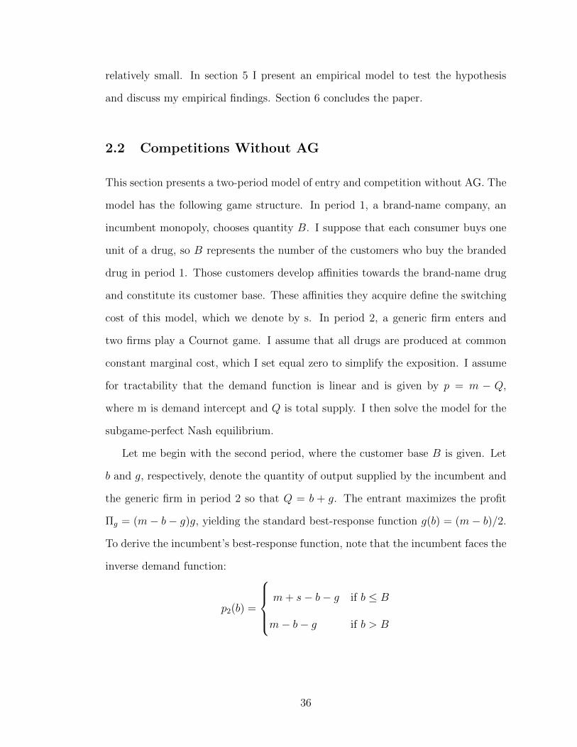
(i) g is relatively small such that B b(g). Then the incumbent’s best response
is b(g)
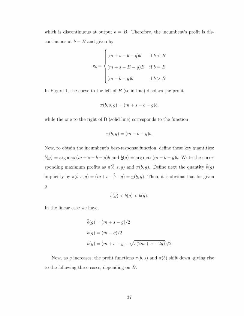
(ii) g takes on an intermediate value so that b(g) < B < b(g). In this range the
incumbent’s best response is B.
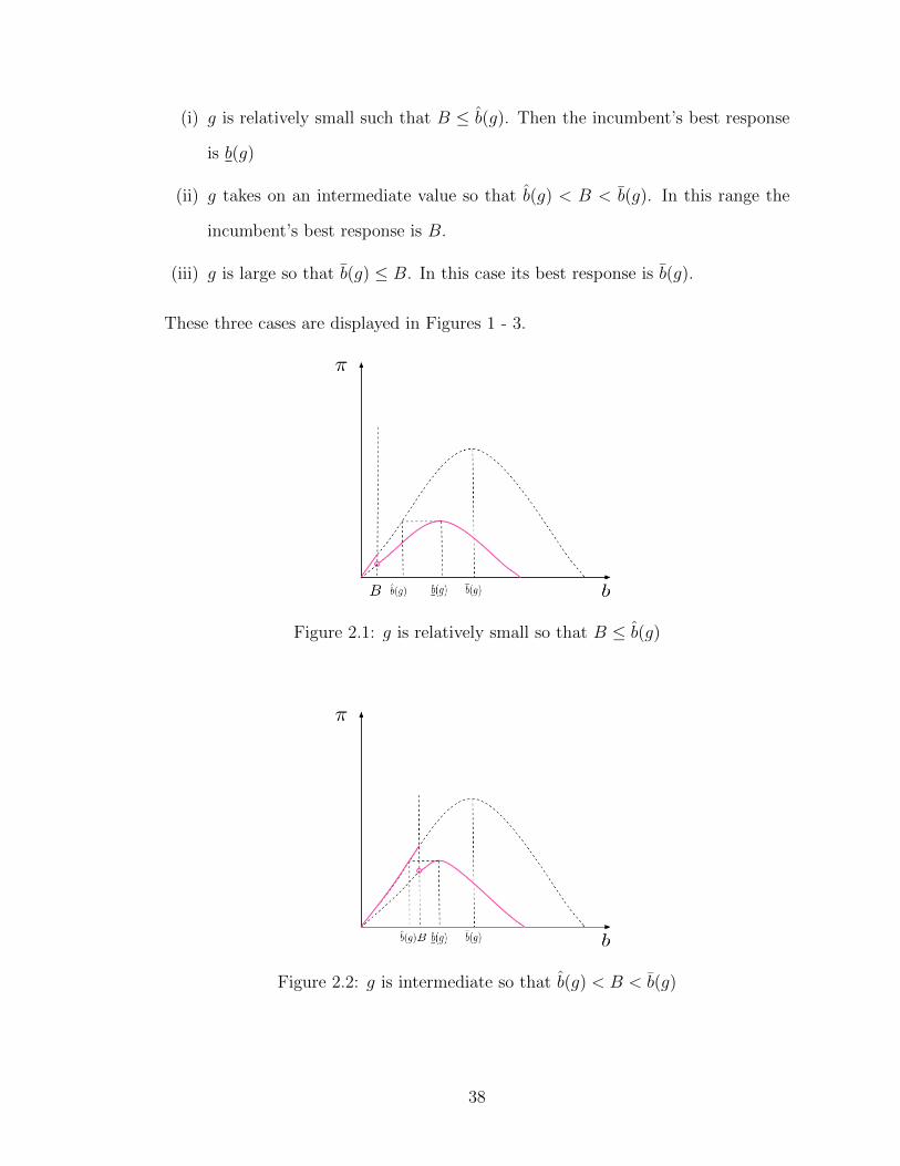
(iii) g is large so that b(g) B. In this case its best response is b(g).
These three cases are displayed in Figures 1 - 3.
Figure 2.1: g is relatively small so that B b(g)
Figure 2.2: g is intermediate so that b(g) < B < b(g)
38
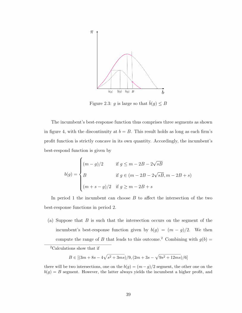
Figure 2.3: g is large so that b(g) B
The incumbent’s best-response function thus comprises three segments as shown
in figure 4, with the discontinuity at b = B. This result holds as long as each firm’s
profit function is strictly concave in its own quantity. Accordingly, the incumbent’s
best-respond function is given by
b(g) =
8>>>>>><
>>>>>>:
(m� g)/2 if g m� 2B � 2psB
B if g 2 (m� 2B � 2psB,m� 2B + s)
(m+ s� g)/2 if g � m� 2B + s
In period 1 the incumbent can choose B to a↵ect the intersection of the two
best-response functions in period 2.
(a) Suppose that B is such that the intersection occurs on the segment of the
incumbent’s best-response function given by b(g) = (m � g)/2. We then
compute the range of B that leads to this outcome.2 Combining with g(b) =
2Calculations show that if
B 2 [(3m+ 8s� 4ps2 + 3ms)/9, (2m+ 3s�
p9s2 + 12ms)/6]
there will be two intersections, one on the b(g) = (m� g)/2 segment, the other one on theb(g) = B segment. However, the latter always yields the incumbent a higher profit, and
39
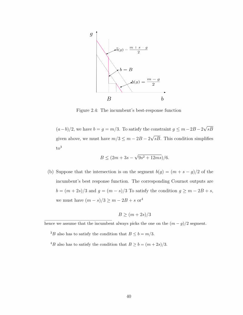
Figure 2.4: The incumbent’s best-response function
(a�b)/2, we have b = g = m/3. To satisfy the constraint g m�2B�2psB
given above, we must have m/3 m� 2B � 2psB. This condition simplifies
to3
B (2m+ 3s�p9s2 + 12ms)/6.
(b) Suppose that the intersection is on the segment b(g) = (m + s � g)/2 of the
incumbent’s best response function. The corresponding Cournot outputs are
b = (m + 2s)/3 and g = (m� s)/3 To satisfy the condition g � m� 2B + s,
we must have (m� s)/3 � m� 2B + s or4
B � (m+ 2s)/3
hence we assume that the incumbent always picks the one on the (m� g)/2 segment.
3B also has to satisfy the condition that B b = m/3.
4B also has to satisfy the condition that B � b = (m+ 2s)/3.
40
(c) Suppose finally that the intersection occurs on the vertical segment of the
incumbent’s best-response function, i. e., g(b) = B Then,
B 2 ((2m+ 3s�p9s2 + 12ms)/6, (m+ 2s)/3).
If we let
B = (2m+ 3s�p9s2 + 12ms)/6,
we can write the incumbent’s equilibrium second-period profit as
⇡b =
8>>>>>><
>>>>>>:
m2/9 if B 2 (0, B]
(m� B + 2s)B/2 if B 2 (B, (m+ 2s)/3)
(m+ 2s)2/9 if B 2 [(m+ 2s)/3,1)
We are now in a position to move to period 1. In that period the incumbent
chooses its output B to maximize the sum of profits in both periods (we ignore
discounting), which are written as
⇧b =
8>>>>>><
>>>>>>:
(m� B)B +m2/9 if B 2 (0, B]
(m� B)B + (m� B + 2s)B/2 if B 2 (B, (m+ 2s)/3)
(m� B)B + (m+ 2s)2/9 if B 2 [(m+ 2s)/3,1)
2.2.1 B 2 [0, B]
The incumbent’s total profit is:
⇧ = (m� B)B +m2/9.
In this case, B has no e↵ect on the incumbent’s period 2 profits. Thus, ⇧ is max-
imized at B = m/2. However, since m/2 > B, the constraint on B is binding.
Therefore, the optimal B is B, and the maximum profit will be ⇧(B).
41
2.2.2 B 2 (B, (m+ 2s)/3)
The incumbent’s total profit is:
⇧ = B(m� B) + (m� B + 2s)B/2.
The unconstrained optimum occurs at B = (3m + 2s)/6, which is greater than B.
Comparing (3m+ 2s)/6 with (m+ 2s)/3, I find:
8>><
>>:
(m+ 2s)/3 > (3m+ 2s)/6 if s > m/2
(m+ 2s)/3 (3m+ 2s)/6 if s m/2
Therefore, when s > m/2, B = (3m+2s)/6 is within this feasible range of B, and
the maximum profit is denoted by ⇧((3m+2s)/6). When s m/2, B = (3m+2s)/6
exceeds the upper limit of the range of B. Therefore, there is no optimal B in this
range, but there is the supremum B = (3m+ 2s)/6.
2.2.3 B 2 [(m+ 2s)/3,1)
The incumbent’s total profit is
⇧ = B(m� B) + (m+ 2s)2/9.
The unconstrained optimum occurs at B = m/2. Comparing m/2 with (m+2s)/3,
I find that: 8>><
>>:
m/2 � (m+ 2s)/3 if s m/4
m/2 < (m+ 2s)/3 if s > m/4
Therefore, when s m/4, the maximum profit is ⇧(m/2) = m2/4 + (m + 2s)2/9.
When s > m/4, the maximum profit is ⇧((m+ 2s)/3) = [2(m+ 2s)(m� s) + (m+
2s)2]/9.
42
2.2.4 Global maxima without AG
So far we identified the local maxima. We now turn to the global maxima for the
incumbent.
When s m/4, the incumbent can choose B 2 (0, B] or B 2 [(m + 2s)/3,1)
and receive the corresponding profits ⇧(B) and ⇧(m/2). Computation shows that
⇧(B) < ⇧(m/2) so the global optimum occurs at B = m/2 and b = (m + 2s)/3.
The incumbent’s equilibrium total profit is ⇧(m/2).
When s 2 (m/4,m/2], the incumbent chooses B 2 (0, B] or B 2 [(m+2s)/3,1)
and obtains the local maximum ⇧(B) and ⇧((m+2s)/3). A calculation establishes
that ⇧(B) < ⇧((m+ 2s)/3) so the global maximum occurs at B = (m+ 2s)/3 and
b = (m+ 2s)/3. The equilibrium total profit is ⇧((m+ 2s)/3).
When s 2 (m/2,m), the incumbent chooses B 2 (0, B] or B 2 (B, (m+2s)/3) or
B 2 [(m+2s)/3,1) and achieves the corresponding local maxima: ⇧(B), ⇧((3m+
2s)/6) and ⇧((m + 2s)/3). Computation shows that ⇧((3m + 2s)/6) exceeds the
other two. Hence, the equilibrium outputs are B = (3m+2s)/6 and b = (3m+2s)/6,
and its total profit is ⇧((3m+ 2s)/6).
These results are summarized in
Proposition 2.1 The equilibrium customer base is given by
B =
8>>>>>><
>>>>>>:
m/2 if s 2 (0,m/4],
(m+ 2s)/3 if s 2 (m/4,m/2],
(3m+ 2s)/6 if s 2 (m/2,m).
The following results are immediate consequences of Proposition 2.1
Proposition 2.2 A) When s 2 (0,m/4], the brand-name firm sells less than its
customer base in the second period; B) When s 2 (m/4,m), the brand-name firm
holds on to its customer base in the second period.
43
From Proposition 2.2, we can see that the brand-name drug is never sold to new
customers in the second period. This implies that those who bought the brand-name
drug in the first period are willing to pay the premium over the generic, which is the
switching cost. This finding explains why, in the real world, the brand-name drugs
are always priced higher than their generic counterparts.
2.3 With AG
In this section we allow the incumbent to introduce an AG through a third party
in period 2. The firm distributing the AG is autonomous and competes fully with
the brand-name drug company and the generic firm. However, we assume that the
incumbent makes a take-it-or-leave-it o↵er to the management of the AG firm so
that that it can collect the profit from AG sales through a contractual agreement
with the AG supplier.
The model is similar to the one developed in the preceding section. In the first
period the incumbent chooses the quantity B. In the second period, it competes
with two generic firms. Let a denote the quantity of the authorized generic supplied,
and b and g the quantities of the brand-name drug and the generic drug supplied in
the second period. With this notation the brand-name company faces the inverse
demand function:
p2 =
8>><
>>:
m+ s� b� a� g if b B;
m� b� a� g if b > B.
44

Note that the demand function is discontinuous at output b = B. Therefore, the
incumbent’s profit is also discontinuous at b = B:
⇡b =
8>>>>>><
>>>>>>:
(m+ s� b� a� g)b if b < B;
(m+ s� B � a� g)B if b = B;
(m� b� a� g)b if b > B.
The incumbent’s best response function can be written as
b(a, g) =
8>>>>>><
>>>>>>:
(m� a� g)/2 if a+ g m� 2B � 2psB;
B if a+ g 2 (m� 2B � 2psB,m� 2B + s);
(m+ s� a� g)/2 if a+ g � m� 2B + s.
Without the customer base, the generic faces the demand p2 = m � b � a � g
and the profit ⇡g = (m � b � a � g)g. The generic firm maximizes it profit ⇡g. Its
best response function is given by
g(b, a) = (m� b� a)/2.
Similarly, the authorized generic faces the same demand p2 = m� b� a� g and
the profit ⇡a = (m� b� a� g)a. The authorized generic distributor maximizes its
profit ⇡a. Its best response is given by
a(b, g) = (m� b� g)/2.
Then, depending on B, the incumbent can adjust the shape of its best response
function so that it can reach the equilibrium either at its lower segment (b = (m�
a � g)/2), middle segment (b = B) or upper segment (b = (m + s � a � g)/2).
According to di↵erent ranges of B, the incumbent’s equilibrium profits (including
45
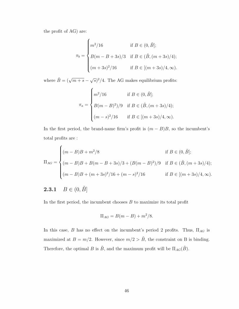
the profit of AG) are:
⇡b =
8>>>>>><
>>>>>>:
m2/16 if B 2 (0, B];
B(m� B + 3s)/3 if B 2 (B, (m+ 3s)/4);
(m+ 3s)2/16 if B 2 [(m+ 3s)/4,1).
where B = (pm+ s�
ps)2/4. The AG makes equilibrium profits:
⇡a =
8>>>>>><
>>>>>>:
m2/16 if B 2 (0, B];
B(m� B)2)/9 if B 2 (B, (m+ 3s)/4);
(m� s)2/16 if B 2 [(m+ 3s)/4,1).
In the first period, the brand-name firm’s profit is (m � B)B, so the incumbent’s
total profits are :
⇧AG =
8>>>>>><
>>>>>>:
(m� B)B +m2/8 if B 2 (0, B];
(m� B)B +B(m� B + 3s)/3 + (B(m� B)2)/9 if B 2 (B, (m+ 3s)/4);
(m� B)B + (m+ 3s)2/16 + (m� s)2/16 if B 2 [(m+ 3s)/4,1).
2.3.1 B 2 (0, B]
In the first period, the incumbent chooses B to maximize its total profit
⇧AG = B(m� B) +m2/8.
In this case, B has no e↵ect on the incumbent’s period 2 profits. Thus, ⇧AG is
maximized at B = m/2. However, since m/2 > B, the constraint on B is binding.
Therefore, the optimal B is B, and the maximum profit will be ⇧AG(B).
46
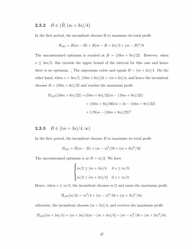
2.3.2 B 2 (B, (m+ 3s)/4)
In the first period, the incumbent chooses B to maximize its total profit
⇧AG = B(m� B) + B(m� B + 3s)/3 + (m� B)2/9.
The unconstrained optimum is reached at B = (10m + 9s)/22. However, when
s 3m/5, this exceeds the upper bound of the interval for this case and hence
there is no optimum. , The supremum exists and equals B = (m + 3s)/4. On the
other hand, when s > 3m/5, (10m+9s)/22 < (m+3s)/4, and hence the incumbent
chooses B = (10m+ 9s)/22 and reaches the maximum profit
⇧AG((10m+ 9s)/22) =(10m+ 9s)/22(m� (10m+ 9s)/22)
+ (10m+ 9s)/66(m+ 3s� (10m+ 9s)/22)
+ 1/9(m� (10m+ 9s)/22)2.
2.3.3 B 2 [(m+ 3s)/4,1)
In the first period, the incumbent chooses B to maximize its total profit
⇧AG = B(m� B) + (m� s)2/16 + (m+ 3s)2/16.
The unconstrained optimum is at B = m/2. We have8>><
>>:
m/2 � (m+ 3s)/4 if s m/3;
m/2 < (m+ 3s)/4) if s > m/3.
Hence, when s m/3, the incumbent chooses m/2 and earns the maximum profit
⇧AG(m/2) = m2/4 + (m� s)2/16 + (m+ 3s)2/16;
otherwise, the incumbent chooses (m+ 3s)/4, and receives the maximum profit
⇧AG((m+ 3s)/4) = (m+ 3s)/4(m� (m+ 3s)/4) + (m� s)2/16 + (m+ 3s)2/16.
47
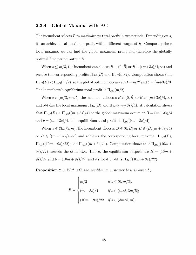
2.3.4 Global Maxima with AG
The incumbent selects B to maximize its total profit in two periods. Depending on s,
it can achieve local maximum profit within di↵erent ranges of B. Comparing these
local maxima, we can find the global maximum profit and therefore the globally
optimal first period output B.
When s m/3, the incumbent can choose B 2 (0, B] or B 2 [(m+3s)/4,1) and
receive the corresponding profits ⇧AG(B) and ⇧AG(m/2). Computation shows that
⇧AG(B) < ⇧AG(m/2), so the global optimum occurs at B = m/2 and b = (m+3s)/3.
The incumbent’s equilibrium total profit is ⇧AG(m/2).
When s 2 (m/3, 3m/5], the incumbent chooses B 2 (0, B] or B 2 [(m+3s)/4,1)
and obtains the local maximum ⇧AG(B) and ⇧AG((m+3s)/4). A calculation shows
that ⇧AG(B) < ⇧AG((m+3s)/4) so the global maximum occurs at B = (m+3s)/4
and b = (m+ 3s)/4. The equilibrium total profit is ⇧AG((m+ 3s)/4).
When s 2 (3m/5,m), the incumbent chooses B 2 (0, B] or B 2 (B, (m+ 3s)/4)
or B 2 [(m + 3s)/4,1) and achieves the corresponding local maxima: ⇧AG(B),
⇧AG((10m+ 9s)/22), and ⇧AG((m+ 3s)/4). Computation shows that ⇧AG((10m+
9s)/22) exceeds the other two. Hence, the equilibrium outputs are B = (10m +
9s)/22 and b = (10m+ 9s)/22, and its total profit is ⇧AG((10m+ 9s)/22).
Proposition 2.3 With AG, the equilibrium customer base is given by
B =
8>>>>>><
>>>>>>:
m/2 if s 2 (0,m/3];
(m+ 3s)/4 if s 2 (m/3, 3m/5];
(10m+ 9s)/22 if s 2 (3m/5,m).
48
2.4 Comparisons
In this section we compare the incumbent’s profit in two regimes at various values
of s.
First, for s 2 (0,m/4], the incumbent’s profit is ⇧(m/2) without AG and
⇧AG(m/2) with AG. Calculations show that when s 2 (0, 0.077m), ⇧(m/2) <
⇧AG(m/2), meaning that launching an AG will be more profitable for the incum-
bent; when s 2 [0.077m,m/4], ⇧(m/2) � ⇧AG(m/2), meaning that the launch of a
AG is less profitable.
When s 2 (m/4,m/3], the incumbent’s profits are ⇧((m + 2s)/3) without AG,
and ⇧AG(m/2) with AG. It can be shown that ⇧((m + 2s)/3) is the greater of the
two; hence the incumbent will not launch AG if the switching cost is within this
range. In all other values of s calculations show that the incumbent receives greater
profits by not launching an AG. We thus conclude that the incumbent launches an
AG only when the switching cost is su�ciently small, namely, if s < 0.077m.
Proposition 2.4 The incumbent launches an AG only when s ¡ 0.077m.
This result contrasts sharply with the standard result from Cournot oligopoly.
In the standard Cournot model an oligopolist can increase total profits by setting up
another company that competes with the parent company providing that starting
such a company is costless; see Baye et al. (1996). This fact also lies at the heart of
the so-called horizontal merger puzzle first formulated by Salant et al. (1983).
Proposition 2.4 leads to the following empirically testable hypothesis.
Hypothesis 1 The brand-name company is more likely to launch the AG when the
switching cost is relatively low.
In the next section we test this hypothesis.
49
2.5 Empirical investigations
2.5.1 Data
In this section we empirically test the hypotheses presented at the end of the pre-
ceding section. To that end, I use the dataset I collected on all the brand-name
drugs that have experienced generic penetration from the beginning of 2001 till the
beginning of 2003.
This data set was constructed by combining information from three di↵erent
resources on the FDA website. The first resource is the First Generics list.5 First
Generics are “those drug products that have never been approved before as generic
drug products and are new generic products to the marketplace”. From this list, I
obtained the information about all the first generics approved from 2001 to 2003,
including the generic names and the dates that they were approved for marketing.
Then I used the name of the generics to find out the corresponding brand-name
drugs in the Orange Book.6 The Orange Book lists all the brand-name drugs and
their generic counterparts, including the names, the dosage and dosage forms, and
the marketing approval dates. After the corresponding brand-name drugs are deter-
mined, I used the Authorized Generics List7 to find out if these brand-name drug
companies had ever launched authorized generics.
5 http://www.fda.gov/Drugs/DevelopmentApprovalProcess/HowDrugsareDevelopedandApproved/DrugandBiologicApprovalReports/ANDAGenericDrugApprovals/ucm050527.htm.
6 http://www.accessdata.fda.gov/scripts/cder/ob/eclink.cfm.
7 http://www.fda.gov/Drugs/DevelopmentApprovalProcess/HowDrugsareDevelopedandApproved/ApprovalApplications/AbbreviatedNewDrugApplicationANDAGenerics/ucm126389.htm.
50
I conjecture that the switching cost from the brand-name drugs to the gener-
ics mainly comes from two factors, “unwilling to switch” and “unable to switch”.
“Unwillingness to switch” to a generic means that a consumer feels a mental and
psychological attachment to the brand-name drug. I measure the degrees of con-
sumer attachment by the times during which there were no other drugs than the
brand-name drugs on the markets, that is, the length of time between the date a
brand-name drug was approved and the date its first generic was approved. As
is mentioned in the introduction, drugs are credence goods. It takes time for con-
sumers to develop a�nities to drugs. Drugs for acute conditions may have immediate
curing e↵ects. However, the same conditions often recur over time, requiring the
consumer to take the same drug (since the brand-name drug is the only drug avail-
able of its kind before the generic entry) repeatedly. Each time of use can make
the consumer feel more confident about the drug’s e�cacy. Similarly, for chronic
illnesses, a longer-term continual use of a brand-name drug may give a consumer a
better understanding of its e↵ects on her health. As these cases imply, the longer
the brand-name drugs have been marketed, the greater the degree of confidence a
consumer has in their e�cacy. Hence the length of time the brand-name drug has
been marketed can serve as a proxy for the consumer switching costs.
However, the brand-name marketing time before generic entry cannot be used to
measure the “mental and psychological attachment” to OTC drugs. OTC drugs are
previous prescription drugs that have been made available over the counter after long
marketing periods with established safety records. From the pre-generic marketing
time, we only know how long the OTC version had been on the market before the
first generic OTC enters., We do not know, however, how long the prescription
version had existed on the market, at home or abroad, before the OTC version first
51
appeared. For this reason, my data set comprises only the data for prescription
drugs.
The other factor defining a consumer switching cost is the consumer’s inability
to switch. Inability to switch means that a consumer has limited freedom to choose
among di↵erent versions (the brand-name version or the generic substitutes) of the
drug. I consider that all the drugs fall into two categories: hospital use and home
use. Hospital use drugs are used administered in hospitals, mainly provided by
caregivers, during surgery or medical tests. On the other hand, home use drugs are
those patients administer themselves at home, like taking tablets orally, applying
cream on the skin. Usually patients who take hospital use drugs are more constrained
in their choices. First, those who receive hospital treatments are more likely to be in
emergency, and therefore take whatever drugs they are given. Second, their choices
are limited by the hospital’s pharmacy: it is possible that the hospital does not
carry the drugs they want to switch to. Third, treatments provided by a caregiver
usually involve more complex procedures. Given their limited knowledge, patients
are more likely to leave the choice of drugs to the doctors. In contrast, patients who
take home use drugs have more freedom to choose. With prescriptions, they can
go to a pharmacy they like best or even an online pharmacy, and choose to get a
brand-name drug or a generic substitute. Therefore, home use drugs should have
lower switching costs relative to hospital use drugs.
To decide which drugs are for Hospital Use and which are for Home Use is not
an easy task, however. To do that, I looked up each drug online to determine its
uses, and I then used the following criteria for classifications. Drugs used in surgery,
or other treatments mainly practiced by caregivers, injection, for example, are con-
sidered Hospital Use drugs; otherwise they are considered for “Home Use”. For
example, Ultane (inhalation liquid) is an anesthesia used before surgery. Therefore
52
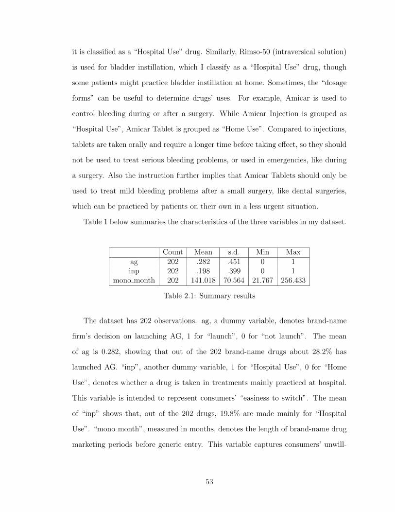
it is classified as a “Hospital Use” drug. Similarly, Rimso-50 (intraversical solution)
is used for bladder instillation, which I classify as a “Hospital Use” drug, though
some patients might practice bladder instillation at home. Sometimes, the “dosage
forms” can be useful to determine drugs’ uses. For example, Amicar is used to
control bleeding during or after a surgery. While Amicar Injection is grouped as
“Hospital Use”, Amicar Tablet is grouped as “Home Use”. Compared to injections,
tablets are taken orally and require a longer time before taking e↵ect, so they should
not be used to treat serious bleeding problems, or used in emergencies, like during
a surgery. Also the instruction further implies that Amicar Tablets should only be
used to treat mild bleeding problems after a small surgery, like dental surgeries,
which can be practiced by patients on their own in a less urgent situation.
Table 1 below summaries the characteristics of the three variables in my dataset.
Count Mean s.d. Min Maxag 202 .282 .451 0 1inp 202 .198 .399 0 1
mono month 202 141.018 70.564 21.767 256.433
Table 2.1: Summary results
The dataset has 202 observations. ag, a dummy variable, denotes brand-name
firm’s decision on launching AG, 1 for “launch”, 0 for “not launch”. The mean
of ag is 0.282, showing that out of the 202 brand-name drugs about 28.2% has
launched AG. “inp”, another dummy variable, 1 for “Hospital Use”, 0 for “Home
Use”, denotes whether a drug is taken in treatments mainly practiced at hospital.
This variable is intended to represent consumers’ “easiness to switch”. The mean
of “inp” shows that, out of the 202 drugs, 19.8% are made mainly for “Hospital
Use”. “mono month”, measured in months, denotes the length of brand-name drug
marketing periods before generic entry. This variable captures consumers’ unwill-
53
ingness to switch (brand loyalty). The mean of mono month is about 12 years (141
months), which is consistent with the fact that the average brand-name marketing
time before generic entry is 13 years. The row of mono month suggests substantial
variations in the length of pre-generic marketing time across di↵erent brand-name
drugs.
2.5.2 Methodology
I assume whether or not a brand-name company launches authorized generics is
related to the switching cost its consumers has to pay to switch to a new drug.
I treat the decision to launch authorized generics as a binary variable, Yi, which
equals 1 if brand-name drug i launches authorized generics, 0 if not. A probit model
is built to analyze the determinants of such a decision. The probability of launching
an authorized generic is defined as:
P (Yi = 1|Xi, ✏i) = �(Xi� + ✏i)
where Xi, a vector of regressors, contains observed factors that explain the decision
of launching authorized generics, while ✏i, with ✏ ⇠ N(0, 1), an error term, captures
the e↵ect of unobserved factors on such decisions. � is a vector of coe�cients to be
estimated. � is the CDF of the standard normal distribution.
2.5.3 Results
In my probit regressions, the dependent variable, ag, is 1 whenever an autho-
rized generic is launched for brand-name drug i. The independent variables are
lnmono month (log-linearized mono month) and inp. As I have mentioned in sec-
tion 5.1, mono month, denoting the length of pre-generic marketing period of brand-
name drug i, is a continuous variable, so is its log-linearized version lnmono month.
54
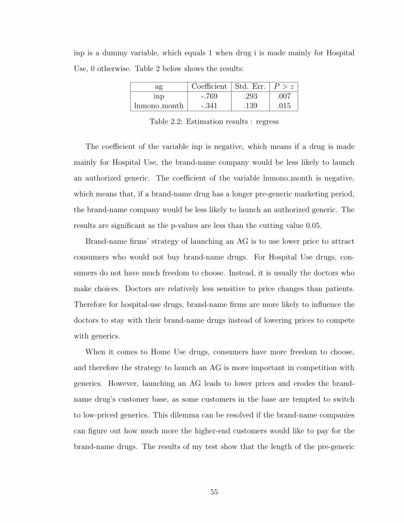
inp is a dummy variable, which equals 1 when drug i is made mainly for Hospital
Use, 0 otherwise. Table 2 below shows the results:
ag Coe�cient Std. Err. P > zinp -.769 .293 .007
lnmono month -.341 .139 .015
Table 2.2: Estimation results : regress
The coe�cient of the variable inp is negative, which means if a drug is made
mainly for Hospital Use, the brand-name company would be less likely to launch
an authorized generic. The coe�cient of the variable lnmono month is negative,
which means that, if a brand-name drug has a longer pre-generic marketing period,
the brand-name company would be less likely to launch an authorized generic. The
results are significant as the p-values are less than the cutting value 0.05.
Brand-name firms’ strategy of launching an AG is to use lower price to attract
consumers who would not buy brand-name drugs. For Hospital Use drugs, con-
sumers do not have much freedom to choose. Instead, it is usually the doctors who
make choices. Doctors are relatively less sensitive to price changes than patients.
Therefore for hospital-use drugs, brand-name firms are more likely to influence the
doctors to stay with their brand-name drugs instead of lowering prices to compete
with generics.
When it comes to Home Use drugs, consumers have more freedom to choose,
and therefore the strategy to launch an AG is more important in competition with
generics. However, launching an AG leads to lower prices and erodes the brand-
name drug’s customer base, as some customers in the base are tempted to switch
to low-priced generics. This dilemma can be resolved if the brand-name companies
can figure out how much more the higher-end customers would like to pay for the
brand-name drugs. The results of my test show that the length of the pre-generic
55
marketing periods of the brand-name drugs may serve as a good proxy for the
how much more. If consumers have had longer experiences of the brand-name
drugs, they would value them considerably more (than generic substitutes). In this
situation, brand-name firms might find it more profitable to exploit the higher end
alone, which renders the launch of AG less likely. On the other hand, if consumers
have had relatively short experience of the brand name drugs, they would value the
brand-name drugs not much more (than the generic substitutes). In this situation,
brand-name firms might find it more profitable to expand their business to the lower
end market with the launch of AG.
2.6 Conclusions
When there is generic competition the brand-name companies sometimes (but not
always) launch generic versions themselves possibly through a third party. Such
generics are called authorized generics to be distinguished from general (unautho-
rized) generics. In this paper I investigate the rationale for such a strategy. To
account for the two puzzles noted in the introduction, I focus on the role of the
customer bases the brand-name companies develop prior to generic entry. I present
a two-period model in which the incumbent develops a customer base as a monopoly
in the first period and readies itself for generic competition in the second period.
I find that, when the switching cost is high, the incumbent creates a larger cus-
tomer base by producing output beyond the short-run optimum. The sub-optimal
profit in the first period is more than o↵set as it allows the brand-name company to
retain a large number of loyal customers willing to pay higher prices for the brand-
name drugs than switching to the generics. Comparatively, when the switching
cost is low, the incumbent does not make such a short-run sacrifice, as it is more
56
di�cult to keep the customer base intact upon generic entry. Authorized gener-
ics provide the incumbent with a means to compete with the generic entrant for
the low-end consumers, who would not pay for the high- priced brand-name drug.
However, authorized generics will reduce the profit of the brand-name drugs on the
high-end consumers, because the additional competition due to the launching of the
authorized generic brings down the price of the generics further. Thus, when the
switching cost is low enough that a reduction in the profit of the brand-name drug
is exceeded by the profit of the authorized generic, the incumbent launches the AG
for the higher combined profit.
From the results above, I conclude that the brand-name company launches the
authorized generics only when the switching cost is small enough. When the switch-
ing cost is high, the incumbent sells more than the short-run profit-maximizing
quantity in the first period to develop a larger customer base it can capitalize on in
the second period. This strategy does not work however if the switching cost is low,
however, the customer bases is more vulnerable to price competition, Therefore it
makes more sense for the brand-name company to compete with the generic entrant
in the lower end market with the authorized generic. The probit regression anal-
ysis gives empirical results largely consistent with the results from the theoretical
analysis.
57
CHAPTER 3
THE MERGER PARADOX AND R&D
3.1 Introduction
Merger is one of the most salient features of the pharmaceutical industry during the
last quarter-century. Grabowski and Kyle (2008), for example, that global share of
the top ten pharmaceutical firms increased from 28.3 percent in 1989 to 48.3 percent
in 2004. What has caused this trend is still debated. One hypothesis is that it is
due to rising R&D costs. Another points to increased competition from generics
possibly intensified by the Hatch-Waxman Act. In this chapter I examine if these
casual explanations make sense in light of the existing theory of merger.
Unfortunately, however, there is no unique theory that explains merger cases
satisfactorily. In fact, modern theory of merger is a poor tool for understanding
real-world merger cases mainly because it is not easy to explain why merger is prof-
itable within the framework of simple models of oligopoly. This so-called “merger
paradox” originates from the work of Salant et al. (1983), who discovered that a
profitable merger in symmetric Cournot oligopoly requires the participation of more
than 80 percent of firms in industry. According to this “80 percent rule”, most
mergers we observe in the real world - mergers between two or three firms - are
unprofitable, thereby leading to the paradox. Since the SSR study, a number of
ways out of the merger paradox have been proposed. For example, Daughety (1990)
has shown that merger among symmetric Cournot firms could be profitable if the
merged firm assumes the role of the Stackelberg leader while all others act as follow-
ers in the post-merger industry. Perry and Porter (1985) have considered the model
where firms are endowed with asymmetric amounts of capital, and found that the
merger among small firms can be profitable if the pooling of their capital assets leads
58
to a su�cient cost reduction for a new firm.1 Similarly, Compte et al. (2002) have
demonstrated the profitability of merger among asymmetric Bertrand firms. David-
son and Deneckere (1986) have shown that the merger among symmetric firms in a
Salop-type spatial model of price competition can be profitable. More recent work
has considered increasingly complicated merger settings: merger under the threat
of entry (Pesendorfer, 2005) and successive mergers (Nocke and Whiston, 2013), for
example.
The objective of the present chapter is to reconsider the profitability of horizontal
merger under symmetric Cournot oligopoly with a new twist: R&D opportunities.
The basic model has two stages; firms first invest in cost-reducing R&D and then
compete in quantities in the homogeneous product market. We then allow an ar-
bitrary number of firms to merge before, or in anticipation of, the arrival of R&D
opportunities. Our first result is that if all R&D firms merge into a single firm in the
presence of non-R&D firms, then such merger is profitable, regardless of the number
of firms in the industry. We can interpret this result loosely in a context where new
ideas for inventing a new drug arrive to a few firms in the industry in a Poisson
process over time. Then these firms receiving news prefer to merge before investing
in R&D. At some future date, another idea is received by a group of firms, which
go on to merge before undertaking investment in R&D. Interpreted this way, our
theory is consistent with the current trend for merger not only in the pharmaceutical
industry but in many other R&D intensive industry.
We then turn out attention to the possibility of profitable merge among a subset
of R&D firms, and find that in this case there re-emerges something similar to the
1They also considered mergers among firms that constituted the competitive fringe inthe dominant-firm setting.
59
notorious SSR rule, although the threshold is lower than 80%. If the number of
merging firms surpasses this new threshold, merger is unprofitable.
3.2 A single R&D firm and merger
Consider an n-firm industry (n � 3). All firms face identical marginal cost fixed
at c > 0. We then suppose that one firm, say, firm 1, finds the opportunity to
invest in cost-reducing R&D. The R&D technology is familiar (e.g., d’Aspremont
and Jacquemin 1988); that is, investing quantity x1 in R&D reduce firm 1’s marginal
cost to c�x1 ⌘ c1 at the quadratic R&D cost gx12, where g is a positive constant and
captures the e�ciency of R&D technology. Without merger, the game develops as
follows. In stage one firm 1 first makes R&D investment, and all other firms observe
the new cost c1 In stage two, all firms play a simultaneous quantity-setting (Cournot)
game in the product market. Consumers regard all the goods as homogeneous.
Demand is assumed linear and is given by p = a�Q, where a > c and Q is industry
output. In this setting we consider the incentives for firm 1 to merge with m firms,
where 1 m n�1. The game sequence with merge is as follows. In the first stage,
firm 1 and m non-R&D firms merge into a new firm, and then the new firm makes
an R&D decision. In the second stage, the new firm and all the other n �m firms
play a Cournot game. The merger paradox says that unless a proposal of merger
involves more than 80% of n firms there is no incentive to merge. We examine how
this so-called 80% rule is a↵ected by R&D opportunities.
As a benchmark, consider the case without merger. It is a routine exercise to
show that in stage two firm 1 receives the net profit
⇡1 = [(a� n(c� x1) + (n� 1)c]2/(n+ 1)2 � gx12 (3.1)
= (a� c+ nx1)2/(n+ 1)2 � gx1
2 (3.2)
60
where x1 is taken as given. All other firms j 6= 1 make the symmetric profit
⇡j = (a� c� x1)2/(n+ 1)2. (3.3)
In stage one firm 1 choose x1 to maximize (3.2), yielding the first-order condition
n(a� c+ nx1)/(n+ 1)2 � gx1 = 0. (3.4)
The second-order is satisfied if
g > n2/(n+ 1)2. (3.5)
Eq (3.4) yields the optimal investment level for firm 1:
x⇤1 = n(a� c)/[g(n+ 1)2 � n2]. (3.6)
We want to make sure that new marginal cost c1 = c� x1 is non-negative. Substi-
tution from (3.6), we write this non-negativity condition as:
g � n(n� 1 + a/c)/(n+ 1)2. (3.7)
Given a > c, condition (3.7) implies condition (3.5). Thus, below we assume that
g satisfies condition (3.7). Substituting from (3.6) into (3.2) yields the maximized
profit for firm 1:
⇡⇤1 = (a� c)2[g2(n+ 1)2 � gn2]/[g(n+ 1)2 � n2]2 (3.8)
= (a� c)2g/[g(n+ 1)2 � n2]. (3.9)
The equilibrium profit to a non-R&D firm obtains from substituting from (3.6) into
(3.3):
⇡⇤j = (a� c)2[g(n+ 1)� n]2/[g(n+ 1)2 � n2]2. (3.10)
A non-R&D firm makes a positive profit if and only if g(n+ 1) > n, or
g > n/(n+ 1). (3.11)
61
Calculations show that condition (3.11) is more restrictive than condition (3.7) if
and only if 2c > a; i.e., if the initial cost is relatively high, condition (3.11) gives
the lower bound on g; otherwise, the lower bound is given by (3.7).
We now examine the profitability of merger between firm 1 and m non-R&D
firms prior to the R&D stage. The merger reduces the total number of firms in
the industry to n �m, including the new firm. After merger, the new firm makes
investment in R&D using the inherited R&D technology. Then all firms engage in
Cournot competition.
The equilibrium with merger is identical to the one without merger obtained
above, except that the number of firms shrinks to n � m firms in the industry.
Thus, by (3.9) the new firm has the profit
⇡⇤(m) = (a� c)2g/[g(n�m+ 1)2 � (n�m)2]. (3.12)
Further, the right-hand side of (3.7) is increasing in n, and so condition (3.7) implies
that the new firm faces a positive marginal cost.
If there is no merger, firm 1 and m firms would have the combined profit ⇡1⇤ +
m⇡j⇤. Substituting from (3.9) and (3.10), we can write this sum as
⇡1⇤ +m⇡j
⇤ = (a� c)2{[g2(n+ 1)2 � gn2] +m[g(n+ 1)� n]2}/[g(n+ 1)2 � n2]2.
If ⇡⇤(m) > ⇡1⇤ +m⇡j
⇤, we say that the merger is profitable.
The profit di↵erence ⇡⇤(m)� [⇡1⇤ +m⇡j
⇤] generally depends not only on m, the
number of participating firms in the merger but also on n, the total number of firms
in the industry, as well as on g, the R&D technology. With the result depending on
so many parameter values, the general conclusion is di�cult to find. However, we
find a very strong result that demonstrates that merger is profitable for any m and
any n.
62
Proposition 3.1 At g = 1 a merger between the (unique) R&D firm and any num-
ber m of non-R&D firms is profitable.
Proof. First, g = 1 satisfies condition (3.7). Substitution yields
⇡⇤(m) = (a� c)2/(2n� 2m+ 1)
⇡1⇤ +m⇡j
⇤ = (a� c)2(2n+ 1 +m)/(2n+ 1)2.
Hence, since n > m,
⇡1⇤(m)� (⇡1
⇤ +m⇡j⇤) = (a� c)2m(2n� 2m+ 1)/[(2n� 2m+ 1)(2n+ 1)2] > 0.
In general, g has the lower bound reflecting the requirement that g has to be
high enough to keep the post-R&D cost non-negative as in condition (9). g is also
bounded from the above because higher g makes R&D less profitable so that the
e↵ect of R&D is swamped by the 80% rule. However, we prove the following general
result (see Appendix for the proof).
Proposition 3.2 For any number of firms in the industry, there is always a prof-
itable merger between the R&D firm and any number of non-R&D firms.
For g 6= 1 our model also exhibits the feature that is akin to of the merger
paradox. Although we can always find a profitable merger with any number of
partners regardless of the total number of firms in the industry, if we hold n fixed,
merger is less likely to be profitable, the smaller the number of participating non-
R&D firms. More specifically, we show in the appendix that as n increases, the
range of g in which two-firm merger is profitable shrinks and converges to one as n
goes to infinity.
63
To better understand the role of R&D in the merger paradox, we next compare
our results with those obtainable from the case in which cost asymmetry is exoge-
nous. Suppose thus that firm 1 has exogenously low cost (c1) relative to other firms,
all of which have cost c > c1. Then, merger between firm 1 and one high-cost firms
is not always profitable. We show it in the environment most favorable to merger;
n = 3. Without merger firm 1 earns the profit
⇡1 = (a� 3c1 + 2c)2/16
while a high-cost firm receives the profit
⇡j = (a� 2c+ c1)2/16.
When firm 1 merges with one high-cost firms, the new firm uses firm 1’s low-cost
technology, Hence, the new firm’s profit is
Then, as c1 ! c, ⇡1 � (⇡1 + ⇡j) ! (a � c)2/9 � (a � c)2/8 < 0. Thus, two-firm
merger can be unprofitable under exogenous cost asymmetry whereas for g = 1
merger between two firms is always profitable for any n.
3.3 Multiple R&D firms and merger
We now consider the industry with k R&D firms, where 2 k < n. As before,
we begin with the case without merger. The game is familiar. In stage one k(<
n � 1) firms simultaneously choose levels of investment xi in R&D, which reduces
the marginal cost from c to ci = c � xi for firm i. The other (n � k) firms do not
engage in R&D and hence have the null action set in the first stage. In stage two,
all n firms obvers all costs and play a quantity-setting (Cournot) game, given the
marginal costs ci for R&D firms i and c for non-R&D firms. In the second-stage
64
game, firm j has the profit
⇡j = [a� (k + 1)c+X
i2K
ci]2/(n+ 1)2
if it is a non-R&D firm and
⇡j = [a� ncj + (n� k)c+X
i2K
ci]2/(n+ 1)2 � gx2
j
if it is an R&D firm, where K denotes the set of R&D firms and K�j is the set
obtained by deleting R&D firm j from the set K. In the first-stage, all firms j 2 K
simultaneously choose their investment levels xj in R&D to maximize the net profit
⇡j = [a� n(c� xj) + (n� k)c+X
i2K�j
ci]2/(n+ 1)2 � gx2
j
where gx2j is the quadratic R&D cost. The first-order condition is
n[a� n(c� xj) + (n� k)c+X
i2K�j
ci]/(n+ 1)2 � gxj = 0 (3.13)
Focusing on the symmetric equilibrium, we can solve for the equilibrium symmetric
R&D level, x⇤.
x⇤ = n(a� c)/[g(n+ 1)2 � n(n� k + 1)] (3.14)
Substituting x⇤ into (??) and rearranging, we can write the representative R&D
firm’s symmetric equilibrium profit as
⇡⇤(k) = g(a� c)2(g(n+ 1)2 � n2)/[g(n+ 1)2 � n(n� k + 1)]2 (3.15)
where the firm subscript j 2 K is suppressed under symmetry.
Suppose next that all the R&D firms in the set K merge to form a new firm
before the R&D stage. Merger reduces the total number of firms to n � k + 1. In
the first stage the new firm, which we call firm 1, chooses the quantity x1 to invest
65
in R&D. In the second stage all firms play a Cournot game. We can express the
new firm’s first-period profit as
⇡1(k) = [a� c+ (n� k + 1)x1]2/(n� k + 2)2 � gx2
1, (3.16)
In the first stage the new firm chooses x1 to maximize (10). The first-order condition
is
(n� k + 1)[a� c+ (n� k + 1)x1]/(n� k + 2)2 � gx1 = 0.
The (symmetric) equilibrium R&D level is expressed as
x(k) = (n� k + 1)(a� c)/[g(n� k + 2)2 � (n� k + 1)2]. (3.17)
Substituting x(k) into (3.16) yields, after rearranging, the following symmetric equi-
librium profit:
⇡(k) = g(a� c)2/[g(n� k + 2)2 � (n� k + 1)2]. (3.18)
The above analysis makes sense if x(k) and ⇡1(k) are positive. Thus we assume
g > (n� k + 1)2/(n� k + 2)2. (3.19)
. The right-hand side increases in n, approaching the limit of 1.
We now compare the profits ⇡(k) and k⇡⇤(k) for the possibility of profitable
merger among R&D firms. As discussed in the preceding section, the profit di↵erence
in general depends on the value of k, n and g. The sharpest result again obtains at
g = 1, which is necessary for g to satisfy the lower bound for all n.
Proposition 3.3 At g = 1 merger of all R&D firms is profitable, regardless of the
k/n ratio.
Proof. ⇡(k)� k⇡⇤(k) > 0 if and only if
[(n+ 1)2 � n(n� k + 1)]2 > k[(n� k + 2)2 � (n� k + 1)2][(n+ 1)2 � n2].
66
Writing n+ 1 = q, this condition is equivalent to
[(q2 � (q � 1)(q � k)]2 � k[(q � k + 1)2 � (q � k)2][q2 � (q � 1)2]
=[(q2 � (q � 1)(q � k)]2 � k(2q � 2k + 1)(2q � 1)
=(k � 1)[(q2(k � 1) + k(2q � 1)] > 0.
Proposition 3.4 has the following explanation. Without R&D a k-firm merger
decreases the combined profit and hence is unprofitable, if the ratio k/n falls below
the Salant-Switzer-Reynolds (SSR) 80-percent threshold. However, with R&D op-
portunities, merger generates three additional e↵ects in favor of merger. First, it
allows firms to economize on the R&D cost (R&D cost-saving e↵ect). Second, since
merger decreases the number of firms, each firm earns a greater gross profit, given
marginal cost, which makes investment in R&D more profitable (profit expansion ef-
fect). Third, a cost reduction leads to an output expansion, causing non-R&D firms
to contract their output (market-share-expansion e↵ect). If all R&D firms merge,
Proposition 1 says that the sum of these e↵ects more than o↵set the SSR e↵ect,
even though the k/n ratio falls short of the SSR threshold, making the post-merger
profit greater than the sum of the pre-merger profits.
To understand the implications R&D has on the success of merger, we demon-
strate that if cost asymmetry merger is exogenous, merger need not be profitable.
Again we consider the case most in favor of merger most; let n = 3 and k = 2
firms have low cost cL while the other firm has high cost c > cL. Without merger
each of the two low cost firms earns the profit ⇡L = (a � 2cL + c)2/16 while after
merging the new firm earns the profit ⇡N = (a � 2cL + c)2/9. Thus, as cL ! c,
⇡N � 2⇡L ! (2� c)2/9� (2� c)2/8 < 0. Thus, merger of two exogenously low cost
67
firms need not be profitable, whereas if cost asymmetry is a consequence of R&D,
merger is profitable.
The analysis in the preceding section implies that g also has upper bounds that
depend on the size of n (and her on the size of k). As shown there, for given k,
the range of g that makes merger profitable shrinks as n is increased and converges
to one as n approaches infinity. Thus, we still have the general observation that
with the total number of firms in the industry fixed at n, a two-firm merger is the
most di�cult to make profitable. In the next section, therefore, we focus on merger
involving two R&D firms but ask the question concerning partner selection.
3.4 Two R&D firms
In this subsection we assume that there are two R&D firms and n � 2 non-R&D
firms in industry. Our focus is whether these two firms find it more attractive to
merge with each other or whether each of them prefers to merge with a non-R&D
firm. To keep things simple, we set g = 1. The two R&D firms, i and j, choose
investments in R&D to maximize the profits
⇡i = (a+ nxi � c� xj)2/(n+ 1)2 � x2
i ,
⇡j = (a+ nxj � c� xi)2/(n+ 1)2 � x2
j .
The first order conditions are
2(a� c+ nxi � xj)/(n+ 1)2 � 2xi = 0, 2(a� c+ nxj � xi)/(n+ 1)2 � 2xj = 0.
Solving for xi and xj, we have
x⇤ = xi = xj = n(a� c)/(3n+ 1).
Therefore, replacing xi and xj in the profit function for i and j, we have
⇡i = ⇡j = (2n+ 1)(a� c)2/(3n+ 1)2.
68
For a non-R&D firm, the profit function is
⇡n = (a� c� xi � xj)2/(n+ 1)2.
Plugging x⇤ into the function, we calculate the profit for a non-R&D firm
⇡n = (a� c)2/(3n+ 1)2
If two R&D firms merge, the post-merger profit for the merged firm is
⇡M = (a� c)2/[2(n� 1) + 1] = (a� c)2/(2n� 1),
which means that each makes
⇡M/2 = (a� c)2/(4n� 2)
If each R&D firm merges with a non-R&D firm, there are two merged firms, each
of which makes
⇡NM = (2n� 3)(a� c)2/(3n� 5)2.
When an R&D firm and a non-R&D firm merge, we need to assign the benefits
of the merger to each firm in order to determine whether the merger is profitable
or not. Since this involves asymmetric firms we assume that the benefits of the
merger is negotiated under the Nash bargaining rule with equal weights. Thus, let
BR denote the benefit to the R&D firm and BN be that of the non-R&D firm. Then,
BR +BN = ⇡NM .
Nash bargaining results in equalization between the firms of the di↵erences between
the benefit of successful bargaining and the profit each receives when bargaining
fails. That is, BR and BN satisfy the following equation
BR � (2n+ 1)(a� c)2/[2(3n+ 1)2] = BN � (a� c)2/[2(3n+ 1)2].
69
Collecting terms, we find the value of the merger to an R&D firm
BR = (a� c)2[(2n� 3)/(3n� 5)2 + (2n+ 1)/(3n+ 1)2 � 1/(3n+ 1)2]/2.
Similarly, the value of the merger to a non-R&D firm
BN = (a� c)2[(2n� 3)/(3n� 5)2 � (2n+ 1)/(3n+ 1)2 + 1/(3n+ 1)2]/2.
We next compare BR with ⇡M/2, the profit per R&D firm if the two R&D firms
merge with each other. If (and only if) BR > ⇡M/2, then, we conclude that each
R&D firm prefers to merge with a non-R&D firm rather than to merge with each
other.
Proposition 3.4 (A) When n = 4, it is more profitable for the R&D firm to merge
with the non-R&D firm; (B) When n � 5, it is more profitable for the R&D firms
to merge with each other.
Proof.
BR � ⇡M/2
=(a� c)2[(2n� 3)/(3n� 5)2 + (2n+ 1)/(3n+ 1)2 � 1/(3n+ 1)2 � 1/(2n� 1)]/2
=(a� c)2{(�9n4 + 30x3 + 89n2 � 160x� 22)/[(3n� 5)2(3n+ 1)2(2n� 1)]}/2.
Let F (n) denote the numerator of the fraction in brackets. By Descartes’ rule of
signs, this function has 2 sign changes in the sequence of coe�cients. �F (n) also has
two sign changes. Thus, F (n) has two positive roots and two negative roots. The two
positive roots are n ⇡ 1.53 and n ⇡ 4.62. Calculations show that F (4) > 0 > F (5).
70
3.5 Conclusions
Motivated by the long-run trend to merge in the pharmaceutical industry, we recon-
sider the merger paradox, which states that, unless a majority of firms in industry
merges into one firm, mergers are not profitable. While a number of authors took up
the challenge of resolving the merger paradox, no one has explored the relationship
between R&D and merger. In this chapter we show that when there is one firm that
does R&D then that firm has an incentive to merge with any number of non-R&D
firms. In light of the paradox then, two firms (one R&D and one non-R&D) have
the incentive to merge, regardless of the total number of firms in industry. Our
second result is that if there are multiple R&D firms and multiple non-R&D firms
in industry, all R&D firms have the incentive to merge even though their number
does not reach the 80% threshold. Finally, we consider the choice of partners for
two R&D firms when there are 2 or more non-R&D firms. We find that when there
are only two non-R&D firms in industry, each R&D firms prefer to merge with a
non-R&D firm. However, if there are 3 or more than non-R&D firms, then they
prefer to merge with each other than with a non-R&D firm.
This research can be extended in a number of directions. First, we can explore
the more general case in which there are k R&D firms and n � k non-R&D firms
and consider the merger incentives of a subset m(< k) of R&D firms. While there
may be any clear-cut answers to this question due to the number of free parameters,
numerical analysis may be applied to find some general results. Secondly, the simple
structure of the present analysis allows one to add more structures. One possible
extension in this direction is the e↵ect of R&D spillovers in the sense of d’Aspremont
and Jacquemin (1988); the main query is whether the existence of spillovers is a
friend or a foe for successful merger.
71
BIBLIOGRAPHY
Appelt, S. (2010). Authorized generic entry prior to patent expiry: Reassessingincentives for independent generic entry. SFB/TR 15 Discussion Paper 357.
Baye, M. R., Crocker, K., and Ju, J. (1996). Divisonalization, franchising, anddivestiture incentives in oligopoly. American Economic Review, 86:223– 236.
Berndt, E. R., Mortimer, R., and Parece, A. (2007). Do authorized generic drugsdeter paragraph iv certification? recent evidence. Working Paper.
Chen, T. (2007). Authorized generics: A prescription for hatch- waxman reform.Virginia Law Review, 93:459–513.
Choi, J. P. (1998). Patent litigation as an information-transmission mechanism.American Economic Review, 88:1249–1263.
Compte, O., Jenny, F., and Rey, P. (2002). Capacity constraints, mergers, andcollusion. European Economic Review, 46:1–29.
d’Aspremont, D. and Jacquemin, A. (1988). Cooperative and non-cooperative R&Din duopoly with spillovers. American Economic Review, 78:1133–1137.
Daughety, A. F. (1990). Beneficial concentration. American Economic Review,80:1234 – 1237.
Davidson, C. and Deneckere, R. (1986). Long-run competition in capacity, short-runcompetition in price, and the cournot model. The RAND Journal of Economics,17(3):404–415.
Grabowski, H. and Kyle, M. (2008). Mergers and alliances in pharmaceuticals:e↵ects on innovation and r&d productivity. The Economics of Corporate Gover-nance and Mergers, 262.
Iizuka, T. (2008). Generic entry in a regulated pharmaceutical market. JapaneseEconomic Review, 60:63–81.
Iizuka, T. (2012). Physician agency and adoption of generic pharmaceuticals. Amer-ican Economic Review, 102:2826–2853.
Klemperer, P. (1987). Markets with consumer switching costs. The Quar- terlyJournal of Economics, 102(2):375–394.
Lemely, M. A. and Shapiro, C. (2005). Probabilistic patents. The Journal of Eco-nomic Perspectives, 19:75–98.
Mossingho↵, G. J. (1999). Overview of the hatch-waxman act and its impact ondrug development process. Food Drug Law Journal, 54:187–194.
72
BIBLIOGRAPHY
Nocke, V. and Whiston, M. (2013). Merger policy with merger choice. AmericanEconomic Review, 103:1006–1033.
Perry, M. K. and Porter, R. H. (1985). Oligopoly and the incentive for horizontalmerger. American Economic Review, 75:219–227.
Pesendorfer, M. (2005). Merger under entry. Rand Journal of Economics, 36:661–679.
Rei↵en, D. and Ward, M. R. (2005). “branded generics” as a strategy to limitcannibanization of pharmacetical markets. Managerial and Decision Economics,28(4-5):251–265.
Salant, S., Switzer, S., and Reynolds, R. (1983). Losses from horizontal merger: thee↵ects of an exogenous changes in industry structure on cournot-nash equilibrium.Quarterly Journal of Economics, 95:185–199.
73
Appendices
74
Appendices
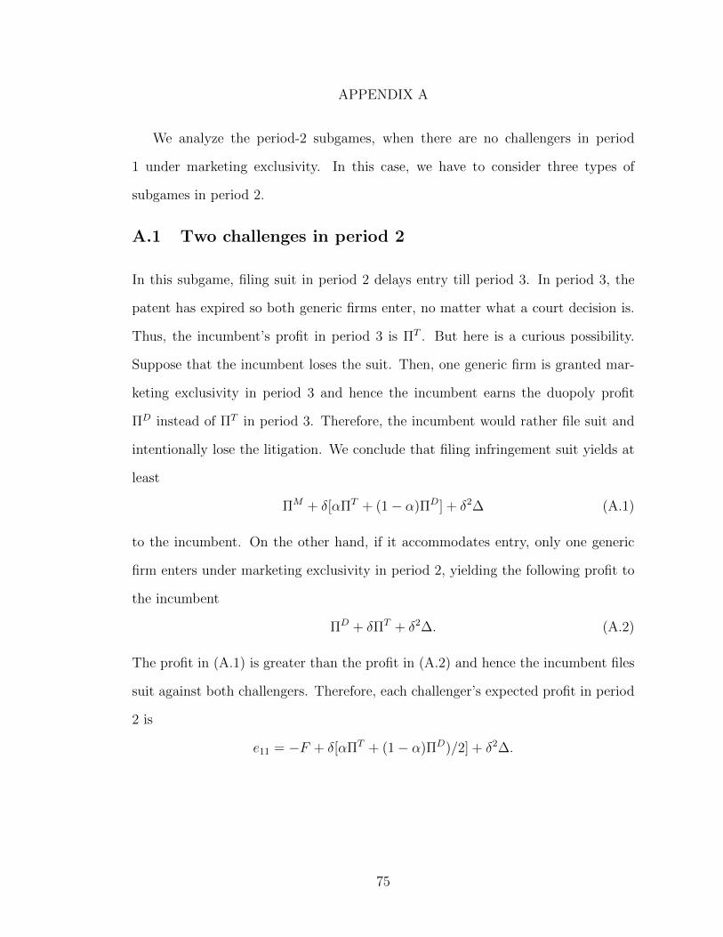
APPENDIX A
We analyze the period-2 subgames, when there are no challengers in period
1 under marketing exclusivity. In this case, we have to consider three types of
subgames in period 2.
A.1 Two challenges in period 2
In this subgame, filing suit in period 2 delays entry till period 3. In period 3, the
patent has expired so both generic firms enter, no matter what a court decision is.
Thus, the incumbent’s profit in period 3 is ⇧T . But here is a curious possibility.
Suppose that the incumbent loses the suit. Then, one generic firm is granted mar-
keting exclusivity in period 3 and hence the incumbent earns the duopoly profit
⇧D instead of ⇧T in period 3. Therefore, the incumbent would rather file suit and
intentionally lose the litigation. We conclude that filing infringement suit yields at
least
⇧M + �[↵⇧T + (1� ↵)⇧D] + �2� (A.1)
to the incumbent. On the other hand, if it accommodates entry, only one generic
firm enters under marketing exclusivity in period 2, yielding the following profit to
the incumbent
⇧D + �⇧T + �2�. (A.2)
The profit in (A.1) is greater than the profit in (A.2) and hence the incumbent files
suit against both challengers. Therefore, each challenger’s expected profit in period
2 is
e11 = �F + �[↵⇧T + (1� ↵)⇧D)/2] + �2�.
75
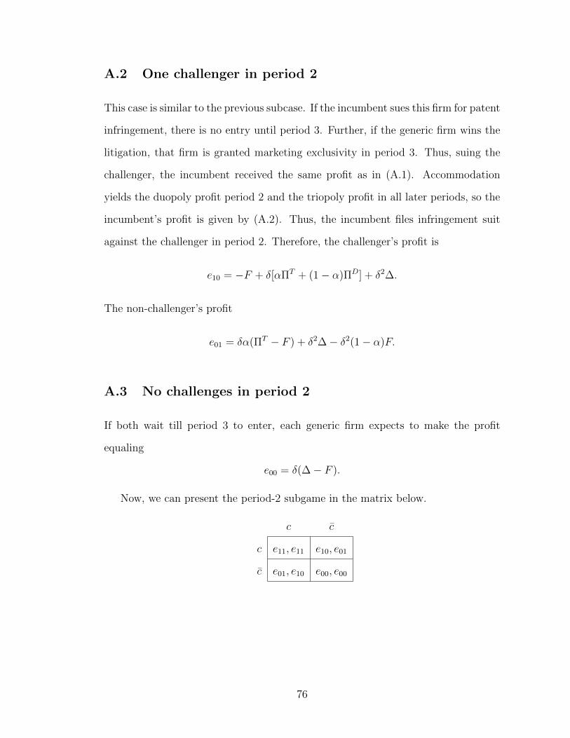
A.2 One challenger in period 2
This case is similar to the previous subcase. If the incumbent sues this firm for patent
infringement, there is no entry until period 3. Further, if the generic firm wins the
litigation, that firm is granted marketing exclusivity in period 3. Thus, suing the
challenger, the incumbent received the same profit as in (A.1). Accommodation
yields the duopoly profit period 2 and the triopoly profit in all later periods, so the
incumbent’s profit is given by (A.2). Thus, the incumbent files infringement suit
against the challenger in period 2. Therefore, the challenger’s profit is
e10 = �F + �[↵⇧T + (1� ↵)⇧D] + �2�.
The non-challenger’s profit
e01 = �↵(⇧T � F ) + �2�� �2(1� ↵)F.
A.3 No challenges in period 2
If both wait till period 3 to enter, each generic firm expects to make the profit
equaling
e00 = �(�� F ).
Now, we can present the period-2 subgame in the matrix below.
c c
c e11, e11 e10, e01
c e01, e10 e00, e00
76
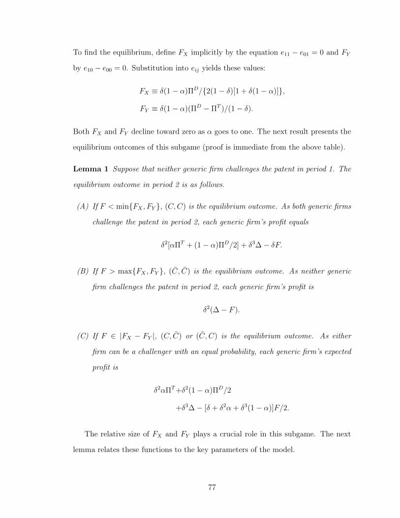
To find the equilibrium, define FX implicitly by the equation e11 � e01 = 0 and FY
by e10 � e00 = 0. Substitution into eij yields these values:
FX ⌘ �(1� ↵)⇧D/{2(1� �)[1 + �(1� ↵)]},
FY ⌘ �(1� ↵)(⇧D � ⇧T )/(1� �).
Both FX and FY decline toward zero as ↵ goes to one. The next result presents the
equilibrium outcomes of this subgame (proof is immediate from the above table).
Lemma 1 Suppose that neither generic firm challenges the patent in period 1. The
equilibrium outcome in period 2 is as follows.
(A) If F < min{FX , FY }, (C,C) is the equilibrium outcome. As both generic firms
challenge the patent in period 2, each generic firm’s profit equals
�2[↵⇧T + (1� ↵)⇧D/2] + �3�� �F.
(B) If F > max{FX , FY }, (C, C) is the equilibrium outcome. As neither generic
firm challenges the patent in period 2, each generic firm’s profit is
�2(�� F ).
(C) If F 2 |FX � FY |, (C, C) or (C, C) is the equilibrium outcome. As either
firm can be a challenger with an equal probability, each generic firm’s expected
profit is
�2↵⇧T+�2(1� ↵)⇧D/2
+�3�� [� + �2↵ + �3(1� ↵)]F/2.
The relative size of FX and FY plays a crucial role in this subgame. The next
lemma relates these functions to the key parameters of the model.
77
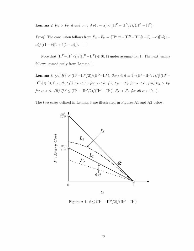
Lemma 2 FX > FY if and only if �(1� ↵) < (⇧T � ⇧D/2)/(⇧D � ⇧T ).
Proof. The conclusion follows from FX�FY = {⇧D/2�(⇧D�⇧T )[1+�(1�↵)]}�(1�
↵)/{(1� �)[1 + �(1� ↵)]}.
Note that (⇧T �⇧D/2)/(⇧D�⇧T ) 2 (0, 1) under assumption 1. The next lemma
follows immediately from Lemma 1.
Lemma 3 (A) If � > (⇧T�⇧D/2)/(⇧D�⇧T ), there is ↵ ⌘ 1�(⇧T�⇧D/2)/[�(⇧D�
⇧T )] 2 (0, 1) so that (i) FX < FY for ↵ < ↵; (ii) FX = FY for ↵ < ↵; (iii) FX > FY
for ↵ > ↵. (B) If � (⇧T � ⇧D/2)/(⇧D � ⇧T ), FX > FY for all ↵ 2 (0, 1).
The two cases defined in Lemma 3 are illustrated in Figures A1 and A2 below.
Figure A.1: � (⇧T � ⇧D/2)/(⇧D � ⇧T )
78
Figure A.2: � > (⇧T � ⇧D/2)/(⇧D � ⇧T )
79
APPENDIX B
PROOF OF PROPOSITION 1.2
The first-stage simultaneous-move game between two generic firms as follows:
c c
c E11, E11 E10, E01
c e01, e10 e00, e00
where the payo↵s are
E11 ⌘ �F + �(1� ↵)⇧D/2 + �2�,
E10 ⌘ �F + �(1� ↵)⇧D + �2�,
E01 ⌘ �2(�� F ),
as derived in the text, whereas E00 takes on these three separate values, derived in
Lemma 4 Case 1: F < min{FX , FY } : E00 ⌘ �2[↵⇧T + (1�↵)⇧D/2] + �3�� �F
Case 2: min{FX , FY } < F < max{FX , FY } : E00 ⌘ �2[↵⇧T + (1 � ↵)⇧D/2] +
�3�� �F [1 + �↵ + �2(1� ↵)]/2
Case 3: F > max{FX , FY } : E00 ⌘ �2(�� F ).
Proof of Proposition 2 has three parts: Part I: (C,C) is the Nash equilibrium
outcome of the above game if E11 �E01 � 0. Letting E11 �E01 = 0 and solving for
the value of F , we find that the above condition is expressed as F /2, where
/2 ⌘ (�(1 � ↵)⇧D/2)/(1 � �2). Part II: Next, for either (C, C) and (C, C) to be
an equilibrium outcome, we must have E10�E00 > 0 and E01�E11 > 0. The latter
inequality is written F > �/2 from the preceding discussion. The former involves
the term E00 and hence there are three cases from Appendix A to consider. The
results also depend on the sign of FX � FY . Further, calculations show that for a
given ↵ < 1, � > FX = �(1� ↵)(⇧D/2)/{(1� �)[1 + �(1� ↵)]} > �/2.
80
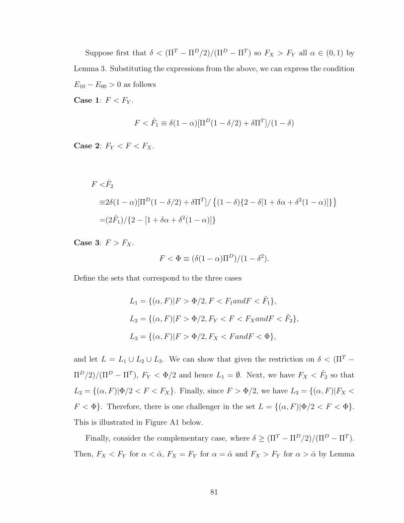
Suppose first that � < (⇧T � ⇧D/2)/(⇧D � ⇧T ) so FX > FY all ↵ 2 (0, 1) by
Lemma 3. Substituting the expressions from the above, we can express the condition
E10 � E00 > 0 as follows
Case 1: F < FY .
F < F1 ⌘ �(1� ↵)[⇧D(1� �/2) + �⇧T ]/(1� �)
Case 2: FY < F < FX .
F <F2
⌘2�(1� ↵)[⇧D(1� �/2) + �⇧T ]/�(1� �){2� �[1 + �↵ + �2(1� ↵)]}
=(2F1)/{2� [1 + �↵ + �2(1� ↵)]}
Case 3: F > FX .
F < � ⌘ (�(1� ↵)⇧D)/(1� �2).
Define the sets that correspond to the three cases
L1 = {(↵, F )|F > �/2, F < F1andF < F1},
L2 = {(↵, F )|F > �/2, FY < F < FXandF < F2},
L3 = {(↵, F )|F > �/2, FX < FandF < �},
and let L = L1 [ L2 [ L3. We can show that given the restriction on � < (⇧T �
⇧D/2)/(⇧D � ⇧T ), FY < �/2 and hence L1 = ;. Next, we have FX < F2 so that
L2 = {(↵, F )|�/2 < F < FX}. Finally, since F > �/2, we have L3 = {(↵, F )|FX <
F < �}. Therefore, there is one challenger in the set L = {(↵, F )|�/2 < F < �}.
This is illustrated in Figure A1 below.
Finally, consider the complementary case, where � � (⇧T � ⇧D/2)/(⇧D � ⇧T ).
Then, FX < FY for ↵ < ↵, FX = FY for ↵ = ↵ and FX > FY for ↵ > ↵ by Lemma
81
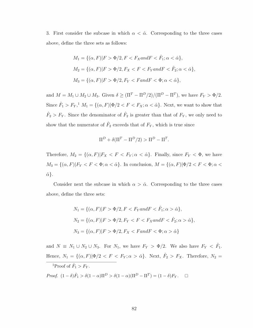
3. First consider the subcase in which ↵ < ↵. Corresponding to the three cases
above, define the three sets as follows:
M1 = {(↵, F )|F > �/2, F < FXandF < F1;↵ < ↵},
M2 = {(↵, F )|F > �/2, FX < F < FY andF < F2;↵ < ↵},
M3 = {(↵, F )|F > �/2, FY < FandF < �;↵ < ↵},
and M = M1 [M2 [M3. Given � � (⇧T � ⇧D/2)/(⇧D � ⇧T ), we have FY > �/2.
Since F1 > FY ,1 M1 = {(↵, F )|�/2 < F < FX ;↵ < ↵}. Next, we want to show that
F2 > FY . Since the denominator of F2 is greater than that of FY , we only need to
show that the numerator of F2 exceeds that of FY , which is true since
⇧D + �(⇧T � ⇧D/2) > ⇧D � ⇧T .
Therefore, M2 = {(↵, F )|FX < F < FY ;↵ < ↵}. Finally, since FY < �, we have
M3 = {(↵, F )|FY < F < �;↵ < ↵}. In conclusion, M = {(↵, F )|�/2 < F < �;↵ <
↵}.
Consider next the subcase in which ↵ > ↵. Corresponding to the three cases
above, define the three sets:
N1 = {(↵, F )|F > �/2, F < FY andF < F1;↵ > ↵},
N2 = {(↵, F )|F > �/2, FY < F < FXandF < F2;↵ > ↵},
N3 = {(↵, F )|F > �/2, FX < FandF < �;↵ > ↵}
and N ⌘ N1 [ N2 [ N3. For N1, we have FY > �/2. We also have FY < F1.
Hence, N1 = {(↵, F )|�/2 < F < FY ;↵ > ↵}. Next, F2 > FX . Therefore, N2 =
1Proof of F1 > FY .
Proof. (1� �)F1 > �(1� ↵)⇧D > �(1� ↵)(⇧D �⇧T ) = (1� �)FY .
82
{(↵, F )|FY < F < FX ;↵ > ↵}. Finally, since FX > �/2, N3 = {(↵, F )|FX <
F < �;↵ > ↵}. Hence, N = {(↵, F )|�/2 < F < �;↵ > ↵}. Finally, suppose
↵ = ↵ so that FX = FY by Lemma 3. By continuity of FX and FY , we can show
that there is one challenger in the set N 0 = {(↵, F )|�/2 < F < �;↵ = ↵}. Thus,
M [N [N 0 = {(↵, F )|�/2 < F < �;↵ 2 (0, 1)}. This is illustrated in Figure A2.
Finally, (C, C) is the Nash equilibrium outcome if and only if E10�E00 < 0 and
E11 � E01 < 0. These are complementary to the conditions under which the other
equilibrium outcomes considered above do not occur, and hence is represented by
the area above the line F = �. Furthermore, Lemma 1B shows that there are no
challengers in period 2, either. Q.E.D.
83
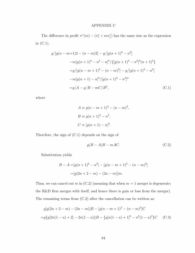
APPENDIX C
The di↵erence in profit ⇡⇤(m)� (⇡⇤1 +m⇡⇤
j ) has the same sine as the expression
in (C.1).
g/[g(n�m+1)2� (n�m)2]� g/[g(n+ 1)2 � n2]
�m[g(n+ 1)2 � n2 � n]2/{[g(n+ 1)2 � n2]2(n+ 1)2}
=g/[g(n�m+ 1)2 � (n�m)2]� g/[g(n+ 1)2 � n2]
�m[g(n+ 1)� n]2/[g(n+ 1)2 � n2]2
=g/A� g/B �mC/B2, (C.1)
where
A ⌘ g(n�m+ 1)2 � (n�m)2,
B ⌘ g(n+ 1)2 � n2,
C ⌘ [g(n+ 1)� n]2.
Therefore, the sign of (C.1) depends on the sign of
g(B � A)B �mAC. (C.2)
Substitution yields
B � A =[g(n+ 1)2 � n2]� [g(n�m+ 1)2 � (n�m)2]
=[g(2n+ 2�m)� (2n�m)]m.
Thus, we can cancel outm in (C.2) (meaning that whenm = 1 merger is degenerate;
the R&D firm merges with itself, and hence there is gain or loss from the merger).
The remaining terms from (C.2) after the cancellation can be written as:
g[g(2n+ 2�m)� (2n�m)]B � [g(n�m+ 1)2 � (n�m)2]C
=g{g[2n(1� u) + 2]� 2n(1� u)}B � {g[n(1� u) + 1]2 � n2(1� u)2}C (C.3)
84
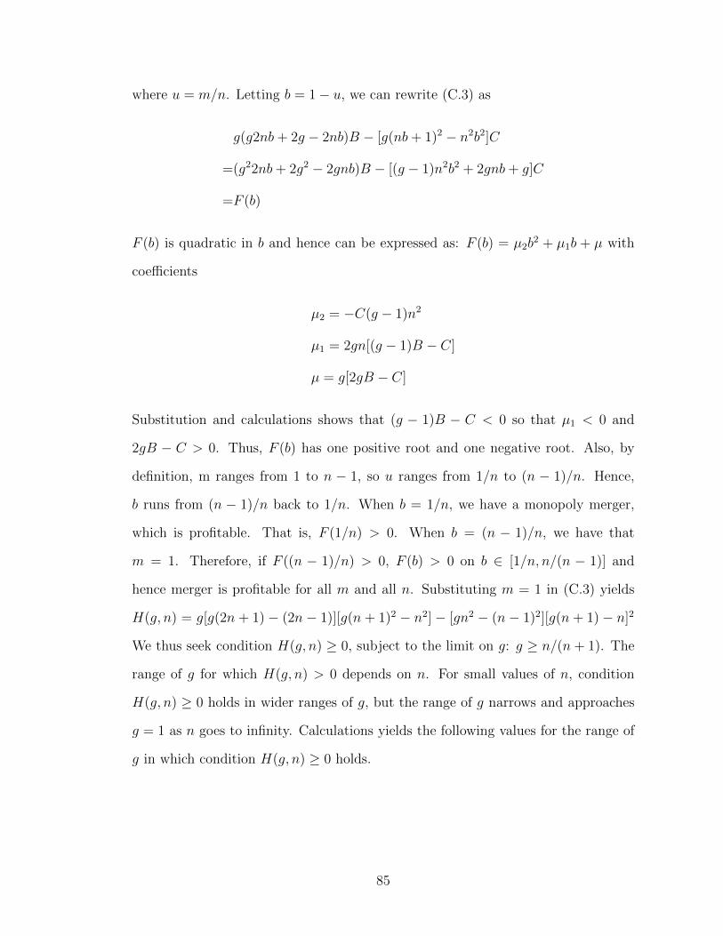
where u = m/n. Letting b = 1� u, we can rewrite (C.3) as
g(g2nb+ 2g � 2nb)B � [g(nb+ 1)2 � n2b2]C
=(g22nb+ 2g2 � 2gnb)B � [(g � 1)n2b2 + 2gnb+ g]C
=F (b)
F (b) is quadratic in b and hence can be expressed as: F (b) = µ2b2 + µ1b + µ with
coe�cients
µ2 = �C(g � 1)n2
µ1 = 2gn[(g � 1)B � C]
µ = g[2gB � C]
Substitution and calculations shows that (g � 1)B � C < 0 so that µ1 < 0 and
2gB � C > 0. Thus, F (b) has one positive root and one negative root. Also, by
definition, m ranges from 1 to n � 1, so u ranges from 1/n to (n � 1)/n. Hence,
b runs from (n � 1)/n back to 1/n. When b = 1/n, we have a monopoly merger,
which is profitable. That is, F (1/n) > 0. When b = (n � 1)/n, we have that
m = 1. Therefore, if F ((n � 1)/n) > 0, F (b) > 0 on b 2 [1/n, n/(n � 1)] and
hence merger is profitable for all m and all n. Substituting m = 1 in (C.3) yields
H(g, n) = g[g(2n + 1) � (2n � 1)][g(n + 1)2 � n2] � [gn2 � (n � 1)2][g(n + 1) � n]2
We thus seek condition H(g, n) � 0, subject to the limit on g: g � n/(n+ 1). The
range of g for which H(g, n) > 0 depends on n. For small values of n, condition
H(g, n) � 0 holds in wider ranges of g, but the range of g narrows and approaches
g = 1 as n goes to infinity. Calculations yields the following values for the range of
g in which condition H(g, n) � 0 holds.
85
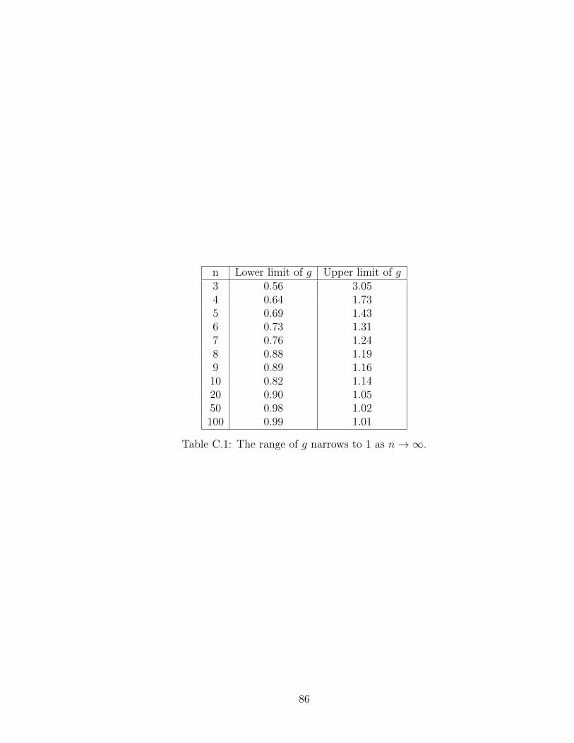
n Lower limit of g Upper limit of g3 0.56 3.054 0.64 1.735 0.69 1.436 0.73 1.317 0.76 1.248 0.88 1.199 0.89 1.1610 0.82 1.1420 0.90 1.0550 0.98 1.02100 0.99 1.01
Table C.1: The range of g narrows to 1 as n ! 1.
86
VITA
JIANGYUN WAN
2006 B.A., Engineering ManagementHubei UniversityWuhan, Hubei, China
2010 M.S., EconomicsFlorida International UniversityMiami, Florida
2011–2015 Doctoral Candidate, EconomicsFlorida International UniversityMiami, Florida International University
PRESENTATIONS
Wan, J., (April, 2014). Patents and entry competition in the pharmaceutical indus-try: The role of marketing exclusivity. Paper presented at the Economics Depart-ment, Florida International University.
Wan, J., (October, 2014). Why authorized generics: Theoretical and empirical in-vestigations. Paper presented at the Economics Department, Florida InternationalUniversity.
87