Embed Size (px)
Citation preview
ESSAYS ON ARBITRAGE THEORY FOR A CLASS OF
INFORMATIONAL MARKETS
by
JUN DENG
A thesis submitted in partial fulfillment of the requirements for the degree of
Doctor of Philosophy
in
Mathematical Finance
Department of Mathematical and Statistical Sciences
University of Alberta
© JUN DENG, 2014
Abstract
This thesis develops three major essays on Arbitrage Theory, Market’s Viabil-
ity and Informational Markets. The first essay (Chapter 3) elaborates the exact
connections among the No-Unbounded-Profit-with-Bounded-Risk (called NUPBR
hereafter) condition, the existence of the numeraire portfolio, and market’s weak/lo-
cal viability. These tight relationships together with the financial crisis become our
principal financial/economic leitmotif for the development of the next essay.
In the second essay (Chapter 4 – Chapter 6), we focus on quantifying with
extreme precision the effect of some additional information/uncertainty on the non-
arbitrage concepts. As a result, we describe the interplay of this extra informa-
tion and the market’s parameters for these non-arbitrage concepts to be preserved.
Herein, we focus on the classical no-arbitrage and the NUPBR condition. This study
contains two main parts. In the first part of this essay (Chapter 4), we analyze prac-
tical examples of market models and extra information/uncertainty, for which we
construct explicit ”classical” arbitrage opportunities generated by the extra infor-
mation/uncertainty. These examples are built in Brownian filtration and in Poisson
filtration as well. The second part (Chapters 5 and 6) addresses the NUPBR con-
dition in two different directions. On the one hand, we describe the pairs of market
model and random time for which the resulting informational market model fulfills
the NUPBR condition. On the other hand, we characterize the random time mod-
els that preserve the NUPBR condition. These results are elaborated for general
market models with special attention to practical models such as discrete-time and
Levy market models.
The last essay (Chapter 7) investigates the effect of additional information on
the Structure Conditions. These conditions are the alternatives to the non-arbitrage
and viability assumption in the Markowitz settings.
ii
Preface
Some of the research conducted for this thesis forms part of an international re-
search collaboration, led by Professor Tahir Choulli at the University of Alberta,
with Professor Monique Jeanblanc and Dr. Anna Aksamit at Universite d’Evry Val
d’Essonne, France and Dr. Junfeng Ma at Bank of Montreal, Canada.
Chapter 3 of this thesis has been published as T. Choulli, J. Deng and J. Ma, “How
non-arbitrage, viability and numeraire portfolio are related”, Accepted in Finance
and Stochastics, 2014.
Chapter 4 of this thesis has been published as A. Aksamit, T. Choulli, J. Deng, and
M. Jeanblanc, “Arbitrages in a progressive enlargement setting”, Arbitrage, Credit
and Informational Risks, Peking University Series in Mathematics Vol. 6, 55-88,
2014.
iii

Acknowledgements
As time passing to the completion of my Ph.D study, first and foremost, I would
like to express my very great appreciation to my supervisor Prof. Tahir Choulli for
his constant supporting of my research and career development during my nearly
four years Ph.D studies. His patience, personality and profound insight were and
are guiding me through the jungle to palace of Science, where I was bewildering,
hesitating, fear of and curious. I am also very grateful for his careful reading through
this long thesis and helping me with the structures, language and typos. To him, I
am deeply indebted.
In the meanwhile, I am very grateful to Prof. Abel Cadenillas, Prof. Christoph Frei,
Prof. Dmitry Kramkov, Prof. Rohana Karunamuni, Prof. Naomi Rothenberg and
Prof. Byron Schmuland for being part of the committee. Thanks for your invaluable
time and patience for reading through this long thesis.
I thank all my teachers, staff and friends of the Department of Mathematical and
Statistical Sciences at University of Alberta. It is my honor to have this opportunity
to study and pursue my doctoral degree in such a friendly environment.
Special thanks go to Prof. Bo Zhang at Renmin University of China, who always
stands by me and encourages me to continue with the path of academy.
Finally, I would like to reserve my gratitude to my parents, lovely sister and family
for trusting in me and supporting me to pursue this selfish endeavors. Without you,
this thesis could be far from completion; without you, I am nothing.
iv
Table of Contents
1 Introduction 1
1.1 Market’s Viability . . . . . . . . . . . . . . . . . . . . . . . . . . . . 1
1.2 Arbitrage Theory . . . . . . . . . . . . . . . . . . . . . . . . . . . . . 2
1.3 Information and Its Role in Finance and Economics . . . . . . . . . 5
1.4 Thesis’ Summary . . . . . . . . . . . . . . . . . . . . . . . . . . . . . 9
2 Notations and Preliminaries 12
2.1 σ-martingale Densities . . . . . . . . . . . . . . . . . . . . . . . . . . 16
2.2 Optional Stochastic Integral . . . . . . . . . . . . . . . . . . . . . . . 17
2.3 Jacod’s Representation for Local Martingales . . . . . . . . . . . . . 21
2.4 Mathematical Formulation for Non-Arbitrage . . . . . . . . . . . . . 27
2.5 Utility Maximization . . . . . . . . . . . . . . . . . . . . . . . . . . . 29
2.6 Mathematical Models for Additional Information . . . . . . . . . . . 30
2.6.1 Progressive Enlargement of Filtration . . . . . . . . . . . . . 30
2.6.2 Honest Times . . . . . . . . . . . . . . . . . . . . . . . . . . . 33
3 Viability versus Non-Arbitrage 37
3.1 Problem Formulation . . . . . . . . . . . . . . . . . . . . . . . . . . . 37
3.2 NUPBR, Weak Viability and Numeraire Portfolio . . . . . . . . . . . 39
3.2.1 The Main Theorem and Its Interpretations . . . . . . . . . . 41
3.2.2 Proof of the Main Theorem . . . . . . . . . . . . . . . . . . . 44
v
3.3 The Proof of The Key Lemma and Its Extensions . . . . . . . . . . . 54
3.3.1 Proof of The Key Lemma: . . . . . . . . . . . . . . . . . . . . 56
3.3.2 Extension to the Case of Real-valued Wealth Processes . . . 60
3.3.3 Extension to the Case of Exponential Utility . . . . . . . . . 63
4 Examples of Informational Arbitrages: Explicit Descriptions 69
4.1 General Theorem . . . . . . . . . . . . . . . . . . . . . . . . . . . . . 70
4.2 Classical Arbitrages in a Brownian Filtration . . . . . . . . . . . . . 74
4.2.1 Last Passage Time at a Given Level . . . . . . . . . . . . . . 75
4.2.2 Last Passage Time at a Level before Maturity . . . . . . . . 76
4.3 Classic Arbitrages in a Poisson Filtration . . . . . . . . . . . . . . . 78
4.3.1 Last Passage Time at a Given Level . . . . . . . . . . . . . . 79
4.3.2 Time of Supremum on Fixed Time Horizon . . . . . . . . . . 80
4.3.3 Time of Overall Supremum . . . . . . . . . . . . . . . . . . . 84
4.4 Classic Arbitrages in Discrete Time . . . . . . . . . . . . . . . . . . . 88
4.5 Classic Arbitrages for Non-honest Times . . . . . . . . . . . . . . . . 91
4.5.1 In a Brownian filtration: Emery’s Example . . . . . . . . . . 91
4.5.2 In a Poisson Filtration . . . . . . . . . . . . . . . . . . . . . . 92
5 Non-arbitrage under Stopping with Random Time 97
5.1 Notations and Preliminary Results on NUPBR . . . . . . . . . . . . 98
5.2 Main Results and their Interpretations . . . . . . . . . . . . . . . . . 104
5.2.1 The Quasi-Left-Continuous Processes . . . . . . . . . . . . . 105
5.2.2 Thin Processes with Predictable Jump Times . . . . . . . . . 108
5.2.3 The General Framework . . . . . . . . . . . . . . . . . . . . . 111
5.3 Stochastics from–and–for Informational Non-Arbitrage . . . . . . . . 115
5.3.1 Projection and Compensator under G and F . . . . . . . . . 116
5.3.2 G-Localization versus F-Localization . . . . . . . . . . . . . . 120
5.3.3 An Important G-local martingale . . . . . . . . . . . . . . . . 128
vi
5.4 Explicit Deflators . . . . . . . . . . . . . . . . . . . . . . . . . . . . . 132
5.5 Proofs of Three Main Theorems . . . . . . . . . . . . . . . . . . . . . 137
5.5.1 Proof of Theorem 5.2 . . . . . . . . . . . . . . . . . . . . . . 138
5.5.2 Intermediate Result . . . . . . . . . . . . . . . . . . . . . . . 145
5.5.3 Proof of Theorem 5.4 . . . . . . . . . . . . . . . . . . . . . . 147
5.5.4 Proof of Theorem 5.5 . . . . . . . . . . . . . . . . . . . . . . 151
5.6 Discrete Time Market Models . . . . . . . . . . . . . . . . . . . . . . 157
5.7 Levy Market Model . . . . . . . . . . . . . . . . . . . . . . . . . . . 170
6 Non-arbitrage for a Class of Honest Times 177
6.1 The Main Results . . . . . . . . . . . . . . . . . . . . . . . . . . . . . 179
6.1.1 The Case of Quasi-left-continuous Processes . . . . . . . . . . 180
6.1.2 Thin Processes with Predictable Jump Times . . . . . . . . . 183
6.1.3 The General Framework . . . . . . . . . . . . . . . . . . . . . 186
6.2 New Stochastic Developments . . . . . . . . . . . . . . . . . . . . . . 188
6.2.1 Comparing Dual Predictable Projections under G and F . . . 188
6.2.2 An Important G-Local Martingale . . . . . . . . . . . . . . . 193
6.3 Explicit Deflators . . . . . . . . . . . . . . . . . . . . . . . . . . . . . 197
6.3.1 The Quasi-Left-Continuous case . . . . . . . . . . . . . . . . 197
6.3.2 The Case of Thin Processes with Predictable Jumps . . . . . 199
6.4 Proofs of Three Main Theorems . . . . . . . . . . . . . . . . . . . . . 203
6.4.1 Proof of Theorem 6.1 . . . . . . . . . . . . . . . . . . . . . . 204
6.4.2 Proof of Theorem 6.2 . . . . . . . . . . . . . . . . . . . . . . 206
6.4.3 Proof of Theorem 6.5 . . . . . . . . . . . . . . . . . . . . . . 208
6.5 Discrete Time Market Models . . . . . . . . . . . . . . . . . . . . . . 210
6.6 Levy Market Model . . . . . . . . . . . . . . . . . . . . . . . . . . . 219
7 Structural Models under Additional Information 224
7.1 The Main Results . . . . . . . . . . . . . . . . . . . . . . . . . . . . . 226
vii
7.1.1 Structure Conditions under Stopping with Random Time . . 227
7.1.2 Structure Conditions under a Class of Honest Times . . . . . 231
7.2 The Key Stochastic Tools . . . . . . . . . . . . . . . . . . . . . . . . 235
7.2.1 Lazaro–Yor’s Representation . . . . . . . . . . . . . . . . . . 235
7.2.2 The Key Stochastic Results for the Part up to Random Horizon237
7.2.3 The Key Stochastic Results for the Part after an Honest Time 246
7.3 Proofs of Theorems 7.1 and 7.3 . . . . . . . . . . . . . . . . . . . . . 250
7.3.1 Proof of Theorem 7.1 . . . . . . . . . . . . . . . . . . . . . . 250
7.3.2 Proof of Theorem 7.3 . . . . . . . . . . . . . . . . . . . . . . 253
Bibliography 257
viii

Chapter 1
Introduction
Since their birth in the PhD thesis of Louis Bachelier (see [16]), mathematical finance
and modern finance has known many successful topics that became pillars of both
areas. Among these topics, we cite Portfolio Analysis that was pioneered by Merton
[109, 110] and Markowitz [108], Arbitrage theory (Arrow and Debreu [13] and Duffie
[56], Delbaen and Schachermayer [47, 50]), and Asset Pricing Theory and hedging
rules (Black-Scholes [23] and Merton [110]).
1.1 Market’s Viability
The market’s viability was defined —up to our knowledge— by Harrison and Kreps
in [69] (see also Kreps [101] and Jouini et al. [85]) as the setting for which there
exists a risk-averse agent who prefers more to less, has continuous preference, and
can find an optimal net trade subject to her/his budget constraint. In terms of the
popular von Neumann-Morgenstern utility, the market’s viability is “essentially”
equivalent to the existence of the solution to utility maximization problems and is
also related to the economic equilibrium and absence of arbitrage opportunities.
1
1.2 Arbitrage Theory
Arbitrage theory is a relative modern topic of Finance which becomes fundamental
since it was directly linked to Asset Pricing Theory of Black-Scholes-Merton (see
[23] and [110]), which was honored by the 1997 Nobel Price in Economics. Probably,
the idea of non-arbitrage is best explained by telling a little joke from the book of
Delbaen and Schachermayer [51]:
”A professor working in Mathematical Finance and a normal person
go on a walk and the normal person sees a $100 bill lying on the street.
When the normal person wants to pick it up, the professor says: do not
try to do that. It is absolutely impossible that there is a $100 bill lying
on the street. Indeed, if it were lying on the street, somebody else would
have picked it up before you.”
Turning to financial markets, loosely speaking, in a rationale and reasonable mar-
ket, there is no possibility that one could make profit without taking any risk. In
other words, there is no financial strategy that makes profit out of nothing and
without any risk (those financial strategies are called arbitrage opportunities). As
the joke says, if there were some free snacks and cheap thrills in the financial mar-
ket, somebody else would have taken the opportunities before you. In the his-
tory of the development of non-arbitrage theory, there are several competing defini-
tions (vary in different market models) such as No-arbitrage (NA), No-Unbounded-
Profit-with-Bounded-Risk (NUPBR), No-Free-Lunch (NFL), No-Free-Lunch-with-
Bounded-Risk (NFLBR), No-Free-Lunch-with-Vanishing-Risk (NFLVR), Asymptotic-
Arbitrage, Immediate-Arbitrage, etc..
To keep the story short, the casting from the economic meta-meaning of non-
arbitrage into a rigorous mathematical framework goes back to the work of Harrison
and Kreps [69] for finite discrete time markets and Harrison–Pliska [70] for complete
2
continuous martingale settings. For their settings, they proved the equivalence be-
tween NA and the existence of equivalent martingale measures. Going beyond finite
discrete time market model becomes more tricky and mathematically complicated.
The key idea brought by Dalang–Morton–Willinger in [44] pushed the study of non-
arbitrage theory to the modern mathematical finance by using the powerful tools
of measurable selection theorem and Kreps-Yan’s separation theorem. The next
ground-breaking seminar papers of Delbaen and Schachermayer [47] and [50] estab-
lished the golden principle of The Fundamental Theorem of Asset Pricing (FTAP,
name given by Dybvig and Ross [58]). It was proved that there is No-Free-Lunch-
with-Vanish-Risk (called NFLVR hereafter) if and only if there exists an Equivalent
Sigma Martingale Measure (called ESMM hereafter).
The economic interpretation of FTAP is that under an equivalent change of our
belief, the financial market is a fair game and evolves as a dynamic of a martingale.
The pricing and valuation of contingent claim is brought back to its intrinsic value
under this equivalent belief. Since its elaboration, the FTAP has known numerous
applications in Finance and Economics including, but not limited to, optimal port-
folio problem, market viability, market efficiency and risk management.
Optimal portfolio problem is a rather antique problem in Finance and Economics,
where economic agents tend to maximize their benefits, gains and wealth. The 1990
and 1997 Nobel Prize winners in Economics, Harry M. Markowitz and Robert Mer-
ton, established the foundation of modern optimal portfolio in their seminar papers
[108], [109] and [110]. Turning to mathematical finance field, Markowitz and Mer-
ton’s framework had been extended, studied and enriched to more general settings
using semimartingale theory, stochastic analysis and convex analysis. For those rich
topics such as utility maximization, forward utility, and mean-variance hedging, we
refer to Kramkov and Schachermayer [98, 99], Schachermayer [128], Delbaen et al.
3
[46], Frei and Schweizer [64, 65], Karatzas et al. [92, 91], Musiela and Zariphopoulou
[112, 114, 113], Choulli and Ma [35], Ma [107], Choulli et al. [36] and the references
therein.
There has been an upsurge interest in understanding the relationship among non-
arbitrage, market’s viability, and utility maximization problem since the time of
Arrow and Debreu. In fact, for discrete markets (i.e. when there are only a finite
number of trading times and scenarios), Arrow and Debreu proved in [13] (see also
[56]), that the market’s viability (i.e. utility maximization admits optimal solution
for a “nice” von Neumann-Morgenstern utility), absence of arbitrage opportuni-
ties and the existence of an equivalent martingale measure are equivalent. These
equivalences were extended to the discrete-time case (with infinity many scenarios).
However, the question of how the existence of optimal portfolio is connected to the
absence of arbitrage (weak or strong form) has been forgotten for the continuous-
time context. Recently, Frittelli proposed in [67] an interesting approach for this
issue, while his obtained results are not applicable in the context of [105]. Also
Karatzas and Kardaras proved in [90] that the NUPBR condition is equivalent to
the existence of the numeraire portfolio, and the NUPBR is the least condition for
the utility maximization problem having a possible solution.
Thus, the FIRST theme of this thesis is to answer the following:
Prob(1.I): How is the market’s viability (or utility maximization problem) re-
lated to non-arbitrage concepts in general continuous time semi-martingale models
and without any assumtpion?
4
1.3 Information and Its Role in Finance and Economics
In Finance and Economics, information means the acquirement of knowledges about
prices, costs, inventory, supply and demand of products, which can be exploited to
by economic agents to reduce uncertainties in their environment (see Rose [122]).
The key to the Economics of uncertainty appears for the first time —up to our
knowledge– as Bernoulli’s utility principle in 1738 ([19]). However this principle
was ignored until 1947, when it was first made respectable and rigorously proved
based on a few assumptions of how rational people make their decisions under un-
certainty by von Neumann and Morgenstern in [138]. Thus, from the economic
standpoint of view, information is a commodity that bears values; and economic
agents desire information because it helps them to make decision and maximize
their state-dependent utilities, especially when they are facing uncertainties. A
good explanation was elaborated by Arrow as follows:
”There is a basic assumption about the nature of information con-
tained in the economics of asymmetric information which I certainly
wish to retain: that information is scarce to the individual, as well as
to society as a whole. Asymmetric information arises because one party
cannot obtain freely (or at all) information available to another.”
In 2001, the scientific community and the Nobel Prize Committee recognized the
deep importance of the information in Economics and Finance by awarding George
Akerlof, Michael Spence, and Joseph E. Stiglitz the 2001 Nobel Price in Economics
for their contribution to the field of markets with asymmetric information (see [2],
[132], [133], [135] and [68]). Asymmetric information means that one party has more
or better information than the other when making decisions, investments and trans-
actions that would lead to adverse selection, moral hazards, and market failure,
especially in insurance markets. Adverse selection used in economics, insurance,
risk management, and statistics refers to a market process in which undesired re-
5
sults occur when buyers and sellers have access to different information. Moral
hazards is a situation where a party will have a tendency to take risks because the
costs that could result will not be felt by the party taking the risk. All of these
economic weaknesses have the potential to lead to market failure and affect the
market’s equilibrium (see Riley [119] and Rothschild and Stiglitz [124]). For the
testing of asymmetric information in insurance markets, we refer to Abbring et al.
[1], Chiappori and Salanie [28], Chiappori et al. [27], Cawley and Philipson [25]
and the references therein. For more details about information and uncertainty and
their roles in Economics, we consult Allen [5] and Arrow [9, 10, 11, 12], Antonelli
[8], Borch [24], Ross [122], Shackle [131], Stigler [134], Wolpert, S. A. and Wolpert,
J. F. [139] and the references therein. For the role of information in other fields such
as accounting, we refer the reader to Rothenberg [123], Hofmann and Rothenberg
[73] and the references therein. In these latter works, the authors studied the rela-
tionship between the quality of information available for production decisions and
performance evaluation to the choice of whether or not production should occur in
teams.
The most common assumption, considered in Finance and Economics, consists of
assuming that all the agents share the same information flow on which their portfo-
lio decisions are based. However, this assumption is too restrictive and unrealistic
in the real world. Asymmetric information arises quite naturally in Economics since
individual’s knowledge and availability of information varies from one agent to an-
other. Many mathematical models have been developed to capture the behaviors
of two agents with different information levels and are both price-taker and unable
to influence the price dynamics of the risky assets. The uninformed (public) trader
acts on the basis of the evolution of the market, while the insider trader possesses
some additional knowledge and could probably make arbitrage.
6
Mathematically speaking, the uninformed agents are assumed to have the public
information modelled by the filtration (Ft)t≥0, while the the extra information is
possessed by the financial managers or insiders only. Examples of the extra informa-
tion can be the IPO price, the possibility of default, the change in the CEO board.
Throughout the thesis, the extra information will be modelled mathematically by
a random time τ or an honest time. This random time represents a retirement
time, a death time, a default time of firms and/or agents, and any time where an
event will occur and affect the markets and/or the agents’ decisions. Usually, the
random time τ is not adapted to the flow of public information (Ft)t≥0 since the
availability of the extra information is not possible before its happening, like the
Subprime mortgage crisis of 2008.
To incorporate the extra information to the public information F := (Ft)t≥0, there
are two main streams in the literature: initial enlargement and progressive
enlargement that generate an enlarged filtration G (see Jeulin [83], Jeulin and
Yor [84], Pardoux [116], Yoeurp [140], Jacod [77] and Meyer [111]). It turns out
that the techniques of enlargement are fitting very well in studying credit risk and
defaultable market (see [22], [82, 81], [60], [43], [20], [102] and the references therein).
The SECOND main theme of this thesis consists of finding how the non-arbitrage
concepts (i.e. NA, NUPBR, NFLVR) would be affected for informational mar-
kets. Here, informational market means that the agents in the market possess
different information levels that they could take advantage of to maximize their
utilities, hedge financial outlays, and even make arbitrages. Precisely, we start with
an arbitrage-free market (called initial market) and we add some extra information
to this initial market. The resulting new market model is called informational mar-
ket. We will investigate the following three problems for this informational market:
Prob(1.II): Are there any arbitrage opportunities in informational markets?
7
Prob(1.III): How are those non-arbitrage concepts affected when some extra in-
formation is partially/fully incorporated into the market?
Prob(1.IV): What are the necessary and sufficient conditions on the extra infor-
mation such that the non-arbitrage conditions are preserved?
In this thesis, we focus on two weaker non-arbitrage concepts: No-Unbounded-
Profit-with-Bounded-Risk (NUPBR) and Structure Conditions (SC) for
three main reasons.
Firstly, for many market models, the NFLVR condition is too much to ask and does
not hold in general, while the utility maximization problem might have a solution
(see Pikovsky [117], Ruf [125] and the references therein). It turns out that the
NUPBR condition is the right non-arbitrage concept that is intimately related to
the weakest forms of markets’ viability (see Choulli et al. [34] and Kardaras [96] for
details about this issue) and is the necessary and sufficient condition for the local
existence of the solution to the utility maximization problem.
Secondly, due to Takaoka [137] and Choulli et al. [34], the NUPBR condition pos-
sesses the ‘dynamic/localization’ feature that the NFLVR and others arbitrage con-
cepts lack to possess. By localization feature, we mean that if the property holds
locally (i.e. the property holds for the stopped models with a sequence of stopping
times increasing to infinity), then it holds globally.
At last, since the seminal work of Markowitz on the optimal portfolio, the quadratic
criterion for hedging contingent claims becomes a very popular and important topic
in mathematical finance, modern finance, and insurance. In this context, two main
competing quadratic approaches were suggested: The local risk minimization and
the mean-variance hedging. For more details about these two methods and their
8
relationship, we refer the reader to [72], [26], [57], [49], [21], [80], [129, 130], [41],[103]
and the references therein. One important common feature for these methods lies in
the assumptions that the market model should fulfill in order that the two methods
admit solutions at least locally. These conditions are known as the Structure Con-
ditions and sound to be the alternative to non-arbitrage condition in this quadratic
context. Indeed, for the case of continuous price processes, it was proved that these
conditions are equivalent to NUPBR, or the existence of a local martingale deflator
for the market model. For details about these equivalence, we refer the reader to
Choulli and Stricker [39]. However, in the general case, the two concepts (i.e. SC
and NUPBR) differ tremendously.
1.4 Thesis’ Summary
This thesis is based on several research papers co-authored by the candidate during
his PhD studies under the supervision of Prof. Tahir Choulli. They include Ak-
samit/Choulli/Deng/Jeanblanc [3, 4], Choulli/Aksamit/Deng/Jeanblanc [30], Choul-
li/Deng [31, 32, 33] and Choulli/Deng/Ma [34]. Beside the current chapter, the
thesis contains five highly innovative chapters and one chapter for the preliminaries.
We keep each chapter of this thesis as independent and self-contained as possible
(some chapters do have intersections in notations for the convenience of reader).
The organization of these six chapters is detailed in the following.
In Chapter 2, we review the main stochastic tools that will be used throughout the
thesis. These tools are essentially from the general theory of stochastic calculus
and the theory of enlargement of filtrations. In addition to these mathematical and
statistical preliminaries, this chapter introduces the reader to the mathematical for-
mulation of some economic/financial concepts that we will deal with throughout the
9
thesis.
Chapter 3 answers completely (Prob(1.I)) and closes the existing gaps in this re-
search direction. Our result already draw the attention of many researchers and had
been investigated and extended to the context of markets with transaction costs.
Our innovative contribution can be described as follows. Firstly, we establish the
equivalence among the NUPBR condition, the existence of the numeraire portfolio,
and the existence of the solution to the utility maximization under an equivalent
probability measure for any nice utility. Furthermore, the equivalent probability
measure under which the optimal portfolio exists can be chosen as close to the
real-world probability measure as we want (but might not be equal). Secondly, un-
der some mild assumptions on the model and the utility, we prove the equivalence
between NUPBR and the local existence of optimal portfolio. These results lead nat-
urally to two new types of viability that we call weak viability and local viability.
In Chapter 4, we give a positive answer to (Prob(1.II)). Precisely, we prove that
there exist classic arbitrage opportunities (i.e. NA) for a class of honest times, when
the market is complete, in progressive enlargement of filtrations. Furthermore, in
the case of Brownian filtration and Poisson filtration, we calculate explicitly the
arbitrage strategies. The failure of the classic arbitrage condition leads us to inves-
tigate the effect of extra information on the NUPBR condition in full generality.
In Chapter 5, we give a complete and precise answer to (Prob(1.III)) and
(Prob(1.IV)) for the NUPBR condition when the semi-martingale model S being
stopped at a random time. For this non-arbitrage notion, we obtain two principal
results. The first result lies in describing the pairs of initial market model and ran-
dom time for which the resulting stopped model fulfills the NUPBR condition. The
second main result characterizes the random time models that preserve the NUPBR
10
property after stopping. Moreover, we construct explicit martingale/pricing densi-
ties (deflators) for some classes of local martingales when stopped at random time.
The first originality of Chapter 6 lies in introducing a class of honest times that
have the potential to preserve the non-arbitrage concepts for the part after-default
of a process. For our family of specific honest times, we give a partial answer to
(Prob(1.III)) and (Prob(1.IV)), when dealing with the NUPBR and the part
“after-default” of the model. In this setting, we obtain two principal results in the
same spirit of Chapter 5. The first result lies in describing the pairs of market
model and random time for which the market model fulfills NUPBR condition after
an honest time. The second main result characterizes the random time models that
preserve the NUPBR condition for the part after an honest time.
In Chapter 7, we give a partial answer to (Prob(1.III)) and (Prob(1.IV)) for the
so-called Structure Conditions when the extra information is added to the initial
model progressively in time. Precisely, for a fixed market model, we prove that
Structure Conditions is preserved under a mild condition and we give the neces-
sary and sufficient condition on the random time for which Structure Conditions is
preserved for any semi-martingale model.
11
Chapter 2
Notations and Preliminaries
In this chapter, we introduce notations, definitions of different concepts (mathe-
matical, statistical or financial/economic), and their preliminary analysis. For all
unexplained mathematical and statistical/stochastic/probabilistic terms, terminolo-
gies and techniques, we refer to Delbaen and Schachermayer [51], Jacod [76], Jacod
and Shiryaev [78], Dellacherie and Meyer [54] and He et al [71].
This chapter contains five sections. In section 2.1, we define σ-martingale density.
Section 2.2 recalls optional stochastic integral and some properties. In Section 2.4,
we give three important non-arbitrage concepts. Section 2.5 introduces the frame-
work of utility maximization problem. In the last section, we present the mathe-
matical models for additional information.
Throughout the remaining chapters of the thesis, our mathematical and economic
models start with a stochastic basis (Ω,A,H := (Ht)t≥0,P). Here, Ω is the sample
space, P is the physical measure (economically means the subjective belief), and H
is a filtration that satisfies the usual conditions of right continuity and completeness,
and represents the flow of information through time.
Definition 2.1: A process is a family X = (Xt)t≥0 of measurable mapping from Ω
12
into some set E. Usually, E is taken as Rd.
If X is a process and T is a random time (i.e. a mapping Ω → R+), we define the
stopped process at T , denoted by XT , by
XTt := XT∧t. (2.1)
Definition 2.2: An H-stopping time is a random time such that for all t ∈ R+, the
set T ≤ t is Ht-measurable.
On the set Ω×R+, we define two σ-fields O(H) and P(H) that are generated by all
cadlag H-adapted processes, and all continuous H-adapted processes respectively.
If S and T are two stopping times, we define four kinds of stochastic intervals:
[[S, T ]] := (ω, t) : t ∈ R+, S(ω) ≤ t ≤ T (ω),
[[S, T [[ := (ω, t) : t ∈ R+, S(ω) ≤ t < T (ω),
]]S, T ]] := (ω, t) : t ∈ R+, S(ω) < t ≤ T (ω),
]]S, T [[ := (ω, t) : t ∈ R+, S(ω) < t < T (ω).
Definition 2.3: An H-predictable stopping time is an H-stopping time such that
the stochastic interval [[0, τ [[ is H-predictable.
Proposition 2.1: Let T be an H-stopping time, which is the debut T (ω) = inft :
(ω, t) ∈ A of an H-predictable set A. If [[T ]] ⊂ A, then T is an H-predictable
time.
The next concept is a sort of counterpart of predictable stopping time.
Definition 2.4: An H-stopping time T is called H-totally inaccessible if P (T =
S < +∞) = 0 for all H-predictable times S.
The following theorem shows that, loosely speaking, any stopping time can be
decomposed into two parts: totally inaccessible part and accessible part.
13
Theorem 2.1: Let T be an H-stopping time. There exist a sequence of H-predictable
stopping times (Sn)n≥1 and a unique (up to P-null set) HT -measurable subset A
on T < +∞, such that the stopping time TA is totally inaccessible, and that the
stopping time TAc satisfies [[TAc ]] ⊂⋃
[[Sn]]. TA is called the H-totally inaccessible
part of T , and TAc its H-accessible part. They are unique, up to a P-null set.
Proof. We refer to Dellacherie [52] (Page 58, Theorem 41) or Jacod and Shiryaev
[78] (Page 20, Theorem 2.22) for the proof.
Definition 2.5: A cadlag H-adapted process X is called quasi-left-continuous if
∆XT = 0 a.s. on the set T < +∞ for every H-predictable time T.
Definition 2.6: A random set A is called H-thin if it is of the form A =⋃n≥1[[Tn]],
where (Tn)n≥1 is a sequence of H-stopping times; if the sequence (Tn)n≥1 satisfies
[[Tn]] ∩ [[Tm]] = ∅ for all n 6= m, it is called the exhausting sequence of A.
Now, we give the definitions of martingale, sub-martingale and super-martingale
that are essentially due to Doob [55].
Definition 2.7: An H-adapted cadlag processX on the stochastic basis (Ω,A,H, P )
is called an H-martingale (resp. sub-martingale, resp. super-martingale) if E|Xt| <
+∞ and for all s ≤ t,
E[Xt|Hs] = Xs, (resp. E[Xt|Hs] ≥ Xs, resp. E[Xt|Hs] ≤ Xs). (2.2)
The set of martingales for a filtration H will be denoted byM(H). As usual, A+(H)
denotes the set of increasing, right-continuous, H-adapted and integrable processes.
If C(H) is a class of processes for the filtration H, we denote by C0(H) the set of
processes X ∈ C(H) with X0 = 0, and by Cloc the set of processes X such that
there exists a sequence of H-stopping times, (Tn)n≥1, that increases to +∞ and the
stopped process XTn belongs to C(H). We put C0,loc = C0 ∩ Cloc.
14
Definition 2.8: An H-semimartingale is a cadlag H-adapted process X of the form
X = X0+M+A, where X0 is a finite-valued andH0-measurable random variable,
M is an H-local martingale and A is a finite variation process.
If A is predictable, we call X a special semimartingale and the decomposition
X = X0 +M +A is called the canonical decomposition of X.
For a generic filtration H and an H-semimartingale X, the set of H-predictable
processes H integrable with respect to X in the sense of semimartingale would be
denoted by L(X,H) and the stochastic integral as H Xt =∫ t
0 HudXu.
Below, we define the optional and predictable projection of a measurable pro-
cess endowed with suitable integrability properties. For their proof, we refer to
Dellacherie and Meyer [54].
Theorem 2.2: Let X be a positive or bounded A-measurable process. There exist
an H-optional process o,H(X) and an H-predictable process p,H(X) such that
E[XT IT<+∞|HT
]= o,H(X)T IT<+∞ a.s. for any H-stopping time T,
E[XT IT<+∞|HT−
]= p,H(X)T IT<+∞ a.s. for any H-predictable time T.
The two processes o,H(X) and p,H(X) are unique up to evanescent set; and they
are called the H-optional projection and H-predictable projection of X respectively.
Now, we state another very important concept – dual predictable projection or
compensator – that would be used frequently in the thesis.
Theorem 2.3: Let A be a process in A+loc(H). There exists a process Ap,H, which
is unique up to an evanescent set, and is an H-predictable process in A+loc(H)
satisfying one of the following three equivalent properties:
(a) A−Ap,H is an H-local martingale.
(b) E(Ap,HT ) = E(AT ) for all H-stopping times T .
15
(c) E[H Ap,H∞ ] = E[H A∞] for all nonnegative H-predictable process H.
The process Ap,H is called the dual H-predictable projection or compensator of A.
The concept of dual predictable projection (or compensator) would be frequently
used throughout the thesis. To distinguish the effect of filtration and probability
measure, we will denote 〈., .〉Q,H to specify the sharp bracket calculated under the
pairs (Q,H), if confusion may rise. When P = Q, then we simply write 〈., .〉H. Simi-
larly for the dual projections, we use (., .)p,Q,H to specify the compensator calculated
under (Q,H), and when P = Q, we simply write (., .)p,H.
2.1 σ-martingale Densities
The definition of σ-martingale goes back to Chou [29] (see also Emery [61]) under
the name of semi-martingales de la classe (∑
m). It results naturally when we
integrate –in the semimartingale sense– an unbounded and predictable process with
respect to a local martingale. We start by defining local martingale density for an
H-semimartingale X.
Definition 2.9: Consider an H-semimartingale X and an H-positive local martin-
gale L > 0. We call L is the local martingale density for X if the product LX is
an H-local martingale.
Definition 2.10: An H-semimartingale is called a σ-martingale if there exists a
real-valued H-predictable process φ such that 0 < φ ≤ 1 and φ X is an H-local
martingale.
Below, we define σ-martingale density for an H-semimartingale X.
Definition 2.11: Consider an H-semimartingale X and a positive H-local martin-
gale K (i.e. K > 0). The process K is called a σ-martingale density for X if the
product KX is an H σ-martingale.
16
The difference and relationship between σ-martingale and local martingale was
discussed by Ansel and Stricker [7].
Proposition 2.2 (Ansel-Stricker): Let X be an Rd-valued H-local martingale and H
be an H-predictable, X integrable Rd-valued integrand in the sense of semimartin-
gale. Then H X is an H-local martingale if and only if there is an increasing
sequence of H-stopping times (Tn)n≥1 ↑ +∞ and a sequence of non-positive inte-
grable random variables (θn), such that
∆(H X)Tn = H∆XTn ≥ θn. (2.3)
Theorem 2.4 (Ansel-Stricker): Let X be an H-local martingale and H X exists in
the sense of semimartingale. If H X is bounded from below with some constant
a, then H X is an H-local martingale.
2.2 Optional Stochastic Integral
Here, we recall optional stochastic integral (or compensated stochastic integral) that
is one of our crucial techniques. We refer to Jacod [76] (Chapter III.4.b p. 106-
109), also studied in Dellacherie and Meyer [54] (Chapter VIII.2 sections 32-35 p.
356-361) and He et al. [71] for the details. Below, we give the definition and some
elementary properties of optional stochastic integral which are important for our
benefits.
Definition 2.12: [[76], Definition (3.80)] Let N be an H-local martingale with
continuous martingale part N c, H an H-optional process, and p ∈ [1,+∞).
(a) The process H is said to be p-integrable with respect to N if
(a.1) The process p,HH is N c integrable and
17
(a.2) The process
(∑(H∆N − p,H(H∆N)
)2)p/2
∈ A+loc(H). (2.4)
The set of p-integrable processes with respect to N is denoted by oLploc(N,H).
(b) For H ∈ oLploc(N,H), the optional stochastic integral of H with respect to N
is the unique local martingale, M , that is p-locally integrable and satisfies
M c = p,HH N c and ∆M = H∆N − p,H(H∆N). (2.5)
It is denoted by M = H N .
It is obvious that the optional stochastic integral is a generalization of the Ito’s
integral (i.e. stochastic integral with predictable integrands). The conditions, given
in the definition, for the existence of optional stochastic integrals are the most
general ones, but they are hard to be verified. The following theorem (see [71] and
[54]) remedies these two defects to some extent.
Theorem 2.5: Let M be an H-local martingale and H be an H-optional process. If√H2 [M ] ∈ A+
loc(H), then H M exists and it is the unique H-local martingale
L such that for every bounded H-martingale N , [L,M ]−H [M,N ] ∈Mloc(H).
Lemma 2.1: Let H be an H-optional process and N be an H-local martingale. Then
H ∈ oL2loc(N,H) and H2 [N,N ] has finite values if and only if p,H (|H∆N |) <
+∞, and H2 [N,N ] ∈ A+loc(H).
Proof. The proof of the lemma is implied in He et al. [71] (see Theorem 9.10 and
the Remarks on pages 232-233). For completeness, we provide the details.
If H2 [N,N ] ∈ A+loc(H), it is clear that H2 [N c, N c] and
∑H2(∆N)2 are both
H-locally integrable. By Yor and Lepingle’s inequality (see [142] and [104]) and the
18
elementary inequality
∑(H∆N − p,H(H∆N)
)2≤ 2
∑(H∆N)2 + 2
∑(p,H(H∆N)
)2,
we deduce∑(
H∆N − p,H(H∆N))2 ∈ A+
loc(H). ThereforeH belongs to oL2loc(N,H).
Conversely, if H ∈ oL2loc(N,H) and H2 [N,N ] is finite, we have H2 [N c, N c] and∑(
H∆N − p,H(H∆N))2
are both H-locally integrable and∑H2(∆N)2 is finite.
Then, for any interval Γ ∈ R+, we derive
∑IΓ
(p,H (H∆N)
)2≤ 2
∑IΓ
(H∆N − p,H (H∆N)
)2+ 2
∑IΓ (H∆N)2
< +∞.
Therefore,∑(
p,H (H∆N))2
is locally bounded. Hence, it is H-locally integrable.
Since H2 [N,N ] ≤ H2 [N c, N c]+2∑(
H∆N − p,H(H∆N))2
+2∑(
p,H (H∆N))2
,
we conclude that H2 [N,N ] is H-locally integrable. This ends the proof of the
lemma.
The optional stochastic integral arises naturally when jumps are incorporated.
The following lemma gives two (maybe the most) commonly known examples.
Lemma 2.2: Let X be an H-semimartingale and M an H-local martingale. Then
the following properties hold:
(a) The optional integral I∆M 6=0 M is well defined and I∆M 6=0 M = Md.
(b) If [X,M ] ∈ Aloc(H), then (∆X)M = [X,M ]− 〈X,M〉.
Proof. (1) Since I∆M 6=0∆M = ∆M and p,H(I∆M 6=0∆M) = 0, the assertion (a)
follows immediately from the definition of optional stochastic integral.
(2) The proof of assertion (b) becomes trivial if one notices that ∆X∆M− p,H(∆X∆M) =
∆[X,M ] − ∆〈X,M〉 and ∆X 6= 0 is a thin set. This ends the proof of the
lemma.
19
Below, we recall some important properties of the optional stochastic integral
that would be used later.
Proposition 2.3: (a) The optional stochastic integral M = H N is the unique
H-local martingale such that, for any H-local martingale Y ,
E ([M,Y ]∞) = E
(∫ ∞0
Hsd[N,Y ]s
).
(b) The process [M,Y ]−H [N,Y ] is an H-local martingale.
(c) If K is locally bounded and predictable, then the following three stochastic
integrals are well defined and are equal K (H X) = (KH)X = H (K X).
(d) If X is purely discontinuous, then H X is also purely discontinuous, for
every process H ∈ oLploc(X,H).
We end this section by a lemma that would be used in last Chapter 7.
Lemma 2.3: Let M and N be two H-locally square integrable local martingale,
H ∈ oL2loc(N,H), and K ∈ oL2
loc(M,H). Then, we have
〈H N,K M〉H =(HK [M,N ]
)p,H−∑
p,H(H∆N
)p,H(K∆M
).
Furthermore, if N or M is quasi-left continuous, then
〈H N,K M〉H =(HK [M,N ]
)p,H.
20
Proof. To this end, we calculate that
[H N,K M ] = 〈H N c,K M c〉+∑
∆ (H N) ∆ (K M) (2.6)
= HK [N c,M c] +HK [M,N ]d
−∑(
H∆N − p,H(H∆N))p,H (K∆M)−
∑p,H(H∆N) p,H (K∆M)
= HK [N,M ]−∑(
H∆N − p,H(H∆N))p,H (K∆M)
−∑
p,H(H∆N) p,H (K∆M). (2.7)
It is easy to see that p,H (K∆M) is locally bounded and due to (2.5), we have∑(H∆N − p,H(H∆N)
)p,H (K∆M) = p,H (K∆M)H N is a local martingale.
Therefore, we get
〈H N,K M〉H =(HK [M,N ]
)p,H−∑
p,H(H∆N
)p,H(K∆M
).
If N or M is quasi-left continuous, then p,H(H∆N
)= 0 or p,H
(K∆M
)= 0.
2.3 Jacod’s Representation for Local Martingales
In this section, we will recall the modern theory of semimartingale. Although it
is much less widely known than the classical semimartingale theory, it would be
essential for our purpose. Most of the results presented in this section can be
founded in Jacod [76], Jacod and Shiryaev [78] and He et al [71]. However the
proofs are not always given in details. We refer to Choulli and Schweizer [37] for a
detailed English proof.
Let us consider an auxiliary measurable space (E, E) which we assume to be
a Blackwell space (i.e., a separable space and for any (E, E) measurable random
variable ξ admits a regular condition distribution with respect to the sub-σ-filed H′
of H). Thoughout this thesis, (E, E) would be (Rd,B(Rd).
21
Definition 2.13: A random measure on R+×E is a family µ = µ(ω, dt, dx), ω ∈ Ω
of nonnegative measure on (R+ × E, B(R+) ⊗ E) satisfying µ(ω, 0 × E) = 0
identically.
Throughout the thesis, on the space(
Ω := Ω× R+ × E, A := A⊗ B(R+)⊗ B(E))
,
we will consider two σ-fields
O(H) = O(H)⊗ E and P(H) = P(H)⊗ E . (2.8)
For an H-adapted cadlag process X, we denote the jump random measure asso-
ciate with X by µ (µHX if confusion may arise), which is given by
µ(ω, dt, dx) :=∑s>0
I∆Xs(ω)6=0δ(s,∆Xs(ω))(dt, dx), (2.9)
where δa is the Dirac measure at the point a.
For an optional functional W on Ω, we define the integral process W ? µ by
W ? µt(ω) :=
∫
[0,t]×EW (ω, s, x)µ(ω, ds, dx), if∫
[0,t]×E |W (ω, s, x)|µ(ω, ds, dx) < +∞
+∞, otherwise.
Another important and useful measure on (Ω, A) is given by
MPµ (B) := EP
[∫R+×E
IB
(ω, t, x) µ(ω, dt, dx)
], for all B ∈ A. (2.10)
Thus, byMPµ [g|P(H)], we denote the unique P(H)-measurable function, providing
it exists, such that for any bounded P(H)-measurable function W ,
MPµ (Wg) := E
(∫R+
∫EW (s, x)g(s, x) µ(ds, dx)
)= MP
µ
(WMP
µ
[g∣∣∣P(H)
]).
Remark 2.1: In this thesis, we shall reserve the notation “?” for integrals with
22
respect to random measures.
Definition 2.14: A random measure µ is called O(H)-optional (resp. predictable) if
the process W ? µ is H-optional (resp. H-predictable) for every O(H)-measurable
(resp. P(H)-measurable) function W.
For any µ, a jump random measure of a process X, we associate a P(H)-
measurable random measure ν satisfying W ?µ−W ?ν is an H-local martingale,
for any P(H)-measurable function W on Ω with |W | ? µ ∈ A+loc(H).
Moreover, there exists a predictable process A ∈ A+(H) and a kernel F (ω, t, dx)
from (Ω× R+,P(H)) into (E, E) such that
ν(ω, dt, dx) = dAt(ω) F (ω, t, dx). (2.11)
For any A-measurable function W , we associate the following processes
Wt(ω) :=
∫EW (ω, t, x)ν(ω, t × dx), (2.12)
Wt(ω) := W (ω, t,∆Xt(ω))I∆X 6=0(ω, t)− Wt(ω). (2.13)
The resulting random measure µ− ν is called a “martingale random measure”. For
the pair of random measures (µ, ν), we consider two types of integrals that corre-
spond to the sets of integrands denoted by G1loc(µ,H) and H1
loc(µ,H) respectively.
These two integrals result in two classes of pure jump local martingales. The two
sets of integrands are defined by
G1loc(µ,H) :=
W ∈ P(H) :
√∑s≤ W
2s ∈ A+
loc(H)
and
H1loc(H, µ) :=
g : g ∈ O(H),Mp
µ[g|P(H)] = 0,√g2 ? µ ∈ A+
loc(H).
(2.14)
23
The resulting integrals are denoted by W ? (µ− ν) and W ?µ when W ∈ G1loc(µ,H)
and W ∈ H1loc(µ,H) respectively.
Now, we present the canonical predictable representation for a semimartingale, which
is based on the stochastic integral with respect to a random measure. For its proof,
we refer to Jacod and Shiryaev [78] (see Theorem 2.34, Page 84).
Theorem 2.6: Let X be an H-semimartingale. Then X has the canonical repre-
sentation:
X = X0 +Xc + h ? (µ− ν) + (x− h(x)) ? µ+B, (2.15)
where Xc is the continuous martingale part of X, B is a predictable finite varia-
tion process and h is a truncation function with the form of h(x) = xI|x|≤1.
For the matrix C with entries Cij := [Xc,i, Xc,j ], the triple (B,C, ν) is called
predictable characteristics of X. Furthermore, we can find a version of the charac-
teristics triplet satisfying
B = b A, C = c A, and ν(ω, dt, dx) = dAt(ω)Ft(ω, dx). (2.16)
Here, A is an increasing and predictable process, b and c are predictable process and
Ft(ω, dx) is a predictable kernel such that
Ft(ω, 0) = 0,∫ (|x|2 ∧ 1
)Ft(ω, dx) ≤ 1,
∆Bt =∫h(x)ν(t, dx), c = 0 on ∆A 6= 0,
at := ν(t,Rd) = ∆AtFt(Rd) ≤ 1.
If X is a special semimartingale, we have the following:
Corollary 2.6.1: Let X be an H-special semimartingale. Then X has the following
24
decomposition:
X = X0 +Xc + x ? (µ− ν) +B, (2.17)
where B is a predictable process with finite variation.
For the following representation theorem, we refer to Jacod [76] (Theorem 3.75,
page 103) and Jacod and Shiryaev [78] (Lemma 4.24, page 185) and recent results
in Choulli and Schweizer [37]. Then the representation of a local martingale with
respect to a semimartingale X is given by the following
Theorem 2.7: [Jacod’s representation] Let X be an H-semimartingale, µ is its
random jump measure, and ν is the random measure compensator of µ. Consider
N ∈M0,loc(H). Then, there exist an H-predictable Xc-integrable process β, N ′ ∈
M0,loc(H) with [N ′, X] = 0, f ∈ G1loc(µ,H) and g ∈ H1
loc(µ,H) such that
N = β Xc +W ? (µ− ν) + g ? µ+N ′, W := f +f
1− a, MP
µ [g|P (H)] = 0,
where f := MPµ [∆N |P (H)], g := ∆N − f , f is defined via (2.12) and f has a
version such that a = 1 ⊂ f = 0. Moreover,
∆N = (f(∆X) + g(∆X)) I∆X 6=0 −f
1− aI∆X=0 + ∆N ′. (2.18)
Remark 2.2: The Jacod Decomposition Theorem would be frequently used in
Chapter 5 and Chapter 6. In the sequel, we shall call (β,W, g,N ′) or (β, f, g,N ′)
the Jacod Parameters of N with respect to X.
The following is a simple but useful result on the conditional expectation with
respect to MPµ .
25
Lemma 2.4: Let f and g be two nonnegative O(H)-measurable functionals. Then,
MPµ
(fg∣∣ P(H)
)2≤MP
µ
(f2∣∣ P(H)
)MPµ
(g2∣∣ P(H)
), MP
µ –a.e. (2.19)
Proof. The proof is the same as the one of the regular Cauchy-Schwarz formula, by
putting f := f/MPµ
(f2∣∣ P(H)
)and g := g/MP
µ
(g2∣∣ P(H)
)and using the simple
inequality xy ≤ (x2 + y2)/2. This ends the proof of the lemma.
The following lemma is borrowed from Jacod (see Theorem 3.75 in [76] or Proposi-
tion 2.2 in [37]).
Lemma 2.5: Let E(N) be a positive local martingale and (β, f, g,N ′) be the Jacod’s
parameters of N . Then, E(N) > 0 (or equivalently 1 + ∆N > 0) implies that
f > 0, MPµ − a.e.
Lemma 2.6: (see Choulli and Schweizer [37]): Let f be a P(H)-measurable
functional such that f > 0 and
((f − 1)2 ? µ
)1/2∈ A+
loc(H). (2.20)
Then, the H-predictable process(
1− a+ f)−1
is locally bounded, and hence
Wt(x) :=ft(x)− 1
1− at + ft∈ G1
loc(µ,H). (2.21)
Here, at := ν(t,Rd) and ft :=∫ft(x)ν(t, dx).
We end this section by recalling a lemma that is useful when one computes
compensator of integral with random measure. It was proved in [71], page 350.
Lemma 2.7: Let W ∈ G1loc(µ,H) and M := W ? (µ − ν). For any N ∈ Mloc(H)
26
such that [M,N ] ∈ Aloc(H), we have
〈W ? (µ− ν), N〉 = (VW ) ? ν, (2.22)
where V := MPµ [∆N |P(H)].
2.4 Mathematical Formulation for Non-Arbitrage
In this section, we recall three important non-arbitrage concepts, precisely, No-
arbitrage, No-Free-Lunch-with-Vanish-Risk and No-Unbounded-Profit-with-Bounded-
Risk. Loosely speaking, in a rationale market, there is no possibility that one could
gain profit without taking any risk. We refer to the book of Delbaen and Schacher-
mayer [51] for this rich topic.
Definition 2.15: Let a be a positive real number and X be an H-semimartingale.
An X-integrable H-predictable process H is called a-admissible if H0 = 0 and
H Xt ≥ −a for all t ≥ 0. H is called admissible if it is admissible for some
a ∈ R+.
Given the semi-martingale X, we denote by K0 the convex cone of L0, given by
K0 :=
H X∞
∣∣∣ H is X − admissible and limt→+∞
H Xt exists
.
By C0, we denote the cone of functions dominated by elements of K0, i.e. C0 :=
K0 − L0+. With C and K, we denote the corresponding intersections with the space
L∞ of bounded functions K := K0 ∩ L∞ and C := C0 ∩ L∞. By C, we denote the
closure of C with respect to the norm topology of L∞.
Definition 2.16: We say that the H-semi-martingale X satisfies the condition of
(a) No Arbitrage (NA) if C ∩ L∞+ = 0.
(b) No Free Lunch with Vanishing Risk (NFLVR) if C ∩ L∞+ = 0.
27
Remark 2.3: (1) It is clear that (b) implies (a). The no-arbitrage property (NA)
is equivalent to K0 ∩ L0+ = 0 and has an obvious interpretation: there should
be no possibility of obtaining a positive profit by trading alone according to an
admissible strategy.
(2) The condition of NFLVR has the following economic interpretation: there
should be no sequence of final payoffs of admissible integrands, fn := Hn XT such
that the negative parts f−n tends to 0 uniformly and such that fn tends almost
surely to a [0,∞]-valued function f0 satisfying P [f0 > 0] > 0. If (NFLVR) is not
satisfied then there is a f0 in L∞+ , not identically 0, as well as a sequence (fn)n≥1
of elements in C, tending almost surely to f0, such that for all n, we have that
fn ≥ f0 − 1n .
Definition 2.17: The H-semi-martingale X is said to satisfy the No-Unbounded-
Profit-with-Bounded-Risk (called NUPBR(P,H)) condition if the set
K1 :=
H X∞
∣∣∣ H X ≥ −1 and limt→+∞
H Xt exists
, (2.23)
is bounded in L0(P) (i.e. bounded in probability under P). When there is no
confusion, we simply call it NUPBR.
Remark 2.4: The terminology of NUPBR is also articulated as The First Kind of
No Arbitrage in Kardaras [94] or (BK) in Kabanov [86].
The following connection among (NA), (NUPBR) and (NFLVR) was proved in [86].
Lemma 2.8: The semimartingale X satisfies (NFLVR) if and only if (NA) and
(NUPBR) are satisfied, i.e., NFLVR = NA + NUPBR.
The fundamental theorem of asset pricing, due to Deblean and Schachermayer’s
seminal papers [47] and [50], could be read as:
Theorem 2.8: Let X be an (H,P)-semimartingale. Then X satisfies NFLVR if and
28

only if there exists a probability measure Q ∼ P such that X is a σ-martingale
with respect to Q.
The precise relationship between NUPBR and σ-martingale density was proved by
Takaoka [137]; and for the case of continuous semi-martingale, we refer to Choulli
and Stricker [39].
Theorem 2.9 (Takaoka): Let XT (i.e. X stopped at T ) be an (H,P)-semimartingale
for a fixed T ∈ (0,+∞). Then XT satisfies the condition of NUPBR if and only
if there exists a σ-martingale density Z for XT , i.e. ZXT is a σ-martingale.
2.5 Utility Maximization
In this subsection, we provide the mathematical definitions of the utility and the
corresponding admissible set of strategies afterwards.
Definition 2.18: A utility function is a function U satisfying the following:
(a) U is continuously differentiable, strictly increasing, and strictly concave on its
effective domain dom(U).
(b) There exists u0 ∈ [−∞, 0] such that dom(U) ⊂ (u0,+∞).
The effective domain dom(U) is the set of r ∈ R satisfying U(r) > −∞.
Given a utility function U , an H-semimartingale X, and a probability Q, we
define the set of admissible portfolios as follows
Aadm(α,U,X,Q) :=H | H ∈ L(X), H X ≥ −α & EQ
[U−(α+ (H X)T )
]< +∞
.
(2.24)
When Q = P , X = S, and U is fixed, we simply denote Aadm(α, S).
The main goal for utility maximization problem is to find the optimal strategy
H ∈ Aadm(α,U,X,Q) that maximizes the following function
MaxH∈Aadm(x,U,X,Q) EQ [U (x+H XT )] = EQ
[U(x+ H XT
)]. (2.25)
29
2.6 Mathematical Models for Additional Information
In the literature, the additional information is usually modelled by a random time τ
(a positive random variable) that would represent the time of default, bankruptcy,
retirement, · · · , etc.. To incorporate the information from τ , probabilitist developed
two main-streams: initial enlargement of filtration and progressive enlargement of
filtration. In the thesis, we will restrict our attention to the informational market
in progressive enlargement of filtration.
2.6.1 Progressive Enlargement of Filtration
The framework of the progressive enlargement is suitable for formulating and char-
acterizing the problems associated with an additional information conveyed by ob-
servations of occurrence of a random time τ . Below, the elementary properties of
progressive enlargement of filtration will be introduced. For their proof, we refer to
Jeulin [83]. For a random time τ : Ω → R+, we denote by D the right-continuous
process Dt = Iτ≤t, and by G = (Gt, t ≥ 0) where
Gt =⋂s>t
Hs ∨ σ(Du, u ≤ s) (2.26)
is the smallest right-continuous filtration which contains H and makes τ a stopping
time. We introduce the H-supermartingale Z and the H-strong supermartingale Z
(without right continuity)
Zt := P (τ > t|Ht), and Zt := P (τ ≥ t|Ht) (2.27)
and we denote by m the H-martingale
m = Z +Do,H, (2.28)
30
where Do,H is the H-dual optional projection of I[[τ,∞[[. Therefore,
Z+ = Z, ∆Do,H = (Z − Z)I[[0,+∞[[, Z− = Z− = p,H(Z), on [[0,+∞[[. (2.29)
Remark 2.5: The decomposition Z = m − Do,H is, in general, different from the
Doob-Meyer decomposition Z = MZ − Dp,H, where MZ is a martingale and
Dp,H is a predictable increasing process. If τ avoids the H-stopping times, or if
all H-martingales are continuous, then Dp,H = Do,H and Z = m − Do,H is the
Doob-Meyer decomposition of Z.
The following theorem characterizes the precise relationship between H-local
martingales and G-local martingales on [[0, τ ]].
Proposition 2.4: [83] Let τ be a random time. Then the following hold:
(a) If X is an H-semimartingale, Xτ (i.e. X stopped at τ) is a G-semimartingale.
(b) If X is an H-local martingale, then
Xt = Xt∧τ −∫ t∧τ
0
1
Zs−d〈X,m〉Hs (2.30)
is a G-local martingale.
Next, we shall study the compensator of the jump measure µ under G and the
canonical representation of Xτ in the progressive enlargement of filtration.
Proposition 2.5: Let µ be the jump measure of X and ν be its H-compensator.
Then, on [[0, τ ]], the G-compensator of µ is given by
νG :=(I[[0,τ ]] µ
)p,G=MPµ [Z|P(H)]
Z−I[[0,τ ]] ν. (2.31)
Proof. Due to Proposition 2.4, for any W ∈ P(H) such that |W |?µ ∈ A+loc, we know
W ? (µ− ν)τ − 1
Z−I[[0,τ ]] 〈W ? (µ− ν),m〉H
31
is a G-local martingale. Therefore, we calculate from Lemma 2.7 that
WI[[0,τ ]] ? µ −WI[[0,τ ]] ? ν −WMP
µ [∆m|P(H)]
Z−I[[0,τ ]] ? ν
= WI[[0,τ ]] ? µ−WMP
µ [Z|P(H)]
Z−I[[0,τ ]] ? ν ∈Mloc(G,P),
where we used the fact that Z− + ∆m = Z. Therefore, (2.31) follows.
Theorem 2.10: Let X be an H-semimartingale with the canonical representation
X = X0 +Xc + (x− h) ? µ+ h ? (µ− ν) +B.
Then the canonical representation of Xτ is given by
Xτ = X0 + Xc + h ? (µG − νG) + (x− h) ? µG + B, (2.32)
where Xc is defined via (2.30) and B := Bτ+I[[0,τ ]]Z−
〈Xc,m〉H+hMPµ [∆m|P(H)]
Z−I[[0,τ ]]? ν.
Proof. By Proposition 2.5, we have
µG = I[[0,τ ]] µ and νG =
(1 +
MPµ [∆m|P(H)]
Z−
)I[[0,τ ]] ν.
Therefore,
Xτ = X0 + I[[0,τ ]] Xc + hI[[0,τ ]] ? (µ− ν) + (x− h) I[[0,τ ]] ? µ+ I[[0,τ ]] B
= X0 + Xc + h ? (µG − νG) + (x− h) ? µG + B,
where Xc is defined via (2.30) and B := Bτ+I[[0,τ ]]Z−
〈Xc,m〉H+hMPµ [∆m|P(H)]
Z−I[[0,τ ]]?ν.
It remains to show the process hMPµ [∆m|P(H)]
Z−I[[0,τ ]] ? µ is locally integrable. Let
(σn)n≥1 be the localizing sequence for the G-locally bounded process Z−1− I[[0,τ ]] (i.e.
Z−1− I[[0,τ ]]∩[[0,σn]] ≤ n); and (Tn)n≥1 be the localizing sequence of V ar([X,m]). Then,
32
we derive
E
|h|∣∣∣MP
µ [∆m|P(H)]∣∣∣
Z−I[[0,τ ]] ? µσn∧Tn
= E
|x|I|x|≤1
∣∣∣MPµ [∆m|P(H)]
∣∣∣Z−
I[[0,τ ]] ? µσn∧Tn
≤ nE
[|x|I|x|≤1
∣∣∣MPµ [∆m|P(H)]
∣∣∣I[[0,τ ]] ? µσn∧Tn
]≤ nE
∑0≤u≤σn∧Tn
|∆Xu|I|∆Xu|≤1|∆mu|
≤ nE [V ar([X,m])σn∧Tn ] < +∞.
This ends the proof of the theorem.
2.6.2 Honest Times
In the theory of enlargement of filtration, one class of random time playing important
role is honest time. One crucial feature of honest time is that the (H ′)-hypothesis
(i.e. every F-martingale is a G-semimartingale) is valid on the whole time interval
]0,+∞[. For a general random time τ and an H-semimartingale X, the process after
τ , X −Xτ may not be a G-semimartingale.
Below, we recall the definition of honest time (see [17], [83] and the references
therein).
Definition 2.19: A random time τ is H-honest, if for any t, there exists an Ht
measurable random variable Tt such that τIτ<t = TtIτ<t.
Now, we are collecting some fundamental results of honest times which will be
used later. For their proof, we refer to Jeulin [83].
Proposition 2.6: Let τ be a random time valued in R+ = [0,+∞]. The following
assertions are equivalent:
(a) τ is an H-honest time.
(b) τ coincides with an end of an H-optional set on τ < +∞.
(c) Zτ = 1, P − a.s. on τ < +∞.
33
(d) P(G) is generated by P(H) and [[0, τ ]].
Remark 2.6: (a) The end of an optional set is honest.
(b) A finite honest time is the end of an optional set.
(c) If τ is honest and A is measurable, the variable τA defined by τA = τ on A,
τA = +∞ on Ac, is honest.
(d) A random variable τ is the end of an optional set if and only if there exists a
set of finite honest times (τn)n≥1 such that supn τn = τ.
Proposition 2.7: Let τ be an H-honest time. Then the following hold:
(a) If H is an P(G)-measurable process, then there exist two P(H)-measurable
processes J and K such that
HI[[0,+∞[[ = JI[[0,τ ]] +KI]]τ,+∞[[.
(b) If H is an O(G)-measurable process, then there exist two O(H)-measurable
processes U and W , and a progressive measurable process V such that
H = UI[[0,τ [[ + V I[[τ ]] +WI]]τ,+∞[[.
Accordingly, for a measurable process N , we have
(c) The G-predictable projection of N , denoted by p,G(N), satisfies:
p,G (N) I[[0,+∞[[ = p,H (NI[[0,τ ]]
) 1
Z−I]]0,τ ]] + p,H (NI]]τ,+∞[[
) 1
1− Z−I]]τ,+∞[[.
(d) The G-optional projection of N , denoted by o,GN , satisfies:
o,G (N) I[[0,+∞[[ = o,H (NI[[0,τ ]]
) 1
ZI[[0,τ ]] + o,H (NI]]τ,+∞[[
) 1
1− ZI]]τ,+∞[[.
The following theorem states the precise relationship between H-local martingale
and G-local martingale on the time interval ]0,+∞[.
34
Theorem 2.11: Let τ be an H-honest time, then:
(a) G satisfies (H ′)-hypothesis, (i.e. every F-martingale is a G-semimartingale).
(b) For all H-local martingale X,
Yt :=
∫ t∧τ
0
1
Zs−d〈X,m〉Hs −
∫ t∧τ
τ
1
1− Zs−d〈X,m〉Hs
is a G-predictable process with finite variation and X := X − Y is a G-local
martingale.
Below, we investigate the compensator of a random measure on ]]τ,+∞[[.
Proposition 2.8: Let µ be the jump measure of X and ν its H-compensator. Then,
on ]]τ,+∞[[, the G-compensator of µ is given by
νGa :=(I]]τ,∞[[ µ
)p,G=
1−MPµ [Z|P(H)]
1− Z−I]]τ,∞[[ ν (2.33)
Proof. Due to Theorem 2.11, for any |W | ? µ ∈ A+loc, we know that
I]]τ,∞[[W ? (µ − ν) + (1− Z−)−1I]]τ,∞[[ 〈W ? (µ − ν),m〉H is a G-local martingale.
Therefore, we calculate from Lemma 2.7 that
WI]]τ,∞[[ ? µ −WI]]τ,∞[[ ? ν +WMP
µ [∆m|P(H)]
1− Z−I]]τ,∞[[ ? ν
= WI]]τ,∞[[ ? µ−WMP
µ [1− Z|P(H)]
1− Z−I]]τ,∞[[ ? ν ∈Mloc(G,P),
where we used the fact that Z− + ∆m = Z. Therefore, (2.33) follows.
Theorem 2.12: The canonical representation of I]]τ,∞[[ X is given by
I]]τ,∞[[ X = X0 +Xc + h ? (µGa − νGa ) + (x− h) ? µGa +B, (2.34)
35
where
Xc := I]]τ,∞[[ Xc +
1
1− Z−I]]τ,∞[[ 〈Xc,m〉H,
B := I]]τ,∞[[ B −1
1− Z−I]]τ,∞[[ 〈Xc,m〉H − h
MPµ [∆m|P(H)]
1− Z−I]]τ,∞[[ ? ν.
Proof. We start by showing that hMPµ [∆m|P(H)]
1−Z− I]]τ,∞[[ ? µ is locally integrable. Let
(Tn) be the localizing sequence of V ar([X,m]). We get
E
|h|∣∣∣MP
µ [∆m|P(H)]∣∣∣
1− Z−I]]τ,+∞[[ ? µTn
= E
|x|I|x|≤1
∣∣∣MPµ [∆m|P(H)]
∣∣∣1− Z−
I]]τ,+∞[[ ? µTn
≤ E
[|x|I|x|≤1
∣∣∣MPµ [∆m|P(H)]
∣∣∣ ? µTn]≤ E
∑0≤u≤Tn
|∆Xu|I|∆Xu|≤1|∆mu|
≤ E [V ar([X,m])Tn ] < +∞.
Then, the proof of the theorem mimics the proof of Theorem 2.10. This ends the
proof of the theorem.
36
Chapter 3
Viability versus Non-Arbitrage
In this chapter, we will discuss the exact relationship among non-arbitrage, viability
and numeraire portfolio without any assumption and for the general continuous-time
market model. Firstly, we establish the equivalence among the No-Unbounded-
Profit-with-Bounded-Risk condition (called NUPBR hereafter), the existence of the
numeraire portfolio, and the existence of the solution to the utility maximization
under an equivalent probability measure for any nice utility. Secondly, under some
mild assumptions on the model and the utility, we prove the equivalence between
NUPBR and the “local” existence of optimal portfolio. These results lead naturally
to two new types of viability that we call weak viability and local viability.
3.1 Problem Formulation
Here, we will discuss the three financial concepts of non-arbitrage, viability and
numeraire portfolio. Among these concepts, the numeraire portfolio is the most re-
cent concept that was introduced by Long in [106]. It is the portfolio with positive
value process such that zero is always the best conditional forecast of the numeraire-
dominated rate of return of every portfolio.
37
What does the literature say about this relationship? For
discrete-time markets, the economic and financial literature provides the most pre-
cise results in this context that we summarize in the following.
Theorem 3.1: For discrete-time market models, the following are equivalent:
(a) The market is viable/Utility Maximization admits solution for a ”nice” von
Neumann-Morgenstern utility,
(b) There are no arbitrage opportunities,
(c) There exists an equivalent martingale measure (EMM hereafter),
(d) The numeraire portfolio exists.
The equivalence among (a), (b) and (c) was termed in the financial literature as
the Fundamental Theorem of Asset Pricing (FTAP hereafter) by Dybvig and Ross
(see Theorems 1 and 2 of [59]). This result goes back to Arrow and Debreu for
discrete markets (see [13] and [56]). In mathematical finance the FTAP stands for
the equivalence between (b) and (c), and for the rest of the thesis, this meaning
will be adopted. The equivalence between (a) and (b) in discrete-time for smooth
utilities was proved by [88] and [118]. The utility maximization problem has been
intensively investigated, under the assumption that (c) holds. This condition allows
authors to use the two rich machineries of martingale theory and convex duality.
These works can be traced back to [92], [66], [46] and [98], and the references therein
to cite few. The main results in this literature focus on finding assumptions on the
utility function for which duality can hold, and/or the solutions to the primal prob-
lem and its dual problem will exist.
The question of how the existence of optimal portfolio is connected to the absence of
arbitrage (weak or strong form) has been forgotten for the continuous-time context.
Recently, Frittelli proposed in [67] an interesting approach for this issue, while his
obtained results are not applicable in the context of [105].
The equivalence between (b) and (c) goes back to Kreps in [101], Harrison–Pliska
38

in [70], and Dalang–Morton–Willinger in [44]. To obtain an analogous equivalence
in the most general framework, Delbaen and Schachermayer had to strengthen the
non-arbitrage condition (by considering NFLVR) while weakening the EMM (by
considering σ-martingale measures). Their approach established the very general
version of the FTAP in their seminal works [47] and [50].
Our Goal: The main aim of this chapter is to elaborate the equivalence among
all four assertions of Theorem 3.1 for the most general continuous-time framework
under no assumption by choosing adequate notions and formulations. This main
result is detailed in Section 3.2, and is based on a key lemma that is important in
itself. In fact this lemma closes the existing gap in the tight connection between (a)
and (b) without changing the underlying probability measure (the original belief).
The proof and the extensions of this lemma are given in Section 3.3.
3.2 NUPBR, Weak Viability and Numeraire Portfolio
In order to elaborate our main results, we start with describing the mathematical
framework and formalizing mathematically the economic concepts used through-
out this chapter. Our mathematical model, herein, is the same as the one defined
in Chapter 2, Section 2.5. For the reader’s convenience, we recall the most im-
portant ingredients of this model. Our model is based on a filtered probability
space (Ω,A,F, P ), where the filtration, F := (Ft)0≤t≤T , satisfies the usual condi-
tions of right continuity and completeness. On this stochastic basis, we consider a
d-dimensional semi-martingale (St)0≤t≤T , that represents the discounted price of d
risky assets. The set of F-predictable processes H that are S-integrable (i.e. H S
exists) in the sense of semimartingale will be denoted by L(S).
Throughout this section, we will focus on utility functions U satisfying the Inada’s
conditions and the Kramkov and Schachermayer’s asymptotic elasticity assumption
39
defined in [100]:
dom(U) = (0,+∞), U ′(0) = +∞, U ′(∞) = 0, and lim supx→∞
xU′(x)
U(x)< 1. (3.1)
These utilities were termed by ”nice” von Neumann-Morgenstern utilities. For any
x > 0, we define the set of wealth processes obtained from admissible strategies with
initial capital x by
X (x) :=X ≥ 0
∣∣ ∃ H ∈ L(S), X = x+H · S. (3.2)
Given a utility function U , a semimartingale X, and a probability Q, we define the
set of admissible portfolios as follows
Aadm(α,U,X,Q) :=H | H ∈ L(X), H ·X ≥ −α & EQ
[U−(α+ (H ·X)T )
]< +∞
.
(3.3)
When Q = P , X = S, and U is fixed, we simply denote Aadm(α, S).
Below, for the reader’s convenience, we recall the definitions of NUPBR, σ-martingale
density and numeraire portfolio.
Definition 3.1: The semi-martingale S is said to satisfy the No-Unbounded-Profit-
with-Bounded-Risk (called NUPBR(P ), hereafter) condition if the following set
K1 := (H · S)T | H S ≥ −1, (3.4)
is bounded in L0(P ) (i.e. bounded in probability under P ).
Definition 3.2: A σ-martingale density for S is any positive local martingale, Z,
such that there exists a real-valued predictable process φ satisfying 0 < φ ≤ 1
and Z(φ ·S) is a local martingale. The set of σ-martingale densities for S will be
40
denoted by
Zloc(S) := Z ∈Mloc(P )∣∣∣ Z > 0, ZS is a σ-martingale . (3.5)
Definition 3.3: Let Q be a probability measure. A process X ∈ X (x0) is called
a numeraire portfolio under Q if X > 0 and for every X ∈ X (x0), the relative
wealth process X/X is a Q-supermartingale .
If Q = P , then X is simply called the numeraire portfolio.
In the following, we will state our principal theorem of this chapter, and discuss its
novelties by comparing it to the existing literature. Afterwards, we will provide its
proof and related technical results.
3.2.1 The Main Theorem and Its Interpretations
Below, we state the principal result of this chapter.
Theorem 3.2: The following properties are equivalent:
(i) S satisfies the NUPBR condition.
(ii) The σ-martingale density for S is not empty.
(iii) There exists a probability Q ∼ P , such that for any utility U satisfying (3.1)
and any x ∈ dom(U), there exists θ ∈ Aadm(x, U, S,Q) such that
maxθ∈Aadm(x,U,S,Q)EQU(x+ (θ · S)T
)= EQU
(x+ (θ · S)T
)< +∞. (3.6)
(iv) For any ε > 0, there exists Qε ∼ P such that E|dQεdP − 1| ≤ ε, and for any
utility U satisfying (3.1) and any x ∈ dom(U), there exists θε ∈ Aadm(x, U, S, Qε)
such that
maxθ∈Aadm(x,U,S,Qε)
EQεU(x+ (θ · S)T
)= EQεU
(x+ (θε · S)T
)< +∞. (3.7)
41
(v) For any ε ∈ (0, 1), there exist Qε ∼ P and θε ∈ Aε,1 := Aadm(1, log, S, Qε)
such that E|dQεdP − 1| ≤ ε and
maxθ∈Aε,1 EQε log
(1 + (θ · S)T
)= EQε log
(1 + (θε · S)T
)< +∞. (3.8)
(vi) The numeraire portfolio exists.
Interpretations of the Main Theorem:
(a) The innovation of this theorem lies in the equivalence among assertions (i), (iii),
(iv), (v) and (vi). The equivalence between (i) and (ii) is exactly Theorem 2.6 of
[137] on which our proof relies heavily on the one hand. On the other hand, by
adding assertion (ii), we show how Theorem 3.1 becomes in our general context. In
our view, Theorem 3.2 is very important from the financial economic side and the
mathematical finance side. Below, we will detail these two views.
(b) From the financial/economic side, our theorem is a generalization of Theorem
3.1 to the most complex market model with no assumption. In fact, by substituting
the viability under an equivalent belief and the NUPBR condition to assertions
(a) and (b) of Theorem 3.1 respectively, we obtained similar important result for
continuous-time framework. Furthermore, our statement (iii) claims that any agent
whose preference fulfills (3.1) can find optimal net trade under the same equivalent
belief. This belief can be chosen as close to the real-world belief as we want (but
might not be equal). This enhances our economic interpretation of the statement
(iii) given by the following.
Definition 3.4: A market is weakly viable when there exist an agent —whose
utility fulfills (3.1)— and an initial capital for which the corresponding optimal
portfolio exists under an equivalent probability measure.
It is worth mentioning that the equivalence between assertions (b) and (d) of The-
orem 3.1 was proved by Long in [106], and was extended afterwards to general and
different contexts by many scholars. For details, we refer the reader to the works
42
of Artzner [14], Becherer [18], Christensen and Larsen [42], Karatzas and Kardaras
[90], Korn et al. [97] and the references therein.
(c) From the mathematical finance perspective, the equivalence between (i) and (vi)
of the theorem was established in [18], [42] and [90]. For this part, our originality lies
in the method used to prove this equivalence. In fact our approach is much shorter,
and much less technical than the one of [90] (our proof does not use the semimartin-
gale characteristics nor the measurable selection theorem that are very powerful
tools but not easy to handle). Furthermore, Becherer and Christensen/Larsen (see
[18] and [42]) connected these two assertions to the existence of growth-optimal
portfolio and the existence of the solution to the log-utility maximization. A sum-
mary of these results is given by Hulley and Schweizer (see Theorem 2.3. of [74]),
where the authors stated that the assertions (i), (vi), and
(vii) The growth-optimal portfolio Xgo exists,
are equivalent. If furthermore
supE[logXT
] ∣∣∣ X ∈ X (1), X− > 0, and E[(logXT )−
]<∞
<∞, (3.9)
then the properties (i), (vi), and (vii) are also equivalent to
(viii) The existence of the solution of the log-utility maximization.
(d) Theorem 3.2 proposes a new formulation for which the equivalence among the
above four properties holds without any assumption and for any utility satisfying
(3.1) –not only the log utility–. This formulation uses the appropriate change of
probability. More importantly, the set of equivalent probabilities —under which
utilities satisfying (3.1) admit optimal portfolios— is variation-dense. The change
of probability measure has been known as a powerful probabilistic technique used
in stochastic calculus to overcome integrability difficulties. Thus, mathematically
speaking, the change of probability in Theorem 3.2 is a natural and adequate for-
mulation that allowed us to establish the exact connection between the viability
43
and the NUPBR with no assumption —such as (3.9)— on the model. It is worth
mentioning that the utility maximization problem might have no solution (even for
the log utility) for models satisfying the NUPBR (see Example 4.3 in [42]). This
explains the intuitive mathematical idea that motivated this change of probability.
Our next question in this discussion is: What is the economic meaning of this prob-
ability change? In order to answer this question, we need to go back to financial
economics, where scholars call the probability measures by agents’ subjective be-
lieves. In this literature, the change of probability measures/believes has been well
received and adopted since a while, and the robust/uncertainty models and the ran-
dom utility theory are among the successful areas of economics in which the change
of probability is central. In this spirit of random utility theory, our assertion (iii)
says that the market’s viability is achieved by a random field utility for which (3.1)
is fulfilled pathwise. In mathematical terms, assertion (iii) is equivalent to
(iii’) There exists a random field utility U(ω, x) and θ ∈ Aadm(x, U) such that
U(ω, .) is a utility fulfilling (3.1) and
maxθ∈Aadm(x,U)
EU(x+ (θ · S)T
)= EU
(x+ (θ · S)T
).
For other situations —where the change of probability is economicly motivated and
strongly supported— and for the random utility theory literature, we refer the reader
to [35] and the references therein.
3.2.2 Proof of the Main Theorem
The proof of the main theorem is based essentially on five lemmas that we start
with. The first three lemmas are dealing with the Fatou convergence of processes
that was defined in Definition 5.2 of Follmer and Kramkov [62], while the fourth
lemma deals with a supermartingale property. The fifth lemma states our second
contribution in this chapter.
44
The following lemma is a variant of Kolmos’ argument and is borrowed from [47].
Lemma 3.1: (see Lemma A1.1 in [47])
Let (fn) be a sequence of [0,+∞[ valued measurable functions on a probability
space (Ω,F , P ). There is a sequence gn ∈ conv(fl, l ≥ n) such that gn converges
almost surely to a [0,+∞] valued function g, and the following properties hold:
(a) If conv(fn, n ≥ 1) is bounded in L0, then g is finite almost surely,
(b) If there are c > 0 and δ > 0 such that for all n
P (fn > c) > δ,
then P (g > 0) > 0.
Definition 3.5: Let J be a dense subset of R+. A sequence of processes (Xn) is
called Fatou convergent on J to a process X if (Xn) is uniformly bounded from
below, and if for any t ≥ 0 we have
Xt = lim sups↓t,s∈J
lim supn→∞
Xns = lim inf
s↓t,s∈Jlim infn→∞
Xns .
If J = R+, the sequence (Xn)n≥1 is called simply Fatou convergent.
The dynamic version of Lemma 3.1 can be found in Follmer and Kramkov [62] and
is recalled below.
Lemma 3.2: (a) Let (Xn)n≥1 be a sequence of non-negative supermartingales.
Let J be a dense countable subset of R+. Then, there exists a sequence Yn ∈
conv(Xn, Xn+1, · · · ) and a supermartingale Y such that Y0 ≤ 0 and (Yn)n≥1 is
Fatou convergent on J to Y.
(b) Let (An)n≥1 be a sequence of increasing processes such that An0 = 0. There
exists a sequence Bn ∈ conv(An, An+1, · · · ) and an increasing process B with val-
ues in R+ such that (Bn)n≥1 is Fatou convergent to B. If there are T > 0, a > 0
and δ > 0 such that P (AnT > α) > δ for all n ≥ 1, then P (BT > 0) > 0.
45

The importance of this lemma lies mainely in the optional decomposition of Kramkov
(see [100]), that we will use in our proof. In fact, we will use its weakest form that
was elaborated by Stricker and Yan in Theorem 2.1 of [136], where the authors used
the set Zloc(S) instead of the set of σ-martingale measures. As a direct consequence
of Lemma 3.2 and Theorem 2.1 of [136], we obtain the following
Lemma 3.3: Suppose that Zloc(S) 6= ∅. Let (θn)n≥1 be such that θn ∈ L(S) and θn ·
S ≥ −1. Then, there exist φn ∈ conv(θk, k ≥ n), θ ∈ L(S), and a nondecreasing
process C such that θ · S ≥ −1, C0 = 0, and
1 + φn · S is Fatou convergent to 1 + θ · S − C. (3.10)
The following lemma is dealing with a supermartingale property.
Lemma 3.4: Let X be any RCLL semimartingale, and π ∈ L(X) such that E(π ·
X) > 0. Then, the following are equivalent:
(a) For any π ∈ L(X) such that E(π ·X) ≥ 0, and any stopping time, τ , we have
E[E(π ·X)τE(π ·X)τ
]≤ 1. (3.11)
(b) For any π ∈ L(X) such that E(π · X) ≥ 0, the ratio E(π · X)/E(π · X) is a
supermartingale.
Proof. The proof of (b) =⇒ (a) is obvious and will be omitted. Suppose that
assertion (a) holds, and consider π ∈ L(X) such that E(π ·X) ≥ 0. Then, for any
pair of stopping times, τ and σ, such that τ ≤ σ P − a.s. and A ∈ Fτ , we put
π := πI]]0,τA]] + πI]]τA,+∞[[, τA :=
τ on A
+∞ on Ac.
Then, we easily calculate
46
E(π ·X)σE(π ·X)σ
=E(π ·X)τE(π ·X)σ
E(π ·X)σE(π ·X)τ
IA + IAc .
Therefore, a direct application of (3.11) for π and σ, we obtain
EE(π ·X)τE(π ·X)σ
E(π ·X)σE(π ·X)τ
IA
≤ P (A),
for any A ∈ Fτ . Hence, the supermartingale property for E(π · X)(E(π · X)
)−1
follows immediately, and the proof of the lemma is achieved.
Now, we state our Key Lemma in this chapter that will be interpreted econom-
ically, proved, and extended to other types of utilities in Section 3.3.
The Key Lemma Let U be a utility function satisfying (3.1). Suppose that there
exists a sequence of stopping times (Tn)n≥1 that increases stationarily to T and
xn > 0 such that
supθ∈Aadm(xn,STn )
EU(xn + (θ · S)Tn
)< +∞, ∀ n ≥ 1. (3.12)
Then, the following are equivalent:
(i) There exists a sequence of stopping times (τn)n≥1 that increases stationarily
to T such that for any n ≥ 1 and any initial wealth x0 > 0, there exists θ(n) ∈
Aadm(x0, Sτn) satisfying
maxθ∈Aadm(x0,Sτn )EU(x0 + (θ · S)τn
)= EU
(x0 + (θ(n) · S)τn
)< +∞. (3.13)
(ii) S satisfies the NUPBR condition.
The remaining part of this section is devoted to the proof of Theorem 3.2.
Proof of Theorem 3.2:
The proof of this theorem will be achieved after three steps. The first step will focus
on proving (i)⇐⇒ (ii)⇐⇒ (iii). The second step will prove (i)⇐⇒ (iv)⇐⇒ (v),
47
while the last step will deal with (v) =⇒ (vi) =⇒ (i).
1) The equivalence (i) ⇐⇒ (ii) is exactly Takaoka’s result (see Theorem 2.6 in
[137]), and its proof will be omitted.
The proof of (i)⇐⇒ (iii) boils down to the proof of (i) =⇒ (iii), since the reverse
implication follows directly from the Key Lemma by considering Q instead of P
and taking τn = T for all n ≥ 1. Suppose that assertion (i) holds. Then, due to
the equivalence between (i) and (ii), we consider Z ∈ Zloc(S) (i.e. a σ-martingale
density for S) and put
Q :=ZT
E [ZT ]· P ∼ P. (3.14)
Let U be a utility function satisfying (3.1) and x ∈ dom(U). For any θ ∈ Aadm(x, U, S,Q),
Z(x+ θ · S) is a nonnegative local martingale, and hence a supermartingale. Then,
the concavity of U leads to
EQU (x+ (θ · S)T ) ≤ U(x/E [ZT ]) < +∞, ∀ θ ∈ Aadm(x, U, S,Q). (3.15)
Therefore, a direct application of the Key Lemma under Q implies the existence of
a sequence of stopping times (τn)n≥1 that increases stationarily to T and a sequence
θ(n) ∈ Aadm(x, U, Sτn , Q) such that
supθ∈Aadm(x,U,Sτn ,Q)
EQU (x+ (θ · S)τn) = EQU(x+ (θ(n) · S)τn
). (3.16)
Thus, thanks to Lemma 3.3, we deduce the existence of (al)l≥1 (al ∈ (0, 1)), θ ∈
L(S), and a nondecreasing RCLL process C such that C0 = 0,
mn∑l=n
al = 1, and x+
mn∑l=n
alθ(l) · Sτl is Fatou convergent to x+ θ · S − C. (3.17)
Hence, assertion (iii) will follow immediately once we prove that θ belongs to
48
Aadm(x, U, S,Q) and it is the optimal solution to (3.6). We start by proving the
admissibility of θ. Due to Fatou’s lemma and the concavity of U , we get
EQU−(x+ θ · ST ) ≤ lim infnEQU−
(x+
mn∑l=n
alθ(l) · Sτl
)
≤ lim infn
mn∑l=n
alEQU−
(x+ θ(l) · Sτl
).
(3.18)
If U(∞) ≤ 0, then we have
mn∑l=n
alEQU−
(x+ θ(l) · Sτl
)= −
mn∑l=n
alEQU
(x+ θ(l) · Sτl
)≤ −U(x) < +∞,
and the admissibility of θ follows immediately from this inequality and (3.18). Sup-
pose that U(+∞) > 0. Then, there exists a real number r such that U(r) > 0, and
the following hold
lim infn
mn∑l=n
alEQU−
(x+ θ(l) · Sτl
)≤ lim inf
n
mn∑l=n
alEQU
(r + x+ θ(l) · Sτl
)− U(x)
≤ U(r + x
E[ZT ]
)− U(x) < +∞.
(3.19)
A combination of these inequalities and (3.18) completes the proof of θ ∈ Aadm(x, U, S,Q).
Furthermore, we get U(x + θ · ST ) ∈ L1(Q). Next, we will prove the optimality of
the strategy θ. To this end, we will start by proving
EQU(x+ θ · ST
)≥ lim sup
nEQU
(x+
mn∑l=n
alθ(l) · Sτl
). (3.20)
If U(+∞) ≤ 0, then the above inequality follows from Fatou’s lemma. Suppose that
U(+∞) > 0. In this case, by mimicking the proof of Lemma 3.2 of [98], we easily
49
prove that
U(yn) : yn := x+
mn∑l=n
alθ(l) · Sτl , n ≥ 1
is Q-uniformly integrable. (3.21)
Denote the inverse of U by φ : (U(0+), U(+∞)) → (0,+∞). Then we derive
EQ[φ(U(yn))] ≤ x/E(ZT ) and due to l’Hospital rule and (3.1) we have
limx→U(+∞)
φ(x)
x= lim
y→+∞
y
U(y)= lim
y→+∞
1
U ′(y)= +∞.
Then, the uniform integrability of the sequence (U(yn))n≥1 follows from the La-
Vallee-Poussin argument. Then, (3.20) follows immediately from this uniform inte-
grability and (3.17). Therefore, we obtain
EQU(x+ θ · ST
)≥ lim sup
nEQU
(x+
mn∑l=n
alθ(l) · Sτl
)
≥ lim supn
mn∑l=n
alEQU
(x+ θ(l) · Sτl
)≥ lim sup
n
mn∑l=n
alEQU (x+ εθ · Sτl) (3.22)
≥ lim infn
mn∑l=n
alEQU (x+ εθ · Sτl)
≥ EQU (x+ εθ · ST ) (3.23)
≥ (1− ε)U(x) + εEQU (x+ θ · ST ) ,
for any θ ∈ Aadm(x, U, S,Q), and any ε ∈ (0, 1). It is clear that the optimality of
θ follows immediately from the above inequalities by letting ε increases to one. It
is obvious that (3.22) follows from (3.16), while (3.23) follows from Fatou’s lemma
and U(x + ε(θ · S)τn) ≥ U((1 − ε)x) > −∞. This proves assertion (iii), and the
proof of (i)⇐⇒ (iii) is achieved.
2) Herein, we will prove (i) ⇐⇒ (iv) ⇐⇒ (v). Since the log-utility satisfies (3.1),
then it is easy to see that the proof of (i)⇐⇒ (v) is similar to the proof of (i)⇐⇒
50
(iv). Thus, we will focus on proving this latter equivalence only.
Suppose that assertion (i) holds. Then, assertion (iv) follows immediately as soon
as we find Qδ equivalent to P whose density converges to one in L1(P ) when δ goes
to zero, and the utility maximization problem admits solution under Qδ for any
δ ∈ (0, 1). To prove this latter claim, we put
q :=ZT
E[ZT ], qδ :=
q
δ + q, Zδ :=
qδE[qδ]
:= qδCδ, Qδ := Zδ · P ∼ P, (3.24)
for any δ ∈ (0, 1). By examining closely the proof of (i) =⇒ (iii), we can easily
conclude that the utility maximization problem admits solution under Qδ whenever
Qδ satisfies similar inequality as in (3.15). Thus, for any utility U satisfying (3.1),
any x ∈ dom(U), any δ ∈ (0, 1), and any θ ∈ Aadm(x, U, S,Qδ), we derive
EQδU (x+ (θ · S)T ) ≤ U(EQδ [x+ (θ · S)T ]
)≤ U
(E [ZT [x+ (θ · S)T ]]
δE(qδ)E(ZT )
)≤ U
(x
δE(qδ)E[ZT ]
)< +∞.
Hence, this allows us to conclude that for any δ ∈ (0, 1) and any utility U satisfying
(3.1), the utility maximization problem admits solution under Qδ. To conclude the
proof of (i) =⇒ (iv), we will prove that Zδ converges to one in L1(P ) when δ goes
to zero. Thanks to
1 > (Cδ)−1 = E
(q
δ + q
)≥ E
[q
1 + q
]=: ∆0,
we deduce that Zδ is positive, bounded by (∆0)−1, and converges almost surely to
one when δ goes to zero. Then, for any ε > 0, the dominated convergence theorem
implies the existence of δ := δ(ε) > 0 such that E|Zδ(ε)−1| < ε. This ends the proof
of (i) =⇒ (iv). The reverse implication follows from (iv) =⇒ (iii) =⇒ (i), and the
proof of (i)⇐⇒ (iv)⇐⇒ (v) is completed.
3) In this last part, we will prove (v) =⇒ (vi) =⇒ (i). Suppose that assertion (v)
51
holds (and hence we have Zloc(S) 6= ∅). Then, it is easy to see that assertion (v)
implies the existence of the numeraire portfolio under each Qε. Therefore, for any
n ≥ 1, there exist 0 < Zn = Cnqn (here qn = nn+q−1 where q is given by (3.24)) that
converges to one in L1(P ), and Wn the numeraire portfolio for S under Qn := Zn ·P .
Hence, a direct application of Lemma 3.3 leads to the existence of (βn)n≥1 (βn ∈
(0, 1)), θ ∈ L(S), and a nondecreasing and RCLL process C such that C0 = 0,
mn∑k=n
βl = 1, and
mn∑k=n
βkWk is Fatou convegent to W = x+ θ · S − C =: W − C.
Let W ∈ X (x) be a wealth process, b ∈ (0, 1), α > 1, and τ be a stopping time.
Then, there exists a sequence of stopping times (τk)k≥1 that decreases to τ and takes
values in(IQ+ ∩ [0, T [
)∪ T such that
on τ < T T ≥ τk > τ, and on τ = T τk = T.
Due to Fatou’s Lemma, we obtain
E(Wτ
Wτ∧ α)≤ E
(Wτ
Wτ∧ α)≤ lim inf
nlim inf
kE
(Wτk∑mn
l=n βlWl(τk)∧ α)
≤ lim infn
lim infkE([mn∑
l=n
βlWτk
Wl(τk)
]∧ α).
Since qn := nn+q−1 is increasing in n, then for any l ≥ n and any k we have
E(qn|Fτk) > b ⊂ E(ql|Fτk) > b = 1 < b−1Zl(τk)
Cl= E(ql
∣∣Fτk)b−1.
52

Hence, we derive
E([mn∑
l=n
βlWτk
Wl(τk)
]∧ α)
= E([mn∑
l=n
βlWτk
Wl(τk)
]∧ αIE(qn|Fτk )≤b
)+
+E([mn∑
l=n
βlWτk
Wl(τk)
]∧ αIE(qn|Fτk )>b
)≤ αP
(E(qn|Fτk) ≤ b
)+ b−1E
(mn∑l=n
βlZl(τk)
Cl
Wτk
Wl(τk)
)≤ αP
(E(qn|Fτk) ≤ b
)+ b−1
mn∑l=n
βlCl.
Since both Cn and qn converge to one when n goes to infinity, and E(qn|Fτk) con-
verges to E(qn|Fτ ) when k goes to infinity, then it is obvious that
αP(E(qn|Fτk) ≤ b
)+ b−1
mn∑l=n
βlCl
converges to b−1,
when k and afterwards n goes to infinity. Hence, we deduce that
E
(Wτ
Wτ
∧ α)≤ b−1,
for any b ∈ (0, 1), any α > 1, and any stopping time τ . Thus, by taking b to one
and α to +∞ and using Fatou’s lemma, we deduce that
E
(Wτ
Wτ
)≤ 1, for any stopping time τ.
A straightforward application of Lemma 3.4 leads to the conclusion that W is the
numeraire portfolio under P . This completes the proof of assertion (vi).
The proof of the remaining implication (i.e. (vi) =⇒ (i)) is easy, and will be detailed
below for the sake of completeness. Suppose that there exists a numeraire portfolio
W ∗. Then, for any θ ∈ L(S) such that 1 + θ · S ≥ 0,
1 + θ · SW ∗
is a nonnegative supermartingale.
53
As a result, for all c > 0, we obtain
P(1 + (θ · S)T
W ∗T> c)≤ c−1E
1 + (θ · S)TW ∗T
≤ c−1.
This clearly implies the boundedness of K(1) in probability and hence S satisfies
the NUPBR. This ends the proof of the theorem.
3.3 The Proof of The Key Lemma and Its Extensions
This section contains three subsections, where we prove the Key Lemma, and de-
velop two of its extensions. The condition (3.12), in the Key Lemma, is vital for
the analysis of the utility maximization problem (see [92], [93], and [98] and the
references therein). Furthermore, (3.12) is irrelevant for the most innovative part of
our lemma which is (i) =⇒ (ii). The reverse implication follows from the seminal
work of Kramkov and Schachermayer (see [98]), and for the sake of completeness,
details will be provided in the proof below. Below, in three parts a), b) and c) we
will discuss the meaning of the Key Lemma, and the importance of its extensions.
(a) What is the meaning of the Key Lemma? In virtue of Theorem 3.2, the
Key Lemma proposes —under assumption (3.12)— an alternative to the equiva-
lence between the NUPBR and the weak viability when working with the real-world
probability measure is not an option. This lemma claims that, under mild assump-
tions, one can use the original belief P and look for the optimal portfolio “locally”
instead of globally. The result of the lemma supports our definition of market’s
local viability as the market’s viability up to a sequence of stopping times that in-
creases stationarily to T (respectively increases to infinity for the infinite horizon
context). Furthermore, as mentioned in the introduction, this lemma closes the ex-
isting gap in quantifying the tightest relationship between the absence of arbitrage
and the utility maximization a la Delbaen and Schachermayer (i.e. without changing
54
measure, but by weakening and/or strengthening the concepts under consideration).
(b) Can NFLVR be substituted into NUPBR in the Key Lemma? The
stability of the NUPBR under the localization is a direct consequence of Takaoka’s
Theorem (see Theorem 2.6 in [137]). In contrast to the NUPBR, Non-Arbitrage
or NFLVR can hold locally and fail globally. Thus, the existence of the optimal
portfolio might not illuminate arbitrage opportunuities in the model and hence
NFLVR might be violated. For the sake of completeness, below we provide an
example.
Example 3.1 Consider the market model where there is one stock on the finite time
horizon [0, 1], with S0 = 1 and S satisfying the stochastic differential equation
dSt = (1/St)dt+dβt. Here β is a standard one-dimensional Brownian motion, and
hence S is the three-dimensional Bessel process. This example was considered in
many papers starting with [48], [6], and [90]. Precisely, in [90] (see Example 4.6),
the authors proved that this market model admits arbitrage opportunities and the
numeraire portfolio given by 1/S = E(− 1S ·β) (which is a local martingale). Here,
with simple calculation, we will prove that the log-utility maximization problem
admits solution for this model. It is worth mentioning that —in general— the
existence of numeraire portfolio does not guarantee the existence of the optimal
portfolio (for more details about this fact, we refer the reader to Example 4.3 of
[42]). If we put
dXt := dSt/St = (1/S2t )dt+ (1/St)dβt,
then it is easy to calculate
log(E(X)T ) =
∫ T
0
1
Sudβu +
1
2
∫ T
0
1
S2u
du, and E
∫ T
0
1
S2u
du ≤ 8 + T < +∞.
This proves that 1S · β is a square integrable martingale and log(E(X)T ) is an
integrable random variable. Hence, by combining this with the supermartingale
55
property of 1+θ·SE(X) —for any θ ∈ L(S) such that 1 + θ · S > 0— we derive
E [log(1 + θ · S1)]− E [log(E(X)1)] = E[log(
1+θ·S1E(X)1
)]≤ log
(E[
1+θ·S1E(X)1
])≤ 0.
Thus, for this model, the optimal portfolio for the log-utility exists, while there
is no equivalent martingale measure.
(c) Why are the extensions of The Key Lemma important? In our view,
the Key Lemma is important for two reasons. The first reason is its role in the
proof of Theorem 3.2 which is vital. Then, the extension of this theorem to the
framework of lemmas 3.5-3.6 will be an obvious motivation for the extension of
the Key Lemma. However, extending Theorem 3.2 certainly will add technical
complexity in the formulation that will make our result difficult to interpret since
the main ideas will be buried with technical conditions. The second reason —
which is our main leitmotif for extending the Key Lemma — resides in studying
the dependence structures of the optimal portfolio on the model’s factors such as
initial wealth, horizon, ..., etcetera. The minimal assumption for the development
of these structures is the existence of the optimal portfolio (at least locally), and
the use of convex duality —that requires the NUPBR condition— is crucial for
the analysis. Our Lemmas 3.5-3.6 claim that the NUPBR holds automatically in
this context. Furthermore, for the exponential case, the martingale density —dual
process— possesses a nice property of local integrability.
3.3.1 Proof of The Key Lemma:
We will start proving the easier part of the lemma, which is (ii) =⇒ (i). Suppose
that S satisfies the NUPBR condition. Thanks to Takaoka’s Theorem (see Theorem
2.6 in [137]), we conclude the existence of a local martingale Z > 0 and a real-valued
predictable process ϕ such that 0 < ϕ ≤ 1 and Z(ϕ · S) ∈ Mloc(P ). Then, for any
θ ∈ L(S) we have θ · S = θϕ · Sϕ where θϕ := θ/ϕ and Sϕ := ϕ · S. Thus, without
56
loss of generality, we assume that ZS is a local martingale. Consider a sequence of
stopping times, (σn)n≥1, that increases stationarily to T such that both Zσn and
ZσnSσn are martingales. Put
Qn := Zσn · P and τn := Tn ∧ σn ↑ T.
Then, Qn is an equivalent martingale measure for Sσn . Since θI[[0,τn]] ∈ Aadm(xn, STn)
whenever θ ∈ Aadm(xn, Sτn), we derive
supθ∈Aadm(xn,Sτn )
EU(xn+(θ ·S)τn
)≤ sup
ψ∈Aadm(xn,STn )
EU(xn+(ψ ·S)Tn
)< +∞, ∀n.
Therefore, a direct application of Theorems 2.1 and 2.2 of [98] implies that for any
n ≥ 0 and any initial wealth x0 > 0, there exists an x0-admissible optimal strategy
θ(n) for Sτn , such that
maxθ∈Aadm(x0,Sτn )EU(x0 + (θ · S)τn
)= EU
(x0 + (θ(n) · S)τn
)< +∞.
This proves assertion (i). In the remaining part of the proof, we will focus on proving
(i) =⇒ (ii). Suppose that assertion (i) holds, and consider x0 = 1 + r such that
r ∈ dom(U). Then, there exists θ(n) ∈ Aadm(1 + r, Sτn) such that
maxθ∈Aadm(1+r,Sτn )EU(
1 + r + (θ · S)τn
)= EU
(1 + r + (θ(n) · S)τn
)< +∞.
For the sake of simplicity, we put τ := τn and θ := θ(n) in what follows. In order to
prove the NUPBR for Sτ , we proceed by assuming that
K := (H · S)τ |H is a 1-admissible strategy for Sτ
is not bounded in L0(P ). Therefore, there exist a sequence of 1-admissible strategy
(θm)m≥1, a sequence of positive real numbers, (cm)m≥1, that increases to +∞, and
57

α > 0 such that
P(
(θm · S)τ ≥ cm)> α > 0.
Consider a sequence of positive numbers, (δm)m≥1, such that
0 ≤ δm → 0, and δmcm → +∞.
Then, put
Xm := δm(θm · S)τ ≥ −δm, for all m ≥ 1.
Hence, an application of Kolmos’s argument to (Xm + δm)m≥1 (see Lemma 3.1)
leads to the existence of a sequence of random variables, (gk)k≥1, such that
0 ≤ gk :=
Nk∑m=k
αmXm +
Nk∑m=k
αmδm ∈ conv(Xm + δm, m ≥ k
),
and gk converges almost surely to X ≥ 0, with P (X > 0) > 0.
Since yk :=
Nk∑m=k
αmδm converges to zero, we conclude that
−yk ≤ Xk :=
Nk∑m=k
αmδm(θm · S)τ converges to X P − a.s., and
−(1 + r)(1− yk) ≤ Xk := (1− yk)(θ · S)τ converges to (θ · S)τ P − a.s.
Consider the new trading strategies
θ(k) :=
Nk∑m=k
αmδmθm +(
1−Nk∑m=k
αmδm
)θ =
Nk∑m=k
αmδmθm + (1− yk)θ.
Then, it is easy to check that 1 + r + θ(k) · Sτ = 1 + r + Xk + Xk ≥ ykr > 0 (due
mainly to −yk ≤ Xk and −(1+r)(1−yk) ≤ Xk). Furthermore, due to the concavity
58
of U , we have
U(
1 + r + (θ(k) · S)τ
)= U
(1 + r + Xk + Xk
)= U
(1 + r + Xk + (1− yk)(θ · S)τ
)≥ U
(1 + r − yk + (1− yk)(θ · S)τ
)= U
(ykr + (1− yk)
[1 + r + (θ · S)τ
])≥ ykU(r) + (1− yk)U
(1 + r + (θ · S)τ
).
This implies that θ(k) ∈ Aadm(1 + r, Sτ ). On the one hand, a combination of the
previous inequality and Fatou’s lemma implies that
EU(
1 + r + X + (θ · S)τ
)− U
(1 + r + (θ · S)τ
)
= E
limk
[U(
1 + r + Xk + Xk
)− (1− yk)U
(1 + r + (θ · S)τ
)− ykU(r)
]
= E
limk
[U(
1 + r + (θ(k) · S)τ
)− (1− yk)U
(1 + r + (θ · S)τ
)− ykU(r)
]
≤ lim infk
EU(
1 + r + (θ(k) · S)τ
)− (1− yk)U
(1 + r + (θ · S)τ
)− ykU(r)
≤ lim infk
EU(
1 + r + (θ · S)τ
)− (1− yk)U
(1 + r + (θ · S)τ
)− ykU(r)
= 0.
(3.25)
On the other hand, since P (X > 0) > 0 and U is strictly increasing, we get
EU(
1 + r + X + (θ · S)τ
)> E
U(
1 + r + (θ · S)τ
).
This is a contradiction with (3.25), and the NUPBR for Sτ is fulfilled. Then, the
global NUPBR for S is a direct consequence of Takaoka’s Theorem (Theorem 2.6 of
[137]), and the proof of the lemma is completed.
59
3.3.2 Extension to the Case of Real-valued Wealth Processes
In this subsection, we will consider a locally bounded semimartingale S and a utility
function U satisfying
dom(U) = IR, U ′(∞) = 0, U ′(−∞) =∞, (3.26)
and
AE+∞(U) := lim supx→+∞
xU ′(x)
U(x)< 1, AE−∞(U) := lim inf
x→−∞
xU ′(x)
U(x)> 1. (3.27)
These conditions are used by Schachermayer in [128], which are essential in his
proofs. In the current setting, the set of admissible strategies will be
Θ(x, S) :=H admissible
∣∣∣ E[∣∣∣U(x+H · ST )
∣∣∣] < +∞. (3.28)
Let us point out that when U(∞) < +∞, the required integrability in the definition
of Θ(x, S) is superfluous and in that case, we simply put Θ(S).
Lemma 3.5: Let U be a utility function satisfying (3.26)–(3.27). Suppose that
there exist a sequence of stopping times (Tn)n that increases stationarily to T and
xn ∈ R such that
supθ∈Θ(xn,STn )
EU(xn + (θ · S)Tn
)< U(+∞), ∀n.
Then, the following properties are equivalent:
(i) There exists a sequence of stopping times (τn)n≥1 that increases stationarily
to T such that for any n ≥ 0 and any initial wealth x0, there exist W ∗n ∈ L0 and
(θm)m≥1 ∈ Θ(x0, Sτn) satisfying
maxθ∈Θ(x0,Sτn )EU(x0 + (θ · S)τn
)= EU(W ∗n) < U(+∞),
60
and
limmE[∣∣∣U(W ∗n)− U(x0 + θm · Sτn)
∣∣∣] = 0.
(ii) S satisfies the NUPBR.
Proof. We start by proving the easier part of the lemma which is (ii) =⇒ (i). Sim-
ilarly as in the proof of (ii) =⇒ (i) of the Key Lemma, we use Takaoka’s Theorem
(see Theorem 2.6 in [137]) and assume without loss of generality that there exists
a positive local martingale Z, such that ZS ∈ Mloc(P ). Consider a localizing se-
quence for Z and ZS that we denote by (σn)n≥1. Then, Zσn and ZσnSσn are both
martingales. Put
Qn := Zσn · P and τn := Tn ∧ σn ↑ T.
Thus, Qn is an equivalent martingale measure for Sσn and for Sτn as well. Since
θI[[0,τn]] ∈ Θ(xn, STn) whenever θ ∈ Θ(xn, S
τn), we get
supθ∈Θ(xn,Sτn )
EU(xn + (θ · S)τn
)≤ sup
ϕ∈Θ(xn,STn )
EU(xn + (ϕ · S)Tn
)< U(+∞), ∀n.
Thus, a direct application of Theorem 2.2 in [128] leads to conclude that for any
n ≥ 0 and any initial wealth x0, there exist W ∗n ∈ L0 and θm ∈ Θ(x0, Sτn) such that
limmE[∣∣∣U(W ∗n)− U(x0 + θm · Sτn)
∣∣∣] = 0,
and
maxθ∈Θ(x0,Sτn )EU(x0 + (θ · S)τn
)= EU(W ∗n) < U(+∞).
This proves assertion (i). Now we focus on proving the reverse implication and start
with assuming that assertion (i) holds. Without loss of generality, we take x0 > 1,
61
and due to
limmE[∣∣∣U(W ∗n)− U
(x0 + (θm · S)τn
)∣∣∣] −→ 0,
we obtain the convergence in probability of U(x0 + (θm · S)τn
)to U(W ∗n). Thus,(
x0 +(θm ·S)τn
)converges in probability to W ∗n when m goes to infinity. By taking
a subsequence, w.l.o.g. we assume that the sequence converges almost surely to W ∗n .
Then, for any λ ∈ (0, 1) and any θ ∈ Θ(x0, Sτn), we derive
λf(λ,m) :=U(x0 + (θm · S)τn + λ((θ − θm) · S)τn
)
−λU(W ∗n)− (1− λ)U(x0 + (θm · S)τn
)
≥ λ[U(x0 + θ · Sτn)− U(W ∗n)
].
(3.29)
Since the RHS term in the above inequality is integrable, then due to Fatou’s lemma,
this implies that
E[(x0 + θ · Sτn −W ∗n)U′(W ∗n)] = E[limλ↓0 limm f(λ,m)]
≤ limλ↓0limm1−λλ
EU(W ∗n)− EU(x0 + (θm · S)τn)
= 0.
By combining the inequality 0 ≤ ξU′(ξ) ≤ U(ξ) − U(0) (for any ξ ∈ L0
+(P )) and
(3.30), we obtain
E[(x0 + (θ · S)τn)U′(W ∗n)] ≤ E[W ∗nU
′(W ∗n)] < +∞, and
x0E[U′(W ∗n)] ≤ E[W ∗nU
′(W ∗n)] < +∞.
(3.30)
Consider the probability measure
R :=U′(W ∗n)
E[U ′(W ∗n)]· P ∼ P.
62
Then, (3.30) becomes
ER [x0 + θ · Sτn ] ≤ ER[W ∗n ] < +∞. (3.31)
Thus, 1 + (θ · S)τn | θ ∈ L(S) and (θ · S) ≥ −1 is bounded in L1(R), and the
NUPBR for Sτn follows. Then, again Theorem 2.6 of [137] implies the global NUPBR
for S, and the proof of the lemma is achieved.
3.3.3 Extension to the Case of Exponential Utility
Even though the exponential utility is a particular case of Subsection 3.3.2, it de-
serves special attention for two reasons. The first reason lies in the popularity of the
exponential utility, while the second reason lies in our belief that for this case, when
S is locally bounded, we may obtain more precise results with less assumptions.
Throughout this section the set of admissible strategies for the model (X,Q) will
be denoted by Θ(X,Q), and is given by
Θ(X,Q) :=θ ∈ L(X)
∣∣ θ ·X are uniformly bounded in (ω, t).
When Q ∼ P , we simply write Θ(X) := Θ(X,P ) for short. Then, the set of local
martingale densities that are locally in L logL will be denoted by
Zf,loc(X,Q) :=Z > 0
∣∣∣ Z, ZX ∈Mloc(Q), Z log(Z) is Q-locally integrable.
(3.32)
when Q = P , we simply write Zf,loc(X).
Definition 3.6: Let Z = E(N) ≥ 0, where N ∈M0,loc(P ). If
V (E)(N) :=1
2〈N c〉+
∑[(1 + ∆N) log(1 + ∆N)−∆N
], (3.33)
is locally integrable, then its compensator is called the entropy-Hellinger process
63
of Z and is denoted by hE(Z,P ) (see [40] for details).
Lemma 3.6: Suppose S is locally bounded. Then the following are equivalent:
(i) There exist a sequence of stopping times (τn)n≥1 increasing stationarily to T
and θn ∈ L(Sτn) such that E
(sup
0≤t≤τnexp
[−(θn · S)t
])< +∞ and
infθ∈Θ(Sτn )
E(e−(θ·S)τn
)= E
(e−(θn·S)τn
). (3.34)
(ii) Zf,loc(S) 6= ∅.
Proof. We start by proving (ii) =⇒ (i). Suppose that assertion (ii) holds, and
consider Z ∈ Zf,loc(S). Then, there exists a sequence of stopping times, (τn)n≥1,
that increases stationarily to T such that Zτn is a martingale and hEt∧τn(Z,P ) is
bounded. Therefore, due to Theorem 3.7 or Proposition 3.6 in [40], we deduce that
Qn := Zτn · P is an equivalent martingale measure for Sτn satisfying the reverse
Holder condition RL logL (P ) (for the definition of reverse Holder condition, we refer
to [46] or [40]). Thus, Theorem 2.1 of [87] implies the existence of the optimal solu-
tion θn ∈ L(Sτn) for (3.34) such that exp[−(θn · S)τn
]= E exp
[−(θn · S)τn
]Z
(E,n)τn
on the one hand. Here, Z(E,n) is the minimal entropy martingale density for Sτn
which is an LlogL-integrable martingale and hence E(
sup0≤t≤τn Z(E,n)t
)< +∞.
On the other hand, by Lemma 3.2 of [46], we conclude the existence of a positive
constant Cn such that exp[−(θn · S)t∧τn
]≤ CnZE,nt∧τn . This ends the proof of asser-
tion (i).
In the remaining part of this proof, we will prove (i) =⇒ (ii). Suppose that assertion
(i) holds and put
U(n)t := exp
(−θn · St∧τn
). (3.35)
Then by mimicking the proof of Lemma 4.1 in [46], we deduce that there exists a
64
sequence of bounded strategies (θ(N))N≥1 ⊂ Θ (Sτn) such that
limN−→+∞
e−(θ(N)·S)τn = U (n)τn P − a.s. & sup
0≤t≤Te−θ
(N)·Sτn ≤ 6 sup0≤t≤T
U(n)t ∈ L1(P ).
(3.36)
Therefore, exp[−(θ(N) · S)τn
]converges to U
(n)τn in L1 when N goes to +∞. For an
arbitrary but fixed θ ∈ Θ(Sτn) and any λ ∈ (0, 1), we denote
φλ,N := −λθ + θ(N) ∈ Θ(Sτn),
and derive
Ee−θ(N)·Sτn − Ee−φλ·Sτn
λ=−Ee−θn·Sτn + Ee−θ
(N)·Sτn
λ+−Ee−φλ·Sτn + Ee−θ
n·Sτn
λ
≤ −Ee−θn·Sτn + Ee−θ
(N)·Sτn
λ→ 0, as N goes to +∞.
Due to (3.36) and the boundedness of (θ · S), it is easy to check that(e−(θ(N)·S)τn − e−(φλ,N ·S)τn
)/λ converges to −e−θn·Sτn (θ · Sτn) in L1(P ) when λ and
N go to zero and infinity respectively. By combining all the above remarks, we obtain
EQn[−(θ · S)τn
]≤ 0, where Qn :=
exp[−(θn · S)τn
]E(
exp[−(θn · S)τn
]) · P. (3.37)
Since θ is arbitrary in Θ(Sτn), we conclude that Qn is an equivalent martingale
measure for Sτn . The density process of this martingale measure will be denoted by
Znt :=E(
exp[−(θn · S)τn
] ∣∣∣Ft)E(
exp[−(θn · S)τn
]) =: Et(N (n)
).
For any θ ∈ Θ(Sτn), and any λ ∈ (0, 1), on the one hand, the convexity of ex leads
to conclude that ((θ · S)τn − (θn · S)τn) exp(−(θn · S)τn) is bounded from below by
− exp(−(θ · S)τn) ∈ L1(P ). On the other hand, again the convexity of ex combined
65
with Fatou’s lemma and the minimality of θn imply that
E(e−(θ·S)τn ((θ − θn) · S)τn
)≤ lim
λ→0E
e−θ·Sτn 1− exp[−λ((θ − θn) · S)τn
]λ
≤ 0,
This proves that (θn · S)τn exp[−(θn · S)τn
]∈ L1(P ). By combining this with
Znτn log(Znτn) =−(θn · S)τn exp(−(θn · S)τn)− exp(−(θn · S)τn) log
(E[exp(−(θn · S)τn)
])E(
exp[−(θn · S)τn
]) ,
we deduce that Znτn log(Znτn) is integrable, and hence Zn is a martingale density for
Sτn that is L logL-integrable. Then, by putting
N :=+∞∑n=1
I]]τn−1,τn]] · N (n),
and applying Lemma 3.7 below, assertion (ii) follows immediately. This ends the
proof of the lemma.
Lemma 3.7: Let (τn)n≥1 be a sequence of stopping times that increases stationarily
to T , and (N (n))n be a sequence of local martingales. Then, the process
N :=
+∞∑n=1
I]]τn−1,τn]] ·N (n), (τ0 = 0),
is a local martingale satisfying the following.
(i) If E(N (n)) > 0 for any n ≥ 1, then E(N) > 0.
(ii) If V (E)(N (n)) ∈ A+loc(P ) for any n ≥ 1, then V (E)(N) ∈ A+
loc(P ).
(iii) If E(N (n)) is a σ-martingale density for Sτn for any n ≥ 1, then E(N) is a
σ-martingale density for S.
66
Proof. It is obvious that
N τn =
n∑k=1
I]]τk−1,τk]] ·N (k) ∈M0,loc(P ).
This proves that N ∈ (M0,loc(P ))loc =M0,loc(P ), and E(N) > 0 since
1 + ∆N = 1 + ∆N (n) > 0 on ]]τn−1, τn]], n ≥ 1.
Then, due to the definition of the operator V (E) given by (3.33), it is also easy to
remark that V (E)(I]]σ,τ ]] ·M) = I]]σ,τ ]] · V (E)(M) for any local martingale M (with
1 + ∆M ≥ 0) and any pair of stopping times τ and σ such that τ ≥ σ. Thus, we get
(V (E)(N)
)τn=
n∑k=1
I]]τk−1,τk]] · V (E)(N (k)) ∈ A+loc(P ).
Hence, we deduce (thanks to Lemma 1.35 of [78]) that V (E)(N) ∈(A+loc(P )
)loc
=
A+loc(P ). This ends the proof of assertion (i) and (ii) of the lemma. To prove the
last assertion, we first remark that E(M) is a σ-martingale density for S if and only
if there exists a predictable process ϕ such that 0 < ϕ ≤ 1 and
ϕ · S + ϕ · [S,M ] ∈M0,loc(P ).
Therefore, since E(N (n)) is a σ-martingale density for Sτn for each n ≥ 1, then there
exists φn such that 0 < φn ≤ 1 and
Yn := φn · S + φn · [Sτn , N (n)] ∈M0,loc(P ), ∀ n ≥ 1. (3.38)
Put φ :=∑+∞
k=1 I]]τk−1,τk]]φk. Thus, it is easy to prove that 0 < φ ≤ 1, and
(φ · S + φ · [S,N ])τn =
n∑k=1
I]]τk−1,τk]] · Yk ∈M0,loc(P ).
67
Hence, φ · S + φ · [S,N ] ∈ (M0,loc(P ))loc = M0,loc(P ), and hence E(N) is a σ-
martingale density for S. This ends the proof of the lemma.
Conclusions
In this chapter, we established the equivalence among the NUPBR condition, the
existence of the numeraire portfolio, market’s weak viability and local viability.
These results together with the next chapter (Chapter 4) constitute an important
motivation for Chapters 5, 6 and 7. In fact, the results of these chapters explain
that one needs to check the validity of the NUPBR condition for any model before
thinking about finding an optimal portfolio in the weakest form possible. Recently, in
mathematical finance, there has been an upsurge interest in developing optimization
problems, hedging and pricing rules for models with additional information. In
virtue of the results of this chapter, these investigations may end to nonsense if the
NUPBR is violated under this extra information.
68
Chapter 4
Examples of Informational
Arbitrages: Explicit Descriptions
This chapter presents some practical examples that admit classic arbitrage oppor-
tunities in informational markets, i.e. some extra information is incorporated into
the markets. The extra information could be the occurrence time of a default event,
the knowledge that only insiders could get, the last passage time of a process, · · · ,
etc. For these markets, we calculate explicitly the arbitrage opportunities.
The financial market in which some assets, with prices adapted with respect to a
reference filtration F = (Ft)t≥0 (public information), are traded. One then assumes
that an agent who has some extra information, and may use those strategies that
are predictable with respect to a larger filtration G, i.e. F ⊂ G. This extra infor-
mation is modeled by the knowledge of some random time τ . We restrict our study
to progressive enlargement of filtration setting, and we pay a particular attention
to honest times.
Our goal is to detect if the knowledge coming from τ allows for some arbitrage, i.e., if
by using G-predictable strategies, the agent can make profit without taking any risk.
69
This chapter is organized as follows: Section 4.1 presents the problem and the
general theorem. In Section 4.2, we study the case of Brownian filtration; while
Section 4.3 deals with the case of Poisson filtration. Those fact are illustrated by
many examples, where we exhibit these arbitrages in a closed form. In Section 4.4,
we deal with arbitrage in a two period discrete time model. In the last Section 4.5,
we study some examples of non-honest times.
4.1 General Theorem
We consider a filtered probability space (Ω,A,F := (Ft)t≥0,P) where the public in-
formation filtration F satisfies the usual hypotheses with F∞ :=∨t≥0Ft ⊂ A, and a
random time τ (i.e., a positive A-measurable random variable and τ would vary in
different examples below). We assume that the financial market where a risky asset
with price S (an F-adapted positive process) and a non-risky asset S0 (assumed,
for simplicity, to have a constant price so that the risk-free interest rate is null) are
traded is arbitrage free. More precisely, without loss of generality we assume that
S is a (P,F)-(local) martingale.
For a generic filtration H and an H-semimartingale X, we denote L(X) the set of
H-predictable processes ϕ integrable with respect to X in the sense of semimartin-
gale, i.e, L(X) := ϕ ∈ P(H) : ϕ X is well defined.
We denote by G := (Gt)t≥0 the progressively enlarged filtration of F by τ , i.e., the
smallest right-continuous filtration that contains F and makes τ a stopping time
defined by
Gt =⋂ε>0
Ft+ε ∨ σ(τ ∧ (t+ ε)), t ≥ 0.
Let us recall the F-supermartingale Z and the strong supermartingale Z (without
70
right-continuity)
Zt := P (τ > t|Ft), and Zt := P (τ ≥ t|Ft), (4.1)
and the F-martingale m given by
m = Z +Do,F. (4.2)
Here, Do,F is the F-dual optional projection of I]]τ,∞]]. Therefore,
Z+ = Z, ∆Do,F = (Z − Z)I]]0,+∞]], Z− = Z− = p,F(Z), on ]]0,+∞]].
Remark 4.1: The definitions of Z, Z and m depend on the random time τ and the
filtration F. In the following examples, they vary from one to another. With an
abuse of notations, we will use Z, Z and m without specifying random time and
filtration, when there is no confusion.
For the reader’s convenience, we recall below the definition of honest time (see
[17], [83] and the references therein).
Definition 4.1: A random time τ is honest, if for any t, there exists an Ft measur-
able random variable Tt such that τIτ<t = TtIτ<t.
A trivial remark is that, in the particular case where τ is an F-stopping time, the
enlarged filtration G and the reference filtration F are identical. Therefore, no-
arbitrage conditions hold.
We denote by Ts the set of all F-stopping times, Th the set of all F-honest times,
and R the set of random times given by
R :=σ r.t.
∣∣ ∃ Γ ∈ A and T ∈ Ts such that σ = T11Γ +∞11Γc
. (4.3)
71
Proposition 4.1: The following inclusions hold
Ts ⊂ R ⊂ Th. (4.4)
Proof. The first inclusion is clear. For the inclusion R ⊂ Th, we give, for ease of
the reader two different proofs. Let us take σ ∈ R.
(1) On σ < t = T < t∩Γ, we have σ = T ∧ t and T ∧ t is Ft-measurable. Thus,
σ is an honest time.
(2) Since Zt = 11T≥tPΓ|Ft+ PΓc|Ft, we derive
11σ<∞Zσ = 11Γ11T<∞ZT = 11Γ11T<∞11T≥TPΓ|FT + PΓc|FT
= 11Γ11T<∞ = 11σ<∞.
Therefore, Zσ = 1, on the set σ <∞. This ends the proof of the proposition.
The following theorem is our principal result for honest times in this chapter.
Theorem 4.1: Assume (S,F) is a complete market, τ is an honest time and m =
1 + ϕ S, where m is defined in (4.2) and ϕ ∈ L(S). Then the following hold.
(a) If τ 6∈ R, then the G-predictable process ϕb = ϕ11[[0,τ ]] is a classical arbitrage
strategy in the market ”before τ”, i.e., in (Sτ ,G).
(b) If τ is not an F-stopping time, and if τ =∞ ∈ F∞, then the G-predictable
process ϕa = −ϕ11]]τ,ν]], with G-stopping time defined as
ν := inf
t > τ : Zt ≤
1−∆Do,Fτ
2
, (4.5)
is a classical arbitrage strategy in the market ”after τ”, i.e., in (S − Sτ ,G).
Proof. (a) From m = Z + Do,F− and Zτ = 1, we deduce that mτ ≥ 1. Since τ /∈ R,
we have P(mτ > 1) = P(Do,Fτ− > 0) > 0. Therefore, the process ϕb = ϕ11[[0,τ ]] is an
arbitrage strategy in (Sτ ,G).
72
(b) From m = Z +Do,F, we have for t > τ , mt−mτ = Zt−Zτ ≥ −1. On the other
hand, using m = Z+Do,F− , we get, for t > τ , mt−mτ = Zt−1+∆Do,F
τ . Assumption
τ =∞ ∈ F∞ ensures that Z∞ = 11τ=∞ and in particular τ <∞ ⊂ Z∞ = 0.
So, G-stopping time ν defined in (4.5) satisfies ν <∞ = τ <∞. Then,
mν −mτ = Zν − 1 + ∆Do,Fτ ≤ ∆Do,F
τ − 1
2≤ 0,
and, as τ is not an F-stopping time,
P(mν −mτ < 0) = P(∆Do,Fτ < 1) > 0.
Hence −∫ t∧ντ ϕsdSs = mτ∧t − mt∧ν is the value of an admissible self-financing
strategy ϕa = −ϕ11]]τ,ν]] with initial value 0 and terminal valuemτ−mν ≥ 0 satisfying
P(mτ −mν > 0) > 0. This ends the proof of the theorem.
We present here two basic examples, in order to show in a first step how arbitrages
can occur in a Brownian filtration, and in a second step that discontinuous models
present some difficulties.
Example 4.1 (Brownian Case) Let dSt = StσdWt, be the price of the risky
asset, where W is a Brownian motion and σ a constant. This martingale S goes
to 0 a.s. when t goes to infinity. Hence the random time τ = supt : St = S∗
where S∗ = sups≥0 Ss is a finite honest time, and obviously leads to an arbitrage
before τ : at time 0, buy one share of S (at price S0), borrow S0, then, at time
τ , reimburse the loan S0 and sell the share of the asset at price Sτ . The gain is
Sτ −S0 > 0 with an initial wealth null. There are also arbitrages after τ : at time
τ , take a short position on S, i.e., hold a self financing portfolio with value V such
that dVt = −dSt, Vτ = 0. Usually shortselling positions are not admissible, since
Vt = −St+Sτ is not bounded below. Here −St+Sτ is positive, hence shortselling
is an arbitrage opportunity.
73
Example 4.2 (Poisson case) Let N be a Poisson process with intensity λ and
Mt := Nt − λt. We define the price process S as dSt = St−ψdMt, S0 = 1 with ψ
a constant satisfying ψ > −1 and ψ 6= 0, so that
St = exp(−λψt+ ln(1 + ψ)Nt) .
Since Ntt goes to λ a.s. when t goes to infinity and ln(1 + ψ)− ψ < 0, St goes to
0 a.s. when t goes to infinity. The random time
τ = sup t : St = S∗
with S∗ = sups≥0 Ss is a finite honest time. The arbitrage strategies are:
(a) If ψ > 0, then Sτ ≥ S0 and an arbitrage opportunity is realized at time τ , with
a long position in the stock. If ψ < 0, then the arbitrage is not so obvious.
We shall discuss that with more details in Section 4.3.
(b) There are arbitrages after τ , selling at time τ a contingent claim with payoff
1, paid at the first time ϑ after τ when St > sups≤τ Ss. For ψ > 0, it reduces
to Sτ = sups≤τ Ss, and, for ψ < 0, one has Sτ− = sups≤τ Ss. At time t0 = τ ,
the non informed buyer will agree to pay a positive price, the informed seller
knows that the exercise will be never done.
4.2 Classical Arbitrages in a Brownian Filtration
In this section, we develop practical market models S and honest times τ within
the Brownian filtration for which we compute explicitly the arbitrage opportunities
for both before and after τ . For other examples of honest times, and associated
classical arbitrages we refer the reader to Fontana et al. [63] (note that the arbitrages
constructed in [63] are different from our arbitrages). Throughout this subsection,
we assume given a one-dimensional Brownian motion W and F is its augmented
74
natural filtration. The market model is represented by the bank account whose
process is the constant one and one stock whose price process is given by
St = exp(σWt −1
2σ2t), σ > 0 given. (4.6)
Remark 4.2: In this subsection, only the market S is fixed. The random time τ
changes from one to another. With an abuse of notations, τ appears in different
examples, when there is no confusion.
It is worth mentioning that in this context of Brownian filtration, for any process
V with locally integrable variation, its F-dual optional projection is equal to its F-
dual predictable projection, i.e., V o,F = V p,F.
4.2.1 Last Passage Time at a Given Level
Proposition 4.2: Consider the market S in (4.6) and the following random times
τ := supt : St = a and ν := inft > τ∣∣ St ≤
a
2,
where 0 < a < 1. Then, the following assertions hold.
(a) The model ”before τ” (Sτ ,G) admits a classical arbitrage opportunity given
by the G-predictable process
ϕb =1
a11S≤aI]]0,τ ]].
(b) The model ”after τ” (S−Sτ ,G) admits a classical arbitrage opportunity given
by G-predictable process
ϕa = −1
a11S≤aI]]τ,ν]].
Proof. It is clear that τ is a finite honest time, and does not belong to the set R
defined in (4.3). Thus τ fulfills the assumptions of Theorem 4.1. We now compute
75
the predictable process ϕ such that m = 1 + ϕ S. To this end, we calculate Z as
follows. Using Jeanblanc et al. [79][exercise 1.2.3.10], we derive
P (τ ≤ t|Ft) = P(
supt<u
Su ≤ a|Ft)
= P(
supuSu ≤
a
St|Ft)
= Ψ
(a
St
)
where Su = exp(σWu − 12σ
2u), W is a Brownian motion independent of F and
Ψ(x) = P(
supu Su ≤ x)
= P( 1U ≤ x) = P( 1
x ≤ U) = (1 − 1x)+, where U is a
random variable with uniform law. Thus we get Zt = 1− (1−St/a)+ (in particular
Zτ = Zτ = 1 and τ is honest), and
dZt = 11St≤a1
adSt −
1
2ad`at
where `a is the local time of S at the level a (see page 252 of He et al. [71] for the
definition of the local time). Therefore, we deduce that
m = 1 + ϕ S, where ϕt := 11St≤a1
a.
Note that ν := inft > τ∣∣ St ≤ a
2 = inft > τ | 1− (1− Sta )+ ≤ 1
2, so ν coincides
with (4.5). Theorem 4.1 ends the proof of the proposition.
4.2.2 Last Passage Time at a Level before Maturity
Our second example, in this subsection, takes into account finite horizon. In this
example, we introduce the following notation
H(z, y, s) := e−zyN(zs− y√
s
)+ ezyN
(−zs− y√
s
), (4.7)
where N(x) is the cumulative distribution of the standard normal distribution.
76
Proposition 4.3: Consider the market S in (4.6) and the following random time
τ1 := supt ≤ 1 : St = b
where b is a real number, 0 < b < 1. Let V and β be given by
Vt := α− γt−Wt, where α =ln b
σand γ = −σ
2
βt := eγVt(γH(γ, |Vt|, 1− t) + sgn(Vt)H
′x(γ, |Vt|, 1− t)
),
with H defined in (4.7), and let ν be as in (4.5). Then, the following hold.
(a) The model ”before τ1”, i.e. (Sτ1 ,G) admits a classical arbitrage opportunity
given by the G-predictable process
θb :=1
σStβtI[[0,τ1]].
(b) The model ”after τ1”, i.e. (S−Sτ1 ,G) admits a classical arbitrage opportunity
given by G-predictable process
θa := − 1
σStβtI]]τ1,ν]].
Proof. The proof of this proposition follows from Theorem 4.1 as long as we can
write the martingale m as a stochastic integral with respect to S. This is the main
focus of the remaining part of this proof. The time τ1 is a finite honest time. From
τ1 = sup t ≤ 1 : γt+Wt = α = sup t ≤ 1 : Vt = 0.
and setting T0(V ) = inft : Vt = 0, we obtain, using standard computations (see
Jeanblanc et al. [79] p. 145-148)
1− Zt = P(τ1 ≤ t|Ft) = (1− eγVtH(γ, |Vt|, 1− t))11T0(V )≤t≤1 + 11t>1,
77
where H is given in (4.7). In particular Zτ = Zτ = 1 and τ is an honest time.
Using Ito’s lemma, we obtain the decomposition of 1 − eγVtH(γ, |Vt|, 1 − t) as a
semimartingale. The martingale part of Z is given by dmt = βtdWt = 1σSt
βtdSt.
This ends the proof of the proposition.
4.3 Classic Arbitrages in a Poisson Filtration
Throughout this subsection, we suppose given a Poisson process N , with intensity
rate λ > 0, and natural filtration F. The stock price process is given by
dSt = St−ψdMt, Mt := Nt − λt, S0 = 1, (4.8)
or equivalently St = exp(−λψt + ln(1 + ψ)Nt), where ψ > −1 and ψ 6= 0. In what
follows, we introduce the notations
α := ln(1 + ψ), µ :=λψ
ln(1 + ψ)and Yt := µt−Nt, (4.9)
so that St = exp(− ln(1 + ψ)Yt). We associate to the process Y its ruin probability
Ψ(x) given by, for x ≥ 0,
Ψ(x) = P(T x <∞), with T x = inft : x+ Yt < 0 . (4.10)
Remark 4.3: In this subsection, only the market S is fixed. The random time τ
changes from one to another. With an abuse of notations, τ appears in different
examples, when there is no confusion.
78
4.3.1 Last Passage Time at a Given Level
Proposition 4.4: Consider the market S in (4.8) with the notations (4.9) and
(4.10). Suppose that ψ > 0 and ϕ given by
ϕ :=Ψ(Y− − a− 1)11Y−≥a+1 −Ψ(Y− − a)11Y−≥a + 11Y−<a+1 − 11Y−<a
ψS−.
For 0 < b < 1, consider the following random time
τ := supt : St ≥ b = supt : Yt ≤ a, where a := − ln(b)/α. (4.11)
Then the following assertions hold.
(a) The random time τ is an honest time.
(b) The model ”before τ” (Sτ ,G) admits a classical arbitrage opportunity given
by the G-predictable process ϕb := ϕI[[0,τ ]].
(c) The model ”after τ” (S−Sτ ,G) admits a classical arbitrage opportunity given
by the G-predictable process ϕa := −ϕI]]τ,ν]], with ν as in (4.5).
Proof. Since ψ > 0, one has µ > λ so that Y goes to +∞ as t goes to infinity, and
τ is finite. The supermartingale Z associated with the time τ is
Zt = P(τ > t|Ft) = Ψ(Yt − a)11Yt≥a + 11Yt<a = 1 + 11Yt≥a (Ψ(Yt − a)− 1) ,
where Ψ is defined in (4.10). We set θ =µ
λ− 1, and deduce that Ψ(0) = (1 + θ)−1
(see Asmussen [15]). Define ϑ1 = inft > 0 : Yt = a and then, for each n > 1,
ϑn = inft > ϑn−1 : Yt = a. It can be proved that the times (ϑn)n are F-predictable
stopping times. The F-dual optional projection Do,F of the process 11[[τ,∞]] equals
Do,F =θ
1 + θ
∑n
11[[ϑn,∞]].
79
Indeed, for any F-optional process U , we have
E(Uτ ) = E(∑
11τ=ϑnUϑn
)= E(
∑E(11τ=ϑn|Fϑn)Uϑn
)and E(11τ=ϑn|Fϑn) = P(T 0 =∞) = 1−Ψ(0) = 1− (1 + θ)−1.
As a result the process Do,F is predictable, and hence Z = m −Do,F is the Doob-
Meyer decomposition of Z. Thus we can get
∆m = Z − p,FZ,
where p,FZ is the F-predictable projection of Z. To calculate p,FZ, we write the
process Z in a more adequate form. To this end, we first remark that
11Y≥a = 11Y−≥a+1∆N + (1−∆N)11Y−≥a
11Y <a = 11Y−<a+1∆N + (1−∆N)11Y−<a.
Then, we obtain
∆m =(Ψ(Y− − a− 1)11Y−≥a+1 −Ψ(Y− − a)11Y−≥a
)∆N
+(11Y−<a+1 − 11Y−<a
)∆N
= ψS−ϕ∆M = ϕ∆S.
Since the two martingales m and S are purely discontinuous, we deduce that m =
1 + ϕ S. Therefore, the proposition follows from Theorem 4.1.
4.3.2 Time of Supremum on Fixed Time Horizon
The second example requires the following notations S∗t := sups≤t Ss and
Ψ(1)(x, t) := P(S∗t > x), Ψ(x, t) := P(
sups<t
Ss < x
), Ψ(t) := Ψ(x, 1) . (4.12)
80
Proposition 4.5: Consider the market S in (4.8) with the notations (4.9) and
(4.12) and the random time τ defined by
τ = supt ≤ 1 : St = S∗t , (4.13)
where S∗t = sups≤t Ss. Then, the following assertions hold.
(a) The random time τ is an honest time.
(b) For ψ > 0, define the G-predictable process η as
ηt := 11t<1
[Ψ(1)
(max(
S∗t−St−(1 + ψ)
, 1), 1− t)−Ψ(1)
(S∗t−St−
, 1− t)]
+11S∗t−<St−(1+ψ) Ψ(1− t)
+[11max(S∗1−,S1−(1+ψ))=S0 − 11max(S∗1−,S1−)=S0
]11t=1. (4.14)
Then, ηb := η11[[0,τ ]] is an arbitrage opportunity for the model (Sτ ,G), and ηa :=
−ηI]]τ,ν]] is an arbitrage opportunity for the model (S − Sτ ,G). Here Ψ(1) and Ψ
are defined in (4.12), and ν is defined similarly as in (4.5).
(c) For −1 < ψ < 0, define the G-predictable process
η(1)t :=
ψIS∗t =St−Ψ( 11+ψ , 1− t) + Ψ(1)(
S∗tSt−(1+ψ) , 1− t)−Ψ(1)(
S∗tSt−
, 1− t)ψSt−
.(4.15)
Then, η(1),b := η(1)11[[0,τ ]] is an arbitrage opportunity for the model (Sτ ,G), and
η(1),a := −η(1)I]]τ,ν]] is an arbitrage opportunity for the model (S − Sτ ,G).
Proof. Note that, if −1 < ψ < 0 the process S∗ is continuous, Sτ < S∗τ = supt∈[0,1] St
on the set (τ < 1) and Sτ− = S∗τ− = supt∈[0,1] St. If ψ > 0, Sτ− < S∗τ− < supt∈[0,1] St
on the set (τ < 1).
Define the sets (En)∞n=0 such that E0 = τ = 1 and En = τ = Tn with n ≥ 1.
The sequence (En)∞n=0 forms a partition of Ω. Then, τ = 11E0 +∑∞
n=1 Tn11En . Note
that τ is not an F stopping time since En /∈ FTn for any n ≥ 1.
81
The supermartingale Z associated with the honest time τ is
Zt = P(τ > t|Ft) = P( sups∈(t,1]
Ss > sups∈[0,t]
Ss|Ft) = P( sups∈[0,1−t]
Ss >S∗tSt|Ft)
= 11(t<1)Ψ(1)(
S∗tSt, 1− t),
with S an independent copy of S and Ψ(1)(x, t) is given by (4.12).
As τ = Tn ⊂ τ ≤ Tn ⊂ ZTn < 1, we have
Zτ = 11τ=1Z1 +∞∑n=1
11τ=TnZTn < 1, and Z = 0 < Z− = ∅.
In the following we will prove assertion (b). Thus, we suppose that ψ > 0, and we
calculate
Do,Ft = P(τ = 1|F1)11t≥1 +
∑n
P(τ = Tn|FTn)11t≥Tn
= 11S∗1=S0, t≥1 +∑n
11Tn<1, S∗Tn−<STnP( sups∈[Tn,1[
Ss ≤ STn |FTn)11t≥Tn
= 11S∗1=S0, t≥1 +∑n
11Tn<1, S∗Tn−<STn−(1+ψ) Ψ(1− Tn)11t≥Tn,
with Ψ is given by (4.12). As before, we write
Do,Ft = 11S∗1=S011t≥1 +
∑s≤t
11s<111S∗s−<Ss−(1+ψ) Ψ(1− s)∆Ns
= 11S∗1=S011t≥1 +
∫ t∧1
011S∗s−<Ss−(1+ψ) Ψ(1− s) dMs
+λ
∫ t∧1
011S∗s−<Ss−(1+ψ) Ψ(1− s)ds.
Remark that we have
11S∗1=S0 =[11max(S∗1−,S1−(1+ψ))=S0 − 11max(S∗1−,S1−)=S0
]∆M1 + 11max(S∗1−,S1−)=S0
82
and
∆m = ∆Z + ∆Do,F = Z − p,FZ + ∆Do,F − p,F(∆Do,F).
Then we re-write the process Z as follows
Z = 11[[0,1[[Ψ(1)
(max(
S∗−S−(1 + ψ)
, 1), 1− t)
∆M + (1−∆M)I[[0,1[[Ψ(1)
(S∗−S−
, 1− t).
This implies that
Z − p,FZ = 11[[0,1[[
[Ψ(1)
(max(
S∗−S−(1 + ψ)
, 1), 1− t)−Ψ(1)
(S∗−S−
, 1− t)]
∆M.
Thus by combining all these remarks, we deduce that
m = m0 + η S, where η is given by (4.14).
Then, the assertion (b) follows immediately from Theorem 4.1.
Next, we will prove assertion (c). Suppose that −1 < ψ < 0, and we calculate
Do,Ft = P(τ = 1|F1)11t≥1 +
∑n
P(τ = Tn|FTn)11t≥Tn
= 11S∗1=S1, t≥1 +∑n
11Tn<1, S∗Tn=STn−P( sups∈[Tn,1[
Ss < STn−|FTn)11t≥Tn
= 11S∗1=S111t≥1 +∑n
11Tn<111S∗Tn=STn−Ψ(STn−STn
, 1− Tn)11t≥Tn,
with Ψ(x, t) is given by (4.12). In order to find the compensator of Do,F, we write
Do,Ft = 11S∗1=S111t≥1 +
∑s≤t
11s<111S∗s=Ss−Ψ(1
1 + ψ, 1− s) ∆Ns
= 11S∗1=S111t≥1 +
∫ t∧1
011S∗s=Ss−Ψ(
1
1 + ψ, 1− s) dMs
+λ
∫ t∧1
011S∗s=Ss−Ψ(
1
1 + ψ, 1− s) ds.
83

As a result, due to the continuity of the process S∗, we get
Do,Ft − p,F(Do,F)t = IS∗t =St−Ψ(
1
1 + ψ, 1− t)∆Mt,
Zt − p,FZt =
[Ψ(1)(
S∗tSt−(1 + ψ)
, 1− t)−Ψ(1)(S∗tSt−
, 1− t)]
∆Nt.
This implies that
∆mt = Zt − p,FZt +Do,Ft − p,F(Do,F)t = ψ11S∗t =St−Ψ(
1
1 + ψ, 1− t)∆Nt
+
Ψ(1)
(S∗t
St−(1 + ψ), 1− t
)−Ψ(1)
(S∗tSt−
, 1− t)
∆Nt.
Since m and S are pure discontinuous F-local martingales, we conclude that m can
be written in the form of
m = m0 + η(1) S, where η(1) is given by (4.15)
and the proof of the assertion (c) follows immediately from Theorem 4.1. This ends
the proof of the proposition.
4.3.3 Time of Overall Supremum
Below, we will present our last example of this subsection. The analysis of this
example is based on the following three functions, where S∗ = supu∈[0,+∞] Su.
Ψ(2)(x) = P(S∗ > x), Ψ(2) = P(S∗ ≤ 1), Ψ(2)(x) = P(S∗ < x). (4.16)
Proposition 4.6: Consider the market S in (4.8) with the notations (4.9) and
(4.16) and the random time τ (2) given by
τ (2) = supt : St = S∗t . (4.17)
84
Then, the following assertions hold.
(a) The random time τ (2) is an honest time.
(b) For ψ > 0, define the G-predictable process ϕ as
ϕt :=11S∗t−<St−(1+ψ)Ψ(2) + Ψ(2)
(max(
S∗t−St−(1+ψ) , 1)
)−Ψ(2)(
S∗t−St−)
St−ψ. (4.18)
Then, ϕb := ϕ11[[0,τ (2)]] is an arbitrage opportunity for the model (Sτ(2),G), and
ϕa := −ϕI]]τ (2),ν]] is an arbitrage opportunity for the model (S − Sτ (2) ,G). Here
Ψ(2) and Ψ(2) are defined in (4.16), and ν is defined in similar way as in (4.5).
(c) For −1 < ψ < 0, define the G-predictable process ϕ as
ϕ(2) :=Ψ(2)( S∗
S−(1+ψ))−Ψ(2)( S∗
S−) + 11S∗=S−Ψ
(2)( 11+ψ )ψ
ψS−. (4.19)
Then, ϕ(2),b := ϕ(2)11[[0,τ (2)]] is an arbitrage opportunity for the model (Sτ(2),G),
and ϕ(2),a := −ϕ(2)I]]τ (2),ν]] is an arbitrage opportunity for the model (S−Sτ (2) ,G).
Here again ν is defined as in (4.5).
Proof. It is clear that τ (2) is an F-honest time. Let us note that τ (2) is finite and,
as before, if −1 < ψ < 0, Sτ (2) < S∗τ (2)
= supt St and S∗ is continuous and if ψ > 0,
Sτ (2) = S∗τ (2)
= supt St.
The supermartingale Z associated with the honest time τ (2) is
Zt = P( sups∈(t,∞]
Ss > sups∈[0,t]
Ss|Ft) = P( sups∈[0,∞]
Ss >S∗tSt|Ft) = Ψ(2)
(S∗tSt
),
with S an independent copy of S and Ψ(2) is given by (4.16). As a result, we deduce
that Zτ (2) < 1.
In the following, we will prove assertion (b). If ψ > 0, by putting (Tn)n the sequence
85
of jumps of the Poisson process N , we derive
Do,Ft =
∑n
P(τ (2) = Tn|FTn)11t≥Tn
=∑n
11S∗Tn−<STnP( sups≥Tn
Ss ≤ STn |FTn)11t≥Tn
=∑n
11S∗Tn−<STn−(1+ψ)Ψ(2)11t≥Tn,
with Ψ(2) = P(sups Ss ≤ 1) given by (4.16).
To get the compensator of Do,F, we rewrite it as
Do,Ft =
∑s≤t
11S∗s−<Ss−(1+ψ)Ψ(2)∆Ns
=
∫ t
011S∗s−<Ss−(1+ψ)Ψ(2)dMs + λ
∫ t
011S∗s−<Ss−(1+ψ)Ψ(2)ds.
Now as we did for the previous propositions, we calculate the jumps of m. To this
end, we re-write Z as follows
Z =
[Ψ(2)
(max(
S∗−S−(1 + ψ)
, 1)
)−Ψ(2)
(S∗−S−
)]∆M + Ψ(2)
(S∗−S−
).
This implies that
Z − p,FZ =
[Ψ(2)
(max(
S∗−S−(1 + ψ)
, 1)
)−Ψ(2)
(S∗−S−
)]∆M.
Hence, we derive
∆m =
[11S∗s−<Ss−(1+ψ)Ψ(2) + Ψ(2)
(max(
S∗−S−(1 + ψ)
, 1)
)−Ψ(2)
(S∗−S−
)]∆M.
Since both martingales m and M are purely discontinuous, we deduce that m =
m0 + ϕ S, where ϕ is given by (4.18). Then, the assertion (b) follows immediately
from Theorem 4.1.
86
In the following, we prove assertion (c). If −1 < ψ < 0, we calculate
Do,Ft =
∑n
P(τ (2) = Tn|FTn)11t≥Tn
=∑n
11S∗Tn=STn−P
(sups≥Tn
Ss < STn−|FTn
)11t≥Tn
=∑n
11S∗Tn=STn−Ψ(2)
(STn−STn
)11t≥Tn,
with Ψ(2)(x) given in (4.16). Therefore,
Do,Ft =
∑s≤t
11S∗s=Ss−Ψ(2)
(1
1 + ψ
)∆Ns
=
∫ t
011S∗s=Ss−Ψ
(2)
(1
1 + ψ
)dMs + λ
∫ t
011S∗s=Ss−Ψ
(2)
(1
1 + ψ
)ds.
Since in the case of ψ < 0, the process S∗ is continuous, we obtain
Z − p,FZ =
[Ψ(2)
(S∗
S−(1 + ψ)
)−Ψ(2)
(S∗
S−
)]∆N,
Do,F − p,F(Do,F) = 11S∗=S−Ψ(2)
(1
1 + ψ
)∆M.
Therefore, we conclude that
∆m = Z − p,FZ +Do,F − p,F(Do,F)
=
Ψ(2)
(S∗
S−(1 + ψ)
)−Ψ(2)
(S∗
S−
)+ 11S∗=S−Ψ
(2)
(1
1 + ψ
)ψ
∆N.
This implies that the martingale m has the form of m = 1 + ϕ(2) S, where ϕ(2)
is given by (4.19) and assertion (c) follows immediately from Theorem 4.1, and the
proof of the proposition is completed.
87
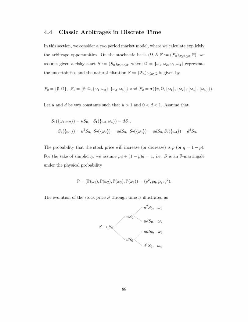
4.4 Classic Arbitrages in Discrete Time
In this section, we consider a two period market model, where we calculate explicitly
the arbitrage opportunities. On the stochastic basis (Ω,A,F := (Fn)0≤n≤2,P), we
assume given a risky asset S := (Sn)0≤n≤2, where Ω = ω1, ω2, ω3, ω4 represents
the uncertainties and the natural filtration F := (Fn)0≤n≤2 is given by
F0 = ∅,Ω, F1 = ∅,Ω, ω1, ω2, ω3, ω4, and F2 = σ(∅,Ω, ω1, ω2, ω3, ω4).
Let u and d be two constants such that u > 1 and 0 < d < 1. Assume that
S1(ω1, ω2) = uS0, S1(ω3, ω4) = dS0,
S2(ω1) = u2S0, S2(ω2) = udS0, S2(ω3) = udS0, S2(ω4) = d2S0.
The probability that the stock price will increase (or decrease) is p (or q = 1 − p).
For the sake of simplicity, we assume pu + (1 − p)d = 1, i.e. S is an F-martingale
under the physical probability
P = (P(ω1),P(ω2),P(ω3),P(ω4)) = (p2, pq, pq, q2).
The evolution of the stock price S through time is illustrated as
S → S0
uS0
u2S0, ω1
udS0, ω2
dS0
udS0, ω3
d2S0, ω4
88
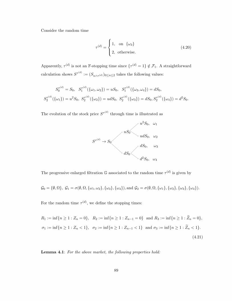
Consider the random time
τ (d) =
1, on ω3
2, otherwise.(4.20)
Apparently, τ (d) is not an F-stopping time since τ (d) = 1 /∈ F1. A straightforward
calculation shows Sτ(d)
:= (Sn∧τ (d))0≤n≤2 takes the following values:
Sτ(d)
0 = S0, Sτ(d)
1 (ω1, ω2) = uS0, Sτ(d)
1 (ω3, ω4) = dS0,
Sτ(d)
2 (ω1) = u2S0, Sτ (d)
2 (ω2) = udS0, Sτ (d)
2 (ω3) = dS0, Sτ (d)
2 (ω4) = d2S0.
The evolution of the stock price Sτ(d)
through time is illustrated as
Sτ(d) → S0
uS0
u2S0, ω1
udS0, ω2
dS0
dS0, ω3
d2S0, ω4
The progressive enlarged filtration G associated to the random time τ (d) is given by
G0 = ∅,Ω, G1 = σ(∅,Ω, ω1, ω2, ω3, ω4), and G2 = σ(∅,Ω, ω1, ω2, ω3, ω4).
For the random time τ (d), we define the stopping times:
R1 := infn ≥ 1 : Zn = 0, R2 := infn ≥ 1 : Zn−1 = 0 and R3 := infn ≥ 1 : Zn = 0,
σ1 := infn ≥ 1 : Zn < 1, σ2 := infn ≥ 1 : Zn−1 < 1 and σ3 := infn ≥ 1 : Zn < 1.
(4.21)
Lemma 4.1: For the above market, the following properties hold:
89
(a) The processes D,m,Z and Z take the form of
D0 = 0, D1 = p1ω3,ω4, D2 = p1ω3,ω4 + 1ω1,ω2,ω4.
m0 = 1, m1 = 1, m2 = p1ω3,ω4 + 1ω1,ω2,ω4.
Z0 = 1, Z1 = 1− p1ω3,ω4, Z2 = 0.
Z0 = 1, Z1 = 1, Z2 = 1ω1,ω2,ω4.
(b) Zτ (d) = 1, τ (d) = supn ≥ 0 : Zn = 1, and τ (d) is an honest time.
(c) The stopping times in (4.21) are given by
R1 = 2, R2 = +∞, R3(ω3) = 2, R3(ω1, ω2, ω4) = +∞,
σ1(ω1, ω2) = 2, σ1(ω3, ω4) = 1,
σ2(ω1, ω2) = +∞, σ2(ω3, ω4) = 2, σ3(ω3) = 2, σ3(ω1, ω2, ω4) = +∞.
Proof. By the definitions of Z and Z, we calculate that
Z0 = P (τ (d) > 0) = 1, Z1 = P (τ (d) > 1|F1) = 1ω1,ω2 + 1ω3,ω4(1− p), Z2 = 0
Z0 = P (τ (d) ≥ 0) = 1, Z1 = P (τ (d) ≥ 1|F1) = 1, Z2 = P (τ (d) ≥ 2|F2) = 1ω1,ω2,ω4.
The calculation for D and m is similar. The proofs of the assertions (b) and (c) are
straightforward. Hence, we omit them here.
Theorem 4.2: Under the current settings, the following properties hold:
(a) For the market Sτ(d)
, there are arbitrage opportunities by using public infor-
mation F and extra information G .
(b) In the market S, there are arbitrage opportunities only in G.
(c) ∆S2 6= 0∩ Z2 = 0∩ Z1 > 0 = ω3 and ∆S2 6= 0∩ Z2 = 1∩ Z1 <
1 = ω4.
Proof. In the market Sτ(d)
, apparently, by takingH1 = 0, H2(ω1, ω2) = 0, H2(ω3, ω4) =
90
−1, one can make an arbitrage. While in the market S, by takingHG1 = 0, HG
2 (ω1, ω2) =
0, HG2 (ω3) = 1, HG
2 (ω4) = −1, only the one with information G can make an
arbitrage since the strategies (HGn )1≤n≤2 are only G-predictable. Assertion (c) is
straightforward to verify. This ends the proof of the theorem.
4.5 Classic Arbitrages for Non-honest Times
In this section, we develop a number of practical examples of market models and
examples of random times that are not honest times and we study the existence of
classical arbitrages.
4.5.1 In a Brownian filtration: Emery’s Example
We present here an example where τ is a pseudo stopping time (see Nikeghbali and
Yor [115] for the definition). Let S be defined through dSt = σStdWt, where W is
a Brownian motion and σ a constant. Consider the random time
τ = sup t ≤ 1 : S1 − 2St = 0.
Proposition 4.7: For the above settings, there is no arbitrage opportunity before
τ , i.e. (Sτ ,G); while arbitrage opportunity exists after τ , i.e. (S − Sτ ,G).
Proof. Note that
τ ≤ t = inft≤s≤1
2Ss ≥ S1 =
inf
t≤s≤12SsSt≥ S1
St
Since Ss/St, s ≥ t and S1/St are independent from Ft, we derive
P(
inft≤s≤1
2SsSt≥ S1
St|Ft)
= P(
inft≤s≤1
2Ss−t ≥ S1−t
)= Ψ(1− t)
where Ψ(u) = P(infs≤u 2Ss ≥ Su). It follows that the supermartingale Z is a
91

deterministic decreasing function. Hence τ is a pseudo stopping time (see [115]) and
S is a G-martingale up to time τ and there are no arbitrages up to τ .
There are obviously arbitrages after τ , since, at time τ , one knows the value of S1
and S1 > Sτ . In fact, for t > τ , one has St > Sτ , and the arbitrage occurs at any
time before 1.
4.5.2 In a Poisson Filtration
This subsection develops similar examples of random times – as in the Brownian
filtration of the previous subsection – and shows that the effects of these random
times on the market’s economic structure differ tremendously from the one of the
previous subsection. In this section, we will work with a Poisson process N having
intensity λ and the compensated martingale Mt = Nt − λt. Denote
Tn := inft ≥ 0 : Nt ≥ n, and Hnt := 11Tn≤t, n = 1, 2. (4.22)
The stock price S is described by
dSt = St−ψdMt, where, ψ > −1, and ψ 6= 0, (4.23)
or equivalently, St = S0 exp(−λψt+ ln(1 + ψ)Nt). Then,
M1t := H1
t − λ(t ∧ T1) := H1t −A1
t ,
M2t := H2
t − (λ(t ∧ T2)− λ(t ∧ T1))) := H2t −A2
t (4.24)
are two F-martingales. Remark that if ψ ∈ (−1, 0), between T1 and T2, the stock
price increases; if ψ > 0, between T1 and T2, the stock process decreases. This would
be the starting point of the existence of arbitrages.
Example 4.3 (Convex Combination of two jump times) Below, we present
an example of random time that avoids stopping times and the non-arbitrage
92

property fails.
Proposition 4.8: Consider the market S in (4.23) with notations (4.22) and (4.24)
and the random time
τ = k1T1 + k2T2, where k1 + k2 = 1 and k1, k2 > 0,
which avoids F-stopping times. Then the following properties hold:
(a) The random time τ is not an honest time.
(b) Zτ = Zτ = e−λk1(T2−T1) < 1, and Z = 0 < Z− = [[T2]].
(c) There is a classical arbitrage before τ , given by
ϕ(1)t := −e−λ
k2k1
(t−T1) (11Nt−≥1 − 11Nt−≥2
) 1
ψSt−11t≤τ. (4.25)
(d) There exist arbitrages after τ : if ψ ∈ (−1, 0), buy at τ and sell before T2; if
ψ > 0, short sell at τ and buy back before T2.
Proof. First, we compute the supermartingale Z:
P(τ > t|Ft) = 11T1>t + 11T1≤t11T2>tP(k1T1 + k2T2 > t|Ft).
On the set E = T1 ≤ t ∩ T2 > t, the quantity P(k1T1 + k2T2 > t|Ft) is
FT1-measurable. It follows that, on E,
P(k1T1 + k2T2 > t|Ft) =P(k1T1 + k2T2 > t, T2 > t|FT1)
P(T2 > t|FT1)= e−λ k1
k2(t−T1)
,
where we used the independence property of T1 and T2 − T1. Therefore,
Zt := P(τ > t|Ft) = 11T1>t + 11T1≤t11T2>te−λ k1
k2(t−T1)
.
93
Since Zt = (1−H1t )+H1
t (1−H2t )e−λ k1
k2(t−T1)
and e−λ(t−T1)dH1t = dH1
t , we deduce
dZt = e−λ k1
k2(t−T1)
(−H2dH1t −H1
t dH2t )− λk1
k2H1t (1−H2
t )e−λ k1
k2(t−T1)
dt
= −e−λk1k2
(t−T1)dH2
t − λk1
k2H1t (1−H2
t )e−λ k1
k2(t−T1)
dt
= dmt − e−λ k1
k2(t−T1)
dA2t − λ
k1
k2H1t (1−H2
t )e−λ k1
k2(t−T1)
dt,
where dmt = −e−λk1k2
(t−T1)dM2
t . Hence,
mτ = 1−∫ τ
0e−λ k1
k2(t−T1)
dM2t = 1 +
∫ τ
T1
e−λ k1
k2(t−T1)
λdt > 1.
Now we start proving the proposition.
(i) Since τ avoids stopping times, Z = Z. Note that Zτ = Zτ = e−λk1(T2−T1) < 1.
Hence, τ is not an honest time. Thus, assertions (a) and (b) hold.
(ii) Now, we prove assertion (c). We will describe explicitly the arbitrage strategy.
Note that T2 ≤ t = Nt ≥ 2. We deduce that
M2t = 11T2≤t −A
2t = 11Nt≥2 −A2
t = 11Nt−≥1∆Nt + 11Nt−≥2(1−∆Nt)−A2t .
Hence,
∆M2t =
(11Nt−≥1 − 11Nt−≥2
)∆Nt =
(11Nt−≥1 − 11Nt−≥2
)∆Mt.
Since M2 and M are both purely discontinuous, we have mt = 1 + φ Mt =
1 + ϕ(1) St, where
φt = −e−λk1k2
(t−T1) (INt−≥1 − INt−≥2
), and ϕ
(1)t = φt
1
ψSt−.
(iii) Arbitrages after τ : At time τ , the value of T2 is known for the one who has
G information. If ψ > 0, then the price process decreases before time T2, while
94

waiting up to time T2 does not lead to an arbitrage. Setting ∆ = T2− τ (which is
known at time τ), there is an arbitrage selling short S at time τ for a delivery at
time τ + 12∆. The strategy is admissible, since between T1 and T2, the quantity
St is bounded by S0(1 + ϕ). This ends the proof of the proposition.
Example 4.4 (Minimum of two scaled jump times) We give now an example
of a non honest random time, which does not avoid F stopping time and induces
classical arbitrage opportunities.
Proposition 4.9: Consider the market S in (4.23) with notations (4.22) and (4.24)
and the random time
τ2 := T1 ∧ aT2, where 0 < a < 1 and β = λ(1/a− 1).
Then, the following properties hold:
(a) τ2 is not an honest time and does not avoid F-stopping times.
(b) Zτ2 = 11T1>aT2e−βaT2(βaT2 + 1) < 1 and Zτ2 = e−βaT2(βaT2 + 1) < 1, and
Z = 0 < Z− = ∅.
(c) m ≡ 1 and M τ is a G-local martingale for any F-local martingale M .
Proof. First, let us compute the supermartingale Z,
Zt = 11T1>tP(aT2 > t|Ft) = 11T1>tP(aT2 > t, T1 > t)
P(T1 > t)
= 11T1>teλt E(11T1>te
−λ( ta−T1)+)
= 11T1>teλt
∫ t/a
te−λ( t
a−x)λe−λxdx+ 11T1>te
λt
∫ ∞t/a
λe−λydy
= 11T1>te−βt(βt+ 1) .
In particular Zτ2 = 11T1>aT2e−βaT2(βaT2+1) < 1. Similar computation as above
leads to Zt = Zt− = 11T1≥te−βt(βt+1). This proves assertions (a) and (b). Since
∆m = Z − Z−, we have ∆m ≡ 0. Hence m is a constant equal to 1 since m is
95

a purely discontinuous F-martingale. This proves assertion (c) and the proof of
the proposition is achieved.
Conclusions
In this chapter, we treated the question whether the no-arbitrage conditions are sta-
ble with respect to progressive enlargement of filtration. Precisely, we proved that
there exist classic arbitrage opportunities for many models of honest times when
the market is complete. Furthermore, in the case of Brownian filtration and Poisson
filtration, we calculated explicitly the arbitrage strategies. One may further inves-
tigate similar problem without assuming market completeness and consider other
examples/classes of non-honest random times.
The failure of the classic arbitrage condition leads us to investigate the stability of
the NUPBR condition in Chapters 5 and 6.
96
Chapter 5
Non-arbitrage under Stopping
with Random Time
This chapter is dedicated to the problem of how an arbitrage-free semimartingale
model is affected when stopped at a random horizon. We focus on weaker non-
arbitrage concept: No-Unbounded-Profit-with-Bounded-Risk (called NUPBR here-
after) concept, which is also known in the literature as the first kind of non-arbitrage.
For this non-arbitrage notion, we obtain two principal results. The first result lies
in describing the pairs of market model and random time for which the resulting
stopped model fulfills NUPBR condition. The second main result characterizes the
random time models that preserve the NUPBR property after stopping for any mar-
ket model. These results are elaborated in a very general market model, and also
some particular and practical models.
Mathematically speaking, we consider a general semimartingale model S satisfying
the NUPBR property under the “public information” and an arbitrary random time
τ and we investigate the following problems:
For which pairs (S, τ), does the NUPBR property hold for Sτ? (Prob(5.I))
97
In Theorem 5.6 we characterize the pairs of initial market S and of random time τ ,
for which (Prob(5.I)) has a positive answer.
Our second main question consists of
For which τ , is NUPBR preserved for any S after stopping at τ? (Prob(5.II))
To deepen our understanding of the precise interplay between S (initial market
model) and τ (the random time model), we address these two principal questions
separately in the case of quasi-left-continuous models, and then in the case of thin
processes with predictable jumps. Afterwards, we combine the two cases and state
the results for the most general framework. The results for the quasi-left-continuous
models are Theorem 5.2 and Proposition 5.3, where the questions (Prob(5.I)) and
(Prob(5.II)) are fully answered respectively. For the case of thin processes with
predictable jumps, our main result is Theorem 5.5. Then, the general case follows
by splitting the process S into a quasi-left-continuous process and a thin process
with predictable jumps.
This problem was studied in the literature (see [63]) for particular case of continuous
filtration, under the hypothesis that τ avoids F-stopping times and that the market
is complete.
5.1 Notations and Preliminary Results on NUPBR
We consider a stochastic basis (Ω,A,F = (Ft)t≥0, P ), where F is a filtration satis-
fying the usual hypotheses (i.e., right continuity and completeness) and represents
the flow of public information through time with F∞ :=∨t≥0Ft ⊆ A. On this
basis, we consider an arbitrary but fixed d-dimensional cadlag F-semimartingale S
that represents the discounted price processes of d-risky assets; while the non-risky
asset’s price is assumed to be constant one.
98
Beside the initial model (Ω,A,F, P, S), we consider a random time τ , i.e., a non-
negative A-measurable random variable. To this random time, we associate the
process D and the filtration G given by
D := I[[τ,+∞[[, G = (Gt)t≥0 , Gt =⋂s>t
(Fs ∨ σ(Du, u ≤ s)
).
The filtration G is the smallest right-continuous filtration which contains F and
makes τ a stopping time. In the probabilistic literature, G is called the progressive
enlargement of F with τ . In addition to G and D, we associate to τ two important
F-supermartingales given by
Zt := P(τ > t
∣∣ Ft) and Zt := P(τ ≥ t
∣∣∣ Ft) . (5.1)
The supermartingale Z is right-continuous with left limits and coincides with the
F-optional projection of I]]0,τ [[, while Z admits right limits and left limits only and
is the F-optional projection of I]]0,τ ]]. The decomposition of Z leads to an important
F-martingale m, given by
m := Z +Do,F, (5.2)
where Do,F is the F-dual optional projection of D (See [83] for more details).
In what follows, H is a generic filtration satisfying the usual hypotheses and Q is a
probability measure on the filtered probability space (Ω,H). The set of martingales
for the filtration H under Q is denoted byM(H, Q). When Q = P , we simply denote
M(H). As usual, A+(H) denotes the set of increasing, right-continuous, H-adapted
and integrable processes.
If C(H) is a class of H adapted processes, we denote by C0(H) the set of processes
X ∈ C(H) with X0 = 0, and by Cloc the set of processes X such that there exists a
99
sequence (Tn)n≥1 of H-stopping times that increases to +∞ and the stopped pro-
cesses XTn belong to C(H). We put C0,loc(H) = C0(H) ∩ Cloc(H).
For a process K with H-locally integrable variation, we denote by Ko,H its dual
optional projection. The dual predictable projection of K (also called the H-
predictable dual projection) is denoted Kp,H. For a process X, we denote o,HX
(resp. p,HX ) its optional (resp. predictable) projection with respect to H.
For an H- semi-martingale Y , the set L(Y,H) is the set of H predictable processes
integrable w.r.t. Y and for H ∈ L(Y,H), we denote H Yt :=∫ t
0 HsdYs.
To distinguish the effect of filtrations, we will denote 〈., .〉F, or 〈., .〉G the sharp
bracket (predictable covariation process) calculated in the filtration F or G, if con-
fusion may rise. We recall that, for general semi-martingales X and Y , the sharp
bracket is (if it exists) the dual predictable projection of the covariation process
[X,Y ].
Below, we recall the non-arbitrage notion that will be addressed in this chapter.
Definition 5.1: An H-semimartingale X satisfies the No-Unbounded-Profit-with-
Bounded-Risk condition under (H, Q) (hereafter called NUPBR(H, Q)) if for any
T ∈ (0,+∞) the set
KT (X,H) :=
(H S)T∣∣ H ∈ L(X,H), and H X ≥ −1
is bounded in probability under Q. When Q ∼ P , we simply write, with an abuse
of language, X satisfies NUPBR(H).
Remark 5.1: (i) It is important to notice that this definition for NUPBR condition
appeared first in [95] (up to our knowledge), and it differs when the time horizon
is infinite from that of the literature given in Delbaen and Schachermayer [47],
100
Kabanov [86] and Karatzas and Kardaras [90] (see Definition 2.17 of Subsection
2.4 in Chapter 2). It is obvious that, when the horizon is deterministic and finite,
the current NUPBR condition coincides with that of the literature. We could
name the current NUPBR as NUPBRloc, but for the sake of simplifying notation,
we opted for the usual terminology.
(ii) In general, when the horizon is infinite, the NUPBR condition of the literature
implies the NUPBR condition defined above. However, the reverse implication
may not hold in general. In fact if we consider St = exp(Wt + t), t ≥ 0, then it
is clear that S satisfies our NUPBR(H), while the NUPBR(H) of the literature is
violated. To see this last claim, it is enough to remark that
limt−→+∞
(St − 1) = +∞ P − a.s. St − 1 = H S ≥ −1 H := I]]0,t]].
The following proposition slightly generalizes Takaoka’s results obtained for a finite
horizon (see Theorem 2.6 in [137]) to our NUPBR context.
Proposition 5.1: Let X be an H-semimartingale. Then the following assertions
are equivalent.
(a) X satisfies NUPBR(H).
(b) There exist a positive H-local martingale, Y and an H-predictable process θ
satisfying 0 < θ ≤ 1 and Y (θ X) is a local martingale.
Proof. The proof of the implication (b)⇒ (a) is based on [137] and is omitted. Thus,
we focus on proving the reverse implication and suppose that assertion (a) holds.
Therefore, a direct application of Theorem 2.6 in [137] to each (St∧n)t≥0, we obtain
the existence of a positive H-local martingale Y (n) and an H-predictable process θn
such that 0 < θn ≤ 1 and Y (n)(θn Sn) is a local martingale. Then, it is obvious
that the process
N :=+∞∑n=1
I]]n−1,n]](Y(n)− )−1 Y (n)
101

is a local martingale and Y := E(N) > 0. On the other hand, the H-predictable
process θ :=∑
n≥1 I]]n−1,n]]θn satisfies 0 < θ ≤ 1 and Y (θ S) is a local martingale.
This ends the proof of the proposition.
For any H-semimartingale X, the local martingales fulfilling the assertion (b) of
Proposition 5.1 are called σ-martingale densities forX. The set of these σ-martingale
densities will be denoted throughout the paper by
L(H, X) :=Y ∈Mloc(H)
∣∣ Y > 0, ∃θ ∈ P(H), 0 < θ ≤ 1, Y (θ X) ∈Mloc(H)
(5.3)
where, as usual, P(H) stands for predictable processes. We state, without proof, an
obvious lemma.
Lemma 5.1: For any H-semimartingale X and any Y ∈ L(H, X), one has
p,H(Y |∆X|) <∞ and p,H(Y∆X) = 0
Remark 5.2: Proposition 5.1 implies that for any process X and any finite stop-
ping time σ, the two concepts of NUPBR(H) (the current concept and the one of
the literature) coincide for Xσ.
Below, we prove that, under infinite horizon, the current NUPBR condition is stable
under localization, while the NUPBR condition defined in the literature fails.
Proposition 5.2: Let X be an H adapted process. Then, the following assertions
are equivalent.
(a) There exists a sequence (Tn)n≥1 of H-stopping times that increases to +∞,
such that for each n ≥ 1, there exists a probability Qn on (Ω,HTn) such that
Qn ∼ P and XTn satisfies NUPBR(H) under Qn.
(b) X satisfies NUPBR(H).
(c) There exists an H-predictable process φ, such that 0 < φ ≤ 1 and (φ X)
satisfies NUPBR(H).
102
Proof. The proof for (a)⇐⇒(b) follows from the stability of NUPBR condition for
a finite horizon under localization which is due to [137] (see also [37] for further
discussion about this issue), and the fact that the NUPBR condition is stable under
any equivalent probability change.
The proof of (b)⇒(c) is trivial and is omitted. To prove the reverse, we assume that
(c) holds. Then Proposition 5.1 implies the existence of an H-predictable process
ψ such that 0 < ψ ≤ 1 and a positive H-local martingale Z = E(N) such that
Z(ψφ X) is a local martingale. Since ψφ is predictable and 0 < ψφ ≤ 1, we deduce
that S satisfies NUPBR(H). This ends the proof of the proposition.
Lemma 5.2: Let X be an H-predictable process with finite variation. Then X
satisfies NUPBR(H) if and only if X ≡ X0 (i.e. the process X is constant).
Proof. It is obvious that if X ≡ X0, then X satisfies NUPBR(H). Suppose that
X satisfies NUPBR(H). Consider a positive H-local martingale Y , and an H-
predictable process θ such that 0 < θ ≤ 1 and Y (θ X) is a local martingale. Let
(Tn)n≥1 be a sequence of H-stopping times that increases to +∞ such that Y Tn and
Y Tn(θ X)Tn are true martingales. Then, for each n ≥ 1, define Qn := (YTn/Y0) P.
Since X is predictable, then (θ X)Tn is also predictable with finite variation and is
a Qn-martingale. Thus, we deduce that (θ X)Tn ≡ 0 for each n ≥ 1. Therefore, we
deduce that X is constant (since XTn − X0 = θ−1 (θ X)Tn ≡ 0). This ends the
proof of the lemma.
Now, let us characterize the σ-martingale density in terms of characteristics of
semimartingale, see also [107].
Theorem 5.1: Let X be an H-semi-martingale with predictable triplet (b, c, ν).
Then X satisfies NUPBR(H) with the σ-martingale density E(N) if and only
if the following two properties hold:
103
(a) The integral
∫ ∣∣∣ (x− h(x) + xf(x))∣∣∣F (dx)+
∫|x|MP
µ
(|g|∣∣∣ P(H)
)< +∞, P ⊗A−a.s and
(5.4)
(b) The following equality holds:
b+ βc+
∫(x− h(x) + xf(x))F (dx) ≡ 0, P ⊗A− a.s. (5.5)
where (β, f, g,N ′) are the Jacod’s parameters of N with respect to X (see (2.18)),
F is the kernel and A is an H-predictable process associated with compensator ν
(see (2.11)).
Proof. Thanks to Ito formula, we deduce that ZX is a σ-martingale if and only if
there exists an H-predictable process 0 < φ ≤ 1 such that φ X+φ [X,N ] is a local
martingale. From the Jacod Decomposition (2.18), we derive that
φ X + φ [X,N ] = φ X + φ [Xc, N c] +∑
φ∆X∆N
= X0 + φ Xc + φh ? (µ− ν) + φ(x− h) ? µ+ φb A+ φβc A
+∑
φ∆X (f(∆X) + g(∆X)) I∆X 6=0
= X0 + φ Xc + φh ? (µ− ν) + φb A
+φβc A+ φ[x− h(x) + x (f(x) + g(x))] ? µ.
Therefore, φ X + φ [X,N ] is a local martingale if and only if the assertions (a)
and (b) are satisfied.
5.2 Main Results and their Interpretations
This section presents our main results and their immediate consequences. To this
end, we start specifying our mathematical setting and the economic concepts.
104
5.2.1 The Quasi-Left-Continuous Processes
In this subsection, we present our two main results on the NUPBR condition under
stopping at τ for quasi-left-continuous processes. The first result consists of charac-
terizing the pairs (S, τ) of market and random time models, for which Sτ fulfills the
NUPBR condition. The second result focuses on determining the models of random
times τ such that, for any semi-martingale S enjoying NUPBR(F), the stopped pro-
cess Sτ enjoys NUPBR(G) .
The following theorem gives a characterization of F-quasi-left-continuous processes
that satisfy NUPBR(G) after stopping with τ . Recall that µ, ν and MPµ are defined
by (2.9), (2.11) and (2.10) in Subsection 2.3 respectively. The proof of this theorem
will be given in Subsection 5.5.1, while its statement is based on the following F-
semimartingale
S(0) := xIψ=0<Z− ? µ, where ψ := MPµ
(IZ>0
∣∣∣P (F)). (5.6)
Theorem 5.2: Suppose that S is F-quasi-left-continuous. Then, the following as-
sertions are equivalent.
(a) Sτ satisfies NUPBR(G).
(b) For any δ > 0, the process
IZ−≥δ (S − S(0)
)satisfies NUPBR(F). (5.7)
(c) For any n ≥ 1, the process (S − S(0))σn satisfies NUPBR(F), where
σn := inft ≥ 0 : Zt < 1/n.
Remark 5.3: 1) From assertion (c) one can understand that the NUPBR(G) prop-
erty for Sτ can be verified by checking whether S − S(0) satisfies NUPBR(F) up
105
to σ∞ := supn σn. This is also equivalent to NUPBR(F) of the same process on
the predictable sets Z− ≥ δ, δ > 0.
2) The functionals ψ and Z− + fm := MPµ (Z
∣∣P(F)) satisfy
ψ = 0 = Z− + fm = 0 ⊂ Z = 0, MPµ − a.e. (5.8)
Indeed, due to Z ≤ IZ>0, we have
0 ≤ Z− + fm = MPµ
(Z∣∣ P(F)
)≤ ψ.
Thus, we get ψ = 0 ⊂ Z− + fm = 0 ⊂ Z = 0 MPµ − a.e. on the one hand.
On the other hand, the reverse inclusion follows from
0 = MPµ
(IZ−+fm=0IZ=0
)= MP
µ
(IZ−+fm=0ψ
).
3) As a result of remark 2) above and Z = 0 < Z− ⊂ [[σ∞]], we deduce that
S(0) is a cadlag F-adapted process with finite variation that takes the form of
S(0) := ∆Sσ∞IZσ∞=0=ψ(σ∞,∆Sσ∞ ) & Zσ∞−>0I[[σ∞,+∞[[.
This proves the claim stated before Theorem 5.2 about the process S(0).
The following corollary is useful for studying the problem (Prob(5.II)), and it
describes examples of F-quasi-left-continuous model S that fulfills (5.6) as well.
Corollary 5.2.1: Suppose that S is F-quasi-left-continuous and satisfies NUPBR(F).
Then, the following assertions hold.
(a) If(S, S(0
)satisfies NUPBR(F), then Sτ satisfies NUPBR(G).
(b) If S(0) ≡ 0, then the process Sτ satisfies NUPBR(G).
(c) If ∆S 6= 0 ∩ Z = 0 < Z− = ∅, then Sτ satisfies NUPBR(G).
(d) If Z > 0 (equivalently Z > 0 or Z− > 0), then Sτ satisfies NUPBR(G).
106
Proof. (a) Suppose that(S, S(0
)satisfies NUPBR(F). Then, it is obvious that
S − S(0) satisfies NUPBR(F), and assertion (a) follows from Theorem 5.2.
(b) Since S satisfies NUPBR(F) and S(0) ≡ 0, then(S, S(0
)≡ (S, 0) satisfies
NUPBR(F), and assertion (b) follows from assertion (a).
(c) It is easy to see that ∆S 6= 0 ∩ Z = 0 < Z− = ∅ implies that S(0) ≡ 0 (due
to (5.8)). Hence, assertions (c) and (d) follow from assertion (b), and the proof of
the corollary is completed.
Remark 5.4: It is worth mentioning that X − Y may satisfy NUPBR(H), while
(X,Y ) may fail NUPBR(H). For a non trivial example, consider Xt = Bt+λt and
Yt = Nt, where B is a standard Brownian motion and N is the Poisson process
with intensity λ.
We now give an answer to the second problem (Prob(5.II)) for the quasi-left-
continuous semimartingales. Later on (in Theorem 5.7) we will generalize this result.
Theorem 5.3: The following assertions are equivalent:
(a) The thin setZ = 0 & Z− > 0
is accessible.
(b) For any (bounded) S that is F-quasi-left-continuous and satisfies NUPBR(F),
the process Sτ satisfies NUPBR(G).
Proof. The implication (a)⇒(b) follows from Corollary 5.2.1–(c), since we have
∆S 6= 0 ∩ Z = 0 < Z− = ∅.
We now focus on proving the reverse implication. To this end, we suppose that
assertion (b) holds, and we consider an F-stopping time σ such that [[σ]] ⊂ Z =
0 < Z−. It is known that σ can be decomposed into a totally inaccessible part σi
and an accessible part σa such that σ = σi ∧ σa. Consider the quasi-left-continuous
F-martingale
M = V − V ∈M0,loc(F)
107
where V := I[[σi,+∞[[ and V := (V )p,F. It is known from [53, paragraph 14, Chapter
XX], that
Z = 0 and Z− = 0 are disjoint from ]]0, τ ]] . (5.9)
This implies that τ < σ ≤ σi P − a.s.. Hence, we get
M τ = −V τ is G-predictable. (5.10)
Since M τ satisfies NUPBR(G), then we conclude that this process is null (i.e. V τ =
0) due to Lemma 5.2. Thus, we get
0 = E(Vτ
)= E
(∫ +∞
0Zs−dVs
)= E
(Zσi−Iσi<+∞
),
or equivalently Zσi−Iσi<+∞ = 0 P−a.s. This is possible only if σi = +∞ P−a.s.
since on σi < +∞ ⊂ σ = σi < +∞ we have Zσi− = Zσ− > 0. This proves
that σ is an accessible stopping time. Since Z = 0 < Z− is an optional thin set,
assertion (a) follows immediately. This ends the proof of the proposition.
5.2.2 Thin Processes with Predictable Jump Times
In this subsection, we outline the main results on the NUPBR condition for the
stopped accessible parts of F-semimartingales with a random time. This boils down
to consider thin semimartingales with predictable jump times only. We start by
addressing the question (Prob(5.I)) in the case of single jump process with pre-
dictable jump time.
Theorem 5.4: Consider an F-predictable stopping time T and an FT -measurable
random variable ξ such that E(|ξ|∣∣ FT−) < +∞ P − a.s..
If S := ξIZT−>0I[[T,+∞[[, then the following assertions are equivalent:
(a) Sτ satisfies NUPBR(G),
108
(b) The process S := ξIZT>0I[[T,+∞[[ = IZ>0 S satisfies NUPBR(F).
(c) There exists a probability measure on (Ω,FT ), denoted by QT , such that QT
is absolutely continuous with respect to P , and S satisfies NUPBR(F, QT ).
The proof of this theorem is long and requires intermediary results that are inter-
esting in themselves. Thus, this proof will be given later in Section 5.5.
Remark 5.5: 1) The importance of Theorem 5.4 goes beyond its vital role, as a
building block for the more general result. In fact, Theorem 5.4 provides two
different characterizations for NUPBR(G) of Sτ . The first characterization is ex-
pressed in term of NUPBR(F) of S under absolute continuous change of measure,
while the second characterization uses transformation of S without any change
of measure. Furthermore, Theorem 5.4 can be easily extended to the case of
countably many ordered predictable jump times T0 = 0 ≤ T1 ≤ T2 ≤ ... with
supn Tn = +∞ P − a.s..
2) In Theorem 5.4, the choice of S having the form S := ξIZT−>0I[[T,+∞[[ is not
restrictive. This can be understood from the fact that any single jump process S
can be decomposed as follows
S := ξI[[T,+∞[[ = ξIZT−>0I[[T,+∞[[ + ξIZT−=0I[[T,+∞[[ =: S + S.
Thanks to T ≤ τ ⊂ ZT− > 0, we have Sτ = ξIZT−=0IT≤τI[[T,+∞[[ ≡ 0
which is (obviously) a G-martingale. Thus, the only part of S that requires careful
attention is S := ξIZT−>0I[[T,+∞[[.
The following result is a complete answer to (Prob(5.II)) in the case of predictable
single jump processes.
Proposition 5.3: Let T be an F-predictable stopping time. Then, the following
assertions are equivalent:
109
(a) On T < +∞, we have
ZT = 0
⊂ZT− = 0
. (5.11)
(b) For any M := ξI[[T,+∞[[ where ξ ∈ L∞(FT ) such that E(ξ|FT−) = 0, M τ
satisfies NUPBR(G).
Proof. We start by proving (a)⇒ (b). Suppose that (5.11) holds; due to the above
Remark 5.5-(2), we can restrict our attention to the case whenM := ξIZT−>0I[[T,+∞[[,
where ξ ∈ L∞(FT ) such that E(ξ|FT−) = 0. Since assertion (a) is equivalent to
[[T ]] ∩ Z = 0 & Z− > 0 = ∅, we deduce that
M := ξIZT>0IZT−>0I[[T,+∞[[ = M is an F-martingale.
Therefore, a direct application of Theorem 5.4 (to M) allows us to conclude that
M τ satisfies the NUPBR(G). This ends the proof of (a)⇒ (b). To prove the reverse
implication, we suppose that assertion (b) holds and consider
M := ξI[[T,+∞[[, where ξ := IZT=0 − P (ZT = 0|FT−).
From (5.9), we obtain T ≤ τ ⊂ ZT > 0 ⊂ ZT− > 0 which implies that
M τ = −P (ZT = 0|FT−)IT≤τI[[T,+∞[[ is G-predictable.
Therefore, M τ satisfies NUPBR(G) if and only if it is a constant process equal to
M0 = 0 (see Lemma 5.2). This is equivalent to
0 = E[P (ZT = 0|FT−)IT≤τI[[T,+∞[[
]= E
(ZT−IZT=0 & T<+∞
).
It is obvious that this equality is equivalent to (5.11), and assertion (a) follows. This
110
ends the proof of the theorem.
We now state the following version of Theorem 5.4, which provides, as already said,
an answer to (Prob(5.I)) in the case where there are countable many arbitrary
predictable jumps. The proof of this theorem will be given in Subsection 5.5.3.
Theorem 5.5: Let S be a thin process with predictable jump times only and satis-
fying NUPBR(F). Then, the following assertions are equivalent.
(a) The process Sτ satisfies NUPBR(G).
(b) For any δ > 0, there exists a positive F-local martingale, Y , such that
p,F (Y |∆S|) < +∞ and
p,F(Y∆SIZ>0 & Z−≥δ
)= 0. (5.12)
Remark 5.6: 1) Suppose that S is a thin process with predictable jumps only,
satisfying NUPBR(F), and that Z = 0 & Z− > 0∩∆S 6= 0 = ∅ holds. Then,
Sτ satisfies NUPBR(G). This follows immediately from Theorem 5.5 by using
Y ∈ L(S,F) and Lemma 5.1.
2) Similarly to Proposition 5.3, we can easily prove that the thin set Z =
0 & Z− > 0 is totally inaccessible if and only if Xτ satisfies NUPBR(G) for
any thin process X with predictable jumps only satisfying NUPBR(F).
5.2.3 The General Framework
Throughout the paper, with any H-semimartingale, X, we associate a sequence of
(H)-predictable stopping times (TXn )n≥1 that exhaust the accessible jump times of
X. Furthermore, we can decompose X as follows.
X = X(qc) +X(a), X(a) := IΓX X, X(qc) := X −X(a), ΓX :=
∞⋃n=1
[[TXn ]]. (5.13)
111
The process X(a) (the accessible part of X) is a thin process with predictable jumps
only, while X(qc) is an H-quasi-left-continuous process (the quasi-left-continuous
part of X).
Lemma 5.3: Let X be an H-semimartingale. Then X satisfies NUPBR(H) if and
only if X(a) and X(qc) satisfy NUPBR(H).
Proof. Thanks to Proposition 5.1, X satisfies NUPBR(H) if and only if there exist
an H-predictable real-valued process φ > 0 and a positive H-local martingale Y such
that Y (φ X) is an H- local martingale. Then, it is obvious that Y (φIΓX X) and
Y (φIΓXc X) are both H-local martingales. This proves that X(a) and X(qc) both
satisfy NUPBR(H).
Conversely, if X(a) and X(qc) satisfy NUPBR(H), then there exist two H-predictable
real-valued processes φ1, φ2 > 0 and two positive H-local martingalesD1 = E(N1), D2 =
E(N2) such that D1(φ1 (IΓX S)) and D2(φ2 (IΓXc X)) are both H-local martin-
gales. Remark that there is no loss of generality in assuming N1 = IΓX N1 and
N2 = IΓXc N2. Put
N := IΓX N1 + IΓXc N2 and ψ := φ1IΓX + φ2IΓX
c .
Obviously, E(N) > 0, E(N) and E(N)(ψ S) are H-local martingales, ψ is H-
predictable and 0 < ψ ≤ 1. This ends the proof of the lemma.
Below, we state the answer to question (Prob(5.I)), in this general framework,
which is a consequence of Theorems 5.2 and 5.4, due to Lemma 5.3.
Theorem 5.6: Suppose that S satisfies NUPBR(F). Then, the following assertions
are equivalent.
(a) The process Sτ satisfies NUPBR(G).
112

(b) For any δ > 0, the process
IZ−≥δ (S(qc) − S(qc,0)) := IZ−≥δ (S(qc) − IΓc S(0))
satisfies NUPBR(F), and there exists a positive F-local martingale, Y , such that
p,F (Y |∆S|) < +∞ and
p,F(Y∆SIZ>0 & Z−≥δ
)= 0.
Proof. Due to Lemma 5.3, it is obvious that Sτ satisfies NUPBR(G) if and only if
both (S(qc))τ and (S(a))τ satisfy NUPBR(G). Thus, using both Theorems 5.2 and
5.5, we deduce that this last fact is true if and only if for any δ > 0, the process
IZ−≥δ (S(qc) − IΓc S(0)) satisfies NUPBR(F) and there exists a positive F-local
martingale Y such that
p,F (Y |∆S|) = p,F (Y |∆S(a)|)< +∞ and
p,F(Y∆SIZ>0, Z−≥δ
)= p,F
(Y∆S(a)IZ>0, Z−≥δ
)= 0.
This ends the proof of the theorem.
Corollary 5.6.1: The following assertions hold.
(a) If either m is continuous or Z is positive (equivalently Z > 0 or Z− > 0), Sτ
satisfies NUPBR(G) whenever S satisfies NUPBR(F).
(b) If S satisfies NUPBR(F) and ∆S 6= 0∩Z = 0 < Z− = ∅, then Sτ satisfies
NUPBR(G).
(c) If S is continuous and satisfies NUPBR(F), then for any random time τ , Sτ
satisfies NUPBR(G).
Proof. 1) The proof of assertion (a) of the corollary follows easily from Theorem
5.6. Indeed, in the two cases, one has Z = 0 < Z− = ∅ which implies that
113
Z = 0, δ ≤ Z− = ∅ and S(qc,0) ≡ 0 (due to (5.8)). Then, due to Lemma 5.1, It
suffices to take Y ∈ L(S,F) —since this set is non-empty— and apply Theorem 5.6.
2) it is obvious that assertion (c) follows from assertion (b). To prove this latter, it
is enough to remark that ∆S 6= 0 ∩ Z = 0, δ ≤ Z− = ∅ implies that
IZ−≥δ S(qc,0) ≡ 0 and ∆SIZ=0,δ≤Z− = 0.
Thus, again, it is enough to take Y ∈ L(S,F) (i.e. Y is the σ-martingale density of
S) and apply Theorem 5.6. This ends the proof of the corollary.
Remark 5.7: Any of the two assertions of the above corollary generalizes the main
result of Fontana et al. [63], obtained under some restrictive assumptions on the
random time τ and the market model as well.
Below, we provide a general answer to question (Prob(5.II)), as a consequence of
Theorems 5.2 and 5.5 and Proposition 5.3.
Theorem 5.7: The following assertions are equivalent:
(a) The thin setZ = 0 & Z− > 0
is evanescent.
(b) For any (bounded) X satisfying NUPBR(F), Xτ satisfies NUPBR(G).
Proof. Suppose that assertion (a) holds, and consider a processX satisfying NUPBR(F).
Then, X(qc,0) := IΓcXX(0) ≡ 0, where X(0) is defined as in (5.6). Hence IZ−≥δ (
X(qc) − IΓcXX(0)
)satisfies NUPBR(F) for any δ > 0, and NUPBR(G) property
of (X(qc))τ follows immediately from Theorem 5.2 on the one hand. On the other
hand, it is easy to see that X(a) fulfills the condition (5.12) with Y ≡ 1. Thus,
thanks to Theorem 5.5 (applied to the thin process X(a) satisfying NUPBR(F)), we
conclude that (X(a))τ satisfies NUPBR(G). Thus, due to Lemma 5.3, the proof of
(a)⇒(b) is completed.
We now suppose that assertion (b) holds. On the one hand, from Proposition
5.3, we deduce that Z = 0 < Z− is accessible and can be covered with the
114
graphs of F-predictable stopping times (Tn)n≥1. On the other hand, a direct ap-
plication of Proposition 5.3 to all single predictable jump F-martingales, we obtain
Z = 0 < Z− ∩ [[T ]] = ∅ for any F-predictable stopping time T . Therefore, we get
Z = 0 < Z− =
∞⋃n=1
(Z = 0 < Z− ∩ [[Tn]]
)= ∅.
This proves assertion (a), and the proof of the theorem is completed.
5.3 Stochastics from–and–for Informational Non-Arbitrage
In this section, we develop new stochastic results that will play a key role in the
proofs and/or the statements of the main results outlined in the previous section.
The first subsection compares the G-compensators and the F-compensators, while
the second subsection studies G-localization and F-localization. Section 5.3.3 is con-
structing a G-local martingale that is vital in the explicit construction of deflators.
We recall that Z− + ∆m = Z (see [84]).
Lemma 5.4: Let Z and Z be the two supermartingales given by (5.1).
(a) The three sets Z = 0, Z = 0 and Z− = 0 have the same debut which is
an F-stopping time that we denote by
R := inft ≥ 0∣∣ Zt− = 0. (5.14)
(b) The following F-stopping times
R0 :=
R on ZR− = 0
+∞ otherwiseand R0 :=
R on ZR
= 0
+∞ otherwise
are such that R0 is a F-predictable stopping time, and
τ ≤ R, τ < R0, P − a.s. (5.15)
115
(c) The G-predictable process
Ht := (Zt−)−1 I[[0,τ ]](t), (5.16)
is G-locally bounded.
Proof. From [53, paragraph 14, Chapter XX], for any random time τ , the sets
Z = 0 and Z− = 0 are disjoint from ]]0, τ ]] and have the same lower bound R,
the smallest F-stopping time greater than τ . Thus, we also conclude that Z = 0
is disjoint from ]]0, τ [[. This leads to assertion (a). The process X := Z−1I]]0,τ [[ being
a cadlag G-supermartingale [141], its left limit is locally bounded. Then, due to
(Z−)−1I]]0,τ ]] = X−,
the local boundedness of H follows. This ends the proof of the lemma.
5.3.1 Projection and Compensator under G and F
The main results of this subsection are summarized in Lemmas 5.5 and 5.6, where
we address the question of how to compute G-dual predictable projections in term
of F-dual predictable projections and vice versa. These results are based essentially
on the following standard result on progressive enlargement of filtration (we refer
the reader to [53, 83] for proofs).
Proposition 5.4: Let M be an F-local martingale. Then, for any random time τ ,
the process M given by
Mt := Mt∧τ −∫ t∧τ
0
d〈M,m〉FsZs−
(5.17)
is a G-local martingale, where m is defined in (5.2).
Remark 5.8: Throughout this chapter, it is worthy to keep in mind that the process
116
X would be defined via (5.17) for any F-local martingale X.
In the following lemma, we express the G–dual predictable projection of an F-locally
integrable variation process in terms of an F–dual predictable projection, and G-
predictable projection in terms of F-predictable projection.
Lemma 5.5: The following assertions hold.
(a) For any F-adapted process V with locally integrable variation, we have
(V τ )p,G = (Z−)−1I]]0,τ ]] (Z V
)p,F. (5.18)
(b) For any F-local martingale M , we have, on [[0, τ ]]
p,G(
∆M
Z
)=
p,F(
∆MIZ>0
)Z−
, and p,G(
1
Z
)=
p,F(IZ>0
)Z−
. (5.19)
(c) For any quasi-left-continuous F-local martingale M , we have, on [[0, τ ]]
p,G(
∆M
Z
)= 0, and p,G
(1
Z− + ∆m(qc)
)=
1
Z−, (5.20)
where m(qc) is the quasi-left-continuous F-martingale defined via (5.13).
Proof. (a) By considering M = V − V p,F and M defined via (5.17), we obtain
V τ = I]]0,τ ]] Vp,F +M+
1
Z−I]]0,τ ]] 〈V,m〉F = M+I]]0,τ ]] V
p,F +1
Z−I]]0,τ ]] (∆m V )p,F,
which proves assertion (a).
(b) Let M be an F-local martingale, then, for any positive integers (n, k) the process
V (n,k) :=∑ ∆M
ZI|∆M |≥k−1, Z≥n−1 has locally integrable variation. Then, by using
the known equality p,G(∆V ) = ∆(V p,G) (see Theorem 76 in pages 149–150 of [54] or
Theorem 5.27 in page 150 of [71]), and applying assertion (a) to the process V (n,k),
117

we get, on ]]0, τ ]]
p,G(
∆M
ZI|∆M |≥k−1, Z≥n−1
)=
1
Z−p,F(
∆MI|∆M |≥k−1, Z≥n−1
).
Since M is a local martingale, by stopping we can exchange limits with projections
in both sides. Then by letting n and k go to infinity, and using the fact that Z > 0
on ]]0, τ ]], we deduce that
p,G(
∆M
Z
)=
1
Z−p,F(
∆MIZ>0
).
This proves the first equality in (5.19), while the second equality follows from Z =
∆m+ Z−:
Z−p,G(Z−1
)= p,G
((Z −∆m)/Z
)= 1− p,G
(∆m/Z
)= 1− (Z−)−1 p,F
(∆mIZ>0
)= 1− p,F
(IZ=0
)= p,F
(IZ>0
).
In the above string of equalities, the third equality follows from the first equality in
(5.19), while the fourth equality is due to p,F(∆m) = 0 and ∆mIZ=0 = −Z−IZ=0.
This ends the proof of assertion (b).
(c) If M is a quasi-left-continuous F-local martingale, then p,F(
∆MIZ>0
)=
0, and the first property of the assertion (c) follows. Applying the first prop-
erty to M = m(qc) and using that, on ]]0, τ ]], one has ∆m(qc) (Z− + ∆m)−1 =
∆m(qc)(Z− + ∆m(qc)
)−1, we obtain
1
Z−p,G(
Z−
Z− + ∆m(qc)
)=
1
Z−
(1− p,G
(∆m(qc)
Z− + ∆m(qc)
))=
1
Z−.
This proves assertion (c), and the proof of the lemma is achieved.
The next lemma proves that Z−1I]]0,τ ]] is Lebesgue-Stieljes-integrable with respect
118
to any process that is F-adapted with F-locally integrable variation. Using this fact,
the lemma addresses the question of how an F-compensator stopped at τ can be
written in terms of a G-compensator, and constitutes a sort of converse result to
Lemma 5.5–(a).
Lemma 5.6: Let V be an F-adapted cadlag process. Then the following hold.
(a) If V belongs to A+loc(F) (respectively V ∈ A+(F)), then the process
U := Z−1I]]0,τ ]] V, (5.21)
belongs to A+loc(G) (respectively to A+(G)).
(b) If V has F-locally integrable variation, then the process U is well defined, its
variation is G-locally integrable, and its G-dual predictable projection is given by
Up,G =
(1
ZI]]0,τ ]] V
)p,G=
1
Z−I]]0,τ ]]
(IZ>0 V
)p,F. (5.22)
In particular, if supp(V ) ⊂ Z > 0, then, on ]]0, τ ]], one has V p,F = Z− Up,G.
Proof. (a) Suppose that V ∈ A+loc(F). First, remark that, due to the fact that Z
is positive on ]]0, τ ]], U is well defined. Let (ϑn)n≥1 be a sequence of F-stopping
times that increases to +∞ such that E (Vϑn) < +∞. Then, if E (Uϑn) ≤ E (Vϑn),
assertion (a) follows. Thus, we calculate
E (Uϑn) = E
(∫ ϑn
0I0<t≤τ
1
ZtdVt
)= E
(∫ ϑn
0
P (τ ≥ t|Ft)Zt
IZt>0dVt
)≤ E (Vϑn) .
The last inequality is obtained due to Zt := P (τ ≥ t|Ft). This ends the proof of
assertion (a) of the lemma.
(b) Suppose that V ∈ Aloc(F), and denote by W := V + + V − its variation. Then
119
W ∈ A+loc(F), and a direct application of the first assertion implies that
(Z)−1
I]]0,τ ]] W ∈ A+loc(G).
As a result, we deduce that U given by (5.21) for the case of V = V + − V − is well
defined and has variation equal to(Z)−1
I]]0,τ ]] W which is G-locally integrable. By
setting Un := I]]0,τ ]] (Z−1IZ≥1/n V
), we derive, due to (5.18),
(Un)p,G =1
Z−I]]0,τ ]]
(IZ≥1/n V
)p,F.
Hence, since Up,G = limn−→+∞ (Un)p,G , by taking the limit in the above equality,
(5.22) follows immediately, and the lemma is proved.
5.3.2 G-Localization versus F-Localization
Lemma 5.7: Let HG be a P(G)-measurable functional. Then, the following hold.
(a) There exist an P(F)-measurable functional HF and a B(R+)⊗P(F)-measurable
functionals KF : R+ × R+ × Ω× Rd → R such that
HG(ω, t, x) = HF(ω, t, x)I]]0,τ ]] +KF(τ(ω), t, ω, x)I]]τ,+∞]]. (5.23)
(b) If furthermore HG > 0 (respectively HG ≤ 1), then we can choose HF > 0
(respectively HF ≤ 1) such that
HG(ω, t, x)I]]0,τ ]] = HF(ω, t, x)I]]0,τ ]].
(c) If LG is an O(G)-measurable functional, then there exist a O(G)-measurable
functional L(1)(t, ω, x), a Pprog(F)-measurable functional L(2)(t, ω, x) and Pprog(F)⊗
B(Rd)-measurable functional, L(3)(t, ω, x, v), such that
LG(t, ω, x) = L(1)(t, ω, x)I]]0,τ [[ + L(1)(t, ω, x)I[[τ ]] + L(3)(t, ω, x, τ)I]]τ,+∞[[,(5.24)
120
where Pprog(F) is the F-progressive σ-field on Ω×R+, and Pprog(F) := Pprog(F)⊗
B(Rd). If furthermore, 0 < LG (respectively LG ≤ 1), then all L(i) can be chosen
such that 0 < L(i) (respectively L(i) ≤ 1), i = 1, 2, 3.
(d) For any F-stopping time, T , and any positive GT -measurable random vari-
able Y G, there exist two positive FT -measurable random variables, Y (1) and Y (2),
satisfying
Y GIT≤τ = Y (1)IT<τ + Y (2)Iτ=T. (5.25)
Proof. (a) We are mimicking the approach of Jeulin [83]. Notice that P(G) is
generated by the process of the form
hG(ω, t, x) := α (s ∧ τ(ω)) fs(ω)g(x)Is<t,
where α and g are Borel measurable functions and fs ∈ Fs. Now, by taking
hF(ω, t, x) := α (s) fs(ω)g(x)Is<t ∈ P(F) and
kF(y, t, ω, x) := α (y ∧ s) fs(ω)g(x)Is<t ∈ B(R+)⊗ P(F)
we have
hG(ω, t, x) = hFI[[0,τ [[ + kF(τ(ω), t, ω, x)I[[τ,+∞]].
Therefore, (5.23) follows immediately.
(b) To prove positivity of HF when HG > 0, we consider
HF
:= (HF)+ + IHF=0 > 0,
and we remark that due to (5.23), we have ]]0, τ ]] ⊂ HG = HF ⊂ HF > 0. Thus,
121
we get
HGI]]0,τ ]] = HFI]]0,τ ]].
Similarly, we consider HF ∧ 1, and we deduce that if HG is upper-bounded by one,
the process HF can also be chosen to not exceed one. This ends the proof of asser-
tion (b).
(c) For the proof of assertion (c), we mimic Jeulin (see [83]) in his proof of Propo-
sition (5,3)–(b). In fact, it is clear that the σ-field O(H) is generated by the func-
tionals H((t, ω, x) := g(x)I[[σ1,σ2]] where σi are G-stopping times such that σ1 < σ2
on σ1 < +∞. Then, it is easy to remark that
H(t, ω, x) = lim sups−→t
H(s, ω, x), where H(s, ω, x) := g(x)I[[σ1,σ2[[(s).
Thus a direct application of assertion (a) to the functional H, we obtain the exis-
tence of an P(F)-measurable functional, J(t, ω, x) , and a B(R+)⊗P(F)-measurable
functional, K(t, ω, x, v), such that
H(s, ω, x) = J(t, ω, x)I]]0,τ ]] +K(t, ω, x, τ)I]]τ,+∞]].
Put
J(t, ω, x) := lim sups−→t
J(s, ω, x), K(t, ω, x, v) := lim sups−→t
K(s, ω, x, v),
and
W (t, ω, x, v) := sup
lim sups→t,s<t
J(s, ω, x), lim sups→t,s>t
K(s, ω, x, v)
.
Then, due to [52] (see also Lemma (4,1) in Jeulin [83]), J is O(F)-measurable, K
is O(F)⊗ B(R+)-measurable and W (t, ω, x, v) is Pprog(F)⊗ B(R+)-measurable. As
a result, we deduce (due to Lemma 5.8 below), that W (t, ω, x) = W (t, ω, x, t) is
122
Pprog(F)-measurable, and we have
H(t, ω, x) = J(t, ω, x)I]]0,τ [[ +W (t, ω, x)I[[τ ]] +K(t, ω, x, τ)I]]τ,+∞]].
Thus, the proof of the first part of the assertion (c) follows from the class monotone
theorem. The proof of the positivity and the upper boundedness follows the same
arguments as in the proof of assertion (b).
(d) The proof of assertion (d) is a direct application of assertion (c) combined with
the fact that for any F-progressively measurable process Y and any F-stopping time
T , we have YT IT<+∞ is FT -measurable. For this last fact, we refer the reader to
Theorem 64 in [54]. This ends the proof of the lemma.
Below, we state a simple and useful lemma that generalizes a result of [38].
Lemma 5.8: If X(t, ω, x, v) is an O(H)⊗ B(R+)-measurable functional, then
X(t, ω, x) := X(t, ω, x, t) is O(H)-measurable.
Proof. The proof of this lemma is immediate from a combination of the class mono-
tone theorem, and the proof of the lemma for the generators of O(H) ⊗ B(R+)
having the form of X(t, ω, x, v) = H(t, ω, x)k(v). Here H is O(H)-measurable and
k is B(R+)-measurable. For these generators, we have X(t, ω, x) = H(t, ω, x)k(t)
which is obviously O(H)-measurable.
In the following, we state and prove our main results of this subsection.
Proposition 5.5: For any α > 0, the following assertions hold:
(a) Let h be a P(H)-measurable functional. Then,√
(h− 1)2 ? µ ∈ A+loc(H) iff
(h− 1)2I|h−1|≤α ? µ and |h− 1|I|h−1|>α ? µ belong to A+loc(H).
(b) Let (σGn )n be a sequence of G-stopping times that increases to infinity. Then,
123
there exists a nondecreasing sequence of F-stopping times, (σFn)n≥1, satisfying the
following properties
σGn ∧ τ = σFn ∧ τ, σ∞ := supnσFn ≥ R P − a.s., (5.26)
and Zσ∞− = 0 P − a.s. on Σ ∩ (σ∞ < +∞), (5.27)
where Σ :=⋂n≥1
(σFn < σ∞).
(c) Let V be an F-predictable and non-decreasing process. Then, V τ ∈ A+loc(G) if
and only if IZ−≥δ V ∈ A+loc(F) for any δ > 0.
(d) Let h be a nonnegative and P(F)-measurable functional. Then, hI]]0,τ ]] ? µ ∈
A+loc(G) if and only if for all δ > 0, hIZ−≥δ ? µ
1 ∈ A+loc(F), where µ1 := Z
centerdotµ.
(e) Let f be positive and P(F)-measurable, and µ1 := Zµ. Then√
(f − 1)2I]]0,τ ]] ? µ ∈
A+loc(G) iff
√(f − 1)2IZ−≥δ ? µ
1 ∈ A+loc(F), for all δ > 0.
Proof. (a) Put W := (h − 1)2 ? µ = W1 + W2, where W1 := (h − 1)2I|h−1|≤α ?
µ, W2 := (h− 1)2I|h−1|>α ? µ and W ′2 := |h− 1|I|h−1|>α ? µ. Note that
√W ≤
√W1 +
√W2 ≤
√W1 +W ′2.
Therefore√W1,W
′2 ∈ A
+loc imply
√W is locally integrable.
Conversely, if√W ∈ A+
loc,√W1 and
√W2 are both locally integrable. Since W1 is
locally bounded and has finite variation, W1 is locally integrable. In the following,
we focus on the proof of the local integrability of W ′2. Denote
τn := inft ≥ 0 : Vt > n, V := W2.
It is easy to see that τn increases to infinity and V− ≤ n on the set ]]0, τn]]. On the set
∆V > 0, we have ∆V ≥ α2. By using the elementary inequality√
1 + nα2−
√nα2 ≤
124
√1 + x−
√x ≤ 1, when 0 ≤ x ≤ n
α2 , we have
√V− + ∆V −
√V− ≥ βn
√∆V on ]]0, τn]], where βn :=
√1 +
n
α2−√
n
α2,
and
(W ′2)τn =
(∑√∆V
)τn≤ 1
βn
(∑∆√V)τn
=1
βn
(√W2
)τn∈ A+
loc(H)
Therefore W ′2 ∈ (A+loc(H))loc = A+
loc(H).
(b) Due to Jeulin [83], there exists a sequence of F-stopping times (σFn)n such that
σGn ∧ τ = σFn ∧ τ. (5.28)
By putting σn := supk≤n σFk , we shall prove that
σGn ∧ τ = σn ∧ τ, (5.29)
or equivalently σFn∧τ < σn∧τ is negligible. Due to (5.28) and σGn is nondecreasing,
we derive
σFn < τ = σGn < τ ⊂n⋂i=1
σGi = σFi ⊂ σFn = σn.
This implies that,
σFn ∧ τ < σn ∧ τ = σFn < τ, & σFn < σn = ∅,
and the proof of (5.29) is completed. Without loss of generality we assume that the
sequence σFn is nondecreasing. By taking limit in (5.28), we obtain τ = σ∞∧τ, P−a.s.
which is equivalent to σ∞ ≥ τ, P−a.s. Since R is the smallest F-stopping time
125

greater or equal than τ almost surely, we obtain, σ∞ ≥ R ≥ τ P − a.s.. This
achieves the proof of (5.26).
On the set Σ, it is easy to show that
I[[0,σFn]] −→ I[[0,σF
∞[[, when n goes to +∞.
Then, thanks again to (5.28) (by taking F-predictable projection and let n go to
infinity afterwards), we obtain
Z− = Z−I[[0,σF∞[[, on Σ. (5.30)
Hence, (5.27) follows immediately, and the proof of assertion (b) is completed.
(c) Suppose that hI[[0,τ ]] ? µ ∈ A+loc(G). Then, there exists a sequence of G-stopping
times (σGn )n≥1 increasing to infinity such that hI[[0,τ ]] ? µσGn is integrable. Consider
(σn)n≥1 a sequence of F-stopping times satisfying (5.26)–(5.27) (its existence is guar-
anteed by assertion (b)). Therefore, for any fixed δ > 0
Wn := MPµ
(Z|P
)IZ−≥δh ? ν
σn ∈ A+(F), (5.31)
or equivalently, this process is cadlag predictable with finite values. Thus, it is
obvious that the proof of assertion (iii) will follow immediately if we prove that the
F-predictable and nondecreasing process
W := MPµ
(Z|P
)IZ−≥δh ? ν is cadlag with finite values. (5.32)
To prove this last fact, we consider the random time τ δ defined by
τ δ := supt ≥ 0 : Zt− ≥ δ.
126
Then, it is clear that I]]τδ,+∞[[ W ≡ 0 and
τ δ ≤ R ≤ σ∞ and Zτδ− ≥ δ P–a.s. on τ δ < +∞.
The proof of (5.32) will be achieved by considering three sets, namely σ∞ = ∞,
Σ∩σ∞ < +∞, and Σc∩σ∞ < +∞. It is obvious that (5.32) holds on σ∞ =∞.
Due to (5.27), we deduce that τ δ < σ∞, P−a.s. on Σ ∩ σ∞ < +∞. Since W is
supported on [[0, τ δ]], then (5.32) follows immediately on the set Σ ∩ σ∞ < +∞.
Finally, on the set
Σc ∩ σ∞ < +∞ =
⋃n≥1
σn = σ∞
∩ σ∞ < +∞,
the sequence σn increases stationarily to σ∞, and thus (5.32) holds on this set. This
completes the proof of (5.32), and hence hIZ−≥δ ? (Z µ) is locally integrable, for
any δ > 0.
Conversely, if hIZ−≥δZ ? µ ∈ A+loc(F), there exists a sequence of F-stopping times
(τn)n≥1 that increases to infinity and(hIZ−≥δZ ? µ
)τn∈ A+(F). Then, we have
E[hIZ−≥δI[[0,τ ]] ? µ(τn)
]= E
[hIZ−≥δZ ? µ(τn)
]< +∞. (5.33)
This proves that hIZ−≥δI[[0,τ ]] ? µ is G-locally integrable, for any δ > 0. Since
(Z−)−1I[[0,τ ]] is G-locally bounded, then there exists a family of G-stopping times
(τδ)δ>0 that increases to infinity when δ decreases to zero, and
[[0, τ ∧ τδ]] ⊂ Z− ≥ δ.
This implies that the process(hI[[0,τ ]] ? µ
)τδ is G-locally integrable, and hence asser-
tion (c) follows immediately.
127
(d) The proof of assertion (d) follows from combining assertions (a) and (b). This
ends the proof of the proposition.
5.3.3 An Important G-local martingale
In this subsection, we introduce a G-local martingale that will be crucial for the
construction of the deflator.
Lemma 5.9: The following nondecreasing process
V Gt :=
∑0≤u≤t
p,F(IZ=0
)uIu≤τ (5.34)
is G-predictable, cadlag, and locally bounded.
Proof. The G-predictability of V G being obvious, it remains to prove that this pro-
cess is G-locally bounded. Since Z−1− I]]0,τ ]] is G-locally bounded, then there exists a
sequence of G-stopping times (τGn )n≥1 increasing to infinity such that
(1
Z−I]]0,τ ]]
)τGn≤ n+ 1.
Consider a sequence of F-stopping times (σn)n≥1 that increases to infinity such that
〈m,m〉σn ≤ n + 1. Then, for any nonnegative F-predictable process H which is
bounded by C > 0, we calculate that
(H V G)σn∧τGn =∑
0≤u≤σn∧τGn
Hup,F(IZ=0
)uIu≤τIZu−≥ 1
n+1
≤∑
0≤u≤σn
Hup,F(I∆m≤− 1
n+1
)u
≤ (n+ 1)2H 〈m,m〉σn ≤ C(n+ 1)3.
This ends the proof of the proposition.
128
The important G-local martingale will result from an optional integral which will
play the role of deflator for a class of processes.
Proposition 5.6: Consider the F-martingale m in (5.2) and m defined via (5.17).
The following process K given by
K :=Z2−
Z2− + ∆〈m〉F
1
ZI]]0,τ ]], (5.35)
belongs to the space oL1loc(m,G) defined in 2.12. Furthermore, the G-local mar-
tingale
L := −K m, (5.36)
satisfies the following
(a) E (L) > 0 (or equivalently 1 + ∆L > 0).
(b) For any M ∈M0,loc(F) and M defined via (5.17), we have
[L, M ] ∈ Aloc(G)(
i.e. 〈L, M〉G exists). (5.37)
Proof. The proof contains three steps. In the first step, we prove that the optional
integral L in (5.36) is well-defined. For the second step, we prove (a). The last step
is focusing on (b).
Step 1: For the sake of simplicity in notations, throughout this proof, we will use
κ := Z2− + ∆〈m〉F. We start by calculating on ]]0, τ ]], making use of Lemma 5.5.
K∆m− p,G(K∆m) =I]]0,τ ]]Z
2−∆m
κZ− p,G
(I]]0,τ ]] Z
2−
κZ∆m
)
=(Z2−∆m− Z−∆〈m〉F)
κ Z+
p,F(IZ>0∆〈m〉F)
κ−
p,F(∆mIZ>0)Z−
κ
=∆m
ZI]]0,τ ]] − p,F
(IZ=0
)I]]0,τ ]] =: ∆V −∆V G.
(5.38)
Here, V G, defined in (5.34), is nondecreasing, cadlag and G-locally bounded (see
Proposition 5.9). Hence, we immediately deduce that∑
(∆V G)2 = ∆V G V G is
129
locally bounded, and in the rest of this part we focus on proving√∑
(∆V )2 ∈
A+loc(G). To this end, we consider δ ∈ (0, 1), and define C := ∆m < −δZ− and
Cc its complement in Ω⊗ [0,+∞[. Then we obtain
√∑(∆V )2 ≤
(∑ (∆m)2
Z2ICI]]0,τ ]]
)1/2
+
(∑ (∆m)2
Z2ICcI]]0,τ ]]
)1/2
≤∑ |∆m|
ZICI]]0,τ ]] +
1
1− δ
(I]]0,τ ]]
1
Z2− [m]
)1/2
=: V1 + V2.
The last inequality above is due to√∑
(∆X)2 ≤∑|∆X| and Z ≥ Z−(1 − δ) on
Cc. Using the fact that (Z−)−1I]]0,τ ]] is G-locally bounded and that m is an F-locally
bounded martingale, it follows that V2 is G-locally bounded. Hence, we focus on
proving the G-local integrability of V1.
Consider a sequence of G-stopping times (ϑn)n≥1 that increases to +∞ and
((Z−)−1I]]0,τ ]]
)ϑn≤ n.
Also consider an F-localizing sequence of stopping times, (τn)n≥1, for the process
V3 :=∑ (∆m)2
1+|∆m| . Then, it is easy to prove
Un :=∑|∆m|I∆m<−δ/n ≤
n+ δ
δV3,
and conclude that (Un)τn ∈ A+(F). Therefore, due to
C ∩ ]]0, τ ]] ∩ [[0, ϑn]] = ∆m < −δZ− ∩ ]]0, ϑn]] ∩ ]]0, τ ]]
⊂ ]]0, τ ]] ∩ ]]0, ϑn]] ∩ ∆m < − δn,
we derive
(V1)ϑn∧τn ≤(Z)−1
I]]0,τ ]] (Un)τn .
130

Since (Un)τn is F-adapted, nondecreasing and integrable, then due to Lemma 5.6, we
deduce that the process V ϑn∧τn1 is nondecreasing, G-adapted and integrable. Since
ϑn ∧ τn increases to +∞, we conclude that the process V1 is G-locally integrable.
This completes the proof of K ∈ oL1loc(m,G), and the process L (given via (5.36))
is a G-local martingale.
Step 2: We now prove assertions (a). Due to (5.38), we have, on ]]0, τ ]],
−∆L = K∆m− p,G(K∆m) = 1− Z−(Z)−1− p,F
(IZ=0
).
Thus, we deduce that 1 + ∆L > 0, and assertion (a) is proved.
Step 3: In the rest of this proof, we will prove (5.37). To this end, let M ∈
M0,loc(F). The formula (5.37) is equivalent to
K [m, M ] ∈ Aloc(G) (or equivalently V4 :=1
ZI]]0,τ ]] [m, M ] ∈ Aloc(G)),
for any M ∈M0,loc(F). Then, it is easy to check that
V4 =Z−
ZI]]0,τ ]] [m, M ] =
1
ZI]]0,τ ]] [m, M ]− 1
Z− ZI]]0,τ ]] [〈m〉F, M ]
=1
ZI]]0,τ ]] [m,M ]− 1
Z− ZI]]0,τ ]] [m, 〈M,m〉F]
− 1
Z−ZI]]0,τ ]] [〈m〉F,M ] +
1
Z2− Z
I]]0,τ ]] [〈m〉F, 〈M,m〉F].
Since m is an F-locally bounded local martingale, all the processes
[m,M ], [m, 〈M,m〉F], [〈m〉F,M ], and [〈m〉F, 〈M,m〉F]
belong to Aloc(F). Thus, by combining this fact with Lemma 5.6 and the G-local
boundedness of Z−p− I]]0,τ ]] for any p > 0, it follows that V4 ∈ Aloc(G). This ends the
131
proof of the proposition.
5.4 Explicit Deflators
This section describes some classes of F-quasi-left-continuous local martingales for
which the NUPBR is preserved after stopping with τ . For these stopped processes,
we describe explicitly their local martingale densities in Theorems 5.8–5.9 with an
increasing degree of generality. We recall that m(qc) was defined in (5.13) and L was
defined in Proposition 5.6.
Theorem 5.8: Suppose that S is a quasi-left-continuous F-local martingale. If S
and τ satisfy
∆S 6= 0 ∩ Z− > 0 ∩ Z = 0 = ∅, (5.39)
then the following equivalent assertions hold
(a) E (L)Sτ is a G-local martingale.
(b) E(IZ=0<Z− m
(qc))S is an F-local martingale.
Proof. We start by giving some useful observations. Since S is F-quasi-left-continuous,
on the one hand we deduce that (Γm is defined in (5.13))
〈S,m〉F = 〈S,m(qc)〉F = 〈S, IΓcm m〉F. (5.40)
On the other hand, we note that assertion (a) is equivalent to E(L(qc))Sτ is a G-local
martingale, where L(qc) is the quasi-left-continuous local martingale part of L given
by L(qc) := IΓcm L = −K m(qc). Here K is given in Proposition 5.6 and
m(qc) := I]]0,τ ]] m(qc) − (Z−)−1I]]0,τ ]] 〈m(qc)〉F.
132
It is easy to check that (5.39) is equivalent to
IZ−>0 & Z=0 [S,m] = 0. (5.41)
We now compute −〈L(qc), S〉G, where S is defined via (5.17). Due to the quasi-
left-continuity of S and that of m(qc), the two processes 〈S,m〉F and 〈m(qc)〉F are
continuous and [S,m(qc)] = [S,m]. Hence, we obtain
K [S, m(qc)] = K [S, m(qc)]−K∆m(qc)(Z−)−1 〈S,m〉F
= (Z)−1I]]0,τ ]] [S,m(qc)] = (Z)−1I]]0,τ ]] [S,m].
It follows that
−〈L(qc), S〉G =(K [S, m(qc)]
)p,G =
((Z)−1I]]0,τ ]] [S,m]
)p,G
= (Z−)−1I]]0,τ ]] (IZ>0 [S,m]
)p,F= (Z−)−1I]]0,τ ]] 〈S,m〉F − (Z−)−1I]]0,τ ]]
(IZ=0<Z− [S,m]
)p,F= (Z−)−1I]]0,τ ]] 〈S,m〉F + (Z−)−1I]]0,τ ]] 〈S,−IZ=0<Z− m
(qc)〉F. (5.42)
The first and the last equality follow from Proposition 2.3 applied to L(qc) and
−IZ=0<Z− m(qc) respectively. The second and the third equalities are due to
(5.40) and (5.22) respectively.
Now, we prove the theorem. Thanks to (5.42), it is obvious that assertion (a) is
equivalent to 〈S,−IZ=0<Z− m(qc)〉F ≡ 0 which in turn is equivalent to assertion
(b). This ends the proof of the equivalence between (a) and (b).
It is also clear that the condition (5.39) or equivalently (5.41) implies that assertion
(b), due to 〈IZ=0<Z− m(qc), S〉F =
(IZ=0<Z− [m,S]
)p,F≡ 0.
Remark 5.9: Suppose that S is a quasi-left-continuous F-local martingale and let
133
R0 be defined in Lemma 5.4–(b). Then, E (L)Sτ
is a G-local martingale, where
S := SR0− +(
∆SR0I
[[R0,+∞[[
)p,F. (5.43)
Indeed, writing
S := SR0 −∆SR0I
[[R0,+∞[[+(
∆SR0I
[[R0,+∞[[
)p,Fit is easy to see that the condition (5.39) is satisfied for S.
Corollary 5.8.1: If S is quasi-left continuous and satisfies NUPBR(F) and ∆S 6= 0∩
Z− > 0 ∩ Z = 0 = ∅, then Sτ satisfies NUPBR(G).
Proof. This follows from Proposition 5.2, Theorem 5.8 and the fact that, if Q is
equivalent to P , then we have
Z− > 0 ∩ Z = 0 = ZQ− > 0 ∩ ZQ = 0.
Here ZQt = Q(τ > t|Ft) and ZQt = Q(τ ≥ t|Ft). This last claim is a direct appli-
cation of the optional and predictable selection measurable theorems, see Theorems
84 and 85 (or apply Theorem 86 directly) in [54].
In order to generalize the previous result, we need to introduce more notations and
recall other notations and some results. For the random measure µ, we associate its
predictable compensator random measure ν. A direct application of Jacod represen-
tation theorem, to the martingale m, leads to the existence of a local martingale m⊥
as well as a P(F)-measurable functional fm, a process βm ∈ L(Sc,F) and an O(F)-
measurable functional gm such that fm ∈ G1loc(µ,F), gm ∈ H1
loc(µ,F) and βm ∈ L(Sc)
such that
m = βm Sc + fm ? (µ− ν) + gm ? µ+m⊥. (5.44)
134
Due to the quasi-left-continuity of S, G1loc(µ,F) (respectively H1
loc(µ,F)) is the set of
all P(F)-measurable functions (respectively all O(F)-measurable functions) W such
that √W 2 ? µ ∈ A+
loc(H).
we introduce µG := I[[0,τ ]] ? µ and its G-compensator measure
νG(dt, dx) := (1 + fm(x)/Zt−)I[[0,τ ]](t)ν(dt, dx). (5.45)
Below, we state our general result that extends the previous theorem.
Theorem 5.9: Suppose that S is an F-quasi-left-continuous local martingale. Con-
sider S(0), ψ, and L defined in (5.6) and (5.36) respectively. If(S, S(0)
)is an
F-local martingale, then E(L+ L(1)
)Sτ is a G-local martingale, where
L(1) := g1 ? (µG − νG), and g1 :=1− ψ
1 + fm/Z−Iψ>0, (5.46)
and E(L+ L(1)
)> 0, i.e. 1 + ∆L+ ∆L(1) > 0.
Proof. We start by recalling from (5.8) that ψ = 0 = Z− + fm = 0 MPµ − a.e..
Thus the functional g1 is a well defined non-negative P(F)−measurable functional.
The proof of the theorem will be completed in two steps. In the first step we prove
that the process L(1) is a well defined local martingale, while in the second step we
prove the main statement of the theorem.
1) Herein, we prove that the integral g1 ?(µG − νG
)is well-defined. To this end, it
is enough to prove that g1 ? µG ∈ A+(G). Therefore, remark that
(1− ψ)I0<Z− = MPµ
(IZ=0<Z−|P(F)
)= MP
µ
(I
[[R0]]|P(F)
)I0<Z−,
135

and calculate
E(g1 ? µ
G(∞))
= E(g1Z ? µ(∞)
)≤ E
(I
[[R0]]? µ(∞)
)= P
(∆S
R06= 0 & R0 < +∞
)≤ 1.
Thus, the process L(1) is a well defined G-martingale.
2) In this part, we prove that E(L+ L(1)
)Sτ is a G-local martingale. To this end,
it is enough to prove that 〈Sτ , L+ L(1)〉G exists and
Sτ +⟨Sτ , L+ g1 ?
(µG − νG
)⟩Gis a G-local martingale. (5.47)
Recall that
L = −Z2−
Z2− + ∆〈m〉F
1
ZI]]0,τ ]] m,
and hence 〈Sτ , L〉G exists due to Proposition 5.6–(b). By stopping, there is no loss
of generality in assuming that S is a true martingale. Then, using similar calculation
as in the first part 1), we can easily prove that
E[|x|g1 ? µ
G(∞)]≤ E
(|∆S
R0|IR0<+∞
)< +∞.
This proves that⟨Sτ , L+ L(1)
⟩Gexists. Now, we calculate and simplify the expres-
sion in (5.47) as follows.
Sτ +⟨Sτ , L+ g1 ?
(µG − νG
)⟩G= S +
1
Z−I]]0,τ ]] 〈S,m〉F + 〈Sτ , L〉G + xg1 ? ν
G
= S +1
Z−I]]0,τ ]] 〈S,m〉 −
1
Z−I]]0,τ ]]
(IZ>0 [S,m]
)p,F+ xg1 ? ν
G
= S +1
Z−I]]0,τ ]]
(IZ=0 [S,m]
)p,F+ xMP
µ
(IZ=0<Z−|P(F)
)IZ−+fm>0I]]0,τ ]] ? ν
= S − xMPµ
(IZ=0<Z−|P(F)
)Iψ=0I]]0,τ ]] ? ν = S ∈Mloc(G).
The second equality is due to (5.42), while the last equality follows directly form the
136
fact that S(0) is an F-local martingale (which is equivalent to xIψ=0<Z−?ν ≡ 0) and
MPµ
(IZ=0<Z−|P(F)
)= I0<Z−(1− ψ). This ends the proof of the theorem.
Remark 5.10: 1) Both Theorems 5.8-5.9 provide methods that build-up explicitly
σ-martingale density for Xτ , whenever X is an F-quasi-left-continuous process
that is a local martingale under a locally equivalent probability measure and is
fulfilling the assumptions of the theorems respectively.
2) The extension of Theorem 5.8 to the general case where S is an F-local martin-
gale (not necessarily quasi-left-continuous) boils down to find a predictable pro-
cess Φ such that Φ is locally bounded, Φ ≥ −1, Φ > 1 is thin and Y (1) := E(ΦL)
will be the martingale density for Sτ . Finding the process Φ will be easy to guess
when we will address the case of thin semimartingale. However the proof of Y (1)
is a local martingale density for Sτ is very technical. The extension of Theorem
5.9 to the case of arbitrary F-local martingale S requires additional careful mod-
ification of the functional g1 so that 1 + Φ(∆L) + ∆L(1) remains positive. While
both extensions remain very feasible, we opted to not overload the paper with
technicalities.
5.5 Proofs of Three Main Theorems
This section is devoted to the proofs of Theorems 5.2, 5.4 and 5.5. They are quite
long, since some integrability results have to be proved. For the reader’s convenience,
we recall the canonical decomposition of S by
S = S0 + Sc + h ? (µ− ν) + b A+ (x− h) ? µ,
137
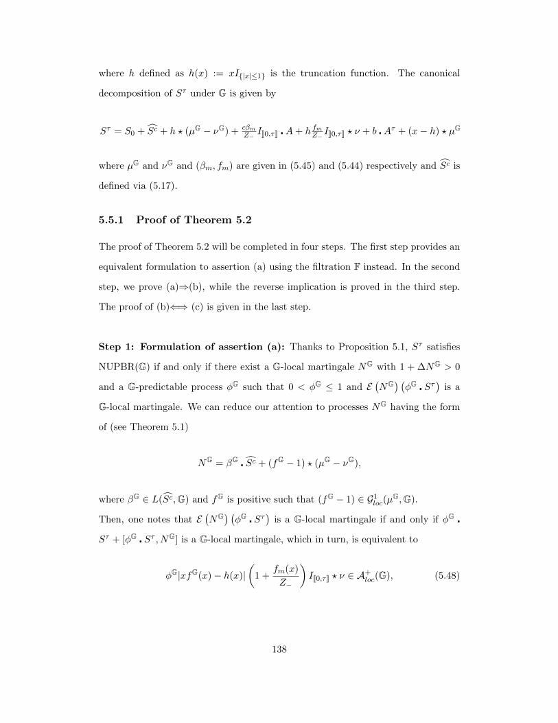
where h defined as h(x) := xI|x|≤1 is the truncation function. The canonical
decomposition of Sτ under G is given by
Sτ = S0 + Sc + h ? (µG − νG) + cβmZ−
I]]0,τ ]] A+ h fmZ− I]]0,τ ]] ? ν + b Aτ + (x− h) ? µG
where µG and νG and (βm, fm) are given in (5.45) and (5.44) respectively and Sc is
defined via (5.17).
5.5.1 Proof of Theorem 5.2
The proof of Theorem 5.2 will be completed in four steps. The first step provides an
equivalent formulation to assertion (a) using the filtration F instead. In the second
step, we prove (a)⇒(b), while the reverse implication is proved in the third step.
The proof of (b)⇐⇒ (c) is given in the last step.
Step 1: Formulation of assertion (a): Thanks to Proposition 5.1, Sτ satisfies
NUPBR(G) if and only if there exist a G-local martingale NG with 1 + ∆NG > 0
and a G-predictable process φG such that 0 < φG ≤ 1 and E(NG) (φG Sτ
)is a
G-local martingale. We can reduce our attention to processes NG having the form
of (see Theorem 5.1)
NG = βG Sc + (fG − 1) ? (µG − νG),
where βG ∈ L(Sc,G) and fG is positive such that (fG − 1) ∈ G1loc(µ
G,G).
Then, one notes that E(NG) (φG Sτ
)is a G-local martingale if and only if φG
Sτ + [φG Sτ , NG] is a G-local martingale, which in turn, is equivalent to
φG|xfG(x)− h(x)|(
1 +fm(x)
Z−
)I[[0,τ ]] ? ν ∈ A+
loc(G), (5.48)
138
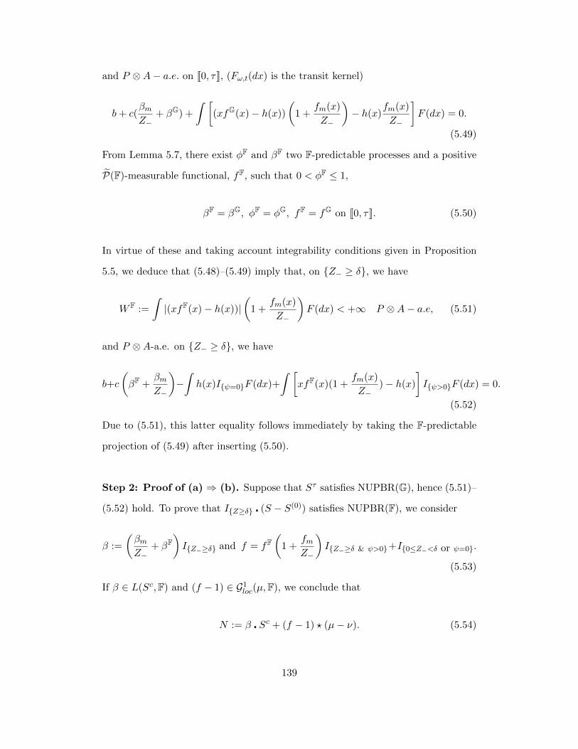
and P ⊗A− a.e. on [[0, τ ]], (Fω,t(dx) is the transit kernel)
b+ c(βmZ−
+ βG) +
∫ [(xfG(x)− h(x))
(1 +
fm(x)
Z−
)− h(x)
fm(x)
Z−
]F (dx) = 0.
(5.49)
From Lemma 5.7, there exist φF and βF two F-predictable processes and a positive
P(F)-measurable functional, fF, such that 0 < φF ≤ 1,
βF = βG, φF = φG, fF = fG on [[0, τ ]]. (5.50)
In virtue of these and taking account integrability conditions given in Proposition
5.5, we deduce that (5.48)–(5.49) imply that, on Z− ≥ δ, we have
W F :=
∫|(xfF(x)− h(x))|
(1 +
fm(x)
Z−
)F (dx) < +∞ P ⊗A− a.e, (5.51)
and P ⊗A-a.e. on Z− ≥ δ, we have
b+c
(βF +
βmZ−
)−∫h(x)Iψ=0F (dx)+
∫ [xfF(x)(1 +
fm(x)
Z−)− h(x)
]Iψ>0F (dx) = 0.
(5.52)
Due to (5.51), this latter equality follows immediately by taking the F-predictable
projection of (5.49) after inserting (5.50).
Step 2: Proof of (a) ⇒ (b). Suppose that Sτ satisfies NUPBR(G), hence (5.51)–
(5.52) hold. To prove that IZ≥δ (S − S(0)) satisfies NUPBR(F), we consider
β :=
(βmZ−
+ βF)IZ−≥δ and f = fF
(1 +
fmZ−
)IZ−≥δ & ψ>0+I0≤Z−<δ or ψ=0.
(5.53)
If β ∈ L(Sc,F) and (f − 1) ∈ G1loc(µ,F), we conclude that
N := β Sc + (f − 1) ? (µ− ν). (5.54)
139
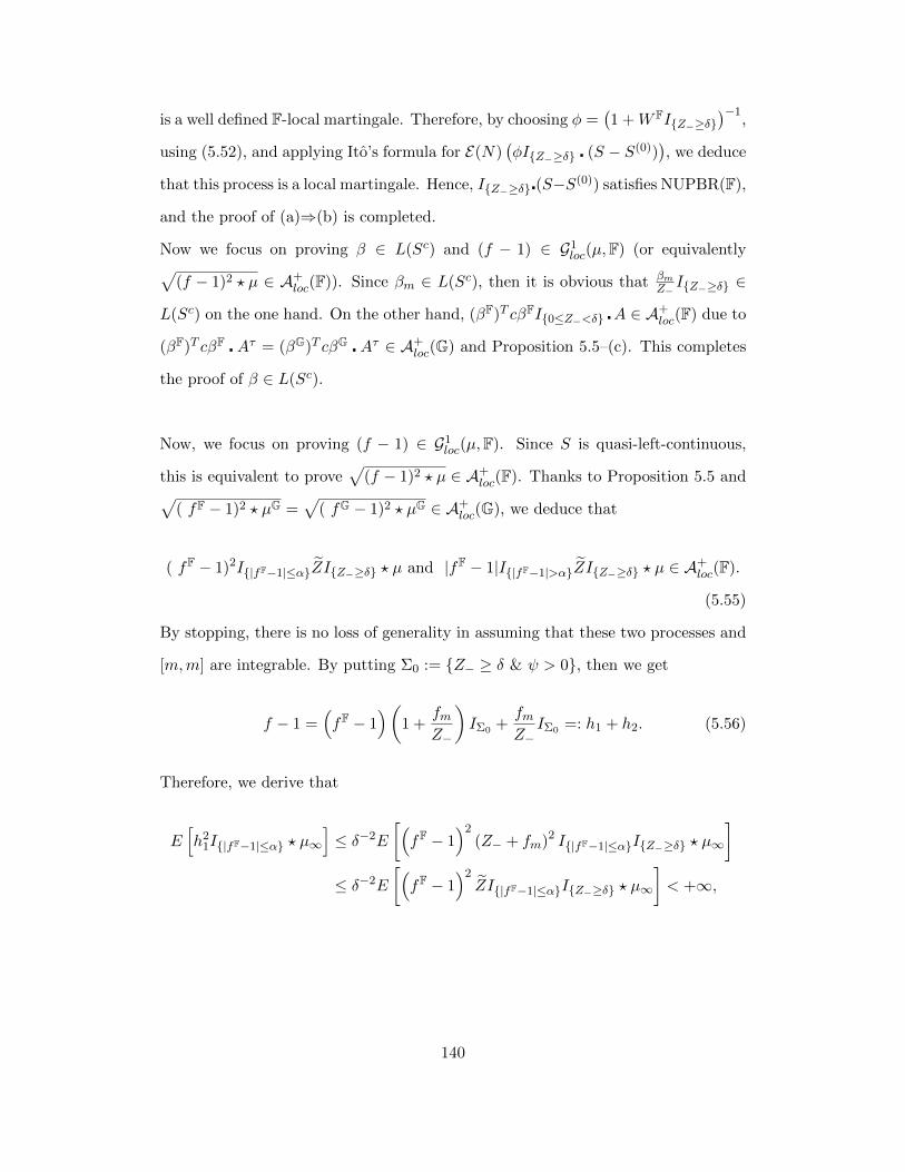
is a well defined F-local martingale. Therefore, by choosing φ =(1 +W FIZ−≥δ
)−1,
using (5.52), and applying Ito’s formula for E(N)(φIZ−≥δ (S − S(0))
), we deduce
that this process is a local martingale. Hence, IZ−≥δ(S−S(0)) satisfies NUPBR(F),
and the proof of (a)⇒(b) is completed.
Now we focus on proving β ∈ L(Sc) and (f − 1) ∈ G1loc(µ,F) (or equivalently√
(f − 1)2 ? µ ∈ A+loc(F)). Since βm ∈ L(Sc), then it is obvious that βm
Z−IZ−≥δ ∈
L(Sc) on the one hand. On the other hand, (βF)T cβFI0≤Z−<δ A ∈ A+loc(F) due to
(βF)T cβF Aτ = (βG)T cβG Aτ ∈ A+loc(G) and Proposition 5.5–(c). This completes
the proof of β ∈ L(Sc).
Now, we focus on proving (f − 1) ∈ G1loc(µ,F). Since S is quasi-left-continuous,
this is equivalent to prove√
(f − 1)2 ? µ ∈ A+loc(F). Thanks to Proposition 5.5 and√
( fF − 1)2 ? µG =√
( fG − 1)2 ? µG ∈ A+loc(G), we deduce that
( fF − 1)2I|fF−1|≤αZIZ−≥δ ? µ and |fF − 1|I|fF−1|>αZIZ−≥δ ? µ ∈ A+loc(F).
(5.55)
By stopping, there is no loss of generality in assuming that these two processes and
[m,m] are integrable. By putting Σ0 := Z− ≥ δ & ψ > 0, then we get
f − 1 =(fF − 1
)(1 +
fmZ−
)IΣ0 +
fmZ−
IΣ0 =: h1 + h2. (5.56)
Therefore, we derive that
E[h2
1I|fF−1|≤α ? µ∞
]≤ δ−2E
[(fF − 1
)2(Z− + fm)2 I|fF−1|≤αIZ−≥δ ? µ∞
]≤ δ−2E
[(fF − 1
)2ZI|fF−1|≤αIZ−≥δ ? µ∞
]< +∞,
140
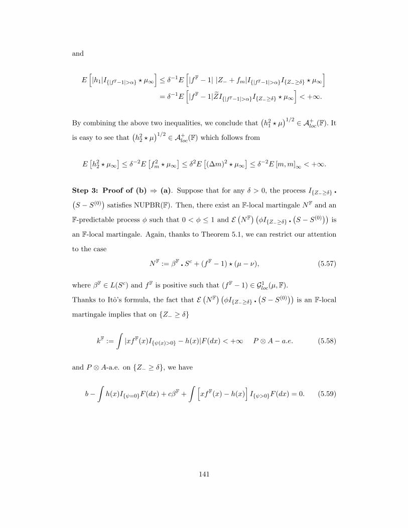
and
E[|h1|I|fF−1|>α ? µ∞
]≤ δ−1E
[|fF − 1| |Z− + fm|I|fF−1|>αIZ−≥δ ? µ∞
]= δ−1E
[|fF − 1|ZI|fF−1|>αIZ−≥δ ? µ∞
]< +∞.
By combining the above two inequalities, we conclude that(h2
1 ? µ)1/2 ∈ A+
loc(F). It
is easy to see that(h2
2 ? µ)1/2 ∈ A+
loc(F) which follows from
E[h2
2 ? µ∞]≤ δ−2E
[f2m ? µ∞
]≤ δ2E
[(∆m)2 ? µ∞
]≤ δ−2E [m,m]∞ < +∞.
Step 3: Proof of (b) ⇒ (a). Suppose that for any δ > 0, the process IZ−≥δ (S − S(0)
)satisfies NUPBR(F). Then, there exist an F-local martingale NF and an
F-predictable process φ such that 0 < φ ≤ 1 and E(NF) (φIZ−≥δ (S − S(0)
))is
an F-local martingale. Again, thanks to Theorem 5.1, we can restrict our attention
to the case
NF := βF Sc + (fF − 1) ? (µ− ν), (5.57)
where βF ∈ L(Sc) and fF is positive such that (fF − 1) ∈ G1loc(µ,F).
Thanks to Ito’s formula, the fact that E(NF) (φIZ−≥δ (S − S(0)
))is an F-local
martingale implies that on Z− ≥ δ
kF :=
∫|xfF(x)Iψ(x)>0 − h(x)|F (dx) < +∞ P ⊗A− a.e. (5.58)
and P ⊗A-a.e. on Z− ≥ δ, we have
b−∫h(x)Iψ=0F (dx) + cβF +
∫ [xfF(x)− h(x)
]Iψ>0F (dx) = 0. (5.59)
141
Consider
βG :=
(βF − βm
Z−
)I]]0,τ ]] and fG :=
fF
1 + fm/Z−Iψ>0I]]0,τ ]] + Iψ=0∪]]τ,+∞[[,
(5.60)
and assume that
βG ∈ L(Sc) and (fG − 1) ∈ G1loc(µ
G). (5.61)
Then, necessarily NG := βG Sc + (fG − 1) ? (µG − νG) is a well defined G-local
martingale satisfying E(NG) > 0. Furthermore, due to (5.59) and to ψ = 0 =
Z− + fm = 0 (see(5.8)), on ]]0, τ ]] we obtain
b+ c
(βG +
βmZ−
)+
∫ (xfG
(1 +
fmZ−
)− h(x)
)F (dx) = 0. (5.62)
Then, by taking φG :=(1 + kFIZ−≥δ
)−1, and applying Ito’s formula for (φGIZ−≥δ
Sτ )E(NG), we conclude that this process is a G-local martingale due to (5.62). Thus,
IZ−≥δ Sτ satisfies NUPBR(G) as long as (5.61) is fulfilled.
Since Z−1− I]]0,τ ]] is G-locally bounded, then there exists a family of G-stopping times
(τδ)δ>0 such that [[0, τδ]] ⊂ Z− ≥ δ (or equivalently IZ−≥δ Sτ∧τδ = Sτ∧τδ) and
τδ increases to infinity when δ goes to zero. Thus, using Proposition 5.2, we deduce
that Sτ satisfies NUPBR(G). This achieves the proof of (b)⇒(a) under (5.61).
To prove that (5.61) holds true, we remark in a first step that Z−1− I]]0,τ ]] is G-locally
bounded and both βm and βF belong to L(Sc). This, easily, implies that βG ∈ L(Sc).
Now, we prove that√
(fG − 1)2 ? µG ∈ A+loc(G). Since
√(fF − 1)2 ? µ ∈ A+
loc(F),
Proposition 5.5 allows us again to deduce that
(fF − 1)2I|fF−1|≤α ? µ ∈ A+loc(F) and |fF − 1|I|fF−1|>α ? µ ∈ A+
loc(F). (5.63)
Without loss of generality, we assume that these two processes and [m,m] are inte-
142
grable. Put
fG − 1 = Iψ>0I]]0,τ ]]Z−(fF − 1)
fm + Z−− Iψ>0I]]0,τ ]]
fmfm + Z−
:= f1 + f2. (5.64)
Then, we calculate
E(f2
1 Ifm+Z−>δ/2∩|fF−1|≤α ? µG∞
)≤(
2δ
)2E[(fF − 1)2I|fF−1|≤α ? µ∞
]< +∞.
and
E√f2
1 Ifm+Z−≤δ/2∩|fF−1|≤α∩Z−≥δ ? µG∞
≤ αE(Ifm+Z−≤δ/2∩Z−≥δ(Z− + fm)−1 ? µG(∞)
)≤ E
(I|fm|≥δ/2 ? µ(∞)
)≤ 4α
δ2E[m,m]∞ < +∞.
This proves that√f2
1 I|fF−1|≤α ? µG ∈ A+
loc(G). Similarly, we calculate
E√f2
1 I|fF−1|>α ? µG∞ ≤ E
(|f1|I|fF−1|>α ? µ
G∞)≤ E
( |fF − 1|1 + fm/Z−
I|fF−1|>α ? µG∞)
≤ E(|fF − 1|I|fF−1|>α ? µ∞
)< +∞.
Thus, by combining all the remarks obtained above, we conclude that√f2
1 ? µG is
G-locally integrable. For the functional f2, we proceed as follows. We calculate
E(f2
2 Ifm+Z−>δ/2 ? µG∞)≤ (2/δ)2E
(f2m ? µ∞
)≤ (2/δ)2E[m,m]∞ < +∞,
and
E√f2
2 Ifm+Z−≤δ/2∩Z−≥δ ? µG∞ ≤ E
(|fm|I|fm|≥δ/2 ? µ(∞)
)≤ (2/δ)E
(f2m ? µ(∞)
)≤ (2/δ)E[m,m]∞ < +∞.
This proves that√f2
2 ? µG is G-locally integrable. Therefore, we conclude that
143
(5.61) is valid, and the proof of (b)⇒(a) is completed.
Step 3: Proof of (b) ⇐⇒ (c). For any δ > 0 and any n ∈ N, we denote
σ∞ := inft ≥ 0 : Zt = 0, τδ := supt : Zt− ≥ δ.
Then, due to ]]σ∞,+∞[[⊂ Z− = 0 ⊂ Z− < δ, we deduce
σ1/δ ≤ τδ ≤ σ∞ and Zτδ− ≥ δ > 0 P − a.s. on τδ <∞ .
Furthermore, setting Σ :=⋂n≥1(σn < σ∞), we have
on Σ ∩ σ∞ <∞ Zσ∞− = 0, and τδ < σ∞ P − a.s.
We introduce the semimartingale X := S − S(0). For any δ > 0, and any H
predictable such that Hδ := HIZ−≥δ ∈ L(X) and Hδ X ≥ −1 , due to Theorem
23 of [54] (page 346 in the French version),
(Hδ X)T = (Hδ X)T∧τδ , and on θ ≥ τδ (Hδ X)T = (Hδ X)T∧θ.
Then, for any T ∈ (0,+∞), we calculate the following
P ((Hδ X)T > c) = P ((Hδ X)T > c & σn ≥ τδ) + P ((Hδ X)T > c & σn < τδ)
≤ 2 supφ∈L(Xσn ):φXσn≥−1
P ((φ X)σn∧T > c) + P (σn < τδ ∧ T ).
(5.65)
It is easy to prove that P (σn < τδ ∧ T ) −→ 0 as n goes to infinity. This can be seen
due to the fact that on Σ, we have, on the one hand, τδ ∧T < σ∞ (by differentiating
the two cases whether σ∞ is finite or not). On the other hand, the event (σn < σ∞)
144
increases to Σ with n. Thus, by combining these, we obtain the following
P (σn < τδ ∧ T ) = P ((σn < τδ ∧ T ) ∩ Σ) + P ((σn < τδ ∧ T ) ∩ Σc)
≤ P (σn < τδ ∧ T < σ∞) + P ((σn < σ∞) ∩ Σc) −→ 0.
(5.66)
Now suppose that for each n ≥ 1, the process (S − S(0))σn satisfies NUPBR(F).
Then a combination of (5.65) and (5.66) implies that for any δ > 0, the process
IZ−≥δ X := IZ−≥δ (S − S(0)) satisfies NUPBR(F), and the proof of (c)⇒ (b)
is completed. The proof of the reverse implcation is obvious due to the fact that
[[0, σn]] ⊂ Z− ≥ 1/n ⊂ Z− ≥ δ, for n ≤ δ−1,
which implies that (IZ−≥δ X)σn = Xσn . This ends the proof of (b) ⇐⇒(c), and
the proof of the theorem is achieved.
5.5.2 Intermediate Result
The proofs of Theorems 5.4 and 5.5 rely on the following intermediatory result about
single jump F-martingales, which is interesting in itself.
Lemma 5.10: Let T be a finite F-predictable stopping time. Then the following
holds.
T ≤ τ ⊂ ZT > 0 ⊂ ZT− > 0 = Γ(T ) :=P(ZT > 0
∣∣∣FT−) > 0.
Proof. It is enough to prove the non-trivial equality ZT− > 0 = Γ(T ). In-
deed, due to E(P (ZT > 0|FT−)IZT−=0
)= P (ZT > 0 = ZT−) = 0, we get
Γ(T ) ⊂ ZT− > 0. On the other hand, due to E(ZT−IΓ(T )c
)= E
(ZT IΓ(T )c
)≤
E(IZT>0 IΓ(T )c
)= 0, we obtain ZT− > 0 ⊂ Γ(T ). This ends the proof of the
lemma.
145
Lemma 5.11: Let R be an equivalent probability to P . Then the following hold.
Z = 0 = ZR = 0, and Z− = 0 = ZR− = 0,
where ZRt := R(τ ≥ t|Ft) and ZR− is the (R,F)-predictable projection of ZR.
Proof. For any F-stopping time σ and any F-predictable stopping time T , due to
E[ZσIZRσ =0
]= E
[Iτ≥σIZRσ =0
]= 0 and
E[ZT−IZRT−=0
]= E
[Iτ≥TIZRT−=0
]= 0,
we obtain ZR = 0 ⊂ Z = 0 and ZR− = 0 ⊂ Z− = 0. The symmetric roles
of R and P complete the proof of the lemma.
Proposition 5.7: Let M be an F-martingale given by M := ξI[[T,+∞[[, where T is an
F-predictable stopping time, and ξ is an FT -measurable random variable. Then
the following assertions are equivalent.
(a) M is an F-martingale under QT given by
dQTdP
:=IZT>0∩Γ(T )
P (ZT > 0∣∣ FT−)
+ IΓc(T ), Γ(T ) := P (ZT > 0|FT−) > 0. (5.67)
(b) On the set T < +∞, we have
E(MT IZT=0<ZT−
∣∣ FT−) = 0, P − a.s. (5.68)
(c) M τ is a G-martingale under QGT :=
(UG(T )/E(UG(T )
∣∣ GT−))·P where
UG(T ) := IT>τ + IT≤τZT−
ZT> 0. (5.69)
Proof. The proof will be achieved in two steps. In Step 1, we prove (a)⇔(b); while
Step 2 focuses on (a)⇔(c). First, we remark that the probability QGT in assertion
146
(c) is well defined since E(LGb (T )
∣∣ GT−) = IT>τ+P (ZT > 0|FT−)IT≤τ > 0 due
to Lemma 5.10.
Step 1: Here, we prove (a)⇐⇒(b). To this end, we calculate that
EQT (ξ∣∣FT−) = IΓ(T )E(ξIZT>0
∣∣FT−)(P (ZT > 0
∣∣FT−))−1
= −IΓ(T )E(ξIZT=0∣∣FT−)
(P (ZT > 0
∣∣FT−)))−1
.
Therefore, we conclude that assertion (a) (or equivalently EQT (ξ|FT−) = 0) is equiv-
alent to (5.68). This ends the proof of (a) ⇐⇒ (b).
Step 2: To prove (a)⇐⇒(c), we calculate that
E(LGb (T )
∣∣ GT−) EQGT(ξIT≤τ|GT−
)= E
(ZT−
ZTξIT≤τ|GT−
)= E
(ξIZT>0|FT−
)IT≤τ = EQT (ξ|FT−)P
(ZT > 0
∣∣FT−) IT≤τ.This equality proves that M τ is a martingale under (G, QG
T ) –where QGT is defined
via (5.69)– if and only if M is a martingale under (F, QT ), and the proof of (a)⇐⇒(c)
is completed. This ends the proof of the proposition.
5.5.3 Proof of Theorem 5.4
For the reader convenience, in order to prove Theorem 5.4, we state a more precise
version of the theorem, in which we describe explicitly the choice for the probability
measure QT .
Theorem 5.10: Suppose that the assumptions of Theorem 5.4 are in force. Then,
the assertions (a) and (b) of Theorem 5.4 are equivalent to the following asser-
tions.
147
(d) S satisfies NUPBR(F, QT ), where QT is
QT :=
(ZTZT−
IZT−>0 + IZT−=0
) P. (5.70)
(e) S satisfies NUPBR(F, QT ), where QT is defined in (5.67).
Proof. The proof of this theorem will be achieved by proving (d) ⇐⇒ (e) ⇐⇒ (b)
and (b)⇒ (a)⇒ (d). These will be carried out in four steps.
Step 1: In this step, we prove (d)⇐⇒ (e). By putting Γ(T ) :=P(ZT > 0
∣∣∣FT−) > 0
and using Lemma 5.10, we deduce that
QT =
(IZT>0
P (ZT > 0∣∣ FT−)
+ IΓ(T )c
)· P, QT :=
(ZTZT−
IZT>0 + IZT−=0
)· P,
where QT and QT are defined in (5.67) and (5.70) respectively. Then it is easy to
see that QT and QT are equivalent. This achieves this first step.
Step 2: This step proves (e)⇐⇒ (b). Assume that (e) holds. Then, there exists a
positive and FT –measurable random variable, Y , such that P − a.s. on T < +∞,
we have
EQT (Y |FT−) = 1, EQT (Y |ξ||FT−) < +∞, & EQT (Y ξIZT−>0|FT−) = 0.
Since Y > 0 on ZT > 0, by putting
Y1 := Y IZT>0 + IZT=0 and Y1 :=Y1
E[Y1|FT−],
it is easy to check that Y1 > 0, Y1 > 0,
E[Y1|FT−
]= 1 and E
[Y1ξIZT>0|FT−
]=E[Y ξIZT>0|FT−
]E[Y1|FT−]
= 0.
148

Therefore, S is a martingale under R1 := Y1 · P ∼ P , and hence S satisfies
NUPBR(F). This proves assertion (b).
To prove the reverse sense, we suppose assertion (b) holds. Then, there exists
0 < Y ∈ L0(FT ), such that E[Y |ξ|IZT>0|FT−] < +∞, E[Y |FT−] = 1 and
E[Y ξIZT>0|FT−] = 0. Then, consider
Y2 :=Y IZT>0P (ZT > 0|FT−)
E[Y IZT>0|FT−]+ IΓc1
, where Γ1 :=E(Y IZT>0|FT−
)> 0.
Then it is easy to verify that Y2 > 0, QT − a.s.,
EQT (Y2|FT−) = 1, and EQT(Y2ξIZT−>0|FT−
)=E[Y ξIZT>0|FT−
]E[Y IZT>0|FT−]
IΓ1 = 0.
This proves assertion (e), and the proof of (e)⇐⇒(b) is achieved.
Step 3: Herein, we prove (a) ⇒ (d). Suppose that Sτ satisfies NUPBR(G). Then
there exists a positive GT -measurable random variable Y G such that on T < +∞,
we have
E[Y GIT≤τ|GT−] = IT≤τ and E[ξY GIT≤τ|GT−] = 0. (5.71)
Due to Lemma 5.7–(d), we deduce the existence of two positive FT -measurable
variables Y (1) and Y (2) such that
Y GIT≤τ = Y (1)IT<τ + Y (2)Iτ=T. (5.72)
149
By inserting (5.72) into the first equation in (5.71), we get
IT≤τ = E[Y GIT≤τ|GT−] = E(ZTY(1) + (ZT − ZT )Y (2)|FT−)
1
ZT−IT≤τ.
Therefore, E(ZTY(1) + (ZT − ZT )Y (2)|FT−)Z−1
T−IZT−>0 = IZT−>0. Thus by
putting
Y :=
[ZT
ZTY (1) + (1− ZT
ZT)Y (2)
]IZT>0 + IZT−=0 > 0, QT − a.s.,
we derive
EQT (Y |FT−) = E(ZTY(1) + (ZT − ZT )Y (2)|FT−)Z−1
T−IZT−>0 + IZT−=0 = 1.
Similarly, by plugging (5.72) into the second equation of (5.71), we obtain
EQT (ξIZT>0Y |FT−) = E((ZTY
(1) + (ZT − ZT )Y (2))ξ∣∣FT−) IZT>0
ZT−= 0.
Then, we conclude that S satisfies the NUPBR(QT ,F). This ends the proof of
(a)⇒(d).
Step 4: This last step proves (b)=⇒(a). Suppose that S satisfies the NUPBR(F).
Then, there exists Y ∈ L1(FT ) such that on T < +∞ we have
E[Y |FT−] = 1, Y > 0, E[Y |ξ|IZT>0|FT−] < +∞, and, E[Y ξIZT>0|FT−] = 0.
Then by considering R := Y · P ∼ P and using Lemma 5.11 (precisely Z = 0 =
ZR = 0), we get
ER[ST∣∣FT−] = ER
[ξIZT>0
∣∣FT−] = ER[ξIZRT >0
∣∣FT−] = 0.
150
Therefore, by applying Proposition 5.7 to M := S under R ∼ P (it is easy to see that
the condition (5.68) in Proposition 5.7 holds for (S, R), i.e. ER(ST IZRT =0|FT−) =
0). Then we conclude that Sτ = Sτ satisfies NUPBR(R,F) and NUPBR(P,F), due
to R ∼ P . This ends the fourth step and the proof of the theorem is completed.
5.5.4 Proof of Theorem 5.5
To highlight the precise difficulty in proving Theorem 5.5, we remark that on T <
+∞,UG(T )
E(UG(T )∣∣ GT−)
=1 + ∆LT −∆V G
T
1−∆V GT
6= 1 + ∆LT =E(L)TE(L)T−
.
where UG(T ) is defined in (5.69). This highlights one of the main difficulties that
we will face when we will formulate the results for possible many predictable jumps
that might not be ordered. Simply, it might not be possible to piece up
UG(Tn) = 1− ∆mTn
ZTnITn≤τ, n ≥ 1
to form a positive G-local martingale density for the process (I∪[[Tn]] S)τ .
Thus, in virtue of the above, the key idea behind the proof of Theorem 5.5 lies in
connecting the NUPBR condition with the existence of a positive supermartingale
(instead) that is a deflator for the market model under consideration.
Definition 5.2: Consider an H-semimartingale X. Then, X is said to admit an
H-deflator if there exists a positive H-supermartingale Y such that Y (θ X) is a
supermartingale, for any θ ∈ L(X,H) such that θ X ≥ −1.
For supermartingale deflators, we reader the reader to Rokhlin [121]. Again, the
above definition differs from that of the literature when the horizon is infinite, while
it is the same as the one of the literature when the horizon is finite (even random).
Below, we slightly generalize [121] to our context.
151
Lemma 5.12: Let X be an H-semimartingale. Then, the following assertions are
equivalent.
(a) X admits an H-deflator.
(b) X satisfies NUPBR(H).
Proof. The proof of this lemma is straightforward, and is omitted.
Now, we start giving the proof of Theorem 5.5.
Proof. of Theorem 5.5 The proof of the theorem will given in two steps, where we
prove (b)⇒(a) and the reverse implication respectively. For the sake of simplifying
the overall proof of the theorem, we remark that
ZQT = 0 = ZT = 0, for any Q ∼ P and any F-stopping time T, (5.73)
where ZQt := Q[τ ≥ t|Ft]. This equality follows from
E[ZT IZQT =0
]= E
[Iτ≥TIZQT =0
]= 0,
(which implies ZQ = 0 ⊂ Z = 0) and the symmetric role of Q and P .
Step 1: Here, we prove (b)⇒ (a). Suppose that assertion (b) holds, and consider
a sequence of F-stopping times (τn)n that increases to infinity such that Y τn is an
F-martingale. Then, setting Qn := Yτn/Y0 P , and using (5.73) and Proposition 5.2,
we deduce that there is no loss of generality in assuming Y ≡ 1. Condition (5.68)
in Proposition 5.7 holds for ∆STnIZTn>0 and ∆STnIZTn>0I[[Tn,+∞[[,. Therefore,
using the notation V G and L defined in (5.34) and (5.36), for each n, (1 + ∆LTn −
∆V GTn
)∆STnITn≤τI[[Tn,+∞[[ is a G-martingale. Then, a direct application of Yor’s
exponential formula, we get that, for any θ ∈ L(Sτ ,G)
E(IΓ L− IΓ V G
)E (θIΓ Sτ ) = E (X)
152

where Γ = ∪n≥1[[Tn]] and
X := IΓ L− IΓ V G +∑n≥1
θTn
(1 + ∆LTn −∆V G
Tn
)∆STnITn≤τI[[Tn,+∞[[.
Consider now the G-predictable process
φ =∑n≥1
ξnI[[Tn]]∩[[0,τ ]] + IΓc∪]]τ+∞[[, where
ξn :=2−n (1 + E(X)Tn−)−1(
1 + E[|∆LTn |
∣∣∣GTn−]+ ∆V GTn− + E
[|θTn
ZTn−ZTn
ITn≤τ∆STn |∣∣∣GTn−]) .
Then, it is easy to verify that 0 < φ ≤ 1 and E (|φ E(X)|var(+∞)) ≤∑
n≥1 2−n =
1. Hence, φE(X) ∈ A(G). Since, ∆LTnI[[Tn,+∞[[ and (1+∆LTn−∆V GTn
)∆STnITn≤τI[[Tn,+∞[[
are G-martingales, we derive
(φ E(X))p,G =∑n≥1
φTnETn−(X)E(∆XTn |GTn−)I[[Tn,+∞[[ = −φE−(X) V G ≤ 0.
This proves that E(X) is a positive σ-supermartingale1 as long as θ∆Sτ ≥ −1. Thus,
thanks to Kallsen [89], we conclude that it is a supermartingale and(IZ−≥δ S
)τadmits a G-deflator. Then, thanks to Lemma 5.12, we deduce that
(IZ−≥δ S
)τsatisfies NUPBR(G). Remark that, due to the G-local boundedness of (Z−)−1I[[0,τ ]],
there exists a family of G-stopping times τδ, δ > 0 such that τδ converges almost
surely to infinity when δ goes zero and
[[0, τ ∧ τδ]] ⊂ Z− ≥ δ ∩ [[0, τ ]].
This implies that Sτ∧τδ satisfies NUPBR(G), and the assertion (a) follows from
Proposition 5.2 (by taking Qn = P for all n ≥ 1). This ends the proof of (b)⇒(a).
1Recall that a process X is said to be a σ-supermartingale if it is a semimartingale and thereexists a predictable process φ such that 0 < φ ≤ 1 and φ X is a supermartingale
153
Step 2: In this step, we focus on (a)⇒(b). Suppose that Sτ satisfies NUPBR(G).
Then, there exists a σ-martingale density under G, for IZ−≥δ Sτ , (δ > 0), that
we denote by DG. Then, from a direct application of Jacod’s representation The-
orem 2.7 and Theorem 5.1, we deduce the existence of a positive P(G)-measurable
functional, fG, such that DG := E(NG) > 0, with
NG := wG ? (µG − νG), wG := fG − 1 +fG − aG
1− aGIaG<1,
where νG was defined in (5.45), and, introducing fm defined in (5.44)
xfGIZ−≥δ ? νG = xfG
(1 +
fmZ−
)I]]0,τ ]]IZ−≥δ ? ν ≡ 0. (5.74)
Thanks to Lemma 5.7, we conclude to the existence of a positive P(F)-measurable
functional, f , such that fGI]]0,τ ]] = fI]]0,τ ]]. Thus (5.74) becomes
UG := xf
(1 +
fmZ−
)I]]0,τ ]]IZ−>δ ? ν ≡ 0.
Introduce the following notations
µ0 := IZ>0 & Z−≥δ µ, ν0 := h0IZ−≥δ ν, h0 := MPµ
(IZ>0|P
),
g :=f(1 + fm
Z−)
h0Ih0>0 + Ih0=0, a0(t) := ν0(t,Rd), (5.75)
and assume that √(g − 1)2 ? µ0 ∈ A+
loc(F). (5.76)
Then, thanks to Lemma 2.6, we deduce that W := (g−1)/(1−a0 + g) ∈ G1loc(µ0,F),
and the local martingales
N0 :=g − 1
1− a0 + g? (µ0 − ν0), Y 0 := E(N0), (5.77)
154
are well defined satisfying 1 + ∆N0 > 0, [N0, S] ∈ A(F), and on Z− > δ we have
p,F(Y 0∆SIZ>0
)Y 0−
= p,F(
(1 + ∆N0)∆SIZ>0
)= p,F
(g
1− a0 + g∆SIZ>0
)= ∆
gxh0
1− a0 + g? ν = ∆
xf(1 + fm/Z−)
1− a0 + g? ν = Z−1
−
p,F (∆UG)1− a0 + g
≡ 0.
This proves that assertion (b) holds under the assumption (5.76).
The remaining part of the proof will show that this assumption always holds. To
this end, we start by noticing that on the set h0 > 0,
g − 1 =f(1 + fm
Z−)
h0− 1 =
(f − 1)(1 + fmZ−
)
h0+
fmZ−h0
+MPµ
(IZ=0|P
)h0
:= g1 + g2 + g3.
Since((f − 1)2I]]0,τ ]] ? µ
)1/2 ∈ A+loc(G), then due to Proposition 5.5–(e)
√(f − 1)2IZ−≥δ ? (Z µ) ∈ A+
loc(F), for any δ > 0.
Then, a direct application of Proposition 5.5–(a), for any δ > 0, we have
(f − 1)2I|f−1|≤α & Z−≥δ ? (Z µ), |f − 1|I|f−1|>α & Z−≥δ ? (Z µ) ∈ A+loc(F).
By stopping, without loss of generality, we assume these two processes and [m,m]
belong to A+(F). Remark that Z−+fm = MPµ
(Z|P
)≤MP
µ
(IZ>0|P
)= h0 that
155
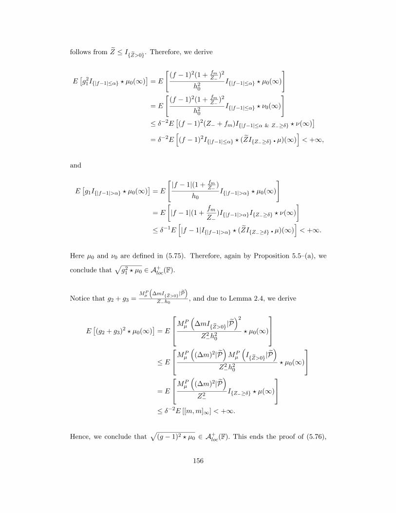
follows from Z ≤ IZ>0. Therefore, we derive
E[g2
1I|f−1|≤α ? µ0(∞)]
= E
[(f − 1)2(1 + fm
Z−)2
h20
I|f−1|≤α ? µ0(∞)
]
= E
[(f − 1)2(1 + fm
Z−)2
h20
I|f−1|≤α ? ν0(∞)
]≤ δ−2E
[(f − 1)2(Z− + fm)I|f−1|≤α & Z−≥δ ? ν(∞)
]= δ−2E
[(f − 1)2I|f−1|≤α ? (ZIZ−≥δ µ)(∞)
]< +∞,
and
E[g1I|f−1|>α ? µ0(∞)
]= E
[|f − 1|(1 + fm
Z−)
h0I|f−1|>α ? µ0(∞)
]
= E
[|f − 1|(1 +
fmZ−
)I|f−1|>αIZ−≥δ ? ν(∞)
]≤ δ−1E
[|f − 1|I|f−1|>α ? (ZIZ−≥δ µ)(∞)
]< +∞.
Here µ0 and ν0 are defined in (5.75). Therefore, again by Proposition 5.5–(a), we
conclude that√g2
1 ? µ0 ∈ A+loc(F).
Notice that g2 + g3 =MPµ
(∆mIZ>0|P
)Z−h0
, and due to Lemma 2.4, we derive
E[(g2 + g3)2 ? µ0(∞)
]= E
MPµ
(∆mIZ>0|P
)2
Z2−h
20
? µ0(∞)
≤ E
MPµ
((∆m)2|P
)MPµ
(IZ>0|P
)Z2−h
20
? µ0(∞)
= E
MPµ
((∆m)2|P
)Z2−
IZ−≥δ ? µ(∞)
≤ δ−2E [[m,m]∞] < +∞.
Hence, we conclude that√
(g − 1)2 ? µ0 ∈ A+loc(F). This ends the proof of (5.76),
156
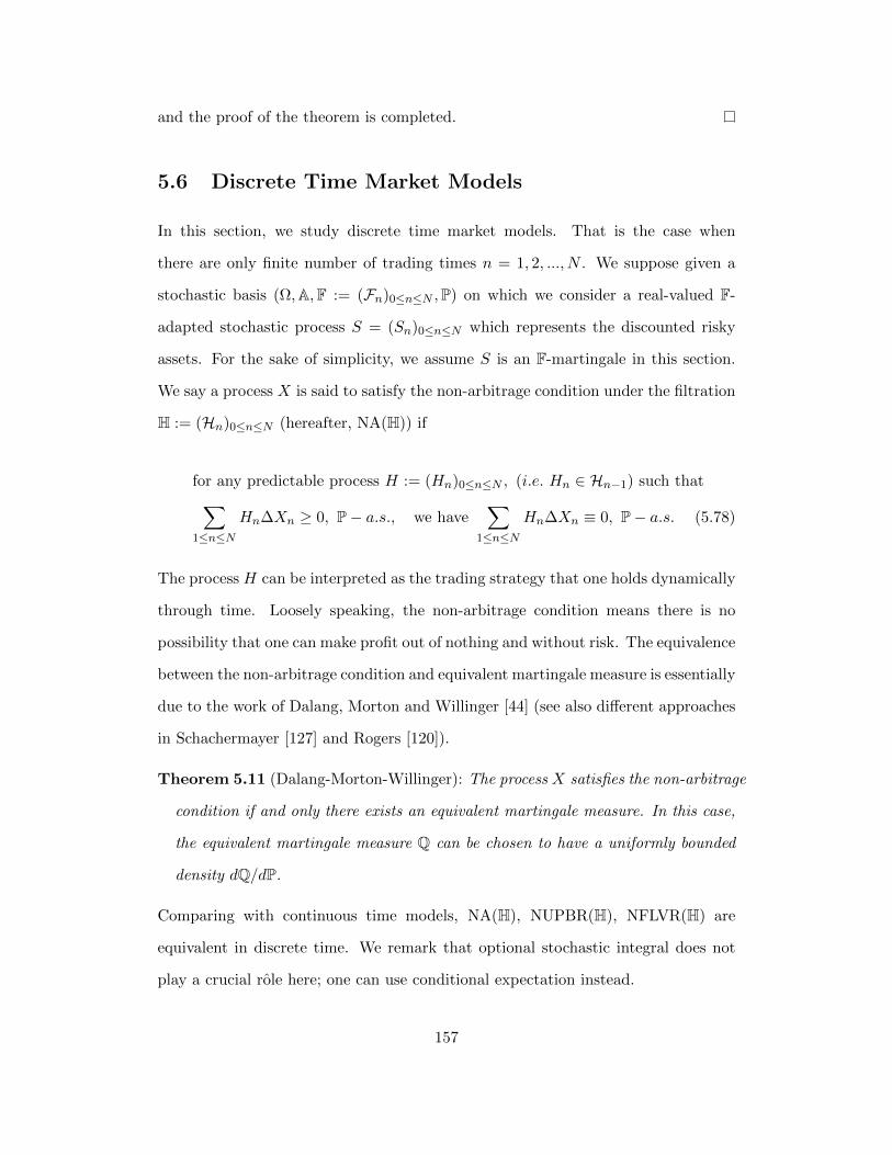
and the proof of the theorem is completed.
5.6 Discrete Time Market Models
In this section, we study discrete time market models. That is the case when
there are only finite number of trading times n = 1, 2, ..., N . We suppose given a
stochastic basis (Ω,A,F := (Fn)0≤n≤N ,P) on which we consider a real-valued F-
adapted stochastic process S = (Sn)0≤n≤N which represents the discounted risky
assets. For the sake of simplicity, we assume S is an F-martingale in this section.
We say a process X is said to satisfy the non-arbitrage condition under the filtration
H := (Hn)0≤n≤N (hereafter, NA(H)) if
for any predictable process H := (Hn)0≤n≤N , (i.e. Hn ∈ Hn−1) such that∑1≤n≤N
Hn∆Xn ≥ 0, P− a.s., we have∑
1≤n≤NHn∆Xn ≡ 0, P− a.s. (5.78)
The process H can be interpreted as the trading strategy that one holds dynamically
through time. Loosely speaking, the non-arbitrage condition means there is no
possibility that one can make profit out of nothing and without risk. The equivalence
between the non-arbitrage condition and equivalent martingale measure is essentially
due to the work of Dalang, Morton and Willinger [44] (see also different approaches
in Schachermayer [127] and Rogers [120]).
Theorem 5.11 (Dalang-Morton-Willinger): The process X satisfies the non-arbitrage
condition if and only there exists an equivalent martingale measure. In this case,
the equivalent martingale measure Q can be chosen to have a uniformly bounded
density dQ/dP.
Comparing with continuous time models, NA(H), NUPBR(H), NFLVR(H) are
equivalent in discrete time. We remark that optional stochastic integral does not
play a crucial role here; one can use conditional expectation instead.
157

In this section, we shall prove that the non-arbitrage property is preserved (under
one mild condition) when the market is stopped at the random horizon τ . Further-
more, we gave the necessary and sufficient conditions (on τ or the stopping times
in (5.80)) to guarantee the stability of the non-arbitrage condition for any market Sτ .
Below, we define some notations related to the random time τ that would be fixed
throughout the discrete time framework. For any random time τ , we associate the
following two Azema supermartingales
Zn := P [τ > n|Fn] and Zn := P [τ ≥ n|Fn], (5.79)
and the F-stopping times
R1 := infn ≥ 1 : Zn = 0, R2 := infn ≥ 1 : Zn−1 = 0
and R3 := infn ≥ 1 : Zn = 0. (5.80)
To incorporate the information from the random time τ , we enlarge the filtration F
to include τ and obtain the filtration G = (Gn)1≤n≤N , where
Gn := Fn ∨ σ(τ ≤ n). (5.81)
The progressively enlarged filtration G is the smallest one that contains F and makes
τ a stopping time.
Lemma 5.13: For any random time τ and the associated stopping times in (5.80),
the following properties hold:
(a) The inclusions hold: Zn−1 = 0 ⊂ Zn = 0 ⊂ Zn = 0 for all n.
(b) R2 is an F-predictable stopping time and R1 ≤ R3 ≤ R2.
(c) τ ≤ R1, Zn−1 and Zn are both positive when n ≤ τ .
158
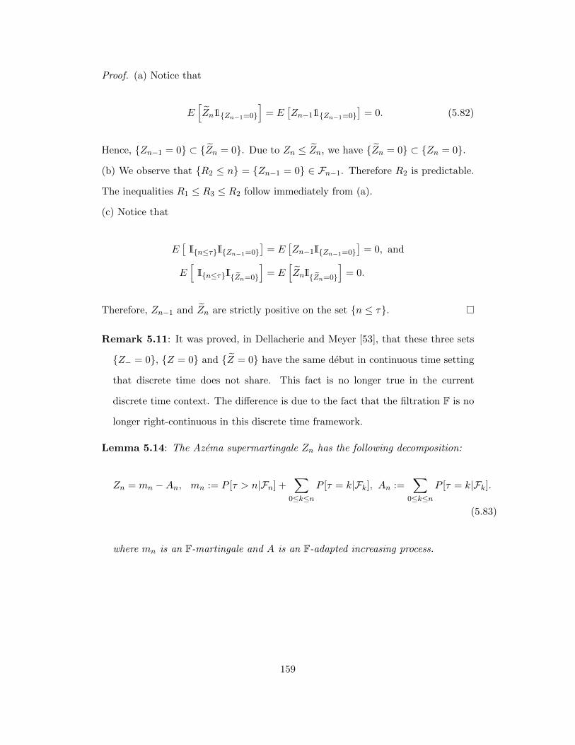
Proof. (a) Notice that
E[Zn1Zn−1=0
]= E
[Zn−11Zn−1=0
]= 0. (5.82)
Hence, Zn−1 = 0 ⊂ Zn = 0. Due to Zn ≤ Zn, we have Zn = 0 ⊂ Zn = 0.
(b) We observe that R2 ≤ n = Zn−1 = 0 ∈ Fn−1. Therefore R2 is predictable.
The inequalities R1 ≤ R3 ≤ R2 follow immediately from (a).
(c) Notice that
E[In≤τIZn−1=0
]= E
[Zn−1IZn−1=0
]= 0, and
E[In≤τIZn=0
]= E
[ZnIZn=0
]= 0.
Therefore, Zn−1 and Zn are strictly positive on the set n ≤ τ.
Remark 5.11: It was proved, in Dellacherie and Meyer [53], that these three sets
Z− = 0, Z = 0 and Z = 0 have the same debut in continuous time setting
that discrete time does not share. This fact is no longer true in the current
discrete time context. The difference is due to the fact that the filtration F is no
longer right-continuous in this discrete time framework.
Lemma 5.14: The Azema supermartingale Zn has the following decomposition:
Zn = mn −An, mn := P [τ > n|Fn] +∑
0≤k≤nP [τ = k|Fk], An :=
∑0≤k≤n
P [τ = k|Fk].
(5.83)
where mn is an F-martingale and A is an F-adapted increasing process.
159
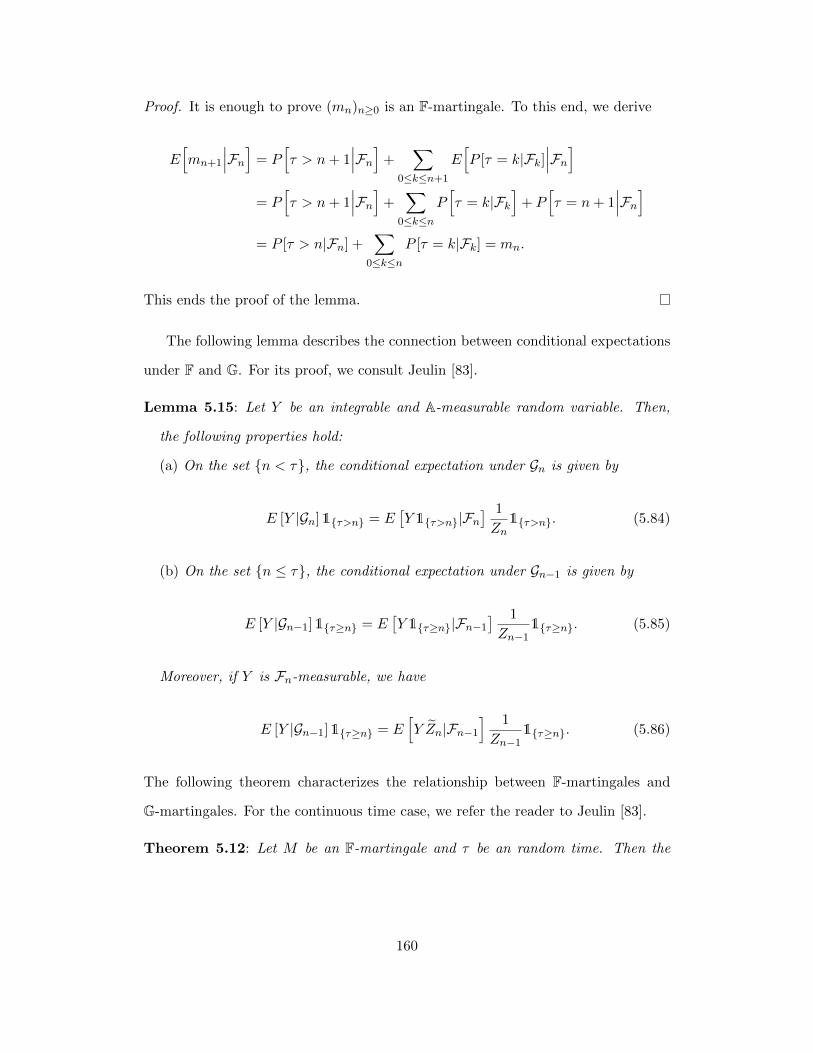
Proof. It is enough to prove (mn)n≥0 is an F-martingale. To this end, we derive
E[mn+1
∣∣∣Fn] = P[τ > n+ 1
∣∣∣Fn]+∑
0≤k≤n+1
E[P [τ = k|Fk]
∣∣∣Fn]= P
[τ > n+ 1
∣∣∣Fn]+∑
0≤k≤nP[τ = k|Fk
]+ P
[τ = n+ 1
∣∣∣Fn]= P [τ > n|Fn] +
∑0≤k≤n
P [τ = k|Fk] = mn.
This ends the proof of the lemma.
The following lemma describes the connection between conditional expectations
under F and G. For its proof, we consult Jeulin [83].
Lemma 5.15: Let Y be an integrable and A-measurable random variable. Then,
the following properties hold:
(a) On the set n < τ, the conditional expectation under Gn is given by
E [Y |Gn]1τ>n = E[Y 1τ>n|Fn
] 1
Zn1τ>n. (5.84)
(b) On the set n ≤ τ, the conditional expectation under Gn−1 is given by
E [Y |Gn−1]1τ≥n = E[Y 1τ≥n|Fn−1
] 1
Zn−11τ≥n. (5.85)
Moreover, if Y is Fn-measurable, we have
E [Y |Gn−1]1τ≥n = E[Y Zn|Fn−1
] 1
Zn−11τ≥n. (5.86)
The following theorem characterizes the relationship between F-martingales and
G-martingales. For the continuous time case, we refer the reader to Jeulin [83].
Theorem 5.12: Let M be an F-martingale and τ be an random time. Then the
160
following process
MGn := Mn∧τ −
∑1≤k≤n
1
Zk−11τ≥kE
[(Mk −Mk−1)Zk|Fk−1
], (5.87)
is a G-martingale.
Proof. Although it can be derived from Jeulin [83], we opt to give a direct proof
here. It is easy to see that
M(n+1)∧τ = Mn∧τ + (Mn+1 −Mn)1τ≥n+1. (5.88)
Then, we get
E[MGn+1
∣∣∣Gn] = E[M(n+1)∧τ −
∑1≤k≤n+1
1
Zk−11τ≥kE
[(Mk −Mk−1)Zk|Fk−1
] ∣∣∣Gn]= Mn∧τ + E
[(Mn+1 −Mn)1τ≥n+1
∣∣∣Gn]−∑
1≤k≤n
1
Zk−11τ≥kE
[(Mk −Mk−1)Zk|Fk−1
]− 1
Zn1τ≥n+1E
[(Mn+1 −Mn)Zn+1|Fn
]= Mn∧τ −
∑1≤k≤n
1
Zk−11τ≥kE
[(Mk −Mk−1)Zk|Fk−1
]= MG
n ,
where we use the following fact that is due to Lemma 5.15
E[(Mn+1 −Mn)1τ≥n+1
∣∣∣Gn] =1
Zn1τ≥n+1E
[(Mn+1 −Mn)Zn+1|Fn
].
This ends the proof of theorem.
In the following proposition, we construct a G-martingale that would serve as
the martingale density for a class of G-semi-martingales.
161
Proposition 5.8: The following process
NGn := −
∑1≤k≤n
1τ≥kE[1Zk>0|Fk−1] +∑
1≤k≤n
Zk−1
Zk1τ≥k (5.89)
is a G-martingale such that 1 + ∆NGn > 0 for all n ≥ 1.
Proof. First, we prove that NG is a G-martingale. To this end, due to Lemma 5.15–
precisely (5.86)– we have
E
[Zn
Zn+1
1τ≥n+1
∣∣∣Gn] = E
[Zn
Zn+1
1Zn+1>0
∣∣∣Gn]1τ≥n+1 = 1τ≥n+1E[1Zn+1>0|Fn].
Thus, as a result, we get
E[NGn+1|Gn
]= E
− ∑1≤k≤n+1
1τ≥kE[1Zk>0|Fk−1] +∑
1≤k≤n+1
Zk−1
Zk1τ≥k
∣∣∣Gn
= −∑
1≤k≤n+1
1τ≥kE[1Zk>0|Fk−1] +∑
1≤k≤n
Zk−1
Zk1τ≥k + E
[Zn
Zn+1
1τ≥n+1
∣∣∣Gn]
= −∑
1≤k≤n+1
1τ≥kE[1Zk>0|Fk−1] +∑
1≤k≤n
Zk−1
Zk1τ≥k + 1τ≥n+1E[1Zn+1>0|Fn]
= −∑
1≤k≤n1τ≥kE[1Zk>0|Fk−1] +
∑1≤k≤n
Zk−1
Zk1τ≥k = NG
n . (5.90)
Secondly, we check the integrability of NG. Indeed,
E[|NGn |] ≤ n+
∑1≤k≤n
E
[Zk−1
Zk1τ≥k
]= n+
∑1≤k≤n
E[Zk−11Zk>0
]≤ 2n.
Finally, we show that 1 + ∆NGn > 0. Indeed
1 + ∆NGn = 1− 1τ≥nE[1Zn>0|Fn−1] +
Zn−1
Zn1τ≥n ≥ 1τ<n +
Zn−1
Zn1τ≥n > 0.
This completes the proof of the proposition.
162
Remark 5.12: It is worthy to notice that∑
1≤k≤n 1τ≥kE[1Zk>0|Fk−1] is the
G-compensator of the G-adapted increasing process∑
1≤k≤n Zk−1/Zk1τ≥k.
Lemma 5.16: The stochastic exponential E(NG) of NG takes the form of
E(NG)n =∏
1≤k≤n(1 + ∆NG
k ). (5.91)
Proof. It is straightforward from the calculation of the stochastic exponential.
Now, we are ready to state our first main theorem for this section.
Theorem 5.13: Consider any random time τ and the F-martingale S. Denote the
probability measure Q ∼ P with density Dn := E(Y )n where
∆Yn := Zn1Zn−1>0E[1Zn=0|Fn−1
]− Zn−11Zn=0, Y0 = 0. (5.92)
Then the following are equivalent:
(a) S is an (F,Q)-martingale;
(b) S is orthogonal to D and Y ;
(c) E(NG)nSn∧τ is a G-martingale.
As a consequence, all the above three equivalent conditions imply that:
(d) Sτ satisfies NA(G,P) and NA(G,Q).
Proof. First, we remark that the probability measure Q is well defined and is equiv-
alent to P. Indeed, it is easy to check that (Yn)n≥1 is an F-martingale and
1 + ∆Yn = Zn1Zn−1>0E[1Zn=0|Fn−1
]+ 1Zn>0 + (1− Zn−1)1Zn=0 > 0,
where we used the fact that on the set Zn > 0, 1 + ∆Yn ≥ 1 and Zn = 0 ⊂
Zn−1 < 1, which is due to Zn−1 = 1 ⊂ Zn = 1. Therefore, D is a strictly
positive martingale.
163
The equivalence between (a) and (b) is obvious. In the following, we will focus on
proving the equivalence between (a) and (c). Recall that
NGn = −
∑1≤k≤n
1τ≥kE[1Zk>0|Fk−1] +∑
1≤k≤n
Zk−1
Zk1τ≥k. (5.93)
Due to Lemma 5.15, we deduce that
E[∆Sk
Zk1τ≥k|Gk−1
]=1τ≥k
Zk−1E[∆Sk1Zk>0|Fk−1
],
E[∆Sk1τ≥k|Gk−1
]=1τ≥k
Zk−1E[∆SkZk|Fk−1
]. (5.94)
Therefore, we derive
E[E(NG)n+1S(n+1)∧τ
∣∣∣Gn+1
]= E(NG)nE
[(1 + ∆NG
n+1)S(n+1)∧τ
∣∣∣Gn]= E(NG)nE
[Sn∧τ + ∆Sn+11n+1≤τ + ∆NG
n+1Sn∧τ + ∆Sn+1∆NGn+11n+1≤τ
∣∣∣Gn]= E(NG)n
Sn∧τ + E
[∆Sn+1Zn+1E
[1Zn+1=0|Fn
] ∣∣∣Fn]1n+1≤τ
Zn
− E(NG)n
1n+1≤τE
[∆Sn+11Zn+1=0
∣∣∣Fn]= E(NG)nSn∧τ + E(NG)n
E[∆Sn+1
Zn+1E
[1Zn+1=0|Fn
]− Zn1Zn+1=0
∣∣∣Fn] 1n+1≤τ
Zn
= E(NG)nSn∧τ + E(NG)nEQ[∆Sn+1
∣∣∣Fn] 1n+1≤τ
Zn.
Thus, (a) implies (c). Conversely, if (c) holds, we have
EQ [∆Sn+1|Fn]1n+1≤τ
Zn= 0, and EQ [∆Sn+1|Fn]1Zn>0 = 0.
Notice that EQ [∆Sn+1|Fn]1Zn=0 = 0, for all n . Thus, we conclude that
EQ [∆Sn+1|Fn] = 0, for all n. This completes the proof of the theorem.
Remark 5.13: We observe from Theorem 5.13 that even though Y is an F-martingale,
164

the stopped process Yn∧τ =∑
k≤n ZkE[1Zk=0|Fk−1
]1k≤τ does not satisfy
NA(G) since it is a G-increasing process. This also sheds some light on the im-
portance of the conditions in Theorem 5.13.
Remark 5.14: It is worthy to notice that, in general, for an F-martingale M , if
M τ satisfies NA(G), we can not conclude M is orthogonal to Y . To prove this
claim, we consider the projection of Y with respect to m as follows
∆Yn = Hn∆mn + ∆mn,
where Hn ∈ Fn−1 and m is an F-martingale, orthogonal to m. If Y is not null, m
is not identical zero. By Theorem 5.12, it is easy to see that mτ is a G-martingale.
However, m can not be orthogonal to Y unless Y is null. Indeed, we can calculate
explicitly the F-martingale m that stays a G-martingale.
∆mn = ∆Yn −Hn∆mn = ∆Yn −E [∆Yn∆mn | Fn−1]
E [(∆mn)2 | Fn−1]∆mn.
Corollary 5.13.1: Let M be an F-martingale. If for all n,
Zn = 0 = Zn−1 = 0. (5.95)
Then the following properties hold:
(a) (Mn∧τ )n≥1 satisfies NA(G);
(b)(E(NG)nMn∧τ
)n≥1
is a G-martingale, where NG is given by (5.89) in Propo-
sition 5.8;
(c) The probability measure Q, given in (5.92) coincides with = P.
In particular, the above three properties hold when Zn > 0 for all n ≥ 1.
Below, we state our second main theorem of this section, where we give the necessary
and sufficient conditions on the random time τ (or equivalently the stopping times
165

in (5.80)) to guarantee the no-arbitrage M τ for any F-martingale M .
Theorem 5.14: Consider a random time τ and the associated stopping times de-
fined in (5.80). Then the following are equivalent:
(a) For any F-martingale M , the stopped process M τ satisfies NA(G).
(b) Zn = 0 = Zn−1 = 0 for all n.
(c) R1 + 1 = R2 = R3.
(d) R3 is an F-predictable stopping time.
(e) The probability Q, defined via (5.92), coincides with = P.
Proof. The proof of the theorem would be achieved after four steps. In the first
step, we prove (b)⇔(c). The second step focuses on (c)⇔(d). The third step deals
with (b)⇔(e). In the last step, we will prove (a) ⇔ (b).
Step 1: The equivalence between (b) and (c) is obvious. Indeed, if (b) holds, it is
trivial that R2 = R3. Conversely, if (c) holds, we derive that
E(Zn−1IZn=0
)= E
(Zn−1IZn=0In≥R3
)= E
(Zn−1IZn=0In≥R2
)= 0.
Hence, we conclude that Zn = 0 ⊂ Zn−1 = 0 for all n.
Step 2: Herein, we will prove (c)⇔(d). If (c) holds, it is easy to see that R3 is an
F-predictable stopping time due to R3 = n = R1 = n− 1 ∈ Fn−1. Conversely,
by the predictability of R3, we have 0 = E[ZR3 ] = E[ZR3−1]; hence ZR3−1 = 0 and
R3 = R2.
Step 3: This step will prove (b)⇔(e). If (b) holds, apparently, Y = 0 and Q = P.
Conversely, if (e) holds, ∆Yn = 0 for all n. Hence, Zn1Zn−1>0E[1Zn=0|Fn−1
]=
Zn−11Zn=0 = 0 and Zn = 0 = Zn−1 = 0 for all n.
166
Step 4: In this step, we focus on the proof of the equivalence between (a) and (b).
Proof of (a)⇒(b): Suppose that for any F-martingale M , the stopped process M τ
satisfies NA(G). Consider
Vn := 1R3>n and Vn :=∑
1≤k≤nE[Vk|Fk−1]− Vk−1 . (5.96)
It is easy to see that Mn := Vn− Vn is an F-martingale. Therefore Mn∧τ = 1− Vn∧τ
satisfies NA(G). Then there exists an equivalent probability Q1 ∼ P such that Vn∧τ
is a (G,Q1)-martingale. Therefore Vn∧τ ≡ 0. Hence, we have
0 = E[Vn∧τ
]= E
∑1≤k≤n
Zk−1∆Vk
=∑
1≤k≤nE[Zk−1
(E[1R3>k|Fk−1
]− 1R3>k−1
)]=∑
1≤k≤nE[Zk−11R3>k
]− E
[Zk−11R3>k−1
]
= −∑
1≤k≤nE[Zk−11R3=k
]= −
∑1≤k≤n
E
Zk−11Zk=0
∏1≤i≤k
1Zi−1>0
= −
∑1≤k≤n
E
Zk−11Zk−1>01Zk=0
∏1≤i≤k
1Zi−1>0
= −
∑1≤k≤n
E[Zk−11Zk−1>01Zk=0
]= −
∑1≤k≤n
E[Zk−11Zk=0
].
In the last equality we used the fact that Zk > 0 ⊂ Zk > 0 ⊂ Zk−1 > 0.
Therefore, for all n, Zn = 0 ⊂ Zn−1 = 0 and R3 ≥ R2.
The proof of (b)⇒(a) follows immediately from Theorem 5.13 or Corollary 5.13.1.
This ends the proof of the theorem.
The following is a sort of surprising corollary
Corollary 5.14.1: Consider a two period model (Ω,A = F2,F := (Fn)n=0,1,2,P)
with an A-measurable random time τ . For any F-martingale M , the stopped
167
process M τ satisfies NA(G) if and only if τ is an F-stopping time.
Proof. If τ is an F-stopping time, it is trivial that M τ satisfies NA(G) for any F-
martingale M . Conversely, for the random time τ , denote Ω2 := τ = 2, Ω1 :=
τ = 1 and Ω1 ∪ Ω2 = Ω. By the definitions of Z and Z, we derive that
Z0 = 1, Z1 = 1, Z2 = IΩ2 , and Z0 = 1, Z1 = P(Ω2|F1), Z2 = 0.
If for any F-martingale M , the stopped process M τ satisfies NA(G), by Theorem
5.14, we know that Z2 = 0 = Ω1 = Z1 = 0 ∈ F1 and τ is an F-stopping
time.
The following theorem is a sort of reverse of Theorem 5.16 and 5.14 and shows
what we can conclude if Xτ satisfies NA(G) for some intergrable process X.
Theorem 5.15: Let X be an arbitrary F-adapted integrable process with the de-
composition Xn = X0 + Mn + An, where ∆An = E[∆Xn|Fn−1] and ∆Mn =
∆Xn−∆An. If Xτ satisfies NA(G), then the following inclusion holds on the set
n ≤ τ
Zn−1E
[(∆Xn)2 Zn|Fn−1
]= E2
[∆XnZn|Fn−1
]⊂E[∆XnZn|Fn−1
]= 0.
(5.97)
Proof. Let QG be the equivalent martingale measure for Xτ with the density process
Dn := E(KG)
n. Thanks to Ito’s formula, this is equivalent to
Xn∧τ +∑
1≤k≤nE[∆KG
k ∆Xk|Gk−1
]1k≤τ, (5.98)
is a G-martingale. Consider the projection of KG with respect to MG given by
∆KGn = HG
n ∆MGn + ∆Kn, (5.99)
168
where MG is defined via (5.87) and K is a G-martingale, orthogonal to MG. Notice
that
Xτ = X0 +MG +∑
1≤k≤n
1
Zk−1E [∆Mk∆mk|Fk−1]1k≤τ +Aτ , (5.100)
and E[∆Kk∆Xk|Gk−1
]= 0 for all k. Hence, the condition (5.98) is equivalent to
for all n
∆An+1
Zn−1E [∆Mn∆mn|Fn−1]+HG
n E[∆MG
n ∆Xn|Gn−1
]≡ 0, on the set n ≤ τ.
(5.101)
In the following, we will transfer the condition (5.101) to the form in terms of the
public information F. To this end, we calculate on the set n ≤ τ that
E[∆MG
n ∆Xn
∣∣∣Gn−1
]= E
[(∆Xn −∆An −
1
Zn−1E [∆Xn∆mn|Fn−1]
)∆Xn
∣∣∣Gn−1
]= E
[(∆Xn − E[∆Xn|Fn−1]− 1
Zn−1E[∆Xn∆mn
∣∣∣Fn−1
])∆Xn
∣∣∣Gn−1
]= E
[(∆Xn −
1
Zn−1E[∆XnZn|Fn−1
])∆Xn
∣∣∣Gn−1
]=
1
Zn−1E[(∆Xn)2 Zn|Fn−1
]− 1
Z2n−1
E2[∆XnZn|Fn−1
],
and
∆An +1
Zn−1E [∆Mn∆mn|Fn−1] =
1
Zn−1E[∆XnZn|Fn−1
].
Therefore,
HGn =
−Zn−1E[∆XnZn|Fn−1
]Zn−1E
[(∆Xn)2 Zn|Fn−1
]− E2
[∆XnZn|Fn−1
]1n≤τ.and
Zn−1E
[(∆Xn)2 Zn|Fn−1
]= E2
[∆XnZn|Fn−1
]⊂E[∆XnZn|Fn−1
]= 0.
169
This ends the proof of the theorem.
5.7 Levy Market Model
In this section, we shall study Levy market model. Suppose that the traded financial
asset is an exponential of a Levy process given by S = S0 exp(X), where
Xt = γt+ σWt +
∫ t
0
∫|x|≤1
xN(dt, dx) +
∫ t
0
∫|x|≥1
xN(dt, dx), (5.102)
N(dt, dx) = N(dt, dx)− νX(dx, dt) and νX(dx, dt) := FX(dx)dt. Here, γ and σ are
real numbers (σ > 0); W = (Wt)t≥0 represents a Brownian motion; N(dt, dx) is a
random measure on [0, T ]⊗R\0, called Poisson random measure; N(dt, dx) is the
compensated Poisson measure with the intensity measure FX(dx)dt, where FX(dx)
is called the Levy measure defined on R\0, satisfying
∫R\0
(|x|2 ∧ 1
)FX(dx) < +∞. (5.103)
For more details about Levy processes, we refer the reader to [126].
The relationship between the random measure µ and its compensator ν of S and
µX(dt, dx) := N(dt, dx) is given by
µ(dt, dx) = Φ(µX(dt, dx)) = the image of µX by the mapping Φ, and
ν(dt, dx) = F (dx)dt, F := Φ(FX) = the image of FX by Φ, (5.104)
where Φ(ω, t, ·) : R −→ R : Φ(ω, t, x) = St−(ω) (ex − 1− x) . To give more details
for the calculation, for any nonnegative P(F)-measurable functional, f , we have
∫f(t, ω, x)F (ω, t, dx) =
∫f(t, ω, St−(ω)(ex − 1− x))FX(dx).
170

Although the Levy market is a particular case of quasi-left-continuous semi-martingale
treated in Subsection 5.2.1, we want to give a practical condition, under which we
will prove the validity of the NUPBR after stopping with τ . This condition is
νG ∼ ν, on [[0, τ ]]. (5.105)
It is easy to prove that this condition is equivalent to the condition where νGX ∼ νX
on [[0, τ ]].
In the same spirit as Theorem 2.18, any local martingale Y in this model can be
decomposed as follows
Y = β Sc + f ? (µ− ν) + g ? µ+ Y ⊥. (5.106)
Here, (β, f, g, Y ⊥) is the Jacod parameters of Y with respect to S .
Denote (βm, fm, gm,m′) be the Jacod parameters of m with respect to (S,F,P) as
m = βm Sc + fm ? (µ− ν) + gm ? µ+m′. (5.107)
The Jacod parameters of m would be fixed throughout this section.
Below, we recall the random measure and its compensator under the enlarged fil-
tration G for Levy market.
Proposition 5.9: Consider the Levy Market S, on [[0, τ ]], we have
(a) The compensator of µ in the filtration G is given by
νG :=(I[[0,τ ]] µ
)p,G=
(1 +
fmZ−
)I[[0,τ ]] ν. (5.108)
171

(b) The canonical representation of Sτ is given by
Sτ = S0 + Sc + h ? (µG − νG) + (x− h) ? µG + B, (5.109)
where Sc is defined via (5.17) and B := I[[0,τ ]] B+ 1Z−I[[0,τ ]] 〈Sc,m〉F+h fmZ− I[[0,τ ]]?ν.
The following proposition proposes a local martingale density for Sτ .
Proposition 5.10: The following process E(NG) is well defined, being a positive
G-local martingale.
E(NG) := E(− 1
Z−βmI[[0,τ ]] Sc −
fmfm + Z−
I[[0,τ ]] ?(µG − νG
)), (5.110)
where Sc is defined via (5.17).
Proof. First, we show that the random integral fmfm+Z−
I[[0,τ ]] ?(µG − νG
)is well
defined. Note that
E[I[[0,τ ]]IMP
µ [Z|P(F)]=0 ? µ]
= E[ZIMP
µ [Z|P(F)]=0 ? µ]
= E[MPµ
[Z|P(F)
]IMP
µ [Z|P(F)]=0 ? µ]
= 0.
Therefore, Z− + fm = MPµ [Z|P(F)] > 0,MP
µ -a.s. on the set [[0, τ ]]. Next, we shall
prove that
fmfm + Z−
I[[0,τ ]] ∈ G1loc(µ
G).
To this end, we consider
δ ∈ (0, 1), Γ := ∆S 6= 0 and Γc its complement in Ω⊗ [0,+∞[.
172
We calculate that
V :=
√√√√ ∑0≤u≤
(fm(∆Su)
Z− + fm(∆Su)IΓI[[0,τ ]]
)2
≤
√√√√ ∑0≤u≤
(fm(∆Su)
Z− + fm(∆Su)I[[0,τ ]]IΓIfm<−δZ−
)2
+
√√√√ ∑0≤u≤
(fm(∆Su)
Z− + fm(∆Su)I[[0,τ ]]IΓIfm≥−δZ−
)2
:= V1 + V2. (5.111)
Due to the G-local boundedness of 1/Z−I[[0,τ ]], we obtain that
V2(t) ≤ 1
1− δ
√√√√ ∑0≤u≤t
(fm(∆Su)
Zu−I[[0,τ ]]IΓIfm≥−δZu−
)2
≤ 1
1− δ
√√√√ ∑0≤u≤t
(f2m(∆Su)
Z2u−
I[[0,τ ]]IΓ
)=
1
1− δ
√f2mI[[0,τ ]]
Z2−
? µ ∈ A+loc(G),
where we used the fact that fm ∈ G2loc(µ,F), i.e. f2
m ? µ ∈ A+loc(F). Again due to the
G-local boundedness of 1/Z−I[[0,τ ]], and f2m ? µ ∈ A+
loc(F), we deduce the existence
of a sequence of G-stopping times (Tn)n≥1 that increases to infinity and a sequence
of F-stopping times, (σn)n≥1, that increases to infinity such that
(Z−)−1I[[0,τ ]] ≤ n on [[0, Tn]] and Ef2m ? ν(σn) < +∞.
173
Then, we derive that
E[V1(Tn ∧ σn)] ≤ E[|fm|
fm + Z−I[[0,τ ]]Ifm<−δZ− ? µTn∧σn
]≤ E
[|fm|
fm + Z−I[[0,τ ]]Ifm<−δ/n ? µσn
]≤ E
[|fm|
fm + Z−ZIfm+Z−>0Ifm<−δ/n ? µσn
]= E
[|fm|Iδ/n<−fm<Z− ? µσn
]≤ n
δE[f2
m ? µσn ] < +∞.
This proves that the process V is G-locally integrable.
Secondly, the positivity of D is obvious. Indeed on [[0, τ ]], we have
1 + ∆N t = 1− fm(∆St)
Zt− + fm(∆St)I∆St 6=0 = I∆St=0 +
Zt−Zt− + fm(∆St)
I∆St 6=0 > 0.
This ends the proof of the proposition.
Theorem 5.16: Let S be the Levy market satisfying NUPBR(F) and τ be a random
time satisfying the condition (5.105). Then Sτ satisfies NUPBR(G).
Proof. Since S satisfies NUPBR(F), there exists a local martingale density DS . Let
(σn)n≥1 be the localizing sequence of DS and DSS. Put Qn := DSσn P ∼ P . By
change of probability, we could work under Qn, ZQt := Qn(τ > t|Ft) and ZQt :=
Qn(τ ≥ t|Ft). Therefore, without loss of generality, we could assume S is an F-local
martingale. We shall prove that E(NG) is a local martingale density of Sτ . Recalling
from Proposition 5.9, we have
Sτ = I[[0,τ ]] Sc + x ? (µG − νG) + xI[[0,τ ]] ? (νG − ν) +I[[0,τ ]]
Z− 〈Sc,m〉F,
NG := − 1
Z−βmI[[0,τ ]] Sc −
fmfm + Z−
I[[0,τ ]] ?(µG − νG
):= N c,G +Nd,G.
174
Then, we calculate that
Sτ +[Sτ , NG
]= Sτ +
[(Sτ )c, N c,G
]+∑
∆Sτ∆NG
= S0 + I[[0,τ ]] Sc + x ? (µG − νG) +xfmZ−
I[[0,τ ]] ? ν +I[[0,τ ]]
Z−βmc A
−I[[0,τ ]]
Z−βmc A−
xfmfm + Z−
I[[0,τ ]] ? µ (5.112)
= S0 + I[[0,τ ]] Sc + x ? (µG − νG) +xfmZ−
I[[0,τ ]] ? ν −xfm
fm + Z−I[[0,τ ]] ? µ.
It remains to show xfmfm+Z−
I[[0,τ ]]?µ ∈ Aloc(G). Let (Tn)n≥1 be the localizing sequence
of [S,m]. To this end, we calculate that
E
[|xfm|
fm + Z−I[[0,τ ]] ? µTn
]= E
[|xfm|
fm + Z−Ifm+Z−>0Z ? µTn
]≤ E [|xfm| ? µTn ] ≤ E [V ar([S,m])Tn ] < +∞.
Notice that xfmZ−
I[[0,τ ]] ? ν is the G-compensator of xfmfm+Z−
I[[0,τ ]] ? µ. From (5.112),
we conclude that Sτ +[Sτ , NG] is a G-local martingale. Thanks to Ito formula,
E(NG)Sτ is a local martingale if and only if Sτ + [Sτ , NG] is a local martingale.
This ends the proof of the theorem.
Corollary 5.16.1: Let Y be a compensated Poisson process and τ be a random
time satisfying the condition (5.105). Then, Y τ satisfies NUPBR(G).
Proof. The proof follows analogy with previous Theorem and the G-local martingale
density is given by NG := − fmfm+Z−
I[[0,τ ]] ? (µG−νG) since the continuous martingale
part is null. For the simplicity of jump measure of Poisson process, we provide a
direct easy proof of the integrability of NG. Let (Tn)n≥1 be the localizing sequence
175
of 1 ? µ. To this end, we calculate that
E
[|fm|
fm + Z−I[[0,τ ]] ? µ
GTn
]= E
[Z|fm|
fm + Z−Ifm+Z−>0 ? µTn
]= E
[|fm|Ifm+Z−>0 ? νTn
]≤ 4E [1 ? νTn ] < +∞.
This ends the proof of the Corollary.
Conclusions:
In this chapter, we obtained two principal results. The first result lies in describ-
ing the pairs of market model and random time for which the resulting stopped
model fulfills NUPBR condition. The second main result characterizes the ran-
dom time models that preserve the NUPBR property after stopping for any market
model. These results are elaborated in a very general market model, and also dis-
crete time and Levy market models. The analysis that drives these results is based
on new stochastic developments in semimartingale theory with progressive enlarge-
ment. Furthermore, we construct explicit martingale densities (deflators) for some
classes of local martingales when stopped at random time.
In the next chapter, we will investigate NUPBR on the stochastic interval ]]τ,+∞[[.
176
Chapter 6
Non-arbitrage for a Class of
Honest Times
This chapter completes the study undertaken in Chapter 5 about non-arbitrage in
informational market. Throughout the chapter, the financial market will be repre-
sented by a d-dimensional semimartingale S, (d-risky assets), and a non-risky asset
(assumed to be constant one) on the stochastic basis (Ω,G,F, P ), where F := (Ft)t≥0
is a filtration satisfying the usual hypotheses (i.e., right continuity and complete-
ness) and represents the flow of public information with F∞ :=∨t≥0Ft ⊆ G.
In this chapter (Ω,G,F, S,P) represents the initial model (the defaultable-free model)
to which we add a fixed random time denoted by τ . In Chapter 5, we addressed the
arbitrage theory for the sub-model (Ω,G, Sτ ), where G is the enlarged filtration that
contains F and the information from τ . Therefore, in virtue of the obtained results,
our main focus is the arbitrage of the sub-model (Ω,G, S − Sτ ). It is known in
the literature that a process satisfies the No-Unbounded-Profit-with-Bounded-Risk
(called NUPBR hereafter) property only if this process is a semimartingale. Thus,
the first question that arises before any arbitrage inquiry is whether the model S−Sτ
is a G-semimartingale. This is the main reason why we focus on random times that
177
are honest times, when dealing with the part ”after” τ . It is known that honest
times (see [83]) preserve the semimartingale structures. It becomes also necessary
via the work of Imkeller [75] (see also Fontana et al. [63]), that for honest times
avoiding stopping times in a Brownian filtration, the NUPBR property is violated
after τ . Thus, the first challenging question is:
Are there honest times for which the NUPBR holds for some models?
The positive answer to this question constitutes our first original contribution of
this chapter. This class of honest times will be described in (6.4) and for this class
of honest times, we will address two important problems.
For which pairs (S, τ), the model (Ω,G, S − Sτ ) is arbitrage free? (Prob(6.I))
The investigating of this problem will lead us to a deep understanding of the precise
parts from both the random time and the initial market model that allow arbitrage
to occur. The second problem focuses on the model of τ such that
(Ω,G, S − Sτ ) is arbitrage free for any arbitrage free S? (Prob(6.II))
This will allow us to single out the class of honest times that preserve the non-
arbitrage considered in the thesis (i.e. NUPBR).
This chapter is organized as follows. In the following section (Section 6.1), we
present our main results, their immediate consequences, and/or their economic and
financial interpretations. These results are formulated for particular as well as gen-
eral framework. Section 6.2 is devoted to new stochastic developments vital for the
proof of the main results, while Section 6.3 deals with the derivation of explicit local
martingale deflators. The last section (Section 6.4) focuses on proving the main
theorems of Section 6.1.
178
6.1 The Main Results
In what follows, H denotes a filtration satisfying the usual hypotheses. For an H-
semi-martingale Y , the set L(Y,H) is the set of H predictable processes integrable
w.r.t. Y and for H ∈ L(Y,H), we denote H Yt :=∫ t
0 HsdYs.
We recall the notion of non-arbitrage that is addressed in this Chapter.
Definition 6.1: An H-semimartingale S satisfies the No-Unbounded-Profit-with-
Bounded-Risk condition under (H, Q) (hereafter called NUPBR(H, Q)) if for any
finite deterministic horizon T , the set
KT (S) :=
(H S)T∣∣ H ∈ L(S,H), and H S ≥ −1
is bounded in probability under Q. When Q ∼ P , we simply write NUPBR(H))
and write S satisfies NUPBR(H) instead of S satisfies the NUPBR(H) property.
For more details about this type of non-arbitrage condition and its relationship to
the literature, we refer to Definition 2.17 of Subsection 2.4 in Chapter 2.
Beside the defaultable-free model represented by (Ω,F, P, S), we consider a finite
random time τ : Ω→ R+. To this random time, we associate the process D and the
filtration G given by
D := I[[τ,+∞[[, G = (Gt)t≥0 , Gt =⋂s>t
(Fs ∨ σ(Du, u ≤ s)
).
Recall two important F-supermartingales given by
Zt := P(τ > t
∣∣ Ft) and Zt := P(τ ≥ t
∣∣∣ Ft) . (6.1)
The decomposition of Z leads to an important F-martingale that we denote by m,
179
given by
m := Z +Do,F, (6.2)
where Do,F is the F-dual optional projection of D = I[[τ,∞[[.
Throughout the chapter, we will assume that
τ is an honest time. (6.3)
For the reader’s convenience, we recall the definition of honest time.
Definition 6.2: A random time σ is honest, if for any t, there exists an Ft-
measurable r.v. σt such that σIσ<t = σtIσ<t.
We refer to Jeulin [83, Chapter 5] and Barlow [17] for more information about
honest times. For the case of quasi-left-continuous processes, we restrict our study
to the following subclass of honest times.
τ is an honest time satisfying Zτ < 1, P − a.s. (6.4)
It is clear that any stopping time satisfies (6.4). Furthermore, in [3], the authors
provided many examples that are not stopping times satisfying (6.4).
We end this section by recalling the following lemma, obtained in Chapter 5.
Lemma 6.1: Let X be an H-predictable process with finite variation. Then X
satisfies NUPBR(H) if and only if X ≡ X0 (i.e. the process X is constant).
6.1.1 The Case of Quasi-left-continuous Processes
In this subsection, we answer (Prob(6.I)) and (Prob(6.II)) for the case of F-quasi-
left-continuous processes.
We start investigating (Prob(6.I)) and characterizing processes S and honest
180
times τ such that S − Sτ satisfies NUPBR(G). To this end, we recall µ, ν are
given in (2.9) and (2.11), P(H) := P(H) ⊗ B(Rd), Z− + ∆m = Z and we state the
following.
Lemma 6.2: The process S(1) given by
S(1) := xfmIZ−<1=Z−+fm ? µ, where fm := MPµ
(∆m
∣∣ P(F))
(6.5)
is an F-semimartingale.
Proof. We remark that f2m?µ is a cadlag locally bounded and nondecreasing process
and for any 0 ≤ u < v, we have
Var(S(1))v −Var(S(1))u ≤√
[S, S]v − [S, S]u
√f2mI]u,v] ? µ.
Therefore, S(1) is a cadlag process with locally integrable variation.
Theorem 6.1: Suppose that S is an F-quasi-left-continuous semimartingale, and τ
is a finite honest time satisfying (6.4). If the process (1− Z−) S − S(1) satisfies
NUPBR(F), then the process S − Sτ satisfies NUPBR(G).
Proof. The proof of this theorem will be given in Subsection 6.4.1.
Corollary 6.1.1: Suppose that S is F-quasi-left-continuous and satisfies NUPBR(F).
Then, the following assertions hold.
(a) If (S, S(1)) satisfies NUPBR(F), then S − Sτ satisfies NUPBR(G).
(b) If S(1) ≡ 0, then S − Sτ satisfies NUPBR(G).
(c) If ∆S 6= 0 ∩ Z = 1 > Z− = ∅, then S − Sτ satisfies NUPBR(G).
(d) If S is continuous, then S − Sτ satisfies NUPBR(G).
Proof. (a) Suppose that (S, S(1)) satisfies NUPBR(F). Then, the process((1− Z−) S − S(1)
)= (S, S(1)) satisfies NUPBR(F). Then assertion (a) follows
181
immediately from Theorem 6.1.
(b) Suppose that S(1) ≡ 0. Then, (S, S(1)) satisfies NUPBR(F) and assertion (b)
follows directly from assertion (a).
(c) Suppose that ∆S 6= 0 ∩ Z = 1 > Z− = ∅. Then, due to
MPµ
((1− Z)IZ−+fm=1
)= MP
µ
[(1−MP
µ
(Z∣∣P(F)
))IZ−+fm=1
]
= MPµ
((1− Z− − fm)IZ−+fm=1
)= 0.
we deduce that ∆S 6= 0 ∩ 1 = Z− + fm ⊂ ∆S 6= 0 ∩ Z = 1. Then, we get
S(1) ≡ 0. Hence assertion (c) follows from assertion (b).
(d) When S is continuous, then ∆S 6= 0∩Z = 1 > Z− ⊂ ∆S 6= 0 = ∅. Hence
assertion (d) follows from assertion (c). This ends the proof of the corollary.
In the following proposition, we answer (Prob(6.II)) for quasi-left-continuous
processes S.
Proposition 6.1: The following assertions are equivalent.
(a) The thin set Z = 1 > Z− is accessible.
(b) Every (bounded) F-quasi-left-continuous martingale X, X−Xτ satisfies NUPBR(G).
Proof. We start by proving that (a)⇒(b). Suppose that the thin set Z = 1 > Z−
is accessible. Consider an F-quasi-left-continuous martingale X, and let X(1) be the
process associated with X as in (6.5). Therefore, since X is quasi-left-continuous, we
have ∆X 6= 0 ∩ Z = 1 > Z− = ∅. Hence, we get X(1) ≡ 0 and by Theorem 6.1,
we deduce that X −Xτ satisfies NUPBR(G). This completes the proof of (a)⇒(b).
To prove the reverse, we assume that assertion (b) holds and consider a sequence
of stopping times (Tn)n≥1 that exhausts the thin set Z = 1 & Z− < 1 (i.eZ = 1 & Z− < 1
=
+∞⋃n=1
[[Tn]]). Then, each Tn (that we denote by T , in the rest
of the proof, for the sake of simplicity) can be decomposed into a totally inacces-
182
sible part T i and an accessible part T a as T = T i ∧ T a. Consider the following
quasi-left-continuous processes
V := I[[T i,+∞[[, and M := V − V p,F =: V − V .
Then, since T i < +∞ ⊂ ZT i = 1, we deduce that T i < +∞ ⊂ τ ≥ T i and
I]]τ,+∞[[ M = −I]]τ,+∞[[ V is G-predictable.
Then, the finite variation process I]]τ,+∞[[ M satisfies NUPBR(G) if and only if it
is null, or equivalently
0 = E(I]]τ,+∞[[ V∞
)= E
(∫ ∞0
(1− Zs−)dVs
)= E
((1− ZT i−)IT i<+∞
).
Therefore, we conclude that T i = +∞, P − a.s., and the stopping time T is an
accessible stopping time. This ends the proof of the proposition.
6.1.2 Thin Processes with Predictable Jump Times
This subsection addresses (Prob(6.I)) and (Prob(6.II)) for the case where the
process S is a single jump process with predictable jump time. The results of this
framework can be easily generalized to the case of finite number of jumps. It is
important to highlight the fact that, in this subsection, we work with the whole
class of honest times and we do not assume the condition (6.4) on τ .
Below, we state our first main result in this context, that answers (6.1). We give
a characterisation of processes S and honest times τ such that S − Sτ satisfies
NUPBR(G).
Theorem 6.2: Suppose that τ is an honest time. Consider an F-predictable stopping
time T and an FT -measurable r.v. ξ such that E(|ξ|∣∣ FT−) < +∞ P − a.s.. If
183
S := ξIZT−<1I[[T,+∞[[, then the following assertions are equivalent.
(a) S − Sτ satisfies NUPBR(G).
(b) S := ξIZT<1I[[T,+∞[[ satisfies NUPBR(F).
(c) There exists a probability measure QT on (Ω,FT ), absolutely continuous with
respect to P such that S satisfies NUPBR(F, QT ).
The proof of this theorem is long and requires intermediary results. Thus, we
postpone the proof to Subsection 6.4.2.
Remark 6.1: Theorem 6.2 provides two equivalent (and conceptually different)
characterisations for the condition that S−Sτ satisfies NUPBR(G). One of these
characterisations uses the NUPBR(F) property under P for a transformation of S,
while the other characterisation is essentially based on the NUPBR(F) property
for S under an absolutely continuous probability measure.
The following theorem answers (Prob(6.II)) for single predictable jump martin-
gales.
Theorem 6.3: Consider an F-predictable stopping time T , and an honest time τ .
Then, the following are equivalent
(a) On T < +∞, we have
ZT = 1
⊂ ZT− = 1 . (6.6)
(b) For any ξ ∈ L∞(FT ) such that E(ξ∣∣ FT−) = 0, the process M −M τ satisfies
NUPBR(G), where M := ξI[[T,+∞[[.
Proof. Suppose that assertion (a) holds, and consider ξ ∈ L∞(FT ) such that E(ξ | FT−) =
0, P − a.s. on T < +∞. Splitting M as M = IZT− < 1ξI[[T,+∞[[ + IZT− <
1ξI[[T,+∞[[ := M1 + M2, and noting that M2 − (M2)τ = 0, one can restrict our
attention to the case where M = M1. Then, it is obvious that (6.6) is equivalent to
184
ZT < 1 = ZT− < 1, and hence
M := IZT<1M = M is an F-martingale.
Thus, assertion (b) follows from a direct application of Theorem 6.2 to M . This
ends the proof of (a)⇒ (b).
To prove the converse, we assume that assertion (b) holds, and we consider the
FT -measurable and bounded r.v. ξ := (IZT=1−P (ZT = 1|FT−))IT<+∞ and the
bounded F-martingale M := ξI[[T,+∞[[. Then, on the one hand, M −M τ satisfies
NUPBR(G). On the other hand, due to T > τ ⊂ ZT < 1, the finite variation
process
M −M τ = −P (ZT = 1|FT−)IT>τI[[T,+∞[[ is G− predictable.
Thus, this finite variation process is null, or equivalently ZT− < 1 ⊂ ZT < 1
P − a.s. on T < +∞. This proves assertion (a), and the proof of the theorem is
completed.
We now extend the main result of single predictable jump to the semimartingale
with countable predictable jumps that answers the question (Prob(6.II)). This
theorem constitutes with Theorem 6.1 the building blocks for the general result
that addresses (Prob(6.II)).
Theorem 6.4: Suppose that τ is an honest time and S is a thin semimartingale
with predictable jumps only (i.e., S(qc) ≡ 0). If there exists a positive F-local
martingale Y , such that
p,F (Y |∆S|) < +∞ and p,F(Y∆SIZ<1 & Z−<1
)= 0, (6.7)
then the process S − Sτ satisfies NUPBR(G).
185
The proof of this theorem is long and is based on the supermartingale deflator
concept that we will define later on. Thus, this proof is postponed to Subsection
6.4.3.
6.1.3 The General Framework
With any cadlag F-semimartingale, X, we associate a sequence of F-predictable
stopping times (TnX)n≥1 that exhaust all the accessible jumps of X. Throughout the
chapter, we use the following notation
ΓX :=+∞⋃n=1
[[TnX ]], X(a) := IΓX X, X(qc) := IΓcXX := X −X(a). (6.8)
We now state the first main result of this subsection, where we characterize pairs
(S, τ) such that S − Sτ satisfies NUPBR (G).
Theorem 6.5: Suppose that τ satisfies (6.4). Consider S(1) given by (6.5). If
(a) The process (1− Z−) S(qc) − IΓc S(1) satisfies NUPBR(F), and
(b) There exists a positive F-local martingale Y satisfying
p,F (Y |∆S|) < +∞ and p,F(Y∆SIZ<1
)= 0 on Z− < 1,
then the process S − Sτ satisfies NUPBR(G).
Proof. The proof will be detailed in Section 6.4.
As a direct consequence of Theorem 6.5, we obtain the following
Corollary 6.5.1: Suppose that τ satisfies (6.4), then the following hold.
(a) If Z = 1 > Z− ∩ ∆S 6= 0 = ∅, then S − Sτ satisfies the NUPBR(G).
(b) If either m is continuous or Z is positive, then S−Sτ satisfies the NUPBR(G)
for any S satisfying NUPBR(F).
(c) If S is continuous and satisfies NUPBR(F), then S−Sτ satisfies the NUPBR(G).
186
Proof. Apparently, assertions (b) and (c) follow from assertion (a). In the remaining
part of the proof, we focus on proving assertion (a). If Z = 1 > Z− ∩ ∆S 6=
0 = ∅, we get S(1) ≡ 0. By taking Y any σ-martingale density of S (it exists since
S satisfies NUPBR), the two conditions (a) and (b) of Theorem 6.5 hold. Hence
S − Sτ satisfies the NUPBR(G).
We conclude this section with our second main general result that answers (Prob(6.II))
in full generality and characterizes honest times τ that preserves the NUPBR.
Theorem 6.6: Suppose that τ satisfies (6.4). Then, the following are equivalent.
(a) For any S satisfying NUPBR(F), the process S − Sτ satisfies NUPBR(G).
(b) The thin set Z = 1 & Z− < 1 is evanescent.
Proof. The implication (b) ⇒ (a) is a trivial consequence of Theorem 6.5 by taking
Y any σ-martingale density for S (since S satisfies the NUPBR(F) and S(1) = 0).
To prove the reverse, we assume that assertion (a) holds, and consider V := I[[T,+∞[[
and M = V −V p,F, where T is any F-stopping time such that [[T ]] ⊂ Z = 1 > Z−.
Since T > τ ⊂ ZT < 1, we derive
M −M τ = SIT>τI[[T,+∞[[ = −P(ZT = 1
∣∣FT−) IT>τI[[T,+∞[[,
and conclude that the finite variation process M − M τ is G-predictable. Thus,
M −M τ satisfies NUPBR(G) if and only if it is a null process. This is equivalent to
0 = E(P(ZT = 1
∣∣FT−) I+∞>T>τ) = E(
(1− ZT−)IZT=1IT<+∞
).
As a result, we get T = +∞, P − a.s. Therefore, assertion (b) follows immediately
from a combination of this and the fact that Z = 1 > Z− ⊂ ∆m 6= 0 is a thin
set. This ends the proof of the theorem.
187

6.2 New Stochastic Developments
This section provides new stochastic results that constitute the key stochastic tools
for the proof of the main results announced in the previous section. These results
complete those elaborated in Section 5.3 of Chapter 5, where we addressed the same
problems for the part up to an arbitrary random time τ . This section contains
two subsections. The first subsection gives the relationship between the dual pre-
dictable projections under F and G, while the second subsection defines two useful
G-semimartingales.
The results of this section are based on the following well known lemma.
Lemma 6.3: Let M be an F-local martingale, and τ be an honest time. Then the
process M (a), defined as
M(a)t := Mt −Mt∧τ +
∫ t
τ∧t
d〈M,m〉Fs1− Zs−
. (6.9)
is a G-local martingale.
Proof. This lemma is a standard result on progressive enlargement of filtration, and
we refer the reader to Jeulin [83] and Barlow [17] for proofs.
Remark 6.2: Throughout this chapter, the process X(a) will be defined via (6.9)
for any F-local martingale X.
6.2.1 Comparing Dual Predictable Projections under G and F
In the following, we start our study by writing the G-compensators/projections in
terms of F-compensators/projections respectively.
Lemma 6.4: Suppose that (6.4) holds, and denote
J := 1− Z− −∆m = 1− Z . (6.10)
188
Then the following assertions hold.
(a) The G-predictable process (1− Z−)−1 I]]τ,+∞[[ is G-locally bounded.
(b) For any F-adapted process V , with locally integrable variation we have
I]]τ,+∞[[ Vp,G = I]]τ,+∞[[
1
1− Z− (J V )p,F , (6.11)
and on ]]τ,+∞[[
p,G (∆V ) =1
1− Z−p,F (J∆V ) . (6.12)
(d) For any F-local martingale M , one has, on ]]τ,+∞[[
p,G(
∆M
1− Z
)=
p,F(
∆MIZ<1
)1− Z−
, and p,G(
1
J
)=
p,F(IZ<1
)1− Z−
. (6.13)
(e) For any quasi-left-continuous F-local martingale M , one has, on ]]τ,+∞[[
p,G(
∆M
J
)= 0, and p,G
(1
1− Z− −∆m(qc)
)=
1
1− Z−, (6.14)
where m(qc) is the quasi-left-continuous part (see (6.8)) of m, defined in (6.2).
Proof. The proof of the lemma will be achieved in four steps.
1) Herein, we prove assertion (a). It is known (see Chapter XX of [53]) that Z = Z
on ]]τ,+∞[[, and
]]τ,+∞[[⊂ Z− < 1 ∩ Z < 1 = Z− < 1 ∩ Z < 1 .
Then, due to our specific assumption (6.4), we deduce that [[τ,+∞[[⊂ Z < 1, and
hence the process
X := (1− Z)−1I[[τ,+∞[[,
is cadlag G-adapted. Combining these with ]]τ,+∞[[⊂ Z− < 1, we easily prove
that sup0≤u≤t
Xu < +∞, P−a.s. This is equivalent to say that X is pre-locally bounded
189

and hence its left limit process X− = (1 − Z−)−1I]]τ,+∞[[ is locally bounded. This
proves assertion (a).
2) This part proves assertion (b). From Lemma 6.3
I]]τ,+∞[[ V − I]]τ,+∞[[ Vp,F + I]]τ,+∞[[(1− Z−)−1 〈V,m〉F
is a G-local martingale. Hence
(I]]τ,+∞[[ V
)p,G= I]]τ,+∞[[ V
p,F − I]]τ,+∞[[(1− Z−)−1 〈V,m〉F,
= I]]τ,+∞[[ Vp,F − I]]τ,+∞[[(1− Z−)−1 (∆m V )p,F ,
= I]]τ,+∞[[(1− Z−)−1 (
(1− Z− −∆m) V)p,F
,
where the second equality follows from [V,m] = ∆m V (see [78]). This ends the
proof of (6.11). The equality (6.12) follows immediately from (6.11) by taking the
jumps in both sides.
3) Now, we prove assertion (c). By applying (6.11) for Vε,δ ∈ Aloc(F) given by
Vε,δ :=∑ ∆M
JI|∆M |≥ε, J≥δ,
we get, on ]]τ,+∞[[,
p,G(
∆M
JI|∆M |≥ε, J≥δ
)= (1− Z−)−1 p,F (∆MI|∆M |≥ε, J≥δ
).
Then, by letting ε and δ go to zero, on ]]τ,+∞[[ we obtain
p,G(
∆M
J
)= (1− Z−)−1 p,F (∆MIJ>0
).
This proves the first equality in (6.13). To prove the remaining equality in (6.13),
190

we write that, on ]]τ,+∞[[,
p,G(
1
J
)= (1− Z−)−1 + (1− Z−)−1 p,G
(∆m
J
)= (1− Z−)−1 + (1− Z−)−2 p,F (∆mIJ>0
)= (1− Z−)−1 − (1− Z−)−1 p,F (IJ=0
)= (1− Z−)−1 p,F
(IZ<1
),
where the second equality follows from the first equality in (6.13) and the third
equality from the fact that p,F(∆m) = 0. This ends the proof of assertion (c).
4) The proof the first equality in (6.14) follows immediately from assertion (c) and
the fact that the thin process p,F (∆MIJ>0)
may take nonzero values on countably
many predictable stopping times only, on which ∆M already vanishes. A direct
application of this first equality implies that on Z− < 1, we have
p,F(
1
1− Z− −∆m(qc)
)=
1
1− Z−+
1
1− Z−p,F
(∆m(qc)
1− Z− −∆m(qc)
)=
1
1− Z−.
This completes the proof of (6.14) as well as the proof of the lemma.
The next lemma focuses on the integrability of the process J−1I]]τ,+∞[[ with respect
to any process with F-locally integrable variation. As a result, we complete our
comparison of G and F compensators.
Lemma 6.5: Let V be a cadlag F-adapted process and
U := (1− Z)−1 I]]τ,+∞[[ V = J−1I]]τ,+∞[[ V . (6.15)
Then, the following assertions hold.
(a) If V is nondecreasing and locally integrable (respectively integrable), then U
is G-locally integrable (respectively G-integrable).
191
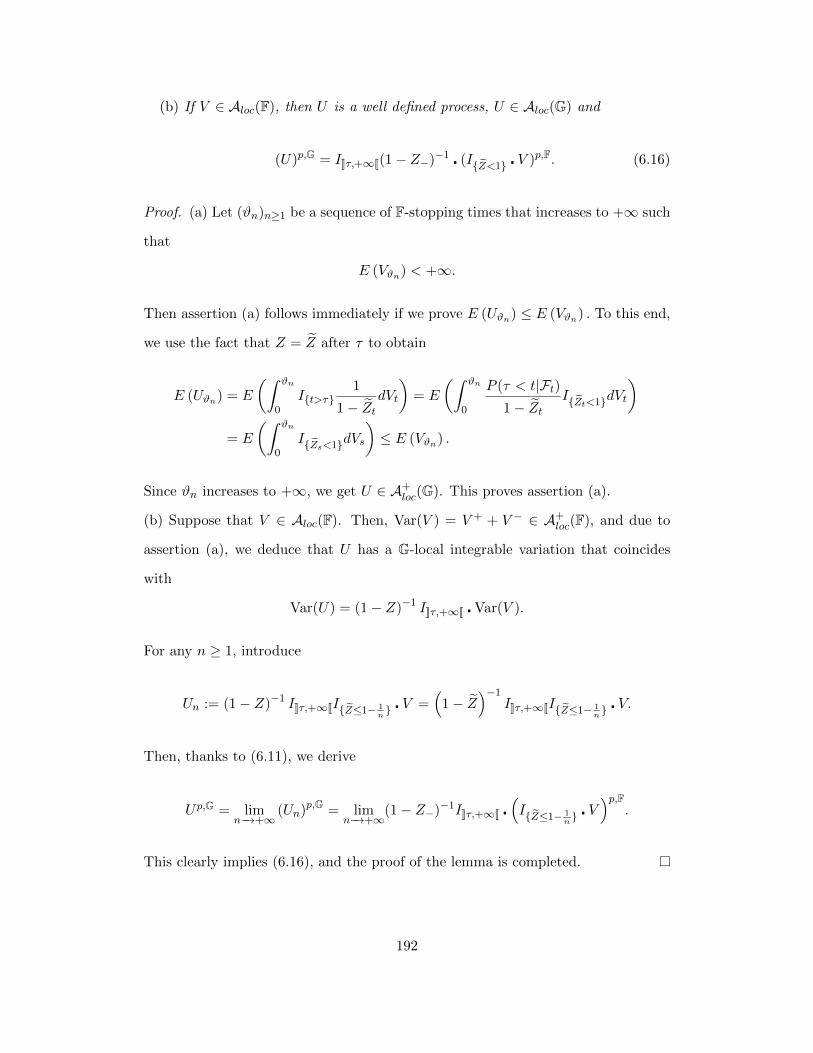
(b) If V ∈ Aloc(F), then U is a well defined process, U ∈ Aloc(G) and
(U)p,G = I]]τ,+∞[[(1− Z−)−1 (IZ<1 V )p,F. (6.16)
Proof. (a) Let (ϑn)n≥1 be a sequence of F-stopping times that increases to +∞ such
that
E (Vϑn) < +∞.
Then assertion (a) follows immediately if we prove E (Uϑn) ≤ E (Vϑn) . To this end,
we use the fact that Z = Z after τ to obtain
E (Uϑn) = E
(∫ ϑn
0It>τ
1
1− ZtdVt
)= E
(∫ ϑn
0
P (τ < t|Ft)1− Zt
IZt<1dVt
)= E
(∫ ϑn
0IZs<1dVs
)≤ E (Vϑn) .
Since ϑn increases to +∞, we get U ∈ A+loc(G). This proves assertion (a).
(b) Suppose that V ∈ Aloc(F). Then, Var(V ) = V + + V − ∈ A+loc(F), and due to
assertion (a), we deduce that U has a G-local integrable variation that coincides
with
Var(U) = (1− Z)−1 I]]τ,+∞[[ Var(V ).
For any n ≥ 1, introduce
Un := (1− Z)−1 I]]τ,+∞[[IZ≤1− 1n V =
(1− Z
)−1I]]τ,+∞[[IZ≤1− 1
n V.
Then, thanks to (6.11), we derive
Up,G = limn−→+∞
(Un)p,G = limn−→+∞
(1− Z−)−1I]]τ,+∞[[ (IZ≤1− 1
n V
)p,F.
This clearly implies (6.16), and the proof of the lemma is completed.
192

6.2.2 An Important G-Local Martingale
In this subsection, we introduce a G-local martingales that will play the role of
deflator for a class of F-local martingale. The construction of this local martingale
relies on the following.
Proposition 6.2: Let τ be an honest time satisfying (6.4). Then, the following
assertions hold.
(a) The nondecreasing process
WGt :=
∑0<u≤t
p,F(IZ=1
)uIu>τ, (6.17)
is G-predictable, cadlag, and locally bounded.
(b) The nonnegative and G-predictable process(1−∆WG)−1
is locally bounded.
Proof. a) Since the process (1−Z−)−1I]]τ,+∞[[ is G-locally bounded under assumption
(6.4), then there exists a sequence of G-stopping times (τn)n≥1 that increases to
infinity such that ((1− Z−)−1I]]τ,+∞[[
)τn ≤ n.Consider a sequence of F-stopping times, (σn)n≥1, that increases to infinity and
〈m,m〉σn ≤ n. Then, for any nonnegative F-predictable process H which is bounded
by C > 0, we derive
(H WG)σn∧τn ≤∑
0≤u≤σn
Hup,F(IZ=1>Z−
)uI1−Zu−≥ 1
n
=∑
0≤u≤σn
Hup,F(I∆m=1−Z−≥ 1
nIZ−≤1− 1
n
)u
≤∑
0≤u≤σn
Hup,F(I∆m≥ 1
n
)u≤ (n)2H 〈m,m〉σn ≤ C(n)3.
This ends the proof of the assertion (a).
193

(b) We first calculate
1−∆WG = 1− p,F(IZ=1
)I]]τ,+∞[[ = I]]0,τ ]]+
p,F(IZ<1
)I]]τ,+∞[[ ≥ I]]0,τ ]]+(1−Z−)I]]τ,+∞[[.
The last inequality follows from 1− Z ≤ IZ<1. Thus, we deduce that
(1−∆WG)−1 ≤ I]]0,τ ]] + (1− Z−)−1I]]τ,+∞[[,
which is locally bounded due to Lemma 6.4–(a). This proves assertion (b), and the
proof of the proposition is completed.
For the construction of the local martingale deflator, we will use, as in Chapter 5,
the optional integral.
Proposition 6.3: Suppose that τ satisfies (6.4) and consider the F-martingale m
in (6.2) and m(a) defined via (6.9). Then, the process K(a) given by
K(a) :=(1− Z−)2
(1− Z−)2 + ∆〈m〉F1
1− ZI]]τ,+∞[[, (6.18)
belongs to oL1loc(m
(a),G) defined in Definition 2.12.
Furthermore, the associated G-local martingale,
LG := K(a) m(a), (6.19)
satisfies the following
(a) E(LG) > 0 (or equivalently 1 + ∆LG > 0) and I]]0,τ ]] LG = 0.
(b) Consider any M ∈M0,loc(F) and M (a) defined in (6.9). Then,
[LG, M (a)] ∈ Aloc(G)(
i.e. 〈LG, M (a)〉G exists). (6.20)
Proof. This proof contains two steps. In the first step, we prove the optional integral
194
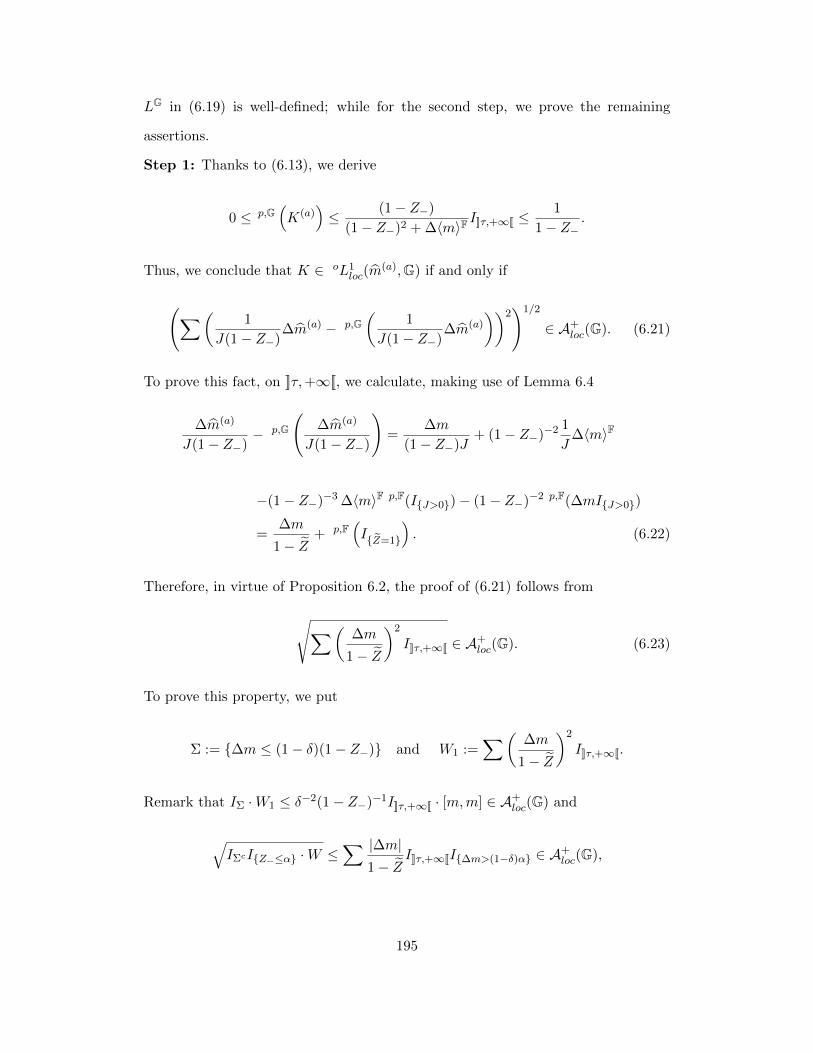
LG in (6.19) is well-defined; while for the second step, we prove the remaining
assertions.
Step 1: Thanks to (6.13), we derive
0 ≤ p,G(K(a)
)≤ (1− Z−)
(1− Z−)2 + ∆〈m〉FI]]τ,+∞[[ ≤
1
1− Z−.
Thus, we conclude that K ∈ oL1loc(m
(a),G) if and only if
(∑(1
J(1− Z−)∆m(a) − p,G
(1
J(1− Z−)∆m(a)
))2)1/2
∈ A+loc(G). (6.21)
To prove this fact, on ]]τ,+∞[[, we calculate, making use of Lemma 6.4
∆m(a)
J(1− Z−)− p,G
(∆m(a)
J(1− Z−)
)=
∆m
(1− Z−)J+ (1− Z−)−2 1
J∆〈m〉F
−(1− Z−)−3 ∆〈m〉F p,F(IJ>0)− (1− Z−)−2 p,F(∆mIJ>0)
=∆m
1− Z+ p,F
(IZ=1
). (6.22)
Therefore, in virtue of Proposition 6.2, the proof of (6.21) follows from
√∑(∆m
1− Z
)2
I]]τ,+∞[[ ∈ A+loc(G). (6.23)
To prove this property, we put
Σ := ∆m ≤ (1− δ)(1− Z−) and W1 :=∑(
∆m
1− Z
)2
I]]τ,+∞[[.
Remark that IΣ ·W1 ≤ δ−2(1− Z−)−1I]]τ,+∞[[ · [m,m] ∈ A+loc(G) and
√IΣcIZ−≤α ·W ≤
∑ |∆m|1− Z
I]]τ,+∞[[I∆m>(1−δ)α ∈ A+loc(G),
195

for any α ∈ (0, 1). Thus, for any α ∈ (0, 1), the process√IZ−≤α ·W1 ∈ A+
loc(G).
Since the process (1 − Z−)−1I]]τ,+∞[[ is G-locally bounded, then there exists a se-
quence of G-stopping times, (σn)n≥1, that increases to infinity such that on ]]τ,+∞[[∩[[0, σn]],
we have Z− ≤ 1−1/(n+1). This implies that for each n, we have√W σn
1 ∈ A+loc(G),
and hence√W1 ∈
(A+loc(G)
)loc
= A+loc(G). This proves (6.23).
Step 2: Assertion (a) follows from I]]0,τ ]] m(a) = 0 and (6.22) implies that
1 + ∆LG = 1 +∆m
1− ZI]]τ,+∞[[ + p,F
(IZ=1
)I]]τ,+∞[[ > 0.
We now prove (6.20). Due to Proposition 2.3 and the G-local boundedness of (1−
Z−)−2I]]τ,+∞[[ (see Lemma 6.4(a)), we deduce that [LG, M (a)] ∈ Aloc(G) if and only
if J−1 [m, M (a)] ∈ Aloc(G). We calculate this quantity
J−1 [m(a), M (a)] = J−1I]]τ,+∞[[ [m,M ] + J−1(1− Z−)−1∆mI]]τ,+∞[[ 〈m,M〉F
+∆M
J(1− Z−)I]]τ,+∞[[ 〈m〉F +
∆〈m〉F
J(1− Z−)2I]]τ,+∞[[ 〈m,M〉F.
On the one hand,
(1− Z−)−1∆mI]]τ,+∞[[, ∆〈m〉F(1− Z−)−2I]]τ,+∞[[ and (1− Z−)−1I]]τ,+∞[[
are G-locally bounded. On the other hand, since [m,M ], ∆M 〈m〉F and 〈m,M〉F
belong to Aloc(F), thanks to Lemma 6.5–(a) we conclude that
J−1I]]τ,+∞[[ [m,M ], J−1I]]τ,+∞[[ (
∆M 〈m〉F)
and J−1I]]τ,+∞[[ 〈m,M〉F
belong to Aloc(G). Therefore, this achieves the proof of (6.20), and the proof of the
proposition is completed.
196
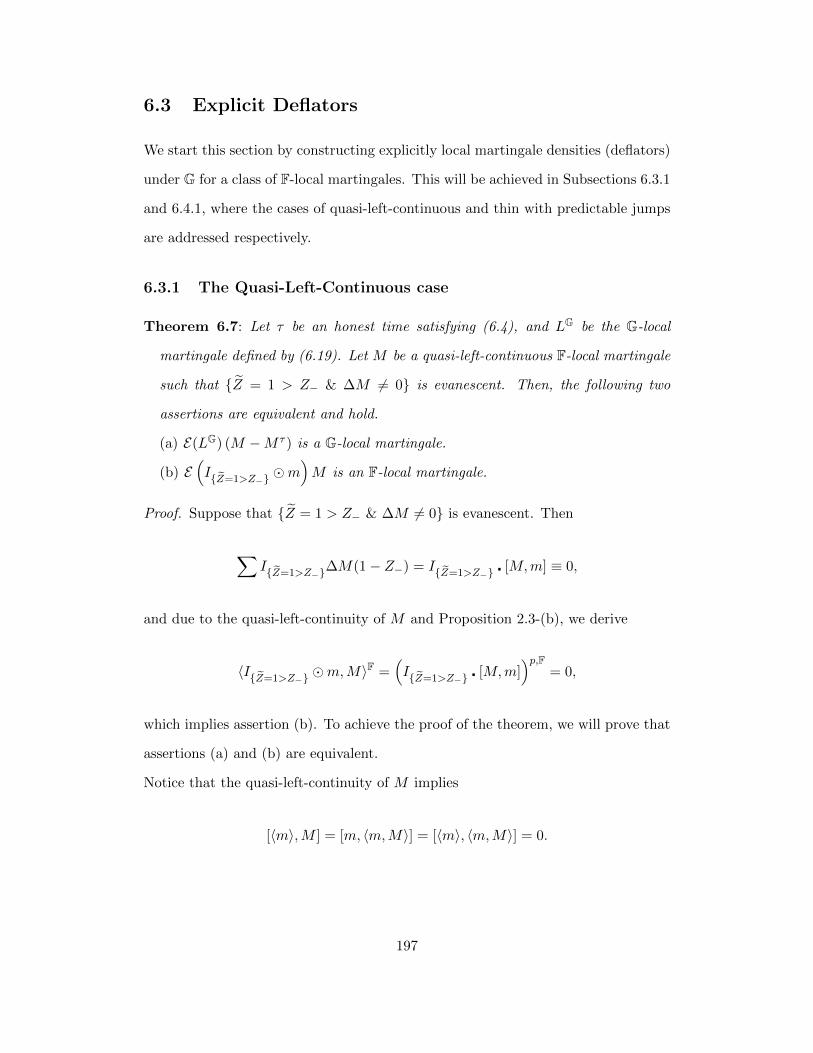
6.3 Explicit Deflators
We start this section by constructing explicitly local martingale densities (deflators)
under G for a class of F-local martingales. This will be achieved in Subsections 6.3.1
and 6.4.1, where the cases of quasi-left-continuous and thin with predictable jumps
are addressed respectively.
6.3.1 The Quasi-Left-Continuous case
Theorem 6.7: Let τ be an honest time satisfying (6.4), and LG be the G-local
martingale defined by (6.19). Let M be a quasi-left-continuous F-local martingale
such that Z = 1 > Z− & ∆M 6= 0 is evanescent. Then, the following two
assertions are equivalent and hold.
(a) E(LG) (M −M τ ) is a G-local martingale.
(b) E(IZ=1>Z− m
)M is an F-local martingale.
Proof. Suppose that Z = 1 > Z− & ∆M 6= 0 is evanescent. Then
∑IZ=1>Z−∆M(1− Z−) = IZ=1>Z− [M,m] ≡ 0,
and due to the quasi-left-continuity of M and Proposition 2.3-(b), we derive
〈IZ=1>Z− m,M〉F =
(IZ=1>Z− [M,m]
)p,F= 0,
which implies assertion (b). To achieve the proof of the theorem, we will prove that
assertions (a) and (b) are equivalent.
Notice that the quasi-left-continuity of M implies
[〈m〉,M ] = [m, 〈m,M〉] = [〈m〉, 〈m,M〉] = 0.
197
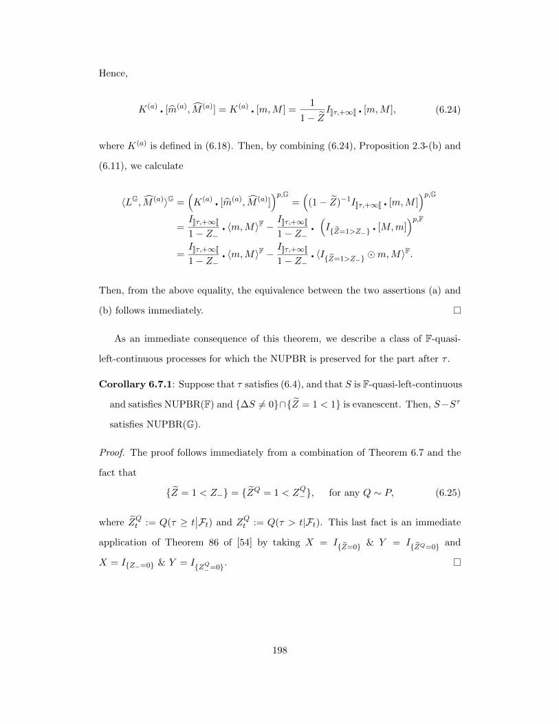
Hence,
K(a) [m(a), M (a)] = K(a) [m,M ] =1
1− ZI]]τ,+∞[[ [m,M ], (6.24)
where K(a) is defined in (6.18). Then, by combining (6.24), Proposition 2.3-(b) and
(6.11), we calculate
〈LG, M (a)〉G =(K(a) [m(a), M (a)]
)p,G=(
(1− Z)−1I]]τ,+∞[[ [m,M ])p,G
=I]]τ,+∞[[
1− Z− 〈m,M〉F −
I]]τ,+∞[[
1− Z−(IZ=1>Z− [M,m]
)p,F=I]]τ,+∞[[
1− Z− 〈m,M〉F −
I]]τ,+∞[[
1− Z− 〈IZ=1>Z− m,M〉
F.
Then, from the above equality, the equivalence between the two assertions (a) and
(b) follows immediately.
As an immediate consequence of this theorem, we describe a class of F-quasi-
left-continuous processes for which the NUPBR is preserved for the part after τ .
Corollary 6.7.1: Suppose that τ satisfies (6.4), and that S is F-quasi-left-continuous
and satisfies NUPBR(F) and ∆S 6= 0∩Z = 1 < 1 is evanescent. Then, S−Sτ
satisfies NUPBR(G).
Proof. The proof follows immediately from a combination of Theorem 6.7 and the
fact that
Z = 1 < Z− = ZQ = 1 < ZQ−, for any Q ∼ P, (6.25)
where ZQt := Q(τ ≥ t∣∣Ft) and ZQt := Q(τ > t|Ft). This last fact is an immediate
application of Theorem 86 of [54] by taking X = IZ=0 & Y = IZQ=0 and
X = IZ−=0 & Y = IZQ−=0.
198
6.3.2 The Case of Thin Processes with Predictable Jumps
The construction of deflators for thin F-local martingales requires the following
results that are interesting in themselves.
Lemma 6.6: Let T be a finite F-predictable stopping time. Then the following holds.
T > τ ⊂ ZT < 1 ⊂ ZT− < 1 = Γ(T ) :=P(ZT < 1
∣∣∣FT−) > 0.
Proof. It is enough to prove the non-trivial equality ZT− < 1 = Γ(T ). Indeed,
due to E(P (ZT < 1|FT−)IZT−=1
)= P (ZT < 1 = ZT−) = 0, we get Γ(T ) ⊂
ZT− < 1. On the other hand, due to
E((1− ZT−)IΓ(T )c
)= E
((1− ZT ) IΓ(T )c
)≤ E
(IZT<1 IΓ(T )c
)= 0,
we obtain ZT− < 1 ⊂ Γ(T ). This ends the proof of the lemma.
Lemma 6.7: Let R be an equivalent probability to P . Then the following hold.
Z = 1 = ZR = 1, and Z− = 1 = ZR− = 1,
where ZRt := R(τ ≥ t|Ft) and ZR− is the (R,F)-predictable projection of ZR.
Proof. For any F-stopping time σ and any F-predictable stopping time T , due to
E[(1− Zσ)IZRσ =1
]= E
[Iτ<σIZRσ =1
]= 0, and
E[(1− ZT−)IZRT−=1
]= E
[Iτ<TIZRT−=1
]= 0,
we obtain ZR = 1 ⊂ Z = 1 and ZR− = 1 ⊂ Z− = 1. The symmetric roles
of R and P complete the proof of the lemma.
Theorem 6.8: Let τ be an F-honest time. Consider an F-predictable stopping time
T and an FT -measurable random variable ξ such that E[|ξ||FT−] < +∞, P -a.s.
199

Define M := ξIZT−<1I[[T,+∞[[,
dQFT
dP:= DF :=
IZT<1 & P (ZT<1|FT−)>0
P (ZT < 1|FT−)+ IP (ZT<1|FT−)=0, and
dQGT
dP:= DG :=
1− ZT−(1− ZT )P (ZT < 1|FT−)
IT>τ + IT≤τ. (6.26)
Then the following assertions are equivalent.
(a) M is a (QFT ,F)-martingale.
(b) On ZT− < 1, we have
E(ξIZT<1
∣∣ FT−) = 0, P − a.s. (6.27)
(c) (M −M τ ) is a (QGT ,G)-martingale.
Proof. The proof of the theorem will be achieved in two steps. In Step 1, we prove
(a)⇐⇒(b); while Step 2 proves (b)⇐⇒(c). First we remark that the two probability
measures QFT and QG
T in (6.26) are well defined due to Lemma 6.6.
Step 1: Herein, we will prove (a)⇐⇒(b). Thanks to E[DF|FT−] = 1, we obtain
EQFT [ξIZT−<1|FT−] = E
[DFξIZT−<1|FT−
]=E[ξIZT<1|FT−
]P (ZT < 1|FT−)
IZT−<1.
Therefore, the equivalence between assertions (a) and (b) follows from a combi-
nation of this equality and the fact that M is a (QFT ,F)-martingale if and only if
EQFT (MT
∣∣ FT−) = 0 on T < +∞.
Step 2: This step will prove (b)⇐⇒ (c). To this end, we first notice that M −M τ
is (QGT ,G)-martingale if and only if EQ
GT [ξIZT−<1 & T>τ|GT−] = 0 on T < +∞.
200
Furthermore, due to Lemma 6.6 and E[DG|GT−] = 1, we have
EQGT [ξIZT−<1 & T>τ|GT−] = E
[DGξIZT−<1IT>τ|GT−
]= E
[ξIT>τ
1− ZT
∣∣∣GT−] 1− ZT−P (ZT < 1|FT−)
IZT−<1 & T>τ
=E[ξIZT<1|FT−
]P (ZT < 1|FT−)
IZT−<1IT>τ, (6.28)
where the last equality in (6.28) follows from the fact that
E(H∣∣ GT−) IT>τ = E
(H(1− ZT )
∣∣ FT−) IT>τ
1− ZT−,
for any random variable H for which the above conditional expectations exist (see
Proposition 5.3 of [83] or Proposition 2.7 in Chapter 2). Therefore, if assertion (b)
holds, then assertion (c) follows immediately from (6.28). Conversely, if assertion
(c) holds, then EQGT [ξIZT−<1IT>τ|GT−] = 0. Thus, a combination of this with
(6.28) leads to E[ξIZT<1|FT−
](1−ZT−) = 0. This proves assertion (b), and the
proof of the theorem is completed.
Remark 6.3: It is important to notice that
DG(T ) :=
(1 +
∆mT
1− ZT
)IT>τ + IT≤τ 6= 1 + ∆N =
ET(LG)
ET− (LG).
This explains one of the main difficulties that we will face when dealing with
countable many predictable jumps. In fact, it might not be possible to piece-up
the sequence(DG(Tn), n ≥ 1
)into a local martingale density when the stopping
times are not ordered. This explains the fact that the proof of the general case
needs a different idea and method.
Theorem 6.9: Let M be a thin F-local martingale (that is M (qc) ≡ 0) such that
201
∆M 6= 0 ∩ Z = 1 > Z− = ∅. Then
E(
(1−∆WG)−1 LG)
(M −M τ ) is a G-local martingale. (6.29)
Proof. Thanks to Ito’s formula, it is immediate that (6.29) is equivalent to
XG := M −M τ + [(1−∆WG)−1 LG,M −M τ ] is a G-local martingale. (6.30)
It is obvious that XG is a G-special semimartingale since 〈LG,M −M τ 〉F exits (see
Proposition 6.3). Hence it is enough to prove that XG is a σ-martingale under G.
Let (Tn)n≥1 be the sequence of predictable stopping times that exhaust the jumps
of M . Then, thanks to Theorem 6.7, since ∆M 6= 0 ∩ Z = 1 > Z− = ∅, we
conclude that for any n ≥ 1,
Mn := (S − Sτ )Tn
(1 +
∆LGTn
1−∆WGTn
)I[[Tn,+∞[[ is a G-martingale. (6.31)
Consider the following G-predictable and positive process that is bounded by one
Φ :=∑n≥1
2−n
1 + ξnI[[Tn]]∩]]τ,+∞[[+IΓc∩[[0,τ ]], ξn := E
[|∆STn |(1 +
|∆LGTn|
1−∆WGTn
)∣∣ GTn−
]ITn<+∞,
where Γ := ∪n≥1[[Tn]]. Then, it is easy to check that ΦXG satisfies E[Var(Φ XG)(∞)
]≤
1. Furthermore, due to (6.31), we calculate
(Φ XG
)p,G=∑n≥1
(Φ Mn)p,G ≡ 0.
This proves that Φ XG is a G-martingale. As a result, XG is a G-local martingale.
This ends the proof of the theorem.
Corollary 6.9.1: Suppose that S is thin, ∆S 6= 0 ∩ Z = 1 > Z− = ∅, and S
satisfies the NUPBR(F). Then S − Sτ satisfies the NUPBR(G).
202
Proof. Since S satisfies the NUPBR(F), then there exist a F-predictable process φ,
a sequence of F-stopping times (Tn)n≥1 that increases to infinity, and a probability
measure Qn ∼ P on (Ω,FTn) such that
0 < φ ≤ 1, φ STn ∈M0,loc(Q,F).
Then, a combination of ∆S 6= 0 ∩ Z = 1 > Z− = ∅ and (6.39) leads to
∆(φ STn) 6= 0 ∩ ZQn = 1 > ZQn− = ∅.
Therefore, by applying directly Theorem 6.9 to φ STn under Qn, we conclude
that φ STn − (φ STn)τ has a local martingale density under (Qn,G). Thus, this
implies that STn − STn∧τ satisfies the NUPBR(G, Qn). Thus, the corollary follows
immediately from Proposition 5.2. This ends the proof of the corollary.
6.4 Proofs of Three Main Theorems
In this section, we will prove three theorems that were not proved in Section 6.1,
namely Theorems 6.1, 6.2 and 6.5. To this end, we introduce some notations that
will be used throughout the rest of the chapter. Recall that µ is the random measure
of the jumps of S, ν is its random measure compensator and the functional fm is
defined in (6.5). Here we put
µG(dt, dx) := I]]τ,+∞[[(t)µ(dt, dx), νG(dt, dx) := I]]τ,+∞[[(t)
(1− fm(x, t)
1− Zt−
)ν(dt, dx).
(6.32)
It is easy to check that νG is the random measure compensator under G of µG. The
canonical decomposition of S − Sτ under G is given by
S−Sτ = Sc(a)
+h?(µG−νG)+bI]]τ,+∞[[A−cβm
1− Z−I]]τ,+∞[[A−h
fm1− Z−
I]]τ,+∞[[?ν+(x−h)?µG,
203
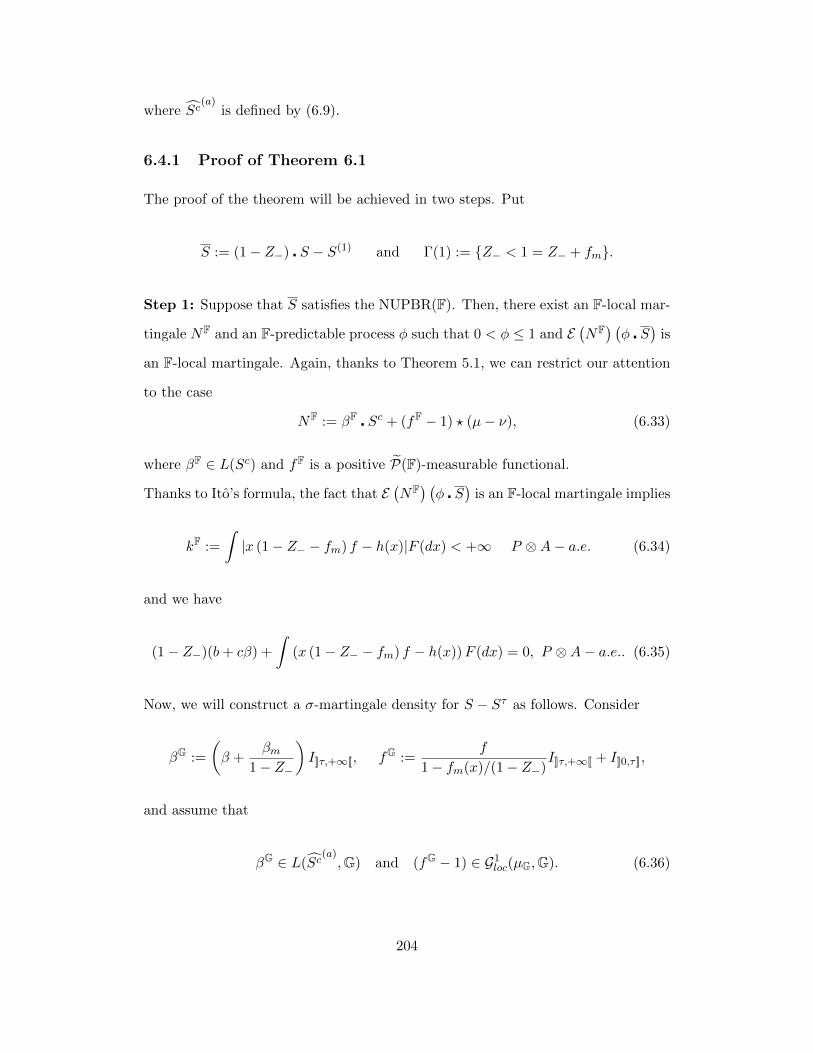
where Sc(a)
is defined by (6.9).
6.4.1 Proof of Theorem 6.1
The proof of the theorem will be achieved in two steps. Put
S := (1− Z−) S − S(1) and Γ(1) := Z− < 1 = Z− + fm.
Step 1: Suppose that S satisfies the NUPBR(F). Then, there exist an F-local mar-
tingale NF and an F-predictable process φ such that 0 < φ ≤ 1 and E(NF) (φ S
)is
an F-local martingale. Again, thanks to Theorem 5.1, we can restrict our attention
to the case
NF := βF Sc + (fF − 1) ? (µ− ν), (6.33)
where βF ∈ L(Sc) and fF is a positive P(F)-measurable functional.
Thanks to Ito’s formula, the fact that E(NF) (φ S
)is an F-local martingale implies
kF :=
∫|x (1− Z− − fm) f − h(x)|F (dx) < +∞ P ⊗A− a.e. (6.34)
and we have
(1− Z−)(b+ cβ) +
∫(x (1− Z− − fm) f − h(x))F (dx) = 0, P ⊗A− a.e.. (6.35)
Now, we will construct a σ-martingale density for S − Sτ as follows. Consider
βG :=
(β +
βm1− Z−
)I]]τ,+∞[[, fG :=
f
1− fm(x)/(1− Z−)I]]τ,+∞[[ + I]]0,τ ]],
and assume that
βG ∈ L(Sc(a),G) and (fG − 1) ∈ G1
loc(µG,G). (6.36)
204
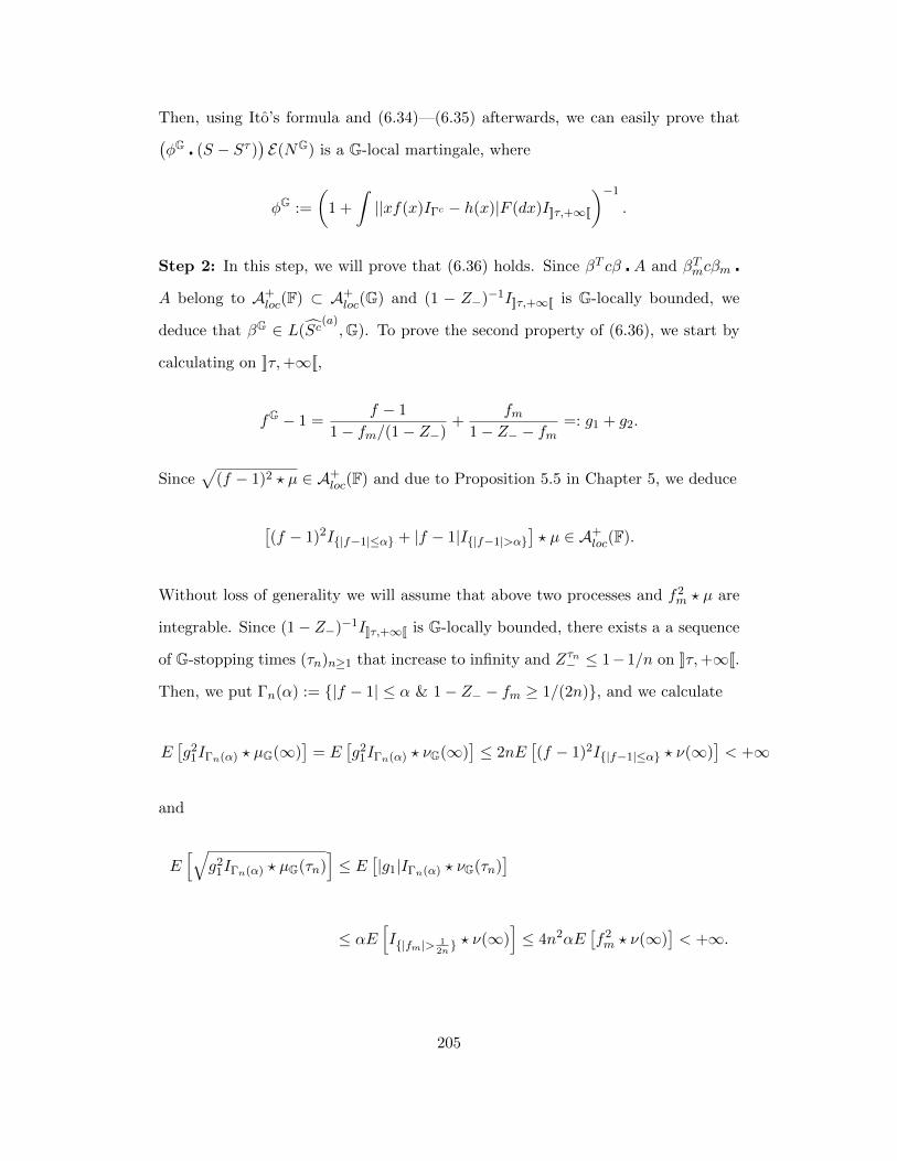
Then, using Ito’s formula and (6.34)—(6.35) afterwards, we can easily prove that(φG (S − Sτ )
)E(NG) is a G-local martingale, where
φG :=
(1 +
∫||xf(x)IΓc − h(x)|F (dx)I]]τ,+∞[[
)−1
.
Step 2: In this step, we will prove that (6.36) holds. Since βT cβ A and βTmcβm
A belong to A+loc(F) ⊂ A+
loc(G) and (1 − Z−)−1I]]τ,+∞[[ is G-locally bounded, we
deduce that βG ∈ L(Sc(a),G). To prove the second property of (6.36), we start by
calculating on ]]τ,+∞[[,
fG − 1 =f − 1
1− fm/(1− Z−)+
fm1− Z− − fm
=: g1 + g2.
Since√
(f − 1)2 ? µ ∈ A+loc(F) and due to Proposition 5.5 in Chapter 5, we deduce
[(f − 1)2I|f−1|≤α + |f − 1|I|f−1|>α
]? µ ∈ A+
loc(F).
Without loss of generality we will assume that above two processes and f2m ? µ are
integrable. Since (1− Z−)−1I]]τ,+∞[[ is G-locally bounded, there exists a a sequence
of G-stopping times (τn)n≥1 that increase to infinity and Zτn− ≤ 1−1/n on ]]τ,+∞[[.
Then, we put Γn(α) := |f − 1| ≤ α & 1− Z− − fm ≥ 1/(2n), and we calculate
E[g2
1IΓn(α) ? µG(∞)]
= E[g2
1IΓn(α) ? νG(∞)]≤ 2nE
[(f − 1)2I|f−1|≤α ? ν(∞)
]< +∞
and
E[√
g21IΓn(α) ? µG(τn)
]≤ E
[|g1|IΓn(α) ? νG(τn)
]
≤ αE[I|fm|> 1
2n ? ν(∞)
]≤ 4n2αE
[f2m ? ν(∞)
]< +∞.
205
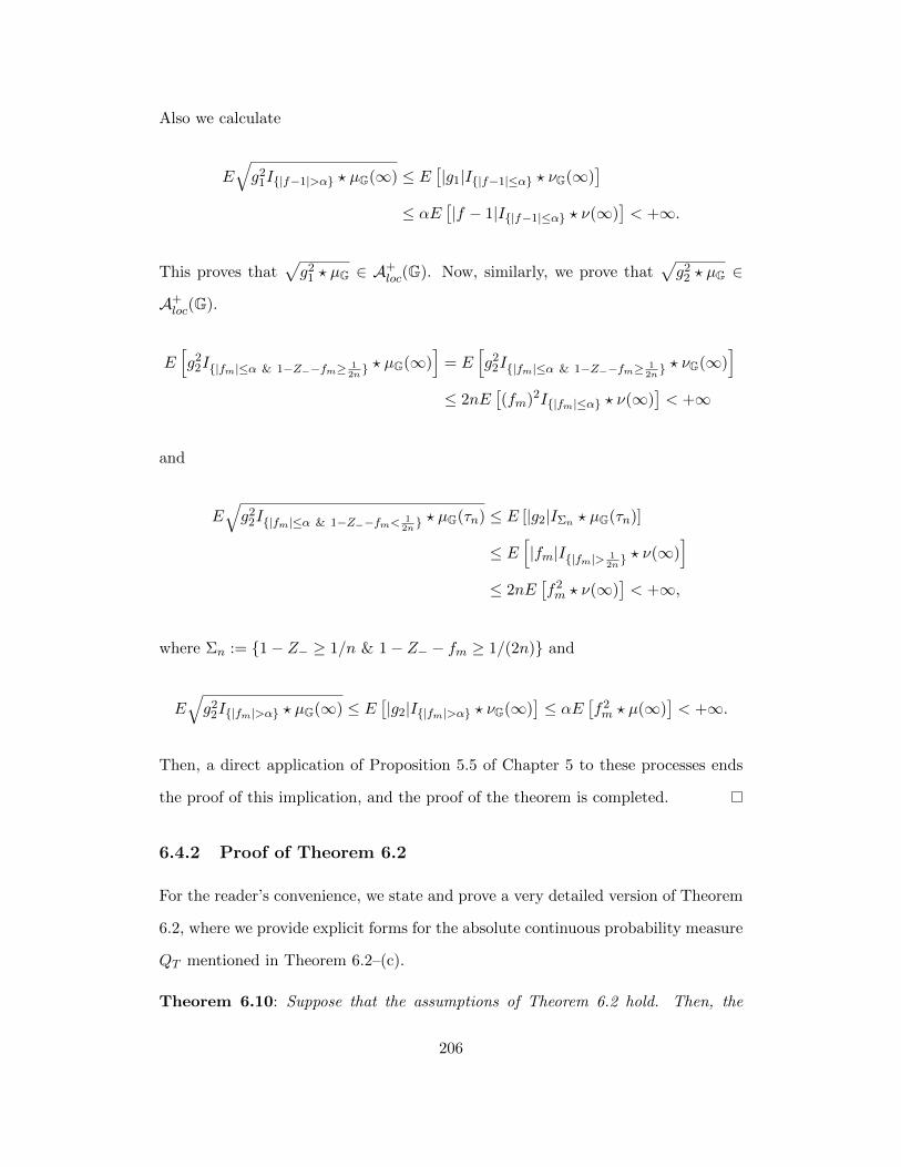
Also we calculate
E√g2
1I|f−1|>α ? µG(∞) ≤ E[|g1|I|f−1|≤α ? νG(∞)
]≤ αE
[|f − 1|I|f−1|≤α ? ν(∞)
]< +∞.
This proves that√g2
1 ? µG ∈ A+loc(G). Now, similarly, we prove that
√g2
2 ? µG ∈
A+loc(G).
E[g2
2I|fm|≤α & 1−Z−−fm≥ 12n ? µG(∞)
]= E
[g2
2I|fm|≤α & 1−Z−−fm≥ 12n ? νG(∞)
]≤ 2nE
[(fm)2I|fm|≤α ? ν(∞)
]< +∞
and
E√g2
2I|fm|≤α & 1−Z−−fm< 12n ? µG(τn) ≤ E [|g2|IΣn ? µG(τn)]
≤ E[|fm|I|fm|> 1
2n ? ν(∞)
]≤ 2nE
[f2m ? ν(∞)
]< +∞,
where Σn := 1− Z− ≥ 1/n & 1− Z− − fm ≥ 1/(2n) and
E√g2
2I|fm|>α ? µG(∞) ≤ E[|g2|I|fm|>α ? νG(∞)
]≤ αE
[f2m ? µ(∞)
]< +∞.
Then, a direct application of Proposition 5.5 of Chapter 5 to these processes ends
the proof of this implication, and the proof of the theorem is completed.
6.4.2 Proof of Theorem 6.2
For the reader’s convenience, we state and prove a very detailed version of Theorem
6.2, where we provide explicit forms for the absolute continuous probability measure
QT mentioned in Theorem 6.2–(c).
Theorem 6.10: Suppose that the assumptions of Theorem 6.2 hold. Then, the
206
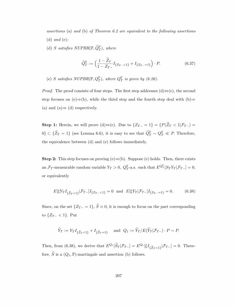
assertions (a) and (b) of Theorem 6.2 are equivalent to the following assertions
(d) and (e):
(d) S satisfies NUPBR(F, QFT ), where
QFT :=
( 1− ZT1− ZT−
IZT−<1 + IZT−=1
)· P. (6.37)
(e) S satisfies NUPBR(F, QFT ), where QF
T is given by (6.26).
Proof. The proof consists of four steps. The first step addresses (d)⇔(e), the second
step focuses on (e)⇒(b), while the third step and the fourth step deal with (b)⇒
(a) and (a)⇒ (d) respectively.
Step 1: Herein, we will prove (d)⇔(e). Due to ZT− = 1 = P (ZT < 1|FT−) =
0 ⊂ ZT = 1 (see Lemma 6.6), it is easy to see that QFT ∼ QF
T P. Therefore,
the equivalence between (d) and (e) follows immediately.
Step 2: This step focuses on proving (e)⇒(b). Suppose (e) holds. Then, there exists
an FT -measurable random variable YT > 0, QFT -a.s. such that EQ
FT [STYT |FT−] = 0,
or equivalently
E[ξYT IZT<1|FT−]IZT−<1 = 0 and E[ξYT |FT−]IZT−=1 = 0. (6.38)
Since, on the set ZT− = 1, S ≡ 0, it is enough to focus on the part corresponding
to ZT− < 1. Put
YT := YT IZT<1 + IZT=1 and Q1 := YT /E(YT |FT−) · P ∼ P.
Then, from (6.38), we derive that EQ1 [ST |FT−] = EQ1 [ξIZT<1|FT−] = 0. There-
fore, S is a (Q1,F)-martingale and assertion (b) follows.
207
Step 3: This step proves (b)⇒ (a). Suppose that S satisfies NUPBR(F). Then,
there exists an FT -measurable Y3 > 0 such that E[Y3ξIZT<1|FT−] = 0. Put
Q3 := Y3/E(Y3|FT−) · P ∼ P and remark that ZT < 1 = ZQ3
T < 1, where
ZQ3t := Q3(τ ≥ t|Ft). Therefore, a direct application of Theorem 6.8 under Q3, we
conclude that S − Sτ = S − Sτ satisfies NUPBR(G), and assertion (a) holds.
Step 4: This last step will prove (a)⇒ (d). Suppose S − Sτ satisfies NUPBR(G).
There exists a positive GT -measurable Y G such that E[ξY GIT>τ|GT−] = 0. Then,
thanks to Jeulin [83] (Proposition 5.3), we deduce the existence of a positive and
FT -measurable Y F such that Y GIT>τ = Y FIT>τ. Then, we calculate
0 = E[ξY GIT>τ|GT−] = E[ξY F(1− ZT )|FT−]IT>τ
1− ZT−= EQ
FT
(ξY F∣∣ FT−) IT>τ = EQ
FT
(ξY F∣∣ FT−) IT>τ,
where Y F := Y FIZT−<1 + IZT−=1. Therefore, by taking conditional expectation
and using the fact that ST IZT−=0 = 0, we obtain
(1− ZT−)EQFT [ξY F∣∣FT−] = 0, or equivalently EQ
FT [ST Y
F∣∣FT−] = 0 P − a.s.
By using the equality E(Y FIT>τ|GT−) = E(Y GIT>τ|GT−) = IT>τ, we deduce
that EQFT [Y F∣∣FT−] = 1. This proves that S satisfies NUPBR(F, QF
T ) and the proof
of the theorem is achieved.
6.4.3 Proof of Theorem 6.5
We start by outlining a number of remarks that simplify tremendously the proof.
Due to Lemma 6.7, on T < +∞, we have
ZQT = 1 = ZT = 1 for any Q ∼ P and any F− stopping time T, (6.39)
208
where ZQt := EQ[Iτ≥t|Ft].
On the other hand, assertion (b) is equivalent to the existence of a positive F-local
martingale Y such that
p,F(Y∆SaIZ<1
)= 0.
These two remarks imply that without loss of generality we will assume that S = Sa
in the rest of the proof.
Consider a sequence of F-stopping times (σn)n≥1 such that Y σn is a martingale, and
put Qn := (Yσn/Y0) · P . Therefore, thanks to Proposition 5.2, it is enough to prove
that assertion (a) holds true under Qn for Sσn . Therefore, without loss of generality,
we assume Y ≡ 1. Put
Xn = ∆STnIZTn<1 and Mn = XnI[[Tn,+∞[[.
Hence, the condition (6.27) in Theorem 6.8 is trivially satisfied for Xn and Mn.
Thus, we deduce that for each n,
(1 + ∆LGTn −∆WG
Tn)∆STnITn>τI[[Tn,+∞[[,
is a G-martingale. Then, for each θ ∈ L(S − Sτ ) such that θT∆S > −1, Yor’s
formula implies that
E(IΓ LG − IΓ ·WG
)E (θIΓ (S − Sτ )) = E
(W (1)
),
where
W (1) := IΓ (LG −WG) +∑n≥1
θTn
(1 + ∆LG
Tn −∆WGTn
)∆STnITn>τI[[Tn,+∞[[,
209
and LG(a)and V (a) are defined in (6.19) and (6.17) respectively. Put
φ =∑n≥1
2−n(1 + E(W (1))Tn−
)−1
(1 + Ξn)I]]τ,+∞[[∩[[Tn]] + IΓc∪[[0,τ ]] and
Ξn : = E[|∆LG
Tn |∣∣∣GTn−]+ ∆WG
Tn + E
[|θTn∆STn |(1− ZTn−)
1− ZTn
∣∣∣GTn−]ITn<+∞.
Then, it is easy to check that φ is G-predictable, 0 < φ ≤ 1, and E(|φ E(W (1))|var(+∞)
)≤∑
n≥1 2−n = 1. Hence φ E(W (1)) ∈ A(G), and using the fact that ∆LGTnI[[Tn,+∞[[
and (1 + ∆LGTn−∆WG
Tn)∆STnITn>τI[[Tn,+∞[[ are G-martingales, we get
(φ E(W (1))
)p,G=∑n≥1
φTnE(
∆W(1)Tn
∣∣GTn−) I[[Tn,+∞[[ = −φE−(W (1)) WG
is a non-increasing process. This proves that E(W (1)) is a positive σ-supermartingale,
and hence it is a supermartingale due to Kallsen [89]. Thus, S − Sτ admits a defla-
tor.
6.5 Discrete Time Market Models
Similar as Section 5.6 of Chapter 5, in the current section, we consider discrete time
market models. That is the case where there are only finite number of trading times
n = 1, 2, ..., N . In this context, we shall investigate the stability of non-arbitrage
after an honest time τ . For τ , we associate the following stopping times:
σ1 := infn ≥ 1 : Zn < 1, σ2 := infn ≥ 1 : Zn−1 < 1 and σ3 := infn ≥ 1 : Zn < 1.
(6.40)
First, we remark that in discrete time we do not assume Zτ < 1 considered in the
previous sections.
Lemma 6.8: For an honest time τ and the associated stopping times in (6.40), the
210
following properties hold for any n ≤ N :
(a) Zn < 1 ⊂ Zn−1 < 1 and Zn < 1 ⊂ Zn < 1.
(b) σ2 is an F-predictable stopping time and σ2 ≤ σ3 and σ1 ≤ σ3.
(c) On τ < n, we have
τ ≥ σ1, Zn−1 < 1, and Zn < 1, P − a.s..
Proof. (a) Notice that
E[(
1− Zn)1Zn−1=1
]= E
[(1− Zn−1)1Zn−1=1
]= 0.
Hence, Zn−1 = 1 ⊂ Zn = 1. Due to Zn ≤ Zn, we have Zn < 1 ⊂ Zn < 1.
(b) Since σ2 ≤ n = Zn−1 < 1 ∈ Fn−1, we conclude that σ2 is predictable. The
inequalities σ2 ≤ σ3 and σ1 ≤ σ3 follow immediately from (a).
(c) Notice that
E[In>τIZn−1=1
]= E
[(1− Zn−1)IZn−1=1
]= 0, and
E[In>τIZn=1
]= E
[(1− Zn)IZn=1
]= 0.
Therefore, Zn−1 < 1 and Zn < 1 on the set n > τ. This ends the proof of the
lemma.
The following lemma, (already stated and proved in Jeulin [83]), describes the
connection between conditional expectations under F and G.
Lemma 6.9: Let Y be an integrable A-measurable random variable. Then, the
following properties hold:
(a) On the set n > τ, the conditional expectation under Gn is given by
E [Y |Gn]1τ<n = E[Y 1τ<n|Fn
] 1
1− Zn1τ<n. (6.41)
211

(b) On the set n > τ, the conditional expectation under Gn−1 is given by
E [Y |Gn−1]1τ<n = E[Y 1τ<n|Fn−1
] 1
1− Zn−11τ<n. (6.42)
Moreover, if Y is Fn-measurable, we have
E [Y |Gn−1]1τ<n = E[Y (1− Zn)|Fn−1
] 1
1− Zn−11τ<n. (6.43)
The following theorem characterizes the relationship between F-martingales and
G-martingales on the stochastic interval ]]τ,+∞[[. For the continuous time case, we
consult Jeulin [83].
Theorem 6.11: Let M be an F-martingale and τ be an honest time. Then the
following process
M (a)n := Mn∨τ −Mτ −
∑1≤k≤n
1
1− Zk−11τ<kE
[(Mk −Mk−1)(1− Zk)|Fk−1
],
is a G-martingale.
Proof. Although it can be derived from Jeulin [83], here we give a direct proof here.
It is easy to see that
M(n+1)∨τ = Mn∨τ + (Mn+1 −Mn)1τ<n+1. (6.44)
212
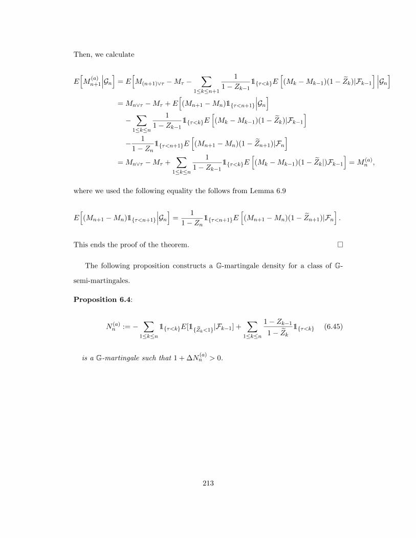
Then, we calculate
E[M
(a)n+1
∣∣∣Gn] = E[M(n+1)∨τ −Mτ −
∑1≤k≤n+1
1
1− Zk−11τ<kE
[(Mk −Mk−1)(1− Zk)|Fk−1
] ∣∣∣Gn]= Mn∨τ −Mτ + E
[(Mn+1 −Mn)1τ<n+1
∣∣∣Gn]−∑
1≤k≤n
1
1− Zk−11τ<kE
[(Mk −Mk−1)(1− Zk)|Fk−1
]− 1
1− Zn1τ<n+1E
[(Mn+1 −Mn)(1− Zn+1)|Fn
]= Mn∨τ −Mτ +
∑1≤k≤n
1
1− Zk−11τ<kE
[(Mk −Mk−1)(1− Zk|)Fk−1
]= M (a)
n ,
where we used the following equality the follows from Lemma 6.9
E[(Mn+1 −Mn)1τ<n+1
∣∣∣Gn] =1
1− Zn1τ<n+1E
[(Mn+1 −Mn)(1− Zn+1)|Fn
].
This ends the proof of the theorem.
The following proposition constructs a G-martingale density for a class of G-
semi-martingales.
Proposition 6.4:
N (a)n := −
∑1≤k≤n
1τ<kE[1Zk<1|Fk−1] +∑
1≤k≤n
1− Zk−1
1− Zk1τ<k (6.45)
is a G-martingale such that 1 + ∆N(a)n > 0.
213
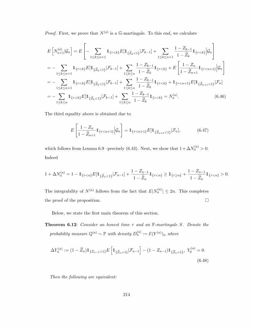
Proof. First, we prove that N (a) is a G-martingale. To this end, we calculate
E[N
(a)n+1|Gn
]= E
− ∑1≤k≤n+1
1τ<kE[1Zk<1|Fk−1] +∑
1≤k≤n+1
1− Zk−1
1− Zk1τ<k
∣∣∣Gn
= −∑
1≤k≤n+1
1τ<kE[1Zk<1|Fk−1] +∑
1≤k≤n
1− Zk−1
1− Zk1τ<k + E
[1− Zn
1− Zn+1
1τ<n+1
∣∣∣Gn]
= −∑
1≤k≤n+1
1τ<kE[1Zk<1|Fk−1] +∑
1≤k≤n
1− Zk−1
1− Zk1τ<k + 1τ<n+1E[1Zn+1<1|Fn]
= −∑
1≤k≤n1τ<kE[1Zk<1|Fk−1] +
∑1≤k≤n
1− Zk−1
1− Zk1τ<k = N (a)
n . (6.46)
The third equality above is obtained due to
E
[1− Zn
1− Zn+1
1τ<n+1
∣∣∣Gn] = 1τ<n+1E[1Zn+1<1|Fn], (6.47)
which follows from Lemma 6.9 –precisely (6.43). Next, we show that 1+∆N(a)n > 0.
Indeed
1 + ∆N (a)n = 1− 1τ<nE[1Zn<1|Fn−1] +
1− Zn−1
1− Zn1τ<n ≥ 1τ≥n +
1− Zn−1
1− Zn1τ<n > 0.
The integrability of N (a) follows from the fact that E|N (a)n | ≤ 2n. This completes
the proof of the proposition.
Below, we state the first main theorem of this section.
Theorem 6.12: Consider an honest time τ and an F-martingale S. Denote the
probability measure Q(a) ∼ P with density D(a)n := E(Y (a))n where
∆Y (a)n := (1− Zn)1Zn−1<1E
[1Zn=1|Fn−1
]− (1− Zn−1)1Zn=1, Y
(a)0 = 0.
(6.48)
Then the following are equivalent:
214
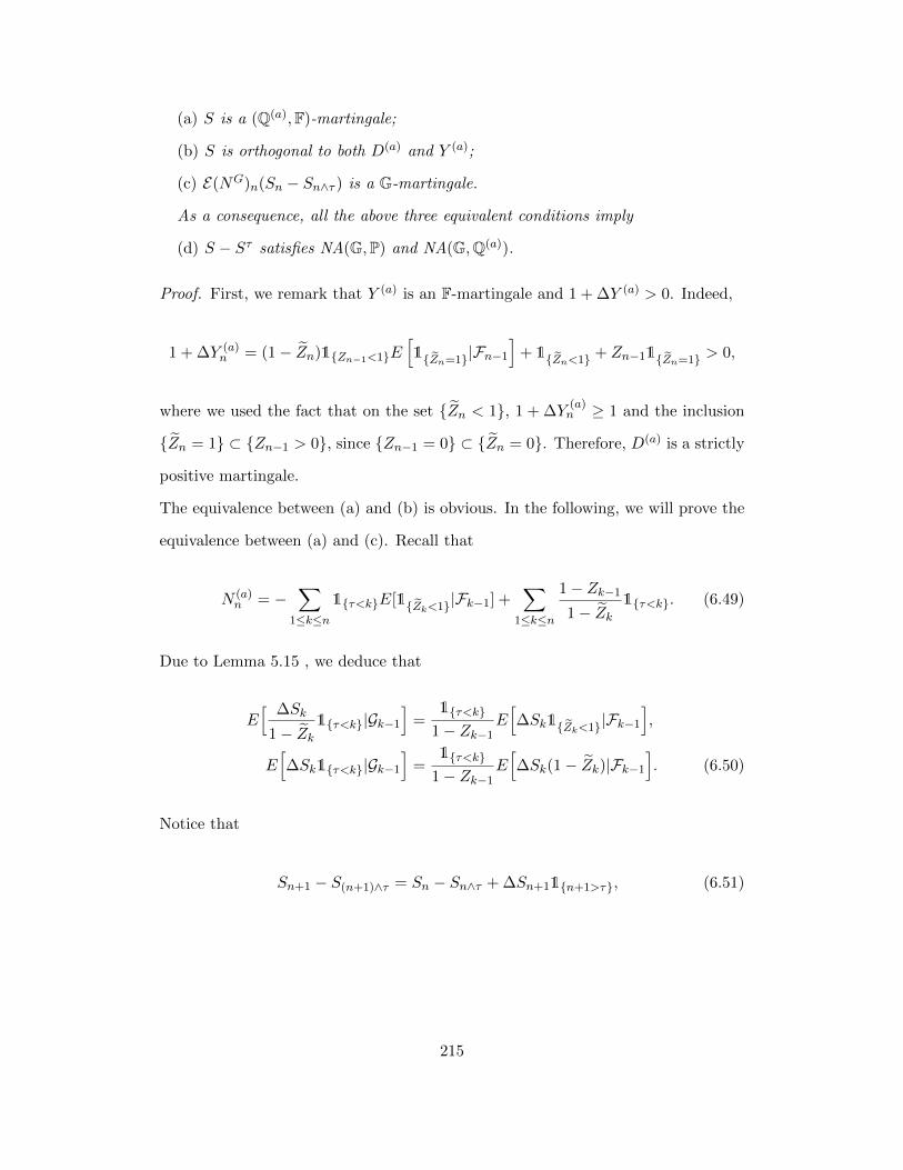
(a) S is a (Q(a),F)-martingale;
(b) S is orthogonal to both D(a) and Y (a);
(c) E(NG)n(Sn − Sn∧τ ) is a G-martingale.
As a consequence, all the above three equivalent conditions imply
(d) S − Sτ satisfies NA(G,P) and NA(G,Q(a)).
Proof. First, we remark that Y (a) is an F-martingale and 1 + ∆Y (a) > 0. Indeed,
1 + ∆Y (a)n = (1− Zn)1Zn−1<1E
[1Zn=1|Fn−1
]+ 1Zn<1 + Zn−11Zn=1 > 0,
where we used the fact that on the set Zn < 1, 1 + ∆Y(a)n ≥ 1 and the inclusion
Zn = 1 ⊂ Zn−1 > 0, since Zn−1 = 0 ⊂ Zn = 0. Therefore, D(a) is a strictly
positive martingale.
The equivalence between (a) and (b) is obvious. In the following, we will prove the
equivalence between (a) and (c). Recall that
N (a)n = −
∑1≤k≤n
1τ<kE[1Zk<1|Fk−1] +∑
1≤k≤n
1− Zk−1
1− Zk1τ<k. (6.49)
Due to Lemma 5.15 , we deduce that
E[ ∆Sk
1− Zk1τ<k|Gk−1
]=
1τ<k
1− Zk−1E[∆Sk1Zk<1|Fk−1
],
E[∆Sk1τ<k|Gk−1
]=
1τ<k
1− Zk−1E[∆Sk(1− Zk)|Fk−1
]. (6.50)
Notice that
Sn+1 − S(n+1)∧τ = Sn − Sn∧τ + ∆Sn+11n+1>τ, (6.51)
215
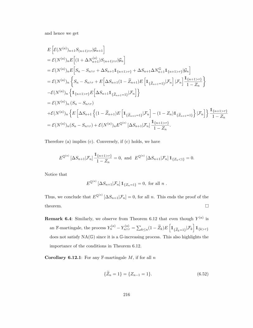
and hence we get
E[E(N (a))n+1S(n+1)∧τ |Gn+1
]= E(N (a))nE
[(1 + ∆N
(a)n+1)S(n+1)∧τ |Gn
]= E(N (a))nE
[Sn − Sn∧τ + ∆Sn+11n+1>τ + ∆Sn+1∆NG
n+11n+1>τ|Gn]
= E(N (a))n
Sn − Sn∧τ + E
[∆Sn+1(1− Zn+1)E
[1Zn+1=1|Fn
]|Fn]1n+1>τ
1− Zn
−E(N (a))n
1n+1>τE
[∆Sn+11Zn+1=1|Fn
]= E(N (a))n (Sn − Sn∧τ )
+E(N (a))n
E[∆Sn+1
(1− Zn+1)E
[1Zn+1=1|Fn
]− (1− Zn)1Zn+1=1
|Fn] 1n+1>τ
1− Zn
= E(N (a))n(Sn − Sn∧τ ) + E(N (a))nEQ(a)
[∆Sn+1|Fn]1n+1>τ
1− Zn.
Therefore (a) implies (c). Conversely, if (c) holds, we have
EQ(a)[∆Sn+1|Fn]
1n+1>τ
1− Zn= 0, and EQ(a)
[∆Sn+1|Fn]1Zn<1 = 0.
Notice that
EQ(a)[∆Sn+1|Fn]1Zn=1 = 0, for all n .
Thus, we conclude that EQ(a)[∆Sn+1|Fn] = 0, for all n. This ends the proof of the
theorem.
Remark 6.4: Similarly, we observe from Theorem 6.12 that even though Y (a) is
an F-martingale, the process Y(a)n − Y (a)
n∧τ =∑
k≤n(1− Zk)E[1Zk=1|Fk
]1k>τ
does not satisfy NA(G) since it is a G-increasing process. This also highlights the
importance of the conditions in Theorem 6.12.
Corollary 6.12.1: For any F-martingale M , if for all n
Zn = 1 = Zn−1 = 1. (6.52)
216

Then the following properties hold:
(a) The process Mn −Mn∧τ satisfies NA(G);
(b)(E(N (a))n (Mn −Mn∧τ )
)n≥1
is a G-martingale, where N (a) is given by (6.45)
in Proposition 6.4;
(c) The probability measure Q(a), given in (6.48), coincides with P.
Below, we state our second main theorem in this section, where we give the
necessary and sufficient conditions on the random time τ (or equivalently the stop-
ping times in (6.40)) to guarantee that the process M −M τ satisfies NA(G) for any
F-martingale M .
Theorem 6.13: Consider an honest time τ and the associated stopping times de-
fined in (6.40). Then the following are equivalent:
(a) For any F-martingale M , the process Mn −Mn∧τ satisfies NA(G).
(b) Zn = 1 = Zn−1 = 1 for all n.
(c) σ1 + 1 = σ2 = σ3.
(d) σ3 is an F-predictable stopping time.
(e) The probability Q(a), defined via (6.48)), coincides with P.
Proof. The proof of the theorem would be achieved after four steps. In the first
step, we prove (b)⇔(c). The second step focuses on (b)⇔(d). The third step deals
with (b)⇔(e). In the last step, we prove (a) ⇔ (b).
Step 1: The equivalence between (b) and (c) is obvious. Indeed, if (b) holds, it is
trivial that σ2 = σ3. Conversely, if (c) holds, we derive that
E(
(1− Zn−1)IZn=1
)= E
((1− Zn−1)IZn=1In<σ3
)= E
((1− Zn−1)IZn=1In<σ2
)= 0.
Hence, we conclude that Zn = 1 ⊂ Zn−1 = 1 for all n.
217
Step 2: Here, we will prove (b)⇔(d). If (b) holds, it is easy to see that σ3 is an
F-predictable stopping time. Conversely, due to the predictability of σ3 and
E[(1− Zn−1)IZn=1
]= E
[(1− Zn−1)In<σ3
]= E
[(1− Zn)In<σ3
]= 0,
we conclude that Zn = 1 ⊂ Zn−1 = 1 for all n.
Step 3: This step will prove (b)⇔(e). If (b) holds, apparently, Y (a) = 0 and Q(a) =
P. Conversely, if (e) holds, ∆Y(a)n = 0 for all n. Hence, (1−Zn)1Zn−1<1E
[1Zn=1|Fn−1
]=
(1− Zn−1)1Zn=1 = 0 and Zn = 1 = Zn−1 = 1 for all n.
Step 4: In this step, we focus on the proof of the equivalence between (a) and
(b). Suppose for any F-martingale M , the stopped process M τ satisfies NA(G).
Consider the F-martingale
Mn :=∑
1≤k≤n
(1Zk=1 − E
[1Zk=1|Fk−1
]).
It is easy to see that Mn −Mn∧τ = −∑
1≤k≤nE[1Zk=1|Fk−1
]1τ<k. Note that
Mn −Mn∧τ is a G predictable decreasing process satisfying NA(G). Therefore it is
null. Then, we deduce that
0 = E [Mn −Mn∧τ ] =∑
1≤k≤nE[E[1Zk=1|Fk−1
]1τ<k
]=∑
1≤k≤nE[(1− Zk−1)1Zk=1
].
Hence, Zk = 1 ⊂ Zk−1 = 1 for all k.
The reverse implication follows immediately from Theorem 6.12 or Corollary 6.12.1.
This ends the proof of the theorem.
218
6.6 Levy Market Model
In this section, we shall study Levy market model on the stochastic interval ]]τ,+∞[[
as Section 5.7 of Chapter 5. Suppose that the traded financial asset is an exponential
of a Levy process given by S = S0 exp(X), where
Xt = γt+ σWt +
∫ t
0
∫|x|≤1
xN(dt, dx) +
∫ t
0
∫|x|≥1
xN(dt, dx), (6.53)
N(dt, dx) = N(dt, dx)− νX(dx, dt) and νX(dx, dt) := FX(dx)dt. Here, γ and σ are
real numbers (σ > 0); W = (Wt)t≥0 represents a Brownian motion; N(dt, dx) is a
random measure on [0, T ]⊗R\0, called Poisson random measure; N(dt, dx) is the
compensated Poisson measure with the intensity measure FX(dx)dt, where FX(dx)
is called the Levy measure defined on R\0, satisfying
∫R\0
(|x|2 ∧ 1
)FX(dx) < +∞. (6.54)
Recall the random measure µ and its compensator ν are defined in (5.104) of Sub-
section 5.7 in Chapter 5.
In the same spirit as in Theorem 2.7, any local martingale Y can be decomposed as
follows
Y = β · Sc + f ? (µ− ν) + g ? µ+ Y ⊥. (6.55)
Here, (β, f, g, Y ⊥) is the Jacod’s components of Y with respect to S .
Let (βm, fm, gm,m′) be the Jacod’s parameters of m with respect to (S,F,P) such
that
m = βm · Sc + fm ? (µ− ν) + gm ? µ+m′. (6.56)
The Jacod parameters of m would be fixed throughout this section in which we
219

assume that
Zτ < 1, and νG ∼ ν on ]]τ,∞[[. (6.57)
Below, we recall the compensator of the random measure µ after τ (see Proposition
2.8 and Theorem 2.12 in Chapter 2).
Proposition 6.5: Consider the Levy market S. On ]]τ,+∞[[, we have
(a) The compensator of µ in the filtration G is given by
νG :=(I]]τ,∞[[ · µ
)p,G=
(1− fm
1− Z−
)I]]τ,∞[[ · ν (6.58)
(b) The canonical representation of I]]τ,∞[[ · S is given by
I]]τ,∞[[ · S = S0 + Sc(a)
+ h ? (µG − νG) + (x− h) ? µG +B, (6.59)
where Sc(a)
is defined via (6.9) and B = I]]τ,∞[[ · B − 11−Z− I]]τ,∞[[ · 〈Sc,m〉F −
h fm1−Z− I]]τ,∞[[ ? ν.
Proposition 6.6: Let τ be an honest time satisfying (6.57). The following process
D(a) is well defined, being a positive G-local martingale,
D(a) := E(N (a)) := E(
1
1− Z−βmI]]τ,∞[[ · Sc
(a)+
fm1− Z− − fm
I]]τ,∞[[ ?(µG − νG
)),
where Sc(a)
is defined via (6.9) and 1 + ∆N (a) > 0.
Proof. Note that
E[I]]τ,+∞[[I1−MP
µ [Z|P(F)]=0 ? µ]
= E[(1− Z)I1−MP
µ [Z|P(F)]=0 ? µ]
= E[(1−MP
µ
[Z|P(F)
])I1−MP
µ [Z|P(F)]=0 ? µ]
= 0.
220
Therefore, 1−Z−−fm = 1−MPµ [Z|P(F)] > 0,MP
µ -a.s. on ]]τ,+∞[[. Let us consider
δ ∈ (0, 1), Γ := ∆S 6= 0 and Γc its complement in Ω⊗ [0,+∞[.
Then, we calculate
V :=
√√√√ ∑0≤u≤·
(fm(∆Su)
1− Z− − fm(∆Su)IΓI]]τ,∞[[
)2
≤
√√√√ ∑0≤u≤·
(fm(∆Su)
1− Z− − fm(∆Su)I]]τ,∞[[IΓIfm<δ(1−Z−)
)2
+
√√√√ ∑0≤u≤·
(fm(∆Su)
1− Z− − fm(∆Su)I]]τ,∞[[IΓIfm≥δ(1−Z−)
)2
:= V1 + V2. (6.60)
Due to the G-local boundedness of (1−Z−)−1I]]τ,∞[[ and fm ∈ G2loc(µ,F) (i.e. f2
m ? µ ∈
A+loc(F)), we obtain that
V1(t) ≤ 1
1− δ
√√√√ ∑0≤u≤t
(fm(∆Su)
1− Zu−I]]τ,∞[[IΓIfm<δ(1−Zu−)
)2
≤ 1
1− δ
√√√√ ∑0≤u≤t
(f2m(∆Su)
(1− Zu−)2I]]τ,∞[[IΓ
)∈ A+
loc(G).
Now, we focus on the proof the G-local integrability of V2. Again due to the G-local
boundedness of (1 − Z−)−1I]]τ,∞[[ and f2m ? µ ∈ A+
loc(F), we deduce the existence of
a sequence of G-stopping times (Tn)n≥1 that increases to infinity and a sequence of
F-stopping times, (σn)n≥1, that increases to infinity such that
(1− Z−)−1I]]τ,+∞[[ ≤ n on [[0, Tn]] and Ef2m ? ν(σn) < +∞.
221
Then, we derive that
E [V2(Tn ∧ σn)] ≤ E[
|fm|1− fm − Z−
I]]τ,∞[[Iδ(1−Z−)≤fm<1−Z− ? µTn∧σn
]≤ E
[|fm|
1− fm − Z−I]]τ,∞[[Iδ/n≤fm<1−Z− ? µσn
]≤ E
[|fm|
1− fm − Z−(1− Z)I1−fm−Z−>0Iδ/n≤fm<1−Z− ? µσn
]= E
[|fm|Iδ/n≤fm<1−Z− ? µσn
]≤ n
δE[f2
m ? µσn ] < +∞.
As a result, V is G-locally integrable.
Secondly, the positivity of D(a) is obvious. Indeed, on ]]τ,+∞[[
1+∆N(a)t = 1+
fm(∆St)
1− Zt− − fm(∆St)I∆St 6=0 = I∆St=0+
1− Zt−1− Zt− − fm(∆St)
I∆St 6=0 > 0.
This ends the proof of the proposition.
Theorem 6.14: Let S be the Levy market satisfying NUPBR(F) and τ be an honest
time satisfying (6.57). Then, S − Sτ satisfies NUPBR(G).
Proof. The proof of the theorem mimics the proof of Theorem 5.16 in Chapter 5.
Here, we only need to show that
∑∆S∆N (a)I]]τ,+∞[[ = x
fm1− Z− − fm
I]]τ,+∞[[ ? µ
is locally integrable. Let (Tn)n≥1 be the localizing sequence of [S,m]. Then, we have
E
[|xfm|
1− fm − Z−I]]τ,+∞[[ ? µTn
]= E
[|xfm|
1− fm − Z−I1−fm−Z−>0(1− Z) ? µTn
]≤ E [|xfm| ? µTn ] ≤ E [V ar([S,m])Tn ] < +∞.
This ends the proof the theorem.
222
Corollary 6.14.1: Let Y be a compensated Poisson process and τ be an honest
time satisfying (6.57). Then Y − Y τ satisfies NUPBR(G).
Proof. The proof is the same as the proof of Corollary 5.16.1 in Chapter 5 and its
proof would be omitted.
Conclusions:
In this chapter, we obtained two principal results in the same spirit as those in Chap-
ter 5. The first result lies in describing the pairs of market model and honest time for
which the model fulfills NUPBR condition after an honest time. The second main
result characterizes the honest time models that preserve the NUPBR condition.
These results are elaborated in a very general market model, and also discrete time
and Levy market models. Furthermore, we construct explicit martingale densities
(deflators) for some classes of local martingales.
223

Chapter 7
Structural Models under
Additional Information
This chapter is dedicated to the question of how an extra information will affect
the stochastic structures of the market. The so-called ”Structure Conditions” (SC)
in the literature is imperative for the ”local” existence of the Markowitz’ optimal
portfolio or the solution to the local risk minimization problem. Herein, we consider
a semi-martingale market model (initial market model) fulfilling Structure Condi-
tions, and an arbitrary random time τ that is not adapted to the flow of the ”public”
information. By adding additional uncertainty to the initial market model, via this
random time τ , those structures may fail.
There are two mainstreams to combine the information coming from τ to the public
information F: The initial enlargement and progressive enlargement of the filtration
F (see [83], [77], [141] and the references therein). Herein, we restrict our attention
to adding the information from τ progressively to F, which results in a progressively
enlarged filtration G.
Precisely, we are dedicated to investigate the following two questions:
224
For which pair (τ, S), does S satisfy SC(G) if S satisfies SC(F)? (Prob(7.I))
and
For which τ , SC(G) holds for any model satisfying SC(F)? (Prob(7.II))
To answer the two problems (Prob(7.I)) and (Prob(7.II)), we split the time hori-
zon [[0,+∞[[ into two disjoint intervals [[0, τ ]] and ]]τ,+∞[[. In other words, we in-
vestigate the impact of τ on the structures of S by studying Sτ and S−Sτ separately.
Our analysis allowed us to conclude that under some mild assumptions on the market
model and the random time, these structures will remain valid on the one hand. Fur-
thermore, we provide two examples illustrating the importance of these assumptions.
On the other hand, we describe the random time models for which these structure
conditions are preserved for any market model. These results are elaborated sepa-
rately for the two contexts of stopping with random time and incorporating totally
a specific class of random times respectively.
Below, we recall the definition of Structure Conditions and two simple but useful
lemmas on Structure Conditions.
Definition 7.1: Let X be an H-adapted process. We say that X satisfies the
Structure Conditions under (H,Q) (hereafter, SC(H,Q)), if there exist M ∈
M20,loc(Q,H) and λ ∈ L2
loc(M,H) such that
X = X0 +M − λ 〈M〉H. (7.1)
When Q = P, we simply put SC(H).
Lemma 7.1: Let V be an H-predictable with finite variation process. Then, V
satisfies SC(H) if and only if V is constant (i.e. Vt ≡ V0, t ≥ 0).
225
Proof. If V satisfies SC(H), then there exist an H-local martingale MV and an
H-predictable process λH ∈ L2loc(M) such that V = V0 + MV + λH 〈MV ,MV 〉H.
Therefore, MV is an H-predictable local martingale with finite variation. Hence M
is null, and V ≡ V0. This ends the proof of the lemma.
The following lemma explains why one can split the study of the Structure
Conditions of (S,G) into two separate cases, namely (Sτ ,G) and (S − Sτ ,G).
Lemma 7.2: (S,G) satisfies the Structure Conditions if and only if both (Sτ ,G)
and (S − Sτ ,G) do.
Proof. The proof follows immediately from the definition.
This chapter is organized as follows. Section 7.1 contains two subsections where
we present the main results before τ and after τ . In Section 7.2, we develop the
stochastic tools that would be crucial to prove the main theorems. The last section
provides the proofs of the main theorems announced in Section 7.1.
7.1 The Main Results
In this section, we will summarize our main results in two subsections. The first
subsection addresses the problems (Prob(7.I)) and (Prob(7.II)) under stopping
with τ (i.e. we study Sτ instead), while the second subsection treats the case of τ
being an honest time and focuses on S−Sτ instead. To elaborate our main results,
we start by a stochastic basis (Ω,A,F = (Ft)t≥0,P), where F is a filtration satisfying
the usual conditions of right continuity and completeness and represents the flow
of “public” information over time. On this filtered probability space we consider a
d-dimensional F-adapted semimartingale, S, that models the tradable risky assets.
226
We assume that S is a special semimartingale with the Doob-Meyer decomposition
S = S0 +MS +AS , (7.2)
whereMS is a locally square integrable F-local martingale andAS is an F-predictable
finite variation process. Thus, (Ω,A,F, S,P) constitutes the initial market model.
In addition to this model, we consider additional information and/or uncertainty
that is modelled by an A-measurable random time τ : Ω → R+ that is fixed from
the beginning and for the entire chapter. To formulate this rigorously, we associate
to τ the process D and the progressive enlargement of filtration G given by
D := I[[τ,+∞[[, G = (Gt)t≥0 , where Gt =⋂s>t
(Fs ∨ σ(Du, u ≤ s)
). (7.3)
Recall the two Azema supermartingales given by
Zt := P(τ > t
∣∣ Ft) and Zt := P(τ ≥ t
∣∣∣ Ft) . (7.4)
The decomposition of Z leads to another important martingale m by
m := Z +Do,F, (7.5)
where Do,F is the F-dual optional projection of D = I[[τ,∞[[. Furthermore, we have
Z+ = Z and Z = Z− + ∆m.
7.1.1 Structure Conditions under Stopping with Random Time
In this section, we will investigate and quantify the effect of stopping with τ on the
Structure Conditions in two different ways. Below, we state the first main result
227

of this subsection, which provides sufficient condition on τ and S for which the
Structure Conditions are preserved after stopping with τ . This answers partially
the problem (Prob(7.I)).
Theorem 7.1: Consider any random time τ and suppose that S satisfies SC(F)
with the Doob-Meyer decomposition S := S0 +MS +AS. If
∆MS 6= 0 ∩ Z = 0 ∩ Z− > 0 = ∅, (7.6)
then Sτ satisfies SC(G).
Proof. The proof requires many intermediary results that are interesting in them-
selves. Therefore, this proof is delegated to Section 7.3.
Our second main theorem of this subsection answers completely the problem
(Prob(7.II)), and describes the random time models for which the Structure Con-
ditions are preserved after stopping with τ .
Theorem 7.2: Let τ be a random time. Then, the following are equivalent.
(a) The thin set Z = 0 ∩ Z− > 0 is evanescent.
(b) For any process X satisfying SC(F), Xτ satisfies SC(G).
Proof. The proof of (a) ⇒ (b) follows immediately from Theorem 7.1. To prove
the reverse sense, we assume that assertion (b) holds. Remark that Z = 0 ∩
Z− > 0 ⊂ ∆m 6= 0, it is a thin set, and consider T a stopping time such that
[[T ]] ⊂ Z = 0 ∩ Z− > 0. Then, M τ satisfies SC(G), where
M = V − V ∈M0(F), V := I[[T,+∞[[ and V := (V )p,F. (7.7)
Since τ < T, P − a.s. on T < +∞ (due to ZT = 0 on T < +∞), we deduce
that
M τ = −(V )τ is G− predictable and satisfies SC(G). (7.8)
228
Hence, by combining (7.8) and Lemma 7.1, we conclude that M τ is null (i.e. (V )τ =
0), or equivalently
0 = E(Vτ
)= E
(∫ +∞
0Zs−dVs
)= E
(ZT−IT<+∞
). (7.9)
Thus T = +∞, P − a.s., and the thin set Z = 0 ∩ Z− > 0 is evanescent (see
Proposition 2.18 on Page 20 in [78]). This ends the proof of the theorem.
Corollary 7.2.1: For any random time τ , if either m is continuous or Z is positive,
then Sτ satisfies SC(G) for any process S that satisfies SC(F).
Proof. Under the condition either m is continuous or Z is positive, the set Z =
0 ∩ Z− > 0 is evanescent. Hence, the proof of the corollary follows immediately
from Theorem 7.2. Below, we detail a direct proof for the case when m is continuous.
In fact this direct proof contains the key ideas for the proof of Theorem 7.1, but
with more delicate arguments due to the jumps.
Suppose that S satisfies SC(F) with the canonical decomposition S = S0 + M −
λ 〈M,M〉F, where M ∈ M2loc(F) and λ ∈ L2
loc(M,F). Put the G-locally square
integrable local martingale (see Jeulin [83])
M := I[[0,τ ]] M − (Z−)−1 I[[0,τ ]] 〈M,m〉F. (7.10)
Then, the canonical decomposition of Sτ under G has the form of
Sτ = S0 + M − λI[[0,τ ]] 〈M,M〉F + (Z−)−1 I[[0,τ ]] 〈M,m〉F. (7.11)
Thus, the proof will follow as long as we find a G-predictable process λ ∈ L2loc(M,G)
such that
−λI[[0,τ ]] 〈M,M〉F + (Z−)−1 I[[0,τ ]] 〈M,m〉F = λ 〈M〉G. (7.12)
229

Indeed, since m is continuous, the Galtchouk-Kunita-Watanabe decomposition of
m with respect to M under F implies the existence of an F-predictable process
βm ∈ L2loc(M) and a locally square integrable F-local martingale m⊥ such that
m = m0 + βm M +m⊥ and 〈M,m⊥〉F = 0. (7.13)
Therefore,
−λI[[0,τ ]] 〈M,M〉F +1
Z−I[[0,τ ]] 〈M,m〉F = −λI[[0,τ ]] 〈M,M〉F +
βmZ−
I[[0,τ ]] 〈M,M〉F
=
(−λ+
βmZ−
)I[[0,τ ]] 〈M,M〉F. (7.14)
It is easy to prove that I[[0,τ ]] 〈M〉F = I[[0,τ ]] 〈M〉G = I[[0,τ ]] 〈M〉G, due to the
continuity of m. Thus, we obtain
Sτ = S0 + M − λ 〈M〉G, (7.15)
where λ :=(λ− βm
Z−
)I[[0,τ ]]. It is obvious that λ ∈ L2
loc(M) due to the local bound-
edness of (Z−)−1 I[[0,τ ]]. This ends the proof of the corollary.
One may wonder what could happen when the condition (7.6) fails. Below, we
provide an example when Z = 0 < Z− is nonempty, and Sτ fails to satisfy SC(G)
(for the arbitrage opportunities in the example, we refer to Aksamit et al. [3]).
Proposition 7.1: Suppose that the stochastic basis (Ω,A,F = (Ft)t≥0, P ) supports
a Poisson process N with intensity λ, and the stock price –denoted by X– is given
by
dXt = Xt−ψdMt, where, ψ > −1, and ψ 6= 0, Mt = Nt − λt.
If
τ = k1T1 + k2T2,
230
where Ti = inft ≥ 0 : Nt ≥ i, i ≥ 1, k1, k2 > 0, and k1 + k2 = 1,
then Xτ does not satisfy SC(G).
Proof. We recall from Aksamit et al. [3] that the Azema supermartingale Z and m
take the forms of:
Z = I[[0,T1[[ + φmI[[T1,T2[[, m = 1− φmI]]T1,T2]] M, where φmt = e−λ k1
k2(t−T1)
. (7.16)
Then, it is easy to calculate that
1
Z−I[[0,τ ]] 〈X,m〉t =
−1
Z−I]]T1,τ ]]X−ψφ
m 〈M〉t
= −λ∫ t
0
1
Zu−I]]T1,τ ]]Xu−ψuφ
mu du = −λ
∫ t
0Xu−ψuI]]T1,τ ]]du
and
⟨X, X
⟩Gt
= I[[0,τ ]] 〈X,X〉t +1
Z−I[[0,τ ]]
(∑∆m(∆X)2
)p,Ft
= λ
∫ t
0X2u−ψ
2uI[[0,τ ]]du− λ
∫ t
0
1
Zu−X2u−ψ
2uφ
mu I]]T1,τ ]]du
= λ
∫ t
0X2u−ψ
2uI[[0,T1]]du,
where X is defined via (7.26). Hence, there is no G-predictable process λ ∈ L2loc(X)
satisfying
1
Z−I[[0,τ ]] 〈X,m〉 = λ
⟨X, X
⟩G, (7.17)
since ]]T1, τ ]] and [[0, T1]] are disjoint. This ends the proof of the proposition.
7.1.2 Structure Conditions under a Class of Honest Times
In this section, we focus on answering the two problems (Prob(7.I)) and (Prob(7.II))
when we totally incorporate a random time. This can be achieved by splitting the
whole half line into two stochastic intervals ]]0, τ ]] and ]]τ,+∞[[. The first part, i.e.
231
Sτ is already studied in the previous section. Thus, this section will concentrate on
studying the Structure Conditions of S on the stochastic interval ]]τ,+∞[[. The first
obstacle that one can face in this study is how far the (H ′)–hypothesis is preserved
on this interval (i.e. any F-semimartingale stays a G-semimartingale)? To overcome
this difficulty that is not our main focus in this chapter, we restrict our study to the
important class of random times, called honest times. Below, we recall its definition.
Definition 7.2: A random time τ is called an honest time, if for any t, there exists
an Ft-measurable random variable τt such that τIτ<t = τtIτ<t.
We refer to Jeulin [83, Chapter 4] for more information on honest times. Through-
out this section, the random time τ is supposed to be honest and satisfies
Zτ < 1, P − a.s. (7.18)
Remark 7.1: This assumption is also crucial for the validity of No-Unbounded-
Profit-with-Bounded-Risk after an honest time. We refer to Choulli et al [4] for
more details on this subject.
Now, we state the two main theorems in this section. This answers partially the
problem (Prob(7.I)) and completely the problem (Prob(7.II)).
Theorem 7.3: Let τ be an honest time satisfying Zτ < 1, a.s.. If S is a process
satisfying SC(F) and
∆MS 6= 0 ∩ Z = 1 > Z− = ∅, (7.19)
then S − Sτ satisfies SC(G).
Proof. The proof will be detailed in Section 7.3.
Theorem 7.4: Let τ be an F-honest time satisfying Zτ < 1, a.s.. Then, the following
are equivalent.
232
(a) The thin set Z = 1 > Z− is evanescent.
(b) For any process X satisfying SC(F), X −Xτ satisfies SC(G).
Proof. The proof of (a) ⇒ (b) is a direct consequence of Theorem 7.3. To prove
the reverse, we assume that assertion (b) holds, and follow similar steps as in the
proof of Theorem 7.2. For the sake of completeness, we give the full details. Since
Z = 1 ∩ Z− < 1 ⊂ ∆m 6= 0, it is a thin set. Let T be any stopping time such
that [[T ]] ⊂ Z = 1 ∩ Z− < 1. Then, consider the following F-martingale,
M = V − V ∈M0(F), where V := I[[T,+∞[[ and V := (V )p,F. (7.20)
Since T > τ ⊂ ZT < 1 (see Jeulin [83] or Choulli et al. [4]) and ZT = 1, we
deduce that τ ≥ T, P − a.s., and
M −M τ = −I]]τ,+∞[[ V (7.21)
which is G-predictable and satisfies SC(G). By combining (7.21) with Lemma 7.1,
we conclude that M −M τ is null (i.e. I]]τ,+∞[[ V = 0). Thus, we get
0 = E(I]]τ,+∞[[ V∞
)= E
(∫ +∞
0(1− Zs−)dVs
)= E
((1− ZT−)IT<+∞
), (7.22)
or equivalently (1−ZT−)IT<+∞ = 0 that implies that T = +∞, P−a.s.. Therefore
the thin set Z = 1 ∩ Z− < 1 is evanescent (see Proposition 2.18 on Page 20 in
[78]). This ends the proof of the theorem.
As a simple corollary, we have
Corollary 7.4.1: For any F-honest time τ satisfying Zτ < 1, P − a.s., if m is
continuous, then S − Sτ satisfies SC(G) for any process S that satisfies SC(F).
Proof. It is enough to notice that under the condition m is continuous, the set
1 = Z > Z− ⊂ ∆m 6= 0 is empty.
233
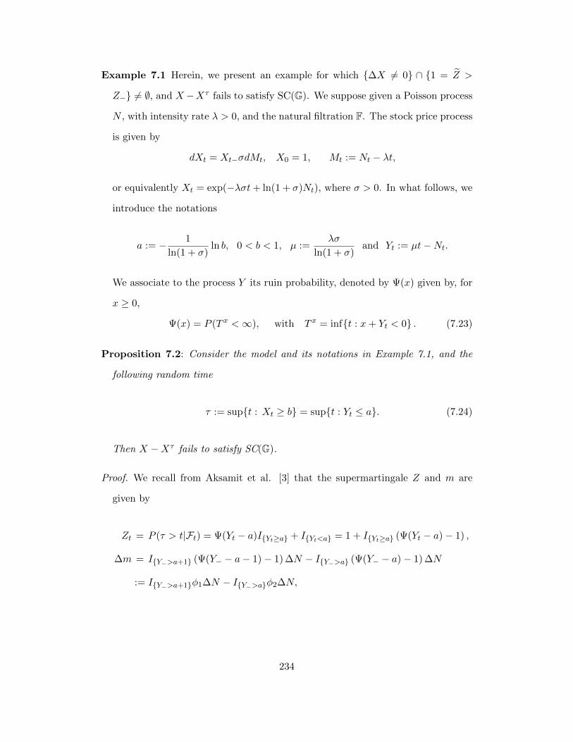
Example 7.1 Herein, we present an example for which ∆X 6= 0 ∩ 1 = Z >
Z− 6= ∅, and X−Xτ fails to satisfy SC(G). We suppose given a Poisson process
N , with intensity rate λ > 0, and the natural filtration F. The stock price process
is given by
dXt = Xt−σdMt, X0 = 1, Mt := Nt − λt,
or equivalently Xt = exp(−λσt+ ln(1 + σ)Nt), where σ > 0. In what follows, we
introduce the notations
a := − 1
ln(1 + σ)ln b, 0 < b < 1, µ :=
λσ
ln(1 + σ)and Yt := µt−Nt.
We associate to the process Y its ruin probability, denoted by Ψ(x) given by, for
x ≥ 0,
Ψ(x) = P (T x <∞), with T x = inft : x+ Yt < 0 . (7.23)
Proposition 7.2: Consider the model and its notations in Example 7.1, and the
following random time
τ := supt : Xt ≥ b = supt : Yt ≤ a. (7.24)
Then X −Xτ fails to satisfy SC(G).
Proof. We recall from Aksamit et al. [3] that the supermartingale Z and m are
given by
Zt = P (τ > t|Ft) = Ψ(Yt − a)IYt≥a + IYt<a = 1 + IYt≥a (Ψ(Yt − a)− 1) ,
∆m = IY−>a+1 (Ψ(Y− − a− 1)− 1) ∆N − IY−>a (Ψ(Y− − a)− 1) ∆N
:= IY−>a+1φ1∆N − IY−>aφ2∆N,
234
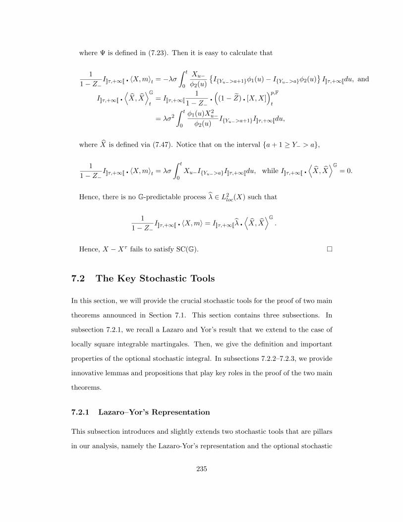
where Ψ is defined in (7.23). Then it is easy to calculate that
1
1− Z−I]]τ,+∞[[ 〈X,m〉t = −λσ
∫ t
0
Xu−φ2(u)
IYu−>a+1φ1(u)− IYu−>aφ2(u)
I]]τ,+∞[[du, and
I]]τ,+∞[[ ⟨X, X
⟩Gt
= I]]τ,+∞[[1
1− Z−(
(1− Z) [X,X])p,Ft
= λσ2
∫ t
0
φ1(u)X2u−
φ2(u)IYu−>a+1I]]τ,+∞[[du,
where X is defined via (7.47). Notice that on the interval a+ 1 ≥ Y− > a,
1
1− Z−I]]τ,+∞[[ 〈X,m〉t = λσ
∫ t
0Xu−IYu−>aI]]τ,+∞[[du, while I]]τ,+∞[[
⟨X, X
⟩G= 0.
Hence, there is no G-predictable process λ ∈ L2loc(X) such that
1
1− Z−I]]τ,+∞[[ 〈X,m〉 = I]]τ,+∞[[λ
⟨X, X
⟩G.
Hence, X −Xτ fails to satisfy SC(G).
7.2 The Key Stochastic Tools
In this section, we will provide the crucial stochastic tools for the proof of two main
theorems announced in Section 7.1. This section contains three subsections. In
subsection 7.2.1, we recall a Lazaro and Yor’s result that we extend to the case of
locally square integrable martingales. Then, we give the definition and important
properties of the optional stochastic integral. In subsections 7.2.2–7.2.3, we provide
innovative lemmas and propositions that play key roles in the proof of the two main
theorems.
7.2.1 Lazaro–Yor’s Representation
This subsection introduces and slightly extends two stochastic tools that are pillars
in our analysis, namely the Lazaro-Yor’s representation and the optional stochastic
235
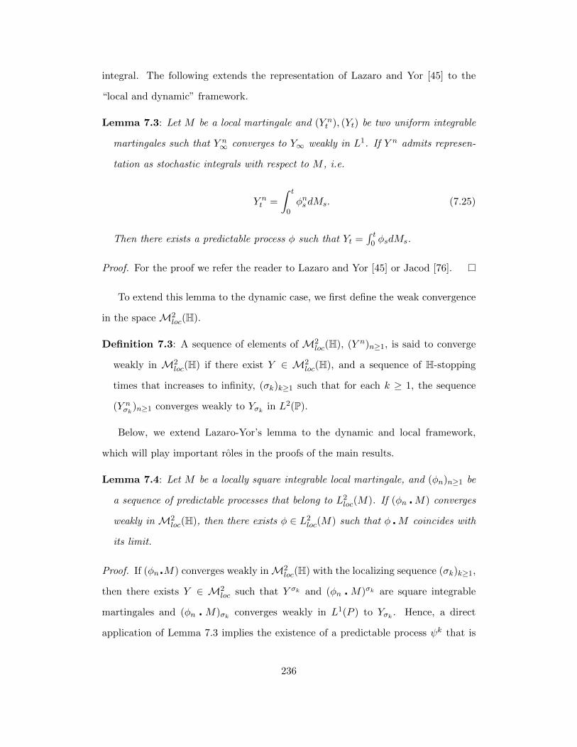
integral. The following extends the representation of Lazaro and Yor [45] to the
“local and dynamic” framework.
Lemma 7.3: Let M be a local martingale and (Y nt ), (Yt) be two uniform integrable
martingales such that Y n∞ converges to Y∞ weakly in L1. If Y n admits represen-
tation as stochastic integrals with respect to M , i.e.
Y nt =
∫ t
0φns dMs. (7.25)
Then there exists a predictable process φ such that Yt =∫ t
0 φsdMs.
Proof. For the proof we refer the reader to Lazaro and Yor [45] or Jacod [76].
To extend this lemma to the dynamic case, we first define the weak convergence
in the space M2loc(H).
Definition 7.3: A sequence of elements of M2loc(H), (Y n)n≥1, is said to converge
weakly in M2loc(H) if there exist Y ∈ M2
loc(H), and a sequence of H-stopping
times that increases to infinity, (σk)k≥1 such that for each k ≥ 1, the sequence
(Y nσk
)n≥1 converges weakly to Yσk in L2(P).
Below, we extend Lazaro-Yor’s lemma to the dynamic and local framework,
which will play important roles in the proofs of the main results.
Lemma 7.4: Let M be a locally square integrable local martingale, and (φn)n≥1 be
a sequence of predictable processes that belong to L2loc(M). If (φn M) converges
weakly in M2loc(H), then there exists φ ∈ L2
loc(M) such that φ M coincides with
its limit.
Proof. If (φn M) converges weakly inM2loc(H) with the localizing sequence (σk)k≥1,
then there exists Y ∈ M2loc such that Y σk and (φn M)σk are square integrable
martingales and (φn M)σk converges weakly in L1(P ) to Yσk . Hence, a direct
application of Lemma 7.3 implies the existence of a predictable process ψk that is
236
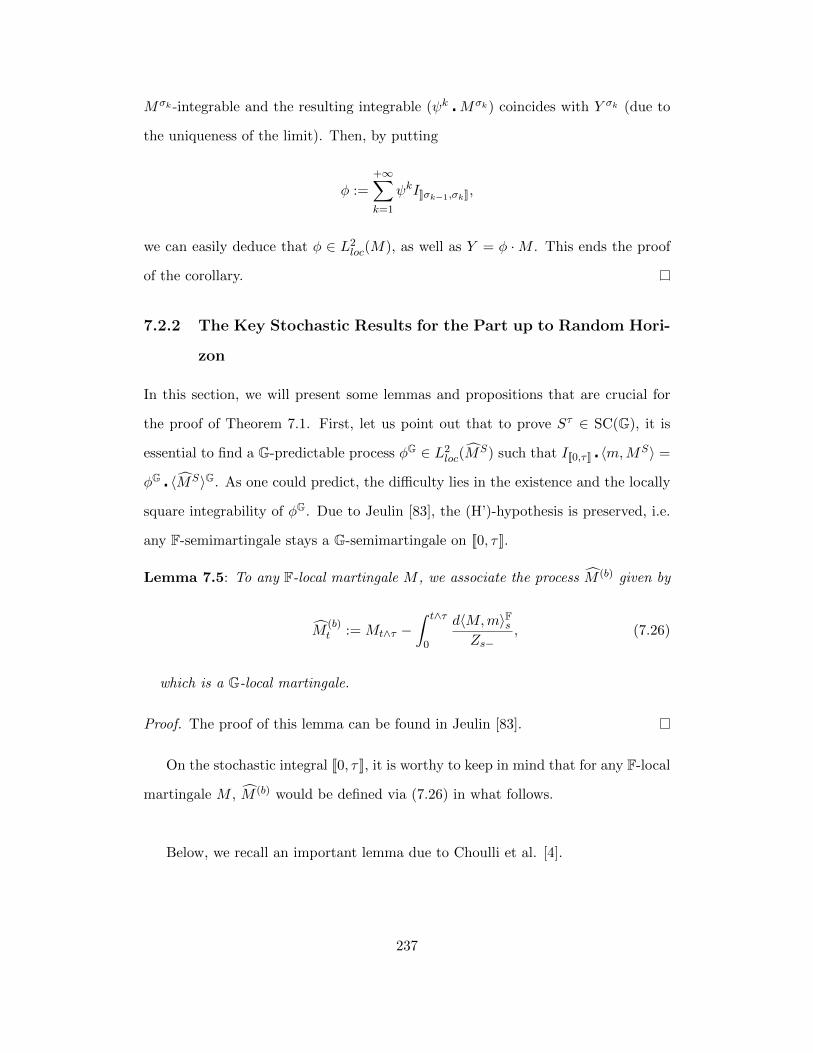
Mσk -integrable and the resulting integrable (ψk Mσk) coincides with Y σk (due to
the uniqueness of the limit). Then, by putting
φ :=+∞∑k=1
ψkI]]σk−1,σk]],
we can easily deduce that φ ∈ L2loc(M), as well as Y = φ ·M . This ends the proof
of the corollary.
7.2.2 The Key Stochastic Results for the Part up to Random Hori-
zon
In this section, we will present some lemmas and propositions that are crucial for
the proof of Theorem 7.1. First, let us point out that to prove Sτ ∈ SC(G), it is
essential to find a G-predictable process φG ∈ L2loc(M
S) such that I[[0,τ ]] 〈m,MS〉 =
φG 〈MS〉G. As one could predict, the difficulty lies in the existence and the locally
square integrability of φG. Due to Jeulin [83], the (H’)-hypothesis is preserved, i.e.
any F-semimartingale stays a G-semimartingale on [[0, τ ]].
Lemma 7.5: To any F-local martingale M , we associate the process M (b) given by
M(b)t := Mt∧τ −
∫ t∧τ
0
d〈M,m〉FsZs−
, (7.26)
which is a G-local martingale.
Proof. The proof of this lemma can be found in Jeulin [83].
On the stochastic integral [[0, τ ]], it is worthy to keep in mind that for any F-local
martingale M , M (b) would be defined via (7.26) in what follows.
Below, we recall an important lemma due to Choulli et al. [4].
237
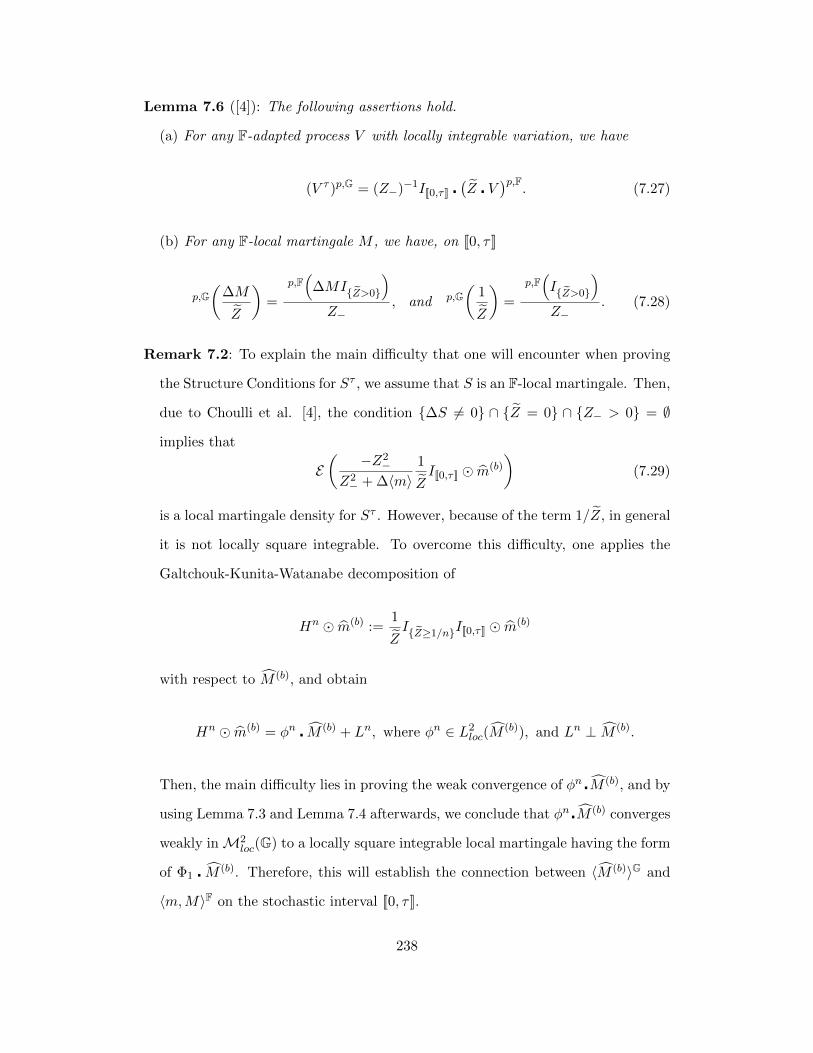
Lemma 7.6 ([4]): The following assertions hold.
(a) For any F-adapted process V with locally integrable variation, we have
(V τ )p,G = (Z−)−1I[[0,τ ]] (Z V
)p,F. (7.27)
(b) For any F-local martingale M , we have, on [[0, τ ]]
p,G(
∆M
Z
)=
p,F(
∆MIZ>0
)Z−
, and p,G(
1
Z
)=
p,F(IZ>0
)Z−
. (7.28)
Remark 7.2: To explain the main difficulty that one will encounter when proving
the Structure Conditions for Sτ , we assume that S is an F-local martingale. Then,
due to Choulli et al. [4], the condition ∆S 6= 0 ∩ Z = 0 ∩ Z− > 0 = ∅
implies that
E(
−Z2−
Z2− + ∆〈m〉
1
ZI[[0,τ ]] m(b)
)(7.29)
is a local martingale density for Sτ . However, because of the term 1/Z, in general
it is not locally square integrable. To overcome this difficulty, one applies the
Galtchouk-Kunita-Watanabe decomposition of
Hn m(b) :=1
ZIZ≥1/nI[[0,τ ]] m(b)
with respect to M (b), and obtain
Hn m(b) = φn M (b) + Ln, where φn ∈ L2loc(M
(b)), and Ln ⊥ M (b).
Then, the main difficulty lies in proving the weak convergence of φn M (b), and by
using Lemma 7.3 and Lemma 7.4 afterwards, we conclude that φn M (b) converges
weakly inM2loc(G) to a locally square integrable local martingale having the form
of Φ1 M (b). Therefore, this will establish the connection between 〈M (b)〉G and
〈m,M〉F on the stochastic interval [[0, τ ]].
238
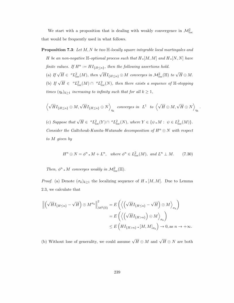
We start with a proposition that is dealing with weakly convergence in M2loc
that would be frequently used in what follows.
Proposition 7.3: Let M,N be two H-locally square integrable local martingales and
H be an non-negative H-optional process such that H [M,M ] and H [N,N ] have
finite values. If Hn := HIH≤n, then the following assertions hold.
(a) If√H ∈ oL2
loc(M), then√HIH≤nM converges in M2
loc(H) to√H M.
(b) If√H ∈ oL2
loc(M) ∩ oL2loc(N), then there exists a sequence of H-stopping
times (ηk)k≥1 increasing to infinity such that for all k ≥ 1,
⟨√HIH≤n M,
√HIH≤n N
⟩ηk
converges in L1 to⟨√
H M,√H N
⟩ηk.
(c) Suppose that√H ∈ oL2
loc(Y )∩ oL2loc(N), where Y ∈ ψ M : ψ ∈ L2
loc(M).
Consider the Galtchouk-Kunita-Watanabe decomposition of Hn N with respect
to M given by
Hn N = φn M + Ln, where φn ∈ L2loc(M), and Ln ⊥M. (7.30)
Then, φn M converges weakly in M2loc(H).
Proof. (a) Denote (σk)k≥1 the localizing sequence of H [M,M ]. Due to Lemma
2.3, we calculate that
∥∥∥(√HIH≤n −√H)Mσk∥∥∥2
M2(H)= E
(⟨(√HIH≤n −
√H)M
⟩σk
)= E
(⟨(√HIH>n
)M
⟩σk
)≤ E
(HIH>n [M,M ]σk
)→ 0, as n→ +∞.
(b) Without lose of generality, we could assume√H M and
√H N are both
239

square integrable. We derive from (a) and Kunita-Watanabe inequality that
E(∣∣∣⟨√HIH≤n M,
√HIH≤n N
⟩∞−⟨√
H M,√H N
⟩∞
∣∣∣)≤ E
(∣∣∣⟨√HIH≤n M,√HIH≤n N
⟩∞−⟨√
HIH≤n M,√H N
⟩∞
∣∣∣)+E
(∣∣∣⟨√HIH≤n M,√H N
⟩∞−⟨√
H M,√H N
⟩∞
∣∣∣)= E
(∣∣∣⟨√HIH≤n M,√HIH>n N
⟩∞
∣∣∣)+ E(∣∣∣⟨√HIH>n M,
√H N
⟩∞
∣∣∣)≤√E(⟨√
HIH≤n M⟩∞
)√E(⟨√
HIH>n N⟩∞
)+
√E(⟨√
HIH>n M⟩∞
)√E(⟨√
H N⟩∞
)→ 0, as n→ +∞.
(c) For any ψ ∈ L2loc(M), using Lemma 2.3, we derive
〈φn M,ψ M〉H = 〈Hn N,ψ M〉H =(Hn [N,ψ M ]
)p,H=⟨√
Hn N,ψ√Hn M
⟩H+∑
p,H(√
Hn∆N)p,H(ψ√Hn∆M
):= V n
1 + V n2 . (7.31)
Thanks to assertions (a) and (b), we deduce that both processes√Hn N and
ψ√Hn M converge weakly in M2
loc(H) to√H N and
√Hψ M, and
V n1 converges locally in L1(P ) to
⟨√H N,ψ
√H M
⟩H. (7.32)
240
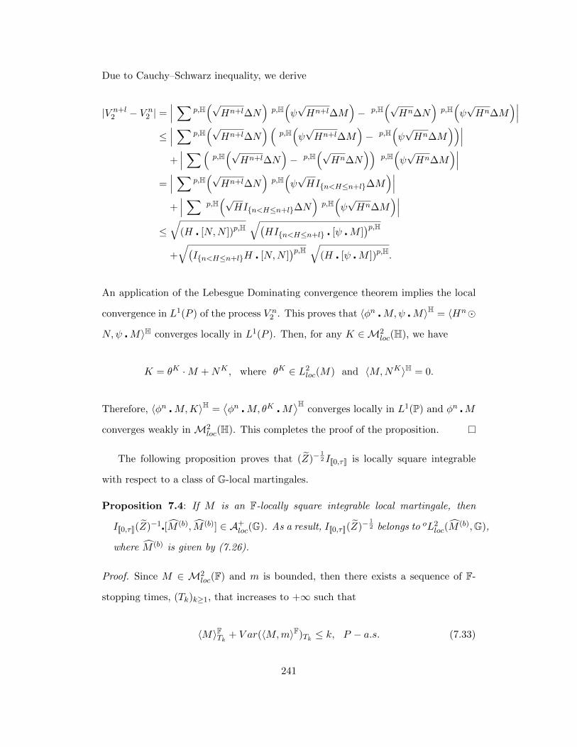
Due to Cauchy–Schwarz inequality, we derive
|V n+l2 − V n
2 | =∣∣∣ ∑ p,H
(√Hn+l∆N
)p,H(ψ√Hn+l∆M
)− p,H
(√Hn∆N
)p,H(ψ√Hn∆M
)∣∣∣≤∣∣∣ ∑ p,H
(√Hn+l∆N
)(p,H(ψ√Hn+l∆M
)− p,H
(ψ√Hn∆M
))∣∣∣+∣∣∣ ∑(
p,H(√
Hn+l∆N)− p,H
(√Hn∆N
))p,H(ψ√Hn∆M
)∣∣∣=∣∣∣ ∑ p,H
(√Hn+l∆N
)p,H(ψ√HIn<H≤n+l∆M
)∣∣∣+∣∣∣ ∑ p,H
(√HIn<H≤n+l∆N
)p,H(ψ√Hn∆M
)∣∣∣≤√
(H [N,N ])p,H√(
HIn<H≤n+l [ψ M ])p,H
+
√(In<H≤n+lH [N,N ]
)p,H √(H [ψ M ])p,H.
An application of the Lebesgue Dominating convergence theorem implies the local
convergence in L1(P ) of the process V n2 . This proves that 〈φn M,ψ M〉H = 〈Hn
N,ψ M〉H converges locally in L1(P ). Then, for any K ∈M2loc(H), we have
K = θK ·M +NK , where θK ∈ L2loc(M) and 〈M,NK〉H = 0.
Therefore, 〈φn M,K〉H =⟨φn M, θK M
⟩Hconverges locally in L1(P) and φn M
converges weakly in M2loc(H). This completes the proof of the proposition.
The following proposition proves that (Z)−12 I[[0,τ ]] is locally square integrable
with respect to a class of G-local martingales.
Proposition 7.4: If M is an F-locally square integrable local martingale, then
I[[0,τ ]](Z)−1[M (b), M (b)] ∈ A+loc(G). As a result, I[[0,τ ]](Z)−
12 belongs to oL2
loc(M(b),G),
where M (b) is given by (7.26).
Proof. Since M ∈ M2loc(F) and m is bounded, then there exists a sequence of F-
stopping times, (Tk)k≥1, that increases to +∞ such that
〈M〉FTk + V ar(〈M,m〉F)Tk ≤ k, P − a.s. (7.33)
241

Since Z−1− I[[0,τ ]] is locally bounded, then there exists a sequence of G-stopping times,
(τk)k≥1, that increases to +∞ and
sup0≤t≤τk
((Zt−)−1It≤τ
)≤ k, P − a.s. (7.34)
Consider
σk := τk ∧ Tk, k ≥ 1, and W := I[[0,τ ]](Z−)−1 〈M,m〉F. (7.35)
Then it is clear that (σk)k≥1 is a localizing sequence for the process W , and due to
Lemma 7.6-(b), we obtain
E
I[[0,τ ]]
Z [M (b)]σk
≤ 2E
I[[0,τ ]]
Z [M ]Tk
+ 2E
I[[0,τ ]]
Z [W ]σk
≤ 2E
IZ>0 [M ]Tk
+ 2E
I[[0,τ ]]
Z− [W ]σk
≤ 2E[M ]Tk + 2kE[W ]σk < +∞.
Hence, Z−1I[[0,τ ]] [M(b)] is locally integrable and I[[0,τ ]](Z)−1/2 ∈ oL2
loc(M(b),G) (see
He et al. [71]).
Throughout the rest of this subsection, we will stick to the following notations
hn := IZ≥ 1n, Hn := Z−
(Z)−1
hn, n ≥ 1. (7.36)
As an application of Proposition 7.3 and Proposition 7.4, in the following, we prove
that φn M (b) converges weakly inM2loc(G), where Hnm(b) = φn M (b) +Ln, φn ∈
L2loc(M
(b)), and Ln ⊥ M (b).
Proposition 7.5: Let M ∈M2loc(F) and M (b) is given by (7.26). Then the follow-
ing hold:
(a)(I[[0,τ ]](Z)−1/2IZ≥1/n M
(b))
converges inM2loc(G) to
(I[[0,τ ]](Z)−1/2 M (b)
).
242
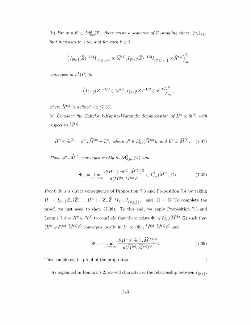
(b) For any K ∈ M2loc(F), there exists a sequence of G-stopping times, (ηk)k≥1
that increases to +∞, and for each k ≥ 1
⟨I[[0,τ ]](Z)−1/2IZ≥1/n M
(b), I[[0,τ ]](Z)−1/2IZ≥1/n K(b)⟩Gηk
converges in L1(P ) to
⟨I[[0,τ ]](Z)−1/2 M (b), I[[0,τ ]](Z)−1/2 K(b)
⟩Gηk,
where K(b) is defined via (7.26).
(c) Consider the Galtchouk-Kunita-Watanabe decomposition of Hn m(b) with
respect to M (b)
Hn m(b) = φn M (b) + Ln, where φn ∈ L2loc(M
(b)), and Ln ⊥ M (b). (7.37)
Then, φn M (b) converges weakly in M20,loc(G) and
Φ1 := limn→+∞
d〈Hn m(b), M (b)〉G
d〈M (b), M (b)〉G∈ L2
loc(M(b),G). (7.38)
Proof. It is a direct consequence of Proposition 7.3 and Proposition 7.4 by taking
H := I[[0,τ ]]Z−(Z)−1, Hn := Z−Z−1I[[0,τ ]]IZ≥ 1
n, and H = G. To complete the
proof, we just need to show (7.38). To this end, we apply Proposition 7.3 and
Lemma 7.4 to Hn m(b) to conclude that there exists Φ1 ∈ L2loc(M
(b),G) such that
〈Hn m(b), M (b)〉G converges locally in L1 to 〈Φ1 M (b), M (b)〉G and
Φ1 := limn→+∞
d〈Hn m(b), M (b)〉G
d〈M (b), M (b)〉G. (7.39)
This completes the proof of the proposition.
As explained in Remark 7.2, we will characterize the relationship between I[[0,τ ]]
243
〈m,M〉F and 〈M (b), M (b)〉G. This is the main focus of the following.
Proposition 7.6: Let M ∈ M2loc(F) and M (b) be given in (7.26). If ∆M 6=
0 ∩ 0 = Z < Z− = ∅, we have
1
Z−I[[0,τ ]] 〈m,M〉F = Φ1 〈M (b)〉G, and Φ1 ∈ L2
loc(M(b),G), (7.40)
where Φ1 := Φ1
(p,F(IZ>0
)(Z2− + ∆〈m〉F
))−1Z−I[[0,τ ]] and Φ1 is given in
(7.38).
Proof. By Proposition 7.5, we know that
limn〈Hn m(b), M (b)〉G = Φ1 〈M (b), M (b)〉G, (7.41)
where Hn and m(b) are defined in (7.36) and (7.26) respectively. Now it remains to
describe explicitly the limit limn 〈Hn m(b), M (b)〉G. To this end, we first calculate
1
Z− [m(b), M (b)] =
1
Z−I[[0,τ ]] [m,M ]− I[[0,τ ]]
∆M
Z2−
〈m〉F − ∆m
Z2−I[[0,τ ]] 〈M,m〉F
+1
Z3−I[[0,τ ]]∆〈m〉F 〈M,m〉F. (7.42)
Then, by integrating Hn on both sides above, and using the properties of optional
integration (see Proposition 2.3 and Proposition 7.3), we obtain
1
Z−I[[0,τ ]] (hn [m,M ])p,F =
1
Z−I[[0,τ ]] (Hn [m,M ])p,G
=( 1
Z−Hn [m(b), M (b)]
)p,G+I[[0,τ ]]
p,G(Hn∆M
)Z2−
〈m〉F
+I[[0,τ ]]
p,G(Hn∆m
)Z2−
〈M,m〉F − I[[0,τ ]]∆〈M,m〉F
Z3−
p,G(Hn)〈m〉F. (7.43)
244
Due to ∆M 6= 0 ∩ 0 = Z < Z− = ∅, we get
p,F(
∆MIZ>0
)= p,F (∆M) = 0.
By taking the limit, we derive
limn
I[[0,τ ]]
Z− (hn [m,M ])p,F =
I[[0,τ ]]
Z−(IZ>0 [m,M ]
)p,F=I[[0,τ ]]
Z− 〈m,M〉F,
limnI[[0,τ ]]
p,G(Hn∆M
)Z2−
〈m〉F = I[[0,τ ]]
−p,F(
∆MIZ=0
)Z2−
〈m〉F = 0, (7.44)
and
limn
p,G (Hn) I[[0,τ ]] = p,F(IZ>0
)I[[0,τ ]],
limnI[[0,τ ]]
p,G(Hn∆m
)Z2−
= I[[0,τ ]]
p,F(
∆mIZ>0
)Z2−
= I[[0,τ ]]
p,F(IZ=0
)Z−
, (7.45)
where in (7.43)-(7.45) we used Lemma 7.6. Then, by combining the above equalities
and (7.38), we conclude that
Φ1 〈M (b)〉G = limn
(Hn [m(b), M (b)]
)p,G= I[[0,τ ]]
p,F(IZ>0
)(1 +
∆〈m〉F
Z2−
) 〈M,m〉F.
The proof of the proposition is completed due to the G-local boundedness of(p,F(IZ>0
))−1I[[0,τ ]] (see Lemma 7.7 below).
Lemma 7.7: The following process
V (b) :=(p,F(IZ>0
))−1I[[0,τ ]] (7.46)
is G-predictable and locally bounded.
Proof. It is enough to notice that Z ≤ IZ>0 and the process (Z−)−1I[[0,τ ]] is G-
locally bounded.
245
7.2.3 The Key Stochastic Results for the Part after an Honest Time
In this section, we will present some lemmas and propositions that are useful for the
proof of Theorem 7.3.
Lemma 7.8: For any F-local martingale M , we associate M (a) given by,
M (a) := I]]τ,+∞[[ M + I]]τ,+∞[[ (1− Z−)−1 〈M,m〉F, (7.47)
which is a G-local martingale.
Proof. The proof can be found in [17], [53] and [83].
Similarly as in the part on [[0, τ ]], we will keep the notation M (a) defined in (7.47)
for any F-local martingale M .
Below, we recall an important lemma due to Choulli et al. [4].
Lemma 7.9: Suppose that Zτ < 1. Then the following assertions hold.
(a) The process (1− Z−)−1I]]τ,+∞[[ is a G-locally bounded and predictable process.
(b) For any F-adapted process with locally integrable variation, V , we have
I]]τ,+∞[[ Vp,G = I]]τ,+∞[[ (1− Z−)−1
((1− Z) V
)p,F. (7.48)
(c) For any process V as in (b), the G-predictable projection of ∆V , is given on
]]τ,+∞[[ by
p,G (∆V ) = (1− Z−)−1 p,F(
(1− Z)∆V). (7.49)
(d) For any F-local martingale, on ]]τ,+∞[[, we have
p,G(
∆M
1− Z
)=
p,F(
∆MIZ<1
)1− Z−
, and p,G(
1
1− Z
)=
p,F(IZ<1
)1− Z−
. (7.50)
246
The following proposition proves that (1 − Z)−12 I]]τ,+∞[[ is locally square inte-
grable with respect to a class of G-local martingales.
Proposition 7.7: Let M be an F-locally square integrable local martingale, then
I]]τ,+∞[[
(1− Z
)−1 [M (a)] ∈ A+
loc(G),
where M (a) is defined via (7.47). As a result, I]]τ,+∞[[
(1− Z
)−1/2∈ oL2
loc(M(a),G).
Proof. Let us denote the localizing sequences ofW := I]]τ,+∞[[ (1− Z−)−1/2〈M,m〉F,
(1− Z−)−1I]]τ,+∞[[ and [M ] by (σn)n≥1, (τn)n≥1 and (Tn)n≥1 respectively. Then, due
to Lemma 7.9, we derive that
E
I]]τ,+∞[[
1− Z [M (a)]σn∧τn∧Tn
≤ 2E
I]]τ,+∞[[
1− Z [M ]Tn
+ 2E
I]]τ,+∞[[
1− Z [W ]σn∧τn
≤ 2E[M ]Tn + E
2I]]τ,+∞[[
1− Z− [W ]σn∧τn
< +∞.
This ends the proof of the proposition.
Throughout the rest of this subsection, we will use the following notations
kn := I1−Z≥ 1n, Kn := (1− Z−)
(1− Z
)−1kn, n ≥ 1. (7.51)
As a counterpart of Proposition 7.5, we have on ]]τ,+∞[[:
Proposition 7.8: Let M ∈M2loc(F), M (a) defined by (7.47) and
Un := Kn (1− Z−)−1 I]]τ,+∞[[, n ≥ 1.
Then, the following assertions hold.
(a)(√
Un M (a))
converges to
(I]]τ,+∞[[√
1−Z M (a)
)in M2
loc(G).
(b) For any L ∈ M2loc(F), there exists a sequence of G-stopping times (ηk)k≥1
247
increasing to infinity such that for all k,⟨√
Un M (a),√Un L
⟩Gηk
converges
in L1(P ) to
⟨I]]τ,+∞[[√
1−Z M (a),
I]]τ,+∞[[√1−Z
L⟩G
ηk
.
Proof. The proof is similar to the proof of Proposition 7.3. Indeed, it is enough
to consider the G-locally bounded process (1 − Z−)−1I]]τ,+∞[[, and use the same
techniques as in Proposition 7.3.
Lemma 7.10: Under the condition Zτ < 1, the following process
V (a) :=(p,F(IZ<1
))−1I]]τ,+∞[[ (7.52)
is G-predictable and locally bounded.
Proof. It is enough to notice that 1− Z ≤ IZ<1 and the process (1−Z−)−1I]]τ,+∞[[
is G-locally bounded.
Proposition 7.9: Let M ∈M2loc(F) and M (a) is given by (7.47). Then, the follow-
ing hold.
(a) Consider the Galtchouk-Kunita-Watanabe decomposition of Kn m(a) with
respect to M (a)
Kn m(a) = θn M (a) + Ln, where θn ∈ L2loc(M
(a)), and Ln ⊥ M (a). (7.53)
Then, (θn M (a)) converges weakly in M2loc(G).
As a result, we have
Φ2 := limn→+∞
d〈Kn m(a), M (a)〉G
d〈M (a), M (a)〉G∈ L2
loc(M(a),G). (7.54)
248
(b) If ∆M 6= 0 ∩ 1 = Z > Z− = ∅, we have
1
1− Z−I]]τ,+∞[[ 〈m,M〉F = Φ2I[[0,τ ]] 〈M (a)〉G, and Φ2 ∈ L2
loc(M(a)),(7.55)
where
Φ2 := Φ2
(p,F(IZ<1
)(1 +
∆〈m〉F
(1− Z−)2
))−1 I]]τ,+∞[[
1− Z−, and Φ2 is given in (7.54).
Proof. (a) It is a consequence of Proposition 7.3 and Lemma 7.4 by taking
Kn := (1− Z−)(
1− Z)−1
I1−Z≥ 1n, and H = G. (7.56)
(b) Now it remains to describe explicitly the limit in (7.54), that is limn 〈Kn
m(a), M (a)〉G. To this end, we first calculate
1
1− Z− [m(a), M (a)] =
1
Z−I]]τ,+∞[[ [m,M ] + I]]τ,+∞[[
∆M
(1− Z−)2 〈m〉F
+∆m
(1− Z−)2I]]τ,+∞[[ 〈M,m〉F +
1
(1− Z−)3I]]τ,+∞[[∆〈m〉F 〈M,m〉F. (7.57)
Then by integrating Kn on both sides above, and using the properties of optional
integration (see Proposition 2.3 and Proposition 7.9), we obtain
1
1− Z−I]]τ,+∞[[ (kn [m,M ])p,F =
1
1− Z−I]]τ,+∞[[ (Kn [m,M ])p,G
=( 1
1− Z−Kn [m(a), M (a)]
)p,G−I]]τ,+∞[[
p,G(Kn∆M
)(1− Z−)2
〈m〉F
−I]]τ,+∞[[
p,G(Kn∆m
)(1− Z−)2
〈M,m〉F − I]]τ,+∞[[∆〈M,m〉F
(1− Z−)3p,G(Kn)〈m〉F. (7.58)
Due to ∆M 6= 0 ∩ 1 = Z > Z− = ∅, we have
p,F(
∆MIZ<1
)IZ−<1 = p,F (∆M) IZ−<1 = 0.
249
By taking the limit, we derive
limn
I]]τ,+∞[[
1− Z− (kn [m,M ])p,F =
I]]τ,+∞[[
1− Z−(IZ<1 [m,M ]
)p,F=I]]τ,+∞[[
1− Z− 〈m,M〉F,
limnI]]τ,+∞[[
p,G(Kn∆M
)(1− Z−)2
〈m〉F = I]]τ,+∞[[
−p,F(
∆MIZ=1
)(1− Z−)2
〈m〉F = 0, (7.59)
and
limn
p,G (Kn) I]]τ,+∞[[ = p,F(IZ<1
)I]]τ,+∞[[,
limnI]]τ,+∞[[
p,G(Kn∆m
)(1− Z−)2
= I]]τ,+∞[[
p,F(
∆mIZ<1
)(1− Z−)2
= −I]]τ,+∞[[
p,F(IZ=1
)1− Z−
. (7.60)
Then, by combining (7.54), (7.58) and (7.59), we conclude that
Φ2 〈M (a), M (a)〉G = limn
(Kn
[m(b), M (a)
] )p,G= I]]τ,+∞[[
p,F(IZ<1
)(1 +
∆〈m〉F
(1− Z−)2
) 〈M,m〉F.
The proof of the proposition is completed.
7.3 Proofs of Theorems 7.1 and 7.3
Now, we have prepared all the ingredients to prove the two main theorems of Section
7.1 (Theorems 7.1 and 7.3).
7.3.1 Proof of Theorem 7.1
Suppose that S satisfies Structure Conditions under F. Then, there exist a lo-
cally square integrable F-local martingale, MS , and an F-predictable process λ ∈
L2loc(M
S ,F) such that
S = S0 +MS +AS = S0 +MS − λ 〈MS〉F. (7.61)
250

For notational simplicity, we put M = MS and M (b) = MS(b)
, where MS(b)
is
defined via (7.26). Then the G-canonical decomposition of Sτ has the form of
Sτ = S0 +M τ − λI[[0,τ ]] 〈M〉F =: S0 + M (b) +1
Z−I[[0,τ ]] 〈M,m〉F − λI[[0,τ ]] 〈M〉F.
Recall the notations in (7.36),
hn := IZ≥ 1n, Hn := Z−
(Z)−1
hn, n ≥ 1.
Consider the following locally square integrable G-local martingale.
N (b) :=1
Z− m(b) − λ M (b). (7.62)
Notice that
1
Z−I[[0,τ ]] [m,M ]− λI[[0,τ ]] [M ] = [N (b), M (b)] +
∆m
Z2−I[[0,τ ]] 〈M,m〉F
+∆M
Z2−I[[0,τ ]] 〈m〉F −
∆〈M,m〉F
Z3−
I[[0,τ ]] 〈m〉F −2λ
Z−∆M 〈M,m〉F +
λ
Z2−
∆〈M,m〉F 〈M,m〉F.
Then, by integrating both sides with Hn and combining the obtained equality with
the properties of the optional integral (see Proposition 2.3 and Lemma 7.6), we
251
derive that
1
Z−I[[0,τ ]] (hn [m,M ])p,F − λI[[0,τ ]] (hn [M ])p,F
=1
Z−I[[0,τ ]] (Hn [m,M ])p,G − λI[[0,τ ]] (Hn [M ])p,G
=(Hn [N (b), M (b)]
)p,G+
p,G(Hn∆M
)(Z−)2
I[[0,τ ]] 〈m〉F −∆〈M,m〉F p,G
(Hn)
(Z−)3I[[0,τ ]] 〈m〉F
− 2λ
Z−p,G(Hn∆M
)I[[0,τ ]] 〈M,m〉F +
λ∆〈M,m〉F
(Z−)2p,G(Hn)I[[0,τ ]] 〈M,m〉F
+
p,G(Hn∆m
)(Z−)2
I[[0,τ ]] 〈M,m〉F. (7.63)
Then, the similar arguments as the limits in (7.44) lead to conclude that
limn
(Hn [N (b), M (b)]
)p,G= I[[0,τ ]]
1
Z− 〈M,m〉F − λI[[0,τ ]] 〈M〉F +R(b) 〈M,m〉F,
where
R(b) :=1
Z−
(− p,F(IZ=0) +
∆〈m〉F
Z2−
p,F(IZ>0)−λ∆〈M,m〉F
Z−p,F(IZ>0)
)I[[0,τ ]].
Again, by applying Proposition 7.3 to Hn N (b) and M (b), we conclude that there
exists Φ(b) ∈ L2loc(M
(b),G) such that
〈Hn N (b), M (b)〉G converges locally in L1 to 〈Φ(b) M (b), M (b)〉G.
Recall that I[[0,τ ]] 〈M,m〉F = Φ1 〈M (b)〉G in (7.55). Thus, the uniqueness of the
limit leads to
I[[0,τ ]]1
Z− 〈M,m〉F − λI[[0,τ ]] 〈M〉F =
(Φ(b) −R(b) Φ1
) 〈M (b)〉G. (7.64)
252
Due to the locally boundedness of Z−1− I[[0,τ ]], it is easy to see that
λG :=(
Φ(b) −R(b) Φ1
)∈ L2
loc(M(b),G), (7.65)
and
Sτ = S0 + M (b) + λG 〈M (b), M (b)〉G. (7.66)
This proves the Structure Conditions for Sτ under G, and the proof of the theorem
is completed.
7.3.2 Proof of Theorem 7.3
Suppose that S satisfies Structure Conditions under F. Then, there exist a lo-
cally square integrable F-local martingale, MS , and an F predictable process λ ∈
L2loc(M
S ,F) such that
S = S0 +MS +AS = S0 +MS − λ 〈MS〉F. (7.67)
For notational simplicity, we put M = MS and M (a) = MS(a)
, where MS(a)
is
defined via (7.47). Then we get
I]]τ,+∞[[ S = I]]τ,+∞[[ M − λI]]τ,+∞[[ 〈M〉F
=: M (a) − 1
1− Z−I]]τ,+∞[[ 〈M,m〉F − λI]]τ,+∞[[ 〈M〉F. (7.68)
Recall the notations in (7.51),
kn := I1−Z≥ 1n, Kn := (1− Z−)
(1− Z
)−1kn, n ≥ 1.
253
Consider the following locally square integrable G-local martingale.
N (a) := − 1
1− Z− m(a) − λ M (a), (7.69)
where m(a) is given by (7.47). Notice that
− 1
1− Z−I]]τ,+∞[[ [m,M ] − λI]]τ,+∞[[ [M ] = [N (a), M (a)] +
∆m
(1− Z−)2I]]τ,+∞[[ 〈M,m〉F
+∆M
(1− Z−)2I]]τ,+∞[[ 〈m〉F +
∆〈M,m〉F
(1− Z−)3I]]τ,+∞[[ 〈m〉F
+2λ
1− Z−∆M 〈M,m〉F +
λ
(1− Z−)2∆〈M,m〉F 〈M,m〉F.
Then, by integrating both sides with Kn and combining the obtained equality with
the properties of the optional integral (see Proposition 2.3 and Lemma 7.9), we
derive
− 1
1− Z−I]]τ,+∞[[ (kn [m,M ])p,F − λI]]τ,+∞[[ (kn [M ])p,F
= − 1
1− Z−I]]τ,+∞[[ (Kn [m,M ])p,G − λI]]τ,+∞[[ (Kn [M ])p,G
=(Kn [N (a), M (a)]
)p,G+
p,G(Kn∆M
)(1− Z−)2
I]]τ,+∞[[ 〈m〉F +∆〈M,m〉F p,G
(Kn)
(1− Z−)3I]]τ,+∞[[ 〈m〉F
+2λ
1− Z−p,G(Kn∆M
)I]]τ,+∞[[ 〈M,m〉F +
λ∆〈M,m〉F
(1− Z−)2p,G(Kn)I]]τ,+∞[[ 〈M,m〉F
+
p,G(Kn∆m
)(1− Z−)2
I]]τ,+∞[[ 〈M,m〉F. (7.70)
Then, the similar arguments as in (7.59) lead to conclude that
limn
(Kn [N (a), M (a)]
)p,G= I]]τ,+∞[[
−1
1− Z−〈M,m〉F−λI]]τ,+∞[[〈M〉F+R(a)〈M,m〉F,
254

where
R(a) :=−1
1− Z−
(− p,F(IZ=1) +
∆〈m〉F
(1− Z−)2p,F(IZ<1
)+λ∆〈M,m〉F
1− Z−p,F(IZ<1
))I]]τ,+∞[[.
Again, by applying Proposition 7.3 to Kn N (a) and M (a), we conclude that there
exists Φ(a) ∈ L2loc(M
(a),G) such that
〈Kn N (a), M (a)〉G converges locally in L1 to 〈Φ(a) M (a), M (a)〉G.
Recall that I]]τ,∞[[ 〈M,m〉F = Φ2 〈M (a)〉G in (7.55). Thus, the uniqueness of the
limit leads to
I]]τ,+∞[[−1
1− Z− 〈M,m〉F − λI]]τ,+∞[[ 〈M〉F =
(Φ(a) −R(a) Φ2
) 〈M (a)〉G.(7.71)
Due to the locally boundedness of (1− Z−)−1I]]τ,+∞[[, it is easy to see that
λG :=(
Φ(a) −R(a) Φ2
)∈ L2
loc(M(a),G), (7.72)
and satisfies
I]]τ,+∞[[ S = M (a) + λG 〈M (a), M (a)〉G. (7.73)
This proves the Structure Conditions for S − Sτ under G, and the proof of the
theorem is completed.
Conclusions:
In this chapter, we addressed the problem that how the Structure Conditions is
affected by some extra information (characterized by a random time) that would be
the knowledge only insider traders could get through time in progressive enlargement
255

of filtration. Our main results are twofold. First of all, for a fixed market model,
we proved that the Structure Conditions are preserved under a mild condition.
Secondly, we singled out the necessary and sufficient conditions on the random time
for which Structure Conditions are preserved in the enlarged filtration for any initial
market model satisfying this structures. Two explicit examples were presented to
illustrate the importance of the condition and the consequence of its failure.
256
Bibliography
[1] J. H. Abbring, J. J. Heckman, P.-A. Chiappori, and J. Pinquet. Adverse se-lection and moral hazard in insurance: Can dynamic data help to distinguish?Journal of the European Economic Association, 1(2-3):512–521, 2003.
[2] G. A. Akerlof. The market for lemons: quality uncertainty and the marketmechanism. Aug, 84(3):488–500, 1970.
[3] A. Aksamit, T. Choulli, J. Deng, and M. Jeanblanc. Arbitrages in a progres-sive enlargement setting. Arbitrage, Credit and Informational Risks, PekingUniversity Series in Mathematics, 6(55-88), 2014.
[4] A. Aksamit, T. Choulli, J. Deng, and M. Jeanblanc. Non-arbitrage up torandom horizon for semimartingale models. submmited, 2014.
[5] B. Allen. Information as an economic commodity. The American EconomicReview, 80(2):268–273, 1990.
[6] S. Ankirchner and P. Imkeller. Finite utility on financial markets with asym-metric information and structure properties of the price dynamics. In Annalesde l’Institut Henri Poincare (B) Probability and Statistics, volume 41, pages479–503. Elsevier, 2005.
[7] J.-P. Ansel and C. Stricker. Couverture des actifs contingents et prix maxi-mum. In Annales de l’IHP Probabilites et statistiques, volume 30, pages 303–315. Elsevier, 1994.
[8] C. Antonelli. The economics of information networks. Elsevier Science Inc.,1992.
[9] K. J. Arrow. Uncertainty and the welfare economics of medical care. TheAmerican economic review, pages 941–973, 1963.
[10] K. J. Arrow. Information and economic behavior. Technical report, DTICDocument, 1973.
[11] K. J. Arrow. The Econonmics of Information, volume 4. Harvard UniversityPress, 1984.
257
[12] K. J. Arrow and G. Chichilnisky. Markets, Information and Uncertainty:Essays in Economic Theory in Honor of Kenneth J. Arrow. Cambridge Uni-versity Press, 1999.
[13] K. J. Arrow and G. Debreu. Existence of an equilibrium for a competitiveeconomy. Econometrica: Journal of the Econometric Society, pages 265–290,1954.
[14] P. Artzner. On the numeraire portfolio. Mathematics of Derivative Securities,15:53, 1997.
[15] S. Asmussen and H. Albrecher. Ruin probabilities, volume 14. World Scientific,2010.
[16] L. Bachelier. Theorie de la speculation. Gauthier-Villars, 1900.
[17] M. Barlow. Study of a filtration expanded to include an honest time. Proba-bility theory and related fields, 44(4):307–323, 1978.
[18] D. Becherer. The numeraire portfolio for unbounded semimartingales. Financeand Stochastics, 5(3):327–341, 2001.
[19] D. Bernoulli. Exposition of a new theory on the measurement of risk. 1954.
[20] F. Biagini and A. Cretarola. Local risk minimization for defaultable markets.Mathematical Finance, 19(4):669–689, 2009.
[21] F. Biagini, P. Guasoni, and M. Pratelli. Mean-variance hedging for stochasticvolatility models. Mathematical Finance, 10(2):109–123, 2000.
[22] T. R. Bielecki and M. Rutkowski. Credit risk: modeling, valuation and hedging.Springer, 2002.
[23] F. Black and M. Scholes. The pricing of options and corporate liabilities. Thejournal of political economy, pages 637–654, 1973.
[24] K. H. Borch. The economics of uncertainty, volume 209. Princeton UniversityPress Princeton, 1968.
[25] J. Cawley and T. Philipson. An empirical examination of information barriersto trade in insurance. Technical report, National bureau of economic research,1996.
[26] A. Cerny, J. Kallsen, et al. On the structure of general mean-variance hedgingstrategies. The Annals of probability, 35(4):1479–1531, 2007.
[27] P.-A. Chiappori, B. Jullien, B. Salanie, and F. Salanie. Asymmetric infor-mation in insurance: General testable implications. The RAND Journal ofEconomics, 37(4):783–798, 2006.
258
[28] P.-A. Chiappori and B. Salanie. Testing for asymmetric information in insur-ance markets. Journal of political Economy, 108(1):56–78, 2000.
[29] C. Ching-Sung. Caracterisation d’une classe de semimartingales. Seminairede Probabilites XIII, pages 250–252, 1979.
[30] T. Choulli, A. Aksamit, J. Deng, and M. Jeanblanc. Non-arbitrage after honesttimes for semimartingale models. submmited, 2014.
[31] T. Choulli and J. Deng. Non-arbitrage for informational discrete time marketmodels. preprint, 2014.
[32] T. Choulli and J. Deng. Structural models under additional information. Arxivpreprint http://arxiv.org/abs/1403.3459, 2014.
[33] T. Choulli and J. Deng. Structure conditions under initial enlargement offiltration. preprint, 2014.
[34] T. Choulli, J. Deng, and J. Ma. How non-arbitrage, viability and numeraireportfolio are related. Accepted in Finance and Stochastics, 2014.
[35] T. Choulli and J. Ma. Explicit description of HARA forward utilities and theiroptimal portfolios. preprint, arXiv:1307.0785, 2013.
[36] T. Choulli, J. Ma, and M.-A. Morlais. Three essays on exponential hedgingwith variable exit times. In Inspired by Finance, pages 117–158. Springer,2014.
[37] T. Choulli and M. Schweizer. Locally Φ-integrable σ-martingale densities forgeneral semimartingales. To appear in Stochastics, 2013.
[38] T. Choulli and M. Schweizer. On Volterra-type semimartingale and theirintegrands. Preprint of University of Alberta and ETH-Zurich, 2013.
[39] T. Choulli and C. Stricker. Deux applications de la decomposition deGaltchouk-Kunita-Watanabe. Seminaire de probabilites XXX, pages 12–23,1996.
[40] T. Choulli and C. Stricker. Minimal entropy–Hellinger martingale measure inincomplete markets. Mathematical Finance, 15(3):465–490, 2005.
[41] T. Choulli, N. Vandaele, and M. Vanmaele. The Follmer–Schweizer decom-position: comparison and description. Stochastic Processes and their Applica-tions, 120(6):853–872, 2010.
[42] M. M. Christensen and K. Larsen. No arbitrage and the growth optimalportfolio. Stochastic Analysis and Applications, 25(1):255–280, 2007.
[43] D. Coculescu, M. Jeanblanc, and A. Nikeghbali. Default times, no-arbitrageconditions and changes of probability measures. Finance and Stochastics,pages 1–23, 2008.
259
[44] R. C. Dalang, A. Morton, and W. Willinger. Equivalent martingale mea-sures and no-arbitrage in stochastic securities market models. Stochastics: AnInternational Journal of Probability and Stochastic Processes, 29(2):185–201,1990.
[45] J. de Sam Lazaro and M. Yor. Sous-espaces denses dans L1 ou H1 etrepresentation des martingales. In Seminaire de Probabilites XII, pages 265–309. Springer, 1978.
[46] F. Delbaen, P. Grandits, T. Rheinlander, D. Samperi, M. Schweizer, andC. Stricker. Exponential hedging and entropic penalties. Mathematical fi-nance, 12(2):99–123, 2002.
[47] F. Delbaen and W. Schachermayer. A general version of the fundamentaltheorem of asset pricing. Mathematische annalen, 300(1):463–520, 1994.
[48] F. Delbaen and W. Schachermayer. Arbitrage possibilities in bessel processesand their relations to local martingales. Probability Theory and Related Fields,102(3):357–366, 1995.
[49] F. Delbaen and W. Schachermayer. The variance-optimal martingale measurefor continuous processes. Bernoulli, pages 81–105, 1996.
[50] F. Delbaen and W. Schachermayer. The fundamental theorem of asset pricingfor unbounded stochastic processes. Mathematische annalen, 312(2):215–250,1998.
[51] F. Delbaen and W. Schachermayer. The mathematics of arbitrage, volume 13.Springer Berlin, 2006.
[52] C. Dellacherie. Capacites et processus stochastiques. No. 67. Springer-Verlag.,1972.
[53] C. Dellacherie, B. Maisonneuve, and P.-A. Meyer. Probabilites et Poten-tiel, chapitres XVII-XXIV: Processus de Markov (fin), Complements de calculstochastique. Hermann, Paris., 1992.
[54] C. Dellacherie and P. Meyer. Probabilites et Potentiel. Hermann, Paris, 1rdedition, 1980.
[55] J. Doob. Stochastic processes. Wiley: New York, 1953.
[56] D. Duffie. Dynamic asset pricing theory. Princeton University Press, 2010.
[57] D. Duffie, H. R. Richardson, et al. Mean-variance hedging in continuous time.The Annals of Applied Probability, 1(1):1–15, 1991.
[58] P. H. Dybvig and S. A. Ross. Arbitrage. The new Palgrave: A dictionary ofEconomics, 1:100–106, 1987.
260
[59] P. H. Dybvig and S. A. Ross. Arbitrage, state prices and portfolio theory.Handbook of the Economics of Finance, 1:605–637, 2003.
[60] N. El Karoui, M. Jeanblanc, and Y. Jiao. What happens after a default:the conditional density approach. Stochastic processes and their applications,120(7):1011–1032, 2010.
[61] M. Emery. Compensation de processus vf non localement integrables.Seminaire de Probabilites XIV 1978/79, pages 152–160, 1980.
[62] H. Follmer and D. Kramkov. Optional decompositions under constraints.Probability Theory and Related Fields, 109(1):1–25, 1997.
[63] C. Fontana, M. Jeanblanc, and S. Song. On arbitrages arising with honesttimes. arXiv preprint arXiv:1207.1759, 2012.
[64] C. Frei and M. Schweizer. Exponential utility indifference valuation in twobrownian settings with stochastic correlation. Advances in Applied Probability,40(2):401–423, 2008.
[65] C. Frei and M. Schweizer. Exponential utility indifference valuation in a gen-eral semimartingale model. In Optimality and Risk-Modern Trends in Math-ematical Finance, pages 49–86. Springer, 2010.
[66] M. Frittelli. The minimal entropy martingale measure and the valuation prob-lem in incomplete markets. Mathematical finance, 10(1):39–52, 2000.
[67] M. Frittelli. No arbitrage and preferences. Instituto LombardoAccademia diScienze e Lettere, pages 179–199, 2007.
[68] S. J. Grossman and J. E. Stiglitz. On the impossibility of informationallyefficient markets. The American economic review, pages 393–408, 1980.
[69] J. M. Harrison and D. M. Kreps. Martingales and arbitrage in multiperiodsecurities markets. Journal of Economic theory, 20(3):381–408, 1979.
[70] J. M. Harrison and S. R. Pliska. Martingales and stochastic integrals inthe theory of continuous trading. Stochastic processes and their applications,11(3):215–260, 1981.
[71] S. He, J. Wang, and J. Yan. Semimartingale Theory and Stochastic Calculus.CRC, 1rd edition, 1992.
[72] D. Heath, E. Platen, and M. Schweizer. A comparison of two quadratic ap-proaches to hedging in incomplete markets. Mathematical Finance, 11(4):385–413, 2001.
[73] C. Hofmann and N. R. Rothenberg. Interim performance measures and privateinformation. The Accounting Review, 88(5):1683–1714, 2013.
261

[74] H. Hulley and M. Schweizer. M6–On minimal market models and minimalmartingale measures. In Contemporary Quantitative Finance, pages 35–51.Springer, 2010.
[75] P. Imkeller. Random times at which insiders can have free lunches. Stochastics:An International Journal of Probability and Stochastic Processes, 74(1-2):465–487, 2002.
[76] J. Jacod. Calcul Stochastique et Probleme de Martingales. Springer, 1rdedition, 1979.
[77] J. Jacod. Grossissement initial, hypothese (H) et theoreme de girsanov.Grossissements de filtrations: exemples et applications, pages 15–35, 1985.
[78] J. Jacod and A. N. Shiryaev. Limit Theorems for Stochastic Processes, vol.288 of Fundamental Principles of Mathematical Sciences. Springer, Berlin,Germany., 2003.
[79] M. Jeanblanc. Mathematical methods for financial markets. Springer, 2009.
[80] M. Jeanblanc, M. Mania, M. Santacroce, M. Schweizer, et al. Mean-variancehedging via stochastic control and bsdes for general semimartingales. TheAnnals of Applied Probability, 22(6):2388–2428, 2012.
[81] M. Jeanblanc and M. Rutkowski. Default risk and hazard process. In Mathe-matical Finance Bachelier Congress. Citeseer, 2000.
[82] M. Jeanblanc and M. Rutkowski. Modelling of default risk: an overview.Mathematical finance: theory and practice, pages 171–269, 2000.
[83] T. Jeulin. Semi-Martingales et Grossissement dune filtration. Springer, 1980.
[84] T. Jeulin and M. Yor. Grossissement dune filtration et semi-martingales:formules explicites. Seminaire de Probabilites XII, pages 78–97, 1978.
[85] E. Jouini, H. Kallal, and C. Napp. Arbitrage and viability in securities marketswith fixed trading costs. Journal of Mathematical Economics, 35(2):197–221,2001.
[86] Y. Kabanov. On the FTAP of Kreps-Delbaen-Schachermayer. Statistics andcontrol of stochastic processes (Moscow, 1995/1996), pages 191–203, 1997.
[87] Y. M. Kabanov and C. Stricker. On the optimal portfolio for the exponentialutility maximization: remarks to the six-author paper. Mathematical Finance,12(2):125–134, 2002.
[88] J. Kallsen. Utility-based derivative pricing in incomplete markets. In Mathe-matical Finance–Bachelier Congress, pages 313–338, 2000.
[89] J. Kallsen. σ-localization and σ-martingales. Theory of Probability & ItsApplications, 48(1):152–163, 2004.
262
[90] I. Karatzas and C. Kardaras. The numeraire portfolio in semimartingale fi-nancial models. Finance and Stochastics, 11(4):447–493, 2007.
[91] I. Karatzas, J. P. Lehoczky, and S. E. Shreve. Optimal portfolio and con-sumption decisions for a small investor on a finite horizon. SIAM journal oncontrol and optimization, 25(6):1557–1586, 1987.
[92] I. Karatzas, J. P. Lehoczky, S. E. Shreve, and G.-L. Xu. Martingale and dualitymethods for utility maximization in an incomplete market. SIAM Journal onControl and Optimization, 29(3):702–730, 1991.
[93] I. Karatzas and H. Wang. Utility maximization with discretionary stopping.SIAM Journal on Control and Optimization, 39(1):306–329, 2000.
[94] C. Kardaras. Finitely additive probabilities and the fundamental theoremof asset pricing. Contemporary Quantitative Finance: Essays in Honour ofEckhard Platen, pages 19–34, 2010.
[95] C. Kardaras. A time before which insiders would not undertake risk. arXivpreprint arXiv:1010.1961, 2010.
[96] C. Kardaras. Market viability via absence of arbitrage of the first kind. Financeand Stochastics, pages 1–17, 2012.
[97] R. Korn, F. Oertel, and M. Schal. Notes and comments: The numeraireportfolio in financial markets modeled by a multi-dimensional jump diffusionprocess. Decisions in Economics and Finance, 26(2):153–166, 2003.
[98] D. Kramkov and W. Schachermayer. The asymptotic elasticity of utility func-tions and optimal investment in incomplete markets. Annals of Applied Prob-ability, pages 904–950, 1999.
[99] D. Kramkov and W. Schachermayer. Necessary and sufficient conditions inthe problem of optimal investment in incomplete markets. Annals of AppliedProbability, pages 1504–1516, 2003.
[100] D. O. Kramkov. Optional decomposition of supermartingales and hedging con-tingent claims in incomplete security markets. Probability Theory and RelatedFields, 105(4):459–479, 1996.
[101] D. M. Kreps. Arbitrage and equilibrium in economies with infinitely manycommodities. Journal of Mathematical Economics, 8(1):15–35, 1981.
[102] D. Lamberton, H. Pham, and M. Schweizer. Local risk-minimization undertransaction costs. Mathematics of Operations Research, 23(3):585–612, 1998.
[103] J. P. Laurent and H. Pham. Dynamic programming and mean-variance hedg-ing. Finance and stochastics, 3(1):83–110, 1999.
[104] D. Lepingle. Une inegalite de martingales. In Seminaire de Probabilites XII,pages 134–137. Springer, 1978.
263
[105] M. Loewenstein and G. A. Willard. Local martingales, arbitrage, and viabilityfree snacks and cheap thrills. Economic Theory, 16(1):135–161, 2000.
[106] J. B. Long. The numeraire portfolio. Journal of Financial Economics,26(1):29–69, 1990.
[107] J. Ma. Minimal Hellinger deflators and HARA forward utilities with appli-cations: hedging with variable horizon. PhD thesis, University of Alberta,2013.
[108] H. Markowitz. Portfolio selection. The journal of finance, 7(1):77–91, 1952.
[109] R. C. Merton. Optimum consumption and portfolio rules in a continuous-timemodel. Journal of economic theory, 3(4):373–413, 1971.
[110] R. C. Merton. Theory of rational option pricing. The Bell Journal of Eco-nomics and Management Science, pages 141–183, 1973.
[111] P. Meyer. Sur une transformation du mouvement brownien due a jeulin etyor. Seminaire de Probabilites XXVIII, pages 98–101, 1994.
[112] M. Musiela and T. Zariphopoulou. Investment and valuation under backwardand forward dynamic exponential utilities in a stochastic factor model. InAdvances in mathematical finance, pages 303–334. Springer, 2007.
[113] M. Musiela and T. Zariphopoulou. Portfolio choice under dynamic investmentperformance criteria. Quantitative Finance, 9(2):161–170, 2009.
[114] M. Musiela, T. Zariphopoulou, et al. Optimal asset allocation under forwardexponential performance criteria. In Markov processes and related topics: aFestschrift for Thomas G. Kurtz, pages 285–300. Institute of MathematicalStatistics, 2008.
[115] A. Nikeghbali and M. Yor. A definition and some characteristic properties ofpseudo-stopping times. Annals of Probability, pages 1804–1824, 2005.
[116] E. Pardoux. Grossissement d’une filtration et retournement du temps d’unediffusion. Seminaire de Probabilites XX 1984/85, pages 48–55, 1986.
[117] I. Pikovsky and I. Karatzas. Anticipative portfolio optimization. Advances inApplied Probability, pages 1095–1122, 1996.
[118] M. Rasonyi and L. Stettner. On utility maximization in discrete-time financialmarket models. The Annals of Applied Probability, 15(2):1367–1395, 2005.
[119] J. G. Riley. Informational equilibrium. Econometrica: Journal of the Econo-metric Society, pages 331–359, 1979.
[120] L. Rogers. Equivalent martingale measures and no-arbitrage. Stochastics: AnInternational Journal of Probability and Stochastic Processes, 51(1-2):41–49,1994.
264
[121] D. B. Rokhlin. On the existence of an equivalent supermartingale density for afork-convex family of stochastic processes. Mathematical Notes, 87(3-4):556–563, 2010.
[122] F. Rose. The economics, concept, and design of information intermediaries:A theoretic approach. Physica-Verlag Heidelberg, 1999.
[123] N. R. Rothenberg. The effect of imprecise information on incentives and teamproduction*. Contemporary Accounting Research, 29(1):176–190, 2012.
[124] M. Rothschild and J. Stiglitz. Equilibrium in competitive insurance markets:An essay on the economics of imperfect information. Springer, 1992.
[125] J. Ruf. Hedging under arbitrage. Mathematical Finance, 23(2):297–317, 2013.
[126] K.-i. Sato. Levy processes and infinitely divisible distributions. Cambridgeuniversity press, 1999.
[127] W. Schachermayer. A Hilbert space proof of the fundamental theorem ofasset pricing in finite discrete time. Insurance: Mathematics and Economics,11(4):249–257, 1992.
[128] W. Schachermayer. Optimal investment in incomplete markets when wealthmay become negative. Annals of Applied Probability, pages 694–734, 2001.
[129] M. Schweizer. On the minimal martingale measure and the mollmer-schweizerdecomposition. Stochastic analysis and applications, 13(5):573–599, 1995.
[130] M. Schweizer. A guided tour through quadratic hedging approaches. Technicalreport, Discussion Papers, Interdisciplinary Research Project 373: Quantifi-cation and Simulation of Economic Processes, 1999.
[131] G. L. S. Shackle. Uncertainty in Economics and other Reflections. CUPArchive, 1968.
[132] M. Spence. Job market signaling. The quarterly journal of Economics,87(3):355–374, 1973.
[133] M. Spence and R. Zeckhauser. Insurance, information, and individual action.The American economic review, pages 380–387, 1971.
[134] G. J. Stigler. The economics of information. The journal of political economy,pages 213–225, 1961.
[135] J. E. Stiglitz and A. Weiss. Credit rationing in markets with imperfect infor-mation. The American economic review, pages 393–410, 1981.
[136] C. Stricker and J.-A. Yan. Some remarks on the optional decomposition the-orem. In Seminaire de Probabilites XXXII, pages 56–66. Springer, 1998.
265
[137] K. Takaoka. A note on the condition of no unbounded profit with boundedrisk. To appear in Finance and Stochastics, 2012.
[138] J. Von Neumann and O. Morgenstern. Theory of Games and Economic Behav-ior (60th Anniversary Commemorative Edition). Princeton university press,2007.
[139] S. A. Wolpert and J. F. Wolpert. Economics of information. Van NostrandReinhold New York, 1986.
[140] C. Yoeurp. Theoreme de girsanov generalise et grossissement d’une filtration.Grossissements de filtrations: exemples et applications, pages 172–196, 1985.
[141] M. Yor. Grossissement dune filtration et semi-martingales: theoremesgeneraux. In Seminaire de Probabilites XII, pages 61–69. Springer, 1978.
[142] M. Yor. Inegalites entre processus minces et applications. CR Acad. Sci.Paris, 286:799–801, 1978.
266