Essays on Advance DemandInformation, Prioritization and RealOptions in Inventory Management

Ph.D. Dissertation

Bisheng Du

Supervisor: Christian Larsen, Professor Ph.D.

CORAL - Centre for Operations Research Applications in Logistics

Department of Economics and BusinessAarhus School of Business and Social Sciences

Aarhus UniversityDenmark

May 2011

Members of the committee

Professor Gudrun Kiesmuller

Department of Supply Chain ManagementFaculty of Business, Economics, and Social Sciences

University of Kiel, Germany

Professor Ruud Teunter

Department of OperationsFaculty of Economics and Business

University of Groningen, The Netherlands

Associate Professor Hartanto Wong (Chairman)

Department of Economics and BusinessAarhus School of Business and Social Sciences

Aarhus University, Denmark

Date of the public defense

26 August, 2011

Acknowledgements

This thesis was written during my studies as a Ph.D. student at the CORAL -

Centre for Operations Research Applications in Logistics, Department of Business

Studies (Now is one of the units in the new Department of Economics and Business),

Aarhus School of Business, Aarhus University in the period from June 2008 to June

2011. Some works were done during my visit to the Tepper School of Business,

Carnegie Mellon University.

I would like to thank the Business School and the Department of Business Stud-

ies, thank the Head of Department Michael Christensen, the faculty members and

the staff of the department, I really enjoyed the comfortable research environment

and all nice colleagues. I would like to thank the members of the CORAL group,

I learned an immeasurable amount from them through the sharing of knowledge,

thoughts and ideas.

My deepest appreciation goes to my academic supervisor, Professor Christian

Larsen, for his patient wisdom, invaluable guidance and support in every aspect of

my Ph.D. study. He helped me to shape up beautiful mathematical models from my

initial research ideas, I am amazed that whenever I had a question, he always had a

nice answer to it.

I would like to thank Professor Anders Thorstenson, the first CORAL member

I met in 2007, I have learned a lot from his smart thinking on research and the

advanced presentations skills.

I would like to thank Professor Alan Scheller-Wolf, who hosted me during my

visiting in the Fall 2009 at the Tepper School of Business, Carnegie Mellon Univer-

sity. His patient guidance and weekly discussions helped me a lot.

I would like to thank Associate Professor Johan Marklund of Lund University,

the committee member of my thesis proposal, his comments and suggestions helped

me a lot in my early drafts, which improved my first publication in IJPE.

i

I would like to thank Dr. Jenny Hongyan Li, for her immeasurable amount of

help and encouragements along with my whole Ph.D. study.

I would like to thank Berit Jensen and Charlotte Sparrevohn for proofreading

my papers.

I would like to thank Ingrid Lautrup who helped me with the room renting when

I first arrived Aarhus in 2008 and assisted me with the administrative works along

with my whole Ph.D. study.

Thanks to the financial assistance for my Ph.D. studies and research was given

by Grant No. 275-07-0094 from the Danish Social Science Research Council.

Thanks to the Otto Mønsteds Fond give me financial support during my visit to

Carnegie Mellon University in the fall 2009.

Finally, I would like to thank my family and friends, for loving me and for

believing in me when I puzzled in my research works, for helping me, encouraging

me, and always supporting me in all kinds of difficulties. They have made my life

very enjoyable during my studies.

Bisheng Du

Aarhus, May 2011

Table of Contents

Acknowledgements i

1 Introduction 11.1 Research topics . . . . . . . . . . . . . . . . . . . . . . . . . . . . 31.2 The structure of the thesis . . . . . . . . . . . . . . . . . . . . . . . 51.3 Summary of papers . . . . . . . . . . . . . . . . . . . . . . . . . . 6

2 Base Stock Policies with Degraded Service to Larger Orders 112.1 Introduction . . . . . . . . . . . . . . . . . . . . . . . . . . . . . . 142.2 Mathematical model . . . . . . . . . . . . . . . . . . . . . . . . . 172.3 Numerical results . . . . . . . . . . . . . . . . . . . . . . . . . . . 262.4 Concluding remarks . . . . . . . . . . . . . . . . . . . . . . . . . . 292.5 Appendix . . . . . . . . . . . . . . . . . . . . . . . . . . . . . . . 302.6 Figures and Tables . . . . . . . . . . . . . . . . . . . . . . . . . . 33

3 Investigating Reservation Policies of Advance Orders in the presence ofHeterogeneous Demand 393.1 Introduction . . . . . . . . . . . . . . . . . . . . . . . . . . . . . . 423.2 The mathematical model . . . . . . . . . . . . . . . . . . . . . . . 453.3 Derivations of order fill rates . . . . . . . . . . . . . . . . . . . . . 483.4 Derivations of average on-hand inventories . . . . . . . . . . . . . . 503.5 Numerical results . . . . . . . . . . . . . . . . . . . . . . . . . . . 533.6 Concluding remarks . . . . . . . . . . . . . . . . . . . . . . . . . . 563.7 Appendices . . . . . . . . . . . . . . . . . . . . . . . . . . . . . . 573.8 Figures and Tables . . . . . . . . . . . . . . . . . . . . . . . . . . 61

4 Advance Demand Information, Capacity Restrictions and CustomerPrioritization 694.1 Introduction . . . . . . . . . . . . . . . . . . . . . . . . . . . . . . 724.2 Literature review . . . . . . . . . . . . . . . . . . . . . . . . . . . 734.3 The mathematical model . . . . . . . . . . . . . . . . . . . . . . . 744.4 An aggregate model . . . . . . . . . . . . . . . . . . . . . . . . . . 824.5 A numerical example . . . . . . . . . . . . . . . . . . . . . . . . . 844.6 Conclusions . . . . . . . . . . . . . . . . . . . . . . . . . . . . . . 864.7 Appendices . . . . . . . . . . . . . . . . . . . . . . . . . . . . . . 87

5 Inventory Rationing with Real Options 1015.1 Introduction . . . . . . . . . . . . . . . . . . . . . . . . . . . . . . 1045.2 Model formulation . . . . . . . . . . . . . . . . . . . . . . . . . . 1055.3 Optimal policy . . . . . . . . . . . . . . . . . . . . . . . . . . . . 110

iii

5.4 Numerical study . . . . . . . . . . . . . . . . . . . . . . . . . . . . 1145.5 Conclusion and remarks . . . . . . . . . . . . . . . . . . . . . . . 1185.6 Figures and Tables . . . . . . . . . . . . . . . . . . . . . . . . . . 119

References 134

List of Figures

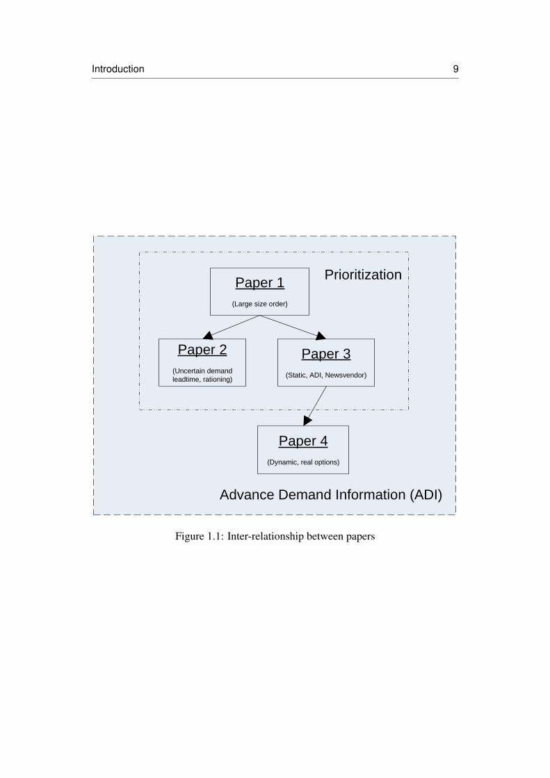
1.1 Inter-relationship between papers . . . . . . . . . . . . . . . . . . . 9

2.1 Illustration of an Erlang process with k = 4 . . . . . . . . . . . . . 332.2 Explanation for (2.12) . . . . . . . . . . . . . . . . . . . . . . . . . 332.3 Average threshold split costs from Tables 2.4(a)-2.4(b) depicted as

a function of ρ. . . . . . . . . . . . . . . . . . . . . . . . . . . . . 332.4 Average threshold split costs from Tables 2.5(a)-2.5(d) depicted as

a function of ρ. . . . . . . . . . . . . . . . . . . . . . . . . . . . . 342.5 Average threshold split costs from Tables 2.6(a)-2.6(b) depicted as

a function of ρ. . . . . . . . . . . . . . . . . . . . . . . . . . . . . 342.6 Average threshold split costs from Tables 2.7(a)-2.7(b) depicted as

a function of ρ. . . . . . . . . . . . . . . . . . . . . . . . . . . . . 35

3.1 (a) All requests received in the time interval [τ + y − L, τ) will beserved ahead of Current-order. All requests received in the timeinterval [τ, τ + r) with a demand realization before time point τ + rwill be served ahead of Current-order. (b) All requests received inthe time interval [τ+y−L, τ+y−r) will be served ahead of Current-order. All requests received in the time interval [τ+y− r, τ+y) witha demand realization before time point τ+ y will be served ahead ofCurrent-order. . . . . . . . . . . . . . . . . . . . . . . . . . . . . . 61

3.2 (a) All requests received in the time interval [τ + y − L, τ + y − d)with a demand realization before time point τ + y will be servedahead of Current-order. (b) All orders received in the time interval[τ+y−L, τ+d−L) will be served ahead of Current-order. All ordersreceived in the time interval [τ+ d− L, τ) with a demand realizationbefore time point τ + d will be served ahead of Current-order. . . . . 61

5.1 The DP structure of this inventory system with real options contract 1195.2 Average profit when c2 is 4, we use the average value of N = 4, 5, 6.

The horizontal axis is p value while the vertical axis is the profit. . . 1195.3 Average profit when c2 is 5, we use the average value of N = 4, 5, 6.

The horizontal axis is p value while the vertical axis is the profit. . . 1205.4 Average profit when c2 is 7, we use the average value of N = 4, 5, 6.

The horizontal axis is p value while the vertical axis is the profit. . . 1205.5 The profit trends when c2 = 7 and N = 4 by use the options price

p = 1, 2, 3, 4, 5, 6. The horizontal axis is p value while the verticalaxis is the profit. . . . . . . . . . . . . . . . . . . . . . . . . . . . . 121

v

List of Tables

2.1 Numerical results when d = 1.25, k = 1, α = 0.90, β = 0.95. Forsimplicity, various subscripts are suppressed. . . . . . . . . . . . . 34

2.2 Numerical results when d = 1.25, k = 2, α = 0.95, β = 0.90. Forsimplicity, various subscripts are suppressed. . . . . . . . . . . . . 35

2.3 All data on threshold split costs grouped on their ρ value. In all 32observations in each group. . . . . . . . . . . . . . . . . . . . . . . 35

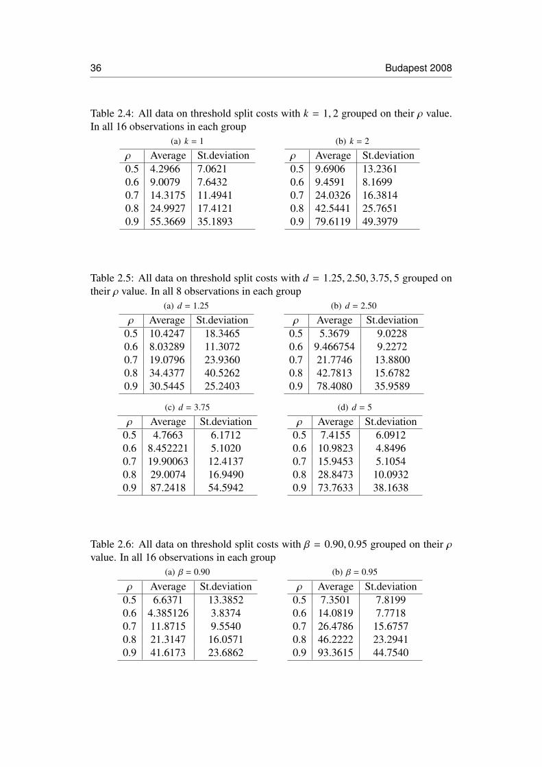
2.4 All data on threshold split costs with k = 1, 2 grouped on their ρvalue. In all 16 observations in each group . . . . . . . . . . . . . . 36

2.5 All data on threshold split costs with d = 1.25, 2.50, 3.75, 5 groupedon their ρ value. In all 8 observations in each group . . . . . . . . . 36

2.6 All data on threshold split costs with β = 0.90, 0.95 grouped ontheir ρ value. In all 16 observations in each group . . . . . . . . . . 36

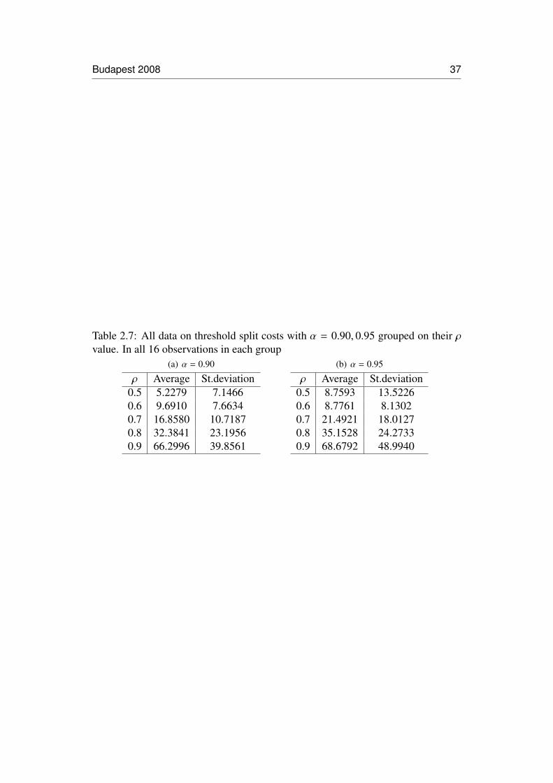
2.7 All data on threshold split costs with α = 0.90, 0.95 grouped ontheir ρ value. In all 16 observations in each group . . . . . . . . . . 37

3.1 (a) Reservation policy FD, L = 4, Y uniform on 0 to L, h = 1, λ = 2,a = 5, b = 1. Av OH is the average on-hand inventory. Revenue isthe expected revenue per time unit, and Profit is expected profit pertime unit. The table is prepared for S = 6 which is the optimal basestock level. . . . . . . . . . . . . . . . . . . . . . . . . . . . . . . 62

3.1 (b) Reservation policy BD, L = 4, Y uniform on 0 to L, h = 1,λ = 2.Av OH is the average on-hand inventory. Revenue is theexpected revenue per time unit, and Profit is expected profit pertime unit. The table is prepared for S = 6 which is the optimal basestock level. . . . . . . . . . . . . . . . . . . . . . . . . . . . . . . 62

3.1 (c) Reservation policy PD, L = 4, Y uniform on 0 to L, h = 1,λ = 2.Av OH is the average on-hand inventory. Revenue is theexpected revenue per time unit, and Profit is expected profit pertime unit. The table is prepared for S = 6 which is the optimal basestock level. . . . . . . . . . . . . . . . . . . . . . . . . . . . . . . 63

3.2 (a) Reservation policy FD, L = 4, Y beta distributed on 0 to L withmean 0.8L and variance 2L2/75, h = 1, λ = 2. The expected profitper time is collect by simulation in Arena, using 10 replications,each with a run length of 100000 starting the inventory system hav-ing no reservations and no outstanding replenishment orders. . . . . 63

vii

3.2 (b) Reservation policy BD, L = 4, Y beta distributed on 0 to L withmean 0.8L and variance 2L2/75, h = 1, λ = 2. The expected profitper time is collect by simulation in Arena, using 10 replications,each with a run length of 100000 starting the inventory system hav-ing no reservations and no outstanding replenishment orders. . . . . 63

3.2 (c) Reservation policy PD, L = 4, Y beta distributed on 0 to L withmean 0.8L and variance 2L2/75, h = 1, λ = 2. The expected profitper time is collect by simulation in Arena, using 10 replications,each with a run length of 100000 starting the inventory system hav-ing no reservations and no outstanding replenishment orders. . . . . 64

3.3 (a) Reservation policy FD, L = 4, Y uniform on 0 to L, h = 1, λ = 2,a = 5, b = −1. Av OH is the average on-hand inventory. Revenueis the expected revenue per time unit, and Profit is expected profitper time unit. The table is prepared for S = 7 which is the optimalbase stock level. . . . . . . . . . . . . . . . . . . . . . . . . . . . . 64

3.3 (b) Reservation policy BD, L = 4, Y uniform on 0 to L, h = 1, λ = 2,a = 5, b = −1. Av OH is the average on-hand inventory. Revenueis the expected revenue per time unit, and Profit is expected profitper time unit. The table is prepared for S = 7 which is the optimalbase stock level. . . . . . . . . . . . . . . . . . . . . . . . . . . . . 65

3.3 (c) Reservation policy PD, L = 4, Y uniform on 0 to L, h = 1, λ = 2,a = 5, b = −1. Av OH is the average on-hand inventory. Revenueis the expected revenue per time unit, and Profit is expected profitper time unit. The table is prepared for S = 7 which is the optimalbase stock level. . . . . . . . . . . . . . . . . . . . . . . . . . . . . 65

3.4 (a) Reservation policy FD, L = 4, Y uniform on 0 to L, h = 1, λ = 2,a = 3, b = −2. Av OH is the average on-hand inventory. Revenueis the expected revenue per time unit, and Profit is expected profitper time unit. The table is prepared for S = 7 which is the optimalbase stock level. . . . . . . . . . . . . . . . . . . . . . . . . . . . . 66

3.4 (b) Reservation policy BD, L = 4, Y uniform on 0 to L, h = 1, λ = 2,a = 3, b = −2. Av OH is the average on-hand inventory. Revenueis the expected revenue per time unit, and Profit is expected profitper time unit. The table is prepared for S = 7 which is the optimalbase stock level. . . . . . . . . . . . . . . . . . . . . . . . . . . . . 66

3.4 (c) Reservation policy PD, L = 4, Y uniform on 0 to L, h = 1, λ = 2,a = 3, b = −2. Av OH is the average on-hand inventory. Revenueis the expected revenue per time unit, and Profit is expected profitper time unit. The table is prepared for S = 7 which is the optimalbase stock level. . . . . . . . . . . . . . . . . . . . . . . . . . . . . 67

4.1 For selected values of w2: the optimal pre-order price and resultingconsequence when using the full model . . . . . . . . . . . . . . . 99

4.2 For selected values of w2: the optimal pre-order price and resultingconsequence when using the aggregate model . . . . . . . . . . . . 99

5.1 N = 4, c2 = 4. (λ = 5, s = 1, r = 12, h = 2, imax = 10, kmax = 10) . . . 1215.2 N = 5, c2 = 4. (λ = 5, s = 1, r = 12, h = 2, imax = 10, kmax = 10) . . . 1225.3 N = 6, c2 = 4. (λ = 5, s = 1, r = 12, h = 2, imax = 10, kmax = 10) . . . 1225.4 N = 4, c2 = 5. (λ = 5, s = 1, r = 12, h = 2, imax = 10, kmax = 10) . . . 1235.5 N = 5, c2 = 5. (λ = 5, s = 1, r = 12, h = 2, imax = 10, kmax = 10) . . . 1235.6 N = 6, c2 = 5. (λ = 5, s = 1, r = 12, h = 2, imax = 10, kmax = 10) . . . 1245.7 N = 4, c2 = 7. (λ = 5, s = 1, r = 12, h = 2, imax = 10, kmax = 10) . . . 1255.8 N = 5, c2 = 7. (λ = 5, s = 1, r = 12, h = 2, imax = 10, kmax = 10) . . . 1265.9 N = 6, c2 = 7. (λ = 5, s = 1, r = 12, h = 2, imax = 10, kmax = 10) . . . 127

1Introduction

1

Introduction 3

Introduction

§1.1 Research topics

In general inventory control concerns balancing demand and supply where in

order to do that in a smooth fashion, some stocks are needed. Most often, this is due

to economics of scale and/or uncertainties in demand and/or supply. Economics of

scale concerns that as there might be some fixed costs when issuing a procurement

or a production order it is advisable to use some reasonable batch sizes, therefore

it will take some time for demand to deplete the inventory and an inventory is oc-

casionally build up. Uncertainty concerns both uncertainties in demand and in the

timing and in the amounts delivered from the supply system. This give rise to safety

stocks, an excess buffer to be kept to provide adequate customer service. The un-

certainty in supply can concern limited capacity in the supply system (due to inflow

of orders from other customers), quality problems, and uncertainties in production

times or in transportation times. Uncertainty of demand is typically concerned with

uncertainty about inter-arrival time of subsequent customer orders and uncertainty

about the magnitudes of these.

In this thesis the economics of scale element is ignored so the focal point of the

thesis is the uncertainty element. For the first three papers this concern a more de-

tailed description of the demand process. Most often, as indicated above, there are

only two random components namely inter-arrival times and customer order sizes,

thus a demand model that is a compound stochastic process. However, other com-

ponents could be added and in this thesis the focus is on two additional components:

4 Introduction

heterogeneity and advance demand information (sometimes abbreviated ADI). Het-

erogeneity concerns, that there can be different customer groups with different ran-

dom patterns, for instance concerning the two first components inter-arrival times

and order size. Advance demand information concerns that, say a customer request

occur at time point t, the customer also specifies time point y + t where he wants to

receive his order. Thus y can be interpreted as a demand lead-time of the customer.

Though this is a common feature in many B2B (Business to Business) settings, it is

ignored in most textbooks on inventory control models. In the thesis these two com-

ponents will be studied with respect to prioritization. When studying heterogeneity

in demands and inventory control, the literature assumes that the different customer

groups should have different service, that is, sometimes a customer belonging to a

lower prioritized customer group should be denied fulfillment, if the inventory level

is critically low. Most often, this literature is not so explicit about putting specific

attributes on what distinguishes the customer groups (except expressing this using

different back-order or lost-sales costs adjoined to each customer group). In Paper 1

the attribute is the size of customer order. It seems reasonable to assume that large

customer orders causes more disturbances upstream and the issuer of a larger order

might be aware of this and thereby may have understanding for that his order gets

lower priority than smaller orders. This is the premise for studying inventory control

policies where degraded service is offered to customers of larger orders. The paper

analysis two plausible policies for degrading the service for larger orders. In Paper

2 the attribute is the demand lead-time which is assumed to be a random variable

but of course known when the customer request is received. Here the issue for the

analysis is when should the customer order be reserved (or tagged) that is any later

arriving request are later tagged customer order after the tagging takes place will

be prioritized lower than this customer order. The paper examines three plausible

reservation policies. In Paper 3 the issue is also prioritization, but it is analyzed in

a static one-period model. Here the focal point is whether a supplier by offering

different prices, before and after the end-customer demand is known to his (priori-

tized) buyers can induce these to make early orders, thereby providing the supplier

Introduction 5

with advance demand information. So the analysis concern how to set the pre-order

price optimally thereby also concerning whether it is optimal to gain knowledge

about advance order information. As this analysis can be quite complex because it

involves several independent decision-makers, the paper also addresses whether the

supplier can derive his optimal pricing decision by using a more aggregated model.

In Paper 4 the uncertainty element is redirected to the supply side, however, many

of the ideas in Paper 3 are mirrored. The focal point is here a manufacturer who

is uncertain about how much capacity in terms of raw material supply he can get.

Therefore he might engage in contracting the future supply of raw material in terms

of making option contracts. So some of his demand for raw material can be cov-

ered by his option contract while the remaining needs must be sourced at the open

market where there might be some limitations (due to various capacity limitations,

like competition from other similar manufacturers) on the amount he can get. One

can interpret that option contracting enables the manufacturer with advance supply

information. Also when comparing to the restricted model with no options one can

assess what is the value of be able to use to option instrument in a similar fashion

as the supplier in Paper 3 could assess the value of his early-ordering pricing.

Therefore the thesis (consisting of the four above mentioned papers) concerns

inventory control models under aspects advance demand information, heteroge-

neous demand, prioritization and option pricing, which motivates the choice of

title. Below, follows a short summary (in terms of abstract presentation) of the four

papers.

§1.2 The structure of the thesis

For the inter-relationship between the papers of the thesis, see Figure 1.1. All

4 papers are within the topic of Advance demand information (ADI). Specifically,

the first three papers (Paper 1,2,3) more focus on the prioritization, or customer

segmentation, by taking customers into multiple demand classes, the supplier serve

them by different prioritization.

6 Introduction

——————————————

Figure 1.1 is about here

——————————————

The arrows in this figure shows the time-line (or sequence) of the research work.

Paper 1 contributed on the attribute of order size. Based on the work of Paper 1, we

extended the contribution to the attribute of uncertain demand lead-time in Paper 2.

Simultaneously, we study the prioritization in a static case in a Newsvendor model,

which is Paper 3. Later on, as a natural extension, we expanded some elements of

this static model into a dynamic case, which is Paper 4.

§1.3 Summary of papers

Paper 1: Base Stock Policies with Degraded Service to Larger Orders

We study an inventory system controlled by a base stock policy assuming a com-

pound renewal demand process. We extend the base stock policy by incorporating

rules for degrading the service of larger orders. Two specific rules are considered,

denoted Postpone(q, t) and S plit(q), respectively. The parameter q distinguishes

between regular orders (of size less than or equal to q) and larger orders. We de-

velop mathematical expressions for the performance measures: order fill rate of the

regular orders and average on-hand inventory level. We make numerical experi-

ments where the postpone parameter t and the base stock levels of each rule are

such that all customers (of both order types) are indifferent between the two rules.

When comparing the difference in the average on-hand inventory levels, we can then

make an assessment of the threshold value of the cost of splitting an order (which

may otherwise be hard to quantify) in the rule S plit(q). Our numerical results indi-

cate that this threshold value is increasing in the variance of the order sizes. Based

on the numerical experiment our conclusion is therefore that when the variance of

the order sizes is low, then Postpone(q, t) seems to be a good option, while when

the variance is high, then S plit(q) is more competitive.

Introduction 7

Paper 2: Investigating Reservation Policies of Advance Orders in the presence of

Heterogeneous Demand

We consider an inventory system where customers provide advance order infor-

mation. Specifically each customer order has two attributes: a request date when

the order is received and a due date specifying when the customer wants his order

delivered. The inventory system is operated as a base stock system where replenish-

ment orders are issued upon the receipt of an order. We assume the demand process

is a Poisson process. As the demand lead-times, that is, the difference between the

due date and the request date, can vary stochastically, the sequence of requests dates

and due dates will differ. Therefore a potentially important issue is then how early

should orders be reserved at the inventory. We explore three logical reservation

policies. These policies also facilitates that the average on-hand inventory can be

specified in a much simpler way than done in Marklund (2006). Assuming that the

revenue of an order (assumed to be of unit size) depends on the demand lead- time

we propose a profit optimization model, where the expected profit is the difference

of the expected revenue and the expected inventory holding costs. We derive the

profit function for each of the three proposed reservation policies. Our numerical

results indicate that unless the revenue of an order with a large demand lead-time

is very large compared to those with a smaller delivery lead-time, the items should

only be reserved in a short time interval before the delivery and most often not at

all.

Paper 3: Advance Demand Information, Capacity Restrictions and Customer

Prioritization

We study a single supplier who must invest in capacity to manufacturer and sell

products to buyers having different priorities. The buyers can place pre-orders be-

fore their demand is observed, and can also issue additional orders upon observing

demand information. Since the supplier guarantees delivery of pre-ordered goods

(these are not constrained by the supplier’s capacity), buyers with lower priorities

8 Introduction

may consider pre-ordering in order to secure inventory. We derive optimal policies

for the supplier and buyers. We show surprisingly that it is optimal for the sup-

plier to set the pre-order price so high that pre-ordering will not be used much even

though pre-ordering should be of benefit to the supplier due to risk sharing. We also

show that the supplier can make a pricing decision using an aggregate model.

Paper 4: Inventory Rationing with Real Options

We consider an inventory system consisting of two supply sources and one

buyer. The first supply source is the real options contract provider while the other

supply source is a capacitated external market. The buyer’s unsatisfied demands are

treated as lost sales. We formulate the problem as a dynamic programming model

in order to perform some numerical investigations. In particular, we study the effect

of using real options compared to a restricted situation where real options are not

applied.

Introduction 9

PrioritizationPaper 1

(Large size order)

Paper 2(Uncertain demandleadtime, rationing)

Paper 3(Static, ADI, Newsvendor)

Paper 4(Dynamic, real options)

Advance Demand Information (ADI)

Figure 1.1: Inter-relationship between papers

2Base Stock Policies with

Degraded Service to Larger

Orders

History: This paper has been published in the International Journal of ProductionEconomics (IJPE), Volume 133, Issue 1, September 2011, Pages 326-333. This work waspresented at the International Society for Inventory Research (ISIR) biennial Conference -15th Symposium, August 2008, Budapest, Hungary.

11

Budapest 2008 13

Base Stock Policies with Degraded Service toLarger Orders

Bisheng Du∗ Christian Larsen†

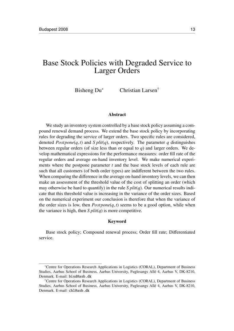
Abstract

We study an inventory system controlled by a base stock policy assuming a com-pound renewal demand process. We extend the base stock policy by incorporatingrules for degrading the service of larger orders. Two specific rules are considered,denoted Postpone(q, t) and S plit(q), respectively. The parameter q distinguishesbetween regular orders (of size less than or equal to q) and larger orders. We de-velop mathematical expressions for the performance measures: order fill rate of theregular orders and average on-hand inventory level. We make numerical experi-ments where the postpone parameter t and the base stock levels of each rule aresuch that all customers (of both order types) are indifferent between the two rules.When comparing the difference in the average on-hand inventory levels, we can thenmake an assessment of the threshold value of the cost of splitting an order (whichmay otherwise be hard to quantify) in the rule S plit(q). Our numerical results indi-cate that this threshold value is increasing in the variance of the order sizes. Basedon the numerical experiment our conclusion is therefore that when the variance ofthe order sizes is low, then Postpone(q, t) seems to be a good option, while whenthe variance is high, then S plit(q) is more competitive.

Keyword

Base stock policy; Compound renewal process; Order fill rate; Differentiatedservice.

∗Centre for Operations Research Applications in Logistics (CORAL), Department of BusinessStudies, Aarhus School of Business, Aarhus University, Fuglesangs Alle 4, Aarhus V, DK-8210,Denmark. E-mail: bisd@asb.dk

†Centre for Operations Research Applications in Logistics (CORAL), Department of BusinessStudies, Aarhus School of Business, Aarhus University, Fuglesangs Alle 4, Aarhus V, DK-8210,Denmark. E-mail: chl@asb.dk

14 Budapest 2008

§2.1 Introduction

It is well known that the larger demand variation, the higher inventory levels are

needed in order to secure adequate service from an inventory system. One reason for

large demand variation may be that the system occasionally receives large customer

orders. Furthermore, these large orders may have negative effects further upstream

in the supply chain. Therefore, as a manager of an inventory system, you would

prefer to receive smaller orders at a more frequent pace rather than receiving orders

with large variation at a less frequent pace. However, assuming that in the short run

you cannot do anything to change the order behavior of your customers, it may be

sensible to introduce a policy implying degraded service to larger orders. Customers

submitting larger orders may also very well be aware of the inconvenience that they

cause and be willing to accept degraded service. Furthermore, such an initiative

may need the customers to change their ordering behavior such that in the long run

one will in fact encounter less variation in the demand pattern.

The considerations raised here are inspired by a discussion that the authors had

recently with the logistics personnel in a larger Danish company where the second

author has been involved in an inventory control project. The aim of this project was

to decide optimal base stock levels when the service measure is order fill rate, that

is, the fraction of orders received where the whole order is delivered instantaneously

from the inventory. This project was reported in Larsen et al. (2008) and some the-

oretical aspects of the project in Larsen and Thorstenson (2008). Obviously, larger

orders can have very negative effects on the order fill rate service measure (thus,

using this service measure, it is implicitly assumed that smaller orders are just as

important as larger ones).

As the source of inspiration is this company project, it is natural that the math-

ematical model developed in this paper takes its point of departure in the model

of this project. Therefore, we study a base stock system with control parameter S

and where all replenishment orders, issued instantaneously upon receipt of an or-

der, have a constant lead-time L. Our extension of the model is the introduction of

Budapest 2008 15

a given positive integer q, based on which orders are distinguished as being either

regular orders (of a size less than or equal to q) or large orders (of a size larger

than q). We introduce two rules, S plit(q) and Postpone(q, t), which both seek to

serve regular orders as well as possible while degrading the service of larger orders.

Postpone(q, t) operates as follows: the parameter t is in the interval between 0 and

L. When receiving a large order, say at time point τ, the order is deliberately back-

logged for t time units before it is attempted to be served. This implies that all reg-

ular orders arriving in the time interval (τ, τ+ t) are served ahead of this large order.

One could interpret Postpone(q, t) not as a rule for degrading service but as a special

case of an advance demand information system where all receipts of larger orders

are known t time units in advance. For studies of inventory systems in the presence

of advance demand information, see among others Hariharan and Zipkin (1995),

Gallego and Ozer (2001) and Marklund (2006). As shown in Hariharan and Zipkin

(1995) one could therefore make the interpretation that the effective replenishment

lead-time of any larger order is L − t. The other rule S plit(q) operates as follows:

each time a larger order is received, it is split into a suborder of size q and a subor-

der of the remaining size. The first suborder is then treated as a regular order while

the second suborder is handled outside the inventory system, directly from the sup-

ply system, thus having a lead-time L. Therefore, the inventory system only faces

orders that are less than or equal to q and all replenishment orders are the original

order eventually truncated by q.

We believe that both rules could be reasonable choices for handling a situation

where one wants to give degraded service to larger orders. As the two rules are quite

different, determining which of the two to use is not immediately obvious. However,

we here present an approach for accomplishing this. When choosing between the

two rules, we propose that one should examine the following 4 elements; 1: the

inconvenience caused to larger orders, 2: the service offered to regular orders, 3: the

inventory investment and 4: the additional costs of splitting an order in the S plit(q)

rule. Our approach involves all 4 elements. We believe that for a given q, a threshold

value of t exists making the customers of the larger orders indifferent between the

16 Budapest 2008

two rules. Later in the paper, we provide a reasonable method for deciding this

threshold value (though the method is somewhat approximate it is convenient for

computations). When this threshold t value is determined, we compute base stock

levels enabling the customers of the regular orders to reach the same order fill rate

level, irrespective of which rule is used. So when going through these two steps, all

customers should be indifferent between to the two rules. The choice of which rule

to apply is then based on which of the two performs best with respect to the last two

elements. In our opinion the rule S plit(q) is a bit harder to administrate as it involves

splitting and monitoring two suborders. Specifically, we imagine there is a cost

incurred when doing a split. However, as this cost of splitting an order may be hard

to quantify, we instead identify its threshold value, making the cost performance of

the two rules equal (as can be seen later, the threshold value is actually measured

relative to the inventory holding cost rate). Therefore, our numerical analysis is

focused on identifying values of the input data where this threshold value is low

(which suggests that Postpone(q, t) is the best choice), and where it is high (which

suggests that S plit(q) is the best choice). As a by-product, our numerical analysis

also provides some insights into how the preference between the rules may alter

upon observing a change in the behavior of the customers of the larger orders due

to the downgrading of their order requests, for instance, if gradually one begins

to see an increased arrival intensity of the order requests but in general a smaller

average order size. Here our results seem to suggest that initially one might prefer

the S plit(q) rule. However, due to a possible change in customer behavior, this

could be altered to a preference for the Postpone(q, t) rule.

There has been a large number of studies of inventory control in the presence of

several (most often two) customer classes. For a good overview of the literature, see

Teunter and Haneveld (2008). The aim of these studies is to design rationing rules

concerning when to backlog (or reject) the demand of the least important customer

class when the inventory level is critically low. In our work, we do not introduce any

critical numbers on the inventory levels for when to deny service of (some) orders.

Furthermore we do not explicitly model several customer classes. Therefore, our

Budapest 2008 17

work is not so closely related to the traditional studies of rationing policies in inven-

tory control systems. When considering the rule Postpone(q, t), our work is more in

line with the paper of Wang et al. (2002) which is motivated by a company analysis

reported in Cohen et al. (1999). They consider a base stock system with two cus-

tomer classes where the service of one of the classes is first attempted after a given

time period (in the paper denoted demand or delivery lead times) has elapsed since

the receipt of the order. As the demand model therein is a Poisson process (thus

without a compound element), the concern about degrading service of larger orders

is obviously outside the scope of this paper. Furthermore, we also generalize the de-

mand model by considering a renewal process instead of a Poisson process. As an

aside, we note that recently a paper by Kocaga and Sen (2007) has been published

which extends the model of Wang et al. (2002) by introducing critical number rules

as seen in the rationing literature, featured in Teunter and Haneveld (2008). When

considering the rule S plit(q), our work has some relation to studies of order split-

ting and multiple sourcing. For a review of these studies, see Thomas and Tyworth

(2006). However, as we exclusively use S plit(q) in comparisons with another rule,

Postpone(q, t), which cannot be cast into the framework of the splitting/sourcing

literature, our work cannot be compared to results obtained in this field.

In Section 2.2, we derive mathematical expressions for the order fill rate of

the regular orders and the average on-hand inventory for the rules S plit(q) and

Postpone(q, t). For each rule, this is done in two stages: first for a general com-

pound renewal process and then in the case of a compound Erlang process, making

the mathematical expressions more computable. We finish this section by deriving a

reasonable threshold value of t, which we find will make customers of larger orders

indifferent between the two rules, and by deriving the threshold value of the split

cost. Then in Section 2.3, we present the results of a numerical study. Finally, we

state some concluding remarks in Section 2.4.

18 Budapest 2008

§2.2 Mathematical model

§2.2.0 Preliminaries

The demand process is a compound renewal process where the time between

order arrivals is specified by a positive continuous random variable T . The size

of a customer order is specified by a positive integer valued random variable X. As

stated in the previous section, we assume a given positive integer q that distinguishes

between regular and large orders. We imagine that q is reasonably large, for instance

the 90% or the 95% quantile of X, as seen later in our numerical experiments.

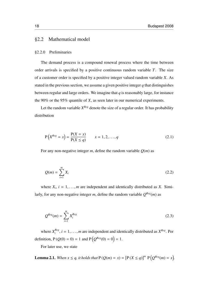
Let the random variable XReg denote the size of a regular order. It has probability

distribution

P(XReg = x

)=

P(X = x)P(X ≤ q)

x = 1, 2, . . . , q (2.1)

For any non-negative integer m, define the random variable Q(m) as

Q(m) =

m∑i=1

Xi (2.2)

where Xi, i = 1, . . . ,m are independent and identically distributed as X. Simi-

larly, for any non-negative integer m, define the random variable QReg(m) as

QReg(m) =

m∑i=1

XRegi (2.3)

where XRegi , i = 1, . . . ,m are independent and identically distributed as XReg. Per

definition, P (Q(0) = 0) = 1 and P(QReg(0) = 0

)= 1.

For later use, we state

Lemma 2.1. When x ≤ q, it holds that P (Q(m) = x) =[P (X ≤ q)

]m P(QReg(m) = x

).

Budapest 2008 19

Proof: See Appendix.

Let τ be an arbitrarily chosen time point which in our paper can either be a time

point of an arrival of a customer with a regular order or a randomly chosen time

point. For any non-negative real number s, the random variable N(τ)s is the number

of customer arrivals in the time interval [τ − s, τ).

§2.2.1 Rule S plit(q)

We first develop an expression for the order fill rate. Let τ be the time point of

an arrival of a customer with a regular order. Let the random variable DL denote the

aggregate demand recorded in the inventory system in the time interval [τ − L, τ).

As all larger orders are truncated by q (and the remaining order of any larger order

is handled outside the inventory system), the probability distribution of DL can be

specified as follows.

When x = 0 or q = 1

P(DL = x

)= P

(N(τ)L = x

)(2.4a)

and when x > 0 and q > 1

P(DL = x

)=

x∑m=dxqe

P (N(τ)L = m)m∑

y=dqm−xq−1 e

(my

)·

[P(X ≤ q)

]y [P(X > q)

]m−y P(QReg(y) = x − (m − y) q

) (2.4b)

Roo f (a), dae is the smallest integer greater than or equal to the real number a

and(

my

)is the binomial coefficient. The order fill rate service measure, abbreviated

OFR, measuring the fraction of regular orders where the whole order is delivered

instantaneously from the inventory, is then

OFRsplit(q)(S ) = P(XReg + DL ≤ S

)(2.5)

We now develop expressions for the average on-hand inventory level. Let τ be

20 Budapest 2008

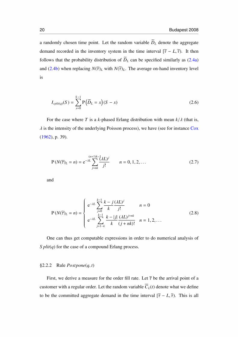
a randomly chosen time point. Let the random variable DL denote the aggregate

demand recorded in the inventory system in the time interval [τ − L, τ). It then

follows that the probability distribution of DL can be specified similarly as (2.4a)

and (2.4b) when replacing N(τ)L with N (τ)L. The average on-hand inventory level

is

Isplit(q)(S ) =

S−1∑x=0

P(DL = x

)(S − x) (2.6)

For the case where T is a k-phased Erlang distribution with mean k/λ (that is,

λ is the intensity of the underlying Poisson process), we have (see for instance Cox

(1962), p. 39).

P (N(τ)L = n) = e−λL(n+1)k−1∑

j=nk

(λL) j

j!n = 0, 1, 2, . . . (2.7)

and

P (N (τ)L = n) =

e−λL

k−1∑j=0

k − jk

(λL) j

j!n = 0

e−λLk−1∑

j=1−k

k − | j|k

(λL) j+nk

( j + nk)!n = 1, 2, . . .

(2.8)

One can thus get computable expressions in order to do numerical analysis of

S plit(q) for the case of a compound Erlang process.

§2.2.2 Rule Postpone(q, t)

First, we derive a measure for the order fill rate. Let τ be the arrival point of a

customer with a regular order. Let the random variable CL(t) denote what we define

to be the committed aggregate demand in the time interval [τ − L, τ). This is all

Budapest 2008 21

the recorded demand in the interval [τ − L, τ − t) and all the recorded demand of

the regular orders in the time interval [τ − L, τ). The reason why only demand of

the regular orders is counted in the latter interval is that all larger orders received in

this interval are still denied access to the inventory at time point τ. The probability

distribution of CL(t) can be specified as follows.

P(CL(t) = 0

)= P (N(τ)L = 0)+

∞∑m=1

[P(X > q)

]m P (N(τ)L = m,N(τ)t = m) (2.9a)

When x > 0

P(CL(t) = x

)=

∞∑m=1

m∑r=max{m−x,0}

P (N(τ)L = m,N(τ)t = r) ·

min{x−m+r,r}∑y=0

(ry

) [P(X ≤ q)

]y [P(X > q)]r−y P

(Q(m − r) + QReg(y) = x

)(2.9b)

The two random variables N(τ)L and N(τ)t are positively correlated and P(N(τ)L ≥

N(τ)t) = 1. The order fill rate service measure, measuring the fraction of regular

orders where the whole order is delivered instantaneously from the inventory, is

then

OFRpostpone(q,t)(S ) = P(XReg + CL(t) ≤ S

)(2.10)

We now derive a measure for the average on-hand inventory level. Let τ be a

randomly chosen time point. Let the random variable CL(t) denote the committed

aggregate demand in the time interval [τ − L, τ). As previously defined, this is all

the recorded demand in the interval [τ − L, τ − t) and all the recorded demand of

the regular orders in the time interval [τ− t, τ). The probability distribution of CL(t)

can be specified as in (2.9a) and (2.9b) when the random variables N(τ)L and N(τ)t

are replaced by N (τ)L and N (τ)L. Therefore the average on-hand inventory level is

22 Budapest 2008

specified as

Ipostpone(q,t)(S ) =

S−1∑x=0

P(CL(t) = x

)(S − x) (2.11)

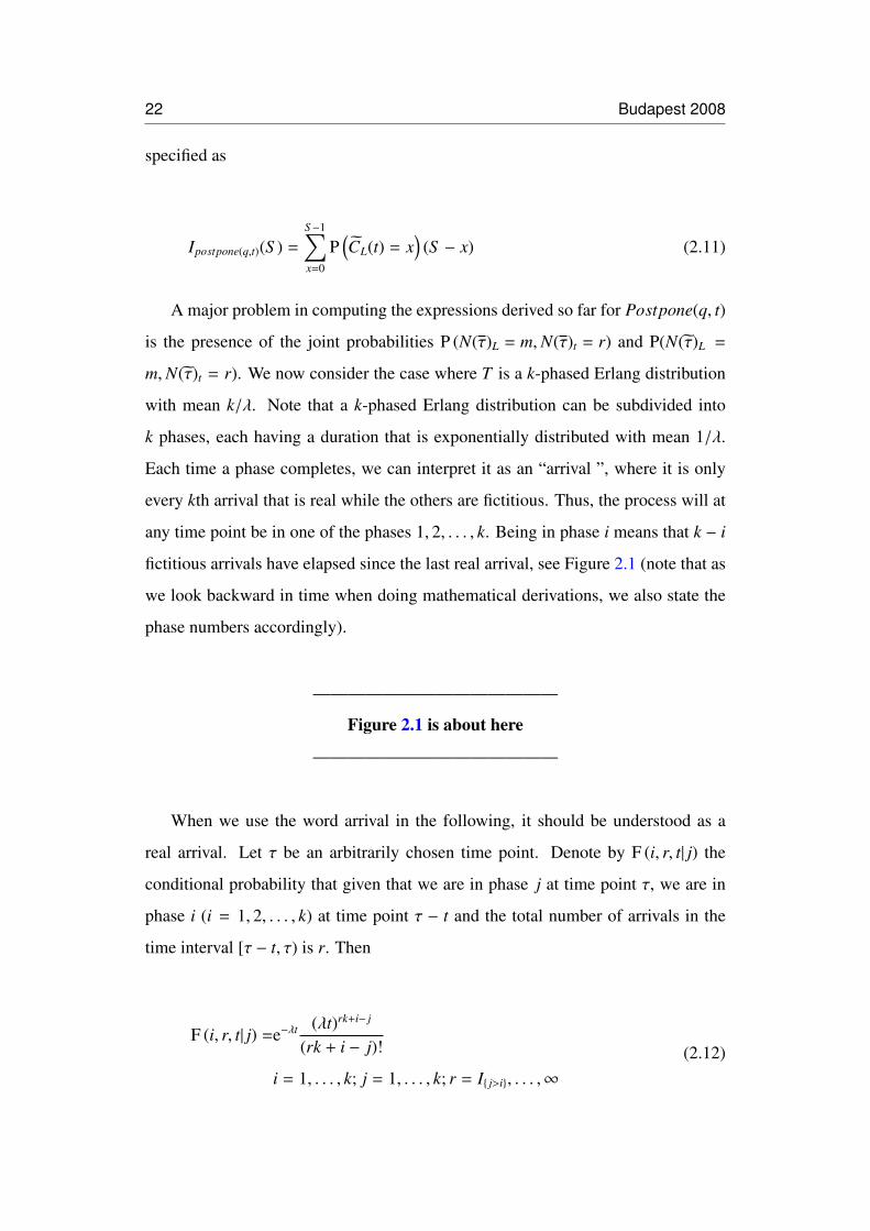
A major problem in computing the expressions derived so far for Postpone(q, t)

is the presence of the joint probabilities P (N(τ)L = m,N(τ)t = r) and P(N (τ)L =

m,N (τ)t = r). We now consider the case where T is a k-phased Erlang distribution

with mean k/λ. Note that a k-phased Erlang distribution can be subdivided into

k phases, each having a duration that is exponentially distributed with mean 1/λ.

Each time a phase completes, we can interpret it as an “arrival ”, where it is only

every kth arrival that is real while the others are fictitious. Thus, the process will at

any time point be in one of the phases 1, 2, . . . , k. Being in phase i means that k − i

fictitious arrivals have elapsed since the last real arrival, see Figure 2.1 (note that as

we look backward in time when doing mathematical derivations, we also state the

phase numbers accordingly).

——————————————

Figure 2.1 is about here

——————————————

When we use the word arrival in the following, it should be understood as a

real arrival. Let τ be an arbitrarily chosen time point. Denote by F (i, r, t| j) the

conditional probability that given that we are in phase j at time point τ, we are in

phase i (i = 1, 2, . . . , k) at time point τ − t and the total number of arrivals in the

time interval [τ − t, τ) is r. Then

F (i, r, t| j) =e−λt (λt)rk+i− j

(rk + i − j)!

i = 1, . . . , k; j = 1, . . . , k; r = I{ j>i}, . . . ,∞

(2.12)

Budapest 2008 23

where the function I{A} is 1 if condition A is true and 0 otherwise. For an expla-

nation of the number rk + i − j in (2.12), see Figure 2.2.

——————————————

Figure 2.2 is about here

——————————————

Let the random variable N(i)L−t denote the total number of arrivals in the time

interval [τ − L, τ − t) given that we are in phase i at time point τ − t. This has

probability distribution

P(N(i)L−t = u

)= e−λ(L−t)

(u+1)k−i∑v=max{uk+1−i,0}

[λ(L − t)]v

v!(2.13)

Let the random variable CL(t|r, u) denote the aggregate committed demand (see

the previous definition) in the time interval [τ − L, τ) given that one has observed r

arrivals in the time interval [τ − t, τ) and u arrivals in the time interval [τ − L, τ − t).

This has probability distribution

P (CL(t|r, u) = x) =

min{r,x−u}∑y=0

(ry

) [P(X ≤ q)

]y [P(X > q)]r−y P

(QReg(y) + Q(u) = x

)(2.14)

Using τ as an arrival point of a customer with a regular order, we get the proba-

bility distribution CL(t) can be specified as follows

P(CL(t) = x

)=

k∑i=1

x∑u=0

P(N(i)L−t = u

) ∞∑r=0

F (i, r, t|1) P (CL(t|r, u) = x) (2.15)

Using τ as a randomly chosen time point, we will at this time point be in phase

is j with probability 1/k. Therefore, the probability distribution of CL(t) can be

24 Budapest 2008

specified as follows

P(CL(t) = x

)=

1k

k∑j=1

k∑i=1

x∑u=0

P(N(i)L−t = u

) ∞∑r=0

F (i, r, t| j) P (CL(t|r, u) = x) (2.16)

This accomplishes that we can get computable expressions for doing numerical

analysis of Postpone(q, t) in the case of a compound Erlang process.

§2.2.3 Implementation

Some of the expressions presented so far can be further simplified when k = 1,

that is the demand process is a compound Poisson process, by using the recursion

scheme of Adelson (1966). Actually, we have developed computer codes, pro-

grammed in Visual Basic for Excel, both for the general Erlangean case (k any

positive integer) and the case k = 1, in order to validate our computer codes as well

as possible. This is done for both rules S plit(q) and Postpone(q, t).

§2.2.4 The case S ≤ q

For this case in particular, the rule S plit(q) is superfluous as not even the trun-

cated suborder of a larger order has any chance of receiving full service. Note that

Postone(q, 0) represents the case where larger orders are not discriminated. We can

prove

Proposition 2.2. When S ≤ q, the performance measures (OFR and average on-

hand inventory) are identical for the rules Postpone(q, 0) and S plit(q).

Proof: See Appendix.

§2.2.5 Choice of t

We derive what we find is a reasonable threshold value of t, making customers

of larger orders indifferent between Postpone(q, t) and S plit(q). Consider a large

Budapest 2008 25

order whose size can be specified by the random variable XLar which has probability

distribution

P(XLar = x

)=

P(X = x)P(X > q)

x = q + 1, q + 2, . . . (2.17)

In Postpone(q, t) a measure for accumulated waiting time of all units of a larger

order is E[XLar

]t. This measure is slightly optimistic as we here assume that any

larger order is instantaneously served after t time units of postponement. Simi-

larly, in S plit(q) a measure for the accumulated waiting time can be specified as

E[max{XLar − q, 0}

]L. Also this measure is slightly optimistic as we here assume

that the truncated suborder (of size q) is served instantaneously. We assume that

both measures are equally optimistic, the value of t that equalizes these two terms

is

t =

L∞∑

j=q+1

( j − q) P(X = j)

∞∑j=q+1

j P(X = j)

(2.18)

The right hand side of (2.18) belongs to the interval between 0 and L. We find

that the right hand side of (2.18) is a good estimate of a t value that makes customers

of larger orders indifferent between Postpone(q, t) and S plit(q). Developing exact

expressions would be very difficult.

§2.2.6 Specification of a threshold split cost

Irrespective of which rule is applied, we assume that a holding cost rate h is

charged on the average on-hand inventory. Furthermore, in the cost evaluation of

S plit(q) we assume that a cost csplit is incurred each time a larger order is split. As

the expected time between successive occurrences of larger orders is E[T ]/P(X >

26 Budapest 2008

q), the cost evaluation of S plit(q) is

h Isplit(S ) + csplitP(X > q)

E[T ](2.19)

while the cost evaluation of Postpone(q, t) is hIpostpone(q,t)(S ). Assume now that

for a given q, t has been settled according to (2.18), such that customers of larger

orders are indifferent between the two rules. Assume then that for each rule, the

base stock levels S postpone(q,t) and S split(q), respectively, have been established such

that customers of regular orders enjoys the same order fill rate and are therefore also

indifferent between the two rules. When equalizing the two cost expressions stated

above and isolating the cost parameters, we then get a threshold value of the split

cost (relative to the inventory holding cost rate)

csplit/h =[Ipostpone(q,t) S postpone(q,t) − Isplit(q) S split(q)] E[T ]

P(X > q)(2.20)

In principle, this threshold value could be negative. However, as the demand

volume faced by the inventory is less under S plit(q) than under Postpone(q, t) (due

to some demand being filtered away from the inventory and sent directly to the

supply system) the result is that generally when the parameters are set such that

customers are indifferent between the two rules, the average on-hand inventory in

Postpone(q, t) is larger than the average on-hand inventory in S plit(q).

§2.3 Numerical results

As indicated in the previous section we have only done implementations of the

model when T is k-phased Erlang distributed with mean k/λ. Throughout this sec-

tion, we keep L fixed at level 4, we also assume that the random variable X is

Budapest 2008 27

(delayed) geometrically distributed. This means that it has probability distribution

P(X = j) = (1 − ρ)ρ j−1 j = 1, 2, . . . (2.21)

where the parameter ρ is in the interval between 0 and 1. The use of the word

“delayed ” is due to (Zipkin (2000),p. 451). Then (2.18) simplifies to

t =1

q + 1 − ρqL (2.22)

and the demand rate d, defined as d = E[X]/E[T ], is

d =λ

k(1 − ρ)(2.23)

When k = 1, this demand process is called a “stuttering ” Poisson process (See

Axsater (2006), p. 82). In Johnston et al. (2003), some empirical evidence is given

for the relevance of such a demand model.

We now make a systematic evaluation of how the two rules compare to each

other. We let the demand rate d attain the values 1.25, 2.5, 3.75, 5 (these values per-

haps seem more obvious choices when multiplying by L as dL = 5, 10, 15, 20). For

each choice of d, we then let ρ = 0.5, 0.6, 0.7, 0.8, 0.9. In order also to investigate

the impact of deviating from the common Poisson process assumption, we let k = 1

and 2. The parameter λ is then given from (2.23). We let q be the α quantile (the

least integer value x making P(X ≤ x) ≥ α) of X where α is either 0.90 or 0.95. We

denote the required order fill rate to the regular orders β and let it be either 0.9 or

0.95. Combining all these parameter values (d, ρ, k, α, β) gives a total of 160 data

sets. Our numerical procedure can now be outlined as follows.

1. Given input (d, ρ, k, α, β).

28 Budapest 2008

2. Compute q as the least integer value x making P(X ≤ x) ≥ α and compute t

by (2.22).

3. Compute S postpone(q,t) as the least integer value of S bringing OFRpostpone(q,t)(S ) ≥

β and compute S split(q) as the least integer value of S bringing OFRsplit(q)(S ) ≥

β. Evaluate the average on-hand inventories Ipostpone(q,t)(S ) and Isplit(q)(S ) by

setting S = S postpone(q,t) and S = S split(q), respectively.

4. Evaluate the threshold split cost relative to the inventory cost by

csplit/h =[Ipostpone(q,t)(S postpone(q,t)) − Isplit(q)(S split(q))]k

λP(X > q)

Here we follows closely the outline given in the introduction. We refrain from

making a formal statistical analysis of variance (ANOVA) on the data material on

the threshold split costs, as this will probably lead us nowhere as all interaction

effects are statistically significant. Instead we inspect the data material more in-

formally. It turns out that csplit/h very much depends on the parameter ρ and it is

generally increasing in ρ. A typical illustration of this is given in Table 2.1. Though

there are also a few exceptions, as illustrated in Table 2.2. The reason is that we

are forced to choose the base stock values as integers. For instance, the reason why

the threshold value csplit/h is about 50 when ρ = 0.5 in Table 2.2 is that the base

stock value securing an order fill rate above 0.9 is actually well above, at level 0.93.

As we will demonstrate later, this phenomenon is most likely to occur when the

demand rate d is low, that is with low-frequent demand. When d is increased, the

selected values of S will in general secure that the actual order fill rate is close to

the required one. Because the pattern see in Table 2.1 is the most typical for our

data, which can also be verified from Table 2.3, we find it natural to group our ob-

servations of the csplit/h values on the values of the ρ parameter. In the following

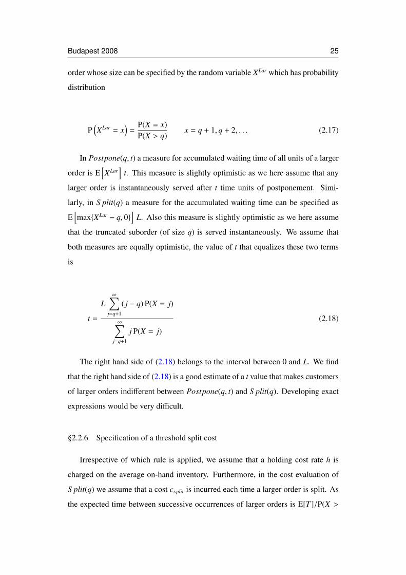
Tables 2.4(a)-2.7(b) and Figure 2.3 - 2.6, we explore how the other input factors

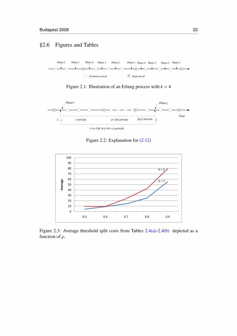
influence the relationship between csplit/h and ρ. From Tables 2.4(a)-2.4(b) and

Figure 2.3 we see that k has some significance. When having an Erlangean arrival

Budapest 2008 29

process (k = 2), the threshold value is in general larger, making S plit(q) more at-

tractive for threshold values falling in between the threshold values of Table 2.4(a)

and Table 2.4(b). Thus, the assumption about the demand process has significance

for the conclusion. It emphasizes the importance of doing a careful analysis of the

data of a demand process in order to specify the appropriate demand model, and not

just automatically choosing a compound Poisson process because it is most con-

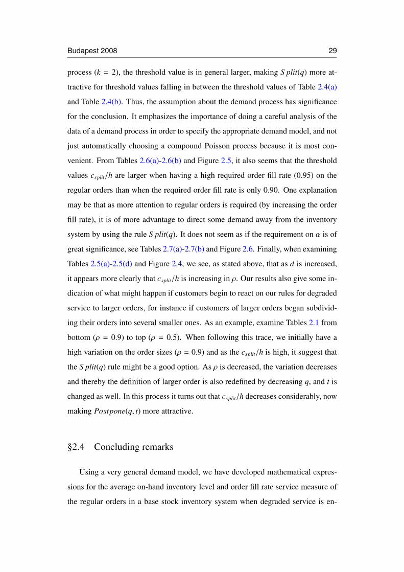
venient. From Tables 2.6(a)-2.6(b) and Figure 2.5, it also seems that the threshold

values csplit/h are larger when having a high required order fill rate (0.95) on the

regular orders than when the required order fill rate is only 0.90. One explanation

may be that as more attention to regular orders is required (by increasing the order

fill rate), it is of more advantage to direct some demand away from the inventory

system by using the rule S plit(q). It does not seem as if the requirement on α is of

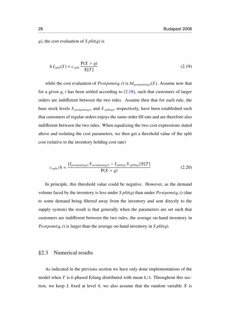
great significance, see Tables 2.7(a)-2.7(b) and Figure 2.6. Finally, when examining

Tables 2.5(a)-2.5(d) and Figure 2.4, we see, as stated above, that as d is increased,

it appears more clearly that csplit/h is increasing in ρ. Our results also give some in-

dication of what might happen if customers begin to react on our rules for degraded

service to larger orders, for instance if customers of larger orders began subdivid-

ing their orders into several smaller ones. As an example, examine Tables 2.1 from

bottom (ρ = 0.9) to top (ρ = 0.5). When following this trace, we initially have a

high variation on the order sizes (ρ = 0.9) and as the csplit/h is high, it suggest that

the S plit(q) rule might be a good option. As ρ is decreased, the variation decreases

and thereby the definition of larger order is also redefined by decreasing q, and t is

changed as well. In this process it turns out that csplit/h decreases considerably, now

making Postpone(q, t) more attractive.

§2.4 Concluding remarks

Using a very general demand model, we have developed mathematical expres-

sions for the average on-hand inventory level and order fill rate service measure of

the regular orders in a base stock inventory system when degraded service is en-

30 Budapest 2008

forced for customers of larger orders. The models (and corresponding computer

codes) may be valuable tools for an organization to explore the impact of various

strategies for degrading the service of larger orders; particularly in recognition of

the fact that these orders may have a very disruptive effect upstream in the supply

chain. We have refrained from doing a cost optimization with respect to service

requirements. This is partly due to the fact that this is a quite complex operation as

we have two service level constraints to consider, and partly due to the fact that we

believe that a cost parameter such as the cost of splitting a larger order may be hard

to quantify. Therefore, our approach is to specify the parameters t, S postpone(q,t) and

S split(q) such that all customers (irrespective whether they issue a regular or a larger

order) will consider the two rules to be equally good. Additionally, we explore the

threshold value of the split cost, thereby establishing when each rule seems to per-

form best. Our numerical investigations reveal that the choice between S plit(q) and

Postpone(q, t) seems to depend on the variance of the order sizes. The lower it is,

the better option is the rule Postpone(q, t). It also seems that deviating from the

common Poisson process assumption as well as the choice of order fill rate offered

to the regular orders does have some impact on this conclusion. Though we examine

a fairly large number of data sets, we look exclusively at the geometric distribution

to describe order sizes. So obviously, further numerical studies could be devoted to

examining other distributions, for instance the negative binomial, the Poisson or the

logarithmic distribution. As noted in the introduction, the rule Postpone(q, t) has

resemblance to an advance demand information system. Therefore, the mathemati-

cal model concerning this rule can easily be adapted to a more general study about

aspects of advance demand information where it need not be solely the customers

of larger orders that provide this information.

Acknowledgement

This work is supported by Grant No. 275-07-0094 from the Danish Social Sci-

ence Research Council. We are grateful for comments received from two anony-

Budapest 2008 31

mous reviewers and Johan Marklund, Lund University, Sweden, that considerably

improved the paper.

§2.5 Appendix

Proof. Proof of Lemma 2.1

We prove by induction in m. When m = 1, the result is given from (2.1). Con-

sider now an integer m′ ≥ 1 and assume that we have shown the result for m = m′−1.

For any x = 0, 1, . . . , q, it holds that

P (Q(m′) = x) =

x∑y=0

P(Q(m′ − 1) = y

)P(X = x − y)

=[P (X ≤ q)

]m′x∑

y=0

P(QReg(m′ − 1) = y

)P(XReg = x − y

)=

[P (X ≤ q)

]m′ P(QReg(m′) = x

)�

Proof. Proof of Proposition 2.2

We claim that for any x = 0, 1, . . . , q−1, it holds that P(DL = x

)= P

(CL(0) = x

).

First, we consider the random variable CL(0). When t = 0, the random variable

N(τ)t is identical to zero. This means that the summation on the right hand side

of (2.9a) vanishes to zero. Also, the right hand side of (2.9b) only gives non-zero

terms if index r = 0. This again forces index m to be less than or equal to x and

index y to be zero. Therefore, we get

P(CL(0) = x

)=

P (N(τ)L = 0) x = 0

x∑m=1

P (N(τ)L = m) P (Q(m) = x) x = 1, 2, . . .(2.24)

Now we consider the random variable DL. If q = 1, our claim follows by

32 Budapest 2008

comparing (2.24) to (2.4a). Assume q > 1. When x ≤ q − 1, the inequality (qm −

x)/(q − 1) > m − 1 is equivalent to the inequality q + m > x + 1, which is true when

q > x, implying d(qm − x)/(q − 1)e = m (note (qm − x)/(q − 1) is always less than

or equal to m). When q > x, it also holds that dx/qe = 1. Therefore, we get from

(2.4a) and (2.4b) that

P(DL = x

)=

P (N(τ)L = 0) x = 0

x∑m=1

P (N(τ)L = m)[P (X ≤ q)

]m P(QReg(m) = x

)x = 1, 2, . . . , q − 1

(2.25)

Lemma 2.1 now verifies our claim. Similarly, we can prove that for any x =

0, 1, . . . , q − 1, it holds that P(DL = x

)= P

(CL(0) = x

). As it is the probabilities

P(DL = x

)= P

(CL(0) = x

)for x = 0, 1, . . . , S −1 that specify the OFR expressions

in (2.5) and (2.10) and it is the probabilities P(DL = x

)= P

(CL(0) = x

)for x =

0, 1, . . . , S − 1 that specify the average on-hand inventory expressions in (2.6) and

(2.11), the result follows from S ≤ q − 1. �

Budapest 2008 33

§2.6 Figures and Tables

Phase 2 Phase 3 Phase 2 Phase 2 Phase 1Phase 3Phase 4Phase 1Phase 4Phase 1

Fictitious arrival Real arrival

Figure 2.1: Illustration of an Erlang process with k = 4

t−τ~ τ~

Phase i Phase j

i arrivals (r-1)k arrivals (k-j) arrivals

i+(r-1)k+k-j=rk+i-j arrivals

Time

Figure 2.2: Explanation for (2.12)

k = 1 

k = 2 

40

50

60

70

80

90

100

Average

 

k = 1 

k = 2 

0

10

20

30

40

50

60

70

80

90

100

0.5 0.6 0.7 0.8 0.9

Average

 

Figure 2.3: Average threshold split costs from Tables 2.4(a)-2.4(b) depicted as afunction of ρ.

34 Budapest 2008

100

β = 0.95 80

90

100

β = 0.95 

60

70

80

90

100

ge 

β 0 90

β = 0.95 

40

50

60

70

80

90

100

Average 

β = 0.90 

β = 0.95 

10

20

30

40

50

60

70

80

90

100

Average 

β = 0.90 

β = 0.95 

0

10

20

30

40

50

60

70

80

90

100

0 5 0 6 0 7 0 8 0 9

Average 

β = 0.90 

β = 0.95 

0

10

20

30

40

50

60

70

80

90

100

0.5 0.6 0.7 0.8 0.9

Average 

β = 0.90 

β = 0.95 

0

10

20

30

40

50

60

70

80

90

100

0.5 0.6 0.7 0.8 0.9

Average 

Figure 2.4: Average threshold split costs from Tables 2.5(a)-2.5(d) depicted as afunction of ρ.

100100d = 3 75

100d = 3.75 

90

100d = 3.75 

90

100

d = 2.50

d = 3.75 

80

90

100

d = 2.50 

d = 3.75 

80

90

100

d = 2.50 

d = 3.75 

70

80

90

100

d = 2.50 

d = 3.75 

d 570

80

90

100

d = 2.50 

d = 3.75 

d = 5 60

70

80

90

100

ge 

d = 2.50 

d = 3.75 

d = 5 60

70

80

90

100

age 

d = 2.50 

d = 3.75 

d = 5 

50

60

70

80

90

100

rage 

d = 2.50 

d = 3.75 

d = 5 

50

60

70

80

90

100

verage 

d 1 25

d = 2.50 

d = 3.75 

d = 5 

40

50

60

70

80

90

100

Average 

d = 1.25

d = 2.50 

d = 3.75 

d = 5 

40

50

60

70

80

90

100

Average 

d = 1.25

d = 2.50 

d = 3.75 

d = 5 

30

40

50

60

70

80

90

100

Average 

d = 1.25

d = 2.50 

d = 3.75 

d = 5 

30

40

50

60

70

80

90

100

Average 

d = 1.25

d = 2.50 

d = 3.75 

d = 5 

20

30

40

50

60

70

80

90

100

Average 

d = 1.25

d = 2.50 

d = 3.75 

d = 5 

20

30

40

50

60

70

80

90

100

Average 

d = 1.25

d = 2.50 

d = 3.75 

d = 5 

10

20

30

40

50

60

70

80

90

100

Average 

d = 1.25

d = 2.50 

d = 3.75 

d = 5 

0

10

20

30

40

50

60

70

80

90

100

Average 

d = 1.25

d = 2.50 

d = 3.75 

d = 5 

0

10

20

30

40

50

60

70

80

90

100

Average 

d = 1.25

d = 2.50 

d = 3.75 

d = 5 

0

10

20

30

40

50

60

70

80

90

100

Average 

d = 1.25

d = 2.50 

d = 3.75 

d = 5 

0

10

20

30

40

50

60

70

80

90

100

0.5 0.6 0.7 0.8 0.9

Average 

d = 1.25

d = 2.50 

d = 3.75 

d = 5 

0

10

20

30

40

50

60

70

80

90

100

0.5 0.6 0.7 0.8 0.9

Average 

d = 1.25

d = 2.50 

d = 3.75 

d = 5 

0

10

20

30

40

50

60

70

80

90

100

0.5 0.6 0.7 0.8 0.9

Average 

d = 1.25

d = 2.50 

d = 3.75 

d = 5 

0

10

20

30

40

50

60

70

80

90

100

0.5 0.6 0.7 0.8 0.9

Average 

d = 1.25

d = 2.50 

d = 3.75 

d = 5 

0

10

20

30

40

50

60

70

80

90

100

0.5 0.6 0.7 0.8 0.9

Average 

d = 1.25

d = 2.50 

d = 3.75 

d = 5 

0

10

20

30

40

50

60

70

80

90

100

0.5 0.6 0.7 0.8 0.9

Average 

d = 1.25

d = 2.50 

d = 3.75 

d = 5 

0

10

20

30

40

50

60

70

80

90

100

0.5 0.6 0.7 0.8 0.9

Average 

Figure 2.5: Average threshold split costs from Tables 2.6(a)-2.6(b) depicted as afunction of ρ.

Table 2.1: Numerical results when d = 1.25, k = 1, α = 0.90, β = 0.95. Forsimplicity, various subscripts are suppressed.

Input Postpone(q, t) S plitρ λ q t S I OFR S I OFR csplit/h0.5 0.625 4 1.3333 13 8.3854 0.9512 13 8.3547 0.9605 0.78530.6 0.5 5 1.3333 15 10.4621 0.9586 14 9.4416 0.9555 26.24840.7 0.375 7 1.2903 17 12.5178 0.9522 16 11.4787 0.9509 33.64720.8 0.25 11 1.25 22 17.5582 0.9565 21 16.4942 0.9583 49.54630.9 0.125 12 1.25 32 27.7277 0.9516 31 26.5900 0.9508 92.4196

Budapest 2008 35

100

80

90

100

60

70

80

90

100

ge 

α = 0 90α = 0.9540

50

60

70

80

90

100

Average 

α = 0.90 α = 0.95

10

20

30

40

50

60

70

80

90

100

Average 

α = 0.90 α = 0.95

0

10

20

30

40

50

60

70

80

90

100

0 5 0 6 0 7 0 8 0 9

Average 

α = 0.90 α = 0.95

0

10

20

30

40

50

60

70

80

90

100

0.5 0.6 0.7 0.8 0.9

Average 

α = 0.90 α = 0.95

0

10

20

30

40

50

60

70

80

90

100

0.5 0.6 0.7 0.8 0.9

Average 

Figure 2.6: Average threshold split costs from Tables 2.7(a)-2.7(b) depicted as afunction of ρ.

Table 2.2: Numerical results when d = 1.25, k = 2, α = 0.95, β = 0.90. Forsimplicity, various subscripts are suppressed.

Input Postpone(q, t) S plitρ λ q t S I OFR S I OFR csplit/h0.5 1.25 5 1.1429 11 6.2502 0.9328 10 5.2646 0.9078 50.46330.6 1 6 1.1765 11 6.4043 0.9021 11 6.3434 0.9134 2.61330.7 0.75 9 1.0811 13 8.4011 0.9063 13 8.3321 0.9142 4.55890.8 0.5 14 1.0526 16 11.4846 0.9070 16 11.3793 0.9101 9.57680.9 0.25 29 1.0256 24 19.6469 0.9024 24 19.5151 0.9012 22.3957

Table 2.3: All data on threshold split costs grouped on their ρ value. In all 32observations in each group.

ρ Average St.deviation0.5 6.9936 10.78940.6 9.2335 7.78570.7 19.1750 14.76920.8 33.7684 23.39680.9 67.4894 43.9498

36 Budapest 2008

Table 2.4: All data on threshold split costs with k = 1, 2 grouped on their ρ value.In all 16 observations in each group

(a) k = 1

ρ Average St.deviation0.5 4.2966 7.06210.6 9.0079 7.64320.7 14.3175 11.49410.8 24.9927 17.41210.9 55.3669 35.1893

(b) k = 2

ρ Average St.deviation0.5 9.6906 13.23610.6 9.4591 8.16990.7 24.0326 16.38140.8 42.5441 25.76510.9 79.6119 49.3979

Table 2.5: All data on threshold split costs with d = 1.25, 2.50, 3.75, 5 grouped ontheir ρ value. In all 8 observations in each group

(a) d = 1.25

ρ Average St.deviation0.5 10.4247 18.34650.6 8.03289 11.30720.7 19.0796 23.93600.8 34.4377 40.52620.9 30.5445 25.2403

(b) d = 2.50

ρ Average St.deviation0.5 5.3679 9.02280.6 9.466754 9.22720.7 21.7746 13.88000.8 42.7813 15.67820.9 78.4080 35.9589

(c) d = 3.75

ρ Average St.deviation0.5 4.7663 6.17120.6 8.452221 5.10200.7 19.90063 12.41370.8 29.0074 16.94900.9 87.2418 54.5942

(d) d = 5

ρ Average St.deviation0.5 7.4155 6.09120.6 10.9823 4.84960.7 15.9453 5.10540.8 28.8473 10.09320.9 73.7633 38.1638

Table 2.6: All data on threshold split costs with β = 0.90, 0.95 grouped on their ρvalue. In all 16 observations in each group

(a) β = 0.90

ρ Average St.deviation0.5 6.6371 13.38520.6 4.385126 3.83740.7 11.8715 9.55400.8 21.3147 16.05710.9 41.6173 23.6862

(b) β = 0.95

ρ Average St.deviation0.5 7.3501 7.81990.6 14.0819 7.77180.7 26.4786 15.67570.8 46.2222 23.29410.9 93.3615 44.7540

Budapest 2008 37

Table 2.7: All data on threshold split costs with α = 0.90, 0.95 grouped on their ρvalue. In all 16 observations in each group

(a) α = 0.90

ρ Average St.deviation0.5 5.2279 7.14660.6 9.6910 7.66340.7 16.8580 10.71870.8 32.3841 23.19560.9 66.2996 39.8561

(b) α = 0.95

ρ Average St.deviation0.5 8.7593 13.52260.6 8.7761 8.13020.7 21.4921 18.01270.8 35.1528 24.27330.9 68.6792 48.9940

3Investigating Reservation

Policies of Advance Orders in the

presence of Heterogeneous

Demand

History: This paper has been re-submitted to the International Journal of ProductionEconomics (IJPE) in March 2011. This work was presented at the European Conferenceon Operational Research (EURO), July 2009, Bonn, Germany; the 9th ISIR SummerSchool on Changing Paradigm for Inventory Management in a Supply Chain Context,August 2009, Karol Adamiecki University of Economics in Katowice, Poland; and theInternational Conference on Production Research (ICPR) 20th, August 2009, Shanghai,China.

39

Shanghai 2009 41

Investigating Reservation Policies of AdvanceOrders in the presence of Heterogeneous

Demand

Bisheng Du∗ Christian Larsen†

Abstract

We consider an inventory system where customers provide advance order infor-mation. Specifically each customer order has two attributes: a request date whenthe order is received and a due date specifying when the customer wants his orderdelivered. The inventory system is operated as a base stock system where replenish-ment orders are issued upon the receipt of an order. We assume the demand processis a Poisson process. As the demand lead-times, that is, the difference between thedue date and the request date, can vary stochastically, the sequence of requests datesand due dates will differ. Therefore a potentially important issue is then how earlyshould orders be reserved at the inventory. We explore three logical reservationpolicies. These policies also facilitates that the average on-hand inventory can bespecified in a much simpler way than done in Marklund (2006). Assuming that therevenue of an order (assumed to be of unit size) depends on the demand lead- timewe propose a profit optimization model, where the expected profit is the differenceof the expected revenue and the expected inventory holding costs. We derive theprofit function for each of the three proposed reservation policies. Our numericalresults indicate that unless the revenue of an order with a large demand lead-timeis very large compared to those with a smaller delivery lead-time, the items shouldonly be reserved in a short time interval before the delivery and most often not atall.

Keyword

Inventory control; Advance demand information; Heterogeneous demand

∗CORAL - Centre for Operations Research Applications in Logistics, Department of BusinessStudies, Aarhus School of Business, Aarhus University, Fuglesangs Alle 4, Aarhus V, DK-8210,Denmark. E-mail: bisd@asb.dk

†CORAL - Centre for Operations Research Applications in Logistics, Department of BusinessStudies, Aarhus School of Business, Aarhus University, Fuglesangs Alle 4, Aarhus V, DK-8210,Denmark. E-mail: chl@asb.dk

42 Shanghai 2009

§3.1 Introduction

We consider an inventory system where customers do not physically appear at

the inventory system. Instead they submit their order requests; for instance by e-

mail or via a web-page organized by the inventory system. They do not expect

instantaneously delivery but instead when submitting their order requests they also

specify a future time point when they want to receive their order. Such a situation

could be realistic in a business to business (B2B) context. The inventory system

could be placed somewhere upstream in a supply chain, say a central warehouse

serving different independent retailers and retail chains as well. It could very well

be that there are different levels of communication exchange between these retail

chains and the central warehouse. In some cases there is a very close cooperation

such that the retailer (or retail chain) well in advance, for instance by giving the cen-

tral warehouse access to their information systems, specify future order requests, in

combination with that orders are freezed when coming into a certain time window.

With others there is less information exchange and therefore orders are received

with a shorter notice. The situation could also occur in a business to consumer

(B2C) setting, when sales are organized through the internet, as witnessed by well

known business cases like Amazon and e-Bay.

Advance order information, or advance demand information as it is most often

denoted in the literature, means that if a request for an order occurs, say at time point

τ, the customer also specifies a time point, say time point y + τ, where he wants to

receive his order. Thus, y can be interpreted as the demand lead-time of the cus-

tomer. In many textbooks on inventory control, like Silver et al. (1998) and Zipkin

(2000) it is tacitly assumed that y = 0 (though the issue is raised in Exercise 7.8 of

Silver et al. (1998) and Exercise 6.1 of Zipkin (2000)). The first paper to make a

systematic analysis of advance demand information in inventory control systems is

Hariharan and Zipkin (1995). Here it is assumed that all customers have the same

demand lead-time and the improvement in performance is equivalent to an equal re-

duction in the replenishment lead-time. A similar study is done in Gallego and Ozer

Shanghai 2009 43

(2001) assuming a periodic review model where customers can have different de-

mand lead-times. Here it is proven that a state dependent (s, S ) policy is optimal.

Lu et al. (2003) and Marklund (2006) extends the model of Hariharan and Zipkin

(1995) by studying multi-level systems; the first studies an assembly system while

the second studies a divergent distribution system. In particular, Marklund (2006)

is our main source of inspiration for this study, because he introduces the idea of a

reservation policy to be applied at the upper level echelon. However, he does not

specify any specific reservation policy, and are most often studying the two extreme

ones: the complete reservation policy and the no reservation policy. The papers

above only consider the inventory control side. However, if customers use differ-

ent demand lead-times probably also the revenues of the orders will depend on the

demand lead-time. Except for a work by Chen (2001) studying advance demand

information and market segmentation the revenue side has not been linked to the

inventory side when studying inventory control in the presence of advance order

information. Our aim is to make a more detailed analysis of the some of the ideas

about reservation indicated in Marklund (2006) and link it to a revenue model ac-

knowledging that the revenue varies with the demand lead-time, in order to develop

a profit maximization model in order to find the optimal base stock level and the op-

timal reservation policy. For completeness of this literature review, for newer con-

tributions on advance demand information see also Tan (2008), Wang and Toktay

(2008), Gayon et al. (2009) and Papier and Thonemann (2010). In finalizing this

literature review we should also mention that there is another line of research study-

ing which sort of inventory control policies should be applied in presence of het-

erogeneous demand. When examining the literature (see Topkis (1968), Evans

(1968), Kaplan (1969), Frank et al. (2003) and Tempelmeier (2006) for periodic re-

view models and Nahmias and Demmy (1981), Dekker et al. (1998), Dekker et al.

(2002), Melchiors et al. (2000), Melchiors (2003) and Deshpande et al. (2003) for

continuous review models) all assume that it is possible to differentiate among the

customer classes by introducing a rationing policy. A rationing policy means that

low prioritized customers are denied access to the inventory when the on hand level

44 Shanghai 2009

is critically low. The reservation policies we consider in this paper do have some

resemblance to rationing. But the implementation is not based on critical numbers

on the on-hand inventory but rather a dynamic updating on the priorities of the order

by considering the time until the due-date.

We study the setting outlined in the start of this section. Furthermore we also as-

sume that seen from the perspective of the inventory system, the demand lead-times

of the customers are random. We will assume the inventory system is controlled by

a base-stock system (thus assuming negligible fixed replenishment costs), where all

replenishment are issued instantaneously upon the receipt of an order. The aim is

to find a good base-stock policy in combination with setting the parameter of the

chosen reservation policy such that the expected profit is maximized. The key ele-

ment in our paper is to study reservation policies. One option is to let the order be

immediately reserved (or tagged, as we sometimes call it in the following) from the

inventory. It means that it cannot be accessed by other customers, whose requests

arrive later. This is denoted complete reservation by Marklund (2006). Another

option is first to reserve it after a certain time delay. We then denote it a partial

reservation policy. This may be sensible if the demand lead time of the customer is

long so keeping the amount free on inventory helps giving adequate service also to

customers with a short demand lead-time. We study three ways of implementing a

partial reservation policy, denoted Forward Delay (FD), Backward Delay (BD) and

Proportional Delay (PD), respectively. Roughly speaking, the difference between

FD and BD, is that under the first policy the order is first tagged at the inventory r

time units (where r is a policy variable) after the request has been registered while

in the second the order is first tagged at the inventory d time units (where d is a

policy variable) before it is needed. One could also interpret it as in the first the

request date is the anchor point while in the second the due date is the anchor point

when deciding when to reserve the order. Finally, in the PD reservation policy the

time until the tagging takes place depends on the actual demand lead time and it is

proportional to it.

In Section 3.2 we will in more detail specify the mathematical assumption be-

Shanghai 2009 45

hind the inventory system and specifying the profit function. As this profit function

requires knowledge about the order fill rate offered to a customer having any de-

mand lead-time as well as the average on-hand inventory, we show in Sections 3.3

and 3.4, respectively, how these expressions can be derived mathematically. In Sec-

tion 3.5 we will present the results of our numerical investigations. Finally, Section

3.6 contains some concluding remarks.

§3.2 The mathematical model

We assume the arrival processes of order requests is a Poisson processes with

intensity λ arrivals per time unit. The non-negative random variable Y , with density

function f (y), represents the demand lead-time of a customer. That is, if an order

request occurs at time point τ and the customer has a demand lead-time y, then the

customer wants to get his demand fulfilled at time point τ + y. As Y is assumed

stochastic it is understood that the customer’s preferences for demand lead times is

outside the control of the inventory system. In the special case where it is a constant

it could represent a scenario that when for instance ordering from the internet only

one option is given for choosing a delivery lead time. Most realistically the random

variable Y is discrete, the customers can only choose between a selected number

of delivery options, or there is only a limited number of different customer classes

(within this class all customers have the same demand lead-time) . However, in

order to be as general as possible we will assume Y is a continuous random variable.

The inventory is controlled by a base stock policy with parameter S (a non-

negative integer). All unfulfilled demand is backlogged. It is assumed that replen-

ishments, which all have a constant lead-time L, are done exactly at the time point

when an order request occurs. Throughout the paper we assume that P(Y < L) = 1,

as any order with a demand lead-time longer than the replenishment lead-time is a

“known” order which can be handled outside the inventory system and is therefore

not interesting when focusing on inventory control.

We now describe the reservation policies. Any order specified by the double

46 Shanghai 2009

(τ, y) (where τ is the arrival time and y is the demand lead time) has a reservation

delay g(y) where 0 ≤ g(y) ≤ y. It means that at time point τ + g(y) the order

will be tagged and any orders having a reservation time after this time point are

served after this order. The order gets complete fulfilment at its due date, time point

τ + y, if the inventory level at that time point minus the total volume of orders,

not yet fulfilled and reserved prior to time point τ + g(y) is larger than or equal

to 1. As the inventory control is a base stock policy with base stock level S and

all replenishment orders are issued exactly when the requests occur, all requests

received prior to time point τ + y − L are fulfilled and resupplied at the inventory

at time point τ + y we can rephrase it to: Any order specified by the double (τ, y)

(where τ is the arrival time and y is the demand lead time) and having a reservation

delay g(y) where 0 ≤ g(y) ≤ y receives complete fulfilment at time point τ + y if

the total volume of orders received in the time [τ + y − L, τ + g(y)) and reserved

prior to time point τ + g(y) is smaller than or equal to S − 1. In order to complete

the description the inventory system, if an order cannot get complete fulfilment the

whole order is put on a waiting list. When receiving incoming replenishments the

waiting list is always attempted to be cleared and any waiting orders are prioritized

according to when they were reserved.

We consider three reservation policies, abbreviated FD, BD and PD, respec-

tively. The Forward Delay FD reservation policy is specified by a parameter r

where 0 ≤ r ≤ L. It means the aforementioned g is specified as g(y) = min(y, r).

If y is small, y ≤ r, it means the order is never reserved. A special case of this

reservation policy, with a constant demand lead-time, is studied in a slightly differ-

ent context in Du and Larsen (2011) where it is denoted “Postpone”. Here it was

used to differentiate larger customer orders from smaller ones. The Backward De-

lay BD reservation policy is specified by a parameter d where 0 ≤ d ≤ L. Here

g(y) = max(y − d, 0). The logic behind the policy is to prioritize orders in accor-

dance with their actual needs. If y is small, y ≤ d, it means the order is reserved

immediately when receiving the request. Finally the Proportional Delay PD reser-

vation policy is characterized by a parameter α where 0 ≤ α ≤ 1 and g(y) = αy.

Shanghai 2009 47

If α is chosen in between 0 and 1, an order is always reserved prior to its due date

and it is never reserved immediately when receiving the request. In that respect PD

is different from FD and BD. This can also be seen as some of the mathematical

derivations concerning this policy are done differently than for the two others. Note

that when r = 0, d = L and α = 0 the reservation policies coincide and is a complete

reservation policy according to the definition in Marklund (2006). If r = L, d = 0

and α = 1 the reservation policies also coincide and can be characterized as a no

reservation case which also have been studied in Marklund (2006).

One could ask is how to make a meaningful comparison between the three reser-

vation policies. Here we compare the expected tag time of the policies. We de-

fine the tag time as the time interval between when the order is reserved and its

need date. For FD the expected tag time is∫ L

r(y − r) f (y)dy while for BD it is∫ d

0y f (y)dy + dP(Y ≥ d). So therefore when comparing the FD and the BD reserva-

tion policies, r and d should be chosen such that

∫ L

r(y − r) f (y)dy =

∫ d

0y f (y)dy + dP (Y ≥ d) (3.1)

For PD the expected tag time is (1 − α)E[Y]. Therefore, when comparing the

FD and PD reservation policies, r and α should be chosen such that

∫ L

r(y − r) f (y)dy = (1 − α)E[Y] (3.2)

Later in Section 3.5 we return to these expressions.

Now we address how to derive a meaningful performance evaluation of the in-

ventory system. We assume that the inventory system gets different revenues of an

order depending on its demand lead-time. Specifically we assume it has a func-

tional form P(y). Furthermore this revenue is only collected if the order is fulfilled

in time, otherwise the revenue is P0 < min {P(y) : 0 ≤ y ≤ L}. Thus in the spirit of

48 Shanghai 2009

Chen (2001) we assume revenue term P0 to be independent of the original demand

lead-time. In order to avoid too involved mathematical expressions and because it

contains no loss of generality we will in the following set P0 = 0. We also assume

that items on inventory are incurred an inventory holding cost at rate h per unit. De-

note by I(S , r), I(S , d) and I(S , α) the average on-hand inventory when base stock

parameter is S (a non-negative integer) and using respectively reservation policy

BD, FD or PD. Denote by OFR(S , r, y), OFR(S , d, y) and OFR(S , α, y) the order

fill rate, which is the probability that an order will be fulfilled at its specified due

date, when the base stock parameter is S and the customer has demand lead-time y

and using respectively reservation policy BD, FD or PD. Then the relevant opti-

mization problems under each of the reservation policies are:

Under reservation policy FD, find r and S that maximizes

max{λ

∫ L

0OFR(S , r, y)P(y) f (y)dy − hI(S , r) : 0 ≤ r ≤ L, S = 0, 1, 2, . . .

}(3.3)

Under reservation policy BD, find d and S that maximizes

max{λ

∫ L

0OFR(S , d, y)P(y) f (y)dy − hI(S , d) : 0 ≤ d ≤ L, S = 0, 1, 2, . . .

}(3.4)

Under reservation policy PD, find α and S that maximizes

max{λ

∫ L

0OFR(S , α, y)P(y) f (y)dy − hI(S , α) : 0 ≤ α ≤ L, S = 0, 1, 2, . . .

}(3.5)

In the following two sections we mathematically derive the order fill rates andthe average on-hand inventories under each of the three reservation policies.

§3.3 Derivations of order fill rates

First we introduce some notation. Let Po(m) be a Poisson distributed random

variable with mean m. For 0 ≤ b ≤ c ≤ L let the random variable N(b, c) de-

note the number of order requests received in the time interval [0, b) having a due

date before time point c. Using the properties about a Poisson process we can

Shanghai 2009 49

show, see Section 3.7.1 of Appendix A, that N(b, c) is Poisson distributed with mean

λ[b P(Y ≤ c − b) +

∫ c

c−b(c − y) f (y)dy

]§3.3.1 Partial reservation policy FD

Here we get, see Section 3.7.2 of Appendix B, , that the order fill rate (specified

as a function of the base stock level S and the reservation policy variable r) for a

customer with demand lead-time y is:

OFR(S , r, y) = P(Po

(λ

[L − y − (r − y)+ +

∫ r

0(r − x) f (x)dx

])≤ S − 1

)(3.6)

Here is (r − y)+ is used as shorthand notation for max{r − y, 0} as we also some-times do in the following. If we assume r = L, which means there is no reservationthen we get

OFR(S , r, y) = P (Po (λ (L − E[Y])) ≤ S − 1) (3.7)

It tells that when there is no reservation, we (very naturally) do not care aboutthe probability distribution of Y , only the mean value matters. This has also beenshown in Hariharan and Zipkin (1995) and it is a realisation of Palms Theorem, seePalm (1938) and also for instance Zipkin (2000) p. 247. If we assume r = 0, whichmeans complete reservation then we get,

OFR(S , r, y) = P (Po (λ (L − y)) ≤ S − 1) (3.8)

§3.3.2 Partial reservation policy BD

Here we get, see Section 3.7.3 of Appendix C, that the order fill rate (specified

as a function of the base stock level S and the reservation policy variable d) for a

customer with demand lead-time y is:

OFR(S , d, y) = P(Po

(λ

[L −min(y, d) +

∫ L

d(d − x) f (x)dx

])≤ S − 1

)(3.9)

50 Shanghai 2009

As a point of validation, note that when d = 0 (no reservation), then OFR(S , d)

is identical to the right hand side of (3.7) and when d = L (complete reservation),

then OFR(S , d) is identical to the right hand side of (3.8).

§3.3.3 Partial reservation policy PD

Consider the time interval [0, c) and let the random variable M(c, α) denote all

customer requests received in this interval that under reservation policy PD will be

reserved prior to time point c. In Section 3.7.4 of Appendix D, we show that when

α > 0, M(c, α) is Poisson distributed with mean λ[cP(Y ≤ c

α) − α

∫ cα

0y f (y)dy

].

From Section 3.7.5 of Appendix E, we get that the order fill rate (specified as a

function of the reservation parameter α and the base stock level S ) for a customer

with demand lead-time y is:

OFR(S , α, y) = P(Po

(λ[L − (1 − α)y − αE[Y]

])≤ S − 1

)(3.10)

As a point of validation, note that when α = 1 (no reservation), then OFR(S , α)

is identical to the right hand side of (3.7) and when α = 0 (complete reservation),

then OFR(S , α) is identical to the right hand side of (3.8).

§3.4 Derivations of average on-hand inventories

When doing this derivation we use the unit tracking methodology of Axsater

(1990), also used by Marklund (2006). Consider an order, Current-order, arriving

at time point τ having a demand lead-time y and a reservation delay g(y). To this

order there is a Considered-item which replenishment is triggered by an order (the

Triggering-order) received at time point t, where t < τ. That is, the Considered-

item is received at the inventory at time point t + L. If t < τ+ y− L the Considered-

item will sit in the inventory and incur a total inventory cost h(τ − t + y − L). At

time point t there will be some orders that are received but not yet reserved at this

Shanghai 2009 51

time point (inclusive the Triggering-order). Consider such an order with demand

lead-time y and reservation delay g(y). This order is reserved prior to time point

τ + g(y) if t ≤ τ + g(y) − g(y). Therefore if τ + g(y) − g(y) ≥ τ + y − L an inventory

carrying Considered-item will have a triggering time point t so distant in time that

all unreserved orders at time point t (received but not yet delivered) are reserved

before Current-order will be reserved. This condition can be rewritten to L ≥ y −

g(y)+g(y). Under reservation policy FD: y−g(y)+g(y) = y−min{y, r}+min{y, r} =

max{y−r, 0}+min{y, r} ≤ L−r+r = L. Under reservation policy BD: y−g(y)+g(y) =

y − max{y − d, 0} + max{y − d, 0} = min{y, d} + max{y − d, 0} ≤ d + L − d = L.

Under reservation policy PD: y − g(y) + g(y) = y − αy + αy = (1 − α)y + αy ≤ L.

thus all the three reservation policies fulfils this condition. Therefore for any of the

three reservation policies, in order to have that Considered-item is designated for

Current-order there must have occurred S − 1 order requests in the time interval

(t, τ+ g(y)) that are reserved prior to time τ+ g(y). As orders arrive with intensity λ,

the probability that Triggering-order occur in an infinitesimal time interval of length

ds around time point t is λds. Therefore, when using the parameterization s = τ− t,

we get for any of our three reservation policies that Considered-item incurs a total

inventory cost of

IUnit(S , y) = hλ∫ ∞

L−yP(XYZ)(s − L + y)ds (3.11)

Where XYZ means “there must have occurred S − 1 order requests in the time

interval (t, τ + g) that are reserved prior to time τ + g”.

In order to make this specification more concrete one can reuse the derivations

made for the order fill rates. Under reservation policy FD we get that the number

of orders arriving in the time interval (t, τ+ min{y, r}) that are reserved prior to time

τ + min{y, r} is Poisson distributed with mean λ[s − (r − y)+ +

∫ r

0(r − x) f (x)dx

].

Under the reservation policy BD, the number of orders arriving in the time interval

(t, τ+min{y, r}) that are reserved prior to time τ+(y−d)+ is Poisson distributed with

mean λ[s + (y − d)+ +

∫ Lr

d(d − x) f (x)dx

]. Finally under the reservation policy PD,

52 Shanghai 2009

the number of orders arriving in the time interval (t, τ+αy) that are reserved prior to

time τ + αy is Poisson distributed with mean λ (s + α(y − E[Y]). Denote by E(S , λ)

an S -phased Erlang distributed random variable with mean S/λ and by gE(S ,λ) its

density function. Then we get that Considered-item incurs a total inventory cost of

IUnit(S , r, y) = h∫ ∞

L−ygE(S ,λ)

(s − (r − y)+ +

∫ r

0(r − x) f (x)dx

)(s−L+y)ds (3.12)

IUnit(S , d, y) = h∫ ∞

L−ygE(S ,λ)

(s − (y − d)+ +

∫ L

d(d − x) f (x)dx

)(s−L+y)ds (3.13)

IUnit(S , α, y) = h∫ ∞

L−ygE(S ,λ) (s + α(y − E(Y))) (s − L + y)ds (3.14)

under the reservation policies FD, BD and PD respectively.

Furthermore one can show that the expected unit inventory costs under each of

the policies are monotone w.r.t. the reservation parameters r, d and α, respectively.

First consider reservation policy FD. Here one can show

δIUnit(S , r, y)δr

=

P(Y ≥ r)P(E(S , λ) ≥ L − r +

∫ r

0(r − x) f (x)dx

)y < r

−P(Y ≤ r)P(E(S , λ) ≥ L − y +

∫ r

0(r − x) f (x)dx

)y > r

(3.15)

Because

P(E(S , λ) ≥ L − r +

∫ r

0(r − x) f (x)dx

)P(Y ≥ r)

≤

∫ L

rP(E(S , λ) ≥ L − y +

∫ r

0(r − x) f (x)dx

)f (y)dy

(3.16)

Shanghai 2009 53

we get that the expected unit inventory cost under policy FD

∫ L

0IUnit(S , r, y) f (y)dy (3.17)

is decreasing in r. A similar argument can be used to show that the expected

unit inventory cost under policy BD

∫ L

0IUnit(S , d, y) f (y)dy (3.18)

is increasing in d. Because

δIUnit(S , α, y)δα

= (E[Y] − y) P (E(S , λ) ≥ L − (1 − α)y − αE[Y]) (3.19)

we get that the expected unit inventory cost under policy PD

∫ L

0IUnit(S , α, y) f (y)dy (3.20)

is convex and decreasing as a function of α.

Therefore seen exclusively from an inventory cost perspective, no reservation

should be offered. The reason is that reservations cause a diminishing polling effect,

because some inefficiency occurs in terms f at some times one can simultaneously

have a positive on-hand inventory (but all are tagged) as well as a positive back-log.

In order to close the gap to the specification of the profit functions in section

3.2, note that for reservation policy FD

hI(S , r) = λ

∫ L

0IUnit(S , r, y) f (y)dy (3.21)

54 Shanghai 2009

and similar for the other reservation policies.

§3.5 Numerical results

Before one can do numerical investigations one has to consider what is an ap-

propriate random variable to describe the demand lead-times? and what is an appro-

priate revenue function? Concerning the latter we assume an affine revenue function

P(y) = a − by where min{a, a − bL} > 0. Thus we look at both the case of an in-

creasing (b < 0) and a decreasing (b < 0) revenue function. Concerning the former,

it seems reasonable to let Y have finite support on [0, L] and a good choice could

then be to let Y be beta distributed; for a specification of this distribution see pp

338-339 of Law and Kelton (1991). Note that the beta distribution as a special case

contains the uniform distribution. In the following we decided that when sticking to

the uniform distribution we developed a computational model, following the outline

of Sections 3.2, 3.3 and 3.4, programmed in Visual Basic to carry out the numerical

investigations, while, partly in order to save time, decided to do the numerical anal-

ysis by using simulations carried out in Arena, Kelton et al. (2007) for the general

case. Without loss of generality we let h = 1, L = 4 and λ = 2 in all the numerical

examples presented.

When Y is uniformly distributed between 0 and L, (3.1) is

d = L −√

2Lr − r2 (3.22)

and (3.2) is

α =2Lr − r2

L2 (3.23)

In Tables 3.1(a-c) we present a numerical study of a situation where the revenue

per order is decreasing in y. This is the assumption made in Chen (2001). The tables

are organized such that for all policies the upper entry represents the situation with

complete reservation and then by traversing downwards the element of reservation

Shanghai 2009 55

is lessened until ending in the lowest entry with no reservation. Also the tables are

organized such that when comparing across reservation policies in each entry, by

(3.22) and (3.23), the expected reservation time is same.

——————————————

Tables 3.1(a-c) are about here

——————————————

We see that reservation is not of advantage. It is important to give order requests

arriving with notice the best possible service as these also give the highest revenue.

One could wonder if this is influenced by that equally many customers have short

demand lead-times as long demand lead-times, that is, demand lead-times are uni-

formly distributed. If we assume that the revenue function is still decreasing but

the majority of the customers have long demand lead-times, and presumably would

be interested in achieving some advantages would that make reservation policies of

advantage? We let Y be beta distributed with mean 0.8L and set up a simulation ex-

periment to investigate this and the results can be seen in Tables 3.2(a-c) (organized

differently compared to the other tables).

——————————————

Tables 3.2(a-c) are about here

——————————————

We still see that the no reservation option is optimal. Apparently though the

individual customer might want advantages in terms of reservation, a “crowding

out” effect makes such an initiative inefficient. Therefore we begin investigating

the case where b < 0. An argument for having b < 0 could be that although the

customers may pay a lower price for accepting a longer delivery time there might

be some benefits in terms of reduced transshipment cost that overall makes the (net)

revenue increasing in y. In Tables 3.3(a-c) we present our result for a case with

b < 0.

56 Shanghai 2009

——————————————

Tables 3.3(a-c) about here

——————————————

We notice that reservation policy FD is dominated by reservation policies BD

and FD. This is also observed in Tables 3.1(a-c) and 3.2(a-c). Apparently, using

information about the specific demand lead-time (in case PD) or information about

the due date and then back schedule (the case BD) is better than to forward schedule

(the case FD). When exploring how to set the reservation parameters we see a very

moderate use of the reservation policy as the optimal r is close 1, the optimal d is

close to 0 and the optimal α is close to 1. We also see that the highest profit is

achieved when using the reservation policy PD. When decreasing b further, see

Tables 3.4(a-c), we very obviously lower the optimal values of r and α and decrease

the optimal value of d. We still see almost dominance of BD and PD over FD

and the best overall solution is still found by using reservation policy PD. This

finding that the PD reservation policy dominates is also seen in other experiments

not reported in the paper.

——————————————

Tables 3.4(a-c) about here

——————————————

However, the general conclusion one can draw from these examples is that one

should be cautious about applying reservation policies. Only in the case where

the revenues associated with orders with large demand lead-times is significantly

larger compared to those with a shorter demand lead-time, one should consider a

(moderate) usage of a reservation policy, which then should by policy PD.

§3.6 Concluding remarks

We have a studied an inventory model with advance order information model

in most general way by letting the demand lead-times be specified by a random

Shanghai 2009 57

variable. We have proposed three partial reservation policies for handling advance

orders. We have for the case of a Poisson process of the order requests, for each of

the reservation policies derived order fill rates for an order of any demand lead-time

and specified the average on-hand inventory. Concerning the latter we have derived

some simpler expressions than seen in Marklund (2006). Among the three reser-

vation policies it is the proportional partial reservation (reservation policy PD) that

dominates. Thus knowledge about the actual demand lead-time is more than knowl-

edge about the due date (reservation policy BD) or knowledge about the request

date (reservation policy FD). But we also see that irrespective of which reservation

policy used, the orders should only be reserved in a short time (and often of zero

time), thus receive limited protection from being overtaken by orders arriving with

a shorter notice. It may seem as paradox. In order to give customers incentives to

provide long demand lead times they should receive some advantages in terms of

some prioritization, implemented as reservation policies like in this paper. However

if there is also large revenues by serving customers with short demand lead-time

this does not seem to be a viable approach.

Acknowledgement

This work is supported by Grant No. 275-07-0094 from the Danish Social Sci-

ence Research Council. The authors wish to thank two anonymous referees for their

valuable comments.

§3.7 Appendices

§3.7.1 Appendix A: Proof that N(b, c) is Poisson distributed

First consider a simplified situation where Y can only attain three different val-

ues: y1, y2 and y3 with probabilities p1, p2 and p3, respectively. Assume that

0 ≤ y1 ≤ c − b ≤ y2 ≤ c ≤ y3 ≤ L. Using the theory about splitting a Poisson pro-

cess, the requests of customers all having a demand lead-time y j arrive according to

58 Shanghai 2009

a Poisson process with intensity λp j, j = 1, 2, 3 and all three Poisson processes are

independent. All the customer requests with a demand lead-time y1 arriving in the

time interval [0, b) will have a need date before c. All the customer requests with

a demand lead-time y2 arriving in the time interval [0, c − y2) will have a need date

before c (and the requests arriving in the interval [c − y2, b) will have a need date

time point at or after c). Finally, no requests with a demand lead-time y3 arriving in

the time interval [0, b) will have a need date time before c. From the theory about

merging independent Poisson processes we therefore get that for this simplified sit-

uation N(b, c) is Poisson distributed with mean λ[bp1 + (c− y2)p2]. For any discrete

distribution of Y , this argument can be generalized to the case that N(b, c) is Pois-

son distributed with mean λ[bP (Y ≤ c − b) +∑

i:b<yi≤c(c − yi)P (Y = yi)]. When Y

is a continuously distribution in order to make a rigorous proof, we need to do a

argumentation through a differential equation:

Focusing on an infinitesimal increment in time by ∆, we get that

P (N(b, c) = x) =

λ∆P (Y ≤ c − ∆) P (N(b − ∆, c − ∆) = x − 1) x ≥ 1

+(1 − λ∆P (Y ≤ c − ∆))P (N(b − ∆, c − ∆) = x)(1 − λ∆P (Y ≤ c − ∆)) P (N(b − ∆, c − ∆) = 0) x = 0

By collecting terms and letting ∆ approach zero, we get

δP (N(b, c) = x)δb

+δP (N(b, c) = x)

δc

=

{λP (Y ≤ c) [P (N(b, c) = x − 1) − P (N(b, c) = x)] x ≥ 1−λP (Y ≤ c) P (N(b, c) = 0) x = 0

We can now verify that when N(b, c) is Poisson distributed with mean λ[bP(Y ≤

c − b) +∫ c

c−b(c − y) f (y)dy

], its probabilities solve the differential equation above.

Strictly speaking, we only needed to provide proof for the most general case. How-

ever, for pedagogical reasons, we also provided a simpler proof for the case where

Y is a discrete random variable.

Shanghai 2009 59

§3.7.2 Appendix B: Derivation of OFR under FD reservation

Consider a customer arriving at time point τwith demand lead-time y and denote

it Current-order. By distinguishing whether y > r or y ≤ r, we have identified which

request will be served prior to Current-order, see the legend of Figure 3.1. These

findings can be summarized as follows: all orders received in the time interval

[τ + y − L, τ − (r − y)+) will be served ahead of Current-order while the orders

received in the time interval [τ − (r − y)+, τ + min(r, y)) with a need date before

time point τ + min(r, y) will be served ahead of Current-order. The latter number

(0 = τ− (r−y)+, b = c = min(r, y)+ (r−y)+ = r) is specified by the random variable

N(r, r). Because we do not know the value of y and the size of Current-order in

advance, the order fill rate is as specified in (3.6).

——————————————

Figure 3.1 is about here

——————————————

§3.7.3 Appendix C: Derivation of OFR under BD reservation

Consider a customer arriving at time point τwith demand lead-time y and denote

it Current-order. Distinguishing between the cases y > d and y ≤ d and summa-

rizing the findings of Figure 3.2, we get that all orders received in the time interval

[τ+ y− L, τ+ max(y, d)− L) will be served ahead of Current-order while the orders

received in the time interval [τ + max(y, d) − L, τ + (y − d)+) with a demand need

date before time point τ + max(y, d) will be served ahead of Current-order. The

latter number (0 = τ + max(y, d) − L, b = τ + (y − d)+ − τ −max(y, d) + L = L − d

and c = τ + max(y, d) − τ −max(y, d) + L = L) is specified by the random variable

N(L − d, L). Because we do not know the value of y and the size of Current-order

in advance, the order fill rate is as specified in (3.9).

——————————————

Figures 3.2 (a) and (b) are about here

——————————————

60 Shanghai 2009

§3.7.4 Appendix D: Proof that M(c, α) is Poisson distributed

Assume first that Y is a discrete random variable. Using the same argumen-

tation as in Section 3.7.1 of Appendix A about first splitting and merging inde-

pendent Poisson processes, we get that M(c, α) is Poisson distributed with mean

λ[cP (Y ≤ c/α)−α

∑i:yi≤c/α

yiP (Y = yi)]. For the case where Y is a continuous random

variable, we have to provide rigorous arguments based on differential equations. By

focusing on a small time increment ∆, we get

P (M(c, α) = x) =

λ∆P (Y ≤ (c − ∆)/α) P (M(c − ∆, α) = x − 1) + x ≥ 1

(1 − λ∆P (Y ≤ (c − ∆)/α))P (M(c − ∆, α) = x)

(1 − λ∆P (Y ≤ (c − ∆)/α))P (M(c − ∆, α) = 0) x = 0

By collecting terms and letting ∆ approach zero, we get

δP (M(c, α) = x)δc

=

λP (Y ≤ c/α) P (M(c, α) = x − 1) − P (M(c, α) = x) x ≥ 1

−λP (Y ≤ c/α)) P (M(c − ∆, α) = 0) x = 0

From this we derive that M(c, α) is Poisson distributed with mean λ∫ c

0P(Y ≤

y/α)dy. To ensure completeness of the specification, note that if α = 0, then obvi-

ously M(c, α) is Poisson distributed with mean λc. In order to show the equivalence

to the discrete case, note that

∫ c

0P(Y ≤

cα

)dy = cP

(Y ≤

cα

)− α

∫ cα

0y f (y)dy

§3.7.5 Appendix E: Derivation of OFR under PD reservation

Consider a customer arriving at time point τwith demand lead-time y and denote

it Current-order. As it will be tagged at time point τ + αy, we need to focus on the

Shanghai 2009 61

number of requests received in the interval [τ+y−L, τ+αy) that are reserved before

time point τ+αy. This number is specified by the random variable M(L−(1−α)y, α)

(0 = τ + y − L and c = τ + αy − τ + y − L = L − (1 − α)y). Because we assume that

P(Y ≤ L) = 1, it holds that c/α ≥ L. Therefore, we get that the number of requests

received in the interval [τ + y − L, τ + αy) that is reserved before Current-order is

Poisson distributed with mean λ[L − (1 − α)y − αE[Y]

]. Therefore, the order fill

rate is as specified in (3.10).

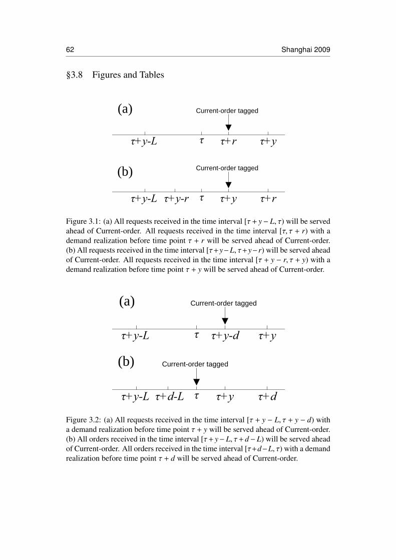
62 Shanghai 2009

§3.8 Figures and Tables

τ+r τ+y

Current-order tagged

ττ+y-L

τ+y τ+r

Current-order tagged

ττ+y-rτ+y-L

(a)

(b)

Figure 3.1: (a) All requests received in the time interval [τ+ y− L, τ) will be servedahead of Current-order. All requests received in the time interval [τ, τ + r) with ademand realization before time point τ + r will be served ahead of Current-order.(b) All requests received in the time interval [τ+y−L, τ+y−r) will be served aheadof Current-order. All requests received in the time interval [τ + y − r, τ + y) with ademand realization before time point τ + y will be served ahead of Current-order.

τ+y-d τ+y

Current-order tagged

ττ+y-L

τ+y τ+dττ+y-L τ+d-L

(a)

(b) Current-order tagged

Figure 3.2: (a) All requests received in the time interval [τ + y − L, τ + y − d) witha demand realization before time point τ + y will be served ahead of Current-order.(b) All orders received in the time interval [τ+ y− L, τ+ d− L) will be served aheadof Current-order. All orders received in the time interval [τ+d−L, τ) with a demandrealization before time point τ + d will be served ahead of Current-order.

Shanghai 2009 63

Table 3.1: (a) Reservation policy FD, L = 4, Y uniform on 0 to L, h = 1, λ = 2, a =

5, b = 1. Av OH is the average on-hand inventory. Revenue is the expected revenueper time unit, and Profit is expected profit per time unit. The table is prepared forS = 6 which is the optimal base stock level.

r Av. OH Revenue Profit0 2.551279 3.613333 1.062054

0.5 2.523217 3.636836 1.1136191 2.456787 3.737113 1.280327

1.5 2.377631 3.920839 1.5432082 2.304997 4.152242 1.847244

2.5 2.249383 4.379493 2.130113 2.214189 4.560289 2.346101

3.5 2.198202 4.672722 2.474524 2.195435 4.710782 2.515348

Table 3.1: (b) Reservation policy BD, L = 4, Y uniform on 0 to L, h = 1, λ = 2.AvOH is the average on-hand inventory. Revenue is the expected revenue per timeunit, and Profit is expected profit per time unit. The table is prepared for S = 6which is the optimal base stock level.

r Av. OH Revenue Profit4 2.551279 3.613333 1.062054

2.063508 2.337913 4.154912 1.8169981.354249 2.246088 4.435627 2.1895390.877501 2.210928 4.587004 2.3760770.535898 2.199201 4.663519 2.4643180.291901 2.196065 4.696843 2.5007780.127017 2.195487 4.708194 2.5127070.031373 2.195435 4.710627 2.515192

0 2.195435 4.710782 2.515348

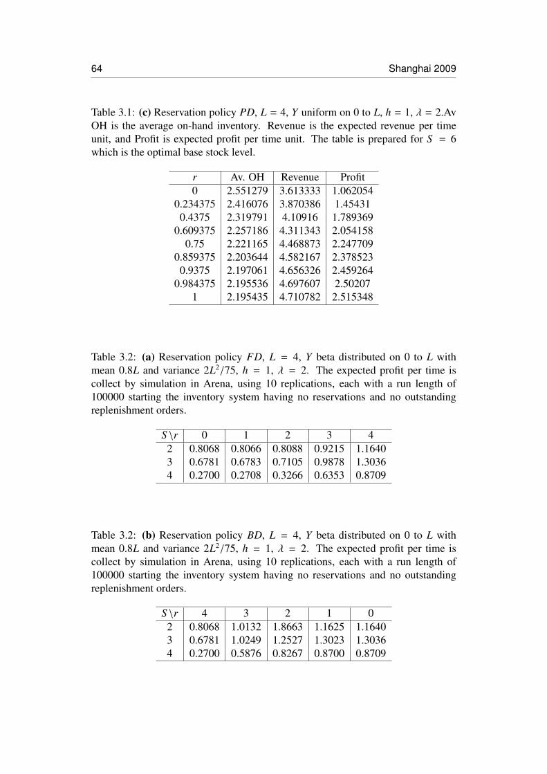
64 Shanghai 2009

Table 3.1: (c) Reservation policy PD, L = 4, Y uniform on 0 to L, h = 1, λ = 2.AvOH is the average on-hand inventory. Revenue is the expected revenue per timeunit, and Profit is expected profit per time unit. The table is prepared for S = 6which is the optimal base stock level.

r Av. OH Revenue Profit0 2.551279 3.613333 1.062054

0.234375 2.416076 3.870386 1.454310.4375 2.319791 4.10916 1.789369

0.609375 2.257186 4.311343 2.0541580.75 2.221165 4.468873 2.247709

0.859375 2.203644 4.582167 2.3785230.9375 2.197061 4.656326 2.459264

0.984375 2.195536 4.697607 2.502071 2.195435 4.710782 2.515348

Table 3.2: (a) Reservation policy FD, L = 4, Y beta distributed on 0 to L withmean 0.8L and variance 2L2/75, h = 1, λ = 2. The expected profit per time iscollect by simulation in Arena, using 10 replications, each with a run length of100000 starting the inventory system having no reservations and no outstandingreplenishment orders.

S \r 0 1 2 3 42 0.8068 0.8066 0.8088 0.9215 1.16403 0.6781 0.6783 0.7105 0.9878 1.30364 0.2700 0.2708 0.3266 0.6353 0.8709

Table 3.2: (b) Reservation policy BD, L = 4, Y beta distributed on 0 to L withmean 0.8L and variance 2L2/75, h = 1, λ = 2. The expected profit per time iscollect by simulation in Arena, using 10 replications, each with a run length of100000 starting the inventory system having no reservations and no outstandingreplenishment orders.

S \r 4 3 2 1 02 0.8068 1.0132 1.8663 1.1625 1.16403 0.6781 1.0249 1.2527 1.3023 1.30364 0.2700 0.5876 0.8267 0.8700 0.8709

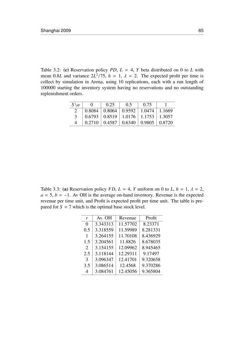
Shanghai 2009 65

Table 3.2: (c) Reservation policy PD, L = 4, Y beta distributed on 0 to L withmean 0.8L and variance 2L2/75, h = 1, λ = 2. The expected profit per time iscollect by simulation in Arena, using 10 replications, each with a run length of100000 starting the inventory system having no reservations and no outstandingreplenishment orders.

S \α 0 0.25 0.5 0.75 12 0.8084 0.8064 0.9592 1.0474 1.16693 0.6793 0.8519 1.0176 1.1753 1.30574 0.2710 0.4587 0.6340 0.9805 0.8720

Table 3.3: (a) Reservation policy FD, L = 4, Y uniform on 0 to L, h = 1, λ = 2,a = 5, b = −1. Av OH is the average on-hand inventory. Revenue is the expectedrevenue per time unit, and Profit is expected profit per time unit. The table is pre-pared for S = 7 which is the optimal base stock level.

r Av. OH Revenue Profit0 3.343313 11.57702 8.23371

0.5 3.318559 11.59989 8.2813311 3.264155 11.70108 8.436929

1.5 3.204561 11.8826 8.6780352 3.154155 12.09962 8.945465

2.5 3.118144 12.29311 9.174973 3.096347 12.41701 9.320658

3.5 3.086514 12.4568 9.3702864 3.084761 12.45056 9.365804

66 Shanghai 2009

Table 3.3: (b) Reservation policy BD, L = 4, Y uniform on 0 to L, h = 1, λ = 2,a = 5, b = −1. Av OH is the average on-hand inventory. Revenue is the expectedrevenue per time unit, and Profit is expected profit per time unit. The table is pre-pared for S = 7 which is the optimal base stock level.

d Av. OH Revenue Profit4 3.343313 11.57702 8.23371

2.063508 3.190394 12.26043 9.0700331.354249 3.122085 12.43928 9.3171950.877501 3.09595 12.47085 9.3749010.535898 3.087416 12.46592 9.3785060.291901 3.085195 12.45698 9.3717830.127017 3.084796 12.45204 9.367240.031373 3.084761 12.45066 9.365903

0 3.084761 12.45056 9.365804

Table 3.3: (c) Reservation policy PD, L = 4, Y uniform on 0 to L, h = 1, λ = 2,a = 5, b = −1. Av OH is the average on-hand inventory. Revenue is the expectedrevenue per time unit, and Profit is expected profit per time unit. The table is pre-pared for S = 7 which is the optimal base stock level.

α Av. OH Revenue Profit0 3.343313 11.57702 8.23371

0.234375 3.240126 11.92687 8.6867470.4375 3.170256 12.203 9.032742

0.609375 3.126555 12.38227 9.2557180.75 3.102021 12.46926 9.367236

0.859375 3.090245 12.49025 9.4000020.9375 3.085846 12.47768 9.391838

0.984375 3.084828 12.45877 9.3739441 3.084761 12.45056 9.365804

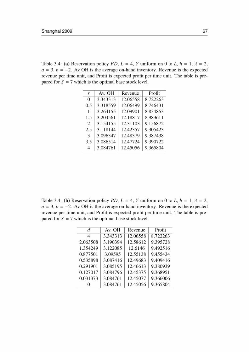
Shanghai 2009 67

Table 3.4: (a) Reservation policy FD, L = 4, Y uniform on 0 to L, h = 1, λ = 2,a = 3, b = −2. Av OH is the average on-hand inventory. Revenue is the expectedrevenue per time unit, and Profit is expected profit per time unit. The table is pre-pared for S = 7 which is the optimal base stock level.

r Av. OH Revenue Profit0 3.343313 12.06558 8.722263

0.5 3.318559 12.06499 8.7464311 3.264155 12.09901 8.834853

1.5 3.204561 12.18817 8.9836112 3.154155 12.31103 9.156872

2.5 3.118144 12.42357 9.3054233 3.096347 12.48379 9.387438

3.5 3.086514 12.47724 9.3907224 3.084761 12.45056 9.365804

Table 3.4: (b) Reservation policy BD, L = 4, Y uniform on 0 to L, h = 1, λ = 2,a = 3, b = −2. Av OH is the average on-hand inventory. Revenue is the expectedrevenue per time unit, and Profit is expected profit per time unit. The table is pre-pared for S = 7 which is the optimal base stock level.

d Av. OH Revenue Profit4 3.343313 12.06558 8.722263

2.063508 3.190394 12.58612 9.3957281.354249 3.122085 12.6146 9.4925160.877501 3.09595 12.55138 9.4554340.535898 3.087416 12.49683 9.4094160.291901 3.085195 12.46613 9.3809390.127017 3.084796 12.45375 9.3689510.031373 3.084761 12.45077 9.366006

0 3.084761 12.45056 9.365804

68 Shanghai 2009

Table 3.4: (c) Reservation policy PD, L = 4, Y uniform on 0 to L, h = 1, λ = 2,a = 3, b = −2. Av OH is the average on-hand inventory. Revenue is the expectedrevenue per time unit, and Profit is expected profit per time unit. The table is pre-pared for S = 7 which is the optimal base stock level.

α Av. OH Revenue Profit0 3.343313 12.06558 8.722263

0.234375 3.240126 12.31705 9.0769240.4375 3.170256 12.49948 9.329226

0.609375 3.126555 12.59338 9.4668250.75 3.102021 12.60652 9.504502

0.859375 3.090245 12.56809 9.4778440.9375 3.085846 12.51239 9.426543

0.984375 3.084828 12.46745 9.3826261 3.084761 12.45056 9.365804

4Advance Demand Information,

Capacity Restrictions and

Customer Prioritization

History: This paper was initially started at the Tepper School of Business, CarnegieMellon University during my visit in the Fall 2009. This work was presented at theEuropean Conference on Operational Research (EURO), July 2010, Lisbon, Portugal; theInternational Society for Inventory Research (ISIR) biennial Conference - 16thSymposium, August 2010, Budapest, Hungary; and the INFORMS annual conference,November 2010, TX-Austin, USA.

69

TXAustin 2010 71

Advance Demand Information, CapacityRestrictions and Customer Prioritization

Bisheng Du∗ Christian Larsen† Alan Scheller-Wolf‡

Abstract

We study a single supplier who must invest in capacity to manufacturer and sellproducts to buyers having different priorities. The buyers can place pre-orders be-fore their demand is observed, and can also issue additional orders upon observingdemand information. Since the supplier guarantees delivery of pre-ordered goods(these are not constrained by the supplier’s capacity), buyers with lower prioritiesmay consider pre-ordering in order to secure inventory. We derive optimal policiesfor the supplier and buyers. We show surprisingly that it is optimal for the sup-plier to set the pre-order price so high that pre-ordering will not be used much eventhough pre-ordering should be of benefit to the supplier due to risk sharing. We alsoshow that the supplier can make a pricing decision using an aggregate model.

Keywords

Advance demand information; Capacity restrictions; Customer prioritization; Pre-order

∗CORAL - Centre for Operations Research Applications in Logistics, Department of Economicsand Business, Aarhus School of Business and Social Sciences, Aarhus University, Fuglesangs Alle4, Aarhus V, DK-8210, Denmark. E-mail: bisd@asb.dk

†CORAL - Centre for Operations Research Applications in Logistics, Department of Economicsand Business, Aarhus School of Business and Social Sciences, Aarhus University, Fuglesangs Alle4, Aarhus V, DK-8210, Denmark. E-mail: chl@asb.dk

‡Tepper School of Business, Carnegie Mellon University, 5000 Forbes Avenue, Pittsburgh, PA15213, USA. E-mail: awolf@andrew.cmu.edu

72 TXAustin 2010

§4.1 Introduction

The inspiration for this paper is based on observations from practice. A vital

auto component and part supplier, located in China, serves several auto manufac-

turers in a specific area. With the dramatic growth of private cars in China, the

demands for cars from some auto manufacturers therefore begin to exceed their

supply, even in the global economic slump of the current financial crisis. Thus,

in order to get more production, major car manufacturers are competing for their

suppliers’ capacity. One way they could try to ensure capacity would be to pre-

order supplies well in advance of the actual sales period, and then later, when they

know the actual demand, they make additional orders if necessary. In the case il-

lustrated above, the motivation for pre-orders comes from the manufacturers (in the

paper, “buyers”), which is because of the competition between auto makers. It may

therefore be realistic that the supplier sets the prices. Hence, this analysis is seen

from the supplier’s perspective. It motivates the study in this paper, which con-

siders a price setting component supplier with several customers, who makes both

pre-orders (before observing demand) and after-orders (after observing demand).

We limit ourselves to study only two buyers and one single selling season, thereby

turning our model into a variant of a newsvendor. The key feature is that the buyers

can make pre-orders before they observe their real demand, and later, when having

observed their real demand they can issue an additional order to be fulfilled to the

extent that the supplier has sufficient capacity. The pre-orders can be considered

as advance demand information from the perspective of the supplier. Pre-ordering

also enables risk-sharing between the supplier and the buyers. We focus on how

the supplier can set the pre-order price optimally given a fixed (market determined)

after-order price.

This paper is organized as follows. In Section 4.2, we review the literature on the

inventory problem with advance booking and multiple demand classes. In Section

4.3, we analyze the two-buyer case with ADI (Advance Demand Information), find

the optimal solution and give its interpretation. Later, in Section 4.4, we analyze

TXAustin 2010 73

the aggregate buyer case with ADI and find the optimal solution. In Section 4.5,

we conduct numerical investigation using different demand distributions. Finally,

in Section 4.6, we present conclusions and suggest future research directions.

§4.2 Literature review

Our work follows two streams of research, which are inventory systems with

advance booking and inventory systems with multiple demand classes, respectively.

The closest work to ours is Dong and Zhu (2007) and Cachon (2004). Based on

the work by Cachon (2004), Dong and Zhu (2007) present a Two-Wholesale-Price

contract that divides the inventory system into Push, Pull and Partial Advance Book-

ing (PAB) sections. Compared with Dong and Zhu (2007), our work extends their

topic into a two demand classes case: there are two customers with different pri-

orities. Therefore, Dong and Zhu (2007) is a special case of our work with only

one customer. In this case, we recover the result of Dong and Zhu (2007). There

are plenty of studies in the advance booking field. One of the earliest works is

Hariharan and Zipkin (1995), who consider the effects of customer order infor-

mation and leadtime on the whole inventory system. In addition, there are also

some other research works, for instance, Chen (2001), Gallego and Ozer (2001),

Frank et al. (2003), Hu (2003), Ozer (2003), Gallego and Ozer (2003), Ozer and Wei

(2004), Marklund (2006), Wang and Toktay (2008), Papier and Thonemann (2010)

have also done plenty of studies within this field.

The other stream important to our work is research on systems with multiple de-

mand classes. Many publications have investigated this field, such as Gayon et al.

(2009) who study a Make-to-Stock system, a supplier with limited capacity and

ADI within multiple customer classes. Arslan et al. (2007) investigates a single

product inventory model with multiple demand classes, which is a model with Pois-

son demand, deterministic replenishment leadtime, and a continuous-review (Q, R)

policy with rationing. In addition, Deshpande et al. (2003), Teunter and Haneveld

(2008), Enders et al. (2009) and Zhou and Zhao (2010) also study the multiple de-

74 TXAustin 2010

mand classes problem from different perspectives. The work by Sen and Zhang

(1999), which considers the newsboy problem with multiple demand classes, is

closest to our work from a methodological point of view. They assume N demand

classes, and each class is charged at different prices: increasing prices or decreas-

ing prices. They derived both the fare allocation limit and the initial capacity and

discussed managerial implication. For more details on the newsvendor problem,

please refer to Porteus (1990) or Porteus (2002).

§4.3 The mathematical model

We assume that there are two buyers, one buyer “H” with a high priority and

another buyer “L” with a low priority. They operate in two separated markets, each

facing a random demand described by the random variables DH and DL, respec-

tively. The buyers pre-order quantities QH1 and QL

1 , respectively. Furthermore, in

anticipation of further orders, the supplier builds capacity. With his capacity, the

supplier should fulfill the orders from the higher priority customer at first, any ex-

cess capacity or inventory can be considered for the lower priority customer. We

assume that both buyers have a given unit sales price r. We could have added more

generality by assuming sales prices rH and rL, respectively. However, in order to

rule out any arbitrage, we let the two buyers operate in separated markets using the

same fixed unit sales price r. The supplier has unit production cost c. All entities

can sell any left-overs at a price of s. As usual, we assume s < c < r. The order of

events is now as follows.

1. The supplier sets pre-order and after-order unit prices w1 and w2, where we

mainly focus on how to optimize w1 while w2 is fixed.

2. Buyers H and L decide (simultaneously and independently of each other) pre-

order amounts QH1 and QL

1 , respectively.

3. The supplier decides how much capacity QH1 + QL

1 + Q2 to develop.

TXAustin 2010 75

4. The two buyers observe actual demand dH and dL drawn from the random

variables DH and DL.

5. Buyer H gets the amount QH1 + RH where the first QH

1 units are charged the

unit price w1 and all remaining units RH = min{max

{dH − QH

1 , 0},Q2

}are

charged the unit price w2. RH is the additional sale (in excess of QH1 ) to buyer

H.

6. Buyer L gets the amount QL1 + RL where the first QL

1 units are charged the unit

price w1 and all remaining units RL = min{max

{dL − QL

1 , 0},max {Q2 − RH, 0}

}are charged the unit price w2. RL is the additional sale (in excess of QL

1) to

buyer L.

7. Buyer H sells the amount min{dH,QH

1 + RH

}in his market at unit price r and

the remaining amount max{QH

1 + RH − dH, 0}

to the scrap market at unit price

s. Similarly, buyer L sells the amount min{dL,QL

1 + RL

}in his market at unit

price r and the remaining amount max{QL

1 + RL − dL, 0}

to the scrap market

at unit price s. The supplier sells any left-overs Q2 − RH − RL to the scrap

market at unit price s.

As the supplier knows that he can sell QH1 + QL

1 units, the decision variable Q2

concerns how much additional capacity he will develop. We want to explore how

the supplier can set his prices w1 and w2 optimally. To avoid a trivial solution, we

will assume that there exist alternative sourcing opportunities concerning the after-

orders. Thus, we assume that w2 is fixed and the analysis is then concerned about

how to set pre-order price w1 optimally.

We here assume that when the buyers determine their pre-order quantities they

have full information about the cost structure of the supplier and they are also aware

that the supplier knows the probability distribution of their demands. Therefore,

when deciding optimal pre-order quantities, they know the optimal reaction (in

terms of the decision variable Q2) of the supplier. Assume in the following that

76 TXAustin 2010

f (x) and g(x) are the density functions of the random variables DH and DL, respec-

tively.

There are two sources of revenue yielding the supplier’s total profit: the first

source is the revenue by selling products from supplier to buyers, the second source

is the revenue by selling products to the secondary salvage market at a discounted

price.

During the initial period, the supplier knows that she will sell QH1 + QL

1 items,

which are the pre-orders from buyer H and buyer L, respectively. Recall that the

quantity of products sold to buyer H are QH1 + RH, RH = min

[(DH − QH

1 )+,Q2

], the

quantity of products sold to buyer L are QL1 + RL, RL = min

[(DL − QL

1)+,Q2 − RH

].

Therefore, there are three situations of demand at H, DH. (1) If DH ≥ QH1 + Q2, H

will buy all Q2 additional units, no supply remain for L. (2) If QH1 ≤ DH ≤ QH

1 + Q2,

H will buy DH − QH1 additional units. All the remaining units, Q2 + QH

1 − DH will

be bought by L if DL ≥ Q2 + QH1 −DH + QL

1 . QL1 ≤ DL ≤ q2 + QH

1 −DH + QL1 , and L

will buy DL − QL1 additional units. If DL ≤ QL

1 , then L will buy no additional units.

(3) If DH ≤ QH1 , all the Q2 additional units will be bought by L if DL ≥ QL

1 + Q2. If

QL1 ≤ DL ≤ QL

1 + q2, then DL −QL1 additional units will be bought. If DL ≤ QL

1 , then

L will buy no additional units.

We now derive the expected value of RH:

E(RH) =

QH1 +q2∫

QH1

(x − QH1 ) f (x) dx + q2 P(DH ≥ QH

1 + q2) (4.1)

And also, the expected value of RL is:

E(RL) =

QH1 +q2∫

QH1

QL

1 +(q2−RH)+∫QL

1

(y − QL1) g(y) dy + (q2 − RH)+ P(DL ≥ QL

1 + (q2 − RH)+)

f (x) dx

+

∫ QH1

0

q2 P(DL ≥ QL1 + q2) +

QL1 +q2∫

QL1

(y − QL1) g(y) dy

f (x) dx

TXAustin 2010 77

Note that the order of integrals is due to Buyer H having the highest priority.

In the first term of the above equation, RH = DH −QH1 can be inserted inside the

integral of RL because RH belongs to the interval (QH1 ,Q

H1 + q2). Then RL is equals

to

E(RL) =

QH1 +q2∫

QH1

(QH1 + q2 − x)P(DL ≥ QH

1 + QL1 + q2 − x) +

QH1 +QL

1 +q2−x∫QL

1

(y − QL1) g(y) dy

f (x) dx

+ P(DH ≤ QH1 )

q2 P(DL ≥ QL1 + q2) +

QL1 +q2∫

QL1

(y − QL1) g(y) dy

(4.2)

The expected revenue for the supplier from selling to buyer H and buyer L is:

w1(QH1 + QL

1) + w2 [E(RH) + E(RL)] (4.3)

The second source of the supplier’s revenue comes from sales to the secondary

market. This can be described by three components. (1) If DH ≥ QH1 + q2, then 0

unit is scrapped. Therefore,

E(LO1) = 0

Where LOi (i = 1, 2, 3) donate the left over products sales to the secondary market

under three situations.

(2) If QH1 ≤ DH ≤ QH

1 +q2, then QH1 +q2−DH units are left over to L. If DL ≤ QL

1 ,

he will buy none of these additional units, so the QH1 + q2 − x units are all scrapped.

If QL1 ≤ DL ≤ QH

1 + QL1 + q2 −DH, then QH

1 + QL1 + q2 −DH −DL units are scrapped.

If DL ≥ QH1 + QL

1 + q2 − DH, then no units are scrapped. Therefore,

E(LO2) =

QH1 +q2∫

QH1

(QH1 + q2 − x)P(DL ≤ QL

1) +

QH1 +QL

1 +q2−x∫QL

1

(QH1 + QL

1 + q2 − x − y) g(y) dy

f (x) dx

(3) If DH ≤ QH1 , all the q2 additional units are left over for L. If DL ≤ QL

1 , all these

78 TXAustin 2010

q2 units are scrapped. If QL1 ≤ DL ≤ QL

1 + q2, then QL1 + q2 − DL units are scrapped.

If DL ≥ QL1 + q2, then 0 unit is scrapped. Therefore,

E(LO3) = P(DH ≤ QH1 )

q2 P(DL ≤ QL1) +

QL1 +q2∫

QL1

(QL1 + q2 − y) g(y) dy

All in all, the revenue from sales to the secondary market is

s [E(LO1) + E(LO2) + E(LO3)] (4.4)

The optimal additional capacity to develop given the pre-order quantities QH1

and QL1 is found by the following optimization model:

ΠS (q2) =w1(QH1 + QL

1) + w2 [E(RH) + E(RL)]

+ s [E(LO1) + E(LO2) + E(LO3)] − c(QH

1 + QL1 + q2

) (4.5)

Denote the optimal solution Q2(QH1 ,Q

L1).

This is a concave function of q2 with first-order derivative, which is dΠS (q2)dq2

(for

more details, see Section 4.7.1 of Appendix):

w2−c−(w2−s)

P(DH ≤ QH1 )P(DL ≤ QL

1 + q2) +

QH1 +q2∫

QH1

P(DL ≤ QH1 + QL

1 + q2 − x) f (x)dx

(4.6)

Therefore, we conclude that the optimal solution, Q2, is 0 if

P(DH ≤ QH1 )P(DL ≤ QL

1) >w2 − cw2 − s

(4.7)

TXAustin 2010 79

Otherwise, it is the unique value of q2 that solves the equation

P(DH ≤ QH1 )P(DL ≤ QL

1 +q2)+

QH1 +q2∫

QH1

P(DL ≤ QH1 +QL

1 +q2−x) f (x)dx =w2 − cw2 − s

(4.8)

Special case: If we assume that QH1 = QL

1 = 0, the first order condition equals∫ q2

0P(DL ≤ q2 − x) f (x) dx = w2−c

w2−s , which means P(DH + DL ≤ q2) = w2−cw2−s . So

the supplier will base his capacity decision on the aggregate demand information,

which is the same as the aggregate model we will present in the next section.

In this way we have derived a reaction function Q2(qH1 , q

L1) of any pair of pre-

order amounts (qH1 , q

L1).

Before we continue, let us examine the cases where DL ≡ 0. In this case, (4.6)

becomes

w2 − c − (w2 − s)P(DH ≤ QH1 + q2) (4.9)

This term is less than or equal to (4.6). Therefore, if Q2(qH1 ,DL ≡ 0) is the

reaction function of the supplier if buyer H is the only buyer, then we conclude that

Q2(qH1 ,DL ≡ 0) ≤ Q2(qH

1 , qL1). This means that the presence of a low prioritized

buyer will always induce the supplier to provide more additional capacity than was

made available if only one buyer was present. This argument does not depend on

the pre-order price w1.

Given that both buyers know the optimal behavior of the supplier, they solve

their own optimization problems.

Denoted by QH1 (qL

1), the optimal pre-order quantity of buyer H is derived so that

he knows the optimal reaction of the supplier as well as the pre-order quantity qL1 of

buyer L. QH1 (qL

1) is the optimal solution to the following optimization problem.

80 TXAustin 2010

Buyer H’s optimization problem:

ΠH(qH1 ) =r

∫ qH1 +Q2(qH

1 ,qL1 )

0x f (x) dx + (qH

1 + Q2(qH1 , q

L1)) P(DH ≥ qH

1 + Q2(qH1 , q

L1))

− w1 qH

1 − w2 E(RH) + s∫ qH

1

0(qH

1 − x) f (x) dx

(4.10)

At first glance, it appears that buyer H’s profit function does not depend on

the probability distribution of DL. However, it does depend on DL as Q2(qH1 , q

L1)

depends on DL, we denote the optimal solution QH1 (qL

1).

This optimization problem has first-order condition on QH1 (see Section 4.7.3 of

Appendix).

Similarly, denoted by QL1(qH

1 ) the optimal pre-order quantity of buyer L is de-

rived so that he knows the optimal reaction of the supplier as well as the pre-order

quantity qH1 of buyer H. This is the optimal solution to the following optimization

problem.

The revenue of buyer L from selling products in the market is dependent on

three situations, based on the sales of buyer H.

(1) If DH ≥ qH1 + Q2(qH

1 , qL1), then the products supplied to buyer L are qL

1 .

E(S L1) = P(DH ≥ qH1 + Q2(qH

1 , qL1))

∫ qL1

0y g(y) dy + P(DL ≥ qL

1)qL1

(4.11)

Where S Li (i = 1, 2, 3) denote the products supplied to buyer L under three situa-

tions.

(2) If qH1 ≤ DH ≤ qH

1 + Q2(qH1 , q

L1), then qH

1 + Q2(qH1 , q

L1) − DH units are left over

TXAustin 2010 81

to L. Then the products supplied to buyer L are E(S L2).

E(S L2) =

qH1 +Q2(qH

1 ,qL1 )∫

qH1

[ qH1 +qL

1 +Q2(qH1 ,q

L1 )−x∫

0

y g(y) dy

+P(DL ≥ qH1 + qL

1 + Q2(qH1 , q

L1) − x) (qH

1 + qL1 + Q2(qH

1 , qL1) − x)

]f (x) dx

(4.12)

(3) If DH ≤ qH1 , all the Q2 additional units are left over to L. Then products from

the supplier to buyer L are E(S L3).

E(S L3) =P(DH ≤ qH1 )

[∫ qL1 +Q2(qH

1 ,qL1 )

0y g(y) dy

+ P(DL ≥ qL1 + Q2(qH

1 , qL1)) (qL

1 + Q2(qH1 , q

L1))

] (4.13)

Buyer L’s optimization problem becomes:

ΠL(qL1) =r [E(S L1) + E(S L2) + E(S L3)]

− w1 qL1 − w2 E(RL) + s

∫ qL1

0(qL

1 − y) g(y) dy(4.14)

This optimization problem has first-order condition on QL1 (see Section 4.7.4 of

Appendix).

In this way the two buyers can continue to iterate until they reach an equilibrium

(QH1 ,Q

L1) characterized by QH

1 (QL1) = QH

1 and QL1(QH

1 ) = QL1 . For each value of w1

under this full information scenario, the supplier then needs to figure out what the

equilibrium is, and then he can compute his expected profit. By varying w1, he

can thus find his optimal pre-order price. It is quite a task to carry out such an

analysis and furthermore there may be several equilibriums. In the following, we

will therefore consider whether the analysis could be carried out by using a more

aggregate model.

82 TXAustin 2010

§4.4 An aggregate model

The aggregate model focuses on the supplier’s point of view, especially when

two buyers are collapsed into one, denoted by A (A stands for aggregate), who

accordingly sells his product at unit price r in a market with random demand DA =

DH + DL. h(x) and H(x) denote the density and distribution function of DA. The

order of events is as follows:

1. The supplier sets unit pre-order and unit after-order prices w1 and w2.

2. Buyer A decides a pre-order amount Q1.

3. The supplier decides how much capacity Q1 + Q2 to develop.

4. Buyer A observes the actual demand d drawn from the random variable DA.

5. Buyer A gets the amount y = min{max{d,Q1},Q1 + Q2} where all units in

excess of Q1 are charged the unit price w2 and all remaining units are charged

the unit price w1.

6. Buyer A sells the amount min{d, y} in his market at unit price r and the re-

maining amount max{y−d, 0} to the scrap market at unit price s. The supplier

sells any left-overs Q1 + Q2 − y at the scrap market.

So in this aggregate model, when the supplier conduct an analysis of how to set

his preorder price optimally, he just assumes for simplicity that he only has one (su-

per) buyer. The mathematics of this model is essentially developed in Dong and Zhu

(2007). So here, we will just summarize the key findings. The reaction function can

now be specified explicitly as (see also (4.9)):

Q2(q1) = max{

H−1(w2 − cw2 − s

)− q1, 0

}(4.15)

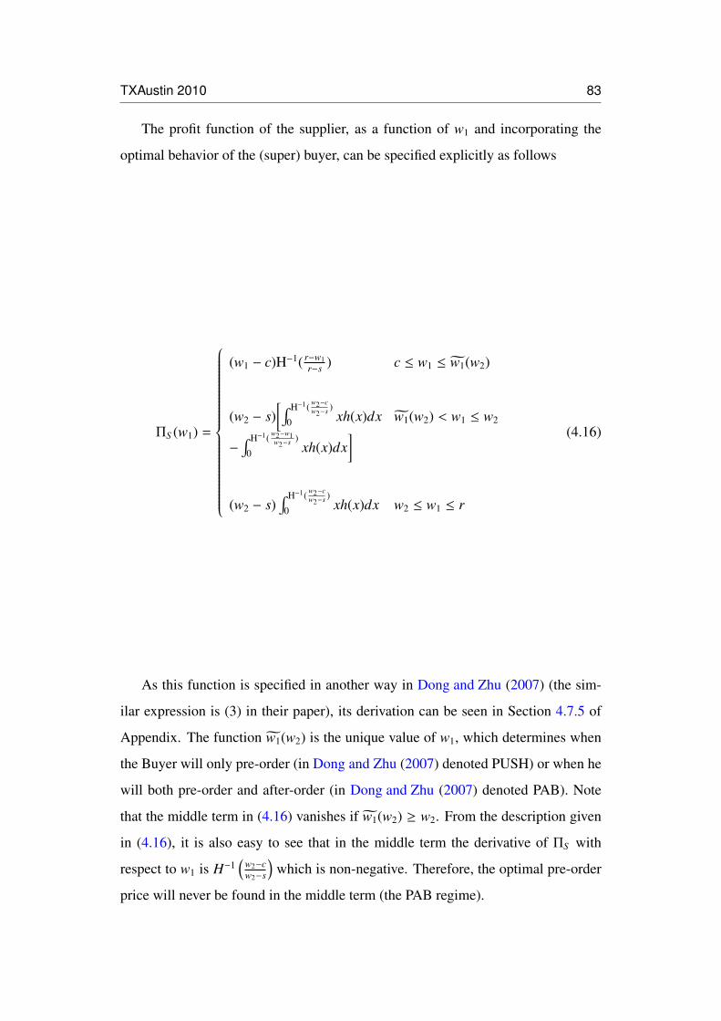
TXAustin 2010 83

The profit function of the supplier, as a function of w1 and incorporating the

optimal behavior of the (super) buyer, can be specified explicitly as follows

ΠS (w1) =

(w1 − c)H−1( r−w1r−s ) c ≤ w1 ≤ w1(w2)

(w2 − s)[∫ H−1( w2−c

w2−s )

0 xh(x)dx w1(w2) < w1 ≤ w2

−∫ H−1( w2−w1

w2−s )

0 xh(x)dx]

(w2 − s)∫ H−1( w2−c

w2−s )

0 xh(x)dx w2 ≤ w1 ≤ r

(4.16)

As this function is specified in another way in Dong and Zhu (2007) (the sim-

ilar expression is (3) in their paper), its derivation can be seen in Section 4.7.5 of

Appendix. The function w1(w2) is the unique value of w1, which determines when

the Buyer will only pre-order (in Dong and Zhu (2007) denoted PUSH) or when he

will both pre-order and after-order (in Dong and Zhu (2007) denoted PAB). Note

that the middle term in (4.16) vanishes if w1(w2) ≥ w2. From the description given

in (4.16), it is also easy to see that in the middle term the derivative of ΠS with

respect to w1 is H−1(

w2−cw2−s

)which is non-negative. Therefore, the optimal pre-order

price will never be found in the middle term (the PAB regime).

84 TXAustin 2010

The optimal profit of the buyer:

ΠB(w1) =

(r − s)∫ F−1

( r−w1r−s

)0

x f (x) dx c ≤ w1 ≤ w1(w2)

(r − w2)∫ F−1

(w2−cw2−s

)0 x f (x) dx w1(w2) < w1 ≤ w2

+(w2 − s)∫ F−1

(w2−w1w2−s

)0 x f (x) dx

+(r − w2) c−sw2−s F−1

(w2−cw2−s

)

(r − w2)∫ F−1

(w2−cw2−s

)0 x f (x) dx w2 ≤ w1 ≤ r

+(r − w2) c−sw2−s F−1

(w2−cw2−s

)

(4.17)

§4.5 A numerical example

We consider a case where s = 2, c = 5 and r = 30. The demand distributions

are negative binomial distributions. We assume that DH and DL have the same

distribution with shape parameter n = 9 and probability parameter p = 0.5, meaning

that they both have mean value 9. Table 4.1 shows our results for the general model.

For each value of w2, the optimal value of w1 is stated (in this analysis restricted

to be integer valued) and its resulting equilibrium values of (QH1 ,Q

L1 ,Q2) and the

resulting expected profits of the three entities, denoted by ΠS , ΠH and ΠL for the

Supplier, Buyer H and Buyer L, respectively.

——————————————

Tables 4.1 is about here

——————————————

As expected, we see that buyer H always has a higher expected profit than buyer

L. Furthermore, as buyer H has the first priority, he does not need to make pre-

orders. When the after-order price is low, the supplier will not develop that much

TXAustin 2010 85

capacity. Therefore, buyer L needs to pre-order. Then the optimal pre-order price is

higher than the after-order price, and yet buyer L is still willing to pre-order so as to

reserve capacity. We also see that buyer H benefits from an increase of w2 from 8 to

10 because this will make the supplier invest in more unreserved capacity (variable

Q2), in which he can exploit better due to his first priority. When w2 gets larger, we

see that it is optimal to set the pre-order price so high that in reality the pre-order

option is virtually, but not entirely ruled out. Note that QL1 appears to be one not due

to rounding but because of the discrete nature of the numerical experiment that QL1

is slightly above 0. From Section 4.7.4 of Appendix, we can formally prove:

dΠL(qL1)

dqL1

|qL1 =0 =rP(DH ≥ qH

1 + Q2) − w1

+ w2

[P(DH ≤ qH

1 ) + P(qH1 ≤ DH ≤ Q2 + qH

1 )]

=rP(DH ≥ qH1 + Q2) − w1 + w2P(DH ≤ Q2 + qH

1 )

Thus even if w1 = w2, we get that the partial derivative of buyer L’s profit func-

tion is positive around 0, and thus he will pre-order, though only in small amounts as

seen in Table 4.2. This partial derivative has nice economic interpretations: If buyer

L decides to pre-order one marginal unit (and currently has pre-ordered none), then

he will of course incur a marginal loss w1. But if the demand of buyer H should

exceed his maximum delivery Q2 + qH1 , then buyer L is secured a marginal sale giv-

ing him a marginal revenue r. On the other hand, if the demand of buyer H is less

than his maximum delivery Q2 + qH1 , then buyer L can decrease his after-order by a

marginal unit giving him a marginal decrease in his purchase costs of w2.

We now turn to the aggregate model. Here the aggregate demand is negatively

binomially distributed with shape parameter n = 18 and probability parameter p =

0.5. Using the approach from above, we get the following results.

——————————————

Tables 4.2 is about here

——————————————

86 TXAustin 2010

We see here almost the same results as in Table 4.2. Thus it indicates that

the supplier, maybe except for the low values of w2, could have reached the same

conclusion about how to set the pre-order price optimally by using the aggregate

model. From this model it is even more apparent that the price setting supplier will

set the pre-order price high enough to keep the option ruled out.

§4.6 Conclusions

We have derived a newsvendor model with two buyers having different priorities

in case of shortages, and a price setting supplier offering a pre-order opportunity.

Though the pre-order opportunity should favor the supplier, enabling him to allocate

some risk to his buyers, it turns out that when he is a price setter, he will set the

price for pre-ordering high enough that this option will not be used by the buyers.

Of course, as the data set presented to support this claim is very limited (though

some more data are available than presented in this paper), it is obvious that more

comprehensive numerical studies should be undertaken. It also seems to be the

case that the supplier can make his pre-order price decision using a more aggregate

model. This is of course of great help as the detailed model is very complex and

involves finding Nash-equilibria.

Acknowledgments

The first two authors are supported by Grant No. 275-07-0094 from the Danish

Social Science Research Council.

TXAustin 2010 87

§4.7 Appendices

§4.7.1 Supplier’s function, first order condition on Q2

The first order deviation on q2 to the supplier’s profit function is equivalent to:

w2

[∂E(RH)∂q2

+∂E(RL)∂q2

]− c + s

[∂E(LO1)∂q2

+∂E(LO2)∂q2

+∂E(LO3)∂q2

]= 0

Where,

∂E(RH)∂q2

=q2 f (QH1 + q2) + P(DH > QH

1 + q2) − q2 f (QH1 + q2)

=P(DH > QH1 + q2)

∂E(RL)∂q2

=

QH1 +q2∫

QH1

[P(DL > QH

1 + QL1 + q2 − x) − (QH

1 + q2 − x)g(QH1 + QL

1 + q2 − x)

+ (QH1 + q2 − x)g(QH

1 + QL1 + q2 − x)

]f (x) dx

+ F(QH1 )

[P(DL > QL

1 + Q2) − q2 g(QL1 + q2) + q2 g(QL

1 + q2)]

=

QH1 +q2∫

QH1

P(DL > QH

1 + QL1 + q2 − x

)f (x) dx + F(QH

1 )P(DL > QL1 + q2)

=F(QH1 + q2) − F(QH

1 ) −

QH1 +q2∫

QH1

G(QH

1 + QL1 + q2 − x

)f (x) dx + F(QH

1 )(1 − G(QL

1 + q2))

=F(QH1 + q2) − F(QH

1 )G(QL1 + q2) −

QH1 +q2∫

QH1

G(QH

1 + QL1 + q2 − x

)f (x) dx

88 TXAustin 2010

Therefore,

∂E(RH)∂q2

+∂E(RL)∂q2

= 1− F(QH1 )G(QL

1 + q2)−

QH1 +q2∫

QH1

G(QH

1 + QL1 + q2 − x

)f (x) dx

Simultaneously, we get

∂E(LO1)∂q2

=0

∂E(LO2)∂q2

=

QH1 +q2∫

QH1

[G(QL1) +

QH1 +QL

1 +q2−x∫QL

1

g(y)dy] f (x)dx =

QH1 +q2∫

QH1

G(QH1 + QL

1 + q2 − x) f (x)dx

∂E(LO3)∂q2

=F(QH1 )

G(QL1) +

QL1 +q2∫

QL1

g(y)dy

= F(QH1 )G(QL

1 + q2)

Therefore, the first order to q2 is:

dΠS (q2)dq2

=w2

1 − F(QH1 )G(QL

1 + q2) −

QH1 +q2∫

QH1

G(QH1 + QL

1 + q2 − x) f (x)dx

− c

+ s

F(QH1 )G(QL

1 + q2) +

QH1 +q2∫

QH1

G(QH1 + QL

1 + q2 − x) f (x)dx

The second order derivative is:

d2ΠS (q2)dq2

2

= − (w2 − s)[F(QH

1 )g(QL1 + q2) + G(QL

1) f (QH1 + q2)

+

QH1 +q2∫

QH1

g(QH1 + QL

1 + q2 − x) f (x)dx]

Thus, d2ΠS (q2)dq2

2< 0, so the supplier’s profit function is concave w.r.t. q2.

TXAustin 2010 89

As the solution to the expression above is equal to dΠS (q2)dq2

= 0, then we can get

w2 − c = (w2 − s)

F(QH1 )G(QL

1 + q2) +

QH1 +q2∫

QH1

G(QH1 + QL

1 + q2 − x) f (x)dx

(4.18)

If we assume that DL = 0, which means that there is only one demand class,then the CDF of it, G(·) = 1. The equation above is equal to

w2 − c = (w2 − s)

F(QH1 ) +

QH1 +q2∫

QH1

f (x)dx

(4.19)

This is exactly the same as the one demand class for QH1 = Q1.

F(QH1 + q2) =

w2 − cw2 − s

(4.20)

§4.7.2 Sensitivity of the optimal additional capacity as function of the pre-orders

In this section, we develop ∂Q2∂qH

1and ∂Q2

∂qL1

by use of an implicit function theorem.

For buyer H, from the implicit function theorem on qH1 , we derive

∂Q2

∂qH1

= −

∂∂qH

1(4.18)

∂∂Q2

(4.18)

= −

f (qH1 + Q2)P(DL ≤ qL

1) +

qH1 +Q2∫

qH1

g(qH1 + qL

1 + Q2 − x) f (x)dx

P(DH ≤ qH1 )g(qL

1 + Q2) +

qH1 +Q2∫

qH1

g(qH1 + qL

1 + Q2 − x) f (x)dx + P(DL ≤ qL1) f (qH

1 + Q2)

(4.21)

Here we get, −1 ≤ ∂Q2∂qH

1≤ 0 and ∂Q2

∂qH1|qH

1 =0 = −1.

90 TXAustin 2010

For buyer L, from the implicit function theorem on qL1 , we derive

∂Q2

∂qL1

= −

∂∂qL

1(4.18)

∂∂Q2

(4.18)

= −

P(DH ≤ qH1 )g(qL

1 + Q2) +

qH1 +Q2∫

qH1

g(qH1 + qL

1 + Q2 − x) f (x)dx

P(DH ≤ qH1 )g(qL

1 + Q2) +

qH1 +Q2∫

qH1

g(qH1 + qL

1 + Q2 − x) f (x)dx + P(DL ≤ qL1) f (qH

1 + Q2)

(4.22)

Also here we get, −1 ≤ ∂Q2∂qL

1≤ 0 and ∂Q2

∂qL1|qL

1 =0 = −1.

§4.7.3 Buyer H’s function, first order condition on QH1

Buyer H’s optimization problem, for simplicity, we use Q2 instead of Q2(qH1 , q

L1),

and use Q′2 donate the partial deviation of Q2 w.r.t. qH1 , ∂Q2(qH

1 ,qL1 )

∂ qH1

.

From (4.10), the first order deviation is

=r[(qH

1 + Q2) f (qH1 + Q2)(1 + Q′2) + (1 + Q′2) P(DH > qH

1 + Q2)

− (qH1 + Q2) f (qH

1 + Q2) (1 + Q′2)]

− w2

[−

qH1 +Q2∫

qH1

f (x) dx + Q2 f (qH1 + Q2)(1 + Q′2) + Q′2 P(DH > qH

1 + Q2)

− Q2 f (qH1 + Q2)(1 + Q′2)

]− w1 + s F(qH

1 )

=r (1 + Q′2) P(DH > qH1 + Q2) − w1 − w2

[F(qH

1 ) + Q′2 − (1 + Q′2)F(qH1 + Q2)

]+ s F(qH

1 )

=r (1 + Q′2) − r (1 + Q′2)F(qH1 + Q2) − w1 − w2 F(qH

1 ) − w2 Q′2+ w2 (1 + Q′2)F(qH

1 + Q2) + s F(qH1 )

=(r − w1) + (r − w2) Q′2 − (r − w2)(1 + Q′2)F(qH1 + Q2) − (w2 − s) F(qH

1 )

=(r − w2)(1 + Q′2)P(DH > qH1 + Q2) + (w2 − w1) − (w2 − s)F(qH

1 )

TXAustin 2010 91

Which is

dΠH(qH1 )

dqH1

= (r−w2)(1 + Q′2)P(DH > qH1 + Q2) + (w2−w1)− (w2− s)F(qH

1 ) (4.23)

Where the optimal solution is QH1 (qL

1).For the special case qH

1 = 0, then Q′2|qH1 =0 = 0 and F(qH

1 ) = 0, we can get

dΠH(qH1 )

dqH1

|qH1 =0 = w2 − w1 (4.24)

d2ΠH(qH1 )

(dqH1 )2

=[−(1 + Q′2)2 f (qH

1 + Q2) + Q′′2 P(DH ≥ qL1 + Q2)

](r − w2)

− (w2 − s) f (qH1 )

(4.25)

§4.7.4 Buyer L’s function, first order condition on QL1

The first order deviation on qL1 to buyer L’s profit function is equivalent to:

r∂ [E(S L1) + E(S L2) + E(S L3)]

∂qL1

− w1 − w2∂E(RL)∂qL

1

+ s G(qL1) = 0 (4.26)

ΠL(qL1) =r [E(S L1) + E(S L2) + E(S L3)]

− w1 qL1 − w2 E(RL) + s

∫ qL1

0(qL

1 − y) g(y) dy(4.27)

Buyer L’s optimization problem is below. For simplex, we use Q2 instead ofQ2(qH

1 , qL1) and use Q′2 donate the partial deviation of Q2 w.r.t. qL

1 . Therefore, from(4.14), the first order deviation is

From equation (4.11) on page 80, we get

∂E(S L1)∂qL

1

=P(DH ≥ qH1 + Q2)P(DL ≥ qL

1)

− Q′2 f (qH1 + Q2)

∫ qL1

0yg(y)dy + P(DL > qL

1)qL1

92 TXAustin 2010

From equation (4.12) on page 81, we get

∂E(S L2)∂qL

1

=

qH1 +Q2∫

qH1

P(DL ≥ qH1 + qL

1 + Q2 − x)(1 + Q′2) f (x) dx

+ Q′2

∫ qL1

0yg(y)dy + P(DL > qL

1)qL1

f (qH1 + Q2)

=(1 + Q′2)

qH1 +Q2∫

qH1

P(DL ≥ qH1 + qL

1 + Q2 − x) f (x) dx

+ Q′2

∫ qL1

0yg(y)dy + P(DL > qL

1)qL1

f (qH1 + Q2)

From equation (4.13) on page 81, we get

∂E(S L3)∂qL

1

=P(DH ≤ qH1 )(1 + Q′2)P(DL ≥ qL

1 + Q2)

=(1 + Q′2)P(DH ≤ qH1 )P(DL ≥ qL

1 + Q2)

∂[E(S L1) + E(S L2) + E(S L3)]∂qL

1

=P(DH ≥ qH1 + Q2)P(DL ≥ qL

1) − Q′2 f (qH1 + Q2)

∫ qL1

0yg(y)dy + P(DL > qL

1)qL1

+ (1 + Q′2)

qH1 +Q2∫

qH1

P(DL ≥ qH1 + qL

1 + Q2 − x) f (x) dx

+ Q′2

∫ qL1

0yg(y)dy + P(DL > qL

1)qL1

f (qH1 + Q2)

+ (1 + Q′2)P(DH ≤ qH1 )P(DL ≥ qL

1 + Q2)

Then,

TXAustin 2010 93

∂[E(S L1) + E(S L2) + E(S L3)]∂qL

1

=P(DH ≥ qH1 + Q2)P(DL ≥ qL

1) + (1 + Q′2)

qH1 +Q2∫

qH1

P(DL ≥ qH1 + qL

1 + Q2 − x) f (x) dx

+ (1 + Q′2)P(DH ≤ qH1 )P(DL ≥ qL

1 + Q2)

From equation (4.2) on page 77, we get

∂E(RL)∂qL

1

=

qH1 +Q2∫

qH1

[Q′2P(DL > qH

1 + qL1 + Q2 − x)

− (qH1 + Q2 − x)g(qH

1 + qL1 + Q2 − x)(1 + Q′2)

−

qH1 +qL

1 +Q2−x∫qL

1

g(y) dy + (qH1 + Q2 − x)g(qH

1 + qL1 + Q2 − x)(1 + Q′2)

]f (x) dx

+ P(DH ≤ qH1 )

[Q′2P(DL > qL

1 + Q2) − (1 + Q′2)Q2 g(qL1 + Q2)

−

qL1 +Q2∫

qL1

g(y) dy + (1 + Q′2)Q2 g(qL1 + Q2)

]

=

qH1 +Q2∫

qH1

[Q′2P(DL > qH

1 + qL1 + Q2 − x) −

qH1 +qL

1 +Q2−x∫qL

1

g(y) dy]f (x) dx

+ P(DH ≤ qH1 )

[Q′2P(DL > qL

1 + Q2) −

qL1 +Q2∫

qL1

g(y) dy]

=Q′2

qH1 +Q2∫

qH1

P(DL > qH1 + qL

1 + Q2 − x) f (x) dx −

qH1 +Q2∫

qH1

G(qH1 + qL

1 + Q2 − x) f (x) dx

+ G(qL1)[F(qH

1 + Q2) − F(qH1 )]

+ Q′2P(DH ≤ qH1 )P(DL > qL

1 + Q2) − F(qH1 )[G(qL

1 + Q2) −G(qL1)]

Then,

94 TXAustin 2010

∂E(RL)∂qL

1

=Q′2

qH1 +Q2∫

qH1

P(DL > qH1 + qL

1 + Q2 − x) f (x) dx −

qH1 +Q2∫

qH1

G(qH1 + qL

1 + Q2 − x) f (x) dx

+ Q′2P(DH ≤ qH1 )P(DL > qL

1 + Q2) + G(qL1)F(qH

1 + Q2) − F(qH1 )G(qL

1 + Q2)

The first order deviation on qL1 to buyer L’s profit function:

r{

(1 − F(qH1 + Q2))(1 − G(qL

1)) + (1 + Q′2)[F(qH1 + Q2) − F(qH

1 )]

−(1 + Q′2)

qH1 +Q2∫

qH1

G(qH1 + qL

1 + Q2 − x) f (x) dx + (1 + Q′2)F(qH1 )

(1 − G(qL

1 + Q2))}

−w1 + s G(qL1) − w2

{Q′2

qH1 +Q2∫

qH1

(1 − G(qH

1 + qL1 + Q2 − x)

)f (x) dx

−

qH1 +Q2∫

qH1

G(qH1 + qL

1 + Q2 − x) f (x)dx

+Q′2F(qH1 )

(1 − G(qL

1 + Q2))

+ G(qL1)F(qH

1 + Q2) − F(qH1 )G(qL

1 + Q2)}

Which is equivalent to

TXAustin 2010 95

r{

1 − F(qH1 + Q2) − G(qL

1) + F(qH1 + Q2)G(qL

1) + F(qH1 + Q2) − F(qH

1 )

+Q′2[F(qH

1 + Q2) − F(qH1 )

]− (1 + Q′2)

qH1 +Q2∫

qH1

G(qH1 + qL

1 + Q2 − x) f (x) dx

+F(qH1 ) − F(qH

1 )G(qL1 + Q2) + Q′2F(qH

1 )(1 − G(qL

1 + Q2))}− w1 + s G(qL

1)

−w2

{Q′2

[F(qH

1 + Q2) − F(qH1 )

]− Q′2

qH1 +Q2∫

qH1

G(qH1 + qL

1 + Q2 − x) f (x) dx

−

qH1 +Q2∫

qH1

G(qH1 + qL

1 + Q2 − x) f (x)dx + Q′2F(qH1 )

−Q′2F(qH1 )G(qL

1 + Q2) + F(qH1 + Q2)G(qL

1) − F(qH1 )G(qL

1 + Q2)}

Then,

r − rG(qL1) − w1 + sG(qL

1) + (r − w2){

F(qH1 + Q2)G(qL

1) − F(qH1 )G(qL

1 + Q2)

−(1 + Q′2)

qH1 +Q2∫

qH1

G(qH1 + qL

1 + Q2 − x) f (x) dx + Q′2[F(qH

1 + Q2) − F(qH1 )G(qL

1 + Q2)]}

Then,

(r − w1) − (r − s)G(qL1) + (r − w2)

[F(qH

1 + Q2)G(qL1) − F(qH

1 + Q2)]

+(r − w2)(1 + Q′2){[

F(qH1 + Q2) − F(qH

1 )G(qL1 + Q2)

]−

qH1 +Q2∫

qH1

G(qH1 + qL

1 + Q2 − x) f (x) dx}

where the optimal solution is QL1(qH

1 ).

96 TXAustin 2010

Therefore, we can conclude,

dΠL(qL1)

dqL1

|qL1 =0 =rP(DH ≥ qH

1 + Q2) − w1

+ w2

[P(DH ≤ qH

1 ) + P(qH1 ≤ DH ≤ Q2 + qH

1 )]

=rP(DH ≥ qH1 + Q2) − w1 + w2P(DH ≤ Q2 + qH

1 )

(4.28)

Furthermore, if qL1 = qH

1 = 0, then we can get

dΠL(qL1)

dqL1

|qL1 =qH

1 =0 = P(DH ≥ Q2) − w1 + w2P(DH ≤ Q2) (4.29)

§4.7.5 One demand class

After the two parties develop their probabilistic forecast, but before the supplier

makes his procurement decision, the buyer informs the supplier that he will buy at

least Q1 units for sure. The additional order size that the supplier must consider is

Q2.

Then the supplier solves:

ΠS A(Q2) =w1 Q1 + w2

Q1+Q2∫Q1

(x − Q1) f (x) dx + Q2 P(D ≥ Q1 + Q2)

− c (Q1 + Q2) + s

[∫ Q1+Q2

Q1

(Q1 + Q2 − x) f (x) dx + Q2 F(Q1)] (4.30)

The subscript S A represents supplier (S) with aggregating (A) demand classes.

Where∫ Q1+Q2

Q1(Q1 + Q2 − x) f (x) dx is the salvage amount when the buyer’s total

demand is more than Q1 but less than Q1 + Q2, and therefore, the additional demand

is x − Q1, the salvage amount is equal to Q2 − (x − Q1) = Q1 + Q2 − x. And also,

Q2 F(Q1) is the salvage amount when the buyer’s demand is less than Q1, so the

salvage value is s Q2.

Illustrated in another way: if total demand ≥ Q1, then, additional demand =

TXAustin 2010 97

x−Q1, and therefore, salvage = Q2 − (x−Q1) = Q1 + Q2 − x. If total demand < Q1,

then, additional demand = 0, and therefore, salvage = Q2.

Therefore, the optimal solution Q∗2(q1) is the solution to the first order derivative

on Q2.

P(D ≤ q1 + Q2) =w2 − cw2 − s

(4.31)

The equation (4.31) is similar to (2) in Cachon (2004) with different assumption

about salvaging.

If q1 ≤ F−1(w2−cw2−s ), then Q∗2(q1) = F−1

(w2−cw2−s

)− q1. If q1 > F−1(w2−c

w2−s ), then ∂∂q2

< 0.

∀q2 ≥ 0, thus Q∗2(q1) = 0. Therefore, in general, we get the optimal Q∗2 w.r.t. q1 is:

Q∗2(q1) =

[F−1

(w2 − cw2 − s

)− q1

]+

(4.32)

The Buyer’s profit function:

ΠBA(q1) =r[∫ q1+Q2

0x f (x)dx + (q1 + Q2) P (D ≥ q1 + Q2)

]− w1 q1 − w2

[∫ q1+Q2

q1

(x − q1) f (x)dx + Q2 P(D ≥ q1 + Q2)]

+ s∫ q1

0(q1 − x) f (x) dx

(4.33)

The subscript BA represents buyer (B) with aggregating (A) demand classes.

Optimal pre-order decision by the buyer

There are three different optimal pre-order decisions by the buyer:

1. PUSH.If c ≤ w1 ≤ w1(w2), q1 = F−1

(r−w1r−s

), and Q∗2(q1) = 0.

98 TXAustin 2010

2. PAB.If w1(w2) < w1 ≤ w2, q1 = F−1

(w2−w1w2−s

), and Q∗2(q1) = F−1

(w2−cw2−s

)−F−1

(w2−w1w2−s

)≥

0.

3. PULL.If w2 ≤ w1 ≤ r, q1 = 0, Q∗2 = F−1

(w2−cw2−s

).

The optimal profit of the supplier

Based on the optimal decisions made by the buyer, we find the optimal profit ofthe supplier with the corresponding interval of w1.

Π∗S A(w1) =

(w1 − c)F−1(

r−w1r−s

)c ≤ w1 ≤ w1(w2)

(w2 − s)[∫ F−1

(w2−cw2−s

)0 x f (x)dx −

∫ F−1(

w2−w1w2−s

)0 x f (x)dx

]w1(w2) < w1 ≤ w2

(w2 − s)∫ F−1

(w2−cw2−s

)0 x f (x)dx w2 ≤ w1 ≤ r

The optimal profit of the buyer

Π∗BA =

(r − s)∫ F−1

( r−w1r−s

)0

x f (x) dx c ≤ w1 ≤ w1(w2)

(r − w2)∫ F−1

(w2−cw2−s

)0 x f (x) dx w1(w2) < w1 ≤ w2

+(w2 − s)∫ F−1

(w2−w1w2−s

)0 x f (x) dx

+(r − w2) c−sw2−s F−1

(w2−cw2−s

)(r − w2)

∫ F−1(

w2−cw2−s

)0 x f (x) dx + (r − w2) c−s

w2−s F−1(

w2−cw2−s

)w2 ≤ w1 ≤ r

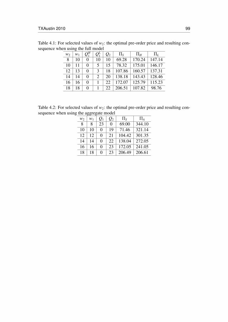
TXAustin 2010 99

Table 4.1: For selected values of w2: the optimal pre-order price and resulting con-sequence when using the full model

w2 w1 QH1 QL

1 Q2 ΠS ΠH ΠL

8 10 0 10 10 69.28 170.24 147.1410 11 0 5 15 78.32 175.01 146.1712 13 0 3 18 107.86 160.57 137.3114 14 0 2 20 138.18 143.43 128.4616 16 0 1 22 172.07 125.79 115.2318 18 0 1 22 206.51 107.82 98.76

Table 4.2: For selected values of w2: the optimal pre-order price and resulting con-sequence when using the aggregate model

w2 w1 Q1 Q2 ΠS ΠA

8 8 23 0 69.00 344.1010 10 0 19 71.46 321.1412 12 0 21 104.42 301.3514 14 0 22 138.04 272.0516 16 0 23 172.05 241.0518 18 0 23 206.49 206.61

5Inventory Rationing with Real

Options

History: This project started at Aarhus on 2011.

101

Aarhus 2011 103

Inventory Rationing with Real Options

Bisheng Du∗

Abstract

We consider an inventory system consisting of two supply sources and onebuyer. The first supply source is the real options contract provider while the othersupply source is a capacitated external market. The buyer’s unsatisfied demands aretreated as lost sales. We formulate the problem as a dynamic programming modelin order to perform some numerical investigations. In particular, we study the effectof using real options compared to a restricted situation where real options are notapplied.

Keyword

Inventory control; Real options; Dynamic programming

∗CORAL - Centre for Operations Research Applications in Logistics, Department of Economicsand Business, Aarhus School of Business and Social Sciences, Aarhus University, Fuglesangs Alle4, Aarhus V, DK-8210, Denmark. E-mail: bisd@asb.dk

104 Aarhus 2011

§5.1 Introduction

In a supply chain there may be suppliers providing contracts for products and a

“market” selling the actual products. In this paper, we present an inventory system

including a real options contract in multiple periods which consist of two supply

sources. A real options is the flexibility of a logistics manager for making decisions

about the manufacturing in their factory, which have great effects on their down-

stream partners.

The real options we consider is a form of supply chain contract, many common

characteristics exist between supply chain contracts and the derivatives literature:

there are some options like contracts, for instance, buy-back policies, backup agree-

ment, quantity flexibility, etc. But the options contracts above are embedded into

a contract. The real options, as we investigate in this paper, which is isolated from

the supply chain contract, can be traded in a market, e.g. Shi et al. (2004).

Barnes-Schuster et al. (2002) investigate a real options problem of a two-period

model with correlated demand. Wu and Kleindorfer (2005) extend the capacity op-

tions into the electronic market with competitive buyers. For more detail on the real

options, please refer to Sick (1995) and Luenberger (1998).

In this paper, we study an inventory system of two supply sources and one buyer,

the buyer’s unsatisfied demands are lost sales. The two supply sources are specified

as follows:

• Supplier: with whom we can make options contract. The options price is p

per unit, and the exercise price is c1 per unit. We assume the options contract

has signed one time period in advance, which means the buyer should decide

the exercise quantity, and then receive the delivery from the supplier in the

next period.

• Market: the external market capacity Cmar is a random variable, the actual

capacity is known at the beginning of each period. Cmar is a random variable.

The purchase cost is c2 per unit.

Aarhus 2011 105

In Section 5.2 the assumptions are stated and the dynamic programming model

is formulated. Some characterization and discussion of special cases are in Section

5.3. A numerical study can be found in Section 5.4 while the conclusion and final

remarks are in Section 5.5.

§5.2 Model formulation

§5.2.0 Notations and parameters list

• p, the options contract price per unit.

• c1, the options exercise price per unit.

• c2, the purchase price per unit from external market.

• n, (n = 1, 2, . . . ,N) denotes the number of remaining decisions.

• Cmar, a random variable, the external market capacity.

• D, a random variable, the current period demand.

• q1n, the number of units with real options contract are exercised at the period

n, where n = 1, 2, . . . ,N.

• q2n, the additional units purchase from the “Market” at the period n, where

n = 1, 2, . . . ,N.

• k, the real options’ capacity of period n, where n = 1, 2, . . . ,N.

• C, the external market capacity of period n, where n = 1, 2, . . . ,N.

• i, the ending inventory of period n, where n = 1, 2, . . . ,N.

• cnew, the new external market capacity in the next period.

• knew, the new options available in the next period.

• kmax, the maximum options available in the current period.

106 Aarhus 2011

• inew, the new inventory available in the next period.

• imax, the maximum inventory available in the current period.

• r, the price selling to the buyers.

• h, the holding cost per period per unit.

• s, the price for the leftover in the last period sold as scrap in the secondary

market.

• ∆, the unit overprice, ∆ = p + c1 − c2.

§5.2.1 Assumptions

Consider an inventory system that operates in a finite horizon of N periods, we

assume the options contract with the supplier have one period time delay, which

means the lead-time of products from the supplier is one period. In contrast, the

products from the external market can be purchased and received simultaneously

within the market’s capacity.

Assumption 5.1. In principle we can build our model and have all situations: (a).

p + c1 ≥ c2, or (b). c1 ≤ p + c1 ≤ c2.

Where p is the contract price per unit, c1 is the exercise price per unit and c2 is

the purchase price per unit from external market. If p + c1 ≥ c2 > c1. There may

also exist the same condition, which is an opposite situation of the basic assumption

above, we may also discuss this case later. If it happens, the reason for the buyer to

choose the supplier with a real options contract is to guarantee supply. In this case,

if the buyer also sells it at the same price, which will reduce the buyer’s profit mar-

gin, therefore, the buyer may also increase the retail price or adjust his distribution

channel policy.

If c1 ≤ p + c1 ≤ c2. The assumption p + c1 ≤ c2 reflects that the product

purchased from the market more than the products from the supplier. The condition

p + c1 ≤ c2 establishes that the buyer is price sensitive. If p + c1 = c2, then the

Aarhus 2011 107

buyer can choose between the market without lead-time delay and the supplier with

lot size guarantee. Given c1 ≤ p + c1, if p = 0, the real options contract is changed,

the options price equals the purchasing cost. On the other hand, the full price real

options contract leverage the payment guaranty from both of them to the buyer.

Assumption 5.2. In each period, the buyer’s on-hand inventory is only available to

the current demands, the unsatisfied demands of previous periods are treated as lost

sales. The inventory of the new period is inew = (i + q1 + q2 − d)+.

Any unsatisfied demands are treated as lost sales. Therefore, if there are de-

mands which are not be fulfilled by the current period’s leftover inventory, then the

current period’s unsatisfied demands will not be delivered in the next period.

§5.2.2 Dynamic programming formulation

The terminology used to define the dynamic programming model of this paper

includes the following main elements:

Stage/Period (n): This inventory system is divided into N periods, there is an

initial stage (Stage 1 or Period N) and a terminating stage (Stage N or Period 1).

The index n (n = 1, 2, . . . ,N) denotes the number of remaining decisions.

State: Each stage has a number of states associated with it. For instance, in

period n, there are three states k,C, i, which represent the real options’ capacity,

external market capacity and the ending inventory of period n.

Decision variable: There are three decision variables in period n (q1n, q2n and

knew). q1n is the number of units with real options contract are exercised at the period

n, where n = 1, 2, . . . ,N. q2n is the additional units purchase from the “Market” at

the period n, where n = 1, 2, . . . ,N. knew is the new options available in the next

period.

Boundary conditions: There are the initial conditions at stage N (or Period 1)

and the terminal conditions at stage 1 (or Period N), therefore, the expected profit

expressions of stage N (or Period 1) and stage 1 (or Period N) are given from the

general expression of period n.

108 Aarhus 2011

——————————————

Figure 5.1 is about here

——————————————

We build the Dynamic Programming models below:

The expected profit of the general period n (where n = 2, . . . ,N − 1) is

Vn(k,C, i)

= maxq1n≤k,q2n≤C,knew≤kmax

−c1q1n − c2q2n + rE[min(i + q1n + q2n,D)

]− hE

[i + q1n + q2n − D

]+− pknew

+∑

d

∑cnew

Vn−1(knew, cnew, (i + q1n + q2n − d)+) P(D = d)P(Cmar = cnew)

(5.1)

Where r is the price selling to the buyers, h is the holding cost per period per

unit, cnew is the new capacity developed for the next period, D is the current period

demand.

In period n, there are three states (k, C, i) and three decision variables (q1n, q2n

and knew). kmax is an upper bound on the number of options that can be bought.

We also consider the expected wasted options, meaning the un-exercised amount

of purchased options.

EWasten(k,C, i) = k − q∗1n

+∑

d

∑cnew

EWasten−1(k∗new, cnew, (i + q∗1n + q∗2n − d)+) P(D = d)P(Cmar = cnew)

(5.2)

Where k∗new, q∗1n, q∗2n are the optimal decision in (5.1).

Aarhus 2011 109

Boundary conditions of period N

In the first stage, which is the period N, the expected profit is:

VN(C) = maxq2N≤C,knew≤kmax

−c2q2N − pknew + rE[min(q2N ,D)

]− hE

[q2N − D

]+

+∑

d

∑cnew

VN−1(knew, cnew, (q2N − d)+) P(D = d)P(Cmar = cnew)

(5.3)

Thus we assume the initial inventory is 0.

In period N, there is only one state (C) and two decision variables (q2N and knew).

Similarly as above, the expected wasted options of period N is,

EWasteN(C)

=∑

d

∑cnew

EWasten−1(k∗new, cnew, (q∗2N − d)+) P(D = d)P(Cmar = cnew)

(5.4)

Where k∗new, q∗2N are the optimal decision in (5.3).

Boundary conditions of period 1

The expected profit when having a real options of k units and the current capac-

ity from the “Market” is Cmar, initial inventory is i, the leftover in the last period

sold as scrap s. Therefore, the expected profit of period 1 (the last stage) is

V1(k,C, i) = maxq11≤k,q21≤C

−c1q11 − c2q21 + rE[min(i + q11 + q21,D)

]+ sE

[i + q11 + q21 − D

]+

(5.5)

In the period 1, there are three states (k, C, i) and two decision variables (q11

and q21).

110 Aarhus 2011

Similarly as above, the expected wasted options of period 1 is,

EWaste1(k,C, i) = k − q∗11 (5.6)

Where q∗11 is the optimal decision in (5.5).

§5.3 Optimal policy

§5.3.1 Special case: kmax = 0, Capacitated Base Stock Policy

If kmax = 0, then no real options can be made, which equals to q1 = 0, and

it means the buyer can only purchase from the market but have no probability to

purchase products from the supplier. Therefore, we solve this multiple periods in-

ventory problem by use backwards recursions method. Then, the expected profit of

the last stage (period 1), which is just a newsvendor:

V1(0,C, i) = maxq21≤C−c2q21 + rE

[min(i + q21,D)

]+ sE

[i + q21 − D

]+

= maxq21≤C−c2q21 + r

[∫ i+q21

0x f (x)dx +

∫ ∞

i+q21

(i + q21) f (x)dx]

+ s∫ i+q21

0(i + q21 − x) f (x)dx

(5.7)

First order derivative on q21, we can get:

∂V1(0,C, i)∂q21

= − c2 + r[(i + q21) f (i + q21) +

∫ ∞

i+q21

f (x)dx − (i + q21) f (i + q21)]

+ s∫ i+q21

0f (x)dx

=r − c2 − (r − s)∫ i+q21

0f (x)dx

(5.8)

Aarhus 2011 111

Therefore, the optimal quantity of q21 is:

F(i + q21) =r − c2

r − s(5.9)

In the normal case, q21 = F−1( r−c2r−s ) − i; when there is no options, the optimal

quantity of options is q21 = 0; when there is not enough capacity, the optimal

quantity of options is q21 = C. Generally,

q∗21 = min(C,max

(F−1

(r − c2

r − s

)− i, 0

))(5.10)

Therefore, given i from period 2, we can get the optimal q21 of period 1, and also,

we can use the given information from period 3, etc., therefore, we use backward

recursions to solve it in periods until period N − 1.

The expected profit of the regular nth (where n = 2, . . . ,N − 1) period is

Vn(k,C, i)

= maxq2n≤cnew

−c2q2n + rE[min(i + q2,D)

]− hE

[i + q2n − D

]+− pknew

+∑

d

∑cnew

Vn−1(knew, cnew, (i + q2n − D)+) P(D = d)P(Cmar = cnew)

(5.11)

§5.3.2 Special case: P(C = 0) = 1

If P(C = 0) = 1, which means the buyer have no chance to purchase products

from the market but only from the supplier with a real options contract. Then, the

112 Aarhus 2011

expected profit of the last stage (period 1) is

V1(k, 0, i) = maxq11≤k−c1q1 + rE

[min(i + q11,D)

]+ sE

[i + q1 − D

]+

= maxq11≤k−c1q11 + r

[∫ i+q11

0x f (x)dx +

∫ ∞

i+q11

(i + q11) f (x)dx]

+ s∫ i+q11

0(i + q11 − x) f (x)dx

(5.12)

Therefore, the optimal quantity of q11 is:

F(i + q11) =r − c1

r − s(5.13)

Similarly, the condition of q11 = 0, which means there is no options, and the

condition of q11 = k, which means there is limited capacity of real options, are also

discussed. Then the general expression of optimal quantity of q11 is,

q∗11 = min(k,max

(F−1

(r − c1

r − s

)− i, 0

))(5.14)

The expected profit of the regular nth (where n = 2, . . . ,N − 1) period is

Vn(k, 0, i)

= maxq1n≤k−c1q1n + rE

[min(i + q1n,D)

]− hE

[i + q1n − D

]+− pknew

+∑

d

∑cnew

Vn−1(knew, cnew, (i + q1n − D)+) P(D = d)P(Cmar = cnew)

(5.15)

§5.3.3 kmax > 0 and P(C = 0) < 1

When kmax > 0 and P(C = 0) < 1, which means there are both supply sources

available: the real options provider and external market.

Aarhus 2011 113

The expected profit of the last stage (period 1) is:

V1(k,C, i) = maxq11≤k,q21≤C

−c1q11 − c2q21 + rE[min(i + q11 + q21,D)

]+ sE

[i + q11 + q21 − D

]+

= maxq11≤k,q21≤C

−c1q11 − c2q21

+ r[∫ i+q11+q21

0x f (x)dx +

∫ ∞

i+q11+q21

(i + q11 + q21) f (x)dx]

+ s∫ i+q11+q21

0(i + q11 + q21 − x) f (x)dx

(5.16)

Note that options are paid in a previous stage.

If c1 ≤ c2, based on different priorities between them, the buyer will first have

to choose the real options provider, after that, if there is some further need, he will

purchase from the external market. Therefore, we will solve∂

∂q11= 0 firstly, and

then given the optimal q∗11, we insert it to the profit expression to solve∂

∂q21= 0.

Obviously we will first use all options before buying in the market, therefore, the

optimal q11 is given as:

q∗11 = max{k,F−1

(r − c1

r − s

)− i

}(5.17)

This optimal expression considered the limited real options quantity. Given q∗11,

114 Aarhus 2011

the first order partial derivative on q21 is:

∂V1(k,C, i)∂q21

= − c2 + r[(i + q∗11 + q21) f (i + q∗11 + q21)

+

∫ ∞

i+q∗11+q21

f (x)dx − (i + q∗11 + q21) f (i + q∗11 + q21)]

+ s∫ i+q∗11+q21

0f (x)dx

=r − c2 − (r − s)∫ i+q∗11+q21

0f (x)dx

(5.18)

Therefore, the optimal quantity of q21, q∗21(q∗11) is:

F(i + q∗11 + q∗21(q∗11)) =r − c2

r − s(5.19)

Therefore, the general solution is:

q∗21 = min(C,max

(F−1

(r − c2

r − s

)− i − q∗11, 0

))(5.20)

The case c1 ≥ c2 could be analyzed similarly.

It is very hard to derive closed form expression for the optimal actions when

rolling the time further back. Therefore we will in the following resort to numerical

analysis.

§5.4 Numerical study

The focal question for OM analysis is: since options give a guarantee for future

delivery, there might be over-price for the material delivered through options. We

define the unit overprice ∆ as ∆ = p + c1 − c2. Therefore the analysis is also done

with regard to sensitivity analysis on this parameter. Because this overprice can

stay constant for many combinations of p and c1, we also study the impact of the

Aarhus 2011 115

composition of options price p and exercise price c1. Finally the main concern of

the analysis is to study the effect of introducing an options arrangement: we always

make comparisons to the case where no options are used. As this comparison can

be quite involved as there are many states, we assume that the analysis is conducted

prior to any knowledge about the capacity development. As a kind of performance

measurement for an options contract, we use

PO =∑

C

VN(C)P(Cmar = C) (5.21)

EWaste =∑

C

EWasteN(C)P(Cmar = C) (5.22)

Similarly the performance of the no-options expected profit is computed as

PN =∑

C

VN(C)|kmax=0 P(Cmar = C) (5.23)

We assume the demand follows Poisson Distribution, D ∼ Po(λ), the Market

capacity follows a Discrete Uniform Distribution, Cmar ∼ [cmin, cmax].

In this numerical investigation, we set the parameters as: λ = 5, s = 1, r =

12, h = 2, imax = 10, kmax = 10. When c1 + p > c2, and p < c2, we assume the

difference between the options paid and the external price is ∆, then, ∆ = c1 + p−c2,

which we may call it “overprice”. Therefore, e.g. N = 3. when c2 = 5 and ∆ = 1,

then p = 1, so c1 = 5.

When there is c1 + p > c2, we compare them for N = 4, 5, 6. When c2 = 4, see

Table 5.1 on N = 4, Table 5.2 on N = 5, Table 5.3 on N = 6. Where PO(4) stands

for the profit with options contract when c1 = 4. This explain how the tables, seen

below, are constructed.

116 Aarhus 2011

——————————————

Tables 5.1- 5.6 are about here

——————————————

When examining the tables we see that the increase in profit using options com-

pared to not using options is modest in the range from 0% to 5%. Naturally the

increase is highest when ∆ is lowest and p is lowest. In these cases, most waste

in terms of unused options can also be seen. In the opposite scenario where the

overprice is negative, the options is very favorable. The results of this analysis are

seen in the Tables 5.7 - 5.9.

——————————————

Tables 5.7 - 5.9 are about here

——————————————

Obviously, the gap between the options case and the no options case is very

dramatic. But we also see that although the options are cheap still some waste in

terms of unused options is encountered.

From Table 5.1 to Table 5.3, we can easily find, along with p increasing from 1

to 3, the profit/ratio/expected waste are all decreasing. But in general, those three

tables are kept with the same trend. The result is obvious, because we set the maxi-

mum inventory and the market capacity, both of them are higher than the real needs.

Therefore, if the buyer can freely choose between the two supply sources, then he

has no constraints on supply, but just options prices. In this case, as the options price

increases, they will loose partial profit by some unexpected waste options, certainly,

when the options price increase, and they will also prefer to keep lower expected

waste options by purchasing mostly from the options contract provider.

Next, we adjust c2 = 5 to find the data by N = 4, 5, 6. When c2 = 5, see Table

5.4 on N = 4. see Table 5.5 on N = 5. see Table 5.6 on N = 6.

If c1 + p < c2, we compare them for N = 4, 5, 6, see Table 5.7 on N = 4, Table

5.8 on N = 5, Table 5.9 on N = 6.

Aarhus 2011 117

——————————————

Figure 5.2 is about here

——————————————

We compare the average profit among N = 4, 5, 6 when c2 = 4, which is shown

in Figure 5.2. If there is no options, the average profit keeps in the lowest level.

Along with the decrease by ∆ from 4 to 1, the average profit is increasing. We

could say, with the alternative scenario of real options contract, the buyers have

more sources to relax their risk, therefore, if there is no more difference on prices

between the real options provider and the external market, they may have more

flexibilities to choose between them, see the highest level when ∆ = 1. Otherwise,

with the uncertainty of the external market and higher price gap between them, the

average profit will keep in a lower level. Figure 5.3 shows similar trend for c2 = 5.

——————————————

Figure 5.3 is about here

——————————————

There are some differences in Figure 5.4, the average profit are given by using

∆ ≤ 0, which means c1 + p ≤ c2, the buyer has more incentive to buy adjustable

amount from the external market.

——————————————

Figure 5.4 is about here

——————————————

When we use the data collected by p = 1, 2, 3, 4, 5, 6 when c2 = 7 and N = 4,

we found that the profits increasing slops are almost the same as the ones when

the buyer adapt “No options” and ∆ = 0,−1,−2,−3. By contrast, when we use

c2 = 4, we can get same decreasing slops when the buyer adapt ∆ = 1, 2, 3, 4 and

“No options”.

118 Aarhus 2011

——————————————

Figure 5.5 is about here

——————————————

§5.5 Conclusion and remarks

We have developed a dynamic programming model to study the use of options

to secure future supply of raw material in a possibly constrained supply market.

The numerical results show a small increase in profits from using this arrangement

in the “normal” case where the total unit price is higher than the external market

price. However, so far not have numerical experiments been conducted. Though the

dynamic programming model is somewhat involved, some obvious opportunities

exist for how it could be further considered. Firstly, the market capacity could

evolve after a Markov chain instead of as in the present model that each realization

of market capacity is independent of what was observed in the previous period.

Secondly, the market price c2 could be decreasing as a function of the available

market capacity. Thirdly the options need not be exercised in the next period, but

could have longer time interval where it is possible to exercise them. There are a lot

of possible future avenues to continue this research work.

Acknowledgement

The author is supported by Grant No. 275-07-0094 from the Danish Social

Science Research Council.

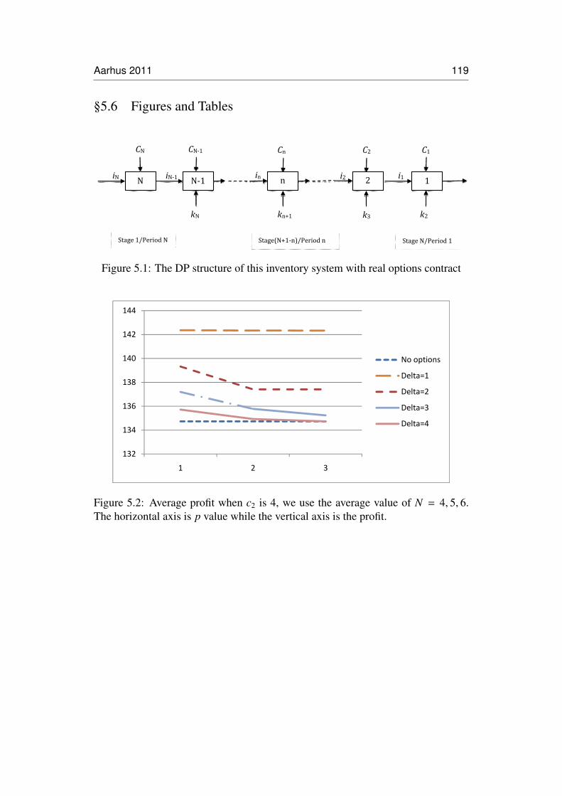
Aarhus 2011 119

§5.6 Figures and Tables

iN 

CN  CN‐1 

kN 

iN‐1 

 

N  N‐1 

C1 

k2 

i1  1 

Cn 

kn+1 

in  n 

C2 

k3 

i2  2 

Stage 1/Period N  Stage(N+1‐n)/Period n Stage N/Period 1

Figure 5.1: The DP structure of this inventory system with real options contract

136

138

140

142

144

No options

Delta=1

Delta=2

132

134

136

1 2 3

Delta=3

Delta=4

Figure 5.2: Average profit when c2 is 4, we use the average value of N = 4, 5, 6.The horizontal axis is p value while the vertical axis is the profit.

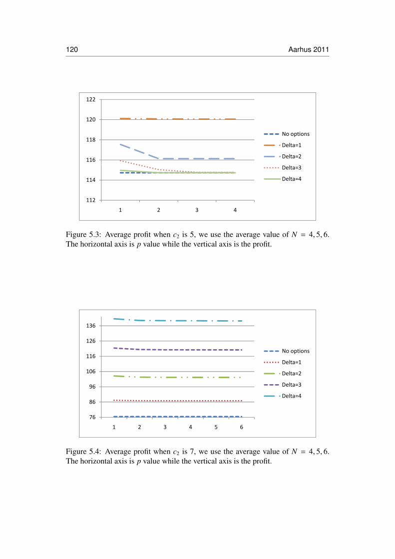
120 Aarhus 2011

116

118

120

122

No options

Delta=1

Delta=2

112

114

1 2 3 4

Delta=3

Delta=4

Figure 5.3: Average profit when c2 is 5, we use the average value of N = 4, 5, 6.The horizontal axis is p value while the vertical axis is the profit.

106

116

126

136

No options

Delta=1

Delta=2

76

86

96

1 2 3 4 5 6

Delta=3

Delta=4

Figure 5.4: Average profit when c2 is 7, we use the average value of N = 4, 5, 6.The horizontal axis is p value while the vertical axis is the profit.

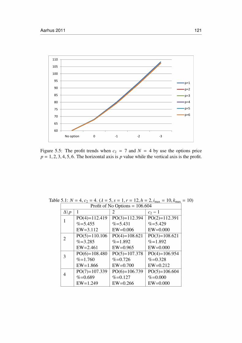
Aarhus 2011 121

80

85

90

95

100

105

110

p=1

p=2

p=3

p=4

60

65

70

75

80

No option 0 ‐1 ‐2 ‐3

p 4

p=5

p=6

Figure 5.5: The profit trends when c2 = 7 and N = 4 by use the options pricep = 1, 2, 3, 4, 5, 6. The horizontal axis is p value while the vertical axis is the profit.

Table 5.1: N = 4, c2 = 4. (λ = 5, s = 1, r = 12, h = 2, imax = 10, kmax = 10)Profit of No Options = 106.604

∆\p 1 2 c2 − 1

1PO(4)=112.419 PO(3)=112.394 PO(2)=112.391%=5.455 %=5.431 %=5.429EW=3.112 EW=0.006 EW=0.000

2PO(5)=110.106 PO(4)=108.621 PO(3)=108.621%=3.285 %=1.892 %=1.892EW=2.461 EW=0.965 EW=0.000

3PO(6)=108.480 PO(5)=107.378 PO(4)=106.954%=1.760 %=0.726 %=0.328EW=1.866 EW=0.700 EW=0.212

4PO(7)=107.339 PO(6)=106.739 PO(5)=106.604%=0.689 %=0.127 %=0.000EW=1.249 EW=0.266 EW=0.000

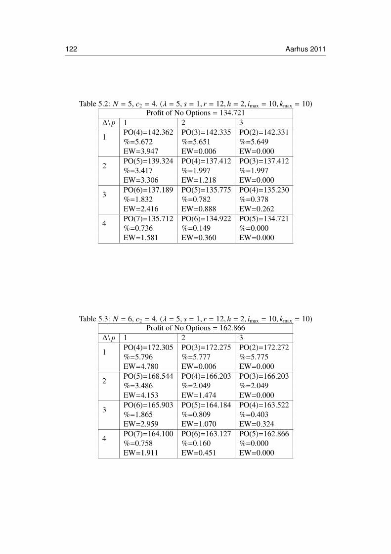
122 Aarhus 2011

Table 5.2: N = 5, c2 = 4. (λ = 5, s = 1, r = 12, h = 2, imax = 10, kmax = 10)Profit of No Options = 134.721

∆\p 1 2 3

1PO(4)=142.362 PO(3)=142.335 PO(2)=142.331%=5.672 %=5.651 %=5.649EW=3.947 EW=0.006 EW=0.000

2PO(5)=139.324 PO(4)=137.412 PO(3)=137.412%=3.417 %=1.997 %=1.997EW=3.306 EW=1.218 EW=0.000

3PO(6)=137.189 PO(5)=135.775 PO(4)=135.230%=1.832 %=0.782 %=0.378EW=2.416 EW=0.888 EW=0.262

4PO(7)=135.712 PO(6)=134.922 PO(5)=134.721%=0.736 %=0.149 %=0.000EW=1.581 EW=0.360 EW=0.000

Table 5.3: N = 6, c2 = 4. (λ = 5, s = 1, r = 12, h = 2, imax = 10, kmax = 10)Profit of No Options = 162.866

∆\p 1 2 3

1PO(4)=172.305 PO(3)=172.275 PO(2)=172.272%=5.796 %=5.777 %=5.775EW=4.780 EW=0.006 EW=0.000

2PO(5)=168.544 PO(4)=166.203 PO(3)=166.203%=3.486 %=2.049 %=2.049EW=4.153 EW=1.474 EW=0.000

3PO(6)=165.903 PO(5)=164.184 PO(4)=163.522%=1.865 %=0.809 %=0.403EW=2.959 EW=1.070 EW=0.324

4PO(7)=164.100 PO(6)=163.127 PO(5)=162.866%=0.758 %=0.160 %=0.000EW=1.911 EW=0.451 EW=0.000

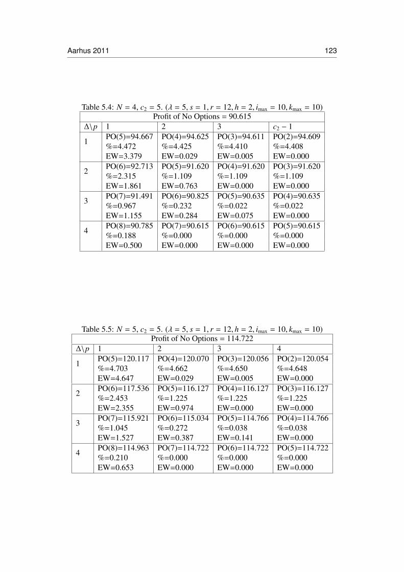
Aarhus 2011 123

Table 5.4: N = 4, c2 = 5. (λ = 5, s = 1, r = 12, h = 2, imax = 10, kmax = 10)Profit of No Options = 90.615

∆\p 1 2 3 c2 − 1

1PO(5)=94.667 PO(4)=94.625 PO(3)=94.611 PO(2)=94.609%=4.472 %=4.425 %=4.410 %=4.408EW=3.379 EW=0.029 EW=0.005 EW=0.000

2PO(6)=92.713 PO(5)=91.620 PO(4)=91.620 PO(3)=91.620%=2.315 %=1.109 %=1.109 %=1.109EW=1.861 EW=0.763 EW=0.000 EW=0.000

3PO(7)=91.491 PO(6)=90.825 PO(5)=90.635 PO(4)=90.635%=0.967 %=0.232 %=0.022 %=0.022EW=1.155 EW=0.284 EW=0.075 EW=0.000

4PO(8)=90.785 PO(7)=90.615 PO(6)=90.615 PO(5)=90.615%=0.188 %=0.000 %=0.000 %=0.000EW=0.500 EW=0.000 EW=0.000 EW=0.000

Table 5.5: N = 5, c2 = 5. (λ = 5, s = 1, r = 12, h = 2, imax = 10, kmax = 10)Profit of No Options = 114.722

∆\p 1 2 3 4

1PO(5)=120.117 PO(4)=120.070 PO(3)=120.056 PO(2)=120.054%=4.703 %=4.662 %=4.650 %=4.648EW=4.647 EW=0.029 EW=0.005 EW=0.000

2PO(6)=117.536 PO(5)=116.127 PO(4)=116.127 PO(3)=116.127%=2.453 %=1.225 %=1.225 %=1.225EW=2.355 EW=0.974 EW=0.000 EW=0.000

3PO(7)=115.921 PO(6)=115.034 PO(5)=114.766 PO(4)=114.766%=1.045 %=0.272 %=0.038 %=0.038EW=1.527 EW=0.387 EW=0.141 EW=0.000

4PO(8)=114.963 PO(7)=114.722 PO(6)=114.722 PO(5)=114.722%=0.210 %=0.000 %=0.000 %=0.000EW=0.653 EW=0.000 EW=0.000 EW=0.000

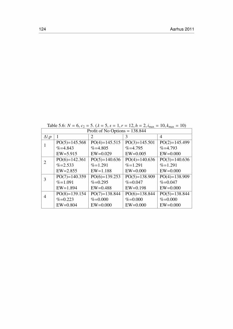
124 Aarhus 2011

Table 5.6: N = 6, c2 = 5. (λ = 5, s = 1, r = 12, h = 2, imax = 10, kmax = 10)Profit of No Options = 138.844

∆\p 1 2 3 4

1PO(5)=145.568 PO(4)=145.515 PO(3)=145.501 PO(2)=145.499%=4.843 %=4.805 %=4.795 %=4.793EW=5.915 EW=0.029 EW=0.005 EW=0.000

2PO(6)=142.361 PO(5)=140.636 PO(4)=140.636 PO(3)=140.636%=2.533 %=1.291 %=1.291 %=1.291EW=2.855 EW=1.188 EW=0.000 EW=0.000

3PO(7)=140.359 PO(6)=139.253 PO(5)=138.909 PO(4)=138.909%=1.091 %=0.295 %=0.047 %=0.047EW=1.894 EW=0.488 EW=0.198 EW=0.000

4PO(8)=139.154 PO(7)=138.844 PO(6)=138.844 PO(5)=138.844%=0.223 %=0.000 %=0.000 %=0.000EW=0.804 EW=0.000 EW=0.000 EW=0.000

Aarhus 2011 125

Tabl

e5.

7:N

=4,

c 2=

7.(λ

=5,

s=

1,r

=12,h

=2,

i max

=10,k

max

=10

)Pr

ofito

fNo

Opt

ions

=60

.193

∆\

p1

23

45

c 2−

1

0PO

(6)=

68.0

19PO

(5)=

67.8

02PO

(4)=

67.7

60PO

(3)=

67.7

41PO

(2)=

67.7

38PO

(1)=

67.7

38%

=13

.002

%=

12.6

41%

=12

.571

%=

12.5

40%

=12

.535

%=

12.5

35E

W=

0.47

5E

W=

0.04

2E

W=

0.04

1E

W=

0.00

6E

W=

0.00

0E

W=

0.00

0

-1PO

(5)=

79.9

29PO

(4)=

79.2

94PO

(3)=

79.1

73PO

(2)=

79.1

43PO

(1)=

79.1

37PO

(0)=

79.1

32%

=32

.788

%=

31.7

33%

=31

.532

%=

31.4

82%

=31

.472

%=

31.4

64E

W=

1.12

8E

W=

0.28

5E

W=

0.04

6E

W=

0.01

1E

W=

0.00

5E

W=

0.00

5

-2PO

(4)=

93.7

55PO

(3)=

93.0

16PO

(2)=

92.8

40PO

(1)=

92.8

16PO

(0)=

92.8

05PO

(-1)

=92

.795

%=

55.7

57%

=54

.530

%=

54.2

37%

=54

.197

%=

54.1

79%

=54

.162

EW

=1.

542

EW

=0.

332

EW

=0.

055

EW

=0.

010

EW

=0.

010

EW

=0.

010

-3PO

(3)=

108.

344

PO(2

)=10

7.52

7PO

(1)=

107.

416

PO(0

)=10

7.39

PO(-

1)=

107.

359

PO(-

2)=

107.

330

%=

79.9

94%

=78

.637

%=

78.4

53%

=78

.409

%=

78.3

58%

=78

.310

EW

=1.

849

EW

=0.

319

EW

=0.

028

EW

=0.

028

EW

=0.

028

EW

=0.

028

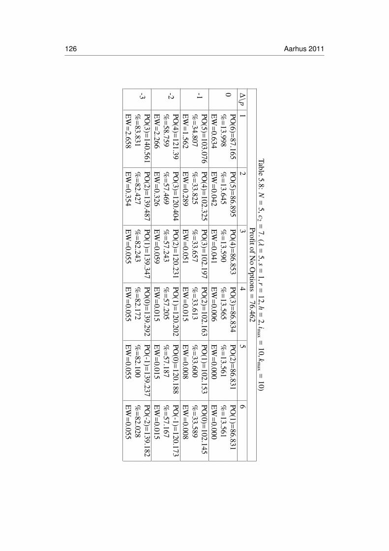
126 Aarhus 2011

Table5.8:

N=

5,c2

=7.(λ

=5,s

=1,r

=12,h

=2,im

ax=

10,k

max

=10)

ProfitofNo

Options

=76.462

∆\p

12

34

56

0PO

(6)=87.165

PO(5)=

86.895PO

(4)=86.853

PO(3)=

86.834PO

(2)=86.831

PO(1)=

86.831%

=13.998

%=

13.645%

=13.590

%=

13.565%

=13.561

%=

13.561E

W=

0.634E

W=

0.042E

W=

0.041E

W=

0.006E

W=

0.000E

W=

0.000

-1PO

(5)=103.076

PO(4)=

102.325PO

(3)=102.197

PO(2)=

102.163PO

(1)=102.153

PO(0)=

102.145%

=34.807

%=

33.825%

=33.657

%=

33.613%

=33.600

%=

33.589E

W=

1.562E

W=

0.289E

W=

0.051E

W=

0.015E

W=

0.008E

W=

0.008

-2PO

(4)=121.39

PO(3)=

120.404PO

(2)=120.231

PO(1)=

120.202PO

(0)=120.188

PO(-1)=

120.173%

=58.759

%=

57.469%

=57.243

%=

57.205%

=57.187

%=

57.167E

W=

2.266E

W=

0.326E

W=

0.059E

W=

0.015E

W=

0.015E

W=

0.015

-3PO

(3)=140.561

PO(2)=

139.487PO

(1)=139.347

PO(0)=

139.292PO

(-1)=139.237

PO(-2)=

139.182%

=83.831

%=

82.427%

=82.243

%=

82.172%

=82.100

%=

82.028E

W=

2.658E

W=

0.354E

W=

0.055E

W=

0.055E

W=

0.055E

W=

0.055

Aarhus 2011 127

Tabl

e5.

9:N

=6,

c 2=

7.(λ

=5,

s=

1,r

=12,h

=2,

i max

=10,k

max

=10

)Pr

ofito

fNo

Opt

ions

=92

.735

∆\

p1

23

45

6

0PO

(6)=

106.

310

PO(5

)=10

5.99

2PO

(4)=

105.

950

PO(3

)=10

5.93

0PO

(2)=

105.

927

PO(1

)=10

5.92

7%

=14

.638

%=

14.2

96%

=14

.250

%=

14.2

29%

=14

.225

%=

14.2

25E

W=

0.79

4E

W=

0.04

2E

W=

0.04

1E

W=

0.00

6E

W=

0.00

0E

W=

0.00

0

-1PO

(5)=

126.

242

PO(4

)=12

5.34

5PO

(3)=

125.

212

PO(2

)=12

5.17

4PO

(1)=

125.

161

PO(0

)=12

5.14

8%

=36

.132

%=

35.1

65%

=35

.021

%=

34.9

80%

=34

.960

%=

34.9

52E

W=

1.99

7E

W=

0.28

9E

W=

0.06

0E

W=

0.01

8E

W=

0.01

2E

W=

0.01

2

-2PO

(4)=

149.

031

PO(3

)=14

7.84

8PO

(2)=

147.

664

PO(1

)=14

7.62

8PO

(0)=

147.

606

PO(-

1)=

147.

584

%=

60.7

06%

=59

.431

%=

59.2

32%

=59

.193

%=

59.1

70%

=59

.146

EW

=2.

909

EW

=0.

342

EW

=0.

067

EW

=0.

022

EW

=0.

022

EW

=0.

022

-3PO

(3)=

172.

777

PO(2

)=17

1.44

5PO

(1)=

171.

276

PO(0

)=17

1.19

3PO

(-1)

=17

1.11

0PO

(-2)

=17

1.02

8%

=86

.313

%=

84.8

76%

=84

.694

%=

84.6

05%

=84

.515

%=

84.4

27E

W=

3.47

0E

W=

0.38

3E

W=

0.08

3E

W=

0.08

3E

W=

0.08

3E

W=

0.08

3

References

R. Adelson. Compound poisson distributions. Operational Research Quarterly, 17

(1):73–75, 1966.

H. Arslan, S. C. Graves, and T. A. Roemer. A single-product inventory model for

multiple demand classes. Management Science, 53(9):1486–1500, 2007.

S. Axsater. Simple solution procedures for a class of two-echelon inventory prob-

lems. Operations Research, 38(1):64–69, 1990.

S. Axsater. Inventory Control. Springer’s International Series. Springer: New York,

Second edition, 2006.

D. Barnes-Schuster, Y. Bassok, and R. Anupindi. Coordination and flexibility in

supply contracts with options. Manufacturing & Service Operations Manage-

ment, 4:171–207, 2002.

G. P. Cachon. The allocation of inventory risk in a supply chain: Push, pull,

and advance-purchase discount contracts. Management Science, 50(2):222–238,

2004.

F. Chen. Market segmentation, advanced demand information, and supply chain

performance. Manufacturing & Service Operations Management, 3(1):53–67,

2001.

M. Cohen, Y.-S. Zheng, and Y. Wang. Identifying opportunities for improving ter-

adyne’s service-parts logistics system. Interfaces, 29(4):1–18, 1999.

D. Cox. Renewal Theory. Methuen: London, 1962.

129

130 References

R. Dekker, M. Kleijn, and P. de Rooij. A spare parts stocking policy based on

equipment criticality. International Journal of Production Economics, 56-57:

67–77, 1998.

R. Dekker, R. Hill, M. Kleijn, and R. Teunter. On the (s − 1, s) lost sales inventory

model with priority demand classes. Naval Research Logistics, 49(6):593–610,

2002.

V. Deshpande, M. Cohen, and K. Donohue. A threshold inventory rationing policy

for service-differentiated demand classes. Management Science, 49(6):683–703,

2003.

L. Dong and K. Zhu. Two-wholesale-price contracts: Push, pull, and advance-

purchase discount contracts. Manufacturing & Service Operations Management,

9(3):291–311, 2007.

B. Du and C. Larsen. Base stock policies with degraded service to larger orders.

International Journal of Production Economics, 133(1):326 – 333, 2011.

P. Enders, I. Adan, A. Scheller-Wolf, and G.-J. van Houtum. Inventory rationing for

a system with heterogeneous customer classes. Working paper, Tepper School of

Business, Carnegie Mellon University, Pittsburgh, PA, 2009.

R. Evans. Sales and restocking in a single item inventory system. Management

Science, 14(7):463–472, 1968.

K. Frank, R. Zhang, and I. Duenyas. Optimal policies for inventory systems with

priority demand classes. Operations Research, 51(6):993–1002, 2003.

G. Gallego and O. Ozer. Integrating replenishment decisions with advance demand

information. Management Science, 47(10):1344–1360, 2001.

G. Gallego and O. Ozer. Optimal replenishment policies for multiechelon inventory

problems under advance demand information. Manufacturing & Service Opera-

tions Management, 5(2):157–175, 2003.

References 131

J.-P. Gayon, S. Benjaafar, and F. de Vericourt. Using imperfect advance demand in-

formation in production-inventory systems with multiple customer classes. Man-

ufacturing & Service Operations Management, 11(1):128–143, 2009.

R. Hariharan and P. Zipkin. Customer-order information, leadtimes, and invento-

ries. Management Science, 41(10):1599–1607, 1995.

X. Hu. Advance demand information and safety capacity as a hedge against demand

and capacity uncertainty. Manufacturing & Service Operations Management, 5

(1):55–58, 2003.

F. Johnston, J. Boylan, and E. Shale. An examination of the size of orders from cus-

tomers, their characterization and the implication for inventory control of slow

moving items. Journal of the Operational Research Society, 54(8):833–837,

2003.

A. Kaplan. Stock rationing. Management Science, 15(5):260–267, 1969.

W. Kelton, R. Sadowski, and D. Sturrock. Simulation with ARENA. McGraw Hill:

Boston, 4th edition, 2007.

Y. Kocaga and A. Sen. Spare parts inventory management with demand lead times

and rationing. IIE Transactions, 39(9):879–898, 2007.

C. Larsen and A. Thorstenson. A comparison between the order and the volume fill

rate for a base-stock inventory control system under a compound renewal demand

process. Journal of the Operational Research Society, 59:798–804, 2008.

C. Larsen, C. H. Seiding, C. Teller, and A. Thorstenson. An inventory control

project in a major danish company using compound renewal demand models.

IMA Journal of Management Mathematics, 19(2):145–162, 2008.

A. Law and W. D. Kelton. Simulation modelling and analysis. McGraw Hill:

Singapore, 1991.

132 References

Y. Lu, J.-S. Song, and D. D. Yao. Order fill rate, leadtime variability, and advance

demand information in an assemble-to-order system. Operations Research, 51

(2):292–308, 2003.

D. G. Luenberger. Investment Science. New York: Oxford University Press, 1998.

J. Marklund. Controlling inventories in divergent supply chains with advance-order

information. Operations Research, 54(5):988–1010, 2006.

P. Melchiors. Restricted time remembering policies for the inventory rationing prob-

lem. International Journal of Production Economics, 81-82:461–468, 2003.

P. Melchiors, R. Dekker, and M. Kleijn. Inventory rationing in an (s,Q) inven-

tory model with two demand classes and lost sales. Journal of the Operational

Research Society, 51(1):111–122, 2000.

N. Nahmias and W. Demmy. Operating characteristics of an inventory system with

rationing. Management Science, 27(11):1236–1245, 1981.

O. Ozer. Replenishment strategies for distribution system under advance demand

information. Management Science, 49:255–272, 2003.

O. Ozer and W. Wei. Inventory control with limited capacity and advance demand

information. Operations Research, 52(6):988–1000, 2004.

C. Palm. Analysis of the erlang traffic formula for busy signal arrangements. Eric-

son Technics, 4:204–212, 1938.

F. Papier and U. W. Thonemann. Capacity rationing in stochastic rental systems

with advance demand information. Operations Research, 58(2):274–288, 2010.

E. L. Porteus. Stochastic inventory theory. In D. Heyman and M. Sobel, editors,

Stochastic Model, volume 2 of Handbooks in Operations Research and Manage-

ment Science. North-Holland, Elsevier, 1990.

References 133

E. L. Porteus. Foundations of Stochastic Inventory Theory. Stanford University

Press, Stanford, CA, 2002.

A. Sen and A. X. Zhang. The newsboy problem with multiple demand classes. IIE

Transactions, 31:431–444, 1999.

D. Shi, R. Hampshire, R. Daniels, and W. Grey. The impact of options trading

on supply chain management. Technical report, IBM Research Report RC23001

(W0403-043), March 2004.

G. Sick. Real options. In D. Heyman and M. Sobel, editors, Finance, volume 9 of

Handbooks in Operations Research and Management Science. North-Holland,

Elsevier, 1995.

E. Silver, D. Pyke, and R. Peterson. Inventory Management, Production Planning

and Scheduling. New York, NY: John Wiley & Sons, Third edition, 1998.

T. Tan. Using imperfect advance demand information in forecasting. IMA Journal

of Management Mathematics, 19:163–173, 2008.

H. Tempelmeier. Supply chain inventory optimization with two customer classes in

discrete time. European Journal of Operations Research, 174:600–621, 2006.

R. Teunter and W. Haneveld. Dynamic inventory rationing strategies for inventory

systems with two demand classes, poisson demand and backordering. European

Journal of Operational Research, 190(1):156–178, 2008.

D. Thomas and J. Tyworth. Pooling lead-time risk by order splitting: a critical

review. Transportation Research: Part E, 42:245–257, 2006.

D. Topkis. Optimal ordering and rationing policies in a nonstationary dynamic

inventory model with n demand classes. Management Science, 15(3):160–176,

1968.

T. Wang and B. L. Toktay. Inventory management with advance demand informa-

tion and flexible delivery. Management Science, 54(4):716–732, 2008.

134 References

Y. Wang, M. Cohen, and Y.-S. Zheng. Differentiating customer service on the basis

of delivery lead-times. IIE Transactions, 34(11):979–989, 2002.

D. J. Wu and P. R. Kleindorfer. Competitive options, supply contracting, and elec-

tronic markets. Management Science, 51:452–466, 2005.

Y. Zhou and X. Zhao. Optimal policies of an inventory system with multiple demand

classes. Tsinghua Science & Technology, 15(5):498–508, 2010.

P. Zipkin. Foundations of Inventory Management. McGraw-Hill: Boston, 2000.