ESSAYS IN THE SOCIAL DETERMINANTS OF HEALTH AND …

University of New MexicoUNM Digital Repository

Economics ETDs Electronic Theses and Dissertations

Summer 7-2-2018

ESSAYS IN THE SOCIAL DETERMINANTSOF HEALTH AND PUBLIC HEALTH POLICYGlen Vincent McDermottUniversity of New Mexico

Follow this and additional works at: https://digitalrepository.unm.edu/econ_etds

Part of the Economics Commons

This Dissertation is brought to you for free and open access by the Electronic Theses and Dissertations at UNM Digital Repository. It has beenaccepted for inclusion in Economics ETDs by an authorized administrator of UNM Digital Repository. For more information, please [email protected].

Recommended CitationMcDermott, Glen Vincent. "ESSAYS IN THE SOCIAL DETERMINANTS OF HEALTH AND PUBLIC HEALTH POLICY."(2018). https://digitalrepository.unm.edu/econ_etds/92

https://digitalrepository.unm.edu?utm_source=digitalrepository.unm.edu%2Fecon_etds%2F92&utm_medium=PDF&utm_campaign=PDFCoverPages

https://digitalrepository.unm.edu/econ_etds?utm_source=digitalrepository.unm.edu%2Fecon_etds%2F92&utm_medium=PDF&utm_campaign=PDFCoverPages

https://digitalrepository.unm.edu/etds?utm_source=digitalrepository.unm.edu%2Fecon_etds%2F92&utm_medium=PDF&utm_campaign=PDFCoverPages

https://digitalrepository.unm.edu/econ_etds?utm_source=digitalrepository.unm.edu%2Fecon_etds%2F92&utm_medium=PDF&utm_campaign=PDFCoverPages

http://network.bepress.com/hgg/discipline/340?utm_source=digitalrepository.unm.edu%2Fecon_etds%2F92&utm_medium=PDF&utm_campaign=PDFCoverPages

https://digitalrepository.unm.edu/econ_etds/92?utm_source=digitalrepository.unm.edu%2Fecon_etds%2F92&utm_medium=PDF&utm_campaign=PDFCoverPages

mailto:[email protected]

i

Glen Vincent McDermott Candidate

Economics

Department

This dissertation is approved, and it is acceptable in quality and form for publication:

Approved by the Dissertation Committee:

Dr. Alok K Bohara, Chairperson

Dr. David van der Goes

Dr. Gabriel R. Sanchez

Dr. Maurice L. Moffett

ii

ESSAYS IN THE SOCIAL DETERMINANTS OF HEALTH

AND PUBLIC HEALTH POLICY

by

GLEN VINCENT MCDERMOTT

B.A, Economics, University of Denver, 1993

M.A., Financial Economics, University of Maine, 2010

M.A., Economics, The University of New Mexico, 2016

DISSERTATION

Submitted in Partial Fulfillment of the

Requirements for the Degree of

Doctor of Philosophy

Economics

The University of New Mexico

Albuquerque, New Mexico

July 2018

iii

DEDICATION

I feel it right and proper to dedicate this work to my wife Stefanie. She is the love

of my life, my partner, and my best friend. Without her, I could not have done what I

have now done.

I too owe a great debt of gratitude to my son and my daughter. In each their own

way, they have sacrificed much as I have pursued this work. Time we missed together

can never be reclaimed yet, selflessly, they smiled each time I left encouraging me on to

some unknown and abstract goal. They remind me what joy there is in life, what

innocence feels like, and what power there is in youth and trust. I’m lucky to have such

wonderful children.

Finally, I would feel remiss if I failed to recognize the role of my mother, who now

watches over and manages my progress from above, and my father, whose keen ear,

thoughtful mind, and ever present words of wisdom have stoked the fires of my

determination and perseverance.

iv

ACKNOWLEDGEMENTS

I would like to acknowledge the kindness and support of my committee. The chair

of my committee, Dr. Alok Bohara has been an inspiration to my success, a trusted

mentor, and a friend. I have truly appreciated the time we have spent working together.

Dr. David van der Goes has provided unyielding encouragement for my ambitions. He

has been single mindedly focused on prodding me forward toward my goal and

encouraging my commitment to the task at hand. Both he and Dr. Gabriel Sanchez have

demonstrated the pragmatic professionalism that are required to successfully complete

this journey. Finally, Dr. Maurice Moffett helped me to keep my foot on the path. He

knocked down hurdles that I had yet to identify and opened doors for me to advance my

professional aspirations. For this, I will always be grateful. Without the support of this

group, it is unlikely that I would be in a position to write this little note of thanks today. I

am humbled in my gratitude.

v

Essays in the Social Determinants of Health and Public Health Policy

By

Glen Vincent McDermott

M.A., Financial Economics, University of Maine, 2010

M.A., Economics, The University of New Mexico, 2014

ABSTRACT

There is broad-based qualitative evidence arguing that stress is a public health

concern. In the search for causality however, economists investigating public health

concerns are often limited to a narrow subset of socio-economic status (SES) factors

which are not well suited to the evaluation of stress/health effects. As a result,

economists have a difficult time answering the “how” and “why” questions which emerge

from the well-respected SES/health gradient. This dissertation focuses on a subset of

stressors credibly affiliated with SES to address two pathways underling the established

SES/Health gradient. Chapter 2 uses the Panel Study of Income Dynamics to test

financial strain (FS) and high-frequency job switching (JS) effects on health. Using

dynamic panel random effects ordered probit specifications, we find support for FS and

JS effects on self-assessed health status. Of course, policy recommendations that follow

are unimaginably vast. In chapters 3 and 4, we focus on breaking down the grand policy

consideration of reducing financial strain into politically viable actions. First, we develop

and test a pragmatic policy analysis method against observable outcomes from two health

policies made by the state of Alaska. In terms of reducing individual year-over-year

vi

health insurance premium volatility, the presented method performs better than the

commonly relied upon actuarial methods. The implication is that adoption of such

analytical methods may result in improved population health. Chapter 4 evaluates the

effects of childhood retrospective circumstances on the experiences of adult financial

strain. Results suggest school experiences, feelings of loneliness, parental work habits,

and maternal relationships are key predictors of adult financial strain.

vii

Table of Contents

by ii Chapter 1: Introduction ....................................................................................................... 1 Chapter 2: The Effects of Financial Strain and Job Switching on Health .......................... 9 Theoretical Motivation and Development .........................................................11 The Estimation Model .......................................................................................12

Data ...................................................................................................................14 Summary Statistics and Variable Construction ................................................. 16 Empirical Specification .....................................................................................19 Initial Conditions ......................................................................................... 21 Attrition Bias ................................................................................................ 21

Correlated Random Error Considerations .................................................... 23

Results and Discussion ......................................................................................24 Concluding Remarks .........................................................................................28

Tables and Figures .............................................................................................29

Table 1: Summary Statistics ........................................................................ 30 Table 2: Attrition Tests, Pooled Probit Specification, IPW clusters............ 31 Table 3: Variable Addition Bias Test - Random Effects Ordered Probit Model

with IPW, modified CRE, and Strict CRE estimations for M, F, and Combined

32

Table 4: Random Effects Ordered Probit Results with Inverse Probability

Weights, Full, Modifed, and Excluded CRE controls ....................................... 33 Table 5: Random Effect Ordered Probit Results - Separate Male and Female

Results 34 Figures ...............................................................................................................35

Figure 1: Summary Table of Findings ........................................................ 35 Chapter 3: State Level Operationalization of Health Policy: A pragmatic approach to

predicting changes in premiums and aggregate market profitability ................. 36 Conceptual Framework and Model Development .............................................40

The Model .................................................................................................... 41 Numeric Examples, Simulation, and Results ....................................................45 Alaska’s Medicaid Expansion Fall 2015 ..................................................... 45

Evaluation of Alaska’s Medicaid Expansion ......................................... 47 Alaska’s Reinsurance Program January 1, 2017.......................................... 50 Evaluation of Alaska’s Reinsurance Program ....................................... 55

Policy Scenario Analysis ...................................................................................58 Concluding Remarks .........................................................................................60

Tables and Figures .............................................................................................62 Table 1: 1332 Waiver Application Details .................................................. 62 Table 2: Yearly cost trends used in Analysis ............................................... 63 Table 3: Results Alaska Medicaid Expansion ............................................. 64 Table 4: Results Alaska Conditions Based Reinsurance Program............... 65

Table 5:Hypotheses - Policy Simulation Analysis...................................... 66 Table 6: Results Alaska Conditions Based Reinsurance Program – Policy

Scenario.............................................................................................................. 67

viii

Figure 1: Medicaid Applications March 2015 – March 2016 ...................... 68

Chapter 4: Adolescent Circumstances and Financial Strain in Adulthood ....................... 69

Data and Methodology ......................................................................................72 Empirical Method ..............................................................................................76 Results and Discussion ......................................................................................80 Concluding Remarks .........................................................................................83 Tables and Figures .............................................................................................84

Table 1: Summary Statistics for Analytical Dataset Before Normalization 84 Table 2: Model and Factor Sensitivities ...................................................... 85 Table 3: Random Forest Coefficients and Standard Errors - Caucasian ..... 86 Figure 1:Model Sensitivities and Weighted Average Effects ...................... 87 Chapter 5: Extended Discussion and Conclusion ............................................................. 88

References: ........................................................................................................................ 92

References Chapter 1 .........................................................................................92 References Chapter 2 .........................................................................................93

References Chapter 3 .........................................................................................97

References Chapter 4 .........................................................................................98 References Chapter 5 .......................................................................................100 Supplementary Materials ................................................................................................ 102

Supplementary Material Chapter 2 ..................................................................................102 Appendix 1: Full Results Tables .....................................................................102

Table A1: Variable Addition Bias Test - Random Effects Ordered Probit

Model, modified CRE, and Strict CRE estimations: M, F, and Combined 102 Table A2: Full specification results Random Effects Ordered Probit

Specifications ............................................................................................. 105 Table A3: Complete Random Effects Ordered Probit Specifications - Male

and Female dependent................................................................................ 107 Appendix 2 ......................................................................................................109

Theoretical Motivation and Development ................................................. 109 The Estimation Model................................................................................ 111

Econometric Method .................................................................................. 113 Dynamic Panel Random Effects Ordered Probit Specification ................. 115 Endogeneity and Instrumental Variables ................................................... 116

Table A2:1 IV First Stage Estimates .................................................. 120 Table A2,2: Two-Stage Residual Inclusion ......................................... 121 Table A2,2: Continued ......................................................................... 122

Supplementary Material Chapter 3 ..................................................................................125 Appendix 1: List of Waiver Definitions ..........................................................125

Appendix 2: Example of Attachment Point Reinsurance Program .................126 Appendix 2: Figures and Tables ...................................................................... 130 Table A2:1 - Charlson Index Group Average Cost and Standard Errors .. 130 Table A2:1 Reinsurance Pool Sufficiency Analysis: WA Reinsurance

Program Wakely Attachment and Detachment Points ............................... 131

Figure A2:2 - APC>L By Charlson Comorbidity Index Score ................. 132 Figure A2:3 - Std. Err. By Charlson Comorbidity Index Score APC>L ... 133 Appendix 3: Mathematical Calculations .........................................................134

ix

Alaska’s Medicaid Expansion: .................................................................. 134

Alaska Conditions Based Reinsurance Program: ...................................... 134

Derivative Calculation for Policy Scenario Analysis (Table 5): ............... 135 Appendix 1: Supplementary Material Chapter 3 .............................................136 Table a1: Retrospective variables used in principle component analysis ...136 Table a1: Continued ....................................................................................137 Table a2: Logit Validation Models .............................................................139

Programs .....................................................................................................................140 Chapter 2 .................................................................................................... 140 Chapter 3: State Based Reinsurance ...........................................................149 Chapter 4 Programs.....................................................................................163 Chapter 4 PCA Development............................................................... 169

Chapter 4 Stata Data Analysis ............................................................. 175

Chapter 4 Matlab Analysis................................................................... 176 PSID Compiler for Chapter 2 .....................................................................181

PSID Compiler Modifications for Chapter 4 ..............................................261

1

Chapter 1: Introduction

1.1. Overview

The establishment of the 2010 Patient Protection and Affordable Care Act (ACA)

was developed, in part, as a solution to concerns over availability of insurance coverage

and access to care. At the same time, the ACA spearheaded a national movement toward

zero-cost preventive care. While the validity of the ACA is hotly debated, the ACA’s

access and preventive care intentions have largely avoided open political conflict. The

surprising unity of purpose inherent in this fact demonstrates a national health policy

commitment to principles laid down in Social Determinates of Health (SDH) research.

Siding decisively on the socio-economic status causes health side of the economic debate

that has raged for almost half a century, our national policy perspective implies that

preventive care improves health. It is unclear today whether the benefits of embracing

SDH priorities outweigh the costs.

Continued debate around the legitimacy of the ACA, problematic program design,

and a long history of attacks which target risk-sharing transfers and subsidization

continue to increase carrier level uncertainty. Increasing uncertainty has sparked a period

of increasing premium inflation and volatility, increased cost-sharing, and rapidly

increasing deductibles. So, while preventive care has become a permanent part of our

national health conscience, so too has increasing levels of financial strain and uncertainty

around the “shock” burden of adverse health events. A compounding feature of the

American economic landscape is the trend toward precarious employment that

undermines income stability and increases both the frequency of job changes and

2

associated search costs. This dissertation emerged as a natural curiosity around the

question, “are increasing tendencies to live financially strained and decreasing

opportunity for long-term stable employment reducing individual health stocks?” The

impetus of Chapter 2 is to answer this question.

There is a great deal of economic history underpinning the well accepted

socioeconomic status health gradient (Halliday, 2007). In Chapter 2, we use this

historical work as a stepping off point to inform on two potential SDH transmittal

pathways running from SES to health. To do so, this research uses an unbalanced panel

consisting of eight waves of the Panel Study of Income Dynamics PSID from 1999

through 2013. Theoretical motivation for this work is drawn from Muurinen (1982) who

posits that health outcomes are likely driven by an individual health depreciation factor

which is, “endogenously related to choices made by the individual.” The theoretic model

is developed from the perspective that the efficiency of converting human capital into

income is not costless, that this cost varies across individuals, and that it is observable in

health outcomes. In this way, this research is built on the standard assumption that the

process of income generation is a function of human capital (Becker, 1967; Becker,

1994) which is stitched into Grossman’s, 1972 health investment model. Emergent

hypotheses are that both financial strain and job-switching frequency cause negative

health consequences. Estimation proceeds with the dynamic panel random effects

ordered probit specification with correlated random errors, and corrections for the initial

conditions problem. This work differs from historical research across two important

dimensions. First, following the course set by (Contoyannis et al., 2004), this study uses a

small T large N dynamic longitudinal survey and differs from prior research on financial

3

strain in this respect. Second, we develop and test the theoretical relationship between

job switching frequency as a causal mechanism in the relationship between SES and

health. We find that both variables are negatively related to self-assessed health status

SAHS, however they effect the individual in different ways. Financial strain “shock” is

negative but has no permanent effect which we attribute to consumption smoothing, and

job-switching frequency exhibits a long-term effect but no meaningful short-term effect.

Of course, policy implications run counter to the national trends of increasing financial

strain and increasing transience in employment, and are thus so broad in declaration as to

be essentially meaningless. As a result, we take two approaches to narrowing the scope

of policy recommendations. Taken in order, Chapter 3 develops a pragmatic policy

evaluation method to assist policy makers in reducing individual level cash-flow shocks

which emerge as a result of imprecise health and health insurance policy.

The development of our policy analysis tool is predicated on a recent trend toward

state management and modification of ACA related policy directives. Although states

have the option of applying for a 1332 waiver to waive or modify elements of the ACA,

few states have the internal capacity to accurately define appropriate values for health

and health insurance policy measures often deferring to the federal benchmarks which

poorly characterize state needs. To further complicate matters, decisions which effect

many are often made on the backs of allegory and hyperbole during rushed sessions and

through analysis periods crammed into overnight hours. Having firsthand experience

with this world, it became clear that an actionable path to reducing financial strain shocks

was to formalize and operationalize the decision making process around a simple to

implement quantitative low overhead model of policy change. We develop our model

4

around reinsurance program design although the methodology is applicable to many

program design efforts.

The overwhelming majority of 1332 waiver applications relate to establishment of

state run reinsurance programs. Access to requisite state level information is made

publically available through the transparent waiver process. Leveraging this information

resource, our research develops a generalizable quantitative health policy evaluation

algorithm. Using simulation and sensitivity modeling, the model is adapted to two policy

changes which took place in Alaska: the expansion of their Medicaid program, and then

the implementation of a state funded conditions based reinsurance program. As a third

validation test of the model’s predictive power we test against the actuarial analysis

generated for the State of Washington’s proposed attachment point reinsurance model. In

the case of Washington State, the model predicted extensive unanticipated liability which

was sufficiently compelling to motivate a change in program parameters. Across

validations, the model predicted results were both statistically credible and reduced year

over year premium volatility relative to the comparable actuarial approaches taken.

Because the population of insured act as an intra-liminal shock absorber for state and

carrier error terms, adoption of such an evaluative method is supportive of reducing

individual level expense volatility. Reduced volatility in expected health and health

services cost directly effects a reduction in financial strain and the rate of consumption of

individual health stock. In chapter 4, we turn our analytical lens to adolescent

circumstances and experiences in order to inform policy makers on youth programs

which are predictive of adult financial strain.

5

Chapter 4 presents a case study of Caucasian adolescent conditions, behaviors,

and experiences and their effects on the probability of adult financial strain. Our research

thus fully embraces SDH preventive aims. SDH theoretical categorization of relevant

factors is broad. SDH factors thought to influence health run the gamut leaving few

stones unturned: poverty, hunger, occupational exposure to hazards and relations at work,

social and economic effects ranging from illness to the experiences of gender relations

and racism, home circumstances, self-efficacy, dietary intake, habitual tendencies,

accumulated deficits of ones’ past, schooling, marital status, socioeconomic status, and

position in the life-course (Lee and Sadana, 2011). Such a broad spectrum of

interlinked influences necessarily cuts across variables of class, housing stock, the

education system, and the operation of markets in goods and labor (Solar & Irwin, 2007).

SDH research is thus both wide with opportunity and fraught with pitfalls. In this study,

we employ both conventional statistical modeling and machine learning approaches to

evaluate a battery of retrospective childhood circumstances on adult tendencies toward

financial strain. This research uses eight waves of the PSID (1999 – 2013) and integrates

the Childhood Retrospective Circumstances Survey which queries 2013 participants in

the PSID on childhood and adolescent events, situations, and behaviors. With greater

than one hundred twenty variables focusing on disparate domains including: health,

education, social, neighborhood, and family influences coupled with SAH theories that

imply a multitude of interconnections, this research uses Principle Component Analysis

to reduce the variable count into orthogonal components which group correlated variables

without a-priori assumptions. We use both individual and ensemble techniques (decision

tree and random forest) machine learning algorithms to evaluate component sensitivity

6

effects with respect to accurate prediction of adult financial strain. After normalization of

results, we use combination forecasting ((Bates and Granger, 1969; Bohara, McNown &

Batts, 1987) to weight model sensitivities for aggregation. Coefficient directional effects

and significance are recovered from bootstrapped training session for our preferred

random forest model. These results are validated against a variety of logit specifications

which are qualitatively similiar. Results are consistent with the perception that students

that enjoy school, tend to be more financially stable in adulthood. Additionally, fathers’

work habits are a robust role modeling tool. We also find a pair of counter intuitive

findings: first, mother’s work habit is positively correlated with offspring tending toward

financial strain in adulthood, and second, that close affectionate maternal relationships

seem to coincide with higher levels of adult financial strain in later life. Past research

(Reed et. al. 2016; Swartz et. al. 2011; Fingerman et. al. 2012; Kirkpatrick, 2013; West

et. al. 2012; Suitor et. al. 2017) is consistent with the second finding; that easy to

approach, forgiving and attentive parents may provide more robust safety nets thus

inhibiting the development of sound financial behavior in offspring. In combination with

mom’s employment characteristics, we posit a direction for future research; that is, the

role of mom’s employment history and mother/adolescent social relationships that

emerge in this research seem to suggest that it is more beneficial to have a strict, and

present mom within the household and less beneficial to have an absent but

easy/forgiving mom in terms of adult tendencies toward adult financial strain. We find

this vein for future research compelling in the context of: increasingly fully employed

mothers, helicopter parenting, youth contending with increasingly precarious

employment, and rising compulsory health insurance expenditures.

7

This dissertation contains several key contributions. Briefly summarized, in

Chapter 2, we use dynamic panel analysis applied to the study of financial strain.

Defining financial strain in the method of Zeldes(1982), we find evidence that financial

strain is not endogenously determined thus helping to inform on the existing indecision

prevalent in the study of income/health relationships. Our findings of the shock nature of

financial strain on health is unique in the literature. Embracing the precarious

employment literature, we introduce job-switching frequency as a measure of

employment stability breaking from the traditional snapshot measure of unemployment

using aggregated transitions into and out of employment constructed from the PSID

employment calendar. Or rational is that this measure more accurately represents an

individuals’ predilections enforcing more distance between behavior and circumstance.

Our finding of a negative and permanent effect validate this approach to the study of

precarious employment in future literature. In chapter 3, we use a simple participation

constraint as a backbone for building consensus among decision makers with respect to

development of health policy. The contribution is two-fold, by developing policy around

a participation constraint, decision makers can easily identify the required data breadth

and depth simplifying collection of relevant information resources which often span

departments buried in silos protected with substantial legal limitations. Further, the

formal expression of assumptions and simulated Monte-carlo sampled confidence

intervals around outcomes provides substantially more informational depth than existing

actuarial methods. As a result, the consolidation of relevant decision making information

is greatly improved defining limitations, the range of unexpected liabilities, and potential

market distortions more clearly and accurately than methods historically used. To our

8

knowledge, this approach is unique in state government. In chapter 4, accepting the

breadth and interactions of SDH factors across disciplines, we employ machine learning

techniques to sift out salient predictive relationships. Our combination forecasting

method of weighting and aggregating model results based on their relative predictability

is a relevant contribution to SDH research.

9

Chapter 2: The Effects of Financial Strain and Job Switching on Health

2. Introduction

This research draws inspiration from Muurinen (1982) who posits that health

outcomes are likely driven by an individual health depreciation factor which is,

“endogenously related to choices made by the individual.” Continuing along the

established line of economic research relating to the socio-economic status SES/health

gradient (Adams, Hurd, McFadden, Merrill, & Ribeiro, 2003; Deaton, 1999, 2003;

Fletcher, Sindelar, & Yamaguchi, 2011; Grossman, 1972; Halliday, 2007; Jacobson,

LaLonde, & Sullivan, 1993; Lindahl, 2005; Newhouse & Friedlander, 1980; Smith, 1999,

2004a, 2004b; Sullivan & Von Wachter, 2009; Wagstaff, Van Doorslaer, & Paci, 1989;

Wilkinson & Marmot, 2003), this work links research on the social determinants of

health, (Babiarz, Widdows, & Yilmazer, 2013; Benach, Benavides, Platt, Diez-Roux, &

Muntaner, 2000; Gallo et al., 2006; O'Neill, Prawitz, Sorhaindo, Kim, & Garman, 2006;

Sullivan & Von Wachter, 2009; Wilkinson & Marmot, 2003) with the aforementioned

economic research relating to the SES/health gradient. It contributes to addressing the

causal gap prevalent in the socio-economic SES/health literature.

We develop our theoretic model from the perspective that the efficiency of

converting human capital into income is not costless, that this cost varies across

individuals, and that it is observable in health outcomes. This approach builds on the

standard assumption that the process of income generation is a function of human capital

(Becker, 1967; Becker, 1994). Indeed, a long history of interdisciplinary research has

wrestled with the nature of the relationship between education, precarious employment,

10

and health implicitly supporting our hypotheses.1 We investigate whether observable

efficiency ‘frictions’ cause negative health outcomes. From a policy perspective, this

work is important on two fronts. First, it highlights the health effects of human

interactions with economic systems. Second, in an international context, this research

introduces evidence that inclusion of financial strain measures (or access to financial

leverage metrics), may help to reduce confounding that biases international comparisons

of national health systems outcomes (Shaw, Benzeval, & Popham, 2014).

Historical works which frame our analysis have been conducted by several

notable authors. Lyons & Yilmazer (2005) tackle a similar research question to the one

proposed in this research. Using a limited cross-sectional sample, the authors find “little

evidence that financial strain contributes to poor health.” The endogenous financial

strain variable is conditioned on a variable denoting an income state which is

significantly different from average income which is explicitly not caused by a health

shock. The sample for which this value was non-zero represented approximately 20% of

the financial strain cases. Likewise (Meer, Miller, & Rosen, 2003) perform a similar

analysis instrumenting wealth shocks with a small sample (approximately 5% of the

sample) for which inheritance is greater than zero. Conditioned on inheritance, the

authors find that the perceived effect of wealth on health fails to remain statistically

significant. In both these works, the analytical window and the relative proportion of the

population that suffers a shock is quite limited. In a parallel vein of research,

Contoyannis, Jones, & Rice, 2004 test the effect of income shocks on SAHS. Their

1 For representative works see (Benach & Muntaner, 2007; Benach, Vives, Amable, 2014).

11

random effect dynamic probit exogenous specification finds little evidence of income’s

effect on SAHS.

Recent literature is split between endogenous and exogenous treatments of SES

on Health (Babiarz et al., 2013; Contoyannis et al., 2004; Cuesta & Budría, 2015;

Gathergood, 2012; Lau & Leung, 2011). In this work, we treat financial strain

exogenously.2 This research differs from historical works across two important

dimensions. First, following the course set by (Contoyannis et al., 2004), this study uses

a small T large N dynamic longitudinal survey and differs from prior research on

financial strain in this respect. Second, we develop and test thetheoretical relationship

between job switching volatility which we consider as a causal mechanism in the

relationship between SES and health.

The remainder of this research is organized along the following lines: Theoretical

Motivation and Development, Data, Empirical Specification, Results and Discussion, and

Concluding Remarks.

2.1. Theoretical Motivation and Development

We assume that individuals are rational utility maximizing agents facing a

dynamic optimization problem across independent variables: Health, Leisure, and a

bundle of non-health related consumption. Utility is discounted by an individual facing

potentially time variant time preferences. As in Grossman (1972), an individual’s Health

is presumed to evolve over time. Consistent with (Muurinen, 1982) individual

observable characteristics are allowed to effect the rate at which health stock is

2 Endogeneity is tested and rejected. Discussion is relegated to Appendix 2.

12

consumed. Individuals are assumed to face a lifetime earnings budget constraint which

depends on wealth, wage, leisure, sick and health activity time, and consumption of non-

health related goods. The underlying problem can be framed as the maximization of

utility subject to a lifetime budget constraint and a health production function. The

optimal health production function is thus derived.3

*

1(H ,P ,P , w ,A , r , ,q ; ,D ,D )x I

it it t t it it t it it i i itH f −= . (1)

Where *

itH is the chosen level of health, a function of last periods health, prices of

consumption goods both non-health and health P ,Px I

t t, the wage rate w it , family assets

A it , the rate of return on investment rt , an individual time preference it , and the rate of

consumption of existing health qit . These chosen factors are then conditioned on

individual level unobservable random variationi , and time invariant and time variant

demographic characteristics D ,Di it .

2.2. The Estimation Model

The information requirements of the theoretical model are broad. To conform the

theoretical model to available data, several simplifying assumptions are required. In our

data, prices and consumption data is limited. We therefore make a simplifying

assumption and treat this estimation as a reduced form model; we do not consider

individual consumption choices beyond the propensity to spend within or in-excess of

3 See Appendix 2 for derivations.

13

earnings. Specifically, we assume that the difference in assets over time is equal to total

income including returns on assets less health and non-health consumption. This is to

suggest that the change in individual wealth is equal to current income less purchases.

The change in assets can therefore be thought of as a function of income Yit ,

consumption of non-health and health goods P X , P IX I

t it t it respectively, and the individual

discount rate i .

(Y ,P X ,P I , )X I

it t it t it iA f = . (2)

Zeldes, 1989 exploits this relationship defining financial strain as a ratio of assets

to income. This method has become a standard in financial strain related research. As

such, in the empirical specification for our model, all price, income, and time preference

is captured by the financial strain variable FS

it.

Our research considers financial strain FS

itand job switching volatility J S

it as

observables which inform on the consumption of health q (F , J )S S

it it itf= . As such, J S

it

substitutes directly into the health production function. As a further simplifying

assumption, we assume that all individuals face the same investment rate of return rt

culminating in the empirically testable health production:

*

1(H ,F , J ; ,D ,D )S S

it it it it i i itH f −= . (3)

Hypotheses which directly emerge from the empirically testable health production

function are defined:

14

H0: Economic strain is not costless and is observable in the relationship between

job switching volatility and health. Our theory posits a negative relationship.

H1: Financial Strain reduces the optimal quantity of health demanded.

The empirical model for the conditional demand for health function arises naturally:

* *

1 1 2 3

1 1

K MS S

it it it it j ji l lit i it

j l

H H F J D D u −

= =

= + + + + + + (4)

Where *

itH and *

1itH − are measured conventionally as a categorical Self-Assessed Health

measure. The vectors of demographic variables D are broken into groups of time-

invariant and time-variant variables respectively denoted by the subscripts t and it and

indexed by j and l. The standard unobservable individual effect is 2~ ( , )i N while

the residual is treated conventionally 2~ (0, )it uu N .

2.3. Data

The Panel Study of Income Dynamics (PSID) over the period 1999 – 2013 is used

for this study. The PSID is a paid multi-generational steady-state panel design

longitudinal survey supported by the National Science Foundation, the Office of

Economic Opportunity, the Assistant Secretary for Planning and Evaluation of the

Department of Health and Human Services, the Departments of Labor and Agriculture,

the National Institute for Child Health and Human Development, and the National

Institute on Aging. The PSID underlies more than 2,000 publications, of which some

appear in top economic and sociology journals. 4

4 For a full background on the development and characteristics of the PSID, see (McGonagle & Schoeni, 2006)

15

Methodological studies by (Belli, 2004; Belli, Shay, & Stafford, 2001) have

shown the PSID Employment History Calendar interviewing methodology “leads to

consistently higher quality retrospective reports in comparison to traditional standardized

question-asking methods.” The biennially collected data used in this research is

comprised of variables from the individual, family, and wealth surveys.

While the PSID is an expressive and deep data collection, there are several

structural limitations to the dataset: cumulative attrition through the aging process and

intermarriage and divorce process, periodicity, focus on head and wife of head as

representative of the entire family, health information that is largely retrospective, and

immigrants to the US are not continually represented in the sample. Also, periodic

modification including the addition and subtraction of survey questions is a perpetual

difficulty. To minimize the effect of these known limitations, several assumptions and

data management processes were invoked to limit the introduction of systematic bias.

The initial dataset for the period 1999 – 2013 consists of 58,595 observations

across 7,495 family groups. The research is constrained to a panel of individuals aged

between 25 and 655. The resulting panel consists of 7,495 family units and 58,589

observations. The PSID methodology limits much of the individual data available to

interviewees who claim themselves, head, wife, or “wife”, the latter representative of

unmarried couples. This reduces the potential universe of relevant observations to 51,867

across the same 7,495 family groups. Allowing individuals to enter the panel after 1999

and leave the panel prior to 2013 (attrition) creates an unbalanced panel of 38,314

5 Individuals enter the dataset when they turn 25, and are aged out of the study when they turn 65 or when they answer yes to the survey question, “Are you currently retired?” This assumption suggests that ‘retirement’ denotes a state where JOBSWITCHING and FSTRESS are downward biased.

16

observations. The exclusion of missing observations within estimated models further

reduces the estimation datasets to between 16,615 and 21,137 observations. The

unbalanced panel exhibits a minimum of 1 observation, a maximum of 8, and a mean

observation value ranging from 4.4 – 4.8 dependent on model specification. Financial

measures NWEALTH, CASHALL, and INCOME are normalized on 2009 dollars. In

regressions which do not employ inverse probability weights, robust standard errors are

used to minimize biases induced by panel autocorrelation and heteroscedasticity.

With respect to measures of income and wealth, in-sample mean deflated family

income is $91,191 which is significantly higher than the national average $81,761 during

the same period6. With the sample representing higher average family income, analysis

of financial and employment variables will tend to be biased downward relative to the

general US population.

2.3.1. Summary Statistics and Variable Construction

A complete list of variables, descriptions, and summary information is presented

in Table 1. In this section we extrapolate on the data manipulations that occurred in

constructing relevant variables for analysis. For brevity, descriptions of variables that are

unmodified can be referenced in Table 1.

[Insert Chapter 2: Table 1 here]

6 U.S. Bureau of the Census, Mean Family Income in the United States [MAFAINUSA646N],

retrieved from FRED, Federal Reserve Bank of St. Louis;

https://fred.stlouisfed.org/series/MAFAINUSA646N, May 6, 2017. Current dollars normalized on

2009 CPI =100 derived from https://fred.stlouisfed.org/series/CPIAUCNS

17

Financial strain, FSTRESS is derived from (Zeldes, 1989) and defined

1

1

_1 1/ 6

( _ _ ) / 2

11 _ * _

6

0

it

it it

it it it

LN NWEALTHif

LN FAMINC LN FAMINC

FSTRESS if LN CASHALL LN FAMINC

Otherwise

−

−

+

=

(5)

In this measure, financial strain is encountered when a family’s wealth is less than 1/6 of

income averaged over the last two periods, or when cash available is less than two

months of prior period income. NWEALTH is constructed as a sum of eight asset types:

value of farm or business, imputed value of checking account, imputed value of other real

estate, imputed value of stocks and bonds, imputed value of vehicles, imputed value of

other assets, imputed value of annuities or IRA accounts and home equity. FAMINC is

defined as taxable income for the period and is the sum of HEAD and WIFE and Other

family members and includes transfer payments and Social Security income. In this

research, FAMINC is constrained to a minimum value of ($0.01) in order to facilitate log

transformation. Likewise, CASHALL is defined as the sum of cash on hand and bank

checking and savings account balances. It is likewise constrained to a positive (0.01)

which explicitly rejects bank account overdrafts and recognizes that even the most

destitute can, by and large, produce some currency. All income and asset classes are log

normal transformed.

Job Switching volatility JOBSWITCHING is also a constructed variable. Using

the PSID employment calendar, we rely on recollection data, which considers monthly

18

employment status for the year prior to the interview. We also incorporate the spot

measure of employment taken at the time of the interview. In this way, we have a total of

thirteen (13) observations over the two-year window between surveys. Transitions out of

employment, and into employment are summed under the assumption that employment

status held in December of the year preceding the interview remains until the

employment question is asked at the time of interview. Likewise, employment status at

the time of the interview is assumed to remain until January of the following year. The

unemployment question at the time of the interview categorizes the type of

unemployment across eight(8) categories. For simplicity, we code UNEMP=1 if

“temporarily laid off,” on “sick leave,” or “looking for work,” and code UNEMP=0 if

“working now,” or are categorized as “Student,” “Other; ‘workfare’; in prison or jail.”

We do not distinguish between voluntary or involuntary bouts of unemployment. The

remaining two categories “Retire” and “Permanently disabled” are dropped from

analysis.

Unemployment is coded MUNEMP=1 if the interviewee responds that they were

not working on their primary job during at least part of the month, and zero otherwise.

We restrict analysis to primary employment only as opposed to consolidating tertiary

employment. In this way, we reflect a conservative measure of job switching volatility.

We measure both transitions into and out of the workforce under the assumption that

while they represent different income and cost opportunities, they also reflect strain

inducing change. The ‘count’ of employment transitions is assumed a random variable

which implies that there is no systematic change in employment status correlated with

19

either survey or non-survey years. The inclusion of secondary job effects is left to future

analysis.

2.4. Empirical Specification

Following in spirt the methodological considerations of Contoyannis et al., 2004,

we use dynamic panel ordered probit primary specification in this research. Consistent

with our empirical model, the reduced-form specification for the latent variable models

we estimate takes the general form

' '

, 1* ( 1,2,3,... ; 2,3,4,...T)it i t it it i ity y x z u i N t −= + + + + = = (6)

where *ity is a latent expression of an individual’s underlying health condition

observable only through the ordinal scale of SAHS. Formally, *ity may be thought of as

falling into bins of unknown dimension. Bins are numerically defined (1,2...,5)its = and

*ity may be thought of as a first order Markov process. In equation (6) i represents the

individual specific time-invariant unobservable random-effect assumed to be uncorrelated

with regressors. The set of potentially endogenous and time invariant regressors is

defined by'

itz , while'

itx represents the set of time variant strictly exogenous variables.

Regression results are derived from of the Ordered Probit Dynamic Panel

specification where the probability of observing a category of SAHS reported at time ity

conditional on the regressors 'itx , 'itz and individual effect i is:

20

1 1 1(y ) ( ' ' ) ( ' ' )itj it j it it i j it it iP P j x z x z − − −= = = − − − − − − − (7)

Where (.) represents the standard normal distribution function. Models allow for the

individual effect to be correlated with the regressors ala (Chamberlain, 1979; Wooldridge

2002, Mundlak, 1978) and correct for the initial conditions problem (Heckman, 1981).

The parameterization of the individual effect takes the form

'

0 2 0 'i i ix H T e = + + + + (8)

in which '

ix is a vector of means of time varying strictly exogenous variables while

2~ (0, )i ee N , 0H is the initial observation represented as a vector of dummy variables

capturing potential SAHS states with “Very Good Health” SAHS=5 as the base category.

T is a vector of time dummies.

The assumption that the density of the random effect is 2~ ( , )N allows the

individual effect to be integrated out yielding the operationalized log-likelihood function

2

22

21 1

1ln ln

2

Tn

itj

i t

L P e d

−

+

−= =

=

(9)

which can be estimated by Gauss-Hermite quadrature.

Dynamic panel SAHS specifications are defined by inclusion of a lagged

dependent variable. The additional regressor relates the estimation to a base-period. In

21

this sense, the initial observation of the base-period becomes a predictor of the next

observation. This estimation feature is known as the initial conditions problem.

2.4.1. Initial Conditions

The initial conditions problem is defined when one cannot claim the initial

observation as deterministic. Heckman (1981), defines two methodological

considerations under which treating the initial observation as deterministic may apply:

exogeneity of the variable and, the observed value of the underlying data generating

process is in equilibrium. We consider these two methodological assumptions in order.

Our data presents with strong serial correlation, and the first observation is not the first

instance of individual SAHS. Therefore, it is hard to argue exogeneity, and treating the

lagged dependent variable as deterministic would produce a miss-specified model.

Second, if the lagged dependent variable is stationary then no informational gain is

achieved by including the initial observation. Given strong state dependence within an

individual over-time, this is not an unattractive alternative with respect to our data,

however, as pointed out by Contyanis et al. 2004, inclusion of AGE and time trends

violates this assumption. Therefore, we find it hard to argue that SAHS is stationary. As

a result, we treat the initial condition as stochastic.

2.4.2. Attrition Bias

In an unbalanced panel potential for bias caused by non-random attrition exists.

We perform several tests of attrition to determine the effect and magnitude of potential

biases. Attrition biases may arise for several reasons: death, transition into and out of the

dataset by marriage, and the possibility of non-random choice to not continue

participation in the survey.

22

Table 2 estimates the probability of being observed in each wave. The

estimations use the base set of variables for our structural models and then include initial

self-assessed health status INITIAL_HEALTH_STATUS. Results demonstrate clear

evidence of negative and significant non-random attrition attributable to FSTRESS, and

JOBSWITCHING. INITIAL_HEALTH_STATUS findings are also negative however

significance varies across model specifications. In general, attrition appears to effect

those with higher levels of mean financial strain, higher mean frequency jobswitchers,

and those with poorer initial health status. As intuition may suspect, the gradient on

initial health status increases as health moves further from the base category of very-good

SAHS. While necessary for bias, attrition is not itself, sufficient.


Verbeek & Nijman, 1992 propose several variable addition tests to identify bias.

In this work, we use two variable addition tests performed on pooled ordered-probit with

cluster corrected standard errors, CRE, and initial conditions corrections. We include a

dummy variable ALLPERIODS that takes the value of 1 if the individual is observed in

all periods, zero otherwise. We also include a count of the number of waves for which

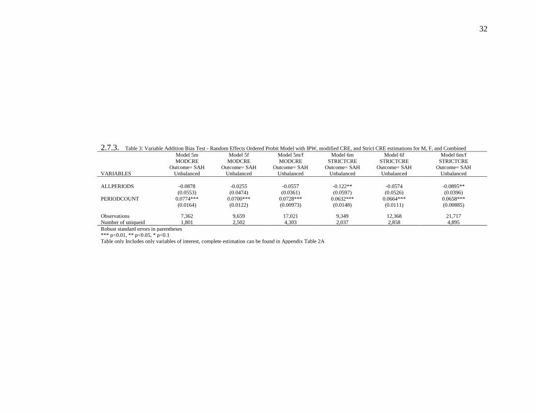
the individual was observed PERIODCOUNT. Table 3 presents these results for our

SAHS outcome variable. Significance in these two variables across our preferred

specification would indicate that our panel likely suffers attrition driven bias. The

positive and significant coefficient of PERIODCOUNT suggests that healthier individuals

tend to participate for longer periods while the ALLPERIOD variable’s insignificance

23

across preferred specifications Table2: Model 5 suggests that full participation is not a

cause of additional bias. We conclude that bias induced by attrition will tend to produce

conservative estimates in our structural equations. In order to control for the effects of

bias, we test both unweighted and weighted panels using inverse probability weights IPW

following (Wooldridge, 2002).


2.4.3. Correlated Random Error Considerations

Correlation between the random effect and time variant regressors, implies that

the outcome variable y is correlated with the error term yielding biased estimation.

Restoring the mean zero assumption requires isolating the effect of unobserved effects on

covariates. Mundlak, Chamberlain and subsequently Wooldridge(2002) approaches

develop around the inclusion of time-invariant means for all time-varying regressors to

isolate the correlated random effect. Coefficients on these correlated random error

(CRE) control variables cannot be easily interpreted for they are constructed on past

present and future observations. To explore the possibility of permanent effects, we

construct past-average means for our variables of interest. We address issues of potential

bias which arise by this modification estimating both strict CRE and our relaxed CRE

formulation for FSTRESS and JOBSWITHCING. Results are substantively similar across

specifications. We use the modified CRE estimation to support our discussion of

permanent effects.

24

2.5. Results and Discussion

We present twelve models to explore the relationship between our variables of

interest and SAHS outcomes. All models reflect the random effect ordered probit

estimation methodology. The first six models (Table 4) are constructed from the full

unbalanced panel. The second six (Table 5) disaggregates results from Table 4: Models

4-6 across gender. We consider the models in order. Table 4: Model 1, applies no CRE

conditioning and presents as our naïve baseline, Table 4: Model 2, modified CRE

corrections on our preferred specification, and Table 4: Model 3, strict enforcement of

CRE conditioning. All models present qualitatively similar results. Table 4: Models 4-6

repeats specifications Models 1-3, imposing inverse probability weighting to control for

biases introduced by attrition. Although model fit degrades when IPW are added (Table

4: Models 4-6), given the qualitatively similar responses across regressions, we prefer the

IPW weighted regressions to the simple unbalanced panel in consideration of the

potential effects of attrition based biases previously noted.7


In our preferred full panel specification Table 4: Model 5, several salient features

emerge. First, although the sign on YSCHOOL is consistent across models. In our

preferred specification, only the CRE time invariant MEAN_YSCHOOL is strongly and

7 Although our model of financial strain includes the great recession. We control for period specific fixed effects by including dichotomous variables for each survey period using 2001 as the base category. Full results can be found in Appendix 1, Table A1. We find significant and negative period specific effects in 2005, 2009 and 2011 relative to the base time period 1999. We attribute a non-significant finding in 2007 as corollary with the recessional period 2001.

25

economically significant (0.0550) corroborating the trend toward treating YSCHOOL as a

stationary variable in adults. In the case of stationary variables of gender MALE, and

race NON_WHITE, we find the conventional and expected relationships suggesting that

MALE report slightly better health than FEMALE (.0543) at conventional confidence, and

minorities report a strongly significant tendency to report poorer SAHS (-.134). With

these results buttressing historical findings, we turn our attention to variables of interest.

The contemporaneous “shock” coefficient on financial strain FSTRESS is both

economically (-.124) and statistically significant (<5%). Interestingly, the shock effect of

JOBSWITCHING fails to achieve significance or sign consistency across specifications.

However, the permanent effect of PAST_JOBSWITCHING_AVERAGE is both

statistically and economically significant (-0.059) and consistent across models.

Conversely, PAST_FSTRESS_AVERAGE fails to achieve significance although it

maintains the expected negative sign across all models. With respect to our theoretical

motivation, this evidence supports both hypotheses: that FSTRESS and JOBSWITCHING

have a negative effect on SAH. That said, the way these conditions effect health is, albeit

intuitive in hindsight, somewhat surprising. FSTRESS appears to be driven by the stress

that emerges from the onset of financial strain. The lack of a FSTRESS permanent effect

suggests that, in general, individuals practice consumption smoothing; they adjust to their

financial circumstances, and adjust rather quickly. This short duration effect is countered

with the permanent JOBSWITCHING effect. We believe the economic and significant

coefficient of PAST_JOBSWITCHING_AVERAGE is symptomatic of underlying distress

which accumulates as an individual struggles with stable employment.

26


While general results are quite interesting, subtle variation emerges between the

sexes with respect to health effects. Table 5: Models 1-6 disaggregate IPW regression

results from Table 4: Models 4-6 into MALE and FEMALE independent regressions.

Results across specifications are qualitatively robust. Referring to Table 5: Models 3 and

4 (the MALE and FEMALE specific representations of our preferred specification), we

find that gender effects vary across AGE with the marginal effect being negative and

significant for MALE (-0.241), and positive for FEMALE (0.125). This finding implies

that as individual’s age, men are more likely to report poorer health, while women tend to

report improving health. Both MALE and FEMALE are negatively effected by financial

shock -0.155 and -0.102 with corresponding confidences of (<1%) and (<5%)

respectively. What stands out to us is the difference in the way permanent

PAST_JOBSWITCHING_AVERAGE effects the sexes. Higher permanent job switching

volatility has no significant effect on men, but is negative (-0.0825) and significant for

women. We believe this a fruitful vein for future research. Why is it that women who,

by the nature of childbearing, tend to enter and leave the workforce at higher rates than

men report poorer SAHS? To us, this immediately raises questions of the psycho-social

stressors of skills erosion (diminishing human capital value), and being “disconnected”

from the economic playing field. Conceivably, there is a third unobservable factor that

effects both job switching volatility and SAHS consistent with Fuchs (1982) comments.

We find a strong motivation to continue this vein of research exploring female

27

perceptions of economic self-worth in the context of employment lapses driven by the

child-rearing experience.

As a byproduct of our research, we shed light on a dynamic that appears to

underlie the common finding that minorities suffer lower SAHS than their Caucasian

counterparts. While our data reflects this long-standing relationship, our preferred male

and female specifications find that the result is primarily driven by minority females who

report significantly poorer health than their male and Caucasian counterparts. In light of

the recognition that the negative effects of higher frequency job-switching

disproportionately effect females, and that minority females report lower SAHS, we feel

that there may exist a relevant socio-economic relationship between the two. We

encourage further research along this line of inquiry.

From a health policy perspective, our research provides evidence that it may be

important to focus outreach on employment stabilization. We find the international trend

toward increasingly prominent precarious employment situations quite worrying. Our

research finds support for the conventional wisdom of temporary income stabilization

across shocks. However, we feel that attention focusing on womens’ experiences with

employment lapses may also be important to highlight. Further, we suggest that at a

higher level of abstraction, habitually used temporary income assistance may provide

observable evidence of higher level jobswitching and provide a means for targeting a

subset of high volatility job switchers. Our findings encourage policy makers to look at

both financial assistance programs and job stability programs when considering

individual economic stability.

28

2.6. Concluding Remarks

In this research, using a dynamic panel random effects ordered probit mythology,

we explore two possible mechanisms that are hypothesized to underlie the accepted

SES/Health gradient: financial strain, and job switching volatility. Using a multi-year

unbalanced longitudinal panel from the Panel Study of Income Dynamics we confirm the

expected presence of the well understood SES/Health gradient, demonstrate the

magnitude of and correct for panel bias induced by various forms of attrition, test and

reject endogeneity in the relationship of SAHS and financial strain and find support for

our theoretically based hypotheses: financial strain and job switching volatility produce

negative health effects. Our key results are summarized in Figure 1.

[Insert Chapter 2: Figure 1 here]

We find that higher job-switching frequency resulted in a strong negative and

permanent effect on self-assessed health which is consistent with grey literature prevalent

in sociological and psychological disciplines. Extending past research into the effects of

income and financial strain on health (Contoyannis et al., 2004; Lyons & Yilmazer,

2005) we find a strong causal significant negative relationship between financial strain

and self-assessed health. The “shock” effect is however, short lived. We find no

evidence of permanent effects. One possible explanation for the lack of permanence is

consumption smoothing. In this sense, our work is supportive of the vast body of

academic work on smooth consumption. Our research suggests that the process of

adjustment is quite rapid. From a policy perspective investment directed at employment

29

stability should not be overlooked in favor of programs that reinforce financial

buttressing. Our work also suggests that the two policy forks may work cooperatively by

targeting different underlying dynamics.

2.7. Tables and Figures

30

2.7.1. Table 1: Summary Statistics

Variable Mean Observations 21717 HSTATUS Self-Assessed Health Status scale 1-5 with 1= Very Poor Health and 5=Very good health 3.771

(0.915) FSTRESS Financial Strain using Net Wealth including Equity 0.172

(0.377) JOBSWITCHING A count of job transitions within the period 0.392

(0.732) AGE Age 45.047

(9.979) AGE2 Age Squared divided by 10 212.878

(89.238) AGE3 Age Cubed divided by 100 104.745

(62.507) NON_WHITE Dummy variable where 0= Caucasian 0.274

(0.446) YSCHOOL Number of years in formal education 13.873

(2.202) MALE Dummy variable where 1=Male 0.430

(0.495) HINSURANCE Dummy variable denoting whether any family member is covered by health insurance 0.943

(0.231) STABLEMAR Dummy variable =1 if married in prior survey and current survey to same spouse 0.741

(0.438) NUMFAMCH Number of children in the household that are under 18 years of age 0.945

(1.176) INITIAL HSTATUS 1 Dummy variable = 1 if HSTATUS at first observation = 1 0.005




(0.486) TIME2 Dummy variable = 1 if Year equal 2001 0.137






(0.356) MEAN_AGE CRE variable: time invariant mean of AGE – avg. all observations 43.999

(9.327) MEAN_AGE2 CRE variable: time invariant mean of AGE2 – avg. all observations 204.073

(80.976) MEAN_AGE3 CRE variable: time invariant mean of AGE3 – avg. all observations 98.902

(55.086) MEAN_YSCHOOL CRE variable: time invariant mean of YSCHOOL – avg. all observations 13.848

(2.136) MEAN_HINSURANCE CRE variable: time invariant mean of HINSURANCE– avg. all observations 0.944

(0.159) MEAN_STABLEMAR CRE variable: time invariant mean of STABLEMAR – avg. all observations 0.721

(0.383) MEAN_NUMFAMCH CRE variable: time invariant mean of NUMFAMCH – avg. all observations 0.964

(0.968) MEAN_FSTRESS_Z2 CRE variable: time invariant mean of FSTRESS_Z2 – avg. all observations 0.171

(0.291) MEAN_FSTRESS_Z1 CRE variable: time invariant mean of FSTRESS_Z1 – avg. all observations 0.296

(0.250) MEAN_JOBSWITCHING CRE variable: time invariant mean of JOBSWITCHING – avg. all observations 0.421

(0.398) PAST_JOBSWITCHING_AVERAGE Modified CRE variable: time invariant mean of JOBSWITCHING- avg. past observations 0.498

(0.597) PAST_FSTRESS_AVERAGE Modified CRE variable: time invariant mean of FSTRESS_Z2 – avg. past observations 0.163

(0.318)

31

2.7.2. Table 2: Attrition Tests, Pooled Probit Specification, IPW clusters

Y=Observed

Y=Observed

Y=Observed

Y=Observed Y=Observed

Y=Observed

Y=Observed

Y=Observed

InitCond InitCond InitCond InitCond InitCond InitCond InitCond InitCond

VARIABLES unbalanced unbalanced unbalanced unbalanced unbalanced unbalanced unbalanced unbalanced

MEAN_FSTRESS -0.0130 -0.229*** -0.0130 -0.234*** -0.245*** -0.228*** -0.0887 0.0210

(0.0805) (0.0869) (0.0805) (0.0770) (0.0735) (0.0716) (0.0701) (0.0722)

MEAN_JOBSWITCHING -0.120*** -0.0676 -0.120*** -0.0818** -0.139*** -0.195*** -0.250*** -0.191***

(0.0425) (0.0466) (0.0425) (0.0401) (0.0385) (0.0379) (0.0372) (0.0384) MEAN_AGE 1.470*** 2.041*** 1.470*** 1.157*** 0.935*** 0.995*** 0.390*** -0.650***

(0.169) (0.198) (0.169) (0.157) (0.150) (0.148) (0.146) (0.157)

MEAN_AGE2 -0.264*** -0.386*** -0.264*** -0.203*** -0.158*** -0.178*** -0.0517 0.177***

(0.0386) (0.0448) (0.0386) (0.0360) (0.0345) (0.0342) (0.0339) (0.0367)

MEAN_AGE3 0.153*** 0.240*** 0.153*** 0.113*** 0.0795*** 0.0963*** 0.00820 -0.158***

(0.0285) (0.0328) (0.0285) (0.0267) (0.0257) (0.0255) (0.0254) (0.0276) MEAN_YSCHOOL -0.0262** -0.0174 -0.0262** -0.0117 -0.00950 0.0291*** 0.0264*** 0.0364***

(0.0109) (0.0117) (0.0109) (0.0105) (0.0102) (0.0100) (0.00993) (0.0102)

MALE 0.102** 0.231*** 0.102** 0.162*** 0.0998** 0.00431 -0.0832** -0.0592

(0.0435) (0.0472) (0.0435) (0.0421) (0.0407) (0.0401) (0.0396) (0.0406)

NON_WHITE -0.170*** -0.0782 -0.170*** -0.117** -0.151*** -0.194*** -0.107** -0.134***

(0.0523) (0.0562) (0.0523) (0.0504) (0.0488) (0.0478) (0.0475) (0.0483)

INITIAL HSTATUS=1 -0.738*** -0.676*** -0.738*** -0.228 -0.677*** -0.351 -0.464* -0.704***

(0.252) (0.255) (0.252) (0.257) (0.248) (0.247) (0.239) (0.249) INITIAL HSTATUS=2 -0.220** -0.197* -0.220** -0.375*** -0.356*** -0.332*** -0.355*** -0.423***

(0.0949) (0.101) (0.0949) (0.0906) (0.0890) (0.0868) (0.0868) (0.0882)

INITIAL HSTATUS=3 -0.170*** -0.154** -0.170*** -0.159*** -0.190*** -0.222*** -0.311*** -0.292***

(0.0594) (0.0636) (0.0594) (0.0571) (0.0553) (0.0543) (0.0540) (0.0549)

INITIAL HSTATUS=4 -0.0985* -0.0720 -0.0985* -0.0888* -0.122** -0.128*** -0.183*** -0.121**

(0.0525) (0.0568) (0.0525) (0.0508) (0.0493) (0.0489) (0.0486) (0.0498) Constant -24.96*** -34.08*** -24.96*** -19.87*** -15.96*** -16.49*** -6.920*** 8.391***

(2.403) (2.829) (2.403) (2.206) (2.093) (2.061) (2.022) (2.170)

Observations 4,895 4,895 4,895 4,895 4,895 4,895 4,895 4,895

Standard errors in parentheses *** p<0.01, ** p<0.05, * p<0.1

32

2.7.3. Table 3: Variable Addition Bias Test - Random Effects Ordered Probit Model with IPW, modified CRE, and Strict CRE estimations for M, F, and Combined

Model 5m Model 5f Model 5m/f Model 6m Model 6f Model 6m/f

MODCRE MODCRE MODCRE STRICTCRE STRICTCRE STRICTCRE

Outcome= SAH Outcome= SAH Outcome= SAH Outcome= SAH Outcome= SAH Outcome= SAH

VARIABLES Unbalanced Unbalanced Unbalanced Unbalanced Unbalanced Unbalanced

ALLPERIODS -0.0878 -0.0255 -0.0557 -0.122** -0.0574 -0.0895**

(0.0553) (0.0474) (0.0361) (0.0597) (0.0526) (0.0396)

PERIODCOUNT 0.0774*** 0.0700*** 0.0728*** 0.0632*** 0.0664*** 0.0658***

(0.0164) (0.0122) (0.00973) (0.0148) (0.0111) (0.00885)

Observations 7,362 9,659 17,021 9,349 12,368 21,717

Number of uniqueid 1,801 2,502 4,303 2,037 2,858 4,895

Robust standard errors in parentheses *** p<0.01, ** p<0.05, * p<0.1

Table only Includes only variables of interest, complete estimation can be found in Appendix Table 2A

33

2.7.4. Table 4: Random Effects Ordered Probit Results with Inverse Probability Weights, Full, Modifed, and Excluded CRE controls

T4_MODEL 1 m/f T4_Model 2 m/f T4_Model 3 m/f T4_Model 4 m/f T4_Model 5 m/f T4_Model 6 m/f

NO-IPW NOIPW-MODCRE NO IPW FULL CRE IPW IPW-MODCRE IPW FULL CRE

Outcome SAH Outcome SAH Outcome SAH SAH-FSTRESS Outcome SAH Outcome SAH

xtoprobit xtoprobit xtoprobit all corrections xtoprobit xtoprobit unbalanced unbalanced unbalanced unbalanced unbalanced unbalanced

FSTRESS -0.132*** -0.124*** -0.0781** -0.131*** -0.124*** -0.0770**

(0.0347) (0.0348) (0.0351) (0.0350) (0.0352) (0.0355) PAST_FSTRESS_AVERAGE -0.0552 -0.0358 -0.0505 -0.0330

(0.0491) (0.0504) (0.0493) (0.0506) MEAN_FSTRESS -0.0832 -0.0995

(0.0705) (0.0728) JOBSWITCHING -0.00390 -0.00415 0.0192 -0.00135 -0.00156 0.0216

(0.0145) (0.0146) (0.0142) (0.0147) (0.0148) (0.0143) PAST_JOBSWITCHING_AVERAGE -0.0551** -0.0532** -0.0611** -0.0590**

(0.0254) (0.0257) (0.0256) (0.0258) MEAN_JOBSWITCHING -0.101*** -0.105***

(0.0331) (0.0347) MALE 0.0501* 0.0528* 0.0773*** 0.0514* 0.0543* 0.0791***

(0.0281) (0.0284) (0.0288) (0.0282) (0.0285) (0.0297) NON_WHITE -0.151*** -0.140*** -0.157*** -0.146*** -0.134*** -0.148***

(0.0339) (0.0344) (0.0353) (0.0340) (0.0345) (0.0362) YSCHOOL 0.0612*** 0.0123 0.00116 0.0596*** 0.0116 -0.000527

(0.00671) (0.0189) (0.0170) (0.00670) (0.0186) (0.0170) STABLEMARRIAGE 0.00111 -0.103* -0.107** 0.00155 -0.107* -0.116**

(0.0323) (0.0556) (0.0475) (0.0322) (0.0554) (0.0473) MEAN_YSCHOOL 0.0560*** 0.0726*** 0.0550*** 0.0726***

(0.0205) (0.0188) (0.0203) (0.0188) MEAN_STABLEMARRIAGE 0.157** 0.157*** 0.163** 0.172***

(0.0678) (0.0605) (0.0677) (0.0608) SIGMA2_U 0.372*** 0.379*** 0.529*** 0.360*** 0.367*** 0.533***

(0.0421) (0.0422) (0.0329) (0.0423) (0.0424) (0.0344)

N 17,021 17,021 21,717 17,021 17,021 21,717 CLUSTERS 4,303 4,303 4,895 4,303 4,303 4,895 LOG LIKELIHOOD -16783.75 -16763.91 -21385.73 -21206.46 -21181.86 -27367.76 AIC 33629.5 33603.81 42849.47 42474.92 42439.73 54813.52

Robust standard errors in parentheses *** p<0.01, ** p<0.05, * p<0.1 Non-significant controls excluded from results for brevity. Full results can be found in the appendix Table A4

34

2.7.5. Table 5: Random Effect Ordered Probit Results - Separate Male and Female Results

T5_MODEL4m T5_MODEL4f T5_Model 5m T3_Model 5f T3_Model 6m T3_Model 6f

IPW IPW IPW-MODCRE IPW-MODCRE IPW FULL CRE IPW FULL CRE

Outcome SAH Outcome SAH Outcome SAH Outcome SAH Outcome SAH Outcome SAH unbalanced unbalanced unbalanced unbalanced unbalanced unbalanced

FSTRESS -0.164*** -0.109** -0.155*** -0.102** -0.124** -0.0419

(0.0539) (0.0459) (0.0546) (0.0459) (0.0526) (0.0479) PAST_FSTRESS_AVERAGE 0.0763 -0.119* 0.106 -0.106

(0.0789) (0.0632) (0.0808) (0.0648) MEAN_FSTRESS 0.0808 -0.208**

(0.128) (0.0896) JOBSWITCHING 0.000360 -0.00512 0.000133 -0.00495 0.0211 0.0223

(0.0231) (0.0191) (0.0233) (0.0191) (0.0223) (0.0188) PAST_JOBSWITCHING_AVERAGE -0.0393 -0.0818** -0.0325 -0.0825**

(0.0421) (0.0321) (0.0428) (0.0323) MEAN_JOBSWITCHING -0.105* -0.115***

(0.0607) (0.0415) AGE -0.372*** 0.0595 -0.392** 0.252* -0.237** -0.0107

(0.127) (0.110) (0.156) (0.140) (0.115) (0.101) AGE2 0.0771*** -0.0155 0.0719** -0.0668** 0.0359 -0.00811

(0.0278) (0.0243) (0.0339) (0.0308) (0.0256) (0.0226) AGE3 -0.0532*** 0.0115 -0.0499** 0.0489** -0.0243 0.00671

(0.0197) (0.0175) (0.0239) (0.0221) (0.0185) (0.0166) NON_WHITE -0.0927* -0.183*** -0.0783 -0.175*** -0.123** -0.173***

(0.0547) (0.0433) (0.0554) (0.0439) (0.0579) (0.0461) YSCHOOL 0.0741*** 0.0512*** 0.0259 0.000762 -0.00556 0.00434

(0.0105) (0.00864) (0.0314) (0.0223) (0.0278) (0.0217) STABLEMARRIAGE 0.131** -0.0676* -0.0325 -0.153** -0.111 -0.110*

(0.0566) (0.0394) (0.0843) (0.0743) (0.0738) (0.0621) MEAN_YSCHOOL 0.0549 0.0579** 0.0937*** 0.0570**

(0.0342) (0.0244) (0.0305) (0.0240) MEAN_STABLEMARRIAGE 0.290*** 0.113 0.360*** 0.0620

(0.110) (0.0882) (0.102) (0.0771) SIGMA2_U 0.368*** 0.346*** 0.379*** 0.350*** 0.558*** 0.506***

(0.0654) (0.0544) (0.0660) (0.0543) (0.0556) (0.0427)


Robust standard errors in parentheses *** p<0.01, ** p<0.05, * p<0.1 Non significatnt controls excluded from results for breviety. Full results can be found in the appendix Table A5

35

2.8. Figures

2.8.1. Figure 1: Summary Table of Findings

Temporary SAHS Effect Permanent SAHS Effect

Financial Strain

Job-switching

Directional effect of an increase in FSTRAIN or JOBSWITCHING on SAHS.

-

- 0

0

36

Chapter 3: State Level Operationalization of Health Policy: A

pragmatic approach to predicting changes in premiums and aggregate

market profitability

3. Introduction

Policy development at the institutional level requires increasingly sophisticated

analysis. In many cases there exists little infrastructure to facilitate cross

organization/nor public-private cooperation. As a result, it is not uncommon for decision

makers to have little or no authority to compel relevant informational sharing. Without

this authority, decision makers are often forced to make due with limited data, sparsely

connected collations, and little recourse. In order to combat internal informational

limitations and exogenous strategies which may lead to sub-optimal, or inefficient policy

making, we develop a pragmatic generalized quantitative model to assist stake holders

and state decision makers in objective policy development through quantitative

evaluation of proposed legislation. In this research, we use proposed health insurance

market reforms upon which to develop and validate our model however the generalized

modeling approach is easily adapted to other markets.

A primary feature of the Affordable Care Act (ACA) is state level health policy

innovation. To implement state-level health policy innovations, the 1332 innovation

waiver can be sought by states to waive elements of the ACA. Early evidence from the

37

development of 1332 waivers suggests wide variation in innovation design. Across

reforms which implement a reinsurance program, divergence in reform design suggests a

gap in underlying theory (see Table 1 below). A detailed review of existing theory

confirms a sparse set of tools available to assist policy makers in operationalizing health

reinsurance market innovation development. Existing theory is primarily focused on two

topics: the prevalence and minimization of distortionary incentives in service and

payment programs, and the effects of uncertainty on profit maximization.


Research by [Zhu, Layton et al. 2013; Layton, McGuire et al. 2016; Geruso and

McGuire 2016; Layton, Ellis et al. 2015] explore efficiencies of payment and risk

adjustment methodologies imposed by the ACA. This literature explores the relationship

between reinsurance programs and problems of adverse selection, regulatory price

distortions, and moral hazard. Findings are consistent across authors; reinsurance

programs are found to be effective at minimizing distortionary incentives and there is no

argument that reinsurance programs can be, and often are, market benefiting.

With respect to incentives for adverse selection in health plan payment systems,

distortionary effects of regulation are taken up by (Layton, Ellis et al. 2015). The authors

focus on the relationship between total plan revenues and costs. The research focuses on

the development of ratios which may be used to inform on price distortions caused by

premium regulation, adverse selection in the market, and inefficiencies generated by

38

benefit distortion to attract more profitable customers. In the evaluation of policy, the

ratios may assist regulators in understanding responses to proposed policy, however,

there exists no quantitative means of evaluating profitability trade-offs among different

payment systems.

Purchases of optimal reinsurance is taken up in expected utility maximization

theory and focuses on carrier reinsurance choices as profit maximizing decisions.

Bernard and Tian (2009) use a static single period model to derive optimal reinsurance

contracts given Value at Risk VaR and Conditional Tail Expectations (CTE) regulatory

constraints. The authors consider the risk-based cost of reinsurance a function of the cost

of required capital. Their research questions focus on variation in reinsurance behaviors

between carriers in the context of price competition. They find that exponentially

growing risk causes exponentially growing risk premiums; an insurer has the choice of

rapidly escalating fixed costs (the reinsurance premium) or rapidly growing VaR capital

requirements.8 This relationship creates an incentive to forgo the purchase of reinsurance

coverage for excessive risk in favor of passing the cost of excessive risk on to the

insured.

Rapid increases in the cost of excessive risk is taken up in (Zhang 2013). Zhang

focuses on carrier reductions in capital requirements by ceding risk to a reinsurer and the

subsequent increase in the reinsurer’s capital requirements. Using this analysis frame,

optimal reinsurance contracts are defined by the degree of correlation between carrier risk

8 A function of the variance in patient cost.

39

and reinsurer total risk. The solution is optimized when total required capital is

minimized across carrier and reinsurer. In the face of price competition, the author

concludes that incentive alignment exists between parties with reinsurance an attracting

equilibrium. At the same time, the author confirms conflicting incentives between carrier

and regulator.9 The conflict in incentives between carriers and regulators is a common

theme throughout the literature. Bernard and Tian, 2009 sum up the conflict noting that

the social-planner/regulator, would prefer adverse states of the world to be considered,

and that firms would attempt to limit exposure to large losses. Growing national interest

in managing health insurance cost is inhibited by this lack of incentive alignment.

One potential answer to aligning incentives is the institution of compulsory

reinsurance at the state or national level funded by assessments or taxes. Yet, there is

little guidance on the form and composition of such programs especially at the state level

where local market distortions may require heterogeneous approaches to policy. Our

research fills a critical gap in the literature. We develop a predictive model which may

be used to evaluate alternative compositions of health insurance market reforms; identify

appropriate threshold values to utilize, and/or define, available funding; and objectively

evaluate the potential for unanticipated program liabilities or market distortions. The

remainder of the paper is dedicated to the Conceptual Framework and Model

Development; Numerical Examples, Simulation, and Results; Policy Scenario Analysis;

and Concluding Remarks.

9 From a policy perspective, substantive market reforms are hindered by opposed incentives between carrier and regulator; profit maximizing firm behavior is predicated on passing excessive risk cost to the consumer while regulator intentions are predicated on protecting consumers from the cost of excessive risk.

40

3.1. Conceptual Framework and Model Development

We approach model development from the perspective that it is sufficient to

determine whether there exists at least one institutionally feasible coordinated strategy of

regulation that can be demonstrated to promote a more efficient outcome than that of the

status-quo. This approach is consistent with (Ostrom, Gardner et al. 1994) and we use

the common pool resource dilemma as a stepping off point. Our pragmatic approach

focuses on inputs which may be effected by policy levers and credible prediction of

changes in market outcomes. In this work, we focus on health insurance market reforms

for their parallel with common pool resource dilemmas but the generalized model can be

conformed to a variety of policy intentions.

Our reinsurance based model is premised on several explicit assumptions. First,

expected medical expenditures are reasonable approximations to ex-post cost. Layton,

Ellis et al. (2015) confirms this assumption finding that reinsurance models are robust to,

“reasonable assumptions about the social planners and consumers’ ability to predict

future medical spending.” Balbas et al. 2015 supports the use of “simple functions” of

the form 1

n

i Biia X

= as useful to yield the optimal reinsurance problem. We therefore

adopt the simple functional form for exposition. The model may be easily adopted to the

calculus of integration without loss of fidelity and such modification is recommended if

the model is to be used as a basis to develop optimal social reinsurance theory (Balbás,

Balbás et al. 2015). Our third primary assumption is that market profitability can be

expressed using firm level profit functions. In this sense, our model reflects a single

41

producer made up of many sub-producers. The effect of chosen parameter values may

therefore effect sub-producers differently. Caution should be taken to minimize

competitive distortions which may arise by uniform application of parameters across sub-

producers.

3.1.1. The Model

Our model is postulated on a simple participation constraint of the form

( ) ( )A BE E .10 From the regulator’s perspective, appropriate regulatory structure

can be tackled and transparent negotiation on model inputs for both the current period (B)

and the post period (A) can be defined, agreed upon by committee, and tested to assure

all parties that the proposed solution is at least as good and the status-quo. Profit in the

pre and post policy states are defined:

1

( ) ( 1) ( 1)A A

Q

A A A A q q A A A A A A A A A A

q

N r N P E c A N r H G B N r =

= − + − + + − −

(1)

1

( ) ( 1) ( 1)Q

B B B B Bq Bq B B B B B A B B B B

q

N r N P E c A N r H G B N r =

= − + − + + − − +

(2)

In the generalized model, where equality is enforced across periods (B) and (A)

and there exists no explicit objective of altering market profitability 0= , pre and post

state aggregate market profitability are identical. Omega, may be thought of as a

residual term used to satisfy a clearly articulated set of regulatory intentions which reflect

market profitability changes.

10 Which states that the expected aggregate profit available to industry after the policy change is equal to or greater than the expected aggregate profit available to the industry before the policy.

42

Regulatory action parameters in the proposed model consist of several malleable

features: Carrier assessment x attached to total written premiums, the number of

covered lives xN and average market premium xr . The assessment may or may not be

subsidized by state tax credits ( 1)xA − . In our model, it is possible that consumers find

themselves without insurance coverage between enrollment opportunities. The net-cost of

those who would like to be insured but are caught between open enrollment periods G (a

catchment pool) is thus captured. Funding of the catchment pool is left to the reader as a

natural extension to the model. For expositional ease, we assume that the cost of the

catchment pool is absorbed by carriers but may be subsidized by state tax or other credits

( 1)xB − . The weighting factor x allows for the size of the catchment pool to be modified,

a function of the type and intent of xH . In many cases x will simply reflect (0,1) where

there is or is not a catchment pool. The carrier portion of revenues which may be used for

overhead and profit x may be adjusted across states, however, in many cases this is

constrained by law to a value of 15% or 20% depending on the market under

consideration. Finally, we introduce xH as a formal method to deal with high cost patients.

We develop two distinct methods of xH : conditions based reinsurance and

attachment point reinsurance. A conditions based reinsurance program defines a number

of high-cost health conditions which define a known population of individuals xN . This

group’s expenses are then covered by a reinsurance program formally defined.

43

1

(1 ) ( )I

x x i i

i

H N w PE c=

= −

(3)

A patient’s membership in this program may exempt all or a portion of carrier expenses

(1 )w− related to the patient. The model is developed in the context that a population

may be subdivided into groups of individuals who suffer a qualifying condition i and

each group i can thus be assigned a probability iP within the population and an expected

cost ( )iE c . It is assumed that the probabilities of succumbing to any condition i are

independent and identically distributed such that 1

1i

i

P

=

= .

The attachment point reinsurance model allows the population of the program to

be defined by accrued costs in excess of an attachment-point. In this sense, an

attachment-point reinsurance program does not discriminate across what types of health

issues are covered. Rather any individual who accrues sufficient yearly cost is passed to

the reinsurance pool. We model a simplified attachment-point reinsurance program as an

“outlier risk sharing” model. Outlier risk sharing models are defined as mandatory

reinsurance for insurers without risk-adjusted premiums (Van Barneveld, Lamers et al.

2001) (Zhu, Layton et al. 2013).11 Formally we express the model

( ( ) )(1 )( ( ) ) ( ( ) ) ( ( ) )(1 ) ( ( ) )x x I i I x I i I iH N P L E c T w E c L N P E c T E c L w E c T= − − + − − + − (4)

11 The authors point out that in outlier-risk-sharing models, health plans are (partially) reimbursed for the expenditures of a member above a certain threshold and these programs have been shown to protect against predictable losses at a relatively modest cost.

44

where there is a total population xN which can be evaluated to determine the probability

( )IP • of incurring patient costs between ( )iL E c T where L reflects an attachment

point, and T a limit to reinsurance plan liability12. It is typical for claims in excess of

this funding level to revert to the carrier. For this proportion of the population ( )iE c

reflects the average patient cost, and as with the conditions based reinsurance program, a

cost-sharing requirement (1 )w− may be imposed where w represents the proportion of

the carriers responsibility 0 1w .

In either model, a limit to the reinsurance fund may be adopted by conditioning

the reinsurance program on a probability of the costs of the patients exceeding available

funds (1 ( ))P c f− .

( )( ) ( ) ( ) (1 ( )) ( ) ( ) ( )x nE H P c f E c P c f E f E c E f= + − −

(5)

In this case, the expected value of xH is the weighted average of the probability of being

compensated for costs ( )E c up to the entire value of the reinsurance fund f plus the

probability that some portion of the expected benefit must be given up to cover patients

in excess of fund reserves ( ) ( )nE c E f .

12 At the state level, it is common for a fixed value fund be available limiting a state’s liability.

45

3.2. Numeric Examples, Simulation, and Results

In this section, we modify our participation constraint model to evaluate two

distinct policy shifts in Alaska’s management of the health insurance industry:

• In the third quarter of 2015, Alaska implemented a Medicaid expansion

program.

• Beginning January 2017, Alaska implemented a conditions based reinsurance

program.

3.2.1. Alaska’s Medicaid Expansion Fall 2015

Alaska maintains a conditions based high-risk pool. To conform our generalized

model to Alaska’s market Medicaid discussion environment, we form our basic model on

a NO state health program prior.13 Additionally, we found in interviews with state

insurance regulators that carrier impact analyses of Medicaid expansion which were

relied upon in the rate review process postulated a negligible change in the individual

market population. Constrained by this frame of reference, we proceed under the

assumption that B AN N= and by extension A BP P= employing the large sample property

qP = ;qq

nn N

N . Further, we assume that the manner in which estimated costs are

calculated across a comprehensive battery of illness states q remains unchanged. Without

a new state sponsored program to fund high cost patients 0XH = , several associated

13 Without alteration in the form or expectations of the high-risk pool, past and future effects are equal value constants which cancel each other out.

46

model constraints are removed: no new assessment X nor a compensatory state tax

rebate A , nor a requirement for a catchment pool of any size funded by assessment B .

It is further assumed that the direct patient care ratio which defines carrier overhead

remains unchanged across the Medicaid expansion. In order to inform on expected rate

changes, all savings in the individual market generated as a result of Medicaid expansion

would be passed on to the consumer implying the possibility that B Ar r . In the case of

Alaska’s Medicaid expansion, the pre-policy period (2015) suffered an aggregate market

loss of 30 million dollars. With finalized rates for 2016 effectuated by the end of

September 2015, quality predictions about the year’s profitability were in hand14. As a

result, we allow for adjustment of the pre-market aggregate profitability state

$30,000,000 = ; i.e. The new premium Ar becomes our output of interest. We conform

our model to the following explicit assumptions

{ ; ; ; ; ; ; ; 0; 0; 0}B A A B B A B A B A A B A B X X XN N P P q q A A B B H = = = = = = = = = =

which allow the pre and post profit functions from (1) and (2) across the participation

constraint to be expressed.

1 1

( ) ( )Q Q

A A q Aq A B q Bq B B

q q

Nr N P E c Nr Nr N P E c Nr = =

= − − − − + =

(5)

14 New Mexico Office of Superintendent of Insurance personnel confirm that carriers tend to understand their yearly profitability with a high degree of certainty during in the third Quarter of the year. Further, this information is used in the final rate setting requests for the following year. MLR reports from CCIIO (https://www.cms.gov/apps/mlr/mlr-search.aspx#/?state=AK&reporting_year=2015; last accessed 11/27/2017) confirm that Premera BCBS underwriting loss occurring in Alaska were 30M in 2015, and 26M in 2014. Faced with a large underwriting loss in 2014 and third quarter predictions of a greater loss in 2015, using a pre-state market in equilibrium would not be a true reflection of the dynamic in the rate setting process for 2016.

https://www.cms.gov/apps/mlr/mlr-search.aspx#/?state=AK&reporting_year=2015

https://www.cms.gov/apps/mlr/mlr-search.aspx#/?state=AK&reporting_year=2015

47

Solving15 (5) for the post policy change premium Ar ,

1 1

( ) ( )

(1 ) (1 )

Q Q

q Aq q Bq

q q

A B

P E c P E c

r rN

= =

−

+ +− −

(6)

it becomes immediately clear that premium changes sought in the year 2015 during the

discussion of and analysis of Medicaid expansion are driven primarily by perceptions in

the aggregated change of expected patient cost of the group ( )AqE c . Medical inflation is

of course a positive constant. In this case

1 1

( ) ( )Q Q

q Aq q Bq

q q

P E c P E c= =

making the expectation of the right hand side of (6) unequivocally positive with 0 .

This implies A Br r for the post-policy state.

3.2.1.1. Evaluation of Alaska’s Medicaid Expansion

In all model predictions, we follow (Layton, McGuire et al. 2016), and treat cost-

risk16 as a normally distributed random variable 2( ) ~ ( , )xE c N . By extension risk-

premium is proportional to the variance of the cost distribution. Our prediction strategy

is two pronged. In the first step, using a log-linear regression, we recover estimates of

patient cost growth over time for two data sources:

• Tomczyk 2016 report17 (Model 1: Table 2)

15 See appendix 3 for solution steps and details. 16 The cost risk is the distribution of the average costs of the consumer market participants. Because the cost risk is a distribution of

averages, the central limit theorem implies that the distribution will be approximately normal. 17 In their analysis, the authors synthesized 2014 ACS data with comprehensive carrier claims data across the period January 2015

48

• Bureau of Labor Statistics Community Population Survey18 Medical Care in the

U.S. City Average over the period 1990-2016 (Table 2: Model 2).

Table 2 presents growth rate results from the log-linear regression across the two

different data sources. As one might expect, the forward looking projections from

Tomczyk (2016), Table 2: Model 1, diverge significantly from the historical BLS

estimation (Table 2: Model 2) in both the magnitude of the growth rate, and the year over

year variation around that growth rate. The higher rate of average cost growth from the

Tomczyk, 2016 analysis is consistent with evidence that Alaska has a historically higher

average medical cost growth-rate than the rest of the country (Snyder, 2014). In this we

find support for the Tomczyk, 2016 annual cost growth-rate. However, the Tomczyk,

2016 forward looking projection used to derive the average medical cost growth-rate is

effectively linear exhibiting little year-over-year (YOY) trend variation. With a wide

geographic region of limited population and medical infrastructure, it is not unreasonable

to assume that small disruptions in the medical delivery infrastructure may generate

larger cost distortions than in more robust and stable medical delivery infrastructures of

neighboring states. With the divergence in first step estimates, step two predictions are

modeled under three alternative scenarios.

through September 2016 to develop their forward looking prediction of total patient cost for the period 2015 to 2026. Using this

projection, Table 2: Model 1, we recover the assumptions used to create the forward looking projection with 9.26%w = ,

2 .000006w = with standard error of .24%w = which represents an approximately linear projection of negligible

year over year volatility. 18 https://data.bls.gov/timeseries/CUUR0000SAM?output_view=pct_12mths last accessed 1/02/2018: 1990-2016; include annual

averages.

https://data.bls.gov/timeseries/CUUR0000SAM?output_view=pct_12mths%20%20

49


In Table 3: Prediction 1, we use Tomczyk 2016 (Table 2: Model 1) results as

inputs. In table 3: Prediction 2, we use BLS (Table 2: Model 2) results as inputs. In

Table 3: Prediction 3, we combine the Alaska specific (Tomczyk 2016) growth-rate with

the BLS estimation of growth rate volatility. We feel this estimation captures the best

information available19 and is our preferred model.


For each simulation, we randomly draw 5000 health cost changes from the

underlying distribution and calculate expected patient cost in the next period

( ) (1 ( )) ( )Aq BqE c E MI E c= + where ( ) $7,724bE c = is calculated by dividing the

Estimated Individual Market Cost 2015 ($217.5m) by the number of market participants

(28,159) in the individual market in 2015 noted by (Tomczyk 2016). Further, we allow

30m= which, as previously noted, reflects mounting concern during 2015 of

substantial individual market losses and is confirmed by 2015 CCIIO MLR reports and

subsequently reported by (Milliman 2017)20 as the total market loss for the period.

19 Tomczyk and coauthors work for Oliver Wyman a Marsh & McLennan actuarial company. Their knowledge of the Alaska individual market is assumed to reflect front line knowledge gleaned from conversations and document review by State of Alaska personnel. However, their method of projection cannot be determined. As a result, while we find the growth rate plausible, such drastic YOY differences between national historical averages and that produced by Wyman give us cause for concern. We thus superimpose national volatility on the local growth rate.

20 Treatment of as an additional random variable only suits to unnecessarily increase the distribution of predicted results. For validation we preferred to narrow the distribution rather than inflate it.

50

Average premium for 2015, 6,738Br = is also gleaned from (Milliman 2017). The

weighted average approved market premium for 2016 (Table 3) was 39.35%21 implying

$9,390Ar = . Finally, .15 = , is set by ACA statute for the individual market.

Across all three simulations, the approved rate exceeds our predicted AYP 95%

confidence bound implying an expected market profitability change

Pr( | ) 30Approved emiumE m . Actual health insurance market profit in 201622 adjusted for

risk adjustment and federal transitional reinsurance and risk corridor exogenous

payments23 implies a change in actual market profitability of $30m + [$11.5m] which,

falls outside the confidence bounds of Estimation 1 and within the confidence bounds of

Estimation 2 and Estimation 3.24

3.2.2. Alaska’s Reinsurance Program January 1, 2017

In early discussions about 2017 premiums, Premera, the final remaining carrier in

the state, made clear to regulators that they would be asking for an increase on the order

of 42%. Development of the reinsurance program was catalyzed by these discussions, as

was the development of the corresponding 1332 waiver application. This set of decisions

21 For 2016, two companies produced rate increases: Moda with a 39.60% premium increase and 72.69% market share, and Premera with a 38.70% premium increase and 27.31% market share. Our used 39.35% premium increase is the weighted average increase across the two carriers.

22 Laurel Andrews,: “Premera books $18 million profit from Obamacare plans in Alaska, prompting state review.” Alaska Dispatch

News, March 31, 2017 wherein Premera defines the breakdown of 2016 profitability. 23 Exogenous federal transfers and intra-state company transfers are not considered. With respect to federal transfers, instability in

the payment make the amount impossible to predict. With respect to intra-state company level transfers, the model predicts aggregate market profitability changes, by including company transfers a double counting of that amount occurs.

24 Note that model fit is more sensitive to price fluctuation than differences in average trends. Model results explicitly suggest that cost volatility drives premium change.

51

was compressed into a brief timeline which limited information available to stakeholders

about the effects of Medicaid expansion. 25 Alaska’s Reinsurance Program was signed

into law June of 2016, nine months after Medicaid expansion had been enacted. We will

now briefly discuss our assumptions about information available to stake-holders during

this period.


Figure 1 assumes that carriers were able to observe changes to Medicaid

applications through March 2016 explicitly assuming that they began their formal 2017

rate preparations in April.26 The data presents with two potential Medicaid expansion

effects. First, a comparison of the slopes of the trends before and after the expansion

(Red and Green trend lines) suggest a discontinuous shift from Red to Green with an

increasing rate of decay to the mean. Alternatively, they could assume that there was a

linear trend (blue line) which suggests a moderate shift in the historical trend of Medicaid

applications, but a relatively stable expectation for the population covered by Medicaid.

25 It is not uncommon for carriers to begin discussion with regulators early in the year in order to get appropriate information to streamline the rate review process which begins in April, however the nature of rate adjustment negotiations make it impossible to know on what date the state became aware of the proposed escalation in rates. The political effort to bring a bill before a special session requires a minimum of two months to prepare, and likely much more time. This suggests that carriers were informing their decision making on no more than four months of information relating to Medicaid expansion. We assume that by February 2016, there was mounting concern about the upcoming rate submission cycle and, coming on the heels of Medicaid expansion, we allow that carriers were able to observe changes in Medicaid applications through March 2016. This suggests that, sometime in April decisions about Medicaid expansion effect on 2017 rates were being concretized.

26 Note however that if carriers actually began to consider rates before April, the slope of the green line becomes increasingly negative implying a regression to the mean across a policy induced spike in enrollments. Thus, the longer window presents a more conservative expression of the likely change in the individual market driven by Medicaid expansion.

52

In 2015, there were 106,249 individuals without health insurance in the state of

Alaska. Enrollment in the individual market in February 2015 consisted of

approximately 21,256.27 Change in the Medicaid pool driven by the expansion would be

drawing individuals from both the uninsured population and the individual market

population.28

In early 2016 as rate decisions were being made for 2017 and discussions about

state funded reinsurance were fomenting, the evidence suggested that Medicaid

expansion was a negligible factor in the individual market and consistent with carrier

impact reports submitted during discussions of Medicaid expansion. Indeed, even with

an additional 7 months of data on Medicaid Applications, the Actuarial Analysis and

Certification produced by (Tomczyk 2016) as part of the Alaska 1332 waiver

application29 confirms a lack of appreciation for the potential Medicaid effect on the

composition of the individual market.

With the creation of a state funded conditions based reinsurance pool in June

2016, for implementation January 1, 2017, carriers began to reevaluate submitted 2017

rate requests. With approximately eight weeks to evaluate market changes induced by

27 By February 1, 2015, it was apparent that fewer than 6433 individuals purchasing qualified health plans in the individual market were dually eligible. It remains unclear whether carriers or state regulators recognized the potential for the exchange population to fall by more than 30%. https://data.cms.gov/Marketplace-Qualified-Health-Plan-QHP-/2015-Qualifying-Health-Plan-Selections-by-Househol/xby3-i2st

28 Even if the growth was being drawn strictly from the individual market it would represent a rate of decline of 3.7% and this would be a hard assumption to justify since the uninsured population dwarfed the exchange population by a ratio of greater than five to 1.

29 https://www.commerce.alaska.gov/web/Portals/11/Pub/Alaska-1332-Waiver-Application-with-Attachments-Appendices.pdf?ver=2017-01-05-112938-193 ,Table 8 – Alaska Coverage Distribution by Category and Income to Poverty Ratio. Indeed, the actuarial firm identified fewer than half of the dually eligible individuals as likely to shift from exchange to Medicaid coverage. In an interview with the insurance department August 2017, it was revealed that the process of applying for Medicaid is cumbersome and timelines were further strained by a need to ramp up staff to deal with the volume of application. None of this information was available at the time carriers were having to submit rates for 2017.

https://data.cms.gov/Marketplace-Qualified-Health-Plan-QHP-/2015-Qualifying-Health-Plan-Selections-by-Househol/xby3-i2st

https://data.cms.gov/Marketplace-Qualified-Health-Plan-QHP-/2015-Qualifying-Health-Plan-Selections-by-Househol/xby3-i2st

https://www.commerce.alaska.gov/web/Portals/11/Pub/Alaska-1332-Waiver-Application-with-Attachments-Appendices.pdf?ver=2017-01-05-112938-193

https://www.commerce.alaska.gov/web/Portals/11/Pub/Alaska-1332-Waiver-Application-with-Attachments-Appendices.pdf?ver=2017-01-05-112938-193

53

reinsurance, and the failure of the state Co-op, Moda, the last remaining carrier Premera

had to appraise a substantially more complicated model than for Medicaid Expansion.

To approximate this market decision environment, we modify our model to allow

for variation in N and correspondingly P across the policy transition. Alaska requires

carriers to cede premiums that they collect on patients that qualify for the reinsurance

fund. To satisfy this constraint, we impose an assessment S

A

X

A

N

N = across all premiums

exactly equal to the dollar value of ceded premiums. Further, collapse of Moda, Alaska’s

other carrier, and the transition of their risk pool into Premera’s risk pool implies an

additional market change. We allow for this by relaxing the assumption of equality in

( )xqE c across policy states so that we may vary the relationship in our policy scenario

simulation. Formally our restrictions are noted:

{ ; ; ( ) ( ); ; 0; 0; 0; ; 0; ; 0}S

H S A

B A A A B Aq Bq B A B A B A A B A B X X X

A

NN N N P P E c E c q q A A B B H

N − = = = = = = = = = = =

We thus express the market decision equation from (1) ,(2),(3) and (5) across the

participation constraint

1 1 1 1

1

( ) ( ) (1 ) ( ) (1 ( )) (1 ) ( ) ( ) ( )

( )

S S SA A AN N NQ

S S S S S

A A A A Aq Aq A A n A A A A n A A n A A

q n n n

QS

A A A A B B B Bq Bq B B B

q

N r N P E c P c f N r w E c N r P c f N r w E c N r E c f N r

N r N r N r N P E c N r

= = = =

=

= − + + − − + − + − − − +

− − − − + =

(7)

In (7) a carrier receives revenues A AN r from which the expenses for all patients

are deducted. The conditions based health reinsurance program reimburses the carrier a

portion (1 )w− for expenses 1

( )

SAN

n

n

E c f=

where w is the carrier’s portion of cost-

54

sharing and S

A Af N r+ the amount which will be allocated to medical expenditures from

the reinsurance pool. Solving30 (7) for the post policy change premium Ar

1 1 1 1

(1 ) ( ) ( ) ( ( ) 1) ( ) ( ) (1 ) ( )

( (1 ) 2 )

S SA AN NQ Q

S

B B A Aq Aq B Bq Bq n A A n

q q n n

A S

A A

N r N P E c N P E c P c f E c f N r w E c

rN N

= = = =

− + − − − + − − +

− −

(8)

we derive our predictive model. Equation (8) is not easily interpreted however several

structural and intuitive relationships bare mention. As in our simple Medicaid expansion

case, the weighted pre-policy revenues, and expected cost differential for the average

market patient feature predominantly in the rate equation. It is also clear that the number

of individuals that are to be ceded to the reinsurance pool S

AN is of critical importance in

defining post policy premiums where a higher number of ceded individuals is associated

with a reduced post policy premium. It naturally follows that lower expected patient

costs of the reinsurance group 1

( )

SAN

n

n

E c=

imparts a premium reducing effect. Likewise,

increases in potential cost to insurers (a reduction f ) imposes a premium increasing

effect. Operationally, the equation must be solved iteratively with the probability of cost

in excess of the reinsurance funding ( ) ( )AP c f f r = ,31 itself a function of the finalized

rateAr .

30 See appendix 3 for solution steps and details.

31 We begin our iteration process with the known $55m Alaska contribution, then after recovering the initial Ar , we include the

initial Ar value in the calculation of ( )P c f and solve again for the output Ar . We continue this iteration process until the

difference between the stepwise values of Ar is less than .0001.

55

3.2.2.1. Evaluation of Alaska’s Reinsurance Program

We implement simulation of outcomes with respect to Alaska’s conditions based

reinsurance program in parallel to that of analysis of the Medicaid expansion. To the cost

and variance predictions of the prior analysis, we add substantial additional information.

Recognizing that across the rate decision period in 2016 development of the 1332 waiver

was occurring, we continue reliance on the 1332 Actuarial Analysis produced by

(Tomczyk 2016) to reflect individual market participations before 24,064BN = and after

23,822AN = .32 Expected average patient medical expenditure for 2016 is constructed as

2016 2015( ) (1 )E c c = + where [.0926,.0727] = reflecting differences in rates of growth

YOY for (Tomczyk 2016) and BLS analysis respectively. From our prior analysis, we

adopt the 2016 market average premium $9,390Br = and inflate it by the approved

premium increase for 2017 $9,390(1 .072) $10,065Ar = + = . The state of Alaska

committed $55,000,000f = to fund the first year of the reinsurance program and

carriers are expected to cede premiums that they collect from the population subject to

reinsurance compensation S

A AN r which is satisfied by iteratively solving the model (8) at

each simulation step. The probability of reinsurance costs in excess of the allocated

funding is calculated as the area under the normally distributed yearly expected

reinsurance pool cost.

32 We posit that these populations may also be treated as random variables. However, in the spirit of trying to minimize the distribution around our output, and consistent with the prior analysis, we treat these as deterministic values and confine our simulation to a single random variable.

56

0 ( ) 1 ( ) ( )SA Af N r

S

A AP c f N r E c dc E c dc+ +

− − + = − (9)

The normally distributed yearly expected reinsurance pool cost is defined using

data supplied by the state of Alaska. The cost data which delineates the cost and number

of encounters for each condition group33. We calculate the expected weighted cost per

visit ( )wE C

1 1 1 1

1

1 1 1 1 1

( ) ( ); ( ) ;

J Y J Y

jy jy yjGj y j y

w g g g gJ Y G J Yg

jy gyj

j y g j y

c v v

E C w E c E c w

v v

= = = =

=

= = = = =

= = =

(10)

and derive the weighted variance wv (Equation 11) of ( )wE C . Across equations 10 and

11 gw is proportion of visits attributable to each of the 33 conditions g G across

companies j J across years y Y . Costs per group gc are calculated across companies

by year notated jyc while visits are per year across companies are notated jyv while R is

the number of groups g with a non-zero weight34.

2

1 1 1

( ( ));

( 1)

G J Yg g g

w g yj

g j y

w c E cv c c

R R= = =

−= =

− (11)

Expressing the variance as a proportion of expected cost / ( )w wv E C we apply

this variance calculation to define the standard deviation of reinsurance pool costs from

33 The cost data provided is confidential and is not publically available. Parties interested in obtaining this data are directed to the Alaska Division of Insurance, 333 Willoughby Ave, 9th Floor; Juneau, AK, 99801.

34 In our data, we have positive weights for 30 of the 33 conditions of the Alaska reinsurance program.

57

which the normal distribution of pool expected expenses is derived. Using this method,

we calculate an ( ) $78,135,359wE C = consistent with figures produced by Benefit

Management LLC35 and from that report we adopt 1300S

AN = individuals.

Reinsurance Prediction Results

The requested rate increase for 2017, $10,065 falls outside our 95% confidence

prediction intervals (Table 4) for all models. This incongruity may suggest that rates set

for 2017 were excessive. To reconcile the model’s predicted output we calculate the

Mean Industry Excess Profit predicted by the model as we did in the Medicaid

expansion case. We calculate the difference between our predicted 95% confidence

bounds and multiply it across the individual market expected population thus we recast

our output in terms of expected market profitability change Pr( | ) 0Approved emiumE .


Our results suggest unexpectedly large 2017 mean industry profits of $61m in our

preferred model (Prediction 3, Table 4). In light of the state’s explicit expectation that all

savings of the reinsurance program be passed on to consumers in total, we would expect

to see a rate reduction of between 25.6% and 32.5% under the assumption that the

35 https://www.wship.org/Docs/WSHIP%20Alaska%20Reinsurance%20Program%20Presentation%202017%2001%2011%20FINAL.pdf

https://www.wship.org/Docs/WSHIP%20Alaska%20Reinsurance%20Program%20Presentation%202017%2001%2011%20FINAL.pdf

58

standing zero-effect of Medicaid expansion on the individual market is maintained. This

finding is confirmed with approved 2018 in Alaska falling 26.5%.36

3.3. Policy Scenario Analysis

In this section, we explore the potential outcomes associated with alternative

policy choices and test the model’s predictions for sensitivity about the preferred

predictive model (Prediction 3, Table 4). We test three alternative policies. In the first

scenario (Scenario 1, Tables 5 and 6) we implement a cost-sharing expectation wherein a

carrier is expected to pay for 15% of reinsurance patient costs, with the program

compensating for the other 85% ( .15w = ). In the second scenario analysis (Scenario 2,

Tables 5 and 6) we posit that under the repeal of the individual mandate, and consistent

with adverse selection, average patient costs in the individual market will increase by 5%;

medical cost inflation .1426 = .


In our third simulation (Scenario 3, Tables 5 and 6) we consider both an increased

cost of patients as in simulation 2, and a corresponding reduction in individual market

participation. Consistent with current media, we assume that loss of the individual

mandate will cause an exodus of individuals from the individual market which drives up

36 http://www.alaskajournal.com/2017-09-20/premera-cuts-rates-further-2018#.WfDb2luPLmE

http://www.alaskajournal.com/2017-09-20/premera-cuts-rates-further-2018#.WfDb2luPLmE

59

the average cost of individuals who remain. In this simulation we retain the increased

cost of scenario 2, and add a 5% reduction in the post-policy population 22,631AN = .

Table 5 below denotes the hypotheses relating to premium change and aggregate market

profitability which emerge directly from the analytical equation (8).


Using the derivative of the analytical equation (8) with respect to changes in w ,

( )AE c , and AN we define a directional expectation for changes in Ar and relative

to the preferred prediction (Prediction 3, Table 4). Arrows in Table 5 denote the

expected direction of change. In the case where arrows are opposing for a given output

as in Simulation 3, the result may be thought of as ambiguous, conditional on the

magnitude of the changes in the input values ( )AE c and AN . Results of the Policy

Scenario Analysis are presented in Table 6.

Under all simulations, our predicted hypotheses are supported for changes in

average yearly premium Ar and Mean Industry Excess Profit respectively.

Additionally in all cases the changes in the outputs are significantly different from the

baseline scenario with all achieving significance of p<.001. We find these results

reassuring in that the model appears to be quite sensitive to and able to differentiate

statistically significant changes in the outcomes of interest given relatively small changes

in the magnitudes of the inputs.

60


In this work, we developed a pragmatic health-policy predictive model designed

specifically to inform policy makers with credible operationalized decision information.

We validate the model against two policy decisions made by the state of Alaska. First,

their adoption of Medicaid expansion September 2015, and subsequently the deployment

of a state funded reinsurance pool which began operation January 2017. Using only

information available to carriers and regulators at the time, our simulation study

accurately predicted market outcomes across these two events. In the case of Medicaid

expansion, our model predicted a difference in market profitability of between $1.7m and

$14m successfully capturing 2016 aggregate profits of 11.5m. Similarly, in the case of

the reinsurance program implementation, our model’s results implied the need for a

significant reduction in premiums (between 25.6% and 32.5%) to maintain the explicit

expectation that all proceeds from the reinsurance program be passed on to the insured.

This finding is confirmed by 2018 Alaska rate approvals which represent a 26.5%

reduction in premiums. We further test the model against several policy scenarios

finding that the hypotheses relationships between the theoretical model and the

operationalized model are consistent, and the model is quite sensitive to even small

changes in the inputs which allows for statistically significant variation between policy

alternatives to be accurately appraised. To complete a robust group of validation

experiments, in Appendix 2, we evaluate an actuarial report produced for the state of

Washington’s conception of an attachment-point reinsurance program. Across these

three diverse policy intentions, our model produced more conservative results than were

61

realized in implementation or developed by conventional actuarial analysis. The

narrower band of volatility around our model’s results across disparate policy intentions

demonstrates the benefit of using this quantitative, pragmatic, market focused analytical

method over existing ad-hoc or actuarial methods which are prevalent in state

government.

62

3.5. Tables and Figures

3.5.1. Table 1: 1332 Waiver Application Details

Sta

te

Ap

pro

ved

/Wit

h

dra

wn/P

end

ing

1332

Wai

ved

Sec

tion

s o

f

AC

A

Rei

nsu

ran

ce

Pro

gra

m

Cond

itio

ns

Lis

t

Att

ach

men

t

Po

int

Det

ach

men

t

Po

int

Car

rier

Res

pon

sibil

ity

Co

st S

har

ing

Cap

Cov

ered

Liv

es

Cov

ered

Liv

es

Gai

ns

Sta

te F

und

s

Per

men

ant

So

luti

on

Fo

reca

st

Chan

ge

In

Pre

miu

ms

AK A Y 1312 (c)(1) Y 33 N/A N/A N/A $55,000,000 24,000 1,643 $55,000,000 N -35.0%

CA W Y 1311(d)(2)(B)(i) N . . . . . 99,000 17,000 . . 0.0%

HI A Y 1301 (a)(1)(C)(ii); 1301 (a)(2); 1304(b)(4)(D)(i) and

(ii); 1311 (b)(1)(B); 1311(f)(3)(B); 1312(a)(2) and

(f)(2)(A)

N . . . . . 170,000 . . Y 0.0%

IA W Y 26 U.S.C. § 36B (26 I.R.C. § 36B);42 U.S.C.§18022(d);42 U.S.C. §18071

Y N/A $100,000 $3,000,000

15% None 54,000 14,500 . N -50.0%

MA P Y 42 USC § 18071(c)(3)(a) N . . . . . 250,000 . . Y -11.3%

MN A Y 1312 (c)(1) Y N/A $50,000 $250,000 20% None 150,000 20,000 $271,000,000 N -25.0%

OK W Y 1312(c)(1) Y N/A $15,000 $400,000 20% None 150,000 22,000 $325,000,000 . -30.0%

OR A Y 1312(c)(1) Y N/A . $1,000,000 50% None 200,793 3,413 $90,000,000 . -7.5%

VT W Y 1311(b)(1)(B); 1311(c)(3); 1311(c)(4); 1311(c)(5); 1311(d)(1); 1311(d)(1); 1311(d)(4)(A); 1311(d)(4)(B);

1311(d)(4)(c);1311(d)(4)(D); 1311(d)(4)(E);

1311(d)(4)(G); 1311(k); 1312(a)(2); 1312(f)(2)(A); 45 CFR 155.330(d)(2)(iii), 155.705(c); 45 CFR 155.720(i)

N . . . . . 75,000 . . Y .

ID Y Not Defined Y . . . . . 88,000 21,000 $16,000,000 . .

NH Y 1312 (c)(1) Y N/A $45,000 $250,000 60% None 40,000 . $28,000,000 -7.3%

For definitions of sections referenced in “Waived Sections of ACA”, see Appendix 1

63

3.5.2. Table 2: Yearly cost trends used in Analysis

Model 1: Wyman+

Model 2: BLS

VARIABLES Y=lnCost Y=lnCost

Year = growth rate = μ 0.0926*** .0727***

(0.0024) (0.0145)

Constant 19.12*** 7.174***

(0.0179) (0.0576)

Observations 12 6

R-squared 0.9925 .8226

Standard errors in parentheses + From values extracted by Wyman (2016), with the exception of Cost 2015 calculated from

Milliman (2017) as ($30m/.16)+30=2015 actual incurred claims.

*** p<0.01, ** p<0.05, * p<0.1

64

3.5.3. Table 3: Results Alaska Medicaid Expansion

Prediction 1 Prediction 2 Prediction 3

Predicted Outcomes Recovered* BLS** Combined***

2016 Average Yearly Premium (AYP) $9,111 $8,931 $9,111

AYP Confidence Bound ($9,070-$9,153) ($8,713-$9,148) ($8,893-$9,328)

Mean Industry Excess Profit (MIEP) $7,833,998 $12,930,214 $7,857,088

MIEP Confidence Bound (millions) ($6.652 -$9.016) ($6.806 -$19.055 ) ($1.736 -$13.979 )

Model Inputs

Premium Pre-Policy $6,738

Average Patient Cost Pre-Policy $7,724

Individual Market Population Post-Policy 28,159

Individual Market Population Pre-Policy 28,159

Built-in 2015 Loss Recovery 30,000,000

Medical Cost Inflation (MCI) 9.26% 7.27% 9.26%

Variation around MCI 0.24% 1.45% 1.45%

Expected Cost after Policy Change $8,439

Observed Market Outcomes

Approved 2016 Annual Premium $9,390

2016 Aggregate Market Profitability**** $11.5m

* Model cost growth rate and variance recovered from Tomczyk, 2016 Actuarial Analysis. In this analysis, Tomczyk projected a 10 year cost inflation. The projection is based on Tomczyk analysis of historical Alaska claims data and we feel this analysis provides crucial medical cost inflation information. However, there is little inherent variation in the forward looking projection evidenced by a very narrow confidence bound. We suspect that the limited variation is a function of smoothing inherent in forward looking projections. ** Model inputs estimated from Bureau of Labor Statistics regional health cost data. In this analysis, we use regional year over year medical cost inflation, and the observed variance around this trend. The regional analysis data presents a significantly lower medical cost trend than the Tomczyk analysis. Intuitively, this leads to an increase in predicted profits which, in light of the Tomczyk claims based analysis may not be warranted. *** Marrying the Alaska specific growth rate of the Tomczyk, 2016 analysis with observed year over year growth rate variation from the regional BLS data, we define our preferred prediction methodology. **** Laurel Andrews,: “Premera books $18 million profit from Obamacare plans in Alaska, prompting state review.” Alaska Dispatch News, March 31, 2017 wherein Premera defines the breakdown of 2016 profitability. We exclude exogenous federal transfers and intra-state company transfers to eliminate industry level double counting.

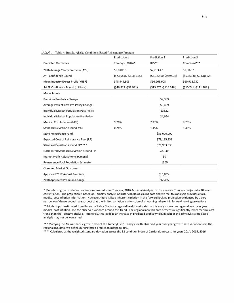
65

3.5.4. Table 4: Results Alaska Conditions Based Reinsurance Program

Prediction 1 Prediction 2 Prediction 3

Predicted Outcomes Tomczyk (2016)* BLS** Combined***

2016 Average Yearly Premium (AYP) $8,010.19 $7,283.47 $7,507.75

AYP Confidence Bound ($7,668.82-$8,351.55) ($5,172.60-$9394.34) ($5,369.88-$9,618.62)

Mean Industry Excess Profit (MIEP) $48,949,803 $66,261,608 $60,918,732

MIEP Confidence Bound (millions) ($40.817 -$57.081) ($15.976 -$116.546 ) ($10.741 -$111.204 )

Model Inputs

Premium Pre-Policy Change $9,389

Average Patient Cost Pre-Policy Change $8,439

Individual Market Population Post-Policy 23822

Individual Market Population Pre-Policy 24,064

Medical Cost Inflation (MCI) 9.26% 7.27% 9.26%

Standard Deviation around MCI 0.24% 1.45% 1.45%

State Reinsurance Fund $55,000,000

Expected Cost of Reinsurance Pool (RP) $78,135,359

Standard Deviation around RP**** $21,903,638

Normalized Standard Deviation around RP 28.03%

Market Profit Adjustments (Omega) $0

Reinsurance Pool Population Estimate 1300

Observed Market Outcomes

Approved 2017 Annual Premium $10,065

2018 Approved Premium Change -26.50%

* Model cost growth rate and variance recovered from Tomczyk, 2016 Actuarial Analysis. In this analysis, Tomczyk projected a 10 year cost inflation. The projection is based on Tomczyk analysis of historical Alaska claims data and we feel this analysis provides crucial medical cost inflation information. However, there is little inherent variation in the forward looking projection evidenced by a very narrow confidence bound. We suspect that the limited variation is a function of smoothing inherent in forward looking projections.

** Model inputs estimated from Bureau of Labor Statistics regional health cost data. In this analysis, we use regional year over year medical cost inflation, and the observed variance around this trend. The regional analysis data presents a significantly lower medical cost trend than the Tomczyk analysis. Intuitively, this leads to an increase in predicted profits which, in light of the Tomczyk claims based analysis may not be warranted.

*** Marrying the Alaska specific growth rate of the Tomczyk, 2016 analysis with observed year over year growth rate variation from the regional BLS data, we define our preferred prediction methodology. **** Calculated as the weighted standard deviation across the 33 condition index of Carrier claim costs for years 2014, 2015, 2016

66

3.5.5. Table 5:Hypotheses - Policy Simulation Analysis

Hypothesized effect of changes in w , ( )AE c and AN on

outcomes of interest Ar and

Policy Simulation 1 Policy Simulation 2 Policy Simulation 3

State institutes a 15% cost sharing requirement for state carriers

In response to revocation of the individual Mandate, patient costs are expected to increase 5%

Patient costs are expected to increase (5%) in response to (5%) exodus of healthy individuals from market.

1

( )(1 )

02( (1 ) 2 )

SAN

nSnA A

AS

A A

E cr N

Nw N N

= −

− −

Ar

+ *

(1 )0

( ) 2( (1 ) 2 )

SA A A

AS

A A A

r N NN

E c N N

−=

− −

+ +

0A

A

r

N

-

1

( ) 0

SAN

n

n

E cw =

= −

-

0( )

A

A

NE C

= −

- -

1 1

(1 ) ( ) 0 (1 ) ( )Q Q

A Aq Aq A Aq Aq

q qA

r P E c r P E cN

= =

= − − −

+

67

3.5.6. Table 6: Results Alaska Conditions Based Reinsurance Program – Policy Scenario

Baseline Policy Simulation Analysis 1 Policy Simulation Analysis 2 Policy Simulation Analysis 3

Predicted Outcomes

Baseline represented by perfered prediction (3) from table 4

State institutes a 15% cost sharing requirement for state carriers

In response to revocation of the individual Mandate, patient costs are expected to increase 5%

Patient costs are expected to increase (5%) in response to (5%) exodus of healthy individuals from market.

2016 Average Yearly Premium (AYP) $7,507.75 $8,163.86*** $8,071.28*** $7,874.40***

AYP Confidence Bound ($5,369.88-$9,618.62) ($9,913.54-$6,414.19) ($10,182.15-$5,960.41) ($5,639.00-$10,109.80)

Mean Industry Excess Profit (MIEP) $60,918,732 $45,288,890 $47,494,425 $52,184,467

MIEP Confidence Bound (millions) ($10.741 -$111.204 ) ($3.608 -$86.970 ) (-$2.819 -$97.780 ) (-$1.078 -$105.436 )

Model Inputs

Cost Sharing (w) 0% 15% 0% 0%

Market Population Post-Policy 23822 23822 23822 22631

Medical Cost Inflation (MCI) 9.26% 9.26% 14.26% 14.26%

Standard Deviation around MCI 1.45% 1.45% 1.45% 1.45%

Premium Pre-Policy $9,389

Average Patient Cost Pre-Policy $8,439

Market Population Pre-Policy 24,064

State Reinsurance Fund $55,000,000

E(Cost) of Reinsurance Pool (RP) $78,135,359

Deviation of E(Cost) RP**** $21,903,638

Market Profit Adjustments (Omega) $0

RP Population Estimate 1300

Confidence derived from two sided T-test with Welch Satterthwaite degrees of freedom calculation and expressed in terms *** p<0.01, ** p<0.05, * p<0.1. **** Calculated as the weighted standard deviation across the 33 condition index of Carrier claim costs for years 2014, 2015, 2016

68

3.5.7. Figure 1: Medicaid Applications March 2015 – March 2016

y = 65.753x + 3210.5

y = -225.43x + 3872.3

y = -283.83x + 6967.4

0

1000

2000

3000

4000

5000

6000

7000

8000

Mar

ch 1

5

Ap

ril

May

June

July

Au

gu

st

Sep

tem

ber

Oct

ob

er

No

vem

ber

Dec

emb

er

Janu

ary

Feb

ruar

y

Mar

ch 1

6

69

Chapter 4: Adolescent Circumstances and Financial Strain in

Adulthood

4. Introduction

With efforts to repeal, replace, or materially augment the Affordable Care Act

falling short of substantive change, the ACA’s focus on preventive medicine appears to

have become a durable feature of our national health conscience. The validation of the

long held proposition that prevention is an important determinant in health outcomes

implicitly aligns our national health policy agenda with Social Determinates of Health

(SDH) research in an unprecedented way. Yet, little interest in addressing SDH concerns

emerges in health related policy beyond politically expedient income/resource

redistributions. In the rapidly evolving trend toward evidence based policy, the

prevalence of “soft” variables and “grey” literature girding qualitative, anecdotal, and

survey based evidence of the influence of SDH on health, limits potential for SDH

considerations in health policy. To address this deficit, there is increasing interest in

prediction of causal effects of SDH on health, however predictability has remained a

challenge. Historical causal research routinely focuses on broad socio-economic status

variables like income, race, and gender. As a result, underlying determinants which vary

between individuals within race or gender, or income brackets remain qualitatively

important but hard to quantify.

70

Historical SDH discourse has laid a strong theoretical foundation and defined

many social experience factors which may be considered causal health pathways (Lee

and Sadana, 2011). Factors are broadly categorized in terms of poverty, hunger,

occupational exposure to hazards and relations at work, social and economic effects of

aging and illness, the experience of ethnic and gender relations including racism, home

circumstances, self-efficacy, dietary intake, habitual behaviors (both positive and

negative), position in the life-course, accumulated deficits of one’s past, schooling,

marital status, and socioeconomic status (Lee and Sadana, 2011) With such a broad

spectrum of potential influencing factors, interactions between them, and linkages to the

broader macro variables of class, housing stock, the education system, and the operation

of markets in goods and labor (Solar & Irwin, 2007) it is easy to see the difficulty in

rigorous study of SDH and causality. As a result, several widely appreciated theoretical

models have developed to inform on linkages between factors and outcomes. Of

particular interest to this research, the eco-social theory37 (Krieger, 2001) which provides

a stepping off point in the development of our treatise. With respect to study

methodology and empirics, several approaches have been historically leveraged.

Analytical methods used in SDH research focus on context analysis, case survey,

cross-design synthesis, Bayesian approaches, meta-analysis, and qualitative comparative

analysis (Pope, Mays & Popay, 2007). Empirical analysis of SDH is often stymied

37 The eco-social theoretical frame which considers lifestyle choice a function of chance

determined by the environment in which people live.

71

because models of causation traverse across disciplines and analysis methods which

academics traditionally keep separate (Lee and Sadana, 2011). Accepting these

limitations, our research attempts to bridge this traverse, focusing on dynamic multiple

analyses and variance decomposition modeling of ‘soft’ variables to gain inference in the

correlations of adolescent experiences on adult probabilities of adult financial strain. Our

research differs in the reliance on machine learning methods and statistical rigor to distill

out salient data-driven relationships across a vast sea of ‘soft’ retrospective variables.

Machine learning is a relatively new phenomenon in SDH research with the

preference for stochastic hypothesis based causality models (Seligman et al, 2017) which

are, by the descriptions above, only applicable to a very narrow band of factors which

may be politically actionable; some notable works (Adams, Hurd, McFadden, Merrill, &

Ribeiro, 2003; Deaton, 1999, 2003; Fletcher, Sindelar, & Yamaguchi, 2011; Halliday,

2007; Jacobson, LaLonde, & Sullivan, 1993; Lindahl, 2005; Newhouse & Friedlander,

1980; Smith, 1999, 2004a, 2004b; Sullivan & Von Wachter, 2009; Wagstaff, Van

Doorslaer, & Paci, 1989; Wilkinson & Marmot, 2003). Our methodological approach is

developed to help inform on correlations between adolescent factors and adult financial

strain which may be used to support qualitative theory. Our findings are correlative in

nature, not necessarily causal. Of course, where our results reflect exogenously

determined childhood experiences causality inference may be implied.

72

4.1. Data and Methodology

Using the framework of Delen, (2010). we employ the widely used Cross

Industry Standard Process for Data Mining (CRISP-DM). The CRISP-DM provides a

structured and systematic way to conduct data-mining analysis. A six step process, we

implement the first five steps. The sixth step is concerned with deployment of the

algorithm which is beyond the context of this investigative case study. The first three

steps of the CRISP-DM process are concerned with understanding the problem, data

acquisition and pre-processing the data. The fourth step is focused on model

development under a comparable analytic methodology, and the fifth and final step in our

process is evaluative in nature assessing the validity and suitability of the models with

respect to one another and the goals of the study.

Data for this study is pooled across 1999 – 2013 waves of the Panel Study of

Income Dynamics (PSID). We integrate the Childhood Retrospective Circumstances

Survey (CRCS) which was conducted in 2013 to gain insight into adolescent behaviors

and experiences. The CRCS was administered to individuals age 19 and older (by

January 1, 2013) who were household heads and spouses/partners in PSID families that

participated in the 2013 wave of the PSID. The CRCS collects information on

parents/guardians, parental relationship quality, childhood health conditions,

socioeconomic status, neighborhood quality, friendships, school experiences, and young

73

adult mentoring.38 We use this retrospective data to sift out adolescent factors that may

contribute to the predictability of a negative SDH outcome, financial strain. Concern

about correlation between variables in the CRCS led us to implement Principle

Component Analysis (PCA) as a variable reduction technique.

PCA (Jolliffe, 1986) is a commonly applied statistical technique for data

compression that produces a series of orthogonal linear combinations of variables. Each

successive principle component generates a new linear combination of variables defined

by maximizing the captured generalized variance that is uncorrelated with prior

components. By arranging the data this way, it is possible to collect tightly correlated

variables into groups which exert a single effect without enforcing a-priori assumptions

on the nature of the relationships between variables. In our model, we use the top 20

principle components representing 45% of generalized dataset variation.39 We use

38 In this analysis we do not use restricted data including exposure to the criminal justice

system, mental health, drug use, and abuse among family members. While, results are

not necessarily generalizable to these conditions, the publically available dataset does

represent a continuum of behavioral interactions across family relationships and

experiences. In this sense, debilitating mental health, drug and alcohol issues, and abuse

might be considered an additional category of extreme negatives. We believe that where

negative life factors are characteristic of an outcome, increasingly negative events which

emerge in restricted data are unlikely to undermine that effect. We feel that bias

introduced to the analysis through exclusion of these extremes tend to downward bias our

results toward zero. The results we present are low estimates, constrained both toward

the mean environment and the mean environment generally more hospitable than one

might expect in a generalized population. 39 The use of retrospective data collected across categorical variables is subject to both

recall bais and individual level response heterogeneity. Recall bias is poorly understood

and population specific. For instance individuals suffering depression and anxiety tend to

emphasize negative experiences, while healthy individuals tend to emphasize positive

experiences. We cannot deduce nor infer the direction and intensity of recall bias in this

population, nor the directional effect of unobservable random error. As a result, there is

74

orthogonal rotation of the factors to facilitate interpretation of composite components.

Orthogonal rotation increases the distance between variable factor loadings yielding more

meaningful cutoffs between ‘important’ and ‘unimportant’ contributing factors. Summary

statistics for the complete set of CRCS variables used to construct the principle

components (PC*) appear in appendix 1: Table A1. Component summary statistics, and

primary contributing factors are presented in Table 1. Contributing factors were defined

as factors with individual score values exceeding .30 in orthogonally rotated components.


To minimize method sensitivity to variable scale, we normalize all components

~N(0,1) across analytical specifications. Several important modifications to the panel

dataset are introduced to conform the dataset for cross-sectional analysis using the

decision tree and random forest classification methods.

For each observation in the original unbalanced dataset, financial strain FSTRAIN

is developed using the method of Zeldes (1989) and is categorized as a dichotomous

variable where zero denotes the absence of financial strain, and one denotes the condition

of financial strain. Formally, financial strain is defined:

significant noise in and between individual recollections. To minimize the latter, we

focus our analytical lens on the homogenous population subset of Caucasian participants.

Caucasian participants represent >70% of all respondents (2,803) with an analytical

dataset of 16,505 observations.

75

1

1

_1 1 / 6

( _ _ ) / 2

11 _ * _

6

0

it

it it

it it it

LN NWEALTHif

LN FAMINC LN FAMINC

FSTRAIN if LN CASHALL LN FAMINC

Otherwise

−

−

+

=

In this measure, financial strain is encountered when a family’s wealth40 is less than 1/6

of income averaged over the last two periods, or when cash available is less than two

months of prior period income.

Using the unbalanced longitudinal panel from the PSID, we collapse the dataset

generating composite average financial strain FSTRAIN and age AGE measures.

FSTRAIN takes on the value 1 if the individual’s composite FSTRAIN average is greater

than the average score across the population, and zero otherwise. AGE is recast as a

dichotomous variable with a value of zero for individuals whose average panel age is less

than 40, and one for others. The AGE threshold41 produces approximately equal

40 NWEALTH is constructed as a sum of eight asset types: value of farm or business,

imputed value of checking account, imputed value of other real estate, imputed value of

stocks and bonds, imputed value of vehicles, imputed value of other assets, imputed value

of annuities or IRA accounts and imputed household equity. FAMINC is defined as

taxable income for the period and is the sum of HEAD and WIFE and Other family

members and includes transfer payments and Social Security Income. In this research

FAMINC is constrained to a minimum value of ($0.01) in order to facilitate log

transformation. Likewise, CASHALL is defined as the sum of cash on hand and bank

checking and savings account balances. It is likewise constrained to a positive (0.01)

which explicitly rejects bank account overdrafts and recognizes that even the most

destitute can, by and large, produce some currency. All income and asset classes are log

normal transformed. 41 Model results are qualitatively similar to alternative thresholds at AGE=35 and

AGE=45. Results can be obtained from the author upon request.

76

proportions of “old” and “young”. The collapsed cross-sectional dataset then expanded

on the number of times an individual was observed. In this manner, we explicitly

frequency weight individuals intentionally rationalizing that an individual who has been

observed more often will have a more representative FSTRAIN average value than those

who are have fewer observations. This approach simplifies the construction of

bootstrapped training datasets increasing the probability that bootstrap sampling

populates datasets with average FSTRAIN measures which are representative of an

individual’s life-course.

4.2. Empirical Method

It is often the case that dichotomous outcomes under a hypothesis of causality are

estimated using logistic regression. Yet, the logistic regression methodology is

predicated on the strong assumption of independence of observations. Given the

frequency weighting explicitly delineated above, it would be hard to argue independence

of observations42. Green, 2010 suggests that, in the presence of an inconsistent estimator,

a robust covariance matrix, “may not give it redemption” (Green, 2012, p. 733).

Consequently, the virtue of a robust covariance matrix in this setting is unclear.

Independence of observations is not an uncommon concern. As a result, there has been

an increasing use of alternative prediction methodologies (machine learning) for real-

42 In our case, the unbalanced panel of repeated observations potentially violates this

assumption. As a test of robustness in our logistic estimation we collapse the panel to a

quartile measure of financial strain and test the high and low quartiles. Results are

consistent.

77

world prediction problems (Delen, 2010). In our analysis, we employ machine learning

methodologies to overcome our known data limitations. We use both individual

(decision trees, DT) and ensemble techniques (bootstrap aggregated random forest

estimation, “bagged” RF) in our analytics. We turn our attention to a brief description of

our estimation methods.

Individual level analysis, DT, is conducted with Classification and Regression

Trees methodology (CART). In this analysis we use a modified CART structure. To

allow for the potential for interactions and minor differences in scale of the regressors,

we mitigate selection bias by using a curvature test selecting the split predictor which

minimizes the p-value of the chi-square tests of independence between each predictor and

the response. Variable effect on model predictive performance (sensitivity) is derived by

summing changes in the probability at every node and dividing by the number of nodes

(predictors). We allow trees to grow to a depth of 150 branches without pruning across

specifications.43

RF is an ensemble classification method which consists of many decision trees44

defined using an outcome, a random draw of a subset of regressors, and bootstrap

replication of observations with replacement. In our model the number of regressors

chosen for each tree is limited to 1/2( )p nN X= where nX is the total number of regressors

available for estimation. Bootstrap replication is limited to the total number of

43 Additional complication of the decision tree fails to improve predictability while

reducing influential component sensitivity. 44 As s template tree, we use the optimal tree structure from the DT analysis.

78

observations in the original dataset and constrained to 30 “training” iterations. Both

specifications are validated using 10-fold (k-fold) validation.

To evaluate model results which differ in scale, we construct sensitivity measures

which define factor contribution to the probability of a successful prediction45. To do so,

we normalize each models sensitivities on the range zero to one. Machine learning

techniques also often ascribe factor importance values differently. Therefore, it is a

common practice to aggregate results across model specifications to produce a composite

measure of variable influence. While the technique of equally weighting results across

models in defining an average effect is common, we feel that models which are more

predictive ought to be weighted more heavily in the average effect than models which

produce weaker results. We implement a novel approach to aggregation of results. The

model factor sensitivity summation column of (TABLE 2) is constructed using weights

derived from a combination forecasting (Bates and Granger, 1969; Bohara, McNown &

Batts, 1987) methodology. Combination forecasting is a method of weighting predictions

as a function of model performance.


45 False prediction is also a potential problem. We test our model with correlation

matricies, Wald tests, and explore alternative probability thresholds to explore the

validity of prediction. We find that the straying from the standard probability cutoff of .5

increases the false prediction rate.

79

To construct model contribution weights, we use a two-step process which is

generalizable to any number of models under consideration. In step one, we regress the

observed outcome on the predicted outcomes from the DT ad RF models under OLS

without a constant using the criteria that 1 2 ... 1n + + + = ; Formally:

2

1

; 1j i ij

i

y B x e =

= + =

In the first step, values reflect the relative linear contribution of each models

prediction ix to accurate prediction of the outcome after controlling for the relative

contributions of all other regressors. A models predictions ix is a vector of predictions

over the range [1-j] observations. An individual model’s proportional contribution can

then be calculated as a non-linear transformation of model parameters:

1

1 1

1 1

1;

1 1

i

i i

B Bin n

i i

eP P

e e

= =

= =

+ +

Because factor sensitivities reflect only the relative contribution of a factor to a

models successful prediction of an outcome, they are not directional in nature. To

provide insight on directional effects of policy implementations, we produce directional

indicators which indicate how a factor’s sensitivity influences the probability of adult

FSTRAIN. Factor coefficients are extracted for our preferred specification RF under the

following methodology.

80

The “bagged” RF methodology uses bootstrap samples of the original dataset to

construct repeated prediction estimations. Estimation coefficients are then averaged

across bootstrap iterations producing the estimation method which is then validated

against the true dataset. To create factor directional effects and significance, we average

factor coefficient values across training iterations (Table 2) and calculate the variation in

factor values across bootstrap samples to construct coefficient standard deviations.

Coefficient robustness to alternative specifications is confirmed with several logistic

regressions. Model results are presented in Appendix 1 Table XY. In Appendix 1: Table

2: model 1, we test the same cross-sectional data structure used in the DT and RF models.

In Appendix 1: Table 2: model 2, we collapse the dataset into a single observation for

each individual, and in Appendix 1: Table 2: Model 3, we test the bottom and top quartile

of financial strain where the quartile is defined

0 0 1 1 2 2 3 3( , ], ( , ], ( , ], ( , ], ( , )q q q q q q q qx x x x x x x x− +

and 100 / ; (1,2,..., )qix k m k m= . In this model, if 1 2q qx x= then 0 1( , ]q qx x

captures all observations and 1 2( , ]q qx x remains empty. Results are qualitatively similar

across specifications.

4.3. Results and Discussion

Variable sensitivity results are presented in Table 2, and graphically in Figure 1.

We focus our attention on the first 5 factors which are both stronger in effect, and more

consistent across model specifications than the remainder. Considering them in order of

81

magnitude, pc12: Happiness at school, pc10: The social dimension of often lonely, pc4:

Dad’s work habits, pc6: Mom’s work habits, and finally pc1: which, focuses on the

maternal relationship with emphasis on communication, understanding, ability to confide

in (mom), and the “closeness” of the relationship.46


Coefficient relationships are described in order. In Caucasian children, happiness

at school (pc12) is strongly predictive of reduced adult FSTRAIN in both economic and

statistical significance. Increasing loneliness also tends to diminish adult FSTRAIN.

While not immediately intuitive, considering the counterfactual of those who are unhappy

in school but never lonely we find it both plausible and intuitively appealing that they

may be more likely to adopt behaviors which lead to increased adult FSTRAIN. We are

encouraged to find a role modeling effect in which fully employed fathers (Pc4) tend to

produce offspring which are less likely to suffer FSTRAIN in later life. An unexpected

and somewhat puzzling result, is that as mothers’ work habits (pc6) tend toward full-time

employment offspring tend toward adult FSTRAIN. At the same time, the coefficient on

pc1 (TABLE 3), is positive (+) and strongly significant <.01. The finding is somewhat

counter-intuitive implying that close affectionate maternal relationships seem to coincide

46 Across the small sample of NON-Caucasian participants, we found that pc1 was also the strongest predominant factor in predicting adult FSTRAIN. Coefficient sign is also consistent with the Caucasian population case study. In this sense, regardless of race/ethnicity, offspring’s response is consistent.

82

with higher levels of FSTRAIN in later life. We find this result supportive of the

literature. See for example: (Reed et. al. 2016; Swartz et. al. 2011; Fingerman et. al.

2012; Kirkpatrick, 2013; West et. al. 2012; Suitor et. al. 2017) which promotes the

argument that, easy to approach, forgiving and attentive parents may provide more robust

safety nets thus inhibiting the development of sound financial behavior in offspring. At

the same time, our results are consistent with works by (Fan et. al., 2017; Herbst, 2014;

Desai et. al., 1989; Bianchi 2000; Vandell et al., 2010) which together suggest that

reduced maternal involvement in childhood and adolescence has adverse effects on adult

behaviors, cognitive reasoning, education, and financial wellbeing.

We suggest a direction for future research; that is, the role of maternal

employment history and the nature and evolution of the maternal/adolescent social

relationships that emerge as a result. In this research, our findings suggest that, among

Caucasian families, it is beneficial to have a strict and present mom within the household

and not as beneficial to have an absent but easy/forgiving mom with respect to adult

tendencies toward FSTRAIN.

While it is hard to distinguish influence across other factors both for their overlap

with one another and the inconsistency of sensitivity measures across specifications, we

would feel negligent if we did not draw attention to the cross specification consistency

with which pc14: non-relative mentorship in work and marriage is estimated. Although

a minor contribution to the predictability of adult FSTRAIN, across models the effect is

quite consistent, and economically significant at the <.01 confidence level with a negative

coefficient value supportive of existing mentorship programs. While this is encouraging,

83

given the low contribution of the factor to the predictability of FSTRAIN, we feel that

attention and resources which focus on inspiring happiness in youth, particularly at

school, and programs which foster an appreciation for and economic incentives toward

forms of employment which are NOT precarious in nature would be a more efficient use

of resources in the context of reducing adult FSTRAIN.


In this research, we focused on correlation of adolescent behaviors and

experiences with a social determinant of health (adult financial strain) outcome.

Although the data had significant limitations including the retrospective nature of

responses and individual heterogeneity in defining cut-points between categorical

responses, several salient relationships emerged. Mother/child relationship status and

work history, father’s work habits, and the importance of school and social behaviors

stood out as import conceptual building blocks for social determinants of health policy

considerations. At the same time, with respect to adult financial strain, non-relative

mentorship appears to have a small but positive effect. Policy implications which stand

out to us are, expand non-relative mentorship programs to include training on responsible

financial stewardship as well as work and marriage. Further, we feel that development of

programs to positively influence adolescent happiness in school would be beneficial as

well as targeting and reducing the national trend toward precarious forms of employment

in lieu of adopting full-time and permanent employees. Such measures may reduce the

tendency for individuals to succumb to adverse SDH events.

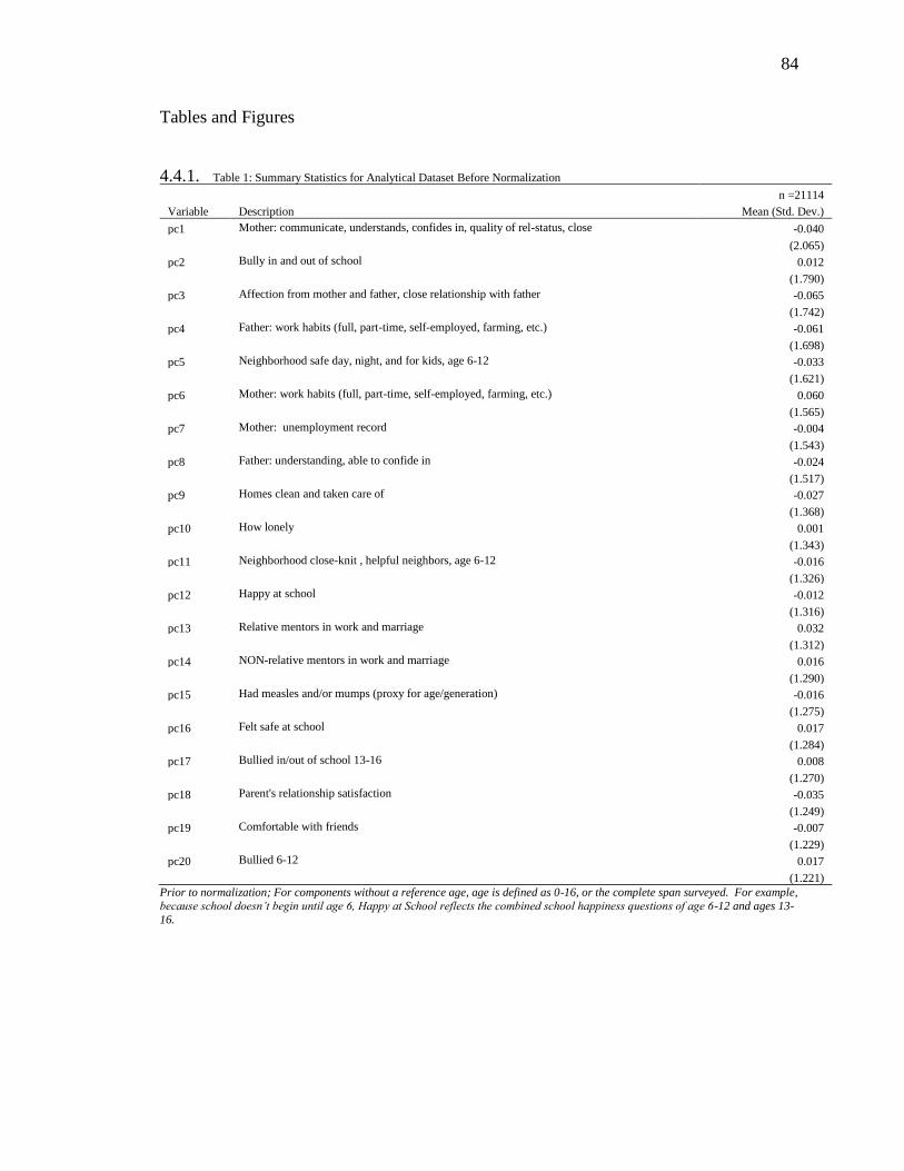
84

Tables and Figures

4.4.1. Table 1: Summary Statistics for Analytical Dataset Before Normalization

n =21114

Variable Description Mean (Std. Dev.)

pc1 Mother: communicate, understands, confides in, quality of rel-status, close -0.040

(2.065)

pc2 Bully in and out of school 0.012

(1.790)

pc3 Affection from mother and father, close relationship with father -0.065

(1.742)

pc4 Father: work habits (full, part-time, self-employed, farming, etc.) -0.061

(1.698)

pc5 Neighborhood safe day, night, and for kids, age 6-12 -0.033

(1.621)

pc6 Mother: work habits (full, part-time, self-employed, farming, etc.) 0.060

(1.565)

pc7 Mother: unemployment record -0.004

(1.543)

pc8 Father: understanding, able to confide in -0.024

(1.517)

pc9 Homes clean and taken care of -0.027

(1.368)

pc10 How lonely 0.001

(1.343)

pc11 Neighborhood close-knit , helpful neighbors, age 6-12 -0.016

(1.326)

pc12 Happy at school -0.012

(1.316)

pc13 Relative mentors in work and marriage 0.032

(1.312)

pc14 NON-relative mentors in work and marriage 0.016

(1.290)

pc15 Had measles and/or mumps (proxy for age/generation) -0.016

(1.275)

pc16 Felt safe at school 0.017

(1.284)

pc17 Bullied in/out of school 13-16 0.008

(1.270)

pc18 Parent's relationship satisfaction -0.035

(1.249)

pc19 Comfortable with friends -0.007

(1.229)

pc20 Bullied 6-12 0.017

(1.221)

Prior to normalization; For components without a reference age, age is defined as 0-16, or the complete span surveyed. For example,

because school doesn’t begin until age 6, Happy at School reflects the combined school happiness questions of age 6-12 and ages 13-

16.

85

4.4.2. Table 2: Model and Factor Sensitivities

Principle Component Description

Decision

Tree

Random

forest

Weighted

Average

pc12 Happy at school 0.987 0.989 0.988

pc10 How lonely 0.958 1.000 0.986

pc4 Father: work habits (full, part-time, self-employed, farming, etc.) 1.000 0.857 0.906

pc6 Mother: Work Habits (full, part-time, self-employed, farming, etc.) 0.941 0.815 0.858

pc1 Mother: communicate, understands, confides in, quality of rel-status, close 0.747 0.710 0.723

pc2 Bully in and out of school 0.498 0.658 0.603

pc9 Homes clean and taken care of 0.311 0.647 0.532

pc7 Mother: Unemployment record 0.515 0.391 0.434

pc3 Affection from mother and father, close relationship with father 0.379 0.427 0.410

pc17 Bullied in/out of school 13-16 0.482 0.356 0.399

pc8 Father: understanding, able to confide in 0.234 0.472 0.391

pc19 Comfortable with friends 0.489 0.286 0.355

pc15 Had measles and/or mumps (proxy for age/generation) 0.489 0.153 0.268

pc11 Neighborhood close-knit , helpful neighbors 0.338 0.217 0.258

pc13 Relative mentors in work and marriage 0.323 0.103 0.178

pc5 Neighborhood safe day, night, and for kids, Age 6-12 0.239 0.112 0.155

pc14 Non-relative mentors in work and marriage 0.131 0.160 0.150

pc16 Felt safe at school (6-16) 0.069 0.159 0.128

pc18 Parent's relationship satisfaction 0.222 0.000 0.076

pc20 Bullied 6-12 0.000 0.011 0.007

Note: For components without a reference age, age is defined as 0-16, or the complete span surveyed. For example, because school doesn’t begin until age 6, Happy at School reflects the combined school happiness questions of age 6-12 and ages 13-16.

86

4.4.3. Table 3: Random Forest Coefficients and Standard Errors - Caucasian

Variable Description Caucasian

pc1 Mother: Communicate, Understands, Confides in, Quality of Relationship-Status, Close 0.0222

(0.0252)

pc2 Bully in and out of school, Age 6-16 -0.0308*

(0.0159)

pc3 Affection from Mother and Father, Close relationship with Father -0.1169***

(0.0281)

pc4 Father: Work Habits (full, part-time, self-employed, farming, etc.) -0.0830***

(0.0180)

pc5 Neighborhood safe day, night, and for kids, Age 6-12 -0.1035***

(0.0312)

pc6 Mother: Work Habits (Full, Part-Time, Self-Employed, Farming, etc.) 0.1086***

(0.0192)

pc7 Mother: Unemployment record 0.0452**

(0.0187)

pc8 Father: Understanding, Able to Confide in 0.1795***

(0.0288)

pc9 Homes Clean and Taken Care of 0.0099

(0.0293)

pc10 How Lonely, Age 6-16 -0.2337***

(0.0220)

pc11 Neighborhood Close-knit , Helpful Neighbors, Age 6-12 0.0746***

(0.0195)

pc12 Happy at School -0.2260***

(0.0234)

pc13 Relative Mentors in Work and Marriage 0.0753***

(0.0247)

pc14 NON-Relative Mentors in Work and Marriage -0.0882***

(0.0243)

pc15 Measles and Mumps (Proxy for age/generation) 0.0601**

(0.0250)

pc16 Felt Safe at School (6-16) -0.0754***

(0.0209)

pc17 Bullied in/out of School 13-16 0.0214

(0.0251)

pc18 Parent's Relationship Satisfaction 0.0216

(0.0258)

pc19 Comfortable with Friends 6-16 -0.1101***

(0.0232)

pc20 Bullied 6-12 0.0553**

(0.0230)

Confidence *<.10; **<.05, ***<.01

Bootstrapped Standard Error; learning samples = 30

For components without a reference age, age is defined as 0-16, or the complete span surveyed. For example, because school doesn’t begin until age 6, Happy at School reflects the combined school happiness questions of age 6-12 and ages 13-16

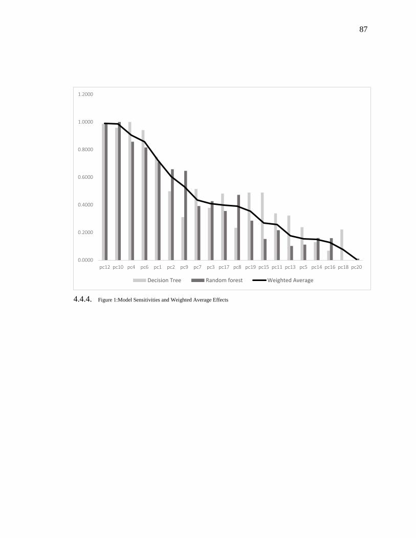
87

4.4.4. Figure 1:Model Sensitivities and Weighted Average Effects

0.0000

0.2000

0.4000

0.6000

0.8000

1.0000

1.2000

pc12 pc10 pc4 pc6 pc1 pc2 pc9 pc7 pc3 pc17 pc8 pc19 pc15 pc11 pc13 pc5 pc14 pc16 pc18 pc20

Decision Tree Random forest Weighted Average

88

Chapter 5: Extended Discussion and Conclusion

This dissertation set out to investigate two potential pathways that gird the

accepted socioeconomic status health gradient. In chapter 2, we developed a theoretic

argument and found statistical support for the hypotheses that financial strain and job-

switching both negatively effected self-assessed health status (SAHS). There is long-

standing research in support of the proposition that SAHS is positively correlated with

health outcomes (see for example: Idler & Benyamini, 1997; Mossey & Shapiro, 1982;

Woo & Zajacova, 2017). We conclude that a reduction in SAHS driven by financial

strain and job switching therefore leads to poorer health outcomes. However, we found

that financial strain and job switching effected change in SAHS differently. Financial

strain, was associated with a “shock” effect but caused no permanent effect. On the other

hand, higher frequency job switching resulted in no “shock” effect but is associated with

a permanent effect. There is a long history of research that supports consumption

smoothing in the face of financial shock (see for example: Baker & Yannelis, 2017;

Gelman et. al., 2015), as well as both increased job searching costs associated with higher

frequency job switching and a myriad of hidden costs including social identity erosion

(see for example: Kidder & Raworth, 2004; Kalleberg, 2009; Benach et. al., 2014). In

this sense, we find support for the existing literature.

In our research, natural policy implications are, of course, to implement programs

which work against the natural flow of the United States’ macro-economic environment

which is tending toward increasingly precarious employment and higher levels of

financial strain among the population (see for example: Kalleberg, 2017; Berger et. al.,

89

2018; Dobbie et. al., 2017; Wilshusen (2011); Wolff, 2016). With such broad and

generalized policy suggestions, and significant experience in the development of policy

and the operation of state government, it was clear to us that while valid, the scope of

recommendations required policy makers to be more creative than is typically found in

practice.

Recognizing the difficulty with developing policy around broad and generalized

recommendations, in chapter 3, we turned our attention to the development of a policy

analysis tool which we demonstrate superior to the existing actuarial methods used to

predict premium and profitability changes in the broad insurance market; something that

actuarial methods were never meant to handle (Borch, 1968). The measure we use to

evaluate changes in the insurance marketplace are two-fold, first we appraise changes in

individual level premiums, second, we evaluate changes in aggregate insurance market

profitability. We find that the error term of actuarial methods falls to the individual in the

form of higher premiums increasing the probability of financial strain ceteris paribus. By

approaching prediction of future premiums and market profitability changes from a

simple profit participation constraint, we develop and demonstrate a credible and

simplified policy development method refocusing policy development on allocation of

prediction error. We find that premium volatility may be reduced for large portions of

the individual population while simultaneously exploring the range of negative and

positive impacts for industry. The additional information may be effectively used to

calibrate policy impacts across supply and demand considerations. However, there are

still significant hurdles to overcome in future research.

90

Chapter 3’s methodological development framed discussion of national health

stock in terms of a common pool resource. In this manner we only needed to

demonstrate improved efficiency over existing market mechanisms under the constraints

of implementable institutional level action and the existence of sub-optimal outcomes as

defined by the appropriators. To that end, we do not provide a means for optimal

allocation of resources conceding “optimization” decisions to the combined experience of

stake holder debate. In development of this chapter, there lay an implicit assumption; a

reduction in events which may trigger financial strain will be effective at reducing

financial strain in the general community. If the population isn’t itself capable of

exercising the intertemporal restraint required to manage existing resources optimally,

then models as the one we propose here may offer improved process efficiencies, but

they are unlikely to affect meaningful change in financial strain outcomes at the

individual level. This led us to explore adolescent circumstances and experiences as

predictors of adult financial strain.

To explore the adolescent experience adult financial strain relationship, chapter 4

focuses the analytical lens on retrospective circumstances data from a supplemental

survey associated with the Panel Study of Income Dynamics, the Childhood

Retrospective Circumstances Survey. With more than 120 variables covering disparate

circumstances from family and school dynamics to childhood chronic diseases and

neighborhood compositions, and Social Determinates of Health crossing boundaries and

interacting without regard to discipline or theory, we felt it unwise to exert a-priori

assumptions to define the interrelationships between variables. As such, we employ

91

principle component analysis and individual and ensemble machine learning techniques

to tease out of the data salient correlations between adolescent events and adult financial

strain circumstances. We found that strong predictors of adult financial strain are related

to feeling of loneliness, happiness at school, father’s work history, and maternal

relationships. The directional relationships are consistent with high functioning academic

loners, those who enjoy school, and mother’s that are both present and relatively strict

having lower levels of financial strain in adulthood. Father’s work experience supports

traditional role modeling. While our findings are consistent with historical research on

self-efficacy in the transition to adulthood (for example see: Mortimer et al., 2016) and

life-course studies (see for example: Schoon, 2013), we recognize that our case study of

Caucasians, bounded by data-mining techniques is neither representative nor can

causality be inferred. As such, our policy recommendations are made less as a

declaration of need, rather it is supportive of existing programs that facilitate a

responsible caretaker at home, stricter and less forgiving parenting styles, enjoyment at

school, and efforts to help father’s achieve fulltime stable employment. With the added

potential benefit that such programs reduce an individual’s probability of becoming

financially strained in later life, we feel that, where possible, funding for such programs

may provide benefit greater than those conceived of at inception.

92

References:

6. References Chapter 1

Bates, J. M., & Granger, C. W. (1969). The combination of forecasts. Journal of the

Operational Research Society, 20(4), 451-468.

Bohara, A., McNown, R., & Batts, J. T. (1987). A re-evaluation of the combination and

adjustment of forecasts. Applied Economics, 19(4), 437-445.

Becker, G. S. (1967). Human capital and the personal distribution of income: An

analytical approach (No. 1). Institute of Public Administration.

Becker, G. S. (1994). Human capital revisited. In Human Capital: A Theoretical and

Empirical Analysis with Special Reference to Education (3rd Edition) (pp. 15-28).

The university of Chicago press.

Contoyannis, P., Jones, A. M., & Rice, N. (2004). The dynamics of health in the British

Household Panel Survey. Journal of Applied Econometrics, 19(4), 473-503.

Fingerman, K. L., Cheng, Y. P., Wesselmann, E. D., Zarit, S., Furstenberg, F., & Birditt,

K. S. (2012). Helicopter parents and landing pad kids: Intense parental support of

grown children. Journal of Marriage and Family, 74(4), 880-896.

Grossman, M. (1972). On the concept of health capital and the demand for health.

Journal of Political economy, 80(2), 223-255.

Halliday, T. J. (2017). Earnings Growth and Movements in Self‐Reported Health. Review

of Income and Wealth, 63(4), 760-776.Halpern-Manners, A., Warren, J. R.,

Raymo, J. M., & Nicholson, D. A. (2015). The impact of work and family life

histories on economic well-being at older ages. Social Forces, 93(4), 1369-1396.

Kirkpatrick Johnson, M. (2013). Parental financial assistance and young adults'

relationships with parents and well‐being. Journal of Marriage and Family, 75(3),

713-733.

Lee, J. H., Sadana, R., & Commission on Social Determinants of Health. (2011).

Improving equity in health by addressing social determinants.

Muurinen, J.-M. (1982). Demand for health: a generalised Grossman model. Journal of

Health economics, 1(1), 5-28.

Reed, K., Duncan, J. M., Lucier-Greer, M., Fixelle, C., & Ferraro, A. J. (2016).

Helicopter parenting and emerging adult self-efficacy: Implications for mental

and physical health. Journal of Child and Family Studies, 25(10), 3136-3149.

Suitor, J. J., Gilligan, M., Pillemer, K., Fingerman, K. L., Kim, K., Silverstein, M., &

Bengtson, V. L. (2017). Applying within-family differences approaches to

93

enhance understanding of the complexity of intergenerational relations. The

Journals of Gerontology: Series B, 73(1), 40-53.

Swartz, T. T., Kim, M., Uno, M., Mortimer, J., & O'Brien, K. B. (2011). Safety nets and

scaffolds: Parental support in the transition to adulthood. Journal of Marriage and

Family, 73(2), 414-429.

West, A., Lewis, J., Roberts, J., & Noden, P. (2017). Young Adult Graduates Living in

the Parental Home: Expectations, Negotiations, and Parental Financial

Support. Journal of Family Issues, 38(17), 2449-2473.


Achen, C. H. (2000). Why lagged dependent variables can suppress the explanatory

power of other independent variables. Ann Arbor, 1001(2000), 48106-41248.

Adams, P., Hurd, M. D., McFadden, D., Merrill, A., & Ribeiro, T. (2003). Healthy,

wealthy, and wise? Tests for direct causal paths between health and

socioeconomic status. Journal of Econometrics, 112(1), 3-56.

Aizawa, Toshiaki and Helble, Matthias. (April 2015). Health and Home Ownership:

Findings for the Case of Japan. ADBI Working Paper 525. Available at

SSRN: https://ssrn.com/abstract=2605794 or http://dx.doi.org/10.2139/ssrn.26057

94

Babiarz, P., Widdows, R., & Yilmazer, T. (2013). Borrowing to cope with adverse health

events: liquidity constraints, insurance coverage, and unsecured debt. Health

economics, 22(10), 1177-1198.

Becker, G. S. (1967). Human capital and the personal distribution of income: An

analytical approach (No. 1). Institute of Public Administration.

Becker, G. S. (1994). Human capital revisited. In Human Capital: A Theoretical and

Empirical Analysis with Special Reference to Education (3rd Edition) (pp. 15-28).

The university of Chicago press.

Belli, R. F. (2004). Improving the quality of retrospective reports: Calendar interviewing

methodologies. Paper presented at the Sixth international conference on logic

and methodology, Amsterdam.

Belli, R. F., Shay, W. L., & Stafford, F. P. (2001). Event history calendars and question

list surveys: A direct comparison of interviewing methods. Public opinion

quarterly, 65(1), 45-74.

Benach, J., Benavides, F. G., Platt, S., Diez-Roux, A., & Muntaner, C. (2000). The

health-damaging potential of new types of flexible employment: a challenge for

public health researchers. American Journal of Public Health, 90(8), 1316.

Benach, J., & Muntaner, C. (2007). Precarious employment and health: developing a

research agenda. Journal of Epidemiology & Community Health, 61(4), 276-277.

https://ssrn.com/abstract=2605794

https://dx.doi.org/10.2139/ssrn.2605794

https://dx.doi.org/10.2139/ssrn.2605794

94

Benach, J., Vives, A., Amable, M., Vanroelen, C., Tarafa, G., & Muntaner, C. (2014).

Precarious employment: understanding an emerging social determinant of

health. Annual review of public health, 35.

Chamberlain, G. (1979). Analysis of covariance with qualitative data: National Bureau of

Economic Research Cambridge, Mass., USA.

Charlson, M., Szatrowski, T. P., Peterson, J., & Gold, J. (1994). Validation of a combined

comorbidity index. Journal of clinical epidemiology, 47(11), 1245-1251.

Contoyannis, P., Jones, A. M., & Rice, N. (2004). The dynamics of health in the British

Household Panel Survey. Journal of Applied Econometrics, 19(4), 473-503.

Crossley, T. F., & Kennedy, S. (2002). The reliability of self-assessed health status.

Journal of Health economics, 21(4), 643-658.

Cuesta, M. B., & Budría, S. (2015). The effects of over-indebtedness on individual

health: IZA Discussion Paper.

Deaton, A. (1999). Inequalities in income and inequalities in health: National bureau of

economic research.

Deaton, A. (2003). Health, inequality, and economic development. Journal of economic

literature, 41(1), 113-158.

DeVaney, S. A., & Lytton, R. H. (1995). Household insolvency: A review of household

debt repayment, delinquency, and bankruptcy. Financial Services Review, 4(2),

137-156.

DuGoff, E. H., Canudas-Romo, V., Buttorff, C., Leff, B., & Anderson, G. F. (2014).

Multiple chronic conditions and life expectancy: a life table analysis. Medical

care, 52(8), 688-694.

Fletcher, J. M., Sindelar, J. L., & Yamaguchi, S. (2011). Cumulative effects of job

characteristics on health. Health economics, 20(5), 553-570.

Ford, E. S., Croft, J. B., Posner, S. F., Goodman, R. A., & Giles, W. H. (2013). Co-

Occurrence.

Fuchs, V. R. (1982). Introduction to" Economic Aspects of Health" Economic Aspects of

Health (pp. 1-12): University of Chicago Press.

Gallo, W. T., Teng, H.-M., Falba, T. A., Kasl, S. V., Krumholz, H. M., & Bradley, E. H.

(2006). The impact of late career job loss on myocardial infarction and stroke: a

10 year follow up using the health and retirement survey. Occupational and

environmental medicine, 63(10), 683-687.

Gathergood, J. (2012). Debt and depression: causal links and social norm effects. The

Economic Journal, 122(563), 1094-1114.

Grossman, M. (1972). On the concept of health capital and the demand for health.


95

Halliday, T. J. (2007). Business cycles, migration and health. Social Science & Medicine,

64(7), 1420-1424.

Halliday, T. J. (2014). Unemployment and Mortality: Evidence from the PSID. Social

Science & Medicine, 113, 15-22.

Heckman, J. J. (1981). The Incidental Parameters Problem and the Problem of Initial

Conditions in Estimating a Discrete Choice Time-Discrete Data Stochastic

Process. Structural analysis of discrete data with econometric application.

Hung, H.-C., Joshipura, K. J., Jiang, R., Hu, F. B., Hunter, D., Smith-Warner, S. A., . . .

Willett, W. C. (2004). Fruit and vegetable intake and risk of major chronic

disease. Journal of the National Cancer Institute, 96(21), 1577-1584.

Jacobson, L. S., LaLonde, R. J., & Sullivan, D. G. (1993). Earnings losses of displaced

workers. The American economic review, 685-709.

Jürges, H. (2008). Self-assessed health, reference levels and mortality. Applied

Economics, 40(5), 569-582.

Lau, C., & Leung, L. (2011). Effect of mortgage debt on health. Department of

Economics, CUNY Graduate Center, NY.

Lindahl, M. (2005). Estimating the effect of income on health and mortality using lottery

prizes as an exogenous source of variation in income. Journal of Human

Resources, 40(1), 144-168.

Lyons, A. C., & Yilmazer, T. (2005). Health and financial strain: Evidence from the

survey of consumer finances. Southern Economic Journal, 873-890.

McGonagle, K. A., & Schoeni, R. F. (2006). The panel study of income dynamics:

Overview and summary of scientific contributions after nearly 40 years. Paper

presented at the conference Longitudinal Social and Health Surveys in an

International Perspective, Montreal.

Meer, J., Miller, D. L., & Rosen, H. S. (2003). Exploring the health–wealth nexus.

Journal of Health economics, 22(5), 713-730.

Mundlak, Y. (1978). On the pooling of time series and cross section data. Econometrica:

journal of the Econometric Society, 69-85.



Newhouse, J. P., & Friedlander, L. J. (1980). The relationship between medical resources

and measures of health: some additional evidence. Journal of Human Resources,

200-218.

O'Neill, B., Prawitz, A. D., Sorhaindo, B., Kim, J., & Garman, E. T. (2006). Changes in

health, negative financial events, and financial distress/financial well-being for

debt management program clients.

96

Shaw, R. J., Benzeval, M., & Popham, F. (2014). To what extent do financial strain and

labour force status explain social class inequalities in self-rated health? Analysis

of 20 countries in the European Social Survey. PloS one, 9(10), e110362.

Smith, J. P. (1999). Healthy bodies and thick wallets: the dual relation between health

and economic status. The journal of economic perspectives: a journal of the

American Economic Association, 13(2), 144.

Smith, J. P. (2004a). The Impact of SES on Health Over the Life-Course. RAND,

unpublished manuscript.

Smith, J. P. (2004b). Unraveling the SES: health connection. Population and

development review, 30, 108-132.

Stavins, J. (2000). Credit card borrowing, delinquency, and personal bankruptcy. New

England Economic Review, 15.

Sullivan, D., & Von Wachter, T. (2009). Job displacement and mortality: An analysis

using administrative data. The Quarterly Journal of Economics, 124(3), 1265-

1306.

Terza JV, Basu A, Rathouz PJ. (2008). Two-Stage Residual Inclusion Estimation:

Addressing Endogeneity in Health Econometric Modeling. Journal of health

economics. 27(3):531-543.

Verbeek, M., & Nijman, T. (1992). Testing for selectivity bias in panel data models.

International Economic Review, 681-703.

Wagstaff, A., Van Doorslaer, E., & Paci, P. (1989). Equity in the finance and delivery of

health care: some tentative cross-country comparisons. Oxford Review of

Economic Policy, 5(1), 89-112.

Wilkinson, R. G., & Marmot, M. (2003). Social determinants of health: the solid facts:

World Health Organization.

Wooldridge, J. M. 2002. Econometric Analysis of Cross Section and Panel Data.

Cambridge, MA: MIT Press.

Zeldes, S. P. (1989). Consumption and liquidity constraints: an empirical investigation.


97


Balbás, A., et al. (2015). Optimal reinsurance under risk and uncertainty. Insurance:

Mathematics and Economics 60: 61-74.

Bernard, C. and W. Tian (2009). Optimal reinsurance arrangements under tail risk

measures. Journal of risk and insurance 76(3): 709-725.

Charlson, M., et al. (2014). The Charlson comorbidity index can be used prospectively to

identify patients who will incur high future costs. PloS one 9(12): e112479.

Geruso, M. and T. G. McGuire (2016). Tradeoffs in the design of health plan payment

systems: Fit, power and balance. Journal of health economics 47: 1-19.

Hilson, D. C., Micahel; Anderson, Michelle; Bingham, Al (2017). Individual Health

Insurance Market Stabilization Analyses, Washington Office of the Insurance

Comissioner.

Layton, T. J., et al. (2015). Assessing incentives for adverse selection in health plan

payment systems. National Bureau of Economic Research.

Layton, T. J., et al. (2016). Risk corridors and reinsurance in health insurance

Marketplaces: insurance for insurers. American journal of health economics.

Milliman (2017). Milliman Individual Health Insurance Market Profile. State of Alaska.

Ostrom, E., et al. (1994). Rules, games, and common-pool resources. University of

Michigan Press.

Roberts, M. D. F., Claudia; Barin, Ozlem; Osterfoss, Margaret; Ecwardson, Nicholas; He,

Xuanhao; Cacari Stone, Lisa (2017). Cost Sharing Trends In Medicaid and non-

Medicaid Expansion States for Benchmark Silver Plans. Robert Wood Johnson

Foundation: Center for Health Policy.

Snyder, L. (2014). Putting Medicaid in the Larger Budget Context: An In-Depth Look at

Four States in FY 2014 and 2015.

Thiessen, M. (2017). Premera cuts rates further in 2018. Alaska Journal of Commerce.

Online, Morris Communications Company, LLC.

Tomczyk, T. M., Ryan; Kaczmarek, Peter (2016). Alaska 1332 Waiver Application:

Actuarial Analyses and Certification.

Van Barneveld, E. M., et al. (2001). "Risk sharing as a supplement to imperfect

capitation: a tradeoff between selection and efficiency." Journal of health

economics 20(2): 147-168.

Zhang, Y. (2013). Reinsurance Arrangements Minimizing the Total Required Capital,

Casualty Society E-Forum, Spring.

98

Zhu, J. M., et al. (2013). The power of reinsurance in health insurance exchanges to

improve the fit of the payment system and reduce incentives for adverse selection.

INQUIRY: The Journal of Health Care Organization, Provision, and Financing

50(4): 255-274.


Adams, P., Hurd, M. D., McFadden, D., Merrill, A., & Ribeiro, T. (2003). Healthy,

wealthy, and wise? Tests for direct causal paths between health and

socioeconomic status. Journal of Econometrics, 112(1), 3-56.

Alvarado, S. E. (2016). Neighborhood disadvantage and obesity across childhood and

adolescence: evidence from the NLSY children and young adults cohort (1986–

2010). Social science research, 57, 80-98.

Bates, J. M., & Granger, C. W. (1969). The combination of forecasts. Journal of the

Operational Research Society, 20(4), 451-468.

Bianchi, S. M. (2000). Maternal employment and time with children: Dramatic change or

surprising continuity?. Demography, 37(4), 401-414.

Bohara, A., McNown, R., & Batts, J. T. (1987). A re-evaluation of the combination and

adjustment of forecasts. Applied Economics, 19(4), 437-445.

Clemen, R. T. (1989). Combining forecasts: A review and annotated

bibliography. International journal of forecasting, 5(4), 559-583.

Deaton, A. (1999). Inequalities in income and inequalities in health: National bureau of

economic research.

Deaton, A. (2003). Health, inequality, and economic development. Journal of economic

literature, 41(1), 113-158.

Delen, D. (2010). A comparative analysis of machine learning techniques for student

retention management. Decision Support Systems, 49(4), 498-506.

Desai, S., Chase-Lansdale, P. L., & Michael, R. T. (1989). Mother or Market? Effects of

Maternal Employment on the Intellectual Ability of 4-Year-Old

Children. Demography, 26(4), 545-561. DOI: 10.2307/2061257

Fan, X., Fang, H., & Markussen, S. (2017). Parental Employment, Absence and

Children’s Educational Gender Gap.

Fletcher, J. M., Sindelar, J. L., & Yamaguchi, S. (2011). Cumulative effects of job

characteristics on health. Health economics, 20(5), 553-570.

99

Fingerman, K. L., Cheng, Y. P., Wesselmann, E. D., Zarit, S., Furstenberg, F., & Birditt,

K. S. (2012). Helicopter parents and landing pad kids: Intense parental support of

grown children. Journal of Marriage and Family, 74(4), 880-896.

Greene, W. H. (2012). Econometric analysis, 71e. Stern School of Business, New York

University.

Halliday, T. J. (2007). Business cycles, migration and health. Social Science & Medicine,

64(7), 1420-1424.

Herbst, C. M. (2017). Are Parental Welfare Work Requirements Good for Disadvantaged

Children? Evidence From Age‐of‐Youngest‐Child Exemptions. Journal of Policy

Analysis and Management, 36(2), 327-357.

Jacobson, L. S., LaLonde, R. J., & Sullivan, D. G. (1993). Earnings losses of displaced

workers. The American economic review, 685-709.

Jolliffe, I.T. (1986) Principal Component Analysis, New York: Springer-Verlag.

Kirkpatrick Johnson, M. (2013). Parental financial assistance and young adults'

relationships with parents and well‐being. Journal of Marriage and Family, 75(3),

713-733.

Krieger, N. (2001). Theories for social epidemiology in the 21st century: an ecosocial

perspective. International journal of epidemiology, 30(4), 668-677.

Lee, J. H., Sadana, R., & Commission on Social Determinants of Health. (2011).

Improving equity in health by addressing social determinants.

Lindahl, M. (2005). Estimating the effect of income on health and mortality using lottery

prizes as an exogenous source of variation in income. Journal of Human

Resources, 40(1), 144-168.

Newhouse, J. P., & Friedlander, L. J. (1980). The relationship between medical resources

and measures of health: some additional evidence. Journal of Human Resources,

200-218.

Pope, C., Ziebland, S., & Mays, N. (2000). Qualitative research in health care: analysing

qualitative data. BMJ: British Medical Journal, 320(7227), 114.

Reed, K., Duncan, J. M., Lucier-Greer, M., Fixelle, C., & Ferraro, A. J. (2016).

Helicopter parenting and emerging adult self-efficacy: Implications for mental

and physical health. Journal of Child and Family Studies, 25(10), 3136-3149.

Seligman, B., Tuljapurkar, S., & Rehkopf, D. (2018). Machine learning approaches to the

social determinants of health in the health and retirement study. SSM-population

health, 4, 95-99.

Smith, J. P. (1999). Healthy bodies and thick wallets: the dual relation between health

and economic status. The journal of economic perspectives: a journal of the

American Economic Association, 13(2), 144.

100

Smith, J. P. (2004a). The Impact of SES on Health Over the Life-Course. RAND,

unpublished manuscript.

Solar, O., & Irwin, A. (2010). A conceptual framework for action on the social

determinants of health.

Suitor, J. J., Gilligan, M., Pillemer, K., Fingerman, K. L., Kim, K., Silverstein, M., &

Bengtson, V. L. (2017). Applying within-family differences approaches to

enhance understanding of the complexity of intergenerational relations. The

Journals of Gerontology: Series B, 73(1), 40-53.

Swartz, T. T., Kim, M., Uno, M., Mortimer, J., & O'Brien, K. B. (2011). Safety nets and

scaffolds: Parental support in the transition to adulthood. Journal of Marriage and

Family, 73(2), 414-429.

Sullivan, D., & Von Wachter, T. (2009). Job displacement and mortality: An analysis

using administrative data. The Quarterly Journal of Economics, 124(3), 1265-

1306.

Vandell, D. L., Belsky, J., Burchinal, M., Vandergrift, N., & NICHD Early Child Care

Research Network, L. (2010). Do Effects of Early Child Care Extend to Age 15

Years? Results From the NICHD Study of Early Child Care and Youth

Development. Child Development, 81(3), 737–756. http://doi.org/10.1111/j.1467-

8624.2010.01431.x

Wagstaff, A., Van Doorslaer, E., & Paci, P. (1989). Equity in the finance and delivery of

health care: some tentative cross-country comparisons. Oxford Review of

Economic Policy, 5(1), 89-112.

West, A., Lewis, J., Roberts, J., & Noden, P. (2017). Young Adult Graduates Living in

the Parental Home: Expectations, Negotiations, and Parental Financial

Support. Journal of Family Issues, 38(17), 2449-2473.

Wilkinson, R. G., & Marmot, M. (2003). Social determinants of health: the solid facts:

World Health Organization.

Zeldes, S. P. (1989). Consumption and liquidity constraints: an empirical investigation.



Baker, S. R., & Yannelis, C. (2017). Income changes and consumption: Evidence from

the 2013 federal government shutdown. Review of Economic Dynamics, 23, 99-

124.

101

Benach, J., Vives, A., Amable, M., Vanroelen, C., Tarafa, G., & Muntaner, C. (2014).

Precarious employment: understanding an emerging social determinant of

health. Annual review of public health, 35.

Berger, L. M., Cancian, M., & Magnuson, K. (2018). Anti-poverty Policy Innovations:

New Proposals for Addressing Poverty in the United States. RSF.

Borch, K., & Mossin, J. (1968). Risk and uncertainty. Springer.

Dobbie, W., Goldsmith-Pinkham, P., & Yang, C. S. (2017). Consumer bankruptcy and

financial health. Review of Economics and Statistics, 99(5), 853-869.

Gelman, M., Kariv, S., Shapiro, M. D., Silverman, D., & Tadelis, S. (2015). How

individuals smooth spending: Evidence from the 2013 government shutdown

using account data (No. w21025). National Bureau of Economic Research.

Idler, E. L., & Benyamini, Y. (1997). Self-rated health and mortality: a review of twenty-

seven community studies. Journal of health and social behavior, 21-37.

Kalleberg, A. L. (2009). Precarious work, insecure workers: Employment relations in

transition. American sociological review, 74(1), 1-22.

Kalleberg, A. L., & Vallas, S. P. (Eds.). (2017). Probing precarious work: Theory,

research, and politics. In Precarious Work (pp. 1-30). Emerald Publishing

Limited.

Kidder, T., & Raworth, K. (2004). 'Good jobs' and hidden costs: Women workers

documenting the price of precarious employment. Gender & Development, 12(2),

12-21.

Mortimer, J. T., Kim, M., Staff, J., & Vuolo, M. (2016). Unemployment, parental help,

and self-efficacy during the transition to adulthood. Work and occupations, 43(4),

434-465.

Mossey, J. M., & Shapiro, E. (1982). Self-rated health: a predictor of mortality among the

elderly. American journal of public health, 72(8), 800-808.



Schoon, I. (2014). Parental worklessness and the experience of NEET among their

offspring. Evidence from the Longitudinal Study of Young People in England

(LSYPE). Longitudinal and Life Course Studies, 5(2), 129-150.

Wilshusen, S. (2011). Meeting the demand for debt relief.

Wolff, E. N. (2016). Household Wealth Trends in the United States, 1962 to 2013: What

Happened over the Great Recession?. RSF.

Woo, H., & Zajacova, A. (2017). Predictive strength of self-rated health for mortality risk

among older adults in the United States: does it differ by race and

ethnicity?. Research on aging, 39(7), 879-905.

102

Supplementary Materials

11. Supplementary Material Chapter 2

11.1. Appendix 1: Full Results Tables

11.1.1. Table A1: Variable Addition Bias Test - Random Effects Ordered Probit Model, modified CRE, and Strict CRE estimations: M, F, and Combined


MODCRE MODCRE MODCRE STRICTCRE STRICTCRE STRICTCRE

Outcome= SAH Outcome= SAH Outcome= SAH Outcome= SAH Outcome= SAH Outcome= SAH VARIABLES Unbalanced Unbalanced Unbalanced Unbalanced Unbalanced Unbalanced

LHSD1 -2.329*** -2.167*** -2.206*** -1.887*** -1.508*** -1.629***

(0.291) (0.227) (0.180) (0.236) (0.184) (0.145) LHSD2 -1.487*** -1.595*** -1.558*** -1.100*** -1.142*** -1.133***

(0.148) (0.123) (0.0948) (0.102) (0.0891) (0.0668) LHSD3 -1.092*** -1.100*** -1.097*** -0.825*** -0.792*** -0.809***

(0.0948) (0.0820) (0.0621) (0.0627) (0.0600) (0.0435) LHSD4 -0.677*** -0.554*** -0.609*** -0.508*** -0.394*** -0.447***

(0.0641) (0.0562) (0.0422) (0.0487) (0.0446) (0.0329) ALL -0.0878 -0.0255 -0.0557 -0.122** -0.0574 -0.0895**

(0.0553) (0.0474) (0.0361) (0.0597) (0.0526) (0.0396) TOTALOBS 0.0774*** 0.0700*** 0.0728*** 0.0632*** 0.0664*** 0.0658***

(0.0164) (0.0122) (0.00973) (0.0148) (0.0111) (0.00885) 1.FSTRESS -0.158*** -0.0989** -0.124*** -0.129** -0.0416 -0.0786**

(0.0538) (0.0454) (0.0348) (0.0514) (0.0477) (0.0351) n_cor_jobswitching 0.00144 -0.00454 -0.00110 0.0192 0.0193 0.0191

(0.0230) (0.0189) (0.0146) (0.0224) (0.0185) (0.0142) past_jobswitching_average -0.0250 -0.0670** -0.0466*

(0.0431) (0.0316) (0.0255) past_FS_average 0.119 -0.106* -0.0284

(0.0807) (0.0639) (0.0501) mm_DEF_FSTRESS_Z2 0.122 -0.189** -0.0740

(0.117) (0.0890) (0.0702) mm_n_cor_jobswitching -0.0848 -0.0927** -0.0848**

(0.0546) (0.0414) (0.0330)

103

Table A1: Continued


AGE -0.416*** 0.274** -0.0332 -0.254** 0.00494 -0.103

(0.156) (0.139) (0.104) (0.113) (0.101) (0.0752) AGE2 0.0791** -0.0724** -0.00455 0.0424* -0.0112 0.0114

(0.0338) (0.0306) (0.0227) (0.0253) (0.0227) (0.0168) AGE3 -0.0548** 0.0527** 0.00436 -0.0289 0.00882 -0.00711

(0.0238) (0.0220) (0.0162) (0.0182) (0.0166) (0.0123) NON_WHITE1 -0.0748 -0.161*** -0.124*** -0.115** -0.168*** -0.142***

(0.0548) (0.0434) (0.0342) (0.0551) (0.0453) (0.0351) YSCHOO 0.0264 0.00186 0.0125 -0.00304 0.00482 0.000727

(0.0324) (0.0222) (0.0189) (0.0280) (0.0216) (0.0170) MALE 0.0475* 0.0724**

(0.0282) (0.0287) HINS -0.0689 0.0405 -0.000822 -0.0418 0.0801 0.0307

(0.101) (0.0828) (0.0642) (0.0894) (0.0726) (0.0565) STABLEMAR -0.0184 -0.155** -0.101* -0.0970 -0.107* -0.107**

(0.0843) (0.0745) (0.0556) (0.0743) (0.0624) (0.0476) NUMFAMCH -0.00956 -0.000244 -0.00148 -0.00169 0.00700 0.00179

(0.0310) (0.0258) (0.0198) (0.0254) (0.0216) (0.0163) d_II_COR_HSTATUS1 -1.193*** -2.085*** -1.794*** -1.392*** -2.421*** -2.096***

(0.364) (0.243) (0.221) (0.379) (0.209) (0.197) d_II_COR_HSTATUS2 -1.767*** -1.773*** -1.780*** -1.946*** -2.041*** -2.003***

(0.155) (0.129) (0.0986) (0.149) (0.118) (0.0914) d_II_COR_HSTATUS3 -1.190*** -1.230*** -1.221*** -1.291*** -1.421*** -1.371***

(0.0850) (0.0779) (0.0575) (0.0764) (0.0703) (0.0516) d_II_COR_HSTATUS4 -0.765*** -0.695*** -0.726*** -0.832*** -0.800*** -0.813***

(0.0595) (0.0556) (0.0406) (0.0570) (0.0538) (0.0391) TIME2 -0.213 -0.0832 -0.131

(0.155) (0.115) (0.0920) TIME3 -0.127 -0.119 -0.121 -0.162 -0.00691 -0.0672

(0.143) (0.112) (0.0876) (0.130) (0.0980) (0.0778) TIME4 -0.201* -0.191** -0.196*** -0.193* -0.113 -0.144**

(0.120) (0.0927) (0.0731) (0.110) (0.0822) (0.0657) TIME5 -0.0927 -0.0908 -0.0913 -0.118 -0.0257 -0.0620

(0.0936) (0.0729) (0.0573) (0.0854) (0.0657) (0.0519) TIME6 -0.123* -0.135** -0.129*** -0.119* -0.0957* -0.105**

(0.0722) (0.0571) (0.0445) (0.0664) (0.0520) (0.0408) TIME7 -0.110** -0.0351 -0.0659* -0.110** -0.00902 -0.0508

(0.0548) (0.0445) (0.0346) (0.0519) (0.0420) (0.0326) mm_AGE 0.107 -0.398* -0.144 0.0839 -0.350* -0.160

104

Table A1: Continued


(0.281) (0.232) (0.179) (0.241) (0.188) (0.148) mm_AGE2 -0.0227 0.0963* 0.0367 -0.0160 0.0814* 0.0384

(0.0626) (0.0519) (0.0400) (0.0536) (0.0421) (0.0330) mm_AGE3 0.0214 -0.0682* -0.0234 0.0166 -0.0558* -0.0236

(0.0457) (0.0382) (0.0294) (0.0393) (0.0310) (0.0243) mm_YSCHOO 0.0544 0.0575** 0.0543*** 0.0892*** 0.0585** 0.0718***

(0.0350) (0.0244) (0.0205) (0.0306) (0.0240) (0.0188) mm_HINS -0.0943 0.0356 -0.0171 -0.0124 0.0424 0.0107

(0.181) (0.150) (0.115) (0.165) (0.141) (0.107) mm_STABLEMAR 0.264** 0.0843 0.129* 0.312*** 0.0292 0.131**

(0.110) (0.0881) (0.0677) (0.100) (0.0771) (0.0603) mm_NUMFAMCH 0.0167 0.0108 0.0164 0.0238 0.00476 0.0196

(0.0405) (0.0333) (0.0256) (0.0360) (0.0297) (0.0228) cut 1 -9.085*** -6.171** -7.064*** -6.899** -9.525*** -8.305***

(3.369) (2.654) (2.089) (2.937) (2.208) (1.766) cut 2 -7.686** -4.666* -5.595*** -5.461* -7.972*** -6.792***

(3.363) (2.655) (2.089) (2.935) (2.207) (1.766) cut 3 -5.931* -2.899 -3.836* -3.704 -6.162*** -5.005***

(3.362) (2.654) (2.088) (2.934) (2.205) (1.765) cut 4 -4.184 -1.138 -2.083 -1.946 -4.376** -3.233*

(3.360) (2.653) (2.087) (2.933) (2.204) (1.764) Sigma2_u 0.396*** 0.343*** 0.371*** 0.530*** 0.500*** 0.518***

(0.0648) (0.0524) (0.0412) (0.0501) (0.0421) (0.0325)

Observations 7,362 9,659 17,021 9,349 12,368 21,717 Number of uniqueid 1,801 2,502 4,303 2,037 2,858 4,895


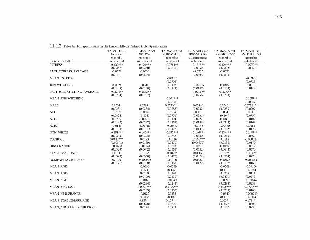
105

11.1.2. Table A2: Full specification results Random Effects Ordered Probit Specifications

T2_MODEL 1

m/f

T2_Model 2 m/f T2_Model 3 m/f T2_Model 4 m/f T2_Model 5 m/f T2_Model 6 m/f

NO-IPW NOIPW-

MODCRE

NOIPW FULL

CRE

IPW-NO CRE IPW-MODCRE IPW FULL CRE

xtoprobit xtoprobit xtoprobit all corrections xtoprobit xtoprobit Outcome = SAHS unbalanced unbalanced unbalanced unbalanced unbalanced unbalanced FSTRESS -0.132*** -0.124*** -0.0781** -0.131*** -0.124*** -0.0770**

(0.0347) (0.0348) (0.0351) (0.0350) (0.0352) (0.0355) PAST_FSTRESS_AVERAGE -0.0552 -0.0358 -0.0505 -0.0330

(0.0491) (0.0504) (0.0493) (0.0506) MEAN_FSTRESS -0.0832 -0.0995

(0.0705) (0.0728) JOBSWITCHING -0.00390 -0.00415 0.0192 -0.00135 -0.00156 0.0216

(0.0145) (0.0146) (0.0142) (0.0147) (0.0148) (0.0143) PAST_JOBSWITCHING_AVERAGE -0.0551** -0.0532** -0.0611** -0.0590**

(0.0254) (0.0257) (0.0256) (0.0258) MEAN_JOBSWITCHING -0.101*** -0.105***

(0.0331) (0.0347) MALE 0.0501* 0.0528* 0.0773*** 0.0514* 0.0543* 0.0791***

(0.0281) (0.0284) (0.0288) (0.0282) (0.0285) (0.0297) AGE -0.107 -0.0332 -0.104 -0.118 -0.0340 -0.105

(0.0824) (0.104) (0.0751) (0.0831) (0.104) (0.0757) AGE2 0.0206 -0.00502 0.0104 0.0227 -0.00475 0.0102

(0.0182) (0.0227) (0.0168) (0.0183) (0.0228) (0.0169) AGE3 -0.0141 0.00466 -0.00642 -0.0153 0.00460 -0.00621

(0.0130) (0.0161) (0.0122) (0.0131) (0.0162) (0.0123) NON_WHITE -0.151*** -0.140*** -0.157*** -0.146*** -0.134*** -0.148***

(0.0339) (0.0344) (0.0353) (0.0340) (0.0345) (0.0362) YSCHOOL 0.0612*** 0.0123 0.00116 0.0596*** 0.0116 -0.000527

(0.00671) (0.0189) (0.0170) (0.00670) (0.0186) (0.0170) HINSURANCE 0.000766 -0.00144 0.0303 -0.00761 -0.00330 0.0312

(0.0529) (0.0642) (0.0565) (0.0532) (0.0648) (0.0570) STABLEMARRIAGE 0.00111 -0.103* -0.107** 0.00155 -0.107* -0.116**

(0.0323) (0.0556) (0.0475) (0.0322) (0.0554) (0.0473) NUMFAMILYCHILDREN 0.0103 -0.000979 0.00190 0.00980 -0.00128 0.000565

(0.0121) (0.0198) (0.0163) (0.0122) (0.0197) (0.0163) MEAN_AGE -0.0398 -0.0399 -0.0589 -0.00138

(0.179) (0.147) (0.179) (0.154) MEAN_AGE2 0.0209 0.0198 0.0246 0.0111

(0.0400) (0.0330) (0.0401) (0.0343) MEAN_AGE3 -0.0165 -0.0149 -0.0190 -0.00844

(0.0294) (0.0243) (0.0295) (0.0253) MEAN_YSCHOOL 0.0560*** 0.0726*** 0.0550*** 0.0726***

(0.0205) (0.0188) (0.0203) (0.0188) MEAN_HINSURANCE -0.0127 0.0156 -0.0340 -0.000219

(0.116) (0.108) (0.118) (0.116) MEAN_STABLEMARRIAGE 0.157** 0.157*** 0.163** 0.172***

(0.0678) (0.0605) (0.0677) (0.0608) MEAN_NUMFAMILYCHILDREN 0.0174 0.0223 0.0167 0.0238

106

Table A2: Continued.

T2_MODEL 1

m/f

T2_Model 2 m/f T2_Model 3 m/f T2_Model 4 m/f T2_Model 5 m/f T2_Model 6 m/f

(0.0257) (0.0229) (0.0256) (0.0233) LHSD1 -2.245*** -2.217*** -1.634*** -2.232*** -2.203*** -1.580***

(0.180) (0.181) (0.146) (0.184) (0.184) (0.149) LHSD2 -1.586*** -1.564*** -1.134*** -1.584*** -1.561*** -1.101***

(0.0959) (0.0957) (0.0669) (0.0990) (0.0988) (0.0689) LHSD3 -1.113*** -1.099*** -0.808*** -1.114*** -1.099*** -0.788***

(0.0627) (0.0625) (0.0435) (0.0636) (0.0634) (0.0441) LHSD4 -0.619*** -0.610*** -0.446*** -0.615*** -0.606*** -0.430***

(0.0424) (0.0424) (0.0329) (0.0429) (0.0429) (0.0332) INITIAL SAH=1 -1.851*** -1.855*** -2.165*** -1.834*** -1.836*** -2.123***

(0.225) (0.223) (0.200) (0.209) (0.207) (0.194) INITIAL SAH=2 -1.811*** -1.812*** -2.044*** -1.777*** -1.781*** -1.998***

(0.101) (0.100) (0.0922) (0.102) (0.101) (0.0944) INITIAL SAH=3 -1.237*** -1.242*** -1.396*** -1.202*** -1.209*** -1.362***

(0.0589) (0.0584) (0.0521) (0.0591) (0.0588) (0.0522) INITIAL SAH=4 -0.732*** -0.735*** -0.825*** -0.710*** -0.713*** -0.802***

(0.0411) (0.0410) (0.0394) (0.0412) (0.0412) (0.0396) TIME 2 - - -0.194** - - -0.208**

(0.0923) (0.0969) TIME3 0.221*** -0.143 -0.113 0.222*** -0.128 -0.120

(0.0346) (0.0885) (0.0782) (0.0350) (0.0893) (0.0823) TIME4 0.0882*** -0.207*** -0.176*** 0.0868*** -0.196*** -0.184***

(0.0329) (0.0739) (0.0661) (0.0332) (0.0744) (0.0698) TIME5 0.126*** -0.0962* -0.0819 0.125*** -0.0869 -0.0875

(0.0313) (0.0578) (0.0522) (0.0318) (0.0584) (0.0548) TIME6 0.0120 -0.131*** -0.117*** 0.0145 -0.121*** -0.117***

(0.0297) (0.0448) (0.0409) (0.0301) (0.0453) (0.0428) TIME7 0.00777 -0.0648* -0.0549* 0.0108 -0.0579 -0.0551

(0.0306) (0.0346) (0.0327) (0.0314) (0.0354) (0.0341) CUTPOINT 1 -6.122*** -5.465*** -6.428*** -6.305*** -5.779*** -5.891***

(1.218) (2.083) (1.747) (1.230) (2.097) (1.856) CUTPOINT 2 -4.662*** -3.999* -4.917*** -4.847*** -4.316** -4.381**

(1.216) (2.082) (1.747) (1.228) (2.096) (1.856) CUTPOINT 3 -2.908** -2.241 -3.130* -3.105** -2.569 -2.610

(1.215) (2.082) (1.746) (1.226) (2.095) (1.855) CUTPOINT 4 -1.161 -0.488 -1.357 -1.379 -0.838 -0.854

(1.214) (2.081) (1.745) (1.225) (2.095) (1.854) SIGMA2_U 0.372*** 0.379*** 0.529*** 0.360*** 0.367*** 0.533***

(0.0421) (0.0422) (0.0329) (0.0423) (0.0424) (0.0344)



107

11.1.3. Table A3: Complete Random Effects Ordered Probit Specifications - Male and Female dependent

T5a_MODEL4m T5a_MODEL4f T5a_Model 5m

T5a_Model 5f

T5a_Model 6m

T5a_Model 6f IPW IPW IPW-

MODCRE IPW-

MODCRE IPW FULL

CRE IPW FULL

CRE SAH-FSTRESS SAH-FSTRESS

Outcome SAH

Outcome SAH

Outcome SAH

Outcome SAH all corrections all corrections xtoprobit xtoprobit xtoprobit xtoprobit

unbalanced unbalanced unbalanced unbalanced unbalanced unbalanced FSTRESS -0.164*** -0.109** -0.155*** -0.102** -0.124** -0.0419

(0.0539) (0.0459) (0.0546) (0.0459) (0.0526) (0.0479) PAST_FSTRESS_AVERAGE 0.0763 -0.119* 0.106 -0.106

(0.0789) (0.0632) (0.0808) (0.0648) MEAN_FSTRESS 0.0808 -0.208**

(0.128) (0.0896) JOBSWITCHING 0.000360 -0.00512 0.000133 -0.00495 0.0211 0.0223

(0.0231) (0.0191) (0.0233) (0.0191) (0.0223) (0.0188) PAST_JOBSWITCHING_AVERAGE -0.0393 -0.0818** -0.0325 -0.0825**

(0.0421) (0.0321) (0.0428) (0.0323) MEAN_JOBSWITCHING -0.105* -0.115***

(0.0607) (0.0415) MALE

AGE -0.372*** 0.0595 -0.392** 0.252* -0.237** -0.0107

(0.127) (0.110) (0.156) (0.140) (0.115) (0.101) AGE2 0.0771*** -0.0155 0.0719** -0.0668** 0.0359 -0.00811

(0.0278) (0.0243) (0.0339) (0.0308) (0.0256) (0.0226) AGE3 -0.0532*** 0.0115 -0.0499** 0.0489** -0.0243 0.00671

(0.0197) (0.0175) (0.0239) (0.0221) (0.0185) (0.0166) NON_WHITE -0.0927* -0.183*** -0.0783 -0.175*** -0.123** -0.173***

(0.0547) (0.0433) (0.0554) (0.0439) (0.0579) (0.0461) YSCHOOL 0.0741*** 0.0512*** 0.0259 0.000762 -0.00556 0.00434

(0.0105) (0.00864) (0.0314) (0.0223) (0.0278) (0.0217) HINSURANCE -0.0927 0.0550 -0.0789 0.0440 -0.0483 0.0858

(0.0856) (0.0674) (0.103) (0.0832) (0.0912) (0.0724) STABLEMARRIAGE 0.131** -0.0676* -0.0325 -0.153** -0.111 -0.110*

(0.0566) (0.0394) (0.0843) (0.0743) (0.0738) (0.0621) NUMFAMILYCHILDREN 0.00220 0.0103 -0.0118 0.00266 -0.00495 0.00816

(0.0197) (0.0158) (0.0310) (0.0257) (0.0255) (0.0216) MEAN_AGE 0.241 -0.340 0.305 -0.231

(0.281) (0.232) (0.260) (0.188) MEAN_AGE2 -0.0437 0.0891* -0.0564 0.0621

(0.0627) (0.0521) (0.0577) (0.0423) MEAN_AGE3 0.0322 -0.0675* 0.0418 -0.0467

(0.0459) (0.0384) (0.0423) (0.0313) MEAN_YSCHOOL 0.0549 0.0579** 0.0937*** 0.0570**

(0.0342) (0.0244) (0.0305) (0.0240) MEAN_HINSURANCE -0.0771 0.00521 -0.0187 0.0321

(0.183) (0.154) (0.183) (0.145) MEAN_STABLEMARRIAGE 0.290*** 0.113 0.360*** 0.0620

(0.110) (0.0882) (0.102) (0.0771) MEAN_NUMFAMILYCHILDREN 0.0159 0.0107 0.0251 0.00893

108

Table A3: Continued T5a_MODEL4m T5a_MODEL4f T5a_Model

5m

T5a_Model

5f

T5a_Model

6m

T5a_Model

6f (0.0406) (0.0333) (0.0369) (0.0301) LHSD1 -2.413*** -2.155*** -2.386*** -2.132*** -1.862*** -1.458***

(0.296) (0.230) (0.304) (0.230) (0.237) (0.188) LHSD2 -1.557*** -1.590*** -1.517*** -1.577*** -1.050*** -1.127***

(0.156) (0.128) (0.156) (0.127) (0.108) (0.0901) LHSD3 -1.126*** -1.102*** -1.105*** -1.093*** -0.790*** -0.782***

(0.0979) (0.0832) (0.0979) (0.0831) (0.0647) (0.0600) LHSD4 -0.687*** -0.557*** -0.673*** -0.551*** -0.479*** -0.387***

(0.0653) (0.0567) (0.0655) (0.0567) (0.0499) (0.0444) INITIAL SAH=1 -1.225*** -2.139*** -1.232*** -2.133*** -1.405*** -2.448***

(0.336) (0.239) (0.331) (0.238) (0.368) (0.216) INITIAL SAH=2 -1.725*** -1.799*** -1.734*** -1.797*** -1.892*** -2.060***

(0.163) (0.132) (0.161) (0.131) (0.164) (0.117) INITIAL SAH=3 -1.148*** -1.227*** -1.162*** -1.229*** -1.276*** -1.416***

(0.0875) (0.0798) (0.0879) (0.0791) (0.0786) (0.0704) INITIAL SAH=4 -0.741*** -0.682*** -0.753*** -0.680*** -0.827*** -0.785***

(0.0602) (0.0565) (0.0605) (0.0563) (0.0580) (0.0540) TIME 2 - - - - -0.373** -0.0954

(0.166) (0.116) TIME3 0.200*** 0.233*** -0.217 -0.0747 -0.283** -0.00881

(0.0535) (0.0463) (0.145) (0.114) (0.140) (0.0996) TIME4 0.0695 0.0999** -0.270** -0.148 -0.290** -0.111

(0.0515) (0.0435) (0.122) (0.0938) (0.120) (0.0833) TIME5 0.115** 0.129*** -0.140 -0.0554 -0.188** -0.0174

(0.0490) (0.0418) (0.0950) (0.0741) (0.0924) (0.0667) TIME6 0.0193 0.00816 -0.147** -0.106* -0.159** -0.0866

(0.0461) (0.0400) (0.0729) (0.0581) (0.0708) (0.0530) TIME7 -0.0269 0.0358 -0.112** -0.0215 -0.128** -0.00261

(0.0498) (0.0405) (0.0569) (0.0452) (0.0558) (0.0428) CUTPOINT 1 -9.910*** -3.796** -6.728** -5.600** -3.328 -7.890***

(1.908) (1.610) (3.358) (2.674) (3.199) (2.215) CUTPOINT 2 -8.532*** -2.295 -5.340 -4.094 -1.905 -6.334***

(1.904) (1.607) (3.353) (2.674) (3.198) (2.213) CUTPOINT 3 -6.804*** -0.541 -3.604 -2.336 -0.167 -4.536**

(1.900) (1.606) (3.351) (2.672) (3.197) (2.212) CUTPOINT 4 -5.096*** 1.202 -1.890 -0.589 1.570 -2.763

(1.897) (1.606) (3.350) (2.672) (3.196) (2.210) SIGMA2_U 0.368*** 0.346*** 0.379*** 0.350*** 0.558*** 0.506***

(0.0654) (0.0544) (0.0660) (0.0543) (0.0556) (0.0427)



109

11.2. Appendix 2

11.2.1. Theoretical Motivation and Development

We assume that individuals are rational utility maximizing agents facing a

dynamic optimization problem. Suppose that the lifetime utility iU of an individual i

may be characterized as

0

1u (H ,L ,X ;D ,D )

(1 )

T

i it it it it i ittt it

U=

=+

(1)

In equation (1), the utility function itu for individual i at time t depends on the

independent variables health (H), Leisure (L), and a bundle of non-health related

consumption (X). Utility is discounted by an individual, and potentially time variant,

time preference it . In this model, D ,Di it are observable individual characteristics which

are thought to effect all choices within the utility function and differentiated as time

invariant and time-variant. As in Grossman (1972), an individual’s Health itH is

presumed to evolve over time according to

1(q ; )Hit it it i itH I − = − , (2)

where itI represents investment in health goods and services (both formal and informal)

and 1(q ; )Hit i it − represents consumption of existing health stock. Consistent with

(Muurinen, 1982) individual observable characteristics are allowed to effect the rate at

which health stock is consumed referenced qit while i denotes individual time invariant

110

unobservable genetic, community, and psychological factors effecting the rate of

depreciation of existing health.

The general health production is thus formed as

1(H , I ,q ; ,D ,D )it it it it it it i itH h −= . (3)

Individuals are assumed to face a lifetime earnings budget constraint

0

1( )

(1 )

TL H S x I

i t it it it it it t it t ittt it

V r A w T T T T P X P I=

= + − − − − − + ,

(4)

where itA is wealth and itw reflects the individual time variant wage rate. Income is the

product of wage rate and the net of total time T after deducting time dedicated to leisure

L

itT , health activitiesH

itT , or sick timeS

itT which is assumed to be a function of health.

Prices for consumption goods itX and health consumption itI are denoted x

tP and I

tP

respectively. Future periods are discounted by tr the prevailing interest rate.

The underlying problem is therefore the maximization of (1) subject to the

lifetime budget constraint (3) and the health production function (2)

The conditional demand curve for health inputs is found to be

*

1(H ,P ,P , w ,A , r , ; ,D ,D )x I

it it t t it it t it i i itI f −= . (5)

Substituting (4) into (2) the optimal health production function is derived.

111

*

1(H ,P ,P , w ,A , r , ,q ; ,D ,D )x I

it it t t it it t it it i i itH f −= . (6)

11.2.2. The Estimation Model

This research is focused on the identification of the effects of economic and

financial strain on health production. In this research, economic strain is defined as Job

Switching Volatility J S

it . We hypothesize that changes in J S

it effect health by varying the

rate at which health stock is consumed. In this context, the consumption of health stock

is the explicit cost of inefficient conversion of human capital into income. Financial

strain FS

it is taken up shortly. However, qit , the rate of health stock consumption, is

assumed to be a function of both J S

it and FS

it :

q (J ,F )S S

it it itf= . (7)

We introduce these variables of interest directly into the health production function by

substitution of (7) into (6).

Following (Zeldes, 1989) financial stress FS

it is defined as a function of income

and wealth where wealth is comprised of cash, cash equivalents, and housing equity. In

our research, we use income itY in place of wage rate w it * ( )L H S

it it itT T T T− − − .

Inclusion of FS

it in the optimal health production function therefore requires exclusion of

w it and A it .. J S

it substitutes directly into *

itH .

112

Because data is unavailable forx

tP and I

tP and it , our empirical specification

makes another simplifying assumption:

1

x I

it it it t it t itA A Y P X P I−− = − − , (8)

which states that the change in individual wealth is equal to current income less

purchases. Savings can therefore be defined as

1

11

1

x I

it it it t it t it itA A Y P X P I Y

−

− = − − = −

+ .

(9)

Or more generally,

(Y ,P X ,P I , )X I

it t it t it iA f = .

(Zeldes, 1989) exploits this relationship defining financial strain / (1/ 6)it itA Y . As

such, in the empirical specification for our model, all price, income, and time preference

is captured by the financial strain variable.

As a further simplifying assumption, we assume that all individuals face the same

investment rate of return rt . The resulting empirically testable health production function

is:

*

1(H ,F , J ; ,D ,D )S S

it it it it i i itH f −= . (10)

113

Direct hypotheses emerging from the empirically testable health production function are

defined:

H0: Economic strain is not costless and is observable in the relationship between job

switching volatility and health. Our theory posits a negative relationship.

H1: Financial Strain reduces the optimal quantity of health demanded.

The empirical model for the conditional demand for health function arises naturally from

(9):

*

1 1 2 3

1 1

K MS S

it it it it j ji l lit i it

j l

H H F J D D u −

= =

= + + + + + + (11)

Where *

itH and 1itH − are measured conventionally as a categorical Self-Assessed Health

measure. The vectors of demographic variables D are broken into groups of time-

invariant and time-variant variables, respectively, denoted by the subscripts t and it and

indexed by j and l. The standard unobservable individual effect is denoted

2~ ( , )i rN while the residual is treated conventionally: 2~ (0, )it uu N .

11.2.3. Econometric Method

Following in spirt the methodological considerations of (Contoyannis et al.,

2004), we use dynamic panel ordered probit and Negative Binomial Count Model

specifications on both balanced and unbalanced panels in this research. We test two

health related outcomes, the SAH and CC. Our models are reduced form models and do

not consider individual consumption choices beyond the propensity to spend within or in-

114

excess of earnings. The reduced-form specification for the latent variable models we

estimate takes the general form

' '

, 1* ( 1,2,3,... ; 2,3,4,...T)it i t it it i ity y x z i N t −= + + + + = = (12)

Where *ity is a latent expression of an individual’s underlying health condition

observable only through the ordinal scale of SAH or CC an index whose value is

conditional on having received health services. Formally, *ity as SAH may be thought of

as falling into bins of unknown dimension. Bins are numerically defined on an ordinal

scale (1,2...,5)its = . Formally

1 * (1,2,...,5)it s it sy s if u y u s−= (13)

with the conventional treatment of 1 1 5, ,s su u u u+= − = and *ity may be interpreted

as a first order Markov process. In equation 12 i represents the individual specific

time-invariant unobservable random-effect assumed to be uncorrelated with regressors

while 2~ (0, )it N .

'

itz represents the set of potentially endogenous and time invariant

regressors, and'

itx represents the set of time variant strictly exogenous variables.

115

11.2.3.1. Dynamic Panel Random Effects Ordered Probit Specification

Regression results Table 3 are derived out of the Pooled Ordered Probit Dynamic

Panel specification where the probability of observing a category of SAH reported at time

ity conditional on the regressors 'itx , 'itz and individual effect i , is:

1 1 1(y ) ( ' ' ) ( ' ' )itj it j it it i j it it iP P j x z x z − − −= = = − − − − − − − (14)

Where (.) represents the standard normal distribution function. All models allow for the

individual effect to be correlated with the regressors ala (Chamberlain, 1979; Mundlak,

1978; Wooldridge, 2002) and correct for the initial conditions problem (Heckman, 1981).

The parameterization of the individual effect take the form

'

0 2 0 'i i ix H T e = + + + + (15)

in which '

ix is a vector of means of time varying strictly exogenous variables and

2~ (0, )i ee N , 0H is the initial observation represented as a vector of dummy variables

capturing potential SAHS states with “Very Good Health” as the base category. T is a

vector of time dummies. Substituting (3) into (1) we derive the random effects

specification for models presented. The effect on health of time variant regressors is the

sum of the parts of the respective coefficients on 2 and .

The assumption that the density of the random effect is 2~ ( , )N allows the

individual effect to be integrated out yielding the operationalized log-likelihood function

116

2

22

21 1

1ln ln

2

Tn

itj

i t

L P e d

−

+

−= =

=

(16)

which can be estimated by Gauss-Hermite quadrature.

Dynamic panel SAHS specifications in main paper tables 4 and 5 include a

lagged dependent variable as an additional regressor thereby relating the estimation to a

base-period. In this sense, the initial observation of the base-period becomes a predictor

of the next observation. This estimation feature is known as the initial conditions

problem.

11.2.4. Endogeneity and Instrumental Variables

Income and wealth have a long history of endogeneity concerns and have been

treated both endogenously and exogenously in historical research. In our research, our

analytical focus on FSTRESS and JOBSWITCHING as the mechanisms of translation

between income and health explicitly controls for the underlying transfer mechanism. As

a test of this hypothesis, we use an independent IV estimation technique Two-Stage

Residual Inclusion 2SRI which uses the residuals from the first stage as added variables

in the second stage with the original the untreated endogenous variable and is an

appropriate model choice for non-linear IV (Terza, Basu, Rathoouz, 2008). A failure of

the included regressors to achieve significance confirms that endogeneity is not a

modeling concern. The method is a two-stage method which requires the first stage to

meet the conditions of standard linear IV estimation. We develop our IV model using the

instrument OWNRENT. OWNRENT is a dichotomous variable with zero(0) denoting

117

“family owns home,” and one(1) denoting “family rents their home.” We posit that

OWNRENT is exogenous to the determination of SAHS, presenting the contextual

relationship as in fig. 1 below.

Figure 1: Exogeneity of Home Ownership on SAHS and chronic disease CC index.

The flow chart (fig. 1) represents our perception of the relationship between home

ownership and SAHS. A priori, one might suspect that home ownership goes with

superior historical earnings and financial behaviors including the ability to save, while

renters may be thought to be less stable earners, have lower credit ratings, and otherwise

have demonstrated poor financial management.47 We might also think that home

ownership itself should benefit individual health. Yet, this is the claim taken up by

(Aizawa & Helble, 2015). In their research, they cannot defend causality between home

ownership and SAHS. They do find that home owner’s exhibit characteristics that tend

to make them more likely to use preventative care and health services but are cautious to

point out that their Grossman framework fails to produce a plausible link between

homeownership and health service usage. Jürges, 2008 tests the relationship between

47 This suspicion is buttressed by the typical business practice of using home ownership as a proxy for fiscal responsibility; home ownership is a common question on loan as well as auto insurance applications to evaluate stability and responsibility. Under these criteria, home ownership acts as a proxy for stability and responsibility which is intuitively appealing.

OWN HOME

F- STRESS

SAH

118

home ownership and SAHS failing to find evidence of causality. Alternatively, renters

are inherently more mobile and less invested in a home. As a result, there is no reason to

suspect that they are engaged with home maintenance and the toxins associated, nor are

they incentivized to stay in a home that proves to be unhealthy by mold, toxic fumes,

poor water quality etc. As such arguments for and against correlation of ownership with

health are suspect to high degrees of heterogeneity and variation.

With this evidence in mind, we estimate the first stage equation:

'

1it i it it itFSTRESS x OWNRENT u = + + + (13)

Where '

itx is the full vector of second stage regressors, and itu is assumed to be strictly

exogenous, normally distributed with mean zero, and uncorrelated across individuals or

over-time. Results in Table A2:1 demonstrate OWNRENT is strongly and economically

significant (8% with CI<.001).

Both F-test of excluded instruments as well as Sanderson-Windmeijer

specification tests strongly reject under identification or weak instruments with an F

statistic of 64.43 and associated p-value < .001. This finding is supported with Lagrange

multiplier tests, and the Cragg-Donald Wald statistic > 139 with Stock-Yogo critical

values for maximum bias of <2.5%. The Hansen J statistic identification test confirms

that the equation is exactly identified. We use Anderson-Ruban Wald tests to test the

joint significance of endogenous regressors and fail to reject that the orthogonality

conditions are valid a conventional confidence intervals.

119

In our model, we use both the first stage residual and the square of the residual.

If these variables are insignificant, then one may conclude that the model is not

endogenous. Results in Table A2:2 confirm the absence of endogeneity.

Our results suggest that in the FSTRESS/SAHS relationship, endogeneity is not an

issue under the conditionality of the Dynamic Panel Random Effects Ordered Probit

model with Mundlak, Chamberlain, and Wooldridge corrections for initial conditions and

correlation between the random component and the regressors.

120

11.2.4.1. Table A2:1 IV First Stage Estimates

Robust FSTRESS Coef. Std. Err. t

OWNRENT -0.080*** 0.010 -8.03

LHSD1 -0.005 0.037 -0.14

LHSD2 0.014 0.015 0.96

LHSD3 0.012 0.008 1.47

LHSD4 -0.007 0.006 -1.07

JOBSWITCHING 0.017*** 0.004 4.27

AGE -0.036 0.032 -1.13

AGE2 0.008 0.007 1.11

AGE3 -0.005 0.005 -1.01

NON_WHITE 0.111*** 0.009 12.65

YSCHOO 0.002 0.006 0.32

MALE -0.006 0.006 -1.11

HINS -0.087*** 0.023 -3.81

STABLEMAR 0.007 0.017 0.39

NUMFAMCH -0.007 0.006 -1.24

d_II_COR_HSTATUS1 0.104** 0.046 2.27

d_II_COR_HSTATUS2 0.026 0.018 1.42

d_II_COR_HSTATUS3 -0.003 0.009 -0.4

d_II_COR_HSTATUS4 -0.012* 0.007 -1.88

TIME2 (omitted)

TIME3 0.009 0.021 0.44

TIME4 0.007 0.018 0.39

TIME5 -0.018 0.014 -1.32

TIME6 -0.019* 0.011 -1.71

TIME7 0.022** 0.009 2.44

mm_AGE 0.028 0.046 0.6

mm_AGE2 -0.005 0.010 -0.52

mm_AGE3 0.003 0.007 0.39

mm_YSCHOO -0.019*** 0.006 -3.31

mm_HINS -0.139*** 0.032 -4.28

mm_STABLEMAR -0.061*** 0.019 -3.2

mm_NUMFAMCH 0.030*** 0.007 4.36

past_JOBSWITCHING_average 0.011* 0.006 1.83

past_FSTRESS_average 0.386*** 0.015 25.85

_cons 0.669 0.476 1.41

N 16615

Clusters 4267

121

11.2.4.2. Table A2,2: Two-Stage Residual Inclusion

T2_Model 6 T2_Model 6 T2_Model 6 T2_Model 6

xtoprobit-

probit(cluster) fs

xtoprobit-

probit(cluster) fs

xtoprobit-

probit(cluster) fs

xtoprobit-

probit(cluster) fs

SAH-FSTRESS SAH-FSTRESS SAH-FSTRESS SAH-FSTRESS

all corrections all corrections all corrections all corrections

full specification full specification full specification full specification

allobs allobs allobs allobs

unbalanced unbalanced unbalanced unbalanced

robust robust robust robust

VARIABLES xb xb xb xb

LHSD1 -1.624*** -1.629*** -2.260*** -2.258***

(0.162) (0.162) (0.196) (0.195)

LHSD2 -1.123*** -1.123*** -1.587*** -1.586***

(0.0731) (0.0731) (0.103) (0.103)

LHSD3 -0.811*** -0.808*** -1.118*** -1.118***

(0.0464) (0.0464) (0.0653) (0.0653)

LHSD4 -0.439*** -0.438*** -0.617*** -0.617***

(0.0346) (0.0346) (0.0440) (0.0440)

1.DEF_FSTRESS_Z2 0.512* 0.196 -0.224 -0.188

(0.272) (0.203) (0.228) (0.229)

n_cor_jobswitching 0.0186 0.0221 0.00429 0.00399

(0.0152) (0.0151) (0.0162) (0.0162)

gen_residual -0.338** -0.161 0.0497 0.0526

(0.154) (0.114) (0.144) (0.144)

sq_gen_residual 0.0126 0.0117 0.000785 -0.0167

(0.0181) (0.0173) (0.0282) (0.0257)

AGE -0.107 -0.103 -0.0594 -0.0572

(0.0790) (0.0791) (0.108) (0.108)

AGE2 0.0120 0.0112 0.00196 0.00151

(0.0176) (0.0176) (0.0236) (0.0235)

AGE3 -0.00803 -0.00739 -0.000542 -0.000232

(0.0128) (0.0128) (0.0167) (0.0167)

NON_WHITE1 -0.151*** -0.150*** -0.124*** -0.136***

(0.0375) (0.0374) (0.0445) (0.0444)

YSCHOO -0.00651 -0.00536 0.00528 0.00520

(0.0180) (0.0180) (0.0197) (0.0196)

MALE 0.0865*** 0.0868*** 0.0625** 0.0608**

(0.0305) (0.0304) (0.0291) (0.0290)

HINS 0.0761 0.0433 -0.0407 -0.0387

(0.0669) (0.0646) (0.0725) (0.0725)

STABLEMAR -0.107** -0.115** -0.106* -0.106*

(0.0491) (0.0491) (0.0573) (0.0573)

NUMFAMCH -0.00851 -0.00900 -0.0117 -0.0117

(0.0167) (0.0167) (0.0204) (0.0204)

d_II_COR_HSTATUS1 -2.036*** -2.049*** -1.859*** -1.856***

(0.193) (0.191) (0.197) (0.198)

d_II_COR_HSTATUS2 -1.981*** -1.981*** -1.745*** -1.749***

(0.0959) (0.0959) (0.104) (0.104)

d_II_COR_HSTATUS3 -1.335*** -1.335*** -1.180*** -1.184***

(0.0537) (0.0537) (0.0602) (0.0604)

d_II_COR_HSTATUS4 -0.787*** -0.788*** -0.701*** -0.700***

(0.0406) (0.0406) (0.0422) (0.0423)

TIME2 -0.166 -0.159

(0.101) (0.101) TIME3 -0.0914 -0.0876 -0.107 -0.105

(0.0860) (0.0861) (0.0918) (0.0919)

122

11.2.4.3. Table A2,2: Continued

T2_Model 6 T2_Model 6 T2_Model 6 T2_Model 6

TIME4 -0.168** -0.163** -0.184** -0.183**

(0.0735) (0.0736) (0.0768) (0.0768)

TIME5 -0.0557 -0.0576 -0.0778 -0.0759

(0.0574) (0.0574) (0.0605) (0.0605)

TIME6 -0.0989** -0.102** -0.113** -0.112**

(0.0450) (0.0449) (0.0475) (0.0475)

TIME7 -0.0577 -0.0490 -0.0528 -0.0518

(0.0361) (0.0359) (0.0369) (0.0368)

mm_AGE -0.0409 -0.0383 -0.0894 -0.0894

(0.158) (0.158) (0.184) (0.184)

mm_AGE2 0.0185 0.0180 0.0301 0.0301

(0.0352) (0.0353) (0.0411) (0.0411)

mm_AGE3 -0.0133 -0.0130 -0.0226 -0.0226

(0.0259) (0.0260) (0.0302) (0.0302)

mm_YSCHOO 0.0785*** 0.0771*** 0.0554** 0.0575***

(0.0197) (0.0198) (0.0219) (0.0218)

mm_HINS -0.0450 -0.00601 -0.0226 -0.00879

(0.121) (0.120) (0.129) (0.129)

mm_STABLEMAR 0.164*** 0.173*** 0.137* 0.144**

(0.0633) (0.0633) (0.0706) (0.0705)

mm_NUMFAMCH 0.0246 0.0249 0.0300 0.0274

(0.0238) (0.0238) (0.0272) (0.0272)

mm_DEF_FSTRESS_Z2 -0.683** -0.349

(0.282) (0.215) mm_n_cor_jobswitching -0.0935** -0.0979***

(0.0364) (0.0363) past_jobswitching_average -0.0573** -0.0595**

(0.0265) (0.0265)

past_FS_average 0.0163 0.00177

(0.105) (0.104)

mm_gen_residual 0.317 0.0835

(0.193) (0.0699) mm_sq_gen_residual 0.0487 -0.0763*

(0.0612) (0.0457) CUT 1 -6.491*** -6.388*** -6.767*** -6.669***

(1.888) (1.894) (2.175) (2.173)

CUT 2 -4.961*** -4.856** -5.272** -5.174**

(1.886) (1.892) (2.174) (2.173)

CUT 3 -3.192* -3.088 -3.527 -3.429

(1.885) (1.891) (2.172) (2.171)

CUT 4 -1.435 -1.331 -1.800 -1.702

(1.884) (1.890) (2.171) (2.170)

SIGMA2_U 0.508*** 0.510*** 0.346*** 0.347***

(0.0347) (0.0347) (0.0426) (0.0427)

Observations 21,137 21,137 16,615 16,615

Number of uniqueid 4,840 4,840 4,267 4,267

Log Likelihood -28584.93 -28588.94 -21923.45 -21923

AIC 57255.87 57259.88 43930.91 43934

123

Endogeneity Tests – Preferred Specification

F test of excluded instruments:

F( 1, 4266) = 64.43

Prob > F = 0.0000

Reject the null that the Beta on excluded instrument is zero.

Sanderson-Windmeijer multivariate specification tests

F( 1, 4266) = 64.43

Prob > F = 0.0000

Cragg-Donald Wald F statistic (Weak Instrument Test) 139.64

Kleibergen-Paap Wald rk F statistic 64.43

Stock-Yogo weak ID F test critical values for single endogenous regressor:

10% maximal IV size 16.38




Source: Stock-Yogo (2005). NB: Critical values are for i.i.d. errors

So while the Anderson-Ruben Wald test is a marginal fail, we can conclude that in the

worst case, endogenity induced bias is less than 2.5%

Hansen J statistic (overidentification test of all instruments):

0.000

(equation exactly identified)

Weak-instrument-robust inference Tests of joint significance of endogenous regressors B1 in main equation

Ho: B1=0 and orthogonality conditions are valid Anderson-Rubin Wald test F(1,4266)= 3.83 P-val=0.0504

Anderson-Rubin Wald test Chi-sq(1)= 3.84 P-val=0.0501

Stock-Wright LM S statistic Chi-sq(1)= 3.91 P-val=0.0480

124

Weak instrument robust tests and confidence sets for linear IV H0: beta[COR_HSTATUS:DEF_FSTRESS_Z2] = 0

Test Statistic p-value Conf. level Conf. Set

AR chi2(1) = 3.82 0.0505 95% [-.883911, .011301]

Wald chi2(1) = 3.66 0.0558 95% [-.853369, .010514]

Both the AR and Wald tests confirm that at the 5% confidence interval, we fail to reject

the null of no correlation between health status and financial strain.

125

12. Supplementary Material Chapter 3

12.1. Appendix 1: List of Waiver Definitions

1301(a)(1)(C)(ii). Definition of a “qualified health plan” as one that agrees to offer at least one silver level

plan and one gold level plan through an Exchange, solely with respect to the requirement that a QHP offer

a silver and a gold level plan through the SHOP.

1302(d), and made available through the SHOP.

1304(b)(4)(D)(i) and (ii). Continuation of participation in SHOP for growing small employers.

1301(a)(2). Solely with respect to the requirement that CO-OPs and multi-state plans be recognized as

qualified health plans in the small group market.

1311 (b)(1)(B). The establishment of a Small Business Health Options Program (SHOP) exchange.

1311(d)(2)(B)(i) - prohibition non-QHP.

1312(c)(1) requires a health insurance issuer to consider “all enrollees in all health plans….offered by such

issuer in the individual market…to be members of a single risk pool.”

26 U.S.C. § 36B (26 I.R.C. § 36B) to allow Iowa to reallocate the described federal funding into the

development of per-member per-month premium credits to lower the monthly premiums for all Iowans

who would purchase the standard plan.

42 U.S.C.§18022(d) to require carriers to only offer a single, standard.

plan, similar to that of the current silver tier.

42 U.S.C. §18071 to eliminate the use of cost sharing reductions.

42 USC § 18071(c)(3)(a), which requires that “[a]n issuer of a qualified health plan making reductions

under this subsection shall notify the Secretary of such reductions and the Secretary shall make periodic

and timely payments to the issuer equal to the value of reductions.”

1311(b)(1)(B) Requires establishment of an American Health Benefit Exchange, including a Small

Business Health Options Program (SHOP) that is designed to assist qualified employers in facilitating the

enrollment of their employees in QHPs and details responsibilities of the exchange.

1311(c)(3) Rating system based on quality and price of plan.

1311(c)(4) Enrollee satisfaction system.

1311(c)(5) Internet portals may be used to direct qualified individuals and qualified employers to QHPs.

1311(d)(1) Specifies which entities are eligible to carry out responsibilities of the Exchange.

1311(d)(1) Specifies which entities are eligible to carry out responsibilities of the Exchange.

1311(d)(4)(A) Requirement that Exchange shall implement procedures for certification of plans.

1311(d)(4)(B) Requirement that Exchange shall provide for the operation of a toll-free telephone hotline.

1311(d)(4)(C) Requirement that Exchange shall maintain an Internet website.

1311(d)(4)(D) Requirement that Exchange shall assign a quality rating to each QHP.

1311(d)(4)(E) Requirement that Exchange shall utilize a standardized format for presentation of plans.

1311(d)(4)(G) Requirement that Exchange shall post to the website a calculator to determine premium tax

credits and cost sharing reductions.

1311(k) Exchange may not establish rules that conflict with or prevent the application of regulations

promulgated by the Secretary of Human Services.

1312(a)(2) Provisions for employee choice among QHPs through an exchange, including requirement that

employer may specify metal level and employee may choose a plan within metal level.

1312(f)(2)(A) Definition of qualified employer.

45 CFR 155.330(d)(2)(iii), 155.705(c).Coordination with individual market.

45 CFR 155.720(i), Reporting for tax administration.

1321(c)(1). Solely with respect to federal establishment of a SHOP in Hawai’i if the State elects not to

establish a SHOP.

126

12.2. Appendix 2: Example of Attachment Point Reinsurance Program

This analysis compares our model to the reinsurance program analysis performed

by (Hilson 2017) with respect to Washington State’s interest in developing a state based

reinsurance program as part of their 1332 waiver request. We begin by defining the

appropriate attachment point model.

Using information culled from (Hilson, Cohen, Anderson, and Bingham, 2017),

we populate our model with an attachment point $66,000L = and detachment point

$1,000,000T = . Populations of interest are defined 297,000AN = and 290,000BN = .48

With respect to premiums, the goal of the program is to reduce premiums by 10% in the

year the plan is introduced. To reconcile the Hisson analytical method with our own, we

define $6,767Br = 49 which sets the desired premium $6090Ar = .50 In the Hilson et. al.

(2017) report, they assume that all the reinsurance funds are passed through to the

consumer; no aggregate change to market profitability 0= . They also define expected

costs for the individual market population of $5,24751. The reinsurance program is

48 The authors use the formula ( *ln(1 % )*( ) 1elasticityofdemand changepremium populationnotsubsidizedPop e += − defined in CEA

brief https://obamawhitehouse.archives.gov/sites/default/files/page/files/201701_individual_health_insurance_market_cea_issue_brief.pdf to evaluate the population change and rely on the brief’s price elasticity of demand of .4.

49 Hilson uses PMPM formulation, our approach operates in terms of yearly averages. To construct our yearly average value we multiply the Hilson generated PMPM pre-state premium times the adjustment factor to bring the premium to the current analysis period (their work is based on 2016 data) $371*(1.52) =563.92*12=$6767.

50 In this formulation, the pre-state is the same year as the post-state and reflects the 2019 year outcomes of “without” the program

Br , and “with” the program Ar .

51 Hilson uses PMPM formulation, our approach operates in terms of yearly averages. To construct our yearly average value we multiply the Hilson generated PMPM pre-state premium times the adjustment factor to bring the premium to the current analysis period (their work is based on 2016 data) 1.278*342.18*12=$5,247

https://obamawhitehouse.archives.gov/sites/default/files/page/files/201701_individual_health_insurance_market_cea_issue_brief.pdf

https://obamawhitehouse.archives.gov/sites/default/files/page/files/201701_individual_health_insurance_market_cea_issue_brief.pdf

127

assumed to be funded by a source exogenous to the individual market which implies

[ , ] 0 = and there is a carrier cost-sharing requirement .5w = . For the report, the

authors assume no change in morbidity across the two periods consistent with

1 1

( ) ( )A A B B

Q Q

q q q q

q q

P E c P E c= =

= .52

The Hilson et. al. (2017) report uses EDGE server data to perform their analysis

and, neither the probabilities nor proportions of the population that are expected to

qualify for the program are stated, nor do the authors provide detail about the average

cost of patients that eventually become covered by the reinsurance program. Our

analysis must therefore make assumptions about the disposition of the underlying

distribution of patient costs across the population.

We assume that ( ( ) ) 0I iP E c T = and to inform our estimation of ( )iE c we draw

on (Charlson, Wells et al. 2014). Their work identifies high cost patients using an index

of chronic conditions, the Charlson Index. Consistent with Hilson et. al. (2017), we

inflate patient costs by an annual trend of 8.5% from 2010 – 2019 to establish

equivalency in the analysis. We further disaggregate the population by Charlson Index

scores, and calculate the average weighted cost and standard deviation of cost of patients

with a cost greater than L (see Table A2:1).

The weighted average used in simulation for cost and deviation is averaged across

years and then across Charlson Index scores. We establish this method of weighted

52 The authors do define an expectation of a 1.6% improvement in the pool’s morbidity under the expectation that lives added by reduced rates are healthier lives, however they do not incorporate it into the analysis, suggesting it as a “Phase II” consideration.

128

averages recognizing that within each Charlson score group, there is a population with

costs greater than L , and that across Charlson Index score groups, the average patient cost

(APC) and the variation around that cost is relatively stable albeit increasing with disease

load as would be expected. See Figure (A2:1 and A2:2). With the model predicated on

these assumptions and methods, we formalize the reinsurance model

( ( ) )(1 )( ( ) )A A I IH N P L E c T w E c L= − −

and the formal pre/post state simulation model takes the form

1 1

( ) ( ( ) )(1 )( ( ) ) ( )A A

Q Q

A A A A q q A I i I A A A B B B Bq Bq B B B B

q q

N r N P E c N P L E c T w E c L N r N r N P E c N r = =

= − + − − − − − + =

The estimation equation is defined

1

( )(1 ) ( ) ( )

( ( ) )(1 )( ( ) )

Q

B B A A B A q q

q

I i

A

N r N r N N P E c

P L E c TN w E c L

=

− − − − +

− −

Our estimation equation suggests that the implied proportion of the population

required to set pre- and post-Policy market profit states equal is a function of the sum of

the MLR weighted net difference in revenues across the transition less the change in

associated patient costs plus any intended market profitability changes divided by the

total potential reinsurance share of patient costs.

Simulating E(c) across 5000 repetitions using the mean $141,357.27 = of the

population cost greater than L and standard deviation ( ) $6,748.91E c = , our model

identifies the required value for ( ( ( ) )) .0151I iE P L E c T = with confidence bands

upper .0178= and lower bound .0124= to inforce 0= . Within the Charlson analytical

dataset, we find a ( ( ( ) )) .023I iE P L E c T = representing the proportion of the

129

population with costs exceeding L . The significant divergence between the proportion of

the population implicitly assumed in (Hilson 2017) analyses, and that of the Charlson

analytical dataset is a cause for concern. The Hilson et. al. (2017) analysis implies that

the reinsurance population is both smaller and less expensive than that represented in the

Charlson dataset.53 This concern is heightened recognizing that, even under the implicit

(Hilson 2017) reinsurance population proportion expectations above, the (Hilson 2017)

analysis implies an average cost per patient between $80,852 and $42,500 an impossibly

low expected patient cost given the $66,000 attachment point. Table A2 uses the

Charlson analytical dataset costs to project the solvency of the reinsurance fund assuming

the calculated population proportions are valid. We include the Charlson Dataset

Population Proportion at mean patient cost as a comparison. The implied deficit between

$48m and $187m is substantial. If, as in the Charlson Dataset, the true population

proportion exceeds 2%, the losses continue to escalate.

We feel that the Hilson et. al. (2017) analysis is optimistic. Our model suggests

that the application of a $66,000 attachment point reinsurance model in Washington State

will produce at least one unanticipated outcome; excessive program liability for the State.

53 We find this implication suspect under the common understanding that the insured in large private self-funded plans (Charlson dataset) are universally assumed to be in considerably better health than those in the individual market.

130

12.2.1. Appendix 2: Figures and Tables

12.2.1.1. Table A2:1 - Charlson Index Group Average Cost and Standard Errors

Total Patient Cost 2010 Data Total Patient Cost 2009 Data Averages

Obs Mean Std. Err. Obs Mean Std. Err. Obs Mean Std. Err.

0 499 143534.7 5063.257 209 117957 5085.472 354 130745.9 5074.365

1 444 121755.8 3476.418 268 119235.3 4559.117 356 120495.6 4017.768

2 419 140120.5 5800.74 357 128616.2 5121.896 388 134368.4 5461.318

3 317 145680.1 5640.494 348 130838.6 4992.169 332 138259.4 5316.332

4 224 133746.2 8294.358 265 135198.2 6143.55 244 134472.2 7218.954

5 154 153508.4 10210.08 206 140167.6 7246.703 180 146838 8728.392

6 143 148801.1 11152.97 170 139921.7 9665.376 156.5 144361.4 10409.17

7 90 156646.6 12703.88 114 125020.7 7900.575 102 140833.7 10302.23

8 86 165211.5 13498.25 113 153206.9 9407.162 99.5 159209.2 11452.71

9 222 182524.6 8116.273 322 198931.4 10282.03 272 190728 9199.152

Weighted Average of Across years, and Down Charlson Index Score 141357.27 6748.91

131

12.2.1.2. Table A2:1 Reinsurance Pool Sufficiency Analysis: WA Reinsurance Program Wakely Attachment and Detachment Points

(Hilson 2017) Population Comparison 297,000 Charlson DataSet

Derived From Simulation Model Population Proportion

High Low At mean Patient Cost

Implicit Proportion of Population that will fall under Reinsurance 1.78% 1.24% 2.30%

Individuals transferred to reinsurance program 5275 3682.8 6831

Average Reinsurance Program Patient Cost $146,199 $133,647 139923

Total Reinsurance pool Liability* $385,579,395 $246,097,586 $477,907,007

Wakely Estimated Reinsurance Pool Fund $197,700,700

Expected Reinsurance Fund Deficit $187,878,695 $48,396,886 $280,206,307

Reinsurance fund shortfall at simulation mean of E(P(L<E(c)<T)=.0148 $118,137,790

* calculated as (1-w)(Total Expense)

132

12.2.1.3. Figure A2:2 - APC>L By Charlson Comorbidity Index Score

0

50000

100000

150000

200000

250000

0 2 4 6 8 10 12

133

12.2.1.4. Figure A2:3 - Std. Err. By Charlson Comorbidity Index Score APC>L

0

2000

4000

6000

8000

10000

12000

14000

0 2 4 6 8 10 12

134

12.3. Appendix 3: Mathematical Calculations

12.3.1. Alaska’s Medicaid Expansion:

{ ; ; ; ; ; ; ; 0; 0; 0}B A A B B A B A B A A B A B X X XN N P P q q A A B B H = = = = = = = = = =

which allows the pre and post profit functions from (1) and (2) across the participation

constraint to be expressed.

1 1

( ) ( )Q Q

A A q Aq A B q Bq B B

q q

Nr N P E c Nr Nr N P E c Nr = =

= − − − − + =

(5)

1 1

(1 ) (1 ) ( ) ( )Q Q

A B q Aq q Bq

q q

Nr Nr N P E c N P E c = =

− − + − +

Solving 5 for the post policy change premium Ar

1 1

( ) ( )

(1 ) (1 )

Q Q

q Aq q Bq

q q

A B

P E c P E c

r rN

= =

−

+ +− −

(6)

12.3.2. Alaska Conditions Based Reinsurance Program:

1 1 1 1 1

( (1 ) ) ( ) (1 ) ( ) (1 ( )) (1 ) ( ) ( ) ( ) (1 ) ( ) ( )

S S SA A AN N N Q Q

S S S S

A A A n A A n A A n A A B B A Aq Aq B Bq Bq

n n n q q

r N N P c f w E c N r P c f w E c N r E c f N r N r N P E c N P E c = = = = =

− − + − − + − − − − + − + − +

Simplify within the brackets

1 1 1 1 1

(1 ) ( ) ( ) ( ) (1 ) ( ) ( )(1 ) ( ) ( ) ( ) ( ) ( ) ( ) ( )

S S S S SA A A A AN N N N N

S S S S S

n A A n n A A A A n A A n A A

n n n n n

w P c f E c P c f N r w E c P c f w E c N r P c f N r E c f N r P c f E c f N r= = = = =

− − + − − − − + − + + +

1 1 1

(1 ) ( ) ( ) ( ) ( ) ( ) ( )

S S SA A AN N N

S S S

n A A n A A n A A

n n n

w E c N r E c f N r P c f E c f N r= = =

− − − + + +

1 1 1

(1 ) ( ) ( ) ( ) ( ) ( ) ( )

S S SA A AN N N

S S S

n A A n A A n A A

n n n

w E c N r E c f N r P c f E c f N r= = =

− − − + + +

Plug the bracketed part back in and solve for Ar

1 1 1 1 1

( (1 ) ) (1 ) ( ) ( ) ( ) ( ) ( ) ( ) (1 ) ( ) ( )

S S SA A AN N N Q Q

S S S S

A A A n A A n A A n A A B B A Aq Aq B Bq Bq

n n n q q

r N N w E c N r E c f N r P c f E c f N r N r N P E c N P E c = = = = =

− − + − − − + + + − + − +

Final Solution for Ar (Equation 8 in main paper)

135

1 1 1 1

(1 ) ( ) ( ) ( ( ) 1) ( ) ( ) (1 ) ( )

( (1 ) 2 )

S SA AN NQ Q

S

B B A Aq Aq B Bq Bq n A A n

q q n n

A S

A A

N r N P E c N P E c P c f E c f N r w E c

rN N

= = = =

− + − − − + − − +

− −

12.3.3. Derivative Calculation for Policy Scenario Analysis (Table 5):

All Ar derivatives calculated from Equation (8)

1

( )(1 )

02( (1 ) 2 )

SAN

nSnA A

AS

A A

E cr N

Nw N N

= −=

− −

(1 )0

( ) 2( (1 ) 2 )

SA A A

AS

A A A

r N NN

E c N N

−=

− −

1 1 1 1 1

2

( ) ( (1 ) 2 ) ( 1) (1 ) ( ) ( ) ( ( ) 1) ( ) ( ) (1 ) ( )

(1 ) 2

S SA AN NQ Q Q

S S

Aq Aq A A B B A Aq Aq B Bq Bq n A A n

q q q n nA

SA

A A

P E c N N N r N P E c N P E c P c f E c f N r w E cr

N N N

= = = = =

− − + − − + − − − + − − +

− −

1 1 1 1

2

( ) 2 ( 1) (1 ) ( ) (1 ) ( ) ( ( ) 1) ( ) ( )

(1 ) 2

S SA AN NQ Q

S S

Aq Aq A B B B Bq Bq n n A A

q q n nA

SA

A A

P E c N N r N P E c w E c P c f E c f N rr

N N N

= = = =

− + − − − − − + − − +

− −

2

(1.0926*8439.24) * 2*(1300) .85* 24064*9389(.85) 24064(8439.24) (.85)78135359 .7(10000000)0

(1 ) 2

A

SA

A A

r

N N N

− − − − +=

− −

Using Equation 8, we recast the equation to solve explicitly for .

1 1 1 1

( (1 ) 2 ) (1 ) ( ) ( ) ( ( ) 1) ( ) ( ) (1 ) ( )

S SA AN NQ Q

S S

A A A B B A Aq Aq B Bq Bq n A A n

q q n n

r N N N r N P E c N P E c P c f E c f N r w E c = = = =

− − − − − − + − + + −

We then take the derivative with respect to our three inputs of interest.

1

( ) 0

SAN

n

n

E cw =

= −

0( )

A

A

NE C

= −

1 1

(1 ) ( ) 0 (1 ) ( )Q Q

A Aq Aq A Aq Aq

q qA

r P E c r P E cN

= =

= − − −

136

13. Appendix 1: Supplementary Material Chapter 3

13.1. Table a1: Retrospective variables used in principle component analysis

Variable Name Description N Mean Stdev

Fam_ParMarried Whether parents are a married couple?* 34,430 0.9454255 0.2271511

Fam_ParRelationSatisfac How satisfied parents were with relationship?*** 35,938 3.107379 0.9783905

Fam_MomParentEffort How much parenting effort by mom?*** 41,382 3.698516 0.6302027

Fam_CumulativeDiv Summ of total parental divorces?**** 35,831 0.1809327 0.5392238

Sta_MovedInChildhood Whether Moved in Childhood?* 42,121 0.6469694 0.4779178

Sta_DadWork05 How much dad worked ages 0-5? 37,018 5.600384 1.123051



Sta_DadUnemp05 How often dad was unemployed and actively looking for work 0-5?*** 36,608 3.87388 0.4402355

Sta_DadUnmep612 How often dad was unemployed and actively looking for work 6-12?*** 37,246 3.844708 0.4863499

Sta_DadUnmep1316

How often dad was unemployed and actively looking for work 13-

16?*** 36,717 3.833973 0.5163178

Sta_MomWork05 How much mom worked ages 0-5?*** 40,993 3.330032 2.209409



Sta_MomUnemp05

How often mom was unemployed and actively looking for work 0-

5?*** 40,580 3.774889 0.649848

Sta_MomUnmep612 How often mom was unemployed and actively looking for work 6-12?*** 40,743 3.747024 0.6374571

Sta_MomUnmep1316

How often mom was unemployed and actively looking for work 13-

16?*** 40,576 3.772871 0.6218208

Sta_SameNeigborhood616 Whether lived in same neighborhood ages 0-16?* 41,106 0.7352455 0.4412078

Sta_CommWithMom Rate communication with mom?*** 41,644 3.683292 1.166102

Sta_MomUnderstood Mom understood problems and worries?*** 41,482 3.104407 0.9342918

Sta_ConfideMom How much child could confide in mom about problems?*** 41,361 2.902783 1.025805

Sta_TensionMom How much tension in relationship with mom?*** 41,357 1.948715 1.001356

Sta_RelationWMom Rate relationship with mom? 41,512 3.859631 1.122403

Sta_CloseMom Wheter emotionally close to mother?*** 41,503 3.308797 0.8190079

Sta_StrictMom How strict was mom?*** 41,207 3.109423 0.8119205

Sta_AffectionMom How much affection mom gave?*** 41,501 3.482085 0.7726333

Sta_CommWithDad Rate communication with dad from poor to excellent?*** 38,243 3.356745 1.226696

Sta_DadUnderstood dad understood problems and worries?*** 38,129 2.644837 0.9918677

Sta_ConfideDad How much child could confide in dad about problems?*** 38,005 2.460834 1.042222

Sta_TensionDad How much tension in relationship with dad?*** 38,025 1.962814 1.030661

Sta_RelationWDad Rate relationship with dad?*** 38,023 3.512216 1.203681

Sta_CloseDad Wheter emotionally close to dad?*** 38,155 2.968602 0.9415811

Sta_StrictDad How strict was dad?*** 37,904 3.117296 0.8871724

Sta_AffectionDad How much affection dad gave?*** 38,198 3.113488 0.9129024

Sta_RelMentorWork

Between age 17 and 30 did you have a relative provide positive

mentoring that helped you succeed (work)?* 41,241 0.4983148 0.5000032

Sta_RelMentorMarriage Between age 17 and 30 did you have a relative provide positive mentoring that helped you succeed (marriage)?* 39,943 0.4538467 0.4978716

Sta_NonRelMentorWork

Between age 17 and 30 did you have a non-relative provide positive

mentoring that helped you succeed (work)?* 41,119 0.5652618 0.4957286

Sta_NonRelMentorMarriage

Between age 17 and 30 did you have a non-relative provide positive

mentoring that helped you succeed (marriage)?* 39,834 0.4747201 0.4993668

Soc_NeighborHelp612 In longest neighborhood during ages 6-12, were neighbors willing to help each other out?*** 41,981 3.663967 0.60855

Soc_NeighborCloseKnit612 In longest neighborhood 6-12, was neighborhood "close-knit"?*** 41,958 3.393513 0.7661119

Soc_NeighborHelp1316

In longest neighborhood during ages 13-16, were neighbors willing to

help each other out?*** 11,727 3.326597 0.7902665

Soc_NeighborCloseKnit1316 In longest neighborhood 13-16, was neighborhood "close-knit"?*** 11,728 3.071965 0.8889601

Soc_Lonely612 How often were you lonley for friends age 6-12?*** 42,075 1.819869 0.8934513

137

13.2. Table a1: Continued


Soc_ComfWithFriends612 How often did youhave a group of friends that you felt comfortable spending time with 6-12?*** 41,790 3.530845 0.7928305

Soc_HadBestFriend612 Between ages 6-12 did you have a best friend?* 41,228 0.8656496 0.3410326

Soc_Lonely1316 How often were you lonley for friends age 13-16?*** 41,630 1.81362 0.8992709

Soc_ComfWithFriends1316

How often did youhave a group of friends that you felt comfortable

spending time with 13-16?*** 41,275 3.498631 0.8149918

Soc_HadBestFriend1316 Between ages 13-16 did you have a best friend?* 41,757 0.871303 0.3348683

Soc_HadBFGF1316

Did you have a romantic partner that you dated for a while, like a

boyfriend or girlfriend ages 13-16?* 41,898 0.4733639 0.499296

Soc_BFGFRelPositive For the most important romantic relationship how would you characterize the relationship?** 19,689 1.563259 0.6280335

Soc_BullyAtSchool612 How often did you pick on or bully kids (in school) 6-12?*** 42,048 1.262914 0.5655056

Soc_BullyOutSchool612 How often did you pick on or bully kids (out of school) 6-12?*** 42,044 1.200195 0.5015486

Soc_BullyAtSchool1316 How often did you pick on or bully kids (in school) 13-16?*** 41,381 1.21406 0.517781

Soc_BullyOutSchool1316 How often did you pick on or bully kids (out of school) 13-16?*** 41,350 1.173325 0.4718176

Sec_NhoodSafeNight612

In longest neighborhood 6-12, was neighborhood safe at night to be out

alone?*** 42,131 3.653153 0.6624177

Sec_NhoodSafeDay612

In longest neighborhood 6-12, was neighborhood safe during day to be

out alone?*** 42,083 3.842407 0.4384247

Sec_NhoodSafeNightKid612 In longest neighborhood 6-12, was neighborhood safe for kids to be out at night alone?*** 41,970 3.636169 0.6723503

Sec_NhoodSafeNight1316

In longest neighborhood 13-16, was neighborhood safe at night to be

out alone?*** 11,759 3.489497 0.7142544

Sec_NhoodSafeDay1316

In longest neighborhood13-16, was neighborhood safe during day to be

out alone?*** 11,725 3.707889 0.5660502

Sec_HhoodSafeNightKid1316 In longest neighborhood 13-16, was neighborhood safe for kids to be out at night alone?*** 11,693 3.463611 0.7423787

Sec_BulliedSch612 How often were you picked on or bullied by kids at school 6-12?*** 42,230 1.840587 0.9053954

Sec_BulliedNhood612

How often were you picked on or bullied by kids in neighborhood 6-

12?*** 42,003 1.583768 0.7803661

Sec_SafeAtSchool612

How often did you feel worried about your physical safety at school 6-

12?*** 42,101 1.374267 0.7062947

Sec_BulliedSch1316 How often were you picked on or bullied by kids at school 13-16?*** 41,435 1.676674 0.8579604

Sec_BulliedNhood1316

How often were you picked on or bullied by kids in neighborhood 13-

16?*** 41,330 1.450278 0.7165534

Sec_SafeAtSchool1316 How often did you feel worried about your physical safety at school 13-16?*** 41,236 1.36878 0.6953041

Health_SAHS Self reported health status ages 0-16 42,246 4.331582 0.8663459

Health_MonthMissSch Did you miss a month or more of school due to a health problem?* 42,060 0.0758203 0.2647135

Health_Measles Before age 17, measles?* 41,751 0.4124692 0.4922846

Health_Mumps Before age 17, mumps?* 41,712 0.3411728 0.474109

Health_Chickenpox Before age 17, Chicken Pox?* 41,997 0.8324404 0.3734792

Health_Vision Before age 17, difficulty seeing even with glasses?* 42,242 0.1316699 0.3381355

Health_Hearing Before age 17, diffidulty hearing?* 42,182 0.0288986 0.1675235

Health_ParSmoked Did one or more of the people who raised you during childhood smoke? 42,008 0.8356027 0.7660126

Health_Asthma Before age 17, did you have Asthma?* 42,220 0.0838228 0.2771252

Health_Diabetes Before age 17, did you have Diabetes?* 41,766 0.0033281 0.057594

Health_RespDisease Before age 17, did you have Respratory Disease?* 42,083 0.1738469 0.3789823

Health_SpeechImpair Before age 17, did you have a Speech Imparment?* 42,022 0.0565894 0.2310591

Health_Allergy Before age 17, did you have an allergic condition?* 42,022 0.1527295 0.3597309

Health_HeartTrouble Before age 17, did you have heart trouble?* 42,068 0.0148807 0.1210768

Health_EarProbs Before age 17, did you have chronic ear problems or infections?* 42,108 0.0887242 0.2843487

Health_Epilepsy Before age 17, did you have epilespy?* 42,109 0.0122539 0.1100184

Health_Headache Before age 17, did you have severe headaches or migraines?* 42,091 0.0913735 0.2881429

Health_StomProb Before age 17, did you have stomach problems?* 42,076 0.0621494 0.2414296

Health_HighBloodPres Before age 17, did you have high blood pressure?* 42,017 0.0066402 0.0812172

Health_HeightInTOT13

Total height in inches age 13 converted from both inch and foot

measures as well as meter responses**** 40,092 62.09674 5.51702

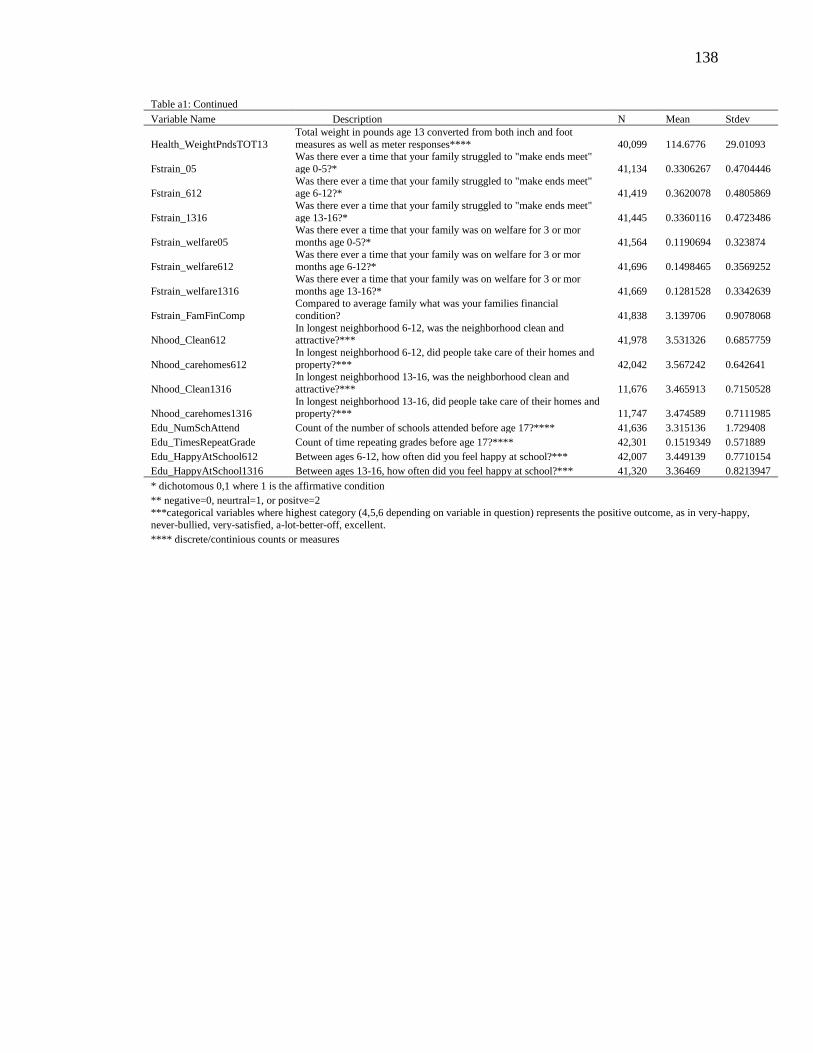
138

Table a1: Continued


Health_WeightPndsTOT13

Total weight in pounds age 13 converted from both inch and foot

measures as well as meter responses**** 40,099 114.6776 29.01093

Fstrain_05

Was there ever a time that your family struggled to "make ends meet"

age 0-5?* 41,134 0.3306267 0.4704446

Fstrain_612 Was there ever a time that your family struggled to "make ends meet" age 6-12?* 41,419 0.3620078 0.4805869

Fstrain_1316

Was there ever a time that your family struggled to "make ends meet"

age 13-16?* 41,445 0.3360116 0.4723486

Fstrain_welfare05

Was there ever a time that your family was on welfare for 3 or mor

months age 0-5?* 41,564 0.1190694 0.323874

Fstrain_welfare612 Was there ever a time that your family was on welfare for 3 or mor months age 6-12?* 41,696 0.1498465 0.3569252

Fstrain_welfare1316

Was there ever a time that your family was on welfare for 3 or mor

months age 13-16?* 41,669 0.1281528 0.3342639

Fstrain_FamFinComp

Compared to average family what was your families financial

condition? 41,838 3.139706 0.9078068

Nhood_Clean612 In longest neighborhood 6-12, was the neighborhood clean and attractive?*** 41,978 3.531326 0.6857759

Nhood_carehomes612

In longest neighborhood 6-12, did people take care of their homes and

property?*** 42,042 3.567242 0.642641

Nhood_Clean1316

In longest neighborhood 13-16, was the neighborhood clean and

attractive?*** 11,676 3.465913 0.7150528

Nhood_carehomes1316 In longest neighborhood 13-16, did people take care of their homes and property?*** 11,747 3.474589 0.7111985

Edu_NumSchAttend Count of the number of schools attended before age 17?**** 41,636 3.315136 1.729408

Edu_TimesRepeatGrade Count of time repeating grades before age 17?**** 42,301 0.1519349 0.571889

Edu_HappyAtSchool612 Between ages 6-12, how often did you feel happy at school?*** 42,007 3.449139 0.7710154

Edu_HappyAtSchool1316 Between ages 13-16, how often did you feel happy at school?*** 41,320 3.36469 0.8213947

* dichotomous 0,1 where 1 is the affirmative condition

** negative=0, neurtral=1, or positve=2

***categorical variables where highest category (4,5,6 depending on variable in question) represents the positive outcome, as in very-happy,

never-bullied, very-satisfied, a-lot-better-off, excellent.

**** discrete/continious counts or measures

139

13.3. Table a2: Logit Validation Models

FSTRAIN Model 1 Model 2 Model 3

VAR Expanded Sample Collapsed Sample

Hi/Lo Quartiles Sample

pc1 0.0218 0.0243 0.0363

(0.0219) (0.0560) (0.1000)

pc2 -0.0310 -0.0287 -0.0231

(0.0206) (0.0525) (0.0927)

pc3 -0.128*** -0.113 -0.0265

(0.0319) (0.0827) (0.145)

pc4 -0.0755*** -0.0871* -0.0758

(0.0187) (0.0453) (0.0751)

pc5 -0.0977*** -0.0600 -0.137

(0.0269) (0.0680) (0.109)

pc6 0.106*** 0.0957* 0.0683

(0.0200) (0.0517) (0.0907)

pc7 0.0471** 0.0533 -0.0232

(0.0223) (0.0572) (0.0868)

pc8 0.187*** 0.154** 0.166

(0.0301) (0.0776) (0.133)

pc9 0.00877 -0.000867 -0.121

(0.0258) (0.0659) (0.113)

pc10 -0.232*** -0.236*** -0.439***

(0.0233) (0.0594) (0.105)

pc11 0.0677*** 0.0713 0.188*

(0.0245) (0.0623) (0.113)

pc12 -0.210*** -0.198*** -0.222**

(0.0207) (0.0528) (0.0899)

pc13 0.0790*** 0.0876 0.114

(0.0231) (0.0592) (0.106)

pc14 -0.0940*** -0.103* -0.296***

(0.0228) (0.0586) (0.105)

pc15 0.0523** 0.0644 0.0951

(0.0241) (0.0660) (0.113)

pc16 -0.0689*** -0.0170 0.102

(0.0236) (0.0589) (0.0970)

pc17 0.0230 0.0186 0.0637

(0.0257) (0.0665) (0.116)

pc18 0.0183 0.00106 -0.0414

(0.0261) (0.0678) (0.118)

pc19 -0.0981*** -0.110** -0.279***

(0.0209) (0.0539) (0.0804)

pc20 0.0546** 0.0386 0.0266

(0.0254) (0.0646) (0.113)

AGE 0.0801 0.222 0.253

(0.0502) (0.136) (0.237)

MALE -0.147*** -0.102 -0.114

(0.0401) (0.103) (0.181)

Constant -1.142*** -1.422*** -2.780***

(0.0377) (0.0963) (0.171)

Observations 16,505 2,803 2,395

Standard errors in parentheses: *** p<0.01, ** p<0.05, * p<0.1

140

14. Programs

*--------------------------------------------------------------------------------------------------------------------

14.1.1. Program Chapter 2

* Authored by Glen McDermott

* University of New Mexico Department of Econ.

* Permanent Phone: 207-902-0354

* Permanent email: [email protected]

*---------------------------------------------------------------------------------------------------------------------

quietly {

clear

clear matrix

clear mata

set more off

capture log close

set matsize 10000

set maxvar 10000

}

*-----------------------------------------------------set log file---------------------------------------------------

display "Enter parameter date: " _request(date)

display $date

log using C:\stata\DRAFT_chapter1finaloutput_$date.smcl ,replace

*------------------------------------------------ working directory----------------------------------------------

cd "C:\stata\"

use .\Dis_Longform_411aaaaadg_bmi_5_20_17.dta

drop if AGE<25

drop if AGE>64

drop if RETIRE==1

xtset uniqueid time

tsfill, full

gen n_cor_jobswitching=.

replace n_cor_jobswitching=0 if cor_jobswitching==0

replace n_cor_jobswitching = cor_jobswitching

gen id=uniqueid

*---------------------------------- calculate Initial financial stress measures----------------------------------

*------------------------ deflate, replace "0" values with small positive value (.01) ------------------------

*---------------------------------- take logs of relevant financial measures -----------------------------------

{

quietly {

//first deflate all relevent variables

global deflatable "FAMINC CASHALL NWEALTH NWEALTH_EQ"

foreach x in $deflatable {

gen t_`x' = `x'*(deflator2009/100)

}

//replace zero values in cash and netwealth with small but positive

//values to make sure log can be calculated


replace t_`x'=.01 if t_`x'==0

}

141

//special replacements:

replace t_CASHALL=.01 if t_CASHALL<0

// to be sure the natural log has a positive value and recognize

//every individual has at least some income, I allow income wealth to remain negative

//but cash cannot be negative

//generate logs of relevant measures


gen LNDEF_`x'=ln(t_`x')

}

}

}

drop if time<5

{

gen ipwdep=0 if year==.

replace ipwdep=1 if ipwdep==.

global variablestvcomplete "AGE YSCHOO LNDEF_FAMINC LNDEF_CASHALL

LNDEF_NWEALTH_EQ NUMFAMCH STABLEMAR COR_HSTATUS BMI"

foreach x in $variablestvcomplete {

by uniqueid: egen IPWm_`x'=mean(`x')

}

logit ipwdep IPWm_*

predict PRobserved, pr

gen ipw=1/PRobserved

}

drop if year==.

//xtdescribe

{

gen rural=1 if BEALS==9 | BEALS==8 | BEALS==6

replace rural=0 if BEALS >=1 & BEALS <6

replace rural=0 if BEALS==7

}

*----------------------------------- begin financial strain measure development --------------------------------

global zeldesfstressmeasures "DEF_FSTRESS_Z1 DEF_FSTRESS_Z2"

global glensfstressmeasures "DEF_FSTRESS_G1 DEF_FSTRESS_G2 DEF_FSTRESS_G3

DEF_FSTRESS_G4 DEF_FSTRESS_G5"

{

gen DEF_FSTRESS_Z1=0

gen t_LNWEALTHRAT_Z1=LNDEF_NWEALTH_EQ/((LNDEF_FAMINC+l.LNDEF_FAMINC)/2)

replace DEF_FSTRESS_Z1=1 if t_LNWEALTHRAT_Z1 <1/6 | LNDEF_CASHALL <

(1/6)*l.LNDEF_FAMINC

replace DEF_FSTRESS_Z1=. if t_NWEALTH_EQ==.

gen DEF_FSTRESS_Z2 = 0

gen t_LNWEALTHRAT_Z2=LNDEF_NWEALTH/((LNDEF_FAMINC+l.LNDEF_FAMINC)/2)



replace DEF_FSTRESS_Z2=. if t_LNWEALTHRAT_Z2==.

gen cont_FSTRESS=.

replace cont_FSTRESS=(((LNDEF_NWEALTH-LNDEF_CASHALL)/ ///

((LNDEF_FAMINC+l.LNDEF_FAMINC)/2))+(LNDEF_CASHALL/LNDEF_FAMINC))/2

bysort uniqueid: egen indstdvcontFS = sd(cont_FSTRESS)

bysort uniqueid: egen indmeancontFS = mean(cont_FSTRESS)

142

gen coefVolcontFS = indstdvcontFS/indmeancontFS

}

---------------GENERATE VARIABLES THAT ARE REQUIRED FOR ANALYSIS--------------------

------------------------------- DEFINE GLOBAL VARIABLES ------------------------------------------------

quietly {

global x "AGE AGE2 AGE3 YSCHOO HINS STABLEMAR NUMFAMCH n_cor_jobswitching

DEF_FSTRESS_Z2"

global y "AGE AGE2 AGE3 YSCHOO HINS STABLEMAR NUMFAMCH"

global ixz "AGE YSCHOO "

global variablesHSTATUS "DEF_FSTRESS_Z2 n_cor_jobswitching AGE AGE2 AGE3 YSCHOO MALE

NON_WHITE1 d_II_COR_HSTATUS1 d_II_COR_HSTATUS2 d_II_COR_HSTATUS3

d_II_COR_HSTATUS4"

global exog "DEF_FSTRESS_Z2"

global ttime "7 8 9 10 11 12"

bysort uniqueid time: egen m_cor_pseudoch = mean(n_COR_PSEUDOCH)

corr m_cor_pseudoch PASTFS

}

gen nyearemp=12-yearemp

// makes increasing value a negative rather than a positive

{

xtset uniqueid time

tab time, generate(TIME)

}

{

sort uniqueid time

foreach var in $x {

bysort uniqueid: egen mean_`var'=mean(`var')

}

gen initob = 0

bysort uniqueid (year): replace initob = 1 if _n == 1

gen I_COR_HSTATUS = COR_HSTATUS if initob==1

by uniqueid:egen ii_COR_HSTATUS = mean(I_COR_HSTATUS)

foreach var in $ixz{

gen II_`var'=`var' if initob==1

}

sort time

reg I_COR_HSTATUS II_* NON_WHITE1 MALE PASTFS

predict p_I_COR_HSTATUS, xb

bysort uniqueid: egen pp_I_COR_HSTATUS=mean(p_I_COR_HSTATUS)

drop p_I_COR_HSTATUS

rename pp_I_COR_HSTATUS p_I_COR_HSTATUS

sort uniqueid time

gen l_COR_HSTATUS=l.COR_HSTATUS

tab ii_COR_HSTATUS, gen(d_II_COR_HSTATUS)

foreach var in $exog {

bysort uniqueid: egen mean2_`var'=mean(`var')

}

}

tab COR_HSTATUS, gen(HSTATUSd)

replace AGE3=AGE3/10

gen L_HSTATUS1 = l.HSTATUSd1

143





gen LHSD1=l.HSTATUSd1





gen l_HSTATUS=l.HSTATUS

sort uniqueid time

replace OWNRENT=0 if OWNRENT==5

*--------------------------------------------- Past average job switching------------------------------------------

gen temp_jsL1 =.

gen temp_jsL2 =.

gen temp_jsL3 =.

gen temp_jsL4 =.

gen temp_jsL5 =.

gen temp_jsL6 =.

gen temp_jsL7 =.

foreach n of num 1/7 {

bysort uniqueid: replace temp_jsL`n'=l`n'.n_cor_jobswitching

}

egen past_jobswitching_average= ///

rmean(temp_jsL1 temp_jsL2 temp_jsL3 temp_jsL4 temp_jsL5 temp_jsL6 temp_jsL7)

gen temp_fL1 =.

gen temp_fL2 =.

gen temp_fL3 =.

gen temp_fL4 =.

gen temp_fL5 =.

gen temp_fL6 =.

gen temp_fL7 =.

foreach n of num 1/7 {

bysort uniqueid: replace temp_fL`n'=l`n'.DEF_FSTRESS_Z2

}

egen past_FS_average= ///

rmean(temp_fL1 temp_fL2 temp_fL3 temp_fL4 temp_fL5 temp_fL6 temp_fL7)

drop temp_f*

---------------------------------------- Collect the estimation sample------------------------------------------------

foreach var in $x {

bysort uniqueid: egen mm_`var'=mean(`var')

}

xtoprobit COR_HSTATUS LHSD1 LHSD2 LHSD3 LHSD4 1.DEF_FSTRESS_Z2 n_cor_jobswitching ///

AGE AGE2 AGE3 NON_WHITE1 YSCHOO MALE HINS STABLEMAR NUMFAMCH

d_II_COR_HSTATUS1 ///

d_II_COR_HSTATUS2 d_II_COR_HSTATUS3 d_II_COR_HSTATUS4 ///

TIME2 TIME3 TIME4 TIME5 TIME6 TIME7 mm_* [pweight=ipw], vce(robust)

gen estimation_sample=e(sample)

summ if estimation_sample==0

144

drop mm_*

drop if estimation_sample==0

*-------------------SUMMARY STATISTICS FOR PAPER (CHAPTER 1) Table 2.7.1--------------------

summ COR_HSTATUS n_cor_jobswitching DEF_FSTRESS_Z1 NWEALTH FAMINC CASHALL ////

YSCHOO AGE MALE NON_WHITE1 LNDEF_FAMINC OWNRENT HINS STABLEMAR

NUMFAMCH

*---------------------------------What factors are affecting attrition in the sample --------------------------------

*-----------------------2.7.2. Table 2: Attrition Tests, Pooled Probit Specification, IPW clusters-------------

preserve

tsfill, full


foreach x in $variablesHSTATUS {

by uniqueid: egen IPW_HS_m_`x'=mean(`x')

}

probit ipwdep IPW_HS_m_* if time==6

outreg2 using c:\stata\Attrition_1_SRHS_$date.xls, ///

replace ct(PROBIT RESPONSE, probit, SRHS, InitCond, vce(cluster uniqueid))

foreach t in $ttime {

probit ipwdep IPW_HS_m_* if time==`t'

outreg2 using c:\stata\Attrition_1_SRHS_$date.xls, ///

append ct(PROBIT RESPONSE, probit, SRHS, InitCond, vce(cluster uniqueid))

}

restore

----------------------------------------------Variable addition testing------------------------------------------

-----------------------2.7.3. Table 3: Variable Addition Bias Test - Random Effects ------------------

-----------------Ordered Probit Model with IPW, modified CRE, and Strict CRE estimations --------

---------------------------------------------for M, F, and Combined--------------------------------------------

// test for bias driven by attition

drop if time<5

drop if year==.

by uniqueid: gen TOTALOBS=_N

gen ALL=1 if TOTALOBS==6

replace ALL=0 if ALL==.

// variable addition tests

preserve

foreach var in $y {


}

sort uniqueid time

xtoprobit COR_HSTATUS LHSD1 LHSD2 LHSD3 LHSD4 DEF_FSTRESS_Z2 n_cor_jobswitching ///

AGE AGE2 AGE3 NON_WHITE1 YSCHOO MALE HINS STABLEMAR NUMFAMCH

d_II_COR_HSTATUS1 d_II_COR_HSTATUS2 d_II_COR_HSTATUS3 d_II_COR_HSTATUS4 ///

TIME2 TIME3 TIME4 TIME5 TIME6 TIME7 mm_* past_* ALL TOTALOBS /*[pweight=ipw]*/ ///

if MALE==1, vce(robust)

estat ic

outreg2 using c:\stata\variableadditiontest_SRHS_$date.xls, ///

replace ct(Model 5m, MODCRE, Outcome=SAH, Unbalanced)


AGE AGE2 AGE3 NON_WHITE1 YSCHOO MALE HINS STABLEMAR NUMFAMCH ///


145



estat ic


append ct(Model 5f, MODCRE, Outcome=SAH, Unbalanced)





, vce(robust)

estat ic


append ct(Model 5m/f, MODCRE, Outcome=SAH, Unbalanced)

restore

preserve

foreach var in $x {


}

sort uniqueid time




TIME2 TIME3 TIME4 TIME5 TIME6 TIME7 mm_* /*past_**/ ALL TOTALOBS /*[pweight=ipw]*/ ///


estat ic


append ct(Model 6m, STRICTCRE, Outcome=SAH, Unbalanced)

sort uniqueid time






estat ic


append ct(Model 6f, STRICTCRE, Outcome=SAH, Unbalanced)

sort uniqueid time





, vce(robust)

estat ic


append ct(Model 6m/f, STRICTCRE, Outcome=SAH, Unbalanced)

restore

*------------------------------ 2.7.4 Table 4: Random Effect Ordered Probit Results ------------------------------

preserve

foreach var in $y {


}


146



TIME2 TIME3 TIME4 TIME5 TIME6 TIME7 past_* /*mm_* [pweight=ipw]*/, vce(robust)

outreg2 using c:\stata\output\TABLE4_boharaIV_$date.xls, ///

append ct(T4_Model 1 m/f, NO-IPW, Outcome SAH, xtoprobit, unbalanced)

estat ic

restore

preserve

foreach var in $y {


}




TIME2 TIME3 TIME4 TIME5 TIME6 TIME7 past_* mm_* /*[pweight=ipw]*/, ///

vce(robust)


append ct(T4_Model 2 m/f, NOIPW-MODCRE, Outcome SAH, xtoprobit, unbalanced)

estat ic

restore

preserve

foreach var in $x {


}




TIME2 TIME3 TIME4 TIME5 TIME6 TIME7 /*past_**/ mm_* /*[pweight=ipw]*/, vce(robust)


append ct(T4_Model 3 m/f, NOIPW FULLCRE, Outcome SAH, xtoprobit, unbalanced)

estat ic

restore

*------------------------------------------------Now add ipw--------------------------------------------------------------

preserve

foreach var in $y {


}




TIME2 TIME3 TIME4 TIME5 TIME6 TIME7 past_* /*mm_* */ [pweight=ipw], vce(robust)


append ct(T4_Mode4 1 m/f, IPW, Outcome SAH, xtoprobit, unbalanced)

estat ic

restore

preserve

foreach var in $y {


}


147



TIME2 TIME3 TIME4 TIME5 TIME6 TIME7 past_* mm_* [pweight=ipw], vce(robust)


append ct(T4_Model 5 m/f,IPW-MODCRE, Outcome SAH, xtoprobit, unbalanced)

estat ic

restore

preserve

foreach var in $x {


}




TIME2 TIME3 TIME4 TIME5 TIME6 TIME7 /*past_**/ mm_* [pweight=ipw], vce(robust)


append ct(T4_Model 6 m/f, IPW-FULLCRE, Outcome SAH, xtoprobit, unbalanced)

estat ic

restore

*----------------------Table 2.7.5: Table 5 Random Effect Ordered Probit Results - Sep M and F-------------

preserve

drop if MALE==0 ///////////// Sets Male

foreach var in $y {

//bysort uniqueid: egen mm_`var'=mean(`var')

}






replace ct(T5_Mode4m, IPW, Outcome SAH, xtoprobit, unbalanced)

estat ic

restore

preserve

drop if MALE==1 ///////////// Sets Female

foreach var in $y {


}






append ct(T5_Mode4f, IPW, Outcome SAH, xtoprobit, unbalanced)

estat ic

restore

preserve


148

foreach var in $y {


}






append ct(T5_Model5m,IPW-MODCRE, Outcome SAH, xtoprobit, unbalanced)

estat ic

restore

preserve


foreach var in $y {


}






append ct(T5_Model5f,IPW-MODCRE, Outcome SAH, xtoprobit, unbalanced)

estat ic

restore

preserve


foreach var in $x {


}






append ct(T5_Model6m, IPW-FULLCRE, Outcome SAH, xtoprobit, unbalanced)

estat ic

restore

preserve


foreach var in $x {


}






append ct(T5_Model6f, IPW-FULLCRE, Outcome SAH, xtoprobit, unbalanced)

estat ic

149

restore

*----------------------------------------------------------------------------------------------------------------------------

14.2. Chapter 3: State Based Reinsurance

* Program validation tables with

* Appendix Washington State Actuarial Report Study.

* Author: Glen McDermott

* Department of Economics, University of New Mexico

* Permanent Phone: 207.902.0354

* Permanent Email:[email protected]

*----------------------------------------------------------------------------------------------------------------------------

*---------------------------------Table 3.5.2 Table 2: Yearly Cost Trends-------------------------------------------

*------------------------Model 1 Values Culled from Wyman Actuarial Report-----------------------------------

quietly {

set obs 23

gen cost=0

gen year=_n

replace cost= 217500000 if year==1












gen lncost=ln(cost)

noisily:reg lncost year

outreg2 using C:\stata\AlaskaMedicaidCostChange_$number.xls, replace

}

*-------------------------Model 2 Values Culled from Bureau of Labor Statistics-----------------------------------

quietly {

clear

set obs 5000

gen year=_n

gen regioncost= .

replace regioncost= 3216 if year ==1

replace regioncost= 3795 if year ==2

replace regioncost = 3609 if year==3




global AKcostmultiplier = (.60+.37+.30)/3

gen AKregioncost=regioncost*$AKcostmultiplier

gen lnAKregioncost=ln(AKregioncost)

reg lnAKregioncost year

gen lnregioncost = ln(regioncost)

noisily: reg lnregioncost year

}

150

*------------------------ Table 3.5.3. Table 3: Results Alaska Medicaid Expansion------------------------------

/// simulate the market profitability change from Chapter 2 equation 6

/// changeinAB=(costbefore-costafter)/(1-mlr)

*----------------------------------------------- Prediction 1 Recovered*----------------------------------------------

clear

set obs 5000

set seed 12345

global PremiumB=6738

global CostB=7724

global AvgInflation=.0926

global stdevAvgInflation=.0028

global aggregatemktloss2015=30000000

global n2016=23038

quietly {

*----------------------------define model pabar=pbbar-((costB-CostA)/(1-maxcosts))+ -----------------------

*---------------------------------aggregatemktloss2015/(n2016(1-maxcosts))------------------------------------

generate randomHinflation=rnormal($AvgInflation, $stdevAvgInflation)

gen PremiumB=$PremiumB

gen CostB=$CostB

gen CostA=CostB*(1+randomHinflation)

gen maxcosts=.15

gen ca_cb=CostA-CostB

gen PremiumAbar= PremiumB+((ca_cb)/(1-maxcosts))+ ///

($aggregatemktloss2015/($n2016*(1-maxcosts)))

histogram PremiumAbar, bin(40) normal

save PremiumAbar, replace

egen t_m_abar=mean(PremiumAbar)

global meanPremiumAbar=t_m_abar[_n]

summ CostA

global stdevpremiumAbar=`r(sd)'

ci means PremiumAbar

}

display $stdevpremiumAbar

display

global upperbound95premiumAbar=$meanPremiumAbar+1.96*$stdevpremiumAbar

global lowerbound95premiumAbar=$meanPremiumAbar-1.96*$stdevpremiumAbar

summ PremiumAbar

display $upperbound95premiumAbar

display $lowerbound95premiumAbar

*---------------------------------------------------- Prediction 2 BLS-------------------------------------------------

clear

set obs 5000

set seed 12345


global CostB=7724




global n2016=23038

quietly {

*---------------------------define model pabar=pbbar-((costB-CostA)/(1-maxcosts))+ ------------------------

*----------------------------------aggregatemktloss2015/(n2016(1-maxcosts))-----------------------------------

151



gen CostB=$CostB


gen maxcosts=.15








summ CostA



}


display



summ PremiumAbar



*--------------------------------------------------- Prediction 3 Combined------------------------------------------

clear

set obs 5000

set seed 12345





global n2016=23038

quietly {

*------------------------------- define model pabar=pbbar-((costB-CostA)/(1-maxcosts))+ ------------------

*---------------------------------------aggregatemktloss2015/(n2016(1-maxcosts))-----------------------------



gen CostB=$CostB


gen maxcosts=.15








summ CostA



}


display

152



summ PremiumAbar



*-------------------Table 3.5.4 Table 4: Results Alaska Conditions Based Reinsurance Program-------------

*------------------------------------------------- Wyman prediction model-------------------------------------------

clear

set matsize 5000

global obs1=5000

set obs $obs1

// step 1, define input values for first run



global CostB=8439.24


//global aggregatemktloss2016=0

global n2016=24064

global n2017=23822

global E_c_r=78135359

global s_c=55000000

global n_trp=1300

global maxcosts=.15

global w=0

global RP_sd = 21903683

global RP_sd_per=.28033


global n2016=24064

global n2017=23822

quietly {

*-------------------------------------note p_nc should be equal to CS_PR_PR------------------------------------

global p_nc=normprob(($s_c-$E_c_r)/$RP_sd)

global n_trp=1300

global maxcosts=.15

matrix randomHinflation =J($obs1,1,.)

matrix costa = J($obs1,1,.)

matrix hrpfloat = J($obs1,1,.)

matrix abarrate = J($obs1,1,.)

forvalues y=1/$obs1 {

set seed 1000`y'

//display "counter = " `y'

local randomHinflation=rnormal($AvgInflation, $stdevAvgInflation)

//display "randominflation = " `randomHinflation'

matrix randomHinflation[`y',1]=`randomHinflation'

local CostA=$CostB*(1+`randomHinflation')

matrix costa[`y',1]=`CostA'

local itterAbar=0

local hrpfloat=rnormal($E_c_r, $RP_sd)

if `hrpfloat'<0 {

local hrpfloat=0

}

//display "hrpfloat = " `hrpfloat'

matrix hrpfloat[`y',1]=`hrpfloat'

153

forvalues x=1/10 {

//display "itterAbar = " ìtterAbar'

local sc=$s_c+($n_trp*ìtterAbar')

local pnc=1-normprob((`sc'-$E_c_r)/$RP_sd)

//display "sc = " `sc'

local numeratorpt1=($PremiumB*$n2016)*(1-$maxcosts)

local numeratorpt2=($n2017*`CostA'-$n2016*$CostB)

local numeratorpt3=($p_nc-1)*(`hrpfloat'-`sc')

local numeratorpt4=(1-$w)*`hrpfloat'

local numeratorpt5=$aggregatemktloss2016

local denominator=($n2017*(1-$maxcosts)-2*$n_trp)

local PremiumAbar=(`numeratorpt1'+`numeratorpt2'-`numeratorpt3'- ///

`numeratorpt4'+`numeratorpt5')/`denominator'

//display "PremiumAbar = " `PremiumAbar'

local test=abs((ìtterAbar'-`PremiumAbar')/ìtterAbar')

//display "test =" `test'

if `test' <= .0001 {

matrix abarrate[`y',1]=`PremiumAbar'

//display "next"

//display " "

continue, break

}

local itterAbar=`PremiumAbar'

}

}

//matrix list abarrate

svmat double abarrate, name(wy_rbara)

svmat double hrpfloat, name(wy_hrpfloat)

svmat randomHinflation, name(wy_randomHinflation)

svmat costa, name(wy_costa)

egen wy_meanPremiumAbar=mean(wy_rbara)

summ wy_rbara

}

global stdevpremiumAbar=r(sd)



gen wy_stdevpremiumAbar=$stdevpremiumAbar

global wyupperbound95premiumAbar=wy_meanPremiumAbar+1.96*$stdevpremiumAbar

global wylowerbound95premiumAbar=wy_meanPremiumAbar-1.96*$stdevpremiumAbar

display $wyupperbound95premiumAbar

display $wylowerbound95premiumAbar

summ wy_meanPremiumAbar

histogram wy_hrpfloat1, bin(100) normal

histogram wy_rbara1, bin(100) normal

clear matrix

*------------------------------------------------bls prediction model-----------------------------------------------------






global n2016=24064

global n2017=23822

154


global s_c=55000000

global n_trp=1300

global maxcosts=.15

global w=0




global n2016=24064

global n2017=23822

quietly {

// note p_nc should be equal to CS_PR_PR

global p_nc=1-normprob(($s_c-$E_c_r)/$RP_sd)

global n_trp=1300

global maxcosts=.15






set seed 1000`y'







local itterAbar=0


if `hrpfloat'<0 {

local hrpfloat=0

}



forvalues x=1/10 {
















if `test' <= .0001 {


//display "next"

155

//display " "

continue, break

}


}

}


svmat double abarrate, name(bls_rbara)

svmat double hrpfloat, name(bls_hrpfloat)

svmat randomHinflation, name(bls_randomHinflation)

svmat costa, name(bls_costa)

egen bls_meanPremiumAbar=mean(bls_rbara)

summ bls_rbara

}




gen bls_stdevpremiumAbar=$stdevpremiumAbar

global blsupperbound95premiumAbar=bls_meanPremiumAbar+1.96*$stdevpremiumAbar

global blslowerbound95premiumAbar=bls_meanPremiumAbar-1.96*$stdevpremiumAbar

display $blsupperbound95premiumAbar

display $blslowerbound95premiumAbar

summ bls_meanPremiumAbar

histogram bls_hrpfloat1, bin(100) normal

histogram bls_rbara1, bin(100) normal

clear matrix

*---------------------------------------------combined wyman and Bls prediction 3---------------------------------






global n2016=24064

global n2017=23822


global s_c=55000000

global n_trp=1300

global maxcosts=.15

global w=0




global n2016=24064

global n2017=23822

quietly {



global n_trp=1300

global maxcosts=.15





156


set seed 1000`y'







local itterAbar=0


if `hrpfloat'<0 {

local hrpfloat=0

}



forvalues x=1/10 {
















if `test' <= .0001 {


//display "next"

//display " "

continue, break

}


}

}


svmat double abarrate, name(c_rbara)

svmat double hrpfloat, name(c_hrpfloat)

svmat randomHinflation, name(c_randomHinflation)

svmat costa, name(c_costa)

egen c_meanPremiumAbar=mean(c_rbara)

summ c_rbara

}




gen c_stdevpremiumAbar=$stdevpremiumAbar

global cupperbound95premiumAbar=c_meanPremiumAbar+1.96*$stdevpremiumAbar

157

global clowerbound95premiumAbar=c_meanPremiumAbar-1.96*$stdevpremiumAbar



summ c_meanPremiumAbar

histogram c_hrpfloat1, bin(100) normal

histogram c_rbara1, bin(100) normal

clear matrix

display "wy upperbound95 = " $wyupperbound95premiumAbar

display "wy lowerboundbound95 = " $wylowerbound95premiumAbar

display "bls upperbound95 = " $blsupperbound95premiumAbar

display "bls lowerboundbound95 = " $blslowerbound95premiumAbar

display "combined upperbound95 = " $cupperbound95premiumAbar

display "combined lowerboundbound95 = "$clowerbound95premiumAbar

*------------------------- Table 3.5.6 Table 6: Results Alaska Conditions Based Reinsurance--------------------

*------------------------------------------------- Policy Scenarios --------------------------------------------------------

*...................................................................Simulation test 1: ……………………………………………….

*...................................................State implements a 15% Coinsurance "Tax"………………………………

local t ="one"

* Combined Wyman and Bls prediction 3

clear matrix







global n2016=24064

global n2017=23822


global s_c=55000000

global n_trp=1300

global maxcosts=.15

global w=.15




global n2016=24064

global n2017=23822

quietly {



global n_trp=1300

global maxcosts=.15






set seed 1000`y'





158



local itterAbar=0


if `hrpfloat'<0 {

local hrpfloat=0

}



forvalues x=1/10 {
















if `test' <= .0001 {


//display "next"

//display " "

continue, break

}


}

}


svmat double abarrate, name(`t'_rbara)

svmat double hrpfloat, name(`t'_hrpfloat)

svmat randomHinflation, name(`t'_randomHinflation)

svmat costa, name(`t'_costa)

egen `t'_meanPremiumAbar=mean(`t'_rbara)

summ `t'_rbara

}

local stdevpremiumAbar=r(sd)

display `stdevpremiumAbar'

//gen `t'_stdevpremiumAbar=$stdevpremiumAbar

local upperbound95premiumAbar=`t'_meanPremiumAbar+1.96*`stdevpremiumAbar'

local lowerbound95premiumAbar=`t'_meanPremiumAbar-1.96*`stdevpremiumAbar'

display ùpperbound95premiumAbar'

display `lowerbound95premiumAbar'

summ `t'_meanPremiumAbar

histogram `t'_hrpfloat1, bin(100) normal

histogram `t'_rbara1, bin(100) normal

// use welch satterthwhithe equation to evaluate degrees of

159

//freedom on t test of two independent samples of equal size with

//different variances

gen `t'_tstat = (`t'_meanPremiumAbar - c_meanPremiumAbar)/ ///

sqrt((c_stdevpremiumAbar^2+`stdevpremiumAbar'^2)/$obs1)

gen `t'_df=(((c_stdevpremiumAbar+`stdevpremiumAbar')/$obs1)^2)/ ///

((1/($obs1-1))*((c_stdevpremiumAbar^2+`stdevpremiumAbar'^2)/$obs1^2))

summ `t'_tstat `t'_df

display "strongly significant at <.001"

*------------------------------------------Simulation Test 2--------------------------------------------------------------

* With the recent pass of the Trump tax bill and the removal of the

* individual mandate: the argument that those leaving the pool are healthy

* -> higher costs for the remaining patients. In this case, we take the

* approach that, all else equal, higher costs imply higher premiums -> 5%

* increase in costs and yields a 7.5% increase in premiums.

local t ="two"

//////// combined wyman and Bls prediction 3

clear matrix







global n2016=24064

global n2017=23822


global s_c=55000000

global n_trp=1300

global maxcosts=.15

global w=0




quietly {



global n_trp=1300

global maxcosts=.15






set seed 1000`y'







local itterAbar=0


160

if `hrpfloat'<0 {

local hrpfloat=0

}



forvalues x=1/10 {
















if `test' <= .0001 {


//display "next"

//display " "

continue, break

}


}

}







summ `t'_rbara

}











// use welch satterthwhithe equation to evaluate degrees of freedom

//on t test of two independent samples of equal size with different variances



161



summ one_tstat one_df `t'_tstat `t'_df


*-----------------------------------------------------Simulation Test 3--------------------------------------------------

* change both population and expected cost

local t ="three"

//////// combined wyman and Bls prediction 3

clear matrix







global n2016=24064

global n2017=23822*.95


global s_c=55000000

global n_trp=1300

global maxcosts=.15

global w=0




quietly {



global n_trp=1300

global maxcosts=.15






set seed 1000`y'







local itterAbar=0


if `hrpfloat'<0 {

local hrpfloat=0

}



forvalues x=1/10 {




162













if `test' <= .0001 {


//display "next"

//display " "

continue, break

}


}

}







summ `t'_rbara

}











// use welch satterthwhithe equation to evaluate degrees of freedom on t

// test of two independent samples of equal size with different variances





summ one_tstat one_df `t'_tstat `t'_df


display "combined upperbound95 = " $cupperbound95premiumAbar

display "combined lowerboundbound95 = "$clowerbound95premiumAbar

* --------------------------- 12.2.1.2 Table A2: REinsurance Pool Sufficiency Analysis----------------------

* simulate the market profitability change from Chapter 2 equation 6

* changeinAB=(costbefore-costafter)/(1-mlr)

163

clear

set obs 5000

set seed 12345

global L=66000

global T=1000000

global Na=297000

global Nb=290000

global rb=6767

global ra=6090

global omega=0

global sumec=5247

global w=.5

global ec=141357.27

global stdevmu=6748.91

global stdevNa=.01051*$Na

global delta=.15

*------------------------- define model p=(($Nb*$rb-$Na*$ra)*(1-$delta)- ------------------------------------

*----------------------($Nb-$Na)*$sumec+$omega)/($Na*(1-$w)*($ec-$L))----------------------------------

generate r_ec=rnormal($ec, $stdevmu)

generate r_Na=rnormal($Na, $stdevNa)

//gen Psick= ((($Nb*$rb-r_Na*$ra)*(1-$delta))-(($Nb-r_Na)* ///

($sumec))+$omega)/(r_Na*(1-$w)*(r_ec-$L))

gen Psick= ((($Nb*$rb-$Na*$ra)*(1-$delta))- ///

(($Nb-$Na)*($sumec))+$omega)/($Na*(1-$w)*(r_ec-$L))

histogram r_Na, bin(400) normal

summ r_Na

histogram Psick, bin(400) normal

save Psick, replace

egen meanPsick=mean(Psick)

summ Psick

global stdevPsick=`r(sd)'

global upperbound95_Psick=meanPsick+(1.96*$stdevPsick)

global lowerbound95_Psick=meanPsick-(1.96*$stdevPsick)

summ Psick

display $upperbound95_Psick

display $lowerbound95_Psick

*---------------------------------------------------------------------------------------------------------------------------

14.3. Chapter 4 Programs

* Chapter 4 Base Program Began 12/2017

* PCA Generation, and Analysis Dataset Construction

* Includes flattening and explicitly developing a frequency weighted dataset

* Written by: Glen McDermott


* Permanent Phone: 207-902-0354

* Permanent email:[email protected]

*---------------------------------------------------------------------------------------------------------------------------

quietly {

clear

clear matrix

clear mata

set more off

capture log close

164

set matsize 10000

set maxvar 10000

}

*-----------------------------------------------------set log file-------------------------------------------------------


display $date

log using C:\stata\Chapter3\DRAFT_chapter3finaloutput_$date.smcl ,replace

*------------------------------------------------working directory--------------------------------------------------

cd "C:\stata\Chapter3"

use .\Dis_Chapter3.dta

// note that this is the unbalanced panel

drop if AGE<25

drop if AGE>64

drop if RETIRE==1

xtset uniqueid time

tsfill, full




gen id=uniqueid

*---------------- calculate Initial financial stress measures-

*---------------- deflate, replace "0" values with small positive value (.01)-

*----------------- take logs of relevent financial measures -

{

quietly {





}

//replace zero values in cash and netwealth with small

//but positive values to make sure log can be calculated



}



//I allow income an wealth to remain negative but cash cannot be negative

//generate logs of relevent measures



}

}

}

{







165

}

logit ipwdep IPWm_*



}

drop if time<5

drop if year==.

xtdescribe

{




}

*-------------------------------------- begin financial strain measure developmment -----------------------------

global zeldesfstressmeasures "DEF_FSTRESS_Z1 DEF_FSTRESS_Z2"

global glensfstressmeasures "DEF_FSTRESS_G1 DEF_FSTRESS_G2 DEF_FSTRESS_G3

DEF_FSTRESS_G4 DEF_FSTRESS_G5"

{


gen

t_LNWEALTHRAT_Z1=LNDEF_NWEALTH_EQ/((LNDEF_FAMINC+l.LNDEF_FAMINC)/2)









gen cont_FSTRESS=.

replace cont_FSTRESS=(((LNDEF_NWEALTH-

LNDEF_CASHALL)/((LNDEF_FAMINC+l.LNDEF_FAMINC)/2))+(LNDEF_CASHALL/LNDEF_FAM

INC))/2




*--------------------- GENERATE VARIABLES THAT ARE REQUIRED FOR ANALYSIS------------------

*----------------------------------------DEFINE GLOBAL VARIABLES---------------------------------------------

quietly {

global x "AGE YSCHOO n_cor_jobswitching HINS STABLEMAR NUMFAMCH"



global xlist Fam_* Sta_* Soc_* Sec_* Health_* Fstrain_* Nhood_* Edu_*

global id uniqueid

bysort uniqueid time: egen m_cor_pseudoch = mean(n_COR_PSEUDOCH)

corr m_cor_pseudoch PASTFS

}

gen nyearemp=12-yearemp // makes increasing value a negative rather than a positive

quietly {

xtset uniqueid time

gen l4maFSTRESS = l4.DEF_FSTRESS_Z2


166



egen ma_DEF_FSTRESS_Z2 = rowmean( l4maFSTRESS l3maFSTRESS l2maFSTRESS l1maFSTRESS

DEF_FSTRESS_Z2)

xtset uniqueid time

gen l4maJS = l4.n_cor_jobswitching




egen ma_JS = rowmean( l4maJS l3maJS l2maJS l1maJS n_cor_jobswitching)

}

{

gen compoundstress=.

replace compoundstress=DEF_FSTRESS_Z2+n_cor_jobswitching

reg DEF_FSTRESS_Z2 AGE

predict noafstress, r

reg COR_HSTATUS AGE

predict noahstatus, r

reg n_COR_PSEUDOCH AGE

predict noapseudoch, r

corr noafstress noahstatus noapseudoch COR_COHORT

xtset uniqueid time


}

{

sort uniqueid time

foreach var in $x {


}

gen initob = 0






}

sort time






sort uniqueid time





}

}





167










sort uniqueid time

forvalues x = 1/100 {

gen bsr`x'= ipw

}


* Sch=School, Nhood=Neighborhood, Health=health, Sta=Stability,

* Soc=Social, Sec=Security Fstrain

forvalues x=1/10 {

gen t_divcounter`x'=0

replace t_divcounter`x'=1 if Sta_AgeParDivorce`x'!=.

}

gen Fam_CumulativeDiv=0

replace Fam_CumulativeDiv=t_divcounter1+t_divcounter2+t_divcounter3+ ///

t_divcounter4+t_divcounter5+t_divcounter6+t_divcounter7+t_divcounter8+ ///

t_divcounter9+t_divcounter10

replace Fam_CumulativeDiv=. if Sta_ParDivorce==.

drop Sta_AgeParDivorce* Sta_ParDivorce

//rename Health_SAHS C_SAHS

drop Fam_WomanW* Fam_MomRel* Fam_ManWho* Fam_DadRel* Sta_AgeMove* ///

Edu_AgeSch* Health_HeightMtype Health_HeightFt Health_HeightIn ///

Health_WeightMtype Health_WeightPounds Health_WeightKG Edu_RepeatGrade ///

Edu_GradeFirstRpt Edu_GradeLastRpt AGE2 AGE3 AGE4 Health_HeightMtr

bysort uniqueid: egen m_Age=mean(AGE)

keep $xlist n_cor_jobswitching DEF_FSTRESS_Z1 DEF_FSTRESS_Z2 uniqueid time ///

AGE* NON_WHITE1 MALE INDWT2013 YSCHOO LNDEF_FAMINC //C_SAHS

summ $xlist

//drop list to have full dataset, implies dropping neighborhood safety measures,

// not asked of those who never moved... so reduces study to only those who have moved.

// dropping these to look at individuals who have always stayed put

// no way to incorporate them in the main analysis, can look at the subgroup

// separately.

drop Sec_NhoodSafeNight1316 Sec_NhoodSafeDay1316 Sec_HhoodSafeNightKid1316 ///

Soc_NeighborHelp1316 Soc_NeighborCloseKnit1316 Nhood_Clean1316 ///

Nhood_carehomes1316

// ALSO DROPPING KIDS WHO CLAIM NO ROMANTIC RELATIONSHIP BETWEEN 13 AND 16

// AGAIN WILL HAVE TO COVER IN SUB-ANALYSIS

drop Soc_BFGFRelPositive

drop if Health_Diabetes==. //drops 1 observation that is missing health answers

by uniqueid: gen count=_N

summ count

*-------------------------------------------------Collapse Dataset -------------------------------------------------

collapse (mean) AGE LNDEF_FAMINC (sum) n_cor_jobswitching DEF_FSTRESS_Z1 ///

DEF_FSTRESS_Z2 (max) $xlist count MALE INDWT2013 YSCHOO NON_WHITE1, ///

by(uniqueid)

168

local vmeans "n_cor_jobswitching DEF_FSTRESS_Z1 DEF_FSTRESS_Z2 LNDEF_FAMINC"

foreach x in `vmeans' {

gen norm_`x'=`x'/count

egen m_`x'=mean(norm_`x')

summ `x'

gen d_`x'=.

local sd=r(sd)

replace d_`x'=0 if `x'<m_`x'

replace d_`x'=1 if `x'>m_`x'

xtile qrt_`x'=`x',nq(4)

gen extr_`x'=1 if qrt_`x'==4

replace extr_`x'=0 if qrt_`x'==1

//drop qrt_`x'

}

Sum

*-------------------------- Expand dataset to create explicit frequency weights------------------------------

*------------------------------Assists in creating a common dataset between---------------------------------

*------------------------------------Matlab and Stata analysis modules ----------------------------------------

expand count

summ

global ncomp 60

//Principal component analysis

//pca $xlist, mineigen(1)

pca $xlist, comp($ncomp) blanks(.3)

rotate, varimax blanks(.3)

* scatterplot of the loadings and score variables

screeplot, yline(1)

save screeplot_rotatedCompVmax, replace

loadingplot

save loadingplot_rotatedCompVmax, replace

//1scoreplot

estat loadings

predict pc1 pc2 pc3 pc4 pc5 pc6 pc7 pc8 pc9 pc10 pc11 pc12 pc13 pc14 pc15 ///

pc16 pc17 pc18 pc19 pc20 pc21 pc22 pc23 pc24 pc25 pc26 pc27 pc28 pc29 pc30 ///


pc46 pc47 pc48 pc49 pc50 pc51 pc52 pc53 pc54 pc55 pc56 pc57, score

summ

*--------------------------------- Create Slimmed Dataset for Analysis (Prog 3_3) ----------------------------

preserve

*…………………………………………………………………………………………………………..

* FOR CREATING A NEW SENSITIVITY DATASET

keep pc* *n_cor_jobswitching *DEF_FSTRESS_Z1 *DEF_FSTRESS_Z2 uniqueid ///

YSCHOO AGE NON_WHITE1 MALE *LNDEF_FAMINC

*………………………………………………………………………………………………………….

gen Dschool=.

replace Dschool=1 if YSCHOO>12

replace Dschool=0 if YSCHOO<=12

foreach v of var *{

label variable `v' "rhs"

}

label variable n_cor_jobswitching "lhs"

label variable DEF_FSTRESS_Z1 "lhs"


169

label variable uniqueid "other"

//label variable time "other"

label variable NON_WHITE1 "rhs"

label variable MALE "rhs"

//label variable OWNRENT "rhs"

label variable LNDEF_FAMINC "rhs"

//label variable sample "other"

gen di_jobswitch=0

egen mm_jobswitch= mean(n_cor_jobswitching)

bysort uniqueid: egen m_jobswitch=mean(n_cor_jobswitching)

replace di_jobswitch=1 if m_jobswitch>mm_jobswitch

label variable di_jobswitch "lhs"

drop m_jobswitch

forvalues v=1/57 {

quietly: summ pc`v'

local sdpc=r(sd)

local meanpc=r(mean)

quietly: replace pc`v'= (pc`v'-`meanpc')/`sdpc'

quietly:summ pc`v'

}

*-------------------------------Export Both CSV and Stata datasets ------------------------------------------

export delimited using ///

"C:\stata\Chapter3\csvpcadata57_js_mfseparate_vmax2_collapsed_expand.csv", ///

replace

/// FOR CREATING A NEW SENSITIVITY DATASET

save pcanlaytical_full57_mfseparate_vmax2_collapsed_expand, replace

//////////////////////////////////////////////////////////////

restore

*-------------------------------------------End Program ---------------------------------------------------------

*---------------------------------------------------------------------------------------------------------------------

14.3.1. Chapter 4 PCA Development

* Generate Summary Statistics pre-normalization Table 4.5.3: Table 1:Summary

* Statistics for Analytical Dataset Before Normalization

* Written By Glen McDermott

* University of New Mexico

* Permanent phone: 207.902.0354


*---------------------------------------------------------------------------------------------------------------------

quietly {

clear

clear matrix

clear mata

set more off

capture log close

set matsize 10000

set maxvar 10000

}

*---------------------------set log file-----------------------------------------------------------------------------


display $date

170

log using C:\stata\Chapter3\DRAFT_chapter3finaloutput_$date.smcl ,replace

*------------------------working directory-----------------------------------------------------------------------


use .\Dis_Chapter3.dta

// note that this is the unbalanced panel

drop if AGE<25

drop if AGE>64

drop if RETIRE==1

xtset uniqueid time

tsfill, full




gen id=uniqueid

*---------------- calculate Initial financial stress measures-----------------------------------------------------

*-----------deflate, replace "0" values with small positive value (.01)---------------------------------------

*----------------- take logs of relevent financial measures -----------------------------------------------------

{

quietly {





}

//replace zero values in cash and netwealth with s

//mall but positive values to make sure log can be calculated



}



// to be sure the natural log has a positive value and

//recogonize every individual has

//I allow income an wealth to remain negative but cash cannot be negative

//generate logs of relevent measures



}

}

}

{







}

logit ipwdep IPWm_*



}

drop if time<5

171

drop if year==.

xtdescribe

{




}

*----------------------------- begin financial strain measure developmment -----------------------------------

{


gen

t_LNWEALTHRAT_Z1=LNDEF_NWEALTH_EQ/((LNDEF_FAMINC+l.LNDEF_FAMINC)/2)









gen cont_FSTRESS=.

replace cont_FSTRESS=(((LNDEF_NWEALTH-

LNDEF_CASHALL)/((LNDEF_FAMINC+l.LNDEF_FAMINC)/2))+(LNDEF_CASHALL/LNDEF_FAM

INC))/2




*------------------------------------------ DEFINE GLOBAL VARIABLES---------------------------------------

quietly {

}

gen nyearemp=12-yearemp // makes increasing value a negative rather than a positive

quietly {

xtset uniqueid time





egen ma_DEF_FSTRESS_Z2 = rowmean( l4maFSTRESS l3maFSTRESS l2maFSTRESS l1maFSTRESS

DEF_FSTRESS_Z2)

xtset uniqueid time





egen ma_JS = rowmean( l4maJS l3maJS l2maJS l1maJS n_cor_jobswitching)

}

{

gen compoundstress=.

replace compoundstress=DEF_FSTRESS_Z2+n_cor_jobswitching

reg DEF_FSTRESS_Z2 AGE

predict noafstress, r

172

reg COR_HSTATUS AGE

predict noahstatus, r

reg n_COR_PSEUDOCH AGE

predict noapseudoch, r

corr noafstress noahstatus noapseudoch COR_COHORT

xtset uniqueid time


}

{

sort uniqueid time

global x "AGE YSCHOO n_cor_jobswitching HINS STABLEMAR NUMFAMCH"


foreach var in $x {


}

gen initob = 0






}

sort time






sort uniqueid time






}

}














sort uniqueid time

forvalues x = 1/100 {

gen bsr`x'= ipw

173

}


* Sch=School, Nhood=Neighborhood, Health=health, Sta=Stability,

* Soc=Social, Sec=Security Fstrain

forvalues x=1/10 {

gen t_divcounter`x'=0

replace t_divcounter`x'=1 if Sta_AgeParDivorce`x'!=.

}

gen Fam_CumulativeDiv=0

replace Fam_CumulativeDiv=t_divcounter1+t_divcounter2+t_divcounter3+ ///

t_divcounter4+t_divcounter5+t_divcounter6+t_divcounter7+t_divcounter8+ ///

t_divcounter9+t_divcounter10

replace Fam_CumulativeDiv=. if Sta_ParDivorce==.

drop Sta_AgeParDivorce* Sta_ParDivorce

global xlist Fam_* Sta_* Soc_* Sec_* Health_* Fstrain_* Nhood_* Edu_*

drop Fam_WomanW* Fam_MomRel* Fam_ManWho* Fam_DadRel* Sta_AgeMove* ///

Edu_AgeSch* Health_HeightMtype Health_HeightFt Health_HeightIn ///

Health_WeightMtype Health_WeightPounds Health_WeightKG Edu_RepeatGrade ///

Edu_GradeFirstRpt Edu_GradeLastRpt AGE2 AGE3 AGE4 Health_HeightMtr

bysort uniqueid: egen m_Age=mean(AGE)

keep $xlist n_cor_jobswitching DEF_FSTRESS_Z1 DEF_FSTRESS_Z2 uniqueid time AGE*

NON_WHITE1 MALE INDWT2013 YSCHOO LNDEF_FAMINC //C_SAHS

global id uniqueid

summ $xlist

//drop list to have full dataset, implies dropping neighborhood safety measures,

// not asked of those who never moved... so reduces study to only those who have moved.

// dropping these to look at individuals who have always stayed put

// no way to incorporate them in the main analysis, can look at the subgroup

// seperately.

drop Sec_NhoodSafeNight1316 Sec_NhoodSafeDay1316 Sec_HhoodSafeNightKid1316 ///

Soc_NeighborHelp1316 Soc_NeighborCloseKnit1316 Nhood_Clean1316 ///

Nhood_carehomes1316

// ALSO DROPPING KIDS WHO CLAIM NO ROMANTIC RELATIONSHIP BETWEEN 13 AND 16

// AGAIN WILL HAVE TO COVER IN SUB-ANALYSIS

drop Soc_BFGFRelPositive

drop if Health_Diabetes==. //drops 1 observation that is missing health answers

by uniqueid: gen count=_N

summ count

collapse (mean) AGE LNDEF_FAMINC (sum) n_cor_jobswitching DEF_FSTRESS_Z1 ///

DEF_FSTRESS_Z2 (max) $xlist count MALE INDWT2013 YSCHOO NON_WHITE1, ///

by(uniqueid)

local vmeans "n_cor_jobswitching DEF_FSTRESS_Z1 DEF_FSTRESS_Z2 LNDEF_FAMINC"

foreach x in `vmeans' {

gen norm_`x'=`x'/count

egen m_`x'=mean(norm_`x')

summ `x'

gen d_`x'=.

local sd=r(sd)

replace d_`x'=0 if `x'<m_`x'

replace d_`x'=1 if `x'>m_`x'

174

xtile qrt_`x'=`x',nq(4)

gen extr_`x'=1 if qrt_`x'==4

replace extr_`x'=0 if qrt_`x'==1

//drop qrt_`x'

}

summ

expand count

summ

global ncomp 60

///////// Principal component analysis

pca $xlist, comp($ncomp) blanks(.3)

rotate, varimax blanks(.3)

* scatterplot of the loadings and score variables

screeplot, yline(1)

save screeplot_rotatedCompVmax, replace

loadingplot

save loadingplot_rotatedCompVmax, replace

*----------------------------------------------------scoreplot--------------------------------------------------------------

estat loadings

predict pc1 pc2 pc3 pc4 pc5 pc6 pc7 pc8 pc9 pc10 pc11 pc12 pc13 pc14 pc15 ///



pc46 pc47 pc48 pc49 pc50 pc51 pc52 pc53 pc54 pc55 pc56 pc57, score

summ

preserve

*------------------------------FOR CREATING A NEW SENSITIVITY DATASET-------------------------

*---------------------------------- Only Need to Run Once below this line --------------------------------------

keep pc* *n_cor_jobswitching *DEF_FSTRESS_Z1 *DEF_FSTRESS_Z2 uniqueid YSCHOO ///

AGE NON_WHITE1 MALE *LNDEF_FAMINC //C_SAHS

gen Dschool=.

replace Dschool=1 if YSCHOO>12

replace Dschool=0 if YSCHOO<=12

foreach v of var *{

label variable `v' "rhs"

}

label variable n_cor_jobswitching "lhs"



label variable uniqueid "other"

label variable NON_WHITE1 "rhs"

label variable MALE "rhs"

label variable LNDEF_FAMINC "rhs"

gen di_jobswitch=0

egen mm_jobswitch= mean(n_cor_jobswitching)

bysort uniqueid: egen m_jobswitch=mean(n_cor_jobswitching)

replace di_jobswitch=1 if m_jobswitch>mm_jobswitch

label variable di_jobswitch "lhs"

drop m_jobswitch

*------4.5.1: Summary Statists for Analytical Dataset Before Normalization----

summ pc1-pc20

*------------------------------------ Normalize pc variables: 0u, 1sd----------------------------------------------

175

forvalues v=1/57 {

quietly: summ pc`v'

local sdpc=r(sd)

local meanpc=r(mean)

quietly: replace pc`v'= (pc`v'-`meanpc')/`sdpc'

quietly:summ pc`v'

}

*-----------------------export datasets for analysis--------------------------

export delimited using ///

"C:\stata\Chapter3\csvpcadata57_js_mfseparate_vmax2_collapsed_expand.csv", ///

replace

/// FOR CREATING A NEW SENSITIVITY DATASET

save pcanlaytical_full57_mfseparate_vmax2_collapsed_expand, replace

restore

*------------------------------ End ------------------------------------------

*---------------------------------------------------------------------------------------------------------------------

14.3.2. Chapter 4 Stata Data Analysis * Glen McDermott


* Permanent Phone: 207.902.0354


*----------------------------------------------------------------------------------------------------------------------

* Logit Robustness and Sensitivity data Appendix 4 table 13.3 Table A2

* Also generate sensitivity data for export to:

* Chapter3DissertationVault_MasterSpreadsheet.xlsx

* Generation of Matlab Dataset for CART and Decision Tree Analysis

*---------------------------------------------------------------------------------------------------------------------

clear

clear matrix

clear mata

set more off

capture log close

set matsize 10001

set maxvar 5000


use pcanlaytical_full57_mfseparate_vmax2_collapsed_expand // From PCA_GENERATION

log using LogitMaleSatelli3_14_18.smcl, replace

gen agegroup=.

replace agegroup=0 if AGE<40 // approximate equal proportions old and young

replace agegroup=1 if AGE<=65 & AGE>=40

summ if d_DEF_FSTRESS_Z2==1

local comps=20 // pick how many components you want to use as inputs

forvalues d=1/57 {

if `d'>`comps' {

drop pc`d'

}

}

matrix APEmargins=J(60,3,.)

logit d_DEF_FSTRESS_Z2 pc* agegroup MALE NON_WHITE1

margins, dydx(*)

logit d_DEF_FSTRESS_Z2 pc* agegroup MALE NON_WHITE1 if NON_WHITE==1

margins, dydx(*)

176

local i=3

matrix likelihood = J(26,1,.)

logit d_DEF_FSTRESS_Z2

matrix likelihood[1,1]=(-2)*è(ll)'


matrix likelihood[2,1]=(-2)*è(ll)'

forvalues v=1/20 {

logit d_DEF_FSTRESS_Z2 pc`v'

matrix likelihood[ì',1]=(-2)*è(ll)'

local ++i

}

matrix list likelihood

matrix sensitivity=J(20,3,.)

forvalues i=1/20 {

matrix sensitivity[ì',1]= likelihood[1,1] - likelihood[2,1]

local third =ì'+2

matrix sensitivity[ì',2]= likelihood[1,1] - likelihood[`third',1]

matrix sensitivity[ì',3]= sensitivity[ì',2] / sensitivity[ì',1]

}

///////////////////// Matrix Results for Analysis Spreadsheet

///////////////// name: Chapter3DissertationVault_MasterSpreadsheet.xlsx

matrix list sensitivity

//////////////////// Export Matlab Analysis Dataset /////////////////////

preserve

keep pc* NON_WHITE1 agegroup MALE d_*

//export delimited using "C:\stata\Chapter3\Chapter3MatlabDatasetEsample_d.csv", replace

restore

*-------------------------------- Table 13.3; Table a2: Logit Validation Models----------------------------------

*………………………………………………… Model 1……………………………………………….


outreg2 using chapter3_logitverification628.xls, replace

summ

duplicates drop

summ


outreg2 using chapter3_logitverification628.xls, append

summ qrt_DEF_FSTRESS_Z2

drop if qrt_DEF_FSTRESS_Z2==2 | qrt_DEF_FSTRESS_Z2==3

summ qrt_DEF_FSTRESS_Z2

replace qrt_DEF_FSTRESS_Z2=0 if qrt_DEF_FSTRESS_Z2==1

replace qrt_DEF_FSTRESS_Z2=1 if qrt_DEF_FSTRESS_Z2==4


outreg2 using chapter3_logitverification628.xls, append

%----------------------------------------------------------------------------------------------------------------------------

14.3.3. Chapter 4 Matlab Analysis % Matlab Program Chapter 3

% Cart and Decision Tree Analysis

% Glen McDermott

% Department of Economics, University of New Mexico

% Permanent Phone: 207-902-0354

177

% Permanent email: [email protected]

%----------------------------------------------------------------------------------------------------------------------------

% Note, coefficients can be found by opening output Classification

% Bagged Ensemble "coefXXXX", then within, open Trained, then within open

% each 1x1 compact vector, then open "Coeffs" a 2x2 structure. Open the

% top right cell, copy and paste Const value to spreadsheet, open "Linear"

% copy vector of linear coefficients to spreadsheet. Repeat this for each

% 1x1 compact vector (number of bootstrap repetitions).

% Then export excel spreadsheet to stata and summarize the coefficients

% for mean and standard deviation.

%----------------------------------------------- Data Preparation ------------------------------------------------------

data=readtable('c:\stata\chapter3\Chapter3MatlabDatasetEsample_d.csv')

RFBOTHcleandata=rmmissing(data)

RFBOTHtrainingData=RFBOTHcleandata

savedRng=1

rng(savedRng); % For reproducibility

BOTHinputTable = RFBOTHtrainingData;

RFWHITEds = data(data.NON_WHITE1~=1,:);

RFWHITEcleandata = rmmissing(RFWHITEds)

WHITEinputTable = RFWHITEcleandata;

RFNONWHITEds = data(data.NON_WHITE1~=0,:);

RFNONWHITEcleandata = rmmissing(RFNONWHITEds)

RFNONWWHITEinputTable = RFNONWHITEcleandata;

%----------------------------------------SOME COMMON VARIABLES-----------------------------------------

COMMONpredictorNames = {'pc1', 'pc2', 'pc3', 'pc4', 'pc5', 'pc6', ...

'pc7', 'pc8', 'pc9', 'pc10', 'pc11', 'pc12','pc13', 'pc14' ...

'pc15', 'pc16', 'pc17', 'pc18', 'pc19', 'pc20', 'agegroup' ...

'MALE', 'NON_WHITE1'};

COMMONCategoricalPredictor = [false, false, false, false, false, ...

false, false, false, false, false, false, false, ...

false, false, false, false, false, false, false, ...

false, true, true, true];

COMMONtemplate = templateTree(...

'MaxNumSplits', 10025);

% --------------------------------COLLECT APPROPRIATE PREDICTORS---------------------------------------

BOTHpredictors = BOTHinputTable(:, COMMONpredictorNames);

BOTHresponse = BOTHinputTable.d_DEF_FSTRESS_Z2;

WHITEpredictors = WHITEinputTable(:, COMMONpredictorNames);

WHITEresponse = WHITEinputTable.d_DEF_FSTRESS_Z2;

NONWHITEpredictors = RFNONWWHITEinputTable(:, COMMONpredictorNames);

NONWHITEresponse = RFNONWWHITEinputTable.d_DEF_FSTRESS_Z2;

% ------------------------------ TRAIN RF CLASSIFIER FOR BOTH M AND F--------------------------------

template = templateTree(...

'SplitCriterion', 'twoing', ...

'MaxNumSplits', 150, ...

'Surrogate', 'off', ...

'ClassNames', [0; 1]);

coef=templateDiscriminant('FillCoeffs','on');

RFBOTHclassificationEnsembleRF = fitcensemble(...

BOTHpredictors, ...

BOTHresponse, ...

'Learners', template, ...

'Method', 'Bag', ...

178

'NumLearningCycles', 30, ...


% ---------------------------------Create the result struct with predict function--------------------------------------

RFBOTHpredictorExtractionFcn = @(t) t(:, COMMONpredictorNames);

RFBOTHensemblePredictFcn = @(x) predict(RFBOTHclassificationEnsembleRF, x);

RFBOTHtrainedClassifier.predictFcn = ...

@(x) RFBOTHensemblePredictFcn(RFBOTHpredictorExtractionFcn(x));

% ---------------------------------Add additional fields to the result struct--------------------------------------------

RFBOTHtrainedClassifier.RequiredVariables = COMMONpredictorNames;

RFBOTHtrainedClassifier.ClassificationEnsemble = ...

RFBOTHclassificationEnsembleRF;

% -------------------------------------------Perform cross-validation----------------------------------------------------

RFBOTHpartitionedModel = ...

crossval(RFBOTHtrainedClassifier.ClassificationEnsemble, 'KFold', 10);

% -----------------------------------------Compute validation predictions----------------------------------------------

[RFBOTHvalidationPredictions, RFBOTHvalidationScores] = ...

kfoldPredict(RFBOTHpartitionedModel);

% ------------------------------------------Compute validation accuracy-----------------------------------------------

aRFBOTHvalidationAccuracy_rf = 1 - ...

kfoldLoss(RFBOTHpartitionedModel, 'LossFun', 'ClassifError');

aRFBOTHimportance_randomforest= ...

predictorImportance(RFBOTHclassificationEnsembleRF);

% --------------------------------------------fit coeficients to models---------------------------------------------------

% ---------------------------------------Train MALE RF CLASSIFIER-----------------------------------------------

RFWHITEclassificationEnsembleRF = fitcensemble(...

WHITEpredictors, ...

WHITEresponse, ...





% --------------------------------Create the result struct with predict function-------------------------------------

RFWHITEpredictorExtractionFcn = @(t) t(:, COMMONpredictorNames);

RFWHITEensemblePredictFcn = @(x) predict(RFWHITEclassificationEnsembleRF, x);

RFWHITEtrainedClassifier.predictFcn = ...

@(x) RFWHITEensemblePredictFcn(RFWHITEpredictorExtractionFcn(x));

% ----------------------------------Add additional fields to the result struct---------------------------------------

RFWHITEtrainedClassifier.RequiredVariables = COMMONpredictorNames;

RFWHITEtrainedClassifier.ClassificationEnsemble = ...

RFWHITEclassificationEnsembleRF;

% ----------------------------------------Perform cross-validation------------------------------------------------

RFWHITEpartitionedModel = ...

crossval(RFWHITEtrainedClassifier.ClassificationEnsemble, 'KFold', 10);

% -----------------------------------Compute validation predictions---------------------------------------------

[RFWHITEvalidationPredictions, RFWHITEvalidationScores] = ...

kfoldPredict(RFWHITEpartitionedModel);

% -------------------------------------Compute validation accuracy----------------------------------------------

aRFWHITEvalidationAccuracy_rf = 1 - ...

kfoldLoss(RFWHITEpartitionedModel, 'LossFun', 'ClassifError');

aRFWHITEimportance_randomforest=. ...

predictorImportance(RFWHITEclassificationEnsembleRF);

% -------------------------NOW DO FEMALE ONLY RANDOM FOREST CLASSIFIER---------------

% ---------------------------------------Train FEMALE RF CLASSIFIER-------------------------------------

179

RFNONWHITEclassificationEnsembleRF = fitcensemble(...

NONWHITEpredictors, ...

NONWHITEresponse, ...





% -------------------------------Create the result struct with predict function---------------------------------

RFNONWHITEpredictorExtractionFcn = @(t) t(:, COMMONpredictorNames);

RFNONWHITEensemblePredictFcn = ...

@(x) predict(RFNONWHITEclassificationEnsembleRF, x);

RFNONWHITEtrainedClassifier.predictFcn = ...

@(x) RFNONWHITEensemblePredictFcn(RFNONWHITEpredictorExtractionFcn(x));

% ----------------------------------Add additional fields to the result struct-----------------------------------

RFNONWHITEtrainedClassifier.RequiredVariables = COMMONpredictorNames;

RFNONWHITEtrainedClassifier.ClassificationEnsemble = ...

RFNONWHITEclassificationEnsembleRF;

% ------------------------------------------Perform cross-validation---------------------------------------------

RFNONWHITEpartitionedModel = ...

crossval(RFNONWHITEtrainedClassifier.ClassificationEnsemble, 'KFold', 10);

% --------------------------------------Compute validation predictions-----------------------------------------

[RFNONWHITEvalidationPredictions, RFNONWHITEvalidationScores] = ...

kfoldPredict(RFNONWHITEpartitionedModel);

% ---------------------------------------Compute validation accuracy------------------------------------------

aRFNONWHITEvalidationAccuracy_rf = 1 - ...

kfoldLoss(RFNONWHITEpartitionedModel, 'LossFun', 'ClassifError');

aRFNONWHITEimportance_randomforest=...

predictorImportance(RFNONWHITEclassificationEnsembleRF);

%--------------------------------------- Extract coeficient estimates---------------------------------------------

coefRFBoth = fitcensemble(...

BOTHpredictors, ...

BOTHresponse, ...


'Learners', coef, ...




coefRFWHITE = fitcensemble(...


WHITEresponse, ...






coefRFNONWHITE = fitcensemble(...








180

%-----------------------------------------------------------------------------------------------------------------------------

% NOW INTO CLASSIFICATION TREE MODEL

%-----------------------------------------------------------------------------------------------------------------------------

% -------------------------------TRAIN THE DECISION TREE FOR BOTH--------------------------------------

DTBOTHclassificationTree = fitctree(...

BOTHpredictors, ...

BOTHresponse, ...

'SplitCriterion', 'gdi', ...




% -----------------------------------Create the result struct with predict function-------------------------------------

DTBOTHpredictorExtractionFcn = @(t) t(:, COMMONpredictorNames);

DTBOTHtreePredictFcn = @(x) predict(DTBOTHclassificationTree, x);

DTBOTHtrainedClassifier.predictFcn = ...

@(x) DTBOTHtreePredictFcn(DTBOTHpredictorExtractionFcn(x));

% -------------------------------------Add additional fields to the result struct---------------------------------------

DTBOTHtrainedClassifier.RequiredVariables = COMMONpredictorNames;

DTBOTHtrainedClassifier.ClassificationTree = DTBOTHclassificationTree;

% --------------------------------------------Perform cross-validation--------------------------------------------------

DTBOTHpartitionedModel = ...

crossval(DTBOTHtrainedClassifier.ClassificationTree, 'KFold', 10);

% --------------------------------------Compute validation predictions------------------------------------------------

[DTBOTHvalidationPredictions, DTBOTHvalidationScores] = ...

kfoldPredict(DTBOTHpartitionedModel);

% ---------------------------------------Compute validation accuracy-------------------------------------------------

aDTBOTHvalidationAccuracy_ctree = 1 - ...

kfoldLoss(DTBOTHpartitionedModel, 'LossFun', 'ClassifError');

aDTBOTHimportance_classtree=predictorImportance(DTBOTHclassificationTree);

% ------------------------------ TRAIN THE DECISION TREE FOR MALE--------------------------------------

DTWHITEclassificationTree = fitctree(...


WHITEresponse, ...





% -------------------------------Create the result struct with predict function----------------------------------------

DTWHITEpredictorExtractionFcn = @(t) t(:, COMMONpredictorNames);

DTWHITEtreePredictFcn = @(x) predict(DTWHITEclassificationTree, x);

DTWHITEtrainedClassifier.predictFcn = ...

@(x) DTWHITEtreePredictFcn(DTWHITEpredictorExtractionFcn(x));

% -------------------------------Add additional fields to the result struct----------------------------------------------

DTWHITEtrainedClassifier.RequiredVariables = COMMONpredictorNames;

DTWHITEtrainedClassifier.ClassificationTree = DTWHITEclassificationTree;

% ---------------------------------------Perform cross-validation--------------------------------------------------------

DTWHITEpartitionedModel = ...

crossval(DTWHITEtrainedClassifier.ClassificationTree, 'KFold', 10);

% -----------------------------------Compute validation predictions----------------------------------------------------

[DTWHITEvalidationPredictions, DTWHITEvalidationScores] = ...

kfoldPredict(DTWHITEpartitionedModel);

% -----------------------------------Compute validation accuracy-------------------------------------------------------

aDTWHITEvalidationAccuracy_ctree = 1 - ...

181

kfoldLoss(DTWHITEpartitionedModel, 'LossFun', 'ClassifError');

aDTWHITEimportance_classtree=predictorImportance(DTWHITEclassificationTree);

% -------------------------TRAIN THE DECISION TREE FOR FEMALE------------------------------------------

DTNONWHITEclassificationTree = fitctree(...







% ----------------------------Create the result struct with predict function---------------------------------------------

DTNONWHITEpredictorExtractionFcn = @(t) t(:, COMMONpredictorNames);

DTNONWHITEtreePredictFcn = @(x) predict(DTNONWHITEclassificationTree, x);

DTNONWHITEtrainedClassifier.predictFcn = ...

@(x) DTNONWHITEtreePredictFcn(DTNONWHITEpredictorExtractionFcn(x));

% --------------------------------Add additional fields to the result struct----------------------------------------------

DTNONWHITEtrainedClassifier.RequiredVariables = COMMONpredictorNames;

DTNONWHITEtrainedClassifier.ClassificationTree = DTNONWHITEclassificationTree;

% ------------------------------------------Perform cross-validation------------------------------------------------------

DTNONWHITEpartitionedModel = ...

crossval(DTNONWHITEtrainedClassifier.ClassificationTree, 'KFold', 10);

% ----------------------------------------Compute validation predictions-----------------------------------------------

[DTNONWHITEvalidationPredictions, DTNONWHITEvalidationScores] = ...

kfoldPredict(DTNONWHITEpartitionedModel);

% ------------------------------------------Compute validation accuracy-------------------------------------------------

aDTNONWHITEvalidationAccuracy_ctree = 1 - ...

kfoldLoss(DTNONWHITEpartitionedModel, 'LossFun', 'ClassifError');

aDTNONWHITEimportance_classtree= ...

predictorImportance(DTNONWHITEclassificationTree);

*----------------------------------------------------------------------------------------------------------------------------- ---

14.4. PSID Compilation Program for Chapter 2 * This script is used to extract, collate and create an global analytical dataset

* From the 1994-2013 Family and Individual PSID Files.

* The script is expandable but requires the user to have identified the

* appropriate relationship between variables across the years of interest.

* For example, in 1994 variable A had ID “B” and in 1995, variable A had ID “C”

* Thus the script need to rename all variables, for they all change names year over year

* Modification is thus likely to be tedius and, albiet intuitively laid out, all changes

* Should be meticioulsy telegraphed across relevant sections.

* Script By Glen McDermott



* Phone: 207.902.0354

*----------------------------------------------------------------------------------------------------------- --------------------

*-----------------------------------------------------------Platform SETUP------------------------------------------------

quietly {

clear

clear matrix

clear mata

set more off

mailto:[email protected]

182

capture log close

set matsize 10000

set maxvar 10000

* set log file

log using c:\stata\dis_bc1.smcl,replace

* working directory

cd "C:\Users\Hay Handsome\Documents\LIBRARIES\University\Dissertation\psid_data\"

* temporary storage *

tempfile FAM94 FAM95 FAM96 FAM97 FAM99 FAM01 FAM03 FAM05 FAM07 FAM09 FAM11

FAM13 1999SVAR 2001SVAR 2003SVAR 2005SVAR 2007SVAR

}

*-------------------------------------------------CHANGE ORDERS------------------------------------------------

quietly {

* because the dataset is so badly unbalanced, I left truncate the dataset with individuals who

* were observed in 1997. Right truncation is allowed to grow through attrition. Because right side

* attrition can be caused by death or departure, it may become important to control for attrition

*

* other outcome variables that might be interesting - use nights in hospital HNIGHTS - use second

* heart attacks HHEART2

*

* approx. line 623, deduce marital status change for wife given marital status change for head

* approx. line 780, didn't collect wife variables for dividend, interest, trust fund, income

*

* Because I have the age of diagnosis for the chronic disease, I can tabulate when a diagnosis was

* made, either before the panel, or during the panel, rather than having all diagnoses appear in the

* last 5 observations. This might clear up the problem with AGE...or age is actually beneficial

* disease starts earlier....if you get past the window, you are more likely to stay healthy...something

* like that.

*-------------------------------------------CHANGED SUCCESSFULLY-----------------------------------------

* Around line 5390, I drop individuals who don't report age, but the way it is written it will drop

* an observation if age is not included, I need to check each individual to see if age is ever included

* if so, keep the observation and impute the missing age. - CHECK AGE BY FIRST YEAR AND

* UNIQUEID, DROPS

* THE WHOLE PERSON, NOT JUST THE OBSERVATIONS WHICH ARE UNDER AGE

* construct BMI index and/or repair overweight (OW) measure. eg define means by m/f

* as it stands few women will be underweight - DONE 1/28

* Around line 5400, I drop if income is <1 in any given period, this may put holes in my already

* sparse data, it might be better to identify individuals where income drops below 0 but only drop the

* individual if income is never > 0 - SINCE INCOME CANNOT BE NEGATIVE, I ASSUME

* THAT INCOME < 0 IS AR

* REPORTING ERROR, AS SUCH I ADJUST ALL INCOME OF 0 OR <0 TO $1 TO

* FACILITATE GENERATING A VALID LOG

**********************************************************************************

}

*----------------------SUPPLEMENTARY DATASETS USED IN THIS ANALYSIS-----------------------

quietly {

insheet using "C:\stata\dissertation data\OCCU_LABOR.csv"

rename cor_occu COR_OCCU

save "C:\stata\dissertation data\OCCU_LABOR.dta", replace

clear

}

*------------------------------------------------------------------------------------------------------- ----------------

* occupation groups - https://www.census.gov/people/eeotabulation/documentation/jobgroups.pd

183

quietly {

insheet using "C:\stata\dissertation data\OCCU_GROUPS.csv"

rename cor_occu COR_OCCU

save "C:\stata\dissertation data\OCCU_GROUPS.dta", replace

clear

}

*--------------------------Import Primary PSID datasets organize collate and merge ------------------------

*

*-------------------------------- Begin "Individual" File Processing --------------------------------------------

* From the Individual cross year file we need, the: 1968 family ID, Individual ID, each

* years interview id, and whether the individual is the head or what

* These are the important variables from 94 forward from the INDIVIDUAL DATASET

quietly {

use ER30001 ER30002 ER31996 ER31997 ER32000 ER32004 ER33101 ER33201 ER33301 ///

ER33401 ER33501 ER33601 ER33701 ER33801 ER33901 ER34001 ER34101 ER34201 ///






ER34002 ER34102 ER34202 ///

using crossyear_ind.dta, clear // last row is a set of sequence numbers

}

*--------------------------------create user friendly names -----------------------------------------------------

quietly{

rename (ER33102 ER33202 ER33302 ER33402 ER33502 ER33602 ER33702 ER33802 ER33902///

ER34002 ER34102 ER34202) ///

(SEQ1994 SEQ1995 SEQ1996 SEQ1997 SEQ1999 SEQ2001 SEQ2003 SEQ2005 SEQ2007 ///

SEQ2009 SEQ2011 SEQ2013)

gen seqlink2013CRSS = SEQ2013

rename (ER31996 ER31997) (stratum_variable cluster_variable)

rename (ER33430 ER33546 ER33637 ER33740 ER33848 ER33950 ER34045 ER34154 ER34268) ///

(IND_WT1997 IND_WT1999 IND_WT2001 IND_WT2003 IND_WT2005 IND_WT2007 ///

IND_WT2009 IND_WT2011 IND_WT2013)

gen INDWT2013=IND_WT2013 // in case a single weight is preferable for an individual

// Dead Section

rename (ER32004) (DEAD)

}

// Rename family and individual id's

rename (ER30001 ER30002) (famid indid)

rename (ER32000) (MALE)

// Alter gender to reflect FEMALE==0 MALE==1

quietly {

replace MALE=0 if MALE==2 // 0 = female turned to dummy variable [0,1]

drop if MALE>2 // gets rid of one ambigious designation [1 observation]

}

// ------------------Next rename the yearly interview number with a user friendly names (UFN)-------------

quietly{

rename (ER33101 ER33201 ER33301 ER33401 ER33501 ER33601 ER33701 ER33801

ER33901 ER34001 ER34101 ER34201) ///

(intid1994 intid1995 intid1996 intid1997 intid1999 intid2001 intid2003 intid2005 ///

intid2007 intid2009 intid2011 intid2013)

}

184

// -------------------link variable for the Childhood Retrospective Circumstances Survey--------------------

quietly{

* Rename yearly head of household variables UFN

rename (ER33103 ER33203 ER33303 ER33403 ER33503 ER33603 ER33703 ER33803 ER33903 ///

ER34003 ER34103 ER34203) ///

(head1994 head1995 head1996 head1997 head1999 head2001 head2003 head2005 head2007 ///

head2009 head2011 head2013)

* -------------------Rename employment Status at interview from individual file UFN ----------------------

rename (ER33111 ER33211 ER33311 ER33411 ER33512 ER33612 ER33712 ///

ER33813 ER33913 ER34016 ER34116 ER34216) ///

(EMP1S1994 EMP1S1995 EMP1S1996 EMP1S1997 EMP1S1999 EMP1S2001 ///

EMP1S2003 EMP1S2005 EMP1S2007 EMP1S2009 EMP1S2011 EMP1S2013)

}

* ------------create a unique id using the standard PSID format family id *1000 + individual id-----------

gen uniqueid=famid*1000+indid

* Store base individual dataset

save .\Dis_dataset\individual_variables, replace

*------------------- --------------------end "Individual" File Processing -------------------------------------------

clear

*--------------Begin - Add required SXXX variables to appropriate family datasets 99 - 2007- ------------

* Add missing SXXX variables to the appropriate Family Datasets 99 - 2007

// NOTE: N_svar.dta and s411a.dta add new "s" variables to existing work,

// this selection ofcherry picked variables from the PSID website was

//constructed and imported after the intial program was developed

quietly {

use allSVAR.dta

keep ER13002 S417 S419 S416 S416A S417A S411 S411A S417 S418 S402

* ----------------------------------------1999 variables of interest ---------------------------------------------------

sort ER13002

save "1999SVAR", replace

use fam1999er.dta

sort ER13002

merge m:m ER13002 using 1999SVAR, keep(matched)

drop _merge

save fam1999er_a.dta, replace

use allSVAR.dta

keep ER17002 S517 S519 S516 S516A S517A S511 S511A S518 S502

*----------------------------------------2001 variables of interest -----------------------------------------------------

sort ER17002


use fam2001er.dta

sort ER17002


drop _merge


clear

use allSVAR.dta

keep ER21002 S617 S619 S616A S617A S611 S611A S616 S618 S602

*-----------------------------------------2003 variables of interest ----------------------------------------------------

sort ER21002

185


use fam2003er.dta

sort ER21002


drop _merge


clear

use allSVAR.dta

keep ER25002 S717 S719 S716A S717A S711 S711A S718 S702 S716

*-----------------------------------------2005 variables of interest ---------------------------------------------------

sort ER25002


use fam2005er.dta

sort ER25002


drop _merge


clear

use allSVAR.dta

keep ER36002 S817 S819 S818 S816A S817A S811 S811A S802 S816

*---------------------------------------------2007 variables of interest --------------------------------------

sort ER36002


use fam2007er.dta

sort ER36002


/*drop _merge */


}

* --------------------------delete temporary datasets created in this step -------------------------------

quietly{

erase 2007SVAR.dta

erase 2005SVAR.dta

erase 2003SVAR.dta

erase 2001SVAR.dta

erase 1999SVAR.dta

}

* --------------------Collect relevant variables, build a wide dataset of 94 - 2013 variables--------------

* …………………………………..1994's FAMILY file variables…………………………………..

quietly {

use ER2002 ER3853 ER2007 ER2005A ER4159B ER2032 ER2008 ER4158 ER4019 ER2069 ///

ER2128 ER2129 ER2130 ER2119 ER2120 ER2121 ER2122 ER2123 ER2124 ER2125 ER2126 ///









ER2988 ER3010 ER3032 ER3054 ///

using fam1994er.dta

rename ER2002 intid1994

186

sort intid1994

save "FAM94", replace

merge 1:m intid1994 using .\Dis_dataset\individual_variables, keep(using matched)

sort famid indid

drop _merge

save FAMIND94, replace

}

*……………………………………….1995's family file variables ………………………………………

quietly {

// number in family unit

//[94]ER2006 [95]ER5005 [96]ER7005 [97]ER10008 [99]ER13009 [01]ER17012

//[03]ER21016 [05]ER25016 [07]ER36016 [09]ER42016 [11]ER47316 [13]ER53016

// number of children in family unit

// [94]ER2010 [95]ER5009 [96]ER7009 [97]ER10012 [99]ER13013 [01]ER17016

//[03]ER21020 [05]ER25020 [07]ER36020 [09]ER42020 [11]ER47320 [13]ER53020

// work disability head

// [94]ER3855 [95]ER6725 [96]ER8971 [97]ER11725 [99]ER15450 [01]ER19615

//[03]ER23015 [05]ER26996 [07]ER38207 [09]ER44180 [11]ER49499 [13]ER55249

// work disability wife

//[94]ER3860 [95]ER6730 [96]ER8976 [97]ER11729 [99]ER15558 [01]ER19723

//[03]ER23142 [05]ER27119 [07]ER39304 [09]ER45277 [11]ER50617 [13]ER56365

// health insurance - coverage last two year...anyone covered including govt prog

//[99]ER15779 [01]ER19840 [03]ER23277 [05]ER27237 [07]ER40409 [09]ER46382

//[11]ER51743

}

quietly {







ER5234 ER5256 ER5278 ER5300 ER5479 ER5501 ER5523 ER5545 ///






using fam1995er.dta


sort intid1995


merge 1:m intid1995 using .\Dis_dataset\individual_variables, ///

keep(using matched)

sort famid indid

drop _merge


}

*………………………………………..1996's family file variables……………………………………….

quietly {


ER7223 ER7224 ER7225 ER7214 ER7215 ER7216 ER7217 ER7218 ER7219 ER7220 ///


187



ER7005 ER7009 ER8971 ER8976 ///








ER8150 ///

using fam1996er.dta


sort intid1996



sort famid indid

drop _merge


}

*……………………………………….1997's family file variables ………………………………………

quietly {

use ER10002 ER10009 ER10004A ER12165 ER12223B ER10035 ER10010 ER12222 ER10011 ///





ER10629 ER10630 ER10631 ER10008 ER10012 ER11725 ER11729 ///








ER11044 ER12084 ///

using fam1997er.dta


sort intid1997



sort famid indid

drop _merge


}

*………………………………………… 1999's family file variables ……………………………………

quietly {

use ER13002 ER15020 S419 ER15447 ER15031 ER15553 ER15554 ER15552 ER13010 ER13012 ///

ER13008A ER15932 ER16424 ER13040 ER13011 ER16516 ER13261 ER13205 ///



ER14509 ER14525 ER14524 S417 ER15928 ER15836 ER15661 ER15662 ER15660 ///


188


ER15558 ER15779 ///

ER14300 ER14301 ER15787 ER15793 S417 S416A S416 S417A S411 S411A ///

ER15541 ER15649 ER15539 ER15647 ER16431C ///

ER15031 ER15111 ER15100 ER15543 ER15651 ER16454 S418 S402 ///










ER14227 ER16518 ///

using fam1999er_a.dta


sort intid1999



sort famid indid

drop _merge


}

*……………………………………… 2001's family file variables……………………………………

quietly {

use ER17002 ER19216 S519 ER19612 ER19227 ER19718 ER19719 ER19717 ER17013 ///

ER17015 ER17007 ///




ER18683 ER18682 S517 ER19989 ER19897 ER19826 ER19827 ER19825 ER20458 ER17786 ///



ER18438 ER18439 ER19848 S516A S516 S517A S511 S511A ///

ER19854 ER19706 ER19814 ER19704 ER19812 ER20377C ///

ER19227 ER19307 ER19296 ER19708 ER19816 ER20450 S518 S502 ///



ER19617 ER19725 ///

ER17408 ER17435 ER17460A ER17486 ER17690 ER17716 ER17742 ER17768 ER17978 ///







ER18355 ER20394 ///



sort intid2001



189

keep(using matched)

sort famid indid

drop _merge


}

*………………………………………2003's family file variables ……………………………………..

quietly {




ER21142 ER21143 ER21144 ER24099 ER24140 ER24142 ER23090 ER22021 ER22020 //

ER22038 ER22037 ER22055 ER22054 S617 ER23426 ER23334 ER23260 ER23261 ///



ER21020 ER23015 ER23142 ER23277 ER21703 ER21704 S616A S616 S617A S611 S611A ///

ER23285 ER23291 ER23120 ER23247 ER23118 ER23245 ER24144A ER22622 ER22702 ///

ER22691 ER23123 ER23250 ER24101 S618 S602 ER23065 ER23192 ER23071 ER23198 ///













sort intid2003



keep(using matched)

sort famid indid

drop _merge


}

*…………………………………….2005's family file variables…………………………………………

quietly {






ER26019 ER26018 ER26036 ER26035 S717 ER27122 ER27126 ER27130 ER27134 ///





ER25829 ER25823 ER25824 ER27245 ER27251 S716A S716 S717A S711 S711A ER27092 ///

ER27215 ER27094 ER27217 ER28043A ER26603 ER26683 ER26672 ER27098 ER27221 ///

ER28002 S718 S702 ER27026 ER27149 ER27014 ER27137 ER27010 ER27133 ER27038 ///


190









ER25508 ER25509 ER25510 ER25511 ER28078 ///



sort intid2005



keep(using matched)

sort famid indid

drop _merge


}

*-----------------------------------------------2007's family file variables ----------------------------------------

quietly {

use ER36002 ER37595 S819 ER38226 ER38222 ER38250 ER38234 ER38215 ER38214 ER38218 ///




ER41029 ER41031 ER38268 ER37020 ER37019 ER37037 ER37036 ER37054 ER37053 S817 ///





ER36841 ER36842 ER40420 ER40426 ER38303 ER39400 ER38305 ER39402 ER41033A S816A ///

S816 S817A S811 S811A ER37621 ER37701 ER37690 ER38309 ER39406 ER40992 S818 S802 ///










ER36515 ER36516 ER41069 ///



sort intid2007



keep(using matched)

sort famid indid

drop _merge


}

*-------------------------------------------------2009's family file variables---------------------------------------------

191

quietly {

use ER42002 ER43586 ER46964 ER44199 ER44195 ER44223 ER44207 ER44188 ER44187 ER44191 ///










ER44276 ER45373 ER44278 ER45375 ER46975A ER43612 ER43692 ER43681 ER44282 ER45379 ///










ER45279 ER42536 ER42537 ER42538 ER42539 ER47012 ///

using fam2009er.dta


sort intid2009



keep(using matched)

sort famid indid

drop _merge


}

*--------------------------------------------------2011's family file variables-------------------------------------------

quietly {

use ER47302 ER48911 ER52368 ER49525 ER49520 ER49555 ER49535 ER49510 ER49509 ER49515 ///


















ER49616 ER50734 ER52399A ER49037 ER49026 ER49620 ER50738 ER52308 ER52366 ER52344 ///

192



ER47856 ER47857 ER52436 ///

using fam2011er.dta


sort intid2011



keep(using matched)

sort famid indid

drop _merge


}

*---------------------------------------------2013's family file variables--------------------------------------------

quietly {

use ER53002 ER54661 ER58181 ER55275 ER55270 ER55304 ER55285 ER55260 ER55259 ///























ER53558 ER53559 ER53560 ER53561 ER53562 ER53563 ER58257 ///

using fam2013er.dta


sort intid2013



keep(using matched)

sort famid indid

drop _merge


}

*------------------------------End collection of relevant "Family" file variables --------------------------------*

*------------------------------------------ Merge the grand dataset --------------------------------------------------*

quietly {

use FAMIND94, clear

193

merge famid indid ///

using FAMIND95 FAMIND96 FAMIND97 FAMIND99 FAMIND01 ///

FAMIND03 FAMIND05 FAMIND07 FAMIND09 FAMIND11 FAMIND13

drop _merge

}

*--------------------------------.Rename grand dataset variables for reshaping-------------------------------------

quietly{


(F_SW1997 F_SW1999 F_SW2001 F_SW2003 F_SW2005 F_SW2007 F_SW2009 F_SW2011 ///

F_SW2013)

rename ( ER21281 ER25270 ER36275 ER42302 ER47615 ER53315 ) ///

( head_additionalplus_job2003 head_additionalplus_job2005 head_additionalplus_job2007 ///

head_additionalplus_job2009 head_additionalplus_job2011 head_additionalplus_job2013 )


( wife_additionalplus_job2003 wife_additionalplus_job2005 wife_additionalplus_job2007 ///

wife_additionalplus_job2009 wife_additionalplus_job2011 wife_additionalplus_job2013 )


( haddjob1_jan2003 haddjob1_jan2005 haddjob1_jan2007 haddjob1_jan2009 haddjob1_jan2011 ///

haddjob1_jan2013 )


( haddjob1_feb2003 haddjob1_feb2005 haddjob1_feb2007 haddjob1_feb2009 haddjob1_feb2011 ///

haddjob1_feb2013 )


( haddjob1_mar2003 haddjob1_mar2005 haddjob1_mar2007 haddjob1_mar2009 haddjob1_mar2011 ///

haddjob1_mar2013 )


( haddjob1_apr2003 haddjob1_apr2005 haddjob1_apr2007 haddjob1_apr2009 haddjob1_apr2011 ///

haddjob1_apr2013 )


( haddjob1_may2003 haddjob1_may2005 haddjob1_may2007 haddjob1_may2009 haddjob1_may2011 ///

haddjob1_may2013 )


( haddjob1_jun2003 haddjob1_jun2005 haddjob1_jun2007 haddjob1_jun2009 haddjob1_jun2011 ///

haddjob1_jun2013 )


( haddjob1_jul2003 haddjob1_jul2005 haddjob1_jul2007 haddjob1_jul2009 haddjob1_jul2011 ///

haddjob1_jul2013 )


( haddjob1_aug2003 haddjob1_aug2005 haddjob1_aug2007 haddjob1_aug2009 haddjob1_aug2011 ///

haddjob1_aug2013 )


( haddjob1_sept2003 haddjob1_sept2005 haddjob1_sept2007 haddjob1_sept2009 haddjob1_sept2011///

haddjob1_sept2013 )


( haddjob1_oct2003 haddjob1_oct2005 haddjob1_oct2007 haddjob1_oct2009 haddjob1_oct2011 ///

haddjob1_oct2013 )


( haddjob1_nov2003 haddjob1_nov2005 haddjob1_nov2007 haddjob1_nov2009 haddjob1_nov2011 ///

haddjob1_nov2013 )


( haddjob1_dec2003 haddjob1_dec2005 haddjob1_dec2007 haddjob1_dec2009 haddjob1_dec2011 ///

haddjob1_dec2013 )


194

( waddjob1_jan2003 waddjob1_jan2005 waddjob1_jan2007 waddjob1_jan2009 waddjob1_jan2011 ///

waddjob1_jan2013 )


( waddjob1_feb2003 waddjob1_feb2005 waddjob1_feb2007 waddjob1_feb2009 waddjob1_feb2011 ///

waddjob1_feb2013 )


( waddjob1_mar2003 waddjob1_mar2005 waddjob1_mar2007 waddjob1_mar2009 waddjob1_mar2011 ///

waddjob1_mar2013 )


( waddjob1_apr2003 waddjob1_apr2005 waddjob1_apr2007 waddjob1_apr2009 waddjob1_apr2011

waddjob1_apr2013 )


( waddjob1_may2003 waddjob1_may2005 waddjob1_may2007 waddjob1_may2009 ///

waddjob1_may2011 waddjob1_may2013 )


( waddjob1_jun2003 waddjob1_jun2005 waddjob1_jun2007 waddjob1_jun2009 waddjob1_jun2011 ///

waddjob1_jun2013 )


( waddjob1_jul2003 waddjob1_jul2005 waddjob1_jul2007 waddjob1_jul2009 waddjob1_jul2011 ///

waddjob1_jul2013 )


( waddjob1_aug2003 waddjob1_aug2005 waddjob1_aug2007 waddjob1_aug2009 waddjob1_aug2011 ///

waddjob1_aug2013 )


( waddjob1_sept2003 waddjob1_sept2005 waddjob1_sept2007 waddjob1_sept2009 waddjob1_sept2011 ///

waddjob1_sept2013 )


( waddjob1_oct2003 waddjob1_oct2005 waddjob1_oct2007 waddjob1_oct2009 waddjob1_oct2011 ///

waddjob1_oct2013 )


( waddjob1_nov2003 waddjob1_nov2005 waddjob1_nov2007 waddjob1_nov2009 waddjob1_nov2011 ///

waddjob1_nov2013 )


( waddjob1_dec2003 waddjob1_dec2005 waddjob1_dec2007 waddjob1_dec2009 waddjob1_dec2011

waddjob1_dec2013 )



haddjob2_jan2013 )



haddjob2_feb2013 )



haddjob2_mar2013 )


( haddjob2_apr2003 haddjob2_apr2005 haddjob2_apr2007 haddjob2_apr2009 haddjob2_apr2011

haddjob2_apr2013 )



haddjob2_may2013 )



haddjob2_jun2013 )

195



haddjob2_jul2013 )



haddjob2_aug2013 )


( haddjob2_sept2003 haddjob2_sept2005 haddjob2_sept2007 haddjob2_sept2009 haddjob2_sept2011 ///

haddjob2_sept2013 )



haddjob2_oct2013 )



haddjob2_nov2013 )



haddjob2_dec2013 )



waddjob2_jan2013 )



waddjob2_feb2013 )



waddjob2_mar2013 )


( waddjob2_apr2003 waddjob2_apr2005 waddjob2_apr2007 waddjob2_apr2009 waddjob2_apr2011 ///

waddjob2_apr2013 )


( waddjob2_may2003 waddjob2_may2005 waddjob2_may2007 waddjob2_may2009 waddjob2_may2011

waddjob2_may2013 )



waddjob2_jun2013 )



waddjob2_jul2013 )



waddjob2_aug2013 )



waddjob2_sept2013 )



waddjob2_oct2013 )



waddjob2_nov2013 )


( waddjob2_dec2003 waddjob2_dec2005 waddjob2_dec2007 waddjob2_dec2009 waddjob2_dec2011 ///

196

waddjob2_dec2013 )



haddjob3_jan2013 )



haddjob3_feb2013 )



haddjob3_mar2013 )


( haddjob3_apr2003 haddjob3_apr2005 haddjob3_apr2007 haddjob3_apr2009 haddjob3_apr2011 ///

haddjob3_apr2013 )



haddjob3_may2013 )



haddjob3_jun2013 )



haddjob3_jul2013 )



haddjob3_aug2013 )


( haddjob3_sept2003 haddjob3_sept2005 haddjob3_sept2007 haddjob3_sept2009 haddjob3_sept2011 ///

haddjob3_sept2013 )



haddjob3_oct2013 )



haddjob3_nov2013 )



haddjob3_dec2013 )



waddjob3_jan2013 )



waddjob3_feb2013 )



waddjob3_mar2013 )


( waddjob3_apr2003 waddjob3_apr2005 waddjob3_apr2007 waddjob3_apr2009 waddjob3_apr2011 ///

waddjob3_apr2013 )


( waddjob3_may2003 waddjob3_may2005 waddjob3_may2007 waddjob3_may2009 ///

waddjob3_may2011 waddjob3_may2013 )


197


waddjob3_jun2013 )



waddjob3_jul2013 )



waddjob3_aug2013 )



waddjob3_sept2013 )



waddjob3_oct2013 )



waddjob3_nov2013 )


( waddjob3_dec2003 waddjob3_dec2005 waddjob3_dec2007 waddjob3_dec2009 waddjob3_dec2011 ///

waddjob3_dec2013 )


( haddjob_w1_bmo1994 haddjob_w1_bmo1995 haddjob_w1_bmo1996 haddjob_w1_bmo1997 ///

haddjob_w1_bmo1999 haddjob_w1_bmo2001 )




rename ( ER2278 ER5277 ER7373 ER10286 ER13423 ER17460A ) ///







( haddjob_nw1_bmo1994 haddjob_nw1_bmo1995 haddjob_nw1_bmo1996 haddjob_nw1_bmo1997 ///

haddjob_nw1_bmo1999 haddjob_nw1_bmo2001 )











( waddjob_w1_bmo1994 waddjob_w1_bmo1995 waddjob_w1_bmo1996 waddjob_w1_bmo1997 ///

waddjob_w1_bmo1999 waddjob_w1_bmo2001 )







198





( waddjob_nw1_bmo1994 waddjob_nw1_bmo1995 waddjob_nw1_bmo1996 waddjob_nw1_bmo1997 ///

waddjob_nw1_bmo1999 waddjob_nw1_bmo2001 )











( haddjob_w1_byr1994 haddjob_w1_byr1995 haddjob_w1_byr1996 haddjob_w1_byr1997 ///

haddjob_w1_byr1999 haddjob_w1_byr2001 )











( haddjob_nw1_byr1994 haddjob_nw1_byr1995 haddjob_nw1_byr1996 haddjob_nw1_byr1997 ///

haddjob_nw1_byr1999 haddjob_nw1_byr2001 )











( waddjob_w1_byr1994 waddjob_w1_byr1995 waddjob_w1_byr1996 waddjob_w1_byr1997 ///

waddjob_w1_byr1999 waddjob_w1_byr2001 )











( waddjob_nw1_byr1994 waddjob_nw1_byr1995 waddjob_nw1_byr1996 waddjob_nw1_byr1997 ///

199

waddjob_nw1_byr1999 waddjob_nw1_byr2001 )











( haddjob_w1_emo1994 haddjob_w1_emo1995 haddjob_w1_emo1996 haddjob_w1_emo1997 ///

haddjob_w1_emo1999 haddjob_w1_emo2001 )











( haddjob_nw1_emo1994 haddjob_nw1_emo1995 haddjob_nw1_emo1996 haddjob_nw1_emo1997 ///

haddjob_nw1_emo1999 haddjob_nw1_emo2001 )











( waddjob_w1_emo1994 waddjob_w1_emo1995 waddjob_w1_emo1996 waddjob_w1_emo1997 ///

waddjob_w1_emo1999 waddjob_w1_emo2001 )











( waddjob_nw1_emo1994 waddjob_nw1_emo1995 waddjob_nw1_emo1996 waddjob_nw1_emo1997 ///

waddjob_nw1_emo1999 waddjob_nw1_emo2001 )





200







( haddjob_w1_eyr1994 haddjob_w1_eyr1995 haddjob_w1_eyr1996 haddjob_w1_eyr1997 ///

haddjob_w1_eyr1999 haddjob_w1_eyr2001 )











( haddjob_nw1_eyr1994 haddjob_nw1_eyr1995 haddjob_nw1_eyr1996 haddjob_nw1_eyr1997 ///

haddjob_nw1_eyr1999 haddjob_nw1_eyr2001 )











( waddjob_w1_eyr1994 waddjob_w1_eyr1995 waddjob_w1_eyr1996 waddjob_w1_eyr1997 ///

waddjob_w1_eyr1999 waddjob_w1_eyr2001 )











( waddjob_nw1_eyr1994 waddjob_nw1_eyr1995 waddjob_nw1_eyr1996 waddjob_nw1_eyr1997 ///

waddjob_nw1_eyr1999 waddjob_nw1_eyr2001 )










201

rename (ER15500 ER19665 ER23065 ER27026 ER38237 ER44210 ER49538 ER55288 ) ///

(n_arth_h1999 n_arth_h2001 n_arth_h2003 n_arth_h2005 n_arth_h2007 n_arth_h2009 n_arth_h2011 ///

n_arth_h2013 )

rename ( ER15608 ER19773 ER23192 ER27149 ER39334 ER45307 ER50656 ER56404 ) ///

( n_arth_w1999 n_arth_w2001 n_arth_w2003 n_arth_w2005 n_arth_w2007 n_arth_w2009 ///

n_arth_w2011 n_arth_w2013 )


( n_asthma_h1999 n_asthma_h2001 n_asthma_h2003 n_asthma_h2005 n_asthma_h2007 ///

n_asthma_h2009 n_asthma_h2011 n_asthma_h2013 )


( n_asthma_w1999 n_asthma_w2001 n_asthma_w2003 n_asthma_w2005 n_asthma_w2007 ///

n_asthma_w2009 n_asthma_w2011 n_asthma_w2013 )


( n_hbloodp_h1999 n_hbloodp_h2001 n_hbloodp_h2003 n_hbloodp_h2005 n_hbloodp_h2007 ///

n_hbloodp_h2009 n_hbloodp_h2011 n_hbloodp_h2013 )


( n_hbloodp_w1999 n_hbloodp_w2001 n_hbloodp_w2003 n_hbloodp_w2005 n_hbloodp_w2007 ///

n_hbloodp_w2009 n_hbloodp_w2011 n_hbloodp_w2013 )


( n_cancer_h1999 n_cancer_h2001 n_cancer_h2003 n_cancer_h2005 n_cancer_h2007 n_cancer_h2009 ///

n_cancer_h2011 n_cancer_h2013 )


( n_cancer_w1999 n_cancer_w2001 n_cancer_w2003 n_cancer_w2005 n_cancer_w2007 ///

n_cancer_w2009 n_cancer_w2011 n_cancer_w2013 )


( n_diab_h1999 n_diab_h2001 n_diab_h2003 n_diab_h2005 n_diab_h2007 n_diab_h2009 ///

n_diab_h2011 n_diab_h2013 )


( n_diab_w1999 n_diab_w2001 n_diab_w2003 n_diab_w2005 n_diab_w2007 ///

n_diab_w2009 n_diab_w2011 n_diab_w2013 )


( n_hattack_h1999 n_hattack_h2001 n_hattack_h2003 n_hattack_h2005 n_hattack_h2007 ///

n_hattack_h2009 n_hattack_h2011 n_hattack_h2013 )


( n_hattack_w1999 n_hattack_w2001 n_hattack_w2003 n_hattack_w2005 n_hattack_w2007 ///

n_hattack_w2009 n_hattack_w2011 n_hattack_w2013 )


( n_hdse_h1999 n_hdse_h2001 n_hdse_h2003 n_hdse_h2005 n_hdse_h2007 n_hdse_h2009 ///

n_hdse_h2011 n_hdse_h2013 )


( n_hdse_w1999 n_hdse_w2001 n_hdse_w2003 n_hdse_w2005 n_hdse_w2007 n_hdse_w2009 ///

n_hdse_w2011 n_hdse_w2013 )


( n_ldse_h1999 n_ldse_h2001 n_ldse_h2003 n_ldse_h2005 n_ldse_h2007 n_ldse_h2009 ///

n_ldse_h2011 n_ldse_h2013 )


( n_ldse_w1999 n_ldse_w2001 n_ldse_w2003 n_ldse_w2005 n_ldse_w2007 n_ldse_w2009 ///

n_ldse_w2011 n_ldse_w2013 )


( n_stroke_h1999 n_stroke_h2001 n_stroke_h2003 n_stroke_h2005 n_stroke_h2007 ///

n_stroke_h2009 n_stroke_h2011 n_stroke_h2013 )


( n_stroke_w1999 n_stroke_w2001 n_stroke_w2003 n_stroke_w2005 n_stroke_w2007 ///

202

n_stroke_w2009 n_stroke_w2011 n_stroke_w2013 )

rename (ER15111 ER19307 ER22702 ER26683 ER37701 ER43692 ER49037 ER54793) ///

(DEBT_IN1999 DEBT_IN2001 DEBT_IN2003 DEBT_IN2005 DEBT_IN2007 DEBT_IN2009 ///

DEBT_IN2011 DEBT_IN2013)


(DEBT_OUT1999 DEBT_OUT2001 DEBT_OUT2003 DEBT_OUT2005 DEBT_OUT2007 ///

DEBT_OUT2009 DEBT_OUT2011 DEBT_OUT2013)


(HSMOKES1999 HSMOKES2001 HSMOKES2003 HSMOKES2005 HSMOKES2007 HSMOKES2009

HSMOKES2011 HSMOKES2013)


(wSMOKES1999 wSMOKES2001 wSMOKES2003 wSMOKES2005 wSMOKES2007 ///

wSMOKES2009 wSMOKES2011 wSMOKES2013)


(TOT_TRANSFERS1999 TOT_TRANSFERS2001 TOT_TRANSFERS2003 ///

TOT_TRANSFERS2005 TOT_TRANSFERS2007 TOT_TRANSFERS2009 TOT_TRANSFERS2011 ///

TOT_TRANSFERS2013)

rename (S418 S518 S618 S718 S818 ER46962 ER52366 ER58179) ///

(TOT_IRA1999 TOT_IRA2001 TOT_IRA2003 TOT_IRA2005 TOT_IRA2007 TOT_IRA2009 ///

TOT_IRA2011 TOT_IRA2013)


(OWN_FB1999 OWN_FB2001 OWN_FB2003 OWN_FB2005 OWN_FB2007 OWN_FB2009 ///

OWN_FB2011 OWN_FB2013)

rename (S416A S516A S616A S716A S816A ER46969 ER52393 ER58210) ///

(NWEALTH_ACC1999 NWEALTH_ACC2001 NWEALTH_ACC2003 NWEALTH_ACC2005 ///

NWEALTH_ACC2007 NWEALTH_ACC2009 NWEALTH_ACC2011 NWEALTH_ACC2013)


(NWEALTH1999 NWEALTH2001 NWEALTH2003 NWEALTH2005 NWEALTH2007 ///

NWEALTH2009 NWEALTH2011 NWEALTH2013)


(NWEALTH_EQ_ACC1999 NWEALTH_EQ_ACC2001 NWEALTH_EQ_ACC2003 ///

NWEALTH_EQ_ACC2005 NWEALTH_EQ_ACC2007 NWEALTH_EQ_ACC2009 ///

NWEALTH_EQ_ACC2011 NWEALTH_EQ_ACC2013)


(NWEALTH_EQ1999 NWEALTH_EQ2001 NWEALTH_EQ2003 NWEALTH_EQ2005 ///

NWEALTH_EQ2007 NWEALTH_EQ2009 NWEALTH_EQ2011 NWEALTH_EQ2013)


(STOCKS1999 STOCKS2001 STOCKS2003 STOCKS2005 STOCKS2007 STOCKS2009 ///

STOCKS2011 STOCKS2013)


(STOCK_ACC1999 STOCK_ACC2001 STOCK_ACC2003 STOCK_ACC2005 ///

STOCK_ACC2007 STOCK_ACC2009 STOCK_ACC2011 STOCK_ACC2013)


(DININGOUT1999 DININGOUT2001 DININGOUT2003 DININGOUT2005 DININGOUT2007 ///

DININGOUT2009 DININGOUT2011 DININGOUT2013)


(DININGOUT_PER1999 DININGOUT_PER2001 DININGOUT_PER2003 ///

DININGOUT_PER2005 DININGOUT_PER2007 DININGOUT_PER2009 ///

DININGOUT_PER2011 DININGOUT_PER2013)

rename (ER25828 ER36846 ER42837 ER48159 ER53853) ///

(RECREATIONEXP2005 RECREATIONEXP2007 RECREATIONEXP2009 ///

RECREATIONEXP2011 RECREATIONEXP2013)


203

(RECREATIONEXP_PER2005 RECREATINEXP_PER2007 RECREATIONEXP_PER2009 ///

RECREATIONEXP_PER2011 RECREATIONEXP_PER2013)


(VACATION2005 VACATION2007 VACATION2009 VACATION2011 VACATION2013)


(VACATION_PER2005 VACATION_PER2007 VACATION_PER2009 VACATION_PER2011 ///

VACATION_PER2013)


(MEDEXP1999 MEDEXP2001 MEDEXP2003 MEDEXP2005 MEDEXP2007 MEDEXP2009 ///

MEDEXP2011 MEDEXP2013)


(SCRIPT1999 SCRIPT2001 SCRIPT2003 SCRIPT2005 SCRIPT2007 SCRIPT2009 SCRIPT2011 ///

SCRIPT2013)


(EXERCISE_HH1999 EXERCISE_HH2001 EXERCISE_HH2003 EXERCISE_HH2005 ///

EXERCISE_HH2007 EXERCISE_HH2009 EXERCISE_HH2011 EXERCISE_HH2013)


(EXERCISE_HW1999 EXERCISE_HW2001 EXERCISE_HW2003 EXERCISE_HW2005 ///

EXERCISE_HW2007 EXERCISE_HW2009 EXERCISE_HW2011 EXERCISE_HW2013)


(EXERCISE_LH1999 EXERCISE_LH2001 EXERCISE_LH2003 EXERCISE_LH2005 ///

EXERCISE_LH2007 EXERCISE_LH2009 EXERCISE_LH2011 EXERCISE_LH2013)


(EXERCISE_LW1999 EXERCISE_LW2001 EXERCISE_LW2003 EXERCISE_LW2005 ///

EXERCISE_LW2007 EXERCISE_LW2009 EXERCISE_LW2011 EXERCISE_LW2013)

rename (ER16431C ER20377C ER24144A ER28043A ER41033A ER46975A ER52399A ER58216) ///

(BEALS1999 BEALS2001 BEALS2003 BEALS2005 BEALS2007 BEALS2009 BEALS2011 ///

BEALS2013)

rename (ER2006 ER5005 ER7005 ER10008 ER13009 ER17012 ER21016 ER25016 ER36016 ER42016 ///

ER47316 ER53016) ///

(NUMFAMU1994 NUMFAMU1995 NUMFAMU1996 NUMFAMU1997 NUMFAMU1999 ///

NUMFAMU2001 NUMFAMU2003 NUMFAMU2005 NUMFAMU2007 NUMFAMU2009 ///

NUMFAMU2011 NUMFAMU2013)


ER47320 ER53020) ///

(NUMFAMCH1994 NUMFAMCH1995 NUMFAMCH1996 NUMFAMCH1997 NUMFAMCH1999 ///

NUMFAMCH2001 NUMFAMCH2003 NUMFAMCH2005 NUMFAMCH2007 NUMFAMCH2009 ///

NUMFAMCH2011 NUMFAMCH2013)


ER49499 ER55249) ///

(DISABH1994 DISABH1995 DISABH1996 DISABH1997 DISABH1999 DISABH2001 ///

DISABH2003 DISABH2005 DISABH2007 DISABH2009 DISABH2011 DISABH2013)


ER50617 ER56365) ///

(DISABW1994 DISABW1995 DISABW1996 DISABW1997 DISABW1999 DISABW2001 ///

DISABW2003 DISABW2005 DISABW2007 DISABW2009 DISABW2011 DISABW2013)


(HINS1999 HINS2001 HINS2003 HINS2005 HINS2007 HINS2009 HINS2011 HINS2013)

}

// -------------------------------------------------------CASHALL-----------------------------------------------------

quietly{


ER54661) (CASHALL1999 CASHALL2001 CASHALL2003 CASHALL2005 CASHALL2007 ///

204

CASHALL2009 CASHALL2011 CASHALL2013)

}

//------------------------------------------------Retirement IRA and Annuities---------------------------------------

quietly{

rename (S419 S519 S619 S719 S819 ER46964 ER52368

ER58181) ///

(RETIRAANNU1999 RETIRAANNU2001 RETIRAANNU2003 RETIRAANNU2005 ///

RETIRAANNU2007 RETIRAANNU2009 RETIRAANNU2011 RETIRAANNU2013)

}

//---------------------------------------Current Chronic Conditions and health status-------------------------------

quietly {

* HASTHMAA - Has Asthma

* HBLOODPA - Has High Blood Pressure

* HCANCERA - Has Cancer

* HDIABA - Has Diab

* HHEART2AA- Has had second heart attack

* HHEARTAA - Has had first heart attack

* HHEARTDA - Has heart disease

* HLUNGDA - Has lung disease

* HOTHRCHRONTYPE - Has other chronic disease type=text

* HOTHRCHRONA Has other chronic disease [0,1]- treated in Charlson Comorbidity

* index as weight (1)

* HSTATUS - Self reported Health Status


ER45272 ER50612 ER56360) ///

(wHSTATUS1994 wHSTATUS1995 wHSTATUS1996 wHSTATUS1997 ///

wHSTATUS1999 wHSTATUS2001 wHSTATUS2003 wHSTATUS2005 wHSTATUS2007 ///

wHSTATUS2009 wHSTATUS2011 wHSTATUS2013)


ER38202 ER44175 ER49494 ER55244) ///

(HSTATUS1994 HSTATUS1995 HSTATUS1996 HSTATUS1997 HSTATUS1999 ///

HSTATUS2001 HSTATUS2003 HSTATUS2005 HSTATUS2007 HSTATUS2009 ///

HSTATUS2011 HSTATUS2013)

}

//-------------------------------------------------------Debt Variables------------------------------------------------

* these are family variables not "head" or "wife"

quietly {

* DEBT1AUTO - First auto payment

* DEBT2AUTO - Second auto payment

* DEBT3AUTO - Third auto payment

* DEBTAUTOXT - Other auto payments

* DEBTCCARD - Credit card debt

* DEBTL1AUTO - Auto lease payment #1

* DEBTL2AUTO - Auto lease payment #2

* DEBTOTHR - Other total debts

* DEBTSTULO - Debt student loans

* DEBTCUR - Current Debt

/*W39. If you added up all of these debts (for all of your family),

about how much would they amount to right now?

N Minimum Maximum Mean Std Dev Excluding Values

3259 10.00 2,000,000.00 11,285.86 42,965.35 0, 999999998, 999999999

Count % Value/Range Text

205

3,259 46.58 1 - 999,999,996 Actual amount

- - 999,999,997 $999,999,997 or more

88 1.26 999,999,998 DK

29 .41 999,999,999 NA; refused

3,621 51.75 0 Inap.: does not have other debts

Years

Available: [84]V10933 [89]V17335 [94]ER3753 [99]ER15031 [01]ER19227 [

03]ER22622 [05]ER26603 [07]ER37621 [09]ER43612

*/

rename (ER48066 ER53762) ///

(DEBT1AUTO2011 DEBT1AUTO2013)

rename (ER48091 ER53786) ///


rename (ER48116 ER53810) ///


rename (ER48128 ER53822) ///

(DEBTAUTOXT2011 DEBTAUTOXT2013)

rename (ER48937 ER54687) ///

(DEBTCCARD2011 DEBTCCARD2013)

rename (ER48071 ER53767) ///

(DEBTL1AUTO2011 DEBTL1AUTO2013)

rename (ER48096 ER53791) ///

(DEBTL2AUTO2011 DEBTL2AUTO2013)

rename (ER54718) ///

(DEBTOTHR2013)

rename (ER48945 ER54697) ///

(DEBTSTULO2011 DEBTSTULO2013)

rename (ER15031 ER19227 ER22622 ER26603 ER37621 ER43612) ///

(DEBTCUR1999 DEBTCUR2001 DEBTCUR2003 DEBTCUR2005 DEBTCUR2007 DEBTCUR2009)

}

//-------------------------------------------------Height and weight and age----------------------------------------------

quietly{

* HHTFT - height in feet

* HHTIN - height in inches

* HWTLBS - weight in pounds

* AGE - age


(wAGE1997 wAGE1999 wAGE2001 wAGE2003 wAGE2005 wAGE2007 wAGE2009 wAGE2011 ///

wAGE2013)


(wHTFT1999 wHTFT2001 wHTFT2003 wHTFT2005 wHTFT2007 wHTFT2009 wHTFT2011 ///

wHTFT2013)


(wHTIN1999 wHTIN2001 wHTIN2003 wHTIN2005 wHTIN2007 wHTIN2009 wHTIN2011 ///

wHTIN2013)


(wWTLBS1999 wWTLBS2001 wWTLBS2003 wWTLBS2005 wWTLBS2007 wWTLBS2009 ///

wWTLBS2011 wWTLBS2013)


(HHTFT1999 HHTFT2001 HHTFT2003 HHTFT2005 HHTFT2007 HHTFT2009 HHTFT2011 ///

HHTFT2013)


(HHTIN1999 HHTIN2001 HHTIN2003 HHTIN2005 HHTIN2007 HHTIN2009 HHTIN2011 ///

206

HHTIN2013)


(HWTLBS1999 HWTLBS2001 HWTLBS2003 HWTLBS2005 HWTLBS2007 HWTLBS2009 ///

HWTLBS2011 HWTLBS2013)


ER42017 ER47317 ER53017) ///

(AGE1994 AGE1995 AGE1996 AGE1997 AGE1999 AGE2001 AGE2003 AGE2005 AGE2007 ///

AGE2009 AGE2011 AGE2013)

}

*----------------------------------------------Additional family variables:---------------------------------------------

quietly {

* CHANGEFU - change in family unit composition

* ETHNIC - identified ethnicity

* MSTATUS - marital status

* OWNRENT - whether own or rent home

* SEX - sex

* YSCHOO - years of schooling

* NEEDS - federal needs standard

* OCCUPA - occupation

* PACOREC - whether in a correctional facility as an adult

* PYCOREC - whether in a correctional facility as a youth

rename (ER2005A ER5004A ER7004A ER10004A ER13008A ER17007 ///

ER21007 ER25007 ER36007 ER42007 ER47307 ER53007) ///

(CHANGEFU1994 CHANGEFU1995 CHANGEFU1996 CHANGEFU1997 CHANGEFU1999 ///

CHANGEFU2001 CHANGEFU2003 CHANGEFU2005 CHANGEFU2007 CHANGEFU2009 ///

CHANGEFU2011 CHANGEFU2013)

* -----------------------------------no ethnic group for "wife" in datasets ---------------------------------------------


ER51908 ER57663) ///

(ETHNIC1997 ETHNIC1999 ETHNIC2001 ETHNIC2003 ETHNIC2005 ETHNIC2007 ///

ETHNIC2009 ETHNIC2011 ETHNIC2013)

*-----------------------------------no change in marital status for "wife" can deduce...?----------------------------

rename (ER4159B ER6999B ER9250B ER12223B ER16424 ER20370 ER24151 ///

ER28050 ER41040 ER46984 ER52408 ER58226) ///

(MSTATUS1994 MSTATUS1995 MSTATUS1996 MSTATUS1997 MSTATUS1999 ///

MSTATUS2001 MSTATUS2003 MSTATUS2005 MSTATUS2007 MSTATUS2009 ///

MSTATUS2011 MSTATUS2013)

* ---------------------------------------------family variable not "head" or "wife"------------------------------------


ER25028 ER36028 ER42029 ER47329 ER53029) ///

(OWNRENT1994 OWNRENT1995 OWNRENT1996 OWNRENT1997 OWNRENT1999 ///

OWNRENT2001 OWNRENT2003 OWNRENT2005 OWNRENT2007 OWNRENT2009 ///

OWNRENT2011 OWNRENT2013)

* -----------------------------------ONLY HAVE SEX FOR HEAD IN FAMILY FILE --------------------------

rename (ER2008 ER5007 ER7007 ER10010 ER13011 ER17014 ER21018 ER25018 ER36018///

ER42018 ER47318 ER53018) (SEX1994 SEX1995 SEX1996 SEX1997 SEX1999 SEX2001 ///

SEX2003 SEX2005 SEX2007 SEX2009 SEX2011 SEX2013)

* ------------------------------------------------years of school Head --------------------------------------------------


ER41037 ER46981 ER52405 ER58223) ///

(YSCHOO1994 YSCHOO1995 YSCHOO1996 YSCHOO1997 YSCHOO1999 YSCHOO2001 ///

YSCHOO2003 YSCHOO2005 YSCHOO2007 YSCHOO2009 YSCHOO2011 YSCHOO2013)

* WIFE completed years of schooling [94]ER4159 [95]ER6999 [96]ER9250 [97]ER12223

207

*[99]ER16517 [01]ER20458 [03]ER24149 [05]ER28048 [07]ER41038 [09]ER46982

*[11]ER52406 [13]ER58224


ER28048 ER41038 ER46982 ER52406 ER58224) ///

(wYSCHOO1994 wYSCHOO1995 wYSCHOO1996 wYSCHOO1997 wYSCHOO1999 ///

wYSCHOO2001 wYSCHOO2003 wYSCHOO2005 wYSCHOO2007 wYSCHOO2009 ///

wYSCHOO2011 wYSCHOO2013)

* -------------------------Needs is a family variable not a "head" or "wife" variable -------------------------


ER20373 ER24142 ER24140 ER28041 ER28039 ER41031 ER41029 ///

ER46973 ER46972 ER52397 ER52396 ER58214 ER58213) ///

(NEEDS1994 NEEDS1995 NEEDS1996 NEEDS1997 NEEDS1998 NEEDS1999 NEEDS2000 ///

NEEDS2001 NEEDS2002 NEEDS2003 NEEDS2004 NEEDS2005 NEEDS2006 NEEDS2007 ///

NEEDS2008 NEEDS2009 NEEDS2010 NEEDS2011 NEEDS2012 NEEDS2013)

* ------------------------------------both PACOREC are individual level variables---------------------------------


(PACOREC1995)


(PYCOREC1995)

}

*-----------Occupation was split across the 2001 - 2003 window. Assemble into a continuous variable------

* corrections for occupation numeration sequence later in the program

* don't have occupation for wife in datasets ..asked 88-93, then again in 2013

quietly{


ER36132 ER42167 ER47479 ER53179) ///

(OCCUPA1994 OCCUPA1995 OCCUPA1996 OCCUPA1997 OCCUPA1999 OCCUPA2001 ///

OCCUPA2003 OCCUPA2005 OCCUPA2007 OCCUPA2009 OCCUPA2011 OCCUPA2013)

}

//--------------------------------------------------Employment variables----------------------------------------------

* EMPS - employment status at time of interview

* EMP01M - retrospective employment status

* (working or not [1,0] for january ... through december

* EMP02M

* EMP03M|

* EMP04M|

* EMP05M|

* EMP06M| note that the question and varaiables changed between 1999 and

* EMP07M| 2001. Upon inspection the difference is minor and I believe

* EMP08M| that the two variables are consistent recording the same thing

* EMP09M|

* EMP10M|

* EMP11M

* EMP12M

quietly {

// heads employment - family level at time of interview


ER42140 ER47448 ER53148) ///

(EMPS1994 EMPS1995 EMPS1996 EMPS1997 EMPS1999 EMPS2001 EMPS2003 EMPS2005 ///

EMPS2007 EMPS2009 EMPS2011 EMPS2013)

* wife’s employment status equiv to EMPS for wife - family file at timme of interview


208

ER42392 ER47705 ER53411) ///

(wEMPS1994 wEMPS1995 wEMPS1996 wEMPS1997 wEMPS1999 wEMPS2001 wEMPS2003 ///

wEMPS2005 wEMPS2007 wEMPS2009 wEMPS2011 wEMPS2013)

* Head - January - from family file ~5600 observations per month


ER25115 ER36120 ER42155 ER47467 ER53167) ///

(EMP01M1994 EMP01M1995 EMP01M1996 EMP01M1997 EMP01M1999 EMP01M2001 ///

EMP01M2003 EMP01M2005 EMP01M2007 EMP01M2009 EMP01M2011 EMP01M2013)

* February


ER36121 ER42156 ER47468 ER53168) ///

(EMP02M1994 EMP02M1995 EMP02M1996 EMP02M1997 EMP02M1999 EMP02M2001


* March


ER36122 ER42157 ER47469 ER53169) ///



* April


ER36123 ER42158 ER47470 ER53170) ///



* May


ER36124 ER42159 ER47471 ER53171) ///



* June


ER36125 ER42160 ER47472 ER53172) ///



* July


ER36126 ER42161 ER47473 ER53173) ///



* August


ER36127 ER42162 ER47474 ER53174) ///



* September


ER36128 ER42163 ER47475 ER53175) ///



* October


ER36129 ER42164 ER47476 ER53176) ///



209

* November


ER36130 ER42165 ER47477 ER53177) ///



* December


ER36131 ER42166 ER47478 ER53178) ///



*----------WIFE's MONTHLY WORK HISTORY - from family file ~2500 observations per year---------

* Wife January through 2001 [94]ER2613 [95]ER5612 [96]ER7708 [97]ER10620

*[99]ER13777 [01]ER17846 [03]ER21383 [05]ER25373 [07]ER36378 [09]ER42407

*[11]ER47724 [13]ER53430


ER42407 ER47724 ER53430) ///

(wEMP01M1994 wEMP01M1995 wEMP01M1996 wEMP01M1997 wEMP01M1999 ///

wEMP01M2001 wEMP01M2003 wEMP01M2005 wEMP01M2007 wEMP01M2009 ///

wEMP01M2011 wEMP01M2013)

* wife fefruary through 2001 [94]ER2614 [95]ER5613 [96]ER7709 [97]ER10621

*[99]ER13778 [01]ER17847 [03]ER21384 [05]ER25374 [07]ER36379 [09]ER42408

*[11]ER47725 [13]ER53431


ER42408 ER47725 ER53431) ///




* wife march throuh 2001 [94]ER2615 [95]ER5614 [96]ER7710 [97]ER10622

*[99]ER13779 [01]ER17848 [03]ER21385 [05]ER25375 [07]ER36380 [09]ER42409

*[11]ER47726 [13]ER53432


ER42409 ER47726 ER53432) ///




* wife april through 2001 [94]ER2616 [95]ER5615 [96]ER7711 [97]ER10623

*[99]ER13780 [01]ER17849 [03]ER21386 [05]ER25376 [07]ER36381 [09]ER42410

*[11]ER47727 [13]ER53433


ER42410 ER47727 ER53433) ///




* wife May through 2001 [94]ER2617 [95]ER5616 [96]ER7712 [97]ER10624

*[99]ER13781 [01]ER17850 [03]ER21387 [05]ER25377 [07]ER36382 [09]ER42411

*[11]ER47728 [13]ER53434


ER42411 ER47728 ER53434) ///




* wife june through 2001 [94]ER2618 [95]ER5617 [96]ER7713 [97]ER10625

*[99]ER13782 [01]ER17851 [03]ER21388 [05]ER25378 [07]ER36383 [09]ER42412

210

*[11]ER47729 [13]ER53435


ER42412 ER47729 ER53435) ///




* wife july through 2001 [94]ER2619 [95]ER5618 [96]ER7714 [97]ER10626

*[99]ER13783 [01]ER17852 [03]ER21389 [05]ER25379 [07]ER36384 [09]ER42413

*[11]ER47730 [13]ER53436


ER42413 ER47730 ER53436) ///




* wife august through 2001 [94]ER2620 [95]ER5619 [96]ER7715 [97]ER10627

*[99]ER13784 [01]ER17853 [03]ER21390 [05]ER25380 [07]ER36385 [09]ER42414

*[11]ER47731 [13]ER53437


ER42414 ER47731 ER53437) ///




* wife september through 200 [94]ER2621 [95]ER5620 [96]ER7716 [97]ER10628

*[99]ER13785 [01]ER17854 [03]ER21391 [05]ER25381 [07]ER36386 [09]ER42415

*[11]ER47732 [13]ER53438


ER42415 ER47732 ER53438) ///




* wife october through 2001 [94]ER2622 [95]ER5621 [96]ER7717 [97]ER10629

*[99]ER13786 [01]ER17855 [03]ER21392 [05]ER25382 [07]ER36387 [09]ER42416

*[11]ER47733 [13]ER53439


ER42416 ER47733 ER53439) ///




* wife novemeber through 2001 [94]ER2623 [95]ER5622 [96]ER7718 [97]ER10630

*[99]ER13787 [01]ER17856 [03]ER21393 [05]ER25383 [07]ER36388 [09]ER42417

*[11]ER47734 [13]ER53440


ER42417 ER47734 ER53440) ///




* wife December through 2001 [94]ER2624 [95]ER5623 [96]ER7719 [97]ER10631

*[99]ER13788 [01]ER17857 [03]ER21394 [05]ER25384 [07]ER36389 [09]ER42418

*[11]ER47735 [13]ER53441


ER42418 ER47735 ER53441) ///



211


}

*--------------------------------------Family Income: FAMINC-----------------------------------

* family variable not "head" or "wife"

quietly{


ER28037 ER41027 ER46935 ER52343 ER58152) ///

(FAMINC1994 FAMINC1995 FAMINC1996 FAMINC1997 FAMINC1999 FAMINC2001 ///

FAMINC2003 FAMINC2005 FAMINC2007 FAMINC2009 FAMINC2011 FAMINC2013)

}

*--------------------------------------Financial Strain--------------------------------------------

* The following variable is a retrospective question posed in

*1996 about trouble paying bills for each *

* year 1991 to 1996, I put them in the variable STRMPBR

* family not "head" or "wife" *

quietly{


(STRMPRB STRMPRB_2ND STRMPRB_3RD STRMPRB_4TH STRMPRB_5TH STRMPRB_6TH)

}

//-------------------------------------Nights in Hopsital: HNIGHTS-----------------------------

quietly{


(HNIGHTS2003 HNIGHTS2005 HNIGHTS2007 HNIGHTS2009 HNIGHTS2011 HNIGHTS2013)

* wife nights in hospital [03]ER23217 [05]ER27180 [07]ER39365

*[09]ER45338 [11]ER50697 [13]ER56443

rename(ER23217 ER27180 ER39365 ER45338 ER50697 ER56443) ///

(wHNIGHTS2003 wHNIGHTS2005 wHNIGHTS2007 wHNIGHTS2009 wHNIGHTS2011 ///

wHNIGHTS2013)

* can do an earlier sum of nights in hospital across years 81,83,84,85,86,87

}

//-----------------------------------------------Dividend Income------------------------------------

quietly {

* DIVTIME - time frame for dividend income

* DIVIDEND - amount of dividend income

* INTTIME - time frame for interest income

* INTEREST - amount of interest income

* TFUNDTIME - trust fund income timeframe

* TFUND - amount of trust fund income

* NETWEALTH - net wealth measure


ER26002 ER37020 ER43011 ER48333 ER54010) ///

(DIVTIME1994 DIVTIME1995 DIVTIME1996 DIVTIME1997 DIVTIME1999 DIVTIME2001 ///

DIVTIME2003 DIVTIME2005 DIVTIME2007 DIVTIME2009 DIVTIME2011 DIVTIME2013)

rename (ER3218 ER6218 ER8335 ER11228 ER14494 ER18650 ///

ER22020 ER26001 ER37019 ER43010 ER48332 ER54009) ///

(DIVIDEND1994 DIVIDEND1995 DIVIDEND1996 DIVIDEND1997 DIVIDEND1999 ///

DIVIDEND2001 DIVIDEND2003 DIVIDEND2005 DIVIDEND2007 DIVIDEND2009 ///

DIVIDEND2011 DIVIDEND2013)


ER26019 ER37037 ER43028 ER48350 ER54027) ///

(INTTIME1994 INTTIME1995 INTTIME1996 INTTIME1997 INTTIME1999 INTTIME2001 ///

INTTIME2003 INTTIME2005 INTTIME2007 INTTIME2009 INTTIME2011 INTTIME2013)


212

ER26018 ER37036 ER43027 ER48349 ER54026) ///

(INTEREST1994 INTEREST1995 INTEREST1996 INTEREST1997 INTEREST1999 ///

INTEREST2001 INTEREST2003 INTEREST2005 INTEREST2007 INTEREST2009 ///

INTEREST2011 INTEREST2013)


ER22055 ER26036 ER37054 ER43045 ER48367 ER54044) ///

(TFUNDTIME1994 TFUNDTIME1995 TFUNDTIME1996 TFUNDTIME1997 ///

TFUNDTIME1999 TFUNDTIME2001 TFUNDTIME2003 TFUNDTIME2005 ///

TFUNDTIME2007 TFUNDTIME2009 TFUNDTIME2011 TFUNDTIME2013)


ER22054 ER26035 ER37053 ER43044 ER48366 ER54043) ///

(TFUND1994 TFUND1995 TFUND1996 TFUND1997 TFUND1999 TFUND2001 ///

TFUND2003 TFUND2005 TFUND2007 TFUND2009 TFUND2011 TFUND2013)

}

//--------------------------------------------------------RACE--------------------------------------------------

quietly{


ER51904 ER57659) ///

(RACEH1997 RACEH1999 RACEH2001 RACEH2003 RACEH2005 RACEH2007 ///

RACEH2009 RACEH2011 RACEH2013)

rename (ER11760 ER15836 ER19897 ER23334 ER27297 ER40472 ER46449 ER51810 ///

ER57549) (RACEW1997 RACEW1999 RACEW2001 RACEW2003 RACEW2005 ///

RACEW2007 RACEW2009 RACEW2011 RACEW2013)

}

*-----------------------------------------Save Grand Dataset Construction-----------------------------------

save .\Dis_dataset\Dissertation_GrandDset , replace

*---------------------------END GRAND INDIVIDUAL/FAMILY DATASET---------------------------

*---------------------Merge in CRCS variables to the grand/individual file--------------------------------

* using the 2013 interview number and the sequence number

quietly {

clear

use CS14V2 CS14V3 CS14V63 CS14V115 CS14V67 CS14V91 CS14V83 CS14V103 ///

CS14V71 CS14V75 CS14V147 CS14V108 CS14V52 CS14V155 CS14V158 CS14V163 ///

CS14V165 CS14V164 CS14V260 CS14V293 CS14V280 CS14V298 CS14V292 ///





CS14V306 CS14V202 CS14V203 CS14V79 CS14V56 CS14V54 CS14V55 CS14V87 CS14V95 ///




CS14V241 CS14V218 CS14V302 CS14V290 CS14V310 CS14V311 ///

using CRSS.dta

rename (CS14V2 CS14V3) (intid2013 seqlink2013CRSS)

sort intid2013 seqlink2013CRSS

save CRSS_needed.dta, replace

use .\Dis_dataset\Dissertation_GrandDset, clear

sort intid2013 seqlink2013CRSS

merge m:1 intid2013 seqlink2013CRSS using CRSS_needed.dta, keep(matched)

sort famid indid

drop _merge

save .\Dis_dataset\Dis_Grand_BC1, replace

213

}

*-----------------------------END CRCS variable assembly and merge-------------------------------

*------------------------------Reshape from WIDE to LONG format----------------------------------

quietly {

clear

use .\Dis_dataset\Dis_Grand_BC1

sort uniqueid

reshape long head intid SEQ CASHALL RETIRAANNU HASTHMAA HBLOODPA ///

HCANCERA HDIABA /*STROKE*/HHEART2AA HHEARTAA HHEARTDA HLUNGDA ///

HOTHRCHRONTYPE HOTHRCHRONA HSTATUS wHASTHMAA wHBLOODPA wHCANCERA

wHDIABA wHHEART2AA wHHEARTAA wHHEARTDA wHLUNGDA wSTROKE ///

wHOTHRCHRONA wHSTATUS DEBT1AUTO DEBT2AUTO DEBT3AUTO DEBTAUTOXT ///

DEBTCCARD DEBTL1AUTO DEBTL2AUTO DEBTOTHR DEBTSTULO DEBTCUR HHTFT ///

HHTIN HWTLBS wHTFT wHTIN wWTLBS AGE wAGE CHANGEFU ETHNIC MSTATUS ///

OWNRENT SEX YSCHOO wYSCHOO NEEDS OCCUPA EMPS EMP1S EMP01M EMP02M ///

EMP03M EMP04M EMP05M EMP06M EMP07M EMP08M EMP09M EMP10M EMP11M ///

EMP12M NUMFAMU NUMFAMCH DISABH DISABW HINS wEMPS wEMP01M wEMP02M ///

wEMP03M wEMP04M wEMP05M wEMP06M wEMP07M wEMP08M wEMP09M wEMP10M ///

wEMP11M wEMP12M FAMINC HNIGHTS wHNIGHTS DIVTIME DIVIDEND INTTIME ///

INTEREST TFUNDTIME TFUND NETWEALTH RACEH RACEW NWEALTH_ACC ///

NWEALTH NWEALTH_EQ_ACC NWEALTH_EQ STOCKS STOCK_ACC ///

DININGOUT_PER RECREATIONEXP RECREATIONEXP_PER VACATION ///

VACATION_PER MEDEXP SCRIPT EXERCISE_HH EXERCISE_HW EXERCISE_LH ///

EXERCISE_LW BEALS DEBT_IN DEBT_OUT HSMOKES wSMOKES TOT_TRANSFERS ///

TOT_IRA OWN_FB n_arth_h n_arth_w n_asthma_h n_asthma_w n_hbloodp_h n_hbloodp_w ///

n_cancer_h n_cancer_w n_diab_h n_diab_w n_hattack_h n_hattack_w n_hdse_h n_hdse_w ///

n_ldse_h n_ldse_w n_stroke_h n_stroke_w haddjob_w1_bmo haddjob_w2_bmo haddjob_w3_bmo ///

haddjob_w4_bmo waddjob_w1_bmo waddjob_w2_bmo waddjob_w3_bmo waddjob_w4_bmo ///

haddjob_nw1_bmo haddjob_nw2_bmo haddjob_nw3_bmo haddjob_nw4_bmo ///

waddjob_nw1_bmo waddjob_nw2_bmo waddjob_nw3_bmo waddjob_nw4_bmo haddjob_w1_byr ///

haddjob_w2_byr haddjob_w3_byr haddjob_w4_byr waddjob_w1_byr waddjob_w2_byr ///

waddjob_w3_byr waddjob_w4_byr haddjob_nw1_byr haddjob_nw2_byr haddjob_nw3_byr ///

haddjob_nw4_byr waddjob_nw1_byr waddjob_nw2_byr waddjob_nw3_byr waddjob_nw4_byr ///

haddjob_w1_emo haddjob_w2_emo haddjob_w3_emo haddjob_w4_emo waddjob_w1_emo ///

waddjob_w2_emo waddjob_w3_emo waddjob_w4_emo haddjob_nw1_emo haddjob_nw2_emo ///

haddjob_nw3_emo haddjob_nw4_emo waddjob_nw1_emo waddjob_nw2_emo ///

waddjob_nw3_emo waddjob_nw4_emo haddjob_w1_eyr haddjob_w2_eyr haddjob_w3_eyr ///

haddjob_w4_eyr waddjob_w1_eyr waddjob_w2_eyr waddjob_w3_eyr waddjob_w4_eyr ///

haddjob_nw1_eyr haddjob_nw2_eyr haddjob_nw3_eyr haddjob_nw4_eyr waddjob_nw1_eyr ///

waddjob_nw2_eyr waddjob_nw3_eyr waddjob_nw4_eyr head_additionalplus_job ///

wife_additionalplus_job haddjob1_jan haddjob1_feb haddjob1_mar haddjob1_apr haddjob1_may ///

haddjob1_jun haddjob1_jul haddjob1_aug haddjob1_sept haddjob1_oct haddjob1_nov ///

haddjob1_dec waddjob1_jan waddjob1_feb waddjob1_mar waddjob1_apr waddjob1_may waddjob1_jun

waddjob1_jul waddjob1_aug waddjob1_sept waddjob1_oct waddjob1_nov waddjob1_dec ///

haddjob2_jan haddjob2_feb haddjob2_mar haddjob2_apr haddjob2_may haddjob2_jun haddjob2_jul ///

haddjob2_aug haddjob2_sept haddjob2_oct haddjob2_nov haddjob2_dec waddjob2_jan ///

waddjob2_feb waddjob2_mar waddjob2_apr waddjob2_may waddjob2_jun waddjob2_jul ///

waddjob2_aug waddjob2_sept waddjob2_oct waddjob2_nov waddjob2_dec haddjob3_jan ///

haddjob3_feb haddjob3_mar haddjob3_apr haddjob3_may haddjob3_jun haddjob3_jul ///

haddjob3_aug haddjob3_sept haddjob3_oct haddjob3_nov haddjob3_dec waddjob3_jan ///

waddjob3_feb waddjob3_mar waddjob3_apr waddjob3_may waddjob3_jun waddjob3_jul ///

waddjob3_aug waddjob3_sept waddjob3_oct waddjob3_nov waddjob3_dec F_SW IND_WT ///

, i(famid indid) j(year)

214

}

*---------------------------------------- Generate a sequential time variable ----------------------------------

* The panel dataset to use factor variables needs a sequential time variable

quietly{

gen time=1 if year==1994

replace time=2 if year==1995











drop if time==.

}

*--------------------INDIVIDUAL VARIABLE MANIPULATIONS--------------------------------------

*--------------------------------DEMOGRAPHICS MISC-----------------------------------------------------

quietly {

/* ER14300 F25 COST OF FOOD EATEN OUT

F25. About how much do you (and everyone else in your family) spend eating out?--AMOUNT


5772 2.00 5,000.00 58.03 134.19 0, 99998, 99999


5,772 82.49 .01 - 99,996.99 Actual amount

- - 99,997.00 $99,997 or more

34 .49 99,998.00 DK

40 .57 99,999.00 NA; refused

1,151 16.45 .00 Inap.: nothing; used food stamps this year*/

//ER14301 DININGOUT_PER

/*ER14301 F25 COST OF FOOD EATEN OUT PER

F25. About how much do you (and everyone else in your family) spend eating

out?--TIME UNIT


3 .04 2 Day

4,553 65.07 3 Week

110 1.57 4 Two weeks

1,635 23.37 5 Month

106 1.51 6 Year

- - 7 Other

34 .49 8 DK

3 .04 9 NA; refused

553 7.90 0 Inap.: used food stamps this year*/

gen COR_DININGOUT=0

replace COR_DININGOUT=DININGOUT*365 if DININGOUT_PER==2




215

replace COR_DININGOUT=DININGOUT if DININGOUT_PER==6

replace COR_DININGOUT=. if DININGOUT_PER>=7

}

//ER25828 RECREATIONEXP

quietly{

/*ER25828 F91 COST OF OTR RECREATION LAST YEAR

F91. How much did you (and your family living there) spend altogether in 2004

on recreation and entertainment, including tickets to movies, sporting events,

and performing arts and hobbies including exercise, bicycles, trailers,

camping, photography, and reading materials?--Do not include costs associated

with the trips and vacations you mentioned above.--AMOUNT


7834 .00 55,000.00 727.66 1,941.23 999998, 999999


1,542 19.27 0 Nothing

6,292 78.63 1 - 999,996 Actual amount

- - 999,997 $999,997 or more

158 1.97 999,998 DK

10 .12 999,999 NA; refused*/

//ER25829 RECREATIONEXP_PER

/*ER25829 F91 TIME UNIT FOR OTR RECREATON


on recreation and entertainment, including tickets to movies, sporting events,

and performing arts and hobbies including exercise, bicycles, trailers,

camping, photography, and reading materials?--Do not include costs associated

with the trips and vacations you mentioned above.--TIME UNIT


2 .02 3 Week

340 4.25 5 Month

5,929 74.09 6 Year

22 .27 7 Other

165 2.06 8 DK

1 .01 9 NA; refused

1,543 19.28 0 Inap.: spent nothing*/

gen COR_RECREATION=0

replace COR_RECREATION=RECREATIONEXP*52 if RECREATIONEXP_PER==3

replace COR_RECREATION=RECREATIONEXP*12 if RECREATIONEXP_PER==5

replace COR_RECREATION=RECREATIONEXP if RECREATIONEXP_PER==6

replace COR_RECREATION=. if RECREATIONEXP_PER>=7

}

//ER25823 VACATION

quietly{

/*ER25823 F90 COST OF TRIPS, VACATIONS LAST YEAR


on trips and vacations, including transportation, accommodations, and

recreational expenses on trips?--AMOUNT


7917 .00 136,000.00 1,320.21 2,925.74 999998, 999999


3,083 38.53 0 Nothing

4,834 60.41 1 - 999,996 Actual amount

216

- - 999,997 $999,997 or more

74 .92 999,998 DK

11 .14 999,999 NA; refused*/

//ER25824 VACATION_PER

/*ER25824 F90 TIME UNIT FOR TRIPS, VACATIONS


on trips and vacations, including transportation, accommodations, and

recreational expenses on trips?--TIME UNIT


- - 3 Week

55 .69 5 Month

4,775 59.67 6 Year

5 .06 7 Other

- - 8 DK

83 1.04 9 NA; refused

3,084 38.54 0 Inap.: spent nothing*/

gen COR_VACATION=0

replace COR_VACATION=VACATION*52 if VACATION==3

replace COR_VACATION=VACATION*12 if VACATION_PER==5

replace COR_VACATION=VACATION if VACATION_PER==6

replace COR_VACATION=. if VACATION_PER>=7

}

//ER15787 MEDEXP

quietly{

/*ER15787 H70 TOT 1997-98 DR/OUTP SURG/DENTAL EXP

H70. About how much did you pay out-of-pocket for doctor, outpatient surgery,

dental bills in 1997 and 1998 combined?


6607 .00 20,000.00 618.04 1,302.01 9999998, 9999999


2,130 30.44 0 Nothing

4,477 63.98 1 - 9,999,996 Actual amount

- - 9,999,997 $9,999,997 or more

372 5.32 9,999,998 DK

18 .26 9,999,999 NA; refused*/

//ER15793 SCRIPT

/*ER15793 H76 TOT 1997-98 PRESCRIP/OTR SVCS EXPENS

H76. About how much did you pay out-of-pocket for prescriptions, in-home

medical care, special facilities, and other services in 1997 and 1998 combined?


6596 .00 60,000.00 395.11 1,239.30 9999998, 9999999


1,737 24.82 0 Nothing

4,859 69.44 1 - 9,999,996 Actual amount

- - 9,999,997 $9,999,997 or more

383 5.47 9,999,998 DK

18 .26 9,999,999 NA; refused*/

}

//ER15541 EXERCISE_HH

quietly{

217

/*ER15541 H12 FREQ OF HEAVY PHYSICAL ACTIVITY

H12. How often do you participate in vigorous physical activity or sports--

such as heavy housework, aerobics, running, swimming, or bicycling?--

NUMBER OF TIMES


6939 .00 99.00 1.34 2.68 998, 999


2,947 42.12 0 Never

3,992 57.05 1 - 100 Actual number of times

18 .26 998 DK

40 .57 999 NA; refused*/

//ER15649 EXERCISE_HW

/*ER15649 H36 FREQ OF HEAVY PHYSICAL ACTIVITY

H36. How often does she participate in vigorous physical activity or sports--

such as heavy housework, aerobics, running, swimming, or bicycling?--

NUMBER OF TIMES


2352 1.00 910.00 2.61 18.89 0, 998, 999



10 .14 998 DK

24 .34 999 NA; refused

4,611 65.90 0 Inap.: never; no wife/"wife" in FU*/

gen COR_HEXERCISE= EXERCISE_HH if head==10

replace COR_HEXERCISE=EXERCISE_HW if head==20 | head==22

replace COR_HEXERCISE=0 if COR_HEXERCISE==.

replace COR_HEXERCISE=. if COR_HEXERCISE>=998

//ER15539 EXERCISE_LH

/*ER15539 H11 FREQ OF LIGHT PHYSICAL ACTIVITY

H11. (I know you have already told me about your condition, but I need to ask

these next questions anyway.) How often do you particpate in light physical

activity -- such as walking, dancing, gardening, golfing, bowling, etc.?

--NUMBER OF TIMES


6935 .00 75.00 1.92 2.17 998, 999


838 11.98 0 Never


20 .29 998 DK

42 .60 999 NA; refused*/

//ER15647 EXERCISE_LW

/*ER15647 H35 FREQ OF LIGHT PHYSICAL ACTIVITY

H35. (I know you have already told me about her condition, but I need to ask

these next questions anyway.) How often does she particpate in light physical

activity -- such as walking, dancing, gardening, golfing, bowling, etc.?

--NUMBER OF TIMES


3524 1.00 150.00 2.30 3.10 0, 998, 999


218


16 .23 998 DK


3,434 49.08 0 Inap.: never; no wife/"wife" in FU*/

gen COR_LEXERCISE= EXERCISE_LH if head==10

replace COR_LEXERCISE=EXERCISE_LW if head==20 | head==22

replace COR_LEXERCISE=0 if COR_LEXERCISE==.

replace COR_LEXERCISE=. if COR_HEXERCISE >= 998

}

//ER16431C BEALS

quietly{

/*ER16431C RURAL-URBAN CODE (BEALE-COLLAPSED)

Beale-Ross Rural-Urban Continuum Code for 1999 Residence - Collapsed Version

These codes are based on matches to the FIPS state and county codes. However,

code values have been increased by one; that is, code 1 here is equivalent to

code 0 as originally used by Beale and Ross. In addition for this variable, we

have collapsed originial codes 9 and 10 into one category to maintain the

anonymity of our respondents.

Metropolitan status is that announced by the Office of Management and Budget

in June 1983, when the current population criteria were first applied to

results of the 1980 Census. Adjacency was determined by both physical boundary

adjacency and a finding that at least 2 percent of the employed labor force

in the nonmetropolitan county commuted to metropolitan central counties.


6963 1.00 9.00 3.50 2.48 0, 99


1,865 26.65 1 Central counties of metropolitan areas of 1 million population or more

1,050 15.01 2 Fringe counties of metropolitan areas of 1 million population or more

1,704 24.35 3 Counties in metropolitan areas of 250 thousand to 1 million population

496 7.09 4 Counties in metropolitan areas of less than 250 thousand population

225 3.22 5 Urban population of 20,000 or more, adjacent to metropolitan area

228 3.26 6 Urban population of 20,000 or more, not adjacent to a metropolitan area

519 7.42 7 Urban population of fewer than 20,000, adjacent to a metropolitan area

670 9.58 8 Urban population of fewer than 20,000, not adjacent to a metropolitan area

206 2.94 9 Completely rural

2 .03 99 NA

32 .46 0 Inap.: foreign country*/

replace BEALS=. if BEALS==99

replace BEALS=. if BEALS==0

}

// ---------------------------------------------NUMBER health insurance----------------------------------------------

quietly{

/*ER15779(1999) "H60 WTR ANY FU MEMBER W/HLTH INS 1997-98"

H60. In 1997 or 1998, was anyone in the family covered by health insurance or

some other kind of health care plan? (Including health insurance obtained

through employment or purchased directly as well as government programs like

Medicare and Medicaid that provide medical care or help pay medical bills.)


6,393 91.37 1 Yes, one or more persons covered

595 8.50 5 No, no one is covered

219

1 .01 8 DK

8 .11 9 NA; refused*/

/*ER57484(2013) "H61D2 WTR ANY FU MEMBER HLTH INSURANCE"

H61D2. Next, please think about health insurance. Including health insurance

obtained through employment, or purchased directly or through a government

program like Medicare and Medicaid that provide medical care or help pay

medical bills, does anyone in (your/the) family living there currently have

health insurance or health care coverage?


7,910 87.28 1 Yes

1,108 12.23 5 No

14 .15 8 DK

31 .34 9 NA; refused*/

replace HINS=0 if HINS==5

replace HINS=. if HINS>7

}

//--------------------------------------------------TRANSFER INCOME-----------------------------------------------

quietly{

/*

1999 Head's and Wife's/"Wife's" Total Transfer Income in 1998 - TOT_TRANSFERS

Beware of outliers. Analysts are urged to exclude or otherwise allow for cases

in which the value is above the top 99 percentile point.

This variable excludes Head's and Wife's/"Wife's" Social Security income.


6997 .00 557,000.00 3,884.05 15,683.11 -


3,916 55.97 0 no tansfer income in 1998

3,081 44.03 1 - 9,999,998 Actual amount of gain

- - 9,999,999 $9,999,999 or more

*/

/*V1220(1970)

quietly {

Total transfer income in 1969 (1970 question)

Sum of variable 1209, the amounts bracketed in V1211 - V1215, plus help

from relatives, income from other sources, and Wife's transfer income


4645 .00 14,082.00 776.32 1,407.84 -


2,749 59.18 0 None

1,896 40.82 1 - 99,998 Actual amount

- - 99,999 $99,999 or more

*/

}

//------------------------------------------------------------Debt-------------------------------------------------------

quietly{

/*W119. Altogether, what is the total dollar value of debts that were

220

brought into the family this way?


120 1.00 190,000.00 20,910.05 31,815.16 0, 999999998, 999999999


120 1.62 1 - 999,999,996 Actual amount

- - 999,999,997 $999,999,997 or more

18 .24 999,999,998 DK

1 .01 999,999,999 NA; refused

7,267 98.12 0 Inap.: no debts added by movers in; neither assets

nor debts added by movers in*/

replace DEBT_IN=. if DEBT_IN >=999999997

replace DEBT_OUT=. if DEBT_OUT>=999999997

}

//------------------------------------------------------------Smoking--------------------------------------------------

quietly{

gen COR_SMOKES = 0

replace COR_SMOKES=1 if HSMOKES==1 & head==10| wSMOKES==1 & head==20 | wSMOKES==1

& head==22

}

//S418(1999) "IMP WTR ANNUITY/IRA (W21) 99" - TOT_IRA - FARM - Family Business

quietly {

/*

W21. Do [you/you or anyone in your family] have any money in private annuities

or Individual Retirement Accounts (IRAs)?

This is an imputed version of a variable used in the creation of the 1999

Wealth summary variables.


5,240 74.89 0 No

1,757 25.11 1 Yes

*/

replace RETIRAANNU=. if RETIRAANNU > 999999997

/*

S102(1984) "IMP WTR FARM/BUS (K122) 84" OWN_FB

K122. Do [you/you or anyone in your family living there] own part or all

of a farm or business?

This is an imputed version of a variable used in the creation of the 1984

Wealth summary variables.


6,262 90.52 0 No

656 9.48 1 Yes

*/

}

//------------------------------------------------- disability head and wife ----------------------------------------------

quietly{

/*V13428(1986) "H12 NOT DO CERTAIN WRK H"

H12. Does this condition keep you from doing some types of work?

221


1,026 14.62 1 Yes

84 1.20 5 No

56 .80 7 Can do nothing

13 .19 8 DK

- - 9 NA; DK

5,839 83.20 0 Inap.: no limiting condition (V13427=5 or 9)

and wife

V13463(1986) "H48 NOT DO CERTAIN WRK W"

H48. Does this condition keep her from doing some types of work?


424 6.04 1 Yes

55 .78 5 No

7 .10 7 Can do nothing

8 .11 8 DK

1 .01 9 NA

6,523 92.95 0 Inap.: only Head in FU (V13449=1); no Wife/"Wife" in FU

(V13451=5); no limiting condition (V13462=5 or 9)

*/

gen COR_DISAB=0

replace COR_DISAB=1 if head==10 & DISABH==1

gen SEVERE_CORDISAB=0

replace SEVERE_CORDISAB=1 if head==1 & DISABH==7

replace COR_DISAB=1 if head==20 & DISABW==1 | head==22 & DISABW==1

replace SEVERE_CORDISAB=1 if head==20 & DISABW==7 | head==22 & DISABW==7

}

// ----------------------------------NUMBER IN FAMILY Unit and children--------------------------------------

quietly {

/* V115(1968):Number of people (children plus adults) in this FAMILY UNIT

(living here) (from listing box)


4802 1.00 16.00 3.71 2.38 -


4,802 100.00 1 - 16 Actual number of people

- - 99 NA */

/*ER2010(1994) "# CHILDREN IN FU"

Number of Persons Now in the FU Under 18 Years of Age

This variable represents the actual number of persons currently in the FU

who are neither Head nor Wife/"Wife" from newborns through those 17 years of

age, whether or not they are actually children of the Head or Wife/"Wife."


10764 .00 9.00 .96 1.23 -


5,546 51.52 0 None

222

5,218 48.48 1 - 18 Actual number*/

}

// Cashall

quietly{

replace CASHALL=. if CASHALL > 999999997

}

// -----------------------------------------Chronic Disease Variable Manipulations----------------------------------

quietly {

/*

H5. Has a doctor ever told you that you have or had any of the following--

i. arthritis or rheumatism?


1,155 16.51 1 Yes

5,799 82.88 5 No

1 .01 0 Wild code

3 .04 8 DK


*/

//global b "COR_n_arth COR_n_asthma COR_n_hbloodp COR_n_cancer COR_n_diab

//COR_n_hattack COR_n_hdse COR_n_ldse COR_n_stroke_h"

global a "n_arth_h n_arth_w n_asthma_h n_asthma_w n_hbloodp_h n_hbloodp_w n_cancer_h n_cancer_w

n_diab_h n_diab_w n_hattack_h n_hattack_w n_hdse_h n_hdse_w n_ldse_h n_ldse_w n_stroke_h

n_stroke_w"

tab time

foreach x in $a {

replace `x'=. if `x'>7

replace `x'=0 if `x'==5

replace `x'=. if time<5

}

//foreach x in $b {

//gen `x'=0

//}

gen COR_n_arth = n_arth_h if head==10

replace COR_n_arth = n_arth_w if head==20 | head==22

gen COR_n_asthma = n_asthma_h if head==10

replace COR_n_asthma = n_asthma_w if head==20 | head==22

gen COR_n_hbloodp =n_hbloodp_h if head==10

replace COR_n_hbloodp =n_hbloodp_w if head==20 | head==22

gen COR_n_cancer = n_cancer_h if head==10

replace COR_n_cancer = n_cancer_w if head==20 | head==22

gen COR_n_diab = n_diab_h if head==10

replace COR_n_diab = n_diab_w if head==20 | head==22

gen COR_n_hattack = n_hattack_h if head==10

replace COR_n_hattack = n_hattack_w if head==20 | head==22

gen COR_n_hdse = n_hdse_h if head==10

replace COR_n_hdse = n_hdse_w if head==20 | head==22

gen COR_n_ldse = n_ldse_h if head==10

replace COR_n_ldse = n_ldse_w if head==20 | head==22

gen COR_n_stroke_h = n_stroke_h if head==10

replace COR_n_stroke_h = n_stroke_w if head==20 | head==22

}

223

// ----------------------------------------------SELF Assessed health---------------------------------------------------

quietly{

/*

H1. Now I have a few questions about your health, including

any serious limitations you might have. Would you (HEAD) say

your health in general is excellent, very good, good, fair, or poor?


1,663 23.77 1 Excellent

2,225 31.80 2 Very good

1,974 28.21 3 Good

800 11.43 4 Fair

292 4.17 5 Poor

2 .03 8 DK


1 .01 0 Wild code

*/

replace HSTATUS=. if HSTATUS > 7

replace wHSTATUS=. if wHSTATUS > 7

gen NHSTATUS=.

replace NHSTATUS=5 if HSTATUS==1 & head==10

replace NHSTATUS=5 if wHSTATUS==1 & head==20 | wHSTATUS==1 & head==22









rename NHSTATUS COR_HSTATUS

}

// ------------------------DEBT - leases auto, credit card, current, student loans, other--------------------------

quietly {

/*

ER48066 - F67. How much are your payments and how often are they made?--

AMOUNT FOR FIRST VEHICLE


1646 1.00 11,700.00 375.17 368.52 0, 999998, 999999


1,646 18.48 1 - 999,996 Actual amount

- - 999,997 $999,997 or more

33 .37 999,998 DK

18 .20 999,999 NA; refused

7,210 80.95 0 Inap.: loan payment was zero; does not

own/lease a vehicle (ER48048=5);

DK, NA, or RF whether own/lease a vehicle (ER48048=8 or 9); NA or RF

number of vehicles that are for personal use (ER48049=99); vehicle not

purchased or purchased before 2009 (ER48061=3 or 5); did not borrow or

finance part of the total price (ER48064=5); NA, DK, RF whether borrowed

or financed part of the total price (ER48064=8 or 9)

224

*/

replace DEBT1AUTO =. if DEBT1AUTO > 999997



replace DEBTAUTOXT =. if DEBTAUTOXT > 999997

/*

ER48937 - W39a. If you added up all credit card and store card debts for

(all of (your/the) family living there), about how much would they amount

to right now?


3273 23.00 435,000.00 7,538.44 12,871.67 0, 9999998, 9999999


3,273 36.75 1 - 9,999,997 Actual amount of credit card and store card debts

26 .29 9,999,998 DK

31 .35 9,999,999 NA; refused

5,577 62.61 0 Inap.: no credit card debt (ER48936=5); DK, NA, or RF whether

FU has credit card debt (ER48936=8 or 9)

*/

replace DEBTCCARD =. if DEBTCCARD > 9999997

/*

ER48071 - F72. How much are your payments and how often are they

made?--AMOUNT FOR FIRST VEHICLE


265 1.00 4,000.00 375.02 314.67 0, 999998, 999999


265 2.98 1 - 999,996 Actual amount

- - 999,997 $999,997 or more

3 .03 999,998 DK

4 .04 999,999 NA; refused

8,635 96.95 0 Inap.: does not own/lease a vehicle

(ER48048=5); DK, NA, or RF

whether own/lease a vehicle (ER48048=8 or 9); NA or RF number

of vehicles that are for personal use (ER48049=99); vehicle not

leased or leased before 2009 (ER48061=1 or 5)

*/

replace DEBTL1AUTO =. if DEBTL1AUTO > 999997

replace DEBTL2AUTO =. if DEBTL2AUTO > 999997

/*

ER54718 - W39B7. If you added up all other debts for all of your

family living there,



107 179.00 320,000.00 11,266.61 32,932.99 0, 9999998, 9999999


107 1.18 1 - 9,999,996 Actual amount

- - 9,999,997 $9,999,997 or more

1 .01 9,999,998 DK

2 .02 9,999,999 NA; refused

225

8,953 98.79 0 Inap.: no other type of debt (ER54696=5);

DK, NA, or RF whether FU has other type of debt (ER54696=8 or 9)

*/

replace DEBTOTHR =. if DEBTOTHR > 9999997

/*

ER48945 - W39B1. If you added up all student loans (for all of (your/the)

family living there),



2119 15.00 550,000.00 28,623.08 37,155.25 0, 9999998, 9999999


2,119 23.79 1 - 9,999,997 Actual amount of student loans

44 .49 9,999,998 DK

14 .16 9,999,999 NA; refused

6,730 75.56 0 Inap.: no student loans (ER48941=0);

DK, NA, or RF whether FU has student loans (ER48941=8 or 9)

*/

replace DEBTSTULO =. if DEBTSTULO > 9999997

/*

ER26603 - W39. If you added up all of these debts (for all of your

family living there),



4066 1.00 2,500,000.00 15,383.49 46,791.050, 999999998,999999999


4,066 50.81 1 - 999,999,996 Actual amount

- - 999,999,997 $999,999,997 or more

113 1.41 999,999,998 DK

31 .39 999,999,999 NA; refused

3,792 47.39 0 Inap.: does not have other debts

*/

replace DEBTCUR =. if DEBTCUR > 999999997

}

// ---------------------------------Net Wealth Variable Modifications and definitions-----------------------------

quietly {

* ------------------------The PSID summarizes wealth net of debt and includes home value. ------------------

/*

S717 AND ER46970

This variable (S717) is constructed as sum of values of seven asset types

(S703, S705, S709, S711, S713, S715, S719) net of debt value (S707)

plus value of home equity.


8002 -363,000.00 42,047,000.00 229,129.45 923,756.23 -


- - -99,999,999 Net worth of -$99,999,999 or less

226

1,001 12.51 -99,999,998 - -1 Actual amount of negative net worth

428 5.35 0 Does not own any asset or home equity,

or their net value is zero;

6,573 82.14 1 - 999,999,998 Actual amount of positive net worth

- - 999,999,999 Net worth of $999,999,999 or more

Constructed wealth variable ER46970, including equity.

Constructed wealth variable, including equity. This imputed variable is

constructed

as sum of values of seven asset types (ER46938, ER46942, ER46950, ER46954,

ER46956, ER46960, ER46964) net of debt value (ER46946) plus value of home

equity (ER46966). All missing data were assigned.


8690 -1,974,000.00 100,555,000.00 250,534.42 1,819,245.18 -


1,565 18.01 -99,999,998 - -1 Actual amount of negative net worth

571 6.57 0 Does not own any asset or home equity,

or their net value is zero

6,554 75.42 1 - 999,999,996 Actual amount of positive net worth

- - 999,999,997 Net worth of $999,999,997 or more

*/

* replace NETWEALTH =. if NETWEALTH >

*-------------------------------------------other net wealth variables -----------------------------------------------

// S416A NWEALTH_ACC

/*S416A ACC WEALTH W/O EQUITY (WEALTH1) 99

Accuracy code for imputation of 1999 wealth summary variables.


5,570 79.61 0 Not Imputed

1,427 20.39 1 Imputed*/

//--------------------------------------------S417A NWEALTH_EQ_ACC---------------------------------------

/*S417A ACC WEALTH W/ EQUITY (WEALTH2) 99




1,570 22.44 1 Imputed*/

//------------------------------------------------S411A STOCK_ACC----------------------------------------------

/*S411A ACC VALUE STOCKS (W16) 99




266 3.80 1 Imputed*/

//------------------------------------------------S416 NWEALTH---------------------------------------------------

/*S416 IMP WEALTH W/O EQUITY (WEALTH1) 99

This variable is constructed as sum of values of seven asset types

(S403, S405, S409, S411, S413, S415, S419) net of debt value (S407).


6997 -898,150.00 27,572,000.00 126,947.17 730,314.27 -

227


- - -99,999,999 Balance of - $99,999,999 or less

937 13.39 -99,999,998 - -1 Actual amount of negative balance

507 7.25 0 Does not own any asset, or their net

value is zero;

5,553 79.36 1 - 999,999,998 Actual amount of positive balance

- - 999,999,999 Balance of $999,999,999 or more*/

//-------------------------------------------------S417 NWEALTH_EQ-----------------------------------------------

/*S417 IMP WEALTH W/ EQUITY (WEALTH2) 99

This variable is constructed as sum of values of seven asset types (S403,

S405, S409, S411, S413, S415, S419) net of debt value (S407) plus value of

home equity.


6997 -898,150.00 27,732,000.00 169,589.42 762,947.95 -



729 10.42 -99,999,998 - -1 Actual amount of negative balance

418 5.97 0 Does not own any asset or home, or their

net value is zero;


- - 999,999,999 Balance of $999,999,999 or more*/

}

//-----------------------------------------------------S411 STOCKS1999---------------------------------------------

quietly {

/*S411 IMP VALUE STOCKS (W16) 99

W16. If you sold all that and paid off anything you owed on it, how much would

you have?

This is an imputed version of a variable used in the creation of the 1999 Wealth

summary variables.


1484 10.00 25,000,000.00 140,217.08 841,750.63 0



- - -99,999,998 - -1 Actual amount of negative balance


- - 999,999,999 Balance of $999,999,999 or more

5,513 78.79 0 Inap.: does not own stocks; would

break even*/

}

//-------------------------------------------------- height, weight, bmi--------------------------------------------------

quietly{

/*

ER27110 - H23. How tall are you?--FEET


7,934 99.15 2 - 7 Actual number of feet

30 .37 8 DK


*/

replace HHTFT =. if HHTFT > 7

replace wHTFT =. if wHTFT > 7

gen COR_HTFT=.

replace COR_HTFT=HHTFT if head==10

228

replace COR_HTFT=wHTFT if head==20 | head==22

drop HHTFT wHTFT

rename COR_HTFT HHTFT

quietly {

/*

ER27111 - H23. How tall are you?--INCHES


7964 .00 11.00 5.45 3.66 98, 99


7,964 99.53 0 - 11 Actual number of inches

13 .16 98 DK


*/

}

replace HHTIN =. if HHTIN > 97

replace wHTIN =. if wHTIN > 97

gen COR_HTIN=.

replace COR_HTIN=HHTIN if head==10

replace COR_HTIN=wHTIN if head==20 | head==22

drop HHTIN wHTIN

rename COR_HTIN HHTIN

quietly {

/*

ER27109 - H22. About how much do you weigh?--POUNDS


7858 50.00 400.00 187.64 41.80 998, 999


1 .01 50 Fifty pounds or less

7,853 98.14 51 - 399 Actual number of pounds

4 .05 400 Four hundred pounds or more

50 .62 998 DK

94 1.17 999 NA; refused

*/

}

replace HWTLBS =. if HWTLBS > 997

replace wWTLBS =. if wWTLBS > 997

gen COR_WTLBS=.

replace COR_WTLBS=HWTLBS if head==10

replace COR_WTLBS=wWTLBS if head==20 | head==22

drop HWTLBS wWTLBS

rename COR_WTLBS HWTLBS

gen BMI=.

gen HTFT=.

replace HTFT=HHTFT*12

gen TOTHT=.

replace TOTHT=HTFT+HHTIN

replace BMI=(HWTLBS/((TOTHT)^2))*703

}

// ---------------------------------------------AGE and cohort modifications------------------------------------------

quietly {

229

/*

ER25017 - Age of 2005 Head - This variable represents the actual

age of the 2005 Head of the FU. The minimum value is usually 18,

although in rare cases a person under 18 might become Head.


8000 16.00 99.00 45.08 16.26 999


8,000 99.98 14 - 120 Actual age

2 .02 999 NA; DK

*/

replace AGE =. if AGE ==999

replace wAGE =. if wAGE ==999

****************Now Connect the HEAD and WIFE responses with the right individual

*----------------------------------------------Begin AGE modifications --------------------------------------

gen COR_AGE=.

replace COR_AGE=AGE if head==10

replace COR_AGE=wAGE if head==20 | head==22

drop AGE wAGE

rename COR_AGE AGE

bysort uniqueid (time):gen t_AGE=AGE[_n+1]

replace AGE=t_AGE-2 if AGE==.

bysort uniqueid (time):replace t_AGE=AGE[_n+2]








gen t_compare=time

bysort uniqueid (time): gen t_marker = _n

gen COHORT=.

replace COHORT=5 if AGE>1 & AGE<=30 & AGE !=. & t_marker==1




replace COHORT=1 if AGE>60 & AGE !=. & t_marker==1

// drop if AGE==.

bysort uniqueid: egen COR_COHORT= sum(COHORT)

tabulate COR_COHORT, gen(COHORT_)

drop COHORT

drop if COHORT_1==1

drop COHORT_1

rename (COHORT_2 COHORT_3 COHORT_4 COHORT_5 COHORT_6) ///

(COHORT_1 COHORT_2 COHORT_3 COHORT_4 COHORT_5)

gen AGE2=AGE^2/10 // generate age square

gen AGE3=AGE^3/100 // generate age cube

gen AGE4=AGE^4/1000

}

// --------------------------------------Changes in Family Unit and Marital Status-----------------------------------

quietly {

230

/*

ER25007 - All recontact cases, including splitoffs from recontacts,

are coded 8 for this variable.

Codes 2-8 have priority over codes 0 and 1, and code 8 has priority over

everything else.


4,892 61.13 0 No change; no movers-in or movers-out

of the family

1,570 19.62 1 Change in members other than head or

wife/"wife" only

313 3.91 2 Head is the same person as in 2003 but

wife/"wife" left or died; head has

new wife/"wife"; used also when cohabiting,

nonrelative female becomes "wife"

213 2.66 3 Wife/"wife" from 2003 is now head

191 2.39 4 2003 female head got married--husband

(usually a nonsample member)

is now head. Used also when cohabiting

nonrelative male becomes head

443 5.54 5 Some followable individual other than 2003

head or wife/"wife" has become

head of this FU. (Used primarily for male

and unmarried female splitoffs.)

107 1.34 6 Some followable female other than 2003 head

got married and her husband is now head.

(Used primarily for married female splitoffs.)

9 .11 7 Female head in 2003 with husband in institution--

husband in FU in 2005 and is now head

234 2.92 8 Other (used for recontacts and recombined

families--these latter are usually heads and wives

who have parted for a wave or more, been interviewed

separately, and who have reconciled at some time since

the 2003 interview but prior to the 2005 interview).

30 .37 9 Neither head nor wife/"wife" (if there is one) is followable

and neither of them was a head or wife/"wife" last year.

(Used primarily for underage splitoff children.)

*/

/*

ER28050 - This change variable uses the definition of marital status

given at ER28049 above.


3,764 47.04 1 2003 head and wife/"wife" or head and husband

of head remained

married to each other in 2005

2,626 32.82 2 2003 head remained unmarried (single, separated,

widowed, divorced)

in 2005. There was no wife,"wife" or husband

in FU in either year

280 3.50 3 2003 head and wife/"wife" or head and husband of

head were married

in 2003; 2005 head is one of these two

231

individuals and divorced or separated

50 .62 4 2003 head and wife/"wife" or head and husband

of head were married

in 2003; 2005 head is one of these two

individuals and is widowed

469 5.86 5 2003 head was unmarried (i.e. no spouse present)

in 2003 but was married by 2005

and has either stayed head or become

wife/"wife" or husband of head for 2005


of head were married in 2003,

became divorced and married someone by 2005


of head were married in 2003,

became widowed and remarried by 2005

793 9.91 8 Other, including all splitoffs except those who

were either head or wife/"wife" in 2003;

recontact family

*/

gen STABLEMAR=0

replace STABLEMAR=1 if MSTATUS==1

gen STABLESINGL=0

replace STABLESINGL=1 if MSTATUS==2

gen FAMDEATH=0

replace FAMDEATH=1 if MSTATUS==4

gen NEWLYWED=0

replace NEWLYWED=1 if MSTATUS==5

gen MARINSTAB=0

replace MARINSTAB=1 if MSTATUS==6 | MSTATUS==3 | MSTATUS==7 | MSTATUS==8

}

// -----------------------------------------------OWN or RENT variables---------------------------------------------

quietly {

/*

ER25028 - A19. Do you (or anyone else in your family living there) own the

(home/apartment), pay rent, or what?


4,784 59.79 1 Owns or is buying home, either fully or jointly;

mobile home owners who rent lots are included here

2,801 35.00 5 Pays rent

417 5.21 8 Neither owns nor rents

*/

replace OWNRENT =. if OWNRENT > 6

}

//-----------------------------------------------------EDUCATION-------------------------------------------------------

quietly {

/*

ER28047 - Head's Completed Education Level

Values in the range 1-16 represent the actual grade of school completed;

e.g., a value of 8 indicates that the Head completed the eighth grade. A code

value of 17 indicates that the Head completed at least some postgraduate work.

Values were computed as follows: If it is not known whether Head attended

college (ER27413=8 or 9) or the number of years of college is unknown

232

(ER27416=8 or 9), then the value is 99. Otherwise, if Head attended college

(ER27413=1), then the value is 12 plus the number of years of college attended

(ER27416). Otherwise, if Head did not attend college, (ER27413=5), the values

are as follows:

(a) if Head is a high school graduate (ER27402=1), the value is 12;

(b) if Head received a GED (ER27402=2), the value is the last grade

finished (ER27405);

(c) if Head neither graduated from high school nor got a GED (ER27402=3),

the value is the last grade finished (ER27410);

(d) if it is not known whether Head graduated from high school, got a GED,

or neither (ER27402=8 or 9), then the value is 99.

Education is asked only when the FU acquires a new Head. In cases where the Head

has

remained the same person from the previous interview (ER27352=5), this variable

has

been carried forward from previous years' data with no updating or other change.

Education

was reasked of all Heads in 1985. See ER28052 for the recency of this

information.

This variable differs from the individual level variable ER33817 in the

treatment of

Heads who received a GED but did not attend college. The family-level

variable value

for such Heads is the grade completed; for the individual-level variable,

the value is 12.


7558 .00 17.00 12.88 2.68 99


27 .34 0 Completed no grades of school

6,907 86.32 1 - 16 Actual number

624 7.80 17 At least some post-graduate work

444 5.55 99 NA; DK

*/

replace YSCHOO =. if YSCHOO == 99

replace wYSCHOO =. if wYSCHOO == 99

gen COR_YSCHOO = .

replace COR_YSCHOO = YSCHOO if head==10

replace COR_YSCHOO = wYSCHOO if head==20 | head==22

drop YSCHOO wYSCHOO

rename COR_YSCHOO YSCHOO

gen SQYSCHOO=YSCHOO^2

}

// -----------------------------------------------Annual Needs Standard-------------------------------------------------

quietly {

/*

ER28041 and ER28039: Annual Needs Standard for the 2004 Family

233

--CENSUS VERSION

This poverty threshold was taken from Census Bureau's website,

http://www.census.gov/hhes/www/poverty/threshld.html. This is Table,

'Poverty Thresholds for 2004 by Size of Family and Number of Related

Children Under 18 Years: 2004.' The threshold values are based on family

size,

the number of persons in the family under age 18, and the age of the

householder.

This variable has been adjusted for changes in family composition

during 2004.

Please refer to Section I, Part 5, of guide to the 1993 PSID data,

93GUIDE.PDF,

for further details about the generation process.

NOTE: The range given is valid for this wave's calculations only.


8002 9,060.00 41,480.00 14,855.57 4,787.52 -


8,002 100.00 9,060 - 42,039 Actual Census needs

ER28041 - Annual Needs Standard for the 2003 Family--CENSUS VERSION

This poverty threshold was taken from Census Bureau's website,

http://www.census.gov/hhes/www/poverty/threshld.html. This is Table,

'Poverty Thresholds for 2003 by Size of Family and Number of Related

Children Under 18 Years.' The threshold values are based on family size,

the number of persons in the family under age 18, and the age of the

householder. This variable has been adjusted for changes in family

composition

during 2003. Please refer to Section I, Part 5, of the guide to the

1993 data,

93GUIDE.PDF, for further details about the generation process.

NOTE: The range given is valid for this wave's calculations only.


8002 8,825.00 40,404.00 14,559.87 4,679.63 -


8,002 100.00 8,825 - 40,948 Actual Census needs

*/

}

// -------------------------------------------------OCCUPATION Variables------------------------------------------

quietly{

/*

ER25127 and ER17272

ER25127 - BC20. Now I have a few questions about each of the jobs you have

told me about. In your work for [EMPLOYER NAME], what (is/was) your (HEAD'S)

occupation (when you left that employer)? What sort of work (do/did) you do?

What (are/were) your most important activities or duties?--CURRENT OR MOST

RECENT MAIN JOB

234

The 3-digit occupation code from 2000 CENSUS OF POPULATION AND HOUSING:

ALPHABETICAL INDEX OF INDUSTRIES AND OCCUPATIONS issued by the U.S.

Department

of Commerce and the Bureau of the Census was used for this variable. Please

refer to www.census.gov/hhes/www/ioindex/ioindex.html for complete listings.


6526 1.00 983.00 474.15 282.29 0, 999


682 8.52 1 - 43 Management Occupations

124 1.55 50 - 73 Business Operations Specialists

101 1.26 80 - 95 Financial Specialists

165 2.06 100 - 124 Computer and Mathematical Occupations

158 1.97 130 - 156 Architecture and Engineering Occupations

56 .70 160 - 196 Life, Physical, and Social Science Occupations

93 1.16 200 - 206 Community and Social Services Occupations

58 .72 210 - 215 Legal Occupations

232 2.90 220 - 255 Education, Training, and Library Occupations

111 1.39 260 - 296 Arts, Design, Entertainment, Sports, and Media

Occupations

184 2.30 300 - 354 Healthcare Practitioners and Technical Occupations

139 1.74 360 - 365 Healthcare Support Occupations

188 2.35 370 - 395 Protective Service Occupations

290 3.62 400 - 416 Food Preparation and Serving Occupations

293 3.66 420 - 425 Building and Grounds Cleaning and Maintenance Occupations

171 2.14 430 - 465 Personal Care and Service Occupations

594 7.42 470 - 496 Sales Occupations

679 8.49 500 - 593 Office and Administrative Support Occupations

102 1.27 600 - 613 Farming, Fishing, and Forestry Occupations

473 5.91 620 - 676 Construction Trades

1 .01 680 - 694 Extraction Workers

387 4.84 700 - 762 Installation, Maintenance, and Repair Workers

593 7.41 770 - 896 Production Occupations

572 7.15 900 - 975 Transportation and Material Moving Occupations

80 1.00 980 - 983 Military Specific Occupations

45 .56 999 NA; DK

1,431 17.88 0 Inap.: did not work for money in 2004 or has not

worked for money since January 1, 2003

(ER25109=5, 8, or 9)

ER17272 - B35. What was your occupation when you started working for your

present employer in 2000?

B36. What sort of work did you do?

The 3-digit occupation code from 1970 Census of Population; Alphabetical Index

of Industries and Occupations issued June 1971 by the U.S. Department of

Commerce and the Bureau of Census was used for this variable. Please refer

to Appendix V2, Wave XIV (1981) documentation, for complete listings.


56 3.00 964.00 499.46 289.93 0, 999

235


8 .11 1 - 195 Professional, Technical, and Kindred Workers

6 .08 201 - 245 Managers and Administrators, except Farm

1 .01 260 - 285 Sales Workers

10 .14 301 - 395 Clerical and Kindred Workers

4 .05 401 - 600 Craftsman and Kindred Workers

11 .15 601 - 695 Operatives, except Transport

2 .03 701 - 715 Transport Equipment Operatives

5 .07 740 - 785 Laborers, except Farm

- - 801 - 802 Farmers and Farm Managers

- - 821 - 824 Farm Laborers and Farm Foremen

9 .12 901 - 965 Service Workers, except Private Household

- - 980 - 984 Private Household Workers

4 .05 999 NA; DK

7,346 99.19 0 Inap.: not working for money now; did not begin

working

for present employer during 2000; same

position as in 2000

*/

replace OCCU =. if OCCU > 998

}

*-----------------------------------------------correctional facility measure-------------------------------------------

quietly {

/*

ER33269 - M30. How many times (was he/she]/were you) ever sentenced

to an adult corrections institution?


578 1.00 20.00 1.84 1.72 0, 98, 99


578 .77 1 - 20 Actual number of times

13 .02 98 DK


74,659 99.21 0 Inap.: none; from Immigrant sample

(ER30001=3001-3511)

; main family nonresponse by 1995 or

mover-out nonresponse

by 1994 (ER33201=0); born or moved in

after the 1995 interview

(ER33201>0 and ER33202=0); under age 13

or aged 50 or over

(ER33204=001-012, 050-125 or 999); never

in school (ER33225=9996);

never been booked or charged (ER33266=5,

8 or 9); never spent time

in a corrections institution (ER33267=5,

8 or 9)

*/

replace PACOREC =. if PACOREC > 97

/*

ER33268

*/

236

replace PYCOREC =. if PYCOREC > 97

}

*----------------------------------------Simple Unemployment Measure----------------------------------------

* At the time of interview, the PSID

* interviewer asks the employment state of the interviewee

quietly {

/*

ER25104 - BC1. We would like to know about what you do--are you

(HEAD) working now, looking for work, retired, keeping house,

a student, or what?--FIRST MENTION


7995 1.00 8.00 1.85 1.56 0, 99


5,957 74.44 1 Working now

41 .51 2 Only temporarily laid off, sick leave or matern

402 5.02 3 Looking for work, unemployed

914 11.42 4 Retired

370 4.62 5 Permanently disabled; temporarily disabled

204 2.55 6 Keeping house

80 1.00 7 Student

27 .34 8 Other; "workfare"; in prison or jail

5 .06 99 NA; DK

2 .02 0 Wild code

*/

*--------------simplify above answers using temporary laid off or unemployed as "unemployed"------------

gen UNEMP = .

replace UNEMP=0 if EMPS<=1 & head==10 | EMPS>=7 & head==10 ///

|wEMPS<=1 & head==20| wEMPS>=7 & head==20 ///

| wEMPS<=1 & head==22| wEMPS>=7 & head==22

replace UNEMP=1 if EMPS == 2 & head==10 | EMPS == 3 & head==10

replace UNEMP=1 if wEMPS==2 & head==20 | wEMPS==3 & head ==20

replace UNEMP=1 if wEMPS==2 & head==22 | wEMPS==3 & head ==22

gen RETIRE=.

replace RETIRE=0 if EMPS<=3 & head==10 | EMPS>=6 & head==10 ///

|wEMPS<=3 & head==20 | wEMPS>=6 & head==20 ///

|wEMPS<=3 & head==22 | wEMPS>=6 & head==22

replace RETIRE=1 if EMPS==4 & head==10 | EMPS==5 & head==10

replace RETIRE=1 if wEMPS==4 & head==20 | wEMPS==5 & head==20

replace RETIRE=1 if wEMPS==4 & head==22 | wEMPS==4 & head==22

}

rename wEMPS wEMP1S

}

// -------------------MONTHLY EMPLOYMENT VARIABLES and MANIPULATIONS--------------------

quietly {

/*

ER21133 AND ER2119 - BC6. When did you (HEAD) start and when did

you stop working for this employer? Please give me all of the start and

stop dates if you have gone to work for (this employer/yourself) more than

once.--JANUARY 2002 FOR CURRENT OR MOST RECENT MAIN JOB

237


4,823 61.66 1 Was working for this employer at least part of this

month

23 .29 9 NA; DK

2,976 38.05 0 Inap.: did not work for this employer at all

during this month;

did not work for money in 2002 or has not

worked for money since

January 1, 2001 (ER21127=5, 8, or 9); began

working for this employer

in 2003 (ER21130=2003)

B39. In which months during 1993 were you working for that employer as your

main job?--JANUARY 1993


5,670 52.68 1 Was working on this job at least part of this month

41 .38 8 DK


5,042 46.84 0 Inap.: did not work on this job at all during this

month; not working for money now; began working for

present employer in 1994

*/

replace EMP01M =. if EMP01M > 7

replace wEMP01M =. if wEMP01M > 7

/* ER21134 AND ER2120 */



/* ER21135 AND ER2121*/



/* ER21136 AND ER2122*/



/* ER21137 AND ER2123*/



/* ER21138 AND ER2124*/



/* ER21139 AND ER2125*/



/* ER21140 AND ER2126*/



/* ER21141 AND ER2127*/



/* ER21142 AND ER2128*/



238

/* ER21143 AND ER2129*/



/* ER21144 AND ER2130*/



*-------------------develop a measure of a employment from monthly employment dummies--------------

gen COR_EMP01M=.

replace COR_EMP01M=EMP01M if head==10

replace COR_EMP01M=wEMP01M if head==20 | head==22

gen COR_EMP02M=.



gen COR_EMP03M=.



gen COR_EMP04M=.



gen COR_EMP05M=.



gen COR_EMP06M=.



gen COR_EMP07M=.



gen COR_EMP08M=.



gen COR_EMP09M=.



gen COR_EMP10M=.



gen COR_EMP11M=.



gen COR_EMP12M=.



gen yearemp= (EMP01M+EMP02M+EMP03M+EMP04M+EMP05M+EMP06M+EMP07M+ ///

EMP08M+EMP09M+EMP10M+EMP11M+EMP12M)

// note that in this measure a higher value is fuller employment

}

*---------------------------------------------------------------------------------------------------------------------------

// FAMILY INCOME VARIABLE

quietly {

/*

ER28037 - The income reported here was collected in 2005 about tax year 2004.

Please note that this variable can contain negative values. Negative

239

values indicate a net loss, which in waves prior to 1994 were bottom-coded

at $1, as were zero amounts. These losses occur as a result of

business or farm losses.

This variable is the sum of these seven variables:

ER27953 Head and Wife/"Wife" Taxable Income-2004

ER28002 Head and Wife/"Wife" Transfer Income-2004

ER28009 Taxable Income of Other FU Members-2004

ER28030 Transfer Income of OFUMS-2004

ER28031 Head Social Security Income-2004

ER28033 Wife/"Wife" Social Security Income-2004

ER28035 OFUM Social Security Income-2004


8002 -39,000.00 5,500,000.00 62,375.62 104,829.96 -


- - -999,999 Loss of $999,999 or more

3 .04 -999,998 - -1 Actual loss

29 .36 0 No family money income in 2004

7,970 99.601 - 9,999,998 Actual amount

- - 9,999,999 $9,999,999 or more

*/

* replace FAMINC =. if FAMINC >

}

*------------------------ GENERATE MEASURE OF PAST FINANCIAL STRAIN--------------------------

* A retrospective question was asked in 1996 about the years 1991-1996 and the

* ability to pay and deal with a variety of indebtedness. The scale appears to

* be defined as an increasing burden up to (7)- None of the above

quietly {

/*

ER8841 AND ER8842 AND ER8843 ETC....G115. Sometimes people

run short of cash. Since January 1991 have you found

yourself unable to pay your bills when they were due, obtained a loan to

consolidate or pay off your debts, had a creditor call or come to see you

to demand payment, had your wages attached or garnished by a creditor, had a

lien filed against your property because you could not pay a bill,

or had your home, car, or other property repossessed?--FIRST MENTION


2,135 25.09 1 Found yourself unable to pay your bills when they were

due

385 4.52 2 Obtained a loan to consolidate or pay off your debts

156 1.83 3 Had a creditor call or come to see you to demand payment

14 .16 4 Had your wages attached or garnished by a creditor

7 .08 5 Had a lien filed against your property because you could

not pay a bill

7 .08 6 Had your home, car, or other property repossessed

5,614 65.96 7 No to all of the above

2 .02 8 DK

7 .08 9 NA; refused

184 2.16 0 Inap.: respondent is not head, wife or "wife"

240

*/

*----------------------------------I assume that answers 7,8,9 all = NOSTRESS ---------------------------------

replace STRMPRB =0 if STRMPRB > 6

replace STRMPRB_2ND =0 if STRMPRB_2ND > 6

replace STRMPRB_3RD =0 if STRMPRB_3RD > 6

replace STRMPRB_4TH =0 if STRMPRB_4TH > 6



// this composite variable is naturally weighted by values 1,2,3,4,5,6 in increasing penalty

gen PASTFS = STRMPRB + STRMPRB_2ND + STRMPRB_3RD + STRMPRB_4TH + ///

STRMPRB_5TH + STRMPRB_6TH

}

//--------------------------------------------------------Hospital Nights ----------------------------------------------

quietly {

/*

ER23090 - H8a. How many nights were you in a hospital altogether in 2002?--DAYS


785 1.00 300.00 8.22 19.41 0, 998


785 10.04 1 - 365 Actual number of days

7 .09 998 DK

- - 999 NA; refused

7,030 89.87 0 Inap.: response given as weeks only; not hospitalized in

2002

*/

*-------------NOTE THAT I DROPPED THE 7 INDIVIDUALS WHO ANSWERED DK ---------------

*

replace HNIGHTS =. if HNIGHTS > 997

replace wHNIGHTS =. if wHNIGHTS > 997

gen COR_HNIGHTS=.

replace COR_HNIGHTS=HNIGHTS if head==10

replace COR_HNIGHTS=wHNIGHTS if head==20 | head==22

drop HNIGHTS wHNIGHTS

rename COR_HNIGHTS HNIGHTS

}

*-------------BEGIN DIVIDEND, INTEREST, and TRUSTFUND INCOME ADJUSTMENTS-------------

* Amounts are cross referenced with the time period of distribution and adjusted

* as necessary.

quietly {

/*

ER26002 - G26b. How much was it?--TIME UNIT


- - 3 Week

- - 4 Two weeks

23 .29 5 Month

886 11.07 6 Year

6 .07 7 Other

170 2.12 8 DK

1 .01 9 NA; refused

241

6,916 86.43 0 Inap.: did not receive income from dividends in 2004

*/

replace DIVTIME =. if DIVTIME > 7

/*

ER26001 - G26b. How much was it?--AMOUNT


914 1.00 300,000.00 4,713.47 15,298.07 0, 999997, 999998, 999999


914 11.42 1 - 999,996 Actual amount

1 .01 999,997 $999,997 or more

139 1.74 999,998 DK

32 .40 999,999 NA; refused

6,916 86.43 0 Inap.: did not receive income from dividends in 2004

*/

replace DIVIDEND =. if DIVIDEND > 999997

gen COR_DIVIDEND = DIVIDEND if DIVTIME==6

replace COR_DIVIDEND = DIVIDEND*12 if DIVTIME==5

replace COR_DIVIDEND = DIVIDEND*2 if DIVTIME==7 /*assume biannual

distributions - if quarterly it underestimates*/



}

//-----------------------------------------------------------INTEREST---------------------------------------------------

quietly {

/*

ER26019 - G26c. How much was it?--TIME UNIT


2 .02 3 Week

- - 4 Two weeks

19 .24 5 Month

1,572 19.65 6 Year

3 .04 7 Other

224 2.80 8 DK

4 .05 9 NA; refused

6,178 77.21 0 Inap.: did not receive income from interest in 2004

*/

replace INTTIME =. if INTTIME > 7

/*

ER26018 - G25c. How much was it?--AMOUNT


1594 1.00 120,000.00 1,541.99 6,386.62 0, 999998, 999999


1,594 19.92 1 - 999,996 Actual amount

- - 999,997 $999,997 or more

180 2.25 999,998 DK

50 .62 999,999 NA; refused

6,178 77.21 0 Inap.: did not receive income from interest in 2004

*/

242

replace INTEREST =. if INTEREST > 999997

gen COR_INTEREST = INTEREST if INTTIME==6

replace COR_INTEREST = INTEREST*12 if INTTIME==5


/*assume biannual distributions - if quarterly it underestimates*/



}

//--------------------------------------------------Trust Fund-------------------------------------------------------------

quietly {

/*

ER26036 - G26d. How much was it?--TIME UNIT


- - 3 Week

- - 4 Two weeks

4 .05 5 Month

56 .70 6 Year

- - 7 Other

4 .05 8 DK

- - 9 NA; refused

7,938 99.20 0 Inap.: no income from trust funds or royalties in 2004

*/

replace TFUNDTIME =. if TFUNDTIME > 7

/*

ER26035 - G25d. How much was it?--AMOUNT


60 27.00 534,000.00 20,437.57 69,143.66 0, 999998, 999999


60 .75 1 - 999,996 Actual amount

- - 999,997 $999,997 or more

3 .04 999,998 DK

1 .01 999,999 NA; refused

7,938 99.20 0 Inap.: did not receive income from trust funds or

royalties in 2004

*/

replace TFUND =. if TFUND > 999997

gen COR_TFUND = TFUND if TFUNDTIME==6

replace COR_TFUND = TFUND*12 if TFUNDTIME==5

replace COR_TFUND = TFUND*2 if TFUNDTIME==7 /*assume biannual distributions

- if quarterly it underestimates*/



}

//----------------------------------ETHNIC and RACE HEAD and WIFE DISCUSSION--------------------------

quietly {

/* ((((((note ethnic is NOT race...more a cultural identifier)))))

ER27397 - See the note at ER27352. This variable indicates the

type of response

we received to this question. Codes 2 and 3 had priority.

243


433 5.41 1 American

1,115 13.93 2 Hyphenated American (e.g., African-American,

Mexican-American)

3,722 46.51 3 National origin (e.g., French, German, Dutch,

Iranian, Scots-Irish)

104 1.30 4 Nonspecific Hispanic identity (e.g., Chicano,

Latino)

1,725 21.56 5 Racial (e.g., white or Caucasian, black)

96 1.20 6 Religious (e.g., Jewish, Roman, Catholic,

Baptist)

52 .65 7 Other (e.g., "a mutt", "Heinz 57", "good old

boy", "hillbilly")

755 9.44 9 NA; DK

*/

*--------------------------------------RACE combined HEAD and WIFE ------------------------------------------

*---------------------------------note that race is not asked of non head or wife designation---------------------

/*

ER11848(1997) "L40/95 RACE OF HEAD 1"

L40/L95. In order to get an idea of the different races and ethnic groups that

participate

in the study, I would like to ask you about your background. Are you white,

black,

American Indian, Aleut, Eskimo, Asian, Pacific Islander, or another race?--

FIRST MENTION

See the note at ER11812.


4,130 61.21 1 White

2,034 30.15 2 Black

40 .59 3 American Indian, Aleut, Eskimo

114 1.69 4 Asian, Pacific Islander

298 4.42 5 Mentions Latino origin or descent

2 .03 6 Mentions color other than black or white

83 1.23 7 Other

- - 8 DK


---------------------------------- NEED TO STITCH TOGETHER THE RACE OF WIFE ----------------------

ER11760(1997) "K34/87 RACE OF WIFE 1"

K34/K87. In order to get an idea of the different races and ethnic groups

that participate in the study,

I would like to ask you about your (wife/"WIFE'S) background. Is she white,

black, American Indian,

Aleut, Eskimo, Asian, Pacific Islander, or another race?--FIRST MENTION

See the note at ER11731.


2,684 39.78 1 White

795 11.78 2 Black

244

18 .27 3 American Indian, Aleut, Eskimo

84 1.24 4 Asian, Pacific Islander

205 3.04 5 Mentions Latino origin or descent

1 .01 6 Mentions color other than black or white

47 .70 7 Other

- - 8 DK


2,893 42.88 0 Inap.: no wife/"wife" in FU

*/

*------------------------------------------------BEGIN RACE DEFINITION ----------------------------------------

gen comborace=.

bysort uniqueid: replace comborace=RACEW if head==20 | head==22

/*WIFE'S RACE SWITCH*/

bysort uniqueid: replace comborace=RACEH if head==10

//------------------------------------------------HEAD'S RACE SWITCH--------------------------------------------

egen RACE = min(comborace), by(uniqueid)

gen COR_RACE = 1 if RACE ==1 /* WHITE = 1 */

replace COR_RACE = 2 if RACE ==2 /* BLACE = 2 */

replace COR_RACE = 3 if RACE ==5 /* HISPANIC = 5 */

* All other races aggregated, notice that total is less than 400 total

* observations

replace COR_RACE = 4 if RACE ==3|RACE==4|RACE==6|RACE==7|RACE==9|RACE==0

gen WHITE=0

gen BLACK=0

gen HISPANIC=0

gen OTHERRACE=0

replace WHITE=1 if COR_RACE==1

replace BLACK=1 if COR_RACE==2

replace HISPANIC=1 if COR_RACE==3

replace OTHERRACE=1 if COR_RACE==4

gen NON_WHITE1=1 if BLACK==1 | HISPANIC==1 | OTHERRACE==1

replace NON_WHITE1=0 if NON_WHITE1==.

}

*-------------------------------------------------- End Race Discussion ----------------------------------------------

*----------------------------------------------Begin Gender Modifications -------------------------------------------

replace SEX=. if SEX==0 // wildcard sex=0 is unknown

replace SEX=0 if SEX==2 /* female = 0 */

*-----------------------------------------BEGIN CRCS MODIFICATIONS ----------------------------------------

* Rename and transform Non-Responses to missing data form "."

*--------------------------------------------------------RENAMING----------------------------------------------------

quietly {

rename CS14V63 PCHCRAsthma

rename CS14V115 PCHCRDepression

rename CS14V67 PCHCRDiabetes

rename CS14V91 PCHCREpil

rename CS14V83 PCHCRHeart

rename CS14V103 PCHCRHighBloodp

rename CS14V71 PCHCRResp

rename CS14V75 PDemSpeech

rename CS14V147 RPCHOthrPsych

rename CS14V108 RPDemDrugsAlc

rename CS14V52 PCHSRHS

rename CS14V155 PCHHT13

245

rename CS14V158 PCHWT13

rename CS14V163 PEMPDad05



rename CS14V260 PEMPDADHoldjob

rename CS14V293 PHMConfideDad

rename CS14V280 PHMConfideMom

rename CS14V298 PHMDADAffection

rename CS14V292 PHMDadUnderstood

rename CS14V172 PHMFinSTR05



rename CS14V285 PHMMomAffection

rename CS14V286 PHMMomParenting

rename CS14V279 PHMMomUnderstood

rename CS14V17 PHMParD

rename CS14V18 PHMParDAgeA

rename CS14V19 PHMParDAgeB

rename CS14V20 PHMParDAgeC

rename CS14V21 PHMParDAgeD

rename CS14V22 PHMParDAgeE

rename CS14V60 PHMPSmoke

rename CS14V297 PHMStrictDAD

rename CS14V284 PHMStrictMom

rename CS14V178 PHMWealthComp

rename CS14V191 PNhood1316

rename CS14V183 PNhood612

rename CS14V41 PNumSchools

rename CS14V261 RPHMCFaughtD

rename CS14V243 RPHMCFaughtM

rename CS14V262 RPHMDadAnxiety

rename CS14V267 RPHMDADDepress

rename CS14V273 RPHMDadDrugs

rename CS14V266 RPHMDAnxityIntfer

rename CS14V248 RPHMMAnxityIntfer

rename CS14V254 RPHMMDepresIntfer

rename CS14V244 RPHMMomAnxiety

rename CS14V249 RPHMMomDepress

rename CS14V255 RPHMMomDrugs

rename CS14V306 RPHMParHarmedPar

rename CS14V202 PRepeatSchGrd

rename CS14V203 PRepeatSchNum

rename CS14V79 PCHAllergy

rename CS14V56 PCHChicenPos

rename CS14V54 PCHMeasles

rename CS14V55 PCHMumps

rename CS14V87 PCHEAR

rename CS14V95 PCHHeadache

rename CS14V99 PCHStomach

rename CS14V169 PEMPMom05



rename CS14V242 PEMPMomHoldjob

246

rename CS14V313 PEMPNonFMentor

rename CS14V213 PBulliedNSCH1316

rename CS14V207 PBulliedNSCH612

rename CS14V212 PBulliedSCH1316

rename CS14V206 PBulliedSCH612

rename CS14V217 PBullyNSCH1316

rename CS14V211 PBullyNSCH612

rename CS14V216 PBullySCH1316

rename CS14V210 PBullySCH612

rename CS14V198 PFrndCom1316

rename CS14V195 PFrndCom612

rename CS14V197 PLone1316

rename CS14V194 PLone612

rename CS14V139 RPCHADD

rename CS14V123 RPCHAnxiety

rename CS14V131 RPCHPanic

rename CS14V224 RPCrArrest26

rename CS14V225 RPCrArrestNUM26

rename CS14V230 RPCrConvicted26

rename CS14V241 RPCrJailtime26

rename CS14V218 RPCrVictim17

rename CS14V302 RPHMDADHarmedC

rename CS14V290 RPHMMomHarmedC

rename CS14V310 RPHMSibHarmedC

rename CS14V311 PEMPFamMentor

*--------------------------------------------------------END RENAMING---------------------------------------------

*-------------------------------------------Replacing missing data with stata convention "."----------------------

replace PCHCRAsthma =0 if PCHCRAsthma == 99

replace PCHCRDepression =0 if PCHCRDepression == 99

replace PCHCRDiabetes =0 if PCHCRDiabetes == 99

replace PCHCREpil =0 if PCHCREpil == 99

replace PCHCRHeart =0 if PCHCRHeart == 99

replace PCHCRHighBloodp =0 if PCHCRHighBloodp == 99

replace PCHCRResp =0 if PCHCRResp == 99

replace PDemSpeech =0 if PDemSpeech == 99

replace PCHSRHS =. if PCHSRHS == 9

replace PCHHT13 =. if PCHHT13 == 99

replace PCHWT13 =. if PCHWT13 == 999

replace PEMPDad05 =. if PEMPDad05 == 9



replace PEMPDADHoldjob =. if PEMPDADHoldjob == 9

replace PHMConfideDad =. if PHMConfideDad == 9

replace PHMConfideMom =. if PHMConfideMom == 9

replace PHMDADAffection =. if PHMDADAffection == 9

replace PHMDadUnderstood =. if PHMDadUnderstood== 9

replace PHMFinSTR05 =. if PHMFinSTR05 == 99



replace PHMMomAffection =. if PHMMomAffection == 9

replace PHMMomParenting =. if PHMMomParenting == 9

replace PHMMomUnderstood =. if PHMMomUnderstood== 9

replace PHMParD =. if PHMParD == 9

247

replace PHMParDAgeA =. if PHMParDAgeA == 99

replace PHMParDAgeB =. if PHMParDAgeB == 99

replace PHMParDAgeC =. if PHMParDAgeC == 99

replace PHMParDAgeD =. if PHMParDAgeD == 99

replace PHMParDAgeE =. if PHMParDAgeE == 99

replace PHMPSmoke =. if PHMPSmoke == 9

replace PHMStrictDAD =. if PHMStrictDAD == 9

replace PHMStrictMom =. if PHMStrictMom == 9

replace PHMWealthComp =. if PHMWealthComp == 9

replace PNhood1316 =. if PNhood1316 == 9

replace PNhood612 =. if PNhood612 == 9

replace PNumSchools =. if PNumSchools == 99

replace PRepeatSchGrd =. if PRepeatSchGrd == 9

replace PRepeatSchNum =. if PRepeatSchNum == 99

replace PCHAllergy =. if PCHAllergy == 99

replace PCHChicenPos =. if PCHChicenPos == 9

replace PCHMeasles =. if PCHMeasles == 9

replace PCHMumps =. if PCHMumps == 9

replace PCHEAR =. if PCHEAR == 99

replace PCHHeadache =. if PCHHeadache == 99

replace PCHStomach =. if PCHStomach == 99

replace PEMPMom05 =. if PEMPMom05 == 9



replace PEMPMomHoldjob =. if PEMPMomHoldjob == 9

replace PEMPNonFMentor =. if PEMPNonFMentor == 9

replace PBulliedNSCH1316 =. if PBulliedNSCH1316== 9

replace PBulliedNSCH612 =. if PBulliedNSCH612 == 9

replace PBulliedSCH1316 =. if PBulliedSCH1316 == 9

replace PBulliedSCH612 =. if PBulliedSCH612 == 9

replace PBullyNSCH1316 =. if PBullyNSCH1316 == 9

replace PBullyNSCH612 =. if PBullyNSCH612 == 9

replace PBullySCH1316 =. if PBullySCH1316 == 9

replace PBullySCH612 =. if PBullySCH612 == 9

replace PFrndCom1316 =. if PFrndCom1316 == 9

replace PFrndCom612 =. if PFrndCom612 == 9

replace PLone1316 =. if PLone1316 == 9

replace PLone612 =. if PLone612 == 9

replace PEMPFamMentor =. if PEMPFamMentor == 9

}

*----------------------------------------------------End CRCS Modifications------------------------------------------

*--------------------------------------- Generate the Childhood Charlson Comorbidity Index --------------------

quietly{

gen C_PSEUDOCH=.

replace PCHCRHeart=1 if PCHCRHeart>0

replace PCHCRHighBloodp=1 if PCHCRHighBloodp>0

replace PCHCRAsthma=1 if PCHCRAsthma>0

replace PCHCRResp=1 if PCHCRResp>0

replace PCHCRDiabetes=1 if PCHCRDiabetes>0

replace PCHCREpil=1 if PCHCREpil>0

replace C_PSEUDOCH=PCHCRHeart+ PCHCRHighBloodp+ ///

PCHCRAsthma + PCHCRResp + PCHCRDiabetes*2 ///

+ PCHCREpil

248

gen C_DEPRESSION = PCHCRDepression

gen C_OTHRPSYCH = RPCHOthrPsych

gen C_DRUG_ALCO = RPDemDrugsAlc

gen C_BMI=(PCHWT13/(PCHHT13^2))*703

* what the hell is this PCHSRHS

}

//-----------------------------------------------Intermediate save ---------------------------------------------------------

save totaldata, replace

*--------END PSID/INDIVIDUAL/FAMILY DATASET GENERATION AND MODIFICATION-----------

*--------BEGIN appending supplementary datasets to PSID/INDIVIDUAL/FAMILY DATASET ------------

* Import occupation labor component - reason, math, language, strength,

* svp=special vocational training, care=community engagement

* reference at top of program

quietly {

merge m:1 COR_OCCU using "c:\stata\dissertation data\OCCU_LABOR.dta"

drop _merge

* Import occupation groups - with 9 major groups and 14 major occupation

* categories from:

* US CENSUS - reference at top of program

merge m:1 COR_OCCU using "C:\stata\dissertation data\OCCU_GROUPS.dta"

sort uniqueid time

drop _merge

* add the CPI deflator

merge m:1 year using "c:\stata\dissertation data\cpi_deflator.dta"

sort uniqueid time

drop _merge

}

*------------------------------------------Modify merge and add relevant variables ----------------------------------

quietly {

destring eeo_job, replace

destring eeo_group, replace

replace eeo_job=10 if COR_OCCU==905 /* add military job var, but - no: math reason etc for it*/

replace eeo_group=15 if COR_OCCU==905 /* add military industry group, but - no: math reason etc. */

}

*-------BEGIN CLEAN AND TRANSFORM DATASET/VARIABLES FOR ECONOMETRIC USE-------

* Cull all extraneous years from analysis set

drop if year<1994| year==1998 | year==2000 | year==2002 | year==2004 | year==2006 | year==2008 ///

| year==2010| year==2012 | year==.

*---------------------------------------------------generate job type dummies--------------------------------------------

quietly {

tabulate eeo_job, gen(temp_job_d)

rename temp_job_d1 notemployed

rename temp_job_d2 mgmtoffice

rename temp_job_d3 professionals

rename temp_job_d4 technicians

rename temp_job_d5 sales

rename temp_job_d6 adminsupport

rename temp_job_d7 craftworkers

rename temp_job_d8 operatives

rename temp_job_d9 Laborers

rename temp_job_d10 service

rename temp_job_d11 military

save .\Dis_Dataset\temp.dta, replace

249

//------------------------------------------- start job history construction ----------------------------------------------

//----------------------------------------- deal with the head of household = 10 ------------------------------------

quietly{

global months "jan feb mar apr may jun jul aug sept oct nov dec"

global keephauxjobs "haddjob1 haddjob2 haddjob3 "

global keepwauxjobs "waddjob1 waddjob2 waddjob3"

global head_by_auxjob "haddjob_w1_byr haddjob_w2_byr haddjob_w3_byr haddjob_w4_byr"

}

////////// step 1: create a dummy variable that points to a start year that is equal to or lesser than the year

// for which data is being collected.

quietly{

// first do head of household working

foreach job in $head_by_auxjob {

gen cond_bh_`job'=1 if `job' > 0 & `job' <= year-1 & head==10 & EMPS==1

gen cond_bh_y_`job'=`job' if `job'>0

}

rename (cond_bh_haddjob_w1_byr cond_bh_haddjob_w2_byr ///

cond_bh_haddjob_w3_byr cond_bh_haddjob_w4_byr) ///

(cond_bh_haddjob1 cond_bh_haddjob2 cond_bh_haddjob3 cond_bh_extrajob)

rename (cond_bh_y_haddjob_w1_byr cond_bh_y_haddjob_w2_byr ///

cond_bh_y_haddjob_w3_byr cond_bh_y_haddjob_w4_byr) ///

(cond_bh_y_haddjob1 cond_bh_y_haddjob2 cond_bh_y_haddjob3 cond_bh_y_extrajob)

foreach njob in $keephauxjobs {

foreach m in $months {

replace `njob'_`m'=1 if cond_bh_`njob'==1

//replace `njob'_`m'=0 if `njob'_`m'==.

//took out this line above 10/4

}

/*bysort uniqueid (time): gen temp_cond_y_`njob' = cond_y_`njob'[_n+1]

if cond_y_`njob' < year-1*/

}

}

//step 2: identify a temporary dummy variable for whether a end year for each job is identified

quietly{

global head_ey_auxjob "haddjob_w1_eyr haddjob_w2_eyr haddjob_w3_eyr haddjob_w4_eyr"

foreach job in $head_ey_auxjob {

gen cond_eh_`job'=1 if `job' > 0 & `job' == (year - 1) & head==10 & EMPS==1

gen cond_eh_y_`job'=`job' if `job'>0

}

rename (cond_eh_haddjob_w1_eyr cond_eh_haddjob_w2_eyr ///

cond_eh_haddjob_w3_eyr cond_eh_haddjob_w4_eyr) ///

(cond_eh_haddjob1 cond_eh_haddjob2 cond_eh_haddjob3 cond_eh_extrajoby)

rename (cond_eh_y_haddjob_w1_eyr cond_eh_y_haddjob_w2_eyr ///

cond_eh_y_haddjob_w3_eyr cond_eh_y_haddjob_w4_eyr) ///

(cond_eh_y_haddjob1 cond_eh_y_haddjob2 cond_eh_y_haddjob3 cond_eh_y_extrajob)

}

/// step 3: identify the end years that are the same as the sample year and correct for jobs that were

// ended mid-survey year

quietly{

global head_em_auxjob "haddjob_w1_em haddjob_w2_em haddjob_w3_em haddjob_w4_em"

foreach bmj in $head_em_auxjob {

gen cond_eh_m_`bmj'= `bmj'

}

250

rename (cond_eh_m_haddjob_w1_em cond_eh_m_haddjob_w2_em ///

cond_eh_m_haddjob_w3_em cond_eh_m_haddjob_w4_em) ///

(cond_eh_m_haddjob1 cond_eh_m_haddjob2 cond_eh_m_haddjob3 cond_eh_m_extrajob)

// a:



// note this looks at each month in the year of the survey and corrects for a job that was terminated

// during the year.

display "`njob'_`m'"

if "`m'" == "jan" {

replace `njob'_`m'=0 if cond_eh_`njob' == 1 & cond_eh_m_`njob'<1

}

if "`m'" == "feb" {


}

if "`m'" == "mar" {


}

if "`m'" == "apr" {


}

if "`m'" == "may" {


}

if "`m'" == "jun" {


}

if "`m'" == "jul" {


}

if "`m'" == "aug" {


}

if "`m'" == "sept" {


}

if "`m'" == "oct" {


}

if "`m'" == "nov" {


}

if "`m'" == "dec" {


}

}

}

}

////////////// now look at jobs that were begun in the survey year and turn the 0=no job month to a 1=job

// month for the period in the year when the job was had

quietly{

global head_bm_auxjob "haddjob_w1_bm haddjob_w2_bm haddjob_w3_bm haddjob_w4_bm"

foreach bmj in $head_bm_auxjob {

251

gen cond_bh_m_`bmj'= `bmj'

}

rename (cond_bh_m_haddjob_w1_bm cond_bh_m_haddjob_w2_bm ///

cond_bh_m_haddjob_w3_bm cond_bh_m_haddjob_w4_bm) ///

(cond_bh_m_haddjob1 cond_bh_m_haddjob2 cond_bh_m_haddjob3 cond_bh_m_extrajob)

// b.


foreach m in $months { // note this looks at each month in the year of the

//survey and corrects for a job that was terminated during the year.


if "`m'" == "jan" {

replace `njob'_`m'=0 if cond_bh_`njob' == 1 & cond_bh_m_`njob'>1

}

if "`m'" == "feb" {


}

if "`m'" == "mar" {


}

if "`m'" == "apr" {


}

if "`m'" == "may" {


}

if "`m'" == "jun" {


}

if "`m'" == "jul" {


}

if "`m'" == "aug" {


}

if "`m'" == "sept" {


}

if "`m'" == "oct" {


}

if "`m'" == "nov" {


}

if "`m'" == "dec" {

replace `njob'_`m'=0 if cond_bh_`njob' == 1 & cond_bh_`njob'>12

}

}

}

}

// now we need to check for the seasonal recollection not just the monthly here's the problem:

// a recollection may remember a season but not a

//month of either beginning or ending a job

// the seasons are winter spring summer and fall. If winter,

252

//I will assume that FEB is the transition month

// this limits the censoring issue...Jan would be the preferred month.

// for spring - APR == 1 , Summer July == 1, and fall OCT == 1

// using the code from step 3 a:

// first check to zero out months AFTER the job is quit in the survey period

// c.

quietly{



// survey and corrects for a job that was terminated during the year.


if "`m'" == "feb" {

replace `njob'_`m'=0 if cond_eh_`njob' == 1 & cond_eh_m_`njob' > 20 & cond_eh_m_`njob'<=21

replace `njob'_mar=0 if cond_eh_`njob' == 1 & cond_eh_m_`njob' > 20 & cond_eh_m_`njob'<=21

}

if "`m'" == "apr" {

replace `njob'_`m' =0 if cond_eh_`njob' == 1 & cond_eh_m_`njob' > 20 & cond_eh_m_`njob'<=22

replace `njob'_may =0 if cond_eh_`njob' == 1 & cond_eh_m_`njob' > 20 & cond_eh_m_`njob'<=22

replace `njob'_jun =0 if cond_eh_`njob' == 1 & cond_eh_m_`njob' > 20 & cond_eh_m_`njob'<=22

}

if "`m'" == "jul" {


replace `njob'_aug=0 if cond_eh_`njob' == 1 & cond_eh_m_`njob' > 20 & cond_eh_m_`njob'<=23

replace `njob'_sept=0 if cond_eh_`njob' == 1 & cond_eh_m_`njob' > 20 & cond_eh_m_`njob'<=23

}

if "`m'" == "oct" {


replace `njob'_nov=0 if cond_eh_`njob' == 1 & cond_eh_m_`njob' > 20 & cond_eh_m_`njob'<=24

replace `njob'_dec=0 if cond_eh_`njob' == 1 & cond_eh_m_`njob' > 20 & cond_eh_m_`njob'<=24

}

}

}

}

//second check to zero out months AFTER the job is quit in the survey period

// d.

quietly{



// note this looks at each month in the year of the survey and corrects for a job that was gained during

// the year.


if "`m'" == "feb" {

replace `njob'_jan=0 if cond_eh_`njob' == 1 & cond_eh_m_`njob'==21

}

if "`m'" == "apr" {

replace `njob'_mar =0 if cond_eh_`njob' == 1 & cond_eh_m_`njob'==22

replace `njob'_feb =0 if cond_eh_`njob' == 1 & cond_eh_m_`njob'==22

replace `njob'_jan =0 if cond_eh_`njob' == 1 & cond_eh_m_`njob'==22

}

if "`m'" == "jul" {

replace `njob'_jun=0 if cond_eh_`njob' == 1 & cond_eh_m_`njob'==23

replace `njob'_may=0 if cond_eh_`njob' == 1 & cond_eh_m_`njob'==23

replace `njob'_apr=0 if cond_eh_`njob' == 1 & cond_eh_m_`njob'==23

253

replace `njob'_mar =0 if cond_eh_`njob' == 1 & cond_eh_m_`njob'==23

replace `njob'_feb =0 if cond_eh_`njob' == 1 & cond_eh_m_`njob'==23

replace `njob'_jan =0 if cond_eh_`njob' == 1 & cond_eh_m_`njob'==23

}

if "`m'" == "oct" {

replace `njob'_sept=0 if cond_eh_`njob' == 1 & cond_eh_m_`njob'==24

replace `njob'_aug=0 if cond_eh_`njob' == 1 & cond_eh_m_`njob' ==24

replace `njob'_jul=0 if cond_eh_`njob' == 1 & cond_eh_m_`njob' ==24

replace `njob'_jun=0 if cond_eh_`njob' == 1 & cond_eh_m_`njob' ==24

replace `njob'_may=0 if cond_eh_`njob' == 1 & cond_eh_m_`njob' ==24

replace `njob'_apr=0 if cond_eh_`njob' == 1 & cond_eh_m_`njob' ==24

replace `njob'_mar =0 if cond_eh_`njob' == 1 & cond_eh_m_`njob' ==24

replace `njob'_feb =0 if cond_eh_`njob' == 1 & cond_eh_m_`njob' ==24

replace `njob'_jan =0 if cond_eh_`njob' == 1 & cond_eh_m_`njob' ==24

}

}

}

}

//--------------------------------------------- now for the wife's jobs --------------------------------------------------

quietly{

global wife_by_auxjob "waddjob_w1_byr waddjob_w2_byr waddjob_w3_byr waddjob_w4_byr"

// first do head of household working

foreach job in $wife_by_auxjob {

//replace `job'=0 if `job'==.

// took out this line 10/4

gen cond_bw_`job'=1 if `job' > 0 & `job' <= year-1 & head==10 & EMPS==1

gen cond_bw_y_`job'=`job' if `job'>0

}

rename (cond_bw_waddjob_w1_byr cond_bw_waddjob_w2_byr ///

cond_bw_waddjob_w3_byr cond_bw_waddjob_w4_byr) ///

(cond_bw_waddjob1 cond_bw_waddjob2 cond_bw_waddjob3 cond_bw_wextrajob)

rename (cond_bw_y_waddjob_w1_byr cond_bw_y_waddjob_w2_byr ///

cond_bw_y_waddjob_w3_byr cond_bw_y_waddjob_w4_byr) ///

(cond_bw_y_waddjob1 cond_bw_y_waddjob2 cond_bw_y_waddjob3 cond_bw_y_wextrajob)

foreach njob in $keepwauxjobs {


replace `njob'_`m'=1 if cond_bw_`njob'==1

}

}

}

// step 2: identify a temporary dummy variable for whether a end year for each job is identified

quietly{

global wife_ey_auxjob "waddjob_w1_eyr waddjob_w2_eyr waddjob_w3_eyr waddjob_w4_eyr"

foreach job in $wife_ey_auxjob {

//replace `job'=0 if `job'==.

//took out this line10/4

gen cond_ew_`job'=1 if `job' > 0 & `job' == (year - 1) & head==10 & EMPS==1

gen cond_ew_y_`job'=`job' if `job'>0

}

rename (cond_ew_waddjob_w1_eyr cond_ew_waddjob_w2_eyr ///

cond_ew_waddjob_w3_eyr cond_ew_waddjob_w4_eyr) ///

(cond_ew_waddjob1 cond_ew_waddjob2 cond_ew_waddjob3 cond_ew_wextrajoby)

rename (cond_ew_y_waddjob_w1_eyr cond_ew_y_waddjob_w2_eyr ///

254

cond_ew_y_waddjob_w3_eyr cond_ew_y_waddjob_w4_eyr) ///

(cond_ew_y_waddjob1 cond_ew_y_waddjob2 cond_ew_y_waddjob3 cond_ew_y_wextrajob)

// step 3: identify the end years that are the same as

//the sample year and correct for jobs that were ended mid-survey year

global wife_em_auxjob "waddjob_w1_em waddjob_w2_em waddjob_w3_em waddjob_w4_em"

foreach bmj in $wife_em_auxjob {

gen cond_ew_m_`bmj'= `bmj'

}

rename (cond_ew_m_waddjob_w1_em cond_ew_m_waddjob_w2_em ///

cond_ew_m_waddjob_w3_em cond_ew_m_waddjob_w4_em) ///

(cond_ew_m_waddjob1 cond_ew_m_waddjob2 cond_ew_m_waddjob3 cond_ew_m_wextrajob)

// a:


foreach m in $months { // note this looks at each month in the year

//of the survey and corrects for a job that was terminated during the year.


if "`m'" == "jan" {

replace `njob'_`m'=0 if cond_ew_`njob' == 1 & cond_ew_m_`njob'<1

}

if "`m'" == "feb" {


}

if "`m'" == "mar" {


}

if "`m'" == "apr" {


}

if "`m'" == "may" {


}

if "`m'" == "jun" {


}

if "`m'" == "jul" {


}

if "`m'" == "aug" {


}

if "`m'" == "sept" {


}

if "`m'" == "oct" {


}

if "`m'" == "nov" {


}

if "`m'" == "dec" {


}

}

255

}

}

////////////// now look at jobs that were begun in the survey year and turn the 0=no job month to a 1=job

// month for the period in the year when the job was had

quietly{

global wife_bm_auxjob "waddjob_w1_bm waddjob_w2_bm waddjob_w3_bm waddjob_w4_bm"

foreach bmj in $wife_bm_auxjob {

gen cond_bw_m_`bmj'= `bmj'

}

rename (cond_bw_m_waddjob_w1_bm cond_bw_m_waddjob_w2_bm ///

cond_bw_m_waddjob_w3_bm cond_bw_m_waddjob_w4_bm) ///

(cond_bw_m_waddjob1 cond_bw_m_waddjob2 cond_bw_m_waddjob3 cond_bw_m_wextrajob)

// b.



// note this looks at each month in the year of the survey and corrects for a job that was terminated

// during the year.


if "`m'" == "jan" {

replace `njob'_`m'=0 if cond_bw_`njob' == 1 & cond_bw_m_`njob'>1

}

if "`m'" == "feb" {


}

if "`m'" == "mar" {


}

if "`m'" == "apr" {


}

if "`m'" == "may" {


}

if "`m'" == "jun" {


}

if "`m'" == "jul" {


}

if "`m'" == "aug" {


}

if "`m'" == "sept" {


}

if "`m'" == "oct" {


}

if "`m'" == "nov" {


}

if "`m'" == "dec" {

replace `njob'_`m'=0 if cond_bw_`njob' == 1 & cond_bw_`njob'>12

256

}

}

}

}

// now we need to check for the seasonal recollection not just the monthly

// here's the problem: a recollection may remember a season but not a month of either beginning or ///

ending a job

// the seasons are winter spring summer and fall. If winter, I will assume that FEB is the transition month

// this limits the censoring issue...Jan would be the preferred month for spring - APR == 1 , Summer July

//== 1, and fall OCT == 1

/// using the code from step 3 a:

//// first check to zero out months AFTER the job is quit in the survey period

// c.

quietly{



//survey and corrects for a job that was terminated during the year.


if "`m'" == "feb" {

replace `njob'_`m'=0 if cond_ew_`njob' == 1 & cond_ew_m_`njob' > 20 & cond_ew_m_`njob'<=21

replace `njob'_mar=0 if cond_ew_`njob' == 1 & cond_ew_m_`njob' > 20 & cond_ew_m_`njob'<=21

}

if "`m'" == "apr" {

replace `njob'_`m' =0 if cond_ew_`njob' == 1 & cond_ew_m_`njob' > 20 & cond_ew_m_`njob'<=22

replace `njob'_may =0 if cond_ew_`njob' == 1 & cond_ew_m_`njob' > 20 & cond_ew_m_`njob'<=22

replace `njob'_jun =0 if cond_ew_`njob' == 1 & cond_ew_m_`njob' > 20 & cond_ew_m_`njob'<=22

}

if "`m'" == "jul" {


replace `njob'_aug=0 if cond_ew_`njob' == 1 & cond_ew_m_`njob' > 20 & cond_ew_m_`njob'<=23

replace `njob'_sept=0 if cond_ew_`njob' == 1 & cond_ew_m_`njob' > 20 & cond_ew_m_`njob'<=23

}

if "`m'" == "oct" {


replace `njob'_nov=0 if cond_ew_`njob' == 1 & cond_ew_m_`njob' > 20 & cond_ew_m_`njob'<=24

replace `njob'_dec=0 if cond_ew_`njob' == 1 & cond_ew_m_`njob' > 20 & cond_ew_m_`njob'<=24

}

}

}

}

//// second check to zero out months AFTER the job is quit in the survey period

// d.

quietly{



// note this looks at each month in the year of the survey and corrects for a job that was gained during

//the year.


if "`m'" == "feb" {

replace `njob'_jan=0 if cond_ew_`njob' == 1 & cond_ew_m_`njob'==21

}

if "`m'" == "apr" {

257

replace `njob'_mar =0 if cond_ew_`njob' == 1 & cond_ew_m_`njob'==22

replace `njob'_feb =0 if cond_ew_`njob' == 1 & cond_ew_m_`njob'==22

replace `njob'_jan =0 if cond_ew_`njob' == 1 & cond_ew_m_`njob'==22

}

if "`m'" == "jul" {

replace `njob'_jun=0 if cond_ew_`njob' == 1 & cond_ew_m_`njob'==23

replace `njob'_may=0 if cond_ew_`njob' == 1 & cond_ew_m_`njob'==23

replace `njob'_apr=0 if cond_ew_`njob' == 1 & cond_ew_m_`njob'==23

replace `njob'_mar =0 if cond_ew_`njob' == 1 & cond_ew_m_`njob'==23

replace `njob'_feb =0 if cond_ew_`njob' == 1 & cond_ew_m_`njob'==23

replace `njob'_jan =0 if cond_ew_`njob' == 1 & cond_ew_m_`njob'==23

}

if "`m'" == "oct" {

replace `njob'_sept=0 if cond_ew_`njob' == 1 & cond_ew_m_`njob'==24

replace `njob'_aug=0 if cond_ew_`njob' == 1 & cond_ew_m_`njob' ==24

replace `njob'_jul=0 if cond_ew_`njob' == 1 & cond_ew_m_`njob' ==24

replace `njob'_jun=0 if cond_ew_`njob' == 1 & cond_ew_m_`njob' ==24

replace `njob'_may=0 if cond_ew_`njob' == 1 & cond_ew_m_`njob' ==24

replace `njob'_apr=0 if cond_ew_`njob' == 1 & cond_ew_m_`njob' ==24

replace `njob'_mar =0 if cond_ew_`njob' == 1 & cond_ew_m_`njob' ==24

replace `njob'_feb =0 if cond_ew_`njob' == 1 & cond_ew_m_`njob' ==24

replace `njob'_jan =0 if cond_ew_`njob' == 1 & cond_ew_m_`njob' ==24

}

}

}

}

// end beginning stages - collect and correlate information identify job transitions

// notes:

/*simple count of job switches (job ended =1 job began =1 => 2 transitions

per job change

periods may be contemporaneous of separated by time (unemployed spell).

data is censored front and back (each interview begins with January and ends

with December

and conducted every other year, during the "offyear" the survey is administered

the survey asks about current employment (weather or not)..at time of survey.

the survey date is one observation during the black period.*/

quietly{

rename (EMP01M EMP02M EMP03M EMP04M EMP05M EMP06M EMP07M EMP08M ///

EMP09M EMP10M EMP11M EMP12M ) ///

(hMEMP_jan hMEMP_feb hMEMP_mar hMEMP_apr hMEMP_may hMEMP_jun ///

hMEMP_jul hMEMP_aug hMEMP_sept hMEMP_oct hMEMP_nov hMEMP_dec)

rename (wEMP01M wEMP02M wEMP03M wEMP04M wEMP05M wEMP06M wEMP07M ///

wEMP08M wEMP09M wEMP10M wEMP11M wEMP12M ) ///

(wMEMP_jan wMEMP_feb wMEMP_mar wMEMP_apr wMEMP_may wMEMP_jun ///

wMEMP_jul wMEMP_aug wMEMP_sept wMEMP_oct wMEMP_nov wMEMP_dec)

global hmainjobcount "hMEMP"

foreach njob in $hmainjobcount {



gen count_`njob'_`m'=0

if "`m'"=="jan" {

bysort uniqueid (time): gen count_dcheck = 1 if EMP1S[_n-1] == 1

replace count_dcheck=0 if EMP1S[_n-1]>1

258

replace count_`njob'_`m'= count_`njob'_`m'+1 if head==10 & count_dcheck == 0 & `njob'_`m'==1 ///

| head==10 & count_dcheck == 1 & `njob'_`m'==0

drop count_dcheck

}

if "`m'"=="feb" {

replace count_`njob'_`m'= count_`njob'_`m'+1 if head==10 & `njob'_jan == 0 & `njob'_`m'==1 ///

| head==10 & `njob'_jan == 1 & `njob'_`m'==0

}

if "`m'"=="mar" {

replace count_`njob'_`m'= count_`njob'_`m'+1 if head==10 & `njob'_feb == 0 & `njob'_`m'==1 ///

| head==10 & `njob'_feb == 1 & `njob'_`m'==0

}

if "`m'"=="apr" {

replace count_`njob'_`m'= count_`njob'_`m'+1 if head==10 & `njob'_mar == 0 & `njob'_`m'==1 ///

| head==10 & `njob'_mar == 1 & `njob'_`m'==0

}

if "`m'"=="may" {

replace count_`njob'_`m'= count_`njob'_`m'+1 if head==10 & `njob'_apr == 0 & `njob'_`m'==1 ///

| head==10 & `njob'_apr == 1 & `njob'_`m'==0

}

if "`m'"=="jun" {

replace count_`njob'_`m'= count_`njob'_`m'+1 if head==10 & `njob'_may == 0 & `njob'_`m'==1 ///

| head==10 & `njob'_may == 1 & `njob'_`m'==0

}

if "`m'"=="jul" {

replace count_`njob'_`m'= count_`njob'_`m'+1 if head==10 & `njob'_jun == 0 & `njob'_`m'==1 ///

| head==10 & `njob'_jun == 1 & `njob'_`m'==0

}

if "`m'"=="aug" {

replace count_`njob'_`m'= count_`njob'_`m'+1 if head==10 & `njob'_jul == 0 & `njob'_`m'==1 ///

| head==10 & `njob'_jul == 1 & `njob'_`m'==0

}

if "`m'"=="sept" {

replace count_`njob'_`m'= count_`njob'_`m'+1 if head==10 & `njob'_aug == 0 & `njob'_`m'==1 ///

| head==10 & `njob'_aug == 1 & `njob'_`m'==0

}

if "`m'"=="oct" {

replace count_`njob'_`m'= count_`njob'_`m'+1 if head==10 & `njob'_sept == 0 & `njob'_`m'==1 ///

| head==10 & `njob'_sept == 1 & `njob'_`m'==0

}

if "`m'"=="nov" {

replace count_`njob'_`m'= count_`njob'_`m'+1 if head==10 & `njob'_oct == 0 & `njob'_`m'==1 ///

| head==10 & `njob'_oct == 1 & `njob'_`m'==0

}

if "`m'"=="dec" {

replace count_`njob'_`m'= count_`njob'_`m'+1 if head==10 & `njob'_nov == 0 & `njob'_`m'==1 ///

| head==10 & `njob'_nov == 1 & `njob'_`m'==0

}

}

}

}

//------------------------------------------------------- now for wife -----------------------------------------------

quietly{

259

global wmainjobcount "wMEMP"

foreach njob in $wmainjobcount {



gen count_`njob'_`m'=0

if "`m'"=="jan" {

bysort uniqueid (time): gen count_dcheck = 1 if wEMP1S[_n-1] == 1

replace count_dcheck=0 if wEMP1S[_n-1]>1





drop count_dcheck

}

if "`m'"=="feb" {





}

if "`m'"=="mar" {





}

if "`m'"=="apr" {





}

if "`m'"=="may" {





}

if "`m'"=="jun" {





}

if "`m'"=="jul" {





}

if "`m'"=="aug" {



260



}

if "`m'"=="sept" {





}

if "`m'"=="oct" {





}

if "`m'"=="nov" {





}

if "`m'"=="dec" {





}

}

}

}

// now look backward from interview employment status to employment status at end of prior year

// and check for changes

quietly{

foreach njob in $hmainjobcount {

bysort uniqueid (time): gen count_dcheck =1 if `njob'_dec[_n-1]==1

replace count_dcheck=0 if `njob'_dec[_n-1]==0

gen count_backcheck_`njob'=0

replace count_backcheck_`njob'= count_backcheck_`njob'+1 ///

if head==10 & count_dcheck == 0 & EMP1S ==1 ///

| head==10 & count_dcheck == 1 & EMP1S == 0

drop count_dcheck

}

foreach njob in $wmainjobcount {

bysort uniqueid (time): gen count_dcheck =1 if `njob'_dec[_n-1]==1

replace count_dcheck=0 if `njob'_dec[_n-1]==0

gen count_backcheck_`njob'=0

replace count_backcheck_`njob'= count_backcheck_`njob'+1 ///

if head==20 & count_dcheck == 0 & wEMP1S ==1 ///

| head==20 & count_dcheck == 1 & wEMP1S == 0

replace count_backcheck_`njob'= count_backcheck_`njob'+1 if ///

head==22 & count_dcheck == 0 & wEMP1S ==1 ///

| head==22 & count_dcheck == 1 & wEMP1S == 0

drop count_dcheck

261

}

gen cond_head_mjob_switching =

count_backcheck_hMEMP+count_hMEMP_jan+count_hMEMP_feb+count_hMEMP_mar+ ///

count_hMEMP_apr+count_hMEMP_may+count_hMEMP_jun+count_hMEMP_jul+ ///

count_hMEMP_aug+count_hMEMP_sept+count_hMEMP_oct+count_hMEMP_nov+count_hMEMP_dec

gen cond_wife_mjob_switching = count_backcheck_wMEMP+ count_wMEMP_jan+ ///

count_wMEMP_feb+count_wMEMP_mar+count_wMEMP_apr+count_wMEMP_may+ ///

count_wMEMP_jun+count_wMEMP_jul+count_wMEMP_aug+count_wMEMP_sept+ ///

count_wMEMP_oct+count_wMEMP_nov+count_wMEMP_dec

gen cor_jobswitching=cond_head_mjob_switching if head==10

replace cor_jobswitching=cond_wife_mjob_switching if head==20 | head==22

}

//------------------------------------- done main job summary --------------------------------------------------------

drop count_*

drop cond_*

*------------------------------------ Generate Pseudo Charlson Index -----------------------------------------------

* CREATE the key variables. COR_PSEUDOCH = pseudo charlson index

* CREATE LHS OUTCOME VARIABLES WEIGHTS: all chronic conditions = 1 except: dwc, hemi,

* renal, and maliganant cancers = 2 while metasticized cancers = 4, since no there are no distinguishing

* variables in the dataset to diagnose malignant from metasticized, I have weighted cancer a 4 covering

* both malignant and metasticized cancers

quietly{

global b "COR_n_arth COR_n_asthma COR_n_hbloodp COR_n_cancer COR_n_diab COR_n_hattack

COR_n_hdse COR_n_ldse COR_n_stroke_h"

foreach x in $b {

bysort uniqueid: gen t_`x' = sum(`x')

}

foreach x in $b {

gen tt_`x'=0

replace tt_`x'=1 if t_`x'>=1

}

gen n_COR_PSEUDOCH= tt_COR_n_stroke_h+tt_COR_n_arth+tt_COR_n_hdse+ //

tt_COR_n_hbloodp+tt_COR_n_asthma+tt_COR_n_ldse+tt_COR_n_diab*2+ //

tt_COR_n_cancer*4+tt_COR_n_hattack

// one more test of the n_COR_PSEUDOCH

replace tt_COR_n_hdse=0 if PCHCRHeart ==1

replace tt_COR_n_hbloodp=0 if PCHCRHighBloodp==1

replace tt_COR_n_asthma=0 if PCHCRAsthma==1

replace tt_COR_n_diab=0 if PCHCRDiabetes==1

gen nb_COR_PSEUDOCH=tt_COR_n_stroke_h+tt_COR_n_arth+tt_COR_n_hdse+ //

tt_COR_n_hbloodp+tt_COR_n_asthma+tt_COR_n_ldse+tt_COR_n_diab*2+ //

tt_COR_n_cancer*4+tt_COR_n_hattack

}

*----------------------------------Save BASE DATASET CONSTRUCTION --------------------------------------

save .\Dis_Dataset\Dis_Longform_411aaaaadg.dta, replace

*----------------------------------END BASE DATASET CONSTRUCTION ---------------------------------------

//////////////////////////////////////////////////////////////////////////////////////////////////////////////////////////////////////////////////////////

14.5. PSID Compiler Modifications for Chapter 4 In the data construction for Chapter 4, we used the CHAPTER 1 PSID Data Compilation Program Above.

To that program, the section “Begin CRCS Modifications” to “End CRCS Modifications has been replaced

with the following code.

262

*--------------------------------------BEGIN CRCS MODIFICATIONS ----------------------------------------*

* Rename and transform Non-Responses to missing data form "."

*

*----------------RENAMING-------------------------------------------------------------------------------*

quietly {

//////// Prefixes: Fam=Family, Sta=Stability

// ER30001

// ER30002

// ER34201

// ER34202

// ER34203

rename CS14V9 Fam_ManWhoRaised

tab Fam_ManWhoRaised, g(F_ManRaised)

/*

CS14V9 "A1B MAN WHO RAISED R "

A1b. Before you were age 17, what man spent the most time raising you?

Codes

1 Biological father

2 Adoptive father

3 Stepfather

4 Other male relative

5 Other male non-relative

7 No man raised me

9 NA; not answered

*/

rename CS14V10 Fam_WomanWhoRaised

tab Fam_WomanWhoRaised, g(F_ManRaised)

/*

CS14V10 "A1A WOMAN WHO RAISED R "

A1a. Before you were age 17, what woman spent the most time raising you?

Codes

1 Biological mother

2 Adoptive mother

3 Stepmother

4 Other female relative

Page 14 of 97

J237694

5 Other female non-relative

7 No woman raised me

9 NA; not answered

*/

rename CS14V11 Fam_ParMarried

replace Fam_ParMarried=. if Fam_ParMarried==0 |Fam_ParMarried==9

replace Fam_ParMarried=0 if Fam_ParMarried==5

/*

CS14V11 "A2A WTR PARENTS MARRIED COUPLE "

A2a. Now think about (your mother/your stepmother/the woman who raised you) and (your father/your

stepfather/the man who raised you). Were they ever married to each other or in a marriage-like

relationship when you were growing up?

Codes

1 Yes

5 No

9 NA; not answered

263

0 Inap.: not raised by two parents (CS14V9=7 or CS14V10=7); raised by two parents

and at least one was a stepparent (CS14V9=3 and CS14V10=1-5 or CS14V9=1-5 and

*/

rename CS14V12 Fam_ParRelationSatisfac

local x "Fam_ParRelationSatisfac"

replace `x'=. if `x'==9 |`x'==0

// change to Higher=better

replace `x'=(-1*`x')+5 if `x'>=1

/*

CS14V12 "A2A1 PARENTS RELATIONSHIP SATISFACTION "

A2a1. (Now think about [your mother/your stepmother/the woman who raised you] and [your father/your

stepfather/the man who raised you]). How satisfied would you say they were with their relationship

(when you were growing up)?

Codes

1 Very satisfied

2 Satisfied

3 Somewhat satisfied

4 Not at all satisfied

9 NA; not answered

0 Inap.: not raised by two parents (CS14V9=7 or CS14V10=7); NA man who raised R

(CS14V9=9); NA woman who raised R (CS14V10=9); parents not in a marriage-like

relationship (CS14V11=5); NA whether parents in marriage-like relationship

(CS14V11=9)

*/

rename CS14V13 Fam_WomanWhoRaisedNMar

local x "Fam_WomanWhoRaisedNMar"

replace `x'=. if `x'==0 |`x'==9


/*

CS14V13 "A2A2 WTR WOMAN WHO RAISED R MARRIED "

A2a2. When you were growing up, was (your mother/your stepmother/the woman who raised you) ever

married

or in a marriage-like relationship with someone (other than [your father/your stepfather/the man who

raised you])?

Codes

1 Yes

5 No

9 NA; not answered

0 Inap.: no man or woman raised R (CS14V9=7 and CS14V10=7); raised by a man only

(CS14V9=1-5 and CS14V10=7); raised by two parents and at least one was a

stepparent (CS14V9=3 and CS14V10=1-5 or CS14V9=1-5 and CS14V10=3); NA woman who

raised R (CS14V10=9); parents in a marriage-like relationship (CS14V11=1); NA

whether parents in marriage-like relationship (CS14V11=9)

*/

rename CS14V14 Fam_MomRelSatisfaction

local x "Fam_MomRelSatisfaction"

replace `x'=. if `x'==9 |`x'==0


replace `x'=(-1*`x')+5 if `x'>=1

/*

CS14V14 "A2A3 MOM RELATIONSHIP SATISFACTION "

A2a3. How satisfied would you say she was with her relationship? If she had more than one, think about

her most significant relationship.

264

Codes

1 Very satisfied

2 Satisfied



9 NA; not answered

0 Inap.: no man or woman raised R (CS14V9=7 and CS14V10=7); raised by a man only

(CS14V9=1-5 and CS14V10=7); raised by two parents and at least one was a

stepparent (CS14V9=3 and CS14V10=1-5 or CS14V9=1-5 and CS14V10=3); NA woman who


whether parents in marriage-like relationship (CS14V11=9); woman who raised R not

in marriage-like relationship (CS14V13=5); NA whether woman who raised R in

marriage-like relationship (CS14V13=9)

*/

rename CS14V15 Fam_ManWhoRaisedNMar

local x "Fam_ManWhoRaisedNMar"

replace `x'=. if `x'==0 |`x'==9


/*

CS14V15 "A2A4 WTR MAN WHO RAISED R MARRIED "

A2a4. When you were growing up, was (your father/your stepfather/the man who raised you) ever married

or in a marriage-like relationship with someone (other than [your mother/your stepmother/the woman who

raised you])?

Codes

1 Yes

5 No

9 NA; not answered

0 Inap.: no man or woman raised R (CS14V9=7 and CS14V10=7); raised by a woman only

(CS14V9=7 and CS14V10=1-5); raised by two parents and at least one was a

stepparent (CS14V9=3 and CS14V10=1-5 or CS14V9=1-5 and CS14V10=3); NA man who


whether parents in marriage-like relationship (CS14V11=9)

*/

rename CS14V16 Fam_DadRelSatisfaction

local x "Fam_DadRelSatisfaction"

replace `x'=. if `x'==9 |`x'==0


replace `x'=(-1*`x')+5 if `x'>=1

/*

CS14V16 "A2A5 DAD RELATIONSHIP SATISFACTION "

A2a5. How satisfied would you say he was with his relationship? If he had more than one, think about

his most significant relationship.

Codes

1 Very satisfied

2 Satisfied



9 NA; not answered

0 Inap.: no man or woman raised R (CS14V9=7 and CS14V10=7); raised by a woman only

(CS14V9=7 and CS14V10=1-5); raised by two parents and at least one was a

stepparent (CS14V9=3 and CS14V10=1-5 or CS14V9=1-5 and CS14V10=3); NA man who


whether parents in marriage-like relationship (CS14V11=9); man who raised R not

265

in marriage-like relationship (CS14V13=5); NA whether man who raised R in


*/

rename CS14V286 Fam_MomParentEffort

local x "Fam_MomParentEffort"

replace `x'=. if `x'==9 |`x'==0


replace `x'=(-1*`x')+5 if `x'>=1

/*

CS14V286 "J9A HOW MUCH PARENTING EFFORT BY MOM "

J9a. Before you were age 17: How much effort did (your mother/your stepmother/the woman who raised

you)

put into watching over you and making sure you had a good upbringing?

Codes

1 A lot

2 Some

3 A little

4 None at all

9 NA; not answered

0 Inap.: not raised by a woman (CS14V10=7); NA woman who raised R (CS14V10=9)

*/

rename CS14V291 Sta_CommWithDad

local x "Sta_CommWithDad"

replace `x'=. if `x'==9 |`x'==0


replace `x'=(-1*`x')+6 if `x'>=1

/*

CS14V291 "J1B COMMUNICATION STATUS W/ DAD "

J1b. Before you were age 17, how would you rate the communication between you and (your father/your

stepfather/the man who raised you)?

Codes

1 Excellent

2 Very good

3 Good

4 Fair

5 Poor

9 NA; not answered

0 Inap.: not raised by a man (CS14V9=7); NA man who raised R (CS14V9=9)

*/

rename CS14V292 Sta_DadUnderstood

local x "Sta_DadUnderstood"

replace `x'=. if `x'==9 |`x'==0


replace `x'=(-1*`x')+5 if `x'>=1

/*

CS14V292 "J2B HOW MUCH DAD UNDERSTOOD R PROBS "

J2b. Before you were age 17: How much did (your father/your stepfather/the man who raised you)

understand your problems and worries?

Codes

1 A lot

2 Some

3 A little

4 Not at all

266

9 NA; not answered


*/

rename CS14V293 Sta_ConfideDad

local x "Sta_ConfideDad"

replace `x'=. if `x'==9 |`x'==0


replace `x'=(-1*`x')+5 if `x'>=1

/*

CS14V293 "J3B HOW MUCH COULD CONFIDE IN DAD "

J3b. Before you were age 17: How much could you confide in him about things that were bothering you?

Codes

1 A lot

2 Some

3 A little

4 Not at all

9 NA; not answered


*/

rename CS14V17 Sta_ParDivorce

local x "Sta_ParDivorce"

replace `x'=. if `x'==0 |`x'==9


/*

CS14V17 "A2B WTR PARENTS SEP/DIVORCED "

A2b. Still thinking about (your mother/your stepmother/the woman who raised you) and (your father/your

stepfather/the man who raised you), did they separate or divorce during your childhood, that is, before

you were 17?

Codes

1 Yes

5 No

9 NA; not answered

0 Inap.: no man or woman raised R (CS14V9=7 and CS14V10=7); NA man who raised R


relationship (CS14V11=5)

*/

rename CS14V18 Sta_AgeParDivorce1

local x "Sta_AgeParDivorce1"

replace `x'=. if `x'==0 |`x'==99

/*

CS14V18 "A3A AGE PARENTS SEP/DIVORCED 1ST TIME "

A3a. What was your age when your parents or guardians first separated?

Codes

1 - 16 Age 1 to 16

99 NA; not answered



relationship (CS14V11=5); parents did not separate or divorce during childhood

(CS14V17=5); NA whether parents separated or divorced during childhood

*/



replace `x'=. if `x'==0 |`x'==99

267

/*

CS14V19 "A3B AGE PARENTS SEP/DIVORCED 2ND TIME "

A3b. What was your age when your parents or guardians next separated?

Codes

1 - 16 Age 1 to 16

99 NA; not answered




(CS14V17=5); only one separation or divorce during childhood; NA whether parents

separated or divorced during childhood (CS14V17=9); NA age parents separated

(CS14V18=99)

*/



replace `x'=. if `x'==0 |`x'==99

/*

CS14V20 "A3C AGE PARENTS SEP/DIVORCED 3RD TIME "

A3c. What was your age when your parents or guardians next separated?

Codes

1 - 16 Age 1 to 16

99 NA; not answered





(CS14V17=9); less than three separations or divorces during childhood; NA age

parents separated

*/



replace `x'=. if `x'==0 |`x'==99

/*

CS14V21 "A3D AGE PARENTS SEP/DIVORCED 4TH TIME "

A3d. What was your age when your parents or guardians next separated?

Codes

1 - 16 Age 1 to 16

99 NA; not answered





(CS14V17=9); less than four separations or divorces during childhood; NA age

parents separated

*/



replace `x'=. if `x'==0 |`x'==99

/*

CS14V22 "A3E AGE PARENTS SEP/DIVORCED 5TH TIME "

A3e. What was your age when your parents or guardians next separated?

Codes

1 - 16 Age 1 to 16

268

99 NA; not answered





(CS14V17=9); less than five separations or divorces during childhood; NA age

parents separated

*/



replace `x'=. if `x'==0 |`x'==99

/*

CS14V23 "A3F AGE PARENTS SEP/DIVORCED 6TH TIME "

A3f. What was your age when your parents or guardians next separated?

Codes

1 - 16 Age 1 to 16

99 NA; not answered





(CS14V17=9); less than six separations or divorces during childhood; NA age

parents separated

*/



replace `x'=. if `x'==0 |`x'==99

/*

CS14V24 "A3G AGE PARENTS SEP/DIVORCED 7TH TIME "

A3g. What was your age when your parents or guardians next separated?

Codes

1 - 16 Age 1 to 16





(CS14V17=9); less than seven separations or divorces during childhood; NA age

parents separated

*/



replace `x'=. if `x'==0 |`x'==99

/*

CS14V25 "A3H AGE PARENTS SEP/DIVORCED 8TH TIME "

A3h. What was your age when your parents or guardians next separated?

Codes

1 - 16 Age 1 to 16





(CS14V17=9); less than eight separations or divorces during childhood; NA age

parents separated

269

*/



replace `x'=. if `x'==0

/*

CS14V26 "A3I AGE PARENTS SEP/DIVORCED 9TH TIME "

A3i. What was your age when your parents or guardians next separated?

Codes

1 - 16 Age 1 to 16





(CS14V17=9); less than nine separations or divorces during childhood; NA age

parents separated

*/



replace `x'=. if `x'==0 |`x'==99

/*

CS14V27 "A3J AGE PARENTS SEP/DIVORCED 10TH TIME "

A3j. What was your age when your parents or guardians next separated?

Codes

1 - 16 Age 1 to 16





(CS14V17=9); less than ten separations or divorces during childhood; NA age

parents separated

*/

rename CS14V30 Sta_MovedInChildhood

local x "Sta_MovedInChildhood"

replace `x'=. if `x'==0 |`x'==9


/*

CS14V30 "A5 WTR MOVED IN CHILDHOOD "

A5. The next questions are about residential moves in your childhood. Did you move during your

childhood, that is, before you were 17?

Codes

1 Yes

5 No

9 NA; not answered

*/

rename CS14V31 Sta_AgeMove1

local x "Sta_AgeMove1"

replace `x'=. if `x'==0 |`x'==99

/*

CS14V31 "A7A AGE 1ST CHILDHOOD MOVE "

A7a. At what age did you first move?

Codes

1 - 16 Age 1 to 16

99 NA; not answered

270

0 Inap.: did not move during childhood (CS14V30=5); NA whether moved during

childhood (CS14V31=9)

*/



replace `x'=. if `x'==0 |`x'==99

/*

CS14V32 "A7B AGE 2ND CHILDHOOD MOVE "

A7b. At what age did you next move?

Codes

1 - 16 Age 1 to 16

99 NA; not answered


childhood (CS14V31=9); only moved one time during childhood; NA age first moved

(CS14V31=99)

*/



replace `x'=. if `x'==0 |`x'==99

/*

CS14V33 "A7C AGE 3RD CHILDHOOD MOVE "

A7c. At what age did you next move?

Codes

1 - 16 Age 1 to 16

99 NA; not answered


childhood (CS14V31=9); moved less than three times during childhood; NA age moved

*/



replace `x'=. if `x'==0 |`x'==99

/*

CS14V34 "A7D AGE 4TH CHILDHOOD MOVE "

A7d. At what age did you next move?

Codes

1 - 16 Age 1 to 16

99 NA; not answered


childhood (CS14V31=9); moved less than four times during childhood; NA age moved

*/



replace `x'=. if `x'==0 |`x'==99

/*

CS14V35 "A7E AGE 5TH CHILDHOOD MOVE "

A7e. At what age did you next move?

Codes

1 - 16 Age 1 to 16

99 NA; not answered


childhood (CS14V31=9); moved less than five times during childhood; NA age moved

*/


271


replace `x'=. if `x'==0 |`x'==99

/*

CS14V36 "A7F AGE 6TH CHILDHOOD MOVE "

A7f. At what age did you next move?

Codes

1 - 16 Age 1 to 16

99 NA; not answered


childhood (CS14V31=9); moved less than six times during childhood; NA age moved

*/



replace `x'=. if `x'==0 |`x'==99

/*

CS14V37 "A7G AGE 7TH CHILDHOOD MOVE "

A7g. At what age did you next move?

Codes

1 - 16 Age 1 to 16

99 NA; not answered


childhood (CS14V31=9); moved less than seven times during childhood; NA age moved

*/



replace `x'=. if `x'==0 |`x'==99

/*

CS14V38 "A7H AGE 8TH CHILDHOOD MOVE "

A7h. At what age did you next move?

Codes

1 - 16 Age 1 to 16

99 NA; not answered


childhood (CS14V31=9); moved less than eight times during childhood; NA age moved

*/



replace `x'=. if `x'==0 |`x'==99

/*

CS14V39 "A7I AGE 9TH CHILDHOOD MOVE "

A7i. At what age did you next move?

Codes

1 - 16 Age 1 to 16

99 NA; not answered


childhood (CS14V31=9); moved less than nine times during childhood; NA age moved

*/



replace `x'=. if `x'==0 |`x'==99

/*

CS14V40 "A7J AGE 10TH CHILDHOOD MOVE "

A7j. At what age did you next move?

272

Codes

1 - 16 Age 1 to 16

99 NA; not answered


childhood (CS14V31=9); moved less than ten times during childhood; NA age moved

*/

rename CS14V160 Sta_DadWork05

local x "Sta_DadWork05"

replace `x'=. if `x'==9 |`x'==0 |`x'==7


replace `x'=(-1*`x')+7 if `x'>=1

/*

CS14V160 "C1 HOW MUCH DAD WORKED R AGE 0-5 "

C1. How much of the time did (your father/your stepfather/the man who raised you) either work for pay

or work in a family business: From when you were born until age 5?

Work for pay includes self-employment; Farming counts as working in a family business.

Codes

1 All

2 Most

3 Some

4 A little

5 Seldom

6 None

7 Deceased / Not living with family

9 NA; not answered


*/



replace `x'=. if `x'==9 |`x'==0 |`x'==7


replace `x'=(-1*`x')+7 if `x'>=1

/*



or work in a family business: When you were between age 6 and 12?


Codes

1 All

2 Most

3 Some

4 A little

5 Seldom

6 None


9 NA; not answered


*/



replace `x'=. if `x'==9 |`x'==0 |`x'==7


replace `x'=(-1*`x')+7 if `x'>=1

273

/*





Codes

1 All

2 Most

3 Some

4 A little

5 Seldom

6 None


9 NA; not answered


*/

rename CS14V163 Sta_DadUnemp05

local x "Sta_DadUnemp05"

replace `x'=. if `x'==9 |`x'==0


replace `x'=(-1*`x')+5 if `x'>=1

/*

CS14V163 "C7A # TIMES DAD UNEMP R AGE 0-5 "

C7a. Before you were age 17, how often was (your father/your stepfather/the man who raised you)

unemployed and actively looking for a job: From when you were born until age 5?

Codes

1 0 times

2 1-2 times

3 3-5 times

4 More than 5 times

9 NA; not answered

0 Inap.: not raised by a man (CS14V9=7); NA man who raised R (CS14V9=9); father

deceased or not living with family from R birth to age 5 (CS14V160=7)

*/

rename CS14V164 Sta_DadUnmep612

local x "Sta_DadUnmep612"

replace `x'=. if `x'==9 |`x'==0


replace `x'=(-1*`x')+5 if `x'>=1

/*



unemployed and actively looking for a job: When you were between age 6 and 12?

Codes

1 0 times

2 1-2 times

3 3-5 times

4 More than 5 times

9 NA; not answered


deceased or not living with family when R age 6-12 (CS14V161=7)

*/

rename CS14V165 Sta_DadUnmep1316

274

local x "Sta_DadUnmep1316"

replace `x'=. if `x'==9 |`x'==0


replace `x'=(-1*`x')+5 if `x'>=1

/*




Codes

1 0 times

2 1-2 times

3 3-5 times

4 More than 5 times

9 NA; not answered


deceased or not living with family when R age 13-16 (CS14V162=7)

*/

rename CS14V166 Sta_MomWork05

local x "Sta_MomWork05"

replace `x'=. if `x'==9 |`x'==0 |`x'==7


replace `x'=(-1*`x')+7 if `x'>=1

/*

CS14V166 "C4 HOW MUCH MOM WORKED R AGE 0-5 "

C4. How much of the time did (your mother/your stepmother/the woman who raised you) either work for

pay

or work in a family business: From when you were born until age 5?


Codes

1 All

2 Most

3 Some

4 A little

5 Seldom

6 None


9 NA; not answered


*/



replace `x'=. if `x'==9 |`x'==0 |`x'==7


replace `x'=(-1*`x')+7 if `x'>=1

/*



pay



Codes

1 All

2 Most

275

3 Some

Page 52 of 97

J237694

4 A little

5 Seldom

6 None


9 NA; not answered


*/



replace `x'=. if `x'==9 |`x'==0 |`x'==7


replace `x'=(-1*`x')+7 if `x'>=1

/*



pay



Codes

1 All

2 Most

3 Some

4 A little

5 Seldom

6 None


9 NA; not answered


*/

rename CS14V169 Sta_MomUnemp05

local x "Sta_MomUnemp05"

replace `x'=. if `x'==9 |`x'==0


replace `x'=(-1*`x')+5 if `x'>=1

/*

CS14V169 "C10A # TIMES MOM UNEMP R AGE 0-5 "

C10a. Before you were age 17, how often was (your mother/your stepmother/the woman who raised you)

unemployed and actively looking for a job: From when you were born until age 5?

Codes

1 0 times

2 1-2 times

3 3-5 times

4 More than 5 times

9 NA; not answered

0 Inap.: not raised by a woman (CS14V10=7); NA woman who raised R (CS14V10=9);

mother deceased or not living with family from R birth to age 5 (CS14V166=7)

*/

rename CS14V170 Sta_MomUnmep612

local x "Sta_MomUnmep612"

replace `x'=. if `x'==9 |`x'==0

276


replace `x'=(-1*`x')+5 if `x'>=1

/*




Codes

1 0 times

2 1-2 times

3 3-5 times

4 More than 5 times

9 NA; not answered


mother deceased or not living with family when R age 6-12 (CS14V167=7)

*/

rename CS14V171 Sta_MomUnmep1316

local x "Sta_MomUnmep1316"

replace `x'=. if `x'==9 |`x'==0


replace `x'=(-1*`x')+5 if `x'>=1

/*




Codes

1 0 times

2 1-2 times

3 3-5 times

4 More than 5 times

9 NA; not answered


mother deceased or not living with family when R age 13-16 (CS14V168=7)

*/

rename CS14V278 Sta_CommWithMom

local x "Sta_CommWithMom"

replace `x'=. if `x'==9 |`x'==0


replace `x'=(-1*`x')+6 if `x'>=1

/*

CS14V278 "J1A COMMUNICATION STATUS W/ MOM "

J1a. Before you were age 17, how would you rate the communication between you and (your mother/your

stepmother/the woman who raised you)?

Codes

1 Excellent

2 Very good

3 Good

4 Fair

5 Poor

9 NA; not answered


*/

rename CS14V279 Sta_MomUnderstood

local x "Sta_MomUnderstood"

277

replace `x'=. if `x'==9 |`x'==0


replace `x'=(-1*`x')+5 if `x'>=1

/*

CS14V279 "J2A HOW MUCH MOM UNDERSTOOD R PROBS "

J2a. Before you were age 17: How much did (your mother/your stepmother/the woman who raised you)

understand your problems and worries?

Codes

1 A lot

2 Some

3 A little

4 Not at all

9 NA; not answered


*/

rename CS14V280 Sta_ConfideMom

local x "Sta_ConfideMom"

replace `x'=. if `x'==9 |`x'==0


replace `x'=(-1*`x')+5 if `x'>=1

/*

CS14V280 "J3A HOW MUCH COULD CONFIDE IN MOM "

J3a. Before you were age 17: How much could you confide in her about things that were bothering you?

Codes

1 A lot

2 Some

3 A little

4 Not at all

9 NA; not answered


*/

rename CS14V281 Sta_TensionMom

local x "Sta_TensionMom"

replace `x'=. if `x'==9 |`x'==0


replace `x'=(-1*`x')+5 if `x'>=1

/*

CS14V281 "J4A HOW MUCH TENSION WITH MOM "

J4a. Before you were age 17: How much tension did you have in your relationship with (your mother/your

stepmother/the woman who raised you)?

Codes

1 A lot

2 Some

3 A little

4 Not at all

9 NA; not answered


*/

rename CS14V282 Sta_RelationWMom

local x "Sta_RelationWMom"

replace `x'=. if `x'==9 |`x'==0


replace `x'=(-1*`x')+6 if `x'>=1

278

/*

CS14V282 "J5A RELATIONSHIP STATUS W/ MOM "

J5a. Before you were age 17, how would you rate your relationship with (your mother/your stepmother/the

woman who raised you)?

Codes

1 Excellent

2 Very good

3 Good

4 Fair

5 Poor

9 NA; not answered


*/

rename CS14V283 Sta_CloseMom

local x "Sta_CloseMom"

replace `x'=. if `x'==9 |`x'==0


replace `x'=(-1*`x')+5 if `x'>=1

/*

CS14V283 "J6A HOW CLOSE WITH MOM "

J6a. Before you were age 17: How emotionally close were you with (your mother/your stepmother/the

woman

who raised you)?

Codes

1 Very

2 Somewhat

3 Not very

4 Not at all

9 NA; not answered


*/

rename CS14V284 Sta_StrictMom

local x "Sta_StrictMom"

replace `x'=. if `x'==9 |`x'==0


replace `x'=(-1*`x')+5 if `x'>=1

/*

CS14V284 "J7A HOW STRICT WAS MOM "

J7a. Before you were age 17: How strict was (your mother/your stepmother/the woman who raised you)

with

her rules for you?

Codes

1 Very

2 Somewhat

3 Not very

4 Not at all

9 NA; not answered


*/

rename CS14V285 Sta_AffectionMom

local x "Sta_AffectionMom"

replace `x'=. if `x'==9 |`x'==0


279

replace `x'=(-1*`x')+5 if `x'>=1

/*

CS14V285 "J8A HOW MUCH AFFECTION MOM GAVE "

J8a. Before you were age 17: How much love and affection did (your mother/your stepmother/the woman

who

raised you) give you?

Codes

1 A lot

2 Some

3 A little

4 None at all

9 NA; not answered


*/

rename CS14V294 Sta_TensionDad

local x "Sta_TensionDad"

replace `x'=. if `x'==9 |`x'==0


replace `x'=(-1*`x')+5 if `x'>=1

/*

CS14V294 "J4B HOW MUCH TENSION WITH DAD "

J4b. Before you were age 17: How much tension did you have in your relationship with (your father/your

stepfather/the man who raised you)?

Codes

1 A lot

2 Some

3 A little

4 Not at all

9 NA; not answered


*/

rename CS14V295 Sta_RelationWDad

local x "Sta_RelationWDad"

replace `x'=. if `x'==9 |`x'==0


replace `x'=(-1*`x')+6 if `x'>=1

/*

CS14V295 "J5B RELATIONSHIP STATUS W/ DAD "

J5b. Before you were age 17, how would you rate your relationship with (your father/your stepfather/the

man who raised you)?

Codes

1 Excellent

2 Very good

3 Good

4 Fair

5 Poor

9 NA; not answered


*/

rename CS14V296 Sta_CloseDad

local x "Sta_CloseDad"

replace `x'=. if `x'==9 |`x'==0


280

replace `x'=(-1*`x')+5 if `x'>=1

/*

CS14V296 "J6B HOW CLOSE WITH DAD "

J6b. Before you were age 17: How emotionally close were you with (your father/your stepfather/the man

who raised you)?

Codes

1 Very

2 Somewhat

3 Not very

4 Not at all

9 NA; not answered


*/

rename CS14V297 Sta_StrictDad

local x "Sta_StrictDad"

replace `x'=. if `x'==9 |`x'==0


replace `x'=(-1*`x')+5 if `x'>=1

/*

CS14V297 "J7B HOW STRICT WAS DAD "

J7b. Before you were age 17: How strict was (your father/your stepfather/the man who raised you) with

his rules for you?

Codes

1 Very

2 Somewhat

3 Not very

4 Not at all

9 NA; not answered


*/

rename CS14V298 Sta_AffectionDad

local x "Sta_AffectionDad"

replace `x'=. if `x'==9 |`x'==0


replace `x'=(-1*`x')+5 if `x'>=1

/*

CS14V298 "J8B HOW MUCH AFFECTION DAD GAVE "

J8b. Before you were age 17, how much love and affection did (your father/your stepfather/the man who

raised you) give you?

Codes

1 A lot

2 Some

3 A little

4 None at all

9 NA; not answered


*/

rename CS14V311 Sta_RelMentorWork

local x "Sta_RelMentorWork"

replace `x'=. if `x'==0 |`x'==9 |`x'==7


/*

CS14V311 "K1 WTR RELATIVE MENTORED WORK LIFE "

281

K1. When you were between age 17 and 30, was there a family member other than (your mother/your

stepmother/the woman who raised you) (and) (your father/your stepfather/the man who raised you) who

provided you with positive support or mentoring that helped you succeed in your work life?

Codes

1 Yes

5 No

7 I have never worked

9 NA; not answered


and NA woman who raised R (CS14V9=9 and CS14V10=9)

*/

rename CS14V312 Sta_RelMentorMarriage

local x "Sta_RelMentorMarriage"

replace `x'=. if `x'==0 |`x'==9 |`x'==7


/*

CS14V312 "K3 WTR RELATIVE MENTORED MARRIAGE "

K3. When you were between age 17 and 30, was there a family member other than (your mother/your

stepmother/the woman who raised you) (and) (your father/your stepfather/the man who raised you) who

provided you with positive support or mentoring that helped you succeed in your interpersonal

relationships, such as marriage or a marriage-like relationship?

Codes

1 Yes

5 No

7 I've never been married/had a marriage-like relationship

9 NA; not answered


and NA woman who raised R (CS14V9=9 and CS14V10=9)

*/

rename CS14V313 Sta_NonRelMentorWork

local x "Sta_NonRelMentorWork"

replace `x'=. if `x'==0 |`x'==9


/*

CS14V313 "K2 WTR NONREL MENTORED WORK LIFE "

K2. When you were between age 17 and 30, was there an adult outside of your family who provided you

with positive support or mentoring that helped you succeed in your work life?

Codes

1 Yes

5 No

9 NA; not answered


and NA woman who raised R (CS14V9=9 and CS14V10=9); has never worked (CS14V311=7)

*/

rename CS14V314 Sta_NonRelMentorMarriage

local x "Sta_NonRelMentorMarriage"

replace `x'=. if `x'==0 |`x'==9


/*

CS14V314 "K4 WTR NONREL MENTORED MARRIAGE "

K4. When you were between age 17 and 30, was there an adult outside of your family who provided you

with positive support or mentoring that helped you succeed in your interpersonal relationships, such as

marriage or a marriage-like relationship?

282

Codes

1 Yes

5 No

9 NA; not answered


and NA woman who raised R (CS14V9=9 and CS14V10=9); never been married or had a


*/

rename CS14V186 Sta_SameNeigborhood616

local x "Sta_SameNeigborhood616"

replace `x'=. if `x'==0 |`x'==9


/*

CS14V186 "D1CA WTR SAME NBHD AGES 6-16 "

D1Ca.Now think back to the neighborhood where you lived the longest when you were between age 13 and

16. Is this the same neighborhood that you just described or a different neighborhood?

Codes

1 Same neighborhood

2 Different neighborhood

9 NA; not answered

*/

rename CS14V41 Edu_NumSchAttend

local x "Edu_NumSchAttend"

replace `x'==. if `x'==99

/*

CS14V41 "A8 # SCHOOLS ATTENDED "

A8. How many schools did you attend before age 17, including home schooling?

IF LESS THAN 1 OR MORE THAN 10, THEN ASK: Please enter a number from 1 to 10.

Codes

1 - 10 Number of schools attended

99 NA; not answered

*/

rename CS14V42 Edu_AgeSchool1

local x "Edu_AgeSchool1"

replace `x'==. if `x'==99 | `x'==0

/*

CS14V42 "A9A AGE START 1ST SCHOOL "

A9a. At what age did you go to this first school?

Codes

1 - 16 Age 1 to 16

99 NA; not answered

0 Inap.: NA number of schools attended (CS14V41=99)

*/



replace `x'==. if `x'==99 | `x'==0

/*

CS14V43 "A9B AGE START 2ND SCHOOL "

A9b. At what age did you go to this next school?

Codes

1 - 16 Age 1 to 16

99 NA; not answered

0 Inap.: only one school attended (CS14V41=1); NA number of schools attended

283

(CS14V41=99); NA age attended first school (CS14V42=99); only one school attended

*/



replace `x'==. if `x'==99 | `x'==0

/*

CS14V44 "A9C AGE START 3RD SCHOOL "

A9c. At what age did you go to this next school?

Codes

1 - 16 Age 1 to 16

99 NA; not answered

0 Inap.: less than three schools attended (CS14V41<3); NA number of schools

attended (CS14V41=99); NA age attended school

*/



replace `x'==. if `x'==99 | `x'==0

/*

CS14V45 "A9D AGE START 4TH SCHOOL "

A9d. At what age did you go to this next school?

Codes

1 - 16 Age 1 to 16

99 NA; not answered

0 Inap.: less than four schools attended (CS14V41<4); NA number of schools


*/



replace `x'==. if `x'==99 | `x'==0

/*

CS14V46 "A9E AGE START 5TH SCHOOL "

A9e. At what age did you go to this next school?

Codes

1 - 16 Age 1 to 16

99 NA; not answered

0 Inap.: less than five schools attended (CS14V41<5); NA number of schools


*/



replace `x'==. if `x'==99 | `x'==0

/*

CS14V47 "A9F AGE START 6TH SCHOOL "

A9f. At what age did you go to this next school?

Codes

1 - 16 Age 1 to 16

99 NA; not answered

0 Inap.: less than six schools attended (CS14V41<6); NA number of schools attended

(CS14V41=99); NA age attended school

*/



replace `x'==. if `x'==99 | `x'==0

284

/*

CS14V48 "A9G AGE START 7TH SCHOOL "

A9g. At what age did you go to this next school?

Codes

1 - 16 Age 1 to 16

99 NA; not answered

0 Inap.: less than seven schools attended (CS14V41<7); NA number of schools


*/



replace `x'==. if `x'==99 | `x'==0

/*

CS14V49 "A9H AGE START 8TH SCHOOL "

A9h. At what age did you go to this next school?

Codes

1 - 16 Age 1 to 16

99 NA; not answered

0 Inap.: less than eight schools attended (CS14V41<8); NA number of schools


*/



replace `x'==. if `x'==99 | `x'==0

/*

CS14V50 "A9I AGE START 9TH SCHOOL "

A9i. At what age did you go to this next school?

Codes

1 - 16 Age 1 to 16

99 NA; not answered

0 Inap.: less than nine schools attended (CS14V41<9); NA number of schools


*/



replace `x'==. if `x'==99 | `x'==0

/*

CS14V51 "A9J AGE START 10TH SCHOOL "

A9j. At what age did you go to this next school?

Codes

1 - 16 Age 1 to 16

99 NA; not answered

0 Inap.: less than ten schools attended (CS14V41<10); NA number of schools


*/

rename CS14V202 Edu_RepeatGrade

local x "Edu_RepeatGrade"

replace `x'=. if `x'==0 |`x'==9


/*

CS14V202 "F1 WTR REPEAT SCHOOL GRADE "

F1. Before age 17, did you ever have to repeat a grade?

Codes

285

1 Yes

5 No

9 NA; not answered

*/

rename CS14V203 Edu_TimesRepeatGrade

replace Edu_TimesRepeatGrade==. if Edu_TimesRepeatGrade==99

/*

CS14V203 "F1A # TIMES REPEAT SCHOOL GRADE "

F1a. How many times?


Codes

1 - 15 Number of grades repeated

99 NA; not answered

0 Inap.: did not repeat a grade in school before age 17 (CS14V202=5); NA whether

repeated a grade in school before age 17 (CS14V202=9)

*/

rename CS14V204 Edu_GradeFirstRpt

replace Edu_GradeFirstRpt==. if Edu_GradeFirstRpt==99

/*

CS14V204 "F1B SCHOOL GRADE REPEATED 1ST "

F1b. What grade did you repeat (the first time you repeated a grade)?

Codes

1 First grade

2 Second grade

3 Third grade

4 Fourth grade

5 Fifth grade

6 Sixth grade

7 Seventh grade

8 Eighth grade

9 Ninth grade

10 Tenth grade

11 Eleventh grade

12 Twelfth grade

99 NA; not answered


repeated a grade in school before age 17 (CS14V202=9)

*/

rename CS14V205 Edu_GradeLastRpt

replace Edu_GradeLastRpt==. if Edu_GradeLastRpt==99

/*

CS14V205 "F1C SCHOOL GRADE REPEATED LAST "

F1c. What grade did you repeat the last time you repeated a grade?

Codes

1 First grade

2 Second grade

3 Third grade

4 Fourth grade

5 Fifth grade

6 Sixth grade

7 Seventh grade

8 Eighth grade

9 Ninth grade

286

10 Tenth grade

11 Eleventh grade

12 Twelfth grade

99 NA; not answered


repeated a grade in school before age 17 (CS14V202=9); repeated one grade in

school before age 17 (CS14V203=1); NA how many grades repeated in school before

age 17 (CS14V203=99)

*/

rename CS14V208 Edu_HappyAtSchool612

local x "Edu_HappyAtSchool612"

replace `x'=. if `x'==9 |`x'==0


replace `x'=(-1*`x')+5 if `x'>=1

/*

CS14V208 "F4 HAPPY AT SCHOOL AGE 6-12 "

F4. When you were between age 6 and 12: How often did you feel happy at school?

Codes

1 A lot

2 Sometimes

3 Rarely

4 Never

9 NA; not answered

*/

rename CS14V214 Edu_HappyAtSchool1316

local x "Edu_HappyAtSchool1316"

replace `x'=. if `x'==9 |`x'==0


replace `x'=(-1*`x')+5 if `x'>=1

/*

CS14V214 "F8 HAPPY AT SCHOOL AGE 13-16 "

F8. When you were between age 13 and 16: How often did you feel happy at school?

Codes

1 A lot

2 Sometimes

3 Rarely

4 Never

9 NA; not answered

*/

rename CS14V52 Health_SAHS

local x "Health_SAHS"

replace `x'=. if `x'==9 |`x'==0


replace `x'=(-1*`x')+6 if `x'>=1

/*

CS14V52 "B1 CHILDHOOD HEALTH STATUS "

B1. These next questions ask about your health during childhood, that is, before age 17. Would you say

that your health during that time was excellent, very good, good, fair or poor?

Codes

1 Excellent

2 Very good

3 Good

4 Fair

287

5 Poor

9 NA; not answered

*/

rename CS14V53 Health_MonthMissSch

local x "Health_MonthMissSch"

replace `x'=. if `x'==0 |`x'==9


/*

CS14V53 "B2 MISS MONTH+ SCHOOL HEALTH REASON "

B2. When you were growing up, before you were 17 years old, did you miss a month or more of school

because of a health problem?

Codes

1 Yes

5 No

9 NA; not answered

*/

rename CS14V54 Health_Measles

local x "Health_Measles"

replace `x'=. if `x'==0 |`x'==9


/*

CS14V54 "B3 WTR HAD MEASLES "

B3. Before you were 17 years old, did you have measles?

Codes

1 Yes

5 No

9 NA; not answered

*/

rename CS14V55 Health_Mumps

local x "Health_Mumps"

replace `x'=. if `x'==0 |`x'==9


/*

CS14V55 "B4 WTR HAD MUMPS "

B4. Before you were 17 years old, did you have mumps?

Codes

1 Yes

5 No

9 NA; not answered

*/

rename CS14V56 Health_Chickenpox

local x "Health_Chickenpox"

replace `x'=. if `x'==0 |`x'==9


/*

CS14V56 "B5 WTR HAD CHICKEN POX "

B5. Before you were 17 years old, did you have chicken pox?

Codes

1 Yes

5 No

9 NA; not answered

*/

rename CS14V57 Health_Vision

288

local x "Health_Vision"

replace `x'=. if `x'==0 |`x'==9


/*

CS14V57 "B6 WTR HAD TROUBLE SEEING "

B6. Before you were 17 years old, did you have difficulty seeing, even with eye glasses?

Codes

1 Yes

5 No

9 NA; not answered

*/

rename CS14V58 Health_Hearing

local x "Health_Hearing"

replace `x'=. if `x'==0 |`x'==9


/*

CS14V58 "B6A WTR HAD DIFFICULTY HEARING "

B6a. Before you were 17 years old, did you have difficulty hearing?

Codes

1 Yes

5 No

9 NA; not answered

*/

rename CS14V61 Health_Asthma

local x "Health_Asthma"

replace `x'=. if `x'==0 |`x'==9


/*

CS14V61 "B8 WTR CHILDHOOD ASTHMA "

B8. Before you were 17 years old, did you have asthma?

Codes

1 Yes

5 No

9 NA; not answered

*/

rename CS14V65 Health_Diabetes

local x "Health_Diabetes"

replace `x'=. if `x'==0 |`x'==9


/*

CS14V65 "B10 WTR CHILDHOOD DIABETES "

B10. Before you were 17 years old, did you have diabetes?

Codes

1 Yes

5 No

9 NA; not answered

*/

rename CS14V69 Health_RespDisease

local x "Health_RespDisease"

replace `x'=. if `x'==0 |`x'==9


/*

CS14V69 "B12 WTR CHILDHOOD RESP DIS "

289

B12. Before you were 17 years old, did you have a respiratory disorder such as bronchitis, wheezing,

hay fever, shortness of breath, or sinus infection?

Codes

1 Yes

5 No

9 NA; not answered

*/

rename CS14V73 Health_SpeechImpair

local x "Health_SpeechImpair"

replace `x'=. if `x'==0 |`x'==9


/*

CS14V73 "B14 WTR CHILDHOOD SPCH IMPAIR "

B14. Before you were 17 years old, did you have a speech impairment?

Codes

1 Yes

5 No

9 NA; not answered

*/

rename CS14V77 Health_Allergy

local x "Health_Allergy"

replace `x'=. if `x'==0 |`x'==9


/*

CS14V77 "B16 WTR CHILDHOOD ALLERGY "

B16. Before you were 17 years old, did you have an allergic condition?

Codes

1 Yes

5 No

9 NA; not answered

*/

rename CS14V81 Health_HeartTrouble

local x "Health_HeartTrouble"

replace `x'=. if `x'==0 |`x'==9


/*

CS14V81 "B18 WTR CHILDHOOD HEART TRBL "

B18. Before you were 17 years old, did you have heart trouble?

Codes

1 Yes

5 No

9 NA; not answered

*/

rename CS14V85 Health_EarProbs

local x "Health_EarProbs"

replace `x'=. if `x'==0 |`x'==9


/*

CS14V85 "B20 WTR CHILDHOOD EAR PROBS "

B20. Before you were 17 years old, did you have chronic ear problems or infections?

Codes

1 Yes

5 No

290

9 NA; not answered

*/

rename CS14V89 Health_Epilepsy

local x "Health_Epilepsy"

replace `x'=. if `x'==0 |`x'==9


/*

CS14V89 "B22 WTR CHILDHOOD EPILEPSY "

B22. Before you were 17 years old, did you have epilepsy or seizures?

Codes

1 Yes

5 No

9 NA; not answered

*/

rename CS14V93 Health_Headache

local x "Health_Headache"

replace `x'=. if `x'==0 |`x'==9


/*

CS14V93 "B24 WTR CHILDHOOD HEADACHE "

B24. Before you were 17 years old, did you have severe headaches or migraines?

Codes

1 Yes

5 No

9 NA; not answered

*/

rename CS14V97 Health_StomProb

local x "Health_StomProb"

replace `x'=. if `x'==0 |`x'==9


/*

CS14V97 "B26 WTR CHILDHOOD STOM PROB "

B26. Before you were 17 years old, did you have stomach problems?

Codes

1 Yes

5 No

9 NA; not answered

*/

rename CS14V101 Health_HighBloodPres

local x "Health_HighBloodPres"

replace `x'=. if `x'==0 |`x'==9


/*

CS14V101 "B28 WTR CHILDHOOD HGH BLOOD PR "

B28. Before you were 17 years old, did you have high blood pressure?

Codes

1 Yes

5 No

9 NA; not answered

*/

rename CS14V153 Health_HeightMtype

/*

CS14V153 "B54 HEIGHT UNIT OF MEASUREMENT "

291

B54. Thinking about when you were 13 years old, how tall were you at that age?

Codes

1 Enter height in feet and inches

2 Enter height in meters

9 NA; not answered

*/

rename CS14V154 Health_HeightFt

local x "Health_HeightFt"

replace `x'=. if `x'==9 | `x'==0

/*

CS14V154 "B54FT HEIGHT AT AGE 13-FEET "

B54FT. ENTER height in feet and inches. If you don't know the exact height, please give us your best

guess.


Codes

2 - 7 Actual number of feet

9 NA; not answered

0 Inap.: reported height in meters (CS14V153=2); NA unit of height measurement

(CS14V153=9)

*/

rename CS14V155 Health_HeightIn

local x "Health_HeightIn"

replace `x'=. if `x'==99

gen Health_HeightInTOT13=Health_HeightFt*12+`x' if Health_HeightMtype==1 // combine feet and

inches into one measurement ((grand height inch measurement))

/*

CS14V155 "B54INCH HEIGHT AT AGE 13-INCHES "

B54INCH. ENTER height in feet and inches. If you don't know the exact height, please give us your best

guess.

IF MORE THAN 11, THEN ASK: Please enter a number from 0 to 11.

Codes

0 - 11 Actual number of inches

99 NA; not answered

*/

rename CS14V156 Health_HeightMtr

local x "Health_HeightMtr"

replace `x'=. if `x'==9.00 |`x'==0.00

replace Health_HeightInTOT13=Health_HeightMtr*39.3701 if Health_HeightMtype==2

/*

CS14V156 "B54METER HEIGHT AT AGE 13 IN METERS "

B54METER. ENTER height in meters. If you don't know the exact height, please give us your best guess.

IF LESS THAN 0.6 OR MORE THAN 2.1, THEN ASK: Please enter a number from 0.60 to 2.10.

Codes

0.60 - 2.10 Actual height in meters

9.00 NA; not answered

0.00 Inap.: reported height in feet and inches (CS14V153=1); NA unit of height

measurement (CS14V153=9)

*/

rename CS14V157 Health_WeightMtype

/*

CS14V157 "B55 WEIGHT UNIT OF MEASUREMENT "

B55. Thinking about when you were 13 years old, how much did you weigh?

292

Codes

1 Enter weight in pounds

2 Enter weight in kilograms

9 NA; not answered

*/

rename CS14V158 Health_WeightPounds

local x "Health_WeightPounds"

replace `x'=. if `x'==999 |`x'==0

gen Health_WeightPndsTOT13=`x'

/*

CS14V158 "B55POUND WEIGHT AGE 13 IN POUNDS "

B55POUND. ENTER weight in pounds. If you don't know the exact weight, please give us your best guess.


Codes

50 - 400 Actual number of pounds

999 NA; not answered

0 Inap.: reported weight in kilograms (CS14V157=2); NA unit of weight measurement

(CS14V157=9)

*/

rename CS14V159 Health_WeightKG

replace Health_WeightKg=. if Health_WeightKg==999

replace Health_WeightPndsTOT13=Health_WeightKG*2.20462 if Health_WeightMtype==2 // combine

feet and inches into one measurement ((grand height inch measurement))

/*

CS14V159 "B55KILO WEIGHT AGE 13 IN KILOS "

B55KILO. ENTER weight in kilograms. If you don't know the exact weight, please give us your best

guess.

IF LESS THAN 36 OR MORE THAN 180.9, THEN ASK: Please enter a number from 36.0 to 180.0.

Codes

36.0 - 180.0 Actual number of kilos

999.0 NA; not answered

0.0 Inap.: reported weight in pounds (CS14V157=1); NA unit of weight measurement

(CS14V157=9)

*/

rename CS14V60 Health_ParSmoked

local x "Health_ParSmoked"

replace `x'=. if `x'==0 |`x'==9 // remember higher is worse in this case, like disease


/*

CS14V60 "B7 WTR PARENT SMOKED DURING CHILDHOOD "

B7. Did (your mother/your stepmother/the woman who raised you) (or) (your father/your stepfather/the

man who raised you) smoke during your childhood?

Codes

1 Yes (one of them)

2 Yes, both of them

5 No (none of them)

9 NA; not answered


(CS14V9=9); NA woman who raised R (CS14V10=9)

*/

rename CS14V210 Soc_BullyAtSchool612

local x "Soc_BullyAtSchool612"

293

replace `x'=. if `x'==9 |`x'==0


replace `x'=(-1*`x')+5 if `x'>=1

/*

CS14V210 "F5A R WAS BULLY AT SCHOOL AGE 6-12 "

F5a. When you were between age 6 and 12: How often did you pick on or bully kids at school?

Codes

1 A lot

2 Sometimes

3 Rarely

4 Never

9 NA; not answered

*/

rename CS14V211 Soc_BullyOutSchool612

local x "Soc_BullyOutSchool612"

replace `x'=. if `x'==9 |`x'==0


replace `x'=(-1*`x')+5 if `x'>=1

/*

CS14V211 "F5B R WAS BULLY OUT OF SCHOOL AGE 6-12 "

F5b. When you were between age 6 and 12: How often did you pick on or bully kids outside of school?

Codes

1 A lot

2 Sometimes

3 Rarely

4 Never

9 NA; not answered

*/

rename CS14V216 Soc_BullyAtSchool1316

local x "Soc_BullyAtSchool1316"

replace `x'=. if `x'==9 |`x'==0


replace `x'=(-1*`x')+5 if `x'>=1

/*

CS14V216 "F9A R WAS BULLY AT SCHOOL AGE 13-16 "

F9a. When you were between age 13 and 16: How often did you pick on or bully kids at school?

Codes

1 A lot

2 Sometimes

3 Rarely

4 Never

9 NA; not answered

*/

rename CS14V217 Soc_BullyOutSchool1316

local x "Soc_BullyOutSchool1316"

replace `x'=. if `x'==9 |`x'==0


replace `x'=(-1*`x')+5 if `x'>=1

/*

CS14V217 "F9B R WAS BULLY OUT OF SCHOOL AGE 13-16 "

F9b. When you were between age 13 and 16: How often did you pick on or bully kids outside of school?

Codes

1 A lot

294

2 Sometimes

3 Rarely

4 Never

9 NA; not answered

*/

rename CS14V182 Soc_NeighborHelp612

local x "Soc_NeighborHelp612"

replace `x'=. if `x'==9 |`x'==0


replace `x'=(-1*`x')+5 if `x'>=1

/*

CS14V182 "D4B NBHD AGE 6-12 HELP EACH OTHER "

D4b. (Think back to the neighborhood in which you lived the longest when you were between age 6 and

12.

How true is each of the following statements about this neighborhood:)

My neighbors were willing to help each other out.

Codes

1 Very true

2 Somewhat true

3 Not very true

4 Not true at all

9 NA; not answered

*/

rename CS14V183 Soc_NeighborCloseKnit612

local x "Soc_NeighborCloseKnit612"

replace `x'=. if `x'==9 |`x'==0


replace `x'=(-1*`x')+5 if `x'>=1

/*

CS14V183 "D5B NBHD AGE 6-12 CLOSE KNIT "


12.


My neighborhood was close-knit.

Codes

1 Very true

2 Somewhat true

3 Not very true

4 Not true at all

9 NA; not answered

*/

rename CS14V194 Soc_Lonely612

local x "Soc_Lonely612"

replace `x'=. if `x'==9 |`x'==0


replace `x'=(-1*`x')+5 if `x'>=1

/*

CS14V194 "E1 HOW OFTEN LONELY AGE 6-12 "

E1. When you were between age 6 and 12: How often were you lonely for friends?

Codes

1 Often

2 Sometimes

3 Not very often

295

4 Never

9 NA; not answered

*/

rename CS14V195 Soc_ComfWithFriends612

local x "Soc_ComfWithFriends612"

replace `x'=. if `x'==9 |`x'==0


replace `x'=(-1*`x')+5 if `x'>=1

/*

CS14V195 "E2 HOW OFTEN COMF W/ FRIENDS AGE 6-12 "

E2. When you were between age 6 and 12: How often did you have a group of friends that you felt

comfortable spending time with?

Codes

1 Often

2 Sometimes

3 Not very often

4 Never

9 NA; not answered

*/

rename CS14V196 Soc_HadBestFriend612

local x "Soc_HadBestFriend612"

replace `x'=. if `x'==0 |`x'==9


/*

CS14V196 "E3 WTR HAD BEST FRIEND AGE 6-12 "

E3. When you were between age 6 and 12: Did you have a best friend?

Codes

1 Yes

5 No

9 NA; not answered

*/

rename CS14V197 Soc_Lonely1316

local x "Soc_Lonely1316"

replace `x'=. if `x'==9 |`x'==0


replace `x'=(-1*`x')+5 if `x'>=1

/*

CS14V197 "E4 HOW OFTEN LONELY AGE 13-16 "

E4. When you were between age 13 and 16: How often were you lonely for friends?

Codes

1 Often

2 Sometimes

3 Not very often

4 Never

9 NA; not answered

*/

rename CS14V198 Soc_ComfWithFriends1316

local x "Soc_ComfWithFriends1316"

replace `x'=. if `x'==9 |`x'==0


replace `x'=(-1*`x')+5 if `x'>=1

/*

CS14V198 "E5 HOW OFTEN COMF W/ FRIENDS AGE 13-16 "

296

E5. When you were between age 13 and 16: How often did you have a group of friends that you felt

comfortable spending time with?

Codes

1 Often

2 Sometimes

3 Not very often

4 Never

9 NA; not answered

*/

rename CS14V199 Soc_HadBestFriend1316

local x "Soc_HadBestFriend1316"

replace `x'=. if `x'==0 |`x'==9


/*

CS14V199 "E6 WTR HAD BEST FRIEND AGE 13-16 "

E6. When you were between age 13 and 16: Did you have a best friend?

Codes

1 Yes

5 No

9 NA; not answered

*/

rename CS14V200 Soc_HadBFGF1316

local x "Soc_HadBFGF1316"

replace `x'=. if `x'==0 |`x'==9


/*

CS14V200 "E7 WTR HAD BF/GF AGE 13-16 "

E7. When you were between age 13 and 16: Did you have a romantic partner or someone that you dated for

a while, like a boyfriend or girlfriend?

Codes

1 Yes

5 No

9 NA; not answered

*/

rename CS14V201 Soc_BFGFRelPositive

local x "Soc_BFGFRelPositive"

replace `x'=. if `x'==0 |`x'==9




/*

CS14V201 "E8 RELATIONSHIP WITH BF/GF POSITIVE? "

E8. For the most important romantic relationship you had when you were between age 13 and 16, would

you

say it was mostly positive, mostly negative, or neutral?

Codes

1 Mostly positive

2 Mostly negative

3 Neutral

9 NA; not answered

0 Inap.: did not have a romantic partner between ages 13-16 (CS14V200=5); NA

whether had a romantic partner between ages 13-16 (CS14V200=9)

*/

297

rename CS14V190 Soc_NeighborHelp1316

local x "Soc_NeighborHelp1316"

replace `x'=. if `x'==9 |`x'==0


replace `x'=(-1*`x')+5 if `x'>=1

/*

CS14V190 "D4C NBHD AGE 13-16 HELP EACH OTHER "

D4c. (Think back to the neighborhood in which you lived the longest when you were between age 13 and

16. How true is each of the following statements about this neighborhood:)

My neighbors were willing to help each other out.

Codes

1 Very true

2 Somewhat true

3 Not very true

4 Not true at all

9 NA; not answered

0 Inap.: lived mostly in the same neighborhood from ages 6-16 (CS14V186=1)

*/

rename CS14V191 Soc_NeighborCloseKnit1316

local x "Soc_NeighborCloseKnit1316"

replace `x'=. if `x'==9 |`x'==0


replace `x'=(-1*`x')+5 if `x'>=1

/*

CS14V191 "D5C NBHD AGE 13-16 CLOSE KNIT "



My neighborhood was close-knit.

Codes

1 Very true

2 Somewhat true

3 Not very true

4 Not true at all

9 NA; not answered


*/

rename CS14V172 Fstrain_05

local x "Fstrain_05"

replace `x'=. if `x'==0 |`x'==9


/*

CS14V172 "C13A WTR FINANCIAL STRUGGLE R AGE 0-5 "

C13a. Before you were age 17, was there ever a time when your family was struggling financially to make

ends meet: From when you were born until age 5?

Codes

1 Yes

5 No

9 NA; not answered

*/



replace `x'=. if `x'==0 |`x'==9


298

/*

CS14V173 "C13B WTR FINANCIAL STRUGGLE R AGE 6-12 "

C13b. Before you were age 17, was there ever a time when your family was struggling financially to make

ends meet: When you were between age 6 and 12?

Codes

1 Yes

5 No

9 NA; not answered

*/



replace `x'=. if `x'==0 |`x'==9


/*

CS14V174 "C13C WTR FINANCIAL STRUGGLE R AGE 13-16 "

C13c. Before you were age 17, was there ever a time when your family was struggling financially to make

ends meet: When you were between age 13 and 16?

Codes

1 Yes

5 No

9 NA; not answered

*/

rename CS14V175 Fstrain_welfare05

local x "Fstrain_welfare05"

replace `x'=. if `x'==0 |`x'==9


/*

CS14V175 "C14A WTR WELFARE 3+ MONTHS R AGE 0-5 "

C14a. Before you were age 17, was there ever a period of 3 months or more when your family was on

welfare or received food stamps: From when you were born until age 5?

Welfare includes General Assistance and other programs for financial aid to people who are poor, or

have a physical disability or mental health condition, but does not include government health insurance

or any unemployment programs or benefits.

Codes

1 Yes

5 No

9 NA; not answered

*/



replace `x'=. if `x'==0 |`x'==9


/*

CS14V176 "C14B WTR WELFARE 3+ MONTHS R AGE 6-12 "

C14b. Before you were age 17, was there ever a period of 3 months or more when your family was on

welfare or received food stamps: When you were between age 6 and 12?




Codes

1 Yes

5 No

9 NA; not answered

299

*/



replace `x'=. if `x'==0 |`x'==9


/*

CS14V177 "C14C WTR WELFARE 3+ MONTHS R AGE 13-16 "

C14c. Before you were age 17, was there ever a period of 3 months or more when your family was on

welfare or received food stamps: When you were between age 13 and 16?




Codes

1 Yes

5 No

9 NA; not answered

*/

rename CS14V178 Fstrain_FamFinComp

local x "Fstrain_FamFinComp"

replace `x'=. if `x'==9 |`x'==0


replace `x'=(-1*`x')+6 if `x'>=1

/*

CS14V178 "C15 R'S FAMILY FINANCE COMP TO AVERAGE "

C15. When you were a child before age 17, compared to the average family at that time, how was the

financial situation of the family that you lived with? If your family lived separately and had

different financial situations, answer for the family you lived with the longest time.

Codes

1 A lot better off than the average family

2 Somewhat better off than the average family

3 Same as the average family

4 Somewhat worse off than the average family

5 A lot worse off than the average family

9 NA; not answered

*/

rename CS14V179 Sec_NhoodSafeNight612

local x "Sec_NhoodSafeNight612"

replace `x'=. if `x'==9 |`x'==0


replace `x'=(-1*`x')+5 if `x'>=1

/*

CS14V179 "D1B NBHD AGE 6-12 SAFE AT NIGHT ALONE "

D1b. Think back to the neighborhood in which you lived the longest when you were between age 6 and 12.

How true is each of the following statements about this neighborhood:

It was safe being out alone in my neighborhood at night.

Codes

1 Very true

2 Somewhat true

3 Not very true

4 Not true at all

9 NA; not answered

*/

rename CS14V180 Sec_NhoodSafeDay612

300

local x "Sec_NhoodSafeDay612"

replace `x'=. if `x'==9 |`x'==0


replace `x'=(-1*`x')+5 if `x'>=1

/*

CS14V180 "D2B NBHD AGE 6-12 SAFE IN DAY "


12.


My neighborhood was safe for children during the daytime.

Codes

1 Very true

2 Somewhat true

3 Not very true

4 Not true at all

9 NA; not answered

*/

rename CS14V181 Sec_NhoodSafeNightKid612

local x "Sec_NhoodSafeNightKid612"

replace `x'=. if `x'==9 |`x'==0


replace `x'=(-1*`x')+5 if `x'>=1

/*

CS14V181 "D3B NBHD AGE 6-12 SAFE AT NIGHT KIDS "


12.


My neighborhood was safe for children during the nighttime.

Codes

1 Very true

2 Somewhat true

3 Not very true

4 Not true at all

9 NA; not answered

*/

rename CS14V187 Sec_NhoodSafeNight1316

local x "Sec_NhoodSafeNight1316"

replace `x'=. if `x'==9 |`x'==0


replace `x'=(-1*`x')+5 if `x'>=1

/*

CS14V187 "D1C NBHD AGE 13-16 SAFE AT NIGHT ALONE "

D1c. Think back to the neighborhood in which you lived the longest when you were between age 13 and

16.

How true is each of the following statements about this neighborhood:

It was safe being out alone in my neighborhood at night.

Codes

1 Very true

2 Somewhat true

3 Not very true

4 Not true at all

9 NA; not answered


301

*/

rename CS14V188 Sec_NhoodSafeDay1316

local x "Sec_NhoodSafeDay1316"

replace `x'=. if `x'==9 |`x'==0


replace `x'=(-1*`x')+5 if `x'>=1

/*

CS14V188 "D2C NBHD AGE 13-16 SAFE IN DAY "



My neighborhood was safe for children during the daytime.

Codes

1 Very true

2 Somewhat true

3 Not very true

4 Not true at all

9 NA; not answered


*/

rename CS14V189 Sec_HhoodSafeNightKid1316

local x "Sec_HhoodSafeNightKid1316"

replace `x'=. if `x'==9 |`x'==0


replace `x'=(-1*`x')+5 if `x'>=1

/*

CS14V189 "D3C NBHD AGE 13-16 SAFE AT NIGHT KIDS "



My neighborhood was safe for children during the nighttime.

Codes

1 Very true

2 Somewhat true

3 Not very true

4 Not true at all

9 NA; not answered


*/

rename CS14V206 Sec_BulliedSch612

local x "Sec_BulliedSch612"

replace `x'=. if `x'==9 |`x'==0


replace `x'=(-1*`x')+5 if `x'>=1

/*

CS14V206 "F2 BULLIED AT SCHOOL AGE 6-12 "

F2. When you were between age 6 and 12: How often were you picked on or bullied by kids at school?

Codes

1 A lot

2 Sometimes

3 Rarely

4 Never

9 NA; not answered

*/

rename CS14V207 Sec_BulliedNhood612

302

local x "Sec_BulliedNhood612"

replace `x'=. if `x'==9 |`x'==0


replace `x'=(-1*`x')+5 if `x'>=1

/*

CS14V207 "F3 BULLIED OUT OF SCHOOL AGE 6-12 "

F3. When you were between age 6 and 12: How often were you picked on or bullied by kids outside of

school?

Codes

1 A lot

2 Sometimes

3 Rarely

4 Never

9 NA; not answered

*/

rename CS14V209 Sec_SafeAtSchool612

local x "Sec_SafeAtSchool612"

replace `x'=. if `x'==9 |`x'==0


replace `x'=(-1*`x')+5 if `x'>=1

/*

CS14V209 "F5 WORRY SAFE AT SCHOOL AGE 6-12 "

F5. When you were between age 6 and 12: How often did you feel worried about your physical safety at

school?

Codes

1 A lot

2 Sometimes

3 Rarely

4 Never

9 NA; not answered

*/

rename CS14V212 Sec_BulliedSch1316

local x "Sec_BulliedSch1316"

replace `x'=. if `x'==9 |`x'==0


replace `x'=(-1*`x')+5 if `x'>=1

/*

CS14V212 "F6 BULLIED AT SCHOOL AGE 13-16 "

F6. When you were between age 13 and 16: How often were you picked on or bullied by kids at school?

Codes

1 A lot

2 Sometimes

3 Rarely

4 Never

9 NA; not answered

*/

rename CS14V213 Sec_BulliedNhood1316

local x "Sec_BulliedNhood1316"

replace `x'=. if `x'==9 |`x'==0


replace `x'=(-1*`x')+5 if `x'>=1

/*

CS14V213 "F7 BULLIED OUT OF SCHOOL AGE 13-16 "

303

F7. When you were between age 13 and 16: How often were you picked on or bullied by kids outside of

school?

Codes

1 A lot

2 Sometimes

3 Rarely

4 Never

9 NA; not answered

*/

rename CS14V215 Sec_SafeAtSchool1316

local x "Sec_SafeAtSchool1316"

replace `x'=. if `x'==9 |`x'==0


replace `x'=(-1*`x')+5 if `x'>=1

/*

CS14V215 "F9 WORRY SAFE AT SCHOOL AGE 13-16 "

F9. When you were between age 13 and 16: How often did you feel worried about your physical safety at

school?

Codes

1 A lot

2 Sometimes

3 Rarely

4 Never

9 NA; not answered

*/

rename CS14V184 Nhood_Clean612

local x "Nhood_Clean612"

replace `x'=. if `x'==9 |`x'==0


replace `x'=(-1*`x')+5 if `x'>=1

/*

CS14V184 "D6B NBHD AGE 6-12 CLEAN "


12.


My neighborhood was clean and attractive.

Codes

1 Very true

2 Somewhat true

3 Not very true

4 Not true at all

9 NA; not answered

*/

rename CS14V185 Nhood_carehomes612

local x "Nhood_carehomes612"

replace `x'=. if `x'==9 |`x'==0


replace `x'=(-1*`x')+5 if `x'>=1

/*

CS14V185 "D7B NBHD AGE 6-12 TOOK CARE OF HOMES "


12.


304

People in my neighborhood took good care of their homes and property.

Codes

1 Very true

2 Somewhat true

3 Not very true

4 Not true at all

9 NA; not answered

*/

rename CS14V192 Nhood_Clean1316

local x "Nhood_Clean1316"

replace `x'=. if `x'==9 |`x'==0


replace `x'=(-1*`x')+5 if `x'>=1

/*

CS14V192 "D6C NBHD AGE 13-16 CLEAN "



My neighborhood was clean and attractive.

Codes

1 Very true

2 Somewhat true

3 Not very true

4 Not true at all

9 NA; not answered


*/

rename CS14V193 Nhood_carehomes1316

local x "Nhood_carehomes1316"

replace `x'=. if `x'==9 |`x'==0


replace `x'=(-1*`x')+5 if `x'>=1

/*

CS14V193 "D7C NBHD AGE 13-16 TOOK CARE OF HOMES "



People in my neighborhood took good care of their homes and property.

Codes

1 Very true

2 Somewhat true

3 Not very true

4 Not true at all

9 NA; not answered


*/

rename CS14V315 CRCSWeight

/*

CS14V315 "CRCS CROSS-SECTIONAL WEIGHT "

CRCS Cross-Sectional Weight

Codes

0.000 - 73,000.000 Actual weight

*/

//////////////////////////////////////////////////////// END CRCS MODIFICATIONS///////////////////////////////////////////////////