Essays in Open Economy Macroeconomics · Economics for acceptance a thesis entitled “Essays in Open Economy Macroeconomics” by Nurbek Jenish. Dated: December 5, 2008 ... Alessia

Essays in Open Economy Macroeconomics

by

Nurbek Jenish

Submitted to the Economics Department

in partial fulfillment of the requirements for the degree of

Doctor of Philosophy

at the

CENTRAL EUROPEAN UNIVERSITY

Budapest, Hungary

October 2008

© Copyright by Nurbek Jenish, 2008


DEPARTMENT OF ECONOMICS

The undersigned hereby certify that they have read and recommend to the Department of

Economics for acceptance a thesis entitled “Essays in Open Economy Macroeconomics” by

Nurbek Jenish.

Dated: December 5, 2008

I certify that I have read this dissertation and that in my opinion it is fully adequate, in scope

and quality, as a dissertation for the degree of Doctor of Philosophy.

Supervisor: _________________________________

Peter Benczur



Internal Examiner: _________________________________

Alessia Campolmi



External Examiner: _________________________________

Roland Straub



Committee Member: _________________________________

Attila Ratfai



Chair: _________________________________

Andras Simonovits

ii


Dated: December 5, 2008

Author: Nurbek Jenish

Title: Essays in Open Economy Macroeconomics

Department: Department of Economics

Degree: Ph.D.

HEREBY I TESTIFY THAT THIS THESIS CONTAINS NO MATERIAL ACCEPTED

FOR ANY OTHER DEGREE IN ANY OTHER INSTITUTION AND THAT IT CONTAINS NO

MATERIAL PREVIOUSLY WRITTEN AND/OR PUBLISHED BY ANOTHER PERSON,

EXCEPT WHERE APPROPRIATE ACKNOWLEDGEMENT IS MADE.

_______________________________________

Signature of Author

Permission is herewith granted to Central European University to circulate and to have

copied for non–commercial purposes, at its discretion, the above title upon the request of individuals

or institutions.

The author reserves other publication rights, and neither the thesis not extensive extracts from

it may be printed or otherwise reproduced without author’s written permission.

iii

Acknowledgements

I would like to express my deepest gratitude to my mentor Professor Peter Benczur for his

teaching, advice and encouragement. Without his continuous support, this dissertation could not

have been written.

I have also had the pleasure of learning from and working with Professors Alessia Campolmi,

Attila Ratfai and Michal Kejak. I would like to thank them all for their valuable comments and

encouragement. I especially thank Viktor Lagutov for his friendship and for providing computing

facilities.

iv

Table of Contents

Table of Contents v

Abstract vii

1 Choice of Exchange Rate Regime for Partially Dollarized Developing Economies 1 1.1 Introduction 1 1.2 Two Country Model 7

1.2.1 Final Goods Market 7 1.2.2 Intermediate Goods Market 9 1.2.3 Home Household Problem 11 1.2.4 Foreign Household Problem 14 1.2.5 Monetary and Fiscal Policy Rules 15 1.2.6 Market Clearing and Equilibrium 16

1.3 Solution Algorithm, Welfare Measure and Parameterization 18 1.3.1 Solution Method, Conditional and Unconditional Welfare 18 1.3.2 Computation of the Welfare Measure 19 1.3.3 Parameterization 22

1.4 Results 25 1.4.1 Benchmark and Related Cases 25 1.4.2 Conditional vs Unconditional Welfare 31 1.4.3 Adding Consumption Habits 32

1.5 Empirical Investigation 34 1.5.1 Theoretical Determinants of Exchange Rate Arrangements

and Data Description 35 1.5.2 Baseline Model of Exchange Rate Regime Choice 36 1.5.3 Regression Results 37

1.6 Conclusion 38

2 Fiscal and Monetary Policy Rules for New EU Member Countries on Their Road

to Euro: Stability Analysis 40

2.1 Introduction 40 2.2 The Model 45

2.2.1 Demand Side of the Economy 46 2.2.2 Production Side of the Economy 47

2.2.2.1 Final Good Market 48 2.2.2.2 Intermediate Goods Producers 50

2.2.3 Inducing Stationarity 56 2.2.4 Closing Small Open Economy and Equilibrium Conditions 57 2.2.5 Rest of the World 58 2.2.6 Fiscal and Monetary Policy Rules 58 2.2.7 Competitive Equilibrium 60

2.3 Solution Algorithm, Parameterization and Definition of Active and Passive Policies 61

2.3.1 Solution Algorithm 61 2.3.2 Parameterization 62

v

2.3.3 Defining Active and Passive Monetary and Fiscal Policies 65 2.4 Determinacy Properties of the Model 69

2.4.1 Inflation Targeting 69 2.4.1.1 Inflation Targeting and Debt Rule 70 2.4.1.2 Inflation Targeting and Deficit Rule 73 2.4.1.3 Inflation Targeting and Composite Fiscal Rule 75

2.4.2 SGP Rules under Inflation Targeting with Managed Exchange Rate 77 2.4.3 SGP Rules under Fixed Exchange Rate Regime 79 2.4.4 Summary of Determinacy Properties and Policy Implications 80

2.5 Conclusion 82

3 Optimal Fiscal and Monetary Policy Rules for New EU Member Countries on

Their Road to Euro 84

3.1 Introduction 84 3.2 Model Overview 89 3.3 Solution algorithm, parameterization and welfare measure 95 3.4 Optimal Monetary and Fiscal Policy Rules 99

3.4.1 Optimized Policy under Inflation Targeting 100 3.4.2 Optimized Policy under Inflation Targeting with Managed Exchange

Rate Regime 104 3.4.3 Optimized Fiscal Policy under Fixed Exchange Rate Regime 108 3.4.4 Summary of Conditional Welfare Results and Policy Implications 109 3.4.5 Maastricht Convergence Criteria and Optimal Monetary and

Fiscal Policy Rules 112 3.5 Conclusion 113

A Appendix for Chapter 1 115

B Appendix for Chapter 2 121

C Appendix for Chapter 3 145

References 154

vi

Abstract

This thesis consists of three essays. The first paper examines the choice of exchange rate

regime in partially dollarized developing economies. The second paper explores stability

consequences of various combinations of alternative monetary and fiscal policy rules for the new

European Union (EU) countries in the process of their accession to the Euro zone. Building on

the results of the second paper, the third essay computes optimal monetary and fiscal policy rules

for these countries.

The first essay examines the choice of exchange rate regime in partially dollarized

developing economies. The study constructs and solves a two-country dynamic stochastic

general equilibrium model. In contrast to the existing literature, the paper allows for asymmetric

monetary rules and households’ preferences across the countries, and assesses welfare

implications of the currency substitution. Series of ordered logit regressions show that the model

predictions largely match the observed data for a panel of 21 developing countries. The main

findings and policy implications are as follows. First, in highly dollarized economies, the fixed

exchange arrangement results in considerably smaller welfare losses than the flexible regime and

hence, is to be preferred. Second, as the degree of dollarization decreases, the relative gain of the

fixed vis-à-vis the floating regime diminishes. Third, decline in the home consumption bias

coupled with the currency substitution entails greater welfare losses, which, again, calls for a

more vigorous exchange rate stabilization.

The second essay explores stability consequences of various combinations of different

monetary and fiscal policy rules for the new EU countries on their road to the Euro zone. The

analysis is undertaken in a two-sector small open economy framework with permanent sector

specific shocks. I consider a variety of monetary rules that are compatible with Exchange Rate

vii

Mechanism-II: inflation targeting, inflation targeting with managed float and fixed exchange rate

regimes. The paper considers fiscal rules that are based on the Stability and Growth Pact (SGP)

fiscal criteria: sixty percent debt-to-GDP ratio, three percent budget deficit and the composite,

which is the combination of the previous two. Further, I introduce distortionary taxes on

consumption and labor income that are used by the fiscal authority to meet the SGP targets.

The main findings and policy implications can be summarized as follows. First, unlike

simple theoretical structures, e.g. Leeper (1991), rational expectation equilibrium can be

consistent with both active monetary and active fiscal policies as well as passive monetary and

passive fiscal policies. This result holds true for all monetary regimes and any of the three fiscal

regimes. Second, if the fiscal authorities in the European Monetary Union (EMU) candidate

countries follow the rule based on the SGP debt criterion they should not be very harsh on the

debt requirement, since it may lead to the indeterminate equilibrium. Third, in contrast to the

fiscal policy based on the debt criterion, in order to ensure unique equilibrium it is desirable to be

quite aggressive in meeting the SGP deficit requirement. Fourth, if the fiscal authorities attempt

to match both fiscal criteria they have to be harsh on both debt and deficit components under any

monetary regime.

The third essay builds on the results of the second paper and computes optimal monetary

and fiscal policy rules for the EMU candidate countries and tests whether or not the Maastricht

nominal exchange rate and inflation criteria are violated. The main findings and policy

implications are as follows. First, under inflation targeting and inflation targeting with managed

float, it is optimal that the central bank aggressively fights inflation regardless of the fiscal rule

employed by the government. Second, under the assumption that nominal exchange rate is close

to its long run equilibrium, the exchange rate stabilization should be achieved more as an

viii

endogenous equilibrium outcome rather than through active monetary policy. Third, it is

desirable that the government tries to achieve both SGP fiscal targets but with a bit more

emphasis on the debt criterion since it entails lower welfare costs. Finally, there is no threat to

violating the Maastricht’s nominal exchange rate and inflation criteria under all monetary and

fiscal policy mixes. However, under inflation targeting there is a possibility of violation of the

nominal exchange rate requirement, which might call for some moderate interventions on the

foreign exchange markets.

ix

Chapter 1

Choice of Exchange Rate Regime for Partially Dollarized

Developing Economies

1.1 Introduction

Choice of appropriate exchange rate regime has been a long-debated topic. Proponents of

a flexible regime argue that it allows a country to pursue monetary policy independently from

foreign monetary policy, thus preventing the transmission of foreign monetary policy shocks.

Moreover, when goods prices are sticky, a floating regime acts as a ‘shock absorber’ by allowing

relative prices to adjust in response to country specific real shocks. This helps to stabilize the

domestic economy in the face of adverse domestic and external shocks. Arguments in favor of a

fixed exchange regime include lower transaction costs and exchange rate risk exposure. The

latter is especially relevant for countries with underdeveloped financial sectors that do not allow

them to hedge against long-term currency risks. Furthermore, countries with weak institutions

can ‘import’ monetary credibility by pegging their currencies to a currency with a credible

central bank.1

Exchange rate arrangements have also a bearing on aggregate demand through balance

sheet effects on borrowing and investment expenditures. In most of developing and emerging

economies, external liabilities are denominated in foreign currencies. Exchange rate depreciation

might reduce net worth of domestic firms through increased expenditures on servicing of

1 Pure flexible and fixed exchange regimes are not only two monetary arrangements a country can choose. There are, of course, many intermediate regimes. See, for instance, Edwards and Savastano (1999) for a detailed discussion of advantages and disadvantages of alternative exchange rate regimes.

1

external debt and reduced revenues in terms of foreign currency.2 However, results of some

theoretical studies suggest that, even in the presence of balance sheet effects, following a

negative external shock flexible exchange regime stabilizes economy better than fixed exchange

rate arrangement.3

Despite the above-listed theoretical arguments in favor of floating exchange rate regime,

not only developing but also developed economies continue to intervene on the foreign exchange

markets to smooth out exchange rate fluctuations. This phenomenon is termed as the “fear of

floating” by Calvo and Reinhart (2000). Recent research by Calvo and Reinhart (2000),

Hausman, Panizza and Stein (2000), and Levy-Yeyati and Sturzenegger (1999) find that

countries, which de jure have switched to floating exchange rates, are de facto still pegging.

Among the factors that potentially explain the “fear of floating” are large unhedged foreign

currency denominated debt and the corresponding high exchange rate risk exposure. Balino,

Bennet, and Borensztein (1999) stress unofficial dollarization.

Dollarization (euroization) is a common phenomenon in most developing and transition

economies. Dollarization can take two forms: currency and asset substitution. The latter refers to

the situation when domestic residents hold foreign currency deposits at either domestic banks or

banks located abroad (cross border deposits). The former is present when domestic residents use

foreign currency for transactions, for example, to buy imports and domestic products. Although

one can get information on the degree of asset substitution from the statistics published by Bank

for International Settlements and International Financial Statistics of IMF, unfortunately, no 2 Domestic firms typically earn their revenues in domestic currency. The reduction in the firms’ net worth causes increase in the risk premium, which in turn, depresses investments and negatively affects aggregate demand. 3For instance, see Gertler et al. (2003) and Cespedes et al. (2004). They argue that under the fixed regime, following the foreign interest rate increase, domestic central bank has to raise interest rate to match the rise. This increase leads to a decrease in a firm’s net worth since future revenues are worth less in current value terms. As a result, the risk premium rises. Alternatively, under floating regime, depreciation makes domestic goods cheaper and boosts exports. If this positive effect dominates increased debt service payments, there would be an increase in net worth and the overall effect would be positive.

2

statistics exists for foreign currency in circulation. However, we can use foreign currency

deposits to broad money (FCD/BM) ratio as a proxy for the degree of dollarization in a particular

country.4 In 1995, as Table A.1 in Appendix A illustrates, the average of FCD/BM ratio was

45.5% in highly dollarized and 16.4% in moderately dollarized developing and transition

economies.5 Clearly, high levels of dollarization in developing economies need to be factored

into the analysis of alternative monetary policy rules and exchange rate regimes.

The recent years have seen an explosion in the literature assessing welfare implications of

alternative monetary policies using dynamic stochastic general equilibrium (DSGE) models of

open economies. This strand of the literature is often referred to as “New Open Economy

Macroeconomics” (NOEM).6 Due to its microeconomic foundations, NOEM approach gained

popularity in studying normative issues related to the conduct of alternative monetary and fiscal

rules. It is argued that choice of exchange rate regime depends on the nature of shocks that

economy faces. Under a real shock, such as technology shock, flexible exchange rate is more

preferable than fixed. Conversely, if economy is hit by a nominal shock, such as monetary shock,

fixed exchange rate is argued to stabilize economy better than flexible.

Within this strand of literature, some studies examine how price setting behavior and

expenditure switching affects the stabilizing properties of different exchange rate regimes.

Devereux and Engel (2000) show that, in the absence of dollarization, the choice of an optimal

exchange rate regime may depend on whether prices are set in the currency of producers (PCP)

or the currency of consumers (LCP). They argue that in an environment of uncertainty created by

4 Clearly, domestic foreign currency deposits at domestic banks also include short-term foreign currency deposits, which can be easily withdrawn and used for transaction purposes. Conversely, foreign currency proceeds from commercial activities are deposited back to foreign currency accounts. 5 IMF Classification is based on observations for 1995. Economies with FCD/BM greater than 30% are considered to be highly dollarized. 6 See Lane (2001), Sarno (2001), Ganelli and Lane (2002) and Bowman and Doyle (2003) for surveys.

3

monetary shocks and under the PCP there is a tradeoff between the fixed and flexible exchange

rate regimes. Senay and Sutherland (2003) argue that if the expenditure switching effect is low,

then flexible exchange rate regime is preferred to the fixed one, but in the case of the strong

expenditure switching effect the fixed regime is superior to the floating regime.

The existing literature on the choice of monetary regimes either completely overlooks the

role of partial dollarization and welfare effects of the currency substitution in developing

economies or focuses only on the extreme case of full dollarization – official adoption of the

foreign currency as a legal tender – and compares it with other monetary environments.7

Majority of small open economy and two-country models of exchange rate determination do not

allow for partial dollarization, they hinge upon the assumptions of no currency substitution and

symmetric monetary rules and households' preferences.8

Most of the existing studies on the currency substitution starting from the seminal paper

by Sargent and Wallace (1981) mainly focused on the (in)determinacy issues under currency

substitution.9 Rogers (1990) studies the transmission of foreign inflation shocks to a small open

economy model under currency substitution. He shows that the flexible exchange regime can

behave similarly to the fixed exchange rate arrangement in absorbing foreign inflationary shocks

under certain conditions. Berg and Borensztein (2000) develop a model of currency substitution

and argue for a more rigid exchange rate regime in highly dollarized economies. However, they

consider a simplified model, and do not evaluate welfare outcomes under the two alternative

regimes.

7 Schmitt-Grohé and Uribe (2001) and Ghironi and Rebucci (2002) are examples of full dollarization studies. 8 See, for example, Gali and Monacelli (2005), Bergin and Tchakarov (2003) and Kollmann (2002). 9 Dupor (2001) shows how perfect substitutability between currencies may result in nominal exchange rate indeterminacy in the context of the fiscal theory of the price level. Airaudo (2004) studies the performance of a simple interest rule in a dollarized developing economy and derives conditions necessary for local equilibrium determinacy.

4

This paper attempts to fill the above cited gaps in the existing literature. The Chapter

studies the stabilization properties of flexible and fixed exchange rate regimes in a partially

dollarized developing economy. It quantifies and compares the welfare outcomes under the two

alternative monetary regimes. The model deals with the currency substitution case.10 The

analysis is carried out within a two-country dynamic stochastic general equilibrium model with

sticky prices, capital adjustment costs and monopolistic competition.11 I follow a vertical

production structure similar to Bergin (2004) and Bergin and Tchakarov (2003). To account for

the well-documented fact that there is a “disconnect” between exchange rate and real economic

variables, I also allow for home bias in the production of final goods.12

Another key distinctive feature of the paper is that there is an asymmetry in the

preferences of domestic and foreign households. Consumers in the developing economy also

value foreign currency for transaction or store of value purposes, whereas foreign consumers

value only their own currency.13 Moreover, monetary rules in two countries are not symmetric.

In contrast to many other papers, this paper calculates conditional welfare, which is a more

appropriate measure for evaluating of alternative policy regimes.14 The algorithm recently

proposed by Schmitt-Grohé and Uribe (2004) makes such an analysis possible. This algorithm

10 Terms currency substitution and dollarization will be used interchangeably throughout the paper. 11 An easier alternative would be to analyze welfare effects of currency substitution in a small open economy framework. However, explicitly modeling foreign country allows for richer dynamics. 12 For instance, see Flood and Rose (1995), Obstfeld and Rogoff (2000), and Duarte and Stockman (2005). 13 Thus, the currency substitution is introduced exogenously. Of course, this is a simple way to introduce multiple currencies into a model. However, it would be of both theoretical and practical interest to examine the performance of alternative exchange rate regimes in endogenously dollarized economies. However, this task is beyond the scope of this paper and left for future research. 14 Kollmann (2002) computes optimal monetary rules in the framework of a small open economy with no dollarization. Bergin and Tchakarov (2003) compute welfare losses arising from the risk under flexible and fixed exchange rate regimes.

5

allows for a second order approximation to the equilibrium conditions of a wide range of

stochastic models.15

The major findings of the paper are as follows. First, in highly dollarized economies,

welfare losses under fixed exchange arrangement are substantially smaller than under the flexible

regime. However, as the degree of dollarization decreases, the relative merit of the fixed vis-à-

vis the floating regime diminishes. These results hold for both PCP and LCP cases. Like in

Bergin and Tchakarov (2003), I find that welfare losses under LCP are smaller than under PCP,

though quantitatively the difference is trivial. Results are also robust under preferences with

habits persistence.

Second, the paper shows that as the degree of substitution between domestic and foreign

currencies increases, dollarized economies become more vulnerable to unexpected foreign

shocks, such as foreign inflation hikes. Not only could such shocks bring the economy off its

stationary equilibrium, but also render the latter locally indeterminate. Such an exposure may

entail substantial welfare losses under the floating regime, even when the two currencies are not

perfect substitutes.

Third, the study also analyzes the effects of the home consumption bias on welfare. The

main finding is that decline in the home consumption bias coupled with currency substitution

results in a greater welfare loss. Again, this calls for more vigorous exchange rate stabilization

policy by the monetary authority.

Finally, I test empirically the predictions of the model. A series of ordered logit

regressions for a panel of 21 developing countries largely support the model’s main prediction –

more dollarized economies tend to choose more rigid exchange rate regimes.

15 Similar algorithms have been proposed by Sims (2000), Collard and Julliard (2001) and Kim et al. (2003).

6

The Chapter is organized as follows. Section 2 describes the model. Section 3 discusses

the solution method, the computation of the welfare measure and provides details on the

parameterization. The results are presented in Section 4. The next section provides the results of

the regression analyses. Section 6 concludes.

1.2 Two country model

The world consists of two countries, home and foreign. Home is a small developing

market. Foreign is a big economy, which is also a host of the reserve currency held by consumers

in the home country. The population of the home country is fraction n of the world total. There

are two sectors of production in both countries: final and intermediate goods. Each country

specializes in the production of one final good, which is not internationally tradable and is

manufactured from internationally traded intermediate composites. In both countries,

monopolistically competitive firms produce intermediate goods. Households in home (foreign)

country own home (foreign) firms and home (foreign) capital, which they rent to home (foreign)

producers. They also supply labor. Labor and capital markets in both countries are competitive.

It is assumed that there are no barriers for trade and no transportation costs. In what follows, the

utility function of a foreign representative consumer and foreign variables are identified with an

asterisk.

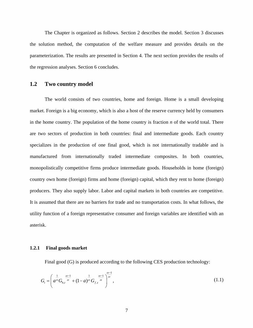
1.2.1 Final goods market

Final good (G) is produced according to the following CES production technology:

11 1 1 1

, ,(1 )t h t f tG a G a G

ωω ω ω

ω ω ω ω

−− −⎛ ⎞

= + −⎜ ⎟⎝ ⎠

, (1.1)

7

where ω is the elasticity of substitution between the home and foreign intermediate goods

composites. a is the weight of the home intermediate goods composite in the production of the

final consumption good. If a>1/2, we say that consumption is biased towards the home goods.

,h tG and ,f tG are aggregates of the home intermediate and the imported foreign intermediate

goods, respectively:

1 1 1

, ,0

( )h t h tG g z

εε εε− −⎛ ⎞

= ⎜ ⎟⎝ ⎠∫ , (1.2)

1 1 1

, ,0

( )f t f tG g z

εε εε− −⎛ ⎞

= ⎜ ⎟⎝ ⎠∫ , (1.3)

where and represent outputs of individual home and foreign firms, respectively.

Symmetrically, the production function of the foreign final good is

, ( )h tg z , ( )f tg z

11 1 1 1

* * *, ,(1 )

t f t h tG a G a G

ωω ω ω

ω ω ω ω

−− −⎛ ⎞

= + −⎜ ⎟⎝ ⎠

. (1.4)

Due to the symmetry in the goods market structure, in this section I will focus only on the home

country.

Final goods market is perfectly competitive and producers maximize profits each period:

( ), , , ,h t t t h t h t f t f tPG P G P Gπ = − − , , (1.5)

where is an overall price index, and P hP fP are price indexes of the home and foreign goods,

all denominated in local currency, and are given as

( )1

1 1 1, ,(1 )t h t f tP aP a Pω ω ω− − −= + − , (1.6)

8

11 1

1, ,

0

( )h t h tP p zε

ε−

−⎛ ⎞= ⎜ ⎟⎝ ⎠∫ , (1.7)

11 1

1, ,

0

( )f t f tP p zε

ε−

−⎛ ⎞= ⎜ ⎟⎝ ⎠∫ . (1.8)

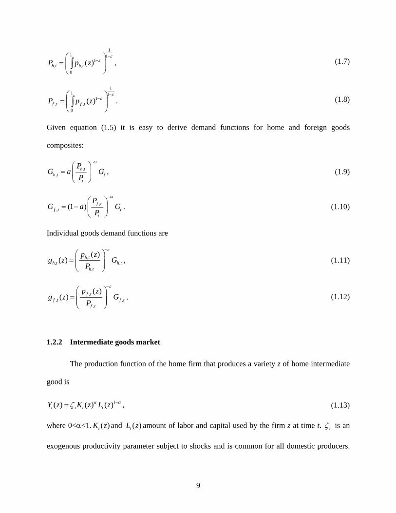
Given equation (1.5) it is easy to derive demand functions for home and foreign goods

composites:

,,

h th t t

t

PG a G

P

ω−⎛ ⎞

= ⎜ ⎟⎝ ⎠

, (1.9)

,, (1 ) f t

f t tt

PG a

P

ω−⎛ ⎞

= − ⎜ ⎟⎝ ⎠

G . (1.10)

Individual goods demand functions are

,, ,

,

( )( ) h t

h t h th t

p zg z G

P

ε−⎛ ⎞

= ⎜ ⎟⎜ ⎟⎝ ⎠

, (1.11)

,, ,

,

( )( ) f t

f t ff t

p zg z G

P

ε−⎛ ⎞

= ⎜ ⎟⎜ ⎟⎝ ⎠

t . (1.12)

1.2.2 Intermediate goods market

The production function of the home firm that produces a variety z of home intermediate

good is

1( ) ( ) ( )t t t tY z K z L zα αζ −= , (1.13)

where 0<α<1. and amount of labor and capital used by the firm z at time t. ( )tK z ( )tL z tζ is an

exogenous productivity parameter subject to shocks and is common for all domestic producers.

9

In the benchmark case, I assume that the prices are set in the currency of the producer both for

domestic and sales abroad, i.e. producer currency pricing (PCP). Price stickiness is introduced in

the form of quadratic price adjustment cost function.

The representative home firm maximizes:

0 , ,0

( )t t n H tt

E zσ π∞

+=∑ , (1.14)

where ,t t nσ + is a pricing kernel (to value date t and t+n payoffs ), since firms are assumed to be

owned by households, and it is equal the household’s marginal rate of substitution between

consumption at t and t+n: '

,, '

,

C t nn tt t n

t n C t

U PP U

σ β ++

+

= .

Each period profit function is

( ), ,( ) ( ) ( ) ( ) ( )h t H t t t H tz p z MC z AC z g zπ = − − , . (1.15)

MCt is a marginal cost function. is a quadratic price adjustment function and is given by ( )tAC z

( )2

, , 1,

, 1

( ) ( )( )

2 ( )H t H t

p tH t

p z p zAC z

p zµ −

−

−= . (1.16)

Minimization of the cost function (for simplicity firm subscript is omitted)

t tt t

t

W L K rP

+ subject to production technology 1t t t tY K Lα αζ −= yields

1 1

1(1 )t t t

t

W r Pα α α

α αλα α ζ

− −

−=−

,

where λ is the real marginal cost (Lagrange multiplier). Therefore, the nominal marginal cost is

1

1(1 )t t t

tt

W r PMC

α α α

α αα α ζ

−

−=−

. Since all firms are assumed to have the same production technology, the

MC will be the same across producers as well as the capital-labor tradeoff equation, which is

given below.

10

( ) ( )1t r t t tPr K z W L zα

α=

−. (1.17)

Substituting equation (1.15) into profit function (1.14) with the expressions for MC, AC and

from equation (1.11) and taking derivative with respect to , ( )h tg z , ( )H tp z , one can get a price-

setting expression similar to that in Bergin and Tchakarov (2003):

,, , , ,

, 1

2, 1 , 1 , 1

, 2, ,,

+

( )( ) ( ) ( ) 1

1 1

( ) ( )1 ( ) 1 .2 1 ( )( )

H tH t H t H t H t

H t

t t n H t H ttH t

t t n H tH t

p zp z MC AC p z

p z( )

p z g zp z E

g zp z

ε µε ε

σµε σ

−

+ + + +

+

⎛ ⎞⎜ ⎟⎜ ⎟⎝ ⎠

⎛ ⎞⎛ ⎞⎜ ⎟⎜ ⎟⎜ ⎟⎜ ⎟

⎝ ⎠⎝ ⎠

= + + −− −

−−

+

e

(1.18)

Unlike the standard case with no price adjustment costs, where the price is a markup over

marginal cost, here we have some additional terms. Now, in equation (1.18) we also have: (i)

price adjustment costs included into the calculation of the final price of good; (ii) the bracketed

term in the middle, which is a backward looking component that indicates firm’s reluctance to

make large changes in price due to the presence of marginal adjustment costs, and (iii) the final

term, forward looking part meaning that firms would increase prices by more today if they

expect their rise in the future.

The optimal price for the foreign market is

*, , /h t h t tp p= . (1.19)

The similar price setting equations are derived for the foreign country.

1.2.3 Home household problem

The representative household lives infinitely many periods. At any time t, the

representative home consumer maximizes her inter-temporal utility function:

11

11 1

00

( )11 1 1

At t t

t tt t

C M LU EP

ηρ ψ

β χ t

ρ η ψ

−− +∞

=

⎧ ⎫⎛ ⎞⎪ ⎪= + −⎨ ⎬⎜ ⎟− − +⎝ ⎠⎪ ⎪⎩ ⎭∑ . (1.20)

The second term in the objective function reflects the utility derived from holding real balances,

for instance, as a means of facilitating transactions and is given as a CES aggregator over

nominal domestic and foreign money: 1 1 1 1 1

,(1 ) ( )At t t f tM M e M

γγ γ γ

γ γ γ γφ φ− − −⎛ ⎞

= + −⎜ ⎟⎜ ⎟⎝ ⎠

. Domestic and

foreign currencies provide utility in a non-separable way. 1 φ− can be thought of as the “degree

of currency substitution”. Lower φ indicates the higher importance of foreign currency for home

residents. γ is the elasticity of substitution between home and foreign currency and is nominal

exchange rate.

te

tχ is an exogenously given money demand shock. Finally, the third term is the

disutility from work.

Consumers receive income from providing labor at the nominal wage rate (W), renting

out capital to firms at the real rental rate (r), receiving real profits from home firms (π ), and

from government transfers (T). In addition to money, home consumers can lend and borrow only

in non-contingent foreign currency denominated nominal bonds that pay interest rate i*.

Consumer owns capital (K) which depreciates at a constant rate (δ), and whose adjustment

incurs costs that are represented by quadratic adjustment cost function depending on parameter

cχ . Households also incur bond adjustment costs which depend on parameter Bχ . Capital

adjustment costs are in changes and incorporated to prevent excessive capital volatility. The

foreign bond adjustment costs are in the form of deviation from steady state level. They serve

two purposes: to ensure that the bond holdings and consumption are stationary, and to indicate

12

the fact that domestic households usually incur some adjustments costs on their foreign currency

bond holdings. 16

The budget constraint of the home household is

1

2

,21

1 ,

1*

, 1 1 , 1 ,0

( )1 1( (1 ) )2 2

(1 ) ( ) .t t

Ft F tt t

t t t t t c t t F t B t t F tt t

t F t t t F t t t t t t h t t

e B BK KPC P K K P e B M e M

K P

e i B M e M PrK W L z dz PT

δ χ χ

π−

−

++

− − −

⎛ ⎞⎛ ⎞−⎜ ⎟⎜ ⎟− ⎝ ⎠⎝ ⎠+ − − + + + + +

= + + + + + + +∫

, =

(1.21)

Consumers maximize equation (1.20) subject to the budget constraint (1.21). Optimization yields

the following first order conditions.

1. Home money demand equation:

(1 ) 11 1 1 11 1 1,

1 1

(1 ) 1t F tt t t tt t t

t t t t

e M

t

M M CC EP P P C

γ ηγ γ γ

ργ γ γρ γ γ γ

ρχ φ φ φ β

−−− − − −

+ +

⎛ ⎞⎛ ⎞ ⎛ ⎞ ⎛ ⎞ ⎛⎜ ⎟+ − = −⎜ ⎟ ⎜ ⎟ ⎜ ⎟ ⎜⎜ ⎟⎝ ⎠ ⎝ ⎠ ⎝ ⎠ ⎝⎜ ⎟

⎝ ⎠

PP

⎞⎟⎠

. (1.22)

2. Foreign money demand equation:

(1 )11 1 1 11 1 1

, , 1

1 1

(1 ) (1 ) 1t F t t F tt t t tt t t

t t t

e M e M

t t t

M C e PC E

P P P C

γ ηγ γ γ

ργ γ γρ γ γ γ

ρχ φ φ φ β

−−− − − −

+

+ +

− + − = −⎛ ⎞⎛ ⎞ ⎛ ⎞ ⎛ ⎞ ⎛⎜ ⎟⎜ ⎟ ⎜ ⎟ ⎜ ⎟ ⎜⎜ ⎟⎜ ⎟⎝ ⎠ ⎝ ⎠ ⎝ ⎠ ⎝⎝ ⎠

e P⎞⎟⎠

. (1.23)

3. Consumption Euler equation:

( ) *, 1 1

1

(1 )1 B F t F t t t t

tt t t

B B C e P iE

P C e P

ρ

ρ

χβ

−+ +−

+

− ++ =

⎛ ⎞⎜ ⎟⎝ ⎠t

. (1.24)

16 See Schmitt-Grohé and Uribe (2003) for a more detailed discussion. There is no role for home currency denominated bonds. It is assumed that foreign consumers do not want to hold them. Hence, home households cannot trade them since they are assumed to be identical as well as intermediate firms since they do not face idiosyncratic technology shocks.

13

4. Consumption-leisure tradeoff:

0tt

t t

WLPC

ψρ− + = . (1.25)

5. Capital accumulation equation:

2 1

1

2 2

11 2

1

11 1

2t t

t

t t tc t t c

t t

K KK K CE r

K C K

ρ

χ β δ χ + +

+

++

+

−−+ = + − +

⎡ ⎤⎛ ⎞⎛ ⎞⎛ ⎞⎢ ⎥⎜ ⎟⎜⎜ ⎟ ⎜⎜ ⎟⎝ ⎠⎢ ⎥⎝ ⎠⎝ ⎠⎣ ⎦

⎟⎟ . (1.26)

1.2.4 Foreign household problem

Foreign consumers maximize:

( )1 1* * * * 1,*

0 *0

( )1 1 1

t

t

t F tt tt

t

C M LU EP

ρ ηψχ

βρ η ψ

− −+∞

=

⎧ ⎫⎛ ⎞⎪ ⎪= + −⎜ ⎟⎨ ⎬⎜ ⎟− − +⎪ ⎪⎝ ⎠⎩ ⎭∑

.

Unlike home consumers, their foreign counterparts do not derive utility from holding home

country currency. Moreover, they do not face bond adjustment costs. Therefore, the budget

constraint of the foreign representative consumer may be written as

(1.27)

1

* * 2* * * * * * * * * * *1

1 , ,*

1* * * * * * * *

,

( )1( (1 ) ) (1 )2

( ) .

t

t

ft tt t t t t c F t F t F t F t

t t t t t f t t t

K KP C P K K B M i B MK

P r K W L z dz P T

δ χ

π

−

++ − −

−+ − − + + + = + +

+ + + +∫

, 1 , 1

0

+

(1.28)

The associated first order conditions of the foreign representative household’s optimization

problem are similar to those of the home consumer with the exception of the money demand and

consumption Euler equations:

,

* *** *

** *1F t ttt t t

M PCC EP PC

ηρ

ρρχ β

−⎛ ⎞ ⎛ ⎞

= −⎜ ⎟ ⎜ ⎟⎜ ⎟⎜ ⎟ , 11t tt ++⎝ ⎠⎝ ⎠

(1.29)

14

* * *1

* *1

(1 )1 0t t t

tt t

C P iE

C P

ρ

ρβ

−+−

+

+− =

⎛ ⎞⎜ ⎟⎝ ⎠

. (1.30)

1.2.5 Monetary and fiscal policy rules

Foreign Rules

It is assumed that the foreign monetary authority follows a constant money growth rule.

The foreign country does not have to worry about maintaining some nominal exchange rate with

the home country, which is a small open economy. The monetary rule is

* *1(1 )t tM g M −= + . (1.31)

For simplicity, I assume that the government’s budget is balanced each period and there is no

government spending and all seignorage revenues are returned to the public in the form of

transfers. The foreign government’s budget constraint is

1

* **

*t t

t

t

M MT

P−

−= . (1.32)

At this point, it is worthwhile noting that foreign transfers exceed the amount of foreign currency

held by foreign consumers by the amount of foreign currency held by the home country. That is,

the foreign economy, being the host of reserve currency, receives additional seignorage revenues

from the home country.

Home Rules

I follow Obstfeld and Rogoff (2000), Devereux and Engel (2000), Bacchetta and Van

Wincoop (2000), and Bergin and Tchakarov (2003) in setting up a money growth rule:

1ln( ) ln( ) (ln( ) ln( ))t t e tM M e eλ−= + − . (1.33)

15

A large negative value of eλ corresponds to the case of a fixed exchange rate regime. However,

for the flexible exchange regime I make some minor modification:

1ln( ) ln( ) ln(1 ) (ln( ) ln( ))t t e tM M g e eλ−= + + + − . (1.34)

To ensure stationarity of nominal exchange rate, eλ is set to a very small negative value close to

zero. When this parameter is zero, the home monetary rule collapses to a constant money growth

rule. ln(1+g) is included into the rule to pin down the steady state value of nominal exchange

rate. Otherwise, nominal exchange rate and hence real variables, such as consumption, will be

indeterminate.

The home government’s budget constraint is similar to the foreign budget constraint:

1t tt

t

M MTP

−−= . (1.35)

1.2.6 Market clearing and equilibrium

Goods market clearing conditions are

,

*, , (1 )

h th t h tnY nG n G= + − , (1.36)

* *, ,(1 ) (1 ) ,f t f tn Y nG n G− = + − f t . (1.37)

Bonds clearing condition implies

*, ,(1 ) 0F t F tnB n B+ − = . (1.38)

The home balance of payments equation is

1

,

*1 , 1, ,

*, *

, , *

( (1 ) ) (1 )

1 + .

t

H t

t t t t t t t tt F tf t f t

H ttH t H t

t t

PC P K K e B e M e i B e M

PP n

, 1F t

tP G PP n P

ωω

δ−+ −

−− ⎛ ⎞⎛ ⎞⎜ ⎟⎜ ⎟ ⎜ ⎟⎝ ⎠ ⎝ ⎠

+ − − + + = + + +

−+ G

−

(1.39)

The home resource constraint may be written as

16

2

1,2, , 11

1 ,20

( )1 1 1( (1 ) ) ( )2 2

t

ft f tf t f tt t

t t t t c B t p tt t

e B B M MK KG C K K e AC z dzK P P P

δ χ χ

−

−++

⎛ ⎞⎛ ⎞−⎜ ⎟⎜ ⎟ −− ⎝ ⎠⎝ ⎠= + − − + + + + ∫ .t

(1.40)

The foreign balance of payments condition is

, ,

1 , 1 , 1 , ,

*, ,* * * * * * * * * * *

* *( (1 ) ) (1 )1 1

F t F t

t t t t t F t t F t F t F t

t t

1

t

F t F tt t

P P M Mn nPC P K K B i B G P G PP n P n P

ω ω

δ+ − −

− −

−⎛ ⎞ ⎛ ⎞ −

+ − − + = + + + +⎜ ⎟ ⎜ ⎟⎜ ⎟ ⎜ ⎟− −⎝ ⎠ ⎝ ⎠. (1.41)

Note that the last term on the right hand side in the foreign balance of payments equation

represents seignorage revenues that the foreign country collects from the home country by the

virtue of being the host of the reserve currency. Foreign resource constraint may be defined as

1* * 2* * * * *1

1 ,* *0

( )1 1( (1 ) ) ( )2

t tt t t t c p t

t t

K KG C K K AC z dK P

δ χ ++

−= + − − + + ∫ z . (1.42)

At the symmetric equilibrium, we have , ,( )H t H tp z P= and , ( )F t F t,p z P= . The same applies to

their foreign counterparts.

Stochastic Processes

Money demand and technology shocks are log-normally distributed and uncorrelated with each

other:

11 1ln( ) ln( )t t

tζ ζρ εζ ζ

−= + , (1.43)

1

1 1

* ** *

* *ln( ) ln( )t t

t

ζ ζρ ε

ζ ζ−= + , (1.44)

12 2ln( ) ln( )t t

tχ χρ εχ χ

−= + , (1.45)

1

2

* ** *2* *ln( ) ln( )t t

t

χ χρ ε

χ χ−= + . (1.46)

17

1.3. Solution algorithm, welfare measure and calibration

1.3.1 Solution method, conditional and unconditional welfare

Most of research dealing with the evaluation of alternative monetary and fiscal policies

rests on the log-linear approximation of the equilibrium conditions – the policy functions - and

consequent second order approximation of the welfare function. The choice of unconditional

expectation is mostly due to its advantages of computational simplicity. This approach may yield

accurate results under certain simplifying assumptions, such as restrictive preferences

specifications and access to government subsidies. In general, for such an approach to give

correct results up to the second order, it is required that the solution to the equilibrium conditions

be also accurate up to the second order. In this paper, I compute second order approximations to

the policy functions and the welfare using the algorithm recently developed by Schmitt-Grohé

and Uribe (2004). I follow them and assume that in initial state all state variables are in their

deterministic steady states and alternative exchange rate regimes are evaluated by the conditional

expectation of the discounted life time utility.

It is a common practice to exclude real monetary balances from the utility function in the

welfare computation. In accordance with this practice, the conditional expectation of lifetime

utility at time t can be written as

( , )s tt t s s

s tV E u C Lβ

∞−

=

= ∑ . (1.47)

Instead of plugging the second order approximations of sC and sL in the above equation to

determine the second order approximation of , we can introduce a new control variable - .

Its law of motion can be written as

tV tV

18

1( ) ( ,t t t tV E V u C L )tβ +− = .

Most of the recent literature on monetary policy uses unconditional welfare index.

However, it neglects the quantitative relevance of transitional dynamics. By now, it is well

known that unconditional welfare index may produce incorrect rankings across alternative

policies, since it omits the transition costs of moving from the deterministic to the stochastic

steady states.17

1.3.2 Computation of the welfare measure

It is assumed that economy begins at time zero, at which all variables of the system are

equal to their respective steady state values. Furthermore, the economy begins from the same

state, which is a non-stochastic steady state and is the same under the two alternative monetary

regimes. For each of the two exchange rate regimes, I compute the conditional expectation of

lifetime utility as of time t. Let flextV and fix

tV be the conditional welfare outcomes as of time t

under flexible fixed exchange rate regime, respectively.

Following the welfare loss measure introduced by Lucas (1987), let flexλ ( fixλ ) be the

fraction of the nonstochastic steady state consumption level that consumers are willing to give up

in order to avoid risk and be as well-off under the stochastic flexible (fixed) exchange rate

regime environment.

Then the loss from uncertainty under flexible regime can be written as

11

1

( )(1 )(1 )1 1

flexflex V V

C

ρ

ρ

β ρλ

−

−

− − −= − + ×⎛ ⎞⎛ ⎞⎜ ⎟⎜ ⎟⎜ ⎟⎝ ⎠⎝ ⎠

100

,

17 See Kim and Kim (2003) for a more detailed discussion.

19

where C is a steady state consumption level, which is the same under both flexible and fixed

regimes.

Similarly, the loss under the fixed regime is given by

11

1

( )(1 )(1 )1 1 100

fixfix V V

C

ρ

ρ

β ρλ

−

−

− − −= − + ×⎛ ⎞⎛ ⎞⎜ ⎟⎜ ⎟⎜ ⎟⎝ ⎠⎝ ⎠

.

Then, the gain (loss) of the fixed over the flexible regime is 18

fix flexλ λ λ= − .

I also decompose conditional welfare costs under both fixed and flexible regimes. Let us

denote by fixmeanλ ( flex

meanλ ) welfare costs due to changes in means and varfixλ ( var

flexλ ) costs due to

variance effect under fixed (flexible) exchange rate regime. Given the second order

approximation to the utility function and steady state levels of consumption, C , and labor, L ,

one can decompose fixλ as follows:

1 1 1 1

0

1 1ˆ ˆˆ ˆ([1 ] , ) ( , ) (1 ) ( ) var( ) var( )2 2

fix tt t t

tu C L u C L E C C L L C C Lρ ψ ρ ψλ β β ρ ψ

∞− + − +

=tL⎧ ⎫− ≈ + − − − −⎨ ⎬

⎩ ⎭∑ ,

where hats over variables represent log-deviations from the deterministic steady states. The

change in mean consumption, fixmeanλ , is computed from the following expression:

1 1

0

ˆ ˆ([1 ] , ) ( , ) (1 ) ( )fix tmean t t

tu C L u C L E C C Lρ ψλ β β

∞− +

=

− = + − −∑ L . (1.48)

The change in conditional variance of consumption is given by

1 1var

0

1 1ˆ ˆ([1 ] , ) ( , ) (1 ) var( ) var( )2 2

fix tt

tu C L u C L C C Lρ ψλ β β ρ ψ

∞− +

=tL⎧ ⎫− = − − +⎨ ⎬

⎩ ⎭∑ . (1.49)

18 When 1ρ = , we can derive a direct formula calculating welfare loss of the flexible vis-à-vis the fixed regime:

. ( )(1 )( )1 100flex fixV Ve βλ − −= − ×

20

It can be easily shown that the following relation holds:

1 1var(1 ) (1 ) (1 ) 1fix fix fix

meanρ ρλ λ λ− −− = − + − 1 ρ− − . (1.50)

As there are no closed-form solutions to (1.48) and (1.49), I simulate the conditional moments

for 2000 periods and compute the discounted sum. I calculate varfixλ from (1.49) and fix

meanλ is

computed using (1.50).The analytical formulas for the computation of conditional moments are

derived and provided in Paustian (2003) and Marzo, Strid and Zagaglia (2006). Similarly, one

can decompose the welfare cost for the flexible exchange rate regime.

To facilitate the comparison with the literature, I also calculate unconditional welfare

costs. Following Bergin and Tchakarov (2003) and Straub and Tchakarov (2004) I decompose

unconditional welfare cost under the fixed exchange rate regime into mean and variance

components:

, 1 ˆ ˆ([1 ] , ) ( , ) ( ) ( )fix umean t tu C L u C L C E C L Eρ ψλ − +− = + − 1 L ,

, 1var

1 1ˆ ˆ([(1 ) , ) ( , ) var( ) var( )2 2

fix ut tu C L u C L C C Lρ ψλ ρ ψ− +− = − − 1 L .

Rearranging these equations, one can get the expressions for the unconditional mean and

variance components:

1/(1 ), 1

1

(1 )ˆ ˆ1 1 (1 ) ( ) ( )fix umean t tE C L E L

C

ρψ

ρ

ρλ ρ−

+−

−⎧ ⎫= − + − −⎨ ⎬⎩ ⎭

,

1/(1 ), 1

var 1

1 1 (1 )ˆ ˆ1 1 (1 ) var( ) var( )2 2

fix ut tC L L

C

ρψ

ρ

ρλ ρ ρ ψ−

+−

−⎧ ⎫= − − − −⎨ ⎬⎩ ⎭

.

The decomposition of the unconditional welfare cost under the flexible exchange rate regime is

undertaken in the same way.

21

1.3.3 Parameterization

The calibrated parameters used for the base model are provided in Table 1.1. The time

period in the model is one quarter. Therefore, I set β=0.99 and choose δ=0.025 for the

depreciation rate. Capital share in the production is set to 0.36. I follow Bergin and Feenstra

(2001) in choosing a value of 0.25 for the interest elasticity of real money balances (1/η). ρ is set

to 4 in line with the empirical findings that the income elasticity of real money demand (ρ/η) is

about unity. I follow Harrigan (1993) and Trefler and Lai (1999) and Bergin and Tchakarov

(2003) by setting the value of elasticity of substitution between foreign and home goods, ω, to 5.

Rotemberg and Woodford (1998) set the degree of monopolistic competition ε to be 7.66, which

implies an average price mark-up of 15%, and I follow this parameterization. The size of the

home country is set to 0.15 for the base model computations. I follow Christiano et al. (1997)

and set ψ=1, which is the inverse of labor supply elasticity. Following Bergin and Tchakarov

(2003), the price adjustment cost is set at µ =50 for both countries, which implies that 95% of the

price has adjusted 4 periods after a monetary shock. As in Bergin and Tchakarov (2003)

investment adjustment cost in the foreign country is set at χc =4, meaning that investment is

about three times more volatile than output. I use the same value for the home country’s capital

adjustment cost parameter in view of the problem related to capital measurement in developing

countries. Introducing bond adjustment costs and assigning a small value to it, χB =0.0004, is

necessary to ensure the stationarity in the net foreign assets position.

It is assumed that the foreign central bank is increasing nominal money at a rate of 5%

per annum, which is equivalent to setting g=0.012272. The home monetary policy reaction

parameter, λe, is set at and , for flexible and fixed exchange regimes, respectively. It

is difficult to estimate the elasticity of substitution between domestic and foreign money, γ,

610−− 310−

22

therefore the parameter is set to 1, which implies Cobb-Douglas monetary aggregate. Foreign

and domestic money do not enter monetary aggregate as perfect substitutes, since I assume that

there are some legal restrictions over the use of foreign money in the home country. The

elasticity of substitution between the currencies will turn out to be an important parameter for the

purposes of welfare evaluation across alternative exchange rate regimes. Later, I will relax the

assumption of no perfect substitutability and will vary γ bringing it closer to the case of perfect

currency substitution. I use the following numerical values for the degree of dollarization,

φ=3/5, 4/5, 17/20, 9/10. These values respectively correspond to FCD/BM=0.4, 0.2,

0.15,0.1.19.

For the variance and persistence of technology shocks, I use common values employed in

the real business cycle literature and also used in Bergin and Tchakarov (2003),

var(ε1)=var(ε*1)=0.012 and ρ1=ρ1*=0.9. I use var(ε2)=var(ε*2)=0.052 and ρ2=ρ2

*=0.9 for monetary

shocks persistence and variance. To simplify analysis, it is assumed that shocks are uncorrelated

with each other.

19 The value for φ is chosen such that at the steady state: f

f

eM FCDeM M BM

=+

reported in Table A.1.

23

Table 1.1. Calibrated parameters

Parameter Value Description

β 0.99 Quarterly subjective discount rate

δ 0.025 Quarterly depreciation rate

α 0.36 Cost share of capital, 1Y K Lα αζ −=

1/η 1/4 Interest elasticity of real money balances

ρ 4 Risk aversion parameter, 11 11 (

1 1 1

AC MUP

η)Lρ ψ

χρ η ψ

−− +⎛ ⎞= + −⎜ ⎟− − +⎝ ⎠

ω 5

Elasticity of substitution between home and foreign intermediate goods in the

production of final good, 1

1 1 1 1

(1 )G a G a G

ωω ω ω

ω ω ω ω

−− −⎛ ⎞

= + −⎜ ⎟⎝ ⎠

n 0.15 Relative size of the home country

ε 7.66 Degree of monopolistic competition in the intermediate goods market

µ 50 Coefficient in price adjustment costs, ( )21

12t t

t

p pp

µ −

−

−

χc 4 Coefficient in investment adjustment costs, 2

1( )12

t tc

t

K KK

χ + −

χB 0.0004 Coefficient in bond adjustment costs,

2

,

2

12

t

ft f t

B

e B B

Pχ

−⎛ ⎞⎛ ⎞−⎜ ⎟⎜ ⎟⎝ ⎠⎝ ⎠20

1/ψ 1 Labor supply elasticity

γ 1 Elasticity of substitution between domestic and foreign money

g 0.012272 Quarterly nominal money growth rate in the foreign money rule

ρ1 0.9 First-order serial correlation of technology shock

ρ2 0.9 First-order serial correlation of monetary shock

20 fB is the steady state value of nominal foreign currency denominated bonds, whose real value is calculated jointly with the steady state values of other real variables.

24

1.4 Results

1.4.1 Benchmark and related cases

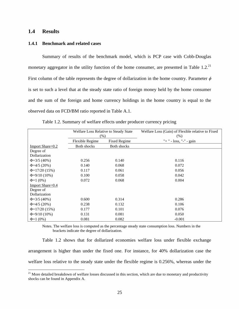
Summary of results of the benchmark model, which is PCP case with Cobb-Douglas

monetary aggregator in the utility function of the home consumer, are presented in Table 1.2.21

First column of the table represents the degree of dollarization in the home country. Parameter φ

is set to such a level that at the steady state ratio of foreign money held by the home consumer

and the sum of the foreign and home currency holdings in the home country is equal to the

observed data on FCD/BM ratio reported in Table A.1.

Table 1.2. Summary of welfare effects under producer currency pricing

Welfare Loss Relative to Steady State

(%) Welfare Loss (Gain) of Flexible relative to Fixed

(%) Flexible Regime Fixed Regime "+ " - loss, "-" - gain Import Share=0.2 Both shocks Both shocks Degree of Dollarization Φ=3/5 (40%) 0.256 0.140 0.116 Φ=4/5 (20%) 0.140 0.068 0.072 Φ=17/20 (15%) 0.117 0.061 0.056 Φ=9/10 (10%) 0.100 0.058 0.042 Φ=1 (0%) 0.072 0.068 0.004 Import Share=0.4 Degree of Dollarization Φ=3/5 (40%) 0.600 0.314 0.286 Φ=4/5 (20%) 0.238 0.132 0.106 Φ=17/20 (15%) 0.177 0.101 0.076 Φ=9/10 (10%) 0.131 0.081 0.050 Φ=1 (0%) 0.081 0.082 -0.001

Notes. The welfare loss is computed as the percentage steady state consumption loss. Numbers in the brackets indicate the degree of dollarization.

Table 1.2 shows that for dollarized economies welfare loss under flexible exchange

arrangement is higher than under the fixed one. For instance, for 40% dollarization case the

welfare loss relative to the steady state under the flexible regime is 0.256%, whereas under the

21 More detailed breakdown of welfare losses discussed in this section, which are due to monetary and productivity shocks can be found in Appendix A.

25

fixed it is 0.14%. Though, the gain of the fixed over the flexible of 0.116% may not seem

substantial, below I will present cases where the loss under the flexible regime can be

substantial. One can also observe that with the decline in the degree of dollarization, the relative

loss of the flexible compared to the fixed regime diminishes. Basically, currency substitution

tends to increase exchange rate volatility (see Table A.6). In the case of no dollarization, the loss

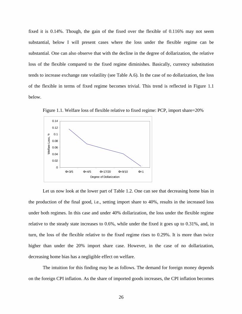
of the flexible in terms of fixed regime becomes trivial. This trend is reflected in Figure 1.1

below.

Figure 1.1. Welfare loss of flexible relative to fixed regime: PCP, import share=20%

0

0.02

0.04

0.06

0.08

0.1

0.12

0.14

Φ=3/5 Φ=4/5 Φ=17/20 Φ=9/10 Φ=1

Degree of Dollarization

Wel

fare

Los

s, %

Let us now look at the lower part of Table 1.2. One can see that decreasing home bias in

the production of the final good, i.e., setting import share to 40%, results in the increased loss

under both regimes. In this case and under 40% dollarization, the loss under the flexible regime

relative to the steady state increases to 0.6%, while under the fixed it goes up to 0.31%, and, in

turn, the loss of the flexible relative to the fixed regime rises to 0.29%. It is more than twice

higher than under the 20% import share case. However, in the case of no dollarization,

decreasing home bias has a negligible effect on welfare.

The intuition for this finding may be as follows. The demand for foreign money depends

on the foreign CPI inflation. As the share of imported goods increases, the CPI inflation becomes

26

more volatile due to the volatility of nominal exchange rate. These fluctuations cause higher

volatility of the foreign money demand by home consumers and this, in turn, results in more

volatile home aggregate demand and increased welfare loss. This can be seen in Figure 1.2

below. The graph shows welfare loss under alternative regimes as a function of import share.

Figure 1.2. Welfare loss as a function of import share: φ=3/5 (40% dollarization)

00.10.20.30.40.50.60.70.80.9

1

0 0.1 0.2 0.3 0.4 0.5 0.6

Import Share

Wel

fare

Los

s, %

FlexibleFixed

Hence, given high degree of dollarization and lower home bias, it is more desirable to stabilize

exchange rate fluctuations.

Another useful exercise is to compare welfare outcomes when prices are set in the local

currency of the buyer (LCP). Table 1.3 presents summary of results under the LCP pricing. One

can observe that welfare losses under the flexible are higher than under the fixed exchange rate

regime. Welfare outcomes have not changed much for both exchange rate regimes, though

welfare loss is slightly smaller under the LCP than under the PCP case at all levels of

dollarization and both monetary regimes.

27

Table 1.3. Summary of welfare effects under local currency pricing



(%): Flexible Regime Fixed Regime "+ " - loss, "-" - gain Import Share=0.2 Both shocks Both shocks Degree of Dollarization Φ=3/5 (40%) 0.216 0.091 0.125 Φ=4/5 (20%) 0.096 0.032 0.064 Φ=17/20 (15%) 0.074 0.030 0.044 Φ=9/10 (10%) 0.058 0.032 0.026 Φ=1 (0%) 0.041 0.056 -0.015 Import Share=0.4 Degree of Dollarization Φ=3/5 (40%) 0.590 0.200 0.390 Φ=4/5 (20%) 0.210 0.057 0.153 Φ=17/20 (15%) 0.140 0.038 0.102 Φ=9/10 (10%) 0.090 0.031 0.059 Φ=1 (0%) 0.030 0.059 -0.029


Again, one can observe that the relative gain of the fixed regime declines with the decrease in the

degree of dollarization as depicted in Figure 1.3.

Figure 1.3. Welfare loss of flexible relative to fixed regime: LCP, import share=20%

-0.04

-0.02

0

0.02

0.04

0.06

0.08

0.1

0.12

0.14

Φ=3/5 Φ=4/5 Φ=17/20 Φ=9/10 Φ=1


Wel

fare

Los

s,%

Theoretically, the choice of price-setting mechanism is deemed to affect the choice of

exchange regime. However, I find that quantitatively the results do not differ much under both

28

pricing mechanisms --when prices are set in the currency of the producer and when prices are set

in the local currency of the buyer. Similar finding was obtained by Bergin and Tchakarov (2003).

The above results have been obtained for the case of Cobb-Douglas monetary aggregator,

that is, domestic and foreign currencies are not perfect substitutes. So far, the results suggest that

if the home bias is high and the two currencies do not enter the home utility function as perfect

substitutes then, quantitatively, the relative gain of the fixed versus the flexible is not very

significant.

Now, let us examine what happens to the welfare when we increase parameter γ, the

elasticity of substitution between the two currencies. Setting γ to infinity would be the case of

perfect substitutability between the domestic and foreign currencies. Obstfeld and Rogoff (1996,

pp 551-53) present a simple model of currency substitution. They argue that when purchasing

power parity (PPP) holds, and there are no legal restrictions (no foreign currency transaction

costs) over the use of the foreign currency, and two currencies are perfect substitutes; then there

may be considerable instability in domestic prices and exchange rates.

Although, the PPP does not hold, and the two currencies are not perfect substitutes in this

model, results presented below support Obstfeld and Rogoff’s (1996) finding. Figure 1.4 plots

the welfare loss as a function of the elasticity of substitution between the home and foreign

currencies. In this experiment, I increase the elasticity of substitution between domestic and

foreign currencies from 1 (Cobb-Douglas monetary aggregator case) to 100 and calculate the

associated welfare losses. I consider monetary shocks and 40 percent degree of dollarization.

One can see that increasing γ results in the increased welfare loss under the flexible exchange

rate regime .Now, welfare loss under the flexible regime is substantial, and is well above one

29

percentage point.22 This stems from significant exchange rate fluctuations and huge currency

swings, which, in turn, cause substantial aggregate fluctuations in the home country. However,

under the fixed exchange regime, increasing γ has almost no effect on the welfare; the welfare

loss is almost unchanged and remains almost the same under the Cobb-Douglas case considered

above. Thus, in highly dollarized developing economies where the elasticity of substitution

between domestic and foreign currencies is high, there is a greater need for a fixed exchange

regime.

Figure 1.4. Welfare loss and the elasticity of substitution between currencies: import share=40% and φ=3/5

0123456789

0 20 40 60 80 100 120

Elasticity of Substitution, γ

Wel

fare

Los

s, %

FlexibleFixed

Another useful experiment is to calculate welfare under the higher risk aversion

parameter, ρ. Table 1.4 reports results for ρ=30. From the table, it can be seen that the welfare

losses for both flexible and fixed regimes have risen; however, these changes are not

substantially different from the results of the benchmark case reported in Table 1.2. Again, we

can observe that with the decline in the level of dollarization, the relative gain of the fixed over

the flexible regime diminishes.

22 Similar experiment has been done for the case of productivity shocks. Qualitatively results were similar; however, quantitatively the welfare losses under flexible exchange regime were not that high like in the case of monetary shocks.

30

Table 1.4. Summary of welfare effects under producer currency pricing: higher risk aversion (ρ=30)



(%): Flexible Regime Fixed Regime "+ " - loss, "-" - gain Import Share=0.2 Both shocks Both shocks Degree of Dollarization Φ=3/5 (40%) 0.354 0.177 0.177 Φ=4/5 (20%) 0.188 0.087 0.101 Φ=17/20 (15%) 0.159 0.077 0.082 Φ=9/10 (10%) 0.137 0.071 0.066 Φ=1 (0%) 0.110 0.089 0.021


1.4.2 Conditional vs unconditional welfare

Table 1.5 presents results of conditional and conditional welfare costs mean-variance

decompositions as well as unconditional welfare costs for fixed and flexible exchange rate

regimes. Unconditional welfare losses are presented in columns 5 and 11. Quick look at the table

shows that as in the case of conditional welfare index, unconditional welfare losses under

floating regime diminishes as the degree of dollarization decreases under both PCP and LCP

cases.

Another observation is that unconditional welfare index underestimates unconditional

costs. As argued before, it ignores the costs associated with the transition from the deterministic

to stochastic steady states. For instance, the unconditional welfare loss under flexible regime

with 40% dollarization is 0.186%, whereas its conditional counterpart is 0.256%. Moreover, one

can observe welfare ranking reversals under LCP case when one uses unconditional measures.

For instance, under LCP case with degrees of dollarization lower than 20% unconditional

welfare losses are smaller than under fixed regime. Further, unconditional measures suggest that

under fixed exchange rate with LCP the lowest welfare loss is when the degree of dollarization is

31

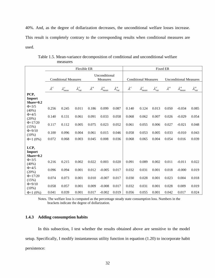
40%. And, as the degree of dollarization decreases, the unconditional welfare losses increase.

This result is completely contrary to the corresponding results when conditional measures are

used.

Table 1.5. Mean-variance decomposition of conditional and unconditional welfare measures

Flexible ER Fixed ER

Conditional Measures Unconditional

Measures Conditional Measures Unconditional Measures

cλ c

meanλ varcλ uλ u

meanλ varuλ cλ c

meanλ varcλ uλ u

meanλ varuλ

PCP, Import Share=0.2

Φ=3/5 (40%) 0.256 0.245 0.011 0.186 0.099 0.087 0.140 0.124 0.013 0.050 -0.034 0.085

Φ=4/5 (20%) 0.140 0.131 0.061 0.091 0.033 0.058 0.068 0.062 0.007 0.026 -0.029 0.054

Φ=17/20 (15%) 0.117 0.112 0.005 0.075 0.023 0.052 0.061 0.055 0.006 0.027 -0.021 0.048

Φ=9/10 (10%) 0.100 0.096 0.004 0.061 0.015 0.046 0.058 0.053 0.005 0.033 -0.010 0.043

Φ=1 (0%) 0.072 0.068 0.003 0.045 0.008 0.036 0.068 0.065 0.004 0.054 0.016 0.039 LCP, Import Share=0.2

Φ=3/5 (40%) 0.216 0.215 0.002 0.022 0.003 0.020 0.091 0.089 0.002 0.011 -0.011 0.022

Φ=4/5 (20%) 0.096 0.094 0.001 0.012 -0.005 0.017 0.032 0.031 0.001 0.018 -0.000 0.019

Φ=17/20 (15%) 0.074 0.073 0.001 0.010 -0.007 0.017 0.030 0.028 0.001 0.023 0.004 0.018

Φ=9/10 (10%) 0.058 0.057 0.001 0.009 -0.008 0.017 0.032 0.031 0.001 0.028 0.009 0.019

Φ=1 (0%) 0.041 0.039 0.001 0.017 -0.002 0.019 0.056 0.055 0.001 0.042 0.017 0.024


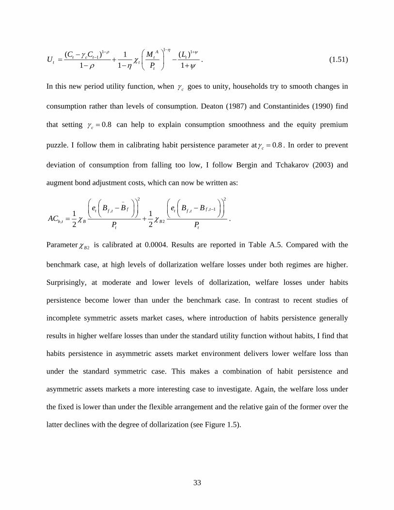
1.4.3 Adding consumption habits

In this subsection, I test whether the results obtained above are sensitive to the model

setup. Specifically, I modify instantaneous utility function in equation (1.20) to incorporate habit

persistence:

32

11 11( ) (1

1 1 1

At c t t t

t tt

C C M LUP

η)ρ ψγ χ

ρ η ψ

−− +− ⎛ ⎞−

= + −⎜ ⎟− − ⎝ ⎠ +. (1.51)

In this new period utility function, when cγ goes to unity, households try to smooth changes in

consumption rather than levels of consumption. Deaton (1987) and Constantinides (1990) find

that setting 0.8cγ = can help to explain consumption smoothness and the equity premium

puzzle. I follow them in calibrating habit persistence parameter at 0.8cγ = . In order to prevent

deviation of consumption from falling too low, I follow Bergin and Tchakarov (2003) and

augment bond adjustment costs, which can now be written as:

2 2

, 1, ,

, 21 12 2

f ft f t t f t

b t B Bt t

e B B e B BAC

P Pχ χ

−

−⎛ ⎞ ⎛⎛ ⎞ ⎛− −⎜ ⎟ ⎜⎜ ⎟ ⎜⎝ ⎠ ⎝⎝ ⎠ ⎝= +

t⎞⎞⎟⎟⎠⎠ .

Parameter 2Bχ is calibrated at 0.0004. Results are reported in Table A.5. Compared with the

benchmark case, at high levels of dollarization welfare losses under both regimes are higher.

Surprisingly, at moderate and lower levels of dollarization, welfare losses under habits

persistence become lower than under the benchmark case. In contrast to recent studies of

incomplete symmetric assets market cases, where introduction of habits persistence generally

results in higher welfare losses than under the standard utility function without habits, I find that

habits persistence in asymmetric assets market environment delivers lower welfare loss than

under the standard symmetric case. This makes a combination of habit persistence and

asymmetric assets markets a more interesting case to investigate. Again, the welfare loss under

the fixed is lower than under the flexible arrangement and the relative gain of the former over the

latter declines with the degree of dollarization (see Figure 1.5).

33

Figure 1.5. Welfare loss of flexible relative to fixed regime: habits persistence, import share=20%

-0.05

0

0.05

0.1

0.15

0.2

0.25

0.3

0.35

Φ=3/5 Φ=4/5 Φ=9/10 Φ=1


Wel

fare

Los

s, %

Results presented in this section suggest that fixed exchange rate regime outperforms

flexible exchange rate regime based on money growth rule in dollarized economies. However, it

would be interesting to see whether or not the results would carry over to the case when central

bank employs floating exchange rate regime based on a standard inflation targeting interest rate

rule.

1.5 Empirical Investigation23

In this section, I use an ordered logit model for the de facto exchange rate classifications

to examine whether or not partial dollarization has influenced the choice of exchange rate

regimes in developing economies. The results of the regression suggest that (i) more dollarized

economies have a tendency to use more rigid exchange regimes, though the estimated coefficient

on dollarization is marginally significant. This is in line with the predictions of the theoretical

model developed in the previous section; (ii) developing countries that are more open to trade

23 The purpose of this exercise is not to conduct a full-fledged econometric analysis, but rather to establish some stylized facts.

34

tend to choose more rigid exchange rate regimes. Above, it is shown that currency substitution

combined with higher import shares entails higher welfare losses and therefore more rigid

exchange rate regimes are desirable; (iii) developing countries that have experienced high

inflation also tend to adopt more fixed regimes, and (iv) countries with sound fiscal policies tend

to have more rigid exchange arrangements.

1.5.1 Theoretical determinants of exchange rate arrangements and data description

According to the theoretical literature, determinants of exchange regime can be grouped

into four broad categories: (i) the optimum currency areas (OCA) fundamentals, (ii) the

stabilization considerations, (iii) the currency crises factors, and (iv) political and institutional

features. In present paper, I focus on the former three groups of determinants.24 The OCA

explanatory variables are trade openness (ratio of trade to GDP), country size (proxied by log of

GDP). The second group – stabilization considerations – includes inflation (consumer price

index) and budget deficit to GDP ratio.25 The last group comprises ratio of non-gold reserves to

broad money and ratio of current account to GDP. I also include the ratio of broad money to

GDP as a proxy for the level of financial development. In addition to the above determinants, I

include foreign currency deposits to broad money ratio as a proxy for the currency substitution.

The panel consists of 21 developing countries observed for the period 1993-1995.26 The

de facto exchange regime classifications are obtained from Reinhart and Rogoff (2001). A slight

modification to Reinhart-Rogoff‘s classification has been made by merging original 14 into 4 24 The choice of specific determinants has been dictated by data availability. 25 Instead of CPI index, I use CPI/(CPI+1) measure in order to account for countries with hyper inflationary episodes. 26 The panel contains 63 observations. List of countries include Argentina, Bolivia, Costa Rica, Nicaragua, Peru, Turkey, Uruguay, Bulgaria, Egypt, El Salvador, Estonia, Honduras, Hungary, Jordan, Mexico, Philippines, Poland, Romania, Sierra Leone, Trinidad and Tobago, Uganda. The data come mainly from IFS statistics of the International Monetary Fund.

35

categories to reduce the number of thresholds to be evaluated. In order to reduce endogeneity

problem, all explanatory variables are lagged one period.

1.5.2 Baseline model of exchange rate regime choice

I describe the choice of exchange rate regimes using a discrete variable, . This

variable can take on one of the four values:27

,i ty

, 0i ty = , if a currency board or hard peg regime is adopted by the country i in year t,

, 1i ty = , if a soft peg regime is used by the country i in year t,

, 2i ty = , if the country i in year t chooses the intermediate regime,

, 3i ty = , if a flexible regime is chosen by the country i in year t,

with probabilities ip , where i=0,1,2,3. The choice is based on the continuous latent variable ,

which represents attractiveness of flexible exchange regime, and is, in turn, a linear function of

explanatory variables discussed previously:

*,i ty

*, ,i t i t i ty X uβ= + ,

,

, for i=1,2,…,N and t=1,…,T.

The probabilities of are given by: ,i ty

, 1Pr( 0) ( )i t i ty F c X β= = − ,

, 2 , 1Pr( 1) ( ) ( )i t i t i ty F c X F c X ,β β= = − − − ,

27 The original 14 categories are no separate legal tender; pre announced peg or currency board arrangement; pre announced horizontal band that is narrower than or equal to +/- 2%; de facto peg; pre announced crawling peg; pre announced crawling band that is narrower than or equal to +/- 2%; de facto crawling peg; de facto crawling band that is narrower than or equal to +/- 2%; pre announced crawling band that is wide than or equal to +/- 2%; de facto crawling band that is narrower than or equal to +/- 5%; moving band that is narrower than or equal to +/- 2%; managed floating; freely floating, and freely falling. The first two regimes are merged into the first category. Third to seventh constitute second group. Eights to twelfths are included into the third category. Finally, freely floating and freely falling represent the last group. Around 14% of observations fall into the currency board or hard peg category, 46% into second, 19% into third, and 21% of observations constitute flexible regime.

36

, 3 , 2Pr( 2) ( ) ( )i t i t i ty F c X F c X ,β β= = − − − ,

, 3Pr( 3) 1 ( )i t i ty F c X , β= = − − ,

where F(⋅) is the cumulative probability distribution of the error term. Although, the country

specific fixed effects model would be of interest, it is not feasible to estimate them. The

maximum likelihood estimator will be inconsistent since, given fixed T, increasing sample size N

will increase the number of fixed effects to be estimated. In the linear fixed effects models, one

can obtain consistent estimates by removing fixed effects from the estimated model using the

Within transformation. This is no longer the case for qualitative limited dependent variable

models with fixed T (Chamberlain, 1980). Therefore, I pool all country-year observations to run

an ordered logit regression.

1.5.3 Regression results

Table 1.6 below presents the results of logit regression of the de facto exchange rate

regimes.28 A negative sign of a coefficient means that an increase in the associated variable

raises the probability of adopting a hard peg. One can observe that model predicts correctly 70

percent of the de facto exchange rate regimes. The results suggest that four out of eight

explanatory variables play a role in choosing the exchange rate regime. The main explanatory

variable of interest – degree of dollarization – has expected sign and is significant at 10 percent

significance level, meaning that more dollarized economies tend to choose more rigid regimes.

More specifically, a one percentage point increase in the degree of dollarization increases the

probability of choosing a hard peg by 0.0004, holding all other explanatory variables at their

means. More open economies also have a tendency to choose more rigid regimes as well as the

28 Ordered probit regression delivers similar results.

37

countries with high inflation rates. Provided that other explanatory variables are kept at their

means, one percentage point increase in the openness increases the probability of choosing a

hard peg by 0.0012, whereas for the inflation rate the increase in the probability is 0.0043.

Table 1.6. Determinants of de facto exchange rate regimes

Variable Coefficient z-statistic Changes in probabilities y=0 y=1 y=2 y=3

DOLLARIZATION -2.450086 -1.782579* -0.0004 -0.0058 0.0040 0.0022 COUNTRY SIZE -0.312695 -1.353680

RESERVES -0.357604 -0.629137 OPENNESS -6.526787 -2.645275** -0.0012 -0.0151 0.0106 0.0057 INFLATION -23.65593 -4.474483** -0.0043 -0.0547 0.0383 0.0207

FINDEV -0.406815 -0.302978 BUDGET DEFICIT -0.363974 -2.912364** -0.0001 -0.0008 0.0006 0.0003

CURRENT ACCOUNT -2.806769 -0.745394 Predictive power1 70%

Notes: * z statistics is significant at 10%; ** z statistics is significant at 1%; 1 - since R2 is meaningless in the ordered logit, I report the appropriate measure of goodness of fit. This measure computes the share of correctly predicted regimes.

1.6 Conclusion

The paper explores the welfare effects of currency substitution in a partially dollarized

developing economy in a two country framework. Unlike the previous studies, the model allows

for asymmetric households preferences and asymmetric monetary rules. The main findings are

threefold.

First, the fixed exchange regime is superior to the flexible in highly dollarized economies

since it results in smaller welfare losses. As the degree of dollarization decreases, the relative

gain of the fixed over the flexible regime abates. The results hold true under both producer and

local currency pricing mechanisms and consumer preferences with habits persistence.

Second, the decline in the home consumption bias coupled with the currency substitution

entails greater welfare losses. Hence, the fixed exchange rate is to be preferred to the flexible.

38

Finally, the paper shows that under the flexible regime dollarized countries with high elasticity

of substitution between domestic and foreign currencies are highly vulnerable to foreign shocks.

Even when two currencies are not perfect substitutes, exposure to foreign shocks may entail very

substantial welfare costs. Therefore, in order to reduce welfare costs, monetary authority should

follow a more vigorous exchange rate stabilization policy.

39

Chapter 2

Fiscal and Monetary Policy Rules for New EU Member Countries

on Their Road to Euro: Stability Analysis

2.1 Introduction

New European Union (EU) member countries in the process of their accession to the

European Monetary Union (EMU) have to comply with the Maastricht admission criteria. Before

adopting the euro, new EU members have to spend two years in the Exchange Rate Mechanism

II (ERM-II) and meet nominal exchange rate and inflation requirements. Namely, the annual

inflation rate in these countries should not exceed by more than 1.5 percent the average of three

best performing inflation countries in the euro zone. Nominal exchange rate should not deviate

more than 15% around the central parity. On the fiscal side, the EMU candidates have to adhere

with the Stability and Growth Pact (SGP) requirements. Under these criteria budget deficit

should not be higher than 3% of GDP and debt-to-GDP ratio should not exceed 60%.

As most of the new EU countries are expected to experience or have already experienced

real exchange rate appreciation, it becomes difficult to meet both Maastricht nominal exchange

rate and inflation criteria. The real exchange rate appreciation is caused by the excessive

productivity growth in the tradable sector (the so-called Balassa-Samuelson effect). Therefore,

policy makers in these countries face the problem of choosing the right monetary and fiscal

policy mix that would allow them to meet the Maastricht inflation and nominal exchange rate as

well as the fiscal criteria.

40

Since the seminal paper by Sargent and Wallace (1981), there has been a revival in the

literature of monetary economics that studies links between monetary and fiscal policies.29 Most

of the existing papers on the design of optimal monetary policies usually ignore the fiscal side.

Fiscal policy is thought to be of little consequence as far as inflation is concerned. This is based

on the following ground. It is believed by some that inflation is a purely monetary phenomenon.

Hence, fiscal policy is not important for inflation determination, at least in the developed

countries.30 However, the recent findings in the field suggest that fiscal policy have an effect on

the price level.31 Woodford (2001) shows that in ‘non-Ricardian’ regimes fiscal policy affects

private sector budget constraints and as a consequence aggregate demand and inflation.32

Moreover, he shows that non-Ricardian policies may be consistent with the existence of rational

expectations equilibrium (REE). There are also fiscal effects of monetary policy. Monetary

policy affects the price level, which in turn affects the real value of outstanding public debt and

the real debt service, provided that monetary policy can affect real and nominal interest rates.33

This channel is usually overlooked on the grounds that seignorage revenues in industrialized

countries constitute a small fraction of total government revenues.

When modeling monetary and fiscal policy interactions, it is well known that given

monetary policy, the determinacy properties of REE crucially depends on the nature of fiscal

policy. Leeper (1991) defines active and passive fiscal and monetary policies. By active

monetary policy he means strong reaction by the Central Bank (CB) to inflation. In the case of

29 See, for instance, Leeper (1991), Sims (1994), Cochrane (1999), 30 In less developed countries, it might be the case that monetary policy is subordinated to fiscal policy, i.e. regime of ‘fiscal dominance’, and is given directives to generate certain amounts of seignorage revenues to finance government budget deficit. 31 See, for example, Woodford (1994, 1995, 1996, 1998) 32 By ‘non-Ricardian’ Woodford (1995, 1996) calls regimes under which the government does not have to subsequently adjust its budget, in present value, in order to neutralize the effects of fiscal disturbances upon private sector budget constraints. 33 See Loyo (1999) for a discussion when inflation explodes because of the fiscal effects of monetary policy.

41

Taylor rule, this corresponds to high values of inflation coefficient, usually greater than unity,

which is in line with the Taylor principle. In contrast, passive fiscal policy is associated with

high values of fiscal policy coefficient, which relates taxes to deficit or debt, whereas under

active fiscal policy the coefficient is relatively low. In other words, active fiscal policy is such

that it is not constrained by budgetary conditions, whereas under passive fiscal policy it has to

generate sufficient tax revenues to balance budget. In this paper, I follow Leeper (1991) in

defining active and passive monetary and fiscal policies.

Leeper (1991) studies the stability properties of monetary and fiscal policies in a closed

economy framework with flexible prices. In a simple theoretical setting, he shows that active

monetary policy together with active fiscal policy results in explosive solution. He further argues

that in order to have unique stationary REE one policy should be passive, while the other should

be active. Passive monetary and passive fiscal policies do not deliver stable determinate

equilibrium. Leith and Wren-Lewis (2000) study determinacy properties of monetary and fiscal

rules in the framework of overlapping generations. Their findings suggest that both monetary and

fiscal policy should be jointly either active or passive to deliver unique REE. The above two

papers considered fiscal regimes based on liability rules with non-distortionary tax instruments -

lump sum taxes. In a more complex theoretical setting with distortionary tax instruments and

government liability based fiscal rule, Schmitt-Grohe and Uribe (2007a) show that combination

of active monetary and active fiscal policies results in unique REE, which is not possible in

Leeper (1991).

The existing research on determinacy analysis of fiscal and monetary policies has been

mainly conducted in a closed economy environments. Moreover, in the context of the euro zone

accession of new EU member countries, the literature paid little attention to examining

42

determinacy properties of fiscal regimes dictated by the SGP and different monetary regimes that

are compatible with ERM-II. 34 Therefore, this paper tries to fill this gap by studying determinacy

properties of various combinations of different monetary and fiscal policy rules for new EU

member countries. Namely, I consider three monetary regimes: inflation targeting, inflation

targeting with managed float (hereinafter also referred to as managed exchange rate regime) and

fixed exchange rate regime. On the fiscal side, I explicitly model fiscal policy based on the

following SGP criteria: 3% budget deficit, 60% debt-to-GDP ratio, and a composite rule based

on the previous two. I introduce distortionary taxes on consumption and labor income that are

used by fiscal authority as instruments to satisfy government budget deficit and government

liabilities requirements. For each of the above fiscal regimes, one tax instrument is used, while

the other is kept at the steady state level. All together, I investigate 18 scenarios: three fiscal

regimes with two different distortionary tax instruments for each of three monetary regimes.

To investigate stabilizing properties of various monetary and fiscal policy mixes, I build a

two-sector small open economy model. The model features sticky prices and monopolistic

competition in both tradable and nontradable sectors, which gives a wider scope for monetary

policy. To account for high productivity growth rates enjoyed by some of the new EU member

countries, I allow for permanent sector-specific productivity shocks, which enables a proper

simulation of the Balassa-Samuelson effect, that is, as an equilibrium driving process. It is

especially relevant for some of the new EU countries being transition economies. In such

economies, high productivity gains (at least initially) tend to be concentrated in the tradable

sector. This fact should not be overlooked when studying monetary and fiscal policy interactions

34In a closed economy framework, Railavo (2004). studies determinacy properties of inflation targeting and its combination with one of the fiscal rules based on the SGP: 3% budget deficit, 60% debt-to-GDP ratio and the mixed rule based on deficit and debt.

43

in the new EU countries.35 Apart from productivity shocks, there are four additional shocks:

government expenditure, foreign interest rate, foreign inflation, foreign import demand and

foreign interest rate shocks.

The main findings of the paper are as follows. Under inflation targeting and the debt rule,

unique REE can also be consistent with active monetary and active fiscal policies as well as

passive monetary and passive fiscal policies. However, it is undesirable that the fiscal authority

takes a very strong stance on the SGP debt criterion since it may bring the economy into

indeterminate equilibrium. This holds true for both consumption and labor income taxes. When

inflation targeting is combined with the deficit rule, in order to have unique equilibrium, fiscal

policy has to be harsh on the SGP deficit requirement compared to the debt rule, whereas the CB

can follow either active or passive policy. Under both active and passive monetary policies based

on inflation targeting, the composite rule produces a determinate solution for a wide range of

positive fiscal policy coefficients, which are consistent with both active and passive fiscal policy.

Similar to inflation targeting, under inflation targeting with managed exchange rate

regime and the fixed exchange rate regime, unique equilibrium can be consistent with (i) both

active and passive fiscal policies under the debt rule, (ii) more passive fiscal policies under the

deficit rule compared to the debt rule. Combination of managed or fixed exchange arrangements

with either active or passive composite fiscal rules also delivers unique REE.

The rest of the Chapter is organized as follows. Section 2 sets up the model and goes

through the optimization problems of households and firms. In this section, I also describe

alternative monetary and fiscal regimes. The next section describes the solution algorithm and

35 One could argue that exclusion of nonstationary productivity processes would not alter determinacy properties of the model. However, it is important to keep this structure if one is to compute optimal monetary and fiscal policy mix and undertake some further analysis relevant for new EU countries.

44

provides details on the calibration. The determinacy results of various combinations of different

monetary and fiscal policy rules are presented in Section 4. Section 5 draws conclusions.

2.2 The model

The model economy has the following structure. There are two countries, home and

foreign. The latter is also referred to as the rest of the world. The foreign country is not modeled

explicitly in the sense that equations describing the foreign economy mainly enter the model in

terms of the exogenously given stationary AR (1) processes. In home country, households

maximize expected lifetime utility, taking prices and wages as given. The production process in

the home country consists of two stages. In the first step, home firms produce intermediate

tradable and nontradable goods in a monopolistically competitive environment. The prices in

both tradable and nontradable intermediate goods sectors are sticky. The capital in both sectors is

assumed to be fixed and there is no investment. Therefore, the production technology in these

sectors is assumed to feature decreasing returns to scale in labor.

In the second stage, the economy produces final good from domestic nontradable,

domestic tradable and foreign intermediate goods composites. Final good is produced in a

perfectly competitive environment, which is then used for private and government consumption.

Money is introduced into the model by assuming that firms’ wage payments are subject to a

cash-in-advance constraint (CIA) that requires that a certain fraction of the wage bill should be

backed with monetary assets.36 This is necessary to allow the government to extract seignorage

revenues. Though seignorage revenues constitute a small fraction of total government revenues

in industrialized countries, one should not neglect it, especially, if one studies interactions 36 An alternative would be to (i) make real monetary balances enter utility function of households; (ii) impose a CIA constraint on the households’ consumption, and (iii) impose CIA constraints both on the wage bill and private consumption.

45

between monetary and fiscal policies. Since the monetary policy have effects upon the real value

of outstanding government debt (provided that much public debt is nominal), through its effects

on the price level, and upon the real debt service (Woodford, 2001).

2.2.1 Demand side of the economy

The representative household lives infinitely many periods and maximizes expected

lifetime utility:

1 1

00

( )max E1 1

t t t

t

C Hρ ψ

βρ ψ

− +∞

=

⎧ ⎫−⎨ ⎬− +⎩ ⎭

∑ ,

subject to a flow budget constraint:

, , , 1 , 1 1 , 1 , , , ,(1 ) (1 ) (1 ) (1 )( )c lt t t t F t H t t F t F t t H t t H t H t N t N t tPC e B B e i B i B W H W Hτ τ− − − −+ + + = + + + + − + +Π , (2.1)

and

, ,t H t NH H H= + t . (2.2)

It is assumed that capital is fixed and there is no capital accumulation. Households receive labor

income subject to the average tax rate, lτ , from supplying labor to tradable and nontradable

sectors in line with (2.2). There is also a tax on consumption, cτ . Households receive profits, Π ,

from firms that produce intermediate goods. It is assumed that these firms are owned by

consumers. Corporate taxation is not considered in this model since it is most relevant for the

evolution of investment, which is absent in the model. HB are domestic currency denominated

government bonds held by consumers. Households also have an access to foreign currency

denominated bonds, FB . is a nominal exchange rate expressed as the number of units of local

currency required to purchase one unit of foreign currency.

e

46

Let us introduce new notation: CPI inflation, 1 1 /t tP Ptπ + += ; tradable and nontradable

goods sectors’ inflation, , 1 , 1 ,/ for = , i t i t i tP P i N Hπ + += ; real wage, , where

. The last equality comes from the household’s optimization problem, since the

labor is mobile across sectors.

/t tw W P= t

,t,t H t NW W W= =

Then, the household’s optimization gives the following FOCs written in real terms.

Euler equation:

1

1 1

1 1 (1 ) 1 1

ct t

t tct t t

CE iC

ρτβτ π

−

+

+ +

⎡ ⎤⎛ ⎞ +⎢ ⎥+ =⎜ ⎟ +⎢ ⎥⎝ ⎠⎣ ⎦

. (2.3)

UIP equation under C-CAPM :

1 1,

1 1

1 1 (1 ) 1 1

ct t t

t Fct t t t

C eE iC e

ρτβτ π

−

+ +

+ +

⎡ ⎤⎛ ⎞ +⎢ ⎥+ =⎜ ⎟ +⎢ ⎥⎝ ⎠⎣ ⎦

t . (2.4)

Labor supply equation:

1 01

lt

t t tct

C Hρ ψτωτ

− −− =

+, . , i N H=

(2.5)

2.2.2 Production side of the economy

Domestic economy produces one final good, which is not internationally tradable and is

manufactured from nontradable intermediate goods composite and intermediate tradable goods

composite. Final good is then split between private and government consumption. Individual

tradable and nontradable intermediate goods are produced in monopolistically competitive

environment. Final good market is assumed to be perfectly competitive. It is assumed that there

are neither barriers for trade nor transportation costs. Labor market is also assumed to be

perfectly competitive.

47

2.2.2.1 Final good market

Economy produces final good, Y, using the following Cobb-Douglas production

technology:

1

1 (1 )

N TY YYγ γ

γ γγ γ

−

−=−

,

where is an aggregate of domestically produced intermediate goods, which is given by: NY

1 11

0

( ) N NY y i diω ωω ω−

−⎡ ⎤

= ⎢ ⎥⎣ ⎦∫ .

Ny is an output of individual firm producing intermediate nontradable good. is a composite

index consisting of both domestic and foreign intermediate tradable goods aggregates and is

given by:

TY

1

1 (1 )

H FT

Y YYε ε

ε εε ε

−

−=−

.

Domestic and foreign intermediate tradable aggregates, in turn, are:

111

0

( ) H HY y i diη ηη η−

−⎡ ⎤

= ⎢ ⎥⎢ ⎥⎣ ⎦∫ , and

121

1

( ) F FY y i diµ µµ µ−

−⎡ ⎤

= ⎢⎢ ⎥⎣ ⎦∫ ⎥ , respectively.

Hy and represent outputs of individual domestic tradable and foreign tradable goods firms,

respectively. In line with the above definitions of final good, nontradable and tradable

intermediate goods aggregates, let us define their respective price indexes.

Fy

The aggregate price index (CPI):

1 N TP P Pγ γ−= .

Tradable price index:

1 T H FP P Pε ε−= ,

48

where

11 1

1

0

( )H HP p i diη

η−

−⎡ ⎤= ⎢ ⎥⎣ ⎦∫ and

12 1

1

1

( )F FP p i diµ

µ−

−⎡ ⎤= ⎢ ⎥⎣ ⎦∫ .

Nontradable price index:

11 1

1

0

( )N NP p i diω

ω−

−⎡ ⎤= ⎢ ⎥⎣ ⎦∫ .

Under the assumption of perfect competition in the final good market, it is easy to derive

the following demand functions.

Demand for individual tradable and nontradable intermediate goods:

( )( ) HH H

H

P iy i YP

η−⎡ ⎤

= ⎢ ⎥⎣ ⎦

,

( )( ) FF F

F

P iy i YP

µ−⎡ ⎤

= ⎢ ⎥⎣ ⎦

,

( )( ) NN N

N

P iy i YP

ω−⎡ ⎤

= ⎢ ⎥⎣ ⎦

.

Demand for tradable and nontradable composites:

1

HH T

T

PY YP

ε−

⎡ ⎤= ⎢ ⎥

⎣ ⎦,

1

(1 ) FF T

T

PY YP

ε−

⎡ ⎤= − ⎢ ⎥

⎣ ⎦,

1

(1 ) TT

PY YP

γ−

⎡ ⎤= − ⎢ ⎥⎣ ⎦,

1N

NPY YP

γ−

⎡ ⎤= ⎢ ⎥⎣ ⎦.

49

2.2.2.2 Intermediate goods producers

Every variety of tradable and nontradable goods is produced by a single firm in a

monopolistically competitive environment. Firm [0,1]i∈ produces good using labor,

. Each variety is then used in the production of the final good. The production function of a

representative firm in both tradable and nontradable sectors exhibits decreasing returns to scale

(DRS) in labor and is subject to permanent productivity shocks:

( )ty i

( )tH i

, , ,( ) ( ) , 0< 1jj t j t j t jY i A H i α α= < , and j=H, N.

,j tA is an exogenous productivity parameter subject to shocks and is common for all producers in

sector j. Since the production function is a DRS in labor, the labor earns a quasi-rent which adds

to the income of households enabling a wedge between labor income and consumption tax.

The log of technology parameter follows an AR(2) process with a unit root:

, , 1ln( ) (1 ) ln (1 ) ln( ) ln( )j t j t j t j tA A A A , 2 ,ϕ ϕ ϕ− −= − + + − +ς , (2.6)

where j=H, N, ς is a zero mean i.i.d. productivity shock and 0 1ϕ≤ < . Such a specification

allows to properly model a permanent productivity increase. Productivity shock at time t

cumulates to the level of productivity also in the future until it gradually reaches new steady

state. Unlike widely employed assumption of perfect competition in the tradable sector, I allow

for monopolistic competition and price stickiness in both tradable and nontradable sectors. This

gives a wider scope for monetary policy.

Following Schmitt-Grohe and Uribe (2007a), I introduce money in the model by

assuming that wage payments in both sectors are subject to the following cash-in-advance

constraint (for simplicity, sector and firm subscripts are omitted):

t t tM W Hν≥ , (2.7)

50

where tM denotes the demand for nominal money balances by a firm in period t and 0ν ≥ is a

fraction of the wage bill that should be backed with monetary assets.

Price Setting in Nontradable Sector

Prices are assumed to be sticky a la Calvo (1983) and Yun (1996) in both tradable and

nontradable sectors. Each period a fraction [0,1)θ ∈ of randomly chosen firms is not allowed to

change the nominal price of the good that it manufactures. The remaining (1 )θ− firms set prices

optimally. In the calibration procedure θ is assumed to be the same for both sectors. However, it

can easily be made different across sectors and will not affect qualitative nature of results. Let us

suppose that firm i gets to choose price ,N tP . Let us also drop, for simplicity, index i. Then, the

firm’s profit maximization problem can be written:

,, ,

s=t

max N t

s tt s N sP

θ σ∞

− Π∑ ,

where ,t sσ is a pricing kernel, which is assumed to be equal to the household’s intertemporal

marginal rate of substitution in consumption. Firm’s profits are given as:

1, , , , (1 (1 ) ) ,N s N s N s t N t t NP a W H i M−Π = − − − + t ,

where is a domestic absorption of domestically produced nontradable goods, which is

defined below. In the derivation of the last expression I use the following assumptions. Let us

assume that firms in both sectors also have a choice of holding bonds denoted

,N sa

,firm tB (again, I

drop firm and sector subscripts). Then, a period-by-period budget constraint of a firm can be

written as:

, 1 (1 )t firm t t t t t t t firm tM B Pa W H M i B− −+ = − + + + 1 , 1− .

51

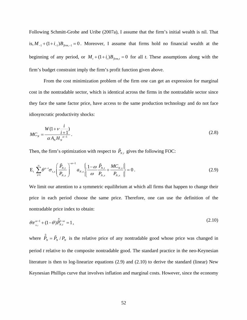
Following Schmitt-Grohe and Uribe (2007a), I assume that the firm’s initial wealth is nil. That

is, . Moreover, I assume that firms hold no financial wealth at the

beginning of any period, or for all t. These assumptions along with the

firm’s budget constraint imply the firm’s profit function given above.

1 1 , 1(1 ) 0firmM i B− − −+ + =

,(1 ) 0t t firm tM i B+ + =

From the cost minimization problem of the firm one can get an expression for marginal

cost in the nontradable sector, which is identical across the firms in the nontradable sector since

they face the same factor price, have access to the same production technology and do not face

idiosyncratic productivity shocks:

1

(1 )1

NN N

iWiMC

A H α

ν

α −

++= . (2.8)

Then, the firm’s optimization with respect to ,N tP gives the following FOC:

1

, ,t , ,

s=t , ,

1E 0N t N t N ss tt s N s

N s N s N s

P P MCa

P P P

ωωθ σ

ω

− −∞

− ⎛ ⎞ ⎧ ⎫−⎪ ⎪,

,

+ =⎜ ⎟ ⎨ ⎬⎜ ⎟ ⎪ ⎪⎝ ⎠ ⎩ ⎭∑ . (2.9)

We limit our attention to a symmetric equilibrium at which all firms that happen to change their

price in each period choose the same price. Therefore, one can use the definition of the

nontradable price index to obtain:

,

1 1,

ˆ(1 ) 1N t N tPω ωθπ θ− −+ − = , (2.10)

where is the relative price of any nontradable good whose price was changed in

period t relative to the composite nontradable good. The standard practice in the neo-Keynesian

literature is then to log-linearize equations (2.9) and (2.10) to derive the standard (linear) New

Keynesian Phillips curve that involves inflation and marginal costs. However, since the economy

ˆ /N NP P P= N

52

is on the balanced growth path and the long run inflation is not zero I follow a different approach

proposed in Schmitt-Grohe and Uribe (2007a).37

We can define two new auxiliary variables 1tx and 2

tx to get rid of the infinite sum in (2.9)

and keep the nonlinear structure. Further, the problem can be cast in a recursive way.

Let

1 1 1

, , , , ,1, , , , ,

s=t s=t+1, , , , ,

N t N s N t N t N t N ss t s tt t t s N s N t t t s N s

N s N s N t N t N s N s

P MC P MC P Mx E a a E a

P P P P P P

ω ω ω

θ σ θ σ− − − − − −

∞ ∞− −⎛ ⎞ ⎛ ⎞ ⎛ ⎞

= = +⎜ ⎟ ⎜ ⎟ ⎜ ⎟⎜ ⎟ ⎜ ⎟ ⎜ ⎟⎝ ⎠ ⎝ ⎠ ⎝ ⎠

∑ ∑ ,

,

C

1 1

, , , , 11, , 1 1 1, ,

s=t+1, , , 1 ,

N t N t N t N t N ts tN t t t t t t s N s

N s N t N t N s N t

P MC P P Ma E E a

P P P P

ω ω

θ σ θ σ− − − − − −

∞+− −

+ + ++

⎛ ⎞ ⎛ ⎞ ⎛ ⎞= +⎜ ⎟ ⎜ ⎟ ⎜ ⎟⎜ ⎟ ⎜ ⎟ ⎜ ⎟⎝ ⎠ ⎝ ⎠ ⎝ ⎠

∑1

,

,

CP

ω

1

, ,1 1, , , 1

, ,, 1

ˆ 1ˆ ˆN t N t

N t N t t t t tN t N tN t

MC PP a E x

P P

ω

ω θ σπ

− −

− −+ +

++

⎛ ⎞⎜ ⎟= +⎜ ⎟⎝ ⎠

11

. (2.11)

Similarly, let

,2 2, , , , , , 1

s=t , 1, 1

ˆ 1ˆ ˆˆ

N ts tt t t s N t N s N t N t t t t t

N tN t

P1x E P a P a E

P

ω

ω ωθ σ θ σπ

−∞

− − − x+ +++

⎛ ⎞⎜ ⎟= = +⎜ ⎟⎝ ⎠

∑ . (2.12)

Using these two auxiliary variables, we can write (2.9) as:

1 2

1t tx xωω

=−

. (2.13)

At equilibrium, domestic absorption is given by: N Na Y= .

Integrating over all firms, one can obtain:

37 Another shortcoming of the approach that involves log-linearization is the necessity to make additional assumptions if one is to accurately calculate welfare from first order approximation to the equilibrium conditions. The steady state in this model is distorted with the distortions coming from monopolistic competition. Therefore, in order to undo the distortions one has assume the existence of factor-input subsidies financed by lump sum taxes that would ensure the competitive long run employment level.

53

1,

, ,,0

( ) N N t

N t N t NN t

P iA H Y di

P

ω

α

−⎛ ⎞

= ⎜ ⎟⎜ ⎟⎝ ⎠∫ .

Following Schmitt-Grohe and Uribe (2007a), let us introduce new variable 1

,,

,0

( )N tN t

N t

P is d

P

ω−⎛ ⎞

= ⎜ ⎟⎜ ⎟⎝ ⎠∫ i .

Then one can derive the law of motion for : ,N ts

1, , , 1 2

,, , ,0

( ) (1 ) (1 ) (1 ) ...N t N t N t N t

N tN t N t N t N t

P i P P Ps di

P P P P

ω

θ θ θ θ θ−

− −⎛ ⎞ ⎛ ⎞ ⎛ ⎞ ⎛ ⎞= = − + − + −⎜ ⎟ ⎜ ⎟ ⎜ ⎟ ⎜ ⎟⎜ ⎟ ⎜ ⎟ ⎜ ⎟ ⎜ ⎟

⎝ ⎠ ⎝ ⎠ ⎝ ⎠ ⎝ ⎠∫ , 2

,

+

,

,, 1

0 ,

ˆ (1 ) (1 )N t

N t jjN t

j N t

PP s

P

ω

ω ωθ θ θ θπ−

∞− −

−=

⎛ ⎞= − = − +⎜ ⎟⎜ ⎟

⎝ ⎠∑ . (2.14)

The state variable represents the resource costs induced by the presence of price

dispersion.38 Therefore, the resource constraint in the nontradable sector is given by:

,N ts

, , , / ,N t N t N t NY A H sα= t . (2.15)

Price Setting in Tradable Sector

Analogously, firm’s minimization problem gives a similar expression for the marginal cost in the

tradable sector:

1

(1 )1

HH H

iWiMC

A Hα

ν

α −

++= . (2.16)

Using the definition of the intermediate tradable domestic goods index one obtains:

,

1 1,

ˆ(1 ) 1H t H tPη ηθπ θ− −+ − = , (2.17)

38 See Schmitt-Grohe and Uribe (2007a) for a more detailed discussion of . ,N ts

54

where ˆ /H H HP P P= is the relative price of any domestically produced tradable good whose price

was changed in period t relative to the aggregate tradable index.

We can follow the same steps that were used for the nontradable sector to obtain the

following equations that characterize price setting in the tradable sector.

11

, , , ,3 1 3, , , , , 1

s=t , , , , 1, 1

ˆ 1ˆ ˆH t H t H t H ts t

t t t s H s H t H t t t t tH t H t H t H tH t

P MC MC P1x E a P a E

P P P P

ηη

ηθ σ θ σπ

− −− −∞

− − −+ +

++

= = +⎛ ⎞⎛ ⎞⎜ ⎟⎜ ⎟ ⎜ ⎟⎝ ⎠ ⎝ ⎠

∑ x . (2.18)

As before:

,4 4, , , , , , 1

s=t , 1, 1

ˆ 1ˆ ˆˆ

H ts tt t t s H t H s H t H t t t t t

H tH t

P1x E P a P a E

P

η

η ηθ σ θ σπ

−∞

− − − x+ +++

⎛ ⎞⎜ ⎟= = +⎜ ⎟⎝ ⎠

∑ , (2.19)

3 4

1t tx xηη

=−

. (2.20)

Absorption of tradable goods is given by *H Ha Y C= + H . Where the last term, *

HC , represents

consumption of domestically produced tradable home goods by the foreign country. In what

follows, the starred variables correspond to the foreign country.

Let us make some assumptions about the foreign country. Foreign demand for traded

home variety i is given by * 1

* **

( )( ) H HH

H t t

P i PC i CP e P

η

ε−−

⎡ ⎤⎡ ⎤= ⎢ ⎥⎢ ⎥

⎣ ⎦ ⎣ ⎦* . Where *ε is a share of home goods

in foreign consumption. I assume producer currency pricing, that is, producers cannot price

discriminate between markets. Since home is a small open economy, we can do the following

simplifications: , . Then, * *t tC Y= *

,F t tP P= *

11, ,* * * *

, * *,

H t H t *H t t

t t t F t

P PC C

e P e Pε ε

−− ⎡ ⎤⎡ ⎤= = ⎢ ⎥⎢ ⎥

⎢ ⎥⎣ ⎦ ⎣ ⎦tY .

Similar to the nontradable sector equilibrium, equations describing equilibrium in the

home tradable sector are:

55

*, , , , / ,H t H t H t H t HY C A H sα+ = t

, 1

, (2.21)

, ,ˆ(1 )H t Hs P η ηθ θπ−

−= − + t H ts , (2.22)

where 1

,,

,0

( )H tH t

H t

P is

P

η−⎛ ⎞

= ⎜⎜⎝ ⎠∫ ⎟⎟ . The state variable ,H ts represents the resource costs in the tradable

sector arising from the presence of price dispersion.

2.2.3 Inducing stationarity

There are two permanent productivity shocks in the economy. Therefore, some variables

such as final good, consumption, and the real wage will not be stationary along the balanced

growth path. The complete set of transformations and definitions of detrended variables are

provided in Appendix. Here, I will briefly outline the transformation procedure. Some of the

variables pertaining to the nontradable sector, such as 1 2,t tx x , are cointegrated with ,N tA .

Similarly, in the tradable sector, variables 3 4,t tx x are cointegrated with ,H tA . Variables related to

the aggregate economy level, such as , are cointegrated with ,, , , , , ,t t t t t H tY C G m w b dt tZ . Where

(1 ), ,t N t H tZ A Aγ ε γ−= can be thought of as an aggregate stochastic growth factor; is the

real money holdings; is the real foreign currency denominated bond holdings;

/t tm M P= t

t, /t t F td e B P=

, , /H t H tb B= tP is the real value of domestic government bonds, and is the government

consumption.

tG

The nonstationary variables are divided by the appropriate cointegrating factors. The list

of variables that do not need to be detrended include , ti tπ , ,H tπ , ,N tπ , jtτ , j=c,l, , te ,f ti , ,

,

tH

ˆNP ˆ

HP , , ,N ts ,H ts , , *ti

*tπ . I further assume that scaling (productivity growth) variables for home

56

variables are expressed in terms of deviations from the foreign counterparts, that is, we do not

have to explicitly detrend appropriate foreign variables.39 Thus some foreign variables, such as

, need not be transformed. In what follows, the variables with hats correspond to detrended

variables unless otherwise stated.40 Some detrended variables are without hats.

*tY

2.2.4 Closing small open economy and equilibrium conditions

To ensure stationarity in the net foreign assets position of home households the interest

rate at which a home household can borrow (lend) in foreign currency is set to equal the

foreign interest rate plus a premium, which is an increasing function of the country’s real foreign

debt (see Schmitt-Grohe and Uribe (2003)):

,F ti

*,

ˆ êxp( ) 1F t t ti i d d⎡ ⎤= + ϒ − −⎣ ⎦ , where and is

a detrended holdings of real foreign currency denominated bonds at time t, and is a detrended

steady state level of debt (see Appendix B for the definitions of detrended foreign currency

denominated debt).

0ϒ > ˆtd

d

The aggregate resource constraint is:

t tY C G= + t

. (2.23)

The balance of payments equation can be written as:

*, , 1 , 1 , ,(1 )t F t F t t F t H t H t t te B i e B C P PY− −= + + − . (2.24)

39 If we were to explicitly model permanent productivity shocks in the foreign country, the aggregate detrending

factor tZ would have taken the following form: *(1 ) (1 )(1 )

, , ,t N t H t H tZ A A Aγ ε γ ε γ− − −= , where *

,H tA is the productivity process in the foreign tradable sector. However, for the sake of simplicity and since the purpose of this paper is not to examine the effect of foreign productivity shocks on the home economy, it is not modeled explicitly in the paper. 40 Please note that , ˆ

NP ˆHP are not detrended variables.

57

2.2.5 Rest of the world

In the foreign block, it is assumed that output, inflation and interest rate follow

exogenous AR(1) processes:

* * * *1ln( / ) ln( / )t tπ ππ π ρ π π−= +ε , (2.25)

* * * *1ln( / ) ln( / )t Y tY Y Y Y Yρ ε−= + , (2.26)

* * * *1ln((1 ) /(1 )) ln((1 ) /(1 ))t I ti i i i iρ ε−+ + = + + + , (2.27)

where πε , iε and Yε are i.i.d. processes and are neither correlated with each other nor with any

other shocks in the model. The bar over the variable denotes the steady state value.

2.2.6 Fiscal and monetary policy rules

The consolidated government prints money, issues one-period nominally risk-free bonds,

collects taxes, and faces an exogenous government expenditure stream.

, , 1(1 )t H t t t H t t t1 tM B T i B M PG− −+ + = + + + , (2.28)

where are total tax revenues and are given as: . Real tax

collections can be written as: .

tΤ ,(c lt t t t t t H t N tT C P W H Hτ τ= + + , )

/ tP, ,( )c lt t t t H t N t tC H H Wτ τ τ= + +

It is also assumed that detrended public consumption follows the following AR(1) process: ˆtG

1 ,ˆ ˆln( / ) ln( / )t g tG G G G g tρ ε−= + , (2.29)

where G is a detrended steady state level of government consumption, and 0 1gρ≤ < .

Real GDP is given by:

,,

F tt t F

t

Pgdp Y Y

P= − t . (2.30)

58

Fiscal rules

The fiscal authority can use three rules: budget deficit rule, debt rule and a composite

rule.

Deficit rule:

1 1 , 1 1( /j jt t t t H t t tG i B P gdp gdpτ τ τ κ− −= +Ω − + − ) / t

t

. (2.31)

That is, one of the available two distorting taxation instruments can only be used at a time, while

the other is kept at its steady state value.

Debt Rule:

2 , 1 1 2( / / ) /j jt H t t t t tB P M P gdp gdpτ τ κ− −= +Ω + − . (2.32)

Composite Rule:

1 1 , 1 1 2 , 1 1 2( / ) / ( / /j jt t t t H t t t t H t t t t tG i B P gdp gdp B P M P gdp gdpτ τ τ κ κ− − − −= + Ω − + − + Ω + − ) / t . (2.33)

In all of the above three fiscal rules j=C, H. jτ denotes the steady state tax rate, j=C,H.

Monetary rules

The domestic monetary authority follows an open-economy version of the Taylor rule:

ln((1 ) /(1 )) ln( / ) ln( / )t t ei i e eπ tπ π+ + = Ω +Ω . (2.34)

Here, again, the bar over a variable denotes steady state. This rule can describe three monetary

regimes: (i) inflation targeting when the CB adjusts interest rate in response to the deviation of

inflation from the desired level. Under this rule, the coefficient on the nominal exchange rate is

assigned a small positive value, 310e−Ω = , to ensure the stationarity of the nominal exchange

rate; (ii) inflation targeting with managed float. Under this monetary regime, the CB changes

interest rate in response to the deviations of both inflation and the nominal exchange rate from

59

their respective targets. Thus, , in the calculations I used 0eΩ > 1eΩ = ; and (iii) the fixed

exchange rate regime: and 310eΩ = 0πΩ = . In this case, the CB does not target inflation but

reacts very aggressively if the nominal exchange rate deviates from the target level, e .41

2.2.7 Competitive equilibrium

Formally, a competitive equilibrium can be defined as a set of stationary processes

, i and ,ˆ ˆ ˆ, , , , ,t

1 2 3 4, , , , , , , ,

ˆ ˆˆ ˆ ˆ ˆˆ ˆ ˆ ˆ ˆ, , , , , , , , , , , , , , , , ,t N t t t t t H t t t H t N t H t N t H t N t t tt t t t HC H m w mc Y mc x x x x b d P P s s S Q eπ π π tt

jtτ for that maximize (for the definitions of transformed variables see Appendix B): 0t ≥

( )1 11

*0 0 1

0

ˆ( )E1 1

tt t tss

t

C HZ Zρ ψρ

βρ ψ

− +∞ −

==

⎧ ⎫⎪ ⎪−⎨ ⎬− +⎪ ⎪⎩ ⎭∑ ∏ ,

where *1/s s sZ Z Z −= , and are subject to the competitive equilibrium conditions: (2.1), (2.3)-(2.5),

(2.7), (2.8), (2.11) - (2.13), (2.15), (2.16), (2.18) - (2.21), (2.23), (2.24), (2.28), (2.30), (B.22) –

(B.24) provided in Appendix, which are all written in stationary variables; (2.2), (2.10), (2.14),

(2.17), (2.22); and depending on the type of fiscal policy, either (2.31), (2.32) or (2.33) written in

stationary form; monetary rule (2.34); and exogenously given stochastic processes (2.6), (2.25)-

(2.27) and (2.29).

41 Setting is arbitrary. However, it is desirable to prevent the weight of the exchange rate objective from driving monetary policy if it is assigned considerably higher value. At the same time, giving much smaller weight to the exchange rate objective would be bringing us back to the case of inflation targeting. Quantitative implications of assigning different values to on welfare outcomes are discussed in Chapter 3. There are also qualitative implications related to the determinacy outcomes which are discussed in the following sections.

1eΩ =

eΩ

60

2.3 Solution algorithm, parameterization and definition of active and

passive policies

2.3.1 Solution algorithm

In this section, I briefly describe the solution algorithm employed in this paper. I follow

Klein’s (2000) procedure to solve a multivariate linear rational expectations model.42 The

technique is based on the generalized Shur form or QZ decomposition of a matrix pencil.

Alternative algorithms, among others, are Blanchard and Kahn (1980), Uhlig (1995), Sims

(1996) and King and Watson (1995a,b).43 The main advantage of Klein (2000) is that it allows

static (intratemporal) equilibrium conditions to be included along with the dynamic

relationships.44

To study the determinacy properties of the model, I undertake a grid search in the interval

[0, 3] with a 0.1 step for policy parameters of interest – inflation coefficient in the augmented

Taylor rule, πΩ , and coefficients in the deficit and debt rules, 1Ω and . The size of this

interval is somewhat arbitrary, but I feel that policy coefficients larger than 3 or negative would

be difficult to communicate to the public or policymakers. For instance, if fiscal feedback

coefficient is negative it would be difficult to explain why the fiscal authority would want to

decrease tax rate if the debt or deficit to GDP ratio increases above the SGP targets. Most of the

results that are presented in the next section, however, are robust to the expansion of the interval

size. For each combination of policy parameters in the grid, I first take a first order

approximation of a system of detrended market clearing and first order conditions around the

steady state. The complete set of transformed first order difference equilibrium conditions are

2Ω

42 Schmitt-Grohe and Uribe (2004) uses Klein’s (2000) procedure for their second order approximation technique. 43 See Klein (2000) for a discussion of pros and cons of alternative algorithms. 44 It is also possible in Sims (1996).

61

presented in Appendix. Instead of manually performing differentiation, I use matlab programs

written by Klein (2000) and Schmitt-Grohe and Uribe (2004) to undertake the complex

generalized Shur decomposition of the system.45 Having implemented the decomposition, it is

now simple to compare the number of stable eigenvalues with the number of the state variables

(both predetermined and exogenously given) of the system. If the number of stable eigenvalues

is equal to the number of states, then the system has unique solution. If the number of stable

eigenvalues is less than the number of states, then the system has no stable solutions, that is, it

explodes. Finally, if the number of stable eigenvalues is greater than the number of states, then

the solution is indeterminate.

2.3.2 Parameterization

The calibrated parameters used in the paper are presented in Table 2.1. The time period in

the model is one quarter. Therefore, I set 0.99β = . The risk aversion parameter, ρ , is set equal

to 1 in order to have a valid transformation when detrending nonstationary variables (see

equations (2.5) and (B.3) in Appendix B).46 I follow Christiano et al. (1997) and set ψ=1.

Following Natalucci and Ravenna (2007), the share of intermediate nontradable and tradable

goods index in the production of the final good is set to be equal 0.5. The share domestic tradable

intermediate goods composite in the production of the tradable index is also set equal 0.5.

Following Schmitt-Grohe and Uribe (2007a), the fraction of firms that cannot change their price

in any given quarter is set at 2/3 meaning that on average firms change their prices every three

quarters. The degree of monopolistic competition in both tradable and nontradable sectors is

45 The codes are available at: http://www.econ.duke.edu/~uribe/2nd_order.htm. 46 This insures that real wage and consumption grow at the same rate.

62

http://www.econ.duke.edu/~uribe/2nd_order.htm

fixed at 5 as in Schmitt-Grohe and Uribe (2007a), implying that the steady state markup of prices

over marginal costs is 25 percent.

The quarterly steady state value of technological growth rate in both tradable and

nontradable sectors, A, is assigned a value of 1.01, which translates into an annual economy wide

growth of 3.5 percent. The fraction of the wage bill that should be backed with monetary assets

is given a value of 0.6, which is similar to Schmitt-Grohe and Uribe (2007a). The parameter

determining the size of an interest rate premium on foreign borrowing, ϒ , is set at 0.004, which

is also needed to ensure stationarity in net foreign assets position. DRS parameter in both

tradable and nontradable sectors is given value of 0.8. 47

Following Natalucci and Ravenna (2007), AR(1) coefficients in the exogenous processes

describing foreign interest rate and foreign inflation are set at 0.9 and 0.25, respectively, and

their corresponding standard deviations at 0.0025 and 0.0149. I follow Masten (2005) and set ϕ ,

parameter in the productivity process, and first-order serial coefficient and the foreign output

processes at 0.95 and 0.7, respectively. The desired deficit-to-GDP and debt-to-GDP ratios are

set in accordance with the SGP target levels at 3 and 60 percent, respectively. Steady state

consumption and labor income taxes are set at 0.2 and 0.3, respectively, which are approximately

the averages in Central and Eastern European countries. Following Altig et al (2005) and

Schmitt-Grohe and Uribe (2007b) standard deviations of technology shocks in both tradable and

nontradable sectors are set 0.0007.

47 Lowering the value of this parameter did not change the qualitative nature of the results.

63

Table 2.1. Model parameterization

Parameter Value Description β 0.99 Quarterly subjective discount rate ρ 1 Risk aversion parameter, 1 1/(1 ) /(1 )C Hρ ψρ ψ− +− − + 1/ψ 1 Labor supply elasticity γ 0.5 Share of tradable and nontradable intermediate goods indexes in the

production of final good, 1 1/( (1 ) )N TY Y Yγ γ γ γγ γ− −= −ω 5 Degree of monopolistic competition in the nontradable intermediate

domestic goods market η 5 Degree of monopolistic competition in the domestic intermediate

nontradable goods market ε 0.5 Share of tradable intermediate domestic and foreign goods in the

production of the tradable index, 1 1/( (1 ) ) T H FY Y Yε ε ε εε ε− −= −

Hα 0.8 DRS parameter, in the production function of domestic tradable intermediate goods, HY AH α=

Nα 0.8 DRS parameter, in the production function of domestic tradable intermediate goods, NY AH α=

cτ 0.2 Steady state value of consumption tax lτ 0.3 Steady state value of labor income tax

ϕ 0.95 Parameter in AR(2) productivity process , , 1ln( ) (1 ) ln (1 ) ln( ) ln( )j t j t j t j tA A A A , 2 ,ϕ ϕ ϕ− −= − + + − +ς

, 2 ,

, j=N, H A 1.01 Steady state value of productivity process,

, , 1ln( ) (1 ) ln (1 ) ln( ) ln( )j t j t j t j tA A A Aϕ ϕ ϕ− −= − + + − +ς ν 0.6 Fraction of the wage bill that should be backed with monetary assets

M WHν≥ θ 2/3 Parameter describing degree of price stickiness

πρ 0.25 AR(1) coefficient in foreign inflation process, * * * *

1ln( / ) ln( / )t tπ ππ π ρ π π−= +ε

Yρ 0.7 AR(1) coefficient in foreign output process, * * * *

1ln( / ) ln( / )t Y t YY Y Y Yρ ε= +−

Iρ 0.9 AR(1) coefficient in foreign interest rate process, * * * *

1ln((1 ) /(1 )) ln((1 ) /(1 ))t I t ii i i iρ ε+ + = + + +−

gρ 0.7 AR(1) coefficient in government consumption process,

1 ,ˆ ˆln( / ) ln( / )t g tG G G G g tρ ε−= +

1κ 0.03 Target deficit-to-GDP ratio, , j=C,L 1 1 , 1 1( /j j

t t t t H t t tG i B P gdp gdpτ τ τ κ− −= +Ω − + − ) / t

t

2κ 0.6 Target debt-to-GDP ratio, 2 , 1 1 2( / / ) /j j

t H t t t t tB P M P gdp gdpτ τ κ− −= +Ω + − , j=C,L

64

ϒ 0.004 Foreign interest rate premium parameter, 48 *

,ˆ êxp( ) 1F t t ti i d d⎡ ⎤= + ϒ − −⎣ ⎦

jςσ 0.0007 Standard deviation technology shock

Gσ 0.007 Standard deviation of government expenditure shock

*iσ 0.0025 Standard deviation of foreign interest rate shock

*Yσ 0.001 Standard deviation of foreign output shock

*πσ 0.0149 Standard deviation of foreign inflation shock

2.3.3 Defining active and passive monetary and fiscal policies

In this paper, I will follow Leeper (1991) in defining active and passive monetary and

fiscal policies. Under inflation targeting rule, an active monetary policy is the one under which

the central bank sets its policy reaction parameter in the Taylor rule greater than unity. In other

words, it raises interest rate more than one to one against the deviation of inflation from the

desired level. Conversely, Leeper (1991) defines fiscal policy as active under which fiscal

authority pays no attention to the state of government debt. Parameters associated with active

fiscal policy are unresponsive to current budgetary conditions, whereas under passive behavior

the fiscal authority is forced to use tax to balance the budget. To make the picture clearer and to

facilitate the comparison with Leeper’s (1991) categorization, below I will briefly outline the

main building blocks of his model and the policy parameter space that delivers determinate

equilibrium. The overview of results obtained in Leeper (1991) is followed by the discussion of

definition of active and passive policies employed in this paper.

48 is the steady state value of foreign currency denominated debt, whose value is assigned exogenously. Otherwise, its steady state value is indeterminate. See equation (B.26).

d

65

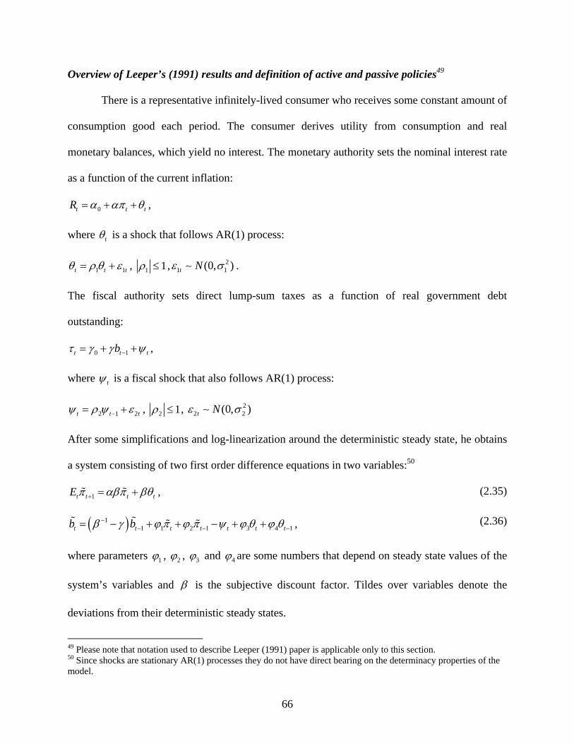
Overview of Leeper’s (1991) results and definition of active and passive policies49

There is a representative infinitely-lived consumer who receives some constant amount of

consumption good each period. The consumer derives utility from consumption and real

monetary balances, which yield no interest. The monetary authority sets the nominal interest rate

as a function of the current inflation:

0t tR tα απ θ= + + ,

where tθ is a shock that follows AR(1) process:

, 21 1(0, )t Nε σ∼ . 1 1t t tθ ρ θ ε= + , 1 1ρ ≤

The fiscal authority sets direct lump-sum taxes as a function of real government debt

outstanding:

0 1t tb tτ γ γ ψ−= + + ,

where tψ is a fiscal shock that also follows AR(1) process:

, 22 2(0, )t Nε σ∼ 2 1 2t t tψ ρ ψ ε−= + , 2 1ρ ≤

After some simplifications and log-linearization around the deterministic steady state, he obtains

a system consisting of two first order difference equations in two variables:50

1t t t tE π αβπ βθ+ = + , (2.35)

( )11 1 2 1 3 4t t t t t tb b 1tβ γ ϕ π ϕ π ψ ϕ θ ϕ−− −= − + + − + + θ − , (2.36)

where parameters 1ϕ , 2ϕ , 3ϕ and 4ϕ are some numbers that depend on steady state values of the

system’s variables and β is the subjective discount factor. Tildes over variables denote the

deviations from their deterministic steady states.

49 Please note that notation used to describe Leeper (1991) paper is applicable only to this section. 50 Since shocks are stationary AR(1) processes they do not have direct bearing on the determinacy properties of the model.

66

Expression in (2.36) states that parameter ( )1β γ− − controls the rate of growth of total

real government liabilities. Moreover, in his model this parameter also happens to be one of the

roots of the system consisting of equations (2.35) and (2.36). The other root is αβ . For the

system to have unique solution, one of the roots should be smaller than one in absolute value,

while other should be greater than one in absolute value. He further defines active and passive

monetary and fiscal policies as follows. Passive fiscal policy is when 1 1β γ− − < and active

fiscal policy if 1 1β γ− − > . That is, when γ is close to zero it is the case of active fiscal policy.

It means that the fiscal authority does not pay attention to real public debt and sets its control

variable as it sees fit. In this case, the central bank has to adjust initial price level to ensure the

existence of stationary equilibrium. That is, the initial price level should be adjusted such that the

present discounted value of future expected real government liabilities converges to zero. On the

other hand, γ has to take a high positive value in order to satisfy 1 1β γ− − < . Under this

scenario, the fiscal authority reacts strongly to the real public debt in order to ensure that the

government liabilities do not explode, that is, behaves in a passive way. In this case fiscal

solvency is guaranteed regardless of the stance of monetary policy. Active monetary policy is

associated with 1αβ > . In this case the inflation feedback parameter is set greater than one

meaning that the central bank takes a strong stance in fighting inflation. On the other hand,

1αβ < describes passive monetary stance. One can observe that for this model to have unique

saddle-path equilibrium, one of the policies should be active while the other has to be passive.

When both policies are active the model results in explosive solution. On the other hand, passive

monetary and passive fiscal policies result in indeterminacy.

67

Defining active and passive policies

Now, let us return to the model considered in this paper. The definition of active/passive

monetary policy comes straight from Leeper (1991). If the monetary authority takes a strong

stance on inflation by increasing interest rate by more than one to one in response to the

deviation of inflation from target I would call such monetary policy as active. It requires that

, that is in line with the Taylor principle. This is similar to Leeper’s (1991) definition of

active monetary policy:

1πΩ >

1αβ > . If then it is the case of passive monetary policy. 1πΩ <

Unlike Leeper (1991), where he considers only lump sum taxation, which is

nondistortionary, in the economy under study I consider distortionary taxation. A priory it is

impossible to make a distinction of whether monetary or fiscal policy is dominant, since

distortionary taxation and endogenous labor supply link parameters of monetary and fiscal policy

in stability analysis. Therefore, in the economy under study analytical derivations that would

explicitly define fiscal policy parameter range corresponding to active/passive regime are not an

easy task and would not provide much value-added to the stability analysis of the model.51

However, the same logic as in Leeper (1991) can be applied to define active and passive policies.

In this paper, I would call fiscal policy active if it is unresponsive to current budgetary

conditions. That is, the fiscal authority assigns a small positive value (close to zero) to its

feedback parameter(s), and/or . This is in line with Leeper’s (1991) definition of active

fiscal policy: if

1Ω 2Ω

γ is close to zero then 1 1β γ− − > is satisfied. It means that commitment of the

government to satisfy the SGP 3% budget deficit and 60% debt to GDP ratio is not strong in the

short run. On the contrary, when and/or1Ω 2Ω take relatively high positive values, I would call

51 In the case of Leeper (1991), the model easily simplifies to two first order difference equations for which the calculation of roots is pretty straightforward. Therefore, one can find parameter intervals pertaining to passive/active regimes.

68

such policy passive. In this case, the fiscal authority strongly increases taxes to ensure that the

SGP fiscal criteria are met. Again, given a relative complexity of the model and presence of

distortionary taxation, it would be a complicated exercise to calculate exact thresholds for

parameters at which active fiscal policy turns into passive.

2.4 Determinacy properties of the model

2.4.1 Inflation targeting

In this section, I consider the determinacy properties of the model when inflation

targeting is combined with one of the three fiscal rules based on the SGP. Inflation targeting is

given by an augmented open economy version of Taylor rule:

ln((1 ) /(1 )) ln( / ) ln( / )t t ei i e eπ tπ π+ + = Ω +Ω .

The monetary authority responds to the deviations of inflation from the desired inflation

target level, π , by adjusting interest rate. The degree of the adjustment is determined by the size

of coefficient πΩ . Under this regime, the CB does not react to the deviations of the nominal

exchange rate regime from its desired level. However, eΩ is set equal to to ensure

stationarity of nominal exchange rate. This is also needed to explicitly model nominal exchange

rate instead of resorting to real exchange rate transformation and/or additional assumption of

perfect risk sharing between countries.

310−

69

2.4.1.1 Inflation targeting and debt rule

Under a consumption (labor) tax based SGP debt rule, the government raises

consumption (labor income) tax if total government liabilities exceed the SGP requirement on

public debt, whereas labor income (consumption) tax is held at the steady state level, lτ ( cτ ).

2 , 1 1 2( / / ) /j jt H t t t t t tB P M P gdp gdpτ τ κ− −= +Ω + − , j=c,l,

where and can be interpreted as a target government debt-to-GDP ratio as in Woodford

(2001). In accordance with the Maastricht requirement on public debt, I set .

2 0κ >

2 0.6κ =

Before turning to the discussion of stability implications of the debt rule under inflation

targeting, let us consider the determinacy properties of inflation targeting regime in the absence

of fiscal policy. The case of no fiscal policy brings us to a standard assumption in dynamic

general-equilibrium models that the public budget is balanced every period. This means that the

real value of public debt is constant. As a result, the government flow budget constraint drops out

from the model structure. This corresponds to a different, non-nested model.52 The results are

presented in Figure B.1 in the line corresponding to 2 0Ω = in both panels. One can note that the

model is determinate and stable even for inflation coefficient being smaller than unity, which is a

necessary determinacy requirement for most of simple closed economy models. This is due to

the fact that the CB still reacts to the nominal exchange rate deviations, though the response is

very small. Further inspection of Figure B.1 shows that the model exhibits REE for quite a wide

range of positive inflation and debt coefficients. The positive values of monetary and fiscal

policy parameters are reasonable. The CB raises interest rate in response to higher inflation,

whereas the fiscal authority has to raise tax rate if the debt-to-GDP ratio exceeds the target ratio.

Under labor income tax, any combination of 2 [0,1.4]Ω ∈ and [0,3]πΩ ∈ deliver unique REE. In

52 This also holds true for inflation targeting with managed float and fixed exchange rate regimes.

70

the case of consumption tax the determinate area is any combination of and

. It is slightly wider than that of labor income tax and allows for higher values of debt

coefficient. The fiscal policy parameter range that delivers unique REE is consistent with both

active and passive fiscal stance. Fiscal policy changes from active to passive as the value of

2 [0,1.8]Ω ∈

[0,3]πΩ ∈

2Ω

increases. Moreover, one can observe that REE under both tax instruments is possible under both

active monetary and active fiscal policies as well as passive monetary and passive fiscal policies,

which is not possible in Leeper (1991) where the condition for the existence of REE is that one

of the policies should be active while the other be passive.

To gain more insights into how fiscal feedback parameters, 1Ω and , can influence the

stability properties of the model and to draw a closer parallel with the Leeper’s (1991) analysis

let us do the following. One can log-linearize (detrended) government budget constraint (B.27),

labor supply equation (B.3), cash-in-advance constraint (B.4) and SGP debt rule (B.31) and

combine them to obtain equation describing the evolution of (detrended) debt. Let us consider

labor income taxation. Under debt rule, (detrended) real debt evolves according to

2Ω

1 21 1

( )( )t ti mb b rest

Z C Gπ νπ ε γ εγ−

⎛ ⎞+= −Ω⎜ ⎟+ + −⎝ ⎠

+ , (2.37)

where a bar over variables denotes steady state and a tilde denotes log-deviation from steady

state level. tZ represents steady state economy wide growth rate. Loosely speaking, the feedback

parameter controls the rate of growth of (detrended) real government liabilities. Roughly

speaking, if the term in the brackets is smaller than one in absolute value, then real public debt

tends to grow at a rate less than economy wide growth rate. In this case fiscal solvency is

2Ω

71

guaranteed regardless of the stance of monetary policy.53 This together with distortionary

taxation and supply side channel can explain why for any 2 [0,1.4]Ω ∈ the model economy is

determinate regardless of monetary stance. On the other hand, if the term in the brackets is

greater than one in absolute value, which is the case, for instance, when 2Ω takes a high positive

value, then liabilities will tend to grow at a rate higher than economy wide growth rate. In this

case, the central bank has to adjust initial price level to ensure the existence of stationary

equilibrium. That is, the initial price level should be adjusted such that the present discounted

value of future expected real government liabilities converges to zero. When under

labor income tax, the central bank fails to adjust the initial price level to ensure fiscal solvency

and the solution is explosive. Thus, the combination of active or passive monetary policy and

‘very’ passive fiscal policies does not result in determinate solution. The same analysis can be

carried over to the consumption tax case.

2 1.9Ω ≥

Railavo (2004) studies determinacy properties of different fiscal policies dictated by the

SGP fiscal criteria and a monetary policy given by a simple Taylor rule in a closed economy

framework. He argues that under the debt rule the model results in an explosive solution when

the monetary policy is active. However, he considers gradualist type fiscal rules where he relates

the change of the tax rate to the deviation of the deficit from the target. Moreover, he solves for

steady state tax rates, whereas in this model I calibrate the equilibrium tax rates based on the data

from new EU member states.

Figures B.2 and B.3 depict impulse responses of main variables to a one percent

government consumption shock for different values of monetary and fiscal policy coefficients.

53 Unlike Leeper (1991), given the model complexity the value of the term in the brackets does not necessarily coincide with one of the roots of system. Therefore, it cannot be used for calculating the threshold at which fiscal policy changes from active to passive.

72

As can be seen from Figure B.2, increased government consumption initially rises aggregate

demand and hence production and inflation, which results in the fall of debt-to-GDP ratio from

its target level. This, in turn, leads to the tax cut, which is more pronounced the higher the value

of the fiscal policy coefficient is. As a result (when 2 1.5Ω = ), there is even an initial rise in

consumption despite the crowding out effect of government purchases. Further, it can be

observed that under more active fiscal policy (low values of fiscal policy coefficient), the

transition of the system to the steady state is associated with higher levels of real public debt and

less volatile consumption. Under labor income tax (Figure B.3), the government shock initially

crowds out consumption and entails lower inflation rate, which, in turn, results in lower interest

rate. Though, such deviations are very negligible. For instance, the initial fall in the inflation rate

is only 0.02 percent relative to the steady state under passive fiscal policy. We can conclude that

distortionary taxation together with endogenous labor supply allows for the existence of REE

when both monetary and fiscal policies are active and when they are both passive.

2.4.1.2 Inflation targeting and deficit rule

I use the accounting definition of the government budget deficit. It is defined as the

difference between real total tax revenues tτ , exogenous government spending , and interest

payments on the outstanding government debt

tG

1 ,t H ti B 1− − . So, the deficit rule can be written as:

1 1 , 1 1( /j jt t t t H t t tG i B P gdp gdpτ τ τ κ− −= +Ω − + − ) / t , j=c, l,

and where is a desired target level for the deficit to GDP ratio. I set it equal 0.03. If

, we have the case of a balanced budget rule.

1 0κ ≥

1 0κ =

Figure B.4 displays determinacy results for the deficit rule. One can see that there is

unique REE for a wide range of positive fiscal and monetary policy coefficients. Under

73

consumption tax, fiscal policy parameter 1 [0.8,3]Ω ∈ and any [0,3]πΩ ∈ are consistent with the

existence of REE. In the case of labor income tax the determinate area is wider relative to the

consumption tax. Any combined with 1 [0.6,3]Ω ∈ [0,3]πΩ ∈ deliver unique equilibrium.

Comparing Figures B.1 and B.4, one can note that for the existence of REE, fiscal policy under

the deficit rule should be more passive than under the debt rule. To better understand the stability

results under the deficit rule let us consider the evolution of (detrended) government liabilities. I

proceed in the same way as in the case of debt rule and consider labor income taxation.

Combining log-linearized government budget constraint (B.27), labor supply equation (B.3),

cash-in-advance constraint (B.4) and the deficit rule (B.30), one can obtain:

( )1 11

1 1( )( )t t

i mib b restZ C G mπ π ν ε γ εγ−

⎛ +⎜ ⎟= −Ω⎜ ⎟+ + − +Ω⎝ ⎠

⎞+ .

(2.38)

It can be observed that parameter 1Ω controls the rate of growth of government debt.

Again, if the term in the brackets is smaller than one in absolute value then fiscal solvency is met

under any monetary stance. Comparing (2.37) and (2.38) one can observe the following. The

lowest possible value of that ensures fiscal solvency has to be considerably higher than the

lowest possible value of which is consistent with REE. This explains why fiscal policy under

the deficit rule has to be more passive compared to the debt rule.

1Ω

2Ω

Figures B.5 and B.6 portray impulse responses to a one percent government expenditure

shock. Solid line in both figures present active monetary and passive fiscal policy case. Dotted

lines show system responses under passive monetary and active fiscal stance. As expected, under

aggressive monetary stance inflation is lower following the shock than under passive monetary

environment under both tax instruments. Furthermore, active fiscal policy is characterized by

74

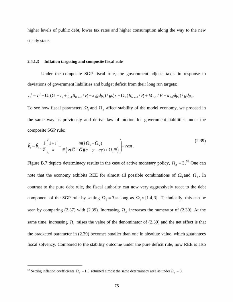
higher levels of public debt, lower tax rates and higher consumption along the way to the new

steady state.

2.4.1.3 Inflation targeting and composite fiscal rule

Under the composite SGP fiscal rule, the government adjusts taxes in response to

deviations of government liabilities and budget deficit from their long run targets:

1 1 , 1 1 2 , 1 1 2( / ) / ( / /j jt t t t H t t t t H t t t t tG i B P gdp gdp B P M P gdp gdpτ τ τ κ κ− − − −= +Ω − + − +Ω + − ) / t ,

To see how fiscal parameters and 1Ω 2Ω affect stability of the model economy, we proceed in

the same way as previously and derive law of motion for government liabilities under the

composite SGP rule:

( )1 2

11

( )1 1( )( )t t

m iib b restZ C G mπ π ν ε γ εγ−

⎛ ⎞Ω +Ω+⎜ ⎟= −⎜ ⎟+ + − +Ω⎝ ⎠

+ . (2.39)

Figure B.7 depicts determinacy results in the case of active monetary policy, .54 One can

note that the economy exhibits REE for almost all possible combinations of and

3πΩ =

1Ω 2Ω . In

contrast to the pure debt rule, the fiscal authority can now very aggressively react to the debt

component of the SGP rule by setting 2 3Ω = as long as 1 [1.4,3]Ω ∈ . Technically, this can be

seen by comparing (2.37) with (2.39). Increasing 2Ω increases the numerator of (2.39). At the

same time, increasing raises the value of the denominator of (2.39) and the net effect is that

the bracketed parameter in (2.39) becomes smaller than one in absolute value, which guarantees

fiscal solvency. Compared to the stability outcome under the pure deficit rule, now REE is also

1Ω

54 Setting inflation coefficients returned almost the same determinacy area as under . 1.5πΩ = 3πΩ =

75

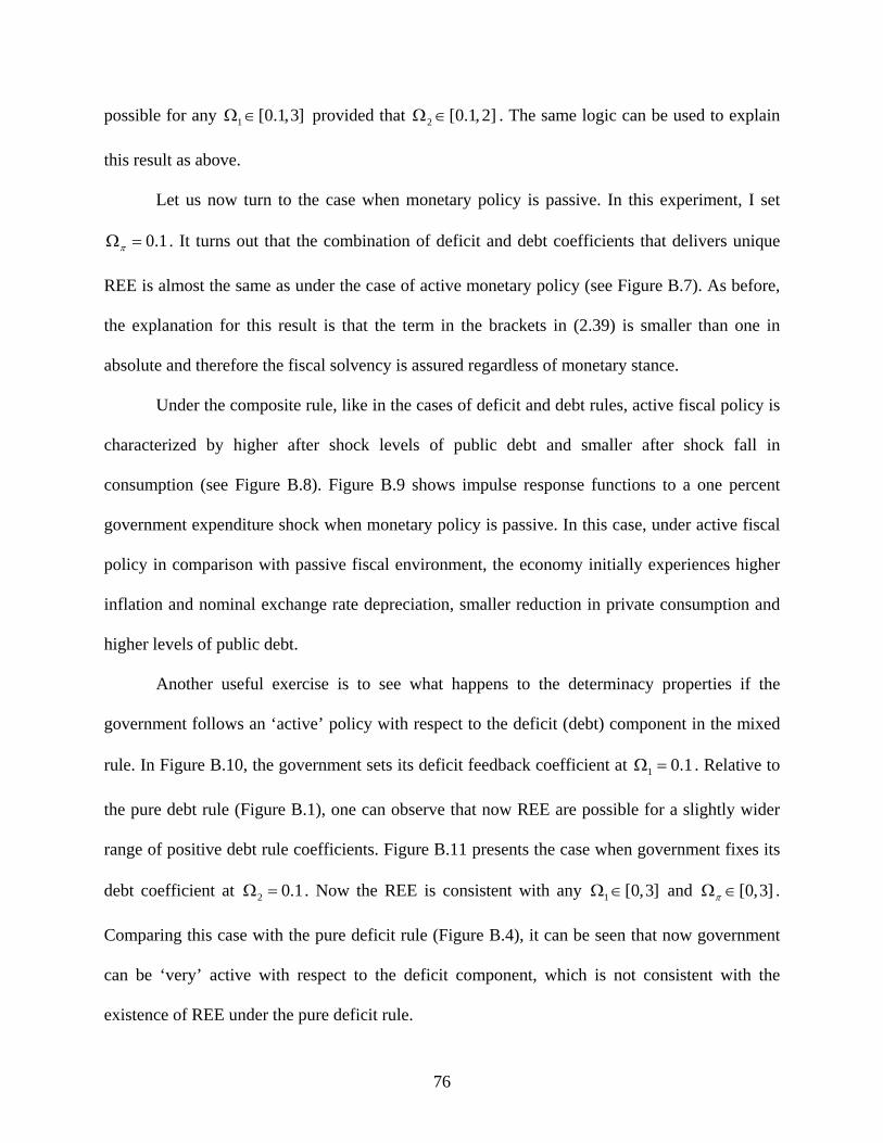
possible for any provided that 1 [0.1,3]Ω ∈ 2 [0.1,2]Ω ∈ . The same logic can be used to explain

this result as above.

Let us now turn to the case when monetary policy is passive. In this experiment, I set

. It turns out that the combination of deficit and debt coefficients that delivers unique

REE is almost the same as under the case of active monetary policy (see Figure B.7). As before,

the explanation for this result is that the term in the brackets in (2.39) is smaller than one in

absolute and therefore the fiscal solvency is assured regardless of monetary stance.

0.1πΩ =

Under the composite rule, like in the cases of deficit and debt rules, active fiscal policy is

characterized by higher after shock levels of public debt and smaller after shock fall in

consumption (see Figure B.8). Figure B.9 shows impulse response functions to a one percent

government expenditure shock when monetary policy is passive. In this case, under active fiscal

policy in comparison with passive fiscal environment, the economy initially experiences higher

inflation and nominal exchange rate depreciation, smaller reduction in private consumption and

higher levels of public debt.

Another useful exercise is to see what happens to the determinacy properties if the

government follows an ‘active’ policy with respect to the deficit (debt) component in the mixed

rule. In Figure B.10, the government sets its deficit feedback coefficient at . Relative to

the pure debt rule (Figure B.1), one can observe that now REE are possible for a slightly wider

range of positive debt rule coefficients. Figure B.11 presents the case when government fixes its

debt coefficient at . Now the REE is consistent with any

1 0.1Ω =

2 0.1Ω = 1 [0,3]Ω ∈ and .

Comparing this case with the pure deficit rule (Figure B.4), it can be seen that now government

can be ‘very’ active with respect to the deficit component, which is not consistent with the

existence of REE under the pure deficit rule.

[0,3]πΩ ∈

76

2.4.2 SGP rules under inflation targeting with managed exchange rate

In this section, I examine stabilizing properties of the model when the CB follows

managed exchange rate regime and the government employs one of three SGP based fiscal

rules.55 Inflation targeting with managed exchange rate regime is described by the same equation

as inflation targeting:


Now, the response of the CB to the deviations of nominal exchange rate from the desired level is

significantly higher. The value of the exchange rate coefficient eΩ is set equal 1, which is

somewhat arbitrary. However, experimenting with smaller and larger positive values did not

change the determinacy region.

Determinate equilibrium under all three SGP rules and managed exchange rate turns out

to be exactly the same as under the corresponding fiscal regimes and inflation targeting (see

Figures B.1, B.4 and B.7). The results are pretty much intuitive. If the model is determinate for

some combination of monetary and fiscal policy parameters when then it should be

determinate for the same combination of policy parameters for reasonably higher values of

310e−Ω =

eΩ .

The same explanation as in the corresponding inflation targeting case for why the model is

locally unique for some combinations of 1Ω and 2Ω for any [0,3]πΩ ∈ under the debt and

deficit rules can also be applied for managed exchange regime. Similar line of argument

explaining stability results for the composite SGP rule and inflation targeting can be employed

for the composite rule under managed exchange regime. I have also studied determinacy

implications when the fiscal authority sets fiscal policy active either with respect to budget

55 Managed exchange rate and inflation targeting with managed exchange rate are used interchangeably throughout the paper .

77

deficit ( ) or debt ( ). In these cases, REE are still similar to those under inflation

targeting and the composite rule.

1 0.1Ω = 2 0.1Ω =

Figures B.12 and B.13 present impulse responses to a one percent government

consumption shock. Comparing it with the inflation targeting case with similar inflation and debt

coefficient values (see Figures B.2 and B.3), one can note that impulse responses are

qualitatively similar. Let us now take a look at Figure B.14, which displays the economy

response to a one percent permanent tradable sector productivity shock. Under both monetary

regimes, the government follows a passive fiscal policy. Following the shock, the price of

tradable goods falls. Under inflation targeting nominal exchange rate depreciates resulting in the

positive deviation of CPI inflation from steady state despite the fall in tradable sector prices.

Depreciation of nominal exchange rate boosts exports, which, in turn, increase GDP.

Consequently, debt-to-GDP ratio falls below the target level requiring a tax cut. This situation is

depicted by negative deviations of the tax rate from the steady state.

Thus, the fiscal and monetary policy parameter combinations that deliver unique REE

under managed exchange regime are similar to those of corresponding fiscal regimes under

inflation targeting. However, as we have seen above, depending on the nature of the shock,

transition dynamics can be different between the two monetary regimes. Again, as in the case of

inflation targeting, the existence of unique equilibrium under the debt and composite rules is also

consistent with both active monetary and active fiscal policies as well as passive monetary and

passive fiscal regimes. The finding that fiscal policy under the deficit rule and inflation targeting

has to be more passive than under the debt rule to have determinate equilibrium also holds for

the managed exchange regime.

78

2.4.3 SGP rules under fixed exchange rate regime

The augmented Taylor rule equation can also describe the fixed exchange rate regime. It

is obtained by setting and . I set 0πΩ = eΩ →+∞ eΩ to be equal 1000. Thus, the fixed regime

is given by:

ln((1 ) /(1 )) ln( / )t ei i e e+ + = Ω t .

Now the CB does not react to the deviations of inflation from the desired target but very strongly

reacts if nominal exchange rate is different from the target level. By stabilizing exchange rate,

the CB curbs CPI inflation through equation (B.24).

Determinate equilibrium for the fixed exchange rate regime and the composite rule is

shown in Figure B.15. Let us consider Panel A which corresponds to the consumption tax

instrument. Determinacy region pertaining to the debt rule can be found by setting . One

can see that REE exist for , which is consistent with both passive and active fiscal

policies. In the case of labor income tax and the debt rule, REE exists for (Panel B).

Similarly, REE under the deficit rule can be found in the line where

1 0Ω =

2 [0,1.8]Ω ∈

2 [0,1.4]Ω ∈

2 0Ω = . Under the deficit

rule and 1 [0.8,3]Ω ∈ 1 [0.6,3]Ω ∈ are parameter values delivering REE for consumption and

labor income taxes, respectively. Under the composite rule, REE is possible for a wide range of

positive fiscal policy coefficients.

Figure B.16 plots responses to a one percent permanent tradable sector productivity

shock when the government follows the debt rule. As expected, the economy initially

experiences fall in the overall CPI index due to the decline in tradable prices and virtually fixed

exchange rate. As time passes, real wages between tradable and nontradable sectors level out.

This translates into higher nontradable inflation and is reflected in figure by upward adjustment

79

of CPI inflation. Compared to a passive fiscal policy, real public debt is higher under an active

fiscal policy all the way along the transition to the steady state. One can also note that

consumption exhibits less volatility when fiscal policy is active.

Let us now turn to the deficit rule. Figure B.17 compares the response of the economy to

a one percent permanent tradable sector productivity shock under fixed exchange regime and

inflation targeting. Unlike the pegged exchange regime under which the nominal exchange rate

remains fixed, under inflation targeting it depreciates by more than 5 percent over 40 quarters.

Depreciation stimulates exports and hence raises GDP at the same time reducing public debt. As

a consequence, debt-to-GDP ratio falls below the target level which results in the tax cut. The

economy experiences disinflation under the fixed regime, though quantitatively the magnitude is

negligible, and higher levels of real public debt and hence higher tax rates than under inflation

targeting.

2.4.4 Summary of determinacy properties and policy implications

To summarize the determinacy results discussed in the previous sections, below I provide

the summary of determinacy properties and attempt to derive some policy implications for the

EMU candidate countries. Table 2.2 presents monetary and fiscal policy parameter combinations

that deliver determinate equilibria. Let us first consider the debt rule. One can note that the fiscal

parameter range under both consumption and labor income taxes and any of three monetary

regimes are consistent with both active and passive fiscal policies. That is, the fiscal authority’s

reaction in response to the deviation of the debt from the 60% target level can be both mild and

relatively aggressive. However, being very harsh on the SGP debt requirement (setting 2 1.9Ω ≥

80

in the case of consumption tax) is undesirable since it may bring the economy into indeterminate

equilibrium.

Table 2.2. Policy parameter combinations consistent with the existence of unique REE

Monetary Regime

Fiscal Rules Tax Inflation Targeting Managed Float Fixed

consumption 2 [0,1.8]Ω ∈ and any

[0,3]πΩ ∈2 [0,1.8]Ω ∈ and any

[0,3]πΩ ∈2 [0,1.8]Ω ∈

Debt

labor 2 [0,1.4]Ω ∈ and any

[0,3]πΩ ∈2 [0,1.4]Ω ∈ and any

[0,3]πΩ ∈2 [0,1.4]Ω ∈

consumption 1 [0.8,3]Ω ∈ and any

[0,3]πΩ ∈1 [0.8,3]Ω ∈ and any

[0,3]πΩ ∈1 [0.8,3]Ω ∈

Deficit

labor 1 [0.6,3]Ω ∈ and any

[0,3]πΩ ∈1 [0.6,3]Ω ∈ and any

[0,3]πΩ ∈1 [0.6,3]Ω ∈

consumption Composite labor

see Figure B.4 see Figure B.4 see Figure B.15

In contrast to the debt rule, if the fiscal authority is to target the deficit rule, it has to be

more aggressive in fulfilling the SGP deficit criterion. Being gentle on the SGP deficit criterion

(setting close to zero) will not generate sufficient tax revenues to guarantee the fiscal

solvency. Therefore, it is recommended that new EU member states take a strong stance in

meeting the Maastricht deficit requirement, no matter what monetary policy is followed by their

CBs.

1Ω

Finally, if the fiscal authorities would like to match both the debt and the deficit

requirements at the same time, they should be harsh on both fiscal criteria. For instance, setting

and delivers determinate equilibrium. However, it is undesirable to be harsh on

the debt requirement and at the same time to be lax with respect to the deficit component, since it

1 3Ω = 2 3Ω =

81

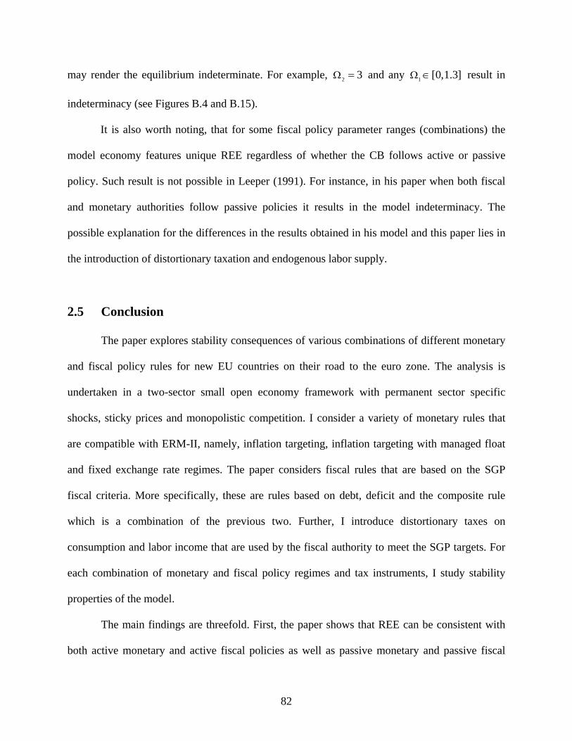
may render the equilibrium indeterminate. For example, 2 3Ω = and any result in

indeterminacy (see Figures B.4 and B.15).

1 [0,1.3]Ω ∈

It is also worth noting, that for some fiscal policy parameter ranges (combinations) the

model economy features unique REE regardless of whether the CB follows active or passive

policy. Such result is not possible in Leeper (1991). For instance, in his paper when both fiscal

and monetary authorities follow passive policies it results in the model indeterminacy. The

possible explanation for the differences in the results obtained in his model and this paper lies in

the introduction of distortionary taxation and endogenous labor supply.

2.5 Conclusion

The paper explores stability consequences of various combinations of different monetary

and fiscal policy rules for new EU countries on their road to the euro zone. The analysis is

undertaken in a two-sector small open economy framework with permanent sector specific

shocks, sticky prices and monopolistic competition. I consider a variety of monetary rules that

are compatible with ERM-II, namely, inflation targeting, inflation targeting with managed float

and fixed exchange rate regimes. The paper considers fiscal rules that are based on the SGP

fiscal criteria. More specifically, these are rules based on debt, deficit and the composite rule

which is a combination of the previous two. Further, I introduce distortionary taxes on

consumption and labor income that are used by the fiscal authority to meet the SGP targets. For

each combination of monetary and fiscal policy regimes and tax instruments, I study stability

properties of the model.

The main findings are threefold. First, the paper shows that REE can be consistent with

both active monetary and active fiscal policies as well as passive monetary and passive fiscal

82

policies, not only under active monetary and passive fiscal policies or vice verse, which is the

case in simple theoretical structures, e.g. Leeper (1991). This result holds true for inflation

targeting and any of the three fiscal regimes. Second, under managed float and fixed exchange

rate regime and any of the three fiscal rules, the government can follow either active or passive

fiscal policy, which is consistent with unique determinate equilibrium. Third, under all three

monetary regimes the fiscal policy under the deficit rule has to be more passive relative to the

debt rule.

The preliminary policy implications emanating from this paper can be summarized as

follows. If the fiscal authorities in the EMU candidate countries follow the rule based on the SGP

debt criterion they should not be very harsh on the debt requirement, since it may lead to the

indeterminate equilibrium. In contrast to the fiscal policy based on the debt rule, in order to

ensure unique equilibrium it is desirable to be aggressive in meeting the SGP deficit requirement.

Finally, if the fiscal authorities attempt to match both fiscal criteria they have to harsh on both

debt and deficit components under any monetary regime.

83

Chapter 3

Optimal Fiscal and Monetary Policy Rules for New EU Member

Countries on Their Road to Euro

3.1 Introduction

In May 2004, ten countries joined the European Union (EU).56 Two additional countries,

Romania and Bulgaria, entered the EU in 2007. The new twelve EU member states also became

members of the economic and monetary union. However, the membership is not full until they

enter the European Monetary Union (EMU). In order to join the EMU and adopt the euro, the

new member states have to comply with the Maastricht convergence criteria. The criteria are

designed in order to guarantee that new member states before joining the EMU also achieve a

high degree of nominal convergence. In particular, the countries have to satisfy the following

requirements before joining the Euro zone. First, an average rate of inflation observed over a

period of one year before the examination should not exceed by more than 1.5 percentage points

that of the three best performing Member States. Second, the countries have to comply with the

nominal exchange rate criterion. For at least the last two years before the examination the

countries should not devalue their currencies against the currency of any Member State and

nominal exchange rate should not deviate more than 15 percent around the central parity. Third,

a Member State should not run budget deficits in excess of 3 percent of GDP, and the ratio of

government debt to GDP should not be higher than 60 percent.57

56 The countries are the Czech Republic, Estonia, Hungary, Latvia, Lithuania, Poland, Slovakia, Slovenia, Cyprus and Malta. 57 There is also the long-term interest rate criterion under which a Member State for the period of one year before the examination has to have an average nominal long-term interest rate that does not exceed by more than 2 percentage

84

Some of the new EU members have enjoyed high productivity growth rates (see Figure

C.1 in Appendix). Such productivity gains (at least initially) tend to be concentrated in the

tradable sector, which is relevant for emerging market economies and transition countries. As a

consequence, some of the new members have already experienced or are expected to experience

real exchange rate appreciation (the so-called Balassa-Samuelson effect). These countries are

likely to face a tradeoff between conforming to the inflation and the nominal exchange rate

criteria. In 2007, some of the EMU candidate countries failed to meet these criteria (see Figures

C.2 and C.3). Therefore, they need to be very hard on these two criteria. As for the fiscal

performance, in 2007 most of the new EU member states were successful in fulfilling them (see

Tables C.3 and C.4). Moreover, the new members being small open economies are also

vulnerable to external shocks, such as foreign inflation and foreign interest rate shocks (see

Table C.1).

Taking into account the exposure to both internal and external shocks and an obligation

to fulfill the Maastricht criteria, several questions arise. First, what should the optimal monetary

and fiscal policy mix be? Second, what kind of tax instruments should be used in order to satisfy

the Maastricht fiscal criteria?58 Finally, whether or not would optimized monetary and fiscal

policies violate the inflation and nominal exchange rate requirements?

Recent papers by Masten (2005), Natalucci and Ravenna (2007) and Lipinska (2007),

among others, compare the performance of alternative monetary rules for the EMU accession

countries. They also examine the compliance of these rules with the Maastricht’s limits on the

nominal exchange rate and inflation. Natalucci and Ravenna (2007) develop a two-sector small

points that of the three best performing Member States. However, in this paper, I focus on the nominal exchange rate and inflation criteria on the monetary side and 3 percent budget deficit and 60 percent debt-to-GDP ratio requirements on the fiscal side. 58 In this paper, I do not consider the ramifications of the use of alternative taxation instruments on the economic growth. I compare the effects of the use of these taxes on the welfare of private agents.

85

open economy (SOE) model to explore dynamic properties of the EMU candidate economy

under alternative monetary rules. Their main conclusion is that the presence of the Balassa-

Samuelson (BS) effect causes a high exchange rate - inflation variability trade-off. This makes it

unlikely for the new member states to comply with the Maastricht criteria. However, they do not

model the BS effect as an equilibrium driving process. Lipinska (2007) derives the micro-

founded loss function and shows that under the chosen parameterization the optimal monetary

policy violates two Maastricht inflation and the nominal interest rate criteria. Unlike the previous

authors, Masten (2005) constructs real exchange rate appreciation as an equilibrium process by

introducing permanent sector-specific productivity shocks. He examines the performance of

inflation targeting regime in a two-sector SOE framework. Contrary to the findings of the

previous authors, he shows that the BS effect need not impose considerable threats to fulfilling

the inflation criterion.

To address the questions posed above, I construct a dynamic stochastic general

equilibrium model (DSGE) of a two sector small open economy. In contrast to the above-listed

studies, which ignore the fiscal side, I explicitly model the fiscal restrictions on the debt and the

deficit set out by the Maastricht Treaty. This allows studying the interaction of alternative

monetary and fiscal policy rules for the EMU candidate countries. Moreover, in contrast to

Lipinska (2007) and Natalucci and Ravenna (2007), I allow for permanent sector specific shocks,

which allows to construct real exchange rate appreciation as the equilibrium process.

The model I consider is the one developed in Chapter 2. Specifically, the model features

two nominal frictions, sticky prices, a cash-in-advance constraint on the wage bill of firms, and

imperfect competition as a source of real rigidity. Aggregate fluctuations are driven by six

shocks: three internal and three external shocks. Internal disturbances comprise temporary

86

variations in government expenditure and permanent neutral technology shocks in both tradable

and nontradable sectors. The latter shocks are important for appropriately modeling the Balassa-

Samuelson effect. External shocks include foreign inflation, foreign interest rate and foreign

import shocks.

I consider three monetary regimes that are compatible with Exchange Rate Mechanism-II

(ERM-II): inflation targeting, inflation targeting with managed exchange rate and the fixed

exchange rate regimes. On the fiscal side, I explicitly model three fiscal policy regimes based on

the Maastricht’s Stability and Growth Pact (SGP) requirements: fiscal rule based on the 60

percent debt-to-GDP ratio requirement (hereinafter referred to as the debt rule), fiscal rule based

on the 3 percent budget deficit condition, and the composite SGP rule which is the combination

of the previous two. Further, I introduce two distortionary tax instruments: consumption and

labor income taxes that are used by the fiscal authority as instruments to meet SGP fiscal

criteria.59

In characterization of optimal policy regime, I depart from the widespread practice in the

New Open Economy Macroeconomics literature of considering models in which steady state is

undistorted. Such an approach often involves the existence of a number of subsidies to product

and factor markets which undo distortions caused by monopolistic competition and bring about

the efficiency of the deterministic steady state.60 Instead, I work with the model whose steady

state is distorted. I use the algorithm developed by Schmitt-Grohe and Uribe (2004) to compute

second order approximations to policy functions and to calculate conditional welfare outcomes

across alternative combinations of monetary and fiscal policies.

59 Ideally, it is desirable to use lump sum taxes, since they do not cause distortions. However, in practice, these taxes are difficult to implement. Therefore, I do not consider them in this paper. In view of the absence of capital, I do not consider corporate taxation either, which is most relevant for the evolution of investment. 60 See Schmitt-Grohe and Uribe (2007a) for a further discussion of potential shortcomings of this approach.

87

The main findings of the paper can be summarized as follows. Under inflation targeting

and inflation targeting with managed float and under all three fiscal rules, the optimal policy

picks the highest possible value for the inflation coefficient in the grid. Further, under all

monetary regimes and consumption tax, the highest welfare level is achieved if the fiscal

authority’s stance with respect to the debt criterion is very mild, which corresponds to the active

fiscal policy. In the case of labor income tax, the fiscal authority should be quite aggressive if the

Maastricht fiscal indicators deviate from the targets, which is the case of passive fiscal policy.61

Another finding is that managing exchange rate entails welfare costs under all fiscal regimes.

Therefore, it is desirable that the CB does only minor interventions to stabilize the exchange rate.

Under all monetary regimes, the use of labor income tax is more desirable than the use of

consumption tax, since it entails smaller welfare losses. Finally, there is no threat to fulfilling the

inflation criterion under all optimized monetary and fiscal policy combinations. However, under

inflation targeting, the nominal exchange rate requirement might be violated.

Thus, the preliminary policy implications emanating from the analysis can be

summarized as follows. First, the CBs in the EMU accession countries should be aggressive in

fighting inflation. Second, if the nominal exchange rates in these countries are close to their long

run equilibrium levels, their stabilization should be achieved more as an endogenous equilibrium

outcome rather than through an active monetary policy. Finally, it is more desirable to use labor

income than consumption tax to meet the Maastricht fiscal criteria.62

The rest of the Chapter 3 is organized as follows. Section 2 provides an overview of the

model. The next section describes the solution algorithm, derives welfare measure and provides

61 I follow Leeper (1991) in defining active and passive fiscal and monetary policies. For a more detailed definition of active/passive policies see Chapter 2. In short, passive fiscal policy is associated with a high value of a fiscal feedback coefficient, while active is with a low value. In contrast, active monetary policy is when the CB aggressively reacts to inflation, e.g. when the inflation coefficient in the Taylor rule is greater than unity. 62 This result might change if the capital is added into the model.

88

details on the model parameterization. Section 4 presents results on optimized monetary and

fiscal policy combinations and tests whether or not there is a threat to comply with the

Maastricht nominal convergence criteria. Section 5 concludes.

3.2 Model overview63

In this section, I briefly outline main building blocks and equations of the model, which

have been derived and discussed in detail in Chapter 2. The model features two countries, home

and foreign. The latter is also referred to as the rest of the world. The foreign country is not

modeled explicitly in the sense that equations describing the foreign economy mainly enter the

model in terms of the exogenously given stationary AR (1) processes. In home country,

households maximize expected lifetime utility, taking prices and wages as given. The production

process in the home country consists of two stages. In the first stage, home firms produce

intermediate tradable and nontradable goods in a monopolistically competitive environment. The

prices in both tradable and nontradable intermediate goods sectors are sticky. The capital in both

sectors is assumed to be fixed and there is no investment. Therefore, the production technology

in these sectors is assumed to feature decreasing returns to scale in labor.

In the second stage, the economy produces final good from domestic nontradable, domestic

tradable and foreign intermediate goods composites. Final good is produced in a perfectly

competitive environment, which is then used for private and government consumption.

63 Detailed derivation of equations and transformation of nonstationary variables are provided in Chapter 2 and Appendix B. In this chapter, I provide only main building blocks of the model.

89

Demand side of the economy

In the home country, there is an infinitely-lived representative consumer, who maximizes his/her

expected lifetime utility

1 1

00

( )max E1 1

t t t

t

C Hρ ψ

βρ ψ

− +∞

=

⎧ ⎫−⎨ ⎬− +⎩ ⎭

∑ ,

subject to a flow budget constraint:

, , , 1 , 1 1 , 1 , , , ,(1 ) (1 ) (1 ) (1 )( )c lt t t t F t H t t F t F t t H t t H t H t N t N t tPC e B B e i B i B W H W Hτ τ− − − −+ + + = + + + + − + +Π .

Households receive labor income subject to the average tax rate, lτ , from supplying labor to

tradable and nontradable sectors in line with

, ,t H t NH H H= + t .

There is also a tax on consumption, cτ . Households receive profits, Π , from firms that produce

intermediate goods. It is assumed that these firms are owned by consumers. Corporate taxation is

not considered in this model since it is most relevant for the evolution of investment, which is

absent in the model. HB are domestic currency denominated government bonds held by

consumers. Households also have an access to foreign currency denominated bonds, FB . is a

nominal exchange rate expressed as the number of units of local currency required to purchase

one unit of foreign currency.

e

Production side of the economy

Final good market

Final good, Y, is manufactured according to the following Cobb-Douglas production

technology:

90

1

1 (1 )

N TY YYγ γ

γ γγ γ

−

−=−

,

where is an aggregate of domestically produced intermediate goods, which is given by: NY

1 11

0

( ) N NY y i diω ωω ω−

−⎡ ⎤

= ⎢ ⎥⎣ ⎦∫ .

Ny is an output of individual firm producing intermediate nontradable good. is a composite

index consisting of both domestic and foreign intermediate tradable goods aggregates and is

given by:

TY

1

1 (1 )

H FT

Y YYε ε

ε εε ε

−

−=−

.

Domestic and foreign intermediate tradable aggregates, in turn, are:

111

0

( ) H HY y i diη ηη η−

−⎡ ⎤

= ⎢ ⎥⎢ ⎥⎣ ⎦∫ , and

121

1

( ) F FY y i diµ µµ µ−

−⎡ ⎤

= ⎢⎢ ⎥⎣ ⎦∫ ⎥ , respectively.

One can use the above definitions of final good, nontradable and tradable intermediate goods

aggregates to define their respective price indexes.

The aggregate price index (CPI):

1 N TP P Pγ γ−= .

Tradable price index:

1 T H FP P Pε ε−= ,

where

11 1

1

0

( )H HP p i diη

η−

−⎡ ⎤= ⎢ ⎥⎣ ⎦∫ and

12 1

1

1

( )F FP p i diµ

µ−

−⎡ ⎤= ⎢ ⎥⎣ ⎦∫ .

Nontradable price index:

91

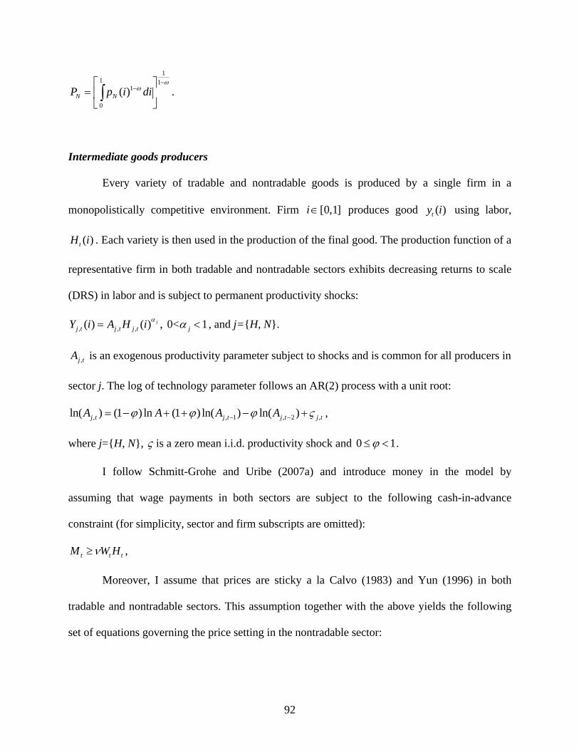
11 1

1

0

( )N NP p i diω

ω−

−⎡ ⎤= ⎢ ⎥⎣ ⎦∫ .

Intermediate goods producers

Every variety of tradable and nontradable goods is produced by a single firm in a

monopolistically competitive environment. Firm [0,1]i∈ produces good using labor,

. Each variety is then used in the production of the final good. The production function of a

representative firm in both tradable and nontradable sectors exhibits decreasing returns to scale

(DRS) in labor and is subject to permanent productivity shocks:

( )ty i

( )tH i

, , ,( ) ( ) , 0< 1jj t j t j t jY i A H i α α= < , and j=H, N.

,j tA is an exogenous productivity parameter subject to shocks and is common for all producers in

sector j. The log of technology parameter follows an AR(2) process with a unit root:

, , 1ln( ) (1 ) ln (1 ) ln( ) ln( )j t j t j t j tA A A A , 2 ,ϕ ϕ ϕ− −= − + + − +ς ,

where j=H, N, ς is a zero mean i.i.d. productivity shock and 0 1ϕ≤ < .

I follow Schmitt-Grohe and Uribe (2007a) and introduce money in the model by

assuming that wage payments in both sectors are subject to the following cash-in-advance

constraint (for simplicity, sector and firm subscripts are omitted):

t t tM W Hν≥ ,

Moreover, I assume that prices are sticky a la Calvo (1983) and Yun (1996) in both

tradable and nontradable sectors. This assumption together with the above yields the following

set of equations governing the price setting in the nontradable sector:

92

,

1 1,

ˆ(1 ) 1N t N tPω ωθπ θ− −+ − = ,

1

(1 )1

NN N

iWiMC

A H α

ν

α −

++= ,

1

, ,1 1, , , 1

, ,, 1

ˆ 1ˆ ˆN t N t

t N t N t t t t tN t N tN t

MC P 11

1

x P a E xP P

ω

ω θ σπ

− −

− −+ +

++

⎛ ⎞⎜ ⎟= +⎜ ⎟⎝ ⎠

,

,2 2, , , 1

, 1, 1

ˆ 1ˆˆ

N tt N t N t t t t t

N tN t

P1x P a E x

P

ω

ω θ σπ

−

−+ +

++

⎛ ⎞⎜ ⎟= +⎜ ⎟⎝ ⎠

,

1 2

1t tx xωω

=−

,

,, ,ˆ (1 )

N tN t N ts P ω ωθ θπ−−= − + 1s .

Nπ is the nontradable sector inflation. NMC is the nontradable sector nominal marginal cost.

is the relative price of any nontradable good whose price was changed in period t relative to the

composite nontradable good. is a domestic absorption of domestically produced nontradable

goods. Parameter

ˆNP

,N sa

θ represents the fraction of randomly chosen firms that is not allowed to

change the nominal price of the good that it manufactures. Auxiliary variables 1tx and 2

tx are

introduced to get rid of the infinite sum arising from the producer maximization problem.

Finally, the state variable represents the resource costs induced by the presence of price

dispersion. Similar price setting expressions are obtained for the tradable sector.

,N ts

93

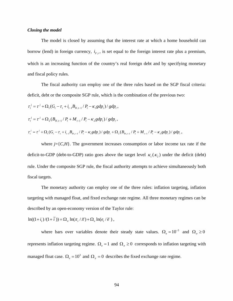
Closing the model

The model is closed by assuming that the interest rate at which a home household can

borrow (lend) in foreign currency, , is set equal to the foreign interest rate plus a premium,

which is an increasing function of the country’s real foreign debt and by specifying monetary

and fiscal policy rules.

,F ti

The fiscal authority can employ one of the three rules based on the SGP fiscal criteria:

deficit, debt or the composite SGP rule, which is the combination of the previous two:


t

,

2 , 1 1 2( / / ) /j jt H t t t t tB P M P gdp gdpτ τ κ− −= +Ω + − ,

1 1 , 1 1 2 , 1 1 2( / ) / ( / /j jt t t t H t t t t H t t t t tG i B P gdp gdp B P M P gdp gdpτ τ τ κ κ− − − −= + Ω − + − + Ω + − ) / t ,

where j=C,H. The government increases consumption or labor income tax rate if the

deficit-to-GDP (debt-to-GDP) ratio goes above the target level 1κ ( 2κ ) under the deficit (debt)

rule. Under the composite SGP rule, the fiscal authority attempts to achieve simultaneously both

fiscal targets.

The monetary authority can employ one of the three rules: inflation targeting, inflation

targeting with managed float, and fixed exchange rate regime. All three monetary regimes can be

described by an open-economy version of the Taylor rule:

ln((1 ) /(1 )) ln( / ) ln( / )t t ei i e eπ tπ π+ + = Ω +Ω ,

where bars over variables denote their steady state values. and 310e−Ω = 0πΩ ≥

represents inflation targeting regime. 1eΩ = and 0πΩ ≥ corresponds to inflation targeting with

managed float case. and describes the fixed exchange rate regime. 310eΩ = 0πΩ =

94

Finally, in the foreign block, I assume that output, inflation and interest rate follow

exogenous AR(1) processes. Domestic government consumption is also assumed to follow an

exogenous AR(1) process.

3.3 Solution algorithm, parameterization and welfare measure

Most of research dealing with the evaluation of alternative monetary and fiscal policies

rests on the log-linear approximation of the equilibrium conditions – the policy functions - and

consequent second order approximation of the welfare function. The choice of unconditional

expectation is mostly due to its advantages of computational simplicity. This approach may yield

accurate results under certain simplifying assumptions, such as restrictive preferences

specifications and access to government subsidies. In general, for such an approach to give

correct results up to the second order, it is required that the solution to the equilibrium conditions

be also accurate up to the second order. In this paper, I compute second order approximations to

the policy functions and the welfare based on the system of stochastically detrended first order

and equilibrium conditions. I use the algorithm recently developed by Schmitt-Grohé and Uribe

(2004). I follow them and assume that in initial state all (transformed) state variables are in their

deterministic steady states. Alternative policy regimes are evaluated by the conditional

expectation of the discounted life time utility.

The calibrated parameters used in this Chapter are the same as in Chapter 2. However, it

is worthwhile highlighting that the results of normative analysis crucially depend both on the

chosen calibration of parameters and on the sources of shocks. Therefore, one should ensure that

the selected calibration of parameters and exogenous processes is able to replicate certain

95

features pertaining to the data of the EMU candidate countries.64 Calibration of the most

parameters and exogenous processes comes from Natalucci and Ravenna (2007) who estimate

them for one of the EMU candidate countries, the Czech Republic.65

In choosing the optimal policy regime, denoted by r, the benevolent government chooses

a policy regime that maximizes the expected lifetime utility of a representative household (see

Appendix B for the definition of the transformed variables):

( )1 11

*0 0 1

0

ˆ( )E1 1

tt t tss

t

C HZ Zρ ψρ

βρ ψ

− +∞ −

==

⎧ ⎫⎪ ⎪−⎨ ⎬− +⎪ ⎪⎩ ⎭∑ ∏ , where *

1/s s sZ Z Z −=

We can define the welfare associated under the optimal policy regime conditional on a

particular state of the economy in period 0 as:

0 00

( , )r t rt t

tV E u C Hβ

∞

=

= ∑ r .

Using the particular functional form for the period utility function ( 1ρ = ), we can

express the above expression in terms of stationary transformation of consumption, : ˆ rtC

*0 0 0

0 0

ˆln ( , )r t t rt t

t tV E Z E u C Hβ β

∞ ∞

= =

= +∑ ∑ rt

r

0r

. (3.1)

Further, let us define . Then, we can rewrite the previous expression as: 0 00

ˆ( , )r t rt t

tV E u C Hβ

∞

=

= ∑

*0 0

0lnr t

tt

V E Z Vβ∞

=

= +∑ .

Let us denote an alternative policy regime by a. Similarly, the conditional welfare associated

with policy regime a can be defined as:

64 For example, Coenen et al. (2008) shows that the welfare gains from monetary policy coordination rise from 0.03 to 1 percent if the share of import in GDP is increased from 10-15 to 32 percent in both regions. 65 Ideally, all parameters and stochastic processes should be estimated from one of the EMU candidate countries. Such an exercise is left for future research.

96

0 00

( , )a t at t

tV E u C Hβ

∞

=

= ∑ a

at

a

0a

.

This can be written in terms of the stationary transformation of consumption as:

*0 0 0

0 0

ˆln ( , )a t t at t

t tV E Z E u C Hβ β

∞ ∞

= =

= +∑ ∑ .

Defining a new variable , we can rewrite the conditional welfare under

policy regime a as:

0 00

ˆ( , )a t at t

tV E u C Hβ

∞

=

= ∑

*0 0

0lna t

tt

V E Z Vβ∞

=

= +∑ .

It is assumed that economy begins at time zero, at which all variables of the system are

equal to their respective initial values. I further assume that the economy begins from the same

state and grows at the same rate under the two alternative policy regimes. This delivers a

constrained optimal policy regime associated with a particular initial state of the economy.66

Let cλ denote the welfare cost of adopting policy regime a instead of the optimal policy

regime r conditional on a particular state of the economy in period zero. cλ is defined as the

fraction of regime r’s consumption process that a representative household is willing to give up

to be as well off under the regime a as under regime r. Then, cλ can be implicitly defined by:

0 00

((1 ) , )a t c rt t

tV E u C Hβ λ

∞

=

= −∑ r .

Using the definitions above, one can further rewrite this expression as:

0 0ln(1 )

1

ca rV V λ

β−

= +−

.

66 In principle, the welfare ranking of alternative exchange rate arrangements might depend upon the initial value (distribution) of the state vector. For further discussion, see Kim et al (2003).

97

Now, we can derive a direct formula for calculating the welfare cost measure of adopting regime

a instead of regime r:

( )( )( )0 01 exp ( ) 1 x100%c a rV Vλ β= − − − .67

I also decompose conditional welfare costs for each combination of alternative monetary and

fiscal policy regimes into mean and variance components. Let λ be the fraction of consumption

of the nonstochastic steady state consumption level that consumers are willing to give up in order

to avoid risk and be as well-off under the stochastic environment under some combination of

monetary and fiscal policies. Let us also denote by meanλ welfare costs due to changes in means

and varλ costs due to variance effect. Given the second order approximation to the utility

function and (detrended) steady state levels of consumption, C , and labor, H , one can

decompose λ as follows:68

1 1

0

1 1([1 ] , ) ( , ) (1 ) ( ) var( ) var( )2 2

tt t t

tu C H u C H E C H H C H Hψ ψλ β β ψ

∞+ +

=t

⎧ ⎫− ≈ + − − − −⎨ ⎬⎩ ⎭

∑ ,

where a tilde denotes log-deviation from the deterministic steady state. The change in mean

consumption, meanλ , is computed from the following expression:

1

0([1 ] , ) ( , ) (1 ) ( )t

mean t tt

u C H u C H E C H ψλ β β∞

+

=

− = + − −∑ H . (3.2)

The change in conditional variance of consumption is given by

1var

0

1 1([1 ] , ) ( , ) (1 ) var( ) var( )2 2

tt t

tu C H u C H C H Hψλ β β ψ

∞+

=

⎧ ⎫− = − − +⎨ ⎬⎩ ⎭

∑ . (3.3)

67 In equation (3.1), *

tZ is a stationary process since the productivity growth rates in both tradable and nontradable sectors are stationary processes (see Appendix B). Hence, the first term in equation (3.1) is finite. Furthermore, it is similar across all alternative policy regimes. Therefore, for the comparisons of conditional welfare under alternative policy regimes we can omit it and compare and instead of calculating and . 0

rV 0

aV 0

rV 0

aV68In the following derivations I already assume that ρ=1.

98

It can be easily shown that the following relation holds:

var(1 ) (1 )(1 )meanλ λ λ− = − − . (3.4)

As there are no closed-form solutions to (3.2) and (3.3), I simulate the conditional moments for

2000 periods and compute the discounted sum. I calculate varλ from (3.3) and meanλ is computed

using (3.4). The analytical formulas for the computation of conditional moments are derived and

provided in Paustian (2003) and Marzo, Strid and Zagaglia (2006).

3.4 Optimal monetary and fiscal policy rules

In this section, I compute optimal policy mix for different combinations of alternative

monetary and fiscal rules. The model setup, equations and monetary and fiscal policy rules are

described in detail in the previous chapter. Monetary rules that are considered are inflation

targeting, inflation targeting with managed float, and fixed exchange rate regime. The fiscal

authority can follow one of the three rules: debt rule, deficit rule, and the composite SGP rule.

Moreover, for each combination of monetary and fiscal regimes, I calculate conditional welfare

under two different tax instruments – consumption and labor income taxes.

I follow Schmitt-Grohe and Uribe (2007a) in defining optimal policy. For a policy rule to

be optimal and implementable I require that (i) the associated equilibrium is locally unique; (ii)

the equilibrium is locally unique everywhere in the neighborhood of radius 0.15 around the

optimized monetary and fiscal policy coefficients; (iii) welfare is at its local optimum within that

neighborhood, and (iv) the volatility of nominal interest rate relative to its target value is low.

Specifically, I impose the condition ln(1 ) 2 ii σ+ > , where iσ denotes the unconditional standard

deviation of the nominal interest rate, and i denotes steady state value of nominal interest rate.

99

The first condition rules out parameter combinations that are associated with

indeterminate equilibrium. The second requirement excludes parameter combinations that are in

the vicinity of a bifurcation point. The welfare calculations near a bifurcation point may be

inaccurate. The third condition rules out the selection of an element of sequence of parameter

combinations associated with increasing welfare that converges to a bifurcation point. The final

condition is used to approximate the zero bound constraint by requiring a low volatility of the

nominal interest rate, since the perturbation method used to approximate the equilibrium is ill-

suited to handle nonnegativity constraints.

In Chapter 2, I have already examined determinate regions for each combination of

monetary and fiscal policy coefficients in the range from 0 to 3 with a step of 0.1. For each

combination of monetary and fiscal policy parameters in the determinate area I calculate

conditional welfare.

3.4.1 Optimized policy under inflation targeting

As already discussed in the previous section, I assume that at time zero all (detrended)

state variables of the economy are equal to their respective steady state values. Therefore, the

non-stochastic steady state is the same across all policy regimes that are considered in this paper.

This makes possible the comparison of alternative combinations of fiscal and monetary rules.

Before proceeding to the discussion of the welfare outcomes, it is worthwhile to briefly describe

monetary and fiscal regimes. Inflation targeting regime is given as:


The monetary authority adjusts interest rate if inflation deviates from the target level, π , which

might be thought of as the average inflation rate of the three best performing countries in the

100

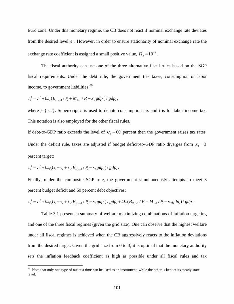
Euro zone. Under this monetary regime, the CB does not react if nominal exchange rate deviates

from the desired level e . However, in order to ensure stationarity of nominal exchange rate the

exchange rate coefficient is assigned a small positive value, 310e−Ω = .

The fiscal authority can use one of the three alternative fiscal rules based on the SGP

fiscal requirements. Under the debt rule, the government ties taxes, consumption or labor

income, to government liabilities:69

2 , 1 1 2( / / ) /j jt H t t t t t tB P M P gdp gdpτ τ κ− −= +Ω + − ,

where j=c, l. Superscript c is used to denote consumption tax and l is for labor income tax.

This notation is also employed for the other fiscal rules.

If debt-to-GDP ratio exceeds the level of 2 60κ = percent then the government raises tax rates.

Under the deficit rule, taxes are adjusted if budget deficit-to-GDP ratio diverges from 1 3κ =

percent target:


) / t

.

Finally, under the composite SGP rule, the government simultaneously attempts to meet 3

percent budget deficit and 60 percent debt objectives:

1 1 , 1 1 2 , 1 1 2( / ) / ( / /j jt t t t H t t t t H t t t t tG i B P gdp gdp B P M P gdp gdpτ τ τ κ κ− − − −= +Ω − + − +Ω + − .

Table 3.1 presents a summary of welfare maximizing combinations of inflation targeting

and one of the three fiscal regimes (given the grid size). One can observe that the highest welfare

under all fiscal regimes is achieved when the CB aggressively reacts to the inflation deviations

from the desired target. Given the grid size from 0 to 3, it is optimal that the monetary authority

sets the inflation feedback coefficient as high as possible under all fiscal rules and tax

69 Note that only one type of tax at a time can be used as an instrument, while the other is kept at its steady state level.

101

instruments, .70 This is similar to the findings by Schmitt-Grohe and Uribe (2007a) in the

case of inflation targeting without interest rate smoothing and output gap feedback. In their view,

under the optimal policy inflation in fact would be forever constant so that in such an economy

inflation volatility would be zero. Their intuition goes as follows and is also relevant for the

results of this paper. In their paper (and also in this paper), the nonstochastic steady state level of

inflation is positive. Therefore, the distortions brought about by price stickiness are present even

in the steady state. Further, the nonstochastic steady state level of welfare is globally concave in

the steady state inflation rate with a maximum at zero inflation. Therefore, in general, consumers

do not like randomizing around the long run steady state of inflation.

3πΩ =

Under the debt rule with consumption tax instrument, the highest welfare is associated

with , which relates to the case of an active fiscal policy. It means that the fiscal

authority’s reaction to the deviation of the debt from the desired target should be minimal. The

conditional welfare associated with these policy parameter combinations is -100.40571, whereas

the (detrended) non-stochastic conditional welfare, which is the same for all policy

combinations,

2 0.2Ω =

100.40181V = − .71 In contrast, when labor income tax is used under the debt rule,

the highest welfare is achieved when the fiscal authority follows a relatively passive fiscal policy

with . Though, the welfare under consumption tax is higher than under labor tax, the

welfare loss of the latter relative to the former is only 0.004 percent.72

2 1.2Ω =

70 This may not hold true under the composite SGP rule if we search for optimal policy regime simultaneously along all three dimensions: inflation, deficit and debt coefficients. Such calculations would require enormous computational time. Therefore, the search for welfare maximizing combinations is implemented along two dimensions. 71 Note that this is not the exact value of the detrended non-stochastic welfare value, since it ignores the first term in (1). However, it is not important for welfare ranking purposes since this term is the same across all policy combinations. 72 Welfare ranking might change if capital is introduced into the model. Quantitatively small conditional welfare losses obtained in this paper are quite common in this strand of literature. For example, Schmitt-Grohe and Uribe

102

Welfare outcomes under inflation targeting and a fiscal rule based on the SGP budget

deficit requirement are provided in the second line of Table 3.1. As already noted, the maximum

welfare under both consumption and labor income taxes are achieved when inflation coefficient

takes the maximum value in the grid, 3πΩ = . In the case of consumption tax, deficit coefficient

associated with the maximum welfare is 1, which is substantially smaller than that under labor

income tax, which equals 3 and is the maximum value in the grid. Thus, like in the case of the

debt rule, welfare cost minimizing fiscal policy under consumption tax has to be less passive

compared to labor income tax situation. However, the welfare loss associated with the deficit

rule and labor income tax relative the consumption tax counterpart is quantitatively negligible. It

is only 0.008 percent of consumption equivalent.

Results of welfare calculations under the composite SGP rule based on both budget

deficit and debt requirements are presented in the last line of Table 3.1. I have experimented

fixing ( ) and searching for optimal combinations of 1Ω 2Ω πΩ and 2Ω ( ). The results of the

experiments always returned the highest possible value for

1Ω

πΩ . Therefore, when calculating

optimal policy combinations under the SGP composite rule and inflation targeting I fix inflation

coefficient at 3. In this case the CB commits itself to fight inflation rigorously, whereas the fiscal

authority has to choose and that ensures determinacy and maximizes the conditional

welfare. Interestingly, under the composite SGP rule with the consumption tax the optimal policy

picks and . That is, it collapses to the debt rule. 73 In contrast to consumption

tax, under labor income tax both coefficients are positive (

1Ω 2Ω

1 0Ω = 2 0.2Ω =

1 2.1Ω = , 2 3Ω = ). One can note that

(2007a) report welfare loss of 0.0029 percentage points relative to the optimal policy under inflation targeting and distortionary taxation. 73 If the fiscal authority is not allowed to set

10Ω = under the composite SGP rule, the optimized policy picks

and with the associated conditional welfare level of -100.40680. 1

0.2Ω =2

0.2Ω =

103

under consumption taxation, it is desirable that the fiscal authority follows the debt rule, whereas

under labor tax the composite SGP rule entails the lowest welfare costs.

Table 3.1. Welfare maximizing monetary and fiscal policy under inflation targeting

Consumption Tax Labor Income Tax

πΩ 1Ω 2Ω Cond. Welfare πΩ 1Ω 2Ω Cond. Welfare

Debt Rule 3 - 0.2 -100.40571 3 - 1.2 -100.40161

Deficit Rule 3 1 - -100.40890 3 3 - -100.40085

Composite SGP

Rule with preset

3πΩ =

3 0 0.2 -100.40571 3 2.1 3 -100.40057

The main observation coming from the results is that under inflation targeting and under

all fiscal rules welfare losses associated with labor income tax are smaller than under

consumption tax.74 Moreover, from the welfare prospective it is desirable that, regardless of the

fiscal policy followed by the government, the CB should take a strong stance in fighting inflation

by setting the inflation coefficient as high as possible.75

3.4.2 Optimized policy under inflation targeting with managed exchange rate regime

Inflation targeting with managed float is described by the similar equation as in the case

of inflation targeting:


Now, indicates that the CB along with the possibility of targeting inflation also more

aggressively responds to the deviations of nominal exchange rate from the target,

1eΩ =

e , than under

74 It would be interesting to see whether or not this would still hold if capital is added into the model. 75 I have experimented enlarging positive range for πΩ . I found that the optimal policy picks the highest value allowed for the inflation coefficient, at least in the case of the debt and deficit rule. In the case of the composite SGP rule, the search for the optimal policy requires optimization along the all three dimensions.

104

the ‘pure’ inflation targeting with 310e−Ω = . Considering the necessity to comply with the

Maastricht’s nominal exchange rate criterion, e may be thought of as the central parity around

which the CB would like to keep exchange rate fluctuations within ±15 percent band. This rule

still allows for exchange rate fluctuations, which would be seen in the following section, though

they are now much smaller compared to inflation targeting. Setting 1eΩ = is somewhat arbitrary.

However, it is desirable to prevent the weight of the exchange rate objective from driving

monetary policy if it is assigned considerably higher value. At the same time, giving much

smaller weight to the exchange rate objective would be bringing us back to the case of inflation

targeting. Quantitative implications of assigning different values to eΩ on welfare outcomes are

discussed below.

Table 3.2. Welfare maximizing monetary and fiscal policy under inflation targeting with

managed exchange rate


πΩ 1Ω 2Ω Cond. Welfare πΩ 1Ω 2Ω Cond. Welfare

Debt Rule 3 - 0.2 -100.48370 3 - 1.2 -100.44826

Deficit Rule 3 0.9 - -100.48519 3 3 - -100.45349

Composite SGP

Rule with preset

3πΩ =

3 0 0.2 -100.48370 3 2.6 3 -100.44714

Table 3.2 presents a summary of conditional welfare results when inflation targeting with

managed float is combined with one of the fiscal rules.76 A quick look at the table reveals some

interesting observations. First, inflation targeting with the highest possible value (in the grid) of

the inflation coefficient still remains a desired practice under the managed float. Under all fiscal 76 Inflation targeting with managed exchange rate regime and managed float will be used interchangeably throughout the paper.

105

regimes, the optimal policy chooses 3πΩ =

3 0.2

. Second, under the debt rule, the optimized

monetary and fiscal policy coefficients have the same values as under inflation targeting with the

respective tax instruments: Ω = and π 2Ω = 3Ω =

1.2Ω =

3Ω = 0Ω = 0.2

under consumption tax , and and

under labor income tax. Moreover, under the consumption tax based composite SGP

rule policy coefficients associated with the highest welfare are the same as under inflation

targeting: , and Ω = .77 The optimal policy under the deficit rule with labor

tax features the same policy parameters as in the case of inflation targeting. Further, one can

observe that, similar to the inflation targeting regime, it is desired to follow the fiscal policy

based on the debt rule with consumption taxation, and employ the composite SGP rule in the

case of labor income tax. Moreover, like in the case of inflation targeting, under the managed

float it is more desirable to use labor income taxation for it entails smaller welfare losses.78

π

2

π 1 2

It can be observed that the levels of conditional welfare associated with any monetary and

fiscal policy mix under the managed float are uniformly smaller than under inflation targeting.

This finding suggests that the interventions on the exchange rate markets in the EMU candidate

countries might entail higher welfare costs.79

Costs of managing nominal exchange rate

Managing exchange rate comes at welfare cost of 0.08 percent under consumption tax

and 0.05 percent under labor income tax relative to the flexible exchange rate environment with

77 If the fiscal authority is not allowed to set

10Ω = under the composite SGP rule, the optimized policy picks

and , which is the same combination as under inflation targeting, with the associated conditional welfare level of -100.48591..

10.2Ω =

20.2Ω =

78 Similar experiments of enlarging the positive range for πΩ were undertaken. Like in the case of inflation targeting, the optimal policy is associated with the highest value allowed for the inflation coefficient. 79 Of course, there are also some positive aspects of managing exchange rate that are not considered here and beyond the scope of this paper. In countries with large unhedged foreign currency denominated debt managing exchange rate reduces exchange rate risk exposure.

106

the debt rule. Trying to reduce exchange rate fluctuations under the deficit rule entails welfare

losses of 0.08 and 0.05 percent under consumption and labor taxes, respectively. Figure 3.1 plots

welfare costs of managing exchange rate relative to the inflation targeting in the case of the debt

rule with consumption tax. It can be seen that higher weights on the exchange rate in the Taylor

rule bring about higher welfare losses. Similar experiments have been carried out for the other

fiscal regimes. The findings are similar: managing exchange rate results in decreased conditional

welfare. Increasing the value of under alternative fiscal rules leads to the increased welfare

losses in the range of 0.04 to 0.2 percent. Assigning large positive values to the exchange rate

coefficient would be bringing us to the fixed exchange rate regime.

eΩ

Figure 3.1. Costs of managing exchange rate under consumption tax debt rule: ,

and

3πΩ =

2 0.2Ω =

0

0,02

0,04

0,06

0,08

0,1

0,12

0,14

0 0,5 1 1,5 2 2,5 3 3

Ωe

Wel

fare

Los

s, %

,5

This finding suggests that if the exchange rate in a given EMU candidate country is

already relatively close to the long run equilibrium it is desirable that its CB does only minor

interventions on the foreign exchange market. That is, the exchange rate stabilization should be

107

achieved more as an endogenous equilibrium outcome rather than through an active monetary

policy.80

3.4.3 Optimized fiscal policy under fixed exchange rate regime

Fixed exchange rate regime is obtained from inflation targeting by setting and : 0πΩ = 310eΩ =

ln((1 ) /(1 )) ln( / )t ei i e e+ + = Ω t .

Under this monetary environment, the CB very strongly responds to the deviations of nominal

exchange rate from the target e . Table 3.3 provides a summary of the welfare maximizing

combinations of fiscal policy coefficients under the fixed exchange rate regime. Quick

observation of the results shows that conditional welfare under all fiscal regimes are uniformly

smaller than under inflation targeting with managed float and inflation targeting. Optimized debt

coefficient is the same under the debt rule with consumption tax as in the corresponding fiscal

regime and inflation targeting and inflation targeting with managed float. In the case of the debt

rule with labor income tax the coefficient is slightly lower compared to inflation targeting and

managed float. The relative losses across different taxation instruments are now much larger

compared to the previous monetary regimes. For instance, the relative loss of employing

consumption tax relative to the use of labor income tax under the debt rule is 0.08 percent

compared to the corresponding loss of 0.004 percent under inflation targeting. Again, like in the

previous monetary arrangements, it is optimal to use the debt rule under consumption taxation

and the composite SGP rule if labor tax is used. At the same time, the stance of fiscal authority in

response to the deviation of the debt from the target should not be aggressive in the former case,

80 Of course, if the exchange rate is relatively far from the long run equilibrium level then it could be still welfare improving for the CB to also stabilize the exchange rate to meet more rapidly the requirements for the membership. Joining the EMU has advantages, which are not accounted for in this type of models.

108

whereas under the labor tax, it has to be quite aggressive with respect to both the debt and the

deficit components under the SGP rule. Again, the use of labor income taxation results in smaller

welfare losses compared to the situation when consumption tax is used.

Table 3.3. Welfare maximizing fiscal policy under fixed exchange rate regime


1Ω 2Ω Cond. Welfare 1Ω 2Ω Cond. Welfare

Debt Rule - 0.2 -100.57038 - 1 -100.49325

Deficit Rule 0.9 - -100.57742 3 - -100.50290

Composite SGP

Rule

0 0.2 -100.57038 3 2 -100.49199

3.4.4 Summary of conditional welfare results and policy implications

Table 3.4 summarizes welfare outcomes for various combinations of different monetary

and fiscal policy rules. It can be seen from the table that the highest welfare is associated with

inflation targeting and labor tax based composite SGP rule with 3πΩ = , 1 2.1Ω = and 2 3Ω = . It

is optimal that the CB vigorously fights inflation. On the fiscal side, the fiscal authority should

try to achieve both targets simultaneously but with a more emphasis on the debt criterion. Should

the government decide to use consumption tax it is desirable to follow the debt rule and the CB

should still be aggressive in combating inflation. However, unlike the composite SGP rule with

labor tax, the fiscal authority’s response to the deviations of the debt from the target should be

minimal: . As already discussed, the intuition behind the optimality of the CB’s strong

anti-inflationary stance is that inflation stabilization helps to reduce inefficient cross-firm price

2 0.2Ω =

109

dispersion and hence reduce volatility of the CPI inflation rate, which is disliked by consumers81.

Thus, the price stability is desirable despite the fact that in this economy increasing inflation has

the additional benefit of increasing seignorage revenues which allows the social planner to lower

distortionary tax rates.82 Moreover, being harsh on inflation helps to meet the Maastricht’s

criterion on the inflation rate required for the Eurozone membership.

Table C.5 reports the unconditional means and standard deviations of key variables under

the optimized policy coefficients. The table shows that the standard deviation of the nominal

interest rate varies between 0.6 to 0.7 percentage points under inflation targeting. At the same

time, the steady state value of the nominal interest rate is 3.04 percent. Considering these two

figures implies that for the nominal interest rate to hit the zero bound, roughly, it must fall more

than 5 standard deviations. The probability of this happening is quite low. Further, it can be

noted from the table that unconditional mean values of consumption under inflation targeting are

higher than under managed and fixed exchange rate arrangements. Moreover, one can observe

from Table C.6 that under inflation targeting “mean component” of the welfare measure is

negative, whereas under the other monetary regimes it is positive.83

81 See Table A.5 for the comparison of standard deviations of the CPI inflation across different monetary and fiscal rules. 82 See Schmitt-Grohe and Uribe (2007b) for a further discussion why price stability is desirable even in the presence of distortionary taxation. 83 To save on computational time, I do not calculate unconditional welfare and do not decompose unconditional welfare loss into the mean and variance components since the ranking obtained through maximizing unconditional utility are different from those obtained through conditional welfare. For instance, see Kim and Kim (2003) and the results of Chapter 1.

110

Table 3.4. Summary of welfare results under optimized monetary and fiscal policy

coefficients Inflation Targeting Inflation Targeting with

Managed Float

Fixed Exchange Regime

Welfare Welfare

Loss, %1

Welfare Welfare

Loss, %1

Welfare Welfare

Loss, %1

Consumption tax -100.40571 0.0051 -100.48370 0.0831 -100.57038 0.1697 Debt Rule

Labor tax -100.40161 0.0010 -100.44826 0.0477 -100.49325 0.09264

Consumption tax -100.40890 0.0083 -100.48519 0.0846 -100.57742 0.1767 Deficit Rule

Labor tax -100.40085 0.0003 -100.45349 0.0529 -100.50290 0.1022

Consumption tax -100.40680 0.0062 -100.48591 0.0853 -100.59117 0.1904 Composite SGP

Rule2 Labor tax -100.40057 0 -100.44714 0.0465 -100.49199 0.0914

Notes: 1 – welfare loss relative to the monetary and fiscal policy mix with the highest welfare, which is inflation

targeting and the composite SGP rule with labor income tax. 2 – in the case of inflation targeting and inflation targeting with managed exchange rate results are reported

when πΩ is fixed at 3. For the sake of comparison, under the composite SGP rule with consumption tax

the results are provided for the case when 1Ω is not allowed to be zero.

Further, it can be seen from Table 3.4 that conditional welfare under managed and fixed

exchange rate regimes are uniformly lower than under inflation targeting. The more aggressively

the CB manages the exchange rate the higher the welfare losses are. This finding, basically,

supports the general argument in favor of flexible exchange rate regimes that in presence of price

stickiness a floating regime allows relative prices to adjust in response to country specific real

demand and supply shocks. This is especially true for the new EU member states that have

already enjoyed or are expected to enjoy higher productivity growth in tradable sector. Thus,

another policy implication arising from the analysis is that it is not desirable to try to smooth

exchange rate fluctuations. Once again, it should be stressed that this result is true if the

exchange rate is already relatively close to its long run equilibrium. In this case, the central bank

should do only minor intervention and let the exchange rate be stabilized endogenously. These

answer the first two questions posed in the beginning of the paper.

111

3.4.5 Maastricht convergence criteria and optimal monetary and fiscal policies

In this section, I test whether or not the Maastricht nominal exchange rate and inflation

criteria are violated if the CB and the government follow optimal monetary and fiscal policies

that were described in the previous section. To test the compliance with the two nominal

convergence criteria under the optimal policy, the economy is disturbed by an initial shock of 1.7

percent to tradable productivity. This roughly generates 30 percent increase in a ten year period

like in Masten (2005) and is roughly equivalent to an annual productivity growth of 2.65 percent

considered by Natalucci and Ravenna (2007). The impulse responses to a 1.7 percent permanent

productivity shock to the tradable sector under selected optimized fiscal and monetary rules are

presented in Figures C.4-C.9 in Appendix C.

Productivity shock to the tradable sector leads to the decrease in domestically produced

tradable goods prices. Given higher productivity, real wages in the tradable sector increase. Due

to mobility of labor between sectors real wages in the nontradable sector also increase, which

results in the higher nontradable sector inflation rate. CPI inflation goes up due to the

depreciation of nominal exchange rate. However, it does not represent risk of violating the

inflation criterion under any of optimized monetary and fiscal policy mixes. Under inflation

targeting nominal exchange rate deviates from the target level by more than 10 percent over a

forty quarters time period. Therefore, there is some possibility that the nominal exchange rate

may be violated under inflation targeting. Under both managed float and fixed exchange rate

regimes, both nominal exchange rate and inflation criteria are satisfied.

As for the compliance with the fiscal limits set by the Maastricht Treaty, one can observe

that the deviation of debt and deficit-to-GDP ratios from the 60 and 3 percent targets in response

to a permanent productivity shock in the tradable sector are not that drastic. For instance, the

112

maximum deviation of the budget deficit takes place under the optimized labor tax based

composite SGP rule and inflation targeting. The budget deficit goes up to 3.4 percent of GDP

and then gradually returns to the three percent level (see Figure C.6.). The maximum deviation of

the debt-to-GDP ratio from the steady state is 4 percent, which roughly corresponds to 62.4

percent. Of course, if the fiscal authorities in the Eurozone accession countries start with lower

initial fiscal conditions, for instance with 2.5% budget deficit and 55%, debt-to-GDP ratio, then

they satisfy the fiscal requirements (see Figure C.10.)

To sum up, there is no threat of violating the inflation criterion under any of optimized

monetary and fiscal policy combinations. However, there is a possibility of not conforming with

the nominal exchange rate requirement under inflation targeting, which calls for some minor

interventions on the foreign exchange rate markets. For instance, if the monetary authority sets,

and at the same time targets inflation aggressively by setting the nominal

exchange rate requirement is met (see Figure C.10). Such an intervention comes at a cost of 0.01

percent, which is rather negligible, relative to the inflation targeting with labor income based

composite SGP rule.

0.1eΩ = 3πΩ =

3.5 Conclusion

The paper has studied welfare implications of different combinations of alternative

monetary and fiscal policy rules for the EMU candidate countries in a small open economy

framework. The paper has considered three monetary regimes that are compatible with ERM II

and three fiscal rules dictated by the SGP fiscal criteria. More specifically, monetary rules

include inflation targeting, inflation targeting with managed float and fixed exchange rate

113

regimes. The fiscal rules comprise the debt, the deficit and the composite SGP rules. Moreover,

for each monetary and fiscal regime, the paper considered two alternative taxation instruments.

The main findings are as follows. First, under all three fiscal regimes and inflation

targeting the highest conditional welfare are attained when the inflation coefficient takes the

highest possible value which is allowed in the grid. Second, the use of labor income tax

instrument is more desirable compared to consumption tax since it entails lower welfare losses

under all monetary and fiscal policy combinations considered in the paper. However, it would be

interesting to see whether this would still be true if capital is added into the model. Third, the

higher the response by the CB to the deviations of nominal exchange rate from the target, the

higher the welfare costs are. This holds true under all fiscal regimes that are considered in the

paper. Fourth, under inflation targeting when consumption tax is used the highest welfare is

associated with more active fiscal policy compared to the situation with labor income tax. This is

also the case under the both inflation targeting with managed float and fixed exchange rate

regimes. Finally, there is no threat to fulfilling the Maastricht inflation criteria under the

optimized monetary and fiscal policy combinations. However, there may be a possibility of not

complying with the nominal exchange rate requirement under inflation targeting regime, which

may call for some minor interventions on the foreign exchange rate markets.

114

Appendix A Appendix for Chapter 1

Table A.1. Reported ratios of foreign currency deposits (FCD) broad money in countries with IMF arrangements since 1986

Country 1990 1991 1992 1993 1994 1995

Highly dollarized economies (FCD/broad money > 30 percent) (18)

Argentina 34.2 35.1 37.1 40.4 43.2 43.9 Azerbaijan . . . . . . . . . 14.8 58.9 50.3 Belarus . . . . . . . . . 40.6 54.3 30.7 Bolivia 70.8 76.8 80.8 83.9 81.9 82.3 Cambodia . . . . . . 26.3 38.8 51.8 56.4 Costa Rica . . . 37.7 31.9 29.5 30.3 31.0 Croatia . . . . . . . . . 53.8 50.2 57.4 Georgia . . . . . . . . . . . . 80.1 30.8 Guinea-Bissau 41.5 34.7 31.6 30.9 31.1 31.2 Lao P. D. R. 42.0 39.4 36.8 41.4 34.4 35.6 Latvia . . . . . . . . . 27.2 27.5 31.1 Mozambique . . . 11.8 16.7 23.2 25.3 32.6 Nicaragua . . . 28.7 37.4 45.6 48.6 54.5 Peru . . . 59.9 65.0 70.2 64.2 64.0 Tajikistan . . . . . . . . . . . . . . . 33.7 Turkey 23.2 29.7 33.7 37.9 45.8 46.1 Uruguay 80.1 78.5 76.2 73.3 74.1 76.1 Median 41.7 36.4 36.8 40.4 48.6 39.7 Average 48.6 43.3 43.0 43.4 49.4 45.5

Moderately dollarized economies (FCD/broad money < 30 percent) (34)1

Albania 2.1 1.3 23.8 20.4 18.5 . . . Armenia . . . . . . . . . . . . 41.6 20.4 Bulgaria 12.0 33.4 23.4 20.3 32.6 28.4 Czech Republic . . . . . . . . . . . . 7.2 5.9 Dominica . . . 3.0 3.9 3.5 2.5 1.5 Ecuador . . . . . . . . . 2.8 5.4 . . . Egypt . . . 50.7 37.3 26.7 23.4 25.1 El Salvador . . . 1.4 1.0 0.9 0.6 1.7 Estonia . . . . . . 23.0 3.8 9.9 11.4

115

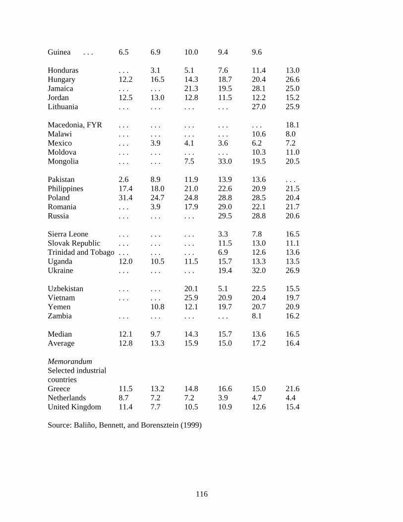
116

Guinea . . . 6.5 6.9 10.0 9.4 9.6 Honduras . . . 3.1 5.1 7.6 11.4 13.0 Hungary 12.2 16.5 14.3 18.7 20.4 26.6 Jamaica . . . . . . 21.3 19.5 28.1 25.0 Jordan 12.5 13.0 12.8 11.5 12.2 15.2 Lithuania . . . . . . . . . . . . 27.0 25.9 Macedonia, FYR . . . . . . . . . . . . . . . 18.1 Malawi . . . . . . . . . . . . 10.6 8.0 Mexico . . . 3.9 4.1 3.6 6.2 7.2 Moldova . . . . . . . . . . . . 10.3 11.0 Mongolia . . . . . . 7.5 33.0 19.5 20.5 Pakistan 2.6 8.9 11.9 13.9 13.6 . . . Philippines 17.4 18.0 21.0 22.6 20.9 21.5 Poland 31.4 24.7 24.8 28.8 28.5 20.4 Romania . . . 3.9 17.9 29.0 22.1 21.7 Russia . . . . . . . . . 29.5 28.8 20.6 Sierra Leone . . . . . . . . . 3.3 7.8 16.5 Slovak Republic . . . . . . . . . 11.5 13.0 11.1 Trinidad and Tobago . . . . . . . . . 6.9 12.6 13.6 Uganda 12.0 10.5 11.5 15.7 13.3 13.5 Ukraine . . . . . . . . . 19.4 32.0 26.9 Uzbekistan . . . . . . 20.1 5.1 22.5 15.5 Vietnam . . . . . . 25.9 20.9 20.4 19.7 Yemen 10.8 12.1 19.7 20.7 20.9 Zambia . . . . . . . . . . . . 8.1 16.2 Median 12.1 9.7 14.3 15.7 13.6 16.5 Average 12.8 13.3 15.9 15.0 17.2 16.4 Memorandum Selected industrial countries

Greece 11.5 13.2 14.8 16.6 15.0 21.6 Netherlands 8.7 7.2 7.2 3.9 4.7 4.4 United Kingdom 11.4 7.7 10.5 10.9 12.6 15.4 Source: Baliño, Bennett, and Borensztein (1999)

Tabl

e A

.2. S

umm

ary

of w

elfa

re e

ffec

ts u

nder

pro

duce

r cur

renc

y pr

icin

g

Wel

fare

Los

s R

elat

ive

to S

tead

y S

tate

(%)

Wel

fare

Los

s (G

ain)

of F

lexi

ble

rela

tive

to

Fixe

d (%

):

F

lexi

ble

Reg

ime

Fixe

d R

egim

e "+

" - l

oss,

"-" -

gai

n Im

port

Sha

re=0

.2

S

hock

sSh

ocks

Sho

cks

Deg

ree

of

Dol

lariz

atio

n B

oth

(1)

Mon

etar

y (2

) Te

chno

logy

(3

) B

oth

(4)

Mon

etar

y (5

) Te

chno

logy

(6

) B

oth:

(1

)-(4

) M

onet

ary:

(2

)-(5

) Te

chno

logy

: (3

)-(6

) Φ

=3/5

(40%

) 0.

256

0.14

8 0.

110

0.14

0

0.06

00.

080

0.11

60.

088

0.03

0Φ

=4/5

(20%

) 0.

140

0.07

9 0.

057

0.06

8

0.02

50.

043

0.07

20.

054

0.01

4Φ

=17/

20 (1

5%)

0.11

7 0.

067

0.05

0 0.

061

0.02

00.

041

0.05

60.

047

0.00

9Φ

=9/1

0 (1

0%)

0.10

0 0.

055

0.04

6 0.

058

0.01

50.

043

0.04

20.

040

0.00

3Φ

=1 (0

%)

0.07

2 0.

025

0.00

5 0.

068

0.01

00.

058

0.00

40.

015

-0.0

53Im

port

Sha

re=0

.4

Deg

ree

of

Dol

lariz

atio

nΦ

=3/5

(40%

) 0.

600

0.32

0 0.

280

0.31

40.

097

0.21

80.

286

0.22

30.

062

Φ=4

/5 (2

0%)

0.23

8 0.

121

0.11

7 0.

132

0.03

60.

096

0.10

60.

085

0.02

1Φ

=17/

20 (1

5%)

0.17

7 0.

088

0.09

1 0.

101

0.02

60.

075

0.07

60.

022

0.01

6Φ

=9/1

0 (1

0%)

0.13

1 0.

059

0.07

2 0.

081

0.01

70.

064

0.05

00.

042

0.00

8Φ

=1 (0

%)

0.08

1 0.

019

0.06

2 0.

082

0.00

90.

074

-0.0

010.

010

-0.0

12

Not

es. T

he w

elfa

re lo

ss is

com

pute

d as

the

perc

enta

ge st

eady

stat

e co

nsum

ptio

n lo

ss. T

he n

umbe

rs in

the

brac

kets

repr

esen

t deg

rees

of d

olla

rizat

ion.

117

Tabl

e A

.3. S

umm

ary

of w

elfa

re e

ffec

ts u

nder

loca

l cur

renc

y pr

icin

g

Wel

fare

Los

s R

elat

ive

to S

tead

y S

tate

W

elfa

re L

oss

(Gai

n) o

f Fle

xibl

e re

lativ

e to

Fix

ed:

Fl

exib

le R

egim

e Fi

xed

Reg

ime

"+ "

- los

s, "-

" - g

ain

Sho

cks

Shoc

ksS

hock

s

Impo

rt S

hare

=0.2

B

oth

(1)

Mon

etar

y (2

) Te

chno

logy

(3

) B

oth

(4)

Mon

etar

y (5

) Te

chno

logy

(6

) B

oth:

(1

)-(4

) M

onet

ary:

(2

)-(5

) Te

chno

logy

: (3

)-(6

) Φ

=3/5

(40%

) 0.

216

0.12

6 0.

091

0.09

10.

043

0.04

80.

125

0.08

30.

043

Φ=4

/5 (2

0%)

0.09

6 0.

061

0.03

50.

032

0.01

30.

019

0.06

40.

048

0.01

6Φ

=17/

20 (1

5%)

0.07

4 0.

048

0.02

70.

030

0.00

90.

021

0.04

40.

039

0.00

6Φ

=9/1

0 (1

0%)

0.05

8 0.

035

0.02

30.

032

0.00

80.

024

0.02

60.

027

-0.0

01Φ

=1 (0

%)

0.

041

0.01

3 0.

028

0.05

60.

010

0.04

6-0

.015

0.00

3-0

.018

Impo

rt S

hare

=0.4

Φ=3

/5 (4

0%)

0.59

0 0.

330

0.26

00.

200

0.00

80.

120

0.39

00.

322

0.14

0Φ

=4/5

(20%

) 0.

210

0.12

7 0.

083

0.05

70.

020

0.03

70.

153

0.10

70.

046

Φ=1

7/20

(15%

) 0.

140

0.08

6 0.

054

0.03

80.

014

0.02

40.

102

0.07

20.

030

Φ=9

/10

(10%

) 0.

090

0.05

8 0.

032

0.03

10.

006

0.02

50.

059

0.05

20.

007

Φ=1

(0%

) 0.

030

0.00

6 0.

024

0.05

90.

010

0.04

9-0

.029

-0.0

04-0

.025

Not

es. T

he w

elfa

re lo

ss is

com

pute

d as

the

perc

enta

ge st

eady

stat

e co

nsum

ptio

n lo

ss. T

he n

umbe

rs in

the

brac

kets

repr

esen

t deg

rees

of d

olla

rizat

ion.

118

Tabl

e A

.4. S

umm

ary

of w

elfa

re e

ffec

ts u

nder

pro

duce

r cur

renc

y pr

icin

g: h

ighe

r ris

k av

ersi

on (ρ

=30)

Wel

fare

Los

s R

elat

ive

to S

tead

y S

tate

(%)

Wel

fare

Los

s (G

ain)

of F

lexi

ble

rela

tive

to F

ixed

(%):

Fl

exib

le R

egim

e Fi

xed

Reg

ime

"+ "

- los

s, "-

" - g

ain

Impo

rt S

hare

=0.2

Sho

cks

Shoc

ksS

hock

sD

egre

e of

D

olla

rizat

ion

Bot

h (1

) M

onet

ary

(2)

Tech

nolo

gy

(3)

Bot

h (4

) M

onet

ary

(5)

Tech

nolo

gy

(6)

Bot

h:

(1)-

(4)

Mon

etar

y:

(2)-

(5)

Tech

nolo

gy:

(3)-

(6)

Φ=3

/5 (4

0%)

0.35

4 0.

179

0.18

4 0.

177

0.06

1

0.11

70.

177

0.11

80.

067

Φ=4

/5 (2

0%)

0.18

8 0.

095

0.09

6 0.

087

0.02

50.

062

0.10

10.

070

0.03

4Φ

=17/

20 (1

5%)

0.15

9 0.

079

0.08

2 0.

077

0.01

90.

058

0.08

20.

060

0.02

4Φ

=9/1

0 (1

0%)

0.13

7 0.

065

0.07

3 0.

071

0.01

50.

059

0.06

60.

050

0.01

4Φ

=1 (0

%)

0.11

0 0.

040

0.07

0 0.

089

0.01

20.

077

0.02

10.

028

-0.0

07

Not

es. T

he w

elfa

re lo

ss is

com

pute

d as

the

perc

enta

ge st

eady

stat

e co

nsum

ptio

n lo

ss. T

he n

umbe

rs in

the

brac

kets

repr

esen

t deg

rees

of d

olla

rizat

ion.

Tabl

e A

.5. S

umm

ary

of w

elfa

re e

ffec

ts u

nder

pro

duce

r cur

renc

y pr

icin

g: h

abits

per

sist

ence

Wel

fare

Los

s R

elat

ive

to S

tead

y S

tate

(%)

Wel

fare

Los

s (G

ain)

of F

lexi

ble

rela

tive

to F

ixed

(%):

Fl

exib

le R

egim

e Fi

xed

Reg

ime

"+ "

- los

s, "-

" - g

ain

Impo

rt S

hare

=0.2

Sho

cks

Shoc

ksS

hock

sD

egre

e of

D

olla

rizat

ion

B

oth

(1)

Mon

etar

y (2

) Te

chno

logy

(3

) B

oth

(4)

Mon

etar

y (5

) Te

chno

logy

(6

) B

oth:

(1

)-(4

) M

onet

ary:

(2

)-(5

) Te

chno

logy

: (3

)-(6

) Φ

=3/5

(40%

) 0.

360

0.05

6 0.

300

0.11

50.

029

0.08

7

0.24

50.

027

0.21

3Φ

=4/5

(20%

) 0.

120

0.02

3 0.

097

0.06

30.

016

0.04

70.

057

0.00

70.

050

Φ=9

/10

(10%

) 0.

062

0.01

2 0.

049

0.05

20.

009

0.04

30.

010

0.00

30.

006

Φ=1

(0%

) 0.

045

0.00

5 0.

041

0.05

00.

002

0.04

8-0

.005

0.00

3-0

.007

Not

es. T

he w

elfa

re lo

ss is

com

pute

d as

the

perc

enta

ge st

eady

stat

e co

nsum

ptio

n lo

ss. T

he n

umbe

rs in

the

brac

kets

repr

esen

t deg

rees

of d

olla

rizat

ion.

119

Tabl

e A

.6. S

elec

ted

(unc

ondi

tiona

l) st

atis

tics o

f the

dom

estic

var

iabl

es. P

CP

case

and

Cob

b-D

ougl

as m

onet

ary

aggr

egat

or

Fl

lexi

ble

Fixe

d

FI=3

/5 (4

0%)

FI=1

(0%

) FI

=3/5

(40%

) FI

=1 (0

%)

M

eans

(in

%)

Std

.Dev

(in

%)

Mea

ns (i

n %

)S

td.D

ev (i

n %

) M

eans

(in

%)

Std

.Dev

(in

%)

Mea

ns (i

n %

)S

td.D

ev (i

n %

) co

nsum

ptio

n

-0

.004

0.

930

-0.0

10

0.

881

0.00

2 0.

948

-0.0

26

0.

931

dom

estic

mon

ey

0.14

2 1.

361

0.08

5

1.70

40.

129

5.04

50.

065

3.38

4ca

pita

l 0.

300

3.

014

0.08

72.

873

0.14

83.

018

0.00

13.

335

infla

tion

0.00

20.

541

0.00

00.

410

0.00

20.

463

-0.0

020.

409

labo

r

0.05

8 2.

918

-0.0

02

2.14

7-0

.020

2.85

3-0

.011

2.18

3ag

greg

ate

dem

and

0.18

9 3.

852

0.03

0 2.

382

0.11

03.

414

-0.0

012.

360

fore

ign

mon

ey

0.13

22.

332

--

0.05

12.

556

--

bond

s 0.

047

2.81

4 -0

.055

4.70

5-0

.012

2.30

20.

065

3.77

9ex

chan

ge ra

te

-209

.360

73

.700

-1

4.81

1

36.2

000.

000

0.00

10.

000

0.00

0

120

Appendix B Appendix for Chapter 2 B.1 Stationary variables

The economy features two permanent productivity shocks. Therefore, some variables such as

output, consumption, and the real wage will not be stationary along the balanced growth path.

Below, I carry out a necessary change to obtain a set of equilibrium conditions that involve only

stationary variables. Before, we proceed to perform a change to induce stationarity, let us rewrite

nominal variables in real terms: . , , ,/ , / , /t t t H t H t t t t F tm M P b B P d e B P= = = t

One can note that variables are cointegrated with ,, , , , , ,t t t t t H t tY C G m w b d tZ . Where

(1 ), ,t N t H tZ A Aγ ε γ−= .1 Variables 1 2,t tx x are cointegrated with . Similarly, ,N tA 3 4,t tx x are cointegrated

with ,H tA .

Now, we can divide these variables by the appropriate cointegrating factors and denote the

corresponding stationary variables with the hats. Some detrended variables do not have the hats.

Let us introduce new and transformed variables:

(1 ), ,t N t H tZ A Aγ ε γ−=

, , ,/ 1N t N t N tZ A A −=

, , ,/ 1H t H t H tZ A A −=

ˆ tt

t

YYZ

=

1 I assume that 1ρ = in order for this transformation to be valid. This can be clearly seen from the household’s FOC with respect to labor.

121

,,

,

ˆ H tH t

H t

YY

A=

,,

,

ˆ N tN t

N t

YY

A=

* *ˆ t tY Y=

ˆ tt

t

CCZ

=

ˆ tt

t t

WwZ P

=

ˆ tt

t t

MmZ P

=

11

,

ˆ tt

N t

xxA

=

22

,

ˆ tt

N t

xxA

=

33

,

ˆ tt

H t

xxA

=

44

,

ˆ tt

H t

xxA

=

ˆ tt

t

GGZ

=

,,

ˆ H tH t

t t

Bb

Z P=

,ˆ t F tt

t t

e Bd

Z P=

t tP PZ= t

,

, ,F t F tP P=

, ,H t H t HP P A= t

,

, ,N t N t N tP P A=

122

1, 1 , 1ˆ t

t t t tt

ZZ

σ σ ++ +=

Scaled internal price ratio:

,

,

ˆˆ

ˆN t

tH t

PQ

P=

Scaled terms of trade:

,

,

ˆˆ

ˆF t

tH t

PS

P=

Using definitions of price indexes, one can get the following identities that will be useful later:

, 1 ( 1)(1ˆ

ˆ ˆˆN t

t tt

PQ S

P)γ ε γ− − −=

, ( 1)(1 )ˆ

ˆ ˆˆH t

t tt

PQ S

Pγ ε γ− − −=

, (1 )ˆ

ˆ ˆˆF t

t tt

PQ S

Pγ ε γ γ− − +=

Variables that do not have to be transformed are:

ti , tπ , ,H tπ , ,N tπ , jtτ , j=c,l, , te ,f ti , , , tH ˆ

NP ˆHP , ,N ts , ,H ts , , *

ti*tπ , *

tY

B.2 Equilibrium conditions in stationary variables

As discussed in the calibration section, I set 1ρ = in order to ensure stationarity in the labor

supply equation.

1 1 1,

1 1

ˆ 1 1 (1 ) 1 ˆ 1

ct t t t

t ct t tt t

C Z eEeC Z

ρτβτ π

−

+ + +

+ +

⎡ ⎤⎛ ⎞ +⎢ + =⎜ ⎟⎜ ⎟ +⎢ ⎥⎝ ⎠⎣ ⎦f ti ⎥ (B.1)

1 1

1 1

ˆ 1 1 (1 ) 1 ˆ 1

ct t t

t ct tt t

C ZEC Z

ρτβτ π

−

+ +

+ +

⎡ ⎤⎛ ⎞ +⎢ + =⎜ ⎟⎜ ⎟ +⎢ ⎥⎝ ⎠⎣ ⎦ti ⎥ (B.2)

1ˆ ˆ 01

lt

t t tct

C Hρ τωτ

− −− =

+ψ (B.3)

123

ˆ ˆt tm w Htν= (B.4)

,t H t N ,tH H H= + (B.5)

, 1, ,

ˆˆ (1 )1

ˆt

tt

tN t

N t N t

iw Pimc

H Pα

ν

α −

++

= (B.6)

, ,ˆ /N t N t N tY H sα= , (B.7)

1

,,

ˆˆ ˆˆ ˆ

N tN t t N t

t

Pa Y

Pγ

−⎛ ⎞

= ⎜ ⎟⎜ ⎟⎝ ⎠

,Y= (B.8)

1

,1 1 1, , , , 1 1

1 , 1, 1

ˆ 1ˆˆ ˆ ˆ ˆˆN t N tt

t N t N t N t t t t tt N tN t

P AZx P a mc E x , 1

,N tZ AP

ω

ω θ σπ

− −

+− −+

+ ++

⎛ ⎞⎜ ⎟= +⎜ ⎟⎝ ⎠

+ (B.9)

,2, , , 1 1

1 , 1, 1

ˆ 1ˆˆ ˆ ˆ ˆˆN t N tt

t N t N t t t t tt N tN t

P AZx P a E xZ AP

ω

ω θ σπ

−

, 12

,N t

+−+

+ ++

⎛ ⎞⎜ ⎟= +⎜ ⎟⎝ ⎠

+ (B.10)

1ˆ1t

2ˆtx xωω

=−

(B.11)

,

1 1,

ˆ(1 ) 1N t N tPωθπ θ− −+ − =ω

, 1s

(B.12)

,,ˆ(1 )

N tN t N ts P ω ωθ θπ−−= − + (B.13)

, 1, ,

ˆˆ (1 )1

ˆt

tt

tH t

H t H t

iw Pimc

H Pα

ν

α −

++

= (B.14)

1

,* *,

,

ˆˆ ˆ /ˆ

H t, ,H t t H t H t

F t

PY Y H

Pαε

−⎛ ⎞

+ =⎜ ⎟⎜ ⎟⎝ ⎠

s (B.15)

1 1 1

, , , ,* * *, *

,

ˆ ˆ ˆ ˆˆ ˆ ˆˆ (1 ) ˆ ˆ

H t H t H t H t

1

*ˆˆH t t t t

t tt t

P P P Pa Y Y Y

e PP Pε γ ε ε

− − −⎛ ⎞ ⎛ ⎞ ⎛ ⎞ ⎛ ⎞

= − + = +⎜ ⎟ ⎜ ⎟ ⎜ ⎟ ⎜ ⎟⎜ ⎟ ⎜ ⎟ ⎜ ⎟ ⎜ ⎟⎝ ⎠ ⎝ ⎠ ⎝ ⎠ ⎝ ⎠

tF t

YP

−

(B.16)

1

,3 1 3, , , , 1 1

1 , 1, 1

ˆ 1ˆˆ ˆ ˆ ˆˆ, 1

,

H ttt H t H t H t t t t t

t H tH t

P AZx P a mc E xZ AP

η

η θ σπ

− −

H t

H t

+− −+

+ ++

⎛ ⎞⎜ ⎟= +⎜ ⎟⎝ ⎠

+ (B.17)

124

,4, , , 1 1

1 , 1, 1

ˆ 1ˆˆ ˆ ˆ ˆˆ, 14

,

H ttt H t H t t t t t

t H tH t

P AZx P a E xZ AP

η

η θ σπ

−

H t

H t

+−+

+ ++

⎛ ⎞⎜ ⎟= +⎜ ⎟⎝ ⎠

+ (B.18)

3ˆ1t

4ˆtx xωω

=−

(B.19)

,

1 1,

ˆ(1 ) 1H t H tPηθπ θ− −+ − =η

, , 1

(B.20)

,ˆ(1 )H ts P η ηθ θπ−

−= − + H t H ts (B.21)

*, 1

1 , ,1

ˆˆ

t t H tt

t H t H tt

e ASe ASππ

−

−−

= (B.22)

, , 1 ,

, , ,1

ˆˆ

N t H t N tt

1H t H t N tt

A AQA AQ

ππ

−

−−

= (B.23)

(1 )(1 )(1 ) * (1 )(1 ), , 1( / )t N t H t t t te e

ε γγ ε γ ε γπ π π π− −−

−= − −

t

(B.24)

ˆ ˆt tY C G= + (B.25)

,*1, 1 1 ,

1

ˆ1ˆ ˆ ˆ ˆ(1 ) ˆH tt t

t F t t H tt t t t

PZ ed i d CZ e Pπ−

− −−

= + + − tY (B.26)

1 11 1 1

1 1ˆ ˆˆ ˆˆ (1 )c l t tt t t t t t t t t t

t t t t

Z Zm b C H i b m GZ Z

τ τ ωπ π

− −− − −+ + + = + + +ˆ t (B.27)

,,

ˆˆ

ˆF t

t t Ft

PGDP Y Y

P= − ˆ

t

ˆ t

(B.28)

ˆˆ c lt t t t tC w Hτ τ τ= + (B.29)

11 1 1 1

ˆˆ ˆ(j j tt t t t t t

t t

ZG i b GDP GDPZ

τ τ τ κπ

−− −= +Ω − + − ) / t , j=c, l (B.30)

1 12 1 1 2

ˆ ˆ(j j t tt t t t

t t t t

Z Zb m GDP GDPZ Z

τ τ κπ π

− −− −= +Ω + − ) / t , j=c, l (B.31)

1 1 11 1 1 2 1 1 2

ˆ ˆˆ ˆ ˆ ( ) ( )/j j t t tt t t t t t t t t

t t t t t t

Z Z ZG i b GDP b m GDP GDPZ Z Z

τ τ τ κ κπ π π

− − −− − −= + Ω − + − +Ω + − t , (B.32)

j=c, l

ln((1 ) /(1 )) ln( / ) ln( / )t t ei i e eπ tπ π+ + = Ω +Ω (B.33)

125

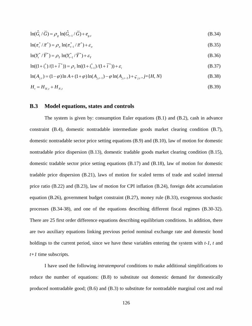
1ˆ ˆln( / ) ln( / )t g tG G G G eρ −= ,g t+ (B.34)

* * * *1ln( / ) ln( / )t tπ ππ π ρ π π−= ε+ (B.35)

* * * *1ln( / ) ln( / )t Y tY Y Y Y Yρ ε−= + (B.36)

* * * *1ln((1 ) /(1 )) ln((1 ) /(1 ))t I ti i i i iρ ε−+ + = + + + (B.37)

, , 1ln( ) (1 ) ln (1 ) ln( ) ln( ), 2 ,j t j tA A A Aj t j tϕ ϕ ϕ− −= − + + − +ς

,t

, j=H, N (B.38)

,t H t NH H H= + (B.39)

B.3 Model equations, states and controls

The system is given by: consumption Euler equations (B.1) and (B.2), cash in advance

constraint (B.4), domestic nontradable intermediate goods market clearing condition (B.7),

domestic nontradable sector price setting equations (B.9) and (B.10), law of motion for domestic

nontradable price dispersion (B.13), domestic tradable goods market clearing condition (B.15),

domestic tradable sector price setting equations (B.17) and (B.18), law of motion for domestic

tradable price dispersion (B.21), laws of motion for scaled terms of trade and scaled internal

price ratio (B.22) and (B.23), law of motion for CPI inflation (B.24), foreign debt accumulation

equation (B.26), government budget constraint (B.27), money rule (B.33), exogenous stochastic

processes (B.34-38), and one of the equations describing different fiscal regimes (B.30-32).

There are 25 first order difference equations describing equilibrium conditions. In addition, there

are two auxiliary equations linking previous period nominal exchange rate and domestic bond

holdings to the current period, since we have these variables entering the system with t-1, t and

t+1 time subscripts.

I have used the following intratemporal conditions to make additional simplifications to

reduce the number of equations: (B.8) to substitute out domestic demand for domestically

produced nontradable good; (B.6) and (B.3) to substitute for nontradable marginal cost and real

126

wage; (B.11) to substitute out 2ˆtx ; (B.12) to express the relative price of the nontradable

intermediate good as a function of nontradable price inflation; (B.14) to substitute for marginal

costs in the tradable sector; (B.16) to substitute for the domestically produced tradable

intermediate good; (B.19) to substitute out 4ˆtx ; (B.20) to substitute for the relative price in the

tradable sector; (B.25) to express the final good as a function of private and public consumption;

(B.28) for the definition of the gross domestic product.

All together, I have 27 first order difference equations in 27 variables. The next step is to

split the variables into controls and states. The state variables are collected in x: endogt

t exogt

xx

x

⎡ ⎤= ⎢ ⎥⎢ ⎥⎣ ⎦

,

where is a vector of endogenous state variables, and endogtx exog

tx is a vector of exogenous state

variables.

'

1 1 1 1 1 1 , 1 , 1 1ˆ ˆˆ ˆ ˆ endog

t t t t t t t N t H t tx e S Q i m b s s d− − − − − − − − −⎡ ⎤= ⎣ ⎦ .

'* * *1 1 1 , , 1

ˆˆ exogt t t t N t H t tx Y G Z Z iπ− − − −

⎡ ⎤= ⎣ ⎦ .

The vector of controls, y, is given by: '1 3

, , ,ˆ ˆ ˆ j

t t t N t t t H t N t t t t t ty C H H i i e x xπ π π τ⎡ ⎤= ⎣ ⎦ , j=c,l

depending on which tax instrument is used.

127

B.4

St

abili

ty r

esul

ts a

nd im

puls

e re

spon

ses

Fi

gure

B.1

. Det

erm

inac

y re

gion

s und

er th

e de

bt ru

le a

nd in

flatio

n ta

rget

ing

Pa

nel A

: Con

sum

ptio

n Ta

x

Pane

l B: L

abor

Inco

me

Tax

N

ote.

A st

ar re

pres

ents

par

amet

er c

ombi

natio

ns fo

r whi

ch e

quili

briu

m is

det

erm

inat

e. B

lank

are

a co

rres

pond

s to

expl

osiv

e so

lutio

ns.

12

8

Figu

re B

.2. G

over

nmen

t con

sum

ptio

n sh

ock

unde

r con

sum

ptio

n ta

x ba

sed

debt

rule

and

infla

tion

targ

etin

g. P

erce

nt d

evia

tions

from

stea

dy

stat

e.

05

1015

2025

3035

40-0

.010

0.01

0.02

0.03

CP

I Inf

latio

n

05

1015

2025

3035

40-0

.050

0.050.1

0.15

Inte

rest

rate

05

1015

2025

3035

40-4-20246

Tax

05

1015

2025

3035

40-0

.50

0.51

1.5

Pub

lic D

ebt

05

1015

2025

3035

40-1

-0.50

0.5

Con

sum

ptio

n

05

1015

2025

3035

40-0

.20

0.2

0.4

0.6

Labo

r

05

1015

2025

3035

40-0

.50

0.51

Rea

l mon

ey

05

1015

2025

3035

40-0

.1

-0.0

50

0.050.1

Nom

inal

ER

N

ote.

Sol

id li

ne:

and

3

πΩ

=2

1.5

Ω=

, dot

ted

line:

3

πΩ

= a

nd

20.

1Ω

=.

12

9

Figu

re B

.3. G

over

nmen

t con

sum

ptio

n sh

ock

unde

r lab

or ta

x ba

sed

debt

rule

and

infla

tion

targ

etin

g. P

erce

nt d

evia

tions

from

stea

dy st

ate.

05

1015

2025

3035

40-0

.04

-0.0

20

0.02

CP

I Inf

latio

n

05

1015

2025

3035

40-0

.1

-0.0

50

0.050.1

Inte

rest

rat

e

05

1015

2025

3035

40-0

.50

0.51

1.52

Tax

05

1015

2025

3035

40-0

.50

0.51

1.5

Pub

lic D

ebt

05

1015

2025

3035

40-0

.4

-0.3

-0.2

-0.10

Con

sum

ptio

n

05

1015

2025

3035

40-0

.10

0.1

0.2

0.3

Labo

r

05

1015

2025

3035

40-0

.20

0.2

0.4

0.6

Rea

l mon

ey

05

1015

2025

3035

40-0

.2

-0.10

0.1

0.2

Nom

inal

ER

N

ote.

Sol

id li

ne:

and

3

πΩ

=2

1Ω

=, d

otte

d lin

e:

3π

Ω=

and

2

0.1

Ω=

.

13

0

Figu

re B

.4. D

eter

min

acy

regi

ons u

nder

the

defic

it ru

le a

nd in

flatio

n ta

rget

ing

Pa

nel A

: Con

sum

ptio

n Ta

x

Pane

l B: L

abor

Inco

me

Tax

N

ote.

see

note

to F

igur

e B

.1.

13

1

Figu

re B

.5. G

over

nmen

t con

sum

ptio

n sh

ock

unde

r con

sum

ptio

n ta

x ba

sed

defic

it ru

le. P

erce

nt d

evia

tions

from

stea

dy st

ate.

N

ote.

Sol

id li

ne:

and

3

πΩ

=1

3Ω

=, d

otte

d lin

e:

0.1

πΩ

= a

nd

10.

8Ω

=.

13

2

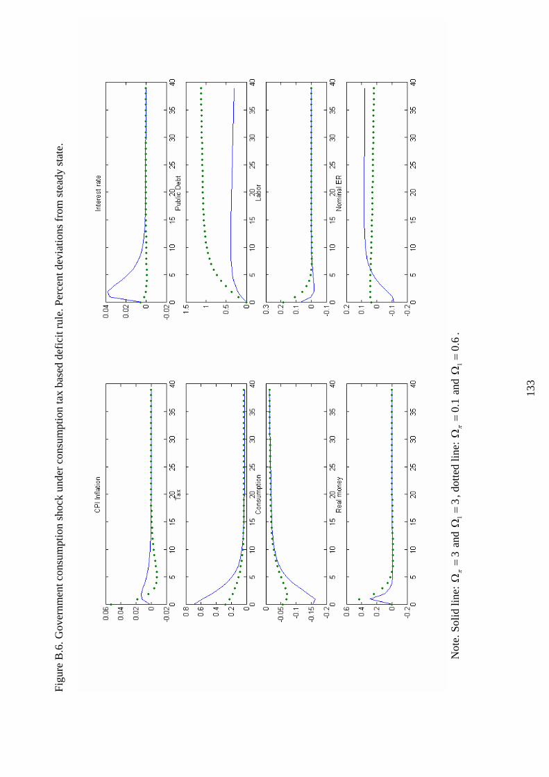
Figu

re B

.6. G

over

nmen

t con

sum

ptio

n sh

ock

unde

r con

sum

ptio

n ta

x ba

sed

defic

it ru

le. P

erce

nt d

evia

tions

from

stea

dy st

ate.

N

ote.

Sol

id li

ne:

and

3

πΩ

=1

3Ω

=, d

otte

d lin

e:

0.1

πΩ

= a

nd

10.

6Ω

=.

13

3

Figu

re B

.7. D

eter

min

acy

regi

ons u

nder

the

com

posi

te S

GP

rule

and

infla

tion

targ

etin

g: Ω

π=3

Pa

nel A

: Con

sum

ptio

n Ta

x

Pane

l B: L

abor

Inco

me

Tax

N

ote.

see

note

to F

igur

e 1.

13

4

Fi

gure

B.8

. Gov

ernm

ent c

onsu

mpt

ion

shoc

k un

der c

onsu

mpt

ion

tax

base

d m

ixed

rule

: 3

πΩ

=. P

erce

nt d

evia

tions

from

stea

dy st

ate.

05

1015

2025

3035

40-50510

x 10

-3C

PI I

nfla

tion

05

1015

2025

3035

40-0

.010

0.01

0.02

0.03

Inte

rest

rate

05

1015

2025

3035

400

0.51

1.52

2.5

Tax

05

1015

2025

3035

40-0

.50

0.51

1.5

Pub

lic D

ebt

05

1015

2025

3035

40-0

.4

-0.3

-0.2

-0.10

Con

sum

ptio

n

05

1015

2025

3035

40-0

.050

0.050.1

0.15

Labo

r

05

1015

2025

3035

40-0

.10

0.1

0.2

0.3

Rea

l mon

ey

05

1015

2025

3035

40-0

.050

0.05

Nom

inal

ER

N

ote.

Sol

id li

ne:

and

1

3Ω

=2

3Ω

=, d

otte

d lin

e:

10.

1Ω

= a

nd

20.

1Ω

=.

13

5

Figu

re B

.9. G

over

nmen

t con

sum

ptio

n sh

ock

unde

r con

sum

ptio

n ta

x ba

sed

mix

ed ru

le:

. Per

cent

dev

iatio

ns fr

om st

eady

stat

e.

0.1

πΩ

=

N

ote.

Sol

id li

ne:

and

1

3Ω

=2

3Ω

=, d

otte

d lin

e:

10.

1Ω

= a

nd

20.

1Ω

=.

13

6

Figu

re B

.10.

Det

erm

inac

y re

gion

s und

er th

e co

mpo

site

rule

and

infla

tion

targ

etin

g: Ω

1=0.

1

Pane

l A: C

onsu

mpt

ion

Tax

Pa

nel B

: Lab

or In

com

e Ta

x

N

ote.

see

note

to F

igur

e B

.1.

13

7

Figu

re B

.11.

Det

erm

inac

y re

gion

s und

er th

e co

mpo

site

rule

and

infla

tion

targ

etin

g: Ω

2=0.

1

Pa

nel A

: Con

sum

ptio

n Ta

x

Pane

l B: L

abor

Inco

me

Tax

N

ote.

see

note

to F

igur

e B

.1.

13

8

Figu

re B

.12.

Gov

ernm

ent c

onsu

mpt

ion

shoc

k un

der c

onsu

mpt

ion

tax

base

d de

bt ru

le a

nd m

anag

ed e

xcha

nge

regi

me.

Per

cent

dev

iatio

ns fr

om

stea

dy st

ate.

N

ote.

Sol

id li

ne:

and

3

πΩ

=2

1.5

Ω=

, dot

ted

line:

3

πΩ

= a

nd

20.

1Ω

=.

13

9

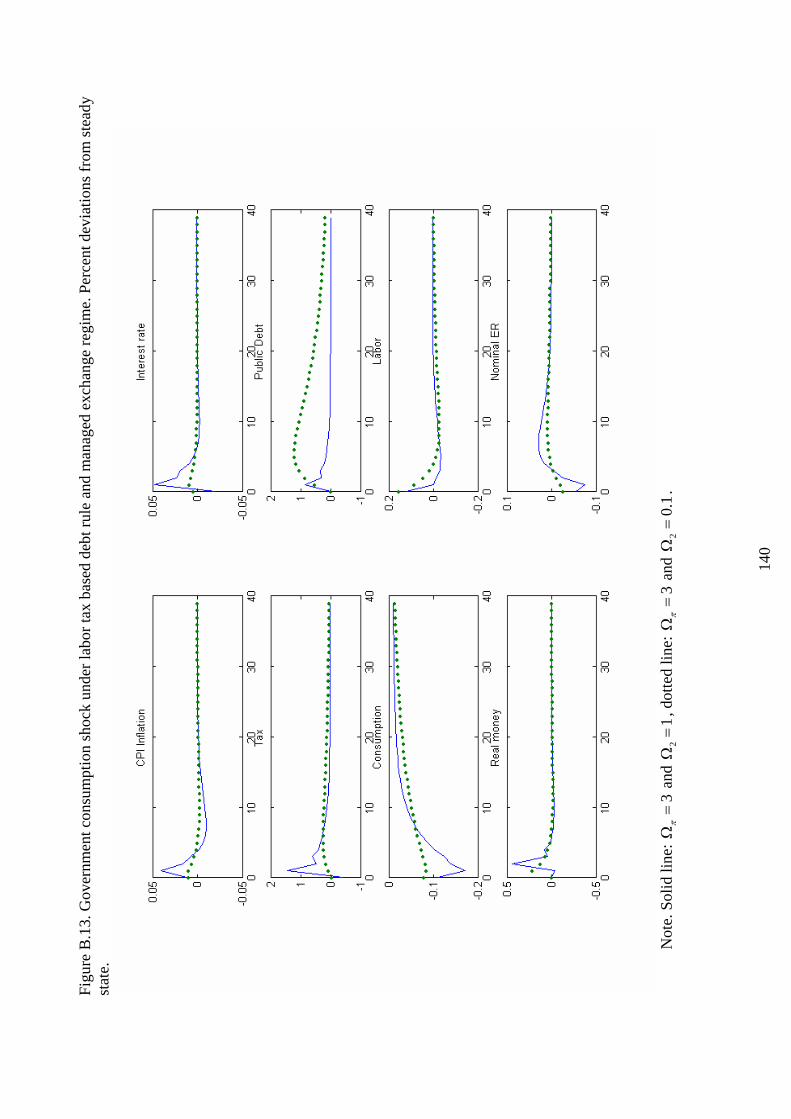
Figu

re B

.13.

Gov

ernm

ent c

onsu

mpt

ion

shoc

k un

der l

abor

tax

base

d de

bt ru

le a

nd m

anag

ed e

xcha

nge

regi

me.

Per

cent

dev

iatio

ns fr

om st

eady

st

ate.

N

ote.

Sol

id li

ne:

and

3

πΩ

=2

1Ω

=, d

otte

d lin

e:

3π

Ω=

and

2

0.1

Ω=

.

140

Figu

re B

.14.

One

per

cent

per

man

ent t

rada

ble

prod

uctiv

ity sh

ock

unde

r con

sum

ptio

n ta

x ba

sed

debt

rule

. Per

cent

dev

iatio

ns fr

om st

eady

stat

e.

N

ote.

Sol

id li

ne: I

nfla

tion

targ

etin

g w

ith

3π

Ω=

and

2

1Ω

=, d

otte

d lin

e: M

anag

ed e

xcha

nge

rate

regi

me

with

3

πΩ

= a

nd

21

Ω=

.

141

Figu

re B

.15.

Det

erm

inac

y re

gion

s und

er th

e co

mpo

site

rule

and

fixe

d ex

chan

ge ra

te re

gim

e

Pane

l A: C

onsu

mpt

ion

Tax

Pa

nel B

: Lab

or In

com

e Ta

x

N

ote.

see

note

to F

igur

e B

.1.

14

2

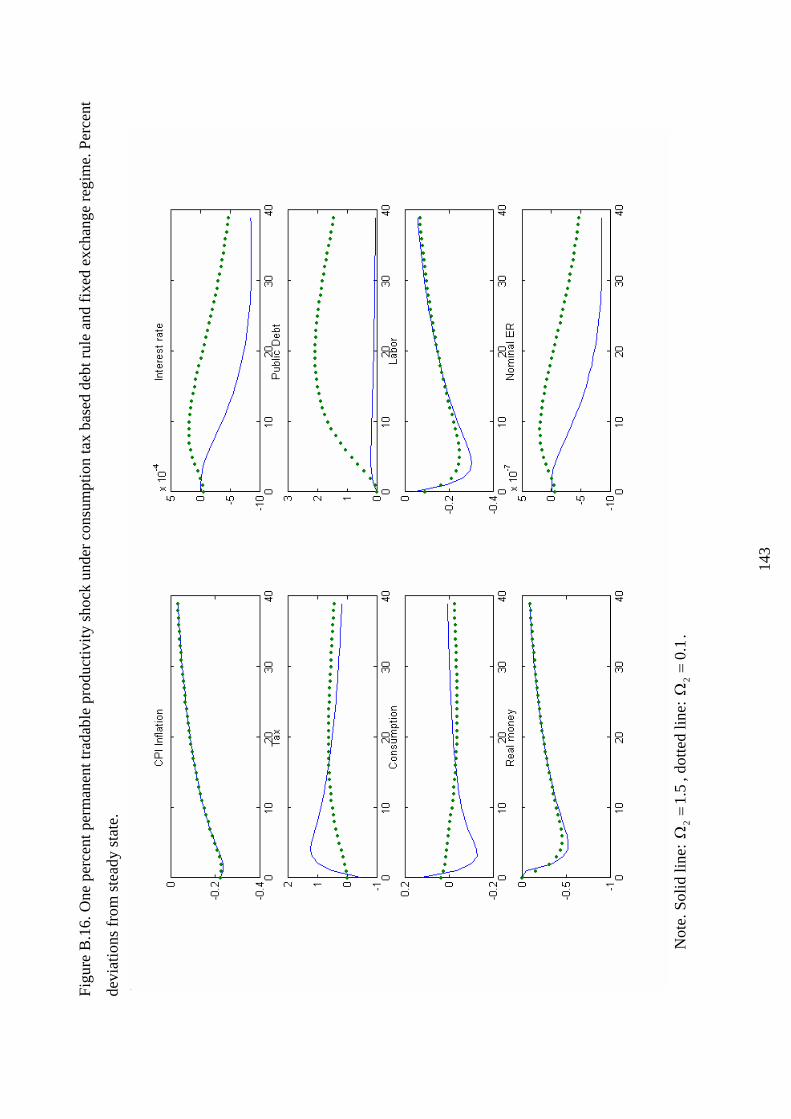
Figu

re B

.16.

One

per

cent

per

man

ent t

rada

ble

prod

uctiv

ity sh

ock

unde

r con

sum

ptio

n ta

x ba

sed

debt

rule

and

fixe

d ex

chan

ge re

gim

e. P

erce

nt

devi

atio

ns fr

om st

eady

stat

e.

N

ote.

Sol

id li

ne:

, dot

ted

line:

2

1.5

Ω=

20.

1Ω

=.

14

3

Figu

re B

.17.

One

per

cent

per

man

ent t

rada

ble

prod

uctiv

ity sh

ock

unde

r con

sum

ptio

n ta

x ba

sed

defic

it ru

le: f

ixed

exc

hang

e ra

te a

nd in

flatio

n ta

rget

ing

regi

mes

. Per

cent

dev

iatio

ns fr

om st

eady

stat

e.

N

ote.

Sol

id li

ne: f

ixed

exc

hang

e re

gim

e w

ith

10.

8Ω

=, d

otte

d lin

e: in

flatio

n ta

rget

ing

with

1

0.8

Ω=

.

14

4

Appendix C

Appendix for Chapter 3

Figure C.1. Total annual labor productivity growth in new EU member states

Source: Lipinska (2007)

Table C.1. Structure of EU economies

countries share on nontradables in consumption1, % share of imports in GDP2, % Czech Republic 42 68

Estonia 39 86 Hungary 44 71 Latvia 37 55

Lithuania 33 58 Poland 37 35

Slovenia 49 59 Slovakia 41 78

Average in the EU-15 51 63 Notes. 1 - average value for the period 2000 - 2005; 2 - average value for the period 2000 - 2007 Source: Lipinska (2007)

145

Table C.2. Inflation Rate of EU economies: percent change compared with previous year, based on the harmonized index of consumer prices

2004 2005 2006Bulgaria 6.1 6.0 7.4Czech Republic 2.6 1.6 2.1Estonia 3.0 4.1 4.4Cyprus 1.9 2.0 2.2Latvia 6.2 6.9 6.6Lithuania 1.2 2.7 3.8Hungary 6.8 3.5 4.0Malta 2.7 2.5 2.6Poland 3.6 2.2 1.3Slovenia 3.7 2.5 2.5Slovakia 7.5 2.8 4.3Euro area 2.1 2.2 2.2

Source: Eurostat

Figure C.2. Inflation rates in the EMU accession countries


146

Figure C.3. Nominal exchange rate fluctuations vs euro in the EMU accession countries


Table C.3. Budget deficits in the EU economies

2004 2005 2006 2007Bulgaria 1.4 1.8 3.0 3.4Czech Republic -3.00 -3.6 -2.7 -1.6Estonia 1.6 1.8 3.4 2.8Cyprus -4.1 -2.4 -1.2 3.3Latvia -1 -0.4 -0.2 0Lithuania -1.5 -0.5 -0.5 -1.2Hungary -6.5 -7.8 -9.2 -5.5Malta -4.6 -3 -2.6 -1.8Poland -5.7 -4.3 -3.8 -2Slovenia -2.3 -1.5 -1.2 -0.1Slovakia -2.4 -2.8 -3.6 -2.2

Notes. government surplus (+)/ government deficit (-) Source: Eurostat

147

Table C.4. Government consolidated gross debt in the EU economies. Percent of GDP

2004 2005 2006 2007Bulgaria 37.9 29.2 22.7 18.2Czech Republic 30.4 29.7 29.4 28.7Estonia 5.1 4.5 4.2 3.4Cyprus 70.2 69.1 64.8 59.8Latvia 14.9 12.4 10.7 9.7Lithuania 19.4 18.6 18.2 17.3Hungary 59.4 61.6 65.6 66Malta 72.6 70.4 64.2 62.6Poland 45.7 47.1 47.6 45.2Slovenia 27.6 27.5 27.2 24.1Slovakia 41.4 34.2 30.4 29.4

Source: Eurostat

148

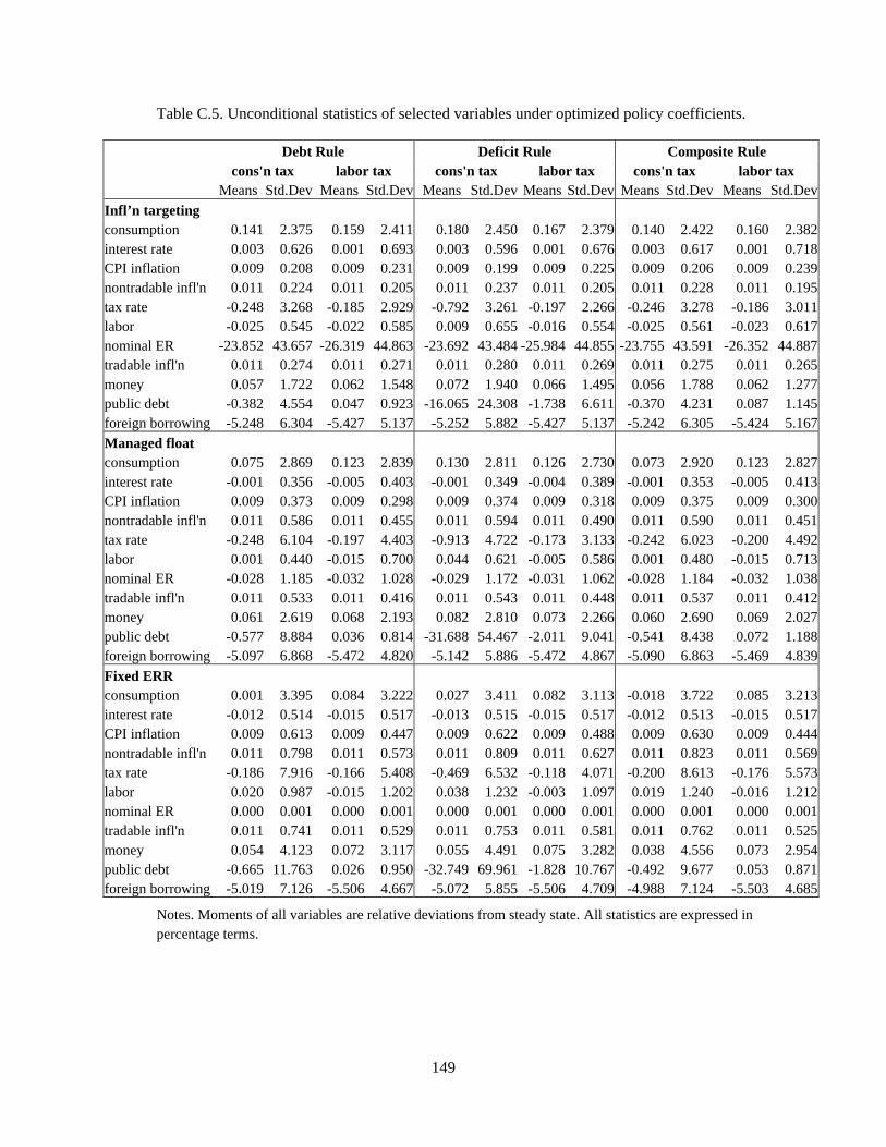
Table C.5. Unconditional statistics of selected variables under optimized policy coefficients.

Debt Rule Deficit Rule Composite Rule cons'n tax labor tax cons'n tax labor tax cons'n tax labor tax Means Std.Dev Means Std.Dev Means Std.Dev Means Std.Dev Means Std.Dev Means Std.Dev

Infl’n targeting consumption 0.141 2.375 0.159 2.411 0.180 2.450 0.167 2.379 0.140 2.422 0.160 2.382interest rate 0.003 0.626 0.001 0.693 0.003 0.596 0.001 0.676 0.003 0.617 0.001 0.718CPI inflation 0.009 0.208 0.009 0.231 0.009 0.199 0.009 0.225 0.009 0.206 0.009 0.239nontradable infl'n 0.011 0.224 0.011 0.205 0.011 0.237 0.011 0.205 0.011 0.228 0.011 0.195tax rate -0.248 3.268 -0.185 2.929 -0.792 3.261 -0.197 2.266 -0.246 3.278 -0.186 3.011labor -0.025 0.545 -0.022 0.585 0.009 0.655 -0.016 0.554 -0.025 0.561 -0.023 0.617nominal ER -23.852 43.657 -26.319 44.863 -23.692 43.484 -25.984 44.855 -23.755 43.591 -26.352 44.887tradable infl'n 0.011 0.274 0.011 0.271 0.011 0.280 0.011 0.269 0.011 0.275 0.011 0.265money 0.057 1.722 0.062 1.548 0.072 1.940 0.066 1.495 0.056 1.788 0.062 1.277public debt -0.382 4.554 0.047 0.923 -16.065 24.308 -1.738 6.611 -0.370 4.231 0.087 1.145foreign borrowing -5.248 6.304 -5.427 5.137 -5.252 5.882 -5.427 5.137 -5.242 6.305 -5.424 5.167Managed float consumption 0.075 2.869 0.123 2.839 0.130 2.811 0.126 2.730 0.073 2.920 0.123 2.827interest rate -0.001 0.356 -0.005 0.403 -0.001 0.349 -0.004 0.389 -0.001 0.353 -0.005 0.413CPI inflation 0.009 0.373 0.009 0.298 0.009 0.374 0.009 0.318 0.009 0.375 0.009 0.300nontradable infl'n 0.011 0.586 0.011 0.455 0.011 0.594 0.011 0.490 0.011 0.590 0.011 0.451tax rate -0.248 6.104 -0.197 4.403 -0.913 4.722 -0.173 3.133 -0.242 6.023 -0.200 4.492labor 0.001 0.440 -0.015 0.700 0.044 0.621 -0.005 0.586 0.001 0.480 -0.015 0.713nominal ER -0.028 1.185 -0.032 1.028 -0.029 1.172 -0.031 1.062 -0.028 1.184 -0.032 1.038tradable infl'n 0.011 0.533 0.011 0.416 0.011 0.543 0.011 0.448 0.011 0.537 0.011 0.412money 0.061 2.619 0.068 2.193 0.082 2.810 0.073 2.266 0.060 2.690 0.069 2.027public debt -0.577 8.884 0.036 0.814 -31.688 54.467 -2.011 9.041 -0.541 8.438 0.072 1.188foreign borrowing -5.097 6.868 -5.472 4.820 -5.142 5.886 -5.472 4.867 -5.090 6.863 -5.469 4.839Fixed ERR consumption 0.001 3.395 0.084 3.222 0.027 3.411 0.082 3.113 -0.018 3.722 0.085 3.213interest rate -0.012 0.514 -0.015 0.517 -0.013 0.515 -0.015 0.517 -0.012 0.513 -0.015 0.517CPI inflation 0.009 0.613 0.009 0.447 0.009 0.622 0.009 0.488 0.009 0.630 0.009 0.444nontradable infl'n 0.011 0.798 0.011 0.573 0.011 0.809 0.011 0.627 0.011 0.823 0.011 0.569tax rate -0.186 7.916 -0.166 5.408 -0.469 6.532 -0.118 4.071 -0.200 8.613 -0.176 5.573labor 0.020 0.987 -0.015 1.202 0.038 1.232 -0.003 1.097 0.019 1.240 -0.016 1.212nominal ER 0.000 0.001 0.000 0.001 0.000 0.001 0.000 0.001 0.000 0.001 0.000 0.001tradable infl'n 0.011 0.741 0.011 0.529 0.011 0.753 0.011 0.581 0.011 0.762 0.011 0.525money 0.054 4.123 0.072 3.117 0.055 4.491 0.075 3.282 0.038 4.556 0.073 2.954public debt -0.665 11.763 0.026 0.950 -32.749 69.961 -1.828 10.767 -0.492 9.677 0.053 0.871foreign borrowing -5.019 7.126 -5.506 4.667 -5.072 5.855 -5.506 4.709 -4.988 7.124 -5.503 4.685

Notes. Moments of all variables are relative deviations from steady state. All statistics are expressed in percentage terms.

149

Table C.6. Conditional welfare costs decomposition of optimal monetary and fiscal policy rules

Inflation Targeting Managed Float Fixed ERR λ meanλ varλ λ meanλ varλ λ meanλ varλ

Cons’n tax debt rule

0.0039 -0.0008 0.0047 0.0819 0.0751 0.0067 0.1684 0.1584 0.0101

Labor tax composite SGP rule

-0.0012 -0.0061 0.0049 0.0455 0.0386 0.0069 0.0904 0.0808 0.0095

Note. λ is computed relative to V .

Figure C.4. 1.7 percent permanent productivity shock under the optimized consumption based debt rule and inflation targeting. Percent deviations from steady state, except for the budget deficit, which is in absolute terms. Time is in quarters.

150

Figure C.5. 1.7 percent permanent productivity shock under the optimized labor tax based deficit rule and inflation targeting. Percent deviations from steady state, except for the budget deficit, which is in absolute terms. Time is in quarters.

Figure C.6. 1.7 percent permanent productivity shock under labor tax based composite SGP rule and inflation targeting: ,3πΩ = 1 2.1Ω = and 2 3Ω = . Percent deviations from steady state,

except for the budget deficit, which is in absolute terms. Time is in quarters.

151

Figure C.7. 1.7 percent permanent productivity shock under the optimized consumption based debt rule and managed float. Percent deviations from steady state, except for the budget deficit, which is in absolute terms. Time is in quarters.

Figure C.8. 1.7 percent permanent productivity shock under the optimized consumption based deficit rule and managed float. Percent deviations from steady state, except for the budget deficit, which is in absolute terms. Time is in quarters.

152

Figure C.9. 1.7 percent permanent productivity shock under the optimized labor based composite SGP rule and fixed exchange rate regime. Percent deviations from steady state, except for the budget deficit, which is in absolute terms. Time is in quarters.

Figure C.10. 1.7 percent permanent productivity shock under the consumption based debt rule with , and . Percent deviations from steady state, except for the budget deficit,

which is in absolute terms. Time is in quarters. 3πΩ = 0.1eΩ = 2 0.2Ω =

153

References

Airaudo, M., 2004. “Multiple Equilibria in a Dollarized Economy: Some Warnings on an

Interest Rate Rule for Turkey,” Working Document No. 7, LUISS Lab on European

Economics.

Altig, D., L. Christiano, M. Eichenbaum, and J. Linde, 2005. “Firm-Specific Capital,

Nominal Rigidities, and the Business Cycles,” NBER Working Paper No. 11034.

Bacchetta, P. and E. van Wincoop, 2000. “Does Exchange-Rate Stability Increase Trade and

Capital Welfare?” American Economic Review 90, 1093-109.

Balino, T., A. Bennett and E. Borensztein, 1999. “Monetary Policy in Dollarized

Economies,” IMF Occasional Paper No.171.

Berg, A. and E. Borensztein, 2000. “The Choice of Exchange Rate Regime and Monetary

Target in Highly Dollarized Economies,” Journal of Applied Economics 3, No.2, 285-324.

Bergin, P., 2004. “How Well Can the New Open Economy Macroeconomics Explain the

Exchange Rate and Current Account?” Working Paper, University of California, Davis.

Bergin, P. and R. Feenstra, 2001. “Pricing-to-Market, Staggered Contracts, and Real

Exchange Rate Persistence,” Journal of International Economics 54, 333-359.

Bergin, P. and I. Tchakarov, 2003. “Does Exchange Rate Matter for Welfare?” Working

Paper, University of California, Davis.

Blanchard, O. and C. Kahn, 1980. “The Solution of Linear Difference Models under Rational

Expectations,” Econometrica 48, 1305–1311.

Bowman, D and B. Doyle, 2003. “New Keynesian, Open-Economy Models and Their

Implications for Monetary Policy,” International Finance Discussion Paper No.762, Board of

Governors of the Federal Reserve System.

Calvo, G., 1983. “Staggered Prices in Utility-Maximizing Framework,” Journal of Monetary

Economics 12, 383-98.

Calvo, G. and C. Reinhart, 2000. “Fear of Floating,” NBER Working Paper No.7993.

154

Céspedes, L. F., R. Chang and A. Velasco, 2004. “Balance Sheets and Exchange Rate

Policy,” American Economic Review 94, 1183–1193.

Chamberlain, G, 1980. “Analysis of Covariance with Qualitative Data”, Review of Economic

Studies 47, No. 1, 225-238.

Christiano, L., M. Eichenbaum and C. Evans, 1997. “Sticky Price and Limited Participation

Models of Money: a Comparison,” European Economic Review 41, 1021-1049.

Cochrane, J, 1999. ”Long-Term Debt and Optimal Policy in the Fiscal Theory of the Price

Level," Working Paper, University of Chicago.

Coenen, G., G. Lombardo, F. Smets, and R. Straub, 2008. “International Transmission and

Monetary Policy Coordination,” ECB Working Paper No. 858.

Collard, F. and M. Juillard, 2001. “Accuracy of Stochastic Perturbation Methods: The Case

of Asset Pricing Models,” Journal of Economic Dynamics and Control 25, 979-999.

Constantinides, G., 1990. “Habit Formation: a Resolution of the Equity Premium Puzzle,”

Journal of Political Economy 98, 519-543.

Deaton, A., 1987. “Life-Cycle Models of Consumption: is the Evidence Consistent with the

Theory?” in Advances in Econometrics Fifth World Congress , Vol. 2, ed. by T. Bewley,

Cambridge University Press, 121-148.

Devereux, M. and C. Engel, 2000. “Monetary Policy in the Open Economy Revisited: Price

Setting and Exchange Rate Flexibility,” NBER Working Paper No.8559.

Duarte, M. and A. Stockman, 2005. “Rational Expectations and Exchange Rates,” Journal of

Monetary Economics 52, 329.

Dupor, B., 2001. “Exchange Rates and the Fiscal Theory of the Price Level“, Journal of

Monetary Economics 45, 613-630.

Edwards, S. and M. Savastano, 1999. “Exchange Rates in Emerging Economies: What Do

We Know? What Do We Need to Know?” NBER Working Paper No.7228.

Flood, R. and A. Rose, 1995. “Fixing Exchange Rates: Virtual Quest for Fundamentals,”

Journal of Monetary Economics 36, 337.

155

Gali, J. and T. Monacelli, 2005. “Monetary Policy and Exchange Rate Volatility in a Small

Open Economy,” Review of Economic Studies 72, 707-734.

Ganelli, G. and P. Lane, 2002. “Dynamic General Equilibrium Analysis: The Open Economy

Dimension,” Trinity Economic paper No. 12, Trinity College, Dublin.

Gertler, M, S. Gilchrist, and F. Natalucci, 2003. “External Constraints on Monetary Policy

and the Financial Accelerator,” NBER Working Paper No. 10128.

Ghironi, F. and A. Rebucci, 2002. “Monetary Rules for Emerging Market Economies,” IMF

Working Paper 02/34.

Harrigan, J., 1993. “OECD Imports and Trade Barriers in 1983,” Journal of International

Economics 35, 91-111.

Hausman, R., U. Panizza and E. Stein, 2000. “Why Do Countries Float the Way They Float?”

Mimeo, Inter-American Development Bank.

Kim, J. and S. Kim, 2003. “Spurious Welfare Reversals in International Business Cycle

Models,” Journal of International Economics, 60(2), 471–500.

Kim, J., S. Kim, E. Schaumburg and C. Sims, 2003. “Calculating and Using Second Order

Accurate Solutions of Discrete Time Dynamic Equilibrium Models,” unpublished

manuscript, Princeton University.

King, R. and M. Watson, 1995a. “The Solution of Singular Difference Systems under

Rational Expectations,” Manuscript, University of Virginia.

King, R. and M. Watson, 1995b. “System Reduction and Solution Algorithms for Singular

Linear Difference Systems under Rational Expectations,” Manuscript, University of Virginia.

Klein, P., 2000. “Using the Generalized Schur Form to Solve a Multivariate Linear Rational

Expectations Model,” Journal of Economic Dynamics and Control 24, 1405-1423.

Kollmann, R., 2002. “Monetary Policy Rules in the Open Economy: Effects on Welfare and

Business Cycles,” Journal of Monetary Economics 49, 989-1015.

Lane, P., 2001. “The New Open Economy Macroeconomics: A Survey,” Journal of

International Economics 54 (2), 235-66.

156

Leeper, E., 1991. “Equilibria under Àctive' and `Passive' Monetary and Fiscal Policies,"

Journal of Monetary Economics 27, 129-147.

Leith, C., S. Wren-Lewis, 2000. “Interactions Between Monetary and Fiscal Rules,” The

Economic Journal, 110, C93-C108.

Levy Yeyati, E. and F. Sturzenegger, 1999. “Classifying Exchange Rate Regimes: Deeds vs.

Words,” unpublished manuscript, Universidad Torcuato Di Tella.

Lipinska, A., 2007. “The Maastricht Convergence Criteria and Optimal Monetary Policy for

the EMU Accession Countries,” CEP Discussion Paper No. 808.

Loyo, E., 1999. “Tight Money Paradox on the Loose: A Fiscalist Hyperinflation," Working

Paper, Kennedy School of Government.

Lucas, R., 1987. Models of Business Cycles, Basil Blackwell, New York.

Marzo, M., I. Strid, and P. Zagaglia, 2006. “Optimal Opportunistic Monetary Policy in a New

Keynesian Model,” unpublished manuscript, Stockholm University.

Masten, I, 2005. “Inflation Targeting in the Presence of Balassa-Samuelson-type Productivity

Shocks,” unpublished manuscript.

Natalucci, F.M., F. Ravenna, 2007. “Monetary Policy Choices in Emerging Market

Economies: the Case of High Productivity Growth,” Journal of Money, Credit and Banking,

forthcoming.

Obstfeld, M. and K. Rogoff, 1996. Foundations of International Macroeconomics, MIT Press,

Cambridge, MA.

Obstfeld, M. and K. Rogoff, 2000. “New Directions for Stochastic Open Economy Models,”

Journal of International Economics 50(1), 117-53.

Paustian, M., 2003. “Gains from Second-Order Approximations,” unpublished manuscript,

University of Bonn.

Railavo, J., 2004. “Stability Consequences of Fiscal Policy Rules,” Working Paper, Bank of

Finland.

157

Reinhart C., K. Rogoff, 2002 “The Modern History of Exchange Rate Arrangements: A

Reinterpretation”, NBER Working Paper No. 8963.

Rogers, J., 1990. “Foreign Inflation Transmission under Flexible Exchange Rates and

Currency Substitution“, Journal of Money, Credit and Banking 22(2), 195-208.

Rotemberg, J. and M. Woodford, 1998. “An Optimization-Based Econometric Framework

for the Evaluation of Monetary Policy,” in B. Bernanke and J. Rotemberg (eds), NBER

Macroeconomic Annual, Cambridge, MA, MIT Press, 297-346.

Sargent, T. and N. Wallace, 1981. “Some Unpleasant Monetarist Arithmetic”, Federal

Reserve Bank of Minneapolis Quarterly Review, Fall, pp.1-17.

Sarno, L., 2001. “Toward a New Paradigm in Open Economy Modeling: Where Do We

Stand,” Federal Reserve Bank of St. Lous Review 83, 21-36.

Schmitt-Grohé, S. and M. Uribe, 2001. “Stabilization Policy and the Costs of Dollarization,”

Journal of Money, Credit, and Banking 33, 482-509.

Schmitt-Grohé, S. and M. Uribe, 2003. “Closing Small Open Economy Models,” Journal of

International Economics 61, 163-185.

Schmitt-Grohé, S. and M. Uribe, 2004. “Solving Dynamic General Equilibrium Models

Using Second Order Approximation to the Policy Function,” Journal of Economic Dynamics

and Control 28, 755-775.

Schmitt-Grohé, S., M. Uribe, 2007a. “Optimal Simple and Implementable Monetary and

Fiscal Rules” Journal of Monetary Economics 54.

Schmitt-Grohé, S., M. Uribe, 2007b. “Optimal Inflation Stabilization in a Medium-Scale

Macroeconomic Model,” in Schmidt-Hebbel, K. and F. Mishkin (Eds.), Monetary Policy

under Inflation Targeting, Central Bank of Chile, 125-186.

Senay, O. and A. Sutherland , 2003. "The Expenditure Switching Effect and Fixed Versus

Floating Exchange Rates," Working Paper.

Sims, C., 1994. “A Simple Model for the Study of the Determination of the Price Level and

the Interaction of Monetary and Fiscal Policy," Economic Theory 4, 381-399.

158

http://www.econ.duke.edu/%7Euribe/dollarization.pdf

http://ideas.repec.org/p/mmf/mmfc03/97.html

http://ideas.repec.org/p/mmf/mmfc03/97.html

Sims, C., 1996. “Solving Linear Rational Expectations Models,” Manuscript, Yale

University.

Sims, C., 2000. “Second Order Accurate Solution of Discrete Time Dynamic Equilibrium

Models,” Princeton University Working Paper.

Straub, R. and I. Tchakarov, 2004. “Non-Fundamental Exchange Rate Volatility and

Welfare,” European Central Bank Working Paper No. 328.

Trefler, D. and H. Lai, 1999. “The Gains from Trade: Standard Errors with the CES

Monopolistic Competition Model,” University of Toronto Manuscript.

Uhlig, H., 1995. “A Toolkit for Analyzing Nonlinear Economic Dynamic Models Easily,”

Discussion Paper 101, Institute for Empirical Macroeconomics, Federal Reserve Bank of

Minneapolis.

Woodford, M., 1994. “Monetary Policy and Price-Level Determinacy in a Cash-in-Advance

Economy," Economic Theory 4, 345-380.

Woodford, M., 1995. “Price-level Determinacy without Control of a Monetary Aggregate,"

Carnegie-Rochester Conference Series on Public Policy 43, 1-46.

Woodford, M., 1996. “Control of the Public Debt: A Requirement for Price Stability?" NBER

Working Paper no. 5684

Woodford, M., 1998. “Public Debt and the Price Level," Working Paper, Princeton

University.

Woodford, M., 2001. “Fiscal Requirements for Price Stability," Journal of Money, Credit and

Banking 33, 669-728.

Yun, T., 1996. “Nominal Price Rigidity, Money Supply Endogeneity, and Business Cycles,”

Journal of Monetary Economics 37, 345-370.

159

Documents

Essays in Open Economy Macroeconomics · Economics for acceptance a thesis entitled “Essays in Open Economy Macroeconomics” by Nurbek Jenish. Dated: December 5, 2008 ... Alessia