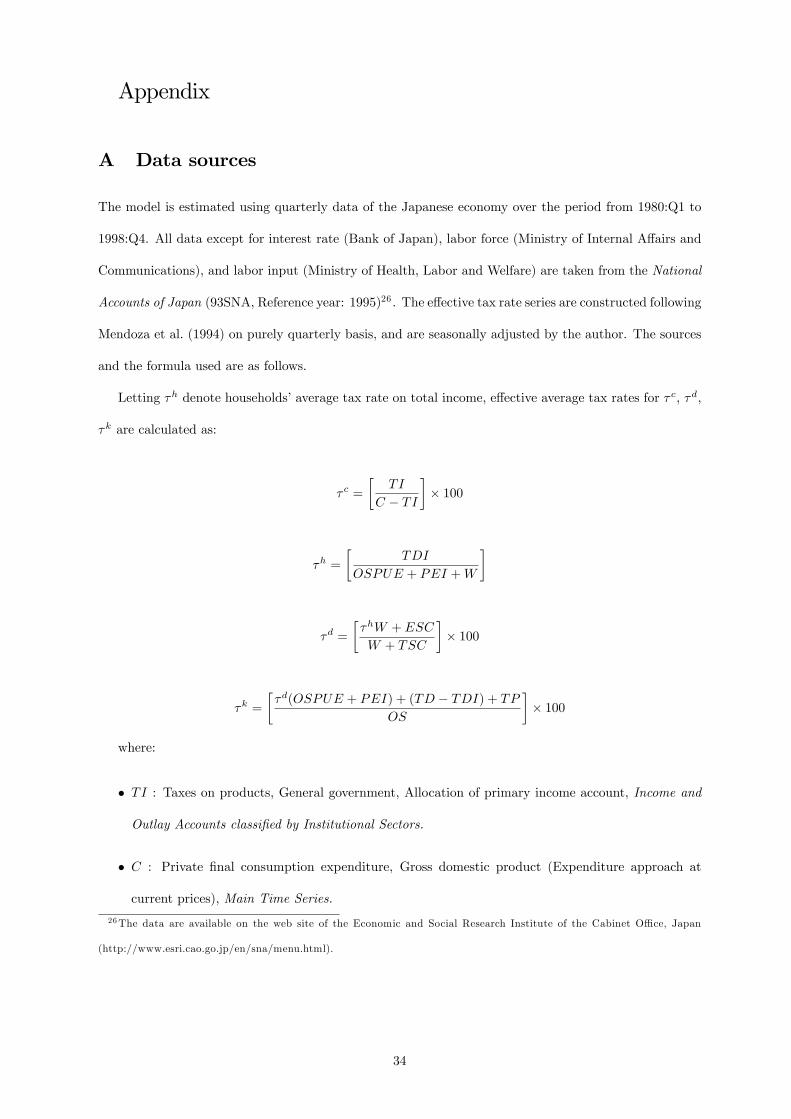
Appendix

A Data sources

The model is estimated using quarterly data of the Japanese economy over the period from 1980:Q1 to

1998:Q4. All data except for interest rate (Bank of Japan), labor force (Ministry of Internal A¤airs and

Communications), and labor input (Ministry of Health, Labor and Welfare) are taken from the National

Accounts of Japan (93SNA, Reference year: 1995)26 . The e¤ective tax rate series are constructed following

Mendoza et al. (1994) on purely quarterly basis, and are seasonally adjusted by the author. The sources

and the formula used are as follows.

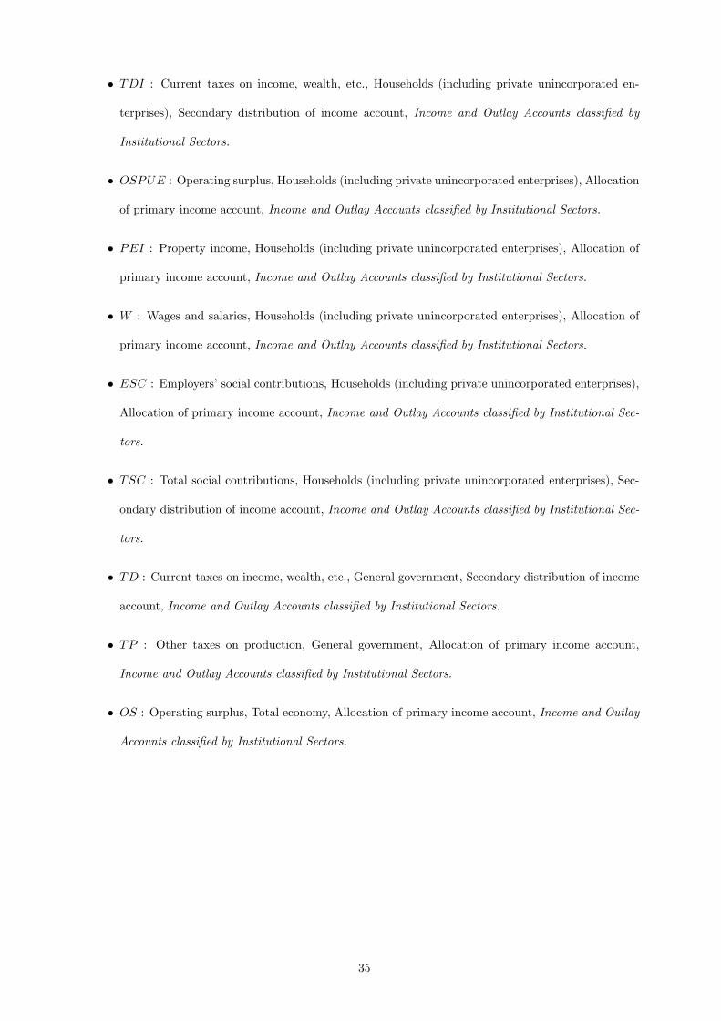
Letting �h denote households�average tax rate on total income, e¤ective average tax rates for � c, �d,

�k are calculated as:

� c =

�TI

C � TI

�� 100

�h =

�TDI

OSPUE + PEI +W

�

�d =

��hW + ESC

W + TSC

�� 100

�k =

��d(OSPUE + PEI) + (TD � TDI) + TP

OS

�� 100

where:

� TI : Taxes on products, General government, Allocation of primary income account, Income and

Outlay Accounts classi�ed by Institutional Sectors.

� C : Private �nal consumption expenditure, Gross domestic product (Expenditure approach at

current prices), Main Time Series.

26The data are available on the web site of the Economic and Social Research Institute of the Cabinet O¢ ce, Japan

(http://www.esri.cao.go.jp/en/sna/menu.html).

34

� TDI : Current taxes on income, wealth, etc., Households (including private unincorporated en-

terprises), Secondary distribution of income account, Income and Outlay Accounts classi�ed by

Institutional Sectors.

� OSPUE : Operating surplus, Households (including private unincorporated enterprises), Allocation

of primary income account, Income and Outlay Accounts classi�ed by Institutional Sectors.

� PEI : Property income, Households (including private unincorporated enterprises), Allocation of

primary income account, Income and Outlay Accounts classi�ed by Institutional Sectors.

� W : Wages and salaries, Households (including private unincorporated enterprises), Allocation of

primary income account, Income and Outlay Accounts classi�ed by Institutional Sectors.

� ESC : Employers�social contributions, Households (including private unincorporated enterprises),

Allocation of primary income account, Income and Outlay Accounts classi�ed by Institutional Sec-

tors.

� TSC : Total social contributions, Households (including private unincorporated enterprises), Sec-

ondary distribution of income account, Income and Outlay Accounts classi�ed by Institutional Sec-

tors.

� TD : Current taxes on income, wealth, etc., General government, Secondary distribution of income

account, Income and Outlay Accounts classi�ed by Institutional Sectors.

� TP : Other taxes on production, General government, Allocation of primary income account,

Income and Outlay Accounts classi�ed by Institutional Sectors.

� OS : Operating surplus, Total economy, Allocation of primary income account, Income and Outlay

Accounts classi�ed by Institutional Sectors.

35

B Log-linearized Model

B.1 Ricardian Households

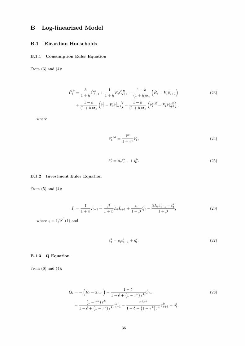
B.1.1 Consumption Euler Equation

From (3) and (4):

CRt =h

1 + hCRt�1 +

1

1 + hEtC

Rt+1 �

1� h(1 + h)�c

�Rt � Et�t+1

�(23)

+1� h

(1 + h)�c

�"bt � Et"bt+1

�� 1� h(1 + h)�c

�� ctilt � Et� ctilt+1

�;

where

� ctilt =�� c

1 + �� c� ct ; (24)

"bt = �b"bt�1 + �

bt : (25)

B.1.2 Investment Euler Equation

From (5) and (4):

It =1

1 + �It�1 +

�

1 + �EtIt+1 +

&

1 + �Qt �

�Et"it+1 � "it1 + �

; (26)

where & � 1=S00(1) and

"it = �i"it�1 + �

it: (27)

B.1.3 Q Equation

From (6) and (4):

Qt = ��Rt � �t+1

�+

1� �1� � +

�1� ��k

��rkQt+1 (28)

+

�1� ��k

��rk

1� � +�1� ��k

��rkrkt+1 �

��k�rk

1� � +�1� ��k

��rk�kt+1 + �

qt :

36

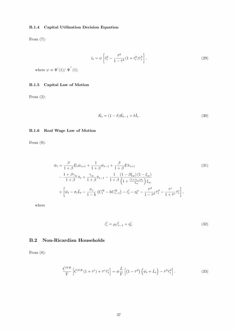
B.1.4 Capital Utilization Decision Equation

From (7):

zt =

�rkt �

��k

1� ��k (1 + rkt )�

kt

�; (29)

where � 0(1)=

00(1):

B.1.5 Capital Law of Motion

From (2):

Kt = (1� �)Kt�1 + �It: (30)

B.1.6 Real Wage Law of Motion

From (9):

wt =�

1 + �Etwt+1 +

1

1 + �wt�1 +

�

1 + �E�t+1 (31)

� 1 + � w1 + �

�t + w1 + �

�t�1 �1

1 + �

(1� ��w) (1� �w)�1 + (1+�w)�l

�w

��w

��wt � �lLt �

�c1� h

�CRt � hCRt�1

�� "lt � �wt �

��d

1� ��d �dt �

�� c

1 + �� c� ct

�;

where

"lt = �l"lt�1 + �

lt: (32)

B.2 Non-Ricardian Households

From (8):

�CNR

�Y

hCNR (1 + �� c) + �� c� ct

i= �w

�L�Y

h�1� ��d

� �wt + Lt

�� ��d�dt

i: (33)

37

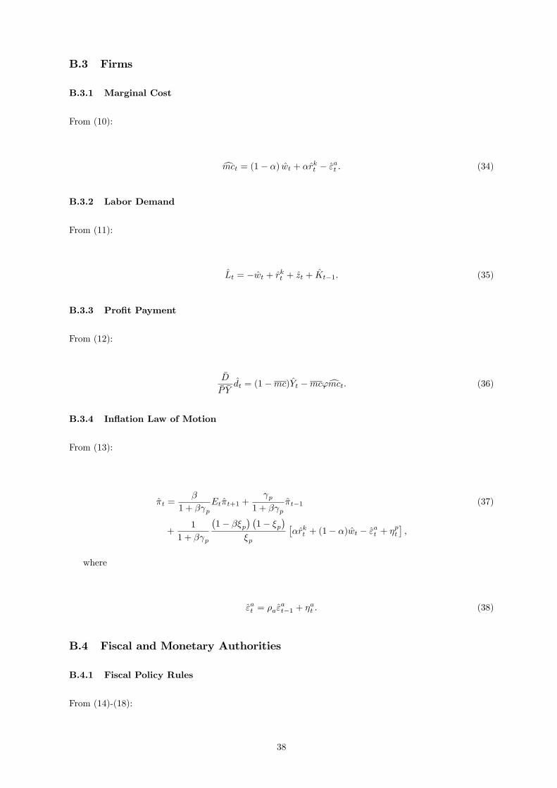
B.3 Firms

B.3.1 Marginal Cost

From (10):

cmct = (1� �) wt + �rkt � "at : (34)

B.3.2 Labor Demand

From (11):

Lt = �wt + rkt + zt + Kt�1: (35)

B.3.3 Pro�t Payment

From (12):

�D�P �Y

dt = (1�mc)Yt �mc'cmct: (36)

B.3.4 In�ation Law of Motion

From (13):

�t =�

1 + � pEt�t+1 +

p1 + � p

�t�1 (37)

+1

1 + � p

�1� ��p

� �1� �p

��p

��rkt + (1� �)wt � "at + �

pt

�;

where

"at = �a"at�1 + �

at : (38)

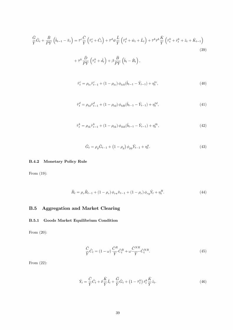
B.4 Fiscal and Monetary Authorities

B.4.1 Fiscal Policy Rules

From (14)-(18):

38

�G�YGt +

�B�P �Y

�bt�1 � �t

�= �� c

�C�Y

�� ct + Ct

�+ ��d �w

�L�Y

��dt + wt + Lt

�+ ��k�rk

�K�Y

��kt + r

kt + zt + Kt�1

�(39)

+ ��k�D�P �Y

��kt + dt

�+ �

�B�P �Y

�bt � Rt

�;

� ct = �tc�ct�1 + (1� �tc)�tcb(bt�1 � Yt�1) + �tct ; (40)

�dt = �td�dt�1 + (1� �td)�tdb(bt�1 � Yt�1) + �tdt ; (41)

�kt = �tk �kt�1 + (1� �tk)�tkb(bt�1 � Yt�1) + �tkt ; (42)

Gt = �gGt�1 +�1� �g

��gyYt�1 + �

gt : (43)

B.4.2 Monetary Policy Rule

From (19):

Rt = �rRt�1 + (1� �r)�r��t�1 + (1� �r)�ryYt + �Rt : (44)

B.5 Aggregation and Market Clearing

B.5.1 Goods Market Equilibrium Condition

From (20):

�C�YCt = (1� !)

�CR

�YCRt + !

�CNR

�YCNRt : (45)

From (22):

Yt =�C�YCt + �

�K�YIt +

�G�YGt +

�1� ��kt

��rkt�K�Yzt: (46)

39

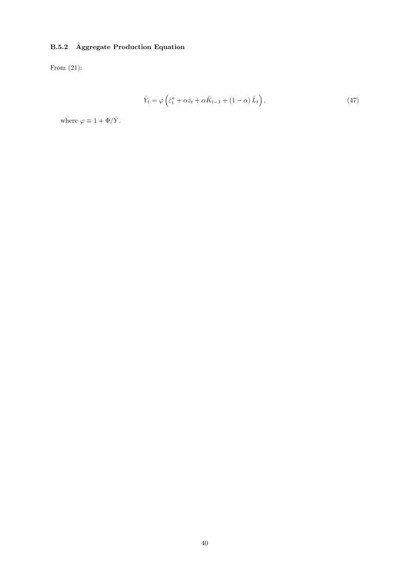
B.5.2 Aggregate Production Equation

From (21):

Yt = '�"at + �zt + �Kt�1 + (1� �) Lt

�; (47)

where ' � 1 + �= �Y :

40

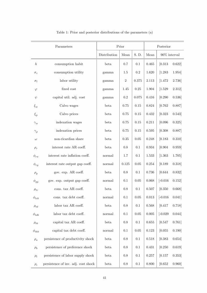
Table 1: Prior and posterior distributions of the parameters (a)

Parameters Prior Posterior

Distribution Mean S. D. Mean 90% interval

h consumption habit beta 0.7 0.1 0.465 [0.313 0.622]

�c consumption utility gamma 1.5 0.2 1.620 [1.283 1.954]

�l labor utility gamma 2 0.375 2.113 [1.472 2.736]

' �xed cost gamma 1.45 0.25 1.904 [1.529 2.312]

capital util. adj. cost gamma 0.2 0.075 0.416 [0.290 0.536]

�w Calvo wages beta 0.75 0.15 0.824 [0.762 0.887]

�p Calvo prices beta 0.75 0.15 0.432 [0.323 0.543]

w indexation wages beta 0.75 0.15 0.211 [0.096 0.325]

p indexation prices beta 0.75 0.15 0.595 [0.308 0.887]

! non-ricardian share beta 0.35 0.05 0.248 [0.183 0.310]

�r interest rate AR coe¤. beta 0.8 0.1 0.934 [0.904 0.959]

�r� interest rate in�ation coe¤. normal 1.7 0.1 1.533 [1.363 1.705]

�ry interest rate output gap coe¤. normal 0.125 0.05 0.254 [0.189 0.318]

�g gov. exp. AR coe¤. beta 0.8 0.1 0.736 [0.644 0.832]

�gy gov. exp. output gap coe¤. normal 0.1 0.05 0.068 [-0.016 0.152]

�tc cons. tax AR coe¤. beta 0.8 0.1 0.507 [0.350 0.668]

�tcb cons. tax debt coe¤. normal 0.1 0.05 0.013 [-0.016 0.041]

�td labor tax AR coe¤. beta 0.8 0.1 0.568 [0.417 0.718]

�tdb labor tax debt coe¤. normal 0.1 0.05 0.005 [-0.029 0.044]

�tk capital tax AR coe¤. beta 0.8 0.1 0.655 [0.547 0.761]

�tkb capital tax debt coe¤. normal 0.1 0.05 0.123 [0.055 0.190]

�a persistence of productivity shock beta 0.8 0.1 0.518 [0.383 0.654]

�b persistence of preference shock beta 0.8 0.1 0.431 [0.250 0.619]

�l persistence of labor supply shock beta 0.8 0.1 0.257 [0.157 0.353]

�i persistence of inv. adj. cost shock beta 0.8 0.1 0.800 [0.652 0.960]

41

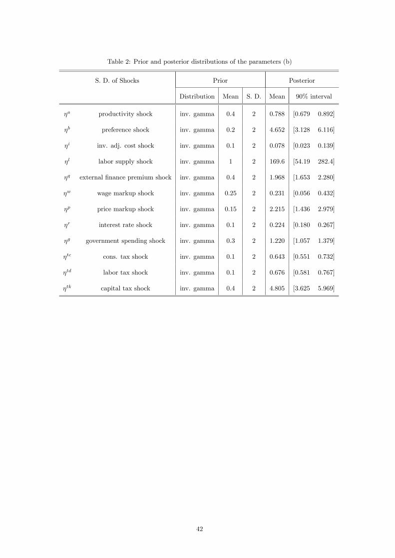
Table 2: Prior and posterior distributions of the parameters (b)

S. D. of Shocks Prior Posterior

Distribution Mean S. D. Mean 90% interval

�a productivity shock inv. gamma 0.4 2 0.788 [0.679 0.892]

�b preference shock inv. gamma 0.2 2 4.652 [3.128 6.116]

�i inv. adj. cost shock inv. gamma 0.1 2 0.078 [0.023 0.139]

�l labor supply shock inv. gamma 1 2 169.6 [54.19 282.4]

�q external �nance premium shock inv. gamma 0.4 2 1.968 [1.653 2.280]

�w wage markup shock inv. gamma 0.25 2 0.231 [0.056 0.432]

�p price markup shock inv. gamma 0.15 2 2.215 [1.436 2.979]

�r interest rate shock inv. gamma 0.1 2 0.224 [0.180 0.267]

�g government spending shock inv. gamma 0.3 2 1.220 [1.057 1.379]

�tc cons. tax shock inv. gamma 0.1 2 0.643 [0.551 0.732]

�td labor tax shock inv. gamma 0.1 2 0.676 [0.581 0.767]

�tk capital tax shock inv. gamma 0.4 2 4.805 [3.625 5.969]

42

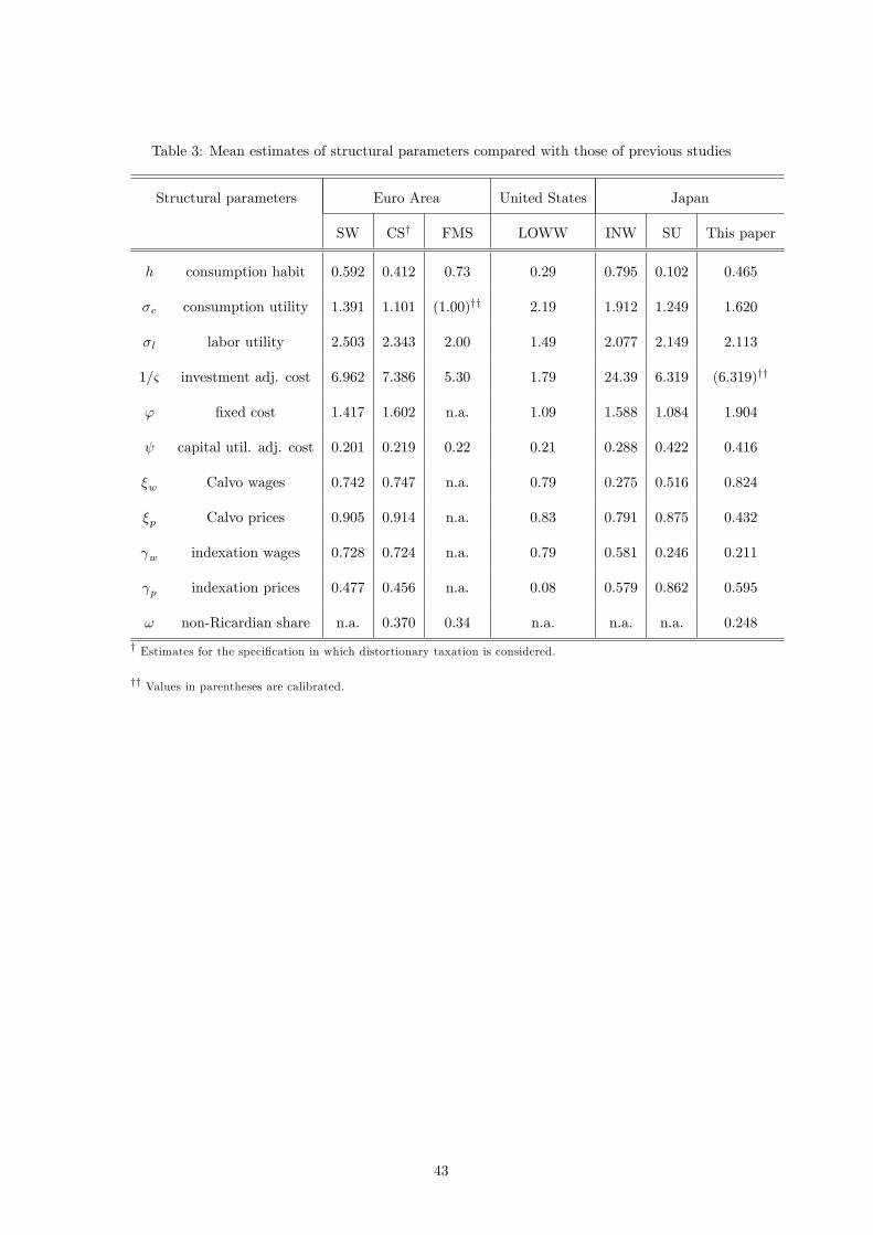
Table 3: Mean estimates of structural parameters compared with those of previous studies

Structural parameters Euro Area United States Japan

SW CSy FMS LOWW INW SU This paper

h consumption habit 0.592 0.412 0.73 0.29 0.795 0.102 0.465

�c consumption utility 1.391 1.101 (1.00)yy 2.19 1.912 1.249 1.620

�l labor utility 2.503 2.343 2.00 1.49 2.077 2.149 2.113

1=& investment adj. cost 6.962 7.386 5.30 1.79 24.39 6.319 (6.319)yy

' �xed cost 1.417 1.602 n.a. 1.09 1.588 1.084 1.904

capital util. adj. cost 0.201 0.219 0.22 0.21 0.288 0.422 0.416

�w Calvo wages 0.742 0.747 n.a. 0.79 0.275 0.516 0.824

�p Calvo prices 0.905 0.914 n.a. 0.83 0.791 0.875 0.432

w indexation wages 0.728 0.724 n.a. 0.79 0.581 0.246 0.211

p indexation prices 0.477 0.456 n.a. 0.08 0.579 0.862 0.595

! non-Ricardian share n.a. 0.370 0.34 n.a. n.a. n.a. 0.248

y Estimates for the speci�cation in which distortionary taxation is considered.

yy Values in parentheses are calibrated.

43

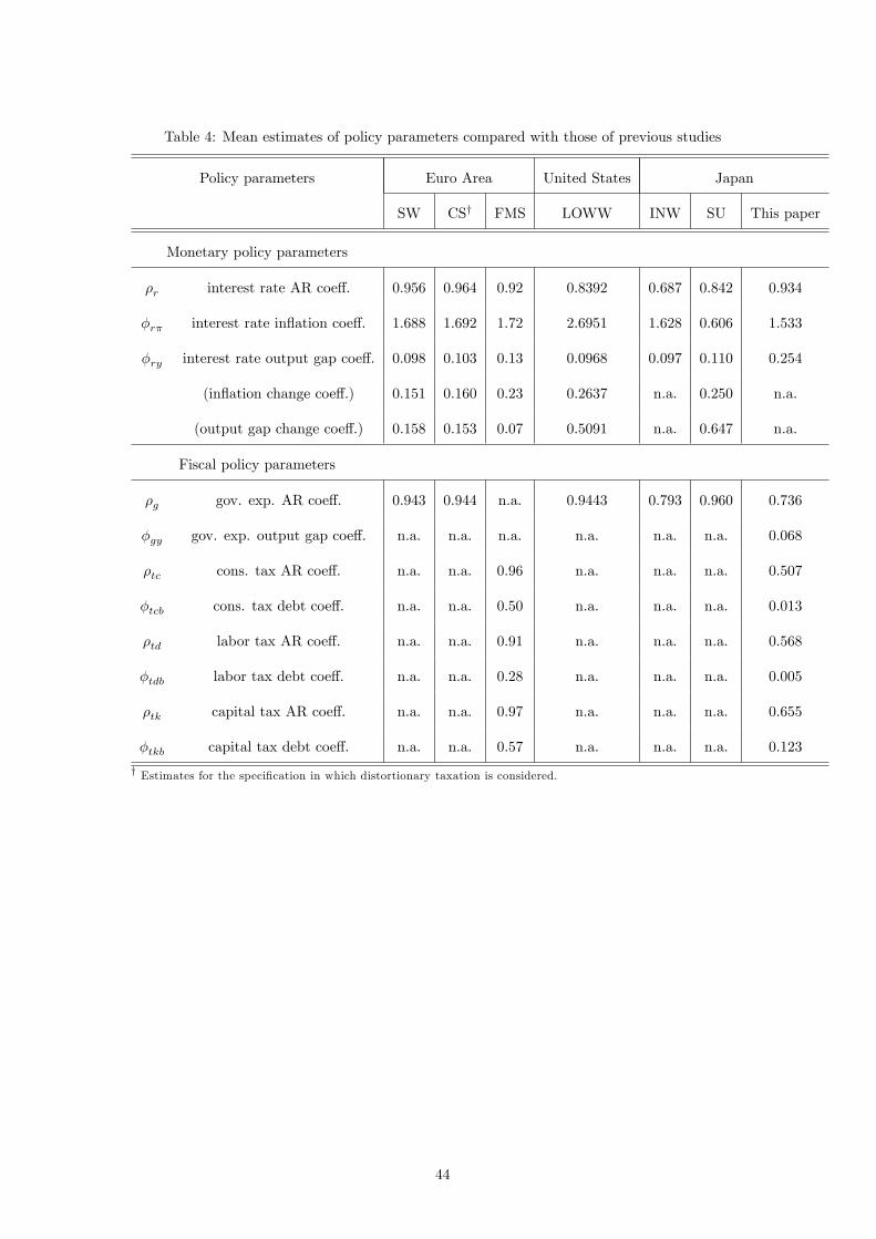
Table 4: Mean estimates of policy parameters compared with those of previous studies

Policy parameters Euro Area United States Japan

SW CSy FMS LOWW INW SU This paper

Monetary policy parameters

�r interest rate AR coe¤. 0.956 0.964 0.92 0.8392 0.687 0.842 0.934

�r� interest rate in�ation coe¤. 1.688 1.692 1.72 2.6951 1.628 0.606 1.533

�ry interest rate output gap coe¤. 0.098 0.103 0.13 0.0968 0.097 0.110 0.254

(in�ation change coe¤.) 0.151 0.160 0.23 0.2637 n.a. 0.250 n.a.

(output gap change coe¤.) 0.158 0.153 0.07 0.5091 n.a. 0.647 n.a.

Fiscal policy parameters

�g gov. exp. AR coe¤. 0.943 0.944 n.a. 0.9443 0.793 0.960 0.736

�gy gov. exp. output gap coe¤. n.a. n.a. n.a. n.a. n.a. n.a. 0.068

�tc cons. tax AR coe¤. n.a. n.a. 0.96 n.a. n.a. n.a. 0.507

�tcb cons. tax debt coe¤. n.a. n.a. 0.50 n.a. n.a. n.a. 0.013

�td labor tax AR coe¤. n.a. n.a. 0.91 n.a. n.a. n.a. 0.568

�tdb labor tax debt coe¤. n.a. n.a. 0.28 n.a. n.a. n.a. 0.005

�tk capital tax AR coe¤. n.a. n.a. 0.97 n.a. n.a. n.a. 0.655

�tkb capital tax debt coe¤. n.a. n.a. 0.57 n.a. n.a. n.a. 0.123

y Estimates for the speci�cation in which distortionary taxation is considered.

44

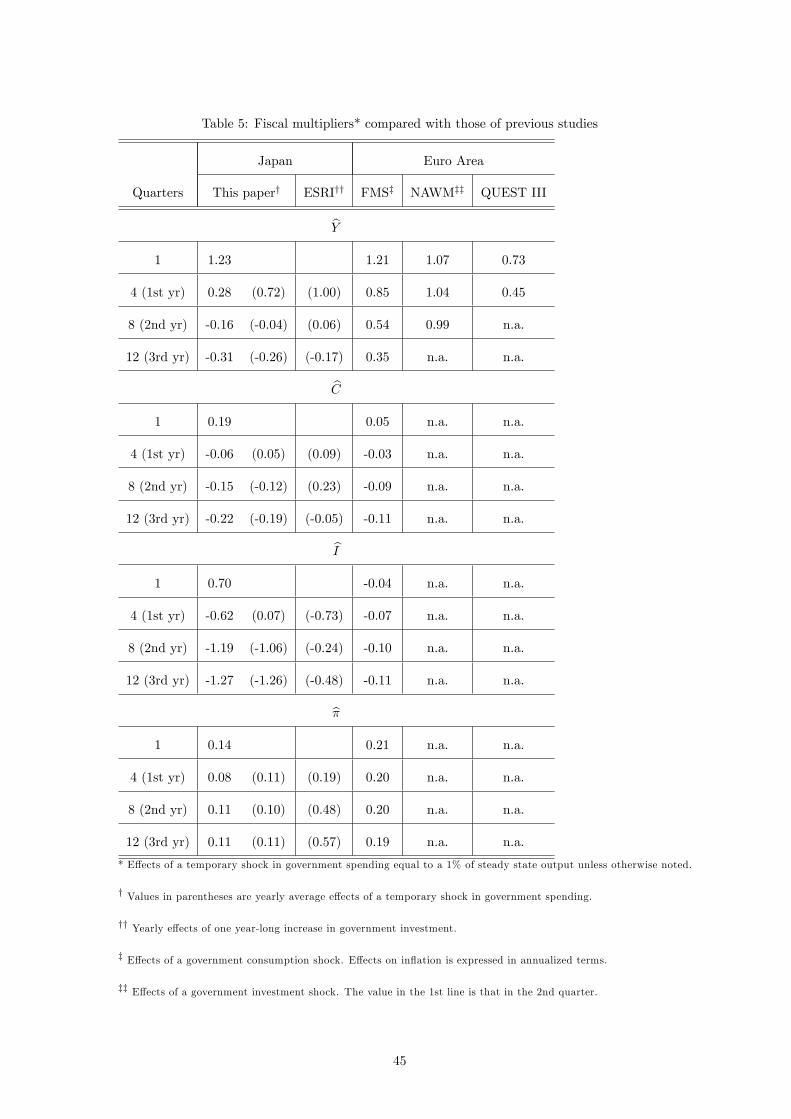
Table 5: Fiscal multipliers* compared with those of previous studies

Japan Euro Area

Quarters This papery ESRIyy FMSz NAWMzz QUEST III

bY1 1.23 1.21 1.07 0.73

4 (1st yr) 0.28 (0.72) (1.00) 0.85 1.04 0.45

8 (2nd yr) -0.16 (-0.04) (0.06) 0.54 0.99 n.a.

12 (3rd yr) -0.31 (-0.26) (-0.17) 0.35 n.a. n.a.

bC1 0.19 0.05 n.a. n.a.

4 (1st yr) -0.06 (0.05) (0.09) -0.03 n.a. n.a.

8 (2nd yr) -0.15 (-0.12) (0.23) -0.09 n.a. n.a.

12 (3rd yr) -0.22 (-0.19) (-0.05) -0.11 n.a. n.a.

bI1 0.70 -0.04 n.a. n.a.

4 (1st yr) -0.62 (0.07) (-0.73) -0.07 n.a. n.a.

8 (2nd yr) -1.19 (-1.06) (-0.24) -0.10 n.a. n.a.

12 (3rd yr) -1.27 (-1.26) (-0.48) -0.11 n.a. n.a.

b�1 0.14 0.21 n.a. n.a.

4 (1st yr) 0.08 (0.11) (0.19) 0.20 n.a. n.a.

8 (2nd yr) 0.11 (0.10) (0.48) 0.20 n.a. n.a.

12 (3rd yr) 0.11 (0.11) (0.57) 0.19 n.a. n.a.

* E¤ects of a temporary shock in government spending equal to a 1% of steady state output unless otherwise noted.

y Values in parentheses are yearly average e¤ects of a temporary shock in government spending.

yy Yearly e¤ects of one year-long increase in government investment.

z E¤ects of a government consumption shock. E¤ects on in�ation is expressed in annualized terms.

zz E¤ects of a government investment shock. The value in the 1st line is that in the 2nd quarter.

45

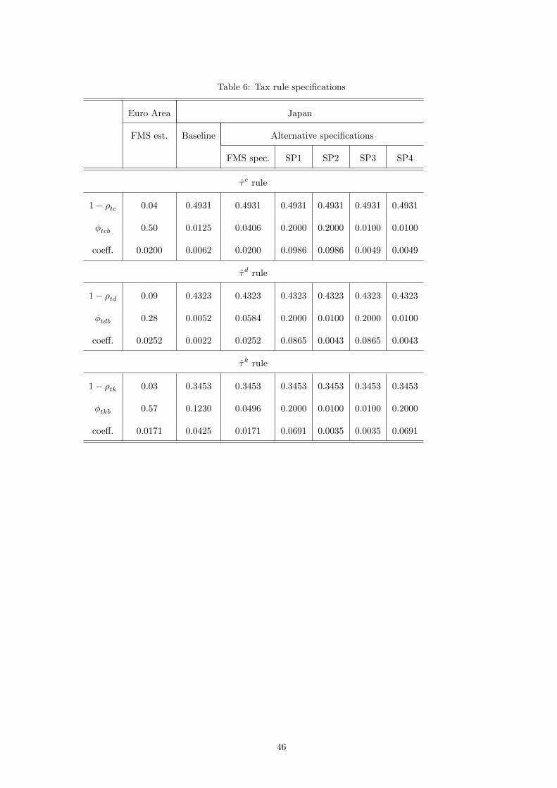
Table 6: Tax rule speci�cations

Euro Area Japan

FMS est. Baseline Alternative speci�cations

FMS spec. SP1 SP2 SP3 SP4

� c rule

1� �tc 0.04 0.4931 0.4931 0.4931 0.4931 0.4931 0.4931

�tcb 0.50 0.0125 0.0406 0.2000 0.2000 0.0100 0.0100

coe¤. 0.0200 0.0062 0.0200 0.0986 0.0986 0.0049 0.0049

�d rule

1� �td 0.09 0.4323 0.4323 0.4323 0.4323 0.4323 0.4323

�tdb 0.28 0.0052 0.0584 0.2000 0.0100 0.2000 0.0100

coe¤. 0.0252 0.0022 0.0252 0.0865 0.0043 0.0865 0.0043

�k rule

1� �tk 0.03 0.3453 0.3453 0.3453 0.3453 0.3453 0.3453

�tkb 0.57 0.1230 0.0496 0.2000 0.0100 0.0100 0.2000

coe¤. 0.0171 0.0425 0.0171 0.0691 0.0035 0.0035 0.0691

46

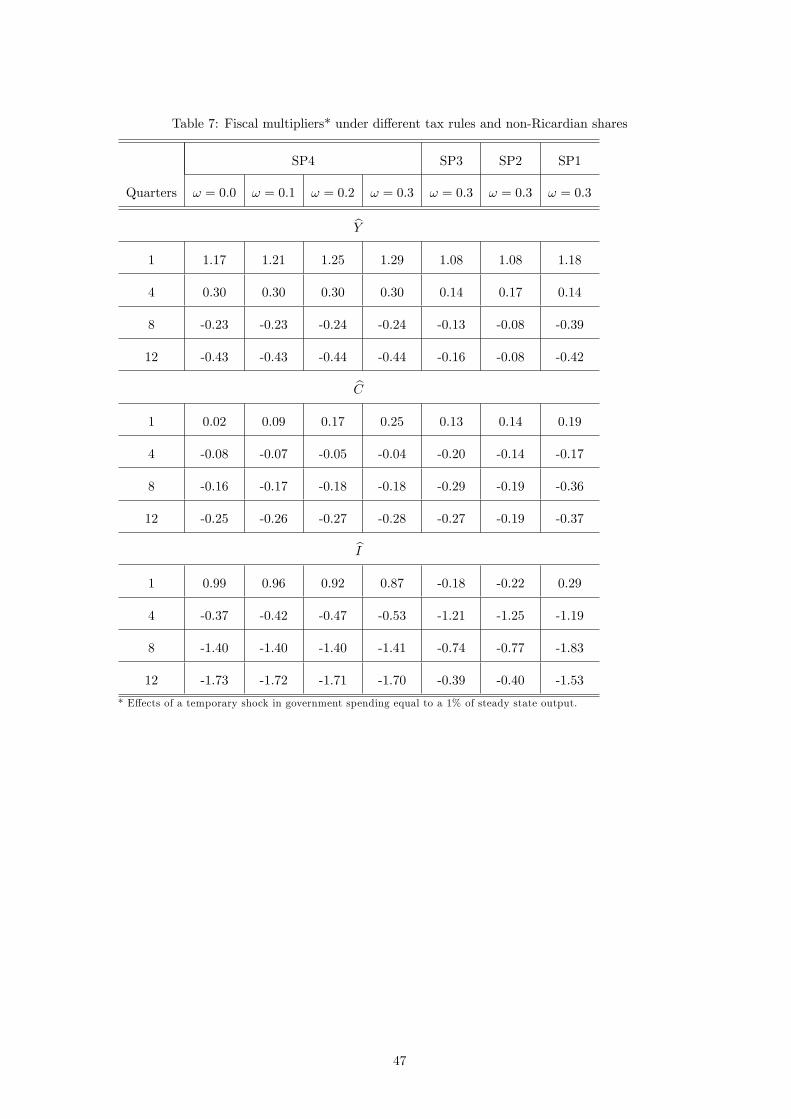
Table 7: Fiscal multipliers* under di¤erent tax rules and non-Ricardian shares

SP4 SP3 SP2 SP1

Quarters ! = 0:0 ! = 0:1 ! = 0:2 ! = 0:3 ! = 0:3 ! = 0:3 ! = 0:3

bY1 1.17 1.21 1.25 1.29 1.08 1.08 1.18

4 0.30 0.30 0.30 0.30 0.14 0.17 0.14

8 -0.23 -0.23 -0.24 -0.24 -0.13 -0.08 -0.39

12 -0.43 -0.43 -0.44 -0.44 -0.16 -0.08 -0.42

bC1 0.02 0.09 0.17 0.25 0.13 0.14 0.19

4 -0.08 -0.07 -0.05 -0.04 -0.20 -0.14 -0.17

8 -0.16 -0.17 -0.18 -0.18 -0.29 -0.19 -0.36

12 -0.25 -0.26 -0.27 -0.28 -0.27 -0.19 -0.37

bI1 0.99 0.96 0.92 0.87 -0.18 -0.22 0.29

4 -0.37 -0.42 -0.47 -0.53 -1.21 -1.25 -1.19

8 -1.40 -1.40 -1.40 -1.41 -0.74 -0.77 -1.83

12 -1.73 -1.72 -1.71 -1.70 -0.39 -0.40 -1.53

* E¤ects of a temporary shock in government spending equal to a 1% of steady state output.

47

0.5 1 1.5 20

2

4

6

0 5 100

2

4

6

0 0.2 0.40

5

10

15

0 200 400 6000

0.5

1

1.5

1 2 30

1

2

3

0 1 20

2

4

6

0 2 4 60

5

10

0.1 0.2 0.3 0.4 0.50

5

10

15

1 20

2

4

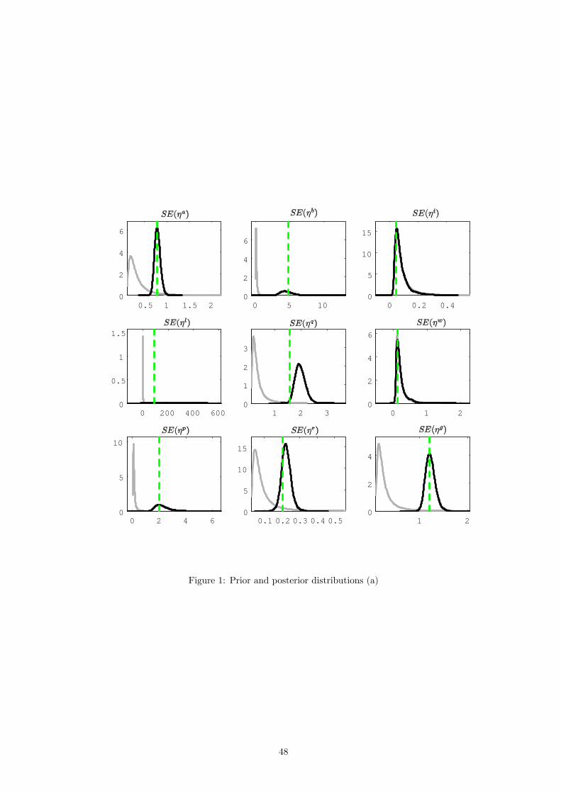
Figure 1: Prior and posterior distributions (a)

48

0.2 0.4 0.6 0.8 10

5

10

15

0.2 0.4 0.6 0.8 10

5

10

15

2 4 6 8 100

1

2

3

0 0.5 10

2

4

1 2 30

1

2

0 2 40

0.5

1

1 2 30

0.5

1

1.5

0 0.5 10

2

4

6

0 0.5 10

1

2

3ψ

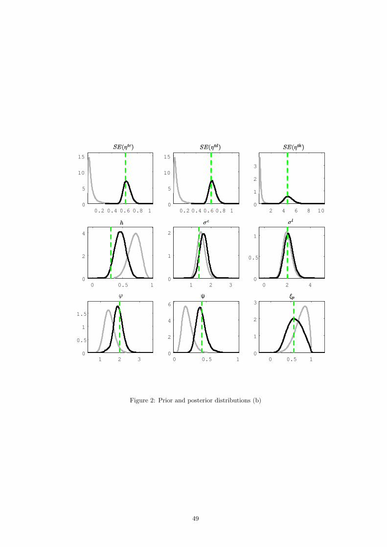
Figure 2: Prior and posterior distributions (b)

49

­0.2 0 0.20.40.60.80

2

4

6

0.2 0.4 0.6 0.80

2

4

6

0.5 10

5

10

0.5 10

10

20

1 1.5 20

2

4

0 0.2 0.40

5

10

0.1 0.2 0.3 0.4 0.50

5

10

0 0.5 10

2

4

0 0.5 10

2

4

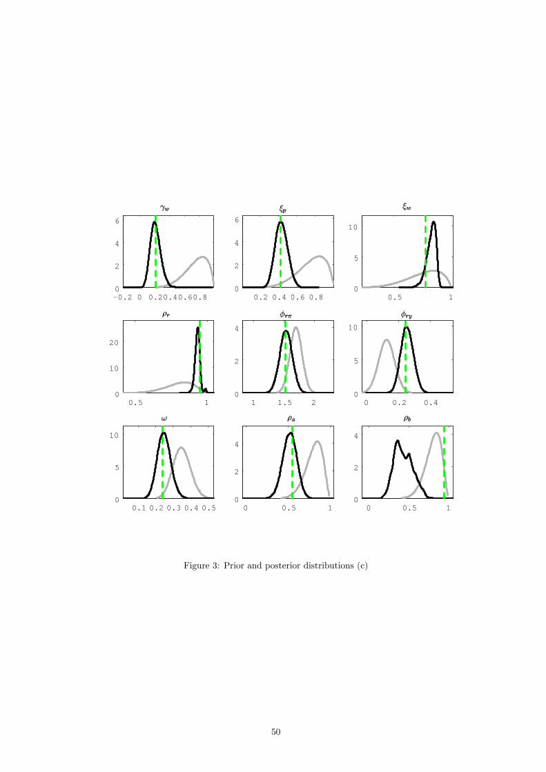
Figure 3: Prior and posterior distributions (c)

50

0.5 10

2

4

6

0 0.2 0.4 0.6 0.80

2

4

6

0.2 0.4 0.6 0.8 1 1.20

2

4

0 0.5 10

2

4

0 0.5 10

2

4

0.5 10

2

4

6

­0.1 0 0.1 0.20

10

20

­0.1 0 0.1 0.20

10

20

0 0.2 0.40

5

10

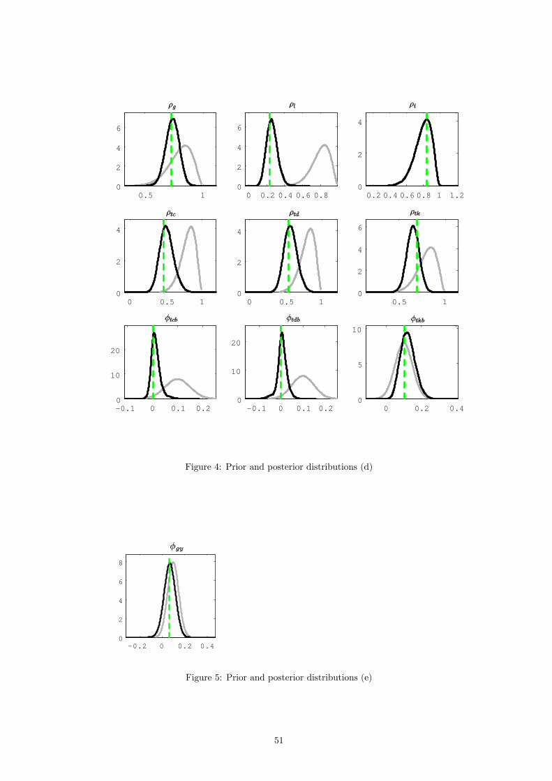
Figure 4: Prior and posterior distributions (d)

­0.2 0 0.2 0.40

2

4

6

8

Figure 5: Prior and posterior distributions (e)

51

10 20 30 40­0.1

0

0.1

0.2

10 20 30 40­0.1

0

0.1

10 20 30 40­0.08

­0.06

­0.04

­0.02

0

10 20 30 40­0.1

0

0.1

0.2

10 20 30 40­0.4

­0.2

0

0.2

10 20 30 400

0.1

0.2

10 20 30 40­0.08

­0.06

­0.04

­0.02

0

10 20 30 400

0.1

0.2

10 20 30 400

0.01

0.02

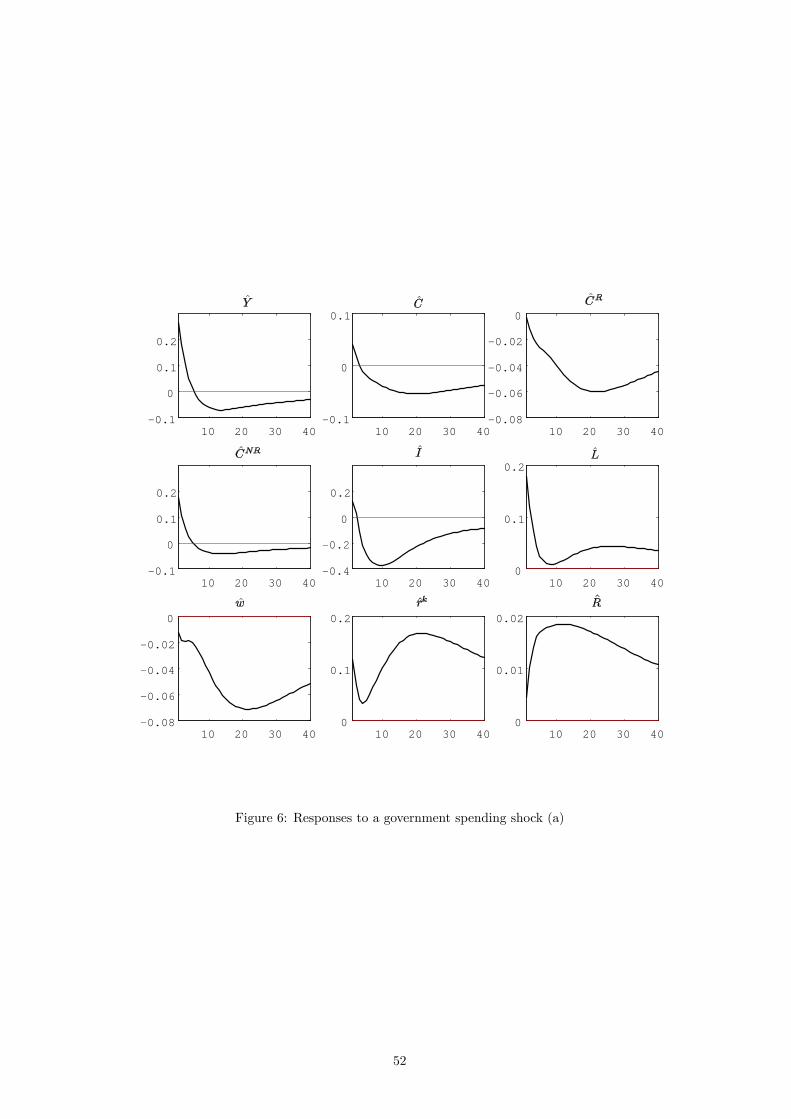
Figure 6: Responses to a government spending shock (a)

52

10 20 30 400

0.2

0.4

0.6

0.8

1

1.2

10 20 30 400

0.002

0.004

0.006

0.008

0.01

0.012

0.014

10 20 30 400

1

2

3

4

5

6x 10

­ 3

10 20 30 400

0.05

0.1

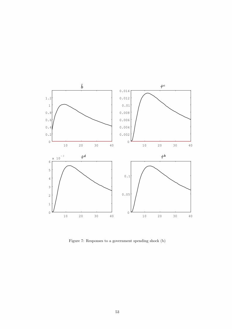
Figure 7: Responses to a government spending shock (b)

53

10 20 30 40­0.03

­0.02

­0.01

0

0.01

10 20 30 40­0.06

­0.04

­0.02

0

0.02

10 20 30 40­0.03

­0.02

­0.01

0

0.01

10 20 30 40­0.1

0

0.1

10 20 30 40­0.02

0

0.02

0.04

10 20 30 40­0.02

­0.01

0

10 20 30 400

2

4

6

8x 10

­ 3

10 20 30 40­0.02

­0.01

0

10 20 30 40­2

­1

0x 10

­ 3

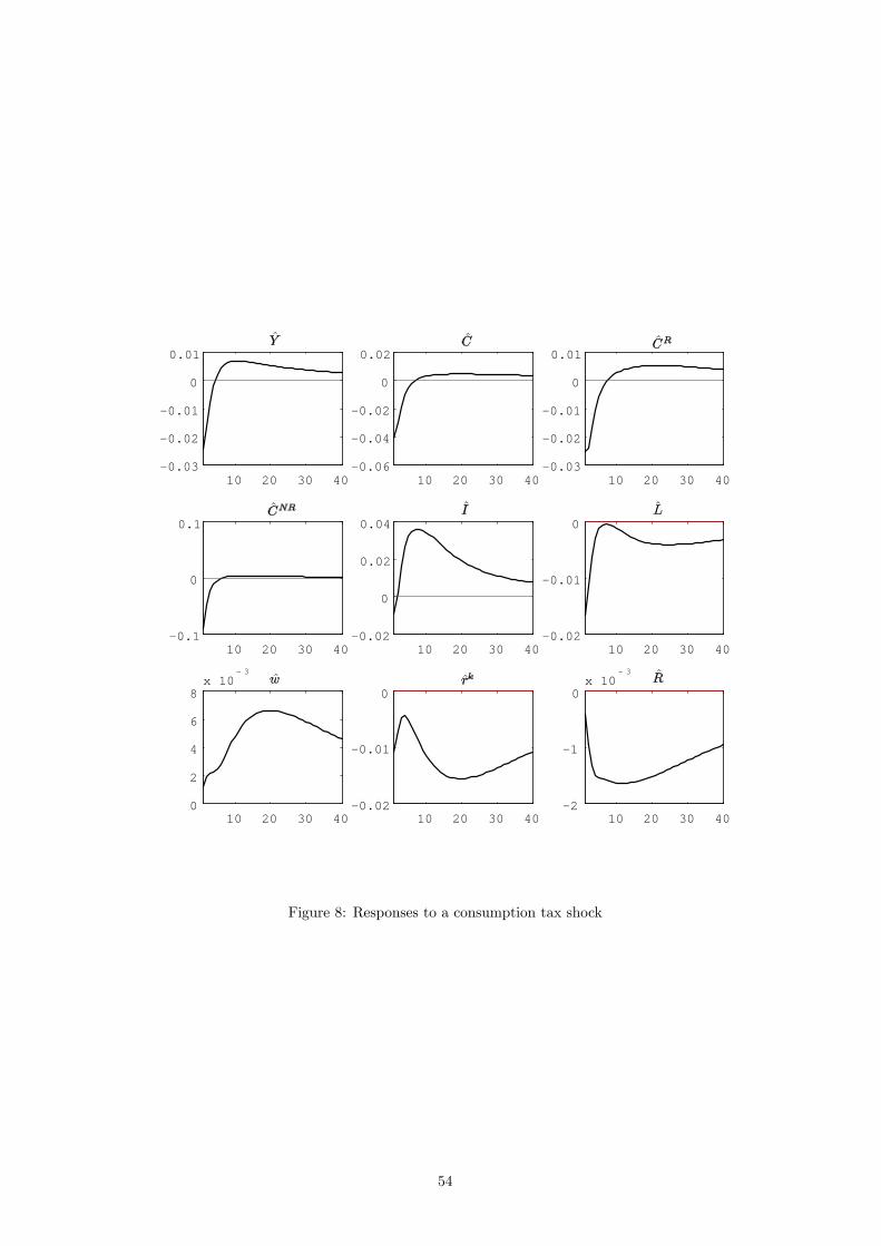
Figure 8: Responses to a consumption tax shock

54

10 20 30 40­0.1

0

0.1

10 20 30 40­0.2

0

0.2

10 20 30 40­0.04

­0.02

0

0.02

0.04

10 20 30 40­0.6

­0.4

­0.2

0

10 20 30 40­0.1

0

0.1

0.2

10 20 30 40­0.08

­0.06

­0.04

­0.02

0

10 20 30 400

0.02

0.04

0.06

10 20 30 40­0.2

­0.1

0

10 20 30 40­0.015

­0.01

­0.005

0

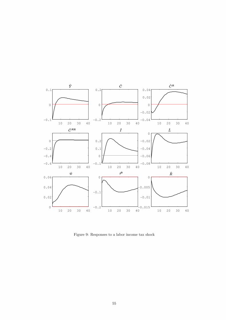
Figure 9: Responses to a labor income tax shock

55

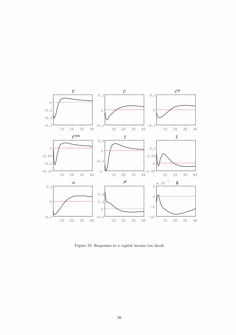
10 20 30 40­0.3

­0.2

­0.1

0

10 20 30 40­0.1

0

0.1

10 20 30 40­0.1

0

0.1

10 20 30 40­0.15

­0.1

­0.05

0

10 20 30 40­1

­0.5

0

0.5

10 20 30 40­0.05

0

0.05

0.1

10 20 30 40­0.1

0

0.1

10 20 30 40­0.2

0

0.2

0.4

10 20 30 40­10

­5

0

5x 10

­ 3

Figure 10: Responses to a capital income tax shock

56

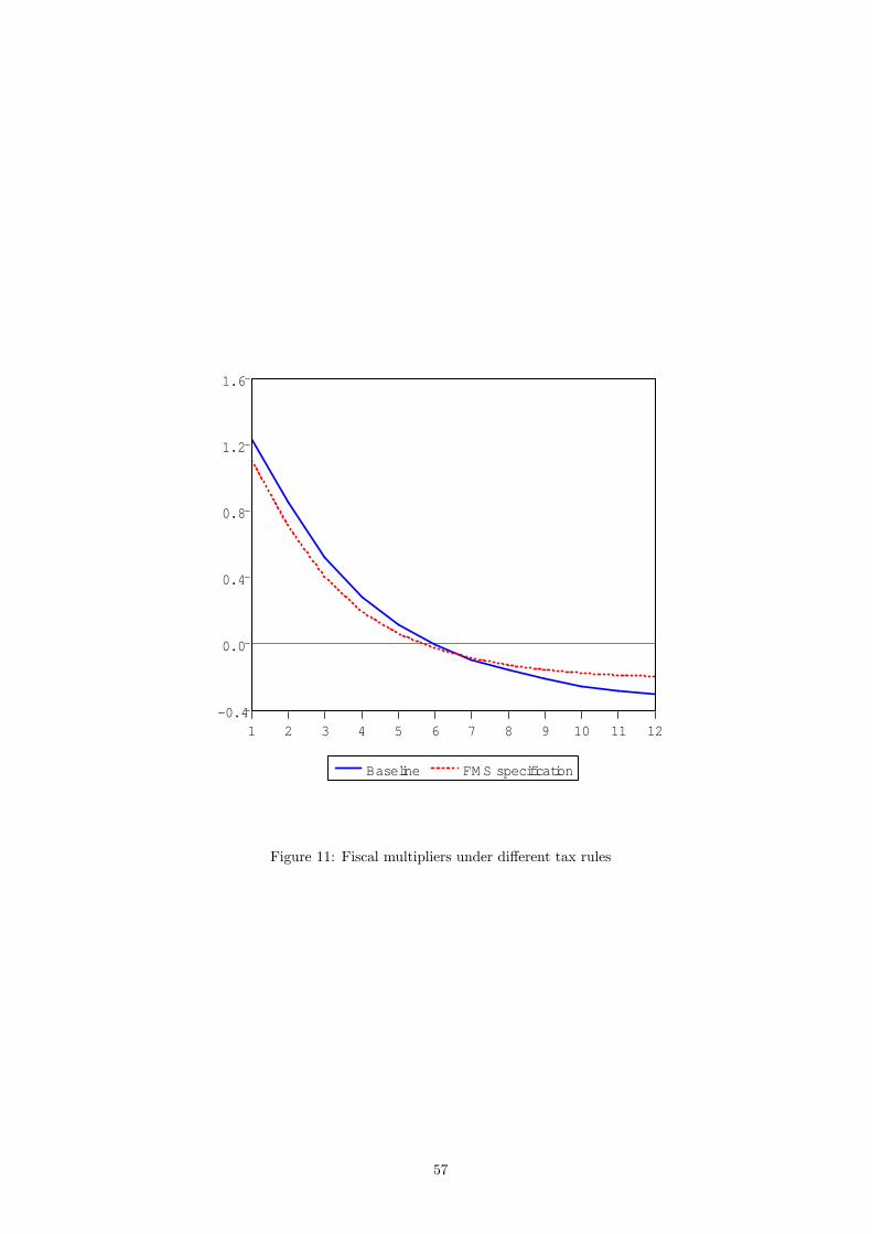
­0.4

0.0

0.4

0.8

1.2

1.6

1 2 3 4 5 6 7 8 9 10 11 12

Baseline FM S specification

Figure 11: Fiscal multipliers under di¤erent tax rules

57

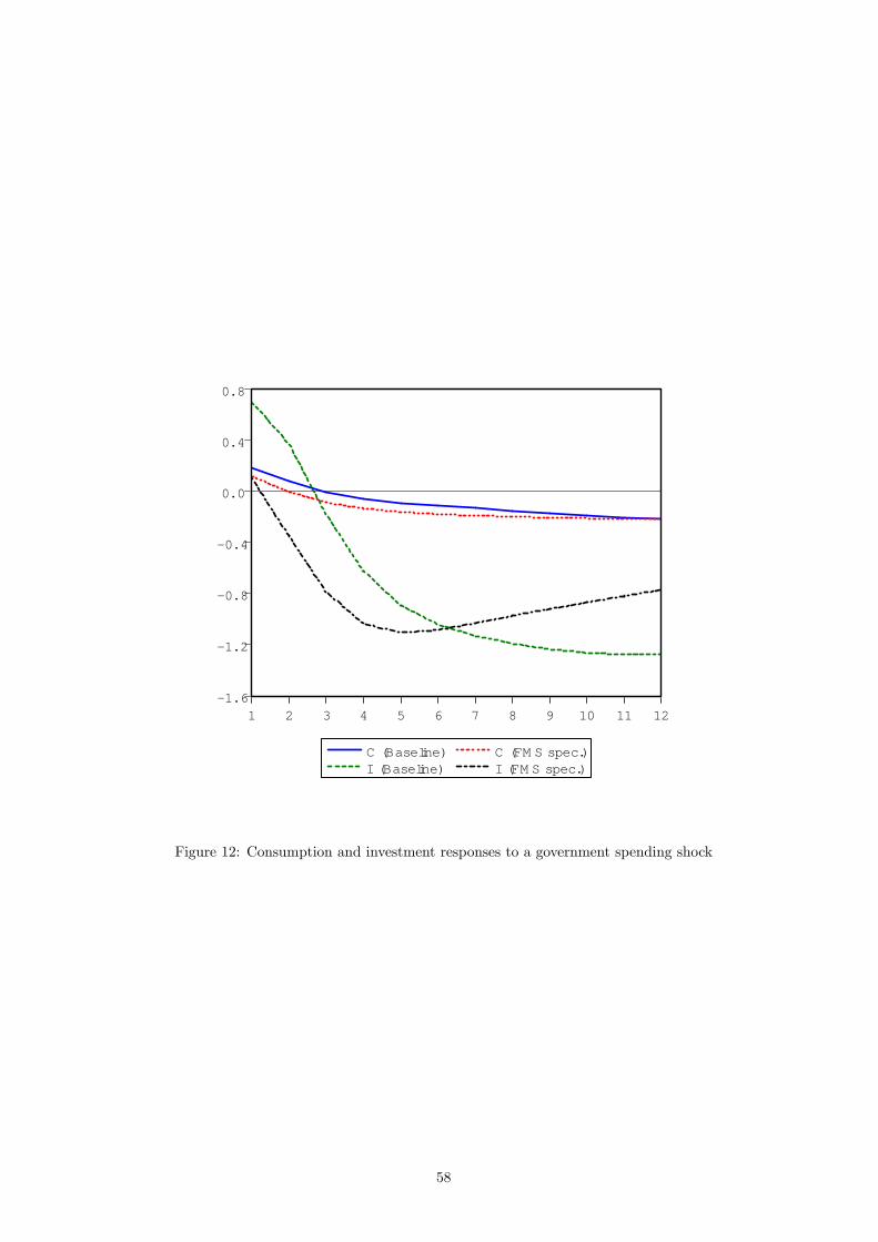
­1.6

­1.2

­0.8

­0.4

0.0

0.4

0.8

1 2 3 4 5 6 7 8 9 10 11 12

C (Baseline) C (FM S spec.)I (Baseline) I (FM S spec.)

Figure 12: Consumption and investment responses to a government spending shock

58

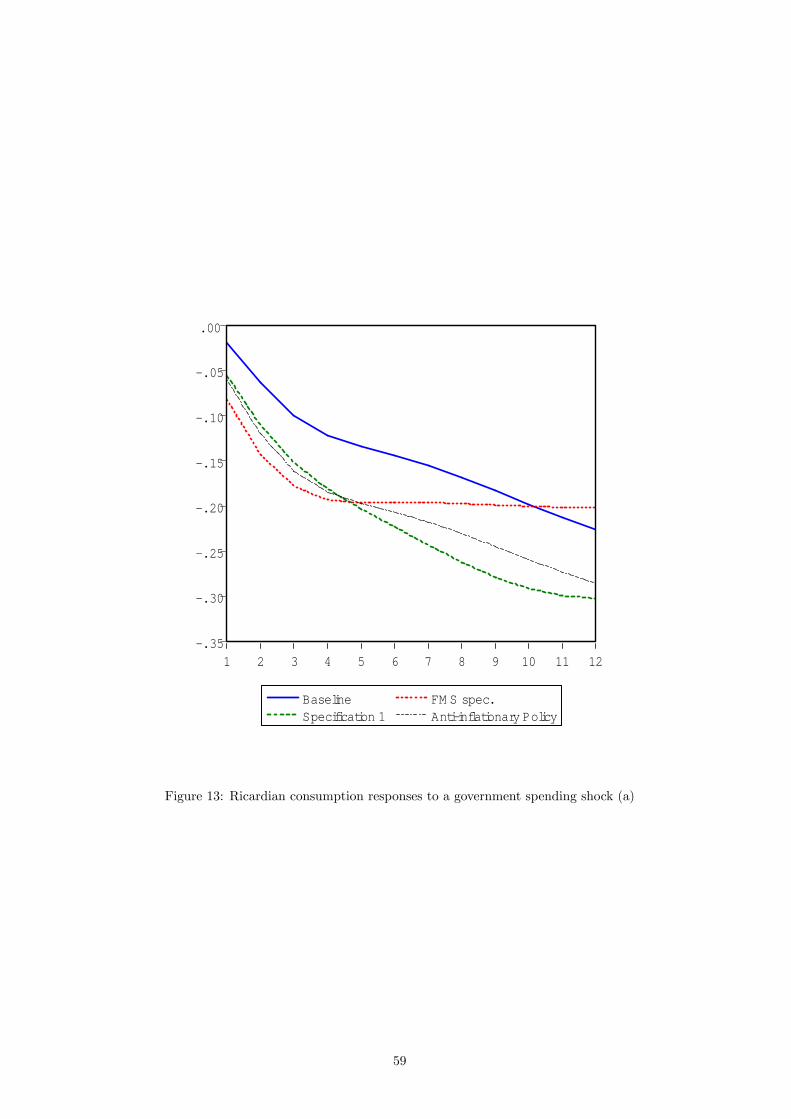
­.35

­.30

­.25

­.20

­.15

­.10

­.05

.00

1 2 3 4 5 6 7 8 9 10 11 12

Baseline FM S spec.Specification 1 Anti­inflationary Policy

Figure 13: Ricardian consumption responses to a government spending shock (a)

59

­2.0

­1.5

­1.0

­0.5

0.0

0.5

1.0

1 2 3 4 5 6 7 8 9 10 11 12

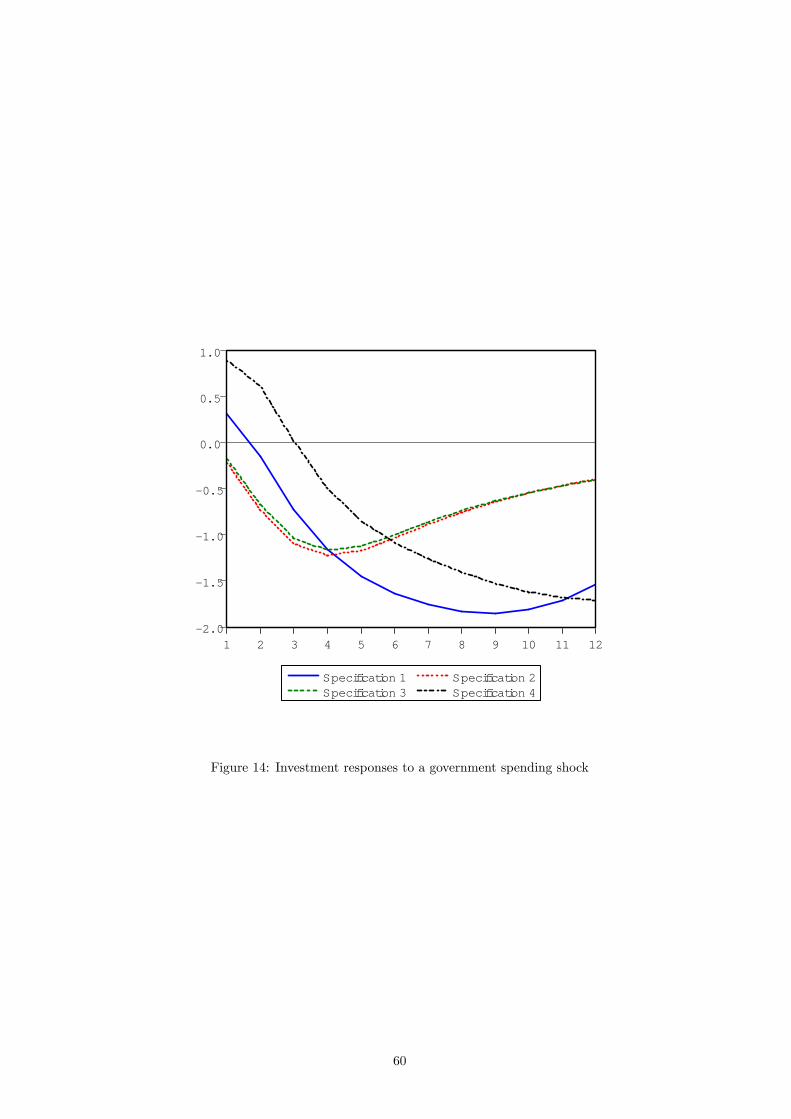
Specification 1 Specification 2Specification 3 Specification 4

Figure 14: Investment responses to a government spending shock

60

­.32

­.28

­.24

­.20

­.16

­.12

­.08

­.04

.00

1 2 3 4 5 6 7 8 9 10 11 12

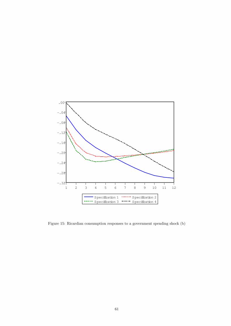
Specification 1 Specification 2Specification 3 Specification 4

Figure 15: Ricardian consumption responses to a government spending shock (b)

61

.0

.1

.2

.3

.4

.5

.6

.7

.8

.9

1 2 3 4 5 6 7 8 9 10 11 12

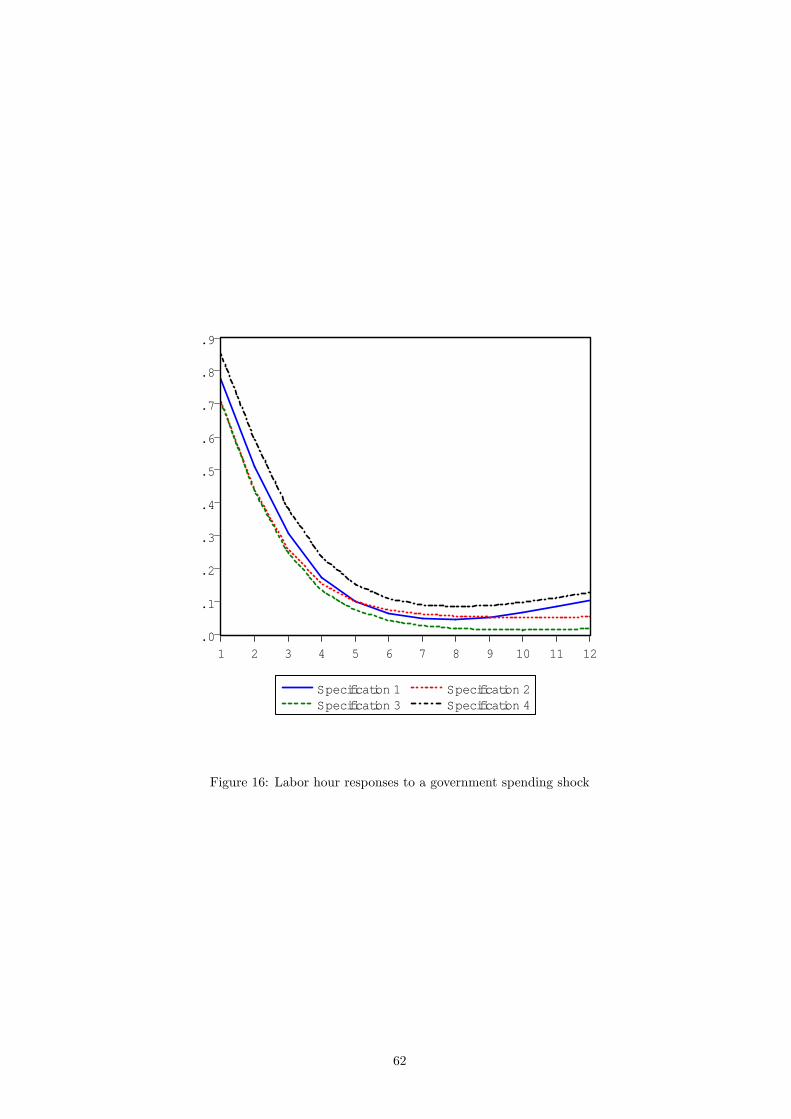
Specification 1 Specification 2Specification 3 Specification 4

Figure 16: Labor hour responses to a government spending shock

62

­0.50

­0.25

0.00

0.25

0.50

0.75

1.00

1.25

1.50

1 2 3 4 5 6 7 8 9 10 11 12

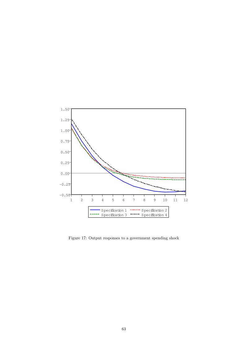
Specification 1 Specification 2Specification 3 Specification 4

Figure 17: Output responses to a government spending shock

63

­1.6

­1.2

­0.8

­0.4

0.0

0.4

0.8

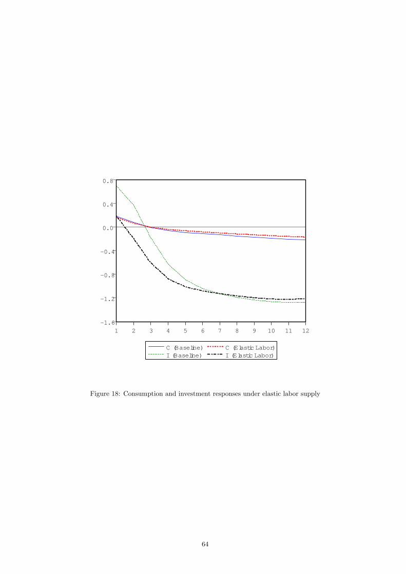
1 2 3 4 5 6 7 8 9 10 11 12

C (Baseline) C (Elastic Labor)I (Baseline) I (Elastic Labor)

Figure 18: Consumption and investment responses under elastic labor supply

64